Bayesian Nonparametrics, Cambridge, 2010
309
Transcript of Bayesian Nonparametrics, Cambridge, 2010

This page intentionally left blank

Bayesian Nonparametrics
Bayesian nonparametrics works – theoretically, computationally. The theory provideshighly flexible models whose complexity grows appropriately with the amount of data.Computational issues, though challenging, are no longer intractable. All that is neededis an entry point: this intelligent book is the perfect guide to what can seem a forbiddinglandscape.
Tutorial chapters by Ghosal, Lijoi and Prunster, Teh and Jordan, and Dunson advancefrom theory, to basic models and hierarchical modeling, to applications and implemen-tation, particularly in computer science and biostatistics. These are complemented bycompanion chapters by the editors and Griffin and Quintana, providing additional mod-els, examining computational issues, identifying future growth areas, and giving linksto related topics.
This coherent text gives ready access both to underlying principles and to state-of-the-art practice. Specific examples are drawn from information retrieval, neuro-linguistic programming, machine vision, computational biology, biostatistics, and bio-informatics.
Nils Lid Hjort is Professor of Mathematical Statistics in the Department of Math-ematics at the University of Oslo.
Chris Holmes is Professor of Biostatistics in the Department of Statistics at theUniversity of Oxford.
Peter M u ller is Professor in the Department of Biostatistics at the University ofTexas M. D. Anderson Cancer Center.
Stephen G. Walker is Professor of Statistics in the Institute of Mathematics,Statistics and Actuarial Science at the University of Kent, Canterbury.

CAMBRIDGE SERIES IN STATISTICAL ANDPROBABILISTIC MATHEMATICS
Editorial BoardZ. Ghahramani (Department of Engineering, University of Cambridge)
R. Gill (Mathematical Institute, Leiden University)F. P. Kelly (Department of Pure Mathematics and Mathematical Statistics,
University of Cambridge)B. D. Ripley (Department of Statistics, University of Oxford)
S. Ross (Department of Industrial and Systems Engineering, University of Southern California)B. W. Silverman (St Peter’s College, Oxford)
M. Stein (Department of Statistics, University of Chicago)
This series of high-quality upper-division textbooks and expository monographs covers all aspectsof stochastic applicable mathematics. The topics range from pure and applied statistics to prob-ability theory, operations research, optimization, and mathematical programming. The bookscontain clear presentations of new developments in the field and also of the state of the art inclassical methods. While emphasizing rigorous treatment of theoretical methods, the books alsocontain applications and discussions of new techniques made possible by advances in computa-tional practice.
A complete list of books in the series can be found athttp://www.cambridge.org/uk/series/sSeries.asp?code=CSPMRecent titles include the following:
6. Empirical Processes in M-Estimation, by Sara van de Geer7. Numerical Methods of Statistics, by John F. Monahan8. A User’s Guide to Measure Theoretic Probability, by David Pollard9. The Estimation and Tracking of Frequency, by B. G. Quinn and E. J. Hannan
10. Data Analysis and Graphics using R (2nd Edition), by John Maindonald and John Braun11. Statistical Models, by A. C. Davison12. Semiparametric Regression, by David Ruppert, M. P. Wand and R. J. Carroll13. Exercises in Probability, by Loıc Chaumont and Marc Yor14. Statistical Analysis of Stochastic Processes in Time, by J. K. Lindsey15. Measure Theory and Filtering, by Lakhdar Aggoun and Robert Elliott16. Essentials of Statistical Inference, by G. A. Young and R. L. Smith17. Elements of Distribution Theory, by Thomas A. Severini18. Statistical Mechanics of Disordered Systems, by Anton Bovier19. The Coordinate-Free Approach to Linear Models, by Michael J. Wichura20. Random Graph Dynamics, by Rick Durrett21. Networks, by Peter Whittle22. Saddlepoint Approximations with Applications, by Ronald W. Butler23. Applied Asymptotics, by A. R. Brazzale, A. C. Davison and N. Reid24. Random Networks for Communication, by Massimo Franceschetti and Ronald Meester25. Design of Comparative Experiments, by R. A. Bailey26. Symmetry Studies, by Marlos A. G. Viana27. Model Selection and Model Averaging, by Gerda Claeskens and Nils Lid Hjort28. Bayesian Nonparametrics, edited by Nils Lid Hjort et al.29. Finite and Large Sample Statistical Theory (2nd Edition), by Pranab K. Sen,
Julio M. Singer and Antonio C. Pedrosa-de-Lima30. Brownian Motion, by Peter Morters and Yuval Peres

Bayesian Nonparametrics
Edited by
Nils Lid HjortUniversity of Oslo
Chris HolmesUniversity of Oxford
Peter MullerUniversity of Texas
M.D. Anderson Cancer Center
Stephen G. WalkerUniversity of Kent

CAMBRIDGE UNIVERSITY PRESSCambridge, New York, Melbourne, Madrid, Cape Town, Singapore,São Paulo, Delhi, Dubai, Tokyo
Cambridge University PressThe Edinburgh Building, Cambridge CB2 8RU, UK
First published in print format
ISBN-13 978-0-521-51346-3
ISBN-13 978-0-511-67536-2
© Cambridge University Press 2010
2010
Information on this title: www.cambridge.org/9780521513463
This publication is in copyright. Subject to statutory exception and to the provision of relevant collective licensing agreements, no reproduction of any partmay take place without the written permission of Cambridge University Press.
Cambridge University Press has no responsibility for the persistence or accuracy of urls for external or third-party internet websites referred to in this publication, and does not guarantee that any content on such websites is, or will remain, accurate or appropriate.
Published in the United States of America by Cambridge University Press, New York
www.cambridge.org
eBook (NetLibrary)
Hardback

Contents
List of contributors page viii
An invitation to Bayesian nonparametricsNils Lid Hjort, Chris Holmes, Peter Mullerand Stephen G. Walker 1
1 Bayesian nonparametric methods: motivation and ideasStephen G. Walker 22
1.1 Introduction 221.2 Bayesian choices 241.3 Decision theory 261.4 Asymptotics 271.5 General posterior inference 291.6 Discussion 33
References 33
2 The Dirichlet process, related priors and posteriorasymptoticsSubhashis Ghosal 35
2.1 Introduction 352.2 The Dirichlet process 362.3 Priors related to the Dirichlet process 462.4 Posterior consistency 492.5 Convergence rates of posterior distributions 602.6 Adaptation and model selection 672.7 Bernshteın–von Mises theorems 712.8 Concluding remarks 74
References 76
v

vi Contents
3 Models beyond the Dirichlet processAntonio Lijoi and Igor Prunster 80
3.1 Introduction 803.2 Models for survival analysis 863.3 General classes of discrete nonparametric priors 993.4 Models for density estimation 1143.5 Random means 1263.6 Concluding remarks 129
References 130
4 Further models and applicationsNils Lid Hjort 137
4.1 Beta processes for survival and event history models 1374.2 Quantile inference 1444.3 Shape analysis 1484.4 Time series with nonparametric correlation function 1504.5 Concluding remarks 152
References 155
5 Hierarchical Bayesian nonparametric models withapplicationsYee Whye Teh and Michael I. Jordan 158
5.1 Introduction 1585.2 Hierarchical Dirichlet processes 1605.3 Hidden Markov models with infinite state spaces 1715.4 Hierarchical Pitman–Yor processes 1775.5 The beta process and the Indian buffet process 1845.6 Semiparametric models 1935.7 Inference for hierarchical Bayesian nonparametric models 1955.8 Discussion 202
References 203
6 Computational issues arising in Bayesian nonparametrichierarchical modelsJim Griffin and Chris Holmes 208
6.1 Introduction 2086.2 Construction of finite-dimensional measures on observables 2096.3 Recent advances in computation for Dirichlet process mixture
models 211References 221

Contents vii
7 Nonparametric Bayes applications to biostatisticsDavid B. Dunson 223
7.1 Introduction 2237.2 Hierarchical modeling with Dirichlet process priors 2247.3 Nonparametric Bayes functional data analysis 2367.4 Local borrowing of information and clustering 2457.5 Borrowing information across studies and centers 2487.6 Flexible modeling of conditional distributions 2507.7 Bioinformatics 2607.8 Nonparametric hypothesis testing 2657.9 Discussion 267
References 268
8 More nonparametric Bayesian models for biostatisticsPeter Muller and Fernando Quintana 274
8.1 Introduction 2748.2 Random partitions 2758.3 Polya trees 2778.4 More DDP models 2798.5 Other data formats 2838.6 An R package for nonparametric Bayesian inference 2868.7 Discussion 289
References 290
Author index 292
Subject index 297

Contributors
David B. DunsonInstitute of Statistics
and Decision SciencesDuke UniversityDurham, NC 27708-0251, USA
Subhashis GhosalDepartment of StatisticsNorth Carolina State UniversityRaleigh, NC 27695, USA
Jim GriffinInstitute of Mathematics, Statistics
and Actuarial ScienceUniversity of KentCanterbury CT2 7NZ, UK
Nils Lid HjortDepartment of MathematicsUniversity of OsloN-0316 Oslo, Norway
Chris HolmesOxford Centre for Gene FunctionUniversity of OxfordOxford OX1 3QB, UK
Michael I. JordanDepartment of Electrical Engineering
and Computer ScienceUniversity of California, BerkeleyBerkeley, CA 94720-1776, USA
Antonio LijoiDepartment of Economics
and Quantitative MethodsUniversity of Pavia27100 Pavia, Italy
Peter MullerDepartment of BiostatisticsM. D. Anderson Cancer CenterUniversity of TexasHouston, TX 77030-4009, USA
Igor PrunsterDepartment of Statistics
and Applied MathematicsUniversity of Turin10122 Turin, Italy
Fernando QuintanaDepartment of StatisticsPontifical Catholic University of Chile3542000 Santiago, Chile
Yee Whye TehGatsby Computational
Neuroscience UnitUniversity College LondonLondon WC1N 3AR, UK
Stephen G. WalkerInstitute of Mathematics, Statistics
and Actuarial ScienceUniversity of KentCanterbury CT2 7NZ, UK
viii

An invitation to Bayesian nonparametricsNils Lid Hjort, Chris Holmes, Peter Muller and Stephen G. Walker
This introduction explains why you are right to be curious about Bayesian nonparametrics –why you may actually need it and how you can manage to understand it and use it. We alsogive an overview of the aims and contents of this book and how it came into existence,delve briefly into the history of the still relatively young field of Bayesian nonparametrics,and offer some concluding remarks about challenges and likely future developments in thearea.
Bayesian nonparametrics
As modern statistics has developed in recent decades various dichotomies, wherepairs of approaches are somehow contrasted, have become less sharp than theyappeared to be in the past. That some border lines appear more blurred than a gen-eration or two ago is also evident for the contrasting pairs “parametric versus non-parametric” and “frequentist versus Bayes.” It appears to follow that “Bayesiannonparametrics” cannot be a very well-defined body of methods.
What is it all about?
It is nevertheless an interesting exercise to delineate the regions of statistical method-ology and practice implied by constructing a two-by-two table of sorts, via the two“factors” parametric–nonparametric and frequentist–Bayes; Bayesian nonparamet-rics would then be whatever is not found inside the other three categories.
(i) Frequentist parametrics encompasses the core of classical statistics, involvingmethods associated primarily with maximum likelihood, developed in the 1920sand onwards. Such methods relate to various optimum tests, with calculation ofp-values, optimal estimators, confidence intervals, multiple comparisons, and soforth. Some of the procedures stem from exact probability calculations for mod-els that are sufficiently amenable to mathematical derivations, while others relate
1

2 An invitation to Bayesian nonparametrics
to the application of large-sample techniques (central limit theorems, delta meth-ods, higher-order corrections involving expansions or saddlepoint approximations,etc.).
(ii) Bayesian parametrics correspondingly comprises classic methodology forprior and posterior distributions in models with a finite (and often low) number ofparameters. Such methods, starting from the premise that uncertainty about modelparameters may somehow be represented in terms of probability distributions, havearguably been in existence for more than a hundred years (since the basic theoremthat drives the machinery simply says that the posterior density is proportional tothe product of the prior density with the likelihood function, which again relatesto the Bayes theorem of c. 1763), but they were naturally limited to a short list ofsufficiently simple statistical models and priors. The applicability of Bayesian para-metrics widened significantly with the advent and availability of modern computers,from about 1975, and then with the development of further numerical methods andsoftware packages pertaining to numerical integration and Markov chain MonteCarlo (MCMC) simulations, from about 1990.
As for category (i) above, asymptotics is often useful for Bayesian parametrics,partly for giving practical and simple-to-use approximations to the exact posteriordistributions and partly for proving results of interest about the performance of themethods, including aspects of similarity between methods arising from frequen-tist and Bayesian perspectives. Specifically, frequentists and Bayesians agree inmost matters, to the first order of approximation, for inference from parametricmodels, as the sample size increases. The mathematical theorems that in vari-ous ways make such statements precise are sometimes collectively referred to as“Bernshteın–von Mises theorems”; see, for example, Le Cam and Yang (1990,Chapter 7) for a brief treatment of this theme, including historical references goingback not only to Bernshteın (1917) and von Mises (1931) but all the way backto Laplace (1810). One such statement is that confidence intervals computed bythe frequentists and the Bayesians (who frequently call them “credibility inter-vals”), with the same level of confidence (or credibility), become equal, to thefirst order of approximation, with probability tending to one as the sample sizeincreases.
(iii) Frequentist nonparametrics is a somewhat mixed bag, covering variousareas of statistics. The term has historically been associated with test proceduresthat are or asymptotically become “distribution free,” leading also to nonparametricconfidence intervals and bands, etc.; for methodology related to statistics basedon ranks (see Lehmann, 1975); then progressively with estimation of probabilitydensities, regression functions, link functions etc., without parametric assumptions;and also with specific computational techniques such as the bootstrap. Again,asymptotics plays an important role, both for developing fruitful approximations

An invitation to Bayesian nonparametrics 3
and for understanding and comparing properties of performance. A good referencebook for learning about several classes of these methods is Wasserman (2006).
(iv) What ostensibly remains for our fourth category, then, that of Bayesian non-parametrics, are models and methods characterized by (a) big parameter spaces(unknown density and regression functions, link and response functions, etc.) and(b) construction of probability measures over these spaces. Typical examples in-clude Bayesian setups for density estimation (in any dimension), nonparametricregression with a fixed error distribution, hazard rate and survival function estima-tion for survival analysis, without or with covariates, etc. The divisions between“small” and “moderate” and “big” for parameter spaces are not meant to be verysharp, and the scale is interpreted flexibly (see for example Green and Richardson,2001, for some discussion of this).
It is clear that category (iv), which is the focus of our book, must meet chal-lenges of a greater order than do the other three categories. The mathematicalcomplexities are more demanding, since placing well-defined probability distri-butions on potentially infinite-dimensional spaces is inherently harder than forEuclidean spaces. Added to this is the challenge of “understanding the prior”; theill-defined transformation from so-called “prior knowledge” to “prior distribution”is hard enough to elicit in lower dimensions and of course becomes even more chal-lenging in bigger spaces. Furthermore, the resulting algorithms, for example forsimulating unknown curves or surfaces from complicated posterior distributions,tend to be more difficult to set up and to test properly.
Finally, in this short list of important subtopics, we must note that the biggerworld of nonparametric Bayes holds more surprises and occasionally exhibits moredisturbing features than one encounters in the smaller and more comfortable worldof parametric Bayes. It is a truth universally acknowledged that a statistician inpossession of an infinity of data points must be in want of the truth – but somenonparametric Bayes constructions actually lead to inconsistent estimation proce-dures, where the truth is not properly uncovered when the data collection grows.Also, the Bernshteın–von Mises theorems alluded to above, which hold very gen-erally for parametric Bayes problems, tend not to hold as easily and broadly in theinfinite-dimensional cases. There are, for example, important problems where thenonparametric Bayes methods obey consistency (the posterior distribution properlyaccumulates its mass around the true model, with increased sample size), but witha different rate of convergence than that of the natural frequentist method for thesame problem. Thus separate classes of situations typically need separate scrutiny,as opposed to theories and theorems that apply very grandly.
It seems clear to us that the potential list of good, worthwhile nonparametricBayes procedures must be rather longer than the already enormously long lists ofBayes methods for parametric models, simply because bigger spaces contain more

4 An invitation to Bayesian nonparametrics
than smaller ones. A book on Bayesian nonparametrics must therefore limit itselfto only some of these worthwhile procedures. A similar comment applies to thestudy of these methods, in terms of performance, comparisons with results fromother approaches, and so forth (making the distinction between the construction ofa method and the study of its performance characteristics).
Who needs it?
Most modern statisticians have become well acquainted with various nonparametricand semiparametric tools, on the one hand (nonparametric regression, smoothingmethods, classification and pattern recognition, proportional hazards regression,copulae models, etc.), and with the most important simulation tools, on the other(rejection–acceptance methods, MCMC strategies like the Gibbs sampler and theMetropolis algorithm, etc.), particularly in the realm of Bayesian applications,where the task of drawing simulated realizations from the posterior distribution is themain operational job. The combination of these methods is becoming increasinglypopular and important (in a growing number of ways), and each such combinationmay be said to carry the stamp of Bayesian nonparametrics.
One reason why combining nonparametrics with Bayesian posterior simulationsis becoming more important is related to practical feasibility, in terms of softwarepackages and implementation of algorithms. The other reason is that such solutionscontribute to the solving of actual problems, in a steadily increasing range of appli-cations, as indicated in this book and as seen at workshops and conferences dealingwith Bayesian nonparametrics. The steady influx of good real-world applicationareas contributes both to the sharpening of tools and to the sociological fact that,not only hard-core and classically oriented statisticians, but also various schools ofother researchers in quantitative disciplines, lend their hands to work in variationsof nonparametric Bayes methods. Bayesian nonparametrics is used by researchersworking in finance, geosciences, botanics, biology, epidemiology, forestry, paleon-tology, computer science, machine learning, recommender systems, to name onlysome examples.
By prefacing various methods and statements with the word “Bayesian” we arealready acknowledging that there are different schools of thought in statistics –Bayesians place prior distributions over their parameter spaces while parametersare fixed unknowns for the frequentists. We should also realize that there are dif-ferent trends of thought regarding how statistical methods are actually used (aspartly opposed to how they are constructed). In an engaging discussion paper,Breiman (2001) argues that contemporary statistics lives with a Snowean “two cul-tures” problem. In some applications the careful study and interpretation of fineraspects of the model matter and are of primary concern, as in various substantive

An invitation to Bayesian nonparametrics 5
sciences – an ecologist or a climate researcher may place great emphasis on de-termining that a certain statistical coefficient parameter is positive, for example,as this might be tied to a scientifically relevant finding that a certain backgroundfactor really influences a phenomenon under study. In other applications such finerdistinctions are largely irrelevant, as the primary goals of the methods are to makeefficient predictions and classifications of a sufficient quality. This pragmatic goal,of making good enough “black boxes” without specific regard to the componentsof the box in question, is valid in many situations – one might be satisfied witha model that predicts climate parameters and the number of lynx in the forest,without always needing or aiming to understand the finer mechanisms involved inthese phenomena.
This continuing debate is destined to play a role also for Bayesian nonparametrics,and the right answer to what is more appropriate, and to what is more important, willbe largely context dependent. A statistician applying Bayesian nonparametrics mayuse one type of model for uncovering effects and another for making predictions orclassifications, even when dealing with the same data. Using different models fordifferent purposes, even with the very same data set, is not a contradiction in terms,and relates to different loss functions and to themes of interest-driven inference;cf. various focused information criteria for model selection (see Claeskens andHjort, 2008, Chapter 6).
It is also empirically true that some statistics problems are easier to attack usingBayesian methods, with machineries available that make analysis and inferencepossible, in the partial absence of frequentist methods. This picture may of courseshift with time, as better and more refined frequentist methods may be developedalso, for example for complex hierarchical models, but the observation remindsus that there is a necessary element of pragmatism in modern statistics work;one uses what one has, rather than spending three extra months on developingalternative methods. An eclectic view of Bayesian methods, prevalent also amongthose statisticians hesitant to accept all of the underlying philosophy, is to usethem nevertheless, as they are practical and have good performance. Indeed a broadresearch direction is concerned with reaching performance-related results aboutclasses of nonparametric Bayesian methods, as partly distinct from the constructionof the models and methods themselves (cf. Chapter 2 and its references). For someareas in statistics, then, including some surveyed in this book, there is an “advantageBayes” situation. A useful reminder in this regard is the view expressed by ArtDempster: “a person cannot be Bayesian or frequentist; rather, a particular analysiscan be Bayesian or frequentist” (see Wasserman, 2008). Another and perhapshumbling reminder is Good’s (1959) lower bound for the number of differentBayesians (46 656, actually), a bound that may need to be revised upwards whenthe discussion concerns nonparametric Bayesians.

6 An invitation to Bayesian nonparametrics
Why now?
Themes of Bayesian nonparametrics have engaged statisticians for about fortyyears, but now, that is around 2010, the time is ripe for further rich developmentsand applications of the field. This is due to a confluence of several different factors:the availability and convenience of computer programs and accessible softwarepackages, downloaded to the laptops of modern scientists, along with methodologyand machinery for finessing and finetuning these algorithms for new applications;the increasing accessibility of statistical models and associated methodological toolsfor taking on new problems (leading also to the development of further methodsand algorithms); various developing application areas paralleling statistics that finduse for these methods and sometimes develop them further; and the broadeningmeeting points for the two flowing rivers of nonparametrics (as such) and Bayesianmethods (as such).
Evidence of the growing importance of Bayesian nonparametrics can also betraced in the archives of conferences and workshops devoted to such themes. Inaddition to having been on board in broader conferences over several decades,an identifiable subsequence of workshops and conferences set up for Bayesiannonparametrics per se has developed as follows, with a rapidly growing number ofparticipants: Belgirate, Italy (1997), Reading, UK (1999), Ann Arbor, USA (2001),Rome, Italy (2004), Jeju, Korea (2006), Cambridge, UK (2007), Turin, Italy (2009).Monitoring the programs of these conferences one learns that development has beenand remains steady, regarding both principles and practice.
Two more long-standing series of workshops are of interest to researchers andlearners of nonparametric Bayesian statistics. The BISP series (Bayesian inferencefor stochastic processes) is focused on nonparametric Bayesian models related tostochastic processes. Its sequence up to the time of writing reads Madrid (1998),Varenna (2001), La Mange (2003), Varenna (2005), Valencia (2007), Brixen (2009),alternating between Spain and Italy. Another related research community is definedby the series of research meetings on objective Bayes methodology. The coordinatesof the O’Bayes conference series history are Purdue, USA (1996), Valencia, Spain(1998), Ixtapa, Mexico (2000), Granada, Spain (2002), Aussois, France (2003),Branson, USA (2005), Rome, Italy (2007), Philadelphia, USA (2009).
The aims, purposes and contents of this book
This book has in a sense grown out of a certain event. It reflects this particular origin,but is very much meant to stand solidly and independently on its constructed feet,as a broad text on modern Bayesian nonparametrics and its theory and methods; inother words, readers do not need to know about or take into account the event thatled to the book being written.

An invitation to Bayesian nonparametrics 7
A background event
The event in question was a four-week program on Bayesian nonparametrics hostedby the Isaac Newton Institute of Mathematical Sciences at Cambridge, UK, in Au-gust 2007, and organized by the four volume editors. In addition to involving a coregroup of some twenty researchers from various countries, the program organized aone-week international conference with about a hundred participants. These repre-sented an interesting modern spectrum of researchers whose work in different waysis related to Bayesian nonparametrics: those engaged in methodological statisticswork, from university departments and elsewhere; statisticians involved in collab-orations with researchers from substantive areas (like medicine and biostatistics,quantitative biology, mathematical geology, information sciences, paleontology);mathematicians; machine learning researchers; and computer scientists.
For the workshop, the organizers selected four experts to provide tutorial lecturesrepresenting four broad, identifiable themes pertaining to Bayesian nonparametrics.These were not merely four themes “of interest,” but were closely associated withthe core models, the core methods, and the core application areas of nonparametricBayes. These tutorials were
• Dirichlet processes, related priors and posterior asymptotics (by S. Ghosal),• models beyond the Dirichlet process (by A. Lijoi),• applications to biostatistics (by D. B. Dunson),• applications to machine learning (by Y. W. Teh).
The program and the workshop were evaluated (by the participants and other parties)as having been very successful, by having bound together different strands of workand by perhaps opening doors to promising future research. The experience madeclear that nonparametric Bayes is an important growth area, but with side-streamsthat may risk evolving too much in isolation if they do not make connections withthe core field. All of these considerations led to the idea of creating the presentbook.
What does this book do?
This book is structured around the four core themes represented by the tutorialsdescribed above, here appearing in the form of invited chapters. These core chap-ters are then complemented by chapters written by the four volume editors. Therole of these complementary chapters is partly to discuss and extend the four corechapters, in suitably matched pairs. These complements also offer further devel-opments and provide links to related areas. This editorial process hence led to thefollowing list of chapters, where the pairs 1–2, 3–4, 5–6, 7–8 can be regarded asunits.

8 An invitation to Bayesian nonparametrics
1 S. G. Walker: Bayesian nonparametric methods: motivation and ideas2 S. Ghosal: The Dirichlet process, related priors and posterior asymptotics3 A. Lijoi and I. Prunster: Models beyond the Dirichlet process4 N. L. Hjort: Further models and applications.5 Y. W. Teh and M. I. Jordan: Hierarchical Bayesian nonparametric models
with applications6 J. Griffin and C. Holmes: Computational issues arising in Bayesian non-
parametric hierarchical models7 D. B. Dunson: Nonparametric Bayes applications to biostatistics8 P. Muller and F. Quintana: More nonparametric Bayesian models for
biostatistics
As explained at the end of the previous section, it would not be possible to have“everything important” inside a single book, in view of the size of the expandingtopic. It is our hope and view, however, that the dimensions we have probed aresound, deep and relevant ones, and that different strands of readers will benefit fromworking their way through some or all of these.
The first core theme (Chapters 1 and 2) is partly concerned with some of thecornerstone classes of nonparametric priors, including the Dirichlet process andsome of its relatives. General principles and ideas are introduced (in the setting ofi.i.d. observations) in Chapter 1. Mathematical properties are further investigated,including characterizations of the posterior distribution, in Chapter 2. The themealso encompasses properties of the behavior of the implied posterior distributions,and, specifically, consistency and rates of convergence. Bayesian methodology isoften presented as essentially a machinery for coming from the prior to the posteriordistributions, but is at its most powerful when coupled with decision theory andloss functions. This is true in nonparametric situations as well, as also discussedinside this first theme.
The second main theme (Chapters 3 and 4) is mainly occupied with the devel-opment of the more useful nonparametric classes of priors beyond those relatedto the Dirichlet processes mentioned above. Chapter 3 treats completely randommeasures, neutral-to-the-right processes, the beta process, partition functions, clus-tering processes, and models for density estimation, with Chapter 4 providingfurther methodology for stationary time series with nonparametrically modeled co-variance functions, models for random shapes, etc., along with pointers to variousapplication areas, such as survival and event history analysis.
The third and fourth core themes are more application driven than the first two.The third core theme (Chapters 5 and 6) represents the important and growing areaof both theory and applications of Bayesian nonparametric hierarchical modeling(an area related to what is often referred to as machine learning). Hierarchical

An invitation to Bayesian nonparametrics 9
modeling, again with Dirichlet processes as building blocks, leads to algorithmsthat solve problems in information retrieval, multipopulation haplotype phasing,word segmentation, speaker diarization, and so-called topic modeling, as demon-strated in Chapter 5. The models that help to accomplish these tasks includeChinese restaurant franchises and Indian buffet processes, in addition to exten-sive use of Gaussian processes, priors on function classes such as splines, free-knot basis expansions, MARS and CART, etc. These constructions are associ-ated with various challenging computational issues, as discussed in some detail inChapter 6.
Finally the fourth main theme (Chapters 7 and 8) focuses on biostatistics. Topicsdiscussed and developed in Chapter 7 include personalized medicine (a growingtrend in modern biomedicine), hierarchical modeling with Dirichlet processes,clustering strategies and partition models, and functional data analysis. Chapter 8elaborates on these themes, and in particular discusses random partition priors andcertain useful variations on dependent Dirichlet processes.
How do alternative models relate to each other?
Some comments seem in order to put the many alternative models in perspective.Many of the models are closely related mathematically, with some being a specialcase of others. For example, the Dirichlet process is a special case of the normalizedrandom measure with independent increments introduced in Chapter 3. Many ofthe models introduced in later chapters are natural generalizations and extensionsof earlier defined models. Several of the models introduced in Chapter 5 extend therandom partition models described in the first four chapters, including, for example,a natural hierarchical extension of the Dirichlet process model. Finally, Chapters 7and 8 introduce many models that generalize the basic Dirichlet process model toone for multiple related random probability measures. As a guideline for choosinga model for a specific application, we suggest considering the data format, the focusof the inference, and the desired level of computational complexity.
If the data format naturally includes multiple subpopulations then it is natural touse a model that reflects this structure in multiple submodels. In many applicationsthe inference of interest is on random partitions and clustering, rather than on arandom probability measure. It is natural then to use a model that focuses on therandom partitions, such as a species sampling model. Often the choice will simplybe driven by the availability of public domain software. This favors the more popularmodels such as Dirichlet process models, Polya tree models, and various dependentDirichlet process models.
The reader may notice a focus on biomedical applications. In part this is areflection of the history of nonparametric Bayesian data analysis. Many early papers

10 An invitation to Bayesian nonparametrics
focused on models for event time data, leading naturally to biomedical applications.This focus is also a reflection of the research experience of the authors. There isno intention to give an exhaustive or even representative discussion of areas ofapplication. An important result of focusing on models rather than applications isthe lack of a separate chapter on hierarchical mixed effects models, although manyof these feature in Chapters 7 and 8.
How to teach from this book
This book may be used as the basis for master’s or Ph.D. level courses in Bayesiannonparametrics. Various options exist, for different audiences and for differentlevels of mathematical skill. One route, for perhaps a typical audience of statis-tics students, is to concentrate on core themes two (Chapters 3 and 4) and four(Chapters 7 and 8), supplemented with computer exercises (drawing on methodsexhibited in these chapters, and using for example the software DPpackage, de-scribed in Jara, 2007). A course building upon the material in these chapters wouldfocus on data analysis problems and typical data formats arising in biomedical re-search problems. Nonparametric Bayesian probability models would be introducedas and when needed to address the data analysis problems.
More mathematically advanced courses could include more of core theme one(Chapters 1 and 2). Such a course would naturally center more on a description ofnonparametric Bayesian models and include applications as examples to illustratethe models. A third option is a course designed for an audience with an interestin machine learning, hierarchical modeling, and so forth. It would focus on corethemes two (Chapters 2 and 3) and three (Chapters 5 and 6).
Natural prerequisites for such courses as briefly outlined here, and by associationfor working with this book, include a basic statistics course (regression methodsassociated with generalized linear models, density estimation, parametric Bayes),perhaps some survival analysis (hazard rate models, etc.), along with basic skills insimulation methods (MCMC strategies).
A brief history of Bayesian nonparametrics
Lindley (1972) noted in his review of general Bayesian methodology that Bayesiansup to then had been “embarrassingly silent” in the area of nonparametric statistics.He pointed out that there were in principle no conceptual difficulties with combining“Bayesian” and “nonparametric” but indirectly acknowledged that the mathematicaldetails in such constructions would have to be more complicated.

An invitation to Bayesian nonparametrics 11
From the start to the present
Independently of and concurrently with Lindley’s review, what can be consideredthe historical start of Bayesian nonparametrics occurred in California. The 1960shad been a period of vigorous methodological research in various nonparametricdirections. David Blackwell, among the prominent members of the statistics de-partment at Berkeley (and, arguably, belonging to the Bayesian minority there),suggested to his colleagues that there ought to be Bayesian parallels to the prob-lems and solutions for some of these nonparametric situations. These conversationsproduced two noteworthy developments, both important in their own right and forwhat followed: (i) a 1970 UCLA technical report titled “A Bayesian analysis ofsome nonparametric problems,” by T. S. Ferguson, and (ii) a 1971 UC Berkeleytechnical report called “Tailfree and neutral random probabilities and their pos-terior distributions,” by K. A. Doksum. After review processes, these became thetwo seminal papers Ferguson (1973) in Annals of Statistics, where the Dirichletprocess is introduced, and Doksum (1974) in Annals of Probability, featuring hisneutral-to-the-right processes (see Chapters 2 and 3 for descriptions, interconnec-tions and further developments of these classes of priors). The neutral-to-the-rightprocesses are also foreshadowed in Doksum (1972). In this very first wave of gen-uine Bayesian nonparametrics work, Ferguson (1974) also stands out, an invitedreview paper for Annals of Statistics. Here he gives early descriptions of and resultsfor Polya trees, for example, and points to fruitful research problems.
We ought also to mention that there were earlier contributions to constructionsof random probability measures and their probabilistic properties, such as Kraftand van Eeden (1964) and Dubins and Freedman (1966). More specific Bayesianconnections, including matters of consistency and inconsistency, were made inFreedman (1963) and Fabius (1964), involving also the important notion of tailfreedistributions; see also Schwartz (1965). Similarly, a density estimation method givenin Good and Gaskins (1971) may be regarded as having a Bayesian nonparametricroot, involving an implied prior on the set of densities. Nevertheless, to the extentthat such finer historical distinctions are of interest, we would identify the start ofBayesian nonparametrics with the work by Ferguson and Doksum.
These early papers gave strong stimulus to many further developments, includ-ing research on various probabilistic properties of these new prior and posteriorprocesses (probability measures on spaces of functions), procedures for densityestimation based on mixtures of Dirichlet processes, applications to survival anal-ysis (with suitable priors on the random survivor functions, or cumulative hazardfunctions, and with methodology developed to handle censoring), a more flexiblemachinery for Polya trees and their cousins, etc. We point to Chapters 2 and 3 forfurther information, rather than detailing these developments here.

12 An invitation to Bayesian nonparametrics
The emphasis in this early round of new papers was perhaps simply on theconstruction of new prior measures, for an increasing range of natural statisticalmodels and problems, along with sufficiently clear results on how to characterize theconsequent posterior distributions. Some of these developments were momentarilyhampered or even stopped by the sheer computational complexity associated withhandling the posterior distributions; sometimes exact results could be written downand proved mathematically, but algorithms could not always be constructed toevaluate these expressions. The situation improved around 1990, when simulationschemes of the MCMC variety became more widely known and implementable,at around the time when statisticians suddenly had real and easily programmablecomputers in their offices (the MCMC methods had in principle been known to thestatistics community since around 1970, but it took two decades for the methodsto become widely and flexibly used; see for example Gelfand and Smith, 1990).The MCMC methods were at the outset constructed for classes of finite-parameterproblems, but it became apparent that their use could be extended to solve problemsin Bayesian nonparametrics as well.
Another direction of research, in addition to the purely constructive and compu-tational sides of the problems, is that of performance: how do the posterior distribu-tions behave, in particular when the sample size increases, and are the implicit limitsrelated to those reached in the frequentist camp? Some of these questions first sur-faced in Diaconis and Freedman (1986a, 1986b), where situations were exhibited inwhich the Bayesian machine yielded asymptotically inconsistent answers; see alsothe many discussion contributions to these two papers. This and similar researchmade it clearer to researchers in the field that, even though asymptotics typicallyled to various mathematical statements of the comforting type “different Bayesiansagree among themselves, and also with the frequentists, as the sample size tendsto infinity” for finite-dimensional problems, results are rather more complicated ininfinite-dimensional spaces; see Chapters 1 and 2 in this book and comments madeabove.
Applications
The history above deals in essence with theoretical developments. A reader sam-pling his or her way through the literature briefly surveyed there will make theanthropological observation that articles written after say 2000 have a differentlook to them than those written around 1980. This partly reflects a broader trend,a transition of sorts that has moved the primary emphases of statistics from moremathematically oriented articles to those nearer to actual applications – there arefewer sigma-algebras and less measure theoretic language, and more attention tomotivation, algorithms, problem solving and illustrations.

An invitation to Bayesian nonparametrics 13
The history of applications of Bayesian nonparametrics is perhaps more com-plicated and less well defined than that of the theoretical side. For natural rea-sons, including the general difficulty of transforming mathematics into efficientalgorithms and the lack of good computers at the beginning of the nonpara-metric Bayes adventure, applications simply lagged behind. Ferguson’s (1973,1974) seminal papers are incidentally noteworthy also because they spell out in-teresting and nontrivial applications, for example to adaptive investment modelsand to adaptive sampling with recall, though without data illustrations. As indi-cated above, the first broad theoretical foundations stem from the early 1970s,while the first noteworthy real-data applications, primarily in the areas of survivalanalysis and biostatistics, started to emerge in the early 1990s (see for examplethe book by Dey, Muller and Sinha, 1998). At the same time rapidly growingapplication areas emerged inside machine learning (pattern recognition, bioin-formatics, language processing, search engines; see Chapter 5). More informa-tion and further pointers to actual application areas for Bayesian nonparametricsmay be found by browsing the programs for the Isaac Newton Institute work-shop 2007 (www.newton.ac.uk/programmes/BNR/index.html) and the CarloAlberto Programme in Bayesian Nonparametrics 2009 (bnpprogramme.carloalberto.org/index.html).
Where does this book fit in the broader picture?
We end this section with a short annotated list of books and articles that provideoverviews of Bayesian nonparametrics (necessarily with different angles and em-phases). The first and very early one of these is Ferguson (1974), mentioned above.Dey, Muller and Sinha (1998) is an edited collection of papers, with an emphasis onmore practical concerns, and in particular containing various papers dealing withsurvival analysis. The book by Ibrahim, Chen and Sinha (2001) gives a comprehen-sive treatment of the by-then more prominently practical methods of nonparametricBayes pertaining to survival analysis. Walker, Damien, Laud and Smith (1999) isa read discussion paper for the Royal Statistical Society, exploring among other is-sues that of more flexible methods for Polya trees. Hjort (2003) is a later discussionpaper, reviewing various topics and applications, pointing to research problems, andmaking connections to the broad “highly structured stochastic systems” theme thatis the title of the book in question. Similarly Muller and Quintana (2004) providesanother review of established results and some evolving research areas. Ghosh andRamamoorthi (2003) is an important and quite detailed, mathematically orientedbook on Bayesian nonparametrics, with a focus on precise probabilistic propertiesof priors and posteriors, including that of posterior consistency (cf. Chapters 1 and

14 An invitation to Bayesian nonparametrics
2 of this book). Lee (2004) is a slim and elegant book dealing with neural networksvia tools from Bayesian nonparametrics.
Further topics
Where might you want to go next (after having worked with this book)? Herewe indicate some of the research directions inside Bayesian nonparametrics thatnevertheless lie outside the natural boundaries of this book.
Gaussian processes Gaussian processes play an important role in severalbranches of probability theory and statistics, also for problems related to Bayesiannonparametrics. An illustration could be of regression data (xi, yi) where yi is mod-eled as m(xi)+εi , with say Gaussian i.i.d. noise terms. If the unknown m(·) functionis modeled as a Gaussian process with a known covariance function, then the poste-rior is another Gaussian process, and Bayesian inference may proceed. This simplescenario has many extensions, yielding Bayesian nonparametric solutions to differ-ent problems, ranging from prediction in spatial and spatial-temporal models (seee.g. Gelfand, Guindani and Petrone, 2008) to machine learning (e.g. Rasmussen andWilliams, 2006). Gaussian process models are also a popular choice for inferencewith output from computer simulation experiments (see e.g. Oakley and O’Hagan(2002) and references there). An extensive annotated bibliography of the Gaus-sian process literature, including links to public domain software, is available atwww.gaussianprocess.org/. Regression and classification methods using suchprocesses are reviewed in Neal (1999). Extensions to treed Gaussian processes aredeveloped in Gramacy (2007) and Gramacy and Lee (2008).
Spatial statistics We touched on spatial modeling in connection with Gaussianprocesses above, and indeed many such models may be handled, with appropriatecare, as long as the prior processes involved have covariance functions determinedby a low number of parameters. The situation is more complicated when onewishes to place nonparametric priors on the covariance functions as well; see somecomments in Chapter 4.
Neural networks There are by necessity several versions of “neural networks,”and some of these have reasonably clear Bayesian interpretations, and a subset ofthese is amenable to nonparametric variations. See Lee (2004) for a lucid overview,and for example Holmes and Mallick (2000) for a particular application. Similarly,flexible nonlinear regression models based on spline bases provide inference thatavoids the restrictive assumptions of parametric models. Bayesian inference forpenalized spline regression is summarized in Ruppert, Wand and Carroll (2003,
An invitation to Bayesian nonparametrics 15
Chapter 16) and implementation details are discussed in Crainiceanu, Ruppert andWand (2005). For inference using exact-knot selection see, for example, Smith andKohn (1996) or Denison, Mallick and Smith (1998). In addition, there is morerecent work on making the splines more adaptive to fit spatially heterogeneousfunctions, such as Baladandayuthapani, Mallick and Carroll (2005) and BARS byDiMatteo, Genovese and Kass (2001).
p � n problems A steadily increasing range of statistical problems involve the“p � n” syndrome, in which there are many more covariates (and hence unknownregression coefficients) than individuals. Ordinary methods do not work, and al-ternatives must be devised. Various methods have been derived from frequentistperspectives, but there is clear scope for developing Bayesian techniques. The popu-lar lasso method of Tibshirani (1996) may in fact be given a Bayesian interpretation,as the posterior mode solution (the Bayes decision under a sharp 0–1 loss function)with a prior for the large number of unknown regression coefficients being that ofindependent double exponentials with the same spread. Various extensions havebeen investigated, some also from this implied or explicit Bayesian nonparametricperspective.
Model selection and model averaging Some problems in statistics are attackedby working out the ostensibly best method for each of a list of candidate mod-els, and then either selecting the tentatively best one, via some model selectioncriterion, or averaging over a subset of the best several ones. When the list of can-didate models becomes large, as it easily does, the problems take on nonparametricBayesian shapes; see for example Claeskens and Hjort (2008, Chapter 7). Furthermethodology needs to be developed for both the practical and theoretical sides.
Classification and regression trees A powerful and flexible methodology forbuilding regression or classifiers via trees, with perhaps a binary option at eachnode of the tree, was first developed in the CART system of Breiman, Friedman,Olshen and Stone (1984). Several attempts have been made to produce Bayesianversions of such schemes, involving priors on large families of growing and prunedtrees. Their performance has been demonstrated to be excellent in several classesof problems; see for example Chipman, George and McCulloch (2007). See in thisconnection also Neal (1999) mentioned above.
Performance Quite a few journal papers deal with issues of performance, com-parisons between posterior distributions arising from different priors, etc.; for somereferences in that direction, see Chapters 1 and 2.

16 An invitation to Bayesian nonparametrics
Computation and software\sindexsoftware packages
A critical issue in the practical use of nonparametric Bayesian prior models isthe availability of efficient algorithms to implement posterior inference. Recallingthe earlier definition of nonparametric Bayesian models as probability models onbig parameter spaces, this might seem a serious challenge at first glance. But werun into some good luck. For many popular models it is possible to marginalizeanalytically with respect to some of the infinite-dimensional random quantities,leaving a probability model on some lower-dimensional manageable space. Forexample, under Gaussian process priors the joint probability model for the realiza-tion at any finite number of locations is simply a multivariate normal distribution.Similarly, various analysis schemes for survival and event history models featureposterior simulation of beta processes (Hjort, 1990), which may be accomplishedby simulating and then adding independent beta-distributed increments over manysmall intervals. Under the popular Dirichlet process mixture-of-normals model fordensity estimation, the joint distribution of the observed data can be characterizedas a probability model on the partition of the observed data points and independentpriors for a few cluster-specific parameters. Also, under a Polya tree prior, or un-der quantile-pyramid-type priors (see Hjort and Walker, 2009), posterior predictiveinference can be implemented considering only finitely many levels of the nestedpartition sequence.
Increased availability of public domain software greatly simplifies the practi-cal use of nonparametric Bayesian models for data analysis. Perhaps the mostwidely used software is the R package DPpackage (Jara, 2007, exploiting theR platform of the R Development Core Team, 2006). Functions in the packageimplement inference for Dirichlet process mixture density estimation, Polya treepriors for density estimation, density estimation using Bernshteın–Dirichlet pri-ors, nonparametric random effects models, including generalized linear models,semiparametric item-response type models, nonparametric survival models, infer-ence for ROC (relative operating characteristic) curves and several functions forfamilies of dependent random probability models. See Chapter 8 for some illustra-tions. The availability of validated software like DPpackage will greatly acceler-ate the move of nonparametric Bayesian inference into the mainstream statisticalliterature.
Challenges and future developments
Where are we going, after all of this? A famous statistical prediction is that “thetwenty-first century will be Bayesian.” This comes from Lindley’s preface to theEnglish edition of de Finetti (1974), and has since been repeated with modifica-tions and different degrees of boldness by various observers of and partakers in the

An invitation to Bayesian nonparametrics 17
principles and practice of statistics; thus the Statistica Sinica journal devoted a fullissue (2007, no. 2) to this anticipation of the Bayesian century, for example. Thepresent book may be seen as yet another voice in the chorus, promising increasedfrequency of nonparametric versions of Bayesian methods. Along with implicationsof certain basic principles, involving the guarantee of uncovering each possibletruth with enough data (not only those truths that are associated with paramet-ric models), then, in combination with the increasing versatility and convenienceof streamlined software, the century ahead looks decidedly both Bayesian andnonparametric.
There are of course several challenges, associated with problems that have notyet been solved sufficiently well or that perhaps have not yet been investigated atthe required level of seriousness. We shall here be bold enough to identify some ofthese challenges.
Efron (2003) argues that the brightest statistical future may be reserved forempirical Bayes methods, as tentatively opposed to the pure Bayes methodologythat Lindley and others envisage. This points to the identifiable stream of Bayesiannonparametrics work that is associated with careful setting and fine-tuning of all thealgorithmic parameters involved in a given type of construction – the parametersinvolved in a Dirichlet or beta process, or in an application of quantile pyramidsmodeling, etc. A subset of such problems may be attacked via empirical Bayesstrategies (estimating these hyper parameters via current or previously availabledata) or by playing the Bayesian card at a yet higher and more complicated level,i.e. via background priors for these hyper parameters.
Another stream of work that may be surfacing is that associated with replac-ing difficult and slow-converging MCMC type algorithms with quicker, accurateapproximations. Running MCMC in high dimensions, as for several methods as-sociated with models treated in this book, is often fraught with difficulties relatedto convergence diagnostics etc. Inventing methods that somehow sidestep the needfor MCMC is therefore a useful endeavour. For good attempts in that direction, forat least some useful and broad classes of models, see Skaug and Fournier (2006)and Rue, Martino and Chopin (2009).
Gelman (2008), along with discussants, considers important objections to thetheory and applications of Bayesian analysis; this is also worthwhile reading be-cause the writers in question belong to the Bayesian camp themselves. The themesthey discuss, chiefly in the framework of parametric Bayes, are a fortiori valid fornonparametric Bayes as well.
We mentioned above the “two cultures” of modern statistics, associated respec-tively with the close interpretation of model parameters and the use of automatedblack boxes. There are yet further schools or cultures, and an apparent growth areais that broadly associated with causality. There are difficult aspects of theories

18 An invitation to Bayesian nonparametrics
of statistical causality, both conceptually and model-wise, but the resulting meth-ods see steadily more application in for example biomedicine, see e.g. Aalen andFrigessi (2007), Aalen, Borgan and Gjessing (2008, Chapter 9) and Pearl (2009).We predict that Bayesian nonparametrics will play a more important role in suchdirections.
Acknowledgements The authors are grateful to the Isaac Newton Institute forMathematical Sciences for making it possible for them to organize a broadly scopedprogram on nonparametric Bayesian methods during August 2007. The efforts andprofessional skills of the INI were particularly valuable regarding the internationalworkshop that was held within this program, with more than a hundred participants.They also thank Igor Prunster for his many helpful efforts and contributions inconnection with the INI program and the tutorial lectures.
The authors also gratefully acknowledge support and research environmentsconducive to their researches in their home institutions: Department of Mathematicsand the Centre for Innovation “Statistics for Innovation” at the University of Oslo,Department of Statistics at Oxford University, Department of Biostatistics at theUniversity of Texas M. D. Anderson Cancer Center, and Institute of Mathematics,Statistics and Actuarial Science at the University of Kent, respectively. They aregrateful to Andrew Gelman for constructive suggestions, and finally are indebtedto Diana Gillooly at Cambridge University Press for her consistently constructiveadvice and for displaying the right amount of impatience.
ReferencesAalen, O. O., Borgan, Ø. and Gjessing, H. (2008). Survival and Event History Analysis: A
Process Point of View. New York: Springer-Verlag.Aalen, O. O. and Frigessi, A. (2007). What can statistics contribute to a causal understand-
ing? Scandinavian Journal of Statistics, 34, 155–68.Baladandayuthapani, V., Mallick, B. K. and Carroll, R. J. (2005). Spatially adaptive
Bayesian penalized regression splines (Psplines). Journal of Computational andGraphical Statistics, 14, 378–94.
Bernshteın, S. (1917). Theory of Probability (in Russian). Moscow: Akademi Nauk.Breiman, L. (2001). Statistical modeling: The two cultures (with discussion and a rejoinder).
Statistical Science, 16, 199–231.Breiman, L., Friedman, J., Olshen, R. A. and Stone, C. J. (1984). Classification and
Regression Trees. Monterey, Calif.: Wadsworth Press.Chipman, H. A., George, E. I. and McCulloch, R. E. (2007). BART: Bayesian additive re-
gression trees. Technical Report, Graduate School of Business, University of Chicago.Claeskens, G. and Hjort, N. L. (2008). Model Selection and Model Averaging. Cambridge:
Cambridge University Press.Crainiceanu, C. M., Ruppert, D. and Wand, M. P. (2005). Bayesian analysis for penal-
ized spline regression using WinBUGS. Journal of Statistical Software, 14, 1–24.http://www.jstatsoft.org/v14/i114.

An invitation to Bayesian nonparametrics 19
Denison, D. G. T., Mallick, B. K. and Smith, A. F. M. (1998). Automatic Bayesian curvefitting. Journal of the Royal Statistical Society, Series B, 60, 333–50.
Dey, D., Muller, P. and Sinha, D. (1998). Practical Nonparametric and SemiparametricBayesian Statisics. New York: Springer-Verlag.
Diaconis, P. and Freedman, D. A. (1986a). On the consistency of Bayes estimates (withdiscussion). Annals of Statistics, 14, 1–67.
Diaconis, P. and Freedman, D. A. (1986b). On inconsistent Bayes estimates of location.Annals of Statistics, 14, 68–87.
DiMatteo, I., Genovese, C. R. and Kass, R. F. (2001). Bayesian curve-fitting with free-knotsplines. Biometrika, 88, 1055–71.
Doksum, K. A. (1972). Decision theory for some nonparametric models. Proceedings ofthe Sixth Berkeley Symposium on Mathematical Statistics, 1, 331–44.
Doksum, K. A. (1974). Tailfree and neutral random probabilities and their posterior distri-bution. Annals of Probability, 2, 183–201.
Dubins, L. E. and Freedman, D. A. (1966). Random distribution functions. Proceedings ofthe Fifth Berkeley Symposium on Mathematical Statistics, 2, 183–214.
Efron, B. (2003). Robbins, empirical Bayes and microarrays. Annals of Statistics, 31,366–78.
Fabius, J. (1964). Asymptotic behavior of Bayes estimates. Annals of Mathematical Statis-tics, 35, 846–56.
Ferguson, T. S. (1973). A Bayesian analysis of some nonparametric problems. Annals ofStatistics, 1, 209–30.
Ferguson, T. S. (1974). Prior distributions on spaces of probability measures. Annals ofStatistics, 2, 615–29.
de Finetti, B. D. (1974). Theory of Probability, Volume 1. Chichester: Wiley.Freedman, D. A. (1963). On the asymptotic behavior of Bayes estimates in the discrete
case. Annals of Mathematical Statistics, 34, 1386–403.Gelfand, A. E., Guindani, M. and Petrone, S. (2008). Bayesian nonparametric modeling
for spatial data analysis using Dirichlet processes (with discussion and a rejoinder).In Bayesian Statistics 8, ed. J. Bernardo, J. O. Berger, and A. F. M. Smith, 175–200.Oxford: Oxford University Press.
Gelfand, A. E. and Smith, A. F. M. (1990). Sampling-based approaches to calculatingmarginal densities. Journal of the American Statistical Association, 85, 398–409.
Gelman, A. (2008). Objections to Bayesian statistics (with discussion and a rejoinder).Bayesian Analysis 3, ed. J. Bernado et al., 445–78. Oxford: Oxford University Press.
Ghosh, J. K. and Ramamoorthi, R. V. (2003). Bayesian Nonparametrics. New York:Springer-Verlag.
Good, I. J. (1959). 46656 varieties of Bayesians. American Statistician, 25, 62–63. Reprintedin Good Thinking, Minneapolis; Minn.: University of Minnesota Press, 1982, pp. 20–21.
Good, I. J. and Gaskins, R. A. (1971). Nonparametric roughness penalties for probabilitydensities. Biometrika, 58, 255–77.
Gramacy, R. B. (2007). tgp: An R package for Bayesian nonstationary, semiparametricnonlinear regression and design by treed Gaussian process models. Journal of Statis-tical Software, 19.
Gramacy, R. B. and Lee, H. K. H. (2008). Bayesian treed Gaussian process models withan application to computer modeling. Journal of the American Statistical Association,103, 1119–30.
Green, P. J. and Richardson, S. (2001). Modelling heterogeneity with and without theDirichlet process. Scandinavian Journal of Statistics, 28, 355–75.

20 An invitation to Bayesian nonparametrics
Hjort, N. L. (1990). Nonparametric Bayes estimators based on Beta processes in modelsfor life history data. Annals of Statistics, 18, 1259–94.
Hjort, N. L. (2003). Topics in nonparametric Bayesian statistics (with discussion). In HighlyStructured Stochastic Systems, ed. P. J. Green, N. L. Hjort, and S. Richardson, 455–87.Oxford: Oxford University Press.
Hjort, N. L. and Walker, S. G. (2009). Quantile pyramids for Bayesian nonparametrics.Annals of Statistics, 37, 105–31.
Holmes, C. C. and Mallick, B. (2000). Bayesian wavelet networks for nonparametricregression. IEEE Transactions on Neural Networks, 11, 27–35.
Ibrahim, J. G., Chen, M.-H. and Sinha, D. (2001). Bayesian Survival Analysis. New York:Springer-Verlag.
Jara, A. (2007). Applied Bayesian non- and semi-parametric inference using DPpackage.Rnews, 7, 17–26.
Kraft, C. H. and van Eeden, C. (1964). Bayesian bio-assay. Annals of Mathematical Statis-tics, 35, 886–90.
Laplace, P. S. (1810). Memoire sure les formules qui sont fonctions de tres grands nombreset sur leurs applications aux probabilites. Oeuvres de Laplace, 12, 301–45.
Le Cam, L. and Yang, G. L. (1990). Asymptotics in Statistics: Some Basic Concepts. NewYork: Springer-Verlag.
Lee, H. K. H. (2004). Bayesian Nonparametrics via Neural Networks. Philadephia, Pa.:ASA-SIAM.
Lehmann, E. L. (1975). Nonparametrics: Statistical Methods Based on Ranks. San Fran-cisco, Calif.: Holden-Day.
Lindley, D. V. (1972). Bayesian Statistics: A Review. Regional Conference Series in AppliedMathematics. Philadelphia, Pa.: SIAM.
von Mises, R. (1931). Wahrscheinlichkeitsrechnung. Berlin: Springer.Muller, P. and Quintana, F. A. (2004). Nonparametric Bayesian data analysis. Statistical
Science, 19, 95–110.Neal, R. (1999). Regression and classification using Gaussian process priors. In Bayesian
Statistics 6, ed. J. M. Bernardo, J. O. Berger, A. P. Dawid and A. F. M. Smith, 69–95.Oxford: Oxford University Press.
Oakley, J. and O’Hagan, A. (2002). Bayesian inference for the uncertainty distribution ofcomputer model outputs. Biometrika, 89, 769–84.
Pearl, J. (2009). Causality: Models, Reasoning and Inference, 2nd edition. Cambridge:Cambridge University Press.
Rasmussen, C. E. and Williams, C. K. I. (2006). Gaussian Processes for Machine Learning.Cambridge, Mass.: MIT Press.
R Development Core Team. (2006). R: A Language and Environment for Statistical Com-puting. Vienna: R Foundation for Statistical Computing. www.R-project.org.
Rue, H., Martino, S. and Chopin, N. (2009). Approximate Bayesian inference for latentGaussian models by using integrated nested Laplace approximations (with discus-sion and a rejoinder). Journal of the Royal Statistical Society Series, Series B, 71,319–72.
Ruppert, D., Wand, M. P. and Carroll, R. J. (2003). Semiparametric Regression.Cambridge: Cambridge University Press.
Schwartz, L. (1965). On Bayes procedures. Zeitschrift fur Wahrscheinlichkeitstheorieund verwandte Gebiete, 4, 10–26.
Skaug, H. J. and Fournier, D. A. (2006). Automatic approximation of the marginal likelihoodin non-Gaussian hierarchical models. Computational Statistics and Data Analysis, 5,699–709.

An invitation to Bayesian nonparametrics 21
Smith, M. and Kohn, R. (1996). Nonparametric regression using Bayesian variable selec-tion. Journal of Econometrics, 75, 317–43.
Tibshirani, R. J. (1996). Regression shrinkage and selection via the lasso. Journal of theRoyal Statistical Society Series, Series B, 58, 267–88.
Walker, S. G., Damien, P., Laud, P. W. and Smith, A. F. M. (1999). Bayesian nonpara-metric inference for random distributions and related functions (with discussion anda rejoinder). Journal of the Royal Statistical Society Series, Series B, 61, 485–528.
Wasserman, L. (2006). All of Nonparametric Statistics: A Concise Course in NonparametricStatistical Inference. New York: Springer-Verlag.
Wasserman, L. (2008). Comment on article by Gelman. Bayesian Analysis 3, ed. J. Bernadoet al., 463–6. Oxford: Oxford University Press.

1
Bayesian nonparametric methods:motivation and ideas
Stephen G. Walker
It is now possible to demonstrate many applications of Bayesian nonparametric methods. Itworks. It is clear, however, that nonparametric methods are more complicated to understand,use and derive conclusions from, when compared to their parametric counterparts. Forthis reason it is imperative to provide specific and comprehensive motivation for usingnonparametric methods. This chapter aims to do this, and the discussions in this partare restricted to the case of independent and identically distributed (i.i.d.) observations.Although such types of observation are quite specific, the arguments and ideas laid out inthis chapter can be extended to cover more complicated types of observation. The usefulnessin discussing i.i.d. observations is that the maths is simplified.
1.1 Introduction
Even though there is no physical connection between observations, there is a realand obvious reason for creating a dependence between them from a modelingperspective. The first observation, say X1, provides information about the unknowndensity f from which it came, which in turn provides information about the secondobservation X2, and so on. How a Bayesian learns is her choice but it is clearthat with i.i.d. observations the order of learning should not matter and hence weenter the realms of exchangeable learning models. The mathematics is by now wellknown (de Finetti, 1937; Hewitt and Savage, 1955) and involves the constructionof a prior distribution �(df ) on a suitable space of density functions. The learningmechanism involves updating �(df ) as data arrive, so that after n observationsbeliefs about f are now encapsulated in the posterior distribution, given by
�(df |X1, . . . , Xn) =∏n
i=1 f (Xi) �(df )∫ ∏ni=1 f (Xi) �(df )
and this in turn provides information about the future observation Xn+1 via thepredictive density
f (Xn+1|X1, . . . , Xn) =∫
f (Xn+1) �(df |X1, . . . , Xn).
22

1.1 Introduction 23
From this it is easy to see that the prior represents what has been learnt aboutthe unknown density function without the presence of any of the observations.Depending on how much is known at this point, that is with no observations, thestrength of the prior ranges from very precise with a lot of information, to so-callednoninformative or default priors which typically are so disperse that they are evenimproper (see e.g. Kass and Wasserman, 1996).
This prior distribution is a single object and is a prior distribution on a suit-able space of density (or equivalent) functions. Too many Bayesians think of thenotion of a likelihood and a prior and this can be a hindrance. The fundamen-tal idea is the construction of random density functions, such as normal shapes,with random means and variances; or the infinite-dimensional exponential fam-ily, where probabilities are assigned to the infinite collection of random parame-ters. It is instructive to think of all Bayesians as constructing priors on spaces ofdensity functions, and it is clear that this is the case. The Bayesian nonparamet-ric statistician is merely constructing random density functions with unrestrictedshapes.
This is achieved by modeling random density functions, or related functions suchas distribution functions and hazard functions, using stochastic processes; Gaussianprocesses and independent increment processes are the two most commonly used.The prior is the law governing the stochastic process. The most commonly usedis the Dirichlet process (Ferguson, 1973) which has sample paths behaving almostsurely as a discrete distribution function. They appear most often as the mixingdistribution generating random density functions: the so-called mixture of Dirichletprocess model (Lo, 1984), which has many pages dedicated to it within this book.This model became arguably the most important prior for Bayesian nonparametricswith the advent of sampling based approaches to Bayesian inference, which arosein the late 1980s (Escobar, 1988).
The outline of this chapter is as follows. In Section 1.2 we consider the impor-tant role that Bayesian nonparametrics plays. Ideas for providing information fornonparametric priors are also discussed. Section 1.3 discusses how many of thepractices and low-dimensional activities of Bayesians can be carried out coherentlyunder the umbrella of the nonparametric model. The special case when the non-parametric posterior is taken as the Bayesian bootstrap is considered. Section 1.4discusses the importance of asymptotic studies. Section 1.5 is a direct consequenceof recent consistency studies which put the model assumptions and true samplingassumptions at odds with each other. This section provides an alternative derivationof the Bayesian posterior distribution using loss functions; as such it is no less arigorous approach to constructing a learning model than is the traditional approachusing the Bayes theorem. So Section 1.5 can be thought of as “food for thought.”Finally, Section 1.6 concludes with a brief discussion.

24 Bayesian nonparametric methods: motivation and ideas
1.2 Bayesian choices
Many of the questions posed to the nonparametric methods are of the type “what ifthis and what if that?” referring to the possibility that the true density is normal orsome other low-dimensional density and so using many parameters is going to behighly inefficient. In truth, it is these questions that are more appropriately directedto those who consistently use low-dimensional densities for modeling: “what if themodel is not normal?”
However, there was a time, and not so long ago, in fact pre–Markov chain MonteCarlo, when Bayesian methods were largely restricted to a few parametric models,such as the normal, and the use of conjugate prior distributions. Box and Tiao(1973) was as deep as it got. It is therefore not surprising that in this environment,where only simple models were available, the ideas of model selection and modelcomparison took hold, for the want of something to do and a need to comparelog–normal and Weibull distributions. Hence, such model assessments were vital,irrespective of any formal views one may have had about the theory of Bayesianmethods (see Bernardo and Smith, 1994, Chapter 2). But it is not difficult toargue that Bayesian model criticism is unsound, and the word that is often used isincoherent.
To argue this point, let us keep to the realm of independent and identically dis-tributed observations. In this case, the prior distribution is a probability measureon a space of density functions. This is true for all Bayesians, even those rely-ing on the normal distribution, in which case the Bayesian is putting probabilityone on the shape of the density function matching those of the normal family.
There is more responsibility on the Bayesian: she gets more out in the form of aposterior distribution on the object of interest. Hence more care needs to be takenin what gets put into the model in the first place. For the posterior to mean anythingit must be representing genuine posterior beliefs, solely derived by a combinationof the data and prior beliefs via the use of the Bayes theorem. Hence, the prior usedmust genuinely represent prior beliefs (beliefs without data). If it does not, how canthe posterior represent posterior beliefs? So a “prior” that has been selected postdata via some check and test from a set of possible “prior” distributions cannotrepresent genuine prior beliefs. This is obvious, since no one of these “priors”can genuinely represent prior beliefs. The posterior distributions based on such apractice are meaningless.
The prior must encapsulate prior beliefs and be large enough to accommodateall uncertainties. As has been mentioned before, years back prior distributionscould not be enlarged to accommodate such problems, and the incoherence ofmodel (prior) selection was adopted for pragmatic reasons, see Box (1980). How-ever, nowadays, it is quite straightforward to build large prior distributions and to

1.2 Bayesian choices 25
undertake prior to posterior analysis. How large a prior should be is a clear matter. Itis large enough so that no matter what subsequently occurs, the prior is not checked.Hence, in may cases, it is only going to be a nonparametric model that is going tosuffice.
If a Bayesian has a prior distribution and suspects there is additional uncertainty,there are two possible actions. The first is to consider an alternative prior and thenselect one or the other after the data have been observed. The second action is toenlarge the prior before observing the data to cover the additional uncertainty. It isthe latter action which is correct and coherent.
Some Bayesians would argue that it is too hard a choice to enlarge the prior orwork with nonparametric priors, particularly in specifying information or puttingbeliefs into nonparametric priors. If this is the case, though I do not believe it tobe true, then it is a matter of further investigation and research to overcome thedifficulties rather than to lapse into pseudo-Bayesian and incoherent practices.
To discuss the issue of pinning down a nonparametric prior we can if needed dothis in a parametric frame of mind. For the nonparametric model one typically hastwo functions to specify which relate to µ1(x) = Ef (x) and µ2(x) = Ef 2(x). If itis possible to specify such functions then a nonparametric prior has typically beenpinned down. Two such functions are easy to specify. They can, for example, beobtained from a parametric model, even the normal, in which case one would take
µ1(x) =∫
N(x|θ, σ 2) π (dθ, dσ )
µ2(x) =∫
N2(x|θ, σ 2) π (dθ, dσ ),
for some probability measure π (dθ, dσ ). The big difference now is that a Bayesianusing this normal model, i.e.
X ∼ N(θ, σ 2) and (θ, σ ) ∼ π (θ, σ ),
would be restricted to normal shapes, whereas the nonparametric Bayesian, whoseprior beliefs about µ1 and µ2, equivalently Ef (x) and Varf (x), coincide with theparametric Bayesian, has unrestricted shapes to work with.
A common argument is that it is not possible to learn about all the parametersof a nonparametric model. This spectacularly misses the point. Bayesian inferenceis about being willing and able to specify all uncertainties into a prior distribution.If one does not like the outcome, do not be a Bayesian. Even a parametric modelneeds a certain amount of data to learn anything reasonable and the nonparametricmodel, which reflects greater starting uncertainty than a parametric model, needsmore data to overcome the additional starting uncertainty. But it is not right to wishaway the prior uncertainty or purposefully to underestimate it.

26 Bayesian nonparametric methods: motivation and ideas
1.3 Decision theory
Many of the Bayesian procedures based on incomplete priors (i.e. priors for whichall uncertainty has not been taken into account) can be undertaken coherently(i.e. using a complete prior) using decision theory. Any selection of parametricmodels can be done under the umbrella of the complete prior. This approach makesextensive use of the utility function for assessing the benefit of actions (such asmodel selection etc.) when one has presumed a particular value for the correctbut unknown density function. Let us consider an example. Which specific densityfrom a family of densities indexed by a parameter θ ∈ � is the best approximationto the data?
If the parametric family of densities is {f (x; θ)}, then the first task is to choose autility function which describes the reward in selecting θ , for the parameter spaceis the action space, when f is the true density. Basing this on a distance betweendensities seems appropriate here, so we can take
u(f, θ ) = −d(f (·; θ), f (·)).The prior is the nonparametric one, or the complete prior �(df ), and so makingdecisions on the basis of the maximization of expected utility, the choice of θ is θ
which maximizes
Un(θ ) = −∫
d(f (·; θ), f (·)) �(df |X1, . . . , Xn).
An interesting special case arises when we take d to be based on the Kullback–Leibler divergence; that is d(g, f ) = ∫ g log(g/f ) in which case we would chooseθ to maximize
Un(θ ) =∫
log f (x; θ) fn(dx)
where fn is the nonparametric predictive density, given by
fn(x) =∫
f (x) �(df |X1, . . . , Xn).
Furthermore, taking �(df ) to be the Bayesian bootstrap (Rubin, 1981), so that fn
is the density with point mass 1/n at each of the data points, then
Un(θ ) = n−1n∑
i=1
log f (Xi ; θ)
and so θ is the maximum likelihood estimator.There are many other types of lower dimensional decisions that can be made
under the larger prior/posterior; see Gutierrez-Pena and Walker (2005). As anexample, suppose it is required to construct a probability on � space when the trueposterior is �(df |X1, . . . , Xn). It is necessary to link up a random f from this

1.4 Asymptotics 27
posterior with a random θ from � space. This can be done by taking θ to maximizeu(f, θ ). An interesting special case arises when the posterior is once again taken tobe the Bayesian bootstrap in which case we can take
fn(dx) =n∑
i=1
wi δXi(dx),
where the (w1, . . . , wn) are from a Dirichlet distribution with parameters all equalto 1. Therefore, a distribution on � space can be obtained by repeated simulationof the weights from the Dirichlet distribution and taking θ to maximize
n∑i=1
wi log f (Xi ; θ).
This is precisely the weighted likelihood bootstrap approach to Bayesian inferenceproposed by Newton and Raftery (1994).
To set up the scene for the next section, let us note that if a Bayesian is makingsuch assessments on utilities, in order to undertake decision theory, then she mustbe willing to think about the true density function and that this comes from a setof possibilities. How is it possible to make such judgments while having discardedthe notion of a true density function?
1.4 Asymptotics
Traditionally, Bayesians have shunned this aspect of statistical inference. The priorand data yield the posterior and the subjectiveness of this strategy does not need theidea of what happens if further data arise. Anyway, there was the theorem of Doob(1949), but like all other Bayesian computations from the past, this theorem involvesassuming that the marginal distribution of the observations depends explicitly onand is fully specified by the chosen prior distribution, that is
p(X1, . . . , Xn) =∫ n∏
i=1
f (Xi) �(df ).
It is unrealistic to undertake asymptotic studies, or indeed any other Bayesianstudies, based on this assumption, since it is not true. Doob’s theorem relies on thisassumption. Even though one knows that this model is mathematically incorrect, itdoes serve as a useful learning model, as discussed earlier.
On the other hand, it is correct to assume the observations are independent andidentically distributed from some true density function f0 and to undertake themathematics on this assumption. One is then asking that the posterior distributionaccumulates in suitable neighborhoods of this true density function.
28 Bayesian nonparametric methods: motivation and ideas
This exposes the Bayesian model as being quite different from the correct as-sumption. There is no conflict here in the discrepancy between the true assumptionand the model assumption. The Bayesian model is about learning from observationsin a way that the order in which they arrive does not matter (exchangeability). Thefirst observation provides information about the true density function and this inturn provides information about the second observation and so on. The Bayesianwrites down how this learning is achieved and specifically how an observation pro-vides information about the true density function. In this approach one obviouslyneeds to start with initial or prior information about the true density function.
In short, the Bayesian believes the data are i.i.d. from some true density functionf0 and then writes down an exchangeable learning model as to how they see theobservations providing information about f0.
So why is consistency important? The important point is that the prior, whichfully specifies the learning model, is setting up the learning model. In a way it isdoing two tasks. One is representing prior beliefs, learnt about f0 before or withoutthe presence of data, and the second is fully specifying the learning model. It is thislatter task that is often neglected by subjective Bayesians.
Hence, the learning part of the model needs to be understood. With an unlimitedamount of data the Bayesian must expect to be able to pin down the densitygenerating her observations exactly. It is perfectly reasonable to expect that as dataarrive the learning is going in the right direction and that the process ends up at f0.If it does not then the learning model (prior) has not been set well, even though theprior might be appropriate as representing prior beliefs.
The basic idea is to ensure that
�(d(f, f0) > ε|X1, . . . , Xn) → 0 a.s. F∞0
where d is some measure of distance between densities. It is typically taken to bethe Hellinger distance since this favors the mathematics. Conditions are assignedto � to ensure this happens and involve a support condition and a further conditionwhich ensures that the densities which can track the data too closely are givensufficiently low prior mass, see Chapter 2.
However, an alternative “likelihood,” given by
l(α)n =
n∏i=1
f (Xi)α
for any 0 < α < 1 yields Hellinger consistency with only a support condition. Canthis approach be justified? It possibly can. For consider a cumulative loss functionapproach to posterior inference, as in the next section.

1.5 General posterior inference 29
1.5 General posterior inference
For observables X1, . . . , Xn, which result in loss l(a,Xi) for each i under actiona, the optimal choice of action a minimizes the cumulative loss function
L(a; X) =n∑
i=1
l(a,Xi).
This is standard theory and widely used in practice. We will not be regarding thesequential decision problem where each observation leads to a decision ai in whichcase the cumulative loss function is
L(a; X) =n∑
i=1
l(ai, Xi),
see, for example, Merhav and Feder (1998). Hence, we assume the observationsarise as a complete package and one decision or action is required.
We will regard, as we have throughout the chapter, the Xi as independent andidentically distributed observations from f0. Most decision approaches to statisticalinference now treat f0 as the target and construct loss functions, equivalently utilityfunctions, which provide estimators for f0.
Here we are interested in constructing a “posterior” distribution which is obtainedvia the minimization of a loss function. If the loss function can be justified then analternative derivation of the Bayesian approach (i.e. the derivation of the Bayesianposterior) is available which is simple to understand.
The prior distribution �(df ), a probability on a space of density functions, willsolely be used to represent prior beliefs about f0, but an alternative learning modelwill be established. So there are n + 1 pieces of information (�, X1, . . . , Xn) andthe cumulative loss in choosing µ(df ) as the posterior distribution is
L(µ; (�, X)) =n∑
i=1
lX(µ, Xi) + l(µ, �),
where lX and l are as yet unspecified loss functions. Hence we treat observablesand prior as information together and find a posterior by minimizing a cumulativeloss function.
Such a loss function is not unusual if one replaces µ by f , or more typically ina parametric approach by θ , and f is taken as the density f (·; θ). The prior is thenwritten as π (θ ). Then loss functions of the type
L(θ ; (π, X)) =n∑
i=1
lX(θ,Xi) + l(θ, π )

30 Bayesian nonparametric methods: motivation and ideas
are commonplace. Perhaps the most important loss function here is the self-information loss function, so that
lX(θ,X) = − log f (X; θ)
and
l(θ, π ) = − log π (θ ).
Minimizing L(θ ; (π, X)) yields the posterior mode.Hence, the loss function, replacing θ with µ, is appropriate if interest is in
finding a posterior distribution. We will first concentrate on l(µ, �). To understandthis we need to understand what � is. It represents information, information aboutthe unknown sampling distribution function which is translated into a probabilitymeasure �. Hence, for any suitable set A, the prior belief that f lies in the set A isgiven by �(A). We need to assess the loss in information in using µ to representprior beliefs rather than using �. This loss in information is well known to beevaluated as
D(µ||�) =∫
µ(df ) log {µ(df )/�(df )}
and hence we take l(µ, �) = D(µ||�).For the loss function lX(µ, X) we have a resource which is first to construct the
loss function lX(f,X) and then to rely on the fact that the expected loss, if µ ischosen as representing beliefs about f , is given by the expectation of lX(f,X) withrespect to µ(df ); and so we take
lX(µ, X) =∫
lX(f,X) µ(df ).
Hence,
L(µ; (�, X)) = −n∑
i=1
∫log f (Xi) µ(df ) + D(µ||�)
and the solution to this problem is given by
µ(df ) = �(df |X1, . . . , Xn),
the Bayesian posterior distribution derived via the Bayes theorem.More generally, we can take a weighting of the two types of loss function so that
now
L(µ; (�, X)) = −αn
n∑i=1
∫log f (Xi) µ(df ) + D(µ||�)
1.5 General posterior inference 31
for αn ≥ 0. The solution to this minimization problem is given by
µ(df ) = �n(df ) =∏n
i=1 f (Xi)αn �(df )∫ ∏ni=1 f (Xi)αn �(df )
.
Such a pseudo-posterior, with αn = α ∈ (0, 1), has previously been considered byWalker and Hjort (2001) for ensuring a strongly consistent sequence of distributionfunctions, provided f0 is in the Kullback–Leibler support of �. That is, for αn =α ∈ (0, 1) it is that
�n(Aε) → 0
with probability one for all ε > 0, where
Aε = {f : d1(f0, f ) > ε}and d1 denotes the L1 distance between density functions.
There are some special cases that arise.
(a) αn = 0, then �n = �.(b) αn = 1, then �n is the “correct” Bayesian posterior distribution.(c) αn = α ∈ (0, 1), �n is the pseudo-posterior of Walker and Hjort (2001).
Indeed, the choice αn = α ∈ (0, 1) could well be seen as one such subjectivechoice for the posterior, guaranteeing strong consistency, which is not guaranteedwith α = 1. A choice of αn = α ∈ (0, 1) reduces the influence of the data, andkeeps a �n closer to the prior than does the choice of αn = 1. This suggests that aprudent strategy would be to allow αn to increase to 1 as n → ∞. But at what rate?We will work out the fastest rate which maintains consistency.
So, now let
�n(Aε) =∫Aε
Rn(f )αn �(df )∫Rn(f )αn �(df )
,
where
Rn(f ) =n∏
i=1
f (Xi)/f0(Xi)
and define
In =∫
Rn(f )αn �(df ).
There has been a lot of recent work on establishing conditions under which wehave, for some fixed c > 0,
Jn > exp(−cnε2n)

32 Bayesian nonparametric methods: motivation and ideas
in probability, where εn → 0 and nε2n → ∞ and
Jn =∫
Rn(f )1/2 �(df ),
see Chapter 2. Essentially, εn depends on the concentration of the prior � aroundf0. Although Walker and Hjort establish εn with
Kn =∫
Rn(f ) �(df ),
the same rate for εn can also be found with Jn for some different constant c. Then,for αn > 1/2,
In >
{∫Rn(f )1/2 �(df )
}2αn
= J 2αnn
and so In > exp(−2cnε2nαn) in probability.
Now let
Ln =∫
Aε
Rn(f )αn �(df )
where Aε = {f : dH(f0, f ) > ε} and dH(f0, f ) is the Hellinger distance betweendensities f0 and f ; that is
dH(f0, f ) ={∫ (√
f0 −√
f)2}1/2
and note that
E√
f (X1)/f0(X1) =∫ √
f0 f = 1 − d2H(f0, f )/2.
Also note that, for α > 1/2, we have
E{(f (X1)/f0(X1)}α = ∫ (f/f0)α f0
= ∫ (f0/f )1−α f
= ∫ (√f0/f)2(1−α)
f
and so
E{(f (X1)/f0(X1)}α ≤ (1 − d2H(f0, f )/2
)2(1−α).
Then it is easy to see that
E(Ln) < exp{−n(1 − αn)ε2}.

References 33
Hence, provided n(1 − αn) → ∞, we have
Ln < exp{−n(1 − αn)ε2/2}in probability. Therefore,
�n(Aε) < exp{−n((1 − αn)ε2/2 − 2cε2nαn)}
in probability and so we are looking to choose αn such that
n[(1 − αn)ε2 − 4cε2
nαn
]→ ∞for all ε > 0. We can therefore take
αn = 1 − ψnε2n
for any ψn → ∞ satisfying ψnε2n → 0. For example, if ε2
n = (log n)/n then wecan take ψn = log n and so αn = 1 − (log n)2/n.
1.6 Discussion
At the heart of this chapter is the idea of thinking about the prior as the probabilitymeasure that arises on spaces of density functions, namely �(df ), and such a priorcan be written this way even if one is using normal distributions.
The argument of this chapter is that the Bayesian model is a learning model andnot incompatible with the assumption that observations are i.i.d. from some densityf0. An interesting point of view in light of this finding is the general construction ofposterior distributions via the use of loss functions. The posterior via Bayes theoremarises naturally, as do alternative learning models, which have the advantage thatthe learning is consistent, having chosen αn = α < 1, which is not automaticallythe case for α = 1.
Having said this, posterior inference via MCMC, which is wholly necessary, isquite difficult for any case save α = 1. For example, try and undertake posteriorinference for the Dirichlet mixture model with α < 1.
ReferencesBernardo, J. M. and Smith, A. F. M. (1994). Bayesian Theory. Chichester: Wiley.Box, G. E. P. (1980). Sampling and Bayes inference in scientific modeling and robustness
(with discussion). Journal of the Royal Statistical Society, Series A, 143, 383–430.Box, G. E. P. and Tiao, G. C. (1973). Bayesian Inference in Statistical Analysis. Reading,
Mass.: Addison-Wesley.Doob, J. L. (1949). Application of the theory of martingales. In Le Calcul des Probabilites
et ses Applications, Colloques Internationaux du Centre National de la RechercheScientifique, 13, 23–37. Paris: CNRS.

34 Bayesian nonparametric methods: motivation and ideas
Escobar, M. D. (1988). Estimating the means of several normal populations by nonpara-metric estimation of the distribution of the means. Unpublished Ph.D. Dissertation,Department of Statistics, Yale University.
Ferguson, T. S. (1973). A Bayesian analysis of some nonparametric problems. Annals ofStatistics, 1, 209–30.
de Finetti, B. (1937). La prevision: ses lois logiques, ses sources subjectives. Annales del’Institut Henri Poincare, 7, 1–68.
Gutierrez-Pena, E. and Walker, S. G. (2005). Statistical decision problems and Bayesiannonparametric methods. International Statistical Review, 73, 309–30.
Hewitt, E. and Savage, L. J. (1955). Symmetric measures on Cartesian products. Transac-tions of the American Mathematical Society, 80, 470–501.
Kass, R. E. and Wasserman, L. A. (1996). The selection of prior distributions by formalrules. Journal of the American Statistical Association, 91, 1343–70.
Lo, A. Y. (1984). On a class of Bayesian nonparametric estimates: I. Density estimates.Annals of Statistics, 12, 351–57.
Merhav, N. and Feder, M. (1998). Universal prediction. IEEE Transactions on InformationTheory, 44, 2124–47.
Newton, M. A. and Raftery, A. E. (1994). Approximate Bayesian inference by the weightedlikelihood bootstrap (with discussion). Journal of the Royal Statistical Society, SeriesB, 56, 3–48.
Rubin, D. B. (1981). The Bayesian bootstrap. Annals of Statistics, 9, 130–34.Walker, S. G. and Hjort, N. L. (2001). On Bayesian consistency. Journal of the Royal
Statistical Society, Series B, 63, 811–21.

2
The Dirichlet process, related priorsand posterior asymptotics
Subhashis Ghosal
Here we review the role of the Dirichlet process and related prior distribtions in nonpara-metric Bayesian inference. We discuss construction and various properties of the Dirichletprocess. We then review the asymptotic properties of posterior distributions. Starting withthe definition of posterior consistency and examples of inconsistency, we discuss generaltheorems which lead to consistency. We then describe the method of calculating posteriorconvergence rates and briefly outline how such rates can be computed in nonparametricexamples. We also discuss the issue of posterior rate adaptation, Bayes factor consistencyin model selection and Bernshteın–von Mises type theorems for nonparametric problems.
2.1 Introduction
Making inferences from observed data requires modeling the data-generating mech-anism. Often, owing to a lack of clear knowledge about the data-generating mech-anism, we can only make very general assumptions, leaving a large portion of themechanism unspecified, in the sense that the distribution of the data is not speci-fied by a finite number of parameters. Such nonparametric models guard againstpossible gross misspecification of the data-generating mechanism, and are quitepopular, especially when adequate amounts of data can be collected. In such cases,the parameters can be best described by functions, or some infinite-dimensional ob-jects, which assume the role of parameters. Examples of such infinite-dimensionalparameters include the cumulative distribution function (c.d.f.), density function,nonparametric regression function, spectral density of a time series, unknown linkfunction in a generalized linear model, transition density of a Markov chain and soon. The Bayesian approach to nonparametric inference, however, faces challengingissues since construction of prior distribution involves specifying appropriate prob-ability measures on function spaces where the parameters lie. Typically, subjectiveknowledge about the minute details of the distribution on these infinite-dimensionalspaces is not available for nonparametric problems. A prior distribution is generallychosen based on tractability, computational convenience and desirable frequentist
35

36 Dirichlet process, priors and posterior asymptotics
behavior, except that some key parameters of the prior may be chosen subjectively.In particular, it is desirable that a chosen prior is spread all over the parameter space,that is, the prior has large topological support. Together with additional conditions,large support of a prior helps the corresponding posterior distribution to have goodfrequentist properties in large samples. To study frequentist properties, it is assumedthat there is a true value of the unknown parameter which governs the distributionof the generated data.
We are interested in knowing whether the posterior distribution eventually con-centrates in the neighborhood of the true value of the parameter. This property,known as posterior consistency, provides the basic frequentist validation of aBayesian procedure under consideration, in that it ensures that with a sufficientlylarge amount of data, it is nearly possible to discover the truth accurately. Lackof consistency is extremely undesirable, and one should not use a prior if the cor-responding posterior is inconsistent. However, consistency is satisfied by manyprocedures, so typically more effort is needed to distinguish between consistentprocedures. The speed of convergence of the posterior distribution to the true valueof the parameter may be measured by looking at the smallest shrinking ball aroundthe true value which contains posterior probability nearly one. It will be desirableto pick up the prior for which the size of such a shrinking ball is the minimumpossible. However, in general it is extremely hard to characterize size exactly, sowe shall restrict ourselves only to the rate at which a ball around the true value canshrink while retaining almost all of the posterior probability, and call this the rateof convergence of the posterior distribution. We shall also discuss adaptation withrespect to multiple models, consistency for model selection and Bernshteın–vonMises theorems.
In the following sections, we describe the role of the Dirichlet process andsome related prior distributions, and discuss their most important properties. Weshall then discuss results on convergence of posterior distributions, and shall oftenillustrate results using priors related to the Dirichlet process. At the risk of being lessthan perfectly precise, we shall prefer somewhat informal statements and informalarguments leading to these results. An area which we do not attempt to coveris that of Bayesian survival analysis, where several interesting priors have beenconstructed and consistency and rate of convergence results have been derived. Werefer readers to Ghosh and Ramamoorthi (2003) and Ghosal and van der Vaart(2010) as general references for all topics discussed in this chapter.
2.2 The Dirichlet process
2.2.1 Motivation
We begin with the simplest nonparametric inference problem for an uncountablesample space, namely, that of estimating a probability measure (equivalently, a

2.2 The Dirichlet process 37
c.d.f.) on the real line, with independent and identically distributed (i.i.d.) obser-vations from it, where the c.d.f. is completely arbitrary. Obviously, the classicalestimator, the empirical distribution function, is well known and is quite satisfac-tory. A Bayesian solution requires describing a random probability measure anddeveloping methods of computation of the posterior distribution. In order to under-stand the idea, it is fruitful to look at the closest parametric relative of the problem,namely the multinomial model. Observe that the multinomial model specifies anarbitrary probability distribution on the sample space of finitely many integers,and that a multinomial model can be derived from an arbitrary distribution bygrouping the data in finitely many categories. Under the operation of grouping, thedata are reduced to counts of these categories. Let (π1, . . . , πk) be the probabilitiesof the categories with frequencies n1, . . . , nk . Then the likelihood is proportionalto π
n11 · · · πnk
k . The form of the likelihood matches with the form of the finite-dimensional Dirichlet prior, which has density † proportional to π
c1−11 · · · πck−1
k .Hence the posterior density is proportional to π
n1+c1−11 · · · πnk+ck−1
k , which is againa Dirichlet distribution.
With this nice conjugacy property in mind, Ferguson (1973) introduced the ideaof a Dirichlet process – a probability distribution on the space of probability mea-sures which induces finite-dimensional Dirichlet distributions when the data aregrouped. Since grouping can be done in many different ways, reduction to a finite-dimensional Dirichlet distribution should hold under any grouping mechanism. Inmore precise terms, this means that for any finite measurable partition {B1, . . . , Bk}of R, the joint distribution of the probability vector (P (B1), . . . , P (Bk)) is a finite-dimensional Dirichlet distribution. This is a very rigid requirement. For this tobe true, the parameters of the finite-dimensional Dirichlet distributions need to bevery special. This is because the joint distribution of (P (B1), . . . , P (Bk)) shouldagree with other specifications such as those derived from the joint distributionof the probability vector (P (A1), . . . , P (Am)) for another partition {A1, . . . , Am}finer than {B1, . . . , Bk}, since any P (Bi) is a sum of some P (Aj ). A basic prop-erty of a finite-dimensional Dirichlet distribution is that the sums of probabilitiesof disjoint chunks again give rise to a joint Dirichlet distribution whose parame-ters are obtained by adding the parameters of the original Dirichlet distribution.Letting α(B) be the parameter corresponding to P (B) in the specified Dirichletjoint distribution, it thus follows that α(·) must be an additive set function. Thusit is a prudent strategy to let α actually be a measure. Actually, the countableadditivity of α will be needed to bring in countable additivity of the random P
constructed in this way. The whole idea can be generalized to an abstract Polishspace.
† Because of the restriction∑k
i=1 πi = 1, the density has to be interpreted as that of the first k − 1 components.

38 Dirichlet process, priors and posterior asymptotics
Definition 2.1 Let α be a finite measure on a given Polish space X. A randommeasure P on X is called a Dirichlet process if for every finite measurable partition{B1, . . . , Bk} of X, the joint distribution of (P (B1), . . . , P (Bk)) is a k-dimensionalDirichlet distribution with paramaeters α(B1), . . . , α(Bk).
We shall call α the base measure of the Dirichlet process, and denote the Dirichletprocess measure by Dα.
Even for the case when α is a measure so that joint distributions are consistentlyspecified, it still remains to be shown that the random set function P is a probabilitymeasure. Moreover, the primary motivation for the Dirichlet process was to exploitthe conjugacy under the grouped data setting. Had the posterior distribution beencomputed based on conditioning on the counts for the partitioning sets, we wouldclearly retain the conjugacy property of finite-dimensional Dirichlet distributions.However, as the full data are available under the setup of continuous data, a gapneeds to be bridged. We shall see shortly that both issues can be resolved positively.
2.2.2 Construction of the Dirichlet process\sindexDirichletprocess!construction
Naive construction
At first glance, because joint distributions are consistently specified, viewing P
as a function from the Borel σ -field B to the unit interval, a measure with thespecified marginals can be constructed on the uncountable product space [0, 1]B
with the help of Kolmogorov’s consistency theorem. Unfortunately, this simplestrategy is not very fruitful for two reasons. First, the product σ -field on [0, 1]B isnot rich enough to contain the space of probability measures. This difficulty canbe avoided by working with outer measures, provided that we can show that P isa.s. countably additive. For a given sequence of disjoint sets An, it is indeed truethat P (∪∞
n=1An) =∑∞n=1 P (An) a.s. Unfortunately, the null set involved in the a.s.
statement is dependent on the sequence An, and since the number of such sequencesis uncountable, the naive strategy using the Kolmogorov consistency theorem failsto deliver the final result.
Construction using a countable generator
To save the above construction, we need to work with a countable generating fieldF for B and view each probability measure P as a function from F to [0, 1]. Thepreviously encountered measure theoretic difficulties do not arise on the countableproduct [0, 1]F .
Construction by normalization
There is another construction of the Dirichlet process which involves normalizinga gamma process with intensity measure α. A gamma process is an independent

2.2 The Dirichlet process 39
increment process whose existence is known from the general theory of Levyprocesses. The gamma process representation of the Dirichlet process is particularlyuseful for finding the distribution of the mean functional of P and estimating of thetails of P when P follows a Dirichlet process on R.
2.2.3 Properties
Once the Dirichlet process is constructed, some of its properties are immediatelyobtained.
Moments and marginal distribution
Considering the partition {A,Ac}, it follows that P (A) is distributed asBeta(α(A), α(Ac)). Thus in particular, E(P (A)) = α(A)/(α(A) + α(Ac)) = G(A),where G(A) = α(A)/M , a probability measure and M = α(R), the total mass ofα. This means that if X|P ∼ P and P is given the measure Dα, then the marginaldistribution of X is G. We shall call G the center measure. Also, observe thatVar(P (A)) = G(A)G(Ac)/(M + 1), so that the prior is more tightly concentratedaround its mean when M is larger, that is, the prior is more precise. Hence the pa-rameter M can be regarded as the precision parameter. When P is distributed as theDirichlet process with base measure α = MG, we shall often write P ∼ DP(M, G).
Linear functionals
If ψ is a G-integrable function, then E(∫
ψdP ) = ∫ ψdG. This holds for indicatorsfrom the relation E(P (A)) = G(A), and then standard measure theoretic argumentsextend this sequentially to simple measurable functions, nonnegative measurablefunctions and finally to all integrable functions. The distribution of
∫ψdP can
also be obtained analytically, but this distribution is substantially more complicatedthan beta distribution followed by P (A). The derivation involves the use of a lotof sophisticated machinery. Interested readers are referred to Regazzini, Guglielmiand Di Nunno (2002), Hjort and Ongaro (2005), and references therein.
Conjugacy
Just as the finite-dimensional Dirichlet distribution is conjugate to the multinomiallikelihood, the Dirichlet process prior is also conjugate for estimating a completelyunknown distribution from i.i.d. data. More precisely, if X1, . . . , Xn are i.i.d. withdistribution P and P is given the prior Dα, then the posterior distribution of P
given X1, . . . , Xn is Dα+∑ni=1 δXi
.† To see this, we need to show that for any measur-able finite partition {A1, . . . , Ak}, the posterior distribution of (P (A1), . . . , P (Ak))
† Of course, there are other versions of the posterior distribution which can differ on a null set for the jointdistribution.

40 Dirichlet process, priors and posterior asymptotics
given X1, . . . , Xn is k-dimensional Dirichlet with parameters α(Aj ) + Nj , whereNj =∑n
i=1 1l{Xi ∈ Aj }, the count for Aj , j = 1, . . . , k. This certainly holds by theconjugacy of the finite-dimensional Dirichlet prior with respect to the multinomiallikelihood had the data been coarsened to only the counts N1, . . . , Nk . Therefore,the result will follow if we can show that the additional information containedin the original data X1, . . . , Xn is irrelevant as far as the posterior distribution of(P (A1), . . . , P (Ak)) is concerned. One can show this by first considering a par-tition {B1, . . . , Bm} finer than {A1, . . . , Ak}, computing the posterior distributionof (P (B1), . . . , P (Bm)) given the counts of {B1, . . . , Bm}, and marginalizing tothe posterior distribution of (P (A1), . . . , P (Ak)) given the counts of {B1, . . . , Bm}.By the properties of finite-dimensional Dirichlet, this coincides with the posteriordistribution of (P (A1), . . . , P (Ak)) given the counts of {A1, . . . , Ak}. Now makingthe partitions infinitely finer and applying the martingale convergence theorem, thefinal result is obtained.
Posterior mean
The above expression for the posterior distribution combined with the formula forthe mean of a Dirichlet process imply that the posterior mean of P given X1, . . . , Xn
can be expressed as
Pn = E(P |X1, . . . , Xn) = M
M + nG + n
M + nPn, (2.1)
a convex combination of the prior mean and the empirical distribution. Thus theposterior mean essentially shrinks the empirical distribution towards the prior mean.The relative weight attached to the prior is proportional to the total mass M , givingone more reason to call M the precision parameter, while the weight attached to theempirical distribution is proportional to the number of observations it is based on.
Limits of the posterior
When n is kept fixed, letting M → 0 may be regarded as making the prior impre-cise or noninformative. The limiting posterior, namely D∑n
i=1 δXi, is known as the
Bayesian bootstrap. Samples from the Bayesian bootstrap are discrete distributionssupported at only the observation points whose weights are distributed accordingto the Dirichlet distribution, and hence the Bayesian bootstrap can be regardedas a resampling scheme which is smoother than Efron’s bootstrap. On the otherhand, when M is kept fixed and n varies, the asymptotic behavior of the poste-rior mean is entirely controlled by that of the empirical distribution. In particular,the c.d.f. of Pn converges uniformly to the c.d.f. of the true distribution P0 and√
n(Pn − P0) converges weakly to a Brownian bridge process. Further, for any
2.2 The Dirichlet process 41
set A, the posterior variance of P (A) is easily seen to be O(n−1) as n → ∞. HenceChebyshev’s inequality implies that the posterior distribution of P (A) approachesthe degenerate distribution at P0(A), that is, the posterior distribution of P (A) isconsistent at P0, and the rate of this convergence is n−1/2. Shortly, we shall see thatthe entire posterior of P is also consistent at P0.
Lack of smoothness
The presence of the point masses δXiin the base measure of the posterior Dirichlet
process gives rise to some peculiar behavior. One such property is the total disregardof the topology of the sample space. For instance, if A is a set such that manyobservations fall close to it but A itself does not contain any observed point, thenthe posterior mean of P (A) is smaller than its prior mean. Thus the presence ofobservations in the vicinity does not enhance the assessment of the probability ofa set unless the observations are actually contained there. Hence it is clear that theDirichlet process is somewhat primitive in that it does not offer any smoothing,quite unlike the characteristic of a Bayes estimator.
Negative correlation
Another peculiar property of the Dirichlet process is negative correlation betweenprobabilities of any two disjoint sets. For a random probability distribution, one mayexpect that the masses assigned to nearby places increase or decrease together, so theblanket negative correlation attached by the Dirichlet process may be disappointing.This again demonstrates that the topology of the underlying space is not consideredby the Dirichlet process in its mass assignment.
Discreteness
A very intriguing property of the Dirichlet process is the discreteness of the distri-butions sampled from it, even when G is purely nonatomic. This property also hasits roots in the expression for the posterior of a Dirichlet process. To see why thisis so, observe that a distribution P is discrete if and only if P (x : P {x} > 0) = 1.Now, considering the model X|P ∼ P and P given Dα measure, the propertyholds if
(Dα × P ){(P, x) : P {x} > 0} = 1. (2.2)
The assertion is equivalent to
(G × Dα+δx){(x, P ) : P {x} > 0} = 1 (2.3)
as G is the marginal of X and the conditional distribution of P |X is Dα+δX. The
last relation holds, since the presence of the atom at x in the base measure ofthe posterior Dirichlet process ensures that almost all random P sampled from

42 Dirichlet process, priors and posterior asymptotics
the posterior process assigns positive mass to the point x. Thus the discretenessproperty is the consequence of the presence of an atom at the observation in thebase measure of the posterior Dirichlet process.
The discreteness property of the Dirichlet process may be disappointing if one’sperception of the true distribution is nonatomic, such as when it has a density.However, discreteness itself may not be an obstacle to good convergence propertiesof estimators, considering the fact that the empirical distribution is also discrete butconverges uniformly to any true distribution.
Support
Even though only discrete distributions can actually be sampled from a Dirichletprocess, the topological support of the Dirichlet measure Dα, which is technicallythe smallest closed set of probability one, could be quite big. The support is actuallycharacterized as all probability measures P ∗ whose supports are contained in thatof G, that is,
supp(Dα) = {P ∗ : supp(P ∗) ⊂ supp(G)}. (2.4)
In particular, if G is fully supported, like the normal distribution on the line, thentrivially every probability measure is in the support of Dα. To see why (2.4) is true,first observe that any supported P ∗ must have P ∗(A) = 0 if A is disjoint from thesupport of G, which implies that G(A) = 0 and so P (A) = 0 a.s. [Dα]. For theopposite direction, we use the fact that weak approximation will hold if probabilitiesof a fine partition are approximated well, and this property can be ensured by thenonsingularity of the Dirichlet distribution with positive parameters.
Self-similarity
Another property of the Dirichlet process which distinguishes it from other pro-cesses is the self-similarity property described as follows. Let A be any set with0 < G(A) < 1, which ensures that 0 < P (A) < 1 for almost all Dirichlet processsamples. Let P |A be the restriction of P to A, that is, the probability distributiondefined by P |A(B) = P (A∩B)/P (A), and similarly P |Ac is defined. Then the pro-cesses {P (A), P (Ac)}, P |A and P |Ac are mutually independent, and moreover P |Afollows DP(MG(A),G|A). Thus the assertion says that at any given locality A, howmass is distributed within A is independent of how mass is distributed within Ac, andboth mass distribution processes are independent of how much total mass is assignedto the locality A. Further, the distribution process within A again follows a Dirichletprocess with an appropriate scale. The property has its roots in the connection be-tween independent gamma variables and the Dirichlet distributed variable formedby their ratios: if X1, . . . , Xk are independent gamma variables, then X =∑k
i=1 Xi
and (X1/X, . . . , Xk/X) are independent. The self-similarity property has many

2.2 The Dirichlet process 43
interesting consequences, an important one being that a Dirichlet process may begenerated by sequentially distributing mass independently to various subregionsfollowing a tree structure. The independence at various levels of allocation, knownas the tail-freeness property, is instrumental in obtaining large weak support of theprior and weak consistency of posterior. In fact, the Dirichlet process is the onlytail-free process where the choice of the partition does not play a role.
Limit types
When we consider a sequence of Dirichlet processes such that the center measuresconverge to a limit G, then there can be three types of limits:
(i) if the total mass goes to infinity, the sequence converges to the prior degen-erate at G;
(ii) if the total mass goes to a finite nonzero number M , then the limit isDP(M, G);
(iii) if the total mass goes to 0, the limiting process chooses a random point fromG and puts the whole mass 1 at that sampled point.
To show the result, one first observes that tightness is automatic here becauseof the convergence of the center measures, while finite dimensionals are Dirichletdistributions, which converge to the appropriate limit by convergence of all mixedmoments. The property has implications in two different scenarios: the Dirichletposterior converges weakly to the Bayesian bootstrap when the precision param-eter goes to zero, and converges to the degenerate measure at P0 as the samplesize n tends to infinity, where P0 is the true distribution. Thus the entire posteriorof P is weakly consistent at P0, and the convergence automatically strengthensto convergence in the Kolmogorov–Smirnov distance, much in the tone with theGlivenko–Cantelli theorem for the empirical distribution. The result is extremelyintriguing in that no condition on the base measure of the prior is required; consis-tency holds regardless of the choice of the prior, even when the true distribution isnot in the support of the prior. This is very peculiar in the Bayesian context, wherehaving the true distribution in the support of the prior is viewed as the minimumcondition required to make the posterior distribution consistent. The rough argu-ment is that when the prior excludes a region, the posterior, obtained by multiplyingthe prior with the likelihood and normalizing, ought to exclude that region. In thepresent context, the family is undominated and the posterior is not obtained byapplying the Bayes theorem, so the paradox is resolved.
Dirichlet samples and ties
As mentioned earlier, the Dirichlet process samples only discrete distributions.The discreteness property, on the other hand, is able to generate ties in the

44 Dirichlet process, priors and posterior asymptotics
observations and is extremely useful in clustering applications. More specifically,the marginal joint distribution of n observations (X1, . . . , Xn) from P which is sam-pled from DP(M, G) may be described sequentially as follows. Clearly, X1 ∼ G
marginally. Now
X2|P,X1 ∼ P and P |X1 ∼ DP
(M + 1,
M
M + 1G + 1
M + 1δX1
), (2.5)
which implies, after eliminating P , that X2|X1 ∼ MM+1G + 1
M+1δX1 , that is, thedistribution of X2 given X1 can be described as duplicating X1 with probability1/(M+1) and getting a fresh draw from G with probability M/(M+1). Continuingthis argument to Xn given X1, . . . , Xn−1, it is clear that Xn will duplicate anyprevious Xi with probability 1/(M + n − 1) and will obtain a fresh draw from G
with probability M/(M + n − 1). Of course, many of the previous Xi are equalamong themselves, so the conditional draw can be characterized as setting to θj
with probability nj/(M +n−1), where the θj are distinct values of {X1, . . . , Xn−1}with frequencies nj respectively, j = 1, . . . , k, and as before, a fresh draw fromG with probability M/(M + n − 1):
Xn|X1, . . . , Xn−1 ∼{
δθjwith probability nj
M+n−1 j = 1, . . . , k
G with probability MM+n−1 ,
where k is the number of distinct observations in X1, . . . , Xn−1 and θ1, . . . , θk arethose distinct values. Also observe that, since (X1, . . . , Xn) are exchangeable, thesame description applies to any Xi given Xj , j = 1, . . . , i − 1, i + 1, . . . , n. Thisprocedure, studied in Blackwell and MacQueen (1973), is known as the generalizedPolya urn scheme. This will turn out to have a key role in the development ofMarkov chain Monte Carlo (MCMC) procedures for latent variables sampled froma Dirichlet process, as in Dirichlet mixtures discussed shortly.
Because of ties in the above description, the number of distinct observations, thetotal number of fresh draws from G including the first, is generally much smallerthan n. The probabilities of drawing a fresh observation at steps 1, 2, . . . , n are1, M/(M + 1), . . . , M/(M + n − 1) respectively, and so the expected number ofdistinct values Kn is
E(Kn) =n∑
i=1
M
M + i − 1∼ M log
n
Mas n → ∞. (2.6)
Moreover, one can obtain the exact distribution of Kn, and its normal and Poissonapproximation, quite easily. The logarithmic growth of Kn induces sparsity that isoften used in machine learning applications.

2.2 The Dirichlet process 45
Sethuraman stick-breaking representation
The Dirichlet process DP(M, G) also has a remarkable representation known as theSethuraman (1994) representation:
P =∞∑i=1
Viδθi, θi
i.i.d.∼ G, Vi =[ i−1∏
j=1
(1 − Yj )
]Yi, Yi
i.i.d.∼ Beta(1,M). (2.7)
Thus P = Y1δθ1 + (1 − Y1)∑∞
i=2 V ′i δθi+1 , where V ′
i = [∏i
j=2(1 − Yj )]Yi+1, so that
P =d Y1δθ1 + (1 − Y )P. (2.8)
This distributional equation is equivalent to the representation (2.7), and can beused to derive various properties of the random measure defined by (2.7) andto generate such a process by MCMC sampling. The weights Vi attached to thepoints θ1, θ2, . . . respectively may be viewed as the result of breaking a stick ofunit length randomly in infinite fragments as follows. First break the stick at alocation Y1 ∼ Beta(1,M) and assign the mass Y1 to a random point θ1 ∼ G. Theremaining mass (1 − Y1) is the split in the proportion Y2 ∼ Beta(1,M) and thenet mass (1 − Y1)Y2 is assigned to a random point θ2 ∼ G. This process continuesinfinitely many times to complete the assignment of the whole mass to countablymany points. What is intriguing is that the resulting process is actually DP(M, G).To get a rough idea why this is so, recall that for any random distribution P andθ ∼ P , the prior for P is equal to the mixture of the posterior distribution P |θwhere θ follows its marginal distribution. In the context of the Dirichlet process,this means that Dα = ∫
Dα+δθdG(θ ). Now if P is sampled from Dα+δθ
, thenP {θ} ∼ Beta(1,M) assuming that α is nonatomic. Thus the random P has a pointmass at θ of random magnitude distributed as Y ∼ Beta(1,M). With the remainingprobability, P is spread over {θ}c, and P |{θ}c ∼ DP(M, G) independently of P {θ}by the self-similarity property of the Dirichlet process, that is P |{θ}c =d P . Thisimplies that the DP(M, G) satisfies the distributional equation (2.8), where Y ∼Beta(1,M), θ ∼ G and are mutually independent of P . The solution of the equationcan be shown to be unique, so the process constructed through the stick-breakingprocedure described above must be DP(M, G).
Sethuraman’s representation of the Dirichlet process has far reaching signif-icance. First, along with an appropriate finite stage truncation, it allows us togenerate a Dirichlet process approximately. This is indispensable in various com-plicated applications involving Dirichlet processes, where analytic expressions arenot available, so that posterior quantities can be calculated only by simulating themfrom their posterior distribution. Once a finite stage truncation is imposed, for com-putational purposes, the problem can be treated essentially as a parametric problemfor which general MCMC techniques such as Metropolis–Hastings algorithms and

46 Dirichlet process, priors and posterior asymptotics
reversible jump MCMC methods can be applied. Another advantage of the sumrepresentation is that new random measures can be constructed by changing thestick-breaking distribution from Beta(1, M) to other possibilities. One exampleis the two-parameter Poisson–Dirichlet process where actually the stick-breakingdistribution varies with the stage. Even more significantly, for more complicatedapplications involving covariates, dependence can be introduced among severalrandom measures which are marginally Dirichlet by allowing dependence in theirsupport points θ , or their weights V or both.
Mutual singularity
There are many more interesting properties of the Dirichlet process, for example anytwo Dirichlet processes are mutually singular unless their base measures share sameatoms; see Korwar and Hollander (1973). In particular, the prior and the posteriorDirichlet processes are mutually singular if the prior base measure is nonatomic.This is somewhat peculiar because the Bayes theorem, whenever applicable, impliesthat the posterior is absolutely continuous with respect to the prior distribution. Ofcourse, the family under consideration is undominated, so the Bayes theorem doesnot apply in the present context.
Tail of a Dirichlet process
We end this section by mentioning the behavior of the tail of a Dirichlet process.Since E(P ) = G, one may think that the tails of G and the random P are equalon average. However, this is false as the tails of P are much thinner almost surely.Mathematically, this is quite possible as the thickness of the tail is an asymptoticproperty. The exact description of the tail involves long expressions, so we do notpresent it here; see Doss and Sellke (1982). However, it may be mentioned thatif G is standard normal, the tail of P (X > x) is thinner than exp[−ex2/2] for allsufficiently large x a.s., much thinner than the original Gaussian tail. In a similarmanner, if G is standard Cauchy, the corresponding random P has finite momentgenerating functions, even though the Cauchy distribution does not even have amean.
2.3 Priors related to the Dirichlet process
Many processes constructed using the Dirichlet process are useful as prior distri-butions under a variety of situations. Below we discuss some of these processes.
2.3.1 Mixtures of Dirichlet processes
In order to elicit the parameters of a Dirichlet process DP(M, G), as the centermeasure G is also the prior expectation of P , it is considered as the prior guess
2.3 Priors related to the Dirichlet process 47
about the parameter P . However, in practice, it is difficult specify a distributionlike Nor(0, 1) as the prior guess; it is more natural to propose a parametric familywith unknown parameters as one’s guess about the data generating mechanism.In other words, the center measure contains additional hyperparameters which arethen given somewhat flat prior distributions. The resulting process is thus a mixtureof Dirichlet process (MDP) studied by Antoniak (1974).
Some of the properties of the MDP are quite similar to the Dirichlet. For in-stance, samples from an MDP are a.s. discrete. Exact expressions for prior meanand variance may be obtained by conditioning on the hyperparameter and finallyintegrating it out. However, the self-similarity and tail-freeness properties no longerhold for the MDP.
The posterior distribution based on an MDP prior is again MDP. To see this,observe that conditionally on the hyperparameter θ , the structure of a Dirichletprocess, and hence its conjugacy property, is preserved. Thus the posterior is amixture of these Dirichlet processes, although the posterior distribution of θ changesfrom its prior density π (θ ) to the posterior density π (θ |data). In many applications,the precision parameter in the MDP set-up is kept unchanged and the base measureGθ admits a density gθ . In this case, the posterior distribution can be found relativelyeasily and is given by
π (θ |data) ∝ π (θ )n∏
i=1
gθ (Xi), (2.9)
provided that the data are actually sampled from a continuous distribution so thatthere are no ties among the observations. This is a consequence of the Blackwell–MacQueen urn scheme describing the joint density of (X1, . . . , Xn) as
∏ni=1 gθ (Xi),
assuming all the X are distinct, and the Bayes theorem.
2.3.2 Dirichlet process mixtures
While the MDP is a parametric mixture of “nonparametric priors,” a very dif-ferent scenario occurs when one mixes parametric families nonparametrically.Assume that given a latent variable θi , the observations Xi follow a parametricdensity ψ(·, θi), i = 1, . . . , n, respectively. The unknown quantities, unlike inthe parametric inference, are not assumed to be equal, but appear, like randomeffects, from a distribution P . The resulting marginal density for any Xi is thusfP (x) = ∫
ψ(x; θ)dP (θ ) and X1, . . . , Xn are independent. Since P is not knownand is completely unrestricted, a Dirichlet process prior may be considered as an ap-propriate prior for P . This induces a prior for the density fP known as the Dirichletprocess mixture (DPM), and serves as an extremely useful Bayesian model for den-sity estimation; see Ferguson (1983) and Lo (1984). The model is very rich under a
48 Dirichlet process, priors and posterior asymptotics
variety of situations, for instance, if the kernel is a normal density with mean θ andscale σ converging to 0, since for any density
∫ 1σ√
2πe− 1
2 (x−θ )2/σ 2f0(θ )dθ → f0(x)
in L1-distance.It is possible to write down the expressions for the posterior mean and the
posterior variance of the density fP (x), but the formulae contain an enormouslylarge number of terms prohibiting any real use of them. Fortunately, computableexpressions can be obtained by MCMC methods by simulating the latent vari-ables (θ1, . . . , θn) from their posterior distribution by a scheme very similar to theBlackwell–MacQueen urn scheme, as studied by Escobar and West (1995) andmany others. As before, we can describe the distribution of any θi given the otherθj and all Xi . The scheme is structurally quite similar to the original Blackwell–MacQueen scheme. However, the presence of the extra Xi in the conditioningchanges the relative weights and the distribution from where a fresh sample isdrawn. More precisely, given θj , j �= i, only conditioning by Xi matters, whichweighs the selection probability of an old θj by ψ(Xi ; θj ), and the fresh draw by∫
ψ(Xi ; θ)dG(θ), and a fresh draw, whenever obtained, is taken from the “baselineposterior” defined by dGb(θ ) ∝ ψ(Xi ; θ)dG(θ).
The kernel used in forming the DPM can be chosen in different ways dependingon purpose. If density estimation on the line is the objective, one may use a location-scale kernel such as the normal density. On the half-line, gamma, log-normal andWeibull mixtures seem to be more appropriate. On the unit interval, mixtures ofbeta densities can be considered. Sometimes, special shapes can be produced byspecial types of mixtures. For instance, a decreasing density on the half-line is ascale mixture of uniform densities, so a prior on a decreasing density can be inducedby the mixture model technique. A prior on symmetric strongly unimodal densitiescan be induced using normal scale mixtures.
2.3.3 Hierarchical Dirichlet processes
A curious process is obtained when one models observations Xij coming from to-tally unknown distributions Fi , and the distributions F1, . . . , Fk themselves, treatedas unknown parameters, are sampled i.i.d. from a Dirichlet process whose centermeasure G is itself randomly sampled from a Dirichlet process. Since Dirichletsamples are discrete, the discreteness of G forces F1, . . . , Fk to share their atoms,and hence ties will be observed in the values of X even across different groups.This feature is often desirable in some genomic and machine learning applications.Because of the presence of two levels of Dirichlet process, the prior on F1, . . . , Fk
is known as the hierarchical Dirichlet process; see Teh, Jordan, Beal and Blei(2006).

2.4 Posterior consistency 49
2.3.4 Invariant and conditioned Dirichlet processes
In some applications, an unknown distribution needs to be moulded to satisfycertain invariance requirements, such as symmetry. Since the Dirichlet processsupports all types of distributions, one needs to symmetrize a random distributionobtained from the Dirichlet process prior as in Dalal (1979). This technique canbe used, for instance, in proposing a prior for the distribution of error, so that alocation or regression parameter can be made identifiable. Another alternative isto constrain the distribution to have median zero. A prior for this was obtainedin Doss (1985a) by conditioning the Dirichlet process to assign probability 1
2 to[0,∞).
2.4 Posterior consistency
2.4.1 Motivation and implications
Now we turn our attention to asymptotic properties of the posterior distributions, andbegin with a discussion on posterior consistency. Consider a sequence of statisticalexperiments parameterized by a possibly infinite-dimensional parameter θ takingvalues in a separable metric space. Let � stand for the prior distribution on θ and�(·|data) stand for (a version of) the posterior distribution.
Definition 2.2 The posterior distribution is said to be consistent at a given θ0, or(θ0, �) is a consistent pair, if for any neighborhood V of θ0, �(θ �∈ V |data) → 0(in probability or a.s.) as the size of the data tends to infinity when θ0 is the truevalue of the parameter.
It may be noted that consistency depends on the choice of a version, but indominated cases, there is essentially only one version that matters.
The importance of consistency stems from the desire to be able to identifycorrectly the data-generating mechanism when an unlimited supply of data is avail-able. Even though this is purely a large sample property, an inconsistent posterioris often an indication of seriously incorrect inference, even for moderate samplesizes. Moreover, consistency can be shown to be equivalent with agreement amongBayesians with different sets of priors; see Diaconis and Freedman (1986).
Consistency has several immediate connections with other properties. First, itmay be observed that it is not necessary to check convergence for every possibleneighborhood; it is enough to consider a class which forms a local sub-base forthe topology, that is, a class whose finite intersections form a base for the topologyat the true value. Consistency implies existence of a rate of convergence also,that is, a shrinking ball around the true value whose posterior probability tends

50 Dirichlet process, priors and posterior asymptotics
to one. Consistency also implies existence of an estimator which is consistent inthe frequentist sense. To construct such an estimator, one may look at the pointsuch that a small ball around it has maximum posterior probability among allballs of equal radius. Then, since balls around the true parameter have posteriorprobability tending to one, and the chosen point, by definition, cannot be beatenin this game, we obtain two small balls both of which have posterior probabilityclose to one. Such balls must intersect, since otherwise the total posterior probabilitywould exceed one. Therefore the two center points, the true parameter value and theestimator, must be infinitesimally close. In other words, the estimator constructed bymaximizing the posterior probability of a ball of small radius around it is consistent.If posterior consistency holds, then for convex parameter spaces such as the spaceof densities with the L1, Hellinger or some bounded metric on it which inducesconvex neighborhoods, the posterior mean gives another consistent estimator.
2.4.2 Doob’s theorem
There is an extremely general theorem by Doob (1948), which essentially ensuresconsistency under any model where consistent estimators exist (such as when i.i.d.observations are available and the model is identifiable), provided we are happy tolive with possible inconsistency on a null set with respect to the prior. While, at thefirst glance, this may be a cheering general fact, the interpretation of nullity in viewof the chosen prior is not satisfactory. It is easy for a null set to be topologicallyhuge. An extreme possibility is exhibited by the prior degenerate at a point θ∗. Inthis case, consistency fails everywhere except for θ0 = θ∗, yet this huge exceptionalset is a null set in view of the prior considered. Thus, to study whether consistencyholds in a given situation, it is important to give sufficient conditions on the truevalue of the parameter and the prior which ensure consistency. It may be notedthat if the parameter space is countable, Doob’s result actually implies consistencyeverywhere provided all points receive positive prior mass.
2.4.3 Instances of inconsistency
For finite-dimensional parameter spaces, consistency is almost guaranteed, at leastfor well-behaved parametric families, if the prior density is positive in the neigh-borhoods of the true parameter. Surprisingly, consistency can fail in infinite-dimensional spaces for quite well-behaved models even for seemingly natural pri-ors. In particular, the condition of assigning positive prior probabilities in usualneighborhoods of the true parameter is not at all sufficient to ensure consistency.
An interesting counterexample was constructed by Freedman (1963) in the con-text of estimating a discrete distribution on natural numbers, which is the simplestnonparametric estimation problem. Let the true distribution of observations be

2.4 Posterior consistency 51
geometric with parameter 14 . Freedman constructed a prior which assigns positive
probability to every weak neighborhood of the true distribution, but the posteriorconcentrates near a wrong value, the geometric distribution with parameter 3
4 . Amore striking and counter-intuitive example was constructed more recently in Kimand Lee (2001) in the context of Bayesian survival analysis, where it was shown thatamong two priors for cumulative hazard function, both with mean equal to the truecumulative hazard, the one with larger prior spread achieves posterior consistencybut the one which is more tightly spread leads to inconsistency.
Freedman’s example is actually generic in the topological sense. If we look at allpossible pairs of true parameter values and priors which lead to consistency, thenthe collection is extremely narrow when the size is measured topologically. A set F
is called meager and considered to be topologically small if F can be expressed as acountable union of sets Ci , i ≥ 1, whose closures Ci have empty interior. Freedman(1963) showed that the collection of “good pairs” is meager in the product space.
Should this result scare a Bayesian into abandoning his approach? No. Thereason is that we are only concerned about a relatively small collection of priors.Therefore, what happens to most priors does not bother us, as long as we canfind a prior incorporating any available subjective features and the correspondingposterior distribution good frequentist properties of the posterior. However, thecounterexample and result above warn against careless use of a prior and emphasizethe need to prove theorems assuring posterior consistency under mild conditionson the true parameter and the prior.
2.4.4 Approaches to consistency
If the posterior has an explicit expression, it may be possible to prove consistencyor rate of convergence by simple Chebyshev-type inequalities. This is often the casein Bayesian survival analysis, where posterior conjugacy holds, for instance, forpriors described by a Levy process. We have also seen that convergence propertiesof the Dirichlet process give rise to posterior consistency. However, these situationsare very special and are not to be expected in all applications.
In the context of estimating a c.d.f., a reasonably general class of priors for whichposterior consistency holds is given by the class of tail-free priors considered inFreedman (1963). For the weak topology, convergence can be assessed throughconvergence of probabilities of the sets in a sufficiently fine partition. Thus one canrestrict attention to the finite-dimensional object given by the probability vectorcorresponding to this fine partition. Interestingly, the posterior distribution of thisvector depends only on the counts of the corresponding cells by the tail-freenessproperty, so the problem reduces to that of estimating parameters in a multinomialdistribution, for which consistency holds under the general conditions that the

52 Dirichlet process, priors and posterior asymptotics
weak support of the tail-free process contains the true distribution. A particularlyimportant tail-free class is given by the Polya tree process; see Lavine (1992). Inthis case, the space is split binarily and each time mass is distributed to the leftand the right parts according to an independent random variable following a betadistribution, whose parameters can vary freely while the remaining mass is assignedto the corresponding right portion. Such priors have generally large weak support,ensuring consistency.
Although the above result is very interesting, it is also somewhat restrictive inthat it is applicable only to the problem of estimating a c.d.f., and only if a tail-freeprior is used. The tail-freeness property is very delicate and can be easily destroyedby common operations like symmetrization or mixing. Indeed, inconsistency mayoccur in this way as Diaconis and Freedman (1986) showed.
2.4.5 Schwartz’s theory
A more useful approach, due to Schwartz (1965), is obtained by putting appropriatesize restrictions on the model and conditions on the support of the prior in thesense of Kullback–Leibler divergence. Below, we describe Schwartz’s theory andits extensions along with some applications, especially to the density estimationproblem.
For the general theory, we assume that the family is dominated. Letpθ,n(X1, . . . , Xn) stand for the joint density of observations and � for the priordistribution. It is possible to let � depend on n, but to keep ideas simple, we assumethat the prior is fixed. Let θ0 stand for the true value of the parameter. Then theposterior probability of any set B can be written as
�(θ ∈ B|X1, . . . , Xn) =∫B
pθ,n(X1,...,Xn)pθ0,n(X1,...,Xn) d�(θ)∫ pθ,n(X1,...,Xn)pθ0,n(X1,...,Xn) d�(θ)
. (2.10)
To establish consistency, we let B be the complement of a neighborhood U of θ0
and show that the above expression with B = U c goes to 0 as n → ∞, either in Pθ0-probability or Pθ0 a.s. A strategy that often works, especially when the observationsare i.i.d., is to show that the numerator in (2.10) converges to zero exponentiallyfast like e−βn for some β > 0, while the denominator multiplied by eβn convergesto infinity for all β > 0. Thus we need to give sufficient conditions to ensure thesetwo separate assertions.
Below we assume that the observations are i.i.d. following a density pθ withrespect to a σ -finite measure ν; we shall indicate later how to extend the result toindependent non-identically distributed or even dependent observations.

2.4 Posterior consistency 53
Kullback–Leibler property
Note that the integrand in the denominator of (2.10) can be written as e−n�n(θ,θ0),and for large n, �n(θ, θ0) := n−1∑n
i=1 log(pθ0(Xi)/pθ (Xi)) behaves like theKullback–Leibler divergence number given by K(pθ0 ; pθ ) = ∫
pθ0 log(pθ0/pθ )dν.Thus the integrand is at least as big as e−2nε for all sufficiently large n ifK(pθ0 ; pθ ) < ε, so the contribution of the part A := {θ : K(pθ0 ; pθ ) < ε} aloneto the integral in the denominator of (2.10) is at least e−2nε�(θ : K(pθ0 ; pθ ) < ε).Since ε > 0 can be chosen arbitrarily small, it is clear that the term in the denomina-tor multiplied by enβ is exponentially big, provided that �(θ : K(pθ0 ; pθ ) < ε) > 0for all ε > 0. The whole argument can easily be made rigorous by an applica-tion of Fatou’s lemma. Thus the last condition emerges as a key condition in thestudy of consistency, and will be referred to as Schwartz’s prior positivity conditionor the Kullback–Leibler property of the prior, or the true parameter is said to bein the Kullback–Leibler support of the prior. Note that the condition essentiallymeans that the prior should assign positive probability to any neighborhood of thetrue parameter, much in the spirit of the “obvious requirement” for consistency.However, the important matter here is that the neighborhood is defined by near-ness in terms of the Kullback–Leibler divergence, not in terms of the topologyof original interest. In many parametric cases, regularity conditions on the familyensure that a Euclidean neighborhood is contained inside such a Kullback–Leiblerneighborhood, so the usual support condition suffices. For infinite-dimensional fam-ilies, the Kullback–Leibler divergence is usually stronger than the metric locallyaround θ0.
Bounding the numerator
To show that the numerator in (2.10) is exponentially small, a naive but straight-forward approach would be to bound �n(θ, θ0) uniformly over θ lying outside thegiven neighborhood U . For individual θ , the above quantity stays below a nega-tive number by the law of large numbers and the fact that the Kullback–Leiblerdivergence is strictly positive. However, to control the integral, one needs to control�n(θ, θ0) uniformly over U c, which poses a tough challenge. If the parameter spaceis compact, a classical approach used by Wald, which bounds the log-likelihoodratio by a maximum of finitely many terms each of which is a sum of integrable i.i.d.variables with negative expectation, is useful. More modern approaches to bound-ing the log-likelihood ratio outside a neighborhood involve bounding bracketingentropy integrals, which is also a strong condition.
Uniformly consistent tests
Clearly, bounding an average by the maximum is not the best strategy. Schwartz’singenious idea is to link the numerator in (2.10) with the power of uniformly

54 Dirichlet process, priors and posterior asymptotics
exponentially consistent tests for the hypothesis θ = θ0 against θ ∈ U c. Underthe existence of such a test, Schwartz (1965) showed that the ratio of the marginaldensity of the observation with θ conditioned to lie outside U to the true jointdensity is exponentially small except on a set with exponentially small samplingprobability. This is enough to control the numerator in (2.10) as required.
Uniformly exponentially consistent tests, that is, tests for which both the type Iand type II error probabilities go to zero exponentially fast, have been well studiedin the literature. If two convex sets of densities C1 and C2 are separated by a positivedistance at least ε in terms of the Hellinger distance, then one can construct a testfor the pair of hypotheses pθ ∈ C1 against pθ ∈ C2 whose error probabilities decaylike e−cnε2
for some universal constant c > 0. In this result, the sizes of C1 andC2 are immaterial; only convexity and their distance matter. Generally, U c is notconvex, so the result does not directly give an exponentially consistent test for testingθ = θ0 against the alternative U c. However, we observe that if U c can be covered byfinitely many convex bodies C1, . . . , Ck , each of which maintains a positive distancefrom θ0, then a uniformly exponentially consistent test φj is obtained for testingθ = θ0 against Cj with both error probabilities bounded by e−c′n. Then define a testφ = maxj φj . Clearly, the power of φ at any point is better than the power of any ofthe φj . In particular, for any j = 1, . . . , k, if pθ ∈ Cj , then Eθ (1−φ) ≤ Eθ (1−φj ).By the given construction, the latter term is already exponentially small uniformlyover Cj . Thus the type II error probability is easily bounded. For the type I errorprobability, we can bound Eθ0φ ≤∑k
j=1 Eθ0φj ≤ ke−c′n, establishing the requiredexponential bound.
The strategy works nicely in many parametric models where a uniformly ex-ponentially consistent test for the complement of a very large ball can often beobtained directly, so that the remaining compact portion may be covered witha finite number of balls. In infinite-dimensional spaces, this is much harder.When the topology under consideration is the weak topology, U c can be cov-ered by finitely many convex sets. To see this, observe that a basic open neigh-borhood U of a true density p0 is described by conditions on finitely many in-tegrals {p : | ∫ ψjp − ∫
ψjp0| < εj , j = 1, . . . , k}, which can be written as∩k
j=1{p :∫
ψjp <∫
ψjp0 + εj } ∩ ∩kj=1{p :
∫ψjp0 <
∫ψjp + εj }. Thus U c is a
finite union of sets of the form {p :∫
ψp ≥ ∫ ψp0 +ε} or {p :∫
ψp0 ≥ ∫ ψp+ε},both of which are convex and separated from p0.
Entropy and sieves
Unfortunately, the procedure runs into difficulty in infinite-dimensional spaceswith stronger topologies, such as for density estimation with the Hellinger orL1-distance, unless the space of densities under consideration is assumed to be

2.4 Posterior consistency 55
compact. For the space of density functions, the complement of a neighborhoodcannot be covered by finitely many balls or convex sets, each maintaining a positivedistance from the true one. However, not everything is lost, and much of the ideacan be carried out with the help of a technique of truncating the parameter space,depending on the sample size. Observe that in the argument, the type II errorprobability will not be problematic whenever the final test is greater than individualtests, so it is only the type I error probability which needs to be properly takencare of. From the bound ke−c′n, it is clear that one may allow k to depend onn, provided that its growth is slower than ec′n, to spare an exponentially smallfactor.
To formalize the idea, let p denote the density function which itself is treated asthe parameter. Let P be a class of density functions where the possible values of p
lie and p0 ∈ P stands for the true density function. For definiteness, we work withthe Hellinger distance on P , although the L1-distance may also be used. In fact, thetwo metrics define the same notion of convergence. Let U = {p : d(p, p0) < ε}for some given ε > 0. Let Pn be a sequence of subsets of P , also called a sieve(possibly depending on ε), gradually increasing to P . Let Nn be the number ofballs of size ε/2 with center in Pn, needed to cover Pn. Any such ball whichintersects U c clearly maintains a distance at least ε/2 from p0. Thus the typeI and type II error probability for testing p = p0 against any ball is boundedby e−nδ, where δ > 0 depends on ε, and can be made explicit if desired. Thenif log Nn < nδ′ for all n and δ′ < δ, then by the discussion in the precedingparagraph, it follows that the numerator in (2.10) is exponentially small, and hence�(p ∈ U c ∩ Pn|X1, . . . , Xn) → 0. The number Nn is called the ε/2-coveringnumber of Pn with respect to the metric d, which is denoted by N (ε/2,Pn, d),and its logarithm is known as the metric entropy. Thus a bound for the metricentropy of the sieve limited by a suitably small multiple of n implies that theposterior probability of U c fades out unless it goes to the complement of the sievePn. In order to complete the proof of posterior consistency, one must show that�(p ∈ Pc
n|X1, . . . , Xn) → 0 by other methods. This is sometimes possible bydirect calculations. Note that Pc
n has small prior probability, so we should expectit to have small posterior probability in some sense if the likelihood is boundedappropriately. Unfortunately, small prior probability of Pc
n does not imply smallposterior probability, since the likelihood may increase exponentially, enhancingthe posterior probability. However, if the prior probability is exponentially small,then so is the posterior probability, under the Kullback–Leibler positivity condition.This follows quite easily by a simple application of Fubini’s theorem applied tothe numerator of (2.10) with B = Pc
n. Thus, to establish consistency, one justneeds to construct a sieve Pn such that log N (ε/2,Pn, d) < nδ′ < nδ, whereδ is defined before, and �(Pc
n) is exponentially small. In particular, the entropy

56 Dirichlet process, priors and posterior asymptotics
condition will hold for a sieve Pn with log N (ε/2,Pn, d) = o(n). The main ideasbehind the result were developed through the works Schwartz (1965), Barron,Schervish and Wasserman (1999) and Ghosal, Ghosh and Ramamoorthi (1999a).It is also interesting to note that the approach through testing is “optimal.” This isbecause a result of Barron (see Theorem 4.4.3 of Ghosh and Ramamoorthi (2003))shows that consistency with exponenial speed holds if and only if one can find asieve whose complement has exponentially small prior probability and a test whichhas exponentially small error probabilities on the sieve.
2.4.6 Density estimation
The above consistency theorem can be applied to derive posterior consistency inBayesian density estimation using the commonly used priors such as the Dirichletmixture or Gaussian processes.
Dirichlet mixtures
To establish the Kullback–Leibler property of a Dirichlet mixture of normal priorat a true density p0, one approximates p0 by pm defined as the convolution ofp0 truncated to [−m,m] for some large m and the normal kernel with a smallbandwidth. This convolution, which is itself a normal mixture, approximates p0
pointwise as well as in the Kullback–Leibler sense under mild conditions on p0.Now a Kullback–Leibler neighborhood around pm includes a set which can bedescribed in terms of a weak neighborhood around p0 truncated to [−m,m]. Sincethe Dirichlet process has large weak support, the resulting weak neighborhoodwill have positive probability, proving the Kullback–Leibler property. Indeed, theargument applies to many other kernels. To construct appropriate sieves, considerall mixture densities arising from all bandwidths h > hn and mixing distribution F
with F [−an, an] > 1 − δ, where an/hn < cn for some suitably small c > 0. Thenthe condition for exponentially small prior probability of the complement of thesieve holds if the prior on the bandwidth is such that �(h < hn) is exponentiallysmall, and the base measure α of the Dirichlet process assigns exponentially smallmass to [−an, an]c. These conditions can be met, for instance, if the prior for h2
is inverse gamma and the base measure of the Dirichlet process of the mixingdistribution is normal. Results of this kind were obtained in Ghosal, Ghosh andRamamoorthi (1999a), Lijoi, Prunster and Walker (2005), Tokdar (2006) and Wuand Ghosal (2008).
Gaussian processes
A prior for density estimation on a compact interval I can also be constructed froma Gaussian process ξ (t) by exponentiating and normalizing to eξ (t)/
∫I
eξ (u)du.

2.4 Posterior consistency 57
Assuming that the true density p0 is positive throughout, it is easy to see that aKullback–Leibler neighborhood of p0 contains a set which is described by theuniform neighborhood in terms of ξ (t) about a function ξ0(t) satisfying p0(t) =eξ0(t)/
∫I
eξ0(u)du. Now, for a Gaussian process, a continuous function ξ0(t) is in thesupport if and only if it belongs to the closure of the reproducing kernel Hilbertspace (RKHS) of the Gaussian process. The Brownian motion and its integrals areGaussian processes with large RKHS. Another possibility is to consider a Gaussianprocess with kernel containing a scale which is allowed to assume arbitrarily largepositive values (so that the prior is actually a mixture of Gaussian processes).Then under extremely mild conditions on the kernel, the overall support of theprocess includes all continuous functions. Further, sieves can easily be constructedusing Borel’s inequality or smoothness properties of Gaussian paths and maximalinequalities for Gaussian processes; see Ghosal and Roy (2006), Tokdar and Ghosh(2007), and van der Vaart and van Zanten (2007, 2008).
Polya tree processes
To estimate the density of the observations using a Polya tree prior, considerfor simplicity binary partitions used in the mass distribution in the tree structureobtained sequentially by the median, quartiles, octiles etc. of a density λ. Furtherassume that the parameters of the beta distributions used to split mass randomly areall equal within the same level of the tree, that is, say the parameters are all equalto am at level m. Then by a theorem of Kraft (1964), it follows that the randomdistributions generated by a Polya tree admit densities a.s. if
∑∞m=1 a−1
m < ∞. Toestablish the Kullback–Leibler property, one needs to strengthen the condition to∑∞
m=1 a−1/2m < ∞ and assume that the density λ has finite entropy in the sense∫
p0(x) log λ(x)dx < ∞; see Ghosal, Ghosh and Ramamoorthi (1999b) for a proof.The Kullback–Leibler property implies posterior consistency with respect to theweak topology. However, since the sample paths of a Polya tree lack appropriatesmoothness, it is difficult to control the size of the space where the prior is essentiallysupported. Under quite strong growth conditions am ∼ 8m on the parameters,appropriate sieves were constructed in Barron, Schervish and Wasserman (1999),giving consistency with respect to the Hellinger distance.
2.4.7 Semiparametric applications
Schwartz’s consistency theory and its extensions lead to very useful consistencyresults in Bayesian semiparametric inference. Diaconis and Freedman (1986) andDoss (1985b) gave examples showing that inconsistency may occur when oneestimates the location parameter θ in the location model X = θ + e,e ∼ F , using a symmetrized Dirichlet (respectively, Dirichlet conditioned to have

58 Dirichlet process, priors and posterior asymptotics
mean zero) prior for F . To understand why this is happening, ignore the issue ofsymmetrization and represent the prior as a mixture of Dirichlet process with θ
acting as a location parameter for the base measure G with p.d.f. g. Then it followsfrom (2.9) that the likelihood for θ given X1, . . . , Xn is
∏ni=1 g(Xi − θ), so the
Bayes estimator is similar to the maximum likelihood estimator (MLE) based onthe above incorrect “parametric” likelihood, which may or may not give the cor-rect result. Also observe that discreteness of Dirichlet samples prohibits the priorputting any mass in the Kullback–Leibler neighborhoods, so Schwartz’s theorydoes not apply there. However, positive results were obtained in Ghosal, Ghosh andRamamoorthi (1999b) for a prior which leads to densities. Indeed, if the true errordensity f0 is in the Kullback–Leibler support of the prior � for the density f of F ,then the true density of observations f0(· − θ0) is in the support of the prior for thedensity of observations. Thus the Kullback–Leibler property is not destroyed by lo-cation shifts, unlike the fragile tail-freeness property of the Dirichlet process whichis lost by symmetrization and location change. For instance, using an appropriatePolya tree, Dirichlet mixture or Gaussian process prior for f , we can ensure thatthe distribution of X is consistently estimated in the weak topology. Now withina class of densities with fixed median, the map (θ, f ) �→ f (· − θ) is both-waycontinuous with respect to the weak topology. Thus consistency for θ follows fromthe weak consistency for the density of the observations, which is obtained withoutdirectly constructing any test or sieves. This clearly shows the power of Schwartz’stheory, especially for semiparametric problems, where the infinite-dimensional partis usually not of direct interest.
2.4.8 Non-i.i.d. observations
The theory of posterior consistency can be extended to independent, non-identicallydistributed variables as well as to some dependent situations. First observe that thedenominator in (2.10) can be tackled essentially in the same way when a law oflarge numbers is applicable to the summands appearing in the log-likelihood ratio.For independent, non-identically distributed random variables, this is possible byKolmogorov’s strong law when variances of the log-likelihood ratio based on eachobservation can be controlled appropriately. For ergodic Markov processes, a lawof large numbers is available too.
To control the numerator, one needs to construct appropriate tests against com-plements of neighborhoods for a given topology. Such tests have been constructedin the literature for applications such as linear regression with nonparametric error(Amewou-Atisso, Ghosal, Ghosh and Ramamoorthi 2003), binary regression withGaussian process prior (Ghosal and Roy, 2006), normal regression with Gaussian

2.4 Posterior consistency 59
process prior (Choi and Schervish, 2007), estimation of the spectral density of atime series using Whittle likelihood (Choudhuri, Ghosal and Roy, 2004) and esti-mating the transition density of a Markov process using Dirichlet mixtures (Tangand Ghosal, 2007). Other important work on consistency includes Diaconis andFreedman (1993) and Coram and Lalley (2006) showing fine balance betweenconsistency and inconsistency in binary regression with a prior supporting onlypiecewise constant functions. The last two works use direct computation, ratherthan Schwartz’s theory, to prove consistency.
2.4.9 Sieve-free approaches
We end this section by mentioning alternative approaches to consistency which donot require the construction of sieves and uniformly exponentially consistent testson them.
Martingale method
Consider the Hellinger distance on the space of densities of i.i.d. observations andassume that the Kullback–Leibler property holds. Then, by utilizing a martingaleproperty of marginal densities, Walker (2004) showed that the posterior probabilityof a set A goes to 0 if the posterior mean of p, when the prior is restricted to A,is asymptotically a positive distance away from the true density p0. Now, whenA = U c, the result is not directly applicable as the posterior mean for the priorrestricted to U c may come close to p0. To obtain the required result, Walker (2004)covered U c with countably many balls, and controlled both the size and priorprobability of each ball. More precisely, Walker (2004) showed that if for any givenε > 0, there is 0 < δ < ε such that each ball has diameter at most δ and thesum of the square root of the prior probabilities of these balls is finite, then theposterior is consistent. The argument also extends to Markov processes as shownby Ghosal and Tang (2006). A lucid discussion on the basis of consistency orinconsistency without referring to sieves is given by Walker, Lijoi and Prunster(2005).
Although the proof of consistency based on the martingale property is veryinteresting and one does not need to construct sieves, the approach does not leadto any new consistency theorem. This is because the condition on the diameter ofeach ball and the summability of square roots of prior probabilities imply existenceof a sieve whose complement has exponentially small prior probability and whichhas ε/2-Hellinger metric entropy bounded by a small multiple of n, that is, theconditions of the consistency theorem obtained from the extension of Schwartz’stheory discussed before, hold.

60 Dirichlet process, priors and posterior asymptotics
Power-posterior distribution
A remarkable finding of Walker and Hjort (2001) is that the posterior distributionis consistent only under the Kullback–Leibler property if the likelihood functionis raised to a power α < 1 before computing the “posterior distribution” using theBayes formula. The resulting random measure may be called the power-posteriordistribution. The above assertion follows quite easily by bounding the numeratorin the Bayes theorem by Markov’s inequality and the denominator by Schwartz’smethod using the Kullback–Leibler property as described before. The greatestadvantage with this approach is that there is no need for any additional size con-straint in the form of tests or entropy bounds, and hence there is no need toconstruct any sieves, provided that one is willing to alter the posterior distribu-tion to make inference. However, usual MCMC methods may be difficult to adapt,especially for density estimation using Dirichlet mixture prior. The Kullback–Leibler property alone can lead to other desirable conclusions such as conver-gence of sequential predictive densities in relative entropy risk as shown by Barron(1999).
2.5 Convergence rates of posterior distributions
2.5.1 Motivation, description and consequences
As mentioned in the introduction, in naive terms, the convergence rate is the sizeεn of the smallest ball centered about the true parameter θ0 such that the posteriorprobability converges to one. In practice, we often just find one sequence εn suchthat the posterior probability of the ball of radius εn around θ0 converges to one, soit may be more appropriate to term this “a rate of convergence.”
Definition 2.3 Let X(n) be data generated by a model P(n)θ . We say that a sequence
εn → 0 is the convergence rate of the posterior distribution �n(·|X(n)) at the trueparameter θ0 with respect to a pseudo-metric d if for any Mn → ∞, we have that�n(θ : d(θ, θ0) ≥ Mnεn) → 0 in P
(n)θ0
probability.
Thus, by rate of convergence, we mean only up to a multiplicative constant,thus disregarding the constants appearing in the bound. At present, the availabletechniques do not guide us to the best possible constants. It is well known that theconvergence rate in regular parametric families is n−1/2, agreeing with the minimaxrate, that is the best convergence rate for estimators. For infinite-dimensional mod-els, the rate of convergence may be n−1/2 or slower. In many cases, the posteriorconvergence rates corresponding to well-known priors agree with the correspondingminimax rate, possibly up to logarithmic factors.

2.5 Convergence rates of posterior distributions 61
There are some immediate consequences of the posterior convergence rate. Ifthe posterior converges at the rate εn, then as in the previous section, the estimatordefined as the center of the ball of radius maximizing the posterior probabilityconverges to the true parameter at rate εn in the frequentist sense. Since the conver-gence rate of an estimator cannot be faster than the minimax rate for the problem, italso follows that the posterior convergence rate cannot be better than the minimaxrate. Thus achieving the minimax rate can be regarded as the ideal goal. For thespecial case of density estimation with the L1 or the Hellinger metric definingthe convergence rate, the posterior mean also converges at the same rate at whichthe posterior converges.
When the parameter space is equipped with the L2-norm and expressions for theposterior mean θ and variance are explicitly available, it may be possible to derivethe convergence rate from Chebyshev’s inequality. When θ stands for the mean ofan infinite-dimensional normal distribution and an appropriate conjugate normalprior is used, the convergence rate can be calculated easily by explicit calculations.In general, this seems to be difficult, so we need to develop a general theory alongthe lines of Schwartz’s theory for posterior consistency for dominated families.
2.5.2 General theory
Let us first consider the i.i.d. case where observations X1, X2, . . . ∼ p, and p isgiven possibly a sequence of prior �. Let εn → 0 be the targeted rate. In densityestimation problems, this is slower than n−1/2, so we assume that nε2
n → ∞. Thebasic ideas we use here were developed by Ghosal, Ghosh and van der Vaart (2000),and are similar to those used to study consistency. See also Shen and Wasserman(2001) and Walker, Lijoi and Prunster (2007) for alternative approaches involvingsomewhat stronger conditions. As in (2.10), we express the posterior probability ofB = {p : d(p, p0) ≥ εn} as a ratio, and show that, under appropriate conditions,(i) the numerator is bounded by e−cnε2
n , where c > 0 can be chosen sufficientlylarge, while (ii) the denominator is at least e−bnε2
n .The above two assertions hold under conditions which can be thought of as the
quantitative analog of the conditions ensuring consistency. This is quite expectedas a rate statement is a quantitative refinement of consistency.
Prior concentration rate
To take care of the second assertion, we replace the Kullback–Leibler positivitycondition by
�(B(p0, εn)) := �{p : K(p0; p) ≤ ε2n, V (p0; p) ≤ ε2
n} ≥ e−b1nε2n , (2.11)

62 Dirichlet process, priors and posterior asymptotics
where V (p0; p) = ∫p0(log(p0/p))2. Thus apart from the fact that the description
of the neighborhood also involves the second moment of the log-likelihood ratio,the condition differs from Schwartz’s condition in requiring a minimum level ofconcentration of prior probability around the true density p0. Intuitively, the likeli-hood function at p with K(p0; p) ≤ ε2
n, apart from random fluctuations, is at leaste−nε2
n . When the variance V (p0; p) is also smaller than ε2n, it can be seen that the
random fluctuations can change the lower bound only slightly, to e−b2nε2n , except
on a set of small probability. The prior probability of the set of such p is at leaste−b1nε2
n by (2.11), leading to assertion (ii).
Entropy and tests
To take care of assertion (i), we follow the testing approach of Schwartz. Notethat, as the alternative {p : d(p, p0) ≥ εn} is getting close to the null p = p0,it is not possible to test the pair with exponentially small type I and type II errorprobabilities uniformly. However, since we now have a better lower bound for thedenominator, our purpose will be served if we can test with both type I and type IIerror probabilities bounded by e−cnε2
n , where c is larger than b appearing in assertion(ii). By the discussion in the previous section, such error probabilities are possiblefor convex alternatives which are separated from p0 by at least εn in terms of theHellinger distance.† To construct the final test, one needs to cover the alternativewith balls of size εn/2 and control their number to no more than ec1nε2
n , that is, satisfythe metric entropy condition log N (εn/2,P, d) ≤ c1nε2
n. The smallest ε satisfyingthe inequality log N (ε/2,P, d) ≤ nε2 appears in the classical theory of minimaxrates in that the resulting rate εn determines the best possible rate achievable by anestimator. Therefore, if the prior concentration rate can be matched with this εn, theposterior will converge at the rate at par with the minimax rate.
Sieves
Of course, satisfying the entropy condition is not generally possible unless P iscompact, so we need to resort to the technique of sieves. As before, if there existsa sieve Pn such that
log N (εn/2,Pn, d) ≤ c1nε2n, (2.12)
then, by replacing εn by a sufficiently large multiple Mεn, it follows that �(p ∈Pn : d(p, p0) ≥ εn) converges to zero. To take care of the remaining part Pc
n,the condition �(Pc
n) ≤ e−c2nε2n suffices, completing the proof that the rate of
convergence is εn.
† Alternatively, the L1-distance can be used, and also the L2-distance if densities are uniformly bounded.

2.5 Convergence rates of posterior distributions 63
2.5.3 Applications
The rate theorem obtained above can be applied to various combinations of modeland prior.
Optimal rates using brackets
First we observe that optimal rates can often be obtained by the following techniqueof bracketing applicable for compact families. By an ε-bracketing of P , we meanfinitely many pairs of functions (lj , uj ), lj (·) ≤ uj (·), d(uj , lj ) < ε, known asε-brackets, such that any p ∈ P is contained in one of these brackets. The smallestnumber of ε-brackets covering P is called the ε-bracketing number of P , denotedby N[ ](ε,P, d). Let εn be the smallest number satisfying log N[ ](ε,P, d) ≤ nε2.For all j , find an εj -bracketing and normalize its upper brackets to p.d.f.s. Nowput the discrete uniform distribution on these p.d.f.s and mix these discrete uniformdistributions according to a thick-tailed distribution λj on the natural numbers.Then the resulting prior automatically satisfies the metric entropy condition andprior concentration condition for the sequence cεn for some c > 0. Although thebracketing entropy log N[ ](ε,P, d) can be larger than the ordinary metric entropylog N (ε,P, d), often they are of equal order. In such cases, the construction leadsto the optimal rate of convergence of the posterior distribution in the sense that thefrequentist minimax rate is achieved. Since the minimax rate is unbeatable, thisrecipe of prior construction leads to the best possible posterior convergence rate.The construction can be extended to noncompact parameter spaces with the help ofsieves.
As for specific applications of the bracketing techniques, consider the Holderclass of densities with smoothness α, which is roughly defined as the class of den-sities on a compact interval with α-many continuous derivatives. The bracketingentropy grows as ε−1/α in this case. This leads to the rate equation nε2 = ε−1/α,leading to the rate n−α/(2α+1), agreeing with the corresponding minimax rate. An-other example is provided by the class of monotone densities, whose bracketingentropy grows as ε−1. The corresponding rate equation is nε2 = ε−1, again leadingto the minimax rate n−1/3 for this problem.
Finite-dimensional models
The conditions assumed in the rate theorem are suboptimal in the sense that forparametric applications, or some other situation for which the calculation involvesEuclidean spaces, the rate equations lead to the best rate only up to a logarithmicfactor. It is possible to remove this extra undesirable factor by refining both theentropy condition and the condition on the concentration of prior probability. Theentropy condition can be modified by considering the local entropy log N (ε/2, {p ∈Pn : ε ≤ d(p, p0) ≤ 2ε}, d), which is smaller in finite-dimensional models but is as

64 Dirichlet process, priors and posterior asymptotics
large as the ordinary metric entropy in many nonparametric models. The conditionon the prior is modified to
�{p : jεn < d(p, p0) ≤ 2jεn}�(B(p0, εn))
≤ eKnj2ε2n for all j. (2.13)
With this modification, the posterior convergence rate in parametric families turnsout to be n−1/2.
Log-spline priors
The improved posterior convergence theorem based on the local entropy conditionand (2.13) has a very important application in density estimation with log-splinepriors. We form an exponential family of densities by a B-spline basis for α-smoothfunctions. A prior is induced on the densities through independent uniform priorson the coefficients. The exponential family based on B-splines approximates anyα-smooth density within J−α, where J is the number of basis elements, so we needto keep increasing J with n appropriately. For a given J , the whole calculation canbe done in R
J . The rate equation is then essentially given by J ∼ nε2n. However,
since the convergence rate εn cannot be better than the rate of approximation J−α,the best trade-off is obtained by J = Jn ∼ n1/(1+2α) and εn ∼ n−α/(1+2α).
Applications of rate theorems to Dirichlet mixtures and Gaussian process priorsare more involved.
Dirichlet mixtures
For the Dirichlet mixture of normal kernel, we consider two separate cases:
(a) the supersmooth case when the true density itself is a mixture of normalwith standard deviation lying between two positive numbers,
(b) the ordinary smooth case when the true density is twice-continuouslydifferentiable but need not itself be a mixture of normal.
The Dirichlet mixture prior used in the first case restricts the variation of thestandard deviation of the normal kernel in between the two known bounds forit. Assume further that both the mixing distribution and the base measure of theDirichlet process are compactly supported. Then one can approximate a normalmixture within ε by a finite mixture of normal with only O(log 1
ε) support points.
Then the calculation essentially reduces to that in a simplex of dimension N =O(log 1
ε). Entropy of the N -simplex grows as ε−N while the concentration rate of
a Dirichlet distribution is e−cN log 1ε . This shows that the Hellinger metric entropy
grows as log2 1ε
and the concentration rate of the Dirichlet mixture prior in Kullback–
Leibler neighborhoods of size ε is e−c log2 1ε . Equating nε2 = log2 1
ε, the best rate of
convergence n−1/2 log n is obtained. The compactness conditions assumed above

2.5 Convergence rates of posterior distributions 65
are easy to relax with the consequence of a slight increase in the power of thelogarithm. Interestingly, the convergence rate is nearly equal to the parametricconvergence rate. Details are given in Ghosal and van der Vaart (2001).
For the ordinary smooth case, one needs to make the scale parameter close to zerowith sufficiently high probability, so a sequence of priors for it can be constructedby scaling a fixed prior by some sequence σn. A twice-continuously differentiabledensity can be approximated by such a normal mixture up to σ 2
n . In this case, the
estimate of entropy is σ−1n log2 1
εand the prior concentration rate is e−cσ−1
n log2 1ε .
Equating σ−1n log2 1
εnwith nε2
n subject to εn ≥ σn gives the optimal frequentist rate
n−2/5 up to some logarithmic factors. Details are given in Ghosal and van der Vaart(2007b).
Gaussian processes
The rate of convergence for density estimation using a Gaussian process prior wascalculated in van der Vaart and van Zanten (2008). In this case, sieves are con-structed from Borell’s inequality and the prior concentration rate from small ballprobability for Gaussian processes. When the true density function is α-smooth,van der Vaart and van Zanten (2008) showed that by using an integrated Brownianmotion (or some other similar processes) whose sample paths are also α-smooth,the minimax rate n−α/(2α+1) is achieved. As mentioned in the last section, anotherway to construct Gaussian processes with large support is to rescale the covariancekernel of the process by a sequence cn. For large cn, the procedure can “packup” the variation of the Gaussian process on a long interval into a Gaussian pro-cess on the unit interval, resulting in rougher sample paths. Thus, starting withan infinitely smooth kernel, by the rescaling technique, one can approximate anycontinuous function. Indeed, it was shown in van der Vaart and van Zanten (2007)that this approximation holds in the right order, while entropies and prior concen-tration change in tune with the rescaling, resulting in the usual rate n−α/(2α+1) forα-smooth densities.
2.5.4 Misspecified models
The general theory discussed so far assumes that the true density belongs to themodel, at least in a limiting sense. If the true density maintains a positive distancefrom the model, the model is called misspecified. Experience with parametric casessuggests that the posterior concentrates around the Kullback–Leibler projection ofthe true density, that is, the density within the model minimizing the Kullback–Leibler divergence from the true density. For general infinite-dimensional cases, atheory of posterior convergence rate for such misspecified models was developed inKleijn and van der Vaart (2006). In analogy with the well-specified case discussed

66 Dirichlet process, priors and posterior asymptotics
earlier, one needs to measure the prior concentration rate near the Kullback–Leiblerprojection and control the size of the sieve. It turns out that some different notionof covering, instead of ordinary metric entropy, is the appropriate concept of size inthe misspecified case. The theory can be applied to several examples. An importantconclusion from their work is that in the semiparametric linear regression modelwith unknown error density, the convergence rate of the posterior at the true value ofthe regression parameter does not suffer any loss if the error density is misspecified,such as a normal density instead of the correct double exponential density.
2.5.5 Non-i.i.d. extensions
Like the theory of consistency, the theory of the convergence rate can also beextended beyond the i.i.d. setup. In Ghosal and van der Vaart (2007a), rate theoremsare derived for any general dependence and for any given (sequence of) metric dn,where one can test the null hypothesis θ = θ0 against balls of the type {θ :dn(θ, θ1) < ξε}, dn(θ1, θ0) > ε and ξ is a universal constant, with both type I andtype II error probabilities bounded by e−cnε2
. In this case, the rate of convergenceεn can again be characterized as the smallest solution of the entropy inequality
supε>εn
log N (ξε, {θ : ε < dn(θ, θ0) ≤ 2ε}, dn) ≤ nε2n (2.14)
and meeting the condition on concentration probability in a Kullback–Leibler neigh-borhood of the joint density
�{θ : K(pnθ0
; pnθ ) ≤ nε2
n, V (pnθ0
; pnθ ) ≤ nε2
n} ≥ e−nε2n . (2.15)
Admittedly, the statement looks complicated, but substantial simplification is pos-sible in the important special cases of independent, non-identically distributed(i.n.i.d.) variables and Markov processes. For i.n.i.d. variables, the Kullback–Leibler divergence measures can be replaced by the sum of individual divergencemeasures and the testing condition holds automatically if dn is the root averagesquared Hellinger distance d2
n(θ, θ0) = n−1∑ni=1 d2(pi,θ , pi,θ0 ), so entropies need
to be evaluated when the distance is measured by dn. For Markov processes, theroot average squared Hellinger distance is given by
∫d2(pθ1(·|x), pθ2(·|x))dν(x),
where pθ (·|x) stands for the transition density and ν is a probability measure.Thus the square-root average squared Hellinger distance emerges as the canonicalmetric for i.n.i.d. or Markov models, playing the role of the Hellinger distancefor i.i.d. observations. The non-i.i.d. extension is extremely useful in estimationsinvolving nonparametric regression with fixed covariates, estimation of the spectral

2.6 Adaptation and model selection 67
density of a time series using the Whittle likelihood and so on. Explicit conver-gence rates were obtained in Ghosal and van der Vaart (2007a) for these modelsand various choices of prior distributions. For instance, for a nonparametric nor-mal regression model with nonrandom covariates, the rate n−α/(2α+1) is obtainedusing a suitable random B-spline series prior when the true regression function isα-smooth.
2.6 Adaptation and model selection
2.6.1 Motivation and description
Given the level of smoothness, we have seen in the last section that the minimaxrate of convergence may be achieved using a suitable prior distribution. However,it is important to know the level of smoothness to construct the appropriate prior.For instance, in constructing a prior for α-smooth densities using an exponentialfamily based on splines, the number of elements in the B-spline basis was chosendepending on the value of α. In particular, this implies that different priors areneeded for different smoothness levels. In practice, the smoothness level of thetarget class is rarely known, so a prior appropriate for a hypothesized class will givesuboptimal rate at a true density if it is actually smoother or coarser than the wronglytargeted class. Therefore the question arises whether we can actually achieve theoptimal rate by using a prior constructed without using the actual knowledge ofsmoothness. If such a prior exists, then the posterior is called rate adaptive orsimply adaptive in short.
In classical statistics, estimators with optimal mean squared error have been con-structed in the adaptive framework, that is, without knowing the correct smoothnesslevel. The property can be considered as an oracle property, in the sense that thelack of knowledge of the smoothness does not diminish the performance of theestimator compared to the oracle, which uses the extra information on smoothness.Although in classical statistics, even the constant appearing in the limiting distri-bution may be matched with that of the oracle estimator, such a goal will not beachieved in the Bayesian framework since the best constants in our nonadaptiveposterior convergence theorems are also unknown.
From the Bayesian point of view, it is natural to treat the unknown level ofsmoothness α as a parameter and put a prior distribution on it. Given the valueof α, a prior for the class of densities may be obtained as before, using the splinebased exponential family. Thus the resulting two-level hierarchical prior is actuallya mixture of the spline series prior constructed before. Then the natural questionis whether the resulting posterior distribution will converge at the right rate for allsmoothness levels, or at least for a rich class of smoothness levels.

68 Dirichlet process, priors and posterior asymptotics
It can be seen that there is a strong connection between adaptation and theposterior probability attached to various smoothness levels. In the hierarchy ofthe models indexed by a smoothness parameter, classes of densities are nested,so a coarser level of smoothness spans a bigger class, increasing the size of thesupport of the prior. This corruption of support leads to larger entropy estimatesslowing down the rate, unless the additional portion can be handled separately.Thus adaptation requires showing that the posterior probability of obtaining acoarser model converges to zero. The treatment of smoother models is some-what different. Assuming that the correct smoothness level is chosen by the priorwith positive probability, the contribution of the smoother priors in the mixturecan be ignored for the purpose of lower bounding the prior concentration, at theexpense of incorporating an irrelevant constant, which is eventually ignored forthe purpose of calculating the rate. Clearly, smoother priors do not contribute toincreasing the size of the support of the mixture prior. Thus, if the posterior asymp-totically ignores models coarser than the true one, adaptation is expected to takeplace.
2.6.2 Infinite-dimensional normal models
The natural strategy for adaptation works in several models. We begin with one
of the simplest cases, the infinite-dimensional normal model: Xiind∼ Nor(θi, n
−1),θ = (θ1, θ2, . . .) ∈ �2, considered in Belitser and Ghosal (2003). The “smoothness”of θ is measured by the behavior of the tail of the sequence θ1, θ2, . . ., and is definedas the largest q for which
∑∞i=1 i2qθ2
i < ∞. It is well kown that the minimax rate ofestimation of θ on the subspace
∑∞i=1 i2qθ2
i < ∞ is n−q/(2q+1). The minimax rateis attained by the Bayes estimator with respect to the prior θi ∼ Nor(0, i−(2q+1)),which we denote by �q . This assertion follows by direct calculations of posteriormean and variance and bounding posterior probabilities of deviations by Cheby-shev’s inequality. However, the prior is clearly dependent on the unknown smooth-ness level q. We consider only countably many possible values of q and supposethat they do not accumulate at any point other than 0 or ∞. Hence we can arrangethe possible values of q in an increasing double sequence . . . , q−1, q0, q1, . . .,where q0 is the true value of smoothness. We attach positive weights λq toeach possible value of q and mix to form the hierarchical prior
∑q λq�q . By
using explicit properties of normal likelihood, an upper bound for the poste-rior probability of each q can be obtained, leading to exponential-type decay�(q < q0|X1, X2, . . .) ≤ e−cnδ
with δ > 0. Here, the fact that the q valuesare separated by a positive distance plays a crucial role. Thus the role of q < q0
is asymptotically negligible. To treat the case q > q0, again due to positive sep-aration, it is easily shown by Chebyshev’s inequality that the contribution of �q ,

2.6 Adaptation and model selection 69
q > q0, to the posterior probability of Cc := {∑∞i=1 i2q0θ2
i > B} is negligible forlarge B. Thus what matters eventually is the contribution of �q0 , for which thecorrect rate n−q0/(2q0+1) is already in force, and that of �q , q > q0, restricted to C.The entropy of C grows as ε−1/q0 , while the rate of concentration of the mixtureprior, due to the presence of the component �q0 in the convex combination, isat least λq0 exp(−cε−1/q0). The last assertion is a consequence of tail behavior ofrandom θ from �q0 and for large N , a lower bound for the probability of a ball{∑N
i=1(θi − θi0)2 ≤ δ} of the form e−cN . Therefore the natural Bayesian strategyfor adaptation works well in the infinite-dimensional normal model.
2.6.3 General theory of Bayesian adaptation
For countably many competing abstract models indexed by α, say, a general resultwas obtained in Ghosal, Lember and van der Vaart (2008) based on some earlierresults by Ghosal, Lember and van der Vaart (2003), Huang (2004) and Lember andvan der Vaart (2007). We allow the index set A for α and the prior λα to depend on n,but we do not make n explicit in the notation. We work with the Hellinger distancefor definiteness. Let εn,α be the usual optimal rate in model α and β stand for the“true value” of α in the sense that the βth model is the best approximating modelfor the true density p0. Let Bβ(ε) be the Kullback–Leibler neighborhood in the truemodel. For simplicity, we do not include sieves in the condition by assuming thatthe required entropy condition holds in the original model, but the result will beeasily modified to the general case assuming that sieves have exponentially small
prior probability e−cnε2n,β . Essentially four basic conditions ensure adaptation.
(i) For each model α, the local entropy condition log N (ε/3, Cα(ε), d) ≤Eαε2
n,α for all ε > εn,α holds, where Cα(ε) = {p : d(p, p0) ≤ 2ε} andEα is a constant free of n.
(ii) For coarser models α < β and any positive integer j , the net prior proba-bilities of Cα(jεn,α) are comparable to that of Bβ(εn,β) by the condition
λα�α(Cα(jεn,α))
λβ�β(Bβ(εn,β))≤ µαeLj2nε2
n,α .
(iii) For finer models α ≥ β, the net prior probabilities of Cα(jεn,β) are compa-rable to that of Bβ(εn,β) by the condition
λα�α(Cα(jεn,β))
λβ�β(Bβ(εn,β))≤ µαeLj2nε2
n,β .

70 Dirichlet process, priors and posterior asymptotics
(iv) For a sufficiently large B, the total prior mass of a Bεn,α-ball in coarsermodels compared to the concentration rate in the true model is significantlysmall in that ∑
α<β
λα�α(Cα(Bεn,α))
λβ�β(Bβ(εn,β))= o(e−2nε2
n,β );
here the constants µα satisfy∑√
µα ≤ enε2n,β .
In the above, we restricted attention to nonparametric models. If parametricmodels with n−1/2-convergence rates are involved, then slight modifications ofthe conditions are necessary, as argued in Section 2.5.3, to avoid an undesirablelogarithmic factor. In the adaptive context, the prior concentration level in ε-ballsthen should be given by a power of ε, say εD and the right-hand side of condition(iv) should be replaced by o(n−3D).
It may be seen that in order to satisfy the required conditions, one may controlthe weight sequence λα suitably, in particular, depending on n. The choice λα ∝µαe−cnε2
n,α is sometimes fruitful.
2.6.4 Density estimation using splines
The above general result applies directly in the context of density estimation inHolder α-classes with log-spline priors as discussed in the last section. Interest-ingly, a simple hierarchical prior obtained by using a single prior on α leads to theoptimal rate n−α/(2α+1) only up to a logarithmic factor, as in Ghosal, Lember andvan der Vaart (2003). The logarithmic factor was removed by using very specialweights in Huang (2004), who also treated a similar problem for nonparametricregression using a wavelet basis. This result requires restricting to finitely manycompeting smoothness classes. For such a case, the same result can be obtainedfrom the general theory of Ghosal, Lember and van der Vaart (2008) by using asequence of weights λα ∝ ∏
γ<α(Cεn,γ )Jn,γ where, as before, Jn,α ∼ n1/(1+2α)
is the dimension of the optimal spline approximation model. Another possibil-ity is to consider a discrete uniform prior on εn,α-nets in Holder classes withλα ∝ µαe−cnε2
n,α .As discussed in Section 2.6.1 and exhibited in the infinite normal model, it is
to be expected that the posterior probability of models coarser than the true onecombined together should be negligible. On the other hand, the posterior probabilityof the complement of a large multiple of εn,β-balls in smoother models is small.In particular, if the true density lies outside the closure of these models, then theposterior probability of smoother models also converges to zero.
2.7 Bernshteın–von Mises theorems 71
2.6.5 Bayes factor consistency
The results become much more transparent when we consider just a pair of com-peting models. Then adaptation is equivalent to the consistency of the Bayes factorof the smoother model relative to the coarser model – the Bayes factor goes toinfinity if the true density belongs to the smoother model while the Bayes factorgoes to zero otherwise. Since we allow the true density to lie outside the models,we interpret Bayes factor consistency in the following generalized sense: the Bayesfactor converges to zero if the true density stays away from the smoother modelsby an amount larger than its convergence rate, while the Bayes factor converges toinfinity if the true density is within the convergence rate of the smoother model.
The asymptotic behavior of Bayes factors has been studied by many authors inthe parametric case, but only a few results are available in the nonparametric case.When the smaller model is a singleton and the prior in the larger model satisfiesthe Kullback–Leibler property, then Dass and Lee (2004) showed Bayes factorconsistency. Their proof uses Doob’s consistency theorem and is heavily dependenton the assumption that there is a positive prior mass at the true density. Hence it isextremely difficult to generalize this result to composite null hypotheses. Anotherresult was obtained by Walker, Damien and Lenk (2004), who showed that if theKullback–Leibler property holds in one model and does not hold in another model,then the Bayes factor shows the same kind of dichotomy. This result helps only if thetwo models separate well, but such a situation is rare. What is commonly observedis nested families with differing convergence rates. In such a case, consistency ofBayes factors can be obtained from the calculation done in our result on adaptation.We can state the result roughly as follows.
Let εn,1 > εn,2 be the two possible rates in the respective competing models andsuppose, for simplicity, the models are given equal weight. Assume that the priorof the εn,j -size Kullback–Leibler neighborhood around the true density in model j
is at least e−nε2n,j , j = 1, 2, and further the prior probability of a large multiple of
an εn,1-size Hellinger ball in model 1 is at most O(e−3nε2n,2). Then the Bayes factor
is consistent.The result applies readily to some goodness-of-fit tests for parametric models
against nonparametric alternatives; see Ghosal, Lember and van der Vaart (2008)for details.
2.7 Bernshteın–von Mises theorems
2.7.1 Parametric Bernshteın–von Mises theorems
The convergence rate of a posterior distribution asserts concentration at the truevalue of the parameter at a certain speed, but does not tell us the asymptotic shape

72 Dirichlet process, priors and posterior asymptotics
of the posterior distribution. For smooth parametric families, a remarkable result,popularly known as the Bernshteın–von Mises theorem, says that the posterior dis-tribution asymptotically looks like a normal distribution centered at the MLE withvariance equal to the inverse of the Fisher information; see van der Vaart (1998) forexample. As a consequence, the posterior distribution of
√n(θ − θn) conditioned
on the sample, where θ is the (random) parameter and θn is the MLE of θ , ap-proximately coincides with its frequentist distribution under the parameter value θ ,where θn carries the randomness. This is a remarkable, and very mysterious result,since the interpretations of randomness in the two situations are quite differentand the two quantities involved in the process are obtained from very differentprinciples. From an application point of view, the importance of the Bernshteın–von Mises theorem lies in its ability to construct approximately valid confidencesets using Bayesian methods. This is very useful especially in complex problemssince the sampling distribution is often hard to compute while the samples from theposterior distribution can be obtained relatively easily using various computationaldevices. The Bernshteın–von Mises phenomenon extends beyond smooth families;see Ghosal, Ghosh and Samanta (1995) for a precise description and a necessaryand sufficient condition leading to the asymptotic matching in the first order. Theprior, which needs only to have positive and continuous density at the true value ofthe parameter, plays a relatively minor role in the whole development.
2.7.2 Nonparametric Bernshteın–von Mises theorems
For infinite-dimensional cases, only very few results are available so far. Here, thevalidity of the phenomenon depends not only on the model, but also heavily on theprior. For estimating a c.d.f. F with a Dirichlet process prior, Lo (1983) showed thatthe posterior of
√n(F − Fn) converges weakly to the F0-Brownian bridge process
a.s. under F0, where Fn stands for the empirical c.d.f. On the other hand, the wellknown Donsker theorem tells us that
√n(Fn − F0) converges weakly to the F0-
Brownian bridge. Thus by the symmetry of the Brownian bridge, again we observethat the two limiting distributions coincide, leading to Bayesian matching. Theresult is extended in the multidimensional case in Lo (1986). Both results use theexplicit structure of the Dirichlet process posterior and hence are difficult to extendto other priors. Recently, the result was substantially generalized to a wide class ofLevy process priors for cumulative hazard functions by Kim and Lee (2004) usingfine properties of Poisson random measures and corresponding conjugacy results.The result concludes that the posterior distribution of
√n(H − Hn), where H is
the cumulative hazard function and Hn is the Nelson–Aalen estimator, convergesweakly to a Brownian motion process a.s. under the true cumulative hazard H0. Fromclassical survival analysis and the martingale central limit theorem, it is known that

2.7 Bernshteın–von Mises theorems 73
the same Brownian motion process appears as the limit of√
n(Hn − H0) when H0
is the true cumulative hazard function.
2.7.3 Semiparametric Bernshteın–von Mises theorems
For semiparametric problems, often only the parametric part θ is of interest. Thusthe marginal posterior distribution of θ is especially of interest. One expects that,in spite of the possibly slower convergence rate of the posterior distribution of thenonparametric part η, the convergence rate for θ is still n−1/2. Indeed, one can hopethat the Bernshteın–von Mises phenomenon holds in the sense that the marginalposterior distribution of
√n(θ − θn) is asymptotically normal and asymptotically
coincides with the frequentist distribution of√
n(θn − θ0) a.s. under the distributiongenerated by (θ0, η0) for most pairs of true values (θ0, η0) of (θ, η). A major barrierin deriving such a result is the fact that even the marginal posterior of θ is obtainedthrough the posterior of the whole parameter (θ, η), making it difficult to studyunless explicit expressions are available. A semiparametric Bernshteın–von Misestheorem was obtained in Shen (2002), but it seems that the conditions are somewhatdifficult to verify. More transparent results with mild and verifiable conditions arehighly desirable. For the specific case of the Cox proportional hazard model, asemiparametric Bernshteın–von Mises theorem was obtained by Kim (2006).
2.7.4 Nonexistence of Bernshteın–von Mises theorems
All the Bernshteın–von Mises results obtained thus far in infinite-dimensionalmodels appear to be associated with convergence rate n−1/2. In principle, thereis no reason why a Bernshteın–von Mises theorem should be restricted to then−1/2-convergence domain. However, certain negative results lead to the suspicionthat the Bernshteın–von Mises theorem may not hold for slower convergence.The first result of this kind was obtained in Cox (1993), where the problem ofestimating the signal in a white noise model was considered, and the signal wasassumed to lie in a Sobolev space. The prior was obtained by expanding the functionin a suitable series and putting independent normal priors on the coefficients.It was observed that the coverage probability of credible intervals constructedfrom the posterior distribution can converge to an arbitrarily small number withincreasing sample size. Thus not only does the Bernshteın–von Mises theoremfail, but it fails in the worst possible way. The main problem seems to be theoptimal trade-off used in smoothing, making the order of the bias the same as thatof the standard deviation. For the infinite-dimensional normal model discussed inSection 2.6.2, it was also shown in Freedman (1999) that the frequentist and theBayesian distributions of the L2-norm of the difference of the Bayes estimator and

74 Dirichlet process, priors and posterior asymptotics
the parameter differ by an amount equal to the scale of interest. This again leadsto the conclusion that the frequentist coverage probability of a Bayesian credibleset for the parameter can be infinitesimally small. This is disappointing since aconfidence set must now be found using only frequentist methds and hence isharder to obtain. Interestingly, if a (sequence of) functional depends only on thefirst pn coordinates where pn/
√n → 0, then the Bernshteın–von Mises theorem
holds for that functional. Indeed, the posterior distribution of the entire pn-vectorconsisting of the first pn-coordinates centered by the MLE is approximated bythe pn-dimensional normal distribution which approximates the distribution of theMLE; see Ghosal (2000) for details.
2.8 Concluding remarks
The nonparametric Bayesian approach to solving problems is rapidly gainingpopularity among practitioners as theoretical properties become increasingly bet-ter understood and computational hurdles are being removed. Nowadays, manynew Bayesian nonparametric methods for complex models arising in biomedi-cal, geostatistical, environmental, econometric and many other applications arebeing proposed. The purpose of this chapter is to give a brief outline of thefundamental basis of prior construction and large sample behavior of the poste-rior distribution. Naturally, it has not been possible to cite every relevant paperhere.
In this chapter, we have reviewed the properties of the Dirichlet process, otherpriors constructed using the Dirichlet process and asymptotic properties of the pos-terior distribution for nonparametric and semiparametric problems. We discussed anaive construction of the Dirichlet process, indicated measure theoretic difficultiesassociated with the approach and subsequently rectified the problem by workingwith a suitable countable generator. We also discussed a method of constructionusing a gamma process. We then discussed basic properties of the Dirichlet processsuch as expressions of prior mean and variance, interpretation of the parametersand posterior conjugacy with implications such as explicit expressions for posteriorexpectation and variance, and some peculiar consequences of the presence of pointmass in the base measure for the posterior Dirichlet process. We further discussedthe discreteness property, characterization of support, self-similarity, convergence,tail behavior and mutual singularity of the Dirichlet process. The joint distributionof samples drawn from a random probability measure obtained from a Dirichletprocess was described by the Blackwell–MacQueen generalized Polya urn schemeand its relation to MCMC sampling, clustering and distribution of distinct obser-vations was discussed. We described Sethuraman’s stick-breaking representation

2.8 Concluding remarks 75
of a Dirichlet process and its potential role in constructing new processes andcomputation involving Dirichlet processes.
The Dirichlet process leads to various new processes through some commonoperations. We discussed the role of a mixture of Dirichlet processes in eliciting aprior distribution. We then thoroughly discussed the importance of kernel smooth-ing applied to a Dirichlet process leading to Dirichlet mixtures. Computationaltechniques through MCMC sampling using the generalized Polya urn structurewere briefly outlined. We also mentioned the role of symmetrization and condition-ing operations especially in semiparametric applications leading to respectively thesymmetrized Dirichlet and conditioned Dirichlet processes.
We discussed consistency and its implications thoroughly. We started with a verygeneral theorem by Doob which concludes consistency at almost all parametervalues with respect to the prior measure. However, null sets could be huge andwe discussed some prominent examples of inconsistency. In fact, we mentionedthat this inconsistency behavior is more common than consistency in a topologicalsense if the prior distribution is completely arbitrarily chosen. We then discussedthe tail-freeness property and its role in providing consistency. In particular, con-sistency follows for Polya tree priors. We then presented the general formulationof Schwartz’s theory of consistency and the role of the condition of prior positivityin Kullback–Leibler neighborhoods. We argued that a size condition on the modeldescribed by the existence of uniformly exponentially consistent tests plays a keyrole, which further reduces to entropy conditions for commonly used metrics. Thisis because a desired test can be constructed by covering the space with small ballsguided by the bounds for metric entropy, finding appropriate tests against these ballsand combining these basic tests. The role of sieves in compactifying a noncompactspace is shown to be extremely important. The general result on consistency wasapplied to density estimation using Dirichlet mixtures or Gaussian process priorsleading to very explicit conditions for consistency for these commonly used priors.We also argued that Schwartz’s theory is an appropriate tool for studying posteriorconsistency in semiparametric problems. Further we indicated how Schwartz’s the-ory can be extended to the case of independent nonidentically distributed and somedependent observations, with applications to estimating binary regression, spectraldensity and transition density using commonly used priors.
We next studied convergence rates of posterior distribution. We discussed thetheory developed in Ghosal, Ghosh and van der Vaart (2000) refining Schwartz’stheory for consistency. It was again seen that the concentration of priors in Kullback–Leibler type neighborhoods and the growth rate of entropy functions determine therate. We explicitly constructed priors using bracketing approximations or expo-nential families based on splines to achieve optimal rates. We further discussedthe convergence rate of Dirichlet mixture priors and Gaussian priors under various

76 Dirichlet process, priors and posterior asymptotics
setups. Extensions to misspecified or non-i.i.d. models were briefly indicated withapplications.
The issue of adaptation was considered next. It was argued that mixing “optimalpriors” by putting a prior distribution on the indexing parameter is a prudent strategy.We described conditions under which this natural Bayesian strategy works, and inparticular showed that the adaptation takes place in an infinite-dimensional normalmodel and class of log-spline densities. We also discussed the connection betweenadaptation and model selection. Under the same conditions, we argued that theposterior probability of the true model increases to one leading to the consistencyof the Bayes factor when only two models are present. Finally, we discussed theimportance of the Bernshteın–von Mises theorem and mentioned some instanceswhere the theorem holds true, and where it fails.
Although a lot of development has taken place in the last ten years, we still needto know much more about finer properties of the posterior distribution in variousapplications. Asymptotics can play a key role in separating a desirable approachfrom an undesirable one. It will be of great interest to compose a catalog of priorsappropriate for applications having desirable posterior convergence properties.
ReferencesAmewou-Atisso, M., Ghosal, S., Ghosh, J. K. and Ramamoorthi, R. V. (2003). Posterior
consistency for semiparametric regression problems. Bernoulli, 9, 291–312.Antoniak, C. (1974). Mixtures of Dirichlet processes with application to Bayesian non-
parametric problems. Annals of Statistics, 2, 1152–74.Barron, A. R. (1999). Information-theoretic characterization of Bayes performance and the
choice of priors in parametric and nonparametric problems. In Bayesian Statistics 6,ed. J. M. Bernardo et al., 27–52. Oxford: Oxford University Press.
Barron, A. R., Schervish, M. and Wasserman, L. (1999). The consistency of posteriordistributions in nonparametric problems. Annals of Statistics, 27, 536–61.
Belitser, E. N. and Ghosal, S. (2003). Adaptive Bayesian inference on the mean of aninfinite-dimensional normal distribution. Annals of Statistics, 31, 536–59.
Blackwell, D. and MacQueen, J. B. (1973). Ferguson distributions via Polya urn schemes.Annals of Statistics, 1, 353–55.
Choi, T. and Schervish, M. (2007). Posterior consistency in nonparametric Bayesian prob-lems using Gaussian process prior. Journal of Multivariate Analysis, 98, 1969–87.
Choudhuri, N., Ghosal, S. and Roy, A. (2004). Bayesian estimation of the spectral densityof a time series. Journal of the American Statistical Association, 99, 1050–59.
Coram, M. and Lalley, S. P. (2006). Consistency of Bayes estimators of a binary regression.Annals of Statistics, 34, 1233–69.
Cox, D. D. (1993). An analysis of Bayesian inference for nonparametric regression. Annalsof Statistics, 21, 903–23.
Dalal, S. R. (1979). Dirichlet invariant processes and applications to nonparametric estima-tion of symmetric distribution functions. Stochastic Processes and Their Applications,9, 99–107.

References 77
Dass, S. C. and Lee, J. (2004). A note on the consistency of Bayes factors for testing pointnull versus nonparametric alternatives. Journal of Statistical Planning and Inference,119, 143–52.
Diaconis, P. and Freedman, D. (1986). On the consistency of Bayes estimates (with discus-sion). Annals of Statistics, 14, 1–67.
Diaconis, P. and Freedman, D. (1993). Nonparametric binary regression: a Bayesian ap-proach. Annals of Statistics, 21, 2108–37.
Doob, J. L. (1948). Application of the theory of martingales. In Le Calcul des Probabiliteset ses Applications, Colloques Internationaux du Centre National de la RechercheScientifique, 13, 23–37. Paris: CNRS.
Doss, H. (1985a). Bayesian nonparametric estimation of the median. I: Computation of theestimates. Annals of Statistics, 13, 1432–44.
Doss, H. (1985b). Bayesian nonparametric estimation of the median. II: Asymptotic prop-erties of the estimates. Annals of Statistics, 13, 1445–64.
Doss, H. and Sellke, T. (1982). The tails of probabilities chosen from a Dirichlet process.Annals of Statistics, 10, 1302–05.
Escobar, M. and West, M. (1995). Bayesian density estimation and inference using mixtures.Journal of the American Statistical Association, 90, 577–88.
Ferguson, T. S. (1973). A Bayesian analysis of some nonparametric problems. Annals ofStatistics, 1, 209–30.
Ferguson, T. S. (1983). Bayesian density estimation by mixtures of normal distributions.In Recent Advances in Statistics, ed. M. Rizvi, J. Rustagi and D. Siegmund, 287–302.New York: Academic Press.
Freedman, D. (1963). On the asymptotic distribution of Bayes estimates in the discretecase. I. Annals of Mathematical Statistics, 34, 1386–403.
Freedman, D. (1999). On the Bernstein–von Mises theorem with infinite-dimensionalparameters. Annals of Statistics, 27, 1119–40.
Ghosal, S. (2000). Asymptotic normality of posterior distributions for exponential familieswith many parameters. Journal of Multivariate Analysis, 74, 49–69.
Ghosal, S., Ghosh, J. K. and Ramamoorthi, R. V. (1999a). Posterior consistency of Dirichletmixtures in density estimation. Annals of Statistics, 27, 143–58.
Ghosal, S., Ghosh, J. K. and Ramamoorthi, R. V. (1999b). Consistent semiparametricBayesian inference about a location parameter. Journal of Statistical Planning andInference, 77, 181–93.
Ghosal, S., Ghosh, J. K. and Samanta, T. (1995). On convergence of posterior distributions.Annals of Statistics, 23, 2145–52.
Ghosal, S., Ghosh, J. K. and van der Vaart, A. W. (2000). Convergence rates of posteriordistributions. Annals of Statistics, 28, 500–31.
Ghosal, S., Lember, J. and van der Vaart, A. W. (2003). On Bayesian adaptation. ActaApplicanadae Mathematica, 79, 165–75.
Ghosal, S., Lember, J. and van der Vaart, A. W. (2008). Nonparametric Bayesian modelselection and averaging. Electronic Journal of Statistics, 2, 63–89.
Ghosal, S. and Roy, A. (2006). Posterior consistency of Gaussian process prior for non-parametric binary regression. Annals of Statistics, 34, 2413–29.
Ghosal, S. and Tang, Y. (2006). Bayesian consistency for Markov processes. Sankhya, 68,227–39.
Ghosal, S. and van der Vaart, A. W. (2001). Entropies and rates of convergence for maximumlikelihood and Bayes estimation for mixture of normal densities. Annals of Statistics,29, 1233–63.

78 Dirichlet process, priors and posterior asymptotics
Ghosal, S. and van der Vaart, A. W. (2007a). Convergence of posterior distributions for noniid observations. Annals of Statistics, 35, 192–223.
Ghosal, S. and van der Vaart, A. W. (2007b). Posterior convergence of Dirichlet mixturesat smooth densities. Annals of Statistics, 29, 697–723.
Ghosal, S. and van der Vaart, A. W. (2010). Fundamentals of Nonparametric BayesianInference. Cambridge: Cambridge University Press, to appear.
Ghosh, J. K. and Ramamoorthi, R. V. (2003). Bayesian Nonparamterics. New York:Springer-Verlag.
Hjort, N. L. and Ongaro, A. (2005). Exact inference for Dirichlet means. Statistical Inferencefor Stochastic Processes, 8, 227–54.
Huang, T. Z. (2004). Convergence rates for posterior distribution and adaptive estimation.Annals of Statistics, 32, 1556–93.
Kim, Y. (2006). The Bernstein–von Mises theorem for the proportional hazard model.Annals of Statistics, 34, 1678–700.
Kim, Y. and Lee, J. (2001). On posterior consistency of survival models. Annals of Statistics,29, 666–86.
Kim, Y. and Lee, J. (2004). A Bernstein–von Mises theorem in the nonparametric right-censoring model. Annals of Statistics, 32, 1492–512.
Kleijn, B. and van der Vaart, A. W. (2006). Misspecification in infinite-dimensionalBayesian statistics. Annals of Statistics, 34, 837–77.
Korwar, R. and Hollander, M. (1973). Contributions to the theory of Dirichlet processes.Annals of Statistics, 1, 706–11.
Kraft, C. H. (1964). A class of distribution function processes which have derivatives.Journal of Applied Probability, 1, 385–88.
Lavine, M. (1992). Some aspects of Polya tree distributions for statistical modeling. Annalsof Statistics, 20, 1222–35.
Lember, J. and van der Vaart, A. W. (2007). On universal Bayesian adaptation. Statisticsand Decisions, 25, 127–52.
Lijoi, A., Prunster, I. and Walker, S. G. (2005). On consistency of nonparametric nor-mal mixtures for Bayesian density estimation. Journal of the American StatisticalAssociation, 100, 1292–96.
Lo, A. Y. (1983). Weak convergence for Dirichlet processes. Sankhya, Series A, 45, 105–11.
Lo, A. Y. (1984). On a class of Bayesian nonparametric estimates. I: Density estimates.Annals of Statistics, 12, 351–57.
Lo, A. Y. (1986). A remark on the limiting posterior distribution of the multiparameterDirichlet process. Sankhya, Series A, 48, 247–49.
Regazzini, E., Guglielmi, A. and Di Nunno, G. (2002). Theory and numerical analysisfor exact distributions of functionals of a Dirichlet process. Annals of Statistics, 30,1376–1411.
Schwartz, L. (1965). On Bayes procedures. Probability Theory and Related Fields, 4,10–26.
Sethuraman, J. (1994). A constructive definition of Dirichlet priors. Statistica Sinica, 4,639–50.
Shen, X. (2002). Asymptotic normality of semiparametric and nonparametric posteriordistributions. Journal of the American Statistical Association, 97, 222–35.
Shen, X. and Wasserman, L. (2001). Rates of convergence of posterior distributions. Annalsof Statistics, 29, 687–714.
Tang, Y. and Ghosal, S. (2007). Posterior consistency of Dirichlet mixtures for estimatinga transition density. Journal of Statistical Planning and Inference, 137, 1711–26.

References 79
Teh, Y. W., Jordan, M. I., Beal, M. and Blei, D. M. (2006). Hierarchical Dirichlet processes.Journal of the American Statistical Association, 101, 1566–81.
Tokdar, S. T. (2006). Posterior consistency of Dirichlet location-scale mixture of normaldensity estimation and regression. Sankhya, 67, 90–110.
Tokdar, S. T. and Ghosh, J. K. (2007). Posterior consistency of Gaussian process priors indensity estimation. Journal of Statistical Planning and Inference, 137, 34–42.
van der Vaart, A. W. (1998). Asymptotic Statistics. Cambridge: Cambridge University Press.van der Vaart, A. W. and van Zanten, H. (2007). Bayesian inference with rescaled Gaussian
process prior. Electronic Journal of Statistics, 1, 433–48.van der Vaart, A. W. and van Zanten, H. (2008). Rates of contraction of posterior distribu-
tions based on Gaussian process priors. Annals of Statistics, 36, 1435–63.Walker, S. G. (2004). New approaches to Bayesian consistency. Annals of Statistics, 32,
2028–43.Walker, S. G., Damien, P. and Lenk, P. (2004). On priors with a Kullback–Leibler property.
Journal of the American Statistical Association, 99, 404–8.Walker, S. G. and Hjort, N. L. (2001). On Bayesian consistency. Journal of the Royal
Statistical Society, Series B, 63, 811–21.Walker, S. G., Lijoi, A. and Prunster, I. (2005). Data tracking and the understanding of
Bayesian consistency. Biometrika, 92, 765–78.Walker, S. G., Lijoi, A. and Prunster, I. (2007). On rates of convergence of posterior
distributions in infinite-dimensional models. Annals of Statistics, 35, 738–46.Wu, Y. and Ghosal, S. (2008). Kullback–Leibler property of kernel mixture priors in
Bayesian density estimation. Electronic Journal of Statistics, 2, 298–331.

3
Models beyond the Dirichlet processAntonio Lijoi and Igor Prunster
Bayesian nonparametric inference is a relatively young area of research and it has recentlyundergone a strong development. Most of its success can be explained by the considerabledegree of flexibility it ensures in statistical modeling, if compared to parametric alternatives,and by the emergence of new and efficient simulation techniques that make nonparametricmodels amenable to concrete use in a number of applied statistical problems. This fastgrowth is witnessed by some review articles and monographs providing interesting andaccurate accounts of the state of the art in Bayesian nonparametrics. Among them wemention the discussion paper by Walker, Damien, Laud and Smith (1999), the book byGhosh and Ramamoorthi (2003), the lecture notes by Regazzini (2001) and the reviewarticles by Hjort (2003) and Muller and Quintana (2004). Here we wish to provide anupdate to all these excellent works. In particular, we focus on classes of nonparametricpriors that go beyond the Dirichlet process.
3.1 Introduction
The Dirichlet process has been a cornerstone in Bayesian nonparametrics since theseminal paper by T. S. Ferguson appeared in the Annals of Statistics in 1973. Itssuccess can be partly explained by its mathematical tractability and it has growntremendously with the development of Markov chain Monte Carlo (MCMC) tech-niques whose implementation allows a full Bayesian analysis of complex statisticalmodels based on the Dirichlet process prior. To date the most effective applicationsof the Dirichlet process concern its use as a nonparametric distribution for latentvariables within hierarchical mixture models employed for density estimation andfor making inferences on the clustering structure of the observations.
Nonetheless, in some cases of interest for statistical applications the Dirichletprocess is not an adequate prior choice and alternative nonparametric models needto be devised. An example is represented by survival analysis: if a Dirichlet prior isused for the survival time distribution, then the posterior, conditional on a samplecontaining censored observations is not Dirichlet. It is, then, of interest to findan appropriate class of random distributions which contain, as a special case, the
80

3.1 Introduction 81
posterior distribution of the Dirichlet process given censored observations. More-over, in survival problems one might be interested in modeling hazard rate functionsor cumulative hazards and the Dirichlet process cannot be used in these situations.On the other hand, in problems of clustering or species sampling, the predictivestructure induced by the Dirichlet process is sometimes not flexible enough tocapture important aspects featured by the data. Finally, in regression analysis onewould like to elicit a prior which depends on a set of covariates, or on time, andthe Dirichlet process is not able to accommodate for this modeling issue. Anyhow,besides these applied motivations, it is useful to view the Dirichlet process as aspecial case of a larger class of prior processes: this allows us to gain a deeperunderstanding of the behavior of the Dirichlet process itself.
Most of the priors we are going to present are based on suitable transforma-tions of completely random measures: these have been introduced and studied byJ. F. C. Kingman and are random measures giving rise to mutually independent ran-dom variables when evaluated on pairwise disjoint measurable sets. The Dirichletprocess itself can be seen as the normalization of a so-called gamma completelyrandom measure. Here it is important to emphasize that this approach sets up a uni-fying framework that we think is useful both for the understanding of the behaviorof commonly exploited priors and for the development of new models. Indeed, evenif completely random measures are quite sophisticated probabilistic tools, their usein Bayesian nonparametric inference leads to intuitive a posteriori structures. Weshall note this when dealing with: neutral-to-the-right priors, priors for cumula-tive hazards, priors for hazard rate functions, normalized random measures withindependent increments, hierarchical mixture models with discrete random mixingdistribution. Recent advances in this area have strongly benefited from the contri-butions of J. Pitman who has developed some probabilistic concepts and modelswhich fit very well within the Bayesian nonparametric framework.
The final part of this section is devoted to a concise summary of some basicnotions that will be used throughout this chapter.
3.1.1 Exchangeability assumption
Let us start by considering an (ideally) infinite sequence of observations X(∞) =(Xn)n≥1, defined on some probability space (�, F ,P) with each Xi taking valuesin a complete and separable metric space X endowed with the Borel σ -algebraX . Throughout the present chapter, as well as in the most commonly employedBayesian models, X(∞) is assumed to be exchangeable. In other words, for any n ≥1 and any permutation π of the indices 1, . . . , n, the probability distribution (p.d.)of the random vector (X1, . . . , Xn) coincides with the p.d. of (Xπ (1), . . . , Xπ (n)). Acelebrated result of de Finetti, known as de Finetti’s representation theorem, states

82 Models beyond the Dirichlet process
that the sequence X(∞) is exchangeable if and only if it is a mixture of sequencesof independent and identically distributed (i.i.d.) random variables.
Theorem 3.1 (de Finetti, 1937) The sequence X(∞) is exchangeable if and only ifthere exists a probability measure Q on the space PX of all probability measureson X such that, for any n ≥ 1 and A = A1 × · · · × An × X
∞, one has
P[X(∞) ∈ A
] =∫PX
n∏i=1
p(Ai) Q(dp)
where Ai ∈ X for any i = 1, . . . , n and X∞ = X × X × · · · .
In the statement of the theorem, the space PX is equipped with the topologyof weak convergence which makes it a complete and separable metric space. Theprobability Q is also termed the de Finetti measure of the sequence X(∞). We willnot linger on technical details on exchangeability and its connections with otherdependence properties for sequences of observations. The interested reader canrefer to the exhaustive and stimulating treatments of Aldous (1985) and Kallenberg(2005).
The exchangeability assumption is usually formulated in terms of conditionalindependence and identity in distribution, i.e.
Xi | pi.i.d.∼ p i ≥ 1
p ∼ Q.(3.1)
Hence, pn =∏ni=1 p represents the conditional p.d. of (X1, . . . , Xn), given p. Here
p is some random probability measure defined on (�, F ,P) and taking values inPX: its distribution Q takes on the interpretation of prior distribution for Bayesianinference. Whenever Q degenerates on a finite-dimensional subspace of PX, theinferential problem is usually called parametric. On the other hand, when thesupport of Q is infinite dimensional then one typically speaks of a nonparametricinferential problem.
In the following sections we focus our attention on various families of priorsQ: some of them are well known and occur in many applications of Bayesiannonparametric statistics whereas some others have recently appeared in the literatureand witness the great vitality of this area of research. We will describe specificclasses of priors which are tailored for different applied statistical problems: eachof them generalizes the Dirichlet process in a different direction, thus obtainingmore modeling flexibility with respect to some specific feature of the prior process.This last point can be appreciated when considering the predictive structure impliedby the Dirichlet process, which actually overlooks some important features of thedata. Indeed, it is well known that, in a model of the type (3.1), the family of

3.1 Introduction 83
predictive distributions induced by a Dirichlet process, with baseline measure α, is
P[Xn+1 ∈ A | X1, . . . , Xn
]= α(X)
α(X) + nP0(A) + n
α(X) + n
1
n
k∑j=1
njδX∗j(A) ∀A ∈ X
where δx denotes a point mass at x ∈ X, P0 = α/α(X) and the X∗j with frequency nj
denote the k ≤ n distinct observations within the sample. The previous expressionimplies that Xn+1 will be a new observation X∗
k+1 with probability α(X)/[α(X)+n],whereas it will coincide with any of the previous observations with probabilityn/[α(X) + n]. Since these probability masses depend neither on the number ofclusters into which the data are grouped nor on their frequencies, an importantpiece of information for prediction is neglected. It is quite complicated to obtain atractable generalization of the Dirichlet process incorporating dependence on boththe number of clusters and the frequencies; however, dependence on the numberof clusters is achievable and the two-parameter Poisson–Dirichlet process, withσ ∈ (0, 1) and θ > −σ , represents a remarkable example. Details will be providedlater, but here we anticipate that the predictive distribution implies that Xn+1 willbe a new value X∗
k+1 with probability [θ +σk]/[θ +n], whereas Xn+1 will coincidewith a previously recorded observation with probability [n − σk]/[θ + n]. Hence,the probability of obtaining new values is monotonically increasing in k and thevalue of σ can be used to tune the strength of the dependence on k.
The analysis of general classes of priors implies that, in most cases and in contrastto what happens for the Dirichlet process, one has to work with nonconjugatemodels. This should not be a big concern, since conjugacy corresponds to meremathematical convenience: from a conceptual point of view, there is no justificationfor requiring conjugacy. On the contrary, one may argue that conjugacy constrainsthe posterior to having the same structure as the prior which, in a nonparametricsetup, may represent a limitation to the desired flexibility. So it is definitely worthexploring the potential of random probability measures which do not have thisfeature and it will be seen that, even if conjugacy fails, one can find many alternativesto the Dirichlet process which preserve mathematical tractability. Since most ofthese general classes of priors are obtained as suitable transformations of completelyrandom measures, in the next subsection we provide a concise digression on thistopic.
3.1.2 A concise account of completely random measures
We start with the definition of completely random measure, a concept introducedin Kingman (1967). Denote, first, by MX the space of boundedly finite measures

84 Models beyond the Dirichlet process
on (X, X ), this meaning that for any µ in MX and any bounded set A in X onehas µ(A) < ∞. Moreover, we let MX stand for the corresponding Borel σ -algebraon MX. For technical details on MX and the construction of MX, one can refer toDaley and Vere-Jones (1988).
Definition 3.2 Let µ be a measurable mapping from (�, F ,P) into (MX, MX)and such that for any A1, . . . , An in X , with Ai ∩ Aj = ∅ for any i �= j , therandom variables µ(A1), . . . , µ(An) are mutually independent. Then µ is termed acompletely random measure (CRM).
An important property of CRMs is their almost sure discreteness (Kingman,1993), which means that their realizations are discrete measures with probability 1.This fact essentially entails discreteness of random probability measures obtainedas transformations of CRMs such as those presented in Sections 3.2 and 3.3, see forexample James (2003). The discreteness of the Dirichlet process was first shown inBlackwell (1973).
A CRM on X can always be represented as the sum of two components: acompletely random measure µc = ∑∞
i=1 JiδXi, where both the positive jumps Ji
and the X-valued locations Xi are random, and a measure with random masses atfixed locations. Accordingly
µ = µc +M∑i=1
Vi δxi(3.2)
where the fixed jump points x1, . . . , xM , with M ∈ {1, 2, . . .} ∪ {∞}, are in X,the (nonnegative) random jumps V1, . . . , VM are mutually independent and theyare independent from µc. Finally, µc is characterized by the Levy–Khintchinerepresentation which states that
E[e− ∫
Xf (x) µc(dx)
]= exp
{−∫R+×X
[1 − e−sf (x)] ν(ds, dx)
}(3.3)
where f : X → R is a measurable function such that∫ |f | dµc < ∞ (almost
surely) and ν is a measure on R+ × X such that∫B
∫R+
min{s, 1} ν(ds, dx) < ∞
for any B in X . The measure ν characterizing µc is referred to as the Levy intensityof µc: it contains all the information about the distributions of the jumps andlocations of µc. Such a measure will play an important role throughout and manyof the results to be presented are stated in terms of ν. For our purposes it will oftenbe useful to separate the jump and location part of ν by writing it as
ν(ds, dx) = ρx(ds) α(dx) (3.4)

3.1 Introduction 85
where α is a measure on (X,X ) and ρ a transition kernel on X × B(R+), i.e.x �→ ρx(A) is X -measurable for any A in B(R+) and ρx is a measure on(R+, B(R+)) for any x in X. If ρx = ρ for any x, then the distribution of thejumps of µc is independent of their location and both ν and µc are termed homo-geneous. Otherwise, ν and µc are termed non-homogeneous.
Example 3.3 (The gamma process) A homogeneous CRM γ whose Levy intensityis given by
ν(ds, dx) = e−s
sds α(dx) (3.5)
is a gamma process with parameter measure α on X. It is characterized by its Laplace
functional which is given by E[e− ∫ f dγ
]= e− ∫ log(1+f ) dα for any measurable
function f : X → R+ such that∫
log(1 + f ) dα < ∞. Now set f = λ1B withλ > 0, B ∈ X such that α(B) < ∞ and 1B denoting the indicator function of setB. In this case one obtains
E[e−λ γ (B)] = [1 + λ]−α(B),
from which it is apparent that γ (B) has a gamma distribution with scale and shapeparameter equal to 1 and α(B), respectively.
Example 3.4 (The σ -stable process) Let σ ∈ (0, 1) and consider a CRM µσ withLevy intensity defined by
ν(ds, dx) = σ
�(1 − σ ) s1+σds α(dx). (3.6)
Then µσ is a σ -stable process with parameter measure α on X. Moreover, for anymeasurable function f : X → R+ such that
∫f σ dα < ∞, the Laplace functional
is of the form E[e− ∫ f dµσ
]= e− ∫ f σ dα. Hence, the Laplace transform of µσ (B)
is that of a positive stable random variable, namely E[e−λµσ (B)
] = e−λσ α(B).
As one may note from (3.3), CRMs are also closely connected to Poisson pro-cesses. Indeed, µc can be represented as a linear functional of a Poisson process �
on R+ × X with mean measure ν. To state this precisely, � is a random subset ofR+×X and if N (A) = card(�∩A) for any A ⊂ B(R+)⊗X such that ν(A) < ∞,then
P[N (A) = k] = (ν(A))k e−ν(A)
k!k = 0, 1, 2, . . . .
It can then be shown that
µc(A) =∫
A
∫R+
s N(ds, dx) ∀A ∈ X . (3.7)

86 Models beyond the Dirichlet process
A detailed treatment of this subject can be found in the superb book by Kingman(1993).
If µ is defined on X = R, one can also consider the cadlag random distributionfunction induced by µ, namely {µ((−∞, x]) : x ∈ R}. Such a random func-tion defines an increasing additive process, that is a process whose increments arenonnegative, independent and possibly not stationary. See Sato (1999) for an ex-haustive account. To indicate such processes we will also use the term independentincrements processes, whereas in the Bayesian literature they are more frequentlyreferred to as Levy processes: this terminology is not completely appropriate since,in probability theory, the notion of Levy process is associated to processes withindependent and stationary increments. We rely on CRMs in most of our expositionsince they represent an elegant, yet simple, tool for defining nonparametric priors.Moreover, one can easily realize that posterior inferences are achieved by virtueof the simple structure featured by CRMs conditional on the data. Indeed, in mostof the examples we will illustrate, a posteriori a CRM turns out to be the sum oftwo independent components: (i) a CRM with no fixed points of discontinuity andwhose Levy intensity is obtained by applying an updating rule to the prior Levyintensity; (ii) a sum of random jumps. These jumps occur at: (a) the a priori fixedpoints of discontinuities with updated jump distribution; (b) the new fixed points ofdiscontinuity corresponding to the observations with jump distribution determinedby the Levy intensity of the CRM. Given this common structure, the specific updat-ing of the involved quantities depends on the specific transformation of the CRMthat has been adopted for defining the prior.
Finally, note that, without loss of generality, one can a priori consider CRMswith no fixed points of discontinuity which implies µ = µc. In the sequel we adoptthis assumption when specifying some of the nonparametric priors we deal withand it will be pointed out how fixed points of discontinuity arise when evaluatingthe posterior distribution, given a sample X1, . . . , Xn.
3.2 Models for survival analysis
Survival analysis has been the focus of many contributions to Bayesian nonpara-metric theory and practice. Indeed, many statistical problems arising in the frame-work of survival analysis require function estimation and, hence, they are ideallysuited for a nonparametric treatment. Moreover, this represents an area where theinterest in generalizations of the Dirichlet process has emerged with particular em-phasis. The main reason for this is due to the particular nature of survival datawhich are governed by some censoring mechanism. The breakthrough in the treat-ment of these issues in a Bayesian nonparametric setup can be traced back toDoksum (1974) where the notion of neutral-to-the-right (NTR) random probability

3.2 Models for survival analysis 87
is introduced. The law of a NTR process can be used as a prior for the distribu-tion function of survival times and the main advantage of Doksum’s definition isthat NTR priors are conjugate (in a sense to be made precise later), even whenright-censored observations are present. While this enables one to model a randomdistribution function for the survival times, a different approach yields priors forcumulative hazards and hazard rates. This has been pursued in a number of paperssuch as Dykstra and Laud (1981), Lo and Weng (1989), Hjort (1990), Kim (1999),Nieto-Barajas and Walker (2004) and James (2005). All the proposals we are goingto examine arise as suitable transformations of CRMs.
3.2.1 Neutral-to-the-right priors
A simple and useful approach for defining a prior on the space of distributionfunctions on R+ has been devised by Doksum (1974) who introduces the notion ofneutral-to-the-right prior.
Definition 3.5 A random distribution function F on R+ is neutral-to-the-right(NTR) if, for any 0 ≤ t1 < t2 < · · · < tk < ∞ and any k ≥ 1, the randomvariables
F (t1),F (t2) − F (t1)
1 − F (t1), . . . ,
F (tk) − F (tk−1)
1 − F (tk−1)
are independent.
The concept of neutrality has been introduced in Connor and Mosimann (1969)and it designates a random vector (p1, . . . , pk+1) of proportions with
∑k+1i=1 pi =
1 such that p1 is independent from p2/(1 − p1), (p1, p2) is independent fromp3/(1 − p1 − p2) and so on. This can be seen as a method for randomly splittingthe unit interval and, as will be shown in Section 3.3.4, it is also exploited inorder to define the so-called stick-breaking priors. In the definition above, one haspi = F (ti) − F (ti−1) for any i = 1, . . . , k, where F (t0) = 0.
We recall the connection between NTR priors and CRMs on R+ which has beenpointed out by Doksum (1974).
Theorem 3.6 (Doksum, 1974) A random distribution function F = {F (t) : t ≥ 0}is NTR if and only if it has the same p.d. of the process
{1 − e−µ((0,t]) : t ≥ 0}, for
some CRM µ on X = R+ such that P[limt→∞ µ((0, t]) = ∞] = 1.
By virtue of this result one can characterize both the prior and, as we shall see,the posterior distribution of F in terms of the Levy intensity ν associated to µ. Forinstance, one can evaluate the prior guess at the shape of F since
E[F (t)] = 1 − E[e−µ((0,t])] = 1 − e− ∫(0,t]
∫R+[1−e−s] ρx (ds) α(dx)
.

88 Models beyond the Dirichlet process
Another feature which makes NTR priors attractive for applications is their conju-gacy property.
Theorem 3.7 (Doksum, 1974) If F is NTR(µ), then the posterior distribution ofF , given the data X1, . . . , Xn, is NTR(µ∗) where µ∗ is a CRM with fixed points ofdiscontinuity.
In light of the previous result it is worth remarking that, in a Bayesian nonpara-metric setup, the term “conjugacy” is used with slightly different meanings. For thisreason, we introduce here a distinction between parametric conjugacy and struc-tural conjugacy. The former occurs when the p.d. of the posterior process is the sameas the p.d. of the prior process with updated parameters: for instance, the posteriordistribution of the Dirichlet process with parameter measure α, given uncensoreddata, is still a Dirichlet process with updated parameter measure α +∑n
i=1 δXi. The
latter, namely structural conjugacy, identifies a model where the posterior processhas the same structure of the prior process in the sense that they both belong tothe same general class of random probability measures. Hence, Theorem 3.7 estab-lishes that NTR priors are structurally conjugate: the posterior of a NTR(µ) processis still NTR. Note that structural conjugacy does not necessarily imply parametricconjugacy: the posterior CRM µ∗ characterizing the NTR process is not necessarilyof the same type as the prior. On the other hand, parametric conjugacy of a specificprior implies structural conjugacy.
An explicit description of the posterior CRM µ∗ has been provided in Ferguson(1974). Denote by �(x) := ∑n
i=1 δXi([x,∞)) the number of individuals still alive
right before x, i.e. the so-called at risk process. Moreover, X∗1, . . . , X
∗k represent the
k distinct observations among X1, . . . , Xn, with 1 ≤ k ≤ n. As mentioned before,we suppose, for notational simplicity, that µ does not have a priori fixed points ofdiscontinuity.
Theorem 3.8 (Ferguson, 1974) If F is NTR(µ) and µ has Levy intensity (3.4), then
µ∗ d= µ∗c +
k∑i=1
Ji δX∗i
(3.8)
where µ∗c is independent from J1, . . . , Jk and the Ji are mutually independent.
Moreover, the Levy intensity of the CRM µ∗c is updated as
ν∗(ds, dx) = e−�(x) s ρx(ds) α(dx).
One can also determine an expression for the p.d. of the jumps Ji at the distinctobservations. To this end, consider the distinct observations in an increasing orderX∗
(1) < · · · < X∗(k). Moreover, let ni = ∑n
j=1 δXj({X∗
(i)}) be the frequency ofthe ith ordered observation in the sample: in terms of the at risk process one has

3.2 Models for survival analysis 89
ni = �(X∗(i)) − �(X∗
(i+1)) for any i = 1, . . . , k with the proviso that X∗(k+1) = ∞.
The p.d. of Ji is given by
Gi(ds) =(1 − e−s)ni e−s ni+1 ρ
X∗(i)
(ds)∫R+(1 − e−v)ni e− v ni+1 ρ
X∗(i)
(dv)
where, for the sake of simplicity, we have set ni := �(X∗(i)) = ∑k
j=i nj . If ν ishomogeneous, then ρ
X∗(i)
= ρ and the distribution of Ji does not depend on the
location where the jump occurs.The above posterior characterization does not take into account the possibility
that the data are subject to a censoring mechanism according to which not allobservations are exact. In particular, in survival analysis, in reliability and in othermodels for the time elapsing up to a terminal event, a typical situation is representedby right-censoring. For example, when studying the survival of a patient subjectto a treatment in a hospital, the observation is right-censored if her/his survivaltime cannot be recorded after she/he leaves the hospital. Formally, right-censoringcan be described as follows. Suppose c1, . . . , cn are n censoring times which canbe either random or nonrandom. For ease of exposition we assume that the ci
are deterministic. To each survival time Xi associate �i = 1(0,ci ](Xi) and setTi = min{Xi, ci}. Clearly �i = 1 if Xi is observed exactly, and �i = 0 if Xi
is right censored and the observed data are then given by (T1,�1), . . . , (Tn,�n).Supposing there are k ≤ n distinct observations among {T1, . . . , Tn}, we recordthem in an increasing order as T ∗
(1) < · · · < T ∗(k). Correspondingly, define
nci :=
∑{j : �j=0}
δTj({T ∗
(i)}) and ni :=∑
{j : �j=1}δTj
({T ∗(i)}) (3.9)
as the number of right-censored and exact observations, respectively, occurring atT ∗
(i) for any i = 1, . . . , k. Finally, set nci =∑k
j=i ncj and ni =∑k
j=i nj .
Theorem 3.9 (Ferguson and Phadia, 1979) Suppose F is NTR(µ) where µ has nofixed jump points. Then the posterior distribution of F , given (T1,�1), . . . , (Tn,�n),is NTR(µ∗) with
µ∗ d= µ∗c +
∑{i: ni≥1}
Ji δT ∗(i). (3.10)
Hence, the posterior distribution of F preserves the same structure of the un-censored case and the jumps occur only at the exact observations, i.e. those dis-tinct observations for which ni is positive. In (3.10) µ∗
c is a CRM without fixedpoints of discontinuity and it is independent from the jumps Ji . Its Levy measure

90 Models beyond the Dirichlet process
coincides with
ν∗(ds, dx) = e−�(x)s ρx(ds) α(dx)
where �(x) = ∑ni=1 δTi
([x,∞)) is the at risk process based on both exact andcensored observations.
Moreover, the p.d. of the jump Ji occurring at each exact distinct observation,i.e. T ∗
(i) with ni ≥ 1, is given by
Gi(ds) =(1 − e−s)ni e−(ni+1+nc
i )s ρT ∗
(i)(ds)∫
R+(1 − e−v)ni e−(ni+1+nci )v ρ
T ∗(i)
(dv).
Also in this case, if ρT ∗
(i)= ρ the distribution of Ji does not depend on the location
at which the jump occurs. We close this subsection with a detailed description oftwo important examples of NTR priors.
Example 3.10 (The Dirichlet process) One might wonder whether the Dirichletprocess defined by Ferguson (1973) is also a NTR prior. This amounts to askingoneself whether there exists a CRM µ such that the random distribution function F
defined by F (t)d= 1 − e−µ((0,t]) for any t > 0 is generated by a Dirichlet process
prior with parameter measure α onR+. The answer to such a question is affirmative.Indeed, if µ is a CRM whose Levy intensity is defined by
ν(ds, dx) = e−s α((x,∞))
1 − e−sα(dx) ds
then Fd= 1 − e−µ is a Dirichlet process with parameter measure α, see Ferguson
(1974). One can, then, apply results from Ferguson and Phadia (1979) in orderto characterize the posterior distribution of a Dirichlet random distribution func-tion given right-censored data. It is to be mentioned that such an analysis wasoriginally developed by Susarla and Van Ryzin (1976) without resorting to thenotion of NTR prior. They show that the Dirichlet process features the property ofparametric conjugacy if the observations are all exact, whereas it does not in thepresence of right-censored data. Indeed, Blum and Susarla (1977) characterize theposterior distribution of a Dirichlet process given right-censored data as a mixtureof Dirichlet processes in the sense of Antoniak (1974). In the present setting, asimple application of Theorem 3.9 allows us to recover the results in Susarla andVan Ryzin (1976). Moreover, Theorem 3.9 implies that the Dirichlet process, inthe presence of right-censored observations, is structurally conjugate when seen asa member of the class of NTR priors. The posterior distribution of the Dirichletrandom distribution function F is NTR(µ∗) with µ∗ as in (3.10). The Levy intensity

3.2 Models for survival analysis 91
of µ∗c coincides with
ν∗(ds, dx) = e−{α((x,∞))+�(x)} s
1 − e−sα(dx) ds
and the distribution of the jump Ji at each exact distinct observation (i.e. T ∗(i) with
ni ≥ 1) coincides with the distribution of the random variable − log(Bi) whereBi ∼ Beta(α((T ∗
(i), ∞))+ ni+1 + nci ; ni). Note that if the observations are all exact,
then F given the data is a Dirichlet process with parameter measure α +∑ni=1 δXi
which coincides with the well-known result proved by Ferguson (1973). �
Example 3.11 (The beta-Stacy process) Having pointed out the lack of parametricconjugacy of the Dirichlet process in a typical inferential problem for survivalanalysis, one might wonder whether, conditionally on a sample featuring right-censored data, there exists a NTR process prior which shares both structural andparametric conjugacy. The problem was successfully faced in Walker and Muliere(1997), where the authors define the beta-Stacy NTR prior. Its description can beprovided in terms of the Levy intensity of µ where, as usual, we are supposingthat a priori µ does not have fixed jump points. To this end, suppose that α issome probability measure on R+ which is absolutely continuous with respect tothe Lebesgue measure and c : R+ → R+ some piecewise continuous function.Use the notation Fα to denote the distribution function corresponding to α, i.e.Fα(x) = α((0, x]) for any x. A beta-Stacy process F with parameters α and c isNTR(µ) if µ is a CRM whose Levy intensity is defined by
ν(ds, dx) = e−s c(x) α((x,∞))
1 − e−sc(x) ds α(dx). (3.11)
Note that one obtains E[F ] = Fα and that the Dirichlet process arises whenc(x) ≡ c. It is to be said, however, that the definition originally provided in Walkerand Muliere (1997) is more general and it allows possible choices of parametermeasures α having point masses. Here, for ease of exposition we confine ourselvesto this simplified case.
Theorem 3.12 (Walker and Muliere, 1997) Let F be a beta-Stacy process with pa-rameters α and c satisfying the conditions given above. Then F , given(T1, �1), . . . , (Tn,�n), is still a beta-Stacy process with updated parameters
α∗((0, t]) = 1 −∏
x∈[0,t]
{1 − c(x) dFα(x) + d�(x)
c(x)α([x,∞)) + �(x)
}
c∗(x) = c(x)α([x,∞)) + �(x) −∑ni=1 δTi
({x})δ�i({1})
α∗([x,∞))

92 Models beyond the Dirichlet process
where �(x) =∑ni=1 δTi
((0, x]) δ�i({1}) is the counting process for the uncensored
observations.
In the previous statement∏
x∈[0,t] denotes the product integral, a quite standardoperator in the survival analysis literature. If lm = maxi=1,...,m |xi − xi−1|, thefollowing definition holds true∏
x∈[a,b]
{1 + dY (x)} := limlm→0
∏j
{1 + Y (xj ) − Y (xj−1)
}where the limit is taken over all partitions of [a, b] into intervals determined bythe points a = x0 < x1 < · · · < xm = b and these partitions get finer and fineras m → ∞. See Gill and Johansen (1990) for a survey of applications of productintegrals to survival analysis. Finally, the Bayes estimator of F , under squared loss,coincides with the distribution function Fα∗ associated to α∗. Interestingly, if thefunction c goes to 0 (pointwise) then Fα∗ converges to the Kaplan–Meier estimator.
Remark 3.13 An appealing feature of NTR processes is that they allow for quite arich prior specification in terms of the parameters of the Levy intensity: in additionto the prior guess at the shape E[F ], it is often also possible to assign a functionalform to Var[F ], whereas in the Dirichlet case, after selecting E[F ], one is left witha single constant parameter to fix. A few details on this can be found in Walker andMuliere (1997) and Walker and Damien (1998).
Remark 3.14 The posterior characterizations in Theorems 3.8 and 3.9 may notseem particularly appealing at first glance. However, they reveal explicitly theposterior structure and constitute the fundamental element for devising a samplingstrategy for achieving posterior inferences. Indeed, relying on some algorithm forsimulating the trajectories of independent increment processes {µ((0, x]) : x ≥ 0},thanks to Theorems 3.8 and 3.9 a full Bayesian analysis can be carried out. Thisallows us to derive Bayes estimates such as E
[F (t) | data
]or any other posterior
quantity of statistical interest, see for example Ferguson and Klass (1972), Damien,Laud and Smith (1995), Walker and Damien (1998, 2000) and Wolpert and Ickstadt(1998).
3.2.2 Priors for cumulative hazards: the beta process
An alternative approach to inference for survival analysis, due to Hjort (1990),consists in assessing a prior for the cumulative hazard defined as
Hx = Hx(F ) =∫ x
0
dF (v)
1 − F (v−)(3.12)

3.2 Models for survival analysis 93
where F (v−) = limz↓0 F (v − z) and the integrand is the hazard rate, i.e. theconditional probability of observing a death/failure/event at time v given that theindividual is still alive (or the system is still functioning or the event has not yetoccurred) at v. From (3.12) one has the following product integral representationof F in terms of the cumulative hazard Hx :
F (t) = 1 −∏
x∈[0,t]
{1 − dHx
}. (3.13)
Hence assessing a prior for the distribution function F is the same as specifying aprior for H = {Hx : x ≥ 0} or for the hazard rate. The relation (3.13) between F
and H suggests that the prior for H should be such that
0 ≤ Hx − Hx− ≤ 1 ∀x (3.14)
almost surely.The main idea is, then, to model H as a CRM µ by setting x �→ Hx := µ((0, x]).
However, due to (3.14), such a CRM must have all jumps of size less than 1. Asshown in Hjort (1990), this happens if and only if the jump part of the Levy intensityν is concentrated on [0, 1], i.e.
ρx((1,∞)) = 0 ∀x > 0. (3.15)
Within this context, Hjort’s beta process prior stands, in terms of relevance, asthe analog of the Dirichlet process for modeling probability distributions. Let,again, c : R+ → R+ be a piecewise continuous function and H0 be the baselinecumulative hazard which, for simplicity, we assume to be absolutely continuous.Consider now the beta CRM µ on R+ which is characterized by the Levy intensity
ν(ds, dx) = c(x) s−1 (1 − s)c(x)−1 ds dH0,x
for any x ≥ 0 and 0 < s < 1. Then, the beta process is defined as H = {µ((0, x]) :x ≥ 0}. In symbols, we write H ∼ Beta(c, H0). Note that E[Hx] = H0,x . Therelation between modeling the cumulative hazard with a CRM and specifying aNTR prior for the distribution function is clarified by the following theorem.
Theorem 3.15 (Hjort, 1990) A random distribution function F is NTR(µ) for someCRM µ if and only if the corresponding cumulative hazard H (F ) = {Hx(F ) : x ≥0} is an independent increments process with Levy intensity satisfying condition(3.15).
For an interesting illustration of further connections between priors for cumula-tive hazards and NTR processes see Dey, Erickson and Ramamoorthi (2003).

94 Models beyond the Dirichlet process
In analogy with NTR processes, a posterior characterization in terms of anupdated CRM with fixed points of discontinuity corresponding to the exact ob-servations can be given for general CRM cumulative hazards, see Hjort (1990).For brevity, here we focus on the beta process. Indeed, an important aspect ofthe beta process, which makes it appealing for applications to survival analysis,is its parametric conjugacy with respect to right-censoring. Recall that �(x) =∑n
i=1 δTi((0, x])δ�i
({1}) is the number of uncensored observations occurring upto time x and �(x) = ∑n
i=1 δTi([x,∞)) is the at risk process. One then has the
following theorem.
Theorem 3.16 (Hjort, 1990) Let (T1, �1), . . . , (Tn,�n) be a sample of survivaltimes. If H ∼ Beta(c, H0) then
H | data ∼ Beta
(c + �,
∫d� + c dH0
c + �
). (3.16)
It follows immediately that the Bayes estimators of H and F , with respect to asquared loss function, are
Hx =∫ x
0
c dH0 + d�
c + �
and
F (t) = 1 −∏[0,t]
{1 − c dH0 + d�
c + �
}respectively. Again, if we let the function c tend to zero, one obtains in the limit theNelson–Aalen and the Kaplan–Meier estimators for H and F , respectively.
In order to highlight the underlying posterior structure, Theorem 3.16 can be re-formulated as follows. Suppose there are k ≤ n distinct values among {T1, . . . , Tn}so that the data can be equivalently represented as (T ∗
(1), nc1, n1), . . . , (T ∗
(k), nck, nk)
with nci and ni defined as in (3.9). If H ∼ Beta(c, H0), then one has
H | datad= H ∗ +
∑{i: ni≥1}
Ji δT ∗(i), (3.17)
where H ∗ d= {µ∗((0, x]) : x ≥ 0} and µ∗ is a beta CRM with updated Levyintensity
ν(ds, dx) = s−1 (1 − s)c(x)+�(x)−1c(x) dH0,x . (3.18)
The random jump at each distinct exact observation (i.e. T ∗(i) with ni ≥ 1) has the
following distribution:
Ji ∼ Beta(
[c(T ∗(i)) + �(T ∗
(i))]dH ∗0,T ∗
(i); [c(T ∗
(i)) + �(T ∗(i))]
{1 − dH ∗
0,T ∗(i)
}),

3.2 Models for survival analysis 95
where dH ∗0,x = [dH0,x + d�(x)]/[c(x) + �(x)]. These jumps can be merged with
the updated beta CRM in (3.18) yielding the posterior representation in (3.16): notethat the posterior baseline hazard in (3.16) is not continuous anymore. This setsup an analogy with what happens in the updating of the Dirichlet process, to beclarified in Section 3.3.1.
Remark 3.17 Recently, an interesting Bayesian nonparametric approach for deal-ing with factorial models with unbounded number of factors was introduced inGriffiths and Ghahramani (2006). The marginal process, termed the Indian buffetprocess, represents the analog of the Blackwell–MacQueen, or Chinese restau-rant, process for the Dirichlet model. As shown in Thibaux and Jordan (2007),the de Finetti measure of the Indian buffet process is a beta process defined ona bounded space X. Specifically, the Indian buffet process is an i.i.d. mixture ofsuitably defined Bernoulli processes with mixing measure the beta process. Suchdevelopments show how classes of random measures can become important alsofor completely different applications than the ones they were designed for. Thiswitnesses the importance of studying general classes of random measures indepen-dently of possible immediate applications.
Two interesting extensions of Hjort’s pioneering work can be found in Kim(1999) and James (2006a). The model adopted in Kim (1999) allows for moregeneral censoring schemes. Let Ni = {Ni,x : x ≥ 0}, for i = 1, . . . , n, be countingprocesses whereNi,x denotes the number of events (these being, for instance, deathsor failures) observed up to time x for the ith counting process. Moreover, let theprocess Yi = {Yi,x : x ≥ 0} be the cumulative intensity associated to Ni , thusentailing that Ni −Yi is a martingale with respect to some filtration (Fx)x≥0. If thecumulative intensity can be represented as
Yi,x =∫ x
0Zi,s dHs (3.19)
where Zi = {Zi,x : x ≥ 0} is an (Fx)x≥0 adapted process, then we havea multiplicative intensity model, a general class of models introduced in Aalen(1978). Moreover, if survival times X1, . . . , Xn are subject to right censoring, withc1, . . . , cn denoting the n (possibly random) censoring times and a∧b := min{a, b},then Ni,x = 1(0,x∧ci ](Xi) is equal to 1 if the ith observation is both uncensoredand not greater than x. In this case the process Zi is such that Zi,x = 1(0,Ti ](x)where Ti = Xi ∧ ci is the possibly right-censored survival time (or time to failureor time to an event) for the ith individual. On the other hand, when data are both leftand right censored with left and right censoring times denoted by e = (e1, . . . , en)and on c = (c1, . . . , cn), respectively, both independent from the Xi , one is led toconsider Ni,x = 1(ei ,ci∧x](Xi). Hence, conditional on e and on c, Ni is a counting

96 Models beyond the Dirichlet process
process governed by a multiplicative intensity model (3.19) with Zi,x = 1(ei ,ci ](x),where ei denotes an entrance time and ci a censoring time. The main result provedin Kim (1999) is structural conjugacy of H = {Hx : x ≥ 0} in (3.19). Specifically,if H is a process with independent increments, then H |data is again a process withindependent increments and fixed points of discontinuity in correspondence to theexact observation with random jumps expressed in terms of the Levy intensity. Forthe case of right-censored observations with H generated by a beta process, Hjort’sresult is recovered.
In James (2006a), the author proposes a new family of priors named spatialneutral-to-the-right processes. This turns out to be useful when one is interested inmodeling survival times X coupled with variables Y which take values in a generalspace. Typically, Y can be considered as a spatial component. A spatial neutral-to-the-right process is a random probability measure associated to a cumulative hazardat y defined by
Ht (dy) =∫
(0,t]µ(dx, dy)
where µ is some CRM on R+ × Y and Y is some complete and separable metricspace. Hence, by (3.7), µ(dx, dy) = ∫
[0,1] s N(ds, dx, dy) where N is a Poissonrandom measure on [0, 1] × R+ × Y whose intensity is
ν(ds, dx, dy) = ρx(ds)dA0(x, y).
In accordance with the previous notation, ρx is, for any x in R+, a measure on[0, 1] and A0 is some hazard measure on R+ × Y which plays the role of baselinehazard. Correspondingly, one has
S(t−) = 1 − F (t−) = exp
{∫[0,1]×(0,t)×Y
log(1 − s) N (ds, dx, dy)
}and p(dx, dy) = S(x−) µ(dx, dy) is the random probability measure on R+ × Y
whose law acts as a prior for the distribution of (X, Y ). James (2006a) shows alsothat the posterior distribution of p, given a sample of exchangeable observations(X1, Y1), . . . , (Xn, Yn), arises as the sum of two independent components: one hasa form similar to the prior, the only difference being an updating of S and µ, andthe other is given by fixed points of discontinuity corresponding to the distinctobservations. The analysis provided by James (2006a) also offers an algorithmfor sampling from the marginal distribution of the observations, which representsan analog of the Blackwell–MacQueen urn scheme for these more general priors.Finally, as pointed out in James (2006a), there are some nice connections betweenthis area of research in Bayesian nonparametrics and the theory of regenerativecomposition structures in combinatorics, see Gnedin and Pitman (2005b).

3.2 Models for survival analysis 97
3.2.3 Priors for hazard rates
A number of papers have focused on the issue of specifying a prior for the hazardrate, instead of the cumulative hazard. For simplicity we assume that the data aregenerated by a p.d. on R+ which is absolutely continuous with respect to theLebesgue measure. Then, the hazard rate is h(x) = F ′(x)/[1 − F (x−)] and a priorfor it can be defined in terms of a mixture with respect to a CRM. Let k( · | · ) besome kernel on R+ × Y, i.e. k is bimeasurable and for any bounded B ∈ B(R+)one has
∫B
k(x|y) dx < ∞ for any y ∈ Y. Then, a prior for the hazard rate coincideswith the p.d. of the random hazard rate defined by
h(x) =∫
Y
k(x|y) µ(dy) (3.20)
where µ is a CRM on (Y,Y ). The corresponding cumulative hazard is clearlygiven by Hx = ∫ x
0 h(s)ds. From (3.20), provided Hx → ∞ for x → ∞ almostsurely, one can define a random density function f as
f (x) = h(x) e−Hx
where S(x) = exp(−Hx) is the survival function at x. Such models are oftenreferred to as life-testing models. The random hazard h in (3.20) can also be usedto define the intensity rate of a counting process Ni = {Ni,x : x ≥ 0} as Zi,x h(x)where Zi = {Zi,x : x ≥ 0} is a process satisfying the same conditions pointedout in Kim (1999). Various specific models proposed in the literature fit within thisframework according to the choices of k, µ and Zi . For example, Dykstra and Laud(1981) consider the case where k(x|y) ≡ 1(0,x](y)β(x) for some measurable andnonnegative function β, Zi,x = 1(0,Ti ](x) and µ is a gamma process characterizedby the Levy intensity (3.5).
The random hazard h = {h(x) : x ≥ 0} corresponding to the mixing kerneldescribed above is termed an extended gamma process with parameters α and β
in Dykstra and Laud (1981) and is again an independent increment process withnonhomogeneous Levy intensity
ν(ds, dx) = e−β(x)−1 s
sds α(dx). (3.21)
Lo and Weng (1989) consider h in (3.20) with a generic kernel k and processZi , and with µ an extended gamma process, or weighted gamma process in theirterminology. Due to linearity of the relation in (3.20), a characterization of the pos-terior distribution of µ given the data would easily yield a posterior representationof the hazard rate h. In order to determine a posterior characterization of µ, it isconvenient to interpret the variable y in the kernel k( · |y) as a latent variable: hencethe posterior distribution of µ arises by mixing the conditional distribution of µ,

98 Models beyond the Dirichlet process
given the data and the latent, with respect to the posterior distribution of the latentvariables, given the data. Such a strategy is pursued in James (2005) where theauthor achieves an explicit posterior characterization for general multiplicative in-tensity models with mixture random hazards (3.20) driven by a generic CRM µ. Forbrevity, here we focus on the simple life-testing model case with exact observationsdenoted by X = (X1, . . . , Xn). The likelihood function is then given by
L (µ; x) = e− ∫Y
Kn(y)µ(dy)n∏
i=1
∫Y
k(xi |y)µ(dy), (3.22)
where Kn(y) = ∑ni=1
∫ xi
0 k(s|y)ds. Now, augmenting the likelihood with respectto the latent variables y = (y1, . . . , yn), (3.22) reduces to
L (µ; x, y) = e− ∫Y
Kn(y)µ(dy)n∏
i=1
k(xi |yi)µ(dxi)
= e− ∫Y
Kn(y)µ(dy)k∏
j=1
µ(dy∗j )nj
∏i∈Cj
k(xi |y∗j ),
where y∗ = (y∗1 , . . . , y∗
k ) denotes the vector of the k ≤ n distinct latent variables,nj is the frequency of y∗
j and Cj = {r : yr = y∗j }. We are now in a position to state
the posterior characterization of the mixture hazard rate.
Theorem 3.18 (James, 2005) Let h be a random hazard rate as defined in (3.20).Then, given X and Y , the posterior distribution of µ coincides with
µ∗ d= µ∗c +
k∑i=1
Ji δY ∗j
(3.23)
where µ∗c is a CRM with intensity measure
ν∗(ds, dy) = e−s Kn(y) ρy(d s) α(dy), (3.24)
the jumps Ji (i = 1, . . . , k) are mutually independent, independent from µ∗c and
their distribution can be described in terms of the Levy intensity of µ.
Hence, we have again the posterior structure of an updated CRM with fixedpoints of discontinuity, the only difference being that in such a mixture setup onehas to deal with both latent variables and observables. Moreover, the p.d. of thejumps Ji corresponding to the latents Y ∗
i is
Gi(ds) ∝ sni e−s Kn(y∗i )ρy∗
i(ds).

3.3 General classes of discrete nonparametric priors 99
To complete the description the distribution of the latent variables Y conditionallyon the data is needed. Setting τnj
(u|y) = ∫R+ snj e−usρy(ds) for any u > 0, one has
f (dy∗1 , .., dy∗
k |X) =∏k
j=1 τnj
(Kn(y∗j )|y∗
j )∏
i∈Cjk(xi, y
∗j )α(dy∗
j )∑nk=1
∑n∈�n,k
∏kj=1
∫Y
τnj(Kn(y)|y)
∏i∈Cj
k(xi, y)α(dx)(3.25)
for any k ∈ {1, . . . , n} and n := (n1, . . . , nk) ∈ �n,k := {(n1, . . . , nk) : nj ≥1,∑k
j=1 nj = n}. We also recall that an alternative posterior characterization,valid when modeling decreasing hazard rate functions, has been provided in Ho(2006) and it is formulated in terms of S-paths. In the light of Theorem 3.18, thedistribution of µ, given X , can in principle be evaluated exactly by integrating (3.23)with respect to (3.25). Performing such an integration is a very difficult task sinceone needs to average with respect to all possible partitions of the integers {1, . . . , n}.Nonetheless, the posterior representation is crucial for devising suitable simulationalgorithms such as those provided in Nieto-Barajas and Walker (2004) and Ishwaranand James (2004). The latter paper contains also a wealth of applications, whichhighlight the power of the mixture model approach to multiplicative intensitymodels.
A variation of the use of weighted gamma or of beta processes for modelinghazards is suggested in Nieto-Barajas and Walker (2002). Consider a sequence(tn)n≥1 of ordered points, 0 < t1 < t2 < · · · , and set λk to be the hazard in theinterval (tk−1, tk]. A first attempt to model the different hazard rates might be basedon independence of the λk: this is done in Walker and Mallick (1997) where theλk are taken to be independent gamma random variables. Alternatively, a discreteversion of Hjort’s model implies that, given a set of failure or death times {t1, t2, . . .},the hazard rates πk = P[T = tk | T ≥ tk] are independent beta-distributed randomvariables. However, in both cases it seems sensible to assume dependence amongthe λk or among the πk . The simplest form of dependence one might introduceis Markovian and this is pursued in Nieto-Barajas and Walker (2002). Hence, ifθk is the parameter of interest, one may set E[θk+1|θ1, . . . , θk] = f (θk) for somefunction f . This assumption gives rise to what the authors name Markov gammaand beta processes. The most interesting feature is that, conditionally on a latentvariable, the hazard rates have a very simple structure which naturally yields aMCMC simulation scheme for posterior inferences. An early contribution to thisapproach is due to Arjas and Gasbarra (1994).
3.3 General classes of discrete nonparametric priors
In this section we will describe in some detail a few recent probabilistic models thatare natural candidates for defining nonparametric priors Q which select discrete

100 Models beyond the Dirichlet process
distributions with probability 1. There are essentially two ways of exploiting suchpriors: (a) they can be used to model directly the data when these are generated by adiscrete distribution; (b) they are introduced as basic building blocks in hierarchicalmixtures if the data arise from a continuous distribution. The latter use will bedetailed in Section 3.4.1.
3.3.1 Normalized random measures with independent increments
Among the various generalizations of the Dirichlet process, the one we will illustratein the present section is inspired by a construction of the Dirichlet process providedin Ferguson (1973). Indeed, a Dirichlet process on a complete and separable metricspace, X, can also be obtained by normalizing the increments of a gamma CRMγ with parameter α as described in Example 3.3: the random probability measurep = γ /γ (X) has the same distribution as the Dirichlet process on X with parametermeasure α. Given this, one might naturally wonder whether a full Bayesian analy-sis can be performed if in the above normalization the gamma process is replacedby any CRM with a generic Levy intensity ν(ds, dx) = ρx(ds) α(dx). ThoughBayesians have seldom considered “normalization” as a tool for defining randomprobability measures, this idea has been exploited and applied in a variety of con-texts not closely related to Bayesian inference such as storage problems, computerscience, population genetics, ecology, statistical physics, combinatorics, numbertheory and excursions of stochastic processes; see Pitman (2006) and referencestherein. Some important theoretical insight on the properties of normalized randommeasures was first given in Kingman (1975), where a random discrete distributiongenerated by the σ -stable subordinator is considered. Further developments canbe found in Perman, Pitman and Yor (1992), where a description of the atoms ofrandom probability measures, obtained by normalizing increasing processes withindependent and stationary increments, in terms of a stick-breaking procedure, isprovided. From a Bayesian perspective, the idea of normalization was taken upagain in Regazzini, Lijoi and Prunster (2003), where a normalized random measurewith independent increments is introduced as a random probability measure on R
obtained by normalizing a suitably time-changed increasing process with indepen-dent but not necessarily stationary increments. A definition stated in terms of CRMsis as follows.
Definition 3.19 Let µ be a CRM on X such that 0 < µ(X) < ∞ almost surely.Then, the random probability measure p = µ/µ(X) is termed a normalized randommeasure with independent increments (NRMI).
Both finiteness and positiveness of µ(X) are clearly required for the normalizationto be well defined and it is natural to express such conditions in terms of the Levy

3.3 General classes of discrete nonparametric priors 101
intensity of the CRM. Indeed, it is enough to have ρx(R+) = ∞ for every x
and 0 < α(X) < ∞. The former is equivalent to requiring that the CRM µ hasinfinitely many jumps on any bounded set: in this case µ is also called an infiniteactivity process. The previous conditions can also be strengthened to necessary andsufficient conditions but we do not pursue this here.
In the following we will speak of homogeneous (nonhomogeneous) NRMIs, ifthe underlying CRM (or, equivalently, the Levy intensity (3.4)) is homogeneous(nonhomogeneous).
Example 3.20 (The σ -stable NRMI) Suppose σ ∈ (0, 1) and let µσ be the σ -stable CRM examined in Example 3.4 with Levy intensity (3.6). If α in (3.6)is finite, the required positivity and finiteness conditions are satisfied. One can,then, define a random probability measure p = µσ /µσ (X) which takes on thename of normalized σ -stable process with parameter σ . This random probabilitymeasure was introduced in Kingman (1975) in relation to optimal storage problems.The possibility of application in Bayesian nonparametric inference was originallypointed out by A. F. M. Smith in the discussion to Kingman (1975).
Example 3.21 (The generalized gamma NRMI) Consider now a generalized gammaCRM (Brix, 1999) which is characterized by a Levy intensity of the form
ν(ds, dx) = σ
�(1 − σ )s−1−σ e−τsds α(dx), (3.26)
where σ ∈ (0, 1) and τ > 0. Let us denote it by µσ,τ . Note that if τ = 0 then µσ,0
coincides with the σ -stable CRM µσ , whereas if σ → 0 the gamma CRM (3.5)is obtained. If α in (3.26) is finite, we have 0 < µσ,τ (X) < ∞ almost surely anda NRMI p = µσ,τ /µσ,τ (X), which is termed the normalized generalized gammaprocess. See Pitman (2003) for a discussion on its representation as a Poisson–Kingman model, a class of random distributions described in Section 3.3.3. Thespecial case of σ = 1/2, corresponding to the normalized inverse Gaussian process,was examined in Lijoi, Mena and Prunster (2005) who also provide an expressionfor the family of finite-dimensional distributions of p.
Example 3.22 (The extended gamma NRMI) A nonhomogeneous NRMI arises byconsidering the extended gamma process of Dykstra and Laud (1981) characterizedby the Levy intensity (3.21). If the function β : X → R+ is such that
∫X
log[1 +β(x)] α(dx) < ∞, then the corresponding NRMI is well defined and will be termedan extended gamma NRMI.
These examples, together with others one could think of by simply providing aLevy intensity, suggest that NRMIs identify a very large class of priors and onemight then wonder whether they are amenable of practical use for inferential pur-poses. A first thing to remark is that, apart from the Dirichlet process, NMRIs are

102 Models beyond the Dirichlet process
not structurally conjugate, see James, Lijoi and Prunster (2006). Nonetheless onecan still provide a posterior characterization of NRMIs in the form of a mixturerepresentation. In the sequel, we will always work with a NRMI, whose underlyingLevy intensity has a non-atomic α in (3.4). Suppose that the data are exchange-able according to model (3.1) where Q is the probability distribution of a NRMI.Since NRMIs are almost surely discrete, data can display ties and we denote byX∗
1, . . . , X∗k the k distinct observations, with frequencies n1, . . . , nk, present within
the sample X = (X1, . . . , Xn). Before stating the posterior characterization, we in-troduce the key latent variable. For any n ≥ 1, let Un be a positive random variablewhose density function, conditional on the sample X , is
qX (u) ∝ un−1 e−ψ(u)k∏
j=1
τnj(u|X∗
j ), (3.27)
where ψ is the Laplace exponent of µ, i.e.
ψ(u) =∫
X
∫R+
(1 − e−u v)ρx(dv) α(dx)
and, for any m ≥ 1, τm(u|x) := ∫R+ sm e−us ρx(ds). The following result states that
the posterior distribution of µ and of p, given a sample X , is a mixture of NRMIswith fixed points of discontinuity in correspondence to the observations and themixing density is qX in (3.27).
Theorem 3.23 (James, Lijoi and Prunster, 2005, 2009) If p is a NRMI obtained bynormalizing µ, then
µ | (X, Un)d= µ
Un+
k∑i=1
J(Un)i δX∗
i, (3.28)
where µUn
is a CRM with Levy intensity ν(Un)(ds, dx) = e−Uns ρx(ds) α(dx), the
nonnegative jumps J(Un)i are mutually independent and independent from µ
Unwith
density function fi(s) ∝ sni e−UnsρX∗
i(ds). Moreover,
p | (X, Un)d= w
µUn
µUn
(X)+ (1 − w)
∑ki=1 J
(Un)i δX∗
i∑kr=1 J
(Un)r
(3.29)
where w = µUn
(X)/[µUn
(X) +∑ki=1 J
(Un)i ].
The above result displays the same posterior structure, namely CRM with fixedpoints of discontinuity, that has already occurred on several occasions in Section 3.2.Here the only difference is that such a representation holds conditionally on asuitable latent variable, which makes it slightly more elaborate. This is due to the

3.3 General classes of discrete nonparametric priors 103
fact that the structural conjugacy property is not satisfied. Nonetheless, NRMIs giverise to more manageable predictive structures than, for instance, NTR processes,see also James, Lijoi and Prunster (2009).
Since the Dirichlet process is a special case of NRMI, it is interesting to seehow the posterior representation of Ferguson (1973) is recovered. Indeed, if µ is agamma CRM with parameter measure α on X such that α(X) = θ ∈ (0,∞), thenµ
Un+∑k
i=1 J(Un)i δX∗
iis a gamma CRM with Levy intensity
ν(Un)(ds, dx) = e−(1+Un)s
sds α∗
n(dx) (3.30)
where α∗n = α +∑k
i=1 ni δX∗i. However, since the CRM characterized by (3.30)
is to be normalized, we can, without loss of generality, set the scale parameter1 + Un in (3.30) equal to 1. The random probability in (3.29) turns out to be aDirichlet process with parameter α∗
n and its distribution does not depend on Un.Note also the analogy with the posterior updating of the beta process sketched afterTheorem 3.16.
In analogy with NTR processes, the availability of a posterior representation isessential for the implementation of sampling algorithms in order to simulate thetrajectories of the posterior CRM. A possible algorithm suggested by the represen-tation (3.28) is
1. sample Un from qX ,
2. sample the jump J(Un)i at X∗
i from the density fi(s) ∝ sni e−UnsρX∗
i(ds),
3. simulate a realization of µUn
with Levy measure ν(Un)(dx, ds) = e−Uns
ρx(ds) α(dx) via the Ferguson and Klass algorithm; see Ferguson and Klass(1972) and Walker and Damien (2000).
For an application of this computational technique see Nieto-Barajas and Prunster(2009).
Example 3.24 (The generalized gamma NRMI) Consider the normalized gener-alized gamma process defined in Example 3.21. The (posterior) distribution of µ,given Un and X , coincides in distribution with the CRM µ
Un+ ∑k
i=1 J(Un)i δX∗
i
where µUn
is a generalized gamma CRM with Levy intensity ν(Un)(ds, dx) =σ
�(1−σ ) s−1−σ e−(Un+1)sds α(dx), the fixed points of discontinuity coincide with the
distinct observations X∗i and the ith jump J
(Un)i is Gamma (Un + 1, ni − σ ) dis-
tributed, for i = 1, . . . , k. Finally, the density function of Un, conditional on X , isqX (u) ∝ un−1 (1 + u)kσ−n e−α(X)(1+u)σ .

104 Models beyond the Dirichlet process
3.3.2 Exchangeable partition probability function
The nature of the realizations of NRMIs and, in general, of discrete random prob-ability measures, quite naturally leads to analysis of the partition structures amongthe observations that they generate. Indeed, given n observations X1, . . . , Xn gen-erated from model (3.1), discreteness of p implies that there might be ties withinthe data, i.e. P[Xi = Xj ] > 0 for i �= j . Correspondingly, define �n to be a ran-dom partition of the integers {1, . . . , n} such that any two integers i and j belongto the same set in �n if and only if Xi = Xj . Let k ∈ {1, . . . , n} and suppose{C1, . . . , Ck} is a partition of {1, . . . , n} into k sets Ci . Hence, {C1, . . . , Ck} is apossible realization of �n. A common and sensible specification for the probabilitydistribution of �n consists in assuming that it depends on the frequencies of eachset in the partition. To illustrate this point, recall that
�n,k :={
(n1, . . . , nk) : ni ≥ 1,
k∑i=1
ni = n
}.
For ni = card(Ci), then (n1, . . . , nk) ∈ �n,k and
P[�n = {C1, . . . , Ck}] = �(n)k (n1, . . . , nk). (3.31)
A useful and intuitive metaphor is that of species sampling: one is not muchinterested in the realizations of the Xi , which stand as species labels thus being ar-bitrary, but rather in the probability of observing k distinct species with frequencies(n1, . . . , nk) in n ≥ k draws from a population.
Definition 3.25 Let (Xn)n≥1 be an exchangeable sequence. Then, {�(n)k : 1 ≤
k ≤ n, n ≥ 1} with �(n)k defined in (3.31) is termed an exchangeable partition
probability function (EPPF).
Indeed, the EPPF defines an important tool which was introduced in Pitman(1995) and it determines the distribution of a random partition of N. It is worthnoting that the fundamental contributions J. Pitman has given to this area of researchhave been deeply influenced by, and appear as natural developments of, some earlierrelevant work on random partitions by J. F. C. Kingman, see, for example, Kingman(1978, 1982).
From the above definition it follows that, for any n ≥ k ≥ 1 and any (n1, . . . , nk) ∈�n,k, �(n)
k is a symmetric function of its arguments and it satisfies the addition rule
�(n)k (n1, . . . , nk) = �
(n+1)k+1 (n1, . . . , nk, 1)+∑k
j=1 �(n+1)k (n1, . . . , nj +1, . . . , nk).
On the other hand, as shown in Pitman (1995), every non-negative symmetric func-tion satisfying the addition rule is the EPPF of some exchangeable sequence, seePitman (1995, 2006) for a thorough and useful analysis of EPPFs.

3.3 General classes of discrete nonparametric priors 105
The availability of the EPPF yields, as a by-product, the system of predictivedistributions induced by Q. Indeed, suppose Q in model (3.1) coincides with adiscrete nonparametric prior and {�(n)
k : 1 ≤ k ≤ n, n ≥ 1} is the associatedEPPF. If the sample X = (X1, . . . , Xn) contains k distinct values X∗
1, . . . , X∗k and
nj of them are equal to X∗j one has
P[Xn+1 = new | X] = �(n+1)k+1 (n1, . . . , nk, 1)
�(n)k (n1, . . . , nk)
,
P[Xn+1 = X∗j | X] = �
(n+1)k (n1, . . . , nj + 1, . . . , nk)
�(n)k (n1, . . . , nk)
.
If p is a NRMI (with nonatomic parameter measure α), the associated EPPF is
�(n)k (n1, . . . , nk) = 1
�(n)
∫ ∞
0un−1 e−ψ(u)
k∏
j=1
∫X
τnj(u|x) α(dx)
du (3.32)
and from it one can deduce the system of predictive distributions of Xn+1, given X ,
P[Xn+1 ∈ dxn+1 | X
] = w(n)k P0(dxn+1) + 1
n
k∑j=1
w(n)j,k δX∗
j(dxn+1) (3.33)
where P0 = α/α(X) and
w(n)k = 1
n
∫ +∞
0u τ1(u|xn+1) qX (u) du, (3.34)
w(n)j,k =
∫ +∞
0u
τnj+1(u|X∗j )
τnj(u|X∗
j )qX (u) du. (3.35)
In the homogeneous case, i.e. ρx = ρ, the previous formulae reduce to those givenin Pitman (2003). Closed form expressions are derivable for some specific NRMI.For example, if p is the σ -stable NRMI, then w
(n)k = k σ/n and w
(n)j,k = (nj − σ ),
see Pitman (1996). On the other hand, if p is the normalized generalized gammaprocess, one has (3.33) with
w(n)k = σ
n
∑ni=0
(ni
)(−1)i βi/σ�
(k + 1 − i
σ; β)∑n−1
i=0
(n−1
i
)(−1)i βi/σ �
(k − i
σ; β) ,
w(n)j,k =
∑ni=0
(ni
)(−1)i βi/σ �
(k − i
σ; β)∑n−1
i=0
(n−1
i
)(−1)iβi/σ �
(k − i
σ; β) (nj − σ ),

106 Models beyond the Dirichlet process
see Lijoi, Mena and Prunster (2007a). The availability of closed form expressionsof the predictive distributions is essential for the implementation of Blackwell–MacQueen-type sampling schemes, which are a key tool for drawing inference incomplex mixture models. Nonetheless, even when no closed form expressions areavailable, drawing samples from the predictive is still possible by conditioning onthe latent variable Un. Indeed, one has
P[Xn+1 ∈ dxn+1 | X, Un = u] ∝ κ1(u) τ1(u|xn+1) P0(dxn+1)
+k∑
j=1
τnj+1(u|X∗j )
τnj(u|X∗
j )δ
X∗j(dxn+1)
where κ1(u) = ∫X
τ1(u|x) α(dx). From this one can implement an analog of theBlackwell–MacQueen urn scheme in order to draw a sample X1, . . . , Xn from p.Let m(dx|u) ∝ τ1(u|x) α(dx) and, for any i ≥ 2, set m(dxi |x1, . . . , xi−1, u) =P[Xi ∈ dxi |X1, . . . , Xi−1, Ui−1 = u]. Moreover, set U0 to be a positive randomvariable whose density function is given by q0(u) ∝ e−ψ(u)
∫X
τ1(u|x) α(dx). Thesampling scheme can be described as follows.
1. Sample U0 from q0.2. Sample X1 from m(dx|U0).3. At step i
(a) sample Ui−1 from qXi−1 (u), where Xi−1 = (X1, . . . , Xi−1);(b) generate ξi from fi(ξ ) ∝ τ1(Ui−1|ξ ) P0(dξ );(c) sample Xi from m(dx|Xi−1, Ui−1), which implies
Xi ={
ξi prob ∝ κ1(Ui−1)X∗
j,i−1 prob ∝ τnj,i−1+1(Ui−1|X∗j,i−1)/τnj,i−1+1(Ui−1|X∗
j,i−1)
where X∗j,i−1 is the j th distinct value among X1, . . . , Xi−1 and nj,i−1 is
the cardinality of the set {Xs : Xs = X∗j,i−1, s = 1, . . . , i − 1}.
3.3.3 Poisson–Kingman models and Gibbs-type priors
Consider a discrete random probability measure p = ∑i≥1 piδXi
where the lo-cations Xi are i.i.d. from a nonatomic probability measure P0 on X. Further-more, suppose the locations are independent from the weights pi . The speci-fication of p is completed by assigning a distribution for the weights. Pitman(2003) identifies a method for achieving this goal: he derives laws, which aretermed Poisson–Kingman distributions, for sequences of ranked random probabilitymasses pi . To be more specific, consider a homogeneous CRM µ whose intensityν(ds, dx) = ρ(ds)α(dx) is such that ρ(R+) = ∞ and α = P0 is a nonatomic

3.3 General classes of discrete nonparametric priors 107
probability measure. Denote by J(1) ≥ J(2) ≥ · · · the ranked jumps of the CRM,set T = ∑
i≥1 J(i) and assume that the p.d. of the total mass T is absolutelycontinuous with respect to the Lebesgue measure on R. Next, define
p(i) = J(i)
T(3.36)
for any i = 1, 2, . . . and denote by S∗ = {(p1, p2, . . .) : p1 ≥ p2 ≥ · · · ≥0,∑
i≥1 pi = 1} the set of all sequences of ordered nonnegative real numbers thatsum up to 1.
Definition 3.26 Let Pρ,t be the conditional distribution of the sequence (p(i))i≥1
of ranked random probabilities generated by a CRM through (3.36), given T = t .Let η be a probability distribution on R+. The distribution∫
R+Pρ,t η(dt)
on S∗ is termed a Poisson–Kingman distribution with Levy intensity ρ and mixingdistribution η. It is denoted by PK(ρ, η).
If η coincides with the p.d. of T , we use the notation PK(ρ) to indicate thecorresponding random probability with masses in S∗. The discrete random prob-ability measure p = ∑
i≥1 p(i)δXi, where the p(i) follow a PK(ρ, η) distribution,
is termed a PK(ρ, η) random probability measure. It is important to remark thatPK(ρ) random probability measures are equivalent to homogeneous NRMIs de-fined in Section 3.3.1. Pitman (2003) derives an expression for the EPPF of ageneral PK(ρ, η) model but it is difficult to evaluate. However, in the special caseof a PK(ρ) model it reduces to the simple expression implied by (3.32) whenthe dependence on the locations of the jumps is removed. Although the potentialuse of general PK(ρ, η) random probability measures for statistical inference isquite limited, their theoretical importance can be traced back to two main reasons:(i) the two-parameter Poisson–Dirichlet process is a PK(ρ, η) model, whereas it isnot a NRMI; (ii) PK(ρ, η) models generate the class of Gibbs-type random prob-ability measure which possess a conceptually very appealing predictive structure.Both examples involve PK(ρ, η) models based on the σ -stable CRM.
Example 3.27 (The two-parameter Poisson–Dirichlet process) One of the mainreasons of interest for the class of PK(ρ, η) priors is due to the fact that it con-tains, as a special case, the two-parameter Poisson–Dirichlet process, introducedin Perman, Pitman and Yor (1992). This process and the distribution of the rankedprobabilities, termed the two-parameter Poisson–Dirichlet distribution, were fur-ther studied in the remarkable papers by Pitman (1995) and Pitman and Yor (1997a).Its name is also explained by the fact that it can be seen as a natural extension of the

108 Models beyond the Dirichlet process
one-parameter Poisson–Dirichlet distribution of Kingman (1975), which corre-sponds to the distribution of the ranked probabilities of the Dirichlet process.
Let ρσ be the jump part of the Levy intensity corresponding to a σ -stable CRM,i.e. ρσ (s) = σs−1−σ /�(1 − σ ), and consider a parameter θ > −σ . Furtherdenote by fσ the density of a σ -stable random variable and define ησ,θ (dt) =σ�(θ )�(θ/σ ) t−θ fσ (t) dt . Then, as shown in Pitman (2003), the PK(ρσ , ησ,θ ) randomprobability measure is a two-parameter Poisson–Dirichlet process, to be abbrevi-ated as PD(σ, θ) process. In many recent papers, especially within the machinelearning community, such a process is often referred to as a Pitman–Yor process.In Section 3.3.4 we will present an alternative stick-breaking construction of thePD(σ, θ ) process.
Among all generalizations of the Dirichlet process, the PD(σ, θ) process standsout for its tractability. The EPPF, which characterizes the induced random partition,of a PD(σ, θ) process is
�(n)k (n1, . . . , nk) =
∏k−1i=1 (θ + iσ )
(θ + 1)n−1
k∏j=1
(1 − σ )nj−1 (3.37)
where (a)n = �(a + n)/�(a) = a(a + 1) · · · (a + n − 1) for any n ≥ 1and (a)0 ≡ 1. Note that if one lets σ → 0 then the EPPF above reduces to�
(n)k (n1, . . . , nk) = θk
(θ )n
∏kj=1 �(nj ) which coincides with the EPPF for the Dirich-
let process as provided by Antoniak (1974). On the other hand, if θ = 0, oneobtains the σ -stable NRMI presented in Example 3.20. Now, denote by mj ≥ 0,j = 1, . . . , n, the number of sets in the partition which contain j objects or, usingagain the species metaphor, the number of species appearing j times in a sampleof size n. Then, an alternative equivalent formulation of (3.37), known as Pitman’ssampling formula, is given by
�∗(m1, . . . , mn) = n!
∏k−1i=1 (θ + iσ )
(θ + 1)n−1∏n
i=1 mi!
n∏i=1
[(1 − σ )i−1
i!
]mi
for any n ≥ 1 and m1, . . . , mn such that mi ≥ 0 and∑n
i=1 i mi = n. The aboveexpression represents a two-parameter generalization of the celebrated Ewens sam-pling formula in population genetics, which can be recovered by letting σ → 0,see Ewens (1972). As highlighted in Section 3.3.2, the availability of the EPPFin (3.37) allows one to determine the system of predictive distributions associatedwith the PD(σ, θ) process. Indeed, if X = (X1, . . . , Xn) is a sample consisting ofk distinct values X∗
1, . . . , X∗k and nj of them are equal to X∗
j , then
P[Xn+1 ∈ dx | X] = θ + kσ
θ + nP0(dx) + 1
θ + n
k∑j=1
(nj − σ ) δX∗j(dx).

3.3 General classes of discrete nonparametric priors 109
As observed in Section 3.1.1, for the PD(σ, θ) process the probability of observinga new value depends, in contrast to the Dirichlet process, also on the number ofdistinct observations. Another distinctive feature, if compared with the Dirichletprocess, is represented by the asymptotic behavior of the number of groups Kn
generated by the first n observations, as n → ∞. For the Dirichlet process, asshown in Korwar and Hollander (1973), Kn ∼ θ log(n) almost surely as n → ∞.Hence, the number of distinct observations increases at a logarithmic rate. Onthe other hand, when the observations are governed by a PD(σ, θ) process, thenKn ∼ Sσ,θn
σ as n → ∞ where Sσ,θ is a positive random variable whose p.d. hasa density on R+ depending on σ and θ , see Pitman (2003). In other words, thenumber of distinct observations under a PD(σ, θ) increases at a higher rate, nσ , thanin the Dirichlet case.
An interesting and closely related class of random probability measures is givenby Gibbs-type priors, introduced in Gnedin and Pitman (2005a). We first aim atdefining such priors and highlighting some of their features. Afterwards we willexplain their connection to Poisson–Kingman models.
By looking at the EPPF of the PD(σ, θ) process (3.37) one immediately recog-nizes that it arises as a product of two factors: the first one depends only on (n, k),whereas the second one depends on the frequencies (n1, . . . , nk) via the product∏k
j=1(1−σ )nj−1. This structure is the main ingredient for defining a general familyof exchangeable random partitions, namely the Gibbs-type random partitions andthe associated Gibbs-type priors.
Definition 3.28 Let p =∑i≥1 pi δXibe a discrete random probability measure for
which the locations Xi are independent from the weights pi and are i.i.d. from anonatomic probability measure P0 on X. Then p is termed a Gibbs-type randomprobability measure if, for all 1 ≤ k ≤ n and for any (n1, . . . , nk) in �n,k, the EPPFcan be represented as
�(n)k (n1, . . . , nk) = Vn,k
k∏j=1
(1 − σ )nj−1, (3.38)
for some σ ∈ [0, 1). The random partition of N determined by (3.38) is termed aGibbs-type random partition.
It is worth noting that Gibbs-type random partitions identify particular exchange-able product partition models of the type introduced by Hartigan (1990). Indeed, ifthe cohesion function c( · ) in Hartigan’s definition depends on the cardinalities ofthe groups, a result of Gnedin and Pitman (2005a) states that it must be of the formc(nj ) = (1 − σ )nj−1 for j = 1, . . . , k, see Lijoi, Mena and Prunster (2007a) formore explanations on this connection.

110 Models beyond the Dirichlet process
From (3.38), it follows that the predictive distributions induced by a Gibbs-typeprior are of the form
P[Xn+1 ∈ dx
∣∣ X] = Vn+1,k+1
Vn,k
P0(dx) + Vn+1,k
Vn,k
k∑j=1
(nj − σ ) δX∗j(dx). (3.39)
The structure of (3.39) provides some insight into the inferential implications ofthe use of Gibbs-type priors. Indeed, the prediction rule can be seen as resultingfrom a two-step procedure: the (n + 1)th observation Xn+1 is either “new” (i.e.not coinciding with any of the previously observed X∗
i ) or “old” with probabilitydepending on n and k but not on the frequencies ni . Given Xn+1 is “new”, it issampled from P0. Given Xn+1 is “old” (namely Xn+1 is equal to one of the alreadysampled X∗
i ), it will coincide with a particular X∗j with probability (nj −σ )/(n−kσ ).
By comparing the predictive distributions (3.39) with those arising from the modelsdealt with so far, one immediately sees that the PD(σ, θ) process (hence, a fortiorithe Dirichlet process) and the normalized generalized gamma process belong to theclass of Gibbs priors. Considered as a member of this general class, the Dirichletprocess is the only prior for which the probability of sampling a “new” or “old”observation does not depend on the number of distinct ones present in the sample. Onthe other hand, one may argue that it is desirable to have prediction rules for whichthe assignment to “new” or “old” depends also on the frequencies ni . However, thiswould remarkably increase the mathematical complexity and so Gibbs priors appearto represent a good compromise between tractability and richness of the predictivestructure. An investigation of the predictive structure arising from Gibbs-type priorscan be found in Lijoi, Prunster and Walker (2008a).
An important issue regarding the class of Gibbs-type priors is the characteriza-tion of its members. In other terms, one might wonder which random probabilitymeasures induce an EPPF of the form (3.38). An answer has been successfully pro-vided by Gnedin and Pitman (2005a). Let ρσ be the jump part of the intensity of aσ -stable CRM and consider PK(ρσ , η) random probability measures with arbitrarymixing distribution η: for brevity we refer to them as the σ -stable PK models. Then,p is a Gibbs-type prior with σ ∈ (0, 1) if and only if it is a σ -stable PK model.Hence, the corresponding Vn,k, which specify the prior completely, are of the form
Vn,k =∫R+
σkt−n
�(n − kσ ) fσ (t)
∫ t
0sn−kσ−1fσ (t − s) dsη(dt),
where fσ denotes, as before, the σ -stable density. Moreover, p is a Gibbs-type priorwith σ = 0 if and only if it is a mixture, with respect to the parameter θ = α(X), ofa Dirichlet process. See Pitman (2003, 2006) and Gnedin and Pitman (2005a) formore details and interesting connections to combinatorics. Finally, the only NRMI,

3.3 General classes of discrete nonparametric priors 111
which is also of Gibbs type with σ ∈ (0, 1), is the normalized generalized gammaprocess (Lijoi, Prunster and Walker, 2008b).
3.3.4 Species sampling models
Species sampling models, introduced and studied in Pitman (1996), are a verygeneral class of discrete random probability measures p = ∑
j≥1 pj δXjin which
the weights pj are independent of the locations Xj . Such a generality provides someinsight on the structural properties of these random probability measures; however,for possible uses in concrete applications, a distribution for the weights pj has tobe specified. Indeed, homogeneous NRMI and Poisson–Kingman models belong tothis class and can be seen as completely specified species sampling models. On theother hand, NTR and nonhomogeneous NRMI do not fall within this framework.
Definition 3.29 Let (pj )j≥1 be a sequence of nonnegative random weights suchthat
∑j≥1 pj ≤ 1 and suppose that (ξn)n≥1 is a sequence of i.i.d. random variables
with nonatomic p.d. P0. Moreover, let the ξi be independent from the pj . Then, therandom probability measure
p =∑j≥1
pj δξj+1 −
∑j≥1
pj
P0
is a species sampling model.
Accordingly, a sequence of random variables (Xn)n≥1, which is conditionallyi.i.d. given a species sampling model, is said to be a species sampling sequence.Moreover, if in the previous definition one has
∑j≥1 pj = 1, almost surely, then
the model is termed proper. We will focus on this specific case and provide adescription of a few well-known species sampling models.
The use of the terminology species sampling is not arbitrary. Indeed, discretenonparametric priors are not well suited for modeling directly data generated by acontinuous distribution (in such cases they are used at a latent level within a hierar-chical mixture). However, as already noted in Pitman (1996), when the data comefrom a discrete distribution, as happens for species sampling problems in ecology,biology and population genetics, it is natural to assign a discrete nonparametric priorto the unknown proportions. More precisely, suppose that a population consists ofan ideally infinite number of species: one can think of pi as the proportion of the ithspecies in the population and ξi is the label assigned to species i. Since the labelsξi are generated by a nonatomic distribution they are almost surely distinct: hence,distinct species will have distinct labels attached. The following characterizationprovides a formal description of the family of predictive distributions induced by aspecies sampling model.

112 Models beyond the Dirichlet process
Theorem 3.30 (Pitman, 1996) Let (ξn)n≥1 be a sequence of i.i.d. random variableswith p.d. P0. Then (Xn)n≥1 is a species sampling sequence if and only if there existsa collection of weights {pj,n(n1, . . . , nk) : 1 ≤ j ≤ k, 1 ≤ k ≤ n, n ≥ 1} suchthat X1 = ξ1 and, for any n ≥ 1,
Xn+1 | (X1, . . . , Xn) ={
ξn+1 with prob pkn+1,n(n1, . . . , nkn, 1)
X∗n,j with prob pkn,n(n1, . . . , nj + 1, . . . , nkn
)
where kn is the number of distinct values X∗n,1, . . . , X
∗n,kn
among the conditioningobservations.
The main issue with the statement above lies in the fact that it guarantees theexistence of the predictive weights pj,n(n1, . . . , nk), but it does not provide any hinton their form. As mentioned earlier, in order to evaluate the predictive distributionit is necessary to assign a p.d. to the weights pj . An alternative to the normalizationprocedure used for NRMI and PK models, is represented by the stick-breakingmechanism which generates species sampling models with stick-breaking weights.Let (Vi)i≥1 be a sequence of independent random variables taking values in [0, 1]and set
p1 = V1, pi = Vi
i−1∏j=1
(1 − Vj ) i ≥ 2.
These random weights define a proper species sampling model if and only if∑i≥1 E
[log(1 − Vi)
] = −∞, see Ishwaran and James (2001). The rationale ofthe construction is apparent. Suppose one has a unit length stick and breaks itinto two bits of length V1 and 1 − V1. The first bit represents p1 and in orderto obtain p2 it is enough to split the remaining part, of length 1 − V1, into twoparts having respective lengths V2(1 − V1) and (1 − V2)(1 − V1). The former willcoincide with p2 and the latter will be split to generate p3, and so on. The Dirichletprocess with parameter measure α represents a special case, which corresponds tothe Sethuraman (1994) series representation: if α(X) = θ , then the Vi are i.i.d. withBeta(1, θ) distribution. Another nonparametric prior which admits a stick-breakingconstruction is the PD(σ, θ) process. If in the stick-breaking construction one takesindependent Vi such that
Vi ∼ Beta(θ + iσ, 1 − σ ),
the resulting p is a PD(σ, θ) process, see Pitman (1995). Moreover, Teh, Gorurand Ghahramani (2007) derived a simple and interesting construction of the betaprocess, which is based on a variation of the stick-breaking scheme described above.
Remark 3.31 There has recently been a growing interest for stick-breaking priorsas a tool for specifying priors within regression problems. Based on an initial

3.3 General classes of discrete nonparametric priors 113
idea set forth by MacEachern (1999, 2000, 2001) who introduced the so-calleddependent Dirichlet process, many subsequent papers have provided variants ofthe stick-breaking construction so to allow either the random masses pj or therandom locations Xi to depend on a set of covariates z ∈ Rd . In this respect, stick-breaking priors are particularly useful, since they allow us to introduce dependencein a relatively simple way. This leads to a family of random probability measures{pz : z ∈ Rd} where
pz =∑j≥1
pj,z δXj,z .
A natural device for incorporating dependence on z into the pj is to let the variablesVi depend on z ∈ Rd : for example one might have Vi,z ∼ Beta(az, bz). As for thedependence of the locations on z, the most natural approach is to take the Xi,z
i.i.d. with distribution P0,z. Anyhow, we will not enter the technical details relatedto these priors: these, and other interesting proposals, are described extensively inChapter 7.
Turning attention back to the PD(σ, θ) process as a species sampling model, theweights pj,n defining the predictive distribution induced by p are known. Indeed,if ξ1, . . . , ξn are i.i.d. random variables with distribution P0, then X1 = ξ1 and, forany i ≥ 2, one has
Xn+1 | (X1, . . . , Xn) ={
ξn+1 with prob (θ + σkn)/(θ + n)
X∗n,j with prob (nn,j − σ )/(θ + n)
with X∗n,j being the j th of the kn distinct species observed among X1, . . . , Xn
and nn,j is the number of times the j th species X∗n,j has been observed. Besides
the characterization in terms of predictive distributions, Pitman (1996) has alsoprovided a representation of the posterior distribution of a PD(σ, θ) process p,given the data X . Suppose E[p] = P0 and let X = (X1, . . . , Xn) be such that itcontains k ≤ n distinct values X∗
1, . . . , X∗k , with respective frequencies n1, . . . , nk.
Then
p | Xd=
k∑j=1
p∗j δX∗
j+1 −
k∑j=1
p∗j
p(k) (3.40)
where p(k) is a PD(σ, θ + kσ ) such that E[p(k)] = P0 and (p∗1, . . . , p
∗k ) ∼
Dir(n1 − σ, . . . , nk − σ, θ + kσ ). The posterior distribution of a PD(σ, θ) processcan also be described in terms of a mixture with respect to a latent random variable,thus replicating the structure already encountered for NRMI. Let X be, as usual,the set of n data with k ≤ n distinct values X∗
1, . . . , X∗k and let Uk be a positive

114 Models beyond the Dirichlet process
random variable with density
qσ,θ,k
(u) = σ
�(k + θ/σ )uθ+kσ−1 e−uσ
.
It can be shown that the distribution of a PD(σ, θ) process, conditional on the dataX and on Uk, coincides with the distribution of a normalized CRM
µUk
+k∑
i=1
J(Uk)i δX∗
i
where µUk
is a generalized gamma process with ρ(Uk)x (ds) = ρ(Uk)(ds) =
σ�(1−σ ) s−1−σ e−Uk s ds. The jumps J
(Uk)i at the observations X∗
i are independent
gamma random variables with E[J (Uk)i ] = (ni −σ )/Uk. Moreover, the jumps J
(Uk)i
and the random measure µUk
are, conditional on Uk, independent. This characteriza-tion shows quite nicely the relation between the posterior behavior of the PD(σ, θ)process and of the generalized gamma NRMI, detailed in Example 3.24. Finally,note that the posterior representation in (3.40) is easily recovered by integrating outUk.
Remark 3.32 Species prediction problems based on these models have been con-sidered by Lijoi, Mena and Prunster (2007b). Specifically, they assume that dataare directed by a Gibbs-type prior. Conditionally on X1, . . . , Xn, exact evaluationsare derived for the following quantities: the p.d. of the number of new species thatwill be detected among the observations Xn+1, . . . , Xn+m; the probability that theobservation Xn+m+1 will show a new species. Various applications, for examplegene discovery prediction in genomics, illustrate nicely how discrete nonparametricpriors can be successfully used to model directly the data, if these present ties. In thiscontext the need for predictive structures, which exhibit a more flexible clusteringmechanism than the one induced by the Dirichlet process, becomes apparent.
3.4 Models for density estimation
Up to now we have mainly focused on nonparametric priors, which select almostsurely discrete probability measures. Due to the nonparametric nature of the models,it is clear that the set of such discrete distributions is not dominated by a fixed σ -finite measure. In the present section we illustrate two different approaches fordefining priors whose realizations yield, almost surely, p.d.s admitting a densityfunction with respect to some σ -finite measure λ on X. The results we are going todescribe are useful, for example, when one wants to model directly data generatedby a continuous distribution on X = R.

3.4 Models for density estimation 115
3.4.1 Mixture models
An important and general device for defining a prior on densities was first suggestedby Lo (1984). The basic idea consists in introducing a sequence of exchangeablelatent variables (θn)n≥1 governed by some discrete random probability measure p
on �, a Polish space endowed with the Borel σ -field, which is convoluted witha suitable kernel k. To be more precise, k is a jointly measurable applicationfrom X × � to R+ and, given the dominating measure λ, the application C �→∫C
k(x, θ )λ(dx) defines a probability measure on X for any θ ∈ �. Hence, for anyθ , k( · , θ) is a density function on X with respect to λ. A hierarchical mixture modelcan, then, be defined as follows
Xi | θi, pind∼ k( · , θi)
θi | p iid∼ p
p ∼ Q.
This is the same as saying that, given the random density
x �→ f (x) =∫
�
k(x, θ ) p(dθ) =∑j≥1
k(x, θj ) pj , (3.41)
the observations Xi are independent and identically distributed and the commonp.d. has density function f . In (3.41), the pj are the probability masses associated tothe discrete mixing distribution p. The original formulation of the model providedby Lo (1984) sets p to coincide with a Dirichlet process: hence it takes on the nameof mixture of Dirichlet process whose acronym MDP is commonly employed in theBayesian literature. It is apparent that one can replace the Dirichlet process in (3.41)with any of the discrete random probability measures examined in Section 3.3. Asfor the choice of the kernels the most widely used is represented by the Gaussiankernel: in this case, if the nonparametric prior is assigned to both mean and variance,then p is defined on � = R×R+. Such an approach to density estimation yields, asa by-product, a natural framework for investigating the clustering structure withinthe observed data. Indeed, given the discreteness of p, there can be ties amongthe latent variables in the sense that P[θi = θj ] > 0 for any i �= j . Possiblecoincidences among the θi induce a partition structure within the observations.Suppose, for instance, that there are k ≤ n distinct values θ∗
1 , . . . , θ∗k among
θ1, . . . , θn and let Cj := {i : θi = θ∗j } for j = 1, . . . , k. According to such a
definition, any two different indices i and l belong to the same group Cj if and onlyif θi = θl = θ∗
j . Hence, the Cj describe a clustering scheme for the observations Xi :any two observations Xi and Xl belong to the same cluster if and only if i, l ∈ Ij
for some j . In particular, the number of distinct values θ∗i among the latent θi
identifies the number of clusters into which the n observations can be partitioned.

116 Models beyond the Dirichlet process
Within the framework of nonparametric hierarchical mixture models, one might,then, be interested in determining an estimate of the density f and in evaluating theposterior distribution of the number of clusters featured by the observed data. Thereare, however, some difficulties that do not allow for an exact numerical evaluationof the quantities of interest. Just to give an idea of the computational problems thatarise, let L ( · |X) denote the posterior distribution of the k distinct latent variablesθ∗i , given the data X = (X1, . . . , Xn). If E[p] = P0 for some nonatomic p.d. P0,
then one has that
L (dθ∗1 · · · dθ∗
k | X) ∝ �(n)k (n1, . . . , nk)
k∏j=1
∏i∈Cj
k(Xi, θ∗j ) P0(dθ∗
j )
where it is to be emphasized that the partition sets Cj depend on the specific vector(n1, . . . , nk) in �n,k and �
(n)k is the EPPF induced by p. In this case a Bayesian
estimate of f would be defined by
E[f (x)
∣∣X]= n∑k=1
∫�k
∫�
k(x, θ )∑
π∈Pn,k
E[p(dθ)|θ∗
1 , . . . , θ∗k
]L (dθ∗
1 · · · dθ∗k |X)
where Pn,k is the space of all partitions π of {1, . . . , n} into n(π ) = k sets.In the previous expression, the quantity E
[p(dθ) | θ∗
1 , . . . , θ∗k
]is the predictive
distribution which, as seen in Section 3.3, can be determined in closed form forvarious priors. Hence, the source of problems in the above expression is the eval-uation of the sum over Pn,k . Analogous difficulties need to be faced when tryingto determine the posterior distribution of the number of clusters Kn among then observations X1, . . . , Xn. These technical issues can be overcome by resortingto well-established MCMC algorithms applicable to hierarchical mixture models.The main reference in this area is represented by the algorithm devised in Escobar(1988, 1994) and Escobar and West (1995) and originally developed for the MDPmodel. Here below we provide a description which applies to any discrete randomprobability measure p for which the EPPF or, equivalently, the induced system ofpredictive distributions is known in explicit form, a fact first noted in Ishwaran andJames (2001, 2003a,b). In order to sample θ1, . . . , θn from the posterior L ( · |X),one exploits the following predictive distributions
P[θi ∈ dθi | θ−i , X] = q∗i,0 P0,i(dθi) +
ki,n−1∑j=1
q∗i,j δθ∗
i,j(dθi) (3.42)
where
P0,i(dθi) = k(Xi, θi)P0(dθi)∫�
k(Xi, θ)P0(dθi),

3.4 Models for density estimation 117
θ−i = (θ1, . . . , θi−1, θi+1, . . . , θn) and ki,n−1 is the number of distinct values θ∗i,j
in the vector θ−i , with nj being the frequency of θ∗i,j in θ−i . As far as the weights
in (3.42) are concerned, they are given by
q∗i,0 ∝ �
(n)ki,n−1+1(ni,1, . . . , ni,ki,n−1, 1)
∫�
k(Xi, θ) P0(dθ)
q∗i,j ∝ �
(n)ki,n−1
(ni,1, . . . , ni,j + 1, . . . , ni,ki,n−1 ) k(Xi, θ∗i,j )
and are such that∑ki,n−1
j=0 q∗i,j = 1. Note that these weights reduce to
q∗i,0 ∝ θ
∫�
k(Xi, θ) P0(dθ), q∗i,j ∝ ni,j k(Xi, θ
∗i,j ),
with ni,j being the frequency with which θ∗i,j appears in θ−i , when p is the Dirichlet
process prior. The algorithm which allows to sample θ1, . . . , θn from the posterior,given X , works as follows.
1. Sample i.i.d. initial values θ(0)1 , . . . , θ
(0)n from P0.
2. At each subsequent iteration t ≥ 1 generate the vector (θ (t)1 , . . . , θ
(t)n ) from the
corresponding distributions
θ(t)1 ∼ P
[θ
(t)1 ∈ dθ1
∣∣ θ (t−1)2 , . . . , θ (t−1)
n , X]
θ(t)2 ∼ P
[θ
(t)2 ∈ dθ2
∣∣ θ (t)1 , θ
(t−1)3 , . . . , θ (t−1)
n , X]
......
θ (t)n ∼ P
[θ (t)n ∈ dθn
∣∣ θ (t)1 , . . . , θ
(t)n−1, X
].
Each iteration from the algorithm will yield the number k(t) of clusters and thedistinct values θ∗
1,t , . . . , θ∗k(t),t
. Using the output of N iterations, after a suitable
number of burn-in period sweeps, one can evaluate a posterior estimate of f
f (x) = 1
N
N∑t=1
∫�
k(x, θ ) E[p(dθ)
∣∣ θ∗1,t , . . . , θ
∗k(t),t
]and the posterior distribution of the number of clusters
P[Kn = k
∣∣ X] ≈ 1
N
N∑t=1
1{k}(k(t)) .
Remark 3.33 There are two possible problems related to the above Gibbs samplingscheme. The first one consists in a slow mixing of the chain. This drawback usuallyappears when the weights q∗
i,j are much greater than q∗i,0. A remedy is represented

118 Models beyond the Dirichlet process
by the addition of a further acceleration step. Once the number k(t) of distinct latentshas been sampled according to the scheme above, one proceeds to re-sampling thevalues of the k(t) distinct latent variables from their marginal distribution. In otherwords, given k(t) and the vector θ (t) = (θ∗
1,t , . . . , θ∗k(t),t
), one re-samples the labels
of θ (t) from the distribution
P[θ∗
1,t ∈ dθ1, . . . , θ∗k(t),t
∈ dθk(t)
∣∣ X, θ (t)]
∝k(t)∏j=1
∏i∈Cj,t
k(Xi, θj ) P0(dθj )
where the Cj,t are sets of indices denoting the membership to each of the k(t) clustersat iteration t . Such an additional sampling step was suggested in MacEachern (1994)and Bush and MacEachern (1996), see also Ishwaran and James (2001). Anotherdifficulty arises for nonconjugate models where it is not possible to sample fromP0,i(dθi) and evaluate exactly the weights q∗
i,0. A variant to the sampler in this casewas proposed by MacEachern and Muller (1998), Neal (2000) and Jain and Neal(2007). Note that, even if these remedies where devised for the MDP, they work forany mixture of random probability measure. �
Remark 3.34 According to a terminology adopted in Papaspiliopoulos and Roberts(2008), the previous Gibbs sampling scheme can be seen as a marginal method inthe sense that it exploits the integration with respect to the underlying p. Thealternative family of algorithms is termed conditional methods: these rely on thesimulation of the whole model and, hence, of the latent random probability measureas well. The simulation of p can be achieved either by resorting to the Ferguson andKlass (1972) algorithm or by applying MCMC methods tailored for stick-breakingpriors; see Ishwaran and James (2001, 2003b), Walker (2007) and Papaspiliopoulosand Roberts (2008). Here we do not pursue this point and refer the interestedreader to the above mentioned articles. In particular, Papaspiliopoulos and Roberts(2008) discuss a comparison between the two methods. It is important to stressthat both approaches require an analytic knowledge of the posterior behavior ofthe latent random probability measure: for marginal methods the key ingredientis represented by the predictive distributions, whereas for conditional methods aposterior representation for p is essential. �
We now describe a few examples where the EPPF is known and a full Bayesiananalysis for density estimation and clustering can be carried out using marginalmethods.
Example 3.35 (Mixture of the PD(σ, θ) process) These mixtures have been ex-amined by Ishwaran and James (2001) and, within the more general framework ofspecies sampling models, by Ishwaran and James (2003a). For a PD(σ, θ) process

3.4 Models for density estimation 119
p, equation (3.37) yields the following weights
q∗i,0 ∝ (θ + σki,n−1)
∫�
k(Xi, θ) P0(dθ), q∗i,j ∝ (ni,j − σ ) k(Xi, θ
∗i,j )
for any j = 1, . . . , ki,n−1. As expected, when σ → 0 one obtains the weightscorresponding to the Dirichlet process.
Example 3.36 (Mixture of the generalized gamma NRMI) If the mixing p is anormalized generalized gamma process described in Example 3.21, one obtains amixture discussed in Lijoi, Mena and Prunster (2007a). The Gibbs sampler is againimplemented in a straightforward way since the EPPF is known: the weights q∗
i,j ,
for j = 0, . . . , ki,n−1, can be determined from the weights of the predictive, w(n−1)ki,n−1
and w(n−1)j,ki,n−1
as displayed in Section 3.3.2. In Lijoi, Mena and Prunster (2007a) it isobserved that the parameter σ has a significant influence on the description of theclustering structure of the data. First of all, the prior distribution on the number ofcomponents of the mixture, induced by p, is quite flat if σ is not close to 0. Thisis in clear contrast to the highly peaked distribution corresponding to the Dirichletcase. Moreover, values of σ close to 1 tend to favor the formation of a large numberof clusters most of which of size (frequency) nj = 1. This phenomenon gives riseto a reinforcement mechanism driven by σ : the mass allocation, in the predictivedistribution, is such that clusters of small size are penalized whereas those fewgroups with large frequencies are reinforced in the sense that it is much more likelythat they will be re-observed. The role of σ suggests a slight modification of theGibbs sampler above and one needs to consider the full conditional of σ as well.Hence, if it is supposed that the prior for σ is some density q on [0, 1], one findsout that the conditional distribution of σ , given the data X and the latent variablesθ , is
q(σ∣∣ X, θ
) = q(σ | θ) ∝ q(σ ) σk−1
k∏j=1
(1 − σ )nj−1
×
n−1∑i=0
(n − 1
i
)(−1)i βi/σ �
(k − i
σ; β
)where, again, n1, . . . , nk are the frequencies with which the Kn = k distinct valuesamong the θi are recorded. This strategy turns out to be very useful when inferringon the number of clusters featured by the data. It is apparent that similar commentsabout the role of σ apply to the PD(σ, θ ) process as well.
We close this subsection with another interesting model of mixture introducedin Petrone (1999a,b): random Bernstein polynomials.

120 Models beyond the Dirichlet process
Example 3.37 (Random Bernstein polynomials) A popular example of a nonpara-metric mixture model for density estimation was introduced by Petrone (1999a,b).The definition of the prior is inspired by the use of Bernstein polynomials for theapproximation of real functions. Indeed, it is well known that if F is a continuousfunction defined on [0, 1] then the polynomial of degree m defined by
BFm (x) =
m∑j=0
F
(j
m
) (m
j
)xj (1 − x)k−j (3.43)
converges, uniformly on [0, 1], to F as m → ∞. The function BFm in (3.43) takes on
the name of Bernstein polynomial on [0, 1]. It is clear that, when F is a distributionfunction on [0, 1], then BF
m is a distribution function as well. Moreover, if thep.d. corresponding to F does not have a positive mass on {0} and β(x; a, b) denotesthe density function of a beta random variable with parameters a and b, then
bFm(x) =
m∑j=1
[F (j/m) − F ((j − 1)/m)] β(x; j,m − j + 1) (3.44)
for any x ∈ [0, 1] is named a Bernstein density. If F has density f , it can be shownthat bF
m → f pointwise as m → ∞. These preliminary remarks on approximationproperties for Bernstein polynomials suggest that a prior on the space of densitieson [0, 1] can be constructed by randomizing both the polynomial degree m and theweights of the mixture (3.44). In order to define properly a random Bernstein prior,let p be, for instance, some NRMI generated by a CRM µ with Levy intensityρx(ds)α(dx) concentrated on R+ × [0, 1] and α([0, 1]) = a ∈ (0,∞). Next, forany integer m ≥ 1, introduce a discretization of α as follows:
α(m) =m∑
j=1
αj,m δj/m
where the weights αj,m are nonnegative and such that∑m
j=1 αj,m = a. One maynote that the intensity ν(m)(ds, dx) = ρx(ds) α(m)(dx) defines a NRMI pm which isstill concentrated on Sm := {1/m, . . . , (m − 1)/m, 1}, i.e.
pm =m∑
j=1
pj,m δj/m
where pj,m = p(((j−1)/m, j/m]), for any j = 2, . . . , m, and p1,m = p([0, 1/m]).Hence, if π is a prior on {1, 2, . . .}, a Bernstein random polynomial prior is definedas the p.d. of the random density f (x) =∑m≥1 π (m) fm(x), where
fm(x) =∫
[0,1]β(x; my,m − my + 1) pm(dy) (3.45)

3.4 Models for density estimation 121
is a mixture of the type (3.41). Conditional on m, fm defines a prior on the spaceof densities on [0, 1]. The previous definition can be given by introducing a vectorof latent variables Y = (Y1, . . . , Yn) and function x �→ Zm(x) = ∑m
j=1 j 1Bj,m(x)
where B1,m = [0, 1/m] and Bj,m = ((j − 1)/m, j/m] for any j = 2, . . . , m.Hence, a Bernstein random polynomial prior can be defined through the followinghierarchical mixture model
Xj | m, p, Yjind∼ Beta(Zm(Yj ), m − Zm(Yj ) + 1) j = 1, . . . , n
Yj | m, pi.i.d.∼ p
p | m ∼ Q
m ∼ π.
The original definition provided in Petrone (1999a) involves a Dirichlet process,p, with parameter measure α and the author refers to it as a Bernstein–Dirichletprior with parameters (π, α). The use of the Dirichlet process is very useful, espe-cially when implementing the MCMC strategy devised in Petrone (1999a,b) since,conditional on m, the vector of weights (p1,m, . . . , pm−1,m) in (3.45) turns out tobe distributed according to an (m − 1)-variate Dirichlet distribution with param-eters (α1,m, . . . , αm,m). Nonetheless, the posterior distribution of (m, pm), givenX = (X1, . . . , Xn), is proportional to π (m)π (p1,m, . . . , pm−1,m)
∏ni=1 fm(Xi)
which is analytically intractable since it consists of a product of mixtures. Forexample, it is impossible to evaluate the posterior distribution π (m|X1, . . . , Xn)which is of great interest since it allows us to infer the number of components inthe mixture and, hence, the number of clusters in the population. As for densityestimation, the Bayesian estimate of f with respect to a squared loss function isgiven by
E[f (x) | X1, . . . , Xn] =∑m≥1
f ∗m(x) π (m|X1, . . . , Xm)
with f ∗m(x) =∑m
j=1 E[pj,m | m,X1, . . . , Xn] β(x; j, m − j + 1). This entails thatthe posterior estimate of f is still a Bernstein random polynomial with updatedweights, see Petrone (1999b).
Given the analytical difficulties we have just sketched, performing a full Bayesiananalysis asks for the application of suitable computational schemes such as theMCMC algorithm devised in Petrone (1999b). The implementation of the algorithmis tailored to the Bernstein–Dirichlet process prior. It is assumed that the distributionfunction x �→ F0(x) = α([0, x])/a is absolutely continuous with density f0. Next,by making use of the latent variables Y , a simple application of Bayes’s theoremshows that
π (m|Y , X) ∝ π (m)m∏
i=1
β(Xi ; Zm(Yj ), m − Zm(Yj ) + 1).

122 Models beyond the Dirichlet process
On the other hand, since p is the Dirichlet process with parameter measure α, onehas the following predictive structure for the latent variables
π (Yj | m, Y−j , X) ∝ q(Xj,m) f0(Yj ) β(Xj ; Zm(Yj ), m − Zm(Yj ) + 1)
+∑i �=j
q∗i (Xj, m) δYi
(3.46)
with Y−j denoting the vector of latent variables obtained by deleting Yj , the densityb
F0m defined as in (3.44) and
q(Xj, m) ∝ a bF0m (Xj ), q∗
i (Xj, m) ∝ β(Xj ; Zm(Yi), m − Zm(Yi) + 1)
such that q(Xj,m) +∑i �=j q∗i (Xj,m) = 1. The predictive distribution in (3.46)
implies that: (i) with probability q(Xj, m) the value of Yj is sampled from adensity f (y) ∝ f0(y) β(Xj ; Zm(y), m − Zm(y) + 1) and (ii) with probabilityq∗
i (Xj,m) the value of Yj coincides with Yi . Hence, one can apply the followingGibbs sampling algorithm in order to sample from the posterior distribution of(m, Y , p1,m, . . . , pm,m). Starting from initial values (m(0), Y (0), p
(0)1,m, . . . , p
(0)m,m),
at iteration t ≥ 1 one samples
1. m(t) from π (m | Y (t−1), X);2. Y
(t)i from the predictive π (Yi | m(t), Y
(t)1 , . . . , Y
(t)i−1, Y
(t−1)i+1 , . . . , Y
(t−1)n , X) de-
scribed in (3.46);3. (p(t)
1,m, . . . , p(t)m,m) from an (m−1)-variate Dirichlet distribution with parameters
(α1,m(t) + n1, . . . , αm(t),m(t) + nm(t) ), where nj is the number of latent variables
in (Y (t)1 , . . . , Y
(t)n ) in Bj,m(t) .
For further details, see Petrone (1999a).
3.4.2 Polya trees
Polya trees are another example of priors which, under suitable conditions, areconcentrated on absolutely continuous p.d.s with respect to the Lebesgue measureon R. A first definition of Polya trees can be found in Ferguson (1974) and asystematic treatment is provided by Lavine (1992, 1994) and Mauldin, Sudderth andWilliams (1992). A useful preliminary concept is that of tail-free prior introducedby Freedman (1963). Let � = {�k : k ≥ 1} be a nested tree of measurable partitionsof X. This means that �k+1 is a refinement of �k , i.e. each set in �k+1 is the unionof sets in �k , and that ∪k≥1�k generates X , with X denoting the Borel σ -algebraof X. One can, then, give the following definition.
Definition 3.38 A random probability measure p on X ⊂ R is tail-free with respectto � if there exist nonnegative random variables {Vk,B : k ≥ 1, B ∈ �k} such that

3.4 Models for density estimation 123
(i) the families {V1,B : B ∈ �1}, {V2,B : B ∈ �2}, . . ., are independent,(ii) if Bk ⊂ Bk−1 ⊂ · · · ⊂ B1, with Bj ∈ �j , then p(Bk) =∏k
j=1 Vj,Bj.
For tail-free processes a structural conjugacy property holds true: if p is tail-freewith respect to �, then p given the data is still tail-free with respect to �.
Polya trees can be recovered as special case of tail-free processes with the Vk,B
variables having a beta distribution. To illustrate the connection, consider the family� of partitions described as follows
�1 ={B0, B1}, �2 ={B00, B01, B10, B11}, �3 ={B000, B001, B010, . . . , B111}and so on. In the above definition of the �i we set B0 = B00 ∪B01, B1 = B10 ∪B11
and, given sets Bε0 and Bε1 in �k+1, one has
Bε0 ∪ Bε1 = Bε
for any ε = (ε1, . . . , εk) ∈ Ek = {0, 1}k . With this notation, the kth partition canbe described as �k = {Bε : ε ∈ Ek}. Finally, let E∗ = ∪k≥1E
k be the set of allsequences of zeros and ones and A = {αε : ε ∈ E∗} a set of nonnegative realnumbers.
Definition 3.39 A random probability measure p is a Polya tree process withrespect to � = {�k : k ≥ 1} and A , in symbols p ∼ PT(A , �), if
(i) {p(Bε0|Bε) : ε ∈ E∗} is a collection of independent random variables,(ii) p(Bε0|Bε) ∼ Beta(αε0, αε1).
The existence of a Polya tree with respect to the parameters A is guaranteed bythe validity of the following conditions expressed in terms of infinite products:
αε0
αε0 + αε1
αε00
αε00 + αε01· · · = 0,
α1
α0 + α1
α11
α10 + α11· · · = 0.
These ensure that the Polya random probability measure is countably additive,almost surely. For a proof of this fact see, for example, Ghosh and Ramamoorthi(2003).
One of the most relevant properties of a Polya tree prior PT(A , �) is that, undera suitable condition on the parameters in A , the realizations of p are, almostsurely, p.d.s that are absolutely continuous. In order to illustrate such a conditionwe confine ourselves to the case where X = [0, 1], the extension to the case X = R
being straightforward. Suppose that � is a sequence of dyadic partitions of [0, 1],i.e. with ε ∈ Ek one has Bε = (
∑kj=1 εj 2−j ,
∑kj=1 εj 2−j + 2−k]. As noted in
Ferguson (1974), using a result in Kraft (1964), one can show that if p ∼ PT(A , �)and the αε1 ··· εk
, seen as a function of the level on the partition tree, increase at a rateof at least k2 or faster, then the p.d. of p is concentrated on the set of probabilitymeasures that are absolutely continuous with respect to the Lebesgue measure.

124 Models beyond the Dirichlet process
The beta distribution in the definition above allows for a straightforward char-acterization of the marginal distribution of the observations. Indeed, if (Xn)n≥1 isan exchangeable sequence of observations governed by a PT(A , �) according tomodel (3.1), then any Bε ∈ �k is such that Bε = ∩k
i=1Bε1···εiand
P[X1 ∈ Bε] = E [p(Bε)] = E
[k∏
i=1
p(Bε1···εi|Bε1···εi−1 )
]
=k∏
i=1
E[p(Bε1···εi
|Bε1···εi−1 )]= αε1
α0 + α1
k∏i=2
αε1···εi
αε1···εi−10 + αε1···εi−11
(3.47)
where we have set, by convention, p(Bε1 |Bε1ε0 ) = p(Bε1 ) and the last two equalitiesfollow, respectively, from the independence among the p(Bε1···εi
|Bε1···εi−1 ) and thefact that each of these random variables has beta distribution. Similar argumentslead one to determine the posterior distribution of a PT(A , �) prior; see Ferguson(1974), Lavine (1992) and Mauldin, Sudderth and Williams (1992).
Theorem 3.40 Let p ∼ PT(A , �) and (Xn)n≥1 is an exchangeable sequence ofrandom elements taking values in X and governed by the p.d. of p. Then
p | X ∼ PT(A ∗n , �)
where A ∗n = {α∗
n,ε : ε ∈ E∗} is the updated set of parameters defined by α∗n,ε =
αε +∑ni=1 1Bε
(Xi) and X = (X1, . . . , Xn).
Hence, Polya trees feature parametric conjugacy. The posterior distribution can beemployed in order to deduce the system of predictive distributions associated to p.Since P
[Xn+1 ∈ Bε | X
] = E [p(Bε) | X] one can combine the previous theoremwith the marginal distribution in (3.47) to obtain a characterization of the predictive
distribution of Xn+1 given the data. Indeed, since p|X d= pn ∼ PT(A ∗n , �), then
for any ε ∈ Ek
P[Xn+1 ∈ Bε | X
] =k∏
i=1
E[pn(Bε1···εi
|Bε1···εi−1 )]
= αε1 + nε1
α0 + α1 + n
k∏j=2
αε1 ··· εj+ nε1 ··· εj
αε1 ··· εj−10 + αε1 ··· εj−11 + nε1 ··· εj−1
where nε1 ··· εj= ∑n
i=1 1Bε1 ··· εj (Xi) is the number of observations in Bε1 ··· εjfor
j ∈ {1, . . . , k}. The displayed expression suggests that, even if the predictive

3.4 Models for density estimation 125
density exists, it can be discontinuous and the discontinuities will depend on thespecific sequence of partitions �.
The partition tree � and the parameters A can be used to incorporate prioropinions on the unknown distribution function. Lavine (1992) provides some hintsin this direction. Suppose, for example, that the prior guess at the shape of p isP0. Hence, one would like to fix the Polya tree such that E[p] = P0. If F0(x) =P0((−∞, x]), for any x in R, and F−1
0 (y) = inf{x : F (x) ≥ y} is the quantilefunction of F0, for any y ∈ [0, 1], then the sequence � of partitions can be fixed insuch a way that
Bε =(
F−10
(k∑
i=1
εi 2−i
), F−1
0
(k∑
i=1
εi 2−i + 2−k
)]for any k ≥ 1 and ε ∈ Ek. Then, by setting αε0 = αε1 for any ε ∈ E∗, one has
E [p(Bε)] =k∏
i=1
αε1···εi
αε1···εi−10 + αε1···εi−11= 2−k = P0(Bε)
for any k ≥ 1 and ε ∈ Ek. Since ∪k≥1�k generates B(R), this implies E[p] = P0.Having centered the prior on the desired P0, one still has to face the issue ofspecifying the actual values of the αε. These control the strength of the prior beliefin P0, in the sense that large αε tend to concentrate the Polya tree around the priorguess P0. Moreover, and more importantly, the choice of A determines the almostsure realizations of p. As we have already noted, if X = [0, 1] and � is a sequenceof nested partitions of X into dyadic intervals, then αε = k2, for any ε ∈ Ek andk ≥ 1, implies that p is (almost surely) absolutely continuous. If, on the other handαε = 2−k, for any ε ∈ Ek and k ≥ 1, then p is a Dirichlet process, which selectsdiscrete probabilities with probability 1. Finally, if αε = 1 for any ε ∈ E∗, thenp is continuous singular with probability 1. See Ferguson (1974) and Mauldin,Sudderth and Williams (1992) for some comments on this issue and further results.
Also alternative strategies are available for selecting the tree of partitions �.For example, suppose the data consist of censored observations, with censoringtimes occurring at c1 < c2 < · · · < cn. Within the partitions �1, . . . , �n, chooseB1 = (c1, ∞), B11 = (c2, ∞), and so on. If p ∼ PT(A , �), then the posterior ofp, given the n censored data, is PT(A ∗, �). The parameters in A ∗ are identicalto those in A , with the exception of α∗
1 = α1 + n, α∗11 = α11 + n − 1, . . .,
α∗11 ··· 1 = α11 ··· 1 + 1. For an application of Polya trees to survival analysis see
Muliere and Walker (1997).Polya trees represent an important extension of the Dirichlet process since they
stand as priors for absolutely continuous distributions on R: nonetheless, theyfeature a serious drawback, since the inferences deduced from a Polya tree prior

126 Models beyond the Dirichlet process
heavily depend on the specific sequence of partitions �. In order to overcome theissue, Lavine (1992) suggests the use of mixtures of Polya trees. This amounts toassuming the existence of random variables θ and ξ such that
p | (θ, ξ ) ∼ PT(A θ , �ξ )
(θ, ξ ) ∼ π.
If the prior π on the mixing parameters satisfies some suitable conditions, thenthe dependence on the partitions is smoothed out and the predictive densities canbe continuous. A similar device is adopted in Paddock, Ruggeri, Lavine and West(2003) where the authors introduce a sequence of independent random variableswhich determine the end points partition elements in �k , for any k ≥ 1. Mixturesof Polya trees are also used in Hanson and Johnson (2002) to model the regressionerror and the authors investigate applications to semiparametric accelerated failuretime models.
3.5 Random means
The investigation of general classes of priors as developed in the previous sectionsis of great importance when it comes to study some quantities of statistical interest.Among these, here we devote some attention to random means, namely to linearfunctionals of random probability measures p(f ) = ∫
f dp, with f being somemeasurable function defined on X. For instance, if the data are lifetimes,
∫x p(dx)
represents the random expected lifetime. The reason for focusing on this topiclies not only in the statistical issues that can be addressed in terms of means, butalso because many of the results obtained for means of nonparametric priors dohave important connections with seemingly unrelated research topics such as, forexample, excursions of Bessel processes, the moment problem, special functionsand combinatorics.
The first pioneering fundamental contributions to the study of means are due toD. M. Cifarelli and E. Regazzini. In their papers (Cifarelli and Regazzini, 1979a,1979b, 1990) they provide useful insight into the problem and obtain closed formexpressions for the p.d. of p(f ) when p is a Dirichlet process. They first determinethe remarkable identity for means of the Dirichlet process
E
[1
{1 + it p(f )}θ]
= exp
{−∫
log(1 + itf ) dα
}∀t ∈ R (3.48)
where f is any measurable function on X such that∫
log(1 + |f |) dα < ∞ andθ = α(X) ∈ (0,∞). The left-hand side of (3.48) is the Stieltjes transform of orderθ of the p.d., say Mα,f , of the Dirichlet mean p(f ), while the right-hand sideis the Laplace transform of
∫f dγ where γ is a gamma process with parameter

3.5 Random means 127
measure α. Equation (3.48) has been termed the Markov–Krein identity because ofits connections to the Markov moment problem, whereas it is named the Cifarelli–Regazzini identity in James (2006b). By resorting to (3.48), Cifarelli and Regazzini(1990) apply an inversion formula for Stieltjes transforms and obtain an expressionfor Mα,f . For example, if θ = 1, the density function corresponding to Mα,f
coincides with
mα,f (x) = 1
πsin (πFα∗(x)) exp
{−PV
∫R
log |y − x| α∗(dy)
}
where α∗(B) = α({x ∈ R : f (x) ∈ B}) is the image measure of α through f ,Fα∗ is the corresponding distribution function and PV
∫means that the integral
is a principal-value integral. In Diaconis and Kemperman (1996) one can findan interesting discussion with some applications of the formulae of Cifarelli andRegazzini (1990). Alternative expressions for Mα,f can be found in Regazzini,Guglielmi and Di Nunno (2002) where the authors rely on an inversion formula forcharacteristic functions due to Gurland (1948).
Since, in general, the exact analytic form of Mα,f is involved and difficult toevaluate, it is desirable to devise some convenient method to sample from Mα,f
or to approximate it numerically. For example, Muliere and Tardella (1998) makeuse of the stick-breaking representation of the Dirichlet process and suggest anapproximation based on a random stopping rule. In Regazzini, Guglielmi andDi Nunno (2002) one can find a numerical approximation of Mα,f .
In Lijoi and Regazzini (2004) it is noted that when the baseline measure α
is concentrated on a finite number of points, then the left-hand side of (3.48)coincides with the fourth Lauricella hypergeometric function, see Exton (1976).Such a connection has been exploited in order to provide an extension of (3.48)where the order of the Stieltjes transform does not need to coincide with the totalmass of the baseline measure α. Other interesting characterizations of Mα,f can alsobe found in Hjort and Ongaro (2005). It is worth noting that Romik (2004, 2005) hasrecently pointed out how the p.d. Mα,f of a Dirichlet random mean coincides withthe limiting distribution of a particular hook walk: it precisely represents the p.d. ofthe point where the hook walk intersects, on the plane, the graph of a continualYoung diagram. Recall that a continual Young diagram is a positive increasingfunction g on some interval [a, b] and it can be seen as the continuous analog ofthe Young diagram which is a graphic representation of a partition of an integer n.Romik (2004, 2005) has considered the problem of determining a formula for thebaseline measure α (with support a bounded interval [ξ1, ξ2]) corresponding to aspecified distribution Mα,f for the Dirichlet random mean. The solution he obtains

128 Models beyond the Dirichlet process
is described by
Fα(x) = 1
πarccot
(1
π mα,f (x)PV∫
[ξ1,ξ2]
mα,f (y)
y − xdy
).
See also Cifarelli and Regazzini (1993) for an alternative representation of Fα andHill and Monticino (1998) for an allied contribution.
There have also been recent contributions to the analysis of linear functionalsof more general classes of priors of the type we have been presenting in thischapter. In Regazzini, Lijoi and Prunster (2003) the authors resort to Gurland’sinversion formula for characteristic functions and provide an expression for thedistribution function of linear functionals p(f ) of NRMIs. This approach can benaturally extended to cover means of the mixture of a Dirichlet process (Nieto-Barajas, Prunster and Walker, 2004). In Epifani, Lijoi and Prunster (2003) one canfind an investigation of means of NTR priors which are connected to exponentialfunctionals of Levy processes: these are of great interest in the mathematical financeliterature. The determination of the p.d. of a linear functional of a two-parameterPoisson–Dirichlet process is the focus of James, Lijoi and Prunster (2008). Theyrely on a representation of the Stieltjes transform of p(f ) as provided in Kerov(1998) and invert it. The formulae they obtain are of relevance also for the studyof excursions of Bessel processes, which nicely highlights the connection of Bayesnonparametrics with other areas in strong development. Indeed, let Y = {Yt , t ≥ 0}denote a real-valued process, such that: (i) the zero set Z of Y is the range of aσ -stable process and (ii) given |Y |, the signs of excursions of Y away from zero arechosen independently of each other to be positive with probability p and negativewith probability p = 1 − p. Examples of this kind of process are the Brownianmotion (σ = p = 1/2), the skew Brownian motion (σ = 1/2 and 0 < p < 1),the symmetrized Bessel process of dimension 2 − 2σ , the skew Bessel process ofdimension 2 − 2σ . Then for any random time T which is a measurable function of|Y |,
AT =∫ T
01(0,+∞)(Ys) ds (3.49)
denotes the time spent positive by Y up to time T and AT /T coincides in distributionwith the distribution of p(f ) where p is a PD(σ, σ ) process and f = 1C , the set C
being such that α(C)/θ = p. See Pitman and Yor (1997b) for a detailed analysis.A recent review on means of random probability measures is provided in Lijoi andPrunster (2009).

3.6 Concluding remarks 129
3.6 Concluding remarks
In the present chapter we have provided an overview of the various classes ofpriors which generalize the Dirichlet process. As we have tried to highlight, mostof them are suitable transformations of CRMs and they all share a common aposteriori structure. As far as the tools for deriving posterior representations areconcerned, there are essentially two general techniques and both take the Laplacefunctional in (3.3) as starting point. The first one, set forth in James (2002) anddeveloped and refined in subsequent papers, is termed Poisson partition calculus:the key idea consists in facing the problem at the level of the Poisson processunderlying the CRM, according to (3.7), and then using Fubini-type arguments.The second approach, developed by the two authors of the present review and firstoutlined in Prunster (2002), tackles the problem directly at the CRM level, interpretsobservations as derivatives of the Laplace functional and then obtains the posteriorrepresentations as Radon–Nikodym derivatives.
A last remark concerns asymptotics, a research area under strong developmentwhich has been accounted for in Chapters 1 and 2. Among the asymptotic proper-ties, consistency plays a predominant role. Despite the general validity of properBayesian Doob-style consistency, the “what if” or frequentist approach to consis-tency set forth by Diaconis and Freedman (1986) has recently gained great attention.The evaluation of a Bayesian procedure according to such a frequentist criterionis appropriate when one believes that data are i.i.d. from some “true” distributionP0 and, nonetheless, assumes exchangeability as a tool which leads to a sensiblerule for making predictions and for inductive reasoning. One is, then, interestedin ascertaining whether the posterior distribution accumulates in suitable neigh-borhoods of P0 as the sample size increases. A few examples of inconsistencyprovide a warning and suggest a careful treatment of this issue. Many sufficientconditions ensuring frequentist consistency are now available and results on ratesof convergence have been derived as well. If one adheres to such a frequentist pointof view, then one should choose, among priors for which consistency has beenproved, the one featuring the fastest rate of convergence. When dealing with thediscrete nonparametric priors examined in Sections 3.2 and 3.3 these considerationsare clearly of interest: in fact, most of them, with the exceptions of the Dirichletand the beta processes, are inconsistent if used to model directly continuous data.However, even an orthodox Bayesian who does not believe in the existence of a“true” P0 and, hence, specifies priors regardless of frequentist asymptotic proper-ties, would hardly use a discrete nonparametric prior on continuous data: this wouldmean assuming a model, which generates ties among observations with probabilitytending to 1 as the sample size diverges, for data which do not contain ties withprobability 1. On the other hand, all the discrete priors we have been describing are

130 Models beyond the Dirichlet process
consistent when exploited in situations they are structurally designed for. Specifi-cally, they are consistent when used for modeling data arising from discrete distribu-tions and, moreover, they are also consistent, under mild conditions, when exploitedin a hierarchical mixture setup for continuous data. Thus, we have agreement of thetwo viewpoints on the models to use. Finally, note that rates of convergence do notseem to discriminate between different discrete priors in a mixture, since they arederived assuming i.i.d. data. In such cases we have to reverse the starting questionand ask “what if the data are not i.i.d. but, indeed, exchangeable?” Then, the as-sessment of a prior should naturally be guided by considerations on the flexibilityof the posterior and on the richness of the predictive structure, which also allow fora parsimonious model specification.
Acknowledgements Both authors wish to express their gratitude to EugenioRegazzini who introduced them to the world of Bayesian statistics and has trans-mitted enthusiasm and skills of great help for the development of their own research.This research was partially supported by MIUR–Italy, grant 2008MK3AFZ.
ReferencesAalen, O. (1978). Nonparametric inference for a family of counting processes. Annals of
Statistics, 6, 701–26.Aldous D. J. (1985). Exchangeability and related topics. In Ecole d’ete de probabilites de
Saint-Flour XIII, Lecture Notes in Mathematics 1117, 1–198. Berlin: Springer.Antoniak, C. E. (1974). Mixtures of Dirichlet processes with applications to Bayesian
nonparametric problems. Annals of Statistics, 2, 1152–74.Arjas, E. and Gasbarra, D. (1994). Nonparametric Bayesian inference from right censored
survival data using the Gibbs sampler. Statistica Sinica, 4, 505–24.Blackwell, D. (1973). Discreteness of Ferguson selections. Annals of Statistics, 1, 356–58.Blum, J. and Susarla, V. (1977). On the posterior distribution of a Dirichlet process given
randomly right censored observations. Stochastic Processes and Their Applications,5, 207–11.
Brix, A. (1999). Generalized gamma measures and shot-noise Cox processes. Advances inApplied Probability, 31, 929–53.
Bush, C. A. and MacEachern, S. N. (1996). A semiparametric Bayesian model for ran-domised block designs. Biometrika, 83, 275–85.
Cifarelli, D. M. and Regazzini, E. (1979a). A general approach to Bayesian analysis ofnonparametric problems. The associative mean values within the framework of theDirichlet process: I (in Italian). Rivista di Matematica per le Scienze Economiche eSociali, 2, 39–52.
Cifarelli, D. M. and Regazzini, E. (1979b). A general approach to Bayesian analysis ofnonparametric problems. The associative mean values within the framework of theDirichlet process: II (in Italian). Rivista di Matematica per le Scienze Economiche eSociali, 2, 95–111.
Cifarelli, D. M. and Regazzini, E. (1990). Distribution functions of means of a Dirichletprocess. Annals of Statistics, 18, 429-442. (Correction in 22 (1994), 1633–34.)
Cifarelli, D. M. and Regazzini, E. (1993). Some remarks on the distribution functions ofmeans of a Dirichlet process. Technical Report 93.4, IMATI–CNR, Milano.

References 131
Connor, R. J. and Mosimann, J. E. (1969). Concepts of independence for proportionswith a generalization of the Dirichlet distribution. Journal of the American StatisticalAssociation, 64, 194–206
Daley, D. J. and Vere-Jones, D. (1988). An Introduction to the Theory of Point Processes.New York: Springer.
Damien, P., Laud, P. and Smith, A. F. M. (1995). Approximate random variate generationfrom infinitely divisible distributions with applications to Bayesian inference. Journalof the Royal Statistical Society, Series B, 57, 547–63.
Dey, J., Erickson, R. V. and Ramamoorthi, R. V. (2003). Some aspects of neutral to theright priors. International Statistical Review, 71, 383–401.
Diaconis, P. and Freedman, D. (1986). On the consistency of Bayes estimates. Annals ofStatistics, 14, 1–26.
Diaconis, P. and Kemperman, J. (1996). Some new tools for Dirichlet priors. In BayesianStatistics 5, 97–106. New York: Oxford University Press.
Doksum, K. (1974). Tailfree and neutral random probabilities and their posterior distribu-tions. Annals of Probability, 2, 183–201.
Dykstra, R. L. and Laud, P. (1981). A Bayesian nonparametric approach to reliability.Annals of Statistics, 9, 356–67.
Epifani, I., Lijoi, A. and Prunster, I. (2003). Exponential functionals and means of neutral-to-the-right priors. Biometrika, 90, 791–808.
Escobar, M. D. (1988). Estimating the means of several normal populations by nonpara-metric estimation of the distribution of the means. Ph.D. Dissertation, Department ofStatistics, Yale University.
Escobar, M. D. (1994). Estimating normal means with a Dirichlet process prior. Journal ofthe American Statistical Association, 89, 268–77.
Escobar, M. D. and West, M. (1995). Bayesian density estimation and inference usingmixtures. Journal of the American Statistical Association, 90, 577–88.
Ewens, W. J. (1972). The sampling theory of selectively neutral alleles. Theoretical Popu-lation Biology, 3, 87–112.
Exton, H. (1976). Multiple hypergeometric Functions and Applications. Chichester: EllisHorwood.
Ferguson, T. S. (1973). A Bayesian analysis of some nonparametric problems. Annals ofStatistics, 1, 209–30.
Ferguson, T. S. (1974). Prior distributions on spaces of probability measures. Annals ofStatistics, 2, 615–29.
Ferguson, T. S. and Klass, M. J. (1972). A representation of independent incrementsprocesses without Gaussian components. Annals of Mathematical Statistics, 43, 1634–43.
Ferguson, T. S. and Phadia, E. G. (1979). Bayesian nonparametric estimation based oncensored data. Annals of Statistics, 7, 163–86.
de Finetti, B. (1937). La prevision: ses lois logiques, ses sources subjectives. Annales deI’nstitut Henri Poincare, 7, 1–68.
Freedman, D. A. (1963). On the asymptotic behavior of Bayes’ estimates in the discretecase. Annals of Mathematical Statistics, 34, 1386–1403.
Ghosh, J. K. and Ramamoorthi, R. V. (2003). Bayesian Nonparametrics. New York:Springer.
Gill, R. D. and Johansen, S. (1990). A survey of product integration with a view towardssurvival analysis. Annals of Statistics, 18, 1501–55.
Gnedin, A. and Pitman, J. (2005a). Exchangeable Gibbs partitions and Stirling triangles.Zap. Nauchn. Sem. S.-Peterburg. Otdel. Mat. Inst. Steklov. (POMI), 325, 83–102.

132 Models beyond the Dirichlet process
Gnedin, A. and Pitman, J. (2005b). Regenerative composition structures. Annals of Proba-bility, 33, 445–79.
Griffiths, T. L. and Ghahramani, Z. (2006) Infinite latent feature models and the In-dian buffet process. In Advances in Neural Information Processing Systems, Vol-ume 18, ed. Y. Weiss, B. Scholkopf and J. Platt, 475–82. Cambridge, Mass.: MITPress.
Gurland, J. (1948). Inversion formulae for the distributions of ratios. Annals of MathematicalStatistics, 19, 228–37.
Hanson, T. and Johnson, W. O. (2002). Modeling regression error with a mixture of Polyatrees. Journal of the American Statistical Association, 97, 1020–33.
Hartigan, J.A. (1990). Partition models. Communications in Statistics Theory and Methods,19, 2745–56.
Hill, T. and Monticino, M. (1998). Constructions of random distributions via sequentialbarycenters. Annals of Statistics, 26, 1242–53.
Hjort, N. L. (1990). Nonparametric Bayes estimators based on beta processes in modelsfor life history data. Annals of Statistics, 18, 1259–94.
Hjort, N. L. (2003). Topics in non-parametric Bayesian statistics. In Highly StructuredStochastic Systems, ed. P. Green, N. L. Hjort and S. Richardson, 455–87. Oxford:Oxford University Press.
Hjort, N. L. and Ongaro, A. (2005). Exact inference for random Dirichlet means. StatisticalInference for Stochastic Processes, 8, 227–54.
Ho, M.-W. (2006). A Bayes method for a monotone hazard rate via S-paths. Annals ofStatistics, 34, 820–36.
Ishwaran, H. and James, L. F. (2001). Gibbs sampling methods for stick-breaking priors.Journal of the American Statistical Association, 96, 161–73.
Ishwaran, H. and James, L. F. (2003a). Generalized weighted Chinese restaurant processesfor species sampling mixture models. Statistica Sinica, 13, 1211–35.
Ishwaran, H. and James, L. F. (2003b). Some further developments for stick-breaking priors: finite and infinite clustering and classification. Sankhya, 65,577–92.
Ishwaran, H. and James, L. F. (2004). Computational methods for multiplicative inten-sity models using weighted gamma processes: proportional hazards, marked pointprocesses, and panel count data. Journal of the American Statistical Association, 99,175–90.
Jain, S. and Neal, R. M. (2007). Splitting and merging components of a nonconjugateDirichlet process mixture model. Bayesian Analysis, 2, 445–72.
James, L. F. (2002). Poisson process partition calculus with applications to exchangeablemodels and Bayesian nonparametrics. ArXiv math.PR/0205093.
James, L. F. (2003). A simple proof of the almost sure discreteness of a class of randommeasures. Statistics and Probability Letters, 65, 363–68.
James, L. F. (2005). Bayesian Poisson process partition calculus with an application toBayesian Levy moving averages. Annals of Statistics, 33, 1771–99.
James, L. F. (2006a). Poisson calculus for spatial neutral to the right processes. Annals ofStatistics, 34, 416–40.
James, L. F. (2006b). Functionals of Dirichlet processes, the Cifarelli–Regazzini identityand beta-gamma processes. Annals of Statistics, 33, 647–60.
James, L. F., Lijoi, A. and Prunster, I. (2005). Bayesian inference via classes of normalizedrandom measures. ArXiv math/0503394.
James, L. F., Lijoi, A. and Prunster, I. (2006). Conjugacy as a distinctive feature of theDirichlet process. Scandinavian Journal of Statistics, 33, 105–20.

References 133
James, L. F., Lijoi, A. and Prunster, I. (2008). Distributions of linear functionals of twoparameter Poisson–Dirichlet random measures. Annals of Applied Probability, 18,521–51.
James, L. F., Lijoi, A. and Prunster, I. (2009). Posterior analysis for normalized randommeasures with independent increments. Scandinavian Journal of Statistics, 36, 76–97.
Kallenberg, O. (2005). Probabilistic Symmetries and Invariance Principles. New York:Springer.
Kerov, S. (1998). Interlacing measures. In Kirillov’s Seminar on Representation Theory,AMS Translation Series 2, Volume 181, 35–83. Providence, R.I.: American Mathe-matical Society.
Kim, Y. (1999). Nonparametric Bayesian estimators for counting processes. Annals ofStatistics, 27, 562–88.
Kingman, J. F. C. (1967). Completely random measures. Pacific Journal of Mathematics,21, 59–78.
Kingman, J. F. C. (1975). Random discrete distributions (with discussion). Journal of theRoyal Statistical Society, Series B, 37, 1–22.
Kingman, J. F. C. (1978). The representation of partition structures. Journal of the LondonMathematical Society, 18, 374–80.
Kingman, J. F. C. (1982). The coalescent. Stochastic Processes and Their Applications, 13,235–48.
Kingman, J. F. C. (1993). Poisson Processes. Oxford: Oxford University Press.Korwar, R. M. and Hollander, M. (1973). Contributions to the theory of Dirichlet processes.
Annals of Probability, 1, 705–11.Kraft, C. H. (1964). A class of distribution function processes which have derivatives.
Journal of Applied Probability, 1, 385–88.Lavine, M. (1992). Some aspects of Polya tree distributions for statistical modelling. Annals
of Statistics, 20, 1222–35.Lavine, M. (1994). More aspects of Polya tree distributions for statistical modelling. Annals
of Statistics, 22, 1161–76.Lijoi, A. and Regazzini, E. (2004). Means of a Dirichlet process and multiple hypergeo-
metric functions. Annals of Probability, 32, 1469–95.Lijoi, A., Mena, R. H. and Prunster, I. (2005). Hierarchical mixture modelling with nor-
malized inverse Gaussian priors. Journal of the American Statistical Association, 100,1278–91.
Lijoi, A., Mena, R. H. and Prunster, I. (2007a). Controlling the reinforcement in Bayesiannonparametric mixture models. Journal of the Royal Statistical Society, Series B, 69,715–40.
Lijoi, A., Mena, R. H. and Prunster, I. (2007b). Bayesian nonparametric estimation of theprobability of discovering new species. Biometrika, 94, 769–86.
Lijoi, A. and Prunster, I. (2009). Distributional properties of means of random probabilitymeasures. Statistics Surveys, 3, 47–95.
Lijoi, A., Prunster, I. and Walker, S. G. (2008a). Bayesian nonparametric estimators derivedfrom conditional Gibbs structures. Annals of Applied Probability, 18, 1519–47.
Lijoi, A., Prunster, I. and Walker, S. G. (2008b). Investigating nonparametric priors withGibbs structure. Statistica Sinica, 18, 1653–68.
Lo, A. Y. (1984). On a class of Bayesian nonparametric estimates: I. Density estimates.Annals of Statistics, 12, 351–7.
Lo, A. Y. and Weng, C.-S. (1989). On a class of Bayesian nonparametric estimates:II. Hazard rate estimates. Annals of the Institute of Statistical Mathematics, 41,227–45.

134 Models beyond the Dirichlet process
MacEachern, S. N. (1994). Estimating normal means with a conjugate style Dirich-let process prior. Communications in Statistics: Simulation and Computation, 23,727–41.
MacEachern, S. N. (1999). Dependent nonparametric processes. In ASA Proceedings of theSection on Bayesian Statistical Science, 50–5. Alexandria, Va.: American StatisticalAssociation.
MacEachern, S. N. (2000). Dependent Dirichlet processes. Technical Report, Departmentof Statistics, Ohio State University.
MacEachern, S. N. (2001). Decision theoretic aspects of dependent nonparametricprocesses. In Bayesian Methods with Applications to Science, Policy and Offi-cial Statistics, ed. E. George, 551–60. Crete: International Society for BayesianAnalysis.
MacEachern, S. N. and Muller, P. (1998). Estimating mixture of Dirichlet process models.Journal of Computational and Graphical Statistics, 7, 223–38.
Mauldin, R. D., Sudderth, W. D. and Williams, S. C. (1992). Polya trees and randomdistributions. Annals of Statistics, 20, 1203–21.
Muliere, P. and Tardella, L. (1998). Approximating distributions of random functionals ofFerguson–Dirichlet priors. Canadian Journal of Statistics, 26, 283–97.
Muliere, P. and Walker, S. G. (1997). A Bayesian non-parametric approach to survivalanalysis using Polya trees. Scandinavian Journal of Statistics, 24, 331–40.
Muller, P. and Quintana, F. A. (2004). Nonparametric Bayesian data analysis. StatisticalScience, 19, 95–110.
Neal, R. M. (2000). Markov chain sampling methods for Dirichlet process mixture models.Journal of Computational and Graphical Statistics, 9, 249–65.
Nieto-Barajas, L. E. and Prunster, I. (2009). A sensitivity analysis for Bayesian nonpara-metric density estimators. Statistica Sinica, 19, 685–705.
Nieto-Barajas, L. E., Prunster, I. and Walker, S. G. (2004). Normalized random measuresdriven by increasing additive processes. Annals of Statistics, 32, 2343–60.
Nieto-Barajas, L. E. and Walker, S. G. (2002). Markov beta and gamma processes formodelling hazard rates. Scandinavian Journal of Statistics, 29, 413–24.
Nieto-Barajas, L. E. and Walker, S. G. (2004). Bayesian nonparametric survival analysisvia Levy driven Markov processes. Statistica Sinica, 14, 1127–46.
Paddock, S. M, Ruggeri, F., Lavine, M. and West, M. (2003). Randomized Polya treemodels for nonparametric Bayesian inference. Statistica Sinica, 13, 443–60.
Papaspiliopoulos, O. and Roberts, G. O. (2008). Retrospective Markov chainMonte Carlo methods for Dirichlet process hierarchical models. Biometrika, 95,169–86.
Perman, M., Pitman, J. and Yor, M. (1992). Size-biased sampling of Poisson point processesand excursions. Probability Theory and Related Fields, 92, 21–39.
Petrone, S. (1999a). Random Bernstein polynomials. Scandinavian Journal of Statistics,26, 373–93.
Petrone, S. (1999b). Bayesian density estimation using Bernstein polynomials. CanadianJournal of Statistics, 27, 105–26.
Pitman, J. (1995). Exchangeable and partially exchangeable random partitions. ProbabilityTheory and Related Fields, 102, 145–58.
Pitman, J. (1996). Some developments of the Blackwell–MacQueen urn scheme. InStatistics, Probability and Game Theory. Papers in Honor of David Blackwell, ed.T. S. Ferguson, L. S. Shapley and J. B. MacQueen, IMS Lecture Notes/Monographs30, 245–67. Hayward, Calif.: Institute of Mathematical Statistics.

References 135
Pitman, J. (2003). Poisson–Kingman partitions. In Statistics and Science: A Festschriftfor Terry Speed, ed. D. R. Goldstein, IMS Lecture Notes/Monographs 40, 1–34.Beachwood, Calif.: Institute of Mathematical Statistics.
Pitman, J. (2006). Combinatorial Stochastic Processes. Lectures from the 32nd SummerSchool on Probability Theory held in Saint-Flour, July 7–24, 2002. Lecture Notes inMathematics 1875. Berlin: Springer.
Pitman, J. and Yor, M. (1997a). The two-parameter Poisson–Dirichlet distribution derivedfrom a stable subordinator. Annals of Probability, 25, 855–900.
Pitman, J., and Yor, M. (1997b). On the relative lengths of excursions derived from a stablesubordinator. In Seminaire de Probabilites XXXI, ed. J. Azema, M. Emery, and M.Yor, Lecture Notes in Mathematics 1655, 287–305. Berlin: Springer.
Prunster, I. (2002). Random probability measures derived from increasing additive pro-cesses and their application to Bayesian statistics. Ph.D. Thesis, University ofPavia.
Regazzini, E. (2001). Foundations of Bayesian Statistics and Some Theory of BayesianNonparametric Methods. Lecture Notes, Stanford University.
Regazzini, E., Guglielmi, A. and Di Nunno, G. (2002). Theory and numerical analysisfor exact distribution of functionals of a Dirichlet process. Annals of Statistics, 30,1376–411.
Regazzini, E., Lijoi, A. and Prunster, I. (2003). Distributional results for means of randommeasures with independent increments. Annals of Statistics, 31, 560–85.
Romik, D. (2004). Explicit formulas for hook walks on continual Young diagrams. Advancesin Applied Mathematics, 32, 625–54.
Romik, D. (2005). Roots of the derivative of a polynomial. American MathematicalMonthly, 112, 66–69.
Sato, K. (1999). Levy Processes and Infinitely Divisible Distributions. Cambridge: Cam-bridge University Press.
Sethuraman, J. (1994). A constructive definition of the Dirichlet process prior. StatisticaSinica, 2, 639–50.
Susarla, V. and Van Ryzin, J. (1976). Nonparametric Bayesian estimation of survival curvesfrom incomplete observations. Journal of the American Statistical Association, 71,897–902.
Teh, Y. W., Gorur, D. and Ghahramani, Z. (2007). Stick-breaking construction for theIndian buffet. In Proceedings of the International Conference on Artifical Intelligenceand Statistics, Volume 11, ed. M. Meila and X. Shen, 556–63. Brookline, Mass.:Microtome.
Thibaux, R. and Jordan, M. I. (2007). Hierarchical beta processes and the Indianbuffet process. Proceedings of the International Conference on Artifical Intelli-gence and Statistics, Volume 11, ed. M. Meila and X. Shen, Brookline, Mass.:Microtome.
Walker, S. G. (2007). Sampling the Dirichlet mixture model with slices. Communicationsin Statistics: Simulation and Computation, 36, 45–54.
Walker, S. G. and Damien, P. (1998). A full Bayesian non–parametric analysis involving aneutral to the right process. Scandinavian Journal of Statistics, 25, 669–80.
Walker, S. G. and Damien, P. (2000). Representation of Levy processes without Gaussiancomponents. Biometrika, 87, 477–83.
Walker, S. G., Damien, P., Laud, P. W. and Smith, A. F. M. (1999). Bayesian nonpara-metric inference for random distributions and related functions. Journal of the RoyalStatistical Society, Series B, 61, 485–527.

136 Models beyond the Dirichlet process
Walker, S. G. and Mallick, B. K. (1997). Hierarchical generalized linear models and frailtymodels with Bayesian nonparametric mixing. Journal of the Royal Statistical Society,Series B, 59, 845–60.
Walker, S. G. and Muliere, P. (1997). Beta–Stacy processes and a generalization of thePolya-urn scheme. Annals of Statistics, 25, 1762–80.
Wolpert, R. L. and Ickstadt, K. (1998). Poisson/gamma random field models for spatialstatistics. Biometrika, 85, 251–67.

4
Further models and applicationsNils Lid Hjort
In this chapter I first extend the discussion in Chapter 3 by elaborating on aspects of thebeta processes and their further potential for use in survival and event history analysis. Ithen describe various other extensions of models for Bayesian nonparametrics, in connec-tions that include quantile inference, shape analysis, stationary time series with unknowncovariance function, and construction of new classes of survival models.
4.1 Beta processes for survival and event history models
The beta process is properly defined in Lijoi and Prunster’s Section 3.2.2, but in asomewhat abstract and roundabout fashion – via the theory of completely randommeasures and their associated Levy measures. We give a more constructive versionnow, in order to have a clearer connection with infinitesimal beta contributions;this is useful both for interpretation and when it comes to utilizing beta pro-cesses and their extensions in more complicated situations than those dealt with inSection 3.2.
4.1.1 Construction and interpretation
Instead of defining the random cumulative hazard rate time-continuous processH (t) = ∫ t
0 dF (s)/F [s, ∞) directly, let us think in terms of time-discrete hazards. IfTm is a random life distribution taking values at time points j/m, with probabilitiesfm,j , for j = 1, 2, . . ., then the associated cumulative hazard rate function is
Hm(t) =∑
j/m≤t
hm,j , where hm,j = fm,j∑k≥j fm,k
.
Let now the hazards hm,j be independent, with
hm,j ∼ Beta[c( j
m
) 1
mh0
( j
m
), c( j
m
){1 − 1
mh0
( j
m
)}], (4.1)
137

138 Further models and applications
where h0(s) and c(s) are given positive functions. Then
E Hm(t) =∑
j/m≤t
m−1h0(j/m) → H0(t) =∫ t
0h0(s) ds
and
Var Hm(t) =∑
j/m≤t
m−1h0(j/m){1 − m−1h0(j/m)}c(j/m) + 1
→∫ t
0
h0(s)
c(s) + 1.
Hjort (1985, 1990) demonstrates that Hm indeed tends to a well-defined time-continuous independent increment process H , and that this limit has Levy repre-sentation agreeing with what is laid out in Section 3.2. Thus a more direct view ofthe beta process is that its increments are independent and satisfy
dH (s) ∼ Beta[c(s) dH0(s), c(s){1 − dH0(s)}], (4.2)
infinitesimally speaking. It is worth remarking that constructing or defining the betaprocess is a harder technical task than for example defining gamma processes, sincethe beta distribution has awkward convolution properties.
The main conjugacy theorem for the beta process, used as a prior for the cumu-lative hazard function for survival data, is given as Theorem 3.16. A good heuristicfor appreciating that result is to combine the prior (4.2) for the dH (s) incrementwith the corresponding likelihood contribution
{1 − dH (s)}Y (s)−dN (s)dH (s)dN (s), (4.3)
with dN(s) being 1 if there is an observed death inside [s, s + ds] and 0 otherwise,and with Y (s) counting the number of individuals at risk at time s. This leads(with some additional care and efforts to make the implied arguments followingfrom (4.3) fully precise; see Hjort, 1990, Section 4) to H still being a beta processgiven the data, as formalized in Theorem 3.16. In particular we are led to properBayesian generalizations of the Nelson–Aalen estimator for the cumulative hazardand the Kaplan–Meier estimator for the survival function; these emerge as thenoninformative limits as the c(s) function tends to zero.
4.1.2 Transitions and Markov processes
In various situations, including applications in biostatistics, demographics and so-ciology, individuals do not merely belong to the “alive” and “dead” categories, asin standard survival analysis, but move between a number of states, say 1, . . . , k –think of “employed,” “unemployed but looking for work,” “retired or permanently

4.1 Beta processes for survival and event history 139
unemployed,” for example. The hazard rates or forces of transition are definedinfinitesimally via
dHj,l(s) = Pr{moves to l inside [s, s + ds] | at j at time s} for j �= l. (4.4)
There are k(k−1) such cumulative hazard functions. For Bayes analysis we may letthese be independent beta processes, say Hj,l ∼ Beta(cj ,H0,j,l). There is indeed aconstruction similar to but rather more elaborate than the one summarized above,as we now need to start with independent Dirichlet distributions, instead of merely(4.1), and the k − 1 associated independent increment processes Hm,j,l (with j
fixed and l �= j ) exhibit dependence among themselves. In the time-continuouslimit these dependences vanish, however, leading, as indicated, to independent betaprocesses.
Under some assumptions individuals will move among the states according toa nonhomogeneous Markov process, characterized by the Hj,l cumulative ratefunctions, where it is also understood that (4.4) depends only upon the processbeing in j at time s, and not upon other aspects of the past. There is again aconjugacy theorem (see Hjort, 1990, Section 5) that the Hj,l remain independentbeta processes but with updated characteristics. In particular, the posterior meansare
Hj,k(t) =∫ t
0
cj (s)h0,j,k(s) ds + dNj,k(s)
cj (s) + Yj (s),
with the Aalen estimators emerging as the prior strength parameters cj tend to zero.There are similarly nonparametric Bayesian estimators and credibility bands forthe full matrix of all transition probabilities Pj,l(s, t); this properly generalizes theAalen–Johansen estimator and associated frequentist tools (see Aalen and Johansen,1978; Aalen, Borgan and Gjessing, 2008, Chapter 3).
There are various results in the event history literature to the effect that the Aalenestimators
∫ t
0 dNj,k/Yj and Aalen–Johansen estimators of transition probabilitiesretain validity and a clear interpretation also when the underlying processes dictatingtransitions between states are not quite Markovian, i.e. when the forces of transi-tion (4.4) have a more complicated dependence on the past. For discussion of suchissues see Datta and Satten (2001, 2002) and Aalen, Borgan and Gjessing (2008,Section 3.3). We envisage that similar conclusions hold true also for the Bayesiancounterparts, i.e. that estimators derived with beta processes and Markovian as-sumptions retain validity also under broader assumptions. Calculations involvingposterior variances, credibility bands, etc., will however need nontrivial modifi-cations. See also Phelan (1990), who reaches results in a framework of Markovrenewal processes, using beta processes.

140 Further models and applications
4.1.3 Hazard regression models
Survival and event history inference are both more important and challenging whenindividuals are not considered as coming from the same homogeneous popula-tion, but rather have recorded characteristics in the form of covariate information.Suppose individual i has covariate vector xi thought to influence his hazard ratefunction hi . The classic semiparametric proportional hazards model of Cox takeshi(s) = h0(s)r(xt
iβ), most typically with r(u) = exp(u) as relative risk function,where h0 is not modeled parametrically. For nonparametric Bayesian inference wewould often have to work with a slight variation of this model assumption, namelythat the cumulative hazard rate functions Hi satisfy
1 − dHi(s) = {1 − dH (s)}r(xtiβ) for i = 1, . . . , n, (4.5)
for a common cumulative hazard rate H ; this is consistent with
Si(t) =∏[0,t]
{1 − dHi(s)} = S(t)exp(xtiβ),
for the survival functions, with S associated with cumulative hazard rate H . Thereason for needing (4.5) rather than hi(s) = h0(s)r(xt
iβ) is that various natural priorspecifications entail discrete sample paths.
The arguably canonical Bayesian extension of Cox regression analysis is to let Hin (4.5) be a beta process (c, H0), independently of the finite-dimensional β, whichis given some prior π (β). Incidentally, the Jeffreys prior for this problem dependson the relative risk function r , and is for example constant over the parameter rangewhen r(u) = exp(u), i.e. for the Cox type model; see De Blasi and Hjort (2007).Calculations are now more complicated than those associated with (4.2)–(4.3), asthe likelihood contribution for the time interval [s, s + ds] takes the form
n∏i=1
{1 − dH (s)}r(xtiβ){Yi (s)−dNi (s)}[1 − {1 − dH (s)}r(xt
iβ)]dNi (s),
where Yi(s) is the risk indicator for individual i at s and dNi(s) is 1 if that individualdies inside [s, s + ds] and 0 otherwise. The precise posterior density of β and theposterior distribution of H given β are worked out in Hjort (1990, Section 6),and various MCMC schemes have been developed for handling the calculations,see in particular Damien, Laud and Smith (1995, 1996) and Laud, Damien andSmith (1998). In particular, one may generate (H,β) samples from the posteriordistribution, making Bayesian inference amenable for any quantity of interest. Anindividual carrying covariate characteristics x and having survived up to time t0
might for example find the precise distribution of his median remaining lifetime,

4.1 Beta processes for survival and event history 141
given all information; this is the random time point
med(x, t0) − t0 =med(x, t0, H, β) − t0 = inf{t ≥ t0:
∏[t0,t]
{1 − dH (s)}r(xtβ) ≤ 12
}−t0.
This would be an instance of tools of use for “personalized medicine,” cf. theintroduction to Chapter 7, where there is a shift of emphasis from traditionalanalysis of βj population parameters to what matters for a given individual. Thedifference between the population median and personal median is well captured inGould (1995).
There are issues with the Cox proportional hazard model that spell trouble undersets of plausible conditions. As explained in Aalen and Hjort (2002), Hjort (2003)and De Blasi and Hjort (2007), various natural assumptions about the biologicalmechanisms underlying survival imply that the relative risk function r(u) needs to bebounded. Sticking to the traditional choice r(u) = exp(u) then leads to imbalanceand biased hazard predictions, particularly in the extreme parts of the covariatespace where xtβ is rather small or rather big. These considerations suggest that itis fruitful to work with the logistic form r(u) = exp(u)/{1 + exp(u)} instead, andmotivate using
dHi(s) = r(xtiγ ) dH (s) for i = 1, . . . , n (4.6)
instead of (4.5). De Blasi and Hjort (2007) develop a semiparametric Bayesianframework for this model, again involving a beta process for H and a prior forγ . Figure 4.1 provides an application of such analysis, pertaining to data froma Danish study of 205 melanoma patients, discussed extensively in Andersen,Borgan, Gill and Keiding (1993) and elsewhere. The covariate x for this particularillustration is the tumor thickness, expressed in mm, after subtracting the samplemean 2.92 mm. In Figure 4.1, the posterior distribution of the random remaininglife median med(x, t0) − t0 is displayed, for an individual with x = 1 (i.e. tumorthickness 3.92 mm), given that he has survived t0 years after the operation, forrespectively t0 = 0, 1, 2. Calculations involve model (4.6) with the Jeffreys priorfor γ and a certain beta process prior for H , and a MCMC regime for simulating(H, γ ) from the appropriate posterior distribution, from which we then computemed(x, t0) − t0.
We note that frequentist tools may also be developed for approaching the problemof predicting median remaining survival time, but these would involve normal large-sample approximations that by the nature of Figure 4.1 would not be expected towork well here.

142 Further models and applications
time
4 6 8 10 12 14 16
0.0
0.1
0.2
0.3 t0 = 0
time
4 6 8 10 12 14
0.00
0.05
0.10
0.15
0.20
0.25
0.30
t0 = 1
time
2 4 6 8 10 12
0.00
0.05
0.10
0.15
0.20
0.25
0.30
0.35
t0 = 2
Figure 4.1 How long can one expect to survive further, when one already has survived acertain period after operation? For a patient with x = 1, corresponding to tumor thickness3.92 mm, the figure displays the posterior distribution of the median remaining lifetime justafter operation (left panel), after one year of survival (central panel) and after two years ofsurvival (right panel). The time unit is years.
4.1.4 Semiparametric competing risks models
A special case of the Markov transitions model above is that of the competing riskmodel, where there are say k types of failure, or potential transitions, from a giveninitial state. Thus, with T the time to transition and D denoting the type of failure,the cause-specific hazard functions are
dHl(s) = Pr{T ∈ [s, s + ds], D = l | T ≥ s} for l = 1, . . . , k.
There is a literature on cumulative incidence functions, here given as
Pl(t) = Pr{T ≤ t, D = l} =∫ t
0
∏[0,s]
{1 − dH·(u)} dHl(s) for l = 1, . . . , k,
writing H· = ∑kl=1 Hl for the combined hazard rate function of T . Sometimes the
emphasis is rather on the cause-specific conditional probabilities
ql(t) = Pr{D = l | T = t} = limε→0
Pr{D = l | T ∈ [t, t + ε]},and how these vary with time; these may also be recovered from the incidencefunctions via dHl(t)/dH·(t). Nonparametric Bayesian inference may proceed afterplacing independent beta process priors on H1, . . . , Hk .
Again the scope for applications becomes significantly wider (and more chal-lenging) when covariate information is taken on board. Suppose data of the form(ti , di, xi) are available for individuals i = 1, . . . , n, where ti is failure time, di thetype of failure, and xi a vector of covariates of fixed dimension, say p; censoring isallowed via the notation di = 0. A class of semiparametric regression models forsuch data takes the form
dHi,l(s) = ql(s, θ )r(xtiβl) dH (s) for l = 1, . . . , k and i = 1, . . . , n. (4.7)

4.1 Beta processes for survival and event history 143
Here ql(s, θ ) represent parametrically modeled cause-specific conditional probabil-ities, satisfying
∑kl=1 ql(s, θ ) = 1; there are k regression vectors βl , one for each of
type of failure; and H is an unknown and nonparametrically modeled cumulativehazard rate function. A convenient class favored in De Blasi and Hjort (2009a,2009b) is the normalized Gompertz type
ql(s, θ ) = exp(al + bls)∑kl′=1 exp(al′ + bl′s)
for l = 1, . . . , k,
where we let (ak, bk) = (0, 0), to ensure identifiability; thus the ql functions have2k − 2 parameters. They further employ the logistic form exp(u)/{1 + exp(u)}for the relative risk function r(u). Issues of identifiability and interpretation arealleviated by pre-centering covariates; an “average individual” with xi = 0 thenhas ql(s, θ )r(0) dH (s) in (4.7). Finally a beta process is used for this H , along with(typically Jeffreys type) priors for θ and the βl; note that the jumps associated withdHi,l(s) of (4.7) are really inside [0, 1], as required. Prior knowledge that some of thexi components have no or low impact on some of the k forces of transition dHi,l(s)may be taken into account when setting up the corresponding βl priors. They showhow this leads to a full Bayesian analysis, with appropriate characterizations of theposterior density of θ, β1, . . . , βk (of dimension 2k − 2 + kp) and the posteriordistribution of H given these parameters. Again, suitable MCMC schemes yieldfull posterior simulation of any quantity of interest, i.e. any function of θ , the βl
and H .As an illustration we consider the mice data set described and analyzed in
Andersen, Borgan, Gill and Keiding (1993). There are two groups of mice; 95mice lived under ordinary laboratory conditions (x = −1) while 82 were keptin a germ-free environment (x = 1). There were three types of death: thymiclymphoma (D = 1), reticulum cell sarcoma (D = 2), and other causes (D = 3).With Jeffreys type priors for the four-dimensional θ involved in modeling ql(s, θ )and the βl parameters for l = 1, 2, 3 in (4.7), and a particular beta prior process forH , analysis of the type reported on in more detail in De Blasi and Hjort (2009b)leads to Figure 4.2, with posterior mean curves and 90% credibility bands forthe cause-specific conditional probabilities ql(s) as a function of time. The figureindicates in particular that the chances that a death is caused by reticulum cellsarcoma behave rather differently in the two environments; this is a likely cause ofdeath, after say 400 days, in a conventional environment, but rather less likely inthe germ-free environment, for mice aged 400 days or more. This is an importantand dynamic component of the competing risks story, though only a part thereof;we refer to De Blasi and Hjort (2009b) for further analysis.

144 Further models and applications
time
p h( t)
200 400 600 800 1000
0.2
0.4
0.6
0.8
1.0
Thymic lymphomaReticulum cell sarcomaOther causes
time
p h( t)
200 400 600 800 1000
0.2
0.4
0.6
0.8
1.0
Thymic lymphomaReticulum cell sarcomaOther causes
Figure 4.2 For the mice data, posterior means and pointwise 90% credible bands aredisplayed for the cause-specific conditional probabilities q1, q2, q3, for the conventionalenvironment (left panel) and for the germ-free environment (right panel). The simulationsample size from the posterior is 1000.
4.2 Quantile inference
Chapter 3 stressed Bayesian prior constructions and inference related to distributionfunctions, hazard rate functions, and densities. It is also possible and sometimesadvantageous to place priors directly on the space of quantile functions, say
Q(y) = F−1(y) = inf{t : F (t) ≥ y} for y ∈ (0, 1).
The “quantile pyramids” of Hjort and Walker (2009) form one such large class ofmechanisms for building random quantile functions. The idea is to start with a den-sity for the median Q( 1
2 ), then to give densities for the two quartiles Q( 14 ) and Q( 3
4 )given the median, then similarly densities for the four octiles Q( 1
8 ),Q( 38 ),Q( 5
8 ),Q( 7
8 ) given the three quartiles, and so on. Thus at level m of the pyramid, oneconstructs
Qm(j/2m) = Qm−1((j − 1)/2m)(1 − Vm,j ) + Qm−1((j + 1)/2m)Vm,j (4.8)
for j = 1, 3, 5, . . . , 2m − 1, in terms of independent variables Vm,j at work at thislevel. Hjort and Walker (2009) give conditions under which there is a well-definedlimit version Q(·) of Qm(·) as m increases, and also provide criteria for decidingwhen this limit is a.s. continuous, or a.s. absolutely continuous. A convenient classof such pyramids emerges by using independent Vm,j ∼ Beta( 1
2am, 12am) above,
with different regimes of am leading to different types of behavior of the full quantilefunction. Thus the quantile pyramids may be seen as natural quantile cousins ofthe Polya trees surveyed in Section 3.4: the Polya trees use a fixed partition and

4.2 Quantile inference 145
a random mass, whereas the quantile pyramids turn this around and use fixedmass but random partitions. There are actually several advantages to working withquantiles, in this way, including clarity of interpretation; see the discussion in Hjortand Walker (2009).
Suppose now that there are observations x1, . . . , xn from a distribution deter-mined by the random quantile function Q. For reasons of practicality one fixes thelevel m of fine-ness (perhaps with m growing slowly with n), and the question ishow one may update the probability mechanism of the vector of qj = Qm(j/2m)for j = 1, 2, . . . , k − 1, with k = 2m. There are at least two ways of carrying outsuch Bayesian updating. The first approach is to use linear interpolation to defineQm(y) for all y, corresponding also to a piecewise linear cumulative Fm with apiecewise constant density fm, defined in terms of q = (q1, . . . , qk−1). Now theBayes theorem may be used, involving the likelihood
Ln(q) =k∏
j=1
(1
k
1
qj − qj−1
)Nj (q),
leading to a well-defined posterior density of q. Here Nj (q) is the number of pointsfalling inside (qj−1, qj ], and we let q0 and qk denote the lower and upper points ofthe support (taking this to be finite). The second approach is to use the so-calledsubstitution or multinomial likelihood
Ln(q) =(
n
N1(q), . . . , Nk(q)
)(1
k
)N1(q) · · ·(1
k
)Nk(q).
It turns out that both approaches give valid quantile inference, and that both arestructurally conjugate (cf. the discussion in Section 3.2.1): the posterior distributionof the vector q corresponds again precisely to a quantile pyramid, under bothlikelihoods, but with updated distributions for the Vm′,j of (4.8) for m′ ≤ m. Theposterior distribution is most conveniently computed via MCMC simulation; seeHjort and Walker (2009) for details and illustrations.
Hjort and Petrone (2007) investigate different forms of Bayesian quantile in-ference using the Dirichlet process, where various exact results are reached thatcannot be attained for a general quantile pyramid. If F is a Dirichlet process withparameter aF0, then aspects of the posterior distribution of Q may be worked out,including formulae for the posterior mean, variance and covariance. Interestingly,Qa(y) = E{Q(y) | data} has the simple form
Q0(y) =n−1∑i=1
(n − 1
i − 1
)yi−1(1 − y)n−ix(i) for y ∈ (0, 1)
when the prior sample size parameter a is sent to zero; here x(i) is the ith orderedobservation. This is actually a quantile function estimator that has been worked

146 Further models and applications
den
sity
21012
0.0
0.1
0.2
0.3
0.4
0.5
0.6
Figure 4.3 A histogram (with more cells than usual) over n = 100 data points from thestandard normal, along with the automatic density estimator of (4.9).
with earlier in the frequentist literature, and is here given independent motivationfrom the noninformative Bayesian perspective. Also noteworthy is the fact thatit is smooth in y, unlike what emerges from the corresponding arguments forthe distribution function – the result there is the empirical distribution functionFn, which is piecewise constant with derivative zero almost everywhere. Thisencourages one to invert the Q0(y) quantile function to its density. The result is
f0(x) =[n−1∑
i=1
(x(i+1) − x(i)) be(F0(x); i, n − 1)]−1
, (4.9)
with be(u; i, n − i) denoting the beta density with the indicated parameters, andF0 being the distribution function associated with Q0; here one needs to solve theequation Q0(y) = x with respect to y for each fixed x. The formula (4.9) maybe viewed as a fully automatic Bayesian density estimator, being associated withthe Dirichlet process for the noninformative limiting case of a → 0. Its support isprecisely the data range [x(1), x(n)], and there are no smoothing parameters to decideon. Figure 4.3 gives an illustration with 100 data points drawn from the standardnormal; see Hjort and Petrone (2007) for further discussion.

4.2 Quantile inference 147
0 100 200 300 400 500 600 700
010
0
shif
t, i
n da
ys
days
Figure 4.4 For the 65 guinea pigs in the control group and the 60 in the treatment group,we display the Bayes estimator (solid line) of the shift function associated with the twosurvival distributions, alongside Doksum’s sample estimator (dotted line). Also given is theapproximate pointwise 90% credibility band.
Quantile inference is rather more than caring for Q = F−1 for a given sam-ple; see for example Parzen (1979) for a wider discussion. Hjort and Petrone(2007) provide Bayesian methods for dealing with the Lorenz curve and the Giniindex, for quantile regression, and finally for Parzen’s (1979) comparison functionπ (y) = G(F−1(y)) and Doksum’s (1974) shift function D(x) = G−1(F (x)) − x,in situations with independent data x ′
1, . . . , x′m from G and x1, . . . , xn from F .
Figure 4.4 gives an illustration of Bayesian output for Doksum’s shift function,using Doksum’s 1974 data. These involve the effect of virulent tubercle bacilli,with 65 guinea pigs in the control group and 60 in the treatment group, the lat-ter having received a dose of such bacilli. The figure displays the Bayes estimateD0(x), seen to be quite close to Doksum’s direct frequentist estimate, along with apointwise 90% credibility band. Here noninformative priors are used, i.e. Dirichletprocesses with parameters say aF0 and bG0, but where a and b are sent to zero inthe calculations. The interpretation of the shift function is that X + D(X) has thesame distribution as X′. The figure illustrates that the weaker pigs (those tendingto die early) will tend to have longer lives with the treatment, whereas the strongerpigs (those tending to have long lives) are made drastically weaker, i.e. their liveswill be shortened.

148 Further models and applications
4.3 Shape analysis
We shall work with shapes of random two-dimensional objects. A general class ofsuch objects emerges by considering the representation
R(s)(cos(2πs), sin(2πs)
)for 0 ≤ s ≤ 1
for the perimeter of the object, with R(s) denoting the radius, in direction 2πs, asmeasured from origo. For this to make sense in the context of shapes and objectswe would typically need R to be continuous and to satisfy R(0) = R(1). It isnow clear that any random process R on [0, 1], with these two properties, gives arandom shape. There have been suggestions in the literature of such approaches,involving Gaussian processes for the random radius, see for example Grenanderand Miller (1994) and Kent, Dryden and Anderson (2000). These constructionsdo not take the a priori positivity constraint into account, however; this somewhatnegative aspect affects both simulation and the likelihood-based methods devel-oped in these papers. Here we attempt instead to construct genuine random radiusprocesses.
One such construction starts by defining R(s) = ∫Kb(s − u) dG(u), where G
is a gamma process (with independent and gamma distributed increments) andKb(u) = b−1K(b−1u) a scaled version of a basis kernel function K , taken to becontinuous and symmetric on its support [−1
2 , 12 ]. We define this radius integral as
being modulo the circle around which it lives, i.e. clockwise modulo its parameterinterval [0, 1]. In other words, u1 = 0.99 is as close a neighbor to s = 0.07 as isu2 = 0.15 (namely 0.08 away), and so on. In order to make the random curve scale-free we normalize the G process, reaching G = G/G[0, 1]. But such a normalizedgamma process is precisely a Dirichlet process.
For illustration we focus here on shapes without prior landmarks, so their distri-butions are meant to be rotation invariant. This corresponds to gamma or Dirichletprocesses with uniform base measures. Thus an effective model for random shapes,invariant with respect to scaling and to rotation, is
R(s)(cos(2πs), sin(2πs)
)with R(s) =
∫Kb(s − u) dGa(u),
where Ga is Dirichlet with parameter aU , with U the uniform density on [0, 1].Figure 4.5 displays four random shapes from this model, with (a, b) = (100, 0.40);here we are using the smooth biweight kernel K(u) = (15/8)(1−4u2)2 on [−1
2 , 12 ],
so the Kb in question has support [−0.20, 0.20]. Properties of this random shape

4.3 Shape analysis 149
0.0−0.5−1.0 0.5 1.0
0.0
−1.0
−0.5
0.5
1.0
Figure 4.5 Four realizations of the two-parameter smoothed Dirichlet shape model, with(a, b) = (100, 0.40).
mechanism include
E R(s) = 1, Var R(s) = S(K)/(ab), E A = π{1 + S(K)/ab},
where A = ∫πR(s)2 ds is the random area of the object, and S(K) = ∫
K2 du;for the biweight kernel, S(K) = (15/8)2(384/945) = 1.4286. We note that highervalues of ab imply more regularity and shapes closer to a circle.
Statistical issues might involve, for example, estimation and assessment of (a, b)from a sample of shapes from a population, perhaps to discriminate one populationfrom another. Methods for handling such problems have been worked out by theauthor and will be published elsewhere. There are also extensions of the two-parameter model above for situations of template matching, where there mightbe landmarks, etc. See Dryden and Mardia (1998) for a broad introduction to the

150 Further models and applications
field of statistical shape analysis, where one now may envisage alternative methodsbased on smoothed Dirichlet processes.
4.4 Time series with nonparametric correlation function
As the chapters in this book in various ways demonstrate, there is a multitude ofcontributions in the literature to nonparametric modeling and analysis of mean func-tions in regression models, distribution functions, probability densities and hazardrate functions, etc. The Bayesian nonparametrics route may however be taken alsofor other types of functions in statistical modeling, such as link functions, varianceheterogeneity and overdispersion functions in regression models, interaction func-tions for point process models, etc. The following briefly reports on a successfulattempt at analyzing stationary time series data with nonparametric modeling ofthe correlation function. An earlier article in the same direction, but employing adifferent type of prior, is Choudhuri, Ghosal and Roy (2004).
Let Y1, Y2, . . . be a stationary time series with finite variance, with covariancesc(u) = cov(Yt , Yt+u) for u = 0,±1,±2, . . . . A necessary and sufficient conditionfor the sequence of covariances to be well defined and positive definite is that
c(u) = 2∫ π
0cos(uλ) dF (λ) for all u = 0,±1,±2, . . . , (4.10)
for some finite measure F on [0, π ], called the power spectrum measure of thetime series. The simple case of a first-order autoregressive model, for example,corresponds to c(u) = σ 2ρu, and to power spectrum density
f0(λ) = σ 2 1
2π
1 − ρ2
1 − 2ρ cos(λ) + ρ2for λ ∈ [0, π]. (4.11)
A way of constructing a nonparametric prior for the covariances is now to viewF of (4.10) as a random measure. It could for example be a gamma process, withindependent increments of the form
dF (λ) ∼ Gamma(af0(λ) dλ, a),
centered at the autocorrelation model (4.11), with large a indicating the strength ofbelief in such a prior guess. Note that the variance of Yt is c(0) = 2F (π ) and thatthe random correlation function may be expressed as
c(u)/c(0) =∫ π
0cos(uλ) dD(λ),
with D = F/F (π ) a Dirichlet process.To perform Bayesian inference we need the posterior distribution of F (and hence
of any c(u) of relevance). Suppose data y1, . . . , yn stem from such a time series,

4.4 Time series with nonparametric correlation function 151
with mean zero. Assuming normality, the log-likelihood function takes the form
�n = −12 log |�| − 1
2yt�−1y − 12n log(2π ),
with � the n × n matrix of c(j − k). Several approximations have been used in theliterature (for purposes different from those in focus now), of the Whittle variety,see Brillinger (2001) and Dzhaparidze (1986). One such is
�n = −12n
1
π
∫ π
0
{log f (λ) + In(λ)
f (λ)
}dλ + constant,
in terms of the periodogramme function
In(λ) = 1
n
1
2π
∣∣∣ n∑k=1
exp(−ikλ)yk
∣∣∣2.This assumes F of (4.10) to have a density f . A further approximation that avoidsthis assumption is as follows: split [0, π] into small intervals (cj−1, cj ] for j =1, . . . , m and define increments
vj = F (cj ) − F (cj−1) and vj = Fn(cj ) − Fn(cj−1) =∫ cj
cj−1
In(λ) dλ,
where Fn is the cumulative periodogramme. Then �n (and �n) are close to �∗n =
− 12n 1
π
∑mj=1 �j (log vj + vj /vj ) + constant, with �j = cj − cj−1 the length of
the j th window.It follows from this that if F is given a prior with independent increments, and
vj ∼ gj (vj ), say, then these increments are approximately independent also givendata, with updated densities close to
gj (vj | data) ∝ gj (vj ) exp{−1
2n1
π�j (log vj + vj /vj )
}.
If in particular the F increment vj has an inverse gamma (aj , bj ) prior, then
vj | data ≈d inverse gamma (aj + 12n�j/π, bj + 1
2n�j vj /π),
with posterior mean
E(vj | data) = aj − 1
aj − 1 + 12n�j/π
bj
aj − 1+
12n�j/π
aj − 1 + 12n�j/π
vj
for j = 1, . . . , m. These are convex combinations of the prior means and the fre-quentist estimates. Via (4.10) this statement translates to the (approximate) posteriormeans of every covariance c(u).

152 Further models and applications
We may also work out what happens to the normalized increments wj = √n(vj −
vj ) as n increases. These are asymptotically independent, with
gj (wj |data)≈gj (vj +wj/√
n) exp[− 1
2n1
π�j
{log(vj +wj/
√n)+ vj
vj + wj/√
n
}].
A Taylor approximation indicates that the influence of the prior density gj vanishesfor large n and that
wj | data ≈d N(0, 2πv2j /�j ).
If the data stem from a time series with underlying true power spectrum densityftr(λ), then the variance here is for large n also close to 2πftr(λj )2�j , with λj
inside the j th window.There is a “fine limit” version of this story, in which the maximum width of the
small intervals tends to zero, and with the number of intervals balanced againsta growing sample size. For each random F in a rather large class of priors ofthe indicated type, there is a.s. process convergence of the normalized posteriorprocess:
√n{F (λ) − Fn(λ)} | data →d A(λ) = W
(2π
∫ λ
0ftr(u)2 du
),
i.e. a time-transformed Brownian motion process. This is a perfect mirror result,in the Bernshteın–von Mises theorem tradition (cf. Chapter 2, Section 2.7), of thefrequentist result that
√n(Fn − Ftr) converges to precisely the same limit A in
distribution. For details, see Hermansen and Hjort (2009).The use of this machinery is to reach inference statements more nonparametric in
nature than those usually associated with time series analyses. One typical task is tofind the predictive distribution, that of the next datum Yn+1. With given covariancefunction terms c(u), this is a normal with mean ξn = ∑n
k=1 bkyk and variance τ 2n ,
say, with the bk coefficients and the τn being explicit functions of the variance matrix� of c(j − k). Parametric Bayes analysis might proceed for example by using aprior on (σ, ρ) of (4.11), and drawing posterior samples of the � matrix through theposterior distribution of (σ, ρ). The nonparametric apparatus instead draws suchsamples of the full � matrix via c(j − k) = 2
∫ π
0 cos((j − k)λ) dF (λ), and reachesconclusions free of any particular assumed parametric structure of the covariancefunction. We may also easily enough make joint inference for say c(1), c(2), c(3).
4.5 Concluding remarks
Below we offer some concluding comments, some pointing to further researchquestions of relevance.

4.5 Concluding remarks 153
4.5.1 Bernshteın–von Mises theorems
The relevance and importance of Bernshteın–von Mises (BvM) theorems are dis-cussed in Chapter 2; in particular, establishing such a theorem, for a certain classof priors, is also a stamp of approval and a guarantee that nothing may go verywrong when data accumulate. It is good, therefore, to report that BvM theoremsindeed have been or may be proven for several of the classes of priors that havebeen discussed in this chapter.
That the BvM holds for the beta processes in the one-sample case and fornonhomogeneous Markov processes with censoring was made clear in Hjort (1990,Sections 4 and 5); the explicit structure of the posterior distributions make it easyto see there that the Bayes methods become asymptotically equivalent to thosebased on Aalen estimators and Kaplan–Meier methods; see also Kim and Lee(2004). The situation is more complicated for the Bayesian beta process approachto Cox proportional hazards regression, but again large-sample equivalence with thefrequentist methods was essentially covered in Hjort (1990, Section 6), with laterextensions in Kim (2006). That BvM holds in the more complicated proportionalhazard model with logistic or bounded relative risk function, cf. Section 4.1.3,was shown in De Blasi and Hjort (2007). Similarly De Blasi and Hjort (2009a)have shown the BvM in the semiparametric competing risks model of Section4.1.4. Finally, BvM results are demonstrated for both the quantile pyramids classof Hjort and Walker (2009, Section 8) and for the Dirichlet quantile process inHjort and Petrone (2007, Section 7), and Hermansen and Hjort (2009) reach partialBvM conclusions for a class of nonparametrically modeled covariance functionsfor stationary time series.
4.5.2 Mixtures of beta processes
There are several ways of using beta processes to build nonparametric envelopesaround given parametric models. Here we briefly consider two approaches, relatedrespectively to mixtures of beta processes and to frailty mechanisms. We learn thateven promising constructions may lead to methods with unfortunate behavior, ifthe details of the construction are not well set up; specifically, the BvM theoremmight not hold.
Let hθ (s) be a parametric hazard rate with cumulative Hθ (s). Giving θ some priorπ (θ ), let H | θ be a beta process (cθ ,Hθ ), for some cθ (·). Thus H is a mixture of betaprocesses, and E dH (s) = h∗(s) ds, with h∗(s) = ∫ hθ (s)π (θ ) dθ . Note that H hasindependent increments given θ , but not marginally. The posterior of θ , given a setof possibly censored data, is proportional to π (θ )L∗
n(θ ) for a certain L∗n, see Hjort
and Kim (2009). Examination of this function reveals that the behavior of Bayesestimators depends in partly unexpected ways on details of the cθ functions, and

154 Further models and applications
there may in particular be inconsistency, even though there is full nonparametricsupport.
The second approach starts from a fixed beta process H with parameters (c, H0),where H0(t) = t is the cumulative hazard rate of the unit exponential. One thendefines 1 − dH (s) = {1 − dH (s)}hθ (s), and again equips θ with a prior π (θ ). Thisis a frailty-motivated random cumulative hazard function, again centered at theparametric family. The posterior is proportional to π (θ )Ln(θ ), for a certain Ln
function, see again Hjort and Kim (2009) for details. This second approach appearsmore robust than the first, and a BvM result has been derived under some conditionson the c function.
4.5.3 Bayesian kriging
We saw in Section 4.4 how nonparametric modeling of the covariance functionleads to fruitful Bayesian methods. Similarly, one may attempt to construct non-parametric models for the covariance function in spatial models, say K(‖u‖) =cov{Z(x), Z(x + u)} in an isotropic situation. This may be done using spectralrepresentations, and under normality assumptions the posterior distribution of K
may be characterized; see Hermansen (2008) for some of the details. This leads tonew methods for spatial interpolation, so-called kriging. To indicate how, supposethe stationary random normal field Z(·) has been observed in locations x1, . . . , xn,and let x be a new position. Then Z(x) given data zd , the vector of Z(xi), is anormal, with mean of the form
m(x,K) = µ + c(K)t�(K)−1(zd − µ1).
Here µ is the mean of Z(x), �(K) is the n × n variance matrix of K(‖xi − xj‖),and c(K) the vector of K(‖x − xi‖). When K is known, m(x,K) is the best spatialinterpolator, called the kriging algorithm (typically with an estimate of µ inserted).The nonparametric Bayes version is now to include an additional layer of variationin K , leading to the more complicated interpolator
m(x) = E{m(x,K) | data}.This conditional expectation would be computed by simulating say 1000 functionsKj from the appropriate posterior distribution, from which one computes �(Kj ),c(Kj ) and hence m(x,Kj ); the final result is the average of these.
4.5.4 From nonparametric Bayes to parametric survival models
It is important to realize that tools and concepts from Bayesian nonparametricsmay lead to fruitful models themselves. An example is that of the two-parameter

References 155
random shape model of Section 4.3, where the role of the Dirichlet process isto be smoothed and moulded into a radius function. Similarly, classes of modelsfor survival and event history data emerge via nonparametric viewpoints, such ascumulative damage processes, the time to hit a threshold, etc.; see Gjessing, Aalenand Hjort (2003) and Hjort (2003) for general perspectives. Here we indicate twosuch examples.
First imagine that individuals i = 1, . . . , n with covariate vectors x1, . . . , xn
carry latent gamma processes Z1, . . . , Zn, of the form Zi(t) ∼ Gamma(aMi (t), 1),and that failure or transition occurs as soon as Zi(t) crosses the threshold aci :
Ti = min{t : Zi(t) ≥ aci} for i = 1, . . . , n.
The survival functions are then Si(t) = Pr{Ti ≥ t} = G(aci, aMi(t)), writingG(u, b) for the probability that Gamma(b, 1) ≤ u. The covariates may be takento influence the threshold, say with ci = exp(xt
iβ), and perhaps also with theindividual clock Mi , say as in Mi(t) = M0(exp(xt
iγ )t) for some base clock M0.Such models are explored in Claeskens and Hjort (2008, Chapter 3), where they areshown often to fit survival data better than competing models. These models alsohave the possibility of “crossing hazards” and “crossing survival curves”, unlikemost of the conventional survival models such as Cox regression; the point is toinclude the biologically plausible possibility that some individuals have a fasterrunning damage process clock than others.
Our second class of examples is associated with the jumps of a beta process. Ifindividuals as above have latent beta processes H1, . . . , Hn then we may imaginethat a failure occurs for individual i as soon as the first beta process jump exceeds athreshold, or perhaps as soon as there have been say k such sharp enough shocks tothe system. Working from such assumptions a variety of survival models emerge;see Hjort and Kim (2009). The Cox proportional hazard model may be seen tocorrespond to a special case.
Acknowledgements Parts of what I have reported on in this chapter stem fromcollaborative work and always stimulating discussions with Pierpaolo De Blasi,Gudmund Hermansen, Yongdai Kim, Sonia Petrone and Stephen Walker.
ReferencesAalen, O. O., Borgan, Ø. and Gjessing, H. K. (2008). Event History Analysis: A Process
Point of View. New York: Springer-Verlag.Aalen, O. O. and Hjort, N. L. (2002). Frailty models that yield proportional hazards.
Statistics and Probability Letters, 58, 335–42.Aalen, O. O. and Johansen, S. (1978). An empirical transition matrix for nonhomogeneous
Markov chains based on censored observations. Scandinavian Journal of Statistics, 5,141–50.

156 Further models and applications
Andersen, P. K., Borgan, Ø., Gill, R. D. and Keiding, N. (1993). Statistical Models Basedon Counting Processes. New York: Springer-Verlag.
Brillinger, D. R. (2001). Time Series: Data Analysis and Theory. Pasadena, Calif.: SIAM.Choudhuri, N., Ghosal, S. and Roy, A. (2004). Bayesian estimation of the spectral density
of a time series. Journal of the American Statistical Association, 99, 1050–59.Claeskens, G. and Hjort, N. L. (2008). Model Selection and Model Averaging. Cambridge:
Cambridge University Press.Damien, P., Laud, P. W. and Smith, A. (1995). Approximate random variate generation
from infinitely divisible distribution with application to Bayesian inference. Journalof the Royal Statistical Society Series, Series B, 57, 547–63.
Damien, P., Laud, P. W. and Smith, A. (1996). Implementation of Bayesian non-parametricinference based on Beta process. Scandinavian Journal of Statistics, 23, 27–36.
Datta, S. and G. A. Satten (2001). Validity of the Aalen–Johansen estimators of stageoccupation probabilities and Nelson–Aalen estimators of integrated transition hazardsfor non-Markov models. Statistics and Probability Letters, 55, 403–11.
Datta, S. and G. A. Satten (2002). Estimation of integrated transition hazards and stageoccupation probabilities for non-Markov systems under dependent censoring. Biomet-rics, 58, 792–802.
De Blasi, P. and Hjort, N. L. (2007). Bayesian survival analysis in proportional hazardmodels with logistic relative risk. Scandinavian Journal of Statistics, 34, 229–57.
De Blasi, P. and Hjort, N. L. (2009a). The Bernstein–von Mises theorem in semipara-metric competing risk models. Journal of Statistical Planning and Inference, 139,2316–28.
De Blasi, P. and Hjort, N. L. (2009b). Semiparametric models for regression analysis ofcompeting risks data. Manuscript.
Doksum, K. (1974). Empirical probability plots and statistical inference for nonlinearmodels in the two-sample case. Annals of Statistics, 2, 267–277.
Dryden, I. L. and Mardia, K. V. (1998). Statistical Shape Analysis. Chichester: Wiley.Dzhaparidze, K. (1986). Parameter Estimation and Hypothesis Testing in Spectral Analysis
of Stationary Times Series. Berlin: Springer.Gjessing, H. K., Aalen, O. O. and Hjort, N. L. (2003). Frailty models based on Levy
processes. Advances in Applied Probability, 35, 532–50.Gould, S. J. (1995). The median isn’t the message. In Adam’s Navel and Other Essays.
London: Penguin Books.Grenander, U. and Miller, M. I. (1994). Representations of knowledge in complex systems
(with discussion). Journal of the Royal Statistical Society, Series B, 56, 549–603.Hermansen, G. H. (2008). Bayesian nonparametric modelling of covariance functions,
with application to time series and spatial statistics. Master’s Thesis, Department ofMathematics, University of Oslo.
Hermansen, G. H. and Hjort, N. L. (2009). Bayesian nonparametric analysis of stationarytime series. Statistical Research Report, Department of Mathematics, University ofOslo.
Hjort, N. L. (1985). Contribution to the discussion of Andersen and Borgan’s “Countingprocess models for life history data: a review”. Scandinavian Journal of Statistics, 12,141–50.
Hjort, N. L. (1990). Nonparametric Bayes estimators based on Beta processes in modelsfor life history data. Annals of Statistics, 18, 1259–94.
Hjort, N. L. (2003). Topics in nonparametric Bayesian statistics (with discussion). In HighlyStructured Stochastic Systems, ed. P. J. Green, N. L. Hjort and S. Richardson, 455–87.Oxford: Oxford University Press.

References 157
Hjort, N. L. and Kim, Y. (2009). Beta processes and their application to event historyanalysis and machine learning. Manuscript.
Hjort, N. L. and Petrone, S. (2007). Nonparametric quantile inference using Dirichletprocesses. In Advances in Statistical Modeling and Inference: Festschrift for KjellDoksum, ed. V. Nair, 463–92. Singapore: World Scientific.
Hjort, N. L. and Walker, S. G. (2009). Quantile pyramids for Bayesian nonparametrics.Annals of Statistics, 37, 105–31.
Kent, J. T., Dryden, I. L. and Anderson, C. R. (2000). Using circulant symmetry to modelfeatureless objects. Biometrika, 87, 527–44.
Kim, Y. (2006). The Bernstein–von Mises theorem for the proportional hazard model.Annals of Statistics, 34, 1678–700.
Kim, Y. and Lee, J. (2004). A Bernstein–von Mises theorem in the nonparametric right-censoring model. Annals of Statistics, 32, 1492–512.
Laud, P. W., Damien, P. and Smith, A. F. M. (1998). Bayesian nonparametric and co-variate analysis of failure time data. In Practical Nonparametric and SemiparametricBayesian Statistics, Lecture Notes in Statistics, Volume 133. New York: Springer.
Parzen, E. (1979). Nonparametric statistical data modeling (with discussion). Journal ofthe American Statistical Association, 74, 105–31.
Phelan, M. J. (1990). Bayes estimation from a Markov renewal process. Annals of Statistics,18, 603–16.

5
Hierarchical Bayesian nonparametric modelswith applications
Yee Whye Teh and Michael I. Jordan
Hierarchical modeling is a fundamental concept in Bayesian statistics. The basic ideais that parameters are endowed with distributions which may themselves introduce newparameters, and this construction recurses. In this review we discuss the role of hierarchicalmodeling in Bayesian nonparametrics, focusing on models in which the infinite-dimensionalparameters are treated hierarchically. For example, we consider a model in which the basemeasure for a Dirichlet process is itself treated as a draw from another Dirichlet process.This yields a natural recursion that we refer to as a hierarchical Dirichlet process. We alsodiscuss hierarchies based on the Pitman–Yor process and on completely random processes.We demonstrate the value of these hierarchical constructions in a wide range of practicalapplications, in problems in computational biology, computer vision and natural languageprocessing.
5.1 Introduction
Hierarchical modeling is a fundamental concept in Bayesian statistics. The basicidea is that parameters are endowed with distributions which may themselvesintroduce new parameters, and this construction recurses. A common motif inhierarchical modeling is that of the conditionally independent hierarchy, in whicha set of parameters are coupled by making their distributions depend on a sharedunderlying parameter. These distributions are often taken to be identical, based onan assertion of exchangeability and an appeal to de Finetti’s theorem.
Hierarchies help to unify statistics, providing a Bayesian interpretation of fre-quentist concepts such as shrinkage and random effects. Hierarchies also provideways to specify nonstandard distributional forms, obtained as integrals over under-lying parameters. They play a role in computational practice in the guise of variableaugmentation. These advantages are well appreciated in the world of parametricmodeling, and few Bayesian parametric modelers fail to make use of some aspectof hierarchical modeling in their work.
158

5.1 Introduction 159
Nonparametric Bayesian models also typically include many classical finite-dimensional parameters, including scale and location parameters, and hierarchicalmodeling concepts are often invoked in specifying distributions for these param-eters. For example, the Dirichlet process DP(α, G0) involves a concentration pa-rameter α, which is generally given a prior distribution in nonparametric (andsemiparametric) models that make use of the Dirichlet process. Moreover, the basemeasure, G0, is often taken to be a parametric distribution and its parameters areendowed with prior distributions as well.
In this chapter we discuss a more thoroughgoing exploitation of hierarchicalmodeling ideas in Bayesian nonparametric statistics. The basic idea is that ratherthan treating distributional parameters such as G0 parametrically, we treat themnonparametrically. In particular, the base measure G0 in the Dirichlet process canitself be viewed as a random draw from some distribution on measures – specificallyit can be viewed as a draw from the Dirichlet process. This yields a natural recursionthat we refer to as a hierarchical Dirichlet process. Our focus in this chapter is onnonparametric hierarchies of this kind, where the tools of Bayesian nonparametricmodeling are used recursively.
The motivations for the use of hierarchical modeling ideas in the nonparametricsetting are at least as strong as they are in the parametric setting. In particular,nonparametric models involve large numbers of degrees of freedom, and hierar-chical modeling ideas provide essential control over these degrees of freedom.Moreover, hierarchical modeling makes it possible to take the building blocks pro-vided by simple stochastic processes such as the Dirichlet process and constructmodels that exhibit richer kinds of probabilistic structure. This breathes life intothe nonparametric framework.
The chapter is organized as follows. In Section 5.2, we discuss the hierarchicalDirichlet process, showing how it can be used to link multiple Dirichlet processes.We present several examples of real-world applications in which such models arenatural. Section 5.3 shows how the hierarchical Dirichlet process can be used tobuild nonparametric hidden Markov models; these are hidden Markov models inwhich the cardinality of the state space is unbounded. We also discuss extensionsto nonparametric hidden Markov trees and nonparametric probabilistic contextfree grammars. In Section 5.4 we consider a different nonparametric hierarchybased on the Pitman–Yor model, showing that it is natural in domains such asnatural language processing in which data often exhibit power-law behavior. Sec-tion 5.5 discusses the beta process, an alternative to the Dirichlet process whichyields sparse featural representations. We show that the counterpart of the Chi-nese restaurant process is a distribution on sparse binary matrices known as theIndian buffet process. We also consider hierarchical models based on the beta

160 Hierarchical nonparametric models with applications
process. In Section 5.6, we consider some semiparametric models that are based onnonparametric hierarchies. Finally, in Section 5.7 we present an overview of someof the algorithms that have been developed for posterior inference in hierarchicalBayesian nonparametric models.
In all of these cases, we use practical applications to motivate these constructionsand to make our presentation concrete. Our applications range from problems inbiology to computational vision to natural language processing. Several of themodels that we present provide state-of-the-art performance in these applicationdomains. This wide range of successful applications serves notice as to the growingpurview of Bayesian nonparametric methods.
5.2 Hierarchical Dirichlet processes
The Dirichlet process (DP) is useful in models for which a component of the modelis a discrete random variable of unknown cardinality. The canonical example of sucha model is the DP mixture model, where the discrete variable is a cluster indicator.The hierarchical Dirichlet process (HDP) is useful in problems in which there aremultiple groups of data, where the model for each group of data incorporates adiscrete variable of unknown cardinality, and where we wish to tie these variablesacross groups (Teh, Jordan, Beal and Blei, 2006). For example, the HDP mixturemodel allows us to share clusters across multiple clustering problems.
The basic building block of a hierarchical Dirichlet process is a recursion inwhich the base measure G0 for a Dirichlet process G ∼ DP(α, G0) is itself a drawfrom a Dirichlet process: G0 ∼ DP(γ,H ). This recursive construction has the effectof constraining the random measure G to place its atoms at the discrete locationsdetermined by G0. The major application of such a construction is to the setting ofconditionally independent hierarchical models of grouped data.
More formally, consider an indexed collection of DPs, {Gj }, one for each ofa countable set of groups and defined on a common probability space (�,�).The hierarchical Dirichlet process ties these random measures probabilistically byletting them share their base measure and letting this base measure be random:
G0 | γ,H ∼ DP(γ,H ),(5.1)
Gj | α, G0 ∼ DP(α, G0), for j ∈ J ,
whereJ is the index set. This conditionally independent hierarchical model inducessharing of atoms among the random measures Gj since each inherits its set of atomsfrom the same G0. To understand the precise nature of the sharing induced by theHDP it is helpful to consider representations akin to the stick-breaking and Chineserestaurant representations of the DP. We consider these representations in the nextthree subsections before turning to a discussion of applications of the HDP.

5.2 Hierarchical Dirichlet processes 161
Note that the recursive construction of the HDP can be generalized to arbitraryhierarchies in the obvious way. Each Gj is given a DP prior with base measureGpa(j ), where pa(j ) is the parent index of j in the hierarchy. As in the two-levelhierarchy in equation (5.1), the set of atoms at the top level is shared throughout thehierarchy, while the multilevel hierarchy allows for a richer dependence structureon the weights of the atoms. Section 5.4 presents an instance of such a hierarchy inthe setting of Pitman–Yor processes.
Other ways to couple multiple Dirichlet processes have been proposed in theliterature; in particular the dependent Dirichlet process of MacEachern, Kottas andGelfand (2001) provides a general formalism. Ho, James and Lau (2006) gives acomplementary view of the HDP and its Pitman–Yor generalizations in terms ofcoagulation operators. See Teh, Jordan, Beal and Blei (2006) and Chapter 7 foroverviews.
5.2.1 Stick-breaking construction
In this section we develop a stick-breaking construction for the HDP. This repre-sentation provides a concrete representation of draws from an HDP and it providesinsight into the sharing of atoms across multiple DPs.
We begin with the stick-breaking representation for the random base measure G0,where G0 ∼ DP(γ,H ). Given that this base measure is distributed according to aDP, we have (Sethuraman, 1994; Ishwaran and James, 2001; see also Section 2.2.3);
G0 =∞∑
k=1
βkδθ∗∗k, (5.2)
where
vk | γ ∼ Beta(1, γ ),
βk = vk
k−1∏l=1
(1 − vl), for k = 1, . . . , ∞ (5.3)
θ∗∗k | H ∼ H.
We refer to the joint distribution on the infinite sequence (β1, β2, . . .) as the GEM(γ )distribution (Pitman, 2002) (“GEM” stands for Griffiths, Engen and McCloskey).
The random measures Gj are also distributed (conditionally) according to a DP.Moreover, the support of each Gj is contained within the support of G0. Thus thestick-breaking representation for Gj is a reweighted sum of the atoms in G0:
Gj =∞∑
k=1
πjkδθ∗∗k. (5.4)

162 Hierarchical nonparametric models with applications
0.8
0.6
0.4
wei
ghts
0.2
0
0.8
0.6
0.4
0.2
0
0.8
0.6
0.4
0.2
0
0.8321
0.6
0.4
0.2
00 10 20 30 0 10 20 30 0 10 20 30 0 10 20 30
Figure 5.1 The HDP stick-breaking construction. The left panel depicts a draw of β, andthe remaining panels depict draws of π1, π2 and π3 conditioned on β.
The problem reduces to finding a relationship between the weights β = (β1, β2, . . .)and πj = (πj1, πj2, . . .). Let us interpret these weight vectors as probability mea-sures on the discrete space {1, . . . , ∞}. Taking partitions over integers induced bypartitions on �, the defining property of the DP (Ferguson, 1973) implies:
πj | α,β ∼ DP(α, β). (5.5)
Some algebra then readily yields the following explicit construction for πj condi-tioned on β:
vjk | α, β1, . . . , βk ∼ Beta
(αβk, α
(1 −
k∑l=1
βl
)),
(5.6)
πjk = vjk
k−1∏l=1
(1 − vjl), for k = 1, . . . , ∞.
Figure 5.1 shows a sample draw of β along with draws from π1, π2 and π3 given β.From equation (5.3) we see that the mean of βk is E[βk] = γ k−1(1 +γ )−k which
decreases exponentially in k. The mean for πj is simply its base measure β; thusE[πjk] = E[βk] = γ k−1(1+γ )−k as well. However the law of total variance showsthat πjk has higher variance than βk: Var[πjk] = E[βk(1−βk)
1+α] + Var[βk] > Var[βk].
The higher variance is reflected in Figure 5.1 by the sparser nature of πj relativeto β.
5.2.2 Chinese restaurant franchise
The Chinese restaurant process (CRP) describes the marginal probabilities of theDP in terms of a random partition obtained from a sequence of customers sittingat tables in a restaurant. There is an analogous representation for the HDP whichwe refer to as a Chinese restaurant franchise (CRF). In a CRF the metaphor ofa Chinese restaurant is extended to a set of restaurants, one for each index in

5.2 Hierarchical Dirichlet processes 163
J . The customers in the j th restaurant sit at tables in the same manner as forthe CRP, and this is done independently in the restaurants. The coupling amongrestaurants is achieved via a franchise-wide menu. The first customer to sit at atable in a restaurant chooses a dish from the menu and all subsequent customerswho sit at that table inherit that dish. Dishes are chosen with probability propor-tional to the number of tables (franchise-wide) which have previously served thatdish.
More formally, label the ith customer in the j th restaurant with a random variableθji that is distributed according to Gj . Similarly, let θ∗
j t denote a random variablecorresponding to the t th table in the j th restaurant; these variables are drawnindependently and identically distributed (i.i.d.) according to G0. Finally, the dishesare i.i.d. variables θ∗∗
k distributed according to the base measure H . We couple thesevariables as follows. Each customer sits at one table and each table serves one dish;let customer i in restaurant j sit at table tj i , and let table t serve dish kjt . Then letθji = θ∗
j tji= θ∗∗
kjtj i.
Let njtk be the number of customers in restaurant j seated around table t andbeing served dish k, let mjk be the number of tables in restaurant j serving dish k,and let K be the number of unique dishes served in the entire franchise. We denotemarginal counts with dots; e.g., nj ·k is the number of customers in restaurant j
served dish k.To show that the CRF captures the marginal probabilities of the HDP, we integrate
out the random measures Gj and G0 in turn from the HDP. We start by integratingout the random measure Gj ; this yields a set of conditional distributions for the θji
described by a Polya urn scheme:
θji | θj1, . . . , θj,i−1, α,G0 ∼mj ·∑t=1
njt ·α + nj ··
δθ∗j t
+ α
α + nj ··G0. (5.7)
A draw from this mixture can be obtained by drawing from the terms on the right-hand side with probabilities given by the corresponding mixing proportions. If aterm in the first summation is chosen then the customer sits at an already occupiedtable: we increment njt ·, set θji = θ∗
j t and let tj i = t for the chosen t . If the secondterm is chosen then the customer sits at a new table: we increment mj · by one, setnjmj ·· = 1, draw θ∗
jmj · ∼ G0, set θji = θ∗jmj · and tj i = mj ·.
Notice that each θ∗j t is drawn i.i.d. from G0 in the Polya urn scheme in equa-
tion (5.7), and this is the only reference to G0 in that equation. Thus we can readilyintegrate out G0 as well, obtaining a Polya urn scheme for the θ∗
j t :
θ∗j t | θ∗
11, . . . , θ∗1m1·, . . . , θ
∗j,t−1, γ,H ∼
K∑k=1
m·kγ + m··
δθ∗∗k
+ γ
γ + m··H, (5.8)

164 Hierarchical nonparametric models with applications
where we have presumed for ease of notation that J = {1, . . . , |J |}. As promised,we see that the kth dish is chosen with probability proportional to the number oftables franchise-wide that previously served that dish (m·k).
The CRF is useful in understanding scaling properties of the clustering inducedby an HDP. In a DP the number of clusters scales logarithmically (Antoniak, 1974).Thus mj · = O(α log nj ··
α) where mj · and nj ·· are respectively the total number of
tables and customers in restaurant j . Since G0 is itself a draw from a DP, wehave that K = O(γ log
∑j
mj ·γ
) = O(γ log( αγ
∑j log nj ··
α)). If we assume that there
are J groups and that the groups (the customers in the different restaurants) haveroughly the same size N , nj ·· = O(N ), we see that K = O(γ log α
γJ log N
α) =
O(γ log αγ
+ γ log J + γ log log Nα
). Thus the number of clusters scales doublylogarithmically in the size of each group, and logarithmically in the number ofgroups. The HDP thus expresses a prior belief that the number of clusters growsvery slowly in N . If this prior belief is inappropriate for a given problem, there arealternatives; in particular, in the language modeling example of Section 5.4.3 wediscuss a hierarchical model that yields power-law scaling.
5.2.3 Posterior structure of the HDP
The Chinese restaurant franchise is obtained by integrating out the random measuresGj and then integrating out G0. Integrating out the random measures Gj yields aChinese restaurant for each group as well as a sequence of i.i.d. draws from the basemeasure G0, which are used recursively in integrating out G0. Having obtained theCRF, it is of interest to derive conditional distributions that condition on the CRF;this not only illuminates the combinatorial structure of the HDP but it also preparesthe ground for a discussion of inference algorithms (see Section 5.7), where it canbe useful to instantiate the CRF explicitly.
The state of the CRF consists of the dish labels θ∗∗ = {θ∗∗k }k=1,...,K , the table tj i
at which the ith customer sits, and the dish kjt served at the t th table. As functionsof the state of the CRF, we also have the numbers of customers n = {njtk}, thenumbers of tables m = {mjk}, the customer labels θ = {θji} and the table labelsθ∗ = {θ∗
j t }. The relationship between the customer labels and the table labels isgiven as follows: θ∗
j t = θ∗∗jkjt
and θji = θ∗j tji
.Consider the distribution of G0 conditioned on the state of the CRF. G0 is
independent from the rest of the CRF when we condition on the i.i.d. draws θ∗,because the restaurants interact with G0 only via the i.i.d. draws. The posterior thusfollows from the usual posterior for a DP given i.i.d. draws:
G0 | γ,H, θ∗ ∼ DP
(γ + m··,
γH +∑Kk=1 m·kδθ∗∗
k
γ + m··
). (5.9)

5.2 Hierarchical Dirichlet processes 165
Note that values for m and θ∗∗ are determined given θ∗, since they are simplythe unique values and their counts among θ∗.† A draw from equation (5.9) can beconstructed as follows (using the defining property of a DP):
β0, β1, . . . , βK | γ,G0, θ∗ ∼ Dirichlet(γ,m·1, . . . , m·K ),
G′0 | γ,H ∼ DP(γ,H ), (5.10)
G0 = β0G′0 +
K∑k=1
βkδθ∗∗k.
We see that the posterior for G0 is a mixture of atoms corresponding to the dishesand an independent draw from DP(γ,H ).
Conditioning on this draw of G0 as well as the state of the CRF, the posteriorsfor the Gj are independent. In particular, the posterior for each Gj follows fromthe usual posterior for a DP, given its base measure G0 and i.i.d. draws θj :
Gj | α, G0, θj ∼ DP
(α + nj ··,
αG0 +∑Kk=1 nj ·Kδθ∗∗
k
α + nj ··
). (5.11)
Note that nj and θ∗∗ are simply the unique values and their counts among the θj .Making use of the decomposition of G0 into G′
0 and atoms located at the dishesθ∗∗, a draw from equation (5.11) can thus be constructed as follows:
πj0, πj1, . . . , πjK | α, θj ∼ Dirichlet(αβ0, αβ1 + nj ·1, . . . , αβK + nj ·K ),
G′j | α, G0 ∼ DP(αβ0,G
′0), (5.12)
Gj = πj0G′j +
K∑k=1
πjkδθ∗∗k.
We see that Gj is a mixture of atoms at θ∗∗k and an independent draw from a DP,
where the concentration parameter depends on β0.The posterior over the entire HDP is obtained by averaging the conditional dis-
tributions of G0 and Gj over the posterior state of the Chinese restaurant franchisegiven θ .
This derivation shows that the posterior for the HDP can be split into a “discretepart” and a “continuous part.” The discrete part consists of atoms at the uniquevalues θ∗∗, with different weights on these atoms for each DP. The continuous partis a separate draw from an HDP with the same hierarchical structure as the originalHDP and global base measure H , but with altered concentration parameters. Thecontinuous part consists of an infinite series of atoms at locations drawn i.i.d.
† Here we make the simplifying assumption that H is a continuous distribution so that draws from H are unique.If H is not continuous then additional bookkeeping is required.

166 Hierarchical nonparametric models with applications
from H . Although we have presented this posterior representation for a two-levelhierarchy, the representation extends immediately to general hierarchies.
5.2.4 Applications of the HDP
In this section we consider several applications of the HDP. These models use theHDP at different depths in an overall Bayesian hierarchy. In the first example therandom measures obtained from the HDP are used to generate data directly, and inthe second and third examples these random measures generate latent parameters.
Information retrieval
The growth of modern search engines on the World Wide Web has brought newattention to a classical problem in the field of information retrieval (IR) – howshould a collection of documents be represented so that relevant documents canbe returned in response to a query? IR researchers have studied a wide variety ofrepresentations and have found empirically that a representation known as termfrequency-inverse document frequency, or “tf-idf,” yields reasonably high-qualityrankings of documents (Salton and McGill, 1983). The general intuition is thatthe relevance of a document to a query should be proportional to the frequencyof query terms it contains (“term frequency”), but that query terms that appear inmany documents should be downweighted since they are less informative (“inversedocument frequency”).
Cowans (2004, 2006) has shown that the HDP provides statistical justificationfor the intuition behind tf-idf. Let xji denote the ith word in the j th documentin some corpus of documents, where the range of xji is a discrete vocabulary �.Consider the following simple model for documents:
G0 | γ,H ∼ DP(γ,H ),
Gj | α, G0 ∼ DP(α, G0), for j ∈ J (5.13)
xji | Gj ∼ Gj for i = 1, . . . , nj ,
where H is the global probability measure over the vocabulary � and where nj isthe number of words in the j th document. (Note that nj = nj ·· where the latterrefers to the general notation introduced in Section 5.2.2; here and elsewhere weuse nj as a convenient shorthand.) In this model, Gj is a discrete measure overthe vocabulary associated with document j and G0 is a discrete measure over thevocabulary that acts to tie together word usages across the corpus. The model ispresented as a graphical model in the left panel of Figure 5.2.

5.2 Hierarchical Dirichlet processes 167
H H H
G0 G G0 0
Gj Gj Gj
x
x
ji ji1 ji2
ji xji
ji
i = 1,..., n j
i = 1,..., n j i = 1,..., n j
i j
i j i j
Figure 5.2 Graphical representations of HDP-based models. Left: An HDP model forinformation retrieval. Center: An HDP mixture model for haplotype phasing. Right: TheHDP-LDA model for topic or admixture modeling.
Integrating out G0 and the Gj as discussed in Section 5.2.2, we obtain thefollowing marginal probabilities for words θ ∈ � in the j th document:
pj (θ ) = n′jθ + αp0(θ )
n′j · + α
,
(5.14)
p0(θ ) = m′·θ + γH (θ )
m′·· + γ,
where n′jθ is the term frequency (the number of occurrences of θ in document j ) and
m′jθ is the number of tables serving dish θ in restaurant j in the CRF representation.
(Note that the need for the specialized “prime” notation in this case is driven by thefact that � is a discrete space in this example. In particular, for each θ ∈ � theremay be multiple k such that θ∗∗
k = θ . The term frequency n′jθ = ∑
k:θ∗∗k =θ nj ·k is
the number of customers eating dish θ regardless of which menu entry they picked.Similarly, m′
jθ =∑k:θ∗∗k =θ mjk .)
If we make the approximation that the number of tables serving a particular dishin a particular restaurant is at most one, then m′
·θ is the document frequency – thenumber of documents containing word θ in the corpus. We now rank documentsby computing a “relevance score” R(j,Q), the log probability of a query Q under

168 Hierarchical nonparametric models with applications
each document j :
R(j,Q) =∑θ∈Q
log pj (θ )
=∑θ∈Q
log
1 + n′jθ
αm′
·θ+γH (θ )m′··+γ
− log(n′j · + α) + log(αp0(θ ))
.
(5.15)
In this score the first term is akin to a tf-idf score, the second term is a normalizationpenalizing large documents, and the third term can be ignored as it does not dependon document identity j . Thus we see that a simple application of the HDP providesa principled justification for the use of inverse document frequency and documentlength normalization. Moreover, in small-scale experiments, Cowans (2004, 2006)found that this score improves upon state-of-the-art relevance scores (Robertsonet al., 1992; Hiemstra and Kraaij, 1998).
Multipopulation haplotype phasing
We now consider a class of applications in which the HDP provides a distributionon latent parameters rather than on the observed data.
Haplotype phasing is an interesting problem in statistical genetics that can beformulated as a mixture model (Stephens, Smith and Donnelly, 2001). Considera set of M binary markers along a chromosome. Chromosomes come in pairsfor humans, so let θi1 and θi2 denote the binary-valued vectors of markers for apair of chromosomes for the ith individual. These vectors are referred to as hap-lotypes, and the elements of these vectors are referred to as alleles. A genotypexi is a vector which records the unordered pair of alleles for each marker; thatis, the association of alleles to chromosome is lost. The haplotype phasing prob-lem is to restore haplotypes (which are useful for predicting disease associations)from genotypes (which are readily assayed experimentally whereas haplotypesare not).
Under standard assumptions from population genetics, we can write the proba-bility of the ith genotype as a mixture model:
p(xi) =∑
θi1,θi2∈Hp(θi1)p(θi2)p(xi | θi1, θi2), (5.16)
where H is the set of haplotypes in the population and where p(xi | θi1, θi2) reflectsthe loss of order information as well as possible measurement error. Given thatthe cardinality of H is unknown, this problem is naturally formulated as a DP

5.2 Hierarchical Dirichlet processes 169
mixture modeling problem where a “cluster” is a haplotype (Xing, Jordan andSharan, 2007).
Let us now consider a multipopulation version of the haplotype phasing problemin which the genotype data can be classified into (say) Asian, European and Africansubsets. Here it is natural to attempt to identify the haplotypes in each populationand to share these haplotypes among populations. This can be achieved with thefollowing HDP mixture model:
G0 | γ,H ∼ DP(γ,H ),
Gj | α, G0 ∼ DP(α, G0), for each population j ∈ J (5.17)
θji1, θji2 | Gji.i.d.∼ Gj, for each individual i = 1, . . . , nj
xji | θji1, θji2 ∼ Fθji1,θji2,
where θji1, θji2 denote the pair of haplotypes for the ith individual in the j thpopulation. The model is presented as a graphical model in the center panel ofFigure 5.2. Xing, Sohn, Jordan and Teh (2006) showed that this model performseffectively in multipopulation haplotype phasing, outperforming methods that lumptogether the multiple populations or treat them separately.
Topic modeling
A topic model or mixed membership model is a generalization of a finite mixturemodel in which each data point is associated with multiple draws from a mixturemodel, not a single draw (Blei, Ng and Jordan, 2003; Erosheva, 2003). As we willsee, while the DP is the appropriate tool to extend finite mixture models to thenonparametric setting, the appropriate tool for nonparamametric topic models isthe HDP.
To motivate the topic model formulation, consider the problem of modeling theword occurrences in a set of newspaper articles (for example, for the purposes ofclassifying future articles). A simple clustering methodology might attempt to placeeach article in a single cluster. But it would seem more useful to be able to cross-classify articles according to “topics”; for example, an article might be mainly aboutItalian food, but it might also refer to health, history and the weather. Moreover, asthis example suggests, it would be useful to be able to assign numerical values tothe degree to which an article treats each topic.
Topic models achieve this goal as follows. Define a topic to be a probabilitydistribution across a set of words taken from some vocabulary W . A document ismodeled as a probability distribution across topics. In particular, let us assume thefollowing generative model for the words in a document. First choose a probability

170 Hierarchical nonparametric models with applications
vector π from the K-dimensional simplex, and then repeatedly (1) select one of theK topics with probabilities given by the components of π and (2) choose a wordfrom the distribution defined by the selected topic. The vector π thus encodes theexpected fraction of words in a document that are allocated to each of the K topics.In general a document will be associated with multiple topics.
Another natural example of this kind of problem arises in statistical genetics.Assume that for each individual in a population we can assay the state of eachof M markers, and recall that the collection of markers for a single individual isreferred to as a genotype. Consider a situation in which K subpopulations whichhave hitherto remained separate are now thoroughly mixed (i.e., their mating pat-terns are that of a single population). Individual genotypes will now have portionsthat arise from the different subpopulations. This is referred to as “admixture.” Wecan imagine generating a new admixed genotype by fixing a distribution π acrosssubpopulations and then repeatedly (1) choosing a subpopulation according toπ and (2) choosing the value of a marker (an “allele”) from the subpopulation-specific distribution on the alleles for that marker. This formulation is essen-tially isomorphic to the document modeling formulation. (The difference is thatin the document setting the observed words are generally assumed to be exchange-able, whereas in the genetics setting each marker has its own distribution overalleles.)
To specify a topic model fully, we require a distribution for π . Taking thisdistribution to be symmetric Dirichlet, we obtain the latent Dirichlet allocation(LDA) model, developed by Blei, Ng and Jordan (2003) and Pritchard, Stephens andDonnelly (2000) as a model for documents and admixture, respectively. This modelhas been widely used not only in the fields of information retrieval and statisticalgenetics, but also in computational vision, where a “topic” is a distribution acrossvisual primitives, and an image is modeled as a distribution across topics (Fei-Feiand Perona, 2005).
Let us now turn to the problem of developing a Bayesian nonparametric version ofLDA in which the number of topics is allowed to be open ended. As we have alludedto, this requires the HDP, not merely the DP. To see this, consider the generation ofa single word in a given document. According to LDA, this is governed by a finitemixture model, in which one of K topics is drawn and then a word is drawn from thecorresponding topic distribution. Generating all of the words in a single documentrequires multiple draws from this finite mixture. If we now consider a differentdocument, we again have a finite mixture, with the same mixture components (thetopics), but with a different set of mixing proportions (the document-specific vectorπ ). Thus we have multiple finite mixture models. In the nonparametric setting theymust be linked so that the same topics can appear in different documents.

5.3 Hidden Markov models with infinite state spaces 171
We are thus led to the following model, which we refer to as HDP-LDA:
G0 | γ,H ∼ DP(γ,H ),
Gj | α, G0 ∼ DP(α, G0), for each document j ∈ J (5.18)
θji | Gj ∼ Gj, for each word i = 1, . . . , nj
xji | θji ∼ Fθji,
where xji is the ith word in document j , H is the prior distribution over topics andFθji
is the distribution over words. The model is presented as a graphical model inthe right panel of Figure 5.2. Note that the atoms present in the random distributionG0 are shared among the random distributions Gj . Thus, as desired, we have acollection of tied mixture models, one for each document.
Topic models can be generalized in a number of other directions. For example, inapplications to document modeling it is natural to ask that topics occur at multiplelevels of resolution. Thus, at a high level of resolution, we might wish to obtaintopics that give high probability to words that occur throughout the documents ina corpus, while at a lower level we might wish to find topics that are focused onwords that occur in specialized subsets of the documents. A Bayesian nonparametricapproach to obtaining this kind of abstraction hierarchy has been presented by Blei,Griffiths, Jordan and Tenenbaum (2004). In the model presented by these authors,topics are arranged into a tree, and a document is modeled as a path down the tree.This is achieved by defining the tree procedurally in terms of a linked set of Chineserestaurants.
5.3 Hidden Markov models with infinite state spaces
Hidden Markov models (HMMs) are widely used to model sequential data andtime series data (Rabiner, 1989). An HMM is a doubly stochastic Markov chain inwhich a state sequence, θ1, θ2, . . . , θτ , is drawn according to a Markov chain on adiscrete state space � with transition kernel π (θt , θt+1). A corresponding sequenceof observations, x1, x2, . . . , xτ , is drawn conditionally on the state sequence, wherefor all t the observation xt is conditionally independent of the other observationsgiven the state θt . We let Fθt
(xt ) denote the distribution of xt conditioned on thestate θt ; this is referred to as the “emission distribution.”
In this section we show how to use Bayesian nonparametric ideas to obtain an“infinite HMM” – an HMM with a countably infinite state space (Beal, Ghahramaniand Rasmussen, 2002; Teh, Jordan, Beal and Blei, 2006). The idea is similar inspirit to the passage from a finite mixture model to a DP mixture model. However,as we show, the appropriate nonparametric tool is the HDP, not the DP. The resultingmodel is thus referred to as the hierarchical Dirichlet process hidden Markov model

172 Hierarchical nonparametric models with applications
(HDP-HMM). We present both the HDP formulation and a stick-breaking formula-tion in this section; the latter is particularly helpful in understanding the relationshipto finite HMMs. It is also worth noting that a Chinese restaurant franchise (CRF)representation of the HDP-HMM can be developed, and indeed Beal, Ghahramaniand Rasmussen (2002) presented a precursor to the HDP-HMM that was based onan urn model akin to the CRF.
To understand the need for the HDP rather than the DP, note first that a classicalHMM specifies a set of finite mixture distributions, one for each value of the currentstate θt . Indeed, given θt , the observation xt+1 is chosen by first picking a state θt+1
and then choosing xt+1 conditional on that state. Thus the transition probabilityπ (θt , θt+1) plays the role of a mixing proportion and the emission distribution Fθt
plays the role of the mixture component. It is natural to consider replacing thisfinite mixture model by a DP mixture model. In so doing, however, we must takeinto account the fact that we obtain a set of DP mixture models, one for each valueof the current state. If these DP mixture models are not tied in some way, thenthe set of states accessible in a given value of the current state will be disjointfrom those accessible for some other value of the current state. We would obtaina branching structure rather than a chain structure. The solution to this problem isstraightforward – we use the HDP to tie the DPs.
More formally, let us consider a collection of random transition kernels, {Gθ :θ ∈ �}, drawn from an HDP:
G0 | γ,H ∼ DP(γ,H ),
Gθ | α, G0 ∼ DP(α, G0) for θ ∈ �,(5.19)
where H is a base measure on the probability space (�, T ). As we shall see,the random base measure G0 allows the transitions out of each state to sharethe same set of next states. Let θ0 = θ∗∗
0 ∈ � be a predefined initial state. Theconditional distributions of the sequence of latent state variables θ1, . . . , θτ andobserved variables x1, . . . , xτ are:
θt | θt−1,Gθt−1 ∼ Gθt−1,
xt | θt ∼ Fθtfor t = 1, . . . , τ .
(5.20)
A graphical model representation for the HDP-HMM is shown in Figure 5.3.We have defined a probability model consisting of an uncountable number of
DPs, which may raise measure-theoretic concerns. These concerns can be dealtwith, however, essentially due to the fact that the sample paths of the HDP-HMM only ever encounter a finite number of states. To see this more clearly,and to understand the relationship of the HDP-HMM to the parametric HMM,it is helpful to consider a stick-breaking representation of the HDP-HMM. This

5.3 Hidden Markov models with infinite state spaces 173
H
G
G
0
0 1 2
x1 x2 x
Figure 5.3 HDP hidden Markov model.
representation is obtained directly from the stick-breaking representation of theunderlying HDP:
G0 =∞∑
k=1
βkδθ∗∗k,
(5.21)
Gθ∗∗l
=∞∑
k=1
πθ∗∗l kδθ∗∗
kfor l = 0, 1, . . . , ∞,
where
θ∗∗k | H ∼ H,
β | γ ∼ GEM(γ ), (5.22)
πθ∗∗k
| α,β ∼ DP(α, β) for k = 1, . . . , ∞.
The atoms θ∗∗k are shared across G0 and the transition distributions Gθ∗∗
l. Since all
states visited by the HMM are drawn from the transition distributions, the statespossibly visited by the HMM with positive probability (given G0) will consist onlyof the initial state θ∗∗
0 and the atoms θ∗∗1 , θ∗∗
2 , . . .. Relating to the parametric HMM,we see that the transition probability from state θ∗∗
l to state θ∗∗k is given by πθ∗∗
l k andthe distribution on the observations is given by Fθ∗∗
k.
This relationship to the parametric HMM can be seen even more clearly if weidentify the state θ∗∗
k with the integer k, for k = 0, 1, . . . , ∞, and if we introduce

174 Hierarchical nonparametric models with applications
integer-valued variables zt to denote the state at time t . In particular, if θt = θ∗∗k
is the state at time t , we let zt take on value k, and write πk instead of πθ∗∗k
. TheHDP-HMM can now be expressed as:
zt | zt−1, πzt−1 ∼ πzt−1,(5.23)
xt | zt , θ∗∗zt
∼ Fθ∗∗zt,
with priors on the parameters and transition probabilities given by equation (5.23).This construction shows explicitly that the HDP-HMM can be interpreted as anHMM with a countably infinite state space.
A difficulty with the HDP-HMM as discussed thus far is that it tends to bepoor at capturing state persistence; it has a tendency to create redundant statesand rapidly switch among them. This may not be problematic for applications inwhich the states are nuisance variables and it is overall predictive likelihood thatmatters, but it can be problematic for segmentation or parsing applications in whichthe states are the object of inference and when state persistence is expected. Thisproblem can be solved by giving special treatment to self-transitions. In particular,let Gθ denote the transition kernel associated with state θ . Fox, Sudderth, Jordanand Willsky (2008) proposed the following altered definition of Gθ (compare toequation (5.19)):
Gθ | α, κ, G0, θ ∼ DP
(α + κ,
αG0 + κδθ
α + κ
), (5.24)
where δθ is a point mass at θ and where κ is a parameter that determines theextra mass placed on a self-transition. To see in more detail how this affects statepersistence, consider the stick-breaking weights πθ∗∗
kassociated with one of the
countably many states θ∗∗k that can be visited by the HMM. The stick-breaking
representation of Gθ∗∗k
is altered as follows (compare to equation (5.23)):
πθ∗∗k
| α,β, κ ∼ DP
(α + κ,
αβ + κδθ∗∗k
α + κ
). (5.25)
Fox, Sudderth, Jordan and Willsky (2008) further place a vague gamma prior onα + κ and a beta prior on κ/(α + κ). The hyperparameters of these distributionsallow prior control of state persistence. See also Beal, Ghahramani and Rasmussen(2002), who develop a related prior within the framework of their hierarchical urnscheme.

5.3 Hidden Markov models with infinite state spaces 175
5.3.1 Applications of the HDP-HMM
In the following sections we describe a number of applications and extensions of theHDP-HMM. An application that we will not discuss, but is worth mentioning, is theapplication of HDP-HMMs to the problem of modeling recombination hotspots andancestral haplotypes for short segments of single nucleotide polymorphisms (Xingand Sohn, 2007).
Speaker diarization
Speech recognition has been a major application area for classical parametricHMMs (Huang, Acero and Hon, 2001). In a typical application, several dozenstates are used, roughly corresponding to the number of phoneme-like segments inspeech. The observations xt are spectral representations of speech over short timeslices.
In many applications, however, the number of states is more fundamentally partof the inferential problem and it does not suffice simply to fix an arbitrary value.Consider an audio recording of a meeting in which the number of people partic-ipating in the meeting is unknown a priori. The problem of speaker diarizationis that of segmenting the audio recording into time intervals associated with in-dividual speakers (Wooters and Huijbregts, 2007). Here it is natural to consideran HDP-HMM model, where a state corresponds to an individual speaker and theobservations are again short-term spectral representations. Posterior inference inthe HDP-HMM yields estimates of the spectral content of each speaker’s voice, anestimate of the number of speakers participating in the meeting, and a diarizationof the audio stream.
Such an application of the HDP-HMM has been presented by Fox, Sudderth,Jordan and Willsky (2008), who showed that the HDP-HMM approach yielded astate-of-the-art diarization method. A noteworthy aspect of their work is that theyfound that the special treatment of self-transitions discussed in the previous sectionwas essential; without this special treatment the tendency of the HDP-HMM toswitch rapidly among redundant states led to poor speaker diarization performance.
Word segmentation
As another application of the HDP-HMM to speech, consider the problem ofsegmenting an audio stream into a sequence of words. Speech is surprisinglycontinuous with few obvious breaks between words and the problem of wordsegmentation – that of identifying coherent segments of “words” and their bound-aries in continuous speech – is nontrivial. Goldwater, Griffiths and Johnson (2006b)proposed a statistical approach to word segmentation based upon the HDP-HMM.The latent states of the HMM correspond to words. An HDP-HMM rather than a
176 Hierarchical nonparametric models with applications
parametric HMM is required for this problem, since there are an unbounded numberof potential words.
In the model, an utterance is viewed as a sequence of phonemes, ρ1, ρ2, . . . , ρτ .The sequence is modeled by an HDP-HMM in which words are the latent states. Aword is itself a sequence of phonemes. The model specification is as follows. First,the number of words n is drawn from a geometric distribution. Then a sequence ofn words, θ1, θ2, . . . , θn, is drawn from an HDP-HMM:
G0 | γ,H ∼ DP(γ,H ),
Gθ | α, G0 ∼ DP(α, G0), for θ ∈ � (5.26)
θi | θi−1,Gθi−1 ∼ Gθi−1, for i = 1, . . . , n
where θ0 ∼ G∅ is a draw from an initial state distribution. Each Gθ is the transitiondistribution over next words, given the previous word θ . This is defined for everypossible word θ , with � the set of all possible words (including the empty word θ0
which serves as an initial state for the Markov chain). The base measure H overwords is a simple independent phonemes model: the length of the word, l ≥ 1,is first drawn from another geometric distribution, then each phoneme ri is drawnindependently from a prior over phonemes:
H (θ = (r1, r2, . . . , rl)) = η0(1 − η0)l−1l∏
t=1
H0(rt ), (5.27)
where H0 is a probability measure over individual phonemes. The probability ofthe observed utterance is then a sum over probabilities of sequences of words suchthat their concatenation is ρ1, ρ2, . . . , ρτ .
Goldwater, Griffiths and Johnson (2006b) have shown that this HDP-HMMapproach leads to significant improvements in segmentation accuracy.
Trees and grammars
A number of other structured probabilistic objects are amenable to a nonparametrictreatment based on the HDP. In this section we briefly discuss some recent devel-opments which go beyond the chain-structured HMM to consider objects such astrees and grammars.
A hidden Markov tree (HMT) is a directed tree in which the nodes correspond tostates, and in which the probability of a state depends (solely) on its unique parentin the tree. To each state there is optionally associated an observation, where theprobability of the observation is conditionally independent of the other observationsgiven the state (Chou, Willsky and Benveniste, 1994).
We can generalize the HDP-HMM to a hierarchical Dirichlet process hiddenMarkov tree (HDP-HMT) model in which the number of states is unbounded. This

5.4 Hierarchical Pitman–Yor processes 177
is achieved by a generalization of the HDP-HMM model in which the transitionmatrix along each edge of the HMT is replaced with sets of draws from a DP (onedraw for each row of the transition matrix) and these DPs are tied with the HDP.This model has been applied to problems in image processing (denoising, scenerecognition) in which the HDP-HMT is used to model correlations among waveletcoefficients in multiresolution models of images (Kivinen, Sudderth and Jordan,2007a, 2007b).
As a further generalization of the HDP-HMM, several groups have considerednonparametric versions of probabilistic grammars (Finkel, Grenager and Manning,2007; Johnson, Griffiths and Goldwater, 2007; Liang, Petrov, Jordan and Klein,2007). These grammars consist of collections of rules, of the form A → BC, wherethis transition from a symbol A to a pair of symbols BC is modeled probabilistically.When the number of grammar symbols is unknown a priori, it is natural to use theHDP to generate symbols and to tie together the multiple occurrences of thesesymbols in a parse tree.
5.4 Hierarchical Pitman–Yor processes
As discussed in Chapters 3 and 4, a variety of alternatives to the DP have beenexplored in the Bayesian nonparametrics literature. These alternatives can providea better fit to prior beliefs than the DP. It is therefore natural to consider hierarchi-cal models based on these alternatives. In this section we shall describe one suchhierarchical model, the hierarchical Pitman–Yor (HPY) process, which is basedon the Pitman–Yor process (also known as the two-parameter Poisson–Dirichletprocess). We briefly describe the Pitman–Yor process here; Example 3.27 inChapter 3 as well as Perman, Pitman, and Yor (1992), Pitman and Yor (1997) andIshwaran and James (2001) present further material on the Pitman–Yor process. InSection 5.4.3 we describe an application of the HPY process to language modelingand present a spatial extension of the HPY process and an application to imagesegmentation.
5.4.1 Pitman–Yor processes
The Pitman–Yor process is a two-parameter generalization of the DP, with a discountparameter 0 ≤ d < 1 and a concentration parameter α > −d. When d = 0the Pitman–Yor process reduces to a DP with concentration parameter α. Wewrite G ∼ PY(d, α,H ) if G is a Pitman–Yor process with the given parametersand base measure H . The stick-breaking construction and the Chinese restaurantprocess have natural generalizations in the Pitman–Yor process. A draw G from

178 Hierarchical nonparametric models with applications
the Pitman–Yor process has the following stick-breaking construction:
G =∞∑
k=1
βkδθ∗k, (5.28)
where the atoms θ∗k are drawn i.i.d. from H , and the weights are obtained as follows:
vk | d, α ∼ Beta(1 − d, α + kd),(5.29)
βk = vk
k−1∏l=1
(1 − vl) for k = 1, . . . , ∞.
We refer to the joint distribution over β1, β2, . . . as the GEM(d, α) distribution, thisbeing a two-parameter generalization of the one-parameter GEM(α) associated withthe DP. Suppose that H is a smooth distribution and let θ1, θ2, . . . be i.i.d. drawsfrom G. Marginalizing out G, the distribution of θi conditioned on θ1, . . . , θi−1
follows a generalization of the Polya urn scheme:
θi | θ1, . . . , θi−1, d, α,H ∼K∑
t=1
nt − d
α + i − 1δθ∗
t+ α + Kd
α + i − 1H, (5.30)
where θ∗t is the t th unique value among θ1, . . . , θi−1, there being nt occurrences
of θ∗t , and K such unique values. In the Chinese restaurant analogy, each θi is a
customer, θ∗t corresponds to a table, and customer i sits at table t if θi = θ∗
t . Thereare two salient properties of this generalized Chinese restaurant process. First, therich-gets-richer property of the original Chinese restaurant process is preserved,which means that there are a small number of large tables. Second, there are a largenumber of small tables since the probability of occupying new tables grows alongwith the number of occupied tables, and the discount d decreases the probabilitiesof new customers sitting at small tables.
When 0 < d < 1 the Pitman–Yor process yields power-law behavior (Pitman,2002; Goldwater, Griffiths and Johnson, 2006a; Teh, 2006a, see also Chapter 3).It is this power-law behavior which makes the Pitman–Yor process more suitablethan the DP for many applications involving natural phenomena. The power-lawnature of the Pitman–Yor process can be expressed in several ways. First, underequation (5.29) we have E[βk] = O(k−1/d ) if 0 < d < 1, which indicates thatcluster sizes decay according to a power law. Second, Zipf’s law can be derived fromthe Chinese restaurant process; that is, the proportion of tables with n customersscales as O(n−1−d ). Finally the Chinese restaurant process also yields Heaps’s law,where the total number of tables in a restaurant with n customers scales as O(nd ).Note that the discount parameter d is the key parameter governing the power-lawbehavior. These various power laws are illustrated in Figure 5.4.

5.4 Hierarchical Pitman–Yor processes 179
100
100 101 102
k
103 104 105
10−5
E[β
k]
10−10
10−15
10−20
100
101
102
103
104
105
100
101
102
103
104
105
# customers in restaurant
# ta
bles
in r
esta
uran
t
100
106
105
104
103
102
101
100
10−1
101
10# customers per table
210
310
410
5
Figure 5.4 Power-law behavior of the Pitman–Yor process. Left: E[βk] versus k. Middle:number of tables in restaurant versus number of customers. Right: number of tables versusnumber of customers at each table. Each plot shows the results of 10 draws (small dots)and their mean (large dots). The log-log plots are well approximated by straight lines,indicating power laws.
5.4.2 Hierarchical Pitman–Yor processes
The hierarchical Pitman–Yor (HPY) process is defined in the obvious manner:
G0 | η, γ,H ∼ PY(η, γ,H ),(5.31)
Gj | d, α,G0 ∼ PY(d, α,G0) for j ∈ J ,
where G0 is the common base measure shared across the different Pitman–Yorprocesses Gj , and is itself given a Pitman–Yor process prior. Similarly to theHDP, this hierarchical construction generalizes immediately to a multiple-levelhierarchy.
Recall that one of the useful facts about the HDP is that it can be representedusing both a stick-breaking representation and a Chinese restaurant franchise rep-resentation. It would be of interest to consider generalizations of these objectsto the HPY process. As we shall see in the following, the Chinese restaurantfranchise can be readily generalized to an HPY analog. Unfortunately, however,there is no known analytic form for the stick-breaking representation of the HPYprocess.
Recall that in the Chinese restaurant franchise representation, each Gj corre-sponds to a restaurant, draws θji ∼ Gj correspond to customers, tables t in restau-rant j correspond to draws θ∗
j t ∼ G0, and dishes correspond to draws θ∗∗k ∼ H . Let
njtk be the number of customers in restaurant j seated at table t and eating dish k,mjk be the number of tables in restaurant j serving dish k, and K be the number ofdishes served throughout the franchise. The conditional distributions given by the

180 Hierarchical nonparametric models with applications
Chinese restaurant franchise for the HPY process are as follows:
θji | θj1, . . . , θj,i−1, α, d,G0 ∼mj ·∑t=1
njt · − d
α + nj ··δθ∗
j t+ α + mj ·d
α + nj ··G0, (5.32)
θ∗j t | θ∗
11, . . . , θ∗1m1·, . . . , θ
∗j,t−1, γ, η,H ∼
K∑k=1
m·k − η
γ + m··δθ∗∗
k+ γ + Kη
γ + m··H, (5.33)
which is a natural generalization of the CRF for the HDP (cf. equation (5.7) andequation (5.8)).
5.4.3 Applications of the hierarchical Pitman–Yor process
In this section we describe an application of the HPY process to language modelingand another application to image segmentation.
Language modeling
Statistical models of sentences in a natural language (e.g. English) are an indispens-able component of many systems for processing linguistic data, including speechrecognition, handwriting recognition and machine translation systems (Manningand Schutze, 1999). In this section we describe an application of the hierarchicalPitman–Yor process in statistical language modeling.
Most statistical language models treat sentences as drawn from Markov modelsof fixed order larger than one. That is, the probability of a sentence consisting of asequence of words (θ1, θ2, . . . , θτ ) is modeled as
p(θ1, . . . , θτ ) =τ∏
t=1
p(θt | θt−n+1, . . . , θt−1), (5.34)
where for simplicity θ−n+2, . . . , θ0 are special “start-of-sentence” symbols, andn ≥ 2 is one plus the order of the Markov model. Such models are known asn-gram models. In typical applications n = 3, corresponding to a second-orderMarkov model and a context consisting of just the previous two words.
In natural languages the size of the vocabulary typically consists of more than104 words. This means that in a 3-gram model the number of parameters is in excessof 1012, making maximum likelihood estimation infeasible. In fact a naıve priortreating parameters corresponding to different contexts independently performsbadly as well – it is important to model dependences across different contexts fora language model to be successful. In the language modeling community suchdependences are achieved by a variety of heuristic smoothing algorithms, whichcombine the counts associated with different contexts in various ways (Chen andGoodman, 1999).

5.4 Hierarchical Pitman–Yor processes 181
It is also possible to take a hierarchical Bayesian point of view on smoothing,and indeed such an approach was considered in a parametric setting by MacKayand Peto (1994). However, word occurrences in natural languages tend to followpower laws, and a nonparametric model such as the HPY process provides a morenatural prior for this domain (Teh, 2006a, 2006b; Goldwater, Griffiths and Johnson,2006a). Indeed, the most successful heuristic smoothing methods are closely relatedto an HPY model.
Given a context u consisting of a sequence of words, let Gu be the distri-bution over the next word following the context u. That is, Gu(θ ) = p(θt =θ | θt−n+1, . . . , θt−1 = u) in equation (5.34). We place a Pitman–Yor prior on Gu,with base measure Gpa(u), where pa(u) is the context with the first word droppedfrom u:
Gu | d|u|, α|u|,Gpa(u) ∼ PY(d|u|, α|u|,Gpa(u)). (5.35)
The parameters of the Pitman–Yor process depend on the length of the context |u|.We recursively place a Pitman–Yor prior on Gpa(u), dropping words from the frontof the context until G∅, the distribution over next words given the empty context ∅.Finally we place a Pitman–Yor prior on G∅:
G∅ | d0, α0,G0 ∼ PY(d0, α0,G0), (5.36)
where G0 is the uniform distribution over the vocabulary. The structure of thishierarchical prior reflects the notion that more recent words in the context are moreinformative in predicting the next word.
Teh (2006a, 2006b) applied the HPY language model to a 14-million word corpus,and found that it produces state-of-the-art prediction results, closely matchingresults using interpolated and modified Kneser–Ney, two of the most widely usedsmoothing algorithms (Chen and Goodman, 1998). Moreover, the HPY languagemodel has been shown to outperform modified Kneser–Ney in the context of anapplication to dialog transcription (Huang and Renals, 2007). These results areunsurprising, as Teh (2006a, 2006b) and Goldwater, Griffiths and Johnson (2006a)showed that interpolated Kneser–Ney can be derived as an approximation to theCRF representation of the HPY language model. In particular, interpolated Kneser–Ney assumes that the number of tables in each restaurant serving each dish is atmost one. This is the same approximation as in the information retrieval examplein Section 5.2.4.
Image segmentation
Models based on the Pitman–Yor process have also had impact in the field ofimage processing, a field that shares with the language modeling domain the fact

182 Hierarchical nonparametric models with applications
that power laws characterize many of the statistics within the domain. In partic-ular, using a database of images that were manually segmented and labeled byhumans (Oliva and Torralba, 2001), Sudderth and Jordan (2009) have shown thatboth the segment sizes and the label occurrences (e.g., “sky,” “grass”) follow long-tailed distributions that are well captured by the Pitman–Yor process. This suggestsconsidering models in which the marginal distributions at each site in an imageare governed by Pitman–Yor processes. Moreover, to share information across acollection of images it is natural to consider HPY priors. In this section we describea model based on such an HPY prior (Sudderth and Jordan, 2009). Our focus isthe problem of image segmentation, where the observed data are a collection ofimages (an image is a collection of gray-scale or color values at each point ina two-dimensional grid) and the problem is to output a partition of each imageinto segments (a segment is a coherent region of the image, as defined by humanlabelings).
Let us consider a generative model for image texture and color, simplifying at firstin two ways: (1) we focus on a single image and (2) we neglect the issue of spatialdependence within the image. Thus, for now we focus simply on obtaining Pitman–Yor marginal statistics for segment sizes and segment labels within a single image.Let us suppose that the image is represented as a large collection of sites, wherea site is a local region in the image (often referred to as a pixel or a super-pixel).Let π ∼ GEM(d, α) be a draw from the two-parameter GEM distribution. Foreach site i, let ti denote the segment assignment of site i, where ti ∼ Discrete(π )are independent draws from π . Given a large number of sites of equal size, thetotal area assigned to segment t will be roughly πt , and segment sizes will followPitman–Yor statistics.
We also assign a label to each segment, again using a two-parameter GEMdistribution. In particular, let β ∼ GEM(η, γ ) be a distribution across labels. Foreach segment t we label the segment by drawing kt ∼ Discrete(β) independently.We also let θ∗∗
k denote an “appearance model”† for label type k, where the θ∗∗k are
drawn from some prior distribution H . Putting this together, the label assigned tosite i is denoted kti . The visual texture and color at site i are then generated by adraw from the distribution θ∗∗
kti.
To obtain a spatially dependent Pitman–Yor process, Sudderth and Jordan (2009)adapt an idea of Duan, Guindani and Gelfand (2007), who used a latent collectionof Gaussian processes to define a spatially dependent set of draws from a Dirichletprocess. In particular, to each index t we associate a zero-mean Gaussian process, ut .At a given site i, we thus have an infinite collection of Gaussian random variables,
† This parameter is generally a multinomial parameter encoding the probabilities of various discrete-valuedtexture and color descriptors.
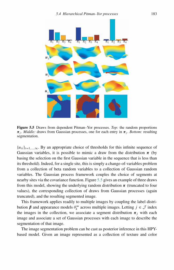
5.4 Hierarchical Pitman–Yor processes 183
u3
π1 π2 π3 π4 π1 π2 π3 π4 π1 π2 π3 π4
u2
u1
Figure 5.5 Draws from dependent Pitman–Yor processes. Top: the random proportionsπj . Middle: draws from Gaussian processes, one for each entry in πj . Bottom: resultingsegmentation.
{uti}t=1,...,∞. By an appropriate choice of thresholds for this infinite sequence ofGaussian variables, it is possible to mimic a draw from the distribution π (bybasing the selection on the first Gaussian variable in the sequence that is less thanits threshold). Indeed, for a single site, this is simply a change-of-variables problemfrom a collection of beta random variables to a collection of Gaussian randomvariables. The Gaussian process framework couples the choice of segments atnearby sites via the covariance function. Figure 5.5 gives an example of three drawsfrom this model, showing the underlying random distribution π (truncated to fourvalues), the corresponding collection of draws from Gaussian processes (againtruncated), and the resulting segmented image.
This framework applies readily to multiple images by coupling the label distri-bution β and appearance models θ∗∗
k across multiple images. Letting j ∈ J indexthe images in the collection, we associate a segment distribution πj with eachimage and associate a set of Gaussian processes with each image to describe thesegmentation of that image.
The image segmentation problem can be cast as posterior inference in this HPY-based model. Given an image represented as a collection of texture and color

184 Hierarchical nonparametric models with applications
descriptors, we compute the maximum a posteriori set of segments for the sites.Sudderth and Jordan (2009) have shown that this procedure yields a state-of-the-artunsupervised image segmentation algorithm.
5.5 The beta process and the Indian buffet process
The DP mixture model embodies the assumption that the data can be partitionedor clustered into discrete classes. This assumption is made particularly clear inthe Chinese restaurant representation, where the table at which a data point sitsindexes the class (the mixture component) to which it is assigned. If we representthe restaurant as a binary matrix in which the rows are the data points and thecolumns are the tables, we obtain a matrix with a single one in each row and allother elements equal to zero.
A different assumption that is natural in many settings is that objects can bedescribed in terms of a collection of binary features or attributes. For example, wemight describe a set of animals with features such as diurnal/nocturnal, avian/non-avian, cold-blooded/warm-blooded, etc. Forming a binary matrix in which the rowsare the objects and the columns are the features, we obtain a matrix in which thereare multiple ones in each row. We will refer to such a representation as a featuralrepresentation.
A featural representation can of course be converted into a set of clusters ifdesired: if there are K binary features, we can place each object into one of 2K
clusters. In so doing, however, we lose the ability to distinguish between classesthat have many features in common and classes that have no features in common.Also, if K is large, it may be infeasible to consider models with 2K parameters.Using the featural representation, we might hope to construct models that use onthe order of K parameters to describe 2K classes.
In this section we discuss a Bayesian nonparametric approach to featural rep-resentations. In essence, we replace the Dirichlet/multinomial probabilities thatunderlie the Dirichlet process with a collection of beta/Bernoulli draws. This isachieved via the beta process, a stochastic process whose realizations provide acountably infinite collection of coin-tossing probabilities. We also discuss someother representations of the beta process that parallel those for the DP. In particu-lar we describe a stick-breaking construction as well as an analog of the Chineserestaurant process known as the Indian buffet process.
5.5.1 The beta process and the Bernoulli process
The beta process is an instance of a general class of stochastic processes knownas completely random measures (Kingman, 1967; see also Chapters 3). The key

5.5 The beta process and the Indian buffet process 185
property of completely random measures is that the random variables obtainedby evaluating a random measure on disjoint subsets of the probability space aremutually independent. Moreover, draws from a completely random measure arediscrete (up to a fixed deterministic component). Thus we can represent such adraw as a weighted collection of atoms on some probability space, as we do for theDP. (Note, however, that the DP is not a completely random measure because theweights are constrained to sum to one for the DP; thus, the independence assertiondoes not hold for the DP. The DP can be obtained by normalizing a completelyrandom measure (specifically the gamma process; see Section 3.3.1).)
Applications of the beta process in Bayesian nonparametric statistics have mainlyfocused on its use as a model for random hazard functions (Hjort, 1990; see alsoChapters 3 and 4). In this case, the probability space is the real line and it isthe cumulative integral of the sample paths that is of interest (yielding a random,nondecreasing step function). In the application of the beta process to featuralrepresentations, on the other hand, it is the realization itself that is of interest andthe underlying space is no longer restricted to be the real line.
Following Thibaux and Jordan (2007), let us thus consider a general probabilityspace (�,�) endowed with a finite base measure B0 (note that B0 is not a prob-ability measure; it does not necessarily integrate to one). Intuitively we wish topartition � into small regions, placing atoms into these regions according to B0
and assigning a weight to each atom, where the weight is a draw from a beta distri-bution. A similar partitioning occurs in the definition of the DP, but in that case theaggregation property of Dirichlet random variables immediately yields a consistentset of marginals and thus an easy appeal to Kolmogorov’s theorem. Because thesum of two beta random variables is not a beta random variable, the construction issomewhat less straightforward in the beta process case.
The general machinery of completely random processes deals with this issue inan elegant way. Consider first the case in which B0 is absolutely continuous anddefine the Levy measure on the product space [0, 1] ⊗ � in the following way:
ν(dω, dθ) = cω−1(1 − ω)c−1dωB0(dθ), (5.37)
where c > 0 is a concentration parameter. Now sample from a nonhomogeneousPoisson process with the Levy measure ν as its rate measure. This yields a set ofatoms at locations (ω1, θ1), (ω2, θ2) . . .. Define a realization of the beta process as
B =∞∑
k=1
ωkδθk, (5.38)
where δθkis an atom at θk with ωk its mass in B. We denote this stochastic process as
B ∼ BP(c, B0). Figure 5.6(a) provides an example of a draw from BP(1, U [0, 1]),where U [0, 1] is the uniform distribution on [0, 1].
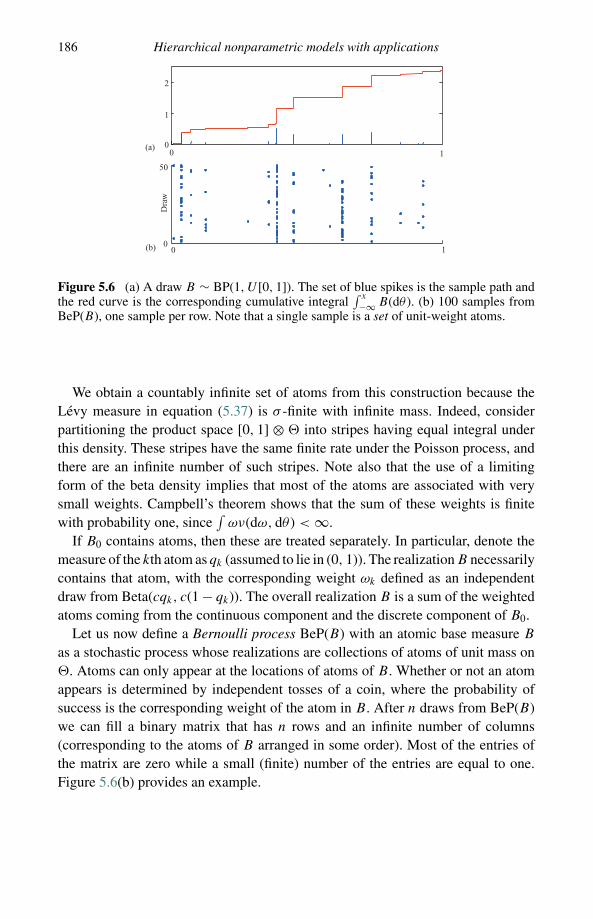
186 Hierarchical nonparametric models with applications
2
1
00
00 1
1(a)
(b)
50D
raw
Figure 5.6 (a) A draw B ∼ BP(1, U [0, 1]). The set of blue spikes is the sample path andthe red curve is the corresponding cumulative integral
∫ x
−∞ B(dθ ). (b) 100 samples fromBeP(B), one sample per row. Note that a single sample is a set of unit-weight atoms.
We obtain a countably infinite set of atoms from this construction because theLevy measure in equation (5.37) is σ -finite with infinite mass. Indeed, considerpartitioning the product space [0, 1] ⊗ � into stripes having equal integral underthis density. These stripes have the same finite rate under the Poisson process, andthere are an infinite number of such stripes. Note also that the use of a limitingform of the beta density implies that most of the atoms are associated with verysmall weights. Campbell’s theorem shows that the sum of these weights is finitewith probability one, since
∫ων(dω, dθ) < ∞.
If B0 contains atoms, then these are treated separately. In particular, denote themeasure of the kth atom as qk (assumed to lie in (0, 1)). The realization B necessarilycontains that atom, with the corresponding weight ωk defined as an independentdraw from Beta(cqk, c(1 − qk)). The overall realization B is a sum of the weightedatoms coming from the continuous component and the discrete component of B0.
Let us now define a Bernoulli process BeP(B) with an atomic base measure B
as a stochastic process whose realizations are collections of atoms of unit mass on�. Atoms can only appear at the locations of atoms of B. Whether or not an atomappears is determined by independent tosses of a coin, where the probability ofsuccess is the corresponding weight of the atom in B. After n draws from BeP(B)we can fill a binary matrix that has n rows and an infinite number of columns(corresponding to the atoms of B arranged in some order). Most of the entries ofthe matrix are zero while a small (finite) number of the entries are equal to one.Figure 5.6(b) provides an example.

5.5 The beta process and the Indian buffet process 187
The beta process and the Bernoulli process are conjugate. Consider the specifi-cation:
B | c, B0 ∼ BP(c, B0),(5.39)
Zi | B ∼ BeP(B) for i = 1, . . . , n,
where Z1, . . . , Zn are conditionally independent given B. The resulting posteriordistribution is itself a beta process, with updated parameters:
B | Z1, . . . , Zn, c, B0 ∼ BP
(c + n,
c
c + nB0 + 1
c + n
n∑i=1
Zi
). (5.40)
This formula can be viewed as an analog of standard finite-dimensional beta/Bernoulli updating. Indeed, given a prior Beta(a, b), the standard update takes theform a → a +∑i zi and b → b + n −∑i zi . In equation (5.40), c plays the roleof a + b and cB0 is analogous to a.
5.5.2 The Indian buffet process
Recall that the Chinese restaurant process can be obtained by integrating out theDirichlet process and considering the resulting distribution over partitions. In theother direction, the Dirichlet process is the random measure that is guaranteed(by exchangeability and de Finetti’s theorem) to underlie the Chinese restaurantprocess. In this section we discuss the analog of these relationships for the betaprocess.
We begin by defining a stochastic process known as the Indian buffet process(IBP). The IBP was originally defined directly as a distribution on (equivalenceclasses of) binary matrices by Griffiths and Ghahramani (2006) and Ghahramani,Griffiths and Sollich (2007). The IBP is an infinitely exchangeable distributionon these equivalence classes, thus it is of interest to discover the random mea-sure that must underlie the IBP according to de Finetti’s theorem. Thibaux andJordan (2007) showed that the underlying measure is the beta process; that is,the IBP is obtained by integrating over the beta process B in the hierarchy inequation (5.39).
The IBP is defined as follows. Consider an Indian buffet with a countably infinitenumber of dishes and customers that arrive in sequence in the buffet line. Let Z∗
denote a binary-valued matrix in which the rows are customers and the columnsare the dishes, and where Z∗
nk = 1 if customer n samples dish k. The first customersamples Poisson(α) dishes, where α = B0(�) is the total mass of B0. A subsequentcustomer n samples dish k with probability mk
c+n−1 , where mk is the number of

188 Hierarchical nonparametric models with applications
customers who have previously sampled dish k; that is, Z∗nk ∼ Bernoulli( mk
c+n−1 ).Having sampled from the dishes previously sampled by other customers, customern then goes on to sample an additional number of new dishes determined by a drawfrom a Poisson( c
c+n−1α) distribution.To derive the IBP from the beta process, consider first the distribution equa-
tion (5.40) for n = 0; in this case the base measure is simply B0. Drawing fromB ∼ BP(B0) and then drawing Z1 ∼ BeP(B) yields atoms whose locations aredistributed according to a Poisson process with rate B0; the number of such atomsis Poisson(α). Now consider the posterior distribution after Z1, . . . , Zn−1 havebeen observed. The updated base measure is c
c+n−1B0 + 1c+n−1
∑n−1i=1 Zi . Treat the
discrete component and the continuous component separately. The discrete com-ponent, 1
c+n−1
∑n−1i=1 Zi , can be reorganized as a sum over the unique values of
the atoms; let mk denote the number of times the kth atom appears in one of theprevious Zi . We thus obtain draws ωk ∼ Beta((c + n − 1)qk, (c + n − 1)(1 − qk)),where qk = mk
c+n−1 . The expected value of ωk is mk
c+n−1 and thus (under Bernoullisampling) this atom appears in Zn with probability mk
c+n−1 . From the continuouscomponent, c
c+n−1B0, we generate Poisson( cc+n−1α) new atoms. Equating “atoms”
with “dishes,” and rows of Z∗ with draws Zn, we have obtained exactly the proba-bilistic specification of the IBP.
5.5.3 Stick-breaking constructions
The stick-breaking representation of the DP is an elegant constructive characteri-zation of the DP as a discrete random measure (Chapter 2). This construction canbe viewed in terms of a metaphor of breaking off lengths of a stick, and it canalso be interpreted in terms of a size-biased ordering of the atoms. In this section,we consider analogous representations for the beta process. Draws B ∼ BP(c, B0)from the beta process are discrete with probability one, which gives hope thatsuch representations exist. Indeed, we will show that there are two stick-breakingconstructions of B, one based on a size-biased ordering of the atoms (Thibauxand Jordan, 2007), and one based on a stick-breaking representation known as theinverse Levy measure (Wolpert and Ickstadt, 1998).
The size-biased ordering of Thibaux and Jordan (2007) follows straightforwardlyfrom the discussion in Section 5.5.2. Recall that the Indian buffet process is definedvia a sequence of draws from Bernoulli processes. For each draw, a Poisson numberof new atoms are generated, and the corresponding weights in the base measure B
have a beta distribution. This yields the following truncated representation:
BN =N∑
n=1
Kn∑k=1
ωnkδθnk, (5.41)

5.5 The beta process and the Indian buffet process 189
where
Kn | c, B0 ∼ Poisson( cc+n−1α),
ωnk | c ∼ Beta(1, c + n − 1), for n = 1, . . . , ∞ (5.42)
θnk | B0 ∼ B0/α for k = 1, . . . , Kn.
It can be shown that this size-biased construction BN converges to B with probabilityone. The expected total weight contributed at step N is cα/{(c + N )(c + N − 1)},while the expected total weight remaining, in B − BN , is cα
c+N. The expected total
weight remaining decreases to zero as N → ∞, but at a relatively slow rate.Note also that we are not guaranteed that atoms contributed at later stages of theconstruction will have small weight – the sizes of the weights need not be indecreasing order.
The stick-breaking construction of Teh, Gorur and Ghahramani (2007) can bederived from the inverse Levy measure algorithm of Wolpert and Ickstadt (1998).This algorithm starts from the Levy measure of the beta process, and generatesa sequence of weights of decreasing size using a nonlinear transformation of aone-dimensional Poisson process to one with uniform rate. In general this approachdoes not lead to closed forms for the weights; inverses of the incomplete betafunction need to be computed numerically. However for the one-parameter betaprocess (where c = 1) we do obtain a simple closed form:
BK =K∑
k=1
ωkδθk, (5.43)
where
vk | α ∼ Beta(1, α),
ωk =k∏
l=1
(1 − vl), (5.44)
θk | B0 ∼ B0/α for k = 1, . . . , ∞.
Again BK → B as K → ∞, but in this case the expected weights decreaseexponentially to zero. Further, the weights are generated in strictly decreasingorder, so we are guaranteed to generate the larger weights first.
The stick-breaking construction for the one-parameter beta process has an in-triguing connection to the stick-breaking construction for the DP. In particular, bothconstructions use the same beta-distributed breakpoints vk; the difference is that forthe DP we use the lengths of the sticks just broken off as the weights while for thebeta process we use the remaining lengths of the sticks. This is depicted graphicallyin Figure 5.7.

190 Hierarchical nonparametric models with applications
ω1ω2
ω3
ω4 π4
π3
π2
π1
Figure 5.7 Stick-breaking construction for the DP and the one-parameter BP. The lengthsπi are the weights for the DP and the lengths ωi are the weights for the BP.
5.5.4 Hierarchical beta processes
Recall the construction of the hierarchical Dirichlet process: a set of Dirichlet pro-cesses are coupled via a random base measure. A similar construction can be carriedout in the case of the beta process: let the common base measure for a set of betaprocesses be drawn from an underlying beta process (Thibaux and Jordan, 2007).Under this hierarchical Bayesian nonparametric model, the featural representationsthat are chosen for one group will be related to the featural representations that areused for other groups.
We accordingly define a hierarchical beta process (HBP) as follows:
B0 | κ,A ∼ BP(κ,A),
Bj | c, B0 ∼ BP(c, B0), for j ∈ J (5.45)
Zji | Bj ∼ BeP(Bj ) for i = 1, . . . , nj ,
where J is the set of groups and there are nj individuals in group j . The hyperpa-rameter c controls the degree of coupling among the groups: larger values of c yieldrealizations Bj that are closer to B0 and thus a greater degree of overlap among theatoms chosen in the different groups.
As an example of the application of the HBP, Thibaux and Jordan (2007) con-sidered the problem of document classification, where there are |J | groups ofdocuments and where the goal is to classify a new document into one of thesegroups. In this case, Zji is a binary vector that represents the presence or absence inthe ith document of each of the words in the vocabulary �. The HBP yields a formof regularization in which the group-specific word probabilities are shrunk towardseach other. This can be compared to standard Laplace smoothing, in which wordprobabilities are shrunk towards a fixed reference point. Such a reference point canbe difficult to calibrate when there are rare words in a corpus, and Thibaux andJordan (2007) showed empirically that the HBP yielded better predictive perfor-mance than Laplace smoothing.
5.5 The beta process and the Indian buffet process 191
5.5.5 Applications of the beta process
In the following sections we describe a number of applications of the beta processto hierarchical Bayesian featural models. Note that this is a rather different class ofapplications than the traditional class of applications of the beta process to randomhazard functions.
Sparse latent variable models
Latent variable models play an essential role in many forms of statistical analysis.Many latent variable models take the form of a regression on a latent vector;examples include principal component analysis, factor analysis and independentcomponents analysis. Paralleling the interest in the regression literature in sparseregression models, one can also consider sparse latent variable models, where eachobservable is a function of a relatively small number of latent variables. The betaprocess provides a natural way of constructing such models. Indeed, under the betaprocess we can work with models that define a countably infinite number of latentvariables, with a small, finite number of variables being active (i.e., non-zero) inany realization.
Consider a set of n observed data vectors, x1, . . . , xn. We use a beta process tomodel a set of latent features, Z1, . . . , Zn, where we capture interactions amongthe components of these vectors as follows:
B | c, B0 ∼ BP(c, B0),(5.46)
Zi | B ∼ BeP(B) for i = 1, . . . , n.
As we have seen, realizations of beta and Bernoulli processes can be expressed asweighted sums of atoms:
B =∞∑
k=1
ωkδθk,
(5.47)
Zi =∞∑
k=1
Z∗ikδθk
.
We view θk as parametrizing feature k, while Zi denotes the features that are activefor item i. In particular, Z∗
ik = 1 if feature k is active for item i. The data point xi
is modeled as follows:
yik | H ∼ H,
xi | Zi, θ, yi ∼ F{θk,yik}k:Z∗ik
=1for k = 1, . . . , ∞,
(5.48)
where yik is the value of feature k if it is active for item i, and the distributionF{θk,yik}k:Z∗
ik=1
depends only on the active features, their values, and their parameters.

192 Hierarchical nonparametric models with applications
Note that this approach defines a latent variable model with an infinite number ofsparse latent variables, but for each data item only a finite number of latent variablesare active. The approach would often be used in a predictive setting in which thelatent variables are integrated out, but if the sparseness pattern is of interest per se,it is also possible to compute a posterior distribution over the latent variables.
There are several specific examples of this sparse latent variable model in theliterature. One example is an independent components analysis model with aninfinite number of sparse latent components (Knowles and Ghahramani, 2007; Teh,Gorur and Ghahramani, 2007), where the latent variables are real valued and xi
is a noisy observation of the linear combination∑
k Z∗ikyikθk . Another example
is the “noisy-or” model of Wood, Griffiths and Ghahramani (2006), where thelatent variables are binary and are interpreted as presence or absence of diseases,while the observations xi are binary vectors indicating presence or absence ofsymptoms.
Relational models
The beta process has also been applied to the modeling of relational data (alsoknown as dyadic data). In the relational setting, data are relations among pairs ofobjects (Getoor and Taskar, 2007); examples include similarity judgments betweentwo objects, protein–protein interactions, user choices among a set of options, andratings of products by customers.
We first consider the case in which there is a single set of objects and relationsare defined among pairs of objects in that set. Formally, define an observation asa relation xij between objects i and j in a collection of n objects. Each object ismodeled using a set of latent features as in equation (5.46) and equation (5.47). Theobserved relation xij between objects i and j then has a conditional distribution thatis dependent only on the features active in objects i and j . For example, Navarroand Griffiths (2007) modeled subjective similarity judgments between objects i andj as normally distributed with mean
∑∞k=1 θkZ
∗ikZ
∗jk; note that this is a weighted
sum of features active in both objects. Chu, Ghahramani, Krause and Wild (2006)modeled high-throughput protein–protein interaction screens where the observedbinding affinity of proteins i and j is related to the number of overlapping features∑∞
k=1 Z∗ikZ
∗jk, with each feature interpreted as a potential protein complex consist-
ing of proteins containing the feature. Gorur, Jakel and Rasmussen (2006) proposeda nonparametric elimination by aspects choice model where the probability of auser choosing object i over object j is modeled as proportional to a weighted sum,∑∞
k=1 θkZ∗ik(1−Z∗
jk), across features active for object i that are not active for objectj . Note that in these examples, the parameters of the model, θk , are the atoms ofthe beta process.
Relational data involving separate collections of objects can be modeled with thebeta process as well. Meeds, Ghahramani, Neal and Roweis (2007) modeled movie

5.6 Semiparametric models 193
ratings, where the collections of objects are movies and users, and the relationaldata consist of ratings of movies by users. The task is to predict the ratings ofmovies not yet rated by users, using these predictions to recommend new moviesto users. These tasks are called recommender systems or collaborative filtering.Meeds, Ghahramani, Neal and Roweis (2007) proposed a featural model wheremovies and users are modeled using separate IBPs. Let Z∗ be the binary matrix ofmovie features and Y ∗ the matrix of user features. The rating of movie i by userj is modeled as normally distributed with mean
∑∞k=1
∑∞l=1 θklZ
∗ikY
∗j l . Note that
this dyadic model cannot be represented using two independent beta processes,since there is a parameter θkl for each combination of features in the two IBPs. Thequestion of what random measure underlies this model is an interesting one.
5.6 Semiparametric models
The nonparametric priors introduced in previous sections can be combined withmore traditional finite-dimensional priors, as well as hierarchies of such priors.In the resulting semiparametric models, the object of inference may be the finite-dimensional parameter, with the nonparametric component treated as a nuisanceparameter to be integrated out. In other cases, the finite-dimensional parameters areto be integrated out and aspects of the nonparametric component are the inferentialfocus. In this section we describe two such semiparametric models based on theHDP. The first model couples the stick-breaking representation of the HDP witha Gaussian hierarchy, while the other is based on the Chinese restaurant franchiserepresentation of the HDP.
5.6.1 Hierarchical DPs with random effects
An important characteristic of the HDP is that the same atoms appear in differentDPs, allowing clusters to be shared across the different groups. The hierarchicalDP with random effects (HDP+RE) model of Kim and Smyth (2007) generalizesthe HDP by allowing atoms in different DPs to differ from each other to bettercapture group-specificity of cluster parameters. This model is based on the stick-breaking representation for HDPs. We begin with the standard representation forthe common random base measure G0 ∼ DP(γ,H ):
β | γ ∼ GEM(γ ),
θ∗∗k | H ∼ H, (5.49)
G0 =∞∑
k=1
βkδθ∗∗k
for k = 1, . . . , ∞.
194 Hierarchical nonparametric models with applications
For each group j ∈ J , the weights and atoms for the group-specific Gj differ fromG0 in the following way:
πj | β ∼ DP(α, β), for j ∈ Jθ∗jk | θ∗∗
k ∼ Tθ∗∗k, (5.50)
Gj =∞∑
k=1
πjkδθ∗jk
for k = 1, . . . , ∞,
where Tθ is a distribution centered at θ ; for example, Tθ might be a normal distri-bution with mean θ .
Kim and Smyth (2007) used the HDP+RE model to model bumps in functionalmagnetic resonance imaging (fMRI) data. fMRI analyses report areas of highmetabolic activity in the brain that are correlated with external stimuli in an attemptto discover the function of local brain regions. Such areas of activity often showup as bumps in fMRI images, and each bump can be modeled well using a normaldensity. An fMRI image then consists of multiple bumps and can be modeledwith a DP mixture. Each individual brain might have slightly different structureand might react differently to the same stimuli, while each fMRI machine hasdifferent characteristics. The HDP+RE model naturally captures such variationswhile sharing statistical strength across individuals and machines.
5.6.2 Analysis of densities and transformed DPs
In this section we describe another approach to introducing group-specific param-eters within the DP framework. The common base measure G0 is still given a DPprior as in equation (5.49), while the group-specific random measures are defineddifferently:
H0 =∞∑
k=1
βkTθ∗∗k,
(5.51)Gj | H0 ∼ DP(α, H0) for j ∈ J .
In the particular case in which H and Tθ are normal distributions with fixed vari-ances, this model has been termed the analysis of densities (AnDe) model byTomlinson and Escobar (2003), who used it for sharing statistical strength amongmultiple density estimation problems.
Sudderth, Torralba, Freeman and Willsky (2008) called the model given byequations (5.49) and (5.51) a transformed DP. The transformed DP is very similarto an HDP, the difference being that the atoms in G0 are replaced by distributionsparametrized by the atoms. If these distributions are smooth the measures Gj will

5.7 Inference for hierarchical nonparametric models 195
not share atoms as in the HDP. Instead each atom in Gj is drawn from Tθ∗∗k
withprobability βk. Identifying an atom of Gj with θ∗∗
k , the Chinese restaurant franchiserepresentation for the HDP can be generalized to the transformed DP. We havecustomers (draws from Gj ) going into restaurants (Gj ) and sitting around tables(draws from H0), while tables are served dishes (atoms in G0) from a franchise-wide menu (G0). In the HDP the actual dish served at the different tables thatorder the same dish are identical. For the transformed DP the dishes that areserved at different tables ordering the same dish on the menu can take on distinctvalues.
Sudderth, Torralba, Freeman and Willsky (2008) used the transformed DP asa model for visual scene analysis that can simultaneously segment, detect andrecognize objects within the scenes. Each image is first preprocessed into a set oflow-level descriptors of local image appearances, and equations (5.49) and (5.51)are completed with a mixture model for these descriptors:
θji | Gj ∼ Gj,(5.52)
xji | θji ∼ Fθjifor j ∈ J and i = 1, . . . , nj ,
where xji is one of nj image descriptors in image j and Fθjiis a distribution over
image descriptors parameterized by θji .The Chinese restaurant franchise representation of the transformed DP translates
to a hierarchical representation of visual scenes, with scenes consisting of multipleobjects and objects consisting of descriptors of local image appearances. To seethis, note that customers (xji) are clustered into tables (object instances), and tablesare served dishes from a global menu (each object instance belongs to an objectcategory). There could be multiple tables in the same restaurant serving variations(different “seasonings”) on a given dish from the global menu. This correspondsto the fact that there could be multiple instances of the same object category ina single visual scene, with each instance being in a different location or havingdifferent poses or lighting conditions (thus yielding transformed versions of anobject category template).
5.7 Inference for hierarchical Bayesian nonparametric models
In this section we discuss algorithmic aspects of inference for the hierarchicalBayesian nonparametric models that we have discussed in earlier sections. Ourtreatment will be brief and selective; in particular, we focus on relatively simplealgorithms that help to convey basic methodology and provide a sense of some ofthe options that are available. An underlying theme of this section is that the vari-ous mathematical representations available for nonparametric models – including

196 Hierarchical nonparametric models with applications
stick-breaking representations, urn models and truncations – can be combined invarious ways to yield a wide range of possible algorithmic implementations.
While we focus on sampling-based inference methods throughout this section,we also note that there is a growing literature on variational methods for inferencein hierarchical Bayesian nonparametric models; examples include Liang, Petrov,Jordan and Klein (2007), Teh, Kurihara and Welling (2008) and Sudderth andJordan (2009).
5.7.1 Inference for hierarchical Dirichlet processes
We begin by considering posterior inference for a simple HDP mixture model. Inthis model, the random measures Gj are drawn from an HDP model according toequation (5.1), and this HDP prior is completed as follows:
θji | Gj ∼ Gj,(5.53)
xji | θji ∼ Fθjifor i = 1, . . . , nj ,
where the ith observation in the j th group is denoted xji and where this observationis drawn from a distribution Fθji
indexed by θji . The latent parameter θji is drawnfrom Gj and can be viewed as indexing the mixture component associated withthe data point xji . We shall assume that H is conjugate to Fθ for simplicity.Nonconjugate models can be treated by adapting techniques from the DP mixtureliterature (cf. Neal, 2000).
Teh, Jordan, Beal and Blei (2006) presented sampling algorithms for the HDPmixture model based on both the CRF representation and the stick-breaking rep-resentation. In the following section we describe the CRF-based sampler. We thenturn to an alternative sampler that is based on the posterior representation of theHDP described in Section 5.2.3.
Chinese restaurant franchise sampler
Recall our notation for the CRF representation of the HDP. Customer i in restaurantj is associated with an i.i.d. draw from Gj and sits at table tj i . Table t in restaurantj is associated with an i.i.d. draw from G0 and serves a dish kjt from a franchise-wide menu. Dish k is associated with an i.i.d. draw from H . If H is an absolutelycontinuous measure then each such dish is unique with probability one. There arenjtk customers in restaurant j sitting at table t and eating dish k, and there are mjk
tables in restaurant j serving dish k.Given this setup, we describe a Gibbs sampler in which the table and dish
assignment variables are iteratively sampled conditioned on the state of all othervariables. The variables consist of {tj i}j∈J ,i=1,...,nj
and {kjt }j∈J ,t=1,...,mj · . The

5.7 Inference for hierarchical nonparametric models 197
parameters θji are integrated out analytically (recall our assumption of conjugacy).Consider the assignment of customer i in restaurant j to a table tj i . To resample tj i
we make use of exchangeability and imagine customer i being the last customer toenter restaurant j . The customer can sit at an already occupied table, can sit at anew table and be served an existing dish, or can sit at a new table and be served anew dish. The probabilities of these events are:
tj i = t with probability ∝ n¬ji
j t ·n
¬ji
j ·· +αfkjt
({xji}),
tj i = tnew, kjtnew = k with probability ∝ α
n¬ji
j ·· +α
m¬ji
·km
¬ji·· +γ
fk({xji}),tj i = tnew, kjtnew = knew with probability ∝ α
n¬ji
j ·· +α
γ
m¬ji·· +γ
fknew({xji}),(5.54)
where tnew and knew denote a new table and new dish, respectively, and wheresuperscript ¬ji denotes counts in which customer i in restaurant j is removed fromthe CRF (if this empties a table we also remove that table from the CRF alongwith the dish served on it). The fractional terms are the conditional priors given bythe CRF in equations (5.7) and (5.8), and fk({xji}) is defined using the followinggeneral notation:
fk({xji}ji∈D) =
∫h(θ )
∏j ′i′∈Dk∪D
fθ (xj ′i′)dθ∫h(θ )
∏j ′i′∈Dk\D
fθ (xj ′i′)dθ
, (5.55)
where D is an arbitrary index set, where Dk = {j ′i ′ : kj ′tj ′i′ = k} denotes theset of indices of data items currently associated with dish k, and where h(·) andfθ (·) denote the densities of H and Fθ respectively. In particular, fk({xji}) is themarginal conditional probability of the singleton data point xji in cluster k, givenall of the other data points currently assigned to cluster k.
The Gibbs update for the dish kjt served at table t in restaurant j is derivedsimilarly. The probabilities of the relevant events in this case are:
kjt =k with probability ∝ m
¬j t
·km
¬j t·· +γ
fk({xji : tj i = t}),knew with probability ∝ γ
m¬j t·· +γ
fknew({xji : tj i = t}).(5.56)
While the computational cost of the Gibbs updates is generally dominated by thecomputation of the marginal conditional probabilities fk(·), the number of possibleevents that can occur at one Gibbs step is one plus the total number of tables ordishes in all restaurants that are ancestors of j , and this number can be large in deepor wide hierarchies.

198 Hierarchical nonparametric models with applications
A drawback of the CRF sampler is that it couples sampling in the variousrestaurants (since all DPs are integrated out). This coupling makes deriving aCRF sampler for certain models (e.g. the HDP-HMM) difficult. An alternativeis to construct samplers that use a mixed representation – some DPs in stick-breaking representation and some in CRP representation – and thereby decouplethe restaurants (Teh, Jordan, Beal and Blei, 2006).
The CRF-based sampler can be easily extended to arbitrary hierarchies. It canalso be extended to the hierarchical Pitman–Yor process discussed in Section 5.4.
Posterior representation sampler
In Section 5.2.3 we showed that the posterior of the HDP consists of a discretepart corresponding to mixture components associated with data and a continuouspart corresponding to components not associated with data. This representation canbe used to develop a sampler which represents only the discrete part explicitly.In particular, referring to equations (5.10) and (5.12), the posterior representationsampler maintains only the weights β and {πj }j∈J . (The atoms {θ∗∗
k }k=1,...,K can beintegrated out in the conjugate setting.) We also make use of cluster index variableszji , defined so that θji = θ∗∗
zji(i.e., zji = kjtji
in the CRF representation).The sampler iterates between two phases: the sampling of the cluster indices
{zji}, and the sampling of the weights β and {πj }. The sampling of the clusterindices is a simple variation on the Gibbs updates in the CRF sampler describedabove. In particular, we define the following Gibbs conditionals:
zji ={
k with probability ∝ πjkfk({xji}),knew with probability ∝ πj0fknew({xji}).
(5.57)
If a new component knew is chosen, the corresponding atom is instantiated in thesampler. Specifically, the weights corresponding to this new atom can be generatedas follows:
v0 | γ ∼ Beta(γ, 1),
(βnew0 , βnew
K+1) = (β0v0, β0(1 − v0)),
vj | α, β0, v0 ∼ Beta(αβ0v0, αβ0(1 − v0)), (5.58)
(πnewj0 , πnew
j K+1) = (πj0vj , πj0(1 − vj )) for j ∈ J .
Finally we set zji = K + 1 and increment K.The second phase resamples the weights {πj }j∈J and β conditioned on the
cluster indices {zji}. The approach is to first integrate out the random measures,leaving a CRP representation as in Section 5.2.2, then the weights {πj }j∈J andβ can be sampled conditionally on the state of the CRF using equations (5.10)and (5.12). Because we are conditioning on {zji}, and customers with different

5.7 Inference for hierarchical nonparametric models 199
values of zji cannot be assigned to the same table, each restaurant effectively getssplit into independent “sub-restaurants,” one for each value of k. (See also therelated direct assignment sampler in Teh, Jordan, Beal and Blei (2006).) Let nj ·k bethe number of observations in group j assigned to component k, and let mjk be therandom number of tables in a sub-restaurant with nj ·k customers and concentrationparameter αβk. The {mjk} are mutually independent and thus a draw for each ofthem can be simulated using the CRP. We can now sample the β and {πj } usingequations (5.10) and (5.12).
5.7.2 Inference for HDP hidden Markov models
The posterior representation sampler of Section 5.7.1 can also be used to derive aGibbs sampler for the HDP-HMM. Consider the formulation of the HDP-HMMgiven in equations (5.23) and (5.24) where we make use of a sequence of latentindicator variables z1, . . . , zτ . We again assume that H is conjugate to Fθ . Note thatthe posterior of the HDP prior for the model (given z1, . . . , zτ ) can be decomposedinto a discrete part consisting of K atoms (corresponding to the K states currentlyvisited by z1, . . . , zτ ), as well as a continuous part consisting of unused atoms. Theweights on the K atoms (equivalently the transition probabilities among the K statescurrently used by the HDP-HMM) can be constructed from a CRF representationof the HDP:
(β0, β1, . . . , βK ) ∼ Dirichlet(γ,m·1, . . . , m·K ),
(πj0, πj1, . . . , πjK ) ∼ Dirichlet(αβ0, αβ1 + nj ·1, . . . , αβK + nj ·K )
for j = 1, . . . , K, (5.59)
where nj ·k is the number of transitions from state j to state k (equivalently thenumber of customers eating dish k in restaurant j ), while m·k is the number of tablesserving dish k in the CRF representation of the HDP. The conditional probabilitiesfor the Gibbs update of zt are as follows:
zt ={
k with probability ∝ πzt−1kπkzt+1fk({xt }),knew with probability ∝ πzt−10βzt+1fknew({xt }).
(5.60)
The three factors on the right-hand side are the probability of transitioning intothe current state, the probability of transitioning out of the current state, and theconditional probability of the current observation xt respectively. The βzt+1 factorarises because transitions from the new state knew have not been observed beforeso we need to use the conditional prior mean β. The weights β and transitionprobabilities πj can be updated as for the posterior representation sampler for plainHDPs.

200 Hierarchical nonparametric models with applications
This simple Gibbs sampler can converge very slowly due to strong dependencesamong the latent states (Scott, 2002). To obtain a faster algorithm we would like toupdate the latent states in a block via the forward-backward algorithm for HMMs;the traditional form of this algorithm cannot, however, be applied directly to theHDP-HMM since there are an infinite number of possible states. The solution is tolimit the number of states to a finite number so that the forward-backward algorithmbecomes feasible. Fox, Sudderth, Jordan and Willsky (2008) proposed doing thisvia a truncation of the stick-breaking process (cf. Ishwaran and James, 2001), whileVan Gael, Saatci, Teh, and Ghahramani (2008) proposed a slice sampling approachwhich adaptively limits the number of states to a finite number (Neal, 2003; Walker,2007).
5.7.3 Inference for beta processes
In this section we describe a Gibbs sampler for the beta process latent variablemodel described in Section 5.5.5. This sampler is based on the stick-breakingrepresentation of the beta process.
Recall that the model is defined in terms of a set of feature weights {ωk}k=1,...,∞and the atoms (feature parameters) {θk}k=1,...,∞. Moreover, corresponding to eachdata item xi , we have a set of binary feature “activities” {Z∗
ik}k=1,...,∞ and latentfeature values {yik}k=1,...,∞. The observed data item xi depends on {θk, yik}k:Z∗
ik=1.The conditional distributions defining the model are given in equations (5.44)
and (5.48), where p(Z∗ik = 1 | ωk) = ωk. Gibbs sampling in this model is straight-
forward except for a few difficulties which we describe below along with theirresolution.
The main difficulty with a Gibbs sampler is that there are an infinite number ofrandom variables that need to be sampled. To circumvent this problem, Teh, Gorurand Ghahramani (2007) propose to use slice sampling (Neal, 2003; Walker, 2007)to truncate the representation adaptively to a finite number of features. Consider anauxiliary variable s with conditional distribution:
s | Z∗, {ωk}k=1,...,∞ ∼ Uniform
[0, min
k:∃i,Z∗ik=1
ωk
], (5.61)
where the supremum in the range of s is the smallest feature weight ωk among thecurrently active features. Conditioned on the current state of the other variables anew value for s can easily be sampled. Conditioned on s, features for which ωk < s
are forced to be inactive since making them active would make s lie outside itsrange. This means that we only need to update the finite number of features forwhich ωk > s. This typically includes all the active features, along with a small

5.7 Inference for hierarchical nonparametric models 201
number of inactive features (needed for the sampler to explore the use of newfeatures).
A related issue concerns the representation of the model within the finite memoryof the computer. Using the auxiliary variable s it is clear that we need only representfeatures 1, . . . , K , where K is such that ωK+1 < s; that is, the model is truncatedafter feature K . As the values of s and the feature weights change over the courseof Gibbs sampling this value of K changes as well. If K is decreased we simplydelete the last few features, while if K is increased we sample the variables ωk,θk and yik corresponding to these new features from their conditional distributionsgiven the current state of the represented features.
The final issue is the problem of sampling the feature weights ω1, . . . , ωK . Unlikethe case of DPs, it is easier in this case to work with the weights directly instead ofthe stick-breaking variables vk . In particular, Teh, Gorur and Ghahramani (2007)showed that the joint probability for the weights is:
p(ω1, . . . , ωK ) = I(0 ≤ ωK ≤ · · · ≤ ω1 ≤ 1)αKωαK
K∏k=1
ω−1k , (5.62)
where I(·) = 1 if the predicate is true and 0 otherwise. For k = 1, . . . , K − 1the conditional probability of ωk given the other variables can be computed fromequation (5.62) and the conditional probability of Z∗
1k, . . . , Z∗nk given ωk. For ωK
we also have to condition on Z∗ik = 0 for all i and k > K; this probability can
be computed using the Levy–Khintchine representation for the beta process (Teh,Gorur and Ghahramani, 2007).
5.7.4 Inference for hierarchical beta processes
In this section we present an inference algorithm for the hierarchical beta processgiven in equation (5.45). The observed data are the variables Zji ; these binaryvectors denote (in the language of document classification) the presence or absenceof words in document i of group j . The underlying measure space � is interpreted asthe vocabulary. (Each element in � is referred to as a “word.”) Let θ1, . . . , θK ∈ �
denote the words that are observed among the documents. That is, these are theθ ∈ � such that Zji(θ ) = 1 for some i and j .
Because both the beta and Bernoulli processes are completely random measures,the posterior over B0 and Bj for j ∈ J decomposes into a discrete part over theobserved vocabulary {θ1, . . . , θK} and a continuous part over �\{θ1, . . . , θK}. Thediscrete part further factorizes over each observed word θk . Thus it is sufficient tofocus separately on inference for each observed word and for the continuous partcorresponding to unobserved words.

202 Hierarchical nonparametric models with applications
For a fixed θk , let a = A(θk), ω0 = B0(θk), ωj = Bj (θk) and zji = Zji(θk). Theslice of the HBP corresponding to θk has the following joint distribution:
ω0 | c0, a ∼ Beta(c0a, c0(1 − a)),
ωj | cj , ω0 ∼ Beta(cjω0, cj (1 − ω0)), for j ∈ J (5.63)
zji | ωj ∼ Bernoulli(ωj ) for i = 1, . . . , nj .
Note that the prior over ω0 is improper if A is continuous and a = 0. This betahierarchy is a special case of the finite Dirichlet hierarchy of equations (5.10)and (5.12) and it is straightforward to use the posterior representation samplerdescribed in Section 5.7.1 to sample from the posterior given the observed zji .Thibaux and Jordan (2007) described an alternative where the ωj are integrated outand rejection sampling is used to sample from ω0.
Finally, we consider the continuous part of the posterior. This component isnot simply the prior, since we have to condition on the fact that no words in�\{θ1, . . . , θK} have been observed among the documents. Thibaux and Jordan(2007) solved this problem by noting that the posterior factors over the levelsindexed by n in the size-biased ordering in equation (5.42). Focusing on each levelseparately, they derived a posterior distribution on the number of atoms in eachlevel, combining this with the posterior over the level-specific weights to obtain theoverall posterior.
5.8 Discussion
Our goal in this chapter has been to place hierarchical modeling in the same centralrole in Bayesian nonparametrics that it plays in other areas of Bayesian statistics.Indeed, one of the principal arguments for hierarchical modeling in parametricstatistics is that it provides control over the large numbers of degrees of freedomthat arise, for example, in random effects models. Such an argument holds a fortioriin the nonparametric setting.
Nonparametric priors generally involve hyperparameters, some of which arefinite dimensional and some of which are infinite dimensional. Sharing the finite-dimensional parameter among multiple draws from such a prior is a naturalmodeling strategy that mimics classical hierarchical modeling concepts. It is ourcontention, however, that this form of control is far too limited, and that the infinite-dimensional parameters should generally also be shared. We have made this pointprincipally by considering examples in applied problem domains. In domains suchas computational vision, information retrieval and genetics, nonparametric mod-els provide natural descriptions of the complex objects under study; in particular,it is natural to describe an image, a document or a genome as the realization

References 203
of a stochastic process. Now, in considering collections of such objects it isnatural to want to share details of the realization among the objects in the col-lection – we wish to share parts of objects, features, recurring phrases and motifs.This can be achieved by coupling multiple draws from a nonparametric prior viatheir infinite-dimensional parameters.
Another advantage of hierarchical modeling in the classical setting is that it ex-pands the repertoire of distributional forms that can be considered. For example,heavy-tailed distributions can be obtained by placing a prior on the scale parameterof lighter tailed distributions. Although this point has been little explored to date inthe nonparametric setting, we expect that it will be a fruitful direction for furtherresearch. In particular, there are stringent computational constraints that limit thenonparametric repertoire, and hierarchical constructions offer one way forward.Indeed, as we have seen, computationally oriented constructions such as urn mod-els and stick-breaking representations often carry over naturally to hierarchicalnonparametric models.
Finally, it is worth noting a difficulty that is raised by hierarchical modeling. Al-though Bayesian hierarchies help to control hyperparameters, they do not removethe need to specify distributions for hyperparameters. Indeed, when hyperparame-ters are placed high in a hierarchy it can be difficult to give operational meaning tosuch hyperparameters. One approach to coping with this issue involves consideringthe marginal probabilities that are induced by a nonparametric prior. For example,we argued that the marginals induced by a Pitman–Yor prior exhibit long tails thatprovide a good match to the power-law behavior found in textual data and imagestatistics. Further research is needed to develop this kind of understanding for awider range of hierarchical Bayesian nonparametric models and problem domains.
Acknowledgements We would like to thank David Blei, Jan Gasthaus, SamGershman, Tom Griffiths, Kurt Miller, Vinayak Rao and Erik Sudderth for theirhelpful comments on the manuscript.
ReferencesAntoniak, C. E. (1974). Mixtures of Dirichlet processes with applications to Bayesian
nonparametric problems. Annals of Statistics, 2, 1152–74.Beal, M. J., Ghahramani, Z. and Rasmussen, C. E. (2002). The infinite hidden Markov
model. In Advances in Neural Information Processing Systems, Volume 14, ed. T. G.Dietterich, S. Becker and Z. Ghahramani, 577–92. Cambridge, Mass.: MIT Press.
Blei, D. M., Griffiths, T. L., Jordan, M. I. and Tenenbaum, J. B. (2004). Hierarchical topicmodels and the nested Chinese restaurant process. In Advances in Neural InformationProcessing Systems, Volume 16, ed. S. Thrun, B. Scholkopt and L. K. Saul. Cambridge,Mass.: MIT Press.
Blei, D. M., Ng, A. Y. and Jordan, M. I. (2003). Latent Dirichlet allocation. Journal ofMachine Learning Research, 3, 993–1022.

204 Hierarchical nonparametric models with applications
Chen, S. F. and Goodman, J. T. (1998). An empirical study of smoothing techniques forlanguage modeling. Technical Report TR-10-98, Computer Science Group, HarvardUniversity.
Chen, S. F. and Goodman, J. T. (1999). An empirical study of smoothing techniques forlanguage modeling. Computer Speech and Language, 13, 359–93.
Chou, K. C., Willsky, A. S. and Benveniste, A. (1994). Multiscale recursive estimation,data fusion, and regularization. IEEE Transactions on Automatic Control, 39, 464–78.
Chu, W., Ghahramani, Z., Krause, R. and Wild, D. L. (2006). Identifying protein complexesin high-throughput protein interaction screens using an infinite latent feature model.In BIOCOMPUTING: Proceedings of the Pacific Symposium, 231–42.
Cowans, P. (2004). Information retrieval using hierarchical Dirichlet processes. In Pro-ceedings of the Annual International Conference on Research and Development inInformation Retrieval, Volume 27, 564–5.
Cowans, P. (2006). Probabilistic document modelling. PhD Thesis, University of Cam-bridge.
Duan, J. A., Guindani, M. and Gelfand, A. E. (2007). Generalized spatial Dirichlet processmodels. Biometrika, 94, 809–25.
Erosheva, E. (2003). Bayesian estimation of the grade of membership model. In BayesianStatistics 7, ed. J. M. Bernado et al., 501–10. Oxford: Oxford University Press.
Fei-Fei, L. and Perona, P. (2005). A Bayesian hierarchical model for learning natural scenecategories. In Proceedings of the IEEE Conference on Computer Vision and PatternRecognition, 524–31. Washington, DC: IEEE Computer Society.
Ferguson, T. S. (1973). A Bayesian analysis of some nonparametric problems. Annals ofStatistics, 1, 209–30.
Finkel, J. R., Grenager, T. and Manning, C. D. (2007). The infinite tree. In Proceedings ofthe Annual Meeting of the Association for Computational Linguistics.
Fox, E., Sudderth, E., Jordan, M. I. and Willsky, A. (2008). An HDP-HMM for systemswith state persistence. In Proceedings of the International Conference on MachineLearning, Volume 25.
Getoor, L. and Taskar, B., editors (2007). Introduction to Statistical Relational Learning.Cambridge, Mass.: MIT Press.
Ghahramani Z., Griffiths, T. L. and Sollich, P. (2007). Bayesian nonparametric latent featuremodels (with discussion and rejoinder). In Bayesian Statistics 8, ed. J. M. Bernado etal. Oxford: Oxford University Press.
Goldwater, S., Griffiths, T. and Johnson, M. (2006a). Interpolating between types and tokensby estimating power-law generators. In Advances in Neural Information ProcessingSystems, Volume 18, ed. Y Weiss, B. Scholkopt and J. Platt. Cambridge, Mass.: MITPress.
Goldwater, S., Griffiths, T. L. and Johnson, M. (2006b). Contextual dependencies in unsu-pervised word segmentation. In Proceedings of the 21st International Conference onComputational Linguistics and 44th Annual Meeting of the Association for Computa-tional Linguistics.
Gorur, D., Jakel, F. and Rasmussen, C. E. (2006). A choice model with infinitely manylatent features. In Proceedings of the International Conference on Machine Learning,Volume 23.
Griffiths, T. L. and Ghahramani, Z. (2006). Infinite latent feature models and the Indianbuffet process. In Advances in Neural Information Processing Systems, volume 18,ed. Y. Weiss, B. Scholkopt and J. Platt, 475–82. Cambridge, Mass.: MIT Press.

References 205
Hiemstra, D. and Kraaij, W. (1998). Twenty-one at TREC-7: Ad-hoc and cross-languagetrack. In Text REtrieval Conference, 174–185.
Hjort, N. L. (1990). Nonparametric Bayes estimators based on beta processes in modelsfor life history data. Annals of Statistics, 18, 1259–94.
Ho, M. W., James, L. F. and Lau, J. W. (2006). Coagulation fragmentation lawsinduced by general coagulations of two-parameter Poisson–Dirichlet processes.http://arxiv.org/abs/math.PR/0601608.
Huang, S. and Renals, S. (2007). Hierarchical Pitman–Yor language models for ASR inmeetings. In Proceedings of the IEEE Workshop on Automatic Speech Recognitionand Understanding, Volume 10.
Huang, X., Acero, A. and Hon, H.-W. (2001). Spoken Language Processing. Upper SaddleRiver, NJ: Prentice-Hall.
Ishwaran, H. and James, L. F. (2001). Gibbs sampling methods for stick-breaking priors.Journal of the American Statistical Association, 96, 161–73.
Johnson, M., Griffiths, T. L. and Goldwater, S. (2007). Adaptor grammars: a frameworkfor specifying compositional nonparametric Bayesian models. In Advances in NeuralInformation Processing Systems, Volume 19, ed. B. Scholkopt, J. Platt and T. Hoffman.Cambridge, Mass.: MIT Press.
Kim, S. and Smyth, P. (2007). Hierarchical Dirichlet processes with random effects. InAdvances in Neural Information Processing Systems, Volume 19, ed. B. Scholkopt,J. Platt and T. Hoffman. Cambridge, Mass.: MIT Press.
Kingman, J. F. C. (1967). Completely random measures. Pacific Journal of Mathematics,21, 59–78.
Kivinen, J., Sudderth, E. and Jordan, M. I. (2007a). Image denoising with nonparametrichidden Markov trees. In IEEE International Conference on Image Processing (ICIP),San Antonio, Tex., 121–4.
Kivinen, J., Sudderth, E. and Jordan, M. I. (2007b). Learning multiscale representationsof natural scenes using Dirichlet processes. In IEEE International Conference onComputer Vision (ICCV), Rio de Janeiro, Brazil.
Knowles, D. and Ghahramani, Z. (2007). Infinite sparse factor analysis and infinite indepen-dent components analysis. In International Conference on Independent ComponentAnalysis and Signal Separation, Volume 7 of Lecture Notes in Computer Science.Springer.
Liang, P., Petrov, S., Jordan, M. I. and Klein, D. (2007). The infinite PCFG using hierarchicalDirichlet processes. In Proceedings of the Conference on Empirical Methods in NaturalLanguage Processing.
MacEachern, S., Kottas, A. and Gelfand, A. (2001). Spatial nonparametric Bayesian models.Technical Report 01-10, Institute of Statistics and Decision Sciences, Duke University.http://ftp.isds.duke.edu/WorkingPapers/01-10.html.
MacKay, D. and Peto, L. (1994). A hierarchical Dirichlet language model. Natural Lan-guage Engineering, 1, 1–19.
Manning, C. D. and Schutze, H. (1999). Foundations of Statistical Natural LanguageProcessing. Cambridge, Mass.: MIT Press.
Meeds, E., Ghahramani, Z., Neal, R. M. and Roweis, S. T. (2007). Modeling dyadic datawith binary latent factors. In Advances in Neural Information Processing Systems,Volume 19, ed. B. Scholkopt, J. Platt and T. Hoffman. Cambridge, Mass.: MIT Press.
Navarro, D. J. and Griffiths, T. L. (2007). A nonparametric Bayesian method for inferringfeatures from similarity judgements. In Advances in Neural Information ProcessingSystems, Volume 19, ed. B. Scholkopt, J. Platt and T. Hoffman. Cambridge, Mass.:MIT Press.

206 Hierarchical nonparametric models with applications
Neal, R. M. (2000). Markov chain sampling methods for Dirichlet process mixture models.Journal of Computational and Graphical Statistics, 9, 249–65.
Neal, R. M. (2003). Slice sampling. Annals of Statistics, 31, 705–67.Oliva, A. and Torralba, A. (2001). Modeling the shape of the scene: A holistic representation
of the spatial envelope. International Journal of Computer Vision, 42, 145–75.Perman, M., Pitman, J. and Yor, M. (1992). Size-biased sampling of Poisson point processes
and excursions. Probability Theory and Related Fields, 92, 21–39.Pitman, J. (2002). Combinatorial stochastic processes. Technical Report 621, Department
of Statistics, University of California at Berkeley. Lecture notes for St. Flour SummerSchool.
Pitman, J. and Yor, M. (1997). The two-parameter Poisson–Dirichlet distribution derivedfrom a stable subordinator. Annals of Probability, 25, 855–900.
Pritchard, J., Stephens, M. and Donnelly, P. (2000). Inference of population structure usingmultilocus genotype data. Genetics, 155, 945–59.
Rabiner, L. (1989). A tutorial on hidden Markov models and selected applications in speechrecognition. Proceedings of the IEEE, 77, 257–85.
Robertson, S. E., Walker, S., Hancock-Beaulieu, M., Gull, A. and Lau, M. (1992). Okapiat TREC. In Text REtrieval Conference, 21–30.
Salton, G. and McGill, M. (1983). An Introduction to Modern Information Retrieval. NewYork: McGraw-Hill.
Scott, S. L. (2002). Bayesian methods for hidden Markov models: Recursive computing inthe 21st century. Journal of the American Statistical Association, 97, 337–51.
Sethuraman, J. (1994). A constructive definition of Dirichlet priors. Statistica Sinica, 4,639–50.
Stephens, M., Smith, N. and Donnelly, P. (2001). A new statistical method for haplotypereconstruction from population data. American Journal of Human Genetics, 68, 978–89.
Sudderth, E. and Jordan, M. I. (2009). Shared segmentation of natural scenes using depen-dent Pitman-Yor processes. In Advances in Neural Information Processing Systems,Volume 21.
Sudderth, E., Torralba, A., Freeman, W. and Willsky, A. (2008). Describing visual scenesusing transformed objects and parts. International Journal of Computer Vision, 77,291–330.
Teh, Y. W. (2006a). A Bayesian interpretation of interpolated Kneser-Ney. Technical ReportTRA2/06, School of Computing, National University of Singapore.
Teh, Y. W. (2006b). A hierarchical Bayesian language model based on Pitman–Yor pro-cesses. In Proceedings of the 21st International Conference on Computational Lin-guistics and 44th Annual Meeting of the Association for Computational Linguistics,985–92. Morristown, NJ: Association for Computational Linguistics.
Teh, Y. W., Gorur, D. and Ghahramani, Z. (2007). Stick-breaking construction for theIndian buffet process. In Proceedings of the International Conference on ArtificialIntelligence and Statistics, Volume 11, ed. M. Meila and X. Shen, 556–63. Brookline,Mass.: Microtone.
Teh, Y. W., Jordan, M. I., Beal, M. J. and Blei, D. M. (2006). Hierarchical Dirichletprocesses. Journal of the American Statistical Association, 101, 1566–81.
Teh, Y. W., Kurihara, K. and Welling, M. (2008). Collapsed variational inference for HDP.In Advances in Neural Information Processing Systems, Volume 20.
Thibaux, R. and Jordan, M. I. (2007). Hierarchical beta processes and the Indian buffetprocess. In Proceedings of the International Workshop on Artificial Intelligence andStatistics, Volume 11, 564–71.
References 207
Tomlinson, G. and Escobar, M. (2003). Analysis of densities. Talk given at the JointStatistical Meeting.
Van Gael, J., Saatci, Y., Teh, Y. W. and Ghahramani, Z. (2008). Beam sampling for theinfinite hidden Markov model. In Proceedings of the International Conference onMachine Learning, Volume 25, 1088–95.
Walker, S. G. (2007). Sampling the Dirichlet mixture model with slices. Communicationsin Statistics: Simulation and Computation, 36, 45.
Wolpert, R. L. and Ickstadt, K. (1998). Simulations of Levy random fields. In PracticalNonparametric and Semiparametric Bayesian Statistics, 227–42. Springer-Verlag.
Wood, F., Griffiths, T. L. and Ghahramani, Z. (2006). A non-parametric Bayesian method forinferring hidden causes. In Proceedings of the Conference on Uncertainty in ArtificialIntelligence, Volume 22, 536–43. AUAI Press.
Wooters, C. and Huijbregts, M. (2007). The ICSI RT07s speaker diarization system. InLecture Notes in Computer Science. Springer.
Xing, E. P., Jordan, M. I. and Sharan, R. (2007). Bayesian haplotype inference via theDirichlet process. Journal of Computational Biology, 14, 267–84.
Xing, E. P. and Sohn, K. (2007). Hidden Markov Dirichlet process: Modeling geneticrecombination in open ancestral space. Bayesian Analysis 2, ed. J. M. Bernado et al.Oxford: Oxford University Press.
Xing, E. P., Sohn, K., Jordan, M. I. and Teh, Y. W. (2006). Bayesian multi-populationhaplotype inference via a hierarchical Dirichlet process mixture. Proceedings of the23rd International Conference on Machine Learning. ACM International ConferenceProceeding Series, Volume 148, 1049–56. New York: ACM Press.

6
Computational issues arising in Bayesiannonparametric hierarchical models
Jim Griffin and Chris Holmes
Chapter 5 highlights the rich dependence structures that can be captured via Bayesiannonparametric models using multistage (nonparametric) hierarchies illustrated graphicallyin Figure 5.2. The applications they present are impressive and we can see real opera-tional benefits provided by the careful specification of additional layers of dependences.In this companion chapter we examine in detail some of the related key issues, includingcomputational challenges and the use of de Finetti’s representation theorem.
6.1 Introduction
Hierarchical models have played a central role in Bayesian inference since thetime of Good (1965) with Lindley and Smith (1972) a key milestone providing thefirst comprehensive treatment of hierarchical priors for the parametric Bayes linearmodel. The Bayesian hierarchies have proved so popular because they provide anatural framework for “borrowing of strength” (a term apparently due to Tukey) orsharing partial information across components through the hierarchical structure.The Bayesian construction also provides a clear distinction from frequentist modelsin that the dependence structures do not have to be directly related to populationrandom effects.
In this chapter we will look a little more closely at a couple of key issues emerg-ing from the work of Teh and Jordan. First, we briefly step back a little and considerthe fundamental notion played by de Finetti’s representation theorem, reiteratingthe operational focus of Bayesian modeling on finite-dimensional specification ofjoint distributions on observables. Second, we explore in depth some of the com-putational challenges and solutions arising in the field of Bayesian nonparametrics.It is perhaps not surprising that when working with infinite-dimensional objects wefind that interesting numerical challenges arise! Bayesian statistics is a surprisinglysimple axiomatic discipline (Bernardo and Smith, 1994), prescriptive in nature, yetthe solutions arising from inference problems rarely have simple analytic form thusnecessitating numerical methods. Again we note that this is hardly surprising as we
208

6.2 Construction of finite-dimensional measures 209
see no reason why in general Nature should adhere to a small collection of compu-tationally convenient model forms for which integrals on parameters have closedform. The history of Bayesian statistics has been marked by the close connections indevelopment between modelers striving for more realistic structures in their mod-els and computational researchers providing the tools to facilitate inference. Theadvancement in Monte Carlo methods post Gelfand and Smith (1990) was drivenby the needs of practitioners looking for richer modeling structures over and abovethe likelihood-conjugate-prior constructions that dominated applied Bayesian workat that time. In a similar manner it is clear that as Bayesian nonparametric methodsdevelop and branch out we will want to see similar innovative progress in the com-putational methods needed to allow inference to take place. As such, computationis a critical part of modern statistics, both Bayesian and non-Bayesian alike.
In the next section we briefly treat the central role played by the representationtheorem, before moving on to discuss computational issues arising in Bayesiannonparametrics.
6.2 Construction of finite-dimensional measures on observables
The infinite-dimensional constructions of Bayesian nonparametrics belies the sim-ple objectives of Bayesian modeling. Bayesian modeling and inference is concernedwith the quantification of prior beliefs about observables via probability distribu-tions and probability calculus. In this quest we may rely on certain structural formsof parametric models (or “likelihoods”) from which we instil our beliefs on ob-servables via beliefs on parameters of such models, interpreted as beliefs aboutthe law limit of observables. The validity of such an operation and the interpreta-tion of this construction is underpinned by de Finetti’s representation theorem andgeneralizations thereof. Hence de Finetti’s representation theorem both motivatesthe construction of prior densities on structural model parameters and providesclear operational interpretation of such priors. To reiterate, by “model” M werefer to the specification of a joint distribution P (x|M) on a set of observablesx = {x1, . . . , xn} with xi ∈ �k . One of the distinguishing features of Bayesianstatistics is that all of Bayesian inference is “model based” (for some backgroundsee the lively discussion in Gelman, 2008).
Loosely speaking, de Finetti’s general representation theorem for real-valuedexchangeable random quantities {x1, . . . , xn}, xi ∈ �k , states that for any jointprobability measure P on {x1, . . . , xn} there exists a measure Q over T , the spaceof all distribution functions on �k such that
P (x1, . . . , xn) =∫T
n∏i
F (xi)dQ(F ),

210 Computational issues of Bayesian nonparametric models
where Q(F ) can be thought about beliefs about the limiting empirical distributionfunction Fn
Q(F ) = limn→∞ P (Fn).
Traditional parametric models can be seen as restricting the span of Q(·) to certainfamilies of distributions of standard form such as “Gaussian” or “gamma.” Thatis, they give probability zero to distributions F ′ outside of the parametric family,Q(F ′) = 0 for F /∈ �Q where �Q denotes the space of parametric probabilitymeasures defined under Q(·). The rationale for nonparametric modeling is to inducea Q(·) which has wider coverage. This then allows for richer forms of dependencestructures in models for observations P (x1, . . . , xn). However, it is worth repeatingthat whatever the span of Q(·) the dimension of P (·) is finite.
One of the great strengths in the hierarchical structures described by Teh andJordan is when the observations are colored as P (x1, . . . , xnx
, y1, . . . , yny, z1, . . .)
for different classes of exchangeable observations {x, y, z, . . .}. Here the hierar-chical construction allows for information to be shared and information transferthrough the hierarchy structure. For certain classes of inference problems there areclear benefits of endowing Q(·) with a nonparametric measure, as ably demon-strated in Chapter 5. As the field moves forward it will be interesting to see whatadditional classes of problems are amenable to benefit from nonparametric struc-tures. As a modeler it is always worth asking what is the price to pay for additionalfreedom. The types of nonparametric priors are to date reasonably small with theDirichlet process by far the most widespread. Yet jumping from the finite to theinfinite is a big step. For example, the Dirichlet process prior only has a singleparameter α, F ∼ DP(α, F0) to control for departures of realizations of the infinite-dimensional random measure F from F0. This can be seen to be quite restrictive.Often we will have strong prior beliefs about certain properties of P (x1, . . . , xn)in particular for the marginal densities P (xi) such as unimodality, symmetry, or“smoothness” in P (xi, xj ) as |xi − xj | → 0. Such properties can be hard to controlwhen Q(·) has such freedom. It is testament to the creativity of modelers that wehave come so far with such currently restrictive nonparametric structures. Greenand Richardson (2001) provide some interesting discussion on the implications ofgoing nonparametric.
As a final remark in this section, and as Teh and Jordan note in the last line ofChapter 5, there is a danger in giving a model too much rope or to put it anotherway “nothing can come from nothing.”
Having considered some of the operational motivation of Bayesian nonparamet-rics and the interpretation as beliefs about limiting distributions on observations wenow turn to some of the computational challenges arising in inference.

6.3 Recent advances in computation 211
6.3 Recent advances in computation for Dirichlet process mixture models
A powerful driving force behind the development and application of Bayesiannonparametric methods has been the availability of efficient computational methodsusing Markov chain Monte Carlo methods (Smith and Roberts, 1993; Tierney,1994). The standard model to be fitted is the Dirichlet process mixture model (Lo,1984). This model can be written hierarchically as
yi ∼ g(yi |φi) i = 1, 2, . . . , n
φi ∼ F i = 1, 2, . . . , n
F ∼ DP(M, H ),
where g(yi |φ) is a probability distribution with parameters φ, M > 0 is a positivemass parameter and H is a distribution. Standard results for the Dirichlet processshow that the realized distribution F can be expressed as
F =∞∑
k=1
wkδθk(6.1)
where w1, w2, w3, . . . are a sequence of positive random variables such that∑∞i=1 wi = 1 almost surely and θ1, θ2, θ3, . . . are an infinite sequence of inde-
pendent and identically distributed random variables with distribution H , whichhas density h for a continuous distribution. This implies that the marginal distribu-tion of yi is a mixture model with an infinite number of components. The commoncomputational approach to fitting this model introduces latent allocation variables(s1, s2, . . . , sn) which yield the modified hierarchical model
yi ∼ g(yi |θsi
)i = 1, 2, . . . , n
p(si = k) = wk i = 1, 2 . . . , n, k = 1, 2, 3 . . .
w1, w2, w3, · · · ∼ GEM(M)
θ1, θ2, θ3, · · · i.i.d.∼ H,
where GEM represents the distribution of the weights in a Dirichlet process (seePitman, 2002). The collection of latent variables will be denoted s = (s1, s2, . . . , sn).This form of model makes explicit the independence of (θ1, θ2, θ3, . . . ) and(w1, w2, w3, . . . ) under the prior which is an important property for posteriorsimulation of Dirichlet process mixture models (and many other infinite mixture

212 Computational issues of Bayesian nonparametric models
models). A useful expression of the GEM process of the weights is through thestick-breaking representation of the Dirichlet process (Sethuraman, 1994) given by
wk = vk
∏j<k
(1 − vj )
where v1, v2, v3, . . . are an infinite sequence of Be(1, M) random variables. Al-ternatively, we can integrate out the infinite sequence from w1, w2, w3, . . . fromthe posterior distribution defined by the augmented model. This can be elegantlyachieved using the Polya urn scheme representation (PUS) of the Dirichlet pro-cess (Blackwell and MacQueen, 1973), which is closely related to the Chineserestaurant process (Aldous, 1985). The PUS expresses the finite distribution of thestochastic process s1, s2, s3, . . . , sn in terms of the distribution of si conditional on(s1, s2, . . . , si−1) which has the form
p(si =k|s1, s2, . . . , si−1)= M
M + i − 1δk=max1≤j≤i−1{sj }+1 +
i−1∑j=1
1
M + i − 1δk=sj .
The marginal posterior distribution of the allocation variables (s1, s2, . . . , sn) canbe derived by integrating (θ1, θ2, θ3, . . . ) from the posterior distribution and has theform
p(s1, s2, . . . , sn|y) ∝ p(s1, s2, . . . , sn)p(y|s1, s2, . . . , sn) (6.2)
where
p(y|s1, s2, . . . , sn) =K∏
i=1
∫ ∏j∈Si
g(yj |θi)h(θi) dθi. (6.3)
Here, K represents the number of distinct values in (s1, s2, . . . , sn) and Si is the setof k = 1, . . . , n for which sk = i. We will call (S1, S2, . . . , SK ) a configuration of(1, 2, . . . , n) and Si a cluster. Clearly, the usefulness of this expression depends onthe availability of an analytic form for
∫ ∏j∈Si
g(yj |θi)h(θi) dθi for any value ofK and configurations (S1, S2, . . . , SK ). In particular, this will be available if h(θ )is conjugate with g(yi |θ ).
The initial work on Markov chain Monte Carlo methods for Dirichlet processmixture models used the marginal posterior in equation (6.2) to define Gibbs sam-pling schemes. Many variations and extensions are possible and this work is re-viewed by MacEachern (1998). Models where the integrals in equation (6.3) are notanalytically available are termed nonconjugate Dirichlet process mixture models.These models are generally more complicated to fit than the conjugate version.Neal (2000), developing ideas of MacEachern and Muller (1998), constructed effi-cient algorithms to fit such models.

6.3 Recent advances in computation 213
The methods described so far offer a wide range of alternatives for fitting Dirichletprocess mixture models. One concern is the mixing over the posterior distributionof (s1, s2, . . . , sn) which can be slow due to “single-site” updating where si issampled conditional on (s1, s2, . . . , si−1, si+1, si+2, . . . , sn). For example, supposethat configurations S ′
1, S′2 and S ′′
1 , S ′′2 are well supported by the data. A single-site
updating scheme can only move between these configurations by visiting interme-diate configurations that differ by moving a single observation from one cluster tothe other. This scheme will mix poorly if there are no well-supported intermediateconfigurations, since only one observation can be moved between clusters at a time.These problems can be addressed using split-and-merge moves (see e.g. Jain andNeal, 2004, 2007) where either a single cluster is split or two clusters are merged topropose a new configuration. This proposal is either accepted or rejected using theMetropolis–Hastings acceptance probability. The sampler will only be efficient ifthe proposals have a reasonable chance of being accepted. Jain and Neal (2004) usestandard Gibbs sampling method for Dirichlet process mixture models to generateproposals that have good acceptance rates. The algorithm for updating a conju-gate Dirichlet process mixture model (Jain and Neal, 2004) works in the followingway.
1. Select two distinct observations i and j uniformly at random.
2. Let S denote the observations k = 1, 2, . . . , n for which k �= i and k �= j andsk = si or sj = si .
3. Define a launch state slaunch using the following process. If si = sj , thenslaunchi is set to be a new component such that s launch
i /∈ {s1, s2, . . . , sn} andlet slaunch
j = sj . Otherwise, if si �= sj , then let slaunchi = si and slaunch
j = sj .
For every k ∈ S, set slaunchk = slaunch
i with probability 12 and slaunch
k = slaunchj
otherwise. Finally if k ∈ {i, j} ∪ S, let s launchk = sk. We then run a standard
single-site Gibbs sampler to update sk for all k ∈ S for t iterations where sk
can only take the values slaunchi or s launch
j .
4. If si = sj , we propose to change the si th cluster into two parts. The newallocations will be given by ssplit which is sampled in the following way.
(a) ssplitk = slaunch
k for k = 1, 2, . . . , n.
(b) If k ∈ S, update ssplitk using a Gibbs sampler restricted as in 3. Let qk be
the probability of the chosen state under the Gibbs sampler.
The proposed state ssplit is accepted with probability
α = min
{1,
p(y∣∣ssplit
)p(ssplit
)p (y|s) p (s)
∏k∈S qk
}.

214 Computational issues of Bayesian nonparametric models
5. If si �= sj , then we have the following.
(a) Propose to merge the si th and sj th clusters and propose the vector smerge
where
• smergei = sj , s
mergej = sj ,
• if k ∈ S, smergek = sj ,
• smergek = sk if k /∈ {i, j} ∪ S.
(b) For k ∈ S calculate the probability under a Gibbs sampling step of allo-cating s launch
k to sk where sk could only take the values si or sj . Let thisprobability be q ′
k:
α = min
{1,
p (y |smerge ) p (smerge)∏
k∈S q ′k
p (y|s) p (s)
}.
The number of intermediate steps of Gibbs sampling, t , is a tuning parameter andcan be chosen to encourage good mixing of the chain, see Jain and Neal (2004) forsome guidelines. Extensions of this algorithm to the nonconjugate case are givenin Jain and Neal (2007).
Posterior simulation of Dirichlet process mixture models using Polya urnschemes are computationally efficient but the extension of these methods to othernonparametric priors depends on the availability of a Polya urn scheme. This has ledto interest in alternative methods which avoid integrating out the random measureF from the posterior. We describe three possible approaches: truncation of F , ret-rospective sampling methods and slice sampling. The truncation method replacesthe infinite-dimensional random distribution function
F∞d=
∞∑k=1
wkδθk
with a finite version
FNd=
N∑k=1
wkδθk
where now∑N
k=1 wk = 1 almost surely. This leads to a finite-dimensional posteriordistribution which can be simulated directly using standard methods. Truncatedversions of the Dirichlet process were initially considered by several authors in-cluding Muliere and and Secchi (1996), Muliere and Tardella (1998), Ishwaran andZarepour (2000) and Ishwaran and James (2000, 2001). The use of these methodsraises two important concerns: (1) how to choose the number of atoms N to in-clude in the truncation to avoid a large probability of a big difference between F
and FN ; and (2) how to update efficiently a potentially large number of parameters.Ishwaran and James (2001) describe solutions to both problems for the more general

6.3 Recent advances in computation 215
class of stick-breaking priors. This class of process is parameterized by two infinitesequences of positive numbers, a = (a1, a2, a3, . . . ) and b = (b1, b2, b3, . . . ) anddefines the weights in equation (6.1) by wk = vk
∏j<k(1 − vj ) for a sequence
of independent random variables v1, v2, v3, . . . for which vi ∼ Be(ai, bi). TheDirichlet process arises if ai = 1 and bi = M for all i. The process can be simplytruncated by setting vN = 1 since wk = 0 for k > N .
Ishwaran and James (2001) argue that N should be chosen to control the differ-ence between the probability of the observations under the truncated and infinite-dimensional priors. The probability under FN is given by
πN (y) =∫ ( n∏
i=1
g(yi |θi)FN (dθi)
)�N (FN )
where �N represents the probability law of FN (this definition extends to theinfinite-dimensional case by setting N = ∞). The distance between the probabilityof the sample under the finite approximation, πN (y), and the infinite-dimensionalversion, π∞(y), can be measured using the L1 distance which will be denoted ‖ · ‖1.Ishwaran and James (2001) derive the following bound:
‖ πN (X) − π∞(X) ‖1≤ 4
[1 − E
{(N−1∑k=1
wk
)n}].
The value of N can be chosen to make this bound small. In the case of a Dirichletprocess prior, they derive a simpler, approximate expression:
4
[1 − E
{(N−1∑k=1
wk
)n}]≈ 4n exp{−(N − 1)/M}.
This allows the simple calculation of a value of N that gives a particular level oferror.
The value of N derived for the approximation is potentially large. Ishwaranand James (2001) show that efficient methods for updating a large number ofparameters are available for the stick-breaking processes. The posterior distributionis now defined on (s1, s2, . . . , sn), v = (v1, v2, . . . , vN−1) and θ = (θ1, θ2, . . . , θN ).Both θ and v can be updated in a block which leads to good mixing properties. TheGibbs sampler has the following steps.
1. The elements of θ are conditionally independent under the full conditionaldistribution. The full conditional of θj is proportional to h(θj )
∏{i|si=j} g(yi |θj ).
2. The elements of v are conditionally independent under the full conditionaldistribution. The full conditional of vj is Be(aj + nj , bj + mj ) where nj =∑n
i=1 I(si = j ) and mj =∑ni=1 I(si > j ).

216 Computational issues of Bayesian nonparametric models
3. Each element of s1, s2, . . . , sn can be updated using the standard mixturemodel update. The parameter si is updated from the distribution p(si = j ) ∝wjg(yi |θj ), j = 1, 2, . . . , N .
Replacing an infinite-dimensional object with a closely approximating finite-dimensional version can allow useful extensions to standard methods, such asthe nested Dirichlet processes (Rodriguez, Dunson and Gelfand, 2008). Furtherexamples are given in Chapter 7.
A drawback with truncation methods is the need to define a truncation pointN . The result of Ishwaran and James (2001) gives a condition for stick-breakingprocesses but fitting results would need to be derived if other classes of nonpara-metric prior were to be fitted. The truncation point also depends on the parametersof the prior which will often be assumed unknown and given a prior themselves.Finding a value of the truncation point which works well for a range of values ofthese parameters which have good posterior support may be difficult. Thereforeit is useful to develop methods which have random truncation points. Remark-ably, it is possible to define methods that use a finite number of parameters inthe sampler but which have the correct posterior under the infinite-dimensionalprior. There are two classes of such methods: retrospective samplers and slicesamplers.
The first proposed method was the retrospective sampler for Dirichlet processmixture models (Papaspiliopoulos and Roberts, 2008) which exploits the followingobservation for stick-breaking processes. We can simulate a draw, φ, from theunknown distribution F using standard inversion sampling for discrete distributions.The algorithm is as follows.
1. Simulate u ∼ unif(0, 1).
2. Find the value of k for which∑k
j=1 wj ≤ u <∑k+1
j=1 wj .
3. Set φ = θk .
A finite value of i must exist since∑i+1
j=1 wj is an increasing sequence boundedby 1. The draw is from a distribution with an infinite number of atoms but onlyinvolves a finite number of random variables v1, v2, . . . , vk and θ1, θ2, . . . , θk . Asample of allocation variables s1, s2, . . . , sn can be simulated in the same wayand the maximum of these sampled values must also be finite. Let that value beKn = max{s1, s2, . . . , sn}. Papaspiliopoulos and Roberts (2008) show that posteriorinference is possible with a Gibbs sampling scheme. Firstly, v1, v2, . . . , vKn
andθ1, θ2, . . . , θKn
can be updated using steps (1) and (2) of the algorithm of Ishwaranand James (2001) with Kn as the truncation point. Secondly, the allocation si isupdated using Metropolis–Hastings methods in the following way.
6.3 Recent advances in computation 217
1. Calculate qj = g(yi |θj ) for j = 1, 2, . . . , Kn and let q�Kn
= max1≤j≤Kn{qj }.
Simulate u ∼ unif(0, 1) and let c =∑Kn
j=1 wjqj + q�Kn
(1 −∑Kn
j=1 wj
). If
u <
∑Kn
j=1 wjqj
c
then find k for which ∑k−1j=1 wjqj
c< u <
∑kj=1 wjqj
c
and set s ′i = k, θ ′ = θ and v′ = v. Otherwise, set θ ′ = θ , v′ = v and k = Kn+1
and use the following algorithm.
Step 1: simulate v′k ∼ Be(ak, bk) and θ ′
k ∼ H .
Step 2: if
u <
∑Kn
j=1 wjqj + q�Kn
∑kj=Kn+1 wj
c,
set s ′i = k. Otherwise set k = k + 1 and return to step 1.
Let K ′n = max{s1, . . . , si−1, s
′i , si+1, . . . , sn} and if K ′
n > Kn define qj =g(yi |θ ′
j ) for Kn < j ≤ K ′n. The proposed value is accepted with probability
α =
q�
K′n
g(yi |θsi)
∑Knj=1 wjqj+q�
Kn
(1−∑Kn
j=1 wj
)∑Kn
j=1 wjqj+q�
K′n
(1−∑Kn
j=1 wj
) if K ′n < Kn
1 if K ′n = Kn
g(yi
∣∣∣θs′i
)q�
Kn
∑Knj=1 wjqj+q�
Kn
(1−∑Kn
j=1 wj
)∑Kn
j=1 wjqj+q�
K′n
(1−∑Kn
j=1 wj
) if K ′n > Kn.
The method can be easily extended to posterior inference in more complicatednonparametric models. See, for example, Jackson, Dary, Doucet and Fitzgerald(2007), Dunson and Park (2008) and Griffin and Steel (2008).
A second method for posterior inference without truncation error is describedby Walker (2007) who proposes a slice sampling scheme for the Dirichlet processmixture models. Slice sampling (Damien, Wakefield and Walker, 1999; Neal, 2003)has become a standard computational tool for simulating from nonstandard distri-bution of a finite number of variables, x, by introducing latent variables, u, whichpreserve the marginal distribution of x. Careful choice of the latent variables willdefine Gibbs sampling schemes for the joint distribution of x and u which havestandard distributions. Sequences of draws of x from the Gibbs samplers will havethe correct marginal distribution. In nonparametric models, slice sampling ideas

218 Computational issues of Bayesian nonparametric models
can be used to define a random truncation point. Latent variables (u1, u2, . . . , un)are introduced such that
p(si = k, ui) = I(ui < wk)
which guarantees that the marginal distribution of si , integrating across ui , is correct,i.e. p(si = k) = wk . Let K be such that
∏Kj=1(1 − vj ) < min{ui}. The posterior
distribution is proportional to
p(w1, w2, . . . , wK )n∏
j=1
I(uj < wsj ) g(yj |θsj )K∏
i=1
h(θi).
Consider now updating si conditional on ui . The probability that si = k is propor-tional to I(ui < wk)g(yi |θk). There are only a finite number of wk greater than ui
and so the full conditional of si given ui will be a discrete distribution with only afinite number of elements. A sufficient condition to find all such atoms is to findthe first K for which
∏Ki=1(1 − vi) < ui . The Gibbs sampler is as follows.
1. Simulate si from the the following discrete distribution
p(si = j ) ∝K∑
j=1
I(wj > ui)g(yi |θj )
for i = 1, 2, . . . , n.
2. The parameters θ1, θ2, . . . , θK are independent under the full conditional dis-tribution and θi is drawn from the distribution proportional to
h(θi)∏
{k|sk=i}g(yk|θi).
3. The parameter vi is updated from a truncated beta distribution which can beinversion sampled. Simulate a uniform random variable ξ and set
vi = 1 − [ξ (1 − b)M + (1 − ξ )(1 − a)M ]1/M,
where
a = max
{0, max
{i|si=k}ui∏
j<k(1 − vj )
}
b = min
{1, min
{i|si>k}1 − ui
vsi
∏j<si ;j �=k(1 − vj )
}.

6.3 Recent advances in computation 219
4. The parameter ui ∼ unif(0, wsi ) where unif(a, b) represents a uniform distribu-tion on (a, b]. Find the smallest value of k for which
∏kj=1(1 − Vj ) < min{ui}
which may involve simulating more breaks vi from a Be(1,M) distribution andatoms θi ∼ H .
A more efficent version of the scheme is introduced by Kalli, Griffin and Walker(2008) who notice that steps 3 and 4 can be replaced by the following step.
3∗. Simulate vi from Be(1 + ni,M + mi) where nj = ∑ni=1 I(si = j ) and
mj = ∑ni=1 I(si > j ). Simulate ui ∼ unif(0, wsi ). Find the smallest value
of k for which∏k
j=1(1 − vj ) < min{ui} which may involve simulating morebreaks vi from a Be(1,M) distribution and atoms θi ∼ H .
The sampling now has similar steps to the Gibbs sampler introduced by Ishwaranand James (2001). The differences are the full conditional of s and the introductionof a random truncation point. The sampler has been extended to more general stick-breaking processes by Kalli, Griffin and Walker (2008) and to the Indian buffetprocess by Teh, Gorur and Ghahramani (2007).
The method is applied to the rather general class of normalized random measures(as discussed in Chapter 3) by Griffin and Walker (2008). These measures expressthe weights wk in equation (6.1) as wk = Jk
/J where {Jk}∞k=1 are the jumps of
a Levy process with Levy density w(x) and J = ∑∞l=1 Jl . The weights will fol-
low a GEM process if the jumps follow a gamma process, which has Levy densityw(x) = Mx−1 exp{−x}. The algorithm exploits the fact that the jumps can be repre-sented as the transformation of a unit intensity Poisson process (τ1, τ2, τ3, . . . ). Thejumps are Jk = W−1(τk) where W−1 is the inverse of W+(x) = ∫∞
xw(y) dy. An
advantage of this approach is that the jumps are ordered J1 > J2 > J3 > . . .
and it is straightforward to find the largest K for which JK > u for any u.They introduce latent variables (u1, u2, . . . , un) and ν to define the augmentedlikelihood
νn−1 exp{−νJ }n∏
i=1
I(ui < Jsi )g(yi |θsi ).
This form is not suitable for MCMC since it involves the infinite random sum J .However, letting L = min1≤i≤n ui , all jumps Jk for which Jk < L can be integratedout to define a workable augmented likelihood
νn−1 exp
{−ν
K∑l=1
Jl
}E
[exp
{−ν
∞∑l=K+1
Jl
}]n∏
i=1
I(ui < Jsi )g(yi |θsi )

220 Computational issues of Bayesian nonparametric models
where K is the number of jumps greater than L. The expectation is availableanalytically from the Levy–Khintchine formula
E
[exp
{−ν
∞∑l=K+1
Jl
}]= exp
{−∫ L
0(1 − exp{−νx})w(x) dx
}.
The integral∫ L
0 (1 − exp{−νx})w(x) dx is univariate and can be evaluated usingstandard quadrature methods. The algorithm for the Dirichlet process mixture modelis as follows.
1. The allocation variable si is drawn from the full conditional distribution
p(si = k) ∝ I(Jk > ui)g(yi |θk).
2. The full conditional distribution of ν is proportional to
νn−1 exp
{−ν
K∑k=1
Jk
}exp
{−M
∫ L
0(1 − exp{−νx})x−1 exp{−x} dx
}which is univariate and can be updated using a Metropolis–Hastings randomwalk proposal.
3. The parameters θ1, θ2, . . . , θK are independent under the full conditional dis-tribution and θi is drawn from the distribution proportional to
h(θi)∏
{k|sk=i}g(yk|θi).
4. The jumps, u1, u2, . . . , un and K can be updated in a block. Let J ′ be thejumps which have observations allocated to them (i.e. Jk is in J ′ if si = k
for some i). If Jk ∈ J ′ then the full conditional distribution is a gamma withshape nk − 1 and mean (nk − 1)/(ν + 1) where nk = ∑n
i=1 I(si = k). Thenu1, u2, . . . , un can be updated by sampling ui ∼ unif
(0, Jsi
)and so L can be
calculated. Finally, the jumps for which Jk > L and nk = 0 can be simulatedfrom a Poisson process with intensity x−1 exp{−(ν + 1)x} on (L, ∞). Eachjump will be associated with a θk which is drawn independently from H .
In general, slice samplers for infinite-dimensional mixture models are attractivecomputationally since we have a finite mixture model conditional on the latentvariables (u1, u2, . . . , un). This allows the researcher to use efficient algorithmsdeveloped for finite-dimensional mixture models to update certain parameters. Forexample, Van Gael, Saatci, Teh and Ghahramani (2008) and Yau, Papaspiliopoulos,Roberts and Holmes (2008) consider nonparametric hidden Markov models, thelatter incorporating a combination of retrospective and slice sampling methods.These authors show that the efficient forward-backward algorithm for updating

References 221
hidden states can be used in these models with slice sampling schemes. It seemsreasonable to assume that similar slice sampling “tricks” will play an important rolein the development of computational methods for other complicated nonparametricmixture models.
ReferencesAldous, D. (1985). Exhangeability and Related Topics, in Ecole d’Ete Probabilities de
Saint-Flour XIII - 1983, 1–198. Berlin: Springer-Verlag.Bernardo, J. and Smith, A. F. M. (1994). Bayesian Theory. Wiley.Blackwell, D. and MacQueen, J. B. (1973). Ferguson distributions via Polya urn schemes,
Annals of Statistics, 1, 353–55.Damien, P., Wakefield, J. C. and Walker, S. G. (1999). Gibbs sampling for Bayesian
nonconjugate and hierarchical models using auxiliary variables, Journal of the RoyalStatistical Society, Series B, 61, 331–44.
Dunson, D. B. and Park, J. H. (2008). Kernel stick breaking processes, Biometrika, 95,307–23.
Gelfand, A. and Smith, A. F. M (1990). Sampling based approaches to calculating marginaldensitites. Journal of the American Statistical Association, 85, 398–409.
Gelman, A. (2008). Objections to Bayesian statistics (with discussion). Bayesian Analysis,3, 445–50.
Good, I. J. (1965). The Estimation of Probabilities: An Essay on Modern Bayesian Methods.Cambridge, Mass.: MIT Press.
Green, P. J. and Richardson, S. (2001). Modelling heterogeneity with and without theDirichlet process, Scandinavian Journal of Statistics, 28, 355–75.
Griffin, J. E. and Steel, M. F. J. (2008). Bayesian nonparametric modelling with the Dirichletprocess regression smoother. Technical Report, CRiSM, University of Warwick.
Griffin, J. E. and Walker, S. G. (2008). Posterior simulation of normalized random measuremixtures, Technical Report, IMSAS, University of Kent.
Ishwaran, H. and James, L. F. (2000). Approximate Dirichlet process computing in finitenormal mixtures: smoothing and prior information, Journal of Computational andGraphical Statistics, 11, 508–32.
Ishwaran, H. and James, L. F. (2001). Gibbs sampling methods for stick-breaking priors.Journal of the American Statistical Association, 96, 161–73.
Ishwaran, H. and Zarepour, M. (2000). Markov chain Monte Carlo in approximate Dirichletand beta two-parameter process hierarchical models. Biometrika, 87, 371–90.
Jackson, E., Davy, M., Doucet, A. and Fitzgerald, W. J. (2007). Bayesian unsupervisedsignal classification by Dirichlet process mixtures of Gaussian processes. InternationalConference on Acoustics, Speech and Signal Processing, Volume 3, 15–20.
Jain, S. and Neal, R. M. (2004). A split-merge Markov chain Monte Carlo procedure for theDirichlet process mixture model. Journal of Computational and Graphical Statistics,13, 158–82.
Jain, S. and Neal. R. M. (2007). Splitting and merging components of a nonconjugateDirichlet process mixture model (with discussion). Bayesian Analysis, 3, 445–500.
Kalli, M., Griffin, J. E. and Walker, S. G. (2008). Slice sampling mixture models. TechnicalReport, IMSAS, University of Kent.
Lindley, D. and Smith, A. F. M. (1972). Bayes estimates for the linear model. Journal ofthe Royal Statistical Society, Series B, 55, 837–47.

222 Computational issues of Bayesian nonparametric models
Lo, A. Y. (1984). On a class of Bayesian nonparametric estimates: I. Density estimates.Annals of Statistics, 12, 351–57.
MacEachern, S. N. (1998). Computational methods for mixture of Dirichlet process models.In Practical Nonparametric and Semiparametric Bayesian Statistics, ed. D. Dey, P.Muller and D. Sinha, 23–44. Lecture Notes in Statistics, Volume 133. New York:Springer.
MacEachern, S. N. and Muller, P. (1998). Estimating mixtures of Dirichlet process models.Journal of Computational and Graphical Statistics, 7, 223–38.
Muliere, P. and Secchi, P. (1996). Bayesian nonparametric predictive inference and boot-strap techniques. Annals of the Institute of Statistical Mathematics, 48, 663–73.
Muliere, P. and Tardella, L. (1998). Approximating distributions of random functionals ofFerguson–Dirichlet priors. Canadian Journal of Statistics, 26, 283–97.
Neal, R. (2000). Markov chain sampling methods for Dirichlet process mixture models.Journal of Computational and Graphical Statistics, 9, 249–65.
Neal, R. M. (2003). Slice sampling. Annals of Statistics, 31, 705–67.Papaspiliopoulos, O. and Roberts, G. O. (2008). Retrospective Markov chain Monte Carlo
methods for Dirichlet process hierarchical models. Biometrika, 95, 169–86.Pitman, J. (2002). Poisson–Dirichlet and GEM invariant distributions for split-and-merge
transformations of an interval partition. Combinatorics, Probability and Computing,11, 501–14.
Richardson, S. and Green, P. J. (1997). On Bayesian analysis of mixtures with an unknownnumber of components (with discussion). Journal of the Royal Statistical Society,Series B, 59, 731–92.
Rodriguez, A., Dunson, D. B. and Gelfand, A. E. (2008). The nested Dirichlet process.Journal of the American Statistical Association, 103, 1131–44.
Sethuraman, J. (1994). A constructive definition of Dirichlet priors. Statistica Sinica, 4,639–50.
Smith, A. F. M. and Roberts, G. O. (1993). Bayesian computation via the Gibbs sampler andrelated Markov chain Monte Carlo methods (with discussion). Journal of the RoyalStatistical Society, Series B, 55, 3–24.
Teh, Y. W., Gorur, D. and Ghahramani, Z. (2007). Stick-breaking construction for theIndian buffet process. In Proceedings of the International Conference on ArtificalIntelligence and Statistics, Volume 11, ed. M. Meila and X. Shen, 556–63. Brookline,Mass.: Microtome.
Tierney, L. (1994). Markov chains for exploring posterior distributions (with discussion).Annals of Statistics, 22, 1701–62.
Van Gael, J., Saatci, Y., Teh, Y. W. and Ghahramani, Z. (2008). Beam sampling for theinfinite hidden Markov model. 25th International Conference on Machine Learning(Helsinki).
Walker, S. G. (2007): Sampling the Dirichlet mixture model with slices. Communicationsin Statistics, 36, 45–54.
Yau, C., Papaspiliopoulos, O., Roberts, G. O. and Holmes, C. (2008). Bayesian nonparamet-ric hidden Markov models with application to the analysis of copy-number-variationin mammalian genomes. Technical Report, Man Institute, University of Oxford.

7
Nonparametric Bayes applications to biostatisticsDavid B. Dunson
This chapter provides a brief review and motivation for the use of nonparametric Bayesmethods in biostatistical applications. Clearly, the nonparametric Bayes biostatistical liter-ature is increasingly vast, and it is not possible to present properly or even mention mostof the approaches that have been proposed. Instead, the focus here is entirely on methodsutilizing random probability measures, with the emphasis on a few approaches that seemparticularly useful in addressing the considerable challenges faced in modern biostatisticalresearch. In addition, the emphasis will be entirely on practical applications-motivated con-siderations, with the goal of moving the reader towards implementing related approachesfor their own data. Readers interested in the theoretical motivation, which is certainly afascinating area in itself, are referred to the cited papers and to Chapters 1–4.
7.1 Introduction
Biomedical research has clearly evolved at a dramatic rate in the past decade, withimprovements in technology leading to a fundamental shift in the way in which dataare collected and analyzed. Before this paradigm shift, studies were most commonlydesigned to be simple and to focus on relationships among a few variables ofprimary interest. For example, in a clinical trial, patients may be randomized toreceive either the drug or placebo, with the analysis focusing on a comparisonof means between the two groups. However, with emerging biotechnology tools,scientists are increasingly interested in studying how patients vary in their responseto drug therapies, and what factors predict this variability. Such questions are offundamental interest in personalizing medicine, so that the physician prescribes themost appropriate therapy given the patient’s history, genetics and lifestyle factors.Given this focus, it has become routine to collect large amounts of information foreach study subject, with the statistician’s challenge then being to perform inferencesand develop predictive models based on the massive amount of data available.Clinical trials and personalized medicine are just one example of a growing trend in
223

224 Nonparametric Bayes applications to biostatistics
biomedicine towards embracing emerging technologies for collection, storage andanalysis of massive amounts of data.
To address big problems of this type, it is crucial one has an appropriate toolbox atone’s disposal. Certainly, classical statistical methods were developed with simplerdata structures and problems in mind. Hence, it has become necessary to considernew statistical paradigms that perform well in characterizing complex data from abroad variety of study designs. In complex settings, it is seldom if ever the case thatone has a defensible parametric model at one’s disposal, and it can be very chal-lenging to check modeling assumptions in high dimensions. Hence, nonparametricor semiparametric models seem to be required. However, classical nonparametricmethods often perform poorly in complex settings due to the curse of dimension-ality and to difficulties in accommodating complicating features of the data, suchas censoring and missing data. Nonparametric Bayes methods provide a widelyuseful paradigm that gains some key advantages of a fully model-based probabilis-tic framework, while being highly flexible and adaptable. In addition, a key to thesuccess of nonparametric Bayes methods in applications is the incorporation of asparseness-favoring structure, which combats the curse of dimensionality. This isaccomplished automatically through the Bayesian penalty for model complexity(Jefferys and Berger, 1992) and is aided through centering on a base parametricmodel.
In this chapter, Section 7.2 describes the use of Dirichlet process (DP) priorsin formulating semiparametric Bayes hierarchical models. Section 7.3 considersmethods for functional data analysis using DP-based methods, while also consider-ing extensions for joint modeling with functional predictors. Section 7.4 describesapproaches for local shrinkage and clustering. Section 7.5 considers methods for hi-erarchical borrowing of information across studies, centers or exchangeable groupsof data. Section 7.6 overviews recent work on flexible modeling of conditional dis-tributions using priors for collections of random probability measures that evolvewith predictors, time and spatial location. Section 7.7 highlights recent applicationsin bioinformatics. Section 7.8 outlines methods for nonparametric Bayes hypothesistesting, and Section 7.9 contains a brief discussion.
7.2 Hierarchical modeling with Dirichlet process priors
7.2.1 Illustration for simple repeated measurement models
Hierarchical modeling has become the standard tool for accommodating depen-dence in longitudinal and nested data structures and for combining informationfrom different studies or data sources. One of the simplest hierarchical models has

7.2 Hierarchical modeling with Dirichlet process priors 225
the form:
yij = µi + εij , εij ∼ N(0, σ 2),
µi ∼ P,(7.1)
where yij is the j th observation within subject (or blocking factor) i, µi is asubject-specific mean, εij is an observation-specific residual, σ 2 is the within-subject variance, and P is the distribution of the subject-specific means, withj = 1, . . . , ni and i = 1, . . . , n. The typical parametric specification of (7.1) letsµi = µ + bi , with µ an overall mean, bi a deviation or random effect for subject i,and bi ∼ N(0, ψ) to characterize heterogeneity among subjects. In this case, P ischosen to correspond to the N(µ, ψ) distribution.
Although (7.1) is very appealing in allowing random variability among subjectswhile borrowing information, one may question the appropriateness of the normalityassumption on P . It is well known that borrowing of information across subjectsis quite sensitive to departures from this assumption. In particular, the normaldistribution has light tails and does not allow some subjects to be very differentfrom other subjects or to have groups of subjects that cluster close together. Hence,outlying subjects tend to have their means over-shrunk towards the populationmean, and the data from such subjects may be overly influential in estimation of µ.
Although one could potentially choose a heavier tailed alternative to the normalrandom effects distribution, such as a t distribution, it is appealing to instead use amore flexible form that allows for the possibility of skewness and multimodality.Even a heavy-tailed distribution, such as the t , has a very restrictive unimodal andsymmetric shape, and in most applications there is no reason a priori to believethat such a shape is required. Refer to Lee and Thompson (2008) for a recentBayesian approach for flexible parametric modeling of random effects distributions.Parametric models, such as extensions of the t distribution that allow skewness,are still restrictive, and do not allow multimodality, which may arise due to latentsubpopulations.
Bayesian nonparametric models incorporate infinitely many parameters in orderto represent more flexibly uncertainty in P . Hence, the term “nonparametric” issomething of a misnomer in that Bayesian nonparametric models are massivelyparametric. However, by including infinitely many parameters within a prior thatis centered on a base parametric model, one can allow a great deal of flexibility,while regularizing through favoring shrinkage towards a simpler parametric form.For example, in the absence of other knowledge, it may be reasonable to guessthat the random effects distribution resembles a Gaussian, while allowing sub-stantial uncertainty in this guess. From a Bayesian perspective, in the absence of
226 Nonparametric Bayes applications to biostatistics
parametric knowledge of P , one should choose a prior for P with support on theset of distributions on the real line. The prior on P is a distribution on distributions.
Bush and MacEachern (1996) proposed to address this problem by choosing aDirichlet process (DP) prior for P (Ferguson, 1973, 1974; readers are referred toChapter 2 for detailed background on properties of the DP). In order to allow P
to be an unknown distribution on the real line, let P ∼ DP(αP0), with α > 0 aconcentration parameter characterizing prior precision and clustering and P0 a basedistribution on �. More formally, P would correspond to a random probabilitymeasure, and P0 to a fixed baseline probability measure. However, to make thepresentation more generally accessible, I follow the common convention of usingP to refer to both the random probability measure and the corresponding distributionfunction.
By choosing a DP prior for P , one allows P to be an unknown distribution, withP0 corresponding to one’s best guess for P a priori and α expressing confidence inthis guess. In particular, P0 is often chosen to correspond to the normal distribution,N(µ0, ψ0), often with a normal-inverse gamma hyperprior then chosen for (µ0, ψ0)to allow the base distribution to have unknown mean and variance. In addition,α is commonly assigned a gamma hyperprior to allow the data to inform morestrongly about clustering in the data and the extent to which P is similar to P0, withGamma(1,1) providing a commonly used choice.
An applied statistician may like to know what choosing a DP(αP0) prior forP implies about their prior beliefs regarding P . For this reason, the constructivestick-breaking representation of Sethuraman (1994) is extremely helpful. The stick-breaking representation implies that P ∼ DP(αP0) is equivalent to letting
P =∞∑
h=1
πhδθh, θh
i.i.d.∼ P0, (7.2)
where πh = Vh
∏l<h(1 − Vl) is a probability weight that is formulated from a
stick-breaking process, with Vhi.i.d.∼ beta(1, α), for h = 1, . . . , ∞, and δθ is a point
mass at θ . Note that the “stick-breaking” terminology arises because starting witha unit probability stick, V1 is the proportion of the stick broken off and assigned toθ1, V2 is the proportion of the remaining 1 − V1 length stick allocated to θ2, andso on.
Using the stick-breaking formulation, Figure 7.1 plots realizations from theDP(αP0) prior for P for a range of different values of α. For values of α close tozero, V1 ≈ 1 and essentially all the probability weight will be assigned to a singleatom. For small values of α, such as α = 1, most of the probability is allocatedto the first few atoms, while for large α, each of the atoms is assigned vanishinglysmall weight, so that P resembles P0. Because the probability weights assigned to

7.2 Hierarchical modeling with Dirichlet process priors 227
0.8
0.2
0.18
0.16
0.14
0.12
0.1
0.08
0.06
0.04
0.02
0
0.7
0.6
0.5
0.4
0.3
0.2
0.1
0.8
0.9
1
0.7
0.6
0.5
0.35
0.3
0.25
0.2
0.15
0.1
0.05
0
0.4
0.3
0.2
0.1
00 1 2
2
3
3
400
0 1 2 3 4
0 12 30 1
Figure 7.1 Realizations from the DP(αP0) prior for P0 corresponding to the standardnormal and for a range of values of α.
the atoms decrease stochastically as the index h grows, we were able to representaccurately realizations from P in Figure 7.1 with only the first 1000 atoms. In fact,even for α = 10, approximately 99% of the probability was allocated to the first50 atoms, {θ1, . . . , θ50}. As a default choice that is widely used in applications andfavors a sparse representation having a few dominating atoms, it is quite commonto let α = 1. For more details on the stick-breaking representation of the DP andbroader classes of stick-breaking priors, see Chapters 2 and 3.
Returning to the discussion of expression (7.1), an important implication of (7.2)is the discrete nature of P . This creates ties among µi , i = 1, . . . , n, with theconfiguration of ties defining clusters, with subjects in a cluster having the samerandom effect value. Letting Si = j denote that subject i belongs to cluster j , wehave µSi
= θ∗Si
, for i = 1, . . . , n, where θ∗j denotes the value of the random effect

228 Nonparametric Bayes applications to biostatistics
for all subjects in cluster j . Note that the ∗ superscript is included to distinguish θ∗h ,
the hth of the clusters represented in the sample of n subjects, from θh, the hth of theinfinitely many atoms in the stick-breaking representation. Choosing a DP prior forthe random effects distribution P has two important consequences: (1) allowing therandom effects distribution to be unknown, avoiding a parametric specification; (2)clustering the n individuals in a sample into k ≤ n clusters defined by the subjects’random effects values. For a comparison of the DP approach with Bayesian modelsof finite mixture models with an unknown number of components, refer to Greenand Richardson (2001).
The clustering property of the DP has been widely exploited in recent years,since it has some appealing practical properties relative to alternative clusteringprocedures. In particular, it avoids assuming that all individuals can be clusteredinto a fixed number of groups, k. Instead, as is again clear from the stick-breakingform in (7.2), the DP assumes that infinitely many clusters are represented inthe overall population, with an unknown number observed in a finite sample ofn subjects. When an (n + 1)st subject is added, there is a positive probability,α/(α + n), that the subject is assigned to a new cluster not yet represented in thesample (Blackwell and MacQueen, 1973).
In clustering there must be some implicit or explicit penalty for model complexityto avoid assigning everyone in the sample to their own cluster to obtain a higherlikelihood. Hence, it is important not to view the DP model as a magic clusteringapproach, which avoids assuming a fixed number of clusters and specification of anarbitrary penalty. Instead, one must carefully consider how the penalty for modelcomplexity or overfitting arises in the DP implementation, while also assessingthe role of the hyperparameters, α and parameters characterizing P0. Under prior(7.2), the prior expectation for the number of clusters is proportional to α log n, sothat the number of clusters tends to increase slowly with the sample size at a ratedetermined by α. However, in addition to α and n, other more subtle factors playa large role in determining the posterior distribution on the number of clusters andthe penality for over-fitting.
To build an intuition, it is useful to consider two extreme clustering cases: apartition with all singletons versus a single cluster. In the first case, each subject isallocated to their own cluster, so that Si = i, for i = 1, . . . , n. This clearly impliesthat µi ∼ P0, for i = 1, . . . , n, which is equivalent to assuming that the randomeffects distribution is P0. Interestingly, in this case in which all the subjects areassigned to their own clusters and we may be very concerned about over-fitting, weare effectively fitting a parametric base model (e.g., a normal hierarchical model).Hence, by assuming that each of the cluster-specific parameters is drawn from thecommon distribution P0, we have avoided the over-fitting problem characteristic ofassigning subjects to many small clusters. At the other extreme, consider Si = 1, for

7.2 Hierarchical modeling with Dirichlet process priors 229
i = 1, . . . , n, so that all the subjects are assigned to the same cluster and we haveµi = µ, for i = 1, . . . , n. In this case, we are effectively fitting a normal modelthat assumes no heterogeneity among subjects (i.e., the random effects distributionhas zero variance). If P �≈ P0 and P �= δµ, then to characterize P appropriately,we must allocate individuals to few clusters.
The question is then what determines the posterior distribution of k, the num-ber of clusters. As mentioned previously, the DP induces a prior on k, which isstochastically increasing in n and α, so that α plays a key role. However, it tendsto be the case that the data inform strongly about α, so that one can obtain ro-bust results by simply choosing a hyperprior for α. A bigger problem, which isnot as widely known, is sensitivity of the posterior distribution of k to the choiceof P0.†
Assuming for the sake of the discussion that P0 corresponds to a N(µ0, σ20 )
distribution, a poor choice of µ0, σ20 will tend to lead to fewer clusters being
chosen. This is clear in examining the conditional posterior probability that subjecti is allocated to a new cluster not occupied by subjects (−i) = {1, . . . , n} \ i,
c
(α
α + n − 1
)∫ ni∏j=1
N(yij ; µi, σ2)dP0(µi), (7.3)
where c is a normalizing constant, while the probability of allocating subject i tothe hth of the k(−i) existing clusters is
c
(n
(−i)h
α + n − 1
) ni∏j=1
N(yij ; θ∗(−i)h , σ 2), (7.4)
where n(−i)h is the number of subjects l ∈ (−i) having µl = θ
∗(−i)h , for h =
1, . . . , k(−i), with k(−i) the number of unique values of {µl}l∈(−i). Note that (7.3) isproportional to the marginal likelihood of the data for subject i integrating over P0.
Clearly, the probability of allocating subject i to a new cluster is strongly de-pendent on P0. For example, suppose that subject i’s data provide compellingevidence that subject i is an outlier, with the observations systematically higherthan those for the other subjects. However, if P0 is chosen so that µ0 < θ
∗(−i)h , for
all h = 1, . . . , k(−i), and σ 20 < σ 2, then the probability of allocating subject i to a
new cluster may be quite small. Choosing σ 20 to be high, so that P0 is supposedly
“noninformative” does not solve this problem, because then the probability of al-locating subject i to a new cluster is critically dependent on exactly how large σ 2
0is. If σ 2
0 is extremely large, then the tendency is to allocate all the subjects to thesame cluster, since in that case we assign very low probability to the introduction
† The importance of this choice was noted in detail by Steve MacEachern in his lecture at the 2007 NonparametricBayes Workshop at the Isaac Newton Institute.

230 Nonparametric Bayes applications to biostatistics
of new clusters. This behavior is not surprising, as clustering is a type of modelselection, and it is well known that a very high variance prior for coefficients thatare not shared across models tends to favor smaller models.
Given these issues, it is clearly important to choose P0 with careful thought. Apartial solution is to specify a hyperprior for parameters, µ0, σ
20 , characterizing P0.
However, one then faces the same issues discussed above in choosing the hyperpa-rameters in this hyperprior. For example, if one chooses a normal inverse-gammahyperprior for (µ0, σ
20 ), then one could view the hyperparameters in the normal
inverse-gamma as fixed parameters characterizing a heavier tailed P0. Hence,the clustering will still be sensitive to hyperparameter choice. There are two reason-able solutions for addressing this issue. The first is to think carefully about plausiblevalues for µ0, σ
20 in the application being considered and to choose an informative
prior. This is an appealing choice, and it tends to be the case that one is locally robustto the chosen informative prior. The second option, which has been widely used, isto standardize the data prior to analysis, and then use a prior with location zero andscale one. For example, one can normalize the yij by subtracting the overall meanand dividing by the overall variance. Although this is unappealing in lacking a fullyBayesian justification, it can be viewed as an empirical Bayes approach that tends tohave good practical performance. For an article on nonparametric empirical Bayesestimation of the base measure, P0, refer to McAuliffe, Blei and Jordan (2006).
7.2.2 Posterior computation
After specifying prior distributions, it is necessary to consider how to update theseprior distributions with information in the data to obtain posterior distributions.In this section, we consider posterior computation for hierarchical model (7.1) inthe case in which P ∼ DP(αP0), with P0 = N(µ0, σ
20 ) and (µ0, σ
20 ) assigned a
normal inverse-gamma hyperprior. Even in this simple hierarchical model, the pos-terior distribution is not analytically tractable and we must rely on approximations.Markov chain Monte Carlo (MCMC) algorithms are the standard approach, thougha wide variety of alternatives have been proposed, including partial predictive re-cursion (Newton and Zhang, 1999), sequential importance sampling (MacEachern,Clyde and Liu, 1999), weighted Chinese restaurant sampling (Ishwaran andTakahara, 2002), and variational Bayes approximations (Blei and Jordan, 2006;Kurihara, Welling and Vlassis, 2007; Kurihara, Welling and Teh, 2007).
Three main types of MCMC algorithms have been proposed for posterior com-putation in DPMs, including the collapsed Gibbs sampler (MacEachern, 1994),the blocked Gibbs sampler (Ishwaran and James, 2001), and reversible jump-typeapproaches (Jain and Neal, 2004; Dahl, 2007). The collapsed, or Polya urn, Gibbssampling algorithm avoids updating the infinitely many parameters characterizing

7.2 Hierarchical modeling with Dirichlet process priors 231
P (refer to expression (7.2)) by marginalizing out P and relying on the Polya urnscheme of Blackwell and MacQueen (1973). In particular, if we let µi ∼ P , withP ∼ DP(αP0), then the joint distribution of µ1, . . . , µn marginalizing out P canbe expressed as
p(S1, . . . , Sn, θ∗1 , . . . , θ∗
k ) = αk−1�(α)
�(α + n)
k∏j=1
p0(θ∗j ) �(nj ), (7.5)
where (θ∗1 , . . . , θ∗
k )′ are the unique values of (µ1, . . . , µn)′, Si = j denotes thatµi = θ∗
j , nj = ∑ni=1 1(Si = j ) is the number of subjects having value θ∗
j , andP0 is assumed to have density p0 with respect to Lebesgue measure (see Petroneand Raftery, 1997, for a derivation of (7.5)). Then, instead of updating P in theMCMC algorithm, we update S = (S1, . . . , Sn)′ and θ∗ = (θ∗
1 , . . . , θ∗k )′ using
a simple Gibbs sampling algorithm proposed by Bush and MacEachern (1996).See West, Muller and Escobar (1994) for a simple description of this type ofapproach.
A useful alternative to the collapsed Gibbs sampler is the blocked Gibbs samplerof Ishwaran and James (2001). The blocked Gibbs sampler relies on approximatingP through truncation of the stick-breaking representation in (7.2). In particular,noting that the probability weights assigned to the atoms tend to decrease rapidlyas the index h increases, it is reasonable to replace the infinite sum with a sumacross the first N terms, which can be accomplished by simply letting VN = 1.Truncations of stick-breaking representations to DPs were originally proposed byMuliere and Tardella (1998). Conveniently, if the base measure P0 is conditionallyconjugate, as is true in the case we consider above, the full conditional distributionsneeded for Gibbs sampling have simple conjugate forms. In particular, the blockedGibbs sampler cycles through steps for
1. allocating each individual to one of the components by sampling the index Si
from a closed form multinomial conditional posterior, with probabilities
Pr(Si = h | −) ={Vh
∏l<h(1 − Vl)
}∏ni
j=1 N(yij ; θh, σ2)∑N
r=1
{Vr
∏s<r (1 − Vs)
}∏ni
j=1 N(yij ; θr , σ 2),
h = 1, . . . , N ;
2. updating the stick-breaking weights from conditionally conjugate beta posteriordistributions
(Vh | −)ind∼ Beta
(1+
n∑i=1
1(Si = h), α+n∑
i=1
1(Si > h)
), h = 1, . . . , N −1,
with VN = 1;

232 Nonparametric Bayes applications to biostatistics
3. updating the atoms (random effects specific to each cluster) by independentsampling from normal posteriors
(θh | −)ind∼ N
(σ−2
0 µ0 + σ−2∑i:Si=h
∑ni
j=1 yij
σ−20 + σ−2
∑i:Si=h ni
,1
σ−20 + σ−2
∑i:Si=h ni
),
h = 1, . . . , N ;
4. updating the hyperparameters (µ0, σ−20 ) by sampling from the conditionally
conjugate normal-gamma posterior
(µ0, σ−20 | −) ∼ N(µ0; µ0, τσ 2
0 )G(σ−20 ; a0, b0),
with N(µ0; µ00, τσ 20 )G(σ−2
0 ; a0, b0) the prior, τ = 1/(τ−1 + N ), µ0 =τ (τ−1µ00+∑N
h=1 θh), a0 = a0+N/2, and b0 = b0+1/2(τ−1µ200+∑N
h=1 θ2h −
τ−1µ20); and
5. updating the within-subject precision σ−2 from its conditionally conjugategamma posterior
(σ−2 | −) ∼ G
(a1 + 1
2
n∑i=1
ni, b1 + 1
2
n∑i=1
ni∑j=1
(yij − θSi)2)
,
where G(a1, b1) is the prior for σ−2, with G(a, b) corresponding to the gammadistribution parameterized to have mean a/b and variance a/b2.
Each of these steps is quite easy to implement, so MCMC computation in theanalysis of variance model with a Dirichlet process prior on the random effectsdistribution is essentially no more difficult than posterior computation in the para-metric case in which a normal distribution is assumed for the random effects. Onepotential issue with the specification in which we let P ∼ DP(αP0) is that itassumes a discrete distribution for the random effects, so that different subjectshave exactly the same random effects value. This may be a useful approximation,but it may be more realistic to suppose that each subject has their own unique ran-dom effect value. Hence, we may instead want to characterize the random effectsdistribution using an unknown continuous density. This can be easily accomplishedusing a minor modification to the above specification to let µi ∼ N(µ0i , σ
20i), with
(µ0i , σ20i) ∼ Q, and Q ∼ DP(αQ0). In this case, the random effect distribution, P ,
is characterized as a DP mixture (DPM) of normals (Lo, 1984; Escobar and West,1995).
The DPM of normals for the random effects distribution can be used for cluster-ing of subjects into groups having similar, but not identical, random effects. Theblocked Gibbs sampler is easily modified to accommodate this case. One com-mon concern with the blocked Gibbs sampler, and other approaches that rely on

7.2 Hierarchical modeling with Dirichlet process priors 233
truncation of the stick-breaking representation to a finite number of terms, is thatin bypassing the infinite-dimensional representation, we are effectively fitting afinite (and hence parametric) mixture model. For example, if we let N = 25 asa truncation level, a natural question is how this is better or intrinsically differentthan fitting a finite mixture model with 25 components. One answer is that N is notthe number of components occupied by the subjects in your sample, but is insteadan upper bound on the number of clusters. In most cases, taking a conservativeupper bound, such as N = 25 or N = 50, should be sufficient, since mixturemodels are most useful when there are relatively few components. In addition, be-cause the weights in the infinite stick-breaking representation (7.2) decrease rapidlyfor typical choices of α, we also obtain an accurate approximation to the DP formodest N .
However, some recent approaches avoid the need for truncation. Walker (2007)proposed a slice sampling approach. Papaspiliopoulos and Roberts (2008) proposedan alternative retrospective MCMC algorithm, which is an easy to implementmodification to the blocked Gibbs sampler that allows one to add adaptively, butnot delete, components as needed as the MCMC algorithm progresses. This canactually result in substantially improved efficiency in some cases. To clarify, notethat one would typically choose a conservative truncation level in implementing theblocked Gibbs sampler, which would then require updating of the stick-breakingweights and atoms for many components that are not needed in that they areassigned very low probabilities and are not occupied by any subjects in the sample.The retrospective sampling approach instead allows one to conduct computationfor the number of components that are needed, though to take advantage of thisefficiency gain it is typically necessary to run a short preliminary chain of 10–100 iterations to choose good starting values. Otherwise, the retrospective MCMCapproach may add a large number of components in the first few sampling steps,and then one is unable to delete these components later in the sampling, resultingin a large computational burden.
7.2.3 General random effects models
Until this point, I have focused for illustration on the simple variance componentmodel in (7.1). However, it is straightforward to extend the ideas to much richerclasses of random effects models. For example, Kleinman and Ibrahim (1998a)placed a DP prior on the distribution of the random effects in a linear mixedeffects model, while Kleinman and Ibrahim (1998b) extended this approach to thebroader class of generalized linear mixed models. Mukhopadhyay and Gelfand(1997) proposed a wide class of DP mixtures of GLMs. Muller and Rosner (1997)used a DPM to obtain a flexible nonlinear hierarchical model for blood count

234 Nonparametric Bayes applications to biostatistics
data, while in more recent work, Muller, Quintana and Rosner (2007) proposeda semiparametric model for multilevel repeated measurement data. Walker andMallick (1997) used Polya tree (PT) priors for nonparametric modeling of randomeffect and frailty distributions. The PT prior is another popular and computationallyattractive nonparametric Bayes prior. From a data analysis perspective, it could beused as an alternative to a DP prior on P in (7.2). For a recent article on mixturesof PT priors, refer to Hanson (2006).
The linear mixed effects model (Laird and Ware, 1982) is used routinely for theanalysis of data from longitudinal studies and studies having multilevel designs(e.g., patients nested within study centers). Focusing on the longitudinal data case,let yi = (yi1, . . . , yi,ni
)′ denote the response data for subject i, with yij the obser-vation at time tij , for j = 1, . . . , ni . Then, the linear mixed effects model has theform
yij = x′ijβ + z′
ij bi + εij , εij ∼ N(0, σ 2),
bi ∼ P,(7.6)
where xij = (xij1, . . . , xijp)′ are fixed effect predictors, β = (β1, . . . , βp)′, zij =(zij1, . . . , zijq)′ are random effect predictors, and P is a random effect distributionon �q .
It is straightforward to allow P to be unknown through the use of a DP priorto induce a discrete random effects distribution, or a DP mixture of Gaussians toinduce an unknown continuous random effects density. In fact, such models havebeen increasingly used in applications. For example, van der Merwe and Pretorius(2003) applied a linear mixed effects model with a DP prior for the random effectsdistribution in an animal breeding application. Ohlssen, Sharples and Spiegelhal-ter (2007) provide a recent overview of the literature on Bayesian semiparametricrandom effects models, and provide a tutorial on routine implementation inWinBUGS. In addition, there is an R package, DPpackage, which provides Rfunctions for efficiently fitting a broad variety of semiparametric Bayes hierarchi-cal models, including not only DPMs but also Polya tree models (Jara, 2007); seeSection 8.6.
However, some subtle issues arise in semiparametric modeling of random ef-fects distributions, which should be carefully considered in fitting such models. Inparticular, in expression (7.6), the posterior distribution of the random momentsof P may impact inferences on β. In parametric models, it is standard practiceto use a multivariate normal distribution with mean zero for P , so that the co-efficients β are then interpretable as fixed effects. In particular, we require thatE(yij | xij , zij ) = x′
ijβ, which is not true if the posterior expectation of the mean ofP is non-zero. Constraining the base measure P0 to have zero mean is not sufficientto ensure that P is centered on zero a posteriori.

7.2 Hierarchical modeling with Dirichlet process priors 235
One way to mitigate this problem is to use a centered parameterization. Forexample, one can let yij = x′
ijβ i + εij , with β i ∼ P . In this case, the fixed effectregression coefficients correspond to the mean of the distribution P . One limitationof this is that one needs to assume that xij = zij , though the extension to allowzij to correspond to a subset of the predictors in xij is straightforward. Anotherlimitation of using a centered parameterization is that the fixed effect coefficientsβ corresponding to the mean of P , which may not be directly available if oneimplements a computation approach, such as the collapsed Gibbs sampler, thatmarginalizes out P .
Two recent alternatives were proposed by Li, Lin and Muller (2009) and Dunson,Yang and Baird (2007). The Li, Lin and Muller (2009) approach uses post-processing to adjust for bias in using a DP prior for the random effects distribution.The Dunson, Yang and Baird (2007) approach instead induces a centered DP orcentered DP mixture prior by considering the DP or DPM prior for the randomeffects distribution as a parameter-expanded version of a centered process withmean and/or variance constraints. The centered DPM is an alternative to previouslyproposed approaches, which constrain a random effects distribution to have median0 (e.g., Burr and Doss, 2005).
7.2.4 Latent factor regression models
Linear mixed effects models and generalized linear mixed effects models are ap-propriate when the same type of response is measured repeatedly over time butnot when data on a subject consist of a multivariate vector of different types ofresponses. In many biomedical studies, one may measure multiple surrogates ofa latent predictor or health response of interest. For example, single-cell gel elec-trophoresis measures the frequency of DNA strand breaks on the individual celllevel through different surrogates for the amount of DNA in the tail of an imagethat resembles a comet. As these different surrogates are on different scales, onecan consider a latent factor regression model, such as
yij = µj + λjηi + εij , εij ∼ N(0, σ 2j ),
ηi = x′iβ + δi, δi ∼ P,
(7.7)
where yi = (yi1, . . . , yip)′ are p different measures of the frequency of strand breaksin cell i, µ = (µ1, . . . , µp)′ are intercept parameters for the different surrogates,λ = (λ1, . . . , λp)′ are factor loadings, with λj > 0 for j = 1, . . . , p, ηi is acontinuous frequency of DNA strand breaks latent variable, ε = (εi1, . . . , εip)′ areidiosyncratic measurement errors, � = diag(σ 2
1 , . . . , σ 2p) is a diagonal covariance
matrix, xi = (xi1, . . . , xip)′ are predictors of frequency of strand breaks (e.g.,

236 Nonparametric Bayes applications to biostatistics
dose of a possible genotoxic agent), and P is an unknown latent variable residualdistribution.
The distribution of the frequency of strand breaks tends to be right skewed,often with a secondary mode in the right tail. Hence, in order to limit parametricassumptions, one can use a DPM of normals for the latent variable residual distri-bution, P . However, latent factor regression models require some restrictions foridentifiability. In the parametric case of expression (7.7), one would typically letP correspond to the standard normal distribution, which is automatically restrictedto have mean 0 and variance 1. Then, the coefficient βj would have a simple in-terpretation as the number of standard deviations the latent trait is shifted for eachunit change in the j th predictor. To induce mean 0 and variance 1 constraints onthe latent variable distribution in the semiparametric case, one can use a centeredDPM prior for P , as in Dunson, Yang and Baird (2007). Such an approach is veryeasy to implement, since a blocked Gibbs sampler can be implemented as if aDPM of normals were used for P , followed by a simple post-processing step. Onecan also apply related approaches in a much broader class of latent variable mod-els that allow mixed categorical and continuous measurements and multiple latentvariables.
7.3 Nonparametric Bayes functional data analysis
7.3.1 Background
In many applications, interest focuses on studying variability in random functions.Some examples of random functions include hormone trajectories over time andbrain images collected using MRI technology. Functional data analysis (FDA)methods are used when data consist of error-prone observations on random functionsthat may differ for the different subjects under study (Ramsay and Silverman, 1997).In order to study heterogeneity among subjects and to borrow strength acrossthe different subjects in estimating their functions, one may consider hierarchicalmodels of the form
yi(t) = ηi(t) + εi(t), εi(t) ∼ N(0, σ 2)
ηi ∼P,(7.8)
where yi(t) is an error-prone observation of the function ηi for subject i at time t ,i = 1, . . . , n, εi(t) is a measurement error, and P is a distribution on �, the spaceof T → � functions. In practice, it is not possible to observe ηi directly at anytime, and we only have measurements of yi(t) for t ∈ ti = (ti1, . . . , ti,ni
)′.In this section, we consider a variety of semiparametric Bayes approaches for
functional data analysis. Section 7.3.2 describes methods based on basis function

7.3 Nonparametric Bayes functional data analysis 237
expansions of ηi . Section 7.3.3 reviews methods that avoid explicit basis functionrepresentations using functional Dirichlet processes. Section 7.3.4 provides anoverview of recent kernel-based approaches, and Section 7.3.5 considers methodsfor joint modeling of related functions and of functional predictors with responsevariables.
7.3.2 Basis functions and clustering
In nonlinear regression and functional data analysis, it is common to simplifymodeling by assuming that the unknown functions fall in the linear span of somepre-specified set of basis functions. For example, focusing on hierarchical model(7.8), suppose that
ηi(t) =p∑
h=1
βihbh(t), ∀t ∈ T , (7.9)
where β i = (βi1, . . . , βip)′ are basis coefficients specific to subject i, and b ={bh}th=1 is a set of basis functions. For example, if ηi could be assumed to bea smooth function, cubic spline basis functions of the following form may bereasonable:
b(t) = {1, t, t2, t3, (t − ξ1)3+, (t − ξ2)3
+, . . . , (t − ξq)3+},
where ξ = (ξ1, . . . , ξq)′ are knot locations, and x+ returns 0 for negative x and x
for positive x.Assuming the basis functions are pre-specified (e.g., by choosing a grid of a
modest number of equally spaced knots), models (7.8) and (7.9) imply that
yij = x′ijβ i + εij , εij ∼ N(0, σ 2), (7.10)
where yij = yi(tij ), xij = [b1(tij ), b2(tij ), . . . , bp(tij )]′, and εij = εi(tij ), fori = 1, . . . , n, j = 1, . . . , ni. Hence, letting β i ∼ Q, one can simply use a linearmixed effects model for functional data analysis. As a flexible semiparametricapproach, one can place a DP prior on Q. As noted by Ray and Mallick (2006) inthe setting of a wavelet model, such an approach induces functional clustering.
To clarify, note that the DP prior for Q implies that each subject is allocated intoone of k ≤ n clusters, with subjects in a cluster having identical values for the basiscoefficients. In particular, letting Si = h denote that subject i is allocated to clusterh, we would have β i = θ∗
h for all subjects having Si = h. Hence, all the subjects ina cluster would also have identical functional trajectories, with subjects in cluster h
having ηi(t) = b(t)θ∗h, for all t ∈ T . Note that this provides a semiparametric Bayes
alternative to frequentist latent class trajectory models (Muthen and Shedden, 1999)

238 Nonparametric Bayes applications to biostatistics
and growth mixture models (Jones, Nagin and Roeder, 2001). Such approaches relyon finite mixture models, with the EM algorithm typically used to obtain maximumlikelihood estimates.
Assuming a DP prior for Q implies that individuals in a functional clusterhave exactly the same value of the measurement error-corrected function, ηi . Thisassumption may be overly restrictive and may result in estimation of a large numberof functional clusters in some cases. Hence, it may be more realistic to suppose thatevery individual has a unique function, ηi , but that the functions for individuals ina cluster are similar to each other. This can be accomplished by using a DP mixtureof multivariate Gaussians as the prior for Q.
Model (7.8) can be easily modified to include fixed and random effect covariates.Posterior computation is straightforward using a very similar approach to thatdescribed in Section 7.2.2 for the simple variance component model (7.1). However,some complications can arise in interpretation of the MCMC output. In particular,the Bayesian semiparametric approach has the appealing property of allowinguncertainty in the number of clusters and the allocation of subjects to these clusters.This has the side effect that the number of clusters and the meaning of the clusterswill change across the MCMC iterations. Hence, it can be quite challenging toobtain meaningful posterior summaries of cluster-specific parameters. This problemis not unique to the functional clustering application, and is typically referred to inthe literature as the label switching problem (Stephens, 2000; Jasra, Holmes andStephens, 2005).
Frequentist analyses of mixture models that are fitted with the EM algorithmdo not face this issue, because the EM algorithm converges to a point estimatecorresponding to a local mode. This point estimate includes the cluster probabilitiesand each of the cluster-specific parameters (e.g., basis coefficients). In performinginferences on the cluster-specific parameters, one ignores the numeric labels foreach of the clusters. However, EM algorithm-based analyses of mixture modelsalso face problems in locating a global mode even when multiple starting pointsare used. In addition, such methods rely on pre-specification or selection of a fixednumber of clusters, while the Bayesian semiparametric approach automaticallyallows uncertainty in the number of clusters.
Fortunately label switching is only a problem if one is interested in performingcluster-specific inferences instead of simply accounting for uncertainty in clusteringwhen conducting predictions or performing inferences on global features. I use theterm “global features” to denote any functional of interest that is not cluster specific.For example, global features may include fixed effect regression coefficients andvalues of ηi(t), for specific subjects or averaged across subjects. Such features canbe estimated easily from the MCMC output without worrying about the fact thatthere are latent cluster indices that are changing in meaning and dimension over the

7.3 Nonparametric Bayes functional data analysis 239
MCMC iterates. For example, one can obtain a posterior mean and 95% credibleinterval by collecting ηi(t) for each of a large number of MCMC iterates, and thenaveraging the samples and calculating the 2.5th and 97.5th percentiles.
The real problem occurs when one wants to estimate the functional trajecto-ries specific to each cluster, and a variety of strategies have been proposed. Onetechnique is to attempt to relabel the clusters at each MCMC iteration using apost-processing algorithm. For examples of post-processing approaches, refer toStephens (2000) and Jasra, Holmes and Stephens (2005). Such approaches tend tobe time consuming to implement and do not seem to address the problem fully.For example, in running an MCMC algorithm under models (7.8) and (7.9) with aDP prior on the distribution of the basis coefficients, the number of clusters mayvary substantially over the MCMC iterations. However, in re-labeling to line upthe clusters from the different iterations, one needs to assume that there is somecoherence in the clusters after re-labeling. Typically, this would at least requirefixing of the number of clusters.
Given the very high-dimensional set of possible partitions of subjects into clus-ters, it is not at all unlikely that one may visit dramatically different configurationsover the MCMC iterations, particularly if an efficient MCMC is used. Hence, in-stead of attempting to align clusters that are in some sense unalignable, it is usefulto view the partition of subjects as a model selection problem, with the MCMCapproaches outlined in Section 7.2.2 providing an approach for model averaging.As is well known in the literature on Bayesian model selection, model averagingis most useful for prediction, and one may commonly encounter difficulties in in-terpretation when averaging over models in which the parameters have differentmeanings. In such settings, it is necessary to perform model selection to maintaininterpretability.
Carrying over this idea to the setting of DP mixture models, one could attempt toidentify an optimal partition of subjects into clusters, with this optimal clusteringthen used to obtain some insight into how the clusters differ. Before reviewingsome of the approaches available to identify an optimal clustering in this setting,it is important to note that one should be very careful to avoid over-interpretationof the estimated partition. Even if one is able to identify the optimal partition fromamong the very high-dimensional set of possible partitions, this partition may haveextremely low posterior probability, and there may be a very large number of par-titions having very similar posterior probability to the optimal partition. This isessentially the same problem that is faced in model selection in high-dimensionalsettings. That said, it is sometimes impossible to bypass the need for selectiongiven the scientific interests in a study. In such settings, the approaches of Medve-dovic and Sivaganesan (2002), Dahl (2006) and Lau and Green (2007) are quiteuseful.

240 Nonparametric Bayes applications to biostatistics
7.3.3 Functional Dirichlet process
The basis function expansion shown in (7.9) clearly requires an explicit choiceof a set of basis functions. For well-behaved, smooth functions of time or a sin-gle predictor, it may be sufficient to choose splines, with knots specified at amodest-dimensional grid of equally spaced locations. However, when T is multi-dimensional (e.g., corresponding to a subset of �2 in image or spatial applicationsor to �r in multivariate regression applications), it can be difficult to pre-specifyan appropriate basis. Crandell and Dunson (2009) proposed a modification, whichallows unknown numbers and locations of knots, while placing a DP prior on thedistribution of the basis coefficients. An alternative is to avoid using an explicitbasis function representation entirely by instead relying on a functional Dirichletprocess (FDP).
The FDP provides a direct approach to specify a prior for P in (7.8) by lettingP ∼ DP(αP0), where P0 corresponds to a Gaussian process (GP). Hence, using thestick-breaking representation, we have
ηi ∼ P =∞∑
h=1
πhδθh, θh ∼ GP(µ, C), (7.11)
where {πh}∞h=1 are defined as in (7.2) and θ = {θ}∞h=1 are functional atoms sampledindependently from a Gaussian process with mean function µ and covariancefunction C, for h = 1, . . . , ∞. The FDP has the same mathematical structure asthe dependent DP proposed by MacEachern (1999), which will be discussed inSection 7.6.2. Gelfand, Kottas and MacEachern (2005) used the FDP for modelingof spatial data.
Under the FDP in (7.11) subjects will be allocated to functional clusters. LettingSi = h denote that subject i is allocated to the hth of the k ≤ n clusters representedin the data set, we have ηi = θ∗
Si, for i = 1, . . . , n. In this case, instead of using
a finite vector of basis coefficients to characterize the functions specific to eachcluster, we take independent draws from a Gaussian process. This avoids the needto specify explicitly a set of basis functions. However, it is necessary to choosemean and covariance functions in the GP, and the number of functional clusters andthe cluster-specific estimates can be quite sensitive to the particular choice made.For a recent book on Gaussian processes, including a discussion of the role of thecovariance function, refer to Rasmussen and Williams (2006).
In implementing posterior computation, it is clearly not possible to estimate thefunctions across the infinitely many locations in T . Hence, in practice one performscomputation for finitely many points, typically corresponding to locations at whichdata are collected along with a tightly spaced grid of additional locations. TheGP base measure then implies a multivariate normal base measure across this
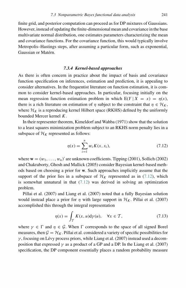
7.3 Nonparametric Bayes functional data analysis 241
finite grid, and posterior computation can proceed as for DP mixtures of Gaussians.However, instead of updating the finite-dimensional mean and covariance in the basemultivariate normal distribution, one estimates parameters characterizing the meanand covariance functions. For the covariance function, this would typically involveMetropolis–Hastings steps, after assuming a particular form, such as exponential,Gaussian or Matern.
7.3.4 Kernel-based approaches
As there is often concern in practice about the impact of basis and covariancefunction specification on inferences, estimation and prediction, it is appealing toconsider alternatives. In the frequentist literature on function estimation, it is com-mon to consider kernel-based approaches. In particular, focusing initially on themean regression function estimation problem in which E(Y | X = x) = η(x),there is a rich literature on estimation of η subject to the constraint that η ∈ HK ,where HK is a reproducing kernel Hilbert space (RKHS) defined by the uniformlybounded Mercer kernel K .
In their representer theorem, Kimeldorf and Wahba (1971) show that the solutionto a least squares minimization problem subject to an RKHS norm penalty lies in asubspace of HK represented as follows:
η(x) =n∑
i=1
wiK(x, xi), (7.12)
where w = (w1, . . . , wn)′ are unknown coefficients. Tipping (2001), Sollich (2002)and Chakraborty, Ghosh and Mallick (2005) consider Bayesian kernel-based meth-ods based on choosing a prior for w. Such approaches implicitly assume that thesupport of the prior lies in a subspace of HK represented as in (7.12), whichis somewhat unnatural in that (7.12) was derived in solving an optimizationproblem.
Pillai et al. (2007) and Liang et al. (2007) noted that a fully Bayesian solutionwould instead place a prior for η with large support in HK . Pillai et al. (2007)accomplished this through the integral representation
η(x) =∫T
K(x, u)dγ (u), ∀x ∈ T , (7.13)
where γ ∈ � and η ∈ G. When � corresponds to the space of all signed Borelmeasures, then G = HK . Pillai et al. considered a variety of specific possibilities forγ , focusing on Levy process priors, while Liang et al. (2007) instead used a decom-position that expressed γ as a product of a GP and a DP. In the Liang et al. (2007)specification, the DP component essentially places a random probability measure

242 Nonparametric Bayes applications to biostatistics
5
4
3
2
1
0
−1
−2
−3
−4−8 −6 −4 −2 0 2 4 6 8 10 12 14
Figure 7.2 Posterior mean progesterone curves (solid lines) and observed progesteronelevels for three selected nonconceptive cycles. Estimated progesterone curves and observeddata are linked by color.
on the locations of the kernels, while the GP places a prior on the coefficients at theresulting countably infinite collection of locations.
MacLehose and Dunson (2009) generalized the Liang et al. (2007) formulationto the functional data analysis setting by letting ηi(x) = ∫
K(x, u)dγi (u), andthen choosing a nonparametric Bayes hierarchical prior for γ = {γ1, . . . , γn}. Inparticular, their specification relied on functional DP and hierarchical DP (HDP)(Tomlinson, 1998; Teh, Jordan, Beal and Blei, 2006) components. The HDP is aprior for modeling of related distributions through incorporating dependence byassuming a common base measure in DPs for each of the distributions, with thisbase measure allowed to be unknown through use of a DP prior. For further detailson the HDP, refer to Chapter 5.
An appealing feature of the MacLehose and Dunson (2009) approach relativeto the approaches described in Sections 7.3.2 and 7.3.3 is the allowance for localborrowing of information through local selection of kernels and locally dependent

7.3 Nonparametric Bayes functional data analysis 243
weights. To illustrate this, consider an application to progesterone trajectory datapreviously analyzed in Brumback and Rice (1998). Data were available for 51women who provided samples over 91 cycles, of which 22 were conception cycles.Taking results from MacLehose and Dunson (2009), Figure 7.2 shows the rawdata and estimated posterior mean progesterone curves for three women randomlyselected from the nonconception group. This figure demonstrates the borrowing ofinformation. In particular, during the baseline phase prior to ovulation (day 0 inthe figure), the progesterone values are quite similar, so there is strong borrowingof information and the estimates are essentially equivalent. However, followingovulation the curves smoothly deviate, with the approach favoring similar shapesacross the curves. Note that the methods of Sections 7.3.2 and 7.3.3 instead borrowinformation only through global clustering and through the parametric base model.Alternative methods for local borrowing of information will be discussed in detailin Section 7.4.
7.3.5 Joint modeling
In biomedical studies, there is very commonly interest in studying the relationshipbetween functional predictors and response variables. For example, the functionalpredictor may correspond to the longitudinal trajectory in the level of an environ-mental exposure, such as air pollution, or to a diagnostic image, while the responsecorresponds to an indicator of an adverse health condition. In such cases, there issubstantial interest in building flexible joint models for relating a subject’s func-tional predictor to their health status, adjusting for possible confounding factors,such as age and demographic variables.
To focus on a motivating application, we consider an epidemiologic study ofearly pregnancy loss (EPL) in which daily urine samples were collected in order tomeasure levels of hormone metabolites over time prior to conception and throughearly pregnancy (Wilcox et al., 1988). Our interest is in studying how progesteronetrajectories following ovulation predict EPL. EPLs are identified when hCG risessoon after implantation but then declines back to baseline levels instead of continu-ing to rise. Progesterone plays a critical role in maintaining the pregnancy, so someclinicians have even suggested treatment with exogenous progesterone as a possi-ble intervention to reduce risk of EPL. Affordable home devices are available formeasuring progesterone metabolites in urine, so an algorithm could potentially beprogrammed into such a device to alert the woman when she is at risk of impendingloss.
Motivated by this application, Bigelow and Dunson (2009) develop a Bayesiannonparametric approach for joint modeling of functional predictors with a re-sponse variable. Their proposed approach relies on a simple extension of the

244 Nonparametric Bayes applications to biostatistics
method proposed in Section 7.3.2. In order to facilitate applications to other set-tings, I will initially present the approach in more generality than considered inBigelow and Dunson (2009). In particular, suppose for subject i, we have datayi = (y′
i1, . . . , y′ip)′, where yij = (yij1, . . . , yij,nij
)′ is a vector of observations oftype j , for j = 1, . . . , p. For example, yi1 may consist of error-prone measure-ments of a functional predictor, while yi2 is 0/1 indicator of a health response. Moregenerally, the yij may correspond to several different types of information collectedon a subject.
We define separate models for each of the components of the data vector asfollows:
yij ∼ fj (β ij ; φj ), j = 1, . . . , p,
β i = (β ′i1, . . . , β
′ip)′ ∼P,
(7.14)
where fj (β ij ; φj ) is the likelihood for component j , defined in terms of the subject-specific parameters β ij = (βij1, . . . , βij,pj
) and population parameters φj , and thedifferent component models are linked through P , the joint distribution for β i . Inparametric joint modeling of multivariate data having a variety of measurementscales, it is common to use latent factor and structural equation models that incor-porate shared latent variables in the different component models. By allowing P tobe unknown through a nonparametric Bayes approach, we obtain a more flexibleclass of joint models.
Bigelow and Dunson (2009) propose to use a DP prior for P with the followingstructure:
P =∞∑
h=1
πhδ�h, �h ∼ P0 = ⊗p
j=1P0j , (7.15)
where π = {πh}∞h=1 are as defined in (7.2), �h = {�hj }pj=1 is a collection of atomscorresponding to the parameters in each of the p different components, and the basemeasure P0 used in generating these atoms is characterized as a product measureof probability measures for each component. For example, in joint modeling ofa longitudinal trajectory with a 0/1 response, P01 may correspond to a Gaussianprocess and P02 to a beta distribution, so that each DP cluster then contains arandom function along with a corresponding probability of an adverse response. Inthis manner, a semiparametric joint model is defined for data having different scales,with dependence in the different types of data collected for a subject induced throughallocating individuals to clusters having different parameters for each componentmodel.
Instead of using a GP for the functional predictor component, Bigelow andDunson (2009) use multivariate adaptive splines with unknown numbers andlocations of knots. They applied this approach to progesterone metabolite and EPL

7.4 Local borrowing of information and clustering 245
0
0
3 3.5
3
2.5
2
1.5
0.5
−0.5
0
1
2
1
−1
−2
−310 20 30 40
Day relative to ovulation
log(
PdG
)- E
arly
Los
ses
log(
PdG
)- C
lini
cal
Pre
gnan
cies
0 10 20 30 40Day relative to ovulation
Figure 7.3 Progesterone data beginning at the estimated day of ovulation for three earlylosses and three clinical pregnancies.
data from Wilcox et al. (1988). Figure 7.3 shows the progesterone data for threerandomly selected early losses and three clinical pregnancies. Figure 7.4 showsthe progesterone data for each of the 16 identified clusters containing more thanone subject, along with the number of pregnancies in the cluster and the estimatedprobability of early pregnancy loss. Note that it is very clear that the identified clus-ters match the data from these plots. In addition, the early loss probabilities varieddramatically across the clusters. This resulted in accurate out of sample predictionof impending losses soon after implantation (results not shown).
7.4 Local borrowing of information and clustering
Until this point, I have focused primarily on methods that rely on different variantsof the DP for modeling of an unknown random effects distribution in a hierarchicalmodel. As discussed above, such methods have the side effect of inducing clusteringof subjects into groups, with groups defined in terms of unique random effects values

246 Nonparametric Bayes applications to biostatistics
5
0
0 20n=87
n=6 n=3 n=9 n=3
n=2n=3n=4
n=2 n=2 n=2
n=5
n=5
n=10 n=4 n=240
−5
5
0
0 20 40−5
5
0
0 20 40−5
5
0
0 20 40−5
5
0
0 20 40−5
5
0
0 20 40−5
5
0
0 20 40−5
5
0
0 20 40−5
5
0
0 20 40−5
5
0
0 20 40−5
5
0
0 20 40−5
5
0
0 20 40−5
5
0
0 20 40−5
5
0
0 20 40−5
5
0
0 20
Day relative to ovulation
Cluster 13:01 [0, 0.39]
Cluster 9:0.88 [0.57, 1]
Cluster 5:0.072 [0, 0.3]
log(
PD
G)
Cluster 1:0.044 [0.01, 0.1] Cluster 2:0.038 [0, 0.19] Cluster 3:0.91 [0.58, 1] Cluster 4:0.86 [0.33, 1]
Cluster 6:0.87 [0. 42,1] Cluster 7:0.95 [0.76, 1] Cluster 8:0.85 [0.33, 1]
Cluster 10:0.89 [0.47, 1] Cluster 11:0.35 [0.03, 0.81] Cluster 12:0.85 [0.31, 1]
Cluster 14:081 [027, 1] Cluster 15:0.77 [0.25, 1] Cluster 16:0.71 [0.24, 1]40
−5
5
0
0 20 40−5
Figure 7.4 Progesterone data for pregnancies in each of the 16 clusters identified in theWilcox et al. (1988) data. Only those clusters containing more than one pregnancy areshown. Below each plot is the estimated probability of early pregnancy loss within thecluster, along with a 95% credible interval.
or unique parameters in a parametric model. One characteristic of this type ofspecification is that clustering occurs globally, in that two individuals are clusteredtogether for all their random effects or none.
For example, focus on the joint model specification in (7.15) and suppose β i ∼ P ,for i = 1, . . . , n. Then, it is clear that either β i = β i′ , with prior probability 1/(1 +α), or β i and β i′ correspond to two independent draws from P0, so that none of theelements of β i can cluster together with the corresponding elements of β i′ (assumingnonatomic P0). Such global clustering is quite restrictive in that two differentsubjects may be quite similar or even identical for most of their random effects,while having important deviations in certain components. An alternative, whichallows local clustering, is to let β ij ∼ Pj , with Pj ∼ DP(αjP0j ), independently forj = 1, . . . , p. However, this approach does not allow for accrual of informationabout similarities between subjects. In particular, if β ij = β i′j then the probability

7.4 Local borrowing of information and clustering 247
should intuitively be increased that β ij ′ = β i′j ′ compared with the case in whichβ ij �= β i′j .
Motivated by this problem, Dunson, Xue and Carin (2008) proposed a matrixstick-breaking process (MSBP), which generalizes the DP stick-breaking structureto allow row and column stick-breaking random variables to induce dependentlocal clustering. Posterior computation for the MSBP can proceed using a simplemodification to the blocked Gibbs sampler of Ishwaran and James (2001). TheMSBP has particular practical advantages over joint DP and independent DP priorsin high-dimensional settings in which subjects can be very similar for most of theircoefficients, while having distinct local deviations. This occurs, for example, whenmodeling of multiple, related functions or images using a basis representation.Often, most of the function or image is quite similar across subjects, suggestingthat most of the basis coefficients are effectively identical. However, it is those localregions of heterogeneity that are most scientific interest.
Motivated by the problem of local clustering in functional data analysis, Petrone,Guindani and Gelfand (2007) proposed a hybrid functional Dirichlet process prior.The hybrid DP is based on the clever idea of introducing a collection of globalspecies, with each individual function formulated from a patchwork of these globalspecies. In particular, a latent Gaussian process is introduced, with the level of thislatent process controlling local allocation to the global species. This results in localclustering of the functions for different individuals, with discontinuities occurringin the functions at changepoints in which the latent process crosses thresholds sothat allocation switches to a different species. Petrone, Guindani and Gelfand (2007)applied this approach to an interesting brain image application. Rodriguez, Dunsonand Gelfand (2009a) proposed an alternative latent stick-breaking process (LaSBP).The LaSBP is defined by introducing a fixed unknown marginal distribution, whichis assigned a stick-breaking prior, and then using a latent Gaussian process copulamodel to control local allocation to the atoms. The LaSBP avoids problems facedby the hybrid DP in performing spatial interpolations by introducing an orderconstraint on the atoms. This constraint also induces skewness, which is appealingin many applications.
Friedman and Meulman (2004) defined a concept of clustering on subsets ofattributes (COSA) in which two subjects can be partially clustered by havingidentical values for a subset of a vector of parameters. Hoff (2006) proposed asimple but clever Bayesian nonparametric version of COSA relying on a DP. Inparticular, if β i = (βi1, . . . , βip)′ represents a vector of subject-specific parametersin a hierarchical model, then Hoff (2006) first lets β i = β+ri×δi , with ri ∈ {0, 1}m,δi ∈ �p and × denoting the elementwise product. Then, letting (ri , δi) ∼ P , withP ∼ DP(αP0), results in clustering of the n subjects into k ≤ n groups. Note thatsubjects in a group will deviate from the baseline in only those attributes having

248 Nonparametric Bayes applications to biostatistics
rij = 1. In this manner, subjects in different DP clusters can be identical for a subsetof their random effects, effectively accommodating a type of local clustering.
7.5 Borrowing information across studies and centers
In biomedical studies, there is very commonly interest in combining informationacross data from different sources. Classical examples include multicenter studies,in which data are collected for individuals in different study centers, and meta-analysis, in which interest focuses on combining results for studies with similarstudy designs, endpoints and predictors. In recent years, there has also been increas-ing interest in attempting to borrow strength across data from disparate sources. Forexample, one may want to combine results from cell assay, animal and epidemio-logic studies in drawing conclusions about the health effects of an environmentalexposure.
In such settings, hierarchical models provide a standard tool for borrowing ofinformation, but flexible approaches are needed to avoid inappropriate borrowing.In this section, I provide an overview of several hierarchical extensions of the DPthat have been proposed for borrowing of information across data from differentsources, including mixtures of DPs, dependent DPs, hierarchical DPs and nestedDPs.
To provide motivation, I will focus on a multicenter study application. In partic-ular, the National Collaborative Perinatal Project (NCPP) was a large prospectiveepidemiologic study conducted from 1959–1974. Pregnant women were enrolledthrough different study centers and were followed over time, with the childrengiven examinations at birth, 4, 8 and 12 months, and 3, 4, 7 and 8 years. Although avariety of data were collected, I will focus here on gestational age at delivery (gad)and birth weight (bw), with yij = (yij1, yij2)′ for the j th woman in study center i,where yij1 =gad and yij2 =bw.
The joint distribution of gad and bw is distinctly non-Gaussian and is notwell characterized by a parametric model. Hence, one can consider the followingGaussian mixture model:
yij ∼ N2(µij , �ij )
(µij , �ij ) ∼ Pi,(7.16)
where Pi is an unknown mixture distribution. This specification results in a jointdistribution for gestational age at delivery and birth weight, which is specific tostudy center. Certainly it is well known in the reproductive epidemiology literaturethat pregnancy outcomes can vary substantially for women of different ethnicitiesand from different socioeconomic groups. Hence, it is appealing to allow differencesbetween study centers, since different centers may serve different types of women.

7.5 Borrowing information across studies and centers 249
However, it is also likely the case that the joint distribution of gad and bw is similarfor different centers, so the question is how to borrow information in specifying aprior for P = {P1, . . . , Pn}.
Muller, Quintana and Rosner (2004) proposed an approach for inducing depen-dence in the Pi through a mixture of independent DPs. In particular, under theirspecification,
Pi = πP ∗0 + (1 − π )P ∗
i , P ∗h
i.i.d.∼ DP(αP0), h = 0, 1, . . . , n, (7.17)
where P ∗0 is a global component that is shared across the different centers, 0 ≤ π ≤
1 is a probability weight on the global component, and P ∗j is a local component
allowing deviations for the j th study. If the joint distribution of gad and bw is verysimilar for the different study centers, then π will be close to one. The Muller,Quintana and Rosner (2004) approach is appealing in working well in practice andbeing simple to implement. In particular, a standard MCMC algorithm for a DPMcan be used after modification to update latent indicators, Zij ∈ {0, 1, . . . , n}, withZij = h denoting that (µij , �ij ) are drawn from P ∗
h . Dunson (2006) modified(7.17) to define a dynamic mixture of DPs (DMDP) appropriate for time seriessettings.
An alternative to (7.17), referred to as the hierarchical DP (HDP), was proposedby Teh, Jordan, Beal and Blei (2006). The HDP is specified as follows:
Pi ∼ DP(αP0), P0 ∼ DP(γP00), (7.18)
so that the mixture distributions for the different study centers are assigned separateDP priors, with sharing induced through the common base measure P0, which isalso given a DP prior. Note that this specification has the property that all the Pi
will have the same atoms, while having distinct but dependent weights on theseatoms. The shared atoms property differs from the specification in (7.17). However,because the subset of atoms in P0 that are occupied by the subjects in the samplewill differ across study centers, the HDP does effectively allow local clusters. TheHDP is covered in detail in Chapter 5.
Note that the specifications (7.17) and (7.18) both allow borrowing of informa-tion across study centers through incorporation of common atoms and dependentweights on these atoms. However, both formulations assume that Pr(Pi = Pi′) = 0,except in limiting cases in which hyperparameters are chosen so that the distribu-tions are identical for all study centers. In many applications, it is of interest toallow clustering of study centers into groups, with each group having a differentnonparametric response distribution. For example, one could then identify medi-cal centers with the same distribution of patient outcomes, while also identifyingoutlying centers.

250 Nonparametric Bayes applications to biostatistics
With this goal in mind, Rodriguez, Dunson and Gelfand (2007) proposed thenested DP (nDP), which lets
Pi ∼∞∑
h=1
πhδP ∗h, P ∗
h
i.i.d.∼ DP(γP0), (7.19)
where the weights π = {πh}∞h=1 are as defined in (7.2). Note that this specificationallows Pi to be exactly equal to Pi′ with prior probability 1/(1+α). When Pi = Pi′ ,the joint distribution of gad and bw in center i is identical to that for center i ′,and these centers are clustered together. Hence, unlike the HDP, which clusterspatients within and across study centers while assuming study centers are distinct,the nDP allows clustering of both study centers and patients within centers. Suchclustering may be of direct interest or may be simply a tool for flexible borrowingof information in estimating the center-specific distributions.
7.6 Flexible modeling of conditional distributions
7.6.1 Motivation
In many applications, it is of interest to study changes in the distribution of aresponse variable Y over time, for different spatial locations, or with variations in avector of predictors, x = (x1, . . . , xp)′. Depending on the study design, the primaryinterest may be
(i) prediction of a health response Y for a new subject given demographic andclinical predictors for that subject;
(ii) inference on the impact of time, space or predictors on the conditional responsedistribution;
(iii) inverse regression problems involving identification of predictor values asso-ciated with an adverse health response;
(iv) clustering of subjects based on their health response while utilizing predictorinformation.
The methods reviewed in Section 7.5 can be used to address these interestswhen there is a single unordered categorical predictor, such as the study center.However, alternative methods are needed in the general case. This section reviewssome approaches for modeling of predictor-dependent collections of distributionsthrough the use of mixture models incorporating priors for collections of dependentrandom probability measures indexed by predictors. In particular, let
PX = {Px : x ∈ X } ∼ P, (7.20)
where Px denotes the random probability measure at location (predictor value)x ∈ X , X is the sample space for the predictors, and P is the prior for the

7.6 Flexible modeling of conditional distributions 251
collection, PX . Here, I use the term predictor broadly to refer also to time andspatial location.
There are a wide variety of applications in which it is useful to incorporate priorsfor dependent collections of distributions. For example, one may be interested inmodeling of conditional densities, f (y | x). Revisiting the reproductive epidemiol-ogy application from Section 7.5, suppose that yi is the gestational age at deliveryfor woman i and xi = (xi1, . . . , xip)′ is a vector of predictors, including age of thewoman and blood level of DDE, a persistent metabolite of the pesticide DDT. Then,it is of interest to assess how the risk of premature delivery, corresponding to theleft tail of the distribution of gestational age at delivery, changes with increasingDDE exposure adjusting for age. In making such assessments, it is appealing tolimit parametric assumptions, and avoid the common epidemiologic practice ofreducing information on gestational age at delivery (gad) to a 0/1 indicator of gad≤ 37 weeks.
To solve this problem, one can consider a mixture model of the form
f (y | x) =∫ ∫
g(y; x, θ , φ)dPx(θ )dπ(φ), (7.21)
where g(y; x, θ , φ) is a parametric model for the conditional density of y givenx, and (7.21) allows deviations from this parametric model through nonparametricmixing. Expression (7.21) contains both parametric and nonparametric components,with the prior distribution for the parameters φ treated as known, while the mixturedistribution for θ is nonparametric and predictor dependent. Some possibilities forg(y; x, θ , φ) include N(y; µ, σ 2), with θ = (µ, σ 2), and N(y; x′β, σ 2), with θ =(β ′, σ 2). The advantage of incorporating a regression component in g(y; x, θ , φ)is that a sparse structure is then favored through centering on a base parametricregression model. In this context, a sparser specification allows subjects to beallocated to few mixture components, while maintaining flexibility. In addition,we allow for interpolation across sparse data regions through the base parametricmodel, addressing the curse of dimensionality.
7.6.2 Dependent Dirichlet processes
One possibility for P in (7.20) is the dependent DP (DDP) originally proposedby MacEachern (1999, 2001; see also De Iorio, Muller, Rosner and MacEachern,2004). In full generality, the DDP is specified as follows:
Px =∞∑
h=1
πh(x)δ�h(x), �hi.i.d.∼ P0, ∀x ∈ X , (7.22)
where πh(x) = Vh(x)∏
l<h{1 − Vl(x)}, for h = 1, . . . , ∞, with the stick-breakingweights {Vh(x)}∞h=1, at any fixed x, consisting of independent draws from a Beta(1, α)

252 Nonparametric Bayes applications to biostatistics
distribution. In addition, �h is a stochastic process over X generated from P0. Forexample, P0 may correspond to a Gaussian process.
Due to complications involved in allowing the weights to depend on predic-tors, most applications of the DDP have assumed fixed weights, resulting in thespecification
Px =∞∑
h=1
πhδ�h(x), �hi.i.d.∼ P0, ∀x ∈ X , (7.23)
where π = {πh}∞h=1 are as defined in (7.2). De Iorio, Muller, Rosner and MacEach-ern (2004) applied this specification to develop ANOVA-type models for collectionof dependent distributions. Gelfand, Kottas and MacEachern (2005) applied theDDP in spatial data analysis applications.
One can also use the fixed π DDP in (7.23) to develop a method for conditionaldensity modeling as in (7.21) by letting
f (y | x) =∞∑
h=1
πhN(y; µh(x), σ 2h ), (µh, σ
2h ) ∼ P0 = P01 ⊗ P02 (7.24)
where P01 is a Gaussian process overX and P02 is a probability measure on �+ (e.g.,corresponding to an inverse-gamma distribution). Note that (7.24) characterizesthe conditional density using an infinite mixture of normals, with the componentmeans varying differentially and nonlinearly with predictors. This specificationis a generalization of typical Gaussian process regression models, which wouldcorrespond to letting π1 = 1, so that the mean varies flexibly while the residualdensity is assumed to be constant and Gaussian. In contrast, the DDP mixture ofnormals in (7.24) allows multimodal residual densities that vary with x.
It is useful to consider the gestational age at delivery application. In that case,there are likely a few dominant mixture components that are assigned most of theprobability weight, with these components corresponding to early preterm birth,preterm birth and full term birth. Specification (7.24) assumes that the probabilityallocated to these components does not vary with age or DDE, but the locations ofthe component can vary. For example, the mean of the preterm birth componentcan shift to earlier weeks as DDE level increases to allow an increasing proportionof babies born too soon at higher exposures.
From this example, it is clear that the fixed π DDP may be overly restrictivein that biologic constraints on the timing of gestation make it more realistic andinterpretable to consider models with fixed locations but weights that depend onpredictors. For example, if we have three dominant components corresponding toearly preterm, preterm and full term, then a varying weights model would allow theprobability of early preterm birth to increase as DDE increases without necessarily

7.6 Flexible modeling of conditional distributions 253
changing the timing and hence the meaning of the early preterm component. Inaddition, a varying weights model is necessary to allow the probability that twosubjects are assigned to the same cluster to depend on predictors.
Motivated by such considerations, Griffin and Steel (2006) proposed an order-based dependent DP, referred to as the π -DDP. The π -DDP allows for predictor-dependent weights in the DDP in a clever manner by allowing the ordering in thestick-breaking weights to depend on predictors. In more recent work, Griffin andSteel (2007) proposed a simplification of the π -DDP, which they used for modelingof the residual component in a flexible regression model. The resulting approach isreferred to as the Dirichlet process regression smoother (DPRS).
An alternative approach that was developed for spatial applications in which it isappealing to allow the weights to vary spatially, was proposed by Duan, Guindaniand Gelfand (2007). This approach places a stochastic process on the weights, whichis carefully specified so that the marginal distributions at any fixed spatial locationmaintain the DP stick-breaking form. De la Cruz-Mesia, Quintana and Muller(2007) recently proposed an alternative extension of the DDP for classificationbased on longitudinal markers. Their approach incorporated dependence in therandom effects distribution across groups.
7.6.3 Kernel-based approaches
As an alternative to the DDP, Dunson, Pillai and Park (2007) proposed an ap-proach based on kernel-weighted mixtures of independent DP basis components.This approach is conceptually related to the kernel regression approach describedin Section 7.3.4 and expression (7.12). However, instead of specifying a priorfor a single function, the goal is to specify a prior for an uncountable collectionof predictor-dependent random probability measures. To motivate the general ap-proach, first consider the case in which there is an single continuous predictor withsupport on [0,1] and interest focuses on modeling the conditional density f (y|x),for all x ∈ [0, 1]. In this case, a simple model would let
f (y|x) = 1
K(x, 0) + K(x, 1)
{K(x, 0)f ∗
0 (y) + K(x, 1)f ∗1 (y)
}, (7.25)
where K is a kernel, with K(x, x) = 1 and K(x, x ′) decreasing as the distancebetween x and x ′ increases, f ∗
0 (y) is an unknown basis density located at x = 0,and f ∗
1 (y) is an unknown basis density located at x = 1. For example, K maycorrespond to a Gaussian kernel, and f ∗
0 , f ∗1 to DP mixtures of normals.
Figure 7.5 provides an example of the behavior of (7.25), letting f ∗0 correspond
to the standard normal density, f ∗1 to a mixture of two normals, and K to the
Gaussian kernel with standard deviation 0.3. As should be clear, using the mixture

254 Nonparametric Bayes applications to biostatistics
0.8f ( y x = 0)
0.7
0.6
0.5
0.4
0.3
0.2
0.1
00 02 2−2 −2
0.8
0.7
0.6
0.5
0.4
0.3
0.2
0.1
00 2−2
0.8
0.7
0.6
0.5
0.4
0.3
0.2
0.1
00 2−2
0.8f ( y x = 0.5)
0.7
0.6
0.5
0.4
0.3
0.2
0.1
00 02 2−2 −2
0.8
0.7
0.6
0.5
0.4
0.3
0.2
0.1
00 2−2
0.8
0.7
0.6
0.5
0.4
0.3
0.2
0.1
00 2−2
f ( y x = 0.1) f ( y x = 0.4)
f ( y x = 0.9) f ( y x = 1)
Figure 7.5 Plot illustrating the kernel mixtures approach in the simple case in whichxi ∈ {0, 1} for all subjects in the sample, and a normal kernel with standard deviation 0.3is chosen.
model (7.25) results in a smoothly morphing profile of conditional densities, withthe densities very close for similar predictor values. In order to generalize thekernel mixture approach of expression (7.25) to allow multiple predictors andmore flexibility, one can potentially allow unknown numbers and locations of basisdensities, similarly to allowing unknown numbers and locations of knots in a splinemodel.

7.6 Flexible modeling of conditional distributions 255
Dunson, Pillai and Park (2007) instead proposed a default approach in which DPbases were automatically placed at the sample predictor values, with each of thesebases assigned a weight controlling its importance. In particular, their proposedweighted mixture of DPs (WMDP) prior had the form
Px =n∑
i=1
(γiK(x, xi)∑nl=1 γlK(x, xl)
)P ∗
i , P ∗i
i.i.d.∼ DP(αP0), ∀x ∈ X , (7.26)
where i = 1, . . . , n indexes subjects in the sample, K : X × X → 1 is a boundedkernel (e.g., Gaussian), γ = (γ1, . . . , γn)′ is a vector of weights, and {G∗
i }ni=1 areindependent DP basis measures.
Dunson, Pillai and Park (2007) applied the WMDP approach for density regres-sion through use of the model
f (y | x) =∫ ∫
N(y; x′β, σ 2)dPx(β)dπ(σ 2), (7.27)
which is a mixture of linear regression models with predictor-dependent weights.This model is related to hierarchical mixtures-of-experts models (Jordan and Jacobs,1994), which are widely used in the machine learning literature, but instead ofassuming a finite number of experts (i.e., mixture components), the number ofexperts is infinite. In addition, instead of a probabilistic decision tree for the weights,a kernel model is used.
From a Bayesian perspective, (7.26) has an unappealing sample-dependenceproperty, so that the approach is not fully Bayesian and lacks coherent updating andmarginalization properties. For this reason, it is useful to consider alternative priorsthat borrow some of the positive characteristics of the kernel-weighted specificationbut without the sample dependence. One such prior is the kernel stick-breakingprocess (KSBP) (Dunson and Park, 2008), which modifies the DP stick-breakingspecification shown in (7.2) as follows:
Px =∞∑
h=1
VhKψh(x, �h)
∏l<h
{VlKψl
(x, �l)}P ∗
h , P ∗h
i.i.d.∼ DP(αP0), (7.28)
where Vhi.i.d.∼ Beta(1, λ), Kψ denotes a kernel having bandwidth ψ , {ψh}∞h=1 is an
infinite sequence of kernel bandwidths sampled from G, and {�h}∞h=1 is an infinitesequence of kernel locations sampled from H .
The KSBP places random basis probability measures at an infinite sequence ofrandom locations, with the weights assigned to these bases in the formulation forPx decreasing stochastically with the index h and the distance from x. In usingthe KSBP as a prior for the mixture distributions in (7.27), one obtains a flexible,
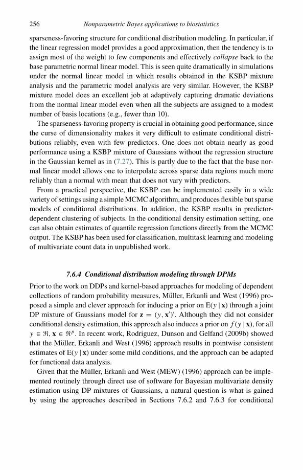
256 Nonparametric Bayes applications to biostatistics
sparseness-favoring structure for conditional distribution modeling. In particular, ifthe linear regression model provides a good approximation, then the tendency is toassign most of the weight to few components and effectively collapse back to thebase parametric normal linear model. This is seen quite dramatically in simulationsunder the normal linear model in which results obtained in the KSBP mixtureanalysis and the parametric model analysis are very similar. However, the KSBPmixture model does an excellent job at adaptively capturing dramatic deviationsfrom the normal linear model even when all the subjects are assigned to a modestnumber of basis locations (e.g., fewer than 10).
The sparseness-favoring property is crucial in obtaining good performance, sincethe curse of dimensionality makes it very difficult to estimate conditional distri-butions reliably, even with few predictors. One does not obtain nearly as goodperformance using a KSBP mixture of Gaussians without the regression structurein the Gaussian kernel as in (7.27). This is partly due to the fact that the base nor-mal linear model allows one to interpolate across sparse data regions much morereliably than a normal with mean that does not vary with predictors.
From a practical perspective, the KSBP can be implemented easily in a widevariety of settings using a simple MCMC algorithm, and produces flexible but sparsemodels of conditional distributions. In addition, the KSBP results in predictor-dependent clustering of subjects. In the conditional density estimation setting, onecan also obtain estimates of quantile regression functions directly from the MCMCoutput. The KSBP has been used for classification, multitask learning and modelingof multivariate count data in unpublished work.
7.6.4 Conditional distribution modeling through DPMs
Prior to the work on DDPs and kernel-based approaches for modeling of dependentcollections of random probability measures, Muller, Erkanli and West (1996) pro-posed a simple and clever approach for inducing a prior on E(y | x) through a jointDP mixture of Gaussians model for z = (y, x′)′. Although they did not considerconditional density estimation, this approach also induces a prior on f (y | x), for ally ∈ �, x ∈ �p. In recent work, Rodriguez, Dunson and Gelfand (2009b) showedthat the Muller, Erkanli and West (1996) approach results in pointwise consistentestimates of E(y | x) under some mild conditions, and the approach can be adaptedfor functional data analysis.
Given that the Muller, Erkanli and West (MEW) (1996) approach can be imple-mented routinely through direct use of software for Bayesian multivariate densityestimation using DP mixtures of Gaussians, a natural question is what is gainedby using the approaches described in Sections 7.6.2 and 7.6.3 for conditional

7.6 Flexible modeling of conditional distributions 257
density estimation. To address this question, I start by contrasting the two typesof approaches. The methods described in Sections 7.6.2 and 7.6.3 provide priorsfor collections of unknown distributions indexed by spatial location, time and/orpredictors. The resulting specification is defined conditionally on the predictors (ortime/space). In contrast, the MEW approach relies on joint modeling of the predic-tors and response to induce a prior on the conditional distributions. Clearly, this onlymakes sense if the predictors can be considered as random variables, which rulesout time, space and predictors that correspond to design points. However, for manyobservational studies, all the predictors can be considered as random variables.
In such settings, the MEW approach is still conceptually quite different fromthe conditional approaches of Sections 7.6.2 and 7.6.3. All the approaches induceclustering of subjects, and the MEW approach is similar to the π -DDP, WMDPand KSBP in allowing predictor-dependent clustering. The predictor-dependentclustering of the MEW approach arises through joint clustering of the responseand predictors. This implies that the MEW approach will introduce new clusters tofit better the distribution of the predictors even if such clusters are not necessaryfrom the perspective of producing a good fit to the response data. For example, insimulations from a normal linear regression model in which the predictors havenon-Gaussian continuous densities, we have observed a tendency of the MEWapproach to allocate individuals to several dominant clusters to fit better the predic-tor distribution. In contrast, the KSBP will tend to collapse on a single dominantcluster containing all but a few subjects in such cases, as a single cluster is suffi-cient to fit the response distribution, and the KSBP does not model the predictordistribution.
Although the sensitivity of clustering to the predictor distribution has some un-appealing characteristics, there are some potential benefits. Firstly, the approachis useful for inverse regression and calibration problems. Griffin and Holmes(2007) recently proposed a MEW-type approach for Bayesian nonparametric cal-ibration in spatial epidemiology. Also, in providing a joint nonparametric modelfor predictors and response variables, the approach can automatically accommo-date predictors that are missing at random through a simple step for imputing thesepredictors from their full conditional posterior distributions during the MCMCalgorithm. Finally, instead of relying entirely on information in the response dis-tribution, the approach tends to change the slope of the regression automatically inregions of the predictor space at which there is a change in the predictor distribution.This may be particularly appealing in semisupervised learning settings in whichthe responses (labels) are only available for a small subset of the subjects. In orderto allow categorical responses and/or predictors, the MEW approach can be easilyadapted to use an underlying normal DPM of Gaussians.
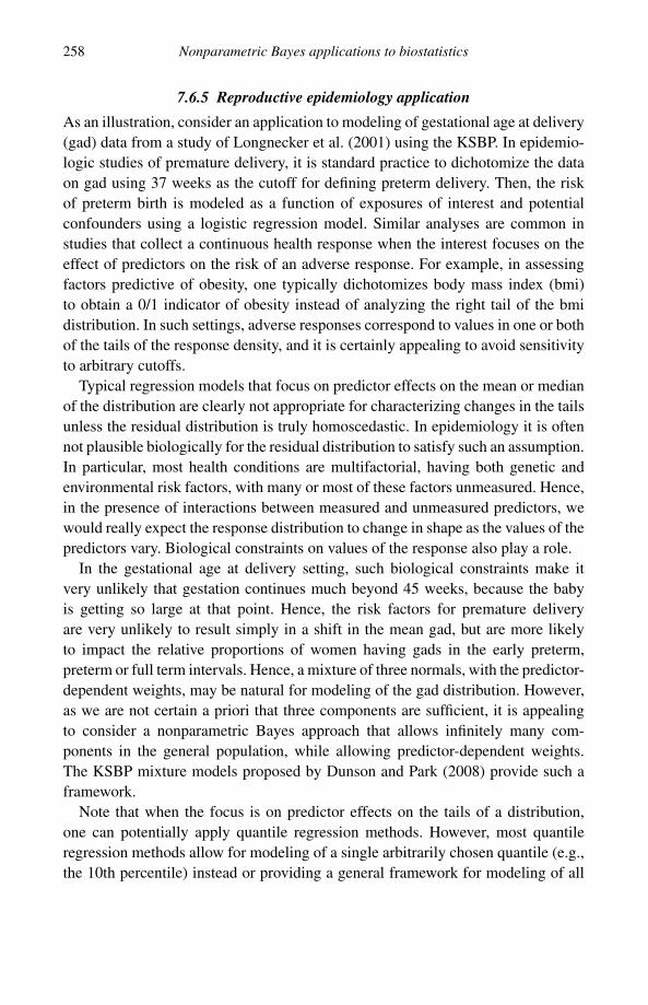
258 Nonparametric Bayes applications to biostatistics
7.6.5 Reproductive epidemiology application
As an illustration, consider an application to modeling of gestational age at delivery(gad) data from a study of Longnecker et al. (2001) using the KSBP. In epidemio-logic studies of premature delivery, it is standard practice to dichotomize the dataon gad using 37 weeks as the cutoff for defining preterm delivery. Then, the riskof preterm birth is modeled as a function of exposures of interest and potentialconfounders using a logistic regression model. Similar analyses are common instudies that collect a continuous health response when the interest focuses on theeffect of predictors on the risk of an adverse response. For example, in assessingfactors predictive of obesity, one typically dichotomizes body mass index (bmi)to obtain a 0/1 indicator of obesity instead of analyzing the right tail of the bmidistribution. In such settings, adverse responses correspond to values in one or bothof the tails of the response density, and it is certainly appealing to avoid sensitivityto arbitrary cutoffs.
Typical regression models that focus on predictor effects on the mean or medianof the distribution are clearly not appropriate for characterizing changes in the tailsunless the residual distribution is truly homoscedastic. In epidemiology it is oftennot plausible biologically for the residual distribution to satisfy such an assumption.In particular, most health conditions are multifactorial, having both genetic andenvironmental risk factors, with many or most of these factors unmeasured. Hence,in the presence of interactions between measured and unmeasured predictors, wewould really expect the response distribution to change in shape as the values of thepredictors vary. Biological constraints on values of the response also play a role.
In the gestational age at delivery setting, such biological constraints make itvery unlikely that gestation continues much beyond 45 weeks, because the babyis getting so large at that point. Hence, the risk factors for premature deliveryare very unlikely to result simply in a shift in the mean gad, but are more likelyto impact the relative proportions of women having gads in the early preterm,preterm or full term intervals. Hence, a mixture of three normals, with the predictor-dependent weights, may be natural for modeling of the gad distribution. However,as we are not certain a priori that three components are sufficient, it is appealingto consider a nonparametric Bayes approach that allows infinitely many com-ponents in the general population, while allowing predictor-dependent weights.The KSBP mixture models proposed by Dunson and Park (2008) provide such aframework.
Note that when the focus is on predictor effects on the tails of a distribution,one can potentially apply quantile regression methods. However, most quantileregression methods allow for modeling of a single arbitrarily chosen quantile (e.g.,the 10th percentile) instead or providing a general framework for modeling of all

7.6 Flexible modeling of conditional distributions 259
quantiles coherently. By using a nonparametric Bayes conditional distribution mod-eling approach, one can do inferences on shifts in the entire tail of the distributioninstead of focusing narrowly on a selected quantile.
Returning to the Longnecker et al. (2007) application, there were 2313 womenin the study, and we implemented the KSBP for model (7.27), with yi = gad andxi = (1, ddei , agei)
′. For the reasons discussed in detail at the end of Section 2.1,we normalized yi, ddei , agei prior to analysis, and then chose the base measurein the KSBP to correspond to the unit information-type prior, N2(0, (X′X)−1/n).In addition, we fixed α = 1 and λ = 1 to favor a few clusters, and used aGaussian kernel, with a single kernel precision, ψh = ψ , assigned a log-normalprior. The retrospective MCMC algorithm described in Dunson and Park (2008)was implemented, with 22000 iterations collected after a burn-in of 8000 iterations.
It is worth commenting on convergence assessments for nonparametric Bayesmixture models, with the KSBP providing one example. In particular, due to thelabel switching problem, the index on the different mixture components can changemeaning across the MCMC iterates. This leads to apparently poor mixing in manycases when one examines traces plots of cluster-specific parameters. However,in the analysis of the Longnecker et al. (2001) pregnancy outcome data and ingeneral applications in which the focus is on density estimation, conditional den-sity estimation or inferences on unknowns that are not cluster specific, one couldcompellingly argue that the label-switching problem is in fact not a problem at all.It is very commonly the case that trace plots of unknowns that are not cluster spe-cific exhibit good rates of convergence and mixing properties, while trace plots forcluster-specific parameters show high autocorrelation and fail standard convergencetests. As long as one is not interested in cluster-specific estimates and inferences,this is no cause for concern, as it just represents the cluster index identifiabilityproblem. In KSBP applications, we monitored the value of the conditional densityat different locations, and observed good mixing and rapid apparent convergence.
Figure 7.6 shows the raw data on dde and gad for the women in the Longneckeret al. (2001) study. The solid line is the posterior mean of the expected value ofgad conditionally on dde. This illustrates that the KSBP mixture model inducesa flexible nonlinear mean regression model, while also allowing the residual dis-tribution to vary with predictors. The dotted lines correspond to 99% pointwisecredible intervals. There is an approximately linear decrease in the mean gad, withthe credible intervals becoming considerably wider for high dde values where dataare sparse.
Figure 7.7 shows the estimated conditional densities of gad in days for differ-ent dde values, with posterior means shown with solid lines and 99% pointwisecredible intervals shown with dashed lines. These figures suggest that the left tailcorresponding to premature deliveries is increasingly fat as dde dose increases.

260 Nonparametric Bayes applications to biostatistics
320
300
280
260
240
220
Ges
tati
onal
age
at d
eliv
ery
200
1800 20 40 60 80 100 120 140 160 180
DDE (mg/L)
Figure 7.6 Raw data on dde and gestational age at delivery for 2313 women in theLongnecker et al. (2001) sub-study of the NCPP. Vertical dashed lines are quintiles of theempirical distribution of DDE, the solid line is the posterior mean regression curve, and thedotted lines are 99% pointwise credible intervals.
However, it is a bit hard to gauge significance of these results based on observing asequence of conditional density estimates. Figure 7.8 provides dose response curvesfor the probability gad falls below different cutoffs, including (a) 33, (b) 35, (c) 37or (d) 40 weeks. Again, solid lines are posterior means and dashed lines are 99%credible intervals. From these plots, it is clear that risk of premature delivery in-creases with level of DDE. It appears that DDE increases risk of early preterm birthprior to 33 weeks, which is an interesting finding given that such births represent amuch more adverse response in terms of short- and long-term morbidity comparedwith 37 week births.
7.7 Bioinformatics
In recent years there has been a paradigm shift in biostatistics, and it is nowstandard to be faced with very high-dimensional data. Hence, there is clearly a

7.7 Bioinformatics 261
0.03
0.02
0.01
0200
f(y
x)
220 240 260 280 300
0.03
0.02
0.01
0200
f(y
x)
220 240 260 280 300
0.03
0.02
0.01
0200
f(y
x)
220 240 260 280 300
0.03
0.02
0.01
0200
f(y
x)
220 240 260 280 300
0.03
0.02
0.01
0200
f(y
x)
220 240Gestational length
Gestational length Gestational length
Gestational lengthGestational length
99th percentile of DDE(105.48)
90th percentile of DDE(53.72)60th percentile of DDE(28.44)
10th percentile of DDE(12.57) 30th percentile of DDE(18.69)
260 280 300
Figure 7.7 Estimated conditional densities of gestational age at delivery in days for differ-ent dde values. Solid lines are posterior means and dashed lines are 99% credible intervals.
need for automated approaches for flexible dimensionality reduction and discoveryof sparse latent structure underlying very high-dimensional data. Mixture modelshave proven to be an extremely useful tool in such settings. For example, there isa vast literature on methods for high-dimensional variable selection using mixturepriors, with one component concentrated at zero and another component beingmore diffuse. Nonparametric Bayes methods have proven extremely useful in thissetting in providing a highly flexible framework for limiting sensitivity to arbitraryassumptions made in parametric modeling, such as knowledge of the number ofmixture components. In this section, we review some of this work to give a flavorof possible applications.
7.7.1 Modeling of differential gene expression
Much of the increased interest in large p, small n problems, which started approxi-mately a decade ago, was initiated by the development and rapidly increasing use of

262 Nonparametric Bayes applications to biostatistics
0.8
0.6
0.4
Pr(
Ges
tati
onal
leng
th <
33)
Pr(
Ges
tati
onal
leng
th <
37)
Pr(
Ges
tati
onal
leng
th <
40)
Pr(
Ges
tati
onal
leng
th <
35)
0.2
0
0.8
0.6
0.4
0.2
00 50 100 150 0 50 100 150
DDE (mg/L)
0.8
0.6
0.4
0.2
00 50 100 150
DDE (mg/L)
0.8
0.6
0.4
0.2
00 50 100 150
DDE (mg/L)
DDE (mg/L)
Figure 7.8 Estimated dose response curves for the probability that gestational age atdelivery is less than (a) 33, (b) 35, (c) 37 or (d) 40 weeks. Solid lines are posterior meansand dashed lines are 99% credible intervals.
microarray technology for measuring expression levels of large numbers of genes.There has been a particular focus on methods for clustering of gene expressionprofiles and for identifying genes that are differentially expressed between twogroups, with these groups often representing normal and diseased or tumor tissue.
Gene expression analyses are particularly suited for nonparametric Bayes anal-yses due to the large sample size in terms of the number of genes and to lackof knowledge of good parametric models for approximating the joint distributionof the gene expression values. Nonparametric Bayes methods provide a flexiblemachinery for characterizing the complex and high-dimensional expression values,inducing a sparse latent structure through partitioning genes into clusters. How-ever, there are some limitations relative to simpler methods in terms of ease ofinterpretation and computational expense.
Medvedovic and Sivaganesan (2002) proposed a Dirichlet process mixture(DPM) model for clustering genes with similar expression patterns, which they

7.7 Bioinformatics 263
accomplished by calculating the pairwise posterior probabilities that two genesare in the same cluster from the Gibbs sampler output. Qin (2006) proposed amodified approach that relied on an iterative weighted Chinese restaurant seatingscheme, designed so that the optimal number of clusters can be estimated simulta-neously with assignment to clusters in an efficient manner. Medvedovic, Yeung andBumgarner (2004) generalized the Medvedovic and Sivaganesan (2002) approachto data containing experimental replicates. Kim, Tadesse and Vannucci (2006) pro-posed an approach that allowed for selection of the variables to cluster upon in theDPM model. Xiang, Qin and He (2007) developed CRCView, which is a web serverproviding an easy to use approach for analysis and visualization of microarray geneexpression data based on a DPM approach.
Do, Muller and Tang (2005) proposed a DPM of normals for the distribution ofgene intensities under different conditions. Their focus was on modeling of differ-ential gene expression between two groups, a problem which has been addressedusing a variety of parametric and nonparametric empirical Bayes approaches (New-ton, Noueiry, Sarkar and Ahlquist, 2004). However, Do, Muller and Tang (2005)demonstrated advantages of the fully Bayes nonparametric approach, includingallowance for estimation of posterior expected false discovery rates.
7.7.2 Analyzing polymorphisms and haplotypes
In addition to gene expression data, there has been substantial interest in identifyinggenotypes that are predictive of an increased risk of disease. Data are now routinelycollected containing the genotypes at a large number of locations (or loci) alongthe genome at which there is variability among individuals in the population. Suchdata are commonly referred to as single nucleotide polymorphisms (SNPs), with asingle SNP consisting of a combination of amino acids, with one on the chromosomeinherited from the mother and one from the father. Because new SNP chips allowinvestigators to collect data routinely from hundreds of thousands of loci, such datapresent quite a challenge to the statistician.
In many cases, instead of casting the net very broadly in searching for diseasegenes and genotypes, investigators narrow down their search to genes in a specificpathway hypothesized to play a key role in disease risk. However, even in this case,there may be many SNPs under consideration. To provide an example, Mulherin-Engel et al. (2005) related SNPs in cytokine gene regulatory regions to risk forspontaneous preterm birth. The number of loci per cytokine at which SNP data werecollected ranged from 1 to 3, with 22 total across the 12 cytokines. At each locithere are 3 possible genotypes. Hence, in seeking to identify genotypes predictiveof an increased risk of preterm birth, there is a very high-dimensional set of modelsunder consideration.

264 Nonparametric Bayes applications to biostatistics
Motivated by this application, Dunson, Herring and Mulherin-Engel (2008) pro-posed a multilevel DP prior that allowed for borrowing of information across func-tionally related genes, while also incorporating a variable selection component.This approach automatically grouped genotypes into null and nonnull clusters ac-cording the genotypes impact on the risk of disease. In unpublished work, we havefound that this type of approach scales nicely to problems involving thousands ofgenotypes, providing clearly improved performance relative to parametric variableselection mixture priors. One of the reasons for this success is that most variableselection mixture priors shrink the nonnull coefficients towards zero, while the DP-based approach allows these coefficients to be shrunk towards other coefficientshaving similar values.
In order to address the dimensionality problem faced in searching for diseasegenotypes relying on high-dimensional SNP data, many articles have proposedhaplotype-based analyses. Haplotypes represent a sequence of amino acids alonga chromosome inherited from one parent. Due to linkage, it tends to be the casethat the number of haplotypes observed in the population is substantially less thanthe number possible. Hence, by using haplotypes as predictors instead of the geno-types formed by a set of SNPs, one clearly obtains a reduction in dimensionality.However, the problem is that current genotyping technology does not allow SNPdata to be converted into haplotypes, because the data are unphased, meaning thatthe amino acid pairs cannot be allocated to the chromosome for their parent oforigin.
This is fundamentally a missing data problem, and a number of approaches havebeen proposed for imputing the missing haplotypes given the SNP data. Xing,Jordan and Sharan (2007) proposed a DPM model to address this missing dataproblem, with the mixture components corresponding to the pool of haplotypes inthe population. Xing, Sohn, Jordan and Teh (2006) generalized this approach tothe multiple population setting through the use of a hierarchical DP (Teh, Jordan,Beal and Blei, 2006). Xing and Sohn (2007) proposed an alternative approachthat used a hidden Markov DP to jointly model genetic recombinations among thefounders of a population and subsequent coalescence and mutation events. The goalof this approach is to identify recombination hotspots and to infer ancestral geneticpatterns. An alternative approach for haplotype inference using a Bayesian hiddenMarkov model was independently developed by Sun, Greenwood and Neal (2007).
7.7.3 New species discovery
There has clearly been an explosion in the types of high-dimensional data generated,and nonparametric Bayes methods have seen greatly increasing use as a tool forbioinformatics. In addition to the applications presented in Sections 7.7.1 and 7.7.2,

7.8 Nonparametric hypothesis testing 265
one very interesting application is to expressed sequence tag (EST) analysis. ESTsprovide a useful tool for gene identification in an organism. In searching for genesusing this technology, a number of interesting design questions arise. In particular,after obtaining a preliminary EST sample, scientists would like to estimate theexpected number of new genes that would be detected from a further sample of agiven size. Such information is critical in making decisions about the number ofadditional samples to sequence.
Lijoi, Mena and Prunster (2007a) addressed this problem using a nonparametricBayes methodology for estimating the probability of discovery of a new species(Lijoi, Mena and Prunster, 2007b). In particular, Lijoi, Mena and Prunster (2007b)derived a closed form expression for a nonparametric Bayes estimator for theprobability of discovery. Their approach is based on a class of priors for speciessampling problems that induce Gibbs-type random partitions.
7.8 Nonparametric hypothesis testing
Most of the nonparametric Bayes literature has focused on approaches for estimationunder a particular model, and there has been relatively limited consideration ofhypothesis testing problems. In biomedical studies, hypothesis testing is oftenof primary interest. For example, in clinical trials, basic science and toxicologystudies, the primary focus is typically on testing the null hypothesis of equalitiesin the response distribution between treatment groups against the alternative thatthere are differences. Estimation is often a secondary interest. In this section wereview some of the work on nonparametric Bayes hypothesis testing.
Motivated by the problem of testing of equalities between groups in a studywith multiple treatment groups, Gopalan and Berry (1998) proposed an approachto adjust for multiple comparisons through use of a DP prior. In particular, lettingyhi denote a continuous health response for the ith individual in group h, for h =1, . . . , p, let yhi ∼ N(µh, σ
2). Then, the interest is in studying local hypotheses:
H0,hl : µh = µl versus H1,hl : µh �= µl.
Clearly, the number of such hypotheses increases rapidly with p, so one faces a
multiple comparisons problem. Gopalan and Berry (1998) proposed letting µhi.i.d.∼
P , with P ∼ DP(αP0). Then, from basic properties of the DP, Pr(H0,hl) = 1/(1+α).Using standard algorithms for posterior computation in DPM models, one can obtainestimates of the posterior hypothesis probabilities.
Motivated by epidemiologic studies having many predictors that may be highlycorrelated, MacLehose, Dunson, Herring and Hoppin (2007) proposed an alter-native approach which assumed that the regression parameters for the different

266 Nonparametric Bayes applications to biostatistics
predictors in a generalized linear model, β1, . . . , βp, were sampled from theprior:
βji.i.d.∼ P = π0δ0 + (1 − π0)P ∗, P ∗ ∼ DP(αP0), (7.29)
where π0 is the prior probability that the j th predictor has a zero coefficient and canthus be excluded from the model. This approach allows one to calculate posteriorprobabilities of H0j : βj = 0 versus H0j : βj �= 0, while clustering the βj for thenonnull predictors. MacLehose, Dunson, Herring and Hoppin (2007) demonstratedimproved performance relative to parametric variable selection priors that replaceP ∗ with a normal distribution.
Note that, whenever using Bayes factors and posterior probabilities as a basis forhypothesis testing, it is important to keep in mind the well-known sensitivity to theprior. This sensitivity occurs regardless of whether one is considering a parametricor nonparametric model. Using expression (7.29) as an example, note that com-monly used parametric variable selection mixture priors would let P ∗ ≡ P0, withP0 chosen to correspond to a normal or heavier tailed density centered at zero. Inthis parametric special case of (7.29), choosing a very high variance P0 will tendto lead to placing high posterior probability on small models having the predictorsexcluded. In the nonparametric case, this same behavior will occur for very highvariance P0. Hence, far from being noninformative, a high variance P0 instead cor-responds to a very informative prior that overly-favors small models. Motivated byapplications to logistic regression selection in genetics and epidemiology, MacLe-hose, Dunson, Herring and Hoppin (2007) proposed to address the problem ofspecification of P0 by using an informative choice, motivated by prior knowledgeof plausible ranges for predictor effects. In the absence of such knowledge, one canpotentially use default choices of P0 that are used in parametric variable selectionsettings, though the theoretical implications of such choices remain to be fullyevaluated.
The MacLehose, Dunson, Herring and Hoppin (2007) approach utilizes a DPprior for dimensionality reduction and clustering of the parameters in a parametricmodel, while assuming that the response distribution belongs to a parametric fam-ily. In order to compare two different nonparametric models, one can potentiallycalculate the marginal likelihoods for each model and then obtain a Bayes factor.For example, suppose that an experiment is run having two groups, and the focusis on testing equalities in the distributions between the two groups without assum-ing a parametric model for the response distribution or for the types of changesbetween the two groups. Then, one could fit a null model, which combines thetwo groups and uses a DPM of Gaussians to characterize the unknown responsedistribution, and an alternative model, which uses separate DPMs of Gaussians for

7.9 Discussion 267
the two groups. Using the method of Basu and Chib (2003) for estimating marginallikelihoods for DPMs, a Bayes factor can then be obtained.
When there are multiple treatment groups, such an approach faces practical dif-ficulties, since it involves running separate MCMC algorithms for each comparisonof interest. In addition, if the treatment groups correspond to increasing doses, thenit is appealing to apply an approach that borrows information across the groups incharacterizing the unknown dose group-specific distributions. Pennell and Dunson(2008) proposed such an approach based on a dynamic mixture of DPs, which al-lows adjacent dose groups to be effectively identical. Dunson and Peddada (2008)proposed an alternative approach for testing of partial stochastic ordering amongmultiple groups using a restricted dependent DP.
In parametric models, Bayesian hypothesis testing and model selection makes theassumption that one of the models under consideration is true. Such an assumptionis often viewed as unrealistic, since it seems unlikely that any parametric model ismore than a rough approximation of the truth. Walker and Gutierrez-Pena (2007)proposed an approach that allows for coherent comparisons of parametric models,while allowing for the fact that none of the models under consideration is true bymodeling the truth using a nonparametric Bayes approach. There has also been somefocus in the literature on using a nonparametric Bayes alternative for goodness-of-fit testing of a parametric model. To derive Bayes factors, Carota and Parmigiani(1996) embedded the parametric model in a nonparametric alternative characterizedas a mixture of Dirichlet processes. They obtained disturbing results showing thatresults are entirely driven by the occurrence of ties. DP mixtures or Polya treescan be used to bypass this problem, with Berger and Guglielmi (2001) providing aPolya tree-based approach.
7.9 Discussion
This chapter has provided a brief overview of some recent nonparametric Bayeswork that is motivated by or relevant to biostatistical applications. The literatureon the intersection between nonparametric Bayes and biostatistics is increasinglyvast, so I have focused on only a narrow slice of this literature. In focusing onapproaches that explicitly incorporate random probability measures, such as theDirichlet process and extensions, I have ignored a rich literature on nonparametricBayes methods for survival analysis. In addition, there are certainly many extremelyinteresting papers that I have overlooked, have not had space to cover, or appearedafter completing this chapter.
Nonparametric Bayes is clearly a new and exciting field, with many importantproblems remaining to be worked out. One clear problem is computational timeand complexity. For example, noting the great potential of the Bayesian approach

268 Nonparametric Bayes applications to biostatistics
in pattern recognition for bioinformatics, Corander (2006) also notes the limi-tation of current Bayesian computational strategies in high-dimensional settings,calling for the evolution of Bayesian computational strategies to meet this need.A number of fast approximations to the posterior have been proposed for DPMsand other nonparametric Bayes models, relying on variational approximations andother strategies. However, such approximations often perform poorly, and there isno general theory or methodology available for assessing approximation accuracy.Some of these issues have been covered in detail in Chapter 5.
Another issue is hyperparameter choice. In having infinitely many parameters,nonparametric Bayes methods tend to be heavily parameterized and to require spec-ification of a number of hyperparameters. This subjective component is somewhatcounter to the nonparametric spirit of avoiding assumptions, and the hyperparam-eters can have a subtle role, making them difficult to elicit. For this reason, it isappealing to have new approaches for subjective prior elicitation that allow forthe incorporation of scientific and background knowledge. Typically, such knowl-edge does not take the form of guesses at parameter values, but instead may berepresented as functional constraints or knowledge of plausible values for functionsof the parameters. It is also appealing to have default priors approaches availablefor routine use.
There is also a pressing need for new methods and ways of thinking about modelselection in nonparametric Bayes. For example, for a given problem (e.g., condi-tional distribution estimation), one can write down many different nonparametricBayes models, so how does the applied statistician go about choosing between thedifferent possibilities? Often such a choice may be pragmatic, motivated by theavailable software for implementation and the plausibility of the results that areproduced. However, it would be appealing to have formal methods for routinelycomparing competing approaches in terms of goodness-of-fit versus parsimony,asymptotic efficiency and other criteria. It may be that different formulations are pri-marily distinguished by sparseness-favoring properties, with “sparseness-favoring”in this context meaning that the approach favors using relatively few parameters incharacterizing the distributions and functions of interest.
ReferencesBasu, S. and Chib, S. (2003). Marginal likelihood and Bayes factors for Dirichlet process
mixture models. Journal of the American Statistical Association, 98, 224–35.Berger, J. O. and Guglielmi, A. (2001). Bayesian and conditional frequentist testing of a
parametric model versus nonparametric alternatives. Journal of the American Statis-tical Association, 96, 174–84.
Bigelow, J. L. and Dunson, D. B. (2009). Bayesian semiparametric joint models for func-tional predictors. Journal of the American Statistical Association, 104, 26–36.

References 269
Blackwell, D. and MacQueen, J. B. (1973) Ferguson distributions via Polya urn schemes.Annals of Statistics, 1, 353–55.
Blei, D. M. and Jordan, M. I. (2006). Variational inference for Dirichlet process mixtures.Bayesian Analysis, 1, 121–44.
Brumback, B. A. and Rice, J. A. (1998). Smoothing spline models for the analysis of nestedand crossed samples of curves. Journal of the American Statistical Association, 93,961–76.
Burr, D. and Doss, H. (2005). A Bayesian semiparametric model for random-effects metaanalysis. Journal of the American Statistical Association, 100, 242–51.
Bush, C. A. and MacEachern, S. N. (1996). A semiparametric Bayesian model for ran-domised block designs. Biometrika, 83, 275–85.
Carota, C. (2006). Some faults of the Bayes factor in nonparametric model selection.Statistical Methods and Application, 15, 37–42.
Carota, C. and Parmigiani, G. (1996). On Bayes factors for nonparametric alternatives. InBayesian Statistics 5, ed. J. M. Bernardo et al., 507–11. Oxford: Oxford UniversityPress.
Chakraborty, S., Ghosh, M. and Mallick, B. (2005). Bayesian non-linear regression forlarge p, small n problems. Journal of the American Statistical Association, underrevision.
Corander, J. (2006). Is there a real Bayesian revolution in pattern recognition for bioinfor-matics? Current Bioinformatics, 1, 161–65.
Crandell, J. L. and Dunson, D. B. (2009). Posterior simulation across nonparametric modelsfor functional clustering. Sankhya, to appear.
Dahl, D. B. (2006). Model-based clustering for expression data via a Dirichlet processmixture model. In Bayesian Inference for Gene Expression and Proteomics, ed.K.-A. Do, P. Muller and M. Vannucci, 201–18. Cambridge: Cambridge UniversityPress.
Dahl, D. B. (2007). Sequentially-allocated merge-split sampler for conjugate and noncon-jugate Dirichlet process mixture models. Journal of Computational and GraphicalStatistics, under revision.
De Iorio, M., Muller, P., Rosner, G. L. and MacEachern, S. N. (2004). An ANOVA modelfor dependent random measures. Journal of the American Statistical Association, 99,205–15.
De la Cruz-Mesia, R., Quintana, F. A. and Muller, P. (2007). Semiparametric Bayesianclassification with longitudinal markers. Applied Statistics, 56, 119–37.
Do, K.-A., Muller, P. and Tang, F. (2005). A Bayesian mixture model for differential geneexpression. Applied Statistics, 54, 627–44.
Duan, J., Guindani, M. and Gelfand, A. E. (2007). Generalized spatial Dirichlet processmodels. Biometrika, 94, 809–25.
Dunson, D. B. (2006). Bayesian dynamic modeling of latent trait distributions. Biostatistics,7, 551–68.
Dunson, D. B., Herring, A. H. and Mulherin-Engel, S. M. (2008). Bayesian selection andclustering of polymorphisms in functionally related genes. Journal of the AmericanStatistical Association, 103, 534–46.
Dunson, D. B. and Park, J.-H. (2008). Kernel stick-breaking processes. Biometrika, 95,307–23.
Dunson, D. B. and Peddada, S. D. (2008). Bayesian nonparametric inference on stochasticordering. Biometrika, 95, 859–74.
Dunson, D. B., Pillai, N. and Park, J.-H. (2007). Bayesian density regression. Journal ofthe Royal Statistical Society B, 69, 163–83.

270 Nonparametric Bayes applications to biostatistics
Dunson, D. B., Xue, Y. and Carin, L. (2008). The matrix stick-breaking process: flex-ible Bayes meta analysis. Journal of the American Statistical Association, 103,317–27.
Dunson, D. B., Yang, M. and Baird, D. D. (2007). Semiparametric Bayes hierarchicalmodels with mean and variance constraints. Discussion Paper, 2007–8, Departmentof Statistical Science, Duke University.
Escobar, M. D. and West, M. (1995). Bayesian density estimation and inference usingmixtures. Journal of the American Statistical Association, 90, 577–88.
Ferguson, T. S. (1973). A Bayesian analysis of some nonparametric problems. Annals ofStatistics, 1, 209–30.
Ferguson, T. S. (1974). Prior distributions on spaces of probability measures. Annals ofStatistics, 2, 615–29.
Friedman, J. H. and Meulman, J. J. (2004). Clustering objects on subsets of attributes (withdiscussion). Journal of the Royal Statistical Society, 66, 815–49.
Gelfand, A. E., Kottas, A. and MacEachern, S. N. (2005). Bayesian nonparametric spatialmodeling with Dirichlet process mixing. Journal of the American Statistical Associa-tion, 100, 1021–35.
Gopalan, R. and Berry, D. A. (1998). Bayesian multiple comparisons using Dirichlet processpriors. Journal of the American Statistical Association, 93, 1130–9.
Green, P. J. and Richardson, S. (2001). Modelling heterogeneity with and without theDirichlet process. Scandinavian Journal of Statistics, 28, 355–75.
Griffin, J. E. and Holmes, C. C. (2007). Bayesian nonparametric calibration with applica-tions in spatial epidemiology. Technical Report, Institute of Mathematics, Statisticsand Actuarial Science, University of Kent.
Griffin, J. E. and Steel, M. F. J. (2006). Order-based dependent Dirichlet process. Journalof the American Statistical Association, 101, 179–94.
Griffin, J. E. and Steel, M. F. J. (2007). Bayesian nonparametric modelling with the Dirichletprocess regression smoother. Technical Report, Institute of Mathematics, Statistics andActuarial Science, University of Kent. Statistica Sinica, to appear.
Hanson, T. (2006). Inference for mixtures of finite Polya tree models. Journal of theAmerican Statistical Association, 101, 1548–65.
Hoff, P. D. (2006). Model-based subspace clustering. Bayesian Analysis, 1, 321–44.Ishwaran, H. and James, L. F. (2001). Gibbs sampling methods for stick-breaking priors.
Journal of the American Statistical Association, 101, 179–94.Ishwaran, H. and Takahara, G. (2002). Independent and identically distributed Monte
Carlo algorithms for semiparametric linear mixed models. Journal of the AmericanStatistical Association, 97, 1154–66.
Jain, S. and Neal, R. M. (2004). A split-merge Markov chain Monte Carlo procedure for theDirichlet process mixture model. Journal of Computational and Graphical Statistics,13, 158–82.
Jara, A. (2007). Applied Bayesian non- and semi-parametric inference using DPpackage.Technical Report, Biostatistical Center, Catholic University of Leuven.
Jasra, A., Holmes, C. C. and Stephens, D. A. (2005). Markov chain Monte Carlo methodsand the label switching problem in Bayesian mixture modeling. Statistical Science,20, 50–67.
Jefferys, W. and Berger, J. (1992). Ockham’s razor and Bayesian analysis. American Statis-tician, 80, 64–72.
Jones, B. L., Nagin, D. S. and Roeder, K. (2001). A SAS procedure based on mixturemodels for estimating developmental trajectories. Sociological Methods & Research,29, 374–93.

References 271
Jordan, M. I. and Jacobs, R. A. (1994). Hierarchical mixtures of experts and the EMalgorithm. Neural Computation, 6, 181–214.
Kim, S., Tadesse, M. G. and Vannucci, M. (2006), Variable selection in clustering viaDirichlet process mixture models, Biometrika, 93, 877–93.
Kimeldorf, G. S. and Wahba, G. (1971). A correspondence between Bayesian estimationon stochastic processes and smoothing by splines. Annals of Mathematical Statistics,41, 495–502.
Kleinman, K. P. and Ibrahim, J. G. (1998a). A semiparametric Bayesian approach to therandom effects model. Biometrics, 54, 921–38.
Kleinman, K. P. and Ibrahim, J. G. (1998b). A semi-parametric Bayesian approach togeneralized linear mixed models. Statistics in Medicine, 17, 2579–96.
Kurihara, K., Welling, M. and Teh, Y. W. (2007). Collapsed variational Dirichlet processmixture models. Twentieth International Joint Conference on Artificial Intelligence,2796–801.
Kurihara, K., Welling, M. and Vlassis, N. (2007). Accelerated variational Dirichlet mixturemodels. Advances in Neural Information Processing Systems, 19, 761–8.
Laird, N. M. and Ware, J. H. (1982). Random-effects models for longitudinal data. Biomet-rics, 38, 963–74.
Lau, J. W. and Green, P. J. (2007). Bayesian model-based clustering procedures. Journalof Computational and Graphical Statistics, 16, 526–58.
Lee, K. J. and Thompson, S. G. (2008). Flexible parametric models for random-effectsdistributions. Statistics in Medicine, 27, 418–34.
Li, Y., Lin, X. and Muller, P. (2009). Bayesian inference in semiparametric mixed modelsfor longitudinal data. Department of Biostatistics Working Paper Series, University ofTexas M. D. Anderson Cancer Center. Biometrika, to appear.
Liang, F., Liao, M., Mao, K., Mukherjee, S. and West, M. (2007). Non-parametric Bayesiankernel models. Discussion Paper, 2007–10, Department of Statistical Science, DukeUniversity, Durham, NC.
Lijoi, A., Mena, R. H. and Prunster, I. (2007a). A Bayesian nonparametric method forprediction in EST analysis. BMC Bioinformatics, 8, to appear.
Lijoi, A., Mena, R. H. and Prunster, I. (2007b). Bayesian nonparametric estimation of theprobability of discovering new species. Biometrika, 94, 769–86.
Lo, A. Y. (1984). On a class of Bayesian nonparametric estimates. 1. Density estimates.Annals of Statistics, 12, 351–7.
Longnecker, M. P., Klebanoff, M. A., Zhou, H. and Brock, J. W. (2001). Associationbetween maternal serum concentration of the DDT metabolite DDE and preterm andsmall-for-gestational-age babies at birth. Lancet, 358, 110–14.
MacEachern, S. N. (1994). Estimating normal means with a conjugate style Dirich-let process prior. Communications in Statistics: Simulation and Computation, 23,727–41.
MacEachern, S. N. (1999). Dependent nonparametric processes. ASA Proceedings of theSection on Bayesian Statistical Science, 50–5. Alexandria, Va.: American StatisticalAssociation.
MacEachern, S. N., Clyde, M. and Liu, J. S. (1999). Sequential importance sampling fornonparametric Bayes models: The next generation. Canadian Journal of Statistics,27, 251–67.
MacLehose, R. F. and Dunson, D. B. (2009). Nonparametric Bayes kernel-based priors forfunctional data analysis. Statistica Sinica, 19, 611–29.
MacLehose, R. F., Dunson, D. B., Herring, A. H. and Hoppin, J. A. (2007). Bayesianmethods for highly correlated exposure data. Epidemiology, 18, 199–207.
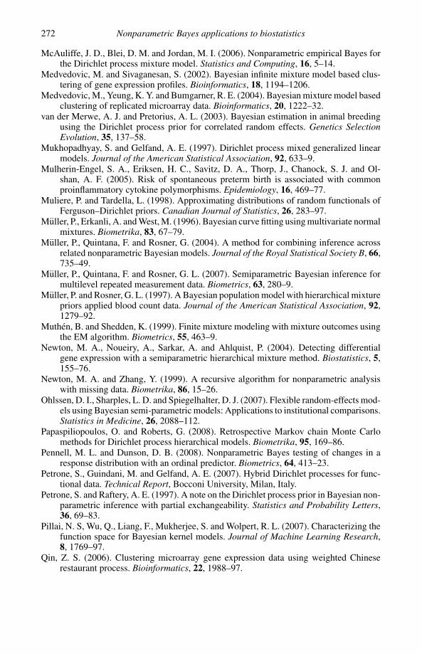
272 Nonparametric Bayes applications to biostatistics
McAuliffe, J. D., Blei, D. M. and Jordan, M. I. (2006). Nonparametric empirical Bayes forthe Dirichlet process mixture model. Statistics and Computing, 16, 5–14.
Medvedovic, M. and Sivaganesan, S. (2002). Bayesian infinite mixture model based clus-tering of gene expression profiles. Bioinformatics, 18, 1194–1206.
Medvedovic, M., Yeung, K. Y. and Bumgarner, R. E. (2004). Bayesian mixture model basedclustering of replicated microarray data. Bioinformatics, 20, 1222–32.
van der Merwe, A. J. and Pretorius, A. L. (2003). Bayesian estimation in animal breedingusing the Dirichlet process prior for correlated random effects. Genetics SelectionEvolution, 35, 137–58.
Mukhopadhyay, S. and Gelfand, A. E. (1997). Dirichlet process mixed generalized linearmodels. Journal of the American Statistical Association, 92, 633–9.
Mulherin-Engel, S. A., Eriksen, H. C., Savitz, D. A., Thorp, J., Chanock, S. J. and Ol-shan, A. F. (2005). Risk of spontaneous preterm birth is associated with commonproinflammatory cytokine polymorphisms. Epidemiology, 16, 469–77.
Muliere, P. and Tardella, L. (1998). Approximating distributions of random functionals ofFerguson–Dirichlet priors. Canadian Journal of Statistics, 26, 283–97.
Muller, P., Erkanli, A. and West, M. (1996). Bayesian curve fitting using multivariate normalmixtures. Biometrika, 83, 67–79.
Muller, P., Quintana, F. and Rosner, G. (2004). A method for combining inference acrossrelated nonparametric Bayesian models. Journal of the Royal Statistical Society B, 66,735–49.
Muller, P., Quintana, F. and Rosner, G. L. (2007). Semiparametric Bayesian inference formultilevel repeated measurement data. Biometrics, 63, 280–9.
Muller, P. and Rosner, G. L. (1997). A Bayesian population model with hierarchical mixturepriors applied blood count data. Journal of the American Statistical Association, 92,1279–92.
Muthen, B. and Shedden, K. (1999). Finite mixture modeling with mixture outcomes usingthe EM algorithm. Biometrics, 55, 463–9.
Newton, M. A., Noueiry, A., Sarkar, A. and Ahlquist, P. (2004). Detecting differentialgene expression with a semiparametric hierarchical mixture method. Biostatistics, 5,155–76.
Newton, M. A. and Zhang, Y. (1999). A recursive algorithm for nonparametric analysiswith missing data. Biometrika, 86, 15–26.
Ohlssen, D. I., Sharples, L. D. and Spiegelhalter, D. J. (2007). Flexible random-effects mod-els using Bayesian semi-parametric models: Applications to institutional comparisons.Statistics in Medicine, 26, 2088–112.
Papaspiliopoulos, O. and Roberts, G. (2008). Retrospective Markov chain Monte Carlomethods for Dirichlet process hierarchical models. Biometrika, 95, 169–86.
Pennell, M. L. and Dunson, D. B. (2008). Nonparametric Bayes testing of changes in aresponse distribution with an ordinal predictor. Biometrics, 64, 413–23.
Petrone, S., Guindani, M. and Gelfand, A. E. (2007). Hybrid Dirichlet processes for func-tional data. Technical Report, Bocconi University, Milan, Italy.
Petrone, S. and Raftery, A. E. (1997). A note on the Dirichlet process prior in Bayesian non-parametric inference with partial exchangeability. Statistics and Probability Letters,36, 69–83.
Pillai, N. S, Wu, Q., Liang, F., Mukherjee, S. and Wolpert, R. L. (2007). Characterizing thefunction space for Bayesian kernel models. Journal of Machine Learning Research,8, 1769–97.
Qin, Z. S. (2006). Clustering microarray gene expression data using weighted Chineserestaurant process. Bioinformatics, 22, 1988–97.

References 273
Ramsay, J. O. and Silverman, B. W. (1997). Functional Data Analysis, Springer.Rasmussen, C. E. and Williams, C. K. I. (2006). Gaussian Processes for Machine Learning.
Cambridge, Mass.: MIT Press.Ray, S. and Mallick, B. (2006). Functional clustering by Bayesian wavelet methods. Journal
of the Royal Statistical Society B, 68, 305–32.Rodriguez, A., Dunson, D. B. and Gelfand, A. E. (2009a). Latent stick-breaking processes.
Journal of the American Statistical Association, to appear.Rodriguez, A., Dunson, D. B. and Gelfand, A. E. (2009b). Nonparametric functional data
analysis through Bayesian density estimation. Biometrika, 96, 149–62.Rodriguez, A., Dunson, D. B. and Gelfand, A. E. (2007). The nested Dirichlet process (with
discussion). Journal of the American Statistical Association, to appear.Sethuraman, J. (1994). A constructive definition of Dirichlet priors. Statistica Sinica, 4,
639–50.Sollich, P. (2002). Bayesian methods for support vector machines: evidence and predictive
class probabilities. Machine Learning, 46, 21–52.Stephens, M. (2000). Dealing with label switching in mixture models. Journal of the Royal
Statistical Society B, 62, 795–809.Sun, S., Greenwood, C. M. T. and Neal, R. M. (2007). Haplotype inference using a Bayesian
hidden Markov model. Genetic Epidemiology, 31, 937–48.Teh, Y. W., Jordan, M. I., Beal, M. J. and Blei, D. M. (2006). Hierarchical Dirichlet
processes. Journal of the American Statistical Association, 101, 1566–81.Tipping, M. E. (2001). Sparse Bayesian learning and the relevance vector machine. Journal
of Machine Learning Research, 1, 211–44.Tomlinson, G. (1998). Analysis of densities. Unpublished Dissertation, University of
Toronto.Walker, S. G. (2007). Sampling the Dirichlet mixture model with slices. Communications
in Statistics: Simulation and Computation, 36, 45–54.Walker, S. G. and Gutierrez-Pena, E. (2007). Bayesian parametric inference in a nonpara-
metric framework. TEST, 16, 188–97.Walker, S. G. and Mallick, B. K. (1997). Hierarchical generalized linear models and frailty
models with Bayesian nonparametric mixing. Journal of the Royal Statistical SocietyB, 59, 845–60.
West, M., Muller, P. and Escobar, M. D. (1994). Hierarchical priors and mixture models,with application in regression and density estimation. In Aspects of Uncertainty: ATribute to D.V. Lindley, ed. P. R. Freeman and A. F. Smith, 363–86. Wiley.
Wilcox, A. J., Weinberg, C. R., O’Connor, J. F., Baird, D. D., Schlatterer, J. P., Canfield, R.E., Armstrong, E. G. and Nisula, B. C. (1988). Incidence of early loss of pregnancy.New England Journal of Medicine, 319, 189–94.
Xiang, Z. S., Qin, Z. H. S. and He, Y. Q. (2007). CRCView: a web server for analyz-ing and visualizing microarray gene expression data using model-based clustering.Bioinformatics, 23, 1843–5.
Xing, E. P., Jordan, M. I. and Sharan, R. (2007). Bayesian haplotype inference via theDirichlet process. Journal of Computational Biology, 14, 267–84.
Xing, E. P. and Sohn, K. (2007). Hidden Markov Dirichlet process: modeling geneticrecombination in open ancestral space. Bayesian Analysis, 2, 501–28.
Xing, E. P., Sohn, K., Jordan, M. I. and Teh, Y. W. (2006). Bayesian multi-populationhaplotype inference via a hierarchical Dirichlet process mixture. Proceedings of the23rd International Conference on Machine Learning. ACM International ConferenceProceeding Series, Volume 148, 1049–56. New York: ACM Press.

8
More nonparametric Bayesian modelsfor biostatistics
Peter Muller and Fernando Quintana
In this companion to Chapter 7 we discuss and extend some of the models and inferenceapproaches introduced there. We elaborate on the discussion of random partition priors im-plied by the Dirichlet process. We review some additional variations of dependent Dirichletprocess models and we review in more detail the Polya tree prior used briefly in Chapter 7.Finally, we review variations of Dirichlet process models for data formats beyond continu-ous responses.
8.1 Introduction
In Chapter 7, Dunson introduced many interesting applications of nonparametricpriors for inference in biomedical problems. The focus of the discussion was onDirichlet process (DP) priors and variations. While the DP prior defines a probabil-ity model for a (discrete) random probability distribution G, the primary objectiveof inference in many recent applications is not inference on G. Instead many appli-cations of the DP prior exploit the random partition of the Polya urn scheme thatis implied by the configuration of ties among the random draws from a discretemeasure with DP prior. When the emphasis is on inference for the clustering, it ishelpful to recognize the DP as a special case of more general clustering models. Inparticular we will review the product partition (PPM) and species sampling models(SSM). We discuss these models in Section 8.2. A definition and discussion ofthe SSM as a random probability measure also appears in Section 3.3.4. Anotheruseful characterization of the DP is as a special case of the Polya tree (PT) prior.A particularly attractive feature of PT priors is the possibility to model absolutelycontinuous distributions. In Section 8.3 we will define PT priors and discuss spe-cific algorithms to implement inference. For more discussion of the PT prior seealso Section 3.4.2. In Section 8.4 we discuss more variations of the dependent DP(DDP) models. In Section 8.5 we review some examples of DP priors for biosta-tistical applications that involve non-continuous data. Finally, in Section 8.6 we
274

8.2 Random partitions 275
discuss implementation details. We show some example R code using the popularR package DPpackage to implement nonparametric Bayesian inference.
8.2 Random partitions
Let [n] = {1, . . . , n} denote a set of experimental units. A partition is a family ofsubsets ρn = {S1, . . . , Sk} with
⋃Sj = [n] and Sj ∩ S� = ∅ for all j �= �. The
partitioning subsets Sj define clusters of experimental units. Often it is convenientto describe a partition by cluster membership indicators si = j if i ∈ Sj . We usenotation nnj = |Sj | and nn = (n1, . . . , nk) to denote the cluster sizes and kn = |ρn|to denote the number of clusters. When the sample size n is understood from thecontext we drop the subindex n in ρ, nj , n and k.
Several probability models p(ρn) are introduced in the literature. For an exten-sive recent review of probability models and Bayesian inference for clustering,see, for example, Quintana (2006). Popular models include the product partitionmodels (PPM), species sampling models (SSM), model based clustering (MBC)and Voronoi tessellations. The PPM (Hartigan, 1990; Barry and Hartigan, 1993)requires a cohesion function c(Sj ) ≥ 0 (see an example below). A PPM for apartition ρ and data y is defined as
p(ρ) ∝∏
c(Si) and p(y | ρ) =k∏
j=1
pj (ySj). (8.1)
Here, pj is any sampling model for the observations in the j th cluster. Model (8.1)is conjugate. The posterior p(θ | y) is again in the same product form.
Most recent applications of such models in biomedical applications use the spe-cial case of DP priors (Ferguson, 1973; Antoniak, 1974). The DP implicitly definesa probability model on p(ρn) by defining a discrete random probability measureG. An i.i.d. sample xi ∼ G, i = 1, . . . , n, includes with positive probability tiesamong the xi . Let x�
j , j = 1, . . . , k ≤ n denote the unique values of xi and defineclusters Sj = {i : xi = x�
j }. By defining the probability of ties the DP prior hasimplicitly defined p(ρn). The probability model is known as the Polya urn and isa special case of the PPM with cohesions c(A) = M × (|A| − 1)! (Dahl, 2003;Quintana and Iglesias, 2003).
A typical recent use of the DP random partition model in biostatistics applicationsappears in Dahl and Newton (2007) who use a clustering model to improve powerfor multiple hypothesis tests by pooling tests within clusters. Dahl (2006) describesa similar model with focus on inference for the clustering only. Tadesse, Sha andVannucci (2005) combine inference on clustering, again based on the DP prior, withvariable selection to identify a subset of genes whose sampling model is defined bythe clustering.

276 More nonparametric Bayesian models for biostatistics
Another class of random partition models are the species sampling models(SSM) (Pitman, 1996). An SSM defines a probability model p(ρ) that dependson ρ only indirectly through the cardinality of the partitioning subsets, p(ρ) =p(|S1|, . . . , |Sk|). The SSM can be alternatively characterized by a sequence of pre-dictive probability functions (PPF) that describe how individuals are sequentiallyassigned either to already formed clusters or to start new ones. Let nj = |Sj | andnn = (n1, . . . , nk). The PPFs are the probabilities pnj (nn) = Pr(sn+1 = j | ρn),j = 1, . . . , kn + 1. Compare Theorem 3.30 in Chapter 3. The opposite is not true.Not every sequence of PPFs characterizes an SSM. Pitman (1996) states the con-ditions. Let nj+ denote n with nj incremented by one. Essentially the PPFs haveto arise as pnj (nn) = p(nj+
n+1)/p(nn), where p(nn) is a probability measure on⋃n{nn} that is symmetric in its arguments. An important implication is that p(nn)
has to arise as the marginal of p(nn+1), i.e., p(nn) = ∑kn+1j=1 p(nj+
n+1). The proba-bility model p(nn) is known as the exchangeable partition probability function. SeeSection 3.3.2 for more discussion. Again, the random clustering implied by the DPmodel is a special case of an SSM, i.e., the random partition model implied by theDP is a special case of both PPM and SSM.
Model based clustering (Banfield and Raftery, 1993; Dasgupta and Raftery,1998) implicitly defines a probability model on clustering by assuming a mixturemodel
p(yi | η, k) =k∑
j=1
τj fj (yi | θj ),
where η = (θ1, . . . , θk, τ1, . . . , τk) are the parameters of a size k mixture model.Together with a prior p(k) on k, the mixture implicitly defines a probability modelon clustering. Consider the equivalent hierarchical model
p(yi | si = j, k, η) = fj (yi | θj ) and Pr(si = j | k, η) = τj . (8.2)
The implied posterior distribution on (s1, . . . , sn) and k implicitly defines a prob-ability model on ρn. Richardson and Green (1997) develop posterior simulationstrategies for mixture of normal models. Green and Richardson (1999) discuss therelationship to DP mixture models.
Heard, Holmes and Stephens (2006) model gene expression profiles with ahierarchical clustering model. The prior model on the random partition is an exampleof model based clustering with a mixture of regression models, a uniform prior onthe number of clusters and a Dirichlet prior for cluster membership probabilities.

8.3 Polya trees 277
8.3 Polya trees
Lavine (1992, 1994) proposed Polya trees (PT) as a useful nonparametric Bayesianprior for random probability measures. In contrast to the DP, an appropriate choice ofthe PT parameters allows the analyst to specify absolutely continuous distributions.In the following discussion we briefly review the definition of the PT model, andgive explicit implementation details for posterior inference under the PT. See alsoSection 3.4.2 for more discussion of the definition. The definition starts with anested sequence � = {πm, m = 1, 2, . . .} of partitions of the sample space �.Without loss of generality, we assume that the partitions are binary. We start with apartition π1 = {B0, B1} of the sample space, � = B0∪B1, and continue with nestedpartitions defined by B0 = B00∪B01, B1 = B10∪B11, etc. Thus the partition at levelm is πm = {Bε, ε = ε1 . . . εm}, where ε are all binary sequences of length m. APT prior for a random probability measure G is defined by beta-distributed randombranching probabilities. Let Yε0 ≡ G(Bε0 | Bε), and letA ≡ {αε} denote a sequenceof nonnegative numbers, one for each partitioning subset. If Yε0 ∼ Beta(αε0, αε1)then we say that G has a PT prior, G ∼ PT(�,A).
The parameters αε are usually chosen as αε = cmr for level m subsets. For r = 2the random probability measure G is a.s. absolutely continuous. With r = −1/2the PT reduces to the DP as a special case. The partitioning subsets Bε can bechosen to achieve a desired prior mean G�. Let qmk = G�−1(k/2m), k = 0, . . . , 2m,denote the inverse c.d.f. under G� evaluated at dyadic fractions. If αε0 = αε1,for example αε = cmr , and the dyadic quantile sets [qmk, qm,k+1) are used as thepartitioning subsets Bε , then E(G) = G�. Alternatively the prior mean can be fixedto G� by choosing αε0/(αε0 + αε1) = G�(Bε0 | Bε) for any choice of the nestedpartitions �.
The main attraction of PT models for nonparametric Bayesian inference is thesimplicity of posterior updating. Assume xi ∼ G, i.i.d., i = 1, . . . , n, and G ∼PT(�,A). Consider first n = 1, i.e., a single sample from the unknown distributionG. The posterior p(G | x) is again a Polya tree, p(G | x) = P(�,A′) with thebeta parameters in A′ defined as
α′ε =
{αε if x1 �∈ Bε
αε + 1 if x1 ∈ Bε.(8.3)
The general case with a sample of size n > 1 follows by induction.The result (8.3) can be used to implement exact posterior predictive simulation,
i.e., simulation from p(xn+1 | x1, . . . , xn). In words, we “drop” a ball down (well,really up) the Polya tree. Starting with (B0, B1) at the root we generate the randomprobabilities (Yε0, Yε1 = 1 −Yε0) for picking the two nested partitions Bε0 and Bε1
at the next level. Recall that Yε0 = P (x ∈ Bε0 | x ∈ Bε) and Yε0 ∼ Beta(α′ε0, α
′ε1).

278 More nonparametric Bayesian models for biostatistics
Going down the tree we run into some good luck. At some level m we will drop theball into a subset Bε , ε = ε1ε2 . . . εm, that does not contain any data point. Fromlevel m onwards, dropping the ball proceeds as if we had no data observed. Thus wecan generate the posterior predictive draw from the base measure G�, restricted toBε . The following algorithm summarizes posterior predictive simulation of xn+1 ∼p(xn+1 | x1 . . . xn).
Algorithm 1
1. Initialize: ε = ∅ (nil).
2. Iteration: Loop over m = 1, 2, . . .:
(a) Posterior PT parameters: Find nε0 = ∑ I (xi ∈ Bε0) and nε1 = ∑ I (xi ∈Bε1), the number of data points in the two partitioning subsets for Bε =Bε0 ∪ Bε1. Let α′
ε0 = αε0 + nε0, and same for α′ε1.
(b) Generate random branching probability: Generate Yε0 ∼ Beta(α′ε0, α
′ε1),
and set εm ∼ Bernoulli(1 − Yε0).
3. Stop the recursion: Stop the iteration over m for the smallest m∗ such thatnε = 0 at m = m∗.
4. Generate xn+1: Draw xn+1 ∼ G�(xn+1 | Bε).
We can use the same algorithm to generate a prior predictive, i.e., marginalsamples xi ∼ G, i.i.d., with G ∼ PT(�,A).
1. Generate x1 ∼ G�
2. Iterate over i = 2, . . . , n:Use algorithm 1 to generate xi ∼ p(xi | x1, . . . , xi−1).
A minor variation of the algorithm computes the posterior mean E(G | x1, . . . , xn).Let x = x1, . . . , xn denote the data. Consider some maximum level M , sayM = 10. For all levels m = 1, . . . , M compute Y ε1ε2···εm−10 = E(Yε1ε2···εm−10 | x) =α′
ε1ε2···0/(α′ε1ε2···0 + α′
ε1ε2···1). Record Y ε1ε2···εm−11 = 1 − Y ε1ε2···εm−10 as the com-
plement to one. Computing Y ε is most elegantly implemented as a recursion. Letε = ε1 . . . εM denote a dyadic number, ε ∈ [0, 1]. We find
E(G(ε) | x1, . . . , xn) ≈M∏
m=1
Y ε1ε2···εm≡ G(ε).
Here G(·) is the p.d.f. for the random measure G.

8.4 More DDP models 279
To generate random draws G ∼ p(G | x1, . . . , xn) proceed as above replacingY ε by Yε0 ∼ Beta(α′
ε0, α′ε1). Let G(ε) =∏M
m=1 Yε1ε2···εm. Plotting G against ε shows
a random posterior draw of G. Plotting multiple draws Gj , j = 1, 2, . . . , J in thesame figure illustrates posterior uncertainty on the random measure.
An important simplification for applications is achieved by restricting the PTprior to finitely many levels, e.g. m ≤ 10. Actual inference differs little, but therequired computational effort is greatly reduced. Posterior predictive draws andposterior estimated densities can still be carried out exactly, as outlined above.Nonparametric Bayesian inference under the PT prior and the finite PT prior forsome important models is implemented in the public domain R packageDPpackage.See Section 8.6 for an example.
Applications of PT models in biomedical problems are less common than thewidely used DP. The limited use of PT priors for nonparametric Bayesian dataanalysis is due in part to the awkward sensitivity of posterior inference to thechoice of the partitioning subsets. Consider a model for density estimation, xi ∼ G,i.i.d., i = 1, . . . , n, with a PT prior for the unknown distribution, G ∼ PT(A,P).The posterior estimate G = E(G | x) shows characteristic discontinuities at theboundaries of the partitioning subsets. An exception is the special case of the DP, i.e.,when αε = αε0 + αε1. In that case the probability model p(G) remains invariantunder any change of the partitioning sequence. Several authors have proposedvariations of the PT prior model to mitigate this undesirable feature of posteriorinference. Hanson and Johnson (2002) and Hanson (2006) defined mixture ofPolya trees, with the mixture being with respect to the centering measure G�.Paddock, Ruggeri, Lavine and West (2003) introduced an explicit perturbation ofthe partition boundaries. The posterior dependence on the partition boundaries isless of an issue when the focus of the inference is not on the density itself. Forexample, Branscum, Johnson, Hanson and Gardner (2008) develop inference forROC curves with a PT prior for the distribution of the recorded measurements fortrue positives and negatives. Hanson and Yang (2007) use PT priors for survivaldata.
8.4 More DDP models
Many applications in biostatistics involve hierarchical models across different sub-populations and naturally lead to models that include several random probabilitymeasures. Appropriate nonparametric probability models require modeling of de-pendent families of random distributions. One of the most commonly used mod-els to achieve this aim are variations of dependent DP (DDP) models. Since thefirst proposal of DDP models in MacEachern (1999) many authors have devel-oped variations and implementations for specific problems. Some are discussed in

280 More nonparametric Bayesian models for biostatistics
Sections 7.5 and 7.6. In this section we review more related models that find use inbiostatistics.
8.4.1 The ANOVA DDP
DDP models define probability models for families of random probability measures{Gx, x ∈ X} in such a way that marginally each Gx follows a DP prior, Gx ∼DP(c, G�
x). Let Gx = ∑h wxhδµxh
. By the definition of the DP prior the pointmasses µxh, h = 1, 2, . . . , are i.i.d. draws from a base measure, and the weightsare generated by the stick-breaking process based on independent beta randomvariables. See, for example, Chapter 7, equation (7.2) for a definition of the DPprior. The DDP introduces the desired dependence of the random measures Gx
across x by defining the dependence of the locations µxh and/or the weights wxh
across x. The independence across h remains untouched. Alternative variations ofthe DDP model differ in the definition of the dependence structure. Consider thecase when X is categorical, for example, when x indexes different studies, differentsubpopulations and/or centers. Perhaps the easiest definition of dependence across{µxh, x ∈ X} for categorical factors x is the ANOVA model. Without loss ofgenerality assume x = (u, v) is bivariate with u ∈ {0, . . . , nu} and v ∈ {0, . . . , nv}referring to two factors. For example, u might be treatment history and v might be anindicator for a relevant molecular marker. We can define a DDP model by assumingµxh = Mh + Auh + Bvh where (Mh,Auh, Bvh, u = 0, . . . , nu, v = 0, . . . , nv)are overall mean and main effects in an ANOVA model. For identifiability we fixA0h = B0h = 0. The weights whx are assumed constant across x, whx ≡ wh. Thisdefines the ANOVA DDP of De Iorio, Muller, Rosner and MacEachern (2004).
An interesting application of the ANOVA DDP to modeling survival data appearsin De Iorio, Johnson, Muller and Rosner (2008). The model implements nonpara-metric regression for event time data without relying on restrictive assumptions likeproportional or additive hazards. In particular, inference allows survival functionsto cross.
Figures 8.1 and 8.2 show the estimated survival functions for data from a studyof infant and childhood mortality in Colombia (Somoza, 1980). A questionnairewas administered to a sample of women between the ages of 15 and 49 elicitingtheir maternity history, educational level, age, union status and information on thesex, date of birth and survival status (at the date of interview) of all their childrenand, if applicable, age at death. We consider data on a subsample of 1437 children(corresponding to the oldest child for each mother). The response of interest is thesurvival time (in years) of a child at the time of the maternal interview. The covariatesof interest are: gender (male/female), birth cohort (1, 1941–1959; 2, 1960–1967;3, 1968–1976) and a binary variable indicating whether a child was born in a rural

8.4 More DDP models 281
1.00
0.95
0.90
0.85
0.80
0
URBAN and MALE
COHORT 1COHORT 2COHORT 3
5 10 15Y
S
1.00
0.95
0.90
0.85
0.80
0 2 4 6 8
COHORT 1COHORT 2COHORT 3
10 12 14
Sj K-M
Figure 8.1 Colombian children data. Posterior survivor functions for urban male childrenfrom the three birth cohorts, under the DDP ANOVA model (left panel) and raw estimates(KM) from the data (right panel). The solid line corresponds to children in the first birthcohort, the dashed line represents a child in the second birth cohort and the dotted linerefers to children in the third birth cohort.
area (yes/no). Around 87% of the observations in the data set were censored. Theoriginal research was conducted to investigate how patterns of childhood mortalityhave changed over time. Also of interest are urban/rural and gender differences.
Inference under the DDP ANOVA model is implemented in the R packagesDPpackage and ddpanova. See Section 8.6 for an example and additionaldetails.
8.4.2 Classification with DDP models
A minor extension of ANOVA DDP models allows their use for nonparametricclassification. Let x ∈ X ≡ {1, . . . , k} index k subpopulations and assume a semi-parametric hierarchical model for outcomes y across the k subpopulations. Letyi denote the outcome for the ith experimental unit and let xi ∈ X denote theknown class label, i.e., the index of the subpopulation containing the ith patient,i = 1, . . . , n. For example, De la Cruz-Mesıa, Quintana and Muller (2007) con-sider data for pregnant women. For each woman yi = (yi1, . . . , yini
) are repeatedmeasurements of a hormone (β-HCG) which shows dramatic changes during preg-nancy. Pregnancies are classified as normal xi = 0 versus not normal xi = 1(spontaneous abortions or other types of adverse pregnancy outcomes). We con-sider the classification problem of predicting (unknown) xn+1 for a future patient,

282 More nonparametric Bayesian models for biostatistics
1.00
0.95
0.90
0.85
0.80
0
RURAL and MALE
COHORT 1COHORT 2COHORT 3
5 10 15Y
S
1.00
0.95
0.90
0.85
0.80
0
URBAN and MALE
COHORT 1COHORT 2COHORT 3
5 10 15Y
S
1.00
0.95
0.90
0.85
0.80
0
RURAL and FEMALE
COHORT 1COHORT 2COHORT 3
5 10 15Y
S
1.00
0.95
0.90
0.85
0.80
0
URBAN amd FEMALE
COHORT 1COHORT 2COHORT 3
5 10 15Y
S
Figure 8.2 Colombian children data. Posterior survivor functions for children from thethree birth cohorts, arranged by rural versus urban and male versus female. The solid linecorresponds to children in the first birth cohort, the dashed line represents a child in thesecond birth cohort and the dotted line refers to children in the third birth cohort.
i = n + 1 conditional observed responses yn+1, i.e.,
p(xn+1 | yn+1, y1, x1, . . . , yn, xn).
Let p(yi | xi = x) = ∫p(yi | θi) dGx(θi) be a semiparametric sampling model
for outcomes in group x, see for example De la Cruz-Mesıa, Quintana and Muller(2007) for details of the model for the pregnancy data. Marginally, for each x ∈ X
we use a DP mixture model, i.e., we assume a DP prior for Gx . The submodels for allx are combined into one encompassing hierarchical model by linking the marginalDP priors through an ANOVA DDP across x. Finally the model is completed byassuming a marginal distribution p(xi) for xi , for example xi ∼ Dir(α1, . . . , αk).

8.5 Other data formats 283
1.0
0.8
0.6
0.4
0.2
0.0
1 2 3 4 5 6
Repeat Measurement j
TRUE NORMALP (
x =
abn
orm
al|d
ata)
TRUE ABNORMAL
Figure 8.3 Pregnancy data: sequentially updated classification probabilities p(xn+1 = 1 |yn+1,1, . . . , yn+1,j , data) for a future case. The probabilities are plotted against j . The solid(dashed) line is for a future case with normal (abnormal) pregnancy.
The ANOVA DDP model defines p(y1, . . . , yn+1 | x1, . . . , xn+1). Together withthe marginal model p(x1, . . . , xn+1) = ∏
p(xi) we can use Bayes theorem toderive the desired p(xn+1 | yn+1, x1, y1, . . . , xn, yn). One of the attractions ofthis principled model-based approach is the possibility for coherent sequentialupdating. Assume yi = (yi1, . . . , yimi
) are repeated measurement data as in thepregnancy example. The classification probability p(xn+1 | yn+1,1, . . . , yn+1,j ,
y1, x1, . . . , yn, xn) can be sequentially updated and reported as increasingly moredata become available for j = 1, . . . , mn+1. Figure 8.3 shows sequentially updatedclassification probabilities p(xn+1 = 1 | yn+1,1, . . . , yn+1,j , y1, x1, . . . , yn, xn)for the pregnancy example. Probabilities are plotted against j for two hypothet-ical future patients. The first patient (solid line) is a woman with a truly normalpregnancy. The second case (dashed line) is a truly abnormal pregnancy. See De laCruz-Mesıa, Quintana and Muller (2007) for details of the simulation. Note how thetwo classification probabilities start to diverge from the third repeat measurementonwards.
8.5 Other data formats
Many discussions of DP models, including most of the discussion in Chapter 7,focus on continuous outcomes. But many biomedical data analysis problems involveother data formats. We briefly review two applications of nonparametric Bayesianinference to categorical and binary data.

284 More nonparametric Bayesian models for biostatistics
z 02 0
32
1−1
−2−3
03
21
−1−2
−3−2 0 1 2 3 4 −2 0
0.015
0.033
0.033
0.919
1 2 3 4
z01
(a) (b)
Figure 8.4 Interrater agreement data. Panel (a) plots draws from the latent probit scores(with a DP mixture of normal prior). Panel (b) shows one posterior draw for the moments ofthe mixture of normal terms (location and scale are shown as triangle and ellipse), togetherwith the corresponding weights (number below the ellipse). Notice the varying degree ofpolychoric correlation across scores.
Kottas, Muller and Quintana (2005) propose nonparametric Bayesian inferencefor multivariate ordinal data, for example the rating of the extent of tumor invasionby two raters. Tumor invasion is coded on an ordinal scale from none to extensiveinvasion. A feature of the data example reported in Kottas, Muller and Quintana(2005) is that the raters tend to agree on extreme cases, but less so on interme-diate cases. This makes it inappropriate to use a bivariate ordinal probit model,as described for example in Johnson and Albert (1999). Instead Kottas, Mullerand Quintana (2005) propose an ordinal probit model based on a DP mixture ofnormal distributions for the latent variable. The mixture of normal model allowsus to formalize the notion of varying degrees of interrater agreement across scores.Let �j denote the variance–covariance matrix of the j th term in the mixture ofnormal model for the latent variables. The correlation of the latent scores is knownas polychoric correlation. We refer to the correlation that is implied by �j for eachterm of the mixture as local polychoric correlation. The use of different �j for eachterm in the mixture allows for varying degrees of interrater agreement, as desired.Figure 8.4 shows imputed ordinal probit scores and summaries of the mixture

8.5 Other data formats 285
1 2 3 5 7 9 11 14SNP (by CHROM)
Figure 8.5 LOH data: gray shades show the probability of increased LOH for a givensample. SNPs are arranged by chromosomes indicated by vertical dashed lines. Darkergray shade indicates higher probability of increased LOH. The underlying model makesminimal assumptions beyond order � exchangeability.
of normal model for the interrater agreement example. The plotted variables z01
and z02 are the latent ordinal probit scores. The observed scores are defined bythresholds on the latent scores; see Kottas, Muller and Quintana (2005) for details.For normal cases (with low scores) the two raters are in strong agreement, i.e., highpolychoric correlation. For extreme cases the strength of agreement is considerablyless.
Quintana, Muller, Rosner and Relling (2008) discusses semiparametric Bayesianinference for binary sequences of indicators of loss of heterozygosity (LOH).Nonparametric inference for sequences of binary indicators subject to a partialexchangeability assumptions are defined in Quintana and Muller (2004). The ex-changeability assumption is order � exchangeability, i.e., the assumption that theprobability model is invariant with respect to any permutation of the sequencethat leaves the order � transition counts unchanged. Quintana and Newton (2000)show that any such distribution can be represented as a mixture of order � Markovchains. The mixture is with respect to the transition probabilities of the Markovchain. In the application to the LOH data we implemented this by a DP prior onthe mixture measure of the transition probabilities. We allow different transitionprobabilities for each region of the chromosome. Regions are defined as sequencesof 55 to 835 SNPs (single nucleotide polymorphism); see Quintana, Muller, Rosnerand Relling (2008) for details. The transition probabilities of the binary Markovchain with states { no LOH, LOH } imply a limiting probability of LOH. Let πcj
denote this limiting probability for region j in chromosome c. We can map theposterior distribution on the transition probabilities into p(πcj | data). Figure 8.5shows Icj ≡ p(πcj > 0.01 | data) by region j , arranged by chromosome c.

286 More nonparametric Bayesian models for biostatistics
0.20
0.15
0.10
0.05
0.00
5 10 15 20 25 30 35 40
Speeds
Galaxy Data
Den
sity
Figure 8.6 Galaxy data. The histogram shows the data with n = 82 observations. Thecurves show the density estimate using a DP mixture model (dashed line), a PT prior (solidline) and a random Bernstein polynomial (dotted line).
8.6 An R package for nonparametric Bayesian inference
An important impediment to the wider use of nonparametric Bayesian models was,until recently, the limited availability of reliable public domain software. This istrue for biomedical applications in particular, where the research focus is oftenon the application, and only limited resources are available for the developmentof problem-specific software. Also reproducibility is an increasingly importantissue. The impact of research publications proposing new methods and approachesremains limited unless readers can reproduce inference and implement the proposedmethods for their problems.
A popular software platform for biomedical research, in particular for bioinfor-matics applications, is the public domain R language (R Development Core Team,2008). The R package DPpackage (Jara, 2007) implements inference for someof the models discussed in Chapter 7, including DP mixture density estimation,PT priors for density estimation, nonparametric random effects models includinggeneralized linear models. DPpackage is available from the package repositoryCRAN. We show a simple example.
Buta (1987) reports velocities (yi) and radial positions (xi) of galaxy NGC7531at 323 different locations. We use the first 82 velocity measurements. The data areavailable as galaxy data set in DPpackage. The following R code implementsdensity estimation using PT priors, a DP mixture model and random Bernsteinpolynomials (Petrone, 1999a, 1999b). See Section 3.4.1 for a discussion of randomBernstein polynomials. Figure 8.6 shows a histogram of the galaxy data and the

8.6 R package for nonparametric Bayesian inference 287
three density estimates based on DP mixture model, the PT prior and the randomBernstein polynomials.
library("DPpackage")
data(galaxy) # Data
galaxy <- data.frame(galaxy,speeds=galaxy$speed/1000)
attach(galaxy)
state <- NULL # MCMC parameters
nburn <- 10000; nsave <- 1000; nskip <- 50; ndisplay <- 10
mcmc <- list(nburn=nburn,nsave=nsave,nskip=nskip,ndisplay=ndisplay,
tune1=0.15,tune2=1.1,tune3=1.1)
## tune parameters only needed for PTdensity()
## POLYA TREE
prior<-list(alpha=1,M=6) # Prior information
# Fitting the model
fit1 <- PTdensity(y=speeds,ngrid=1500,prior=prior,mcmc=mcmc,
state=state,status=TRUE)
## DIRICHLET PROCESS
# Prior information
prior <- list(a0=2,b0=4,m2=rep(20,1),s2=diag(100000,1),
psiinv2=solve(diag(0.5,1)), nu1=4,nu2=4,tau1=1,tau2=100)
# Fitting the model
fit2 <- DPdensity(y=speeds,ngrid=1500,prior=prior,mcmc=mcmc,
state=state,status=TRUE)
## BERNSTEIN DIRICHLET PROCESS
# Prior information
prior <- list(aa0=2.01,ab0=1.01,kmax=1000,a0=1,b0=1)
# Fitting the model
fit3 <- BDPdensity(y=speeds,ngrid=1500,prior=prior,mcmc=mcmc,
state=state,status=TRUE)
rg <- range(c(fit1$dens,fit2$dens,fit3$fun)) ## Plots
hist(galaxy$speeds,xlim=c(5,40),nclass=30,ylim=rg)
lines(fit1$x1,fit1$dens,lty=1,lwd=2)
lines(fit2$x1,fit2$dens,lty=2,lwd=2)
lines(fit3$grid,fit3$fun,lty=3,lwd=2)
Inference for the ANOVA DDP is implemented in the LDDPdensity() functionof DPpackage. For the following example we generate n = 500 observations eachfrom an assumed simulation truth Fo
0 = N (3, 0.8) and Fo1 = 0.6 N (1.5, 0.8) +

288 More nonparametric Bayesian models for biostatistics
0.4
0.3
0.2
0.1
0.0
0 2 4 6Y
p
0.30
0.25
0.20
0.15
0.10
0.50
0.00
0 2 4 6Y
p
F 0 F 1
Figure 8.7 Simulated mixture of normal data. The figures show the simulation truth (dashedline) and the estimated distributions Fx = E(Fx | data) (solid lines). The posterior meansare equal to the posterior predictive distribution for a future observation Fx = p(yn+1 |xn+1 = x, data).
0.4N(4, 0.6). Based on the simulated data we estimate {F0, F1} under a DDPANOVA prior for {F0, F1}. We assume Fx(y) = ∫ N (y; m, s) dGx with {G0, G1} ∼DDP ANOVA. The DDP ANOVA model is based on an ANOVA model µxh =Mh +xAh, i.e., a main effect for x = 1 and a common intercept Mh. Let d = (1, x)denote a design vector and let βh = (Mh, Ah) denote the vector of ANOVA pa-rameters. The DDP ANOVA model for {F0, F1} can be written as a mixture of DPmodel
y | x ∼∫
N (y; β ′d, σx) dG(β) with G ∼ DP(G�, α).
See De Iorio, Muller, Rosner and MacEachern (2004) for more details of themodel. The data structure prior in the R code fragment below sets the parametersfor the base measure G�, a hyperprior on the residual variance σx and the totalmass parameter α. We assume 1/σ 2
x ∼ Ga(τ1/2, τ2/2) and α ∼ Ga(a0, b0). LetB ∼ IW (ν, A) denote an inverse Wishart random (q × q) matrix B with expec-tation E(B) = A−1/(ν − q − 1). The base measure is G�(β) = N (µb,�b) withconditionally conjugate hyperpriors µb ∼ N (m, S) and �b ∼ IW (ν, ψ). Figure8.7 shows the density estimates Fx = E(Fx | data), x = 0, 1. The estimates areproduced by the R code below.

8.7 Discussion 289
library(DPpackage)
## prepare simulated data: mixture of two normals
nobs <- 50; y1 <-rnorm(nobs, 3,.8)
y21 <- rnorm(nobs,1.5, 0.8); y22 <- rnorm(nobs,4.0, 0.6)
y2 <- ifelse(runif(nobs)<0.6,y21,y22); y <- c(y1,y2)
trt <- c(rep(0,nobs),rep(1,nobs)) # design matrix with a
single factor
xpred <- rbind(c(1,0),c(1,1)) # design matrix for posterior
predictive
m <- rep(0,2); psiinv <- diag(1,2); s <- diag(100,2) # prior
prior <- list(a0=1,b0=1/5,nu=4,m=m,s=s,psiinv=psiinv,
tau1=0.01,tau2=0.01)
## Fit the DDP ANOVA model
mcmc <- list(nburn=100, nsave=500, nskip=5, ndisplay=100)
fit <- LDDPdensity(y~trt,prior=prior,mcmc=mcmc,state=NULL,status=TRUE,
grid=seq(-1,7,length=200),xpred=xpred)
## Estimated densities F_x (posterior predictive distributions)
plot(fit$grid,fit$dens[1,],type="l")
lines(fit$grid, dnorm(fit$grid, 3.0, 0.8), lty=2) # simulation truth
# ... and x0=(1,1)
plot(fit$grid,fit$dens[2,],type="l",xlab="Y",ylab="p",bty="l")
p2 <- 0.6*dnorm(fit$grid, 1.5, 0.8) + 0.4*dnorm(fit$grid, 4.0, 0.6)
lines(fit$grid,p2, lty=2)
The implementation of DDP ANOVA in DPpackage is based on the R packageddpanova which can be downloaded from http://odin.mdacc.tmc.edu/∼pm. The ddpanova package has additional options, including options forcensored event time data.
8.7 Discussion
We have discussed some extensions and elaborations of the models introduced inChapter 7. The discussion is by no means an exhaustive list of Bayesian nonpara-metric models. Keeping to the theme of Chapter 7 we have focused on modelsthat find applications in biostatistics. This focus excluded, for example, interestingrecent applications with spatial and spatiotemporal data.
Many more nonparametric Bayesian models and methods are reviewed in otherchapters of this volume, including among many others, the beta process, and theIndian buffet process. As an alternative to the R package discussed, DPpackage,the package bayesm (Rossi and McCulloch, 2008) also implements many of theDP-based models.

290 More nonparametric Bayesian models for biostatistics
References
Antoniak, C. E. (1974). Mixtures of Dirichlet processes with applications to Bayesiannonparametric problems. Annals of Statistics, 2, 1152–74.
Banfield, J. D. and Raftery, A. E. (1993). Model-based Gaussian and non-Gaussian clus-tering. Biometrics, 49, 803–21.
Barry, D. and Hartigan, J. A. (1993). A Bayesian analysis for change point problems.Journal of the American Statistical Association, 88, 309–19.
Branscum, A. J., Johnson, W. O., Hanson, T. E. and Gardner, I. A. (2008). Bayesiansemiparametric roc curve estimation and disease diagnosis. Statistics in Medicine, 27,2474–96.
Buta, R. (1987). The structure and dynamics of ringed galaxies, iii. Astrophysical Journal,Supplement Series, 64, 1–37.
Dahl, D. B. (2003). Modal clustering in a univariate class of product partition models.Technical Report 1085, Department of Statistics, University of Wisconsin.
Dahl, D. B. (2006). Model-based clustering for expression data via a Dirichlet processmixture model. In Bayesian Inference for Gene Expression and Proteomics, ed. K.-A.Do, P. Muller and M. Vannucci, 201–18. Cambridge: Cambridge University Press.
Dahl, D. B. and Newton, M. A. (2007). Multiple hypothesis testing by clustering treatmenteffects. Journal of the American Statistical Association, 102, 517–26.
Dasgupta, A. and Raftery, A. E. (1998). Detecting features in spatial point processes withclutter via model-based clustering. Journal of the American Statistical Association,93, 294–302.
De Iorio, M., Johnson, W., Muller, P. and Rosner, G. (2008). A ddp model for survivalregression. Technical Report, Texas University M. D. Anderson Cancer Center.
De Iorio, M., Muller, P., Rosner, G. L. and MacEachern, S. N. (2004). An anova modelfor dependent random measures. Journal of the American Statistical Association,99, 205–15.
De la Cruz-Mesıa, R., Quintana, F. and Muller, P. (2007). Semiparametric Bayesianclassification with longitudinal markers, Applied Statistics, 56, 119–37.
Ferguson, T. S. (1973). A Bayesian analysis of some nonparametric problems. Annals ofStatistics, 1, 209–30.
Green, P. J. and Richardson, S. (1999). Modelling heterogeneity with and without theDirichlet process. Technical Report, Department of Mathematics, University of Bristol.
Hanson, T. E. (2006). Inference for mixtures of finite Polya tree models. Journal of theAmerican Statistical Association, 101, 1548–64.
Hanson, T. and Johnson, W. (2002). Modeling regression error with a mixture of polyatrees. Journal of the American Statistical Association, 97, 1020–33.
Hanson, T. and Yang, M. (2007). Bayesian semiparametric proportional odds models.Biometrics, 63, 88–95.
Hartigan, J. A. (1990). Partition models. Communications in Statistics, Part A – Theoryand Methods, 19, 2745–56.
Heard, N. A., Holmes, C. C. and Stephens, D. A. (2006). A quantitative study of generegulation involved in the immune response of Anopheline mosquitoes: an applicationof Bayesian hierarchical clustering of curves. Journal of the American StatisticalAssociation, 101, 18–29.
Jara, A. (2007). Applied Bayesian non- and semi-parametric inference using dppackage.Rnews, 17–26.
Johnson, V. E. and Albert, J. H. (1999). Ordinal Data Modeling. New York: Springer.Kottas, A., Muller, P. and Quintana, F. (2005). Nonparametric Bayesian modeling for

References 291
multivariate ordinal data. Journal of Computational and Graphical Statistics, 14, 610–25.
Lavine, M. (1992). Some aspects of Polya tree distributions for statistical modelling. Annalsof Statistics, 20, 1222–35.
Lavine, M. (1994). More aspects of Polya tree distributions for statistical modelling. Annalsof Statistics, 22, 1161–76.
MacEachern, S. (1999). Dependent nonparametric processes. In ASA Proceedings of theSection on Bayesian Statistical Science, 50–5. Alexandria, Va.: American StatisticalAssociation.
Paddock, S., Ruggeri, F., Lavine, M. and West, M. (2003). Randomised Polya tree modelsfor nonparametric Bayesian inference. Statistica Sinica, 13, 443–60.
Petrone, S. (1999a). Bayesian density estimation using Bernstein polynomials. CanadianJournal of Statistics, 27, 105–26.
Petrone, S. (1999b). Random Bernstein polynomials. Scandinavian Journal of Statistics,26, 373–93.
Pitman, J. (1996). Some developments of the Blackwell–MacQueen urn scheme. In Statis-tics, Probability and Game Theory. Papers in Honor of David Blackwell, ed. T. S.Ferguson, L. S. Shapeley and J. B. MacQueen, IMS Lecture Notes/Monographs, 245–68. Hayward, Calif.: Institute of Mathematical Statistics.
Quintana, F. A. (2006). A predictive view of Bayesian clustering. Journal of StatisticalPlanning and Inference, 136, 2407–29.
Quintana, F. A. and Iglesias, P. L. (2003). Bayesian clustering and product partition models.Journal of the Royal Statistical Society, Series B, 65, 557–74.
Quintana, F. A. and Newton, M. A. (2000). Computational aspects of nonparametricBayesian analysis with applications to the modeling of multiple binary sequences.Journal of Computational and Graphical Statistics, 9, 711–37.
Quintana, F. and Muller, P. (2004). Nonparametric Bayesian assessment of the order ofdependence for binary sequences. Journal of Computational and Graphical Statistics,13, 213–31.
Quintana, F., Muller, P., Rosner, G. and Relling, M. (2008). A semiparametric Bayesianmodel for repeatedly repeated binary outcomes. Journal of the Royal Statistical Soci-ety, Series C, 57, 419–31.
R Development Core Team (2008). R: A Language and Environment for StatisticalComputing. Vienna: R Foundation for Statistical Computing.http://www.R-project.org
Richardson, S. and Green, P. J. (1997). On Bayesian analysis of mixtures with an unknownnumber of components (with discussion). Journal of the Royal Statistical Society,Series B, 59, 731–92.
Rossi, P. and McCulloch, R. (2008). bayesm: Bayesian Inference for Marketing/Micro-econometrics. R package version 2.2-2. http://faculty.chicagogsb.edu/peter.rossi/research/bsm.html
Somoza, J. L. (1980). Illustrative analysis: infant and child mortality in Colombia. WorldFertility Survey Scientific Reports 10. The Hague: International Statistical Institute.
Tadesse, M. G., Sha, N. and Vannucci, M. (2005). Bayesian variable selection in clusteringhigh-dimensional data. Journal of the American Statistical Association, 100, 602–17.

Author index
Aalen, O. O., 18, 95, 139, 141,155
Acero, A., 175Ahlquist, P., 263Albert, J. H., 284Aldous, D. J., 82, 212Amewou-Atisso, M., 58Andersen, P. K., 141, 143Anderson, C. R., 148Antoniak, C. E., 47, 90, 108, 164, 275Arjas, E., 99
Baird, D. D., 235, 236Baladandayuthapani, V., 15Banfield, J. D., 276Barron, A. R., 56, 57, 60Barry, D., 275Basu, S., 267Beal, M., 48, 160, 161, 171, 172, 174, 196, 198,
199, 242, 249, 264Belitser, E. N., 68Benveniste, A., 176Berger, J. O., 224, 267Bernardo, J. M., 24, 208Bernshteın, S., 2Berry, D. A., 265Bigelow, J. L., 243, 244Blackwell, D., 44, 84, 212, 228, 231Blei, D. M., 48, 160, 161, 169–71, 196, 198, 199, 230,
242, 249, 264Blum, J., 90Borgan, Ø., 18, 139, 141, 143Box, G. E. P., 24Branscum, A. J., 279Breiman, L., 4, 15Brillinger, D. R., 151Brix, A., 101Brumback, B. A., 243Bumgarner, R. E., 263Burr, D., 235Bush, C. A., 118, 226, 231Buta, R., 286
Carin, L., 247Carota, C., 267Carroll, R. J., 15Chakraborty, S., 241Chen, M.-H., 13Chen, S. F., 180, 181Chib, S., 267Chipman, H. A., 15Choi, T., 59Chopin, N., 17Chou, K. C., 176Choudhuri, N., 59, 150Chu, W., 192Cifarelli, D. M., 126–8Claeskens, G., 5, 15, 155Clyde, M., 230Connor, R. J., 87Coram, M., 59Corander, J., 268Cowans, P., 166, 168Cox, D. D., 73Crainiceanu, C. M., 15Crandell, J. L., 240
Dahl, D. B., 230, 239, 275Dalal, S. R., 49Daley, D. J., 84Damien, P., 13, 71, 92, 103, 140, 217Dary, M., 217Dasgupta, A., 276Dass, S. C., 71Datta, S., 139De Blasi, P., 140, 141, 143, 153de Finetti, B. D., 16, 22, 82De Iorio, M., 251, 280, 288De la Cruz-Mesia, R., 253, 281–3Denison, D. G. T., 15Dey, D., 13Dey, J., 93Di Nunno, G., 39, 127Diaconis, P., 12, 49, 52, 57, 59, 127, 129DiMatteo, I., 15Do, K.-A., 263
292

Author index 293
Doksum, K. A., 11, 86–8, 147Donnelly, P., 168, 170Doob, J. L., 27, 50Doss, H., 46, 49, 57, 235Doucet, A., 217Dryden, I. L., 148–9Duan, J., 253Duan, J. A., 182Dubins, L. E., 11Dunson, D. B., 216, 217, 235, 236, 240, 242–7, 249,
250, 253–6, 258, 264, 265, 266Dykstra, R. L., 87, 97, 101Dzhaparidze, K., 151
Efron, B., 17Epifani, I., 128Erickson, R. V., 93Erkanli, A., 256Erosheva, E., 169Escobar, M. D., 23, 48, 116, 194, 231, 232Ewens, W. J., 108Exton, H., 127
Fabius, J., 11Feder, M., 29Fei-Fei, L., 170Ferguson, T. S., 11, 13, 23, 37, 47, 88–92, 100, 103,
118, 122–5, 162, 226, 275Finkel, J. R., 177Fitzgerald, W. J., 217Fournier, D. A., 17Fox, E., 174, 175, 200Freedman, D. A., 11, 12, 49–52, 57, 59, 73, 122, 129Freeman, W., 194, 195Friedman, J. H., 15, 247Frigessi, A., 18
Gorur, D., 112, 189, 192, 200, 201, 219Gardner, I. A., 279Gasbarra, D., 99Gaskins, R. A., 11Gelfand, A. E., 12, 14, 161, 182, 209, 216, 233, 240,
247, 250, 252, 253, 256Gelman, A., 17, 209Genovese, C. R., 15George, E. I., 15Getoor, L., 192Ghahramani, Z., 95, 112, 171, 172, 174, 187, 189,
192, 193, 200, 201, 219, 220Ghosal, S., 36, 56–9, 61, 65–72, 74, 75, 150Ghosh, J. K., 13, 36, 56–8, 61, 72, 75, 123Ghosh, M., 241Gill, R. D., 92, 141, 143Gjessing, H., 18, 139, 155Gnedin, A., 96, 109, 110Goldwater, S., 175–8, 181Good, I. J., 5, 11, 208Goodman, J. T., 180, 181Gopalan, R., 265Gould, S. J., 141Gramacy, R. B., 14
Green, P. J., 3, 210, 228, 239, 276Greenwood, C. M., 264Grenager, T., 177Grenander, U., 148Griffin, J. E., 217, 219, 253, 257Griffiths, T. L., 95, 171, 175–8, 181, 187, 192Guglielmi, A., 39, 127, 267Guindani, M., 14, 182, 247, 253Gull, A., 168Gurland, J., 127Gutierrez-Pena, E., 26, 267
Hancock-Beaulieu, M., 168Hanson, T. E., 126, 234, 279Hartigan, J. A., 109, 275He, Y. Q., 263Heard, N. A., 276Hermansen, G. H., 152–4Herring, A. H., 264, 265, 266Hewitt, E., 22Hiemstra, D., 168Hill, T., 128Hjort, N. L., 5, 13, 15, 16, 31, 39, 60, 87, 92–4, 127,
138–41, 143–7, 152–5, 185Ho, M. W., 161Hoff, P. D., 247Hollander, M., 46, 109Holmes, C. C., 14, 220, 238, 239, 257, 276Hon, H.-W., 175Hoppin, J. A., 265, 266Huang, S., 181Huang, T. Z., 69, 70Huang, X., 175Huijbregts, M., 175
Ibrahim, J. G., 13, 233Ickstadt, K., 92, 188, 189Iglesias, P. L., 275Ishwaran, H., 99, 112, 116, 118, 161, 177, 200,
214–16, 219, 230, 247
Jakel, F., 192Jackson, E., 217Jacobs, R. A., 255Jain, S., 118, 213, 214, 230James, L. F., 84, 87, 95, 96, 98, 99, 102, 112, 116, 118,
127–9, 161, 177, 200, 214–16, 219, 230, 247Jara, A., 10, 16, 234, 286Jasra, A., 238, 239Jefferys, W., 224Johansen, S., 92, 139Johnson, M., 175–8, 181Johnson, V. E., 284Johnson, W. O., 126, 279, 280Jones, B. L., 238Jordan, M. I., 48, 95, 160, 161, 169–71, 174, 175, 177,
182, 184, 185, 187, 188, 190, 196, 198, 199, 200,202, 230, 242, 249, 255, 264
Kallenberg, O., 82Kalli, M., 219

294 Author index
Kass, R. E., 23Kass, R. F., 15Keiding, N., 141, 143Kemperman, J., 127Kent, J. T., 148Kerov, S., 128Kim, S., 193, 194, 263Kim, Y., 51, 72, 73, 87, 95–7, 153–5Kimeldorf, G. S., 241Kingman, J. F. C., 83, 84, 86, 100, 101, 104, 108, 184Kivinen, J., 177Klass, M. J., 92, 103, 118Kleijn, B., 65Klein, D., 177, 196Kleinman, K. P., 233Knowles, D., 192Kohn, R., 15Korwar, R. M., 46, 109Kottas, A., 161, 240, 252, 284Kraaij, W., 168Kraft, C. H., 11, 57, 123Krause, R., 192Kurihara, K., 196, 230
Laird, N. M., 234Lalley, S. P., 59Laplace, P. S., 2Lau, J. W., 161, 239Lau, M., 168Laud, P. W., 13, 87, 92, 97, 101, 140Lavine, M., 52, 122, 125, 126, 277, 279Le Cam, L., 2Lee, H. K. H., 14Lee, J., 51, 71, 72, 153Lee, K. J., 225Lehmann, E. L., 2Lember, J., 69–71Lenk, P., 71Li, Y., 235Liang, F., 241Liang, P., 177, 196Liao, M., 241Lijoi, A., 56, 59, 61, 100–2, 106, 109–11, 114, 119,
127, 128, 265Lin, X., 235Lindley, D. V., 10, 208Liu, J. S., 230Lo, A. Y., 23, 47, 72, 87, 97, 115, 211, 232Longnecker, M. P., 258–60
Muller, P., 13, 118, 212, 231, 233, 235, 249, 251, 253,256, 263, 280–5, 288
MacEachern, S. N., 113, 118, 161, 212, 226, 230, 240,251, 279, 280, 288
MacKay, D., 181MacLehose, R. F., 242, 265, 266MacQueen, J. B., 44, 212, 228, 231Mallick, B. K., 14, 15, 99, 234, 237, 241Manning, C. D., 177, 180Mao, K., 241Mardia, K. V., 149
Martino, S., 17Mauldin, R. D., 122, 124, 125McAuliffe, J. D., 230McCulloch, R. E., 15, 289McGill, M., 166Medvedovic, M., 239, 262Meeds, E., 192, 193Mena, R. H., 101, 106, 109, 114, 119, 265Merhav, N., 29Meulman, J. J., 247Miller, M. I., 148Monticino, M., 128Mosimann, J. E., 87Mukherjee, S., 241Mukhopadhyay, S., 233Mulherin-Engel, S. A., 263Muliere, P., 91, 92, 125, 127, 214, 231Muthen, B., 237
Nagin, D. S., 238Navarro, D. J., 192Neal, R. M., 14, 15, 118, 192, 193, 196, 200, 212–14,
217, 230, 264Newton, M. A., 27, 230, 263, 275, 285Ng, A. Y., 169, 170Nieto-Barajas, L., 87, 99Nieto-Barajas, L. E., 103, 128Noueiry, A., 263
O’Hagan, A., 14Oakley, J., 14Ohlssen, D. I., 234Oliva, A., 182Olshen, R. A., 15Ongaro, A., 39, 127
Paddock, S. M., 126, 279Papaspiliopoulos, O., 118, 216, 220, 233Park, J.-H., 217, 253–5, 258Parmigiani, G., 267Parzen, E., 147Pearl, J., 18Peddada, S. D., 267Pennell, M. L., 267Perman, M., 100, 107, 177Perona, P., 170Peto, L., 181Petrone, S., 14, 119–21, 145–7, 153, 247, 286Petrov, S., 177, 196Phadia, E. G., 89, 90Phelan, M. J., 139Pillai, N. S., 241, 253, 255Pitman, J., 96, 100, 101, 104–12, 128, 161, 177, 178,
211, 276Prunster, I., 56, 59, 61, 100–3, 106, 109–11, 114, 119,
128, 129, 265Pretorius, A. L., 234Pritchard, J., 170
Qin, Z. S., 263Quintana, F. A., 13, 234, 249, 253, 275, 281–5

Author index 295
R Development Core Team, 16, 286Rabiner, L., 171Raftery, A. E., 27, 276Ramamoorthi, R. V., 13, 36, 56–8, 93, 123Ramsay, J. O., 236Rasmussen, C. E., 14, 171, 172, 174, 192,
240Ray, S., 237Regazzini, E., 39, 100, 126–8Relling, M., 285Renals, S., 181Rice, J. A., 243Richardson, S., 3, 210, 228, 276Roberts, G. O., 118, 211, 216, 220, 233Robertson, S. E., 168Rodriguez, A., 216, 247, 250, 256Roeder, K., 238Romik, D., 127Rosner, G. L., 233, 249, 251, 280, 285, 288Rossi, P., 289Roweis, S. T., 192, 193Roy, A., 57, 58, 59, 150Rubin, D. B., 26Rue, H., 17Ruggeri, F., 126, 279Ruppert, D., 15
Saatci, Y., 200, 220Salton, G., 166Samanta, T., 72Sarkar, A., 263Sato, K., 86Satten, G. A., 139Savage, L. J., 22Schutze, H., 180Schervish, M., 56, 57, 59Schwartz, L., 11, 52, 54, 56Scott, S. L., 200Secchi, P., 214Sellke, T., 46Sethuraman, J., 45, 112, 161, 212, 226Sha, N., 275Sharan, R., 169, 264Sharples, L. D., 234Shedden, K., 237Shen, X., 61, 73Silverman, B. W., 236Sinha, D., 13Sivaganesan, S., 239, 262Skaug, H. J., 17Smith, A. F. M., 12, 13, 15, 24, 92, 101, 140, 208,
209, 211Smith, M., 15Smith, N., 168Smyth, P., 193, 194Sohn, K., 169, 175, 264Sollich, P., 187, 241Somoza, J. L., 280Spiegelhalter, D. J., 234Steel, M. F. J., 217, 253Stephens, D. A., 238, 239, 276
Stephens, M., 168, 170, 238, 239Stone, C. J., 15Sudderth, E., 174, 175, 177, 182, 184, 194–6,
200Sudderth, W. D., 122, 124, 125Sun, S., 264Susarla, V., 90
Tadesse, M. G., 263, 275Takahara, G., 230Tang, F., 263Tang, Y., 59Tardella, L., 127, 214, 231Taskar, B., 192Teh, Y. W., 48, 112, 160, 161, 169, 178, 181, 189, 192,
196, 198–201, 219, 220, 230, 242, 249, 264Tenenbaum, J. B., 171Thibaux, R., 95, 185, 187, 188, 190, 202Thompson, S. G., 225Tiao, G. C., 24Tibshirani, R. J., 15Tierney, L., 211Tipping, M. E., 241Tokdar, S. T., 56, 57Tomlinson, G., 194, 242Torralba, A., 182, 194, 195
van der Merwe, A. J., 234van der Vaart, A. W., 36, 57, 61, 65–7, 69–72, 75van Eeden, C., 11Van Gael, J., 200, 220Van Ryzin, J., 90van Zanten, H., 57, 65Vannucci, M., 263, 275Vere-Jones, D., 84Vlassis, N., 230von Mises, R., 2
Wahba, G., 241Wakefield, J. C., 217Walker, S., 168Walker, S. G., 13, 16, 26, 31, 56, 59–61, 71, 87, 91,
92, 99, 103, 110, 111, 118, 125, 128, 144, 145,153, 200, 217, 219, 233, 234, 267
Wand, M. P., 15Ware, J. H., 234Wasserman, L., 23Wasserman, L. A., 3, 5, 56, 57, 61Welling, M., 196, 230Weng, C.-S., 87, 97West, M., 48, 116, 126, 231, 232, 241, 256, 279Wilcox, A. J., 243–6Wild, D. L., 192Williams, C. K. I., 14, 240Williams, S. C., 122, 124, 125Willsky, A., 174–6, 194, 195, 200Wolpert, R. L., 92, 188, 189, 241Wood, F., 192Wooters, C., 175Wu, Q., 241Wu, Y., 56

296 Author index
Xiang, Z. S., 263Xing, E. P., 169, 175, 264Xue, Y., 247
Yang, G. L., 2Yang, M., 235, 236, 279
Yau, C., 220Yeung, K. Y., 263Yor, M., 100, 107, 128, 177
Zarepour, M., 214Zhang, Y., 230

Subject index
asymptotics, 2, 27, 35, 49, 268
Bayesian adaptation, 69Bayesian bootstrap, 26, 27, 40, 43Bayesian kriging, 154Bayesian modeling and inference, 209Bernoulli process, 186Bernstein–Dirichlet process, 121Bernshteın–von Mises theorems, 2, 36, 71, 153beta process, 8, 17, 92, 137, 184, 192
conjugacy, 94, 138hierarchical, 190inference, 200mixtures, 153
beta-Stacy process, 91binary data, 285bioinformatics, 13, 260
expressed sequence tag analysis, 265gene expression analyses, 262, 276haplotype phasing, 168, 264loss of heterozygosity data, 285SNP data, 263
biostatistics, 223, 274child mortality study, 280gestational age at delivery data, 258multicenter study, 248progesterone trajectory data, 243tumor invasion data, 284
blocked Gibbs sampler, 231see truncation of measure
borrowing information, 225, 242, 248, 264
calibration, 257causality, 17childhood mortality study, 280Chinese restaurant franchise, 162, 196Chinese restaurant process, 9, 162, 177Cifarelli–Regazzini identity, 127classification, 15, 190, 253, 281clustering process, 8, 44, 115, 228, 237, 245, 274, 276coherency, 255collapsed Gibbs sampler, 230competing risks, 142
conditional distributionsflexible modeling of, 250, 256
conjugacy, 39, 83, 88, 187consistency, 3, 8, 11, 12, 13, 28, 31, 36, 49convergence rate of posterior distribution, 36, 60, 152CRF, Chinese restaurant franchise, 162CRP, Chinese restaurant process, 162cumulative hazard, 11, 92, 97, 137curse of dimensionality, 251, 256
DDP, dependent Dirichlet process, 252de Finetti’s theorem, 81, 187, 209density estimation, 8, 11, 56, 64, 70, 114dependent Dirichlet process, 113, 161, 251, 279Dirichlet distribution, 37Dirichlet process, 8, 17, 80, 90, 160, 211, 226
conjugacy, 39construction, 38dependent, 113, 161, 251, 279functional, 240hierarchical, 48, 160, 249mixtures, 46, 115, 249, 262multilevel, 264nested, 250self-similarity, 42support, 42transformed, 194
discrete nonparametrics, 99DP, Dirichlet process, 160DPpackage, 286
empirical Bayes, 17event history analysis, 137exchangeability, 28, 81, 158, 285expressed sequence tag analysis, 265
FDP, functional Dirichlet process, 240featural representation, 184functional data analysis, 236, 256functional Dirichlet process, 240
gamma process, 85Gaussian process, 9, 14, 182
297

298 Subject index
GEM distribution, 161, 211gene expression analyses, 262, 276gestational age at delivery data, 258Gibbs-type random partition, 109goodness-of-fit testing, 267graphical model, 166, 169, 171, 172
haplotype phasing, 168, 264hazard, 97HBP, hierarchical beta process, 190HDP, hierarchical Dirichlet process, 160HDP-HMM, hierarchical Dirichlet process hidden
Markov model, 171HDP-HMT, hierarchical Dirichlet process hidden
Markov tree, 176Heaps’s law, 178heavy-tailed distribution, 203, 225Hellinger distance, 32hidden Markov model, 171hidden Markov tree, 176hierarchical beta process, 190hierarchical Dirichlet process, 160, 176, 249
inference, 196with random effects, 193
hierarchical Dirichlet process hidden Markov model,171
hierarchical model, 8, 158, 211, 224, 248mixed effect, 10
hierarchical Pitman–Yor process, 179high-dimensional data, 15, 247, 260, 264HMM, hidden Markov model, 171HMT, hidden Markov tree, 176HPY, hierarchical Pitman–Yor, 179hyperparameter, 47, 202, 228, 230, 268hypothesis testing, 265
IBP, Indian buffet process, 187image processing, 181incoherence, 24Indian buffet process, 9, 95, 187information retrieval, 166informative prior, 266inverse Levy measure, 189
joint modeling, 243, 257
kernel-based approaches, 241, 253kernel stick-breaking process, 255, 258KSBP, kernel stick-breaking process, 255Kullback–Leibler divergence, 26
label-switching problem, 238, 259language modeling, 13, 180large-sample techniques, 2, 36latent Dirichlet allocation, 170latent variable model, 191, 200, 235, 261Levy intensity, 84Levy measure, 100, 185
inverse, 189Levy process, 86Levy representation, 84, 220
linear mixed effects model, 234loss function, 29loss of heterozygosity data, 285
machine learning, 8, 13, 14, 44marginal likelihood, 229, 266marginal method, 118Markov process, 138Markov–Krein identity, 127MCMC, 2, 4, 12, 17, 44, 116, 122, 140, 196, 199, 200,
211collapsed Gibbs sampling, 230mixing, 213, 259retrospective sampling, 216slice sampling, 217, 233truncation of random measure, 214, 231
metric entropy, 55, 62missing data, 257, 264misspecification, 65mixed membership model, 169model averaging, 15, 239model selection, 5, 15, 36, 67, 239, 268multicenter study, 248multilevel Dirichlet process, 264multiple comparisons, 265, 275multiplicative intensity model, 95
nested Dirichlet process, 250neural network, 14neutral-to-the-right process, 8, 11, 86
spatial, 96noninformative prior, 40, 146normalization, 100
ordinal data, 284
parametric conjugacy, 88parametric models, 154, 210
as base models, 251, 256partition probability function, 104Pitman–Yor process, 108, 177
hierarchical, 179Polya tree, 9, 11, 13, 122, 277Polya urn scheme, 44, 163, 178, 212, 231, 274Poisson–Dirichlet process, 46, 107, 177Poisson–Kingman model, 106Poisson process, 85power-law behavior, 178, 181predictive density, 22predictive distribution, 83predictor effects on tails, 258prior belief, 24, 125, 164, 177, 209, 210, 226product partition model, 274progesterone trajectory data, 243proportional hazards, 4, 140
quantile inference, 17, 144, 258
random Bernstein polynomial, 119random effects, 158, 193, 208, 225, 232, 245random effects model, 233random mean, 126

Subject index 299
random measure, 8completely, 84, 184normalized, 100, 219tail free, 122
random partitions, 275recommender systems, 193relational model, 192retrospective sampling, 216, 233
semiparametric models, 193, 234, 237, 281shape analysis, 148shrinkage, 158, 225, 264size-biased ordering, 188skewness, 225, 247slice sampling, 217, 233SNP data, 263software packages, 4, 16, 234, 263, 286spatial model, 14
speaker diarization, 175species sampling model, 111, 265, 276splines, 9, 14, 67, 70, 240
adaptive, 15, 244stick-breaking representation, 45, 112, 161, 177, 188,
212, 226structural conjugacy, 88survival analysis, 8, 11, 13, 86, 137, 280
time series, 8, 150topic model, 169transformed Dirichlet process, 194truncation of measure, 214tumor invasion data, 284
word segmentation, 175
Zipf’s law, 178