Bayesian Discovery of Threat Networks - arXiv

5324 IEEE TRANSACTIONS ON SIGNAL PROCESSING, VOL. 62, NO. 20, 2014

Bayesian Discovery of Threat NetworksSteven Thomas Smith, Senior Member, IEEE, Edward K. Kao, Member, IEEE,Kenneth D. Senne, Life Fellow, IEEE, Garrett Bernstein, and Scott Philips

Abstract—A novel unified Bayesian framework for networkdetection is developed, under which a detection algorithm isderived based on random walks on graphs. The algorithm detectsthreat networks using partial observations of their activity, andis proved to be optimum in the Neyman-Pearson sense. Thealgorithm is defined by a graph, at least one observation, and adiffusion model for threat. A link to well-known spectral detectionmethods is provided, and the equivalence of the random walkand harmonic solutions to the Bayesian formulation is proven.A general diffusion model is introduced that utilizes spatio-temporal relationships between vertices, and is used for a specificspace-time formulation that leads to significant performance im-provements on coordinated covert networks. This performance isdemonstrated using a new hybrid mixed-membership blockmodelintroduced to simulate random covert networks with realisticproperties.

Index Terms—Network detection, optimal detection, maxi-mum likelihood detection, community detection, network theory(graphs), graph theory, diffusion on graphs, random walks ongraphs, dynamic network models, Bayesian methods, harmonicanalysis, eigenvector centrality, Laplace equations.

I. INTRODUCTION

NETWORK detection is the objective in many diversegraph analytic applications, ranging from graph parti-

tioning, mesh segmentation, manifold learning, communitydetection [44], network anomaly detection [10], [30], andthe discovery of clandestine networks [32], [43], [52], [56],[70]. A new Bayesian approach to network detection is de-veloped and analyzed in this paper, with specific applicationto detecting small, covert networks embedded within muchlarger background networks. The novel approach is based ona Bayesian probabilistic framework where the probability ofthreat is derived from an observation model and an a priorithreat diffusion model. Specifically, observed threats from oneor more vertices are propagated through the graph using a

Manuscript received November 15, 2013; revised March 17, 2014; acceptedMay 29, 2014. Date of publication July 08, 2014; date of current versionSeptember 8, 2004. The associate editor coordinating the review of thismanuscript and approving it for publication was Prof. Francesco Verde. Thiswork is sponsored by the Assistant Secretary of Defense for Research &Engineering under Air Force Contract FA8721-05-C-0002. Opinions, inter-pretations, conclusions and recommendations are those of the author and arenot necessarily endorsed by the United States Government.

S. T. Smith, K. D. Senne, G. Bernstein, and S. Philips are with the MITLincoln Laboratory, Lexington, MA 02420 USA (e-mail: [email protected];[email protected]; [email protected]; [email protected]).

E. K. Kao is with the MIT Lincoln Laboratory, Lexington, MA 02420 USA,and also with the Department of Statistics, Harvard University; CambridgeMA USA 02138 (e-mail: [email protected]).

Color versions of one or more of the figures in this paper are availableonline at http://ieeexplore.ieee.org.

Digital Object Identifier 10.1109/TSP.2014.2336613

model based on random walks represented as Markov chainswith absorbing states. The resulting network detection algo-rithm is proved to be optimum in the Neyman–Pearson senseof maximizing the probability of detection at a fixed falsealarm probability. In the specific case of space-time graphswith time-stamped edges, a model for threat diffusion yieldsthe new space-time threat propagation algorithm, which isshown to be an optimal detector for covert networks withcoordinated activity.

Network detectors are analyzed using both a stochasticframework of random walks on the graph and a probabilisticframework. The two frameworks are shown to be equivalent,providing an original, unified approach for Bayesian networkdetection. Performance for a variety of Bayesian network de-tection algorithms is shown with both a stochastic blockmodeland a new hybrid mixed-membership blockmodel (HMMB)introduced to simulate random covert networks with realisticproperties.

Using insights from algebraic graph theory, the connectionbetween this unified framework and other spectral-based net-work detection methods [18], [22], [44] is shown, and thetwo approaches are contrasted by comparing their differentoptimality criteria based on detection probability and subgraphconnectivity properties. The random walk framework providesa connection with many other well-known graph analyticmethods that may also be posed in this context [7], [11],[15], [34], [46], [54], [62]. In contrast to other research onnetwork detection, rather than using a sensor network to detectsignals [3], [13], [30], the signal of interest in this paper is thenetwork. In this sense the paper is also related to work on so-called manifold learning methods [8], [10], [16], although thenetwork to be detected is a subgraph of an existing network,and therefore the methods described here belong to a classof network anomaly detection [10] as well as maximum-likelihood methods for network detection [21].

Threat network discovery is predicated on the existence ofobservations of network relationships. Detection of networkcommunities is most likely to be effective if the communitiesexhibit high levels of connection activity. The covert networksof interest in this paper exist to accomplish nefarious, illegal,or terrorism goals, while “hiding in plain sight” [70]. Covertnetworks necessarily adopt operational procedures to remainhidden and robustly adapt to losses of parts of the network [9],[52], [61], [66].

This paper’s major contributions are organized into a de-scription of the novel approach to Bayesian network detectionin Section III, and showing and comparing detection perfor-mance using simulations of realistic networks in Section IV.

1053-587X c© 2014 IEEE. Translations and content mining are permitted for academic research only. Personal use is also permitted, but republication/redistribution requires IEEE permission. See http://www.ieee.org/publications˙standards/publications/rights/index.html for more information.

arX

iv:1

311.

5552

v3 [

cs.S

I] 8

Sep

201

4

mailto:[email protected]





http://ieeexplore.ieee.org

http://www.ieee.org/publications_standards/publications/rights/index.html

SMITH et al.: BAYESIAN DISCOVERY OF THREAT NETWORKS 5325

Fundamental new results are established in Theorems 1–3,which prove a maximum principal for threat propagation,provide a nonnegative basis for the principal invariant sub-space, and prove the equivalence between the probabilisticand stochastic realization approaches of threat propagation.The Neyman–Pearson optimality of threat propagation is es-tablished in Theorem 4.

II. BACKGROUND

A. Notation

A graph G = (V,E) is defined by two sets, the verticesV , and the edges E ⊂ [V ]2, in which [V ]2 denotes theset of 2-element subsets of V [17]. For example, the setsV = { 1, 2, 3 }, E =

{{1, 2}, {2, 3}

}describe a simple

graph with undirected edges between vertices 1 and 2, and 2and 3: 1 −− 2 −− 3 . The order and size of G are definedto be #V and #E, respectively. A subgraph G′ ⊆ G is agraph (V ′, E′) with V ′ ⊆ V and E′ ⊆ E. If E′ contains alledges in E with both endpoints in V ′, then G′ = G[V ′] is theinduced subgraph of V ′. The adjacency matrix A = A(G)of G is the {0, 1}-matrix with aij = 1 iff { i, j } ∈ E. Inthe example, A =

(0 1 01 0 10 1 0

). The adjacency matrix of simple

or undirected graphs is necessarily symmetric. The degreematrix D = Diag(A·1) is the diagonal matrix of the vectorof degrees of all vertices, where 1 = (1, . . . , 1)T is the vectorof all ones. The neighborhood N(u) =

{v : {u, v} ∈ E

}of a vertex u ∈ V is the set of vertices adjacent to u, orequivalently, the set of nonzero elements in the u-th row of A.The vertex space V (G) of G is the vector space of functionsf : V → {0, 1}.

A directed graph Gσ is defined by an orientation mapσ : [V ]2 → V × V (the ordered Cartesian product of Vwith itself) in which the first and second coordinates arecalled the initial and terminal vertices, respectively. A stronglyconnected graph is a connected graph for which a directedpath exists between any two vertices. The incidence matrixB = B(Gσ) of Gσ is the (0,±1)-matrix of size #V -by-#Ewith Bie = ±1, if i is an terminal/initial vertex of σ(e), and0 otherwise. For example, the directed graph 1 ←− 2 −→ 3

has incidence matrix B =(

1 0−1 −1

0 1

). The unnormalized

Laplacian matrix or Kirchhoff matrix Q of a graph, the(normalized) Laplacian matrix L, and the generalized orasymmetric Laplacian matrix Ł are, respectively,

Q = BBT = D−A, (1)

L = D−1/2QD−1/2 = I−D−1/2AD−1/2, (2)

Ł = D−1/2LD1/2 = D−1Q = I−D−1A. (3)

In the example, Ł is immediately recognized as a discretizationof the second derivative −d2/dx2, i.e. the negative of the1-d Laplacian operator ∆ = ∂2/∂x2 + ∂2/∂y2 + · · · thatappears in physical applications. The connection between theLaplacian matrices and physical applications is made throughGreen’s first identity, a link that explains many theoretical andperformance advantages of the normalized Laplacian over theKirchhoff matrix across applications [14], [64], [67], [68].

Solutions to Laplace’s equation on a graph are directlyconnected to random walks or discrete Markov chains on thevertices of the graph, which provide stochastic realizations forharmonic problems. A (right) stochastic matrix T of a graphis a nonnegative matrix such that T1 = 1. This representsa state transition matrix of a random walk on the graphwith transition probability tij of jumping from vertex vito vertex vj . The Perron–Frobenius theorem guarantees ifT is irreducible (i.e. G is strongly connected) then thereexists a stationary probability distribution pv on V such thatpTT = pT [26], [28]. Random walk realizations can be usedto describe the solution to harmonic boundary value problems,e.g. equilibrium thermodynamics [47], [51], in which givenvalues are proscribed at specific “boundary” vertices.

B. Network Detection

Network detection is a special class of the more generalgraph partitioning (GP) problem in which the binary decisionof membership or non-membership for each graph vertex mustbe determined. Indeed, the network detection problem for agraph G of order N results in a 2N -ary multiple hypothesis testover the vertex space V (G), and, when detection optimality isconsidered, an optimal test involves partitioning the measure-ment space into 2N regions yielding a maximum probabilityof detection (PD). This NP-hard combinatoric problem iscomputationally and analytically intractable. In general, net-work detection methods invoke various relaxation approachesto avoid the NP-hard network detection problem. The newBayesian threat propagation approach taken in this paper is togreatly simplify the general 2N -ary multiple hypothesis testby applying the random walk model and treating it as Nindependent binary hypothesis tests. This approach is related toexisting network detection methods by posing an optimizationproblem on the graph—e.g. threat propagation maximizesPD—and through solutions to Laplace’s equation on graphs.Because many network detection algorithms involve suchsolutions, a key fact is that the constant vector 1 = (1, . . . , 1)T

is in the kernel of the Laplacian,

Q1 = 0; Ł1 = 0. (4)

This constant solution does not distinguish between verticesat all, a deficiency that may be resolved in a variety of ways.

Efficient graph partitioning algorithms and analysis ap-peared in the 1970s with Donath and Hoffman’s eigenvalue-based bounds for graph partitioning [18] and Fiedler’s con-nectivity analysis and graph partitioning algorithm [22] whichestablished the connection between a graph’s algebraic prop-erties and the spectrum of its Kirchhoff Laplacian ma-trix Q = D−A [Eq. (1)]. Spectral methods solve the graphpartitioning problem by optimizing various subgraph connec-tivity properties. Similarly, the threat propagation algorithmdeveloped here in Section III optimizes the probability ofdetecting a subgraph for a specific Bayesian model. Thoughthe optimality criteria for spectral methods and threat prop-agation are different, all these network detection methodsmust address the fundamental problem of avoiding the trivialsolution of constant harmonic functions on graphs. Threat


propagation avoids this problem by using observation verticesand a priori probability of threat diffusion (Section III-A).Spectral methods take a complementary approach to avoidthis problem by using an alternate optimization criterion thatdepends upon the network’s topology.

The cut size of a subgraph—the number of edges necessaryto remove to separate the subgraph from the graph—is quan-tified by the quadratic form sTQs, where s = (±1, . . . ,±1)T

is a ±1-vector who entries are determined by subgraph mem-bership [50]. Minimizing this quadratic form over s, whosesolution is an eigenvalue problem for the graph Laplacian,provides a network detection algorithm based on the modelof minimal cut size. However, there is a paradox in the appli-cation of spectral methods to network detection: the smallesteigenvalue of the graph Laplacian λ0(Q) = 0 corresponds tothe eigenvector 1 constant over all vertices, which fails todiscriminate between subgraphs. Intuitively this degenerateconstant solution makes sense because the two subgraphs withminimal (zero) subgraph cut size are the entire graph itself(s ≡ 1), or the null graph (s ≡ −1). This property manifestsitself in many well-known results from complex analysis, suchas the maximum principle.

Fiedler showed that if rather the eigenvector ξ1 correspond-ing to the second smallest eigenvalue λ1(Q) of Q is used(many authors write λ1 = 0 and λ2 rather than the zero offsetindexing λ0 = 0 and λ1 used here), then for every nonpositiveconstant c ≤ 0, the subgraph whose vertices are defined bythe threshold ξ1 ≥ c is necessarily connected. This algorithmis called spectral detection. Given a graph G, the numberλ1(Q) is called the Fiedler value of G, and the correspondingeigenvector ξ1(Q) is called the Fiedler vector. Completelyanalogous with comparison theorems in Riemannian geometrythat relate topological properties of manifolds to algebraicproperties of the Laplacian, many graph topological propertiesare tied to its Laplacian. For example, the graph’s diameter Dand the minimum degree dmin provide lower and upperbounds for the Fiedler value λ1(Q): 4/(nD) ≤ λ1(Q) ≤n/(n− 1)·dmin [41]. This inequality explains why the Fiedlervalue is also called the algebraic connectivity: the greater theFiedler value, the smaller the graph diameter, implying greatergraph connectivity. If the normalized Laplacian L of Eq. (2)is used, the corresponding inequality involving the generalizedeigenvalue λ1(L) = λ1(Q,D) involves the graph’s diame-ter D and volume V : 1/(DV ) ≤ λ1(L) ≤ n/(n− 1) [14].

Because in practice spectral detection with its implicit as-sumption of minimizing the cut size oftentimes does not detectintuitively appealing subgraphs, Newman introduced the alter-nate criterion of subgraph “modularity” for subgraph detec-tion [44]. Rather than minimize the cut size, Newman proposesto maximize the subgraph connectivity relative to backgroundgraph connectivity, which yields the quadratic maximizationproblem maxs sTMs, where M = A− V −1ddT is New-man’s modularity matrix, A is the adjacency matrix, (d)i = diis the degree vector, and V = 1Td is the graph volume [44].Newman’s modularity-based graph partitioning algorithm, alsocalled community detection, involves thresholding the valuesof the principal eigenvector of M. Miller et al. [38]–[40] alsoconsider thresholding arbitrary eigenvectors of the modularity

matrix, which by the Courant minimax principle biases theNewman community detection algorithm to smaller subgraphs,a desirable property for many applications. They also outlinean approach for exploiting observations within the spectralframework [38].

Other graph partitioning methods invoke alternate relaxationapproaches that yield practical detection/partitioning algo-rithms such as semidefinite programming (SDP) [6], [35], [69].A class of graph partitioning algorithms is based on infiniterandom walks on graphs [59]. Zhou and Lipowsky defineproximity using the average distance between vertices [72].Anderson et al. define a local version biased towards spe-cific vertices [4]. Mahoney et al. develop a local spectralpartitioning method by augmenting the quadratic optimizationproblem with a locality constraint and relaxing to a convexSDP [37]. An important dual to network detection is theproblem of identifying the source of an epidemic or rumorusing observations on the graph [53], [54]. Another relatedproblem is the determination of graph topologies for whichepidemic spreading occurs [11], [62]. The approach adopted inthis paper has fundamentally different objectives and propaga-tion models than the closely-related epidemiological problems.These problems focus on disease spreading to large portions ofthe entire graph, which arises because disease may spread fromany infected neighbor—yielding a logical OR of neighborhooddisease. Network detection focuses on discovering a subgraphmost likely associated with a set of observed vertices, assum-ing random walk propagation to the observations—yielding anarithmetic mean of neighborhood threat. All of these methodsare related to spectral partitioning through the graph Laplacian.

III. BAYESIAN NETWORK DETECTION

The Bayesian model developed here depends upon threatobservation and propagation via random walks over both spaceand time, and the underlying probabilistic models that governinference from observation to threat, then propagation of threatthroughout the graph. Bayes’ rule is used to develop a networkdetection approach for spatial-only, space-time, and hybridgraphs. The framework assumes a given Markov chain modelfor transition probabilities, and hence knowledge of the graph,and a diffusion model for threat. Neyman–Pearson optimalityis developed in the context of network detection with a simplebinary hypothesis, and it is proved that threat propagation isoptimum in this sense.

The framework is sufficiently general to capture graphsformed by many possible relationships between entities, fromsimple graphs with vertices that represent a single type ofentity, to bipartite or multipartite graphs with heterogeneousentities. For example, an email network is a bipartite graphcomprised of two types of vertices: individual people and in-dividual email messages, with edges representing a connectionbetween people and messages. Without loss of generality, allentity types to be detected are represented as vertices in thegraph, and their connections are represented by edges weightedby scalar transition probabilities.

Network detection is the problem of identifying a specificsubgraph within a given graph G = (V,E). Assume that


within G, a foreground or “threat” network V Θ exists definedby an (unknown) binary random variable:

Definition 1 Threat is a {0, 1}-valued discrete random vari-able. Threat on a graph G = (V,E) is a {0, 1}-valued functionΘ ∈ V (G). Threat at the vertex v is denoted Θv . A vertexv ∈ V is in the foreground if Θv = 1, otherwise v is in thebackground.

The foreground or threat vertices are the set V Θ = { v :Θv = 1}, and the foreground or threat network is the inducedsubgraph GΘ = G[V Θ]. A network detector of the subgraphGΘ is a collection of binary hypothesis tests to decide whichof the graph’s vertices belong to the foreground vertices V Θ.Formally, a network detector is an element of the vertex spaceof G:

Definition 2 Let G = (V,E) be a graph. A network detec-tor φ on G is a {0, 1}-valued function φ ∈ V (G). The inducedsubgraph Gφ = G[V φ] of V φ = { v : φv = 1 } is called theforeground network and the induced subgraph Gφ = G[V φ]

of V φ = { v : φv = 0 } is called the background network, inwhich φ denotes the logical complement of φ.

The correlation between a network detector φ and theactual threat network defined by the function Θ determinesthe detection performance of φ, measured using the detector’sprobability of detection (PD) and probability of false alarm(PFA). The PD and PFA of φ are the fraction of correct andincorrect foreground vertices determined by φ:

PDφ = #(V φ ∩ V Θ)/#V Θ, (5)

PFAφ = #(V φ ∩ V Θ)/#V Θ. (6)

Observation models are now introduced and applied in thesequel to threat propagation models in the contexts of spatial-only graphs, space-time graphs whose edges have time stamps,and finally a hybrid graphs with edges of mixed type. Assumethat there are C observed vertices { vb1 , . . . , vbC } ⊂ V atwhich observations are taken. In the resulting Laplacian prob-lem, these are “boundary” vertices, and the rest are “interior.”The simplest case involves scalar measurements; however,there is a straightforward extension to multidimensional ob-servations.

Definition 3 Let G = (V,E) be a graph. An observation onthe graph is a vector z : { vb1 , . . . , vbC } → M ⊂ RC fromC vertices to a measurement space M ⊂ RC .

Ideally, observation of a foreground and/or backgroundvertices unequivocally determines whether the observed ver-tices lie in the foreground or background networks, i.e. givena foreground graph GΘ = G[V Θ] and a foreground vertexv ∈ V Θ, an observation vector z evaluated at v would yieldz(v) = 1, and z evaluated at a background vertex v′ ∈ V Θ

would yield z(v′) = 0. In general, it is assumed that theobservation z(v) at v and the threat Θv at v are not statisticallyindependent, i.e. f

(z(v) | Θv

)6= f

(z(v)

)for probability

density f , so that there is positive mutual information between

z(v) and Θv . Bayes’ rule for determining how likely a vertexis to be a foreground member or not depends on the modellinking observations to threat:

Definition 4 Let GΘ = G[V Θ] be the foreground graphof a graph G determined by Θ ∈ V (G), and letz : { vb1 , . . . , vbC } →M ⊂ RC be an observation on G. Theconditional probability density f

(z(v) | Θv

)is called the

observation model of vertex v ∈ V .

The simplest, ideal observation model equates threat withobservation so that fideal

(z(v) | Θv

)= δz(v)Θv

in which δijis the Kronecker delta. Though the threat network hypothesesare being treated here independently at each vertex, thisframework allows for more sophisticated global models thatinclude hypotheses over two or more vertices.

The remainder of this section is devoted to the developmentof Bayesian methods of using measurements on a graph todetermine the probability of threat on a graph in variouscontexts—spatial-only, space-timed, and the hybrid case—thenshowing that these methods are optimum in the Neyman–Pearson sense of maximizing the probability of detection ata given false alarm rate. The motivating problem is:

Problem 1 Detect the foreground graph GΘ = G[V Θ] in thegraph G = (V,E) with an unknown foreground Θ ∈ V (G)and known observation vector z(vb1 , . . . , vbC ).

This problem is addressed by computing the probability ofthreat P (Θv) at all graph vertices from the measurementsat observed vertices using an observation model and theapplication of Bayes’ rule.

A. Spatial Threat Propagation

A spatial threat propagation algorithm is motivated anddeveloped now, which will be used in the subsequent space-time generalization, and will demonstrate the connection tospectral network detection methods. A vertex is declared tobe threatening if the observed threat propagates to that vertex.We wish to compute the probability of threat P (Θv = 1 | z) atall vertices v ∈ V in a graph G = (V,E) given an observationz(vb1 , . . . , vbC ) on G. Implicit in Problem 1 is a coordinatedthreat network in which threat propagates via network connec-tions, i.e. graph edges. For simplicity, probabilities conditionedon the observation z will be written

θv = P (Θv | z) (7)

with an implied dependence on the observation vector z andthe event Θv = 1 expressed as Θv .

To model the diffusion of threat throughout the graph, weintroduce an a priori probability ψv at each vertex v thatrepresents threat diffusion at v. ψv is the probability that threatpropagates through vertex v to its neighbors, otherwise threatpropagates to an absorbing “non-threat” state with probability1− ψv . A threat diffusion event at v is represented by the{0, 1}-valued r.v. Ψv:


Definition 5 The threat diffusion model of a graphG = (V,E) with observation z is given by the a priori{0, 1}-valued event Ψv that threat Θv propagates through vwith probability ψv .

Threat propagation on the graph from the observed verticesto all other vertices is defined as an average over all randomwalks between vertices and the observations. A single randomwalk between v and an observed vertex vbc is defined by thesequence

walkv→vbc = (vw1, vw2

, . . . , vwL) (8)

with endpoints vw1= v and vwL

= vbc , comprised of L stepsalong vertices vwl

∈ V . The probabilities for each step of therandom walk are defined by the elements of the transitionmatrix tvu from vertex v to u, multiplied by the a priori prob-ability ψv that threat propagates through v. The assumptionthat G is strongly connected guarantees the existence of awalk between every vertex and every observation. Threat maybe absorbed to the non-threat state with probability 1− ψvwl

at each step. The simplest models for both the transitionand a priori probabilities are uniform: tij = 1/ degree(vi) for(i, j) ∈ E, i.e. T = D−1A, and ψv ≡ 1. The implications ofthese simple models as well as more general weighted modelswill be explored throughout this section.

The indicator function

Iwalkv→vbc=∏L

l=1Ψ(l)vwl

(9)

determines whether threat propagates along the walk or isabsorbed into the non-threat state (the superscript ‘(l)’ allowsfor the possibility of repeated vertices in the sequence). Thedefinition of threat propagation is captured in three parts:(1) a single random walk, walkv→vbc , with Iwalkv→vbc

= 1yields threat probability θvbc at v; (2) the probability of threataveraged over all such random walks; (3) the random variableobtained by averaging the r.v. Θvbc

over all such randomwalks. Formally,

Definition 6 (Threat Propagation). Let G = (V,E) be astrongly connected graph with threat probabilities θvb1 , . . . ,θvbC at observed vertices vb1 , . . . , vbC and the threat diffusionmodel ψv for all v ∈ V . (1) For a random walk on G from vto observed vertex vbc with transition matrix T, walkv→vbc =(vw1

, vw2, . . . , vwL

), if events Ψvwl≡ 1 for all vertices vwl

along the walk, then the threat propagation from vbc to valong walkv→vbc is defined to be θvbc ; otherwise, the threatequals zero. (2) Threat propagation to vertex v is defined asthe expectation of threat propagation to v along all randomwalks emanating from v,

θv = limK→∞

1

K

∑k

Iwalk

(k)v→vbc(k)

θvbc(k), (10)

where the kth walk terminates at the observed vertex vbc(k).

(3) Random threat propagation to vertex v is defined as therandom variable

Θv = limK→∞

1

K

∑k

Iwalk

(k)v→vbc(k)

Θ(k)vbc(k)

(11)

v

Single hop walk

P(Θv | z) = P(v→vb)P(Θvb)

= ψvP(Θvb)

vbz

v

Multiple hop walk

vbz

1

2

v

Random walk

Θv = lim K –1�k Iv→vb(k)Θvb

(k) → P(Θv | z) = P(v→vb)P(Θvb

)

vbz

1

2

3 4ψ3

ψ1

ψ2

ψ4

ψv

ψ1

ψ2

ψv

ψv

P(Θv | z) = P(v→vb)P(Θvb)

= ψ1ψ2ψvP(Θvb)

a.s.

Fig. 1. Illustration of the random walk representation for threat propagationfrom Definition 6 and Eqs. (11) and (33), for the case of a single observation.The upper illustration shows the simplest, trivial case with a single hop fromthe observation to the vertex. The middle illustration shows the next simplestcase with multiple hops. The lower illustration shows an example of thegeneral case, comprised of the simpler multiple hop case.

with independent draws Θ(k)vbc(k)

of the observed threat.

Fig. 1 illustrates threat propagation of Definition 6 andEq. (11) [and Eq. (33) from the sequel] for the simple-to-general cases of a single hop, multiple hops, and an arbitraryrandom walk. By the law of large numbers,

Θva.s.→ θv as K →∞. (12)

The random walk model is described using the distinctyet equivalent probabilistic and stochastic realization repre-sentations. The probabilistic representation describes the threatprobabilities by a Laplacian system of linear equations, whichamounts to equating threat at a vertex to an average ofneighboring probabilities. In contrast, the stochastic realizationrepresentation presented below in Section III-A2 describes theevolution of a single random walk realization whose ensemblestatistics are described by the probabilistic representation,presented next.

1) Probabilistic Approach: Consider the (unobserved)vertex v 6∈ { vb1 , . . . , vbC } with neighbors N(v) ={ vn1 , . . . , vndv

} ⊂ V and dv = degree(v). The probabilisticequation for threat propagation from the neighbors of a ver-tex v follows immediately from Definition 6 from first-stepanalysis, yielding the threat propagation equation:

θv = ψv∑

u∈N(v)tvuθu, (13)

which is simply the average of the neighboring threat proba-bilities weighted by transition probabilities tvu = (T)vu. Notethat because Aθ ≥ θ, θv is a subharmonic function on thegraph [19], [28]. In the simplest case of uniform transitionprobabilities, T = D−1A and

θv =ψvdv

∑u∈N(v)

θu. (14)


Expressed in matrix-vector notation, Eqs. (13) and (14) be-come

θ = ΨTθ and θ = ΨD−1Aθ, (15)

where (θ)v = θv , Ψ = Diag(ψv) is the diagonal matrix ofa priori threat diffusion probabilities, T, D, and A are,respectively, the transition, degree, and adjacency matrices.The threat probabilities at the observed vertices vb1 , . . . , vbCare determined by the observation model of Definition 4,and threat probabilities at all other vertices are determinedby solving Eq. (15), as with all Laplacian boundary valueproblems.

As seen in the spectral network detection methods inSection II-B, many network detection algorithms exploit prop-erties of the graph Laplacian, and therefore must addressthe fundamental challenge posed by the implication of themaximum principle that harmonic functions are constant [19]in many important situations [Eq. (4)], and because the con-stant function does not distinguish between vertices, detectionalgorithms that rely only on solutions to Laplace’s equationprovide a futile approach to detection. If the boundary isconstant, i.e. the probability of threat on all observed verticesis equal, then this is the probability of threat on every vertexin the graph. The later example is relevant in the practical casein which there a single observation. The maximum principleapplies directly to threat propagation with uniform prior Ψ = Iand uniform probability of threat po on the observed vertices:Eqs. (15) are recognized as Laplace’s equation, (I−T)θ = 0or (I−D−1A)θ = 0, whose solution is trivially θ = po1.Equivalently, from the stochastic realization point-of-view, theprobability of threat on all vertices is the same because averageover all random walks between any vertex to a boundary(observed) vertex is trivially the observed, constant probabilityof threat po.

The following maximum principle establishes the existenceof a unique non-negative threat probability on a graph giventhreat probabilities at observed vertices:

Theorem 1 (Maximum Principle for Threat Propagation).Let G = (V,E) be a connected graph with positive probabilityof threat θvb1 , . . . , θvbC at observed vertices vb1 , . . . , vbCand the a priori probability ψv that threat propagates throughvertex v. Then there exists a unique probability of threat θv atall vertices such that θv ≥ 0 and the maximum threat occursat the observed vertices.

Proof: That θv exists follows from the connectivity of G, andthat it takes its maximum on the boundary follows immediatelyfrom Eq. (14) because the threat at all vertices is necessarilybounded above by their neighbors. Now prove that θv isnonnegative by establishing a contradiction. Let θm be theminimum of all θv < 0. Because ψm ≤ 1, Eq. (14) impliesthat θm ≥ Avg[N(m)], the weighted average value of theneighbors of m. Therefore, there exists a neighbor n ∈ N(m)such that θn ≤ θm. But θm is by assumption the minimumvalue. Therefore, θn = θm for all n ∈ N(m). Because G isconnected, θv ≡ θm is constant for all unobserved verticeson G. Now consider the minimum threat θi for which i ∈ N(b)

is a neighbor of an observed vertex b. By Eq. (14),

θi = ψid−1i

(∑j∈N(i)\b θj + θb

), (16)

≥ ψid−1i

((di − 1)θi + θb

). (17)

Therefore,

θi ≥ψiθb

(1− ψi)di + ψi≥ 0, (18)

a contradiction. Therefore, the minimum value of θv is non-negative.

This theorem is intuitively appealing because it showshow nonuniform a priori probabilities ψv yield a nonconstantand nonnegative threat on the graph; however, the theoremconceals the crucial additional “absorbing” state that allowsthreat to dissipate away from the constant solution. This slightdefect will be corrected shortly when the equivalent stochasticrealization Markov chain model is introduced. Models aboutthe likelihood of threat at specific vertices across the graph areprovided by the a priori probabilities ψv , which as discussedabove prevent the uninformative (yet valid) solution of con-stant threat across the graph given an observation of threat ata specific vertex.

A simple model for the a priori probabilities is degree-weighted threat propagation (DWTP),

ψv =1

dv(DWTP), (19)

in which threat is less likely to propagate through high-degreevertices. Another simple model sets the mean propagationlength proportional to the graph’s average path length l(G)yields length-weighted threat propagation (LWTP)

ψv ≡ 2−1/ l(G) (LWTP). (20)

For almost-surely connected Erdos–Renyi graphs withp = n−1 log n, l(G) = (log n− γ)/ log log n + 1/2 andγ = 0.5772 . . . is Euler’s constant [25]. A model akin tobreadth-first search (BFS) sets the a priori probabilities to beinversely proportional to the Dijkstra distance from observedvertices, i.e.

ψv ∝ 1/ dist(v, { vb1 , . . . , vbC }) (BFS). (21)

Defining the generalized Laplacian operator

Łψ def= I−ΨD−1A, (22)

the threat propagation equation Eq. (15) written as

Łψθ = 0, (23)

connects the generalized asymmetric Laplacian matrix of withthreat propagation, the solution of which itself may be viewedas a boundary value problem with the harmonic operator Łψ .Given observations at vertices vb1 , . . . , vbC , the harmonicthreat propagation equation is(

Łψii Łψib)(

θiθb

)= 0 (24)

where the generalized Laplacian Łψ =(Łψii

ŁψbiŁψibŁψbb

)and the

threat vector θ =(θiθb

)have been permuted so that observed


vertices are in the ‘b’ blocks (the “boundary”), unobservedvertices are in ‘i’ blocks (the “interior”), and the observationvector θb is given. The harmonic threat is the solution toEq. (24),

θi = −(Łψii )−1(Łψibθb). (25)

Eq. (24) is directly analogous to Laplace’s equation ∆ϕ = 0given a fixed boundary condition. As discussed in the nextsubsection and Section II-B, the connection between threatpropagation and harmonic graph analysis also provides a linkto spectral-based methods for network detection. In practice,the highly sparse linear system of Eq. (25) may be solved bysimple repeated iteration of Eq. (13), or using the biconjugategradient method, which provides a practical computationalapproach that scales well to graphs with thousands of verticesand thousands of time samples in the case of space-time threatpropagation, resulting in graphs of order ten million or more.In practice, significantly smaller subgraphs are encountered inapplications such as threat network discovery [56], for whichlinear solvers with sparse systems are extremely fast.

2) Stochastic Realization Approach: The stochastic realiza-tion interpretation of the Bayesian threat propagation equations(13) is that the probability of threat for one random walkfrom v to the observed vertex vbc is

θv | walkv→vbc = θvbc , (26)

and the probability of threat θv at v equals the threat proba-bility averaged over all random walks emanating from v. Thisis equivalent to an absorbing Markov chain with absorbingstates [49] at which random walks terminate. The absorbingvertices for the threat diffusion model are the C observedvertices, and an augmented state reachable by all unobservedvertices representing a transition from threat to non-threat withprobability 1− ψv . The (N + 1)-by-(N + 1) transition matrixfor the Markov chain corresponding to threat propagationequals

T =

N−C C 1

N−C G H 1−ψN−CC 0 I 01 0 0 1

(27)

in which G and H are defined by the block partition

ΨD−1A =

(N−C C

N−C G HC ∗ ∗

)(28)

with ‘∗’ denoting unused blocks, and ψN−C =(ψ1, ψ2, . . . , ψN−C)T is the vector of a priori threatdiffusion probabilities from 1 to N − C. The observedvertices vb1 , . . . , vbC are assigned to indices N − C + 1, . . . ,N , and the augmented “non-threat” state is assigned toindex N + 1.

According to this stochastic realization model, the threatat a vertex for any single random walk that terminates at anabsorbing vertex is given by the threat level at the terminalvertex, with the augmented “non-threat” vertex assigned athreat level of zero; the threat is determined by this resultaveraged over all random walks. Ignoring the a priori proba-bilities, this is also precisely the stochastic realization model

for equilibrium thermodynamics and, in general, solutions toLaplace’s equation [47], [51].

As in Eq. (4), the uniform vector (N+1)−11N+1 is the lefteigenvector of T because T is a right stochastic matrix, i.e.T·1 = 1. For an irreducible transition matrix of a stronglyconnected graph, the Perron–Frobenius theorem [26], [28]guarantees that this eigenvalue is simple and that the con-stant vector is the unique invariant eigenvector correspondingto λ = 1, a trivial solution that, as usual, poses a fundamentalproblem for network detection. However, neither version of thePerron–Frobenius theorem applies to the transition matrix T ofan absorbing Markov chain because T is not strictly positive,as required by Perron, nor is T irreducible, as required byFrobenius—the absorbing states are not strongly connected tothe graph.

To guarantee the existence of nonnegative threat propagatingover the graph, we require a generalization of the Perron–Frobenius theorem for reducible nonnegative matrices of theform found in Eq. (27). The following theorem introduces anew version of Perron–Frobenius that establishes the existenceof a nonnegative basis for the principal invariant subspace ofa reducible nonnegative matrix.

Theorem 2 (Perron–Frobenius for a Reducible Nonnega-tive Matrix). Let T be a reducible, nonnegative, order nmatrix of canonical form,

T =

(Q R0 Ir

), (29)

such that the maximum modulus of the eigenvalues of Q isless than unity, |λmax(Q)| < 1, and rank R = r. Then themaximal eigenvalue of T is unity with multiplicity r andnondefective. Furthermore, there exists a nonnegative matrix

E =

((I−Q)−1R

Ir

)(30)

of rank r such thatTE = E, (31)

i.e. the columns of E span the principal invariant subspaceof T.

The proof follows immediately by construction and astraightforward computation involving the partition E =

(E1

E2

)with the choice E2 = Ir, resulting in the nonnegative solutionto Eq. (31), E1 = (I−Q)−1R = (I + Q + Q2 + · · · )R.

Theorem 2 has immediate application to threat propagation,for by definition the probability of threat on the graph isdetermined by the vector θa =

(θiθab

)such that Tθa = θa

and θab =

(θb0

)is determined by the probabilities of threat

θb = (θN−C+1, . . . , θN )T at observed vertices vb1 , . . . ,vbC [cf. Eq. (24)] augmented with zero threat θa

N+1 = 0 atthe “non-threat” vertex. From Eqs. (27) and (29), Q = G,R =

(H 1 − ψN−C

), and Rθa

b = Hθb. Therefore, thevector that satisfies the proscribed boundary value problemequals

θa =

((I−G)−1Hθb

θab

). (32)


As is well-known [49], the hitting probabilities of a randomwalk from an unobserved vertex to an observed vertex aregiven by the matrix U = (I−G)−1H; therefore, an equiv-alent definition of threat probability θv from Eq. (32) is theprobability that a random walk emanating from v terminatesat an observed vertex, conditioned on the probability of threatover all observed vertices:

θv =∑

cP (walkv→vbc )P (Θvbc

). (33)

We have thus proved the following theorem establishing theequivalence between the probabilistic and stochastic realiza-tion approaches of threat propagation.

Theorem 3 (Harmonic threat propagation). The vec-tor θ =

(θiθb

)∈ RN is a solution to the boundary value

problem of Eq. (24) if and only if the augmented vectorθa =

(θiθab

)∈ RN+1 is a stationary vector of the absorbing

Markov chain transition matrix T of Eq. (27) with givenvalues θa

b. Furthermore, θ is nonnegative.

This theorem will also provide a connection to the spectralmethod for network detection discussed in Section II-B.

B. Space-Time Threat Propagation

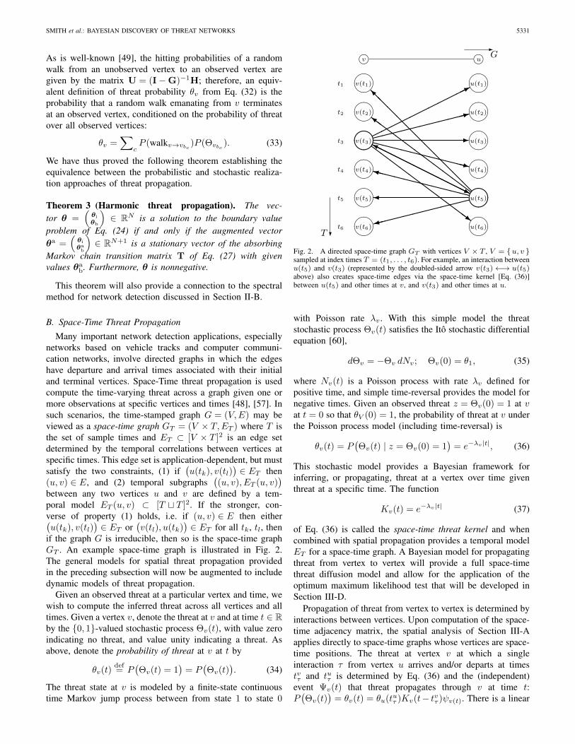
Many important network detection applications, especiallynetworks based on vehicle tracks and computer communi-cation networks, involve directed graphs in which the edgeshave departure and arrival times associated with their initialand terminal vertices. Space-Time threat propagation is usedcompute the time-varying threat across a graph given one ormore observations at specific vertices and times [48], [57]. Insuch scenarios, the time-stamped graph G = (V,E) may beviewed as a space-time graph GT = (V × T,ET ) where T isthe set of sample times and ET ⊂ [V × T ]2 is an edge setdetermined by the temporal correlations between vertices atspecific times. This edge set is application-dependent, but mustsatisfy the two constraints, (1) if

(u(tk), v(tl)

)∈ ET then

(u, v) ∈ E, and (2) temporal subgraphs((u, v), ET (u, v)

)between any two vertices u and v are defined by a tem-poral model ET (u, v) ⊂ [T t T ]2. If the stronger, con-verse of property (1) holds, i.e. if (u, v) ∈ E then either(u(tk), v(tl)

)∈ ET or

(v(tl), u(tk)

)∈ ET for all tk, tl, then

if the graph G is irreducible, then so is the space-time graphGT . An example space-time graph is illustrated in Fig. 2.The general models for spatial threat propagation providedin the preceding subsection will now be augmented to includedynamic models of threat propagation.

Given an observed threat at a particular vertex and time, wewish to compute the inferred threat across all vertices and alltimes. Given a vertex v, denote the threat at v and at time t ∈ Rby the {0, 1}-valued stochastic process Θv(t), with value zeroindicating no threat, and value unity indicating a threat. Asabove, denote the probability of threat at v at t by

θv(t)def= P

(Θv(t) = 1

)= P

(Θv(t)

). (34)

The threat state at v is modeled by a finite-state continuoustime Markov jump process between from state 1 to state 0

iv iu -Gt1

t2

t3

t4

t5

t6?T

��v(t1)

��v(t2)

��v(t3)

��v(t4)

��v(t5)

��v(t6)

��u(t1)

��u(t2)

��u(t3)

��u(t4)

��u(t5)

��u(t6)

@@

@@

@@@

@@@@I

ZZZ

ZZZ

ZZZ

ZZ}

HHHHH

HHH

HHHY

XXXXX

XXXXXXy

� ��9

��

��

��*

��

��:

-XXXXXXXXXXXz

HHHHHH

HHHHHj

ZZZZZZZZZZZ~

Fig. 2. A directed space-time graph GT with vertices V × T , V = {u, v }sampled at index times T = (t1, . . . , t6). For example, an interaction betweenu(t5) and v(t3) (represented by the doubled-sided arrow v(t3)←→ u(t5)above) also creates space-time edges via the space-time kernel [Eq. (36)]between u(t5) and other times at v, and v(t3) and other times at u.

with Poisson rate λv . With this simple model the threatstochastic process Θv(t) satisfies the Ito stochastic differentialequation [60],

dΘv = −Θv dNv; Θv(0) = θ1, (35)

where Nv(t) is a Poisson process with rate λv defined forpositive time, and simple time-reversal provides the model fornegative times. Given an observed threat z = Θv(0) = 1 at vat t = 0 so that θV (0) = 1, the probability of threat at v underthe Poisson process model (including time-reversal) is

θv(t) = P(Θv(t) | z = Θv(0) = 1

)= e−λv|t|, (36)

This stochastic model provides a Bayesian framework forinferring, or propagating, threat at a vertex over time giventhreat at a specific time. The function

Kv(t) = e−λv|t| (37)

of Eq. (36) is called the space-time threat kernel and whencombined with spatial propagation provides a temporal modelET for a space-time graph. A Bayesian model for propagatingthreat from vertex to vertex will provide a full space-timethreat diffusion model and allow for the application of theoptimum maximum likelihood test that will be developed inSection III-D.

Propagation of threat from vertex to vertex is determined byinteractions between vertices. Upon computation of the space-time adjacency matrix, the spatial analysis of Section III-Aapplies directly to space-time graphs whose vertices are space-time positions. The threat at vertex v at which a singleinteraction τ from vertex u arrives and/or departs at timestvτ and tuτ is determined by Eq. (36) and the (independent)event Ψv(t) that threat propagates through v at time t:P(Θv(t)

)= θv(t) = θu(tuτ )Kv(t− tvτ )ψv(t). There is a linear


transformation

θv(t) = ψv(t)K(t− tvτ )θu(tuτ )

=

∫ ∞−∞

ψv(t)K(t− tvτ )δ(σ − tuτ )θu(σ) dσ (38)

from the threat probability at u to v. Discretizing time, thetemporal matrix Kuv

τ for the discretized operator has the sparseform

Kuvτ =

(0 . . . 0K(tk − tvτ ) 0 . . . 0

), (39)

where 0 represents an all-zero column, tk represents a vectorof discretized time, and the discretized function K(tk − tvτ )appears in the column corresponding to the discretized timeat tuτ . Threat propagating from vertex v to u along the sameinteraction τ is given by the comparable expression θu(t) =θv(t

vτ )K(t− tuτ ), whose discretized linear operator Kvu

τ takesthe form

Kvuτ =

(0 . . . 0K(tk − tuτ ) 0 . . . 0

)(40)

[cf. Eq. (39)] where the nonzero column corresponds to tvτ .The sparsity of Kuv

τ and Kvuτ will be essential for practical

space-time threat propagation algorithms. The collection ofall interactions determines a weighted space-time adjacencymatrix A for the space-time graph GT . This is a matrix oforder #V ·#T whose temporal blocks for interactions betweenvertices u and v equals,(

Auu Auv

Avu Avv

)=

(0

∑l K

vuτl∑

l Kuvτl

0

). (41)

Note that with the space-time threat kernel of Eq. (37), if Gis irreducible, then so is GT .

As with spatial-only threat propagation of Eq. (13), thespace-time threat propagation equation is

θ = ΨW−1Aθ (42)

or θv(tk) =ψv(tk)∑u,l kvu;kl

∑u,lkvu;klθu(tl) (43)

in which θ is the (discretized) space-time vector ofthreat probabilities, A = (kvu;kl) is the (weighted) space-time adjacency matrix, and W = Diag(A·1) and Ψ =diag

(ψ1(t1), . . . , ψN (t#T )

)are, respectively, the space-time

diagonal matrices of the space-time vertex weights and a prioriprobabilities that threat propagates through each spatial vertexat a specific time. In contrast to the treatment of spatial-onlythreat propagation in Section III-A, the space-time graph isnecessarily a directed graph, consistent with the asymmetricspace-time adjacency matrix of Eq. (41).

By assumption, the graph G is irreducible, implying thatthe space-time graph GT is also irreducible. Therefore, The-orem 1 implies a well-defined solution to the space-timethreat propagation equation of Eq. (42) for a set observationsat specific vertices and times, vb1(tb1), . . . , vbC (tbC ). Yetthe Perron–Frobenius theorem for the space-time LaplacianŁ = I−W−1A poses precisely the same detection challengeas with spatial-only propagation: if the a priori probabilitiesare constant and equal to unity, i.e. Ψ = I, and the observed

probability of threat is constant, then the space-time proba-bility of threat is also constant for all spatial vertices and alltimes, yielding a hopeless detection method.

However, the advantage of time-stamped edges is that thetimes can be used to detected temporally coordinated networkactivity—we seek to detect vertices whose activity is corre-lated with that of threat observed at other vertices. Accordingto this model of threat networks, the a priori probability thata threat propagates through vertex v at time tk is determinedby the Poisson process used to model the probability of threatas a function of time:

ψv(tk) =1

dv

∑u,l

kvu;kl, (44)

where dv is the spatial degree of vertex v, i.e. the number ofinteractions associated with a spatial vertex. If all interactionsarrive/depart at the same time at v, then the a priori probabilityof threat diffusion is unity at this time, but different timesreduce this probability according to the stochastic processfor threat. Thus space-time threat propagation for coordinatedactivity is determined by the threat propagation equation,

θ = D−1Aθ (45)

in which D = diag(d1I, . . . , dNI

)is the block-diagonal

space-time matrix of (unweighted) spatial degrees and A is theweighted space-time adjacency matrix as in Eq. (42). This al-gorithm may also be further generalized to account for spatial-only a priori probability models such as the distance from ob-served vertices by replacing 1/dv in Eq. (45) with ψ′v/dv andan a priori model as in Eq. (19), yielding the threat propagationequation θ = Ψ′D−1Aθ with Ψ′ = diag

(ψ′1I, . . . , ψ

′NI).

C. Hybrid Threat Propagation

The temporal kernels introduced for time-stamped edgesin Section III-B are appropriate for network detection appli-cations that involve time-stamped edges; however, there aremany applications in which such time-stamped informationis either unavailable, irrelevant, or uncertain. Ignoring smallrouting delays, computer network communication protocolsoccur essentially instantaneously, and text documents maydescribe relationships between sites independent of a spe-cific timeframe. Integrating spatio-temporal relationships frommultiple information sources necessitates a hybrid approachcombining, where appropriate, the spatial-only capabilities ofSection III-A with the space-time methods of Section III-B.

In situations such as computer communication networks inwhich the timescale of the relationship is much smaller thanthe discretized timescale, then connections from one vertex toanother arrive at the same discretized time, and the temporalblocks for connections between vertices u and v replacesEq. (41) and equals,(

Auu Auv

Avu Avv

)=

(0 II 0

). (46)

In situations such as time-independent references within textdocuments in which threat at any time at vertex u implies a


threat at all times at vertex v, and vice versa, the temporalblocks for connections between vertices u and v equals,(

Auu Auv

Avu Avv

)=

(0 (#T )−111T

(#T )−111T 0

), (47)

i.e. a space-time clique between u and v. This equivalent thespace-time model with Poisson rate λ = 0.

D. Neyman–Pearson Network Detection

Network detection of a subgraph within a graph G = (V,E)of order N is treated as N independent binary hypothesistests to decide which of the graph’s N vertices do notbelong (null hypothesis H0) or belong (hypothesis H1) to thenetwork. Maximizing the probability of detection (PD) for afixed probability of false alarm (PFA) yields the Neyman–Pearson test involving the log-likelihood ratio of the competinghypotheses. We will derive this test in the context of networkdetection, which both illustrates the assumptions that ensuredetection optimality, as well as indicates practical methodsfor computing the log-likelihood ratio test and achieving anoptimal network detection algorithm. It will be seen that afew basic assumptions yield an optimum test that is equivalentto the Bayesian threat propagation algorithm developed in theprevious section. If any part of the graph is unknown or uncer-tain, then the Markov transition probabilities may be treated asrandom variables and either marginalized out of the likelihoodratio, yielding Neyman–Pearson optimality in the averagesense, or the maximum likelihood estimate may be used inthe suboptimum generalized likelihood ratio test (GLRT) [63].We will not cover extensions to unknown parameters in thispaper. The optimum test involves the graph Laplacian, whichallows comparison of Neyman–Pearson testing to several othernetwork detection methods whose algorithms are also relatedto the properties of the Laplacian.

An optimum hypothesis test is now derived for the presenceof a network given a set of observations z according to theobservation model of Definition 4. Optimality is defined in theNeyman–Pearson sense in which the probability of detectionis maximized at a constant false alarm rate (CFAR) [63].For the general problem of network detection of a subgraphwithin graph G of order N , the decision of which of the2N hypothesis Θ = (Θv1 , . . . ,ΘvN )T to choose involves a2N -ary multiple hypothesis test over the measurement spaceof the observation vector z, and an optimal test involvespartitioning the measurement space into 2N regions yielding amaximum PD. This NP-hard general combinatoric problem isclearly computationally and analytically intractable. However,Eq. (11) following Definition 6 guarantees that the threats ateach vertex are independent random variables, allowing thegeneral 2N -ary multiple hypothesis test to be greatly simplifiedby treating it as N independent binary hypothesis tests at eachvertex.

At each vertex v ∈ G and unknown threat Θ: V → {0, 1}across the graph , consider the binary hypothesis test for theunknown value Θv ,

H0(v): Θv = 0 (vertex belongs to background)H1(v): Θv = 1 (vertex belongs to foreground).

(48)

Given the observation vector z : {vb1 , . . . , vbC} ⊂ V →M ⊂RC with observation models f

(z(vbj ) | Θvbj

), j = 1, . . . ,

C, the PD and PFA are given by the integrals PD =∫Rf(z |

Θv = 1) dz and PFA =∫Rf(z | Θv = 0) dz, where R ⊂M is

the detection region in which observations are declared to yieldthe decision Θv = 1, otherwise Θv is declared to equal 0. Theoptimum Neyman–Pearson test uses the detection region Rthat maximizes PD at a fixed CFAR value PFA0, yielding thelikelihood ratio (LR) test [63],

f(z | Θv = 1)

f(z | Θv = 0)

H1(v)

≷H0(v)

λ (49)

for some λ > 0. Likelihood ratio tests are also used for graphclassification [36].

Finally, a simple application of Bayes’ theorem to the har-monic threat θv = f(Θv | z) provides the optimum Neyman–Pearson detector [Eq. (49)] because

f(z | Θv = 1)

f(z | Θv = 0)=f(Θv = 1 | z)

f(Θv = 0 | z)· f(Θv = 0)

f(Θv = 1)

=θv

1− θv· f(Θv = 1)

f(Θv = 0)

H1(v)

≷H0(v)

λ, (50)

results in a threshold of the harmonic space-time threat prop-agation vector of Eq. (7),

θvH1(v)

≷H0(v)

threshold, (51)

with the prior ratio f(Θv = 1)/f(Θv = 0) and the monotonicfunction θv 7→ θv/(1− θv) being absorbed into the detectionthreshold. By construction, the event Θv = 1 is equivalent toa random walk between v and one of the observed verticesvb1 , . . . , vbC , along with one of the events Θvb1

= 1, . . . ,ΘvbC

= 1, as represented in Eq. (33). Note that θv and equiv-alently the likelihood ratio are continuous functions of theprobabilities P (walkv→vbc ) and P (Θvbc

); therefore, equalityof the likelihood ratio to any given threshold exists only ona set of measure zero. If the prior ratio is constant for allvertices, then the threshold is also constant, and the likelihoodratio test [Eq. (51)] for optimum network detection becomes

θH1

≷H0

threshold. (52)

This establishes the detection optimality of harmonic space-time threat propagation.

Because the probability of detecting threat is maximizedat each vertex, the probability of detection for the entiresubgraph is also maximized, yielding an optimum Neyman–Pearson test under the simplification of treating the 2N -arymultiple hypothesis testing problem as a sequence of N binaryhypothesis tests. Summarizing, the probability of networkdetection given an observation z is maximized by computingf(Θv | z) using a Bayesian threat propagation method andapplying a simple likelihood ratio test, yielding the followingtheorem that equates threat propagation with the optimumNeyman–Pearson test.


Theorem 4 (Neyman–Pearson Optimality of Threat Prop-agation). The solution to Bayesian threat propagation ex-pressed in Eqs. (24) or (32) yields an optimum likelihood ratiotest in the Neyman–Pearson sense.

IV. MODELING AND PERFORMANCE

Evaluation of network detection algorithms may be ap-proached from the perspectives of theoretical analysis orempirical experimentation. Theoretical performance boundshave only been accomplished for simple network models, i.e.cliques [23], [33], [42] or dense subgraphs [5] embeddedwithin Erdos–Renyi backgrounds, and there are no theoreticalresults at all for more complex network models that char-acterize real-world networks [58]. If representative networkdata with truth is available, one may evaluate algorithmperformance with specific data sets [71]. However, real-worlddata sets of covert networks with truth is unknown to theauthors. Therefore, network detection performance evaluationmust be conducted on simulated networks using generativemodels. We begin with a simple stochastic blockmodel [65],explore this model’s limitations, then introduce a new networkmodel designed to address these defects while at the same timeencompassing the characteristics of real-world networks [1],[2], [12], [45], [70]. Varying model parameters also yields in-sight on the dependence of algorithm performance on differentnetwork characteristics.

For each evaluation, we compare performance between thespace-time threat propagation [STTP; Section III-B], breadth-first search spatial-only threat propagation [BFS; Eq. (21)], andmodularity-based spectral detection algorithm [SPEC] [40].The performance metric is the standard receiver operatingcharacteristic (ROC), which in the case of network detectionis the probability of detection (i.e. the percentage of trueforeground vertices detected) versus the probability of falsealarms (i.e. the percentage of background vertices detected)as the detection threshold is varied.

A. Detection Performance On Stochastic Blockmodels

1) Stochastic Blockmodel Description: The stochasticblockmodel captures the sparsity of real-world networks andbasic community structure [27] using a simple network frame-work [65]. For a graph of order N divided into K com-munities, the model is parameterized by a N -by-K {0, 1}membership matrix Π and a K-by-K probability matrix Sthat defines the probability of an edge between two ver-tices based upon their community membership. Therefore,the probability of an edge is determined by the off-diagonalterms of the matrix ΠSΠT. By the classical result of Erdos–Renyi [20], each community is almost surely connected ifSkk > logNk/Nk in which Nk is the number of verticesin community k. We introduce the activity parameter rk ≥ 1and set Skk = rk logNk/Nk to adjust a community’s densityrelative to its Erdos–Renyi connectivity threshold.

2) Experimental Setup and Results: The objective of thisexperiment is to quantify detection performance of a fore-ground network with varying activity given observations froma small fraction of its members. Fig. 3 illustrates the ROC

0

0.2

0.4

0.6

0.8

1

PD

0 0.2 0.4 0.6 0.8 1

STTP, rfg = 2 STTP, rfg = 1.1 BFS, rfg = 2 BFS, rfg = 1.1 SPEC, rfg = 2 SPEC, rfg = 1.11000 trials

PFA

Fig. 3. Detection ROC curves of the three different algorithms at two levels offoreground activity, 1.1· logNfg/Nfg and 2· logNfg/Nfg. Data is simulatedusing the stochastic blockmodel with 1000 Monte Carlo trials each with anindependent draw of the random network and single threat observation.

detection performance with a graph of order N = 256 andK = 3 with two background communities of order 128, anda foreground community of order 30 randomly embedded inthe background. The probability matrix is,

S =

0.08 0.02 0.020.02 0.08 0.020.02 0.02 rfg·0.1

,

parameterized by the activity rfg relative to the Erdos–Renyiforeground connectivity threshold log 30/30 ≈ 0.1. A simpletemporal model is used with all foreground interactions atthe same time (i.e. perfect coordination), and backgroundinteractions uniformly distributed in time (i.e. uncoordinated).

Results are shown for both sparsely connected (rfg = 1.1)and moderately connected (rfg = 2) foreground networks. Thesimulations show that excellent ROC performance is achiev-able if temporal information is exploited (STTP) with highlycoordinated foreground networks with sparse to moderateconnectivity. Because of the use of temporal information,STTP outperforms BFS. Spectral methods, which are designedto detect highly connected networks perform poorly on sparseforeground networks, and improve as foreground networkconnectivity increases, especially in the low PFA region inwhich SPEC performs better than BFS threat propagation. Thisresult is consistent with expectations and recent theoreticalresults for spectral methods applied to clique detection [5],[42]. Continuous likelihood ratio tests possess ROC curves thatare necessarily convex upwards [63]; therefore, the ROCs forthreat propagation algorithms applied to data generated fromrandom walk propagation are necessarily convex. The resultsof Fig. 3 show both threat propagation and spectral meth-ods applied to data generated from a stochastic blockmodel.Because the spectral detection algorithm is not associatedwith a likelihood ratio test, convexity of its ROC curves isnot guaranteed—indeed, the spectral ROC curve with rfg = 2is seen to be concave in the high PD region. All threat


X (L × K)

i(K)

N

i

N N × N

ij

ijm

S

B (K × K)

i

j

i

j

Membership

Activitylevel Community

interaction

Sparsityil(L) (L)

jiz(K)

ijz(K)

(K)

(K)

(K × K)

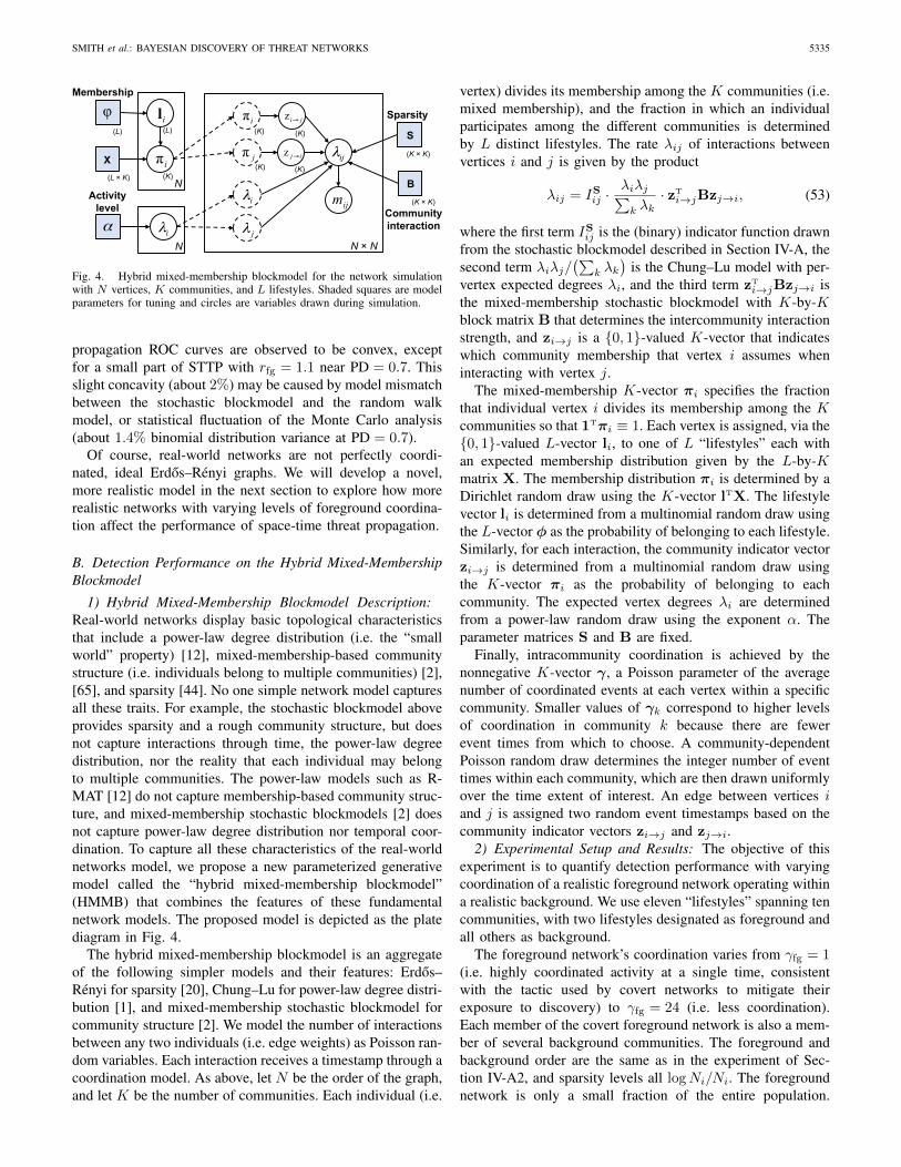
Fig. 4. Hybrid mixed-membership blockmodel for the network simulationwith N vertices, K communities, and L lifestyles. Shaded squares are modelparameters for tuning and circles are variables drawn during simulation.

propagation ROC curves are observed to be convex, exceptfor a small part of STTP with rfg = 1.1 near PD = 0.7. Thisslight concavity (about 2%) may be caused by model mismatchbetween the stochastic blockmodel and the random walkmodel, or statistical fluctuation of the Monte Carlo analysis(about 1.4% binomial distribution variance at PD = 0.7).

Of course, real-world networks are not perfectly coordi-nated, ideal Erdos–Renyi graphs. We will develop a novel,more realistic model in the next section to explore how morerealistic networks with varying levels of foreground coordina-tion affect the performance of space-time threat propagation.

B. Detection Performance on the Hybrid Mixed-MembershipBlockmodel

1) Hybrid Mixed-Membership Blockmodel Description:Real-world networks display basic topological characteristicsthat include a power-law degree distribution (i.e. the “smallworld” property) [12], mixed-membership-based communitystructure (i.e. individuals belong to multiple communities) [2],[65], and sparsity [44]. No one simple network model capturesall these traits. For example, the stochastic blockmodel aboveprovides sparsity and a rough community structure, but doesnot capture interactions through time, the power-law degreedistribution, nor the reality that each individual may belongto multiple communities. The power-law models such as R-MAT [12] do not capture membership-based community struc-ture, and mixed-membership stochastic blockmodels [2] doesnot capture power-law degree distribution nor temporal coor-dination. To capture all these characteristics of the real-worldnetworks model, we propose a new parameterized generativemodel called the “hybrid mixed-membership blockmodel”(HMMB) that combines the features of these fundamentalnetwork models. The proposed model is depicted as the platediagram in Fig. 4.

The hybrid mixed-membership blockmodel is an aggregateof the following simpler models and their features: Erdos–Renyi for sparsity [20], Chung–Lu for power-law degree distri-bution [1], and mixed-membership stochastic blockmodel forcommunity structure [2]. We model the number of interactionsbetween any two individuals (i.e. edge weights) as Poisson ran-dom variables. Each interaction receives a timestamp through acoordination model. As above, let N be the order of the graph,and let K be the number of communities. Each individual (i.e.

vertex) divides its membership among the K communities (i.e.mixed membership), and the fraction in which an individualparticipates among the different communities is determinedby L distinct lifestyles. The rate λij of interactions betweenvertices i and j is given by the product

λij = ISij ·λiλj∑k λk

· zT

i→jBzj→i, (53)

where the first term ISij is the (binary) indicator function drawnfrom the stochastic blockmodel described in Section IV-A, thesecond term λiλj/

(∑k λk

)is the Chung–Lu model with per-

vertex expected degrees λi, and the third term zTi→jBzj→i is

the mixed-membership stochastic blockmodel with K-by-Kblock matrix B that determines the intercommunity interactionstrength, and zi→j is a {0, 1}-valued K-vector that indicateswhich community membership that vertex i assumes wheninteracting with vertex j.

The mixed-membership K-vector πi specifies the fractionthat individual vertex i divides its membership among the Kcommunities so that 1Tπi ≡ 1. Each vertex is assigned, via the{0, 1}-valued L-vector li, to one of L “lifestyles” each withan expected membership distribution given by the L-by-Kmatrix X. The membership distribution πi is determined by aDirichlet random draw using the K-vector lTX. The lifestylevector li is determined from a multinomial random draw usingthe L-vector φ as the probability of belonging to each lifestyle.Similarly, for each interaction, the community indicator vectorzi→j is determined from a multinomial random draw usingthe K-vector πi as the probability of belonging to eachcommunity. The expected vertex degrees λi are determinedfrom a power-law random draw using the exponent α. Theparameter matrices S and B are fixed.

Finally, intracommunity coordination is achieved by thenonnegative K-vector γ, a Poisson parameter of the averagenumber of coordinated events at each vertex within a specificcommunity. Smaller values of γk correspond to higher levelsof coordination in community k because there are fewerevent times from which to choose. A community-dependentPoisson random draw determines the integer number of eventtimes within each community, which are then drawn uniformlyover the time extent of interest. An edge between vertices iand j is assigned two random event timestamps based on thecommunity indicator vectors zi→j and zj→i.

2) Experimental Setup and Results: The objective of thisexperiment is to quantify detection performance with varyingcoordination of a realistic foreground network operating withina realistic background. We use eleven “lifestyles” spanning tencommunities, with two lifestyles designated as foreground andall others as background.

The foreground network’s coordination varies from γfg = 1(i.e. highly coordinated activity at a single time, consistentwith the tactic used by covert networks to mitigate theirexposure to discovery) to γfg = 24 (i.e. less coordination).Each member of the covert foreground network is also a mem-ber of several background communities. The foreground andbackground order are the same as in the experiment of Sec-tion IV-A2, and sparsity levels all logNi/Ni. The foregroundnetwork is only a small fraction of the entire population.


0

0.2

0.4

0.6

0.8

1PD

0 0.2 0.4 0.6 0.8 1PFA

STTP, γfg = 1 STTP, γfg = 10 STTP, γfg = 24 BFS, γfg = 1 SPEC, γfg = 11000 trials

Fig. 5. Detection ROC curves of the three different algorithms at threelevels (γfg = 1, 10, 24) of foreground coordination. Spectral detection andBFS threat propagation do not use temporal information so their performanceis unaffected by the coordination level.

Foreground actors are characterized by two distinct lifestylesrepresenting their memberships in the covert community aswell as different background communities. The backgroundcommunities are intended to represent various business, home,industry, religious, sports, or other social interactions.

Fig. 5 illustrates the ROC performance with these param-eters, varying the level of foreground coordination. ThroughEq. (44), space-time threat propagation is designed to performwell with highly coordinated networks, consistent with theresults observed in Fig. 5 in which STTP performs best atthe higher coordination levels and outperforms the breadth-first search and modularity-based spectral detection methods.The spectral detection algorithm is expected to perform poorlyin this scenario because, as discussed in Section II-B, it reliesupon a relatively dense foreground network, which does notexist in this simulated dataset with realistic properties of covertnetworks.

V. CONCLUSIONS

A Bayesian framework for network detection can be used tounify the different approaches of network detection algorithmsbased on random walks/diffusion and algorithms based onspectral properties. Indeed, using the concise assumptions forrandom walks and threat propagation laid out in Definition 6,all the theoretical results follow immediately, including theproof of equivalence, an exact, closed-form, efficient solution,and Neyman–Pearson optimality. Not only is this theoreticallyappealing, but it provides direct practical benefits througha new network detection algorithm called space-time threatpropagation, that is shown to achieve superior performancewith simulated covert networks. Bayesian space-time threatpropagation is interpreted both as a random walk on a graphand, equivalently, as the solution to a harmonic boundary valueproblem. Bayes’ rule determines the unknown probability ofthreat on the uncued nodes—the “interior”—based on threat

observations at cue nodes—the “boundary.” Hybrid threatpropagation algorithms appropriate for heterogeneous spatio-temporal relationships can be obtained from this general threatdiffusion model. This new method is compared to well-knownspectral methods by examining competing notions of networkdetection optimality. To model realistic covert networks real-istically embedded within realistic backgrounds, a new hybridmixed-membership blockmodel based on mixed membershipof random graphs is introduced and used to assess algorithmdetection performance on graphs with varying activity andcoordination. In the important situations of low foregroundactivity with varying levels of coordination, the examples showthe superior detection performance of Bayesian space-timethreat propagation compared to other spatial-only and uncuedspectral methods.

ACKNOWLEDGMENTS

The authors gratefully acknowledge the consistently incisiveand constructive comments from our reviewers, which greatlyimproved this paper. We also thank Professor Patrick Wolfe fororiginally suggesting the deep connection with random walkson graphs.

REFERENCES

[1] W. AIELLO, F. CHUNG, and L. LU. “A random graph model for powerlaw graphs,” Experimental Mathematics 10 (1) : 53–66 (2001).

[2] E. M. AIROLDI, D. M. BLEI, S. E. FIENBERG, and E. P. XING.“Mixed-membership stochastic blockmodels,” JMLR 9 : 1981–2014(2008).

[3] M. ALANYALI, S. VENKATESH, O. SAVAS, and S. AERON. “DistributedBayesian hypothesis testing in sensor networks,” in Proc. 2005 AmericanControl Conf. Boston MA, pp. 5369–5374 (2004).

[4] R. ANDERSEN, F. R. K. CHUNG, and K. LANG. “Local graph partition-ing using PageRank vectors,” in Proc. 47th IEEE Symp. Foundations ofComputer Science (FOCS). pp. 475–486 (2006).

[5] E. ARIAS-CASTRO and N. VERZELEN. “Community detection inrandom networks,” arXiv:1302.7099 [math.ST]. Mar. 18 2013[Online]. Available: 〈http://arxiv.org/abs/1302.7099〉.

[6] S. ARORA, S. RAO, and U. VAZIRANI. “Geometry, flows, and graph-partitioning algorithms,” Comm ACM 51 (10) : 96–105 (2008).

[7] K. AVRACHENKOV, N. LITVAK, M. SOKOL, and D. TOWSLEY.“Quick detection of nodes with large degrees,” Internet Mathe-matics doi:10.1080/15427951.2013.798601, 12 Nov. 2013. Feb. 272014 [Online]. Available: 〈http://www.tandfonline.com/doi/abs/10.1080/15427951.2013.798601〉.

[8] M. BELKIN and P. NIYOGI. “Laplacian eigenmaps for dimensionalityreduction and data representation,” Neural Computation 15 : 1373–1396(2003).

[9] K. CARLEY. “Estimating vulnerabilities in large covert networks,” inProc. 16th Intl. Symp. Command and Control Research and Tech.(ICCRTS). (San Diego, CA) (2004).

[10] K. M. CARTER, R. RAICH, and A. O. HERO III. “On local intrinsic di-mension estimation and its applications,” IEEE Trans. Signal Processing58 (2) : 650–663 (2010).

[11] D. CHAKRABARTI, Y. WANG, C. WANG, J. LESKOVEC, andC. FALOUTSOS. “Epidemic thresholds in real networks,” ACM T. Inform.Syst. Se., 10 (4) : 13.1–13.26 (2008).

[12] D. CHAKRABARTI, Y. ZHAN, and C. FALOUTSOS. “R-MAT: A recur-sive model for graph mining,” in Proc. 2004 SIAM Intl. Conf. DataMining. pp. 442–446 (2004).

[13] J.-F. CHAMBERLAND and V. V. VEERAVALLI. “Decentralized detectionin sensor networks,” IEEE Trans. Signal Processing 51 (2) : 407–416(2003).

[14] F. R. K. CHUNG. Spectral Graph Theory, Regional Conference Seriesin Mathematics 92. Providence, RI: American Mathematical Society(1994).

http://arxiv.org/abs/1302.7099


[15] F. R. K. CHUNG and W. ZHAO. “PageRank and random walks ongraphs,” in Fete of Combinatorics and Computer Science, Bolyai SocietyMathematical Studies 20 : 43–62, Vienna: Springer (2010).

[16] J. A. COSTA and A. O. HERO III. “Geodesic entropic graphs fordimension and entropy estimation in manifold learning,” IEEE Trans.Signal Processing 52 (8) : 2210–2221 (2004).

[17] R. DIESTEL. Graph Theory. New York: Springer-Verlag, Inc. (2000).[18] W. E. DONATH and A. J. HOFFMAN. “Lower bounds for the partitioning

of graphs,” IBM J. Res. Development 17 : 420–425 (1973).[19] E. B. DYNKIN and A. A. YUSHKEVICH. Markov Processes: Theorems

and Problems. New York: Plenum Press (1969).[20] P. ERDOS and A. RENYI, “On the evolution of random graphs,” Pubs.

Mathematical Institute of the Hungarian Academy of Sciences 5 : 17–61(1960).

[21] J. P. FERRY, D. LO, S .T. AHEARN, and A. M. PHILLIPS. “Networkdetection theory,” in Mathematical Methods in Counterterrorism, eds.N. MEMON et al., pp. 161–181, Vienna: Springer (2009).

[22] M. FIEDLER. “A property of eigenvectors of non-negative symmetricmatrices and its application to graph theory,” Czech. Math. J. 25 : 619–633 (1975).

[23] S. FORTUNATO and M. BARTHELEMY. “Resolution limit in communitydetection,” PNAS 104 (1) : 36–41 (2007).

[24] S. FORTUNATO. “Community detection in graphs,” Physics Reports486 : 75–174 (2010).

[25] A. FRONCZAK, P. FRONCZAK, and J. A. HOŁYST. “Average path lengthin random networks,” Phys. Rev. E 70 : 056110 (2004).

[26] F. R. GANTMACHER. Matrix Theory. Vol. 2. New York: Chelsea (1959).[27] M. GIRVAN and M. E. J. NEWMAN. “Community structure in social

and biological networks,” PNAS 99 (12) : 7821–7826 (2002).[28] C. GODSIL and G. ROYLE. Algebraic Graph Theory. New York:

Springer-Verlag, Inc. (2001).[29] M. O. JACKSON. Social and Economic Networks, Princeton U. Press

(2008).[30] A. SANDRYHAILA and J. F. MOURA. “Discrete signal processing on

graphs: Frequency analysis,” IEEE Trans. Signal Processing 62 (12) :3042–3054 (2014).

[31] D. KOLLER and N. FRIEDMAN. Probabilistic Graphical Models. Cam-bridge, MA: MIT Press (2009).

[32] V. E. KREBS. “Uncloaking terrorist networks,” First Monday 7 (4)(2002). Feb. 27 2014 [Online]. Available: 〈http://firstmonday.org/ojs/index.php/fm/article/view/941〉.

[33] J. M. KUMPULA, J. SARAMAKI, K. KASKI, and J. KERTESZ. “Limitedresolution in complex network community detection with Potts modelapproach,” Eur. Phys. J. B 56 : 41–45 (2007).

[34] J. LESKOVEC and C. FALOUTSOS. “Sampling from large graphs,” inProc. 12th ACM SIGKDD Intl. Conf. Knowledge Discovery and DataMining pp. 631–636 (2006).

[35] J. LESKOVEC, K. J. LANG, and M. MAHONEY. “Empirical comparisonof algorithms for network community detection,” in Proc. 19th Intl.Conf. World Wide Web (WWW’10). Raleigh, NC, pp. 631–640 (2010).

[36] J. G. LIGO, G. K. ATIA, and V. V. VEERAVALLI. “A controlled sensingapproach to graph classification,” in Proc. IEEE Intl. Conf. Acoustics,Speech and Signal Processing (ICASSP). Vancouver, BC (2013).

[37] M. W. MAHONEY, L. ORECCHIA, and N. K. VISHNOI. “A local spec-tral method for graphs: With applications to improving graph partitionsand exploring data graphs locally,” J. Machine Learning Research 13 :2339–2365 (2012).

[38] B. A. MILLER, M. S. BEARD, and N. T. BLISS. “Eigenspace Analysisfor Threat Detection in Social Networks,” in Proc. 14th Intl. Conf.Informat. Fusion (FUSION). Chicago, IL (2011).

[39] B. A. MILLER, N. T. BLISS, and P. J. WOLFE. “Toward signalprocessing theory for graphs and other non-Euclidean data,” in Proc.IEEE Intl. Conf. Acoustics, Speech and Signal Processing, pp. 5414–5417 (2010).

[40] B. A. MILLER, N. T. BLISS, and P. J. WOLFE. “Subgraph detectionusing eigenvector L1 norms,” in Proc. 2010 Neural Information Pro-cessing Systems (NIPS). Vancouver, Canada (2010).

[41] B. MOHAR. “The Laplacian Spectrum of Graphs,” in Graph Theory,Combinatorics, and Applications, 2, eds. Y. ALAVI, G. CHARTRAND,O. R. OELLERMANN, and A. J. SCHWENK. New York: Wiley, pp. 871–898 (1991).

[42] R. R. NADAKUDITI and M. E. J. NEWMAN. “Graph spectra and thedetectability of community structure in networks,” Phys. Rev. Lett. 108,188701 (2012).

[43] J. NEVILLE, O. SIMSEK, D. JENSEN, J. KOMOROSKE, K. PALMER,and H. GOLDBERG. “Using relational knowledge discovery to preventsecurities fraud,” in Proc. 11th ACM SIGKDD Intl. Conf. KnowledgeDiscovery and Data Mining pp. 449–458 (2005).

[44] M. E. J. NEWMAN. “Finding community structure in networks usingthe eigenvectors of matrices,” Phys. Rev. E, 74 (3) (2006).

[45] . “The structure and function of complex networks,” SIAM Rev.45 (2) : 167–256 (2003).

[46] J.-P. ONNELA and N. A. CHRISTAKIS. “Spreading paths in partiallyobserved social networks,” Phys. Rev. E, 85 (3) : 036106 (2012).

[47] M. N. OZISIK. Boundary Value Problems of Heat Conduction. ScrantonPA: International Textbook Company, 1968.

[48] S. PHILIPS, E. K. KAO, M. YEE, and C. C. ANDERSON. “Detectingactivity-based communities using dynamic membership propagation,”in Proc. IEEE Intl. Conf. Acoustics, Speech and Signal Processing(ICASSP). Kyoto, Japan (2012).

[49] M. A. PINSKY and S. KARLIN. An Introduction to Stochastic Modeling.New York: Academic Press (2010).

[50] A. POTHEN, H. SIMON, and K.-P. LIOU. “Partitioning sparse matriceswith eigenvectors of graphs,” SIAM J. Matrix Anal. Appl. 11 : 430–45(1990).

[51] K. K. SABELFELD and N. A. SIMONOV. Random Walks on Boundariesfor Solving PDEs. Utrecht, The Netherlands: VSP International SciencePublishers, 1994.

[52] M. SAGEMAN. Understanding Terror Networks. Philadelphia, PA:U. Pennsylvania Press (2004).

[53] D. SHAH and T. ZAMAN. “Rumors in a network: Who’s the culprit?,”IEEE Trans. Inf. Theory 57 (8) : 5163–5181 (2011).

[54] D. SHAH. “Gossip Algorithms,” Foundations and Trends in Networking3 (1)1–125 (2009).

[55] A. SHAMIR. “A survey on mesh segmentation techniques,” ComputerGraphics Forum 27 (6) : 1539–1556 (2008). Sep. 3 2012 [Online]. Avail-able: 〈http://www.faculty.idc.ac.il/arik/site/mesh-segment.asp〉.

[56] S. T. SMITH, A. SILBERFARB, S. PHILIPS, E. K. KAO, and C. C.ANDERSON. “Network Discovery Using Wide-Area Surveillance Data,”in Proc. 14th Intl. Conf. Informat. Fusion (FUSION). Chicago, IL(2011).

[57] S. T. SMITH, S. PHILIPS, and E. K. KAO. “Harmonic space-time threatpropagation for graph detection,” in Proc. IEEE Intl. Conf. Acoustics,Speech and Signal Processing (ICASSP). Kyoto, Japan (2012).

[58] S. T. SMITH, K. D. SENNE, S. PHILIPS, E. K. KAO, and G. BERN-STEIN. “Covert Network Detection,” Lincoln Laboratory J. 20 (1) : 47–61 (2013).

[59] D. A. SPIELMAN and S.-H. TENG. “Nearly-linear time algorithms forgraph partitioning, graph sparsification, and solving linear systems,” inProc. 36th ACM Symp. Theory of Computing (STOC), pp. 81–90 (2004).

[60] D. STIRZAKER. Stochastic Processes and Models. Oxford UniversityPress (2005).

[61] R. TRINQUIER. Modern Warfare: A French View of Counterinsurgency.Westport, CT: Praeger Security International (2006).

[62] P. VAN MIEGHEM, D. STEVANOVIC, F. KUIPERS, C. LI, R. VAN DEBOVENKAMP, D. LIU, and H. WANG. “Decreasing the spectral radiusof a graph by link removals” Phys. Rev. E 84 : 016101 (2011).

[63] H. L. VAN TREES. Detection, Estimation, and Modulation Theory,Part 1. New York: John Wiley and Sons, Inc. (1968).

[64] U. VON LUXBURG, O. BOUSQUET, and M. BELKIN. “Limits of spectralclustering,” in Advances in Neural Information Processing Systems 17,eds. L. K. SAUL, Y. WEISS, and L. BOTTOU. Cambridge, MA: MITPress (2005).

[65] S. WASSERMAN and K. FAUST. Social Network Analysis. CambridgeUniversity Press. (1994).

[66] D. J. WATTS. “Networks, dynamics, and the small-world phenomenon,”American Journal of Sociology 13 (2) : 493–527 (1999).

[67] Y. WEISS. “Segmentation using eigenvectors: A unifying view,” in Proc.of the Intl. Conf. Computer Vision 2 : 975 (1999).

[68] S. WHITE and P. SMYTH. “A spectral clustering approach to findingcommunities in graphs,” in Proc. 5th SIAM Intl. Conf. Data Mining,eds. H. KARGUPTA, J. SRIVASTAVA, C. KAMATH, and A. GOODMAN.Philadelphia PA, pp. 76–84 (2005.)

http://firstmonday.org/ojs/index.php/fm/article/view/941

http://firstmonday.org/ojs/index.php/fm/article/view/941

http://papers.nips.cc/paper/4044-subgraph-detection-using-eigenvector-l1-norms

http://papers.nips.cc/paper/4044-subgraph-detection-using-eigenvector-l1-norms

http://www.faculty.idc.ac.il/arik/site/mesh-segment.asp


[69] H. WOLKOWICZ and Q. ZHAO. “Semidefinite programming relaxationsfor the graph partitioning problem,” Discrete Applied Mathematics 96–97 : 461–479 (1999).

[70] J. XU and H. CHEN. “The topology of dark networks,” Comm. ACM51 (10) : 58–65 (2008).

[71] M. J. YEE, S. PHILIPS, G. R. CONDON, P. B. JONES, E. K. KAO, S. T.SMITH, C. C. ANDERSON, and F. R. WAUGH. “Network discovery withmulti-intelligence sources,” Lincoln Laboratory J. 20 (1) : 31–46 (2013).

[72] H. ZHOU and R. LIPOWSKY. “Network Brownian Motion: A NewMethod to Measure Vertex-Vertex Proximity and to Identify Commu-nities and Subcommunities,” in Computational Science—ICCS 2004,Lecture Notes in Computer Science 3038 : 1062–1069. Berlin: Springer(2004).

Steven Thomas Smith (M’86–SM’04) is a SeniorStaff Member at MIT Lincoln Laboratory, Lexing-ton, MA. He received the B.A.Sc. degree in electricalengineering and mathematics from the University ofBritish Columbia, Vancouver, BC in 1986 and thePh.D. degree in applied mathematics from HarvardUniversity, Cambridge, MA in 1993. He has over15 years experience as an innovative technologyleader with statistical data analytics, both theoryand practice, and broad leadership experience rang-ing from first-of-a-kind algorithm development for

groundbreaking sensor systems to graph-based intelligence architectures. Hiscontributions span diverse applications from optimum network detection,geometric optimization, geometric acoustics, statistical resolution limits, andnonlinear parameter estimation. He received the SIAM Outstanding PaperAward in 2001 and the IEEE Signal Processing Society Best Paper Awardin 2010. He was associate editor of the IEEE Transactions on SignalProcessing in 2000–2002, and currently serves on the IEEE Sensor Array andMultichannel committee. He has taught signal processing courses at Harvardand for the IEEE.

Edward K. Kao (M’03) is a Lincoln scholar at MITLincoln Laboratory in the Intelligence and DecisionTechnologies Group. Since joining Lincoln in 2008,he has been working on graph-based intelligence,where actionable intelligence is inferred from inter-actions and relationships between entities. Applica-tions include wide area surveillance, threat networkdetection, homeland security, and cyber warfare, etc.In 2011, he entered the Ph.D. program at HarvardStatistics. Current research topics include: causalinference on peer influence effects, statistical models

for community membership estimation, information content in network infer-ence, and optimal sampling and experimental design for network inference.

Kenneth D. Senne (S’65–M’72–SM’95–F’02–LF’08) serves as Principal Staff in the ISR andTactical Systems Division at Lincoln Laboratory.His research examines the application of large dataanalytics to decision support problems. He joinedthe Laboratory in 1972 to work on the designand collision avoidance application of the Mode-Sbeacon system for the Federal Aviation Adminis-tration. From 1977 to 1986 he contributed to thedevelopment of anti-jam airborne communicationsystems and super resolution direction finding with

adaptive antennas. In 1986 he was asked to set up an array signal processinggroup as part of a large air defense airborne electronics program. This effortresulted in the pioneering demonstration of a large scale, real-time embeddedadaptive signal processor. In 1998 he was promoted to head the Air DefenseTechnology Division. In 2002 he established the Laboratory’s TechnologyOffice, with responsibility for managing technology investments, includingthe internal innovative research program. Prior to joining Lincoln Laboratoryhe earned a Ph.D. degree in electrical engineering from Stanford Universitywith foundational research on digital adaptive signal processing and he servedas Captain in the U.S. Air Force with the Frank J. Seiler Research Laboratoryat the Air Force Academy. He was elected Fellow of the IEEE in 2002.

Garrett Bernstein is a Computer Science Ph.D.student at the University of Massachusetts Amherst.At MIT Lincoln Laboratory, he was a member ofthe technical staff in the Intelligence and Deci-sion Technologies Group. His research focused onstatistical inference and machine learning appliedto diverse problems, such as graph detection al-gorithms, model simulation, semantic analysis, andmilitary operational effectiveness. Prior to joiningthe Laboratory, he received a bachelor’s degree inapplied and engineering physics and and engineering

master’s degree in computer science, both from Cornell University.

Scott Philips is currently a data scientist at PalantirTechnologies. Before joining Palantir, Scott spentfive years as a member of the technical staff inthe Intelligence and Decision Technologies Group.While he was at Lincoln Laboratory, his researchfocused on developing statistical algorithms for theexploitation of data from intelligence, surveillance,and reconnaissance sensors. Scott received his doc-toral degree in electrical engineering in 2007 fromthe University of Washington, where his researchfocused on signal processing and machine learning

algorithms for the detection and classification of sonar signals.

Bayesian Discovery of Threat Networks - arXiv

Documents

Transcript of Bayesian Discovery of Threat Networks - arXiv