OptiStruct Optimization
276
www.altairhyperworks.com | HyperWorks is a division of
Transcript of OptiStruct Optimization

Altair Engineering Contact Information Web site www.altairhyperworks.com
FTP site Address: Login: Password:
ftp.altair.com or ftp2.altair.com or http://ftp.altair.com/ftp ftp <your e-mail address>
Location Telephone e-mail
Australia 61.3.9016.9042 [email protected]
Brazil 55.11.3884.0414 [email protected]
China 86.21.6117.1666 [email protected]
France 33.1.4133.0992 [email protected]
Germany 49.7031.6208.22 [email protected]
India 91.80. 6629.4500 1.800.425.0234 (toll free)
Italy 39.800.905.595 [email protected]
Japan 81.3.5396.2881 [email protected]
Korea 82.31.716.4321 [email protected]
New Zealand 64.9.413.7981 [email protected]
North America 248.614.2425 [email protected]
Scandinavia 46.46.286.2052 [email protected]
United Kingdom 01926.468.600 [email protected]
The following countries have distributors for Altair Engineering:
Asia Pacific: Indonesia, Malaysia, Singapore, Taiwan, Thailand
Europe: Czech Republic, Hungary, Poland, Romania, Spain, Turkey. Copyright© Altair Engineering Inc. All Rights Reserved for: HyperMesh® 1990-2013; HyperCrash® 2001-2013; OptiStruct® 1996-2013; RADIOSS®1986-2013; HyperView®1999-2013; HyperView Player® 2001-2013; HyperStudy® 1999-2013; HyperGraph®1995-2013; MotionView® 1993-2013; MotionSolve® 2002-2013; HyperForm® 1998-2013; HyperXtrude® 1999-2013; Process Manager™ 2003-2013; Templex™ 1990-2013; MediaView™ 1999-2013; BatchMesher™ 2003-2013; TextView™ 1996-2013; HyperMath® 2007-2013; ScriptView™ 2007-2013; Manufacturing Solutions™ 2005-2013; HyperWeld® 2009-2013; HyperMold® 2009-2013; solidThinking® 1993-2013; solidThinking Inspire™ 2009-2013; solidThinking Evolve™ 1993-2013; Durability Director™ 2009-2013; Suspension Director™ 2009-2013; AcuSolve® 1997-2013; and AcuConsole® 2006-2013.
In addition to HyperWorks® trademarks noted above, GridWorks™, PBS GridWorks®, PBS Professional®, PBS™, PBS Works™ and Portable Batch System® are trademarks of ALTAIR ENGINEERING INC. All are protected under U.S. and international laws and treaties. Copyright© 1994-2013.
Additionally, the Altair software is protected under patent #6,859,792 and other patents pending. All other marks are the property of their respective owners.
ALTAIR ENGINEERING INC. Proprietary and Confidential. Contains Trade Secret Information. Not for use or disclosure outside of ALTAIR and its licensed clients. Information contained in HyperWorks® shall not be decompiled, disassembled, or “unlocked”, reverse translated, reverse engineered, or publicly displayed or publicly performed in any manner. Usage of the software is only as explicitly permitted in the end user software license agreement.
Copyright notice does not imply publication.

HyperWorks 12.0 Proprietary Information of Altair Engineering, Inc.
3
Table of Contents OptiStruct for Structural Optimization
Including Concept Methodologies and Optimization Examples
Table of Contents .................................................................................................................... 3
Chapter 1: Introduction ............................................................................................ 7
1 – HyperWorks Overview ............................................................................................... 7
1.1 – HyperWorks Tool Descriptions ............................................................................... 9
1.2 – OptiStruct Integration with HyperWorks ................................................................ 12
2 – RADIOSS Overview ................................................................................................ 13
2.1 – RADIOSS Process ............................................................................................... 13
Chapter 2: Theoretical Background ...................................................................... 15
1 – Optimization ............................................................................................................ 15
1.1 – Design Variable .................................................................................................... 15
1.2 – Response ............................................................................................................. 17
1.2.1 – Subcase Independent Response ....................................................................... 17
1.3 – Objective Function ................................................................................................ 23
1.4 – Constraint Functions............................................................................................. 24
2 – Gradient-based Optimization ................................................................................... 27
2.1 – Gradient Method ................................................................................................... 28
2.2 – Sensitivity Analysis ............................................................................................... 29
2.3 – Move Limit Adjustments ....................................................................................... 33
2.4 – Constraint Screening ............................................................................................ 33
2.4.1 – Regions and Their Purpose ............................................................................... 35
2.5 – Discrete Design Variables .................................................................................... 36

HyperWorks 12.0 Proprietary Information of Altair Engineering, Inc.
4
Chapter 3: HyperMesh Optimization Interface and Setup .................................. 37
1 – Model Definition Structure ....................................................................................... 37
1.1 – Input/Output Section ............................................................................................. 38
1.2 – Subcase Information Section ................................................................................ 41
1.3 – Bulk Data Section ................................................................................................. 41
2 – Optimization Setup .................................................................................................. 42
2.1 – Optimization GUI .................................................................................................. 42
2.2 – Design Variable [ DTPL] ....................................................................................... 43
2.3 – Responses [DRESP1] .......................................................................................... 44
2.4 – Dconstraints [DCONSTR] ..................................................................................... 45
2.5 – Obj. reference [DOBJREF] ................................................................................... 46
2.6 – Objective [DESOBJ] ............................................................................................. 47
2.7 – Table entries [DTABLE] ........................................................................................ 48
2.8 – Dequations [DEQATN] ......................................................................................... 49
2.9 – Discrete DVs [DDVAL] .......................................................................................... 50
2.10 – Opti. control [DOPTPRM] ................................................................................... 51
2.11 – Constr. Screen [DSCREEN] ............................................................................... 52
3 – How to Setup an Optimization in HyperMesh .......................................................... 53
Chapter 4: Concept Design ................................................................................... 59
1 – Topology Optimization ............................................................................................ 59
1.1 – Homogenization method ....................................................................................... 60
1.2 – Density method .................................................................................................... 60
Exercise 4a – Topology Optimization of a Hook with Stress Constraints ....................... 61
Exercise 4b – Topology Optimization of a Control Arm .................................................. 69
Exercise 4c: Pattern Repetition using Topology Optimization ........................................ 75
2 – Design Interpretation - OSSmooth ........................................................................... 83
2.1 – OSSmooth Input Data .......................................................................................... 85
2.2 – Running OSSmooth ............................................................................................. 87

HyperWorks 12.0 Proprietary Information of Altair Engineering, Inc.
5
4.3 – Interpretation of Topography Optimization Results ............................................... 88
4.4 – Shape Optimization Results, Surface Reduction and Surface Smoothing ............. 89
Exercise 4d – OSSmooth surfaces from a topology optimization ................................... 91
3 – Topography Optimization ........................................................................................ 95
3.1 – Design Variables for Topography Optimization ..................................................... 95
3.1.1 – Variable Generation ........................................................................................... 96
3.1.2 – Multiple Topography Design Regions ................................................................ 97
Exercise 4e – Topography Optimization of an L-Bracket Including Autobead Reinterpretation ............................................................................................................. 99
4 – Free-size Optimization........................................................................................... 109
Exercise 4f – Free-size optimization of Finite Plate with hole ...................................... 113
Chapter 5: Fine-Tuning ........................................................................................ 119
1 – Size Optimization .................................................................................................. 119
1.1 – Design Variables for Size Optimization ............................................................... 120
Exercise 5a – Size Optimization of a Rail Joint ............................................................ 121
Exercise 5b – Discrete Size Optimization of a Welded Bracket ................................... 129
2 – Shape Optimization ............................................................................................... 137
2.1 – Design Variables for Shape Optimization ........................................................... 138
2.2 – HyperMorph ....................................................................................................... 139
2.2.1 – The Three Basic Approaches to Morphing ....................................................... 139
Exercise 5c – Cantilever L-beam Shape Optimization ................................................. 141
Exercise 5d – Shape Optimization of a Rail Joint ........................................................ 149
3 – Free-shape Optimization ....................................................................................... 167
3.1 – Defining Free-shape Design Regions ................................................................. 167
3.2 – Free-shape Parameters ...................................................................................... 169
3.2.1 – Direction type .................................................................................................. 169
3.2.2 – Move factor ..................................................................................................... 170
3.2.3 – Number of layers for mesh smoothing ............................................................. 170

HyperWorks 12.0 Proprietary Information of Altair Engineering, Inc.
6
3.2.4 – Maximum shrinkage and growth ...................................................................... 171
3.2.5 – Constraints on Grids in the Design Region ...................................................... 172
Exercise 5e – Free-shape Optimization of a Compressor Bracket ............................... 175
Exercise 5f - Shape Optimization of a 3-D Bracket using the Free-shape Method ...... 183
Appendix A: Topology Exercises Using Solid Thinking Inspire ...................... 193
Exercise A1: Getting Started using Inspire .................................................................. 195
Exercise A2: Topology Optimization Using Multiple Load Cases in Inspire .................. 211
Appendix B: Composite Shell Element Optimization ........................................ 257
Exercise B1: Optimizing a Plate with Hole Test Coupon (PCOMPP-STACK-PLY) ...... 259

Chapter 1: Introduction
HyperWorks 12.0 OptiStruct for Structural Optimization 7 Proprietary Information of Altair Engineering, Inc.
Chapter 1
Introduction
1- HyperWorks Overview
HyperWorks®, The Platform for Innovation™, is built on a foundation of design optimization, performance data management, and process automation. HyperWorks is an enterprise simulation solution for rapid design exploration and decision-making. As one of the most comprehensive CAE solutions in the industry, HyperWorks provides a tightly integrated suite of best-in-class tools for modeling, analysis, optimization, visualization, reporting, and performance data management. Leveraging a revolutionary “pay-for-use” token-based business model, HyperWorks delivers increased value and flexibility over other software licensing models. Firmly committed to an open-systems philosophy, HyperWorks continues to lead the industry with the broadest interoperability to commercial CAD and CAE solutions.
HyperWorks 12.0 is the new version of Altair’s CAE software suite. It includes a large number of new functionalities to support optimization-driven product design and predictive multi-physics analysis, combined with a strong focus on usability and performance. Highlights are:
Revolutionary Business Model – Enriching the value of the HWU
• AcuSolve – Finite element computational fluid dynamics (CFD) solver licensed under HyperWorks
• One low unit-draw for all RADIOSS solutions - 25 HWU for up to 4 processors.
• License decay function for massive use of RADIOSS finite element solver for simulation driven innovation
• solidThinking – “where ideas take shape” is now part of the HyperWorks offering
• Next generation simulation data management solution fully integrated • More HyperWorks enabled partners through the HyperWorks Partner Alliance
• New licensing technology now fully owned and developed by Altair helps to better manage und utilize HyperWorks licenses
Let Engineers be Engineers – Integrated, easy to us e CAE desktop solution
• New framework for the integration of finite element and multi-body dynamics pre- and post-

Chapter 1: Introduction
8 OptiStruct for Structural Optimization HyperWorks 12.0 Proprietary Information of Altair Engineering, Inc.
processing, as well as data and process management - Modern and easy to learn graphical user interface - Extended result visualization capabilities- Tight integration with enterprise services
• HyperMesh extends meshing dominance- Acoustic cavity meshing - Extensions to mid-surface algorithms • CAD in CAE - Extended toolset for geometry creation and manipulation
• Full 3D visualization of shell and beam models in modeling environment • Result math to derive custom result types
• Video-animation overlay to compare test and simulation
• Tight integration of automation development environment ScriptView with HyperMesh and HyperView
• Expanded third party software interfacing including new CAD reader technology as well as well-rounded solver interfaces
• Access to on-line learning with interactive, self-paced learning guides from inside the applications
Extended Collaboration – Integrated, Natural, Affor dable Simulation Knowledge Management
• Manage personal and team CAE data from well integrated GUIs inside HyperWorks.
• Share data among multiple engineering teams for collaboration between users with the appropriate access rights.
• Connect to PDM systems to obtain product BOM (Bill of Materials) and CAD geometry.
• Capture the best practices and automate the most tedious phases of the product development process.
• Author, edit, and execute processes inside HyperWorks or in standalone mode.
• Run, monitor and manage your CAE jobs locally or on a cluster via a drag-n-drop desktop client interface.
Solver Power – Best in class Scalability, Quality, Repeatability
• Added AcuSolve – Native finite element computational fluid dynamics (CFD) solver • Advanced Mass Scaling technology is a breakthrough in explicit simulation performance
• A new multi-domain implementation increases accuracy of detailed explicit simulation• Hybrid-MPP for explicit solver for extended scalability
• Further increased scalability thru SPMD version for frequency response analysis as well as other solver performance improvements
• New non-linear implicit structural solutions for a wide range of contact, material and post-buckling problems
• New structural analysis types like response spectrum, complex eigenvalues, and pre-stressed normal modes
• Generalized method for component mode synthesis
Customizable end-to-end multi-body solution for aut omotive and mechanism design

Chapter 1: Introduction
HyperWorks 12.0 OptiStruct for Structural Optimization 9 Proprietary Information of Altair Engineering, Inc.
• Full vehicle wizard support for H-Tire and F-Tire in MotionView and MotionSolve• Greatly improved controls co-simulation and solver robustness of MotionSolve
• All new automated and modular assembly management in MotionView • Built-in, easy-to-use, and powerful file management system in MotionView
Design and Optimization – Key to simulation driven innovation
• Innovative application of the Equivalent Static Load Method for the optimization of geometric and material non-linear problems
• New manufacturing constraints for topology optimization
• A new global search option to avoid being stuck in a local solution• New algorithms for multi-objective and robust design
• Easy to use multi-Excel spreadsheet optimization and study
Engineering and Manufacturing Solutions – Knowledge capture for vertical processes
• New user profiles for CFD, Noise and Vibrations (NVH), Crash, and drop test simulation • Advanced crash modeling environment HyperCrash tightly integrated
• Durability Director for solving from load assessment to life estimation
• AcuConsole, pre-processor for AcuSolve CFD solver, including automatic mesh generation for complex geometries
• Expanded modeling of physical phenomena for metal and polymer extrusion, stamping, welding, and mold filling
1.1 - HyperWorks Tool Descriptions Below is the list of applications that are part of HyperWorks, for extra information about them go to www.altairhyperworks.com web page or go to HyperWorks online documentation.
HyperWorks Desktop HyperWorks Desktop
Integrated user environment for modeling and visualization
HyperMesh Universal finite element pre- and post-processor MotionView Multi-body dynamics pre- and post-processor HyperView High performance finite element and mechanical systems post-
processor, engineering plotter, and data analysis tool HyperGraph Engineering plotter and data analysis tool ScriptView HyperWorks IDE (Integrated Development Environment) for developing
and debugging TCL and HyperMath Language (HML) scripts Templex General purpose text and numeric processor
HyperWorks Solvers
OptiStruct Design and optimization software using finite elements and multi-body dynamics
Chapter 1: Introduction
10 OptiStruct for Structural Optimization HyperWorks 12.0 Proprietary Information of Altair Engineering, Inc.
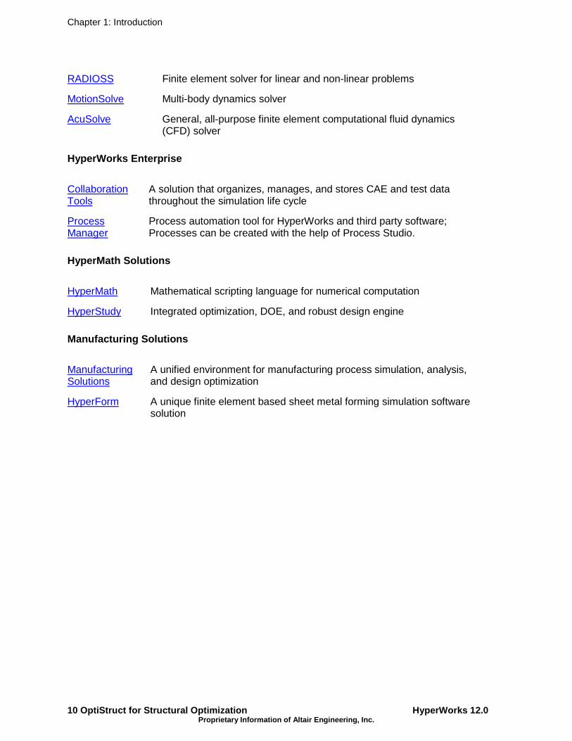
RADIOSS Finite element solver for linear and non-linear problems
MotionSolve Multi-body dynamics solver
AcuSolve General, all-purpose finite element computational fluid dynamics (CFD) solver
HyperWorks Enterprise
Collaboration Tools
A solution that organizes, manages, and stores CAE and test data throughout the simulation life cycle
Process Manager
Process automation tool for HyperWorks and third party software; Processes can be created with the help of Process Studio.
HyperMath Solutions
HyperMath Mathematical scripting language for numerical computation
HyperStudy Integrated optimization, DOE, and robust design engine
Manufacturing Solutions
Manufacturing Solutions
A unified environment for manufacturing process simulation, analysis, and design optimization
HyperForm A unique finite element based sheet metal forming simulation software solution

Chapter 1: Introduction
HyperWorks 12.0 OptiStruct for Structural Optimization 11 Proprietary Information of Altair Engineering, Inc.
HyperXtrude An finite element solver and user environment that enables engineers to analyze material flow and heat transfer problems in extrusion and rolling applications
HyperMold Provides a highly efficient and customized environment for setting up models for injection molding simulation with Moldflow and Moldex3D
HyperWeld Provides an efficient interface for setting up models and analyzing friction stir welding with the HyperXtrude Solver
Forging Provides a highly efficient and customized environment for setting up models for complex three-dimensional forging simulation with DEFOM3D
Results Mapper Process Manager-based tool that provides a framework to initialize a structural model with results from a forming simulation
Engineering Solutions
CFD High quality tools for CFD applications enabling the engineer to perform modeling, optimization and post-processing tasks efficiently.
NVH HyperWorks environment customized for automotive full vehicle NVH modeling and analysis needs.
Crash Tailored environment in HyperWorks that efficiently steers the Crash CAE specialist in CAE model building, starting from CAD geometry and finishing with a runnable solver deck in both solvers RADIOSS and LS-DYNA.
Drop Test The Drop Test Manager is an automated solution that allows the user to either simulate a single drop test or a choice of multiple iterations with the aim of finding the sensitivity of process variables like initial orientation and drop height in a typical drop test by controlling the run parameters and conditions with ease.
Durability Director
Solver-neutral, process-oriented customization of HyperWorks that addresses many of the challenges associated with assessing the fatigue life of mechanical components.
Suspension Director
Industry specific solution that is integrated with MotionView and utilizes many aspects of HyperWorks to assist with the engineering of vehicle suspensions.
HyperCrash CAE pre-processor tool developed to support the non-linear finite element solver, Altair RADIOSS
CAE Result Player
HyperView Player Plug-in and stand-alone utility to share and visualize 3-D CAE models and results

Chapter 1: Introduction
12 OptiStruct for Structural Optimization HyperWorks 12.0 Proprietary Information of Altair Engineering, Inc.
solidThinking
solidThinking Comprehensive NURBS-based 3D modeling and rendering environment for industrial design
solidThinking Inspired
Innovative morphogenesis form generation technology
1.2 – OptiStruct Integration with HyperWorks OptiStruct is part of the HyperWorks toolkit, as described earlier this is a finite element solver designed to solve linear and non-linear simulations. Along with the HyperWorks suite explicit solver, RADIOSS, HyperWorks can simulate structures, fluid, fluid-structure interaction, sheet metal stamping, and mechanical systems. Multi-body dynamics simulation is made possible through the integration with MotionSolve.
The solvers consist of loosely integrated executables (see picture below). To the user the integration is seamless through the run script provided. Based on the file naming convention, the right executable or combination of executables is chosen.
Solver Overview
The pre-processing for OptiStruct is done using HyperMesh or HyperCrash and the post-processing is done using HyperView and HyperGraph. For more information about the HyperWorks suite of products, please refer to our online help documentation.

Chapter 1: Introduction
HyperWorks 12.0 OptiStruct for Structural Optimization 13 Proprietary Information of Altair Engineering, Inc.
2 – RADIOSS Overview Altair® RADIOSS® is a leading structural analysis solver for highly non-linear problems
under dynamic loadings. It is highly differentiated for Scalability, Quality and Robustness, and consists of features for multi-physics simulation and advanced materials such as composites. RADIOSS is used across all industry worldwide to improve the crashworthiness, safety, and manufacturability of structural designs. For over 20 years, RADIOSS has established itself as a leader and an Industry standard for automotive crash and impact analysis.
Finite element solutions via RADIOSS include:
o Explicit dynamic analysis o Non-linear implicit static analysis o Transient heat transfer and thermo-mechanical coupling o Explicit Arbitrary Euler-Lagrangian (ALE) formulation o Explicit Computational Fluid Dynamics (CFD) o Smooth Particle Hydrodynamics (SPH) o Incremental sheet metal stamping analysis with mesh adaptivity o Linear static analysis o Normal modes analysis o Linear and non-linear buckling analysis
A typical set of finite elements including shell, solid, bar, and spring elements, rigid bodies as well as loads, a number of materials, and contact interfaces are available for modeling complex events.
2.1 – RADIOSS Process

Chapter 1: Introduction
14 OptiStruct for Structural Optimization HyperWorks 12.0 Proprietary Information of Altair Engineering, Inc.

Chapter 2: Theoretical Background
HyperWorks 12.0 OptiStruct for Structural Optimization 15 Proprietary Information of Altair Engineering, Inc.
Chapter 2
Theoretical Background
1 – Optimization Optimization can be defined as the automatic process to make a system or component as good as possible based on an objective function and subject to certain design constraints. There are many different methods or algorithms that can be used to optimize a structure, in OptiStruct is implemented some algorithms based on Gradient Method, this method will be discussed in detail later on this book.
Models used in optimization are classified in various ways, such as linear versus nonlinear, static versus dynamic, deterministic versus stochastic, or permanent versus transient. Then it is very important that the user include a-priori all of the important aspects of the problem, so that they will be taken into account during the solution.
Mathematically an optimization problem can be stated as:
Objective Function: ψ0(p) ⇒ min(max) (target)
Subject to constraint Functions: ψi(p) ≤0
Design Space: pl ≤ pj ≤ pu where l is the lower bound and u is
the upper bound on the design variables
where:
ψψψψ0(p) and ψψψψi(p) represent the system responses or a target value for system identification study, and pj represents the vector of design variables (p1,p2,…,pn).
1.1 – Design Variable Design Variables or DVs are system parameters that can vary to optimize system performance. For OptiStruct the type of parameter or DV defines the optimization type:
o TOPOLOGY: is a mathematical technique that optimized the material distribution for a structure within a given package space. DVs are defined as a fictitious density

Chapter 2: Theoretical Background
16 OptiStruct for Structural Optimization HyperWorks 12.0 Proprietary Information of Altair Engineering, Inc.
for each element, and these values are varied from 0 to 1 to optimize the material distribution.
o TOPOGRAPHY: Topography optimization is an advanced form of shape optimization in which a design region for a given part is defined and a pattern of shape variable-based reinforcements within that region is generated using OptiStruct.
o FREE-SIZE: This is a special method designed by Altair to optimize 2D structure where the design variables are the thickness of each element. This method is very useful for aerospace structures where shear panels are preferable to truss structures.
o SHAPE: is an automated way to modify the structure shape based on predefined shape variables to find the optimal shape. DVs are used to modify the geometry shape of the component, on HyperMesh it is used HyperMorph to define this parameter.
o SIZE: is an automated way to modify the structure parameters to find the optimal design. DVs are any Scalar parameter (thickness, 1D properties, material properties, etc…) that affects the system response.
o GAUGE: Particular case of size optimization when the DV are PSHELL thickness.
o FREE-SHAPE: is an automated way to modify the structure shape based on set of nodes that can move totally free on the boundary to find the optimal shape. DVs are defined based a set of nodes.
o COMPOSITE SHUFFLE: is an automated way to determine the optimum laminate stack sequence. DVs are the plies sequence of stacking. It is used for composite material only defined using PCOMP(G) or PCOMPP.

Chapter 2: Theoretical Background
HyperWorks 12.0 OptiStruct for Structural Optimization 17 Proprietary Information of Altair Engineering, Inc.
1.2 – Response Response for OptiStruct is any value or function that is dependent of the Design Variable and is evaluated during the solution.
OptiStruct allows the use of numerous structural responses, calculated in a finite element analysis, or combinations of these responses to be used as objective and constraint functions in a structural optimization.
Responses are defined using DRESP1 bulk data entries. Combinations of responses are defined using either DRESP2 entries, which reference an equation defined by a DEQATN bulk data entry, or DRESP3 entries, which make use of user-defined external routines identified by the LOADLIB I/O option. Responses are either global or subcase (loadstep, load case) related. The character of a response determines whether or not a constraint or objective referencing that particular response needs to be referenced within a subcase.
1.2.1 - Subcase Independent Response
o Mass, Volume [ mass, volume]
Both are global responses that can be defined for the whole structure, for individual properties (components) and materials, or for groups of properties (components) and materials.
o Fraction of mass, Fraction of design volume [ massfrac, volumefrac]
Both are global responses with values between 0.0 and 1.0. They describe a fraction of the initial design space in a topology optimization. They can be defined for the whole structure, for individual properties (components) and materials, or for groups of properties (components) and materials.
D
Di
f V
VV
0
=
where: Vf : Volume fraction
DiV : Designable volume at current iteration;
DV0 : Initial Designable volume;
0M
MM i
f =
where: Mf : Mass fraction Mi : Total mass at current iteration; M0 : Total Initial mass;

Chapter 2: Theoretical Background
18 OptiStruct for Structural Optimization HyperWorks 12.0 Proprietary Information of Altair Engineering, Inc.
If, in addition to the topology optimization, a size and shape optimization is performed, the reference value (the initial design volume in the case of volume fraction, or initial total mass in the case of mass fraction) is not altered by size and shape changes. This can, on occasion, lead to negative values for these responses. If size and shape optimization are involved, it is recommended to use Mass or Volume responses instead of Mass Fraction or Volume Fraction, respectively.
In order to constrain the volume fraction for a region containing a number of properties (components), a DRESP2 equation needs to be defined to sum the volume of these properties (components), otherwise, the constraint is assumed to apply to each individual property (component) within the region. This can be avoided by having all properties (components) use the same material and applying the volume fraction constraint to that material.
These responses can only be applied to topology design domains. OptiStruct will terminate with an error if this is not the case.
o Center of gravity [ cog ]
This is a global response that may be defined for the whole structure, for individual properties (components) and materials, or for groups of properties (components) and materials.
o Moments of inertia [ inertia ]
This is a global response that may be defined for the whole structure, for individual properties (components) and materials, or for groups of properties (components) and materials.
o Weighted compliance [ weighted comp ]
The weighted compliance is a method used to consider multiple subcases (loadsteps, load cases) in a classical topology optimization. The response is the weighted sum of the compliance of each individual subcase (loadstep, load case).
∑ ∑== iTiiiiW wCwC fu
2
1
This is a global response that is defined for the whole structure.
o Weighted reciprocal eigenvalue (frequency) [ weighted freq ]
The weighted reciprocal eigenvalue is a method to consider multiple frequencies in a classical topology optimization. The response is the weighted sum of the reciprocal eigenvalues of each individual mode considered in the optimization.
[ ] 0uMK =−=∑ iii
iw
wf λ
λ with
This is done so that increasing the frequencies of the lower modes will have a larger effect on the objective function than increasing the frequencies of the higher modes. If the frequencies of all modes were simply added together, OptiStruct would put more effort into increasing the higher modes

Chapter 2: Theoretical Background
HyperWorks 12.0 OptiStruct for Structural Optimization 19 Proprietary Information of Altair Engineering, Inc.
than the lower modes. This is a global response that is defined for the whole structure.
o Combined compliance index [ compliance index ]
The combined compliance index is a method to consider multiple frequencies and static subcases (loadsteps, load cases) combined in a classical topology optimization. The index is defined as follows:
∑ ∑
∑+=
j
j
j
ii w
w
NORMCwSλ
This is a global response that is defined for the whole structure.
The normalization factor, NORM, is used for normalizing the contributions of compliances and eigenvalues. A typical structural compliance value is of the order of 1.0e4 to 1.0e6. However, a typical inverse eigenvalue is on the order of 1.0e-5. If NORM is not used, the linear static compliance requirements dominate the solution.
The quantity NORM is typically computed using the formula
minmaxλCNF =
where Cmax is the highest compliance value in all subcases (loadsteps, load cases) and λλλλmin is the lowest eigenvalue included in the index.
In a new design problem, the user may not have a close estimate for NORM. If this happens, OptiStruct automatically computes the NORM value based on compliances and eigenvalues computed in the first iteration step.
o Von Mises stress in a topology or free-size optimiz ation
Von Mises stress constraints may be defined for topology and free-size optimization through the STRESS optional continuation line on the DTPL or the DSIZE card. There are a number of restrictions with this constraint:
o The definition of stress constraints is limited to a single von Mises permissible stress. The phenomenon of singular topology is pronounced when different materials with different permissible stresses exist in a structure. Singular topology refers to the problem associated with the conditional nature of stress constraints, i.e. the stress constraint of an element disappears when the element vanishes. This creates another problem in that a huge number of reduced problems exist with solutions that cannot usually be found by a gradient-based optimizer in the full design space.
o Stress constraints for a partial domain of the structure are not allowed because they often create an ill-posed optimization problem since elimination of the partial domain would remove all stress constraints. Consequently, the stress constraint applies to the entire model when active, including both design and non-

Chapter 2: Theoretical Background
20 OptiStruct for Structural Optimization HyperWorks 12.0 Proprietary Information of Altair Engineering, Inc.
design regions, and stress constraint settings must be identical for all DSIZE and DTPL cards.
o The capability has built-in intelligence to filter out artificial stress concentrations around point loads and point boundary conditions. Stress concentrations due to boundary geometry are also filtered to some extent as they can be improved more effectively with local shape optimization.
o Due to the large number of elements with active stress constraints, no element stress report is given in the table of retained constraints in the .out file. The iterative history of the stress state of the model can be viewed in HyperView or HyperMesh.
o Stress constraints do not apply to 1-D elements.
o Stress constraints may not be used when enforced displacements are present in the model.
o Bead discreteness fraction [ beadfrac ]
This is a global response for topography design domains. This response indicates the amount of shape variation for one or more topography design domains. The response varies in the range 0.0 to 1.0 (0.0 < BEADFRAC < 1.0), where 0.0 indicates that no shape variation has occurred, and 1.0 indicates that the entire topography design domain has assumed the maximum allowed shape variation.
Static Subcase o Static compliance [ compliance ]
The compliance C is calculated using the following relationship:
∫==
==
V
TT
T
σdvεKuu
fKufu
21
21
with21
C
or
C
The compliance is the strain energy of the structure and can be considered a reciprocal measure for the stiffness of the structure. It can be defined for the whole structure, for individual properties (components) and materials, or for groups of properties (components) and materials. The compliance must be assigned to a static subcase (loadstep, load case).
In order to constrain the compliance for a region containing a number of properties (components), a DRESP2 equation needs to be defined to sum the compliance of these properties (components), otherwise, the constraint is assumed to apply to each individual property (component) within the region. This can be avoided by having all properties (components) use the same material and applying the compliance constraint to that material.

Chapter 2: Theoretical Background
HyperWorks 12.0 OptiStruct for Structural Optimization 21 Proprietary Information of Altair Engineering, Inc.
o Static displacement [ static displacement ]
Displacements are the result of a linear static analysis. Nodal displacements can be selected as a response. They can be selected as vector components or as absolute measures. They must be assigned to a static subcase (loadstep, load case).
o Static stress of homogeneous material [ static stress ]
Different stress types can be defined as responses. They are defined for components, properties, or elements. Element stresses are used, and constraint screening is applied. It is also not possible to define static stress constraints in a topology design space (see above). This is a static subcase (loadstep, load case) related response.
o Static strain of homogeneous material [ static strain ]
Different strain types can be defined as responses. They are defined for components, properties, or elements. Element strains are used, and constraint screening is applied. It is also not possible to define strain constraints in a topology design space. This is a subcase (loadstep, load case) related response.
o Static stress of composite lay-up [ composite stress ]
Different composite stress types can be defined as responses. They are defined for PCOMP components or elements. Ply level results are used, and constraint screening is applied. It is also not possible to define composite stress constraints in a topology design space. This is a subcase (loadstep, load case) related response.
o Static strain of composite lay-up [ composite strain ]
Different composite strain types can be defined as responses. They are defined for PCOMP components or elements. Ply level results are used, and constraint screening is applied. It is also not possible to define composite strain constraints in a topology design space. This is a subcase (loadstep, load case) related response.
o Static failure in a composite lay-up [composite failure ]
Different composite failure criterion can be defined as responses. They are defined for PCOMP components or elements. Ply level results are used, and constraint screening is applied. It is also not possible to define composite failure criterion constraints in a topology design space. This is a subcase (loadstep, load case) related response.
o Static force [ static force ]
Different force types can be defined as responses. They are defined for components, properties, or elements. Constraint screening is applied. It is also not possible to define force constraints in a topology design space. This is a static subcase (loadstep, load case) related response.

Chapter 2: Theoretical Background
22 OptiStruct for Structural Optimization HyperWorks 12.0 Proprietary Information of Altair Engineering, Inc.
Normal Modes Subcase o Frequency [ frequency ]
Natural frequencies are the result of a normal modes analysis, and must be assigned to the normal modes subcase (loadstep, load case).
Buckling Subcase o Buckling factor [ buckling ]
The buckling factor is the result of a buckling analysis, and must be assigned to a buckling subcase (loadstep, load case). A typical buckling constraint is a lower bound of 1.0, indicating that the structure is not to buckle with the given static load. It is recommended to constrain the buckling factor for several of the lower modes, not just of the first mode.
Frequency Response Subcase o Frequency response displacement [ frf displacement ]
Displacements are the result of a frequency response analysis. Nodal displacements can be selected as a response. They can be selected as vector components in real/imaginary or magnitude/phase form. They must be assigned to a frequency response subcase (loadstep, load case).
o Frequency response velocity [ frf velocity ]
Velocities are the result of a frequency response analysis. Nodal velocities can be selected as a response. They can be selected as vector components in real/imaginary or magnitude/phase form. They must be assigned to a frequency response subcase (loadstep, load case).
o Frequency response acceleration [ frf acceleration ]
Accelerations are the result of a frequency response analysis. Nodal accelerations can be selected as a response. They can be selected as vector components in real/imaginary or magnitude/phase form. They must be assigned to a frequency response subcase (loadstep, load case).
o Frequency response stress [ frf stress ]
Different stress types can be defined as responses. They are defined for components, properties, or elements. Element stresses are not used in real/imaginary or magnitude/phase form, and constraint screening is applied. It is not possible to define stress constraints in a topology design space. This is a frequency response subcase (loadstep, load case) related response.
o Frequency response strain [ frf strain ]
Different strain types can be defined as responses. They are defined for components, properties, or elements. Element strains are used in real/imaginary or magnitude/phase form, and constraint screening is applied. It is not possible to define strain constraints in a topology design space. This is a frequency response subcase (loadstep, load case) related response.

Chapter 2: Theoretical Background
HyperWorks 12.0 OptiStruct for Structural Optimization 23 Proprietary Information of Altair Engineering, Inc.
o Frequency response force [ frf force ]
Different force types can be defined as responses. They are defined for components, properties, or elements in real/imaginary or magnitude/phase form. Constraint screening is applied. It is also not possible to define force constraints in a topology design space. This is a frequency response subcase (loadstep, load case) related response.
All FRF responses can be output as:
All freq → All evaluated points on the freq range. Vector = { iy }
Freq = → Argument value on a specific frequency f. Scalar = ( )fy
sum → Sum of all arguments. Scalar ∑=
=m
iiy
1
avg → Average of all arguments. Scalar mym
ii /
1∑==
ssq → Sum of square of the arguments. Scalar ∑=
=m
iiy
1
2
rss → Square root of sum of squares of the arguments. Scalar ∑=
=m
iiy
1
2
max → Maximum value of arguments. Scalar = ( )iymax
min → Minimum value of arguments. Scalar = ( )iymin
avgabs → Average of absolute value of arguments. Scalar mym
ii /
1
∑=
=
maxabs → Maximum of absolute value of arguments. Scalar = ( )iymax
minabs → Minimum of absolute value of arguments. Scalar = ( )iymin
sumabs → Sum of absolute value of arguments. Scalar ∑=
=m
iiy
1
o Fatigue [ fatigue ]
It is the life or damage evaluated in a fatigue sequence for a group of elements or properties.
o Function [ function ]
It is a generic equation defined using the dequations panel [DEQATN].
1.3 – Objective Function The Objective function is a model response to be maximized or minimized.
There are two ways to specify an objective in OptiStruct. Either a single response can be minimized or maximized or you can choose to minimize the maximum value, or maximize the minimum value, of a number of normalized responses.

Chapter 2: Theoretical Background
24 OptiStruct for Structural Optimization HyperWorks 12.0 Proprietary Information of Altair Engineering, Inc.
In the first instance, where a single response is defined as the objective, a DESOBJ card must be included in the Subcase Information section of the input file. The DESOBJ card references a response, (DRESP1 or DRESP2), which is defined in the Bulk Data section of the input file. If the response, to which the DESOBJ card refers, is associated with a single subcase, the DESOBJ card must be placed within that subcase definition. If the response is associated with more than one subcase, the DESOBJ card must appear before the first SUBCASE statement.
Example: Objective is to minimize the value of the response with ID 1.
DESOBJ(MIN) = 1
The second instance, where the objective references multiple responses, requires DOBJREF bulk data entries and MINMAX or MAXMIN subcase information entries. The DOBJREF cards reference responses (DRESP1 or DRESP2) and provide positive and negative reference values for these responses. Multiple DOBJREF cards may occur in the input file and they may or may not use the same Design Objective IDs. The reference values allow for normalization of different responses. The value of the response is divided by the appropriate reference value. When the value of the response is positive, the positive reference value is used. When the value of the response is negative, the negative reference value is used.
The MINMAX or MAXMIN cards reference the DOBJREF cards. If all DOBJREF cards use the same DOID, only one occurrence of MAXMIN or MINMAX is required. If different DOIDs are used on the DOBJREF cards, multiple occurrences of MINMAX and MAXMIN cards may be required, but a MINMAX statement cannot appear in the same input file as a MAXMIN statement. MINMAX or MAXMIN statements must appear before the first SUBCASE statement.
Example: Objective is to minimize the maximum of all DOBJREF's with DOID 1 and DOID 2.
MINMAX = 1
MINMAX = 2
Example: Design objective for MINMAX (MAXMIN) problems - DOID 1 - references design response 10 in subcase 2 - negative reference value = -1.0, positive reference value = 1.0.
$--(1)--$--(2)--$--(3)--$--(4)--$--(5)--$--(6)--$--(7)--
DOBJREF 1 10 2 1.0 1.0
1.4 – Constraint Functions On all almost every engineering design there are constraints that need to be satisfied. These constraints can be defined as a lower bound or an upper bound on any response that is dependent of the design variable. To better understand it lets propose a model where there are 3 constraints.

Chapter 2: Theoretical Background
HyperWorks 12.0 OptiStruct for Structural Optimization 25 Proprietary Information of Altair Engineering, Inc.
A cantilever beam loaded with force F=24000 N. Where the cross-section parameters: Width b [20,40] and height h [30,90] can vary on their range to minimize the beam weight, subject to these constraint:
1) Max normal stress cannot exceed the σσσσmax value,
2) Max shear stress cannot exceed the ττττmax and
3) Height h should not be larger than twice the width b.
Mathematically this problem can be stated as:
Objective : min Weight (b,h)
Design Variables: bL < b < bU, 20 < b < 40
hL < h < hU, 30 < h < 90
Design Constraints: σ (b,h) = 6F/(bh2) ≤ σmax, with σmax = 70 MPa
τ (b,h) =F/(bh) ≤ τmax, with τmax = 15 MPa
h ≥≥≥≥ 2*b

Chapter 2: Theoretical Background
26 OptiStruct for Structural Optimization HyperWorks 12.0 Proprietary Information of Altair Engineering, Inc.
This problem can be described graphically as shown below:
Cantilever beam problem (Optimum (b=24.9, h=64.3) W = 8).
BEAM
0.010.020.030.040.050.060.070.080.090.0
100.0
0.00 10.00 20.00 30.00 40.00 50.00
b (mm)
h (m
m)
σ=70 τ=15
ττττ > 15
ττττ < 15
σσσσ>70
σσσσ<70
W = 5
W = 7
W = 9
W = 11
FEASIBLE DOMAIN
UNFEASIBLE DOMAIN
OPTIMUM

Chapter 2: Theoretical Background
HyperWorks 12.0 OptiStruct for Structural Optimization 27 Proprietary Information of Altair Engineering, Inc.
2 – Gradient-based Optimization OptiStruct uses an iterative procedure known as the local approximation method to solve the optimization problem. This approach is based on the assumption that only small changes occur in the design with each optimization step. The result is a local minimum. The biggest changes occur in the first few optimization steps and, as a result, not many system analyses are necessary in practical applications.
The design sensitivity analysis of the structural responses (with respect to the design variables) is one of the most important ingredients to take the step from a simple design variation to a computational optimization.
The design update is computed using the solution of an approximate optimization problem, which is established using the sensitivity information. OptiStruct has three different methods implemented: the optimality criteria method, a dual method, and a primal feasible directions method. The latter are both based on a convex linearization of the design space. Advanced approximation methods are used.
The optimality criteria method is used for classical topology optimization formulations using minimum compliance (reciprocal frequency, weighted compliance, weighted reciprocal frequency, compliance index) with a mass (volume) or mass (volume) fraction constraint.
The dual or primal methods are used depending upon the number of constraints and design variables. The dual method is of advantage if the number of design variables exceeds the number of constraints (common in topology and topography optimization). The primal method is used in the opposite case, which is more common in size and shape optimizations. However, the choice is made automatically by OptiStruct.

Chapter 2: Theoretical Background
28 OptiStruct for Structural Optimization HyperWorks 12.0 Proprietary Information of Altair Engineering, Inc.
2.1 – Gradient Method This is an optimization algorithm that can be called Gradient Descent Method, or just Gradient Method. It is used to find a minimum of a function using the gradient value; the algorithm can be described as:
1. Start from a X0 point
2. Evaluate the function F(Xi) and the gradient of the function ∇F(Xi) at the Xi.
3. Determine the next point using the negative gradient direction: Xi+1 = Xi - γ ∇F(Xi).
4. Repeat Steps 2 to 3 until the function converged to the minimum.
The picture below shows how this work:
This is a very simplified overview of this method, if the user needs more information it can be found on any Optimization text book
Gradient-based methods are effective when the sensitivities (derivatives) of the system responses, with respect to the design variables, can be computed easily and inexpensively.
The local approximation method is best suited to situations where:
• Design Sensitivity Analysis (DSA) is available.
• The method is applied to linear static and dynamic problems integrated mostly with FEA Solvers (i.e. OptiStruct).
Gradient-based methods depend on the sensitivity of the system responses with respect to changes in design variables in order to understand the effect of the design changes and optimize the system.
For linear structural analysis codes, you can implement the derivatives of the structural responses using either finite difference or analytical methods (such as the Adjoint Method). Here, the responses are written as explicit algebraic equations with the needed continuity requirements and are easily differentiable.
X0
X1
X2
X3

HyperWorks 12.0 Proprietary Information of Altair Engineering, Inc.
For example, using first order finite difference method, you can calculate the gradient of ψi(p) as:
In finite element based structural optimization, you can state the linear static equation as KU = F, where K is the stiffness matrix and U is the displacement vector to be determined, and F is the applied force vector. Differentiating this with respect to the design variable X yields the following:
Rearranging terms gives the following equation:
You can obtain gradients of stresses and strains, etc, by chain rule differentiation.
2.2 – Sensitivity Analysis The response quantity,
The sensitivity of this response with respect to the design variable of the response, is:
Two approaches to sensitivity analysis, the possible. Given the equation of motion:
and its derivative with respect to design variable
one can calculate the sensitivity of th
Using this equation, the largest cost in the calculation of the response gradient is the forward-backward substitution required for the calculation of the derivative of the displacement vector with respect to the design varia One forward-backward substitution is required for each design variable.
Chapter 2: Theoretical Background
OptiStruct for Structural OptimizationProprietary Information of Altair Engineering, Inc.
For example, using first order finite difference method, you can calculate the gradient
In finite element based structural optimization, you can state the linear static K is the stiffness matrix and U is the displacement vector to be
determined, and F is the applied force vector. Differentiating this with respect to the design variable X yields the following:
Rearranging terms gives the following equation:
an obtain gradients of stresses and strains, etc, by chain rule differentiation.
Analysis The response quantity, g, is calculated from the displacements as:
The sensitivity of this response with respect to the design variable x,
Two approaches to sensitivity analysis, the Direct and Adjoint variable possible. Given the equation of motion:
and its derivative with respect to design variable x,
one can calculate the sensitivity of the displacement vector u as:
Using this equation, the largest cost in the calculation of the response gradient is the substitution required for the calculation of the derivative of the
displacement vector with respect to the design variable. This is called the direct methodbackward substitution is required for each design variable.
Chapter 2: Theoretical Background
for Structural Optimization 29
For example, using first order finite difference method, you can calculate the gradient
In finite element based structural optimization, you can state the linear static K is the stiffness matrix and U is the displacement vector to be
determined, and F is the applied force vector. Differentiating this with respect to the design
an obtain gradients of stresses and strains, etc, by chain rule differentiation.
or the gradient
variable method are
Using this equation, the largest cost in the calculation of the response gradient is the substitution required for the calculation of the derivative of the
direct method.

Chapter 2: Theoretical Background
30 OptiStruct for Structural OptimizationProprietary Information of Altair Engineering, Inc.
If constraints are active in more than one load case, and the load is a function of the design variable (say body force or pressure loads fforward-backward substitutions must be performed for each active load case. are not a function of the design variables, but there are active load cases with multiple boundary conditions, then the set ofeach active boundary condition.
For the Adjoint variable method of sensitivity analysis, the vector (adjoint variable) is introduced, which is calculated as:
Then the derivative of the constraint
When the adjoint variable method for sensitivity analysis is used, a single forwardbackward substitution is needed for each retained constraint. substitution is needed to calculate the vector
There are typically a small number of design variables in shape and size optimization (say 5 to 50) and a large number of constraints. from stress constraints. If there are 20,000 elements, each with a single stress constrainand 10 load cases, there are a total of 200,000 possible stress constraints.
There are typically a large number of design variables in topology optimization (between 1 and 3 per element) and a small number of constraints. constraints are not usually considered in topology optimization, it makes sense that the Adjoint variable method of sensitivity analysis be used for topology optimization (in order to reduce computational costs).
For shape and sizing optimization, it sensitivity analysis. However, in some cases, when there are a large number of design variables and a small number of constraints, the adjoint variable method should be used. For example, in a topography optimization, thebe calculated for can be reduced using constraint screening. constraints that are not close to being violated are ignored. violated, or nearly violated, are retained. retained in a small region of the structure, say at a stress concentration, only a few of the most critical need to be retained.
The sensitivities of responses with respect to design variablExcel spreadsheet (see OUTPUT, MSSENS) or plotted in HyperGraph (See OUTPUT, HGSENS). For contouring in HyperView, the sensitivities of topology and gauge design variables can be exported to H3D format. H3DGAUGE, respectively).
The Excel spreadsheet allows the modification of design variables and then computes approximated responses. running OptiStruct again. See the image below.
for Structural Optimization HyperWorks Proprietary Information of Altair Engineering, Inc.
If constraints are active in more than one load case, and the load is a function of the design variable (say body force or pressure loads for shape optimization), then the set of
backward substitutions must be performed for each active load case. If the loads are not a function of the design variables, but there are active load cases with multiple boundary conditions, then the set of forward-backward substitutions must be performed for each active boundary condition.
variable method of sensitivity analysis, the vector (adjoint variable) is introduced, which is calculated as:
Then the derivative of the constraint can be calculated as:
When the adjoint variable method for sensitivity analysis is used, a single forwardbackward substitution is needed for each retained constraint. This forward-backward substitution is needed to calculate the vector a.
typically a small number of design variables in shape and size optimization (say 5 to 50) and a large number of constraints. The large number of constraints comes
If there are 20,000 elements, each with a single stress constrainand 10 load cases, there are a total of 200,000 possible stress constraints.
There are typically a large number of design variables in topology optimization (between 1 and 3 per element) and a small number of constraints. Because stress
re not usually considered in topology optimization, it makes sense that the variable method of sensitivity analysis be used for topology optimization (in order to
For shape and sizing optimization, it is often beneficial to use the Direct However, in some cases, when there are a large number of design
variables and a small number of constraints, the adjoint variable method should be used. For example, in a topography optimization, the number of constraints that gradients need to
be calculated for can be reduced using constraint screening. With constraint screening, constraints that are not close to being violated are ignored. Only constraints that are
e retained. Also, if there are many stress constraints that are retained in a small region of the structure, say at a stress concentration, only a few of the most critical need to be retained.
The sensitivities of responses with respect to design variables can be exported to an Excel spreadsheet (see OUTPUT, MSSENS) or plotted in HyperGraph (See OUTPUT,
For contouring in HyperView, the sensitivities of topology and gauge design variables can be exported to H3D format. (See OUTPUT, H3DTOPOL and OUTPUT,
The Excel spreadsheet allows the modification of design variables and then computes approximated responses. This can be used to make design studies without
See the image below.
HyperWorks 12.0
If constraints are active in more than one load case, and the load is a function of the or shape optimization), then the set of
If the loads are not a function of the design variables, but there are active load cases with multiple
backward substitutions must be performed for
variable method of sensitivity analysis, the vector (adjoint variable) a
When the adjoint variable method for sensitivity analysis is used, a single forward-backward
typically a small number of design variables in shape and size optimization The large number of constraints comes
If there are 20,000 elements, each with a single stress constraint,
There are typically a large number of design variables in topology optimization Because stress
re not usually considered in topology optimization, it makes sense that the variable method of sensitivity analysis be used for topology optimization (in order to
irect method for However, in some cases, when there are a large number of design
variables and a small number of constraints, the adjoint variable method should be used. number of constraints that gradients need to
With constraint screening, Only constraints that are
Also, if there are many stress constraints that are retained in a small region of the structure, say at a stress concentration, only a few of the
es can be exported to an Excel spreadsheet (see OUTPUT, MSSENS) or plotted in HyperGraph (See OUTPUT,
For contouring in HyperView, the sensitivities of topology and gauge design OUTPUT,
The Excel spreadsheet allows the modification of design variables and then This can be used to make design studies without

Chapter 2: Theoretical Background
HyperWorks 12.0 OptiStruct for Structural Optimization 31 Proprietary Information of Altair Engineering, Inc.
Example spreadsheet output showing that modification of field C10 yields approximate results in the lower right of the spreadsheet, identified by a border surround here.
File Creation
This file is only created when size or shape optimization is performed. Output of this file is controlled by the SENSITIVITY and SENSOUT I/O options.
File Format
The only values that can be changed in this file are those listed in the "New" column. All other values are either fixed or their calculation is fixed. When the .slk file is created, the values in the "New" column match those in the "Reference" column. These values may be adjusted, but should always remain within the design variable's bounds.
Each size and shape design variable in the model is listed in the left-hand column of the sensitivity table. Information concerning a particular design variable is given in the row where its label is listed. The current value and the upper and lower bounds of the design variables are given in the columns, "Reference," "Lower," and "Upper" respectively.
Each referenced response in the model has its own column. These response columns are on the right-hand side of the sensitivity table. The calculated sensitivity of a response to changes in a design variable at the current iteration is given in the row corresponding to that design variable and the column corresponding to that response.
Beneath the list of design variables, in the left-hand column, are the headings "Response lower bound," "Response reference," and "Response upper bound". If a response is constrained, the constraint value will be given in either the "Response lower bound" or the "Response upper bound" row of the column corresponding to that response. The value given in the "Response reference" row is the calculated value of the response using the design variable reference values.

Chapter 2: Theoretical Background
32 OptiStruct for Structural Optimization HyperWorks 12.0 Proprietary Information of Altair Engineering, Inc.
At the bottom of the left-hand column are the headings: "Response linear," "Response reciprocal," and "Response conservative". The response values in these rows are the predicted values of the responses for three different approximations. Initially, these values will match one another and the "Response reference" value for each response. This is because these are the predicted values of the response at the given variable settings, which initially are the same settings used to calculate the "Response reference" value. Once the design variable values in the "New" column are altered, these values will change.
The "Response linear" row predicts the response value using linear approximation. This is calculated as:
where:
1R is the predicted response value.
0R is the response reference value.
vnvv ,...,2,1 are the new values of the design variables.
000 ,...,2,1 vnvv are the reference values of the design variables.
dvn
dR
dv
dR
dv
dR,...,
2,
1 are the sensitivities of the response to the design variables.
The "Response reciprocal" row predicts the response value using reciprocal approximation. This is calculated as:
where:
1R is the predicted response value.
0R is the response reference value.
vnvv ,...,2,1 are the new values of the design variables.
000 ,...,2,1 vnvv are the reference values of the design variables.
dvn
dR
dv
dR
dv
dR,...,
2,
1 are the sensitivities of the response to the design variables.

HyperWorks 12.0 Proprietary Information of Altair Engineering, Inc.
The "Response conservativeof the above approximations where linear approximation is used, when the sensitivity is positive, and reciprocal approximation is used when the sensitivity is negative. all sensitivities are positive, the conservative prediction will match the linear presensitivities are negative, it will match the reciprocal prediction, but if there is a mixture of positive and negative sensitivities for a given response then the conservative prediction will match neither the linear nor the reciprocal pr
The normalized values simply show the predicted response as a fraction of the response reference value.
2.3 - Move Limit Adjustments As the design moves away from its initial point in the approximate optimization problem, the approximate values convergence, as the approximate optimum designs are not near the actual optimum design. Move limits on the design variables, and/or intermediate design variables, are used to protect the accuracy of the approximations.
Small move limits lead to smoother convergence. due to the small design changes at each iteration. oscillations between infeasible designs as critical consthe approximations themselves are accurate, large move limits can be used. limits in the approximate optimization problem are 20% of the current design variable value. If advanced approximation concep
Even with advanced approximation concepts, it is possible to have poor approximations of the actual response behavior with respect to the design variables. best to use larger move limits for accuratethat are not so accurate.
Note that the same set of design variable move limits must be used for all of the response approximations. It is important to look at the approximations of the responses that are driving the design. These are the objective function and most critical constraints. objective function moves in the wrong direction, or critical constraints become even more violated, it is a sign that the approximations are not accurate. variable move limits are reduced. convergence may be slowed, as design variables that are a long way from the optimum design are forced to change slowly. variables that keep hitting the same upper or lower move limit bound are increased. limits are automatically adjusted by OptiStruct.
2.4 - Constraint Screening During the optimization process atconstraints of the design problem are evaluated. optimization problem has two potential disadvantages:
1. This can result in a big optimization problem with a large numand design variables. Most optimization algorithms are designed to handle either a large number of responses or a large number of design variables, but not both.
Chapter 2: Theoretical Background
OptiStruct for Structural OptimizationProprietary Information of Altair Engineering, Inc.
Response conservative" row predicts the response value using a combination approximations where linear approximation is used, when the sensitivity is
positive, and reciprocal approximation is used when the sensitivity is negative. all sensitivities are positive, the conservative prediction will match the linear presensitivities are negative, it will match the reciprocal prediction, but if there is a mixture of positive and negative sensitivities for a given response then the conservative prediction will match neither the linear nor the reciprocal prediction.
The normalized values simply show the predicted response as a fraction of the response
Move Limit Adjustments
As the design moves away from its initial point in the approximate optimization problem, the approximate values become less accurate. This can lead to slow overall convergence, as the approximate optimum designs are not near the actual optimum design. Move limits on the design variables, and/or intermediate design variables, are used to
approximations. They appear as:
Small move limits lead to smoother convergence. Many iterations may be required
due to the small design changes at each iteration. Large move limits may lead to oscillations between infeasible designs as critical constraints are calculated inaccurately. the approximations themselves are accurate, large move limits can be used. limits in the approximate optimization problem are 20% of the current design variable value. If advanced approximation concepts are used, move limits up to 50% are possible.
Even with advanced approximation concepts, it is possible to have poor approximations of the actual response behavior with respect to the design variables. best to use larger move limits for accurate approximations and smaller move limits for those
Note that the same set of design variable move limits must be used for all of the It is important to look at the approximations of the responses that
These are the objective function and most critical constraints. objective function moves in the wrong direction, or critical constraints become even more violated, it is a sign that the approximations are not accurate. In this case, all of the design variable move limits are reduced. However, if the move limits become too small, convergence may be slowed, as design variables that are a long way from the optimum design are forced to change slowly. Therefore, the move limits on the individual design variables that keep hitting the same upper or lower move limit bound are increased. limits are automatically adjusted by OptiStruct.
Constraint Screening During the optimization process at each iteration the objective function(s) and all
constraints of the design problem are evaluated. Retaining all of these responses in the optimization problem has two potential disadvantages:
This can result in a big optimization problem with a large number of responses and design variables. Most optimization algorithms are designed to handle either a large number of responses or a large number of design variables, but not both.
Chapter 2: Theoretical Background
for Structural Optimization 33
" row predicts the response value using a combination approximations where linear approximation is used, when the sensitivity is
positive, and reciprocal approximation is used when the sensitivity is negative. Therefore, if all sensitivities are positive, the conservative prediction will match the linear prediction. If all sensitivities are negative, it will match the reciprocal prediction, but if there is a mixture of positive and negative sensitivities for a given response then the conservative prediction will
The normalized values simply show the predicted response as a fraction of the response
As the design moves away from its initial point in the approximate optimization This can lead to slow overall
convergence, as the approximate optimum designs are not near the actual optimum design. Move limits on the design variables, and/or intermediate design variables, are used to
Many iterations may be required Large move limits may lead to
traints are calculated inaccurately. If the approximations themselves are accurate, large move limits can be used. Typical move limits in the approximate optimization problem are 20% of the current design variable value.
ts are used, move limits up to 50% are possible.
Even with advanced approximation concepts, it is possible to have poor approximations of the actual response behavior with respect to the design variables. It is
approximations and smaller move limits for those
Note that the same set of design variable move limits must be used for all of the It is important to look at the approximations of the responses that
These are the objective function and most critical constraints. If the objective function moves in the wrong direction, or critical constraints become even more
is case, all of the design However, if the move limits become too small,
convergence may be slowed, as design variables that are a long way from the optimum on the individual design
variables that keep hitting the same upper or lower move limit bound are increased. Move
each iteration the objective function(s) and all Retaining all of these responses in the
ber of responses and design variables. Most optimization algorithms are designed to handle either a large number of responses or a large number of design variables, but not both.

Chapter 2: Theoretical Background
34 OptiStruct for Structural Optimization HyperWorks 12.0 Proprietary Information of Altair Engineering, Inc.
2. For gradient-based optimization, the design sensitivities of these responses need to be calculated. The design sensitivity calculation can be very computationally expensive when there are a large number of responses and a large number of design variables.
Constraint screening is the process by which the number of responses in the optimization problem is trimmed to a representative set. This set of retained responses captures the essence of the original design problem while keeping the size of the optimization problem at an acceptable level. Constraint screening utilizes the fact that constrained responses that are a long way from their bounding values (on the satisfactory side) or which are less critical (i.e. for an upper bound more negative and for a lower bound more positive) than a given number of constrained responses of the same type, within the same designated region and for the same subcase, will not affect the direction of the optimization problem and therefore can be removed from the problem for the current design iteration.
Consider the optimization problem where the objective is to minimize the mass of a finite element model composed of 100,000 elements, while keeping the elemental stresses below their associated material's yield stress. In this problem, we have 100,000 constraints (the stress for every element must be below its associated material's yield stress) for each subcase. For every design variable, 100,000 sensitivity calculations must be performed for each subcase, at every iteration. Because design variable changes are restricted by move limits, stresses are not expected to change drastically from one iteration to the next. Therefore, it is wasteful to calculate the sensitivities for those elements whose stresses are considerably lower than their associated material's yield stress. Also the direction of the optimization will be driven primarily by the highest elemental stresses. Therefore, the number of required calculations can be further reduced by only considering an arbitrary number of the highest elemental stresses.
Of course there is trade-off involved in using constraint screening. By not considering all of the constrained responses, it may take more iterations to reach a converged solution. If too many constrained responses are screened, it may take considerably longer to reach a converged solution or, in the worst case, it may not be able to converge on a solution if the number of retained responses is less than the number of active constraints for the given problem.
Through extensive testing it has been found that, for the majority of problems, using constraint screening saves a lot of time and computational effort. Therefore, constraint screening is active in OptiStruct by default. The default settings consider only the 20 most critical (i.e. for an upper bound most positive and for a lower bound most negative) constraints that come within 50 percent of their bound value (on the satisfactory side) for each response type, for each region, for each subcase.
The DSCREEN bulk data entry controls both the screening threshold and number of retained constraints. Different DSCREEN settings are allowed for all of the response types supported by the DRESP1 bulk data entry. Responses defined by the DRESP2 bulk data entry are controlled by a single DSCREEN entry with RTYPE = EQUA. Likewise, responses defined by the DRESP3 bulk data entry are controlled by a single DSCREEN entry with RTYPE = EXTERNAL. It is important to ensure that DRESP2 and DRESP3 definitions that use the same region identifier use similar equations. (In order for constraint screening to work effectively, responses within the same region should be of similar magnitudes and demonstrate similar sensitivities, the easiest way to ensure that is through the use of similar variable combinations).

Chapter 2: Theoretical Background
HyperWorks 12.0 OptiStruct for Structural Optimization 35 Proprietary Information of Altair Engineering, Inc.
In order to reduce the burden on the user, it is possible to allow the screening criteria to be automatically and adaptively adjusted in an effort to retain the least number of responses necessary for stable convergence. Setting RTYPE=AUTO on the DSCREEN bulk data entry will enable this feature. Region definition is also automated with this setting. This setting is useful for less experienced users and can be particularly useful when there are many local constraints. However, there are some drawbacks; experienced users may be able to achieve better performance through manual definition of screening criteria, more memory may be required to run with RTYPE=AUTO, and manual under-retention of constraints will require less memory and may, therefore, be desirable for very large problems (even with compromised convergence stability and optimality).
2.4.1 – Regions and Their Purpose In OptiStruct, a region is a group of responses of the same type.
Regions are defined by the region identifier field on the DRESP1, DRESP2, and DRESP3 bulk data entries used to define the responses. If the region identifier field is left blank or set to 0, then each property associated with the response forms its own region. The same region identifier may be used for responses of different types, but remember that because they are not of the same type they cannot form the same region.
Example 1
(1) (2) (3) (4) (5) (6) (7) (8) (9) (10) DRESP1 1 label STRESS PSHELL SMP1 1
2 3
DRESP1 with ID 1 defines stress responses for all the elements that reference the PSHELL definitions with PID 1, 2, or 3. As no region identifier is defined, the stress responses for each PSHELL form their own regions. So, all of the stress responses for elements referencing PSHELL with PID1 are in a different region than all of the stress responses for elements referencing PSHELL with PID2, which in turn are in a different region than all of the stress responses for elements referencing PSHELL with PID3. If this response definition is constrained in an optimization problem, and the default settings for constraint screening are assumed, then 20 elemental stresses are considered for each of the three PSHELL definitions, i.e. 20 for each region, giving a total of 60 retained responses.
Example 2 (1) (2) (3) (4) (5) (6) (7) (8) (9) (10)
DRESP1 2 label STRESS PSHELL 1 SMP1 1 2
(1) (2) (3) (4) (5) (6) (7) (8) (9) (10)
DRESP1 3 label STRESS PSHELL 1 SMP1 3
All of the stress responses defined in the DRESP1 entries above form a single region - notice the non-zero entries in field 6 (0 is equivalent to leaving it blank). Now if these response definitions (which are of the same type (STRESS), with the same non-zero entry in field 6) are constrained in an optimization problem (assuming the default settings for

Chapter 2: Theoretical Background
36 OptiStruct for Structural Optimization HyperWorks 12.0 Proprietary Information of Altair Engineering, Inc.
constraint screening), then 20 elemental stresses are considered in total for the three PSHELL definitions because they form a single region.
2.5 – Discrete Design Variables OptiStruct uses a gradient-based optimization approach for size and shape optimization. This method does not work well for truly discrete design variables, such as those that would be encountered when optimizing composite stacking sequences. However, the method has been adopted for discrete design variables where the discrete values have a continuous trend, such as when a sheet material is provided with a range of thicknesses. The adopted method works best when the discrete intervals are small. In other words, the more continuous-like the design problem behaves, the more reliable the discrete solution will be. For example, satisfactory performance should not be expected if a thickness variable is given two discrete values 0 and T.
It is known that rigorous methods such as branch and bound are very time consuming computationally. Therefore, we developed a semi-intuitive method that is targeted at solving relatively large size problems efficiently. It is recommended to benchmark the discrete design against the baseline continuous solution. This helps to quantify the trade-off due to discrete variables and to understand whether the discrete solution is reasonable. As local optima are always a barrier for none convex optimization problems, and discrete variables tend to increase the severity of this phenomenon, it could be helpful to run the same design problem from several starting points, especially when the optimality of a solution is in doubt.
It is also possible to mix these discrete variables with continuous variables in an optimization problem.
Discrete design variables are activated by referencing a DDVAL entry on a DESVAR card.
The DDVOPT parameter on the DOPTPRM card allows you to choose between a fully discrete optimization or a two phased approach where a continuous optimization is performed first, and a discrete optimization is started from the continuous optimum.

Chapter 3: Optimization Interface and Setup
HyperWorks 12.0 OptiStruct for Structural Optimization 37 Proprietary Information of Altair Engineering, Inc.
Chapter 3
Optimization Interface and Setup
1 – Model Definition Structure The input deck is formed in three different sections, as shown in the following image:
Input deck example

Chapter 3: Optimization Interface and Setup
OptiStruct for Structural Optimization 38 HyperWorks 12.0 Proprietary Information of Altair Engineering, Inc.
1.1 – Input/Output Section The I/O Section is the first part of an OptiStruct input file - it controls the overall running of the analysis or optimization. It controls for example, the type, format, and frequency of the output, the type of run (analysis, check, or restart), and the location and names of input, output, and scratch files.
This is not a required section. If the user doesn’t specify any I/O control this section will not be on the input deck, but OptiStruct has a default I/O setup that will generate these outputs:
1- ANALYSIS
o ASCII output files:
o <model_file_name>.out This file is always created. It contains a report with comments on the solution process.
o <model_file_name>.stat This file is always created. This file provides details on CPU and elapsed time for each solver module.
o HTML Reports:
o <model_file_name>.html This file is always created. This file contains a problem summary and results summary of the run.
o <model_file_name>_frames.html This file is output when the H3D FORMAT is chosen. The file contains two frames. The top frame opens one of the .h3d files using the HyperView Player browser plug-in. The bottom frame opens the _menu.html file, which facilitates the selection of results to be displayed.
o <model_file_name>_menu.html This file is output when the H3D FORMAT is chosen. This file facilitates the selection of the appropriate .h3d file, for the HyperView Player browser plug-in in the top frame of the _frames.html file, based on chosen results.
o Model results:
o <model_file_name>.res The .res file is a HyperMesh binary results file.
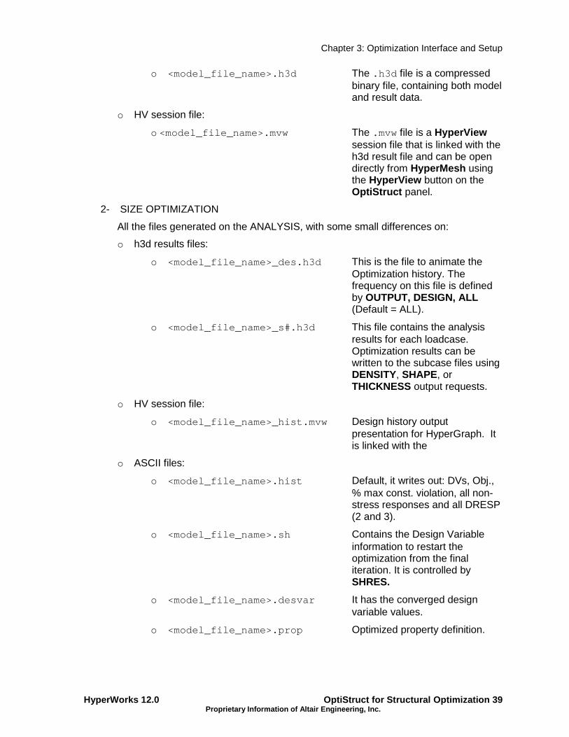
Chapter 3: Optimization Interface and Setup
HyperWorks 12.0 OptiStruct for Structural Optimization 39 Proprietary Information of Altair Engineering, Inc.
o <model_file_name>.h3d The .h3d file is a compressed binary file, containing both model and result data.
o HV session file:
o <model_file_name>.mvw The .mvw file is a HyperView session file that is linked with the h3d result file and can be open directly from HyperMesh using the HyperView button on the OptiStruct panel.
2- SIZE OPTIMIZATION
All the files generated on the ANALYSIS, with some small differences on:
o h3d results files:
o <model_file_name>_des.h3d This is the file to animate the Optimization history. The frequency on this file is defined by OUTPUT, DESIGN, ALL (Default = ALL).
o <model_file_name>_s#.h3d This file contains the analysis results for each loadcase. Optimization results can be written to the subcase files using DENSITY, SHAPE, or THICKNESS output requests.
o HV session file:
o <model_file_name>_hist.mvw Design history output presentation for HyperGraph. It is linked with the
o ASCII files:
o <model_file_name>.hist Default, it writes out: DVs, Obj., % max const. violation, all non-stress responses and all DRESP (2 and 3).
o <model_file_name>.sh Contains the Design Variable information to restart the optimization from the final iteration. It is controlled by SHRES.
o <model_file_name>.desvar It has the converged design variable values.
o <model_file_name>.prop Optimized property definition.

Chapter 3: Optimization Interface and Setup
OptiStruct for Structural Optimization 40 HyperWorks 12.0 Proprietary Information of Altair Engineering, Inc.
o <model_file_name>.hgdata Output history for HyperGraph. It is controlled by deshis = Yes (Default = Yes).
3- SHAPE OPTIMIZATION
All the files generated on SIZE optimization and two more ASCII files.
o ASCII files:
o <model_file_name>.grid Contain the node information translation for the final optimization iteration.
o <model_file_name>.oss It has the information to run OSSMOTH to generate the optimum topology for the model.
4- TOPOLOGY OPTIMIZATION
All the files generated on SIZE optimization, except the files .prop and .desvar and three more ASCII files:
o ASCII files:
o <model_file_name>.oss It has the information to run OSSMOTH to generate the optimum topology for the model.
o <model_file_name>.HM.comp.cmf HyperMesh command file that can be used to isolate the elements in components based on the optimized density.
o <model_file_name>.HM.ent.cmf HyperMesh command file that can be used to isolate the elements in sets based on the optimized density.
5- TOPOGRAPHY
All files generated on the SHAPE optimization.
6- GAUGE
All files generated on the SIZE optimization.
7- FREE-SHAPE
All files generated on the SHAPE optimization.
8- FREE-SIZE
All the files generated on TOPOLOGY optimization, except the file .hm.COMP.CMF.
9- COMPOSITE SHUFFLE
All the files generated on SIZE optimization, two more ASCII files:
o ASCII file:

Chapter 3: Optimization Interface and Setup
HyperWorks 12.0 OptiStruct for Structural Optimization 41 Proprietary Information of Altair Engineering, Inc.
o <model_file_name>.prop It has the information to run OSSMOTH to generate the optimum topology for the model.
o HTML Reports
o <model_file_name>.shuf.html Laminate layout for the optimization iterations.
1.2 – Subcase Information Section The Subcase or Case Control Section contains information for specific subcases. It identifies which loads and boundary conditions are to be used in a subcase. It can control the output type and frequency, and may contain objective and constraint information for optimization problems. For more information on Solution Sequences, please see the table included on the Solution Sequences page of the online help.
Descriptions for individual Subcase Control entries can be accessed in the online help.
1.3 – Bulk Data Section The Bulk Data Section contains all finite element data for the finite element model, such as grids, elements, properties, materials, loads and boundary conditions, and coordinates systems. For optimization, it contains the design variables, responses, and constraint definitions. The bulk data section begins with the BEGIN BULK statement.

Chapter 3: Optimization Interface and Setup
OptiStruct for Structural Optimization 42 HyperWorks 12.0 Proprietary Information of Altair Engineering, Inc.
2 – Optimization Setup
The optimization cards can be divided in two groups according to the section on the input deck that the cards are localized.
o Subcase Information Entry
DESGLB DESOBJ DESSUB DESVAR MINMAX or MAXMIN MODEWEIGHT MODTRAK NORM REPGLB REPSUB WEIGHT
o BULK Data Entry
BEAD BMFACE DCOMP DCONADD DCONSTR DDVAL DEQATN DESVAR DLINK DLINK2 DOBJREF DOPTPRM DREPADD DREPORT DRESP1 DRESP2 DRESP3 DSCREEN DSHAPE DSHUFFLE DSIZE DTABLE DTPG DTPL DVGRID DVMREL1 DVMREL2 DVPREL1 DVPREL2
The complete descriptions of these cards are available in the online help.
2.1 – Optimization GUI The optimization setup in HyperMesh can be made from three different areas:
Optimization Panel
Optimization Menu

Chapter 3: Optimization Interface and Setup
HyperWorks 12.0 OptiStruct for Structural Optimization 43 Proprietary Information of Altair Engineering, Inc.
Model Browser
2.2 – Design Variable [DTPL] To create and edit a design variable, the user can chose one of the three options shown below:
Optimization panel Optimization Menu Model Browser
The procedure to create a design variable will be described later on each chapter as it defines the type of optimization that will be performed and has a different setup for each type.

Chapter 3: Optimization Interface and Setup
OptiStruct for Structural Optimization 44 HyperWorks 12.0 Proprietary Information of Altair Engineering, Inc.
2.3 – Responses [DRESP1] To create and edit a response, the user can chose one of the three options shown
below:
Optimization panel Optimization Menu Model Browser
This will open the response panel:
On the response panel the user needs to:
1. Input a name to the response that needs to have less than 8 characters.
2. Choose the type of the response.
3. Choose where this response have to be evaluated:
a. If this is total or by entity. Ex. Mass, vol. etc.
b. Choose the nodes/elements and the direction this will be evaluated. Ex. Static displacement.
c. Exclude a group of elements that it should not be evaluated. Ex. Static Stress
d. For composite response the plies where it should be evaluated. Ex. Composite stress.
e. For FRF response choose between real, imaginary, magnitude and phase and the request (All freq; Freq =; sum; avg; ssq; rss; max; min; avgabs; maxabs; minabs; sumabs).
4. Define a region, if necessary.
5. Create the response.

Chapter 3: Optimization Interface and Setup
HyperWorks 12.0 OptiStruct for Structural Optimization 45 Proprietary Information of Altair Engineering, Inc.
2.4 – Dconstraints [DCONSTR] To create and edit a design constraint, the user can chose one of the three options shown below:
Optimization panel Optimization Menu Model Browser
This will open the constraints panel:
On the constraints panel the user needs to:
1. Input a name for this constraint.
2. Select the response where this limits will be applied.
3. If this response is dependent of the loadstep, a yellow button will appear and the user needs to select the appropriate loadsteps where this limits should be applied.
4. Create the constraint.

Chapter 3: Optimization Interface and Setup
OptiStruct for Structural Optimization 46 HyperWorks 12.0 Proprietary Information of Altair Engineering, Inc.
2.5 – Obj. reference [DOBJREF] To create and edit an objective reference vector, the user can chose one of the three options shown below:
Optimization panel Optimization Menu Model Browser
This will open the objective reference panel:
On the objective reference panel the user needs to:
1. Input a name for this reference vector.
2. Select the response where these coefficients will be applied. The positive and negative value should be used together if the user is looking for the maximum or minimum absolute value, for example min(max(|S3|)). The most common usage is the positive reference. min(max(von Mises)).
3. Define if it is applied to all loadsteps or to specific ones.
4. Create the Objective reference vector.

Chapter 3: Optimization Interface and Setup
HyperWorks 12.0 OptiStruct for Structural Optimization 47 Proprietary Information of Altair Engineering, Inc.
2.6 – Objective [DESOBJ] To create and edit an objective function, the user can chose one of the three options shown below:
Optimization panel Optimization Menu Model Browser
This will open the objective panel:
On the objective panel the user needs to:
1. Select the response that will be optimized.
2. Define if the response will be minimized or maximized.
3. For MinMax or MaxMin response with multiple values the user needs to use the objective reference vector that can be created using the procedure described on the last section.

Chapter 3: Optimization Interface and Setup
OptiStruct for Structural Optimization 48 HyperWorks 12.0 Proprietary Information of Altair Engineering, Inc.
2.7 – Table entries [DTABLE] To create and edit a list of constants, the user can chose one of the three options shown below:
Optimization panel Optimization Menu Model Browser
This will open the Table Entries panel:
On the Table Entries panel the user needs to:
1. Input the name and the value of all constants that can be used to define the generic functions and create them.

Chapter 3: Optimization Interface and Setup
HyperWorks 12.0 OptiStruct for Structural Optimization 49 Proprietary Information of Altair Engineering, Inc.
2.8 – Dequations [DEQATN] To create and edit a function or design equation, the user can chose one of the three options shown below:
Optimization panel Optimization Menu Model Browser
This will open the Dequations panel:
On the Dequations panel the user needs to:
1. Input the name for the function.
2. Input the mathematical expression for the function. Ex. F(x,y)=x**2+2+y.
3. Create the function.

Chapter 3: Optimization Interface and Setup
OptiStruct for Structural Optimization 50 HyperWorks 12.0 Proprietary Information of Altair Engineering, Inc.
2.9 – Discrete DVs [DDVAL] To create and edit a Discrete Design Variable list, the user can choose one of the three options shown below:
Optimization panel Optimization Menu Model Browser
This will open the Discrete Design Variables panel:
On the Discrete Design Variables panel the user needs to:
1. Input the name for the list.
2. Input the list values separated by comma or with X0, Xf and ∆X to automatically generate it.
3. Create the list.
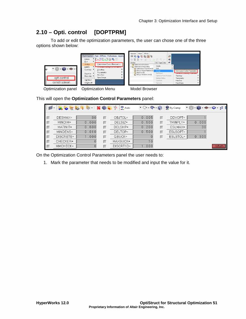
Chapter 3: Optimization Interface and Setup
HyperWorks 12.0 OptiStruct for Structural Optimization 51 Proprietary Information of Altair Engineering, Inc.
2.10 – Opti. control [DOPTPRM] To add or edit the optimization parameters, the user can chose one of the three options shown below:
Optimization panel Optimization Menu Model Browser
This will open the Optimization Control Parameters panel:
On the Optimization Control Parameters panel the user needs to:
1. Mark the parameter that needs to be modified and input the value for it.

Chapter 3: Optimization Interface and Setup
OptiStruct for Structural Optimization 52 HyperWorks 12.0 Proprietary Information of Altair Engineering, Inc.
2.11 – Constr. screen [DSCREEN] To add or edit the optimization parameters the user can chose one of the three options shown below:
Optimization panel Optimization Menu Model Browser
This will open the Constraint Screening panel:
On the Constraint Screening panel the user needs to:
1. Mark the response type that the solver will assign a sub-group.
2. Define the threshold that is a reference value to compare with the normalized constraint Φ to select the sub-group that will be monitored by the solver. If f >= threshold*Φ and the N < max retained, the response is added to the monitored list.

HyperWorks 12.0 Proprietary Information of Altair Engineering, Inc.
3 – How to setup an optimization Let us propose a very simple problem, a 2D cantilever beam that will be simulated using CBAR element with a PBARL property
Optimization model description (2 D)
• Geometry:
o (L = 1000, h0 = 10, b
• One load case: Normal Modes
o First mode
• Material: STEEL
o ρ = 7.8e-9 t/mmo E = 210000 Mo ν = 0.3
Chapter 3: Optimization Interface
OptiStruct for Structural Proprietary Information of Altair Engineering, Inc.
( )
15 h 5
15 b 5
ton040.51
≤≤≤≤
−≤ EMass
fMin
How to setup an optimization in HyperMesha very simple problem, a 2D cantilever beam that will be simulated using
CBAR element with a PBARL property. The model properties are described below:
Optimization model description (2 D)
= 10, b0 = 10 mm)
One load case: Normal Modes
/mm3 [RHO] Density MPa [E] Young’s modulus
- [nu] Poisson’s ratio
Optimization Interface and Setup
for Structural Optimization 53
HyperMesh a very simple problem, a 2D cantilever beam that will be simulated using
described below:

Chapter 3: Optimization Interface and Setup
OptiStruct for Structural Optimization 54 HyperWorks 12.0 Proprietary Information of Altair Engineering, Inc.
Step 1 - Setup the Finite element analysis. This model is already setup on a HyperMesh database, named beam.hm, and the input deck is shown below:
SUBCASE 1 SPC = 1 METHOD(STRUCTURE) = 2 BEGIN BULK GRID 1 0.0 0.0 0.0 GRID 2 1000.0 0.0 0.0 CBAR 1 1 1 20.0 1.0 0.0 PBARL 1 1 BAR + + 10.0 10.0 MAT1 1210000.0 0.3 7.80E-09 EIGRL 2 1 MASS SPC 1 1 1234560.0 SPC 1 2 3 0.0 ENDDATA
Step 2 - Define the Design Variables. On the main menu, select Optimization > Create > Size Desvars:
This is created in the bulk data section:
DESVAR 1 b10.0 5.0 15.0 DESVAR 2 c10.0 5.0 15.0
Create a Design variable as shown above for b and c. Associate them with the Dimension 1 and Dimension 2 of the beam property as shown below:

Chapter 3: Optimization Interface and Setup
HyperWorks 12.0 OptiStruct for Structural Optimization 55 Proprietary Information of Altair Engineering, Inc.
This is created in the bulk data section: DVPREL1 1 PBARL 1DIM1 0.0
+ 1 1.0
DVPREL1 2 PBARL 1DIM2 0.0
+ 2 1.0
Step 3 - Define the Responses. On the main menu, select Optimization > Create > Response:
Create a Response as shown above. Create f1 for first frequency and another response named Mass for the total mass on the model.
This is created in the bulk data section:
DRESP1 1 f1 FREQ 1 DRESP1 2 Mass MASS
Step 4 - Define the constraints. On the main menu, select Optimization > Create > Constraints:
Create a Constraint CMass as shown below:
This is created in the Subcase Information section:
DESGLB 2
This is created in the bulk data section:
DCONSTR 1 2 5.00E-04
DCONADD 2 1

Chapter 3: Optimization Interface and Setup
OptiStruct for Structural Optimization 56 HyperWorks 12.0 Proprietary Information of Altair Engineering, Inc.
Step 5 - Define the Objective On the main menu, select Optimization > Create > Objective:
Create an objective function Maximize f1 as shown below:
This is created in the Subcase Information section:
DESOBJ(MAX)=1
Step 6 - Run the Simulation On the main menu, select Application > OptiStruct:
Select the directory where it should run:

Chapter 3: Optimization Interface and Setup
HyperWorks 12.0 OptiStruct for Structural Optimization 57 Proprietary Information of Altair Engineering, Inc.
FINAL SETUP DESGLB 2 SUBCASE 1 SPC = 1 METHOD(STRUCTURE) = 2 DESOBJ(MAX)=1 BEGIN BULK DESVAR 1 b10.0 5.0 15.0 DESVAR 2 c10.0 5.0 15.0 DVPREL1 1 PBARL 1DIM1 0.0 + 1 1.0 DVPREL1 2 PBARL 1DIM2 0.0 + 2 1.0 DRESP1 1 f1 FREQ 1 DRESP1 2 Mass MASS DCONSTR 1 2 5.00E-04 DCONADD 2 1 GRID 1 0.0 0.0 0.0 GRID 2 1000.0 0.0 0.0 CBAR 1 1 1 20.0 1.0 0.0 PBARL 1 1 BAR + + 10.0 10.0 MAT1 1210000.0 0.3 7.80E-09 EIGRL 2 1 MASS SPC 1 1 1234560.0 SPC 1 2 3 0.0 ENDDATA

Chapter 3: Optimization Interface and Setup
OptiStruct for Structural Optimization 58 HyperWorks 12.0 Proprietary Information of Altair Engineering, Inc.

Chapter 4: Concept Design
HyperWorks 12.0 OptiStruct Optimization 59 Proprietary Information of Altair Engineering, Inc.
Chapter 4
Concept Design
1 – Topology Optimization Topology Optimization is a mathematical technique that produces an optimized shape and material distribution for a structure within a given package space. By discretizing the domain into a finite element mesh, OptiStruct calculates material properties for each element. The OptiStruct algorithm alters the material distribution to optimize the user-defined objective under given constraints.
Example of a topology optimization
OptiStruct solves topological optimization problems using either the homogenization or density method. Under topology optimization, the material density of each element should take a value of either 0 or 1, defining the element as being either void or solid, respectively. Unfortunately, optimization of a large number of discrete variables is computationally prohibitive. Therefore, representation of the material distribution problem in terms of continuous variables has to be used.

Chapter 4: Concept Design
OptiStruct Optimization 60 HyperWorks 12.0 Proprietary Information of Altair Engineering, Inc.
1.1 - Homogenization method
For the homogenization method, the material of the structure is represented as a porous continuum with certain periodic microstructure or layered composites of different ranks of densities. The homogenization method implemented in OptiStruct uses a material microstructure that contains periodic rectangular voids (hexahedral voids in 3-D). The design variables for each element are the breadth and depth of these rectangular voids and their orientations. These define the elasticity properties and the density of the material.
Using a normalized formulation, the density of an element may be determined by:
( )( )ba −−−= 0.10.10.1ρ
where (1.0 – a)(1.0 – b) represents the total volume of void in an element. It is easy to see that a=b=0 represents the state of void for this element, and a=1 or b=1 implies that the element is solid, i.e. filled with the 'real' material. Intermediate values of a and b represent fictitious material.
The void size variables are considered to be continuous variables varying between 0 and 1. The void orientation of each element is also a continuous variable, which is determined by the orientation of the principle strain. Note that while the real material is isotropic, the fictitious material of intermediate density is anisotropic.
1.2 - Density method
With the density method, the material density of each element is directly used as the design variable, and varies continuously between 0 and 1; these represent the state of void and solid, respectively. As with the homogenization method, intermediate values of density represent fictitious material.
With this method, the stiffness of the material is assumed to be linearly dependent on the density. This material formulation is consistent with our understanding of common materials. For example, steel, which is denser than aluminum, but is stronger than aluminum. Following this logic, the representation of fictitious material at intermediate densities is more realistic under the density approach. An anisotropic representation of the semi-dense material is not consistent with the behavior of the real isotropic material, although it is more 'efficient' due to optimal material orientation.
In general, the optimal solution of problems, using both formulations (Homogenization and Density), involves large gray areas of intermediate densities in the structural domain. Such solutions are not meaningful when we are looking for the topology of a given material, and not meaningful when considering the use of different materials within the design space. Therefore, techniques need to be introduced to penalize intermediate densities and to force the final design to be represented by densities of 0 or 1 for each element. The penalization technique used for the density approach is the "power law representation of elasticity properties," which can be expressed for any solid 3-D or 2-D element as follows:
( ) KK pρρ =
where K and K represent the penalized and the real stiffness matrix of an element, respectively, ρ is the density and p the penalization factor which is always greater than 1.

Chapter 4: Concept Design
HyperWorks 12.0 OptiStruct Optimization 61 Proprietary Information of Altair Engineering, Inc.
Exercise 4a: Topology Optimization of a Hook with Stress Constraints In this exercise, a topology optimization is performed on a bracket-hook modeled with shell elements. The structural model with loads and constraints applied is shown in the figure below. The objective is to minimize the volume of the material used in the model subject to certain stress constraints. Topology optimization is performed to find the optimal material placement and reduce the volume. This optimization normalizes each element according to its density and lets you remove elements that have low density.
FEA model
The structural model is loaded into HyperMesh Desktop. The constraints, loads, subcases and material properties are already defined in the model. The topology design variables and the optimization problem set up will be defined using HyperMesh and OptiStruct will be used to determine the optimal material layout. The results will then be reviewed in HyperView.
Objective function: Minimize mass.
Constraints: Von Mises stress < 120.
Design Variables: The density of each element in the design space.
Problem setup
You should copy the file: hook.fem
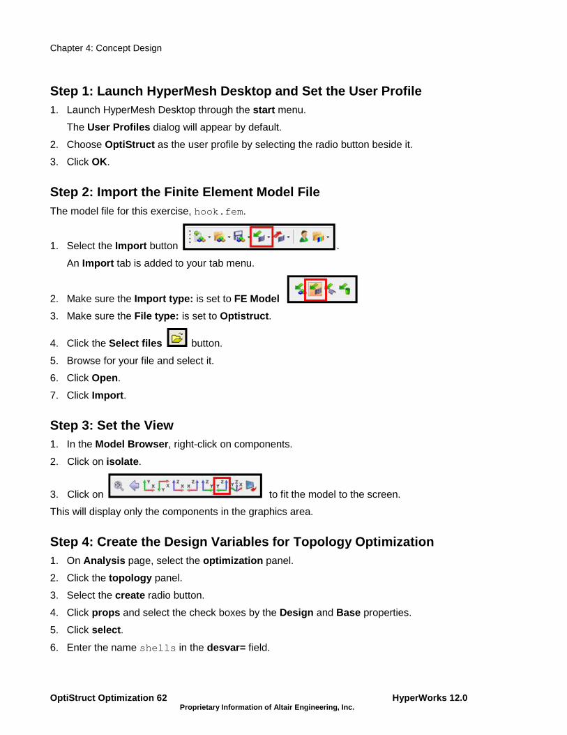
Chapter 4: Concept Design
OptiStruct Optimization 62 HyperWorks 12.0 Proprietary Information of Altair Engineering, Inc.
Step 1: Launch HyperMesh Desktop and Set the User P rofile 1. Launch HyperMesh Desktop through the start menu.
The User Profiles dialog will appear by default.
2. Choose OptiStruct as the user profile by selecting the radio button beside it.
3. Click OK.
Step 2: Import the Finite Element Model File The model file for this exercise, hook.fem.
1. Select the Import button .
An Import tab is added to your tab menu.
2. Make sure the Import type: is set to FE Model
3. Make sure the File type: is set to Optistruct .
4. Click the Select files button.
5. Browse for your file and select it.
6. Click Open .
7. Click Import .
Step 3: Set the View 1. In the Model Browser , right-click on components.
2. Click on isolate .
3. Click on to fit the model to the screen.
This will display only the components in the graphics area.
Step 4: Create the Design Variables for Topology Op timization 1. On Analysis page, select the optimization panel.
2. Click the topology panel.
3. Select the create radio button.
4. Click props and select the check boxes by the Design and Base properties.
5. Click select .
6. Enter the name shells in the desvar= field.

Chapter 4: Concept Design
HyperWorks 12.0 OptiStruct Optimization 63 Proprietary Information of Altair Engineering, Inc.
7. Set the component type: switch to PSHELL .
8. Click create .
9. Select the parameters subpanel.
10. Toggle minmemb off to mindim= .
11. For mindim= , enter 6.
12. Toggle maxmemb off to maxdim= .
13. For maxdim= , enter 21.
14. Under stress constraint: , toggle from none to stress= .
15. For stress= , enter 120.
16. Click update .
A topology design variable (DESVAR) is created.
17. Click return to get back to the optimization menu.
This sets the optimization to optimize the shell elements in the Design and Base components to
create structural members between 6 and 21 units in width with thicknesses that vary between
zero and the thickness of the shell. The optimization will use 120 as the maximum stress for
any element within the design region when validating the design.
Step 5: Create the Responses A detailed description is available in the OptiStruct User's Guide, under Responses.
1. In the optimization panel, click responses to go to the Responses panel.
2. To create the response, click the response type: switch and select mass from the pop-up menu.
3. Name the new response mass.
4. Click create to create the new response.
5. Click return to go back to the optimization panel.
Step 6: Define the Constraints In this example, there are no need for additional constraints since setting a stress target in the
design variable serves as a constraint that will limit the amount of material used in the result.

Chapter 4: Concept Design
OptiStruct Optimization 64 HyperWorks 12.0 Proprietary Information of Altair Engineering, Inc.
Step 7: Define the Objective Function In this example, the objective is to minimize the compliance.
1. Select the objective panel.
2. Click the switch in the upper left corner of the panel and select min from the pop-up menu.
3. Click response = and select mass from the response list.
4. Click loadstep and select Forces from the list of loadsteps used for this objective.
5. Click create .
The objective function is now defined.
6. Click return to return to the optimization panel.
Step 8: Save the HyperMesh Database
1. Click the Save .hm file button .
A Save file... browser window pops up.
2. Select the directory where you would like to save the database and enter the name for the database, hook_opt.hm in the File name: field.
3. Click save .
Step 9: Submit the Job to OptiStruct 1. From the Analysis page, select the OptiStruct panel.
2. Click save as… following the input file: field.
3. Select the directory where you would like to write the OptiStruct model file and enter the name for the model, hook_opt.fem, in the File name: field.
.fem is the suggested extension for OptiStruct input decks.
4. Click Save.
Note the name and location of the hook_opt.fem file displays in the input file: field.
5. Make sure the memory options: toggle is set to memory default .
6. Click the run options: switch and select optimization .
7. Make sure the export options: toggle is set to all .
8. Click OptiStruct .
This launches the OptiStruct job. If the job was successful, new results files can be seen in the directory where the OptiStruct model file was written. The hook_opt.out file is a good place to look for error messages that will help to debug the input deck if any errors are present.
Step 9: View an Isosurface Plot of the Density Resu lts

Chapter 4: Concept Design
HyperWorks 12.0 OptiStruct Optimization 65 Proprietary Information of Altair Engineering, Inc.
1. While still in the OptiStruct panel, click the green HyperView button.
Five additional pages get added to the Hypermesh Desktop session. The results for the optimization are loaded in pages 2 thru 6.
2. Use the Next Page icon to change the client to HyperView
3. Click the iso Value toolbar button .
4. Select the Result type: Element densities (s) .
5. In the Model view of the browser, set the Design Iteration to the last one.
6. Change the value by typing in the Current value: field (in the Iso panel) or by using the slider to move between zero and one.
The isosurface post-processing feature (shown for this model at 0.3) is an excellent tool to use for viewing the density results from OptiStruct.

Chapter 4: Concept Design
OptiStruct Optimization 66 HyperWorks 12.0 Proprietary Information of Altair Engineering, Inc.
You will see the isosurface in the graphics window interactively update when you change the current value to a new number. Use this tool to get a better look at the material layout and the load paths from OptiStruct.
Step 10: View the Element Stress Results
1. Click the Next Page toolbar button to move to the third page.
The third page which has results loaded from the analysis of the last iteration is displayed; this contains the linear static results for the subcase in the original file.
2. Click the Contour toolbar button .
3. Select the first pull-down menu below the Result type: and select Element stresses .
4. Select the second pull down menu and select vonMises .
5. In the Model View of the browser, set the displayed Iteration to the last one.
7. Click Apply .
8. Similarly, review the results from the other load cases too.
Von Mises Stress results shown
Notice that there are some local regions where the stresses are still higher than the target; this is because topology stress constraints should be interpreted as global stress control.
The functionality has some ways to filter out the artificial or local stresses caused by point loading or boundary conditions, but those artificial stresses will not be completely removed unless the geometry is changed by shape optimization.

Chapter 4: Concept Design
HyperWorks 12.0 OptiStruct Optimization 67 Proprietary Information of Altair Engineering, Inc.
Note: There might still be high local stress regions which can be improved more effectively with local shape and size optimization.

Chapter 4: Concept Design
OptiStruct Optimization 68 HyperWorks 12.0 Proprietary Information of Altair Engineering, Inc.

Chapter 4: Concept Design
HyperWorks 12.0 OptiStruct Optimization 69 Proprietary Information of Altair Engineering, Inc.
Exercise 4b: Topology Optimization of a Control Arm The purpose of this exercise is to determine the best topology using the minimum mass for a control arm that is manufactured using a single draw mode. The arm needs to have a symmetric geometry because it will be used on both sides of the vehicle.
The image below defines the finite element model that defines where the material can be removed or not. There are two different regions that are denominated Design (blue) in which OptiStruct will be allowed to remove material and Non-design (red) which will not be changed.
The control arm can be considered totally fixed for all load cases as follows:
o NODE(3) X,Y and Z . (Bolted)
o NODE(4) Y and Z . (Cylindrical joint)
o NODE(7) Z. (Damp link)
This control arm needs to support three different load cases, and the design criterion for each load case is defined as strength constraints as:
1. Car turning on a intersection: corner = (0,1000,0) N Umax (2699) <= 0.02 mm
2. Car braking: brake = (1000,0,0) N Umax (2699) <= 0.05 mm
3. Car passing in a pothole: pothole (0,0,1000) N Umax (2699) <= 0.04 mm
Problem Setup You should copy the file: carm.fem
Node 2699
Node 7
Node 3
Node 4

Chapter 4: Concept Design
OptiStruct Optimization 70 HyperWorks 12.0 Proprietary Information of Altair Engineering, Inc.
Step 1: Import the model: carm.fem into HyperMesh Desktop.
Step 2: Define properties. Create two properties named: design and nondesign, with a card image of PSOLID which use the material steel.
Optimization will be performed on the elements that have the property “design”.
Model Browser tree showing created properties
Step 3: Assign the properties to the components.
In the Model Browser , right-click on the component, select Assign , select the appropriate property and click on Apply .
Assign the property design to the design component and nondesign to the nondesign property.
Step 4: Define three different loadsteps: Corner (1 ), Brake (2) and Pothole (2).
As was described on the beginning of this exercise, this part needs to perform well on three different load cases and as we can see below that each has different directions of loading. It is necessary to define independent load cases for each one.
1. Create the following constraints in a Load Collector named SPC:
NODE(3) constrained in X,Y and Z translation. (Bolted)
NODE(4) constrained in Y and Z translation. (Cylindrical joint)
NODE(7) constrained in Z translation. (Damp link)
2. Create the load collector corner (1) and create a force F = (0,1000,0) N applied on Node(2699)
3. Create a load collector brake (2) and create a force F = (1000,0,0) N applied on Node(2699)
4. Create a load collector pothole (3) and create a force F = (0,0,1000) N applied on Node(2699)

Chapter 4: Concept Design
HyperWorks 12.0 OptiStruct Optimization 71 Proprietary Information of Altair Engineering, Inc.
5. Define linear static load steps for each of these load cases using the SPC load collector as the SPC entry and each respective load collector as the LOAD entry.
Model Browser after the load steps have been created.
Step 5: Run the analysis from the OptiStruct panel.
It should take a few minutes to complete the run. Once you have the results, review them and fill out the values below:
Corner (1) Total displacement (2699) = _________
Brake (2) Total displacement (2699) = _________
Pothole (3) Total displacement (2699) = _________
Mass of the model = _________
It is important to run an initial analysis to understand the model solution. If the responses are far-off from the desired values, the model needs to be modified or the optimization problem should be redefined. It is very important at this point for the user to validate the problem and understand if the optimization setup makes sense.
Step 6: Define a topology design variable for the d esign region.
1. Create a new design space named Design with a PSOLID type using the property Design .
2. In the pattern grouping subpanel, set the pattern type to 1-pln sym, setting anchor node to Node 1and first node to Node 2.

Chapter 4: Concept Design
OptiStruct Optimization 72 HyperWorks 12.0 Proprietary Information of Altair Engineering, Inc.
3. Similarly in the draw subpanel, define the draw type as single using Node 5 as the anchor node and Node 6 as the first node. Set the obstacle to the property non-design. Setting the obstacle ensures that the resulting design, if manufactured with a draw process, will be optimized in a way that allows all obstacles to clear the tooling etc for the selected draw vector.
Step 7: Define a volume response (total) named volume.
Step 8: Define a static displacement response on th e ball join node (2699), select total displacement, and name it disp.

Chapter 4: Concept Design
HyperWorks 12.0 OptiStruct Optimization 73 Proprietary Information of Altair Engineering, Inc.
Step 9: In the constraints panel, use the displacem ent constraint to create an upper bound constraint for each loadstep as follows . Don’t forget to check the checkbox next to upper bound and click create when each loadstep is complete.
Constraint Name Response Loadstep Upper Bound
Corner Disp Corner 0.02
Brake Disp Brake 0.05
Pothole Disp Pothole 0.04
Step 10: Create the objective function as type min and response volume.
Step 11: Submit the optimization run from the OptiS truct panel as carm_opt.fem.
Step 12: Review the results answer these questions:
1. Did the solution converge to a feasible solution?
2. How many iterations did the solution take to converge and what is the final volume of the part?
3. Plot the Iso-contour for the density on the last iteration, does it look like a manufacturable part?
Design proposed by OptiStruct

Chapter 4: Concept Design
OptiStruct Optimization 74 HyperWorks 12.0 Proprietary Information of Altair Engineering, Inc.

Chapter 4: Concept Design
HyperWorks 12.0 OptiStruct Optimization 75 Proprietary Information of Altair Engineering, Inc.
Exercise 4c: Pattern Repetition using Topology Optimization This exercise demonstrates how to perform topology optimization using pattern repetition. The model is a rectangular plate with a concentrated force on one edge and two constraints on the opposite edge. Two other rectangular plates with a scaled size of 0.6 and 0.3 from the original plate with forces and boundary conditions applied in different directions are also modeled to highlight the difference in the topology results between with and without pattern repetitions.
The objective is to minimize the compliance for the single subcase. The volume fraction of the design space is limited to 0.3. The design spaces are the three plates.
Problem Setup
You should copy the file: no_repeat.fem

Chapter 4: Concept Design
OptiStruct Optimization 76 HyperWorks 12.0 Proprietary Information of Altair Engineering, Inc.
Step1: Launch HyperMesh Desktop, Set the User Profi le, and Import the File
Import no_repeat.fem into HyperMesh Desktop in a new session.
Step 2: Create the Topology Design Variables 1. From the Analysis page, enter the optimization panel.
2. Click topology to enter the panel.
3. Make sure the create subpanel is selected using the radio buttons on the left-hand side of the panel.
4. Click desvar = and enter dv1.
5. Click props and select the property labeled first by checking the box beside it.
6. Click select .
7. Set the type: selector to PSHELL .
8. Click create .
9. Select the parameters subpanel using the radio buttons on the left-hand side of the panel.
10. Toggle minmemb off to mindim= .
11. Click mindim= and enter 2.0.
12. Click update .
13. Repeat steps 3 through 12 for the components called second and third with desvar names dv2 and dv3, respectively.
This defines the design space.
14. Click return .
Step 3: Create the Volume Fraction and Compliance R esponse 1. Enter the responses panel.
2. Click response = and enter volfrac.
3. Set the switch under response type: to volumefrac .
4. Verify that the toggle in the center of the panel is set to total .
5. Click create .
This creates the volume fraction response.
6. Click response = and enter comp.
7. Set the selector under response type: to compliance .
8. Verify that the toggle in the center of the panel is set to total .
9. Click create .
This creates the compliance response.
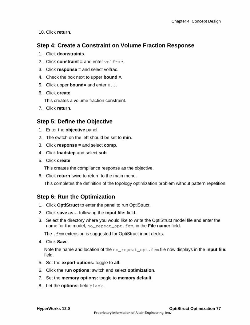
Chapter 4: Concept Design
HyperWorks 12.0 OptiStruct Optimization 77 Proprietary Information of Altair Engineering, Inc.
10. Click return .
Step 4: Create a Constraint on Volume Fraction Resp onse 1. Click dconstraints .
2. Click constraint = and enter volfrac.
3. Click response = and select volfrac.
4. Check the box next to upper bound =.
5. Click upper bound= and enter 0.3.
6. Click create .
This creates a volume fraction constraint.
7. Click return .
Step 5: Define the Objective 1. Enter the objective panel.
2. The switch on the left should be set to min .
3. Click response = and select comp .
4. Click loadstep and select sub .
5. Click create .
This creates the compliance response as the objective.
6. Click return twice to return to the main menu.
This completes the definition of the topology optimization problem without pattern repetition.
Step 6: Run the Optimization 1. Click OptiStruct to enter the panel to run OptiStruct.
2. Click save as… following the input file: field.
3. Select the directory where you would like to write the OptiStruct model file and enter the name for the model, no_repeat_opt.fem, in the File name: field.
The .fem extension is suggested for OptiStruct input decks.
4. Click Save.
Note the name and location of the no_repeat_opt.fem file now displays in the input file: field.
5. Set the export options: toggle to all .
6. Click the run options: switch and select optimization .
7. Set the memory options: toggle to memory default .
8. Let the options: field blank.
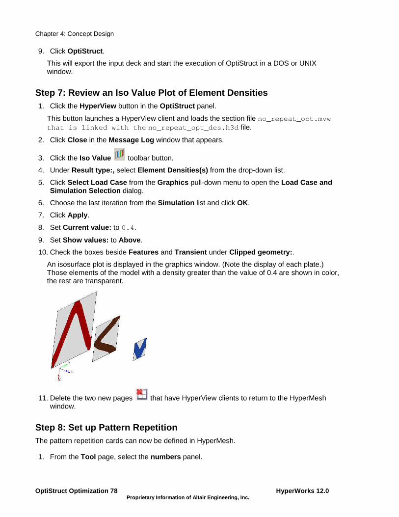
Chapter 4: Concept Design
OptiStruct Optimization 78 HyperWorks 12.0 Proprietary Information of Altair Engineering, Inc.
9. Click OptiStruct .
This will export the input deck and start the execution of OptiStruct in a DOS or UNIX window.
Step 7: Review an Iso Value Plot of Element Densiti es 1. Click the HyperView button in the OptiStruct panel.
This button launches a HyperView client and loads the section file no_repeat_opt.mvw that is linked with the no_repeat_opt_des.h3d file.
2. Click Close in the Message Log window that appears.
3. Click the Iso Value toolbar button.
4. Under Result type:, select Element Densities(s) from the drop-down list.
5. Click Select Load Case from the Graphics pull-down menu to open the Load Case and Simulation Selection dialog.
6. Choose the last iteration from the Simulation list and click OK.
7. Click Apply .
8. Set Current value: to 0.4.
9. Set Show values: to Above .
10. Check the boxes beside Features and Transient under Clipped geometry: .
An isosurface plot is displayed in the graphics window. (Note the display of each plate.) Those elements of the model with a density greater than the value of 0.4 are shown in color, the rest are transparent.
11. Delete the two new pages that have HyperView clients to return to the HyperMesh window.
Step 8: Set up Pattern Repetition The pattern repetition cards can now be defined in HyperMesh.
1. From the Tool page, select the numbers panel.

Chapter 4: Concept Design
HyperWorks 12.0 OptiStruct Optimization 79 Proprietary Information of Altair Engineering, Inc.
2. Click the nodes button and select by id .
3. Enter all of the following values after id= , separating them with commas:
1329 66 6 46 507 447 487 928 892 948
4. Press Enter .
5. Click the green button on .
6. Click return to exit the Numbers panel.
7. From the Mask tab menu, select 1 for the Elements row under the Isolate column to only display the elements in the model.
8. From the Analysis page, enter the optimization panel.
9. Click topology to enter the panel.
10. Select the pattern repetition subpanel using the radio buttons on the left side of the panel.
11. Double click the desvar= and select dv1 .
12. Make sure the switch is pointing to master .
13. Toggle from system to coordinates .
14. Click the green first button and choose node ID 6.
15. Notice that the blue border moves over second after the first has been selected; now choose the second node ID 46.
16. Choose the third node ID 1329.
17. Click the anchor button and choose the node ID 66.
18. Click update on the right side to create a master DTPL card.
19. Click desvar= and select dv2 .
20. Click the switch and select slave .
21. Make sure master= is pointing to dv1 .
22. Set the following values: sx= 0.6, sy= 0.6, sz= 1.0.

Chapter 4: Concept Design
OptiStruct Optimization 80 HyperWorks 12.0 Proprietary Information of Altair Engineering, Inc.
23. Click the first button and choose the node ID 447.
24. For the second button, choose the node ID 487.
25. For the third button, choose the node ID 1329.
26. For the anchor button, choose the node ID 507.
27. Click the update button on the right side to create the slave DTPL card.
28. Click desvar= and select dv3 .
29. Click the switch and change to slave .
30. Make sure the master= button is pointing to dv1 .
31. Set the following values: sx= 0.3, sy= 0.3, sz= 1.0.
32. Click the first button and choose the node ID 892.
33. For the second button, choose the node ID 928.
34. For the third button, choose the node ID 1329.
35. For the anchor , choose the node ID 948.
36. Click the update button on the right side to create the slave DTPL card.
The above modification identifies the first DTPL card with ID 1 (on the first component) as the master. The DTPL’s of ID 2 (second component) and ID 3 (third component) are slaves and dependent on DTPL of ID1. The second component is scaled 0.6 in both the x and y axis, while the third component is scaled 0.3 in both the x and y axis with respect to the first component.
37. Click return twice.
Step 9: Run the Optimization Problem 1. From the Analysis page click OptiStruct to run the solver.
2. Click save as… following the input file: field.
3. Select the directory where you would like to write the OptiStruct model file and enter the name for the model, repeat_opt.fem in the File name: field.
4. Click Save.
Note that the name and location of the repeat_opt.fem file is now displayed in the input file: field.
5. Set the export options: toggle to all .
6. Click the run options: switch and select optimization .
7. Set the memory options: toggle to memory default .
8. Keep the options: field blank.
9. Click OptiStruct .
This will export the input deck and start the execution of OptiStruct in a DOS or UNIX window.

Chapter 4: Concept Design
HyperWorks 12.0 OptiStruct Optimization 81 Proprietary Information of Altair Engineering, Inc.
Step 10: Review an Iso Value Plot of Element Densit ies 1. From the OptiStruct panel, click the green HyperView button.
This button launches HyperView and loads the section file repeat_opt.mvw that is linked with the repeat_opt_des.h3d file.
A Message Log window will appear, indicating the location of the .h3d file.
2. Click Close to exit the Message Log window.
3. Click the Iso Value toolbar button.
4. Choose Select Load Case from the Graphics pull-down menu to open the Load Case and Simulation Selection dialog.
5. Choose the last design under Simulation .
6. Click Apply .
7. Set current value: to 0.38.
8. Set Show: to Above .
9. Check the boxes for Features and Transparent under Clipped geometry: .
An iso surface plot is displayed in the graphics window. Those parts of the model with a density greater than the value of 0.38 are shown in color, and the rest are transparent.
10. Click File on the menu bar and choose Exit to quit HyperView .

Chapter 4: Concept Design
OptiStruct Optimization 82 HyperWorks 12.0 Proprietary Information of Altair Engineering, Inc.

Chapter 4: Concept Design
HyperWorks 12.0 OptiStruct Optimization 83 Proprietary Information of Altair Engineering, Inc.
2 – Design Interpretation – OSSmooth OSSmooth is a semi-automated design interpretation software, facilitating the recovery of a modified geometry resulting from a structural optimization, for further use in the design process. The tool has two incarnations; a standalone version that comes with the OptiStruct installation, and a dependent version that is embedded in HyperMesh.
OSSmooth has several uses, it can be used to:
o Interpret topology optimization results, creating an iso-density boundary surface (Iso-surface).
o Interpret topography optimization results, creating beads or swages on the design surface.
o Recover and smooth geometry resulting from a shape optimization.
o Reduce the amount of surface data from a given set of triangular patches by combining smaller patches.
o Smooth surface data given as triangular patches.
The following flowchart provides an overview of how OSSmooth works to interpret optimization results from OptiStruct:
OSSmooth requires a parameter file (generally has the file extension .oss) to run. This parameter file may be generated by the OSSmooth panel in HyperMesh or it may be generated manually through a text editor. At the completion of an optimization run, OptiStruct automatically exports an OSSmooth parameter file <prefix>.oss with certain default settings depending on the type of optimization run.

Chapter 4: Concept Design
OptiStruct Optimization 84 HyperWorks 12.0 Proprietary Information of Altair Engineering, Inc.
In addition to the parameter file, OSSmooth also requires the input file (<prefix>.fem), the shape file (<prefix>.sh), and/or the grid file (<prefix>.grid) from an OptiStruct run. The grid file <prefix>.grid contains the grid point locations after a topography or shape optimization and is output at the end of a topography or shape optimization run. The shape file, <prefix>.sh, contains the element density information of a topology optimization and is output at the end of an optimization run.
Note: OSSmooth currently does not recognize OptiStruct long-format input data. A possible work-around for this problem is to import the long-format input file into HyperMesh and export it using the regular OptiStruct template before running OSSmooth.
The interpreted design from OSSmooth can be exported as a finite element mesh in the bulk data format, as IGES surfaces, as a stereolithography file, or as a Hyper3D file.

Chapter 4: Concept Design
HyperWorks 12.0 OptiStruct Optimization 85 Proprietary Information of Altair Engineering, Inc.
2.1 – OSSmooth Input Data input_file example # Identifies the files to be interpreted by OSSmooth.
(one argument) arg1 The file name (without extension).
output_file example.nas # Name of the file to be output by OSSmooth.
(one argument) arg1 Full name of the file output by OSSmooth.
output_code 1 # Identifies the type of output.
(two arguments) arg1 Output format for iso-surface [default=3] : (1) Nastran (2) IGES (3) STL (4) H3D arg2 Output control for tet-meshing [Default: no tet.] (1) Tetra4 + Tria3 (2) Tetra10 + Tria6 (3) Tetra4 (4) – Tetra10
units 1 (one argument) [default =1] (1) inch (2) mm (4) foot (6) m (10) cm
autobead 1
(three arguments) arg1 Operation flag: (0 ) autobead off ( 1 ) autobead on arg2 Threshold value for creating autobead. Real between 0.0 and 1,0, default = 0.3. arg3 Bead layer[integer] [default =1] ( 1 ) Create 1 layer bead ( 2 ) – create 2 layers bead
isosurface 0.3
# Generate threshold surface from a topology optimization by applying automatic geometry creation.
(three arguments)
arg1 Operation flag [integer]: [default = 1]
( 0 )– isosurface off ( 1 ) – isosurface on
arg2 Type of surface created [integer]: [default = 3]
( 0 ) – isosurface only ( 1 ) – isosurface with Optimization-based smoothing ( 2 ) – Element threshold surface ( 3 ) – isosurface with Laplacian smoothing
arg3 Density threshold for creating isosurface.
[real, between 0.0 and 1.0, default = 0.3] opti_smoothing # Optimization-based smoothing [Only used if isosurface arg2=1].
(two arguments) arg1 Unit-less surface distance coefficient
[real, default = 0.0] Defines closeness of the smooth surface from the threshold surface.
arg2 Smooth isosurface boundary flag [integer]: ( 0 ) – boundary not included in smoothing
[default] ( 1 ) – boundary included in smoothing
laplacian_smoothing 10 20.0 0 # Laplacian smoothing [Only used if isosurface arg3=3].
(three arguments) arg1 Number of iteration for Laplacian smoothing
[integer >= 0, default = 10] arg2 Feature angle threshold in degrees
[real, default = 30.0] arg3 Smooth isosurface boundary flag [integer]:
( 0 ) boundary not included in smoothing ( 1 ) boundary included in smoothing [default]

Chapter 4: Concept Design
OptiStruct Optimization 86 HyperWorks 12.0 Proprietary Information of Altair Engineering, Inc.
remesh 1 # Remeshes the region surrounding the recovered geometry to facilitate smooth mesh transition. [Only available in the HyperMesh integrated version].
(one argument) arg1 Remesh autobead surface or/and isosurface
flag [integer]: ( 0 ) remesh off [default] ( 1 ) remesh on
surface_reduction 1 5.0 # Reduces the number of surfaces representing the geometry. Can reduce the number of surfaces by up to 80%.
(two arguments) arg1 Surface reduction flag [integer]:
( 0 ) no surface reduction [default] ( 1 ) do surface reduction
arg2 Feature angle threshold in degrees [real, default = 10.0]
pure_surf_smoothing 1 5 20.0 # Surface smoothing only. (three arguments)
arg1 Pure surface smoothing flag [integer]: ( 0 ) no surface smoothing [default] ( 1 ) Optimization-based smoothing ( 2 ) Laplacian smoothing
arg2 Number of iteration [Only used if G1=2] [integer >= 0, default = 10]
arg3 Feature angle threshold in degrees [Only used if G1=2]
[real, default = 30.0] pure_surf_reduction # Surface reduction only.
(two arguments) arg1 Pure surface reduction flag [integer]:
( 0 ) no surface reduction [default] ( 1 ) do surface reduction
arg2 Feature angle threshold in degrees [real, default = 10.0]

Chapter 4: Concept Design
HyperWorks 12.0 OptiStruct Optimization 87 Proprietary Information of Altair Engineering, Inc.
OSS Example Input File
Statement Description
input_file example Identifies the root of the input files as example, so OSSmooth will look for the files example.fem , example.grid , and example.sh .
output_file example.stl The resulting output will be example.stl .
output_code 3 The output will be in stereolithography format.
autobead 1 0.3 1 Topography results will be interpreted using the autobead feature with a threshold value of 30% creating single depth beads.
isosurface 1 3 0.3 Topology results will be interpreted by creating an iso-density boundary surface with at a density value of 30% and smooth using laplacian smoothing.
laplacian_smoothing 10 30 1 The laplacian smoothing will run for 10 iterations, consider a feature angle of 30-degrees and including the boundary in the smoothing.
remesh 1 The two rows of elements around the recovered geometry will be remeshed in an attempt to smooth the mesh transition.
2.2 – Running OSSmooth To run OSSmooth from the HyperMesh solver panel:
1. From the pull-down menu Tools > Solver .
2. Click the switch and select OSSmooth .
3. After input file: , enter <prefix>.oss.
4. Click solve .
To run OSSmooth from the HyperMesh ossmooth panel:
1. Select the OSSmooth panel on the post page.
2. Select the OptiStruct input file <prefix.fem> using the file= browser.
3. Edit the OSSmooth input data by making selections on the screen.
4. Click OSSmooth .
This will write a new <prefix.oss> file with the screen settings, run OSSmooth, and load the geometry recovered by OSSmooth if the data format is IGES, STL, or Nastran.

Chapter 4: Concept Design
OptiStruct Optimization 88 HyperWorks 12.0 Proprietary Information of Altair Engineering, Inc.
2.3 – Interpretation of Topography Optimization Res ults The autobead feature of OSSmooth allows OptiStruct topography optimization results to be interpreted as one or two level beads. The following figure shows the level of detail captured in both cases; while the 2-level approach captures more details, it is more complicated to manufacture than the 1-level interpretation, often without significant performance gain.
Autobead interpretation of topography optimization result.
One example of post-processing of topography optimization is shown below with the following parameter setting in the OSSmooth parameter file:
#general parameters input_file decklid output_file decklid.fem output_code 1
#specific parameters autobead 1 0.300 1 remesh 1
Autobead result from topography optimization.
Some topography performances are relying on the half translation part. OSSmooth can interpolate topography optimization results to 2-layer autobead (autobead third argument 2). Here is one example of creating 2-layer autobead with the following parameter settings in the OSSmooth parameter file:

Chapter 4: Concept Design
HyperWorks 12.0 OptiStruct Optimization 89 Proprietary Information of Altair Engineering, Inc.
#general parameters input_file decklid output_file decklid.nas output_code 1
#specific parameters autobead 1 0.300 2
2-layer autobead result from topography optimization.
2.4 – Shape Optimization Results, Surface Reduction and Surface Smoothing OSSmooth may also be used to reduce and smooth surfaces or the surfaces of a domain. The parameter statements pure_surf_reduction and pure_surf_smoothing may be used for this purpose.
The file defined by input_file must be in the OptiStruct bulk data format, and OSSmooth can smooth the surface or the surfaces of a domain of the model.
The usage in the OSSmooth parameter file is as follows:
#general parameters input_file surf output_file surf.stl output_code 3 #specific parameters pure_surf_smoothing 2 10 30.000 pure_surf_reduction 1 10.000

Chapter 4: Concept Design
OptiStruct Optimization 90 HyperWorks 12.0 Proprietary Information of Altair Engineering, Inc.

Chapter 4: Concept Design
HyperWorks 12.0 OptiStruct Optimization 91 Proprietary Information of Altair Engineering, Inc.
Exercise 4d – OSSmooth Surfaces from a Topology Optimization The purpose of this exercise is to export from HyperMesh the optimized control arm obtained using topology optimization from exercise 4.2. The IGES format was chosen to make it easy to import in any CAD system.
Design proposed by OptiStruct
Problem Setup
You should copy the following files: CONTROL_ARM.fem, CONTROL_ARM.oss, and CONTROL_ARM.sh.

Chapter 4: Concept Design
OptiStruct Optimization 92 HyperWorks 12.0 Proprietary Information of Altair Engineering, Inc.
Step 1: Launch HyperMesh Desktop and Set the User P rofile to OptiStruct
Step 2: Generate a new mesh for FE reanalysis using OSSmooth
1. Go to the Post > OSSmooth panel.
2. Load the optimization CONTROL_ARM.fem file into the model field and the CONTROL_ARM.sh file into the result files field.
3. Ensure that the iso surface option is checked, set the threshold to 0.33, and set the autobead option to none.
4. Set output to BULK to output a tetra- and tria-meshed FE model, or choose one of the other options for a geometric interpretation.
5. Click the OSSmooth button to create a newly meshed model based on the optimization results.
When requesting a geometric interpretation, OSSmooth will extract a mesh first, and then present the user with a panel to convert the FE model to surface data allowing the user to choose surface options. To continue, set the options to desired quality settings or retain the defaults and press FE -> Surf .
FEM from OSSmooth reinterpretation

Chapter 4: Concept Design
HyperWorks 12.0 OptiStruct Optimization 93 Proprietary Information of Altair Engineering, Inc.
Partially transparent view of IGES geometry from FE->surf calculations.

Chapter 4: Concept Design
OptiStruct Optimization 94 HyperWorks 12.0 Proprietary Information of Altair Engineering, Inc.

Chapter 4: Concept Design
HyperWorks 12.0 OptiStruct Optimization 95 Proprietary Information of Altair Engineering, Inc.
3 – Topography Optimization
Topography optimization is an advanced form of shape optimization in which a design region for a given part is defined and a pattern of shape variable-based reinforcements within that region is generated using OptiStruct.
The approach in topography optimization is similar to the approach used in topology optimization, except that shape variables are used rather than density variables. The design region is subdivided into a large number of separate variables whose influence on the structure is calculated and optimized over a series of iterations. The large number of shape variables allows the user to create any reinforcement pattern within the design domain instead of being restricted to a few.
3.1 - Design Variables for Topography Optimization OptiStruct solves topography optimization problems using shape optimization with internally generated shape variables. One or more design domains are defined using the DTPG card. These cards must, in turn, reference PSHELL , PCOMP or DESVAR definitions. If a DESVAR definition is referenced, it must be a shape design variable, meaning that it must, in turn, be referenced by one or more DVGRID cards. If a PSHELL or PCOMP definition is referenced, OptiStruct generates shape variables using the parameters defined on the DTPG card, creating internal DVGRID data for the nodes associated with the PSHELL or PCOMP definitions. In both cases, the end result is that each DTPG card references a single shape variable. This shape variable then gets converted into topography shape variables.
Basic topography shape variables follow the user-defined parameters on the DTPG card (minimum bead width, and draw angle), they are circular in shape, and they are laid out across the design domain in a roughly hexagonal distribution . Each topography shape variable has a circular central region of diameter equal to the minimum bead width. Grids within this region are perturbed as a group, which prevents the formation of any reinforcement bead of less than the minimum bead width. Grids outside of the central circular region of the topographical variables are perturbed as the average of the variables to which they are nearest. This results in smooth transitions between neighboring variables. If two adjacent variables are fully perturbed, all of the nodes between them will be fully perturbed. If one variable is fully perturbed and its neighbor is unperturbed, the nodes in between will form a smooth slope connecting them at an angle equal to the draw angle. The spacing of the variables is determined by the minimum bead width and the draw angle in such a way that no part of the bead reinforcement pattern forms an angle greater than the draw angle.
Pattern grouping options link topographical variables together in such a way that the desired reinforcement patterns are formed. Linear, planar, circular, radial, etc. shaped reinforcements are controlled by single variables, ensuring that the reinforcements follow the desired pattern. One-plane, two-plane, three-plane and cyclical symmetry pattern grouping options also use a similar approach to ensure that symmetry is created in the solution.
Although topography optimization is primarily a tool for creating bead type reinforcements in shell elements, it can accommodate solid models as well. Many pattern grouping options (such as planar and cylindrical) are intended to be used with solid models since they effectively reduce 3-D problems into 2-D ones.

Chapter 4: Concept Design
OptiStruct Optimization 96 HyperWorks 12.0 Proprietary Information of Altair Engineering, Inc.
3.1.1 – Variable Generation
There are three methods of automatically generating shape variables for topography optimization using the DTPG card. The first two, element normal and draw vector are performed entirely in OptiStruct. The third (user-defined ) requires that the input data contain one or more shape design variables that are used as the design domain.
Element normal
This method is the easiest one to use. When norm is entered for the draw direction, the normal vectors of the elements are used to define the draw vector for the shape variables. This method is especially effective for curved surfaces and enclosed volumes where the beads are intended to be drawn normal to the surface.
Beads created using the element normal
method of determining draw vector.
Draw vector
This method allows you to define the draw vector that is used for generating the shape variables. The X, Y, and Z components of the draw vector in the nodal coordinate system are entered. This method is useful when all beads must be drawn in the same direction. Note that the draw angle may not be maintained while using this method.
Beads created using the Draw vector method of determining draw vector.

Chapter 4: Concept Design
HyperWorks 12.0 OptiStruct Optimization 97 Proprietary Information of Altair Engineering, Inc.
User-defined
This method allows you to set up the vectors and heights for the topography optimization. A DESVAR card is referenced in place of a PSHELL or PCOMP card. All of the grids with DVGRID cards associated with that DESVAR card are considered part of the design domain. The DESVAR and DVGRID entries are redefined to reflect the minimum bead width and draw angle parameters that have been set by the user. The vectors and magnitudes of the displacement vectors on each DVGRID card for each grid are retained, so these entries must be left blank on the DTPG card. This allows you to create a design domain in which each node can have its own draw vector and draw height. For more information about it, see the example Using Topography Optimization to Forge a Design Con cept Out of a Solid Block.
Example of Topography optimization using DVGRID direction
3.1.2 – Multiple Topography Design Regions
OptiStruct generates topography shape variables for each design domain defined by a DTPG card. It allows for overlapping of design domains. A grid that is in more than one design domain will be a part of shape variables for each design domain. For automatically generated bead variables, the draw height is divided by the number of bead variables acting on that grid. Thus, if a grid is a part of two DTPG cards that have draw heights of 3.0mm and 5.0mm, the draw heights become 1.5mm and 2.5mm. If this is not desired, simply make sure that no grid is in more than one design domain. In cases where two design components touch each other and the design domains are not user-defined (i.e. PSHELL or PCOMP definitions are referenced), a row of non-design elements needs to be inserted between them to prevent averaging. If the bead variables are user-defined (i.e. DESVAR definition is referenced), no averaging will be performed. It is assumed that the user intends to have the shape variables overlap, which will result in the grid deflection being cumulative between multiple influencing bead cards.
Bead Discreteness Fraction The bead discreteness fraction is a response that can be used to control the amount of shape variation for topography design domains. This response indicates the amount of shape variation for one or more topography design domains. The response varies in the range 0.0 to 1.0 (0.0 < BEADFRAC < 1.0), where 0.0 indicates that no shape variation has occurred, and 1.0 indicates that the entire topography design domain has assumed the maximum allowed shape variation.

Chapter 4: Concept Design
OptiStruct Optimization 98 HyperWorks 12.0 Proprietary Information of Altair Engineering, Inc.

Chapter 4: Concept Design
HyperWorks 12.0 OptiStruct Optimization 99 Proprietary Information of Altair Engineering, Inc.
Exercise 4e: Topography Optimization of an L-Bracke t Including Autobead Reinterpretation
This exercise focuses on the topography optimization of an L-bracket modeled with an attached mass. The bracket is modeled with shell elements. The objective is to maximize the frequency of the first mode by introducing beads or swages to the bracket. This can be achieved by using topography optimization. The model is shown in the figure below. The regions around the holes are specified as non-designable, while the bulk of the bracket is available for developing stiffening beads.
L-bracket layout.
The optimization problem for this exercise is stated as:
Objective: Maximize 1st frequency mode.
Constraints: Bead dimensions and layout.
Design variables: Perturbation of nodes normal to the shell's mid-plane.
This exercise includes:
• Setting up a topography optimization in HyperMesh
• Post-processing topography results
• Generate a new model based on a topography result

Chapter 4: Concept Design
OptiStruct Optimization 100 HyperWorks 12.0 Proprietary Information of Altair Engineering, Inc.
Step 1: Launch HyperMesh Desktop, Set the User Prof ile, and Retrieve the File 1. Launch HyperMesh Desktop.
A User Profiles… dialog will appear.
2. Choose OptiStruct as the user profile.
3. Click OK.
This loads the user profile. It includes the appropriate template, macro menu, and import reader, paring down the functionality of HyperMesh to what is relevant for generating models in Bulk Data Format for OptiStruct.
4. From the File menu on the toolbar, select Open… and browse to open the Lbkttopog.hm file from the class model directory.
Step 2: Create Design Variables for Topography Opti mization For topography optimization, a design space and a bead definition need to be defined. The following section outlines how this is done. For further information on bead definition, please refer to the DTPG card in online Reference Guide manual.
In this tutorial, the values of a bead width of 15mm, a bead height of 5mm, and draw angle of 85 degrees will be used. Symmetry of the bead pattern should be forced along the symmetry line of the design space.
1. From the Analysis page, click on the optimization panel.
2. Click on the topography panel.
3. Select the create subpanel using the radio buttons on the left-hand side of the panel.
4. Click desvar= and type topo.
5. Click props .
6. Check the box next to design and click select .
7. Click create to create the shape design variables for the selected component.
A topography design space definition, topo, has been created. All elements organized into the design component collector are now included in the design space.
8. Select the bead params subpanel using the radio buttons on the left side of the panel.
9. By default, the field next to desvar = should contain the name of the newly created design space; if not, click on desvar = and select topo from the list of topographical design spaces.
10. Click minimum width= and enter 15.
This parameter controls the width of the beads in the model. Recommended value is between 1.5 and 2.5 times the average element width.
11. Click draw angle= and enter 85.
Chapter 4: Concept Design
HyperWorks 12.0 OptiStruct Optimization 101 Proprietary Information of Altair Engineering, Inc.
This parameter controls the angle of the sides of the beads. The recommended value is between 60 and 75 degrees.
12. Click draw height= and enter 5.
This parameter sets the maximum height of the beads to be drawn.
13. Check the box next to buffer zone .
This parameter establishes a buffer zone between elements in the design domain and elements outside the design domain.
14. Set boundary skip: to load & spc .
This tells OptiStruct to leave nodes at which loads or constraints are applied out of the design space.
15. Set the draw direction: toggle to normal to elements .
This parameter defines the direction in which the shape variables are created.
16. Click update .
A bead definition has been created for the design space topo. Based on this information, OptiStruct will automatically generate circular bead variable definitions throughout the design variable domain as shown on the DTPG card in the Reference Guide.
17. Select the pattern grouping subpanel using the radio buttons on the left-hand side of the panel.
18. By default, the field next to desvar = should contain the name of the newly created design space; if not, click on desvar = and select topo from the list of topographical design spaces.
19. Click the pattern type: switch and select 1-pln sym from the pop-up menu.
20. Click anchor node and enter 337.
21. Click first node and enter 613.
22. Click update .
23. Select the bounds subpanel using the radio buttons on the left side of the panel.
24. By default the field next to desvar = should contain the name of the newly created design space; if not, click on desvar = and select topo from the list of topographical design spaces.
25. Click upper bound and enter 1.0 (default).
26. Click lower bound and enter 0.0 (default).
27. Click update .
The upper bound sets the upper bound on grid movement equal to UB*HGT and the lower bound sets the lower bound on grid movement equal to LB*HGT.
28. Click return to go to the optimization panel.
Step 3: Create First Mode as a Response A detailed description on Responses can be found in the online OptiStruct User’s Guide under Responses.
1. Select the responses panel.

Chapter 4: Concept Design
OptiStruct Optimization 102 HyperWorks 12.0 Proprietary Information of Altair Engineering, Inc.
2. Click response = and enter FREQ.
3. Select the switch below response type and select frequency from the pop-up menu.
4. Click Mode Number: and enter 1.
5. Click create .
A response, FREQ, is defined for the frequency of the 1st mode.
6. Click return to go to the optimization panel.
Step 4: Maximize the First Mode as the Objective In this example, the objective is to maximize the frequency response defined in the previous section.
1. Select the objective panel from the optimization panel.
2. Click the switch in the upper left corner of the panel, and select max from the pop-up menu.
3. Click response = and select FREQ from the response list.
A loadstep button should appear in the panel.
4. Click loadstep and select STEP from the subcase (loadstep) list.
5. Click create .
The objective function is now defined.
6. Click return twice to go to the main menu.
Step 5: Save the Database 1. Select the Files panel toolbar button.
2. Select the hm file subpanel.
3. Click save as… to set the directory in which to save the file and, in File name: , type Lbkttopog.hm.
4. Click Save.
Step 6: Run OptiStruct 1. Select the OptiStruct panel on the Analysis page.
2. Click save as… following the input file: field.
3. Select the directory where you would like to write the OptiStruct model file and enter the name for the model, Lbkttopog.fem, in the File name: field.
The .fem extension is used for OptiStruct input decks.
4. Click Save.
Note the name and location of the Lbkttopog.fem file now displays in the input file: field.
5. Set the export options: toggle to all .

Chapter 4: Concept Design
HyperWorks 12.0 OptiStruct Optimization 103 Proprietary Information of Altair Engineering, Inc.
6. Click the run options: switch, and select optimization .
7. Set the memory options: toggle to memory default .
8. Click OptiStruct .
This launches the OptiStruct job. If the job was successful, new results files can be seen in the directory where the OptiStruct model file was written. The lbkttopog.out file is a good place to look for error messages that will help to debug the input deck if any errors are present.
lbkttopog.grid An OptiStruct file where the perturbed grid data is written.
lbkttopog.hgdata
HyperGraph file containing data for the objective function, constraint functions, design variables, and response functions for each iteration.
lbkttopog.hist An OptiStruct output file for xy plotting containing the iteration history of the objective function, maximum constraint violation, design variables, DRESP1 type responses, and DRESP2 type responses.
lbkttopog.html HTML report of the optimization, giving a summary of the problem formulation and the results from the final iteration.
lbkttopog.oss OSSmooth file with a default density threshold of 0.3. The user may edit the parameters in the file to obtain the desired results.
lbkttopog.out The OptiStruct output file containing specific information on the file set up, the set up of the optimization problem, estimate for the amount of RAM and disk space required for the run, information for each optimization iteration, and compute time information. Review this file for warnings and errors that are flagged from processing the lbkttopog.fem file.
Lbkttopog_des.h3d
HyperView binary results file for information on shape changes.
Lbkttopog_s1_h3d
HyperView binary results file for displacement and stress results for subcase 1.
lbkttopog.sh Shape file for the final iteration. It contains the material density, void size parameters and void orientation angle for each element in the analysis. The .sh file may be used to restart a run and, if necessary, run OSSmooth files for topology optimization.
lbkttopog.stat Summary of analysis process, providing CPU information for each step during analysis process.
Shape contour information is output from OptiStruct for all iterations. In addition, Eigenvector results are output for the first and last iteration by default. This section describes how to view those results using HyperView.

Chapter 4: Concept Design
OptiStruct Optimization 104 Proprietary Information of
Step 7: View a Transient Animation of Shape Contour Changes 1. From the OptiStruct panel, click the green
This launches HyperView in a new page within the HyperMesh Desktop and loadslbkttopog_des.h3d.
A Message Log window appears telling the location of the
2. Click Close to exit the window.
3. Set the animation mode menu to
4. Click on the button to start the animation.
5. Click the button for Animation Controls
6. Move the Max Frame Rate: slider to adjust the animation speed.
7. Click on the Delete Page icon
Step 8: Apply the Optimized Topography to the Model1. Once back to HyperMesh, click return
2. From the Post page, click on the
3. Click simulation = and select DESIGN
4. Click data type = and select Shape Change
5. Choose displacements using the radio buttons on the left
6. Click the component selection switch and select
7. Click nodes and select all from the extended entity selection switch.
8. Click mult = and enter 1.
9. Click apply .
The final nodal positions are applied to the structure. Be careful with saving the model now, the HyperMesh database has changed.Results can now be viewed on the final shape.
10. Click reject to get back the original shape and
HyperWorks 12Proprietary Information of Altair Engineering, Inc.
Step 7: View a Transient Animation of Shape Contour Changes panel, click the green HyperView button.
This launches HyperView in a new page within the HyperMesh Desktop and loads
window appears telling the location of the .h3d file.
Set the animation mode menu to Transient as shown below:
button to start the animation.
Animation Controls .
slider to adjust the animation speed.
to close the HyperView client and return to HyperMesh.
Step 8: Apply the Optimized Topography to the Model return to exit the OptiStruct panel.
page, click on the apply result panel.
DESIGN - ITER 12 from the list of simulations.
Shape Change .
using the radio buttons on the left-hand side of the panel.
Click the component selection switch and select total disp .
from the extended entity selection switch.
The final nodal positions are applied to the structure. Be careful with saving the model now, the HyperMesh database has changed. This model can be used for further analyses. Results can now be viewed on the final shape.
to get back the original shape and return to go back to main menu.
HyperWorks 12 .0
Step 7: View a Transient Animation of Shape Contour Changes
This launches HyperView in a new page within the HyperMesh Desktop and loads
to close the HyperView client and return to HyperMesh.
hand side of the panel.
The final nodal positions are applied to the structure. Be careful with saving the model now, This model can be used for further analyses.
to go back to main menu.

Chapter 4: Concept Design
HyperWorks 12.0 OptiStruct Optimization 105 Proprietary Information of Altair Engineering, Inc.
Step 9: Extract/Import Final (concept) Geometry Usi ng OSSmooth and Autobead 1. From the Post page, select the OSSmooth panel.
2. For file: , select the OptiStruct base input file from which to extract the final geometry.
3. For output: , select the IGES output format of the final geometry.
− The default output format is STL. Other format options are: Mview , Nastran , IGES, and H3D.
� If you select IGES as the output format, select the output unit type . The default is mm (millimeters).
4. Select load geom to load the new geometry into the current HyperMesh session.
5. Check the box next to autobead and enter a value of 0.3 for the bead threshold: .
6. Leave the rest of the options at their default settings.
7. Click OSSmooth .
8. Click Yes to overwrite.
The new geometry will be automatically loaded into the existing HyperMesh file, turn off the display of all the elements to view the new concept geometry.
9. OSSmooth can automatically create geometry based on the new mesh. Click FE->Surf to generate new geometry from the optimization results. Click Save&Exit to continue.
9. Using the Mask tab, click on Isolate for Geometry and on Hide for Load Collectors .

Chapter 4: Concept Design
OptiStruct Optimization 106 HyperWorks 12.0 Proprietary Information of Altair Engineering, Inc.
10. Use the Model Browser to uncheck geometry display for the original components design and fixed.

Chapter 4: Concept Design
HyperWorks 12.0 OptiStruct Optimization 107 Proprietary Information of Altair Engineering, Inc.
The new geometry for the optimized part displayed in the HyperMesh Desktop graphics window

Chapter 4: Concept Design
OptiStruct Optimization 108 HyperWorks 12.0 Proprietary Information of Altair Engineering, Inc.

Chapter 4: Concept Design
HyperWorks 12.0 OptiStruct Optimization 109 Proprietary Information of Altair Engineering, Inc.
4 – Free-size Optimization Free size optimization was developed in order to take advantage of the flexibility of the thickness parameter when performing topological optimization on shell elements. The element density method used for topology optimization is best managed when optimizing solid elements but does not work as precisely when modifying the density of shells. Shell property cards, however, offer a easy and straightforward “fix” by use of altering the thickness, and free-size optimization is able to alter the thickness of elements in the design space per-element to obtain a topology-like optimization result. For isotropic materials, this is a very straightforward process which will be presented in the next exercise in this chapter. Prior to this, however, there is another application of free-size optimization that bears reviewing.
Free size optimization is particularly valuable when optimizing composite structures. The purpose of composite free-sizing optimization is to create design concepts that utilize all the potentials of a composite structure where both structure and material can be designed simultaneously. By varying the thickness of each ply with a particular fiber orientation for every element, the total laminate thickness can change ‘continuously’ throughout the structure, and at the same time, the optimal composition of the composite laminate at every point (element) is achieved simultaneously. At this stage, a super-ply concept should be adopted, in which each available fiber orientation is assigned a super-ply whose thickness is free-sized.
For a shell cross-section (shown below), free-size optimization allows thickness to vary freely between T and T0 for each element; this is in contrast to topology optimization which targets a discrete thickness of either T or T0.
Free size definition
In addition, in order to neutralize the effect of stacking sequence, the SMEAR option is usually a good choice for this design phase unless the user intended to follow through with the stacking preference of the super-ply laminate model.
Coupling between total Thickness and Laminate Families (%0 %45…)
To determine the optimum laminate OptiStruct uses the SMEAR technology that captures the stacking sequence effects:
o A = Stacking Sequence independent
o B = 0 (Symmetric)
o D = At2/12 - Stacking Sequence Independent
In OptiStruct, additional manufacturing constraints are available for free-sizing optimization. As a composite laminate is typically manufactured through a stacking and curing process, certain manufacturing requirements are necessary in order to limit undesired side

Chapter 4: Concept Design
OptiStruct Optimization 110 HyperWorks 12.0 Proprietary Information of Altair Engineering, Inc.
effects emerging during this curing process. For example, one typical such constraint for carbon fiber reinforced composite is that plies of a given orientation cannot be stacked successively for more than 3 or 4 plies. This implies that a design concept that contains areas of predominantly a single fiber orientation would never satisfy this requirement. Therefore, to achieve a manufacturable design concept, manufacturing requirements for the final product need to be reflected during the concept design stage. For the particular constraint mentioned above, for instance, the design concept would offer enough alternative ply orientations to break the succession of plies of the same orientation if the percentage of each fiber orientation is controlled (e.g. no ply orientation should drop below 15%). In addition, balancing of a pair of ply orientations could be useful for practical reasons. For example, balancing 45° and -45° plies would eliminate twisting of a plate bended along the 0 axis. In order to address these needs, the following manufacturing constraints are made available for composite free-sizing:
• Lower and upper bounds on the total thickness of the laminate.
• Lower and upper bounds on the thickness of individual orientations.
• Lower and upper bounds on the thickness percentage of individual orientations.

Chapter 4: Concept Design
HyperWorks 12.0 OptiStruct Optimization 111 Proprietary Information of Altair Engineering, Inc.
• Thickness balancing between two given orientations.
• Constant thickness of individual orientations.
Example: Cantilever plate
The cantilever plate is shown in the following figure. Base-plate thickness T0 is zero. The optimization problem is stated as: Minimize Compliance Subject to Volume fraction < 0.3
Cantilever Plate
The next figure shows the final results of topology and free-size optimization as performed on this plate, side by side. As expected, the topology result created a design with 70% cavity, while the free-size optimization arrived at a result with a zone of variable thickness panel.
Topology result Free-size result Compliance of both designs

Chapter 4: Concept Design
OptiStruct Optimization 112 HyperWorks 12.0 Proprietary Information of Altair Engineering, Inc.
It is not surprising to see that the free-size design outperforms the topology design in terms of compliance since continuous variation of thickness offers more design freedom.
It should be emphasized that free-size offers a concept design tool alternative to topology optimization for structures modeled with 2-D elements. It does not replace a detailed size optimization that would fine tune the size parameters of an FEA model of the final product.
To illustrate the close relationship between free-size and topology formulation consider a 3-D model of the same cantilever plate, shown previously. The thickness of the plate is modeled in 10 layers of 3-D elements.
Cantilever plate – 3-D model 3-D topology result
The topology design of the 3-D model, shown above, looks similar to the free-size results shown previously. This should not be surprising because when the plate is modeled in 3-D, a variable thickness distribution becomes possible under the topology formulation that seeks a discrete density value of either 0 or 1 for each element. If infinitely fine 3-D elements are used, a continuous variable thickness of the plate can be achieved via topology optimization. The motivation for the introduction of free-size is based on the conviction that limitations due to 2-D modeling should not become a barrier for optimization formulation. In regards to the 3-D modeling of shell, topology optimization is equivalent to the application of extrusion constraint(s) in the thickness direction of a 3-D modeled shell.
It is important to point out that while free-size often creates variable thickness shells without extensive cavity, it does not prevent cavity if the optimizer demands it. For the example already shown, we can see cavity in the free-size result in the 45 degree region, adjacent to the support, and in the upper and lower corners of the free end.
Free-size optimization is defined through the DSIZE bulk data entry that is supported in the HyperMesh optimization panel. Features available for free-size include: minimum member size control, symmetry, pattern grouping and pattern repetition, and stress constraints applied to von Mises stresses of the entire structure.
Involving both topology and free-size in the same optimization problem is not recommended since penalization on topology components creates a bias that could lead to sub-optimal solutions.

Chapter 4: Concept Design
HyperWorks 12.0 OptiStruct Optimization 113 Proprietary Information of Altair Engineering, Inc.
Exercise 4f: Free-size Optimization of a Plate with a Hole This exercise shows the process of optimizing a plate designed with a through-hole in its basic design. The objective is to determine the optimum plate configuration which corresponds to the load paths and handles the loading conditions.
Model view, no loading conditions shown
Model Information The left side of the model is constrained in all 6 degrees of freedom along the entire edge. The right side of the model is free and loads are placed at the midpoint of the free edge.
• Geometry:
o (L = 457.2 mm, b = 152.4 mm, Thk = 2 mm, hole diam. = 12.7 mm)
• Two load cases:
o Force = -10 N, Z-direction.
o Moment = -250 N mm, X-direction
• Material: Steel. (Standard steel properties)
Problem Setup
You should copy the file: Iso_Plate_with_hole.hm
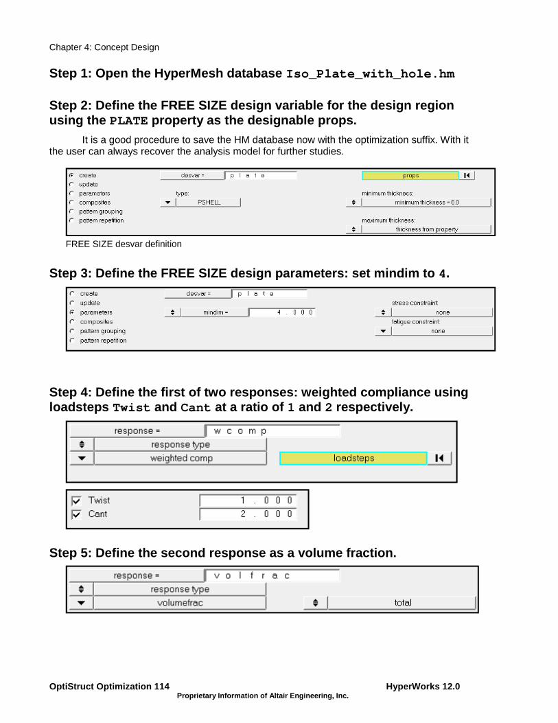
Chapter 4: Concept Design
OptiStruct Optimization 114 HyperWorks 12.0 Proprietary Information of Altair Engineering, Inc.
Step 1: Open the HyperMesh database Iso_Plate_with_hole.hm
Step 2: Define the FREE SIZE design variable for th e design region using the PLATE property as the designable props. It is a good procedure to save the HM database now with the optimization suffix. With it the user can always recover the analysis model for further studies.
FREE SIZE desvar definition
Step 3: Define the FREE SIZE design parameters: set mindim to 4.
Step 4: Define the first of two responses: weighted compliance using loadsteps Twist and Cant at a ratio of 1 and 2 respectively.
Step 5: Define the second response as a volume frac tion.

Chapter 4: Concept Design
HyperWorks 12.0 OptiStruct Optimization 115 Proprietary Information of Altair Engineering, Inc.
Step 6: Create a constraint for the volume fraction response, setting the upper bound to 0.3.
Step 7: Define minimize the weighted compliance as the objective.
Step 8: Submit the optimization run as Iso_plate_with_hole_opt.fem.
Job submission panel
Step 9: Open the results in HyperView and view the element thickness for the final iteration of the optimization.
Resulting element thickness

Chapter 4: Concept Design
OptiStruct Optimization 116 HyperWorks 12.0 Proprietary Information of Altair Engineering, Inc.
Step 10: Return to HyperMesh and use the *.HM.comp. cmf file to sort the elements into collectors based on their optimiz ed thickness.
1. Click the Delete Page button until the main graphics display returns to the
HyperMesh client.
2. Once back within HyperMesh, click on the menu option File > Run > Command File .
3. Select the file named Iso_plate_with_hole_opt.HM.comp.cmf from the directory
where the optimization was run and click Open . HyperMesh Desktop will process the
file and sort all of the elements from the existing model into new component collectors
based on the final thickness in the last iteration of the optimization. New materials are
also created which duplicate the existing material from which the optimized elements
were sorted.
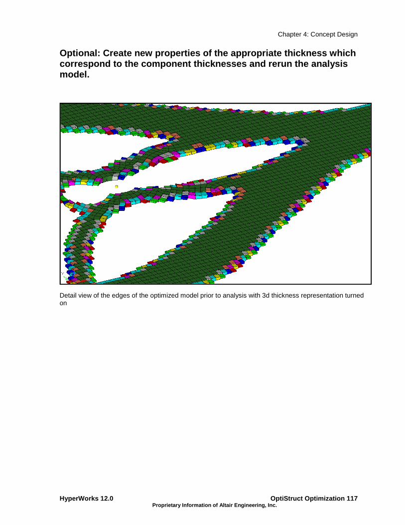
Chapter 4: Concept Design
HyperWorks 12.0 OptiStruct Optimization 117 Proprietary Information of Altair Engineering, Inc.
Optional: Create new properties of the appropriate thickness which correspond to the component thicknesses and rerun t he analysis model.
Detail view of the edges of the optimized model prior to analysis with 3d thickness representation turned on

Chapter 4: Concept Design
OptiStruct Optimization 118 HyperWorks 12.0 Proprietary Information of Altair Engineering, Inc.

Chapter 5: Fine Tuning Design
HyperWorks 12.0 OptiStruct Optimization 119 Proprietary Information of Altair Engineering, Inc.
Chapter 5
Fine Tuning Design
1 – Size Optimization OptiStruct has the capability of performing size optimization. Size optimization can be performed simultaneously with the other types of optimization.
In size optimization, the properties of structural elements such as shell thickness, beam cross-sectional properties, spring stiffness, and mass are modified to solve the optimization problem.
Defining size variables in OptiStruct is done very similarly to other size optimization codes. Each size variable is defined using a DESVAR bulk data entry. If a discrete design variable is desired, a DDVAL bulk data entry needs to be referenced for the design variable values. The DESVAR cards are related to size properties in the model using a DVPREL1 or DVPREL2 bulk data entry. Each DVPREL bulk data entry must reference at least one DESVAR bulk data entry to be active during the optimization. HyperWorks includes a pre-processor called HyperMesh that can be used to set up any number of size variables for the properties.
The following responses are currently available as the objective or as constraint functions:
Mass Volume Center of Gravity
Moment of Inertia Static Compliance Static Displacement
Natural Frequency Buckling Factor Static Stress, Strain, Forces
Static Composite Stress, Strain, Failure Index
Frequency Response Displacement, Velocity, Acceleration
Frequency Response Stress, Strain, Forces
Weighted Compliance Weighted Frequency Combined Compliance Index
Function

Chapter 5: Fine Tuning Design
OptiStruct Optimization 120 HyperWorks 12.0 Proprietary Information of Altair Engineering, Inc.
1.1 – Design Variables for Size Optimization In finite elements, the behavior of structural elements (as opposed to continuum elements), such as shells, beams, rods, springs, and concentrated masses, are defined by input parameters, such as shell thickness, cross-sectional properties, and stiffness. Those parameters are modified in a size optimization. Some structural elements have several parameters depending on each other; like beams in which the area, moments of inertia, and torsional constants depend on the geometry of the cross-section.
The property itself is not the design variable in size optimization, but the property is defined as a function of design variables. The simplest definition, as defined by the design-variable-to-property relationship DVPREL1, is a linear combination of design variables defined on a DESVAR statement such that:
∑ ⋅+= ii CDVCp 0
where p is the property to be optimized, and Ci are linear factors associated to the design variable DVi.
Using the equation utility DEQATN, more complicated functional dependencies using even trigonometric functions can be established. Such design-variable-to-property relations are then defined using the DVPREL2 statement.
For a simple gage optimization of a shell structure, the design-variable-to-property relationship turns into
iDVt =
where the gage thickness t is identical to the design variable.
If a discrete design variable is desired, a DDVAL bulk data entry needs to be referenced on the DESVAR bulk data entry for the design variable values.

Chapter 5: Fine Tuning Design
HyperWorks 12.0 OptiStruct Optimization 121 Proprietary Information of Altair Engineering, Inc.
Exercise 5a – Size Optimization of a Rail Joint This exercise demonstrates how to perform a size optimization on an automobile rail joint modeled with shell elements. The structural model with loads and constraints applied is shown in the figure below. The deflection at the end of the tubular cross-member should be limited. The optimal solution would use as little material as possible.
Structural model of a rail joint.
The structural model, shown above, is loaded into HyperMesh. The constraints, loads, material properties, and subcases (loadsteps) are already defined in the model. Size design variables and optimization parameters are defined, and OptiStruct is used to determine the optimal gauges for the components. The results are then reviewed in HyperView.
The optimization problem for this tutorial is stated as:
Objective: Minimize volume.
Constraints: A given maximum nodal displacement at the loading grid point for two loading conditions.
Design variables: Gauges of the two parts.
Problem Setup
You should copy this file: joint_size.hm

Chapter 5: Fine Tuning Design
OptiStruct Optimization 122 HyperWorks 12.0 Proprietary Information of Altair Engineering, Inc.
Step 1: Launch HyperMesh, set the User Profile and Retrieve the File
1. Launch HyperMesh .
2. Choose the OptiStruct user profile dialog and click OK.
This loads the user profile. It includes the appropriate template, macro menu, and import reader, paring down the functionality of HyperMesh to what is relevant for generating models in Bulk Data Format for OptiStruct. The User Profiles… GUI can also be accessed from the Preferences menu on the toolbar. Select the Optimization panel from the Analysis page.
3. From the toolbar, select Open Model… .
4. Select the joint_size.hm file.
5. Click Open .
Step 2: Create the Size Design Variables for Optimi zation
1. From the Analysis page, select the optimization panel.
2. Click on the size panel.
3. Make sure the desvar subpanel is selected using the radio buttons on the left-hand side of the panel.
4. Click desvar = and enter tube .
5. Click initial value = and enter 1.0 .
6. Click lower bound = and enter 0.1 .
7. Click upper bound = and enter 5.0 .
8. Make sure the move limit toggle is set to move limit default .
9. Make sure the discrete design variable (ddval) toggle is set to no ddval .
10. Click create .
A design variable, tube, has been created. The design variable has an initial value of 1.0, a lower bound of 0.1, and an upper bound of 5.0.
11. Repeat steps 4 through 10 to create the design variable rail using the same initial value, lower, and upper bounds.
A design variable, rail, has been created. The design variable has an initial value of 1.0, a lower bound of 0.1, and an upper bound of 5.0.
12. Select the generic property subpanel using the radio buttons on the left-hand side of the panel.
13. Click Name = and enter tube_th .
14. Click prop and select tube2 from the list of property collectors.
15. Make sure the toggle is set to Thickness T .

Chapter 5: Fine Tuning Design
HyperWorks 12.0 OptiStruct Optimization 123 Proprietary Information of Altair Engineering, Inc.
16. Click designvars .
The list of design variables appears.
17. Check the box next to tube .
Note the linear factor (value is box beside tube) automatically gets set to 1.000.
18. Click return .
19. Click create .
A design variable to property relationship, tube_th, has been created relating the design variable tube to the thickness entry on the PSHELL card for the property tube2.
20. Repeat steps 13 through 19 to create the design variable to property relationship rail_th relating the design variable rail to the thickness entry on the PSHELL card for the property tube1.
21. Click return to go to the optimization panel.
Step 3: Create the Volume and Static Displacement R esponse
A detailed description can be found in the OptiStruct User's Guide under Responses.
1. Enter the responses panel.
2. Click response = and enter volume .
3. Click the response type: switch and select volume from the pop-up menu.
4. Ensure the regional selection is set to total (this is the default).
5. Click create .
A response, volume, is defined for the total volume of the model.
6. Click response = and enter X_Disp .
7. Click the response type: switch and select static displacement from the pop-up menu.
8. Click nodes and select by id from the pop-up menu.
9. Enter 3143 (node at center of rigid spider at loading point) and press Enter .
10. Select dof1 and click create .
A response, X_Disp, is defined for the x-displacement of the node 3143.
11. Click response = and enter Z_Disp .
12. Click nodes and select by id from the pop-up menu.
13. Enter 3143 (node at center of rigid spider at loading point) and press Enter .
14. Select dof3 and Click create .
A response, Z_Disp, is defined for the z-displacement of the node 3143.
15. Click return to go to the optimization panel.

Chapter 5: Fine Tuning Design
OptiStruct Optimization 124 HyperWorks 12.0 Proprietary Information of Altair Engineering, Inc.
Step 4: Create Constraints on Displacement Response
A response defined as the objective cannot be constrained. In this case, you cannot constrain the response volume.
Upper bound constraints are to be defined for the responses X_Disp and Z_Disp.
1. Enter the dconstraints panel.
2. Click constraint = and enter Disp_X .
3. Check the box for upper bound = .
4. Click upper bound = and enter 0.9 .
5. Click response = and select X_Disp from the list of responses.
A loadsteps button should appear in the panel.
6. Click loadsteps .
7. Check the box next to FORCE_X and click select .
8. Click create .
A constraint is defined on the response X_Disp. The constraint is an upper bound with a value of 0.9. The constraint applies to the subcase FORCE_X.
9. Click constraint = and enter Disp_Z .
10. Check the box for upper bound = .
11. Click upper bound = and enter 1.6 .
12. Click response = and select Z_Disp from the list of responses.
13. Click loadsteps .
14. Check the box next to FORCE_Z and click select .
15. Click create .
A constraint is defined on the response Z_Disp. The constraint is an upper bound with a value of 1.6. The constraint applies to the subcase FORCE_Z.
16. Click return to go to the optimization panel.
Step 5: Define the Objective Function
In this example, the objective is to minimize the volume response defined in the previous section.
1. Click objective to enter the panel.
2. The switch in the left should be set to min .
3. Click response = and select volume from the response list.
4. Click create .
The objective function is now defined.
5. Click return to go to the optimization panel.

Chapter 5: Fine Tuning Design
HyperWorks 12.0 OptiStruct Optimization 125 Proprietary Information of Altair Engineering, Inc.
Step 6: Save the HyperMesh Database
1. Select the Files panel toolbar button.
2. Click save as…
3. Select the directory where you would like to save the database and enter the name for the database, joint_sizeOPT.hm , in the File name: field.
4. Click save .
Step 7: Run the Optimization Problem
1. From the Analysis page, select the OptiStruct panel.
2. Click save as…
3. Select the directory where you would like to write the model file and enter the name for the file name, joint_sizeOPT.fem , in the File name: field.
The .fem file name is used for OptiStruct input decks.
4. Click Save.
Note the name and location of the joint_sizeOPT.fem file displays in the input file: field.
5. Set the export options: toggle to all .
6. Click the run options: switch and select optimization .
7. Set the memory options: toggle to memory default .
8. Click OptiStruct to run the optimization.
This launches the OptiStruct job. If the job was successful, new results files can be seen in the directory where the OptiStruct model file was written. The joint_sizeOPT.out file is a good place to look for error messages that will help to debug the input deck if any errors are present.
These are some important results files for Size Optimization :
Step 8: View the Size Optimization Results (gauge t hickness)
1. Once you see the message Process completed successfully in the command window, click the HyperView button.
HyperView will launch and the results will be loaded. A message window appears to inform about the successful loading of the model and result files into HyperView. Notice that all three h3d files get loaded, each into a different page in HyperView. Files joint_sizeOPT_des.h3d , joint_sizeOPT_s1.h3d , and joint_sizeOPT_s2.h3d get loaded in page 1, page 2, and page 3, respectively. The optimization iteration results (gauge thickness) are loaded in the first page. Note that the name of the page is displayed as Design History to indicate that the results correspond to optimization iterations.
2. Click Close to close the message window.
3. Click the Contour toolbar button.

Chapter 5: Fine Tuning Design
OptiStruct Optimization 126 HyperWorks 12.0 Proprietary Information of Altair Engineering, Inc.
4. Make sure the first pull-down list below Result type: is Element Thicknesses (s) .
5. Make sure the second pull-down list is on Thickness .
6. Make sure the field below Averaging method is None .
7. The left side of the HyperView GUI is the results browser, and at the top of the browser are the Load Case and Simulation selection drop-down boxes.
8. In the iteration list, scroll down to the last iteration and choose the last for e.g.: Iteration [3] and click OK.
9. Click Apply .
A contoured image representing shell thickness should be visible. Each element in the model is assigned a legend color, indicating the thickness value for that element for the current iteration.
Thickness contour at last iteration
Step 9: View the Displacement Results
It is helpful to view the deformations of the model to determine if the boundary conditions have been met and also to see if the model is deforming as expected. These analysis results are available in pages 2 and 3.
1. Click the Next Page toolbar button to move to the second page.
The second page, which has results loaded from the file joint_sizeOPT_s1.h3d , is displayed. Note that the name of the page is displayed as Subcase 1 – FORCE_X to indicate that the results correspond to subcase 1.
2. Set the animation mode to Linear Static .
3. Click the Contour toolbar button.
4. Select the first pull-down menu below Result type: and select Displacement [v] .
5. Select the second pull-down menu and select X.

Chapter 5: Fine Tuning Design
HyperWorks 12.0 OptiStruct Optimization 127 Proprietary Information of Altair Engineering, Inc.
6. Click on Apply .
The resulting contours represent the x component displacement field resulting from the applied loads and boundary conditions.
7. Click the Measure toolbar button.
8. Click Add to add a new measure group.
The Measure panel helps measure different results. Here, we will measure the displacement at node 3143 for which we have constrained the displacement.
9. Click the pull-down menu and select Nodal Contour as shown below.
10. Click on Nodes , which opens a new window to select nodes By ID .
11. Click By ID to open a new window.
12. Enter 3143 in the field next to Node ID and click Ok.
The x-displacement value for 3143 (center of rigid spider, where loading is applied) is shown in the graphic area. Note that the x-displacement is larger than the upper bound constraint, which was defined earlier, of 0.9.
13. In the Load Case and Simulation selection drop-down, select the last iteration by double clicking on the last Iteration #.
The contour now shows the x-displacement results for Subcase 1 (FORCE_X) and iteration 4, which corresponds to the end of the optimization iterations. Note that the x-displacement is now less than 0.9.
Displacement on X-direction for the X-Force load case at the last iteration
14. Click the Next Page button again to move to the third page.
The third page shows results loaded from the joint_sizeOPT_s2.h3d file. Note that the name of the page is displayed as Subcase 2 – Force_Z to indicate that the results correspond to subcase 2.
15. Click the Contour toolbar button.
16. Select the first pull-down menu below Result type: and select Displacement [v] .

Chapter 5: Fine Tuning Design
OptiStruct Optimization 128 HyperWorks 12.0 Proprietary Information of Altair Engineering, Inc.
17. Select the second pull-down menu and select Z.
18. Click on Apply .
The resulting contours represent the z component displacement field resulting from the applied loads and boundary conditions.
19. Repeat steps 8 through 14 to measure and display the z-displacement value for node 3143.
Z Displacement for Z-Force load case at the last iteration
1. The solution converged to a feasible solution?
2. How many iterations did convergence require and what is the final volume of the part?
3. What are the resulting gauges for the rail and tube?

Chapter 5: Fine Tuning Design
HyperWorks 12.0 OptiStruct Optimization 129 Proprietary Information of Altair Engineering, Inc.
Exercise 5b – Discrete Size Optimization of a Welde d Bracket This exercise demonstrates how to perform a size optimization on a welded bracket modeled with shell elements using discrete design variables. The structural model with loads and constraints applied is shown in the figure below. The objective is to minimize the amount of material used in the model subject to certain stress specifications.
The structural model, as shown in the figure, is loaded into HyperMesh. The constraints, loads, material properties, and subcases (loadsteps) are already defined in the model. Size design variables and optimization parameters are defined, and OptiStruct is used to determine the optimal gauges. The results are then reviewed in HyperView.
The optimization problem is stated as:
Objective: Minimize volume.
Constraints: Maximum von Mises stress of the brackets < 120 MPa.
Design variables: Gauges of the brackets.
Problem Setup
You should copy this file: bracket_size.hm
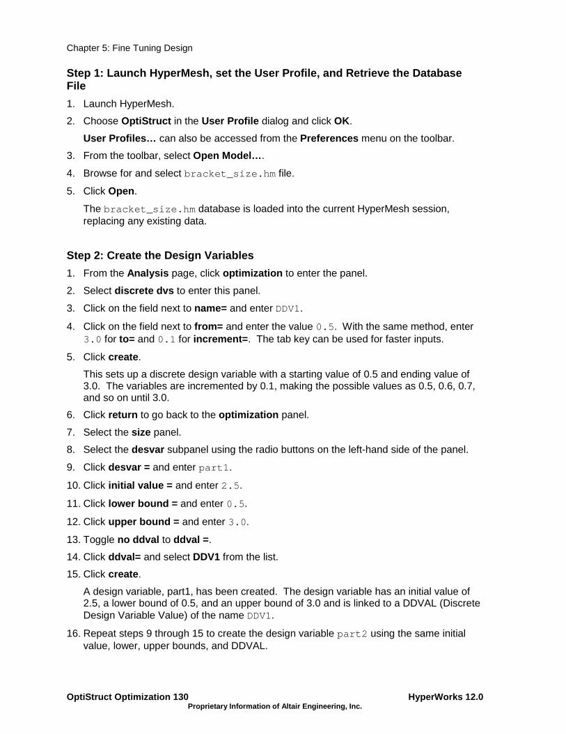
Chapter 5: Fine Tuning Design
OptiStruct Optimization 130 HyperWorks 12.0 Proprietary Information of Altair Engineering, Inc.
Step 1: Launch HyperMesh, set the User Profile, and Retrieve the Database File
1. Launch HyperMesh.
2. Choose OptiStruct in the User Profile dialog and click OK.
User Profiles… can also be accessed from the Preferences menu on the toolbar.
3. From the toolbar, select Open Model… .
4. Browse for and select bracket_size.hm file.
5. Click Open .
The bracket_size.hm database is loaded into the current HyperMesh session, replacing any existing data.
Step 2: Create the Design Variables
1. From the Analysis page, click optimization to enter the panel.
2. Select discrete dvs to enter this panel.
3. Click on the field next to name= and enter DDV1.
4. Click on the field next to from= and enter the value 0.5 . With the same method, enter 3.0 for to= and 0.1 for increment= . The tab key can be used for faster inputs.
5. Click create .
This sets up a discrete design variable with a starting value of 0.5 and ending value of 3.0. The variables are incremented by 0.1, making the possible values as 0.5, 0.6, 0.7, and so on until 3.0.
6. Click return to go back to the optimization panel.
7. Select the size panel.
8. Select the desvar subpanel using the radio buttons on the left-hand side of the panel.
9. Click desvar = and enter part1 .
10. Click initial value = and enter 2.5 .
11. Click lower bound = and enter 0.5 .
12. Click upper bound = and enter 3.0 .
13. Toggle no ddval to ddval = .
14. Click ddval= and select DDV1 from the list.
15. Click create .
A design variable, part1, has been created. The design variable has an initial value of 2.5, a lower bound of 0.5, and an upper bound of 3.0 and is linked to a DDVAL (Discrete Design Variable Value) of the name DDV1.
16. Repeat steps 9 through 15 to create the design variable part2 using the same initial value, lower, upper bounds, and DDVAL.

Chapter 5: Fine Tuning Design
HyperWorks 12.0 OptiStruct Optimization 131 Proprietary Information of Altair Engineering, Inc.
17. Select the generic property subpanel using the radio buttons on the left-hand side of the panel.
18. Click dvprel = and enter part1_th .
19. Click the entity selection switch and choose prop .
20. Click prop and select part1 from the list of component collectors.
21. A property selection switch now appears below the prop button.
22. Click the property selection switch and select Thickness T from the pop-up menu.
23. Click on designvars .
The list of design variables appears.
24. Check the box next to part1 .
25. Note that the linear factor (value in box beside part1 ) automatically gets set to 1.000 .
26. Click return .
27. Click create .
A design variable to property relationship, part1_th, has been created, relating the design variable part1 to the thickness entry on the PSHELL card for the component part1.
28. Repeat steps 19 through 26 to create the design variable to property relationship part2_th, relating the design variable part2 to the thickness entry on the PSHELL card for the component part2.
29. Click return to go to the Optimization Setup panel.
Step 3: Create the Responses
A detailed description can be found in the OptiStruct User's Guide under Responses.
1. Select the responses panel.
2. Click response = and enter volume .
3. Click the response type: switch and select volume from the pop-up menu.
4. Click create .
A response, volume, is defined for the total volume of the model.
5. Click response = and enter stress1 .
6. Click the response type: switch and select static stress from the pop-up menu.
7. Click props .
8. Click one of the green shell elements in the graphics window to select the component part1 .
9. Click select .
A stress type selector switch appears.
10. Click the stress type selector switch and select von mises from the pop-up menu.

Chapter 5: Fine Tuning Design
OptiStruct Optimization 132 HyperWorks 12.0 Proprietary Information of Altair Engineering, Inc.
11. Click the selector switch below the stress selector and choose the both surfaces option.
12. Click create .
A response, stress1, is defined for the von Mises stress of the elements in the component part1.
13. Click response = and enter stress2 .
14. Click props .
15. Click one of the pink shell elements in the graphics window to select the component part2 .
16. Click select .
17. Click create .
A response, stress2, is defined for the von Mises stress of the elements in the component part2.
18. Click return to go to the Optimization Setup panel.
Step 4: Create Constraints
A response defined as the objective cannot be constrained. In this case, you cannot constrain the response volume.
Upper bound constraints are to be defined for the responses stress1 and stress2.
1. Select the dconstraints panel.
2. Click constraint = and enter stress1 .
3. Click response = and select stress1 from the list of responses.
A loadsteps button should appear in the panel.
4. Click loadsteps .
5. Check the box next to STEP and click select .
6. Check the box next to upper bound = .
7. Click upper bound = and enter 100 .
8. Click create .
A constraint is defined on the response stress1. The constraint is an upper bound with a value of 100. The constraint applies to the subcase STEP.
9. Click constraint = and enter stress2 .
10. Click response = and select stress2 from the list of responses.
11. Click loadsteps .
12. Check the box next to STEP and click select .
13. Check the box next to upper bound = .
14. Click upper bound = and enter 120 .

Chapter 5: Fine Tuning Design
HyperWorks 12.0 OptiStruct Optimization 133 Proprietary Information of Altair Engineering, Inc.
15. Click create .
A constraint is defined on the response stress2. The constraint is an upper bound with a value of 120. The constraint applies to the subcase STEP.
16. Click return twice to go to the main menu.
Step 5: Define the Objective Function
In this example, the objective is to minimize the volume response defined in the previous section.
1. Select the objective panel.
2. Click the switch in the upper left corner of the panel, and select min from the pop-up menu.
3. Click response = and select volume from the response list.
4. Click create .
The objective function is now defined.
5. Click return to return to the Optimization Setup panel.
Step 6: Submit the Job
1. From the Analysis page, select OptiStruct to enter the panel.
2. Click save as… .
3. Select the directory where you would like to write the OptiStruct model file and enter the name for the model, discrete_bracket_size.fem , in the file: field.
.fem is the suggested extension for OptiStruct input decks.
4. Click Save.
Note the name and location of the discrete_bracket_size.fem file displays in the input file: field.
5. Set the export options: toggle to all .
6. Click the run options: switch and select optimization .
7. Set the memory options: toggle to memory default .
8. Click OptiStruct .
This launches the OptiStruct job. If the job was successful, new results files can be seen in the directory where the OptiStruct model file was written. The bracket_size.out file is a good place to look for error messages that will help to debug the input deck if any errors are present.
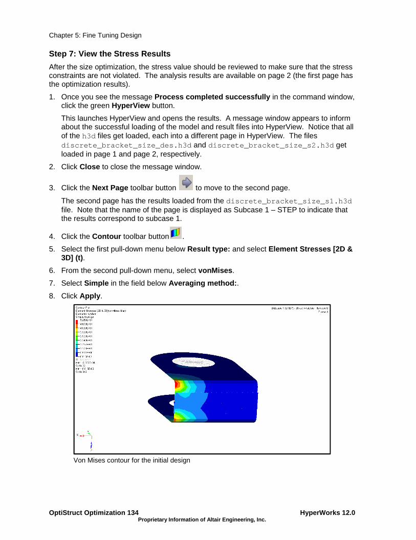
Chapter 5: Fine Tuning Design
OptiStruct Optimization 134 HyperWorks 12.0 Proprietary Information of Altair Engineering, Inc.
Step 7: View the Stress Results
After the size optimization, the stress value should be reviewed to make sure that the stress constraints are not violated. The analysis results are available on page 2 (the first page has the optimization results).
1. Once you see the message Process completed successfully in the command window, click the green HyperView button.
This launches HyperView and opens the results. A message window appears to inform about the successful loading of the model and result files into HyperView. Notice that all of the h3d files get loaded, each into a different page in HyperView. The files discrete_bracket_size_des.h3d and discrete_bracket_size_s2.h3d get loaded in page 1 and page 2, respectively.
2. Click Close to close the message window.
3. Click the Next Page toolbar button to move to the second page.
The second page has the results loaded from the discrete_bracket_size_s1.h3d file. Note that the name of the page is displayed as Subcase 1 – STEP to indicate that the results correspond to subcase 1.
4. Click the Contour toolbar button .
5. Select the first pull-down menu below Result type: and select Element Stresses [2D & 3D] (t) .
6. From the second pull-down menu, select vonMises .
7. Select Simple in the field below Averaging method: .
8. Click Apply .
Von Mises contour for the initial design

Chapter 5: Fine Tuning Design
HyperWorks 12.0 OptiStruct Optimization 135 Proprietary Information of Altair Engineering, Inc.
A contoured image representing von Mises stresses should be visible. Each element in the model is assigned a legend color, indicating the von Mises stress value for that element resulting from the applied loads and boundary conditions. If you did not change the Iteration step, you should be contouring the stress of the initial step. To contour the final step, set the last iteration of that loadcase using the status bar.
The Load Case and Simulation Selection area is located to the top of the Results browser on the left hand side of the GUI.
9. Click the last Iteration # in the Simulation: list.
Notice only two iterations are displayed; the First and Last (FL) is the default setting for optimization runs. To change this setting, add an OUTPUT control card with a frequency setting of ALL .
10. Click OK.
This will now contour your final iteration of that loadcase. Review the stress to see that it is under the proper constraints.
Von Mises contour for the optimum design
Review
The .out file contains a summary of the optimization process. From the information in the .out file, you can see how the objective, constraints, and design variables are changing from one iteration to the next.
Has the volume been minimized for the given constraints?
Have the stress constraints been met?
What are the resulting gauges for the two parts?

Chapter 5: Fine Tuning Design
OptiStruct Optimization 136 HyperWorks 12.0 Proprietary Information of Altair Engineering, Inc.
Hints
Go to the des.h3d page, clear the contour if one was applied, set to the last simulation step and apply the Element Thickness contour.
Append discrete_bracket_size.mvw to review objective, constraints, and other information.
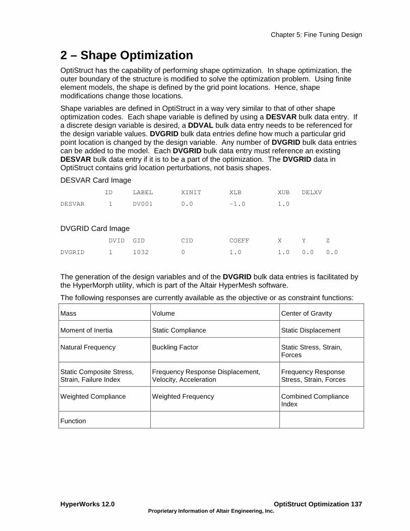
Chapter 5: Fine Tuning Design
HyperWorks 12.0 OptiStruct Optimization 137 Proprietary Information of Altair Engineering, Inc.
2 – Shape Optimization OptiStruct has the capability of performing shape optimization. In shape optimization, the outer boundary of the structure is modified to solve the optimization problem. Using finite element models, the shape is defined by the grid point locations. Hence, shape modifications change those locations.
Shape variables are defined in OptiStruct in a way very similar to that of other shape optimization codes. Each shape variable is defined by using a DESVAR bulk data entry. If a discrete design variable is desired, a DDVAL bulk data entry needs to be referenced for the design variable values. DVGRID bulk data entries define how much a particular grid point location is changed by the design variable. Any number of DVGRID bulk data entries can be added to the model. Each DVGRID bulk data entry must reference an existing DESVAR bulk data entry if it is to be a part of the optimization. The DVGRID data in OptiStruct contains grid location perturbations, not basis shapes.
DESVAR Card Image
ID LABEL XINIT XLB XUB DELXV
DESVAR 1 DV001 0.0 -1.0 1.0
DVGRID Card Image
DVID GID CID COEFF X Y Z
DVGRID 1 1032 0 1.0 1.0 0.0 0.0
The generation of the design variables and of the DVGRID bulk data entries is facilitated by the HyperMorph utility, which is part of the Altair HyperMesh software.
The following responses are currently available as the objective or as constraint functions:
Mass Volume Center of Gravity
Moment of Inertia Static Compliance Static Displacement
Natural Frequency Buckling Factor Static Stress, Strain, Forces
Static Composite Stress, Strain, Failure Index
Frequency Response Displacement, Velocity, Acceleration
Frequency Response Stress, Strain, Forces
Weighted Compliance Weighted Frequency Combined Compliance Index
Function

Chapter 5: Fine Tuning Design
OptiStruct Optimization 138 HyperWorks 12.0 Proprietary Information of Altair Engineering, Inc.
2.1 – Design Variables for Shape Optimization In finite elements, the shape of a structure is defined by the vector of nodal coordinates (x). In order to avoid mesh distortions due to shape changes, changes of the shape of the structural boundary must be translated into changes of the interior of the mesh.
The two most commonly used approaches to account for mesh changes during a shape optimization are the basis vector approach and the perturbation vector approach. Both approaches refer to the definition of the structural shape as a linear combination of vectors.
Using the basis vector approach, the structural shape is defined as a linear combination of basis vectors. The basis vectors define nodal locations.
∑ ⋅= ii BVDVx
where x is the vector of nodal coordinates, BVi is the basis vector associated to the design variable DVi.
Using the perturbation vector approach, the structural shape change is defined as a linear combination of perturbation vectors. The perturbation vectors define changes of nodal locations with respect to the original finite element mesh.
Description of a shape design variable
Original location:
Perturbations (DVGRID):
Magnitude of perturbations (DESVAR):
Mesh nodal movement:
where X is the vector of nodal coordinates, X(0) is the vector of nodal coordinates of the initial design, ∆∆∆∆Xj is the perturbation vector associated to the design variable α.
The initial nodal coordinates are those defined with the GRID entity. The perturbation vectors are defined on the DVGRID statement, which is referenced by the design variable entity DESVAR.
If a discrete design variable is desired, a DDVAL bulk data entry needs to be referenced on the DESVAR bulk data entry for the design variable values.
Note :
In OptiStruct, only the perturbation vector approach is available. The DVGRID cards must contain perturbation vectors.
},,,{ )0()0(3
)0(2
)0(1
)0(nxxxxX ⋯=
},,,,{ 321 nxxxxX ∆∆∆∆=∆ ⋯
},,,,{ 321 nααααα ⋯=
∑=
∆+=n
jjj XXX
1
)0( α

Chapter 5: Fine Tuning Design
HyperWorks 12.0 OptiStruct Optimization 139 Proprietary Information of Altair Engineering, Inc.
2.2 – HyperMorph HyperMorph is a tool in HyperMesh to morph the shape of a finite element model in ways that are useful, logical and intuitive. It enables rapid shape changes on the FE mesh without severely sacrificing the mesh quality. This is a very powerful tool to automatic generate the shape design variable described above.
2.2.1 – The Three Basic Approaches to Morphing
The Domains and Handles Concept
The Domains and Handles approach involves dividing the mesh into domains containing elements or nodes and placing handles at the corners of those domains. HyperMorph can automatically divide the mesh into logical domains or you can manually define your own domains and handles. When the handles are moved, the shape of the mesh changes according to the domain boundaries. The domains and handles approach also allows for parametric morphing of lengths, angles, radii, and arc angles as well as morphing the mesh to match geometric data and other meshes. The domains and handles approach is the most difficult approach to learn but it is also the most powerful. This approach is most useful for making detailed changes to any mesh (local domains) as well as general changes to space frame type meshes (global domains).
Morph Example using handles and domain concept
The Morph Volume Concept
The Morph Volume approach involves surrounding the mesh with one or more morph volumes, which are highly deformable six-sided prisms. A number of methods exist to create the morph volumes, including single and matrix creation as well as the interactive on-screen method. Morph volumes support tangency between adjoining edges and allow for multiple control points along their edges. Handles placed at the corners and along the edges of the morph volumes allow for the morphing of the morph volumes which in turn morphs the mesh inside the morph volumes. The morph volume approach is quick and intuitive and is most useful for making large scale changes to complex meshes.
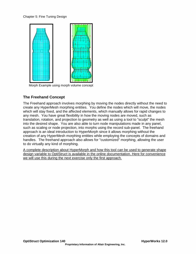
Chapter 5: Fine Tuning Design
OptiStruct Optimization 140 HyperWorks 12.0 Proprietary Information of Altair Engineering, Inc.
Morph Example using morph volume concept
The Freehand Concept
The Freehand approach involves morphing by moving the nodes directly without the need to create any HyperMesh morphing entities. You define the nodes which will move, the nodes which will stay fixed, and the affected elements, which manually allows for rapid changes to any mesh. You have great flexibility in how the moving nodes are moved, such as translation, rotation, and projection to geometry as well as using a tool to "sculpt" the mesh into the desired shape. You are also able to turn node manipulations made in any panel, such as scaling or node projection, into morphs using the record sub-panel. The freehand approach is an ideal introduction to HyperMorph since it allows morphing without the creation of any HyperMesh morphing entities while employing the concepts of domains and handles. The freehand approach also allows for "customized" morphing, allowing the user to do virtually any kind of morphing.
A complete description about HyperMorph and how this tool can be used to generate shape design variable to OptiStruct is available in the online documentation. Here for convenience we will use this during the next exercise only the first approach.
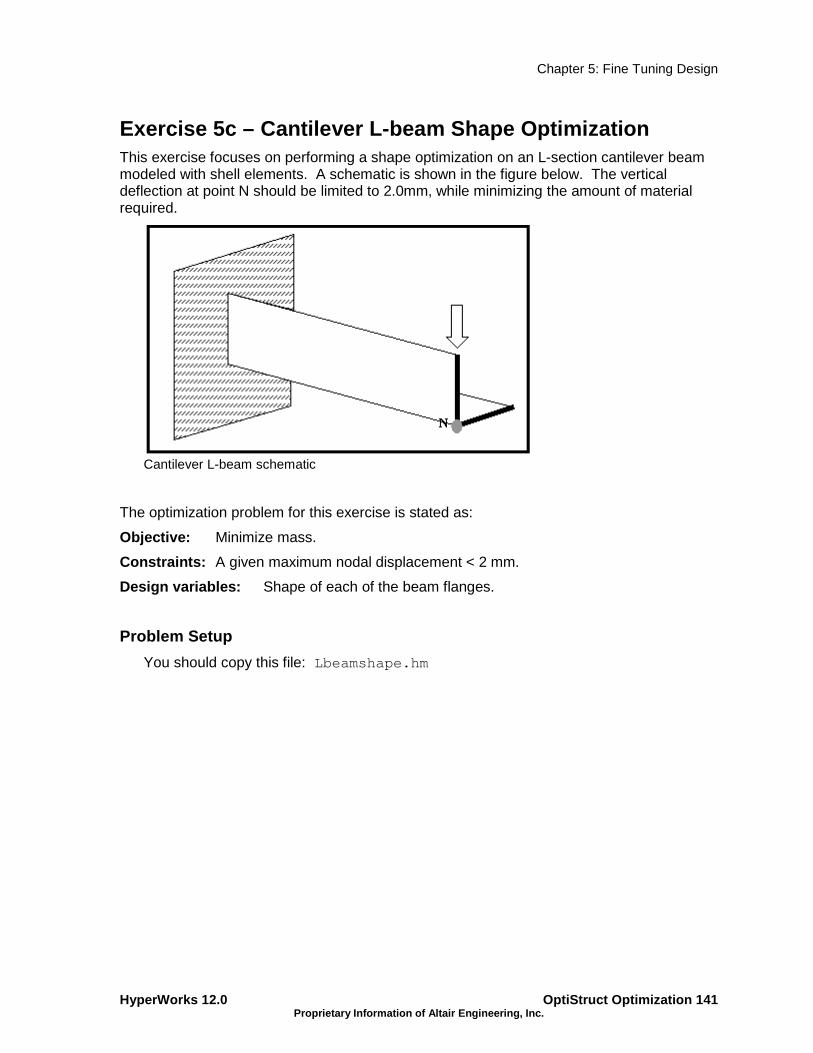
Chapter 5: Fine Tuning Design
HyperWorks 12.0 OptiStruct Optimization 141 Proprietary Information of Altair Engineering, Inc.
Exercise 5c – Cantilever L-beam Shape Optimization This exercise focuses on performing a shape optimization on an L-section cantilever beam modeled with shell elements. A schematic is shown in the figure below. The vertical deflection at point N should be limited to 2.0mm, while minimizing the amount of material required.
Cantilever L-beam schematic
The optimization problem for this exercise is stated as:
Objective: Minimize mass.
Constraints: A given maximum nodal displacement < 2 mm.
Design variables: Shape of each of the beam flanges.
Problem Setup
You should copy this file: Lbeamshape.hm

Chapter 5: Fine Tuning Design
OptiStruct Optimization 142 HyperWorks 12.0 Proprietary Information of Altair Engineering, Inc.
Step 1: Launch HyperMesh and Set the User Profile
1. Launch HyperMesh Desktop.
A User Profiles… dialog will appear.
2. Choose OptiStruct as the user profile and click OK.
This loads the user profile. It includes the appropriate template, macro menu, and import reader, paring down the functionality of HyperMesh to what is relevant for generating models in Bulk Data Format for OptiStruct.
Step 2: Retrieve the Lbeamshape.hm File
1. On the toolbar, select Open Model… .
2. Select the Lbeamshape.hm file, located in model files directory.
3. Click Open .
Step 3: Creating Shapes using HyperMorph
This section makes use of HyperMorph. For a more detailed description of the functionality of HyperMorph, please refer to the HyperMorph section of the HyperMesh documentation.
1. From Analysis page click on optimization panel.
2. Select the HyperMorph panel.
3. Select the domains panel.
4. Select the create subpanel using the radio buttons on the left-hand side of the panel.
5. Click the switch next to global domain and select the auto functions from the pop-up menu.
6. Click generate on the right side of the panel.
A number of domains and handles are created which will enable us to morph the shape of the beam.
There are two types of handles: global handles, which are represented by larger red balls and local handles, which are represented by smaller yellow balls. We will only be dealing with the local handles in this exercise.
7. Click return to return to the HyperMorph panel.
8. Select the morph panel.
9. Select the move handles subpanel using the radio buttons on the left side of the panel.
10. Click the right-hand switch and select translate instead of interactive from the pop-up menu.
11. If the handles button is not already highlighted, click on it.
12. Select the local handle that is located at the node where the load is applied by clicking on it in the graphics window (local handles are indicated by a yellow ball).
13. Click y val = and enter -10.0 .

Chapter 5: Fine Tuning Design
HyperWorks 12.0 OptiStruct Optimization 143 Proprietary Information of Altair Engineering, Inc.
14. Click morph .
The beam changes shape so that the handle you selected moved -10.0 in the y-direction. Note how the mesh adjusted to this change in shape.
15. Select the save shape subpanel using the radio buttons on the left side of the panel.
16. Click name = and enter shape1 .
17. Click color and choose a color from the palette.
18. Set the toggle beneath shape = to as node perturbations .
19. Click save .
20. Click Yes to the message regarding the perturbations, as shown above.
We have now saved this shape as shape1, later we can associate it to a design variable.
21. Click undo all .
The model returns to its original shape.
Figure showing handles to be morphed

Chapter 5: Fine Tuning Design
OptiStruct Optimization 144 HyperWorks 12.0 Proprietary Information of Altair Engineering, Inc.
22. Repeat steps 9 through 21 for the local handles 3, 4 and 5. Referring to the figure above translate handles 3 and 4 by x=-10 and handle 5 by y=-10. Save the shapes after morphing each handle as shape2, shape3 and shape4, respectively.
IMPORTANT: Remember to undo all after every saved shape. Otherwise the nodal changes for preexisting shapes will be saved in the current shape along with the most recent changes.
23. Click return twice to go to the optimization panel.
Step 4: Create Design Variables for Shape Optimizat ion
1. On the Analysis page in the optimization panel, select shape .
2. Select the desvar subpanel using the radio buttons on the left side of the panel.
3. Toggle the switch to multiple desvars from single desvar .
4. Click shapes , (the yellow button that appears).
5. Check the boxes next to shape1 , shape2 , shape3 , and shape4 and click select .
6. Click create .
Four shape design variables are created using the shapes that were saved earlier.
7. Click return to go to the optimization panel.
A potential variation in shape of the vertical flange of the L-beam that could be achieved using the set up described.
Step 5: Create Mass and Static Displacement for Nod es as Responses
Two responses are defined in this tutorial, a mass response for the objective function and a displacement response for the constraint. A detailed description can be found in the OptiStruct User's Guide under Responses.
1. Select the responses panel (accessed through the optimization panel on the Analysis page).
2. Click response = and enter Mass.
3. Click the response type: switch and select mass from the pop-up menu.
4. Click create .
A response, mass, is defined for the total mass of the model.

Chapter 5: Fine Tuning Design
HyperWorks 12.0 OptiStruct Optimization 145 Proprietary Information of Altair Engineering, Inc.
5. Click response = and enter Disp .
6. Click the response type: switch and select static displacement from the pop-up menu.
Figure showing node to be selected while defining displacement response.
7. Select the response node by clicking on the node shown in the above figure.
TIP: In order to see the selected node more clearly, you may want to hide the domains and handles first by right-clicking on them in the Model Browser and selecting Hide from the context-sensitive menu.
8. Select dof 2 .
Dofs 1, 2, and 3 refer to translation in the X, Y, and Z directions.
Dofs 4, 5, and 6 refer to rotation about the X, Y, and Z axes.
9. Click create .
A response, disp, is defined for the y-displacement of the node selected.
10. Click return to go to the optimization panel.
Step 6: Apply Design Constraint on Static Displacem ent Response
A response defined as the objective cannot be constrained (mass, in this case).
A lower bound constraint is to be defined for the displacement response defined in the previous section.
1. Select the dconstraints panel (accessed from the optimization panel on the Analysis page).
2. Click on constraint = and enter Constr .

Chapter 5: Fine Tuning Design
OptiStruct Optimization 146 HyperWorks 12.0 Proprietary Information of Altair Engineering, Inc.
3. Click response = and select Disp from the list of responses.
A loadsteps button should appear in the panel.
4. Click loadsteps .
5. Check the box next to load and click select .
6. Check the box next to lower bound = .
7. Click lower bound = and enter -2.0 .
Note this is a lower bound as the response is negative.
8. Click create .
A constraint is defined on the response disp . The constraint is a lower bound with a value of -2.0 . The constraint applies to the subcase Load.
9. Click return twice to go to the main menu.
Step 7: Define Minimize Mass as Objective Function
In this example, the objective is to minimize the mass response defined in the previous section.
1. Select the objective panel (accessed from the optimization panel on the Analysis page).
2. Click the switch in the upper left corner of the panel, and select min from the pop-up menu.
3. Click response = and select mass from the response list.
4. Click create .
The objective function is now defined.
5. Click return to go to the optimization panel.
Step 8: Save the Database as a HyperMesh File
1. Select the Files panel toolbar button.
2. Select the hm file subpanel.
3. Click save as… to set the directory in which to save the file and, in File name: , type lbeamshape_opt.hm .
4. Click Save.
Step 9: Run OptiStruct
1. Select the OptiStruct panel on the Analysis page.
2. Click save as… following the input file: field.
3. Select the directory where you would like to write the OptiStruct model file and enter the name for the model, lbeamshape_opt.fem , in the File name: field.

Chapter 5: Fine Tuning Design
HyperWorks 12.0 OptiStruct Optimization 147 Proprietary Information of Altair Engineering, Inc.
The .fem extension is suggested for OptiStruct input decks.
4. Click Save.
Note the name and location of the lbeamshape_opt.fem file displays in the input file: field.
5. Set the memory options: toggle, located in the center of the panel, to memory default .
6. Click the run options: switch, located at the left of the panel, and select optimization .
7. Set the export options: toggle to all .
8. Click OptiStruct .
This launches the OptiStruct job. If the job was successful, new results files can be seen in the directory where the OptiStruct model file was written. The lbeamshape_opt.out file is a good place to look for error messages that will help to debug the input deck if any errors are present.
Step 10: View the Deformed Structure
It is helpful to view the deformed shape of a model to determine if the boundary conditions have been defined correctly and also to check if the model is deforming as expected. In this section, use the Deformed panel to review the deformed shape for the last design iteration and a scale factor, and overlay the undeformed shape.
1. While still in the OptiStruct panel, click the green HyperView button.
2. Close the Message Log window that details the result files loaded into HyperView.
In HyperView, the loaded .h3d files contain optimization results on page 1 and analysis results on page 2.
3. Click the Contour panel toolbar button .
4. Under Result type:, select Shape change (v) .
5. Click Apply .
6. From the Load Case and Simulation drop-down selector, select the last Iteration # under Simulation .
The final shape for Iteration # can be seen.
Step 11: View a Transient Animation of Shape contou r changes
1. On the toolbar, use the Animation Mode drop-down selector to change the animation
mode to Transient .
2. Click the play button to begin the animation.
3. The Speed frame rate slider is used to adjust the animation speed. Drag the slider to the left to slow the animation.
4. After reviewing the animation, click the stop button to stop the animation and move Current time: back to 0.

Chapter 5: Fine Tuning Design
OptiStruct Optimization 148 HyperWorks 12.0 Proprietary Information of Altair Engineering, Inc.
Step 12: Plot a Contour of Displacements
1. Click the Next Page arrow to go to page 2, which contains the analysis results.
2. Click the Contour panel toolbar button.
3. Under Result type: , select Displacement (v) .
4. Select the last Iteration (#) under Simulation in the Load Case and Simulation Selection dialog.
5. Click Apply .
A plot of the displacements on your final shape should be displayed. Note that the maximum displacements for Iteration # is still below 2.0.

Chapter 5: Fine Tuning Design
HyperWorks 12.0 OptiStruct Optimization 149 Proprietary Information of Altair Engineering, Inc.
Exercise 5d – Shape Optimization of a Rail Joint Shape optimization requires you to have knowledge of the kind of shape you would like to change in the structure. This may include finding the optimum shape to reduce stress concentrations to changing the cross-sections to meet specific design requirements. Therefore, you need to define the shape modifications and the nodal movements to reflect the shape changes. Shape optimization requires the use of two cards DESVAR and DVGRID. They can be defined using HyperMorph . These cards are included in the OptiStruct input file along with the objective function and constraints to run the shape optimization.
In this exercise you will perform a shape optimization on a rail-joint. The rail-joint is made of shell elements and has one load case. The shape of the joint is modified to satisfy stress constraints while minimizing mass.
Rail joint
The optimization problem for this exercise is state d as:
Objective: Minimize mass
Constraint: Maximum von Mises stress of the joint < 200 MPa
Design variables: Shape variables
Problem Setup
You should copy the file: rail_joint_original.hm

Chapter 5: Fine Tuning Design
OptiStruct Optimization 150 HyperWorks 12.0 Proprietary Information of Altair Engineering, Inc.
Step 1: Launch HyperMesh, Set the User Profile and Retrieve the File
1. Launch HyperMesh Desktop.
2. Choose OptiStruct in the User Profile dialog and click OK.
This loads the user profile. It includes the appropriate template, macro menu, and import reader, paring down the functionality of HyperMesh to what is relevant for generating models in Bulk Data Format for OptiStruct .
The User Profiles… GUI can also be accessed from the Preferences menu on the toolbar.
3. From the toolbar, select Open Model… .
4. Select the rail_joint_original.hm file.
Step 2: Run the Baseline Analysis
1. From the Analysis page, click on OptiStruct .
2. Click save as… , enter rail_joint_original.fem as the file name, and click Save.
3. Set the export options: toggle to all .
4. Click the run options: switch and select analysis .
5. Set the memory options: toggle to memory default .
6. Keep the options: field blank .
The message …Processing complete appears in the window at the completion of the job. OptiStruct also reports error messages if any exist. The file rail_joint_original.out can be opened in a text editor to find details regarding any errors. This file is written to the same directory as the .fem file.
7. Close the DOS window or shell and click return .
Step 3: View the Maximum von Mises Stress
This step describes how to view the results in HyperView which will be launched from within the OptiStruct panel of HyperMesh .
HyperView is a complete post-processing and visualization environment for finite element analysis (FEA), multi-body system simulation, video and engineering data.
1. Once you see the message Process completed successfully in the command window, click the HyperView button.
HyperView will launch and the results will be loaded. A message window appears to inform about the successful loading of the model and result files into HyperView.
2. Click Close to close the message window.
3. Click the Contour toolbar button .

Chapter 5: Fine Tuning Design
HyperWorks 12.0 OptiStruct Optimization 151 Proprietary Information of Altair Engineering, Inc.
4. Select the first pull-down menu below Result type: and select Element Stresses [2D & 3D] (t) .
5. Select the second pull-down and select von Mises .
6. Click Apply .
Von Mises stress for the Initial Design
7. Take note of the Maximum von Mises Stress of the joint and close the HyperView panel
by clicking the Previous Page button .
8. Back in HyperMesh , click return to exit the panel.
Step 4: Display Node Numbers
1. From Tool page, select numbers panel.
2. Click nodes and select by sets .
3. Select node set by clicking the check box to the left of node .
4. Click select .
16 nodes are highlighted on screen.
5. Click on to display node IDs.
6. Click return .
Step 5: Build 2-D Domains on the Rail
1. In the Model Browser window, expand the Component list.
2. Right-click on the component PSHELL and click on Isolate .
All other components are turned off for ease of visualization.
3. From the Analysis page, select the optimization panel.
4. Go to the HyperMorph panel, and select domains .
5. Toggle the radio button on the left to partitioning .

Chapter 5: Fine Tuning Design
OptiStruct Optimization 152 HyperWorks 12.0 Proprietary Information of Altair Engineering, Inc.
6. Verify that domain angle = 50 .
7. Verify that curve tolerance = 8.0000 .
8. Toggle back the radio button to create .
9. Click the switch (small triangle) and select 2D domains .
10. Toggle all elements to elems .
11. Click elems and select by sets from the pop-up window.
12. Check the boxes for rail_set1 and rail_set2 .
13. Click select .
14. Click create .
Rail domains
Step 6: Split the Circular Edge Domains Around the Opening of the Rail
The following steps show the procedure to split each of the two circular domains (as shown in the previous figure) into four curved edge domains.
1. Toggle the radio button to edit edges subpanel.
2. Verify the top selector is split .
3. Click domain and select the circular edge-domain passing through nodes 1300, 1305, 1311, 1316.
4. Click node and select node 1311 from the display. Refer to the previous figure.
5. Click split .
The circular domain is split at Node 1311 and a new handle is created at node1311.
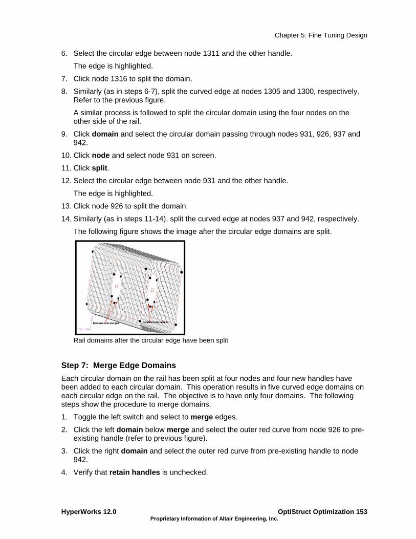
Chapter 5: Fine Tuning Design
HyperWorks 12.0 OptiStruct Optimization 153 Proprietary Information of Altair Engineering, Inc.
6. Select the circular edge between node 1311 and the other handle.
The edge is highlighted.
7. Click node 1316 to split the domain.
8. Similarly (as in steps 6-7), split the curved edge at nodes 1305 and 1300, respectively. Refer to the previous figure.
A similar process is followed to split the circular domain using the four nodes on the other side of the rail.
9. Click domain and select the circular domain passing through nodes 931, 926, 937 and 942.
10. Click node and select node 931 on screen.
11. Click split .
12. Select the circular edge between node 931 and the other handle.
The edge is highlighted.
13. Click node 926 to split the domain.
14. Similarly (as in steps 11-14), split the curved edge at nodes 937 and 942, respectively.
The following figure shows the image after the circular edge domains are split.
Rail domains after the circular edge have been split
Step 7: Merge Edge Domains
Each circular domain on the rail has been split at four nodes and four new handles have been added to each circular domain. This operation results in five curved edge domains on each circular edge on the rail. The objective is to have only four domains. The following steps show the procedure to merge domains.
1. Toggle the left switch and select to merge edges.
2. Click the left domain below merge and select the outer red curve from node 926 to pre-existing handle (refer to previous figure).
3. Click the right domain and select the outer red curve from pre-existing handle to node 942.
4. Verify that retain handles is unchecked.

Chapter 5: Fine Tuning Design
OptiStruct Optimization 154 HyperWorks 12.0 Proprietary Information of Altair Engineering, Inc.
5. Click merge .
Notice the pre-existing handle is removed.
6. Repeat steps 1 through 5 to merge two edge domains between node 1316 and node 1300 on the other side of the rail.
Rail domains after few domains are merged
Step 8: Build 2-D Domains on the Tube
1. In the Model Browser window, expand the Component .
2. Right-click on the component PSHELL.1 and click Show .
3. Toggle back the radio button to create .
4. Make sure the switch (small triangle) is selected to 2D domains .
5. Click elems and select by sets from the pop-up window.
6. Check the boxes for elem_set1 .
7. Click select .
8. Click create .
9. Repeat steps 5 through 8 to create three more 2-D domains for elements in sets elem_set2 , elem_set3 , and elem_set4 , respectively.
10. Click return and go back to the HyperMorph module.

Chapter 5: Fine Tuning Design
HyperWorks 12.0 OptiStruct Optimization 155 Proprietary Information of Altair Engineering, Inc.
Domains on Rail and Tube Joint
Step 9: Create Shapes
In this step, three shapes are created using the created domains and handles.
1. Click morph .
We use the alter dimensions subpanel in HyperMorph to modify the curvatures of selected edge domains.
2. Toggle to alter dimensions .
3. Toggle the right switch and select curve ratio .
4. Toggle center calculation and change the setting to by edges .
5. Toggle the switch below and select hold ends .
Holding two ends of a selected edge domain allows a change of curvature of the selected edge without altering its end points.
6. Leave the other settings with the defaults.
7. Under edges only , click domains and select red edge-domains as shown in the following figure. You might need to zoom in for easier picking operation.
8. Verify that a total of eight edge domains are selected and highlighted on screen.

Chapter 5: Fine Tuning Design
OptiStruct Optimization 156 HyperWorks 12.0 Proprietary Information of Altair Engineering, Inc.
Morph edge domains
9. Click curve ratio = and enter 20 .
10. Click morph .
A new curvature is applied to the selected eight edge domains. See the following figure below.
11. Toggle the radio button to save shape .
12. Click on shape = , enter the name sh1 .
13. Toggle as handle perturbation to as node perturbation .
14. Click on the color button and change the color of the shape vectors or leave the default color.
15. Click save .
Shape vectors (arrows) are created of the selected color.
16. Click undo all to prepare for the generation of the next shape.
17. Click the Model Browser tab, right-click on Shape and select Hide .
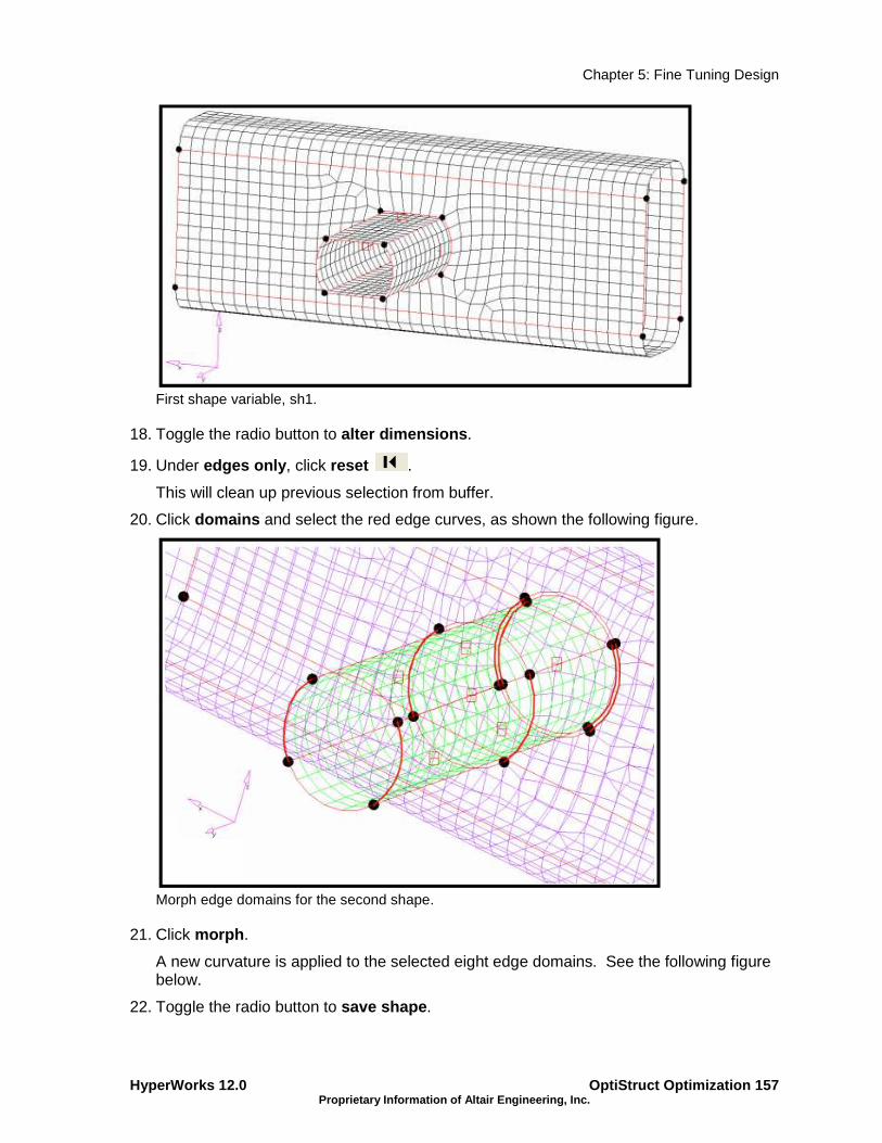
Chapter 5: Fine Tuning Design
HyperWorks 12.0 OptiStruct Optimization 157 Proprietary Information of Altair Engineering, Inc.
First shape variable, sh1.
18. Toggle the radio button to alter dimensions .
19. Under edges only , click reset .
This will clean up previous selection from buffer.
20. Click domains and select the red edge curves, as shown the following figure.
Morph edge domains for the second shape.
21. Click morph .
A new curvature is applied to the selected eight edge domains. See the following figure below.
22. Toggle the radio button to save shape .

Chapter 5: Fine Tuning Design
OptiStruct Optimization 158 HyperWorks 12.0 Proprietary Information of Altair Engineering, Inc.
23. Click on shape = , enter the name sh2 .
24. Toggle as handle perturbation to as node perturbation .
25. Click on the color button and change the color of the shape vectors or leave the default color.
26. Click save .
Shape vectors (arrows) are created of the selected color.
27. Click undo all to prepare for the generation of the next shape.
28. Click the Model Browser tab, right-click on Shape and select Hide .
Refer to the following figure for the new shape changes.
Second shape variable, sh2.
29. Toggle the radio button to apply shapes .
In HyperMorph, a new shape can be created as a linear combination of existing shapes.
30. Click shapes and select both sh1 and sh2 .
31. Click Select .
Verify that the multiplier is 1.0.
32. Click apply .
33. Toggle the radio button to save shapes .
34. Click shape = and enter sh3 .
35. Make sure that the toggle is set to node perturbations .
The new shape sh3 includes influences from both sh1 and sh2 shapes, as shown in the next figure.
36. Click save .
37. Click the Model Browser tab, right-click on Shape and select Hide .
Do NOT click undo all at this moment because we will create one more shape based on this third shape change.

Chapter 5: Fine Tuning Design
HyperWorks 12.0 OptiStruct Optimization 159 Proprietary Information of Altair Engineering, Inc.
The third shape variable, sh3, converts the tube to a square cross-section
An additional shape variable is created using the shape created in the previous step.
38. In the Model Browser window, right-click on the component PSHELL and select Hide .
These components are turned off for ease of visualization.
39. Toggle the radio button to alter dimensions .
40. Under edges only , click reset .
This will clean up previous selection from buffer.
41. Switch the top selector from curve ratio to distance = .
This feature allows you to shorten the distance between selected domains.
42. Switch the end a: selector from two handles to nodes and handles .
43. Click node a and pick node as shown in the next figure.
44. Click node b and pick node as shown in the next figure.

Chapter 5: Fine Tuning Design
OptiStruct Optimization 160 HyperWorks 12.0 Proprietary Information of Altair Engineering, Inc.
Setup for the fourth shape variable, sh4
Once nodes a and b are selected, the distance between node a and node b is measured automatically and appears in distance = field.
The distance between node a and node b is about 43.
45. Click handles under node a , and select the 8 handles shown by the downward pointing arrows in the previous figure.
To select, click the handles on the screen until they are highlighted.
46. Click handles under node b and similarly as in the previous step, select the 8 handles near the opposite face of the tube.
47. Toggle the bottom selector and select hold middle .
48. In the Model Browser window, right-click on the component PSHELL and click on Show .
These components are turned on for ease of visualization.
49. Click distance = and enter 20.
50. Click morph .
A rectangular shape appears to the joint as shown in the next figure.
51. Toggle the button to save shape .
52. Click shape = and enter sh4 .
53. Make sure that the toggle is set to node perturbations .
54. Click save .
55. Click undo all to restore the mesh to the baseline configuration.
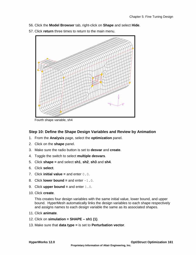
Chapter 5: Fine Tuning Design
HyperWorks 12.0 OptiStruct Optimization 161 Proprietary Information of Altair Engineering, Inc.
56. Click the Model Browser tab, right-click on Shape and select Hide .
57. Click return three times to return to the main menu.
Fourth shape variable, sh4
Step 10: Define the Shape Design Variables and Revi ew by Animation
1. From the Analysis page, select the optimization panel.
2. Click on the shape panel.
3. Make sure the radio button is set to desvar and create .
4. Toggle the switch to select multiple desvars .
5. Click shape = and select sh1 , sh2 , sh3 and sh4 .
6. Click select .
7. Click initial value = and enter 0.0 .
8. Click lower bound = and enter -1.0 .
9. Click upper bound = and enter 1.0 .
10. Click create .
This creates four design variables with the same initial value, lower bound, and upper bound. HyperMesh automatically links the design variables to each shape respectively and assigns names to each design variable the same as its associated shapes.
11. Click animate .
12. Click on simulation = SHAPE – sh1 (1) .
13. Make sure that data type = is set to Perturbation vector .

Chapter 5: Fine Tuning Design
OptiStruct Optimization 162 HyperWorks 12.0 Proprietary Information of Altair Engineering, Inc.
14. Click modal to animate the first shape variable.
15. Click next and then animate to see the next shape variable, and so forth.
16. Click return three times to return to the optimization panel.
Step 11: Create the Mass and Static Stress Response
1. Enter the responses panel.
2. Click response = and enter Mass.
3. Click on the response type switch and select mass from the pop-up menu.
4. Ensure the regional selection is set to total (this is the default).
5. Click create .
A response, mass, is defined for the total mass of the model.
6. Click response = and enter Stress .
7. Click on the response type switch and select static stress from the pop-up menu.
8. Click the props button and select the PSHELL.1 component which contains skin shells.
9. Do NOT select any element under excluding: .
10. Make sure that the toggle is selected to von Mises .
11. Toggle the bottom switch to select both surfaces .
12. Click create.
A response, Stress, is defined for the model.
13. Click return to go back to the optimization panel.
Step 12: Create Constraints on Stress Response
In this step we set the upper and lower bound constraint criteria for this analysis.
1. Enter the dconstraints panel.
2. Click constraint= and enter con .
3. Check the box for upper bound only.
4. Click upper bound= and enter 200 .
5. Select response= and set it to Stress .
6. Click loadsteps and check STEP.
7. Click select .
8. Click create .
9. Click return to the main menu.

Chapter 5: Fine Tuning Design
HyperWorks 12.0 OptiStruct Optimization 163 Proprietary Information of Altair Engineering, Inc.
Step 13: Define the Objective
1. Enter the objective panel.
2. The switch on the left should be set to min .
3. Click response= and select Mass .
4. Click create .
5. Click return to exit the optimization panel.
Step 14: Define Control Cards Required for Shape Op timization
Without this control card defined, optimization gets terminated by quality check and you do not get the converged results.
1. From the Analysis page, click the control cards panel.
2. Click the Next button twice and chose the PARAM card.
3. Check the box next to CHECKEL .
4. Click the YES button under CHECKEL_V1 to change to NO.
5. Click return twice.
Step 15: Run the Optimization Problem
1. From the Analysis page, enter the OptiStruct panel.
2. Click save as… , enter rail_joint_opt.fem as the file name , and click Save.
3. Click export options: switch and select All .
4. Click the run options: switch and select optimization .
5. Make sure the memory options: toggle is set to memory default .
6. Click OptiStruct to run the optimization.
The message …Processing complete appears in the window at the completion of the job. OptiStruct also reports error messages if any exist. The file carm_complete.out can be opened in a text editor to find details regarding any errors. This file is written to the same directory as the .fem file.
7. Close the DOS window or shell.
Step 16: Review the Shape Optimization Results
1. Once you see the message Process completed successfully in the command window, click the green HyperView button.
HyperView is launched and the results are loaded. A message window appears to inform about the successful loading of the model and result files into HyperView. Notice that all three .h3d files get loaded, each in a different page of HyperView.
2. Click Close to close the message window.

Chapter 5: Fine Tuning Design
OptiStruct Optimization 164 HyperWorks 12.0 Proprietary Information of Altair Engineering, Inc.
3. Rail_joint_opt_des.h3d will be opened in page 1 and Rail_joint_opt.h3d will be opened in page 2 of HyperView.
4. Click the Contour toolbar button.
Note the Result type: is Shape Change [v] ; this should be the only results type in the “file_name”_des.h3d file.
The second pull-down menu shows mag .
5. Click Apply to display the shape change.
Note the contour is all blue this is because your results are on the first design step or Iteration 0.
6. At the left of the GUI, use the drop-down selector list to change the iteration number from Iteration 0 to the last iteration .
Each element of the model is assigned a legend color, indicating the density of each element for the selected iteration.
Shape optimization results are applied to the model.
Shape change converged (Scale 2x)
Step 17: View a Contour Plot of the Stress on Top o f the Shape Optimized Model
1. Click the Next Page arrow in the toolbar to move to the next page.
2. Click the Contour toolbar button.
Note the Result type: is Element Stresses [2D & 3D] [t].
The second pull-down menu shows von Mises .
3. At the bottom of the GUI, click on the name Subcase 1 (STEP) <> Model Step to activate the Load Case and Simulation Selection dialog.
4. Select the last iteration by double-clicking on the last Iteration listed.
5. Click Apply .
The stress contour shows on top of the shape changes applied to the model. Verify that this value is around the constraint value specified.

Chapter 5: Fine Tuning Design
HyperWorks 12.0 OptiStruct Optimization 165 Proprietary Information of Altair Engineering, Inc.
Von Mises Stress for the last iteration (Max < 200 MPa)
Reviewing the Results
Is your design objective of minimizing the volume obtained? If not, can you explain why?
Are your design constraints satisfied?
Which shape has the most influence in this problem setup?
What is the percentage decrease in compliance?
Can size optimization be introduced to the joint?

Chapter 5: Fine Tuning Design
OptiStruct Optimization 166 HyperWorks 12.0 Proprietary Information of Altair Engineering, Inc.

Chapter 5: Fine Tuning Design
HyperWorks 12.0 OptiStruct Optimization 167 Proprietary Information of Altair Engineering, Inc.
3 – Free-shape Optimization Free-shape optimization uses a proprietary optimization technique developed by Altair Engineering Inc., wherein the outer boundary of a structure is altered to meet with pre-defined objectives and constraints. The essential idea of free-shape optimization, and where it differs from other shape optimization techniques, is that the allowable movement of the outer boundary is automatically determined, thus relieving users of the burden of defining shape perturbations.
Free-shape design regions are defined through the DSHAPE bulk data entry. Design regions are identified by the grids on the outer boundary of the structure (the edge of a shell structure or the surface of a solid structure). These grids are listed on the DSHAPE entry.
Free-shape optimization allows these design grids to move in one of two ways:
1. For shell structures; grids move normal to the surface edge in the tangential plane.
2. For solid structures; grids move normal to the surface.
During free-shape optimization, the normal directions change with the change in shape of the structure, thus for each iteration the design grids move along the updated normals.
3.1 – Defining Free-shape Design Regions
Ideally, free-shape design regions should be selected where it can be assumed that the shape of the structure is most sensitive to the concerned responses. For example, it would be appropriate to select grids in a high stress region when the objective is to reduce stress.
Free-shape design regions should be defined at different locations on the structure where it is desired for the shape to change independently. For solid structures, feature lines often define natural boundaries for free-shape design regions. Containing any feature lines inside a free-shape design region should be avoided unless the intention is to smooth the feature lines during an optimization. Likewise for a shell structure, sharp corners should not be contained inside a free-shape design region unless the intention is to smooth out such corners.
The DSHAPE card identifies the design region through the GRID continuation card, shown here:
(1) (2) (3) (4) (5) (6) (7) (8) (9) (10)
GRID GID1 GID2 GID3 GID4 GID5 GID6 GID7 GID8 GID9 … …

Chapter 5: Fine Tuning Design
OptiStruct Optimization 168 HyperWorks 12.0 Proprietary Information of Altair Engineering, Inc.
2D - A free-shape design region is defined on the curved edge of the plate by selecting the edge grids; the grids are free to move in the normal direction on the tangential plane.
3D - A free-shape design region is defined on a surface of the solid structure by selecting the face surface grids; the grids are free to move normal to the surface.
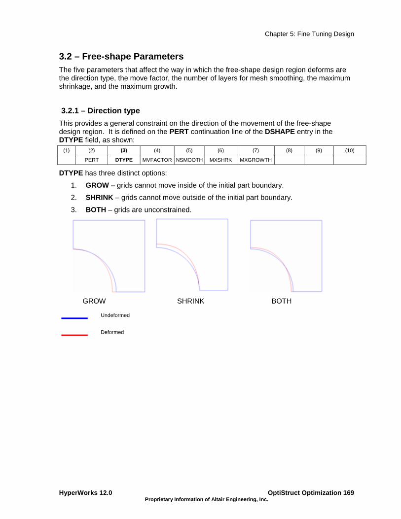
Chapter 5: Fine Tuning Design
HyperWorks 12.0 OptiStruct Optimization 169 Proprietary Information of Altair Engineering, Inc.
3.2 – Free-shape Parameters The five parameters that affect the way in which the free-shape design region deforms are the direction type, the move factor, the number of layers for mesh smoothing, the maximum shrinkage, and the maximum growth.
3.2.1 – Direction type
This provides a general constraint on the direction of the movement of the free-shape design region. It is defined on the PERT continuation line of the DSHAPE entry in the DTYPE field, as shown:
(1) (2) (3) (4) (5) (6) (7) (8) (9) (10)
PERT DTYPE MVFACTOR NSMOOTH MXSHRK MXGROWTH
DTYPE has three distinct options:
1. GROW – grids cannot move inside of the initial part boundary.
2. SHRINK – grids cannot move outside of the initial part boundary.
3. BOTH – grids are unconstrained.
GROW SHRINK BOTH
Undeformed
Deformed

Chapter 5: Fine Tuning Design
OptiStruct Optimization 170 HyperWorks 12.0 Proprietary Information of Altair Engineering, Inc.
3.2.2 – Move factor
The maximum allowable movement in one iteration of the grids defining a free-shape design region, is specified as:
MVFACTOR*mesh_size
where "mesh_size" is the average mesh size of the design region defined in the same DSHAPE card.
MVFACTOR is defined on the PERT continuation line of the DSHAPE entry. (1) (2) (3) (4) (5) (6) (7) (8) (9) (10)
PERT DTYPE MVFACTOR NSMOOTH MXSHRK MXGROWTH
The default value of MVFACTOR is 0.5. A smaller MVFACTOR will make free-shape optimization run slower but with more stability. Conversely, a larger MVFACTOR will make free-shape optimization run faster but with less stability.
MVFACTOR affects the maximum movement in one iteration.
Undeformed shape
Shape at iteration 1 with MVFACTOR = 0.5(default)
Shape at iteration 1 with MVFACTOR = 1.0
3.2.3 – Number of layers for mesh smoothing
With free-shape optimization, internal grids adjacent to those grids defining the design region are moved to avoid mesh distortion. The number of layers of grids to be included in the mesh smoothing buffer may be defined by the NSMOOTH field on the PERT continuation line of the DSHAPE entry.

Chapter 5: Fine Tuning Design
HyperWorks 12.0 OptiStruct Optimization 171 Proprietary Information of Altair Engineering, Inc.
(1) (2) (3) (4) (5) (6) (7) (8) (9) (10)
PERT DTYPE MVFACTOR NSMOOTH MXSHRK MXGROWTH
The default value of NSMOOTH is 10. A larger NSMOOTH will give a larger smoothing buffer, and consequently will work better in avoiding mesh distortion; however, it will result in a slower optimization.
NSMOOTH=5, 5 layers of grids move along with the design boundary.
NSMOOTH=1, only 1 layer of grids move along with the design boundary.
3.2.4 – Maximum shrinkage and growth
The maximum shrinkage and growth provide a simple way to limit the total amount of deformation of the free-shape design region. These parameters are defined on the PERT continuation line of the DSHAPE entry. (1) (2) (3) (4) (5) (6) (7) (8) (9) (10)
PERT DTYPE MVFACTOR NSMOOTH MXSHRK MXGROWTH

Chapter 5: Fine Tuning Design
OptiStruct Optimization 172 HyperWorks 12.0 Proprietary Information of Altair Engineering, Inc.
The design region is offset to form two barriers; MXSHRK is the offset in the shrinkage direction and MXGROWTH is the offset in the growth direction. The design region is then constrained to deform between these two barriers.
Deformation space defined by the maximum growing/shrinking distance
3.2.5 – Constraints on Grids in the Design Region
It is possible to identify additional constraints on certain grids in free-shape design regions. Three types of constraints are available for specified grids as defined by CTYPE# on the GRIDCON continuation line of the DSHAPE entry:
1. FIXED – grid cannot move due to free-shape optimization.
2. VECTOR – grid is forced to move along the specified vector.
3. PLANAR – grid is forced to remain on a plane for which the specified vector defines the normal direction.
Note: VECTOR is used to constrain a grid to move along a line, thus it makes no difference by rotating the vector by 180 degrees.
Constraints are defined on the GRIDCON continuation line as follows: (1) (2) (3) (4) (5) (6) (7) (8) (9) (10)
GRIDCON GCMETH GCSETID1 / GDID1
CTYPE1 CID1 X1 Y1 Z1
GCMETH GCSETID2 / GDID2
CTYPE2 CID2 X2 Y2 Z2

Chapter 5: Fine Tuning Design
HyperWorks 12.0 OptiStruct Optimization 173 Proprietary Information of Altair Engineering, Inc.
Example showing CTYPE = VECTOR
This example demonstrates a simple case where it is necessary to use the "DIR" constraint type to force grids to move in a predefined direction.
A free-shape optimization is performed on a quarter model of a rectangular plate with a hole, as shown here:
The curved edge is the free-shape design region. Without any constraints on the free-shape design region, the grids at the ends of the curved edge do not move exactly along the line of the straight edge, but move slightly outward, as shown here:
In order to prevent this phenomenon, the grids at the ends of the curved edge (shown in yellow below) are both constrained to move along the vector indicated by the red arrows.

Chapter 5: Fine Tuning Design
OptiStruct Optimization 174 HyperWorks 12.0 Proprietary Information of Altair Engineering, Inc.
Using these constraints - corner grids moving along the constrained direction - the grids at the ends of the curved edge now move as desired, along the line of the straight edge, as shown here:

Chapter 5: Fine Tuning Design
HyperWorks 12.0 OptiStruct Optimization 175 Proprietary Information of Altair Engineering, Inc.
Exercise 5e - Free-shape Optimization of a Compress or Bracket
In this exercise, shape optimization on a solid model will be performed using the free-shape optimization method along with manufacturing constraints, such as symmetry and mesh barrier constraints. The objective of this optimization is to reduce the stress by changing the geometry of the model.
Problem Statement
Objective: Minimize mass
Constraint: Maximum von Mises stress of the joint < 62 MPa
Design variables: Shape variables normal to the node set selected

Chapter 5: Fine Tuning Design
OptiStruct Optimization 176 HyperWorks 12.0 Proprietary Information of Altair Engineering, Inc.
Step 1: Launch HyperMesh, Set the User Profile, and Retrieve the Model
1. Launch HyperMesh Desktop .
2. Choose OptiStruct in the User Profile dialog and click OK.
This loads the user profile. It includes the appropriate template, macro menu, and import reader, paring down the functionality of HyperMesh to what is relevant for generating models in Bulk Data Format for OptiStruct.
User Profiles… can also be accessed from the Preferences pull-down menu on the toolbar.
3. Select the Open Model… panel toolbar button.
4. Select the freeshape3d_mfg.hm file.
5. Click Open .
The freeshape3D_mfg.hm database is loaded into the current HyperMesh session, replacing any existing data. Note the location of freeshape3D_mfg.hm now displays in the file: field.
Step 2: Create Free-shape Design Variables (DSHAPE Cards)
1. From the Analysis page, click optimization .
2. Click free shape .
3. In the Create sub-panel, click on desvar= , and enter shape .
4. Click on nodes and select by sets check the box next to shape_nodes click on select.
Free-shape design space
5. Click create .
6. Click on the parameters subpanel and check the box for options and select the direction as grow , mvfactor at 0.5 and nsmooth as 10 and click update .

Chapter 5: Fine Tuning Design
HyperWorks 12.0 OptiStruct Optimization 177 Proprietary Information of Altair Engineering, Inc.
7. Click return twice to exit the panel.
Step 3: Convert the existing shell elements to crea te the Barrier Mesh Face (BMFACE)
1. Go to the 2D page.
2. Enter the elem types panel.
3. Click on elems to get the extended entity list.
4. Select by collector .
5. Check the box next to barrier .
6. On 2D& 3D subpanel, click on CTRIA3 in the field next to tria3 .
7. Select BMFACE from the list of options.
8. Click on CQUAD4 in the field next to quad4.
9. Select BMFACE from the list of options.
10. Click update .
Step 4: Define the 1-Plane Symmetry Constraint
The manufacturing constraint options for free-shape are: (Draw direction constraint, Extrusion constraint, Pattern grouping: 1-plane symmetry constraint, Maximum growing/shrinking distance control, Side constraint, and Mesh barrier constraint)
In this exercise we will define the 1-plane symmetry constraint and mesh barrier constraint.
1. From the Analysis page, click optimization .
2. Click free shape ; make sure that the desvar selected is set to shape .
3. Click on pattern grouping in the free shape panel.
4. Select the pattern type: 1-pln sym .
The 1-plane symmetry constraints in free-shape will produce symmetric designs regardless of the initial mesh, boundary conditions or loads. The plane of symmetry is defined by specifying the anchor and the first nodes. The plane of symmetry will then be perpendicular to the vector from the anchor node to the first node and pass through the anchor node.
5. Click anchor node and input the node id= 2 and press Enter .
This selects the node with the ID of 2.
6. Click first node and input the node id= 1.

Chapter 5: Fine Tuning Design
OptiStruct Optimization 178 HyperWorks 12.0 Proprietary Information of Altair Engineering, Inc.
This selects the node with the ID of 1.
7. Click the update button to update the design variables.
This completes the definition of the symmetry constraint.
Defining 1-plane symmetry
Step 5: Define the Mesh Barrier (sidecon) Constrain t
A mesh barrier constraint allows control on the total deformation extent of a design boundary/surface; mesh barrier will constrain the design boundary/surface to deform within the restricted design space and never penetrate the barrier.
The barrier should be constructed by shell elements with the smallest number of elements possible.
For this exercise, the mesh barrier was already created and the component name is barrier .
1. Click on sidecon in the free shape panel.
2. Click on desvar = and select shape .
3. Click on Barrier mesh: component= and select barrier from the list.
4. Click update .
5. Click return to go back to the main menu.

Chapter 5: Fine Tuning Design
HyperWorks 12.0 OptiStruct Optimization 179 Proprietary Information of Altair Engineering, Inc.
Mesh barrier component
Step 6: Define Responses for Optimization
1. Click on responses panel.
2. Enter Stress in the response= field.
3. Set the response type to static stress .
4. Switch from props to elems and click on elems button and click by sets .
5. Check the box next to stress and click select .
6. Choose von mises and click create .
7. Click response= and assign mass .
8. Set the response type: to mass .
9. Click create .
10. Click return to go back to the optimization panel.
Step 7: Define Constraints for Optimization
1. Select the dconstraints panel.
2. Click constraint= and type the name stress .
3. Click response= select stress .
4. Activate upper bound = and assign a value 62 .
5. Click on loadsteps , activate ls2 , and click select .

Chapter 5: Fine Tuning Design
OptiStruct Optimization 180 HyperWorks 12.0 Proprietary Information of Altair Engineering, Inc.
6. Click create .
7. Click return .
Step 8: Define the Objective Function
1. Choose the objective panel.
2. Click the left-most toggle and select min .
3. Click response= and select mass .
4. Click create .
5. Click return twice to go back to the main menu.
Step 9: Define the SHAPE Card
Only displacement and stress results are available in the _s#.h3d file by default. In order to look at stress results on top of a shape change that was applied to the model in HyperView, a SHAPE card needs to be defined.
1. From the Analysis page, select the control cards panel.
2. Click the green next button three times and select SHAPE.
3. Set format to h3d and both TYPE and OPTION to ALL .
4. Click return twice to go back to the main menu.
Step 10: Run the optimization
1. From Analysis page, click OptiStruct .
2. Click save as… following the input file: field.
3. Select the directory where you would like to write the OptiStruct model file and enter the name for the model, freeshape3d_mfgopt.fem , in the File name: field.
4. Click Save.
Note that the name and location of the freeshape3d_mfgopt.fem file is displayed in the input file: field.
5. Set the export options toggle to all .
6. Click the run options switch and select optimization.
7. Set the memory options toggle to memory default .
8. Click OptiStruct .
This launches an OptiStruct run in a separate (DOS or UNIX) shell.
If the optimization was successful, no error messages are reported to the shell. The optimization is complete when the line Processing complete appears in the shell.

Chapter 5: Fine Tuning Design
HyperWorks 12.0 OptiStruct Optimization 181 Proprietary Information of Altair Engineering, Inc.
Step 11: View Shape Results
1. While in the OptiStruct panel of the Analysis page, click the green HyperView button.
Note that the message window pops up to indicate that the files freeshape3d_mfgopt_des.h3d and freeshape3d_mfgopt_s4.h3d are opened.
2. Click Close to close the window.
freeshape3d_mfgopt_des.h3d will be opened in page 1 and freeshape3d_mfgopt_s4.h3d will be opened in page 2 of HyperView.
3. Click the Next Page arrow to move to page 2.
4. From Graphics menu, click on Select Load Case .
This will bring up the Load Case and Simulation Selection dialog which is also accessible from the lower right portion of the status bar.
5. Select Iteration14 from beneath Simulation (load final iteration results).
6. Click OK.
7. Go to the Deformed panel .
8. Set the Result type: to Shape change(v).
9. Click Apply .
Shape optimization results are applied to the model.
Step 12: View a Contour Plot of the Stress on Top o f the Shape Optimized Model
1. Go to the Contour panel and select Element Stresses (2D & 3D) (t) as the Result type: .
2. Select von Mises as the stress type .
3. Click on Elements and click By set and pick the set stress click on Add and close .
4. Click Apply .

Chapter 5: Fine Tuning Design
OptiStruct Optimization 182 HyperWorks 12.0 Proprietary Information of Altair Engineering, Inc.
Von Mises Stress contour on Final shape
1. Is your design objective of minimizing the mass obtained? If not, can you explain why?
2. Are your design constraints satisfied?

Chapter 5: Fine Tuning Design
HyperWorks 12.0 OptiStruct Optimization 183 Proprietary Information of Altair Engineering, Inc.
Exercise 5f - Shape Optimization of a 3-D Bracket u sing the Free-shape Method In this exercise, shape optimization on a solid bracket model will be performed using the Free-Shape optimization method. The objective of this optimization is to reduce the stress by changing the geometry of the bracket model.
The essential idea of free-shape optimization, and where it differs from other shape optimization techniques, is that the allowable movement of the outer boundary is automatically determined, thus relieving users of the burden of defining shape perturbations.
The optimization problem for this tutorial is stated as:
Objective: Minimize (Max Von Mises Stress)
Constraints: No Constraints
Design variables: Grids move normal to the surface.
Problem Setup
You should copy this file: free_shape3D.hm

Chapter 5: Fine Tuning Design
OptiStruct Optimization 184 HyperWorks 12.0 Proprietary Information of Altair Engineering, Inc.
Step 1: Set the User Profile and Retrieve the File
1. Launch HyperMesh Desktop .
2. Choose OptiStruct as the User Profile and click OK.
This loads the user profile. It includes the appropriate template, macro menu, and import reader, paring down the functionality of HyperMesh to what is relevant for generating models in Bulk Data Format for OptiStruct .
User Profiles… can also be accessed from the Preferences menu on the toolbar.
3. Select the Open Model… panel toolbar button.
4. Select the free_shape3D.hm file, located in the HyperWorks installation directory under <install_directory>/tutorials/hwsolvers/optistruct/ .
5. Click Open .
The free_shape3D.hm database is loaded into the current HyperMesh session, replacing any existing data. Note the location of free_shape3D.hm now displays in the file: field.
6. Click return to go to the main menu.
Step 2: Create Free-shape Design Variables (DSHAPE Cards)
1. From the Analysis page, click on optimization .
2. Select the free shape panel.
3. Click name= and enter shape .
4. Select nodes shown in the figure (select only the face nodes that are also on shells).
Free-shape design space
5. Click create .
6. Click return to go to the main menu.

Chapter 5: Fine Tuning Design
HyperWorks 12.0 OptiStruct Optimization 185 Proprietary Information of Altair Engineering, Inc.
Step 3: Define the Optimization Responses
1. Select responses panel.
2. Enter Stress in the response= field.
3. Set the response type to static stress .
4. Click the prop button and select the stress_faces component which contains skin shells.
5. Click on the button below von mises and select both surfaces .
6. Click create .
7. Click return to go back to the optimization panel.
Step 4: Define the Objective Reference
1. Click obj reference .
2. Enter MAX_STR in the dobjref= field.
3. Check pos reference ; this gives the value 1.0 .
4. Click response and select stress .
5. Click create .
6. Click return to go back to the optimization panel.
Step 5: Define the Objective Function
1. Choose the objective panel.
2. Click the left-most toggle and select minmax .
3. Click dobjrefs and select MAX_STR.
4. Click create .
5. Click return twice to go back to main menu.
Step 6: Define the SHAPE Card
Only displacement and stress results are available in the _s#.h3d file by default. In order to look at stress results on top of a shape change that was applied to the model in HyperView, a SHAPE card needs to be defined.
1. From the Analysis page, select the control cards panel.
2. Select SHAPE.
3. Use the green next button to see more cards.
4. Set both TYPE and OPTION to ALL .
5. Click return twice to go back to the main menu.

Chapter 5: Fine Tuning Design
OptiStruct Optimization 186 HyperWorks 12.0 Proprietary Information of Altair Engineering, Inc.
Step 7: Run the optimization.
1. From Analysis page, click the OptiStruct .
2. Click save as… following the input file: field.
3. Select the directory where you would like to write the OptiStruct model file and enter the name for the model, Free_Shape3D.fem , in the File name: field.
4. Click Save.
Note that the name and location of the Free_Shape3D.fem file is displayed in the input file: field.
5. Set the memory options toggle to memory default .
6. Click the run options switch and select optimization .
7. Set the export options toggle to all .
8. Click OptiStruct .
This launches an OptiStruct run in a separate (DOS or UNIX) shell.
If the optimization was successful, no error messages are reported to the shell. The optimization is complete when the line Processing complete appears in the shell.
Post-process the Free-shape Optimization Results.
This section describes how to view the results in HyperView which will be launched from within the OptiStruct panel of HyperMesh.
HyperView is a complete post-processing and visualization environment for finite element analysis (FEA), multi-body system simulation, video and engineering data.
Step 8: View Shape Results
1. While in the OptiStruct panel of the Analysis page, click the green HyperView button.
Note that the message window pops up to indicate that Free_Shape3D_des.h3d and Free_Shape3D.h3d are opened.
2. Click Close to close the Message Log window.
Free_Shape3D_des.h3d will be opened in page 1 and Free_Shape3D.h3d will be opened in page 2 of HyperView.
3. Click to move to page 2.
4. From the Graphics menu, click on Select Load Case .
This will bring up the Load Case and Simulation Selection dialog which is also accessible from the lower right portion of the status bar.
5. Select Iteration6 from Simulation (load final iteration results).
6. Click OK.
7. Go to the Deformed panel .

Chapter 5: Fine Tuning Design
HyperWorks 12.0 OptiStruct Optimization 187 Proprietary Information of Altair Engineering, Inc.
8. Set the Result type: to Shape change .
9. Click Apply .
Shape optimization results are applied to the model.
Step 9: View a Contour Plot of the Stress on Top of the Shape Optimized Model
1. Go to the Contour panel and select Element Stresses [2D & 3D] as the Result type:.
2. Select von Mises as the stress type .
3. Click Apply .
The stress contour shows on top of the shape changes applied to the model.

Chapter 5: Fine Tuning Design
OptiStruct Optimization 188 HyperWorks 12.0 Proprietary Information of Altair Engineering, Inc.
Setup a New Free-shape Optimization Simulation with Moving Constraints.
In the previous run, no constraints were applied on the movement of the DSHAPE grids. Therefore, grids are free to move and the part thickness increases as shown in the figure below.
Free-shape results without constraints
In practice, however, there will be some sort of constraints imposed upon the movement of grids due to manufacturability. For this tutorial model, thickness must be unchanged to avoid any interference with other parts.
The next step will describe how to define constraints on DSHAPE grids such that the thickness of design space will remain unchanged.
Step 10: Add Constraints on DSHAPE Grids
The constraints on free-shape design grids will be created separately for curved and flat parts of the design space. The parts of the design space that are grouped as curved and those grouped as flat are illustrated in the figure below.

Chapter 5: Fine Tuning Design
HyperWorks 12.0 OptiStruct Optimization 189 Proprietary Information of Altair Engineering, Inc.
Design space on curved and flat part
The constraints on the curved part will be created using a local rectangular coordinate system (the other constraints on the flat part do not need a local coordinate system). Therefore, a local rectangular coordinate system (z-axis will point to normal to DSHAPE surface) needs to be created first.
1. Back in HyperMesh , click return and go to 1D page.
2. Click systems .
3. Choose the create by axis direction subpanel.
4. Click nodes and select node ID 20999 (See the following figure).
5. Click origin and select the same node (ID 20999) as nodes .
6. Click x-axis and select node ID 15989.
7. Click xy-plane and select node ID 19462.
Local coordinate system
8. Click create .

Chapter 5: Fine Tuning Design
OptiStruct Optimization 190 HyperWorks 12.0 Proprietary Information of Altair Engineering, Inc.
9. Click return .
10. From the Analysis page, click on optimization .
11. Select the free shape panel.
12. Select the gridcon subpanel.
The constraints on the flat part will be created first without any coordinate system.
13. Click desvar= and select shape .
14. Select constraint type as planar .
15. Select nodes shown in the following figure.
Constraints on Free Shape design space
16. Click the vector definition switch and select vectors .
17. Select N1, N2, N3 as those three nodes on plane geometry (as shown in the figure below).

Chapter 5: Fine Tuning Design
HyperWorks 12.0 OptiStruct Optimization 191 Proprietary Information of Altair Engineering, Inc.
Three nodes to defined the plane
18. Click add .
These nodes will move only on the specified plane above. Next, the constraints on the curved part will be created using a local coordinate system.
19. Select constraint type as vector .
20. Click nodes .
21. Select nodes shown in the following figure (select only the nodes that are on the curved part).
Constraints on free-shape design space on curved part
22. Click the direction selector and select local system .
23. Select the local coordinate system created in the previous step.
24. Click the vector definition switch and select vector .

Chapter 5: Fine Tuning Design
OptiStruct Optimization 192 HyperWorks 12.0 Proprietary Information of Altair Engineering, Inc.
25. Click the direction definition switch below vector , and select z-axis from the pop-up menu.
26. Click add .
27. Click return twice to get back to the main menu.
Step 11: Re-run the model
1. From the Analysis page, click OptiStruct .
2. Click save as… following the input file: field.
3. Select the directory where you would like to write the OptiStruct model file and enter the name for the model, Free_Shape3D_const.fem , in the File name: field.
4. Click Save.
Note that the name and location of the Free_Shape3D_const.fem file is displayed in the input file: field.
5. Set the memory options toggle to memory default .
6. Click the run options switch and select optimization .
7. Set the export options toggle to all .
8. Click OptiStruct .
Step 12: Post-process the New Free-shape Optimizati on Results.
Follow the previously described steps on how to post-process the results (optimization results without constraints) using HyperView, and compare the final shape change and stress results.

APPENDIX A: Composite Exercise
HyperWorks 12.0 OptiStruct Optimization 193 Proprietary Information of Altair Engineering, Inc.
APPENDIX A
Topology Optimization Exercises using Solid Thinking Inspire

APPENDIX A: Composite Exercise
OptiStruct Optimization 194 HyperWorks 12.0 Proprietary Information of Altair Engineering, Inc.
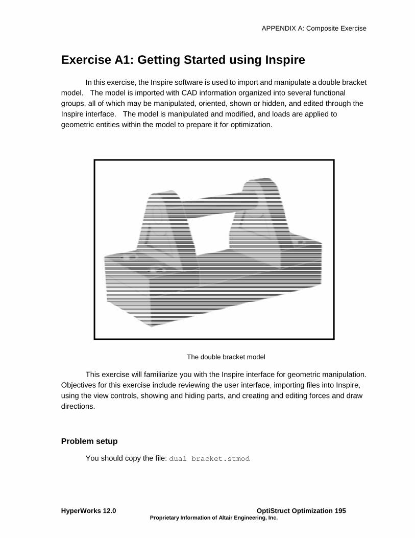
HyperWorks 12.0 Proprietary Information of Altair Engineering, Inc.
Exercise A1: Getting Started using Inspire
In this exercise, the Inspire software is used to import and manipulate model. The model is imported with CAD information organized into several functional groups, all of which may be manipulated, oriented, shown or hidden, and edited through the Inspire interface. The model is manipulated and modified, and geometric entities within the model to prepare it for optimization.
This exercise will familiarize you with the Inspire interface for geometric manipulation. Objectives for this exercise include reviewing tusing the view controls, showing and hiding parts, and creating and editing forces and draw directions.
Problem setup
You should copy the file:
APPENDIX A: Composite
OptiStruct OptimizationProprietary Information of Altair Engineering, Inc.
1: Getting Started using Inspire
In this exercise, the Inspire software is used to import and manipulate model. The model is imported with CAD information organized into several functional groups, all of which may be manipulated, oriented, shown or hidden, and edited through the Inspire interface. The model is manipulated and modified, and loads are applied to geometric entities within the model to prepare it for optimization.
The double bracket model
This exercise will familiarize you with the Inspire interface for geometric manipulation. Objectives for this exercise include reviewing the user interface, importing files into Inspire,
iew controls, showing and hiding parts, and creating and editing forces and draw
You should copy the file: dual bracket.stmod
Composite Exercise
OptiStruct Optimization 195
In this exercise, the Inspire software is used to import and manipulate a double bracket model. The model is imported with CAD information organized into several functional groups, all of which may be manipulated, oriented, shown or hidden, and edited through the
loads are applied to
This exercise will familiarize you with the Inspire interface for geometric manipulation. mporting files into Inspire,
iew controls, showing and hiding parts, and creating and editing forces and draw

APPENDIX A: Composite Exercise
OptiStruct Optimization 196 Proprietary Information of Altair
Step 1: Open the Dual Bracket Model
1. Start Inspire.
2. The toolbar across the top of the application displays all of the tools available in
cursor moves over the various icons in the group, they glow with a yellow border.
3. Click the folder in the Files icon group on the f
4. In the Open File window, browse to the
5. Select the dual bracket.stmod file from the
HyperWorks 12.0Proprietary Information of Altair Engineering, Inc.
Step 1: Open the Dual Bracket Model
The toolbar across the top of the application displays all of the tools available in Inspire
cursor moves over the various icons in the group, they glow with a yellow border.
icon group on the far left of the toolbar.
window, browse to the class model directory.
file from the class model directory.
HyperWorks 12.0
Inspire. As the
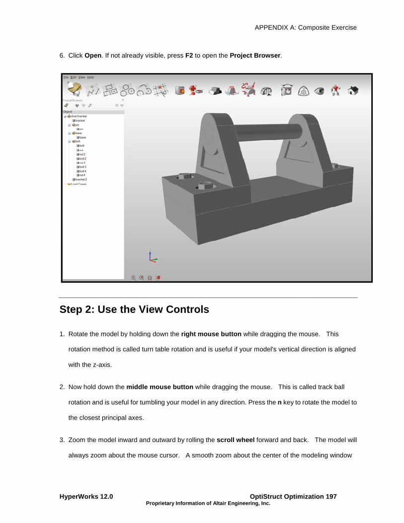
HyperWorks 12.0 Proprietary Information of Altair Engineering, Inc.
6. Click Open. If not already visible, press
Step 2: Use the View Controls
1. Rotate the model by holding down the
rotation method is called turn table rotation
with the z-axis.
2. Now hold down the middle mouse button
rotation and is useful for tumbling your model in any direction. Press the
the closest principal axes.
3. Zoom the model inward and outward by rolling the
always zoom about the mouse cursor. A smooth zoom about the center of the modeling window
APPENDIX A: Composite
OptiStruct OptimizationProprietary Information of Altair Engineering, Inc.
. If not already visible, press F2 to open the Project Browser.
the View Controls
Rotate the model by holding down the right mouse button while dragging the mouse. This
turn table rotation and is useful if your model's vertical direction is aligned
iddle mouse button while dragging the mouse. This is called
and is useful for tumbling your model in any direction. Press the n key to rotate the model to
Zoom the model inward and outward by rolling the scroll wheel forward and back. The model will
always zoom about the mouse cursor. A smooth zoom about the center of the modeling window
Composite Exercise
OptiStruct Optimization 197
while dragging the mouse. This
and is useful if your model's vertical direction is aligned
while dragging the mouse. This is called track ball
key to rotate the model to
forward and back. The model will
always zoom about the mouse cursor. A smooth zoom about the center of the modeling window

APPENDIX A: Composite Exercise
OptiStruct Optimization 198 Proprietary Information of Altair
can be performed by pressing the
and down.
4. Fit the model by clicking the Fit All
the F key. If parts are selected, clicking the
into the selected parts. Pressing the
pressing F repeatedly with different parts selected to see the effect.
5. Pan the model by holding both the
Press the c key to center the model.
Step 3: Show and Hide Parts
You can show and hide parts by using the
1. Move the mouse over the Show/Hide
icon. These icons reveal additional functi
2. Left-click on the Show/Hide tool, the red cube to the left of the main icon.
3. The icon will glow and the mouse cursor will change to
mode.
4. Left-click one or more parts in the modeling window. The parts turn transparent as you select them,
and are grayed out in the Project Browser
HyperWorks 12.0Proprietary Information of Altair Engineering, Inc.
can be performed by pressing the Alt key and the middle mouse button while sliding the mouse up
Fit All icon in the lower left corner of the application, or by pressing
key. If parts are selected, clicking the Fit Selected icon or pressing the F
into the selected parts. Pressing the F key again will zoom out to show the entire model. Try
repeatedly with different parts selected to see the effect.
Pan the model by holding both the Shift key and the right mouse button while moving the mouse.
key to center the model.
d Hide Parts
You can show and hide parts by using the Show/Hide icon in the toolbar or with keyboard shortcuts.
Show/Hide icon group. New icons appear to the left and right of the main
icon. These icons reveal additional functionality, while keeping the main toolbar uncluttered.
tool, the red cube to the left of the main icon.
The icon will glow and the mouse cursor will change to , indicating that you are in show/hide
click one or more parts in the modeling window. The parts turn transparent as you select them,
Project Browser.
HyperWorks 12.0
while sliding the mouse up
icon in the lower left corner of the application, or by pressing
F key will zoom
out to show the entire model. Try
while moving the mouse.
icon in the toolbar or with keyboard shortcuts.
icon group. New icons appear to the left and right of the main
onality, while keeping the main toolbar uncluttered.
, indicating that you are in show/hide
click one or more parts in the modeling window. The parts turn transparent as you select them,

HyperWorks 12.0 Proprietary Information of Altair Engineering, Inc.
5. Right-click to exit the show/hide mode. The selected objects are hidden in the modeling window.
APPENDIX A: Composite
OptiStruct OptimizationProprietary Information of Altair Engineering, Inc.
click to exit the show/hide mode. The selected objects are hidden in the modeling window.
Composite Exercise
OptiStruct Optimization 199
click to exit the show/hide mode. The selected objects are hidden in the modeling window.

APPENDIX A: Composite Exercise
OptiStruct Optimization 200 Proprietary Information of Altair
6. To show parts that are hidden, select the
7. Click on a transparent part while holding down the
pressed, the cursor changes to
HyperWorks 12.0Proprietary Information of Altair Engineering, Inc.
show parts that are hidden, select the Show/Hide tool again to enter show/hide mode.
Click on a transparent part while holding down the Shift key. Note that while the Shift
.
HyperWorks 12.0
tool again to enter show/hide mode.
Shift key is

HyperWorks 12.0 Proprietary Information of Altair Engineering, Inc.
8. Click on the remaining transparent parts, then right
APPENDIX A: Composite
OptiStruct OptimizationProprietary Information of Altair Engineering, Inc.
transparent parts, then right-click to exit the show/hide mode.
Composite Exercise
OptiStruct Optimization 201
click to exit the show/hide mode.

APPENDIX A: Composite Exercise
OptiStruct Optimization 202 Proprietary Information of Altair
9. To isolate a part, click on it in the modeling window, and then click the
Show/Hide icon group.
• To hide all parts in the model, hover over the
satellite icon.
HyperWorks 12.0Proprietary Information of Altair Engineering, Inc.
To isolate a part, click on it in the modeling window, and then click the Isolate eyeball icon in the
To hide all parts in the model, hover over the Show/Hide icon group and select the
HyperWorks 12.0
eyeball icon in the
icon group and select the Hide All

HyperWorks 12.0 Proprietary Information of Altair Engineering, Inc.
• To reverse which parts are shown and hidden, hover over the
the Reverse All satellite icon.
10. Using keyboard shortcuts is another way you can show, hide, or isolate
• Show all of the parts by pressing the
• Hide parts by selecting them and pressing the
• Isolate parts by selecting them and pressing the
Step 4: Apply a Force and Draw Direction
1. Isolate one of the brackets in the model by selecting it and pressing the
APPENDIX A: Composite
OptiStruct OptimizationProprietary Information of Altair Engineering, Inc.
To reverse which parts are shown and hidden, hover over the Show/Hide icon group and select
satellite icon.
Using keyboard shortcuts is another way you can show, hide, or isolate parts.
Show all of the parts by pressing the A key.
Hide parts by selecting them and pressing the H key.
Isolate parts by selecting them and pressing the I key.
Step 4: Apply a Force and Draw Direction
Isolate one of the brackets in the model by selecting it and pressing the I key.
Composite Exercise
OptiStruct Optimization 203
icon group and select

APPENDIX A: Composite Exercise
OptiStruct Optimization 204 Proprietary Information of Altair
HyperWorks 12.0Proprietary Information of Altair Engineering, Inc.
HyperWorks 12.0

HyperWorks 12.0 Proprietary Information of Altair Engineering, Inc.
2. Create a distributed force by clicking the
toolbar.
3. Move the mouse cursor over the front face of the bracket and left
4. A mini-toolbar will appear when creating or editing forces. Enter
+/- button to change the direction of the f
APPENDIX A: Composite
OptiStruct OptimizationProprietary Information of Altair Engineering, Inc.
Create a distributed force by clicking the Apply Forces tool in the Loads icon group in the main
Move the mouse cursor over the front face of the bracket and left-click to apply a distributed force.
toolbar will appear when creating or editing forces. Enter 45 N in the text field and press the
button to change the direction of the force.
Composite Exercise
OptiStruct Optimization 205
icon group in the main
click to apply a distributed force.
in the text field and press the

APPENDIX A: Composite Exercise
OptiStruct Optimization 206 Proprietary Information of Altair
5. Now, create a draw direction on the bracket by left
Controls icon. (You'll learn more about draw directions in later tutorials.)
6. Click the Singe Draw Direction
7. Left-click the bracket. A blue plane appears with four corner arrows pointing toward the front of the
bracket, indicating the draw direction (the direction the mold will be pulled away from the part).
HyperWorks 12.0Proprietary Information of Altair Engineering, Inc.
Now, create a draw direction on the bracket by left-clicking the Draw Direction tool on the
icon. (You'll learn more about draw directions in later tutorials.)
tool.
t. A blue plane appears with four corner arrows pointing toward the front of the
bracket, indicating the draw direction (the direction the mold will be pulled away from the part).
HyperWorks 12.0
tool on the Shape
t. A blue plane appears with four corner arrows pointing toward the front of the
bracket, indicating the draw direction (the direction the mold will be pulled away from the part).

HyperWorks 12.0 Proprietary Information of Altair Engineering, Inc.
8. Right-click on empty space or press
APPENDIX A: Composite
OptiStruct OptimizationProprietary Information of Altair Engineering, Inc.
click on empty space or press Esc to exit the tool.
Composite Exercise
OptiStruct Optimization 207

APPENDIX A: Composite Exercise
OptiStruct Optimization 208 Proprietary Information of Altair
Step 5: Edit the Force and Draw Direction
Once objects have been created, it is easy to create more objects of the same type or edit those objects by double-clicking on them in the modeling window.
1. Double-click the blue plane to edit the parting direction. Yo
mini-toolbar appears.
2. Click on one of the grey planes to activate it and change the orientation of the draw direction.
HyperWorks 12.0Proprietary Information of Altair Engineering, Inc.
Edit the Force and Draw Direction
Once objects have been created, it is easy to create more objects of the same type or edit clicking on them in the modeling window.
click the blue plane to edit the parting direction. You are now in edit mode, and a
Click on one of the grey planes to activate it and change the orientation of the draw direction.
HyperWorks 12.0
Once objects have been created, it is easy to create more objects of the same type or edit
u are now in edit mode, and a
Click on one of the grey planes to activate it and change the orientation of the draw direction.
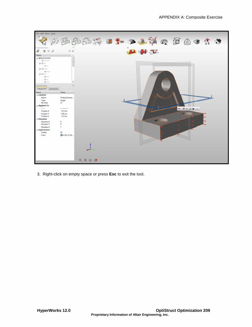
HyperWorks 12.0 Proprietary Information of Altair Engineering, Inc.
3. Right-click on empty space or press
APPENDIX A: Composite
OptiStruct OptimizationProprietary Information of Altair Engineering, Inc.
click on empty space or press Esc to exit the tool.
Composite Exercise
OptiStruct Optimization 209

APPENDIX A: Composite Exercise
OptiStruct Optimization 210 Proprietary Information of Altair
4. Double-click one of the red force
toolbar reappears.
HyperWorks 12.0Proprietary Information of Altair Engineering, Inc.
click one of the red force arrows on the front face. You are now in edit mode, and a mini
HyperWorks 12.0
arrows on the front face. You are now in edit mode, and a mini

HyperWorks 12.0 Proprietary Information of Altair Engineering, Inc.
5. You can edit the force by entering a magnitude in the text field, or change its direction by pressing
the +/-, X, Y, Z and buttons. You can also create more forces by
below:
APPENDIX A: Composite
OptiStruct OptimizationProprietary Information of Altair Engineering, Inc.
You can edit the force by entering a magnitude in the text field, or change its direction by pressing
buttons. You can also create more forces by selecting another face, as shown
Composite Exercise
OptiStruct Optimization 211
You can edit the force by entering a magnitude in the text field, or change its direction by pressing
selecting another face, as shown

APPENDIX A: Composite Exercise
OptiStruct Optimization 212 Proprietary Information of Altair
6. Right-click on empty space or press
You have completed your first lesson in
HyperWorks 12.0Proprietary Information of Altair Engineering, Inc.
click on empty space or press Esc to exit the tool.
You have completed your first lesson in Inspire.
HyperWorks 12.0

HyperWorks 12.0 Proprietary Information of Altair Engineering, Inc.
Exercise A2: Topology Optimization Using Multiple
Load Cases in Inspire
The Inspire software can be used to perform loadwithout the need for meshing, giving designers and analysts a quick technique for generating optimized shapes for a given set of load paths. This exercise builds upon topicspracticed within the previous exercise which include files into Inspire, using the view controls, showing and hiding parts, and creating and editing forces and draw directions.
This exercise will showcase using Inspire to create unit load cases, apply symmetry planes, create forces and supports, apply symmetry planes, create single draw direction pattern grouping, run an optimization, and explore the shapes generated by t
Problem setup
You should copy the file:
APPENDIX A: Composite
OptiStruct OptimizationProprietary Information of Altair Engineering, Inc.
: Topology Optimization Using Multiple
Inspire
The Inspire software can be used to perform load-normalized topology optimization without the need for meshing, giving designers and analysts a quick technique for generating optimized shapes for a given set of load paths. This exercise builds upon topicspracticed within the previous exercise which include reviewing the user interface,
iew controls, showing and hiding parts, and creating and editing
The Y-bracket model in Inspire
This exercise will showcase using Inspire to create unit load cases, apply symmetry reate forces and supports, apply symmetry planes, create single draw direction
pattern grouping, run an optimization, and explore the shapes generated by t
You should copy the file: y-bracket.stmod
Composite Exercise
OptiStruct Optimization 213
: Topology Optimization Using Multiple
normalized topology optimization without the need for meshing, giving designers and analysts a quick technique for generating optimized shapes for a given set of load paths. This exercise builds upon topics and skills
he user interface, importing iew controls, showing and hiding parts, and creating and editing
This exercise will showcase using Inspire to create unit load cases, apply symmetry reate forces and supports, apply symmetry planes, create single draw direction
pattern grouping, run an optimization, and explore the shapes generated by the solution run.

APPENDIX A: Composite Exercise
OptiStruct Optimization 214 HyperWorks 12.0 Proprietary Information of Altair Engineering, Inc.
Step 1: Open the Y-bracket Model
1. Start Inspire.
2. Click the folder in the Files icon group on the toolbar.
3. In the Open File window, browse to the course model directory.
4. Select the y-bracket.stmod file from the course model directory.
5. Click Open. If not already visible, press F2 and F3 to open the Project Browser and Property
Editor.
6. Use the right mouse button to adjust the view so that the y-bracket is positioned, as shown below:

HyperWorks 12.0 Proprietary Information of Altair Engineering, Inc.
Step 2: Define the Design Space
1. If it is not already open, select
APPENDIX A: Composite
OptiStruct OptimizationProprietary Information of Altair Engineering, Inc.
Step 2: Define the Design Space
If it is not already open, select View > Project Browser to open the Project Browser
Composite Exercise
OptiStruct Optimization 215
Project Browser.

APPENDIX A: Composite Exercise
OptiStruct Optimization 216 Proprietary Information of Altair
2. In the y-bracket folder, two parts are listed
in the Project Browser to select it. The three cylindrical holes in the bracket turn yellow. While we will
be placing loads and supports on the boss materials, we do not want to subtract any material from
this part during optimization, so we do not want to include it in the design space.
3. In the y-bracket folder, right-click on
HyperWorks 12.0Proprietary Information of Altair Engineering, Inc.
folder, two parts are listed — Boss Materials and Bracket. Click on Boss Materials
in the Project Browser to select it. The three cylindrical holes in the bracket turn yellow. While we will
be placing loads and supports on the boss materials, we do not want to subtract any material from
zation, so we do not want to include it in the design space.
click on Bracket and select Design Space.
HyperWorks 12.0
Boss Materials
in the Project Browser to select it. The three cylindrical holes in the bracket turn yellow. While we will
be placing loads and supports on the boss materials, we do not want to subtract any material from

HyperWorks 12.0 Proprietary Information of Altair Engineering, Inc.
4. Click on an empty space in the modeling window. The red
material will be carved from during optimization.
APPENDIX A: Composite
OptiStruct OptimizationProprietary Information of Altair Engineering, Inc.
Click on an empty space in the modeling window. The red-brown color indicates the area that
arved from during optimization.
Composite Exercise
OptiStruct Optimization 217
brown color indicates the area that

APPENDIX A: Composite Exercise
OptiStruct Optimization 218 Proprietary Information of Altair
Step 3: Create the First Load Case Using the Project
Browser
1. In the Project Browser, right-click on the
2. A new load case appears in the Load Cases
that you can rename it.
HyperWorks 12.0Proprietary Information of Altair Engineering, Inc.
Step 3: Create the First Load Case Using the Project
click on the Load Cases folder and select New > Load Case
Load Cases folder, and the text field is automatically highlighted so
HyperWorks 12.0
Step 3: Create the First Load Case Using the Project
New > Load Case.
folder, and the text field is automatically highlighted so

HyperWorks 12.0 Proprietary Information of Altair Engineering, Inc.
3. Rename the load case "Load Case X" and press
bold, indicating that it is the current
added to it automatically.
Step 4: Create a Center Hole Support
1. Select the Apply Supports tool from the
2. Click on the front boss material to apply the support.
APPENDIX A: Composite
OptiStruct OptimizationProprietary Information of Altair Engineering, Inc.
Rename the load case "Load Case X" and press Enter. The name of the load cases is shown in
current load case. Any new loads or supports that you create will be
Step 4: Create a Center Hole Support
tool from the Loads icon group.
Click on the front boss material to apply the support.
Composite Exercise
OptiStruct Optimization 219
. The name of the load cases is shown in
s that you create will be

APPENDIX A: Composite Exercise
OptiStruct Optimization 220 Proprietary Information of Altair
3. In the Project Browser, Support 1
X, as it is the current load case.
4. Right-click or press Esc to exit the tool.
Step 5: Apply Forces to Boss Materials
HyperWorks 12.0Proprietary Information of Altair Engineering, Inc.
Support 1 is added to the All Loads and Supports folder and to
to exit the tool.
Step 5: Apply Forces to Boss Materials
HyperWorks 12.0
folder and to Load Case

HyperWorks 12.0 Proprietary Information of Altair Engineering, Inc.
1. Select the Apply Forces tool from the
2. Click on one of the rear boss materials to apply the force.
3. The force is initially applied in the negative X direction. Click the
it to the positive X direction.
APPENDIX A: Composite
OptiStruct OptimizationProprietary Information of Altair Engineering, Inc.
tool from the Loads icon group.
Click on one of the rear boss materials to apply the force.
The force is initially applied in the negative X direction. Click the +/- icon in the mini toolbar to reverse
Composite Exercise
OptiStruct Optimization 221
icon in the mini toolbar to reverse

APPENDIX A: Composite Exercise
OptiStruct Optimization 222 Proprietary Information of Altair
4. Force 1 appears in the Project Browser in b
X.
HyperWorks 12.0Proprietary Information of Altair Engineering, Inc.
appears in the Project Browser in both the All Loads and Supports folder and
HyperWorks 12.0
folder and Load Case
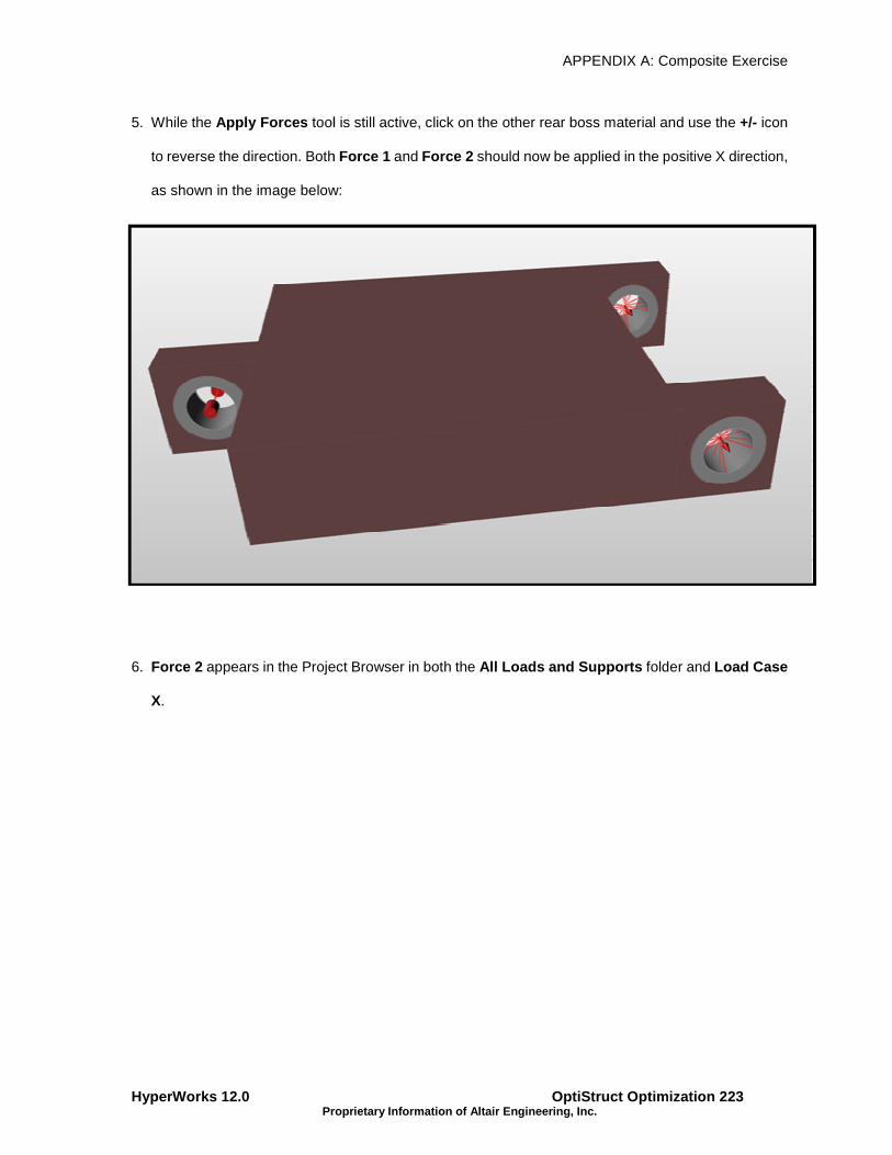
HyperWorks 12.0 Proprietary Information of Altair Engineering, Inc.
5. While the Apply Forces tool is still active, click on the other rear boss material and use the
to reverse the direction. Both
as shown in the image below:
6. Force 2 appears in the Project Browser in both the
X.
APPENDIX A: Composite
OptiStruct OptimizationProprietary Information of Altair Engineering, Inc.
tool is still active, click on the other rear boss material and use the
to reverse the direction. Both Force 1 and Force 2 should now be applied in the positive X direction,
as shown in the image below:
appears in the Project Browser in both the All Loads and Supports folder and
Composite Exercise
OptiStruct Optimization 223
tool is still active, click on the other rear boss material and use the +/- icon
should now be applied in the positive X direction,
folder and Load Case

APPENDIX A: Composite Exercise
OptiStruct Optimization 224 Proprietary Information of Altair
7. Right-click or press Esc to exit the tool.
Step 6: Create the Seco
Menu
1. In the Project Browser, right-click on
HyperWorks 12.0Proprietary Information of Altair Engineering, Inc.
to exit the tool.
Step 6: Create the Second Load Case Using the Context
click on Load Case X and select New > Load Case.
HyperWorks 12.0
nd Load Case Using the Context

HyperWorks 12.0 Proprietary Information of Altair Engineering, Inc.
2. A new load case is added in the
Enter. This is now the current load
APPENDIX A: Composite
OptiStruct OptimizationProprietary Information of Altair Engineering, Inc.
A new load case is added in the Project Browser. Rename the load case "Load Case Y" and press
. This is now the current load case.
Composite Exercise
OptiStruct Optimization 225
. Rename the load case "Load Case Y" and press

APPENDIX A: Composite Exercise
OptiStruct Optimization 226 Proprietary Information of Altair
3. We want to use the same support from Load Case X in Load Case Y, so right
the All Loads and Supports Folder
Load Case Y.
HyperWorks 12.0Proprietary Information of Altair Engineering, Inc.
We want to use the same support from Load Case X in Load Case Y, so right-click on
All Loads and Supports Folder in the Project Browser and select Include in Load Cases >
HyperWorks 12.0
click on Support 1 in
Include in Load Cases >

HyperWorks 12.0 Proprietary Information of Altair Engineering, Inc.
4. Support 1 is added to Load Case Y
APPENDIX A: Composite
OptiStruct OptimizationProprietary Information of Altair Engineering, Inc.
Load Case Y in the Project Browser.
Composite Exercise
OptiStruct Optimization 227

APPENDIX A: Composite Exercise
OptiStruct Optimization 228 Proprietary Information of Altair
5. Click the icons next to Force 1 and
the modeling window.
HyperWorks 12.0Proprietary Information of Altair Engineering, Inc.
and Force 2 in the Project Browser to temporarily hide these forces in
HyperWorks 12.0
in the Project Browser to temporarily hide these forces in

HyperWorks 12.0 Proprietary Information of Altair Engineering, Inc.
6. Select the Apply Forces tool from the
7. Add two more forces, one to each of
toolbar, click the Y and then click the
8. Force 3 and Force 4 have been added to
APPENDIX A: Composite
OptiStruct OptimizationProprietary Information of Altair Engineering, Inc.
tool from the Loads icon group.
Add two more forces, one to each of the rear boss materials in the negative Y direction. In the mini
and then click the +/- icon to reverse the direction.
have been added to Load Case Y in the Project Browser.
Composite Exercise
OptiStruct Optimization 229
the rear boss materials in the negative Y direction. In the mini

APPENDIX A: Composite Exercise
OptiStruct Optimization 230 Proprietary Information of Altair
9. Right-click or press Esc to exit the tool.
Step 7: Create the Third Load Case by
Clicking-and-Dragging
1. In the Project Browser, right-click on
HyperWorks 12.0Proprietary Information of Altair Engineering, Inc.
xit the tool.
Step 7: Create the Third Load Case by
Dragging
click on Load Case Y and select New > Load Case.
HyperWorks 12.0

HyperWorks 12.0 Proprietary Information of Altair Engineering, Inc.
2. Rename the load case "Load Case Z" and press
APPENDIX A: Composite
OptiStruct OptimizationProprietary Information of Altair Engineering, Inc.
Rename the load case "Load Case Z" and press Enter. This is now the current load case.
Composite Exercise
OptiStruct Optimization 231
. This is now the current load case.

APPENDIX A: Composite Exercise
OptiStruct Optimization 232 Proprietary Information of Altair
3. Click on Support 1 in the All Loads and Supports Folder
Load Case Z.
HyperWorks 12.0Proprietary Information of Altair Engineering, Inc.
All Loads and Supports Folder in the Project Browser and drag it to
HyperWorks 12.0
in the Project Browser and drag it to

HyperWorks 12.0 Proprietary Information of Altair Engineering, Inc.
4. Click the icons next to Force 3
in the modeling window.
APPENDIX A: Composite
OptiStruct OptimizationProprietary Information of Altair Engineering, Inc.
Force 3 and Force 4 in the Project Browser to temporarily hide these forces
Composite Exercise
OptiStruct Optimization 233
to temporarily hide these forces

APPENDIX A: Composite Exercise
OptiStruct Optimization 234 Proprietary Information of Altair
5. Select the Apply Forces tool from the
6. Add two more forces, one to each of the rear boss materials in the positive Z direction. In the mini
toolbar, click the Z to set the direction.
HyperWorks 12.0Proprietary Information of Altair Engineering, Inc.
tool from the Loads icon group.
Add two more forces, one to each of the rear boss materials in the positive Z direction. In the mini
to set the direction.
HyperWorks 12.0
Add two more forces, one to each of the rear boss materials in the positive Z direction. In the mini

HyperWorks 12.0 Proprietary Information of Altair Engineering, Inc.
7. Force 5 and Force 6 have been added to
APPENDIX A: Composite
OptiStruct OptimizationProprietary Information of Altair Engineering, Inc.
have been added to Load Case Y in the Project Browser
Composite Exercise
OptiStruct Optimization 235
Project Browser.

APPENDIX A: Composite Exercise
OptiStruct Optimization 236 Proprietary Information of Altair
8. Right-click or press Esc to exit the tool.
9. Click the Show All button at the top of the
forces applied to the model. Select the part and hold down the
transparent.
HyperWorks 12.0Proprietary Information of Altair Engineering, Inc.
to exit the tool.
button at the top of the Project Browser to display all of the loads and
forces applied to the model. Select the part and hold down the Command key to make it
HyperWorks 12.0
to display all of the loads and
key to make it

HyperWorks 12.0 Proprietary Information of Altair Engineering, Inc.
Step 8: Add Symmetry Planes
1. Select the Symmetry tool from the
2. Select the Symmetric tool from the toolbar.
3. Click on the bracket in the modeling window to select it. Three red symmetry planes
APPENDIX A: Composite
OptiStruct OptimizationProprietary Information of Altair Engineering, Inc.
Step 8: Add Symmetry Planes
tool from the Shape Controls icon group. A toolbar appears.
tool from the toolbar.
Click on the bracket in the modeling window to select it. Three red symmetry planes
Composite Exercise
OptiStruct Optimization 237
icon group. A toolbar appears.
Click on the bracket in the modeling window to select it. Three red symmetry planes appear.

APPENDIX A: Composite Exercise
OptiStruct Optimization 238 Proprietary Information of Altair
4. Shape Control 1 is added to the
HyperWorks 12.0Proprietary Information of Altair Engineering, Inc.
is added to the Shape Controls folder in the Project Browser.
HyperWorks 12.0

HyperWorks 12.0 Proprietary Information of Altair Engineering, Inc.
5. Click the plane in the Y direction to deselect it. The plane turns gray.
6. Press Esc or right-click to exit the tool.
APPENDIX A: Composite
OptiStruct OptimizationProprietary Information of Altair Engineering, Inc.
Click the plane in the Y direction to deselect it. The plane turns gray.
click to exit the tool.
Composite Exercise
OptiStruct Optimization 239

APPENDIX A: Composite Exercise
OptiStruct Optimization 240 Proprietary Information of Altair
Step 9: Add a Draw Direction
1. Select the Draw Direction tool from the
2. Select the Split Draw Direction
3. Click on the bracket in the modeling window to select it. Three planes appear; the blue plane
indicates the currently selected parting plane.
4. Parting Direction 1 is added to the
HyperWorks 12.0Proprietary Information of Altair Engineering, Inc.
Step 9: Add a Draw Direction
tool from the Shape Controls icon group. A toolbar appears.
tool from the toolbar.
Click on the bracket in the modeling window to select it. Three planes appear; the blue plane
indicates the currently selected parting plane.
is added to the Shape Controls folder in the Project Browser.
HyperWorks 12.0
icon group. A toolbar appears.
Click on the bracket in the modeling window to select it. Three planes appear; the blue plane

HyperWorks 12.0 Proprietary Information of Altair Engineering, Inc.
5. Press Esc or right-click to exit the tool.
Step 10: Run Optimization
1. Click the Run Optimization
APPENDIX A: Composite
OptiStruct OptimizationProprietary Information of Altair Engineering, Inc.
ick to exit the tool.
Step 10: Run Optimization
icon to open the Run Optimization window.
Composite Exercise
OptiStruct Optimization 241
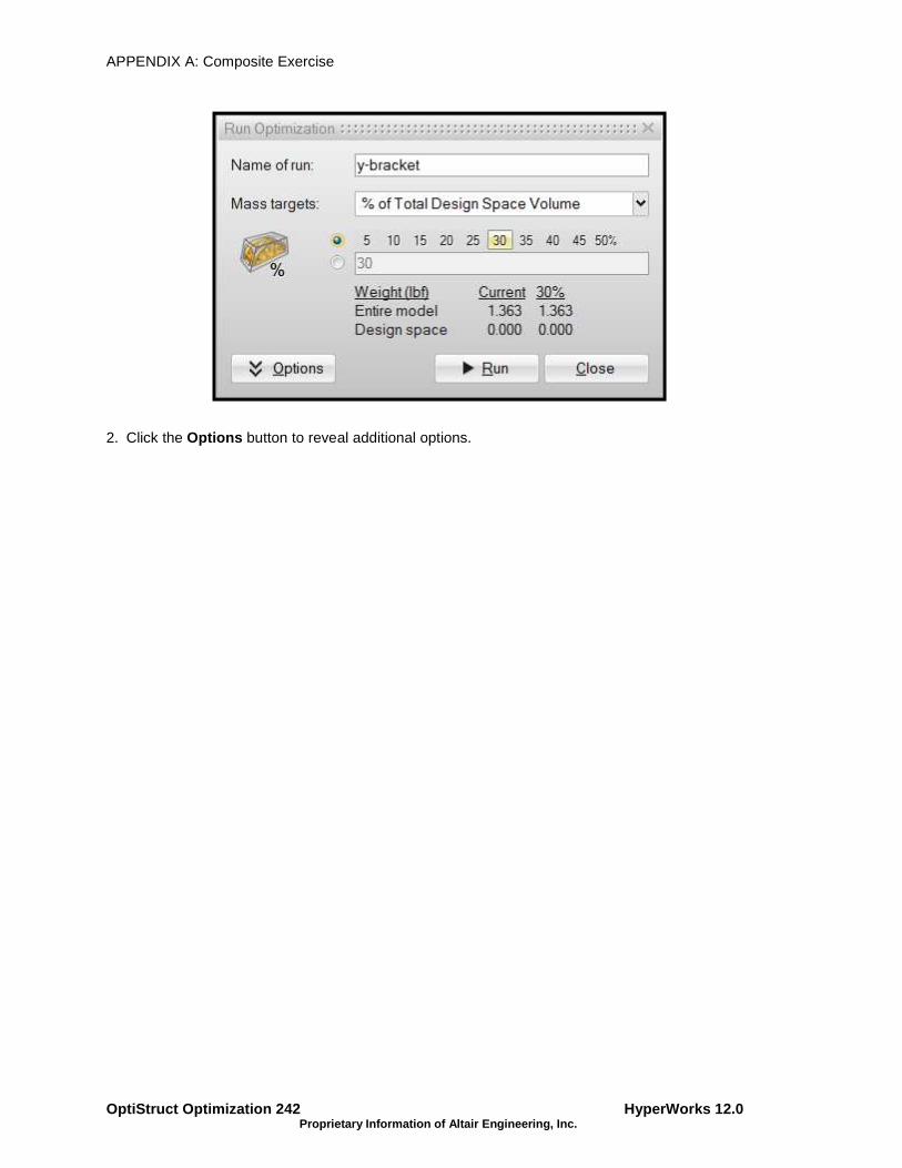
APPENDIX A: Composite Exercise
OptiStruct Optimization 242 Proprietary Information of Altair
2. Click the Options button to reveal additional options.
HyperWorks 12.0Proprietary Information of Altair Engineering, Inc.
button to reveal additional options.
HyperWorks 12.0

HyperWorks 12.0 Proprietary Information of Altair Engineering, Inc.
3. Under Mass targets, select
choose 30 percent.
4. Under Thickness control, change the
APPENDIX A: Composite
OptiStruct OptimizationProprietary Information of Altair Engineering, Inc.
, select % of Total Design Space Volume from the drop down menu and
, change the Minimum to 0.3 in. (This will speed up the optimization.)
Composite Exercise
OptiStruct Optimization 243
from the drop down menu and
. (This will speed up the optimization.)
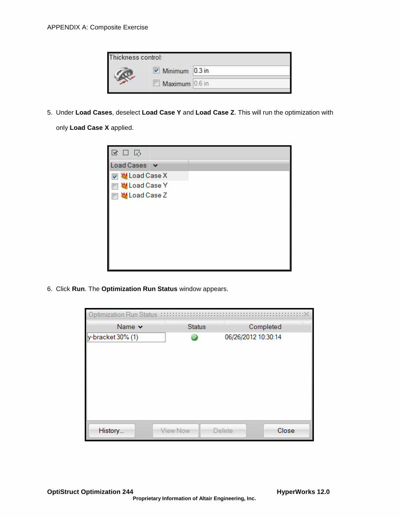
APPENDIX A: Composite Exercise
OptiStruct Optimization 244 Proprietary Information of Altair
5. Under Load Cases, deselect Load Case Y
only Load Case X applied.
6. Click Run. The Optimization Run Status
HyperWorks 12.0Proprietary Information of Altair Engineering, Inc.
Load Case Y and Load Case Z. This will run the optimization with
Optimization Run Status window appears.
HyperWorks 12.0
. This will run the optimization with

HyperWorks 12.0 Proprietary Information of Altair Engineering, Inc.
7. Click on the name of the run and then the
shape is displayed.
8. Click on the part to open the
the original part, with a (1) after the part name to indicate it was the first optimization run.
9. Repeat the above procedure to run an optimization for
APPENDIX A: Composite
OptiStruct OptimizationProprietary Information of Altair Engineering, Inc.
Click on the name of the run and then the View Now button to view the results. The optimized
Click on the part to open the Shape Explorer. The optimized shape is listed as an alternative to
the original part, with a (1) after the part name to indicate it was the first optimization run.
Repeat the above procedure to run an optimization for Load Case Y.
Composite Exercise
OptiStruct Optimization 245
button to view the results. The optimized
ed shape is listed as an alternative to
the original part, with a (1) after the part name to indicate it was the first optimization run.

APPENDIX A: Composite Exercise
OptiStruct Optimization 246 Proprietary Information of Altair
10. Repeat the above procedure to run an optimization for
11. The optimization runs for Load Case Y
in the Project Browser and the
HyperWorks 12.0Proprietary Information of Altair Engineering, Inc.
Repeat the above procedure to run an optimization for Load Case Z.
Load Case Y and Load Case Z now appear as additional alternatives
and the Shape Explorer.
HyperWorks 12.0
now appear as additional alternatives

HyperWorks 12.0 Proprietary Information of Altair Engineering, Inc.
Step 11: Explore Optimized Shapes
1. Now run the optimization one more time using all three load cases simultaneously. Click the
Optimization icon to open the
APPENDIX A: Composite
OptiStruct OptimizationProprietary Information of Altair Engineering, Inc.
Step 11: Explore Optimized Shapes
Now run the optimization one more time using all three load cases simultaneously. Click the
icon to open the Run Optimization window, and select all three load cases.
Composite Exercise
OptiStruct Optimization 247
Now run the optimization one more time using all three load cases simultaneously. Click the Run
window, and select all three load cases.

APPENDIX A: Composite Exercise
OptiStruct Optimization 248 Proprietary Information of Altair
2. Click Run. The Optimization Run Status
3. Click the Close button. When the optimization is complete, a green flag appears above the
Optimization icon, indicating that the run completed successfully.
4. Click the green flag to view the optimized shape.
HyperWorks 12.0Proprietary Information of Altair Engineering, Inc.
Optimization Run Status window appears.
button. When the optimization is complete, a green flag appears above the
icon, indicating that the run completed successfully.
Click the green flag to view the optimized shape.
HyperWorks 12.0
button. When the optimization is complete, a green flag appears above the Run

HyperWorks 12.0 Proprietary Information of Altair Engineering, Inc.
5. Click on the part to open the
optimized shape. Changing the topology adds and subtracts material, giving you an idea of how this
impacts the shape. Notice that as you drag the slider to the right, additional structures emerge. This
indicates that you need to re
APPENDIX A: Composite
OptiStruct OptimizationProprietary Information of Altair Engineering, Inc.
Click on the part to open the Shape Explorer, and drag the Topology slider to explore the
optimized shape. Changing the topology adds and subtracts material, giving you an idea of how this
impacts the shape. Notice that as you drag the slider to the right, additional structures emerge. This
indicates that you need to re-run the optimization with a higher percentage of material.
Composite Exercise
OptiStruct Optimization 249
slider to explore the
optimized shape. Changing the topology adds and subtracts material, giving you an idea of how this
impacts the shape. Notice that as you drag the slider to the right, additional structures emerge. This
run the optimization with a higher percentage of material.

APPENDIX A: Composite Exercise
OptiStruct Optimization 250 Proprietary Information of Altair
6. Click the Run Optimization icon to open the
7. Under Mass targets, change the
8. Under Thickness control, change the
HyperWorks 12.0Proprietary Information of Altair Engineering, Inc.
icon to open the Run Optimization window.
, change the % of Total Design Space Volume to 40 percent.
, change the Minimum to 0.4 in.
HyperWorks 12.0

HyperWorks 12.0 Proprietary Information of Altair Engineering, Inc.
9. Click Run. When the optimization is complete, click the green flag to view the optimized shape.
10. The result is improved, but still not optimal.
11. Try running optimization again, this time with a
This should produce a result similar to the one below:
APPENDIX A: Composite
OptiStruct OptimizationProprietary Information of Altair Engineering, Inc.
. When the optimization is complete, click the green flag to view the optimized shape.
The result is improved, but still not optimal.
Try running optimization again, this time with a % of Total Design Space Volume
This should produce a result similar to the one below:
Composite Exercise
OptiStruct Optimization 251
. When the optimization is complete, click the green flag to view the optimized shape.
% of Total Design Space Volume to 45 percent.

APPENDIX A: Composite Exercise
OptiStruct Optimization 252 Proprietary Information of Altair
Step 12: Change the Design Space and Re
1. Click the Switch to Design Space
2. Select the Push/Pull Faces tool.
HyperWorks 12.0Proprietary Information of Altair Engineering, Inc.
Step 12: Change the Design Space and Re-run Optimization
Switch to Design Space icon on the Shape Explorer.
tool.
HyperWorks 12.0
run Optimization

HyperWorks 12.0 Proprietary Information of Altair Engineering, Inc.
3. Right-click-and-drag to reposition the model, then left
2.75 inches to make the design space asymmetric.
4. Right-click-and-drag to reposition
inches.
APPENDIX A: Composite
OptiStruct OptimizationProprietary Information of Altair Engineering, Inc.
drag to reposition the model, then left-click on the right front face and push it inward
2.75 inches to make the design space asymmetric.
drag to reposition the model, then left-click on the rear face and push it inward 1.25
Composite Exercise
OptiStruct Optimization 253
click on the right front face and push it inward
click on the rear face and push it inward 1.25

APPENDIX A: Composite Exercise
OptiStruct Optimization 254 Proprietary Information of Altair
5. Right click on press Esc to exit the
6. Right-click-and-drag to reposition the model, then double
activate the Symmetric tool.
7. Click on the red plane in the Z direction to deactivate it.
HyperWorks 12.0Proprietary Information of Altair Engineering, Inc.
to exit the Push/Pull Faces tool.
drag to reposition the model, then double-click one of the red symmetry planes, to
Click on the red plane in the Z direction to deactivate it.
HyperWorks 12.0
click one of the red symmetry planes, to

HyperWorks 12.0 Proprietary Information of Altair Engineering, Inc.
8. Right-click or press Esc to exit the tool.
APPENDIX A: Composite
OptiStruct OptimizationProprietary Information of Altair Engineering, Inc.
to exit the tool.
Composite Exercise
OptiStruct Optimization 255

APPENDIX A: Composite Exercise
OptiStruct Optimization 256 Proprietary Information of Altair
9. Re-run optimization with all three load cases active and a
percent. This should produce a result similar to the one below:
10. Click on the part to open the Shape Explorer
shape.
HyperWorks 12.0Proprietary Information of Altair Engineering, Inc.
run optimization with all three load cases active and a % of Total Design Space Volume
duce a result similar to the one below:
Shape Explorer, and adjust the Topology to explore the optimized
HyperWorks 12.0
% of Total Design Space Volume to 45
to explore the optimized

APPENDIX B: Composite Exercise
HyperWorks 12.0 OptiStruct Optimization 257 Proprietary Information of Altair Engineering, Inc.
APPENDIX B
Composite Shell Element Optimization
Composite Exercise

APPENDIX B: Composite Exercise
OptiStruct Optimization 258 HyperWorks 12.0 Proprietary Information of Altair Engineering, Inc.

APPENDIX B: Composite Exercise
HyperWorks 12.0 OptiStruct Optimization 259 Proprietary Information of Altair Engineering, Inc.
Exercise B1: Optimizing a Plate with Hole Test
Coupon (PCOMPP-STACK-PLY)
For this example we need to design a cantilever beam made with composites plies that can have angles 0, 45, -45 and 90 degrees. It needs to support an in-plane force at middle of the unconstrained end.
This is an optimization-driven design of a test coupon subjected to an in-plane load, where:
o The objective is to determine the minimum mass
o Max Disp. < 3.00e-01.
o Parameters (PLATE) laminate definition
o Min of each family (ANGLE) → 10% (PPMIN)
o Manufacturable thickness (in) → 0.05 (PTMAN)
o BALANCED 45 AND -45 FAMILIES.
To achieve this optimum design we will introduce you to the process called “Optimization Driven Design for Composite”, which is divided in 3 phases:
o PHASE I - Free Size Optimization, (Ply topology)
o PHASE II - Size Optimization (Thickness and number of plies)

APPENDIX B: Composite Exercise
OptiStruct Optimization 260 HyperWorks 12.0 Proprietary Information of Altair Engineering, Inc.
o PHASE III – Shuffle Optimization (Stacking Sequence).
Model Information:
• PCOMP with 4 plies 0, 45, -45 and 90
• Geometry:
o (L = 20, h = 10, t = 0.2 mm)
• Load case:
o Force = 1N
• Material:
E1 = 1.3e5 MPa E2 = E3 = 9850 MPa
υ12 = υ13 = 0.3 υ23 = 0.36 - G12 = G13 = 3450 MPa G23 = 3100 MPa
Problem Setup
Copy the file plate_with_hole_opti_phase1.hm
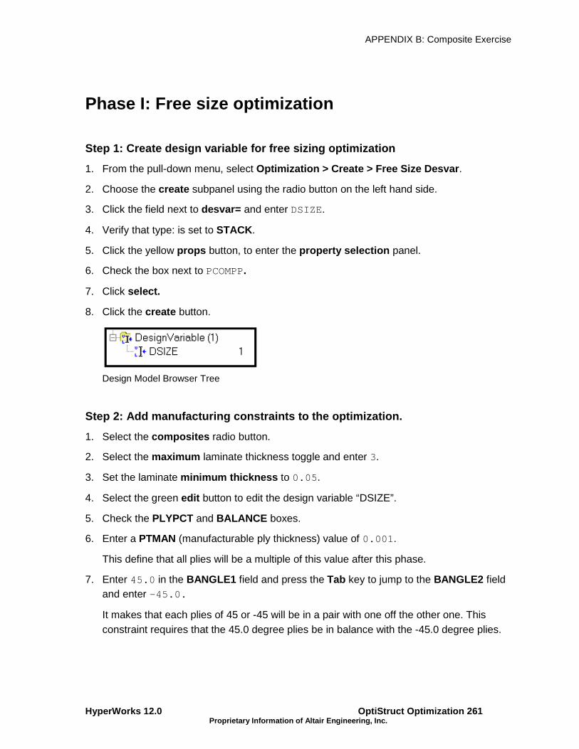
APPENDIX B: Composite Exercise
HyperWorks 12.0 OptiStruct Optimization 261 Proprietary Information of Altair Engineering, Inc.
Phase I: Free size optimization
Step 1: Create design variable for free sizing opti mization
1. From the pull-down menu, select Optimization > Create > Free Size Desvar.
2. Choose the create subpanel using the radio button on the left hand side.
3. Click the field next to desvar= and enter DSIZE.
4. Verify that type: is set to STACK.
5. Click the yellow props button, to enter the property selection panel.
6. Check the box next to PCOMPP.
7. Click select.
8. Click the create button.
Design Model Browser Tree
Step 2: Add manufacturing constraints to the optimi zation.
1. Select the composites radio button.
2. Select the maximum laminate thickness toggle and enter 3.
3. Set the laminate minimum thickness to 0.05.
4. Select the green edit button to edit the design variable “DSIZE”.
5. Check the PLYPCT and BALANCE boxes.
6. Enter a PTMAN (manufacturable ply thickness) value of 0.001.
This define that all plies will be a multiple of this value after this phase.
7. Enter 45.0 in the BANGLE1 field and press the Tab key to jump to the BANGLE2 field and enter -45.0.
It makes that each plies of 45 or -45 will be in a pair with one off the other one. This constraint requires that the 45.0 degree plies be in balance with the -45.0 degree plies.

APPENDIX B: Composite Exercise
OptiStruct Optimization 262 HyperWorks 12.0 Proprietary Information of Altair Engineering, Inc.
8. Return to the free size composite page.
9. Click update to apply changes.
10. Go to the pattern grouping subpanel and select 1-pln sym as the pattern type .
11. Click on anchor node and enter the ID 2111. Click on first node and enter 2220.
12. Click update to update the design variable and click return to exit the panel.
Step 3: Create the 2 responses (mass and disp2111) for the optimization.
1. From the pull-down menu, select Optimization > Create > Responses.
2. Enter disp2111 in the response= field.
3. Select static displacement for the response type .
4. Select the node where the load is applied or by ID node # 2111.
5. Select total disp.
6. Click create.
7. Create a second response named volume .
8. Select volume for the response type.
9. Click create.
10. Click return to exit the panel.
Response Model Browser Tree
Step 4: Create a displacement constraint (disp2111 < 5e-1)
1. From the pull-down menu, select Optimization > Create > Constraints.
2. Enter Cdisp2111 in the constraint= field.
3. Click response= and select disp2111 as the design response .

APPENDIX B: Composite Exercise
HyperWorks 12.0 OptiStruct Optimization 263 Proprietary Information of Altair Engineering, Inc.
4. Check the box next to upper bound and enter a value of 5.00e-01.
5. Click loadstep and select Lateral.
6. Click select.
7. Click create.
8. Click return.
Constraint Model Browser Tree
Step 5: Create the objective function as minimize volume
1. From the pull-down menu, select Optimization > Create > Objective.
2. Click the response= field and select volume.
3. Click create.
4. Click return to exit the panel.
Objective Model Browser Tree
Step 6: Add required OUTPUT cards
1. From the pull-down menu, select Setup > Create > Control Cards.
2. Click next until you see OUTPUT.
3. Click OUTPUT.
4. Change the number_of_outputs = to 2.
5. Set the first row as H3D for the KEYWORD and the FREQ to ALL.
6. Set the second as FSTOSZ for the KEYWORD and YES for the FREQ.
7. Click return.

APPENDIX B: Composite Exercise
OptiStruct Optimization 264 HyperWorks 12.0 Proprietary Information of Altair Engineering, Inc.
Note that second request will create a “FILENAME_sizing.fem” file that will have
incorporated ply and element set information that includes ply patch configurations for each ply type.
• The default is to repeat the super-ply 4 times for each ply defined on the PCOMP(G) property that will give a total of 16 plies.
• This is the default value and can be changed to adding the number of desired ply sequence repetitions at the end of the line in *.fem file. For
example: OUTPUT,FSTOSZ,YES,5 This request would result in the PCOMP ply sequence being repeated 5 times for a total of 20 plies.
Step 7: Run the optimization
1. From the pull-down menu, select Optimization > OptiStruct.
2. Set export options , run options and memory options to all, optimization and memory default, respectively.
3. Click OptiStruct.
Step 8: Review the Free Size results
1. When the job is complete, click HyperView and load the results into HyperView.
2. First, it is interesting to look at the optimization history to understand the design evolution, it can be done opening the file *_hist.mvw:

APPENDIX B: Composite Exercise
HyperWorks 12.0 OptiStruct Optimization 265 Proprietary Information of Altair Engineering, Inc.
Optimization History Plots
One important result is to understand how the total element thickness is distributed over the topography of the laminate. Thickness changes can be displayed per-ply as shown below:

APPENDIX B: Composite Exercise
OptiStruct Optimization 266 HyperWorks 12.0 Proprietary Information of Altair Engineering, Inc.
The breakdown of element thickness distribution

APPENDIX B: Composite Exercise
HyperWorks 12.0 OptiStruct Optimization 267 Proprietary Information of Altair Engineering, Inc.
Phase II: Sizing optimization
Step 1: Import the fem generated from the OS run an d review
Because of the output settings we created on the model prior to running the previous optimization, OptiStruct has created a file including the various changes to the plies sorted by sizing.
Import the HyperMesh FEA model
plate_with_hole_opti_phase1_sizing.9.fem
Save the HyperMesh database as plate_with_hole_opti_phase2.hm.
Review the model PLY, STACK, SET, DESVAR and DVPREL1 cards.
• ELEM SET cards will list what elements will be used for each ply.
• Note that the PLY cards have the individual ply description
• STACK card will show how the plies are stacked
• DESVAR cards will provide the initial, minimum and maximum thickness for each ply.
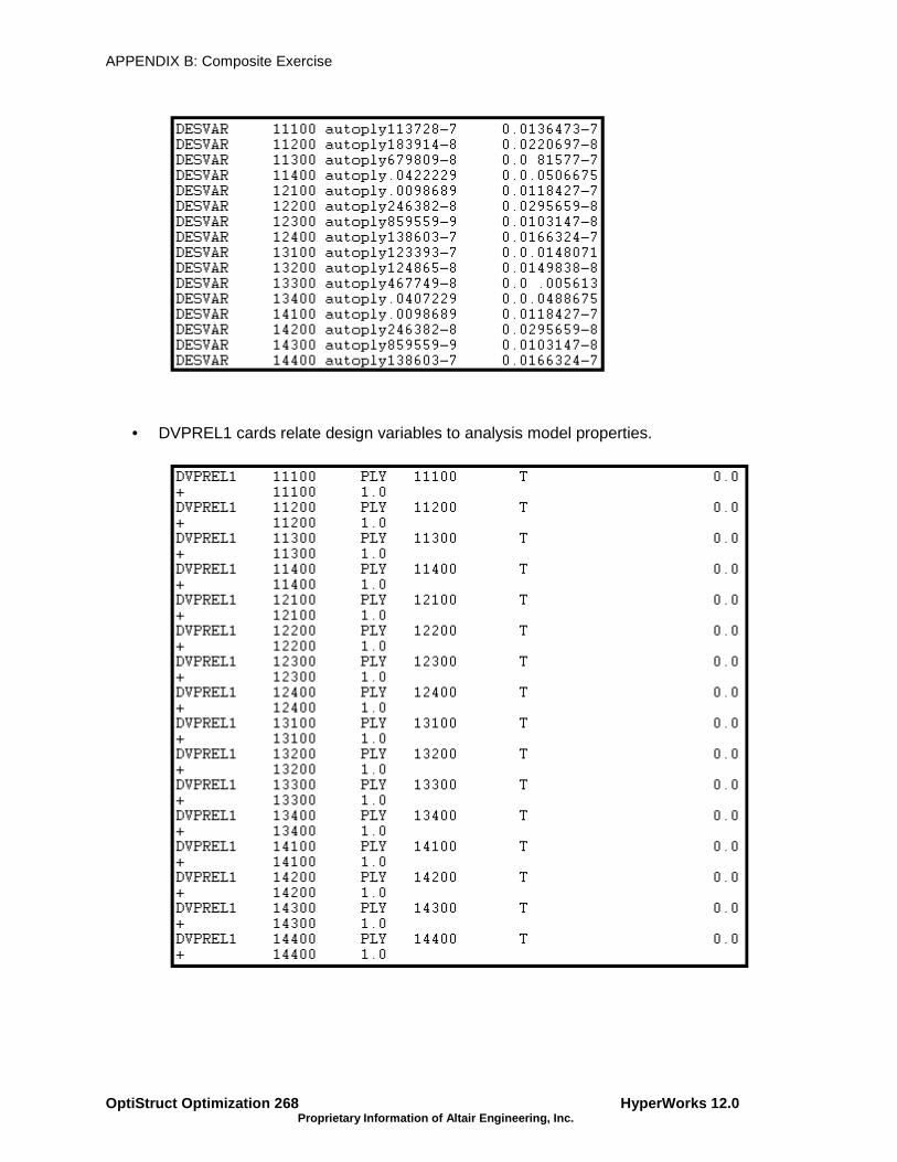
APPENDIX B: Composite Exercise
OptiStruct Optimization 268 HyperWorks 12.0 Proprietary Information of Altair Engineering, Inc.
• DVPREL1 cards relate design variables to analysis model properties.
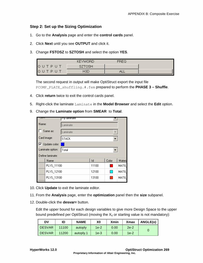
APPENDIX B: Composite Exercise
HyperWorks 12.0 OptiStruct Optimization 269 Proprietary Information of Altair Engineering, Inc.
Step 2: Set up the Sizing Optimization
1. Go to the Analysis page and enter the control cards panel.
2. Click Next until you see OUTPUT and click it.
3. Change FSTOSZ to SZTOSH and select the option YES.
The second request in output will make OptiStruct export the input file PCOMP_PLATE_shuffling.#.fem prepared to perform the PHASE 3 – Shuffle .
4. Click return twice to exit the control cards panel.
5. Right-click the laminate Laminate in the Model Browser and select the Edit option.
9. Change the Laminate option from SMEAR to Total.
10. Click Update to exit the laminate editor.
11. From the Analysis page, enter the optimization panel then the size subpanel.
12. Double-click the desvar= button.
Edit the upper bound for each design variables to give more Design Space to the upper bound predefined per OptiStruct (moving the X0 or starting value is not mandatory):
DV ID NAME X0 Xmin Xmax ANGLE(o)
DESVAR 11100 autoply 1e-2 0.00 2e-2 0
DESVAR 11200 autoply.1 1e-3 0.00 1e-2
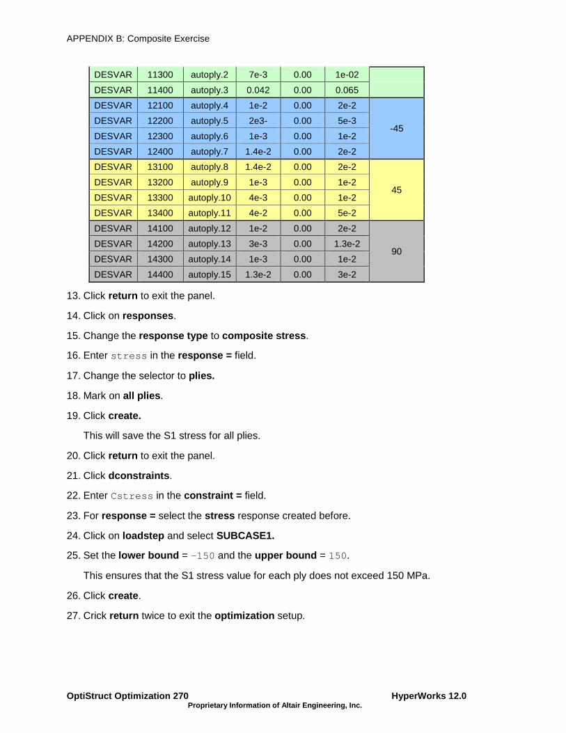
APPENDIX B: Composite Exercise
OptiStruct Optimization 270 HyperWorks 12.0 Proprietary Information of Altair Engineering, Inc.
DESVAR 11300 autoply.2 7e-3 0.00 1e-02
DESVAR 11400 autoply.3 0.042 0.00 0.065
DESVAR 12100 autoply.4 1e-2 0.00 2e-2
-45 DESVAR 12200 autoply.5 2e3- 0.00 5e-3
DESVAR 12300 autoply.6 1e-3 0.00 1e-2
DESVAR 12400 autoply.7 1.4e-2 0.00 2e-2
DESVAR 13100 autoply.8 1.4e-2 0.00 2e-2
45 DESVAR 13200 autoply.9 1e-3 0.00 1e-2
DESVAR 13300 autoply.10 4e-3 0.00 1e-2
DESVAR 13400 autoply.11 4e-2 0.00 5e-2
DESVAR 14100 autoply.12 1e-2 0.00 2e-2
90 DESVAR 14200 autoply.13 3e-3 0.00 1.3e-2
DESVAR 14300 autoply.14 1e-3 0.00 1e-2
DESVAR 14400 autoply.15 1.3e-2 0.00 3e-2
13. Click return to exit the panel.
14. Click on responses.
15. Change the response type to composite stress.
16. Enter stress in the response = field.
17. Change the selector to plies.
18. Mark on all plies.
19. Click create.
This will save the S1 stress for all plies.
20. Click return to exit the panel.
21. Click dconstraints.
22. Enter Cstress in the constraint = field.
23. For response = select the stress response created before.
24. Click on loadstep and select SUBCASE1.
25. Set the lower bound = -150 and the upper bound = 150.
This ensures that the S1 stress value for each ply does not exceed 150 MPa.
26. Click create.
27. Crick return twice to exit the optimization setup.

APPENDIX B: Composite Exercise
HyperWorks 12.0 OptiStruct Optimization 271 Proprietary Information of Altair Engineering, Inc.
Step 3: Run the optimization
1. From the pull-down menu, select Optimization > OptiStruct.
2. Set export options , run options and memory options to all, optimization & memory default.
3. Click OptiStruct.
Step 4: Review the Size results
First, it is interesting to look at the optimization history to understand the design evolution, it can be done opening the file .hgdata to plot the displacement:
Measurement of the volume of the design space as a function of iteration

APPENDIX B: Composite Exercise
OptiStruct Optimization 272 HyperWorks 12.0 Proprietary Information of Altair Engineering, Inc.
Maximum constraint violation per iteration
Maximum displacement of Node 2111 as a function of iteration
o It shows that the model had converged for a feasible solution with an optimum volume.

APPENDIX B: Composite Exercise
HyperWorks 12.0 OptiStruct Optimization 273 Proprietary Information of Altair Engineering, Inc.
28. Now it is important to review the thickness of each plies, which can be found in the *.out
file: note that OS removed some of the plies from the model entirely: e.g. thickness is zero.

APPENDIX B: Composite Exercise
OptiStruct Optimization 274 HyperWorks 12.0 Proprietary Information of Altair Engineering, Inc.
Phase III: Shuffling optimization
In this phase, the sequence in the stacking patterns of the patches created in phase 2 will be optimized with additional design constraints.
1. Import the file plate_with_hole_opti_phase2_shuffling.4.fem on a new HM
database.
2. Save this database as plate_with_hole_opti_phase3.hm.
3. From the Analysis page, go to control cards > OUTPUT.
4. Change SZTOSH,YES to PROPERTY,LAST.
5. Click Return to exit the panel.
6. Select control card: DEBUG.
7. Enter 2 for number_of_debugs.
8. Define the DEBUG card to help on understand the shuffle steps:
DEBUG, SHUFHTML,1
This will generate a file in a HTML format with a table with the shuffle iterations: *_suffle_shuf.hist.html
DEBUG, SHUFTEXT,1
This will generate a text file with the stack sequences during the shuffle iterations: *_suffle.shuf
9. Exit the control cards panel.
10. From the pull-down menu, select Optimization > Edit > Composite Shuffle Desvar.
11. Click on dshuffle and select the DSIZE dshuffle card.
12. Go to parameter subpanel.
13. Mark on pairing constraint.
14. Define a pair constraint to 45 and -45 degrees.

APPENDIX B: Composite Exercise
HyperWorks 12.0 OptiStruct Optimization 275 Proprietary Information of Altair Engineering, Inc.
15. Click update to update the pairing constraint. Click on edit and fill the card as shown below:
• MAXSUCC: limits the number of plies of the same type (orientation) that are adjacent to each other.
16. Save the model and submit the optimization.
17. Review the file: PCOMP_PLATE.shuf.html.
0o Plies -45o Plies 45o Plies 90o Plies
• The table shows the shuffling iterations from beginning to the last. • DSHUFFLE constrains to limit the number of like adjacent plies to a maximum of four;
SUMMARY Composite optimization is a three phase task:
1. Begins with Free Size optimization that determines composite patch size, shape, and location. On this phase OS output the input deck that is then used in the second phase,
2. Size optimization (ply bundle optimization), to determine optimum ply bundle thickness and required number of plies per patch.

APPENDIX B: Composite Exercise
OptiStruct Optimization 276 HyperWorks 12.0 Proprietary Information of Altair Engineering, Inc.
3. Shuffling optimization is the last phase used to optimize stacking sequence and meet ply book rules, improve performance, and improve manufacturability.
Final stacking sequence for ply lay up for composite plate with hole example