Bayesian Phylogenetic Analysis of Combined Data

Syst. Biol. 53(1):47–67, 2004Copyright c© Society of Systematic BiologistsISSN: 1063-5157 print / 1076-836X onlineDOI: 10.1080/10635150490264699

Bayesian Phylogenetic Analysis of Combined Data

JOHAN A. A. NYLANDER,1 FREDRIK RONQUIST,1 JOHN P. HUELSENBECK,2 AND JOSE LUIS NIEVES-ALDREY3

1Department of Systematic Zoology, Evolutionary Biology Centre, Uppsala University, Norbyvagen 18 D, SE-752 36 Uppsala, Sweden;E-mail: [email protected] (J.A.A.N)

2Section of Ecology, Behavior and Evolution, Division of Biological Sciences, University of California–San Diego, La Jolla, California 92093-0116, USA3Departamento de Bioversidad y Biologıa Evolutiva, Museo Nacional de Ciencias Naturales, Jose Gutierrez Abascal 2, 28006 Madrid, Spain

Abstract.— The recent development of Bayesian phylogenetic inference using Markov chain Monte Carlo (MCMC) techniqueshas facilitated the exploration of parameter-rich evolutionary models. At the same time, stochastic models have becomemore realistic (and complex) and have been extended to new types of data, such as morphology. Based on this foundation, wedeveloped a Bayesian MCMC approach to the analysis of combined data sets and explored its utility in inferring relationshipsamong gall wasps based on data from morphology and four genes (nuclear and mitochondrial, ribosomal and proteincoding). Examined models range in complexity from those recognizing only a morphological and a molecular partitionto those having complex substitution models with independent parameters for each gene. Bayesian MCMC analysis dealsefficiently with complex models: convergence occurs faster and more predictably for complex models, mixing is adequatefor all parameters even under very complex models, and the parameter update cycle is virtually unaffected by modelpartitioning across sites. Morphology contributed only 5% of the characters in the data set but nevertheless influencedthe combined-data tree, supporting the utility of morphological data in multigene analyses. We used Bayesian criteria(Bayes factors) to show that process heterogeneity across data partitions is a significant model component, although not asimportant as among-site rate variation. More complex evolutionary models are associated with more topological uncertaintyand less conflict between morphology and molecules. Bayes factors sometimes favor simpler models over considerably moreparameter-rich models, but the best model overall is also the most complex and Bayes factors do not support exclusion ofapparently weak parameters from this model. Thus, Bayes factors appear to be useful for selecting among complex models,but it is still unclear whether their use strikes a reasonable balance between model complexity and error in parameterestimates. [Bayes factors; Bayesian analysis; combined data; Cynipidae; gall wasps; MCMC; model heterogeneity; modelselection.]

Increasingly, phylogenetic problems are being ad-dressed using data from several different sources:morphology and molecules, DNA and protein, mito-chondrial and nuclear genes, coding and noncodingsequences. Previously, it has been common to addresssuch mixed data sets using the parsimony method.Where parametric methods have been applied, they havetypically excluded some data (such as morphology) be-cause of a lack of appropriate stochastic models, and theyhave often ignored obvious heterogeneity across datapartitions because of the computational complexity ofthe maximum likelihood (ML) approach (for exceptions,see Yang, 1996b; DeBry, 1999; Pupko et al., 2002; Thorneand Kishino, 2002).

The recent development of Bayesian inference of phy-logeny using Markov chain Monte Carlo (MCMC) esti-mation of posterior probability distributions has madeit easier to address complex, parameter-rich stochas-tic models within a statistical framework, opening upthe possibility for combined data analysis recognizingamong-partition heterogeneity in data source and inproperties of the evolutionary process. Recent stochas-tic models developed for new types of data, such asmorphology (Lewis, 2001a; Ronquist and Huelsenbeck,in prep.), now make it possible to include virtuallyany kind of character used today to infer phylogenyin such analyses, and the computational efficiency ofthe Bayesian MCMC approach allows each data par-tition to be treated using more realistic evolution-ary models. However, combined statistical analysis us-ing Bayesian MCMC techniques introduces a wholerange of questions that have not been addressed pre-

viously, while providing a new perspective on oth-ers. Here, we describe a Bayesian MCMC approachto combined data analysis, using empirical resultsfrom one combined data set to address some of thesequestions.

Bayesian MCMC Approach to Combined Data

Bayesian phylogenetic inference based on heteroge-neous data is a straightforward extension of the methodsalready described for homogeneous data (see recent re-views by Huelsenbeck et al., 2001; Lewis, 2001b; Holderand Lewis, 2003). Assume that the data set X consistsof two distinct partitions Xa and Xb and allow the sub-stitution model parameters, θa and θb , respectively, to becompletely different for the two partitions. In the modelswe explored, we further assumed that the two data sub-sets evolve on the same topology, τ , with the same set ofbranch lengths, ν, but that the overall rate differs acrosspartitions according to a rate multiplier, denoted ma andmb for the two partitions. In other words, effective branchlengths are potentially different but proportional acrosspartitions, as in the ML model proposed by Yang (1996;note that Yang used c instead of m for the multiplier).Using Bayes’s rule (see for instance Huelsenbeck et al.,2001), the joint posterior probability distribution for thismodel becomes

f (τ, ν, θa , θb , ma , mb | X)

= f (τ, ν, θa , θb , ma , mb) f (X | τ, ν, θa , θb , ma , mb)f (X)

,

47

by guest on February 18, 2016http://sysbio.oxfordjournals.org/

Dow

nloaded from

http://sysbio.oxfordjournals.org/

48 SYSTEMATIC BIOLOGY VOL. 53

where f (τ, ν, θa , θb , ma , mb) is the prior probability of themodel parameters, f (X | τ, ν, θa , θb , ma , mb) is the proba-bility of the data given model parameters (the likelihoodfunction), and f(X) is the model likelihood (also calledthe integrated or predictive likelihood), which is a mul-tidimensional sum and integral of the probability of thedata over all parameter values.

The posterior probability distribution, which is thecentral quantity in Bayesian inference, is typically es-timated using MCMC techniques instead of being de-rived analytically. The procedure is started with an arbi-trary set of parameter values. In each cycle (generation)of the Markov chain, one parameter or a block of param-eters is updated using a stochastic proposal mechanism.The most common mechanism used in Bayesian phy-logenetic inference, Metropolis sampling, involves theproposal of a new state based on an arbitrary proposaldistribution, q , and then acceptance of this state with aprobability determined by the product of three ratios: theprior ratio, the likelihood ratio, and the proposal ratio.Assume, for instance, that we wish to update the sub-stitution model parameters for partition a from θa to θ∗

a .The acceptance probability r would then become

r = min[

1,f (θ∗

a )f (θa )

× f (Xa | τ, v, ma , θ∗a )

f (Xa | τ, v, ma , θa )× q (θa | θ∗

a )q (θ∗

a | θa )

].

When updating a homogeneous model or a param-eter shared across all partitions, the calculation of thelikelihood ratio (the second ratio in the product) alwaysinvolves the entire data set. However, updating a parti-tioned parameter only requires consideration of the af-fected data partition, Xa in this case. The calculation ofthe likelihood ratio is by far the most computationallycomplex operation in MCMC analysis, and the speed ofthe calculation is roughly proportional to the size of thedata set. Thus, the increase in the number of parametersin a partitioned model over that in a similar homoge-neous model is largely offset by the speed gained in eachcycle of the chain. The net result is that the time requiredfor updating all model parameters a given number oftimes will remain roughly constant regardless of modelpartitioning. However, more complex models will ofcourse have more dimensions in their parameter spaces,which might cause difficulties for the MCMC samplingprocedure.

Convergence and Mixing

Theory predicts that a properly constructed Markovchain, if run long enough, will produce a valid sam-ple from the posterior probability distribution (Tierney,1994). However, the greatest practical problem in MCMCanalysis is to determine when the chain is sufficientlyclose to its target distribution (the posterior distributionof interest) for the samples to provide a good approx-imation of this distribution. One of the most powerfulapproaches used to address this question is compari-son of the results from independent runs started fromdifferent points in parameter space. In the phylogenetic

context, we expect integration over topology to be partic-ularly difficult; therefore, starting the independent runsfrom different, randomly chosen topologies should pro-vide a good test of whether the chains are providingvalid samples from the posterior probability distribution(Huelsenbeck et al., 2002).

It is useful to distinguish two potential sources of prob-lems with MCMC estimation of a target distribution:convergence and mixing. The difference between themis best explained if we consider a posterior distributionwith two separate regions, each containing roughly halfof the total probability. Typically, a MCMC run startssampling from a region with extremely low posteriorprobability because starting values are set arbitrarily orchosen randomly. When the chain has settled into thehigh-density regions of the distribution, it can be said tohave converged, and the overall likelihood will tend tovary less than during the initial burn-in period. How-ever, we still do not know how long it will take thechain to adequately sample both regions of high den-sity in the posterior distribution; this is determined bythe mixing behavior of the chain. The slower the mix-ing, the longer it will take the chain to move from one tothe other of the high-density regions. Whereas the gen-eration plot of the overall likelihood gives a preliminaryidea of whether convergence might have occurred, as-sessment of the mixing behavior requires examinationof the plots of all model parameters. This is particularlytrue when Metropolis coupling is used, because this tech-nique allows the chain to jump between different regionsin parameter space with little effect on overall likelihood(Huelsenbeck et al., 2001).

Bayesian Model Selection

Analyzing combined data using Bayesian MCMCmethods allows us to specify partition-specific substi-tution models. As more partitions are being considered,the complexity of the joint model increases as does thecomplexity of the issue of model selection. One strategyfor model selection for Bayesian MCMC analysis is to fita substitution model to each partition prior to the anal-ysis using, for example, a hierarchical likelihood-ratiotest (hLRT; Huelsenbeck and Crandall, 1997; Posada andCrandall, 2001), the Akaike information criterion (AIC;Akaike, 1973), or the Bayesian information criterion (BIC;Schwartz, 1978), all of which are based on ML estimates.The Markov chain is then run using a composite ‘super-model’ that consists of several submodels.

It is not self-evident, however, that such an approachwill necessarily lead to an optimal composite model.Most importantly, the selection of an optimal model forone partition should not ignore information from otherpartitions. For example, the methods mentioned abovedepend on point estimates of the topology and other pa-rameters, and it is well known that different topologiesmight rank models differently (Sanderson and Kim, 2000;Posada and Crandall, 2001). Thus, selecting an optimalmodel for each partition separately, on the best tree im-plied by the data from that partition, might result in a


Dow

nloaded from


2004 NYLANDER ET AL.—BAYESIAN COMBINED ANALYSIS 49

combination of models that could not be optimal on thesame topology. Furthermore, considering each partitionseparately may result in overparameterization, becausesuch an approach makes it difficult to discover when itis appropriate for two partitions to share parameters.

Unfortunately, computational problems make it dif-ficult to apply directly the methods described aboveto parameter-rich partitioned models. Furthermore,Bayesian statisticians often object in general to modeltesting based on point estimates, because such methodsare not taking the uncertainty of the topology and otherparameters into account. The argument is that a modelwith substantial posterior probability for a large rangeof parameter values could have a higher marginal (total)likelihood than a model with a narrow peak in its likeli-hood, even though the latter model may have the high-est ML value. In such situations, Bayesian statisticianshave argued, it would be unwise to compare models onlybased on the merits of a single point; instead, we shouldconsider the entire parameter space and prefer the modelwith the largest total likelihood (Bollback, 2002; Holderand Lewis, 2003). An additional problem with the ML ap-proach is that it favors the more parameter-rich modelin comparisons of nested models unless the parameter-rich models are penalized as in AIC or BIC. That is, thefavored model might contain parameters that have littleor no explanatory value (Burnham and Anderson, 2002).The Bayesian approach does not always favor the moreparameter-rich of two nested models; on the contrary,there is some concern that Bayesian methods may, un-der some circumstances, put too much emphasis on thesimpler model. This phenomenon is known as Lindley’sparadox, and it can occur with large data sets when theestimate from the complex model is close to the simplemodel (Bartlett, 1957; Lindley, 1957).

Because of the problems with the likelihood approach,we explored Bayesian model comparison based on Bayesfactors. Assume that we wish to compare how well twomodels, M0 and M1, describe the processes generating adata set X. The Bayes factor in favor of model 1 overmodel 0, B10, is calculated as the ratio of the modellikelihoods f (X | Mi ):

B10 = f (X | M1)f (X | M0)

.

The model likelihoods, f (X | Mi ), are the same as thef (X) denominator of Bayes’s rule; the conditioning ona model is implicit in the latter.

The Bayes factor can be interpreted as the posteriorodds of model 1 to model 0 in a Bayesian inference prob-lem where we start with equal probability of the twomodels being true (Kass and Raftery, 1995; Wasserman,2000). Alternatively, the Bayes factor can be viewed sim-ply as a comparison of the predictive likelihoods of themodels (Gelfand and Dey, 1994; Kass and Raftery, 1995;Wasserman, 2000) or a comparison of the ability of themodels to update the priors (Lavine and Schervish, 1999;Wasserman, 2000). Both the latter comparisons would be

TABLE 1. Interpretation of the Bayes factor (B10) (taken from Kassand Raftery, 1995).

2 loge (B10) B10 Evidence against M0

0 to 2 1 to 3 not worth more thana bare mention

2 to 6 3 to 20 positive6 to 10 20 to 150 strong>10 >150 very strong

valid even, although strictly speaking none of the mod-els is likely to be an exact (true) description of the pro-cess under study. The Bayes factor comparison can beapplied to any set of models, regardless of whether theyare nested or not (as can AIC and BIC but not hLRT),and it is based on integration over the uncertainty in allparameter values rather than on ML point estimates (asopposed to AIC, BIC, and hLRT).

The Bayes factor is not used in a normal statistical testof whether a hypothesis should be rejected or acceptedgiven some subjective cutoff value. Instead, the Bayesfactor evaluates the relative merits of competing mod-els, and the interpretation is left to the scientist. Jeffreys(1961) originally provided some guidelines for this in-terpretation, which have been modified by other work-ers. We use a version originally presented by Kass andRaftery (1995) (Table 1).

Questions Regarding Combined Phylogenetic Analysis

We applied combined Bayesian MCMC analysis to anempirical data set consisting of morphological and nu-cleotide data for 32 exemplar species of gall wasps (Hy-menoptera: Cynipidae) and outgroups. The exemplarsspan the entire diversity of the family and include phy-tophagous guests in galls (inquilines) and gall inducerson a variety of both herbaceous and woody host plants(Table 2; Ronquist, 1999).

The morphological data consisted of 166 characters,which have previously been shown to partly resolvethe phylogeny with strong support values using parsi-mony methods (Liljeblad and Ronquist, 1998). The nu-cleotide data are almost entirely original to this studyand consisted of a total of 3,080 aligned base pairs (bp)from four genes: two nuclear protein-coding genes (elon-gation factor 1α F1 copy [EF1α] and long-wavelengthopsin [LWRh]), one mitochondrial protein-coding gene(cytochrome oxidase c subunit I [COI]), and nuclear 28Sribosomal DNA (rDNA). We analyzed the data using arange of models of varying complexity (dimensionality)and explored the following questions.

What is the relationship between model complexity andcomputational complexity?—It is difficult to predict howMCMC estimation of the posterior probability distribu-tion is affected by an increase in model complexity. Thechain can be updated faster in those generations wheremodel parameters affecting only some of the partitionsare changed; however, more parameters also means thateach parameter will be visited more rarely. More param-eters will also affect the complexity and the shape of theposterior distribution, which might slow convergence


Dow

nloaded from



TABLE 2. Taxa of gall wasps (Cynipidae) and outgroups (Figitidae, Liopteridae, Ibaliidae) used in the analysis. Brief biological data are givenfor each exemplar genus. GenBank accession numbers are given for all sequences; a dash indicates missing data.

GenBank nos.

Taxon Morphologya Host plantb Biologyc COI 28S EF1α LWRh

CynipidaeSynergini

Synergus crassicornis Quercus (Fg) inquiline AY368909 AY368936 AY368962 AY371051Ceroptres cerri C. clavicornis Quercus (Fg) inquiline AY368910 AY368935 — AY371052Periclistus brandtii Rosa (Ro) inquiline AF395181 AF395152 AF395173 AF395189Synophromorpha sylvestris S. rubi Rubus (Ro) inquiline AY368911 AY368937 AY368961 —

“Aylacini”Xestophanes potentillae Potentilla (Ro) galler AY368912 AY368938 AY368963 —Diastrophus turgidus Rosaceae galler AY368913 AY368939 AY368964 —Gonaspis potentillae Potentilla (Ro) galler AY368914 AY368940 AY368965 —Liposthenes glechomae Glechoma (La) galler AY368915 AY368941 AY368966 AY371053Liposthenes kerneri Nepeta (La) galler AY368916 AY368942 AY368967 AY371054Antistrophus silphii A. pisum Asteraceae galler AY368917 AY368943 AY368968 AY371055Rhodus oriundus Salvia (La) galler AY368918 AY368944 AY368969 AY371056Hedickiana levantina Salvia (La) galler AY368919 AY368945 AY368970 AY371057Neaylax verbenaca N. salviae Salvia (La) galler AY368920 AY368946 AY368971 AY371058Isocolus rogenhoferi Asteraceae galler AY368921 AY368947 AY368972 AY371059Aulacidea tragopogonis Asteraceae galler AY368922 AY368948 AY368973 AY371060Panteliella bicolor P. fedtschenkoi Phlomis (La) galler AF395180 AF395153 AF395172 AF395188Barbotinia oraniensis Papaver (Pa) galler AF395179 AF395150 AF395171 AF395187Aylax papaveris Papaver (Pa) galler AY368923 AY368949 AY368974 AY371061Iraella luteipes Papaver (Pa) galler AY368924 AY368950 AY368975 —Timaspis phoenixopodos Asteraceae galler AY368925 AY368951 AY368976 AY371062Phanacis hypochoeridis Asteraceae galler AY368926 AY368952 AY368977 —Phanacis centaureae Asteraceae galler AY368927 AY368953 AY368978 —

EschatoceriniEschatocerus acaciae Acacia (Fb) galler AY368928 AY368954 AY368979 AY371063

DiplolepidiniDiplolepis rosae Rosa (Ro) galler AF395174 AF395157 AF395166 AF395182

PediaspidiniPediaspis aceris Acer (Sa) galler AY368929 AY368955 AY368980 AY371064

CynipiniPlagiotrochus quercusilicisd Quercus (Fg) galler AF395178 AF395154 AF395162 AF395186Andricus kollari A. quercusradicis Quercus (Fg) galler AF395176 AF395156 AF395168 AF395184Neuroterus numismalis Quercus (Fg) galler AY368930 AY368956 AY368981 —Biorhiza pallida Quercus (Fg) galler AY368931 AY368957 AY368982 AY371065

FigitidaeParnips nigripes — parasitoid AY368932 AY368958 AY368983 AY371066

LiopteridaeParamblynotus virginianus P. zonatus — parasitoid AY368933 AY368959 AY368984 —

IbaliidaeIbalia rufipes — parasitoid AY368934 AY368960 AY368985 —

aSpecies coded for morphology if different from the species sequenced.bGenus or family of host plant attacked by the exemplar genus if phytophagous. A few rarely used host plants have been omitted; see Ronquist and Liljeblad

(2001) for more information. If all members of the genus attack the same host-plant genus, then the family to which that genus belongs is indicated in brackets: Fb =Fabaceae; Fg = Fagaceae; La = Lamiaceae; Pa = Papaveraceae; Ro = Rosaceae; Sa = Sapindaceae.

cCynipidae are either inquilines (phytophagous guests) in galls or gall inducers. The outgroups are endoparasitoids attacking various insect larvae.dSpecies name recently designated a senior synonym of P. fusifex.

and mixing. However, more realistic models may lead toposterior distributions that are easier to traverse usingMCMC, despite the increase in the number of parame-ters. We examined the computational speed, time to con-vergence, and mixing over the entire range of models toexamine these questions empirically.

Do morphological data influence multigene analyses?—Morphological data are potentially important in phy-logenetic inference for many reasons. For instance,morphological characters are crucial in placing fossils inphylogenies and thus in dating branching events. How-ever, the ability to combine morphological and molecu-lar data in a single analysis is particularly important if it

can be shown that morphology has significant influenceon the phylogenetic estimate even when combined withmultigene data sets. This question has remained largelyunexplored with parametric methods, because only re-cently were stochastic models seriously considered formorphological data (Lewis, 2001a). We used an extendedversion of Lewis’s models (Ronquist and Huelsenbeck, inprep.) in evaluating whether the 166 morphological char-acters in our data set significantly affected the phyloge-netic estimate when combined with the 3,080 nucleotidecharacters from the four different genes.

Are composite models better?—When it becomes pos-sible to analyze partitioned models easily, an obvious


Dow

nloaded from



question is how important it is to recognize across-partition heterogeneity in evolutionary processes. To ex-amine this question, we used Bayes factor comparisons tolook at the increase in model likelihood associated withthe introduction of different model components account-ing for within-partition or across-partition heterogeneityin the molecular portion of the data set.

Are complex models associated with increased variance oftopology estimates?—Complex models are generally asso-ciated with more error variance in parameter estimates.If the error variance is excessive, it becomes a problemknown as overparameterization or overfitting (Burnhamand Anderson, 2002). However, overly simple modelscan also be problematic. In particular, oversimplifiedevolutionary models might lead to dramatically low-ered topological variance and exaggerated clade proba-bility values in Bayesian phylogenetic inference (Suzukiet al., 2002). To examine the relationship between modelcomplexity and the precision of parameter estimates,we compared topology and tree-length estimates acrossmodels. We also looked at the effect of model complexityon the conflict between the morphological and molecularpartitions.

Is the Bayesian MCMC approach sensitive to the inclu-sion of superfluous parameters in a complex model?—It maybe difficult to design complex models that adequatelyexplain a process under study without including oneor a few parameters that are superfluous in the sensethat (1) the data are not powerful enough to signifi-cantly alter their prior probability distribution or (2) theposterior probability distribution coincides with a lessparameter-rich submodel. Such “superfluous” parame-ters might cause problems with MCMC estimation of theposterior distribution. We searched the posterior distri-butions of more complex models for such parametersto see whether they were present and, if so, whetherthere was any apparent effect on convergence or on theposterior distributions of other model parameters. If theBayesian MCMC approach were sensitive to superfluousparameters, it might be difficult to design appropriatecomposite models that would result in successful com-bined analysis.

Do Bayes factors strike a reasonable balance between modelcomplexity and error variance?—The ability to allow het-erogeneity across data partitions in model parametersopens up a Pandora’s Box of model choice problems,which are difficult to address without good model se-lection criteria and procedures. Standard likelihood ra-tio tests have a tendency to prefer complex models(Gelfand and Day, 1994; Burnham and Anderson, 2002)and various procedures have been developed to punishparameter-rich models (Akaike, 1973; Schwartz, 1978). Intheory, the Bayes factor comparison does not suffer fromthis problem; a simple model can be favored over a moreparameter-rich model even if the models are nested. Welooked for instances of simple models winning over morecomplex ones and cases where the Bayes factor would fa-vor model reduction by supporting the exclusion of weakparameters.

MATERIALS AND METHODS

Data

We assembled DNA and morphological data for 29 gallwasp exemplars and three outgroup exemplars, the lat-ter representing the families Figitidae, Liopteridae, andIbaliidae (Table 2). Previous phylogenetic analyses in-dicate that Figitidae is the sister group to Cynipidaeand that the Liopteridae and Ibaliidae are successivelymore distant outgroups (Ronquist, 1999). The gall waspsample included representatives of all described tribesof the only extant subfamily. All major wasp genera ofphytophagous guests in cynipid galls, also known asinquilines, were represented except for the genus Sa-phonecrus, which is considered close to if not embeddedwithin Synergus (Ronquist, 1994, 1999; Nieves-Aldrey,2001; Ronquist and Liljeblad, 2001). A broad selectionof gall inducers attacking herbaceous and woody hostplants was also included. At least half the describedgenera were included for all tribes except the Cynipini,or the oak gallers. This tribe, comprising more than 40described genera, was represented by only four generabut is widely thought to be monophyletic (Kinsey, 1920;Askew, 1984; Ronquist, 1994, 1999; Liljeblad and Ron-quist, 1998; Nieves-Aldrey, 2001; Ronquist and Liljeblad,2001; Stone et al., 2002).

The morphological data were taken from Liljebladand Ronquist (1998) and consist of 166 parsimony-informative discrete characters: 164 external morpholog-ical characters and two ecological characters (alterationof sexual/asexual generations, and host-plant choice)(Liljeblad and Ronquist, 1998: appendix 1). Some mul-tistate characters were treated as ordered and othersas unordered, as specified by Liljeblad and Ronquist(1998).

As far as possible, DNA data were collected from thesame species for which we had morphological data. Ina few cases, an exact match could not be obtained, butDNA sequences were obtained, from a close relative andthese taxa were combined into a single terminal in the fi-nal analyses (Table 2). We sequenced parts of four genes:COI (1,078 bp), the nuclear protein-coding genes LWRh(481 bp) and EF1α, (367 bp), and the nuclear 28S rDNA(1,154 bp) (GenBank accession numbers in Table 2). De-tails of the DNA amplification protocols and primerswere given by Rokas et al. (2002). The protein-codinggenes (COI, LWRh, and EF1α) were easily aligned byeye. The ribosomal sequences (28S) differed in length,and some of the more variable regions were difficultto align manually. We used ClustalW 1.81 (Thompsonet al., 1994) for this alignment. We applied a range ofcosts for the gap opening and gap extension penal-ties, and the individual alignments were subjected toparsimony bootstrap (Felsenstein, 1985) analyses usingPAUP∗ (Swofford, 1998). Supported groups were largelycongruent among the resulting trees. The alignment re-sulting from the use of the default settings in ClustalW isavailable from TreeBase (http://www.treebase.org, ac-cession S970).


Dow

nloaded from



Parsimony Analyses of Morphological Data

For comparison with the Bayesian analysis, the mor-phological data set was subjected to parsimony analy-sis with equal character weights (standard parsimony)and with characters weighted according to degree ofhomoplasy using Goloboff’s (1993) concave weightingfunction with the constant of concavity (k) set to 2 (im-plied weights parsimony). These analyses were com-pleted using PAUP∗ (Swofford, 1998). A bootstrap major-ity rule consensus tree was calculated using 1,000 pseu-doreplicates, each with five random addition sequencesfollowed by tree bisection–reconnection (TBR) branchswapping and saving only one tree per pseudoreplicate(multrees = no).

Models of Character Evolution

For single DNA data partitions, we used standard sub-stitution models: Jukes–Cantor (JC; Jukes and Cantor,1969), Hasegawa–Kishino–Yano (HKY; Hasegawa et al.,1985), and general time reversible (GTR; Lanave et al.,1984; Tavare, 1986; Rodrıguez et al., 1990). Rates wereeither assumed to be equal or to vary across sites ac-cording to a gamma distribution (; Yang, 1994) withor without a proportion of invariable sites (I; Gu et al.,1995). For morphological data, we used the Mk (Markovk) model of Lewis (2001a) extended to deal with orderedmultistate characters and a new type of coding bias (onlyparsimony-informative characters scored) (Ronquist andHuelsenbeck, in prep.). The Mk model assumes equalstate frequencies; it is possible to extend it to deal withunequal state frequencies, but we did not do so. TheMk model could be combined with equal or gamma-distributed rates across “sites” (i.e., characters) but notwith a proportion of invariable “sites” because constantmorphological characters were absent in the data ma-trix, making it impossible to estimate the proportion ofinvariable sites/characters.

We combined these elementary models in differentways to explore a range of composite models of dif-ferent complexity (Table 3). First, we analyzed morpho-logical and nucleotide data separately using 1-Mk and1-GTRI models (where 1 denotes a single data parti-tion). Then we combined morphology and nucleotidedata in models with either a single morphological anda single nucleotide partition (2-Mk-JC, 2-Mk-GTR, 2-Mk-HKYI, and 2-Mk-GTRI models) or a singlemorphological and four nucleotide partitions, each ofthe latter corresponding to a different gene (5-Mk-JC,5-Mk-GTR, 5-Mk-HKYI, and 5-Mk-GTRI models).We allowed different data partition to evolve at a dif-ferent rate, but branch lengths were assumed to be pro-portional across partitions (Yang, 1996b; Ronquist andHuelsenbeck, 2003). In the five-partition models, we alsoallowed the nucleotide models to be unique for each par-tition, i.e., we allowed stationary state frequencies andall other substitution model parameters to be indepen-dent across partitions. The number of free parameters inthe examined evolutionary models ranged from 1 to 45(Table 3).

TABLE 3. Summary of the models under which data were analyzed.The models contained one (either morphology or DNA), two (one mor-phology and one DNA), or five (one morphology and four DNA) datapartitions. All parameters were allowed to be partition specific. Thecharacter-substitution models are given for the morphological and nu-cleotide (DNA) data. The number of free parameters is given excludingbranch-length and topology parameters. Mk = Markov k model; JC =Jukes–Cantor model; HKY = Hasegawa–Kishino–Yano model; GTR =general time reversible model; I = proportion of invariant sites; = gamma rate variation; m = rate multiplier.

Morphology No. freeModel Partitions model DNA model parameters

1-Mk 1 Mk+ 11-GTRI 1 GTR+I+ 102-Mk-JC 2 Mk, m JC, m 12-Mk-GTR 2 Mk, m GTR, m 92-Mk-HKYI 2 Mk+, m HKY+I+, m 82-Mk-GTRI 2 Mk+, m GTR+I+, m 125-Mk-JC 5 Mk, m JC, m 45-Mk-GTR 5 Mk, m GTR, m 365-Mk-HKYI 5 Mk+, m HKY+I+, m 295-Mk-GTRI 5 Mk+, m GTR+I+, m 45

Priors on Model Parameters

For the prior on topology, we assumed that all labeledtrees are equally likely. We used an exponential priorwith inverse scale parameter 1.0, Exponential(1.0), forbranch lengths. For stationary state frequencies, we useda flat Dirichlet prior, Dirichlet(1,1,1,1). For the five nu-cleotide substitution rate ratios of the GTR model (scaledto the G-T rate) and the transition/transversion rate ra-tio of the HKY model, we used Exponential(ln 2) priors.These put 50% prior probability on rate ratios <1.0. Weused a Uniform(0,50) prior on the shape parameter of thegamma distribution of rate variation and a Uniform(0,1)prior on the proportion of invariable sites.

Estimation of the Posterior Probability Distribution

We used Metropolis-coupled MCMC (Metropoliset al., 1953; Hastings, 1970; Geyer, 1991), as implementedin MrBayes 3.0 (Huelsenbeck and Ronquist, 2001; Ron-quist and Huelsenbeck, 2003), to estimate the posteriorprobability distribution. The gamma distribution of ratevariation across sites was approximated by a discretedistribution with four categories, each category beingrepresented by its mean rate. All chains, including cou-pled chains in the same run, were started from different,randomly chosen trees. Starting values for other parame-ters were set arbitrarily: branch lengths to 0.1, stationarybase frequencies to 0.25, rates in rate sets to 1.0, invariantproportion to 0.0, and gamma shape to 0.5.

We randomly picked a combination of a parameter(or block of parameters) and an updating mechanismin each generation of the chain. The relative probability,or proposal rate, of picking each parameter–mechanismcombination was determined by a probability factor as-sociated with the updating mechanism. Assume that amodel contained a tree updated by a mechanism with aproposal rate of 15.0 and two shape parameters updatedby a mechanism with a proposal rate of 1.0. Then we


Dow

nloaded from



would update the tree with probability 15/17 and eachshape parameter with probability 1/17 in every genera-tion of the chain.

We used the following Metropolis proposals. Topol-ogy and branch lengths were updated using the LO-CAL mechanism (proposal rate 15.0, tuning parame-ter 2.0∗loge [1.1]; Larget and Simon, 1999), a stochas-tic TBR mechanism (proposal rate 3.0, tuning param-eter 2.0∗loge [1.61], extension probability 0.5), and abranch multiplier (proposal rate 3.0, tuning parameter2.0∗loge [2.59]). All other mechanisms were assigned aproposal rate of 1.0. Base frequencies were updated us-ing a Dirichlet proposal (Dirichlet tuning parameter 300),rate ratios (transition/transversion rate ratio, GTR rateratios scaled to the G-T rate, and partition rate multipli-ers scaled to the rate of the first partition) were updatedusing a uniform proposal within a sliding window (size1.0), the gamma shape parameter was updated using auniform proposal within a sliding window (size 0.5), andthe proportion of invariable sites was updated using auniform proposal within a sliding window (size 0.1).

We used four Metropolis-coupled chains with incre-mental heating, and the heating parameter was set to0.2. In every generation, we randomly picked two chainsand used a Metropolis mechanism to swap their states(Huelsenbeck and Ronquist, 2001). For each model, weran four different runs of 2,000,000 generations each,sampling values every 100th generation.

Convergence Monitoring

For the initial determination of burn-in (the number ofgenerations before apparent stationarity), we examinedthe plot of overall model likelihood against generationof the chain to find the point where the likelihood plotleveled off and started to fluctuate around a stable value.To provide additional confirmation of convergence andappropriate mixing, we compared results from the fourindependent runs. We checked that all runs had simi-lar mean and variance of model likelihood after burn-in.We also compared posterior distributions and generationplots for all substitution model parameters, including to-tal tree length, to check that the runs were producing sim-ilar marginal posterior distributions and that they weremixing appropriately over these distributions. We alsocompared majority rule consensus trees from the inde-pendent runs to check that topology and clade credibilityvalues were similar. Convergence after the initially de-termined burn-in phase was confirmed in all cases bythese additional tests. Final results were based on thepooled samples from the stationary phases of the fourindependent runs.

Estimation of Model Likelihood

The critical element that must be estimated to calcu-late Bayes factors is the model likelihood f (X | Mi ). Thislikelihood is usually impossible to evaluate analyticallywhen the parameter space is large, but it can be estimatedin a number of ways. In phylogenetics, different estima-

tors have been used to calculate Bayes factors for compar-ing models. Suchard et al. (2001) used a method called theSavage–Dickey ratio (Verdinelli and Wasserman, 1995),which is restricted to comparing nested models. Aris-Brosou and Yang (2002) used a controversial method de-scribed by Aitkin (1991) that uses the arithmetic meanof the likelihood values sampled from the posterior dis-tribution. We used the estimator proposed by Newtonand Raftery (1994), which is the harmonic mean of thelikelihood values sampled from the stationary phase ofthe MCMC run. This estimator is given by

f (X | Mi ) =[

1n

n∑j=1

f (X | τ j , ν j , θ j )−1]−1

,

where f (X | τ j , v j , θ j ) is the likelihood for a sample jout of a total of n from the joint posterior distribution.The harmonic mean estimator is less sensitive to the occa-sional occurrence of high likelihood values and more sen-sitive to low values than the arithmetic mean estimator ofAitkin (1991). Because high extremes are more likely to bea problem than low extremes, the harmonic mean shouldperform better than the arithmetic mean. Although someworkers have questioned the general stability of the har-monic mean estimator, it should be sufficiently accuratefor comparison of models with distinctly different modellikelihoods given that the sample from the posterior dis-tribution is large ( Newton and Raftery, 1994; Gamerman,1997). The value of the harmonic mean estimator wascalculated using MrBayes, scaling all likelihood valuesto the smallest value sampled and taking full advantageof the numerical range of double-precision floating pointvalues.

RESULTS

Computational Efficiency

Because many of the proposals changed parametersthat affected only one or a few of the data partitions in acomplex model, the computational time per MCMC cy-cle was shorter in partitioned analyses (Table 4). For allbut the simplest model (Mk-JC), analyzing the data infive instead of two partitions provided a drastic increasein computational speed per generation, as expected. Forexample, the average computing speed was 20.0 genera-tions/sec for the 45-parameter model 5-Mk-GTRI butonly 11.2 generations/sec for the 12-parameter model 2-Mk-GTRI. Thus, analysis under the more parameter-rich model was nearly twice as fast as that under theless parameter-rich model, despite an almost fourfoldincrease in the number of parameters. Another strik-ing effect is that allowing gamma-distributed rate vari-ation across sites slows down the analysis consider-ably because the chain is integrating out the gammadistribution using the discrete four-category approxi-mation, essentially quadrupling the number of compu-tational operations needed to evaluate the likelihoodratio.


Dow

nloaded from



TABLE 4. Effect of model complexity on computational speed and time to apparent stationarity. All values are the average of four independentanalyses on a 1.0 GHz AMD Athlon processor running Linux. Time to convergence (burn-in) was estimated as the number of generations requiredbefore the overall model likelihood reached apparent stationarity.

No. free Speed Update Time toModel parameters (generations/sec) cycle (sec) convergence (sec)a

Two-partition models2-Mk-JC 1 51.0 0.43 206 (157, 254)b

2-Mk-HKYI 8 12.2 2.21 984 (820, 1,148)2-Mk-GTR 9 47.0 0.51 553 (277, 851)c

2-Mk-GTRI 12 11.2 2.41 2,410 (1,964, 3,125)Five-partition models

5-Mk-JC 4 51.3 0.43 171 (136, 214)5-Mk-HKYI 29 20.3 1.92 443 (394, 493)5-Mk-GTR 36 60.1 0.50 237 (150, 333)5-Mk-GTRI 45 20.0 1.95 1,038 (650, 1,700)

aValues are mean (min, max) for the four independent runs.bBased on only two runs; the remaining runs took 8,600 and 10,400 sec to converge.cBased on three runs; the last run took 8,300 sec to converge.

A more relevant comparison than computational timeper generation is the update cycle, i.e., the computationaltime required for a single update of all model parametersor parameter blocks. Because update mechanisms wereselected randomly in the MCMC implementation, theactual update cycle for any parameter could vary con-siderably over short time spans. The times given hereare the expectations over long runs (Table 4). Going fromtwo to five data partitions leads to a slight but notice-able decrease in the update cycle in the five-partitionmodels. This decrease could be due to improved cachingefficiency because the small number of data requiredfor many updates in the five-partition models might in-crease the probability of cache hits, leading to the proces-sor accessing the data much faster. Without such effects,the update cycle would presumably have been similarregardless of the number of partitions. Again, themost striking effect is associated with allowing gamma-distributed rates across sites (Table 4).

Even though the update cycle remains constant, theincrease in dimensionality of the posterior probabilitydistribution might cause prolonged burn-in periods forthe more complex models. However, this effect wasnot observed. On the contrary, the five-partition mod-els reached apparent stationarity more quickly than didthe corresponding two-partition models (Table 4). For in-stance, apparent stationarity occurred on average morethan twice as fast in the 45-parameter 5-Mk-GTRImodel as in the 12-parameter 2-Mk-GTRI model. Fur-thermore, convergence was unpredictable for the sim-plest models. For the 2-Mk-JC model, only two of fourruns converged in a time period comparable to that ofother models; the remaining two runs took 40–50 timeslonger to converge (Fig. 1). The slightly more compli-cated 5-Mk-JC model had one of four runs with a 20-timelonger convergence than the others.

Morphology Versus DNA

For the comparison between the morphological andnucleotide data, we considered analyses under three

models: 1-Mk (morphology only), 1-GTRI (DNAonly), and 2-Mk-GTRI (all data combined).

Results from analysis of the morphological data un-der the 1-Mk model (Fig. 2a) are similar to those ob-tained from standard parsimony analysis of the samedata (not shown), but they conform even more closelyto the results from bootstrapped implied-weights par-simony analysis (constant of concavity, k = 2) (Fig. 2b).From this implied-weight analysis, the Bayesian resultsdiffer only in being slightly more resolved and havingsupport values that are generally higher, especially forsome of the weaker groupings in the implied-weightsanalysis. This observation supports the intuitive anal-ogy between homoplasy-weighted parsimony analysisand parametric analysis allowing rate variation acrosssites.

Analysis of the molecular data under the 1-GTRImodel confirms some morphological results but sug-gests different groupings in many cases (Fig. 2c). Thereare two areas of particularly strong conflict. First, themolecular data suggest that the woody non-oak gallers(Diplolepis, Pediaspis, and Eschatocerus) form basal lin-eages in the Cynipidae instead of being closely related

FIGURE 1. Generation plot of the marginal log likelihood,f (X | τ, v, θ ), for the combined data analyzed under the 2-Mk-JC model.


Dow

nloaded from



FIGURE 2. Comparison of the phylogenetic information in the morphological and molecular partitions and their influence on the combinedanalysis. Groups discussed in the text are indicated on the trees. A bold branch indicates a posterior probability of 1.0. IR group = inquilines+ Aylacini Rosaceae gallers. (a) Majority-rule consensus tree based on the morphological data analyzed under the 1-Mk model. (b) Bootstrapconsensus tree from an implied-weights parsimony analysis (constant of concavity, k = 2) of the morphological data. (c) Majority-rule consensustree based on the molecular data analyzed under the 1-GTRI model. (d) Majority-rule consensus tree based on the combined data analyzedunder the 2-Mk-GTRI model.


Dow

nloaded from



to the oak gallers (Plagiotrochus, Andricus, Neuroterus,and Biorhiza), as indicated by the morphological data(Figs. 2a, 2b). Second, the molecular data suggest that theoak inquilines (Synergus and Ceroptres) are not related tothe rose inquilines (Periclistus and Synophromorpha) andthe Aylacini Rosaceae gallers (Diastrophus, Gonaspis, andXestophanes) (Fig. 2c), whereas the morphological datastrongly support the monophyly of this entire assem-blage, referred to here as the IR group (Inquilines + Ay-lacini Rosaceae gallers). In these cases, one can possiblyargue that the morphological result is more likely thanthe molecular result (see Discussion). In most other caseswhere the molecules and morphology conflict, however,the molecular result is much more reasonable. For in-stance, the grouping of Phanacis and Timaspis is more inline with previous expectations and the results of stan-dard parsimony analysis of morphological data (Lilje-blad and Ronquist, 1998) than is the 1-Mk result; theplacement of Liposthenes with other Lamiaceae gallers,such as Panteliella and Rhodus, appears more likely thanthe placement of this genus basal to the IR group as sug-gested by morphology; and the grouping of all poppygallers (Aylax, Iraella, and Barbotinia) in a single clade isnot in strong conflict with morphology and is in line withthe observation that gall wasps in general are extremelyconservative in their host-plant preferences (Ronquistand Liljeblad, 2001).

In the results of the combined analysis (Fig. 2d), thereis ample evidence of influence from both the morpholog-ical (166 characters) and the molecular (3,080 bp) data. Inmany cases, the two data sets support each other, suchas the increased support for the Liposthenes clade (0.58with morphology, <0.50 with molecules, 0.76 in com-bined analysis), the Aulacidea–Isocolus clade (0.98 withmorphology, 0.52 with molecules, 1.00 in combined anal-ysis), and the oak gallers (Plagiotrochus, Andricus, Neu-roterus, and Biorhiza; 0.96 with morphology, 0.94 withmolecules, 1.00 in combined analysis). In many cases ofconflict, the molecular result prevails, as expected. How-ever, the morphological data are strong enough to changethe position of the oak inquilines (Synergus and Cerop-tres), such that the IR group becomes monophyletic inthe combined analysis. This is quite a dramatic changecompared with the molecular result (Fig. 2c).

Are Partitioned Models Better?

The estimated model likelihoods indicate a dramaticincrease in model fit when going from two-partitionmodels to their five-partition equivalents. The increaseranged from almost 600 to >900 log likelihood units (Ta-bles 5, 6). However, other model components were evenmore important than allowing across-partition hetero-geneity. Allowing within-partition rate variation was byfar the most important model component (accounting foran increase of roughly 3,000 log likelihood units in thetwo available comparisons; Table 6). Allowing rate vari-ation across molecular partitions but not within them (5-Mk-GTR) was far less successful than allowing rate varia-tion within a single molecular partition (2-Mk-GTRI);

TABLE 5. Estimated model likelihood (predictive likelihood),f (X | Mi ), for the different models.

Model No. parameters loge f (X | Mi )

Two-partition models2-Mk-JC 1 −31,6342-Mk-HKYI 8 −27,3962-Mk-GTR 9 −30,2892-Mk-GTRI 12 −27,121

Five-partition models5-Mk-JC 4 −30,9625-Mk-HKYI 29 −26,6825-Mk-GTR 36 −29,3775-Mk-GTRI 45 −26,543

the difference was more than 2,000 log likelihood unitsin favor of the simpler model (Table 5). Allowing morerealistic substitution models was also important, but theincrease was dramatic only when going from JC to GTR(1,345 or 1,585 log likelihood units; Table 6), not whengoing from HKY to GTR (139 or 278 log likelihood units;Table 6), indicating that accounting for unequal base fre-quencies and unequal transition and transversion rateswas more important than allowing all six substitutiontypes to have their unique rate.

Do Complex Models Have Increased Topological Variance?

Complex models are associated with more topologi-cal uncertainty than are simple models. This is clearlyseen when looking at the 95% credible sets of trees, i.e.,the set obtained by starting with the sampled tree hav-ing the highest posterior probability and then addingtrees in order of decreasing probability until the cumula-tive probability is 0.95. For instance, the simplest model(2-Mk-JC) had only three trees in its 95% credible set,whereas the most complex model (5-Mk-GTRI) had472 (Table 7). The most important factor by far is whetheror not within-partition rate variation is accounted for inthe model. Models allowing rate variation within par-titions (8–45 parameters) had 236–472 trees in their 95%credible sets, whereas models that did not allow rate vari-ation (1–36 parameters) had only 1–31 trees. Even if thiseffect is controlled for, however, the introduction of moreparameters usually seems to increase topological uncer-tainty. For instance, the 5-Mk-JC model had 11 trees in its95% credible set whereas the 5-Mk-GTR model had 31,and the 5-Mk-HKYI model had 389 trees whereas the5-Mk-GTRI model had 472.

For models with rate variation, there also seems to bea positive correlation between topological uncertaintyand tree length uncertainty (Table 7). The normalizedSD of tree length (the SD divided by the mean) was 0.083for the most complex of the rate-variation models (5-Mk-GTRI) but only 0.041 for the simplest (2-Mk-HKYI). There was also a tendency for more complexrate-variation models to have trees with longer branches.Models without rate variation showed no differences ei-ther in tree length or in tree length variation.

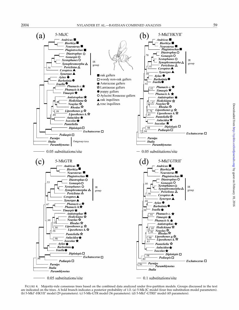
The majority rule consensus trees obtained under theeight different models were relatively similar (Figs. 3, 4).Of 29 possible clades, 18 were supported in all consensus


Dow

nloaded from



TABLE 6. Effect of various model components on model likelihood.

Model likelihood Bayes factor

Model component Model comparison (M1/M 0) loge f (X | M1) loge f (X | M0) loge B10 2loge B10

Data partition 5-Mk-JC/2-Mk-JC −30,962 −31,634 672 1,3445-Mk-HKYI/2-Mk-HKYI −26,682 −27,396 714 1,4285-Mk-GTR/2-Mk-GTR −29,377 −30,289 912 1,8245-Mk-GTRI/2-Mk-GTRI −26,543 −27,121 578 1,156

Rate variation 2-Mk-GTRI/2-Mk-GTR −27,121 −30,289 3,168 6,3365-Mk-GTRI/2-Mk-GTR −26,543 −29,377 2,834 5,668

Substitution model 2-Mk-GTR/2-Mk-JC −30,289 −31,634 1,345 2,6905-Mk-GTR/5-Mk-JC −29,377 −30,962 1,585 3,170

Substitution rates 2-Mk-GTRI/2-Mk-HKYI −27,121 −27,396 275 5505-Mk-GTRI/2-Mk-HKYI −26,543 −26,682 139 278

trees. An additional five were supported in nearly alltrees, and there was more variation in the remainingsix. The trees obtained under models allowing within-partition rate variation were identical with two excep-tions: the 5-Mk-GTRI tree (Fig. 4d) was unusual ingrouping Parnips with Paramblynotus instead of with theCynipidae, and the 2-Mk-GTRI tree was unusual inplacing the Phanacis–Timaspis clade more basally (Fig. 3d)than the other rate-variation trees did. Trees obtained un-der models with equal rates within partitions were moreheterogeneous, differing among themselves in the place-ment of the poppy galler clade (Iraella, Barbotinia, and Ay-lax), the Phanacis–Timaspis clade, and the inquilines Syn-ergus and Ceroptres (Figs. 3a, 3c, 4a, 4c). A characteristicfeature of the equal-rates models was that they resolvedthe woody non-oak galling clade as (Pediaspis(Diplolepis,Eschatocerus)), partly supporting the morphology tree,whereas the rate-variation models resolved the clade as(Eschatocerus(Diplolepis, Pediaspis)). Except for this differ-ence, the complex model trees were more congruent withthe morphology tree than were the trees from simplermodels (Figs. 2–4), even though many differences stillpersisted.

Differences between model extremes were quite strik-ing for some taxa (Figs. 3, 4). For instance, Synergus

TABLE 7. Effect of model structure on tree uncertainty. Topological uncertainty increases when model complexity grows, as indicated bythe increasing number of trees contained in the 95% and 99% credible sets and the decreasing average clade probability in the consensus tree.However, allowing rate variation has a much stronger effect than does the total number of parameters per se. Tree length uncertainty is positivelycorrelated with increased uncertainty concerning tree topology for models allowing within-partition rate variation.

Credible tree sets Tree length

Model No. Parameters 95% 99% Mean supporta Mean NSDb

Two-partition models2-Mk-JC 1 3 6 0.971 1.935 0.0162-Mk-HKYI 8 236 797 0.953 3.727 0.0412-Mk-GTR 9 1 9 0.994 1.923 0.0162-Mk-GTRI 12 378 1,032 0.946 2.835 0.033

Five-partition models5-Mk-JC 4 11 35 0.920 1.920 0.0165-Mk-HKYI 29 389 1,032 0.941 5.060 0.0605-Mk-GTR 36 31 65 0.949 1.854 0.0175-Mk-GTRI 45 472 1,223 0.936 7.324 0.083

aArithmetic mean of the posterior clade probabilities on the majority-rule consensus tree or, when this tree was not fully resolved (the 5-Mk-JC model), on a fullyresolved tree based on the majority-rule consensus but with compatible groups included.

bNormalized SD.

groups with Ceroptres in a basal clade supported by aposterior probability of 1.0 under the simplest model (2-Mk-JC; Fig. 3a). In contrast, the posterior probability forSynergus + Ceroptres was only 0.02 under the most com-plex model (5-Mk-GTRI; Fig. 4d), which placed bothgenera within a terminal IR clade supported by a pos-terior probability of 1.0. Under the simplest model, theposterior probability of the IR group being monophyleticwas <0.00005. However, such extreme topological dif-ferences were uncommon among the more complexmodels.

Sensitivity to Superfluous Parameters

Among the models we examined, we had difficul-ties finding superfluous parameters, i.e., parameters forwhich the data were weak and the posterior distributionmainly reflected the prior. The parameters that came clos-est were the gamma shape and proportion of invariantsites for the two protein-coding nuclear gene fragments(EF1α and LWRh) in the five-partition models (5-Mk-HKYI and 5-Mk-GTRI). These fragments were short,many sites were constant, and there was little evidenceof rate variation in the remaining sites. These factorsled to a posterior probability distribution with a den-sity throughout most of the parameter space for both


Dow

nloaded from



FIGURE 3. Majority-rule consensus trees based on the combined data analyzed under two-partition models. Groups discussed in the textare indicated on the trees. A bold branch indicates a posterior probability of 1.0. (a) 2-Mk-JC model (one free substitution model parameter).(b) 2-Mk-HKYI model (eight parameters). (c) 2-Mk-GTR model (nine parameters). (d) 2-Mk-GTRI model (12 parameters).


Dow

nloaded from



FIGURE 4. Majority-rule consensus trees based on the combined data analyzed under five-partition models. Groups discussed in the textare indicated on the trees. A bold branch indicates a posterior probability of 1.0. (a) 5-Mk-JC model (four free substitution model parameters).(b) 5-Mk-HKYI model (29 parameters). (c) 5-Mk-GTR model (36 parameters). (d) 5-Mk-GTRI model (45 parameters).


Dow

nloaded from



FIGURE 5. Generation plots and correlations of some of the parameters in the 5-Mk-GTRI model. (a) Proportion of invariant sites (p) forthe COI partition. (b) Proportion of invariant sites (p) for the LWRh partition. (c) Gamma shape (α) for the COI partition. (d) Gamma shape(α) for the LWRh partition. (e) Correlation plot between (α) and p for the COI partition. (f) Correlation plot between α and p for the LWRhpartition.

the proportion of invariants and gamma shape (Figs. 5b,5d). This result was in stark contrast with the focuseddistributions seen for the other two genes in the five-partition models or for all genes combined in the two-partition models. When examined closely, the diffusedistributions appear to be due to a concentration of theposterior density to two opposite combinations of pa-rameter values: either the proportion of invariant sitesis high and the rate variation moderate (high α), or theproportion of invariant sites is low and the rate varia-tion considerable (low α). The correlation between theparameters is obvious when comparing the correlation

plots between proportion of invariant sites and gammashape for the COI and LWRh partitions (Figs. 5e, 5f). Themarginal distributions of gamma shape and proportionof invariant sites show that the posterior distribution ishighly peaked in the region with a high proportion ofinvariant sites and moderate rate variation (high α) eventhough there is a significant tail expanding into the re-gion with the reverse parameter combination (Fig. 6).The long tails in the marginal posterior distributions ledto slower mixing than typically observed, although theposterior distribution appeared to be adequately coveredover the entire length of the run. The slower mixing did


Dow

nloaded from



FIGURE 6. Marginal posterior distributions of two parameters ofthe 5-Mk-GTRI model, for which the mixing of the chain is relativelyslow. (a) Gamma shape (α) for the LWRh partition. (b) Proportion ofinvariant sites (p) for the LWRh partition.

not appear to affect convergence and mixing for otherparameters. For instance, the marginal posterior distri-butions of gamma shape and proportion of invariantsfor the other gene fragments (COI and 28S) remained fo-cused, and the chain mixed rapidly over them (Figs. 5a,5c). Apparent convergence of overall model likelihoodalso remained unaffected: the number of update cyclesto convergence was roughly the same as those for thesimpler five-partition models (cf. Table 4).

We also found some examples of parameter sets forwhich the marginal posterior distributions broadly co-incided with a submodel. The best examples were thesix substitution rates of the GTR model for the nuclearprotein-coding gene fragments in the most complex five-partition model. For both partitions, the posterior dis-tribution suggested that the rates fell into two distinct

TABLE 8. Bayes factor comparisons between all models. Entries are twice the log of the Bayes factor in the comparison between models M 0

and M1 (2loge B10). The column models are arbitrarily labeled M 0; thus, positive values indicate support for the row model over the columnmodel. Underlined entries indicate comparisons where the less parameter-rich model is favored by the Bayes factor.

2-Mk-JC 2-Mk-HKYI 2-Mk-GTR 2-Mk-GTRI 5-Mk-JC 5-Mk-HKYI 5-Mk-GTR 5-Mk-GTRI

2-Mk-JC 02-Mk-HKYI 8,477 02-Mk-GTR 2,691 −5,786 02-Mk-GTRI 9,026 549 6,335 05-Mk-JC 1,344 −7,133 −1,347 −7,682 05-Mk-HKYI 9,905 1,428 7,214 878 8,560 05-Mk-GTR 4,515 −3,962 1,824 −4,512 3,170 −5,390 05-Mk-GTRI 10,183 1,706 7,493 1,157 8,839 279 5,669 0

classes, transitions and transversions, with only moder-ate variation within classes (Fig. 7). Thus, these parti-tions might have been more appropriately analyzed us-ing an HKY model. However, the use of the complexGTR model did not seem to cause problems with over-all convergence or mixing of other model parameters.Furthermore, going from a five-partition HKY to a five-partition GTR model had relatively little influence on treeuncertainty (cf. Table 7).

Avoiding Overparameterization

In general, Bayes factor comparisons favored themodel with the highest number of parameters (Table 8),but there were two exceptions. The second mostparameter-rich model (5-Mk-GTR), having 36 parame-ters, lost to both of the two-partition models allowingwithin-partition rate variation, one with eight parame-ters (2-Mk-HKYI) and the other with 12 parameters(2-Mk-GTRI). Again, this illustrates the importanceof modeling rate variation (cf. Table 6) but also showsthat Bayesian model selection can help the investigatoravoid an inappropriate sequence of parameter addition.However, in all comparisons of nested models, the morecomplex model was favored; twice the log of the Bayesfactor ranged from 279 to 10,183, far above the criticalthreshold of 10 required for the Bayes factor to be con-sidered very strong evidence in favor of the better model(Table 1). The best model overall (5-Mk-GTRI) wasalso the most parameter-rich of the models we tried.

To further test whether the Bayes factor might favormodel reduction in some cases, we examined the weakestparameters in the most complex model. We estimated themodel likelihood for six additional models obtained byreduction from the 5-Mk-GTRI model: (1) proportionof invariant sites for the EF1α partition was removed; (2)gamma shape for the EF1α partition was removed; (3)proportion of invariant sites for the LWRh partition wasremoved; (4) gamma shape for the LWRh partition wasremoved; (5) an HKY model was used instead of a GTRmodel for the EF1α partition; and (6) an HKY model wasused instead of a GTR model for the LWRh partition.In all these cases, the model likelihood decreased; thedecrease ranged from 6 to 17 log likelihood units. Thus,Bayes factor comparisons still provided strong support(Table 1) for the inclusion of all of these parameters.


Dow

nloaded from



FIGURE 7. Generation plots of the substitution rates for the EF1α partition under the 5-Mk-GTRI model. The rates are given as proportionsof the rate sum. (a, b) The two transition rates, rAG and rCT. (c–f) The four transversion rates, rCG, rAT, rGT, and rAC.

DISCUSSION

Computational Feasibility of Combined Analysis

Our results demonstrate the computational efficiencyof the Bayesian MCMC approach in dealing with com-posite models for heterogeneous data sets. The updatecycle is virtually unaffected by model partitioning, andpartitioned models reach apparent stationarity faster andmore reliably than do unpartitioned models (Table 4).The occasional failure of two of the simplest models toconverge rapidly suggests that the shape of the posteriordistribution might be more important than its dimen-sionality in determining convergence. In other words,the simplest models seem to be associated with poste-rior distributions that have a very complex shape, whichoccasionally traps the Markov chains on their way to theregion of high posterior density, even though Metropoliscoupling is used to accelerate convergence and escape lo-cal maxima (Fig. 1). This phenomenon could be coupled

with the low topological variance in the posterior prob-ability distribution of the simplest models. Adjustmentsof the tuning parameters of the MCMC runs may havesped up convergence for the simplest models, but it isunlikely that simple fine tuning would have alleviatedthe problem completely.

The most complex models included both parameterswith relatively diffuse posterior distributions and pa-rameter sets whose posteriors nearly coincided with asubmodel. Mixing was slower for parameters with dif-fuse posterior distributions (Figs. 5b, 5d), but the poste-rior remained focused and mixing was rapid for otherparameters (Figs. 5a, 5c), suggesting that the BayesianMCMC approach is robust to the inclusion of a modestnumber of weak parameters in models.

Despite these encouraging results, there must be a limitto the number of parameters that can be successfully in-cluded in a model even under Bayesian MCMC analy-sis. Our preliminary observations from analysis under a


Dow

nloaded from



radically overparameterized model with 12 partitionsand 121 substitution model parameters indicate that thisis indeed the case. Many of the parameters in this modelhad diffuse posterior distributions, and the chain did notreach stationarity or mix rapidly enough over all thesedistributions to provide a reasonable sample during therun length used for the other models (2,000,000 gener-ations) (Figs. 8a, 8b). The overall likelihood reached ap-parent stationarity rapidly (Fig. 8c) and the chain seemedto sample successfully over some marginal posterior dis-tributions that remained focused (Fig. 8d). However, theestimates of overall likelihood and the samples of thefocused model parameters should be regarded with cau-tion in the lack of appropriate indications of convergenceand adequate mixing for the remaining model parame-ters. The results obtained under this model illustrate wellhow important it is to monitor convergence and mixingfor all model parameters; it is not sufficient to look justat the overall likelihood (Fig. 8c).

Because theoretical considerations predict that the up-date cycle will be unaffected by model partitioning, weexpect our results concerning computational speed toapply generally. However, the convergence and mixingbehavior is likely to be influenced by the peculiarities ofeach data set and the details of the MCMC run; therefore,

FIGURE 8. MCMC analysis under a radically overparameterized model with 121 free substitution model parameters (12-Mκ-GTRI).(a) Generation plot of the gamma shape parameter (α) for the EF1α partition (first codon positions only). (b) Generation plot of the C-T rateparameter (rCT) for the COI partition (first codon positions only). (c) Generation plot of the marginal log likelihood, f (X | τ, v, θ ). (d) Generationplot of α for the COI partition (first codon positions only).

more data are needed before it can be safely concludedthat convergence is generally faster for moderately com-plex models than for simple models.

Combining Morphology and Molecules

Previously, morphology has been ignored in paramet-ric inference of phylogeny for several reasons. Most im-portantly, there has been skepticism directed towardthe appropriateness of probabilistic models for mor-phological data, and only recently have such modelsbeen considered seriously (Lewis, 2001a; Ronquist andHuelsenbeck, in prep.). However, the slow progress inthe development of parametric methods for morphol-ogy may also be attributed to a widely held belief thatmorphology would contribute little to parametric infer-ence of phylogeny. Our results clearly show that this isnot necessarily the case, not even when multigene datasets are available. The morphological data contributed<5% of the characters in our data set but still had sig-nificant influence on the tree from the combined analy-sis. Of course, the influence of a morphological data setwill depend on its size and the strength of the phyloge-netic signal in it. Although our data set was fairly largeand did provide strong support for several groupings,


Dow

nloaded from



several parts of the phylogeny were not well resolved,so this data set is not extremely “clean.” Even some ofthe weaker signals in our morphological data, such as thesupport for the monophyly of the genus Liposthenes, didshow through in the combined analysis (Fig. 2d), whichsuggests that there is generally a good potential for mor-phological phylogenetic signal to contribute to the resultof a combined statistical analysis.

Although statistical analysis of morphological phy-logenies is controversial, the difference comparedwith parsimony analysis may not be so dramatic inpractice. Our comparisons between parametric andstandard/implied-weights parsimony analysis of thesame morphological data actually indicate that thetwo methods tend to give similar phylogenetic results(Figs. 2a, 2b).

As molecular data sets increase in size, morphologicaldata will have less and less influence on the results of acombined analysis. However, conflicts between morpho-logical and molecular signal could still contribute impor-tant information, either about shortcomings in molecu-lar models or about interesting aspects of morphologicalevolution. Furthermore, morphological data will remainimportant for placing fossils and thus for dating split-ting events in phylogenies. We hope that these reasonsare sufficient to make combined analysis of morphologyand molecules, where applicable, a common practice instatistical phylogenetics.

Recognizing Across-Partition Heterogeneityin Molecular Data

Our results indicate that evolutionary models formultigene data sets can be improved considerably byrecognizing across-partition heterogeneity in model pa-rameters such as overall rate, individual substitutionrates, base frequencies, and gamma shape. This improve-ment in fit associated with partitioned models has beennoted before in the ML framework (Yang, 1996b; DeBry,1999; Pupko et al., 2002). However, even though across-partition heterogeneity is significant, other model com-ponents seem to be even more important, particularlythose that deal with within-partition rate variation (forsimilar conclusions, see Wakely, 1994; Sullivan et al.,1995; Yang, 1996a) and some of the substitution rate andbase frequency parameters. Until these model compo-nents have been accounted for, it might not be worth-while considering partitioned models. We suspect thatthese conclusions are valid for most of the combineddata sets used in phylogenetic analysis, but only explicitmodel comparison for each data set can guarantee thatit conforms to the general pattern.

Priors in Complex Models

So far, there has been little discussion about priors inBayesian phylogenetic inference. Rather than noninfor-mative, many of the commonly used priors have beencounterinformative in the sense that they put a lot ofprobability on unlikely parameter values. For instance,most workers would consider a tree with any branch

length above 1.0 as suspect. Across a branch of thatlength, we would expect one change in every charac-ter and such massive amounts of change would makeit difficult to even recognize homology between molecu-lar sequences. However, it has been common to associatebranch lengths with uniform prior distributions from 0 toa large, arbitrary cutoff value. Such priors place consid-erable emphasis on trees with long branches. Considerfor instance a uniform(0,10) prior on branch lengths fora 30-taxon problem with 2 ∗ 30 − 3 = 57 branches: sucha prior places less than (1/10)57 = 10−57 probability ontrees with all branches shorter than 1.0. When the data arestrong enough, even such an extreme prior will have neg-ligible impact on the posterior distribution. One couldeven argue that if the data overrode an extreme prior,it would provide additional evidence for the inferencebased on the posterior distribution.

However, selecting appropriate priors becomesmore important when dealing with complex models.Parameter-rich models inevitably contain fewer data perparameter and it may be difficult to exclude all param-eters for which the posterior distribution will reflect theprior to some extent. If appropriate priors are chosen,one can hope that weak-data parameters do not causeproblems with the rest of the analysis, but an extremeprior showing through would destroy the credibility ofthe results. As expected, pilot runs conducted when thisstudy was initiated showed several cases where counter-informative or extreme priors affected posterior distribu-tions. This was particularly the case for uniform priorson branch lengths and uniform priors on substitutionrate ratios of the GTR model. For this reason, we usedexponential priors on both of these parameters in the fi-nal runs, such that more prior probability was put onmoderate parameter values.

Thus, it is important to avoid extreme priors and tomonitor convergence and mixing for all model parame-ters to discover potential problems with weak data whenanalyzing complex models using the Bayesian MCMCapproach.

Model Sensitivity and Topological Incongruence

Recent computer simulations have shown that withcertain types of extreme model deviations, Bayesian in-ference can result in excessively high posterior probabil-ities for clades (Suzuki et al., 2002). The incongruence be-tween the trees obtained under different models in ourstudy (Figs. 3, 4) also illustrates the model sensitivityof the Bayesian approach. However, the incongruenceonly affected a small number of taxa; about two thirds ofthe clades remained constant under all models. Further-more, model sensitivity of the topology decreased, veryhigh posterior clade probabilities became less common,and conflict between morphology and molecules wasweakened as model complexity increased. It is a matterof speculation whether even more complex models, forinstance allowing process heterogeneity across the tree,might continue this trend, but the Bayesian MCMC ap-proach certainly seems to encourage fruitful exploration


Dow

nloaded from



of this question in the future. In any case, preliminarysimulation results and observations from other data setssuggest that there is indeed a general tendency for over-simplified models to be associated with excessive credi-bility in topologies that may not be correct.

A much-debated issue is whether different types ofdata should be combined in the first place (e.g., deQueiroz et al., 1995), and a number of tests have beenused to address this question (Huelsenbeck and Bull,1996; Cunningham, 1997; Barker and Lutzoni, 2002;Buckley et al., 2002; Dowton and Austin, 2002). A Bayesfactor test of combinability is a straightforward exten-sion of the partitioning techniques used here. The inte-grated likelihood of a model in which the morphologicaland molecular partition had unlinked topologies is com-pared with that of a model in which these partitions hadlinked topologies but unlinked branch lengths. The onlynew component needed for this type of analysis is anMCMC sampler that will change a topology with twoindependent sets of branch lengths.

As long as we do not know whether current modelsare missing important components, however, it is diffi-cult to provide an appropriate answer to the combinabil-ity question. In the context of the models explored here,it seems likely that a formal Bayes factor comparisonwould suggest that our morphological and moleculardata partitions evolved on different topologies. Never-theless, we would be inclined to interpret this suggestionas the result of model imperfection rather than true mis-match between morphological and molecular trees. Theevolutionary explanations for topological incongruenceseem relatively far-fetched in comparison with the possi-ble model components that might be missing. Examplesof the latter include morphological convergence, whichmight explain why morphology groups the two cladesof gall inducers on woody hosts (the oak gallers and thewoody non-oak gallers) but the molecules do not, andmolecular process heterogeneity across the tree, whichmight explain why the three longest terminal branches(the woody non-oak gallers) appear basally in the molec-ular tree but not in the morphological tree. Potentially,both of these hypotheses can be addressed with appro-priate stochastic models. Until this is done, it seemspremature to consider explanations involving processescausing topological incongruence.

Bayesian Model Selection

Thus far, model selection in statistical phylogeneticshas usually been based on criteria comparing ML es-timates (for exceptions, see Suchard et al., 2001; Aris-Brosou and Yang, 2002; Bollback, 2002). Our resultsillustrate several advantages of adopting a Bayesianapproach to model comparison instead. The comparisonis based on the model likelihood, which can be conve-niently estimated using the harmonic mean of the likeli-hood values from the MCMC samples. Despite the warn-ings issued in the literature concerning the sensitivity ofthe harmonic estimator, we observed the estimate to bereasonably stable among independent MCMC runs. The

maximum range of the estimate among the four inde-pendent runs for any of the 18 different models analyzedwas seven log likelihood units, which was negligible incomparison with the differences among models.

Unlike standard likelihood ratio tests, Bayesian modelcomparison integrates over uncertainty in model param-eters. This integration makes the result more generallyvalid because it does not depend on a single topology ora particular set of ML point estimates of model parame-ters. An additional advantage of the Bayesian approachis that it allows comparison of nonnested models, unlikelikelihood ratio tests.

Our results show that Bayesian model comparison canfavor simple models over much more complicated ones.In the most extreme example, an 8-parameter model(2-MkG-HKYIG) was preferred over a 36-parametermodel (5-Mk-GTR). Preference for a simpler model onlyoccurred in comparisons between nonnested modelsamong the results reported here (Table 8).

It is difficult to answer the general question of whetherBayesian model selection strikes a reasonable balance be-tween model complexity and estimation error. Amongthe models we tried, the best one was also the mostparameter rich. It was difficult to find components inthis model (5-Mk-GTRI) that were not well justified.A couple of parameters had diffuse or strongly skewedmarginal posterior distributions, i.e., the gamma shapeand the proportion of invariants for the two small nuclearprotein-coding gene fragments (EF1α and LWRh), andsome parameter sets had posterior distributions largelycoinciding with a submodel, i.e., the substitution rates ofthe GTR model for the same gene fragments. However,the model likelihood decreased when any of these pa-rameters were excluded from the model, indicating thatthey were important. Albeit the decrease seemed smallin relation to the total model likelihood, it was still suffi-cient to indicate strong support for the inclusion of theseparameters (cf. Table 1). We experienced problems withconvergence and mixing in models that appeared to beradically overparameterized and are therefore not in aposition to say whether Bayesian model selection crite-ria would have favored exclusion of some parametersfrom these models. Practical problems of obtaining con-vergence and mixing may turn out to be a more severeconstraint on model complexity than are Bayesian modelselection criteria per se.

We are confident that likelihood ratio tests would havegiven results similar to those of the Bayesian selection cri-teria for the nested model comparisons. Standard hLRTs,the AIC, and the BIC applied to the four individualmolecular partitions all suggested models for each parti-tion similar or identical to the ones in the 5-Mk-GTRImodel (unpubl. data). Adding ML values across parti-tions and estimating the morphology partition ML us-ing extremely long MCMC runs indicated that apply-ing any of these selection criteria to the combined dataand the range of models examined here would have re-sulted in the same preferred model as did the Bayesianapproach. It seems likely that this will be the generalpattern: Bayesian and likelihood approaches will give


Dow

nloaded from



similar results. Thus, in practice the main advantage ofthe Bayesian model selection approach is its computa-tional convenience and its applicability to all types ofmodel comparisons.

Even though Bayes factors provide good orientationtools in the selection among models, many aspects ofmodel choice still will have to depend on the judgmentof the investigator. The range of models to be tested mustbe determined by the investigator, but it is difficult toavoid some arbitrariness in this step. For instance, wedecided to test models in which the partitions corre-sponded to genes, but other ways of partitioning the datamight have been considered, such as lumping the threeprotein-coding genes and then dividing these sites intotwo or three partitions based on codon position. Alterna-tively, we could have considered codon models insteadof single-nucleotide models for the protein-coding genes.One of the most exciting features of the Bayesian ap-proach is that it allows investigators to examine a largerset of models than has been possible previously, andone can foresee future Bayesian implementations thatsystematically walk through a large space of predefinedmodels either in sequences of runs on individual modelsor in runs simultaneously averaging across all availablemodels (Suchard et al., 2001).

Phylogeny and Evolution of Gall Wasps

In many ways, the combined analyses presented heresupport previous conclusions concerning the phylogenyand evolution of gall wasps based purely on morpholog-ical data (Ronquist, 1994; Liljeblad and Ronquist, 1998;Ronquist and Liljeblad, 2001). For instance, these dataconfirm the rarity of host-plant shifts, the presence ofthree unrelated Asteraceae galling clades (Aulacidea +Isocolus, Antistrophus, and Phanacis + Timaspis), the dis-tinctness of the Diastrophus lineage from other gallers ofwoody host plants, and the close relationship betweenthe Aylacini Rosaceae gallers and the inquilines (the IRclade).

However, there are also two major conclusions fromprevious work that are not upheld in this analysis. First,the inquilines do not form a monophyletic group; in-stead, the current results suggest that the IR clade hasthe inquilines as basal lineages and the gallers (Diastro-phus + Gonaspis and Xestophanes) nested deeply inside.Although this set of relationships is certainly possible,it would imply a rather complicated history of shiftsbetween gall induction and inquilinism within a smallcynipid subclade, which is unlikely given that there hasnot been a single shift between these life strategies inother parts of the gall-wasp phylogeny. The result is alsosurprising in view of the fact that the inquilines form oneof the most well-supported clades in the morphologicalanalysis (Figs. 2a, 2b).

The second surprising result is the grouping of threegallers of woody non-oak hosts (Pediaspis, Diplolepis, andEschatocerus) outside the rest of the Cynipidae (Figs. 2–4).These genera have traditionally been regarded as beingclose to the oak gallers (e.g., Kinsey, 1920; Weidner, 1968),

and this conclusion has been supported by morphologi-cal data, albeit not as strongly as inquiline monophyly. Itis of course possible that the morphological result is dueto convergence among gall inducers attacking woodyhost plants and that the woody non-oak gallers are in-deed basal in the Cynipidae phylogeny, as suggested inthe present analysis. However these three terminal taxaalso have the longest terminal branches in the molecularphylogeny (Fig. 2c), which might indicate problems inthe analysis of the molecular data.

These and other questions pertaining to gall-waspphylogeny and evolution will be examined in more de-tail elsewhere in the context of a phylogenetic analysisbased on a larger taxon sample (Nylander et al., in prep.).

ACKNOWLEDGMENTS

We are grateful to the following people for supplying and identi-fying specimens and for assistance in field work: James Cook, JohanLiljeblad, Zhiwei Liu, Goran Nordlander, Juli Pujade, Antonis Rokas,Kathy Schick, Mikael Sporrong, Graham Stone, Zoe Tsekoura, andHege Vardal. Afsaneh Ahmadzadeh gave valuable help with labora-tory work. Computational facilities were provided by Mikael Thol-lesson and the Linnaean Center of Bioinformatics, Uppsala. Chris Si-mon, Thomas Buckley, David Posada, and an anonymous reviewergave valuable comments that improved the manuscript. This researchwas supported by a grant to J.A.A.N from the Helge Ax:on JohnsonFoundation, a Swedish Research Council grant to F.R. (621-2001-2963),NSF grants to J.P.H. (DEB-0075406 and MCB-0075404), and fundingfrom the Spanish Ministry of Science and Technology, research projectREN2002-03518, to J.L.N-A.

REFERENCES

Aitkin, M. 1991. Posterior Bayes factors. J. R. Stat. Soc. B 53:111–142.Akaike, H. 1973. Information theory as an extension of the maxi-

mum likelihood principle. Pages 267–281 in Second InternationalSymposium on Information Theory (B. N. Petrov and F. Csaki, eds.).Akademiai Kiado, Budapest.

Aris-Brosou, S., and Z. Yang. 2002. Effects of models of rate evolution onestimation of divergence dates with special reference to the metazoan18S ribosomal RNA phylogeny. Syst. Biol. 51:703–714.

Askew, R. R. 1984.The biology of gallwasps. Pages 223–271 in Biologyof gall insects (T. N. Anantakrishnan, ed.). Edward Arnold, London.

Barker, F. K., and F. M. Lutzoni. 2002. The utility of the incongruencelength difference test. Syst. Biol. 51:625–637.

Bartlett, M. S. 1957. A comment on D. V. Lindley’s statistical paradox.Biometrika 44:187–192.

Bollback, J. P. 2002. Bayesian model adequacy and choice in phyloge-netics. Mol. Biol. Evol. 19:1171–1180.

Buckley, T. R., P. Arensburger, C. Simon, and G. K. Chambers. 2002.Combined data, Bayesian phylogenetics, and the origin of the NewZealand cicada genera. Syst. Biol. 51:4–18.

Burnham, K. P., and D. R. Anderson. 2002. Model selection and mul-timodel inference, a practical information-theoretic approach, 2ndedition. Springer, New York.

Cunningham, C. W. 1997. Can three incongruence tests predict whendata should be combined? Mol. Biol. Evol. 14:733–740.

DeBry, R. W. 1999. Maximum likelihood analysis of gene-based andstructure-based process partitions, using mammalian mitochondrialgenomes. Syst. Biol. 48:286–299.

de Queiroz, A., M. J. Donoghue, and J. Kim. 1995. Separate versuscombined analysis of phylogenetic evidence. Annu. Rev. Ecol. Syst.26:657–681.

Dowton, M., and A. D. Austin. 2002. Increased congruence does notnecessarily indicate increased phylogenetic accuracy—The behaviorof the incongruence length difference test in mixed-model analyses.Syst. Biol. 51:19–31.


Dow

nloaded from



Felsenstein, J. 1985. Confidence limits on phylogenies: An approachusing the bootstrap. Evolution 39:783–791.

Gamerman, D. 1997. Markov chain Monte Carlo: Stochastic simulationfor Bayesian inference. Chapman and Hall, London.

Gelfand, A. E., and D. K. Dey. 1994. Bayesian model choice: Asymp-totics and exact calculations. J. R. Stat. Soc. B 56:501–514.

Geyer, C. J. 1991. Markov chain Monte Carlo maximum likelihood.Pages 156–163 in Computing science and statistics: Proceedings ofthe 23rd Symposium on the Interface (E. M. Keramidas, ed.). InterfaceFoundation, Fairfax Station.

Goloboff, P. A. 1993. Estimating character weights during tree search.Cladistics 9:83–91.

Gu, X., Y.-X. Fu, and W.-H. Li. 1995. Maximum likelihood estimation ofthe heterogeneity of substitution rate among nucleotide sites. Mol.Biol. Evol. 12:546–557.

Hasegawa, M., H. Kishino, and T. Yano. 1985. Dating of the human-apesplitting by a molecular clock of mitochondrial DNA. J. Mol. Evol.21:160–174.

Hastings, W. 1970. Monte Carlo sampling methods using Markovchains and their applications. Biometrika 57:97–109.

Holder, M., and P. O. Lewis. 2003. Phylogeny estimation: Traditionaland Bayesian approaches. Nat. Genet. 4:275–284.

Huelsenbeck, J. P., and J. J. Bull. 1996. A likelihood-ratio test to detectconflicting phylogenetic signal. Syst. Biol. 45:92–98.

Huelsenbeck, J. P., and K. A. Crandall. 1997. Phylogeny estimation andhypothesis testing using maximum likelihood. Annu. Rev. Ecol. Syst.28:437–466.

Huelsenbeck, J. P., B. Larget, R. E. Miller, and F. Ronquist. 2002. Potentialapplications and pitfalls of Bayesian inference of phylogeny. Syst.Biol. 51:673–688.

Huelsenbeck, J. P., and F. Ronquist. 2001. MrBayes: Bayesian inferenceof phylogeny. Biometrics 17:754–755.

Huelsenbeck, J. P., F. Ronquist, R. Nielsen, and J. P. Bollback. 2001.Bayesian inference of phylogeny and its impact on evolutionary bi-ology. Science 294:2310–2314.

Jeffreys, H. 1961. Theory of probability, 3rd edition. Oxford Univ. Press,Oxford, U.K.

Jukes, T. H., and C. R. Cantor. 1969. Evolution of protein molecules.Pages 21–132 in Mammalian protein metabolism (H. M. Munro, ed.).Academic Press, New York.

Kass, R. E., and A. E. Raftery. 1995. Bayes factors. J. Am. Stat. Assoc.90:773–795.

Kinsey, A. C. 1920. Phylogeny of cynipid genera and biological charac-teristics. Bull. Am. Mus. Nat. Hist. 42:357–402.

Lanave, C., G. Preparata, C. Saccone, and G. Serio. 1984. A new methodfor calculating evolutionary substitution rates. J. Mol. Evol. 20:86–93.

Larget, B., and D. L. Simon. 1999. Markov chain Monte Carlo algo-rithms for the Bayesian analysis of phylogenetic trees. Mol. Biol.Evol. 16:750–759.

Lavine, M., and M. J. Schervish. 1999. Bayes factors: What they are andwhat they are not. Am. Stat. 53:119–122.

Lewis, P. O. 2001a. A likelihood approach to estimating phylogeny fromdiscrete morphological character data. Syst. Biol. 50:913–925.

Lewis, P. O. 2001b. Phylogenetic systematics turns over a new leaf.Trends Ecol. Evol. 16:30–37.

Liljeblad, J., and F. Ronquist. 1998. A phylogenetic analysis of higher-level gall wasp relationships (Hymenoptera: Cynipidae). Syst. Ento-mol. 23:229–252.

Lindley, D. V. 1957. A statistical paradox. Biometrika 44:187–192.Metropolis, N., A. Rosenbluth, M. Rosenbluth, A. Teller, and E. Teller

1953. Equations of state calculations by fast computing machines. J.Chem. Phys. 21:1087–1092.

Newton, M. A., and A. E. Raftery. 1994. Approximate Bayesian infer-ence by the weighted likelihood bootstrap (with discussion). J. R.Stat. Soc. B Met. 56:3–48.

Nieves-Aldrey, J. L. 2001. Hymenoptera, Cynipidae. Pages 1–636 inFauna Iberica, Volume 16 (M. A. Ramos, ed.). Museo Nacional deCiencias Naturales, CSIC, Madrid.

Posada, D., and K. A. Crandall. 2001. Selecting the best-fit model ofnucleotide substitution. Syst. Biol. 50:580–601.

Pupko, T., D. Huchon, Y. Cao, N. Okada, and M. Hasegawa. 2002.Combining multiple data sets in a likelihood analysis: Which modelsare the best? Mol. Biol. Evol. 19:2294–2307.

Rodrıguez, J., L. Oliver, A. Marın, and R. Medina. 1990. The generalstochastic model of nucleotide substitution. J. Theor. Biol. 142:485–501.

Rokas, A., J. A. A. Nylander, F. Ronquist, and G. N. Stone. 2002. Amaximum-likelihood analysis of eight phylogenetic markers in gall-wasps (Hymenoptera: Cynipidae): Implications for insect phyloge-netic studies. Mol. Phylogenet. Evol. 22:206–219.

Ronquist, F. 1994. Evolution of parasitism among closely relatedspecies: Phylogenetic relationships and the origin of inquilinism ingall wasps (Hymenoptera, Cynipidae). Evolution 48:241–261.

Ronquist, F. 1999. Phylogeny, classification and evolution of theCynipoidea. Zool. Scr. 28:139–164.

Ronquist, F., and J. P. Huelsenbeck. 2003. MrBAYES 3: Bayesian phylo-genetic inference under mixed models. Bioinformatics 19:1572–1574.

Ronquist, F., and J. Liljeblad. 2001. Evolution of the gall wasp–hostplant association. Evolution 55:2503–2522.

Sanderson, M. J., and J. Kim. 2000. Parametric phylogenetics? Syst. Biol.49:817-829.

Schwartz, G. 1978. Estimating the dimensions of a model. Ann. Stat.6:461–464.

Stone, G. N., K. Schonrogge, R. Atkinson, D. Bellido, and J. Pujade-Villar. 2002. The population biology of oak gall wasps (Hymenoptera,Cynipidae). Annu. Rev. Entomol. 47:633–668.

Suchard, M. A., R. E. Weiss, and J. S. Sinsheimer. 2001. Bayesian se-lection of continuous-time Markov chain evolutionary models. Mol.Biol. Evol. 18:1001–1013.

Sullivan, J., K. E. Holsinger, and C. Simon. 1995. The effect of topologyon estimates of among-site rate variation. J. Mol. Evol. 42:308–312.

Suzuki, Y., G. V. Glazko, and M. Nei. 2002. Overcredibility of molecularphylogenies obtained by Bayesian phylogenetics. Proc. Natl. Acad.Sci. USA 99:16138–16143.

Swofford, D. L. 1998. PAUP∗: Phylogenetic analysis using par-simony (∗and other methods), version 4. Sinauer, Sunderland,Massachusetts.

Tavare, S. 1986. Some probabilistic and statistical problems on the anal-ysis of DNA sequences. Lect. Math. Life Sci. 17:57–86.

Thompson, J. D., D. G. Higgins, and T. J. Gibson. 1994. CLUSTAL W:Improving the sensitivity of progressive multiple sequence align-ment through sequence weighting, positions-specific gap penaltiesand weight matrix choice. Nucleic. Acids. Res. 22:4673–4680.

Thorne, J. L., and H. Kishino. 2002. Divergence time and evolutionaryrate estimation with multilocus data. Syst. Biol 51:689–702.

Tierney, L. 1994. Markov chains for exploring posterior distributions(with discussion). Ann. Stat. 22:1701–1762.

Verdinelli, I., and L. Wasserman. 1995. Computing Bayes factors using ageneralization of the Savage–Dickey density ratio. J. Am. Stat. Assoc.90:614–618.

Wakely, J. 1994. Substitution-rate variation among sites and the estima-tion of transition bias. Mol. Biol. Evol. 11:436–442.

Wasserman, L. 2000. Bayesian model selection and model averaging. J.Math. Psychol. 44:92–107.

Weidner, H. 1968. Zur kenntnis der Gallwespentribus Aulacini (Hy-menoptera, Cynipidae). Entomol. Z. (Frankf. Main) 78:105–120.

Yang, Z. 1994. Maximum likelihood phylogenetic estimation fromDNA sequences with variable rates over sites: Approximate meth-ods. J. Mol. Evol. 39:306–314.

Yang, Z. 1996a. Among-site rate variation and its impact on phyloge-netic analysis. Trends Ecol. Evol. 11:367–372.

Yang, Z. 1996b. Maximum likelihood models for combined analyses ofmultiple sequence data. J. Mol. Evol. 42:587–596.

First submitted 30 April 2003; reviews returned 6 August 2003;final acceptance 9 October 2003

Associate Editor: Thomas Buckley


Dow

nloaded from


Bayesian Phylogenetic Analysis of Combined Data

Documents

Transcript of Bayesian Phylogenetic Analysis of Combined Data