REVIEW

Molecular Phylogenetics and EvolutionVol. 16, No. 3, September, pp. 317–330, 2000doi:10.1006/mpev.2000.0785, available online at http://www.idealibrary.com on

Multiple Sequence Alignment in Phylogenetic AnalysisAloysius Phillips,1 Daniel Janies, and Ward Wheeler

Department of Invertebrates, American Museum of Natural History, Central Park Westat 79th Street, New York, New York 10024-5192

Received September 28, 1999; revised January 27, 2000

transmission. To date, most of the focus in phylogenet-

Multiple sequence alignment is discussed in light of

homology assessments in phylogenetic research. Pair-wise and multiple alignment methods are reviewed asexact and heuristic procedures. Since the object ofalignment is to create the most efficient statement ofinitial homology, methods that minimize nonhomol-ogy are to be favored. Therefore, among all possiblealignments, the one that satisfies the phylogenetic op-timality criterion the best should be considered thebest alignment. Since all homology statements aresubject to testing and explanation this way, consis-tency of optimality criteria is desirable. This consis-tency is based on the treatment of alignment gaps ascharacter information and the consistent use of a costfunction (e.g., insertion–deletion, transversion, andtransition) through analysis from alignment to phy-logeny reconstruction. Cost functions are not subjectto testing via inspection; hence the assumptions theymake should be examined by varying the assumedvalues in a sensitivity analysis context to test for therobustness of results. Agreement among data may beused to choose an optimal solution set from all of thoseexamined through parameter variation. This idea ofconsistency between assumption and analysis throughalignment and cladogram reconstruction is not lim-ited to parsimony analysis and could and should beapplied to other forms of analysis such as maximumlikelihood. © 2000 Academic Press

INTRODUCTION AND BACKGROUND

Like all things phylogenetic, DNA sequence align-ment has sparked debate about the proper methodol-ogy with which to analyze these data. Sequence infor-mation has become a fundamental tool of not justsystematic evolutionary research but also of ecology,bioconservation, disease control, viral origins, andeven HIV demographics and the legal intricacies of

1 Current address: Department of Biological Sciences, ColumbiaUniversity, New York, NY 10027.

317

ics has been placed on cladogram construction. How-ever, all analyses of relationships derived from se-quence data are fundamentally based upon alignment.Morrison and Ellis (1997) have recently examined theeffects of different sequence alignment methods onphylogenetic topology. They conclude that variation inthe resulting phylogeny is more dependent on the modeof alignment than on the method of phylogenetic recon-struction. This is not surprising, since the data beinganalyzed are not simply “theory neutral” observations,but the outcome of the alignment process.

Here, we discuss the basic methodology of pairwisesequence alignment and its extensions to multiple se-quence alignment with respect to homology assess-ment and phylogenetic analysis. We also discuss sev-eral issues that arise from the interdependence ofsequence alignment and phylogenetic reconstruction.

HYPOTHESIS TESTING AND PRIMARYHOMOLOGY

The initial step in any phylogenetic analysis is toestablish provisional (putative or primary) homologystatements across taxa. Molecular sequence alignmentis, in essence, a procedure by which we can recognizeand describe potential homology among nucleotide oramino acid positions. Multiple sequence alignment al-gorithms create potential homologies (in the form ofcolumns of bases in the data matrix). Primary homol-ogy (sensu dePinna, 1991) or topographic identity (sen-su Brower and Scharawoch, 1996) is generally estab-lished through the computation of a pairwise similaritycost function. These putative homologies are then sub-jected to some form of phylogenetic analysis.

In a parsimony framework a logical means of assess-ing the quality of homology statements is cladisticcharacter congruence (Kluge, 1989). Character congru-ence argues that among all competing hypotheses, theones that are defended by the greatest number of in-dependent congruent characters are the best sup-

1055-7903/00 $35.00Copyright © 2000 by Academic PressAll rights of reproduction in any form reserved.

ported. The degree of character congruence in any data

WetOowwcdcWinbscstotp

wsSontmct1btrt

am

ity. There are two modes of assessing this similarity,

318 REVIEW

set is based on its phylogenetic topology. Logicallythen, the most parsimonious cladogram resulting froman alignment should be derived from the same set ofassumptions that were used to generate that align-ment. If not, the data set is generated under one set ofassumptions and analyzed under another set of as-sumptions. Within this paradigm the best alignment isthat which yields the most parsimonious cladogram.The hypothesis, which satisfies Occam’s razor, requiresthe fewest ad hoc hypotheses (homoplasies); therefore,the alignment(s) that yield the most parsimonious cla-dogram(s) best satisfies our desire to maximize homol-ogy.

The sine quae non of sequence alignment are gaps.hen sequences differ in length, insertion–deletion

vents (indels) are postulated as required to explainhe variation and their places held by gap characters.perationally, if a cost is not assigned to the insertionf gaps during alignment a trivial alignment will resulthere both sequences will have gaps at each positionere there is a potential mismatch with an alignment

ost of zero. During cladogram construction, insertion–eletion events are frequently (if implicitly) assigned aost of zero (Swofford and Olsen, 1990; Giribet andheeler, 1999). The operation used to insert gaps dur-

ng alignment should also be reflected in the phyloge-etic analysis of that alignment. Gaps should thereforee treated as a 5th character state in nucleotide dataets (or a 21st state in amino acid data sets) with theost of transformation between a gap and the othertates in the cladogram determined by the assump-ions of the alignment process. If a gap cost (or penalty)f “two” is assigned during alignment, indels (inser-ions or deletions) should also cost “two” in judginghylogenetic trees based on that alignment.Alignment and phylogenetic analysis, no matterhich algorithms or optimality criteria are used, are

ensitive to the choice of cost functions (Fitch andmith, 1983). Various weights must be assigned a pri-ri to alignment parameters (assumptions) such asucleotide mismatch cost (including any transition–ransversion bias) and gap cost. Since homology assess-ents are sensitive to parameter variation the out-

ome of the phylogenetic analysis is dependent uponhese values. Using sensitivity analysis (Wheeler,995), the effect of one’s choice of parameter values cane explored by examining many cost function combina-ions. The numerous results produced by different pa-ameter sets can be assessed via character congruenceo assay their ramifications for homology.

PAIRWISE ALIGNMENT

The initial step in nearly all methods of sequencenalysis is pairwise alignment. Most sequence align-ent methods seek to optimize the criterion of similar-

local and global. Local methods try to determine ifsubsegments of one sequence (A) are present in an-other (B). These methods have their greatest utility indata base searching and retrieval (e.g., BLAST, Alts-chul et al., 1990). Although they may be of utility indetecting sequences with a certain degree of similaritythat may or may not be homologous, in phylogeneticanalysis it is assumed that the sequences being com-pared are orthologous. Global methods make compari-sons over the entire lengths of the sequences; in otherwords, each element of sequence A is compared witheach element in sequence B. Global comparison is theprincipal method of alignment for phylogenetic analy-sis.

The crux of similarity maximization is the calcula-tion of the minimum edit distance between two se-quences. The edit distance is the number of operations(substitutions, insertions, or deletions) required to con-vert sequence A into sequence B. Each operation mustbe given a cost (or penalty). The aggregate optimal costwill be a measure that reflects the similarity of the twosequences. The fundamental method of pairwise se-quence alignment was first described by Needlemanand Wunsch (1970). The Needleman–Wunsch (N-W)method was initially intended for proteins but appliesto any pairwise edit distance problem. The procedureseeks to maximize a similarity measure between twosequences. Smith et al. (1981) have shown that theSellers’ metric (1974) which minimizes a distance met-ric is equivalent to the N-W algorithm. These algo-rithms are an example of dynamic programming (Bell-man, 1957) which permits a larger problem to beresolved by solving smaller subproblems recursivelyand assembling them into a final global result.

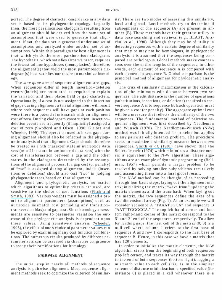
The N-W method can be thought of as proceedingthrough four basic steps: laying out the alignment ma-trix; initializing the matrix; “wave front” updating thematrix elements; and the trace back. When laying outthe matrix, the two sequences define the axes of atwo-dimensional array (Fig. 1). As an example we willconsider sequence A “TAAATTGCA” and sequence B“AATTTGGGCCA.” The top left-hand corner and bot-tom right-hand corner of the matrix correspond to the59 and 39 end of the sequences, respectively. To allowfor leading gaps, the first cell of the matrix (0, 0) is anull cell where column 1 refers to the first base ofsequence A and row 1 corresponds to the first base ofsequence B. Hence, in this case we have a matrix thathas 120 elements.

In order to initialize the matrix elements, the N-Walgorithm starts from the beginning of both sequences(top left corner) and traces its way through the matrixto the end of both sequences (bottom right), logging amismatch value to each cell (Fig. 1). In the simplestscheme of distance minimization, a specified value (forinstance 0) is placed in a cell whenever there is a

1

cttu

across the row to the right. Cell (0, 1) has only one

319REVIEW

matching state between sequences, regardless of posi-tion. All nonidentical states are assigned a value ofone. More elaborate schemes of mismatch-scoring func-tions can be instituted by referring to a predefinedmismatch-scoring matrix.

During the wavefront update of the matrix, each cellin the matrix is assigned a new value (Fig. 2a–2d). Thisvalue results from a comparison of three neighbors ofmatrix cell (i, j): the cell to the immediate left (i, j 21), directly above (i 2 1, j), and diagonal above and to

the left (i 2 1, j 2 1). A diagonal path implies aorrespondence between sequence elements whetherhere is a match or a mismatch. A gap is inserted intohe alignment by moving across a row or down a col-mn. Gaps are assigned a cost (.0) or a trivial align-

ment will be generated with a gap at every potentialmismatch (total score 5 0). The new value of cell (i, j)will be the minimum path cost of the three possibleroutes from its neighbors (Fig. 2). The value of theseroutes is calculated by adding the cell value of theprevious cell (i, j 2 1; i 2 1, j; or i 2 1, j 2 1) plusthe gap cost in the case of a gap or the mismatch cost inthe case of a correspondence. When a gap is institutedthe mismatch costs are ignored since no base corre-spondence is implied:

D~i, j! 5 min$d~i 2 1, j 2 1! 1 mismatch cost,

d~i 2 1, j! 1 gap cost,

d~i, j 2 1! 1 gap cost},

given that d(i0, j0) 5 0.In the example here (Figs. 1–3), the gap cost is set to

10 and the mismatch cost is set at 1. The update beginsin the null cell of the top left-hand corner (Fig. 2a). Theinitial value of this cell is zero. The operation continues

FIG. 1. An initialized matrix of a pairwise nucleotide sequencecomparison with an assigned mismatch cost of 1.

neighbor cell, (0, 0). Therefore, cell (0, 1) is assigned avalue of 10, that being the gap cost of 10 plus the valueof the previous cell (0, 0), which is zero. Cell (0, 2) isassigned a value of 20, a gap cost of 10 plus the cellvalue of its only neighbor (0, 1) also 10. This processcontinues across the row, sequentially adding the gapcost to the next cell. The procedure is repeated forcolumn 0 as each cell in that column only has oneneighbor. Cell (1, 1) is the first cell where the optimaldetermination of path cost is performed (Fig. 2a). Forcell (1, 1), the path cost from cell (0, 1) is 20, 10 from thegap cost and 10 from the cell value of (0, 1). The same

FIG. 2. Wavefront updating of the matrix elements correspond-ing to the first two nucleotides in sequences A and B from Fig. 1.Each cell in the matrix has its value reassigned based on an optimalpathcost calculation. (a) The leading cell of the matrix at the top left(0, 0) has a default value of zero. Each horizontal or vertical path toa cell is assigned a gap cost of 10 and the previously assignedmismatch costs are abandoned. A diagonal path to a cell withholdsthe cell’s mismatch value (1). Each path, whether horizontal, verti-cal, or diagonal, brings with it the value of the cell from which thatpath originated. The cells in the first row and column of the matrixcontinuously accrete a gap cost of 10. Cell (1, 1) is the first cell in thematrix that must discriminate which of the three paths is optimal.An asterisk (p) designates which are the lowest path costs. In thisinstance it is the diagonal path from cell (0, 0). These optimal pathsare retained in memory. (b) Once the optimal path(s) have beenretained the value of the cell from which the path originated is nolonger necessary and is not reported. The large arrows representoptimal paths to each cell retained in memory. The process is re-peated for cells (2, 1) and (1, 2). The optimal path for cell (2, 1) is onthe diagonal. Cell (1, 2) has two optimal paths, one on the diagonaland one from directly above. (c) The final cell (2, 2) undergoes theoptimization procedure with a single optimal path on the diagonal.(d) A fully updated matrix with the optimal paths retained.

These contiguous cell to cell paths are forged during

320 REVIEW

is true of the path cost from cell (1, 0), 10 from the gapcost and 10 from the cell value. The path cost from (0,0) to (1, 1) is 1; there is no gap cost since it is on thediagonal and the cell value of cell (0, 0) is 0, but amismatch cost is applied since cell (1, 1) represents acorrespondence of an A and a T (Fig. 2a). The new cellvalue entered into cell (1, 1) is 1. At this time, the pathfrom which that value was derived is logged. If twopath costs are equal, an arbitrary choice is usuallymade, but both paths can be retained in memory. Eachcell in turn undergoes this process until all cells areupdated (Figs. 2b–2d, 3).

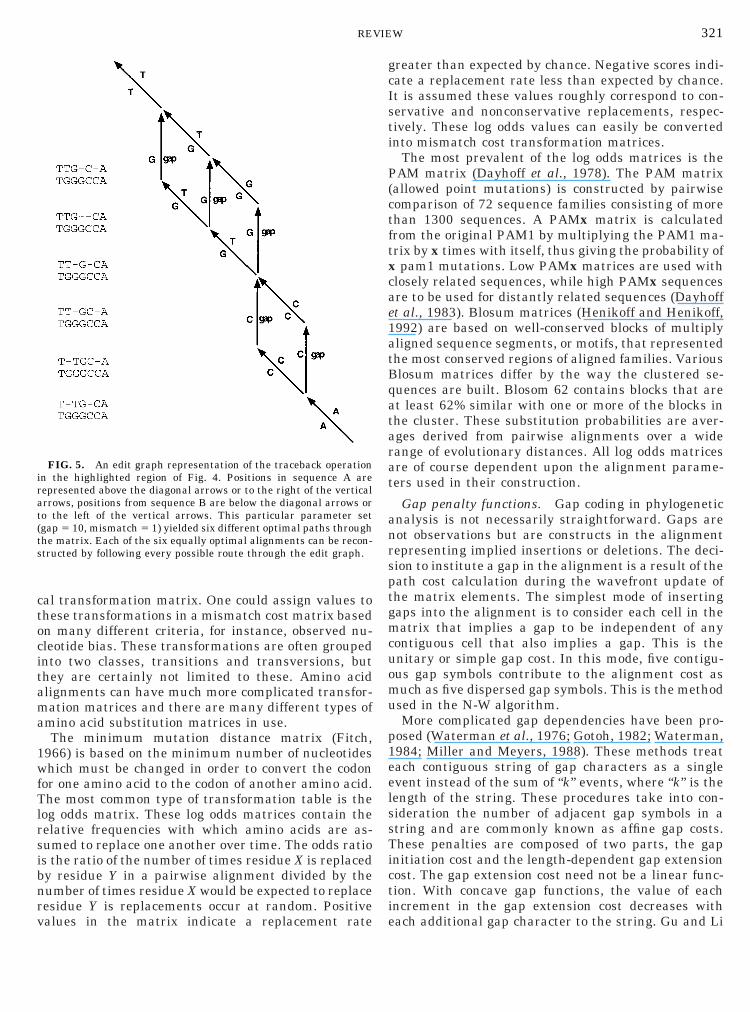
All possible alignments, whether optimal or subop-timal, are represented as pathways through the array.The traceback begins at the terminal (bottom right)element of the matrix. Any previously retained lowestpath cost notation that can be connected consecutivelythrough (i 2 1, j), (i, j 2 1), or (i 2 1, j 2 1) is tracedback through the matrix (Fig. 4). This trajectory rep-resents a sequence of edit operations which transformssequence A into sequence B. This edit path forms thealignment. An uninterrupted diagonal through the ar-ray would represent no gap assignments. There may bemore than one optimal pathway (Fig. 5); with thisparticular parameter set there are six possible path-ways through the matrix. The traceback proceduremerely recognizes any series of retained cell to cellpaths that are contiguous through the entire matrix.

FIG. 3. A fully updated pairwise matrix of the complete se-quences with the optimal paths. The cell values are retained only forillustration; they represent local edit distances. The terminal cell(10, 12) represents the global edit distance between sequences A andB.

the wavefront update and it is at this point that posi-tional homology is established.

Cost functions. The gap cost and mismatch costassociated with the N-W algorithm are in a dynamicrelationship; increasing mismatch cost will createmore gaps in the alignment and increasing gap costwill increase the number of mismatches. Accordingly,an alignment may only be optimal for a particularcombination of mismatch and gap costs. Alter thesevalues and the optimal alignment may alter as wellyielding a different phylogenetic data set. How, then,does one decide which combination of parameter sets touse? In general these choices are arbitrary. The follow-ing is a discussion of various implementations of costfunctions in the N-W algorithm. There is a myriad ofvariations on the implementation of cost functions.Most of these implementations are attempts to mimicbiological processes or constraints, which are thoughtto regulate the evolution of DNA or protein sequences.

Mismatch cost functions. There are many varia-tions on the type of mismatch costs one can assignwhen laying out the N-W matrix. Aside from binarycost functions (0 5 nucleotide match or 1 5 mismatch),a transformation matrix of substitution costs can beinstituted which will assign a separate penalty for eachclass of mismatches observed. Nucleotide sequencealignment has six types of mismatches in a symmetri-

FIG. 4. The traceback procedure begins at the terminal cell(bottom right corner) in the matrix and tracks a path back throughthe matrix following all retained optimal paths until the top left cell(0, 0) is reached.

greater than expected by chance. Negative scores indi-

c

irat(ts

321REVIEW

cal transformation matrix. One could assign values tothese transformations in a mismatch cost matrix basedon many different criteria, for instance, observed nu-cleotide bias. These transformations are often groupedinto two classes, transitions and transversions, butthey are certainly not limited to these. Amino acidalignments can have much more complicated transfor-mation matrices and there are many different types ofamino acid substitution matrices in use.

The minimum mutation distance matrix (Fitch,1966) is based on the minimum number of nucleotideswhich must be changed in order to convert the codonfor one amino acid to the codon of another amino acid.The most common type of transformation table is thelog odds matrix. These log odds matrices contain therelative frequencies with which amino acids are as-sumed to replace one another over time. The odds ratiois the ratio of the number of times residue X is replacedby residue Y in a pairwise alignment divided by thenumber of times residue X would be expected to replaceresidue Y is replacements occur at random. Positivevalues in the matrix indicate a replacement rate

FIG. 5. An edit graph representation of the traceback operationn the highlighted region of Fig. 4. Positions in sequence A areepresented above the diagonal arrows or to the right of the verticalrrows, positions from sequence B are below the diagonal arrows oro the left of the vertical arrows. This particular parameter setgap 5 10, mismatch 5 1) yielded six different optimal paths throughhe matrix. Each of the six equally optimal alignments can be recon-tructed by following every possible route through the edit graph.

cate a replacement rate less than expected by chance.It is assumed these values roughly correspond to con-servative and nonconservative replacements, respec-tively. These log odds values can easily be convertedinto mismatch cost transformation matrices.

The most prevalent of the log odds matrices is thePAM matrix (Dayhoff et al., 1978). The PAM matrix(allowed point mutations) is constructed by pairwisecomparison of 72 sequence families consisting of morethan 1300 sequences. A PAMx matrix is calculatedfrom the original PAM1 by multiplying the PAM1 ma-trix by x times with itself, thus giving the probability ofx pam1 mutations. Low PAMx matrices are used withlosely related sequences, while high PAMx sequences

are to be used for distantly related sequences (Dayhoffet al., 1983). Blosum matrices (Henikoff and Henikoff,1992) are based on well-conserved blocks of multiplyaligned sequence segments, or motifs, that representedthe most conserved regions of aligned families. VariousBlosum matrices differ by the way the clustered se-quences are built. Blosom 62 contains blocks that areat least 62% similar with one or more of the blocks inthe cluster. These substitution probabilities are aver-ages derived from pairwise alignments over a widerange of evolutionary distances. All log odds matricesare of course dependent upon the alignment parame-ters used in their construction.

Gap penalty functions. Gap coding in phylogeneticanalysis is not necessarily straightforward. Gaps arenot observations but are constructs in the alignmentrepresenting implied insertions or deletions. The deci-sion to institute a gap in the alignment is a result of thepath cost calculation during the wavefront update ofthe matrix elements. The simplest mode of insertinggaps into the alignment is to consider each cell in thematrix that implies a gap to be independent of anycontiguous cell that also implies a gap. This is theunitary or simple gap cost. In this mode, five contigu-ous gap symbols contribute to the alignment cost asmuch as five dispersed gap symbols. This is the methodused in the N-W algorithm.

More complicated gap dependencies have been pro-posed (Waterman et al., 1976; Gotoh, 1982; Waterman,1984; Miller and Meyers, 1988). These methods treateach contiguous string of gap characters as a singleevent instead of the sum of “k” events, where “k” is thelength of the string. These procedures take into con-sideration the number of adjacent gap symbols in astring and are commonly known as affine gap costs.These penalties are composed of two parts, the gapinitiation cost and the length-dependent gap extensioncost. The gap extension cost need not be a linear func-tion. With concave gap functions, the value of eachincrement in the gap extension cost decreases witheach additional gap character to the string. Gu and Li

(1995) analyzed gap length in processed pseudogenes

wcwsMaiaer

snttdtgetcTWpWssl(smpoa(

ittaTittae6anacey

322 REVIEW

and found the length distribution to be a log function.This implies a gapping function of wg 5 a 1 b ln k

here a is the gap initiation cost, b is the gap extensionost and k is the gap length. Although many algorithmshich incorporate concave gap costs have been de-

cribed in the literature (Knight and Meyers, 1995;iller and Meyers, 1988; Allison, 1993), few computer

pplications actually include them. An additional mod-fication in gapping is to allow gaps at the beginningnd end of a sequence to be free of any cost. Cost-freend gaps should be used with caution as this enters theealm of local alignment.

One of the most problematic areas in phylogeneticequence alignment is the influence of long gaps. Dy-amic programming cannot look forward into the ma-rix. The wavefront update, which establishes the op-imal path costs, is unidirectional and can only base itsecision to institute a gap or correspondence based onhe observed cost function up to the present point. As aap becomes increasingly long it may become moreconomical to begin to apply mismatches than to ex-end the gap even though there may be a high scoringontiguous string of matches later on in the matrix.his is apparent in many 18S ribosomal data sets (seehiting et al., 1997). Long gaps are particularly a

roblem when memory-saving modifications of the N--algorithm are applied (see below). Gotoh (1982) de-

igned an algorithm to deal with this issue which as-igned a constant cost for any gap exceeding a specifiedength. Another approach also developed by Gotoh1990) uses a series of linear functions of decreasinglope, which approximate a concave function. Theseore complex gapping functions contribute to the com-

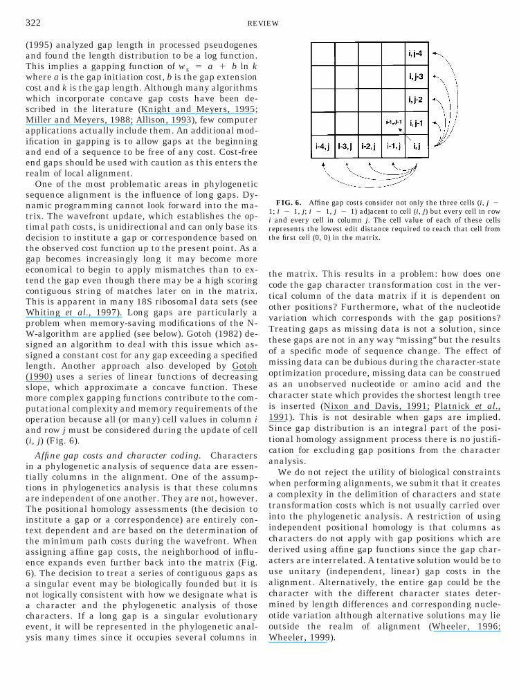
utational complexity and memory requirements of theperation because all (or many) cell values in column ind row j must be considered during the update of celli, j) (Fig. 6).

Affine gap costs and character coding. Charactersn a phylogenetic analysis of sequence data are essen-ially columns in the alignment. One of the assump-ions in phylogenetics analysis is that these columnsre independent of one another. They are not, however.he positional homology assessments (the decision to

nstitute a gap or a correspondence) are entirely con-ext dependent and are based on the determination ofhe minimum path costs during the wavefront. Whenssigning affine gap costs, the neighborhood of influ-nce expands even further back into the matrix (Fig.). The decision to treat a series of contiguous gaps assingular event may be biologically founded but it is

ot logically consistent with how we designate what ischaracter and the phylogenetic analysis of those

haracters. If a long gap is a singular evolutionaryvent, it will be represented in the phylogenetic anal-sis many times since it occupies several columns in

the matrix. This results in a problem: how does onecode the gap character transformation cost in the ver-tical column of the data matrix if it is dependent onother positions? Furthermore, what of the nucleotidevariation which corresponds with the gap positions?Treating gaps as missing data is not a solution, sincethese gaps are not in any way “missing” but the resultsof a specific mode of sequence change. The effect ofmissing data can be dubious during the character-stateoptimization procedure, missing data can be construedas an unobserved nucleotide or amino acid and thecharacter state which provides the shortest length treeis inserted (Nixon and Davis, 1991; Platnick et al.,1991). This is not desirable when gaps are implied.Since gap distribution is an integral part of the posi-tional homology assignment process there is no justifi-cation for excluding gap positions from the characteranalysis.

We do not reject the utility of biological constraintswhen performing alignments, we submit that it createsa complexity in the delimition of characters and statetransformation costs which is not usually carried overinto the phylogenetic analysis. A restriction of usingindependent positional homology is that columns ascharacters do not apply with gap positions which arederived using affine gap functions since the gap char-acters are interrelated. A tentative solution would be touse unitary (independent, linear) gap costs in thealignment. Alternatively, the entire gap could be thecharacter with the different character states deter-mined by length differences and corresponding nucle-otide variation although alternative solutions may lieoutside the realm of alignment (Wheeler, 1996;Wheeler, 1999).

FIG. 6. Affine gap costs consider not only the three cells (i, j 21; i 2 1, j; i 2 1, j 2 1) adjacent to cell (i, j) but every cell in rowi and every cell in column j. The cell value of each of these cellsrepresents the lowest edit distance required to reach that cell fromthe first cell (0, 0) in the matrix.

Methods for saving computational effort and mem-

bfomrcursfiota

stdqTanmat

m

the subpath to each adjacent cell and the added cost of

t

323REVIEW

ory. There have been many attempts at conservingcomputational effort and memory requirements for dy-namic programming in general. One can assume that itis not necessary to explore the entire pairwise matrixto find the optimal edit distance. Using a diagonal paththrough the matrix as the null optimal, one need onlyconsider a portion of the matrix a certain distance fromthe diagonal. Ukkonen (1985) utilizes the notion thatthe optimal solution is somewhere near the diagonal bydefining a boundary (2k 1 1) around the diagonalased on the number of gaps present in the sequence soar. Meyers and Miller (1988) devised a method basedn Hirschberg (1975) which does not require that theatrix be retained permanently as in the N-W algo-

ithm. The edit distance score is used in a divide-and-onquer procedure that recursively bisects the matrixntil there is a series of smaller alignments whichequire less computational effort. The alignments areubsequently concatenated. Gotoh (1990) then modi-ed the traceback procedure to include all possibleptimal alignments. These methods are generalizableo the multiple sequence alignment problem (Carillond Lipman, 1988) described below.

MULTIPLE SEQUENCE ALIGNMENT

The N-W algorithm was originally defined for twoequences. In principle, the procedure can be extendedo any number of sequences, thereby defining an N-imensional matrix. However, the addition of se-uences opens up an immense computational problem.he number of cells in a true simultaneous multiplelignment matrix are exponentially related to theumber of taxa and sequence length. Even using theethods that save storage and effort, simultaneous

lignment of more than a few sequences is computa-ionally intractable.

Sankoff and Cedergren (1983) proposed a tree-basedultiple alignment method within an N-dimensional

N-W framework. Their method requires, however, thatthe cladogram of relationships is known a priori andalignments are performed with the cost of each cell inthe alignment space determined by the “known” cla-dogram. Initially, a space is created with )0

n Ln 1 1cells (n is the number of the sequences and L theirlengths). A pass is made through this space as with thetwo-dimensional method, updating each cell. The up-dated cost of each cell would be the minimum of thecost of each adjacent cell incremented by the cost of thecurrent cell, as determined by the known tree. For ntaxa there are 2n 2 1 cells to be examined (all thecombinations, indels, and base matches and mis-matches) to determine the cost of each cell.

This is a straightforward extension of the two-di-mensional N-W case. As with the 2-d case, the cost ofeach cell is determined by the minimum of the sum of

the path to the current cell. Where the cost of cell (i, j)for sequences A and B and transformation cost set “w”,

dij 5 minH di,j 2 1 1 w~“—”, Bj!di 2 1,j 1 w~Ai, “—”!di 2 1,j 2 1 1 w~Ai, Bj!

Jfor two sequences becomes

dij· · ·k 5 minHdi,j 2 1,· · ·k 1 w~“—”, Bj, . . . , ck!

di 2 1,j· · ·k 1 w~Ai, “—”, . . . , ck!···

Jdi, j,· · ·k 2 1 1 w~Ai, Bj, . . . , “—”!,

when “k” sequences are included. The minimizationoccurs over all possible combinations of gaps andmatches for a total of 2k 2 1 path to cell i, j, . . . , k. Inhis general case, the “w” set of transformation costs

would be based on the predetermined tree. The parsi-moniously reconstructed (but not searched) length ofthe a priori tree is used for the “w” costs.

If the tree of relationships were not known ahead oftime (the most likely case), the alignment procedurecould be repeated for each possible scheme of relation-ships or phylogenetic searching could be performed foreach cell. Given that the number of cells in the align-ment space is exponentially related to the number oftaxa, and the number of trees is combinatorially de-pendent on the number of taxa, this type of approach,though exact, would be intractable for all but thesmallest data sets.

HEURISTIC MULTIPLE ALIGNMENT

As a result of this combinatorial complexity, simul-taneous alignment of all sequences is rarely attempted.Instead, a series of pairwise alignments are performedand these subalignments amalgamated into a multiplealignment. The intermediate pairwise alignments areadded together following a tree-like pattern. The orderby which this is carried out is determined by a “guidetree” (Feng and Doolittle, 1987). Each node of the treerepresents a separate pairwise alignment. Mindell(1991) advocated using known phylogenies to guidealignments but the required phylogenetic informationis often unavailable. In most evolutionary studies, theobject of performing a multiple alignment is to allowphylogenetic analysis with a set of putative homologiesunbiased by initial assumptions of relationship. Pre-conceived notions of relationships will bias the analy-sis.

The phylogeny resultant from analysis of a multiplealignment is obviously dependent on the order in whichthe sequences are accreted. However, if gap assign-

ment is unambiguous, many different guide tree topol-

hb“oa

324 REVIEW

ogies will lead to the same phylogeny. Thus, the guidetree topology is separate and distinct from the topologyof the phylogenetic tree derived from the alignment.

Several methods are currently in use to progres-sively align sequences via pairwise accretion. The dif-ferences among them center on two areas: (1) tech-niques of establishing an alignment topology ortopologies (guide tree), and (2) how the aligned se-quence positions at the nodes are combined to createthe complete multiple alignment. The guide tree can beestablished using a pairwise distance-based approachor by choosing from many guide trees in a parsimonyframework. The results of each pairwise alignment inthe guide tree can produce a consensus sequence whichis resolved later, or the character state can be resolvedas soon as possible within the alignment process. Thedecision to choose one mode over another tends to bebased on computational effort, the methods that iteratethrough multiple guide trees being the most consump-tive of computational resources.

Distance-based guide trees. Initially, guide treeswere determined based on distance methods (Feng andDoolittle, 1987, 1990; adapted by Higgins and Sharp,1988, 1989; Higgins et al., 1992; Thompson et al.,1994). Thompson et al. (1994) described the procedureas follows. A similarity score is calculated from a pair-wise alignment between every possible pair of se-quences (Wilbur and Lipman, 1983). A distance matrixcomposed of these scores is used to calculate a den-dogram using the UPGMA method of Sneath and Sokal(1973) as an alignment topology. This topology is usedto direct the alignment of the most similar sequences ina N-W procedure. The CLUSTAL alignment program(Thompson et al., 1994) (ftp://ftp-igbmc.u-strasbg.fr/pub/) aligns the most similar sequences first. A consen-sus sequence is substituted for the sequence pair. Con-sensus sequences incorporate only bases present in allsequences or use partial (75%) consensus. Gaps in-serted in any alignments are preserved throughout thealignment. Clustal progressively aligns the next mostsimilar sequence to the consensus of the growing clus-ter or the next two most similar sequences to eachother (Fig. 7). Only a single multiple alignment isconstructed. However, an industrious user could spec-ify various alignment topologies and run the programrepeatedly to explore the relationship between align-ment topology and phylogenetic results.

There are other methods based on sequence similar-ity (Hein, 1989a,b, 1990; Konings et al., 1987). Thesemethods differ in how the distance tree is determinedand how the tree interacts with the actual alignment.Hein (1989a,b, 1990) extended the process by adding aparsimony step. In TREEALIGN (Hein, 1989a,b),(ftp://ftp.ebi.ac.uk/pub/software/unix/treealign.tar.Z),pairwise distances are used to construct an alignment

topology and an initial alignment with observed se-quences at the edges of the tree. The alignment topol-ogy is converted to a parsimony tree and used to directan alignment algorithm. During alignment, potentialancestral sequences are created at each node in thealignment topology using parsimony (Fig. 8). Althougha parsimony score is attached to the alignment topol-ogy, no other trees are constructed for comparison. Thealignment topology is subjected to nearest neighborinterchanges until all branches are swapped or a user-defined number of swapping cycles is reached. Se-quences are aligned along the resultant tree via agraph comparison algorithm similar to that of Sankoffand Cedergren (1983). Ancestral sequences are deter-mined for each node via dynamic programming. Basemismatches (e.g., A in sequence 1 and C in sequence 2)are incorporated in the ancestral sequences by theunion of the bases (A 1 C). A choice between thealternatives is postponed until evidence higher up inthe tree points to either A or C (Fig. 8). If nothingfavors A or C an arbitrary choice is made (J. Hein, pers.commun.).

Parsimony-based alignment topologies. Any singleaddition order can lead to a result that is not globallyoptimal. This is one of the most severe problems ofnonexact solutions. In MALIGN (Wheeler and Glad-

FIG. 7. Tree-based depiction of multiple alignment strategy inCLUSTAL. Let all base changes and gaps cost 1. A distance tree iscreated by UPGMA. In the downpass terminal sequences are relatedby a dendrogram. (A) A pairwise alignment of two most “closelyrelated” terminal sequences. An unknown residue X is used to place-

old any disagreement. Then a pairwise alignment is performedetween the consensus produced at the previous node with next mostclosely related” sequence. (B) In the up pass, progressive alignmentf the consensus sequences and terminal sequences is used to resolveny ambiguities and to introduce gaps.

ment cost. In the heuristic option termed “build,” align-

icdtmc

325REVIEW

stein, 1994) (ftp://ftp.amnh.org/pub/people/wheeler/malign/), many alignment topologies are used to ex-plore multiple alignments. Various alignmenttopologies can be constructed via random addition ofsequences and branch-swapping. As sequences are ac-creted alignment topologies (subtrees) are produced byadding sequences to the branch that produces the leastcostly alignment. Minimization occurs by searching forthe least costly path through a N-W matrix determinedby the sequences and costs associated with acceptingnucleotide mismatches or inserting gaps. Subtrees arethen combined to produce a complete multiple align-ment.

Alignment cost can be improved through branchswapping (Fig. 9). MALIGN performs branch swappingby removing taxa and adding them back to all the otherpossible addition points on the cladogram or alignmenthierarchy. The cost of the most parsimonious align-ment topology is then assigned as the multiple align-

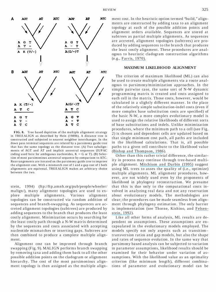
FIG. 8. Tree based depiction of the multiple alignment strategyn TREEALIGN as described by Hein (1989b). A distance tree isonstructed and subjected to nearest neighbor interchanges. In theown pass terminal sequences are related by a parsimony guide treehat has the same topology as the distance tree. (A) Two subalign-ents of AGT and AT and implicit ancestral sequences (IUPAC

oding used here for ambiguous nucleotides, K 5 G or T). (B) Selec-tion of most parsimonious ancestral sequence by comparison to ATC.Rearrangements are iterated on the parsimony guide tree to improvethe alignment cost. With a mismatch cost of 1 and a gap cost of 1 bothalignments are equivocal. TREEALIGN makes an arbitrary choicebetween the two.

ments are constructed by adding taxa to an alignmenttopology at each of the possible addition points andalignment orders available. Sequences are stored atsubtrees as partial multiple alignments. As sequencesare accreted, alignment topologies (subtrees) are pro-duced by adding sequences to the branch that producesthe least costly alignment. These procedures are anal-ogous to heuristic cladogram construction algorithms(e.g., Farris, 1970).

MAXIMUM LIKELIHOOD ALIGNMENT

The criterion of maximum likelihood (ML) can alsobe used to create multiple alignments via a route anal-ogous to parsimony/minimization approaches. In thesimple pairwise case, the same sort of N-W dynamicprogramming matrix is created and costs assigned toeach cell in the matrix. Those costs, however, would becalculated in a slightly different manner. In the placeof the relatively simple substitution-indel costs (even ifmore complex base substitution costs are specified) ofthe basic N-W, a more complex evolutionary model isused to assign the relative likelihoods of different sortsof base substitutions and indels. Unlike minimizationprocedures, where the minimum path to a cell (see Fig.2) is chosen and dependent cells are updated based onthat single minimum cost path, all paths are includedin the likelihood calculations. That is, all possiblepaths to a given cell contribute to the likelihood value(Bishop and Thompson, 1986).

Other than this rather trivial difference, the similar-ity in process may continue through tree-based multi-ple alignment. Mitchison and Durbin (1995) suggestusing ML trees to asses the quality of (i.e., optimize)multiple alignments. ML alignment procedures, how-ever, are not widely used even by the proponents oflikelihood in phylogeny reconstruction. We presumethat this is due only to the computational costs in-volved in analyzing real data and not any reservationabout evolutionary models. The methodologies areclear; the procedures can be made seamless from align-ment through phylogeny estimation. The only barrieris implementation (see Thorne, Kishino, and Felsen-stein, 1992).

Like all other forms of analysis, ML results are de-pendent on assumptions. These assumptions are en-capsulated in the evolutionary models employed. Themodels specify not only aspects such as transition–transversion ratios and gap models, but also the shapeand rates of sequence evolution. In the same way thatparsimony based analysis can be subjected to variationin parameter assumptions, likelihood results should beexamined for their behavior under variation of as-sumptions. With the likelihood value as an optimalitycriterion (like minimum length), different combina-tions of parameter and evolutionary model can be

“tte

326 REVIEW

tested to maximize the criterion of choice. These oper-ations would be identical to those for minimization/parsimony, but with a different criterion of optimality.

PARAMETER SENSITIVITY

The phylogenetic analysis of nucleic acid sequences,as with other data, is unavoidably based on explicitand implicit assumptions. Results of multiple align-ment and phylogenetic analysis, no matter the algo-rithms, are sensitive to choice of evolutionary model.At the fore are character transformation models. Forexample, various weights must be assigned to param-eters such as transitions, transversions, and insertion–deletion events. There are no known means of deter-mining, a priori, which alignment parameters areappropriate for recovering evolutionary relationships.

Simple homogeneous weighting does not avoid theissue of arbitrary, yet crucial, assumptions. As an ex-ample, transversion–transition ratio and gap costs are

FIG. 9. Tree based depiction of an example multiple alignment stbuild” step, terminal sequences are related by a cladogram that reshere are three possible guide trees, A, B, and C. After the tree searo potentially improve optimization of character changes. The alignmxample alignment topology A and C produce the same optimal alig

generally not directly measurable. These values arestatements of process and they can be inferred appro-priately only from a predetermined phylogenetic pat-tern. The interaction between the specification of val-ues a priori and their inference a posteriori is a generaland central problem in molecular phylogenetic analy-sis.

One of the benefits of likelihood techniques is thatthe method can estimate the values of its own param-eters by simultaneously varying parameters untilglobal maximum likelihood is achieved. In the case ofalignment, the likelihood of an alignment based on oneset of parameters (e.g., indel cost, transversion ratio)can be compared to that based on another. Unlike thenumerical values derived from parsimony analyses, alikelihood of 0.1 for an alignment with a gap cost oftwice that of base changes is superior to a likelihood of0.01 based on gaps costing four times base changes.Continuing this logic, the maximum likelihood align-ment over all (or some heuristic subset) of analysis

egy in MALIGN. Let all base changes 5 1 and gaps cost 5 2. In eachs from a random or user-specified addition sequence. For these taxais conducted, each alignment is then subjected to branch swappingthat produces the shortest tree is the best alignment. In this simpleent.

ratultchentnm

parameters gives both the alignment and the maxi- space with each of the N parameters defining an axis

327REVIEW

mum likelihood estimate of each of the components ofthe model. The costs of alignments based on weightedparsimony are not comparable in this way. A cost (orderived cladogram length) of two is not necessarilysuperior to a length of four. Each solution is mostparsimonious for its own set of parameters and notcomparable from parsimonious solution to parsimoni-ous solution.

Alignment space and congruence. In order to esti-mate the multiple alignment parameters, both a modeland a space are posited. The model determines thegeneral means of calculating likelihoods based on boththe form of the model and the assumed values of itsparameters. To perform the likelihood estimates, thelikelihood is calculated for each point in the parameterspace. The point with the maximum value gives thelikelihood estimate of the alignment, and the pointsalong each axis give the parameter values.

If several sources of information are to be used, eachdata set may require a unique model. It is unclear howto assess the ensemble phylogenetic conclusions. Theuse of external criteria offers a way of accommodatingsuch results. If an external criterion can be defined, thebehavior of each solution can be calculated and com-pared to those of other solutions. One such externalcriterion is congruence. As used by Wheeler (1995),congruence measures can be posited and all solutionsassayed. The set of analysis parameters which maxi-mizes (or minimizes) this value is then optimal. Thepotential problem with this approach is that differentoptimality criteria may be used within and amongmodels. Those solutions, which are optimal by one cri-terion, may not be with another.

Sensitivity analysis. Even though the basic align-ment parameters of transversion–transition and gap–change cost ratios are unmeasurable in the absence ofa predetermined phylogeny, it is possible to estimatetheir values through appeal to an external optimalitycriterion. The most reasonable for phylogenetic analy-sis must be congruence (whether taxonomic [Nelson,1979] or character based [Mickevich and Farris, 1981],but see Miyamoto [1981, 1985]). Without any way ofobjectively measuring the accuracy of reconstruction,only the agreement among data can be used to arbi-trate among competing hypotheses.

In order to estimate the sensitivity of an analysis tovariation in parameter values, the range of each of theparameters must be determined. This establishes the“analysis space” of the problem. In this space, all pos-sible combinations of parameter values are present;hence all analytical conclusions are implied. Thesecombinations of values are sampled and their analyti-cal consequences determined (see Fitch and Smith,1983; and Vingron and Waterman, 1994). This would,in the most general case, involve an N-dimensional

bounded by the parameter ranges. The two parametersof insertion–deletion cost and transversion–transitionratio would constitute the axes of a simple analysisspace (Fig. 10). A sampling regime would consist oftaking parameter pairs (transversion–transition ratio,gap–change cost ratio) from this space, aligning thesequences, erecting hypotheses of relationship basedon these values, and assaying congruence with an ex-ternal data set.

Even with only two parameters, the available anal-ysis universe is infinite. Each of the parameters can, atleast numerically, achieve any positive real value. Re-alistic sampling of such a space may be difficult. Thesevalues are not boundless and may be constrained bythe logic of the triangle inequality as formulated forcharacter analysis (Wheeler, 1995).

Within these theoretical limits, a residuum of possi-ble values exists for the analysis parameters. With twoparameters, a plane bounded on two adjacent sides isdefined (Fig. 10). Since any and all combinations ofparameter values which fall in this plane are possibleat least logically, they must all be examined (or at leastsome sample). To accomplish this sampling, alignmentand phylogeny reconstruction must be performed withsufficient combinations of possible values to representthe behavior of the entire space. This is a relativelystraightforward procedure (if time-consuming). Foreach point (a combination of transversion–transitionand gap–change value ratios) to be sampled, the se-quences are aligned and phylogeny reconstructed. Bothalignment and phylogeny reconstruction are per-formed using the same combination of parameter val-ues. At each of these points, some measure of congru-ence is calculated with respect to some external dataset, the variation of which can be used to assay both themost appropriate values for the unmeasurable param-eters and the effects of variation in these parametervalues on the overall conclusions of the analysis.

If some congruence measure is plotted with respectto the parameter values, a “congruence surface” is gen-erated, the relief in this surface denoting the areas ofrelative congruence and incongruence. This surfacecan be used to estimate the values of the analyticalparameters. As with statistical inference, two types ofdecision (estimate of parameter values) can be made—“best” and “robust.” A “best” decision is made by choos-ing the set (or sets) of parameter values at which theoptimality criterion is maximized. According to thistype of decision, the set of values for transversion–transition ratio and gap–change ratio that maximizecongruence would be chosen. On the other hand, a“robust” decision selects a range of parameter valuesrather than settling on a single set. This range definesa subset of the analysis space in which some statementis supported. For example, an area might be specified

328 REVIEW

in which some particular group was monophyletic, butthis clade was not supported generally.

The Mickevich and Farris (1981) measure of congru-ence seeks to assess the degree of character conflictamong multiple data sets. The statistic of Mickevichand Farris (1981) quantifies the degree of characterconflict by measuring the number of extra steps forcedupon the individual data sets when they are combined.In this way, the additional conflict created by the com-bination of the data is assessed separately from thatderived from internal character conflict. The value gen-erated is simply the length of the most parsimoniouscladogram(s) derived from the combined data minusthe sum of the lengths of the cladograms from theconstituent data sets. This number of steps is normal-ized through division by the length of the combineddata. A value of zero implies complete character con-gruence, while higher values denote increasing degreesof character conflict between the data sets. No topologystatement is implied or required. In fact, data sets,which have zero taxonomic congruence, can have 100%character congruence. This can occur if one data set

FIG. 10. Graphical representation of an alignment parameter senB genes from 35 carnivore taxa. The incongruence length differencedatasets from the treelength of the combined data set and dividing thcombined 2 treelength 12S 2 treelength 16S 2 treelength cytB)/treegap costs including 1, 2, 4, 8, and 16, and transition/transversion rayielded the least internal data conflict were gap cost of 2 and a tran

yields an unresolved bush and the second yields one ofits many potential resolutions.

CONCLUSIONS

In many ways, alignment is where phylogeneticanalysis was 20 years ago. Many investigators stilladvocate creating alignments “by hand,” asserting thatthe human brain is better at determining homology,that computer analysis is not “biological.” Computerprograms for performing alignments are in their in-fancy and users are often unfamiliar with the numer-ical and methodological assumptions made. Presenta-tions at conferences may cite alignment software, butleave crucial information such as gap costs or searchalgorithms undescribed. Clearly, an increase in analyt-ical sophistication and clarity is warranted in this pri-mary stage of phylogenetic analysis.

We advocate three aspects of phylogenetic align-ment-reconstruction: (1) the definition of an optimalitycriterion for alignment, (2) the consistent use of anal-ysis assumptions in both alignment and phylogeny re-

ivity analysis of a data set consisting of the 12S, 16S and cytochromeD) was calculated by subtracting the treelengths of the individual

value by the treelength of the combined data set {ILD 5 (treelengthgth combined}. The alignment parameters explored were a range ofs of 1, 2, 4, 8, and transitions only. The alignment parameters thation/transversion ratio of 1 with an ILD of 0.02569.

sit(ILatlentiosit

construction, and (3) the examination of these assump-

A

B

B

B

C

D

as a prerequisite to correct phylogenetic trees. J. Mol. Evol. 25:351–360.

G

G

G

G

H

H

H

H

329REVIEW

tions through sensitivity analysis to examine therobustness of conclusions.

Since alignment seeks to minimize nonhomology,parsimony seems the most logical of optimality criteriafor alignment. That alignment which implies a cla-dogram of minimal length will, by definition, minimizenonhomology. This is not, of course, the only criterion,maximum likelihood being another. Whatever is cho-sen, though, that logic must be followed through theentire process from alignment to phylogenetic recon-struction. Whatever cost regime (indels and base sub-stitutions), however defined, must be applied consis-tently. Without this connection, alignments might wellimply other cladograms than the analyses generate, orconversely, resultant cladograms might imply differentalignments. The final point, that of testing assump-tions through sensitivity analysis, is based on and re-quires the first two. If analysis parameters are appliedobjectively and consistently, assumptions can betested. By “tested,” we mean that the effects variationsin these assumptions have on phylogenetic conclusionscan be assayed. It may be that a result is entirelydependent on specific values of indels cost or transi-tion–transversion ratio. Only by varying these valuesand examining their perturbations can we assay therobustness of our conclusions.

These points are not specific to parsimony-basedmethods. Although we favor this approach, likelihoodmethods could equally well meet these three require-ments. Our arguments are more for consistency, re-peatability, and transparency in analysis than for anyparticular optimality criterion or epistemologicalcreed.

REFERENCES

Allison, L. (1993). Normalization of affine gap costs used in optimalsequence alignment. J. Theor. Biol. 161: 263–269.

ltschul, S. W., Gish, W., Miller, W., Meyers, E. W., and Lipman,D. J. (1990). Basic local alignment tool. J. Mol. Biol. 215: 403–410.

ellman, R. E. (1957). “Dynamic Programming,” Princeton Univ.Press, Princeton, NJ.

ishop, M. J., and Thompson, E. A. (1986). Maximum likelihoodalignment of DNA sequences. J. Mol. Biol. 190: 159–165.

rower, A. V. Z., and Scharawoch, V. (1996). Three steps of homologyassessment. Cladistics 12: 265–272.

arillo, H., and Lipman, D. (1988). The multiple sequence alignmentproblem in biology. SIAM J. Appl. Math. 48: 1073–1082.

Dayhoff, M. O., Barker, W. C., and Hunt, L. T. (1983). Establishinghomologies in protein sequences. Methods Enzymol. 91: 524–545.

ayhoff, M. O., Schwartz, R. M., and Orcutt, B. C. (1978). A model ofevolutionary change in proteins. In “Atlas of Protein Sequence andStructure” (M. O. Dayhoff, Ed.), Vol. 5, Suppl. 3, pp. 345–352, Natl.Biomed. Res. Found., Washington, DC.

Farris, J. S. (1970). A method for computing Wagner trees. Syst.Zool. 19: 83–92.

Feng, D., and Doolittle, R. F. (1987). Progressive sequence alignment

Feng, D., and Doolittle, R. F. (1990). Progressive alignment andphylogenetic tree construction of protein sequences. Methods En-zomol. 183: 375–387.

Fitch, W. M. (1966). An improved method of testing for evolutionaryhomology. J. Mol. Biol. 16: 9–16.

Fitch, W. M., and Smith, T. F. (1983). Optimal sequence alignments.Proc. Natl. Acad. Sci. USA 80: 1382–1386.iribet, G., and Wheeler, W. C. (1999). On gaps. Mol. Phylogenet.Evol. 13: 132–143.otoh, O. (1982). An improved algorithm for matching biologicalsequences. J. Mol. Biol. 162: 705–708.otoh, O. (1990). Optimal sequence alignment allowing for longgaps. Bull. Math. Biol. 52: 359–373.u, X., and Li, W.-H. (1995). The size distribution of insertion anddeletions in human and rodent pseudogenes suggests a logarith-mic gap penalty for sequence alignment. J. Mol. Evol. 40: 464–473.ein, J. (1989a). A new method that simultaneously aligns andreconstructs ancestral sequences for any number of homologoussequences, when a phylogeny is given. Mol. Biol. Evol. 6: 649–668.ein, J. (1989b). A tree reconstruction method that is economical inthe number of pairwise comparisons used. Mol. Biol. Evol. 36:396–405.ein, J. (1990). Unified approach to alignment and phylogenies.Methods Enzomol. 183: 626–644.enikoff, S., and Henikoff, J. G. (1992). Amino acid substitutionmatrices from protein blocks. Proc. Natl. Acad. Sci. USA 89:10915–10919.

Higgins, D. G., Bleasby, A. J., and Fuchs, R. (1992). CLUSTAL V:Improved software for multiple sequence alignment. CABIOS 8:189–191.

Higgins, D. G., and Sharp, P. M. (1988). CLUSTAL: A package forperforming multiple sequence alignment on a microcomputer.Gene 73: 237–244.

Higgins, D. G., and Sharp, P. M. (1989). Fast and sensitive multiplesequence alignments on a microcomputer. CABIOS 5: 151–153.

Hirschberg, D. S. (1975). A linear space algorithm for computingmaximal common subsequences. Commun. ACM 18: 341–343.

Kluge, A. J. (1989). A concern for evidence and a phylogenetic hy-pothesis of relationships among Epicrates (Boidae, Serpentes).Syst. Zool. 38: 7–25.

Knight, J. R., and Meyers, E. W. (1995). Approximate regular ex-pression pattern-matching with concave gap penalties. Algorith-mica 14: 85–121.

Konings, D. A., Hogweg, P., and Hesper, B. (1987). Evolution of theprimary and secondary structures of the E1a mRNAs of the ade-novirus. Mol. Biol. Evol. 4: 300–314.

Meyers, E., and Miller, W. (1988). Sequence comparison with con-cave weighting functions. Bull. Math. Biol. 50: 97–120.

Meyers, E., and Miller, W. (1988). Optimal alignments in linearspace. CABIOS 4: 11–17.

Mickevich, M. F., and Farris, J. S. (1981). The implications of con-gruence in Menidia. Syst. Zool. 30: 351–370.

Miller, W., and Meyers, E. W. (1988). Sequence comparison withconcave weighting functions. Bull. Math. Biol. 50: 97–120.

Mindell, D. (1991). Aligning DNA sequences: homology and phyloge-netic weighting. In “Phylogenetic Analysis of DNA Sequences”(M. J. Miyamoto and J. Cracraft, Eds.), pp. 73–89. Oxford Univer-sity Press, New York.

Mitchison, G., and Durbin, R. (1995). Tree-based maximal likelihoodmatrices and hidden Markov models. J. Mol. Evol. 41: 1139–1151.

Miyamoto, M. M. (1981). Congruence among character sets in phy-logenetic studies in the frog genus Leptodactylus. Syst. Zool. 321:

N

N

N

d

P

S

S

S

S

S

Thompson, J. D., Higgins, D. G., and Gibson, T. J. (1994). CLUSTALW: Improving the sensitivity of progressive multiple sequence

T

U

V

W

W

W

W

W

W

W

W

330 REVIEW

43–51.Miyamoto, M. M. (1985). Consensus cladograms and general classi-

fications. Cladistics 1: 186–189.Morrison, D. A., and Ellis, J. T. (1997). Effects of nucleotide sequence

alignment on phylogeny estimation: A case study of 18S rDNAs ofApicomplexa. Mol. Biol. Evol. 14: 428–441.eedleman, S. B., and Wunsch, C. D. (1970). A general methodapplicable to the search for similarities in the amino acid sequenceof two proteins. J. Mol. Biol. 48: 443–453.elson, G. J. (1979). Cladistic analysis and synthesis: Principles anddefinitions, with a historical note on Adanson’s Familles des Plan-tes (1763–1764). Syst. Zool. 28: 1–21.ixon, K. C., and Davis, J. I. (1991). Polymorphic taxa, missingvalues and cladistic analysis. Cladistics 7: 233–241.

e Pinna, M. C. C. (1991). Concepts and tests of homology in thecladistic paradigm. Cladistics 7: 367–394.

latnick, N. I., Griswold, C. E., and Coddington, J. A. (1991). Onmissing entries in cladistic analysis. Cladistics 7: 337–343.

ankoff, D. D., and Cedergren, R. J. (1983). Simultaneous compari-son of three or more sequences related by a tree. In “Time Warps,String Edits, and Macromolecules: The Theory and Practice ofSequence Comparison” (D. Sankoff and J. B. Kruskal, Eds.), pp.253–264, Addison-Wesley, Reading, MA.

ellers, P. H. (1974). On the theory and computation of evolutionarydistances. SIAM J. Appl. Math. 26: 787–793.

mith, T. F., Waterman, M. S., and Fitch, W. M. (1981). Comparativebiosequence metrics. J. Mol. Evol. 18: 38–46.

neath, P. H. A., and Sokal, R. R. (1973). “Numerical Taxonomy,”Freeman and Company, San Francisco.

wofford, D. L., and Olsen, G. J. (1990). Phylogeny reconstruction. In“Molecular Systematics” (D. M. Hillis and C. Moritz, Eds.), 1st ed.,pp. 411–501, Sinauer, Sunderland, MA.

alignment through sequence weighting, position specific gap pen-alties and weight matrix choice. Nucleic Acids Res. 22: 4673–4680.

horne, J. L., Kishino, H., and Felsenstein, J. (1992). Inching to-wards reality: An improved likelihood model of sequence evolution.J. Mol. Evol. 34: 3–16.

kkonnen, U. (1985). Finding approximate patterns in strings. J.Alg. 6: 132–137.

ingron, M., and Waterman, M. S. (1994). Sequence alignment andpenalty choice, Review of concepts, case studies and implications.J. Mol. Biol. 235: 1–12.

aterman, M. S., Smith, T. F., and Beyer, W. A. (1976). Somebiological sequence metrics. Adv. Math. 20: 367–387.

aterman, M. S. (1984). General methods of sequence comparison.Math. Biol. 46: 473–500.

heeler, W. C. (1995). Sequence alignment, parameter sensitivity,and the phylogenetic analysis of molecular data. Syst. Biol. 44:321–331.

heeler, W. C. (1996). Optimization alignment: The end of multiplesequence alignment in phylogenetics? Cladistics 12: 1–9.

heeler, W. C. (1999). Fixed character states and the optimization ofmolecular sequence data. Claudistics 15: 379–385.

heeler, W. C., and Gladstein, D. L. (1994). MALIGN, version 1.93.American Museum of Natural History, New York.

hiting, M., Carpenter, J., Wheeler, Q., and Wheeler, W. (1997). TheStrepsiptera problem: Phylogeny of the holometabolous insect or-ders inferred from 18S and 28S ribosomal dna sequences andmorphology. Syst. Biol. 46: 1–68.

ilbur, J., and Lipman, D. (1984). The context dependent compari-son of biological sequences. SIAM J. Appl. Math. 44: 557–567.