Multiple sequence alignment using Hidden Markov model with augmented set based on BLOSUM 80 and its...

Information Sciences 182 (2012) 93–114

Contents lists available at ScienceDirect

Information Sciences

journal homepage: www.elsevier .com/locate / ins

Multiple sequence alignment using the Hidden Markov Model trainedby an improved quantum-behaved particle swarm optimization

Jun Sun ⇑, Xiaojun Wu, Wei Fang, Yangrui Ding, Haixia Long, Webo XuKey Laboratory of Advanced Control for Light Industry (Ministry of Education, China), Jiangnan University, No. 1800, Lihu Avenue, Wuxi, Jiangsu 214122, ChinaDepartment of Computer Science and Technology, Jiangnan University, No. 1800, Lihu Avenue, Wuxi, Jiangsu 214122, China

a r t i c l e i n f o a b s t r a c t

Article history:Available online 18 November 2010

Keywords:Multiple sequence alignmentHidden Markov ModelParameter optimizationQuantum-behaved particle swarmoptimizationPopulation diversity

0020-0255/$ - see front matter � 2010 Elsevier Incdoi:10.1016/j.ins.2010.11.014

⇑ Corresponding author. Address: Department of CChina. Tel./fax: +86 510 85912136.

E-mail address: [email protected] (J. Sun

Multiple sequence alignment (MSA) is an NP-complete and important problem in bioinfor-matics. For MSA, Hidden Markov Models (HMMs) are known to be powerful tools. How-ever, the training of HMMs is computationally hard so that metaheuristic methods suchas simulated annealing (SA), evolutionary algorithms (EAs) and particle swarm optimiza-tion (PSO), have been employed to tackle the training problem. In this paper, quantum-behaved particle swarm optimization (QPSO), a variant of PSO, is analyzed mathematicallyfirstly, and then an improved version is proposed to train the HMMs for MSA. The proposedmethod, called diversity-maintained QPSO (DMQPO), is based on the analysis of QPSO andintegrates a diversity control strategy into QPSO to enhance the global search ability of theparticle swarm. To evaluate the performance of the proposed method, we use DMQPSO,QPSO and other algorithms to train the HMMs for MSA on three benchmark datasets.The experiment results show that the HMMs trained with DMQPSO and QPSO yield betteralignments for the benchmark datasets than other most commonly used HMM trainingmethods such as Baum–Welch and PSO.

� 2010 Elsevier Inc. All rights reserved.

1. Introduction

Multiple sequence alignment (MSA) of nucleotides or amino acids is one of the most important and challenging problemsin bioinformatics. It is an extension of pairwise alignment to incorporate more than two sequences at a time. Multiple align-ment methods try to align all of the sequences in a given query set, and the resulting aligned sequences are often used toconstruct phylogenetic trees, to find protein families, to predict secondary and tertiary structures of new sequences, andto demonstrate the homology between new sequences and existing families [38]. Multiple sequence alignment is computa-tionally difficult to produce and most formulations of the problem lead to NP-complete combinatorial optimization prob-lems [66]. Nevertheless, the utility of these alignments in bioinformatics has led to the development of a variety ofmethods suitable for aligning three or more sequences.

The technique of dynamic programming is theoretically applicable to any number of sequences. However, since it is com-putationally expensive in both time and memory, it is rarely used for more than three or four sequences in its most basicform. One method to tackle this problem is to use the so-called ‘‘progressive alignment’’ strategies [17,60]. Put it briefly,the progressive alignment strategy repeats the following steps until all given sequences are aligned. First, two sequencesare chosen from the given multiple sequences. Then the two sequences are aligned by the dynamic programming algorithm

. All rights reserved.

omputer Science and Technology, Jiangnan University, No. 1800, Lihu Avenue, Wuxi, Jiangsu 214122,

).

http://dx.doi.org/10.1016/j.ins.2010.11.014

mailto:[email protected]

http://dx.doi.org/10.1016/j.ins.2010.11.014

http://www.sciencedirect.com/science/journal/00200255

http://www.elsevier.com/locate/ins

94 J. Sun et al. / Information Sciences 182 (2012) 93–114

and finally are replaced with the resulting pairwise alignment. Though it is certain that this strategy allows us to align a largenumber of given sequences in a practical amount of computation time, the resulting alignment is often not necessarily opti-mal, because the result is affected by the local (partial) information produced by each pairwise alignment. The most well-known representative utilizing progressive alignments is the MSA program Clustal W [60].

An alternative to progressive alignment methods is to use stochastic optimization method, such as simulated annealing(SA) [26,34] or evolutionary algorithms (EAs) [7,39,62]. These approaches execute a series of steps of updating the alignmentto improve the objective function value, which measures multiple alignment quality, to find an optimal alignment. The EAsevolve a population of alignments in a quasi evolutionary manner and gradually improve the fitness of the population asmeasured by the objective function.

Another efficient approach, based on probabilistic models such as Hidden Markov Models (HMMs) [2,3,27,36], is cur-rently one of the most popular techniques for multiple sequence alignment. HMMs have been applied to MSA and haveshown to be efficient tools for the problem [23]. For MSA, HMMs are employed to create an operation sequence of gap inser-tion and deletion instruction to align the sequences. Generally, an HMM topology used for the MSA problem requires roughlyas many states as the average length of the sequences in the problem. Therefore, one issue of the HMM approach is that thereis no known deterministic algorithm that can guarantee to yield an optimally trained HMM within reasonable computationaltime. The most common way to deal with this problem is to employ approximation algorithm based on statistics and re-esti-mation, such as the most widely used Baum–Welch (BW) algorithm which is known as forward–backward algorithm [4]. Thegradient methods [3] were also used to optimize the parameters of an HMM. However, these methods are local search tech-niques that usually result in sub-optimally trained HMM. Another possibility is to estimate the parameters of an HMM byrandom optimization algorithms, such as SA [14] and EAs [28,51]. SA or EAs ensure a higher chance of reaching a global opti-mum by starting with single or multiple random search points and updating the candidate solutions randomly. However, it isalways complained that SA and EAs encounter some faults such as lack of local search ability, premature convergence andslow convergence speed.

During the last decade, the development in optimization theory saw the emergence of swarm intelligence, a category ofrandom search methods of solving global optimization problems. Ant colony (AC) and particle swarm optimization (PSO) aretwo paradigms of this kind of methods [8,9,15,24,50,64], and recently have shown to be efficient tools for solving the MSAproblem [29,46].

The PSO algorithm was originally proposed by Kennedy as a simulation of social behavior of bird flock [24]. It can be easilyimplemented and is computationally inexpensive, since its memory and CPU speed requirements are low. PSO has beenproved to be an efficient approach for many continuous global optimization problems and in some cases it does not sufferthe difficulties encountered by GA [1]. During the last decade, there have been a lot of remarkable developments in the fieldof PSO, particularly in improvements and applications of the algorithm [9,13,16,22,25,32,37,43,44,50,63,68,69].

Recently, a new variant of PSO, called quantum-behaved particle swarm optimization (QPSO), has been proposed in orderto improve the global search ability of the original PSO [53–55]. The iterative equation of QPSO is far different from that ofPSO in that it is needs no velocity vectors for particles, has fewer parameters to adjust and can be implemented more easily.It has been proved that this iterative equation leads QPSO to be global convergent [59].

The QPSO algorithm has been aroused the interests of many researchers from different communities. It has been shown tosuccessfully solve a wide range of continuous optimization problems. Among these applications, it has been used to tackleconstraint optimization problems [57], multi-objective optimization problems [40], neural network training [31], economicdispatch problems [58], electromagnetic design [11,35], semiconductor design [48], clustering problems [56], system iden-tification [18], mechanical design [12], image processing [19,30], bioinformatics [5,6], to name only a few.

In addition to the applications, many efficient strategies have been proposed to improve the QPSO algorithm. For exam-ple, Liu et al. introduced the mutation operation into QPSO to improve the search ability of the algorithm [33]. In [67], theauthors proposed a local QPSO (LQPSO) as a generalized local search operator and incorporated LQPSO into a main QPSOalgorithm, which leads to a hybrid QPSO scheme QPSO-LQPSO with enhanced searching qualities. In [12], it was shown thatchaotic mutation operation could diversify the population of QPSO and thus improve the performance of the algorithm. Pantet al. developed a new variant of QPSO, which used interpolation based recombination operator for generating a new solu-tion vector in the search space [41]. They also proposed a new mutation operator called Sobal mutation to enhance the per-formance of the QPSO algorithm [42]. In [21], the authors proposed a new improved QPSO, using the better recordinglocations of all particles and the mutation of the best behaved particle in order to filtrate the particle swarm and acceleratethe convergence.

While empirical evidence has shown that the QPSO algorithm works well, there has thus far been little insight into how itworks and the algorithm has not been used to solve the MSA problem. In this paper, we make analyses for a single particle’sbehavior in QPSO, deriving the sufficient and necessary condition for probabilistic boundedness of the particle that can guar-antee the particle swarm to converge. Then based on the analyses, we propose an improved QPSO, called diversity-main-tained QPSO (DMQPSO), in which the diversity is maintained at a certain level to enhance the global search ability ofQPSO. Finally, the DMQPSO algorithm is used to train the HMMs for MSA and tested on three benchmark datasets.

The rest of this paper is organized as follows. In Section 2, we describe the topology and training of the HMM used forMSA. Section 3 presents the principle of QPSO. Section 4 presents the analyses of the QPSO algorithm and the proposedDMQPSO algorithm. Section 5 describes how to apply DMQPSO to HMM training for MSA. The experiment results on bench-mark datasets are provided and discussed in Section 6. Some concluding remarks are offered in the last section.

J. Sun et al. / Information Sciences 182 (2012) 93–114 95

2. Hidden Markov Model for MSA

2.1. Topology of HMM for MSA

The HMM structure used in this study is the standard topology for the MSA problem originally suggested by Krogh et al.[27]. Fig. 1 shows a simple topology example of the HMM described as a directed graph. The HMM consists of a set of q states(S1, S2, . . . ,Sq) that are divided into three groups: match (M), insert (I) and delete (D). In addition, there are two special states:begin state and end state. States are connected to each other by transition probability aij where aij P 0 (1 6 i,j 6 q) andPl

j¼1aij ¼ 1 ð1 6 i 6 qÞ. A match or insert state (Sj) emits an observable (a symbol) (vk) from an output alphabet R with a

probability bj(k) where bj(k) P 0 (1 6 j 6 q, 1 6 k 6m) andPm

k¼1bjðkÞ ¼ 1 ð1 6 j 6 qÞ. Here m is the number of observables.Delete state, begin state and end state do not emit observables and thus are called silent states.

Starting from begin state to end state, the HMM generates sequences (strings of observables) by making nondeterministicwalks that randomly go from state to state according to the transitions. Each walk yields a path p = (p1,p2, . . . ,pp) of visitedstates and a sequence consisting of emitted observable states on the path. When the HMM is applied to MSA, the sequence ofobservables is given in the form of an unaligned sequence of amino acids. The goal of MSA is thus to find a path p whichgenerate best alignment. We can use forward and Viterbi algorithms to determine the probability of a given sequence (o)being generated by an HMM (k), i.e., P(ojk) and derive the path p with maximal probability of generating (o) [45].

2.2. Training HMM for MSA

For a given sequence (o) and an HMM (k), the goal of training the HMM is to determine the parameters (transition andemission probabilities) of k such that P(ojk) is maximized. This task is usually tackled by either Baum–Welch technique thatis based on statistical re-estimation formulas [45], or by random search methods such as SA [14] or EAs [28,51,62]. Beforetraining, the length of the HMM should be determined. A commonly used estimate is the average length of the sequences tobe aligned. After training, a better model length can be chosen with a heuristic method known as model surgery[27].

The quality of the HMM needs to be evaluated during the training. Generally, a log-odds score is used for this purpose,which is based on a log-likelihood score [45] given by

log-oddsðO; kÞ ¼ 1N

XN

i¼1

log2PðOijkÞ

PðOijkNÞð1Þ

where O = (O1,O2, . . . ,ON) is the set of unaligned sequences, k is the trained HMM, and kN is a null-hypothesis model. In thispaper, a random model is chosen as the null-hypothesis model.

The final step after the training of the HMM is to interpret the learned sequences as a multiple sequence alignment. TheHMM model from the training phase is considered to be a profile for the set of sequences. Thus the unaligned sequence canbe aligned by such a profile HMM k.

3. Quantum-behaved particle swarm optimization

In the PSO with M individuals, each individual is treated as a volume-less particle in the D-dimensional space, with thecurrent position vector and velocity vector of particle i at the nth iteration represented as Xi;n ¼ ðX1

i;n;X2i;n; . . . ;XD

i;nÞ andVi;n ¼ ðV1

i;n;V2i;n; . . . ;VD

i;nÞ. The particle moves according to the following equations:

Vji;nþ1 ¼ w � Vj

i;n þ c1rji;n Xj

i;n � Pji;n

� �þ c2Rj

i;n Xji;n � Gj

n

� �ð2Þ

Xji;nþ1 ¼ Xj

i;n þ Vji;nþ1 ð3Þ

Fig. 1. An example of HMM of length 3 for MSA problem.


for i = 1,2, . . .,M; j = 1,2, . . .,D, where c1 and c2 are called acceleration coefficients. The parameter w is known as the inertiaweight which can be adjusted to balance the explorative search and the exploitive search of the particle. VectorPi;n ¼ ðP1

i;n; P2i;n; . . . ; PD

i;nÞ is the best previous position (the position giving the best objective function value or fitness value)of particle i and called personal best (pbest) position, and vector Gn ¼ ðG1

n;G2n; . . . ;GD

n Þ is the position of the best particle amongall the particles in the population and called global best (gbest) position. Without loss of generality, we consider the followingmaximization problem:

Maximize f ðXÞ; s:t: X 2 S # RD ð4Þ

where f(X) is an objective function continuous almost everywhere and S is the feasible space. Accordingly, Pi,n can be updatedby

Pi;n ¼Xi;n if f ðXi;nÞ > f ðPi;n�1ÞPi;n�1 if f ðXi;nÞ 6 f ðPi;n�1Þ

�ð5Þ

and Gn can be found by Gn = Pg,n, where g = argmax16i6M[f(Pi,n)]. The parameters rji;n and Rj

i;n are sequences of two different

sequences of random numbers distributed uniformly within (0,1), which is denoted by rji;n;R

ji;n � Uð0;1Þ. Generally, the value

of Vji;n is restricted in the interval [�Vmax, Vmax].

Trajectory analysis in [10] showed that convergence of the PSO algorithm may be achieved if each particle converges to itslocal attractor, pi;n ¼ ðp1

i;n; p2i;n; � � � pD

i;nÞ defined at the coordinates

pji;n ¼

c1rji;nPj

i;n þ c2Rji;nGj

n

c1rji;n þ c2Rj

i;n

; 1 6 j 6 D ð6Þ

or

pji;n ¼ uj

i;n � Pji;n þ ð1�uj

i;nÞ � Gjn ð7Þ

where uji;n ¼ c1rj

i;n=ðc1rji;n þ c2Rj

i;nÞ with regard to the random numbers rji;n and Rj

i;n in Eqs. (2) and (4). In PSO, the accelerationcoefficients c1 and c2 are generally set to be equal, i.e. c1 = c2, and thus uj

i;n is a sequence of uniformly distributed randomnumbers within (0,1). As a result, Eq. (7) can be restated as

pji;n ¼ uj

i;n � Pji;n þ ð1�uj

i;nÞ � Gjn; uj

i;n � Uð0;1Þ ð8Þ

In QPSO, each single particle is treated as a spin-less one moving in quantum space. Thus state of the particle is charac-terized by wave function w, where jwj2 is the probability density function of its position. Inspired by convergence analysis ofthe particle in PSO [10], we assume that, at the nth iteration,particle i flies in the D-dimensional space with a d potential wellcentered at pj

i;n on the jth dimension (1 6 j 6 D). Let Yji;nþ1 ¼ jX

ji;nþ1 � pj

i;nj, we can obtain the normalized wave function at iter-ation n + 1

wðYji;nþ1Þ ¼

1ffiffiffiffiffiffiffiLj

i;n

q exp �Yji;nþ1=Lj

i;n

� �ð9Þ

which satisfies the bound condition that wðYji;nþ1Þ ! 0 as Yj

i;nþ1 !1. Lji;n is the characteristic length of the wave function. By

the statistical interpretation of wave function, the probability density function is given by

QðYji;nþ1Þ ¼ jwðY

ji;nÞj

2 ¼ 1

Lji;n

exp �2Yji;nþ1=Lj

i;n

� �ð10Þ

and thus the probability distribution function is

FðYji;nþ1Þ ¼ 1� exp �2Yj

i;nþ1=Lji;n

� �ð11Þ

Using Monte Carlo method, we can measure the jth component of position of particle i at the (n + 1)th iteration by

Xji;nþ1 ¼ pj

i;n �Lj

i;n

2ln 1=uj

i;nþ1

� �uj

i;nþ1 � Uð0;1Þ ð12Þ

where uji;nþ1 is a sequence of random numbers uniformly distributed within (0,1). The value of Lj

i;n is determined by:

Lji;n ¼ 2a � jXj

i;n � Cjnj ð13Þ

where Cn ¼ ðC1n;C

2n; . . . ;CD

n Þ is called mean best (mbest) position defined by the average of the pbest positions of all particles,

i.e. Cjn ¼ ð1=MÞ

PMi¼1Pj

i;n ð1 6 j 6 DÞ. Thus the position of the particle updates according to the following equation:

Xji;nþ1 ¼ pj

i;n � a � jXji;n � Cj

nj � ln 1=uji;nþ1

� �ð14Þ


The parameter a in Eqs. (13) and (14) is called contraction–expansion (CE) coefficient, which can be adjusted to balance thelocal search and the global search of the algorithm during the optimization process. The current position of the particle inQPSO is thus updated according to Eqs. (8) and (14).

The QPSO algorithm starts with the initialization of the particle’s current positions and their pbest positions (settingPi,0 = Xi,0), followed by the iteration of updating the particle swarm. At each iteration, the mbest position of the particle swarmis computed and the current position of each particle is updated according to Eqs. (8) and (14). Before each particle updatesits current position, its fitness value is evaluated and then its pbest position and the current gbest position are updated. In Eq.(14), the probability of using either operation ‘‘+’’ or operation ‘‘�’’ is equal to 0.5. The search procedure continues until thetermination condition is met.

We outline the procedure of the QPSO algorithm as follows:

Procedure of the QPSO:

Step 1: Initialize the population;Step 2: Execute the following steps;Step 3: Compute mean best position C;Step 4: Properly select the value of a;Step 5: For each particle in the population, execute from Step 6 to Step 8;Step 6: Evaluate the objective function value f(XBiB,n);Step 7: Update Pi,n and Gn;Step 8: Update each component the particle’s position according to Eqs. (8) and (14);Step 9: While the termination condition is not met, return to step 2;

Step 10: Output the results;

4. Analysis of QPSO and the diversity-maintained QPSO

4.1. Analysis of QPSO

The weighting of the control parameter a in the QPSO algorithm may result in a kind of explosion as position coordinatescareen toward infinity. This section demonstrates that properly selected a can prevent explosion, and further, that this coef-ficient can induce the particle to be probabilistic bounded.

It appears from Eq. (14) that each dimension is updated independently from the others. The only link between the dimen-sions of the problem space is introduced via the objective function, and in turn, through the locations of the personal andglobal best positions found so far, as well as the mean best position among particles. Without loss of universality, the issueof probabilistic boundedness for a particle in the D-dimensional space can be reduced to the one of a single particle in theone-dimensional space. Therefore, Eqs. (14) can be simplified as:

Xnþ1 ¼ p� a � jXn � Cj � lnð1=unþ1Þ unþ1 � Uð0;1Þ ð15Þ

In the above equation, p, along with C, is treated as a probabilistic bounded random variable, instead of a constant as in [10].Here, the probabilistic boundedness of p and C means that P{supjpj <1} = 1 and P{supjCj <1} = 1. The position sequence{Xn} is a sequence of random variables and {un} is a sequence of independent identically distributed (i.i.d) random variableswith un � U(0,1) for all n.

Now we tackle the behavior of the particle in QPSO, beginning by rewriting Eq. (15) as

Xnþ1 � C ¼ p� C � a � jXn � Cj � lnð1=unþ1Þ un � Uð0;1Þ ð16Þ

The following theorem can be deduced based on this equality.

Theorem 1. The necessary and sufficient condition that the position sequence of the particle {Xn} is probabilistic bounded is thata 6 ec � 1.781, where c � 0.577215665 is called Euler constant.

Proof. Let kn = aln(1/un). Since kn is a continuous random variable, P{kn = 1} = 0. Considering that P{supjC � pj <1} = 1, wehave P{supjC � pj/(1 � kn) <1} = 1. Let supjC � pj/(1 � kn) = r, where 0 < r <1, and we have that for every n > 0, jC � pj/(1 � kn) 6 r namely,

jC � pj 6 rð1� knÞ ð17Þ

Proof of sufficiency: According to (16), we have

jXn � Cj 6 jC � pj þ a � jXn�1 � Cj � lnð1=unÞ ¼ jC � pj þ knjXn�1 � Cj ð18Þ

Thus we can obtain the inequality below by replacing jC � pj in (18) by that in (17)

jXn � Cj � r 6 knðjXn�1 � Cj � rÞ


from which we find that

jXn � Cj 6 r þ ðjX0 � Cj � rÞYn

i¼1

ki ð19Þ

SinceQn

i¼1ki > 0, the following inequality holds.

sup jXn � Cj 6 sup r þ ðjX0 � Cj � rÞYn

i¼1

ki

" #6 r þ supðjX0 � Cj � rÞ � sup

Yn

i¼1

ki

!

Refer to Theorem A1 in Appendix, we have that, whenever a 6 ec,

Pfsup bn <1g ¼ P supYn

i¼1

ki

!<1

( )¼ 1

where bn ¼Qn

i¼1ki. Since r <1, P{sup(jX0 � Cj � r) <1} = 1. Therefore

Pfsup jXn � Cj <1gP P r þ supðjX0 � Cj � rÞ � supYn

i¼1

ki

!<1

( )¼ P supðjX0 � Cj � rÞ � sup

Yn

i¼1

ki

( )<1

( )

P P ½supðjX0 � Cj � rÞ <1� \ ðsup bn <1Þf g ¼ P ¼ PfsupðjX0 � Cj � rÞ <1gþ Pfsup bn <1g� P ½supðjX0 � Cj � rÞ <1� [ ðsup bn <1Þf g

¼ 1þ 1� P ½supðjX0 � Cj � rÞ <1� [ ðsup bn <1Þf gP 1

We immediately have that P{supjXn � Cj <1} = 1, implying that jXn � Cj is probabilistic bounded. Consequently, Xn is alsoprobabilistic bounded.

Proof of necessity: According to (16), we have the following inequality

jXn � CjP �jC � pj þ a � jXn�1 � Cj � lnð1=unÞ ¼ �jC � pj þ knjXn�1 � Cj ð20Þ

Replacing jC � pj in (20) by that in (17), we find that

jXn � Cj þ r P knðjXn�1 � Cj þ rÞ ð21Þ

from which we obtain

jXn � Cj þ r P ðjX0 � Cj þ rÞYn

i¼1

ki ð22Þ

Thus we have that

supðjXn � Cj þ rÞP sup ðjX0 � Cj þ rÞYn

i¼1

ki

" #¼ sup½ðjX0 � Cj þ rÞbn� ¼ supðjX0 � Cj þ rÞ � sup bn

where bn ¼Qn

i¼1ki. Consequently, it follows that

PfsupðjXn � Cj þ rÞ <1g 6 PfsupðjX0 � Cj þ rÞ � sup bn <1g ¼ P ½supðjX0 � Cj þ rÞ <1� \ ½sup bn <1�f g ð23Þ

If Xn is bounded, P{supjXn � Cj <1} = 1. Since r <1, P{sup(jXn � Cj + r) <1} = 1. Inequality (23) immediately results inP{[sup(jX0 � Cj + r) <1] \ [supbn <1]} = 1. Due to the probabilistic boundedness of jX0 � Cj, we have that P{sup(jX0 �Cj + r) <1} = 1, from which we obtain P{supbn <1} = 1. According to Theorem A1 in Appendix, we have that a 6 ec is thenecessary condition for the probabilistic boundedness of Xn.

This completes the proof of the theorem. h

The above theorem reveals that the behavior of the particle in QPSO is related to the convergence of bn. Besides, the par-ticle is also influenced by point C. In practice, when the QPSO algorithm is running, the personal best positions of all the par-ticles converge to the same point. This implies that limn?1jC � pj = 0, leading to the fact that if and only if a < ec,limn?1jXn � Cj = 0 or limn?1jXn � pj = 0, according to (19). According to the proof of Theorem A1 in Appendix, whena = ec, the bn can be any positive real number and the particle’s position is probabilistic bounded. However, when a > ec,the particle diverges. In [55], it was shown by stochastic simulation results that when a 6 1.7, the particle is probabilisticbounded, and when a P 1.8, it diverges. Thus, it is verified that the theoretical results of the particle’s behavior are consistentwith the simulation results.


4.2. The proposed DMQPSO

In a PSO system, with the fast information flow among particles due to its collectiveness, the diversity of the particleswarm declines rapidly, leaving the PSO algorithm with great difficulties in escaping local optima. In the QPSO algorithm,diversity loss of the whole population is also inevitable. Inspired by works undertaken by Ursem and Riget et al. [47,65],we propose a diversity-maintained QPSO (DMQPSO) in this paper.

As in [47,65], the population diversity of the DMQPSO is denoted as dn and is measured by average Euclidean distancefrom the particle’s current position to the centroid of the swarm, namelyffiffiffiffiffiffiffiffiffiffiffiffiffiffiffiffiffiffiffiffiffiffiffiffiffiffiffiffiffiffiffiffiffiv

dn ¼ ½1=ðM � jAjÞ� �XM

i¼1

XD

j¼1

Xji;n � �Xj

n

h i2uut ð24Þ

where �Xjn ¼ ð1=MÞ

PMi¼1Xj

i;n In (24), jAj is the length of longest the diagonal in the search space, and D is the dimension of theproblem. Hence, we may guide the search of the particles with the diversity measures when the algorithm is running.

At the beginning of the search, the diversity of the population is relatively high after initialization. With the developmentof evolution, the convergence of the particle makes the diversity be declining, which, accordingly, is enhancing the localsearch ability (exploitation) but weakening the global search ability (exploration) of the algorithm. At early or middle stageof the evolution, the decline of the diversity is necessary for the particle swarm to search effectively. However, after middleor at later stage, the particles may converge into such a small region that the diversity of the swarm is very low and furthersearch is difficult. At that time, if the particle with global best position is at local optima or sub-optima, premature conver-gence occurs.

To avoid the premature convergence and improve the performance of the algorithm, we introduce a diversity controlmethod into QPSO and develop the DMQPSO algorithm. But unlike to Uresem’s and Riget’s works [47,65], in DMQPSO, onlylow bound dlow is set for dn to prevent the diversity from constantly decreasing. The procedure of the algorithm is as follows.After initialization, the algorithm is running in convergence mode. In Section 3, the analysis of QPSO has shown thatwhen a 6 ec, the particle is probabilistic bounded, which leads to convergence of the particle swarm, or otherwise the par-ticle swarm explodes. In this study, the convergence mode is realized by varying a linearly on the course of running. That is, ais calculated as

a ¼ ða1 � a2Þ � ðnmax � nÞ=nmax þ a2 ð25Þ
where a1 and a2 (a1 > a2) are the initial and final values of a, respectively, n is the current iteration number and nmax is themaximum number of allowable iterations. This parameter control method is also adopted in the original QPSO and can resultin good performance of the algorithm generally [54,55]. On the course of evolution, if the diversity measure of the swarmdrops to below the low bound dlow, the particle swarm turns to be in explosion mode in which the particles are controlledto explode to increase the diversity until it is larger than dlow. As suggested by the analyses of QPSO, we mayset a = a0 > ec � 1.781 to make the particle diverge, which in turn results in the increase of dn. We outline the DMQPSO algo-rithm below.
Procedure of the DMQPSO

Step 0: Initialize particles with random position; set the pbest position of each particle as Pi,0 = Xi,0;Step 1: For n = 1 to nmax (maximum number of iterations), execute the following steps;Step 2: Calculate the mean best position C among the particles;Step 3: Compute the value of a according to (25) (in convergence mode);Step 4: Measure dn according to Eq. (24). If dn < dlow, set a = a0 (in explosion mode);Step 5: For each particle, execute Step 6 to Step 9;Step 6: Compute its objective function f(Xi,n). If f(Xi,n) > f(Pi,n), then Pi,n = Xi,n;Step 7: Select the current global best (gbest) position Gn;Step 8: For each dimension of each particle, get the stochastic point pj

i;n by Eq. (8);Step 9: Update each component of the current position by Eq. (14) and return to Step 1;

It can be seen that DMQPSO runs in convergence mode during the most of the iterations. Only when the diversity declinesto below dlow do the particles fly in explosion mode. The explosion process is transitory, and once diversity is over the thresh-old, the population returns to convergence mode again. Moreover, our preliminary experiment results for several widelyused benchmark function showed that setting dlow � 10�4 may lead the algorithm to good performance in general.

5. DMQPSO trained HMMs for MSA

5.1. Training HMMs by DMQPSO

Now we turn our attention to the application of DMQPSO to training the HMM for MSA. When using the DMQPSO algo-rithm to train the HMM, we keep the length of the HMM constant during training and only optimize the parameters of the


HMM, namely, the transition and emission probabilities. The candidate solution for the HMM is represented as the positionof a particle with real encoding of l transitions and m emission probabilities. Thus the dimension of the search space for theHMM training is l + m.

During each iteration of DMQPSO, a copy of the population is created. All particles in this copy are normalized such thatthe constraints on the transition and emission probabilities mentioned in Section 2 are satisfied. Each particle in the copypopulation X0 is evaluated either by the log-odds in Eq. (1) or by sum-of-pairs score (SOP) which is described in the nextsubsection.

The procedure of HMM training with DMQPSO is outline as follows:

Step 0: Initialize the populations of particles’ current positions X and personal best positions P, and normalize P.Step 1: For n = 1 to nmax (maximum number of iterations), execute the following steps;Step 2: Copy populations of particle’s current positions X to X0;Step 3: Calculate the mean best position C among the particles;Step 4: Compute the value of a according to (25) (in convergence mode);Step 5: Measure dn according to Eq. (24). If dn < dlow, set a = a0 (in explosion mode);Step 6: Normalize the population X0;Step 7: For each particle, execute Steps 8–11;Step 8: Compute its objective function of its position in X0 by f ðX 0i;nÞ. If f ðX0i;nÞ > f ðPi;nÞ, then Pi;n ¼ X 0i;n ;Step 9: Select the current global best (gbest) position Gn;

Step 10: For each dimension of each particle, get the stochastic point pji;n by Eq. (8);

Step 11: Update each component of the current position in population X by Eq. (14) and return to Step 1;

5.2. MSA with the trained HMM

After training of the HMM with DMQPSO, the output gbest position of the particles represents the optimized parametersof the HMM, i.e. transition and emission probabilities. The trained HMM can be considered as a profile for the set of se-quences. Thus we can align multiple sequences based on the HMM using Viterbi algorithm [45]. Finally, the resulting align-ment of multiple sequences is evaluated according to the sum-of-pairs score (SOP) [46].

5.3. Scoring of MSA

We can employ two different methods of scoring the testing alignment obtained by the experiments. The first one doesnot rely on any form of prior knowledge about the structure of resulting alignment, while the second requires a referencealignment for comparison, where the reference alignment is referred to a manually refined alignment that is believed tobe of high quality. Both of the scoring methods are based on the widely used sum-of-pairs (SOP) scoring function.

For the experiments without prior knowledge regarding the structure of the resulting alignments, we use the standardsum-of-pairs scoring as follows:

sum-of-pairs ðSOPÞ ¼Xn�1

i¼1

Xn

j¼iþ1

Dðli; ljÞ ð26Þ

where li is aligned sequence i, and D is a distance metric. In this study, the widely accepted BLOSUM62 replacement matrix in[20] is used as the distance metric. To prevent the accumulation of many gaps in an alignment, we deduct from the sum-of-pairs function an affine gap cost given by

Gap Cost ¼ GOPþ n� GEP ð27Þ
where GOP is a fixed penalty for opening a gap, GEP is the penalty for extending the gap, and n is the number of gap symbolsin the gap. With the gap cost calculated for each gap in each of the aligned sequences, the sum of these costs is then deductedfrom the sum-of-pairs score.
In the experiments when the reference alignment is available, a modified sum-of-pairs is employed to evaluate the align-ment [61]. Given the tested alignment of N sequences consisting of M columns, we denote the ith column of the alignment byAi1, Ai2, . . .,AiN. For each pair of residues Aij and Aik, pijk is defined such that pijk = 1 if residues Aij and Aik from the test alignmentare aligned with each other in the reference alignment; otherwise pijk = 0. Thus we define the column score by

Si ¼XN

j¼1;j–k

XN

k¼1

pijk ð28Þ

The sum-of-pairs score for the test alignment is then given by

sum-of-pairs ðSOPÞ ¼XN

i¼1

SiPMri¼1Sri

ð29Þ

where Mr is the number of columns in the reference alignment and Sri is the score Si for the ith column in the referencealignment.


6. Experiments

6.1. Benchmark datasets

We tested the performance of DMQPSO in training the HMMs for MSA on three benchmark dataset: (1) simulated nucle-otide data sets, (2) three protein families, and (3) amino-acid data sets from benchmark alignment database.

6.1.1. Benchmark dataset ANucleotide sequences (20 sequences, �300 characters) were generated with the program Rose [52] (JC model, mean sub-

stitution rate = 0.013, and insert/delete probability = 0.03) as follows: a root random sequence (of length 500) was evolvedon a random tree to yield sequences of ‘low’ or ‘high’ mean divergences, i.e. with an average number of substitutions per siteof 0.5 or 1.0, respectively. Furthermore, the insertion/deletion length distribution was set to ‘short’ (frequencies of gaps oflength 1–3 = 0.8, 0.1, 0.1) or ‘long’ (frequencies of gaps of length 1–7 = 0.3, 0.2, 0.1, 0.1, 0.1, 0.1, 0.1). Hence the four ‘meandivergence-mean gap length’ conditions tested here are ‘low-short’ ‘low-long’, ‘high-short’, and ‘high-long’. 50 random datasets were generated under each of the four combinations of settings, and the average performance is reported. On this data-set, sum-of-pairs given by Eq. (26) is employed to score the resulting alignments.

6.1.2. Benchmark dataset BThe second dataset consisted of four large sets of unaligned sequences for the three protein families G5, CagY_M, Inter-

feron and Biopterin_H, which were extracted from the Pfam database at website http://pfam.jouy.inra.fr/browse.shtml [49].The average, minimum and maximum lengths, number of sequences and size of training set of each family are listed in Table1. All of these protein families have previously been used in MSA studies with HMMs and GAs [14,62].

In order to check over-fitting of the HMM model, the four protein family sets were divided into training and validationsets. The size of each training set was 150 as shown in Table 1. The validation sets were the original datasets excluding thetraining sets. On this dataset, the sum-of-pairs score function is also given by Eq. (26).

6.1.3. Benchmark dataset CThe third group of datasets was from BAliBASE (benchmark alignment database) database. The database can be found at

website http://www.cs.nmsu.edu/�jinghe/CS516BIOINFO/Fall05/BAliBASE/align_index.html. It contains several manuallyrefined multiple sequence alignments specifically designed for the evaluation and comparison of multiple sequence align-ment methods. We selected twelve sequence sets from the first reference set in BALIBASE database, which are listed in Table2. The first column in the table lists the names of selected sequence sets, N is the number of sequences in each set, the thirdcolumn includes the average, minimum and maximum lengths of the sequences in each set and the fourth column lists the

Table 1The four protein families.

Family N LESQ (min, max) LESQ T

G5 277 79 (67, 88) 79 150CagY_M 549 31 (24, 35) 31 150Interferon 375 164 (23, 200) 164 150Biopterin_H 343 170 (13, 359) 170 150

N, number of sequences; LSEQ, length of sequences, and T, size of training set.

Table 2The 12 benchmark datasets from BAliBASE.

Name N LSEQ (min, max) Identity (%)

1aboA 5 (49, 80) <251idy 5 (49, 58) <25451c 5 (70, 87) 20–401krn 5 (66, 82) >351bbt3 5 (149, 192) <25kinase 5 (263, 276) <251pii 4 (247, 259) 20–405ptp 5 (222, 245) >35gal4 5 (335, 395) <251ajsA 4 (258, 387) <25glg 5 (438, 486) 20–401tag 5 (806, 928) >35

http://pfam.jouy.inra.fr/browse.shtml

http://www.cs.nmsu.edu/~jinghe/CS516BIOINFO/Fall05/BAliBASE/align_index.html

http://www.cs.nmsu.edu/~jinghe/CS516BIOINFO/Fall05/BAliBASE/align_index.html


identity of the sequences. Since the reference alignments for these datasets are available, we employed the sum-of-pairsscore in Eq. (29) for determining the quality of the resulting test alignments.

6.2. Experiment settings

6.2.1. Parameter settings of the algorithmsThe proposed DMPSO algorithm, QPSO, PSO and BW algorithm were used to train the HMMs on the datasets. The popu-

lation with the size of 20 in DMQPSO, QPSO and PSO were initialized randomly with uniform distribution in the search scope[0,1]D. The parameters of PSO and QPSO were determined according to published recommendations [50,54,55]. For DMQPSO,the values of a1 and a2 in convergence mode was controlled as in the original QPSO [54,55], while in explosion mode, it wasset to be 2.0, in consistent with the fact that setting a0 > ec � 1.781 can make the particle explode. Our preliminary exper-iments showed that the performance of DMQPSO on MSA problems was not sensitive to the value of a0 as long as a0 was setto be larger than 1.781. It appeared that if the population diversity was below the low bound dlow, the algorithm needed only

Table 3The results of HMM log-odds scores for nucleotide sequences and the average execution time over 20 runs ofeach experiment (Bold figures represent the best results obtained for each sequence set).

Nucleotide Algorithms Average log-odds score(standard deviation)

Normalized score Average executiontime (h)

Low-short BW 394.6 �1.2140 0.0404PSO 418.4 (7.35) �0.4018 4.3503QPSO 448.8 (9.68) 0.6356 4.3435DMQPSO 458.9 (5.80) 0.9802 4.3543

Low-long BW 226.5 �0.7540 0.0378PSO 215.8 (8.26) �0.9158 4.2912QPSO 310.7 (4.68) 0.5195 4.3277DMQPSO 352.4 (3.76) 1.1502 4.3421

High-short BW 186.3 �0.9481 0.0345PSO 195.6 (2.31) �0.7374 5.3179QPSO 253.8 (3.45) 0.5811 5.4497DMQPSO 276.9 (2.41) 1.1044 5.4770

High-long BW 280.8 �0.6056 0.0371PSO 256.4 (8.52) �1.0696 5.3424QPSO 345.8 (9.73) 0.6304 5.3689DMQPSO 367.6 (8.43) 1.0449 5.3726

Table 4The results of SOP scores for the final alignments of nucleotide sequences and the average execution time over20 runs of each experiment (Bold figures represent the best results obtained for each sequence set).

Nucleotide Algorithms Average SOP score(standard deviation)


Low-short CW 2514.9 0.2836 –BW 2024.7 �1.2356 0.0430PSO 2154.3 (25.36) �0.8339 5.9012QPSO 2638.4 (20.364) 0.6663 5.9824DMQPSO 2784.7 (10.54) 1.1197 6.1269

Low-long CW 8760.7 �0.5038 –BW 8623.9 �0.6942 0.0419PSO 8430.8 (15. 0154) �0.9629 5.9170QPSO 9873.3 (18.462) 1.0444 5.9249DMQPSO 9925.1 (16.5) 1.1165 5.9293

High-short CW 4316.5 �0.128 –BW 4270.2 �1.2093 0.0477PSO 4294.7 (13.5643) �0.6371 5.8703QPSO 4351.9 (13.375) 0.6988 5.8937DMQPSO 4376.6 (12.645) 1.2756 5.9122

High-long CW 7781.7 �0.0683 –BW 7418.2 �0.9695 0.0469PSO 7538.5 (22.8645) �0.6713 6.5177QPSO 7848.8 (29.6881) 0.0981 6.5305DMQPSO 8458.9 (25.8046) 1.6109 6.5763


a few iterations to restore the diversity to above dlow, and accordingly, the total number of iterations spent in explosion modewas much fewer than that spent in convergence mode. Therefore, there are little differences among the numbers of iterationsin explosion mode caused by different value of a0. As long as a0 > 1.781, it has less effect on the performance of algorithmthan a1 and a2 in convergence mode. Here we recommend that a0 be set to 2.0 for HMM training problems, according to ourpreliminary experiments.

Another important parameter of DMQPSO is dlow, whose value determines the level at which the diversity was maintainedto balance the exploration and exploitation of the swarm at the later stage of search. If it is set too large, DMQPSO has stron-ger global search ability but the efficiency of local search is weakened; if too small, the algorithm has better local conver-gence but the global ability of DMQPSO is not significantly enhanced compared to the original QPSO. Our preliminaryexperiments suggested that selecting the value of dlow in the interval [10�3, 10�6] can result in satisfactory performanceof the algorithm. In our study, we set dlow to be 10�4 which appeared to lead DMQPSO to the good performance on average,although for each instance in our experiments, a better solution may be obtained by selecting other value for dlow. Here welist the detailed parameter settings for PSO, QPSO and DMQPSO as follows:

0 200 400 600 800 1000300

320

340

360

380

400

420

440

460

No. of Iteration

Log-

odds

Sco

re

Low-Short Nucleotide Sequences

BW

PSO

QPSO

DMQPSO

BW

PSO

QPSO

DMQPSO

0 200 400 600 800 1000-500

0

500

1000

1500

2000

2500

3000

No. of Iteration

Sum

-of-

Pai

rs S

core

Low-short Nucleotide Sequences

BWCWPSOQPSODMQPSO

BWPSO CW

DMQPSO

QPSO

(a) (b)

Fig. 2. Average fitness values found by the algorithms during training of the HMM for low-short nucleotide sequences, with the fitness values being (a) log-odds scores and (b) sum-of-pairs scores.

Table 5The results of HMM log-odds scores for the training sets of the four protein families and the average executiontime over 20 runs of each experiment (Bold figures represent the best results obtained for each sequence set).



G5 BW 103.146 �0.8232 0.0595PSO 101.4500 (1.89) �0.8694 8.6404QPSO 154.94 (1.06) 0.5876 8.9469DMQPSO 173.94 (0.94) 1.1051 9.0768

CagY_M BW 11.178 �1.2711 0.0357PSO 20.090 (1.14) �0.2958 7.0527QPSO 28.255 (0.92) 0.5978 7.5136DMQPSO 31.649 (0.48) 0.9692 7.6140

Interferon BW 158.314 �0.4138 0.0714PSO 141.736 (2.41) �1.1985 12.2936QPSO 179.549 (1.43) 0.5913 12.5230DMQPSO 188.63 (1.11) 1.0211 12.7288

Biopterin_H BW 162.431 �1.1474 0.0754PSO 179.521 (4.38) �0.0738 14.3029QPSO 179.549 (1.43) �0.0721 14.4857DMQPSO 201.284 (4.82) 1.2933 14.7279


PSO: population size M = 20; w decreasing linearly from 0.9 to 0.4; c1 = c2 = 2.0; Vmax = 1.0.QPSO: population size M = 20; a1 = 1.0 and a2 = 0.5.

DMQPSO: population size M = 20; a1 = 1.0 and a2 = 0.5; a0 = 2.0; dlow = 0.0001.

6.2.2. Other experiment configurationsFor nucleic acids, all pairwise alignments were computed with the affine-gap-score algorithm and the IUB substitution

score table was used as the distance metric in the sum-of-pairs scoring function, and for penalties, a GOP of 15 and a GEPof 7 were used. For amino-acid data, the BLOSUM62 replacement matrix is used as the distance metric in the sum-of-pairsscoring function with GOP and GEP set to be 11 and 2, respectively. These parameter values were configured as in [46].

For each set of sequences in datasets A, B and C, we performed HMM training experiments with the four training algo-rithms with log-odds score and sum-of-pairs score as the objective function, respectively. Except for BW, a deterministicalgorithm given a fixed initial HMM, we repeated each experiment 20 times with each run executing 1000 iterations.

Table 6The results of HMM log-odds scores for the validation sets of the four protein families and the averageexecution time over 20 runs of each experiment (Bold figures represent the best results obtained for eachsequence set).



G5 BW 78.357 �1.4202 0.0529PSO 141.4500 (2.42) 0.1033 6.9691QPSO 154.94 (1.12) 0.4291 7.0767DMQPSO 173.94 (0.85) 0.8878 7.0856

CagY_M BW 12.832 �1.4766 0.1729PSO 20.090 (2.13) 0.3478 10.4372QPSO 20.255 (1.08) 0.3892 10.4611DMQPSO 21.649 (0.56) 0.7396 10.5357

Interferon BW 102.652 �0.7919 0.3196PSO 95.736 (1.54) �0.9324 17.9688QPSO 179.549 (1.28) 0.7699 18.1971DMQPSO 188.63 (1.06) 0.9544 18.2801

Biopterin_H BW 171.281 �0.3689 0.3254PSO 162.292 (2.38) �1.1665 19.9303QPSO 179.549 (1.28) 0.3648 20.268DMQPSO 188.63 (1.06) 1.1706 20.8479

Table 7The results of SOP scores (divided by 1000) for the final alignments of the training sets of the four proteinfamilies and the average execution time over 20 runs of each experiment (Bold figures represent the bestresults obtained for each sequence set).



G5 CW 189 �0.5737 –BW 192 �0.4525 0.0737PSO 176 (113.1) �1.0989 13.1803QPSO 229 (63.7) 1.0423 13.2774DMQPSO 230 (18.4) 1.0827 13.3631

CagY_M CW �142 �1.1306 –BW �138 �0.9067 0.0602PSO �120 (131.5) 0.1007 9.8439QPSO �106 (103.37) 0.8844 9.8653DMQPSO �103 (96.53) 1.0523 10.0782

Interferon CW 3226 �0.9456 –BW 3294 �0.8429 0.0873PSO 3772 (101.4) �0.1216 15.7066QPSO 4136 (98.5) 0.4277 15.7198DMQPSO 4835 (87.17) 1.4825 15.753

Biopterin_H CW 4015 �0.6142 –BW 4113 �0.3697 0.0945PSO 3924 (59.27) �0.8412 18.2017QPSO 4328 (92.39) 0.1666 18.6513DMQPSO 4926 (113.46) 1.6585 19.6002


6.3. Experiment results

6.3.1. Results for dataset ATables 3 and 4 summarize the experiments results for HMM training on dataset A. Table 3 lists the results of experiments

where the log-odds score was used as the quality measure for the HMMs. It is shown that the DMQPSO algorithm was able togenerate the HMMs that had better average log-odds scores than the HMMs trained with BW, PSO and QPSO, and the QPSOalgorithm has the second best performance in training the HMMs among all the algorithms. Table 4 shows the results foraverage best sum-of-pairs score for alignments produced by the HMMs for the training sets. The sum-of-pairs scores foralignments generated by Clustal W (CW) are also listed in Table 4. As evident from the results, DMQPSO and QPSO achievedthe best and the second best sum-of-pairs scores among all the methods. Alignments with Clstal W showed to yield betterscores than those produced by the HMMs trained with PSO and BW.

Table 8The results of HMM log-odds scores for the BAliBASE test sets and the average execution time over 20 runs ofeach experiment (Bold figures represent the best results obtained for each sequence set).



1aboA BW 46.3814 �1.2643 0.0012PSO 63.8205 (0.6243) �0.3374 0.0366QPSO 84.2931 (0.8274) 0.7506 0.0397DMQPSO 86.1835 (0.6321) 0.8511 0.0440

1idy BW 42.0576 �1.2887 0.0011PSO 59.7932 (0.4202) �0.2217 0.0355QPSO 71.4864 (0.7630) 0.4818 0.0378DMQPSO 80.5751 (0.5721) 1.0286 0.0425

451c BW 68.3522 �1.2966 0.0016PSO 89.1605 (0.5126) 0.0405 0.0426QPSO 106.3024 (0.6950) 1.142 0.0440DMQPSO 90.3075 (0.7453) 0.1142 0.0470

1krn BW 69.0222 �1.1604 0.0013PSO 81.9846 (0.9212) �0.4851 0.0402QPSO 103.6417 (0.8287) 0.6432 0.0413DMQPSO 110.5327 (0.6451) 1.0022 0.0448

1bbt3 BW 172.3816 �0.7714 0.0035PSO 169.2160 (0.8528) �0.8687 0.4926QPSO 211.4329 (0.7319) 0.4293 0.5279DMQPSO 236.8514 (0.5421) 1.2108 0.5754

kinase BW 214.9693 �0.8306 0.0074PSO 211.2745 (0.8959) �0.8681 0.7359QPSO 356.8937 (0.6798) 0.6109 0.7513DMQPSO 403.8526 (0.4665) 1.0878 0.7789

1pii BW 213.0459 �1.3629 0.0061PSO 277.0576 (0.9306) �0.0996 0.6736QPSO 328.1439 (0.8513) 0.9087 0.6925DMQPSO 310.1645 (0.4472) 0.5538 0.7245

5ptp BW 266.5928 �1.0248 0.0058PSO 311.5647 (0.9254) �0.6103 0.6474QPSO 428.8537 (0.6151) 0.4706 0.6612DMQPSO 504.1372 (0.6508) 1.1644 0.6850

gal4 BW 347.2819 �1.0125 0.0119PSO 389.3147 (0.7413) �0.5863 1.5203QPSO 484.5218 (0.6931) 0.3792 1.5871DMQPSO 567.3841 (0.5916) 1.2195 1.6979

1ajsA BW 326.4896 �1.1082 0.0089PSO 381.6639 (0.8374) �0.5289 0.7655QPSO 483.7352 (0.5643) 0.5427 0.7994DMQPSO 536.2753 (0.4375) 1.0944 0.8154

glg BW 380.7306 �0.8528 0.0180PSO 395.1211 (0.9201) �0.7034 5.7376QPSO 486.5318 (0.5950) 0.2458 5.7533DMQPSO 589.0737 (0.7475) 1.3105 5.7845

1tag BW 729.3726 �0.9815 0.0415PSO 763.7521 (1.0002) �0.6484 8.9221QPSO 875.6509 (0.7841) 0.4357 9.1275DMQPSO 953.9467 (0.5324) 1.1943 9.3188


Fig. 2 illustrates typical examples of the convergence of average log-odds scores and sum-of-pairs scores during searchprocess averaged over 20 runs of each the algorithm. It is shown that BW converged very fast to local optima. PSO hadthe fastest convergence speed among the three heuristics but may encounter premature convergence. Although the DMPSOalgorithm had the slowest convergence speed, it was able to find the solutions with the best quality due to its stronger globalsearch ability.

6.3.2. Results for dataset BTables 5–8 list the experiment results for HMM training and validation sets of dataset B. Tables 5 and 6 are the results for

the experiments where log-odds scores were used as fitness value. It reflects that DMQPSO had better log-odds scores forHMM training than any of its competitors and QPSO yielded better scores than PSO and BW. The PSO algorithm showedto not have better log-odds scores than BW for some sequence sets such as family G5, Interferon, validation sets of CagY_Mand validation sets of Interferon. Tables 7 and 8 summarize the results for sum-of-pairs scores used as fitness values. It isevident that DMQPSO and QPSO yielded the best and the second best scores, respectively. Fig. 3 shows that DMQPSO andQPSO had the better convergence properties than their competitors.

6.3.3. Results for dataset CTable 8 shows the results obtained from the experiments conducted on dataset C when the log-odds scores were used as

the fitness functions. The DMQPSO and QPSO algorithms were able to produce the HMMs that had better average log-oddsscores than the HMMs trained with BW and PSO, whereas the results of PSO were only comparable to those of BW.

Table 9 shows the experiment results obtained from the experiments performed on dataset C with the best SOP scoresused as the fitness values. Apart from the results for the HMM methods, the table also shows the scores achieved by the wellknown and widely used Clustal W and the scores obtained by SA-trained HMMs recorded from [46]. The results of DMQPSOwere better than those of QPSO, PSO and BW, but not as good as those of Clustal W on some sequence sets. However, theresults are still remarkable considering that Clustal W is a highly specialized algorithm for multiple sequence alignment,which, for instance, estimates the evolutionary distance between all sequences in the set to create an evolutionary tree be-fore it aligns the sequences (using iterative pairwise alignment) [17]. Our comparison shows that DMQPSO and QPSO pro-duced better scores than BW, SA and PSO for all test sets. This is quite remarkable since BW and SA are the most commonlyused techniques for HMM training.

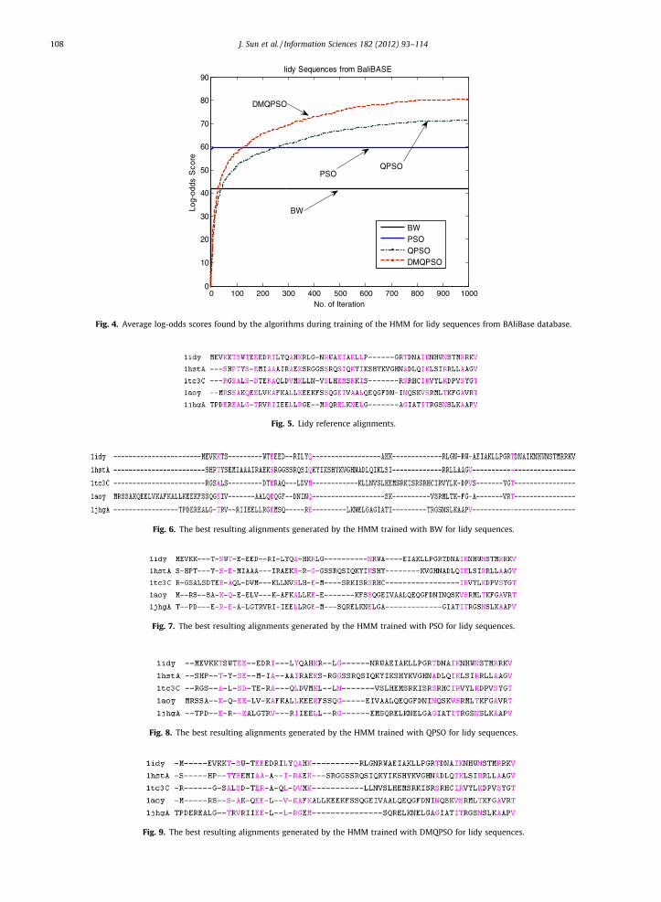
Fig. 4 shows that DMQPSO had the best convergence properties among all the training algorithms. Moreover, Figs. 5–9show the reference alignments of lidy sequences and the best resulting alignments obtained by the HMMs trained withBW, PSO, QPSO and DMQPSO.

6.4. Further evaluation

In order to make an overall performance comparison among all the tested methods, we normalized the average scoresover all the tested algorithms provided in Tables 3–9, listing these normalized scores in the corresponding tables. The nor-malized score is defined by

2

4

6

8

10

12

14

16

18

20

Log-

odds

Sco

re

Fig. 3.values

0 200 400 600 800 10000

0

0

0

0

0

0

0

0

0

0

No. of Iteration

Interferon Protein Sequence form Pfam database

BW

PSO

QPSO

DMQPSO

PSOBW

QPSO

DMQPSO

0 200 400 600 800 1000-0.5

0

0.5

1

1.5

2

2.5

3

3.5

4x 10

6

No. of Iteration

Sum

-of-

Pai

rs S

core

Interferon Protein Sequence form Pfam database

BWCWPSOQPSODMQPSO

PSO

BW

CW

DMQPSO

QPSO

(a) (b)

Average fitness values found by the algorithms during training of the HMM for Interferon protein sequences from Pfam database, with the fitnessbeing (a) log-odds scores and (b) sum-of-pairs scores.

Table 9The results of SOP scores for the BAliBASE test sets and the average execution time over 20 runs of eachexperiment (Bold figures represent the best results obtained for each sequence set).

Nucleotide Algorithms SOP score Normalized score Average execution time (h)

1aboA CW 0.714 �0.031 –BW 0.6418 �1.4491 0.0022PSO 0.6974 �0.3571 0.0432QPSO 0.7519 0.7133 0.0469DMQPSO 0.7728 1.1238 0.0501

1idy CW 0.705 0.2266 –BW 0.5132 �1.2328 0.0021PSO 0.5658 �0.8326 0.0412QPSO 0.7763 0.7691 0.0439DMQPSO 0.8158 1.0697 0.0491

451c CW 0.7190 1.3568 –BW 0.3989 �1.0766 0.0025PSO 0.4519 �0.6737 0.0518QPSO 0.5027 �0.2875 0.0540DMQPSO 0.6301 0.681 0.0584

1krn CW 1.000 0.8623 –BW 0.8182 �0.9183 0.0023PSO 0.7863 �1.2308 0.0472QPSO 0.9585 0.4558 0.0491DMQPSO 0.9968 0.831 0.0520

1bbt3 CW 0.638 �0.1148 –BW 0.5347 �1.4478 0.0053PSO 0.6219 �0.3226 0.6618QPSO 0.7146 0.8736 0.6873DMQPSO 0.7253 1.0117 0.7226

kinase CW 0.7360 1.1469 –BW 0.2268 �1.2261 0.0087PSO 0.3061 �0.8566 0.8055QPSO 0.5753 0.398 0.8318DMQPSO 0.6053 0.5378 0.8513

1pii CW 0.8640 1.1266 –BW 0.1647 �1.2266 0.0073PSO 0.2738 �0.8595 0.7369QPSO 0.6372 0.3634 0.7514DMQPSO 0.7064 0.5962 0.7853

5ptp CW 0.9660 1.0588 –BW 0.6053 �1.2958 0.0062PSO 0.6831 �0.7879 0.7183QPSO 0.8572 0.3486 0.7372DMQPSO 0.9074 0.6763 0.7420

gal4 CW 0.483 0.3865 –BW 0.2017 �1.4019 0.0121PSO 0.3185 �0.6593 1.5898QPSO 0.5294 0.6815 1.6812DMQPSO 0.5784 0.9931 1.7420

1ajsA CW 0.571 0.6134 –BW 0.2864 �1.2105 0.0097PSO 0.3245 �0.9663 1.2831QPSO 0.5914 0.7442 1.3207DMQPSO 0.6031 0.8191 1.3863

glg CW 0.9410 0.9836 –BW 0.5691 �1.361 0.0246PSO 0.6684 �0.735 6.5017QPSO 0.8569 0.4534 6.6381DMQPSO 0.8895 0.659 6.7512

1tag CW 0.9630 1.373 –BW 0.6453 �1.14 0.0457PSO 0.6931 �0.7619 15.7178QPSO 0.7953 0.0465 15.807DMQPSO 0.8504 0.4823 15.8623


0 100 200 300 400 500 600 700 800 900 10000

10

20

30

40

50

60

70

80

90

No. of Iteration

Log-

odds

Sco

re

lidy Sequences from BaliBASE

BWPSOQPSODMQPSO

BW

PSOQPSO

DMQPSO

Fig. 4. Average log-odds scores found by the algorithms during training of the HMM for lidy sequences from BAliBase database.

Fig. 5. Lidy reference alignments.

Fig. 6. The best resulting alignments generated by the HMM trained with BW for lidy sequences.

Fig. 7. The best resulting alignments generated by the HMM trained with PSO for lidy sequences.

Fig. 8. The best resulting alignments generated by the HMM trained with QPSO for lidy sequences.

Fig. 9. The best resulting alignments generated by the HMM trained with DMQPSO for lidy sequences.


Table 10The average normalized scores for all sets of tested sequences (Bold figures represent the best results obtained for each sequence set).

Algorithms Average normalized log-odds score Average normalized SOP score Total average normalized score

CW – 0.2654 0.2654BW �1.0079 �1.0833 �1.0422PSO �0.5470 �0.7055 �0.6190QPSO 0.5444 0.5294 0.5376DMQPSO 1.0105 0.9940 1.0030


Normalized score ðNSÞ ¼ ðSi � SÞ=rS ð30Þ

where Si is the score, S is the mean of the scores and rS is the standard deviation of the scores. After that, we averaged thenormalized log-odds scores, the normalized SOP scores and all of the two kinds of normalized scores over all the testedsequence sets (named as total normalized scores), and listed them in Table 10. It is shown that each type of normalizedscores produced by the DMQPSO-trained HMMs was better than that by any other competitor, indicating that the HMMstrained by DMQPSO had the best overall performance on the MSA problems of the sequence sets. The QPSO algorithmshowed the second best overall performance and the BW method performed worst in training the HMMs for the MSA prob-lems. CW outperformed the PSO-trained HMMs but its performance was worse than that of the HMMs trained by QPSO orDMQPSO, which implies that a good training algorithm is crucial for the HMM to play to its advantages in solving MSAproblems.

A further evaluation of the training algorithms was undertaken by comparing the computational costs of the algorithms.Since CW program is progressive alignment method that does not involve HMM training and can achieve multiple sequencealignment within 1 min, we only recorded and compared the computational consumptions of the algorithms in HMM train-ing for MSAs. The average execution time over 20 runs of each experiment is listed in Tables 3–8. It is evident that BW con-sumed the least computational time since it is a local search technique. DMQPSO was slightly more time-consuming intraining the HMMs for MSA than QPSO and PSO, due to computation of the diversity measure. However, it was worthwhileto consume tolerably more computational time to obtain the significant performance advantages of DMQPSO over itscompetitors.

7. Conclusions

In this paper, we analyzed the QPSO algorithm and proposed an improved version of the algorithm, DMQPSO, to train theHMMs for MSA. The proposed DMQPSO, along with QPSO, PSO and BW, was tested in training the HMMs on three benchmarkdatasets. The results were evaluated to compare the performances of all the competitor algorithms.

The analysis of QPSO showed that when CE coefficient a 6 ec � 1.781, the particle’s position is in probabilistic bounded, orotherwise it diverges. Based on this proposition, we introduced a diversity maintaining strategy into QPSO and thus devel-oped the DMQPSO algorithm, in which a is set to be larger than 1.781 to make the particles explode once the populationdiversity declines to below the pre-specified threshold value d low. By maintaining the diversity above the threshold, theDMQPSO algorithm can avoid the premature convergence effectively and thus has much stronger global search ability thanQSPO.

From the experiment results for training the HMMs for MSA, it can be observed that with log-odds scores as the objectivefunctions (or fitness values), DMQPSO was able to produce the HMMs that had better average log-odds scores than theHMMs trained with BW, PSO and QPSO for all three training sets. It is reflects that with sum-of-pairs as the objective func-tion, DMQPSO was also able to yield better HMMs than its competitors. On the third dataset, the resulting alignments by theHMMs trained with DMQPSO and QPSO did not have better sum-of-pairs scores on some sequence sets than those by ClustalW program, which is a highly specialized algorithm for multiple sequence alignment. In order to make an overall perfor-mance evaluation, we averaged the normalized scores of the tested methods and found that the DMQPSO-trained HMMshad the best average normalized scores, namely, the best overall performance in the tested MSA problems than Clustal Wand the HMMs trained by any other compared training method. Moreover, comparison of the execution time among thealgorithms shows that in each experiment, the proposed DMQPSO algorithm consumed slightly more CPU time. However,considering its significant performance advantages over its competitors, we can conclude that DMQPSO is a very efficientapproach of training the HMMs for MSA problems.

Acknowledgements

This work is supported by Natural Science Foundation of Jiangsu Province, China (Project No: BK2010143), by theFundamental Research Funds for the Central Universities (Project No: JUSRP21012), by the innovative research teamproject of Jiangnan University (Project No: JNIRT0702), and by National Natural Science Foundation of China (Project No:60973094).


Appendix A

Lemma A1. We have the following improper integral
Z 1
0ln½lnð1=xÞ�dx ¼ �c ðA1Þ

where c � 0.577215665 is called Euler constant.

Proof. Letting s = 1/x, we haveR 1

0 ln½lnð1=xÞ�dx ¼R1

0 e�s ln sds. Since CðmÞ ¼R 1

0 xm�1e�xdx, where C(�) is the gamma function,C0ðmÞ ¼

R 10 xm�1e�x ln xdx. We have C0ð1Þ ¼

R 10 e�x ln xdx ¼ �c, which implies that
Z 1
0ln½lnð1=xÞ�dx ¼

Z 1

0e�s ln sds ¼ C0ð1Þ ¼ �c

This completes the proof of the theorem. h

Lemma A2. If {un} is a sequence of independent identically distributed random variables with un �U(0,1) for all n and fn = ln[ln(1/un)], then

1n

Xn

i¼1

fi!a:s:�c ðA2Þ

Proof. Since {un} is a sequence of independent identically distributed (i.i.d.) random variables, {fn} is also a sequence of i.i.d.random variables. Lemma A1 implies that

EðfnÞ ¼ Efln½lnð1=unÞ�g ¼Z 1

0ln½lnð1=xÞ�dx ¼ �c;

Thus, by Kolmogorov’s Strong Law of Large Number, we have

1n

Xn

i¼1

fn!a:s:

EðfnÞ ¼ �c �

Theorem A1. Let ki = aln(1/ui) and bn ¼Qn

i¼1ki, where ui � U(0,1). The necessary and sufficient condition that bn is probabilisticbounded, i.e. P{supbn <1} = 1 is that a < ec � 1.781.

Proof. Let fi = ln[ln(1/ui)] and consider the following three possible cases:

(a) If a < ec, we have the following proof.
(i) From Lemma A2, we have that "m 2 Z+, $K1 2 Z+ such that whenever k P K1
P lna� c� 1=m < ln aþ ð1=kÞXk

i¼1

fi < ln a� cþ 1=m

( )¼ 1 ðA3Þ

Since a < ec, lna < c. We have

lna� cþ 1=m < 1=m; ðA4Þ

and therefore

ln aþ ð1=kÞXk

i¼1

fi < 1=m

( ) ln aþ ð1=kÞ

Xk

i¼1


( )

ln a� c� 1=m < ln aþ ð1=kÞXk

i¼1


( )

From (A3), we have

P lnaþ ð1=kÞXk

i¼1

fi < 1=m

( )P P ln aþ ð1=kÞ

Xk

i¼1


( )

P P ln a� c� 1=m < ln aþ ð1=kÞXk

i¼1


( )¼ 1


and thus

P ln aþ ð1=kÞXk

i¼1

fi < 1=m

( )¼ 1 ðA5Þ

Since �m/k < 1/m, we find that

lnaþ ð1=kÞXk

i¼1

fi < �m=k

( )¼ lnaþ ð1=kÞ

Xk

i¼1

fi < 1=m

( )� �m=k 6 ln aþ ð1=kÞ

Xk

i¼1

fi < 1=m

( )

resulting in the fact that

P ln aþ ð1=kÞXk

i¼1

fi < �m=k

( )¼ P ln aþ ð1=kÞ

Xk

i¼1

fi < 1=m

( )� P �m=k 6 lnaþ ð1=kÞ

Xk

i¼1

fi < 1=m

( )

¼ 1� P �m=k 6 ln aþ ð1=kÞXk

i¼1

fi < 1=m

( )ðA6Þ

(ii) "m 2 Z+, $K2 = m2 such that whenever k P K2, �m/k > �1/m, from which we have

�m=k 6 lnaþ ð1=kÞXk

i¼1

fi < 1=m

( ) �1=m < ln aþ ð1=kÞ

Xk

i¼1

fi < 1=m

( )

and thus have

P �m=k 6 lnaþ ð1=kÞXk

i¼1

fi < 1=m

( )6 P �1=m < ln aþ ð1=kÞ

Xk

i¼1

fi < 1=m

( )ðA7Þ

From (A6) and (A7), we have that "m 2 Z+, $K = max(K1, K2) such that whenever k P K,

P lnaþð1=kÞXk

i¼1

fi <�m=k

( )¼ 1�P �m=k6 lnaþð1=kÞ

Xk

i¼1

fi < 1=m

( )P 1� P �1=m6 lnaþð1=kÞ

Xk

i¼1

fi < 1=m

( )

which is equivalent to

P\1

m¼1

[1n¼1

\1k¼n

ðlnaþ ð1=kÞXk

i¼1

fi < �m=kÞ( )

P 1� P\1

m¼1

[1n¼1

\1k¼n

ð�1=m < ln aþ ð1=kÞXk

i¼1

fi < 1=mÞ( )

¼ 1� P limn!1ð1=nÞ

Xn

i¼1

fi ¼ � lna

( )ðA8Þ

Since ð1=nÞPn

i¼1fi!a:s:�c, we can get that P limn!1ð1=nÞ

Pni¼1fi ¼ � ln a

� �¼ Pfln a ¼ cg. The condition that a < ec implies that

P{lna = c} = 0, so

P limn!1ð1=nÞ

Xn

i¼1

fi ¼ � ln a

( )¼ 0 ðA9Þ

From inequality (A8), we can obtain

P\1

m¼1

[1n¼1

\1k¼n

ðlnaþ ð1=kÞXk

i¼1

fi < �m=kÞ( )

P 1� P limn!1ð1=nÞ

Xn

i¼1

fi ¼ � ln a

( )¼ 1� 0 ¼ 1

and thus PT1

m¼1

S1n¼1

T1k¼nðln aþ ð1=kÞ

Pki¼1fi < �m=kÞ

n o¼ 1, implying that P limn!1ðn ln aþ

Pni¼1fn ¼ �1

� �¼ 1 and thus

P limn!1 ln½anQni¼1 lnð1=uiÞ� ¼ �1

� �¼ 1. Consequently we have P{limn?1bn = 0} = 1 or bn!

p0. Since convergence in proba-

bility implies convergence in distribution, we immediately have bn!d

0.

(b) If a = ec, lna = c. Since ð1=nÞPn

i¼1fi!a:s:�c, we obtain that P limn!1jð1=nÞ

Pni¼1fi þ cj ¼ 0

� �¼ 1 and in turn

P limn!1jð1=nÞ

Xn

i¼1

fi þ ln aj ¼ 0

( )¼ 1


which means that "m 2 Z+, $K 2 Z+, such that whenever k P K, P jð1=kÞPk

i¼1fi þ lnaj < 1=mn o

¼ 1, namely

PXk

i¼1

fi þ k ln a

�� < k=m

( )¼ P ln ak

Yk

i¼1

lnð1=uiÞ" #��

�� < k=m

( )¼ Pfln bk < k=mg ¼ 1 ðA10Þ

The above proposition is equivalent to the following one that

P\1

m¼1

[1n¼1

\1k¼n

ðln bk < k=mÞ( )

¼ P\1

m¼1

ðlimn!1

ln bn <1Þ( )

¼ Pflimn!1

ln bn <1g ¼ 1

scilicet that P{limn?1bn <1} = 1, which means that when n ?1, the limit of bn can be any positive real number, but notinfinity, implying that bn

(iii) If a > ec, lna > c. Since ð1=nÞPn

i¼1fi!a:s:�c, we havePflimn!1jð1=nÞ

Pni¼1fi þ ln aj > 0g ¼ 1, which means that $b > 0, such

that

P limn!1

ð1=nÞXn

i¼1

fi þ ln a

�� ¼ b

( )¼ 1 ðA11Þ

And it is then easy to deduce that "m 2 Z+, $K 2 Z+, such that whenever k P K, Pfjjð1=kÞPk

i¼1fi þ ln aj � bj < 1=mg ¼ 1,namely,

P b� 1=m < ð1=kÞXk

i¼1

fi þ lna

�� < 1=mþ b

( )¼ 1

Thus we can obtain that

P ð1=kÞsumki¼1fi þ ln a

�� > b� 1=m� �

¼ PXk

i¼1

fi þ k ln a

�� > kb� k=m

( )¼ P ln ak

Yk

i¼1

lnð1=uiÞ" #��

�� > kb� k=m

( )

¼ Pfj ln bkj > kb� k=mg ¼ 1

Since kb > kb � k/m, {jlnbkj > kb � k/m} {jlnbkj > kb}, resulting in P{jlnbkj > kb} P P{jlnbkj > kb � k/m} = 1. Due to the proper-ties of probability measure, P{jlnbkj > kb} = 1. The proposition is equivalent to the following one that

P\1

m¼1

[1n¼1

\1k¼n

ðj ln bkj > kbÞ( )

¼ P\1

m¼1

ðlimn!1j ln bkj ¼ þ1Þ

( )¼ P lim

n!1j ln bkj ¼ þ1

n o¼ 1 ðA12Þ

This proves that when n ? +1, bn is divergent.

From the above three cases, we find that the theorem follows. This completes the proof of the theorem. h

References

[1] P.J. Angeline, Evolutionary optimization versus particle swarm optimization: philosophy and performance differences, Evolutionary Programming VII,Lecture Notes in Computer Science 1447 (1998) 601–610.

[2] R.deA. Araújo, Swarm-based translation-invariant morphological prediction method for financial time series forecasting, Information Sciences 180(2010) 4784–4805.

[3] P. Baldi, Y. Chauvin, T. Hunkapiller, M.A. McClure, Hidden Markov Models of biological primary sequence information, in: Proceedings of NationalAcademy of Sciences USA, vol. 91, 1994, pp. 1059–1063.

[4] L.E. Baum, T. Petrie, G. Soules, N. Weiss, A maximization technique occurring in the statistical analysis of probabilistic functions of Markov chains,Annals of Mathematical Statistics 41 (1970) 164–171.

[5] Y. Cai, J. Sun, J. Wang, Y. Ding, N. Tian, X. Liao, W. Xu, Optimizing the codon usage of synthetic gene with QPSO algorithm, Journal of Theoretical Biology254 (2008) 123–127.

[6] W. Chen, J. Sun, Y. Ding, W. Fang, W. Xu, Clustering of gene expression data with quantum-behaved particle swarm optimization, in: Proceedings of theTwenty First International Conference on Industrial, Engineering and Other Applications of Applied Intelligent Systems (IEA/AIE 2008), 2008, pp. 388–396.

[7] K. Chellapilla, G.B. Fogel, Multiple sequence alignmentusing evolutionary programming, in: Proceedings of the First Congress on EvolutionComposition, 1999, pp. 445–452.

[8] M. Chica, Ó. Cordón, S. Damas, J. Bautista, Multiobjective constructive heuristics for the 1/3 variant of the time and space assembly line balancingproblem: ACO and random greedy search, Information Sciences 180 (2010) 3465–3487.

[9] M. Clerc, The swarm and the queen: towards a deterministic and adaptive particle swarm optimization, in: Proceedings of 1999 Congress onEvolutionary Computation, 1999, pp. 1951–1957.

[10] M. Clerc, J. Kennedy, The particle swarm-explosion, stability and convergence in a multidimensional complex space, IEEE Transactions on EvolutionaryComputation 6 (2002) 58–73.

[11] L.S. Coelho, P. Alotto, Global optimization of electromagnetic devices using an exponential quantum-behaved particle swarm optimizer, IEEETransactions on Magenetics 44 (2008) 1074–1077.


[12] L.S. Coelho, A quantum particle swarm optimizer with chaotic mutation operator, Chaos, Solitons & Fractals 37 (2008) 1409–1418.[13] W. Du, B. Li, Multi-strategy ensemble particle swarm optimization for dynamic optimization, Information Sciences 178 (2008) 3096–3109.[14] S.R. Eddy, Multiple alignment using Hidden Markov Models, in: Proceedings of the International Conference on Intelligent Systems for Molecular

Biology, 1995, pp. 114–120.[15] I. Ellabib, P. Calamai, O. Basir, Exchange strategies for multiple ant colony system, Information Sciences 177 (2007) 1248–1264.[16] A. Elhossini, S. Areibi, R. Dony, Strength pareto particle swarm optimization and hybrid EA-PSO for multi-objective optimization, Evolutionary

Computation 18 (2010) 127–156.[17] D.F. Feng, R.F. Doolittle, Progressive sequence alignment as a prerequisite to correct phylogenetic trees, Journal of Molecular Evolution 25 (1987) 351–

360.[18] F. Gao, Parameters estimation on-line for Lorenz system by a novel quantum-behaved particle swarm optimization, Chinese Physics B 17 (2008) 1196–

1201.[19] H. Gao, W. Xu, J. Sun, Y. Tang, Multilevel thresholding for image segmentation through an improved quantum-behaved particle swarm algorithm, IEEE

Transactions on Instrumentation and Measurement 59 (2010) 934–946.[20] S. Henikoff, J.G. Henikoff, Amino acid substitution matrices from protein blocks, in: Proceedings of National Academy of Sciences USA, vol. 89, 1992, pp.

10915–10919.[21] Z. Huang, Y.J. Wang, C.J. Yang, C.Z. Wu, A new improved quantum-behaved particle swarm optimization model, in: Proceedings of the 5th IEEE

Conference on Industrial Electronics and Applications, 2009, pp. 1560–1564.[22] S. Janson, M. Middendorf, A hierarchical particle swarm optimizer and its adaptive variant, IEEE Transactions on Systems, Man and Cybernetics, Part B:

Cybernetics 6 (2005) 1272–1282.[23] K. Karplus, C. Barrett, R. Hughey, Hidden Markov Models for detecting remote protein homologies, Bioinformatics 14 (1998) 846–856.[24] J. Kennedy, R.C. Eberhart, Particle swarm optimization, in: Proceedings of IEEE International Conference on Neural Networks, 1995, pp. 1942–

1948.[25] J. Kennedy, Bare bones particle swarms, in: Proceedings of IEEE Swarm Intelligence Symposium, Indianapolis, IN, 2003, pp. 80–87.[26] J. Kim, S. Pramanik, M.J. Chung, Multiple sequence alignment using simulated annealing, Bioinformatics 10 (1994) 419–426.[27] A. Krogh, M. Brown, I.S. Mian, K. Sjolander, D. Haussler, Hidden Markov Models in computational biology: applications to protein modeling, Journal of

Molecular Biology 235 (1994) 1501–1531.[28] S. Kwong, C. Chau, K. Man, K. Tang, Optimisation of HMM topology and its model parameters by genetic algorithm, Pattern Recognition 34 (2001) 509–

522.[29] Z.-J. Lee, S.-F. Su, C.-C. Chuang, K.-H. Liu, Genetic algorithm with ant colony optimization (GA-ACO) for multiple sequence alignment, Applied Soft

Computing 8 (2008) 55–78.[30] X.J. Lei, A.L. Fu, Two-dimensional maximum entropy image segmentation method based on quantum-behaved particle swarm optimization algorithm,

in: Proceedings of Fourth International Conference on Nature Computation, 2008, pp. 692–696.[31] S.-Y. Li, R.-G. Wang, W.-W. Hu, J.-Q. Sun, A new QPSO based BP neural network for face detection, Advances in Soft Computing, Fuzzy Information and

Engineering, vol. 40, Springer, 2007.[32] X. Li, Niching without niching parameters: particle swarm optimization using a ring topology, IEEE Transactions on Evolutionary Computation 14

(2010) 150–169.[33] J. Liu, W.B. Xu, J. Sun, Quantum-behaved particle swarm optimization with mutation operator, in: Proceedings of the 17th IEEE International

Conference on Tools with Artificial Intelligence, 2005, pp. 237–240.[34] A.V. Lukashin, J. Engelbrecht, S. Brunak, Multiple alignment using simulated annealing: branch point definition in human mRNA splicing, Nucleic Acids

Research 20 (1992) 2511–2516.[35] S.M. Mikki, A.A. Kishk, Quantum particle swarm optimization for electromagnetics, IEEE Transactions on Antennas and Propagation 54 (2006) 2764–

2775.[36] G. Mongillo, S. Deneve, Online learning with Hidden Markov Models, Neural Computation 20 (2008) 1706–1716.[37] M.A. Montes de Oca, T. Stutzle, M. Birattari, M. Dorigo, Frankenstein’s PSO: a composite particle swarm optimization algorithm, IEEE Transactions on

Evolutionary Computation 13 (2009) 1120–1132.[38] D.W. Mount, Bioinformatics: Sequence and Genome Analysis, Cold Spring Harbor Laboratory Press, 2001.[39] C. Notredame, D.G. Higgins, SAGA: sequence alignment by genetic algorithm, Nucleic Acids Research 24 (1996) 1515–1524.[40] S.N. Omkara, R. Khandelwala, T.V.S. Ananthb, G.N. Naika, S. Gopalakrishnana, Quantum behaved particle swarm optimization (QPSO) for multi-

objective design optimization of composite structures, Expert Systems with Applications 36 (2009) 11312–11322.[41] M. Pant, R. Thangaraj, A. Abraham, A new quantum behaved particle swarm optimization, in: Proceedings of the 10th Annual Conference on Genetic

and Evolutionary Computation, 2008, pp. 87–94.[42] M. Pant, R. Thangaraj, V.P. SinghSobol, Sobal mutated quantum particle swarm optimization, International Journal of Recent Trends in Engineering 1

(2009) 95–99.[43] R. Poli, Mean and variance of the sampling distribution of particle swarm optimizers during stagnation, IEEE Transactions on Evolutionary

Computation 13 (2009) 712–721.[44] D. Parrott, X. Li, Locating and tracking multiple dynamic optima by a particle swarm model using speciation, IEEE Transactions on Evolutionary

Computation 10 (2006) 440–458.[45] L.R. Rabiner, A tutorial on Hidden Markov Models and selected applications in speech recognition, in: Proceedings of the IEEE, 1989, pp. 257–285.[46] T.K. Rasmussen, T. Krink, Improved Hidden Markov Model training for multiple sequence alignment by a particle swarm optimization-evolutionary

algorithm hybrid, BioSystems 72 (2003) 5–17.[47] J. Riget, J.S. Vesterstrøm, A Diversity-Guided Particle Swarm Optimizer – The ARPSO, Technical Report, University of Aarhus, Denmark, 2002.[48] S.L. Sabata, L.S. Coelho, A. Abrahamc, MESFET DC model parameter extraction using quantum particle swarm optimization, Microelectronics Reliability

49 (2009) 660–666.[49] E.L. Sonnhammer, S.R. Eddy, R. Durbin, Pfam: a comprehensive database of protein families based on seed alignments, Proteins 28 (1997) 405–420.[50] Y. Shi, R.C. Eberhart, A modified particle swarm optimizer, in: Proceedings of IEEE International Conference on Evolutionary Computation, 1998, pp.

69–73.[51] M. Slimane, G. Venturini, J.A. de Beauville, T. Brouard, A. Brandeau, Optimizing Hidden Markov Models with a genetic algorithm, Lecture Notes in

Computer Science 1063 (1996) 384–396.[52] J. Stoye, D. Evers, F. Meyer, Rose: generating sequence families, Bioinformatics 14 (1998) 157–163.[53] J. Sun, B. Feng, W.B. Xu, Particle swarm optimization with particles having quantum behavior, in: Proceedings of Congress on Evolutionary

Computation, Portland, USA, June 2004, pp. 326–331.[54] J. Sun, W.B. Xu, B. Feng, A global search strategy of quantum-behaved particle swarm optimization, in: Proceedings of IEEE Conference on Cybernetics

and Intelligent Systems, Singapore, December 2004, pp. 111–116.[55] J. Sun, W.B. Xu, B. Feng, AddTaptive parameter control for quantum-behaved particle swarm optimization on individual level, in: Proceedings of IEEE

International Conference on Systems, Man and Cybernetics, Hawaii, October 2005, vol. 4, pp. 3049–3054.[56] J. Sun, W.B. Xu, B. Ye, Quantum-behaved particle swarm optimization clustering algorithm, in: Proceedings of the International Conference on

Advanced Data Mining and Applications, 2006, pp. 340–347.[57] J. Sun, J. Liu, W.B. Xu, Using quantum-behaved particle swarm optimization algorithm to solve non-linear programming problems, International

Journal of Computer Mathematics 84 (2007) 261–272.


[58] J. Sun, W. Fang, D. Wang, W. Xu, Solving the economic dispatch problem with a modified quantum-behaved particle swarm optimization method,Energy Conversion and Management 50 (2009) 2967–2975.

[59] J. Sun, W. Fang, Z. Xie, C.-H. Lai, W. Xu, Particle swarm optimization with particles having quantum behavior: convergence analysis and performanceevaluation, submitted for publication.

[60] J.D. Thompson, D.G. Higgins, T.J. Gibson, CLUSTALW: improving the sensitivity of progressive multiple sequence alignment through sequenceweighting, position-specific gap penalties and weight matrix choice, Nucleotide Acids Research 22 (1994) 4673–4680.

[61] J. Thompson, F. Plewniak, O. Poch, A comprehensive comparison of multiple sequence alignment programs, Nucleotide Acids Research 27 (1999) 2682–2690.

[62] R. Thomsen, Evolving the topology of Hidden Markov Models using evolutionary algorithms, in: Proceedings of Parallel Problem Solving from NatureVII (PPSN), 2002, pp. 861–870.

[63] P.K. Tripathi, S. Bandyopadhyay, S.K. Pal, Multi-objective particle swarm optimization with time variant inertia and acceleration coefficients,Information Sciences 177 (2007) 5033–5049.

[64] C. Twomey, T. Stützle, M. Dorigo, M. Manfrin, M. Birattari, An analysis of communication policies for homogeneous multi-colony ACO algorithms,Information Sciences 180 (2010) 2390–2404.

[65] R.K. Ursem, Diversity-Guided evolutionary algorithms, in: Proceedings of the Parallel Problem Solving from Nature Conference, 2002, pp. 462–471.[66] L. Wang, T. Jiang, On the complexity of multiple sequence alignment, Journal of Computational Biology 1 (1994) 337–348.[67] J. Wang, Y. Zhou, Quantum-behaved particle swarm optimization with generalized local search operator for global optimization, in: Proceedings of

International Conference on Intelligent Computing, 2007, pp. 344–352.[68] Y. Wang, Y. Yang, Particle swarm optimization with preference order ranking for multi-objective optimization, Information Sciences 179 (2009) 1944–

1959.[69] Q. Wu, R. Law, Complex system fault diagnosis based on a fuzzy robust wavelet support vector classifier and an adaptive Gaussian particle swarm

optimization, Information Sciences 180 (2010) 4514–4528.

Multiple sequence alignment using Hidden Markov model with augmented set based on BLOSUM 80 and its...

Documents

Transcript of Multiple sequence alignment using Hidden Markov model with augmented set based on BLOSUM 80 and its...