arX

iv:2

105.

1149

0v2

[st

at.A

P] 1

9 N

ov 2

021

Hidden Markov and semi-Markov models

When and why are these models useful for classifying

states in time series data?

Sofia Ruiz-Suarez1,2, Vianey Leos-Barajas3,4, and Juan Manuel Morales1

1INIBIOMA (CONICET-Universidad Nacional del Comahue), Quintral

1250, Bariloche, Rio Negro, Argentina

2Universidad de Rosario, Facultad de Ciencias Economicas, Bv. Orono

1261, Rosario,Argentina

3Department of Statistical Sciences, University of Toronto, 700 University

Ave, Toronto, ON, M5G 1Z5, Canada

4School of the Environment, University of Toronto, 33 Wilcocks St,

Toronto, ON, M5S 3E8, Canada

Abstract

Hidden Markov models (HMMs) and their extensions have proven to be powerful

tools for classification of observations that stem from systems with temporal depen-

dence as they take into account that observations close in time are likely generated

from the same state (i.e. class). When information on the classes of the observations

is available in advanced, supervised methods can be applied. In this paper, we provide

details for the implementation of four models for classification in a supervised learning

context: HMMs, hidden semi-Markov models (HSMMs), autoregressive-HMMs, and

autoregressive-HSMMs. Using simulations, we study the classification performance

under various degrees of model misspecification to characterize when it would be im-

portant to extend a basic HMM to an HSMM. As an application of these techniques

we use the models to classify accelerometer data from Merino sheep to distinguish

between four different behaviors of interest. In particular in the field of movement

ecology, collection of fine-scale animal movement data over time to identify behavioral

states has become ubiquitous, necessitating models that can account for the dependence

structure in the data. We demonstrate that when the aim is to conduct classification,

various degrees of model misspecification of the proposed model may not impede good

classification performance unless there is high overlap between the state-dependent

distributions, that is, unless the observation distributions of the different states are

difficult to differentiate.

Keywords— animal behavior, classification, movement ecology, temporal dependence.

1 Introduction

The aim in the classification problem is either to allocate data to different groups of interest, or

to discover sets of patterns that reflect important dynamics of interest. For systems that exhibit

temporal dependence, the goal is to correctly assign different segments of data to a finite set of

groups, taking into account that observations near each other (in time) are likely to correspond to

the same group. For example, in computational linguistics the goal is to identify words and phrases

in spoken language, i.e speech recognition (Juang and Rabiner, 1991; Deng and Li, 2013); in meteo-

rology, weather change can be monitored analyzing sequential measures from meteorological radars

(Rico-Ramirez and Cluckie, 2008; Ruiz-Suarez et al., 2019); in neurophysiology, different brain ac-

tivities can be distinguished assessing physiological variables such as heart rate or electrocardio-

grams through time(Cheng and Chan, 1998; Inan et al., 2006); and in ecology, a set of biologically

relevant animal behaviors can be identified from observed acceleration data (Nathan et al., 2012;

Leos-Barajas et al., 2017).

In ecology, a lot of attention has been paid to understand and model animal movement (Mevin B. Hooten et al.,

2017) as it plays important roles in the fitness and evolution of species(Nathan, 2008), the structur-

ing of populations and communities (Morales et al., 2010), and responses to environmental change

(Jonsen, 2016). In order to understand how animals move as they respond to internal conditions

and external environments, it is essential to be able to distinguish between a set of biologically

relevant behaviors. Tri-axial acceleration (ACC) data is now commonly recorded using biologging

devices, allowing researchers to investigate the performance, energy expenditure, and behavior of

free-living animals (Williams et al., 2020). These devices measure the change in speed over time

in three directions, which can be described relative to the body of the individual. With this in-

formation it is possible to identify different activity patterns to then distinguish between different

behaviors (Wilson et al., 2008; Williams et al., 2015).

There are several techniques used to solve classification problems (Trevor Hastie et al., 2001):

classification trees, logistic regression, discriminant analysis, neural networks, boosted regression

trees, random forests, deep learning methods, nearest neighbors, support vector machines, etc.

Many of these techniques have been proposed to classify animal behavior from accelerometer data.

For example, (Nathan et al., 2012) identified behavioral modes of griffon vultures using a selection

of nonlinear and decision tree methods; (Carroll et al., 2014) trained a support vector machine to

classify penguin behavior as either ‘prey handling’ or ‘swimming’; (Williams et al., 2015) examined

the ability of k-nearest neighbour algorithms to distinguish between flight behaviors of Andean

condors and griffon vultures; (Chakravarty et al., 2019) developed an hybrid model combining

biomechanical features and support vector machines to identify between four possible behaviors of

Kalahari Meerkats; and (Studd et al., 2019) used a random forest algorithm and a manually created

decision tree to associate observed behaviors of North American red squirrels with logger recorded

acceleration and temperature. All these methods assume that the observations are independent,

yet time series data presents sequential correlation. This characteristic of the data can be exploited

to improve the prediction accuracy of the classifiers (Geurts, 2001; Dietterich, 2002).

The class of hidden Markov models (HMMs) (Zucchini et al., 2017; Fruhwirth-Schnatter et al.,

2019) provide an intuitive framework for the classification of systems with temporal dependence

that experience changes in patterns over time connected with underlying shifts in a latent process of

interest. HMMs assume that the observation(s) at each point in time are the result of the unknown

(hidden) ‘state’ (or class) of the system. The state of the system is assumed to change over time

according to the Markov property, i.e. the conditional probability distribution of future states

(conditional on both past and present states) depends only upon the present state. Thus, an HMM

is defined as a doubly stochastic process composed of an observation process Xt and a (latent)

state process Ct, where the state process is usually taken to be a first-order Markov chain and the

distribution of Xt depends only on the current state Ct and not on previous state or observations.

As such, HMMs provide a clear manner in which to do classifications of processes that evolve over

time, as they take into account the sequential dependence present in the data and the temporal

structure of the consecutive states.

HMMs can be used for state prediction (supervised approach) or to make inferences about

drivers of behavior (unsupervised approach). In the supervised learning context information on the

classes of the observations is available in advanced (there is a pre labelled data set), and the number

of possible states are known by the user. Alternatively, in the unsupervised learning context there

are no labelled data and the number of states is not pre-defined. HMMs have successfully been

implemented to classify accelerometer data: (Li et al., 2010) utilized an HMM to recognize human

physical activities using two-second summary features from tri-axial acceleration data; (Wang et al.,

2011) presented an HMM to recognize six human daily activities from sensor signals collected from

a single waist-worn tri-axial accelerometer; (Leos-Barajas et al., 2017) provided the details neces-

sary to implement and assess an HMM in both the supervised and unsupervised learning context

and outlined two applications to marine and aerial systems (shark and eagle) using unsupervised

learning.

HMMs are models mostly formulated in discrete time, and as the state process is assumed to be

a first order Markov chain, the number of consecutive time points that the system spends in a given

state (sojourn time), follows a geometric distribution (Zucchini et al., 2017; Langrock and Zucchini,

2011). The popularity of HMMs stems, in part, from the ease with which they can be extended to

accommodate other forms of dependence and structures. For instance, the state-duration distribu-

tion can be generalized so that the underlying stochastic process is a semi-Markov chain. These

models are called hidden semi-Markov models (HSMM) (Yu, 2010), and by being more flexible they

allow more realism, improving the classifications when the sojourn time distributions are far from

being geometric. HSMMs have been successfully applied in many areas, mostly in speech recogni-

tion (Chen et al., 2006; Hung-Yan Gu et al., 1991; Hieronymus et al., 1992; Oura et al., 2006), but

also to classify human activities of daily living (Duong et al., 2005; Chung and Liu, 2008), hand-

writing (Kashi et al., 1997; Benouareth et al., 2007), and human genes in DNA (Kulp et al., 1996).

HSMMs have also been used for language identification (Marcheret and Savic, 1997), the prediction

of protein structure (Aydin et al., 2006), event recognition in videos (Hongeng and Nevatia, 2003),

financial time series modelling (Bulla and Bulla, 2006), classification of music (XiaoBing Liu et al.,

2008), and remote sensing (Pieczynski, 2007), among others.

Classical HMMs and HSMMs assume independence between the observations conditional on the

state, but sometimes data is taken at high temporal resolution making this assumption unrealistic

which can affect the performance of the classifiers. In such cases, autoregressive structure can be

considered to model the observations of each state, leading to autorregresive HMMs and HSMMs

(AR(p)-HMM and AR(p)-HSMM) (Xu and Liu, 2020), also commonly known as Markov-switching

models. Even though these models have been extensively studied, as far as we are aware, these

HMM extensions have not been used to classify acceleration data into animal behaviors.

In this paper, we give an overview of HMM, HSMM, AR(p)-HMM and AR(p)-HSMM; we

explain the structure of these models in the supervised classification context, how they can be

relaxed and their differences in modelling, inference, estimation, and prediction. We present their

formulations and derivations as a compilation of the literature published on this topic extending

them to HSMMs with or without autorregresive structure. We then study how these models perform

classifications under different scenarios in order to characterize when it would be important to

extend an HMM to an HSMM. Finally, we use them to classify accelerometer data from domestic

Merino sheep (Ovis aries) to distinguish between four different behavioral states.

2 Models

2.1 Hidden Markov Model (HMM)

HMMs are composed of two layers: a latent process {Ct}Tt=1, commonly referred to as the state

process, satisfying the Markov property; and an observable state-dependent process {Xt}Tt=1, where

P (Xt|X1,X2, . . . Xt−1, Ct) = P (Xt|Ct) (Figure 1 (a)). At each point in time t, Ct is assumed to

take on one of J possible values, Ct ∈ {1, 2, . . . , J}, where J denotes the number of states.

Figure 1: Diagrams of model structure (a)HMM : Ct denotes the latent Markov process andXt denotes the observation process whose distribution depends on the state Ct. (b) HSMMexample: Ct denotes the latent semi-Markov process and Xt the observation process. C∗

t

indicates the Markovian process of the non absorbing times (that is, state at time t is equalto the state at time t − 1), and for each of them dt gives the values of the sample sojourntimes.

The dynamics of the state process C is governed by a J × J transition probability matrix

(t.p.m), Γ, with entries γij = Pr(Ct+1 = j|Ct = i), for i, j ∈ {1, . . . , J}. The initial probabilities

are denoted by δi = Pr(C1 = i), i, j = 1, . . . , J .

By definition, the assumption of a first-order Markov chain structure for the state process implies

that the number of consecutive time points that the process spends in a given state before switching,

i.e. the sojourn time, follows a geometric distribution with parameter γii. As a consequence, the

most likely sojourn time for every state of an HMM is one, and the probability of remaining in

a given state decays geometrically. To complete the definition of an HMM, we denote the state-

dependent distributions of the observation process (univariate or multivariate) as fj(x) = Pr(Xt =

x|Ct = j), for j = 1, . . . J . The state-dependent distributions can be discrete or continuous and it is

common to assume the same parametric distribution across all states. Therefore an HMM is defined

by the pair of stochastic processes {Xt, Ct}, the state dependent distributions f1(x), . . . , fJ(x), the

transition probability matrix Γ, and the initial probability vector δ = (δ1, . . . , δJ).

2.2 Hidden Semi-Markov Model (HSMM)

One of the limitations of a basic HMM is the assumption that the sojourn time follows a geometric

distribution. In fact, much work has been done to extend the basic HMM and explicitly model the

sojourn time by other discrete-valued distributions, resulting in the class of hidden semi-Markov

models (HSMM) (Yu, 2010). Like an HMM, an HSMM is a doubly stochastic process composed

of two layers: a state process {Ct}Tt=1 and an observable state-dependent process {Xt}

Tt=1. For

an HSMM, however, the state process is now assumed to be a semi-Markov chain where the so-

journ time in a given state is taken to follow any valid discrete distribution (e.g. Poisson, negative

binomial). We provide definitions and notation of an HSMM in the remainder of the section.

In order to formalize the structure of the model, we first divide the times t into two disjoint

categories depending on state Ct:

1. Non absorbing time(NAT): The state at time t is different than the state at time t − 1.

(Ct 6= Ct−1)

2. Absorbing time(AT): The state at time t is equal to the state at time t− 1. (Ct = Ct−1).

The subsequence of states of non absorbing times is a first-order Markov process, while the

sequence of Ct values is a finite-state semi-Markov chain. For simplicity, in this paper we assume

that state switches occurred at time t = 1 and t = T , such that C1 6= C0 and CT 6= CT+1. A

HSMM with that simplifying assumption is called a right censored HSMM (Guedon, 2003).

For each state i of the non absorbing times, the sojourn time is a realization of the corresponding

sojourn-time distribution di. Suppose that t∗ is a non absorbing time of state i then the probability

that the state i lasts u steps, di(u) = Pr(Ct∗+u+1 6= i ∧ Ct∗+v = i, v = 1, ...u|Ct∗ = i), u ≥ 1.

For an HSMM, the t.p.m contains the conditional transition probabilities (Γ)ij = γij = Pr(Ct+1 =

j|Ct = i, Ct+1 6= i) i 6= j, j = 1, . . . , J with γii = 0 ∀i = 1 . . . , J . The probabilities of

self-transitions are determined by di-sojourn distributions.

In Figure 1(b) an example of a 3-state HSMM (Ct ∈ {1, 2, 3}) is represented. The Markovian

layer C∗t governs the change of states and gives rise to a run of d values all equal to C∗

t . These d

values are realizations from the sojourn time distributions di (i = 1, 2, 3). In this example C∗1 = 1

and d1 = 3, indicating that the semi-Markov process starts with three ones, i.e. C1 = 1, C2 = 1

and C3 = 1. Then C∗2 = 2 and d2 = 1, indicating that the sequence follows with a single 2, C4 = 2

. Next C∗3 = 1 and d1 = 4, so four ones are added to the sequence, C5 = 1, C6 = 1,C7 = 1,

C8 = 1 and so on. The observation process is akin to an HMM in that the observations Xt are

random variables that depend on the values of Ct. Therefore a HSMM can be defined by the

pair of stochastic process {Xt, Ct}, Xt dependent on a semi-Markov chain Ct, the state dependent

distributions f1(x), . . . , fJ(x), the sojourn-time distributions d1(u). . . . , dJ (u), the t.p.m Γ, and the

initial state distribution δ = (δ1, . . . , δJ ).

For the remainder of this article, we use the following notation. The observed sequence of length

l, (Xt,Xt+1 . . . ,Xt+l) is denoted by X t:t+l, and the state sequence (Ct, Ct+1, . . . Ct+l) is denoted by

Ct:t+l. We use C [t1;t2] = i to denote that the vector of state variables {Ct1 = i, Ct1+1 = i, . . . , Ct2 =

i} takes on the value i with state changes occurring at t1 and t2 + 1, Ct1−1 6= i and Ct2+1 6= i. We

let C [t1;t2 = i denote similarly that the sequence of state variables {Ct1 = i, . . . , Ct2 = i} take on

the value i with a state change occurring at time t1, i.e. Ct1−1 6= i, but allow for Ct2+1 ∈ {1, . . . , J}.

Similarly Ct1;t2] = i denotes a state change at time t2 + 1 but allows for Ct1−1 ∈ {1, . . . , J}. By

C[t1=i we mean that at time t1 the system switched from some other state to i, and by Ct1]=i that

at time t1 the state will end and transit to some other state. Finally, we let θ = (θδ,θP ,θΓ,θd) be

the vector of parameters of the HSMM: θδ the initial probabilities, θP the parameters of the state

dependence distributions fi(x), θΓ the conditional transition probabilities of the t.p.m, and θd the

parameters of the sojourn time distributions di(u).

2.3 Autoregressive Structure (AR(p)-HMM and AR(p)-HSMM)

In basic HMMs and HSMMs, we assume conditional independence of X given C. However, for

time series collected at fine temporal scales, the autocorrelation structure may not adequately be

captured using this framework. A common extension is to assume that the state-dependent distri-

bution of {Xt}Tt=2 depends on the current state Ct as well as on a subset of previous observations.

This new assumption leads to an important class of models called Markov-switching models or

autoregressive hidden (semi-)Markov models (Hamilton, 1994). In this framework, given the cur-

rent state, {Xt} is assumed to follow state-dependent Gaussian autoregressive processes of order p

(AR(p)):

xt = µi +

p∑

k=1

ωkixt−k + ǫti with ǫti ∼ N(0,Σi)

where µi, ωki and Σi are the conditional mean, autoregressive parameters and covariance matrix

conditioned on Ct = i. We denote the state-dependant distributions of an AR(p)-HSMM as

fi(xt) = f(xt|Ct = i,xt−p:t−1)

and the joint distribution for vector xt:t′ with t < t′ as,

fi(xt:t′) =

t′∏

k=t

f(xk|Ck = i,xk−p:k−1) =

t′∏

k=t

fi(xk).

The use and statistical properties of HMMs with autoregressive structure have been studied and for-

malized (Yang, 2000; Francq and Zakoian, 2001), and further generalized for HSMMs (Xu and Liu,

2020). AR(p)-HSMM have been also used to perform classification in an unsupervised man-

ner; (Bryan and Levinson, 2015) demonstrates its application to speech signal recognition and

(Duong et al., 2005) proposed the use of a switching hidden semi-Markov model to recognize hu-

man activities of daily living. However, to our knowledge, the use of AR(p)-HSMM to perform

supervised classification has not been studied or applied.

3 Classification via Supervised Learning

In many applications, the primary objective of the analysis is to accurately predict the latent states

of the system. The observations themselves are not of real interest as their function is merely to

provide information about the states (Zucchini et al., 2017). For processes that evolve over time

(or in sequence), HMMs (and their extensions) can be applied to classify observations into different

latent states while taking into account that observations close to one another in time are likely to

have arisen from the same state. In this section we discuss the implementation of HMMs, HSMMs,

and their respective autoregressive versions, in a supervised learning approach.

Supervised learning methods assume that there is a data set for which labels are available for all

samples. This labelled data set is used to fit the model and assess its predictive capability. Then,

the labelled data set is distributed among the train set to fit the model and the test set to measure

the accuracy of the final model. Finally, once the model has been evaluated, it can be used to

classify unlabelled data. Thus, when the aim is to perform classification using HMMs or HSMMs

with a supervised approach, the steps are: split the labelled data, train the model (section 3.1),

predict hidden states (section 3.2), estimate the classification error (section 3.3), and eventually

classify unlabelled data.

3.1 Inference

Inference for θ is done via use of the complete-data likelihood as both the observations and values

of the states are known in the training data. The complete-data likelihood is expressed as the joint

distribution of the observations, Xt, and states, Ct,

f (c1:T ,x1:T |θ) = Pr (C1:T = c1:T ,X1:T = x1:T |θ)

= δC1dC1

(u1)

T∏

t=1

fCt(xt)

∏

r is NAT

γcr−1,crdCr(ur)

Note that for the autoregressive case fCt(xt) depends on the p previous observations, i.e.

fCt(xt) = fCt

(xt|xt−p:t−1). The complete-data likelihood of an HMM necessarily has dCr(.) ∼

Geom(λr).

The complete-data likelihood can be expressed as a product of the terms of the t.p.m., ini-

tial distribution, state-dependent distributions and sojourn time distributions, which allows the

complete-data log-likelihood to be written as a sum,

log(f(c1:T ,x1:T ,θ)) = log(δC1)+ log(dC1

(u1))+

T∑

t=1

log(fCt(xt))+

∑

t∈ NAT

log(γcr−1,cr)+ log(dCr(ur))

For K independent time series, the complete-data likelihood is the product of the individual

complete-data likelihoods. As we conduct inference in a Bayesian framework, we first specify prior

distributions for all parameters f(θ) and derive the joint posterior distribution f(θ|x1:T ,C1:T ) ∝

f(c1:T ,x1:T ,θ)f(θ). In particular, the joint log posterior distribution can be expressed as a sum

of the components of the complete-data log likelihood and prior distributions. Full details of the

prior distributions specified and derivation of the joint posterior distribution are provided in the

Appendix (S1).

3.2 State prediction

The objective of classification, in this context, is to determine which states are likely to have

generated the observations. This process is known as state decoding and can be done in one of two

general ways: (i) local state decoding – identify the most likely state at each point in time or (ii)

global state decoding – identify the sequence of states that is most likely to have generated the full

observation sequence. In what follows we formalize and discuss the most common algorithms and

their adaptations to HSMMs and AR-HSMMs for state decoding.

3.2.1 Local State Decoding

Local state decoding is the process of determining at time t, what label of the state Ct is most likely

to have generated the observation xt. To do so, we compute and use the marginal probabilities

Pr(Ct = i|X1:T ) via use of the forward-backward algorithm, which can be expressed as a function

of the so-called forward probabilities {αt}Tt=1 and backward probabilities {βt}

Tt=1. For the basic

HMM, these quantities are given as

αt(j) = Pr (X1:t, Ct = j) βt(j) = Pr (Xt+1:T |Ct = j)

where βT (j) = 1, for all j ∈ {1, . . . , J} so that

αt(j) = fj(xt)∑

i

γi,jαt−1(i) βt(j) =∑

i

βt+1(i)γi,jfi(xt+1)

Given αt(j) and βt(j), we can express the marginal probability as,

Pr (Ct = j|X1:T ) =αt(j)βt(j)

Pr(X1:T ).

Further details are given in Bishop (2012) and Zucchini et al. (2017). Derivation of the marginal

state probabilities for the HSMM are similar to the HMM, while further adaptations are considered

for the AR(p)-HSMM. We first express the forward and backwards probabilities as follows:

αt(j) = Pr(

X1:t, Ct] = j)

βt(j) = Pr(

Xt+1:T |Ct] = j,X t−p:t

)

It is also possible to give recurrence equations that express αt(·) in terms of αt−d(·) and βt(·)

in terms of βt+d(·). For t = 2, . . . , T and j = 1, . . . , J it can be shown that,

αt(j) =∑

d∈D

∑

i 6=j αt−d(i)γijdj(d)fj(xt−d+1:t)

βt(j) =∑

d∈D

∑

i 6=j βt+d(i)γjidi(d)fi(xt+1:t+d)

Full details provided in Appendix S2.1. Let the marginal probabilities be expressed as ξt(j) =

Pr (Ct = j,X1:T ) and let β∗t (j) = Pr(X t+1:T |C[t+1 = j) (or β∗t (j) = Pr(Xt+1:T |C[t+1 = j,X t−p:t)

for the AR(p)-HSMM case). It follows from the definition of β∗t (j) that,

βt(j) =∑

i 6=j

γjiβ∗t (j)

β∗t (j) =∑

d∈D

dj(d)βt+d(j)fj(xt+1:t+d)

We can then calculate the marginal probabilities as follows (full details provided in the Appendix

S2.1). For t = 2, . . . , T and j = 1, . . . , J

ξt(j) = ξt+1(j) + αt(j)∑

i 6=j

γjiβ∗t (i) − β∗t (j)

∑

i 6=j

αt(i)γij

For local state assignment, we use Ct = argmaxj∈1,...,J {ξt(j)}.

3.2.2 Global State Decoding

Global state decoding is a manner to identify the most likely sequence of states that could have

given rise to the observed time series data. For this task, we determine the sequence c1, c2, . . . , cT

that maximizes the conditional probability Pr(C1:T |X1:T ) or equivalently the joint probability

Pr(C1:T ,X1:T ) via use of the Viterbi algorithm(Viterbi, 1967). For the basic HMM we first define

ψ1i = Pr (C1 = i,X1) = δifi (x1)

and for t = 2, . . . , T,

ψti = maxc1:t−1

Pr (C1:t−1, Ct = i,X1:t)

Given the following recursion,

ψtj =

(

maxi

(ψt−1,iγij)

)

fj (xt) (1)

the most probable state sequence is obtained by

iT = argmaxψT ii=1,...,m

and for t = T − 1, T − 2, . . . , 1

it = argmaxi=1,...,m

(

ψtiγi,it+1

)

Global state decoding for an HSMM is similar to that of a basic HMM, but also requires that

most likely sojourn times be determined in addition to the most likely state sequence. We define

ψt(j, d) = maxc1:t−d

Pr(

C1:t−d,C [t−d+1:t]=j,X1:T

)

Similar to the basic HMM, it is possible to obtain the following recursion (full details provided

in Appendix S2.2). For t = 2, . . . , T , d = 1, . . . ,D and j = 1, . . . , J

ψt(j, d) = maxi 6=jd′≤t

{

ψt−d(i, d′)γijdj(d)fj(xt−d+1:t)

}

Then, starting at time T , the most likely sequence of states and duration times is determined by

(iT , dT ) = argmaxψT (j, d)j=1,...,Jd=1,...D

and for t = T − 1, . . . 1

(it, dt) = argmaxj 6=it+1

d=1,...D

(

ψt−d(j, d′)γj,it+1

dit+1(d)fit+1

(xt−d+1:t))

The results of local and global state decoding are often very similar but not identical (Zucchini et al.,

2017). One advantage of local state decoding via the forward-backward algorithm over global state

decoding via the Viterbi algorithm is that it provides an estimated probability for every possible

state in all times. These probabilities provide information about the uncertainty over the predic-

tions which can be useful for model comparison.

3.3 Classification Error

Given a fitted model, we can assess its capacity to classify the states correctly via both local and

global state decoding. One of the most common measures to estimate prediction accuracy is the

following classification accuracy index: the number of correct state predictions divided by the total

number of observations in the time series. We can compute this measure from both the local and

global decoding output. However, although this manner of estimating the prediction accuracy gives

a general measure of the performance of the model, it does not take into account the uncertainty

over the classification. Another manner to assess prediction capacity of our models is to use cross-

entropy as it makes use of predicted probabilities of the states obtained via local state decoding

and is given as,

CE = −

J∑

c=1

yx,c log (px,c)

where yx,c is a binary indicator of whether state label c is the correct classification for observation

x (yx,c = 1 when the classification is correct), and px,c is the predicted probability observation that

x is generated by state c. The cross-entropy index increases as the predicted probability diverges

from the actual label, such that a perfect model would have a CE value of 0.

To measure out-of-sample prediction accuracy (or error), we adapt leave-one-out cross valida-

tion to our application and use a leave-one time series-out cross-validation approach (Geisser, 1975;

Refaeilzadeh et al., 2009). By doing so, we make the assumption that each time series is indepen-

dent of each other and fulfill the requirement that the training and test sets are independent in

order for cross-validation approaches to be valid.

4 Simulation Study

In some applications the assumption that the sojourn times follow geometric distributions (HMMs)

is far from being realistic. In such cases, HSMMs may be considered more appropriate as they allow

each state to have a variable duration time (Yu, 2010). However, when the main goal is to conduct

classification it may not be necessary to extend the model to obtain correct state predictions. In

this study we aim to characterize in which scenarios the state predictions of an HMM strongly

differ from those of an HSMM, in order to understand when violating the assumption of geometric

sojourn times can affect the accuracy of classifications.

We simulate different scenarios of univariate time series of length 3000 from a 2-state HSMM

with different sojourn times and observation distributions. Across all cases we assume Gaussian

distributions for the observations and negative binomial distributions for the sojourn times. We

propose three scenarios differing on the overlap between the observation distributions: the first

assumes that f1(xt) ∼ N(0, 1) and f2(xt) ∼ N(0.3, 1) (high overlap), the second one assumes

that f1(xt) ∼ N(0, 1) and f2(xt) ∼ N(1, 1) (medium overlap) and the last one assumes that

f1(xt) ∼ N(0, 1) and f2(xt) ∼ N(3, 1) (low overlap). The overlap degree gives an idea of how

similar are the observation distributions. A high overlap implies that the distributions are almost

equal, i.e the area between them includes at least 80% of them. A medium overlap indicates

that the distributions are similar but they differ in at least a 40%, and finally a low overlap

indicates that the distributions are different, sharing at most a 15% of them. For each scenario

we fix different parameter values for the negative binomial distributions: d1 ∼ NB(m1, k1) and

d2 ∼ NB(m2, k2), where m1 and m2 are the means and k1 and k2 the dispersion parameters.

When k = 1 the negative binomial is a geometric distribution with probability 1/(m + 1), and as

k takes values greater than 1 the dispersion of the distribution increases, moving away from the

geometric distribution. In order to characterize different scenarios, we first set an average and a

difference between m1 and m2 ((m1 +m2)/2 and m1 −m2). We consider as average between m1

and m2: 90, 40 and 20, and as difference between them: 3, 15 and 30. We then vary k1 and k2

so that either k1 equals 1 (one is geometric: k1 = 1 and k2 = 10 or k2 = 30) or both k1 and

k2 are greater than one (none are geometric: k1 = 30 and k2 = 50 or k1 = 80 and k2 = 100).

The values of ki and mi (i = 1, 2) were selected seeking to consider as many schemes as possible.

When ki = 1 the most probable values is 1 and as the value of mi increases the distributions

have longer tails. When ki = 10 or ki = 30 the most probable value is nearer mi, obtaining

more concentrated distributions for ki = 30 and more dispersed distributions for ki = 10. The

difference between m1 and m2 indicates how similar are the means of sojourn times of the two

states. For each parameter combination, we simulate ten time series of length 3000. To assess

and compare the classification accuracy under both models (HMM and HSMM) we use leave-one

time series-out cross-validation approach as follows: we fit both models with all the simulated time

series but one, then sampling from the joint posterior distribution obtained, we predict 30 times

the hidden states of the simulated time series that we left out using Viterbi and FB algorithms.

Finally we calculate the accuracy index of both predictions and the cross entropy value from the

local decoding output. To fit the model we consider uninformative priors: N(0, 5) and TN(0, 5)

for the mean and standard deviation of the observation distributions and TN(20, 50) for the mean

and dispersion parameter of the sojourn time distributions. To perform the analysis we used R

(R Core Team, 2019), to conduct parameter estimation we used Stan (Carpenter et al., 2017) and

to implement the Viterbi algorithm for the HSMM we used the “hsmm.viterbi” function of the R

package “hsmm” (https://cran.r-project.org/web/packages/hsmm/index.html). The code is

available at https://github.com/sofiar/HMM-HSMM-classification.

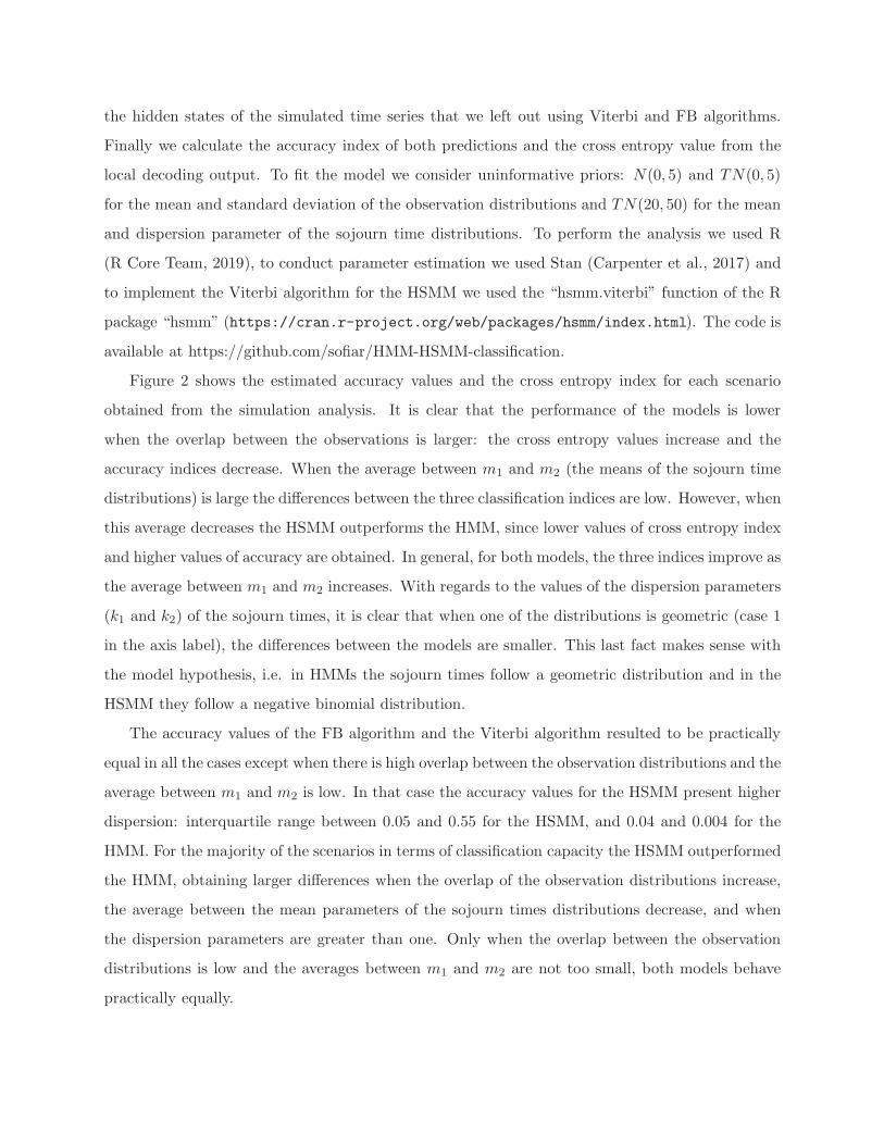
Figure 2 shows the estimated accuracy values and the cross entropy index for each scenario

obtained from the simulation analysis. It is clear that the performance of the models is lower

when the overlap between the observations is larger: the cross entropy values increase and the

accuracy indices decrease. When the average between m1 and m2 (the means of the sojourn time

distributions) is large the differences between the three classification indices are low. However, when

this average decreases the HSMM outperforms the HMM, since lower values of cross entropy index

and higher values of accuracy are obtained. In general, for both models, the three indices improve as

the average between m1 and m2 increases. With regards to the values of the dispersion parameters

(k1 and k2) of the sojourn times, it is clear that when one of the distributions is geometric (case 1

in the axis label), the differences between the models are smaller. This last fact makes sense with

the model hypothesis, i.e. in HMMs the sojourn times follow a geometric distribution and in the

HSMM they follow a negative binomial distribution.

The accuracy values of the FB algorithm and the Viterbi algorithm resulted to be practically

equal in all the cases except when there is high overlap between the observation distributions and the

average between m1 and m2 is low. In that case the accuracy values for the HSMM present higher

dispersion: interquartile range between 0.05 and 0.55 for the HSMM, and 0.04 and 0.004 for the

HMM. For the majority of the scenarios in terms of classification capacity the HSMM outperformed

the HMM, obtaining larger differences when the overlap of the observation distributions increase,

the average between the mean parameters of the sojourn times distributions decrease, and when

the dispersion parameters are greater than one. Only when the overlap between the observation

distributions is low and the averages between m1 and m2 are not too small, both models behave

practically equally.

Figure 2: Values of the three indices computed for the simulation study. By column theindex calculated (Cross Entropy, Forward-Backward Accuracy and Viterbi Accuracy), byrow the degree of overlap between the observation distributions (high, medium and low). Ineach box, the x-axis refers to the configuration of the dispersion parameters of the sojourntimes (k1 and k2): for label 1 k1 = 1 (one is geometric) and for label 2 neither k1 nor k2

equals 1 (none is geometric). Groups of three consecutive values of each box correspond tothe different averages between m1 and m2 (20,40 and 90), and for each of them in order thethree possible difference between m1 and m2 (3,15 and 30). Points represent the medianvalue and bars depict the first and the third quartile. With black the values obtained forthe HMMs and with gray the values obtained for the HSMMs.

5 Sheep acceleration Data

We aim to classify accelerometer data from domestic merino sheep to distinguish between four

different behavioral states. As animal accelerometer data is typically collected at a fine temporal

resolution, leading to high temporal dependence of the observation process, we proposed the use

of HMMs and HSMMs to classify the states. Fieldwork was conducted at the ”Campo Anexo

Pilcaniyeu” from INTA (National Institute of Agricultural Technology) Bariloche, Patagonia Ar-

gentina. The data were collected from 25 different sheep during September and December of 2019.

The animals were equipped with collars containing a DailyDiary(Wilson et al., 2008) developed at

Swansea University, which were programmed to record 40 acceleration data per second (frequency

of 40 Hz) and 13 magnetometer data per second (frequency of 13 Hz). The units where fixed on

the top of the animal’s neck and recorded acceleration in three axes: anterior–posterior (surge),

lateral (sway) and dorso-ventral (heave).

In order to obtain the labelled data set, recording sessions were done on September 24th,

2019, and December 17th, 2019. These recordings served as the groundtruthing for our behavior

recognition scheme. The acceleration data obtained was smoothed considering the moving average

of windows of ten observations (a quarter of a second). From the observed data we distinguished

four behaviors: (i)Inactive (when the animal is still: resting or vigilant), (ii) Walk (normal walking

speed with the head raised), (iii) Fast Walk (when the animal runs or moves fast) and (iv) Foraging

(when the animal eats or looks for food. This can involve some walking but it is slow and with the

head down). Manual classification was made at a 1s temporal resolution.

To define the variables involved in the observational process of the models, we identify the best

characteristics that differentiate each behavior, i.e. we determine acceleration-derived features with

low overlapping distributions between the states. To accomplish that, we analyzed the acceleration

axes and two derived values: the vectorial dynamic body acceleration(VeDBA, (Qasem et al., 2012))

and the head pitch angle (Wilson et al., 2008). The VeDBA is the square root of the sum of the

squares of the three acceleration axes; this quantity can be considered as a proxy of the animal

energy expenditure (Qasem et al., 2012). The head pitch can be derived from an approximation of

the running mean of the surge sensors and it is a proxy of the angle of the head. It is primarily

used to determine if the animal’s head is facing upwards, in a neutral position, or downwards.

In the case of the sheep, the head pitch gives important information. The head of the animal

looking down (negative pitch values) indicates foraging or searching behavior, the head in a neutral

position (pitch values near zero) indicates that the sheep is probably in an inactive state, and finally

a variable orientation of the head measured at a level of one or two seconds (high variance of the

pitch values) implies that the the sheep could be running or walking. The VeDBA index also gives

useful information: low VeDBA values indicates less activity (inactive behavior) and high values

indicates more activity (walk and fast walk behaviors). After analyzing several summary statistics

derived from these quantities and seeking to differentiate as best as possible the pre-established

behaviors, we selected three summary statistics over a one second window: log(Mean.VeDBA), the

logarithm of the mean VeDBA over one second; Mean.Pitch, the mean Pitch angle over one second;

and the log(Sd.Pitch), the logarithm of the standard deviation of the Pitch angle over one second.

To distinguish between the four behavioral states and considering a 1s temporal scale, we

analyzed the classifications derived from four models: (i) HMM, (ii)AR(1)-HMM, (iii) HSMM and

(iv)AR(1)-HSMM. The following assumptions were made:

- ∀t = 1, . . . , T , Ct ∈ {1, 2, 3, 4}, with 1 = Walk, 2 = Fast-Walk, 3 = Inactive and 4 = Foraging

- δ = (14 ,14 ,

14 ,

14)

- ∀t = 1, . . . , T , Xt = (X1t ,X

2t ,X

3t ) with, X

1t the log(Mean.VeDBA) , X2

t the Mean.Pitch, and

X3t the log(Sd.Pitch)

For the non autoregressive models (i-iii)

- For i ∈ {1, 2, 3, 4} P (Xt|Ct = i) ∼ N(µi,Σi), with Σi a diagonal matrix.

For the autoregressive models (ii-iv)

- For i ∈ {1, 2, 3, 4} P (Xt|Ct = i) ∼ N(αi + βixt−1,Σi), with Σi a diagonal matrix.

and for the both HSMMs (iii-iv)

- For i ∈ {1, 2, 3, 4} di ∼ NB(mi, ki), where mi is the mean and ki the dispersion parameter.

In order to assess the classification performance of the four models described above, we con-

ducted a similar leave-one time series-out cross-validation approach as detailed in the previous

section. To simplify the analysis, we considered the times series from each video as independent.

However, as multiple videos correspond to the same animal it could be possible to add a random

effect to take into account a potential correlation across time series from the same individual. In

this case we first fit the four models with all the time series but one, and then predicted the

remaining time series with the two decoding algorithms 100 times (sampling 100 times from the

joint posterior distributions). Finally we calculated the two accuracy indices and the cross entropy

value. Generally, when the aim is to identify different behaviors from acceleration data, one can

incorporate previous knowledge about the mean, mode and/or variance into the distribution of

the observations and sojourn times for each behavior. For instance, in the case of the sheep it is

possible to assume that the sojourn time distribution of the resting class will contain larger values

when compared to other sojourn time distributions, and that the distribution of mean pitch of the

eating behavior should place almost all probability mass on negative values. As such, to fit the

models we considered normal priors with high standard deviation and values of mean that differ

according to each behavior. The list of the priors used are provided in the Appendix S3.

Furthermore, we fit the four models with all the time series available to analyze the ability of

them to capture the structure of the system. In order to measure predictive capacity we computed

a root mean square error (RMSE) over the observations: for each observed time series and model,

using a 100 sample of the previously fitted posterior, we computed 100 predictions (using the

FB algorithm) of the hidden states and the observation process. We then calculated the RMSE

between the predictions and observations. To evaluate the goodness of fit we finally compared the

estimations of the sojourn times assuming geometric distributions (HMM and AR(1)-HMM) and

as negative binomial distributions (HSMM and AR(1)-HSMM) with the empirical distributions

obtained from the observed sojourn times.

After discarding the videos that had not captured sheep or those for which acceleration data

was not available, a total of 18 videos from eight different animals were obtained from the ses-

sion of September and a total of 49 videos from 17 different animals from the session of De-

cember. Out of 67 time series with a total duration of two hours and 53 minutes, a 62.27%

were from the Inactive behavior, a 33.51% from the Foraging state, a 3.75% corresponded to

the Walk class, and the remaining 0.47% to the Fast Walk state. The data used is available at

https://doi.org/10.6084/m9.figshare.14473455.

Figure 3 shows two examples of the signal patterns obtained for the four behaviors. When

the sheep is inactive, the log(Sd.Pitch) and the log(Mean.VedBA) are low, meaning that the

orientation of the head is almost constant and the energy expenditure is very low. When the sheep

is eating or searching, the VeDBA values are higher and the pitch angle is lower. The patterns of

the Walk behavior are similar to the previous one, however, the pitch angle values can be higher

and less constant. The highest values of the standard deviation of the log(Mean.Pitch) and of

the log(Mean.VedBA) are obtained when the sheep is running. It also can be noticed that the four

behaviors have different duration times: the inactive state is the one that lasts the longest, followed

by the Foraging state, then the Walk behavior and finally the Fast Walk state.

Figure 4 displays the boxplots obtained considering all the labelled data available for each

behavior for the three variables considered. It can be observed that for the three variables the dis-

tributions are fairly different between the four states. Even though the values of log(Mean.VedBA)

for the Walk and Foraging states are similar, for the Inactive behavior are clearly lower and for the

Fast Walk behavior higher. In regards to the Mean.Pitch, the Fast Walk and Inactive behaviors

show similar distributions, but for the Walk state the values of Mean.Pitch are lower and for the

Foraging behavior are even minor (with dispersion). Finally, in spite of the fact that the values of

log(Sd.Pitch) present greater dispersion, they are well differentiated between the four classes.

Figure 5 shows the values of the three classification indices calculated for each model. In all cases

the models behave in a similar way and predict correctly. However, the models with autoregressive

structure (AR(1)-HMM and AR(1)-HSMM) show less dispersion in all indices, suggesting less

uncertainty over the classifications. When comparing the performances of the FB algorithm and

the Viterbi algorithm no significant differences can be appreciated in the values of the accuracy

index, suggesting that global and local decoding perform similarly in terms of classifications.

The estimated RMSE values(given in Appendix S4) reveal that there are no important differ-

ences in the predictive capacity between the four models. The estimated RMSE behaves similarly

across the three variables, except for the case of Log(Mean.VeDBA) for which the non autoregressive

models (HMM and HSMM) show less uncertainty. However, when analyzing the goodness of fit of

the hidden process, it is clear that the estimations of the sojourn times of the HMMs differ from the

estimations of the HSMMs (Figure 6). The empirical distribution of the sojourn times for the Walk

and the Fast Walk behaviors evidence that the most likely dwell time is different from one, indicat-

ing that modeling these times with a geometric distribution would not be appropriate. Although

in the case of the Inactive and the Foraging behaviors this pattern is less clear, the estimations of

the HSMMs provide better approximations of the observed process.

6 Discussion

We presented an overview of how to use HMMs and HSMMs with or without autoregressive struc-

ture in the observation process to perform supervised classification of time series data. We described

Figure 3: Two examples of the three features calculated from the acceleration signal loggedfrom one sheep: log(Mean.VedBA), Mean.Pitch and log(Sd.Pitch). Different colors rep-resent the signals corresponding to each of the four behaviors: Inactive (rest or vigilance),Walk, Foraging and Fast Walk.

�6

�4

�2

0

2

Foraging Fast Walk Inactive Walk

Lo

g(M

ea

n.V

eD

BA

)

�40

0

40

80

Fast Walk Inactive WalkForaging

Me

an

.Pitch

�2

0

2

4

Fast Walk Inactive WalkForaging

Bahaviour

log

(Sd

.Pitch

)

Figure 4: Boxplots of the log(Mean.VedBA), Mean.Pitch and log(Sd.Pitch) for each ofthe four behaviors: Inactive (rest or vigilance), Walk, Foraging and Fast Walk.

AR(1)-HMM HMM AR(1)-HSMM HSMM

0.00

0.25

0.50

0.75

1.00

0.00

0.25

0.50

0.75

1.00

0

10

20

30

Model

Accura

cy F

BC

ross E

ntr

opy

Accura

cy V

iterb

i

Figure 5: Boxplots of the accuracy values of both decoding algorithms and Cross Entropyindex obtained by the leave-one time series-out cross-validation analysis for the four modelsconsidered: AR(1)-HMM, HMM, AR(1)-HSMM and HSMM.

Figure 6: Fitted distributions of the sojourn times for each behavior. The histogram displaysthe empirical distribution of the observed sojourn times while the four fitted models aredisplayed in color. The error bars indicate the pointwise estimates of the first and thirdquartile.

how to extend an HMM to an HSMM, we detailed the model structures and presented the algo-

rithms to predict the hidden states. We then studied cases under which the classifications from

both models applied to time series data truly differ.

When the final aim is to conduct state classification, from the simulation study we can conclude

that when the state-dependent distributions have high overlap and the most likely dwell time is

clearly different from one, unlike the geometric distribution, HSMMs outperform HMMs as the

accuracy index is higher and the associated uncertainty is lower. However, when the overlap

between the observation distributions is small or when the difference between the means of the

sojourn time distributions is at least 25-35 units of time (regardless of their shape), the difference

between models are minor.

We applied two HMMs and two HSMMs to sheep accelerometer data obtaining accurate pre-

dictions from all of them: in all cases we obtained values of accuracy index greater than 0.87

on average. Nonetheless, we could not see important differences between the performance of the

four models as the error measures were similar. According to the simulation study results, this

could be explained mainly due to the low overlap between the observation distributions, although

the estimations of the sojourn time distributions were more consistent with the semi-Markovian

approach. However, due to the manner in which the data were collected, it was not possible to

obtain enough information to distinguish between vigilance and resting thus having to consider

both as just one behavior (Inactive). The acceleration data from these two behaviors is practically

identical, however the times that sheep spend in these two behaviors are vastly different: long rest

times and much shorter vigilance times. We posit that if the data set could be more complete,

extending the recording sessions in order to observe enough resting samples, different performance

should be achieved between the four models.

When it comes to decide which model to use, the main consideration is the final goal of the

analysis. When the aim is to conduct classification, the focus is on the ability to distinguish between

different categories to then predict the unobserved states. However, if the aim is to also provide a

mechanism for data generation, the robustness of the model hypotheses becomes relevant. In those

cases, correct specifications and accurate estimations should be taken into account to achieve the

objectives of the analysis.

When the aim is to select a model with good classification performance, various degrees of

model misspecification may not result in state predictions that differ greatly from those obtained

from the correctly specified model. For example, from our simulations it can be concluded that if

the mean of the sojourn time distributions differ in more than 25-35 units of time, simple models

incorrectly specified can perform equally as well as those that are correctly specified. However, if

there is a high overlap between the state distributions, correctly specified models will improve the

performance of the analysis.

When the goal is to classify observations from time series data, HMMs and HSMMs resulted

to be appropriate as they explicitly include sequential correlation into the analysis. Due to the

structure of these models, they allow to distinguish between the sequential dependence present in

the data and the temporal structure of consecutive states. The difference between an HMM and

an HSMM is that the latter allows for explicit duration modeling of the behavioral process. When

there is significant overlap between the observation distributions and the sojourn times distributions

do not have geometric form, considering extending the model to improve the model specifications

should benefit the accuracy of the classifications. However, when the observation distributions

are different between states and even more, if the sojourn time distributions also differ, even if

the model fails in some assumptions, the classifications from an HMM can be as accurate as the

classifications from an HSMM that is better specified. In these cases, we recommend the use of

HMMs even if they are not correctly specified. As HSMMs are more complex models with a larger

number of parameters than HMMs, they come at the cost of a more computationally expensive

inferential process.

In practice when working with animal acceleration data observed labels may not be perfectly

known. In certain cases, animals can be monitored in a laboratory setting (Wilson et al., 2008),

reducing the possibility of noisy labels. However, in other cases when the animal being studied

cannot be observed in a controlled environment, it is not easy to collect a robust labelled set.

The presence of noisy labels can affect the classification performance leading to lower prediction

accuracy (Frenay and Verleysen, 2014). Many studies have been devoted to the study of label

noise and the development of techniques to deal with it (Saez et al., 2014; Garcia et al., 2015;

Wang et al., 2021), nevertheless until now there are no studies that consider this point to conduct

classification of acceleration data. The inclusion of measurement error in the state process could

be an interesting point for future research in the area of supervised classification with HMMs and

HSMMs.

In addition, more often than not, labelled data will not be available. Although the use of HMMs

and HSMMs under the unsupervised approach is typically applied for different purposes than in

classification, they can be equally useful. They can be used to discover groups of similar patters in

the data and to have an approximate representation of the data generating process. When trying

to identify behaviors from acceleration data without a training set, as multiple movement modes

can correspond to the same behavior, the estimated states may not map to specific behaviors

(Leos-Barajas et al., 2017). This last fact should be considered when interpreting the predicted

states. The limitation in such unsupervised learning settings, is to get a clear measure of the classi-

fication performance, as there is no manner to validate the state labels (Trevor Hastie et al., 2001).

The implementation of HMMs and their extensions within an unsupervised learning framework can

be particularly interesting as a direction for future research.

References

Z. Aydin, Y. Altunbasak, and M. Borodovsky. Protein secondary structure prediction for a single-

sequence using hidden semi-Markov models. BMC Bioinformatics, 7(1):178, 2006. ISSN 1471-

2105. doi: 10.1186/1471-2105-7-178.

A. Benouareth, A. Ennaji, and M. Sellami. Arabic Handwritten Word Recognition Using HMMs

with Explicit State Duration. EURASIP Journal on Advances in Signal Processing, 2008(1):

247354, 2007. ISSN 1687-6180. doi: 10.1155/2008/247354.

C. M. Bishop. Model-based machine learning. Philosophical Transactions of the Royal Society

A: Mathematical, Physical and Engineering Sciences, 371(1984):20120222–20120222, Dec. 2012.

ISSN 1364-503X, 1471-2962. doi: 10.1098/rsta.2012.0222.

J. D. Bryan and S. E. Levinson. Autoregressive Hidden Markov Model and the Speech Signal.

Procedia Computer Science, 61:328–333, 2015. ISSN 18770509. doi: 10.1016/j.procs.2015.09.151.

J. Bulla and I. Bulla. Stylized facts of financial time series and hidden semi-markov models.

Computational Statistics & Data Analysis, 51(4):2192–2209, 2006. ISSN 0167-9473. doi: https:

//doi.org/10.1016/j.csda.2006.07.021.

B. Carpenter, A. Gelman, M. Hoffman, D. Lee, B. Goodrich, M. Betancourt, M. Brubaker, J. Guo,

P. Li, and A. Riddell. Stan: A probabilistic programming language. Journal of Statistical

Software, 76:1, 2017. doi: DOI10.18637/jss.v076.i01.

G. Carroll, D. Slip, I. Jonsen, and R. Harcourt. Supervised accelerometry analysis can identify

prey capture by penguins at sea. Journal of Experimental Biology, 217(24):4295–4302, Dec.

2014. ISSN 0022-0949, 1477-9145. doi: 10.1242/jeb.113076.

P. Chakravarty, G. Cozzi, A. Ozgul, and K. Aminian. A novel biomechanical approach for animal

behaviour recognition using accelerometers. Methods in Ecology and Evolution, 10(6):802–814,

June 2019. ISSN 2041-210X, 2041-210X. doi: 10.1111/2041-210X.13172.

K. Chen, M. Hasegawa-Johnson, A. Cohen, S. Borys, Sung-Suk Kim, J. Cole, and Jeung-Yoon

Choi. Prosody dependent speech recognition on radio news corpus of american english. IEEE

Transactions on Audio, Speech, and Language Processing, 14(1):232–245, 2006. doi: 10.1109/

TSA.2005.853208.

W. T. Cheng and K. L. Chan. Classification of electrocardiogram using hidden markov models. In

Proceedings of the 20th Annual International Conference of the IEEE Engineering in Medicine

and Biology Society. Vol.20 Biomedical Engineering Towards the Year 2000 and Beyond (Cat.

No.98CH36286), pages 143–146 vol.1, 1998. doi: 10.1109/IEMBS.1998.745850.

P.-C. Chung and C.-D. Liu. A daily behavior enabled hidden markov model for human behavior

understanding. Pattern Recognition, 41(5):1572–1580, 2008. ISSN 0031-3203. doi: https://doi.

org/10.1016/j.patcog.2007.10.022.

L. Deng and X. Li. Machine learning paradigms for speech recognition: An overview. IEEE

Transactions on Audio, Speech, and Language Processing, 21(5):1060–1089, 2013. doi: 10.1109/

TASL.2013.2244083.

T. G. Dietterich. Machine Learning for Sequential Data: A Review. In T. Caelli, A. Amin,

R. P. W. Duin, D. de Ridder, and M. Kamel, editors, Structural, Syntactic, and Statistical

Pattern Recognition, Lecture Notes in Computer Science, pages 15–30. Springer Berlin Heidel-

berg, 2002. ISBN 978-3-540-70659-5.

T. V. Duong, H. H. Bui, D. Q. Phung, and S. Venkatesh. Activity recognition and abnormal-

ity detection with the switching hidden semi-markov model. In 2005 IEEE Computer Society

Conference on Computer Vision and Pattern Recognition (CVPR’05), volume 1, pages 838–845

vol. 1, June 2005. doi: 10.1109/CVPR.2005.61.

C. Francq and J.-M. Zakoian. Stationarity of multivariate Markov–switching ARMA mod-

els. Journal of Econometrics, 102(2):339–364, June 2001. ISSN 03044076. doi: 10.1016/

S0304-4076(01)00057-4.

B. Frenay and M. Verleysen. Classification in the presence of label noise: A survey. IEEE

Transactions on Neural Networks and Learning Systems, 25(5):845–869, 2014. doi: 10.1109/

TNNLS.2013.2292894.

S. Fruhwirth-Schnatter, G. Celeux, and C. P. Robert, editors. Handbook of mixture analysis. CRC

Press, Taylor & Francis Group, Boca Raton, 2019. ISBN 978-1-4987-6381-3.

L. P. Garcia, A. C. de Carvalho, and A. C. Lorena. Effect of label noise

in the complexity of classification problems. Neurocomputing, 160:108–119,

2015. ISSN 0925-2312. doi: https://doi.org/10.1016/j.neucom.2014.10.085. URL

https://www.sciencedirect.com/science/article/pii/S0925231215001241.

S. Geisser. The predictive sample reuse method with applications. Journal of the American

Statistical Association, 70(350):320–328, 1975. doi: 10.1080/01621459.1975.10479865.

P. Geurts. Pattern extraction for time series classification. In L. De Raedt and A. Siebes, editors,

Principles of Data Mining and Knowledge Discovery, pages 115–127, Berlin, Heidelberg, 2001.

Springer Berlin Heidelberg.

Y. Guedon. Estimating hidden semi-Markov chains from discrete sequences.

Journal of Computational and Graphical Statistics, 12(3):604–639, 2003. doi: 10.1198/

1061860032030.

J. Hamilton. Time Series Analysis. Princeton University Press, Princeton, NJ, 1994.

J. L. Hieronymus, D. McKelvie, and F. R. McInnes. Use of acoustic sentence level and lexical

stress in hsmm speech recognition. In Proceedings of the 1992 IEEE International Conference

on Acoustics, Speech and Signal Processing - Volume 1, ICASSP’92, page 225–227, USA, 1992.

IEEE Computer Society. ISBN 0780305329.

S. Hongeng and R. Nevatia. Large-scale event detection using semi-hidden markov models. In

Proceedings of the Ninth IEEE International Conference on Computer Vision - Volume 2, ICCV

’03, page 1455, USA, 2003. IEEE Computer Society. ISBN 0769519504.

Hung-Yan Gu, Chiu-Yu Tseng, and Lin-Shan Lee. Isolated-utterance speech recognition using

hidden markov models with bounded state durations. IEEE Transactions on Signal Processing,

39(8):1743–1752, 1991. doi: 10.1109/78.91145.

O. T. Inan, L. Giovangrandi, and G. T. A. Kovacs. Robust neural-network-based classification of

premature ventricular contractions using wavelet transform and timing interval features. IEEE

Transactions on Biomedical Engineering, 53(12):2507–2515, 2006. doi: 10.1109/TBME.2006.

880879.

I. Jonsen. Joint estimation over multiple individuals improves behavioural state inference from

animal movement data. Scientific Reports, 6(1):20625, 2016. ISSN 2045-2322. doi: 10.1038/

srep20625.

B. H. Juang and L. R. Rabiner. Hidden markov models for speech recognition. Technometrics, 33

(3):251–272, 1991. doi: 10.1080/00401706.1991.10484833.

R. S. Kashi, J. Hu, W. L. Nelson, and W. Turin. On-line handwritten signature verification

using hidden markov model features. In Proceedings of the Fourth International Conference on

Document Analysis and Recognition, volume 1, pages 253–257 vol.1, 1997. doi: 10.1109/ICDAR.

1997.619851.

D. Kulp, D. Haussler, M. G. Reese, and F. H. Eeckman. A generalized hidden Markov model for

the recognition of human genes in DNA. Proceedings. International Conference on Intelligent

Systems for Molecular Biology, 4:134–142, 1996. ISSN 1553-0833 (Print).

R. Langrock and W. Zucchini. Hidden markov models with arbitrary state dwell-time distributions.

Computational Statistics & Data Analysis, 55(1):715–724, 2011. ISSN 0167-9473. doi: https:

//doi.org/10.1016/j.csda.2010.06.015.

V. Leos-Barajas, T. Photopoulou, R. Langrock, T. Patterson, Y. Watanabe, M. Murgatroyd, and

Y. Papastamatiou. Analysis of animal accelerometer data using hidden Markov models. Methods

in Ecology and Evolution, Feb. 2017. doi: 10.1111/2041-210X.12657.

A. Li, L. Ji, S. Wang, and J. Wu. Physical activity classification using a single triaxial accelerometer

based on HMM. In IET International Conference on Wireless Sensor Network 2010 (IET-WSN

2010), pages 155–160, Nov. 2010. doi: 10.1049/cp.2010.1045.

E. Marcheret and M. Savic. Random walk theory applied to language identification. In 1997

IEEE International Conference on Acoustics, Speech, and Signal Processing, volume 2, pages

1119–1122 vol.2, 1997. doi: 10.1109/ICASSP.1997.596138.

Mevin B. Hooten, Devin S. Johnson, Brett T. McClintock, and JuanM. Morales. Animal Movement:

Statistical Models for Telemetry Data. CRC Press, 2017.

J. M. Morales, P. R. Moorcroft, J. Matthiopoulos, J. L. Frair, J. G. Kie, R. A. Powell, E. H. Merrill,

and D. T. Haydon. Building the bridge between animal movement and population dynamics.

Philosophical Transactions of the Royal Society of London B: Biological Sciences, 365(1550):

2289–2301, jul 2010. ISSN 0962-8436, 1471-2970. doi: 10.1098/rstb.2010.0082.

R. Nathan. PNAS-2008-Nathan-19050-1. Proceedings of the National Academy of Sciences, 105

(49):19050–19051, 2008.

R. Nathan, O. Spiegel, S. Fortmann-Roe, R. Harel, M. Wikelski, and W. M. Getz. Using tri-axial

acceleration data to identify behavioral modes of free-ranging animals: general concepts and

tools illustrated for griffon vultures. Journal of Experimental Biology, 215(6):986–996, Mar.

2012. ISSN 0022-0949, 1477-9145. doi: 10.1242/jeb.058602.

K. Oura, Heiga Zen, Y. Nankaku, Akinobu Lee, and K. Tokuda. Hidden semi-markov model based

speech recognition system using weighted finite-state transducer. In 2006 IEEE International

Conference on Acoustics Speech and Signal Processing Proceedings, volume 1, pages I–I, 2006.

doi: 10.1109/ICASSP.2006.1659950.

W. Pieczynski. Multisensor triplet markov chains and theory of evidence. Int. J. Approx. Reasoning,

45(1):1–16, May 2007. ISSN 0888-613X. doi: 10.1016/j.ijar.2006.05.001.

L. Qasem, A. Cardew, A. Wilson, I. Griffiths, L. Halsey, E. Shepard, A. Gleiss, and R. Wilson.

Tri-axial dynamic acceleration as a proxy for animal energy expenditure; should we be summing

values or calculating the vector? PloS one, 7:e31187, 02 2012. doi: 10.1371/journal.pone.0031187.

R Core Team. R: A Language and Environment for Statistical Computing. R Foundation for

Statistical Computing, Vienna, Austria, 2019. URL https://www.R-project.org.

P. Refaeilzadeh, L. Tang, and H. Liu. Cross-Validation, pages 532–538. Springer US, Boston, MA,

2009. ISBN 978-0-387-39940-9. doi: 10.1007/978-0-387-39940-9 565.

M. A. Rico-Ramirez and I. D. Cluckie. Classification of ground clutter and anomalous propagation

using dual-polarization weather radar. IEEE Transactions on Geoscience and Remote Sensing,

46(7):1892–1904, 2008. doi: 10.1109/TGRS.2008.916979.

S. Ruiz-Suarez, M. Sued, L. Vidal, P. Salio, D. Rodriguez, S. Nesbitt, and Y. Garcia Skabar.

Tecnicas de clasificacion supervisada para la discriminacion entre ecos meteorologicos y no me-

teorologicos usando informacion de un radar de banda C. Meteorologica, 44:45–65, 2019.

E. K. Studd, M. Landry-Cuerrier, A. K. Menzies, S. Boutin, A. G. McAdam, J. E. Lane, and M. M.

Humphries. Behavioral classification of low-frequency acceleration and temperature data from a

free-ranging small mammal. Ecology and Evolution, 9(1):619–630, Jan. 2019. ISSN 2045-7758.

doi: 10.1002/ece3.4786. Publisher: John Wiley & Sons, Ltd.

J. A. Saez, M. Galar, J. Luengo, and F. Herrera. Analyzing the presence of noise in multi-class prob-

lems: alleviating its influence with the one-vs-one decomposition. Knowl Inf Syst, 38:179–206,

2014. doi: https://doi.org/10.1007/s10115-012-0570-1.

Trevor Hastie, Robert Tibshirani, and Jerome Friedman. The Elements of Statistical Learning.

Springer, New York, NY, USA, 2001.

A. Viterbi. Error bounds for convolutional codes and an asymptotically optimum decoding algo-

rithm. IEEE Transactions on Information Theory, 13(2):260–269, 1967. doi: 10.1109/TIT.1967.

1054010.

J. Wang, R. Chen, X. Sun, M. F. H. She, and Y. Wu. Recognizing Human Daily Activities From

Accelerometer Signal. Procedia Engineering, 15:1780–1786, Jan. 2011. ISSN 1877-7058. doi:

10.1016/j.proeng.2011.08.331.

J. Wang, Y. Liu, and C. Levy. Fair classification with group-dependent label noise. In Proceedings

of the 2021 ACM Conference on Fairness, Accountability, and Transparency, pages 526–536,

2021.

H. J. Williams, E. L. C. Shepard, O. Duriez, and S. A. Lambertucci. Can accelerometry be used to

distinguish between flight types in soaring birds? Animal Biotelemetry, 3(1), Dec. 2015. ISSN

2050-3385. doi: 10.1186/s40317-015-0077-0.

H. J. Williams, L. A. Taylor, S. Benhamou, A. I. Bijleveld, T. A. Clay, S. de Grissac, U. Demsar,

H. M. English, N. Franconi, A. Gomez-Laich, R. C. Griffiths, W. P. Kay, J. M. Morales, J. R.

Potts, K. F. Rogerson, C. Rutz, A. Spelt, A. M. Trevail, R. P. Wilson, and L. Borger. Optimizing

the use of biologgers for movement ecology research. Journal of Animal Ecology, 89(1):186–206,

2020. doi: https://doi.org/10.1111/1365-2656.13094.

R. Wilson, E. Shepard, and N. Liebsch. Prying into the intimate details of animal lives: Use of a

daily diary on animals. Endangered Species Research, 4:123–137, 01 2008. doi: 10.3354/esr00064.

XiaoBing Liu, DeShun Yang, and XiaoOu Chen. New approach to classification of chinese folk

music based on extension of hmm. In 2008 International Conference on Audio, Language and

Image Processing, pages 1172–1179, 2008. doi: 10.1109/ICALIP.2008.4590068.

Z. Xu and Y. Liu. A Regularized Vector Autoregressive Hidden Semi-Markov Model, with Appli-

cation to Multivariate Financial Data. arXiv:1804.10308 [stat], Feb. 2020. arXiv: 1804.10308.

M. Yang. Some properties of vector autoregressive processes with Markov-switching coefficients.

Econometric Theory, 16:23–43, Feb. 2000. doi: 10.1017/S026646660016102X.

S.-Z. Yu. Hidden semi-Markov models. Artificial Intelligence, 174(2):215–243, Feb. 2010. ISSN

00043702. doi: 10.1016/j.artint.2009.11.011.

W. Zucchini, I. L. MacDonald, and R. Langrock. Hidden Markov Models for Time Series: An

Introduction Using R, Second Edition. CRC Press, Dec. 2017. ISBN 978-1-4822-5384-9.