Abstract—In this paper three different rating migration models

are implemented by means of real financial data. The models consider alternative hypotheses in order to manage the rating class NR (no rating). Rating transition probabilities, default probabilities and the firm survival functions are, among all proposed indicators, the most important. They are evaluated for each of the three models. Data refers to long-term ratings from Standard & Poor’s historical file, from 1975 to 2007. The mathematical tools used are, semi-Markov and backward recurrence time processes.

Keywords— Migration models, Rating transitions, Default studies, NR rating class, Semi-Markov chains, Backward process

I. INTRODUCTION URRENTLY ten organizations are designated as nationally recognized statistical rating organizations

(NRSRO) by the United States Securities and Exchange Commission. Precisely five rating agencies are from United States, two from Canada and three from Japan. Among them Moody’s and Standard & Poor’s (S&P) are the oldest, most widely respected, and by far the largest. They cover about the 80% of the credit evaluation global market. These days the set of people knowing the importance of credit ratings become always larger. Indeed the number of individuals, enterprises and public entities in need of borrow money directly from investors instead of taking a loan from a bank, is increasing. Moreover the number of investors and market participants that need raising money in the capital markets thanks to the interests received for the capital invested, is increasing too. Financial institutions such as banks normally take on credit risk by granting loans. They also take on debt of other companies or the debt of governments. By contrast, commercial companies normally acquire credit risk by delivering products in exchange for payments. More details on such types of credit can be found for example in [7]. Then credit ratings are useful because they

G. D’Amico is with the Department of Drug Sciences, University “G.

D’Annunzio” ITALY (e-mail: g.damico@unich.it). G. Di Biase is with the Department of Drug Sciences, University “G.

D’Annunzio” ITALY (phone: 0039-0871-3554608; fax 0039-0871-3554622; e-mail: dibiase@unich.it).

J. Janssen is with the JACAN & EURIA, University of Bretagne Occidental FRANCE (e-mail: janssenja@wanadoo.fr).

R. Manca is with the Department of Mathematics for Actuarial,Economic and Financial Decisions, University “La Sapienza” ITALY (e-mail: raimondo.manca@iniroma1.it).

help the process of issuing and purchasing bonds and other debt issues by acquiring a qualified measure of the relative credit risk. As a general rule, the more high this measure is, of an issuer or an issue indifferently, the lower the interest rate the issuer have to pay to attract investors. Conversely, an issuer with a lower credit risk measure has to pay an higher interest rate to balance the greater risk assumed by investors.. In forming their opinions, rating agencies use qualified analysts or mathematical models, or a combination of the two. The rating assessed are monitored and reviewed by the agencies. In conducting this surveillance the NRSRO may consider many factors including: identification of the issues either upgraded or downgraded, changes in business climate, changes in credit markets, new technologies that may affect the issuer’s earnings, new facts that may influence the projected revenues, growing or shrinking debt burdens, extraordinary capital spending, issuer performance, changes of the rules, changes of the financial or corporate structure, and so on. Moreover specific factors may influence specific issuers and debt issues: for example the creditworthiness of a state or municipality may be affected by population shifts or lower incomes of taxpayers. The frequency of surveillance depends on specific risks for an individual issuer or issue or for pools of rated entities or instruments. The agencies may schedule periodic meetings with the company aimed at know factors affecting the opinion of the issuer’s creditworthiness. On the other hand the entities may ask a check from the rating agencies. As consequence the ratings are subject to adjustments. In this paper we managed historical database by S&P and focused our attention on the long term rating. The basic S&P long term rating scale goes from AAA (the highest rating), i.e. extremely strong capacity to meet financial commitments to C, i.e. a bankruptcy petition has been filed or similar action taken, but payments of financial commitments are continued. In between there are seven kind of ranks, see i.e. [5], [7]. The rating D means the payment default on financial commitments. A quite different attention deserves the rating NR (no rating), see Subsection 5.2 below. The ratings change with time and one way of following their evolution is by means of Markov processes, see. [3], [22], [23], [27]. Consequently the rating migration problem can be seen as a stochastic dynamic system. Advances on

Semi-Markov Backward Credit Risk Migration Models: a Case Study G. D’Amico, G. Di Biase, J. Janssen, R. Manca

C

INTERNATIONAL JOURNAL OF MATHEMATICAL MODELS AND METHODS IN APPLIED SCIENCES

Issue 1, Volume 4, 2010 82

study of dynamic systems have been obtained in [2], [7], [10], [12], [20], [21], [24], [25], [29], [40].

II. PROBLEMS OF MARKOV MODELS Although in the industry almost models make use of

Markov chains the problem of the poor fitting of Markov process in the credit risk environment has been outlined, [1], [6], [11], [18], [31], [28], [30], [37].

Some of these problems include: the duration inside a state. Actually the probability of

changing rating depends on the time that a firm remains in the same rating, see in particular [6]. Under the Markov assumption, this probability depends only on the rank own at previous transition;

the dependence of the rating evaluation from the epoch of the assessment. This means that, in general, the rating evaluation depends on when it is done and, in particular, on the business cycle;

the dependence of the new rating from all history of the firm’s rank evolution, not only from the last evaluation. Actually the effect exists only in the downward cases but not in the case of upward ratings in the sense that if a firm gets a lower rating (for almost all rating classes ) then there is a higher probability that the next rating will be lower than the preceding one.

Recently semi-Markov models applied to rating evolution have been appeared in literature, see e.g. [12], [15], [26], [39], [16]. In the last quoted paper also a backward process has been introduced in the model. In this paper a real data application of the semi-Markov model with backward is presented

III. SEMI-MARKOV PROCESS In order to consider dependence of the rating evaluation

from the laps of time in which a firm remains in the same rating a homogeneous semi-Markov process is introduced. Fundamental references for semi-Markov processes are [32], [36], [38], [41].

Given a probability space let us consider two random variables:

Jn, n∈ and Tn, n∈ respectively with state space E, that represents the rating at the n-th transition, and that represents the time of the n-th transition:

:nJ EΩ → :nT Ω →

That is (Tn- Tn-1) represents the duration in time in which the firm has been in state Jn-1. In this way, we can not only consider the randomness on the ranks gotten from the firms but also the randomness on the time spent in each state.

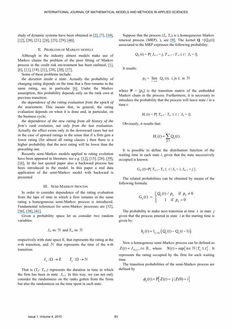
Suppose that the process (Jn, Tn) is a homogeneous Markov renewal process (MRP), ), see [9]. The kernel Q =[Qij(t)] associated to the MRP expresses the following probability:

Qij (t) = P[ Jn+1 = j, T n+1 - T n ≤ t | Jn = i].

It results:

pij = limt →∞

Qij (t); i, j∈I, t∈

where P = [pij] is the transition matrix of the embedded Markov chain in the process. Furthermore, it is necessary to introduce the probability that the process will leave state i in a time t:

Hi (t) = P[ Tn+1 - Tn ≤ t | Jn = i].

Obviously, it results that:

( ) ( )i ijj I

H t Q t∈

= ∑ .

It is possible to define the distribution function of the

waiting time in each state i, given that the state successively occupied is known:

Gij (t)=P[ Tn+1- Tn ≤ t | Jn = i, Jn+1 = j ].

The related probabilities can be obtained by means of the following formula:

( ) if 0( )

1 if 0ij ij ij

ijij

Q t / p pG t

p≠⎧⎪= ⎨ =⎪⎩

.

The probability to make next transition at time t in state j

given that the process entered in state i at the starting time is given by:

{ } ( )0( ) 1 ( ) ( 1) .ij ij ijtb t Q t Q t>= − −

Now a homogenous semi-Markov process can be defined as

( )( ) ,N tZ t J t= ∈ , where { }( ) sup | nN t n T t= ∈ ≤ . It

represents the rating occupied by the firm for each waiting time.

The transition probabilities of the semi-Markov process are defined by

[ ]( ): P ( ) | (0)ij t Z t j Z iφ = = =

INTERNATIONAL JOURNAL OF MATHEMATICAL MODELS AND METHODS IN APPLIED SCIENCES

Issue 1, Volume 4, 2010 83

and it is well known that they can be computed by solving the following evolution equations, e.g. [26]:

1( ) 1 ( ) ( ) ( ).

t

ij ij i i jE E

t Q t b tβ β ββ β ϑ

φ δ ϑ φ ϑ∈ ∈ =

⎛ ⎞= − + −⎜ ⎟

⎝ ⎠∑ ∑∑ (1)

In order to taking into account the exact time in which the

system entered the state, also a backward recurrence time process ( )( ), 0B B t t= ≥ it is introduced, see e.g. [16], [33], [34]. It is defined as

( )( ) N tB t t T= −

and represents the time since last jump. To avoid misunderstandings about its meaning, we report directly the sentence by Feller [19]: “… a bus arrival at a particular location. A person arriving at the bus stop has a waiting time until the next bus arrives. The waiting time is the forward recurrence time. The backward recurrence time is how long the person missed the previous bus.”

It is very important to consider the backward time values because to different values of B(t) correspond different values of the transition probabilities.

The transition probabilities are conditioned by the entrance time into the state i and to the fact that there are no transitions in the system for l times. Under this hypothesis the formulas of the conditional probabilities above defined have to be rewritten

Then the transition probabilities become, see [16],

[ ]( ; ) P ( ) | (0) ; (0) .bij l t Z t j Z i B lφ = = = =

They can be computed bay solving the following evolution

equations:

1

( ; ) ( ; ) ( ; ) ( , )t

bij ij i j

E

l t D l t b l tβ ββ ϑ

φ ϑ φ ϑ∈ =

= + ∑∑

where Dij(l;t) and bij(l;t) represent respectively the probability do not have transitions from state i for next t periods given that the entrance in state i occurred l periods before, and the probability do have next transitions from state i in state j after t periods given that the entrance in state i occurred l periods before. They are defined as follows:

( )

1 ( )if

; 1 ( )

0 if

iE

iji

E

Q l ti j

D l t Q l

i j

ββ

ββ

∈

∈

⎧− +⎪

⎪ =⎪= ⎨ −⎪⎪

≠⎪⎩

∑

∑

( ) ( );

1 ( )

ijij

iE

b l tb l t

Q lββ∈

+=

− ∑

where l is the length of the initial backward time. With this generalization of the model, it is possible to

consider the complete time of duration in a state in the rating migration model.

IV. PROBLEM SOLUTION THROUGH A SEMI-MARKOV RELIABILITY CREDIT RISK MODEL

In order to construct the models able to compute the probabilities and the indicators we used in our credit risk framework, it is necessary to recall some of concepts of the reliability theory, see i.e. Limnios and Oprisan [33], [35], [4]. Indeed our approach considers the rating migration models as particular system reliability models.

Let us consider a reliability system S that can be at every time t in one of the states of { }1, ,E m= … . The stochastic

process of the successive states of S is { }( ), 0Z Z t t= ≥ . The state set is partitioned into sets U and D, so that:

, , , .E U D U D U U E= ∅ = ≠ ∅ ≠∪ ∩

The subset U contains all good states in which the system

is working and the subset D contains all bad states in which the system is not working well or has failed.

Typical indicators used in reliability theory are the following:

(i) the reliability function R giving the probability that the

system was always working from time 0 to time t:

( ]( ) ( ) : 0,R t P Z u U u t⎡ ⎤= ∈ ∀ ∈⎣ ⎦

(ii) the point wise availability function A giving the

probability that the system is working on at time t whatever happens on ( ]0,t :

[ ]( ) ( )A t P Z t U= ∈

(iii) the maintainability function M giving the probability

that the system will leave the set D within the time t being in D at time 0:

( ]( ) 1 ( ) , 0, .M t P Z u D u t⎡ ⎤= − ∈ ∀ ∈⎣ ⎦

INTERNATIONAL JOURNAL OF MATHEMATICAL MODELS AND METHODS IN APPLIED SCIENCES

Issue 1, Volume 4, 2010 84

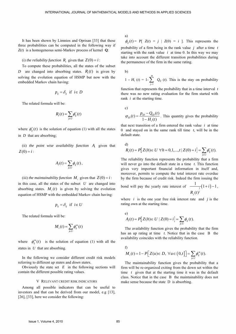
It has been shown by Limnios and Oprisan [33] that these

three probabilities can be computed in the following way if Z(t) is a homogeneous semi-Markov process of kernel Q:

(i) the reliability function iR given that (0)Z i= : To compute these probabilities, all the states of the subset

D are changed into absorbing states. ( )iR t

is given by solving the evolution equation of HSMP but now with the embedded Markov chain having:

if ij ijp i Dδ= ∈

The related formula will be:

( ) ( )ri ij

j UR t tφ

∈

= ∑

where ( )r

ij tφ is the solution of equation (1) with all the states

in D that are absorbing; (ii) the point wise availability function iA given that (0)Z i= :

( ) ( )i ijj U

A t tφ∈

= ∑ ,

(iii) the maintainability function iM given that (0)Z i= :

in this case, all the states of the subset U are changed into absorbing states. ( )iM t is given by solving the evolution equation of HSMP with the embedded Markov chain having:

if ij ijp i Uδ= ∈

The related formula will be:

( ) ( )mi ij

j U

M t tφ∈

= ∑

where ( )m

ij tφ is the solution of equation (1) with all the

states in U that are absorbing. In the following we consider different credit risk models

referring to different up states and down states. Obviously the state set E in the following sections will

contain the different possible rating values.

V RELEVANT CREDIT RISK INDICATORS Among all possible indicators that can be useful to

investors and that can be derived from our model, e.g [13], [26], [33], here we consider the following:

a) ( )ij tφ = P[ Z(t) = j | Z(0) = i ]. This represents the

probability of a firm being in the rank value j after a time t starting with the rank value i at time 0. In this way we may take into account the different transition probabilities during the permanence of the firm in the same rating.

b)

1 - Hi (t) = 1-

1

m

j=∑ Qij (t). This is the stay on probability

function that represents the probability that in a time interval t there was no new rating evaluation for the firm started with rank i at the starting time.

c)

( )( )1 ( )iD iD

iDi

p Q ttH t

ϕ−

=−

. This quantity gives the probability

that next transition of a firm entered the rank value i at time 0 and stayed on in the same rank till time t, will be in the default state.

d)

[ ]( ) ( ) 0,1,..., | (0) ( ).ri ij

j UR t P Z h U h t Z i tφ

∈

= ∈ ∀ = = = ∑The reliability function represents the probability that a firm will never go into the default state in a time t. This function gives very important financial information in itself and, moreover, permits to compute the total interest rate overdue by the firm because of credit risk. Indeed the firm issuing the

bond will pay the yearly rate interest of ( )1

1 1 1( ) t

j

iR t

+ − ,

where i is the one year free risk interest rate and j is the rating own at the starting time.

e)

[ ]( ) ( ) | (0) ( ).i ijj U

A t P Z h U Z i tφ∈

= ∈ = = ∑

The availability function gives the probability that the firm has an up rating at time t. Notice that in the case B the availability coincides with the reliability function.

f)

( ]( ) 1 ( ) , 0, ( ).mi ij

j UM t P Z u D u t tφ

∈

⎡ ⎤= − ∈ ∀ ∈ =⎣ ⎦ ∑

The maintainability function gives the probability that a firm will be re-organized exiting from the down set within the time t given that at the starting time it was in the default class. Notice that in the case B the maintainability does not make sense because the state D is absorbing.

INTERNATIONAL JOURNAL OF MATHEMATICAL MODELS AND METHODS IN APPLIED SCIENCES

Issue 1, Volume 4, 2010 85

g) ( ; )b

ij l tφ represents the probability of a firm being in the

rank j after a time t given that it was into rank i at current time and it obtained this rank l periods before.

h) 1 ( )

1 ( )i

i

H l tH l

− +−

represents the probability to not have any

new rating evaluation for t periods given that at current time the firm had rank i and it obtained this rank l periods before.

i)

[ ]( )

( ; ) P ( ) : | (0) ; (0)

; .

bi

bij

j U

R l t Z h U h t Z i B l

l tφ∈

= ∈ ∀ ≤ = =

= ∑

It represents the probability that a firm will never go into default states in a time t given that at current time it had the rank i and it obtained this rank l periods before.

We would like to underline that this indicator is actually the most significant to an investor.

l)

[ ]( ; ) ( ) | (0) , (0) ( ; ).b bi ij

j UA l t P Z t U Z i B l l tφ

∈

= ∈ = = = ∑

The availability function gives the probability that the firm has an up rating at time t given that at current time the firm had rank i and it obtained this rank l periods before.

m)

[ ]0 1

( ; )1 ( ) , 0,..., | (0) , , 0

( ; ).

bi

b mij

j U

M l tP Z h D h t Z i T l T

l tφ∈

= − ∈ ∀ = = = − >

= ∑

The maintainability function gives the probability that a firm will be re-organized exiting from the down set within the time t given that at current time the firm had rank i and it obtained this rank l periods before.

VI DATA AND SPECIFIC MODELS USED FOR THE ANALYSIS Data refers to long-term ratings at the respective dates from

complete Standard & Poor’s historical file from 1975 to 2007, i.e. all firms rated by S&P from all over the world up to the beginning of the worldwide financial crisis. In detail they refer to Entity ratings history, Instruments ratings history and Issue/Maturity ratings history. An entity is a firm issuing stock or bond; an instrument or a issue/maturity is a stock or bonds sold by an entity at particular time. They regard both Global Issuers and Structured Finance instruments (GI&SF) that Standard & Poor’s has rated. This sector -formerly known as the Corporate Finance covers corporate, financial institution, insurance, utility, transportation, non United States-based, and

sovereign issuers. GI&SF includes Structured Finance products: Asset-Backed Commercial paper, Asset-Backed Securities, Commercial Mortgage-Backed Securities, Collateralized Debt Obligations, Corporations, Financial Institutions, Regional and Local Governments, Insurance, Real Estate Companies, Residential Mortgage Backed Securities, Servicer Evaluations, Sovereigns, Utilities. Not include the Public Finance. The regions covered are: Asia-Pacific, Australia/New Zealand, Canada, Emerging Markets, Europe, Middle East, Africa, Latin America and United States.

By referring to different up states and down states in this paper we considered different credit risk models.

A. Model 1 This model considers the following state space:

{ }1 AAA, AA, A, BBB, BB, B, CCC, D .E = It is divided in:

{ }1 1AAA, AA, A, BBB, BB, B, CCC ; {D}U D= =

where the down set is formed by the only state D, i.e. default state, that here it is considered as an absorbing state: when a firm get it, it is impossible to have a new transition. The transition matrix has special analytic properties, see [17]. Furthermore the maintainability function does not make sense.

In the data manipulation process the items of information became 135.455 transitions among the states carried out from 1975, January 1, to 2007, July 16.

B. Model 2 In this model the state NR (no rating) gets in the state set.

The space set is formed by:

{ }2 AAA, AA, A, BBB, BB, B, CCC, D, NR .E = An issuer designated NR is not rated. In other words, at

some point during their rating history, it has rating withdrawn and is removed from consideration, but is surveilled with the aim of capturing a potential default. Ratings are withdrawn when programs rated are terminated and the relevant debt extinguished or when the entity leaves the public fixed-income market. Other reasons that makes a firm NR include: mergers, acquisitions, lack of cooperation, insufficient information, matter of policy or redemptions.

As usual the space set is splitted in two subsets:

{ }2 2AAA, AA, A, BBB, BB, B, CCC ; {D, NR}.U D= = None of the down states is absorbing; that is the transitions

from these states and into these states are possible. Moreover the maintainability function M has a precise meaning in the financial environment. In general a firm get rank D or NR

INTERNATIONAL JOURNAL OF MATHEMATICAL MODELS AND METHODS IN APPLIED SCIENCES

Issue 1, Volume 4, 2010 86

after a reorganization or when it is re-evaluated by the rating agency afterwards a new financial situation occur.

In the data manipulation process the items of information became 266.560 transitions among the states carried out from 1975, January 1, to 2007, July 16.

C. Model 3 The state set is now:

{ }3 AAA, AA, A, BBB, BB, B, CCC,D, NR1, NR2 .E = In this model two kind of no rating rank are considered:

NR1 and NR2. Precisely, a firm is considered enter state NR1 when gets in it coming from an investment grade (AAA, AA, A or BBB), whereas enter state NR2 when gets in it coming from a speculative grade (BB, B, CCC or D).

In this case the space set is partitioned as:

{ }3 3AAA, AA, A, BBB, BB, B, CCC, NR1 ; {D, NR2}.U D= = Also in this case none of the down states is absorbing; that

is the transitions from these states and into these states are possible.

VII SOME RESULTS AND CONCLUSIONS The models described above are implemented by means of

real data. At this point it should be clear that a huge amount of results are obtained. By means of data descript above we constructed the semi-Markov kernel Q =[Qij(t)] and we derived the transition probabilities ( )ij tφ and all the others

credit risk indicators. All the quantities are obtained for each arrival state, for each arrival time conditioned to each starting state. Here only some results are reported, but they are all, obviously, available upon request to the authors.

A. Results from model 1 In Table I, Table II, Table III the transition probabilities

obtained by solving the evolution equation are reported for some times. They represent the probability of a firm being in the rank value j after a time t starting with the rank value i at time 0

TABLE I

TRANSITION PROBABILITIES (6)ijφ

AAA AA A BBB BB B CCC D

AAA 0,365 0,254 0,180 0,103 0,048 0,031 0,010 0,009

AA 0,093 0,426 0,306 0,107 0,035 0,020 0,007 0,006

A 0,056 0,171 0,464 0,206 0,057 0,029 0,009 0,009

BBB 0,039 0,081 0,223 0,386 0,156 0,075 0,022 0,018

BB 0,024 0,050 0,107 0,247 0,259 0,200 0,064 0,050

B 0,015 0,029 0,056 0,103 0,183 0,310 0,138 0,167

CCC 0,008 0,018 0,034 0,045 0,065 0,154 0,143 0,533

D 0,000 0,000 0,000 0,000 0,000 0,000 0,000 1,000

TABLE II TRANSITION PROBABILITIES (12)ijφ

AAA AA A BBB BB B CCC D

AAA 0,174 0,258 0,257 0,151 0,067 0,047 0,017 0,028

AA 0,093 0,281 0,320 0,166 0,064 0,041 0,014 0,022

A 0,068 0,189 0,344 0,212 0,085 0,054 0,019 0,029

BBB 0,051 0,124 0,249 0,260 0,131 0,094 0,034 0,057

BB 0,037 0,085 0,169 0,215 0,158 0,145 0,059 0,131

B 0,024 0,055 0,104 0,142 0,136 0,168 0,078 0,292

CCC 0,013 0,030 0,055 0,068 0,067 0,092 0,050 0,626

D 0,000 0,000 0,000 0,000 0,000 0,000 0,000 1,000

TABLE III TRANSITION PROBABILITIES (18)ijφ

AAA AA A BBB BB B CCC D

AAA 0,113 0,226 0,276 0,174 0,078 0,057 0,022 0,054

AA 0,083 0,228 0,301 0,186 0,080 0,056 0,020 0,046

A 0,069 0,184 0,300 0,205 0,093 0,066 0,025 0,058

BBB 0,056 0,142 0,248 0,215 0,114 0,089 0,035 0,101

BB 0,044 0,106 0,191 0,190 0,120 0,109 0,045 0,195

B 0,030 0,073 0,131 0,141 0,104 0,108 0,048 0,365

CCC 0,016 0,038 0,068 0,071 0,053 0,059 0,027 0,668

D 0,000 0,000 0,000 0,000 0,000 0,000 0,000 1,000

Table IV shows the evolution of the survival probabilities up t, give that it entered with rank value i at the time 0.

TABLE 4 SURVIVAL PROBABILITIES ( )iR t

Time AAA AA A BBB BB B CCC

t=1 0,9995 0,9995 0,9992 0,9985 0,9980 0,9909 0,7662

t=2 0,9986 0,9989 0,9981 0,9967 0,9931 0,9636 0,6574

t=3 0,9973 0,9979 0,9969 0,9943 0,9855 0,9296 0,5848

t=4 0,9956 0,9967 0,9954 0,9911 0,9754 0,8956 0,5330

t=5 0,9935 0,9953 0,9935 0,9871 0,9633 0,8630 0,4958

t=6 0,9911 0,9937 0,9914 0,9824 0,9499 0,8335 0,4669

t=7 0,9885 0,9917 0,9888 0,9771 0,9360 0,8070 0,4434

t=8 0,9855 0,9896 0,9860 0,9711 0,9218 0,7830 0,4244

t=9 0,9824 0,9871 0,9828 0,9647 0,9080 0,7613 0,4087

t=10 0,9790 0,9844 0,9792 0,9578 0,8945 0,7416 0,3953

t=11 0,9754 0,9815 0,9754 0,9507 0,8815 0,7239 0,3840

t=12 0,9716 0,9783 0,9713 0,9434 0,8690 0,7078 0,3740

t=13 0,9677 0,9748 0,9669 0,9360 0,8570 0,6930 0,3652

t=14 0,9635 0,9712 0,9623 0,9285 0,8456 0,6796 0,3573

t=15 0,9593 0,9673 0,9574 0,9210 0,8347 0,6671 0,3501

t=16 0,9548 0,9632 0,9524 0,9136 0,8243 0,6557 0,3436

t=17 0,9503 0,9589 0,9473 0,9061 0,8143 0,6450 0,3377

t=18 0,9456 0,9545 0,9420 0,8987 0,8048 0,6351 0,3322

INTERNATIONAL JOURNAL OF MATHEMATICAL MODELS AND METHODS IN APPLIED SCIENCES

Issue 1, Volume 4, 2010 87

In Table V, Table VI, Table VII, Table VIII we show the backward transition probabilities, for some values of l and t.

TABLE V

TRANSITION PROBABILITIES (0;9)bijφ

AAA AA A BBB BB B CCC D

AAA 0,240 0,269 0,229 0,131 0,059 0,040 0,014 0,018

AA 0,096 0,334 0,322 0,144 0,051 0,031 0,011 0,013

A 0,064 0,186 0,386 0,214 0,076 0,043 0,014 0,017

BBB 0,046 0,107 0,243 0,304 0,143 0,091 0,030 0,035

BB 0,031 0,069 0,145 0,232 0,193 0,171 0,066 0,092

B 0,020 0,043 0,083 0,132 0,159 0,221 0,103 0,239

CCC 0,011 0,025 0,045 0,060 0,071 0,119 0,078 0,591

D 0,000 0,000 0,000 0,000 0,000 0,000 0,000 1,000

TABLE VI

TRANSITION PROBABILITIES (1;9)bijφ

AAA AA A BBB BB B CCC D

AAA 0,258 0,279 0,217 0,120 0,056 0,039 0,014 0,017

AA 0,094 0,360 0,323 0,133 0,045 0,026 0,009 0,009

A 0,059 0,182 0,409 0,214 0,072 0,039 0,013 0,013

BBB 0,042 0,098 0,243 0,323 0,147 0,089 0,029 0,029

BB 0,029 0,064 0,142 0,244 0,205 0,174 0,065 0,077

B 0,019 0,040 0,078 0,135 0,171 0,240 0,110 0,207

CCC 0,012 0,027 0,050 0,072 0,095 0,165 0,112 0,468

D 0,000 0,000 0,000 0,000 0,000 0,000 0,000 1,000

TABLE VII

TRANSITION PROBABILITIES (3;9)bijφ

AAA AA A BBB BB B CCC D

AAA 0,362 0,309 0,176 0,081 0,035 0,022 0,007 0,006

AA 0,088 0,469 0,298 0,094 0,027 0,015 0,005 0,004

A 0,046 0,175 0,502 0,189 0,050 0,024 0,008 0,006

BBB 0,033 0,080 0,247 0,399 0,141 0,068 0,019 0,013

BB 0,021 0,045 0,114 0,258 0,271 0,186 0,060 0,045

B 0,013 0,028 0,057 0,114 0,186 0,316 0,129 0,156

CCC 0,008 0,018 0,039 0,058 0,094 0,209 0,210 0,363

D 0,000 0,000 0,000 0,000 0,000 0,000 0,000 1,000

TABLE VIII

TRANSITION PROBABILITIES (5;9)bijφ

AAA AA A BBB BB B CCC D

AAA 0,540 0,294 0,101 0,037 0,015 0,009 0,003 0,002

AA 0,070 0,613 0,241 0,053 0,013 0,007 0,002 0,001

A 0,027 0,139 0,642 0,148 0,027 0,012 0,003 0,002

BBB 0,018 0,049 0,210 0,543 0,122 0,042 0,011 0,005

BB 0,011 0,024 0,063 0,236 0,421 0,178 0,045 0,021

B 0,008 0,015 0,030 0,074 0,193 0,464 0,134 0,082

CCC 0,005 0,009 0,026 0,049 0,091 0,231 0,372 0,217

D 0,000 0,000 0,000 0,000 0,000 0,000 0,000 1,000

They represent the probability for a firm to have a rating j

after a time t, given that it was into rank i at current time and it entered the state l periods before.

In Table IX, Table X and Table XI there are the firm

survival probability given that it was in rating i at time 0 with backward value respectively equal to 0, 1 and 2

TABLE IX

SURVIVAL PROBABILITIES (0; )biR t

times AAA AA A BBB BB B CCC

l=0 t=1 1,000 0,999 0,999 0,999 0,998 0,991 0,766

l=0 t=2 0,999 0,999 0,998 0,997 0,993 0,964 0,657

l=0 t=3 0,997 0,998 0,997 0,994 0,985 0,930 0,585

l=0 t=4 0,996 0,997 0,995 0,991 0,975 0,896 0,533

l=0 t=5 0,994 0,995 0,994 0,987 0,963 0,863 0,496

l=0 t=6 0,991 0,994 0,991 0,982 0,950 0,833 0,467

l=0 t=7 0,988 0,992 0,989 0,977 0,936 0,807 0,443

l=0 t=8 0,986 0,990 0,986 0,971 0,922 0,783 0,424

TABLE X

SURVIVAL PROBABILITIES (1; )biR t

times AAA AA A BBB BB B CCC

l=1 t=1 0,998 0,999 0,999 0,998 0,994 0,964 0,782

l=1 t=2 0,996 0,998 0,998 0,995 0,986 0,932 0,709

l=1 t=3 0,994 0,997 0,996 0,992 0,975 0,899 0,657

l=1 t=4 0,991 0,996 0,995 0,988 0,963 0,869 0,615

l=1 t=5 0,989 0,995 0,993 0,983 0,950 0,841 0,581

l=1 t=6 0,986 0,993 0,990 0,978 0,936 0,816 0,555

l=1 t=7 0,983 0,991 0,987 0,971 0,923 0,793 0,532

l=1 t=8 0,979 0,988 0,984 0,965 0,909 0,772 0,513

TABLE XI

SURVIVAL PROBABILITIES (2; )biR t

times AAA AA A BBB BB B CCC

l=2 t=1 0,996 0,999 0,998 0,996 0,988 0,931 0,766

l=2 t=2 0,995 0,998 0,997 0,993 0,978 0,899 0,711

l=2 t=3 0,993 0,997 0,996 0,990 0,966 0,869 0,664

l=2 t=4 0,991 0,996 0,994 0,985 0,953 0,841 0,628

l=2 t=5 0,988 0,994 0,991 0,980 0,939 0,816 0,599

l=2 t=6 0,986 0,992 0,989 0,974 0,926 0,793 0,575

l=2 t=7 0,983 0,990 0,986 0,968 0,912 0,772 0,555

B. Results from model 2 In Table XII, Table XIII, Table XIV the transition

probabilities obtained by solving the evolution equation are reported for some times. They represent the probability of a

INTERNATIONAL JOURNAL OF MATHEMATICAL MODELS AND METHODS IN APPLIED SCIENCES

Issue 1, Volume 4, 2010 88

firm being in the rank value j after a time t starting with the rank value i at time 0. Notice that the results related to state BB are omitted for lack of space.

TABLE XII TRANSITION PROBABILITIES (6)ijφ

AAA AA A BBB B CCC D NR

AAA 0,204 0,124 0,127 0,090 0,034 0,012 0,004 0,362

AA 0,070 0,277 0,196 0,089 0,027 0,009 0,003 0,293

A 0,054 0,118 0,307 0,139 0,030 0,010 0,003 0,292

BBB 0,048 0,074 0,158 0,253 0,050 0,015 0,005 0,303

B 0,040 0,055 0,083 0,091 0,196 0,076 0,027 0,318

CCC 0,049 0,066 0,096 0,085 0,112 0,106 0,045 0,378

D 0,066 0,091 0,130 0,108 0,071 0,039 0,030 0,400

NR 0,077 0,116 0,165 0,130 0,056 0,020 0,007 0,363

TABLE XIII TRANSITION PROBABILITIES (12)ijφ

AAA AA A BBB B CCC D NR

AAA 0,103 0,130 0,169 0,125 0,051 0,018 0,006 0,334

AA 0,072 0,164 0,195 0,125 0,046 0,016 0,006 0,316

A 0,066 0,126 0,215 0,140 0,049 0,017 0,006 0,315

BBB 0,064 0,109 0,178 0,162 0,060 0,021 0,007 0,321

B 0,062 0,099 0,147 0,130 0,091 0,036 0,013 0,336

CCC 0,066 0,106 0,156 0,128 0,078 0,036 0,013 0,340

D 0,070 0,116 0,169 0,134 0,065 0,025 0,011 0,337

NR 0,071 0,122 0,179 0,137 0,059 0,021 0,007 0,333

TABLE XIV TRANSITION PROBABILITIES (18)ijφ

AAA AA A BBB B CCC D NR

AAA 0,078 0,128 0,180 0,134 0,056 0,020 0,007 0,327

AA 0,071 0,139 0,188 0,134 0,054 0,019 0,007 0,321

A 0,069 0,126 0,194 0,139 0,056 0,020 0,007 0,321

BBB 0,068 0,119 0,182 0,145 0,060 0,021 0,007 0,324

B 0,068 0,116 0,172 0,137 0,068 0,025 0,009 0,330

CCC 0,069 0,119 0,175 0,137 0,064 0,025 0,009 0,330

D 0,070 0,122 0,179 0,138 0,061 0,022 0,008 0,328

NR 0,070 0,124 0,183 0,138 0,059 0,021 0,007 0,326

In Table XV we reported the time evolution of the firm survival probabilities up to time t, give that it entered with rank value i at the starting time 0.

In Table XVI we reported the time evolution of the firm maintainability function up to time t, give that it entered with rank value i at the starting time 0.

TABLE XV

SURVIVAL PROBABILITIES ( )iR t

Time AAA AA A BBB BB B CCC

t=1 0,775 0,858 0,856 0,875 0,905 0,893 0,725

t=2 0,627 0,755 0,753 0,768 0,799 0,775 0,552

t=3 0,510 0,667 0,666 0,674 0,701 0,664 0,431

t=4 0,425 0,591 0,589 0,590 0,613 0,566 0,340

t=5 0,355 0,523 0,521 0,516 0,533 0,481 0,275

t=6 0,297 0,463 0,462 0,452 0,463 0,409 0,226

t=7 0,254 0,410 0,410 0,396 0,403 0,349 0,189

t=8 0,219 0,363 0,363 0,348 0,350 0,298 0,158

t=9 0,190 0,322 0,322 0,306 0,305 0,256 0,133

t=10 0,165 0,286 0,286 0,269 0,265 0,220 0,113

t=11 0,142 0,253 0,254 0,237 0,231 0,189 0,097

t=12 0,123 0,225 0,225 0,208 0,201 0,162 0,083

t=13 0,107 0,200 0,200 0,184 0,176 0,140 0,072

t=14 0,093 0,177 0,178 0,162 0,153 0,121 0,062

t=15 0,081 0,158 0,158 0,143 0,134 0,104 0,053

t=16 0,071 0,140 0,141 0,126 0,117 0,090 0,046

t=17 0,063 0,125 0,125 0,111 0,103 0,079 0,040

t=18 0,055 0,111 0,111 0,098 0,090 0,068 0,035

TABLE XVI

MAINTAINABILITY

FUNCTION ( )iM t

Time D NR

t=1 0,130 0,258

t=2 0,277 0,467

t=3 0,435 0,610

t=4 0,570 0,712

t=5 0,675 0,790

t=6 0,756 0,844

t=7 0,819 0,882

t=8 0,863 0,911

t=9 0,897 0,931

t=10 0,921 0,947

t=11 0,939 0,958

t=12 0,952 0,966

t=13 0,962 0,973

t=14 0,970 0,979

t=15 0,976 0,984

t=16 0,981 0,987

t=17 0,985 0,990

t=18 0,988 0,993

INTERNATIONAL JOURNAL OF MATHEMATICAL MODELS AND METHODS IN APPLIED SCIENCES

Issue 1, Volume 4, 2010 89

In Tab. XVII, Tab. XVIII, Tab. XIX, Tab. XX we show the backward transition probabilities, for some values of l and t.

TABLE XVII

TRANSITION PROBABILITIES (0;9)bijφ

AAA AA A BBB B CCC D NR

AAA 0,136 0,131 0,155 0,113 0,046 0,016 0,005 0,341

AA 0,072 0,201 0,198 0,113 0,039 0,013 0,005 0,308

A 0,062 0,125 0,243 0,141 0,042 0,015 0,005 0,308

BBB 0,058 0,097 0,172 0,188 0,058 0,019 0,006 0,316

B 0,054 0,082 0,122 0,118 0,125 0,050 0,018 0,334

CCC 0,062 0,092 0,135 0,115 0,090 0,054 0,021 0,356

D 0,070 0,108 0,157 0,128 0,069 0,029 0,015 0,351

NR 0,073 0,121 0,174 0,136 0,058 0,021 0,007 0,339

TABLE XVIII

TRANSITION PROBABILITIES (1;9)bijφ

AAA AA A BBB B CCC D NR

AAA 0,150 0,133 0,152 0,109 0,044 0,016 0,005 0,337

AA 0,072 0,210 0,201 0,111 0,037 0,013 0,004 0,304

A 0,060 0,125 0,253 0,141 0,041 0,014 0,005 0,303

BBB 0,057 0,096 0,173 0,189 0,059 0,019 0,006 0,315

B 0,055 0,083 0,125 0,121 0,123 0,047 0,017 0,334

CCC 0,061 0,092 0,134 0,115 0,093 0,056 0,020 0,351

D 0,070 0,109 0,158 0,128 0,069 0,028 0,019 0,347

NR 0,068 0,116 0,170 0,136 0,062 0,023 0,008 0,344

TABLE XIX

TRANSITION PROBABILITIES (3;9)bijφ

AAA AA A BBB B CCC D NR

AAA 0,166 0,133 0,147 0,102 0,041 0,014 0,005 0,341

AA 0,071 0,236 0,198 0,105 0,034 0,012 0,004 0,296

A 0,057 0,125 0,279 0,136 0,038 0,013 0,004 0,294

BBB 0,057 0,095 0,178 0,200 0,055 0,018 0,006 0,309

B 0,055 0,083 0,125 0,118 0,123 0,045 0,016 0,342

CCC 0,061 0,092 0,135 0,114 0,098 0,065 0,017 0,344

D 0,068 0,106 0,153 0,124 0,067 0,026 0,034 0,351

NR 0,061 0,108 0,160 0,129 0,062 0,022 0,008 0,381

TABLE XX

TRANSITION PROBABILITIES (5;9)bijφ

AAA AA A BBB B CCC D NR

AAA 0,174 0,134 0,142 0,098 0,039 0,014 0,005 0,346

AA 0,067 0,266 0,191 0,100 0,032 0,011 0,004 0,286

A 0,053 0,125 0,311 0,132 0,035 0,012 0,004 0,277

BBB 0,055 0,091 0,178 0,226 0,052 0,017 0,006 0,297

B 0,056 0,083 0,123 0,114 0,139 0,043 0,015 0,337

CCC 0,056 0,083 0,122 0,105 0,115 0,088 0,016 0,340

D 0,064 0,095 0,136 0,113 0,063 0,023 0,077 0,361

NR 0,065 0,112 0,164 0,124 0,057 0,019 0,006 0,386

In Table XXI, Table XXII and Table XXIII there are the

firm survival probability given that it was in rating i at time 0 with backward value respectively equal to 0, 1 and 2.

TABLE XXI

SURVIVAL PROBABILITIES (0; )biR t

times AAA AA A BBB BB B CCC

l=0 t=1 0,775 0,858 0,856 0,875 0,905 0,893 0,725

l=0 t=2 0,685 0,791 0,790 0,800 0,824 0,802 0,601

l=0 t=3 0,644 0,755 0,754 0,755 0,769 0,737 0,553

l=0 t=4 0,635 0,731 0,730 0,724 0,732 0,695 0,545

l=0 t=5 0,633 0,715 0,714 0,705 0,705 0,669 0,558

l=0 t=6 0,634 0,704 0,704 0,693 0,689 0,655 0,577

l=0 t=7 0,642 0,697 0,698 0,685 0,679 0,649 0,596

l=0 t=8 0,649 0,691 0,691 0,680 0,673 0,647 0,611

TABLE XXII

SURVIVAL PROBABILITIES (1; )biR t

times AAA AA A BBB BB B CCC

l=1 t=1 0,706 0,824 0,821 0,805 0,807 0,786 0,640

l=1 t=2 0,669 0,778 0,774 0,755 0,758 0,728 0,584

l=1 t=3 0,647 0,748 0,745 0,725 0,722 0,688 0,574

l=1 t=4 0,635 0,726 0,726 0,705 0,700 0,666 0,583

l=1 t=5 0,644 0,714 0,714 0,695 0,687 0,655 0,596

l=1 t=6 0,650 0,703 0,704 0,687 0,678 0,650 0,608

l=1 t=7 0,655 0,697 0,697 0,682 0,672 0,649 0,619

l=1 t=8 0,658 0,692 0,693 0,678 0,669 0,649 0,629

TABLE XXIII

SURVIVAL PROBABILITIES (2; )biR t

times AAA AA A BBB BB B CCC

l=2 t=1 0,671 0,795 0,787 0,753 0,746 0,715 0,585

l=2 t=2 0,641 0,759 0,757 0,723 0,716 0,681 0,585

l=2 t=3 0,647 0,739 0,739 0,707 0,699 0,664 0,594

l=2 t=4 0,652 0,722 0,722 0,697 0,688 0,654 0,603

l=2 t=5 0,656 0,713 0,712 0,690 0,679 0,652 0,611

l=2 t=6 0,659 0,704 0,705 0,685 0,674 0,650 0,623

l=2 t=7 0,655 0,695 0,697 0,681 0,669 0,649 0,634

In Table XXIV, Table XXV and Table XXVI we reported the time evolution of the firm maintainability function up to time t, give that it entered with rank value i at the starting time 0 with backward value respectively equal to 0, 1 and 2.

INTERNATIONAL JOURNAL OF MATHEMATICAL MODELS AND METHODS IN APPLIED SCIENCES

Issue 1, Volume 4, 2010 90

TABLE XXIV

MAINTAINABILITY

FUNCTION (0; )iM t

Time D NR

t=1 0,130 0,258

t=2 0,277 0,467

t=3 0,435 0,610

t=4 0,570 0,712

t=5 0,675 0,790

t=6 0,756 0,844

t=7 0,819 0,882

t=8 0,863 0,911

TABLE XXV

MAINTAINABILITY

FUNCTION (1; )iM t

Time D NR

t=1 0,284 0,368

t=2 0,445 0,615

t=3 0,575 0,721

t=4 0,679 0,789

t=5 0,761 0,840

t=6 0,819 0,877

t=7 0,864 0,905

t=8 0,896 0,925

TABLE XXVI

MAINTAINABILITY

FUNCTION (2; )iM t

Time D NR

t=1 0,428 0,591

t=2 0,560 0,685

t=3 0,668 0,752

t=4 0,747 0,806

t=5 0,810 0,846

t=6 0,853 0,877

t=7 0,884 0,898

C. Results from model 3 In Table XXVII there are the firm survival probability

given that it was in rating i at time 0 without backward. Whereas in Table XXVIII there are the firm survival

probability given that it was in rating i at time 0 with a backward value equal to 1.

TABLE XXVII

SURVIVAL PROBABILITIES (0; )iR t

Time AAA AA A BBB BB B CCC

t=1 1,000 1,000 1,000 1,000 1,000 0,933 1,000

t=2 1,000 1,000 1,000 1,000 0,972 0,773 0,875

t=3 1,000 1,000 1,000 1,000 0,972 0,747 0,871

t=4 1,000 1,000 1,000 0,999 0,971 0,647 0,828

t=5 1,000 1,000 1,000 0,998 0,967 0,645 0,819

t=6 1,000 1,000 1,000 0,998 0,932 0,512 0,743

t=7 1,000 1,000 0,999 0,997 0,928 0,510 0,674

t=8 0,999 0,999 0,997 0,991 0,902 0,499 0,644

t=9 0,994 0,997 0,993 0,984 0,884 0,479 0,599

t=10 0,988 0,996 0,990 0,978 0,871 0,404 0,514

t=11 0,981 0,993 0,987 0,971 0,853 0,395 0,426

t=12 0,971 0,990 0,978 0,957 0,806 0,304 0,383

t=13 0,961 0,985 0,967 0,940 0,765 0,212 0,300

t=14 0,951 0,979 0,956 0,925 0,737 0,199 0,264

t=15 0,939 0,972 0,944 0,910 0,711 0,162 0,225

t=16 0,933 0,967 0,936 0,899 0,693 0,155 0,189

t=17 0,927 0,962 0,927 0,888 0,674 0,148 0,161

t=18 0,921 0,957 0,917 0,876 0,655 0,142 0,136

TABLE XXVIII

SURVIVAL PROBABILITIES (1; )iR t

Time AAA AA A BBB BB B CCC

t=1 1,000 1,000 1,000 1,000 0,923 0,692 0,750

t=2 1,000 1,000 1,000 1,000 0,885 0,524 0,500

t=3 1,000 1,000 1,000 1,000 0,807 0,434 0,500

t=4 1,000 1,000 1,000 0,999 0,727 0,349 0,500

t=5 1,000 1,000 1,000 0,998 0,724 0,348 0,500

t=6 1,000 0,998 0,998 0,992 0,710 0,320 0,500

t=7 0,998 0,994 0,996 0,986 0,697 0,280 0,500

t=8 0,994 0,991 0,994 0,982 0,689 0,264 0,497

t=9 0,989 0,987 0,991 0,975 0,676 0,237 0,487

t=10 0,982 0,981 0,985 0,958 0,603 0,209 0,451

t=11 0,972 0,974 0,977 0,939 0,563 0,165 0,415

t=12 0,964 0,968 0,969 0,924 0,539 0,148 0,391

t=13 0,954 0,961 0,960 0,907 0,515 0,124 0,127

t=14 0,948 0,956 0,953 0,896 0,495 0,109 0,115

t=15 0,943 0,952 0,945 0,883 0,477 0,096 0,101

t=16 0,938 0,948 0,938 0,871 0,460 0,084 0,088

t=17 0,933 0,943 0,929 0,858 0,444 0,073 0,076

t=18 0,930 0,941 0,925 0,850 0,435 0,067 0,069

INTERNATIONAL JOURNAL OF MATHEMATICAL MODELS AND METHODS IN APPLIED SCIENCES

Issue 1, Volume 4, 2010 91

From these results it is possible to see that the duration effect is adequately described by the backward process. Indeed significant differences arise for different values of the backward time.

The model 2 gives us additional information with respect to the model 1. Indeed by consideration also of the NR state, it is possible to quantify the probability that the firm will be re-organized through the entrance in a new up rating class.

Finally model 3 gives us the possibility to distinguish between entrance into NR class from investment grade and speculative grade. In this way the model gives more accurate forecasting of the system.

REFERENCES [1] E.I. Altman, The importance and subtlety of credit rating migration,

Journal of Banking and Finance, 22, 1998, pp. 1231-1247. [2] F.I. Arunaye, H. White, On the Ermanno-Bernoulli and Quasi-Ermanno-

Bernoulli Constants for Linearizing Dynamical Systems, Wseas Transactions on Mathematics, 7(3), 2008, pp. 71-77.

[3] A. Bangia, F.X. Diebold, A. Kronimus, C. Schagen, T. Schuermann, Ratings migration and the business cycle, with application to credit portfolio stress testing, Journal of Banking & Finance, 26, 2002, pp. 445-474.

[4] A. Blasi, J. Janssen, R. Manca, Numerical treatment of homogeneous and non-homogeneous semi-Markov reliability models, Communications in Statistics, Theory and Models, 33, 2004, 697-714.

[5] C. Bluhm, L. Overbeck, C. Wagner, An introduction to credit risk management, London: Chapmann & Hall, 2002.

[6] L. Carty, J. Fons, Measuring changes in corporate credit quality. The Journal of Fixed Income, 4, 1994, pp. 27-41.

[7] G. Chacko, A. Sjoman, H. Motohashi, V. Dessan, Credit derivatives, Wharton School Publishing, New Jersey, 2006.

[8] E. Çinlar, Markov renewal theory, Advances in Appl. Probability, 1, 1969, 123-187.

[9] E. Çinlar, Markov renewal theory: a survey, Management Science, 21, 1975, 727-752.

[10] G. Corradi, J. Janssen, R. Manca, Numerical treatment of homogeneous semi-Markov processes in transient case, Methodology and Computing in Applied Probability, 6, 2004, 233-246.

[11] M. Crouhy, D. Galai, R. Mark, A comparative analysis of current credit risk models. Journal of Banking and Finance, 24, 2000, 59-117.

[12] G. D’Amico, G. Di Biase, Dynamic Concentration /Inequality Indices of Economic Systems. In proceedings of the International Conference “Recent Advances in Applied Mathematics” (C.A. Bolucea, V. Mladenov, E. Pop, M. Leba, N. Mastorakis, Eds.), (Tenerife, Spain), pp. 312-316, Wseas Press, 2009

[13] G. D’Amico, G. Di Biase, J. Janssen, R. Manca, Homogeneous and Non-Homogeneous Semi-Markov Backward Credit Risk Migration Models. In Financial Hedging, P.N. Catlere editor, Nova Science Publishers, 2009.

[14] G. D’Amico, G. Di Biase, J. Janssen, R. Manca, Semi-Markov Backward Credit Risk Migration Models Compared with Markov Models. In proceedings of the 3RD International Conference on Applied Mathematics, Simulation, Modelling} (P. Pardalos, N. Mastorakis, V. Mladenov and Z. Bojkovic, Eds.), (Athens, Greece), pp. 112-116, Wseas Press, 2009.

[15] G. D’Amico, J. Janssen, R. Manca, Homogeneous discrete time semi-Markov reliability models for credit risk Management, Decisions in Economics and Finance, 28, 2005, pp. 79-93.

[16] G. D’Amico, J. Janssen, R. Manca, Initial and Final Backward and Forward Discrete Time Non-Homogeneous Semi-Markov Credit Risk models. Methodology and Computing in Applied Probability, DOI 10.1007/s11009-009-9142-6, 2009.

[17] G. D’Amico, J. Janssen, R. Manca, The dynamic behaviour of non-homogeneous single uni-reducible Markov and semi-Markov chains. In A. Naimzada, S. Stefani, A. Torriero (eds): Networks: Topology and Dynamic. Lectures Notes in Economic and Mathematical Systems, Springer, pp. 195-211, 2008.

[18] D. Duffie, K.J: Singleton, Credit Risk, Scottsdale: Princeton, 2003.

[19] W. Feller, An introduction to probability theory and its applications, vol.II, 2-nd ed., John Wiley & Sons, New York-London-Sydney, 1971.

[20] R. Howard, Dynamic probabilistic systems: vol 1, Wiley, New York:, 1971.

[21] R. Howard, Dynamic probabilistic systems: vol 2, Wiley, New York, 1971.

[22] Y. Hu, R. Kiesel, W. Perraudin, The estimation of transition matrices for sovereign credit ratings, Journal of Banking and Finance, 26, 2002, pp. 1383-1406.

[23] R.B. Israel, J.S. Rosenthal, Z.W. Jason, Finding generators for Markov chains via empirical transitions matrices, with applications to credit ratings. Mathematical Finance, 11, 2001, pp. 245-265.

[24] J. Janssen, R. Manca, Numerical solution of non homogeneous semi-Markov processes in transient case, Methodology and Computing in Applied Probability, 3, 2001, pp.271-293.

[25] J. Janssen, R. Manca, Applied Semi-Markov Processes, Springer, New York. 2006.

[26] J. Janssen, R. Manca, Semi-Markov risk models for Finance, Insurance and Reliability, Springer, New York. 2007.

[27] A.J. Jarrow, D. Lando, S.M. Turnbull, A Markov model for the term structure of credit risk spreads, The Review of Financial Studies, 10, 1997, pp. 481-523.

[28] D. Kavvathas, Estimating credit rating transition probabilities for corporate bonds, University of Chicago, working paper, 2001.

[29] V. Korolyuk, A. Swishchuk, Semi-Markov random evolutions, Kluwer Academic Publisher, New York, 1995.

[30] D. Lando, T.M. Skodeberg, Analyzing Rating transitions and rating drift with continuous observations. Journal of Banking and Finance, 26, 2002, pp. 423-444.

[31] D. Lando, Credit risk modeling. Scottsdale, Princeton, 2004. [32] P. Levy, Processus semi-Markoviens. In Proc. of International Congress

of Mathematics, Amsterdam, 1954. [33] N. Limnios, G. Oprişan, Semi-Markov Processes and Reliability

modeling, Birkhauser, Boston, 2001. [34] A. Lucas, A. Monteiro, G.V. Smirnov, Nonparametric estimation for

non-homogeneous semi-Markov processes: an application to credit risk, Working paper Vrije Universiteit Amsterdam, working paper, 2006.

[35] S. Osaki, Stochastic system reliability modeling: Series in Modern Applied Mathematics. Singapore: World Scientific Publishing Co, 1985.

[36] R. Pyke, Markov renewal processes: definitions and preliminary properties, Annals Mathematical Statistics, 32, 1961, 1231-1242.

[37] P. Nickell, W. Perraudin, S. Varotto, Stability of rating transitions, Journal of Banking and Finance, 24, 2000, pp. 203-227.

[38] W.L. Smith, Regenerative stochastic processes, Pro. Roy. Soc. Ser. A. London, 1955.

[39] A. Vasileiou, P.C.G. Vassiliou, An Inhomogeneous semi-Markov model for the term structure of credit risk spreads, Advances in Applied Probability, 38, 2006, pp. 171-198.

[40] Y. Wu, C. Fyfe, The On-line Cross Entropy Method for Unsupervised Data Exploration, Wseas Transactions on Mathematics,6(12), 2007, pp. 865--877.

[41] J. Yackel, Limit Theorems for Semi-Markov Processes. Transactions of the American Mathematical Society, 123, 1966, 402-424.

INTERNATIONAL JOURNAL OF MATHEMATICAL MODELS AND METHODS IN APPLIED SCIENCES

Issue 1, Volume 4, 2010 92