Combining cattle activity and progesterone

measurements using hidden semi-Markov

Models

JARED O’CONNELL, FREDE AAKMANN TØGERSEN,

NICOLAS C. FRIGGENS, PETER LØVENDAHL AND

SØREN HØJSGAARD

Hourly pedometer counts and irregularly measured concentrations of the

hormone progesterone were available for a large number of dairy cattle. A

hidden semi-Markov was applied to this bivariate time series data for the pur-

poses of monitoring the reproductive status of cattle. In particular, the ability

to identify oestrus is investigated as this is of great importance to farm man-

agement. Progesterone concentration is a more accurate, but more expensive

than pedometer counts, and we evaluate the added benefits of amodel that

includes this variable. The resulting model is biologically sensible, but vali-

dation is difficult. We utilise some auxilliary data to demonstrate the model’s

performance.

Key words: dairy cow, EM–algorithm, oestrus detection, online data, stream-

ing data, time-series.

1 INTRODUCTION

Accurate detection of reproductive status in cattle is critical to efficient farm

management. There currently exist a number of on-farm systems for this purpose.

Some of these systems involve either measuring “activity" (counts from a pedome-

ter per hour) or the concentration of progesterone (measured at the time of milking).

Jared O’Connell, Department of Genetics & Biotechnology, Aarhus University, Den-mark (e-mail jared.oconnell@agrsci.dk)

1

2 O’CONNELL, TØGERSEN, FRIGGENS, LØVENDAHL AND HØJSGAARD

Both measures are proxies for the reproductive status of a cow, with progesterone

being the more expensive, but also more accurate predictor.Little work has been

done utilising both measures simultaneously, that is, analysing them as a multi-

variate time series. Combining the two measures is expectedto lead to improved

prediction of reproductive status in addition to furthering the understanding of the

reproductive cycle in cattle. This paper extends some initial ideas by Friggens and

Løvendahl (2007). Automated oestrus detection using pedometers has been pre-

viously explored using a variety of methodologies, see Firk, Stamer, Junge, and

Krieter (2002) for a review.

In this paper we investigate hidden semi-Markov models as a possible method-

ology for monitoring the reproductive status of cattle based on proxy measure-

ments. Progesterone level is a reliable indicator of oestrus (Friggens, Bjerring,

Ridder, Højsgaard, and Larsen 2008), however a financial cost is associated with

each measurement taken. Activity measurements are essentially free after the ini-

tial setup overhead, but the data is much noisier leading to missed oestruses and

false positives. Univariate models for each measure and a bivariate model using

both measures were estimated with the data to assess the utility of each variable and

the improvements that can be gained by using both.

In Section 2, we give some biological background and describe the available

data. In Section 3, we introduce hidden semi-Markov models and the methods of

parameter estimation and prediction and show how they were applied to our data.

Section 4 contains results and Section 5 summarises our workand covers future

areas of investigation.

COMBINING CATTLE ACTIVITY AND PROGESTERONE MEASUREMENTS USING

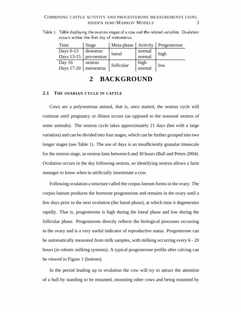
HIDDEN SEMI-MARKOV MODELS 3Table 1. Table displaying the ovarian stages of a cow and the related variables. Ovulationoccurs within the �rst day of metoestrus.Time Stage Meta-phase Activity ProgesteroneDays 0-13 dioestrus

lutealnormal

highDays 13-15 pro-oestrus normalDay 16 oestrus

follicularhigh

lowDays 17-20 metoestrus normal

2 BACKGROUND

2.1 THE OVARIAN CYCLE IN CATTLE

Cows are a polyoestrous animal, that is, once started, the oestrus cycle will

continue until pregnancy or illness occurs (as opposed to the seasonal oestrus of

some animals). The oestrus cycle takes approximately 21 days (but with a large

variation) and can be divided into four stages, which can be further grouped into two

longer stages (see Table 1). The use of days is an insufficiently granular timescale

for the oestrus stage, as oestrus lasts between 6 and 30 hours(Ball and Peters 2004).

Ovulation occurs in the day following oestrus, so identifying oestrus allows a farm

manager to know when to artificially inseminate a cow.

Following ovulation a structure called the corpus luteum forms in the ovary. The

corpus luteum produces the hormone progesterone and remains in the ovary until a

few days prior to the next ovulation (the luteal phase), at which time it degenerates

rapidly. That is, progesterone is high during the luteal phase and low during the

follicular phase. Progesterone directly reflects the biological processes occurring

in the ovary and is a very useful indicator of reproductive status. Progesterone can

be automatically measured from milk samples, with milking occurring every 6 - 20

hours (in robotic milking systems). A typical progesteroneprofile after calving can

be viewed in Figure 1 (bottom).

In the period leading up to ovulation the cow will try to attract the attention

of a bull by standing to be mounted, mounting other cows and being mounted by

4 O’CONNELL, TØGERSEN, FRIGGENS, LØVENDAHL AND HØJSGAARD

other cows. This is sometimes referred to as standing heat and is traditionally how

a stockman would identify a cow that is about to ovulate, allowing them to proceed

with artificial insemination or bring the cow to a bull. This behaviour leads to an

increase in the number of counts on a pedometer the cow is wearing, and so can be

exploited for automated detection of oestrus. Having a stockman manually detect

oestrus in farms with hundreds of cows is expensive and inaccurate, so automated

systems are of great interest. These spikes in activity (together with the correspond-

ing drops in progesterone) are illustrated in Figure 1.

cow 10000000617 parity 2

Ac

tiv

ity

co

un

t

02

06

01

00

0 20 40 60 80

05

15

25

Days after calving

Pro

ge

ste

ron

e (

ng

/L)

Figure 1. Top: The raw hourly activity counts from a pedometer against timesince calving(grey), the black line is as 24 hour centered moving average .Bottom: The progesteroneconcentrations over the same time and cow. The dashed vertical lines are times when anartificial insemination occurred (an indicator of oestrus). Note that these occur after a dropin progesterone and during a brief spike in activity levels.

COMBINING CATTLE ACTIVITY AND PROGESTERONE MEASUREMENTS USING

HIDDEN SEMI-MARKOV MODELS 5

2.2 DATA

The data was collected at the Danish Cattle Research Centre.Activity data

consisted of counts per hour from ALPROR© pedometers by DeLaval. Progesterone

is measured in nanograms per millilitre (ng/mL) at milking times (Friggens et al.

2008). Progesterone and activity data from 58 cows were analysed. These cows

were selected from a database of 424 cows using filtering rules described below.

Three criteria were applied to individual cows to determinewhether they were

suitable for this analysis. Firstly, a cow had to have becamepregnant for us to

consider it. The only sure case of an oestrus occurring is when a cow has become

pregnant and we used this in our model validation. Seconding, only cows with both

progesterone and activity data available were used in this work, since we wish to

evaluate the benefits of measuring both variables. Thirdly,for reasons described in

Section 3.4, series starting at the time of a calving event were desirable, so cows

without a single measurement of either variable during the first 21 days after calv-

ing were also discarded. After filtering the data, we were left with 58 cows and data

spanning 128,578 hours with 112,775 activity counts and 1,917 progesterone mea-

surements. The median time between progesterone measurements was 49 hours.

We rounded the time of progesterone measurements to the nearest hour and

merged these with activity measurements to create a time series of bivariate data,

suitable to be analysed as a Markov chain (in respect to the timing of observations).

Most hours had only an activity count available, and in thesecases progesterone was

treated as a missing value. Useful auxiliary information was the date of artificial

inseminations and the dates when a cow gave birth. Combiningthese allowed us

to determine when a successful artificial insemination occurred and hence when we

can be certain oestrus occurred.

6 O’CONNELL, TØGERSEN, FRIGGENS, LØVENDAHL AND HØJSGAARD

0 50 100 150 200

0.0

00

.01

0.0

20

.03

0.0

4

Raw activity

De

ns

ity

0 5 10 15 20 25

0.0

00

.02

0.0

40

.06

0.0

8

Progesterone (ng/L)

De

ns

ity

Figure 2. Left: Histogram of the raw activity data across the entire population.Right:Histogram of the raw progesterone data across the entire population.

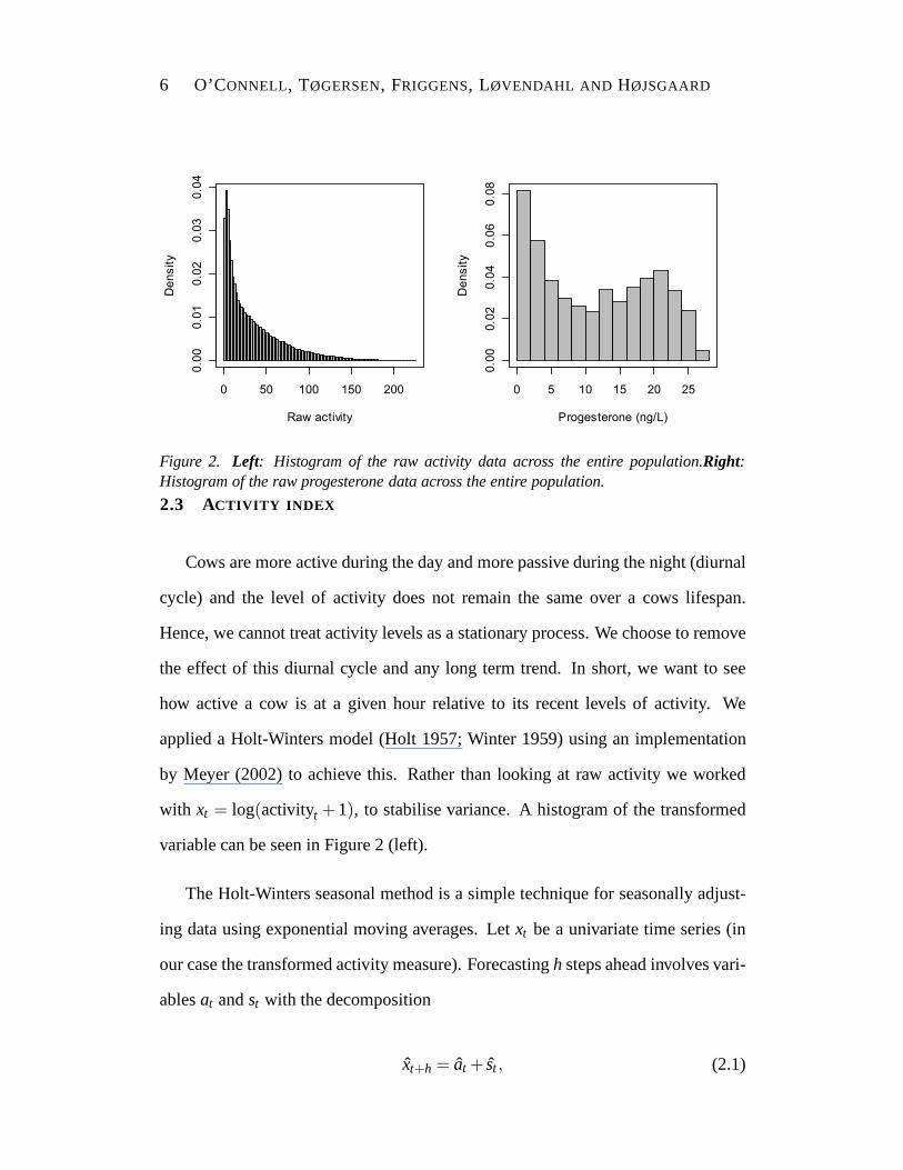
2.3 ACTIVITY INDEX

Cows are more active during the day and more passive during the night (diurnal

cycle) and the level of activity does not remain the same overa cows lifespan.

Hence, we cannot treat activity levels as a stationary process. We choose to remove

the effect of this diurnal cycle and any long term trend. In short, we want to see

how active a cow is at a given hour relative to its recent levels of activity. We

applied a Holt-Winters model (Holt 1957; Winter 1959) usingan implementation

by Meyer (2002) to achieve this. Rather than looking at raw activity we worked

with xt = log(activityt + 1), to stabilise variance. A histogram of the transformed

variable can be seen in Figure 2 (left).

The Holt-Winters seasonal method is a simple technique for seasonally adjust-

ing data using exponential moving averages. Letxt be a univariate time series (in

our case the transformed activity measure). Forecastingh steps ahead involves vari-

ablesat andst with the decomposition

xt+h = at + st , (2.1)

COMBINING CATTLE ACTIVITY AND PROGESTERONE MEASUREMENTS USING

HIDDEN SEMI-MARKOV MODELS 7

and the updating formulae

at = α(xt − st−p)+(1−α)at−1 andst = β (xt − at)+(1−β )st−p. (2.2)

Here we have a local component,at , and a seasonal component,st , with period,p,

set to 24 to remove the diurnal trend. The parametersα andβ are estimated by

minimising the sum of squared errors of one step ahead predictions.

If we assume that our Holt-Winters model captures typical cow behaviour, then

the residuals of the one-step-ahead predictions should be large when the cow de-

viates from normal behaviour. That is, when a cow becomes atypically active (a

possible standing heat event) we should observe a large positive residual. Hence-

forth, we call the one-step-ahead residuals the activity index. A histogram of the

activity index can be viewed in Figure 3, (center). We used the activity index as it

does not introduce any lag and does not unnecessarily smooththe data (smoothing

is already implicit in the hidden semi-Markov models). Visual inspection of the

activity index along with the timing of artificial inseminations and drops in proges-

terone suggests they were correlated, confirming that this index was a reasonable

variable to use (Figure 3, right).

Alternative methods for oestrus detection solely using pedometer readings are

in active development, see Jonsson et al. (2008) and references therein. Roelofs,

van Eerdenburg, Soede, and Kemp (2005) provide a method using simple statistical

tests. Firk et al. (2002) review a number of methods. The aim of this research was to

investigate the relation between progesterone and activity, rather than developing an

absolute best technique for oestrus detection with activity readings. Furthermore,

different activity measures (or indeed any variable) can beeasily “plugged in" to

hidden Markov or semi-Markov models at a later date.

8 O’CONNELL, TØGERSEN, FRIGGENS, LØVENDAHL AND HØJSGAARD

0 1 2 3 4 5

0.0

0.1

0.2

0.3

log(activity_count+1)

Density

-5 0 5

0.0

00.0

50.1

00.1

5

Activity index

Density

41 42 43 44 45 46 47

-6-4

-20

24

6

Days from calving

Activity index

0 1 2 3 4 5

0.0

0.1

0.2

0.3

0.4

log(activity_count+1)

Density

-6 -4 -2 0 2 4 6

0.0

00.0

50.1

00.1

50.2

0

Activity index

Density

80 81 82 83 84 85 86

-6-4

-20

24

6

Days from calvingA

ctivity index

Figure 3. Left column: Histogram oflog(activity+ 1) for two individual cows.Centre:One-step-ahead forecast residuals from a Holt-Winters model for the same cows (the activityindex). Right: The activity index in grey with a 24 hour rolling mean overlayed in black,the dashed vertical line is when artificial insemination occurred.

3 METHODOLOGY

We give a brief summary of Markov chains, Hidden Markov and semi-Markov

models, or HMMs and HSMMs respectively. For a complete introduction we refer

the reader to Rabiner (1989). Implementation of all models was done using a com-

bination of R (R Development Core Team 2008) and the C programming language.

We have released this implementation as an R package called mhsmm (O’Connell

and Højsgaard 2009b) and a paper has been submitted on its use(O’Connell and

Højsgaard 2009a). We only consider the discrete time case here, as activity mea-

sures are hourly counts and the times of progesterone measurements were rounded

to the nearest hour.

COMBINING CATTLE ACTIVITY AND PROGESTERONE MEASUREMENTS USING

HIDDEN SEMI-MARKOV MODELS 9

3.1 DISCRETE MARKOV CHAINS

A discrete Markov chain is a random process (in discrete time) taking discrete

values (states) from the state spaceS, that is,St ∈ S= {1, . . . ,J} for t = 1,2, . . . ,T.

The processSt is a Markov chain if it has the Markov property,

P(St+1 = st+1|S0 = s0,S1 = s1, . . . ,St = st) = P(St+1 = st+1|St = st) (3.1)

for anys0,s1, . . . ,st+1 ∈ S. That is, the state at any given timet +1 depends only on

the previous states through the state at timet. Let pi j = P(St+1 = j|St = i) with the

properties∑Jj=1 pi j = 1 andpi j ≥ 0 so thatP = (pi j ) is the transition matrix of the

Markov chain. To fully specify the model we require the distribution of the initial

stateπi = P(S0 = i). For later use we notice that under this model, the probability

of spendingu consecutive time steps in statei is

di(u) = P(St+u+1 6= i,St+u = i,St+u−1 = i, . . . ,St+2 = i|St+1 = i,St 6= i)(3.2)

= pu−1ii (1− pii). (3.3)

We call this the duration density and this is inherently geometrically distributed for

any Markov chain. This may be an unreasonable assumption formany real world

processes; see Section 3.3 for a discussion.

3.2 HIDDEN MARKOV MODELS

Suppose we can only observe a variableXt related to the stateSt but not the

state itself. This situation is visualised in Figure 4. The conditional distribution

of the observed variableXt conditioned on the unobserved (or hidden) stateSt is

referred to as the emission distribution. We refer to the parameters defining such a

process as a hidden Markov model, henceforth referred to as an HMM. These mod-

10 O’CONNELL, TØGERSEN, FRIGGENS, LØVENDAHL AND HØJSGAARD

els have been used for a variety of different applications, such as speech recognition

(Rabiner 1989), weather modeling (Hughes, Guttorp, and Charles 1999) and DNA

sequence analysis (Krogh, Mian, and Haussler 1994).

Figure 4. Visual representation of a hidden Markov process.Xt are some observed variablesand St is the unobserved, hidden state.

In addition to the usual Markov chain parameters,π andP, a HMM also requires

an emission distribution to be defined

bi(xt) = P(Xt = xt |St = i) (3.4)

for examplebi(x) may be a multivariate Gaussian distribution. We assume thatthe

emitted variables are conditionally independent given theunderlying state, that is,

P(Xt = xt ,Xt−1 = xt−1|St = i) = P(Xt = xt |St = i). (3.5)

A full HMM is hence specified byθ = (π ,P,b).

The Baum-Welch algorithm is the original procedure for estimating the param-

COMBINING CATTLE ACTIVITY AND PROGESTERONE MEASUREMENTS USING

HIDDEN SEMI-MARKOV MODELS 11

eters of a HMM (Baum, Petrie, Soules, and Weiss 1970). This technique was later

grouped with a more general class of algorithms for incomplete data, named the

Expectation-Maximisation (EM) algorithm (Dempster, Laird, and Rubin 1977). Ra-

biner (1989) provides a very clear overview.

3.3 HIDDEN SEMI-MARKOV MODELS

A severe limitation of standard HMMs is the implicit geometrically distributed

duration time of states in the model (Equation 3.3) as many ofthe real world prob-

lems we wish to model do not have geometric sojourn times. Forexample, the

reproductive states of cows are not a memoryless process since a follicular stage

is likely to occur after 18 days in a luteal stage. A potentialsolution to this issue

is to explicitly estimated(u), producing what is referred as a hidden semi-Markov

model, henceforth called an HSMM. Ferguson (1980) was the first to propose such

models along with an algorithm to fit them, Rabiner (1989) provides a good sum-

mary. Guédon (2003) developed a more efficient algorithm anda method to deal

with right censoring which we have implemented.

In a standard discrete Markov chain the state duration density has the form,

di(u) = puii (1− pii ) whereas in a semi-Markov model, we modeldi(u) explicitly.

That is, in addition to the parameters already defined for theHMM, we now have

explicit probabilities for our state duration density,θ = (π,P,b,d). Guédon (2003)

utilises a non-parametric probability mass function ofd(u) in his derivations, but

then proposes an ad-hoc method to introduce parametric distributions (for example

Poisson). The procedure has been followed here.

12 O’CONNELL, TØGERSEN, FRIGGENS, LØVENDAHL AND HØJSGAARD

3.3.1 Parameter estimation

The complete data likelihood of a HSMM is

P(X = x,S= s;θ) = πs∗1ds∗1

(u1)

{

R

∏r=2

ps∗r−1s∗r ds∗r (ur)

}

ps∗R−1s∗RDs∗R

(uR)T

∏t=1

bst (xt)

(3.6)

wheres∗r is the rth visited state andur is the time spent in that state. Guédon

proposed using the survivor function

Di(u) = ∑v≥u

di(v) (3.7)

for the sojourn time in the last state so we do not have to assume the process is

leaving a state immediately after timeT. This is particularly important for online

applications where we wish to estimate the most recent stateso we can monitor

some process.

As we have not observed the state sequence, maximising this likelihood con-

stitutes an incomplete data problem. A local maximum can be found using the

Expectation-Maximisation, or EM, algorithm. We briefly outline the procedure be-

low.

The EM algorithm involves iterating over two steps until convergence. In the

E-step, we calculate the expected complete data likelihoodgiven the value of the

parameters at iterationk and the observed data,

Q(θ |θ (k)) = E[log(P(X = x,S= s;θ))|X = x;θ (k)]. (3.8)

This term is typically broken down into a sum of terms involving subsets of the

parameters. The M-step then involves choosingθ (k+1) as the values that maximise

Q(θ |θ (k)). These steps are repeated until convergence. We now providethe specific

COMBINING CATTLE ACTIVITY AND PROGESTERONE MEASUREMENTS USING

HIDDEN SEMI-MARKOV MODELS 13

terms calculated for a HSMM;

The E-step:

For HSMMs, the E-step involves estimating three separate terms; the probability

of being in statei at timet,

γt(i) = P(St = i|X = x;θ), (3.9)

the probability that the process left statei at timet and entered statej at t +1

ξt(i, j) = P(St = i,St+1 = j|X = x;θ), (3.10)

and finally the expected number of times a process spentu time steps in statei

ηi,u = P(Su 6= i,Su−v = i,v = 1, . . . ,u|X = x;θ) (3.11)

+T

∑t=1

P(St+u+1 6= i,St+u−v = i,v = 0, . . . ,u−1,St 6= i|X = x;θ).

These values can be calculated via a dynamic programming method known as the

forward-backward algorithm. It should be noted that the derivations and algorithms

involved are complex; we refer the reader to Guédon (2003) for details.

The M-step:

The starting and transition probabilities are implicit from the definition of the

Markov chain,

π ′i = γ1(i) p′i j =

∑T−1t=1 ξt(i, j)

∑T−1t=1 ∑i 6= j ξt(i, j)

. (3.12)

Guédon provides derivations fordi(u) as a non-parametric probability mass func-

14 O’CONNELL, TØGERSEN, FRIGGENS, LØVENDAHL AND HØJSGAARD

tion, but then proposes an ad-hoc solution for using parametric distributions with

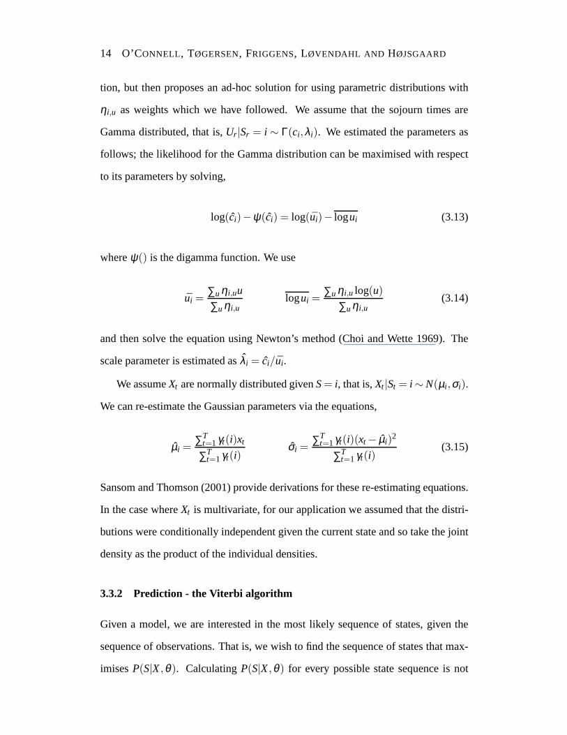
ηi,u as weights which we have followed. We assume that the sojourntimes are

Gamma distributed, that is,Ur |Sr = i ∼ Γ(ci ,λi). We estimated the parameters as

follows; the likelihood for the Gamma distribution can be maximised with respect

to its parameters by solving,

log(ci)−ψ(ci) = log(ui)− logui (3.13)

whereψ() is the digamma function. We use

ui =∑u ηi,uu

∑u ηi,ulogui =

∑u ηi,u log(u)

∑uηi,u(3.14)

and then solve the equation using Newton’s method (Choi and Wette 1969). The

scale parameter is estimated asλi = ci/ui.

We assumeXt are normally distributed givenS= i, that is,Xt |St = i ∼ N(µi ,σi).

We can re-estimate the Gaussian parameters via the equations,

µi =∑T

t=1 γt(i)xt

∑Tt=1 γt(i)

σi =∑T

t=1γt(i)(xt − µi)2

∑Tt=1 γt(i)

(3.15)

Sansom and Thomson (2001) provide derivations for these re-estimating equations.

In the case whereXt is multivariate, for our application we assumed that the distri-

butions were conditionally independent given the current state and so take the joint

density as the product of the individual densities.

3.3.2 Prediction - the Viterbi algorithm

Given a model, we are interested in the most likely sequence of states, given the

sequence of observations. That is, we wish to find the sequence of states that max-

imisesP(S|X,θ). CalculatingP(S|X,θ) for every possible state sequence is not

COMBINING CATTLE ACTIVITY AND PROGESTERONE MEASUREMENTS USING

HIDDEN SEMI-MARKOV MODELS 15

computationally feasible. A dynamic programming technique known as the Viterbi

algorithm (Forney Jr 1973), can be used to maximiseP(S|X,θ) in a computationally

feasible manner. It should be noted that this is distinct from taking argmaxi γt(i) as

the state at timet, which is the individually most likely state. We start by defining

the variable

δt( j) = maxs1,...,st−1

P(St+1 6= j,St = j,S1 = s1, . . . ,St−1 = st−1,X1 = x1, . . . ,Xt−1 = xt−1;θ)

(3.16)

with the special case at the last time step

δT( j) = maxs1,...,sT−1

P(ST = j,S1 = s1, . . . ,ST−1 = sT−1,X1 = x1, . . . ,XT = xT ;θ),

(3.17)

where we are only concerned with the probability of being in state j at timeT,

not with leaving the state atT +1. The variableδ can be calculated via induction

with the initialisation step

δ1( j) = b j(x1)d j(1)π j (3.18)

the recursion step

δt( j) = b j(xt)max

{

max1≤u≤t

[

(

∏u−1v=1 b j(xt−v)

)

d j(u)maxi 6= j(

pi j δt−u(i))

]

;

(

∏tv=1b j(xt−v)

)

d j(t +1)πi

}

. (3.19)

16 O’CONNELL, TØGERSEN, FRIGGENS, LØVENDAHL AND HØJSGAARD

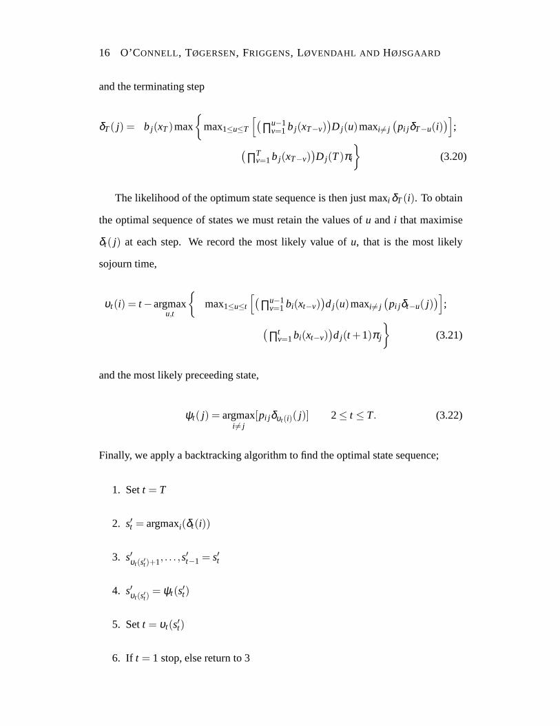
and the terminating step

δT( j) = b j(xT)max

{

max1≤u≤T

[

(

∏u−1v=1 b j(xT−v)

)

D j(u)maxi 6= j(

pi j δT−u(i))

]

;

(

∏Tv=1b j(xT−v)

)

D j(T)πi

}

(3.20)

The likelihood of the optimum state sequence is then just maxi δT(i). To obtain

the optimal sequence of states we must retain the values ofu and i that maximise

δt( j) at each step. We record the most likely value ofu, that is the most likely

sojourn time,

υt(i) = t−argmaxu,t

{

max1≤u≤t

[

(

∏u−1v=1 bi(xt−v)

)

d j(u)maxi 6= j(

pi j δt−u( j))

]

;

(

∏tv=1bi(xt−v)

)

d j(t +1)π j

}

(3.21)

and the most likely preceeding state,

ψt( j) = argmaxi 6= j

[pi j δυt(i)( j)] 2≤ t ≤ T. (3.22)

Finally, we apply a backtracking algorithm to find the optimal state sequence;

1. Sett = T

2. s′t = argmaxi(δt(i))

3. s′υt(s′t)+1, . . . ,s′t−1 = s′t

4. s′υt(s′t)= ψt(s′t)

5. Sett = υt(s′t)

6. If t = 1 stop, else return to 3

COMBINING CATTLE ACTIVITY AND PROGESTERONE MEASUREMENTS USING

HIDDEN SEMI-MARKOV MODELS 17

3.3.3 Missing data

Missing data occurs in both of the observed variables for ourapplication. Pedometer

readings for a given hour may fail to be recorded due to hardware problems or a cow

being away from the stable. There are many missing progesterone measurements

due to the fact it is measured at a much sparser resolution than activity (less than

2% of activity recordings have a matching progesterone measurement). As such,

we require a method for handling missing observations, which is straight forward

for HSMMs. If an observationxt is missing we setb j(xt) = 1 for all j, that is, there

is no contribution to the likelihood at that time step.

3.4 APPLICATION TO CATTLE DATA

Three models were investigated; two univariate models using each variable and

one model using both variables. The states identifiable by each combination of

variables differ. For each univariate model we used three states, but with different

definitions. The activity only model contained states;

SActivity = {post-partum anoestrus, standing heat, not standing heat}

(Figure 5, top). For progesterone measurements we had

SProgesterone= {post-partum anoestrus, luteal, follicular}

(Figure 5, bottom). Standing heat occurs near the beginningof the follicular state

but the follicular state is much longer. The bivariate modelused six states, the

combination of activity and progesterone allowing us to break the follicular stage

up into three different sub-stages in addition to the PPA andluteal states (Figure 6).

We definet = 1 as the hour immediately following a calving. This is a useful

18 O’CONNELL, TØGERSEN, FRIGGENS, LØVENDAHL AND HØJSGAARD

way to arrange the data as we know that the cow will be in post-partum anoestrus at

this time. Gaussian emission distributions were used for each variable. We worked

with log(progesterone+ 1) rather than raw progesterone to stabilise the variance.

Gamma distributions were used for the distribution of sojourn times for each state.

Starting values for distribution parameters were found viamanual inspection of the

data and biological knowledge of the ovarian cycle as detailed in Section 2.1.

PPA Luteal Follicular

PPA Not standing

heatStanding heat

Figure 5.Top: The underlying states for a univariate activity model.Bottom: The underly-ing states for a univariate progesterone model.

PPA Luteal

Follicular 1

Follicular 2(standing heat)

Follicular 2(silent heat)

Follicular 3

Figure 6. The hidden states used for the bivariate HSMM. The use of both variables allowus to break the follicular stage up into three different sub-stages.

4 RESULTS

Validation for this data is difficult as the true timing of ovulation is never known.

One proxy is when a successful artificial insemination occurs, that is, an insemina-

tion that results in a cow giving birth approximately 280 days later. We take two

COMBINING CATTLE ACTIVITY AND PROGESTERONE MEASUREMENTS USING

HIDDEN SEMI-MARKOV MODELS 19Table 2. Success and error rates for prediction of a follicular stage by an univariate activityHSMM.TP=True positive FP=False positive FN=False negativeSensitivity TP

TP+FN Error rate FPTP+FP

Count 97/137 16/113Proportion 0.71 0.14

approaches here, first investigating the ability of the activity-only model to predict

the states of a progesterone-only model. Secondly, we validate the bivariate model

using successful insemination times as proxies for ovulation.

4.1 PREDICTION OF FOLLICULAR STATE BY ACTIVITY-ONLY MODEL

We estimated parameters for two separate univariate modelsfor each variable

using the methods described in Section 3. The Viterbi algorithm was applied to find

the optimal state sequences. We then looked at how well the state sequence from

the activity model aligned with that from the progesterone model, treating the state

sequence from progesterone as validation data. According to biological knowledge,

standing heat should occur near the beginning of the follicular stage (Ball and Peters

2004). We considered a predictedstanding heatfrom the activity model that was

bounded (in time) by a predictedfollicular state from the progesterone model to be

a correct prediction. We do not claim that the state sequencefrom progesterone is

truth, but a closer reconstruction of the biological statesof the cow.

Two possible prediction errors can occur in this framework;false positive (pre-

diction of standing heat outside a follicular state) and false negative (failure to pre-

dict standing heat within a follicular stage). An example ofsome correctly predicted

follicular stages is shown in Figure 7. The results are summarised in Table 2.

20 O’CONNELL, TØGERSEN, FRIGGENS, LØVENDAHL AND HØJSGAARD

cow 10000000257 parity 3

Ac

tiv

ity

in

de

x

-3-1

01

23 PPA

Not-oestrusOestrus

0 10 20 30 40 50 60

05

15

25

Days after calving

Pro

ge

ste

ron

e (

ng

/L) PPA

lutealfollicular

Figure 7. Top: The activity index against time since calving.Bottom: The progesteroneconcentrations over the same time and cow. Predicted statesby the respective univariatemodels are shown on the horizontal shaded bars. This is an example where an activity-onlymodel has correctly found oestrus events occur within a follicular stage.

4.2 OESTRUS DETECTION

We compared the bivariate model and the activity-only univariate model as on-

line systems by using information about successful artificial inseminations and ap-

plying cross validation. Cross validation was used as follows; We iterated through a

set of 58 cows with successful pregnancies, excluding one cow’s full data sequence

and estimating the HSMM parameters using the remaining data. We then applied

the Viterbi algorithm to the left-out cow’s sequence up until the time of successful

insemination. Finally, we compared the time of the most recent predicted (if any)

oestrus event by the models to the artificial insemination event. Artificial insemina-

tion is thought to be best applied within twenty four hours following oestrus so we

expect a positive difference between AI and the last detected oestrus hour.

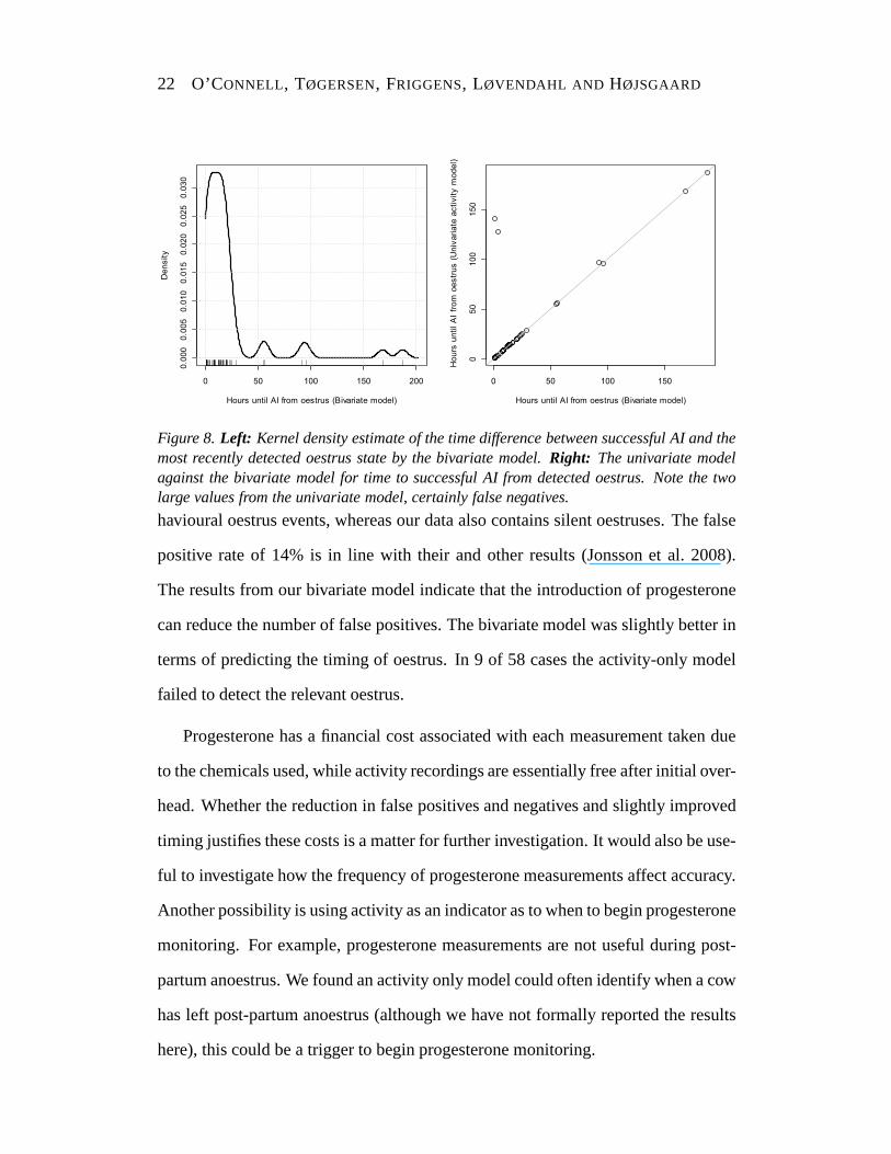
A kernel density estimate of the bivariate models time differences can be viewed

COMBINING CATTLE ACTIVITY AND PROGESTERONE MEASUREMENTS USING

HIDDEN SEMI-MARKOV MODELS 21Table 3. Table comparing times to successful arti�cial insemination from oestrus as de-tected by the bivariate and univariate activity models. Times less than one daycan be considered a successful detection with certainty, times between one andtwo days are also likely successful detections.Days 1.00 2.00 3.00 4.00 5.00 6.00 7.00 8.00

Time to AI < Days (bivariate) 0.84 0.89 0.93 0.95 0.96 0.96 0.96 1.00(activity only) 0.68 0.73 0.77 0.77 0.80 0.84 0.84 0.88

in Figure 8 (left) and a comparison of the two models in Figure8 (right). The

results for each model are summarised in Table 3 where we can see that the bivariate

model had slightly lower times indicating better performance. The activity-only

model failed to detect any oestrus in 7 of the 58 cases as well as the two obvious

false negatives that can be seen on the graph, a false negative rate of at least 0.16.

The bivariate model essentially uses the activity measure to narrow the window of

oestrus with the follicular stage, so it is not surprising the models are comparable in

terms of oestrus timing (when the activity model actually finds the oestrus).

We have limited our analysis to insemination events that ledto a pregnancy. The

majority of inseminations do not lead to a pregnancy and we have excluded these

failed inseminations from the analysis. Inseminations mayfail due to incorrect

timing, technical problems with the process or cow infertility. We can only be

certain an oestrus has occurred if a cow becomes pregnant andhence have used

these events to validate our model.

5 DISCUSSION

We have investigated and compared univariate and bivariateHSMMs for two

different variables related to cattle reproduction. Approximately 70% of follicular

states were predicted by the activity-only model. This is less accurate than results

reported by Roelofs et al. (2005). However those detectionsrates were for be-

22 O’CONNELL, TØGERSEN, FRIGGENS, LØVENDAHL AND HØJSGAARD

0 50 100 150 200

0.0

00

0.0

05

0.0

10

0.0

15

0.0

20

0.0

25

0.0

30

Hours until AI from oestrus (Bivariate model)

De

ns

ity

0 50 100 150

05

01

00

15

0

Hours until AI from oestrus (Bivariate model)

Ho

urs

un

til

AI

fro

m o

es

tru

s (

Un

iva

ria

te a

cti

vit

y m

od

el)

Figure 8.Left: Kernel density estimate of the time difference between successful AI and themost recently detected oestrus state by the bivariate model. Right: The univariate modelagainst the bivariate model for time to successful AI from detected oestrus. Note the twolarge values from the univariate model, certainly false negatives.

havioural oestrus events, whereas our data also contains silent oestruses. The false

positive rate of 14% is in line with their and other results (Jonsson et al. 2008).

The results from our bivariate model indicate that the introduction of progesterone

can reduce the number of false positives. The bivariate model was slightly better in

terms of predicting the timing of oestrus. In 9 of 58 cases theactivity-only model

failed to detect the relevant oestrus.

Progesterone has a financial cost associated with each measurement taken due

to the chemicals used, while activity recordings are essentially free after initial over-

head. Whether the reduction in false positives and negatives and slightly improved

timing justifies these costs is a matter for further investigation. It would also be use-

ful to investigate how the frequency of progesterone measurements affect accuracy.

Another possibility is using activity as an indicator as to when to begin progesterone

monitoring. For example, progesterone measurements are not useful during post-

partum anoestrus. We found an activity only model could often identify when a cow

has left post-partum anoestrus (although we have not formally reported the results

here), this could be a trigger to begin progesterone monitoring.

COMBINING CATTLE ACTIVITY AND PROGESTERONE MEASUREMENTS USING

HIDDEN SEMI-MARKOV MODELS 23

6 ACKNOWLEDGMENTS

This work was supported by the BIOSENS project funded by the Danish Min-

istry of Food, Agriculture and Fisheries and the Danish Cattle Industry via Finance

Committee Cattle, and by The Danish Council for Strategic Research through the

AUREGAB project.

REFERENCES

Ball, P. J. H. and Peters, A. R. (2004),Reproduction in Cattle, 3rd ed., Blackwell

Publishing.

Baum, L., Petrie, T., Soules, G., and Weiss, N. (1970), “A Maximization Tech-

nique Occurring in the Statistical Analysis of Probabilistic Functions of Markov

Chains,”The Annals of Mathematical Statistics, 41, 164–171.

Choi, S. and Wette, R. (1969), “Maximum likelihood estimation of the parameters

of the gamma distribution and their bias,”Technometrics, 11, 683–690.

Dempster, A., Laird, N., and Rubin, D. (1977), “Maximum Likelihood from Incom-

plete Data via the EM Algorithm,”Journal of the Royal Statistical Society. Series

B (Methodological), 39, 1–38.

Ferguson, J. (1980), “Hidden Markov Analysis: An Introduction,” Hidden Markov

Models for Speech.

Firk, R., Stamer, E., Junge, W., and Krieter, J. (2002), “Automation of oestrus

detection in dairy cows: a review,”Livestock Production Science, 75, 219–232.

Forney Jr, G. (1973), “The Viterbi algorithm,”Proceedings of the IEEE, 61, 268–

278.

Friggens, N., Bjerring, M., Ridder, C., Højsgaard, S., and Larsen, T. (2008), “Im-

proved Detection of Reproductive Status in Dairy Cows UsingMilk Progesterone

24 O’CONNELL, TØGERSEN, FRIGGENS, LØVENDAHL AND HØJSGAARD

Measurements,”Reproduction in Domestic Animals, 43, 113–121.

Friggens, N. and Løvendahl, P. (2007), “The Potential of On-Farm Fertility Profiles:

In-Line Progesterone and Activity Measurements,” .

Guédon, Y. (2003), “Estimating Hidden Semi-Markov Chains From Discrete Se-

quences,”Journal of Computational & Graphical Statistics, 12, 604–639.

Holt, C. (1957), “Forecasting Trends and Seasonals by Exponentially Weighted

Moving Averages,”ONR Memorandum, 52.

Hughes, J., Guttorp, P., and Charles, S. (1999), “A non-homogeneous hidden

Markov model for precipitation occurrence,”Journal of the Royal Statistical So-

ciety (Series C): Applied Statistics, 48, 15–30.

Jonsson, R., Bjorgvinsson, T., Blanke, M., Poulsen, N., Højsgaard, S., Munksgaard,

L., Denmark, D., and Aarhus, D. (2008), “Oestrus Detection in Dairy Cows Us-

ing Likelihood Ratio Tests,”The International Federation of Automatic Control,

658–663.

Krogh, A., Mian, I., and Haussler, D. (1994), “A hidden Markov model that finds

genes in E. coli DNA,”Nucleic Acids Research, 22, 4768–4778.

Meyer, D. (2002), “Naive time series forecasting methods,”R News, 2, 7–10.

O’Connell, J. and Højsgaard, S. (2009a), “Hidden Semi Markov Models for Mul-

tiple Observation Sequences – The mhsmm Package for R,”Submitted to the

Journal of Statistical Software.

— (2009b), “mhsmm: Parameter estimation and prediction forhidden Markov

and semi-Markov models for data with multiple observation sequences,” URLhttp://cran.r-project.org/web/packages/mhsmm/index.html. R pack-

age version 0.3.0.

R Development Core Team (2008),R: A Language and Environment for Statistical

Computing, R Foundation for Statistical Computing, Vienna, Austria.ISBN 3-

COMBINING CATTLE ACTIVITY AND PROGESTERONE MEASUREMENTS USING

HIDDEN SEMI-MARKOV MODELS 25

900051-07-0.

Rabiner, L. (1989), “A tutorial on hidden Markov models and selected applications

in speech recognition,”Proceedings of the IEEE, 77, 257–286.

Roelofs, J., van Eerdenburg, F., Soede, N., and Kemp, B. (2005), “Various behav-

ioral signs of estrous and their relationship with time of ovulation in dairy cattle,”

Theriogenology, 63, 1366–1377.

Sansom, J. and Thomson, P. (2001), “Fitting hidden semi–Markov models to break-

point rainfall data,”Journal of Applied Probability, 38, 142–157.

Winter, P. (1959), “Forecasting Sales by Exponentially Weighted Moving Aver-

ages,” .