Using interesting sequences to interactively build Hidden Markov Models

Data Min Knowl Disc (2010) 21:186–220DOI 10.1007/s10618-010-0171-0

Using interesting sequences to interactively buildHidden Markov Models

Szymon Jaroszewicz

Received: 20 March 2009 / Accepted: 6 March 2010 / Published online: 7 April 2010The Author(s) 2010

Abstract The paper presents a method of interactive construction of global HiddenMarkov Models (HMMs) based on local sequence patterns discovered in data. Themethod is based on finding interesting sequences whose frequency in the database dif-fers from that predicted by the model. The patterns are then presented to the user whoupdates the model using their intelligence and their understanding of the modelleddomain. It is demonstrated that such an approach leads to more understandable mod-els than automated approaches. Two variants of the problem are considered: miningpatterns occurring only at the beginning of sequences and mining patterns occur-ring at any position; both practically meaningful. For each variant, algorithms havebeen developed allowing for efficient discovery of all sequences with given minimuminterestingness. Applications to modelling webpage visitors behavior and to modellingprotein secondary structure are presented, validating the proposed approach.

Keywords Interesting pattern · Frequent sequence mining · Hidden Markov Model

1 Introduction

Sequence databases are at the heart of several important applications such as WebMining, bioinformatics or speech analysis and recognition. Mining frequent sequencesis an important approach to analysis of such data. Unfortunately, as is the case with mostfrequent pattern based approaches, sequence mining typically produces thousands offrequent sequences which are very difficult for the user to analyze, due not only to

Responsible editor: Johannes Fürnkranz and Arno Knobbe.

S. Jaroszewicz (B)National Institute of Telecommunications, Warsaw, Polande-mail: [email protected]; [email protected]

123

Using interesting sequences to interactively build Hidden Markov Models 187

their quantity but also to redundancies between them. This paper addresses the prob-lem by incorporating an explicit global model of background knowledge into thesequence mining problem. The model helps identify truly interesting patterns, takinginto account what is already known about the data.

The user provides a (possibly empty) description of their current knowledge aboutthe domain and a database from which new knowledge is to be discovered. Knowledgedescription has the form of a global probabilistic model from which precise probabi-listic inferences can be made. In Jaroszewicz and Simovici (2004), Jaroszewicz andScheffer (2005), and Jaroszewicz et al. (2009) a Bayesian network was used for thispurpose due to its flexibility, understandability, as well as the fact that it represents afull joint probability distribution making inference possible. In the case of sequencedata, similar advantages are shared by Hidden Markov Models (HMMs) (Rabiner1989; Welch 2003), and for that reason they have been used to model backgroundknowledge in the presented approach.

Based on the model and the data, interesting patterns are discovered. A patternis defined to be interesting if its frequency in the data differs significantly from thatpredicted by the global model. The patterns are then presented to the user whosetask is to interpret them and update the model. The new, updated model is then usedagain together with the data to find a new set of interesting patterns. The procedure isrepeated several times until the desired quality of the global model has been reached.

The approach to mining interesting sequences presented in this paper follows thesame cycle. First, sequences are discovered whose frequency in a database differssignificantly from the predictions of the HMM. Such sequences are considered inter-esting and are shown to the user who updates the HMM by adding more hidden statesrepresenting new underlying behavior, by modifying lists of possible output symbolsin existing states or by adding new transitions between states. The HMM parame-ters are then retrained using the Baum-Welch algorithm (a variant of the ExpectationMaximization approach) and the process is repeated.

In Jaroszewicz et al. (2009) it has been demonstrated that interactive modelconstruction, using human intelligence in the process, gives models which representthe domain much better than models built using fully automated methods. Similarconclusions have been reached in this paper.

The advantage of this approach is that the new states added to the HMMs haveclear, user defined meaning. The lists of symbols emitted in each state are also muchshorter and more coherent. The resulting model is thus understandable, and all hiddenstates have clear interpretations. As our experiments have shown, this is usually notpossible with automatic methods. An additional benefit is that the Baum-Welch algo-rithm turned out to work much better with hand-built models resulting in much fasterconvergence and better avoidance of local optima.

A drawback of the proposed method is that it requires intensive human involvement,and sometimes a significant effort is needed to explain the discovered interesting pat-terns. However, it is argued that such an approach is usually necessary if meaningfulinternal structure is to be obtained.

The approach has been tested on the web server log of the National Institute ofTelecommunications in Warsaw (author’s employer). The application proved thatthe proposed approach is highly practical and produces accurate models which are

123

188 S. Jaroszewicz

understandable and easy to interpret. Another application which is presented in thispaper is about modelling protein secondary structure using publicly available data.

2 Related research

There has been a significant amount of work on mining frequent patterns in sequencedata, full discussion is beyond the scope of this work, see for example thorough over-views in Laxman and Sastry (2006) and in Han et al. (2007).

An idea of incorporating background knowledge (defined as a formal model givingwell defined predictions) into the pattern discovery process has already been suggestedin Hand (2002). The paper presented a high level framework of which the currentapproach [and that in Jaroszewicz and Simovici (2004); Jaroszewicz and Scheffer(2005); Jaroszewicz et al. (2009)] can be considered a specific case. The paper (Hand2002) is very general and does not give specific details on how the background knowl-edge should be represented or what discovery methods should be used.

Section 5 of Laxman and Sastry (2006) describes approaches to testing significanceof sequence patterns based on comparing with a background model. The purpose how-ever is to test statistical significance, and the models are thus simple (based on inde-pendence assumption) and fixed throughout the discovery process; user’s backgroundknowledge and intervention do not come into the picture as they do in our approach.In Laxman and Sastry (2005) a separate, small HMM with special structure is builtfor each temporal pattern (episode). Such small HMMs are later used for significancetesting. The use of a global model being a mixture of small episode models is alludedto, but not developed further. In Prum et al. (1995) a similar approach has been usedto derive expected probabilities of DNA sequences.

Zaiane and his collegues (Zaiane et al. 2007; Satsangi and Zaiane 2007) haveworked on discovering so called contrast sequences. This is similar to a single stageof the interactive model building process described here, except that two datasets arecompared, while in our approach one of the datasets is replaced by an HMM. Asa result, Zaiane et al.’s overall methodology and the discovery algorithms are verydifferent from methods proposed in this paper.

There has been some related work in the fields of biological sequence modellingand speech recognition (Low-Kam et al. 2009), where a set of unexpected patterns isfound whose probability, as predicted by an HMM, is low. The idea however is more inline with Laxman and Sastry (2006) than with the approach proposed here. No explicitmodel building is considered, and in fact, the exact structure of the model used is notdescribed, presumably it is just a simple Markov model over the symbols. The modeldoes not change during the discovery process. Furthermore, contrary to our approach,stationarity assumption is made which is not suitable for shorter sequences.

In Spiliopoulou (1999) and Li et al. (2007) background knowledge is also incor-porated into the sequence mining process. However it is stored as a set of rules andthere is no global probabilistic model. Unexpectedness is defined in a syntactic ratherthan probabilistic fashion. See Jaroszewicz and Simovici (2004) and Jaroszewicz et al.(2009) for a discussion of drawbacks of rule based representations and advantages ofhaving a unified model.

123


A somewhat related technique is adaptive HMM learning (Huo et al. 1995; Leeand Gauvin 1996; Huo and Lee 1997). The approach is essentially based on placinga prior on the HMM parameters. The prior is usually obtained using the EmpiricalBayes procedure (Huo et al. 1995; Robbins 1956). This allows, for example, for tun-ing a speech recognition system to a new speaker using a prior based on parametersobtained for several other speakers. While there are similarities to our approach, e.g.the prior plays the role of background knowledge, the method is fundamentally dif-ferent. There is no notion of an interesting pattern, model parameters are updatedbased on new data only. The update is meant to adapt the model to idiosyncrasies ofnew data while using older data as a prior, not to build a single general model. In ourapproach there is a single dataset which remains static; it is the interesting patternsused to update the model which change from iteration to iteration. Also, contrary toour approach, in adaptive HMM learning the update is done automatically and onlyto model’s parameters, not its structure. Model’s understandability is not an explicitgoal of adaptive HMM learning.

Another related technique is semisupervised learning of HMMs (Inoue and Ueda2003; Ji et al. 2009), where labeled examples may be viewed as user provided guidesmodifying the model built on unlabeled data. The nature of the process is clearlydifferent from the proposed approach.

This work is based on an earlier paper (Jaroszewicz 2008) by the author, but hasbeen significantly expanded. All parts related to mining interesting sequences startingat arbitrary point in time are new. So is the application to modelling protein second-ary structure. Comparison with automatically built models has also been significantlyexpanded.

3 Definitions and notation

Let us begin by describing the mathematical notation used. Vectors are denoted bylowercase boldface Greek letters, and matrices with uppercase boldface roman letters.All vectors are assumed to be row vectors, explicit transposition ′ is used for columnvectors.

Superscripts are used to denote time (or, more precisely, position counting fromthe beginning of a database sequence) and subscripts to denote elements of vectors,e.g. π t

i denotes i th element of the vector π at time t . Since matrices will not changewith time in our applications, superscripts on matrices will denote matrix power, e.g.(P)t is the matrix P raised to the power t ; parentheses around the matrix are added tofurther avoid confusion.

Let us fix a set of symbols O = {o1, . . . , om}. All sequences will be constructedover this set. It will also play the role of the set of output symbols of all HMMs.Sequences of symbols will be denoted with bold lowercase letters s and d, where swill denote temporary sequences being worked on and d sequences in the database.|s| denotes the length of sequence s. Following our convention, st is the symbol of s attime t , or more precisely, the symbol at distance t from the beginning of the sequence,with the first symbol being at index 0. Further, if o ∈ O , then so will denote a sequence

123

190 S. Jaroszewicz

obtained by appending o to s, and os the sequence obtained by prepending o at thebeginning of s. An empty sequence will be denoted with λ.

3.1 Hidden Markov Models

Let us now describe HMMs which will be used to represent knowledge about systemswith discrete time. Only most important facts will be given, full details can be foundin literature (Rabiner 1989; Welch 2003).

A HMM is a modification of a Markov Chain, such that the state the model is inis not directly visible. Instead, every state emits output symbols according to its ownprobability distribution. For example, while modelling website visitors’ behavior, theinternal states could correspond to visitor’s intentions (e.g. ‘wants to find a specificcontent’) and output symbols to the pages he/she actually visits.

Formally, an HMM is a quintuple 〈Q, O,π0, P, E〉 where Q = {q1, . . . , qn} isa set of states, O = {o1, . . . , om} the set of output symbols, π0 = (π0

1, . . . ,π0n) a

vector of initial probabilities for each state, and P an n by n transition matrix, wherePi j is the probability of a transition occurring from state qi to state q j . Finally E is ann by m emission probability matrix such that Ei j gives the probability of observingan output symbol o j provided that the HMM is in state qi . Where convenient, we willuse shorthand notation Eio to denote the probability of emitting symbol o in state qi .

Notice that the vector π t of state probabilities at time t can be computed as π t =π0(P)t . Similarly πE is the vector of probabilities of observing each symbol providedthat π is the vector of state probabilities.

We will now discuss how to determine the probability that a given sequence ofoutput symbols is produced by an HMM. For that aim a key concept of forward prob-abilities will be introduced; full details can be found in Rabiner (1989) and Welch(2003).

Let s be a sequence of symbols, t = |s|. Further, let zt denote the state the HMMis in at time t . The forward probabilities of a sequence s in the HMM are defined as

α(s, i) = Pr{u0 = s0, u1 = s1, . . . , ut−1 = st−1, zt = qi },

where u0, u1, . . . , ut−1 is the sequence of symbols output by the HMM at times0, 1, . . . , t − 1 respectively, and s0, s1, . . . , st−1 are symbols at respective positionsin the sequence s. Simply speaking, this is the probability that the HMM has emittedthe sequence s and ended up in state qi at time t (that is after emitting the last symbolof s). Grouping the forward probabilities for all ending states we obtain a vector

α(s) = (α(s, 1), α(s, 2), . . . , α(s, n)).

The probability that the HMM emits a sequence s (starting at t = 0) can be computedby summing the elements of α(s).

An important property of the α probabilities is that they can be efficiently computedusing dynamic programming by extending the sequence, symbol by symbol, using thefollowing formula:

123


α(λ, i) = π0i ,

α(so, i) =n∑

j=0

α(s, j)E joP j i . (1)

Another important problem related to HMMs is estimating their parameters(starting, transition and emission probabilities) based on a given sequence database.This is usually achieved using the Baum-Welch algorithm which is a variant of theExpectation Maximization method. The details can be found in Rabiner (1989) andWelch (2003) and will be omitted here.

The Baum-Welch algorithm only guarantees convergence to a local minimum, andhas been reported to be slow. In practice we have noticed the algorithm is very depen-dent on the emission probabilities matrix E. If output symbols convey a reasonableamount of information about internal states, the algorithm converges quickly and reli-ably, if on the other hand this information is highly ambiguous, the process is slowand often ends up in a local optimum. This issue is discussed in detail and illustratedby experiments in later sections, where it will be argued that estimating parameters ofinteractively built HMMs is significantly easier than for fully connected ones.

4 Discovery of interesting sequences starting at the beginning of databasesequences

We begin with a more detailed description of how background knowledge is beingrepresented. As mentioned above, user’s knowledge about the problem is encodedusing a HMM. However the model will usually be much sparser than fully connectedmodels used in most HMM applications.

The user needs to provide the hidden states of the model; typically new states areadded incrementally during the discovery process. For every hidden state, the userneeds to specify possible transitions, symbols which can be emitted from that state,and whether the state can be an initial state (i.e. can have a nonzero starting probabil-ity). The user thus provides the structure of the model but not the starting, transitionand emission probabilities which will be estimated from data using the Baum-Welchalgorithm.

The key component of the interactive global HMM construction using the proposedframework is finding interesting sequences of output symbols. There are several waysto formulate the concept of an interesting sequence. This paper will provide two suchformulations. In this section we will present an approach which assumes that minedsequences are prefixes of database sequences (i.e. they start at t = 0) and in the fol-lowing section we will extend the approach to sequences starting at arbitrary locationswithin database sequences. Both approaches have important practical applications,examples of which will be shown in later sections.

Let the provided database D contain N sequences of symbols, each starting at t = 0

D = {d1, . . . , dN }.

123

192 S. Jaroszewicz

Let s be a sequence of symbols also starting at time t = 0. Denote by PrHMM{s}the probability that the sequence s is generated by HMM (starting at time t = 0).Analogously, the probability of observing that sequence in data is defined as

PrD{s} = |{d ∈ D : s is a prefix of d}||D| ,

that is, as the percentage of sequences in the database of which s is a prefix. A sequencewhose probability of occurrence is greater than or equal to ε is called ε-frequent.

The interestingness of s is defined [analogously to Jaroszewicz and Simovici (2004)]as

I(s) =∣∣∣PrD{s} − PrHMM{s}

∣∣∣ , (2)

that is, as the absolute difference between the probabilities predicted by the HMM andobserved in data. A sequence is called ε-interesting if its interestingness is not lowerthan ε.

It is easy to see that the following observation holds.

Observation 1 If I(s) ≥ ε then either PrD{s} ≥ ε or PrHMM{s} ≥ ε.

That is, for a sequence to be ε-interesting it is necessary for it to be ε-frequent either indata or in the HMM. This observation motivates an algorithm for finding all ε-interest-ing symbol sequences starting at t = 0 for a user specified minimum interestingnessthreshold ε. The algorithm is shown in Fig. 1, its key steps are described in detail inthe following paragraphs.

4.1 Finding frequent sequences in data

There are several algorithms for finding frequent sequences in data (Han et al. 2007).The situation analyzed in this section is much simpler however, since all sequences

Fig. 1 The algorithm for finding all ε-interesting sequences starting at t = 0

123


Fig. 2 An algorithm for finding all ε-frequent sequences in a HMM

are assumed to start at t = 0. A significantly less complicated approach is thereforeused.

First, all sequences in D are sorted in lexicographical order and scannedsequentially. When scanning the i th sequence di , the longest common prefix p ofdi and di−1 is computed. Counts of all prefixes of p are incremented by 1. All prefixesof di−1 which are longer than p will never appear again (because of the lexicographicalscanning order), so those whose support is lower than ε are removed, and those whosesupport is greater than or equal to ε are added to the result set. The scanning processthen moves on to the next record.

4.2 Finding frequently occurring sequences in a HMM

A more interesting problem is to find all sequences which are emitted by an HMMwith probability greater or equal to a given threshold.

This part has been implemented in the style of a depth first version of the wellknown Apriori algorithm (Agrawal et al. 1993). The sequences are built symbol bysymbol beginning with the empty sequence λ. We use the fact that appending addi-tional symbols to a sequence cannot increase its probability of occurrence, so if asequence is found to be infrequent, all sequences derived from it can be skipped. Toefficiently compute the probability of each sequence being emitted by the HMM weuse the forward probabilities (α) which can be efficiently updated using Eq. 1. Theupdating is performed simultaneously with appending symbols to sequences, and theforward probabilities are simply passed down the search tree. The algorithm is shownin Fig. 2.

The approach is very efficient since computing probabilities in HMMs can be donemuch more efficiently than computing supports in large datasets.

5 Discovery of interesting sequences starting at arbitrary time

In this section we present a modification of the above approach to mining patternswhich can start at any point in time, not necessarily at t = 0. For this to be possi-ble, some of the definitions introduced above need to be modified. In order to avoid

123

194 S. Jaroszewicz

unnecessarily complicated notation, this section will intentionally redefine some ofthe symbols used before. The definitions of support in data and in the HMM becomesomewhat more involved since they need to account for the fact that each sequencemay appear at several moments in time.

First, we need to define the support of s in a single database sequence d:

suppd(s) = |{0 ≤ t ≤ |d| − |s| : s0 = dt ∧ s1 = dt+1 ∧ · · · ∧ s|s|−1 = dt+|s|−1}|.

Informally, this is simply the number of occurrences of s in d. For a database D ={d1, . . . , dN } the support is defined as

suppD(s) =N∑

i=1

suppdi (s),

that is, as the number of occurrences of s in the whole database.Let PrHMM,t {s} denote the probability that the HMM emits the sequence s with s0

emitted at time t . Define the support of a sequence s with time horizon T as

suppHMM,T (s) =T −|s|∑

t=0

PrHMM,t {s},

that is, as the expected number of occurrences of the sequence s in the first T symbolsemitted by the HMM. Notice that this quantity can indeed be interpreted as statisticalexpectation since expectation of a sum is a sum of expectations even for dependentrandom variables.

Since the support of a sequence in an HMM will be compared with its support indata, we introduce the following definition

Definition 1 The support of sequence s in a HMM with respect to a database D ={d1, . . . , dN } is defined as

suppHMM/D(s) =N∑

i=1

suppHMM,|di |(s).

Intuitively this is the expected support of s in data, if the data were generated from theHMM. The sum in the formula comes from the fact that, in order to generate D, themodel HMM would have been used N times to generate N sequences each of lengthequal to the corresponding sequence in D. The expected support of s in i th sequencein D would then be equal to suppHMM,|di |(s).

To define the interestingness of a sequence s, we need to compare its support in thedatabase D with analogous support computed based on the HMM’s expectations:

I(s) =∣∣suppD(s) − suppHMM/D(s)

∣∣∑N

i=1 |di |. (3)

123


When the database contains only a single sequence, D = {d}, the definition simplifiesto

I(s) =∣∣suppd(s) − suppHMM,|d|(s)

∣∣|d| .

Let us now make an observation which will allow us to find all sequences withgiven minimum interestingness threshold.

Observation 2 If I(s) ≥ ε then either

suppD(s) ≥ ε

N∑

i=1

|di |

or

suppHMM/D(s) ≥ ε

N∑

i=1

|di |.

This motivates an algorithm for finding all ε-interesting sequences beginning at anypoint in time which is practically identical to the one in Fig. 1, with the only exceptionthat the minimum support thresholds used are ε

∑Ni=1 |di | instead of just ε. The details

have thus been omitted. The algorithm does however require finding sequences, start-ing at arbitrary point in time, which are frequent in data and frequent according to theHMM. Those tasks differ significantly from the case of mining interesting sequencesbeginning at t = 0.

Finding frequent sequences in data is a well-researched problem, many algorithmsare available. The description of those methods is beyond the scope of this paper, seee.g. Laxman and Sastry (2006) or Han et al. (2007) for an overview. The modificationto accommodate mining in more than one database sequence at a time is easily incor-porated into those approaches. We used a depth first version of the sequence orientedvariant of the Apriori algorithm with an extra optimization that a list of locations atwhich a sequence was found is reused when counting support of its supersequences.

We will now focus on the more interesting problem of mining frequent sequencesstarting at any time point in HMMs. As the development will be fairly long it has beenplaced in a separate section.

6 Finding frequent sequences in HMMs

Before we begin describing the mining algorithm, we need to introduce anotherimportant concept related to HMMs, namely that of backward probabilities (Rabiner1989; Welch 2003). Let s be a sequence of output symbols, the backward probabilitiesof s are defined as

β(s, t, i) = β(s, i) = Pr{ut = s0, ut+1 = s1, . . . , ut+|s|−1 = s|s|−1, zt = qi },

123

196 S. Jaroszewicz

where ut , ut+1, . . . , ut+|s|−1 is the sequence of symbols output by the HMM at timest, t + 1, . . . , t + |s| − 1 respectively, s0, s1, . . . , st−1 are symbols at respective posi-tions in the sequence s, and zt is the state the HMM is in at time t . Intuitively, this isthe probability that, starting at time t , the model will emit the sequence s, given thatat time t it was in state qi . As will soon become apparent those probabilities do notdepend on t , so the index can be dropped. Denote

β(s) = (β(s, 1), β(s, 2), . . . , β(s, n)).

Similarly to forward probabilities, backward probabilities can be efficiently updatedusing dynamic programming:

β(λ, i) = 1,

β(os, i) = Eio

n∑

j=1

Pi jβ(s, j). (4)

The name of those quantities comes from the fact the probabilities are updated ‘back-wards’ beginning with the last emitted symbol. Note also, that, as mentioned before,the above formulas do not depend on the starting time t . This property is crucial forcomputing supports of sequences since the same backward probabilities of a sequencecan be reused to compute its support at any point in time. More details on backwardprobabilities can be found in Rabiner (1989) or Welch (2003).

We are now ready to discuss issues related to the main topic of this section. Toeffectively mine frequent sequences in an HMM we need to satisfy two conditions:monotonicity property of support must hold, and an efficient way of computing sup-ports must be devised. These two points are addressed below.

Theorem 1 Let s be a sequence, o an output symbol, D = {d1, . . . , dN } a databaseof sequences, and HMM a Hidden Markov Model. Then

suppHMM/D(s) ≥ suppHMM/D(os).

Proof Notice first that PrHMM,t {s} ≥ PrHMM,t−1{os}, the probability of observing asequence s at time t cannot be less than the probability of observing s at time t andobserving the symbol o at time t − 1. Using this fact and the definitions we have

suppHMM/D(s) =N∑

i=1

suppHMM,|di |(s) =N∑

i=1

|di |−|s|∑

t=0

PrHMM,t {s}

≥N∑

i=1

|di |−|s|∑

t=1

PrHMM,t {s} ≥N∑

i=1

|di |−|s|∑

t=1

PrHMM,t−1{os}

=N∑

i=1

|di |−|s|−1∑

t=0

PrHMM,t {os} = suppHMM/D(os).

123


Notice that we are extending the sequence ‘backwards’ since that is how the β

probabilities used in the algorithm are computed.We will now address the issue of efficient computation of supports of sequences in

an HMM. Notice that the probability of observing a sequence s beginning at time t ,can be computed as (Rabiner 1989; Welch 2003)

PrHMM,t {s} = π tβ(s)′,

where ′ denotes vector transpose and π t is the state probability distribution at timet . Since the β probabilities do not depend on t , they need to be computed only oncefor each sequence and can then be reused at each time step. Let us now rewrite thedefinition of support of a sequence in an HMM with respect to a database D using theabove formula. Denote

�(|s|) =N∑

i=1

|di |−|s|∑

t=0

π t .

We now obtain the following equations

suppHMM,T (s) =T −|s|∑

t=0

PrHMM,t {s} =T −|s|∑

t=0

π tβ(s)′ =⎛

⎝T −|s|∑

t=0

π t

⎞

⎠ β(s)′,

and

suppHMM/D(s) =N∑

i=1

suppHMM,|di |(s) =⎛

⎝N∑

i=1

|di |−|s|∑

t=0

π t

⎞

⎠ β(s)′ = �(|s|)β(s)′. (5)

Notice that �(|s|) depends only on the length of the sequence s, and can thus be cached,and computed only if a given sequence length has not been seen before. Moreover avery efficient way to compute �(|s|) will be presented below. Equation 5 togetherwith Theorem 1 motivate the frequent sequence mining algorithm presented in Fig. 3.

Computing �(|s|). An obvious, brute force way to compute �(|s|) is to performsuccessive multiplications by the transition matrix to get values of π t for all neces-sary values of t . Time needed for computing �(|s|) using this method can becomesignificant for long sequences. Indeed, the time complexity is O(n2T + n

∑Ni=1 |di |),

where T = maxi |di | is the time horizon, and n the number of states in the model.The first term comes from the computation of π t vectors by matrix multiplicationsand the second is the time spent computing the actual sums. A much faster approachis described below.

We will make use of the concept of diagonalizability (van Loan and Golub 1996;Meyer 2001). A matrix P is diagonalizable if it can be written in the form

P = VLV−1,

123

198 S. Jaroszewicz

Fig. 3 An algorithm for mining sequences frequent in an HMM with respect to a database D

where L is a diagonal matrix containing eigenvalues of P, and V is a matrix whosecolumns are eigenvectors of P. It is a well known (and easy to prove) fact, that ifthe matrix P is diagonalizable, then its powers can be computed using the followingformula:

(P)t = V(L)t V−1.

Suppose that the transition matrix P is diagonalizable. The equation

�(|s|) =N∑

i=1

|di |−|s|∑

t=0

π t =N∑

i=1

|di |−|s|∑

t=0

π0(P)t = π0N∑

i=1

|di |−|s|∑

t=0

V(L)t V−1

= π0V

⎛

⎝N∑

i=1

|di |−|s|∑

t=0

(L)t

⎞

⎠ V−1

shows that the problem can be reduced to computing another matrix L′ =∑Ni=1

∑|di |−|s|t=0 (L)t . Since the matrix L is diagonal, so is the matrix L′. Moreover

computing it can be performed separately for each element on the diagonal. Let lidenote the i th element on the diagonal of L, and l ′i the i th element on the diagonal ofL′. We have

l ′i =N∑

i=1

|di |−|s|∑

t=0

lit =

⎧⎪⎨

⎪⎩

∑Ni=1

1−li max(0,|di |−|s|+1)

1−li, if |li | < 1,

∑Ni=1 max(0, |di | − |s| + 1), if li = 1,∑Ni=1

∑|di |−|s|t=0 li t , if |li | = 1, li �= 1.

(6)

The equation is obtained by using formulas for partial sums of the geometric series.The last sum is used for complex eigenvalues with module 1. The maxima are includedto ensure that database sequences shorter than s are omitted from the sums. Noticethat since the transition matrix is the so called stochastic matrix, the modules of all

123


its eigenvalues are less than or equal to one (Meyer 2001) so all possible cases arecovered.

While it is easy to construct a non-diagonalizable transition matrix, transitionmatrices learnt from data were, in our experiments, always diagonalizable. The jus-tification is as follows. The set of non-diagonalizable matrices has measure zero, soit is very unlikely for a random matrix not to be diagonalizable (Uhlig 2001). It turnsout that the transition matrices learned from real data are close enough to randomto be almost always diagonalizable. If however the transition matrix is not diago-nalizable, the implementation detects this and performs the calculations using bruteforce approach. Sufficient conditions for diagonalizability of a matrix are that all itseigenvalues be distinct, or that its eigenvectors be linearly independent (van Loan andGolub 1996; Meyer 2001; Uhlig 2001).

The computation of eigenvalues and the inversion of the V matrix can be performedonce and reused for all |s|. When the matrix is diagonalizable the time of computing�(|s|) is O(n3 +nN ), where the n3 part (n is the number of states in the HMM) comesfrom matrix multiplication, inversion and eigenvalue decomposition, and the nN partcomes from the computations performed in Eq. 6 for each eigenvalue. An exception isthe case when P has complex eigenvalues with module 1, when the time complexitymay become O(n3 + n

∑Ni=1 |di |). This case however seems to only occur for spe-

cially crafted transition matrices and we never encountered it in our experiments. Inany case, the time complexity is still better than for the brute force approach as longas n < T , quite a reasonable assumption.

Notice that (except the unlikely case of complex eigenvalues with module 1) thecomputation time needed to count the support of a given sequence does not depend onthe length of sequences in the database. As a consequence, the algorithm for miningfrequent sequences in an HMM will not depend on the length of sequences, only on thenumber of states in the HMM and (weakly) on the number of sequences. Sequencesof arbitrary length can thus be mined with ease.

7 Experimental evaluation, mining web server logs

We will first consider the method for mining interesting sequences starting at timet = 0. The approach will be evaluated experimentally on web server log data. Weblog of the server of the National Institute of Telecommunications in Warsaw has beenused. Full data covered the period of about 1 year, the first 100,000 events have beenused for experiments. The presented method has been applied to create a model of thebehavior of visitors to the Institutes’s webpage.

After starting with a simple initial model, new internal states were added with theassumption that the new states represent underlying patterns of user behavior such as‘access to e-mail account through the web interface’ or ‘access a paper in the Insti-tutes’s journal’. The identification of the underlying behavior and model updating wasdone entirely by the user.

Recall that the user specifies the structure of the model, that is the states, possibletransitions between those states, and symbols which can be emitted in each state. Actualvalues of all probabilities are found automatically using the Baum-Welch algorithm.

123

200 S. Jaroszewicz

7.1 Data preprocessing

Each record in a weblog contains a description of a single event, such as a file beingretrieved. Several items such as date and time of the event, the referenced file, anerror code, etc. are recorded. The required data format is, however, a database ofsequences (each sequence corresponding to a single user session) of pages visited byusers. Unfortunately the log does not contain explicit information about sessions andthe data had to be sessionized in order to form training sequences. There are severalsessionizing methods (Dunham 2003). Here, the simplest approach has been used,events originating from a single source which were <30 min apart were considered tobelong to the same session. Despite its simplicity the method worked very well. Othermethods, e.g. involving a limit on total session time were problematic, for examplecould not handle automated web crawlers’ sessions which were very long. At the endof each training sequence an artificial _END_ symbol has been added such that an endof a session could be explicitly modelled.

Another choice that had to be made was the set of output symbols. Since the servercontains a very large number of available files, assigning a separate symbol to everyone of them would have introduced thousands of output symbols. This would lead toenormous models, adversely affecting understandability. Also, the analyst is typicallymore interested in the behavior of visitors at a higher level and cannot investigate eachof the thousands of files separately. On top of that, probability estimation in case ofrarely accessed files would be highly unreliable. To solve this problem only the top-level directory of each accessed file was used as an output symbol. As the Institute’swebsite’s content is logically divided into subdirectories such as journal, peopleetc., such an approach gives a better overview of users’ behavior than specific files.If finer level analysis is required it is probably better to build a separate model whichcovers only a subset of available pages in greater detail.

7.2 An initial model

As the author had no idea on how the initial model should look like, an empty modelgiven in Fig. 4 was used. The _all_ state can initially emit any of the symbolspresent in the log. The quit state can emit only the artificial _END_ symbol. Themodel corresponds to a user randomly navigating from page to page before endingthe session.

As more states are added, emitted symbols will be removed from the _all_ state.This will allow for better identification of the internal state of the model based on theoutput symbol, leading to better understandability, as well as better and more efficientparameter estimation using the Baum-Welch algorithm.

Fig. 4 The initial HMM describing the behavior of webpage visitors

123


7.3 Typical patterns of model updating

We will now discuss two general patterns of model updates which will become usefulwhile building the model. Of course the list is by no means exhaustive, there are verydiverse possible underlying behaviors which can cause a pattern to become interesting,identifying all of them is impossible. However the following two patterns occur quitefrequently, as will be seen in the weblog model construction.

The first pattern occurs when a distribution of the number of successive visits toa given directory needs to be modelled. This can be achieved by adding a chain ofinternal states, each emitting only the symbol corresponding to that directory. Nodesin the chain typically have edges to nodes outside the chain, for example to the nodedenoting the end of a session. Such a chain can exactly model the distribution of thenumber of visits not greater than its length. The final state of a chain often has a selfloop to model larger numbers of visits using the geometric distribution. The actualtransition probabilities will easily be found by the Baum-Welch algorithm. The chainpattern will be very frequently employed in the Web log data modelling below.

Sometimes, several symbols are output repeatedly, mixed with each other. Theactual order of the symbols is not important or interesting, but their probability differsfrom model predictions resulting in patterns being output by the algorithm. In such acase we can add a collection of fully connected hidden states, each emitting one of thesymbols. After learning the weights, the underlying behavior will be modelled well,and patterns related to that group of output symbols will disappear, allowing new,possibly more interesting patterns to become visible. This pattern will be employedbelow to model access to various elements of the main webpage such as images, CSSstylesheets and JavaScript.

7.4 Model construction

We will now describe a few most interesting stages of model construction.The first interesting sequences discovered were related to the Sophos antivirus

program whose updates are available on the intranet. The most interesting sequencewas sophos,sophos; its probability in data was 11.48% while the initial modelpredicted it to be only 1.17%. The second most interesting sequence was one in whichthe sophos directory has been accessed four times. It is curious that every sessioncontained either two or four or more accesses to this directory; for over a year there hasnot been a single session where the directory would have been accessed only once oronly three times. The reason most probably lies in the internal behavior of the antivirusupdate software.

In order to better predict the probabilities of those sequences the model has beenupdated by adding new states shown in Fig. 5. Each of the new states, except_all_sink, emits only the sophos symbol. In addition, that symbol has beenremoved from the list of symbols emitted by the _all_ state.

As the new states emit only the symbol sophos which has been removed fromremaining initial states, any session which begins by accessing the antivirus’ directoryhas to pass through the leftmost node in Fig. 5. It is thus clear that this part of the HMM

123

202 S. Jaroszewicz

Fig. 5 The fragment of the HMM describing accesses to Sophos antivirus updates

models only sessions accessing this section of the website. Of course the probabilityof starting in the _all_ state will now have decreased by about 0.117, that is by theprobability of starting in the sophos2a state.

Looking further into the segment newly added to the HMM we see that there arein total five states emitting only the sophos symbol connected in a chain. Noticethat the first state can only transition to the second sophos state with probability 1.Therefore any session which begins in the sophos directory has to visit it at leasttwice. From the second state in the chain we can either end the session (moving to thequit state) or visit the sophos directory twice more. After that we can either getmore data from the antivirus directory (sophos_more state) or start visiting otherpages. For that purpose, the _all_sink state is used to model sessions in which,after some initial sequence, arbitrary pages can be visited. Here it is used to modelsessions where, after downloading antivirus updates, the visitor moves to another partof the website. This state will be reused throughout the HMM to model final parts ofother types of sessions too.

The above modification is a typical application of the chain of states patterndescribed in Sect. 7.3. Notice that we don’t have to set specific probabilities, e.g.that of quitting after visiting the sophos directory exactly twice. They will be estab-lished automatically by the Baum-Welch algorithm. Of course it is possible that asession occurs which does not match the chain of states exactly; its probability willthen be predicted to be zero. This is not a problem if such sessions occur infrequently,otherwise they will themselves become interesting patterns and the model will haveto be updated to better accommodate them.

After the new states have been added, the probabilities of related sequences werepredicted accurately, and new sequences became interesting. The most interestingsequences with respect to the updated model were about the directory journal con-taining articles in PDF format published in the journal edited at the Institute. Almost2% of all sessions contained the sequence journal,journal,/favicon.ico,which according to the model should appear extremely infrequently. In addition the/favicon.ico file was absent and generated an error.

It turned out that the file /favicon.ico is the default location for a small iconappearing in the web-browser next to webpage address. On the Institute’s website thisfile was however located at img/favicon.ico which was marked in the headersof all HTML files. PDF files, however, did not contain this information which caused

123


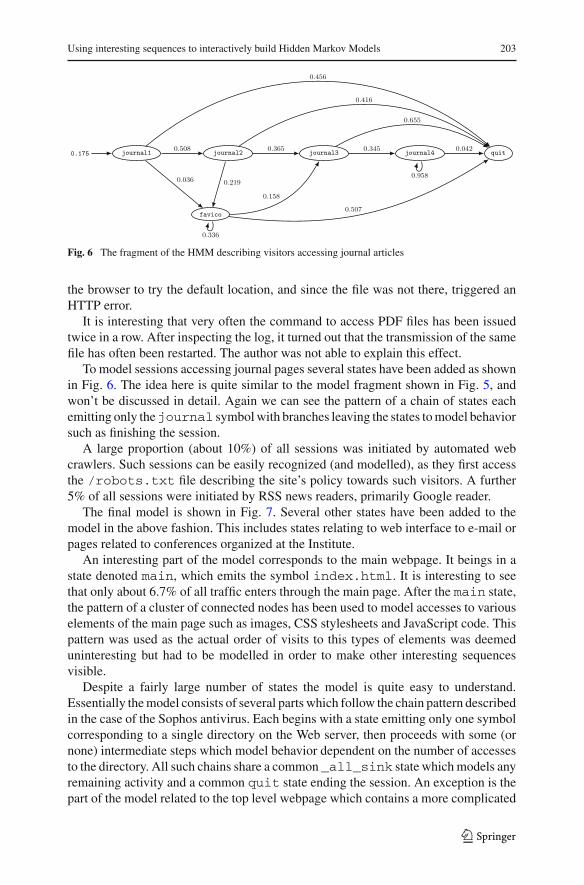
Fig. 6 The fragment of the HMM describing visitors accessing journal articles

the browser to try the default location, and since the file was not there, triggered anHTTP error.

It is interesting that very often the command to access PDF files has been issuedtwice in a row. After inspecting the log, it turned out that the transmission of the samefile has often been restarted. The author was not able to explain this effect.

To model sessions accessing journal pages several states have been added as shownin Fig. 6. The idea here is quite similar to the model fragment shown in Fig. 5, andwon’t be discussed in detail. Again we can see the pattern of a chain of states eachemitting only thejournal symbol with branches leaving the states to model behaviorsuch as finishing the session.

A large proportion (about 10%) of all sessions was initiated by automated webcrawlers. Such sessions can be easily recognized (and modelled), as they first accessthe /robots.txt file describing the site’s policy towards such visitors. A further5% of all sessions were initiated by RSS news readers, primarily Google reader.

The final model is shown in Fig. 7. Several other states have been added to themodel in the above fashion. This includes states relating to web interface to e-mail orpages related to conferences organized at the Institute.

An interesting part of the model corresponds to the main webpage. It beings in astate denoted main, which emits the symbol index.html. It is interesting to seethat only about 6.7% of all traffic enters through the main page. After the main state,the pattern of a cluster of connected nodes has been used to model accesses to variouselements of the main page such as images, CSS stylesheets and JavaScript code. Thispattern was used as the actual order of visits to this types of elements was deemeduninteresting but had to be modelled in order to make other interesting sequencesvisible.

Despite a fairly large number of states the model is quite easy to understand.Essentially the model consists of several parts which follow the chain pattern describedin the case of the Sophos antivirus. Each begins with a state emitting only one symbolcorresponding to a single directory on the Web server, then proceeds with some (ornone) intermediate steps which model behavior dependent on the number of accessesto the directory. All such chains share a common _all_sink state which models anyremaining activity and a common quit state ending the session. An exception is thepart of the model related to the top level webpage which contains a more complicated

123

204 S. Jaroszewicz

Fig. 7 The final HMM describing website visitors’ behavior

loopback behavior involving images, cascading stylesheets and JavaScript. This excep-tion shows that automatically adding chains of states based on interesting symbols isnot a good overall strategy.

123


It should also be stressed that each state in the model has been explicitly added bythe user and thus its meaning and purpose are clear and well defined. Also, the listof emitted symbols in each state is usually short, significantly improving understand-ability. This is typically not the case for automatically built models, as will be shownin Sect. 10, where interactive and automatic approaches are compared.

The final model in Fig. 7 predicts the probability of all possible input sequenceswith accuracy better than 0.01. We can thus say that either a sequence is modelled well,or it appears very infrequently and is thus of little importance to the overall picture ofvisitors’ behavior.

Let us briefly comment on the efficiency of the proposed approach. Since the specialcase of sequences starting at t = 0 is considered, frequent sequence mining in dataand in HMM is very fast. The computation time is almost completely dominated bythe Baum-Welch algorithm. The algorithm can be quite slow, but we discovered thatwhen the emission probability matrix E provides enough information about the inter-nal state of the model given the output symbol, the algorithm requires few iterations.This is the case in the presented application, where many states may emit only a singlesymbol. The model shown in Fig. 7 converged in just five iterations. The computationtook a few minutes on a dataset of 100,000 log events using a Python implementation.

A more thorough performance analysis is given for the more computationallydemanding task of mining sequences starting at an arbitrary point in time.

8 Experimental evaluation, protein secondary structure

In this section we present an application of the algorithm for finding interestingsequences starting at an arbitrary time point to analysis of protein secondary structure.Let us first give a brief description of the problem.

Proteins are long sequences of amino-acids. When a protein molecule is synthe-sized in a living cell, amino-acids are added to it one by one. The overall structure ofthe protein molecule does not physically remain linear, but folds in a very complicatedway. The shape of the molecule determines its chemical properties, so predicting thestructure of the protein molecule based on the sequence of amino-acids, from whichit is built, is a practically important problem. An easier subproblem is predicting theso called secondary structure, that is, not the shape of the whole molecule, just theshape of small local fragments. This is the problem we will look at in this section.More biological background can be found in Hunter (1993).

A dataset from the UCI repository containing several amino-acid sequencesannotated with secondary structure of protein they encode at each given location wasused in the experiments. Overall, there are 20 amino-acids denoted with uppercaseletters. Additionally there are three high-level types of secondary structure, α-helix,β-strand and coil denoted by letters h, e and c respectively. Each sequence ele-ment contains both the amino-acid and the type of secondary structure present at thislocation. The problem now is to discover relationships between sequences of amino-acids and secondary structure of the protein they encode.

In this section, the proposed method of mining interesting sequences beginning atarbitrary time points is used to address this task. The problem has received significant

123

206 S. Jaroszewicz

attention in literature (Qian and Sejnowski 1988; Bouchaffra and Tan 2006; Asai et al.1993), and we do not aim at building a competitive secondary structure predictionsystem. Rather we want to demonstrate the presented approach on real data.

The set of output symbols has been chosen to have 60 elements. Each output symbolconsists of two letters, the first denoting one of the 20 amino acids and the second, thetype of structure at this location. The information on the amino-acid and the structureis thus encoded jointly in the symbol. Another solution could be to use HMMs withmultiple output symbols per state. The initial HMM contained only a single state whichcould emit all possible symbols and had an edge to itself with transition probability 1.

The minimum interestingness threshold of 0.0001 was used. The first five mostinteresting sequences are given in the Table 1.

Due to large number of symbols, interestingness values are not high, but neverthe-less it is possible to see clear patterns. In all cases the probability predicted by theHMM was lower than data count, thus the values of interestingness are marked aspositive. An interpretation is suggested for each pattern.

Looking at all the patterns, the hypothesis is that: sequences of amino-acids A, K,L tend to produce the helix structure h, and sequences of amino-acids A, G and S, thecoil structure c. Note that A is present in the rules for both helix and coil structures.This is not a contradiction and means that it is simply less likely to produce the thirdtype of structure (strand). To validate the hypothesis we also looked at most interestingsequences of length three, shown in Table 2. They confirm the above findings, andsuggest further that D and K might also be related to the coil structure.

In order to update the model to reflect those findings, three new states have beenadded:

state h1 which emits only symbols Ah, Kh, Lh, and whose meaning is that a helix isbeing generated by a sequence of As, Ks and Ls.

state c1 which emits only symbols Ac and Kc. This state denotes the process ofgenerating a coil while adding a sequence of amino-acids A and K.

Table 1 The first five most interesting sequences discovered from the protein structure data

Sequence Interestingness Proposed interpretation

Ah, Ah +0.0029 A sequence of As is likely to produce a helixGc, Sc +0.0027 A sequence of Gs and Ss is likely to produce a coilAc, Ac +0.0027 A sequence of As is likely to produce a coilAh, Lh +0.0025 A sequence of As and Ls is likely to produce a helixKh, Ah +0.0025 A sequence of Ks and As is likely to produce a helix

Table 2 The most interestingsequences of length threediscovered from the proteinstructure data

Sequence Interestingness

Ac, Ac, Ac +0.0010Kc, Ac, Kc +0.0008Dc, Gc, Sc +0.0008Ah, Ah, Kh +0.0008Kh, Ah, Ah +0.0006

123


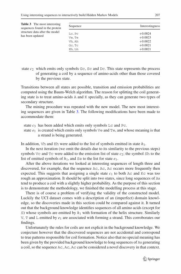
Table 3 The most interestingsequences found in the proteinstructure data after the modelhas been updated

Sequence Interestingness

Lc, Pc +0.0024Ve, Te +0.0023Vh, Ah +0.0022Gc, Tc +0.0021Eh, Lh +0.0021

state c2 which emits only symbols Gc, Sc and Dc. This state represents the processof generating a coil by a sequence of amino-acids other than those coveredby the previous state.

Transitions between all states are possible, transition and emission probabilities arecomputed using the Baum-Welch algorithm. The reason for splitting the coil generat-ing state is to treat amino-acids A and K specially, as they can generate two types ofsecondary structure.

The mining procedure was repeated with the new model. The new most interest-ing sequences are given in Table 3. The following modifications have been made toaccommodate them:

state c3 has been added which emits only symbols Lc and Pc.state e1 is created which emits only symbols Ve and Te, and whose meaning is that

a strand is being generated.

In addition, Vh and Eh were added to the list of symbols emitted in state h1.In the next iteration (we omit the details due to its similarity to the previous steps)

symbols Vc and Tc were added to the emission list of state c2; the symbol Sh to thelist of emitted symbols of h1, and Se to the list for state e1.

After the above iterations we looked at interesting sequences of length three anddiscovered, for example, that the sequence Ac, Ac, Ac occurs more frequently thenexpected. This suggests that assigning a single state c1 to both Ac and Kc was toorough an approximation. It should be split into two states, since long sequences of Astend to produce a coil with a slightly higher probability. As the purpose of this sectionis to demonstrate the methodology, we finished the modelling process at this stage.

There is of course a problem of verifying the validity of the constructed model.Luckily the UCI dataset comes with a description of an (imperfect) domain knowl-edge, so the discoveries made in this section could be compared against it. It turnedout that the background knowledge identifies sequences of all amino acids (except forS) whose symbols are emitted by h1 with formation of the helix structure. SimilarlyV, T and L emitted by e1 are associated with forming a strand. This corroborates ourfindings.

Unfortunately the rules for coils are not explicit in the background knowledge. Weconjecture however that the discovered sequences are not accidental and correspondto true patterns responsible for coil formation. Notice also that no special meaning hasbeen given by the provided background knowledge to long sequences of As generatinga coil, so the sequence Ac, Ac, Ac can be considered a novel discovery in that context.

123

208 S. Jaroszewicz

Fig. 8 Efficiency of mining interesting sequences. Computation times versus minimum interestingnessthreshold

9 Experimental evaluation, performance

We will now evaluate the performance of the proposed algorithms. We will concentrateon mining sequences starting at an arbitrary point in time, as this problem is muchmore challenging computationally.

To test performance, a large database had to be used. To this purpose, we down-loaded raw DNA data from the DNA Data Bank of Japan. We used the TSA datasetfor our experiments,1 which contains 3,226 raw DNA sequences totalling 2,730,222symbols.

The algorithm was implemented in Python and tested on a 1.7 GhZ Pentiummachine. The HMM had 10 hidden states, transition and emission probabilities werecalculated using the Baum-Welch algorithm.

We will separately report computation times for the whole interesting sequencemining procedure (including the Baum-Welch algorithm and mining frequentsequences in data), and for mining frequent patterns in the HMM, as this is one of themain contributions of the paper and takes just a small fraction of the total computationtime. The HMM mining times include both the time of finding frequent sequencesin the HMM and of counting support of sequences which were frequent only in data(Step 5, Fig. 1).

We begin by reporting times for the first 100 sequences (58,503 symbols) withvarying minimum interestingness threshold. The relatively small size of data was cho-sen, such that we can experiment with a broad range of thresholds. The results areshown in Fig. 8. As can be expected both times grow fast when the minimum inter-estingness becomes small, but the computations remain possible even for very lowthresholds. It is also clear that mining in the HMM takes only a small fraction of thetotal time, so improvements in efficiency are possible by e.g. using a better algorithmfor mining frequent sequences in data. As already mentioned, this is a well researchedarea, which is beyond the scope of this paper.

1 Available by anonymous FTP from ftp://ftp.ddbj.nig.ac.jp/ddbj_database/ddbj/ddbjtsa.seq.gz. Retrievedon March 19, 2009.

123

ftp://ftp.ddbj.nig.ac.jp/ddbj_database/ddbj/ddbjtsa.seq.gz


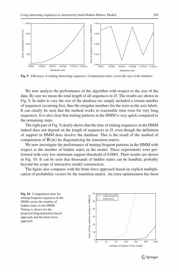
Fig. 9 Efficiency of mining interesting sequences. Computation times versus the size of the database

We now analyze the performance of the algorithm with respect to the size of thedata. By size we mean the total length of all sequences in D. The results are shown inFig. 9. In order to vary the size of the database we simply included a certain numberof sequences occurring first, thus the irregular numbers for the sizes in the axis labels.It can clearly be seen that the method works in reasonable time even for very longsequences. It is also clear that mining patterns in the HMM is very quick compared tothe remaining steps.

The right part of Fig. 9 clearly shows that the time of mining sequences in the HMMindeed does not depend on the length of sequences in D, even though the definitionof support in HMM does involve the database. This is the result of the method ofcomputation of �(|s|) by diagonalizing the transition matrix.

We now investigate the performance of mining frequent patterns in the HMM withrespect to the number of hidden states in the model. These experiments were per-formed with very low minimum support threshold of 0.0001. Their results are shownin Fig. 10. It can be seen that thousands of hidden states can be handled, probablybeyond the scope of interactive model construction.

The figure also compares with the brute force approach based on explicit multipli-cation of probability vectors by the transition matrix. An extra optimization has been

Fig. 10 Computation time formining frequent sequences in theHMM versus the number ofhidden states in the HMM.Timing is shown for theproposed diagonalization basedapproach and the brute forceapproach

123

210 S. Jaroszewicz

used of caching probability vectors for each t . It can be seen that the time needed tomine frequent sequences in the model using the brute force method is much longer, andfor larger (but still practical) numbers of states would have a noticeable contributionto the total pattern mining time (Fig. 9).

10 Comparison with automatic HMM construction

In this section a thorough experimental comparison with automatic HMM construc-tion will be presented. Several aspects of both types of models such as complexity,prediction accuracy and understandability will be analyzed. By ‘automatic HMM con-struction’ we mean creating a model with a specified number of states and randomparameters, and applying the Baum-Welch algorithm to the model. In order to recoverthe structure, transitions which are assigned small probabilities are assumed to beabsent. The same rule is applied to emission probabilities. The Baum-Welch algo-rithm is assumed to have converged when the maximum difference between any ofthe probabilities in the model between successive iterations was <0.001. The algo-rithm was allowed to run until convergence occurred, there was no limit on the numberof iterations.

10.1 A small artificial example

We will begin by showing a small artificial example which will illustrate several issuesand differences between automatic and interactive construction of HMMs. We willstart with a small HMM shown in Fig. 11, generate a sequence database using thatmodel, and try to reconstruct the original using automatic and interactive approaches.Despite its simplicity, the model will be sufficient to demonstrate several interestingproperties of both methods.

The HMM has three states and two output symbols a and b. Emission probabilitiesof the symbols in each state are shown inside the ellipse depicting the state. Two of the

Fig. 11 A small artificial HMMused in learning examples 0 . 5

a:0 .8b:0.2

0 . 5a:0 .2b:0.8

a:0 .8b:0.2

1

0 .5

0 . 5

0 . 5

0 . 5

123


Fig. 12 Artificial example: automatically built HMM

states are more likely to output the symbol a and the remaining one the symbol b. Theoverall structure is such that the a symbols are more likely to be emitted in sequenceswhose length is even. The relationship is of course not perfect but the behavior iseasily detected by looking at output frequencies. For example the probability of thesequence aa being emitted by the model at any time point is about 0.38, while for aband ba it is about 0.22 and for bb about 0.18.

In the first experiment an attempt was made to relearn the HMM from Fig. 11 basedon data simulated from it. The training data consisting of 100 sequences, each 1,000symbols long, have been generated from the original model. The data thus consists ofone hundred thousand symbols, which should be sufficient to learn all the probabilitieswell.

The learned model is given in Fig. 12. The model has been shown as the matricesof its parameters, not as a graph, since there is little structure in the learned modeland the graph would be too cluttered. Probabilities in transition and emission matricesmay not add up to one due to rounding.

One immediately notices that the original structure has not been uncovered. Con-trary to the original model, all possible edges are present in the HMM. Also the tran-sition and initial probabilities are quite different. The emission matrix shows somesimilarity to the original HMM, with two states much more likely to emit an a but theprobabilities themselves are significantly different.

On the other hand it turns out that the model fits the data very well. One way tocheck this is to mine interesting sequences in the learned model with respect to the datait was trained on. The most interesting sequence turned out to be baaab with inter-estingness of 0.0062. So the probabilities of all sequences in data and in the learnedmodel differ by at most this, relatively small, value.

Another way is to compare the likelihoods of the original and relearned modelsgiven the training data. The likelihood of the original model was 0.18 × 10−28948

while that of the learned model 0.20 × 10−29000. The difference of 50 orders of mag-nitude is in fact very small taking into account how tiny both values are. Such lowvalues of likelihood are typical in Bayesian inference problems. For comparison, thelikelihood of a model with random weights was 0.12 × 10−30257, over 1,300 ordersof magnitude lower than that of the original model.

To summarize, the structure of the learned model is very different from the originalmodel, even though both models fit the data very well. In fact starting the learningprocess with different random initializations of the parameters results in differentmodels of very similar quality. The explanation is that different HMMs can repre-sent the same underlying random process, thus being probabilistically equivalent.See Balasubramanian (1993) for a detailed discussion of this phenomenon.

It can thus be concluded, that even with a perfect model learning procedure onecannot hope to always uncover the correct internal structure. If we want to model the

123

212 S. Jaroszewicz

true underlying process, external knowledge (in the approach proposed in this paper:human intelligence and understanding of the analyzed domain) must in general beincluded in the learning process.

Another problem is that of convergence, the Baum-Welch algorithm is only guar-anteed to converge to a local minimum and the convergence can be quite slow. Ittook 153 iterations to learn the three state model described above, which is quite longcompared to other models analyzed in this section. Problems arising from the localoptimality of solutions will be discussed below.

Since in real situations the underlying model is not known, it is difficult to decidehow well the model fits the data just based on its likelihood. Interesting patterns presenta viable alternative here, as the value of interestingness is easy to interpret.

Let us now try to discover the structure using the interactive procedure proposed inthis paper. We begin with a model shown in Fig. 13a. The model has two states eachemitting one of the symbols; all transitions between states are possible. After settingthe parameters to random initial values, and applying the Baum-Welch algorithm,model weights are obtained. We now find interesting sequences in the training datawith respect to the model, of which five most interesting ones are shown in Table 4.Signed values of interestingness are shown to facilitate interpretation.

The meaning of discovered patterns is not immediately clear, but after a carefulexamination, comparing the first and fourth pattern shows that the predicted probabil-ity of the sequence aa is too low and that of the sequence a too high. This suggests thatmodelling sequences with even number of as needs special attention. Other patternsconfirm this, as patterns with an even number of as have their probability predictedto be too low, and patterns with an odd number of as, too high.

All two element sequences mined from the model in Fig. 13a had very low inter-estingness (< 5 × 10−5), so the initial HMM learned to represent them very well,despite not being able to accurately model longer sequences. This is understandable,as the Baum-Welch algorithm only looks at probabilities conditioned on the previousstate. This proves that mining longer sequences can indeed bring practical benefits.

Fig. 13 Models used in theinteractive HMM constructionprocedure

a

b

(a) (b)

Table 4 Five most interestingsequences found in datagenerated from the model inFig. 11 with respect to the modelin Fig. 13a

Sequence I = PrD − PrHMM PrD PrHMM

baab +0.013 0.064 0.051aab +0.010 0.149 0.139aaa −0.010 0.230 0.240bab −0.010 0.071 0.081baa +0.010 0.149 0.139

123


An obvious way to fix the initial model is shown in Fig. 13b. Additional two stateshave been added in order to explicitly model the cases when a occurs an even numbertimes. The interestingness of the most interesting pattern was 0.0014, comparable tothe change in the values of modelled parameters used as the stopping criterion forBaum-Welch algorithm. It is thus reasonable to assume that the model explains thedata sufficiently well. While this HMM has more states than the original one, it hasa much more understandable structure. Moreover each state emits only one symbolwhich is good for convergence of the Baum-Welch algorithm, only 35 iterations werenecessary. The likelihood of the model given training data was 0.1×10−28949, almostidentical to that of the original model, better than that of automatically learned oneabove.

We will now look into the issue of convergence of the Baum-Welch algorithmfor various models. Another possibility of model modification is one which leads tothe original model structure based on which the data was generated. Unfortunatelyin such a case the Baum-Welch algorithm fails to converge to the optimal solution(the interestingness of the most interesting pattern stayed at 0.013, and the likelihooddid not improve over the simpler initial model). In this respect the structure with oneadditional state shown in Fig. 13b behaves much better.

If however the Baum-Welch algorithm is given some hint on how to tune the param-eters, it may perform better. If for example we set initial emission probabilities fora close 1 in two states which we expect to emit that symbol, and close to 0 in theremaining state, the algorithm converges rapidly (15 iterations) to the correct modelwith interestingness of the most interesting sequence and likelihood practically iden-tical to that of the original model. Therefore the discovered patterns may help the userto guide the Baum-Welch algorithm to a better solution.

This may suggest that better results of automatic model discovery might be obtainedif emission probabilities were restricted such that only one symbol can be emitted fromeach state. In order to test this hypothesis a four state HMM has been created with therestriction that three of the states can only emit the symbol a and the remaining state,the symbol b. This corresponds to the user built automaton in Fig. 13b. All transitionswere possible and their probabilities have been initialized to random values.

The resulting automaton is shown in Fig. 14. In order to make the model easierto interpret, it is visualized as a graph with the width of each edge proportional tothe corresponding transition probability. It can be seen that the automaton looks quitedifferent from the one in Fig. 13b. More edges are present and the structure is muchless clear. After careful examination one might infer that double as are more likely toemitted, but this requires effort, as there are many edges and self loops with nonzeroprobability confusing the picture. The automaton took 40 iterations to train, less thanother automatically built models shown in this section. This confirms that a close rela-tion between symbols and internal states improves performance of the Baum-Welchalgorithm.

Let us now summarize the conclusions following from this simple example. TheBaum-Welch algorithm is not always able to discover the correct structure for two rea-sons: several HMM structures can be equivalent for a given problem, or the algorithmmay fail to converge to the correct optimum. The interactive approach makes it possi-ble to work around both those problems. Of course, the user might not always be able

123

214 S. Jaroszewicz

Fig. 14 Automatically builtmodel with state output symbolsfixed a

a a

b

to uncover the true structure (especially since there may be many possible structures),but in any case, the nature of the incorrectly modelled aspect of the data (somethingcauses pairs of as to occur more frequently one after another in the example above)is much easier to see from the patterns. Also, the patterns may give the user a hinton how to set the initial emission probabilities, thus helping an automatic algorithmto discover better model parameters. The method also provides an indicator of thequality of the model, often more practical than the value of model’s likelihood.

10.2 Web log and protein secondary structure examples continued

Let us now compare the final interactively built model for the Web log data given inFig. 7 with models built automatically. An arbitrary number of 20 hidden states hasbeen picked for the HMM, and the Baum-Welch algorithm has been used to computethe transition and emission probabilities. Figure 15 shows the resulting HMM, retain-ing only edges corresponding to transition probabilities >0.01. Figure 16 displays thesame automaton with all edges corresponding to transition probabilities >0.001.

Each node contains the symbols emitted by the corresponding state (for clarity, onlysymbols with emission probabilities >0.01 are shown). Note that this is in contrastwith user built models, where state labels were assigned by the user based on eachstate’s intended meaning. Looking at Fig. 15, it can be seen that the model’s structureis not a good description of users’ behavior. In the upper part of the picture, there is aconnected group of nodes related to the web based e-mail interface, but they are notconnected to the rest of the graph. Moreover, nodes related to e-mail are also presentin the large cluster of nodes below. The Sophos antivirus nodes are present and thediscovered patterns could be inferred from their transition probabilities, albeit withsome effort. Other discovered patterns are not clearly visible and it would be very hardto infer them from transition probabilities.

Adding more edges to the picture, as seen in Fig. 16, does not help. On the contrary,it makes the automaton practically incomprehensible.

It should also be noted that the Baum-Welch algorithm on the hand-built modelconverged much faster than in the case of an automatically built model. The automaticcase usually required about a 100 iterations. This is another, this time real-life, exam-ple of the above described phenomenon of negative influence of ambiguity in emittedsymbols on the convergence and efficiency of the Baum-Welch algorithm.

123


Fig. 15 Automatically build HMM for the weblog example. Only edges corresponding to probabilities>0.01 are shown

We will now give a more principled comparison of the complexity and quality ofautomatically and interactively built models. To this end we need to define precisemeasures of model quality and complexity.

It is tempting to measure the quality of a model using the value of its likelihoodgiven the data. This approach however turns out not to be suitable for the problem athand. The reason is that in the interactively built models several nodes are left uncon-nected, corresponding to zero transition probabilities. If any such transition occursin the data, model’s likelihood will be simply zero. We have thus assessed model’squality based on its prediction accuracy, i.e. how well it predicts the next symbol in asequence based on symbols preceding it.

More formally model’s prediction accuracy on a given database is defined as

AccD(HMM) =∑

d∈D∑{

PrHMM{so}PrHMM{s} : so is a prefix of d

}

∑d∈D |d| − 1

,

that is, the average of the probabilities of each symbol in data conditional on thesequence preceding it. If the HMM predicts a zero probability for s, an arbitrarychoice of 0, is made for the predicted conditional probability, that is, the next symbolis assumed to be predicted incorrectly.

123

216 S. Jaroszewicz

Fig. 16 Automatically build HMM for the weblog example. Edges corresponding to probabilities >0.001are shown

Model’s complexity is defined simply as the number of nonzero parameters in themodel, that is, the total number of nonzero initial, transition and emission probabilities:

Compl(HMM) =∣∣∣{i : π0

i > 0}∣∣∣ + ∣∣{i, j : Pi j > 0}∣∣ + ∣∣{i, j : Ei j > 0}∣∣ .

Of course the original, automatically built, model is likely to have very high com-plexity. In order to make the comparison meaningful we must be able to control thecomplexity of automatically built models. To that end we use a postprocessing step inwhich a given percentage of lowest probabilities in the model are set to zero.

The final interactively built model in Fig. 7 has 36 states so, for the current exper-iment, an automatically built model with 36 states has been used for comparison. Asin the previous cases, the automatically built model has been learned using the Baum-Welch algorithm starting with randomly chosen parameter values. In order to helpassess the models’ future accuracy, the data has been split into training and test sets.The training set was used to build the model and the test set to assess its accuracy.

Figure 17 shows the complexity vs. accuracy tradeoff for automatically built modelfor the weblog data. The final interactively built model from Fig. 7 is marked on the

123


Fig. 17 The tradeoff between complexity and accuracy of the automatically built HMM for the Web logmining example. The black dot shows the complexity and accuracy of the interactively built model

Fig. 18 The tradeoff between complexity and accuracy of the automatically built HMM for the proteinsecondary structure example. The black dot shows the complexity and accuracy of the interactively builtmodel

figure with a black dot. An analogous experiment has been conducted for the proteinsecondary Structure example, the results are shown in Fig. 18.

In the automatically built models, many probabilities turned out to be close to zero,so even a tiny probability threshold significantly reduces model complexity with littleeffect on accuracy. For this reason, the figures show complexity only up to 500 and200 respectively giving a more detailed picture in the interesting region. Low overallaccuracy for the protein example is the result of a large number of symbols (60), whichmakes prediction difficult.

Interactively built models have overall worse accuracy than complete automaticallybuilt ones. In principle nothing prevents the user from continuing with interactiveupdates to the model until the accuracy increases further. However reaching the accu-racy of full automatically built models would be quite laborious, and would probablydefy the purpose of interactive modelling, since very small divergences between themodel and data would be hard to explain; and the main appeal of the proposed methodlies in the fact that all elements are included in the model for a well understood reason.Automatically built HMMs do not possess this advantage.

It can also be seen that for a given complexity, interactively built models weremore accurate. This is especially true in the case of protein data. For the Web log

123

218 S. Jaroszewicz

data the difference is less visible, but interactive models still performed better. It canalso be seen that the difference between interactively and automatically built HMMsis slightly larger on the test set, which suggests that human explanations generalizebetter.

Notice also, that low complexity does not mean understandability. Recall Fig. 15.The HMM shown in this figure has complexity of only 139, yet, as discussed above,it conveys very little information about the internal structure of the process.

11 Conclusions

An approach to interactive construction of global HMMs based on local patternshas been presented. Two cases most important from the practical point of view havebeen discussed: mining interesting sequences starting at the beginning of databasesequences, and mining interesting sequences starting at arbitrary location, have beenaddressed.

Experiments have shown that the proposed methodology is capable of producinghighly understandable, yet accurate models. In the experiments, interactively builtHMMs achieved accuracy equal to or better than automatic models of comparablecomplexity. Moreover, interactively built models were much more understandablebecause they were built by a human, and every new state was added with a clear inten-tion of its function. Additionally, human added model states had a limited number ofemitted symbols and different states emitted disjoint sets of symbols, which furtherimproved model’s clarity. In contrast automatically built models were hard to interpret,typically, states emitted large numbers of symbols, and their sets of emitted symbolsoverlapped.

Experimental evidence has been given that automatic HMM weight learning oftenfails to discover the internal structure of even very simple models. This turns out tobe inevitable, as it is possible for several HMMs to generate the exact same stochasticprocess. In view of this, requiring an analyst to do the actual updating, while beingguided by the interesting patterns seems to be the correct approach if models withmeaningful internal structure are required.

A disadvantage of the approach is that the process requires ‘manual labor’, and thatconsiderable effort may be required to understand the causes of interesting patterns.However, since automatic procedures cannot in general be guaranteed to discovermeaningful internal structure, such an approach seems indeed unavoidable if infor-mation is to be gleaned on the underlying behavior of the process which is generatingthe data.

Efficiency of the proposed approach is very good; in the presented experimentseven very large datasets have been successfully analyzed. This is especially true forthe step of the proposed algorithms in which frequent sequences in HMMs are mined.The proposed approach based on diagonalization of the transition matrix, makes thecomputation time of this step negligible. The simple brute force approach based onrepeated matrix multiplications has been shown to perform much worse, and to haverunning time which may have a tangible contribution to the running time of the wholeinteresting pattern discovery process.

123


It should also be noted that parameter learning using the Baum-Welch algorithmis much easier for interactively constructed models. The convergence is much faster(tens instead of hundreds of iterations) and there is much less of a chance of endingup in a local minimum. This has been conjectured and confirmed experimentally toresult from the fact that output symbols in interactively built models depend on theinternal state in a less ambiguous fashion. Moreover it is sometimes possible to usethe interesting patterns to set some of the initial model parameters (e.g. assign initialemission probabilities to states) such that a local minimum can be avoided.

References

Agrawal R, Imielinski T, Swami A (1993) Mining association rules between sets of items in large databases.In: ACM SIGMOD conference on management of data, pp 207–216

Asai K, Hayamizu S, Handa K (1993) Prediction of protein secondary structure by the Hidden MarkovModel. Bioinformatics 9(2):141–146

Balasubramanian V (1993) Equivalence and reduction of Hidden Markov Models. A.I. Technical Report1370, Artificial Intelligence Laboratory, MIT

Bouchaffra D, Tan J (2006) Protein fold recognition using a structural Hidden Markov Model. In: Interna-tional conference on pattern recognition, vol 3. Los Alamitos, CA, pp 186–189

Dunham MH (2003) Data mining, introductory and advanced topics, Part III. http://engr.smu.edu/~mhd/dmbook/part3.ppt

Han J, Cheng H, Xin D, Yan X (2007) Frequent pattern mining: current status and future directions. DataMin Knowl Discov 15(1):55–86

Hand D (2002) Pattern detection and discovery. In: Hand D, Adams N, Bolton R (eds) Pattern detectionand discovery. Springer, Berlin, pp 1–12

Hunter L (1993) Molecular biology for computer scientists. In: Hunter L (ed) Artificial intelligence andmolecular biology, chap 1. AAAI Press, Menlo Park, pp 1–46

Huo Q, Lee CH (1997) On-line adaptive learning of the continuous density Hidden Markov Model basedon approximate recursive Bayes estimate. IEEE Trans Speech Audio Process 5(2):161–172

Huo Q, Chan C, Lee CH (1995) Bayesian adaptive learning of the parameters of hidden Markov model forspeech recognition. IEEE Trans Speech Audio Process 3(5):334–345

Inoue M, Ueda N (2003) Exploitation of unlabeled sequences in Hidden Markov Models. IEEE TransPattern Anal Mach Intell 25:1570–1581

Jaroszewicz S (2008) Interactive HMM construction based on interesting sequences. In: Proceedings oflocal patterns to global models (LeGo’08) workshop at the 12th European conference on principlesand practice of knowledge discovery in databases (PKDD’08), Antwerp, Belgium, pp 82–91

Jaroszewicz S, Scheffer T (2005) Fast discovery of unexpected patterns in data, relative to a Bayesiannetwork. In: 11th ACM SIGKDD international conference on knowledge discovery and data mining(KDD 2005), Chicago, IL, pp 118–127

Jaroszewicz S, Simovici D (2004) Interestingness of frequent itemsets using Bayesian networks as back-ground knowledge. In: 10th ACM SIGKDD international conference on knowledge discovery anddata mining (KDD 2004), Seattle, WA, pp 178–186

Jaroszewicz S, Scheffer T, Simovici D (2009) Scalable pattern mining with Bayesian networks as back-ground knowledge. Data Min Knowl Discov 18(1):56–100

Ji S, Watson L, Carin L (2009) Semisupervised learning of Hidden Markov Models via a homotopy method.IEEE Trans Pattern Anal Mach Intell 31:275–287

Laxman S, Sastry P (2005) Discovering frequent episodes and learning Hidden Markov Models: a formalconnection. IEEE Trans Knowl Data Eng 17(11):1505–1517

Laxman S, Sastry P (2006) A survey of temporal data mining. Sadhana 31(2):173–198Lee CH, Gauvin JL (1996) Bayesian adaptive learning and map estimation of HMM. In: Lee CH, Soong

F, Paliwal K (eds) Automatic speech and speaker recognition: advanced topics. Springer, New York,pp 83–108

Li D, Laurent A, Poncelet P (2007) Mining unexpected sequential patterns and rules. Technical ReportRR-07027, Laboratoire d’Informatique de Robotique et de Microélectronique de Montpellier

123

http://engr.smu.edu/~mhd/dmbook/part3.ppt

http://engr.smu.edu/~mhd/dmbook/part3.ppt

220 S. Jaroszewicz

Low-Kam C, Mas A, Teisseire M (2009) Mining for unexpected sequential patterns given a Markov model.http://www.math.univ-montp2.fr/~mas/lmt_siam09.pdf

Meyer C (2001) Matrix analysis and applied linear algebra book and solutions manual. SIAM, PhiladelphiaPrum B, Rodolphe F, de Turckheim E (1995) Finding words with unexpected frequencies in DNA

sequences. J R Stat Soc Ser B 57:205–220Qian N, Sejnowski T (1988) Predicting the secondary structure of globular proteins using neural network

models. J Mol Biol 202:865–884Rabiner LR (1989) A tutorial on Hidden Markov Models and selected applications in speech recognition.

Proc IEEE 77(2):257–286Robbins H (1956) An empirical bayes approach to statistics. In: Proceedings of the third Berkeley sym-

posium on mathematical statistics and probability, vol 1: contributions to the theory of statistics,University of California Press, pp 157–163

Satsangi A, Zaiane O (2007) Contrasting the contrast sets: an alternative approach. In: Eleventh internationaldatabase engineering and applications symposium (IDEAS 2007), Banff, Canada

Spiliopoulou M (1999) Managing interesting rules in sequence mining. In: Proceedings of the third Euro-pean conference on principles of data mining and knowledge discovery, pp 554–560

Uhlig F (2001) Transform linear algebra. Prentice Hall, Upper Saddle Rivervan Loan C, Golub G (1996) Matrix computations. Johns Hopkins University Press, LondonWelch L (2003) Hidden Markov Models and the Baum-Welch algorithm. IEEE Inform Theory Soc Newsl

53(4):1,10–13Zaiane O, Yacef K, Kay J (2007) Finding top-n emerging sequences to contrast sequence sets. Tech. Rep.

TR07-03, Department of Computing Science, University of Alberta, Edmonton, AB, Canada

123

http://www.math.univ-montp2.fr/~mas/lmt_siam09.pdf

Using interesting sequences to interactively build Hidden Markov Models

Documents

Transcript of Using interesting sequences to interactively build Hidden Markov Models