
stochastic algorithms, symmetric markov perfect equilibrium ...
21
Ž . Econometrica, Vol. 69, No. 5 September, 2001 , 12611281 STOCHASTIC ALGORITHMS, SYMMETRIC MARKOV PERFECT EQUILIBRIUM, AND THE ‘CURSE’ OF DIMENSIONALITY BY ARIEL PAKES AND PAUL MCGUIRE 1 This paper introduces a stochastic algorithm for computing symmetric Markov perfect equilibria. The algorithm computes equilibrium policy and value functions, and generates Ž . a transition kernel for the stochastic evolution of the state of the system. It has two features that together imply that it need not be subject to the curse of dimensionality. First, the integral that determines continuation values is never calculated; rather it is approximated by a simple average of returns from past outcomes of the algorithm, an approximation whose computational burden is not tied to the dimension of the state space. Second, iterations of the algorithm update value and policy functions at a single Ž . rather than at all possible points in the state space. Random draws from a distribution set by the updated policies determine the location of the next iteration’s updates. This selection only repeatedly hits the recurrent class of points, a subset whose cardinality is not directly tied to that of the state space. Numerical results for industrial organization problems show that our algorithm can increase speed and decrease memory requirements by several orders of magnitude. KEYWORDS: Dynamic games, stochastic algorithms, curse of dimensionality. Ž . APPLIED ANALYSIS OF DYNAMIC INDUSTRIAL organization I.O. problems is limited by the burden of computing equilibrium policies. These are typically obtained by computing a fixed point to a mapping of a function whose domain is a subset of R n , where n is the number of state variables in the problem. In I.O. problems n typically equals the number of state variables per agent times the Ž . Ž . maximum number of agents ever active. If each state variable takes on K Ž distinct values and we impose symmetry on the policy functions so that each . agent’s policy is the same function of its own and its competitors’ states , then the number of possible state vectors, or the dimension of the fixed point calculation, grows geometrically in the number of agents and exponentially in the number of states per agent. This is one source of the ‘‘curse of dimensional- ity’’ in computing equilibria. The other is in the integral determining the continuation value for each agent active at each point; the number of terms in this sum grows in the same manner. We introduce a stochastic algorithm that may circumvent these computational Ž Ž .. problems for Markov Perfect models Maskin and Tirole 1988, 1994 in which the state vector evolves as an ergodic Markov Process. This is because our Ž. algorithm i never attempts to obtain accurate policies on the entire state space, Ž. and ii never calculates continuation values; rather it uses an average of the value of outcomes from past iterations to approximate them. 1 We thank the referees, G. Chamberlain, D. Fudenberg, G. Gowrisankaran, K. Judd, D. Pollard, Ž . J. Rust, and especially a co-editor for helpful comments, and the NSF Grant SBR95-12106 for financial support. 1261
-
Upload
khangminh22 -
Category
Documents
-
view
1 -
download
0
Transcript of stochastic algorithms, symmetric markov perfect equilibrium ...

Ž .Econometrica, Vol. 69, No. 5 September, 2001 , 1261�1281
STOCHASTIC ALGORITHMS, SYMMETRIC MARKOVPERFECT EQUILIBRIUM, AND THE ‘CURSE’
OF DIMENSIONALITY
BY ARIEL PAKES AND PAUL MCGUIRE1
This paper introduces a stochastic algorithm for computing symmetric Markov perfectequilibria. The algorithm computes equilibrium policy and value functions, and generates
Ž .a transition kernel for the stochastic evolution of the state of the system. It has twofeatures that together imply that it need not be subject to the curse of dimensionality.First, the integral that determines continuation values is never calculated; rather it isapproximated by a simple average of returns from past outcomes of the algorithm, anapproximation whose computational burden is not tied to the dimension of the statespace. Second, iterations of the algorithm update value and policy functions at a singleŽ .rather than at all possible points in the state space. Random draws from a distributionset by the updated policies determine the location of the next iteration’s updates. Thisselection only repeatedly hits the recurrent class of points, a subset whose cardinality isnot directly tied to that of the state space. Numerical results for industrial organizationproblems show that our algorithm can increase speed and decrease memory requirementsby several orders of magnitude.
KEYWORDS: Dynamic games, stochastic algorithms, curse of dimensionality.
Ž .APPLIED ANALYSIS OF DYNAMIC INDUSTRIAL organization I.O. problems islimited by the burden of computing equilibrium policies. These are typicallyobtained by computing a fixed point to a mapping of a function whose domain isa subset of Rn, where n is the number of state variables in the problem. In I.O.problems n typically equals the number of state variables per agent times theŽ . Ž .maximum number of agents ever active. If each state variable takes on K
Ždistinct values and we impose symmetry on the policy functions so that each.agent’s policy is the same function of its own and its competitors’ states , then
the number of possible state vectors, or the dimension of the fixed pointcalculation, grows geometrically in the number of agents and exponentially inthe number of states per agent. This is one source of the ‘‘curse of dimensional-ity’’ in computing equilibria. The other is in the integral determining thecontinuation value for each agent active at each point; the number of terms inthis sum grows in the same manner.
We introduce a stochastic algorithm that may circumvent these computationalŽ Ž ..problems for Markov Perfect models Maskin and Tirole 1988, 1994 in which
the state vector evolves as an ergodic Markov Process. This is because ourŽ .algorithm i never attempts to obtain accurate policies on the entire state space,
Ž .and ii never calculates continuation values; rather it uses an average of thevalue of outcomes from past iterations to approximate them.
1We thank the referees, G. Chamberlain, D. Fudenberg, G. Gowrisankaran, K. Judd, D. Pollard,Ž .J. Rust, and especially a co-editor for helpful comments, and the NSF Grant SBR95-12106 for
financial support.
1261

A. PAKES AND P. MCGUIRE1262
Recall that in a finite state ergodic Markov Process every sample path will, infinite time, wander into the recurrent class of points, say R, and once in R will
Ž Ž ..stay within it forever see, for e.g., Freedman 1983, Ch. 1 . Thus to analyze theimpacts of an event from an initial condition in R all we require is knowledge ofthe policies on R.
Our algorithm is asynchronous, it only calculates policies for a single point atŽ .each iteration its location . The policies of each active agent at that point are
obtained from a simple single agent maximization problem and maximize thatiteration’s estimate of the agent’s continuation value. These policies set thedistribution of the next iteration’s state. A random draw from that distribution istaken and used to update the algorithm’s location. This process eventuallyconfines itself to selecting points in R. Depending on the economics of theproblem, the number of points in R need not grow in the number of state
Ž .variables in n at all.The algorithm uses an average of past outcome to estimate the continuation
values needed to determine policies. The estimates associated with the currentiteration’s location are updated by treating the random draw used to update thelocation of the algorithm as a Monte Carlo draw from the integral determiningcontinuation values. That draw is evaluated and then averaged with the values ofdraws obtained from the same location in prior iterations to determine the newestimate of continuation values. Though this is both faster and has less memoryrequirements than explicitly integrating over possible future outcomes, it is also
Ž .less precise particularly in early iterations . This generates a tradeoff betweenthe computational burden per point, and the number of iterations needed for a
Žgiven level of precision. Since the precision of the estimate does not neces-.sarily depend on the dimension of the integral being estimated, while the cost
of doing the summation explicitly does, the larger is n the more we expect thetradeoff to favor our procedure.
Our rules for updating continuation values are similar to the rules used inŽsome of the recent economic literature on learning both in the context of single
agent intertemporal decision problems and in the context of matrix games;Ž . Ž .examples include Fudenberg and Levine 1999 , Lettau and Uhlig 1999 , and
Ž .Sargent 1993 . Moreover, just as in that literature, our algorithm can beendowed with a behavioral interpretation by assuming that agents actually usedour rules to form estimates of continuation values and then chose their policiesto maximize the estimated values. We differ from that literature in dealing withgames whose state vectors evolve over time and in focusing on how the learning
Žalgorithm can be used to help compute Nash equilibria instead of on its.behavioral or limit properties .
We do not know of general conditions which insure, a priori, that ouralgorithm will converge to the desired policies. We can, however, use conditionsthat insure convergence has occurred to build a stopping rule for the algorithmŽwhich is the most we expect from applying fixed point algorithms to mappings
Ž . .that are not contractions; see Judd 1999 and the literature cited there . Also

STOCHASTIC ALGORITHMS 1263
the computational advantages of our algorithm vary with the structure of theŽ .problem e.g. with n and with the cardinality of the recurrent class . However,
numerical results indicate that our algorithm is free of convergence problemsand can convert problems that would have taken years on the current genera-tion of supercomputers to problems that can be done in a few hours on our workstation.
The next section outlines a Markov Perfect model of industry dynamics. Thisboth helps to focus the subsequent discussion and provides a framework forcomputing examples. Section 2 considers the burden of computing equilibriumpolicies using pointwise backward solution algorithms. Section 3 introduces ouralgorithm and Section 4 contains numerical results that provide an indication ofits power. A closing section considers related issues and an Appendix illustrateshow easy it is to program our algorithm.
1. A SIMPLE MODEL
This section outlines a model of industry dynamics due to Ericson and PakesŽ . 21995; henceforth EP that is easy to work with. In the model firms invest toexplore profit opportunities. Profits in any period depend on the firm’s and itscompetitors’ level of quality or efficiency.
We let i index levels of efficiency, and assume i�ZZ�, the positive integers.� �Let s �ZZ be the number of firms with efficiency level i, so the vector s� s ;i i
��i�ZZ is the ‘‘market structure.’’ Profits for a firm at i when the marketŽ .structure is s are given by � i, s . Extensions in which i is a vector are discussed
below.Ž .� � can vary with demand and cost primitives, and with an equilibrium
3 Ž .assumption. Given � � an incumbent has two choices. It chooses whether toexit or remain active and if it remains active it chooses an amount of investment.
Ž .If it exits it receives a sell-off value of � dollars and never reappears . If itinvests x it incurs a cost of cx and has a probability distribution of improve-ments in i that is stochastically increasing in x.
Ž .Thus if we let � be the discount rate, and p i�, s��x, i, s provide the firm’sperceptions of the joint probability that its own efficiency in the next period will
Ž .be i� and the industry structure will be s� conditional on x, i, s , the Bellman
2 Ž . Ž .For more on the model and extensions to it largely made by others , see Pakes 2000 .3 Ž .The publicly available program for computing our dynamic equilibria has three examples of � �
Ž .each programmed up to parameters set by the user . To access a description of, and code for, thisŽ .algorithm as well as a number of auxiliary programs designed to help analyze its results , either
download the needed directories from Ariel Pakes’ Harvard web page, or FTP to ‘‘econ.yale.edu’’,use ‘‘anonymous’’ as login, and your own user-name as ‘‘password.’’ Then change directory to
Ž .‘‘pub�mrkv-eqm’’ and copy all needed files. The ‘‘read.me’’ file, or Pakes 2000 , will start you off.

A. PAKES AND P. MCGUIRE1264
� Ž .�equation for the value of the firm V i, s is
Ž . Ž . Ž .1 V i , s �max � , � i , s½Ž . Ž .� sup �cx�� V i�, s� p i�, s��x , i , s .Ý 5
Ž .x0
ŽThe max operator determines if the continuation value the expression after the. Ž .comma is greater than the sell-off value � . If not the firm shuts down. If so
Ž .the firm chooses investment x0 . x determines the probabilities of incre-ments in the firm’s state over the period.
We assume that this increment can be written as a difference of twoindependent random variables, i.e.
i � i �� �� .t�1 t t t
� represents the outcome of the firm’s investment process and has probabilities� Ž . �4given by a family p ��x , x�RR that is stochastically increasing in x. � is an
Ž .exogenous random variable with probabilities � . Its precise interpretationdepends on the structure of the profit function but it typically represents
Žcommon demand or supply shocks e.g. competition from outside the industry,.or factor prices . The � ’s of different firms are independent, but the realization
of � is common across firms. Both � and � are non-negative integer valuedŽrandom variables with finite support; ��0 if x�0 a firm cannot advance
. Ž . Ž .without some investment , and 0 �0 as is p 0�x for all finite x.Thus if s is the vector providing the states of the competitors of a firm ati
� � �state i when the industry structure is s, and q s � i, s, � provides the firm’siperceived probability that the states of its competitors in the next period will bes� conditional on a particular value of � ,i
Ž . Ž .2 p i�� i*, s��s*�x , i , s
Ž . � � Ž . � Ž .� p �� i*� i���x q s �s*�e i* � i , s, � � ,ˆÝ i�
Ž . Žwhere e i is a vector that puts one in the ith slot and zero elsewhere so thatŽ . .s*�e i* gives the states of next year’s competitors if s��s* and i�� i* . Note� �that q �� i, s, � embodies the incumbent’s beliefs about entry and exit.
For simplicity we assume there is only one potential entrant a period whoŽ .pays an amount x ��� to enter, and enters one period later at statee
e e eŽ . �� � with probability p � . The entrant only enters if the value ofentering is greater than x .4e
That describes the primitives of the model. At an equilibrium the perceivedŽ � � �.distributions of future industry structures the q s � i, s, � used to determinei
4 Different entry models are easy to accommodate provided the distribution of i’s at which entryoccurs is fixed over time. That is, the ‘‘ability’’ of entrants must progress at the same pace as the‘‘ability’’ of the outside alternative; else entry would eventually go to zero and stay there.
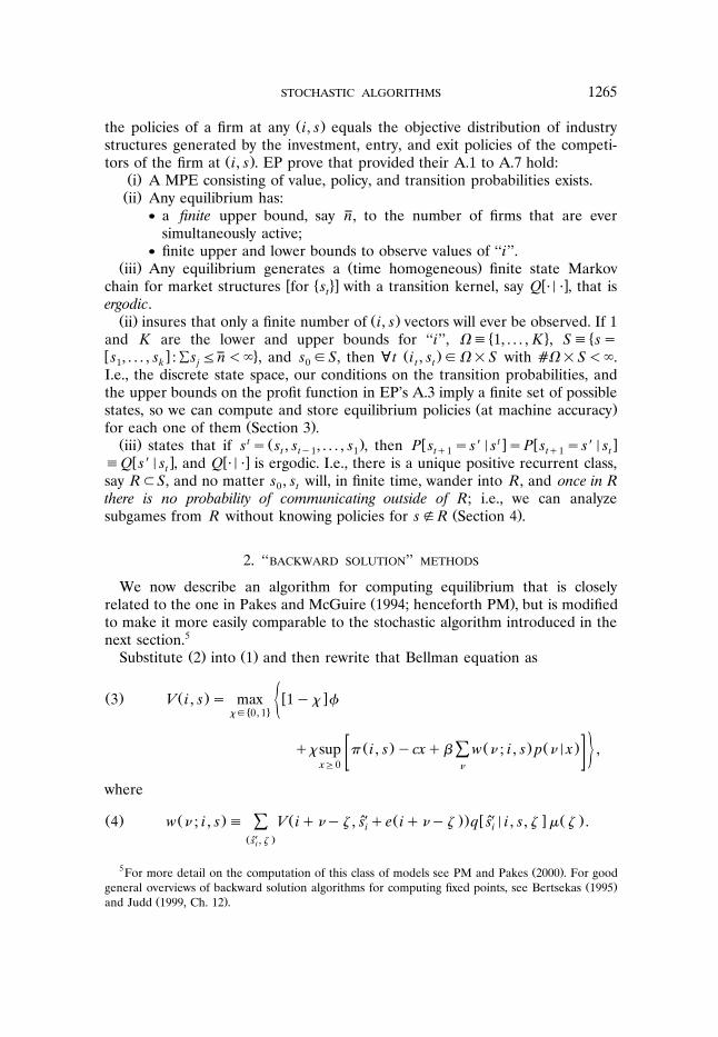
STOCHASTIC ALGORITHMS 1265
Ž .the policies of a firm at any i, s equals the objective distribution of industrystructures generated by the investment, entry, and exit policies of the competi-
Ž .tors of the firm at i, s . EP prove that provided their A.1 to A.7 hold:Ž .i A MPE consisting of value, policy, and transition probabilities exists.Ž .ii Any equilibrium has:
� a finite upper bound, say n, to the number of firms that are eversimultaneously active;
� finite upper and lower bounds to observe values of ‘‘i’’.Ž . Ž .iii Any equilibrium generates a time homogeneous finite state Markov
� � 4� � �chain for market structures for s with a transition kernel, say Q �� � , that istergodic.Ž . Ž .ii insures that only a finite number of i, s vectors will ever be observed. If 1
� 4 �and K are the lower and upper bounds for ‘‘i’’, �� 1, . . . , K , S� s�� � 4 Ž .s , . . . , s :Ýs �n�� , and s �S, then t i , s ���S with ���S��.1 k j 0 t tI.e., the discrete state space, our conditions on the transition probabilities, andthe upper bounds on the profit function in EP’s A.3 imply a finite set of possible
Ž .states, so we can compute and store equilibrium policies at machine accuracyŽ .for each one of them Section 3 .
Ž . t Ž . � t � � �iii states that if s � s , s , . . . , s , then P s �s��s �P s �s��st t�1 1 t�1 t�1 t� � � ��Q s��s , and Q �� � is ergodic. I.e., there is a unique positive recurrent class,t
say RS, and no matter s , s will, in finite time, wander into R, and once in R0 tthere is no probability of communicating outside of R; i.e., we can analyze
Ž .subgames from R without knowing policies for s�R Section 4 .
2. ‘‘BACKWARD SOLUTION’’ METHODS
We now describe an algorithm for computing equilibrium that is closelyŽ .related to the one in Pakes and McGuire 1994; henceforth PM , but is modified
to make it more easily comparable to the stochastic algorithm introduced in thenext section.5
Ž . Ž .Substitute 2 into 1 and then rewrite that Bellman equation as
Ž . Ž . � �3 V i , s � max 1�� �½� 4�� 0, 1
Ž . Ž . Ž .�� sup � i , s �cx�� w � ; i , s p ��x ,Ý 5x0 �
where
Ž . Ž . Ž � Ž .. � � � Ž .4 w � ; i , s � V i���� , s �e i���� q s � i , s, � � .ˆ ˆÝ i i�Ž .s , �i
5 Ž .For more detail on the computation of this class of models see PM and Pakes 2000 . For goodŽ .general overviews of backward solution algorithms for computing fixed points, see Bertsekas 1995
Ž .and Judd 1999, Ch. 12 .

A. PAKES AND P. MCGUIRE1266
� Ž .4The w � ; i, s are the continuation value of the firm conditional on the currentŽ .year’s investment resulting in a particular � and the current state being i, s .
They are constructed by summing over the probability weighted outcomes forŽ �. Ž .the competitors’ states the s and the common shock � .i
� Ž . Ž . 4Let V be the support of � , and note that w � ; i, s : � , i, s �V���S w � w 4 Ž .RR determines all policies. Pick a w�W� w : w�RR and use 3 to compute� �
Ž .the decision rules and value function generated by w at each i, s , sayxw �T w, � w �T w, and V w �T w. These decision rules determine transitionx � Vprobabilities, say qw �T w asq
Ž . w � � � � � � � 45 q s �s � i , s, � �Pr s �s � i , s, � , the policies generated by wˆ ˆ ˆ ˆi i i i
Ž w . wfor a formal description of q , see equations 6 to 8 in EP . Now substitute Vw Ž . � �and q into 4 and compute w �T w. If w�w , then the equilibriumw
conditions are satisfied for the policies, value functions, and transition probabili-ties generated by w. Consequently the search for equilibrium policies can berecast as a search for a w�W that satisfies the fixed point w�T w. Any such ww
Žwill be denoted by w* i.e. we abuse notation slightly by not distinguishing.between a particular, and the set of, equilibrium values .
A backwards solution technique for finding w* holds an estimate of w inmemory, circles through the s�S in some predetermined order, and uses T tow
Ž .update each component of w �; � , s . The algorithm continues iterating untilTw j �w j. Its computational burden is essentially the product of:Ž . Ž .a the number of points evaluated at each iteration �S ;Ž .b the time per point evaluated; andŽ .c the number of iterations.
Ž . Ž .Both a and b grow rapidly in the number of state variables. To examineŽ .how a increases, temporarily allow L state variables per firm and recall that n
Ž .is the maximum number of firms ever active. The rate of increase in a dependson whether we increase L or n. If i �1, . . . , k for l�1, . . . , L, then absentl
L Žfurther restrictions, K����k , an exponential in L Section 5 considers.possible restrictions . Each of the n firms can only be at K distinct states, so
n�S�K . However the policy functions are exchangeable in the state variablesof a firm’s competitors so we do not need to differentiate between two vectors of
Ž .competitors that are permutations of one another. As shown in Pakes 1994 thisimplies that the combinatoric
K�n�1ž /n
is an upper bound for �S; but for n large enough this bound is tight. The boundŽ .increases geometrically rather than exponentially in n. All numerical results
Ž . Ž .we discuss both PM’s and ours impose symmetry. Still a increases geometri-cally in n and exponentially in L.Ž .b is primarily determined by the time to calculate the expected value of
Ž .future outcomes the w above . Say m firms are active from s, and that there is

STOCHASTIC ALGORITHMS 1267
positive probability on each of � points for each of the m�1 competitors ofŽ .each firm � typically grows exponentially in L . Then to compute the required
expectation we sum over � m possible future states, so the average computa-Ž . m Ž .tional burden per point is proportional to Ý f m m� , where f m is the
fraction of points with m firms active.6
3. A STOCHASTIC ALGORITHM
The stochastic algorithm is asynchronous; it only updates policies at a singleŽ . js�S at each iteration j , and as a result must update both this location, s , and
its estimate of continuation values, w j. As in the literature on Q-Learning,7Ž .these updates are made to mimic what would happen if i actual agents chose
policies assuming w j provided the correct evaluation of possible future out-Ž .comes, ii nature resolved the randomness conditional on those policies and
j�1 Ž . j�1chose an s , and iii the agents treated s as a random draw from the statesthat could have occurred and averaged its estimated value with those of the
j jŽ j.previous draws from s to update w s .Thus the stochastic algorithm replaces the deterministic update operator
Ž .T : W�W, with a Markov transition kernel, say QQ �, ��s, w , which takes S�WwŽ j j.into a probability distribution on S�W. At iteration j, QQ ��s , w is used to
simulate s j�1, and s j�1 is then used to form a Monte Carlo update of theŽ j.continuation values the w . This generates sample paths for s which eventually
stay within a recurrent subset of S, say R, and hence reduces the number ofŽŽ . .points that must be updated a above from �S to �R. The Monte Carlo
j Ž Ž . .updates of the w reduce the computational burden per point i.e. b abovefrom m� m to m, but introduces simulation error in w. To average out that
Ž . Ž .error we need a large number of iterations. So the use of QQ reduces a and b ,Ž .but increases c . However since neither �R, m, nor the number of iterations
are necessarily related to the dimension of the state space, the stochasticalgorithm may eliminate the curse of dimensionality altogether.
Ž j j. Ž .Let w , s �W�S be the jth iteration values of w, s . Policies for the jthj jŽ j.iteration for each i with s �0 are chosen by substituting w � : i, s fori
Ž . Ž . Ž Ž j j. Ž j j..w � : i, s into 4 and choosing x �, s : w , � �, s : w to maximize iteration j’s
6 The computational burden of obtaining the optimal policies given this sum need not grow in mŽ .at all it does not in our example . The cardinality of this summand could be reduced by using
symmetry restrictions, but this would require us to find the probabilities associated with each uniques� vector, a computationally burdensome task.i
7 Ž .See Barto, Bradtke, and Singh 1995 , especially Sec. 7.3, and the literature cited there.Ž .Bertsekas and Tsikilis 1996, chapter 5 , point out that Q-Learning can be obtained from the
Ž . Ž .‘‘TD � �k ’’ class of algorithms, algorithms that use a TD � method for updating the valuefunction and k-iterations between policy updates, by setting ��0, k�1; they refer to it as
Žasynchronous optimistic policy iteration see also their references to the reinforcement learning.literature . We thank John Rust for pointing us to the relationship between our algorithm and this
literature.

A. PAKES AND P. MCGUIRE1268
estimated value, i.e. as the solution to
Ž . Ž j j .6 V i , s : w
� �� max 1�� �½� 4�� 0, 1
j j jŽ . Ž . Ž .�� sup � i , s �cx�� w � ; i , s p ��x .Ýx 5�
Similarly if the potential entrant pays x dollars to enter and, if it enters,ebecomes an incumbent in the next period at i minus the common shock � , thene
jŽ j. � 4the entry policy, say � s � 0, 1 , ise
Ž . jŽ j j . jŽ j Ž ..7 � s : w �1�� w 0; i , s �e i �x ,e e e e
Ž .where e i is a K-vector that has one for its i element and zero elsewhere.e eŽ j j. j�1These policies determine QQ �, ��s , w . To draw an s from this QQ:
Ž . j�1 Ž .i draw the common shock � from � ,Ž . Ž Ž j j.ii for each active incumbent each i for which � i, s : w �1 and each of
j . j�1 Ž Ž j j.. j�1the s firms active at i , draw � from p ��x i, s : w and compute i��i�� j�1, andŽ . Ž Ž j. . j�1iii if there is entry if � w �1 , compute i �� .e e
j�1 Ž . Ž .Then if s counts the number of outcomes from ii and iii equal to r,r
j�1 j�1s � s ; r�� .r
jŽ j.To update w � ; i, s we first form the jth iteration’s evaluation of being inŽ .the location determined by i, � when all the other competitors locations and �
are determined by their random draws, or
Ž . j�1 j�1 Ž j�1 . j8 V i���� , s �e i���� : wˆŽ .i
Ž . Ž .as defined in 6 . Note that 8 is the current iteration’s perception of the valuejŽ .of a random draw from the integral defining w � ; i, s . Hence we increment
jŽ . Ž . jŽ .w � ; i, s by a fraction of the difference between 8 and w � ; i, s . MoreŽ . � Ž . �formally let w s � w � ; i, s ; ��V, i�� . Then:
�j j�1 jŽ . Ž . Ž Ž . .if s�s , then w s �w s or w s is not updated ,
�jif s�s , then
Ž . j�1Ž j . jŽ j .9 w � ; i , s �w � ; i , s
j j�1 j�1 j�1 j j jŽ . Ž . Ž .�� j, s V i���� , s �e i���� : w �w � ; i , s ,ˆ½ 5i
Ž . Ž . Ž .where the � j, s � 0, 1 are chosen: i to be a function of informationŽ .available at iteration j, and ii to have a sum that tends to infinity and a
squared sum that remains bounded as the number of times the point is hit tendsŽ .to infinity. � j, s equal to the inverse of the number of past iterations for which
j jŽ .s �s, a choice that implies that the w �; i, s are the simple a erage of past

STOCHASTIC ALGORITHMS 1269
Ž .draws on the conditional continuation values of firms at i, s , will satisfy theseconditions.8
Ž j j. Ž . j j�1Ž .Let WW � ; i, s : w be the expectation of 8 conditional on w , and let � sŽ .be the difference between 8 and this expectation. Then
j�1Ž . jŽ . Ž . � Ž j . jŽ . j�1 Ž .�w s �w s �� j, s WW s : w �w s �� s ,
� j�1Ž . j � jŽ .with E � s �w �0. The update will tend to increase or decrease w � ; i, saccording as the expectation of this random draw is greater or less than
jŽ . Ž . Ž . Ž .w � ; i, s . At the equilibrium i.e. at w* , WW s : w* �w* s , so once we are atw* we tend to stay their. When w j equals w* our algorithm generates an ergodic
� j4Markov process for s and hence will, in a finite number of iterations, wanderŽ .into the recurrent class R and stay in R thereafter.
j j Ž .We have shown how to update both w and s the Appendix has more detail .We still need a rule for when to stop the iterations. Since we only obtainaccurate policies on RS, our stopping rule mimics a definition of equilibriumon subsets of S rich enough to enable us to analyze subgames from thosesubsets.
3.1. Equilibrium Policies and Stopping Rules
For any function f with domain S, and any S*S, let f�S* denote therestriction of f to S*. Our algorithm eventually focuses in on an S**S. Wesay w�S* generates policies for S**S* if it contains the information needed
Ž . Ž . Ž .to calculate x �, s : w , � �, s : w , and � s : w for all s�S**. For w�S* toeenable us to analyze subgames from S** it must contain this information for
� 4�each element of all possible sequences, s , for all s �S**.� ��t t
DEFINITION: w�S* generates equilibrium policies for subgames from S** iffw�S* generates policies for S** and:
Ž . � 4d.i inf Pr s �S**�s , w �1, s �S**, and,� t � t tŽ . Žd.ii the policies generated by w�S* satisfy the equilibrium conditions 6a to
Ž ..6d in EP 1995 s�S**.
Ž . Ž .d.i insures that w�S* generates subgames from S** while d.ii insures thatthose subgames are Markov Perfect equilibria.
The next theorem provides sufficient conditions for w�S* to generate equilib-rium policies for subgames from S** and is the basis for our stopping ruleŽ Ž . Ž . Ž . Ž .. wcondition t.i below insures d.i above, while t.ii insures d.ii . Write s� r˜iff the policies generated by w imply a positive probability of moving from s to r˜Ž . Ž . Ž .of s communicating with r . Even if d.i and d.ii are satisfied, there will be˜
Ž .s�S** that could communicate with r�S** if feasible though not optimal˜policies are followed. The set of such r determine �S**�S*, and to check for
8 Ž . Ž .The conditions are Robbins and Monroe’s 1951 regularity conditions. Rupport 1991 considersŽ .their importance and optimal weighting schemes see also Section 3.2 .

A. PAKES AND P. MCGUIRE1270
Ž . Žequilibrium policies on S** we need estimates of w s on �S**�S* theŽ . .algorithm only produces accurate estimates of w s for s�S** . Condition
Ž .Ž . Ž .t.ii b states that all we require of the w s for s��S**�S* is that theseŽ . Ž . Ž .w s w* s this insures that if a policy is not chosen it is indeed not optimal ,
so we obtain them elsewhere.
THEOREM 1: Assume that for a w�W there is an S**S*S such that w�S*generates policies s�S** and:
Ž . wt.i if �s�S**� s�, then s��S**; andŽ . Ž .t.ii a s�S** and �V, if s �0,i
Ž . � � Ž . � w Ž � . Ž .w � ; i , s � V i���� , s �e i���� : w q s � i , s, � � .ˆ ˆÝ i i�s , �i
Ž . Ž . Ž . Ž . Ž .b s��S**�S*, �w** s w* s , such that w s w** s .Then w�S* generates equilibrium policies for subgames from S*.
Ž . wPROOF: From t.i , q �0 whenever i�S** but j�S**. An inductive argu-i jment shows that if Q has this property, then so does Q� �QQ��1, �1. Thus
� 4 � 4 � t, s �S**�Pr s �S**�s , w �1� lim inf Pr s �S*�s , w �t � t T �� t �� � T � tŽ . Ž . Ž . Ž . Ž . Ž .1, which proves d.i . To prove d.ii , let w s �w s if s�S** and w s �w* s˜ ˜
Ž .if s��S**�S*. Since w* satisfies t.ii , it is straightforward to check that the� �policies generated by w�S* satisfy the equilibrium conditions 6a to 6d in EP˜
� Ž . Ž . Ž .� s � S**. So it suffices to show that � �, s : w , x �, s : w , � s : w �e� Ž . Ž . Ž .�� �, s : w , x �, s : w , � s : w , s�S**.˜ ˜ ˜e
Ž . � w� �Take s�S**. If � i, s : w �1 and s has positive q �� i, s, � probability,i� Ž . Ž . Ž . Ž .Ž .then s �e i�� �S**, so w 0; i, s �w 0; i, s by t.ii a . Similarly, since theˆ ˜i
Ž . Ž . Ž .support of � is independent of x, if x i, s : w �0 then w � ; i, s �w � ; i, s , and˜Ž . Ž Ž .. Ž Ž ..if � s : w �1 then w 0; i , s�e i �w 0; i , s�e i . The remaining cases˜e e e e eŽ . Ž . Ž Ž . . Ž . Ž . Ž .are: a � i, s; w �0 or � s : w �0 ; and b � i, s : w �1 but x i, s : w �0.e
Ž . � Ž . Ž . Ž .� � Ž .a � � sup � i, s � cx � �Ý w � ; i, s p � � x sup � i, s � cx �x � xŽ . Ž .� Ž .�Ý w � ; i, s p ��x �� i, s�w �0, where the second inequality follows from˜ ˜�
Ž .Ž . Ž Ž . Ž . .t.ii b to prove � s : w �0�� s; w �0 substitute x for � here .˜e e eŽ . � � Ž . Ž .� Ž . 4 � � Ž .b � 0 sup Ý w � ; i, s � w 0; i, s p � � x � cx sup Ý w � ; i, s �˜x x Ž .� Ž . 4 Ž .w 0; i, s p ��x �cx �x i, s�w �0, where the first inequality follows from˜
Ž .Ž . Ž .the optimality condition for x, the second from t.ii b , and � from � i, s : wŽ . Ž .�1�w 0; i, s �w 0; i, s . Q.E.D.˜
Our stopping rule is based on checking the two conditions of Theorem 1 for aw generated by the algorithm. To perform the check we need: a candidate for
Ž . Ž . Ž . Ž .S** w , and a w** s �w* s for s��S**�S*. To obtain S** w note that� �any recurrent class of the process generated by Q �, ��w satisfies the Theorem’s
Ž . � �condition t.i . Further w�W the process generated by Q �, ��w is a finiteŽstate Markov chain, and all such chains have at least one recurrent class see
Ž . Ž . � �Freedman 1983, Ch. 1 . Thus to obtain S** w , use Q �, ��w to simulate a� 4sequence s , collect the set of states visited at least once between j�J andj 1

STOCHASTIC ALGORITHMS 1271
Ž J2�J 1. Ž . J1�J 2 J2�J 1j�J S , and set S** w �S . Provided both J and J �J ��, S2 1 2 1� � Ž .will converge to a recurrent class of Q �, ��w , thus satisfying our condition t.i ,Ž .Ž .and our test need only check condition t.ii a on this set. That check requires a
Ž . Ž .w** s w* s for s��S**�S* but, as we note below, our initial conditionŽ 1. 1w is greater than w*, so setting w**�w will do.
3.2. Details of the Algorithm
Ž 1A number of more detailed choices still need to be made e.g. w and the� Ž .4.� j, s . We begin with some results from a related artificial intelligenceliterature that both help make those choices and clarify the issues surroundingthe convergence of our algorithm.
� j4The stochastic algorithm generates a random sequence w , whose ‘‘incre-Ž j. jment,’’ V ��w �w , has a distribution, conditional on information available at
iteration j, determined by w j. We look for a zero root of the conditionalŽ . Ž .expectation of this increment this defines a w* . Robbins and Monroe 1951
introduced a scalar version of a similar problem and provided conditions thatinsured w j �w* in mean square.9 That paper stimulated a literature applying
Žstochastic iterative solution techniques to an assortment of problems seeŽ . .Ruppert 1991 for an accessible review . The branch most closely related to our
Ž . Žproblem is often referred to as reinforcement or machine learning seeŽ . .Bertsekas and Tsikilis 1996 and the literature they cite .
Ž .The reinforcement learning literature typically deals with: i single agentŽ .dynamic programming problems in which, ii agents choose controls from a
Ž .finite set of possible values, and iii if the algorithm is asynchronous, all pointsŽ . ŽŽ .in the state space are recurrent i.e. S�R . The use of discrete controls ii
.above leads to algorithms that simulate different future values for differentchoices of those controls. Instead we simulate values for alternative outcomesŽ Ž ..our w �; i, s , and choose a continuous control that determines the probabilityof those outcomes.10 Still the algorithms are similar and convergence proofsrelated to those used in the machine learning literature can be adapted to thesingle agent version of our problem when S�R. These convergence proofs are
Žof two types; the first is based on the existence of a smooth potential or. w ŽLyapunov function, f : RR �RR, which ‘‘looks inward’’ has a gradient whose
9 Ž .Blum 1954 , generalizes to the finite dimensional case and almost sure convergence. RobbinsŽ j.and Monroe study the case where both the function V ��w and the family of conditional
Ž .distributions may be unknown ‘‘nature’’ generates the needed draws . In our case we can constructwŽ . Ž j. jq �� � and compute the expectation of V ��w �w , but both these tasks are computationally
Ž . wŽ .burdensome especially for large state spaces . We can, however, obtain random draws from q �, �Ž .and evaluate V ��w easily.
10As noted, one advantage of our choices is that they imply a finite state space. Also therandomness in outcomes conditional on x implies that we need only experiment with policies thatmaximize the iteration’s estimated values, and the availability of first order conditions helps findthose policies.

A. PAKES AND P. MCGUIRE1272
.dot product with the expected increment is negative , and the other is based onŽ . 11the operator T defined in Section 2 being a contraction mapping.w
Now consider the S�R assumption. The advantage of asynchronous algo-rithms when S�R stems from the fact that in the asynchronous case thefrequency with which a particular point is updated tends to the probability ofthat point in the ergodic distribution, and the precision of the estimatesassociated with the point increases in this frequency. Thus provided the esti-mates that will be used intensively are associated with points with more weightin the ergodic distribution, the asynchronous procedure will provide relativelyprecise estimates of intensively used points and will not waste much time onpoints that are rarely used. This advantage is likely to be even more importantwhen R is small relative to S, and there is a literature on algorithms thatreplace the R�S condition with other requirements. These include using aw1 w*, since then all feasible policies will be sampled, and an updating
Žprocedure that maintains this inequality this requires us to modify the way wecompute continuation values and increases computational burden per point; see
Ž ..the Appendix to Barto, Bradtke, and Singh 1995 .Moving from single agent problems to Markov Perfect Games is yet more
difficult. The games we analyze do not produce a T that is a contractionwmapping, and we have not been able to find a smooth potential function for ourproblem. Hence like other algorithms in use for computing fixed points that are
Ž Ž ..not contractions see Judd 1999 , we cannot insure convergence a priori. Stillwe can use a w1 �w* and we can keep track of whether the sufficient conditionsfor convergence given by our theorem are satisfied.
Detailed Choices. To complete the description of the algorithm we need toŽ Ž .choose initial conditions, the weights for the iterative procedure the � j, s in
Ž ..equation 9 , the frequency with which we construct an S** and test conditionŽ .Ž .t.ii a , and the norm for that test. We consider each of these in turn.
1 Ž . Ž .We tried two w ’s; i the value of w � from the one firm problem for the i ofŽ . Ž . Ž . Ž . Ž .the i, s couple we are after, and ii � i, s � 1�� . Since i does not mimic
Ž . Ž . Ž .V i, s when Ýs is large, we expected the relative performance of � i, s � 1��ito improve with market size, but even at small market sizes it did quite a bitbetter.12
The stochastic approximation literature has a discussion of efficient choices� Ž .4for � j, s . These are typically functions of j and the number of times the
jŽ .point s has been visited by iteration j, say h s . Since later iterations’ valua-tions are likely to be closer to w* than those from early iterations, efficient
11 Ž . ŽFor more detail, see Bertsekas and Tsikilis 1996, Ch. 4 ; Ch. 7 contains an extension to zero.sum games . Typically a weighted maximum norm is used and T can have a unitary modulus ofw
� j4contraction provided it has a unique fixed point and generates bounded w sequences.12 ŽBoth are easy to calculate since nothing is in memory for a point the first time it is visited,Ž . . Ž . Ž . Ž .� i, s has to be calculated then anyway; see the Appendix . EP prove that V i V i, s i, s ��
Ž . Ž . Ž . Ž .�S, whereas though our examples had � i, s � 1�� V i, s i, s ���S, this conditiondepends on the primitives used. Note that our discussion assumes that we do not have information
� Ž .4 Ž .on w � for a close though not identical set of primitives; else we might use them.

STOCHASTIC ALGORITHMS 1273
Ž Ž ..weighting schemes down-weight early outcomes see Ruppert 1991 . TheŽ . Žsimple procedure we used started with our initial conditions and � j, s � 1�
jŽ ..�1h s , but after a million iterations was restarted with initial values given byjŽ .the final values from the prior million and h s reset to 1 for those s visited
during the million iterations. We iterated on this ‘averaging’ procedure severaltimes before going to one long run.
The long run was interrupted every million iterations to perform the test wenow describe, and stopped when the test criteria were satisfied. When j was a
Ž .test iteration, we set S** j equal to the set of points visited during the lastmillion iterations and calculated firm values for all active firms and the potential
Ž . Ž . � Žentrant at each such s�S** j twice: once as in equation 6 labelled V i, s�j.�w , and once explicitly summing over the probabilities of those values produc-
ing
Ž j .V * i , s�w
� � Ž .�max 1�� ��� sup � i , s �cx½� x
j� �j wŽ . Ž . Ž . Ž .�� V i�, s �w p i�� i , x , � q s � i , s, � � .ˆ ˆÝ 5i i
Our test consists of comparing V to V *. As in the reinforcement learningliterature we are more concerned with precision at frequently visited points so aweighted Euclidean norm of V�V *, with weights proportional to the empiricaldistribution of visits in the long run, is used for the test.13
Ž j. Ž .As noted we are not able to compute V * i, s�w for all s�S** j solelyj Ž Ž j. jŽ . Ž .from w �S** we require V i, s�w , and hence w s , for some s�S** j that
Ž .could communicate with S** j if feasible but nonoptimal policies were fol-. 1Ž . jŽ .lowed . We began by substituting w s for w s for those s. However it was
Ž j.clear from the earlier runs that the weight assigned to V i, s�w for s�S**Ž .was so small that a number of procedures for choosing the needed w s led to
the same results, so for computational ease our later runs set the probability ofŽ .an s whose w s was needed and not in memory to zero and renormalized so
the remaining probabilities summed to one.14
Possible Problems. Note that the computational burden of the test does go upexponentially in the number of state variables and that this is the only part ofour algorithm that has this property. Also the use of our norm implies that wemay stop with imprecise estimates at infrequently visited points. To mitigate anyresultant problems the output of the algorithm includes a count of how many
13 Ž .Critical values are given below. Note that we have modified the formal test in two ways: i forŽ .efficiency we use the iterations needed to construct S** to improve the estimate of w, and ii we
Ž .perform the tests on the value functions per se instead of on w as this makes diagnostics easier.Also, to ease storage requirements, before the test we discarded all those points that were not usedsince the last test.
14A similar point, i.e. that the imprecision in estimates associated with points of small probabilitytend to have little effect on the precision at other points, is perhaps the most important numericalfinding of the reinforcement learning literature.

A. PAKES AND P. MCGUIRE1274
times each point has been visited. If the analyst needs policies from aninfrequently visited s, one can either use local restart procedures to obtain moreprecise estimates in the required neighborhood, or revert to pointwise calcula-tions that use the reliably computed values as terminal values for their locations.
4. NUMERICAL RESULTS
We begin with evidence on the precision of the stochastic algorithm and thenconsider its computational burden. All our calculations are for the differentiated
Ž .product model analyzed in PM 1994 , an example published before the stochas-tic algorithm was available.
Table I compares the value and policy functions computed by PM to thosegenerated by a stochastic algorithm that averaged after each of the first tenmillion iterations, and then ran uninterrupted for an additional ten million.
� 4 Ž . Ž . 15PM’s model had �� 0, 1 and p ��1�x �ax� 1�ax ; so we compare theŽ . Ž Ž ..results on V � and p ��1�x � . The entries appearing in the table weight the
Ž . Ž Ž .. Ž .estimates of V � and p 1�x � at each i, s by the number of times thedifferent combinations were visited in the long run.
This table shows very little difference in the results from the two algorithms.Interestingly this is in spite of the fact that due to computational costs PM setn�6 and the stochastic algorithm finds .2% of the points in the ergodicdistribution had seven active firms.16
To answer the question of whether the two sets of results had differentimplications for other statistics of interest, we substituted the stochastic algo-rithm’s policies into the simulations PM used to characterize their dynamicequilibrium, and recalculated PM’s descriptive tables. Our simulation used
TABLE IaEXACT VS. STOCHASTIC FIXED POINT
StandardMean Deviation Correlation
Ž . Ž .p ��1�x stochastic .6403 14.46 .9993Ž i, s.Ž . Ž .p ��1�x exact .6418 14.43 ���Ž i, s.Ž . Ž .V i, s stochastic 12.40 643.8 .9998Ž . Ž .V i, s exact 12.39 639.6 ���
a The entries are weighted sample statistics with weights equal to visit frequencies.
15A computational advantage of this choice is that it allows for an analytic solution for theoptimal x j as a function of w j. Note that in applied work we generally can, by choice of number ofdecision periods per data period, translate the two point distribution of outcomes per decision
Žperiod into a very rich family for increments in � over data periods though � must be chosen.relative to the decision period .
16 The only place the stochastic algorithm uses a bound on n is in the procedure that stores andŽ . Žretrieves information see the Appendix . Since this can be increased at little cost without
.computing all possible values and policies , we set n�10 for all runs.

STOCHASTIC ALGORITHMS 1275
TABLE II
‘‘DISCRETE’’ STATISTICS FROM SIMULATION RUNS
Ž . Ž . Ž . Ž . Ž .1 2 3 4 5
Stochastic Fixed Point
StandardExact Standard Deviation
ŽFixed Average Deviation Max�Min policies.Point 100 runs 100 runs 100 runs constant
Percentage of periods with n firms activen�3 61.9 58.3 02.9 64.0�49.7 02.84 34.4 33.7 02.6 40.0�27.7 02.55 03.2 06.3 00.8 08.1�04.7 00.76 00.5 01.5 00.3 02.4�00.9 00.37 00.0 00.2 00.1 00.3�00.0 00.18 00.0 00.0 00.0 00.0�00.0 00.0
Ž .different starting values s and different random draws than PM’s. Still our0Žresults on the distributions of the continuous valued random variables i.e., the
.one firm concentration ratios, the price cost margins, the realized firm values, . . .were virtually identical to those published in PM. On the other hand, as columnsŽ . Ž .1 and 2 of Table II illustrate, there were noticeable differences in thedistribution of the number of firms active in different periods.
The number of firms active is a discontinuous function of both the estimatesŽ .of the value function, and of the values of the random draws including s . To0
Ž . Ž .separate out the differences between columns 1 and 2 caused by differencesin estimated policies we ran the stochastic algorithm one hundred times, andsimulated 10,000 periods of output from each estimate of w. We then compared
Ž Ž ..the variance in the distribution of the number of firms active column 3 to thevariance we obtained when we ran 100 independent simulations from the same
Ž Ž .. Ž . Ž .w column 5 . The differences between the squares of columns 3 and 5estimate the fraction of the variance in the distribution of the number of firmsactive caused by differences in policies. It is too small to be of much concern.17
There is no evidence of meaningful differences in the policy outputs from the‘‘exact’’ and the stochastic algorithms.
Moving to an analysis of computational burden, note that n for PM’s problemŽis largely determined by their M the number of consumers serviced by the
.market . Table III pushes M up from PM’s initial M�5 by units of 1 untilM�10. Each run of the algorithm averaged after each of the first seven millioniterations, and then began a long run which was interrupted every millioniterations to run the test. The algorithm stopped only if the weighted correlationbetween our test value functions was over .995 and the difference between theirweighted means were less than 1%. The bottom panel of the table provides
17Another way to see this is to note that, except possibly at the upper tail of the distribution ofŽ . Ž .entrants, the standard errors in column 3 are large relative to the differences between columns 1
Ž .and 2 ; and since PM incorrectly set n�6, we do not expect the upper tails to be comparable.

A. PAKES AND P. MCGUIRE1276
TABLE IIIaCOMPARISONS FOR INCREASING MARKET SIZE
M� 5 6 7 8 9 10
Percentage of equilibria with n firms activen�3 58.3 00.8 00.0 00.0 00.0 00.04 33.7 77.5 48.9 04.4 00.7 00.15 06.3 16.8 41.4 62.3 33.0 07.26 01.5 04.2 07.3 25.0 44.3 41.87 00.2 00.6 02.2 06.5 15.3 34.38 00.0 00.1 00.2 01.7 05.9 13.19 00.0 00.0 00.0 00.0 00.8 03.5
10 00.0 00.0 00.0 00.0 00.0 00.0Average n
3.43 4.26 4.64 5.39 5.95 6.64
Minutes per Million Iterations5.5 6.5 7.5 8.6 10 11
Minutes per Test3.6 8.15 17.1 42.8 100 120
Ž .Number of Iterations millions7�5 7�2 7�21 7�4 7�9 7�3
Ž .Number of Points thousands21.3 30.5 44.2 68.1 98.0 117.5
aAll runs were on a Sun SPARCStation 2.
statistics that enable us to assess how the computational burden changed withmarket size. The top panel provides the distribution of the number of firm’sactive from a 100,000 period simulation and the estimated w.
The number of points in the last row refers to the number of points visited atleast once in the last million iterations. This will be our approximation to the
Ž .size of the recurrent class �R . There were 21,300 such points when M�5. Asexpected n increases in M. However �R does not increase geometrically in n.The top part of the panel makes it clear why; when we increase M the numberof distinct points at which there are a large number of firms active doesincrease, but the larger market no longer supports configurations with a smallnumber of firms. Indeed though the function relating �R to M seems initiallyconvex, it then turns concave giving the impression that it may asymptote to afinite upper bound.
Comparisons to the backward solution algorithm will be done in terms of bothmemory and speed. The ratio of memory requirements in the two algorithms is
Žeffectively �R��S. �R��S�3.3% when n�6, about .4% when n�10 then7.�S�3.2�10 , and would decline further for larger n.
The CPU time of the stochastic algorithm is determined by the time periteration, the number of iterations, and the test time. The time per iteration isessentially a function of the number of firms active so that the ratio of theaverage number of active firms to the time per million iterations only variedbetween 1.53 and 1.65 minutes. The number of iterations until our test criteriawas satisfied varied quite a bit between runs, but did not tend to increase in M.

STOCHASTIC ALGORITHMS 1277
Thus absent test times, the average CPU time needed for our algorithm seemsto grow linearly in the average number of firms active. Given the theoreticaldiscussion this is as encouraging a result as we could have hoped for.
As noted the test times do grow exponentially in the number of firms and inour runs they rose from about 3 minutes when M�5 to over two hours whenM�10. By M�10 the algorithm spends ten times as much time computing thetest statistic after each million iterations as it spends on the iterations them-selves. More research on stopping procedures that make less intensive use ofour test seems warranted.18
Comparing our CPU times to those from backward solution algorithms, wefind that when n�6 the stochastic algorithm took about half the c.p.u. timeŽ .about a third if one ignores test time . When n�10 even the most optimisticprojection for the backward techniques leads to a ratio of c.p.u. times of .4%Ž ..09% without test times . If n grew much beyond that, or if there were morethan one state variable per firm, the backward solution algorithm simply could
Ž .not be used even on the most powerful of modern computing equipment . Incontrast, we have analyzed several such problems on our workstation.
5. RELATED RESULTS
As noted, our algorithm’s computational advantages should be particularlylarge for models in which there are a large number of state variables and�R��S. Our example focussed on the relationship between n, �R and �S.
Ž .Applied I.O. models often also require a large number of states per firm or L .We noted that without further restrictions �S grows exponentially in L.19
However, our experience is that in I.O. models �R tends to grow much slowerin L then does �S. For example in differentiated product models where the
Žstate vector details different characteristics of the products e.g., the size, mpg,.and hp of cars , the primitives often indicate that certain combinations of
Žcharacteristics are never produced in equilibrium e.g. large cars with a high.mpg, or small cars with a low mpg . Alternatively in locational models where
there is an initial locational choice and then a plant specific cost of productionŽ .or quality of product that responds to investments, �R tends to be linear inthe number of locations.20
18 Even procedures that screen on necessary conditions for equilibria before going to the full test� 4 � 4 � 4can be quite helpful. We have used the fact that if w is close to w* , then the changes in w ought
to be a martingale to compute such screens.19Often further restrictions are available. Models with multi-product firms, i.e. in which there may
be only one state variable per product but there are many products per firm, are an importantŽ Ž ..example see Gowrisankaran 1999 .
20 Still some problems will be too large for our algorithm. Recent papers in the AI literature thatŽ .combine reinforcement learning techniques similar to those used here with approximation methods
Ž . Žin the spirit of those described in Judd 1999 should then prove helpful see Ch. 6 in Bertsekas andŽ .Tsikilis 1996 , and the related work on approximations for single agent structural estimation
Ž . Ž ..problems by Keane and Wolpin 1994 and Rust 1997 .

A. PAKES AND P. MCGUIRE1278
The usefulness of our techniques for computing Nash equilibria will also varywith aspects of the problem not discussed here. For example to compute theequilibria of models in which behavior depends on values ‘‘off the equilibrium’’path, as is true in many models with collusion, the algorithm will have to bemodified so that it samples from the relevant nonequilibrium paths. On theother hand the fact that the algorithm mimics what would happen if agents were
Ž .actually choosing policies based on our fairly intuitive learning rules, natureselected a market outcome from the distribution determined by their actions,and the agents used that outcome to update their estimate of continuationvalues, makes it possible that related techniques will be useful where standardNash equilibrium behavior is not.21
Finally we note that we have ne er had a run of the stochastic algorithm thatdid not converge. This is in marked contrast to results using backward solutionalgorithms where convergence problems do occur and one has to resort to an
Ž .assortment of costly procedures to overcome them see PM .
Department of Economics, 117 Littauer Center, Har ard Uni ersity, CambridgeMA 02138-3001, U.S.A.; [email protected] ard.edu
andEconomic Growth Center, Yale Uni ersity, New Ha en CT 06520, U.S.A.;
Manuscript recei ed December, 1996; final re ision recei ed August, 2000.
APPENDIX: OUTLINE OF A COMPUTER PROGRAM
Let j�Z� index the iteration of the algorithm, and s j provide its location at iteration j;j Ž j j j . js � s ,s , . . . , s , so s is the number of active firms with state vector equal to i at iteration j. Let1 2 k iŽ . � � Žh j : Z �Z denote the number of times location s has been hit prior to iteration j note thatsŽ . . Ž . � Ž . 4h j �0 is possible . Finally V s � V i, s ; i with s �0 will be called the permutation cycle ofs i
Ž .value functions at s similarly for profits, policies, . . . .The algorithm calls three subroutines, and we describe them first. Next we note what is in
memory at iteration j, and we conclude by showing how iteration j�1 updates that information.
Subroutines Needed
Ž . Ž .The first calculates the permutation cycle of profits for a given s, or � s see Section 1 . Thissubroutine is called when a point is hit for the first time, and the calculated values are stored inmemory. The second subroutine calculates initial values for the w’s associated with an s that is
� 1Ž . 4 � Ž . Ž .visited for the first time, w � ; s , ��V . As noted one possibility is to use � i�� , s � 1�� , �4�V, i with s �0 , in which case the initial conditions are taken directly from the profiti
calculation.
21 Note that though the interpretation of our algorithm as a learning algorithm is a usefulpedagogic device, its empirical validity depends on several issues. These include the method bywhich information on past outcomes is made available to the agents currently active, and thenumber of updates possible per unit of time.

STOCHASTIC ALGORITHMS 1279
The third subroutine stores and retrieves the information associated with alternative values of s.We used a trinary tree for this purpose. This starts by searching for the location of the active firm
Ž . Ž .with the highest ‘‘i’’. The search from any given i can move to: i a larger i, ii a smaller i, or,Ž .having found the correct i, iii begin a search for the i of the active firm with the next highest i.
Note that the depth of this search grows logarithmically in the number of points stored. There areŽalternative variants of trees, and alternative storage and retrieval schemes such as hashing
.functions that might prove more efficient.
In Memory at Iteration j
� 4 Ž .For simplicity assume �� 0, 1 . Then for each s with h j 1, we have in memory the vectors
� jŽ . jŽ . Ž . Ž .4w 0, s , w 1, s , � s , and h j .s
There is nothing in memory for points that have not been visited.
Step 1: Calculating Policies at s j.
j Ž j j . Ž .Assume we are at s � s , . . . , s and let p x be the probability that ��1. There are two cases1 kŽ . Ž .to consider, h j 1 and h j �0.s s
Ž . j Ž . �� � �4If h j 1, then for all i�� with s �0, calculate the couple � , x � 0, 1 , R that solvess i
Ž .�Ž .max � 1�� �
� Ž j . Ž . jŽ j . Ž Ž .. jŽ j .�4�� sup � i , s �x�� p x w 1; i , s �� 1�p x w 0; i , s .x
jŽ j. Ž j j. jŽ j. Ž j j.These policies, say x i, s �x i, s �w and � i, s �� i, s �w , maximize future value if the jthŽ j.iteration’s conditional valuations the w are correct.
Ž .If h j �0, call the subroutines that compute profits and initial conditions. Then calculate thes� 1Ž . 1Ž .4policies that maximize the analogous expression with w 1; s , w 0; s substituted for
� jŽ . jŽ .4w 1; s , w 0; s .
Ž .Step 2: Updating s j .
Recall that a firm’s state variable can take on only K values. Begin by setting a set of K countersŽto zero these will count the number of firms at each different value of the state variable at iteration
.j�1 .j�1 Ž .Draw � , the change in value of the outside alternative, from � . Then, starting from the
j jŽ j. j jlowest value of i with s �0, do the following. If � i, s �0, skip all firms at s and go to s . Ifi i i�1jŽ j. j j�1 � jŽ j.�� i, s �1, then for each of the s firms at i draw � from p ��x i, s , and up the counter ati i
location i�� j�1 �� j�1 by one.iThis determines exit and the next iteration’s i for all incumbents that remain active. We need
also to account for possible entry. Recall that in the simplest entry model a potential entrant pays xedollars to enter, and, if it enters, becomes an incumbent at location i� i �� j�1 in the next period.e
jŽ j Ž .. Ž .Thus the value of entry exceeds the cost of entry only if � w 0; i , s �e i �x , where e i is ae e e eK-vector that has one for its i element and zero elsewhere. If this condition is satisfied up theecounter at i �� j�1 by one.e
Ž . j�1The vector of values from the set of counters ordered from the lowest location is s .
Step 3: Updating w j.
Ž . Ž .If h j �h j�1 , that is if location s was not hit at iteration j, then the data in memory fors sŽ . Ž . Ž .location s are not changed. If h j�1 �h j �1 we do update. Assume that h j 1 and recalls s s
thatj�1 � j�1 j�1 �s �e i�� ��i
A. PAKES AND P. MCGUIRE1280
is the vector providing the outcomes of the random draws from location s for all but the ith firm.� 4Then for �� 0, 1 ,
j�1 Ž . � Ž . Ž Ž . .� jŽ . � Ž Ž . .�w � ; i , s � h j � h j �1 w � ; i , s � 1� h j �1s s s
j�Ž j�1 j�1 � j�1 j�1 � � j�1 �4�V i���� , s �e i�� �� �e i���� .i
� j�1 � j�1 j�1 � � j�1 �The couple, i���� , s �e i�� �� �e i���� , provides the state that wouldj�1 ihave been achieved had the firm’s own research outcome been � , but those of its competitors and ofthe outside alternative been determined by the realizations of the simulated random variables from
Ž .Step 2. Thus the j�1 st estimate of the value of the research outcome � is a weighted average of:Ž . � Ž . Ž Ž . .� Ž .i the iteration j estimate of that value with weight equal to h j � h j �1 , and ii the jths s
Ž .iteration’s evaluation of the state determined by i���� j�1 , and the actual realization of theŽ . � 1Ž . 1Ž .4simulated research outcomes of all competitors. If h j �0 use w 0; i, s , w 1; i, s fors
� jŽ . jŽ .4w 0; i, s , w 1; i, s and do the same calculation.Ž .That completes the iteration of our algorithm it now returns to Step 1 and continues . We note
that most of the procedures used in the dynamic programming literature for improving the accuracyŽ Ž .of updates could also be used in our Step 3 see Ch. 6 of Bertsekas and Tsikilis 1996 and Judd
Ž ..1999 .
REFERENCES
Ž .BARTO, A. G., S. I. BRADTKE, AND S. SINGH 1995 : ‘‘Learning to Act Using Real-Time DynamicProgramming,’’ Artificial Intelligence, 72, 81�138.
Ž .BERTSEKAS, D. 1995 : Dynamic Programming and Optimal Control, Volumes 1&2. Belmont, MA:Athena Scientific Publications.
Ž .BERTSEKAS, D., AND J. TSITSIKLIS 1996 : Neuro-Dynamic Programming. Belmont, MA: AthenaScientific Publications.
Ž .BLUM, J. 1954 : ‘‘Multivariate Stochastic Approximation Methods,’’ Annals of Mathematics andStatistics, 25, 737�744.
Ž .ERICSON, R., AND A. PAKES 1995 : ‘‘Markov Perfect Industry Dynamics: A Framework for EmpiricalWork,’’ Re iew of Economic Studies, 62, 53�82.
Ž .FREEDMAN, D. 1983 : Marko Chains. New York: Springer Verlag.Ž .FUDENBERG, D., AND D. LEVINE 1999 : Learning in Games. Cambridge: MIT Press.
Ž .GOWRISANKARAN, G. 1999 : ‘‘Efficient Representation of State Spaces for Some Dynamic Models,’’Journal of Economic Dynamics and Control, 23, 1077�1098.
Ž .JUDD, K. 1999 : Numerical Methods in Economics. Cambridge, Mass: M.I.T. Press.Ž .KEANE, M., AND K. WOLPIN 1994 : ‘‘The Solution and Estimation of Discrete Choice Dynamic
Programming Models by Simulation and Interpolation: Monte Carlo Evidence,’’ Re iew ofEconomics and Statistics, 76, 648�672.
Ž .LETTAU, M., AND H. UHLIG 1999 : ‘‘Rules of Thumb versus Dynamic Programming,’’ AmericanEconomic Re iew, 148�174.
Ž .MASKIN, E., AND J. TIROLE 1988 : ‘‘A Theory of Dynamic Oligopoly: I and II,’’ Econometrica, 56,549�599.
Ž .��� 1994 : ‘‘Markov Perfect Equilibrium,’’ Harvard Institute of Economic Research DiscussionPaper.
Ž .PAKES, A. 1994 : ‘‘Dynamic Structural Models, Problems and Prospects,’’ in Ad ances in Economet-rics, Proceedings of the Sixth World Congress of the Econometric Society, ed. by J. J. Laffont and C.Sims. NY: Cambridge University Press.
Ž .��� 2000 : ‘‘A Framework for Applied Dynamic Analysis in I.O.,’’ NBER Discussion Paper�8024.
Ž .PAKES, A., AND P. MCGUIRE 1994 : ‘‘Computing Markov-Perfect Nash Equilibria: NumericalImplications of a Dynamic Differentiated Product Model,’’ RAND Journal of Economics, 25,555�589.

STOCHASTIC ALGORITHMS 1281
Ž .ROBBINS, H., AND S. MONROE 1951 : ‘‘A Stochastic Approximation Method,’’ Annals of Mathematicsand Statistics, 22, 400�407.
Ž .RUPPERT, D. 1991 : ‘‘Stochastic Approximation,’’ in the Handbook of Sequential Analysis, ed. by B.Ghosh and P. K. Sen. New York: Marcel Dekker Inc.
Ž .RUST, J. 1997 : ‘‘Using Randomization to Break the Curse of Dimensionality,’’ Econometrica, 65,487�516.
Ž .SARGENT, T. 1993 : Bounded Rationality in Macroeconomics. Oxford: Oxford University Press.