Pattern Recognition 37 (2004) 1315–1324www.elsevier.com/locate/patcog

A multiscale edge detection algorithm based on waveletdomain vector hidden Markov tree model

Junxi Suna, Dongbing Gub;∗, Yazhu Chena, Su ZhangaaInstitute of Biomedical Engineering, Shanghai Jiaotong University, Shanghai 200030, China

bDepartment of Computer Science, University of Essex, Wivenhoe Park, Colchester CO4 3SQ, UK

Received 31 January 2003; received in revised form 28 August 2003; accepted 12 November 2003

Abstract

The wavelet analysis is an e5cient tool for the detection of image edges. Based on the wavelet analysis, we presentan unsupervised learning algorithm to detect image edges in this paper. A wavelet domain vector hidden Markov tree(WD-VHMT) is employed in our algorithm to model the statistical properties of multiscale and multidirectional (subband)wavelet coe5cients of an image. With this model, each wavelet coe5cient is viewed as an observation of its hidden stateand the hidden state indicates if the wavelet coe5cient belongs to an edge. The WD-VHMT model can be learned by anexpectation–maximization algorithm. After the model is learned, we employ an extended Viterbi algorithm to uncover thehidden state sequences according to the maximum a posterior estimation. The experiment results of the edge detection forseveral images are provided to evaluate our algorithm.? 2004 Pattern Recognition Society. Published by Elsevier Ltd. All rights reserved.

Keywords: Edge detection; Hidden Markov tree (HMT) models; Expectation–maximization (EM); Wavelets

1. Introduction

The edge detection is very useful for image processingand computer vision, as it can locate signi>cant variationsof gray images [1,2]. Normally, an edge detection algorithmincludes two steps: the image enhancement that estimatesimage spatial derivatives and the pixel classi>cation thatclassi>es image pixels into two groups, edge or non-edge.

The image spatial derivative operators possess thehigh-pass characteristics. They can enhance edges, but theyare sensible to noise and could result in spurious edgepixels. Because of the discontinuity of gray values, theycould fail to locate image edges [3]. Using regularization>lters can smooth images in order to reduce the deriva-tive sensibility to noise. The regularization can be per-formed by convolving an image with a Gaussian >lter, or a

∗ Corresponding author. Tel.: +44-1206-574800; fax: +44-1206-872788.

E-mail address: dgu@essex.ac.uk (D. Gu).

cubic spline >lter [4]. The Canny edge detection [5] and theMar–Hildretch edge detection [6] are two representative reg-ularized methods that combine gradient operators or Laplaceoperators with Gaussian >lters. All regularized edge detec-tors possess the band-pass characteristics. DiFerent band-width >lters generate edge maps in diFerent spatial scales.Edge maps in larger scales are more likely to capture theglobal information of an image and thus are less susceptibleto noise, whereas edge maps in smaller scales are more sen-sitive to local gray variations and are more likely to containdetails of an image. For our human vision, edges in naturalimages do occur over a wide range of scales. Therefore, itis necessary for edge detection techniques to fuse the multi-scale edge information of an image to obtain a robust edgemap [4,6,7].

The wavelet transform can provide the multiscale infor-mation of an image and has good time-spatial characteris-tics. In Refs. [8–10], Mallat and his colleagues presentedtheir wavelet domain multiscale edge detection approaches.In their researches, the edges are classi>ed as the singularity

0031-3203/$30.00 ? 2004 Pattern Recognition Society. Published by Elsevier Ltd. All rights reserved.doi:10.1016/j.patcog.2003.11.006

1316 J. Sun et al. / Pattern Recognition 37 (2004) 1315–1324

points that can be detected as the local maxima of gradientmoduli or the zero-crossings of wavelet coe5cients. In Ref.[2], the zero-crossings of M-band wavelet coe5cients arelocated and viewed as the edges. These multiscale edge de-tection approaches have made signi>cant improvement forthe image edge detection. However, further investigation onhow to fuse the multiscale information of an image to gen-erate an edge map at the image pixel level is still necessary.

Since the edges are key visual features of images forhuman, the most straightforward way to detect them is toclassify as the edge points those points whose gray val-ues are larger than a pre-de>ned threshold. However, it isdi5cult to precisely pre-de>ne a threshold value for eachscale. In addition, the casual dependencies between waveletcoe5cients of diFerent scales and the cross-correlation be-tween wavelet coe5cients of diFerent subbands are ignored.Nowak proposed a Bayesian approach to detect edges basedon a multiscale hidden Markov model (MHMM) [11]. Inhis approach, two hidden state values are de>ned: the state“0” for non-edge and the state “1” for edge. The multi-scale data is an observation of the hidden states. It has beenfound that the observations of the state “0” are distributedwith a low variance Gaussian function since they representsmooth regions and the observations of the state “1” are dis-tributed with a high variance Gaussian function since theyrepresent singularity regions [12]. Therefore, the waveletcoe5cients in each scale can be described by a two-statemixture Gaussian function. The casual dependencies of thewavelet coe5cients are modeled as a pyramidal data struc-ture with Markov properties. The presence of edges is testedby using Bayes factors of the states. The wavelet domainhidden Markov tree (WD-HMT) model is a similar versionto the MHMM [12]. It characterizes the clustering prop-erty of wavelet coe5cients as a non-Gaussian function andthe persistence property of wavelet coe5cients as an HMMbased on a quad-tree. Due to the learning ability of an HMM[13], the WD-HMT models have been applied to many ar-eas, such as classi>cation and feature extraction [12], imagede-noising and segmentation [14–17], and texture analysisand texture synthesis [19]. In this paper, we intend to em-ploy this model to capture the casual dependencies of thewavelet coe5cients for the edge detection.

An image can be decomposed into three high pass sub-bands by a dyadic orthogonal discrete wavelet transform. InRef. [12], the wavelet coe5cients in each subband have beenmodeled as an individual WD-HMT, which is referred to asthe scalar WD-HMT [23]. Three models have to be trainedseparately for an image. It leads to long computation time.Moreover, the scalar WD-HMT model does not take into ac-count the cross-correlation between the wavelet coe5cientsof diFerent subbands. In fact, the experiments have shownthat the cross-correlation is important in characterizing tex-ture images [21]. Recently, an analysis of the spearmanrank correlation coe5cients among three subbands has beenperformed and the cross-correlation has been justi>ed [25].The cross-correlation was also taken into account in [18,22].

In [23], the wavelet coe5cients in diFerent subbands aregrouped into a vector. A vector WD-HMT (WD-VHMT)model is used to model the wavelet coe5cients. The sub-band marginal distributions and the cross-correlation acrosssubbands are captured in covariance matrixes. It has beensuccessfully applied to image retrieval based on texture in-formation.

In this paper, we adopt the WD-VHMTmodel in our mut-liscale edge detection algorithm that can fuse the multiscaleinformation to generate an edge map at the pixel resolutionlevel. The >rst step in our algorithm is to train the model.This is implemented by an expectation–maximization (EM)learning algorithm. In the second step, an extended Viterbialgorithm is developed to recognize the hidden states orclassify pixels into edge or non-edge groups. The extendedViterbi algorithm has been used for the image classi>cationin Ref. [20].

In the following, we formulate the statistic models ofwavelet domain in Section 2. Section 3 explains our mut-liscale edge detection algorithm based on the model. It in-cludes the training of the model by an EM algorithm and theclassi>cation of the hidden states by the extended Viterbialgorithm. Section 4 presents our experimental results. Fi-nally, our conclusions are provided in Section 5.

2. Statistic modeling of wavelet coe�cients

In the framework of theWD-VHMT, there are three statis-tic relationships needed to model in order to capture the char-acteristics of wavelet coe5cients. The >rst one is the modelthat describes independent wavelet coe5cients of each scale.It is a two-state mixture Guassian Model proposed in Ref.[12]. The second one is the model that describes the in-terscale casual dependencies of wavelet coe5cients verti-cally across scales. It is a tree structure model with thehidden Markov property. The third one is the covariancethat describes the cross-correlation of wavelet coe5cientshorizontally across subbands. The third model is integratedinto the >rst one in the form of a multi-dimensional vectorGuassian model [23]. More complex statistic models mayalso reNect further relationships between wavelet coe5-cients in the same scale, but they have less impact on theclassi>cation and would cause large computational load.Therefore, our WD-VHMT model will concentrate on thethree statistic models mentioned above.

2.1. The two-state mixture Guassian model for individualwavelet coe6cients

After an image is processed by a wavelet transform, itswavelet coe5cients in the same scale are distributed withcertain patterns: most wavelet coe5cients have small valuesand a few wavelet coe5cients have large values [12]. Thewavelet coe5cients with small values correspond to smoothregions in the image since they contain very little signal

J. Sun et al. / Pattern Recognition 37 (2004) 1315–1324 1317

information. The wavelet coe5cients with large values cor-respond to singularity regions in the image since they rep-resent signi>cant signal information. The latter is an indi-cation for edges. A hidden stochastic state variable s canbe de>ned, which takes two values: either edge (s = 1) ornon-edge (s = 0). Then, the corresponding wavelet coe5-cients for s = 0 will satisfy a zero-mean Guassian distribu-tion with a small variance and the corresponding waveletcoe5cients for s=1 will satisfy a zero-mean Guassian dis-tribution with a large variance. The zero-mean values arecaused by the wavelet transform that adopts the wavelet >l-ters with zero sums.

In the following, all wavelet coe5cients and their corre-sponding hidden states for an image are denoted as vector wand s. All wavelet coe5cients and their corresponding hid-den states for a scale j in an image are denoted as vector wj

and sj . For the scale j, we denote a wavelet coe5cient at anode i as wij and the corresponding hidden state is denotedas sij . A hidden state at the scale j is described by its prob-ability mass function (pmf)p(sij), which can be denoted bya vector Pj

Pj =

[p(sij = 0)

p(sij = 1)

]: (1)

Conditioning on a hidden state sij , the condition probabilitydensity function (pdf ) f(wij | sij) of the wavelet coe5cientswij follows a zero-mean Guassian function. Then, we canhave the pdf of the wavelet coe5cients wij

f(wij) =1∑

m=0

f(wij | sij = m)p(sij = m); (2)

where m is the state value that is either 0 or 1 and p(sij =0) + p(sij = 1) = 1. Formula (2) indicates that f(wij) is atwo-state mixture Guassian function.

In the scale j, the condition pdf of the wavelet coe5cientsin same subbands is assumed mutually independent in thispaper, That is

p(wj | sj) =∏

i

p(wij | sij): (3)

Actually, due to the spatial continuity of an edge, it may notbe true. Further investigation on this relationship is left forour future work.

2.2. The HMT for interscale casual dependencies

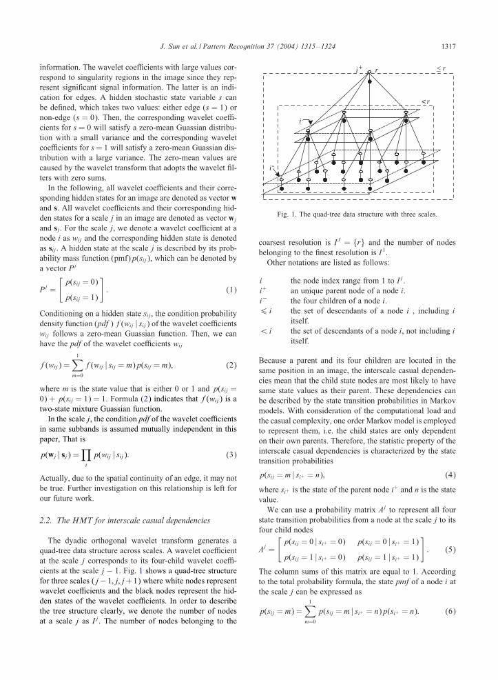
The dyadic orthogonal wavelet transform generates aquad-tree data structure across scales. A wavelet coe5cientat the scale j corresponds to its four-child wavelet coe5-cients at the scale j − 1. Fig. 1 shows a quad-tree structurefor three scales (j−1; j; j+1) where white nodes representwavelet coe5cients and the black nodes represent the hid-den states of the wavelet coe5cients. In order to describethe tree structure clearly, we denote the number of nodesat a scale j as I j . The number of nodes belonging to the

-

+ r r<

r<

i

i

_

i

Fig. 1. The quad-tree data structure with three scales.

coarsest resolution is I J = {r} and the number of nodesbelonging to the >nest resolution is I 1.

Other notations are listed as follows:

i the node index range from 1 to I j .i+ an unique parent node of a node i.i− the four children of a node i.6 i the set of descendants of a node i , including i

itself.¡i the set of descendants of a node i, not including i

itself.

Because a parent and its four children are located in thesame position in an image, the interscale casual dependen-cies mean that the child state nodes are most likely to havesame state values as their parent. These dependencies canbe described by the state transition probabilities in Markovmodels. With consideration of the computational load andthe casual complexity, one order Markov model is employedto represent them, i.e. the child states are only dependenton their own parents. Therefore, the statistic property of theinterscale casual dependencies is characterized by the statetransition probabilities

p(sij = m | si+ = n); (4)

where si+ is the state of the parent node i+ and n is the statevalue.

We can use a probability matrix Aj to represent all fourstate transition probabilities from a node at the scale j to itsfour child nodes

Aj =

[p(sij = 0 | si+ = 0) p(sij = 0 | si+ = 1)

p(sij = 1 | si+ = 0) p(sij = 1 | si+ = 1)

]: (5)

The column sums of this matrix are equal to 1. Accordingto the total probability formula, the state pmf of a node i atthe scale j can be expressed as

p(sij = m) =1∑

m=0

p(sij = m | si+ = n)p(si+ = n): (6)

1318 J. Sun et al. / Pattern Recognition 37 (2004) 1315–1324

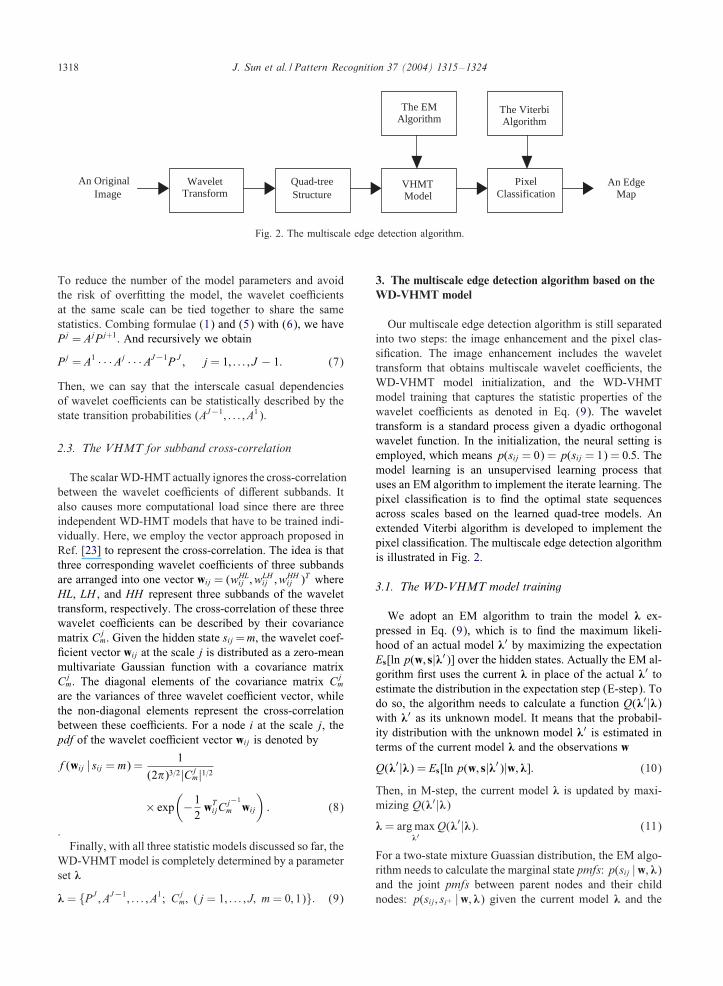
An OriginalImage

WaveletTransform

Quad-treeStructure

VHMTModel

PixelClassification

An EdgeMap

The EMAlgorithm

The ViterbiAlgorithm

Fig. 2. The multiscale edge detection algorithm.

To reduce the number of the model parameters and avoidthe risk of over>tting the model, the wavelet coe5cientsat the same scale can be tied together to share the samestatistics. Combing formulae (1) and (5) with (6), we havePj = AjPj+1. And recursively we obtain

Pj = A1 · · ·Aj · · ·AJ−1P J ; j = 1; : : : ; J − 1: (7)

Then, we can say that the interscale casual dependenciesof wavelet coe5cients can be statistically described by thestate transition probabilities (AJ−1; : : : ; A1).

2.3. The VHMT for subband cross-correlation

The scalarWD-HMT actually ignores the cross-correlationbetween the wavelet coe5cients of diFerent subbands. Italso causes more computational load since there are threeindependent WD-HMT models that have to be trained indi-vidually. Here, we employ the vector approach proposed inRef. [23] to represent the cross-correlation. The idea is thatthree corresponding wavelet coe5cients of three subbandsare arranged into one vector wij = (wHL

ij ; wLHij ; wHH

ij )T whereHL, LH , and HH represent three subbands of the wavelettransform, respectively. The cross-correlation of these threewavelet coe5cients can be described by their covariancematrix Cj

m. Given the hidden state sij =m, the wavelet coef->cient vector wij at the scale j is distributed as a zero-meanmultivariate Gaussian function with a covariance matrixCj

m. The diagonal elements of the covariance matrix Cjm

are the variances of three wavelet coe5cient vector, whilethe non-diagonal elements represent the cross-correlationbetween these coe5cients. For a node i at the scale j, thepdf of the wavelet coe5cient vector wij is denoted by

f(wij | sij = m) =1

(2�)3=2|Cjm|1=2

× exp(−12wT

ijCj−1

m wij

): (8)

.Finally, with all three statistic models discussed so far, the

WD-VHMTmodel is completely determined by a parameterset [

[ = {PJ ; AJ−1; : : : ; A1; Cjm; (j = 1; : : : ; J; m = 0; 1)}: (9)

3. The multiscale edge detection algorithm based on theWD-VHMT model

Our multiscale edge detection algorithm is still separatedinto two steps: the image enhancement and the pixel clas-si>cation. The image enhancement includes the wavelettransform that obtains multiscale wavelet coe5cients, theWD-VHMT model initialization, and the WD-VHMTmodel training that captures the statistic properties of thewavelet coe5cients as denoted in Eq. (9). The wavelettransform is a standard process given a dyadic orthogonalwavelet function. In the initialization, the neural setting isemployed, which means p(sij = 0) = p(sij = 1) = 0:5. Themodel learning is an unsupervised learning process thatuses an EM algorithm to implement the iterate learning. Thepixel classi>cation is to >nd the optimal state sequencesacross scales based on the learned quad-tree models. Anextended Viterbi algorithm is developed to implement thepixel classi>cation. The multiscale edge detection algorithmis illustrated in Fig. 2.

3.1. The WD-VHMT model training

We adopt an EM algorithm to train the model [ ex-pressed in Eq. (9), which is to >nd the maximum likeli-hood of an actual model [′ by maximizing the expectationEs[lnp(w; s|[′)] over the hidden states. Actually the EM al-gorithm >rst uses the current [ in place of the actual [′ toestimate the distribution in the expectation step (E-step). Todo so, the algorithm needs to calculate a function Q([′|[)with [′ as its unknown model. It means that the probabil-ity distribution with the unknown model [′ is estimated interms of the current model [ and the observations w

Q([′|[) = Es[lnp(w; s|[′)|w; []: (10)

Then, in M-step, the current model [ is updated by maxi-mizing Q([′|[)[ = argmax

[′Q([′|[): (11)

For a two-state mixture Guassian distribution, the EM algo-rithm needs to calculate the marginal state pmfs: p(sij |w; [)and the joint pmfs between parent nodes and their childnodes: p(sij ; si+ |w; [) given the current model [ and the

J. Sun et al. / Pattern Recognition 37 (2004) 1315–1324 1319

observation w in E-step. In M-step, these probabilities areused to update [′. The Baum–Welch algorithm can be usedto calculate p(sij |w; [) and p(sij ; si+ |w; [) [13,24]. Then,we can use the following formulas to update the model pa-rameters:

p(sj = m) =1I j

∑i

p(sij = m |wj ; [);

p(sij = m | si+ = n) =p(sij = m; si+ = n |wj ; [)

I jp(si+ = n);

�jm =

1I jp(sj = m)

∑i

wijp(sij = m |wj ; [);

Cjm =

1I jp(sj = m)

∑i

�ijm�Tijmp(sij = m |wj ; [); (12)

where

�ijm = [wHLij − �j

m; wLHij − �j

m; wHHij − �j

m]T :

3.2. The pixel classi;cation

After the WD-VHMT model [ is obtained, the followingproblem is how to >nd the optimal states for the waveletcoe5cients. According to the MAP rule and the conditionalindependence of the wavelet coe5cients (3), the pixel clas-si>cation based on the WD-VHMT model can be describedas

Qs = argmaxs

p6J (s |w; [) = argmaxs

p6J (s;w | [): (13)

That is, given an observation vectorw and amodel parameterset [, to >nd the most likely state path Qs across the quad-tree.We extend the Viterbi algorithm to implement Eq. (13) bystarting from the bottom of the quad-tree (j=1) to the top ofthe quad-tree (j= J ) based on the dynamical programming.The algorithm is non-iterative and requires two sweeps onthe quad-tree.

Further simplifying Eq. (13) yields

maxs

p6J (s;w | [)

=maxs6r

p6J (s6r ;w6r | [);

=maxsr

{pJ (sr ;wr | [)max

s¡rp¡J (s¡r;w¡r | Qsr ; [)

};

=pJ ( Qsr ;wr | [)

×{∏

r−maxs6r−

p¡J (s6r− ;w6r− | Qsr ; [)}

; (14)

where Qsr = argmaxsr

pJ (sr ;wr |[). We can de>ne the second

item in Eq. (14) as a function �j(si+) associated with thescale j in order to sweep across the entire trees

�j(si+) = maxs6i

p6j(s6i ;w6i | si+ ; [): (15)

Then, the following iterative equation is obtained accordingto Eq. (14)

�j(si+) = maxsi

{pj(si;wi | si+ ; [)

∏i−

�j−1(si)

}: (16)

The hidden states can be found by

’j(si+) = argmaxi

�(si+): (17)

The extended Viterbi algorithm works in two sweepsacross the quad-tree: an UP procedure going from the >neresolution to the coarse resolution to calculate Eqs. (16) and(17) and a DOWN procedure going from the coarse resolu-tion to the >ne resolution to >nd Qs. The complete procedurescan be stated as follows:

(1) UP procedure:(a) Initialization (j = 1; i∈ I 1):

�1(si+) = maxsi

{f(wi1 | si1; [)p(si1 | si+)}; (18)

’1(si+) = argmaxsi

�1(si+): (19)

(b) Recursion (j = 2; : : : ; J − 1; i∈ I j):

�j(si+) = maxsi

{p(sij ;wij | si+ ; [)

×∏i−

�j−1(si)

}; (20)

’j(si+) = argmaxsi

�j(si+): (21)

(2) DOWN procedure:(a) Initialization (j = J; i∈ I J ):

Qsr = argmaxsr

f(wrJ | srJ )p(srJ )∏r−

�¡J (sr−); (22)

(b) Recursion (j = J − 1; J − 2; : : : ; 1):

Qsi = argmaxsi

’j( Qsi+): (23)

3.3. The algorithm implementation

Our multiscale edge detection algorithm is shown in Fig.2. In the >rst step, we used the Haar wavelet to transformimages since the Haar wavelet is orthogonal and linear inphase. Its 2-D >lters include a low-pass >lter and threehigh-pass >lters. The low-pass >lter is the scale (smooth-ing) >lter: hLL = 1

2

[ 11

11

]. The high-pass >lters are the ver-

tical wavelet >lter: gHL = 12

[11

−1−1

], the horizontal wavelet

>lter: gLH = 12

[1−1

1−1

], and the diagonal wavelet >lter:

gHH = 12

[−11

1−1

].

The dyadic orthogonal wavelet transform is decimatedand characterizes original images only down to the >nestresolution level of 2× 2 pixel window. The edge detection

1320 J. Sun et al. / Pattern Recognition 37 (2004) 1315–1324

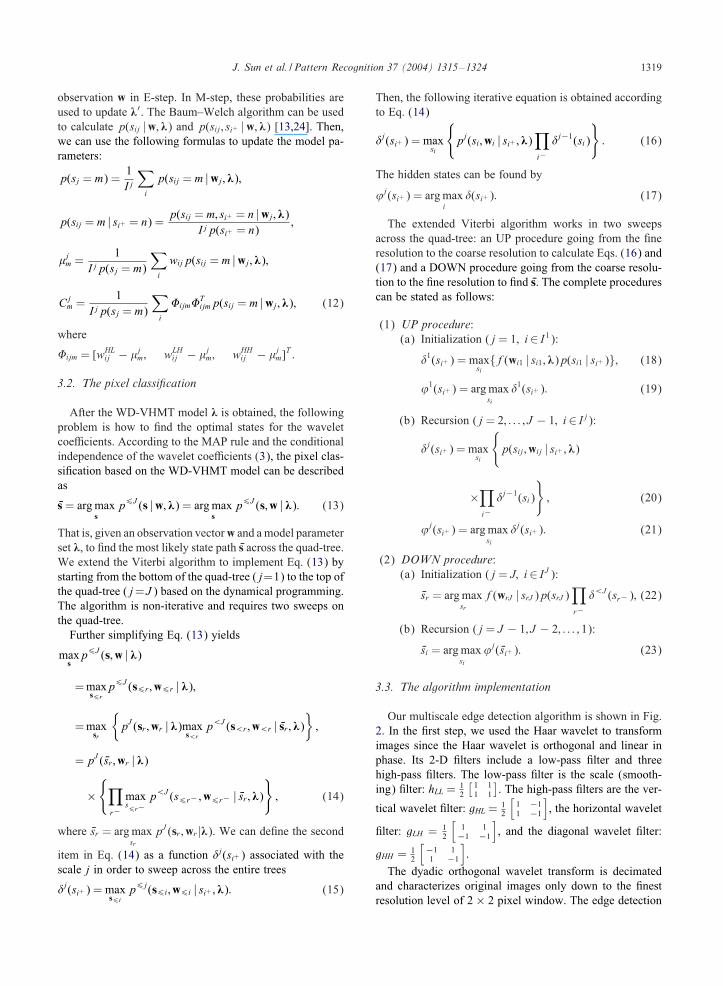
Fig. 3. Two 256× 256× 8 original images.

at the pixel resolution level cannot be directly obtained.To solve the problem, we employed non-decimated wavelettransform to get an enhanced image at the pixel resolutionlevel and regarded it as the lowest level of the quad-treedata structure in the WD-VHMTmodel. Then, the >nal edgemap can be detected at the pixel resolution level.

The extended Viterbi algorithm is the third step in Fig. 2.It starts from the root nodes of the quad-tree and descendsto the leaves of the tree in order to combine all coarse scaleinformation. However, at very coarse scales, the likelihoodof the wavelet coe5cients does not contain signi>cant in-formation because the pixels at very coarse resolution cor-respond to large regions of the pixels at the >nest resolution.To use very coarse scales would lead to appearance of theedge blocks. Therefore, it is reasonable to use the limitednumber of scales. The scale number J can be set such thatan image with size 2J × 2J at the scale J contains enoughinformation about edges.

4. Experiment results

In our experiments, two 256× 256× 8 images shown inFig. 3 were >rst used to test our algorithm. Then, the com-parisons with a Guassian pyramid edge detection algorithmand a Canny edge detection algorithm were made to evalu-ate our algorithm. A personal computer with CPU 550 MHz

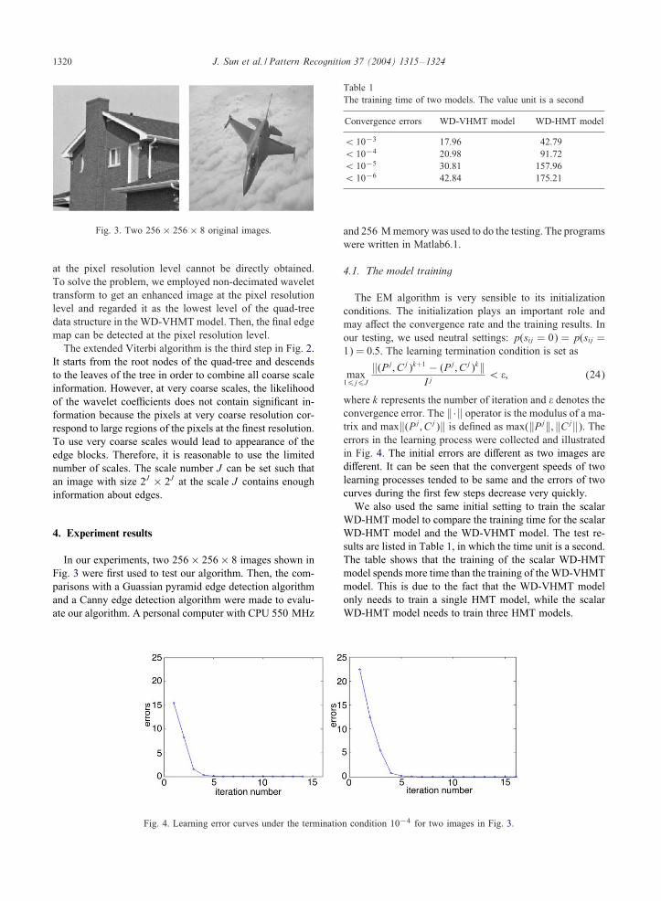
Fig. 4. Learning error curves under the termination condition 10−4 for two images in Fig. 3.

Table 1The training time of two models. The value unit is a second

Convergence errors WD-VHMT model WD-HMT model

¡ 10−3 17.96 42.79¡ 10−4 20.98 91.72¡ 10−5 30.81 157.96¡ 10−6 42.84 175.21

and 256 Mmemory was used to do the testing. The programswere written in Matlab6.1.

4.1. The model training

The EM algorithm is very sensible to its initializationconditions. The initialization plays an important role andmay aFect the convergence rate and the training results. Inour testing, we used neutral settings: p(sij = 0) = p(sij =1) = 0:5. The learning termination condition is set as

max16j6J

‖(Pj; Cj)k+1 − (Pj; Cj)k‖I j

¡ ; (24)

where k represents the number of iteration and denotes theconvergence error. The ‖·‖ operator is the modulus of a ma-trix and max‖(Pj; Cj)‖ is de>ned as max(‖Pj‖; ‖Cj‖). Theerrors in the learning process were collected and illustratedin Fig. 4. The initial errors are diFerent as two images arediFerent. It can be seen that the convergent speeds of twolearning processes tended to be same and the errors of twocurves during the >rst few steps decrease very quickly.

We also used the same initial setting to train the scalarWD-HMT model to compare the training time for the scalarWD-HMT model and the WD-VHMT model. The test re-sults are listed in Table 1, in which the time unit is a second.The table shows that the training of the scalar WD-HMTmodel spends more time than the training of the WD-VHMTmodel. This is due to the fact that the WD-VHMT modelonly needs to train a single HMT model, while the scalarWD-HMT model needs to train three HMT models.

J. Sun et al. / Pattern Recognition 37 (2004) 1315–1324 1321

Fig. 5. Edge maps obtained by our algorithm: (a) and (b) are the edge maps obtained in three diFerent scales; (c) and (d) are the >nal edgemaps at the pixel resolution level.

Fig. 6. Three edge maps for the house image with three diFerent training termination conditions: (a) the error is under 10−3, (b) the erroris under 10−5, and (c) the error is under 10−6.

4.2. Our algorithm results

With the learnedmodels whose convergence error is 10−4,the extended Viterbi algorithm was used to detect edges. Theresults obtained by our algorithms are illustrated in Fig. 5.The number of the wavelet decomposition scale is 4. Figs.5(a) and (b) are the edge maps obtained in three diFerentscales. Figs. 5(c) and (d) are the >nal edge maps at thepixel resolution level, which result from the fusion of theinformation in Figs. 5(a) and (b).

The >nal edge maps with other three diFerent trainingtermination conditions listed in Table 1 are presented in Fig.6. The number of the wavelet decomposition scale is still4. Three edge maps in Fig. 6 shows when the accuracy ofthe training is high enough (¡ 10−3), the edge maps tendto have the same results.

We also investigate the eFectiveness of the number of thewavelet decomposition scales on our algorithm. Figs. 5(c)and (d) are the edge maps with the decomposition scale 4.The results with the decomposition scale 3 and 5 are shownin Fig. 7. The same convergence error 10−4 is used for allthree scales. It can be seen that there are no signi>cant dif-ferences in the edge maps with three diFerent scales. Thereason is that the parameter sets of the WD-VHMT mod-els for diFerent decomposition scales in our algorithm areapproximately same.

4.3. Comparisons with Gaussian pyramid edge detectionalgorithm

The Gaussian pyramid edge detection algorithm is one ofthe traditional structure edge detection algorithms. A com-parison between our algorithm and a Gaussian pyramid edgedetection algorithm was made for the images in Fig. 3. Themultiscale edge detection based on the Gaussian pyramidalgorithms contains three steps: (1) the Gaussian pyramidrepresentation of an original image is obtained by iterativelyusing the Gaussian >lter through downsampling, (2) a Sobeldetector is applied to the image at the coarsest resolution,(3) the algorithm detects the edges at the >ne resolutionguided by the edge information at the coarser resolution.This process continues down through the pyramid represen-tation until the edges in the original image are discovered.

The results of this Gaussian pyramid edge detection al-gorithm are shown in Fig. 8 with three scales. A simplethreshold operation is used to identify the edges. In Fig. 8,we can see that the edge maps are dependent on the scales.Due to no multiscale information fusion, the edge informa-tion is signi>cantly reduced when the scale is increased. Incontrast, our results in Fig. 5 (scale 4) and in Fig. 7 (scales3 and 5) have no such problem. The main reason is thatour algorithm fuses the multiscale information and takes thecausal dependencies of wavelet coe5cients into account.

1322 J. Sun et al. / Pattern Recognition 37 (2004) 1315–1324

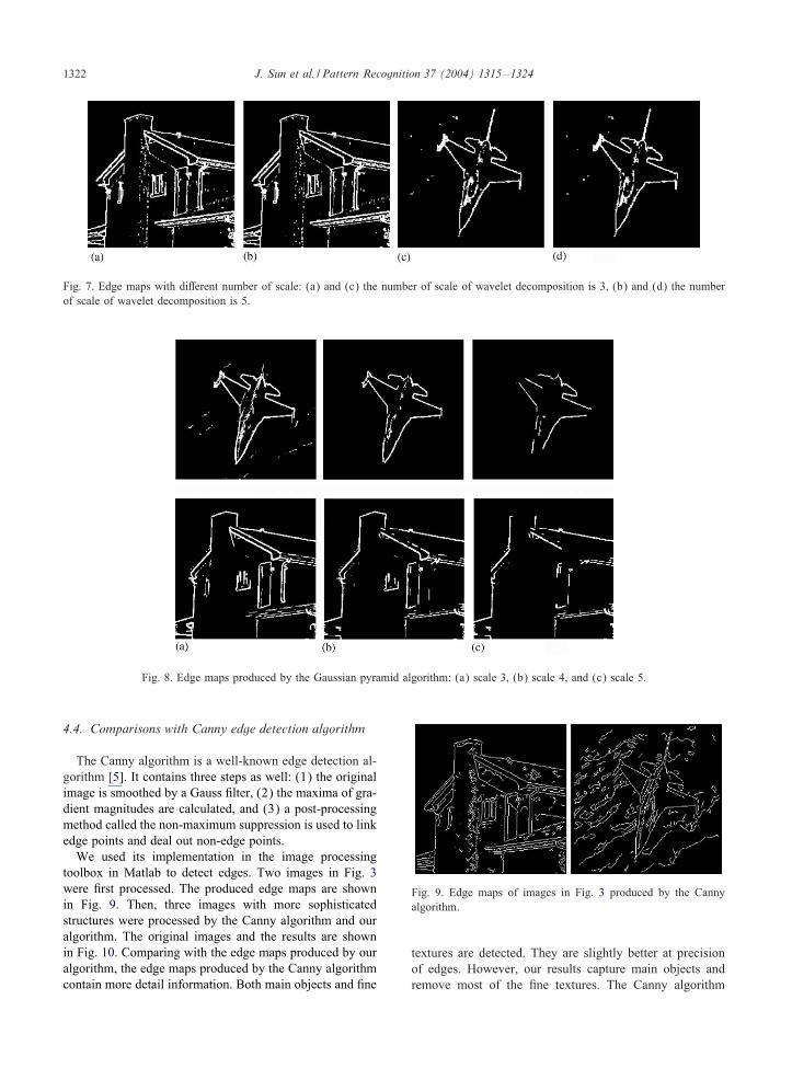
Fig. 7. Edge maps with diFerent number of scale: (a) and (c) the number of scale of wavelet decomposition is 3, (b) and (d) the numberof scale of wavelet decomposition is 5.

Fig. 8. Edge maps produced by the Gaussian pyramid algorithm: (a) scale 3, (b) scale 4, and (c) scale 5.

4.4. Comparisons with Canny edge detection algorithm

The Canny algorithm is a well-known edge detection al-gorithm [5]. It contains three steps as well: (1) the originalimage is smoothed by a Gauss >lter, (2) the maxima of gra-dient magnitudes are calculated, and (3) a post-processingmethod called the non-maximum suppression is used to linkedge points and deal out non-edge points.

We used its implementation in the image processingtoolbox in Matlab to detect edges. Two images in Fig. 3were >rst processed. The produced edge maps are shownin Fig. 9. Then, three images with more sophisticatedstructures were processed by the Canny algorithm and ouralgorithm. The original images and the results are shownin Fig. 10. Comparing with the edge maps produced by ouralgorithm, the edge maps produced by the Canny algorithmcontain more detail information. Both main objects and >ne

Fig. 9. Edge maps of images in Fig. 3 produced by the Cannyalgorithm.

textures are detected. They are slightly better at precisionof edges. However, our results capture main objects andremove most of the >ne textures. The Canny algorithm

J. Sun et al. / Pattern Recognition 37 (2004) 1315–1324 1323

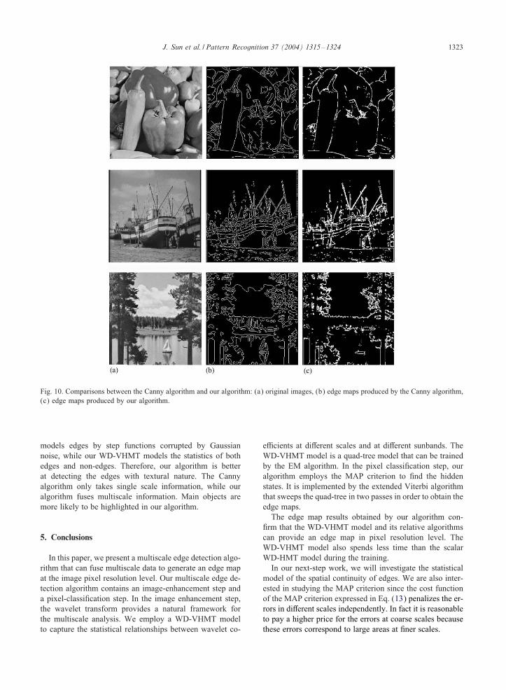
Fig. 10. Comparisons between the Canny algorithm and our algorithm: (a) original images, (b) edge maps produced by the Canny algorithm,(c) edge maps produced by our algorithm.

models edges by step functions corrupted by Gaussiannoise, while our WD-VHMT models the statistics of bothedges and non-edges. Therefore, our algorithm is betterat detecting the edges with textural nature. The Cannyalgorithm only takes single scale information, while ouralgorithm fuses multiscale information. Main objects aremore likely to be highlighted in our algorithm.

5. Conclusions

In this paper, we present a multiscale edge detection algo-rithm that can fuse multiscale data to generate an edge mapat the image pixel resolution level. Our multiscale edge de-tection algorithm contains an image-enhancement step anda pixel-classi>cation step. In the image enhancement step,the wavelet transform provides a natural framework forthe multiscale analysis. We employ a WD-VHMT modelto capture the statistical relationships between wavelet co-

e5cients at diFerent scales and at diFerent sunbands. TheWD-VHMT model is a quad-tree model that can be trainedby the EM algorithm. In the pixel classi>cation step, ouralgorithm employs the MAP criterion to >nd the hiddenstates. It is implemented by the extended Viterbi algorithmthat sweeps the quad-tree in two passes in order to obtain theedge maps.

The edge map results obtained by our algorithm con->rm that the WD-VHMT model and its relative algorithmscan provide an edge map in pixel resolution level. TheWD-VHMT model also spends less time than the scalarWD-HMT model during the training.

In our next-step work, we will investigate the statisticalmodel of the spatial continuity of edges. We are also inter-ested in studying the MAP criterion since the cost functionof the MAP criterion expressed in Eq. (13) penalizes the er-rors in diFerent scales independently. In fact it is reasonableto pay a higher price for the errors at coarse scales becausethese errors correspond to large areas at >ner scales.

1324 J. Sun et al. / Pattern Recognition 37 (2004) 1315–1324

Acknowledgements

The authors wish to thank the anonymous reviewersfor their constructive comments and suggestions whichimproved the quality of this paper.

References

[1] V. Torre, T.A. Poggio, On edge detection, IEEE Trans. PatternAnal. Mach. Intell. 8 (2) (1986) 147–163.

[2] T. Aydin, Y. Yemez, E. Anarim, B. Sankur, Multidirectionaland multiscale edge detection via M-band wavelet transform,IEEE Trans. Image Process. 5 (9) (1996) 1371–1377.

[3] D. Ziou, S. Tabbone, Edge Detection Techniques-An Over-view, Technical Report No. 195, Department of Mathematicsand Informatique, Universit de Sherbrooke, 1997.

[4] B. Gunsel, E. Panayirci, A.K. Jain, Boundary detectionusing multiscale Markov random >elds pattern recognition,Proceedings of the 12th International Conference on ComputerVision and Image Processing, Jerusalem, Israel, Vol. 2, 1994,pp. 173–177.

[5] J. Canny, A computational approach to edge detection, IEEETrans. Pattern Anal. Mach. Intell. 8 (6) (1986) 679–698.

[6] D. Marr, E.C. Hildreth, Theory of edge detection, Proc. R.Soc. London B207 (1980) 187–217.

[7] Y. Lu, R.C. Jain, Reasoning about edges in scale space, IEEETrans. Pattern Anal. Mach. Intell. 14 (4) (1992) 450–468.

[8] S. Mallat, S. Zhong, Characterization of signals frommultiscale edges, IEEE Trans. Pattern Anal. Mach. Intell. 14(7) (1992) 710–732.

[9] S. Mallat, W.L. Hwang, Singularity detection and processingwith wavelets, IEEE Trans. Inf. Theory 38 (2) (1992)617–643.

[10] S. Mallat, Zero-crossing of a wavelet translation, IEEE Trans.Inf. Theory 37 (4) (1991) 1019–1033.

[11] R.D. Nowak, Multiscale hidden Markov models for Bayesianimage analysis, Technical Report, MSU-ENGR-004-98,Michigan State University, 1998.

[12] M. Crouse, R. Nowak, R. Baraniuk, Wavelet-based statisticalsignal processing using hidden Markov models, IEEE Trans.Signal Process. 4 (6) (1998) 886–902.

[13] L.R. Rabiner, A Tutorial on hidden Markov models andselected applications in speech recognition, Proc. IEEE 77 (2)(1989) 257–285.

[14] J. Romberg, H. Choi, R. Baraniuk, Shift-invariant denoisingusing wavelet-domain hidden Markov Trees, Proceedingsof the 33rd Asilomar Conference on Signals Systems andComputers, Paci>c Grove, CA, October 1999.

[15] J.K. Romberg, H. Choi, R. Baraniuk, Bayesian tree structuredimage modeling using Wavelet-Domain Hidden MarkovModel, Proceedings of SPIE, Vol. 3816, Denver, CO, July1999, pp. 31–44.

[16] H. Choi, R. Baraniuk, Image segmentation using waveletdomain classi>cation, Proceedings of SPIE, Vol. 3816,Denver, CO, July 1999, pp. 306–320.

[17] H. Choi, R. Baraniuk, Multiscale image segmentation usingWavelet-Domain Hidden Markov Models, IEEE Trans. ImageProcess. 10 (9) (2001) 1309–1321.

[18] G. Fan, X. Xia, Wavelet-based statistical image processingusing hidden Markov tree model, Proceedings of theConference on Information Science and Systems, PrincetonUniversity, March 15–17, 2000.

[19] G. Fan, X. Xia, Maximum likelihood texture analysisand classi>cation using Wavelet-Domain Hidden MarkovModels, Proceedings of the 34th Asilomar Conferenceon Signals, Systems and Computers, Vol. 2(2), 2000,pp. 921–925.

[20] J. LafertTe, P. PTerez, F. Heitz, Discrete Markov image modelingand inference on the quad-tree, IEEE Trans. Image Process.9 (3) (2000) 390–404.

[21] E.P. Simoncelli, J. Portilla, Texture characterization via jointstatistics of wavelet coe5cient magnitudes, Proceedings ofIEEE International Conference on Image Processing, Oct 4–7,Chicago, Illinois, 1998.

[22] H. Cheng, C.A. Bouman, Multiscale Bayesian segmentationusing a trainable context model, IEEE Trans. Image Process.10 (4) (2001) 511–525.

[23] M.N. Do, A.C. Lozano, M. Vetterli, Rotation invarianttexture retrieval using steerable wavelet-domain hiddenMarkov models, Proceedings of SPIE Conference on WaveletApplications in Signal and Image Processing VIII, San Diego,USA, August 2000.

[24] P. Dempster, N.M. Laird, D.B. Rubin, Maximum likelihoodfrom incomplete data via the EM algorithm, J. R. Statist. Soc.39 (Ser. B) (1977) 1–38.

[25] Y. Hou, J. Song, F. Zhou, C. Wen, X. Yang, A new documentsegmentation based on subbands by wavelet domain hiddenMarkov tree model, Chinese J. Electron. 30 (8) (2002)1180–1183.

About the Author—JUNXI SUN received B.Sc. and M.Sc. degrees in electronic engineering in 1995 and 2000 from Changchun Instituteof Optics and Fine Mechanics, China. He is currently a candidate for the Ph.D. degree in biomedical engineering in Shanghai JiaotongUniversity, China. His main research interests include statistical image processing and recognition.

About the Author—DONGBING GU received B.Sc. and M.Sc. degrees in control theory from Beijing Institute of Technology, Chinaand a Ph.D. degree in Changchun University of Science and Technology, China. Since 2000, he has been a lecturer in the department ofcomputer science, University of Essex, UK. His research interests include image processing and autonomous robots.

About the Author—YAZHU CHEN graduated from Shanghai Jiaotong University, China in 1962. Due to her prominent contribution inthe >eld of biomedical engineering, she was elected a member of Chinese Academy of Engineering in 1996. She is currently a professorin biomedical engineering and director of biomedical instrument institute, Shanghai Jiaotong University. Her main research currentlyconcentrates on development of image guided cancer treatment systems using high intensity focused ultrasound.

About the Author—SU ZHANG received a B.Sc. degree from Nanjing Science and Technology University, China in 1990. She received theM.Sc. and Ph.D. degrees in Northwest Polytechnic University, China in 1996 and 2000. She is currently an associate professor in biomedicalengineering, Shanghai Jiaotong University, China and her main research interests include pattern recognition and intelligent system.