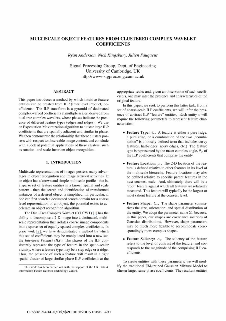
0-7803-9404-6/05/$20.00 ©2005 IEEE 437

MULTISCALE OBJECT FEATURES FROM CLUSTERED COMPLEX WAVELET

COEFFICIENTS

Ryan Anderson, Nick Kingsbury, Julien Fauqueur

Signal Processing Group, Dept. of Engineering

University of Cambridge, UK

http://www-sigproc.eng.cam.ac.uk

ABSTRACT

This paper introduces a method by which intuitive feature

entities can be created from ILP (InterLevel Product) co-

efficients. The ILP transform is a pyramid of decimated

complex-valued coefficients at multiple scales, derived from

dual-tree complex wavelets, whose phases indicate the pres-

ence of different feature types (edges and ridges). We use

an Expectation-Maximization algorithm to cluster large ILP

coefficients that are spatially adjacent and similar in phase.

We then demonstrate the relationship that these clusters pos-

sess with respect to observable image content, and conclude

with a look at potential applications of these clusters, such

as rotation- and scale-invariant object recognition.

1. INTRODUCTION

Multiscale representations of images possess many advan-

tages in object recognition and image retrieval activities. If

an object has a known and simple multiscale profile - that is,

a sparse set of feature entities in a known spatial and scale

pattern - then the search and identification of transformed

instances of a desired object is simplified. In particular, if

one can first search a decimated search domain for a coarse

level representation of an object, the potential exists to ac-

celerate an object recognition algorithm.

The Dual-Tree Complex Wavelet (DT CWT) [1] has the

ability to decompose a 2-D image into a decimated, multi-

scale representation that isolates coarse image components

into a sparse set of equally spaced complex coefficients. In

prior work [2], we have demonstrated a method by which

this set of coefficients may be manipulated into a new set,

the Interlevel Product (ILP). The phases of the ILP con-

sistently represent the type of feature in the spatio-scalar

vicinity, where a feature type may be a step edge or a ridge.

Thus, the presence of such a feature will result in a tight

spatial cluster of large similar-phase ILP coefficients at the

This work has been carried out with the support of the UK Data &

Information Fusion Defence Technology Centre.

appropriate scale; and, given an observation of such coeffi-

cients, one may infer the presence and characteristics of the

original feature.

In this paper, we seek to perform this latter task; from a

set of coarse-scale ILP coefficients, we will infer the pres-

ence of abstract ILP “feature” entities. Each entity c will

require the following parameters to represent feature char-

acteristics:

• Feature Type: θc. A feature is either a pure ridge,

a pure edge, or a combination of the two (“combi-

nation” is a loosely defined term that includes curvy

features, half-ridges, noisy edges, etc.) The feature

type is represented by the mean complex angle, θc, of

the ILP coefficients that comprise the entity.

• Feature Location: µc. The 2-D location of the fea-

ture is defined relative to other features in its level of

the multiscale hierarchy. Feature locations may also

be defined relative to specific parent features in the

next coarsest scale. And, ultimately, there will be a

“root” feature against which all features are relatively

measured. This feature will typically be the largest or

most salient feature at the coarsest level.

• Feature Shape: Σc. The shape parameter summa-

rizes the size, orientation, and spatial distribution of

the entity. We adopt the parameter name Σc because,

in this paper, our shapes are covariance matrices of

Gaussian distributions. However, shape parameters

may be much more flexible to accommodate corre-

spondingly more complex shapes.

• Feature Saliency: αc. The saliency of the feature

refers to the level of contrast of the feature, and cor-

responds to the magnitude of the comprising ILP co-

efficients.

To create entities with these parameters, we will mod-

ify the traditional EM-trained Gaussian Mixture Model to

cluster large, same-phase coefficients. The resultant entities

438

Re

Im

Fig. 1. Relationship between the complex phase of an ILP coef-

ficient in the 15◦ subband and the nature of a ∼15

◦ feature in the

vicinity. Note that this phase-to-feature relationship is constant in

all subbands (with appropriately oriented features).

should not only be robust to multiscale misalignment (dis-

cussed further in [2]), but they should also possess semantic

meaning with regard to visually identifiable image features.

We begin in section 2 with a more detailed description

of the ILP transform with examples; section 3 describes the

modified GMM routine we use, and section 4 shows the re-

sults. We conclude in section 5 with further discussion on

the motivation for this methodology and future work.

2. THE ILP TRANSFORM

For an N × M pixel image, the ILP is a pyramid of L lev-

els, where each level l = 1 . . . L possesses N

2l × M

2l × 6complex coefficients, where the six values at each spatial

location correspond to six directional subbands at 15◦, 45◦,

75◦, 105◦, 135◦, and 165◦; thus, it is identical in dimen-

sion to the DT CWT upon which it is based. It is created by

multiplying the DT-CWT coefficients at the corresponding

location and level l by the complex conjugate of a phase-

doubled, interpolated version of their l + 1 parent coeffi-

cients; this process is outlined in detail in [2].

The phases of DT CWT coefficients are dependent upon

the spatial offset of directional features, and are therefore

unreliable to represent objects consistently. By contrast,

the phases of the ILP are only influenced by the nature of

the feature in the vicinity. Specifically, the relationship of

phase with local feature type is shown in Figure 1; large-

magnitude values that are purely real or purely imaginary

indicate edges and ridges (respectively) that are high-contrast

and ideal. Large magnitude ILP coefficients that possess

both imaginary and real components indicate hybrid fea-

tures (which can include curves, wide ridges, or ridge-edge

combinations), and small magnitude coefficients indicate

areas that are generally flat (where the phase is random and

meaningless).

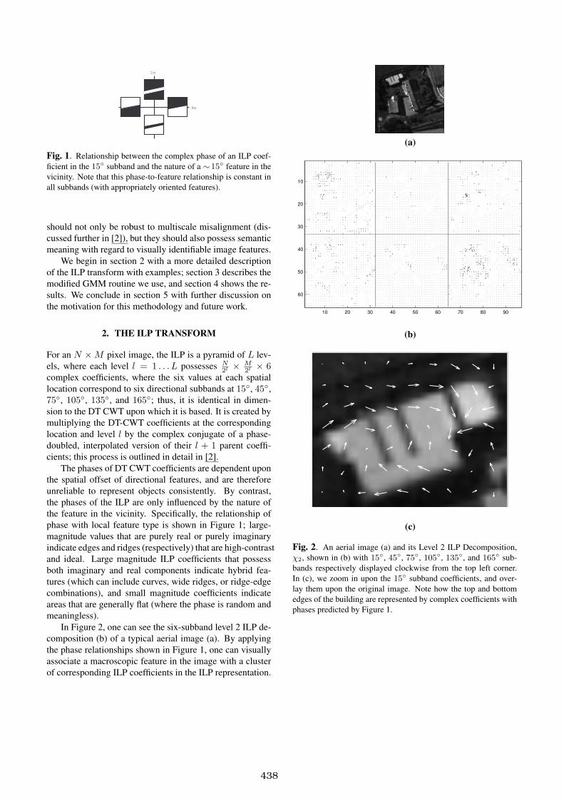
In Figure 2, one can see the six-subband level 2 ILP de-

composition (b) of a typical aerial image (a). By applying

the phase relationships shown in Figure 1, one can visually

associate a macroscopic feature in the image with a cluster

of corresponding ILP coefficients in the ILP representation.

(a)

10 20 30 40 50 60 70 80 90

10

20

30

40

50

60

(b)

(c)

Fig. 2. An aerial image (a) and its Level 2 ILP Decomposition,

χ2, shown in (b) with 15◦, 45

◦, 75◦, 105

◦, 135◦, and 165

◦ sub-

bands respectively displayed clockwise from the top left corner.

In (c), we zoom in upon the 15◦ subband coefficients, and over-

lay them upon the original image. Note how the top and bottom

edges of the building are represented by complex coefficients with

phases predicted by Figure 1.

439

For instance, in (c), one can consider the top edge of the

upper-left white building as an abstract feature that corre-

sponds to the cluster of ILP coefficients that are positive-real

(i.e. pointing to the right) in the corresponding location of

the 15◦ subband. These positive-real coefficients extend not

only along the length of the edge, but are somewhat broad

in the direction normal to the edge as well. This “soften-

ing” of edges and ridges in the ILP domain allows us to use

smooth Gaussian clusters to represent these originally crisp

features, provided that the cluster can be associated with a

complex phase (which would be positive-real, in this case).

3. EM ALGORITHM FOR DIRECTIONAL

CLUSTERING

The Gaussian Mixture Model builds a set of k Gaussian

clusters upon i data points x, where each cluster c = 1 . . . k

is weighted by a value, αc, and possesses the following dis-

tribution:

p(xi|µc, Σc) =1

(2π)d

2 |Σc|1

2

e−

1

2(xi−µc)

TΣ

−1

c(xi−µc) (1)

The parameters µ, Σ, and α are determined through the

iterative Expectation-Maximization algorithm [3] by which

the log likelihood expression

k∑

c=1

N∑

i=1

log(p(xi|µc,Σc))p(c|xi, Θc) (2)

is maximized with respect to each parameter, while all

other parameters remain fixed. We calculate p(c|xi, Θc) us-

ing Bayes’ Rule and αc as a prior, and Θc refers to the com-

plete parameter set {µc, Σc, αc, θc} for all c ∈ k. The up-

date parameters for the αc cluster weights are

αnew

c=

1

N

N∑

i=1

p(c|xi, Θc) (3)

Equation (1) is used to model single-instance data points

at the given xi locations. If we were to imagine that the data

point xi was independently and repeatedly observed in the

same location βi times, the joint probability of this event

can be expressed as

p(xi, βi|µc, Σc) =1

Qi

(p(xi|µc, Σc))βi (4)

where Qi is a normalizing constant. If we allow βi to

take on any positive real value, rather than just integer mul-

tiples, we can also accommodate any data set where indi-

vidual xi locations are weighted by any value of βi.

Our ILP data, however, is a set of continuous complex

ILP coefficients from level l, χl, where xi is the location

of the χ(i)th

lcoefficient, and we need to create a real scalar

value βi,c with respect to cluster c to use Equation (4). Our

clusters must be designed such that the largest adjacent sets

of these coefficients (in the same directional subband) with

similar phase should be clustered together and represented

by their mean phase, θc. Thus, we define βi,c to be the

projection of the χ(i)th

lcoefficient onto a unit vector with

the proposed cluster phase θc:

βi,c = ℜ[

(χ(i)

l)∗ · ejθc

]

(5)

and j =√−1. We can now model these real-valued

projections as βi,c instances of a single-instance data point

at that location. Note, however, that these values will be

negative if the difference between 6 χ(i)

land θc is greater

than 90◦. These negative values cause difficulty with the

convergence of the EM algorithm, and are not perceptually

sensible; we do not necessarily want a clustering algorithm

to over-penalize a region that contains coefficients with op-

posing phase. Thus, we set a lower bound of zero upon βi,c,

which is equivalent to setting the magnitude of opposite-

phase coefficients to zero.

Our expression for p(xi|µc, Σc) has now become

p(xi, βi,c|µc, Σc, θc) =

1

Qi

[

1

(2π)d

2 |Σc|1

2

e−

1

2((xi−µc)

TΣ

−1

c(xi−µc)

]

βi,c

(6)

Inserting these new values into equation (2) produces

the following expression:

k∑

c=1

N∑

i=1

[

log1

Qi

− (7)

βi,c

2

[

log |Σc| + (xi − µc)T Σ−1

c(xi − µc)

]

p(c|xi, Θc)

]

We maximize equation (7) with respect to Σc and µc by

differentiating and setting the result to zero, and solving for

each of these variables. The procedure for determining Σc

and µc is almost identical to the original GMM derivation,

which is explained comprehensively in [4]. The resulting

iterative update equations for Σc and µc are shown below:

µnew

c=

∑

N

i=1βi,cp(c|xi,Θc)xi

∑

N

i=1βi,cp(c|xi, Θc)

Σnew

c=

∑

N

i=1βi,cp(c|xi, Θc)(xi − µnew

c)(xi − µnew

c)T

∑

N

i=1βi,cp(c|xi,Θc)

From our interpretation of βi,c as multiple instances of

a data point at xi, we can see that the update equation for

αnew, equation (3), may be rewritten as

440

αnew

c=

∑

N

i=1βi,cp(c|xi)

∑

N

i=1βi,c

(8)

Note that we have abbreviated p(c|xi, Θc) to p(c|xi) for

brevity in the upcoming equations. For the update equations

of our additional parameter, θc, we show an explicit deriva-

tion below. For simplification, we define

Ki,c = −1

2

(

log |Σc| + (xi − µc)T (Σc)

−1(xi − µc))

(9)

Substituting equations (9) and (5) into equation (7), and

dropping constant terms, our new maximization expression

is

k∑

c=1

N∑

i=1

ℜ[

(χ(i)

l)∗ · ejθc

]

Ki,cp(c|xi) (10)

=k

∑

c=1

N∑

i=1

[

ℜ[χ(i)

l] cos θc + ℑ[χ

(i)

l] sin θc

]

Ki,cp(c|xi)

Differentiating equation (10) with respect to θc and setting

it to zero provides us with

N∑

i=1

[

−ℜ[χ(i)

l] sin θc + ℑ[χ

(i)

l] cos θc

]

Ki,cp(c|xi) = 0

⇒ sin θc

cos θc

=

∑

N

i=1ℑ[χ

(i)

l]Ki,c [p(c|xi)]

∑

N

i=1ℜ[χ

(i)

l]Ki,c [p(c|xi)]

⇒ θnew

c= tan−1

∑

N

i=1ℑ[χ

(i)

l]Ki,c [p(c|xi)]

∑

N

i=1ℜ[χ

(i)

l]Ki,c [p(c|xi)]

(11)

and thus equation (11) is our update equation for θnew

c.

Thus, we have update equations for all of our cluster param-

eters.

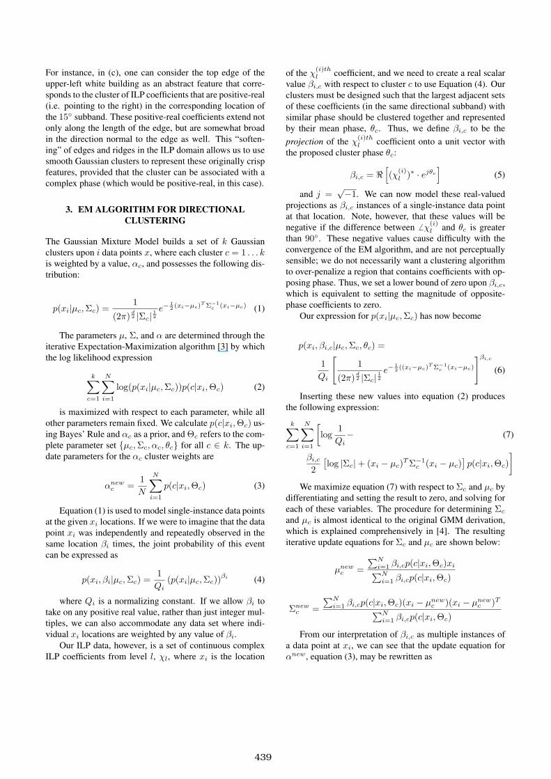
One problem remains with this approach, however, and

it is illustrated in Figure 3. If a coefficient at location xi is

opposite-phase to the nearest cluster c1, its βi,c1value will

be zero, and its “membership” in class c1, represented by

p(c1|xi), will also be zero. Therefore, it will instead have

strong membership in the next closest similar-phase class,

c2, regardless of the distance between xi and µc2. As a re-

sult, the covariance matrix Σc2will expand inappropriately

to include xi, and µc2will be biased. To prevent this effect,

we alter βi,c to disregard phase differences for the purpose

of membership calculation only:

˜βi,c = |χ(i)

l| (12)

Our likelihood expression for membership calculation is

now

Fig. 3. A demonstration of the shortcomings of the “pure” EM

procedure described above. In this two-cluster example, the high-

lighted coefficient near the bottom of the left cluster (c1) actually

has 100% membership in the right cluster (c2), due to its phase. As

a result, cluster c2 expands inappropriately to accommodate this

coefficient, and becomes too large and off-centered. We therefore

use Equations 12-14 to ignore phase as a factor in cluster member-

ship.

p̃(xi, βi,c|µc, Σc, θc) =

1

Qi

[

1

(2π)d

2 |Σc|1

2

e−

1

2((xi−µc)

TΣ

−1

c(xi−µc)

]

β̃i,c

(13)

And, from Bayes’ Rule, the resulting expression for the

membership function is now

p(c|xi) =p̃(xi, βi,c|µc,Σc, θc) · αc

∑

k

d=1p̃(xi, βi,d|µd, Σd, θd) · αd

(14)

With this membership function, we ensure that our clus-

ters remain relatively compact, although we cannot guaran-

tee homogeneity in phase.

We initialize the parameter values of each cluster to have

θ0

c= 0◦, α0

c= 1

k, and Σ0

c= I . Initial values for µ0

c

are established by using a non-maximal suppression algo-

rithm based on the magnitudes of the ILP coefficients, with

a radius of suppression that decreases until k well-separated

peaks are identified.

4. RESULTS

In Figure 4, we see the ILP coefficients of Figure 2 clustered

with 10 coefficients per subband. Note that clusters are de-

veloped for each subband independently; there is no interac-

tion between subbands in the clustering procedure. As with

all clustering algorithms, determining the number of clus-

ters that are required to effectively represent image features

is an important aspect, and work will continue in this area.

For this example, iterations continue until all cluster means

441

Fig. 4. Trained Gaussian clusters, 10 per subband, to represent

the data shown in Figure 2. The angle of the arrow in each cluster

represents the ILP direction θc, and the magnitude represents αc,

the relative weight of the cluster.

and complex directions shift less than 0.1 samples and 0.1

radians between iterations.

Our ILP clustering technique has been used upon several

aerial images with varying degrees of success. Predictably,

its greatest successes occur on images with clear structural

components; that is, images containing objects with domi-

nant, well-spaced multiscale edges and ridges. As one may

expect, random textures and flat areas are difficult to cluster

into sparse feature representations, and ILP clusters should

accordingly be used only to represent objects and areas that

are defined by their shapes, rather than their textures.

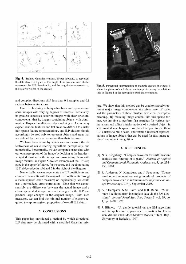
We have two criteria by which we can measure the ef-

fectiveness of our clustering algorithm: perceptually, and

numerically. Perceptually, we can compare cluster data with

our own perception of the image by looking at the heaviest-

weighted clusters in the image and associating them with

image features; in Figure 5, we see examples of the 15◦ step

edge in the upper left farm, for instance, and the dominating

135◦ ridge-edge in subband 5 in the right of the diagram.

Numerically, we can regenerate the ILP coefficients and

compare the results with the original ILP coefficients through

a mean-squared error measure; or, equivalently, we could

use a normalized cross-correlation. Note that we cannot

sensibly use differences between the actual image and a

cluster-generated image, as small changes in the ILP can

produce large changes in the original image. With such

measures, we can find the minimal number of clusters re-

quired to capture a given proportion of overall ILP data.

5. CONCLUSIONS

This paper has introduced a method by which directional

ILP data may be clustered with a modified Gaussian mix-

Fig. 5. Perceptual interpretation of example clusters in Figure 4,

where the phases of each cluster are interpreted using the relation-

ship in Figure 1 at the appropriate subband orientation.

ture. We show that this method can be used to sparsely rep-

resent major image components at a given level of scale,

and the parameters of these clusters have clear perceptual

meaning. By reducing image content into this sparse for-

mat, we are able to perform fast searches for various per-

mutations and affine transformations of a desired object, in

a decimated search space. We therefore plan to use these

ILP clusters to build scale- and rotation-invariant represen-

tations of image objects that can be used for fast image re-

trieval and object recognition.

6. REFERENCES

[1] N.G. Kingsbury, “Complex wavelets for shift invariant

analysis and filtering of signals,” Journal of Applied

and Computational Harmonic Analysis, no. 3, pp. 234–

253, 2001.

[2] R. Anderson, N. Kingsbury, and J. Fauqueur, “Coarse

level object recognition using interlevel products of

complex wavelets,” in International Conference on Im-

age Processing (ICIP) , September 2005.

[3] A.P. Dempster, N.M. Laird, and D.B. Rubin, “Maxi-

mum likelihood from incomplete data via the EM algo-

rithm,” Journal Royal Stat. Soc., Series B, vol. 39, no.

1, pp. 1–38, 1977.

[4] J. Blimes, “A gentle tutorial on the EM algorithm

and its application to parameter estimation for Gaus-

sian Mixture and Hidden Markov Models.,” Tech. Rep.,

University of Berkeley, 1997.

442