ADAPTIVE ATTRIBUTE-BASED ROUTING IN CLUSTERED WIRELESS SENSOR NETWORKS

'

&

$

%

ADAPTIVE ATTRIBUTE-BASED ROUTING IN

CLUSTERED WIRELESS SENSOR NETWORKS

WANG KE

Dissertation submitted in partial fulfillment

of the requirements for the degree of

Doctor of Philosophy

BOSTON

UNIVERSITY

BOSTON UNIVERSITY

COLLEGE OF ENGINEERING

Dissertation



by

WANG KE

E. E., University of Campinas, 1995M. S., Columbia University, 1998

Submitted in partial fulfillment of the

requirements for the degree of

Doctor of Philosophy

2006

Approved by

First Reader

Thomas D. C. Little, Ph.D.Professor of Electrical and Computer Engineering

Second Reader

Jeffrey Carruthers, Ph.D.Associate Professor of Electrical and Computer Engineering

Third Reader

Venkatesh Saligrama, Ph.D.Associate Professor of Electrical and Computer Engineering

Fourth Reader

Murat Alanyali, Ph.D.Assistant Professor of Electrical and Computer Engineering

Acknowledgments

I would like to thank first my advisor Prof. Thomas D. C. Little, without whose

support and acceptance I would not have been able to even embark in this long

journey. His support and patience while I explored different paths along the road

helped me mature into someone who can determine his own research direction and

goals. I am indebted to my former colleague, Prithwish Basu, who taught me the

nitty gritty details of how to be a PhD student. His going forth ahead of me helped

me see how the road can be trodden. My colleagues Salma Abu Ayyash and Ashish

Aggarwal contributed in discussion, ideas and encouragement as fellow sojourners.

I am deeply indebted to my parents, without whose daily love, support and

encouragement I would not have been able to take any steps in life, much less in this

doctorate program. I am deeply thankful to all my brothers and sisters in Christ in

my church. They are the family I have found in this foreign land, who made me feel

at home, and have been with me ever since I arrived here as a young, inexperienced

and immature graduate student. Their love helped me grow as a person, and for

that I am deeply indebted. I want to thank my fiance, for joining me in this journey,

for being with me while I finish this degree, for sharing the burden with me. I want

to thank my brother and sister-in-law, who have always encouraged me and often

invited me to their home. Last but not least, I want to thank my Lord Jesus Christ,

who is the true source of all the blessings in my life, whose gift of love and eternal life

is the only unfathomable wonder that can never be understood nor described even if

untold numbers of dissertations were written in the subject, but whose reality is the

giver of everlasting meaning to all things.

This dissertation is based upon work supported by the National Science Founda-

tion under Grant No. ANI-0073843 and No. CNS-0435353. I thank them for their

support. Any opinions, findings, and conclusions or recommendations expressed in

iii

this material are those of the author and do not necessarily reflect the views of the

National Science Foundation.

iv



(Order No. )

WANG KE

Boston University, College of Engineering, 2006

Major Professor: Thomas D. C. Little, Ph.D.,Professor of Electrical and Computer Engineer-ing

ABSTRACT

Technological advances make the existence of extremely large wireless sensor net-

works (WSNET) with multiple sensing capabilities a reality to be considered. Such

networks may be deployed incrementally by potentially different owners, with no

single addressing system guarantees. Moreover, multiple small tasks, each requiring

a fraction of the network’s resources, may be presented to the whole WSNET. Like-

wise, larger, unforeseen applications may be tasked to multiple smaller networks that

had been deployed for different goals. It is thus essential that the underlying routing

mechanism be selective enough to propagate data only to relevant parts of the net-

work, and adaptive enough to offer services that can conciliate different addressing

needs and meets different application level communication requirements.

It is shown in this dissertation that an attribute based routing scheme meets the

demands above. A hierarchy of clusters is overlaid on the network, based on a set

v

of attributes that reflect containment and adjacency relationships. Sensors with the

same attribute value are clustered together and elect a leader (the attribute based

router) within the cluster. These routers use cluster member information to route

data to relevant regions in the network. Different hierarchies may be overlaid simul-

taneously, allowing multiple addressing schemes to coexist. Furthermore, packets are

forwarded based on a set of routing rules. These routing rules are specified based on

the cluster hierarchy and present different traversal modes, resulting in different per-

formance levels that can be used to meet different application level communication

needs.

The specification of attribute hierarchies, data structures for routing, algorithms

for cluster formation and maintenance, as well as routing rules sets for tree traversal

mode and mesh traversal mode of the hierarchies are presented in this dissertation. It

is shown through analysis that significant gains over broadcast schemes are achieved

in the presence of high data dissemination request rates in which skewed access pat-

terns exist. Moreover, it is shown through analysis that the performance of tree

based traversal modes surpasses mesh traversal modes in transmission costs for ad-

dress resolution in the worst scenario case, but underperforms when considering the

speed of the resolution process and the path length formed.

vi

Contents

1 Introduction 1

1.1 Problem Description . . . . . . . . . . . . . . . . . . . . . . . . . . . 3

1.2 Solution Overview . . . . . . . . . . . . . . . . . . . . . . . . . . . . 5

1.2.1 Contribution . . . . . . . . . . . . . . . . . . . . . . . . . . . 7

1.2.2 Significance . . . . . . . . . . . . . . . . . . . . . . . . . . . . 8

1.3 Organization of the Dissertation . . . . . . . . . . . . . . . . . . . . . 9

2 Example Application Scenarios 10

2.1 Multiple Logical Domains in a University . . . . . . . . . . . . . . . . 10

2.2 Applications in the Wilderness . . . . . . . . . . . . . . . . . . . . . . 15

2.3 Interconnecting Two Sensor Network Applications . . . . . . . . . . . 17

2.4 Other Examples . . . . . . . . . . . . . . . . . . . . . . . . . . . . . . 19

3 Background and Related Work 24

4 An Attribute Based Routing Scheme For Wireless Sensor Networks 34

4.1 Design . . . . . . . . . . . . . . . . . . . . . . . . . . . . . . . . . . . 35

4.2 Attribute Based Clustering . . . . . . . . . . . . . . . . . . . . . . . . 40

4.2.1 Algorithms for Cluster Formation and Maintenance . . . . . . 43

4.2.2 Routing Between Cluster Leaders . . . . . . . . . . . . . . . . 53

4.3 Rules Based Routing in Clustered WSNET . . . . . . . . . . . . . . . 55

4.3.1 Naming . . . . . . . . . . . . . . . . . . . . . . . . . . . . . . 56

4.3.2 Clustering . . . . . . . . . . . . . . . . . . . . . . . . . . . . . 57

vii

4.3.3 Routing Information Storage . . . . . . . . . . . . . . . . . . . 58

4.3.4 Rules-Based Routing . . . . . . . . . . . . . . . . . . . . . . . 63

5 Performance Evaluation 77

5.1 Example . . . . . . . . . . . . . . . . . . . . . . . . . . . . . . . . . . 77

5.2 Cost Analysis of Data Dissemination in Attribute Hierarchy and Flood-

ing Techniques . . . . . . . . . . . . . . . . . . . . . . . . . . . . . . 80

5.2.1 Analytical Results . . . . . . . . . . . . . . . . . . . . . . . . 82

5.3 Attribute Resolution . . . . . . . . . . . . . . . . . . . . . . . . . . . 91

6 Conclusion and Future Work 108

6.1 Conclusions . . . . . . . . . . . . . . . . . . . . . . . . . . . . . . . . 108

6.2 Future Work . . . . . . . . . . . . . . . . . . . . . . . . . . . . . . . . 110

A Pseudocode for Cluster Formation and Maintenance Algorithms 111

B Attribute Tagging and Representation 122

C Communication Directives 126

Bibliography 131

Vita 139

viii

List of Tables

2.1 Inquiries Addressed to “In-the-nest” Sensors . . . . . . . . . . . . . . 22

5.1 Performance Metrics for different Routing Schemes . . . . . . . . . . 95

ix

List of Figures

1·1 Structure Health Monitoring Sensor Network. Illustration from [1]. . 1

1·2 Habitat Monitoring Sensors. Illustration from [2]. . . . . . . . . . . . 2

1·3 Intrusion Detection and Tracking . . . . . . . . . . . . . . . . . . . . 3

1·4 Different ways for obtaining average temperature of the sensor network. 6

2·1 Attribute hierarchy for postal system sensor deployment on campus . 11

2·2 Attribute hierarchy for logical administrative regions for on campus

sensor deployment . . . . . . . . . . . . . . . . . . . . . . . . . . . . 12

2·3 How packets logically cross different attribute hierarchies. . . . . . . . 13

2·4 How packets physically cross different attribute hierarchies. . . . . . . 14

2·5 Sensors deployed in a forest . . . . . . . . . . . . . . . . . . . . . . . 15

2·6 Connecting two sensor network applications . . . . . . . . . . . . . . 17

2·7 Great Duck Island and two deployed sensor networks . . . . . . . . . 19

2·8 Attribute Hierarchy for Queries to Great Duck Island sensor network 21

4·1 Data and Routing in Networks . . . . . . . . . . . . . . . . . . . . . . 36

4·2 Sensor network supporting a two dimensional data space . . . . . . . 37

4·3 Addresses in a sensor network supporting the two dimensional data

space . . . . . . . . . . . . . . . . . . . . . . . . . . . . . . . . . . . 38

4·4 Addresses in a sensor network translated into a hierarchy of attributes 39

4·5 Different ways for obtaining average temperature of the sensor network. 39

4·6 Examples of Attribute Containment Hierarchies . . . . . . . . . . . . 42

4·7 Finite State Machine for cluster formation . . . . . . . . . . . . . . . 44

x

4·8 Cluster Formation Process. . . . . . . . . . . . . . . . . . . . . . . . . 47

4·9 Attribute Containment based Clustering. . . . . . . . . . . . . . . . . 48

4·10 Finite State Machine for leader rotation . . . . . . . . . . . . . . . . 49

4·11 Finite State Machine for LEADER ALIVE packet exchange with k-hop

neighbors . . . . . . . . . . . . . . . . . . . . . . . . . . . . . . . . . 51

4·12 Finite State Machine for joining existing clusters . . . . . . . . . . . . 52

4·13 Creation and Maintenance of Unicast Routes between Cluster Leaders 54

4·14 Inquiry Routing in C-DAG instances. . . . . . . . . . . . . . . . . . . 55

4·15 Cluster Equivalency . . . . . . . . . . . . . . . . . . . . . . . . . . . . 57

4·16 Graph Structure of an Attribute Hierarchy for Routing. . . . . . . . . 59

4·17 Structures to Index Packets Received Without Attribute Hierarchy. . 61

4·18 Structure to Track Application Cluster Routing Information. . . . . . 62

4·19 Packet format for cluster formation and unicast packets . . . . . . . 73

5·1 Example Network . . . . . . . . . . . . . . . . . . . . . . . . . . . . . 77

5·2 Inquiry propagation when there is: (a) one hierarchy level, (b) two

hierarchy levels, and (c) three hierarchy levels. . . . . . . . . . . . . . 83

5·3 Effect of Rate of Inquiry and Clusterhead Rotation Period on Gains:

2 levels in the Containment Hierarchy . . . . . . . . . . . . . . . . . . 88


3 levels in the Containment Hierarchy . . . . . . . . . . . . . . . . . . 88

5·5 Gain vs. probability for proportional rotation periods : Two levels in

C-DAG . . . . . . . . . . . . . . . . . . . . . . . . . . . . . . . . . . 89


Fair Power Consumption . . . . . . . . . . . . . . . . . . . . . . . . . 91

5·7 Hierarchical view of the clusters and routing schemes . . . . . . . . . 92

xi

5·8 Propagation path for Tree traversal when resolving unknown destina-

tion address . . . . . . . . . . . . . . . . . . . . . . . . . . . . . . . . 97

5·9 Propagation path for Mesh traversal when resolving unknown desti-

nation address . . . . . . . . . . . . . . . . . . . . . . . . . . . . . . . 100

5·10 Memory requirements with increasing number of nodes in the network 102

5·11 Memory requirements vs. Number of Levels in the Hierarchy . . . . . 102

5·12 Expected Maximum Number of Transmissions (NumTxMax) . . . . 103

5·13 NumTxMax vs. Number of Levels in the Hierarchy . . . . . . . . . . 103

5·14 Expected Minimum Number of Transmissions (NumTxMin) . . . . . 104

5·15 NumTxMin vs. Number of Levels in the Hierarchy . . . . . . . . . . 105

5·16 Expected Maximum Number of Hops (NumHopMax) between Source

and Destination . . . . . . . . . . . . . . . . . . . . . . . . . . . . . . 105

5·17 NumHopMax vs. Number of levels in the hierarchy . . . . . . . . . . 106

5·18 Expected Minimum Number of Hops (NumHopMin) between Source

and Destination . . . . . . . . . . . . . . . . . . . . . . . . . . . . . . 106

5·19 NumHopMin vs. Number of levels in the hierarchy . . . . . . . . . . 107

xii

List of Algorithms

1 Tree Traversal within the same attribute Hierarchy. . . . . . . . . . . 70

2 Mesh Traversal within the same attribute Hierarchy. . . . . . . . . . . 71

3 Handling Packets With No Attribute Hierarchy. . . . . . . . . . . . . 72

4 Cluster Formation Algorithm . . . . . . . . . . . . . . . . . . . . . . 112

5 k-neighbor updates - LeaderAlive Packet Management . . . . . . . . 113

6 Leader updates - LeaderUpdate Timer Management . . . . . . . . . 114

7 Rotation Timer Management . . . . . . . . . . . . . . . . . . . . . . 115

8 Successor Send Packet Management . . . . . . . . . . . . . . . . . . 116

9 NewCluster Timer Management . . . . . . . . . . . . . . . . . . . . 116

10 JoinCluster Timer Management . . . . . . . . . . . . . . . . . . . . . 117

11 ClusterInfo Packet Management . . . . . . . . . . . . . . . . . . . . 118

12 CatalogSend Timer Management . . . . . . . . . . . . . . . . . . . . 119

13 CatalogUpdate Timer Management . . . . . . . . . . . . . . . . . . . 119

14 CatalogInfo Timer Management . . . . . . . . . . . . . . . . . . . . 120

15 CatalogTxfer Timer Management . . . . . . . . . . . . . . . . . . . . 120

16 ModifyCH Packet Management . . . . . . . . . . . . . . . . . . . . . 121

xiii

List of Abbreviations

CBCB . . . . . . . . . . . . . Combined Broadcast and Content-Based routing

CBM . . . . . . . . . . . . . Content Based Multicast

C-DAG . . . . . . . . . . . . . Containment Directed Acyclic Graph

CH . . . . . . . . . . . . . Containment Hierarchy

DAG . . . . . . . . . . . . . Directed Acyclic Graph

DDF . . . . . . . . . . . . . Directed Diffusion

DIFS . . . . . . . . . . . . . Distributed Index of Features in Sensor networks

DIM . . . . . . . . . . . . . Distributed Index of Multi-dimensional data

FIB . . . . . . . . . . . . . Forwarding Information Base

GEAR . . . . . . . . . . . . . Geographical and Energy Aware Routing

GHT . . . . . . . . . . . . . Geographical Hash Tables

GPS . . . . . . . . . . . . . Global Positioning System

GPSR . . . . . . . . . . . . . Greedy Perimeter Stateless Routing

HEED . . . . . . . . . . . . . Hybrid Energy-Efficient Distributed

LAN . . . . . . . . . . . . . Local Area Network

LEACH . . . . . . . . . . . . . Low Energy Adaptive Clustering Hierarchy

MD5 . . . . . . . . . . . . . Message Digest 5

NE . . . . . . . . . . . . . North East

NW . . . . . . . . . . . . . North West

xiv

P2P . . . . . . . . . . . . . Peer-to-Peer

SAPF . . . . . . . . . . . . . Simple Active Packet Format

SE . . . . . . . . . . . . . SouthEast

SW . . . . . . . . . . . . . SouthWest

SHA . . . . . . . . . . . . . Secure Hash Algorithm

SINA . . . . . . . . . . . . . Sensor Information Networking Architecture

SRT . . . . . . . . . . . . . Semantic Routing Tree

TBF . . . . . . . . . . . . . Trajectory Based Forwarding

TTDD . . . . . . . . . . . . . Two-Tier Data Dissemination

TTL . . . . . . . . . . . . . Time-To-Live

WSNET . . . . . . . . . . . . . Wireless Sensor Network

xv

1

Chapter 1

Introduction

Figure 1·1: Structure Health Monitoring Sensor Network. Illustra-tion from [1].

Technological advances nowadays endow smaller and smaller electronic devices

with more and more data gathering capabilities [3, 4, 5]. Coupled with networking

capacities, such devices form powerful collaborative information gathering systems

that become the remote “eyes” and “ears” of a large community of users. We call

such systems Sensor Networks. Nodes in the network can sample data and can route

data. Data collection can be performed periodically or triggered by an external event.

Such flexibility allows researchers to obtain data with a precision hitherto unavail-

able that will help them formulate realistic models of the physical environment that

surrounds them. Monitoring of soil conditions may increase agricultural productiv-

2

ity [6]; building structural monitoring (Fig. 1·1) will increase security in areas affected

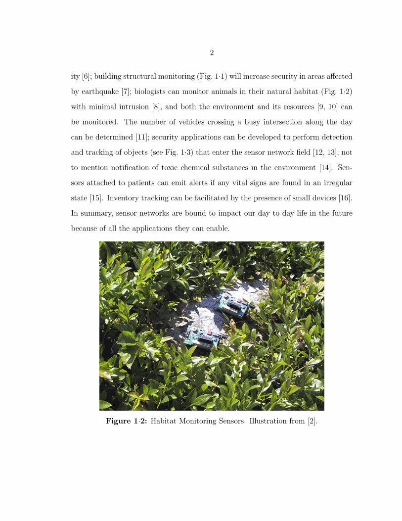
by earthquake [7]; biologists can monitor animals in their natural habitat (Fig. 1·2)

with minimal intrusion [8], and both the environment and its resources [9, 10] can

be monitored. The number of vehicles crossing a busy intersection along the day

can be determined [11]; security applications can be developed to perform detection

and tracking of objects (see Fig. 1·3) that enter the sensor network field [12, 13], not

to mention notification of toxic chemical substances in the environment [14]. Sen-

sors attached to patients can emit alerts if any vital signs are found in an irregular

state [15]. Inventory tracking can be facilitated by the presence of small devices [16].

In summary, sensor networks are bound to impact our day to day life in the future

because of all the applications they can enable.

Figure 1·2: Habitat Monitoring Sensors. Illustration from [2].

3

��

��

��

��

��

��

Path taken byintruder

Deployed sensors��

��

active and track the intruderArea in which sensors become

AB

C

D

E

F

G

H

IJ

K

LM

N

O

P

QR

Figure 1·3: Intrusion Detection and Tracking

1.1 Problem Description

Sensor network applications have thus far been developed monolithically, i.e., sensors

are programmed and deployed for a single task, with all communication paradigms

set for one purpose. In such systems rarely is there a need for addressing any el-

ement beyond the application domain, e.g., a sensor in a temperature monitoring

application needing to route data for an object tracking application. However, with

the decreasing cost of the devices, and the increasing number of sensing capabili-

ties a single device exhibits (i.e., a single mote [4] can sense light, relative humidity,

temperature, pressure and has a 2-axis accelerometer, with the potential of attach-

ing microphones and, with an expansion board [17], even videocameras), a deployed

sensor network has resources that can fulfill multiple tasks.

We envision this ability of multiple task fulfillment as more than reconfiguring all

4

nodes in a single sensor network to perform a second task. It involves sensor networks

deployed for different applications, but which are co-located together, communicating

with each other and cooperating together to perform a larger, previously unforeseen

task. In the same way, it involves a large sensor network deployed initially over a

wide area allocating part of its resources to fulfill an unrelated task requested after

its initial deployment.

Due to this increase in both the sensing capabilities of each sensor and flexibility in

data collection schemes, a wide area sensor network may become a resource shared by

multiple communities across diverse research disciplines, each having different data

requirements and different communication needs. In such scenarios it is extremely

likely that inquiries1 will arrive at high rates but very unlikely that all inquiries

need be propagated to the whole network (reflecting different areas of interest from

the users of the sensor network). Ideally, inquiries should be propagated only to

the sensors that possess relevant information, so as to save bandwidth and conserve

energy, which is a limited resource for battery-operated sensors [5]. Also, sensor

networks deployed at different times for different purposes should be able to exchange

data between them, and the underlying routing mechanism should be adaptive to

support different application-level communication needs that occur due to re-tasking

of sensor networks. Furthermore, the underlying routing mechanism must be able

to scale to a very large number of devices, which is expected for deployed sensor

networks in the future [18, 19]. Support for data-centric models is thus expected for

such large scale networks, in which there is no assurance of globally unique hardware

IDs [18, 20]. Globally unique hardware IDs are essential in host-centric data routing

mechanisms, in which the emphasis is in finding a specific host, and thus the need to

1Inquiry is a term we use to denote a generic way to task portions of the sensor network withrequests for new types of data with different performance expectations.

5

differentiate one host from the other. In data-centric routing, however, the emphasis

is on finding the data requested, and this is independent of the specific host possessing

the data. In fact, given the emphasis in locating data, and the potential number of

sensors devices deployed at any single time being extremely large, enforcing globally

unique hardware IDs becomes an unnecessary burden on the manufacturers, and an

unnecessary feature for routing.

The challenge and the goal of our work is then to provide a unified routing

infrastructure that can be scaled to large numbers of sensors and that can:

• Offer flexible naming/addressing schemes that can target sets of nodes in the

network dynamically based on data traffic patterns;

• Support multiple naming/addressing schemes concurrently based on deployed

applications’ communication needs;

• Dynamic support for multiple packet forwarding schemes, in order to support

different application level performance requirements and;

• Enable internetworking of multiple sensor network systems deployed at different

times.

1.2 Solution Overview

In order to achieve our goal as described in the previous Section, we propose first

establishing a virtual overlay of attribute-based hierarchical clusters on the network.

The hierarchy of attributes reflects containment relationships, with higher level clus-

ters encompassing lower level clusters. The clusters of sensors established are at-

tribute equivalent, i.e., any two sensors belonging to an attribute-based cluster pos-

sess the same attribute value. The attributes chosen are those that ideally have an

6

a priori high probability of being inquired, but this is not strictly necessary. Within

each cluster a leader (or clusterhead) is elected. Clusterheads at different hierarchy

levels maintain paths to one another, and are responsible for collecting attribute

information of cluster member nodes. This information is used by the clusterheads

to route inquiries to relevant parts of the sensor network, eliminating dissemination

of redundant and energy consumptive traffic.

Subquadrant (leaf) cluster leaderQuadrant level cluster leaderLeader for the whole network

average collectionPath of cluster

Path of subquadrant (leaf)cluster average collection

Figure 1·4: Different ways for obtaining average temperature of thesensor network.

Once attribute equivalent regions have been established, clusterheads can coor-

dinate intra- and inter-cluster data dissemination based on the application require-

ments. Thus part of the sensor network that is being tasked with an object tracking

application may have different routing rules than another part which has been given

the task of collecting soil humidity profile. Different performance expectations from

the application may also result in different routing rules. For instance, consider a grid

based collection of sensor clusters as depicted in the tracking application example

shown in Fig. 1·3. If in such a sensor field we wish to obtain the average temper-

ature, one method is to collect the cluster temperature at the leaf cluster level in

parallel and transmit the result up the hierarchy all the way to the sensor that is

the leader of the cluster encompassing the whole network (right side of Fig. 1·4). If

7

data delay is not an issue, however, a scheme that has less redundant transmission

is to start data collection at a corner cluster, and then route the cluster value to one

neighbor cluster, in a zig-zag pattern, until all leaf clusters have been covered (left

side of Fig. 1·4). Clusterheads thus act as attribute-based routers, and can support

different routing rules based on the application needs.

1.2.1 Contribution

The main contribution in our work is the design of a single unified routing infras-

tructure for sensor networks that is flexible in its naming/addressing and packet

forwarding schemes.

Our attribute-based routing scheme tracks often-inquired attributes in the form

of a hierarchy. Multiple hierarchies may be tracked simultaneously, thus supporting

different addressing needs of applications. In this way frequent network-wide flood-

ings to reach sensors satisfying specific attributes are avoided. Also cluster leaders

support different application level communication needs by selecting dynamically

matching routing rules. New attributes, which do not belong to any hierarchy and

for which no known path exists, may trigger an address resolution procedure that

will reach the whole network. Such address resolution will depend on the prevailing

routing rules, as we shall see in Chapter 5.

Components of our solution include a set of algorithms that create and maintain

a hierarchy of clusters in the sensor network that reflect a hierarchy of attributes.

The algorithms elect leaders within each cluster, perform leader rotation for load

balancing and leader role recovery to provide fault tolerance. In addition, dynamic

addition and deletion of attributes within the hierarchy is also provided, as well as

joining of subsequently deployed sensors to an already existing and hierarchically

clustered sensor network. Pseudo code for three forms of attribute based address

8

resolution schemes are provided, of which two are for resolving attributes within the

same attribute hierarchy and one for resolving attributes that do not belong to the

hierarchy. The former two has different performance levels when analyzed under dif-

ferent metrics, so they can be dynamically selected by applications to meet different

goals. The latter one enables interconnecting two networks in which neither has prior

knowledge of the other’s attribute hierarchy. We provide also analysis of the costs

incurred for data dissemination within the hierarchy and flooding based schemes, as

well as performance level estimation of the two different address resolution modes.

1.2.2 Significance

We showed in the beginning of this chapter how sensor networks are finding widespread

deployment. Data dissemination in sensor networks is an important issue as such

networks grow in size and the need to conserve energy by limiting redundant trans-

missions grow [3, 21]. Our work establishes an infrastructure, with basic routing

units (the attribute based clusters), upon which recurrent data traffic patterns can

be mapped to and used as destination regions. In this way overflowing of data packet

transmissions to neighboring irrelevant parts of the network is reduced.

Furthermore, the prospective of highly ubiquitous sensor networks, coupled with

the potential diversity of the user base in tasking the network with new and differ-

ent sensing applications, demand a routing infrastructure that offers differentiated

schemes that yield different performance levels to meet the different end goals of

the applications. Otherwise, applications are prevented from reaching their full po-

tential because their data communication needs (e.g., fast propagation to neighbor

sensors) run counter to the paradigm set in the underlying routing behavior (e.g.,

hierarchical approach to facilitate data aggregation). Our solution proposes dynamic

routing scheme selection by utilizing sets of routing rules to determine routing be-

9

havior. Different routing behavior is translated into different sets of routing rules,

which applications may choose dynamically to meet their objectives.

1.3 Organization of the Dissertation

In Chapter 2 we present example scenarios of sensor network applications employing

the attribute based routing infrastructure we propose. We discuss related work and

background in Chapter 3. Our core ideas, together with algorithms, Finite State

Machines (FSM) and pseudo-code of routing rules set are described in Chapter 4.

Performance analysis in terms of inquiry dissemination and address resolution (and

consequent path setup) for different routing schemes is presented in Chapter 5. We

conclude in Chapter 6 with future work directions. Appendix A contains the pseudo-

code for the cluster formation and maintenance algorithms, and appendix B discusses

how attributes can be effectively indexed within the sensor network (as opposed to

always having them present in their string based representation).

10

Chapter 2

Example Application Scenarios

In this chapter we present some examples that will highlight the properties of the

infrastructure we propose. We show how multiple address schemes can be reconciled

and used by applications to route data between them, how multiple routing rules are

necessary, how two networks may be interconnected and even how non-containment

based attribute hierarchies can be formed to respond to inquiries that are essentially

unrelated to containment based location attributes.

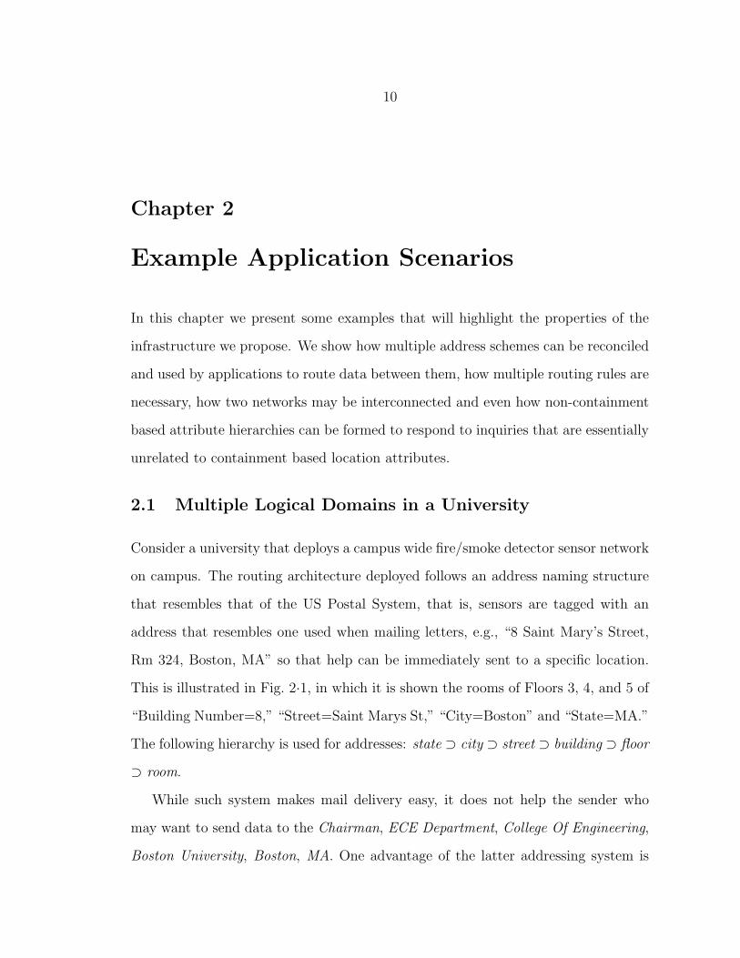
2.1 Multiple Logical Domains in a University

Consider a university that deploys a campus wide fire/smoke detector sensor network

on campus. The routing architecture deployed follows an address naming structure

that resembles that of the US Postal System, that is, sensors are tagged with an

address that resembles one used when mailing letters, e.g., “8 Saint Mary’s Street,

Rm 324, Boston, MA” so that help can be immediately sent to a specific location.

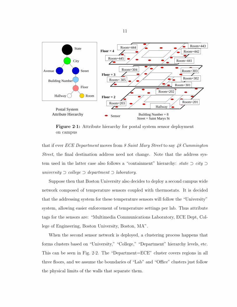
This is illustrated in Fig. 2·1, in which it is shown the rooms of Floors 3, 4, and 5 of

“Building Number=8,” “Street=Saint Marys St,” “City=Boston” and “State=MA.”

The following hierarchy is used for addresses: state ⊃ city ⊃ street ⊃ building ⊃ floor

⊃ room.

While such system makes mail delivery easy, it does not help the sender who

may want to send data to the Chairman, ECE Department, College Of Engineering,

Boston University, Boston, MA. One advantage of the latter addressing system is

11

Attribute HierarchyPostal System

Floor

Hallway Room

Avenue Street

City

State

Building NumberRoom=301

Room=302

Room=303Room=304

Room= 305

Room=445

Room=444 Room=443

Room=442

Room=441

Room=203

Room=202

Room=201

SensorStreet = Saint Marys StBuilding Number = 8

Hallway

Floor = 4

Floor = 3

Floor = 2

Figure 2·1: Attribute hierarchy for postal system sensor deploymenton campus

that if ever ECE Department moves from 8 Saint Mary Street to say 48 Cummington

Street, the final destination address need not change. Note that the address sys-

tem used in the latter case also follows a “containment” hierarchy: state ⊃ city ⊃university ⊃ college ⊃ department ⊃ laboratory.

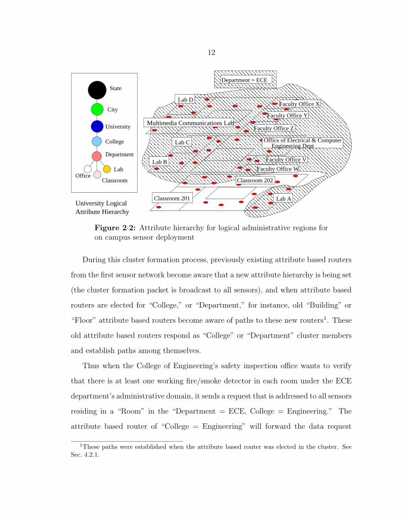
Suppose then that Boston University also decides to deploy a second campus wide

network composed of temperature sensors coupled with thermostats. It is decided

that the addressing system for these temperature sensors will follow the “University”

system, allowing easier enforcement of temperature settings per lab. Thus attribute

tags for the sensors are: “Multimedia Communications Laboratory, ECE Dept, Col-

lege of Engineering, Boston University, Boston, MA”.

When the second sensor network is deployed, a clustering process happens that

forms clusters based on “University,” “College,” “Department” hierarchy levels, etc.

This can be seen in Fig. 2·2. The “Department=ECE” cluster covers regions in all

three floors, and we assume the boundaries of “Lab” and “Office” clusters just follow

the physical limits of the walls that separate them.

12

��

��

��

��

University LogicalAttribute Hierarchy

City

State

College

University

Department

Lab

ClassroomOffice

Faculty Office V

Faculty Office W

Office of Electrical & ComputerEngineering Dept

Lab A

Lab B

Lab C

Lab D

Faculty Office Z

Faculty Office Y

Faculty Office X

Department = ECE

Multimedia Communications Lab

Classroom 201

Classroom 202

Figure 2·2: Attribute hierarchy for logical administrative regions foron campus sensor deployment

During this cluster formation process, previously existing attribute based routers

from the first sensor network become aware that a new attribute hierarchy is being set

(the cluster formation packet is broadcast to all sensors), and when attribute based

routers are elected for “College,” or “Department,” for instance, old “Building” or

“Floor” attribute based routers become aware of paths to these new routers1. These

old attribute based routers respond as “College” or “Department” cluster members

and establish paths among themselves.

Thus when the College of Engineering’s safety inspection office wants to verify

that there is at least one working fire/smoke detector in each room under the ECE

department’s administrative domain, it sends a request that is addressed to all sensors

residing in a “Room” in the “Department = ECE, College = Engineering.” The

attribute based router of “College = Engineering” will forward the data request

1These paths were established when the attribute based router was elected in the cluster. SeeSec. 4.2.1.

13

to the “Department = ECE,” which then forwards the request to all the “Room”

attribute based routers in its domain, requesting to obtain an answer to the inquiry:

“number of fire/smoke sensors.” Depending on the type of routing scheme selected,

the propagation from “Department = ECE” to “Room” clusters may involve higher

level hierarchy nodes in the Postal System hierarchy.

“Room” attribute based routers, upon receiving the request, flood each room with

requests for all fire/smoke sensors to report their status. Upon gathering the infor-

mation, they send the information back to the “Department = ECE” router, which

will report the final data to the “Safety Inspection Office, College of Engineering”

University LogicalAttribute Hierarchy

City

State

College

University

LabOffice

Classroom

Floor

Building Number

Avenue Street

City

State

Hallway

Department

Attribute HierarchyPostal System

Room

��

��

Packet’s traversal path throughthe logical hierarchies

?

Figure 2·3: How packets logically cross different attribute hierarchies.

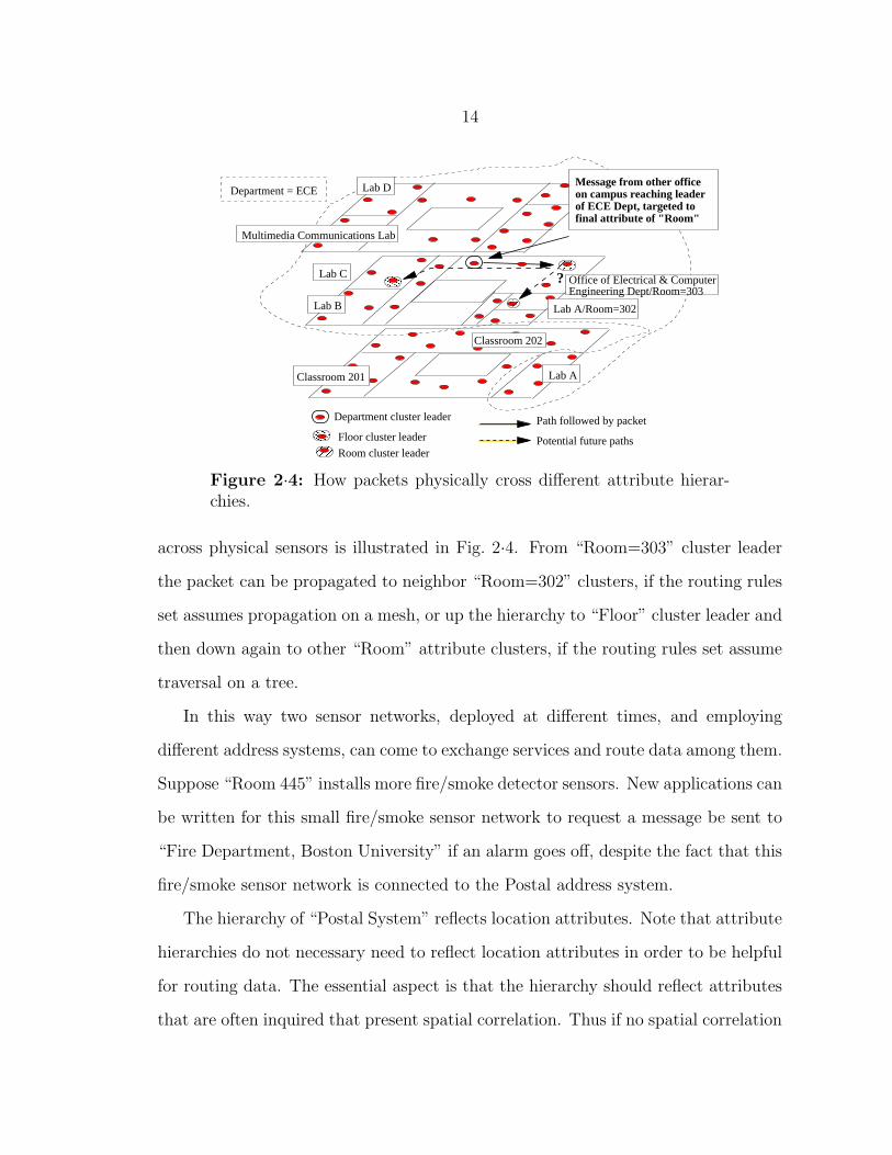
The packet traversal through the logical nodes in the two hierarchies is depicted

in Figs. 2·3 and 2·4. The leader of the “Department=ECE” cluster is also a member

of a “Room” cluster so the packet is sent to its “Room” leader. The packet traversal

across hierarchies in a logical way is depicted in Fig. 2·3 while the packet traversal

14

on campus reaching leaderof ECE Dept, targeted to

Message from other office

final attribute of "Room"

��

��

��

��

?

Department cluster leader

Floor cluster leader

Room cluster leaderPotential future paths

Path followed by packet

Classroom 201 Lab A

Lab B

Multimedia Communications Lab

Lab D

Lab C

Classroom 202

Department = ECE

Office of Electrical & ComputerEngineering Dept/Room=303

Lab A/Room=302

Figure 2·4: How packets physically cross different attribute hierar-chies.

across physical sensors is illustrated in Fig. 2·4. From “Room=303” cluster leader

the packet can be propagated to neighbor “Room=302” clusters, if the routing rules

set assumes propagation on a mesh, or up the hierarchy to “Floor” cluster leader and

then down again to other “Room” attribute clusters, if the routing rules set assume

traversal on a tree.

In this way two sensor networks, deployed at different times, and employing

different address systems, can come to exchange services and route data among them.

Suppose “Room 445” installs more fire/smoke detector sensors. New applications can

be written for this small fire/smoke sensor network to request a message be sent to

“Fire Department, Boston University” if an alarm goes off, despite the fact that this

fire/smoke sensor network is connected to the Postal address system.

The hierarchy of “Postal System” reflects location attributes. Note that attribute

hierarchies do not necessary need to reflect location attributes in order to be helpful

for routing data. The essential aspect is that the hierarchy should reflect attributes

that are often inquired that present spatial correlation. Thus if no spatial correlation

15

of attributes can be exploited (e.g., the inquiries need be propagated to all the nodes

in the network), then the hierarchical clustering scheme is not maintained, and a flat

(i.e., all nodes belong to the same cluster) flooding structure can be employed.

In Sec. 4.2.1 we discuss the possibility of dynamically maintaining attribute nodes

in the hierarchy to reflect traffic patterns. In Chapter 5 we present an analysis of the

transmission costs for disseminating inquiries in the presence of different number of

attributes in a hierarchy.

2.2 Applications in the Wilderness

Subquadrant cluster leaderSubquadrant boundaryQuadrant boundary

Tree Traversal

Subquadrant

Quadrant

ForestAttributeHierarchy

Subquadrant

Quadrant

Forest

Mesh Traversal

��

��

��

��

��

��

��

��

��

� � � ��

��

��

��

��

��

��

�

��

!�!!�!""

FireDestroyed sensor

Forest cluster leader

Quadrant cluster leaderDirection of Fire Propagation

Figure 2·5: Sensors deployed in a forest

Consider the following scenario: multi-modal sensors are deployed over an area for

climate monitoring, and are collecting average values of temperature and humidity

when suddenly fire is detected. One local application, designed to detect and track

how the fire propagates, is awakened and immediately alerts neighbor sensors so that

the fire front can be detected. This scenario is depicted in Fig. 2·5.The communication needs of the sensor network while in the first stage of mon-

itoring average temperature and humidity can be thought of as hierarchical. Data

is slowly aggregated within each cluster by the cluster leader and sent to the base

16

station. Thus sensors communicate using the “Tree traversal” mode found on the

upper right side of Fig. 2·5. However, the communication needs of the fire detection

application add a new component: the necessity for clusters to communicate with

neighbor clusters, so that the fire propagation can be tracked over time. The way the

fire propagates is also recorded and this information is spread to contiguous clusters,

as in the event of a fire there is no guarantee that the top hierarchical leader has

survived the fire. This situation is also depicted in Fig. 2·5, in which the sensor

which plays the role of Forest leader, as well as Quadrant SouthWest leader has been

destroyed by the fire. If the tree traversal hierarchical mode is the only communica-

tion mode, then other quadrant leaders would not be able to detect the fire in time.

However, by using the “Mesh traversal” mode (lower right side of Fig. 2·5) at the

lowest level of the attribute hierarchy (Subquadrant clusters), sensors are able to

spread the alarm and continue detecting the fire front.

The example above illustrates how different applications may require different

communication patterns. It is definitely possible, given the sensors are multimodal [4]

that other applications are also present, e.g., wildlife tracking (needs to be able to

communicate with neighboring sensors, to alert them of the tracked object, and

needs to be able to send logged data back to base station), which would further drive

the need for a common, yet flexible routing infrastructure. In Sec. 4.3.4 we present

pseudo-code for two attribute hierarchy traversal modes. These two modes result in

different packet forwarding patterns which can be selected by applications based on

their needs (e.g., faster response from destination sensor or less transmission cost in

resolving unknown attribute based address).

17

University Logical Attribute Hierarchy Forest Attribute Hierarchy

City

State

College

University

Department

LabOffice

State

City

Subquadrant

Quadrant

Forest

��

��

��

��

��

��

��

��

��

��

��

��

� � �

��

��

��

Figure 2·6: Connecting two sensor network applications

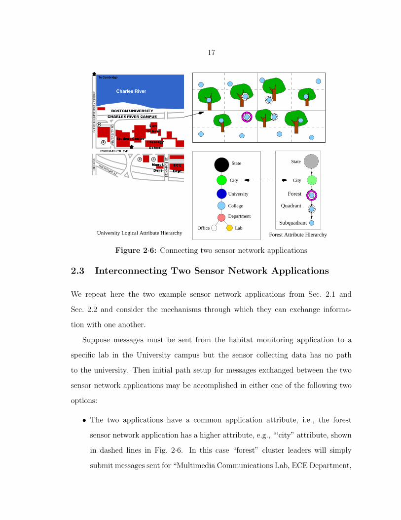
2.3 Interconnecting Two Sensor Network Applications

We repeat here the two example sensor network applications from Sec. 2.1 and

Sec. 2.2 and consider the mechanisms through which they can exchange informa-

tion with one another.

Suppose messages must be sent from the habitat monitoring application to a

specific lab in the University campus but the sensor collecting data has no path

to the university. Then initial path setup for messages exchanged between the two

sensor network applications may be accomplished in either one of the following two

options:

• The two applications have a common application attribute, i.e., the forest

sensor network application has a higher attribute, e.g., “‘city” attribute, shown

in dashed lines in Fig. 2·6. In this case “forest” cluster leaders will simply

submit messages sent for “Multimedia Communications Lab, ECE Department,

18

College of Engineering, Boston University, Boston, MA” to their “city” level

cluster leaders. Once the message gets to “city” level, path resolution can be

finished by going once more up (to “state”) and them coming down (“city” →“state” → “city”) or simply be propagated at “city” level until the intended

“city” cluster is found (“city” → “city”).

• The two applications have no common higher level attributes, i.e., “Forest” is

the highest level attribute for the network deployed for habitat and fire alarm

monitoring. In this case the top level “Forest” cluster will maintain paths to

neighboring sensor networks. Once messages to “Multimedia Communications

Lab, ECE Department, College of Engineering, Boston University, Boston,

MA” reach the “Forest” leader, if no known path exists, the message will be

sent to all adjacent neighboring clusters, until it reaches a cluster leader with

matching lower level attributes (“Forest” → “state”).

By clustering sensors into hierarchical attribute equivalent regions we avoid ad-

dress resolution at the sensor level, but perform address resolution hierarchically,

starting at the highest cluster level first, and proceeding level by level until reaching

the sensor level. We leverage information gathered by cluster leaders during the

cluster formation process to minimize the need for transmission each time a new

inquiry with a different destination attribute set is issued. An address resolution

scheme that operates at the sensor level would be a flooding mechanism, in which

messages are propagated to each and every sensor in the network. In Chapter 5 we

study performance comparison of different address resolution schemes.

19

��

��

��

��

��

��

��

��

��

��

� � � � � � � � � � � � � � � � � � � �

��

Warmer Region

Low Temperature

Cooler Region

Normal

Ground Temperature Sensor

With Heavy Vegetation

Uncovered Region

Nest Temperature Sensor

Figure 2·7: Great Duck Island and two deployed sensor networks

2.4 Other Examples

So far we have presented examples that exploit location based attributes that sat-

isfied containment based relationships. How would inquiries that are not explicitly

based on containment attributes be implemented in this infrastructure? To address

this issue, we consider inquiries that are tasked to sensors in a habitat monitoring

application (e.g., in Great Duck Island [22]). Hypothetically, let two networks be

deployed at different points in time. The first, depicted at the center of Fig. 2·7,

shows an on-the-ground network of temperature sensors, while the second, depicted

at the right of Fig. 2·7, shows an in-the-nest network of temperature sensors that

monitor the behavior of the birds in the island.

Assume that all sensors can communicate with one another, and the set of com-

mon attributes with which they have been tagged include location and the sensing

capabilities of moisture, temperature and light. For “on-the-ground” sensors noise

20

level and wind direction and intensity can be sensed, while for “in-the-nest” sensors

occupancy of i adult birds or j eggs or chicks can be determined. Suppose further

that the list below represent inquiries that might be posed to the network:

• Occupancy of the nests: when is a bird present?

• What is the difference between the nest temperature and the ambient temper-

ature?

• When do birds leave their nests?

• Do birds forage in the rain or other bad weather?

• Alert remote locations when significant event occurs: an egg hatches, a bird

leaves or arrives at a nest, etc.;

• Capture state (weather etc.) when a bird exits or enters the nest;

• Correlated events: time that 50% of birds have left the nest to forage.

Since all sensors can communicate with each other, the resultant sensor network

we work with is composed of the addition of the two initially deployed networks.

This resultant network can be seen in the two maps of the sensors in the island that

are shown right next to the attribute hierarchy in Fig. 2·8.The inquiries listed do not depend explicitly on location based attributes that

belong to a hierarchy satisfying containment relationships. However, in that list of

inquiries, we can detect some that depend solely on one type of sensor (e.g. relating

to the attributes within the nest), and inquiries that depend on the collaboration of

close range sensors (e.g. inquiries that relate the behavior of the birds to the state

of the island outside of the nests). This “close range” condition is in fact an implicit

location based attribute that tasked sensors must fulfill. Thus a proposed attribute

21

Nest within1 hop to

Ground sensor

Ground (3−hop)

Island

Nest sensors and within−1−hop−Ground sensors

Other Nest

Formed 3−hop Ground Clusters

��

��

��

��

��

��

��

��

� � � � � � � � � � � � � � � � � � � � � � � � � � � � � � � � � � � � � � � � � � � � �

��

��

��

��

Figure 2·8: Attribute Hierarchy for Queries to Great Duck Islandsensor network

hierarchy must include a condition that allows sensors that satisfy the proximity

attribute to be formed.

One such attribute hierarchy is proposed in the center of Fig. 2·8. In it “in-

the-nest” sensors are subordinated to “on-the-ground” sensors, while the latter is

bounded by a hop count qualifier. Since “on-the-ground” attribute extends to the

whole island, only by giving a hop count qualifier will we form multiple clusters (this

is provisioned in our algorithm as described in Sec. 4.2.1). The clusters formed can

be seen in the left side to the attribute hierarchy in Fig. 2·8. Sensors that satisfy “in-

the-nest” and “within-1-hop-to-Ground-sensor” then form their own clusters (mostly

of one member only). If a subordinate “in-the-nest” sensor finds itself surrounded

by other non-“on-the-ground” sensors, then it will become leader of a “other-nest”

cluster. In the right side to the attribute hierarchy in Fig. 2·8 we show the “in-the-

nest” sensors surrounded by “on-the-ground” sensors within one hop.

With these clusters formed, then the inquiries on the left side of Table 2.1 can

22

be simply posed to the “in-the-nest” sensors (which encompasses both “other-nest”

and “within-1-hop-to-Ground”). Inquiries will first be sent to the leaders of “on-

the-ground” cluster leaders, and passed on to the appropriate lower level cluster

leaders. Sensors with the appropriate answers will respond to their cluster leaders

and these will be sent back through “on-the-ground” cluster leaders. Intra-cluster

processing by leaders of “within-1-hop-to-Ground-sensors” clusters is performed for

the inquiries listed on the right side of Table 2.1, before the answers are aggregated

at “on-the-ground” cluster leaders and sent back to the leader of the “Island” cluster.

Table 2.1: Inquiries Addressed to “In-the-nest” SensorsTo all “in-the-nest” To “Within-1-hop-to-Ground”

Occupancy of the nests: when isa bird present?

What is the difference betweenthe nest temperature and the am-bient temperature?

When do birds leave their nest? Do birds forage in the rain orother bad weather?

Alert remote locations when sig-nificant event occurs: an egghatches, a bird leaves or arrivesat a nest, etc.;

Capture state (weather etc.)when a bird exits or enters thenest;

Correlated events: time that 50%of birds have left the nest to for-age.

As can be seen, it is definitely possible to extend the attribute hierarchy con-

cept to non-containment based location attribute hierarchies. The process however

is more elaborate and involves defining spatially correlated relationships (not neces-

sarily containment) that will allow data propagation to take place more easily. In

this dissertation we focus on enabling attribute based routing for attribute hierar-

chies that are location based or spatially correlated with containment and adjacency

23

relationships clearly defined.

A vehicular network will benefit from continuous adjacent attribute value regions

(i.e., “I-93N”) when propagating information, so that data packets will not be dis-

seminated nor collected from irrelevant regions, i.e., data packets will not flow to nor

from “I-95N” during an intersection.

We have shown in this chapter how our infrastructure can be applied to facilitate

deployment of sensor network applications under various scenarios. In the next

chapter we will give the background and related work of our research topic.

24

Chapter 3

Background and Related Work

Diffusion algorithms have been proposed as the underlying routing mechanism for

sensor networks [18, 23, 24]. In diffusion, data sinks subscribe to receive data by

flooding their interest to the whole network. The interest would carry desired at-

tributes of the data, such as type, periodicity, location, etc. The flooding establishes

a gradient field (an inverted routing tree rooted at the node) for the data of interest.

Sensors receiving interests but have no matching data store this interest and rebroad-

cast it, if receiving it for the first time. Those sensors which do have matching data

reply, broadcasting their data to local neighbors. Neighbor nodes that receive data

check their list of received interests. If there is a match, the data is forwarded back

through the gradient field. Data then may reach the sink through multiple paths.

The data sink will then reinforce (positively or negatively) certain paths according to

some optimality criteria (least latency, energy of the nodes along the path, etc.) [25].

In-network processing and data aggregation can take place at nodes in which different

source paths meet. This emphasis on in-network processing is the major distinction

between Directed Diffusion and Declarative Routing Protocol mechanisms [19, 24].

Diffusion mechanisms are simple, robust, localized, form paths in which data ag-

gregation or in-network processing nodes may be elected, and is data-centric, in that

the “destination” of data packets is not any specific host per se but hosts that satisfy

certain attributes. But since communication energy expenditures dominate in sen-

sor devices [3, 21], flooding of interests to the whole network can be very expensive,

25

especially if there is a large user base that spans across multiple disciplinary fields

issuing many varied interests. We show a theoretical cost estimation in Chapter 5.

Modifications to the basic diffusion algorithm have been proposed [26, 27], in which

data sources may actively push data to data sinks, or hybrid cases (attempting a mid-

dle rendezvous for data source and data sink paths). The underlying dissemination

mechanism is still a network-wide flooding.

In order to reduce the redundant transmission of packets, location information

is explored in order to direct how data can be routed. Greedy Perimeter Stateless

Routing (GPSR) [28] and Geographical and Energy Aware Routing (GEAR) [29] are

two examples of geographical based routing. Both assume an initial greedy approach

to route data based on location information. GPSR routes data around holes (re-

gions in which the current node is geographically the closest to the destination node

but the next hop link would need to go to a geographically more distant node – this

basically means the greedy algorithm does not work) by traversing along the perime-

ter region of the hole, while GEAR uses a learning algorithm that propagates higher

costs around holes, so that later packets will be automatically routed around holes.

Trajectory Based Forwarding (TBF) [30] specifies trajectories that data can follow.

Two Tier Data Dissemination (TTDD) [31] has data sources build uniform grids of

data dissemination nodes. TTDD’s main emphasis is in efficiently supporting sink

mobility. In their scheme the space is subdivided into uniform squares (a “grid” of

data dissemination nodes is built from the data source) and data sinks flood their

interests inside the square. When an interest packet reaches a node on the grid, it

is propagated along the grid to the source, at which point data are sent back to the

sink. Content Based Multicast (CBM) [32] has a similar approach to a hybrid model

of Diffusion, in which data sinks pull data from a specified region of interest, and

data sources push data to a specified region in which information is relevant (e.g.,

26

sensors detecting a target moving eastward may push alarm data further towards

eastern parts of the network). Rumor Routing [33] establishes paths to events by

employing agents, which are packets with a high TTL field, that are propagated from

node to node, leaving information on observed events. Queries are also propagated

in the same way, and data are sent back when there is a rendezvous of two paths.

While these schemes do not rely on network wide floodings, most [28, 29, 30, 32, 31]

need the presence of location services to operate, and their addressing scheme is in-

dependent of the applications they support. In other words, a data sink must know

a priori the region to which send the data request [28, 29, 30, 32]. TTDD is focused

on supporting sink mobility, and does not support inquiries that requests data from

same attribute regions. Rumor routing likewise does not offer direct support for

queries that request data from regions of sensors. In the schemes above there is no

exploitation of potential spatial correlation of sensor data to forward and request

packets.

Including sensor data to help the routing process can be found in [34, 35, 36, 37].

In [34] sensors are clustered and the clusterhead queries cluster members regarding an

observed event until the information it possesses satisfies a threshold value according

to a utility metric. Requests for the event are forwarded based on the gradient levels

established by the information utility metric. This work is a generalized approach to

diffusion, in which information utility metric values replaces the simpler hop-count-

to-source gradient field. It is not clear if the utility metric function can be easily

generalized to route different queries for multiple events. Work in [35] discusses ways

to route data when data are spatially correlated. It uses a correlation index to deter-

mine the optimal one level cluster size to aggregate data. Our clustering approach

is similar, but we extend hierarchies to include potential multiple levels and propose

explicit discrete regions for the correlation index (equal attributes yield correlation

27

value of 1, while different attributes yield correlation index of 0). ACQUIRE [36]

proposes a query propagation scheme in which the sensor receiving a query perform

a d-hop look-ahead to see if there is information that can answer the query. If not

the query is then propagated (through Random Walk or other mechanism). The

authors do not propose laying a foundational routing mechanism, but attempt to

exploit potential data redundancy in the network to answer queries.

Our work closely resembles Semantic Routing Trees (SRT) [37]. SRT proposes

overlaying a tree on the sensor network, in which sensors track the value of a single

attribute. Parent sensors know the value range of the attribute of all of its descen-

dant sensors, and forward queries to a child only if it and its descendants can answer

the query. A generalized approach to content based networking is CBCB (Com-

bined Broadcast and Content-Based routing) [38]. CBCB assumes the existence of a

broadcast layer that reaches all nodes in the network. In [38] nodes broadcast their

predicates, i.e., a set of constraints over the attributes, along the broadcast tree.

Matching data is attracted and forwarded to the nodes issuing the predicates. Nodes

along the broadcast tree track the predicates issued and only forward relevant data

that has been requested. Our work does not attempt to track query routing at every

node in the network, instead, we form attribute equivalent clusters of sensors and

use these clusters to route queries to relevant sensors. By changing how such clusters

are formed, i.e., by adding or removing specific nodes in the attribute hierarchy, we

can determine the granularity of control we desire in the query propagation and thus

achieve higher gains by avoiding redundant traffic in the network. In addition, we

seek to enable internetworking of different sensor network systems that are employing

different address naming and/or routing schemes.

Semantics based query routing has been studied by the Peer-to-Peer (P2P) net-

work community [39, 40, 41]. A taxonomy for “content” network is described at [42].

28

Work in [40] proposes clustering nodes together (i.e., adding logical edges) based

on content similarity, while [39] suggests that nodes in the network should “learn

about” the contents of other nodes in the network so that queries may be more

efficiently forwarded. In particular, [41] offers an ontology-based solution to what

content similarity may mean, by offering a matching process that involves a con-

cept/content’s “name,” “attributes” and “relationships.” As can be seen, overlay

P2P networks have the flexibility of exploiting dynamic changes to the network

topology by adding/removing logical links. The papers above seem to assume a

static knowledge representation system, i.e., a content categorization system, an on-

tology, etc., that is static. The problem they try to solve can roughly be stated as:

given that there is this knowledge system, how to form networks/forward queries

such that a quantifiable metric (e.g. latency) is minimized. Semantic Web Services

and other semantic based services [43, 44, 45] often focus on how to specify ser-

vices through different languages [46, 47, 48], without special consideration to the

underlying routing mechanism. Our proposal focus the problem on a different per-

spective, given the network of nodes with their locations, data attributes available

and a inquiry forwarding process, how do we enable forming the categorization sys-

tem (say a attribute hierarchy) that will minimize a quantifiable metric (again, e.g.,

data latency). Our work can be seen as laying the foundation for the development

of semantic routing in sensor networks. Establishment of attribute clusters is useful

to implement semantic routing [49]. The attribute equivalent regions built can also

be used in resource exposure schemes as those found in [50]. In addition to that, we

offer application level control of routing behavior through routing rules.

The advantages of being able to select the routing protocol at run-time have been

pointed out by the active network community [51]. Work in [52] proposes encapsulat-

ing packets in SAPF (Simple Active Packet Format) headers, which carry indicators

29

to an active node’s FIB (Forwarding Information Base), guiding packet forwarding

behavior at run-time. The routing example shown in [52] is tree based. In [53] the

authors propose an overlay scheme that allows active nodes to coexist with passive

nodes. The active nodes track communication paths to each other reactively. Our

work shows how dynamic routing protocol selection can be implemented in attribute

clustered WSNETs. We show the routing rules and the performance analysis for both

the tree and the mesh traversal modes. Furthermore, we show how the changing den-

sity of “active routers” (in our case attribute based routers or cluster leaders) in the

network, achieved through changing the number of levels in the attribute hierarchy,

affects the expected performance of the two routing schemes.

Many clustering algorithms have been proposed in the literature [54, 55, 56, 57,

58, 18, 59]. Work in [54] selects clusterheads based on node ID, while [55] proposes

forming clusters based on link quality. Clustering is proposed in both cases to pro-

vide scalability and service guarantees. Admission control and bandwidth allocation

are all performed within the cluster. Amis et al. [56] propose an election algorithm

that chooses clusterheads in such a way that these form a dominating set. Moreover,

nodes are guaranteed to be at most d hops away from a clusterhead. McDonald and

Znati [60] propose to form clusters in order to offer probabilistic bounds on path

availability. The path availability model is built on top of a mobility model that is

presented in the same paper. Banerjee and Khuller [57] proposed algorithms that

form and maintain a hierarchical set of clusters under mobility. The clusters formed

satisfy certain design objectives, such as nodes belonging to a constant number of

clusters at one hierarchy level, low overlap between two clusters, etc. Ramachan-

dran et al. [58] propose algorithms that form star shaped clusters at a pre-defined

maximum size, with the Bluetooth [61] model in mind. Estrin et al. [18] proposed

a clustering mechanism that can ensure bi-directional link connectivity for nodes in

30

the network. Ghiasi et al. [59] propose an optimal k-clustering algorithm for sensor

networks, in which k clusterheads are selected and the clusters are balanced. It is

shown that this problem is solved optimally using min-cost network flow.

The clustering algorithms above attempt formation of clusters that satisfy certain

invariant properties (leaders have lowest ID), communication metrics (link quality, bi-

connectivity) or topological properties (maximum cluster radius, balanced clusters,

path availability, etc). Our algorithms form clusters that reflect possible traffic pat-

terns. By tying attributes that are relevant to inquiries posed to the sensor network

to the overlaid cluster structure, we are establishing clusters that reflect application

level communication needs rather than network level topological criteria.

The design of clustering algorithms that satisfy application level communication

needs can also be found in [62, 63, 64]. Clusterheads in LEACH (Low Energy Adap-

tive Clustering Hierarchy [62]) and HEED (Hybrid Energy-Efficient Distributed Clus-

tering [63]) are all elected through a randomized algorithm which guarantees that the

role of being a clusterhead is shared by all available nodes. HEED specifically uses

residual energy in clusterhead election. Bandyopadhyay and Coyle [64] use stochas-

tic geometry to derive an expression for the communication cost of cluster members

to the clusterhead. From this expression the cluster radius and the probability of a

node becoming a clusterhead is obtained. Our work differs from the above in that

there is no support in the clustering algorithms (or architectures) above to exploit

biased communication patterns in sensor networks, which we believe will be evident

if a large sensor network becomes a shared resource. In contrast, our clustering al-

gorithm has provision for insertion and removal of cluster levels that can exploit the

biased patterns of inquiry traffic and thus achieve higher savings.

This capacity to exploit traffic patterns through hierarchy levels to minimize

energy expenditure, and the absence of the necessity of GPS-based geography coor-

31

dinates are the distinguishing marks of our work with respect to DataSpace [65] and

SINA (Sensor Information Networking Architecture [66]). DataSpace [65] is a gen-

eralized geographical (using GPS coordinates) based routing architecture that can

support querying and monitoring of objects in the DataSpace. It uses hierarchical

data cubes (which represent 3D regions in space) and directory services in data cubes

to achieve its goals. There is no discussion of any specific “clustering” mechanism

per se, for objects wishing to belong to DataSpace register with the directory service

of the data cube it is in. Clustering and attribute-based naming are both mentioned

in SINA, however, the clustering algorithm is not tied to the attributes of sensors,

and is proposed only to facilitate scalable operations.

Because our work supports delivering queries to relevant regions of the net-

work, this can be seen as complementary to data-centric storage approaches, such as

GHT (Geographic Hash Tables) [67], DIMENSIONS [68], DIFS (Distributed Index

of Features in Sensor networks) [69], DIM (Distributed Index of Multi-dimensional

data) [70] and Fractionally Cascaded Information (FCI) [71]. GHT proposes using

a hash function that produces geographical coordinates once given a key. Sensors

nearest to the coordinates store the key-value pair. Structured replication is used

to avoid any node becoming a hotspot due to the high frequency of a key’s occur-

rence. In DIM the hash function accepts as input multiple attributes (i.e., supports

multi-dimensional data), and the closer the attribute values of the input, the closer

the outputs of the hash function are in geographical coordinates. DIFS proposes

establishing a hierarchy in the network, in which root nodes track the narrowest

range of attribute values over the largest spatial coverage, while leaf nodes track the

widest range of attribute values over the smallest spatial coverage. This construc-

tion allows load balancing over index nodes and supports range queries as well. Our

approach establishes hierarchies within the network and summaries of information

32

so that queries may be routed to where the sensors containing the information are.

Data is stored in the sensors detecting the event and not moved (nor replicated) in

other sensors.

DIMENSIONS [68] advocates aggregating data hierarchically by clusterheads and

using wavelet transforms to produce multi-resolution views of the network. Thus a

query that did not require full resolution view of the data could be answered at a

higher hierarchy level. Gao et al. [71] makes a similar argument and propose that

sensors should only know a fraction of the information from distant parts of the

network. They partition the network by using a quadtree structure, in which the

root node is a square covering the whole network and the leaf node is a square re-

gion containing one sensor. Sensors within a node share information with sensors

in sibling nodes. The required information (such as maximum temperature within

the four nodes) is then forwarded to the parent node. Thus every sensor knows of

the maximum temperature of the square regions (nodes in the quadtree) it belongs

to, all the way up to the root node. In this structured format, queries are bounded

in complexity, as the authors show in their paper. In the two schemes above clus-

ters form independently of the content of the sensors or the frequency and “shape”

of queried regions. In contrast, our clusters are formed essentially based on the

attributes queried and relevant regions.

Work in [72, 73, 74, 50, 75] are related to programming sensor networks. Welsh [50]

describes a region based communication programming primitive that allows pro-

grammers to treat regions as single abstractions. These regions may be defined by

connectivity, location or other properties of the nodes (i.e., they are marked by an

ontology of attributes). The routing process in our architecture can benefit from the

expressiveness of the abstractions above and implement more efficient routing rules.

SensorWare [72, 73] and Mate provide general frameworks that allow mobile code to

33

be shipped and executed on remote sensor nodes. Work in [75] proposes a frame-

work on which routing services can be built. It defines tunable state information,

programmable state-collecting module and programmable data-forwarding module,

written based on code from a shared library. Our attribute based routing scheme

can be built on top of this framework.

We have shown in this chapter various background work related to clustering

algorithms and the ways in which our work differs, improves or simplifies the ap-

proaches taken to adapt to sensor networks. Our chief contribution is in the unified

approach to routing for sensor networks, in which the routing elements (attribute

based clusters) can be dynamically adjusted to match incoming traffic, and routing

behavior (routing rules set) can be changed to support application level communica-

tion needs. In the next chapter we offer an in-depth presentation of the components

of our solution.

34

Chapter 4

An Attribute Based Routing Scheme For

Wireless Sensor Networks

In this section we describe the various elements of our proposed solution and methods

to evaluate their performance. We first start by describing our design philosophy and

the insights from previous research work that guided in our design. The we proceed

to describe the two parts that are the foundation of our work: the algorithms that

establish an hierarchical set of clusters in the network, which become the units for

routing in our framework, followed by the specification of data structures and routing

rules that allow dynamic behavior change in the way a packet may traverse the

attribute hierarchy. We will next proceed to describe routing in sensor networks and

our design philosophy.

Routing is concerned with delivering information from a source host to a desti-

nation host accurately and within expected performance bounds. The information

starts at the source host and flows through a finite sequence of hosts until it reaches

the destination host. Any two consecutive hosts in the sequence are neighbors and

the resulting sequence of links is called a path (or route) between source and desti-

nation. If there is no path between any two hosts in the network, then the network

is partitioned.

To establish communication between source and destination these elements are

necessary: a reference system with specific names by which source and destination

35

identify themselves and the elements in the space in which they exist; and the knowl-

edge needed to traverse the space that separates the source from the destination.

This knowledge itself can be centralized, in which case it can be located in the

source (e.g., source based routing), or can be bound with the information (e.g.,

agent like delivery system); or it can be distributed, so that specific spots in between

the source and destination are selected to forward packets appropriately, in other

words, to establish routers in the network. Centralized approaches do not scale well.

Binding too much information with the data (in agent like schemes) incurs in higher

transmission costs, since the agent itself needs be propagated in addition to the data.

This argues against their deployment in sensor networks, since energy is a resource

that must be used sparingly.

In the design of our routing architecture, we chose to distribute the knowledge of

network traversal from source to destination to multiple selected nodes. That is, we

choose specific routers within the network that receive the task of delivering data.

In this way the stored knowledge needed to deliver data is also distributed, which

scales better with increasing network size, and assigning this role dynamically enable

load balancing among sensors in the network. In the next subsections we describe

our design decisions and functionality specifications of our routing scheme.

4.1 Design

When designing routing schemes, one important question is to consider how infor-

mation exists within the network, and how requests for such information are made.

Information can be represented by data sets, and requests for information can be

seen as a set of points of interest, in which each point of interest maps to at least one

data set. Each point of interest has associated with it an access probability, which

represents the frequency in which the community of users looks for that information.

36

Data sets may exist replicated within different hosts in the network.

��

��

AC

DB

E

E

Packet

?

Packet

?A

C

DB

��

��

� � ��

��

��

��

!�!!�!"�""�" #�#�##�#�#$�$�$$�$�$

Figure 4·1: Data and Routing in Networks

In the past routing algorithms focused on reaching a specific host. This paradigm

can be justified when the hosts are few when compared with existing data sets, that

is, many data sets were mapped to a relatively few hosts. This is illustrated in the

top part of Fig. 4·1, in which the packet sent by A wants to reach hosts B, C or

D, which possess the data A desires. With the advent of sensor networks, however,

there is a reversal on the numbers on each side. With the decreasing cost of sensors,

it is envisioned that many physical phenomena will be monitored through network

of sensors, that is, sensors sample the same phenomenon at different points in space

and time (thus intrinsic to sensor applications is the notion of location and relative

time). These sensors often collect highly correlated or even same data values. Under

such circumstances, finding a specific host is not as essential as finding the desired

data, for such data may be replicated in many hosts. This converse situation is

illustrated in the bottom part of Fig. 4·1, in which the data A desires is stored in all

but a few hosts.

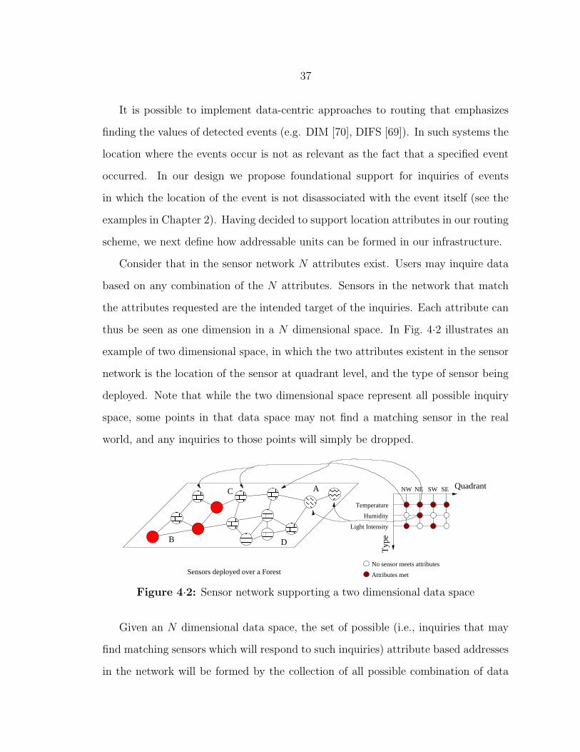
37

It is possible to implement data-centric approaches to routing that emphasizes

finding the values of detected events (e.g. DIM [70], DIFS [69]). In such systems the

location where the events occur is not as relevant as the fact that a specified event

occurred. In our design we propose foundational support for inquiries of events

in which the location of the event is not disassociated with the event itself (see the

examples in Chapter 2). Having decided to support location attributes in our routing

scheme, we next define how addressable units can be formed in our infrastructure.

Consider that in the sensor network N attributes exist. Users may inquire data

based on any combination of the N attributes. Sensors in the network that match

the attributes requested are the intended target of the inquiries. Each attribute can

thus be seen as one dimension in a N dimensional space. In Fig. 4·2 illustrates an

example of two dimensional space, in which the two attributes existent in the sensor

network is the location of the sensor at quadrant level, and the type of sensor being

deployed. Note that while the two dimensional space represent all possible inquiry

space, some points in that data space may not find a matching sensor in the real

world, and any inquiries to those points will simply be dropped.

B

C

D

A

Attributes met

No sensor meets attributes

��

��

��

��

��

��

��

��

��

Sensors deployed over a Forest

Light Intensity

Typ

e

Temperature

Humidity

QuadrantSESWNENW

Figure 4·2: Sensor network supporting a two dimensional data space

Given an N dimensional data space, the set of possible (i.e., inquiries that may

find matching sensors which will respond to such inquiries) attribute based addresses

in the network will be formed by the collection of all possible combination of data

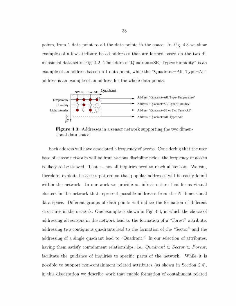
38

points, from 1 data point to all the data points in the space. In Fig. 4·3 we show

examples of a few attribute based addresses that are formed based on the two di-

mensional data set of Fig. 4·2. The address “Quadrant=SE, Type=Humidity” is an

example of an address based on 1 data point, while the “Quadrant=All, Type=All”

address is an example of an address for the whole data points.

Light Intensity

Typ

e

Temperature

Humidity

QuadrantSESWNENW

Address: "Quadrant=SE, Type=Humidity"

Address: "Quadrant=All, Type=Temperature"

Address: "Quadrant=SE or SW, Type=All"

Address: "Quadrant=All, Type=All"

Figure 4·3: Addresses in a sensor network supporting the two dimen-sional data space

Each address will have associated a frequency of access. Considering that the user

base of sensor networks will be from various discipline fields, the frequency of access

is likely to be skewed. That is, not all inquiries need to reach all sensors. We can,

therefore, exploit the access pattern so that popular addresses will be easily found

within the network. In our work we provide an infrastructure that forms virtual

clusters in the network that represent possible addresses from the N dimensional

data space. Different groups of data points will induce the formation of different

structures in the network. One example is shown in Fig. 4·4, in which the choice of

addressing all sensors in the network lead to the formation of a “Forest” attribute;

addressing two contiguous quadrants lead to the formation of the “Sector” and the

addressing of a single quadrant lead to “Quadrant.” In our selection of attributes,

having them satisfy containment relationships, i.e., Quadrant ⊂ Sector ⊂ Forest,

facilitate the guidance of inquiries to specific parts of the network. While it is

possible to support non-containment related attributes (as shown in Section 2.4),

in this dissertation we describe work that enable formation of containment related

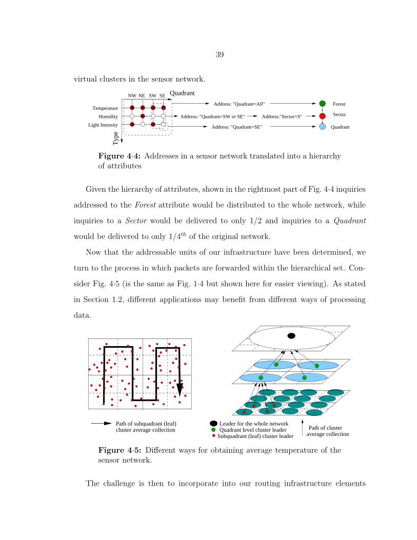
39

virtual clusters in the sensor network.

Quadrant

Forest

Sector

Light Intensity

Typ

eTemperature

Humidity

QuadrantSESWNENW

Address: "Quadrant=SW or SE"

Address: "Quadrant=All"

Address: "Quadrant=SE"

Address:"Sector=S"

Figure 4·4: Addresses in a sensor network translated into a hierarchyof attributes

Given the hierarchy of attributes, shown in the rightmost part of Fig. 4·4 inquiries

addressed to the Forest attribute would be distributed to the whole network, while

inquiries to a Sector would be delivered to only 1/2 and inquiries to a Quadrant

would be delivered to only 1/4th of the original network.

Now that the addressable units of our infrastructure have been determined, we

turn to the process in which packets are forwarded within the hierarchical set. Con-

sider Fig. 4·5 (is the same as Fig. 1·4 but shown here for easier viewing). As stated

in Section 1.2, different applications may benefit from different ways of processing

data.

Subquadrant (leaf) cluster leaderQuadrant level cluster leaderLeader for the whole network

average collectionPath of cluster

Path of subquadrant (leaf)cluster average collection

Figure 4·5: Different ways for obtaining average temperature of thesensor network.

The challenge is then to incorporate into our routing infrastructure elements

40

that can change the behavior of packet processing during deployment time at the

request of applications that are being deployed. The design choice we selected is by

the utilization of routing rules set, and have the routing agent interpret the rules

set. Using sets of rules to change routing behavior is more lightweight in terms

of transmission cost than, for instance, sending mobile agents. By giving a set of

functions that invoke lower level processing capabilities, routing rules can be written

to change packet processing from the left side of Fig. 4·5 to the right side of Fig. 1·4.

In Section 4.2 we describe how virtual attribute hierarchies are specified and how

the clustering mechanism take place within the sensor network and we follow in

Section 4.3 with a description of the rules based routing properties in our scheme,

together with pseudo-code for three routing rules set.

4.2 Attribute Based Clustering

Because most sensors in a sensor network are intended to monitor phenomena and

report results elsewhere, they can be collectively modeled as a large spatially dis-

tributed database [65, 76]. Examples of inquiries (information requests) that might

be posed include:

• How many nests in the northeast section of the forest currently have birds in

them?

• What is the average temperature in the laboratories in the basement of building

10?

• Detect congestion in the intersection of Main and Broadway and control traffic

lights to relieve the congestion.

• What is the frequency of vibration at 12:00?

41

If we relied on data flooding to disseminate the inquiries within the sensor net-

work, all sensors would be affected whenever a new inquiry were posed to the network,

which can be energy inefficient. In order to achieve savings in communication costs,

we propose clustering the sensors according to attributes that are meaningful to the

inquiries and that can be exploited to reduce unnecessary traffic, in other words,

attributes that encompass regions of sensor networks which possess data that are

often queried. One candidate that fulfills the requirements is to establish hierarchies

of attributes that are location based, and in which upper level hierarchies contain

lower level hierarchies. By location we mean attributes that are spatially related

and by containment we imply that sensors that share a common lower level attribute

automatically share all upper level hierarchy attributes.

We choose the location attribute as the clustering criterion for several reasons: (1)

location attributes are general enough to be used in most environments (e.g., we can

define “geographical section” clusters for sensors covering a national park, “room”

clusters inside a building, etc.); (2) hierarchies can also be easily built (room ⊂ floor

⊂ building, etc.); (3) the containment of lower level clusters by higher level ones

allows us finer control over the selection of sensors that will receive an inquiry; and

(4) it is easier to implement adaptive schemes which go back and forth between pure

flooding schemes, which is the same as having only one cluster containing all sensors,

and hierarchically clustered schemes, depending on the dynamic cost effectiveness

analysis.

In the presence of these hierarchical clusters, lower level clusterheads collect clus-

ter member information into “catalogs” and send them to their upper level clus-

terheads. When inquiries arrive, they are processed and relayed by the top level

clusterhead to the lower level clusterheads according to the catalog information pos-

sessed. Only when the inquiries arrive at the relevant clusters are they flooded to

42

all the sensors in the clusters. Such location based containment hierarchies map

themselves naturally to many scenarios (buildings, geographical areas) and can be

represented as directed acyclic graphs (DAGs), as can be seen from the examples in

Fig. 4·6. We call such DAGs Containment-DAGs or C-DAGs for short and we refer

to these containment based attribute hierarchies Containment Hierarchies or CH for

short.

[Country]

[Coast]

[State]

[Weather−balloon]

[Buoy]

Temperature Pressure

[Building]

[Floor]

[Corridor] [Room] [Tree]

[Nest]

[Section]

[Forest] [Town]

[Root]

[Garden]

[House]

[Neighborhood]

[Closet]

Temperature Humidity Motion Chemical

Figure 4·6: Examples of Attribute Containment Hierarchies

In Fig. 4·6 we show three examples of containment DAGs (C-DAGs). Nodes in

black represent attributes that are relevant for users of the sensor network. White

boxes represent types of data that can be collected by deployed sensors. Thus the left-

most C-DAG can be used to collect information regarding temperature and humidity

conditions in a building, while the rightmost C-DAG can be used for temperature

and pressure sensors monitoring weather conditions along the coast. In the center

C-DAG of Fig. 4·6 we show an example of two attribute hierarchies (for “Forest” and

for “Town”) that have a common relevant attribute (“Tree”). In the figure, sensors

with the same room number automatically share the same floor number. Sensors in

the same garden have to be in the same neighborhood.

Our work applies mainly to static or almost static sensor networks, as represented

by habitat, traffic or structural integrity monitoring applications [7, 8, 11], and by

43

sensor network fields deployed for target classification and tracking [13]. It is possible

to support non-location based clusters (e.g., sensors belonging to the same “family”)

by forming initially a location-based attribute hierarchy and establishing registration

and update mechanisms to cope with physical distance and/or mobility. This is

however reserved for future work. We present next our clustering algorithm.

4.2.1 Algorithms for Cluster Formation and Maintenance

The algorithms we developed form same-attribute clusters with one clusterhead and

rotate the clusterhead functionality among cluster members. Rotating clusterhead is

a load balancing mechanism to avoid energy depletion of a single device that carries

the role of clusterhead, since clusterheads are called to perform more functions,

e.g., inquiry forwarding, than a cluster member. Since inquiry forwarding within

the cluster hierarchy takes place between clusterheads, this rotation mechanism also

avoids depleting energy along a path between clusterheads. Because of the higher

processing activity demands, devices with higher energy levels are selected in the

rotation process.

Clusterheads will also gather information regarding their cluster members so as

to be able to decide whether to flood or drop inquiries that reach them. Cluster sizes

are constrained whenever possible, so as to avoid managing disproportionately large

clusters. Unicast routes are established among adjacent level clusterheads in the pro-

cess to facilitate any future information exchange. In addition the algorithms detect

and recover from clusterhead failures and support dynamic membership updates, ef-

fectively allowing dynamic C-DAG updates at the node level (i.e., the containment

relationships may adapt to the types of inquiries during deployment). Specific parts

of the algorithms are presented below.

44

CLUST_FORMpacket with more suitableReceives

leader information. ResendsCLUST_FORM packet.

MEMBERCLUSTER

UNCLUSTERED

CLUSTERLEADER

CLUST_FORMReceivespacket. Resend CLUST_FORMif it contains more suitableleader information.

CLUST_FORMReceives

CLUST_FORM packet.leader information. Resend

packet with suitableReceives CLUST_FORM

timer.

packet with no suitableleader information or abovemaximum hop threshold. StartCandidacy

CLUST_FORM

leader information.packet with less suitableReceives

Candidacy timertime−out. Send

withCLUST_FORMself as leader.

Figure 4·7: Finite State Machine for cluster formation

Cluster Formation

We propose a modified clustering algorithm called leader algorithm in [77] to form

clusters (thus we will call clusterheads cluster leaders interchangeably) by attribute

values and potentially limited by hop-count. Fig. 4·7 describes the finite state ma-

chine of our cluster formation algorithm. For clarity’s sake, the finite state machines

from Fig. 4·7 to Fig. 4·12 do not contain steps that handle catalog collection and

exchange, since these are not essential for understanding the clustering aspects of

the algorithms. All cluster formation decisions are localized and all clusters across

all hierarchy levels are formed in one network-wide flooding. This flooding is part of

the maintenance cost which is independent of the inquiry arrival rate, and which is

used to set up the virtual infrastructure that helps achieving communication gains

as inquiries are forwarded to targeted areas. Our cluster formation algorithm is

summarized as follows:

• One device (e.g., a base-station) starts the clustering process by broadcasting a

cluster formation packet CLUST FORM. Devices which hear this packet wait for an

45

amount of time which is based on their energy levels [18]. The specific waiting

period is given by a function which is composed of two parts: a deterministic

part which inversely reflects the energy level of the sensor, summed to a random

variable distributed uniformly between (−Tw, Tw). Assuming discrete energy

levels i, in which energy level i < i + 1, the deterministic part of the function

generates waiting times Ti, Ti > Ti+1, and which Ti − Ti+1 > 2Tw.

• The device with shortest waiting time generates a random number to be used as

cluster ID and broadcasts its candidacy packet first. Leader candidates which

hear such a broadcast cancel their timers and rebroadcast the higher energy

leader’s candidacy packet with hop count increased by one. Ties are broken by

deterministic methods (i.e., lowest id). The same packets received more than

once are dropped.

• Devices which had selected leaders but which hear more suitable leader candi-

dates switch leaders and rebroadcast the new leader’s candidacy packet.

• When a device hears a cluster formation packet from a neighbor device which

has a different attribute value in one of its CH levels (e.g., sensor 23 in room

445 hears from a sensor in room 442), it will try to become a leader candidate

of the region with new attribute value and new cluster ID (sensor 23 becomes

leader candidate for room 445).

• Devices keep track of the hop count to the leader they are selecting and the

neighbor devices through which they heard the packet. If it exceeds a pre-

defined CH level threshold value, then the device will become a leader candidate

and form a new cluster within the same attribute value region (thus room 445

may have more than one cluster). We call this hop-count based new cluster

formation.

46

• Cluster leaders at the lowest CH level wait for a time before flooding (within

the cluster) a request for cluster member information from its members. All

cluster leaders wait a time-out period (proportional to the cluster hop-threshold

number, collect any member related information into a “catalog” and forward a

summary of the information they collected to their higher level leader. This is

so that top level leaders can make informed decisions on whether to forward or

drop an arriving inquiry. The time-out period is set initially to a default value,

which is up to the design engineer deploying the network. Sensors receiving

the first request for catalog information track their hop distance to the leader

(hl), and know the maximum cluster hop radius (hmax). Thus they wait for a

period of time proportional to hmax − hl before sending their information up-

stream towards the cluster leader. If in the meantime they receive any cluster

member information which is downstream from the cluster leader, this infor-

mation is aggregated with their own and sent afterward upstream. Leaders

collect the maximum cluster hop radius information, and during subsequent

rotation times, this information is transmitted together with the catalog col-

lection packet, making the collection of catalog information faster if the cluster

radius is smaller than the maximum allowed.

47

� � � � � ��

� � � � � ��

� � � ��

� � � � � � ��

� � � � � ��

� � � � � � ��

� � � � � ��

� � � � � ��

� � � � � ��

� � � � � � � ��

� � � � � � � ��

� � � � � ��

� � � ��

� � � � � � � ��

� � � � � � � ��

� � ��

� � ��

� � ��

� � �� ! !! !! !

" "" "" "# ## ## #

$ $$ $$ $% %% %% %& & && & && & &' ' '' ' '' ' '

( (( (( (( () )) )) )) )

* * ** * ** * ** * *+ + ++ + ++ + ++ + +

, ,, ,, ,, ,- -- -- -- -

. .. .. ./ // // /00112233

4455

6677 8899

::;;

<<==

> >> >> >???

@@AABBCCD DD DEE

FFGG

H HH HH HH HI II II II I

J JJ JJ JJ JK KK KK KK K

L LL LL LL LM MM MM MM M

NNNOOP PP PP PP PQ QQ QQ QQ Q

Entry point for query Sensors R RR RSST T TT T TU UU U V VV VW W

[Floor = 3]

[Floor = 3]

[Floor = 1]

[Floor = 2]

[Room = 3] [Room = 4][ Room = 1 ] [ Room = 2 ]

[Floor = 1]

[Floor = 2]

[Room = 2] [Room = 3] [ Room = 4 ][ Room = 1 ]

[Room = 3] [Room = 4][ Room = 1 ] [ Room = 2 ]

[Room = 2] [Room = 3] [ Room = 4 ][ Room = 1 ]

Floor leaderBuilding leader Room leader Room cluster Floor cluster

BC D E

F

IJ

K L

M

PQ

R

A

H

NO

S

G

BC D E

F

IJ

K L

M

PQ

R

A

H

NO

S

G

BC D E

F

IJ

K L

M

PQ

R

A

H

NO

S

G

BC D E

F

IJ

K L

M

PQ

R

A

H

NO

S

G

Figure 4·8: Cluster Formation Process.

48

Note that clustering happens simultaneously across all CH levels. Thus our clus-

tering scheme requires only one network-wide broadcast for the formation of the

clusters at all CH levels. Although we apply node energy level as an attribute for

leader selection, this is is not intrinsic to the algorithm and is not limiting. Any

function of a sensor’s attributes (e.g., sensors locating with a specific area, node ID,

etc) can be used for leadership candidacy. The hop-count based new cluster forma-

tion rule is overridden when there is attribute change in a lower level CH value. If

there is no lower level, then new clusters may be formed as soon as the hop-count

limit is reached. This is to avoid having different clusters in the same room answer

to different floor leaders.

��

��

��

��

��

��

��

��

��

��

��

� � � � � � � � � � � � � � � � � � � � � � � � � � � � � � � � � � � �

��

��

��

��

��

��

��

��

��

��

��

��

��

��

��

��

� � � � � � � � � � � � � � � � � � � � � � � �

!�!�!�!!�!�!�!!�!�!�!!�!�!�!!�!�!�!

"�"�"�""�"�"�""�"�"�""�"�"�""�"�"�" #�#�#�#�#�#�##�#�#�#�#�#�##�#�#�#�#�#�##�#�#�#�#�#�##�#�#�#�#�#�#$�$�$�$�$�$�$$�$�$�$�$�$�$$�$�$�$�$�$�$$�$�$�$�$�$�$$�$�$�$�$�$�$

%�%%�%&�&&�&

'�''�''�''�'(�((�((�((�(

)�)�))�)�))�)�)*�*�**�*�**�*�*

+�++�++�+,�,,�,,�,-�--�--�-.�..�..�./�/�//�/�//�/�/0�0�00�0�00�0�0

1�1�11�1�11�1�12�22�22�2

3344

5566 7788 99:: ;;<<

==>>

??@@

AABB C�CC�CD�DD�D

E�EE�EF�FF�FGGHH

IIJJKKLL

M�MM�MN�NN�NOOPP

Q�QQ�QQ�QR�RR�RR�R

SSTTUUVV W�WW�WXX

Y�YY�YZ�ZZ�Z

[�[�[\�\

[Floor = 3]

[Floor = 1]

[Floor = 2] Floor leader

Room leader

Building leader

Sensors

Entry point for query

Floor cluster

Room cluster

[Room = 3] [Room = 4]

[Room = 2] [Room = 3] [ Room = 4 ]

[ Room = 1 ] [ Room = 2 ]

[ Room = 1 ]

BC D E

F

IJ

K L

M

PQ

R

A

H

NO

S

G

Figure 4·9: Attribute Containment based Clustering.

We show an example of our clustering algorithm in Fig. 4·8 and 4·9. Cluster

formation starts from node A, which elects itself as building, floor, and room leader

(top left of Fig. 4·8). When it broadcasts the cluster formation packet, node M

accepts A’s building leadership, but notices that the packet came from a different

floor and room, and elects itself as leader of its floor and its room (top right of

Fig. 4·8). Upon M ’s broadcast, node O accepts M ’s floor leadership, but keeps its

own room leadership candidacy and eventually becomes room leader (bottom left of

49

Fig. 4·8). Node S accepts leadership from A and M , canceling any candidacy timers

it may have. As cluster formation packet propagates, new room clusters are formed

(bottom right of Fig. 4·8) if the rooms are large (e.g., rooms 1 and 2 on floor 3)

but since different floor clusters cannot be formed in the same room, there is only

one floor cluster on floor 2. On floor 1, nodes G and H both broadcast their floor

candidacy close to one another, but G is the “most suitable” leader because we used

the lowest id function as tie breaker (bottom right of Fig. 4·8). Node H remained

room leader because of the hop distance between itself and G. The building cluster

encompassing all sensors has not been shown for sake of clarity. At the end of the

cluster formation process, the clusters formed are shown in Fig. 4·9).

Cluster Leader Rotation

CLUSTERLEADERNEW_LEADERReceives

packet. Restart Rotationtimer.

Receivespacket with less suitableleader information.

NEW_LEADER

Receives NEW_LEADERwith more suitable leaderinformation. ResendNEW_LEADER.

packet

Send Rotation timer time−out.

NEW_LEADER packetwith self as leader.

Receives

suitable leader information.

NEW_LEADER packet.Resend if it contains more

Send Rotation timer time−out.

Rotation.

NEW_LEADER packetwith self as leader. Restart

MEMBERCLUSTER

Figure 4·10: Finite State Machine for leader rotation

Leader rotation avoids single devices from being completely energy-depleted due

to their burden in the clusterhead role. The same cluster ID that was generated

during cluster formation time is kept throughout deployment period of the sensor

network. The rotation period is adjusted according to the frequency of inquiries

50

arriving at the cluster and to the leader’s level in the hierarchy level (higher level

leaders rotate less). The steps in our algorithm are:

1. After a certain time-out interval, the sensor with the highest energy left in the

cluster floods the cluster announcing its leadership candidacy, establishing a

routing tree rooted at itself;

2. If multiple candidacies are heard, the “most suitable” (determined through a

localized decision) is selected;

3. The old leader, upon time-out, unicasts its catalog information to the newly

elected leader via the routing tree, and the new leader sends an catalog infor-

mation update to its higher level leader. This update establishes the unicast

route from the new leader to the higher level leader.

Fig. 4·10 shows the finite state machine of the rotation algorithm with the char-

acteristics listed above.

Higher level leaders that are aware of repeated inquiries to popular lower level CH

instances (e.g., the floor leader repeatedly gets requests to room 445) may appoint

as its successor a sensor in the lower level CH instance. This can be achieved by

flooding the cluster before the expected time out, inhibiting sensors not in the lower

level CH instance from sending candidacy packets (only sensors from room 445 would

time-out and send candidacy packets).

Cluster Recovery Algorithms

Cluster leaders send periodic LEADER ALIVE messages to its k-hop neighbors (k being

a tunable parameter of the algorithm). These neighbors also keep a copy of what-

ever information the cluster leader is maintaining. The neighbor which detects cluster

leader failure floods the cluster identifying itself as “interim leader” (see Fig. 4·11)

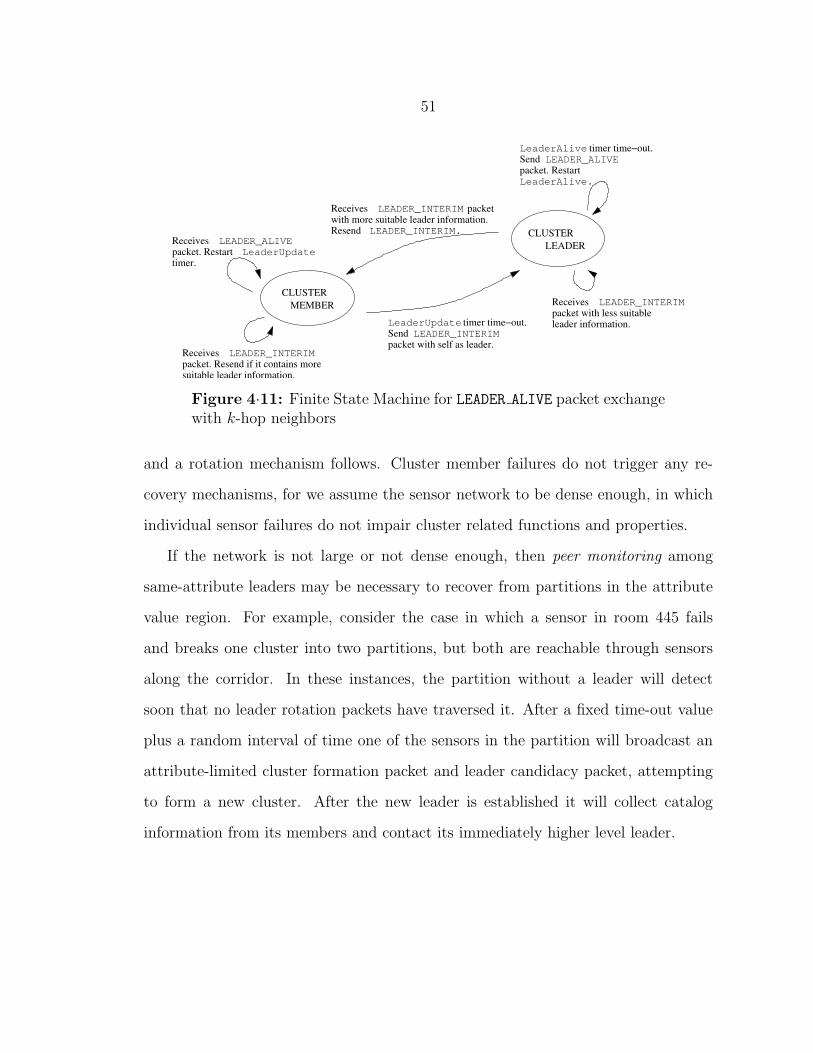
51

CLUSTERLEADER

LeaderAlive timer time−out.Send LEADER_ALIVE

LeaderAlive.packet. Restart

LEADER_ALIVEReceivespacket. Restart LeaderUpdatetimer.

Receives LEADER_INTERIM packetwith more suitable leader information.Resend LEADER_INTERIM.

MEMBERCLUSTER

Send LeaderUpdate timer time−out.

LEADER_INTERIMpacket with self as leader.

Receives LEADER_INTERIM

Receives LEADER_INTERIMpacket with less suitableleader information.

packet. Resend if it contains moresuitable leader information.

Figure 4·11: Finite State Machine for LEADER ALIVE packet exchangewith k-hop neighbors

and a rotation mechanism follows. Cluster member failures do not trigger any re-

covery mechanisms, for we assume the sensor network to be dense enough, in which

individual sensor failures do not impair cluster related functions and properties.

If the network is not large or not dense enough, then peer monitoring among

same-attribute leaders may be necessary to recover from partitions in the attribute

value region. For example, consider the case in which a sensor in room 445 fails

and breaks one cluster into two partitions, but both are reachable through sensors

along the corridor. In these instances, the partition without a leader will detect

soon that no leader rotation packets have traversed it. After a fixed time-out value

plus a random interval of time one of the sensors in the partition will broadcast an

attribute-limited cluster formation packet and leader candidacy packet, attempting

to form a new cluster. After the new leader is established it will collect catalog

information from its members and contact its immediately higher level leader.

52

Cluster Join and CH Update Algorithms

Newly deployed sensors will attempt to join the neighboring clusters that first answers

the join request (this is the default have the same attribute values. They do so

by broadcasting a request for membership packet. If no answer is received for n

such broadcasts (each broadcast will be separated by a period of time which is of

exponentially increasing interval length) then the sensor remains isolated and will

cluster only when a cluster formation packet arrives. Thus all initial sensors are

isolated until “triggered” by an external signal from their base-station, as described

previously.

CLUSTER_INFO packetpacket. Send suitable

if possible.

JOIN_CLUSTERReceives

thresholdJOIN_CLUSTERSends packet.

times, startAfterNewClustertimer.

Resend if it containsmore suitable leaderinformation.

ReceivesNEW_CLUSTER packet.

CLUSTER_INFOReceivespacket with no suitable

timer.NewClustermaximum hop threshold. Startleader information or above

NewCluster

with self as leader.

timer time−out.Send NEW_CLUSTER packet

NEW_CLUSTER

leader informationpacket with less suitableReceives

NEW_CLUSTER

leader informationpacket with more suitableReceives

packet with suitable leaderReceives CLUSTER_INFO/NEW_CLUSTER

information.

CLUSTERLEADER

MEMBERCLUSTER

UNCLUSTERED

Receives JOIN_CLUSTERpacket. Send suitableCLUSTER_INFO

packet if possible.

Figure 4·12: Finite State Machine for joining existing clusters

However, if there are clustered sensors nearby, they will answer the membership

request by sending their CH instance information, as well as all of their CH cluster

information. The new sensor may join the closest clustered network (at each CH

level), if attributes match, or may attempt to form a new cluster. Fig. 4·12 shows

the finite state machine for cluster join and update algorithms. In case a join is

53

performed, catalog-related information is forwarded to its leader.

This mechanism effectively supports dynamic CH updates. That is, given an at-

tribute hierarchy, a virtual overlay of hierarchical clusters can be formed and changed

during deployment to reflect changes to the hierarchy. If we update the hierarchy by

adding an attribute node, then sensors receiving the CH update are effectively the

same as newly deployed sensors which do not have a cluster leader (in that level)

but which are in an already deployed network. These sensors will request member-

ship but will receive cluster information without any matching CH level instance,

at which point they will group themselves together and elect new leaders. These

new leaders will contact (potentially through flooding the higher level cluster) their

higher level leaders and lower level leaders (if existent) and re-establish the unicast

communication architecture among adjacent level clusterheads.

To complete our discussion of dynamic CH updates, note that the removal of

a level does not affect any member, since sensors kept all information for all CH

levels. They simply erase the information regarding that level. Leaders of the level

below the removed one send catalog update information to leaders two levels up in

the old CH (such paths were formed when the higher level leaders were elected). In

the next section we show how packets can be routed within the hierarchy, and path

maintenance issues.

4.2.2 Routing Between Cluster Leaders

Cluster leaders from adjacent hierarchy levels maintain paths to each other. When a

packet is unicast, nodes along the path overhear the next hop neighbor rebroadcast

the packet before considering the packet delivered. If the rebroadcast from the

downstream neighbor is not overheard, the current node will perform a local hop-

restricted flood to find a new downstream neighbor to the final destination node.

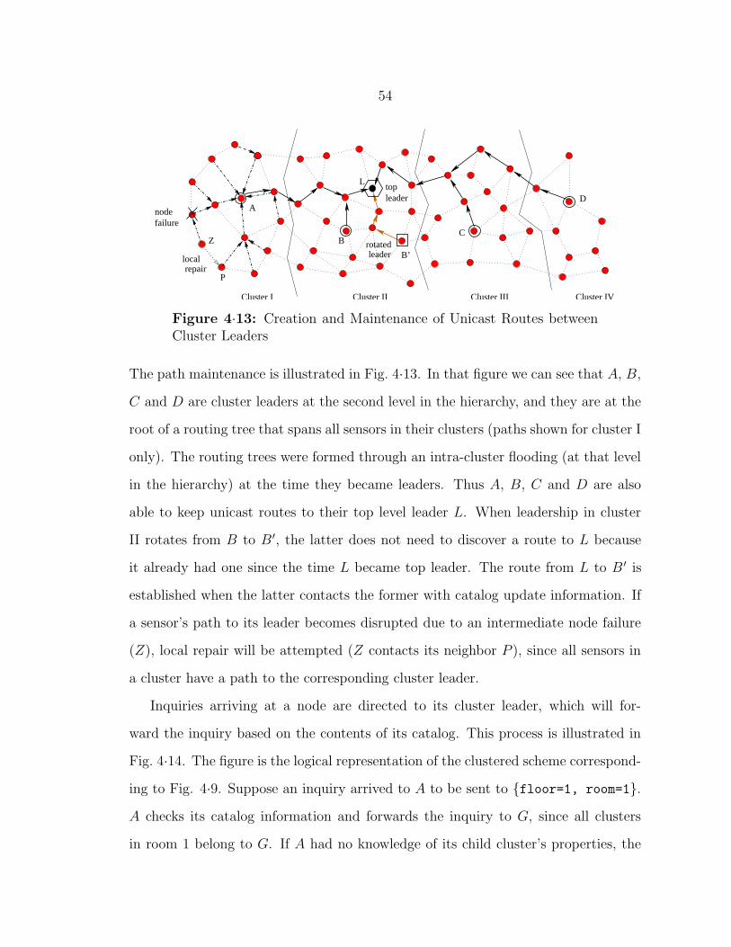
54

nodefailure

Z

A

BC

D

L

P

localrepair

B’rotatedleader

topleader

Cluster I Cluster II Cluster III Cluster IV

Figure 4·13: Creation and Maintenance of Unicast Routes betweenCluster Leaders

The path maintenance is illustrated in Fig. 4·13. In that figure we can see that A, B,

C and D are cluster leaders at the second level in the hierarchy, and they are at the

root of a routing tree that spans all sensors in their clusters (paths shown for cluster I

only). The routing trees were formed through an intra-cluster flooding (at that level

in the hierarchy) at the time they became leaders. Thus A, B, C and D are also

able to keep unicast routes to their top level leader L. When leadership in cluster

II rotates from B to B ′, the latter does not need to discover a route to L because

it already had one since the time L became top leader. The route from L to B ′ is

established when the latter contacts the former with catalog update information. If

a sensor’s path to its leader becomes disrupted due to an intermediate node failure

(Z), local repair will be attempted (Z contacts its neighbor P ), since all sensors in

a cluster have a path to the corresponding cluster leader.

Inquiries arriving at a node are directed to its cluster leader, which will for-

ward the inquiry based on the contents of its catalog. This process is illustrated in

Fig. 4·14. The figure is the logical representation of the clustered scheme correspond-

ing to Fig. 4·9. Suppose an inquiry arrived to A to be sent to {floor=1, room=1}.A checks its catalog information and forwards the inquiry to G, since all clusters

in room 1 belong to G. If A had no knowledge of its child cluster’s properties, the

55

G J A QM

A EDCG H J K L

A

RM N PFB QI O

Inquiry for {Floor 1, Room 1}

Inquiry for {Floor 3, Room 2}

Room 1Room 2 Room 2

Room 1

Floor 2 Floor 3Floor 1

Floor Leaders

Room Leaders

Same Attribute Leaders

Building Leaders

Sensed data

Figure 4·14: Inquiry Routing in C-DAG instances.

inquiry would have been forwarded to all child cluster leaders (G, J , M , Q and

A). Likewise, if an inquiry is received by N regarding {floor=3, room=2}, when

the inquiry reaches M , M can redirect the inquiry directly to O and P . Note that

because inquiries do not cross cluster boundaries, an inquiry that reaches O will not

be forwarded to P and vice-versa.

Having laid down the foundations of establishing a virtual hierarchy of clusters

in the network, in the following sections we will present infra-structure to support

routing rules set that dictate how packets are delivered in the network (like the

behavior exemplified by Fig. 4·14) which yield different performance levels. The

different performance levels can be selected by applications to match their higher

level objectives.

4.3 Rules Based Routing in Clustered WSNET

Routing behavior in the large scale can be determined by how incoming packets are

processed. In our infrastructure we use sets of rules that guide packet behavior based

on the existing overlaid attribute hierarchy. Rules are interpreted, and rules sets can

be supported concurrently so that each application may forward packets based on

the application requirements. In the following sections we show the components of

our solution, which include the specification of address names in the routing rules,

56

the data structures used to track routing information, and the pseudo-code for three

sets of routing rules set.

4.3.1 Naming

Address names in our routing scheme are composed of a sequence of attributes.

Attributes possess name, type and value. Attribute names are specified as strings.

The default type for all attributes is string, unless otherwise specified. Additional

possible types are char, short, integer, float and double. If the type is an char, then

the value is stored in one byte. Two bytes for short, 4 for int and float and 8 for

double. String values are stored in an array of chars, with a special termination

character like C strings.

We assume that sensors that are deployed are tagged with location based at-

tributes that are relevant to the users of the sensor network. That is, users select

these attributes in their inquiries. These location-based attributes can be as specific

as GPS coordinates or can be as generic as Quadrant, Subquadrant, etc.

Attributes are only well-defined in the context of an attribute hierarchy. Attribute

hierarchies are represented via a C-DAG specified through a file, and brings with it a

list of all attribute names and their respective types, together with possible values for

each attribute. In addition, containment relationships and adjacency relationships

are clearly defined for attribute names and attribute values, respectively. This means

that given two attribute names, we must be able to tell whether one is contained in

the other (e.g., subquadrant ⊂ quadrant, GPS X coordinate 6⊂ GPS Y coordinate).

Likewise, given two attribute values (e.g., “NorthEast” and “NorthWest”), when

queried, “NorthEast” IsAdjacentTo “NorthWest” returns true. See appendix B for

more details.

A hash function (such as MD5 or SHA) generates a message digest for the file

57

specifying the attribute hierarchy that is used as the identifier for this hierarchy.

When sending information packets, sensors attach the hierarchy’s identifier together

with the set of attributes that form the address. The order of appearance of the

attributes in an address is relevant: most encompassing attributes (higher in the

hierarchy) appear first.

4.3.2 Clustering

��

��

��

��

��

��

��

�� SouthWest

SouthEast

NorthEastNorthWest

Quadrant

�� SouthWest

NorthEastNorthWest

SouthEastAdjacent

EquivalentCluster

B

C A

D

RepresentationC−DAG

Quadrant

Forest

GPS Coord. XGPS Coord. Y

Subquadrant ��

�� !�!!�!

"�""�"#�##�#$�$$�$%�%%�% &�&&�&'�''�'

(�((�()�))�)

*�*�**�*�**�*�*+�+�++�+�++�+�+

,�,,�,-�--�-

.�..�./�//�/

0�0�00�0�00�0�00�0�00�0�01�1�11�1�11�1�11�1�11�1�1

2�2�22�2�22�2�22�2�22�2�23�3�33�3�33�3�33�3�33�3�3

4�4�4�4�44�4�4�4�44�4�4�4�45�5�5�5�55�5�5�5�55�5�5�5�5

6�6�66�6�66�6�66�6�66�6�67�7�77�7�77�7�77�7�77�7�7

A

B

C

D Temp=67,6768,69,69

Catalog

Temp=68Humid.=30,30

CatalogCatalogTemp=67,67Light=110

Temp=64Light=100, 105

Catalog

Figure 4·15: Cluster Equivalency

It is assumed that sensors in the network will be clustered according to the

attribute nodes defined in a C-DAG, as described in Sec. 4.2. Sensors should thus be

separated into attribute equivalent clusters, as shown in the bottom part of Fig. 4·15,

with the leaders representing each cluster (top part of Fig. 4·15) as depicted by the

C-DAG.

Due to the broadcast nature of the clustering formation protocol, sensors know

whether they are “border” cluster sensors (that is, they are within range of a sensor

that belongs to another cluster) or not. Border cluster sensors will overhear the

broadcast of a neighbor that selects a different leader, if their neighbor belongs to

the same attribute hierarchy, or the retransmission of the original cluster formation

58

packet in which the sender specifically flags as not belonging to any cluster in the

hierarchy being formed. In such transmission the sender usually also transmits infor-

mation about the clusters of the hierarchy to which it belongs. Thus border cluster

sensors are able to inform their cluster leaders of adjacent cluster’s attributes. In

Fig. 4·15 the adjacency relationships are represented by dark lines connecting the

cluster leaders.

Sensors that reside on the path between border cluster sensors and the cluster

leader learn a route to the attribute region represented by the adjacent cluster. Other

routes that sensors may learn include paths to their cluster leaders (information

obtained during cluster formation time), and occasionally paths to clusters a sensor

is not a member of (this information is usually learnt when the sensor lies in the path

that a lower level cluster leader used to send catalog information to an upper level

cluster leader). Sensors store these path information in a routing table structure we

describe next.

4.3.3 Routing Information Storage

The data structure we use to store routing information is better viewed as composed

of three parts: the first part is composed of graph structures representing known

attribute hierarchies and which is indexed by the hierarchy identifiers. The second

part lists attributes which have been received (i.e., found in a packet) yet whose

attribute hierarchy is unknown. The third part lists current membership clusters the

sensor is part of, and routing information to cluster members. For simplicity we will

refer this three-part structure as routing table, even though it is not technically a

table.

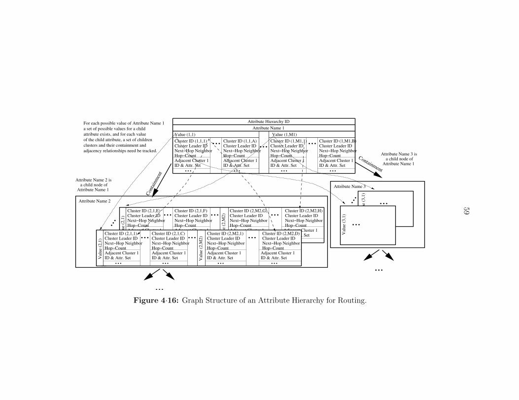
59

For each possible value of Attribute Name 1a set of possible values for a childattribute exists, and for each value

adjacency relationships need be tracked.

of the child attribute, a set of children clusters and their containment and

Containment

Conta

inmen

t

Val

ue (3

,1)

Adjacent Cluster 1ID & Attr. Set...


Cluster ID (2,1,E)Cluster Leader IDNext−Hop NeighborHop−CountAdjacent Cluster 1ID & Attr. Set...

...

Val

ue (2

,1) ...

Val

ue (2

,M2)...

Next−Hop NeighborHop−Count


Cluster ID (2,1,F)Cluster Leader IDNext−Hop NeighborHop−Count

Cluster ID (2,M2,G)Cluster Leader IDNext−Hop NeighborHop−Count

Cluster ID (2,M2,H)Cluster Leader ID

Attribute Name 1

Attribute Name 3 isa child node of

...Adjacent Cluster 1ID & Attr. Set ...

Adjacent Cluster 1ID & Attr. Set ...

Adjacent Cluster 1ID & Attr. Set ...

Adjacent Cluster 1ID & Attr. Set

...

Attribute Name 3

Val

ue (3

,1)

...

......

Cluster ID (2,1,C)Cluster Leader IDNext−Hop NeighborHop−Count

Cluster ID (2,M2,1)Cluster Leader IDNext−Hop NeighborHop−Count

Cluster ID (2,M2,D)Cluster Leader IDNext−Hop NeighborHop−Count

Cluster ID (2,1,1)Cluster Leader IDNext−Hop NeighborHop−Count

...Adjacent Cluster 1ID & Attr. Set ... ... ...

...

...

Attribute Name 2

...

Val

ue (2

,M2)......

Val

ue (2

,1)

ID & Attr. SetAdjacent Cluster 1ID & Attr. Set

Adjacent Cluster 1ID & Attr. Set

Adjacent Cluster 1

Attribute Name 1

Attribute Name 2 isa child node of

...Value (1,M1)

...Value (1,1)

Attribute Name 1Attribute Hierarchy ID

...Cluster ID (1,1,1) Cluster ID (1,1,A) Cluster ID (1,M1,1) Cluster ID (1,M1,B)Cluster Leader IDNext−Hop NeighborHop−Count

Cluster Leader IDNext−Hop NeighborHop−Count



Figure 4·16: Graph Structure of an Attribute Hierarchy for Routing.

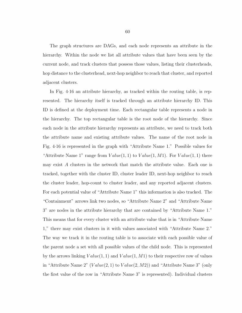
60

The graph structures are DAGs, and each node represents an attribute in the

hierarchy. Within the node we list all attribute values that have been seen by the

current node, and track clusters that possess those values, listing their clusterheads,

hop distance to the clusterhead, next-hop neighbor to reach that cluster, and reported

adjacent clusters.

In Fig. 4·16 an attribute hierarchy, as tracked within the routing table, is rep-

resented. The hierarchy itself is tracked through an attribute hierarchy ID. This

ID is defined at the deployment time. Each rectangular table represents a node in

the hierarchy. The top rectangular table is the root node of the hierarchy. Since

each node in the attribute hierarchy represents an attribute, we need to track both

the attribute name and existing attribute values. The name of the root node in

Fig. 4·16 is represented in the graph with “Attribute Name 1.” Possible values for

“Attribute Name 1” range from V alue(1, 1) to V alue(1,M1). For V alue(1, 1) there

may exist A clusters in the network that match the attribute value. Each one is

tracked, together with the cluster ID, cluster leader ID, next-hop neighbor to reach

the cluster leader, hop-count to cluster leader, and any reported adjacent clusters.

For each potential value of “Attribute Name 1” this information is also tracked. The

“Containment” arrows link two nodes, so “Attribute Name 2” and “Attribute Name

3” are nodes in the attribute hierarchy that are contained by “Attribute Name 1.”

This means that for every cluster with an attribute value that is in “Attribute Name

1,” there may exist clusters in it with values associated with “Attribute Name 2.”

The way we track it in the routing table is to associate with each possible value of

the parent node a set with all possible values of the child node. This is represented

by the arrows linking V alue(1, 1) and V alue(1,M1) to their respective row of values

in “Attribute Name 2” (V alue(2, 1) to V alue(2,M2)) and “Attribute Name 3” (only

the first value of the row in “Attribute Name 3” is represented). Individual clusters

61

representing a parent node track those clusters of a child node individually. These

are the dashed arrows that link “Cluster ID(1,1,1)” under V alue(1, 1) in “Attribute

Name 1” to the clusters in the first row of values in “Attribute Name 2” and the

arrow linking “Cluster ID(1,M1,1)” to “Cluster ID(2,M2,H).”

Thus in this first part, known instances (i.e., clusters with matching attributes)

of nodes in the attribute hierarchy are tracked, together with their containment and

adjacency relationships. Since multiple clusters may exist, each is also tracked with

respect to the cluster leader ID and cluster ID. Because of the rotation process, cluster

leader ID may change often, yet the cluster ID should remain constant throughout

deployment time.

Next−Hop 1 Hop Count 1 Time Recv. 1Next−Hop 2 Hop Count 2 Time Recv. 2Next−Hop 3 Hop Count 3 Time Recv. 3

Attr Name (1,1) Attr Val (1,1) Attr Name (1,N1) Attr Val (1,N1)Attr Name (2,1) Attr Val (2,1) Attr Name (2,N2) Attr Val (2,N2)Attr Name (3,1) Attr Val (3,1) Attr Name (3,N3) Attr Val (3,N3)

Attr Val (1,1) Attr Val (X11,Y11) I(X11,Y11)Attr Val (1,2) Attr Val (X12,Y12) I(X12,Y12)

Attr Val (1,N1) Attr Val (X1N1,Y1N1) I(X1N1,Y1N1)Attr Val (2,1) Attr Val (X21,Y21) I(X21,Y21)

123

1 E(1,1) E(X11,Y11)1 E(1,2) E(X12,Y12)

1 E(1,N1) E(X1N1,Y1N1)2 E(2,1) E(X21,Y21)

Attr Name (1,1)Attr Name (1,2)

Attr Name (1,N1)Attr Name (2,1)

(b)

(a)

Figure 4·17: Structures to Index Packets Received Without AttributeHierarchy.

The second part of the routing table is composed of two more data structures.

The first one brings with it the attribute name-value pairs found in a packet, the

neighbor through which the packet was received, the hop-distance to the original

sender and the time received. We can see the representation of this first structure in

Fig. 4·17(a). The leftmost column indexes the number of packets with distinct list

of attribute name-value pairs, and each element in the column tracks the next-hop

neighbor from which the packet was received, the hop count to the original sender,

time received and the list of attribute name-value pairs. The second structure stores

62

the attributes seen in a packet individually, and indexes a series of entries from the

first table from which specific values can be found. In Fig. 4·17(b) the leftmost

column is a list of individual attribute names. Each attribute name tracks all the

possible values seen (Attr Val(1,1) to Attr Val (X11,Y11)), together with the indices

of packets in the first structure in which the value appeared (Attr Val(1,1) appeared

in packets {1, ..., E(1,1)}, Attr Val (X11,Y11) appeared in packets {I(X11,Y11), ...,

E(X11,Y11)}, etc.). Entries in these two tables are deleted after a time-out period.

That is, sensors that do not identify which hierarchies they belong to are not assumed

to have relevance in the long term deployment of the sensor network.

Attr Val (M,NM)Member M Name Attr Name (M,1) Attr Val (M,1) Attr Name (M,NM) Next−Hop M Hop Count M

Attr Val (1,N1)Member 1 Name Attr Name (1,1) Attr Val (1,1) Attr Name (1,N1) Next−Hop 1 Hop Count 1

Attr Val (1,N1)Member 1 Name Attr Name (1,1) Attr Val (1,1) Attr Name (1,N1) Next−Hop 1 Hop Count 1

App Cluster ID 1

App Cluster ID 2

Figure 4·18: Structure to Track Application Cluster Routing Infor-mation.

The third part of the routing table is used for tracking routing information within

application clusters. It is indexed by the Application cluster ID, followed by its

cluster members’ names, a list of attribute name-value pairs that each member must

match, the next hop neighbor and the hop count to reach the member. This can

be seen in Fig. 4·18. Application clusters should be small in nature, and a flat

table structure is reserved to track routing information. If a hierarchical approach is

required, it should be implemented at the application level.

As we can see, sensors store only a next-hop value for an attribute value re-

gion. Every sensor in the network is essentially a distributed routing knowledge

storage point. When senders transmit packets to a destination and include their own

attribute hierarchy identifiers and attribute lists, they are essentially distributing

63

hop-by-hop information on how to be reached to the sensors along the way. In the

examples above either the sender is essentially announcing itself to nearby sensors

and thus forming paths to itself (in the case of cluster formation), or the sender is

already aware of paths to the destination (in the adjacency information update and

the catalog update cases). We discuss in the next section issues in routing packets

for which a path to the destination may not be known.

4.3.4 Rules-Based Routing

In our proposed framework the routing process is an interpreted one and behavior is

defined by routing rules. Rules sets are tracked through IDs (specified at deployment

time) and are classified according to whether they are independent of any specific

application:

• Application Independent - application independent sets are default routing

rules set that are either present in the nodes before deployment or is propagated

at cluster formation time. Nodes may hold different application independent

sets simultaneously. If an application needs to invoke other set of routing rules

for packet processing, it must indicate so by adding a routing rule set identifier

in the packet header. If the requested routing rule set is not present in the

node, then default routing behavior is adopted. Identifiers for these rules set

may be pre-defined strings or numeric IDs.

• Application Dependent - applications may bring with them their own set of

routing rules, though, and these may be changed dynamically. If applications

do not require change of routing rules at all nodes in the network, but only on

a small subset, then they may request forming a small cluster for this purpose.

Nodes that become members of such cluster either must possess the same rout-

ing rule set or request the set from the cluster leader. Clusters formed with the

64

purpose of changing routing rules are called application clusters. Nodes may

change membership status of application clusters at will. Application clusters

are established through modified (simpler) versions of the attribute based hi-

erarchical clustering algorithms. Members of the application cluster are given

“names,” that is, a string that identifies a particular set of attribute name-value

pairs. Nodes matching the set assume the “name” given. Thus even in appli-

cation clusters the identification of cluster members is attribute based. The

purpose of these clusters is just to enable different communication patterns for

a small subset of nodes, and thus no inherent support exists for managing high

numbers of members. There is no limitation on the possible number of mem-

bers, but a single cluster with many members will have significant performance

degradation.

By setting routing as an interpreted process, we allow dynamic configuration of

nodes to support different communication patterns and thus meet different commu-

nication needs from the various applications that share the network. It should be

noticed that when a path exists (e.g., that connects a sensor to its cluster leader),

and sensors along the path are aware of the destination, then a data packet would

be merely forwarded along the path. It is essentially when a destination address

is not known, that it then needs be “resolved,” i.e., a set of sensors with matching

attributes must be found. Depending on the address resolution scheme, the resulting

path will be different, and yield different performance results.

We present default routing rules (that can be used for address resolution) that

mimic well known algorithms for routing in meshes [78] and trees [79] (see Alg. 1

and 2). We believe that supplying these basic routing algorithms and at the same

time giving more lower level control of the routing functionality is the best approach

for WSNET application development. Developers may come up with their own

65

routing rule set and these may be re-used by other application developers.

We assume that the routing process will read from a configuration file and store

the routing rules. Changes to the routing rules may be implemented as soon as

the changes are made if the underlying host OS supports signaling. Otherwise the

application must wait until the routing process becomes aware of the changes through

its periodic checking of the file status.

Rules Each rule in our rules based routing is composed of two parts: (1) a con-

ditional statement and (2) an action statement. If the conditions specified are true,

then the action is carried out. Otherwise, the following rule in the rule set is checked.

If no conditional statement turns out true after going through all the rules, the packet

is simply dropped. Our rules based approach essentially imposes a priority scheme

over possible next-hop destinations. Each conditional statement defines a subset of

all possible incoming packet states, and each action statement essentially defines a

possible next-hop destination. Thus the order in which the rules are placed within

the rule set reflects the priority assigned to each possible “state-destination” associa-

tion. Ideally, the first rule in the rule set should reflect the most common applicable

rule in the network. Because of this “condition-action” separation, the rule set can

actually be described by a series of if-then-else statements.

We show here two sets of routing rules as example of application independent

routing rules set. The first is to route packets within the same attribute hierarchy

and the second to route between different attribute hierarchies.

Within the Attribute Hierarchy When sending packets within the same hi-

erarchy, sensors may follow an algorithm like Algorithm 1. A sensor receiving a

packet initially checks whether the destination address matches a known routing en-

try (Lines 9 and 10 - in this paragraph all Line references are with respect to Alg. 1).

66

If the sensor itself belongs to the region satisfying the attributes sought, then the

packet is flooded (Line 12). If there is a routing entry E matching the destination

address and the packet was not received from the neighbor to which the packet need

be sent to reach E, then the packet can be forwarded to that neighbor. Otherwise,

the information stored in the sensor’s routing entry probably is outdated and the

destination address should be treated as unknown (after Line 15. If the sensor is a

cluster leader, and the packet with an unknown destination address came from the

parent cluster leader (Lines 16 and 17), then the packet is forwarded to any children

clusters that have at least partially matched attributes, that is, there is no known

attribute in the child cluster that has a different value than the values specified in

the destination address (Line 19). If no such child cluster exist, then the packet is

dropped. If the packet did not come from a parent cluster leader then the packet may

be (1) forwarded to a higher level leader (Line 24) if there are attributes further up

in the hierarchy that needs be resolved; (2) sent back to children clusters that have

fuller matches with the destination attributes, assuming all the attributes from the

root node to the current leader level are matched (Line 27) or (3) dropped, if neither

of the two prior conditions can be satisfied (Line 29). Condition (2) above is correct

because at cluster formation time all cluster leaders under the same parent instance

know of each other. Thus, if a packet is destined to “Building=PHO, Floor=3,”

then if a packet reaches a cluster leader for “Building=PHO, Floor=3”, this packet

can be forwarded to all “Floor=3” clusters (Line 26). In this way any attribute that

need be resolved under “Building, Floor” can be resolved at lower level clusters.

The Mesh traversal algorithm (Alg. 2), unlike the Tree traversal (Alg. 1) one,

drops packets that have been seen before (Line 8 in Alg. 2). In the tree traversal,

unknown destination packets may be sent to higher level cluster leaders (Line 24 of

Alg. 1), and these may eventually forward the packets back (Line 27 of Alg. 1). The

67

Mesh traversal algorithm forwards packets of unresolved attributes to neighbor clus-

ters (Line 21 in Alg. 2). Notice the different approach each routing rule establishes

on resolving unknown addresses: while in the tree case the packets are forwarded up

the hierarchy level, in the mesh the packets are simply spread towards other adjacent

clusters. These two resolution modes also characterize the intrinsic communication

pattern each rules set supports. Sensor networks that are deployed for different ap-

plications will benefit from being able to support switching between the two modes,

as we will show in the next chapter.

Full knowledge of how to route packets based on the attributes specified is only

possible in the presence of an attribute hierarchy. The attribute hierarchy brings

information on all possible attribute names and values, as well as containment and

adjacency relationships. Therefore with the full knowledge of the attribute hierarchy

a sensor not only knows whether the attributes sought can be satisfied, but also how

to forward a packet to the appropriate regions to find suitable sensors. The root node

of the attribute hierarchy must have full knowledge of the entire attribute hierarchy.

Between Attribute Hierarchies Routing packets between two sensor network

applications may happen in two ways, (A) the two applications share the same

geographic space, that is, either two sensor networks have been deployed at the same

location, or two applications are sharing the same sensors, or (B) the two applications

are separated by one or more sensor network in-between.

In case (A) above, since the two sensor networks are in the same geographic region,

any cluster formation packet or new leader packet from one application will be stored

by the sensor and the information shared by the other. Applications become thus

mutually aware of each other’s attribute hierarchies and can route packets between

them.

However, to have a priori knowledge of the attribute hierarchy is not always

68

feasible, especially in the case (B) above, when we are connecting two sensor networks

that are far apart geographically and are not aware of each other’s presence. This may

happen when the sending network is probing the space around it to find networks

with sensors satisfying certain attributes. That is, the sender specifies attributes

that it believes a desired destination sensor must possess. Since this involves a very

subjective evaluation of possible attributes, we propose a prioritized approach to the

attribute matching process. The sender flags that there is no attribute hierarchy ID

attached to the packet, and will flag either a single status for all attributes listed, or

that each attribute will have its own status. The possible status are:

• Required - the packet must be delivered in the end to sensors that matches

all name-value specifications of the “required” attributes. If no known sensor

matches all the attributes then the packet is dropped.

• Preferred - the packet must be delivered to sensors that match the most number

of name-value specifications of preferred attributes. In case two or more groups

of sensors satisfy different sets of attributes but the sets have the same number

of elements, the packet will be forwarded to all the groups. “Required” at-

tributes have precedence over “preferred” attributes. If “preferred” attributes

co-exist with “required” attributes in the same packet, the packet will be sent

to the sensors that satisfy all the “required” attributes and the most number of

“preferred” attributes. The packet will not be delivered even if one “required”

attribute is not satisfied, independently of how many “preferred” attributes are

matched.

• Exploring - “exploring” attributes are only relevant when there are no “re-

quired” attributes in the packet, and when no “preferred” attributes are matched.

In this case, the packet will be forwarded first to the sensors that match the

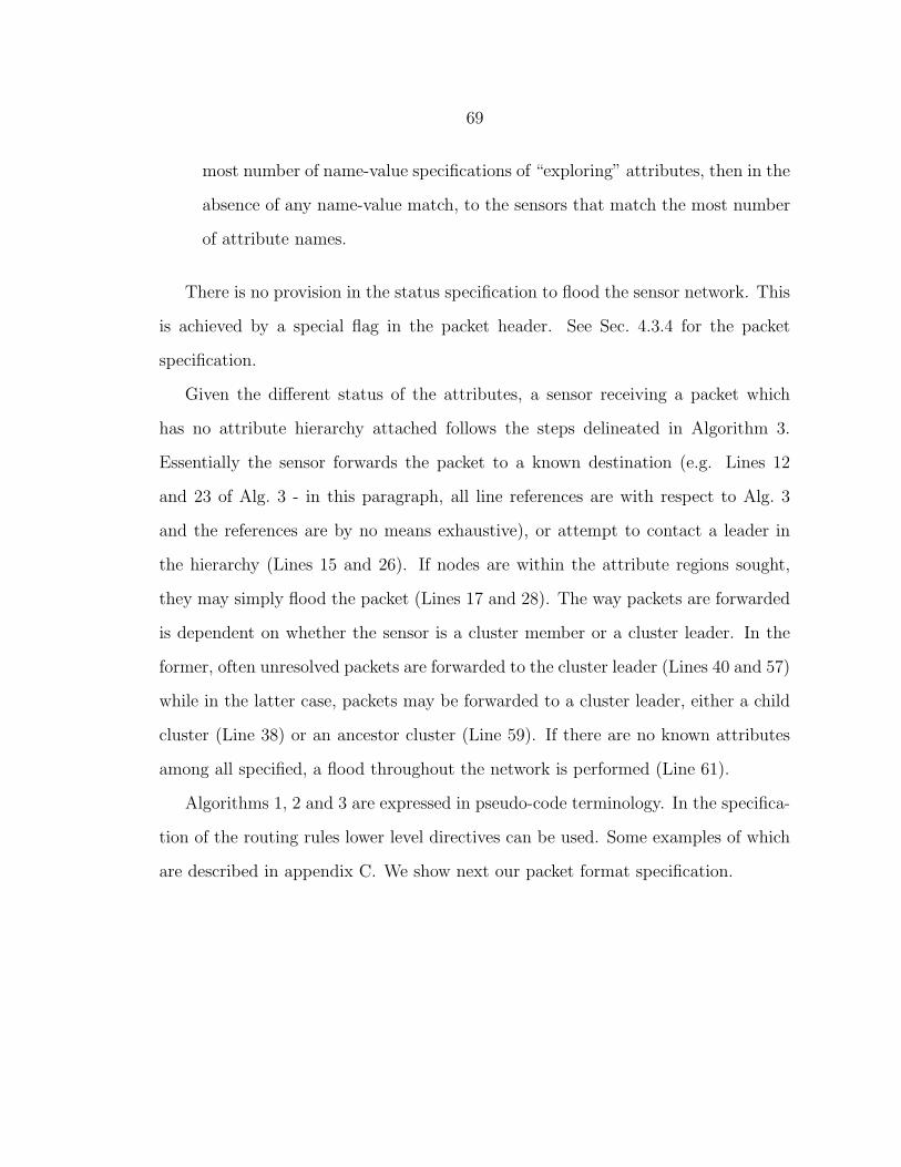
69

most number of name-value specifications of “exploring” attributes, then in the

absence of any name-value match, to the sensors that match the most number

of attribute names.

There is no provision in the status specification to flood the sensor network. This

is achieved by a special flag in the packet header. See Sec. 4.3.4 for the packet

specification.

Given the different status of the attributes, a sensor receiving a packet which

has no attribute hierarchy attached follows the steps delineated in Algorithm 3.

Essentially the sensor forwards the packet to a known destination (e.g. Lines 12

and 23 of Alg. 3 - in this paragraph, all line references are with respect to Alg. 3

and the references are by no means exhaustive), or attempt to contact a leader in

the hierarchy (Lines 15 and 26). If nodes are within the attribute regions sought,

they may simply flood the packet (Lines 17 and 28). The way packets are forwarded

is dependent on whether the sensor is a cluster member or a cluster leader. In the

former, often unresolved packets are forwarded to the cluster leader (Lines 40 and 57)

while in the latter case, packets may be forwarded to a cluster leader, either a child

cluster (Line 38) or an ancestor cluster (Line 59). If there are no known attributes

among all specified, a flood throughout the network is performed (Line 61).

Algorithms 1, 2 and 3 are expressed in pseudo-code terminology. In the specifica-

tion of the routing rules lower level directives can be used. Some examples of which

are described in appendix C. We show next our packet format specification.

70

Algorithm 1 Tree Traversal within the same attribute Hierarchy.

1: CDAG ← {Subquadrant ⊂ Quadrant ⊂ Forest};2: RoutingTable ← Routing table used by current application;3: SensorAttributes ← Attributes current sensor possesses;4: SensorClusters ← Set of clusters the current sensor belongs to;5: SensorClusterLeader ← Set of clusters the current sensor is leader of;6: N (X, Y ) = function that returns the number of consecutively matched attributes be-

tween X and Y , starting from the first attribute in both X and Y ;7: Received packet P;8: DestAttrList ← list of attribute name-value pairs of the destination in P;9: Find E ∈ RoutingTable | (N (DestAttrList,E) is maximized) ;

10: if (E = DestAttrList) then

11: if (E ∈ SensorClusters) then

12: Flood P in E; Return;13: else if (P.PrevHop 6∈ {path between current sensor ∧ E}) then

14: Send P to E; Return;15:

16: if (∃ L ∈ SensorClusterLeader | (L = P.NextHop)) then

17: if (P.PrevHop is parent node in CDAG) ∨ (sensor is root leader) then

18: if (∃ children node | known attributes of children node match DestAttrList) then

19: Send P to children node in CDAG;20: else

21: Drop packet P;22: else

23: if (∃ unmatched attribute at level L or higher between the sensor and DestAt-

trList) then

24: Send P to parent of L;25: else if (all attributes from root to level L match between the sensor and DestAt-

trList ∧ ∃ child cluster with increased attribute match) then

26: Send P to sibling clusters;27: Send P to child cluster;28: else

29: Drop P;30: else

31: Send P to leader of P.NextHop;

71

Algorithm 2 Mesh Traversal within the same attribute Hierarchy.

1: CDAG ← {Subquadrant ⊂ Quadrant ⊂ Forest};2: RoutingTable ← Routing table used by current application;3: SensorClusters ← Set of clusters the current sensor belongs to;4: SensorClusterLeader ← Set of clusters the current sensor is leader of;5: N (X, Y ) = function that returns the number of consecutively matched attributes be-

tween X and Y , starting from the first attribute in both X and Y ;6: Received packet P;7: if (P was received before) then

8: Return;9: DestAttrList ← list of attribute name-value pairs of the destination in P;

10: Find E ∈ RoutingTable | (N (DestAttrList,E) is maximized) ;11: if (E = DestAttrList) then

12: if (E ∈ SensorClusters) then

13: Flood P in E; Return;14: else if (P.PrevHop 6∈ {path between current sensor ∧ E}) then

15: Send P to E; Return;16:

17: if (∃ L ∈ SensorClusterLeader | (L = P.NextHop)) then

18: if (∃ children node | known attributes of children node match DestAttrList) then

19: Send P to children node in CDAG;20: else if (∃ adjacent cluster C at same level of L with matching attribute ∧ no copy

of P came from C) then

21: Forward P to all such C;22: else

23: Drop P;24: else

25: Send P to leader of P.NextHop;

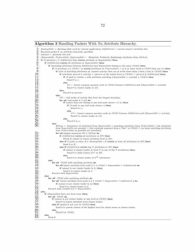
72

Algorithm 3 Handling Packets With No Attribute Hierarchy.

1: RoutingTable ← Routing table used by current application; SelfAttrList ← current sensor’s attribute list;

2: Received packet P, no attribute hierarchy specified;

3: AttrList ← attribute list of P;

4: (RequiredAttr, PreferredAttr, ExploringAttr) ← (Required, Preferred, Exploring) attributes from AttrList;

5: if (∃ attribute r ∈ SelfAttrList that matches attribute in RequiredAttr) then

6: if (SelfAttrList matches all attributes in RequiredAttr) then

7: if (matching attributes between SelfAttrList and RequiredAttr belong to the same CDAG) then

8: if (∃ attribute p ∈ CDAG | (p matches attributes in PreferredAttr) ∧ (p is at lower level in CDAG than any r)) then

9: if ({set of matching attributes p} (named matchp) that are at levels lower than r form a line in CDAG) then

10: if (attribute plowest ∈ matchp) ∧ (plowest at the lowest level in CDAG) ∧ (plowest 6∈ SelfAttrList) then

11: if (∃ path to cluster c with attribute matching {RequiredAttr ∪ matchp} ∈ CDAG) then

12: Send P to c;

13: else

14: LC ← lowest common ancestor node in CDAG between SelfAttrList and {RequiredAttr ∪ matchp}

15: Send P to cluster leader in LC;

16: else

17: Flood P in plowest;

18: else

19: LN ← leaf nodes of matchp that form the longest branches;

20: for all leaf nodes L ∈ LN do

21: if (sensor does not belong to any leaf node cluster c ∈ L) then

22: if (∃ path to any leaf node cluster c) then

23: Send P to c;

24: else

25: LC ← lowest common ancestor node in CDAG between SelfAttrList and {RequiredAttr ∪ matchp}

26: Send P to cluster leader in LC;

27: else

28: Flood P in c;

29: else

30: RPseqs ← {sequences of attributes from RequiredAttr ∪ matching attributes from PreferredAttr | (all attributesfrom RequiredAttr are present) ∧ (the resultant sequence form a “line” in CDAG) ∧ (as many matching attributesfrom PreferredAttr as possible are included)}

31: for all longest sequences RP ∈ RPSeqs do

32: if (SelfAttrList matches all attributes in RP) then

33: Flood in cluster at lowest attribute level in RP;

34: else if (∃ path to entry E ∈ RoutingTable | E matches at least all attributes in RP) then

35: Send P to E;

36: else if (SelfAttrList matches top T attributes in RP) then

37: if (sensor is cluster leader at level C in any of the T attributes) then

38: Send P to child cluster of C in RP;

39: else

40: Send P to cluster leader of T th attributes;

41: else

42: for all CDAG with matching attribute do

43: for all lowest attribute level node L ∈ { CDAG ∩ RequiredAttr ∩ SelfAttrList} do

44: if (sensor is not cluster leader in L) then

45: Send P to cluster leader in L

46: Flood P with RequiredAttr

47: else

48: for all CDAG with matching attribute do

49: for all lowest attribute level node L ∈ { CDAG ∩ RequiredAttr ∩ SelfAttrList } do

50: if (sensor is not cluster leader in L) then

51: Send P to cluster leader in L

52: Flood P with (SelfAttrList ∩ RequiredAttr)

53: else

54: if (RequiredAttr have not been seen) then

55: for all CDAG do

56: if (sensor is not cluster leader at any level in CDAG) then

57: Send P to lowest attribute level cluster leader;

58: else if (sensor is not root in CDAG) then

59: Send P to parent cluster of the highest level for which sensor is cluster leader;

60: else

61: Flood P in CDAG;

62: else

63: Drop P;

73

Cluster Formation Packet

Cluster ID

Dest. ID

# Hopsvalue

Dest. ID

namename

PKT TYPE

Hier. ID

Routing IDPKT LEN

Cluster ID

Prev Hop Node Attr

Tie−breaker

Next Hop Node Attr

PKT TYPE

Source Attr.

Routing ID

Pkt Type Data

PKT LEN

Leader ID

Pkt Type DataFLAG

Hier. ID

FLAG

# Hops valueTie−breaker

Sender ID

Leader ID

Packet Type Dependent Information Terminator Character

Packet Specification

Unicast Packet Format

Dest. Attr.

valuenamevaluename

Sender ID

Figure 4·19: Packet format for cluster formation and unicast packets

74

Packet Formats

Packets in our routing scheme are composed of multiple fields. Fig. 4·19 brings

the specification for the cluster formation type of packet, and packets for unicast

communications. Cluster formation packets are flooded to the whole network, and

brings with them information regarding the clusters that are being formed, while

unicast packets bring specification of the destination, source and in-between node

addresses.

1. [Flag] – the first field is used for flagging. We specify one byte, and the bits

have the following meaning:

(a) bit 1 – existence of destination hierarchy ID (see appendix B).

(b) bit 2 – set if intra-hierarchy routing.

(c) bit 3,4 – specify which routing rules to use. If bits are

00 use the default application independent routing rules set;

01 indicates an application independent routing rules set but one other

than the default;

10 indicates an application dependent routing rules set

11 indicates an application formed intra-cluster routing rules set

(d) bit 5 – existence of source attribute based address

(e) bit 6 to 8 – unused.

2. [Sender ID] – specifies the link layer’s sender’s hardware address.

3. [Dest ID] – specifies the link layer’s destination’s hardware address. If set to

a specific sensor, then it is the “unicast” option, otherwise, all sensors within

range receive the packet (“broadcast”).

75

4. [Pkt Len] – specifies the length of the packet, in bytes. In “unicast” mode, sen-

sors which finds themselves not belonging to the Dest ID may shut themselves

down during the entire length of the transmission.

5. [Routing ID] – this field brings the ID for the routing rules set used. The

IDs for application independent routing rules set are integer numbers, while

IDs for application dependent routing rules set must bring with it the sensor’s

hardware ID and an application specified identifier (name or process number).

6. [Pkt Type] – the various types of packets exchanged in our attribute based

routing scheme. It contains all the clustering formation packet types, catalog

exchange/building, plus data exchange packet types.

7. [Dest Attr] – this field specifies the attributes of the intended destination. It

may initially bring with it the Attribute Hierarchy ID of which the attributes

are part of (in which case bit 1 of the flag byte will be set). A special null byte

is the terminator character that separates the Hierarchy ID and the name and

the value fields of each attribute (see Fig. 4·19).

8. [Next Hop Node Attr] – this field has the attributes of the neighbor node in the

attribute hierarchy to which the packet is intended. Its format is the same as

[Dest Attr]. When bit 2 is set, the field does not have the attribute hierarchy

subfield and assumes the same hierarchy as the one found under [Dest Attr].

9. [Prev Hop Node Attr] – this field has the attributes of the neighbor node in

the attribute hierarchy from which the packet came. Its format is the same as

[Next Hop Node Attr].

10. [Source Attr] – this field’s presence in the packet is indicated by having bit 5

of the flag byte set. Its format is the same as [Next Hop Node Attr].

76

11. [Pkt Type Data] – this field varies according to the type of the packet. Fig. 4·19

shows the contents for a CLUST FORMATION packet, with fields for Attribute

Hierarchy ID, attribute name-value pair, cluster leader, hop count, and tie-

breaker information for leader election mechanism.

We have shown in this chapter the fundamental building blocks of our infrastruc-

ture. By setting an attribute hierarchy and overlaying such virtual hierarchy on the

sensor network, we essentially laid down the units (attribute equivalent clusters of

sensors) in the routing infrastructure that can form attribute-based addresses. Main-

tenance of such units is performed through the Algorithms described in Sec. 4.2.1.

Once such units are established in the network, routing rules are used to guide data

packets. If the destination address is not known, then default routing rules set are

invoked and the unknown destination address is “resolved” to matching sensors in

the network. This matching process establishes a connecting path between source

(cluster) and destination (cluster), which can be used for future data communication

needs. The mechanism through which the resolution took place will yield differ-

ent resulting paths that connect source to destination. Applications with different

performance expectations can choose from different routing rules set to meet their

requirements.

In the next chapter we show how having dynamically configurable addressable

units can reduce transmission costs. We present a theoretical analysis on a square

sensor network being overlaid with a two or three level quadtree attribute hierarchy

and subject to different biased access patterns. Moreover, we show theoretical pre-

dictions on the performance of the two proposed routing schemes in terms of their

costs and resultant path formed during the address resolution process.

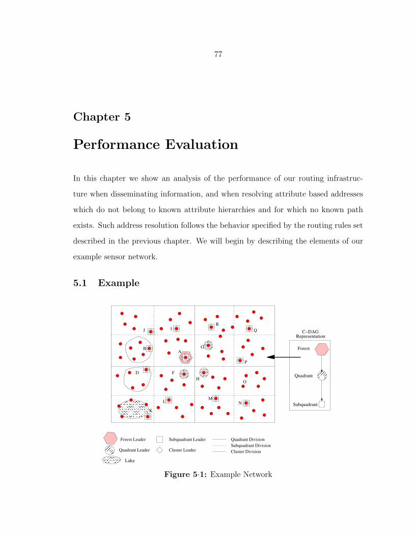
77

Chapter 5

Performance Evaluation

In this chapter we show an analysis of the performance of our routing infrastruc-

ture when disseminating information, and when resolving attribute based addresses

which do not belong to known attribute hierarchies and for which no known path

exists. Such address resolution follows the behavior specified by the routing rules set

described in the previous chapter. We will begin by describing the elements of our

example sensor network.

5.1 Example

��

��

��

��

��

��

��

� � ��

��

Quadrant DivisionSubquadrant DivisionCluster DivisionCluster Leader

Forest Leader

Quadrant Leader

Subquadrant Leader


Subquadrant

Quadrant

Forest

Lake

AB

D F

G

H

IJ

L MN

O

P

QR

K

Figure 5·1: Example Network

78

The deployed sensor network example we will study is illustrated by Fig. 5·1while the representative C-DAG is the 3 level single child structure shown in right

side of the same Figure. Because at each hierarchy level there is only one child, we

interchangeably will refer to such hierarchy as “line” hierarchy. We discuss next all

the aspects of its deployment and attributes assigned. There are N sensors spread

uniformly over a square region of side L.

Sensors in the field are initially tagged with appropriate attributes, including lo-

cation oriented ones. A GPS capable device can be used to communicate the correct

geographical coordinates to a sensor before it is deployed. For indoor applications,

a similar device with pre-assigned human readable location attributes may be used,

that is, the device would imprint “Quadrant=NE” or “Subquadrant=NE” tags onto

the sensors. The attributes that are being tagged prior to deployment are consid-

ered core attributes. We assume that once deployed, it will not be necessary (nor

feasible) to update these core attributes. Note that derived attributes may still be

added after deployment, e.g., sensors with “Quadrant=SW,Subquadrant=SW” and

“Quadrant=SW,Subquadrant=SE” are assigned the “Lake=Walden” attribute. We

call these derived attributes dynamic attributes.

We discuss in appendix B practical considerations of attribute tagging. For now,

we assume sensors are tagged with core attributes, and all sensors know the different

relationships among the attributes (e.g., containment and adjacency relationships).

Some sensors also have the full name-value information of all possible core attributes,

while other sensors only know the name-value information of attributes with which

it had been tagged (these sensors may not become cluster leaders).

Thus in the deployed sensor network example considered above sensors deployed

have the following attributes:

• Name: X, Values: xmin ≤ X ≤ xmax

79

• Name: Y , Values: ymin ≤ Y ≤ ymax

• Name: Forest, Values:“Lorien”

• Name: Quadrant, Values: NE,NW,SE, SW

• Name: Subquadrant, Values: NE,NW,SE, SW

The C-DAG is represented by the three last attributes and form a line: Subquadrant

⊂Quadrant⊂ Forest. From the C-DAG the containment relationships follow, which

are:

• Subquadrant ⊂ Quadrant

• Quadrant ⊂ Forest

Adjacency relationships are defined separately (see appendix B) and can be ex-

pressed as:

• Quadrant

– NW adjacent NE, NW adjacent SW, NE adjacent SE, SW adjacent SE

• Subquadrant (the adjacency relationships below concern two subquadrants S1

and S2 - subquadrant adjacency relationships are conditional on the adjacency

of the quadrants):

– NE adjacent NW, SE adjacent SW, S1 Quadrant ∈ NW, S2 Quadrant ∈NE

– SE adjacent NE, SW adjacent NW, S1 Quadrant ∈ NW, S2 Quadrant ∈SW

80

– SE adjacent NE, SW adjacent NW, S1 Quadrant ∈ NE, S2 Quadrant ∈SE

– NE adjacent NW, SE adjacent SW, S1 Quadrant ∈ SW, S2 Quadrant ∈SE

The relationships above assume that the sensor knows that adjacency rules are

commutative (i.e., if Q1 adjacent to Q2, then Q2 is adjacent to Q1).

Communication among the sensors follow two patterns:

1. The “tree” like pattern, in which lower level cluster leaders communicate their

data to their immediately higher level cluster leaders, and these in turn forward

the collected information to their upper level leaders. This communication

pattern is used by the climate monitoring application and;

2. The “mesh” like pattern, in which lower level clusters send packets to their

adjacent (same level) clusters. This communication pattern is used by the fire

detection/warning application.

The two rules set can be described by Algorithms 1 and 2.

These are the elements of the deployed sensor network. We will provide in the

following sections two theoretical analysis of this example. The first one shows how

effectively the clustering scheme can reduce redundant transmissions when compared

to flooding schemes, while the second one compares the two in-hierarchy routing

schemes described in Sec. 4.3.4.

5.2 Cost Analysis of Data Dissemination in Attribute Hier-

archy and Flooding Techniques

In this section we present an analysis to establish the effectiveness of creating and

maintaining containment based attribute hierarchies (CHs) over the lifetime of a

81

sensor network as compared to a flooding-based scheme. We focus on the commu-

nication cost for the dissemination of inquiries since power consumption in a sensor

node is dominated by radio communication [37].

Preliminary Considerations The interaction of a community of users with a

deployed sensor network can be represented as inquiries that arrive to the sensor

network with a rate λ. Each arriving inquiry affects a portion Q of the sensors in the

network according to a probability distribution function PQ. The set of all possible

portions Q is denoted S. We make the following simplifications before proceeding to

some theoretical analysis:

1. We assume that the cost of assigning attributes to the sensors so that they

become aware of them is the same for both schemes;

2. We assume a Poisson arrival rate λ which represents the rate of arrival of

requests for data of a type not queried previously and/or from sensors of a

different attribute, i.e., requests that trigger a flooding in the flooding-based

schemes. As stated previously, our scenario is consisted of a network of multi-

modal sensors. This network is a shared resource, and its users are members

from diverse research communities. The arrival λ models the multiple inquiries

that are initiated by this aggregate pool of users.

3. We assume that answers to inquiries traverse through paths formed during

inquiry propagation, and such paths form an inverted tree structure. The exact

number of transmissions needed to send the collected data back is dependent

on the tree structure of each scheme (attribute hierarchies and flooding), and is

left for future research. However, since the underlying mechanism is the same

(tree structures), we believe that the order of magnitude of the number the

transmissions in both cases is similar.

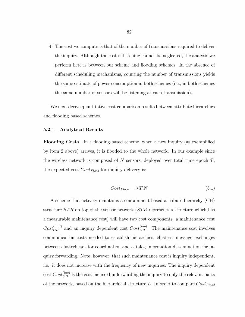
82

4. The cost we compute is that of the number of transmissions required to deliver

the inquiry. Although the cost of listening cannot be neglected, the analysis we

perform here is between our scheme and flooding schemes. In the absence of

different scheduling mechanisms, counting the number of transmissions yields

the same estimate of power consumption in both schemes (i.e., in both schemes

the same number of sensors will be listening at each transmission).

We next derive quantitative cost comparison results between attribute hierarchies

and flooding based schemes.

5.2.1 Analytical Results

Flooding Costs In a flooding-based scheme, when a new inquiry (as exemplified

by item 2 above) arrives, it is flooded to the whole network. In our example since

the wireless network is composed of N sensors, deployed over total time epoch T ,

the expected cost CostFlood for inquiry delivery is:

CostFlood = λT N (5.1)

A scheme that actively maintains a containment based attribute hierarchy (CH)

structure STR on top of the sensor network (STR represents a structure which has

a measurable maintenance cost) will have two cost components: a maintenance cost

Cost(mnt)CH and an inquiry dependent cost Cost

(inq)CH . The maintenance cost involves

communication costs needed to establish hierarchies, clusters, message exchanges

between clusterheads for coordination and catalog information dissemination for in-

quiry forwarding. Note, however, that such maintenance cost is inquiry independent,

i.e., it does not increase with the frequency of new inquiries. The inquiry dependent

cost Cost(inq)CH is the cost incurred in forwarding the inquiry to only the relevant parts

of the network, based on the hierarchical structure L. In order to compare CostFlood

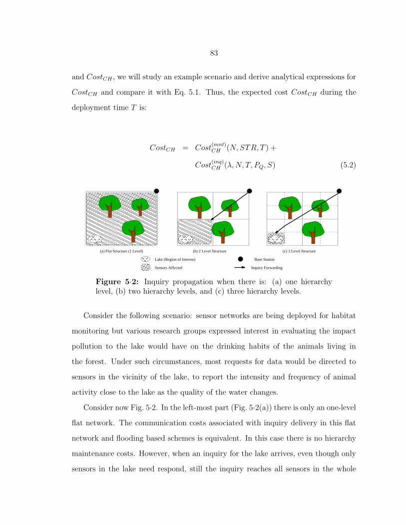
83

and CostCH , we will study an example scenario and derive analytical expressions for

CostCH and compare it with Eq. 5.1. Thus, the expected cost CostCH during the

deployment time T is:

CostCH = Cost(mnt)CH (N,STR, T ) +

Cost(inq)CH (λ,N, T, PQ, S) (5.2)

��

��

��

��

��

��

��

��

��

��

��

��

� �

��

��

��

Inquiry Forwarding

Base Station

Sensors Affected

Lake (Region of Interest)

(c) 3 Level Structure(b) 2 Level Structure(a) Flat Structure (1 Level)

Figure 5·2: Inquiry propagation when there is: (a) one hierarchylevel, (b) two hierarchy levels, and (c) three hierarchy levels.

Consider the following scenario: sensor networks are being deployed for habitat

monitoring but various research groups expressed interest in evaluating the impact

pollution to the lake would have on the drinking habits of the animals living in

the forest. Under such circumstances, most requests for data would be directed to

sensors in the vicinity of the lake, to report the intensity and frequency of animal

activity close to the lake as the quality of the water changes.

Consider now Fig. 5·2. In the left-most part (Fig. 5·2(a)) there is only an one-level

flat network. The communication costs associated with inquiry delivery in this flat

network and flooding based schemes is equivalent. In this case there is no hierarchy

maintenance costs. However, when an inquiry for the lake arrives, even though only

sensors in the lake need respond, still the inquiry reaches all sensors in the whole

84

square area, since there is no mechanism to distinguish one sensor from another.

In Fig. 5·2(b) we establish a hierarchy with one extra upper level (two levels total)

and divide the area into four quadrants. In this case the same inquiry will affect

only 1/4 of the sensors affected in Fig. 5·2(a) plus sensors involved in forwarding the

inquiry from the base station to the lower-left quadrant. In this case a maintenance

cost exists to establish and preserve the structure of quadrants (i.e., establishing

the clusters that map to the four quadrants, choosing clusterheads and maintaining

load balancing schemes), as well as inquiry forwarding costs. In Fig. 5·2(c) we add

another level. With this we reduce the number of sensors affected by the inquiry to

only 1/16 of those in Fig. 5·2(a) and to 1/4 of those in Fig. 5·2(b). The trade-off in

Fig. 5·2(c) is a higher maintenance cost for the two extra levels and a higher inquiry

forwarding cost, if the region relevant to the inquiry is far from the base-station.

In our example, first the inquiry is forwarded from the point of entry (e.g., a

base station) to the top level (level = 1) leader. If the inquiry is for the whole

network, the latter floods it, otherwise it forwards the inquiry to appropriate leaders

at level = 2 (with appropriate region attribute). These will likewise determine

whether the inquiry is for their whole region, in which case they flood the region,

or forward the inquiry to appropriate sub-region leaders (these will then flood their

sub-region, and so on). The cost of flooding the network is N , while that of a region

with level = 2 is N/4 and a sub-region with level = 3, N/16 etc. Unicasts from the

base station to the top level leader have estimated cost of the order of√

2N since

there are as many hops in the longest path in the square area. Likewise, the cost

estimate for forwarding the inquiry from a level 2 leader to a level 3 leader is of the

order of√

2N2

.

Cost of Containment Hierarchy Maintenance CH scheme has an associated

“maintenance cost” for the entire epoch due to the periodic rotation of clusterheads.

85

Suppose the clusterhead rotation period at level = i is Ti for i = 1 to `max. The

total maintenance cost is then given by:

Cost(mnt)CH = N + 2N

`max∑

i=1

T

Ti

+√

2N`max∑

i=2

2i T

Ti

(5.3)

Initial clustering involves one network-wide broadcast that contributes N (first

term in Eq. 5.3) to the cost since each node transmits a broadcast packet only

once. The rest of the terms correspond to cluster maintenance costs. There are TTi

clusterhead rotations at level = i. Each rotation at level = i requires one broadcast

at that level followed by all sensors in the cluster responding to update the catalog

information. The broadcast contributes N to the cost at each level and so does the

catalog update step. This accounts for the second term in Eq. 5.3. The third term

corresponds to the unicast cost of communication of catalogs between cluster leaders,

and is a simplification of 4√

2N TT1

+16√

2N2

TT2

+ · · · , that is, the cost of four quadrants

sending catalogs to the forest leader (crossing a diagonal of√

2N), added to the cost

of 16 subquadrants sending catalog information to quadrant leaders, etc.

Cost of Inquiry Dissemination Now, consider a model where one particular

region at level = `max receives an inquiry with probability p. For example, the

region getting inquiry in Fig. 5·2(b) (we will henceforth refer to this region as R). For

simplicity, we assume that inquiries involving the rest of the possible combinations

are equiprobable with probability q, e.g., q = 1−p

14for `max = 2. In this model, the

average cost incurred for dissemination of inquiries over time T is given by:

Cost(inq)CH = λT{

√2N +

∑

Q∈S

PQCQ} (5.4)

In Eq. 5.4 the estimated cost of forwarding an inquiry from the base station to

the top level leader is of the order of√

2N . This analysis assumes the presence

86

of one leader per attribute-value region. The second term expresses the cost of

disseminating the inquiry to its intended destinations while using the constructed

hierarchy. The summation occurs over all elements Q in the set S of all possible

combinations of sub-regions in the sensor network. In general there are s = 4`max−1

sub-regions and hence |S| = 2s − 1. PQ is the probability of an inquiry involving

the particular combination of sub-regions Q from the set S and CQ is the cost of

disseminating that particular style of inquiry. If Q spans all sub-regions in the

network (level = 1), then CQ = N ; if it only spans m < 4 sub-regions at level = 2,

then CQ = m(√

2N + N4). If Q involves m sub-regions r1, r2, . . . , rm at level = 2

and also involves specific subregions inside each of these rk’s at level = 3 (say,

{r11, . . . , r1n1 ; r21, . . . , r2n2 ; · · · ; rm1, . . . , rmnm}, then the cost is given by:

CQ =m

∑

k=1

{√

2N + nk(

√2N

2+

N

16)} (5.5)

The CQ term for a general level i ≤ `max can be expressed similarly as a sum of

costs due to unicast and scoped broadcast within attribute sub-regions as have been

illustrated above (not presented here). For `max = 2 the total average cost incurred

for dissemination of inquiries for the epoch T is given by:

Cost(inq)CH = λT{p(

√2N +

N

4) +

3

14(1− p)(

√2N +

N

4) +

6

14(1− p)(2

√2N +

N

2) +

4

14(1− p)(3

√2N +

3N

4) +

1

14(1− p)N +

√2N} (5.6)

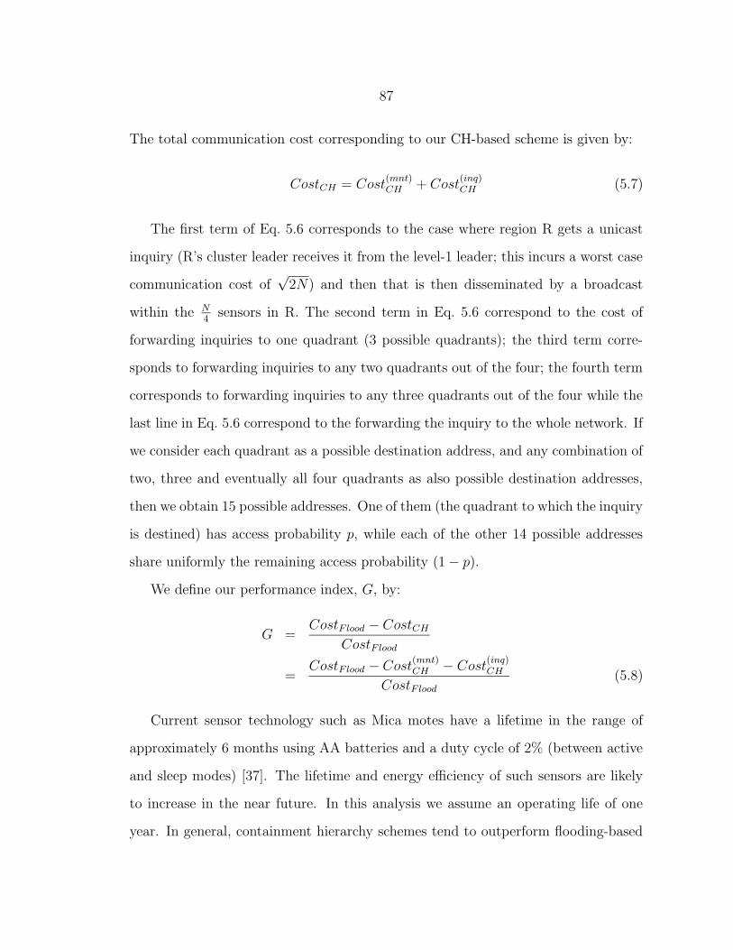
87

The total communication cost corresponding to our CH-based scheme is given by:

CostCH = Cost(mnt)CH + Cost

(inq)CH (5.7)

The first term of Eq. 5.6 corresponds to the case where region R gets a unicast

inquiry (R’s cluster leader receives it from the level-1 leader; this incurs a worst case

communication cost of√

2N) and then that is then disseminated by a broadcast

within the N4

sensors in R. The second term in Eq. 5.6 correspond to the cost of

forwarding inquiries to one quadrant (3 possible quadrants); the third term corre-

sponds to forwarding inquiries to any two quadrants out of the four; the fourth term

corresponds to forwarding inquiries to any three quadrants out of the four while the

last line in Eq. 5.6 correspond to the forwarding the inquiry to the whole network. If

we consider each quadrant as a possible destination address, and any combination of

two, three and eventually all four quadrants as also possible destination addresses,

then we obtain 15 possible addresses. One of them (the quadrant to which the inquiry

is destined) has access probability p, while each of the other 14 possible addresses

share uniformly the remaining access probability (1− p).

We define our performance index, G, by:

G =CostFlood − CostCH

CostFlood

=CostFlood − Cost

(mnt)CH − Cost

(inq)CH

CostFlood

(5.8)

Current sensor technology such as Mica motes have a lifetime in the range of

approximately 6 months using AA batteries and a duty cycle of 2% (between active

and sleep modes) [37]. The lifetime and energy efficiency of such sensors are likely

to increase in the near future. In this analysis we assume an operating life of one

year. In general, containment hierarchy schemes tend to outperform flooding-based

88

schemes for larger time epochs due to amortization of the clustering cost.

0 0.2 0.4 0.6 0.8 10

0.1

0.2

0.3

0.4

0.5

0.6

Level 2 Rotation Period, T2 (days)

Gai

n ov

er F

lood

ing

(G)

N=10000; T=365 days; T1=5 T

2; p=0.5

λ = 64 Q/dayλ = 128 Q/dayλ = 256 Q/dayλ = 512 Q/dayλ = 1024 Q/dayλ = 2048 Q/day

0 0.2 0.4 0.6 0.8 10

0.1

0.2

0.3

0.4

0.5

0.6

Level 2 Rotation Period, T2 (days)

Gai

n ov

er F

lood

ing

(G)

N=10000; T=365 days; T1=5 T

2; p=0.067


Figure 5·3: Effect of Rate of Inquiry and Clusterhead Rotation Periodon Gains: 2 levels in the Containment Hierarchy

1 2 3 4 5 6 7 8 9 10

0.36

0.38

0.4

0.42

0.44

0.46

T3 (days)

Gai

n ov

er F

lood

ing

(G)

N=10000; T=365 days; T1=10 T

3; T

2=5 T

3; p=0.1


1 2 3 4 5 6 7 8 9 10

0.32

0.34

0.36

0.38

0.4

0.42

T3 (days)

Gai

n ov

er F

lood

ing

(G)

N=10000; T=365 days; T1=10 T

3; T

2=5 T

3; p=uniform


Figure 5·4: Effect of Rate of Inquiry and Clusterhead Rotation Periodon Gains: 3 levels in the Containment Hierarchy

First we study the case in which inquiries for one sub-region are extremely pop-

ular (p = 0.5). Results for this case are shown in Fig. 5·3(a). We see that as λ

increases, the dependence of G over the the rotation periods T1, T2 diminishes. This

is expected as T1, T2 influence the fixed maintenance cost due to attribute based

clustering – as more inquiries arrive into the sensor network, the fixed cost penalty

almost vanishes. In Fig. 5·3(b) we study the case in which all 15 combinations of

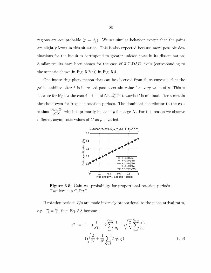
89

regions are equiprobable (p = 115

). We see similar behavior except that the gains

are slightly lower in this situation. This is also expected because more possible des-

tinations for the inquiries correspond to greater unicast costs in its dissemination.

Similar results have been shown for the case of 3 C-DAG levels (corresponding to

the scenario shown in Fig. 5·2(c)) in Fig. 5·4.One interesting phenomenon that can be observed from these curves is that the

gains stabilize after λ is increased past a certain value for every value of p. This is

because for high λ the contribution of Cost(mnt)CH towards G is minimal after a certain

threshold even for frequent rotation periods. The dominant contributor to the cost

is thusCost

(inq)CH

λTNwhich is primarily linear in p for large N . For this reason we observe

different asymptotic values of G as p is varied.

0 0.2 0.4 0.6 0.8 10

0.1

0.2

0.3

0.4

0.5

Prob (Inquiry ∈ Specific Region)

Gai

n ov

er F

lood

ing

(G)

N=10000; T=365 days; T1=20 / λ; T

2=0.5 T

1

λ = 64 Q/dayλ = 128 Q/dayλ = 256 Q/dayλ = 512 Q/dayλ = 1024 Q/day

Figure 5·5: Gain vs. probability for proportional rotation periods :Two levels in C-DAG

If rotation periods Ti’s are made inversely proportional to the mean arrival rates,

e.g., Ti = ai

λ, then Eq. 5.8 becomes:

G = 1− (1

λT+ 2

`max∑

i=1

1

ai

+

√

2

N

`max∑

i=2

2i

ai

)−

(

√

2

N+

1

N

∑

Q∈S

PQCQ) (5.9)

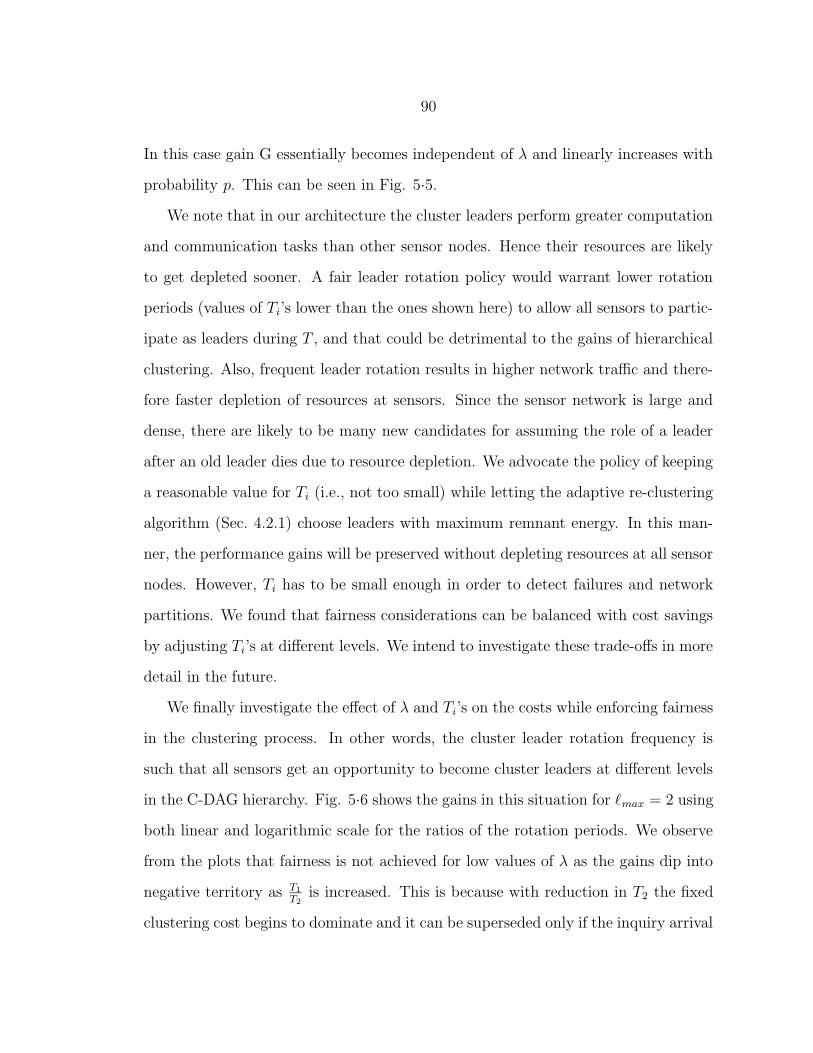
90

In this case gain G essentially becomes independent of λ and linearly increases with

probability p. This can be seen in Fig. 5·5.We note that in our architecture the cluster leaders perform greater computation

and communication tasks than other sensor nodes. Hence their resources are likely

to get depleted sooner. A fair leader rotation policy would warrant lower rotation

periods (values of Ti’s lower than the ones shown here) to allow all sensors to partic-

ipate as leaders during T , and that could be detrimental to the gains of hierarchical

clustering. Also, frequent leader rotation results in higher network traffic and there-

fore faster depletion of resources at sensors. Since the sensor network is large and

dense, there are likely to be many new candidates for assuming the role of a leader

after an old leader dies due to resource depletion. We advocate the policy of keeping

a reasonable value for Ti (i.e., not too small) while letting the adaptive re-clustering

algorithm (Sec. 4.2.1) choose leaders with maximum remnant energy. In this man-

ner, the performance gains will be preserved without depleting resources at all sensor

nodes. However, Ti has to be small enough in order to detect failures and network

partitions. We found that fairness considerations can be balanced with cost savings

by adjusting Ti’s at different levels. We intend to investigate these trade-offs in more

detail in the future.

We finally investigate the effect of λ and Ti’s on the costs while enforcing fairness

in the clustering process. In other words, the cluster leader rotation frequency is

such that all sensors get an opportunity to become cluster leaders at different levels

in the C-DAG hierarchy. Fig. 5·6 shows the gains in this situation for `max = 2 using

both linear and logarithmic scale for the ratios of the rotation periods. We observe

from the plots that fairness is not achieved for low values of λ as the gains dip into

negative territory as T1

T2is increased. This is because with reduction in T2 the fixed

clustering cost begins to dominate and it can be superseded only if the inquiry arrival

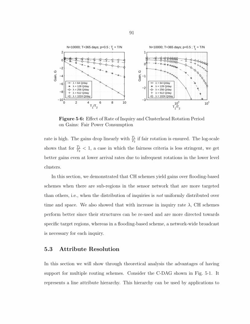
91

0 2 4 6 8 10−10

−8

−6

−4

−2

0

2

T1/T

2

Gai

n, G

N=10000; T=365 days; p=0.5 ; T1 = T/N


100

101

−3

−2

−1

0

1

T1/T

2

Gai

n, G

N=10000; T=365 days; p=0.5 ; T1 = T/N


Figure 5·6: Effect of Rate of Inquiry and Clusterhead Rotation Periodon Gains: Fair Power Consumption

rate is high. The gains drop linearly with T1

T2if fair rotation is ensured. The log-scale

shows that for T1

T2< 1, a case in which the fairness criteria is less stringent, we get

better gains even at lower arrival rates due to infrequent rotations in the lower level

clusters.

In this section, we demonstrated that CH schemes yield gains over flooding-based

schemes when there are sub-regions in the sensor network that are more targeted

than others, i.e., when the distribution of inquiries is not uniformly distributed over

time and space. We also showed that with increase in inquiry rate λ, CH schemes

perform better since their structures can be re-used and are more directed towards

specific target regions, whereas in a flooding-based scheme, a network-wide broadcast

is necessary for each inquiry.

5.3 Attribute Resolution

In this section we will show through theoretical analysis the advantages of having

support for multiple routing schemes. Consider the C-DAG shown in Fig. 5·1. It

represents a line attribute hierarchy. This hierarchy can be used by applications to

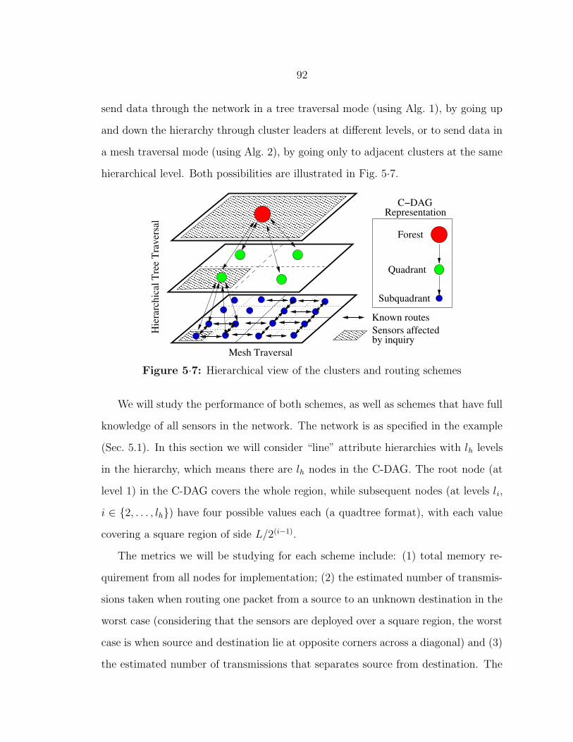
92

send data through the network in a tree traversal mode (using Alg. 1), by going up

and down the hierarchy through cluster leaders at different levels, or to send data in

a mesh traversal mode (using Alg. 2), by going only to adjacent clusters at the same

hierarchical level. Both possibilities are illustrated in Fig. 5·7.

��

��

��

��

��

��


Sensors affectedby inquiry

Subquadrant

Quadrant

Forest

Known routes

Hie

rarc

hica

l Tre

e Tr

aver

sal

Mesh Traversal

Figure 5·7: Hierarchical view of the clusters and routing schemes

We will study the performance of both schemes, as well as schemes that have full

knowledge of all sensors in the network. The network is as specified in the example

(Sec. 5.1). In this section we will consider “line” attribute hierarchies with lh levels

in the hierarchy, which means there are lh nodes in the C-DAG. The root node (at

level 1) in the C-DAG covers the whole region, while subsequent nodes (at levels li,

i ∈ {2, . . . , lh}) have four possible values each (a quadtree format), with each value

covering a square region of side L/2(i−1).

The metrics we will be studying for each scheme include: (1) total memory re-

quirement from all nodes for implementation; (2) the estimated number of transmis-

sions taken when routing one packet from a source to an unknown destination in the

worst case (considering that the sensors are deployed over a square region, the worst

case is when source and destination lie at opposite corners across a diagonal) and (3)

the estimated number of transmissions that separates source from destination. The

93

difference between (2) and (3) is that the former takes into account all transmissions

triggered by routing the packet, while the latter counts only the estimated number

of transmission taken specifically to deliver the packet from source to destination.

Essentially (1) allows us to gauge how scalable each scheme is in terms of the amount

of memory needed. Metric (2) allows us to compare the cost of resolving an unknown

destination address, while (3) is an estimate of how quickly the destination address

can be found or how quickly data can be transmitted to the destination, assuming

both being directly proportional to the hop distance that separates source from des-

tination. In other words, we assume that the average maximum delay is proportional

to the estimates in (3) in the absence of concurrent traffic.

When estimating the number of transmissions triggered or taken to deliver the

packet, i.e., items (2) and (3) above, for non-flooding type of schemes, we consider

that the path the packet takes is composed of consecutive straight line segments. One

estimate of the number of transmissions is the product of the length of the segment

by the linear node density. The node density is given by ρ = N/L2, thus one estimate

of the number of neighbors that lie on a line segment within transmission radius R

is R√

ρ. On the average, assuming the sensors are uniformly distributed and the

whole network connected, the number of transmissions should not be greater than

this value, for this value reflects the number nodes that lie in the segment. We are

assuming the routing scheme will not present as a rule a sharp zigzag pattern while

routing packets, but instead will attempt to route packets around the segment. If

this value is � 1, then we are overestimating the number of transmissions needed.

Estimates made in this way can still be used for comparison between different routing

schemes, though, since the overestimation comes from the high node density value

and will be reflected by all routing schemes.

An estimate that is closer to the minimum number of transmissions needed to

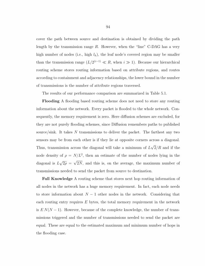
94

cover the path between source and destination is obtained by dividing the path

length by the transmission range R. However, when the “line” C-DAG has a very

high number of nodes (i.e., high lh), the leaf node’s covered region may be smaller

than the transmission range (L/2(i−1) � R, when i � 1). Because our hierarchical

routing scheme stores routing information based on attribute regions, and routes

according to containment and adjacency relationships, the lower bound in the number

of transmissions is the number of attribute regions traversed.

The results of our performance comparison are summarized in Table 5.1.

Flooding A flooding based routing scheme does not need to store any routing

information about the network. Every packet is flooded to the whole network. Con-

sequently, the memory requirement is zero. Here diffusion schemes are excluded, for

they are not purely flooding schemes, since Diffusion remembers paths to published

source/sink. It takes N transmissions to deliver the packet. The farthest any two

sensors may be from each other is if they lie at opposite corners across a diagonal.

Thus, transmission across the diagonal will take a minimum of L√

2/R and if the

node density of ρ = N/L2, then an estimate of the number of nodes lying in the

diagonal is L√

2ρ =√

2N , and this is, on the average, the maximum number of

transmissions needed to send the packet from source to destination.

Full Knowledge A routing scheme that stores next hop routing information of

all nodes in the network has a huge memory requirement. In fact, each node needs

to store information about N − 1 other nodes in the network. Considering that

each routing entry requires E bytes, the total memory requirement in the network

is E N(N − 1). However, because of the complete knowledge, the number of trans-

missions triggered and the number of transmissions needed to send the packet are

equal. These are equal to the estimated maximum and minimum number of hops in

the flooding case.

95

Table 5.1: Performance Metrics for different Routing SchemesFlooding Full Tree (One level informa-

tion)Tree (Full cluster in-formation)

Mesh

Memory 0 E N(N−1)

E 43 (4(lh−1)−1)+E N lh E 2N lh E (4lh + N +

2(2(lh−1) − 1)√

N)

Num TxMax N

√2N

√N (2(lh−1) −

1)( 2√

22(lh−1) + 3

√

22 +√

5) + N

2(2lh−2)

4√

2N(1 − 12(lh−1) ) +

N

2(2lh−2)

2√

2N(2lh −2

2(lh−1) ) +√N( 8−4

√

22(lh−1) ) +

N

2(2lh−2)

Min N L√

2/R max( L

R(2(lh−1) −

1)( 2√

22(lh−1) + 3

√

22 +√

5),∑lh

i=2(4(i−2)d L

√

2R2(i−1) e+

4(i−2) 2d L√

5R2(i−1) e +

(4(i−2) + 1)d L√

2R2(i−2) e)) +

N

2(2lh−2)

max( 4L√

2R

(1 −1

2lh−1 ),∑lh

i=2 2d L√

2R2(i−2) e)+

N

2(2lh−2)

max(L2√

2R

(2lh −2

2(lh−1) ) +L(8−4

√

2)

R 2(lh−1) , 2lh (2(lh−1)−1)) + N

2(2lh−2)

Num HopsMax

√2N

√2N 4

√2N(1− 1

2(lh−1) ) 2√

2N(1− 12(lh−1) ) +

√

N(4−2√

2)

2(lh−1)

Min L√

2/R L√

2/R max( 4L√

2R

(1− 12lh−1 ),

∑lh

i=2 2d L√

2R2(i−2) e) max( L

R(2√

2(1 −1

2(lh−1) ) +4−2

√

22(lh−1) ), 2 (2(lh−1) −1))

96

Cluster Flooding In both Flooding and Full Knowledge schemes destination

sensors are sure to be reached. In “Tree” or “Mesh” schemes below, however, packets

reaching the intended leaf cluster(s) still need to reach the sensors. Assuming the

intended destination address “resolves” into one leaf cluster, to flood that cluster the

number of additional transmissions is equal to ρ (L/2(lh−1))2 = N/2(2lh−2) is needed.

This term appears in all “NumTx” entries in Table 5.1.

Tree (One level information) In our clustered hierarchical scheme, each node

that is not cluster leader tracks leaders of the cluster it belongs across all hierarchy

levels (E N lh). Assuming one cluster per attribute value, we have one cluster for

the root node, four clusters for the node at the second level, 16 for the node at the

third level, etc. Each cluster leader tracks the routing information of its four children

clusters. Leaf cluster leaders track information about their cluster members. Since

leaf clusters cover the whole network, it requires N entries. Thus it is E 4(1 + 4 +

42 + ... + 4lh−2) + E N = E 4(4lh−1 − 1)/3 + E N . The sum of the two factors shown

in this paragraph is the memory requirement equation for “Tree” in Table 5.1.

When a packet with an unknown destination is received, it is sent to the cluster

leaders through the hierarchy all the way up to the root node if no matching attributes

are found. The longest segment that separates the root to a second level cluster leader

is L√

2, while the longest segment that separates the second level cluster leader to a

third level child cluster is L√

2/2. Thus the sum of the segment lengths is at most

UL = L√

2(1 + 1/2 + · · ·+ 1/2(lh−2)) = L2√

2(1− 1/2(lh−1))

Also, assuming the packet reaches the root node, the root node must send “down”

the packet to all its child clusters, which may in turn pass it down again, all the way to

the leaf cluster leaders, at which point the cluster leader that satisfies the destination

address attributes floods the packet to its cluster. In this process of forwarding the

packet down the C-DAG, from the root node to the second level cluster leaders four

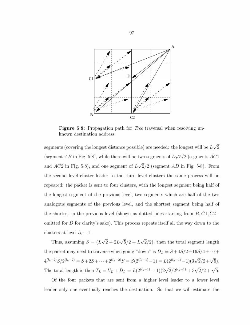
97

D

A

B

C1

C2

Figure 5·8: Propagation path for Tree traversal when resolving un-known destination address

segments (covering the longest distance possible) are needed: the longest will be L√

2

(segment AB in Fig. 5·8), while there will be two segments of L√

5/2 (segments AC1

and AC2 in Fig. 5·8), and one segment of L√

2/2 (segment AD in Fig. 5·8). From

the second level cluster leader to the third level clusters the same process will be

repeated: the packet is sent to four clusters, with the longest segment being half of

the longest segment of the previous level, two segments which are half of the two

analogous segments of the previous level, and the shortest segment being half of

the shortest in the previous level (shown as dotted lines starting from B,C1, C2 -

omitted for D for clarity’s sake). This process repeats itself all the way down to the

clusters at level lh − 1.

Thus, assuming S = (L√

2 + 2L√

5/2 + L√

2/2), then the total segment length

the packet may need to traverse when going “down” is DL = S+4S/2+16S/4+ · · ·+4(lh−2)S/2(lh−2) = S+2S+· · ·+2(lh−2)S = S(2(lh−1)−1) = L(2(lh−1)−1)(3

√2/2+

√5).

The total length is then TL = UL + DL = L(2(lh−1) − 1)(2√

2/2(lh−1) + 3√

2/2 +√

5.

Of the four packets that are sent from a higher level leader to a lower level

leader only one eventually reaches the destination. So that we will estimate the

98

number of transmissions that can cover the worst case (i.e., sender and receiver are

farthest apart), we take the longest segment at each level, and thus TL = 2UL =

L4√

2(1− 1/2(lh−1)).

The higher estimate on the maximum number of transmissions is obtained by

multiplying the length obtained by√

N/L (see “NumTxMax” and “NumHopsMax”

equations in Table 5.1), while an estimate on the minimum number of transmissions

is obtained by dividing the length by R (see the “NumTxMin” and “NumHopsMin”

equations for L/(R2(lh−1))� 1 in Table 5.1).

However, in the case in which the transmission range is much higher than the leaf

attribute region side, the number of transmissions is lower bounded by the number

of attribute regions the packet crosses. Given that there are four different segments

that the root node needs to send to reach the level 2 leaders, each of the two segments

of equal length (AC1 and AC2 in Fig. 5·8) will generate 4(i−2) segments of length

L√

5/(R2(i−1)) at level i ≥ 2. In the same way we count 4(i−2) segments for the

shortest segment (AD in Fig. 5·8) and 4(i−2) +1 for the longest. The “+1” is because

we must also count the transmission costs incurred when the packet was coming

up the hierarchy towards the root node. Each segment counts at least once (i.e., we

round up the cost) no matter how small its length is with respect to the transmission

radius R, because it represents one distinct attribute region. When we sum up for

all levels in the hierarchy we obtain the corresponding expression in Table 5.1.

When we consider the number of hops that can separate source from destination,

the worst case is if the source and destination eventually are “resolved” by going

through the longest segment across all levels of the hierarchy. This is represented by

the corresponding equation in Table 5.1.

Tree (Full cluster information) For a tree scheme in which cluster leaders

track all information from its cluster members the following memory requirement

99

is necessary for a cluster leader at level i: ρ (L/2(i−1))2 = N/2(2i−2). Since this is

a quadtree format, there are exactly 4(i−1) children cluster leaders at level i, thus

the memory requirement for cluster leaders to track cluster member information is

exactly lhN . Adding this to the requirement of N nodes tracking their lh cluster

leaders, the total memory requirement is 2lhN , as seen in Table 5.1. For the Tree

traversal mode with full cluster information, it is not necessary for the root node to

forward the packet down to all of its children clusters. Since it has information of

all the sensors in the network, it can forward the packet to the child cluster that

contains the desired destination attributes. Thus the number of transmissions and

the number of hops in this case is the same, and it corresponds to the case in which

the longest segment is taken both when the packet is coming “up” the hierarchy and

going “down” the hierarchy to the destination leaf cluster.

Mesh We study the performance of a routing scheme in a mesh like topology at

only one attribute hierarchy level (say lh). In a mesh like routing scheme, we assume

each cluster leader tracks only its (at most) four neighbor clusters, resulting in a

memory requirement of E 4 4(lh−1). Also all sensors track their cluster leader (E N of

memory), and sensors that lie at the attribute border will track the two clusters for

which it is the border. At level lh, the total length of the border is 2(2(lh−1) − 1)L,

which, when multiplied by√

N/L and summed with the other terms, results in the

memory requirement equation seen in Table 5.1.

We assume that when a packet with an unknown destination is received it will

be transmitted to the neighbor clusters other than the ones from which the packet

arrived. Thus if a packet is sent from the lower left cluster leader, with a destination

that is unknown to the cluster leader, but whose final sink is in the top right cluster,

then the packet will be propagated across all attribute regions. The total length

traversed as the packet is distributed in the network is longer if the cluster leaders

100

E

A

B1

B2

C

D

Figure 5·9: Propagation path for Mesh traversal when resolving un-known destination address

are located close to opposite corners across the diagonal, in the zigzag pattern shown

in Fig. 5·9. In this figure we show the traversal taken when there are three nodes

in the line C-DAG. The cluster leader of the lower left attribute region (A) sends

the packet to its immediate neighbor cluster leaders (B1 and B2). As these are

located close to the corner across the diagonal the length traversed is 2L√

2/2(lh−1).

To increase the length traversed, as the packet gets closer to the top left and bot-

tom right corners, we assume the cluster leaders are located at the corners of their

respective attribute regions. In this way we force comparison of the worst case in

a mesh approach with the worst case of the tree based scheme analyzed previously.

Notice that essentially the packet traverse the diagonals of squares with side length

2jL/2(i−1), j ∈ {1, 2, 3, ..., 2(i−1)} in a regular fashion, discounting the borders and the

top left and bottom right corners. The total length traversed, and the corresponding

expected number of transmissions (both maximum and minimum) are given by the

corresponding expressions in Table 5.1.

When the transmission radius R� L/2(i−1), then it takes at least one transmis-

sion to cross one attribute region, and assuming each attribute region will transmit to

101

two of its immediate neighbors (with top and right border attribute regions transmit-

ting only once), the total number of transmissions will be 2(2(lh−1)− 1) + 2(2(lh−1)−1)2 = 2lh(2(lh−1) − 1), as seen in the table.

The shortest path that separates the source from the destination must traverse

2(2(lh−1) − 1) + 1 attribute regions (the +1 is because the source attribute region

also must be traversed). However, if the packet goes through only the diagonals,

only 2(2(lh−1)−1) diagonals need be crossed. One of the attribute region leaders will

receive the packet from the left and can immediately forward to the upper region,

without needing to traverse itself. Thus the worst case scenario is actually when the

source is at the top left corner while the destination is at the bottom right corner

(or vice-versa). In this case there are additional four traversals across the border

of the attribute region (4(L/2(lh−1))) and two less diagonal traversals. This explains

the second term in the “NumHopMax” and the second term in the first argument to

the max function in “NumHopMin.” When we are considering the minimum number

of hops, this must be lower bounded by the number of attribute regions that need

be crossed (2(2(lh−1) − 1)), since in principle the cluster leader only tracks the four

adjacent clusters. We show some plots of the equations of Table 5.1 in Figures 5·10–

5·19.

A high number of levels will involve transmission costs to cross adjacent clusters

in the Mesh case and costs to resolve all the way to the leaf cluster in the Tree (one

level info) case. These costs surpass those of the mere flooding schemes and should

be avoided. The cost for resolving an unknown address in the Tree (full cluster

info) case remains constant. However, the memory requirements are high (Figs. 5·10

and 5·11).We can see from Fig. 5·12 and Fig. 5·13 that the expected number of transmis-

sions to resolve an unknown address in the worst case is higher for the Mesh traversal

102

102

103

104

105

103

104

105

106

107

108

109

1010

Number of Nodes in the Network

Num

ber

of E

xpec

ted

Rou

ting

Ent

ries

Lh=4 levels; L=1000 m; R=30 m

FullTreeTree − full cluster infoMesh

Figure 5·10: Memory requirements with increasing number of nodesin the network

2 3 4 5 6 7 810

3

104

105

106

107

Number of Levels in the Hierarchy

Num

ber

of E

xpec

ted

Rou

ting

Ent

ries

N=2000 nodes; L=1000 m; R=30 m

FullTreeTree − full cluster infoMesh

Figure 5·11: Memory requirements vs. Number of Levels in theHierarchy

103

102

103

104

105

101

102

103

104

105


Exp

ecte

d M

axim

um N

umbe

r of

Tra

nsm

issi

ons


FloodFullTreeTree − full cluster infoMesh

Figure 5·12: Expected Maximum Number of Transmissions(NumTxMax)

2 3 4 5 6 7 810

1

102

103

104

105


Exp

ecte

d M

axim

um N

umbe

r of

Tra

nsm

issi

ons

N=2000 nodes; L=1000 m; R=30 m


Figure 5·13: NumTxMax vs. Number of Levels in the Hierarchy

104

mode than for the Tree cases. In fact, when cluster leaders track full cluster infor-

mation, the performance dramatically improves. This is because the root node need

not propagate the packet with unknown address down to all of its children clusters.

We can see that the high number of levels in the attribute hierarchy contributes

to the inefficiency of the process (Fig. 5·13 and 5·15). With the increase in the

number of hierarchies, the packet with unknown destination address need essentially

be distributed to the whole network in the Mesh and Tree (with one level informa-

tion) schemes at increasing levels of granularity (i.e., covering more of the network),

contributing to their performance degradation.

102

103

104

105

101

102

103

104

105


Exp

ecte

d M

inim

um N

umbe

r of

Tra

nsm

issi

ons



Figure 5·14: Expected Minimum Number of Transmissions(NumTxMin)

When we consider the number of hops metric, we find that Mesh schemes are

able to find shorter paths between source and destination. The only drawback is

that Mesh schemes currently only cross spatially adjacent attribute regions. Thus

when the number of levels in the hierarchy increases, there is a corresponding increase

in the hop distance (Figs. 5·17 and 5·19).

105

2 3 4 5 6 7 810

1

102

103

104

105


Exp

ecte

d M

inim

um N

umbe

r of

Tra

nsm

issi

ons

N=2000 nodes; L=1000 m; R=30 m


Figure 5·15: NumTxMin vs. Number of Levels in the Hierarchy

102

103

104

105

101

102

103

Nodes in the Network

Exp

ecte

d M

axim

um N

umbe

r of

Hop

s be

twee

n S

rc/D

st


Flood = FullTreeMesh

Figure 5·16: Expected Maximum Number of Hops (NumHopMax)between Source and Destination

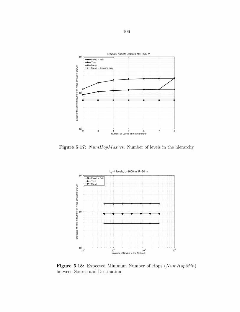
106

2 3 4 5 6 7 810

1

102

103


Exp

ecte

d M

axim

um N

umbe

r of

Hop

s be

twee

n S

rc/D

st

N=2000 nodes; L=1000 m; R=30 m

Flood = FullTreeMeshMesh − distance only

Figure 5·17: NumHopMax vs. Number of levels in the hierarchy

102

103

104

105

101

102

103


Exp

ecte

d M

inim

um N

umbe

r of

Hop

s be

twee

n S

rc/D

st


Flood = FullTreeMesh

Figure 5·18: Expected Minimum Number of Hops (NumHopMin)between Source and Destination

107

2 3 4 5 6 7 810

1

102

103


Exp

ecte

d M

inim

um N

umbe

r of

Hop

s be

twee

n S

rc/D

st

N=2000 nodes; L=1000 m; R=30 m

Flood = FullTreeMeshMesh − distance only

Figure 5·19: NumHopMin vs. Number of levels in the hierarchy

From the graphs in Fig. 5·10- 5·19 we can see that if the network is composed

of heterogeneous nodes, in which some nodes have higher capacity, then a Tree (full

cluster info) scheme will be the most economical in transmission costs related to

address resolution issues. Sensor networks that have a high inquiry arrival, especially

from a large user base, will benefit from the increased savings in Tree based address

resolution schemes, while applications that require fast response can invoke Mesh

traversal mode for their data packets.

108

Chapter 6

Conclusion and Future Work

6.1 Conclusions

In the future the routing demands of large scale sensor network or resultant inter-

connection of various smaller scale sensor networks differ greatly from the routing

demands of currently deployed sensor networks. Inquiries arriving at such networks

are unlikely to require all the resources from all the nodes in the network. If the un-

derlying routing mechanism cannot guide traffic to the relevant parts of the network

then much energy is wasted in redundant transmission. In addition to that, multiple

applications being supported by such networks will have different communication

needs. A routing infrastructure that cannot accommodate diverse traversal modes

in the network is bound to limit the performance of the deployed applications.

In this dissertation we have proposed a routing infrastructure that can guide data

traffic to reach sets of sensors within the network in a manner that can be selected

by the application to meet its performance requirements. This is achieved by es-

tablishing a virtual overlay of attribute based hierarchical clusters on the network.

The attributes of the hierarchy describe sensors that are often the target of user

inquiries and satisfy containment and adjacency relationships. The hierarchy is de-

scribed through DAGs, in which parent nodes are clusters that contain clusters that

represent child nodes. By establishing these attribute based clusters as potential

destination addresses of inquiries we maintain the data-centric emphasis in rout-

109

ing yet are able to guide traffic to only sensors that match the required attributes.

Multiple hierarchies can be supported simultaneously, thus enabling multiple appli-

cations to select the set of sensors that best meet their own addressing needs. By

supporting multiple hierarchies simultaneously, inquiries that possess cross-hierarchy

attributes may also be resolved within the network, and thus we reutilize the virtual

infrastructure overlaid.

We propose algorithms that form such hierarchy of clusters, together with al-

gorithms that enable load balancing and fault tolerance with respect to the role of

cluster leader. Also we propose algorithms that enable dynamic changes to the virtual

hierarchical clustering structure. We show through analysis that such hierarchical

schemes offer increased communication gains as opposed to flooding mechanisms for

disseminating new inquiries.

In this dissertation we also propose that the routing process be an interpreted

one, and routing behavior be determined by a set of routing rules. Different routing

rules then provide different packet traversal behavior, resulting in different perfor-

mance results when data transmission occurs. We propose pseudo-code for tree based

traversal mode and mesh based traversal modes in the presence of the virtual overlay.

Such traversal modes are key in forming paths to unknown destination attributes.

In other words, when a packet with an unknown destination attribute is met, a

resolution procedure is carried out, based on the behavior determined by the rules

set, and at the end of which, assuming the destination attribute exists within the

network, a path is formed. We obtain through analysis the transmission costs asso-

ciated with such address resolution procedure, the memory requirements of tracking

attributes within each traversal mode, and the resultant hop length of the formed

path. We show that tree based traversal modes saves transmission costs in the res-

olution process but forms longer paths and the resolution process takes longer to

110

finish. Applications can then choose the traversal mode according to its performance

requirements.

6.2 Future Work

Much is still left to complete work in attribute based routing in clustered WSNETs.

Specifically, analysis of the performance of the infrastructure when facing inquiries

like the ones posed at Great Duck Island (Sec. 2.4) remains to be done. The opti-

mality analysis of the tradeoff between the number of levels in the hierarchy and the

gains obtained poses itself as a very challenging and yet rewarding problem. Differ-

ent traversal modes and their performance expectations can also contribute to the

increased performance of applications being executed over deployed sensor networks

in the future.

111

Appendix A

Pseudocode for Cluster Formation and

Maintenance Algorithms

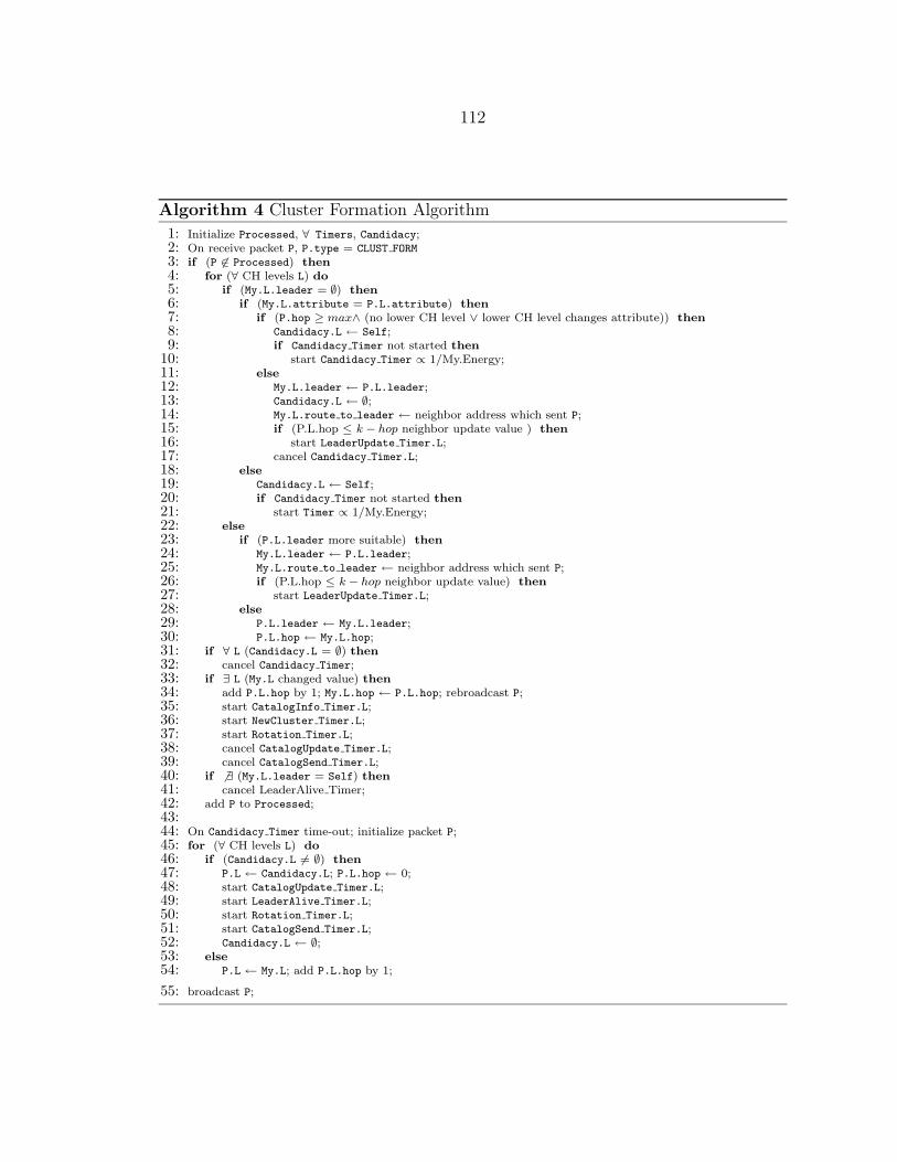
112

Algorithm 4 Cluster Formation Algorithm

1: Initialize Processed, ∀ Timers, Candidacy;2: On receive packet P, P.type = CLUST FORM

3: if (P 6∈ Processed) then

4: for (∀ CH levels L) do

5: if (My.L.leader = ∅) then

6: if (My.L.attribute = P.L.attribute) then

7: if (P.hop ≥ max∧ (no lower CH level ∨ lower CH level changes attribute)) then

8: Candidacy.L ← Self;9: if Candidacy Timer not started then

10: start Candidacy Timer ∝ 1/My.Energy;11: else

12: My.L.leader ← P.L.leader;13: Candidacy.L ← ∅;14: My.L.route to leader ← neighbor address which sent P;15: if (P.L.hop ≤ k − hop neighbor update value ) then

16: start LeaderUpdate Timer.L;17: cancel Candidacy Timer.L;18: else

19: Candidacy.L ← Self;20: if Candidacy Timer not started then

21: start Timer ∝ 1/My.Energy;22: else

23: if (P.L.leader more suitable) then

24: My.L.leader ← P.L.leader;25: My.L.route to leader ← neighbor address which sent P;26: if (P.L.hop ≤ k − hop neighbor update value) then

27: start LeaderUpdate Timer.L;28: else

29: P.L.leader ← My.L.leader;30: P.L.hop ← My.L.hop;31: if ∀ L (Candidacy.L = ∅) then

32: cancel Candidacy Timer;33: if ∃ L (My.L changed value) then

34: add P.L.hop by 1; My.L.hop ← P.L.hop; rebroadcast P;35: start CatalogInfo Timer.L;36: start NewCluster Timer.L;37: start Rotation Timer.L;38: cancel CatalogUpdate Timer.L;39: cancel CatalogSend Timer.L;40: if 6 ∃ (My.L.leader = Self) then

41: cancel LeaderAlive Timer;42: add P to Processed;43:44: On Candidacy Timer time-out; initialize packet P;45: for (∀ CH levels L) do

46: if (Candidacy.L 6= ∅) then

47: P.L ← Candidacy.L; P.L.hop ← 0;48: start CatalogUpdate Timer.L;49: start LeaderAlive Timer.L;50: start Rotation Timer.L;51: start CatalogSend Timer.L;52: Candidacy.L ← ∅;53: else

54: P.L ← My.L; add P.L.hop by 1;

55: broadcast P;

113

Algorithm 5 k-neighbor updates - LeaderAlive Packet Management

1: On receive packet P, P.type = LEADER ALIVE;2: if (P 6∈ Processed) then3: for (∀ P.L 6= ∅) do4: if (My.L.attribute = P.L.attribute) ∧ (My.L.leader = P.L.leader)

then5: start LeaderUpdate Timer.L;6: My.L.route to leader ← neighbor address which sent P;7: My.L.Catalog ← P.L.Catalog;8: if (P.L.hop ≤ 1) then9: delete P.L;

10: else11: decrease P.L.hop by 1;12: if 6 ∃ (P.L) then13: drop P;14: else15: rebroadcast P;16: add P to Processed;17:

18:

19: On LeaderAlive Timer.L time-out;20: initialize packet P, P.type ← LEADER ALIVE;21: if (P 6∈ Processed) then22: if (My.L.leader = Self) then23: P.L ← My.L;24: P.L.hop ← k − hop neighbor alive value;25: P.L.Catalog ← My.L.Catalog;26: start LeaderAlive Timer.L;27: broadcast P;28: add P to Processed;

114

Algorithm 6 Leader updates - LeaderUpdate Timer Management

1: On LeaderUpdate Timer.L time-out;2: start InterimLeader Timer.L ∝ 1

My.Energy ;3:

4:

5: On InterimLeader Timer.L time-out;6: initialize packet P, P.type ← LEADER INTERIM;7: My.L.failed leader ← My.L.leader;8: My.L.leader ← Self;9: P.L ← My.L;

10: start LeaderAlive Timer.L;11: if My.L.Catalog = ∅ then

12: start CatalogUpdate Timer.L;13: start CatalogSend timer.L;14: broadcast P;15:

16:

17: On receive packet P, P.type = LEADER INTERIM;18: if (P 6∈ Processed) then

19: for (∀ P.L 6= ∅) do

20: if (My.L.failed leader = ∅) then


22: if (My.L.leader = P.L.failed leader) then

23: cancel InterimLeader Timer.L;24: My.L.failed leader ← My.L.leader;25: My.L.leader ← P.L.leader;26: My.L.route to leader ← neighbor address which sent P;27: else

28: if (My.L.failed leader = P.L.failed leader) then


30: if (P.L.leader more suitable) then

31: My.L.leader ← P.L.leader;32: My.L.route to leader ← neighbor address which sent P;33: else

34: delete P.L;35: if (∃ L | My.L.leader updated information from P) then

36: cancel LeaderAlive Timer.L;37: cancel CatalogSend Timer.L;38: if P.L.hop ≤ k − hop neighbor update value then

39: start LeaderUpdate Timer.L;40: start Rotation Timer.L;41: start NewCluster Timer.L;42: ∀ L, add P.L.hop by 1;43: rebroadcast P;44: add P to Processed;

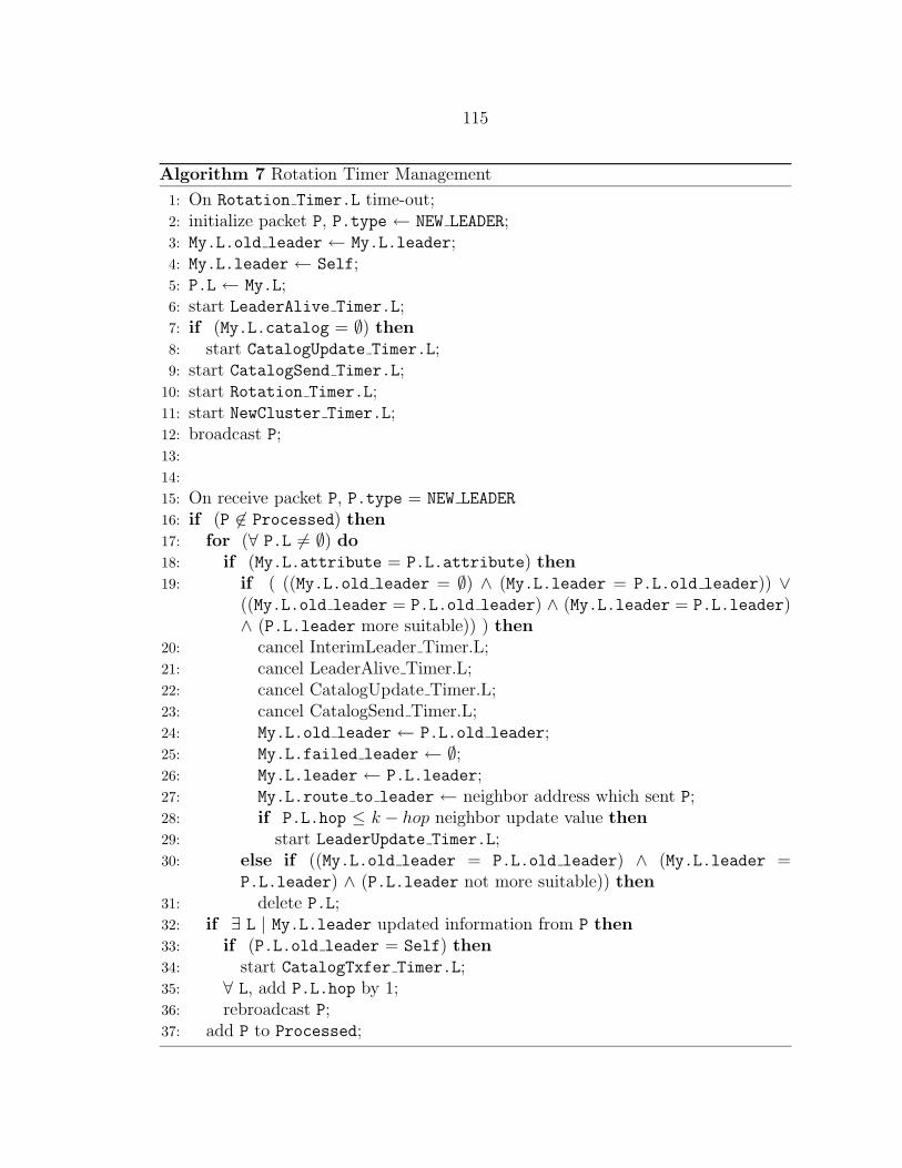
115

Algorithm 7 Rotation Timer Management

1: On Rotation Timer.L time-out;2: initialize packet P, P.type ← NEW LEADER;3: My.L.old leader ← My.L.leader;4: My.L.leader ← Self;5: P.L ← My.L;6: start LeaderAlive Timer.L;7: if (My.L.catalog = ∅) then8: start CatalogUpdate Timer.L;9: start CatalogSend Timer.L;

10: start Rotation Timer.L;11: start NewCluster Timer.L;12: broadcast P;13:

14:

15: On receive packet P, P.type = NEW LEADER

16: if (P 6∈ Processed) then17: for (∀ P.L 6= ∅) do18: if (My.L.attribute = P.L.attribute) then19: if ( ((My.L.old leader = ∅) ∧ (My.L.leader = P.L.old leader)) ∨

((My.L.old leader = P.L.old leader) ∧ (My.L.leader = P.L.leader)∧ (P.L.leader more suitable)) ) then

20: cancel InterimLeader Timer.L;21: cancel LeaderAlive Timer.L;22: cancel CatalogUpdate Timer.L;23: cancel CatalogSend Timer.L;24: My.L.old leader ← P.L.old leader;25: My.L.failed leader ← ∅;26: My.L.leader ← P.L.leader;27: My.L.route to leader ← neighbor address which sent P;28: if P.L.hop ≤ k − hop neighbor update value then29: start LeaderUpdate Timer.L;30: else if ((My.L.old leader = P.L.old leader) ∧ (My.L.leader =

P.L.leader) ∧ (P.L.leader not more suitable)) then31: delete P.L;32: if ∃ L | My.L.leader updated information from P then33: if (P.L.old leader = Self) then34: start CatalogTxfer Timer.L;35: ∀ L, add P.L.hop by 1;36: rebroadcast P;37: add P to Processed;

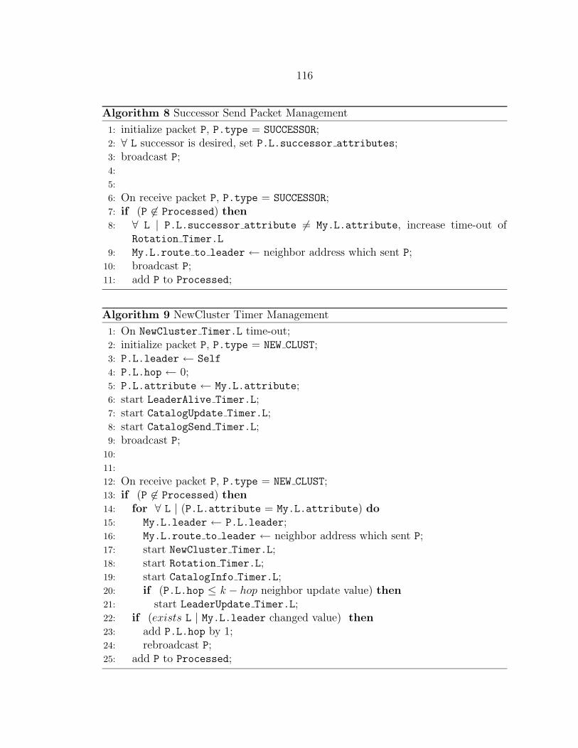
116

Algorithm 8 Successor Send Packet Management

1: initialize packet P, P.type = SUCCESSOR;2: ∀ L successor is desired, set P.L.successor attributes;3: broadcast P;4:

5:

6: On receive packet P, P.type = SUCCESSOR;7: if (P 6∈ Processed) then8: ∀ L | P.L.successor attribute 6= My.L.attribute, increase time-out of

Rotation Timer.L

9: My.L.route to leader ← neighbor address which sent P;10: broadcast P;11: add P to Processed;

Algorithm 9 NewCluster Timer Management

1: On NewCluster Timer.L time-out;2: initialize packet P, P.type = NEW CLUST;3: P.L.leader ← Self

4: P.L.hop ← 0;5: P.L.attribute ← My.L.attribute;6: start LeaderAlive Timer.L;7: start CatalogUpdate Timer.L;8: start CatalogSend Timer.L;9: broadcast P;

10:

11:

12: On receive packet P, P.type = NEW CLUST;13: if (P 6∈ Processed) then14: for ∀ L | (P.L.attribute = My.L.attribute) do15: My.L.leader ← P.L.leader;16: My.L.route to leader ← neighbor address which sent P;17: start NewCluster Timer.L;18: start Rotation Timer.L;19: start CatalogInfo Timer.L;20: if (P.L.hop ≤ k − hop neighbor update value) then21: start LeaderUpdate Timer.L;22: if (exists L | My.L.leader changed value) then23: add P.L.hop by 1;24: rebroadcast P;25: add P to Processed;

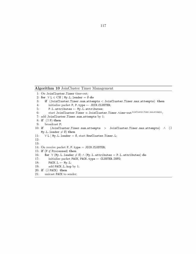
117

Algorithm 10 JoinCluster Timer Management

1: On JoinCluster Timer time-out;2: for ∀ L ∈ CH | My.L.leader = ∅ do

3: if (JoinCluster Timer.num attempts < JoinCluster Timer.max attempts) then

4: initialize packet P, P.type ← JOIN CLUSTER;5: P.L.attributes ← My.L.attributes;6: start JoinCluster Timer ∝ JoinCluster Timer.time-outJoinCluster Timer.num attempts;7: add JoinCluster Timer.num attempts by 1;8: if (∃ P) then

9: broadcast P;10: if (JoinCluster Timer.num attempts > JoinCluster Timer.max attempts) ∧ (∃

My.L.leader 6= ∅) then

11: ∀ L | My.L.leader = ∅, start NewCluster Timer.L;12:13:14: On receive packet P, P.type = JOIN CLUSTER;15: if (P 6∈ Processed) then

16: for ∀ (My.L.leader 6= ∅) ∧ (My.L.attributes = P.L.attributes) do

17: initialize packet PACK, PACK.type ← CLUSTER INFO;18: PACK.L ← My.L;19: add PACK.L.hop by 1;20: if (∃ PACK) then

21: unicast PACK to sender;

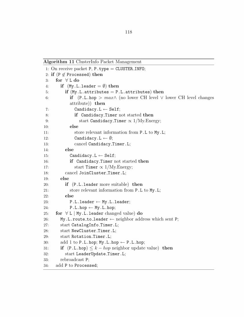
118

Algorithm 11 ClusterInfo Packet Management

1: On receive packet P, P.type = CLUSTER INFO;2: if (P 6∈ Processed) then3: for ∀ L do4: if (My.L.leader = ∅) then5: if (My.L.attributes = P.L.attributes) then6: if (P.L.hop > max∧ (no lower CH level ∨ lower CH level changes

attribute)) then7: Candidacy.L ← Self;8: if Candidacy Timer not started then9: start Candidacy Timer ∝ 1/My.Energy;

10: else11: store relevant information from P.L to My.L;12: Candidacy.L ← ∅;13: cancel Candidacy Timer.L;14: else15: Candidacy.L ← Self;16: if Candidacy Timer not started then17: start Timer ∝ 1/My.Energy;18: cancel JoinCluster Timer.L;19: else20: if (P.L.leader more suitable) then21: store relevant information from P.L to My.L;22: else23: P.L.leader ← My.L.leader;24: P.L.hop ← My.L.hop;25: for ∀ L | My.L.leader changed value) do26: My.L.route to leader ← neighbor address which sent P;27: start CatalogInfo Timer.L;28: start NewCluster Timer.L;29: start Rotation Timer.L;30: add 1 to P.L.hop; My.L.hop ← P.L.hop;31: if (P.L.hop) ≤ k − hop neighbor update value) then32: start LeaderUpdate Timer.L;33: rebroadcast P;34: add P to Processed;

119

Algorithm 12 CatalogSend Timer Management

1: On CatalogSend Timer.L time-out, L > 1;2: initialize packet P, P.type ← CATALOG SEND;3: store catalog information in P.L;4: P.L.leader ← Self;5: P.L.attributes ← My.L.attributes;6: P.(L-1).leader ← My.(L-1).leader;7: unicast P to My.(L-1).leader;8:

9:

10: On receive packet P, P.type = CATALOG SEND;11: if (P 6∈ Processed) then12: if (Self = P.(L-1).leader) then13: if (P.L.attributes not found in My.L.cluster index) then14: store P.L.attributes in My.L.cluster index;15: k ← index of P.L.attributes in My.L.cluster index;16: update My.L.cluster index.k.catalog information;17: else18: unicast P to P.(L-1).leader;19: My.L.cluster index.k.route to leader ← neighbor address which sent P;20: add P to Processed;

Algorithm 13 CatalogUpdate Timer Management

1: On CatalogUpdate Timer.L time-out;2: initialize packet P, P.type ← CATALOG UPDATE;3: P.L ← My.L;4: broadcast P;5:

6:

7: On receive packet P, P.type = CATALOG UPDATE;8: if (P 6∈ Processed) then9: for ∀ L | ( P.L.attributes = My.L.attributes) do

10: if (CatalogInfo Timer.L not set) then11: start CatalogInfo Timer.L;12: add P.L.hop by 1;13: My.L.route to leader ← neighbor address which sent P;14: if ∃ L | ( P.L.hop changed value) then15: rebroadcast P;16: add P to Processed;

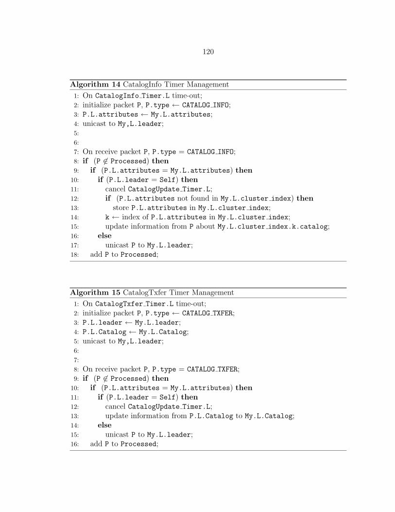
120

Algorithm 14 CatalogInfo Timer Management

1: On CatalogInfo Timer.L time-out;2: initialize packet P, P.type ← CATALOG INFO;3: P.L.attributes ← My.L.attributes;4: unicast to My,L.leader;5:

6:

7: On receive packet P, P.type = CATALOG INFO;8: if (P 6∈ Processed) then9: if (P.L.attributes = My.L.attributes) then

10: if (P.L.leader = Self) then11: cancel CatalogUpdate Timer.L;12: if (P.L.attributes not found in My.L.cluster index) then13: store P.L.attributes in My.L.cluster index;14: k ← index of P.L.attributes in My.L.cluster index;15: update information from P about My.L.cluster index.k.catalog;16: else17: unicast P to My.L.leader;18: add P to Processed;

Algorithm 15 CatalogTxfer Timer Management

1: On CatalogTxfer Timer.L time-out;2: initialize packet P, P.type ← CATALOG TXFER;3: P.L.leader ← My.L.leader;4: P.L.Catalog ← My.L.Catalog;5: unicast to My,L.leader;6:

7:

8: On receive packet P, P.type = CATALOG TXFER;9: if (P 6∈ Processed) then

10: if (P.L.attributes = My.L.attributes) then11: if (P.L.leader = Self) then12: cancel CatalogUpdate Timer.L;13: update information from P.L.Catalog to My.L.Catalog;14: else15: unicast P to My.L.leader;16: add P to Processed;

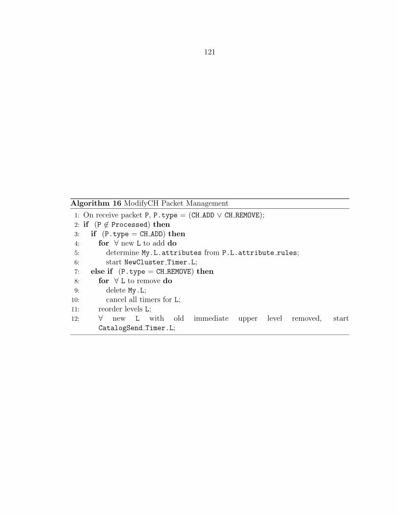
121

Algorithm 16 ModifyCH Packet Management

1: On receive packet P, P.type = (CH ADD ∨ CH REMOVE);2: if (P 6∈ Processed) then3: if (P.type = CH ADD) then4: for ∀ new L to add do5: determine My.L.attributes from P.L.attribute rules;6: start NewCluster Timer.L;7: else if (P.type = CH REMOVE) then8: for ∀ L to remove do9: delete My.L;

10: cancel all timers for L;11: reorder levels L;12: ∀ new L with old immediate upper level removed, start

CatalogSend Timer.L;

122

Appendix B

Attribute Tagging and Representation

Attributes are assigned to a sensor in a specific human language (e.g., English).

While this is human readable, an attribute that is spelled “temperature” and has a

string representation would need 11 bytes for storage and transmission. If we desire

to limit the energy spent in transmission more than the cost of adding storage, one

way to reduce the number of bytes required in transmission is to index the set of

attribute names and their respective values.

The way the attributes are indexed is as follows: two files, one called “Attribute

Name Value Index” (ANV-IDX) and the other called “Attribute Name Value In-

stance” (ANV-IST) will be used. ANV-IDX contains only the indices while ANV-

IST contains the representation in a specific human language of the attribute’s name

and possible values. The first row of ANV-IDX has the index range (from 1 to N).

The first column of ANV-IDX has the indices used for attribute names. The second

column contains its type (integer, double, string), while subsequent numbers in each

row represent the indices used for all possible attribute values associated. The file

ANV-IST will contain in correspondent locations (i.e., at correspondent column, row

positions) the specific representation of an attribute’s name and possible values in

a human language. Relational symbols (<, ≤, >, ≥, =, 6=) are used to represent a

range for numeric attributes. If the type of attribute is string, the row containing its

possible values is assumed ordered (i.e., the order of the possible values is the order

of appearance in the row, not its lexicographical value).

123

A third file, called “Attribute Relationship Rules” (ARR) lists the dependency re-

lationships between different attributes names (e.g., containment) or attribute values

(e.g., adjacency). Essentially ARR should contain (1) the C-DAG used to represent

the attribute hierarchy and (2) other relationships that concern attribute values (e.g.,

adjacency relationships). These rules do not refer to any attribute in its full name,

but only to the indices found in ANV-IDX. In this way the ARR rules do not depend

on the specific language in which the attribute is specified. Also, if two attribute

hierarchies share the same structure and same adjacency properties, the same ANV

and ARR files can be used.

C-DAGs are described by multiple rows in the ARR, each row containing first

the parent node, followed by the symbol ⊃ and then the child node, followed by the

symbol ⊃ and then by the grandchild node, and so forth as decided by the writer of

ARR, or until a leaf node is reached. For single root C-DAGs, the number of rows

used to describe the C-DAG will be at least the same as the number of leaf nodes.

After the C-DAG is described, a single element line containing the index repre-

senting a node in the C-DAG is stored. The lines that follow this single element line

describe the adjacency relationships of the attribute represented, until a new single

element line is encountered, or the file terminates.

In the lines that describe adjacency relationships, each line is possibly split into

two parts. The first part include pairs containing the indices of two attribute values

that are adjacent. The two elements that compose the pair are separated by whites-

pace, while the pairs themselves are separated by commas. The second part of the

line starts after the last pair, and it includes the values that attributes higher in the

hierarchy must have in order for the adjacency conditions to be true.

In this second part, the keywords “S1” indicates the sensor that represents the

first element in the pair, while “S2” indicates the sensor that represents the second

124

element. The second part is composed of “sentences” split again by commas. Each

sentence starts with “S1” (or “S2”), which is followed then by the index of a higher

level hierarchy, and then by the symbol ∈ (or 6∈), and finally by the set of values

the attribute indicated must have. If there are no conditions then the second part is

blank.

All sensors deployed will have ARR stored. Together with the ARR file it will

also be stored the hash code (e.g., applying MD5 algorithm to ARR) of the ARR file.

If sensors being tagged with the core attributes are also storing the ANV files, then

instead of storing the full name and value of each attribute, they will store only the

indices of the attribute names and values as found in the ANV files. If, however, the

sensors are not storing the ANV files, then the full name and value of the attributes,

together with the indices used for them in the ANV files will be stored in the sensor.

Also to be stored with the sensor is the hash number of the ANV-IDX file.

When sensors transmit packets, they have two options: use the full string rep-

resentation of the attributes’ name and values stored, or use the encoded format.

Essentially the encoded format consists of sending initially the hashcodes of ARR

and ANV-IDX files, followed then by the indices of the attributes descriptive of the

destination. The hashcodes for ARR and ANV-IDX guarantee that nodes that have

the same hashcodes for ARR and ANV-IDX will act in a consistently equal manner.

By not using the hashcode for ANV-IST we are allowing sensors that have the

same attributes but using different language representations to communicate with

one another. If we adopt a “default” language for specifying ARR files, then we can

also support ARR files that are written in different languages. Without agreement

on what the “default” language should be, ARR files that are written in different

languages will yield different hashcodes and sensors cannot exchange packets, even

though both ARR files describe the same set of relationships.

125

Sensors that do not have full ANV files but which receive a packet with unknown

attributes will forward the packet to their cluster leader. Sensors that have full ARR

and ANV-IDX and ANV-IST files that receive packets with unknown attributes or

unmatched hashcodes will simply rebroadcast the packet when first received, and

dropped if heard before.

Foreign sensors which do not share the same ANV and ARR files will simply

list the desired attributes (names and values) in the full string representation and

broadcast. If no response is received after a threshold number of requests, the sensor

may request to receive any new ANV-IDX and ARR files from neighboring nodes.

When new dynamic attributes are introduced, with their names and range of

values, the node initiating the update assigns indices to the new names and values.

Nodes receiving the new attributes store them in “Attribute Name Value Index

Dynamic” (ANV-IDX-Dyn) and “Attribute Name Value Instance Dynamic” (ANV-

IST-Dyn) files. The order in which the attributes are stored is based on the indices

assigned (lower indices stored first). The hash function must allow for concatenation,

and the original hashcode for ANV-IDX is the starting point for the hash function

applied to ANV-IDX-Dyn. Subsequent packets will bring this resultant hashcode in

their headers. Since all sensors have ARR files, any updates sent will be received by

all sensors and a new hashcode for ARR is produced.

126

Appendix C

Communication Directives

In this appendix we explain some directives that can be used to write routing rules.

• Communication directives

– sendTo - this takes as an argument a set of attribute value pairs and a

formatted outgoing packet. It will attempt unicast transmission between

the host and the attribute region it wants to reach;

– floodIn - this floods the outgoing packet. It will take as argument a node

in the attribute hierarchy. This is the region within which to flood the

packet. If the node selected is not one of the sensor’s ancestor nodes, the

packet is dropped.

• Operators

– isAdjacent and isContained (⊂) - these are specified in the attribute hi-

erarchy specification file (see appendix B).

– relational operators (<,≤,>,≥) - the “order” of string values is determined

by the order of their appearance in the attribute hierarchy specification

file.

– equality operators (==, ! =) - evaluated by string comparison or numeric

comparison.

127

• Flow Control - the if-else-if expression is also supported for flow control.

There can be an arbitrary number of “else-if”s that follow an “if.”

• Application Cluster control commands:

– AppFormCluster - this command forms the application clusters. The spec-

ification of the cluster obeys the following format: the cluster name, fol-

lowed by “{”, and then a series of “{ <member-name> : (<attribute

name 1>, <attribute value 1>, ..., (<attribute name N>, <attribute

value N>) },” separated by commas and followed by “}”;

– AppClusterSendTo - this commands takes as argument the application

cluster name, the member name the packet must be sent to, and the

formatted outgoing packet;

– AppClusterFloodTo - this commands takes as argument the application

cluster name and the formatted outgoing packet. The packet is flooded

to all cluster members.

• Routing Data access commands:

– NumberAttrHierarchy - returns the number of hierarchies the routing pro-

cess is aware of;

– AttrHierarchyAt - takes a number as argument and returns the corre-

sponding name of the attribute hierarchy stored by the routing process;

– NodesInAttrHierarchy - returns the number of nodes in an attribute hier-

archy

– NodeAtAttrHierarchy - takes an attribute hierarchy name and a number

as arguments and returns the corresponding node. The order by which

128

nodes are listed is in a breadth-first-search manner as stored in the routing

table. Alternatively, instead of the number, it takes a string composed

of: {attribute name 1, attribute name 2,...,attribute name N}, in which

attribute name 1 is a root node in the hierarchy, attribute name i + 1

is a child of attribute name i (1 ≤ i < N) and attribute name N is

the attribute name of the node sought. The returned value is a string

composed of; { i, (attribute name 1, ..., attribute name N), (attribute

value N1, ..., attribute value NM) }, that is, the order of the node in the

node list, the sequence of attribute names from the root node to the node

itself, and a sequence of possible M values the node has that has been

seen by the routing process.

– NodeInstanceAtAttrHierarchy - like NodeAtAttrHierarchy but looking for

a specific instance of a node. Takes in as arguments the attribute hierarchy

and a string composed of: {(<attribute name 1>, <attribute value 1>),

..., (<attribute name N>, <attribute value N>)}. Returns two numbers

(i,j) in which i indicates the order of the node in the node list, and j the

order of the node value given the node. Negative numbers indicate that

the sought element was not found.

– ChildrenNodesOf - this command returns the children of a node. This

node may be specified either through {<attribute hierarchy name>,(<attribute

name 1>, ..., <attribute name N>)}, or through attribute hierarchy name

and a number (see NodeAtAttrHierarchy for how to interpret the number

and the sequence of attributes). The list returned is a string composed of

{ {(attribute name 1, i1, (attribute value 11),...,(attribute value 1N1)}, ...,

{attribute name M), iM , (attribute value M1, ..., attribute value MNM}

}. That is, a list composed of the M children nodes the specified node

129

possesses, their indices in the node list, together with the known values

associated with each child node.

– ChildNodeAt - this command takes as an argument a node in the hierarchy

and two numbers (i,j). See item ChildrenNodesOf for how to specify

the node in the hierarchy. The first number is the ith child node while

the second number is the jth possible value that that specific child node

possesses. The order of the child node (specified by i), as well as the

order of the possible value (specified by j) are as in the string returned

by ChildrenNodesOf.

– ParentNodeOf - this command takes as an argument: (1) an attribute

hierarchy and (2) either a node specification or a number (see ChildrenN-

odesOf for an explanation of the number and how to specify a node). It

returns the specified node’s parent in the following format: { (attribute

name 1, ..., attribute name N), i, (attribute value N1, ..., attribute value

NM) }, that is, the sequence of attribute names that goes from a root

node (attribute name 1) through children nodes (attribute name i + 1 is

child node of attribute name i, 1 ≤ i < N) all the way to the parent node

(attribute name N), and then all the M possible values of the parent node

that the routing process has seen.

– ClustersOf - this command takes in as an argument (1) an attribute hier-

archy and (2) either two numbers (i,j) or a node instance specification (see

NodeInstanceAtAttrHierarchy for an explanation of what the two num-

bers mean and how to specify a node instance). It returns a set composed

of all known cluster IDs of the node instance.

– AdjacentClusterOf - this command takes in as an argument (1) an at-

tribute hierarchy, (2) either a node instance specification or a pair of

130

numbers (see NodeInstanceAtAttrHierarchy for an explanation), and (3)

a cluster ID as returned by ClustersOf. It returns a set of cluster IDs of

adjacent clusters.

– ParentClusterOf - this command takes in as an argument (1) an attribute

hierarchy, (2) either a node instance specification or a pair of numbers

(see NodeInstanceAtAttrHierarchy for an explanation), and (3) a cluster

ID as returned by ClustersOf. It returns the parent cluster’s ID.

– ChildrenClusterOf - this command takes in as an argument (1) an at-

tribute hierarchy, (2) either a node instance specification or a pair of

numbers (see NodeInstanceAtAttrHierarchy for an explanation), and (3)

a cluster ID as returned by ClustersOf. It returns the following string:

{ (attribute name 1, (attribute value 11, (cluster ID 11,1, ..., cluster ID

C1,1)), ..., (attribute value M1, (cluster ID 11,M , ..., cluster ID C1,M ))), ...,

(attribute name N , (attribute value 1N , (cluster ID 1N,1, ..., cluster ID

CN,1)), ..., (attribute value MN , (cluster ID 1N,M , ..., cluster ID CN,M )))

}. That is, a list composed of children nodes’ names, together with all

possible values each name possesses, and seen clusters of each child in-

stance.

• Handlers

– Self - gives a handle for the application to refer to the sensor it belongs

to.

– IncomingPacket - accesses the current incoming packet being processed.

– OutgoingPacket - handle through which the application may format an

outgoing packet in the way it desires.

Bibliography

[1] E. Straser and A. Kiremidjian. A Modular Wireless Damage Monitoring Systemfor Structures. Technical report, Dept. of Civil Engineering, Stanford University,Stanford, CA, September 1998. The John A. Blume Earthquake EngineeringCenter Technical Report No. 128.

[2] A. Mainwaring, R. Szewczyk, J. Anderson, and J. Polastre. Habitat Monitoringon Great Duck Island. http://www.greatduckisland.net/people.php, 2002.

[3] G. J. Pottie and W. J. Kaiser. Wireless Integrated Network Sensors. Commu-nications of the ACM, 43(5):51–58, May 2000.

[4] J. Hill and D.E. Culler. MICA: A Wireless Platform For Deeply EmbeddedNetworks. IEEE Micro, 22(6):12–24, Nov–Dec 2002.

[5] R. Min, M. Bhardwaj, S. H. Cho, N. Ickes, E. Shih, A. Sinha, A. Wang, andA. Chandrakasan. Energy-Centric Enabling Technologies for Wireless SensorNetworks. IEEE Wireless Communications (formerly IEEE Personal Commu-nications), 9(4):28–39, Aug 2002.

[6] M. Hamilton, B. Reinert, and J. Wallace. Emerging sensor net applications.Invited Panel First ACM International Conference on Embedded NetworkedSensor Systems (Sensys’03), November 2003.

[7] J. Paek, K. Chintalapudi, R. Govindan, J. Caffrey, and S. Masri. A WirelessSensor Network for Structural Health Monitoring: Performance and Experience.In Proceedings of the Second IEEE Workshop on Embedded Networked Sensors(EmNetS’05), pages 1–9, Sydney, Qld., Australia, May 2005.

[8] A. Mainwaring, D. Culler, J. Polastre, R. Szewczyk, and J. Anderson. WirelessSensor Networks for Habitat Monitoring. In Proceedings of the First ACM Inter-national Workshop on Wireless Sensor Networks and Applications (WSNA’02),pages 88–97, Atlanta, GA, USA, 2002.

[9] R. Cardell-Oliver, K. Smettem, M. Kranz, and K. Mayer. Field Testing a Wire-less Sensor Network for Reactive Environmental Monitoring. In Proceedingsof the International Conference on Intelligent Sensors, Sensor Networks andInformation Processing (ISSNIP’04), pages 7–12, Melbourne, Vic., Australia,December 2004.

131

132

[10] J. Lundquist, D. Cayan, and M. Dettinger. Meteorology and Hydrology inYosemite National Park: A Sensor Network Application. In Proceedings of theSecond International Workshop on Information Processing in Sensor Networks(IPSN’03), pages 518–528, Palo Alto, CA., USA, April 2003.

[11] S. Coleri, S. Y. Cheung, and P. Varaiya. Sensor Networks for Monitoring Traffic.In Proceedings of the Forty-Second Annual Allerton Conference on Communi-cation, Control, and Computing, U. of Illinois, Urbana, IL, USA, September2004.

[12] D. Li, K. Wong, Y. H. Hu, and A. Sayeed. Detection, Classification and Trackingof Targets. IEEE Signal Processing Magazine, 19(2):17–29, March 2002.

[13] R. R. Brooks, P. Ramanathan, and A. M. Sayeed. Distributed Target Classifi-cation and Tracking in Sensor Networks. Proceedings of the IEEE, 91(8):1163–1171, August 2003.

[14] L.L.C. SAFER Systems and RAE Systems Inc. SAFER Systems AnnouncesNew Release for SAFER Real-Time Chemical Emergency Response Solu-tion. http://www.raesystems.com/~raedocs/Press_Releases/06.21.05_

SAFER_Real_9%.2_joint.pdf, June 2005.

[15] K. Lorincz, D. Malan, T. Fulford-Jones, A. Nawoj, A. Clavel, V. Shnayder,G. Mainland, and M. Welsh. Sensor Networks for Emergency Response: Chal-lenges and Opportunities. IEEE Pervasive Computing, 3(4):16–23, Oct-Dec2004.

[16] M. L. McKelvin, Jr., M. L. Williams, and N. M. Berry. Integrated Radio Fre-quency Identification and Wireless Sensor Network Architecture for AutomatedInventory Management and Tracking Applications. In Proceedings of the 2005Richard Tapia Celebration of Diversity in Computing Conference, pages 44–47,Albuquerque, NM, USA, 2005.

[17] Crossbow Technology Inc. Stargate Gateway. URL, 2003. http://xbow.com/

Products/productsdetails.aspx?sid=85.

[18] D. Estrin, R. Govindan, J. Heidemann, and S. Kumar. Next Century Challenges:Scalable Coordination in Sensor Networks. In Proceedings of the Fifth AnnualACM/IEEE International Conference on Mobile Computing and Networking(MobiCom’99), pages 263–270, Seattle, WA., USA, August 1999.

[19] D. A. Coffin, D. J. Van Hook, S. M. McGarry, and S. R. Kolek. DeclarativeAd-hoc Sensor Networking. In Proceedings of the SPIE Integrated CommandEnvironments Conference, pages 109–120, San Diego, CA, USA, July 2000.

133

[20] I. F. Akyildiz, W. Su, and Y. Sankarasubramaniamand E. Cayirci. A Surveyon Sensor Networks. IEEE Communications Magazine, 40(8):102–114, August2002.

[21] D. Estrin, A. Sayeed, and M. Srivastava. Wireless Sensor Networks. http:

//nesl.ee.ucla.edu/tutorials/mobicom02, 2002. Tutorial in the Eighth An-nual International Conference on Mobile Computing and Networking (Mobi-Com’02).

[22] M. Baer. The Ultimate on-the-fly Network. http://www.wired.com/wired/

archive/11.12/network_pr.html, December 2003.

[23] C. Intanagonwiwat, R. Govindan, and D. Estrin. Directed Diffusion: A Scalableand Robust Communication Paradigm for Sensor Networks. In Proceedingsof the Sixth International Conference on Mobile Computing and Networking(MobiCom’00), pages 56–67, Boston, MA, August 2000.

[24] J. Heidemann, F. Silva, C. Intanagonwiwat, R. Govindan, D. Estrin, andD. Ganesan. Building Efficient Wireless Sensor Networks with Low-Level Nam-ing. In Proceedings of the Symposium on Operating Systems Principles, pages146–159, Chateau Lake Louise, Banff, Alberta, Canada, October 2001.

[25] C. Intanagonwiwat, D. Estrin, R. Govindan, and J. Heidemann. Impact ofNetwork Density on Data Aggregation in Wireless Sensor Networks. In Proceed-ings of the Twenty-Second International Conference on Distributed ComputingSystems (ICDCS’02), pages 457–458, Vienna, Austria, July 2002.

[26] J. Heidemann, F. Silva, and D. Estrin. Matching Data Dissemination Algorithmsto Application Requirements. In Proceedings of the First International Confer-ence on Embedded Networked Sensor Systems (Sensys’03), pages 218–229, LosAngeles, CA, USA, November 2003.

[27] B. Krishnamachari and J. Heidemann. Application-Specific Modelling of Infor-mation Routing in Wireless Sensor Networks. In Workshop on Multihop WirelessNetworks (MWN’04), in conjunction with the Twenty-Third IEEE InternationalPerformance, Computing and Communications Conference (IPCCC’04), pages717–722, Phoenix, AZ, USA, April 2004.

[28] B. Karp and H. T. Kung. Greedy Perimeter Stateless Routing for Wireless Net-works. In Proceedings of the Sixth Annual International Conference on MobileComputing and Networking (MobiCom’00), pages 243–254, Boston, MA, August2000.

[29] Y. Yu, R. Govindan, and D. Estrin. Geographical and Energy Aware Routing: ARecursive Data Dissemination Protocol for Wireless Sensor Networks. Technical

134

report, UCLA Computer Science Department Technical Report UCLA/CSD-TR-01-0023, May 2001.

[30] D. Niculescu and B. Nath. Trajectory Based Forwarding and Its Applications. InProceedings of the Ninth Annual International Conference on Mobile Computingand Networking (MobiCom’03), pages 260–272, San Diego, CA, USA, September2003.

[31] F. Ye, H. Luo, J. Cheng, S. Lu, and L. Zhang. TTDD: A Two-tier Data Dissem-ination Model for Large-scale Wireless Sensor Networks. In Proceedings of theEigth Annual International Conference on Mobile Computing and Networking(MobiCom.02), pages 148–159, Atlanta, GA, USA, September 2002.

[32] H. Zhou and S. Singh. Content Based Multicast (CBM) in Ad Hoc Networks.In Proceedings of the First ACM International Symposium on Mobile Ad hocNetworking & Computing (MobiHoc), pages 51–60, Boston, MA, USA, 2000.

[33] D. Branginsky and D. Estrin. Rumor Routing Algorithm for Sensor Networks. InProceedings of the First ACM International Workshop on Wireless Sensor Net-works and Applications (WSNA’02), pages 22–31, Atlanta, GA, USA, Septem-ber 2002.

[34] M. Chu, H. Haussecker, and F. Zhao. Scalable Information-Driven Sensor Query-ing and Routing for ad hoc Heterogeneous Sensor Networks. International Jour-nal of High Performance Computing Applications, 16(3):293–313, 2002.

[35] S. Pattem, B. Krishnamachari, and R. Govindan. The Impact of Spatial Corre-lation on Routing with Compression in Wireless Sensor Networks. In Proceed-ings of the Third International Symposium on Information Processing in SensorNetworks (IPSN’04), pages 28–35, Berkeley, CA, USA, April 2004.

[36] N. Sadagopan, B. Krishnamachari, and A. Helmy. The ACQUIRE Mecha-nism for Efficient Querying in Sensor Networks. In Proceedings of the FirstIEEE International Workshop on Sensor Network Protocols and Applications(SNPA’03), pages 149–155, Anchorage, AK, USA, May 2003.

[37] S. Madden, M. Franklin, J. Hellerstein, and W. Hong. The Design of an Ac-quisitional Query Processor for Sensor Networks. In Proceedings of the ACMSIGMOD International Conference on Management of Data, pages 491–502,San Diego, CA, USA, June 2003.

[38] A. Carzaniga, M. J. Rutherford, and A. L. Wolf. A Routing Scheme for Content-Based Networking. In Proceedings of the Twenty-Third Annual Joint Conferenceof the IEEE Computer and Communications Society (INFOCOM’04), volume 2,pages 918–928, Hong Kong, China, March 2004.

135

[39] S. Joseph. NeuroGrid: Semantically Routing Queries in Peer-to-Peer Networks.In Revised Papers from the NETWORKING 2002 Workshops on Web Engi-neering and Peer-to-peer Computing, pages 202–214, London, United Kingdom,2002. Springer-Verlag.

[40] A. Crespo and H. Garcia-Molina. Semantic Overlay Networks for P2P Systems.Technical report, Computer Science Department, Stanford University. http:

//www-db.stanford.edu/~crespo/publications/op2p.pdf.

[41] S. Castano, A. Ferrara, S. Montanelli, E. Pagani, and G. P. Rossi. Ontology-Addressable Contents in P2P Networks. In Proceedings of the First Workshop onSemantics in Peer-to-Peer and Grid Computing (SemPGRID’03), pages 55–68,Budapest, Hungary, May 2003.

[42] H. T. Kung and C. H. Wu. Content Networks: Taxonomy and New Approaches.Santa Fe Institute series. Oxford University Press, 2002.

[43] T. Berners-Lee, J. Hendler, and O. Lassila. The Semantic Web. ScientificAmerican, 284(5):28–37, May 2001.

[44] S. McIlraith, T. C. Son, and H. Zeng. Semantic web services. IEEE IntelligentSystems. Special Issue on the Semantic Web, 16(2):46–53, Mar–Apr 2001.

[45] G. Jiang, W. Chung, and G. Cybenko. Semantic Agent Technologies for TacticalSensor Networks. In Proceedings of the SPIE Conference on Unattended GroundSensor Technologies and Applications, volume 5090, pages 311–320, Orlando,FL, September 2003.

[46] D. Fensel, F. van Harmelen, I. Horrocks, D. L. McGuinness, and P. F. Patel-Schneider. OIL: An Ontology Infrastructure for the Semantic Web. IEEE In-telligent Systems. Special Issue on the Semantic Web, 16(2):38–45, Mar–Apr2001.

[47] The DARPA Agent Markup Language. URL. http://www.daml.org/.

[48] A. Ankolekar, M. Burstein, J. R. Hobbs, O. Lassila, D. Martin, D. McDermott,S. A. McIlraith, S. Narayanan, M. Paolucci, T. Payne, and K. Sycara. Daml-s: Web service description for the semantic web. In Proceedings of the FirstInternational Semantic Web Conference (ISWC’02), pages 348–363, Sardinia,Italy, June 2002.

[49] K. Wang, S. Abu Ayyash, and T. D. C. Little. Semantic Internetworking ofSensor Systems. In Proceedings of the First IEEE International Conference onMobile Ad-hoc and Sensor Systems (MASS’04), pages 484–492, Ft. Lauderdale,Florida, USA, October 2004.

136

[50] M. Welsh. Exposing Resource Tradeoffs in Region-Based Communication Ab-stractions for Sensor Networks. ACM SIGCOMM Computer CommunicationReview, 34(1):119–124, January 2004.

[51] C. Prehofer and Q. Wei. Active Networks for 4G Mobile Communication: Moti-vation, Architecture, and Application Scenarios. In Lecture Notes in ComputerScience – Proceedings of the International Federation for Information Process-ing, Communications Systems Technical Committee (IFIP-TC6) Fourth Inter-national Working Conference on Active Networks (IWAN’02), volume 2546,pages 132–145, London, United Kingdom, 2002. Springer-Verlag.

[52] C. Tschudin, H. Gulbrandsen, and H. Lundgren. Active Routing for Ad-hocNetworks. IEEE Communications Magazine, Special issue on Active and Pro-grammable Networks, 38(4):122–127, April 2000.

[53] S. Calomme and G. Leduc. Performance Study of an Overlay Approach to ActiveRouting in Ad Hoc Networks. In Proceedings of the Third Annual MediterraneanAd Hoc Networking Workshop (Med-Hoc-Net’04), pages 24–35, Bodrum, Turkey,June 2004.

[54] C. R. Lin and M. Gerla. Adaptive Clustering for Mobile Wireless Networks.IEEE Journal on Selected Areas in Communications (JSAC), 15(7):1265–1275,September 1997.

[55] R. Ramanathan and M. Steenstrup. Hierarchically-Organized Multihop MobileNetworks for Quality-of-service Support. Mobile Networks and Applications,Special issue on Mobile Multimedia Communications, 3(1):101–119, June 1998.

[56] A. D. Amis, R. Prakash, T. H. P. Vuong, and D. T. Huynh. Max-Min D-ClusterFormation in Wireless Ad Hoc Networks. In Proceedings of the Nineteenth An-nual Joint Conference of the IEEE Computer and Communications Societies(INFOCOM’00), volume 1, pages 32–41, Tel Aviv, Israel, March 2000.

[57] S. Banerjee and S. Khuller. A Clustering Scheme for Hierarchical Controlin Multi-hop Wireless Networks. In Proceedings of the Twentieth AnnualJoint Conference of the IEEE Computer and Communications Societies (IN-FOCOM’01), volume 2, pages 1028–1037, Anchorage, AK, USA, April 2001.

[58] L. Ramachandran, M. Kapoor, A. Sarkar, and A. Aggarwal. Clustering Algo-rithms for Wireless Ad Hoc Networks. In Proceedings of the Fourth InternationalWorkshop on Discrete Algorithms and Methods for Mobile Computing and Com-munications (DIALM’00), pages 54–63, Boston, MA, USA, 2000.

137

[59] S. Ghiasi, A. Srivastava, X. Yang, and M. Sarrafzadeh. Optimal Energy AwareClustering in Sensor Networks. Sensors Journal, 2(7):258–269, July 2002. http://www.mpdi.net/sensors.

[60] B. McDonald and T. F. Znati. A Mobility-Based Framework for Adaptive Clus-tering in Wireless Ad Hoc Networks. IEEE Journal on Selected Areas in Com-munications (JSAC), 17(8):1466–1487, August 1999.

[61] Bluetooth Consortium. URL. http://www.bluetooth.com.

[62] W. Heinzelman, A. Chandrakasan, and H. Balakrishnan. Energy-Efficient Com-munication Protocols for Wireless Microsensor Networks. In Proceedings ofthe Thirty-Third Annual Hawaii International Conference on Systems Science(HICSS’00), volume 8, page 8020, Hawaii, January 2000.

[63] O. Younis and S. Fahmy. HEED: A Hybrid, Energy-Efficient, Distributed Clus-tering Approach for Ad-hoc Sensor Networks. IEEE Transactions on MobileComputing, 3(4):366–379, Oct-Dec 2004.

[64] S. Bandyopadhyay and E. Coyle. An Energy Efficient Hierarchical ClusteringAlgorithm for Wireless Sensor Networks. In Proceedings of the Twenty-SecondAnnual Joint Conference of the IEEE Computer and Communication Societies(INFOCOM’03), volume 3, pages 1713–1723, San Francisco, CA, USA, 2003.

[65] T. Imielinski and S. Goel. DataSpace - Querying and Monitoring Deeply Net-worked Collections in Physical Space - special issue on networking the physicalworld. IEEE Personal Communications, 7(5):4–9, October 2000.

[66] C. C. Shen, C. Srisathapornphat, and C. Jaikaeo. Sensor Information Network-ing Architecture and Applications. IEEE Personal Communications, 8(4):52–59,August 2001.

[67] S. Ratnasamy, B. Karp, L. Yin, F. Yu, D. Estrin, R. Govindan, and S. Shenker.GHT: A Geographic Hash Table for Data-Centric Storage. In Proceedings of theFirst ACM International Workshop on Wireless Sensor Networks and Applica-tions (WSNA’02), pages 78–87, Atlanta, GA, USA, September 2002.

[68] D. Ganesan, D. Estrin, and J. Heidemann. DIMENSIONS: Why do we needa new Data Handling architecture for Sensor Networks? ACM SIGCOMMComputer Communication Review, 33(1):143–148, January 2003.

[69] B. Greenstein, D. Estrin, R. Govindan, S. Ratnasamy, and S. Shenker. DIFS: ADistributed Index for Features in Sensor Networks. In Proceedings of the FirstIEEE International Workshop on Sensor Network Protocols and Applications(SNPA’03), pages 163–173, Anchorage, AK, USA, May 2003.

138

[70] X. Li, Y. J. Kim, R. Govindan, and W. Hong. Multi-dimensional Range Queriesin Sensor Networks. In Proceedings of the First International Conference onEmbedded Networked Sensor Systems (Sensys’03), pages 63–75, Los Angeles,CA, USA, November 2003.

[71] J. Gao, L. J. Guibas, J. Hershberger, and L. Zhang. Fractionally CascadedInformation in a Sensor Network. In Proceedings of the Third InternationalSymposium on Information Processing in Sensor Networks (IPSN’04), pages311–319, 2004.

[72] A. Boulis and M. B. Srivastava. A Framework for Efficient and ProgrammableSensor Networks. In Proceedings of the IEEE Open Architectures and NetworkProgramming (OPENARCH’02), pages 117–128, New York, NY, USA, June2002.

[73] A. Boulis, C. Han, and M. B. Srivastava. Design and Implementation of a Frame-work for Efficient and Programmable Sensor Networks. In Proceedings of theFirst International Conference on Mobile Systems, Applications, and Services(MobiSys’03), pages 187–200, San Francisco, CA, USA, May 2003.

[74] P. Levis and D. Culler. Mate: A Tiny Virtual Machine for Sensor Networks.In Proceedings of the Tenth International Conference on Architectural Supportfor Programming Languages and Operating Systems (ASPLOS X), pages 85–95,San Jose, CA, USA, October 2002.

[75] Y. He, C. S. Raghavendra, S. Berson, and B. Braden. A Programmable RoutingFramework for Autonomic Sensor Networks. In Proceedings of the AutonomicComputing Workshop, Fifth Annual International Workshop on Active Middle-ware Services (AMS’03), pages 60–68, Seattle, WA, USA, June 2003.

[76] P. Bonnet, J. E. Gehrke, and P. Seshadri. Querying the Physical World. IEEEPersonal Communications, Special Issue on Smart Spaces and Environments,7(5):10–15, October 2000.

[77] J. A. Hartigan. Clustering Algorithms. Wiley, New York, NY, 1975.

[78] K. M. Al-Tawil, M. Abd-El-Barr, and F. Ashraf. A Survey and Comparison ofWormhole Routing Techniques in a Mesh Networks. IEEE Network, 11(2):38–45, Mar–Apr 1997.

[79] M. D. Schroeder, A. D. Birrell, M. Burrows, H. Murray, R. M. Needham, andT. L. Rodeheffer. Autonet: a High-speed, Self-configuring Local Area NetworkUsing Point-to-point Links. IEEE Journal on Selected Areas in Communications(JSAC), 9(8):1318–1335, October 1991.

139

Vita

Wang Ke, or “Andrew,” as he is known by his friends, received his Ph.D. in ElectricalEngineering at Boston University (BU) after a long journey. He received his M.S.degree in Electrical Engineering in 1998 from Columbia University and his Engen-heiro Eletrico degree in 1995 from University of Campinas (Universidade Estadualde Campinas - Unicamp), Campinas, Sao Paulo, Brazil. He is currently a researchassistant in the Multimedia Communications Laboratory at Boston University. Hisresearch interests include routing architectures for sensor networks that are based onuser-specified attributes and that can adapt dynamically to meet application com-munication needs; resource specification, discovery and application execution mod-eling in wireless ad hoc networks and scalable network video delivery. “Andrew”has co-authored many conference and journal articles, and has served as reviewerfor journals and conferences. He is a student member of the IEEE and ACM. Hereceived the Student Travel Award for ACM Sensys 2003.

ADAPTIVE ATTRIBUTE-BASED ROUTING IN CLUSTERED WIRELESS SENSOR NETWORKS

Documents

Transcript of ADAPTIVE ATTRIBUTE-BASED ROUTING IN CLUSTERED WIRELESS SENSOR NETWORKS