routing problem
64
To my grandmother, your love, support and encouragement is second to none. thank you for standing with me all the way. I love and appreciate you i
Transcript of routing problem
To my grandmother, your love, support and encouragement is second tonone. thank you for standing with me all the way. I love and appreciateyou
i
AcknowledgementsI would like to express my sincere gratitude to my supervisor, Mr A Masache for his
advice and guidance throughout the period of research. I would also like to thank
my collegues Brain Kusotera, Kholwani Dube and Albert Mukumbukeni for their
advice and assistance in model and software development. special thanks to my
family for their support, financial and otherwise. special thanks to Mr Taruvinga
for assistance in data collection. above all I give thanks to the Almighty who causes
us to triumph in His Name, for without Him I would not have made it this far.
ii
Abstract
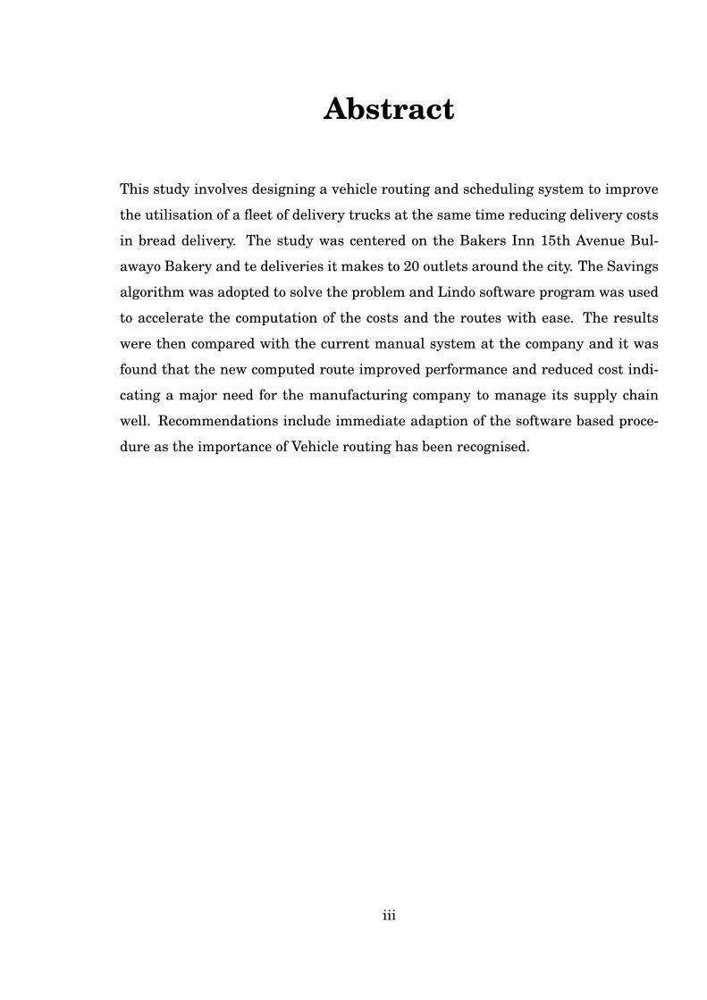
This study involves designing a vehicle routing and scheduling system to improve
the utilisation of a fleet of delivery trucks at the same time reducing delivery costs
in bread delivery. The study was centered on the Bakers Inn 15th Avenue Bul-
awayo Bakery and te deliveries it makes to 20 outlets around the city. The Savings
algorithm was adopted to solve the problem and Lindo software program was used
to accelerate the computation of the costs and the routes with ease. The results
were then compared with the current manual system at the company and it was
found that the new computed route improved performance and reduced cost indi-
cating a major need for the manufacturing company to manage its supply chain
well. Recommendations include immediate adaption of the software based proce-
dure as the importance of Vehicle routing has been recognised.
iii
Contents
1 Introduction 11.1. Background . . . . . . . . . . . . . . . . . . . . . . . . . . . . . . . . . 21.2. Current Bakers Inn Distribution System . . . . . . . . . . . . . . . . 31.3. Problem Statement . . . . . . . . . . . . . . . . . . . . . . . . . . . . . 51.4. Purpose of Study . . . . . . . . . . . . . . . . . . . . . . . . . . . . . . 51.5. Objectives of Project . . . . . . . . . . . . . . . . . . . . . . . . . . . . . 61.6. Significance of Study . . . . . . . . . . . . . . . . . . . . . . . . . . . . 61.7. Assumptions . . . . . . . . . . . . . . . . . . . . . . . . . . . . . . . . . 61.8. Delimitations of the Study . . . . . . . . . . . . . . . . . . . . . . . . . 7
2 Literature Review 82.1. Introduction . . . . . . . . . . . . . . . . . . . . . . . . . . . . . . . . . 82.2. The Vehicle Routing Problem . . . . . . . . . . . . . . . . . . . . . . . 92.3. Variants of the Vehicle Routing Problem . . . . . . . . . . . . . . . . . 11
2.3.1. The Travelling Salesman Problem (TSP) . . . . . . . . . . . . 112.3.2. Multiple Travelling Salesmen Problem . . . . . . . . . . . . . 112.3.3. Capacitated Vehicle Routing Problem . . . . . . . . . . . . . . 122.3.4. Vehicle Routing Problem with Time Windows (VRPTW) . . . . 132.3.5. Vehicle Routing Problem in Hazardous Material (HAZMAT) . 142.3.6. Vehicle Routing Problem with Pick-Up and Delivery (VRPPD) 142.3.7. Time depended VRP . . . . . . . . . . . . . . . . . . . . . . . . 152.3.8. Dynamic Vehicle Routing . . . . . . . . . . . . . . . . . . . . . 16
2.4. Solution techniques for the VRP . . . . . . . . . . . . . . . . . . . . . . 172.4.1. Savings algorithm . . . . . . . . . . . . . . . . . . . . . . . . . . 172.4.2. Simulated annealing . . . . . . . . . . . . . . . . . . . . . . . . 182.4.3. Tabu Search . . . . . . . . . . . . . . . . . . . . . . . . . . . . . 192.4.4. Ant Colony Optimisation . . . . . . . . . . . . . . . . . . . . . . 202.4.5. The Sequential Insertion Algorithm . . . . . . . . . . . . . . . 212.4.6. Neighborhood Search . . . . . . . . . . . . . . . . . . . . . . . . 21
2.5. Sweep algorithm . . . . . . . . . . . . . . . . . . . . . . . . . . . . . . . 212.6. The Fisher and Jaikumar algorithm . . . . . . . . . . . . . . . . . . . 222.7. Taburoute . . . . . . . . . . . . . . . . . . . . . . . . . . . . . . . . . . 232.8. Recent work . . . . . . . . . . . . . . . . . . . . . . . . . . . . . . . . . 232.9. Overview . . . . . . . . . . . . . . . . . . . . . . . . . . . . . . . . . . . 24
iv
3 Methodology 253.1. Introduction . . . . . . . . . . . . . . . . . . . . . . . . . . . . . . . . . 253.2. Data Sources . . . . . . . . . . . . . . . . . . . . . . . . . . . . . . . . . 253.3. Sampling design and sampling frame . . . . . . . . . . . . . . . . . . 263.4. Modeling Methodology . . . . . . . . . . . . . . . . . . . . . . . . . . . 263.5. Model Formulation . . . . . . . . . . . . . . . . . . . . . . . . . . . . . 27
3.5.1. Objective function . . . . . . . . . . . . . . . . . . . . . . . . . . 283.5.2. The Constraints . . . . . . . . . . . . . . . . . . . . . . . . . . . 28
3.6. Heuristics algorithms . . . . . . . . . . . . . . . . . . . . . . . . . . . . 343.6.1. Savings Based Algorithm . . . . . . . . . . . . . . . . . . . . . 343.6.2. Neighborhood Search Algorithm . . . . . . . . . . . . . . . . . 36
3.7. Routing System in Operation . . . . . . . . . . . . . . . . . . . . . . . 373.8. Summary . . . . . . . . . . . . . . . . . . . . . . . . . . . . . . . . . . . 38
4 Data Analysis and Discussions 394.1. Introduction . . . . . . . . . . . . . . . . . . . . . . . . . . . . . . . . . 394.2. Data Analysis . . . . . . . . . . . . . . . . . . . . . . . . . . . . . . . . 394.3. Current System . . . . . . . . . . . . . . . . . . . . . . . . . . . . . . . 404.4. Proposed Model . . . . . . . . . . . . . . . . . . . . . . . . . . . . . . . 414.5. Comparison of results . . . . . . . . . . . . . . . . . . . . . . . . . . . . 424.6. Overview . . . . . . . . . . . . . . . . . . . . . . . . . . . . . . . . . . . 45
5 Conclusion and Recommendations 465.1. Conclusion . . . . . . . . . . . . . . . . . . . . . . . . . . . . . . . . . . 465.2. Limitations . . . . . . . . . . . . . . . . . . . . . . . . . . . . . . . . . . 475.3. Recommendations . . . . . . . . . . . . . . . . . . . . . . . . . . . . . . 475.4. Implications . . . . . . . . . . . . . . . . . . . . . . . . . . . . . . . . . 485.5. Further Research . . . . . . . . . . . . . . . . . . . . . . . . . . . . . . 48
v
List of Figures
3.1 Distribution of shops in the City centre . . . . . . . . . . . . . . . . . 303.2 Distribution of customers in Eastern Bulawayo . . . . . . . . . . . . . 313.3 Distribution of customers in Western Bulawayo . . . . . . . . . . . . 323.4 Distribution of customers in Nothern Bulawayo . . . . . . . . . . . . 333.5 The Savings Algorithm Flow Chart . . . . . . . . . . . . . . . . . . . 34
4.1 Capacity utilisation comparison . . . . . . . . . . . . . . . . . . . . . . 434.2 Total distance travelled by fleet . . . . . . . . . . . . . . . . . . . . . . 44
5.1 Capacity utilisation comparison . . . . . . . . . . . . . . . . . . . . . . 545.2 Capacity utilisation comparison . . . . . . . . . . . . . . . . . . . . . . 555.3 Capacity utilisation comparison . . . . . . . . . . . . . . . . . . . . . . 565.4 Capacity utilisation comparison . . . . . . . . . . . . . . . . . . . . . . 57
vi
List of Tables
4.1 Manual routing results . . . . . . . . . . . . . . . . . . . . . . . . . . . 414.2 Designed system results . . . . . . . . . . . . . . . . . . . . . . . . . . 424.3 Results comparison . . . . . . . . . . . . . . . . . . . . . . . . . . . . . 43
5.1 Customer details . . . . . . . . . . . . . . . . . . . . . . . . . . . . . . 53
vii
Chapter 1
Introduction
In the last 30 years, designing an efficient supply chain and operating the chain
efficiently has become one of the most important issues for an increasing number
of organisations. The increasing economic challenges and pressure from competi-
tors has forced manufacturing companies to devise better ways of controlling every
step in their supply chain from their warehouses to customers. Transportation
costs have a significant impact on the operating costs of the firm. On realization of
this, many researchers and practitioners are seeking new and better ways to gain
competitive advantage over competitors in distribution networks. Integration and
organization of various aspects of distribution have become critical to lower costs
and increase an firm’s efficiency.
Due to recent fluctuations in the Zimbabwean economy, matching supply to de-
mand has become even more challenging. Nowadays there is a growing need for
more robust supply chains that are responsive to the changes in the market con-
ditions. The usual models of supply chain management are often disapproved by
practitioners for their strong assumptions, among which is full knowledge of the
underlying demand distribution. In most real world applications, scarcity demand
data makes it very hard to determine a demand distribution that fits the observed
Introduction 2
data.
This results in the logistics and inventory managers making important decisions
using partial or even inaccurate information such as inaccurate forecasts about
future demands resulting in unnecessary measures been put in place. This ulti-
mately has an overbearing effect on any organization as it not only undermines
the decision maker and researchers’ capabilities but also in loss of the so limited
but much needed monetary resource. With the economy still recovering from re-
cession, most industries are struggling and competition to gain large stake in the
consumer market is high, thus resources need to be managed and used well.
1.1. Background
Bakers Inn 15th Avenue Factory is one of the production and manufacturing com-
panies that supplies its products to Bakers Inn shops (outlets) in and around Bu-
lawayo. Bread is moved between different stages incurring holding costs and in-
ventory costs. Supply chains of Bakers Inn consists of a manufacturing shop and
2 distributors. Distributors are immediate customers of the company. Effective
management of such a supply chain is a key success factor for the company to
strengthen its position in the industry and increase its market share. Many com-
panies have to consider designing their distribution network in order to reduce
high logistics costs and increase the service level to their customers. It is antic-
ipated that new network designs will reduce the logistics cost to a considerable
amount, because of consolidated demand at the shops and making palletized high
volume transportation possible. In this study we consider a vehicle routing prob-
lem of Bakers Inn from factory to shop outlets together with transportation costs
between them.
The system resembles a popular approach called vendor managed inventory in lit-
erature. A vendor manages the inventory levels of its customers by considering
current inventory at their depots and locations. The aim is to minimize the system
Introduction 3
wide cost by simultaneously considering inventory and transportation components.
The vendor is likened to the production company and the customers to the shops.
There exist two approaches on the transportation factor that can be utilized. The
first one is direct delivery approach whereby each customer is allocated a truck.
The quantity ordered by a customer will be directly delivered by the dedicated
truck and then the truck will come back to the factory. The second approach is
to deliver orders placed by different customers using the same truck and this is
called milk run. Meanwhile the truck carries different customers’ loads and deliv-
ers them in a sequence. This requires determining a route for each truck. In these
scenarios, the problem will be composed of both inventory decisions and routing
decisions. This research considers a milk run system which will be compared with
the present data of a company in order to measure its effects on the system, in
terms of performance measures.
However the company has always been more concerned with reducing cost (in-
ternal) and increase profitability, and not much attention has been placed on man-
agement of inventory routing. Vehicle routing in today’s business environment has
financial implications on all parties concerned. Research on and implementation of
VRP principles in improving it is of great strategic significance to any production
company today. The aim is to design the distribution system between Bakers Inn
Factory and shop outlets by determining the time and amount of delivery to each
shop outlet and also construct delivery routes with the objective of costs minimiza-
tion.
1.2. Current Bakers Inn Distribution System
Bakers Inn Zimbabwe is so popular in that it has become a household name when
it comes to quality products in Bulawayo town. The continuous ability of the serv-
ing staff to treat every customer as a king complemented with continued efforts
in quality improvements has also lead to better customer satisfaction; as a result
Introduction 4
the company has gained customers who are able to do repeated business. The
present inventory distribution system from the factory to the shops is as follows.
The customers of Bakers Inn 15th Avenue Factory are the shop outlets and they
are directly served from the factory. Inventory that belongs to the factory is held
at warehouses around the factory. Customers (shops) place their orders to the
management of the factory. The management transfers the orders to the trans-
port department after the necessary adjustments are made. Orders are processed;
truck loads and delivery patterns are formed by the transport department. The
transport department operates a dedicated fleet of vehicles for the company.
The costs incurred by the company are made on the basis of total distance travelled
(kilometers) regardless of load carried. According to this transportation scheme,
transportation is made in full truckloads. Distance is calculated as the total length
of the route from the factory to shop and back to the factory. This will mean that
the company incurs cost for the empty vehicles coming back from customers. Ve-
hicles used are an expensive mode of transport, in terms of the loading capacity
and fuel consumption. Cost per unit volume, carried per unit distance travelled is
higher than using higher capacity trucks.
Shop outlets hold inventories in their own warehouses. They are free in deter-
mining their inventory levels and ordering decisions. Transportation costs related
to transfer between factory and shops belongs to the factory. The company uti-
lizes about 3 tonne trucks for transportation. Since there is no transportation cost
incurred by the customers, they place orders in an irregular manner. The main
attraction in the ordering decision is to gain incentives related to ordering quan-
tities. However, this practice results in high fluctuations in delivered orders and
very high inventories in their warehouses depending on their sales. At present,
the system operates as a push system. The sales shops place orders every day. Ac-
cording to these orders, the production company plans tomorrow’s production. The
responsibility of the production department is to make the product according to the
daily plan and make the product ready to be delivered on the following day.
Introduction 5
1.3. Problem Statement
Thus the factory faces two main problems. Bakers Inn 15th Ave planning periods
do not coincide with periods of forecast prospect. The reason being that produc-
tions are done daily that is production is almost uniform. The monthly total of
production orders is usually greater than monthly sales targets due to rationing
game among customers in case of scarce inventory at the warehouse. In addition,
the cost effectiveness of the delivery system to all the customers leaves a lot to be
desired. The mode of transport and the routes are randomly planned by the trans-
port department which doesn’t consider load in truck but distance covered.
1.4. Purpose of Study
In trying to develop a solution to the above stated problem we will focus on vehicle
routing efficiency gains from solving the transportation problem. As stated earlier
on Bakers Inn is experiencing difficulties in its delivery system also being caused
by lack of proper order estimation per customer and irregularities in system of de-
livery.
The research therefore intends to use the vehicle routing problem to establish a
cost effective delivery network which also puts into consideration truck capacity
and also to forecast how much each customer may require to establish a single dis-
patch time period where all deliveries are made.
Thus the study seeks to reduce challenges faced in making the following decisions
• The order in which to supply to shops
• Maximisation of vehicle capacity
• Delivery routes to use
Introduction 6
As a result, we seek to establish a delivery policy that is cost effective and time
efficient for the organization.
1.5. Objectives of Project
The researcher seeks achieve the following objectives by undertaking the study:
• To establish the benefit of VRP to the delivery system and its contribution to
overall company performance
• To improve distance management of delivery system
• Minimize distribution cost by determining order in which to supply shops,
how to deliver to shops and which delivery route to use.
1.6. Significance of Study
There has been not much research done in Zimbabwe on application of Vehicle
Routing Problem in bread supply chain. The research will also present an effec-
tive solution approach for a real life practical distribution and inventory manage-
ment problem that has not been addressed before. The research will contribute
immensely to perishable food supply chains in Zimbabwe particularly in develop-
ing and improving food supply performance in light of increasing competition in
distribution networks. This will lower costs and increase efficiency. The research
will go a long way particularly in helping managers involved in the studied com-
pany to design, develop and manage a food supply chain in a manner that enables
them to reduce costs and gain competitive advantage over their competitors
1.7. Assumptions
Decisions regarding who needs to be visited and how much should be delivered will
be guided by the following assumptions about what constitutes good solutions.
Introduction 7
• Quantity delivered per visit is maximal
• Trucks are sent out with a full load
1.8. Delimitations of the Study
The researcher has put forward the following delimitations
• The data drawn from Bakers Inn Bulawayo Factory only due to resource and
time constraints, as the research has to be conducted within a short period
of time, but for future studies geographical diversified samples can be consid-
ered.
• This will be a single case design by which simulation based results of routing
might not duplicate well in reality
Chapter 2
Literature Review
2.1. Introduction
In most organizations the role of logistics management is changing. Many compa-
nies are realizing that the value for a customer can, in part, be created through
logistics management (Anon 1996). Customer values can be created through prod-
uct availability, timeliness and consistency of delivery, ease of placing orders , and
other elements of logistic service. According to (Walters and Rainbird 2007) the
quest for superior performance and customer satisfaction or customer value crite-
rion has been amongst the top priority for many organizations in the world. The
common ingredient in all the success is the presence of a soundly formulated and
effectively implemented strategy (Grant 2005). VRP has drawn the attention of
many researchers and business leaders regardless of them not offering insight into
the implementation thus benefiting on costs reduction.
Supply chain management is an important area that helps maximize profits for
the company as well as other supply chain members, which integrate and coordi-
nate across their whole network (Lambert et al 1998). Managing the supply chain
Literature Review 9
has become a way of improving profits by reducing uncertainty and enhancing cus-
tomer service. The inventory decisions of upstream and downstream members of
supply chain and transportation techniques among them constitute the focus of the
study. According to Global Supply Chain Forum supply chain management is the
integration of key business processes from the end user through to original suppli-
ers that provide products, services and information that add value for customers
and other stake holders. This frame work includes eight key supply chain manage-
ment processes which are : customer relationship management, customer service
management, demand management, order fulfillment, manufacturing flow man-
agement, supplier relationship management and returns management (Lambert
2008). Supply chain management is mainly concerned with distribution logistics
that includes transportation management and inventory control.
Early research concentrated on treating these two logistical aspects separately.
However, the inventory allocation and vehicle routing decisions are connected in
the following ways: In order to determine which customers must be served and the
amount to supply each selected customer (the inventory allocation decision), the
routing cost information is needed so that the marginal profit for each customer
can be accurately computed. On the other hand delivery cost for each customer
depends on the vehicle routes, which in turn requires information about customer
selection and amount of inventory allocated for each customer.
2.2. The Vehicle Routing Problem
Christofides (1985) describes the Vehicle Routing Problem (VRP) as the distribu-
tion problem in which vehicles based at a central facility (depot) are required to
visit geographically dispersed customers in order to fulfil known customer require-
ments. The (VRP) is one of visiting a set of customers using a fleet of vehicles, re-
specting constraints on the vehicles, customers, drivers, and so on, the goal being
to minimize the costs of operation, which normally involves reducing a combination
of the number of vehicles and the total distance travelled or time taken. Because
Literature Review 10
of the size of routing problems that need to be routinely solved in industry, local
search techniques (sometimes combined with meta-heuristics) are generally used
to produce solutions to routing problems. These methods scale well and can pro-
duce reliably good solutions.
According to Fisher and Jaikumar (1981), vehicle routing is a challenging logis-
tics management problem. They observed that there are many variations of the
problem ranging from school bus routing to the dispatching of delivery trucks for
consumer goods. In all cases, the basic components of the problem are a fleet of
vehicles with fixed capabilities (capacity, speed, etc.) and a set of demands for
transporting certain objects (school children, consumer goods, etc.) between speci-
fied pickup and delivery points.
The basic problem as first stated by Dantzig and Ramser (1959) can be defined
with G = (V,A) being a directed graph where V = v1, ..., vN is a set of vertices
representing N customers, and with v1 representing the depot where M identical
vehicles, each with capacity Q, are located. E = (vi, vj)/vi, vjεV, i 6= j is the edge
set connecting the vertices. Each vertex, except for the depot (V/v1), has a non-
negative demand qi and a non-negative service time si. A matrix C = [cij] is defined
on A. [cij] can be used to describe either cost, time or distance of travel for identical
vehicles in use. Hence, the terms cost, time, and distance are used interchangeably,
although denotes the travel time between nodes i and j in the formulation provided
below. The basic VRP is to route the vehicles one route per vehicle, each starting
and finishing at the depot, so that all customers are supplied with their demands
and the total travel cost is minimized. The basic VRP makes a number of assump-
tions, including utilizing a homogeneous fleet, a single depot, one route per vehicle
and many more. These assumptions can be eliminated by introducing additional
constraints to the problem. This implies increasing the complexity of the problem,
and, by restriction, classifies the extended problem as an np-hard problem (non-
deterministic polynomial time problem), which is a method of generating potential
solutions using some form of trial and error (non-determinism). It should be noted
Literature Review 11
that most of these additional constraints are often implemented in isolation, with-
out integration, due to the increased complexity of solving such problems. We will
therefore briefly explain some of the most common variants of the vehicle routing
problem below.
2.3. Variants of the Vehicle Routing Problem
2.3.1. The Travelling Salesman Problem (TSP)
The simplest, and probably most famous of routing problems known to researchers
is the TSP that seeks a minimum-total-length route visiting every one of N points
in a given set V = 1, 2, ...N exactly once across an arc set A. The distance between
all point combinations in A(i, j), where (i, j) ∈ V/i 6= j, is known. Although a
number of TSP variations exist, our interest is in the variant where multiple sales-
men are routed simultaneously. Hence, this will lead us to the multiple travelling
salesman problem.
2.3.2. Multiple Travelling Salesmen Problem
The MTSP is similar to the notoriously difficult TSP that seeks an optimal tour
of N cities, visiting each city exactly once with no sub-tours. In the MTSP, the N
cities must be partitioned into M tours, with each tour resulting in a TSP for one
salesperson. The MTSP is more difficult than the TSP because it requires deter-
mining which cities to assign to each salesperson, as well as the optimal ordering
of the cities within each salesperson’s tour (Kara. et al, 2005). Consider a complete
directed graph G = (V,A) where V is the set of N nodes (or cities to be visited), A
is the set of arcs and C = [cij] is the cost (distance) matrix associated with each arc
(i, j) to A. The cost matrix can be symmetric, asymmetric, or Euclidean. The lat-
ter refers to the straight-line distance measured between the two geographically
dispersed nodes where there are M salesmen based at the depot. The single de-
pot MTSP consists of finding tours for the M salesmen subject to each salesman
starting and ending at the depot, each node is located in exactly one tour, and the
Literature Review 12
number of nodes visited by a salesman lies within a predetermined time (or dis-
tance) interval. The objective is to minimize the cost of visiting all the nodes. For
any salesman, ui denotes the number of nodes visited on that salesman’s route up
to node i, with corresponding parameters K and L denoting the minimum and max-
imum number of nodes visited by any one salesman, respectively. We can therefore
state that 1 ≤ ui ≤ L when i ≥ 2,and when xi1 = 1,then K ≤ ui ≤ L.
Next we consider a variant where each of the M salespeople has a predefined, yet
similar, capacity. An analogy is having salespeople travelling with samples in their
vehicles. Not only do their cars have limited space for the samples, but each cus-
tomer visited may require a different number of the samples. As a variant of the
MTSP it is referred to as the Capacitated Multiple Travelling Salesman Problem
(CMTSP). This therefore leads us to the vehicle routing problem. In this problem,
M salesmen have to cover the cities given. Each city must be visited by exactly one
salesman. Every salesman starts from the same city (called the depot) and must at
the end of his journey return to this city again. We now want to minimize the sum
of the distances of the routes. Both the TSP and M-TSP problems are pure routing
problems in the sense above.
2.3.3. Capacitated Vehicle Routing Problem
Drexl (2011) described the capacitated vehicle routing problem (CVRP) can be de-
scribed as follows. Given are a set of identical vehicles stationed at one depot and
equipped with a limited loading capacity, and a set of geographically dispersed cus-
tomers with a certain demand for a homogeneous good. The task is to determine
an optimal (with respect to an objective function) tour plan, that is, a set of vehicle
routes, specifying which customers are visited by which vehicle in which sequence,
such that each customer is visited exactly once, the complete demand of each cus-
tomer is satisfied, and the loading capacity of the vehicles is maintained on each
tour. The objective is to minimize overall cost or travelled distance.
Literature Review 13
The problem can be formulated as a graph theoretic problem, where G = (V,A)
is a complete graph, V the vertex set (customers, and the depot, usually labelled
with 0) and A is the arc set (the paths connecting all customers and the depot).
A non-negative demand is associated with each vertex, and a cost cij is associated
with each edge in A. If the cost matrix associated with the graph, representing
the distance or travel time, is asymmetric (a common situation in urban contexts),
then the problem is called the asymmetric CVRP. This routing problem is where
our main focus is on and where the problem has been derived. A detailed formula-
tion of the problem and methods to solve it exactly are described by Vigo and Toth
(1998). These methods include branch-and-bound, branch-and-cut, and set parti-
tioning algorithms. The size of the problems which can be solved exactly is up to
100 customers, using the branch-and-bound approach (Fisher, 1995). Bigger prob-
lems and most real-world problems can be solved using heuristic and metaheuristic
methods, which provide only a suboptimal solution. We are going to consider this
case in the scope of this dissertation.
2.3.4. Vehicle Routing Problem with Time Windows (VRPTW)
In a Vehicle Routing Problem with Time Windows (VRPTW) the capacity constraint
still holds and each customer i is associated with a time interval [ai, bi], called the
time window, and with a time duration, si, the service time. This problem is often
common in real world applications, since the assumption of complete availability
over time of the customers made in CVRP is often unrealistic. Time windows can be
set to any width, from days to minutes, but their width is often empirically bound
to the width of the planning horizon. In other words, if we plan the distribution
for the next nine days, that is the planning horizon is nine days long, and we set
the time windows’ width to be in the order of few minutes, it will be much harder
to find a feasible solution than in the case the time windows are a few hours wide.
Note that the presence of time windows imposes a series of precedences on visits,
which make the problem asymmetric, even if the distance and time matrices were
originally symmetric. VRPTW is also NP-hard and even to find a feasible solution
Literature Review 14
to VRPTW is an NP-hard problem. The additional constraints in VRPTW call for
more articulate variants of the basic methods used to obtain an exact solution for
CVRP and therefore the performances tend to worsen. A good overview on the
VRPTW formulation and on exact, heuristic, and metaheuristic approaches can be
found in the paper written by Cordeau et al.
2.3.5. Vehicle Routing Problem in Hazardous Material (HAZ-
MAT)
Meng et al. (2005) point out that all researches done in general are related with
two different variants of HAZMAT routing problems A large number of researches
relating to first category of HAZMAT routing are available in literatures that em-
ploy a single or multi-objective shortest path algorithms for finding non dominated
paths minimizing risks or other attributes in transportation process for a given
origin-destination pair. In contrast researches related to second category aiming
for optimal routing and scheduling of a fleet of vehicles to distribute HAZMAT
from a depot point to a fixed number of customers satisfying their demand and
time window requirements are very limited in literatures.
2.3.6. Vehicle Routing Problem with Pick-Up and Delivery
(VRPPD)
The problems that need to be solved in real-life situations are usually much more
complicated than the classical VRP. One complication that arises in practice is that
goods not only need to be brought from the depot to the customers, but also must
be picked up at a number of customers and brought back to the depot. This prob-
lem is well known as VRP with Pick-Up and Delivery (VRPPD). In the literature,
the VRPPD is also called VRP with Backhauls (VRPB) (Ropke and Pisinger 2006;
Bianchessi and Righini 2007). The problem can be divided into two independent
CVRPs (Ropke and Pisinger 2006); one for the delivery (linehaul) customers and
one for the pickup (backhaul) customers, such that some vehicles would be desig-
Literature Review 15
nated to linehaul customers and others to backhaul customers. In the case where
the demand is the transportation of people, the problem is commonly called ”diala-
ride”. These problems always include time windows for pick-up and/or delivery
and also constraints that express the user inconvenience of waiting too long at the
pick-up point and impose a limit on riding time. When the demand is a transport
of goods, sometimes the problem can be simplified, according to the characteristics
of the transport process. For instance, in courier services, all delivered goods leave
from the depot and all pick-ups return to the depot. Moreover, it can be safely
assumed, in many circumstances, that all deliveries can be performed before the
pick-ups, thus reducing the impact of capacity constraints.
2.3.7. Time depended VRP
An interesting extension of the VRPTW in urban environments is the Time De-
pendent VRPTW, where the arc costs on the graph depend on time. This situation
is quite common in most cities, since the time taken to travel from a location to
another one depends on the traffic load, which varies with the time of the day. Par-
ticular care must be taken in defining the time dependency of the cost function.
If the horizon of interest is discretised into small intervals, and the travel times
vary in discrete jumps from an interval to the next, then Ichoua et al(2000) noted
how this approach, although being quite used, does produce solutions which may
go against common-sense. This happens when the FIFO property is violated, that
is, a vehicle departing later may arrive earlier than an earlier departing vehicle,
even following the same route. Therefore formulations where travel time and cost
functions vary continuously are to be preferred. In the cited work by Ichoua et
al., an algorithm solving such a problem is presented. The algorithm was tested
on Solomon’s 100-customer Euclidean problems. The travel times were calculated
adjusting the travel speed in order to account for the time period (morning rush,
middle of the day, evening rush). The solutions obtained in the time dependent
case are compared with the ones computed assuming that travel times are static,
and the results show that accounting for time dependency pays back, providing
Literature Review 16
better quality routes.
2.3.8. Dynamic Vehicle Routing
The Vehicle Routing Problem (VRP) has been studied with much interest within
the last three to four decades. The majority of these works focus on the static
and deterministic cases of vehicle routing in which all information is known at the
time of the planning of the routes. In most real-life applications though, stochastic
and/or dynamic information occurs parallel to the routes being carried out. Real life
examples of stochastic and/or dynamic routing problems include the distribution of
oil to private households, the pick-up of courier mail/packages and the dispatching
of buses for the transportation of elderly and handicapped people. In these exam-
ples the customer profiles (i.e. the time to begin service, the geographic location,
the actual demand etc.) may not be known at the time of the planning or even
when service has begun for the advance request customers. Two distinct features
make the planning of high quality routes in this environment much more difficult
than in the deterministic environment; Firstly, the constant change, secondly, the
time horizon.
Psaraftis(1995) used the following classification of the static routing problem; if
the output of a certain formulation is a set of preplanned routes that are not re-
optimized and are computed from inputs that do not evolve in real-time. While he
refers to a problem as dynamic if the output is not a set of routes, but rather a
policy that prescribes how the routes should evolve as a function of those inputs
that evolve in real-time. In Static Vehicle Routing Problems all information rele-
vant to the planning of the routes is assumed to be known by the planner before
the routing process begins and information relevant to the routing doesn’t change
after the route has been constructed. The information which is assumed to be rel-
evant, includes all attributes of the customers such as the geographical location of
the customers, the onsite service time and the demand of each customer. Further-
more, system information as for example the travel times of the vehicle between
Literature Review 17
the customers must be known by the planner. In Dynamic Vehicle Routing Prob-
lems not all information relevant to the planning of the routes is known by the
planner when the routing process begins and information can change after the ini-
tial routes have been constructed.
Obviously, the DVRP is a richer problem compared to the conventional static VRP.
If the problem class of VRP is denoted P(VRP) and the problem class of DVRP is de-
noted P(DVRP), then P (V RP ) ≤ P (DV RP ). The dynamic vehicle routing problem
calls for online algorithms that work in real-time since the immediate requests
should be served, if possible. Since conventional static vehicle routing problems
are NP-hard, then it is not always possible to find optimal solutions to problems
of realistic sizes in a reasonable amount of computation time. This implies that
the dynamic vehicle routing problem also belongs to the class of NP-hard prob-
lems, since a static VRP should be solved each time a new immediate request is
received. Psaraftis(1995) refers to the solution xt of the current problem pt as a
tentative solution. The tentative solution corresponds to the current set of inputs
and only those. If no new requests for service are received during the execution of
this solution, the tentative route is said to be optimal.
2.4. Solution techniques for the VRP
2.4.1. Savings algorithm
The savings algorithm is a heuristic algorithm, and therefore it does not provide
an optimal solution to the problem with certainty. The method does, however, often
yield a relatively good solution. That is, a solution which deviates little from the op-
timal solution. The Clarke and Wright savings algorithm is one of the most known
heuristic that was developed by Clarke and Wright (1964). The vehicle routing
problem, for which the algorithm has been designed, is characterized as follows.
From a depot goods must be delivered in given quantities to given customers. For
the transportation of the goods a number of vehicles are available, each with a
Literature Review 18
certain capacity with regard to the quantities. Every vehicle that is applied in
the solution must cover a route, starting and ending at the depot, on which goods
are delivered to one or more customers. The basic savings concept expresses the
cost savings obtained by joining two routes into one route. When the two routes
(0, ..., i, 0) and (0, j, ..., 0) can feasibly be merged into a single route (0, ..., i, j, ..., 0), a
distance saving Sij = Ci0 + C0j − Cij is generated. At every iteration the feasible
combination of two routes that leads to the largest saving in the routing cost is per-
formed. The heuristic stops when a feasible merge of routes that leads to a saving
is no longer possible. The best feasible merge version is also known as the parallel
version of Clarke and Wright Heuristic algorithm approach (savings algorithm).
2.4.2. Simulated annealing
Simulated annealing (SA) is a random-search technique which exploits an analogy
between the way in which a metal cools and freezes into a minimum energy crys-
talline structure (the annealing process) and the search for a minimum in a more
general system; it forms the basis of an optimisation technique for combinatorial
and other problems and is a generalization of the Monte Carlo method modelled
after the way liquids freeze in the process of annealing. A thermodynamic system
goes from a high-energy, disordered state into a frozen, more ordered one. Using
this analogy a thermodynamic system corresponds to the current solution of the
combinatorial problem, the energy equation for the thermodynamic system corre-
sponds to the objective function, and the ground state is analogous to the global
minimum. Initially, a thermodynamic system starts at an energy level E and tem-
perature T. While T is being kept constant, the initial configuration is perturbed
and changes in energy dE are observed. If the change in energy is negative, new
configuration is accepted. If the change in energy is positive, new configuration is
accepted with probability:
e−dE/T
Literature Review 19.
The process is then repeated until good sampling statistics are gathered for the
current temperature, then the temperature is decreased and the whole process is
repeated until the frozen state is achieved. Simulated annealing is used in various
combinatorial optimization problems, in particular in circuit design problems. SA
has the advantage of being able to deal with highly nonlinear models, chaotic and
noisy data and many constraints. It is a robust and general technique as well as
very versatile as it does not rely on any restrictive properties of the model. How-
ever, SA has the weakness of being metaheuristic and requiring a lot of choices to
be made into an actual algorithm.
2.4.3. Tabu Search
Glover describes Tabu Search (TS) as a meta-heuristic superimposed on another
heuristic. The high level approach is to prevent the algorithm from going in cycles
by forbidding or penalizing moves which take the next iteration of the solution to
points in the solution space previously visited (those points are declared ”tabu”).
Tabu method was modelled after observed human behaviour given a similar set
of circumstances, humans will act slightly differently on different occasions. This
randomness might cause an error, but may also be beneficial and cause an improve-
ment. TS operates in this fashion, except that it does not make random choices, but
operates on the premises that there is no point in accepting a poor solution unless
it is to avoid a path already investigated. This provides for investigation of new re-
gions of the problems solution space, avoiding local minima and ultimately finding
the desired solution. TS first looks for a local minimum, and to avoid repeating the
solutions it already examined, it stores them in one or more Tabu lists. The orig-
inal intent of the list is not to prevent a previous move from being repeated, but
rather to insure that it is not reversed. The role of the memory can change during
the course of the algorithm execution . At initialization the goal is to make a coarse
examination of the solution space (referred to as diversification), but as candidate
locations are identified the search is more focused to produce local optimal solu-
Literature Review 20
tions (referred to as intensification). Different TS methods differ primarily in the
size and adaptability of the Tabu memory, having them customized to a particular
problem. The method is still actively researched, and is constantly being improved.
Tabu Search in being used in integer programming problems, scheduling, routing,
travelling salesman and related problems.
2.4.4. Ant Colony Optimisation
Bullnheimer et al.(1999) describe Ant Systems as a distributed meta-heuristics
for solving hard combinatorial optimization problems, first used to solve the TSP.
They are based on observed behavior of real ant colonies in search of food. In the
traveling salesman problem, a set of cities is given and the distance between each
of them is known. The goal is to find the shortest tour that allows each city to be
visited once and only once. In more formal terms, the goal is to find a Hamiltonian
tour of minimal length on a fully connected graph. In ant colony optimization, the
problem is tackled by simulating a number of artificial ants moving on a graph that
encodes the problem itself: each vertex represents a city and each edge represents
a connection between two cities. A variable called pheromone is associated with
each edge and can be read and modified by ants. Ant colony optimization is an
iterative algorithm. At each iteration, a number of artificial ants are considered.
Each of them builds a solution by walking from vertex to vertex on the graph with
the constraint of not visiting any vertex that she has already visited in her walk. At
each step of the solution construction, an ant selects the next vertex to be visited
according to a stochastic mechanism that is biased by the pheromone: when in
vertex i, the next vertex is selected stochastically among the previously unvisited
ones. In particular, if j has not been previously visited, it can be selected with a
probability that is proportional to the pheromone associated with edge (i, j). At the
end of an iteration, on the basis of the quality of the solutions constructed by the
ants, the pheromone values are modified in order to bias ants in future iterations
to construct solutions similar to the best ones previously constructed.
Literature Review 21
2.4.5. The Sequential Insertion Algorithm
Solomon(1987) divides VRP tour-building algorithms into either sequential or par-
allel methods. Sequential procedures construct one route at a time until all cus-
tomers are scheduled. Parallel procedures are characterized by the simultaneous
construction of routes, while the number of parallel routes may either be limited
to a predetermined number, or formed freely. In the sequential version the first
saving ski or s;1 that can feasibly be used to extend the current route (0, i, ....j, 0)
by merging with another route containing edge (k, 0) or containing edge (0, 1) is
determined first. Then the merge operation is implemented and repeated with the
current route until no feasible merge is possible.
2.4.6. Neighborhood Search
In mathematical optimization, Neighborhood Search is a technique that tries to
find good or near-optimal solutions to a mathematical optimization problem by re-
peatedly trying to improve the current solution by looking for a better solution
which is in the neighborhood of the current solution. In that sense, the neighbor-
hood of the current solution includes a possibly large number of solutions which
are near to the current solution. Obviously, there is a degree of looseness in that
definition in that the neighborhood might include just those solutions that require
a single change from the current solution, or it might include the larger set of solu-
tions that differ in two or more values from the current solution. The neighborhood
search also interoperates within it the hill climber algorithm.
2.5. Sweep algorithm
The sweep algorithm is generally attributed to Gillett and Miller although its prin-
ciple can be traced back to Wren and Wren and Holliday. It applies to planar
instances of the VRP. Feasible routes are created by rotating a ray centred at the
depot and gradually including customers in a vehicle route until the capacity or
Literature Review 22
route length constraint is attained. A new route is then initiated and the process
is repeated until the entire plane has been swept.
This algorithm scores high on simplicity, but does not seem to be superior to CW
both in terms of accuracy and speed. It is also rather inflexible. Again, the greedy
nature of the sweep mechanism makes it difficult to accomodate extra constraints
and the fact that the algorithm assumes a planars tructures everely limits its ap-
plicabilityI. n particular, the algorithm is not well suited to instances defined in an
urban setting with a grid street layout. A number of heuristics generate feasible
vehicle routes (sometimes called petals in this context) and determine a best com-
bination through the solution of a set partitioning problem. Prime examples of this
approach are the 1-petal algorithm of Foster and Ryan and Ryan et al and the 2-
petal heuristic of Renaud et al where, in addition to single routes, double vehicle
routes are also generated. These extensions provide accuracy gains with respect to
the sweep algorithm.
2.6. The Fisher and Jaikumar algorithm
The Fishera nd Jaikumar algorithm is a two-phase process in which feasible clus-
ters of customers are first created by solving a generalized assignment problem
(GAP), and a vehicle route is determined on each cluster by means of a travel-
ling salesman problem (TSP) algorithm. To formulate the GAP, it is necessary to
first determine a seed for each route from which customer distances are computed.
Since the GAP is NP-hard, it is usually solved by means of a Lagrangian relaxation
technique. While good results were reported for this algorithm in the early 1980s
we have some misgivings about its performance. The original article provides in-
teger solutions values without providing the rounding or truncating rule, and the
solutions cannot be verified, which makes the assessment of the algorithm difficult.
Literature Review 23
2.7. Taburoute
With respect to earlier TS implementations, the Taburoute heuristic of Gendreau
et al is rather involved and contains several innovative features. The neighbour-
hood of xt is the set of all solutions reachable from xt by removing a vertex v from
its current route r and inserting it in another routes containing one of its closest
neighbours by means of a generalized insertion (GENI) procedure. Reinserting v in
route r is then declared tabu for 0 iterations, where 0 is randomly drawn from the
interval [5, 10], as suggested by Taillard in the context of the quadratic assignment
problem. Intermediate infeasible solutions are considered and penalized through
the use of self-adjusting penalty parameters, as explained earlier. Periodic reopti-
misations of the individual vehicle routes are performed by means of the GENIUS
heuristic for the TSP. A continuous diversification strategy is also applied to pe-
nalise frequently moved vertices. This is done by adding to the objective function a
term proportional to the relative past movement frequency of the vertex currently
being considered. False starts are also employed: this allows a limited search
starting from several initial solutions, and a full search is then performed using
the most promising starting point.
2.8. Recent work
Masache et al, (2012) released an article where they used the CW savings algo-
rithm conjoined with the sequential insertion algorithm to to solve the routing
problem of efficient ARV distribution in the Limpopo province of South Africa citing
a high mortality rate in the region due to the inefficient drug distribution system
that was in operation. In a similar endevour, the researcher would like to create
an efficient bread delivery system but will difer on the choice of methods used to
solve the problem. The savings algorithm will be the main algorithm used to solve
the main problem but due to its weakness to identify the optimal solution, it will
be coupled with the nighbourhood search algorithm to enable the most beneficial
solution to be reached instead of employing the use of the sequential insertion al-
Literature Review 24
gorithm. the researcher also wishes to employ the use of Lingo to solve the problem
instead of Visual Basic.
2.9. Overview
After evaluation of the problem as well as the potential variants which the prob-
lem under study can be classified under, the Bakers Inn problem was seen to be a
capacitated vehicle routing problem as according to the definition given for the ca-
pacitated vehicle routing problem. This is because the problem involves a capacity
constraint. Due to lack of proper planning, vehicles make deliveries in an irregular
fashion which can see them sometimes making deliveries which undermine total
capacity.
We can also identify the Clark Wright savings algorithm and Neighbourhood search
algorithm as the best combinational algorithms to use in obtaining a solution. The
savings algorithm is chosen due to the fact that it takes into account the vehicle
capacity as a constraint regardless of the fact that the solution it gives may not
always be optimal. However, this is where the neighbourhood search algorithm
complements the savings algorithm in that aspect as it then will calculate for the
best solution at hand. Thus the two algorithms combined will give us the most
optimal solution having taken into consideration all constraints.
Chapter 3
Methodology
3.1. Introduction
This chapter highlights the mathematical techniques and the methodology used in
the development of the vehicle routing model, algorithm and software. The model
of designing a vehicle routing and scheduling system to improve fleet utilization
and reduce delivery costs whilst satisfying customer demand is formulated. Our
case has 25 customers. Savings algorithm and Neighborhood search algorithm will
be implemented to come up with software to solve the problem. The solutions from
both softwares are then compared with results from the manual routing process
that the company is currently doing.
3.2. Data Sources
Research studies normally utilise two main sources for data collection: primary
and secondary. Primary data are collected by the researcher expressly for the re-
search while secondary data are those used in the research but were not gathered
directly and purposefully for the project (Hair et al, 2007; Cooper and Schindler
Methodology 26
2006). There are several benefits of applying secondary data, for example, access
to secondary data usually requires less time and budgetary resources. The data
that was applied for the research analysis is an example of secondary data. The
internal data was obtained from sales marketing reports, accounting and financial
records and miscellaneous reports of Bakers Inn Company.
3.3. Sampling design and sampling frame
The basic idea behind sampling is that by selecting some of the elements in a
population, conclusions can be drawn about the entire population (Cooper and
Schindler, 2006). The several reasons for sampling have been identified to include
lower cost, greater accuracy of results, greater speed of data collection, availability
of population elements. This research is based on a cluster sample of the population
studied, and this allowed minimum data to be collected for analysis. Conclusions
about how the entire population responded were drawn from the whole sample.
The population for this research study consists of 25 Bakers Inn Bulawayo shops
and 1 manufacturing site. For the purpose of this study, the target population in-
cluded managers and statisticians involved in vehicle routing control in Bakers Inn
factory and shops.
3.4. Modeling Methodology
The major aim of this project is to design a vehicle routing and scheduling optimi-
sation system. As a result present critical stages applicable to model building and
also the development of the routing and scheduling software.
• Stage one: Identify the real problem
This stage requires us to know the origin of the problem and basic information
required. As outlined before, the problem at hand is a capacitated vehicle routing
problem, of which we seek to develop a transportation optimization system.
Methodology 27
• Stage two: Formulate a mathematical model to represent the prob-
lem
This stage involves identifying mathematical operative processes at work; we ex-
press the situation at hand in terms of mathematical variables and create mathe-
matical relations involving parameters.
• Stage 3: Develop a software
Develop a computer based procedure for deriving solutions to the problem from the
model. This step involves development of an algorithm. Developed software will
work based on the Savings based and the Neighborhood search algorithm. I will
develop the software using a framework language called Lingo.
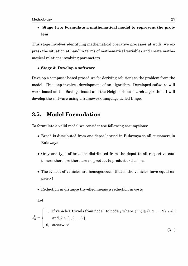
3.5. Model Formulation
To formulate a valid model we consider the following assumptions:
• Bread is distributed from one depot located in Bulawayo to all customers in
Bulawayo
• Only one type of bread is distributed from the depot to all respective cus-
tomers therefore there are no product to product exclusions
• The K fleet of vehicles are homogeneous (that is the vehicles have equal ca-
pacity)
• Reduction in distance travelled means a reduction in costs
Let
xkij =
1, if vehicle k travels from node i to node j where, (i, j) ∈ {1, 2....., N}, i 6= j,
and, k ∈ {1, 2...., K},
0, otherwise(3.1)
Methodology 28
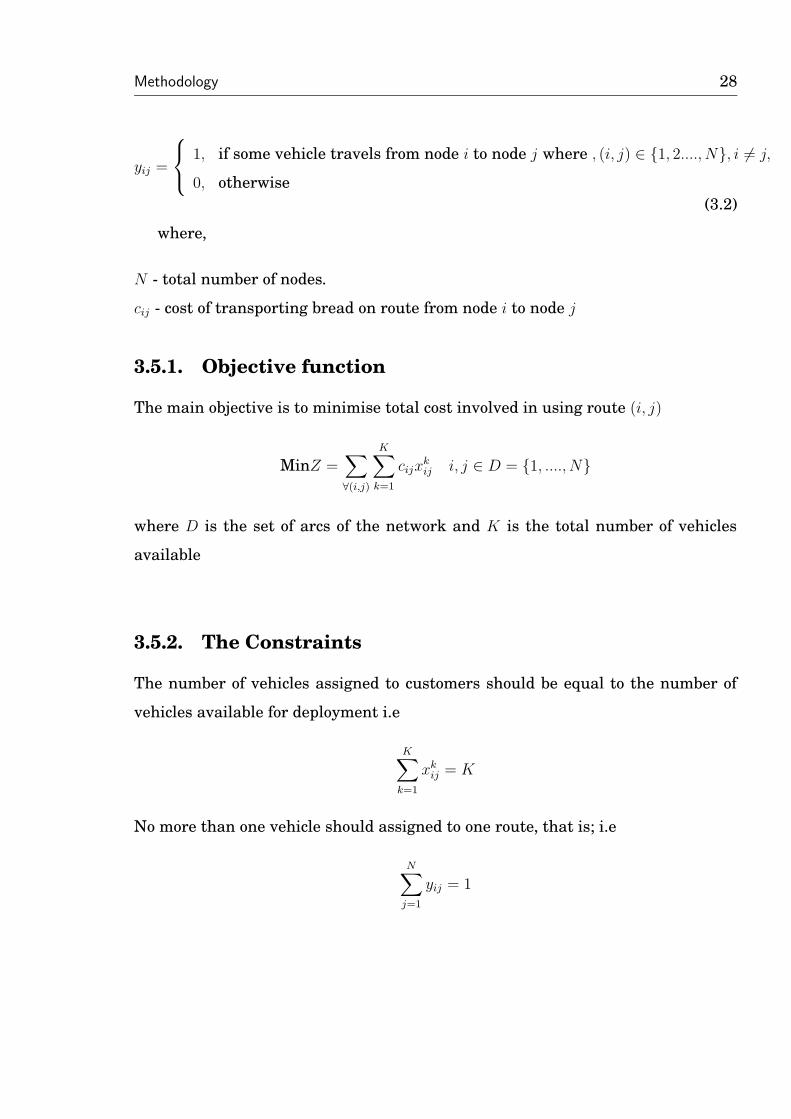
yij =
1, if some vehicle travels from node i to node j where , (i, j) ∈ {1, 2...., N}, i 6= j,
0, otherwise(3.2)
where,
N - total number of nodes.
cij - cost of transporting bread on route from node i to node j
3.5.1. Objective function
The main objective is to minimise total cost involved in using route (i, j)
MinZ =∑
∀(i,j)
K∑
k=1
cijxkij i, j ∈ D = {1, ...., N}
where D is the set of arcs of the network and K is the total number of vehicles
available
3.5.2. The Constraints
The number of vehicles assigned to customers should be equal to the number of
vehicles available for deployment i.e
K∑
k=1
xkij = K
No more than one vehicle should assigned to one route, that is; i.e
N∑
j=1
yij = 1
Methodology 29
The number of vehicles assigned to all feasible arcs should not exceed the total
number of available vehicles in the routing system i.e
N∑
i=1
N∑
j=1
yij = K
Required capacity to satisfy demand at each node should not exceed the capacity
of the vehicle assigned for the delivery i.e
N∑
i=1
N∑
j=1
dixij ≤ v
Model Summary
MinZ =∑
∀(i,j)
K∑
k=1
cijxij i, j ∈ D = {1, ....., N} (3.3)
subject to
K∑
k=1
xkij = K ∀j ∈ {1, ....., N} (3.4)
N∑
j=1
yij = 1 ∀i ∈ {1, ...., N} (3.5)
N∑
i=1
N∑
j=1
yij = K ∀k ∈ {1, ...., K} (3.6)
N∑
i=1
N∑
j=1
dixij ≤ v ∀k ∈ {1, ...., K} (3.7)
yij, xkij ∈ 0, 1 ∀k ∈ {1, ...., K} (3.8)
yij, xij ≥ 0 (3.9)
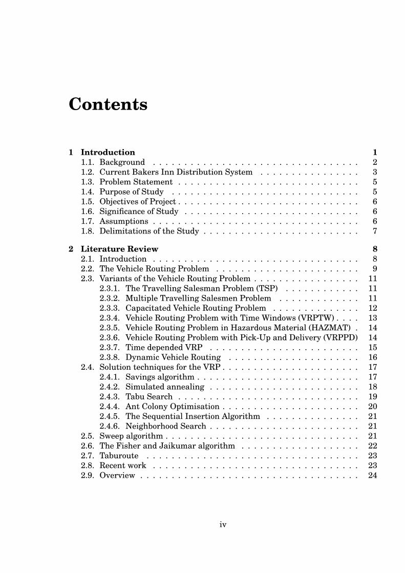
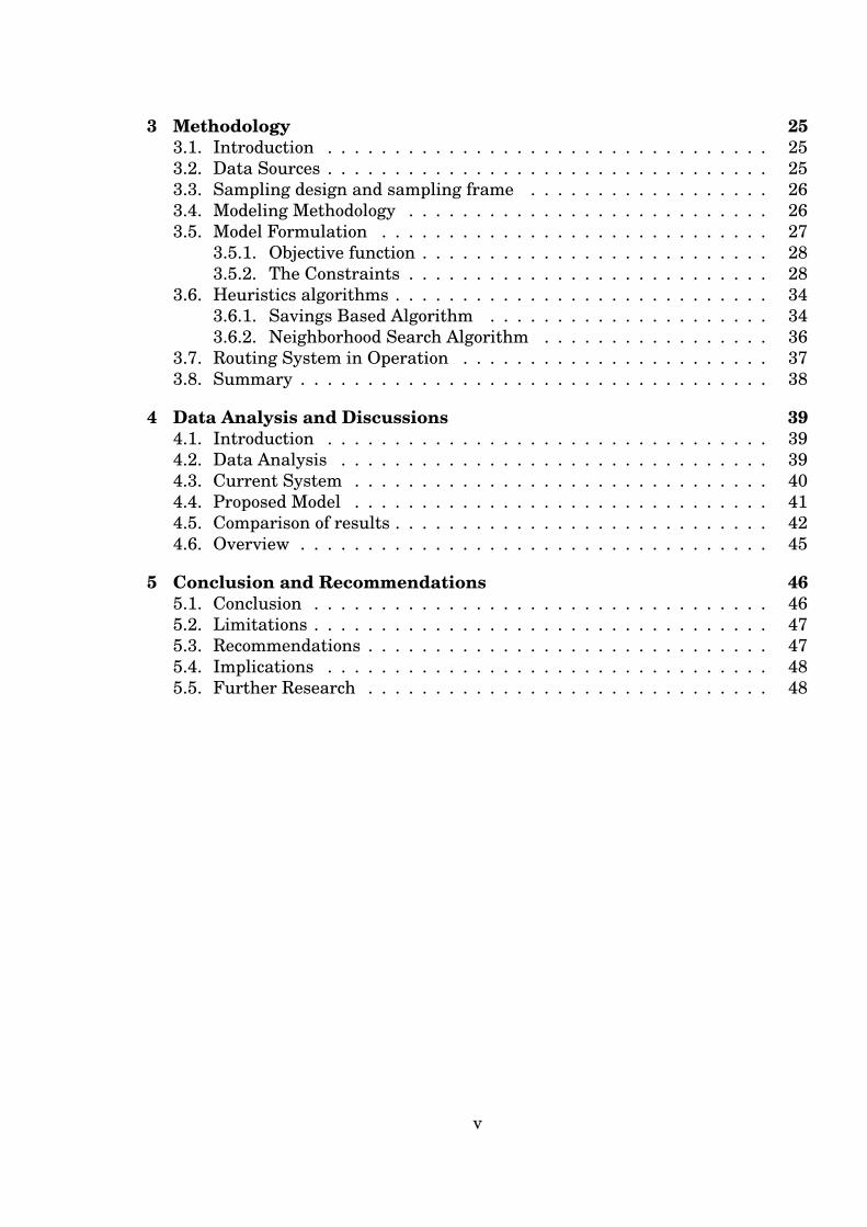
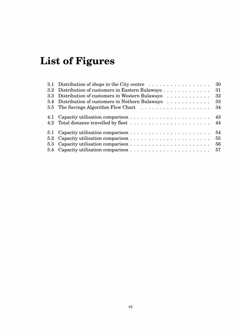
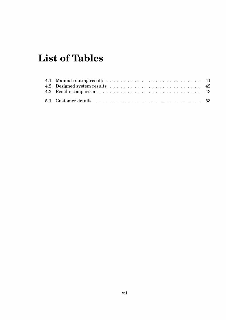
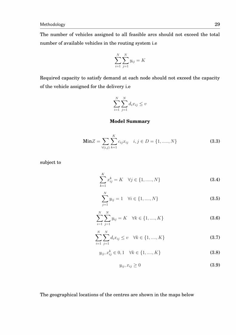
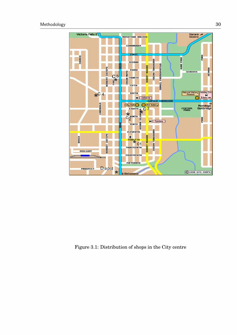
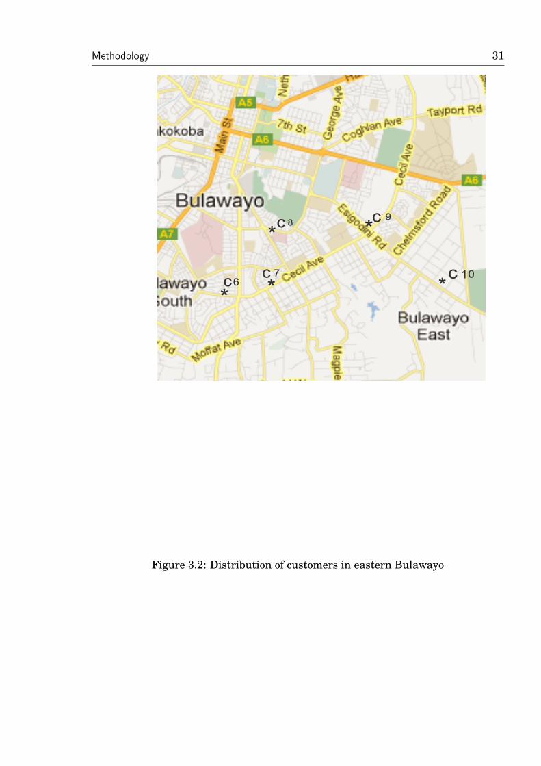
The geographical locations of the centres are shown in the maps below
Methodology 30
Figure 3.1: Distribution of shops in the City centre
Methodology 31
Figure 3.2: Distribution of customers in eastern Bulawayo
Methodology 32
Figure 3.3: Distribution of customers in northern Bulawayo
Methodology 33
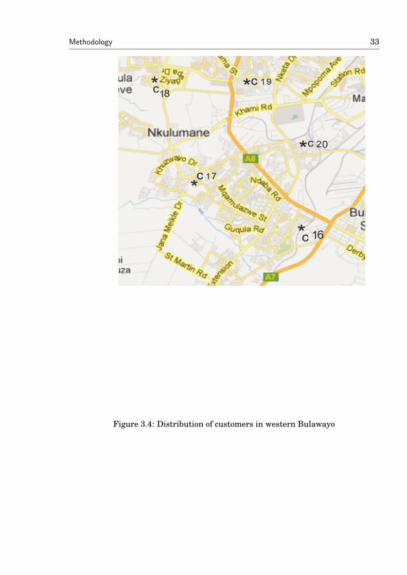
Figure 3.4: Distribution of customers in western Bulawayo
Methodology 34
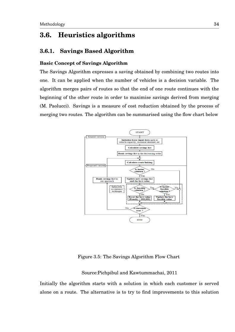
3.6. Heuristics algorithms
3.6.1. Savings Based Algorithm
Basic Concept of Savings Algorithm
The Savings Algorithm expresses a saving obtained by combining two routes into
one. It can be applied when the number of vehicles is a decision variable. The
algorithm merges pairs of routes so that the end of one route continues with the
beginning of the other route in order to maximise savings derived from merging
(M. Paolucci). Savings is a measure of cost reduction obtained by the process of
merging two routes. The algorithm can be summarised using the flow chart below
Figure 3.5: The Savings Algorithm Flow Chart
Source:Pichpibul and Kawtummachai, 2011
Initially the algorithm starts with a solution in which each customer is served
alone on a route. The alternative is to try to find improvements to this solution
Methodology 35
by combining customers of two trips into one without changing order in which cus-
tomers are visited (Poot et al. 2002). Since transport costs are provided, savings
that result from using the merged routes instead of two routes can be calculated.
Denoting the transportation cost between two given points i and j by Cij , the total
transportation costs, Da, of using two routes is given by:
Da = C0i + Ci0 + C0j + Cj0
Equivalently the transportation cost, Db, of using one merged route is:
Db = C0i + Cij + Cj0
By combining the two routes one obtains the savings Sij :
Sij = Da −Db = Ci0 + C0j − Cij
Relatively large values of Sij indicate that it is attractive, with regard to costs, to
visit points i and j on the same route such that point j is visited immediately after
point i. However, i and j cannot be combined if in doing so the resulting tour vio-
lates one or more of the constraints of the VRP.
Merge Feasibility Concept
Initialisation Step
Each vehicle serves exactly one customer. That is, for each vertex i = 1, ...., n gen-
erate a route (0, i, 0) iteration. The connection (or merge) of two distinct routes can
determine a better solution (in terms of routing cost).
STEP 1: Calculate the savings Sij = Da − Db = Ci0 + C0j − Cij for every pair
(i, j) of demand points.
STEP 2: Rank the savings Sij and list them in descending order of magnitude. This
creates the savings list. Process the savings list beginning with the topmost entry
Methodology 36
in the list (the largest Sij ).
STEP 3: For the savings Sij under consideration, merge routes servicing customers
i and j if no route constraints will be violated through the merge of the two routes
.
STEP 4: If the savings list Sij has not been exhausted, return to Step 3, processing
the next entry in the list; otherwise, stop: the solution to the VRP consists of the
routes created during Step 3. (Any points that have not been assigned to a route
during Step 3 must each be served by a vehicle route that begins at the depot D
and visits the unassigned point and returns to D.)
3.6.2. Neighborhood Search Algorithm
Neighborhood search algorithms are a wide class of improvement methods that at
each iteration search the ”’neighborhood”’ of the current solution to find a better
solution, (Ahuja et al. 2002). A neighborhood search algorithm for an optimisation
problem (where we wish to minimise an objective function) starts with a feasible
solution x1 of the problem. For each feasible solution x, an associated neighborhood
of x, denoted N(x), is a set of feasible solutions that can be obtained by perturbing
solution x using some pre-specified scheme. Elements of N(x) are called neighbors
of x. The neighborhood search iteratively obtains a sequence x1, x2, , .... of feasible
solutions. At the kth iteration, the algorithm determines a solution xk+1 with a
lower objective function value than xk. The algorithm terminates when it finds a
solution that is at least as good as any of its neighbors. Typically, multiple runs of
the neighborhood search algorithm are performed with different starting solutions,
and the best locally optimal solution is selected.
Outline of the algorithm
1. Initialise: find an initial solution
x, k ← 1
Methodology 37
2. Shake: generate a random solution
x′
∈ Nk(x)
3. Local search: x′
→ x′′
4. If x′′ is better than x then
x ← x′′ and k ← 1 (centre the search around x
′′ and search again with a small
neighbourhood).
else
k ← k + 1 (enlarge the neighbourhood)
end if
k = kmax
3.7. Routing System in Operation
The system considered in this study consists of a manufacturing unit located in
Bulawayo producing bread and confectionary. The manufactured products are de-
livered to 20 shops. The delivery takes place by means of a fleet of 4 homogeneous
vehicles with limited capacity, which are available. The demand of shops, which
is assumed deterministically known, is fulfilled by the factory. The movement of
a vehicle implies a fixed usage cost, which is related to vehicle insurance and de-
preciation or drivers and a variable shipping cost depending on both transported
quantities and travelled distance. The assumption that is made is that each vehi-
cle used can make at most one trip to a shop during each day and a vehicle cannot
deliver to the same shop on the same day, and therefore partial servicing is not al-
lowed. According to the shop’s inventory positions the factory decides the day and
the sequence that the shops are visited. The vehicle routes are formed such that
they start from the factory to the shops that should be delivered and then back
Methodology 38
to the factory. The company simulteneosly decides the amounts of delivery and of
each product to each shop and determines the routes in order to minimize the total
cost, which consists of inventory holding and transportation costs.
3.8. Summary
In this chapter we had an indepth look into the methodology of choice which we will
use to solve our problem and outlined the steps to be taken in solving the problem.
In the next chapter we look at our results and conclude on whether the designed
method is more effective or not.
Chapter 4
Data Analysis and Discussions
4.1. Introduction
This chapter entails the software design of the software coded. The software was
used to solve the problem and analyse the results. Coding of the software was done
using Lingo programming language. We collected the data used for the analysis
over a one month period in one week intervals. A comparison between the cur-
rently used routing system and the developed software routing system was done to
identify whether there has been improvement if the new routing system is used.
4.2. Data Analysis
The analysis of the data was done in two stages, first stage is computation of the
distribution according to the current system in operation at Bakers Inn and the
second is to analyse the results with the proposed system. Finally we compare re-
sults from the proposed system with the system currently in place to see how well
the proposed system performs. In the analysis, 20 of the major customers were
considered and 4 trucks, each with a capacity of 2800 loaves availed. The shops
Data Analysis and Discusssions 40
were distributed relatively evenly with 5 in the city centre, 5 in the northern sur-
bubs, 5 in the eastern surbubs and 5 in the western surbubs. In order for us to
solve the problem, a distance matrix was needed. Information was obtained from
the distance log books of the truck drivers. This, however was not too accurate and
so distances were computed using latitudes and longitudes of customer locations
which were provided. The distances were calculated using the Vincenty’s formula
given below:
Distance(km)= ACOS(COS(RADIANS(90− Lat1)COS(RADIANS(90− Lat2)) +
SIN(RADIANS(90 − Lat1))SIN(RADIANS(90 − Lat2))COS(RADIANS(Long1 −
Long2)))R
The calculation was done in MS Excel and the figures were averaged out against
corresponding values from the divers’ logs to improve accuracy as the values calcu-
lated from the Vincenty’s formula are also not absolutely accurate as highlighted
by Masache et al,(2012).
4.3. Current System
The current process is that managers from shops place orders to the warehouse.
They are free in determining their and ordering decisions. The orders placed are in
an irregular manner. On the other hand, the process of transportation and delivery
of orders is done by any person on duty responsible for scheduling the orders at the
warehouse. A driver is then assigned a group of locations to deliver to. Each driver
has an average of 5 shops he or she has to serve each day. Thus 4 vehicles are used
everyday for delivering the products. This process is done according to human
discretion where the person responsible groups orders according to areas where
they are supposed to be delivered. In these situations the driver is not given the
order he or she should follow when delivering the order, instead the driver has to
plan his or her drop order. The table 4.1 below shows the average distance and cost
accoring to the company schedular on a given day.
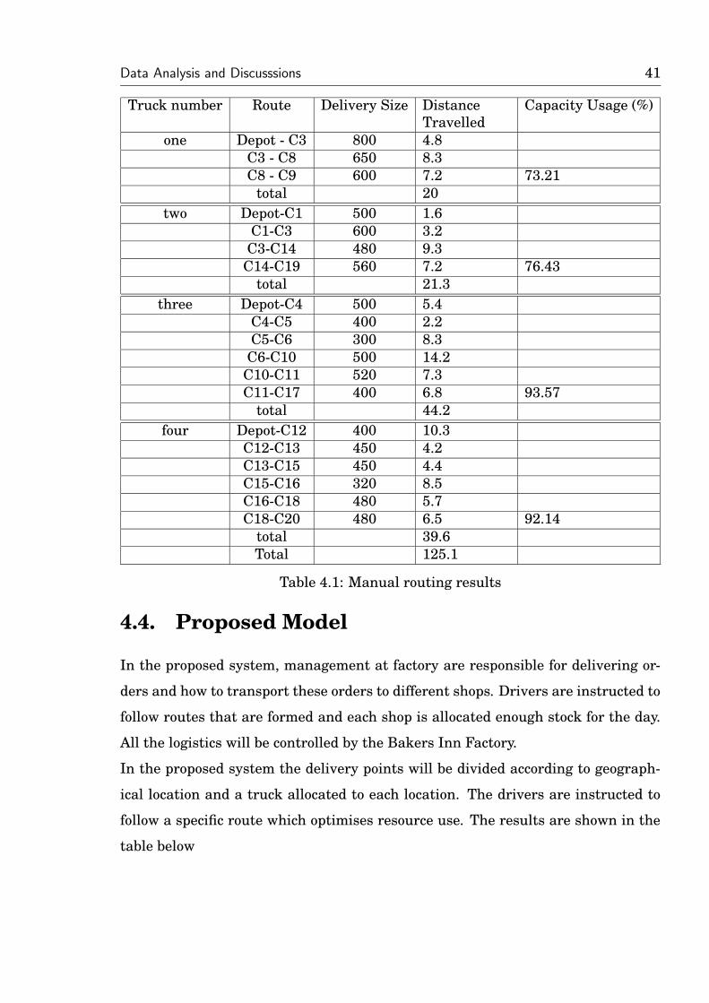
Data Analysis and Discusssions 41
Truck number Route Delivery Size DistanceTravelled
Capacity Usage (%)
one Depot - C3 800 4.8C3 - C8 650 8.3C8 - C9 600 7.2 73.21
total 20two Depot-C1 500 1.6
C1-C3 600 3.2C3-C14 480 9.3C14-C19 560 7.2 76.43
total 21.3three Depot-C4 500 5.4
C4-C5 400 2.2C5-C6 300 8.3
C6-C10 500 14.2C10-C11 520 7.3C11-C17 400 6.8 93.57
total 44.2four Depot-C12 400 10.3
C12-C13 450 4.2C13-C15 450 4.4C15-C16 320 8.5C16-C18 480 5.7C18-C20 480 6.5 92.14
total 39.6Total 125.1
Table 4.1: Manual routing results
4.4. Proposed Model
In the proposed system, management at factory are responsible for delivering or-
ders and how to transport these orders to different shops. Drivers are instructed to
follow routes that are formed and each shop is allocated enough stock for the day.
All the logistics will be controlled by the Bakers Inn Factory.
In the proposed system the delivery points will be divided according to geograph-
ical location and a truck allocated to each location. The drivers are instructed to
follow a specific route which optimises resource use. The results are shown in the
table below
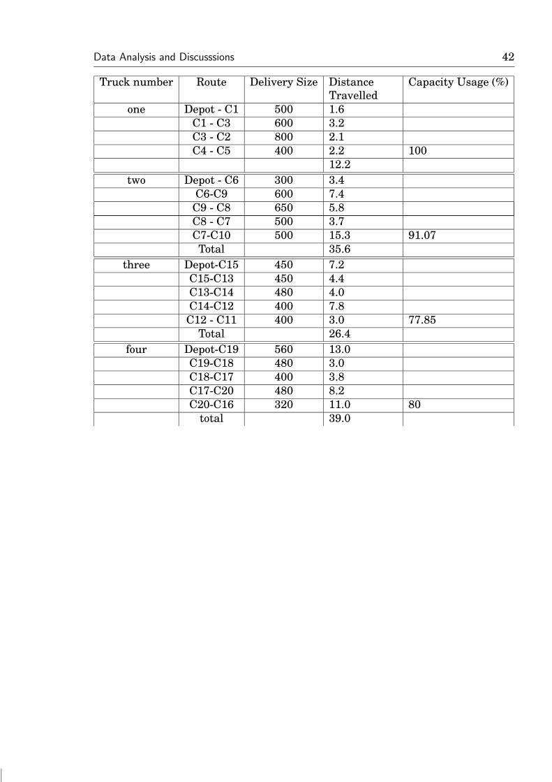
Data Analysis and Discusssions 42
Truck number Route Delivery Size DistanceTravelled
Capacity Usage (%)
one Depot - C1 500 1.6C1 - C3 600 3.2C3 - C2 800 2.1C4 - C5 400 2.2 100
12.2two Depot - C6 300 3.4
C6-C9 600 7.4C9 - C8 650 5.8C8 - C7 500 3.7C7-C10 500 15.3 91.07Total 35.6
three Depot-C15 450 7.2C15-C13 450 4.4C13-C14 480 4.0C14-C12 400 7.8C12 - C11 400 3.0 77.85
Total 26.4four Depot-C19 560 13.0
C19-C18 480 3.0C18-C17 400 3.8C17-C20 480 8.2C20-C16 320
Data Analysis and Discusssions 43
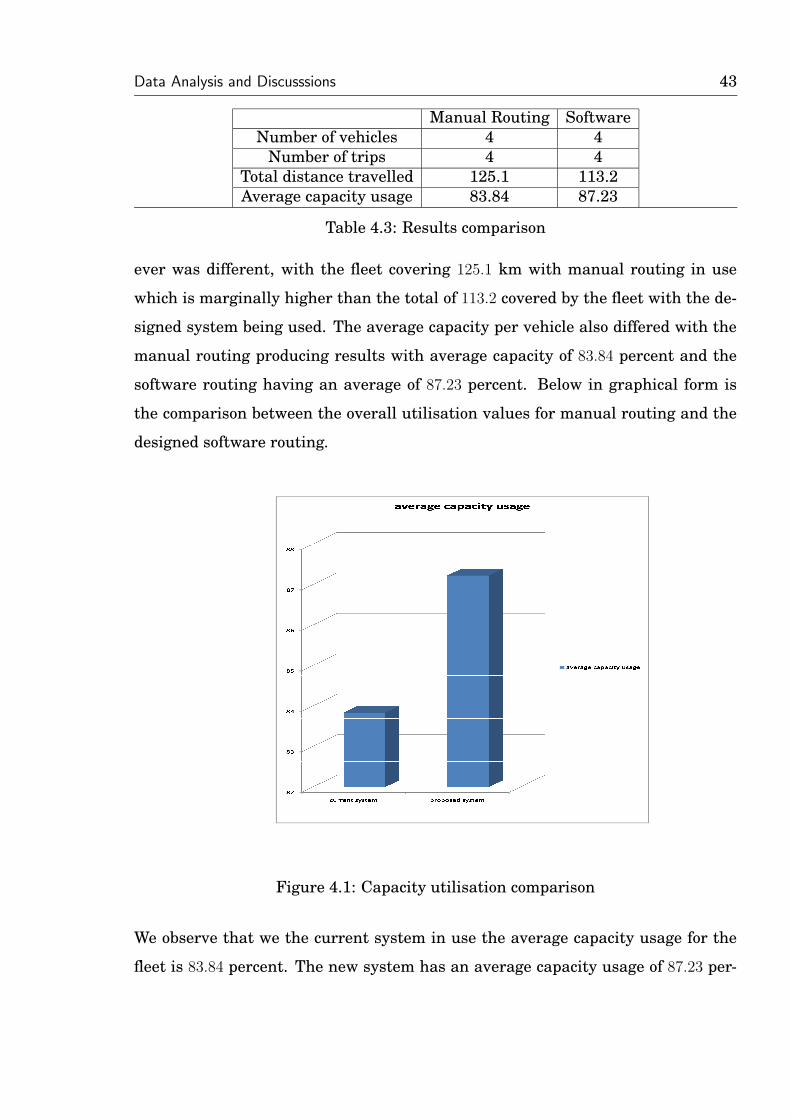
Manual Routing SoftwareNumber of vehicles 4 4
Number of trips 4 4Total distance travelled 125.1 113.2Average capacity usage 83.84 87.23
Table 4.3: Results comparison
ever was different, with the fleet covering 125.1 km with manual routing in use
which is marginally higher than the total of 113.2 covered by the fleet with the de-
signed system being used. The average capacity per vehicle also differed with the
manual routing producing results with average capacity of 83.84 percent and the
software routing having an average of 87.23 percent. Below in graphical form is
the comparison between the overall utilisation values for manual routing and the
designed software routing.
Figure 4.1: Capacity utilisation comparison
We observe that we the current system in use the average capacity usage for the
fleet is 83.84 percent. The new system has an average capacity usage of 87.23 per-
Data Analysis and Discusssions 44
cent which is evidently higher and this shows great improvement under the new
system.
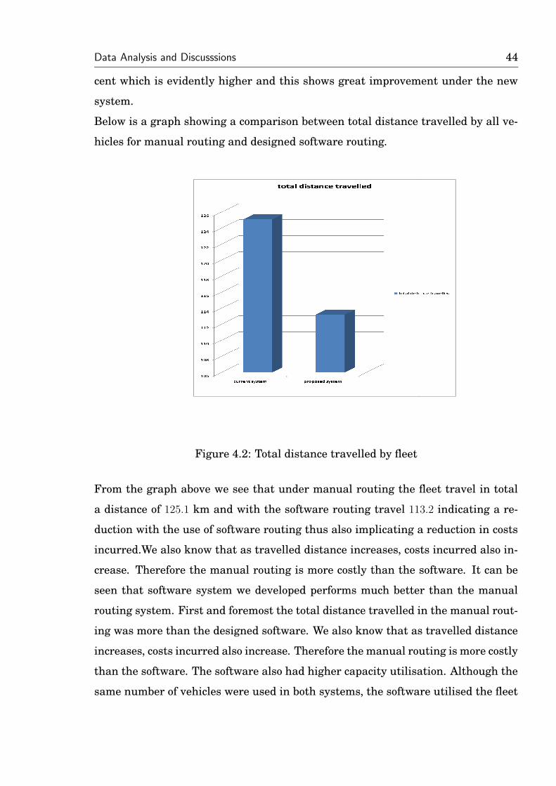
Below is a graph showing a comparison between total distance travelled by all ve-
hicles for manual routing and designed software routing.
Figure 4.2: Total distance travelled by fleet
From the graph above we see that under manual routing the fleet travel in total
a distance of 125.1 km and with the software routing travel 113.2 indicating a re-
duction with the use of software routing thus also implicating a reduction in costs
incurred.We also know that as travelled distance increases, costs incurred also in-
crease. Therefore the manual routing is more costly than the software. It can be
seen that software system we developed performs much better than the manual
routing system. First and foremost the total distance travelled in the manual rout-
ing was more than the designed software. We also know that as travelled distance
increases, costs incurred also increase. Therefore the manual routing is more costly
than the software. The software also had higher capacity utilisation. Although the
same number of vehicles were used in both systems, the software utilised the fleet
Data Analysis and Discusssions 45
in less trips travelled. The same number of trips were also made but the designed
software proved overally more effective. thus as cited from Clark and Wright, the
combining of routes will result in reduced distance and in turn a reduction in costs.
4.6. Overview
We also realise that according to the objectives set in chapter one:
• To establish the benefit of VRP to the delivery system and its contribution to
overall company performance - VRP has observed to be very important to the
organisation as it reduces company costs and through reducing distance trav-
elled by fleet and increasing capacity utilisation and thus ultimately reducing
cost. We take for example the total distance covered by truck one in its initial
route: Depot-C3-C8-C9 which covered a total of 20km as compared to the new
route the truck will take: depot-C1-C3-C2-C4-C5 in which the truck covers
more customers but only covers 12.2 km.
• To improve distance management of delivery system - distance management
has been improved greatly as the fleet has improved on the distance covered
by indivial trucks thereby reducing distance travelled collectively as specific
routes have been developed. Thus, the improvement observed of 113.2 km
against 125.1 km from the old system.
• Minimize distribution cost by determining order in which to supply shops,
how to deliver to shops and which delivery route to use - we realise that since
distance has lessened and capacity utilisation has improved, the organisation
reduces cost and achieves better handling of its distribution finances
This indicates that all objectives have been met as intended by the research.
Chapter 5
Conclusion and Recommendations
5.1. Conclusion
This research was based on an analysis of Bakers Inn Production Company in Zim-
babwe, and sought to gather data and information concerning how this company
has adopted and implemented Vehicle routing practices. The company displayed
a relatively low rate of adoption and implementation of Vehicle Routing practices
although indicated some form of vehicle routing practices in place.
The idea of the research was to design a vehicle routing and scheduling sys-
tem to improve fleet utilization and reduce delivery costs by minimising distance
travelled whilst satisfying customer demand. The problem was solved by using
the Savings Algorithm and the Neighborhood Search Method. The distances were
estimated using Vincenty’s formula in Microsoft Excel. Due to the fact that compu-
tation may be tedious and time consuming, a software was used to implement the
algorithms and come up with a solution. The solution obtained from the software
was compared with the current manual routing system. It can be that, although
the fleet utilisation was similar, the software produced better results in terms of
Conclusion and Recommendations 47
distance travelled, capacity utilisation and number of trips. In general the re-
searcher observes that the model formulated provided a better solution than the
current system and thus encourages the oranisation to implement vehicle routing
as it will benefit them immensely.
5.2. Limitations
The researcher faced certain limitations:
• The data was drawn from Bakers Inn Bulawayo Factory only due to resource
and time constraints, as the research had to be conducted within a short pe-
riod of time, but for future studies geographical diversified samples can be
considered
• The software of choice had a limited capacity which forced the sample to be
trimmed from the original size
• The unavailability of distance data records in some instances which caused
the reduction in accuracy
5.3. Recommendations
We therefore recommend that the company should implement this software based
routing procedure as it will significantly save their long run operational costs. They
should also get accurate distance or longitude and latitude points for their cus-
tomers as this would enable the accurate calculation of the distances and thereby
significantly and effectively implement this routing software. The operational rules
of routing strictly according to a certain cluster area should be relaxed as this might
not be the most optimal thing to do at that particular point in time, hence should
allow for the overlapping between cluster areas.
Conclusion and Recommendations 48
5.4. Implications
The implications appear both on theoretical and managerial implications. Impli-
cations from a theoretical (strictly research focus perspective) is that it contributes
to the body of knowledge in certain areas. The results of this case study have
strengthened the argument of IRP management within Zimbabwean companies
that relates to the reduction of costs of logistics and transportation. Secondly, the
results of this research have provided more validity for the findings of previous
studies in the field of vehicle routing in general. The findings suggest that man-
agers must consider vehicle routing as a significant element of their cost reduction
process. This will ensure that distribution strategies for the future are developed
in collaboration with vehicle routing strategies in order to develop a comprehen-
sive supply chain network strategy that benefits every member of the chain.The
results show that Bakers Inn Factory has not fully grasped the importance of Ve-
hicle Routing and incorporated it into its operations.
A general challenge observe was the continued use of manual routing in general
instead of vehicle routing and an investigation into this has shown that the gen-
erality of management locally is ignorant to the use and benefits of VRP to the
economic sector. Thus there is a need to create awareness in the sector of this and
other forms of heuristics as they can generate a great amount of savings in finances
for many organisations as well as improving management of resources and people.
5.5. Further Research
The research involved finding an optimal way of transporting fuel from a depot
to several service stations while using the Savings Algorithm and Neighborhood
Search Method. Assumptions made included homogeneous fleet, single depot, mul-
tiple customers and only one product being distributed. The model did not include
time of delivery and other heuristic methods to find solution. Further areas to
research on include:
Conclusion and Recommendations 49
• Multiple depot vehicle routing and scheduling
• Vehicle routing and scheduling of more than one fuel thereby requiring prod-
uct to product exclusions
• Use of other solution methods like Ant Colony Optimisation, Simulated An-
nealing, Tabu Search, etc; and comparing to find the optimal solution amongst
those optimal solutions
• Vincenty’s formula is accurate but not exact, therefore designing of software
that would take the road distances from maps and use those distances to come
up with a more accurate (exact) solution
• Inventory routing should be considered also as a solution method
Bibliography
Ahuja R., Ergun O., Orlin J., Punnen A.,(2002); A survey of large scale neighbour-hood search tchniques, Discrete Applied Mathematics, 75-102
Bullnheimer B, Hartl RF and Strauss C (1999). An improved ant system algo-rithm for the vehicle routing problem. Annal Opns Res 89: 561-581.
Calvete, H. I., Gale, C., Oliveros, M. J.and Sanchez-Valverde, B.,(2004), VehicleRouting Problems with Soft Time Windows: An Optimization Based Approach;Monografias del Seminario Matematico Garcia de Galdeano 31, 293-304;
Christofides, N. (1985a), ”Vehicle routing”, in: E.L. Lawler, J.K. Lenstra, A.H.G.Rinnooy Kan and D.B. Shmoys, (eds.), The Traveling Salesman Problem. AGuided Tour of Combinatorial Optimization, Wiley, Chichester, 431-448.
Cooper D. and Schindler P(2006); Business Research methods, MacGraw-HillIrwin
Dorigo, M., Birattari, M. and Stutzle, T.; Ant Colony Optimization; Univer-site Libre de Bruxelles, Belgium; IEEE Computational Intelligence Magazine,November 2006; (2006)
Dantzig G. B. and Ramser J. H.,(1959); Management Science, Vol. 6, No. 1, . 80-91
Drexl M. (2011). Rich Vehicle Routing in Theory and Practice. Technical Report2011-04.
Fisher ML (1995). Vehicle routing. In: Ball MO, Magnanti TL, Monma CL andNemhauser GL (eds). Network Routing, Handbooks in Operations Research andManagement Science, vol. 8. North-Holland: Amsterdam, 1-33.
Fisher, M. L. and Jaikumar, R.,(1981). A generalized assignment heuristic forvehicle routing. Networks, 11(2):109-124,
BIBLIOGRAPHY 51
Ghadim M.R.K and Mamaghani A.,(2011) Algorithm of ”vehicle routing schedul-ing problem” for business managers in the third millennium.
Grant, R. M.,(2005). Contemporary strategy analysis. 5th ed. Malden, MA:Blackwell.
Hair J.F. Jr, Money A.H, Samouel P. and Pagi M.,(2007); Research methods forbusiness, The UK: John Wiley and Son Ltd
Ingber, L., (1993), ”Simulated annealing: practice versus theory”, Mathl. Comput.Modelling 18, 11, 29-57.
Ichoua S, Gendreau M and Potvin J-Y (2000). Diversion issues in real-timevehicle dispatching.Transport Sci 34: 426-438.
Lambert D. (2008) Supply Chain Management: Processes, Partnership, Perfor-mance, 3rd Edition
Lambert, D.M.; Cooper, M.C. and Pagh, J.D. (1998); Supply Chain Management:Implementation issues and research opportunities, The International Journal ofLogistics Management, Vol. 9 No 2, pp. 1-19.
Larsen J. (2001). Parallelization of the Vehicle Routing Problem with TimeWindows. Phd Thesis No 62
Lysgaard, J.; Clarke and Wright’s Savings Algorithm(1997); Department ofManagement Science and Logistics, The Aarhus School of Business;
Masache A., Mashira H., Maphosa D.,(2012); Antiretroviral Drug DistributionRouting System in Limpopo Province of South Africa, Journal of Mathematicsand System Science 2 : 512-522
Pichpibul T, Kawtummachai R(2012); An improved Clarke and Wright savingsalgorithm for the capacitated vehicle routing problem, ScienceAsia 38 (2012):307318
Pillac V. (2012) Dynamic Vehicle Routing: Solutions and Computational methods.
Psaraftis, H. N. (1995). Dynamic Vehicle Routing : Status and Prospects. Annalsof Operations Research, 61, 143-164.
BIBLIOGRAPHY 52
Ropke S., Pisinger D,(2005); A general heuristic for Vehicle Routing Problems,1-44
Shaw, P. (1998). ”Using Constraint Programming and Local Search Methodsto Solve Vehicle Routing Problems.” In Principle and Practice of ConstraintProgramming-CP98. Pisa, Italy, Oct. 1998. Berlin: Springer-Verlag. LNCS..
Solomon MM (1987). Algorithms for the vehicle routing and scheduling problemwith time window constraints. Opns Res 35: 254-265.
Toth P and Vigo D (1998). Exact solution of the vehicle routing problem. In:Crainic TG and Laporte G (eds). Fleet Management and Logistics. Kluwer:Boston, 1-31.
Vigo D (1996) A heuristic algorithm for the asymmetric capacitated vehicle rout-ing problem. Eur J Oper Res 89, 10826.
Walters D, Rainbird M. (2007) Strategic Operations Management: A value chainapproach. Basingstoke, Palgrave Macmillan
www.finance.gov.au/publications/finance-circulars/2006/docs/Intro to CB analysis
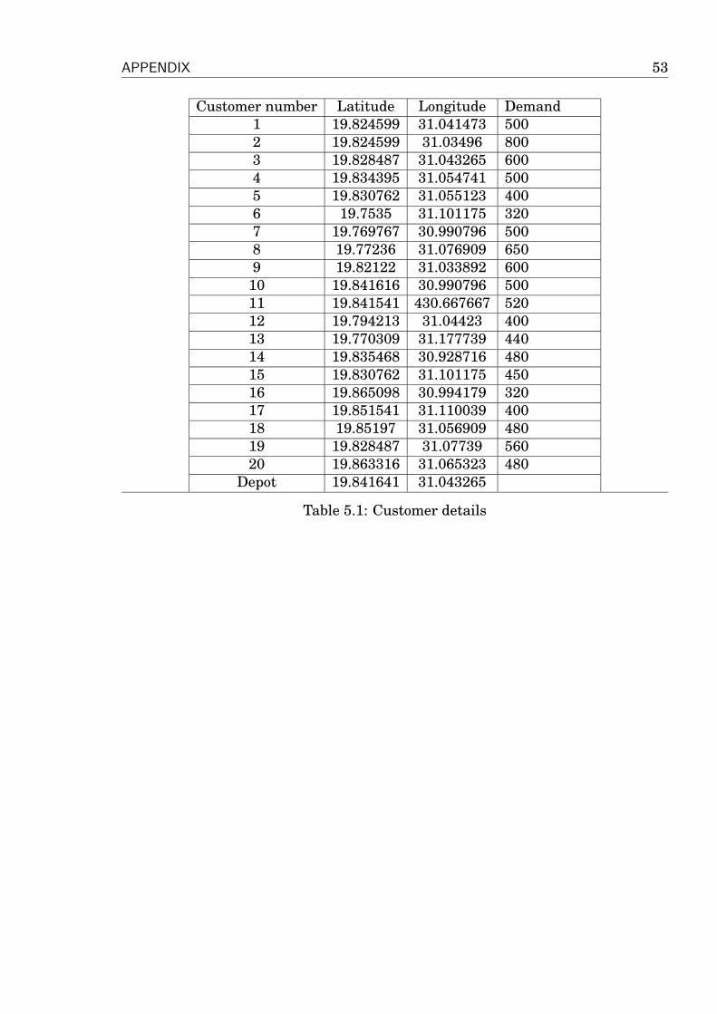
APPENDIX 53
Customer number Latitude Longitude Demand1 19.824599 31.041473 5002 19.824599 31.03496 8003 19.828487 31.043265 6004 19.834395 31.054741 5005 19.830762 31.055123 4006 19.7535 31.101175 3207 19.769767 30.990796 5008 19.77236 31.076909 6509 19.82122 31.033892 600
10 19.841616 30.990796 50011 19.841541 430.667667 52012 19.794213 31.04423 40013 19.770309 31.177739 44014 19.835468 30.928716 48015 19.830762 31.101175 45016 19.865098 30.994179 32017 19.851541 31.110039 40018 19.85197 31.056909 48019 19.828487 31.07739 56020 19.863316 31.065323 480
Depot 19.841641 31.043265
Table 5.1: Customer details

APPENDIX 54
Figure 5.1: Capacity utilisation comparison
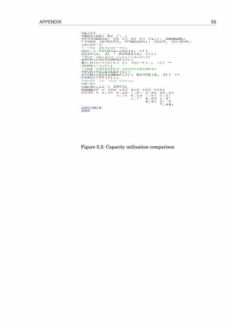
APPENDIX 55
Figure 5.2: Capacity utilisation comparison
APPENDIX 56
Figure 5.3: Capacity utilisation comparison
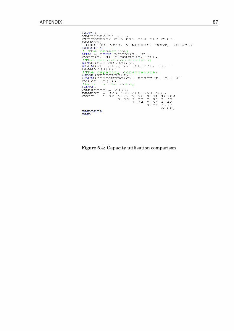
APPENDIX 57
Figure 5.4: Capacity utilisation comparison