Two Solution Representations for Solving Multi-Depot Vehicle Routing Problem with Multiple Pickup...

Computers & Industrial Engineering xxx (2015) xxx–xxx

Contents lists available at ScienceDirect

Computers & Industrial Engineering

journal homepage: www.elsevier .com/ locate/caie

Two solution representations for solving multi-depot vehicle routingproblem with multiple pickup and delivery requests via PSO

http://dx.doi.org/10.1016/j.cie.2015.04.0110360-8352/� 2015 Elsevier Ltd. All rights reserved.

⇑ Corresponding author.E-mail addresses: [email protected] (V. Kachitvichyanukul), Pandhapon.Som-

[email protected] (P. Sombuntham), [email protected](S. Kunnapapdeelert).

Please cite this article in press as: Kachitvichyanukul, V., et al. Two solution representations for solving multi-depot vehicle routing problem with mpickup and delivery requests via PSO. Computers & Industrial Engineering (2015), http://dx.doi.org/10.1016/j.cie.2015.04.011

Voratas Kachitvichyanukul b,⇑, Pandhapon Sombuntham a, Siwaporn Kunnapapdeelert b

a Accenture Solution Company Limited, Thailandb Industrial and Manufacturing Engineering, Asian Institute of Technology, Klongluang, Pathumthani 12120, Thailand

a r t i c l e i n f o

Article history:Available online xxxx

Keywords:Vehicle routingMulti-depotMultiple pickup and delivery requestsParticle swarm optimizationSolution representation

a b s t r a c t

Two solution representations for solving the generalized multi-depot vehicle routing problem with mul-tiple pickup and delivery requests (GVRP-MDMPDR) is presented in this paper. The representations areused in conjunction with GLNPSO, a variant of PSO with multiple social learning terms. The computa-tional experiments are carried out using benchmark test instances for pickup and delivery problem withtime windows (PDPTW) and the generalized vehicle routing problem for multi-depot with multiplepickup and delivery requests (GVRP-MDMPDR). The preliminary results illustrate that the proposedmethod is capable of providing good solutions for most of the test problems.

� 2015 Elsevier Ltd. All rights reserved.

1. Introduction can be a source or destination for any commodity. A commodity

The vehicle routing problem (VRP) was first proposed byDantzig and Ramser (1959). The key decision is to determine theoptimal sequence of customers to be visited by each vehicle, whichsatisfied such criteria as travel distance, time, and cost involved inthe operation. Several variants of VRP have been studied to addressthe wide variety of conditions in real world applications. For exam-ple, capacitated VPR (CVRP) addressed the VRP under the limita-tions of vehicle’s capacity. Heterogeneous fleet VRP (HVRP), anextension of CVRP, has similar characteristics as CVRP but allowsthe vehicles to have different capacities. VRP with time windows(VRPTW) requires that the customer must be served within aspecific time interval. VRP with simultaneous pickup and delivery(VRPSPD) deals with the customer requirement that involvessimultaneous pickups and deliveries, and multi depot VRP(MDVRP) contains more than one depot.

The vehicle routing problem with pickup and delivery (VRPPD)is a problem where the service required by customers may be boththe pickups and deliveries of commodities. It can be further subdi-vided as delivery-first and pickups-seconds, mixed pickups anddeliveries, and simultaneous pickups and deliveries. Berbeglia,Cordeau, and Laporte (2009) classified the pickup and deliveryproblem (PDP) into three groups according to the pickup–deliveryrelation. The first group is many-to-many problem which any node

may be picked up from one of many locations, and delivered toone of several locations as well. The second group is one-to-many-to-one problem where commodities are originally availableat the depot for delivery to customers. The commodities availableat the customers must be first picked up and delivered back tothe depot. Such characteristic is normally found in many previousstudies of VRPPD. The last one, one-to-one problem, each commod-ity can be called a request which has a given origin and destination.

Variants of VRP including PDs with various constraints areknown to be the NP-hard problems which may require excessivelylong computational time to find the optimal solutions for largeproblems. Consequently, numerous metaheuristic approaches havebeen developed for solving large VRP problems. Neural Networks(NNs), Genetic Algorithm (GA), Simulated Annealing (SA), TabuSearch (TS), Ant Colony Optimization (ACO), and Particle SwarmOptimization (PSO) had all been tried as solution methods for theproblems although these methodologies do not guarantee to findoptimal solutions but they are quite capable of providing goodsolutions or near optimal solutions within the reasonable time.

Particle Swarm Optimization (PSO) was first proposed byKennedy and Eberhart (1995) and it has been demonstrated tobe very effective as a solution method for many intractable combi-natorial problems. Several real-valued PSO algorithms were devel-oped for solving variants of VRP such as CVRP, VRPSPD, andVRPTW; (Ai & Kachitvichyanukul (2009a, 2009b, 2009c)); and theresults confirmed that PSO can be very effective for solvinggeneralized vehicle routing problems.

Sombuntham and Kachitvichyanukul (2010) proposed a particleswarm optimization algorithm for multi-depot vehicle routing

ultiple

http://dx.doi.org/10.1016/j.cie.2015.04.011

mailto:[email protected]





http://www.sciencedirect.com/science/journal/03608352

http://www.elsevier.com/locate/caie


2 V. Kachitvichyanukul et al. / Computers & Industrial Engineering xxx (2015) xxx–xxx

problem with multiple pickup and delivery requests. The solutionrepresentation SD1 is a general one and the algorithm is notrestricted only to PDPTW problem. However, the computationalexperiments are only reported for the test instances from Li andLim (2001) for the PDPTW.

This paper extends the SD1 solution representation fromSombuntham and Kachitvichyanukul (2010) and proposes twonew solution representations, named SD2 and SD3, for solving bothPDPTW and GVRP-MDMPDR. Computational experiments are car-ried out using the test instances for the PDPTW from Li and Lim(2001) and test problem instances for GVRP-MDMPDR fromSombuntham and Kunnapapdeelert (2012). The preliminaryresults show that the algorithm is able to provide good solutionsto most of the test problems.

2. Problem description

A customer is generally defined as a place which must be servedby a vehicle from a depot in many previous studies of vehicle rout-ing problem. In this paper, the term customer is replaced by a moregeneral term, location, to reflect that a location may have bothpickup and delivery requirements. For pickup and delivery prob-lem, a ‘‘request’’ is a commodity that requires a vehicle to collectfrom an origin and deliver to a destination. Although direct ship-ment is allowed, each location can play only one of these threeroles: pickup location, delivery location, and vehicle station ordepot. However, in real situation, a direct shipment may berequired and each location can play multiple roles. Each locationmay have several items to be picked up and delivered to severalother locations. This VRP that allows a location to play multipleroles and may have various pickup items delivered to differentlocations is denoted as the generalized vehicle routing problemfor multiple depots with multiple pickup and delivery requests(GVRP-MDMPDR). This situation can be depicted as shown in Fig. 1.

In this paper, vehicle routes are formed in such a way that.

(1) the total routing cost is minimized;(2) the number of vehicle is minimized;(3) the fulfilled demand is maximized.

In addition, the following restrictions must be met:(4) each request is served exactly once by a vehicle;

Pickup & delivery locations of each request

Fig. 1. The VRP with man

Please cite this article in press as: Kachitvichyanukul, V., et al. Two solution reppickup and delivery requests via PSO. Computers & Industrial Engineering (2015

(5) the load of a vehicle never exceeds its capacity;(6) each route starts and ends at the indicated terminals, which

may or may not be a depot;(7) the number of vehicles used do not exceed maximum num-

ber of available vehicles;(8) the total duration of each route (including travel and service

time) does not exceed a preset limit.

3. Mathematical model formulation

The mathematical model for the problem is an extension of themodel found in Ropke and Pisinger (2006). The objective functionin this study considers the total distance, the number of vehiclesused, and the number of fulfilled request and all vehicles areallowed to serve any requests if the assigned request does notexceed the vehicle’s capacity. Moreover, a location can have multi-ple requests, i.e., a location can simultaneously be a pickup node, adelivery node, and a depot. The model was first reported inSombuntham and Kachitvichyanukul (2010) and it is included herefor ease of reference. The definitions of sets, input parameters, andthe main decision variables in the model are described below:

Sets

y-

res),

P

to-many r

entationhttp://dx

Set of pickup nodes for request P = {1, 2, . . . , R} where Ris the total number of requests

D
Set of delivery nodes for request D{1 + R, 2 + R, . . . , 2R}where r þ R denotes destination node of request r
N
Set of all pickup and delivery nodes N ¼ P [ D Nk Subset of nodes visited by vehicle k K Set of all vehicles V Set of all nodes. V ¼ N [ fs1 . . . smg [ fs01 . . . s0mg
where sk represents node of the start station of vehiclek; k 2 K

s0k represents node of end station of vehiclek; k 2 K

A
Set of ði; jÞ which is an arc from node i to node j, wherei; j 2 V
Input parameters
Ck Capacity of vehicle k 2 K f k Fixed cost of vehicle k 2 K if it is used
Vehicle Routes

equests.

s for solving multi-depot vehicle routing problem with multiple.doi.org/10.1016/j.cie.2015.04.011


V. Kachitvichyanukul et al. / Computers & Industrial Engineering xxx (2015) xxx–xxx 3

Pp

gk

lease citeickup and

Variable cost per distance unit of vehicle k 2 K
Hi Penalty cost if the request for pick up at node i is not
served, i 2 P.
dij; tij Distance and travel time between node i and node j,
for i and j 2 N. Travel times satisfy the triangleinequality; tij 6 til þ tlj for all i; j; l 2 V; and arenonnegative

Since a visit to a node may be restricted to certain timeinterval and the service cannot occur instantaneously, thetime window with the fixed and variable service times areincluded in the model

si
Fixed service time when visiting node i ei Variable service time per item units of node i ½ai; bi� Time window in which the visit at the particular
location must start; a visit to node i can only take placebetween time ai and bi

li
Quantity of goods to be loaded onto the vehicle atnode i for i 2 P
�uj
Quantity of goods to be unloaded from the vehicle atnode j for j 2 D
Decision variables
xijk A binary variable with the value 1 if vehicle k travels
from node i to node j and is zero otherwise, wherei; j 2 V ; k 2 K

Sik
A nonnegative time that indicates when vehicle kstarts the service at location i; i 2 V ; k 2 K
Lik
A nonnegative quantity that is an upper bound on theamount of goods on vehicle k arriving at node i, wherei 2 V ; k 2 K . Sik and Lik are defined only when vehicle kactually visits node i
zi
A binary variable that indicates if a pickup request atnode i, where i 2 P, is placed on the request bank. Thevalue is one if the request is placed in the request bankand zero otherwise
The detailed mathematical model can now be described. Theobjective is to minimize the weighted sum of the distance traveled,the sum of the fix cost for each used vehicle, and the penalty costassociated with number of requests that were not scheduled asgiven in Eq. (1). The constraints are given in Eqs. (2)–(16).

Minimize aXk2K

gk

Xði;jÞ2A

dijxijkþbXk2K

Xj2P

f k xsk ;j;kþcXi2P

Hi zi ð1Þ

Subject to :Xk2K

Xj2Nk

xijk�zi 61 8i2 P ð2ÞXj2V

xijk�Xj2V

xj;jþr;k¼0 8k2K;8i2 P ð3ÞX

j2P[ s0kf g

xsk ;j;k ¼1 8k2K ð4Þ

Xi2D[ skf g

xi;s0k;k ¼1 8k2K ð5Þ

Xi2V

xijk�Xi2V

xj;i;k¼0 8k2K;8j2N ð6Þ

xijk¼1) Sikþ siþ li�eiþ tij6 Sjk 8k2K;8 i; jð Þ 2A ð7Þai 6 Sik6 bi 8k2K;8i2V ð8ÞSik6 Siþr;k 8k2K;8i2 P ð9Þxijk¼1) Lik�uiþ li¼ Ljk 8k2K;8ði; jÞ 2A ð10ÞLik 6Ck 8k2K;8i2V ð11ÞLskk¼ Ls0

kk¼0 8k2K ð12Þ

xijk 2 0;1f g 8k2K;8ði; jÞ 2A ð13Þzi 2 0;1f g 8i2 P ð14ÞSik P 0 8k2K;8i2V ð15ÞLik P 0 8k2K;8i2V ð16Þ

this article in press as: Kachitvichyanukul, V., et al. Two solution repdelivery requests via PSO. Computers & Industrial Engineering (2015

In the objective function, Eq. (1), a; b, and c are the weights thatreflect the relative importance of each cost component. Eq. (2)ensures that each pickup location is visited or that the correspond-ing request is placed in the request bank. Eq. (3) ensures that thedelivery location is visited if the pickup location is visited and thatthe visit is performed by the same vehicle. Eqs. (4) and (5) ensurethat a vehicle leaves every start terminal and a vehicle enters everyend terminal. Together with Eq. (6) this ensures that consecutivepaths between sk and s0k are formed for each vehicle k 2 K. Eqs.(7) and (8) ensure that Sik is set correctly along the paths and thatthe time windows are obeyed. These constraints also make subtours impossible. Eq. (9) ensures that each pickup occurs beforethe corresponding delivery. Eqs. (10)–(12) ensure that the loadvariables are set correctly along the paths and that the capacityconstraints of the vehicles are enforced.

This study focuses on the case when one location has manyassociated items that must be shipped to several different loca-tions. The pickup and delivery nodes of each request in the math-ematical model are modeled separately and the constraints are notin integer-linear form. This makes it much easier to understand theproblem description and the formulation. Since the problem willbe solved via metaheuristic, the integer-linear form of the modelis not required. Moreover, the model did not require the pickedup items to be shipped back to the depot and can support manyvariants of VRP such as VRPTW, CVRP, HVRP, VRPPD, and PDPTW.

4. Solution representations and decoding procedure for GVRP-MDMPDR

Solution representation and decoding procedure are the keyelements in the design of effective particle swarm optimizationalgorithm. Sombuntham and Kachitvichyanukul (2010) presenteda PSO-based algorithm with solution representation SD1 forsolving GVRP-MDMPDR problem using a variant of PSO withmultiple social learning terms, GLNPSO by Pongchairerks andKachitvichyanukul (2009). The solution representation SD1 ignoresthe information of the origin–destination pairs of the requests andonly uses the customer priority list and vehicle reference coordi-nates to construct the solutions. They reported that the algorithmprovided consistent solution quality. However, the route construc-tion procedure used in SD1 is quite complex with excessively highcomputational time. To improve the solution quality and solutiontime, two new solution representations, SD2 and SD3, are proposedhere along with their corresponding decoding procedures.

5. Solution representation SD2 and decoding procedure

The solution representation SD2 utilizes the position of a parti-cle to generate a priority list of pickup and delivery locations fromthe requests along with vehicle assignment. Suppose that r repre-sents the total number of requests, the total number of dimensionsof each particle is 3r (2r for the pick-up and delivery locations and 1rfor the vehicle assignment). Each dimension of the particle is filledwith a randomly generated number. The ranking of the randomnumber is used to prioritize the requests. The first 2r dimensionsindicate the priorities of pickup and delivery operations of eachrequest. The next r dimensions are used to find the assigned vehi-cle number for each request. The schematic representation of theparticle is explained in Fig. 2 below.

The decoding procedure is performed in 3 steps: (1) construc-tion of pickup–delivery priority list, (2) assignment of vehicle,and (3) construction of vehicle route. Figs. 3–5 illustrate the decod-ing procedure SD2 for the problem with 5 requests and 3 vehicles.As shown in Fig. 3, the first step of the decoding procedure is toconstruct a priority list for pickup and delivery by first extracting

resentations for solving multi-depot vehicle routing problem with multiple), http://dx.doi.org/10.1016/j.cie.2015.04.011


Convert to Pick up–Delivery Priority List Convert to Vehicle Assignment

1 2 3 4 … … 2r-1 2r 2r+1 2r+2 … 3r

Request 1 Request 2 Request RPriority Priority Priority

Fig. 2. Illustration of SD2 Solution representation.

First Part of the ParticlePosition Index 1 2 3 4 5 6 7 8 9 10Value 0.12 0.21 0.26 0.47 0.78 0.65 0.37 0.18 0.39 0.89Request Number (1) (1) (2) (2) (3) (3) (4) (4) (5) (5) Position Index 1 8 2 3 7 9 4 6 5 10Value 0.12 0.18 0.21 0.26 0.37 0.39 0.47 0.65 0.78 0.89Request Number (1) (4) (1) (2) (4) (5) (2) (3) (3) (5) Position Index 1 2 3 4 5 6 7 8 9 10Operation Type Pickup Pickup Delivery Pickup Delivery Pickup Delivery Pickup Delivery Delivery

Request Number (1) (4) (1) (2) (4) (5) (2) (3) (3) (5)

Fig. 3. Illustration of the construction of a Pickup–Delivery Priority List by SD2.

Second Part of the ParticleValue 0.15 1.51 1.80 0.47 2.80

Request Number (1) (2) (3) (4) (5)

noitamrofnItnemngissAelciheV1 2 2 1 3

Request Number (1) (2) (3) (4) (5)

Fig. 4. Illustration of vehicle assignment by SD2.

Vehicle DataOperation SequenceVehicle 1 Pickup Pickup Delivery Delivery Vehicle Start Station End StationRequest # (1) (4) (1) (4) 1 1 1

2 2 2Vehicle 2 Pickup Delivery Pickup Delivery 3 4 4 Request # (2) (2) (3) (3)

Request DataVehicle 3 Pickup Delivery Request Pickup DeliveryRequest # (5) (5) Number Location Location

32 2 1 3 3 2

Perform constraint checking yielded the following Vehicle Routes

1 1

4 4 35 4 2

Vehicle 1 1-4-3-1 Vehicle 2 2-1-3-2 Vehicle 3 4-2-4

Fig. 5. Illustration of vehicle route construction by SD2.


all 2r values from a particle and rearrange the list in ascendingorder. All values in the list is then assigned a corresponding requestnumber. Each request number must be presented twice in the list.The first occurrence is for pickup operation while the latter occur-rence is for the delivery operation. For the second step, the vehicleassignment procedure is illustrated in Fig. 4 by converting thevalue in the second part of the particle from the ð2r þ 1Þth dimen-sion to the ð3rÞth dimension into vehicle assignment for eachrequest. As shown in Fig. 4, the value in each dimension is roundedup and the number indicates which vehicle number is beingassigned while the position of such value represents its corre-sponding request number. The last step is the construction of theoperation sequences and vehicle route as illustrated in Fig. 5 by


using the data from Figs. 3 and 4. Each operation sequence of arequest, pickup or delivery, is assigned to a vehicle based on vehi-cle assignment one by one. The problem constraints such as timewindow, vehicle capacity, and maximum route time are checkedin this step. This step may generate routes that are different fromthe original vehicle assignment but the route constructionprocedure is deterministic and for the same set of data, the routegenerated by the decoding method is unique.

A formal algorithm steps for transforming the known data intothe appropriate form for computing are explained in Algorithm 1.Although the assignment process is completed in step 3d ofAlgorithm 1, there might still be some unassigned requests andthey must be added into the vehicle routes by using the feasibility




improvement procedures named ARR1 and ARR2 in step 3e. ARR1and ARR2 are discussed in later section.

Algorithm 1. Decoding Algorithm for SD2

The notation used in Algorithm 1 is given below.

Notations

Pp

hlh

leaseickup

Position of lth particle at the hth dimension
N Set of locations, Ni is the location index with ith priority.
fN1;N2; . . . ;Nng
L Set of all requests, fL1; L2; . . . ; Lrg W Vehicle assignment list, where Wij is vehicle index with
jth priority corresponding to location priority ith.fW11;W12; . . . ;Wnmg

Up
Set of unfulfilled requests which has pas a pickuplocation, p ¼ Ni where Ni 2 N.
Dl
The delivery location of requestl where l 2 L. Rc Route of vehicle c; c ¼ 1;2; . . . ;m. Mc Set of requests assigned to vehicle c; c ¼ 1;2; . . . ;m. Olj Operation sequence (pickup–delivery sequences) of jth
vehicle corresponding to lth particle

For a problem with m vehicles, and r requests, decoding ParticlePosition hlh (position of lth particle at the hth dimension) intoVehicle Operation sequences, Olj, and Route, Rlj. (operationsequence and route of jth vehicle corresponding to lth particle).The route of vehicle is the sequence of nodes to visit while theoperation sequence consists of pick-up and delivery of requestsfor each of the node visited.

1. Constructing Pickup–Delivery Priority List ðNÞa. Build set S = {1, 2, 3, . . ., 2r � 1, 2r} and N ¼ Ø.b. Select c from set S where hlc ¼ minh2Shlh.c. Add c to last position in set N.d. Remove c from set S.e. Repeat step 1.b until S ¼ Ø.f. For each c in set N, set c ¼ dc

2e.g. Set i = 1

i. Start from earlier position of N and set m ¼ k ¼ 0.ii. Consider cj (value at mth position of N).

iii. If cj ¼ i, set k ¼ kþ 1.iv. If k = 2, set cj ¼ cj þ r; i ¼ iþ 1 and repeat from 1.g.i until

i ¼ r þ 1.Otherwise, set m ¼ mþ 1 and repeat step1.g.ii.

2. Construct vehicle assignment list ðWÞa. Set i = 1, W ¼ Ø.

b. Set c ¼ dhl;2nþi2 e (rounding up the value)

c. Add c to the last position in set W, and i ¼ iþ 1.d. Repeat 2.b until i ¼ r þ 1.

3. Construct vehicle routea. Set k = 1.b. Add operation, pickup or delivery, one by one to the

operation sequence of a vehicle Wk.i. Set c ¼ Nk and b ¼Wk.

ii. If Nk 6 r, make a candidate operation sequence of vehicleby inserting c and c þ r into the last positions of Olb.

iii. Sort Olb based on the position value in N.iv. Convert Olb into Rlb.v. Check feasibility of the candidate route by evaluating all

constraints: vehicle capacity, location time window,maximum, and route time restriction constraints.

cite this article in press as: Kachitvichyanukul, V., et al. Two solution repand delivery requests via PSO. Computers & Industrial Engineering (2015

vi. If a feasible solution is found, keep the route Rlb and Olb

and add c to Mc . Otherwise remove c and c þ r from Olb.
c. If k ¼ r, go to step 3.d. Otherwise set k ¼ kþ 1, and go to
step 3.b.d. Improve routes by eliminate repeating visited location in

each route, for each vehicle j = 1, 2, . . . , m.i. Set S = Ø.

iii. Identify locations which the vehicle visits more thanonce, and add locations number to S.

ii. For each c in S, and for each repeating position of c in Rlj,remove one position of location c from Rlj and move alloperations which take place at the removed position toanother position which is also location c and still existsin Rlj. If it is feasible and total distance is reduced, saveRlj and update Olj.

e. Add any remaining requests by using either proceduresARR1 or ARR2 (to be discussed later).

6. Solution representation SD3 and decoding procedure

The solution representation SD3 is different from SD2 mainly inthe vehicle assignment procedure. In SD3, vehicle orientationpoints with radius coverage are used to generate vehicle assign-ment. The solution representation for SD3 is shown in Fig. 6.Note that the first part of the solution representation is the sameas SD2 while the second part now consists of 3m dimension to rep-resent ðx; yÞ coordinate of the orientation point and the coverageradius. The concept is similar to the solution representation SR2for VRP proposed by Ai and Kachitvichyanukul (2009b) whereroute construction is performed by using the information regard-ing vehicle orientation points and their coverage. The first part ofthe decoding procedure for SD3 is the same as that of SD2 thattransforms the first 2r dimension of particle into the operation pri-ority of requests at the first step as shown in Fig. 6 when r refers tonumber of requests and m represents number of vehicle.

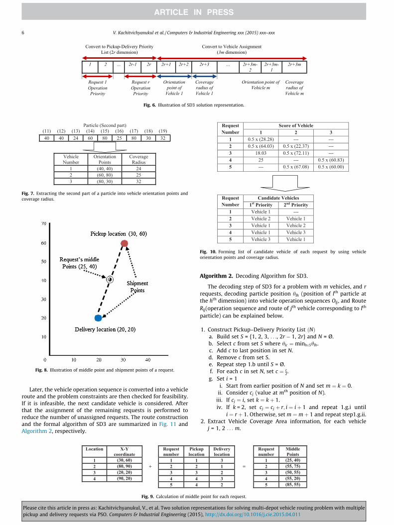
The next step is to convert the next 3m dimension into the vehi-cle assignment by extracting the coordinates of vehicle orientationpoints including the vehicle coverage radius as depicted in Fig. 7.Such coordinates and radius are used for defining a coverage areaof each vehicle when the coordinates are considered as the center.The virtual location of a request is defined as the middle point(Cartesian coordinates in two dimensions) between pickup anddelivery locations of each request. Moreover, the ‘‘shipment point’’is defined as either pickup or delivery location of the request. Oncethe middle point and shipment points of the request are within thecoverage area of a vehicle, the request will be assigned to that vehi-cle. The explanation of a request’s middle point and shipmentpoints is shown in Fig. 8 and the example of middle points calcu-lation is presented in Fig. 9.

Next step is the construction of vehicle routes based on theinformation obtained from previous section. Vehicle routes areconstructed by considering a pickup operation of a request fromthe pickup–delivery list one by one. A candidate vehicle of arequest must be the vehicle that its coverage area covers the mid-dle point or at least one of shipment points. Each candidate is thenassigned a numerical score which can be calculated based on 2 dif-ferent methods depend on the situation of the vehicle. The firstmethod is for the situation that the pickup location is the start sta-tion of the vehicle or the delivery location is the end station of thevehicle. The score for this situation is half of the distance betweenthe other shipment point and the vehicle orientation point.Otherwise, the score is the Euclidean distance between the middlepoint of a request and the vehicle orientation point. The request isthen assigned to a candidate vehicle based on ascending order ofthe scores as shown in Fig. 10.



Convert to Pickup-Delivery Priority Convert to Vehicle AssignmentList (2r ()noisnemid 3m dimension)

1 2 … 2r-1 2r 2r+1 2r+2 2r+3 … 2r+3m-2

2r+3m-1

2r+3m

Request 1 Request r Orientationpoint of

Vehicle 1

Coverage radius of Vehicle 1

Orientation point ofVehicle m

Coverage radius of Vehicle m

OperationOperationPriorityPriority

Fig. 6. Illustration of SD3 solution representation.

Particle (Second part) (11) (12) (13) (14) (15) (16) (17) (18) (19)40 40 24 60 80 25 80 30 32

VehicleNumber

Orientation Points

Coverage Radius

1 (40, 40) 242 (60, 80) 253 (80, 30) 32

Fig. 7. Extracting the second part of a particle into vehicle orientation points andcoverage radius.

Fig. 8. Illustration of middle point and shipment points of a request.

Request Number

Score of Vehicle 1 2 3

1 0.5 x (28.28) --- --- 2 0.5 x (64.03) 0.5 x (22.37) --- 3 18.03 0.5 x (72.11) --- 4 25 --- 0.5 x (60.83)5 --- 0.5 x (67.08) 0.5 x (60.00)

Request Number

Candidate Vehicles 1st Priority 2nd Priority

1 Vehicle 1 ---2 Vehicle 2 Vehicle 13 Vehicle 1 Vehicle 24 Vehicle 1 Vehicle 35 Vehicle 3 Vehicle 1

Fig. 10. Forming list of candidate vehicle of each request by using vehicleorientation points and coverage radius.


Later, the vehicle operation sequence is converted into a vehicleroute and the problem constraints are then checked for feasibility.If it is infeasible, the next candidate vehicle is considered. Afterthat the assignment of the remaining requests is performed toreduce the number of unassigned requests. The route constructionand the formal algorithm of SD3 are summarized in Fig. 11 andAlgorithm 2, respectively.

Location X-Y coordinate

Request number

Picklocat

1 (30, 60) +

1 12 (80, 90) 2 23 (20, 20) 3 34 (90, 20) 4 4

5 4

Fig. 9. Calculation of middle


Algorithm 2. Decoding Algorithm for SD3.

The decoding step of SD3 for a problem with m vehicles, and rrequests, decoding particle position hlh (position of lth particle atthe hth dimension) into vehicle operation sequences Olj, and RouteRlj(operation sequence and route of jth vehicle corresponding to lth

particle) can be explained below.

1. Construct Pickup–Delivery Priority List ðNÞa. Build set S = {1, 2, 3, . . ., 2r � 1, 2r} and N = Ø.b. Select c from set S where hlc ¼minh2Shlh.c. Add c to last position in set N.d. Remove c from set S.e. Repeat step 1.b until S = Ø.f. For each c in set N, set c ¼ c

2.g. Set i = 1

i. Start from earlier position of N and set m ¼ k ¼ 0.ii. Consider cj (value at mth position of N).

iii. If cj ¼ i, set k ¼ kþ 1.iv. If k = 2, set cj ¼ cj þ r; i ¼ iþ 1 and repeat 1.g.i until

i ¼ r þ 1. Otherwise, set m ¼ mþ 1 and repeat step1.g.ii.2. Extract Vehicle Coverage Area information, for each vehicle

j = 1, 2 . . . m.

up ion

Delivery location

Requestnumber

Middle Points

3=

1 (25, 40) 1 2 (55, 75) 2 3 (50, 55) 3 4 (55, 20) 2 5 (85, 55)

point for each request.



Position Index 1 2 3 4 5 6 7 8 9 10 Operation Type Pickup Pickup Delivery Pickup Delivery Pickup Delivery Pickup Delivery Delivery

Request Number (1) (4) (1) (2) (4) (5) (2) (3) (3) (5)

Request Number

Candidate Vehicle Vehicle 1 Pickup Pickup Delivery Delivery Pickup Delivery

Request Number (1) (4) (1) (4) (3) (3) 1st 2nd 1 1 -

Vehicle 2 Pickup Delivery

Checking of Constraints 2 2 1

Request Number (2) (2) 3 1 24 1 3

Vehicle 3 Pickup Delivery

Request Number (5) (5)

Vehicle Route Vehicle 1 1-4-3-2-1Vehicle 2 2-1-2Vehicle 3 4-2-4

Fig. 11. Route construction of SD3 based on the Pickup–Delivery Priority List and candidate vehicles list.


a. Set the coordinate ðxrefj; yrefjÞ of the orientation point,xrefj ¼ hl;2nþ3j�2 and yrefj ¼ hl;2nþ2j�1.

b. Set coverage radius, gj ¼ hl;2nþ3j.3. Construct Candidates Vehicles, for each request i = 1, 2, . . . , r.ðWÞa. Compute a request middle point,

repxi ¼xPiþ xDi

2; ð17Þ

repyi ¼yPiþ yDi

2ð18Þ

(ðxPi; yPiÞ and ðxDi

; yDiÞ are coordinates of pickup and delivery

location of request i.)b. Build set S = {1, 2, . . . , m}, and Wi ¼ Ø.c. Assign score for each vehicle j = 1, 2, . . . , m and set

scoreij ¼ �1.i. If pickup location is the same location as vehicle j start

station,

Pleasepickup

ffiffiffiffiffiffiffiffiffiffiffiffiffiffiffiffiffiffiffiffiffiffiffiffiffiffiffiffiffiffiffiffiffiffiffiffiffiffiffiffiffiffiffiffiffiffiffiffiffiffiffiffiffiffiffiffiffiffiffiffiq

cite tand

scoreij ¼ ðxDi� xrefjÞ2 þ ðyDi

� yrefjÞ2 ð19Þ

ii. Else if delivery location is the same location as vehicle jend station,

ffiffiffiffiffiffiffiffiffiffiffiffiffiffiffiffiffiffiffiffiffiffiffiffiffiffiffiffiffiffiffiffiffiffiffiffiffiffiffiffiffiffiffiffiffiffiffiffiffiffiffiffiffiffiffiffiffiffiffiq
scoreij ¼ ðxPi
� xrefjÞ2 þ ðyPi� yrefjÞ2 ð20Þ

iii. Otherwise, if the middle point of request i is within vehi-cle j’s coverage area,

ffiffiffiffiffiffiffiffiffiffiffiffiffiffiffiffiffiffiffiffiffiffiffiffiffiffiffiffiffiffiffiffiffiffiffiffiffiffiffiffiffiffiffiffiffiffiffiffiffiffiffiffiffiffiffiffiffiffiffiffiffiffiffiffiffiffiffiffiffiq
scoreij ¼ ðrepxi � xrefjÞ2 þ ðrepyi � yrefjÞ2 ð21Þ
iv. Remove j from S. If scoreij P 0, add j to Wi.d. Sort Wi based on the score in ascending order.

4. Construct Vehicle Routea. For each request k and set of candidate vehicle Wk for

request k.b. Add operation, pickup or delivery, one by one to the opera-

tion sequence of a vehiclei. c ¼ Nk where c is the (pickup or delivery) operation of

request k.ii. b ¼Wkj (b is the candidate vehicle j of request k from set Wk).

iii. If Nk 6 r, make a candidate operation sequence of vehi-cle by inserting c and c þ r into the last positions of Olb.Otherwise next request k, and go to step 4.b.

iv. Sort Olb based on the position value in N.v. Convert Olb into Rlb.

his article in press as: Kachitvichyanukul, V., et al. Two solution repdelivery requests via PSO. Computers & Industrial Engineering (2015

vi. Check feasibility of the candidate route by evaluating allconstraints: vehicle capacity, location time window,maximum, and route time restriction constraints.

vii. If a feasible solution is found, update the route Rlb andOlb and add c to Mc . Otherwise remove c and c þ r fromOlb and remove vehicle b from Wk.

viii. If Wk ¼ Ø, set next request k, and go to step 4.b.Otherwise, set next vehicle j, and go to step 4.b.ii.

c. If no more request, go to step 4.d. Otherwise set nextrequest k, and go to step 4.b.

d. Improve routes by eliminate repeating visited location ineach route, for each vehicle j = 1, 2, . . . , m.i. Set S = Ø.

ii. Identify locations which the vehicle visits more thanonce, and add locations number to S.

iii. For each c in S, and for each repeating position of c in Rlj,remove one position of location c from Rlj and move alloperations which take place at the removed positionto another position which is also location c and stillexists in Rlj. If it is feasible and total distance is reduced,save Rlj and update Olj.

e. Add the remaining request by using procedures ARR1 orARR2.

7. Feasibility improvement procedures ARR1 and ARR2

The proposed solution representations, SD2 and SD3 and thedecoding methods are designed for solving VRPs using theGLNPSO algorithm. As the obtained results rely on random searchwhich might lead to solutions with some unfulfilled requests.Therefore, a feasibility improvement procedure for determiningthe appropriate sequences and vehicles to assign the unfulfilledrequests are required. This section describes 2 different feasibilityimprovement procedures called ARR1 and ARR2.

The basic idea of ARR1 is simply to insert a request into theroute at the positions that lead to more number of unfulfilledrequests assigned as a primary criterion with the least increasein distance assigned as a secondary criteria. For each of the unful-filled requests, the distance between the pickup location and thenearest location exists in the route is used as the criteria for select-ing of vehicle for insertion. After the admissible placement forpickup location is found, the procedure attempts to insert the




associated delivery location to all possible positions of the vehicleroute after the pickup location. This insertion idea that considersthe pickup location first and follows by the delivery location is sim-ilar to the single pair insertion, SPI, by Nanry and Barnes (2000)and it is included in Algorithm 3.

The second feasibility improvement procedure, ARR2, is toinsert pickup and delivery operations of unfulfilled requests intoa vehicle operation sequence. For a given request, a vehicle isselected in the same way as ARR1 based on the shortest distancebetween the pickup location and existing location in the route.The pickup operation of the request is then inserted as the firstoperation sequence of the vehicle while the delivery operation isinserted into the last operation sequence. The better placementof pickup operation is determined by trying to move the placementto later positions. The best placement is found only when feasibil-ity is met as well as the least increase in distance is found. For theplacement for delivery operation, it can be determined by using thesame idea as that of pickup operation but in reverse directionwhich is given in Algorithm 4.

Algorithm 3. Add Remaining Requests 1 (ARR1).For each unfulfilled request k in set U,

1. Evaluate all vehicles based on the distance between the pickuplocation of request k and closest location existed in the route.Assign priority to the vehicle based on the distances startingfrom the first priority vehicle, c = 1.

2. Set R = the route of vehicle c;Q = set of requests assigned to thevehicle c.

3. Start from first location existed in the route; insert the pickuplocation after it.

4. Set R0 = the route after insertion and Q 0 = the request assign-ment list.

5. Determine possible request assignments based on the newcandidate route R0 and add newly assigned requests to Q 0 iffeasibility is found.

6. For each position l in R0 that follows the pickup location,a. Insert the delivery location of request k after the position l in

R0.b. Add request k to Q 0 and check for feasibility.c. If feasible, determine possible request assignments based on

the new candidate route R0 and add newly assigned requeststo Q 0 .

d. If one of the following conditions is satisfied.� kQ 0k > kQk.� kQ 0k ¼ kQk, and less total distance.

Set R ¼ R0 and ¼ Q 0.7. Consider next location in route and repeat step 3 until all loca-

tions in the route is considered8. If request k R Q , set c ¼ c þ 1 and repeat step 2. Otherwise,

save R and Q to the route and request assignment of vehicle c,and update operation sequence of the vehicle and U.

Algorithm 4. Add Remaining Requests 2 (ARR2).For each unfulfilled request k in set U,

1. Evaluate all vehicles based on the distance between the pickuplocation of request k and closest location ðBkÞ existed in theroute., Assign priority to the vehicle based on the distances.Start from the first priority vehicle, c = 1.

2. Set O = the vehicle c’s operation sequence, Q = set of requestsassigned to the vehicle c.


3. Insert the pickup operation after the operation performed at Bk

and delivery operation after the last operation sequence in O.4. Set O ¼ Ob and Db = total distance if feasibility is met. Otherwise

Ob ¼ Ø and Db = a very large value.5. For each position l later than the position of the pickup opera-

tion of request ka. Move the delivery operation of the position before position

l.b. Set O ¼ Ob and Db = total distance if feasibility is met and

new total distance < Db.6. If Ob ¼ Ø, change position of pickup operation. Otherwise go to

step 8.7. If the new position of inserting results in less distance incre-

ment than the distance between the pickup location and thenext closest vehicle, repeat step 5. Otherwise go to step 6.

8. Add k to Q and determine possible request assignments basedon the new candidate route R and add newly assigned requeststo Q if feasibility is found.

9. Save Ob;R and Q to operation sequence, request assignment, androute of vehicle c then update U.

8. Computational experiments

The proposed algorithms are implemented using the ETLibobject library from Nguyen, Ai, and Kachitvichyanukul (2010)using the class library from for GLNPSO, a variant of PSO with mul-tiple social learning terms. According to the characteristics of theproblem, the GVRP-MDMPDR model allows each location to servemore than one role, the test problem instances must contain thecharacteristics that each location can have multiple requests andeach location can serve more than one role. Since the PDPs arethe problems that each location can play only one of the threeroles, pickup location, delivery location, and vehicle station, thePDP is only the special case of GVRP-MDMPDR where each locationis playing only one role. Consequently, the test problem instancesfor PDPTW of Li and Lim (2001) can be used for initial test.Additional datasets that allow a location to play multiple rolesare provided in Sombuntham and Kunnapapdeelert (2012). Thealgorithms are implemented with C# with Microsoft VisualStudio 2008. The program runs on the platform of Intel� CoreTM, CPU 2.83 GHz with 2.96 GB RAM.

8.1. Pickup and delivery problem with time windows instances

The first set of benchmark problems tested is the 100-locationPDPTW from Li and Lim (2001). The instances consist of three sce-narios of location distribution, i.e. clustered locations, randomlydistributed locations, and half-random-half-clustered locations.Each location can have multiple requests and can serve multipleroles such as vehicle station, pickup and delivery location.

The parameters are set as follows. Maximum number of itera-tion and number of particle are set as 1000 and 100, respectively.Constant values such as inertia weight and number of neighborsare set follow the work of Ai and Kachitvichyanukul (2009a). Thenumber of neighbors is five and inertia weight is linearly decreas-ing from 0.9 to 0.4. Acceleration constants for global best, personalbest, local best, and near neighbor best are set as 0.5, 0.5, 1.5, and1.5, respectively. The GLNPSO algorithm with 3 solution represen-tations, SD1, SD2, and SD3 are run 5 times for each test probleminstance to ensure performance of the algorithm as presented inTables 1a, 1b, and 1c where NV denotes number of vehiclesrequired for the solution.

The results imply that the solution quality obtained from SD1and SD3 are quite similar when applied for solving the problem



Table 1aResults of PDPTW (Clustered locations).

Case Best known solution SD1 SD2 SD3

Average % deviation Average % deviation Average % deviation

NV Distance NV Distance NV Distance NV Distance

lc101 10 828.94 0.00 0.00 0.00 0.00 0.00 0.00lc102 10 828.94 0.00 0.00 0.00 0.00 0.00 0.73lc103 9 1035.35 4.44 �5.59 11.11 �18.00 11.11 �19.37lc104 9 860.01 0.00 2.81 0.00 14.83 0.00 8.42lc105 10 828.94 0.00 0.00 0.00 0.00 0.00 0.00lc106 10 828.94 2.00 7.43 0.00 0.29 0.00 0.00lc107 10 828.94 0.00 0.00 0.00 0.32 0.00 0.00lc108 10 826.44 2.00 1.57 0.00 0.46 0.00 0.31lc109 9 1000.6 11.11 �17.25 11.11 �7.42 11.11 �16.55lc201 3 591.56 0.00 0.00 0.00 0.00 0.00 0.00lc202 3 591.56 0.00 0.00 13.33 3.82 0.00 0.00lc203 3 585.56 0.00 0.96 0.00 4.62 0.00 1.02lc204 3 590.6 0.00 4.34 0.00 9.02 0.00 2.16lc205 3 588.88 0.00 0.26 0.00 0.04 0.00 0.00lc206 3 588.49 0.00 0.00 0.00 2.01 0.00 0.00lc207 3 588.29 0.00 0.00 0.00 1.97 0.00 0.00lc208 3 588.32 0.00 0.00 0.00 0.97 0.00 0.00

Average 1.15 �0.32 2.09 0.76 1.31 �1.37

Bold number in the table indicates the minimum average percentage deviation in its row.

Table 1bResults of PDPTW (Random locations).




lr101 19 1650.8 0.00 0.66 0.00 0.00 1.05 0.17lr102 17 1487.57 0.00 4.85 0.00 3.12 0.00 3.37lr103 13 1292.68 0.00 5.21 0.00 10.97 0.00 6.99lr104 9 1013.39 15.56 9.33 13.33 11.13 15.56 9.14lr105 14 1377.11 0.00 1.50 1.43 1.58 1.43 1.30lr106 12 1252.62 3.33 3.24 13.33 12.50 1.67 0.74lr107 10 1111.31 12.00 9.93 20.00 15.13 10.00 8.26lr108 9 968.97 2.22 1.30 11.11 10.43 6.67 4.81lr109 11 1208.96 16.36 11.42 23.64 17.99 12.73 9.09lr110 10 1159.35 16.00 7.20 24.00 15.86 22.00 9.85lr111 10 1108.9 10.00 7.54 14.00 9.46 6.00 4.48lr112 9 1003.77 22.22 18.13 26.67 26.68 22.22 19.13lr201 4 1253.23 0.00 1.79 10.00 4.70 0.00 0.82lr202 3 1197.67 33.33 12.02 33.33 28.33 20.00 10.48lr203 3 949.4 0.00 20.26 6.67 27.71 0.00 16.95lr204 2 849.05 50.00 22.42 50.00 35.07 20.00 7.85lr205 3 1054.02 26.67 23.40 33.33 28.48 33.33 20.05lr206 3 931.63 0.00 17.48 13.33 45.29 0.00 10.86lr207 2 903.06 90.00 31.25 50.00 50.12 50.00 19.29lr208 2 734.85 20.00 21.27 50.00 36.63 10.00 17.58lr209 3 930.59 20.00 16.92 33.33 30.86 13.33 12.17lr210 3 964.22 33.33 36.69 20.00 52.76 0.00 37.52lr211 2 911.52 50.00 13.37 50.00 32.84 50.00 10.97

Average 18.31 12.92 21.63 22.07 12.87 10.52



that the locations are clustered. The SD3 is more robust than SD1and SD2 for the cases with random and half-random-half-clustereddistributed with large maximum route time. However, SD1 is moreeffective than the others for the cases with half-random-half-clus-tered location with short planning.

As mentioned earlier, the final solutions based on SD1, SD2,and SD3 might still have some unfulfilled requests in the solu-tions. The improvement procedures, ARR1 and ARR2, are addedto improve the solutions by reducing the unfulfilled requests. Apreliminary experiment is first carried out to assess the effective-ness of ARR1 and ARR2 by using three different versions of SD2,i.e., SD2 without ARRs, SD2 with ARR1, and SD2 with ARR2. The


test problems from Dataset A from Sombuntham andKunnapapdeelert (2012) are used. The experiments are performedusing the accelerated constants for global best, personal best,local best, and near neighbor best of 0, 1, 1, and 2 with 10 repli-cations for each problem instance and the results are presented inTable 2.

Table 2 illustrates that the ARR1 provide the better solutionsthan that of ARR2. However, ARR1 consumes more computationaltime than the ARR2. Average percentage deviation of objectivefunction from SD2 using ARR2 from those of ARR1 including thepercentage of time improved from ARR1 when use ARR2 are com-puted to compare potential of improvement between these two



Table 1cResults of PDPTW (Mixed cluster and random locations).




lrc101 14 1708.8 0.00 0.64 2.86 1.05 0.00 1.07lrc102 12 1558.07 3.33 2.11 11.67 5.16 6.67 4.10lrc103 11 1258.74 0.00 3.17 10.91 12.66 5.45 6.82lrc104 10 1128.4 2.00 4.84 8.00 10.80 6.00 8.30lrc105 13 1637.62 3.08 1.31 6.15 2.97 6.15 2.36lrc106 11 1424.73 12.73 4.65 20.00 12.04 10.91 5.31lrc107 11 1230.15 0.00 4.76 10.91 14.92 7.27 6.37lrc108 10 1147.43 10.00 3.27 12.00 17.11 12.00 12.22lrc201 4 1406.94 20.00 27.80 20.00 40.73 15.00 31.54lrc202 3 1374.27 20.00 10.03 53.33 21.85 33.33 10.50lrc203 3 1089.07 26.67 8.01 26.67 14.65 0.00 0.71lrc204 3 818.66 0.00 0.89 0.00 18.31 0.00 2.98lrc205 4 1302.2 15.00 28.41 20.00 39.58 5.00 33.64lrc206 3 1159.03 26.67 18.39 53.33 39.38 33.33 24.86lrc207 3 1062.05 33.33 37.96 33.33 47.10 20.00 30.03lrc208 3 852.76 13.33 14.64 26.67 33.68 0.00 5.93

Average 11.63 10.68 19.74 20.75 10.07 11.67


Table 2Comparison of feasibility improvement procedure using SD2.

Instance SD2 without ARRs SD2 with ARR1 SD2 with ARR2

Objective function Time (s) Objective function Time (s) Objective function Time (s)

Average SD Average SD Average SD

Aac1 1982.33 209.51 8.27 891.66 13 32.88 925.55 36.64 22.32Aac2 2203.77 172.57 8.4 802.92 29.59 39.61 885.26 51.28 21.31Aar1 3531.79 147.82 8.41 2102.92 80.53 41.81 2209.92 113.84 22.95Aar2 a a 8.08 2377.03 110.3 36.72 2502.89 81.05 27.61Aarc1 2895.66 204.27 8.44 1554.12 74.54 42.88 1622.45 68.38 22.58Aarc2 3079.77 188.85 8.37 1726.28 36.08 39 1801.59 58.96 23.93

a The value is large due to remained unfulfilled requests.

Table 3Deviation of the results of ARR2 from ARR1.

Instances Deviation of ARR2 from ARR1

% Average deviationof objective function

% Average timedeviation

Aac1 3.80 �32.12Aac2 10.25 �46.20Aar1 5.09 �45.11Aar2 5.29 �24.81Aarc1 4.40 �47.34Aarc2 4.36 �38.64

Table 4Results of the proposed algorithm on data set A.

Instance Best solution so far Objective function

SD1 SD2 with ARR2

AVG SD %Dev AVG SD

Aac1 864.22 887.59 0.00 0.03 928.23 7Aac2 782.54 865.75 6.27 0.11 906.28 6Aar1 2004.06 2244.04 73.31 0.12 2194.54 11Aar2 2373.18 2513.50 4.39 0.06 2585.79 11Aarc1 1436.74 1464.19 21.60 0.02 1603.38 9Aarc2 1679.34 1697.77 13.91 0.01 1814.67 10

A bold number indicates the minimum average deviation of the entire row.A number with asterisk (⁄) indicates that it takes the greatest computational time com



procedures as illustrated in Table 3. The results showed that ARR2is preferable than the ARR1.

8.2. Experimental results on test problems for GVRP-MDMPDR

The performances of the two solution representations are fur-ther evaluated in this section by using test problem instances pro-vided in Sombuntham and Kunnapapdeelert (2012). All of PSOparameters are the same as those used in previous experimentexcept that the number of iteration and number of particles are

Average computationaltime (s)

SD3 with ARR2

%Dev AVG SD %Dev SD1 SD2 SD3

8.90 0.07 886.10 16.87 0.03 244.82⁄ 39.87 44.353.66 0.16 795.05 13.00 0.02 263.47⁄ 41.90 47.328.72 0.10 2043.59 28.57 0.02 246.46⁄ 44.03 56.452.11 0.09 2434.54 39.40 0.03 220.68⁄ 46.31 63.412.98 0.12 1560.72 72.73 0.09 348.42⁄ 41.17 55.365.11 0.08 1741.77 34.79 0.04 284.98⁄ 41.68 55.33

pare to other algorithms.



Table 5Results of the SD2 and SD3 on data set B, C, D, and E.

Instance Best solution so far Objective function Time (s) %

SD2 SD3

AVG SD % Dev AVG SD % Dev SD2 SD3

Bac1 1805.82 2147.19 204.11 0.19 1856.58 36.75 0.03 128 155 22Bac2 1897.47 2305.76 195.91 0.22 2007.80 67.45 0.06 120 150 25Bar1 4196.45 4506.90 281.53 0.07 4274.32 85.19 0.02 127 193 52Bar2 7848.43 8606.65 213.15 0.10 8314.79 300.90 0.06 403 546 35Barc1 2838.10 3316.33 182.87 0.17 2942.79 83.52 0.04 128 174 36Barc2 3123.40 3405.79 131.80 0.09 3200.26 65.24 0.02 127 187 47Cac1 3379.24 3941.54 106.81 0.04 3950.34 124.20 0.04 386 400 3Cac2 4297.98 4791.03 97.37 0.05 4705.29 132.25 0.04 368 400 9Car1 6153.78 7023.89 113.00 0.05 6856.13 126.68 0.02 405 475 17Car2 7643.92 8645.09 170.41 0.04 8461.05 212.92 0.02 420 530 26Carc1 4406.78 4972.85 85.82 0.08 4964.94 263.89 0.08 364 427 17Carc2 4320.85 5225.43 156.91 0.04 5125.09 110.68 0.02 362 474 31Dc1 2715.44 3307.91 632.43 0.22 2914.33 214.21 0.07 419 490 17Dc2 2670.12 3220.42 270.24 0.21 2754.97 61.23 0.03 398 488 23Dr1 3424.96 3727.13 183.92 0.09 3539.90 152.87 0.03 483 527 9Dr2 3484.56 3929.62 244.38 0.13 3805.01 299.78 0.09 479 607 27Drc1 4388.53 4648.49 217.15 0.06 4636.59 209.36 0.06 497 600 21Drc2 4865.68 5185.40 222.91 0.07 5405.75 181.78 0.11 509 642 26Ec1 3100.78 4275.60 428.44 0.38 3653.50 378.50 0.18 412 471 15Ec2 3165.58 3878.82 132.48 0.23 3337.96 196.99 0.05 384 434 13Er1 3404.02 3979.25 446.22 0.17 3658.98 113.50 0.07 469 563 20Er2 3260.52 4269.31 392.73 0.31 3593.54 224.56 0.10 465 619 33Erc1 4157.00 5057.35 232.08 0.22 4245.51 137.43 0.02 412 493 20Erc2 6882.52 7812.98 326.96 0.14 7062.69 175.38 0.03 426 570 34


set as 1000 and 50, respectively. In this experiment, 5 replicationsare applied on dataset A as presented in Table 4.

The results depict that SD3 provides the best quality of solu-tion when the locations are clustered and randomly distributedwhereas SD1 provides the best solution quality for the remaininginstances. Considering the computational effort, it is clear thatSD1 requires much longer computational time than SD3 andSD2, respectively. Moreover, computing time of SD1 is at least 3times longer than those of SD2 and SD3. This demonstrated thatSD2 and SD3 are preferable to SD1. The proposed algorithms, SD2and SD3, are further tested with the remaining test probleminstances, namely B, C, D, and E, and the results are shown inTable 5.

The result in Table 5 illustrates that SD3 provides the bettersolution quality than that of SD2 in most cases. Only 2 caseinstances, Cac1 and Drc2, are found that SD2 have better perfor-mance than SD3. The computational times of SD3 are slightlyhigher than those of SD2 for all cases.

9. Conclusions

Two solution representations, SD2 and SD3, and their associ-ated decoding methods for solving multi depot vehicle routingproblem with pickup and delivery request are proposed in thispaper. The two solution representations and decoding methodswere implemented using GLNPSO which is the variant of PSOwith multiple social learning terms. The proposed algorithmswere first evaluated by using test problem instances for PDPTW.The results showed that in most cases SD3 provided better solu-tions for PDPTW than those from SD1 and SD2, respectively.

Two feasibility improvement procedures, ARR1 and ARR2, arealso proposed to reduce the number of unfulfilled requests thatmay remain in the solution. The experimental results indicate thatthe ARR2 is more appropriate to deal with such problem than theARR1. The feasibility improvement procedure ARR2 is then addedto both SD2 and SD3 and the experiments are further conducted


for solving GVRP-MDMPDR by using test problem dataset fromSombuntham and Kunnapapdeelert (2012). The results confirmedthat the PSO framework with solution representation, SD3, andfeasibility improvement procedure, ARR2, is the best among thealgorithms tested for solving variant of VRPs such as PDPTW andGVPR-MDMPDR.

Acknowledgements

The authors thank the anonymous reviewers for their valu-able comments. The second author acknowledge the financialsupport of the Asian Institute of Technology during his studyperiod at the Institute prior to his current affiliation. This workwas supported by Thailand Research Fund under GrantMLSC525009. The development of the object library for evolu-tionary techniques (ETLib) received financial support from the2008 Royal Thai Government Joint Research Program forVisiting Scholars.

References

Ai, T. J., & Kachitvichyanukul, V. (2009a). A particle swarm optimization for vehiclerouting problem with time windows. International Journal of OperationalResearch, 6(4), 519–537.

Ai, T. J., & Kachitvichyanukul, V. (2009b). Particle swarm optimization and twosolution representations for solving the capacitated vehicle routing problem.Computers & Industrial Engineering, 56(1), 380–387.

Ai, T. J., & Kachitvichyanukul, V. (2009c). A particle swarm optimization for thevehicle routing problem with simultaneous pickup and delivery. Computers &Operations Research, 36, 1693–1702.

Berbeglia, G., Cordeau, J. -F., & Laporte, G. (2009). Dynamic pickup and deliveryproblems. European Journal of Operational Research, in press, CorrectedProof (http://dx.doi.org/10.1016/j.ejor.2009.04.024).

Dantzig, G. B., & Ramser, J. H. (1959). The truck dispatching problem. ManagementScience, 6(1), 80–91.

Kennedy, J., & Eberhart, R. (1995). Particle swarm optimization. In Proceedings ofIEEE international conference on neural networks (Vol. 4, pp. 1942–1948).

Li, H., & Lim, A. (2001). A metaheuristic for the pickup and delivery problem withtime windows. In Proceedings of the 13th international conference on tools withartificial intelligence, ICTAI-2001, Dallas, USA (pp.160–170).


http://refhub.elsevier.com/S0360-8352(15)00160-6/h0005









http://dx.doi.org/10.1016/j.ejor.2009.04.024





Nanry, W. P., & Barnes, J. W. (2000). Solving the pickup and delivery problem withtime windows using reactive tabu search. Transportation Research B, 34, 107–121.

Nguyen, S., Ai, T. J., & Kachitvichyanukul, V. (2010). Object library for evolutionarytechniques ETLib: User’s guide. Thailand: Asian Institute of Technology.

Pongchairerks, P., & Kachitvichyanukul, V. (2009). Particle swarm optimizationalgorithm with multiple social learning structures. International JournalOperational Research, 6(2), 176–194.

Ropke, S., & Pisinger, D. (2006). An adaptive large neighborhood search heuristic forthe pickup and delivery with time windows. Transportation Science, 40, 455–472.


Sombuntham, P., & Kunnapapdeelert, S. (2012). Benchmark problem instances forgeneralized multi-depot vehicle routing problems with pickup and deliveryrequests. In Proceedings of the 13th Asia pacific industrial engineering &management systems conference 2012, Thailand (pp. 290–297).

Sombuntham, P., & Kachitvichyanukul, V. (2010). Multi-depot vehicle routingproblem with pickup and delivery requests. IAENG Transactions on EngineeringTechnologies, 5, 71–85.















Two Solution Representations for Solving Multi-Depot Vehicle Routing Problem with Multiple Pickup...

Documents

Transcript of Two Solution Representations for Solving Multi-Depot Vehicle Routing Problem with Multiple Pickup...