Proceedings of the 2007 IEEE Symposium on ComputationalIntelligence in Scheduling (CI-Sched 2007)

Improving the Performance of Genetic Algorithm in CapacitatedVehicle Routing Problem using Self Imposed Constraints

Ziauddin Ursani, Ruhul Sarker, and Hussein A. Abbass,

School of Information Technology and Electrical Engineering,University ofNew South Wales,

ADFA Campus, Northcott Drive, Canberra, ACT2600Australia

Abstract- The Capacitated Vehicle Routing Problem(CVRP) is a well known member of the family of NP hardproblems. In the past few decades, a number of heuristics wasintroduced to solve this problem but no heuristic can claim towork well in all possible scenarios. In the literature, GeneticAlgorithm (GA) even lags behind the other heuristics. In thispaper, we reveal some of the reasons for the inferiorperformance of GA, and propose a number of mechanisms toimprove its performance. A number of test problems are solvedto demonstrate the usefulness of the algorithm.

I. INTRODUCTION

he Vehicle Routing Problem (VRP) was first introduced

by Dantzig and Ramser [1], where the objective is to findthe route with the lowest cost for a number of homogeneousvehicles, stationed at a depot, destined to satisfyheterogeneous demand of customers, situated atgeographically dispersed locations, such that, the route ofeach vehicle should start and end at the depot, and eachcustomer must be visited only once by only one vehicle. Thecapacitated version of the problem is known as CVRP whichhas the additional constraint that the route of any vehicleshould not contain the set of customers with demand greaterthan the capacity of vehicle.

This problem has attracted enormous interest in theresearch community, partially due to the simple definition,practical importance and computational challenges to

The first author acknowledges financial support by a University CollegePost Graduate Research Scholarship, UNSW ADFA.

Mr. Z. Ursani is a Ph.D. research candidate with the School ofInformation Technology and Electrical Engineering (ITEE), AustralianDefence Force Academy (ADFA), University of New South Wales(UNSW). (phone: +61262688180; fax: +6162688581; e-mail:z.ursaniwadfa.edu.au).

Dr. R. Sarker is a Senior Lecturer with the School of InformationTechnology and Electrical Engineering (ITEE), Australian Defence ForceAcademy (ADFA), University of New South Wales (UNSW). (phone:+61262688051; fax: +61262688581; e-mail: r.sarkergadfa.edu.au).

Dr. H. Abbass is an Associate Professor with the School of InformationTechnology and Electrical Engineering (ITEE), Australian Defence ForceAcademy (ADFA), University of New South Wales (UNSW). (phone:+61262688158; fax: +61262688581; e-mail: h.abbassgadfa.edu.au).

achieve optimality. A number of heuristics and meta-heuristics are applied to this problem. Those heuristicsinclude Local and Neighborhood Search, Simple andGranular Tabu Search, Simulated and DeterministicAnnealing, Ant colony and artificial life systems,evolutionary and population search etc. Some of the mostsuccessful work produced among these are Parallel anditerative search [2], Granular Tabu Search [3], Large ScaleNeighborhood Search [4], [5] and Evolutionary Strategy [6].People have also applied GAs and hybrid GAs [7]-[9].Although GA is a very popular global optimizationtechnique, it is not as successful as other heuristics on multi-route problems, particularly in the case of CVRP. In thispaper we have analyzed the performance of GA andidentified the reasons for its inferior performance in CVRP.We have also suggested a number of modifications toimprove the performance ofGA on CVRP. The performanceof the proposed algorithm is validated by solving a numberof well known bench mark problems that have appeared inthe literature.

This paper is organized as follows: We analyze theproblem in section II. In section III we have explained ouralgorithm. Experiments and results are detailed in sectionIV. Finally in section V conclusions and future work isspecified.

II. PROBLEM ANALYSIS

GA performs relatively well on the traveling salesmanproblem (TSP) but not so well on VRP. Among many otherreasons, ambiguous data representation is a key reasonbehind its inferior performance. To date, PathRepresentation (PR) is considered the most suitablerepresentation. However it has proved to be suitable forsingle route problems only such as TSP. It is unable toperform well in multiple routes mainly because of itsdifficulty in identifying terminal points of each sub-route.We explain this point using an example. Let us consider thatthere are 9 customers numbered from 1 to 9, such that thedemand of each customer is equivalent to its number ID.Now let us consider 235897614 is our chromosome. Let usalso consider that each vehicle can accommodate amaximum demand of 25. Considering the above

1-4244-0704-4/07/$20.00 ©2007 IEEE 220

Proceedings of the 2007 IEEE Symposium on ComputationalIntelligence in Scheduling (CI-Sched 2007)

chromosome, the first route will consist of customers 2358,because if we add customer 9 to the route, the total demandof the route will become 27, exceeding the vehicle capacityof 25. The next route will consist of customers 9761. Thelast customer number 4 cannot be included in this routebecause if it does, the capacity constraint will be violated.Hence the last route will consist of customer 4 alone. Bylooking carefully at the chromosome, we can see that we candivide this chromosome in several different sub-routes whilesatisfying the capacity constraint and respecting thesequence altogether. For example, it can be divided into sub-routes 2358-976-14. These routes lie within the capacitylimit of the vehicle. It can also be divided into legal routes235-897-614, 235-89-7614, 23-589-7614, and 2-3589-7614.There are many other possibilities if we do not stickourselves to 3-route limit. Therefore, how can we find whichset of sub-routes represents the minimum cost solution? Noclear answer found to this question in the literature. This isthe major difficulty of representational issues in GeneticAlgorithms, because of which it cannot compete with otherheuristics. Prins [9] has come up with the idea of trying totest all possible subsets of routes to find out the best set ineach evaluation. But this scheme is computationallyexpensive, with a complexity of order (nb), where n is thenumber of customers and b is the highest number ofcustomers present in any route. If we consider the 5th testproblem of Christofieds [10], which has 199 customers and17 routes, then for one individual in a given generation, thisscheme will require around 199xI99/17 = 2330 normalfitness evaluations in its best case scenario. When comparedto real world situations, this data set is relatively small; andthe idea of Prins may fail in wider goods distributionnetwork.To deal with this problem, we have come up with a novel

idea of imposing various constraints to identify theterminator for each sub-route (i.e. it tells the GA where toterminate the route). The terminator will be placed once anyof these constraints is about to be violated. We haveidentified a number of constraints for this purpose, asdiscussed bellow:* Route Constraint (RC): No route length should exceed

particular limit.* Active Route Constraint (ARC): Active route is the

route length starting from first customer and ending atthe last customer (omitting the leg distances from andtowards the depot). We can set a particular limit for theactive route also.

* Edge Constraint (EC): The Euclidean distance betweenany two consecutive customers should not exceed aparticular limit.

* Customer Number Constraint (CNC): This constraintlimits number of customers in any route.

After identifying the constraints the next step is to decideon suitable values for their parameters, which can guide theGA towards good solutions. It is obvious that values for

these parameters will be different for each and every type ofproblem. Although it is difficult to set the values, we havesuccessfully set them adaptively through a clusteringscheme. Clustering can also be used in routing forinitialization, but the proposed scheme has never been usedin any routing problem from this point of view. The schemeis described below.

A. Clustering SchemeThis scheme is similar to the k-nearest neighbor algorithm

with the addition of a capacity on each bin of the cluster. Itconsists of the following steps,

1) Randomly generate n points in the customer landscape,where n should be the upper integer of the ratio of the totalcustomer demand to the vehicle capacity.

2) Allocate the customers to these points, in the order offirst to last customer. The customer must be allocated to thepoint which is the nearest to it as compared to other points.These allocations will form n clusters. A customer cannot beallocated to a cluster if the total demand of the clusterexceeds the capacity constraint of a vehicle.

3) Calculate the centroid of each of the cluster.4) Reshuffle the order of customers, through random

insertion.5) Taking these centroids as new points, repeat the steps 2

to 4, until the clustering stabilizes, i.e. difference betweennew and old centroids become close to zero.

This is also called crisp clustering as each customer isdecisively assigned to a particular cluster [11]. Theclustering scheme described above is suitable for standardCVRP only, i.e. the problem without externally imposedroute constraint. It is so because we have considered onlycapacity constraint during clustering. But if we are solvingadvanced version of CVRP - i.e. problems with externallyimposed route constraint - we will have also to considerroute constraints along with the capacity constraint in point2 of the above clustering scheme. To impose a routeconstraint we must estimate the optimized route length ofthe route concerned. To know this value, we can test theeffect of adding a customer to each cluster before decidingon which cluster to add the customer to. This may increasethe computational cost of clustering but will eliminate theneed for optimization of individual routes after clustering.

B. SelfImposed ConstraintsAfter having the optimized cluster paths, we can say that

we have obtained the solution structure, which is notnecessarily optimal but a better individual in a good shape,having some locally optimized properties. If we are able toidentify those properties or parameters, these parametervalues can be used in the GA as self imposed constraints fordeciding on when to terminate a route when reading andevaluating a chromosome. To understand this point,consider 1st christofied's data set with 50 customers. Afterapplying the above clustering scheme, we got the solutionshown in figure- 1. The best known solution found yet of the

221

Proceedings of the 2007 IEEE Symposium on ComputationalIntelligence in Scheduling (CI-Sched 2007)

above data set is shown in figure-2.By comparing the two solutions we can see that they are

very similar in shape. Now let us compare the variousproperties of the two solutions, which are consolidated intable I.

TABLE IPROPERTY COMPARISON BETWEEN TWO SOLUTIONS

PropertySolution after

Best SolutionclusteringLongest Route 124.11 118.52Longest Active Route 100.22 88.95Longest Edge 20.10 15.03

Q

1 9

41

4,

39

30

1 B 4 7

o 46

14-

As per table-1, the solution after clustering has slightlygreater values of longest route, longest active route andlongest edge as compared to the best known solution. If weuse these values of the sample solution as self imposedconstraints in our algorithm, then these constraints willterminate the sub-routes at more suitable places, where wecan have low cost solutions. Consider the same previousexample of section II, where we were dealing with thechromosome 235897614. Let us consider these customersform 3 different clusters i.e. 235, 897 and 614. Then themost suitable division of the chromosome into sub-routeswill be 235-897-614. However if we consider only thecapacity constraint, we will come up with a solution 2358-9761-4. Now if we apply self imposed constraints of longestroute, longest active route and longest edge, the first route2358 may violate one of these constraints and may end up tobe 235. Naturally then, the next customer, 8, will join thesecond route. Again the second route will serve only thefollowing 3 customers i.e. 897 due to its capacity constraintand the rest will move to the last route ending up in adesirable solution of 235-897-614.

0° AZ32/271

t24

2348

84-43

2G 31

334

I,I 106 21

2 29J2

3

36

Fig. 2. Best Known Solution - Cost = 524.61

III. PROPOSED ALGORITHM

The algorithm consists of 3 phases, as shown in figure-3.The first phase is clustering, which is used to create initialpopulation. It is followed by a local GA. We call it local GA(LGA) because it is applied to parts of the chromosome. The3rd phase consists of local search (LS). If the solution isimproved in this phase, then it goes back to the local GAand the procedure is repeated between LGA and LS until noimprovement is possible in LS. All of these phases aredescribed below in details.

40

22

28

142 4.- -

~44

° 37 0

1- I A e<'

I/11 lii

o0,. j

46oe

27 2

........

<A 48

26

34

Fig. 3. Over all Algorithm Scheme21

-zG~ A. Initial Population29The initial population is created through the clustering

scheme described in section II A. The population size is keptequal to the total number of customers. After the creation of

35 the initial population, constraint values are calculated asdescribed in section II B from the best individual of the

36 population. The best individual is the one which gives theminimum sum of all individual route distances.

Fig. 1. Solution obtained after Clustering - Cost = 535.80

222

1 9

41

13

4..1 .,4-,

Ii

24

~23ab 4............ .....................

z1

tlSs

I u

Proceedings of the 2007 IEEE Symposium on ComputationalIntelligence in Scheduling (CI-Sched 2007)

B. Local Genetic AlgorithmThe local genetic algorithm is applied to all possible pairs

of routes. We extract any two routes from the parentchromosome and form a mini-dataset. Then we apply LGAon that mini-dataset in two stages. In the first stage, allconstraints are relaxed and in the second stage constraintsare imposed. The first stage starts with random generation ofinitial population. The population size is made equal to thenumber of customers present in the mini-dataset.Tournament Selection of team size 2 (binary tournament) isused. The fitness cost is the total distance covered byvehicles, only one vehicle at this stage as all constraints arerelaxed. Minimizing the fitness cost is our objective. Forbinary genetic operators our choice is partially mappedcrossover. It is applied with probability equal to 0.6.Combination of 3 unary operators, inversion, insertion andswap mutations are applied with probabilities equal to 0.15,0.1 and 0.05 respectively. Cloning of individuals is donewith probability of 0.1. The termination condition is set asthe number of non-improved generations equal to 5 timesthe population size. Second stage gets evolved populationfrom the first. All the other parameters remain the same inthe second stage. But since all the constraints are applied atthis stage, the fitness cost will be the distances covered byone or more vehicles whatever the case may be. Note thatthe local GA is applied on the best solution of the populationonly. If local GA brings multiple changes to the solution,then multiple copies of solutions are developed each with asingle change. The best solution from these individuals isselected for the application of LGA again. The process isrepeated till no improvement is possible through LGA.

C. Local SearchLocal Search is applied to all the individuals, which are

products of local GA. It consists of the following operations.1. Swap: Position of two or more consecutive customers

is swapped. In the usual neighborhood search terminology itis called )-opt neighborhood, if customers belong to thesame route and )-interchange neighborhood if customersbelong to different routes [5], where X is the number ofcustomers swapped.

2. Insertion: One or more customers are taken out fromtheir position and inserted in another position. In terms ofneighborhood search, it is called string relocation [5].

3. Inversion: Whole segment of customers between twopositions is inverted.

4. Swap-unequal: Two unequal strings of customers areswapped. It is called string exchange in neighborhood search[5].The following new operations are introduced to enlarge

the neighborhood.5. Swap-Partially Inverted (SPI): It is a combination of

segment exchange and inversion. A position of two equal orunequal strings of customers are swapped, afterwards one ofthem is inverted.

6. Swap-Fully Inverted (SFI): It is the same operation as5, except that, both the swapped strings are inverted thistime.

7. Insertion-Inverted (II): It is a combination of inversionand insertion. A string of customers is taken out from theirposition and inserted at another place. Then it is inverted.

IV. EXPERIMENTS AND RESULTS

We coded the above algorithm in C++, with Microsoftvisual C++ v6 compiler. The operating system wasMicrosoft Windows XP professional, version 2002. Theprogram was executed on Pentium-4, 3.2 GHz processorwith 1 GB RAM.

In our experiments, to see the effect of each and everyphase of our algorithm, we applied our algorithm in partsand have studied their effect over the best and averageresults. First we applied only phase-I i.e. clustering. Table IIshows the results of these experiments. In our next set ofexperiments, Local GA was applied after clustering. Theresults of these experiments are shown in Table III. In ournext set of experiments, Local Search was also introduced toimprove the solution. The algorithm was allowed to iteratebetween local GA and Local search as shown in figure-3.The results of such experiments are shown in Table IV. Inour final set of experiments we allowed 1% deterioration ofsolution through our local search mechanism. We alsointroduced another self imposed constraint, i.e., CustomerNumber Constraint. The results of such experiments areshown in Table V.

For the above experiments, we chose 14 data sets ofChristofied. These results are based on the best solutionsamong 30 program executions, which were run on differentrandomly generated seeds. In these tables, column 1 showsthe serial number of the data set, column 2 shows thenumber of customers, present in the data set. Column 3shows the value of the best known solution appeared in theliterature. Column 4a shows the minimum solution value in30 executions of the program, whereas column 4b shows thedifference in percentage of this solution against the bestknown solution in literature. Finally columns 5a, 5b and 5cshow the average solution values of all 30 results, theirdifference in percentage from best known solutions and theaverage cpu times in seconds respectively.One can see that after the clustering, the average of best

values obtained is 8.61% away from the best knownsolutions. After the application of local GA, this valuedecreases to 1.02%. The value is reduced to 0.85% after theapplication of Local GA - Local Search cycle and finally ittouches the value of only 0.45% after allowing 1% solutiondeterioration and introduction of an additional self imposedconstraint, i.e. a customer number constraint. This provesthat each part of algorithm contributes to the solution qualitypositively and has its important role to play. It should benoted that self imposed constraints are at work in both thesections i.e. Local GA and Local Search.

223

Proceedings of the 2007 IEEE Symposium on ComputationalIntelligence in Scheduling (CI-Sched 2007)

TABLE IIRESULTS AFTER CLUSTERING

1 2

Nr. ofSr. Nr. Custs

1 50

2 75

3 100

4 150

5 199

6 50

7 75

8 100

9 150

10 199

11 120

12 100

13 120

14 100

Avg

3 4Minimum

AAverage

Best a b A bKnown Dist %diff Dist %diff524.61 524.61 0.00 533.44 1.68

835.26 881.32 5.51 903.18 8.13

826.14 884.65 7.08 892.24 8.00

1028.42 1132.7 10.14 1141.6 11.00

1291.29 1462.7 13.28 1497.1 15.94

555.43 567.32 2.14 578.25 4.11

909.68 957.56 5.26 976.57 7.35

865.94 950.31 9.74 977.99 12.94

1162.55 1300.5 11.87 1331 14.49

1395.85 1592.0 14.05 1643 17.71

1042.11 1068.8 2.56 1082.4 3.86

819.56 829.32 1.19 830.61 1.35

1541.14 2061.8 33.79 2167.5 40.65

866.37 900.39 3.93 916.02 5.73

8.61 10.93

c

Time0.42

10.82

8.44

50.03

310.22

0.81

7.39

14.63

88.02

278.08

20.83

0.44

21.5

16.61

59.16

TABLE IIIRESULTS AFTER CLUSTERING AND LOCAL GA

1 2 3 4Minimum

AAverage

Nr. of Best a b a b cSr. Nr. Custs known Dist %diff Dist %diff Time

1 50 524.61 524.61 0.00 526.74 0.41 1.92

2 75 835.26 845.46 1.22 860.64 3.04 18.01

3 100 826.14 840.76 1.77 849.30 2.80 32.40

4 150 1028.42 1059.40 3.01 1069.93 4.04 141.61

5 199 1291.29 1318.01 2.07 1335.87 3.45 579.98

6 50 555.43 555.43 0.00 564.49 1.63 2.81

7 75 909.68 930.64 2.30 945.32 3.92 12.78

8 100 865.94 867.41 0.17 892.14 3.03 42.98

9 150 1162.55 1182.33 1.70 1204.65 3.62 194.16

10 199 1395.85 1416.64 1.49 1453.05 4.10 547.08

11 120 1042.11 1043.57 0.14 1049.64 0.72 70.26

12 100 819.56 819.56 0.00 821.29 0.21 10.86

13 120 1541.14 1546.14 0.32 1571.62 1.98 121.39

14 100 866.37 866.79 0.05 875.97 1.11 36.96

Avg 1.02 2.43 129.51

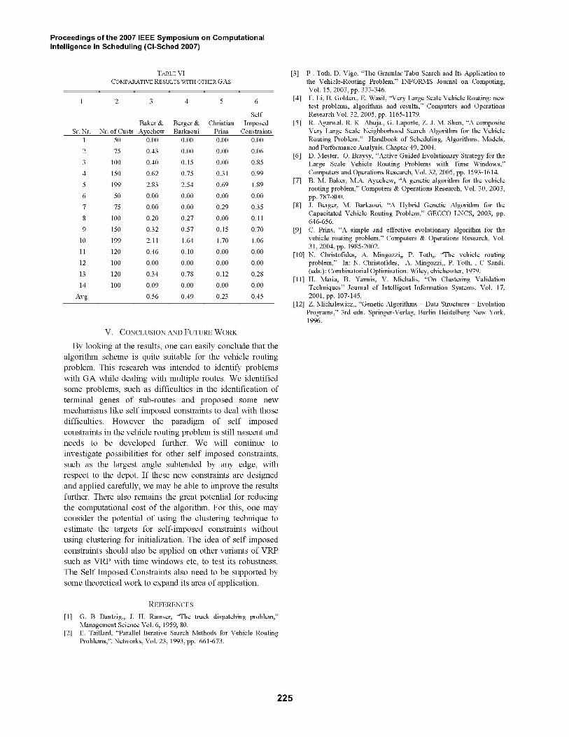
Now let us compare our results with 3 popular GAs [7]-[9] applied to VRP, as appeared in the literature. Thecomparisons are shown in Table-VI. The columns onlyshow percentage gap from best known solutions found sofar. Percentages of the 5th data set are recalculated for allalgorithms because a new solution [6] was found after thepublication of these algorithms. In the paper of Baker &Ayechew [7], there was miscalculation in percentagedifferences in solutions of 5th and 10th data sets, it is alsocorrected here. Values from Christian Prins paper [9] aregiven which he obtained under one setting, because we have

not configured settings of our algorithm separately fordifferent data sets. From the table, one can easily see that thealgorithm of self imposed constraints have got bettersolutions than two GAs [7], [8]. However solutions still legbehind the 3rd GA [9]. But as we discussed earlier in ourproblem analysis, that evaluation process of Prins algorithmi.e. checking all possible subsets of routes iscomputationally expensive and may fail in real worldscenario, where we are dealing with several thousandcustomers with several hundred routes, therefore ouralgorithm can still be considered competitive and promising.

TABLE IVRESULTS AFTER CLUSTERING AND LOCAL GA-LOCAL SEARCH CYCLE

1 2 3 4Minimum

Nr. of Best a b aSr. Nr. Cust. known Dist %diff Dist

1 50 524.61 524.61 0.00 526.71

2 75 835.26 845.46 1.22 859.76

3 100 826.14 839.60 1.63 846.71

4 150 1028.42 1042.78 1.40 1065.41

5 199 1291.29 1313.53 1.72 1330.72

6 50 555.43 555.43 0.00 563.73

7 75 909.68 930.64 2.30 944.02

8 100 865.94 867.41 0.17 888.95

9 150 1162.55 1182.12 1.68 1201.60

10 199 1395.85 1416.64 1.49 1446.95

1 1 120 1042.11 1042.11 0.00 1046.72

12 100 819.56 819.56 0.00 821.29

13 120 1541.14 1546.14 0.32 1569.94

14 100 866.37 866.37 0.00 875.13

Avg 0.85

SAverage

b%diff0.40

2.93

2.49

3.60

3.75

1.49

3.78

2.66

3.36

3.66

0.44

0.21

1.87

1.01

2.26

c

Time1.83

19.69

41.89

216.40

788.05

2.81

17.22

60.17

259.63

747.19

119.00

15.26

165.00

47.85

178.72

TABLE VRESULTS AFTER ALLOWING 10% DETERIORATION OF SOLUTION

1 2 3 4Minimum

Nr. of Best a b aSr. Nr. Cust. known Dist %diff Dist

1 50 524.61 524.61 0.00 524.84

2 75 835.26 835.77 0.06 855.53

3 100 826.14 833.14 0.85 841.09

4 150 1028.42 1038.65 0.99 1057.30

5 199 1291.29 1315.72 1.89 1333.00

6 50 555.43 555.43 0.00 557.59

7 75 909.68 912.89 0.35 926.26

8 100 865.94 866.87 0.11 880.44

9 150 1162.55 1170.67 0.70 1197.08

10 199 1395.85 1410.66 1.06 1437.90

1 1 120 1042.11 1042.11 0.00 1046.76

12 100 819.56 819.56 0.00 820.01

13 120 1541.14 1545.4 0.28 1565.98

14 100 866.37 866.37 0.00 868.67

Avg 0.45

SAverage

b%diff0.04

2.43

1.81

2.81

3.23

0.92

1.82

1.67

2.97

3.01

0.45

0.06

1.61

0.27

1.65

c

Time3.20

32.00

85.13

344.20

1111.37

4.40

25.20

86.13

395.10

1382.10

163.43

26.30

209.23

61.30

280.65

224

Proceedings of the 2007 IEEE Symposium on ComputationalIntelligence in Scheduling (CI-Sched 2007)

TABLE VI [3] P Toth, D. Vigo, "The Granular Tabu Search and Its Application toCOMPARATIVE RESULTS WITH OTHER GAs the Vehicle-Routing Problem," INFORMS Journal on Computing,

Vol. 15, 2003, pp. 333-346.

1 2 3 4 5 6 [4] F. Li, B. Golden., E. Wasil, "Very Large Scale Vehicle Routing: newtest problems, algorithms and results," Computers and Operations

Self Research Vol. 32, 2005, pp. 1165-1179.Baker & Berger & Christian Imposed [5] R. Agarwal, R. K Ahuja., G. Laporte, Z. J. M. Shen, "A composite

Sr. Nr. Nr. of Custs Ayechew Barkaoui Prins Constraints Very Large Scale Neighborhood Search Algorithm for the Vehicle1 50 0.00 0.00 0.00 0.00 Routing Problem," Handbook of Scheduling, Algorithms, Models,2 75 0.43 0.00 0.00 0.06 and Performance Analysis. Chapter 49, 2004.2 750.43 0.00 0.00 0.06

[6] D. Mester, 0. Braysy, "Active Guided Evolutionary Strategy for the3 100 0.40 0.15 0.00 0.85 Large Scale Vehicle Routing Problems with Time Windows,"

4 150 0.62 0.75 0.31 0.99 Computers and Operations Research, Vol. 32, 2005, pp. 1593-1614.

5 199 2.83 2.54 0.69 1.89 [7] B. M. Baker, M.A. Ayechew, "A genetic algorithm for the vehicle5 1992.83 2.54 0.69 1.89

routing problem," Computers & Operations Research, Vol. 30, 2003,6 50 0.00 0.00 0.00 0.00 pp. 787-800.

7 75 0.00 0.00 0.29 0.35 [8] J. Berger, M. Barkaoui, "A Hybrid Genetic Algorithm for theCapacitated Vehicle Routing Problem," GECCO LNCS, 2003, pp.

8 100 0.20 0.27 0.00 0.1 1 646-656.

9 150 0.32 0.57 0.15 0.70 [9] C. Prins, "A simple and effective evolutionary algorithm for the

10 199 2.11 1.64 1.70 1.06 vehicle routing problem," Computers & Operations Research, Vol.

11 120 0.46 0.10 0.00 0.00 31, 2004, pp. 1985-2002.

[10] N. Christofides, A. Mingozzi,, P. Toth,, "The vehicle routing12 100 0.00 0.00 0.00 0.00 problem," In: N. Christofides, A. Mingozzi,, P. Toth, , C Sandi.

13 120 0.34 0.78 0.12 0.28 (eds.): Combinatorial Optimisation. Wiley, chichesster, 1979.[11] H. Maria, B. Yannis, V. Michalis, "On Clustering Validation

14 100 0.09 0.00 0.00 0.00 Techniques" Journal of Intelligent Information Systems, Vol. 17,

Avg 0.56 0.49 0.23 0.45 2001, pp. 107-145.[12] Z. Michalewicz,, "Genetic Algorithms + Data Structures = Evolution

Programs," 3rd edn. Springer-Verlag, Berlin Heidelberg New York,1996.

V. CONCLUSION AND FUTURE WORK

By looking at the results, one can easily conclude that thealgorithm scheme is quite suitable for the vehicle routingproblem. This research was intended to identify problemswith GA while dealing with multiple routes. We identifiedsome problems, such as difficulties in the identification ofterminal genes of sub-routes and proposed some newmechanisms like self imposed constraints to deal with thosedifficulties. However the paradigm of self imposedconstraints in the vehicle routing problem is still nascent andneeds to be developed further. We will continue toinvestigate possibilities for other self imposed constraints,such as the largest angle subtended by any edge, withrespect to the depot. If these new constraints are designedand applied carefully, we may be able to improve the resultsfurther. There also remains the great potential for reducingthe computational cost of the algorithm. For this, one mayconsider the potential of using the clustering technique toestimate the targets for self-imposed constraints withoutusing clustering for initialization. The idea of self imposedconstraints should also be applied on other variants of VRPsuch as VRP with time windows etc, to test its robustness.The Self Imposed Constraints also need to be supported bysome theoretical work to expand its area of application.

REFERENCES[1] G. B Dantzig,, J. H. Ramser, "The truck dispatching problem,"

Management Science Vol. 6, 1959, 80.[2] E. Taillard, "Parallel Iterative Search Methods for Vehicle Routing

Problems,". Networks, Vol. 23, 1993, pp. 661-673.

225