Geographical Quadtree RoutingChen Avin, Yaniv Dvory, Ran Giladi

Department of Communication Systems EngineeringBen Gurion University of the Negev

Beer Sheva 84105, IsraelEmail: avin@cse.bgu.ac.il, dvory@bgu.ac.il, ran@cse.bgu.ac.il

Abstract—We present Greedy-Quadtree-Greedy guaranteeddelivery routing algorithm (GQG), a geographical routing al-gorithm that relies on a well known data structure from imageprocessing, i.e., Quadtree, for network hierarchy and geographi-cal addresses. GQG makes greedy forwarding based on locationinformation that is extracted from the Quadtree. Overcoming onlocal minimums is done by a novel concept of greedy like routingwhich is based on tree distances. This property greatly improveshop stretch efficiency and load balancing in comparison to thestandard tree routing. We provide algorithms for address dis-tribution, network topology discovery, and geographical routingwith guaranteed delivery. We keep all broadcasts bounded toone hop, and node’s routing state dependent on the nodes degreerather than the overall network size. We prove the correctnessof our algorithms and present simulations that show that thisrouting system has very low stretch and good load balancing.

Index Terms—geographical routing, routing algorithms,Quadtree, addressing, forwarding, data centers.

I. INTRODUCTION

As communication networks in general and specifically theInternet, continue to grow in size, we are facing networkswith larger number of routing elements. Geographical routinghas been proposed as a scalable routing system due to itsreduced routing state and forwarding tables. This type ofalgorithms take advantage of geographical information nodeshave of their own, their neighbors and the destination phisicallocation, in order to route the messages in the network.This information allows nodes to maintain a small routingstate, which greatly reduces memory use and lookup time,and therefore scales much better. Such algorithms dependon geographical information which has recently become lesscostly, more available, and accurate with the development andspread of GPS and other positioning systems.

Initially geographic routing algorithms provided simplenon guaranteed delivery schemes [1], [2], [3], some packetscould not reach their destination and were dropped. Differentapproach algorithms relied on wide or bounded messageflooding, which caused significant amount of overhead, andmight not guarantee delivery.

The next generation of geographic routing algorithms [4],[5], [6], [7] guaranteed delivery using two basic modes. First,they route the packet in a greedy mode towards the destination,i.e., each node forward the packet to one of its neighborsthat is geographically closer to the destination. Second, whena packet reaches a local minimum (a.k.a void), i.e., a node

that is the closest to the destination among its neighbors, itswitched to a different routing mode in order to escape thelocal minimum. Some of the algorithms define switching backto greedy mode after passing the void, i.e., when the packetreaches a node closer to the destination than the last localminimum, these type of algorithms are known as Greedy-Face-Greedy (GFG).

The first geographic routing algorithm that achieved guar-anteed delivery was initially called compass routing [8], andwas later called Face routing. Face routing is a very popularmethod to bypass voids and is used in many of the existinggeographic routing algorithms [4], [5], [6], [9], [7] in dif-ferent variations which gradually improved the routing hopefficiency. Face routing works only in planar graphs and mightbe very inefficient in route selections. Distributed planarizationworks nicely in some graphs models like unit disk graphs, butin general setting, planarization is not always possible, andwhen it is, it could still be complex and costly [10].

Other existing geographical routing algorithms use prepro-cessing of the network topology with different methods [?],[11], [12], [13]. This is done in order to distribute virtualcoordinates to the nodes to increase convexity of the voidsin the virtual topology, which will significantly reduce theprobability of a packet to reach a local minimum.

In the paper Geographic Routing without Planarization[14], Leong et. al offered GDSTR, a tree based guaranteeddelivery geographical routing algorithm. The tree is build suchthat each node is the root of an area containing its sub-tree.Thereason GDSTR is able to guarantee the delivery of packets ina connected network is that the tree traversal forwarding modealone, is guaranteed to deliver the packet to any node in thenetwork when greedy forwarding fails. One complication ofthe proposed method is in cases the destination lies in theintersection of the areas rooted by two or more nodes. In thiscase, packet delivery is guaranteed by systematic depth firstsearch in all the subtrees with areas containing the destination.

Paper Overview and Main Contributions: We adopt asimilar approach to [14] and develop a distributed, guaranteeddelivery, geographic routing algorithm that uses tree basedrouting where greedy routing fails. The basic structure weuse to build our tree and to distribute addresses to nodesis a Quadtree [15]. Quadtree is a well known data structurewhich has many applications in data clustering, computationalgeometry, image processing and more. The basic idea of

Quadtree is to cover a plane region of interest by a square,and then recursively partition it into four smaller squares untileach square contains a single point of interest, which, in ourcase, is simply a vertex. We are not aware of previous usageof Quadtree in the context of geographical routing.

Based on a Quadtree, which provides hierarchical parti-tioning of the network into areas with no overlap, we definegeographical addresses and a tree. This tree allows us to routepackets with no routing errors or local searches. Moreover, ouraddressing enables the use of unique and relatively short geo-graphical addresses that reduce the overhead of each messageand the size of the routing tables. The length of the addressesdepends on the density of the nodes.

The routing system we develop, Greedy-Quadtree-Greedy(GQG), takes the advantage of the stateless hop efficientgreedy routing, as well as the guaranteed delivery of treebased routing. A message is routed throughout the network ina greedy manner until it gets to a local minimum then switchesto tree mode routing. The packet will return to greedy modeafter passing the local minimum. To increase route efficiencyand to achieve better load balancing we extend the Quadtreeinto a MultiQuadtree network infrastructure that can supportseveral roots. In addition we allow shortcuts during the treemode routing (route on edges that are not part of the tree).This shortcuts provide a sort of geographical routing on thetree but they avoid local minimum, reduce the stretch of theroute and increase load balancing.

We provide algorithms for MultiQuadtree network discov-ery, address distribution and geographical routing with guaran-teed delivery. We prove the correctness of our algorithms andpresent simulations that show this routing system has very lowstretch (i.e., the routes that the algorithm finds are close to theshortest routes in the network) and good load balancing.

Due to space constrains, proofs for some lemmas andtheorems are provided in the full version.

II. MULTIQUADTREE NETWORK AND ADDRESSES

A. Quadtree Geographical Address

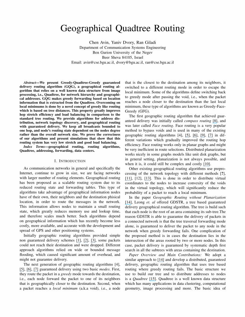
Consider a squared area in the plane, S and a set of nodes(communication stations) V distributed in S. As mentioned,the idea of Quadtree is to recursively partition S into foursmaller squares until each square contains only one vertex, i.e.,empty sub-squares stop to partition. Let QuadtreeS (V ) be theunique Quadtree partitioning of V , in the following we assumeS is known and drop it from the notation. See for example Fig.1 for a Quadtree we generated from a set of 17,168 weatherstations around the world, taken from Mathematica 7.

The Quadtree(V ) partitioning can be used to give ad-dresses to squares and nodes. An empty Quadtree address,∅, represent the whole original square area, then recursivelyeach of the four quarters will get the address of the partitionedsquare with added suffix to represent which quarter it is. Inthe following manner, the bottom left quarter will get the ”00”suffix, the top left will get ”01”, the bottom right will get ”10”and the top right will get ”11”. A node’s address is the addressof the smallest square that it is contained in after the described

Fig. 1. Quadtree of 17,168 weather stations around the world.

partitioning is done. For v ∈ V , let Qadd(v) be the uniqueQuadtree address of node v resulting from Quadtree(V ).

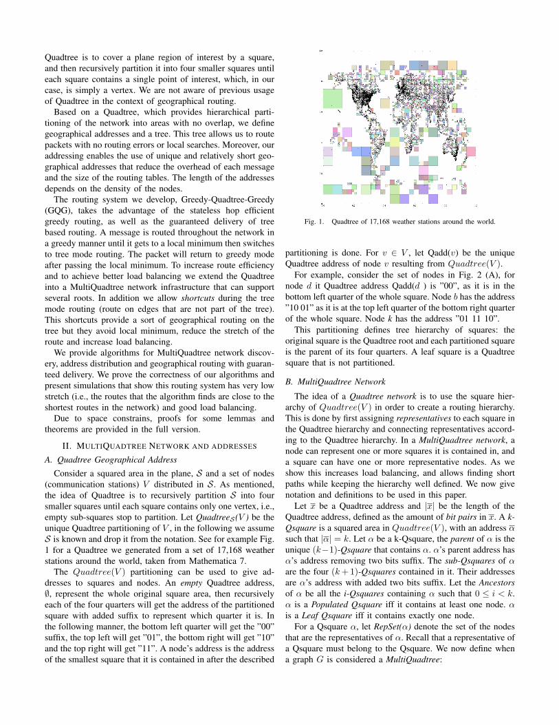
For example, consider the set of nodes in Fig. 2 (A), fornode d it Quadtree address Qadd(d ) is ”00”, as it is in thebottom left quarter of the whole square. Node b has the address”10 01” as it is at the top left quarter of the bottom right quarterof the whole square. Node k has the address ”01 11 10”.

This partitioning defines tree hierarchy of squares: theoriginal square is the Quadtree root and each partitioned squareis the parent of its four quarters. A leaf square is a Quadtreesquare that is not partitioned.

B. MultiQuadtree Network

The idea of a Quadtree network is to use the square hier-archy of Quadtree(V ) in order to create a routing hierarchy.This is done by first assigning representatives to each square inthe Quadtree hierarchy and connecting representatives accord-ing to the Quadtree hierarchy. In a MultiQuadtree network, anode can represent one or more squares it is contained in, anda square can have one or more representative nodes. As weshow this increases load balancing, and allows finding shortpaths while keeping the hierarchy well defined. We now givenotation and definitions to be used in this paper.

Let x be a Quadtree address and |x| be the length of theQuadtree address, defined as the amount of bit pairs in x. A k-Qsquare is a squared area in Quadtree(V ), with an address αsuch that |α| = k. Let α be a k-Qsquare, the parent of α is theunique (k−1)-Qsquare that contains α. α’s parent address hasα’s address removing two bits suffix. The sub-Qsquares of αare the four (k+1)-Qsquares contained in it. Their addressesare α’s address with added two bits suffix. Let the Ancestorsof α be all the i-Qsquares containing α such that 0 ≤ i < k.α is a Populated Qsquare iff it contains at least one node. αis a Leaf Qsquare iff it contains exactly one node.

For a Qsquare α, let RepSet(α) denote the set of the nodesthat are the representatives of α. Recall that a representative ofa Qsquare must belong to the Qsquare. We now define whena graph G is considered a MultiQuadtree:

!

"

#

$ %

&

'

()

*+ ++

,-

"

# ,! '

"'

)

(.',!#-

**

.

+*

!"#$%&'()*+,

!"#!"!"#""#"!!"#""#""!"#""#!""!#"!"!#""""#""!"#!!!!""#!!"!#!"!"#""#!!$%&&'()

!"#!"!" ""#"!!"#""#""!"#""#!""!#"!"!#""""#""

""

!"#!!

!"

!!""#!!

""

"!#!"

"!

*+,-.

!"#""#!!

!"#""

*+,-.

/0*-'()

" & $ %

/0( 120

13044

Fig. 2. MultiQuadtree network example: (A) G(V, E) and Quadtree(V ).(B) The MultiQuadtree hierarchy. (C) Qadd and TSet tables.

Definition 1. A graph G(V,E) is a MultiQuadtree network iff:There exist an assignment of representatives to all populatedQsquares in Quadtree(V ) s.t.

1) Any representative of populated k-Qsquare inQuadtree(V ), where k > 0, has a link (i.e. edgee ∈ E) to at least one representative of its parentQsquare.

2) Any representative of populated k-Qsquare inQuadtree(V ), that is not a leaf Qsquare, haslinks (i.e. edges e ∈ E) to at least one representative ofeach one of its populated sub-Qsquares.

In the above definition we consider nodes as connected tothemselves. A root of a MultiQuadtree network is a representa-tive of the 0-Qsquare. Note that a graph that is a MultiQuadtreemust have certain edges according to definition 1, but haveno limitation on additional edges. The following lemma is aconsequence of the definition:

Lemma 1. A MultiQuadtree network is connected.

The definition of a MultiQuadtree network allows nodes torepresent several Qsquares in the hierarchy and therefore theymay have few addresses. For v ∈ V , let TSet(v) be the setof addresses of all the Qsquares v represent, including its leafQsquare with the address Qadd(v). Formally, for any Qsquareα such that v ∈ RepSet(α), v will keep the Quadtree addressα in its TSet(v).

Fig 2 illustrates the above definitions: (A) present graphG(V,E) which is a MultiQuadtree network according toDefinition 1 and the Quadtree(V ) partitioning. (B) showsthe MultiQuadtree network hierarchy; arrows are stretchedfrom Qsquare representatives to their populated sub-Qsquaresrepresentatives. (C) The Qadd and TSet of all the nodes, forexample: nodes a and b represent the 0-Qsquare (they areboth roots for this MultiQuadtree network), as they are bothconnected to representatives from all populated 1-Qsquare,which are b, c, d, e for node a and b, d, e, f for node b. Node b,as a representative for Qsquare ”10”, is also connected to all

of its populated sub-Qsquares representatives g, h, and b itself.Node c represents 11 as it is connected to the representativesof its populated sub-Qsquares f and itself, in the same waynode f also represents 11.

One concern of a Quadtree Network is the need of ”long”edges. We claim that the average length of edges in a Quadtreenetworks is of the same order as the minimum spanning tree(MST). For example, the average edge length of the MST ofn points located at

√n ×√n grid on the unit square is 1√

nwhile the average edge length of a Quadtree Network of thesepoints is 2√

n. We ran both MST and random Quadtree network

construction on the points of Fig. 1, the average edge lengthin the MST came to 0.0018, while in the Quadtree Networkit was 0.00503 which is only 2.78 times bigger.

III. QUADTREE BASED ROUTING ALGORITHMS

The main routing algorithm we offer is a combinationof two routing modes, the first is greedy mode in which anode forward a message to the neighbor that is physicallyclosest to the destination (and closer than the node itself). Thisrequiers a way to calculate the physical distance based on theQuadtree addresses, which are the only information a nodehas on the location of its neighbores and of the destination.We call this function Gdist. The second routing mode is calledQuadtree mode. In this mode a node routes a message to theneighbor that is closest in the MultiQuadtree hierarchy to thedestination. We call the function of calculating this type ofdistance MQdist.

Let w, d be two nodes in V. Let Gdist(w, d) be the Greedydistance between node w and d.• Gdist(w, d) is the euclidean distance between the bottom

left corners of the squared area represented by Qadd(w)and Qadd(d) the Quadtree addresses of the nodes.

Now since leaf Qsquares are disjoint clearly:

Lemma 2. Gdist(w, d) ∈ R+ and Gdist(w, d) = 0 iff w = d.

In order to define MQdist let lmp(x, y) to be the longest,even lengthed, matching prefix of x and y, where x, y aretwo Quadtree addresses. A closer look at lmp(x, y) shows usthat by definition, it is the Quadtree address of the smallestcommon ancestor Qsquare of the squares represented byaddresses x and y. Let MQdist(w,α) be the MultiQuadtreenetwork distance between node w and Qsquare α with addressα.• MQdist(w,α) is calculated in the following way:

minw∈TSet(w)

(|w|+ |α| − 2× |lmp(w,α)|)

Again the distance is zero only when the two are the same:

Lemma 3. MQdist(w, d) = 0 where d = Qadd(d) iff w = d.

Lemma 2 and 3 present two properties that will allow usroute messages in the network with guarenteed delivery.

A. Quadtree Routing with ShortcutsQuadtree mode routing works using edges that are not

necessarily the tree edges, as long as the node we route the

message to is closer to the destination on the tree. This is anovel concept of greedy like routing which is based on thetree distance we defined earlier - MQdist. We calculate thetree distance from a node to the Quadtree address of the targetbased on the TSet of the node, which defines the locationsof the node in the MultiQuadtree network hierarchy. In thisway a node looks at all its neighbors, and may use any link ithas when routing in Quadtree mode rather than just lookingat its parent and sub-Qsquares in the hierarchy. This propertyleads to a better hop efficiency and better load balancing assimulations show.

Let N(v) denote the neighbors of v, i.e., all nodes thatv is connected to. The Quadtree mode routing is defined inalgorithm 1.

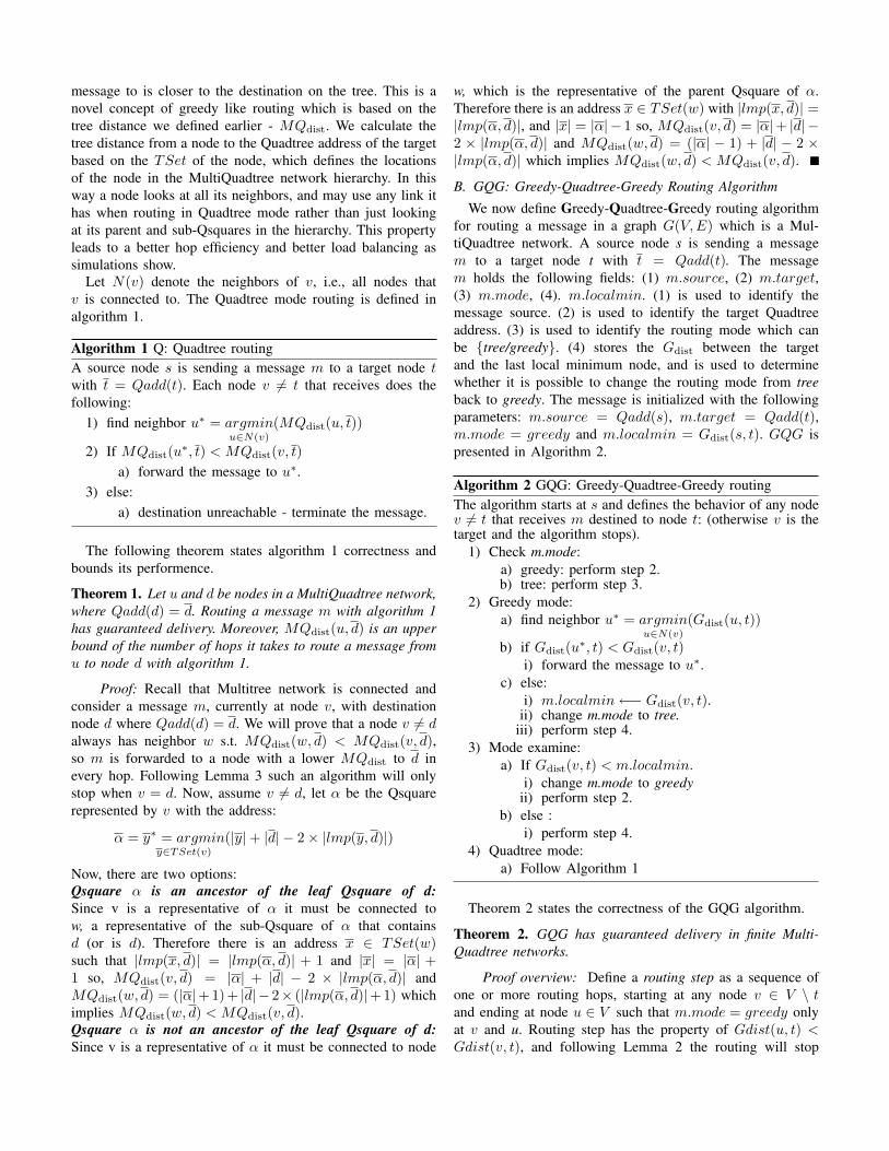
Algorithm 1 Q: Quadtree routingA source node s is sending a message m to a target node twith t = Qadd(t). Each node v 6= t that receives does thefollowing:

1) find neighbor u∗ = argminu∈N(v)

(MQdist(u, t))

2) If MQdist(u∗, t) < MQdist(v, t)a) forward the message to u∗.

3) else:a) destination unreachable - terminate the message.

The following theorem states algorithm 1 correctness andbounds its performence.

Theorem 1. Let u and d be nodes in a MultiQuadtree network,where Qadd(d) = d. Routing a message m with algorithm 1has guaranteed delivery. Moreover, MQdist(u, d) is an upperbound of the number of hops it takes to route a message fromu to node d with algorithm 1.

Proof: Recall that Multitree network is connected andconsider a message m, currently at node v, with destinationnode d where Qadd(d) = d. We will prove that a node v 6= dalways has neighbor w s.t. MQdist(w, d) < MQdist(v, d),so m is forwarded to a node with a lower MQdist to d inevery hop. Following Lemma 3 such an algorithm will onlystop when v = d. Now, assume v 6= d, let α be the Qsquarerepresented by v with the address:

α = y∗ = argminy∈TSet(v)

(|y|+ |d| − 2× |lmp(y, d)|)

Now, there are two options:Qsquare α is an ancestor of the leaf Qsquare of d:Since v is a representative of α it must be connected tow, a representative of the sub-Qsquare of α that containsd (or is d). Therefore there is an address x ∈ TSet(w)such that |lmp(x, d)| = |lmp(α, d)| + 1 and |x| = |α| +1 so, MQdist(v, d) = |α| + |d| − 2 × |lmp(α, d)| andMQdist(w, d) = (|α|+1)+ |d|− 2× (|lmp(α, d)|+1) whichimplies MQdist(w, d) < MQdist(v, d).Qsquare α is not an ancestor of the leaf Qsquare of d:Since v is a representative of α it must be connected to node

w, which is the representative of the parent Qsquare of α.Therefore there is an address x ∈ TSet(w) with |lmp(x, d)| =|lmp(α, d)|, and |x| = |α| − 1 so, MQdist(v, d) = |α|+ |d| −2 × |lmp(α, d)| and MQdist(w, d) = (|α| − 1) + |d| − 2 ×|lmp(α, d)| which implies MQdist(w, d) < MQdist(v, d).

B. GQG: Greedy-Quadtree-Greedy Routing Algorithm

We now define Greedy-Quadtree-Greedy routing algorithmfor routing a message in a graph G(V,E) which is a Mul-tiQuadtree network. A source node s is sending a messagem to a target node t with t = Qadd(t). The messagem holds the following fields: (1) m.source, (2) m.target,(3) m.mode, (4). m.localmin. (1) is used to identify themessage source. (2) is used to identify the target Quadtreeaddress. (3) is used to identify the routing mode which canbe {tree/greedy}. (4) stores the Gdist between the targetand the last local minimum node, and is used to determinewhether it is possible to change the routing mode from treeback to greedy. The message is initialized with the followingparameters: m.source = Qadd(s), m.target = Qadd(t),m.mode = greedy and m.localmin = Gdist(s, t). GQG ispresented in Algorithm 2.

Algorithm 2 GQG: Greedy-Quadtree-Greedy routingThe algorithm starts at s and defines the behavior of any nodev 6= t that receives m destined to node t: (otherwise v is thetarget and the algorithm stops).

1) Check m.mode:a) greedy: perform step 2.b) tree: perform step 3.

2) Greedy mode:a) find neighbor u∗ = argmin

u∈N(v)

(Gdist(u, t))

b) if Gdist(u∗, t) < Gdist(v, t)i) forward the message to u∗.

c) else:i) m.localmin←− Gdist(v, t).

ii) change m.mode to tree.iii) perform step 4.

3) Mode examine:a) If Gdist(v, t) < m.localmin.

i) change m.mode to greedyii) perform step 2.

b) else :i) perform step 4.

4) Quadtree mode:a) Follow Algorithm 1

Theorem 2 states the correctness of the GQG algorithm.

Theorem 2. GQG has guaranteed delivery in finite Multi-Quadtree networks.

Proof overview: Define a routing step as a sequence ofone or more routing hops, starting at any node v ∈ V \ tand ending at node u ∈ V such that m.mode = greedy onlyat v and u. Routing step has the property of Gdist(u, t) <Gdist(v, t), and following Lemma 2 the routing will stop

only at the destination after at most |V | − 1 routing steps.By definition Greedy forwarding is a routing step of one hop.According to Theorem 1 Quadtree forwarding has guaranteeddelivery, therefore it will always return to greedy mode.Quadtree mode reduces the MQdist at every hop, thereforea sequence of Quadtree mode hops makes a routing step of atmost |V | − 1 hops and we are done.

IV. MULTIQUADTREE NETWORK DISCOVERY ANDADDRESSES DISTRIBUTION

Our routing algorithm is based on that each node v know itsQadd(v) and its TSet(v), namely what Qsquares it represents.We offer two additional, local, distributed, algorithms for Mul-tiQuadtree Networks; the first, QAD, allocates the Quadtreeaddresses to the nodes and the second, discover the networkand selects representatives.QAD - Quadtree Address Distribution Algorithm: Thisalgorithm is initiated once all the nodes in the network knowtheir own coordinates, and are able to communicate with theirneighbors. During the algorithm nodes are locally negotiatingwith neighbors to determine their exact Quadtree addresses,and it ends when each node v in the network is familiar withits exact Qadd(v), and the Quadtree addresses of its neighbors.QAD is presented in the full version of the paper.MQD - MultiQuadtree Network Discovery Algorithm: Thisalgorithm is initiated after the QAD algorithm finished and allthe nodes in the network have their own and their neighborsQuadtree addresses, After running the algorithm all nodes inthe network are familiar with their TSets, and can start routingmessages with Algorithms 1 or 2.

MQD algorithm is built from two main phases: The firstphase is a bottom-up and works its way from the Multi-Quadtree network leafs towards its root(s). This phase purposeis to make sure that a node v will be a representative candidatefor a Qsquare α if and only if it is connected to a candidate ofeach populated sub-Qsquare of α (i.e., condition 2 in definition1). Messages in this phase are sent only by candidates, initiallyall nodes are candidate as leafs, but the number of themreduces as the algorithm climes the Quadtree hierarchy.

The second phase works its way from the MultiQuadtreenetwork root(s) towards the leafs. This phase purpose is tomake sure that a representative candidate for a Qsquare α willbecome a representative for α if and only if it is connectedto a representative of α’s parent Qsquare (i.e., condition 1in definition 1), unless α is the root Qsquare and becomes arepresentative without having a parent.

It is not trivial for this algorithm to work correctly in adistributed manner, with only local knowledge at each nodein the network topology, and with keeping all the broadcastsbounded to one hop only. The reason is that in order for a nodeto become a ”representative candidate” for a Qsquare α it hasto know which of α’s sub-Qsquare is populated. Knowing thisisn’t trivial as the ”populating” node of a certain sub-Qsquarescan be several hops away.

We overcome this challenge by defining a data structurecalled Dynasty map. The dynasty map for node v is a matrix

of bits with size 4 × |Qadd(v)| denoted by Dmap(v). Nodev uses its Dynasty Map in the first phase of MQD algorithmfor informing its neighbors on existing populated Qsquares itknows of. That way they can decide wether they are qualifiedunder Definition 1 to represent a certain Qsquare or not.

Node v maintains another data structure similar to itsDmap(v), that can be combined with Dmap(v). This is wherev marks all the relevant Qsquares for which it got phaseone message (meaning it is connected to their candidates).Crossing this information with Dmap(v), node v can observewether it can become representative candidate for a qsquare.

To state the correctness of the algorithm we need thedefinitions bellow followed by the formal theorem:

Definition 2. Let a Maximal MultiQuadtree network bea MultiQuadtree network where each node that can be aQsquare α representative is Qsquare α representative.

Theorem 3. After running MQD algorithm we result with aMaximal MultiQuadtree Network.

Theorem 3 is very important for load balancing prepossesssince it is better to use more edges and different nodes whenrouting in Quadtree mode.

V. SIMULATION

Simulation Setup: We implemented Algorithms MQD,QAD, Q and GQG in the C++ based simulation platformOMNET++ 4. We studied these algorithms using differenttopologies and network models, but here we report only asubset of the results. For each simulation we first distributedN nodes uniformly at random in the unit square. Then weensure the MultiQuadtree network condition by creating arandom representatives trees. Trees construction is made byrandomly choosing T roots to be level 0 representatives,followed by recursively connecting each representative to arandomly chosen representative for each of its populated sub-squares. In this paper we consider two topologies for additionaledges. i) Pure tree: we do not add any edges, this model isused for comparison and allow us to eliminate the use of thenon tree edges. ii) Distance related model: edges are addedrandomly with probability proportional to the reciprocal of thelength of the edge to power of two (i.e., shorter edges havehigher probability). The probability is normalized to achievea desired average degree, D, in the network.

For each model the final MultiQuadtree network to be usedis discovered by the MQD algorithm described in section IV.To test the algorithms then, we choose uniformly at random5% out of the

(N2

)pairs to communicate and compare the

performance of both the Q algorithm (Quadtree routing, Al-gorithm 1) and the GQG algorithm (Greedy-Quadtree-Greedyalgorithm, Algorithm 2). The results reported are an averageof several simulations.

Main Results: Fig. 3 (A) present the accumulative loaddistribution using different routing algorithms over the theDistance related graph. The X axis is the amount of messagesforwarded by the nodes. This axis is logarithmic, and present-ing 20 messages bins. The Y axis shows the accumulating

!"

#"

$""

!"#$%&'"()$#&*$%%&+

%,%

!"#$%&#$$

'()*+,-$%.$/+*$0%1 2%%

'()*+,-$%.$/+*$0%1323%%

!"#$99%%&'()*(+*,-./01

"

%"

&"

' '" '"" '"""

-$'.$!)/,$"0&!"#$%&'"()$#&*$%%&

!"#" $%&'()

62002770467141!"#$%&#$$

38001720283104'"()*#$$

81032069108+'+

!

"

#$

#%

#&

!"#$%&#'#()*%+,-."/*,*(0%.#0+"

!"!#$%&'()*+#,#-#.

"#$%&'()*+#,#-#.

!"!#$%&'()*+#,#-#/

"#$%&'()*+#,#-#/

$

%

&

!

$ # % ' & ( !

!"#$%&#'#()*%+,-."/*,*(0%.#0+"

!"#$%&'$$%($)$(

!"#

!"$

%"!

%"&

!"#$%&'(&)*

!"#$%&'()*(+%$(,)- ./.0)123 !"#$%&'()*(+%$(,)- ./.0)124

!"#$%&'()*(+%$(,)- /0)123 !"#$%&'()*(+%$(,)- /0)124

567()17((0)124 567()17((0)123

'"$

!"!

!"&

!"(

!"" #"" $"" %"" &"" '"" ("" )""

!"#$%&'(&)*

!"#$%&'()*+"

(A) (B) (C)

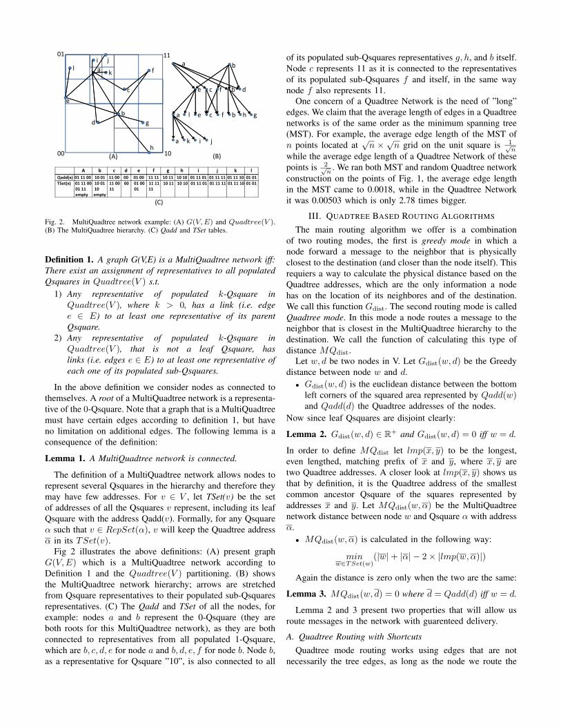
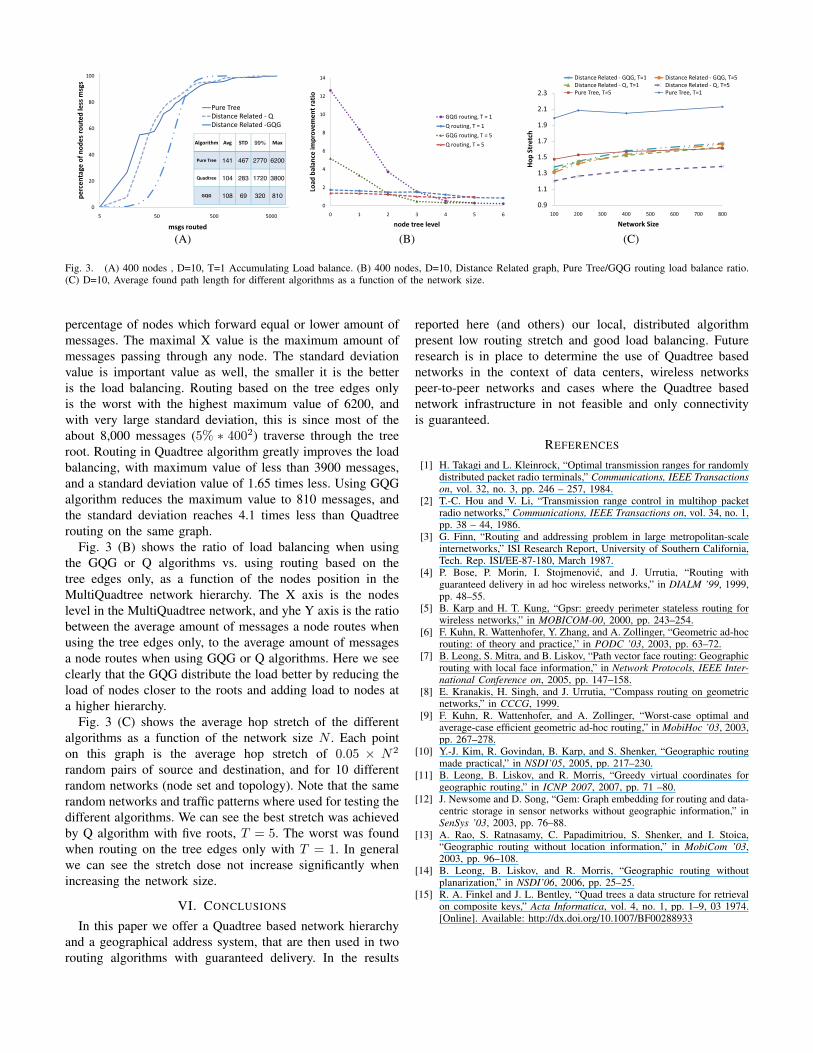
Fig. 3. (A) 400 nodes , D=10, T=1 Accumulating Load balance. (B) 400 nodes, D=10, Distance Related graph, Pure Tree/GQG routing load balance ratio.(C) D=10, Average found path length for different algorithms as a function of the network size.

percentage of nodes which forward equal or lower amount ofmessages. The maximal X value is the maximum amount ofmessages passing through any node. The standard deviationvalue is important value as well, the smaller it is the betteris the load balancing. Routing based on the tree edges onlyis the worst with the highest maximum value of 6200, andwith very large standard deviation, this is since most of theabout 8,000 messages (5% ∗ 4002) traverse through the treeroot. Routing in Quadtree algorithm greatly improves the loadbalancing, with maximum value of less than 3900 messages,and a standard deviation value of 1.65 times less. Using GQGalgorithm reduces the maximum value to 810 messages, andthe standard deviation reaches 4.1 times less than Quadtreerouting on the same graph.

Fig. 3 (B) shows the ratio of load balancing when usingthe GQG or Q algorithms vs. using routing based on thetree edges only, as a function of the nodes position in theMultiQuadtree network hierarchy. The X axis is the nodeslevel in the MultiQuadtree network, and yhe Y axis is the ratiobetween the average amount of messages a node routes whenusing the tree edges only, to the average amount of messagesa node routes when using GQG or Q algorithms. Here we seeclearly that the GQG distribute the load better by reducing theload of nodes closer to the roots and adding load to nodes ata higher hierarchy.

Fig. 3 (C) shows the average hop stretch of the differentalgorithms as a function of the network size N . Each pointon this graph is the average hop stretch of 0.05 × N2

random pairs of source and destination, and for 10 differentrandom networks (node set and topology). Note that the samerandom networks and traffic patterns where used for testing thedifferent algorithms. We can see the best stretch was achievedby Q algorithm with five roots, T = 5. The worst was foundwhen routing on the tree edges only with T = 1. In generalwe can see the stretch dose not increase significantly whenincreasing the network size.

VI. CONCLUSIONS

In this paper we offer a Quadtree based network hierarchyand a geographical address system, that are then used in tworouting algorithms with guaranteed delivery. In the results

reported here (and others) our local, distributed algorithmpresent low routing stretch and good load balancing. Futureresearch is in place to determine the use of Quadtree basednetworks in the context of data centers, wireless networkspeer-to-peer networks and cases where the Quadtree basednetwork infrastructure in not feasible and only connectivityis guaranteed.

REFERENCES

[1] H. Takagi and L. Kleinrock, “Optimal transmission ranges for randomlydistributed packet radio terminals,” Communications, IEEE Transactionson, vol. 32, no. 3, pp. 246 – 257, 1984.

[2] T.-C. Hou and V. Li, “Transmission range control in multihop packetradio networks,” Communications, IEEE Transactions on, vol. 34, no. 1,pp. 38 – 44, 1986.

[3] G. Finn, “Routing and addressing problem in large metropolitan-scaleinternetworks,” ISI Research Report, University of Southern California,Tech. Rep. ISI/EE-87-180, March 1987.

[4] P. Bose, P. Morin, I. Stojmenovic, and J. Urrutia, “Routing withguaranteed delivery in ad hoc wireless networks,” in DIALM ’99, 1999,pp. 48–55.

[5] B. Karp and H. T. Kung, “Gpsr: greedy perimeter stateless routing forwireless networks,” in MOBICOM-00, 2000, pp. 243–254.

[6] F. Kuhn, R. Wattenhofer, Y. Zhang, and A. Zollinger, “Geometric ad-hocrouting: of theory and practice,” in PODC ’03, 2003, pp. 63–72.

[7] B. Leong, S. Mitra, and B. Liskov, “Path vector face routing: Geographicrouting with local face information,” in Network Protocols, IEEE Inter-national Conference on, 2005, pp. 147–158.

[8] E. Kranakis, H. Singh, and J. Urrutia, “Compass routing on geometricnetworks,” in CCCG, 1999.

[9] F. Kuhn, R. Wattenhofer, and A. Zollinger, “Worst-case optimal andaverage-case efficient geometric ad-hoc routing,” in MobiHoc ’03, 2003,pp. 267–278.

[10] Y.-J. Kim, R. Govindan, B. Karp, and S. Shenker, “Geographic routingmade practical,” in NSDI’05, 2005, pp. 217–230.

[11] B. Leong, B. Liskov, and R. Morris, “Greedy virtual coordinates forgeographic routing,” in ICNP 2007, 2007, pp. 71 –80.

[12] J. Newsome and D. Song, “Gem: Graph embedding for routing and data-centric storage in sensor networks without geographic information,” inSenSys ’03, 2003, pp. 76–88.

[13] A. Rao, S. Ratnasamy, C. Papadimitriou, S. Shenker, and I. Stoica,“Geographic routing without location information,” in MobiCom ’03,2003, pp. 96–108.

[14] B. Leong, B. Liskov, and R. Morris, “Geographic routing withoutplanarization,” in NSDI’06, 2006, pp. 25–25.

[15] R. A. Finkel and J. L. Bentley, “Quad trees a data structure for retrievalon composite keys,” Acta Informatica, vol. 4, no. 1, pp. 1–9, 03 1974.[Online]. Available: http://dx.doi.org/10.1007/BF00288933