A multi-objective heuristic approach for the casualty collection points location problem
Upload
independentCategory
view
2download
0
Contributions to Management Science
Reza Zanjirani Farahani • Masoud Hekmatfar
Facility Location
Concepts, Models, Algorithms and Case Studies
Editors
Masoud Hekmatfar
ISBN 978-3-7908-2150-5 e-ISBN 978-3-7908-2151-2DOI 10.1007/978-3-7908-21 -
Dr. Reza Zanjirani Farahani
51 2
Centre for Maritime StudiesNational University of [email protected]
ISSN 1431-1941
Editors
Springer Dordrecht Heidelberg London New York
Library of Congress Control Number: 2009922331
c© Springer-Verlag Berlin Heidelberg 2009This work is subject to copyright. All rights are reserved, whether the whole or part of the material isconcerned, specifically the rights of translation, reprinting, reuse of illustrations, recitation, broadcasting,reproduction on microfilm or in any other way, and storage in data banks. Duplication of this publicationor parts thereof is permitted only under the provisions of the German Copyright Law of September 9,1965, in its current version, and permission for use must always be obtained from Springer. Violationsare liable to prosecution under the German Copyright Law.The use of general descriptive names, registered names, trademarks, etc. in this publication does notimply, even in the absence of a specific statement, that such names are exempt from the relevant protectivelaws and regulations and therefore free for general use.
Cover design: WMXDesign GmbH, Heidelberg, Germany
Printed on acid-free paper
Physica-Verlag is a brand of Springer-Verlag Berlin HeidelbergSpringer-Verlag is part of Springer Science+Business Media (www.springer.com)
Amirkabir University of TechnologyDepartment of Industrial Engineering
ToProfessor Zvi Drezner,to whom we are greatly indebted for hisgenerous scientific contribution in the area ofFacility Location
Contents
Introduction : : : : : : : : : : : : : : : : : : : : : : : : : : : : : : : : : : : : : : : : : : : : : : : : : : : : : : : : : : : : : : : : : : 1
1 Distance Functions in Location Problems . . . . . . . . . . . . . . . . . . . . . . . . . . . . . . . . 5Marzie Zarinbal
2 An Overview of Complexity Theory . . . . . . . . . . . . . . . . . . . . . . . . . . . . . . . . . . . . . . . 19Milad Avazbeigi
3 Single Facility Location Problem . . . . . . . . . . . . . . . . . . . . . . . . . . . . . . . . . . . . . . . . . . 37Esmaeel Moradi and Morteza Bidkhori
4 Multifacility Location Problem . . . . . . . . . . . . . . . . . . . . . . . . . . . . . . . . . . . . . . . . . . . . 69Farzaneh Daneshzand and Razieh Shoeleh
5 Location Allocation Problem . . . . . . . . . . . . . . . . . . . . . . . . . . . . . . . . . . . . . . . . . . . . . . . 93Zeinab Azarmand and Ensiyeh Neishabouri Jami
6 Quadratic Assignment Problem . . . . . . . . . . . . . . . . . . . . . . . . . . . . . . . . . . . . . . . . . . . 111Masoumeh Bayat and Mahdieh Sedghi
7 Covering Problem . . . . . . . . . . . . . . . . . . . . . . . . . . . . . . . . . . . . . . . . . . . . . . . . . . . . . . . . . . . 145Hamed Fallah, Ali NaimiSadigh, and Marjan Aslanzadeh
8 Median Location Problem . . . . . . . . . . . . . . . . . . . . . . . . . . . . . . . . . . . . . . . . . . . . . . . . . . 177Masoomeh Jamshidi
9 Center Problem . . . . . . . . . . . . . . . . . . . . . . . . . . . . . . . . . . . . . . . . . . . . . . . . . . . . . . . . . . . . . . 193Maryam Biazaran and Bahareh SeyediNezhad
10 Hierarchical Location Problem . . . . . . . . . . . . . . . . . . . . . . . . . . . . . . . . . . . . . . . . . . . . 219Sara Bastani and Narges Kazemzadeh
vii
viii Contents
11 Hub Location Problem . . . . . . . . . . . . . . . . . . . . . . . . . . . . . . . . . . . . . . . . . . . . . . . . . . . . . . 243Masoud Hekmatfar and Mirsaman Pishvaee
12 Competitive Location Problem . . . . . . . . . . . . . . . . . . . . . . . . . . . . . . . . . . . . . . . . . . . . . 271Mohammad Javad Karimifar, Mohammad Khalighi Sikarudi,Esmaeel Moradi, and Morteza Bidkhori
13 Warehouse Location Problem . . . . . . . . . . . . . . . . . . . . . . . . . . . . . . . . . . . . . . . . . . . . . . 295Zeinab Bagherpoor, Shaghayegh Parhizi, Mahtab Hoseininia,Nooshin Heidari, and Reza Ghasemi Yaghin
14 Obnoxious Facility Location . . . . . . . . . . . . . . . . . . . . . . . . . . . . . . . . . . . . . . . . . . . . . . . 315Sara Hosseini and Ameneh Moharerhaye Esfahani
15 Dynamic Facility Location Problem . . . . . . . . . . . . . . . . . . . . . . . . . . . . . . . . . . . . . . . 347Reza Zanjirani Farahani, Maryam Abedian, and Sara Sharahi
16 Multi-Criteria Location Problem . . . . . . . . . . . . . . . . . . . . . . . . . . . . . . . . . . . . . . . . . . 373Masoud Hekmatfar and Maryam SteadieSeifi
17 Location-Routing Problem . . . . . . . . . . . . . . . . . . . . . . . . . . . . . . . . . . . . . . . . . . . . . . . . . 395Anahita Hassanzadeh, Leyla Mohseninezhad, Ali Tirdad,Faraz Dadgostari, and Hossein Zolfagharinia
18 Storage System Layout . . . . . . . . . . . . . . . . . . . . . . . . . . . . . . . . . . . . . . . . . . . . . . . . . . . . . . 419Javad Behnamian and Babak Eghtedari
19 Location-Inventory Problem . . . . . . . . . . . . . . . . . . . . . . . . . . . . . . . . . . . . . . . . . . . . . . . 451Mohamadreza Kaviani
20 Facility Location in Supply Chain . . . . . . . . . . . . . . . . . . . . . . . . . . . . . . . . . . . . . . . . . 473Meysam Alizadeh
21 Classification of Location Models and Location Softwares . . . . . . . . . . . . . 505Sajedeh Tafazzoli and Marzieh Mozafari
22 Demand Point Aggregation Analysis for Location Models . . . . . . . . . . . . . 523Ali NaimiSadigh and Hamed Fallah
Appendix: Metaheuristic Methods : : : : : : : : : : : : : : : : : : : : : : : : : : : : : : : : : : : : : : : : : : 535Zohre Khoban and Saeed Ghadimi
Index . . . . . . . . . . . . . . . . . . . . . . . . . . . . . . . . . . . . . . . . . . . . . . . . . . . . . . . . . . . . . . . . . . . . . . . . . . . . . . . 545
Introduction
The mathematical science of facility locating has attracted much attention in dis-crete and continuous optimization over nearly last four decades. Investigators havefocused on both algorithms and formulations in diverse settings in both the privatesectors (e.g., industrial plants, banks, retail facilities, etc.) and the public sectors(e.g., hospitals, post stations, etc.).
Facility location problems locate a set of facilities (resources) to minimize thecost of satisfying some set of demands (of the customers) with respect to some set ofconstraints. Facility location decisions are critical elements in strategic planning fora wide range of private and public firms. The branches of locating facilities are broadand long-lasting, influencing numerous operational and logistical decisions. Highcosts associated with property acquisition and facility construction make facilitylocation or relocation projects long-term investments. Decision makers must selectsites that will not only perform well according to the current system state, but alsowill continue to be profitable for the facility’s lifetime, even as environmental factorschange, populations shift, and market trends evolve. Finding robust facility locationsis thus a difficult task, demanding decision makers to account for uncertain futureevents.
Location science is an area of analytical study that can be traced back to Pierre deFermat, Evagelistica Torricelli (a student of Galileo), and Battista Cavallieri. Eachone independently proposed (and some say solved) the basic Euclidean spatial me-dian problem early in the seventeenth century.
The study of location theory started formally in 1909 when Alfred Weber con-sidered how to locate a single warehouse in order to minimize the total distancebetween the warehouse and several customers. After that, location theory was drivenby a few applications. Location theory gained researchers’ interest again in 1964with a publication by Hakimi (1964), who wanted to locate switching centers in acommunications network and police stations in a highway system.
The term “location problem” refers to the modeling, formulation, and solution ofa class of problems that can best be described as locating facilities in some givenspaces. Deployment, positioning, and locating are frequently used as synonymous.There are differences between location and layout problems: the facilities in locationproblems are small relative to the space in which they are sited and the interaction
R.Z. Farahani and M. Hekmatfar (eds.), Facility Location: Concepts, Models, 1Algorithms and Case Studies, Contributions to Management Science,DOI 10.1007/978-3-7908-2151-2 0, c� Physica-Verlag Heidelberg 2009
2 Introduction
among facilities may occur; but in layout problems, the facilities to be located arelarge relative to the space in which they are positioned, and the interaction amongfacilities is common.
There are four components that describe location problems: customers, who areassumed to be already located at points or on routes, facilities that will be located,a space in which customers and facilities are located, and a metric (standard) thatindicates distances or time between customers and facilities.
Facility location models are used in a variety of applications. Some of them in-clude locating warehouses within a supply chain to minimize the average time tomarket, locating noxious material to maximize their distances from the public, locat-ing railroad stations to minimize the unpredictability of delivery schedules, locatingautomatic teller machines to serve bank customers better, etc. Facility location mod-els can differ in their objective function, the distance metric applied, the number andsize of the facilities to locate, and several other decision indices. Depending on thespecific application, inclusion and consideration of these various indices in the prob-lem formulation will lead to very different location models.
Facility location books are numerous. Francis et al. (1992) introduced someprevalent models such as single/multi facility location problems, quadratic assign-ment location problems (QAP) and covering problems. Mirchandani and Francis(1990) wrote about discrete location theory. The network based location theorybook by Daskin (1995) focused on discrete location problems. Drezner (1995)represented some models and applications in location environments. Drezner andHamacher (2002) published a book about the theory and applications of facilitylocation. Nickel and Puerto (2005) extended a complete survey in the area of contin-uous and network based location models especially about median location problems.
In this book, most of the subjects are seen in an equal trend; classical modelssuch as single facility location problem, multiple facility location problem, medianproblem, center problem and covering problem, contemporary models such as hi-erarchical facility location problem, hub location problem and competitive locationproblem and advanced models such as location in supply chain.
The arrangement of the chapters has a reasonable style in which the predecessorsand successors have been regarded from concepts viewpoints; that is, to solve oneof the P-center models, it has to be converted to some covering problems, thereforethe covering chapter is followed by center chapter.
Most chapters have a similar trend to represent their concepts in which appli-cation and classification are included in part one, mathematical modeling, solutiontechnique and some case studies in parts two, three and four, respectively.
Because of the importance of distances in objective functions of location prob-lems, in Chap. 1 different kinds of distances in location problems are discussed.Chap. 2 introduces complexities employed in location problems.
Chapters 3–9 discuss some prevalent and classic concepts in location theory. Sin-gle facility and multiple facility location problems are treated in Chaps. 3 and 4,respectively, in which traditional concepts of location problems are introduced.Some prevalent models in both discrete and continuous spaces are introduced inthese chapters.
Introduction 3
Location area can be divided into three parts: location problems, allocation prob-lems and location-allocation problems. We represent location-allocation problemsin Chap. 5. In some cases of location problems, locating needs to consider dis-tances and interactions between facilities, therefore we face quadratic assignmentproblems, which are discussed in Chap. 6. In covering problems, customers needto be with a specific distance through facilities which are servicing; these prob-lems introduced different kinds of covering problems that are discussed in Chap. 7.Median problems are considered as the main topics in the location allocation prob-lems. These problems try to find the median points among some candidate pointsto minimize the sum of costs, and most of their applications are in private areas. InChap. 8, we study these kinds of problems as median problems. Public and emer-gency services need to be located to satisfy all customers, thus center problems haveemerged to minimize the maximum distances between the facilities and the demandpoints (customers). In Chap. 9 we introduce these problems and their applications.
After Chap. 9, we will introduce some contemporary concepts in location prob-lems. The first of them is the hierarchical facility location problem, which isdiscussed in Chap. 10. This chapter deals with different levels and categories of fa-cilities, which have to be located with some relationships among them. In Chap. 11,hub location problems have been addressed. In some cases we want to eliminatesome interactions between demand points (customers) and facilities to reduce thecomplexity of their networks, therefore we introduce some facilities as hub pointsand reduce these relations. This leads to minimizing the total cost of the network.
In Chap. 12, we cover some concepts about competitive areas not monopolizedas competitive location problems. In these areas, facilities that have to be locatedneed to compete with other facilities to gain a market share. In some areas facil-ities are warehouses and have to be located to satisfy customer demands, thus inChap. 13 we will introduce warehouse location problems in which different kindsof siting and solution methods are discussed. In some cases, we need to locate somehazardous facilities that have to be far from public places. Their objectives mini-mize these kinds of facilities’ exposure and, are introduced in a separate chapter asan obnoxious facility location problem (Chap. 14). The nature of facility locationproblems leads to considering future uncertainty. Thus in real world, we face prob-lems which have no definite planning horizon. In Chap. 15, we treat these problemsas dynamic facility location problems. In many real world cases, we face some in-compatible objective functions, therefore a separate chapter is introduced as a multicriteria location problem, which deals with conflicted objectives and includes mostfacility location topics (Chap. 16).
In Chap. 17, we represent location routing problems which not only discuss locat-ing some new facilities in some candidate points but also set routing between thesefacilities and demand points (customers). In this, we treat vehicle routing problemsas a subordinate of the location routing problem. Inventory costs have a major effecton location problems and there is a close relationship between objective functionsof delivery locating points and inventory costs, therefore it is better to consider in-ventory costs determining minimum costs in dealing with satisfying demand points(customers). Products need to be put into storage locations before they can be picked
4 Introduction
to fulfill customer orders, therefore the layout of storage will be an important matterwhich leads to better efficiency and delivery. This concept (different with warehouselocation problem) which deals with siting of warehouses rather than their layoutsin location areas as storage system layout is represented in Chap. 18. We repre-sent location-inventory problems in a specific chapter (Chap. 19) which explainsinventory concepts and their parameters in the siting of facilities. Nowadays, supplychains have been expanded in modern environments. In Chap. 20, two separate con-cepts are combined: supply chain and location. This chapter discusses relationshipsbetween supply chains and siting problems in modern areas named supply chain inlocation. The classification of facility location problems together with introducingsome prevalent facility location softwares are covered in Chap. 21. Location prob-lems often interest to find locations of new facilities that provide services of somekind to existing facilities. Sometimes finding all new facilities is not an econom-ical task and an analysis is needed to aggregate the demand data by representinga collection of individuals as one demand point. In Chap. 22, this kind of analy-sis for demand point aggregation is represented. Finally, an appendix is introduced,and it contains meta-heuristic algorithms employed to determine and solve facilitylocation models.
We express our appreciation for editorial who managed to edit successfully themanuscripts that were characterized by a great variety of individual preferences instyle and layout, and to Dr. Werner A. Muller, Springer Executive Vice Presidentin Business/Economics and Statistics, Dr. Niels Peter Thomas, Springer Editor inBusiness/Economics, Alice Blanck, Business/Economics and Statistics Editorialand also Indhu Arumugam, SPi Technologies India Private Ltd., project managerfor their support.
References
Daskin MS (1995) Network and discrete location: Models, algorithms, and applications. Wiley,New York
Drezner Z (1995) Facility location: A survey of application and methods. Springer, BerlinDrezner Z, Hamacher H (2002) Facility location: Applications and theory. Springer, BerlinFrancis RL, McGinnis LF, White JA (1992) Facility layout and location: An analytical approach.
Prentice Hall, Englewood Cliffs, NJHakimi SL (1964) Optimum locations of switching centers and the absolute centers and medians
of a graph. Oper Res 12:450–459Mirchandani PB, Francis RL (1990) Discrete location theory. Wiley, New YorkNickel S, Puerto J (2005) Location theory: A unified approach. Springer, Berlin
Chapter 1Distance Functions in Location Problems
Marzie Zarinbal
Distance is a numerical description of how far apart objects are at any given momentin time. In physics or everyday discussion, distance may refer to a physical length,a period of time, or it is estimated based on other criteria.
While making location decisions, the distribution of travel distances among theservice recipients (clients) is an important issue.
Most classical location studies focus on the minimization of the mean (or total)distance (the median concept) or the minimization of the maximum distance (thecenter concept) to the service facilities. (Ogryczak 2000) In these studies, the loca-tion modeling is divided into four broad categories:
1. Analytic models. These models are based on a large number of simplifying as-sumptions such as the fix cost of locating facility. The travel distances follow theManhattan metric.
2. Continuous models. These models are the oldest location models, deal with ge-ometrical representations of reality, and are based on the continuity of locationarea. The classic model in this area is the Weber problem. Distances in the Weberproblem are often taken to be straight-line or Euclidean distances but almost allkind of the distance functions can be used here (Jiang and Xu 2006; Hamacherand Nickel 1998).
In the study of continuous location theory, it is generally assumed that the customersmay be treated as points in space. This assumption is valid when the dimensions ofthe customers are small relative to the distances between the new facility and thecustomers. However, it is not always the case. Sometimes, we should not ignorethe dimensions of the customers. Some researchers have treated the customers asdemand regions representing the demand over a region.
Jiang and Xu (2006) discussed that some researchers such as Brimberg andWesolowsky in 1997, 2000 and 2002 and Nickel et al. in 2003 used the distancebetween the facility and the closest point of a demand region; and in the others, thedistance between the facility and a demand region may be calculated as some formof expected or average travel distance.
R.Z. Farahani and M. Hekmatfar (eds.), Facility Location: Concepts, Models, 5Algorithms and Case Studies, Contributions to Management Science,DOI 10.1007/978-3-7908-2151-2 1, c� Physica-Verlag Heidelberg 2009
6 M. Zarinbal
3. Network models. Network models are composed of links and nodes. Absolute1-median, un-weighted 2-center and q-criteria L-median on a tree models aresome well-known models in this area. Distances are measured with respect to theshortest path.
4. Discrete models. In these models, there are a discrete set of candidate locations.Discrete N -median, un-capacitated facility location, and coverage models aresome well-known models in this area. Like the distances in continuous models,all kind of the distance functions can be used here but sometimes it could be spec-ified exogenously (Hamacher and Nickel 1998; Fouard and Malandain 2005).
Distances and norms are usually defined on the finite space En and take real values.In discrete geometry, however, we sometimes need to have discrete distances definedonZn with their values inZ. Since Zn is not a vector space, the notion of distancesand norms had to be extended.
1.1 Distance and Norms Specifications
Assume X D .x1, y1/ and Y D .x2, y2/. Then d.X; Y / is the distance function be-tween points X and Y , and has these characteristics (Fouard and Malandain 2005).
d.X; Y / � 0 8X; Y Possitivity; (1.1)
d.X; Y / D 0 , X D Y 8X; Y Definition; (1.2)
d.X; Y / D d.Y;X/ 8X; Y Symmetry; (1.3)
d.X; Y / � d.X;R/C d.R; Y / 8X; Y Triangular Inequality: (1.4)
1.2 Distances Function
The distances function between points X D .x1, x2; : : : ; xn/ and Y D .y1,y2; : : : ; yn/ is called dk;p.X; Y / the Minkowski distance of order p, which de-fines as follows:
dK;p.X; Y / D
nXiD1
ki jxi � yi jp! 1
p
: (1.5)
� IF k1 D k2 D : : : D kn D kp then we have
dK;p.X; Y / D K
nXiD1
jxi � yi jp! 1
p
: (1.6)
1 Distance Functions in Location Problems 7
Equation (1.6) is called the weighted dk;p-norm. (K is distance function’s weight)
� IF k1 D k2 D : : : D kn D 1 then we have
dK;p.X; Y / D
nXiD1
jxi � yi jp! 1
p
: (1.7)
The parameters k1 and k2 of the dk;p-norm can be seen as unequal weights ornon symmetric distance irregularities along the axis directions. An empirical workshowed that the accuracy of distance estimations in the dk;p-norm is better than theweighted dk;p-norm. (Uster and Love 2003)
In the situation of (1.7), we can define some famous distance functions such as:
� IF p D 1 the 1-norm, rectilinear, Manhattan or right angle distances can beobtained: (1.8)
dK;p.X; Y / DnXiD1
jxi � yi j: (1.8)
Rectilinear distances are applicable when travel is allowed only on two perpendic-ular directions such as North–South and East–West arteries. This distance is alsopopular among researchers because the analysis is usually simpler than employingother metrics (Drezner and Wesolowsky 2001).
The Rectilinear distance is also called Taxicab Norm distances; because it is thedistance a car would drive in a city lay-out in square blocks (if there are no one-waystreets).
� IF p D 2 the 2-Norm or Euclidean distances can be obtained by (1.9)
dK;p.X; Y / D
nXiD1
jxi � yi j2! 1
2
: (1.9)
It is what would be obtained if the distance between two points were measured witha ruler: the “intuitive” idea of distance.
Air travel or travel over water can be exactly modeled by Euclidean distances(Drezner and Wesolowsky 2001).
� IF p D 1 the Infinity Norm or Chebyshev distance can be obtained (1.10)
d1.X; Y / D limp!1
nXiD1
jxi � yi jp! 1
p
D max.jx1 � y1j ; : : : ; jxn � ynj/:
(1.10)
d1 and d1 are obviously discrete distances, but not d2. The parameter d2 is the mostcommonly used continuous distance, because of its rotation invariance.
8 M. Zarinbal
1.3 Different Kinds of Distances
There are also other kinds of distances used in real problems. Some of them are asfollows:
1.3.1 Aisle Distance
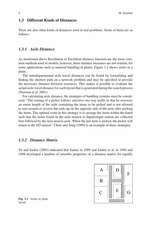
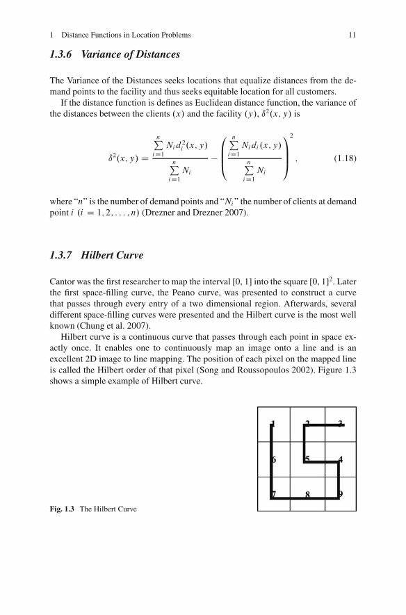
As mentioned above Rectilinear or Euclidean distance function are the most com-mon methods used in models, however, these distance measures are not realistic forsome applications such as material handling in plants. Figure 1.1 shows aisles in aplant.
The interdepartmental aisle travel distances can be found by formulating andfinding the shortest path on a network problem and may be specified to providethe necessary distance between resources. This makes it possible to evaluate theactual aisle travel distance for each layout that is generated during the search process(Norman et al. 2001).
For calculating aisle distance, the strategies of handling systems must be consid-ered. “The routing of a picker follows selective one-way traffic in that he traversesan entire length of the aisle containing the items to be picked and is not allowedto turn around or reverse but ends up on the opposite side of the aisle after pickingthe items. The optimal route in this strategy is to arrange the items within the batchsuch that the items found in the aisle nearest to Input/output station are collectedfirst followed by the next nearest aisle. When the last item is picked, the picker willreturn to the I/O station”. Chew and Tang (1999) is an example of these strategies.
1.3.2 Distance Matrix
Yu and Sarker (2003) indicated that Sarker in 1989 and Sarker et al. in 1994 and1998 developed a number of amoebic properties of a distance matrix for equally
Fig. 1.1 Aisles in plantlayout
1 Distance Functions in Location Problems 9
spaced linear locations to generate different assignments of machines to locationsthat minimize the total unidirectional and/or bi-directional flows. The form of adistance matrix may vary as its corresponding location assignment changes.
dXY D jX � Y j D8<:X � Y if 1 � Y < X � L
Y � X if 1 � X < Y � L
0 if 1 � Y D X � L
: (1.11)
Each location distance can be decomposed into two directional distances that aredefined below.
� Backward: dB is a backward distance matrix, with its element dBXY .
dBXY D�X � Y if 1 � Y < X � L
0 else: (1.12)
� Forward: dF is a forward distance matrix, with its element dFXY (Yu andSarker 2003)
dFXY D�Y � X if 1 � X < Y � L
0 else: (1.13)
1.3.3 Minimum Lengths Path
The distance between two points on P is the minimum length of any path betweenthose points that lies on P . The “facility center”, or “1-center”, of the facility is thepoint of P that minimizes the maximum distance to a facility. There are some algo-rithms to find minimum lengths path (shortest path) such as Dijkstra Algorithm andthe algorithm of Mitchell et al. which is a continuous version of Dijkstra Algorithm(Aronov et al. 2005).
1.3.4 Block Distance
Dearing et al. (2005) discussed that block distances are a special case of norm dis-tances which were introduced to location models by Witzgall et al. in 1964, andWard and Wendell in 1985. Block distances are used to model travel distance in ap-plications where travel directions are restricted to the fundamental directions. Alsoit has a wide usage in barriers problems.
They can also be viewed as a generalization of distances in fixed orientations asintroduced in 1987 by Widmayer et al. (Dearing et al. 2005) where it is assumedthat all fundamental directions have unit length, that is
kakk D 1 8k D 1; 2; : : : : ; 2n; (1.14)
where jjakjj is the Euclidean norm of ak .
10 M. Zarinbal
The block distance between the points, X1 and X2 with respect to a given set offundamental directions a1, a2; : : : ; a2n is denoted by dp.X1;X2/ and is defined as
dp.X1;X2/ D ˛12 C ˇ12; (1.15)
where ˛12 and ˇ12 are nonnegative scalars so that (Dearing et al. 2005)
X2 �X1 D ˛12ak C ˇ12akC1 8k D 1; 2; : : : : ; 2n: (1.16)
1.3.5 Gauges Measures
Most of the references in the literature concerning continuous location problemshave considered distances induced by norms. There are also a number of papersthat consider the use of gauges defined by the Minkowski functional of a compactconvex set (not necessarily symmetric) containing the origin in its interior. Thesefunctions have been used in location theory to model situations where the symmetryproperty of a norm does not make sense.
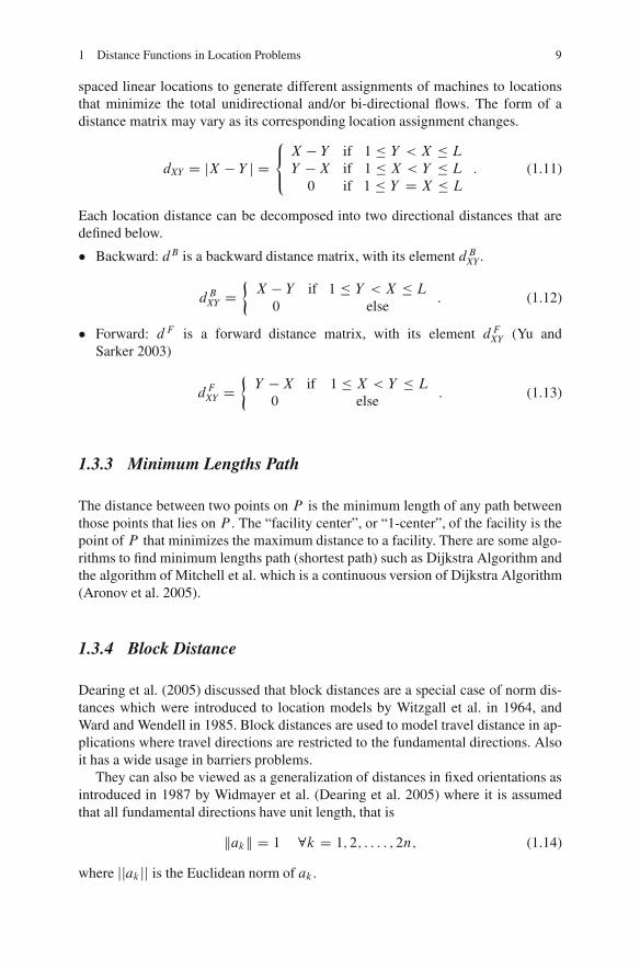
There are also general models where the definiteness property of the gauge ofa compact convex set is relaxed. Relaxing definiteness introduces the existence ofzero-distance regions (Fig. 1.2).
Gauges of compact convex sets have a very interesting property: The distancebetween two points is the shortest path between them using only fundamental direc-tions of the unit ball.
Let be a closed convex set containing the origin. The function ' defined by
�.x/ D inff˛ > 0 W x 2 ˛ g (1.17)
is called the gauge of � . The set � will be called the unit ball associated with '. Wedefine the distance from y to x by '.y � x).
If in addition � is symmetric with respect to the origin, ' is a norm and thesymmetry property of a norm ('.y � x/ D '.x � y/) added to '.y � x/ properties.(Hinojosa and Puerto 2003).
Fig. 1.2 Zero-DistanceRegion
1 Distance Functions in Location Problems 11
1.3.6 Variance of Distances
The Variance of the Distances seeks locations that equalize distances from the de-mand points to the facility and thus seeks equitable location for all customers.
If the distance function is defines as Euclidean distance function, the variance ofthe distances between the clients .x/ and the facility .y/, ı2.x; y/ is
ı2.x; y/ D
nPiD1
Nid2i .x; y/
nPiD1
Ni
�
0BB@
nPiD1
Nidi .x; y/
nPiD1
Ni
1CCA2
; (1.18)
where “n” is the number of demand points and “Ni” the number of clients at demandpoint i .i D 1; 2; : : : ; n/ (Drezner and Drezner 2007).
1.3.7 Hilbert Curve
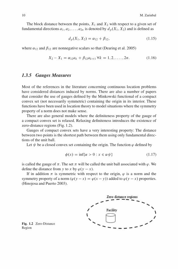
Cantor was the first researcher to map the interval [0, 1] into the square [0, 1]2. Laterthe first space-filling curve, the Peano curve, was presented to construct a curvethat passes through every entry of a two dimensional region. Afterwards, severaldifferent space-filling curves were presented and the Hilbert curve is the most wellknown (Chung et al. 2007).
Hilbert curve is a continuous curve that passes through each point in space ex-actly once. It enables one to continuously map an image onto a line and is anexcellent 2D image to line mapping. The position of each pixel on the mapped lineis called the Hilbert order of that pixel (Song and Roussopoulos 2002). Figure 1.3shows a simple example of Hilbert curve.
Fig. 1.3 The Hilbert Curve
12 M. Zarinbal
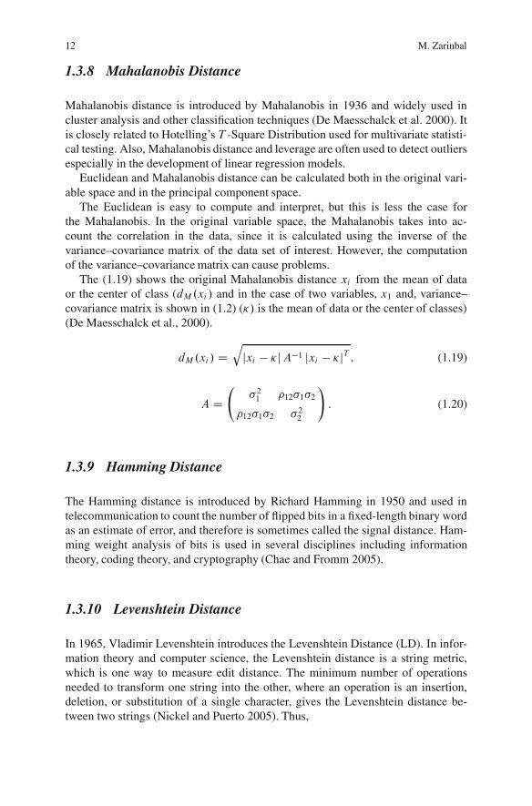
1.3.8 Mahalanobis Distance
Mahalanobis distance is introduced by Mahalanobis in 1936 and widely used incluster analysis and other classification techniques (De Maesschalck et al. 2000). Itis closely related to Hotelling’s T -Square Distribution used for multivariate statisti-cal testing. Also, Mahalanobis distance and leverage are often used to detect outliersespecially in the development of linear regression models.
Euclidean and Mahalanobis distance can be calculated both in the original vari-able space and in the principal component space.
The Euclidean is easy to compute and interpret, but this is less the case forthe Mahalanobis. In the original variable space, the Mahalanobis takes into ac-count the correlation in the data, since it is calculated using the inverse of thevariance–covariance matrix of the data set of interest. However, the computationof the variance–covariance matrix can cause problems.
The (1.19) shows the original Mahalanobis distance xi from the mean of dataor the center of class (dM.xi / and in the case of two variables, x1 and, variance–covariance matrix is shown in (1.2) (�/ is the mean of data or the center of classes)(De Maesschalck et al., 2000).
dM.xi / Dq
jxi � �jA�1 jxi � �jT ; (1.19)
A D
�21 �12�1�2
�12�1�2 �22
!: (1.20)
1.3.9 Hamming Distance
The Hamming distance is introduced by Richard Hamming in 1950 and used intelecommunication to count the number of flipped bits in a fixed-length binary wordas an estimate of error, and therefore is sometimes called the signal distance. Ham-ming weight analysis of bits is used in several disciplines including informationtheory, coding theory, and cryptography (Chae and Fromm 2005).
1.3.10 Levenshtein Distance
In 1965, Vladimir Levenshtein introduces the Levenshtein Distance (LD). In infor-mation theory and computer science, the Levenshtein distance is a string metric,which is one way to measure edit distance. The minimum number of operationsneeded to transform one string into the other, where an operation is an insertion,deletion, or substitution of a single character, gives the Levenshtein distance be-tween two strings (Nickel and Puerto 2005). Thus,
1 Distance Functions in Location Problems 13
LD (“IBM”, “IBN”) D 1, since one substitution is needed to transform IBM toIBN.
LD (“Success”, “Successful”) D 3, since three additions are needed to transformSuccess to Successful.
LD is robust to spelling errors and small local differences between the strings(Chae and Fromm 2005).
1.3.11 Hausdorff Distance
This kind of distance metric is used in continues models and is defines as follows:If there are two compact sets, A and B , the Hausdorff distance between them is
dH.A;B/ D max.maxx2A d2.x; B/;max
y2B d2.y; A/; (1.21)
where (Nickel and Puerto 2005)
d2.x; B/ D miny2B d2.x; y/: (1.22)
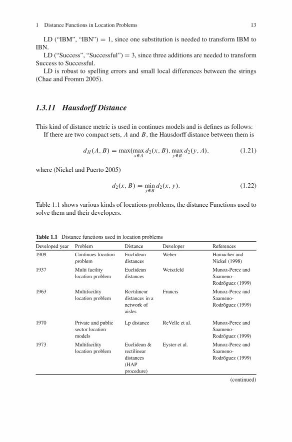
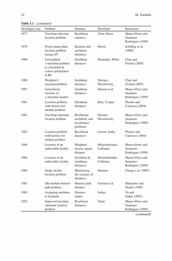
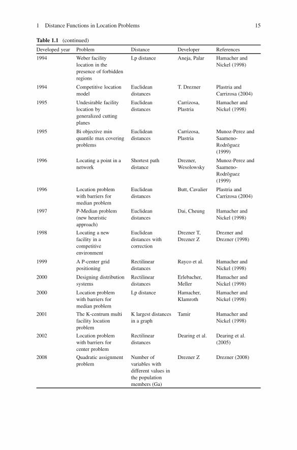
Table 1.1 shows various kinds of locations problems, the distance Functions used tosolve them and their developers.
Table 1.1 Distance functions used in location problems
Developed year Problem Distance Developer References
1909 Continues locationproblem
Euclideandistances
Weber Hamacher andNickel (1998)
1937 Multi facilitylocation problem
Euclideandistances
Weiszfeld Munoz-Perez andSaameno-Rodroguez (1999)
1963 Multifacilitylocation problem
Rectilineardistances in anetwork ofaisles
Francis Munoz-Perez andSaameno-Rodroguez (1999)
1970 Private and publicsector locationmodels
Lp distance ReVelle et al. Munoz-Perez andSaameno-Rodroguez (1999)
1973 Multifacilitylocation problem
Euclidean &rectilineardistances(HAPprocedure)
Eyster et al. Munoz-Perez andSaameno-Rodroguez (1999)
(continued)
14 M. Zarinbal
Table 1.1 (continued)
Developed year Problem Distance Developer References
1977 Traveling salesmanlocation problem
Rectilinearsistances
Chan, Hearn Munoz-Perez andSaameno-Rodroguez (1999)
1978 Fixed charge plantlocation problem(using LP)
Random andeuclideandistances
Morris Schilling et al.(2000)
1980 Unweighted1-maximin problemin a bounded &convex polyhedronin Rk
Euclideandistances
Dasarathy, White Chae andFromm (2005)
1980 Weighted 1maximin problem
Euclideandistances
Drezner,Wesolowsky
Chae andFromm (2005)
1981 Generalizedversions of1-maximin models
Euclideandistances
Hansen et al. Munoz-Perez andSaameno-Rodroguez (1999)
1981 Location problemwith barriers formedian problem
Euclideandistances
Katz, Cooper Plastria andCarrizosa (2004)
1982 Traveling salesmanlocation problem
Rectilinear,euclidean, andLp distanceproblems
Drezner,Wesolowsky
Munoz-Perez andSaameno-Rodroguez (1999)
1983 Location problemwith barriers formedian problem
Rectilineardistances
Larson, Sadiq Plastria andCarrizosa (2004)
1986 Location of anundesirable facility
Weightedinverse squaredistance
Melachrinoudis,Cullinane
Munoz-Perez andSaameno-Rodroguez (1999)
1986 Location of anundesirable facility
Euclidean &rectilineardistances
Melachrinoudis,Cullinane
Munoz-Perez andSaameno-Rodroguez (1999)
1986 Single facilitylocation problem
Minimizingthe variance ofdistances
Maimon Chung et al. (2007)
1987 The median shortestpath problem
Shortest pathdistance
Current et al. Hamacher andNickel (1998)
1989 Assigning machinesto locations
Distancematrix
Sarker Yu andSarker (2003)
1992 Improved travelingsalesman locationproblem
Rectilineardistances
Tamir Munoz-Perez andSaameno-Rodroguez (1999)
(continued)
1 Distance Functions in Location Problems 15
Table 1.1 (continued)
Developed year Problem Distance Developer References
1994 Weber facilitylocation in thepresence of forbiddenregions
Lp distance Aneja, Palar Hamacher andNickel (1998)
1994 Competitive locationmodel
Euclideandistances
T. Drezner Plastria andCarrizosa (2004)
1995 Undesirable facilitylocation bygeneralized cuttingplanes
Euclideandistances
Carrizosa,Plastria
Hamacher andNickel (1998)
1995 Bi objective minquantile max coveringproblems
Euclideandistances
Carrizosa,Plastria
Munoz-Perez andSaameno-Rodroguez(1999)
1996 Locating a point in anetwork
Shortest pathdistance
Drezner,Wesolowsky
Munoz-Perez andSaameno-Rodroguez(1999)
1996 Location problemwith barriers formedian problem
Euclideandistances
Butt, Cavalier Plastria andCarrizosa (2004)
1997 P-Median problem(new heuristicapproach)
Euclideandistances
Dai, Cheung Hamacher andNickel (1998)
1998 Locating a newfacility in acompetitiveenvironment
Euclideandistances withcorrection
Drezner T,Drezner Z
Drezner andDrezner (1998)
1999 A P-center gridpositioning
Rectilineardistances
Rayco et al. Hamacher andNickel (1998)
2000 Designing distributionsystems
Rectilineardistances
Erlebacher,Meller
Hamacher andNickel (1998)
2000 Location problemwith barriers formedian problem
Lp distance Hamacher,Klamroth
Hamacher andNickel (1998)
2001 The K-centrum multifacility locationproblem
K largest distancesin a graph
Tamir Hamacher andNickel (1998)
2002 Location problemwith barriers forcenter problem
Rectilineardistances
Dearing et al. Dearing et al.(2005)
2008 Quadratic assignmentproblem
Number ofvariables withdifferent values inthe populationmembers (Ga)
Drezner Z Drezner (2008)
16 M. Zarinbal
1.4 Summary
The distance functions and its definition play an important role in facility locationproblems. As it is shown above, we have various kinds of distance function with dif-ferent definitions. Each of them has its own domain, advantages, and disadvantages.For defining the distance function, one must consider the semantic of the problem,the distance characteristic, and its usage domain.
References
Aronov B, VanKreveld M, VanOostrum R, Varadarajan K (2005) Facility location on a polyhedralsurface. Discrete Comput Geom 30:357–372
Chae A, Fromm H (2005) Supply chain management on demand. Springer, BerlinChew EP, Tang LC (1999) Travel time analysis for general item location assignment in a rectangu-
lar warehouse. Eur J Oper Res 112:582–597Chung KL, Huang YL, Liu YW (2007) Efficient algorithms for coding Hilbert curve of arbitrary-
sized image and application to window query. Inf Sci 177:2130–2151Dearing PM, Klamroth K, Segars R Jr (2005) Planar location problems with block distance and
barriers. Ann Oper Res 136:117–143De Maesschalck R, Jouan-Rimbaud D, Massart DL (2000) The Mahalanobis distance. Chem Intell
Lab Syst 50:1–18Drezner Z (2008) Extensive experiments with hybrid genetic algorithms for the solution of the
quadratic assignment problem. Comput Oper Res 35:717–736Drezner T, Drezner Z (1998) Facility location in anticipation of future competition. Location Sci
6:155–173Drezner T, Drezner Z (2007) Equity models in planar location. Comput Manage Sci 4:1–16Drezner Z, Wesolowsky GO (2001) On the collection depots location problem. Eur J Oper Res
130:510–518Fouard C, Malandain G (2005) 3-D chamfer distances and norms in anisotropic grids. Image Vision
Comput 23:143–158Hamacher HW, Nickel S (1998) Classification of location models. Location Sci 6:229–242Hinojosa Y, Puerto J (2003) Single facility location problems with unbounded unit balls. Math
Method Oper Res 58:87–104Jiang J, Xu Y (2006) MiniSum location problem with farthest Euclidean distances. Math Methodol
Oper Res 64:285–308Munoz-Perez J, Saameno-Rodroguez JJ (1999) Location of an undesirable facility in a polygonal
region with forbidden zones. Eur J Oper Res 114:372–379Nickel S, Puerto J (2005) Location theory: A unified approach. Springer-Verlag, BerlinNorman BA, Arapoglu R, Smith AE (2001) Integrated facilities design using a contour distance
metric. IIE Trans 33:337–344Ogryczak W (2000) Inequality measures and equitable approaches to location problems. Eur
J Oper Res 122:347–391Plastria F, Carrizosa E (2004) Optimal location and design of a competitive facility. Math Program
100:247–265Schilling DA, Rosing KE, ReVelle CS (2000) Network distance characteristics that affect compu-
tational effort in p-median location problems. Eur J Oper Res 127:525–536
1 Distance Functions in Location Problems 17
Song Z, Roussopoulos N (2002) Using Hilbert curve in image storing and retrieving. Inf Syst27:523–536
Uster H, Love RF (2003) Formulation of confidence intervals for estimated actual distances.Eur J Oper Res 151:586–601
Yu J, Sarker BR (2003) Directional decomposition heuristic for a linear machine-cell locationproblem. Eur J Oper Res 149:142–184
Chapter 2An Overview of Complexity Theory
Milad Avazbeigi
Computational complexity theory (Shortly: Complexity Theory) has been a centralarea of theoretical computer science since its early development in the mid-1960s.Its subsequent rapid development in the next three decades, has not only establishedit as a rich, exciting theory, but also has shown strong influence on many otherrelated areas in computer science, mathematics, and operation research (Du andKo 2000). However, the notions of algorithms and complexity are meaningful onlywhen they are defined in terms of formal computation models (Du and Ko 2000).
Apparently, we need some models to base the foundation of complexity theoryon them. In this chapter, we introduce only three basic models: deterministic tur-ing machine (DTM), non-deterministic turing machine (NTM) and Oracle machinemodels. It should be noted there are also some other models (see Du and Ko 2000).
Using such models, allows us to separate the complexity notion from any phys-ical machine. Hence, we can measure the time complexity of algorithms andhardness of problems independent from a specific machine which runs the algo-rithm(s). It should be noted that these are just abstract models; means, are definedmathematically (Sipser 1996).
The structure of this chapter is as follows. We first discuss why we actually needcomplexity theory. Then, we introduce three basic models of computation: DTMand NTM and Oracle model. Then we present a brief introduction about the conceptof bigO notation which is widely used in the complexity theory. In Sect. 2.5, the de-cision problems as a special form of problems are described. Following this section,the basic concepts of reduction are presented, which help us to make relationshipsbetween different classes of complexity and also provide a rich tool to identify theunknown complexity class of a new problem. Finally, we introduce the most popularclasses of complexity: P , NP, NP-complete and NP-hard. In each class, also, someknown problems are presented.
R.Z. Farahani and M. Hekmatfar (eds.), Facility Location: Concepts, Models, 19Algorithms and Case Studies, Contributions to Management Science,DOI 10.1007/978-3-7908-2151-2 2, c� Physica-Verlag Heidelberg 2009
20 M. Avazbeigi
2.1 Advantage of Complexity Theory
As quoted in previous section, by using computation models, we try to generalizeour results of algorithms runs to other problem instances, computers and imple-mentations. However, without such computational models, and by just relying onphysical machines, it would be difficult however to base a theory on the detailedspecification of the physical objects and even if we could, the theory might not bevery useful, because we would need to modify it for every different set of hardware(Martin 1996). In doing so, we attempt to define the execution time as a functionof the size of the problem. Also Time is not measured in second, minutes or anyanother similar measures. Roughly speaking, we try to measure it as the number ofsteps that has to be taken to resolve an instance of the problem at hand which isapparently independent from any specific computer or machine.
2.1.1 Computational Complexity
1. Defines clearly what solving a problem “efficiently” means.2. Categorizes problems into those that can be solved efficiently and those that
cannot.3. Estimates the amount of time (or memory) needed to solve problems (Daskin
1995).
These are main reasons underlying the use of “complexity theory”. Using complex-ity theory, we can evaluate an algorithm in front of the problem at hand to understandwhether the existing algorithm can resolve the given problem completely as the sizeof the problem grows or not. Also, we can compare algorithms in respect to the timeand resources they need, to resolve a given problem. Recognition of the complexityclass of a problem is another important help of this theory (2). Most of the time,the recognized complexity class of a problem, determines our future approach wechoose to resolve the problem. For example, if we realize that the problem at hand isNP-complete (which is described in next sections), we shift our concentration fromexact solutions to approximate and usually so called heuristic and meta-heuristicapproaches.
2.2 Abstract Models of Computation: Abstract Machines
2.2.1 Preliminary Definitions
2.2.1.1 String
The basic data structure in complexity theory is usually considered as “String”. Allother data structure can be encoded and presented by strings. A string is a finite
2 An Overview of Complexity Theory 21
sequence of symbols. For instance, the word “string” is a string of over the symbolsof English letters (Du and Ko 2000).
2.2.1.2 Language
If A is the set of strings that machine M accepts, we say that A is the language ofmachine M and write L.M/ D A (Sipser 1996); we say that M accepts A or Mrecognizes.
A machine may accept several strings, but it always accepts only one language.For convenience, we often work only on strings of the alphabet f0; 1g (Du andKo 2000). To show that this does not impose a serious restriction on the theory, wenote that a simple method can be constructed of encoding strings over any finitealphabet into the strings over f0; 1g.
2.2.2 Turing Machine Models
The standard computer model in computability theory is the Turing machine, intro-duced by Alan Turing in 1936 (Turing 1936).
2.2.2.1 Deterministic Turing Machine (DTM) (Du and Ko 2000)
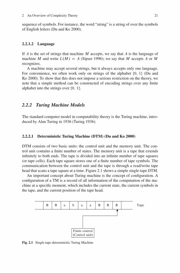
DTM consists of two basic units: the control unit and the memory unit. The con-trol unit contains a finite number of states. The memory unit is a tape that extendsinfinitely to both ends. The tape is divided into an infinite number of tape squares(or tape cells). Each tape square stores one of a finite number of tape symbols. Thecommunication between the control unit and the tape is through a read/write tapehead that scans a tape square at a time. Figure 2.1 shows a simple single-tape DTM.
An important concept about Turing machine is the concept of configuration. Aconfiguration of a TM is a record of all information of the computation of the ma-chine at a specific moment, which includes the current state, the current symbols inthe tape, and the current position of the tape head.
Finite control(Control unit)
B B B B a a b a B Tape
Fig. 2.1 Single-tape deterministic Turing Machine
22 M. Avazbeigi
2.2.2.2 Non-Deterministic Turing Machine (NTM) (Du and Ko 2000)
The Turing machine described in the previous section is a deterministic machine,because for each configuration of a machine there is at most one move to make,and hence there is at most one next configuration. If we allow more than one movesfor some configurations, and hence those configurations have more than one nextconfiguration, then the machine is called a nondeterministic Turing machine (NTM).
In complexity theory, we use the concept of Turing machines to model our com-putations and as described in Sect. 2.1, to make independent the computations fromhardware of computer. To see examples about these models, see example of Duand Ko (2000) and Sipser (1997). Speaking in an imprecise manner, a computationchanges the configuration of a machine and takes the machine from one configura-tion to a new configuration. Finally, a finite number of computations take us from aninitial state of machine to target (desired) state of machine which can be consideredas the answer to the problem to be resolved.
2.2.2.3 Oracle Turing Machine (Du and Ko 2000)
A function-oracle DTM is an ordinary DTM equipped with an extra tape, called thequery tape, and two extra states, called the query state and the answer state. Theoracle machineM works as follows: First, on input x and with oracle function f , itbegins the computation at the initial state and behaves exactly like the ordinary TMwhen it is not in any of the special states.
The machine is allowed to enter the query state to make queries to the oracle, butit is not allowed to enter the answer state from any ordinary state. Before it enters thequery state, machine M needs to prepare the query string y by writing the string yon the query tape and leaving the tape head of the query tape scanning the square tothe right of the rightmost square of y. After the oracle machine M enters the querystate, the computation is taken over by the “oracle” f , which will do the followingfor the machine: it reads the string y on query tape; it replaces y by the string f .y/;and it puts the tape head of the query tape back scanning the leftmost square off .y/; it puts the tape head of the query tape back scanning the left most square off .y/; and it puts the machine into answer state. Then the machine continues fromthe answer state as usual. The actions taken by the oracle count as only one unitof time.
2.3 Big-O Notation (Wood 1987)
The complexity of computational problems can be discussed by fixing a model ofcomputation and then considering how much of the machines resources are requiredfor the solutions. In order to make a meaningful comparison of the inherent com-plexity of two problems, it is necessary to look at instances over a range of sizes.
2 An Overview of Complexity Theory 23
The most common approach is to compare the growth rates of the two runtimes,each viewed as a function of the instance size (Martin 1996).
We measure the time and space complexity of a problem or program by totalfunction from N to N , since time and space are measured in positive integral unitsas is the size of input data. In order to compare time or space complexities of prob-lems or programs we are usually interested only in their order, that is, multiplicativeconstants and lower-order terms are ignored. The big-O notation is used for thispurpose.
Given the two functions f , g: N ! N , we write f .n/ D O.g.n//, if there arepositive integers c and d such that, for all n � d ,
f .n/ � cg.n/; (2.1)
cf .n/ � g.n/: (2.2)
In this case f is said to be big-O of g.Similarly, we write f .n/ D ˝.g.n//, if there are positive integers c and d such
that, for all n � d ,In this case we say f is big-omega of g.
If f .n/ D O.g.n// and f .n/ D ˝.g.n//, then we write f .n/ D �.g.n//, thatis, f is big-theta of g.Whenever f .n/ D O.g.n//, then g.n/ is an upper bound for f .n/ and wheneverf .n/ D ˝.g.n//, g.n/ is a lower bound for f .n/.
Remember that the big-O notation compares only the rate of growth of functionsrather than their values, so when f .n/ D �.g.n//, f .n/ and g.n/ have the samerates of growth, but can be very different in their values.
2.3.1 Example
Take the polynomials f .x/ D 6x4 � 2x3 C 5; g.x/ D x4. We say f .x/ has orderO.g.x// or O.x4/. From the definition of order, jf .x/j � cjg.x/j for all x > 1,where c is a constant.
Proof.
j6x4 � 2x3 C 5j � 6x4 C 2x3 C 5 where x:1; (2.3)
j6x4 � 2x3 C 5j � 6x4 C 2x4 C 5x4 because x3 < x4; and so on; (2.4)
j6x4 � 2x3 C 5j � 13x4: (2.5)
So we can say:f .x/ is O.g.x// as x ! 1: (2.6)
24 M. Avazbeigi
2.4 Time Complexity
Now, using big-O notation, we can talk about complexity of algorithms in frontof problems. As mentioned before, big-O notation gives us a tool to talk aboutcomplexity of algorithms in respect to steps (approximately) they take to resolvethe problem at hand, so we make our models independent from a specific hardwareconfiguration or implementation.
Also it is important to say in analysis of algorithms, we are interested in worstcase analysis of algorithms; the longest time they take to resolve a problem.
2.4.1 Constant Time
In computational complexity theory, constant time, orO.1/ time, refers to the com-putation time of a problem when the time needed to solve that problem does notdepend on the size of the data it is given as input.
For example accessing any single element in an array takes constant time as onlyone operation has to be made to locate it.
It can be noted, if the number of elements is known in advance and does notchange, however, such an algorithm can still be said to run in constant time. Forexample, think about a problem as finding of an unknown chose square of a chessboard. It is clear that, growth of board size changes the number of steps has to betaken to find the square. However, for any specific size of board, it is a constantpredefined value. So our algorithm in front of this problem takes constant time.
2.4.2 Linear Time (Sipser 1996)
In computational complexity theory, an algorithm is said to take linear time, orO.n/time, if the asymptotic upper bound for the time it requires is proportional to the sizeof the input, which is usually denoted n. Informally spoken, the running time in-creases linearly with the size of the input. For example, finding the minimal valuein an unordered array takes O.n/ time because all the items in array have to bechecked.
2.4.3 Polynomial Time (Papadimitriou 1994)
In computational complexity theory, polynomial time refers to the computation timeof a problem where the run time, m.n/, is no greater than a polynomial function ofthe problem size, n. Written mathematically using big O notation, this states thatm.n/ D O.nk/ where k is some constant that may depend on the problem.
2 An Overview of Complexity Theory 25
Mathematicians sometimes use the notion of “polynomial time on the lengthof the input” as a definition of a “fast” or “feasible” computation, as opposed to“super-polynomial time”, which is anything slower than that. Exponential time isone example of a super-polynomial time.
2.4.4 Exponential Time (Sipser 1996)
In complexity theory, exponential time is the computation time of a problem wherethe time to complete the computation,m.n/, is bounded by an exponential functionof the problem size, n. In other words as the size of the problem increases linearly,the time to solve the problem increases exponentially.
Written mathematically, there exists k > 1 such that m.n/ D O.kn/ and thereexists c such that m.n/ D O.cn/.
2.5 Decision Problems
In computability theory and computational complexity theory, a decision problem isa question in some formal system with a yes-or-no answer, depending on the valuesof some input parameters. For example, the problem “given two numbers x and y,does x evenly divide y?” is a decision problem. The answer can be either “yes” or“no”, and depends upon the values of x and y.
A formal definition of decision problem is “A decision problem is any arbitraryyes-or-no question on an infinite set of inputs”. Because of this, it is traditional todefine the decision problem equivalently as: the set of inputs for which the problemreturns yes (Martin 1996).
For every optimization problem, there is a Decision Problem version. Hence,we can convert an optimization problem into a decision problem which means aquestion with answer “yes” or “no”. Satisfiability problem is a popular and classicexample of decision problems which is described in Sect. 2.7.
2.6 Reduction
A reduction is a way of converting one problem into another problem in such away that, if the second problem is solved, it can be used to solve the first problem(Sipser 1996).
For example, suppose you want to find your way around a new city. You knowthis would be easy if you had a map. This demonstrates reducibility. The problemof finding your way around the city is reducible to the problem of obtaining a mapof the city (Sipser 1996).
Many examples also can be found in mathematics. For example the problem ofsolving a system of linear equations reduces to the problem of inverting matrix.
26 M. Avazbeigi
2.6.1 Linear Reduction
Linear reductions are used widely in complexity theory. Linear reduction in litera-ture is defined as follows (Brassard and Bratley 1988):
Let A and B be two solvable problems. A is linearly reducible to B , denotedA �l B , if the existence of an algorithm for B that works in a time in O.t.n//,for any function t.n/, implies that there exists an algorithm for A that also worksin a time in O.t.n//. When A �l B and B �l A both hold. A and B are linearlyequivalent, denoted A �l B .
2.6.2 Polynomial Reduction
Another important definition is polynomial reduction (Brassard and Bratley 1988):Let X and Y be two problems. Problem X is polynomially reducible to problem
Y in the sense of Turing, denotedX ��T Y; if there exists an algorithm for solvingX
in a time that would be polynomial if we took no account of the time needed to solvearbitrary instances of problem Y . In other words, the algorithm for solving problemX may make whatever use it chooses of an imaginary procedure that can somehowmagically solve problem Y at no cost. When X ��
T Y and Y ��T X simultaneously,
then X and Y are equivalent in the sense of Turing, denoted Y ��T X .
2.6.3 Polynomial Reduction: Many-One Polynomially Reducible
We introduced the decision problems as the problems in which we simply look foranswer “yes” or “no”. The restriction to decision problems allows us to introduce asimplified notion of polynomial reduction:
Let X � I and Y � J be two decision problems. Problem X is many-onereducible to problem Y , denoted by X ��
m Y; if there exists a function f W I ! J
computable in polynomial time, known as the reduction function between X and Y ,such that
WhenX ��m Y and Y ��
m X both hold, thenX and Y are many-one polynomiallyequivalent, denoted X ��
m Y (Brassard and Bratley 1988).
2.7 Examples
In this section some classic problems that we would refer to them in Sect. 2.8, arepresented. Here our aim is just explanation of problems. In Sect. 2.8, we analyzethese problems from the view of complexity theory.
2 An Overview of Complexity Theory 27
2.7.1 Traveling Salesman Optimization Problem
Given: A graph G.N;A/ with node set N and link set A. Associated with each link.i; j / in A is a nonnegative link length dij .
Find: circuit that visits all nodes and is of minimum total length (Daskin 1995).As we said in Sect. 2.5, any optimization problem has a decision version. The
corresponding decision problem to Traveling Salesman Problem (TSP) is: “Given anumber n of cities, n � 3 integer, a non negative nxn distance matrix of integersC D Œcij , and a non negative integer L: Is there a closed tour passing from everycity exactly once, with total length � L‹”.
This is the general form of TSP. By specifying the actual graph on which thetraveling salesman problem is to be solved, we are specifying an instance of theproblem.
When we speak of the size of an instance of a problem, we are referring to a wayof characterizing how big the problem is (Daskin 1995).
In TSP the number of nodes and the number of links in a problem will constitutean adequate description of the size of a problem.
2.7.2 Satisfiability Problem
Given: A Boolean expression – a function of true/false variables.Question: Is there an assignment of truth values (TRUE or FALSE) to the vari-
ables such that the expression is TRUE (Daskin 1995).As the problem shows, satisfiability (SAT) problem is essentially expressed in
the form of a decision problem. We just need to acquire the answer “yes” or “no”.A Boolean function is a function whose variable values and function value are
all in fTRUE, FALSEg. We often denote TRUE by 1 and FALSE by 0 (Du andKo 2000).
It can be shown that, given a general Boolean formula, we can construct an equiv-alent one in conjunctive normal form (CNF), that is a formula like:
“C1 AND C2 AND: : : AND Cm”where Ci; i D 1; : : : ; m are clauses consisting of disjunctions of Boolean vari-
ables, simple or negated.(x1 OR x2 OR x3) and (x1 OR :x2) and (x2 OR :x3) and (x3 OR :x1) and
(:x1 OR :x2 OR :x3).Now, the decision problem is:Given a Boolean formula in conjunctive normal form (CNF), is it satisfiable?
That is, is there a set of “true-false” values to be assigned to the various variables,such that the compound proposition is true?
28 M. Avazbeigi
2.7.3 Hamiltonian Cycle Problem
Given: A graph G.N;A/ where N is the set of nodes or vertices and A is the set oflinks.
Question: Does the graph contain a cycle that visits every vertex (i.e., a path thatvisits each node exactly once except the first node which is also visited at the lastnode on the path)? (Daskin 1995).
2.7.4 Clique Problem
Given: An undirected graph G D .N; A/ where N is the set of nodes or verticesand A is the set of links.
Question: A clique in G is a set of nodes K � N such that fu; vg 2 A for everypair of nodes u, v 2 K . Given a graph G and an integer k, the k-Clique problemconsists of determining whether there exists a clique of k nodes in G (Brassard andBratley 1988).
2.8 Complexity Classes
Now, after introduction of computation models (Turing machine models), big-Onotation, different time complexities, decision problems and concepts of reduction,we are prepared to talk about complexity classes of problems.
First it is necessary to present a formal definition of complexity classes. Also itis necessary to note that there are some other classes, which are not presented herebecause this chapter aims to present an introduction to complexity theory. For moreinformation about other complexity classes see references at the end of chapter.
In computational complexity theory, a complexity class is a set of problems ofrelated complexity. A typical complexity class has a definition of the form: the setof problems that can be solved by abstract machine M using O.f .n// of resourceR (n is the size of the input) (Du and Ko 2000).
2.8.1 Class P
P is a class of languages that are decidable in a polynomial time on a deterministicsingle-tape Turing machine (Sipser 1996).
The class P plays a central role in our theory and is important because:P is invariant for all models of computation that are polynomially equivalent to
the deterministic single-tape Turing machine.
2 An Overview of Complexity Theory 29
P roughly corresponds to the class of problems that are realistically solvable ona computer.
Item 1 indicates that problems in P class are not affected by the particulars ofthe model of computation that we are using.
Item 2 indicates whenever we prove a problem falls in Class P , an algorithm canbe found which can solve the problem in polynomial time, means the run time,m.n/,is no greater than a polynomial function of the problem size, n. Written mathemati-cally using big O notation, this states thatm.n/ D O.nk/ where k is some constantthat may depend on the problem.
We describe algorithms with numbered stages. The notion of stage of an algo-rithm is analogous to the step of a Turing machine, though of course, implementingone stage of an algorithm on a Turing machine, in general require many Turingmachine steps (Sipser 1996).
To show an algorithm runs in polynomial time, we need to show two things. First,we have to give a polynomial upper bound (see Sect. 2.3 about big-O notation) ofthe stages that the algorithm uses when it runs on an input of length n. Then wehave to examine the individual stages in the description of the algorithm to be sureeach can be implemented in polynomial time on a reasonable deterministic model(Sipser 1996). In fact, the number of stages and running time of each stage both arebounded by polynomial functions. Kozen (2006) states that Cobham and Edmondsare “generally credited with the invention of the notion of polynomial time”.
As quoted in Sect. 2.1, complexity theory helps us to determine whether analgorithm is efficient or not. Now we can define an efficient algorithm as: An al-gorithm is efficient (or polynomial-time) if there exists a polynomial p.n/ such thatthe algorithm can solve any instance of size n in a time in O.p.n// (Brassard andBratley 1988).
2.8.1.1 Example of Problems in P
P is known to contain many natural problems, including the decision versions oflinear programming, calculating the greatest common divisor.
In 2002, it was shown that the problem of determining “if a number is prime” isin P (Agrawal et al. 2004). It is clear that this is a decision problem requires “yes”or “no” answer.
Sorting a set of integers also is another example of P class problems. This isbecause, an algorithm can be found capable of solving the problem in polynomialtime. A classic known algorithm for sorting is select method.
2.8.2 Class NP
NP is the class of decision problems for which there exists a proof system such thatthe proofs are succinct and easy to check.
30 M. Avazbeigi
In fact, in order to prove a problem is in NP, we do not require that there shouldexists an efficient way to find a proof of x when x 2X; only there should ex-its an efficient way to check the validity of a proposed short proof (Brassard andBratley 1988).
Equivalent to the verifier-based definition is the following characterization: NPis the set of decision problems solvable in polynomial time by a non-deterministicTuring machine.
The two definitions of NP as the class of problems solvable by a nondeterministicTuring machine (TM) in polynomial time and the class of problems verifiable bya deterministic Turing machine in polynomial time are equivalent (The proof isdescribed by many textbooks, Sipser 1997, Sect. 2.7.3).
If we remember the definition of Class P , we immediately realize that all prob-lems in P are in NP also. This is because we can verify all decision versions ofproblems in P in polynomial time.
2.8.2.1 Example of Problems in NP
For the class NP, we simply require that any “yes” answer is “easily” verifiable. Inorder to explain the verifier-based definition of NP, let us consider the subset sumproblem:
Assume there is a set of integers. The task of deciding whether a subset with sumzero exists is called the subset sum problem.
Assume that we are given some integers, such as f � 1; �2; 3; 9; 8g, and wewish to know whether some of these integers sum up to zero. In this example, theanswer is “yes”, since the subset of integers f � 1; �2; 3g corresponds to the sum.�1/ C .�2/ C 3 D 0. It is clear that evaluation of each possible answer with nmember take O.n/ operation and hence can be verified in polynomial time.
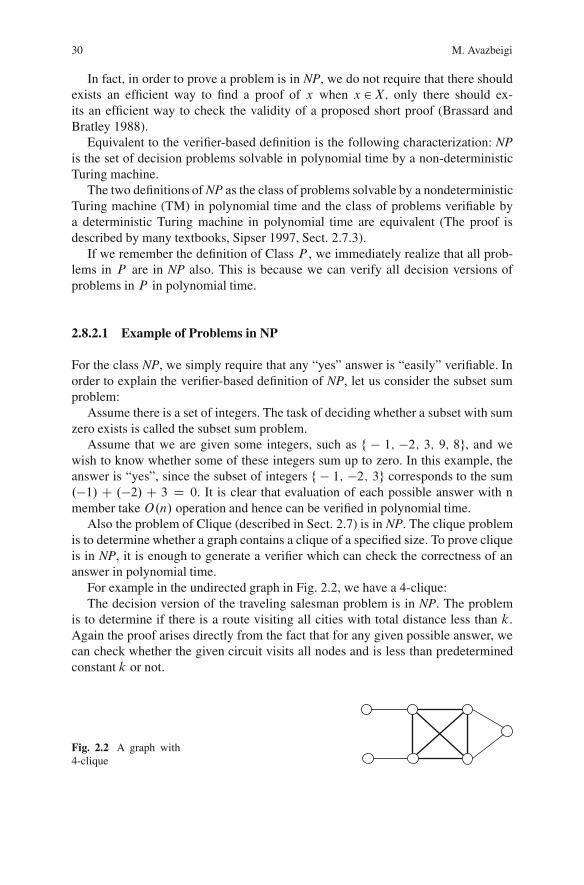
Also the problem of Clique (described in Sect. 2.7) is in NP. The clique problemis to determine whether a graph contains a clique of a specified size. To prove cliqueis in NP, it is enough to generate a verifier which can check the correctness of ananswer in polynomial time.
For example in the undirected graph in Fig. 2.2, we have a 4-clique:The decision version of the traveling salesman problem is in NP. The problem
is to determine if there is a route visiting all cities with total distance less than k.Again the proof arises directly from the fact that for any given possible answer, wecan check whether the given circuit visits all nodes and is less than predeterminedconstant k or not.
Fig. 2.2 A graph with4-clique
2 An Overview of Complexity Theory 31
2.8.3 Class NP-Complete
A decision problemX is NP-complete if: X 2 NP; and for every problem Y 2 NP;Y ��
T X (Brassard and Bratley 1988)Item 1 indicates, first we need to prove the given problem belongs to class NP.
From definition of class NP, we need to prove that a certificate exists which can beverified in polynomial time.
Item 2 indicates that all the other problems in NP, polynomially transform to it.The concepts of reductions presented in Sect. 2.6.
So if the problemX is NP-complete and the problemZ is in NP,Z is NP-complete if and only if X ��
T Z.If X ��
m Z then Z is NP-complete (Brassard and Bratley 1988).This is so important to us, because suppose we have a pool of problems that have
already been shown to be NP-complete. To proveZ is NP-complete, we can choosean appropriate problem X from the pool and show X is polynomially reducible toZ (either many-one to in the sense of Turing). Several thousand problems have beenenumerated in this way.
From a historical view, the concept of “NP-complete” was introduced by StephenCook in a paper entitled “The complexity of theorem-proving procedures” on pages151–158 of the Proceedings of the 3rd Annual ACM Symposium on Theory ofComputing in 1971.
2.8.3.1 Cooks Theorem
In the celebrated Cook–Levin theorem (independently proved by Leonid Levin),Cook proved that the Boolean satisfiability problem is NP-complete (See Gary andJohnson 1979 or Papadimitrious and Steiglits 1982 for proof). In 1972, RichardKarp proved that several other problems were also NP-complete (Karp 1972); thusthere is a class of NP-complete problems (besides the Boolean satisfiability prob-lem). Since Cook’s original results, thousands of other problems have been shownto be NP-complete by reductions from other problems previously shown to be NP-complete; many of these problems are collected in Garey and Johnson’s 1979 bookComputers and Intractability: A Guide to NP-completeness.
From reduction concepts, a key characteristic of NP-complete problems is thatif a polynomial time algorithm can be found for any such problem, then it willalso solve all NP-complete problems in polynomial time. If we could find such analgorithm we would have shown that P D NP.
2.8.3.2 P D NP Problem
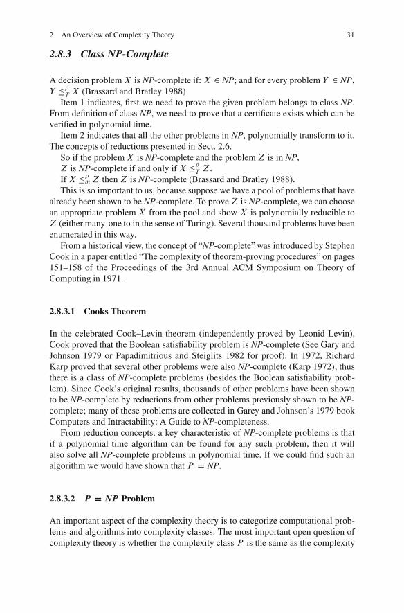
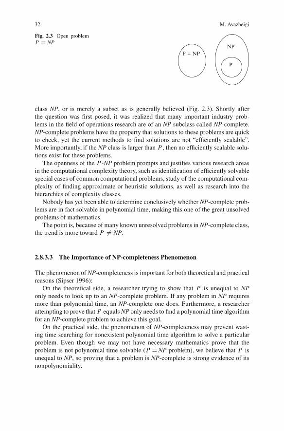
An important aspect of the complexity theory is to categorize computational prob-lems and algorithms into complexity classes. The most important open question ofcomplexity theory is whether the complexity class P is the same as the complexity
32 M. Avazbeigi
Fig. 2.3 Open problemP D NP
P = NP NP
P
class NP, or is merely a subset as is generally believed (Fig. 2.3). Shortly afterthe question was first posed, it was realized that many important industry prob-lems in the field of operations research are of an NP subclass called NP-complete.NP-complete problems have the property that solutions to these problems are quickto check, yet the current methods to find solutions are not “efficiently scalable”.More importantly, if the NP class is larger than P , then no efficiently scalable solu-tions exist for these problems.
The openness of the P -NP problem prompts and justifies various research areasin the computational complexity theory, such as identification of efficiently solvablespecial cases of common computational problems, study of the computational com-plexity of finding approximate or heuristic solutions, as well as research into thehierarchies of complexity classes.
Nobody has yet been able to determine conclusively whether NP-complete prob-lems are in fact solvable in polynomial time, making this one of the great unsolvedproblems of mathematics.
The point is, because of many known unresolved problems in NP-complete class,the trend is more toward P ¤ NP.
2.8.3.3 The Importance of NP-completeness Phenomenon
The phenomenon of NP-completeness is important for both theoretical and practicalreasons (Sipser 1996):
On the theoretical side, a researcher trying to show that P is unequal to NPonly needs to look up to an NP-complete problem. If any problem in NP requiresmore than polynomial time, an NP-complete one does. Furthermore, a researcherattempting to prove thatP equals NP only needs to find a polynomial time algorithmfor an NP-complete problem to achieve this goal.
On the practical side, the phenomenon of NP-completeness may prevent wast-ing time searching for nonexistent polynomial time algorithm to solve a particularproblem. Even though we may not have necessary mathematics prove that theproblem is not polynomial time solvable (P D NP problem), we believe that P isunequal to NP, so proving that a problem is NP-complete is strong evidence of itsnonpolynomiality.
2 An Overview of Complexity Theory 33
2.8.3.4 Example of Problems in NP-complete
Since the introduction of NP-complete class, many problems have been proved tobe in NP-complete class. Here there is an in-complete list of problems (Du andKo 2000):
� Boolean satisfiability problem (SAT)� Knapsack problem� Hamiltonian cycle problem� Traveling salesman problem� Sub graph isomorphism problem� Subset sum problem� Clique problem� N -puzzle� Vertex cover problem� Independent set problem� Graph coloring problem
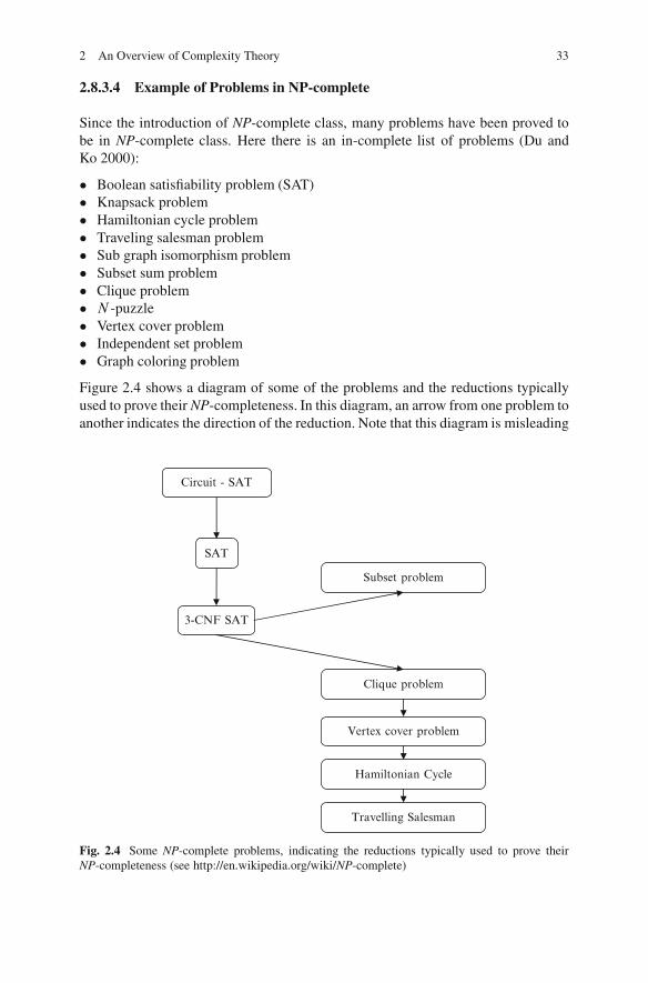
Figure 2.4 shows a diagram of some of the problems and the reductions typicallyused to prove their NP-completeness. In this diagram, an arrow from one problem toanother indicates the direction of the reduction. Note that this diagram is misleading
3-CNF SAT
Clique problem
Subset problem
Vertex cover problem
Hamiltonian Cycle
Travelling Salesman
Circuit - SAT
SAT
Fig. 2.4 Some NP-complete problems, indicating the reductions typically used to prove theirNP-completeness (see http://en.wikipedia.org/wiki/NP-complete)
34 M. Avazbeigi
as a description of the mathematical relationship between these problems, as thereexists a polynomial-time reduction between any two NP-complete problems; but itindicates where demonstrating this polynomial-time reduction has been easiest.
The Hamiltonian cycle problem was shown to be NP-complete by Karp (1972).As the Fig. 2.4 shows, TSP is also a NP-complete problem. To show that the TSPdecision problem is NP-complete, we need to show two things: (a) that the TSP-decision problem is in class NP and (b) that a known NP-complete problem reducesto the TSP-decision problem (For this problem Hamiltonian cycle problem). Toshow (a), we note that, given any cycle, we can compute the cost of the cycle inpolynomial time and therefore determine in polynomial time if the cycle has lengthless than or equal to B (in which case it would be a “yes” instance to the TSP-decision problem). Thus the TSP-decision problem is in class NP. To show (b), weconstruct a complete graph with the same vertex set as that found in the HCP. Foreach link in the new graph, if the corresponding link exits in the instance of the HCP,let the link length be 1; otherwise let the link length be 2. Clearly, the HCP has asolution if and only if the TSP on this complete graph has a solution with valuesless than or equal to n where n is the number of nodes in the vertex set (this proof ischose from Daskin 1995).
2.8.4 Class NP-Hard
NP-hard (nondeterministic polynomial-time hard), in computational complexitytheory, is a class of problems informally “at least as hard as the hardest problemsin NP.” A problemH is NP-hard if and only if there is an NP-complete problem L
that is polynomial time Turing reducible to H , i.e. L�T H . In other words, L canbe solved in polynomial time by an oracle machine with an oracle forH . Informallywe can think of an algorithm that can call such an oracle machine as subroutine forsolving H , and solves L in polynomial time if the subroutine call takes only onestep to compute (Gary and Johnson 1979). NP-hard problems may be of any type:decision problems, search problems, optimization problems.
Such problems are ones such that an NP-complete problem polynomially reducesto the problem in question, but the problem under study is not provable in the classNP. Formally, the term NP-hard is also used to describe the optimization versionsof the decision problems that are NP-complete (Daskin 1995).
2.8.4.1 Example of Problems in NP-Hard
An example of an NP-hard problem is the decision problem SUBSET-SUM. Wealready described this problem. The problem is, given a set of integers, does anynon-empty subset of them add up to zero? That is a yes/no question, and happensto be NP-complete. Another example of an NP-hard problem is the optimization
2 An Overview of Complexity Theory 35
problem of finding the least-cost route through all nodes of a weighted graph ortraveling salesman problem that we described it in Sect. 2.7.
There are also decision problems that are NP-hard but not NP-complete, for ex-ample the halting problem. This is the problem “given a program and its input, willit run forever?” That’s a yes/no question and hence, a decision problem. It is easyto prove that the halting problem is NP-hard but not NP-complete. For example theBoolean satisfiability problem can be reduced to the halting problem by transform-ing it to the description of a Turing machine that tries all truth value assignmentsand when it finds one that satisfies the formula it halts and otherwise it goes intoan infinite loop. It is also easy to see that the halting problem is not in NP sinceall problems in NP are decidable in a finite number of operations, while the haltingproblem, in general, is not (Garey and Johnson 1979).
2.9 Further Reading
Some classic books on complexity theory and network flows are Garey and Johnson(1979), Ahuja et al. (1993), Karp (1972), Papadimitriou and Steiglitz (1982), andSahni and Horowitz (1978).
References
Agrawal M, Kayal N, Saxena N (2004) PRIMES is in P. Ann Math 160(2):781–793Ahuja RK, Magnanti TL, Orlin JB (1993) Network flows: theory, algorithms, and applications.
Prentice-Hall, Englewood Cliffs, NJ. ISBN: 013617549XBrassard G, Bratley P (1988) Algorithmics theory and practice. Prentice-Hall, Englewood
Cliffs, NJCook S (1971) The complexity of theorem-proving procedures. Proceedings of the third annual
ACM symposium on theory of Computing, pp 151–158Daskin MS (1995) Network and discrete location models: Algorithms, and applications. Wiley,
New YorkDu D, Ko K (2000) Theory of computational complexity. Wiley, New YorkGarey MR, Johnson DS (1979) Computers and intractability: A guide to the theory of NP-
completeness. W.H. Freeman, San Francisco, CAKarp RM (1972) Reducibility among combinational problems. In: Miller R, Thatcher J (eds) Com-
plexity of computer computations. Plenum Press, New York, pp 86–103Kozen DC (2006) Theory of computation. Springer-Verlag, BerlinMartin JC (1996) Introduction to languages and the theory of computation. McGraw-Hill,
New YorkPapadimitriou CH (1994) Computational complexity. Addison-Wesley, Reading, MAPapadimitrious CH, Steiglits K (1982) Combinatorial optimization: Algorithms and complexity.
Prentice-Hall, Englewood Cliffs, NJSahni S, Horowitz E (1978) Combinational problems: Reducibility and approximation. Oper Res
26:718–759
36 M. Avazbeigi
Sipser M (1996) Introduction to the theory of computation. Preliminary Edition. PWS PublishingSipser M (1997) Introduction to the theory of computation. PWS PublishingTuring A (1936) On computable numbers with an application to the entscheidnungs problem. Proc
Lond Math Soc ser 2, 42:230–265Wood D (1987) Theory of computation. Wiley, New York
Chapter 3Single Facility Location Problem
Esmaeel Moradi and Morteza Bidkhori
This chapter will focus on the simplest types of location problems, single facilitylocation problem. These problems occur on a regular basis when working, layoutproblems (e.g., we may need to locate a machine in a shop, or items inside a ware-house). Also, on a larger scale, they can occur in, say, choosing the location of awarehouse to serve customers to whom goods must be delivered.
The models shall be studied as being “quick and dirty.” They are “quick” in thesense that they can be used quickly and easily, and “dirty” in the send that theyare approximate. The use of these models should be considered particularly whensome location decision must be made quickly and with limited resource availablefor decision analysis.
When we wish to locate a single new facility in the plane, we often would liketo minimize an objective function involving Euclidean or rectilinear distances be-tween the new facility and a collection of existing facilities having known planarlocations. The first objective function we consider is that of total travel distance, ortotal travel cost.
A number of interesting one-facility location problems exist and are amenable tothe analysis presented in this chapter. Some typical examples of one-facility locationproblems are the location of:
1. New warehouse relative production facilities and customers.2. Hospital, fire station or library in a metropolitan area.3. New classroom building on a college campus.4. New airfield to be used to provide supplies for a number of military bases.5. Component in an electrical network.
In practice, many factors have an impact on location decisions. The relative im-portance of these factors depends on whether the scope of a particular locationproblem is international, national, statewide, or communitywide. For example, if weare trying to determine the location of a manufacturing facility in a foreign country,factors such as political stability, foreign exchange rates, business climate, duties,and taxes play a role. If the scope of the location problem is restricted to a fewcommunities, then factors like community services, property tax incentive, localbusiness climate, and local government regulations are more important.
R.Z. Farahani and M. Hekmatfar (eds.), Facility Location: Concepts, Models, 37Algorithms and Case Studies, Contributions to Management Science,DOI 10.1007/978-3-7908-2151-2 3, c� Physica-Verlag Heidelberg 2009
38 E. Moradi and M. Bidkhori
It is often extremely difficult to find a single location that meets all these objec-tives at the desired level. For example, a location in the Midwest may offer a highlyskilled labor pool, but construction and land costs may be too high.
This chapter is organized as follows. In Sect. 3.1, we consider a general problemformulation with rectilinear or square Euclidean or Euclidian or lp-norm distances,and Sect. 3.2, we consider solution techniques for discrete and continuous space.Continuous space is divided to MiniSum and MiniMax problem with various dis-tances. MiniMax problem involving Euclidean distances is called the circle coveringproblem, which can be interpreted as the problem of covering all existing facility lo-cations with a circle of minimum radius. MiniMax problems are more specializedthan MiniSum problems and seem to be of interest, principally in cases where aworst case analysis is quite important. Finally, Sect. 3.3 represents one real worldcase studies briefly.
3.1 Problem Formulation
In this section, we represent a general problem formulation that is involving the dis-tance traveled per trip with rectilinear or square Euclidean or Euclidian or lp-normdistances. In final section we discus about regional facilities.
3.1.1 A General Formulation of the Problem
3.1.1.1 Model Inputs
Model inputs of this model are as follows:
i : the index of existing facilitiesn: the number of existing facilities
3.1.1.2 Model Outputs (Decision Variables)
Model outputs of this model are as follows:
X D .x; y/: coordinates of the location of new facilityd.xi ; yi /: the distance between of new facility and existing facility i
3.1.1.3 Parameters
Parameters of this model are as follows:
Pi D .ai ; bi /: coordinates of the location of existing facility iwi : weights of existing facility i
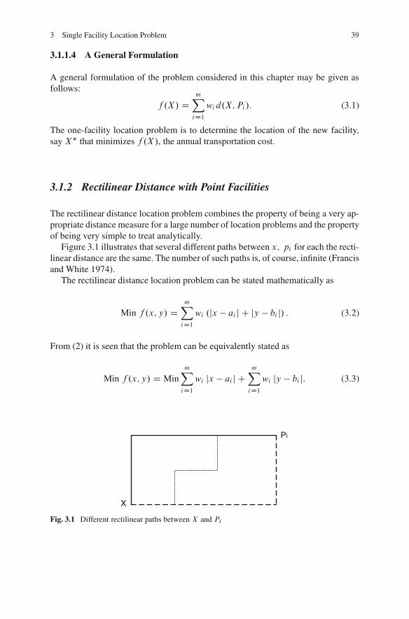
3 Single Facility Location Problem 39
3.1.1.4 A General Formulation
A general formulation of the problem considered in this chapter may be given asfollows:
f .X/ DmXtD1
wi d.X; Pi/: (3.1)
The one-facility location problem is to determine the location of the new facility,say X� that minimizes f .X/, the annual transportation cost.
3.1.2 Rectilinear Distance with Point Facilities
The rectilinear distance location problem combines the property of being a very ap-propriate distance measure for a large number of location problems and the propertyof being very simple to treat analytically.
Figure 3.1 illustrates that several different paths between x; pi for each the recti-linear distance are the same. The number of such paths is, of course, infinite (Francisand White 1974).
The rectilinear distance location problem can be stated mathematically as
Min f .x; y/ DmXiD1
wi .jx � ai j C jy � bi j/ : (3.2)
From (2) it is seen that the problem can be equivalently stated as
Min f .x; y/ D MinmXiD1
wi jx � ai j CmXiD1
wi jy � bi j: (3.3)
X
Pi
Fig. 3.1 Different rectilinear paths between X and Pi
40 E. Moradi and M. Bidkhori
where each quantity on the right-hand side can be treated as separate optimizationproblems:
Min f .x; y/ DmXiD1
wi jx � ai j; (3.4)
Min f .x; y/ DmXiD1
wi jy � bi j : (3.5)
3.1.3 Square Euclidean Distance with Point Facilities
In some facility location problems, cost is not a simple linear function of distance.As an example, the cost associated with the response of a fire truck to a fire isexpected to be nonlinear with distance. Depending on the location problem, f .X/can take on a number of different formulations. One nonlinear form of f .X/ treatedin this chapter is the gravity problem. Suppose that cost is proportional to the squareof the Euclidean distance between X and Pi . Thus, the function becomes
f .X/ DmXtD1
wi�.x � ai /2 C .y � bi /2
�: (3.6)
Location problem having the formulation given by (3.6) are referred to as gravityproblems (Francis and White 1974).
3.1.4 Euclidean Distance with Point Facilities
The function of Euclidean distance is
f .X/ DmXtD1
wi�.x � ai /2 C .y � bi /2
�0:5: (3.7)
Euclidian distance applies for some network location problems as well as someinstances involving conveyors and air travel. Some electrical wiring problems andpipeline design problems are also examples of Euclidean distance problems (Francisand White 1974).
3.1.5 LP-Norm Distance with Point Facilities
Norms are usually employed as the basis for distance predicting functions in con-tinuous location models. Since norms are convex functions, incorporating a norm in
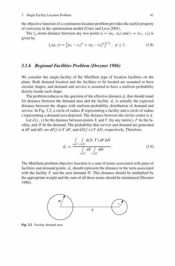
3 Single Facility Location Problem 41
the objective function of a continuous location problem provides the useful propertyof convexity in the optimization model (Uster and Love 2001).
The lp-norm distance between any two points u D .u1; u2/ and v D .v1; v2/ isgiven by
lp.u; v/ D �ju1 � v1jp C ju2 � v2jp�1=p
; p � 1 : (3.8)
3.1.6 Regional Facilities Problem (Drezner 1986)
We consider the single-facility of the MiniSum type of location facilities on theplane. Both demand location and the facilities to be located are assumed to havecircular shapes, and demand and service is assumed to have a uniform probabilitydensity inside each shape.
The problem reduces to the question of the effective distance de that should standfor distance between the demand area and the facility. de is actually the expecteddistance between the shapes with uniform probability distribution of demand andservice. In Fig. 3.2, a circle of radius R representing a facility and a circle of radiusr representing a demand area depicted. The distance between the circles center is d .
Let d.x; y/ be the distance between pointsX and Y (by any metric), F be the fa-cility, andD be the demand. The probability that service and demand are generatedat dF and dD, are dF=s x2F dF, and dD=s x2F dD, respectively. Therefore,
de D
Rx2F
Ry2D
d.X; Y / dF dD
Rx2F
dFR
y2DdD
: (3.9)
The MiniSum problem objective function is a sum of terms associated with pairs offacilities and demand points. de should represent the distance in the term associatedwith the facility F and the area demand D. This distance should be multiplied bythe appropriate weight and the sum of all these terms should be minimized (Drezner1986).
R
d
r
Fig. 3.2 Facility demand area
42 E. Moradi and M. Bidkhori
3.2 Solution Techniques
3.2.1 Techniques for Discrete Space Location Problems(Heragu 1997)
Our focus is primarily on the single-facility location problem. We provide both dis-crete space and continuous space models. The single facility for which we seeka location may be the only one that will serve all the customers, or it may be anaddition to a network of existing facilities that are already serving customers.
3.2.1.1 Qualitative Analysis
The location scoring method is a very popular, subjective decision-making tool thatis relatively easy to use. It consists of these steps:
� Step 1. List all the factors that are important-that have an impact on the locationdecision.
� Step 2. Assign an appropriate weight (typically between 0 and 1) to each factorbased on the relative importance of each.
� Step 3. Assign a score (typically between 0 and 100) to each location with respectto each factor identified in step 1.
� Step 4. Compute the weighted score for each factor for each location by multi-plying its weight by the corresponding score.
� Step 5. Compute the sum of the weighted scores for each location and choose alocation based on these scores.
Although step 5 calls for the location decision to be made solely on the basisof the weighted scores, those scores were arrived at in a subjective manner, andhence a final location decision must also take into account objective measures suchas transportation cost, loads, and operating costs (Heragu 1997).
3.2.1.2 Quantitative Analysis
Several quantitative techniques are available to solve the discrete space, single fa-cility location problem. Each is appropriate for a specific set of objectives andconstraints.
For example, the so-called MiniMax location model is appropriate for determin-ing the location of an emergency service facility, where the objective is to minimizethe maximum distance traveled between the facility and any customer.
The reader may be wondering: If the set of plants including their locations isgiven, where is the location problem? To answer this question, consider the follow-ing problem: We have m plants in a distribution network that serves n customers.Due to an increase in demand at one or more of these n customers, it has become
3 Single Facility Location Problem 43
necessary to open an additional plant the new plant could be located at p possiblesites. To evaluate which of the p sites will minimize distribution (transportation)costs, we can set up p transportation models, each with n customers and m C 1
plants, where the .m C 1/ plant corresponds to the new location being evaluated.Solving the model will tell us not only the distribution of goods from the m C 1
plant (including the new one from the location being evaluated) but also the cost ofthe distribution. The location that yields the least overall distribution cost is the onewhere the new facility should be located (Heragu 1997).
3.2.1.3 Hybrid Analysis
A disadvantage of the qualitative method is that a location decision is made basedentirely on a subjective evaluation. Although the quantitative method overcomes thisdisadvantage, it does not allow us to incorporate unquantifiable factors that have amajor impact on the location decision. For example, the quantitative techniques caneasily consider transportation and operational costs, but intangible factors, such asthe attitude of a community toward businesses, potential labor unrest, and reliabilityof auxiliary service providers, though important in choosing a location, are difficultto capture. We need a method that incorporates subjective as well as quantifiablecost and other factors.
This model classifies the objective and subjective factors important to the specificlocation problem being addressed as:
� Critical;� Objective;� Subjective.
The meaning of the latter two factors is obvious, but the meaning of criticalfactors needs some discussion. In every location decision, at least one factor usuallydetermines whether or not a location will be considered for further evaluation. Forexample, if water is used extensively in a manufacturing process (e.g., a brewery),then a site that does not have an adequate water supply now or in the future isautomatically removed from consideration. This is an example of a critical factor.Some factors can be objective and critical or subjective and critical. For example,the adequacy of skilled labor may be a critical factor as well as a subjective factor.
After the factors are classified, they are assigned numeric values:
CFij: if location i satisfies critical factor j , 0 otherwiseOFij: cost of objective factor j at location iSFij: numeric value assigned (on a scale of 0–1) to subjective factor j for loca-tion i .Wj : weight assigned to subjective factor J.0 � Wj � 1/.
Assume that we have m candidate locations and p critical, q objective, and rsubjective factors. We can determine the overall critical factor measure .CFMj /,
44 E. Moradi and M. Bidkhori
objective factor measure .OFMj / and subjective factor measure .CFMj / for eachlocation i with these equations:
CFMi D CFi1CFi2 : : :CFiP DPYjD1
CFij; i D 1; : : : ; m; (3.10)
OFMI Dmax
"qP
jD1OFij
#�
qPjDi
OFij
max
"qP
jD1OFij
#� min
"qPjDi
OFij
# ; i D 1; : : : ; m; (3.11)
SFMi DRXjD1
wj SFij; i D 1; : : : ; m: (3.12)
The location measure LMj for each location is then calculated as:
LMi D CFMŒ˛OFMi C .1� ˛/SFMi ; (3.13)
where is the weight assigned to the objective factor measure? Notice that even if onecritical factor is not satisfied by a location i , then CFMj and hence LMj are equalto zero. The OFMj values are calculated so that the location with the maximumP
OFij gets an OFMj value of zero and the one with the smallestP
OFij value getsan OFMj value of one. Equation (3.13) assumes that the objective factors are costbased. If any of these factors are profit based, then a negative sign has to be placed infront of each such objective factor and (3.13) can still be used. This works becausemaximizing a linear profit function z is the same as minimizing �z.
After LMj is determined for each candidate location, the next step is to selectthe one with the greatest LMj value. Because the a weight is subjectively assignedby the user, it may be a good idea for the user to evaluate the LMj values for var-ious appropriate a weights, analyze the trade off between objective and subjectivemeasures, and choose a location based on this analysis (Heragu 1997).
3.2.2 Techniques for Continues Space Location Problems
3.2.2.1 MiniSum Problems for Rectilinear Distance
Median method with point facilities. As the name implies, the median method findsthe median location (defined later) and assigns the new facility to it. This methodis used for single-facility location problems with rectilinear distance. Consider mfacilities in a distribution network. Due to marketplace reasons (e.g., increased cus-tomer demand), it is desired to add another facility to this network. The interactionbetween the new facility and existing ones is known. The problem is to locate thenew facility to minimize the total interaction cost between each existing facility andthe new one.
3 Single Facility Location Problem 45
We can rewrite expression (1) as follows:
Min f .X/ DmXiD1
wi jxi � xj CmXiD1
wi jyi � yj: (3.14)
Because the x and y terms can be separated, we can solve the optimal x and ycoordinates independently. Here is the median method:
Median method’s steps
� Step 1. List the existing facilities in no decreasing order of the x coordinates.� Step 2. Find the j th x coordinate in the list (created in step I) at which the
cumulative weight equals or exceeds half the total weight for the first time;
j�1XiD1
wi <mXiD1
wi2
andjXiD1
wi �mXiD1
wi2: (3.15)
� Step 3. List the existing facilities in no decreasing order of the y coordinate.
� Step 4. Find the kth y coordinate in the list (created in step 3) at which thecumulative weight equals or exceeds half the total weight for the first time:
k�1XiD1
wi <mXiD1
wi2
andkXiD1
wi �mXiD1
wi2: (3.16)
The optimal location of the new facility is given by the j th x coordinate and the kth
y coordinate identified in steps 2 and 4, respectively.Programmed mathematical method with point facilities. Although the median
method is the most efficient algorithm for the rectilinear distance, single facilitylocation problem, we present programmed mathematical method for solving it. It in-volves transforming the nonlinear, unconstrained model given by (3.14) into anequivalent linear. Consider the following notation:
xCi D
(.xi � x/ if .xi � x/ > 00 otherwise
; (3.17)
x�i D
(.xi � x/ if .xi � x/ � 0
0 otherwise: (3.18)
We can observe that
jxi � xj D xCi C x�
i ; (3.19)
xi C x� D xCi � x�
i : (3.20)
46 E. Moradi and M. Bidkhori
A similar definition of yCi ; y
�i yield
jyi � yj D yCi C y�
i ; (3.21)
yi C y� D yCi � y�
i : (3.22)
Thus the transformed linear model is:
MinnXiD1
wi .xCi C x�
i C yCi C y�
i /: (3.23)
Subject to
xi C x D xCi C x�
i ; i D 1; : : : ; n; (3.24)
yi C y D yCi � y�
i ; i D 1; : : : ; n; (3.25)
xCi ; x
�i ; y
Ci ; y
�i � 0; i D 1; : : : n; (3.26)
x; y unrestricted in sign: (3.27)
For this model to be equivalent to (3.14), the solution must be such that either xCi
or x�i , but not both, is greater than zero. [If both are, then the values of x and x
do not satisfy their definition in (3.17) and (3.18).] Similarly, only one of yCi ; y
�i
must be greater than zero. Fortunately these conditions are automatically satisfiedin the preceding linear model. This can be easily verified by contradiction. Assumethat in the solution to the transformed model, xC
i and y�i take on values p and q,
where p; q > 0. We can immediately observe that such a solution cannot be optimalbecause one can choose another set of values for, xC
i ; x�i as follows:
xCi D p � minfp; qg; x�
i D q � minfp; qg: (3.28)
And obtain a feasible solution to the model that yields a lower objective value thanbefore because the new xC
i ; x�i values are less than their previously assumed val-
ues. More over, at least one of the new values of xCi ; x
�i is zero according to the
expression (3.28). This means that the original set of values for xCi ; x
�i could not
have been optimal. Using a similar argument, we can show that either yC or y�will take on a value of zero in the optimal solution.
The model described by expressions (3.19), (3.21), (3.23) and (3.27), can besimplified by noting that xiC can be substituted as x � x�
i C xCi from equality
(3.20) and the fact that x is unrestricted in sign. Also y may be substituted similarly,resulting in a model with 2n fewer constraints and variables.
Contour line method for point facilities. Contour lines are important because ifthe optimal location determined is infeasible, we can move along the contour lineand choose a feasible point that will have a similar cost. Also, if subjective factorsneed to be incorporated, we can use contour lines to move away from the optimallocation determined by the median method to another point that better satisfies thesubjective criteria.
3 Single Facility Location Problem 47
We now provide an algorithm to construct contour lines, describe the steps, andillustrate with a numeric example. Algorithm for drawing contour lines is as follows:
� Step 1. Draw a vertical line through the x coordinate and a horizontal line throughthe y coordinate of each facility.
� Step 2. Label each vertical line vi ; i D 1; 2; : : : ; p, and horizontal line Hi; i D1; 2; : : : ; q, where
� Vi D sum of weights of facilities whose x coordinates fall on vertical line i� Hi D sum of weights of facilities whose y coordinates fall on horizontal line j
� Step 3. Set i D j D 1 and N0 D D0 D �mPiD1
wi .
� Step 4. Set Ni D Ni�1 C 2Vi ; andDi D Di�1 C 2Hi . Increment i D i C 1 andj D j C 1.If i � p or j � q, repeat 4. Otherwise, set i D j D 0.
� Steps 5. Determine Sij, the slope of the contour lines through the region boundedby vertical lines i and i C 1 and horizontal lines j and j C 1 using the equationSi D �Ni=Di . Increment i D i C 1 and j D j C 1.
� Step 6. If i � p or j � q, go to step 5. Otherwise, select any point .x; y/ anddraw a contour line with slope Sij in the region Œi; j in which .x; y/ appears sothat the line touches the boundary of this region. From one of the endpoints ofthis line, draw another contour line through the adjacent region with the corre-sponding slope. Repeat this until you get a contour line ending at point .x; y/.You now have a region bounded by contour lines with .x; y/ on the boundary ofthe region.
There are four points about this algorithm. First, the numbers of vertical andhorizontal lines need not be equal. Two facilities may have the same x coordinatebut not the same y coordinate, thereby requiring one horizontal line and two verticallines. In fact, this is why the index i of Vi ; ranges from one to p and that of Hi
ranges from one to q.Second, the Ni and Di computed in steps 3 and 4 correspond to the numerator
and denominator, respectively, of the slope equation of any contour line through theregion bounded by the vertical lines i and iC1 and the horizontal lines j and j C1.To verify this, consider the objective function (14) when the new facility is locatedat some point .x; y/ that is, x D x; y D y:
f .X/ DmXiD1
wi jxi � xj CmXiD1
wi jyi � yj: (3.29)
By noting that the V 0i s and H 0
i s calculated in step 2 of the algorithm correspondto the sum of the weights of facilities whose x; y coordinates are equal to thex; y coordinates, respectively, of the i; j distinct lines and that we have p; q suchcoordinates or lines .p � m; q � m/, we can rewrite (29) as follows:
f .X/ DmXiD1
Vi jxi � xj CmXiD1
Hi jyi � yj: (3.30)
48 E. Moradi and M. Bidkhori
Suppose that x is between the s and .SCl/, (distinct) x coordinates or vertical lines(since we have drawn vertical lines through these coordinates in step 1). Similarly,let y be between the t and .t C l/ vertical lines, then
f .X/ DSXiD1
Vi .x � xi /CPX
iDSC1Vi .xi � x/C
tXiD1
Hi .y � yi /CqX
iDtC1Hi .yi � y/:
(3.31)
Rearranging the variable and constant terms and added and subtracted terms we canreach this equation (for details see Heragu 1997):
f .X/ D"2
sXiD1
Vi �mXiD1
wi
#x C
"2
tXiD1
Hi �mXiD1
wi
#y C c: (3.32)
Equation (3.26) is f .X/ D Nsx CDty C c, which can be rewritten as
y D �NSDt
x C .f .X/ � c/: (3.33)
This expression for the total cost function at x; y or, in fact, any other point in theregion Œs; t has the form y D mx C c, where the slope N D �Ns=Dt . This isexactly how the slopes are computed in step 5 of the algorithm.
We have shown that the slope of any point x; y within a region Œs; t bounded byvertical lines sand s C 1 and horizontal lines t and t C 1 can be easily computed.Thus the contour line (or is cost line) through x; y in region Œs; t may be readilydrawn. Proceeding from one line in one region to the next line in the adjacent regionuntil we come back to the starting point .x; y/ then gives us a region of points inwhich any point has a total cost less than or equal to that of .x; y/.
Third, the lines V0; VPC1 andH0; HPC1 are required for defining the “exterior”regions. Although they are not included in the algorithm steps, the reader must takecare to draw these lines.
Fourth, once we have determined the slopes of all the regions, the user maychoose any point .x; y/ other than a point that minimizes the objective functionand draw a series of contour lines in order to get a region that contains points (i.e.,facility locations) yielding as good or better objective function values than .x; y/.Thus step 6 could be repeated for several points to yield several such regions. Begin-ning with the innermost region, if any point in it is feasible, we use it as the optimallocation. If not, we can go to the next innermost region to identify a feasible point.We repeat this procedure until we get a feasible point (Heragu 1997).
3.2.2.2 MiniSum Square Euclidean Distance
Programmed mathematical method with point facilities. This problem can be for-mulated as follows:
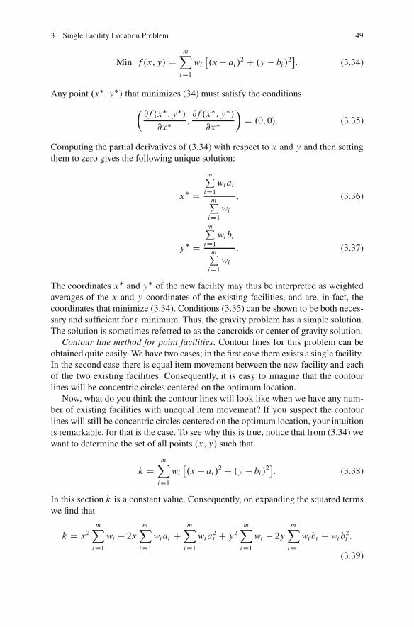
3 Single Facility Location Problem 49
Min f .x; y/ DmXtD1
wi�.x � ai /
2 C .y � bi /2�: (3.34)
Any point .x�; y�/ that minimizes (34) must satisfy the conditions�@f .x�; y�/
@x� ;@f .x�; y�/
@x�
�D .0; 0/: (3.35)
Computing the partial derivatives of (3.34) with respect to x and y and then settingthem to zero gives the following unique solution:
x� D
mPiD1
wi ai
mPiD1
wi
; (3.36)
y� D
mPiD1
wi bi
mPiD1
wi
: (3.37)
The coordinates x� and y� of the new facility may thus be interpreted as weightedaverages of the x and y coordinates of the existing facilities, and are, in fact, thecoordinates that minimize (3.34). Conditions (3.35) can be shown to be both neces-sary and sufficient for a minimum. Thus, the gravity problem has a simple solution.The solution is sometimes referred to as the cancroids or center of gravity solution.
Contour line method for point facilities. Contour lines for this problem can beobtained quite easily. We have two cases; in the first case there exists a single facility.In the second case there is equal item movement between the new facility and eachof the two existing facilities. Consequently, it is easy to imagine that the contourlines will be concentric circles centered on the optimum location.
Now, what do you think the contour lines will look like when we have any num-ber of existing facilities with unequal item movement? If you suspect the contourlines will still be concentric circles centered on the optimum location, your intuitionis remarkable, for that is the case. To see why this is true, notice that from (3.34) wewant to determine the set of all points .x; y/ such that
k DmXiD1
wi�.x � ai /2 C .y � bi /2
�: (3.38)
In this section k is a constant value. Consequently, on expanding the squared termswe find that
k D x2mXiD1
wi � 2x
mXiD1
wi ai CmXiD1
wi a2i C y2
mXiD1
wi � 2ymXiD1
wi bi C wi b2i :
(3.39)
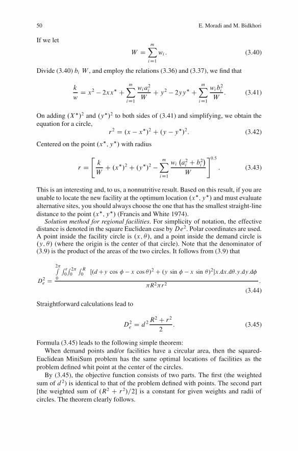
50 E. Moradi and M. Bidkhori
If we let
W DmXiD1
wi : (3.40)
Divide (3.40) bi W , and employ the relations (3.36) and (3.37), we find that
k
wD x2 � 2xx� C
mXiD1
wi a2iW
C y2 � 2yy� CmXiD1
wi b2iW
: (3.41)
On adding .X�/2 and .y�/2 to both sides of (3.41) and simplifying, we obtain theequation for a circle,
r2 D .x � x�/2 C .y � y�/2: (3.42)
Centered on the point .x�; y�/ with radius
r D"k
WC .x�/2 C .y�/2 �
mXiD1
wi�a2i C b2i
�W
#0:5: (3.43)
This is an interesting and, to us, a nonnutritive result. Based on this result, if you areunable to locate the new facility at the optimum location .x�; y�/ and must evaluatealternative sites, you should always choose the one that has the smallest straight-linedistance to the point .x�; y�/ (Francis and White 1974).
Solution method for regional facilities. For simplicity of notation, the effectivedistance is denoted in the square Euclidean case byDe2. Polar coordinates are used.A point inside the facility circle is .x; /, and a point inside the demand circle is.y; / (where the origin is the center of that circle). Note that the denominator of(3.9) is the product of the areas of the two circles. It follows from (3.9) that
D2e D
2�R0
R r0
R 2�0
R R0 Œ.dCy cos � � x cos /2 C .y sin � � x sin /2x:dx:d:y:dy:d�
�R2�r2:
(3.44)
Straightforward calculations lead to
D2e D d2
R2 C r2
2: (3.45)
Formula (3.45) leads to the following simple theorem:When demand points and/or facilities have a circular area, then the squared-
Euclidean MiniSum problem has the same optimal locations of facilities as theproblem defined whit point at the center of the circles.
By (3.45), the objective function consists of two parts. The first (the weightedsum of d2) is identical to that of the problem defined with points. The second part[the weighted sum of .R2 C r2/=2] is a constant for given weights and radii ofcircles. The theorem clearly follows.
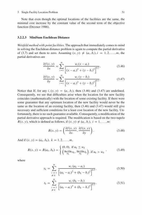
3 Single Facility Location Problem 51
Note that even though the optimal locations of the facilities are the same, theminimal cost increase by the constant value of the second term of the objectivefunction (Drezner 1986).
3.2.2.3 MiniSum Euclidean Distance
Weisfeld method with point facilities. The approach that immediately comes to mindin solving the Euclidean distance problem is again to compute the partial derivativeof (3.7) and set them to zero. Assuming .x; y/ ¤ .ai ; bi /; i D 1; 2; : : : ; m, thepartial derivatives are
@f .x; y/
@xD
mXiD1
wi .x � ai /h.x � ai /
2 C .y � bi/2i0:5 ; (3.46)
@f .x; y/
@yD
mXiD1
wi .y � bi/h.x � ai /
2 C .y � bi/2i0:5 : (3.47)
Notice that If, for any i; .x; y/ D .ai ; bi /, then (3.46) and (3.47) are undefined.Consequently, we see that difficulties arise when the location for the new facilitycoincides (mathematically) with the location of some existing facility. If there weresome guarantee that any optimum location of the new facility would never be thesame as the location of an existing facility, then (3.46) and (3.47) would still givenecessary and sufficient conditions for a least cost location of the new facility. Un-fortunately, there is no such guarantee available. Consequently, a modification of thepartial derivative approach is required. The modification is based on the two-tupeloR.x; y/, which is defined as follows, if .x; y/ ¤ .ai ; bi /; i D 1; : : : ; m:
R.x; y/ D�@f .x; y/
@x;@f .x; y/
@y
�: (3.48)
And if .x; y/ D .ak; bk/; k D 1; 2; : : : ; m,
R.x; y/ D R.ak; bk/ D(.0; 0/; if uk � wk
uk�wk
uksk;
uk�wk
uktk
; if uk � wk
: (3.49)
where
sk DmX
i D 1¤ k
wi .ak � ai /h.ak � ai /2 C .bk � bi/
2i0:5 : (3.50)
tk DmX
i D 1¤ k
wi .bk � bi /h.ak � ai /2 C .bk � bi/
2i0:5 : (3.51)
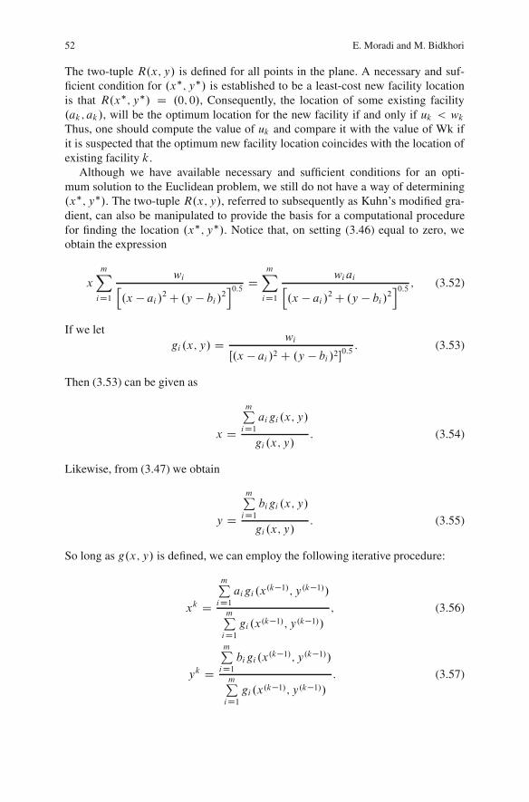
52 E. Moradi and M. Bidkhori
The two-tuple R.x; y/ is defined for all points in the plane. A necessary and suf-ficient condition for .x�; y�/ is established to be a least-cost new facility locationis that R.x�; y�/ D .0; 0/, Consequently, the location of some existing facility.ak; ak/, will be the optimum location for the new facility if and only if uk < wkThus, one should compute the value of uk and compare it with the value of Wk ifit is suspected that the optimum new facility location coincides with the location ofexisting facility k.
Although we have available necessary and sufficient conditions for an opti-mum solution to the Euclidean problem, we still do not have a way of determining.x�; y�/. The two-tuple R.x; y/, referred to subsequently as Kuhn’s modified gra-dient, can also be manipulated to provide the basis for a computational procedurefor finding the location .x�; y�/. Notice that, on setting (3.46) equal to zero, weobtain the expression
x
mXiD1
wih.x � ai /2 C .y � bi /
2i0:5 D
mXiD1
wi aih.x � ai /
2 C .y � bi/2i0:5 ; (3.52)
If we letgi .x; y/ D wi
Œ.x � ai /2 C .y � bi /20:5: (3.53)
Then (3.53) can be given as
x D
mPiD1
ai gi .x; y/
gi .x; y/: (3.54)
Likewise, from (3.47) we obtain
y D
mPiD1
bigi .x; y/
gi .x; y/: (3.55)
So long as g.x; y/ is defined, we can employ the following iterative procedure:
xk D
mPiD1
aigi .x.k�1/; y.k�1//
mPiD1
gi .x.k�1/; y.k�1//; (3.56)
yk D
mPiD1
bigi .x.k�1/; y.k�1//
mPiD1
gi .x.k�1/; y.k�1//: (3.57)
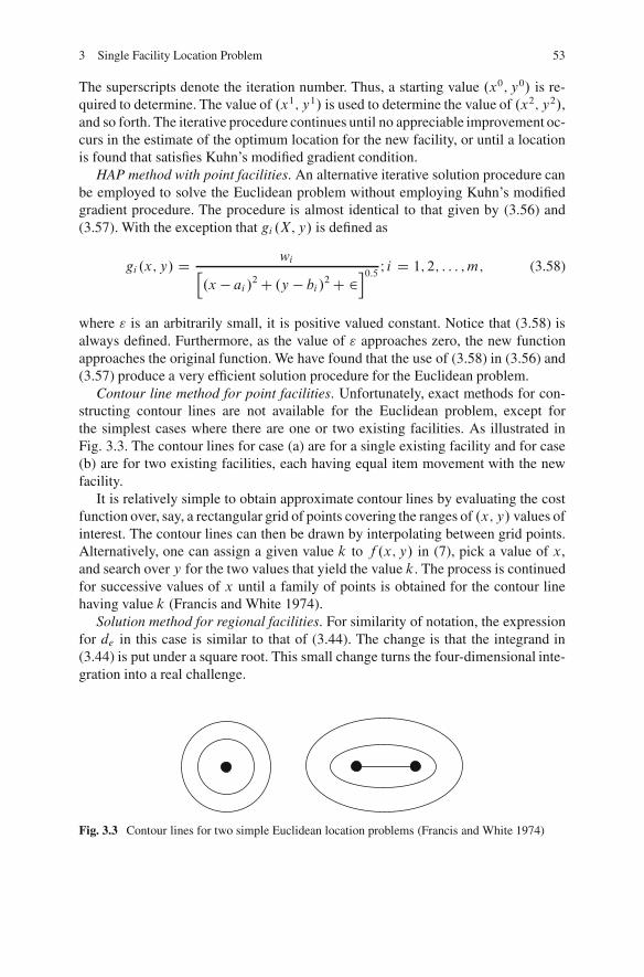
3 Single Facility Location Problem 53
The superscripts denote the iteration number. Thus, a starting value .x0; y0/ is re-quired to determine. The value of .x1; y1/ is used to determine the value of .x2; y2/,and so forth. The iterative procedure continues until no appreciable improvement oc-curs in the estimate of the optimum location for the new facility, or until a locationis found that satisfies Kuhn’s modified gradient condition.
HAP method with point facilities. An alternative iterative solution procedure canbe employed to solve the Euclidean problem without employing Kuhn’s modifiedgradient procedure. The procedure is almost identical to that given by (3.56) and(3.57). With the exception that gi .X; y/ is defined as
gi .x; y/ D wih.x � ai /2 C .y � bi /
2 C 2i0:5 I i D 1; 2; : : : ; m; (3.58)
where " is an arbitrarily small, it is positive valued constant. Notice that (3.58) isalways defined. Furthermore, as the value of " approaches zero, the new functionapproaches the original function. We have found that the use of (3.58) in (3.56) and(3.57) produce a very efficient solution procedure for the Euclidean problem.
Contour line method for point facilities. Unfortunately, exact methods for con-structing contour lines are not available for the Euclidean problem, except forthe simplest cases where there are one or two existing facilities. As illustrated inFig. 3.3. The contour lines for case (a) are for a single existing facility and for case(b) are for two existing facilities, each having equal item movement with the newfacility.
It is relatively simple to obtain approximate contour lines by evaluating the costfunction over, say, a rectangular grid of points covering the ranges of .x; y/ values ofinterest. The contour lines can then be drawn by interpolating between grid points.Alternatively, one can assign a given value k to f .x; y/ in (7), pick a value of x,and search over y for the two values that yield the value k. The process is continuedfor successive values of x until a family of points is obtained for the contour linehaving value k (Francis and White 1974).
Solution method for regional facilities. For similarity of notation, the expressionfor de in this case is similar to that of (3.44). The change is that the integrand in(3.44) is put under a square root. This small change turns the four-dimensional inte-gration into a real challenge.
Fig. 3.3 Contour lines for two simple Euclidean location problems (Francis and White 1974)
54 E. Moradi and M. Bidkhori
First calculate an approximation for d2 for a large d , i.e., d R; R. let I bethe integrand. Then
I 2 D .d C y cos � � x cos /2 C .y sin � � x sin /2: (3.59)
With appropriate integrand, we have
d2e Š d2 C R2 C r2
4C .R2 C r2/2
64d2: (3.60)
And if the last term is ignored (since d is large), then (3.60) is similar to (3.45).Therefore, for a large d ,
de Špd2 C .R2 C r2/=4: (3.61)
Is a good approximation of de. Note that the approximation (3.60) is not defined ford D 0 and tat it is far off for a small d , while de turns out to be quite accurate forsmall d , also.
The exact calculation of de is long and tedious. You can see the summarized ofexact calculation of de in Drezner (1986).
The goodness of the approximation of de to de was checked in Drezner (1986),the ratio between the two was calculated. The ratio de=de was found to be between0.75 (for r D d D 0) and 1 (for large d and any r).
Finally, it was checked the goodness of the approximation:
dA Drd2 C 4
9.R2 C r2/: (3.62)
The number 4/9 was chosen so that dA D de for r D d D 0. It was found thatde � dA � 1:07de, which is a better approximation than de.
The point facilities location problem in two regions with different norms. Supposethe plane is divided by a straight line into two regions with different norms. Wefind the location of a single new facility such that the sum of the distances fromthe existing facilities to this point is minimized. This is a non-convex optimizationproblem. We have the optimal solution lies in the rectangular hull of the existingpoints.
Suppose the plane, R2, is divided by a straight line, y D mx, into two region,�1, with an lP1, and �2 with an lP2 norm .p1; p2 � 1/. Suppose also that there arerespectively, n1 and n2 points on each side. The problem is to find the location ofa new point such that the sum of the weighted distances from the existing n1 C n2points to this is minimized. Mathematically the problem can be stated as
p1 W minx
( Xpi 2�1
wi d.x; pi /CXpi 2�2
wi d.x; pi /
); (3.63)
3 Single Facility Location Problem 55
where d.x; pi / is the shortest distance, induced by the norms, between the existingpoint pi D .ai ; bi /, and the new point x D .x; y/I wi ’s > 0 are given weightsassigned to the pi ’s. when x and pi are both on the same side of the dividing line,then the problem reduces to a single norm problem; for the l1 and l2; d.x; pi / is therectilinear or Euclidean distances between them. The difficulty arises when x andpi are on different sides of the boundary line.
We consider the special case of l1 and l2 with the boundary line y D mx. Notethat without loss of generality we assume that the line passes through the origin.There are also make the more realistic assumption that for the points on the �1 side,the shortest distance may involve passing through the boundary.
Model properties. There are some properties of the problem for the special case ofl1 and l2 norms. We have a fixed point p 2 �2, an x 2 �1, and a fixed (straight) linesegment L of any orientation. Let
d.x; p/ D minz2l fk1.x; z/C k2.z; p/g ; (3.64)
where k1 and k2 are arbitrary norms. Then d is a convex function of X .There is a characterization of the crossing (gate) points on the boundary line and
the shortest path connecting two points on different sides of the line.Suppose R2 is divided by a straight line, y D mx, into two regions, �1 and �2,
whit l1, and l2 norms, respectively. Assume, without loss of generality, that m > 0.Then for any pair of given points p1 D .a1; b1/ 2 �1 and p2 D .a1; b1/ 2 �2the shortest path form p1 to p2 passes through the line segment connecting points.a1; m a1/ and .b1=m; b1/ on the boundary line.
The intersection of the shortest path connecting points p1 2 �1 and p2 2 �2whit the boundary line y D mx .m > 0/ is either one of the points (a1;ma1) and.b1=m; b1/, or the point .x; mx/, with x given above, if a1 � x � b1=m.
There is optimal solution to the overall problem in the rectangular hull of theexisting points. The rectangular hull of a set of points is defined as the smallestrectangle with sides parallel to the (x and y axes) containing the set.
Solution procedure. Big square small square (BSSS) method is a geometrical branchand bound algorithm.
The procedure start with the rectangular hull,R, of the existing points, it containsthe optimal solution then we partitionR into four rectangles by drawing vertical andhorizontal lines through the middle of its sides. At partitioning level k, denote theserectangles by Rk1; Rk2; RK3, and, Rk4. We take the points at the center of eachrectangle and evaluate the objective at these points. The best solution provides anupper bound for the overall problem.
The distance between points inside a rectangle is taken to be zero. The distancebetween a point pi outside a rectangle R and the point inside that rectangle is takento be the distance between pi and the closest point to it on the boundary of R whichcould either be a corner point ofR, or the projection of pi ontoR. note that since Ris closed and convex, such a point indeed exists.
56 E. Moradi and M. Bidkhori
A sub-square for which the lower bound exceeds the value of the best knownsolution is fathomed. The process continues until the larger side of the sub-rectangleis less than a given tolerance, ". The steps of the algorithm are outlined below. Theinput to the algorithm is a set of existing points, and the termination tolerance ".The output is the optimal location of the new facility, Xb, and the optimal objectivevalue, fb .
Algorithm
1. Find the rectangular hull of existing facilities, R; set L D 0; fb D 1; and letd� D max fx�
max xmin; y�
max yming;2. Set l D lC1, and partitionR into four equal sub-rectanglesRl;1; Rl;2; Rl;3; Rl;4.
Calculate the objective value flr at the midpoint of each sub-rectangle. If minrfflrg< fb , update fb to this value.
3. For each demand point pi find the minimum distance dir from pi to Rl;r ;
r D 1; : : : ; 4; lbl;r D Pi wi dir. If lbL;r > fb , fathom RL;r and set lbL;r D 1.
4. Set l 0b D minrflbL;r g and r 0 D argminrflbL;r g. If l 0b D 1, go to step(6); else,if (0.5)L d� < " go to step (5); else, set R D RL;r 0 : fathom RL;r 0 and setRL;r 0 D 1, and go to step (2).
5. If lb0 < fb , set fb D l 0b, define Xb as the center of sub-rectangle RL;r 0 , andfathom this rectangle.
6. Set L D L � 1; if L D 0 go to step (7); else, if unfathomed sub-rectangles atlevel L are found, choose the one with the most favorable lb; donet it as R, andreturn to step (2); else, repeat step (6).
7. Terminate the algorithm with optimal new facility location Xb having the objec-tive function value fb (Zaferanieh et al. 2008).
3.2.2.4 MiniSum LP-Norm Distance (Francis et al. 1992)
Weiszfeld procedures. The Weiszfeld procedure depends upon the convexity of theEuclidean metric, and thus, utilizes the first order necessary and sufficient condi-tions. Since it is impossible to express the unknown variables x1 and x2 in closedform equations, the first order derivatives cannot be solved directly. Instead, an itera-tion function is obtained by using these derivatives. In order to eliminate the obviousdifficulty caused by the discontinuities in the derivatives, we use an approximationof the lp-norm in the objective function. We employ the following hyperbolic ap-proximation of the lp-norm.
Nlp.u; v/ D�.u1 � v1/
2 C 2p=2C.u2 � v2/
2 C 2p=2�1=p
;where p � 0;2> 0:(3.65)
We use the notation Qs.X/ to denote the objective functions of the approximatedlp-norm for single facility location problem.
3 Single Facility Location Problem 57
xkC1t D
nPjD1
wj�xkt � ajt
�2 C 2.p=2/�1 � Nlp �xk; aj ��1�p ajt
nPjD1
wj�xkt � ajt
�2 C 2.p=2/�1 � Nlp �xk; aj ��1�p ; t D 1; 2 : (3.66)
It should be noted that in order to deal with a well-formulated problem, we assumethat all new facilities are chained. New facility i is chained if there exists a positivew1ij where j is any existing facility or if there exists a positive w1ij where r is anychained new facility (Uster and Love 2001).
In addition, the convergence of the Weiszfeld algorithm is discussed in Uster andLove (2000).
Bounding method. The Weiszfeld procedure is basically an iterative steepest-descent algorithm with a predetermined step size. Therefore, to terminate theiterative procedure, a stopping rule or a bound for the best objective function value isrequired. The rectangular bound at iteration is obtained by solving a rectangular dis-tance location problem. The bound problem involves locating the same number offacilities in the original problem with respect to the existing facility locations withnewly created weights. At iterations, the percent difference between the optimumobjective function value of the rectangular bound problem and the current objectivefunction value of the original problem is calculated. If this difference is smaller thana termination value that prespecified by the user, the procedure is terminated (Usterand Love 2001). A rectangular bound for the iterative can be obtained by using theHolder inequality given by
NXiD1
j˛iˇi j �
NXiD1
j˛i jp!1=p NX
iD1jˇi jq
!1=q; (3.67)
where ˛ and ˇ are N-dimensional vectors, p > 1 and 1=p C 1=q D 1. TakingN D 2 for the planar location model and letting
˛1 D�x1 � aj1
�2 C 21=2
; (3.68)
ˇ1 D�xk1 � aj1
�2 C 2.p�1/=2
; (3.69)
˛2 D�x2 � aj2
�2 C 21=2
; (3.70)
ˇ2 D�xk2 � aj2
�2 C 2.p�1/=2
: (3.71)
We obtain
˛1ˇ1 C ˛2ˇ2 � ..˛1/p C .˛2/
p/1=p ..ˇ1/q C .ˇ2/
q/1=q: (3.72)
58 E. Moradi and M. Bidkhori
Rearranging terms, we have
Nlp.x; aj /��
xk1 � aj1�2 C 2
p=2 C�xk2 � aj2
�2 C 2p=2�1=q � ˛1ˇ1 C ˛2ˇ2:
(3.73)
Rewriting the second term on the left-hand side, we obtain
Nlp.x; aj /� Nlp �xk; aj ��p�1 � ˛1ˇ1 C ˛2ˇ2: (3.74)
In order to obtain the cost function of the minimum model, we multiply both sidesby wj and sum for j D 1; : : : ; n. Thus, we have
S.X/ DnX
jD1wi lp.x; aj / �
nXjD1
wi˛1ˇ1
.lp.xk; ai //p�1 CnX
jD1wi
˛2ˇ2
.lp.xk; ai //p�1 :
(3.75)
Minimizing both sides of the inequality over x gives
S.x�/ � minx
8<:
nXjD1
wi˛1ˇ1
.lp.xk; ai //p�1 CnX
jD1wi
˛2ˇ2
.lp.xk; ai //p�1
9=; : (3.76)
Without changing the direction of the inequality, the terms ˛1 and ˛2 can be sim-plified as jx1 � ˛j1j and jx2 � ˛j2j, respectively. Thus, the bound as a rectangulardistance problem, QS BK (X), is found as
�S B
K.xR/ D minxR
2
nXjD1
ujˇxR1 � aj1
ˇC minxR
2
nXjD1
ujˇxR1 � aj1
ˇ; (3.77)
where
uj D wjˇ1
. Qlp.xk; aj //p�1 and vj D wjˇ2
. Qlp.xk; aj //p�1 ; j D 1; : : : ; n:
(3.78)
For notational convenience, we denote the solution of a rectangular distance locationproblem by xR , and thus, the bound at an iteration k is given by QS BK .xR�/. LetQsj .X/; j D 1; : : : ; n, denote the terms in Qs.X/. Then the first derivatives of Qsj .X/with respect to x1 and x2 are
@ QSj .x/@x1
D wj
�x1 � aj1
�2 C 2.p�1/=2
. Qlp.xk; aj //p�1
�.x1 � aj1/
˛1
�: (3.79)
3 Single Facility Location Problem 59
And
@ QSj .x/@x2
D wj
�x2 � aj2
�2 C 2.p�1/=2
. Qlp.xk; aj //p�1
�.x2 � aj2/
˛2
�; j D 1; : : : ; n:
(3.80)
By letting e ! 0 and using the equality .xt � ˛jt / D sign.xt � ˛jt /jxt � ˛jt j, fort D 1; 2, we can simplify the last terms and obtain
@ QSj .x/@x1
D wj
�x1 � aj1
�2 C 2.p�1/=2
. Qlp.xk; aj //p�1 sign.x1 � aj1/; (3.81)
And
@ QSj .x/@x2
D wj
�x2 � aj2
�2 C 2.p�1/=2
. Qlp.xk; aj //p�1 sign.x2 � aj2/; j D 1; : : : ; n: (3.82)
Thus, uj and vj can be rewritten as
uj Dˇˇ@ QSj .xk/
@x1
ˇˇ and vj D
ˇˇ@ QSj .xk/
@x2
ˇˇ ; j D 1; : : : ; n: (3.83)
3.2.2.5 MiniMax Problems
There is another class of single facility location problems that we should mention,called MiniMax problems. One of the best known such problems, called the circlecovering problem, involves enclosing m known points in the plane within a circleof minimum radius. The circle covering problem is equivalent to the problem oflocating a new facility with respect to m existing facilities so as to minimize themaximum Euclidean distance from the new facility to the existing facilities. Thecircle covering problem may be of interest in locating a transmitter of some kind,or a receiver, so as to “cover” m stations with as strong signal strength as possible.Also, the problem of stationing a helicopter so as to minimize the maximum timefor it to respond to an emergency at anyone of m sites is closely related to the circlecovering problem. Contrary to what one might think, the circle covering problemcannot be solved by inspection (or at least no one has yet been able to do so). Thereare, however, very efficient and relatively simple algorithms for solving the problem.
If we draw a circle about each of the m points of radius r . The intersection of them circles. Consists of all points whose maximum Euclidean distance to them givenpoints is r or less. If we imagine reducing r until the intersection of the circlesis a single point, we obtain the solution to the circle covering problem. Such anapproach is now quite feasible when one has a computer terminal with the facilityfor displaying circles, provided that m is not too large.
60 E. Moradi and M. Bidkhori
Another problem, which we might term the diamond covering problem, occurwhen we replace the Euclidean distances of the circle covering problem by recti-linear distances. Here by “diamond” we mean a square with each edge making anangle of ˙45ı with an axis; the radius of the diamond is half the length of the linesegment joining opposite vertices. The diamond covering problem is easy to solveby applying a 45ı rotation we obtain an equivalent square covering problem whichwe solve by constructing a smallest enclosing rectangle. If the rectangle is square,its center is a MiniMax location. Otherwise, we extend the shortest of a pair of edgesto have the same length as the longer pair, and take the center of a square so con-structed as a MiniMax location. Of course, we must apply a revel 45ı rotation totranslate our answer back to a solution of the original problem in some cases therewill be more than one smallest enclosing diamond, resulting in alternative optimumlocations. As with the circle covering problem, it is easy construct contour sets. Theset of all points such that the maximum rectilinear distance between the points andthe m existing facilities is at most r consists of t intersection of m diamonds, withdiamond i having a center at point i and a radius of r , for i D 1; : : : ; m. Much thesame comments apply to these contour sets as made above for the circle coveringproblem.
Circle covering problem. In this section we consider two approaches for solving thecircle covering problem.The first approach is basically geometrical in nature and isparticularly well suited for planar circle covering problems. The second approach ismore general, in the sense that it can be used not only for planar problems but foranalogous problems in three or more dimensions. For the first approach we presentan algorithm. For the second approach we show how to convert the problem intoan equivalent quadratic programming problem. Most available algorithms for solv-ing quadratic programming can then be applied to solve the equivalent problem.Let, first state the problem of interest precisely. We wish to minimize the functiong.x; y/ defined by
g.x; y/ D maxfŒ.x � ai /2 C .y � bi /
21=2 W 1 � i � mg: (3.84)
Here, as usual, the points .ai ; bi / arem existing facility locations, and .x; y/ is a newfacility to be located in such a way as to minimize g.x; y/. A problem equivalent tominimizing g.x; y/ is as follows:
Min Z (3.85)
Subject toŒ.x � ai /
2 C .y � bi /21=2 � Z; 1 � i � m: (3.86)
The equivalent problem has the following geometrical interpretation. The con-straints state that each existing facility location must lie in a circle with center .x; y/and radius z, so that the geometrical problem is to find a smallest circles that enclosesall the existing facility locations.
3 Single Facility Location Problem 61
We now consider briefly an algebraic approach to the circle covering problemwhich is valid in any number of dimensions. WithX and Pi denoting the location ofthe new facility and existing facility i , respectively, the Euclidean distance betweenthe two locations is the square root of the following term (where the superscriptdenotes the transpose operation):
.x � pi/T .x � pi /: (3.87)
Hence an equitant version of the circle covering problem is as follows:
Min u (3.88)
Subject to.x � pi /T .x � pi/ � u; i D 1; : : : ; m: (3.89)
Because.x � pi/
T .x � pi / D xT x � 2pTi X C PTI pi : (3.90)
An equivalent way to write the constraints is as follows:
xT x � 2pTi X C PTI pi � u; i D 1; : : : ; m: (3.91)
But now if we make the following change of variables,
v D xT x � u: (3.92)
We obtain the following equivalent version of the problem:
Min xT x � u: (3.93)
Subject to2pTi x � v � pTi PI ; i D 1; : : : ; m (3.94)
The latter problem is a quadratic programming problem with a convex objectivefunction and linear constraints, and thus is solvable by most quadratic programmingalgorithms.
MiniMax location problems with rectilinear distances. The problem we considernow is one of finding a new facility location that will minimize the followingfunction:
g.x; y/ D maxfWiŒjx � ai j C jy � bi jC hi W 1 � i � mg: (3.95)
As a possible example of the problem, suppose that .x; y/ is the location of a “con-venience” center and that “users” of the center are located at the existing’ facilitylocations, the points .ai ; bi / through .am; bm/. User i require a time of hi to prepareto go to the center and then travels to the center at a time per unit distance of wi , so
62 E. Moradi and M. Bidkhori
that wi Œjx � ai j C jy � bi jC hi is the total time to prepare to go to the center andthen go there. The center is to be located so that the maximum such time for anyuser will be minimized.
An alternative but equivalent formulation of the problem of minimizing g.x; y/is the following one:
Min z (3.96)
Subject toWI Œjx � ai j C jy � bi jC hi � z; i D 1; : : : ; m: (3.97)
Because all the weights are positive, we can also write the problem as follows:
Min z (3.98)
Subject to
jx � ai j C jy � bi j � z � hi
wi; i D 1; : : : ; m (3.99)
The constraints of the latter formulation state that the existing facility location.ai ; bi / is to be in a diamond with center .x; y/ and radius .z � hi /=wi fori D 1; : : : ; m. Let us denote the problem with all unit weights and all zero ad-dends by UP, which represents “unweighed problem.” Similarly, we let WPA denotethe weighted problem with some nonzero addends, and we let UPA denote the un-weighed problem with some nonzero addends. For UP, the simplest problem, weconclude that the problem is one of finding a diamond of minimum radius that willcontain all the existing facility locations. We now give an approach to solve the moregeneral problem UPA. This approach is based on the fact inequality.
jx � ai j C jy � bi j � ri � z � hi : (3.100)
Equivalent is to the following four inequalities:
x � ai C y � bi � ri ; (3.101)
x � ai � y C bi � ri ; (3.102)
�x C ai � y C bi � ri ; (3.103)
�x C ai C y � bi � ri : (3.104)
We can use this fact to transform UPA to a linear program which can be solved asfollows. Compute the following numbers:
c1 D minfai C bi � hi W i D 1; : : : ; mg; (3.105)
c2 D minfai C bi C hi W i D 1; : : : ; mg; (3.106)
c3 D minf�ai C bi � hi W i D 1; : : : ; mg; (3.107)
c4 D minf�ai C bi C hi W i D 1; : : : ; mg; (3.108)
c5 D minfc2 � c1; c4 � c3g: (3.109)
3 Single Facility Location Problem 63
The minimum objective function value is c5=2, and the MiniMax locations are thelocations on the line segment L joining the following two points:
�x�1 ; y
�1
� D 1
2.c1 � c3; c1 C c3 C c5/; (3.110)
�x�2 ; y
�2
� D 1
2.c2 � c4; c2 C c4 � c5/: (3.111)
Consider the construction of level lines for the function g.x; y/ of the problemWPA. To construct level lines we construct level sets; the boundaries of the levelsets are the level lines. Level lines are of interest for exactly the same reasons wediscussed earlier for the MiniSum problems; they allow us to evaluate easily locationother than the optimal locations [those that minimize the function g.x; y/]. Let usdenote a level set of g.x; y/ of boundary value Z by S.z/, so that S.z/ D f.x; y/ Wg.x; y/ � zg. We construct S.z/ as follows. Given a value of Z of interest, we firstcompute the following numbers:
c1.z/ D min
�ai C bi C z � hi
wiW i D 1; : : : ; m
; (3.112)
c2.z/ D min
�ai C bi C �z C hi
wiW i D 1; : : : ; m
; (3.113)
c3.z/ D min
��ai C bi C z � hi
wiW i D 1; : : : ; m
; (3.114)
c4.z/ D min
��ai C bi C �z C hi
wiW i D 1; : : : ; m
: (3.115)
The level S.z/ is then as follows:
S.z/ D f.x; y/ W c2.z/ � x C y � c1.z/; c4.z/ � �x C y � c3.z/g: (3.116)
If at least one of the inequalities c2.z/ � c1.z/; c4.z/ � c3.z/ does not hold, youhave chosen a value ofZ that is smaller than the minimum value of g.x; y/ and thelevel set will be empty; thus you mast pick another value ofZ which is large enoughso that both of inequalities hold. Supposing the level set to be nonempty, you shouldbe able to see that the level set is a rectangle, with two parallel sides making aC45ıangle with the x axis and the other two parallel sides making a � 45ı angle withthe x axis. The vertices of the level set, starting at the top corner and proceedingclockwise, are as follows:
v1.z/ D 1
2.c1.z/� c3.z/; c1.z/C c3.z//; (3.117)
v2.z/ D 1
2.c1.z/� c4.z/; c1.z/C c4.z//; (3.118)
64 E. Moradi and M. Bidkhori
v3.z/ D 1
2.c2.z/� c4.z/; c2.z/C c4.z//; (3.119)
v4.z/ D 1
2.c2.z/� c3.z/; c2.z/C c3.z//: (3.120)
Hence you can plot a level set of value Z by first choosing Z, computing c1.z/through c1.z/, checking to be sure that the inequalities c2.z/ � c1.z/; c4.z/ � c3.z/,are satisfied by the Z you have chosen, computing v1.z/ through v4.z/ and plot-ting the four points, and then constructing lines joining v1.z/ and v2.z/; v2.z/ andv3.z/; v3.z/ and v4.z/; v4.z/ and v1.z/. The rectangle the lines enclose is the levelset of value Z, and its boundary is the level lines of value Z.
MiniMax problems with Tchebychev and rectilinear distances. In Sect. 3.2.2.4 wesaw that the diamond covering problem could be interpreted, given a 45ı rotation,as a square covering problem, and that this interpretation led to a simple solutionprocedure for the diamond covering problem. What we do now is to exploit thisdiscovery in a systematic way. As a result, we will obtain an efficient means ofsolving WAP, the MiniMax weighted rectilinear distance problem with addends.
Consider two points X and Y in the plane. Suppose that X and Y are the end-points of the hypotenuse H of a right triangle, with the other two sides of thetriangle, denoted by A and B , being parallel to the horizontal and vertical axes, re-spectively. We have seen earlier that the length of the hypotenuseH is the Euclideandistance betweenX and Y , while the sum of the lengths of sides A and B is the rec-tilinear distance between X and Y . We now introduce a new distance, called theTchebychev distance between X and Y , defined to be the maximum of the lengthsof sides A and B . In other words, if A is longer than B , then A is the Tchebychevdistance between X and Y , while if A is not longer than B , then B is the Tcheby-chev distance between X and Y . We denote the Tchebychev distance between Xand Y by t.X; V /. Thus if X D .X1; X2/, and Y D .Y1; Y2/, then
t.X; Y / D maxfjx1 � y1j ; jx2 � y2jg: (3.121)
What does a contour set of Tchebychev distance look like? Consider the set of allpoints X whose Tchebychev distance from the origin is at most 1, that is, the 1set of all points X D .X1;X2/ satisfying t.x; 0/ � 1, or, equivalently, satisfyingmax fjX1jjX2j � 1g. The latter inequality is equivalent to jX1j � 1 and jX2j � 1.But these last two inequalities are in turn equivalent to
�1 � x1 � 1 and � 1 � x2 � 1: (3.122)
Hence the set of all pointsX whose Tchebychev distance from the origin is at most1 is a square with its center at the origin and each side of length 2. This square isthe Tchebychev analog of a circle with center at the origin and radius 1 and theTchebychev analog (for rectilinear distance) of a diamond with center at the originand radius 1. Of course, if we rotate a diamond by 45ı, we obtain a square, a resultthat should give you a good clue about the relationship between Tchebychev, andrectilinear distances.
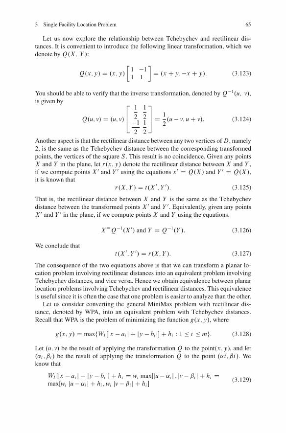
3 Single Facility Location Problem 65
Let us now explore the relationship between Tchebychev and rectilinear dis-tances. It is convenient to introduce the following linear transformation, which wedenote by Q.X; Y /:
Q.x; y/ D .x; y/
�1 �11 1
�D .x C y;�x C y/: (3.123)
You should be able to verify that the inverse transformation, denoted by Q�1.u; v/,is given by
Q.u; v/ D .u; v/
2641
2
1
2�12
1
2
375 D 1
2.u � v; u C v/: (3.124)
Another aspect is that the rectilinear distance between any two vertices ofD, namely2, is the same as the Tchebychev distance between the corresponding transformedpoints, the vertices of the square S . This result is no coincidence. Given any pointsX and Y in the plane, let r.x; y/ denote the rectilinear distance between X and Y ,if we compute points X 0 and Y 0 using the equations x0 D Q.X/ and Y 0 D Q.X/,it is known that
r.X; Y / D t.X 0; Y 0/: (3.125)
That is, the rectilinear distance between X and Y is the same as the Tchebychevdistance between the transformed points X 0 and Y 0. Equivalently, given any pointsX 0 and Y 0 in the plane, if we compute pointsX and Y using the equations.
XDQ�1.X 0/ and Y D Q�1.Y /: (3.126)
We conclude thatt.X 0; Y 0/ D r.X; Y /: (3.127)
The consequence of the two equations above is that we can transform a planar lo-cation problem involving rectilinear distances into an equivalent problem involvingTchebychev distances, and vice versa. Hence we obtain equivalence between planarlocation problems involving Tchebychev and rectilinear distances. This equivalenceis useful since it is often the case that one problem is easier to analyze than the other.
Let us consider converting the general MiniMax problem with rectilinear dis-tance, denoted by WPA, into an equivalent problem with Tchebychev distances.Recall that WPA is the problem of minimizing the function g.x; y/, where
g.x; y/ D maxfWI Œjx � ai j C jy � bi jC hi W 1 � i � mg: (3.128)
Let .u; v/ be the result of applying the transformation Q to the point(x; y), and let.˛i ; ˇi / be the result of applying the transformation Q to the point .˛i; ˇi/. Weknow that
WI Œjx � ai j C jy � bi jC hi D wi maxŒju � ˛i j ; jv � ˇi j C hi DmaxŒwi ju � ˛i j C hi ;wi jv � ˇi j C hi
(3.129)
66 E. Moradi and M. Bidkhori
We can thus conclude that
g.x; y/ D maxfmaxŒwI Œju � ˛i jChi ;wiCjv � ˇi jChi W i D 1; : : : ; mg: (3.130)
Suppose that we know define the function g1.u/ and g2.u/ as follows:
g1.u/ D maxfwI ju � ˛i j C hi W i D 1; : : : ; mg; (3.131)
g2.u/ D maxfwI jv � ˇi j C hi W i D 1; : : : ; mg: (3.132)
It then follows that
maxfmaxŒwI ju � ˛i j C hi ;wi jv � ˇi j C hi W i D 1; : : : ; mg Dmaxfg1.u/; g2.u/g: (3.133)
The reason for the latter equality is that regardless of the order in which we computethe maximum of a collection of numbers, we obtain the same result.
If you examine the latter equation, you can see that the term on the left is thesame as the term on the right in our most recent equation for g.x; y/; hence weobtain a very useful result as follows: Given
.u; v/ D Q.x; y/: (3.134)
We haveg.x; y/ D maxfg1.u/; g2.u/g: (3.135)
The consequence of our result is that we can minimize g.x; y/ by solving two inde-pendent minimization problems as follows:
1. We minimize g1.u/ and obtain a minimizing point, say u.2. Next, we minimize g2.u/ and obtain a minimizing point, say v.3. We can then apply the inverse transformation to .u�; v�/ to obtain a point, say.x�; y�/, and conclude that .x�; y�/ minimizes g.x; y/.
4. Further, the minimum value of g.x; y/ is equal to max fg1.u�/; g2.u�/g (Franciset al. 1992).
3.3 Case Study (Heragu 1997)
We now present a relocation project undertaken by a small facility. A small manu-facturing company currently located in a university “tech park” has witnessed majorgrowth since introducing an innovative technology into the marketplace. Its ownernow wants to find a new location and build a bigger facility. In January she hiredsenior industrial and management engineering (IME) students at the university toinvestigate several potential locations and select the one that best suits her needs.
3 Single Facility Location Problem 67
The student group adopted the following five step approach, which is based on thehybrid analysis discussed earlier.
� Step 1. Determination of requirements: The students conducted interviews withthe owner and facility manager to determine these company specific requirementsfor the new facility:
– The company will relocate in New York or Vermont.– At least 15,000 ft of space is required.– A power source of three phase, 440 W, and 200 A electrical service is manda-
tory to power the atomizers used in the manufacturing process.– The current rent is $7.50 per square foot per year; the company wants to pay
between $3.50 and $4.50 per square foot.– The company wants to move within the next 8 months.– All suppliers and vendors should be within 100 miles of the facility.– A lease of 1–2 years is preferred.– There should be adequate room for expansion.– An industrial park or shared facility is preferred.– The facility should be located close to major highways and airports.– A loading bay is required; easy access to the bay is desired.– The new facility should be built to suit.– The facility maintenance costs should be low or the owner of the building
must pay the maintenance and related expenses.– The general condition of the building should be good.– The building should not be considered high risk by insurance companies.– It is desirable to have secretarial services available nearby.– The local and state taxes must be reasonable.
� Step 2. Classification of location factors: Based on the interview with the owner,the IME students classified the requirements into three categories:
Critical factors
– Minimum space requirement– Three phase, 440W , 200A electrical service– Support service providers and vendors within 100 miles
Objective factors
– Rent– Space rented or leased– Maintenance and insurance costs and taxes
Subjective factors
– Shared facility– Build to suit– Condition of loading bay– Proximity to airport and major highways– Lease length
68 E. Moradi and M. Bidkhori
– Secretarial support– Condition of building
� Step 3. Data collection: This step requires the most time, but it is very importantand should be done carefully. Information on potential sites and locations wasobtained from sources such as these:
– Chamber of Commerce– Economic Development Council– Real estate brokers– Facility owners
� Step 4. Elimination of sites not meeting critical objectives and development ofa rating chart: From the ten sites for which data were collected, four did notsatisfy the first or the second critical requirement. For the remaining six sites,machine shops and other support service providers as well as vendors were within100 miles. The IME student group devised a chart showing the weights of theobjective and subjective factor.
� Step 5. Site visits and site evaluation: The students visited all six sites. Data andrated collected for the sites.
After careful evaluation, the six sites were rated on this evaluation; the Cohoes,New York, site appears to be the best location, with Bennington, Vermont, as a(close) second best location (Heragu 1997).
References
Drezner Z (1986) Location of regional facilities. Naval Res Logist Quart 33:523–529Francis Rl, White JA (1974) Facility layout and location: An analytical approach. Prentice Hall,
Englewood Cliffs, NJFrancis Rl, McGinnis LF, White JA (1992) Facility layout and location: An analytical approach.
Prentice Hall, Englewood Cliffs, NJHeragu SS (1997) Facilities design. PWS publishing company, a division of International Thomson
Publishing Inc. BostonUster H, Love RF (2000) The convergence of the Weiszfeld algorithm. Management
Science/Information Systems AreaUster H, Love RF (2001) A generalization of the rectangular bounding method for continuous
location models. Comput Math Appl 44:181–191Zaferanieh M, Taghizadeh KH, Brimberg J, Wesolowsky GO (2008) A BSSS algorithm for the sin-
gle facility location problem in two regions with different norms. Eur J Oper Res 190(1):79–89
Chapter 4Multifacility Location Problem
Farzaneh Daneshzand and Razieh Shoeleh
In the previous chapter, we studied the case of a single new facility to be locatedrelative to a number of existing facilities. In this chapter we consider the problemof optimally locating more than one new facilities with respect to locations of anumber of existing facilities (demand points), the locations of which are known.
While the problems are natural extension of those of single facility location, thereare two important conditions:
1. At least two facilities are to be located2. Each new facility is linked to at least one other new facility
If the first condition contracted, this problem is considered as a single facility lo-cation problem (SFLP) and if the second condition contracted, we can consider theproblem as some of independent single facility location problems. Thus the SFLPcan be considered as a spatial case of the multifacility location problem (MFLP).
4.1 Applications and Classifications
As it is expected, applications of MFLPs occur in the same contexts as discussedin the chapter “Single Facility Location Problem” by Esmaeel Moradi and MortezaBidkhori, this volume for SFLP. Ostresh (1977) represented some applications ofthe MFLP as follows:
1. A system of warehouses is to be established to serve a set of predeterminedregions.
2. Industrial and commercial establishments tend to be more concentrated than ex-pected on the basis of minimizing transport costs alone.
3. In large organizations (such as the Federal government) face to face communica-tion must take place between adjacent (usually) levels of the hierarchy.
R.Z. Farahani and M. Hekmatfar (eds.), Facility Location: Concepts, Models, 69Algorithms and Case Studies, Contributions to Management Science,DOI 10.1007/978-3-7908-2151-2 4, c� Physica-Verlag Heidelberg 2009
70 F. Daneshzand and R. Shoeleh
A classification of different types of MFLP and their properties is shown in thefollowing statement:
� Area solution: discrete, continual� The space in which facilities are located: planer location, sphere location� Objective function: MiniMax, MiniSum� Type of the distance: rectangular distance, Euclidean distance, squared Euclidean
distance, lp distance� Parameters: stochastic, deterministic� How facilities are assumed: point, region
Researchers have worked on a variety of MFLPs. However no research has beenconducted on many types of MFLPs resulted from multiplying the above items.
4.2 Models
In this section we introduce MFLP models represented and developed as mathemat-ical models.
4.2.1 MiniSum
The MiniSum multifacility location problem consisting of finding locations of newfacilities which will minimize a total cost function consists of a sum of costs di-rectly proportional to the distances between the new facilities, and costs directlyproportional to the distances between new and existing facilities.
The general-model for this problem can be stated as follows:
4.2.1.1 Model Assumptions
The assumptions of this model are as follows:
� The area solution is continual� The space in which facilities are located is planer� The objective function is MiniSum� Type of the distance can be either rectangular, Euclidean, squared Euclidean orlp distance
� Parameters are deterministic� Facilities are assumed as points
4 Multifacility Location Problem 71
4.2.1.2 Model Inputs
Model inputs of this model are:
n: Number of new facilitiesm: Number of existing facilitieswij : Nonnegative weight between new facility i and existing facility j by a unitdistancevik : Nonnegative weight between new facilities i and k by a unit distanced.Xj ; Pi /: Distance between the location of new facility j and existing facility id.Xj ;Xk/: Distance between the location of new facilities j and kPj W .aj ; bj / The location coordinates of existing facility j
4.2.1.3 Model Output (Decision Variable)
Model output of this model is:
Xi W .xi ; yi / The location coordinates of new facility i
4.2.1.4 Objective Function
MinX
1�j<k�nvjk:d.Xj ; Xk/ C
nXjD1
mXiD1
wji:d.Xj ; Pi /: (4.1)
Thus each of the m new facilities is to be located with respect to the n existingfacilities and also with respect to the other new facilities. The location of Xj maydepend on the location of some point Xk because of the terms involving vjk. Forconvenience in the presentation, we assume all the wji and all the vjk are positive.
Notice that it is the cost proportional to the distance between new facilities whichdistinguish the MFLP from SFLP. In fact, when terms vji are zero then (4.1) may bewritten as
MinnX
jD1
mXiD1
wji:d.Xj ; Pi /: (4.2)
And (4.2) just defines a one-facility total cost expression. So that (4.2) is the sum ofn different one-facility cost expression and may be written as
MinnX
jD1
Min
mXiD1
wji:d.Xj ; Pi /
!: (4.3)
Since the location of one new facility has no effect upon the cost of locating othernew facilities for the special case where all vij are zero, locations of new facilitiesmay be found by solving n SFLP independently.
72 F. Daneshzand and R. Shoeleh
4.2.1.5 Rectangular Distance MiniSum Location Problem
In this section, we consider MFLP when we have rectangular distance. The objec-tive of this problem is minimization of the weighted sum of the rectangular distancebetween the locations of new facilities and new and existing facilities. For formu-lation of this problem if in (4.1) we replace the d.Xj ; Pi / and d.Xj ;Xk/ by (4.4)and (4.5) The Rectangular MFLP problem can be formulated as (4.6) this problemis of added interest since it will be shown that its optimal solution can be used tocompute both a lower and an upper bound for the value of the optimal solution tothe Euclidean problem.
d.Xj ; Xk/ D ˇxj � xk
ˇC ˇyj � yk
ˇ; (4.4)
d.Xj ; Pi / D ˇxj � ai
ˇC ˇyj � bi
ˇ; (4.5)
MinX
1�j<k�nvjk�ˇxj � xk
ˇC ˇyj � yk
ˇ�
CnX
jD1
mXiD1
wji�ˇxj � ai
ˇC ˇyj � bi
ˇ�: (4.6)
The objective function is converted into two minimum problems:
Min f D Min f1.x/C Min f2.x/: (4.7)
where:
f1.X/ DX
1�j<k�nvjk
ˇxj � xk
ˇCnX
jD1
mXiD1
wji
ˇxj � ai
ˇ; (4.8)
f2.Y / DX
1�j<k�nvjk
ˇyj � yk
ˇCnX
jD1
mXiD1
wji
ˇyj � bi
ˇ: (4.9)
Just like single facility location case in the chapter “Single Facility Location Prob-lem” by Esmaeel Moradi and Morteza Bidkhori, this volume, optimum x coordinateof new facilities can be found independent from optimum y coordinates. As yousee the objective function is nonlinear and we should make it linear. The methodof linearization is very similar to the method we used in single facility location inthe chapter “Single Facility Location Problem” by Esmaeel Moradi and MortezaBidkhori, this volume.
Linearization
Given numbers a, b, p and q,If
a � b � p C q D 0;
p: q D 0;
p � 0; q � 0:
4 Multifacility Location Problem 73
Thenja � bj D p C q:
So minimizing the objective function is equivalent to the following problem:
MinX
1�j<k�nvjk.pjk C qjk/C
nXjD1
mXiD1
wji.rji C sji/; (4.10)
Subject to
xj � xk � pjk C qjk D 0 1 � j < k � n; (4.11)
xj � rji C sji D ai i D 1; : : : ; m; j D 1; : : : ; n; (4.12)
pjk; qjk � 0 1 � j < k � n; (4.13)
rji; sji � 0 i D 1; : : : ; m; j D 1; : : : ; n; (4.14)
pjkqjk D 0 1 � j < k � n; (4.15)
rji:sji D 0 i D 1; : : : ; m; j D 1; : : : ; n; (4.16)
xj unrestricted; j D 1; 2; : : : ; n: (4.17)
As in the single facility location for any basic feasible solution, if pjk is in the basicfeasible solution, qjk will not be and vice versa. Likewise, if rji is in the basic feasiblesolution, sji will not be and vice versa. Since variables not in the basic feasiblesolution are zero, the multiplicative constraints will be therefore satisfied for everyfeasible solution. Minimizing f2 is the same as what was done for f1.
4.2.1.6 Squared Euclidean Distance MiniSum Location Problem
In this section, we consider MFLP when we have squared Euclidean distance. Theobjective of this problem is minimization of the weighted sum of the square of theEuclidean distance between the locations of new facilities and new and existingfacilities. The problem considered in this section is also referred to as a “quadraticfacility location problem” and the “gravity problem”.
Although there aren’t too many situations where there are physical reasons forusing squared Euclidean distance, there are at least two reasons for the gravityproblem. First, in some cases the solution to the gravity problem can be usedto approximate the solution to the location problem where costs increase linearlywith Euclidean distance. Second, there exist location problems where costs increasequadratically with the Euclidean distance between facilities.
For formulation of this problem if in (4.1) we replace the d.Xj , Pi/ andd.Xj ;Xk/ by (4.18) and (4.19) the squared Euclidean MFLP problem can formulateas (4.20)
d.Xj ;Xk/ D .xj � xk/2 C .yj � yk/
2; (4.18)
74 F. Daneshzand and R. Shoeleh
d.Xj ;Xi / D .xj � ai /2 C .yj � bi /2; (4.19)
Minf DX
1�j<k�nvjk:
�.xj � xk/
2 C .yj � yk/2�
CnX
jD1
mXiD1
wji:�.xj � ai /2 C .yj � bi/
2�: (4.20)
4.2.1.7 Contour Lines for Squared Euclidean MFLP
In MFLP construction of contour lines is possible expect for certain special casewhen n D 2. In this section we want to observe the property of contour lines forsquared Euclidean MFLP
Let f .x; y/ given in (4.20) be written as f .x; y/ D f .x/C f .y/ where
f .x/ DX
1�j<k�nvjk.xj � xk/
2 CnX
jD1
mXiD1
wji.xj � ai /2: (4.21)
And
f .y/ DX
1�j<k�nvjk.yj � yk/
2 CnX
jD1
mXiD1
wji.yj � bi /2: (4.22)
If n D 2, contour lines for f .x/ are concentric ellipses centered on (x�; y�/ andcontour lines for f .y/ are concentric ellipses centered on (x�; y�/
Because of the squared Euclidean MFLP is separable and symmetric in x and y,only f .x/ is considered and contour line is defined as the set of all points (x1; x2/for which
k D v12.x1 � x2/CmXiD1
w1i .x1 � ai /2 CmXiD1
w1i .x2 � ai /2: (4.23)
And k is a constant denoting the value of the contour line. By expanding and col-lecting terms it is seen that (4.23) can be expressed in the form of a general conicsection:
Ax21 C Bx1x2 C Cx22 CDx1 C Ex2 C F D 0; (4.24)
where
A D v12 CmXiD1
w1i ;
B D �2v12;
C D v12 CmXiD1
w2i ;
4 Multifacility Location Problem 75
D D �2mXiD1
w1iai ;
E D �2mXiD1
w2i ai ;
D DmXiD1
w1i a2i C
mXiD1
w2ia2i � k:
A sufficient condition given by Thomas (1968) for (4.24) to be an ellipse is for thediscriminate, B2 � 4AC , to be negative. Direct substitution gives
B2�4AC D 4v212�4v212�4v12
mXiD1
w1iCmXiD1
w2i
!�4
mXiD1
w1i
! mXiD1
w2i
!< 0:
(4.25)
Assuming the problem is well formulated (4.24) is the equation for a rotated ellipseas noted by the presence of the x1x2 term. Due to symmetry a similar result is foundfor the y variables. Furthermore, by definition of a contour line since k achieves itssmallest value at (x�
1 ; x�2 / the contour line is centered on the optimum location with
respect to the nonrotated axes (Eyster and White 1973).
4.2.1.8 Euclidean Distance MiniSum Location Problem
The Euclidean multifacility location problem often assumes that the transportationcosts from the new facility to a demand point are proportional to the Euclideandistance between these points, with the factor of proportionality (weight) dependingon the demand point.
Here, this problem is mathematically formulated:
MinP
1�j<k�nvjk:
�.xj � xk/
2 C .yj � yk/2�1=2
CnP
jD1
mPiD1
wji:�.xj � ai /2 C .yj � bi/
2�1=2: (4.26)
It is interesting to note that when all the existing facility locations are collinear, thatis, all lie on a single line, the Euclidean model essentially includes the rectilineardistance model.
4.2.2 MiniMax
Minimization of a sum of weighted distances that was introduced in Sect. 4.1.1 maynot be a proper goal when the facilities to be located must provide services of an
76 F. Daneshzand and R. Shoeleh
urgent nature. Therefore in this section we introduce some multifacility locationproblems with MiniMax objective function and by different type of distances.
4.2.2.1 Model Assumptions
Model assumptions of this model are as follows:
� The area solution is continual� The space in which facilities are located is planer� The objective function is MiniMax� Type of the distance can be either rectangular, Euclidean, squared Euclidean orlp distance
� Parameters are deterministic� Facilities are assumed as points
4.2.2.2 Model Inputs
We have all the inputs in previous model.
4.2.2.3 Model Outputs (Decision Variables)
The outputs of this model are similar to the previous model.
4.2.2.4 Objective Function
Min f D Maxf vjk:d.Xj ; Xk/;wji:d.Xj ; Pi /g: (4.27)
4.2.2.5 Rectangular Distance MiniMax Location Problem
The problem considered is that of locating n new facilities among m existing facil-ities with the objective of minimizing the maximum weighed Rectangular distanceamong all facilities.
Minf D Max˚wji
ˇxj � ai
ˇC ˇyj � bi
ˇj D 1; : : : ; n; i D 1; : : : ; mI
vjk
ˇxj � xk
ˇC ˇyj � yk
ˇ1 � j < k < n
�: (4.28)
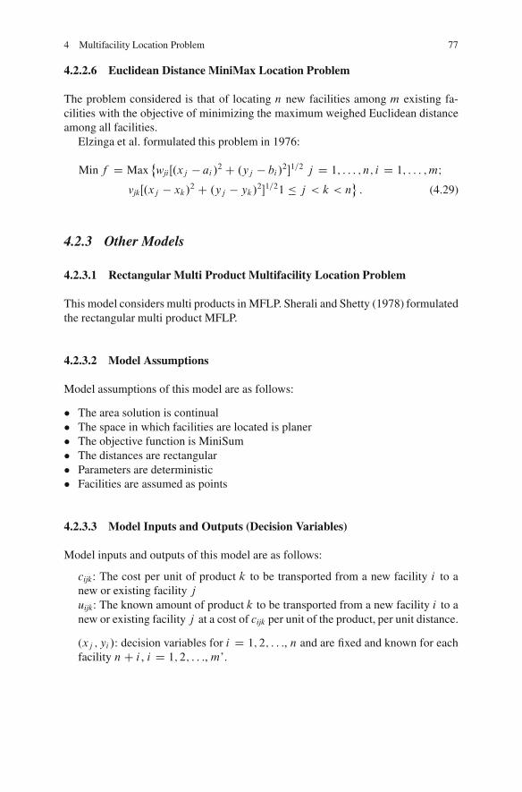
4 Multifacility Location Problem 77
4.2.2.6 Euclidean Distance MiniMax Location Problem
The problem considered is that of locating n new facilities among m existing fa-cilities with the objective of minimizing the maximum weighed Euclidean distanceamong all facilities.
Elzinga et al. formulated this problem in 1976:
Minf D Max˚wjiŒ.xj � ai /2 C .yj � bi/
21=2 j D 1; : : : ; n; i D 1; : : : ; mIvjkŒ.xj � xk/
2 C .yj � yk/21=21 � j < k < n
�: (4.29)
4.2.3 Other Models
4.2.3.1 Rectangular Multi Product Multifacility Location Problem
This model considers multi products in MFLP. Sherali and Shetty (1978) formulatedthe rectangular multi product MFLP.
4.2.3.2 Model Assumptions
Model assumptions of this model are as follows:
� The area solution is continual� The space in which facilities are located is planer� The objective function is MiniSum� The distances are rectangular� Parameters are deterministic� Facilities are assumed as points
4.2.3.3 Model Inputs and Outputs (Decision Variables)
Model inputs and outputs of this model are as follows:
cijk: The cost per unit of product k to be transported from a new facility i to anew or existing facility juijk: The known amount of product k to be transported from a new facility i to anew or existing facility j at a cost of cijk per unit of the product, per unit distance.
(xj ; yi /: decision variables for i D 1; 2; : : :, n and are fixed and known for eachfacility nC i , i D 1; 2; : : :, m’.
78 F. Daneshzand and R. Shoeleh
4.2.3.4 Objective Function
The objective function of this model and its related constraints are as follows:
MinpXkD1
nXiD1
nCm0XjD1
cijkuijk˚ˇxi � xj
ˇC ˇyi � yj
ˇ�: (4.30)
The objective function may be written as:
MinpXkD1
nXiD1
wij˚ˇxi � xj
ˇC ˇyi � yj
ˇ�; (4.31)
wij DpXkD1
.cijkuijk C cjikujik/ j D nC 1; : : : ; nCm0: (4.32)
4.2.3.5 Multifacility Location Problem on Sphere
As it is known, one of the assumptions when locating facilities is concerned withthe size of the area covering the destinations (or the demand points). If the areacovering the demand points is sufficiently small, then this part of the earth’s surfacecan be approximated by a plane. When the destination points are widely separated,the area covering these points can no longer be approximated by a plane and theformulations we discussed so far is not suitable.
Problems concerning location of international headquarters, distribution/marketing centers, detection station placement, and placement of radio transmittersfor long range communication may fall into this category.
The location problem on a sphere is more complicated than its counterpart on theplane, because unlike on plane the solution space is not convex on sphere.
Dhar and Rao (1982) formulated this problem. Any point on the sphere can bedefined by its latitude ��=2 � ˚ � �=2 and longitude �� � � � and dij is theshortest distance between points i and j .
4.2.3.6 Model Assumptions
Model assumptions of this model are as follows:
� The area solution is continual� The space in which facilities are located is on sphere� The objective function is MiniSum� Parameters are deterministic� Facilities are assumed as points� The distance is defined as
dij D Arc cosŒcos˚i cos˚j cos.i � j /C sin˚i sin˚j : (4.33)
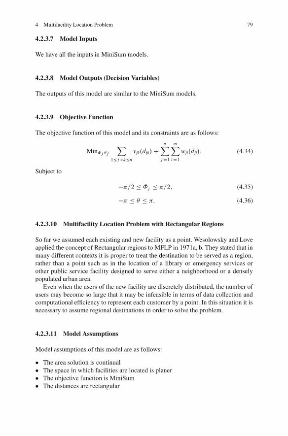
4 Multifacility Location Problem 79
4.2.3.7 Model Inputs
We have all the inputs in MiniSum models.
4.2.3.8 Model Outputs (Decision Variables)
The outputs of this model are similar to the MiniSum models.
4.2.3.9 Objective Function
The objective function of this model and its constraints are as follows:
Min˚j j
X1�j<k�n
vjk.djk/CnX
jD1
mXiD1
wji.dji/: (4.34)
Subject to
��=2 � ˚j � �=2; (4.35)
�� � � �: (4.36)
4.2.3.10 Multifacility Location Problem with Rectangular Regions
So far we assumed each existing and new facility as a point. Wesolowsky and Loveapplied the concept of Rectangular regions to MFLP in 1971a, b. They stated that inmany different contexts it is proper to treat the destination to be served as a region,rather than a point such as in the location of a library or emergency services orother public service facility designed to serve either a neighborhood or a denselypopulated urban area.
Even when the users of the new facility are discretely distributed, the number ofusers may become so large that it may be infeasible in terms of data collection andcomputational efficiency to represent each customer by a point. In this situation it isnecessary to assume regional destinations in order to solve the problem.
4.2.3.11 Model Assumptions
Model assumptions of this model are as follows:
� The area solution is continual� The space in which facilities are located is planer� The objective function is MiniSum� The distances are rectangular
80 F. Daneshzand and R. Shoeleh
� Parameters are deterministic� Facilities are assumed as regions
4.2.3.12 Model Inputs
We have all the inputs in MiniSum models in addition to the following inputs:Ri D �
ai1 ; ai2�
Rectangular region i , where ai1 < ai2 and bi1 < bi2Ai : The area of Ri
4.2.3.13 Model Outputs (Decision Variables)
The outputs of this model are similar to MiniSum models.
4.2.3.14 Objective Function
The objective function of this model and its constraints are as follows:
MinnX
jD1
mXiD1
wij
Ai
ZRi
Z �ˇxj � ai
ˇC ˇyj � bi
ˇ�daidbi
CX
i�j<k�nvjk�ˇxj � xk
ˇC ˇyj � yk
ˇ�: (4.37)
4.2.3.15 Stochastic Multifacility Location Problem
In many cases the parameters of the model are not deterministic. This model isrepresented and solved by Seppalla (1975). In order to define a stochastic decisionmodel, we should first determine the stochastic parameters, how they are distributed,whether they are correlated, and which decision criterion will be used in industrialapplications. The set of stochastic elements of planning models are often restrictedto consist only of demands for products, while other parameters or variables, suchas unit costs, capacities and locations, are considered to be fixed.
4.2.3.16 Model Assumptions
Model assumptions of this model are as follows:
� The area solution is continual� The space in which facilities are located is planer� The objective function is MiniSum� The distances are Euclidean
4 Multifacility Location Problem 81
� Parameters are stochastic� Facilities are assumed as points� The weights vjk, wji for all i; j and k are normally distributed random variables
4.2.3.17 Model Inputs
The inputs of this model are similar to the MiniSum model in addition to the fol-lowing:
˛: is a predetermined probabilityı: is an assistingP f.g: is a probability operator
4.2.3.18 Model Outputs (Decision Variables)
The output of this model is similar to the MiniSum model.
4.2.3.19 Objective Function
The objective function of this model and its constraints are as follows:
Min ı: (4.38)
Subject to
P
8<:
X1�j<k�n
vjk:�.xj � xk/
2 C .yj � yk/2�1=2
CnX
jD1
mXiD1
wji:�.xj � ai /2 C .yj � bi/
2�1=2 � ı
9=; � ˛: (4.39)
4.3 Solution Techniques
4.3.1 MiniSum
4.3.1.1 Rectangular Distance MiniSum Location Problem
The rectangular distance multifacility location problem always has a minimum costsolution where the x coordinate of each new facility is equal to the x coordinate ofsome existing facility and the same is true for y coordinate (Francis et al. 1992).
82 F. Daneshzand and R. Shoeleh
If we call p1 the linear programming problem obtained in (4.10) a straight for-ward linear programming of p1 can be time consuming when a large number of newand existing facilities are involved.
Depending on the characteristics of a particular multifacility Rectangular loca-tion problem, the optimum solution can be sometimes obtained in an iterative modeby solving some single facility location problems. Also, a dual formulation of thelinear programming problem (p1) can provide more efficient solution to the rectan-gular MFLP (Francis et al. 1992).
� Francis (1964) solved a special case of the MFLP, with rectilinear distance whenthe weights are equal.
� Cabot et al. (1970) decomposed the location problem into two independent sub-problems, each of which is equivalent to a linear programming problem whichis essentially the dual of a minimal cost network flow problem. The dual vari-ables in each of the optimum tableaus to the two flow problems give the x and ycoordinates respectively of the optimum locations of the new facilities.
� Pritsker and Ghare (1970) suggested a gradient technique for this problem. Thebasic contribution of them was a derivation of necessary conditions for an optimalsolution and an algorithm for obtaining optimal solutions to the decomposedproblems.
� Rao (1973) considered a direct search approach to the RMFLP in detail, howeverhe demonstrated that the gradient technique was basically a primal simplex-basedlinear programming approach, and in the presence of degeneracy, the optimalityconditions were not sufficient. A necessary condition for optimality to be suffi-cient in special cases and the main difficulties associated with the direct searchapproach were discussed.
� Wesolowsky and Love (1971a, b) and Morris (1975) showed that the problemwith linear locational constraints could be solved by linear programming.
� A thorough set of necessary and sufficient optimality conditions were developedby Juel and Love (1976).
� Idrissi et al. (1989) developed a dual problem for the constrained multifacilityminisum location problems involving mixed norms. General optimality condi-tions were obtained providing new algorithms which are decomposition methodsbased on the concept of partial inverse of a multifunction.
� A nonlinear approximation method was developed by Wesolowsky and Love(1972), where any number of linear and (or) nonlinear constraints defining aconvex feasible region can be included.
� The hyperboloid approximation procedure for solving the perturbed rectilineardistance MFLP was also proposed by Eyster et al. (1973).
� Morris (1975) used the dual problem of Rectangular MFLP and then reduced it toa problem with substantially fewer variables and constraints. He stated that linearand pairwise constraints limiting distances between new points and between newand existing points can be imposed to restrict the location of new points.
� Picard and Ratliff (1978) solved the problem via at most (m � 1) minimum cutproblems on derived networks containing at most (n � 2) vertices. They showed
4 Multifacility Location Problem 83
that the optimum location of new facilities is dependent on the relative orderingsof old facilities but not on the distances between them.
� Subsequently, Kolen (1981) exhibited the equivalence of the method of Sheraliand Shetty and Picard and Ratliff. The main difference between these two proce-dures was principally in the computational implementation. Moreover, this typeof approach is known to be the most effective way of solving the rectilinear dis-tance MFLP.
� A modified version of the method of Picard and Ratliff (1978) was proposed byCheung (1980).
� Dax (1986) presented a new method that, as he stated, handles efficiently therectilinear distance Problem MFLP having large clusters, i.e. where several newfacilities are located together at one point. This paper states and proves a new nec-essary and sufficient optimality condition. This condition transforms the problemof computing a descent direction into a constrained linear least-squares prob-lem. The latter problem is solved by a relaxation method that takes advantageof its special structure. The new technique is incorporated into the direct searchmethod.
� As an alternative to linear programming, a simple approach which sometimesfinds optimal locations was presented by (Francis et al. 1992) as coordinate de-scent. By deleting the term that shows the relationship between new facilities inobjective function, the problem is converted to some single facility location prob-lems to which we can apply median conditions. The first coordinate we chooseis the first variable and the second coordinate is the second variable, and so on. Itis continued until we obtain the same vector by coordinate descent that we haveobtained previously by coordinate descent, at which point we stop.
� Allen (1995) developed a dual-based lower bound to the multifacility `p distancelocation problem and he stated that the bound is as good or better than otherbounds.
4.3.1.2 Squared Euclidean Distance MiniSum Location Problem
In this problem, it is obvious that the function that is to be minimized is strictly con-vex, and unlike the Euclidean distance case, it has continuous first partial derivativeswith respect to x and y.
Consequently the optimal solution is unique and the approach to finding optimalsolution is the same for the SFLP; partial derivation of (4.20) with respect to eachvariable are computed and set to equal to zero.
The result of the partial derivation computation is two sets of line equation oninvolving the x coordinate (and y coordinate) of the new facilities.
To compute the partial derivations, it is convenient to define a new quantity Ovikwhere
Ovik D�
vij k > j
vkj k � j: (4.40)
84 F. Daneshzand and R. Shoeleh
Computing the partial derivation of (4.21) with respect to xi and (4.22) with respectto yi gives, for j D 1; : : :; n,
@f
@xjD 2
nXkD1
Ovik.xj � xk/C 2
mXiD1
wji.xj � ai /: (4.41)
And@f
@yjD 2
nXkD1
Ovik.yj � yk/C 2
mXiD1
wji.yj � bi /: (4.42)
If we set the (4.41) and (4.42) to zero and solve it, the optimum values of the x andy coordinates for the new facilities are related by the following expressions:
xj D
nPkD1
Ovikxk CmPiD1
wjiai
nPkD1
Ovik CmPiD1
wji
: (4.43)
And
yj D
nPkD1
Ovikyk CmPiD1
wjibi
nPkD1
Ovik CmPiD1
wji
: (4.44)
Furthermore, White (1971) established that the optimum solution to the multifacilityproblem is given by
x� D A�1Wa: (4.45)
and
y� D A�1W b; (4.46)
where x� and y� are n 1 column vectors giving the optimum coordinate locationsfor the new facilities, a and b arem1 column vectors giving the x and y coordinatelocations, respectively, for the existing facilities W is an n m matrix containingthe weights wij , and A is an n n nonsingular matrix given as follows:
A D
266666666664
nPkD1
Ov1k CPi
w1i �Ov12 : : : : �Ov1n
�Ov21nP
kD1Ov2k CP
i
w2i : : : �Ov2n:
:
:
:
:
:
:
:
�Ovn1 �Ovn2 : : : :nP
kD1Ovnk CP
i
wni
377777777775: (4.47)
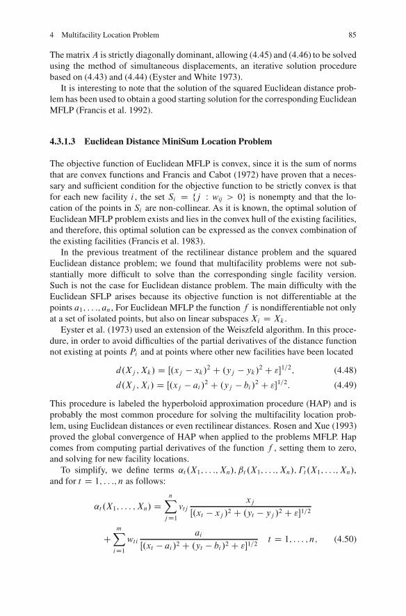
4 Multifacility Location Problem 85
The matrixA is strictly diagonally dominant, allowing (4.45) and (4.46) to be solvedusing the method of simultaneous displacements, an iterative solution procedurebased on (4.43) and (4.44) (Eyster and White 1973).
It is interesting to note that the solution of the squared Euclidean distance prob-lem has been used to obtain a good starting solution for the corresponding EuclideanMFLP (Francis et al. 1992).
4.3.1.3 Euclidean Distance MiniSum Location Problem
The objective function of Euclidean MFLP is convex, since it is the sum of normsthat are convex functions and Francis and Cabot (1972) have proven that a neces-sary and sufficient condition for the objective function to be strictly convex is thatfor each new facility i , the set Si D fj W wij > 0g is nonempty and that the lo-cation of the points in Si are non-collinear. As it is known, the optimal solution ofEuclidean MFLP problem exists and lies in the convex hull of the existing facilities,and therefore, this optimal solution can be expressed as the convex combination ofthe existing facilities (Francis et al. 1983).
In the previous treatment of the rectilinear distance problem and the squaredEuclidean distance problem; we found that multifacility problems were not sub-stantially more difficult to solve than the corresponding single facility version.Such is not the case for Euclidean distance problem. The main difficulty with theEuclidean SFLP arises because its objective function is not differentiable at thepoints a1; : : :; an, For Euclidean MFLP the function f is nondifferentiable not onlyat a set of isolated points, but also on linear subspaces Xi D Xk.
Eyster et al. (1973) used an extension of the Weiszfeld algorithm. In this proce-dure, in order to avoid difficulties of the partial derivatives of the distance functionnot existing at points Pi and at points where other new facilities have been located
d.Xj ;Xk/ D Œ.xj � xk/2 C .yj � yk/2 C "1=2; (4.48)
d.Xj ;Xi / D Œ.xj � ai /2 C .yj � bi /2 C "1=2: (4.49)
This procedure is labeled the hyperboloid approximation procedure (HAP) and isprobably the most common procedure for solving the multifacility location prob-lem, using Euclidean distances or even rectilinear distances. Rosen and Xue (1993)proved the global convergence of HAP when applied to the problems MFLP. Hapcomes from computing partial derivatives of the function f , setting them to zero,and solving for new facility locations.
To simplify, we define terms ˛t .X1; : : :; Xn/; ˇt .X1; : : :; Xn/; �t .X1; : : :; Xn/,and for t D 1; : : :; n as follows:
˛t .X1; : : : ; Xn/ DnX
jD1vtj
xj
Œ.xt � xj /2 C .yt � yj /2 C "1=2
CmXiD1
wt iai
Œ.xt � ai /2 C .yt � bi /2 C "1=2t D 1; : : : ; n; (4.50)
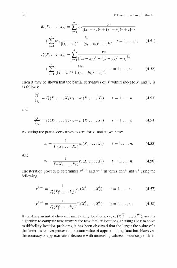
86 F. Daneshzand and R. Shoeleh
ˇt .X1; : : : ; Xn/ DnX
jD1vtj
yj
Œ.xt � xj /2 C .yt � yj /2 C "1=2
CmXiD1
wt ibi
Œ.xt � ai /2 C .yt � bi /2 C "1=2t D 1; : : : ; n; (4.51)
�t.X1; : : : ; Xn/ DnX
jD1
vij
Œ.xt � xj /2 C .yt � yj /2 C "1=2
CmXiD1
wt i
Œ.xt � ai /2 C .yt � bi /2 C "1=2
t D 1; : : : ; n: (4.52)
Then it may be shown that the partial derivatives of f with respect to xt and yt isas follows:
@f
@xtD �t.X1; : : : ; Xn/xt � ˛t .X1; : : : ; Xn/ t D 1; : : : ; n; (4.53)
and
@f
@ytD �t .X1; : : : ; Xn/yt � ˇt .X1; : : : ; Xn/ t D 1; : : : ; n: (4.54)
By setting the partial derivatives to zero for x1 and y1 we have:
xt D 1
�t .X1; : : : ; Xn/˛t .X1; : : : ; Xn/ t D 1; : : : ; n: (4.55)
And
yt D 1
�t .X1; : : : ; Xn/ˇt .X1; : : : ; Xn/ t D 1; : : : ; n: (4.56)
The iteration procedure determines xkC1 and ykC1in terms of xk and yk using thefollowing:
xkC1t D 1
�t.Xk1 ; : : : ; X
kn /˛t .X
k1 ; : : : ; X
kn / t D 1; : : : ; n; (4.57)
ykC1t D 1
�t .Xk1 ; : : : ; X
kn /ˇt .X
k1 ; : : : ; X
kn / t D 1; : : : ; n: (4.58)
By making an initial choice of new facility locations, say ˛t .X.0/1 ; : : :; X
.0/n /, use the
algorithm to compute new answers for new facility locations. In using HAP to solvemultifacility location problems, it has been observed that the larger the value of ©the faster the convergences to optimum value of approximating function. However,the accuracy of approximation decrease with increasing values of " consequently, in
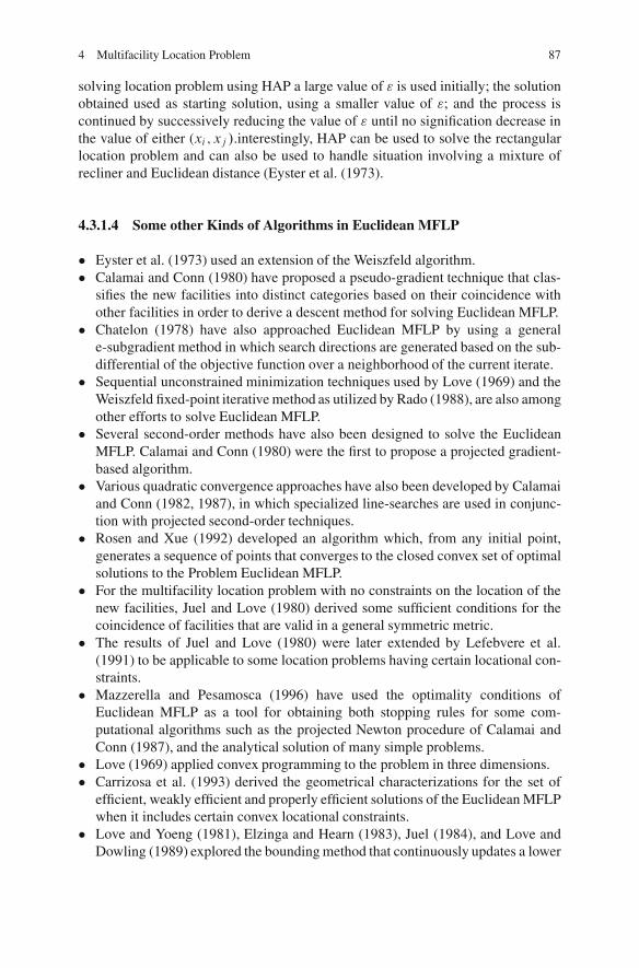
4 Multifacility Location Problem 87
solving location problem using HAP a large value of " is used initially; the solutionobtained used as starting solution, using a smaller value of "; and the process iscontinued by successively reducing the value of " until no signification decrease inthe value of either (xi ; xj /.interestingly, HAP can be used to solve the rectangularlocation problem and can also be used to handle situation involving a mixture ofrecliner and Euclidean distance (Eyster et al. (1973).
4.3.1.4 Some other Kinds of Algorithms in Euclidean MFLP
� Eyster et al. (1973) used an extension of the Weiszfeld algorithm.� Calamai and Conn (1980) have proposed a pseudo-gradient technique that clas-
sifies the new facilities into distinct categories based on their coincidence withother facilities in order to derive a descent method for solving Euclidean MFLP.
� Chatelon (1978) have also approached Euclidean MFLP by using a generale-subgradient method in which search directions are generated based on the sub-differential of the objective function over a neighborhood of the current iterate.
� Sequential unconstrained minimization techniques used by Love (1969) and theWeiszfeld fixed-point iterative method as utilized by Rado (1988), are also amongother efforts to solve Euclidean MFLP.
� Several second-order methods have also been designed to solve the EuclideanMFLP. Calamai and Conn (1980) were the first to propose a projected gradient-based algorithm.
� Various quadratic convergence approaches have also been developed by Calamaiand Conn (1982, 1987), in which specialized line-searches are used in conjunc-tion with projected second-order techniques.
� Rosen and Xue (1992) developed an algorithm which, from any initial point,generates a sequence of points that converges to the closed convex set of optimalsolutions to the Problem Euclidean MFLP.
� For the multifacility location problem with no constraints on the location of thenew facilities, Juel and Love (1980) derived some sufficient conditions for thecoincidence of facilities that are valid in a general symmetric metric.
� The results of Juel and Love (1980) were later extended by Lefebvere et al.(1991) to be applicable to some location problems having certain locational con-straints.
� Mazzerella and Pesamosca (1996) have used the optimality conditions ofEuclidean MFLP as a tool for obtaining both stopping rules for some com-putational algorithms such as the projected Newton procedure of Calamai andConn (1987), and the analytical solution of many simple problems.
� Love (1969) applied convex programming to the problem in three dimensions.� Carrizosa et al. (1993) derived the geometrical characterizations for the set of
efficient, weakly efficient and properly efficient solutions of the Euclidean MFLPwhen it includes certain convex locational constraints.
� Love and Yoeng (1981), Elzinga and Hearn (1983), Juel (1984), and Love andDowling (1989) explored the bounding method that continuously updates a lower
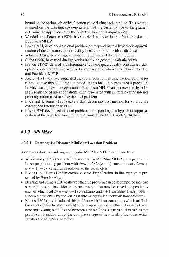
88 F. Daneshzand and R. Shoeleh
bound on the optimal objective function value during each iteration. This methodis based on the idea that the convex hull and the current value of the gradientdetermine an upper bound on the objective function’s improvement.
� Wendell and Petersen (1984) have derived a lower bound from the dual toEuclidean MFLP.
� Love (1974) developed the dual problem corresponding to a hyperbolic approxi-mation of the constrained multifacility location problem with lp distances.
� White (1976) gave a Varignon frame interpretation of the dual problem.� Sinha (1966) have used duality results involving general quadratic forms.� Francis (1972) derived a differentiable, convex quadratically constrained dual
optimization problem, and achieved several useful relationships between the dualand Euclidean MFLP.
� Xue et al. (1996) have suggested the use of polynomial-time interior point algo-rithm to solve this dual problem based on this idea, they presented a procedurein which an approximate optimum to Euclidean MFLP can be recovered by solv-ing a sequence of linear equations, each associated with an iterate of the interiorpoint algorithm used to solve the dual problem.
� Love and Kraemer (1973) gave a dual decomposition method for solving theconstrained Euclidean MFLP.
� Love (1974) developed the dual problem corresponding to a hyperbolic approxi-mation of the objective function for the constrained MFLP with lp distance.
4.3.2 MiniMax
4.3.2.1 Rectangular Distance MiniMax Location Problem
Some procedures for solving rectangular MiniMax MFLP are shown here:
� Wesolowsky (1972) converted the rectangular MiniMax MFLP into a parametriclinear programming problem with 5mn C 5=2n.n � 1/ constraints and 2mnCn.n � 1/C 2n variables in addition to the parameters.
� Elzinga and Hearn (1973) recognized some simplifications in linear program pre-sented by Wesolowsky.
� Dearing and Francis (1974) showed that the problem can be decomposed into twosub problems that have identical structures and that may be solved independentlyeach of which had 2mnCn.n�1/ constraints and nC1 variables. Each problemis solved efficiently by converting it into an equivalent network flow problem.
� Morris (1973) has introduced this problem with linear constraints which (a) limitthe new facilities location and (b) enforce upper bounds on the distances betweennew and existing facilities and between new facilities. He uses dual variables thatprovide information about the complete range of new facility locations whichsatisfies the MiniMax criterion.
4 Multifacility Location Problem 89
� Drezner and Wesolowsky (1978) presented a method involved the numerical in-tegration of ordinary differential equations and was computationally superior tomethods using nonlinear programming.
4.3.2.2 Euclidean Distance MiniMax Location Problem
The application of nonlinear duality theory shows Euclidean minimax MFLP canalways be solved by maximizing a continuously differentiable concave objectivesubject to a small number of linear constraints. This leads to a solution procedurewhich produces very good numerical results. Love et al. (1973) presented a non-linear programming method for computing the solution to MFLPs using Euclideandistances when the MiniMax criterion is to be satisfied.
4.3.3 Solution Techniques for other Models
In this section we introduce some solution techniques for the models shown inSect. 1.3
� A specialized simplex based-algorithm was derived by Sherali and Shetty (1978)for solving rectangular multiproduct MFLP.
� Dhar and Rao (1982) presented an iterative solution for MFLP on sphere.The procedure involved the approximation of the domain of objective functionwhich in the limit approaches to that of the original objective function. Aykinand Babu (1987) considered Euclidean, squared Euclidean and the great circledistances. They formulated an algorithm and investigated its convergence prop-erties.
� Wesolowsky and Love (1971a, b) considered the problem of MFLP with rectan-gular regions for the cases n D 1 or 2. They used a simple gradient reductiontechnique to solve the single facility problem. As they stated, the procedure be-comes very complex when n > 2. Aly and Marucheck (1982) stated that ifthere is interfacility interaction among the new facilities, a gradient-free non-linear search algorithm is utilized. Computational experience suggests that thisalgorithm is expedient even in the solution of large problems.
� Seppalla (1975) stated that in order to be able to solve the stochastic MFLP, wemust transform it into the deterministic equivalent forms.
4.3.4 Some Heuristic and Metaheuristic Methods
There are a few heuristics methods for solving MFLP:
� Vergin and Rogers (1967) introduced a simple heuristic for solving MFLP withEuclidean distance. This procedure locates each of new facilities in a temporary
90 F. Daneshzand and R. Shoeleh
location at each step and locates the next new facility according to the facilitieslocated so far. After all n new facilities are located in this manner the process isrepeated and the readjustment process is continued until no further movementsoccur during a complete round of adjustment evaluations.
� Davoud Pour and Nosraty (2006) solved the MFLP with ant-colony optimizationmetaheuristic when the distances are rectangular and Euclidian. This algorithmproduces optimal solutions for problem instances of up to 20 new facilities.
4.4 Case Study
Smallwood (1965) introduced a model for the placement of n detection stations soas to maximize the probability that at least one of them will detect any enemy eventoccurring within the area. This research was done within boundaries of USA andUSSR. The model is based on five assumptions that one of them is the assumptionof plane area that was made in order to allow the use of the relatively convenientCartesian coordinate system. Each of these assumptions can be relaxed to reducethe error of the model.
References
Allen WR (1995) An improved bound for the multifacility location model. Oper Res Lett17(4):175–180
Aly AA, Marucheck AS (1982) Generalized Weber problem with rectangular regions. J Oper ResSoc 33(11):983–989
Aykin T, Babu AJG (1987) Multifacility location problems on a sphere. Int J Math Math Sci10(3):583–596
Cabot AV, Francis RL, Stary MA (1970) A network flow solution to a rectilinear distance facilitylocation problem. AIIE Trans 2(2):132–141
Calamai PH, Charalambous C (1980) Solving multifacility location problem involving euclideandistances. Naval Res Logist Quart 27:609–620
Calamai PH, Conn AR (1980) A stable algorithm for solving the multifacility location probleminvolving euclidean distances. SIAM J Sci Stat Comput 1:512–525
Calamai PH, Conn AR (1982) A Second-order method for moving the continuous multifacilitylocation problem. In: Watson GA (ed) Numerical analysis: proceeding of the ninth bien-nial conference, Dundee, Scotland, Lecture Notes in Mathematics, vol 912. Springer, Berlin,pp 1–25
Calamai PH, Conn AR (1987) A projected Newton method for Lp norm location problems. MathProgram 38:75–109
Carrizosa E, Conde E, Fernandez FR, Puerto J (1993) Efficiency in euclidean constrained locationproblems. Oper Res Lett 14:291–295
Chatelon JA (1978) A subgradient algorithm for certain minimax and minisum Problems. MathProgram 15:130–145
Cheung To-Yat (1980) Multifacility location problem with rectilinear distance by the minimum-Cut approach. ACM Trans Math Softw 6(3):387–390
4 Multifacility Location Problem 91
Davoud Pour H, Nosraty M (2006) Solving the facility and layout and location problem by ant-colony optimization-metaheuristic. Int J Prod Res 44(23):5187–5196
Dax A (1986) An efficient algorithm for solving the rectilinear multifacility location problem. IMAJ Numer Anal 6:343–355
Dearing PM, Francis RL (1974) A network flow solution to a multifacility minimax location prob-lem involving rectangular distances. Transport Sci 9:126–141
Dhar UR, Rao JR (1982) domain approximation method for solving multifacility location problemson a sphere. J Oper Res Soc 33(7):639–645
Drezner Z, Wesolowsky GO (1978) A trajectory method for the optimization of the multifacilitylocation problem with distances. Manage Sci 24(14):1507–1514
Elzinga DJ, Hearn DW (1973) A note on a minimax location problem. Transport Sci 7:100–103.Elzinga DJ, Hearn DW (1983) On stopping rules for facilities location algorithm. AIIE Trans
15:81–82Elzinga DJ, Hearn DW, Randolph WR (1976) Minimax multifacility location with euclidean dis-
tances. Transport Sci 10(4):321–336Eyster JW, White JA (1973) Some properties of the squared euclidean distance location problem.
AIIE Trans 5(3):275–280Eyster JW, White JA, Wierwille WW (1973) On solving multifacility location problems using a
hyperboloid approximation procedure. AIIE Trans 5:1–6Francis RL (1964) On the location of multiple new facilities with respect to existing facilities. J Ind
Eng 15(2):106–107Francis RL, Cabot AV (1972) Properties of a multifacility location problem involving euclidean
distances. Naval Res Logist Quart 19:335–353Francis RL, McGinnis LF, White JA (1983) Locational analysis. Eur J Oper Res 12:220–252Francis RL, McGinnis LF, White JA (1992) Facility layout and location: an analytical approach,
2nd edn. Prentice Hall, Englewood Cliffs, NJIdrissi HO, Lefebvre, Michelot (1989) Duality constrained multifacility location problems with
mixed norms and applications. Ann Oper Res 18:71–92Juel H (1984) On a rational stopping rule for facilities location algorithms. Naval Res Logist Quart
31:9–11Juel H, Love RF (1976) An efficient computational procedure for solving the multifacility rectilin-
ear facilities location problem. Oper Res Quart 27(3):697–703Juel H, Love RF (1980) Sufficient conditions for optimal facility location to coincide. Transport
Sci 14:125–129Kolen A (1981) Equivalence between the direct search approach and the cut approach to the recti-
linear distance location problem. Oper Res 29(3):616–620Lefebvere O, Michelot C, Plastria F (1991) Sufficient conditions for coincidence in minisum mul-
tifacility location problem with a general metric. Oper Res 39(3):437–442Love RF (1969) Locating facilities in three-dimensional space by convex programming. Naval Res
Logist Quart 16(4):503–516Love RF (1972) A computational procedure for optimally locating a facility with respect to several
rectangular regions. J Region Sci 12(2):233–242Love RF (1974) The dual of a hyperbolic approximation to the generalized constrained multifacil-
ity location problem with lp distances. Manage Sci 21:22–33Love RF, Dowling PD (1989) A generalized bounding method for multifacility location models.
Oper Res 37(4):653–657Love RF, Kraemer S (1973) A dual decomposition method for minimizing transportation costs in
multifacility location problems. Transport Sci 7(4):297–316Love RF, Yoeng WY (1981) A stopping rule for facilities location algorithms. AIIE Trans
13:357–362Love RF, Wesolowsky GO, Kraemer SA (1973) A multifacility minimax location method for eu-
clidean distances. Int J Prod Res 11(1):37–45Mazzerella F, Pesamosca G (1996) The analytical solution of some EMFL minisum problems.
Isolde VII, June 25–July 3
92 F. Daneshzand and R. Shoeleh
Morris JG (1973) A linear programming approach to the solution of constrained multifacility min-imax location problems where distances are rectangular. Oper Res Quart 24:419–435
Morris JG (1975) Linear programming solution to the generalized rectangular distance weber prob-lem. Naval Res Logist Quart 22:155–164
Ostresh LM (1977) The multifacility location problem: applications and descent theorems.J Region Sci 17:409–419
Picard J, Ratliff HD (1978) A cut approach to the rectilinear distance facility location problem.Oper Res 26(3):422–433
Pritsker AAB, Ghare PM (1970) locating new facilities with respect to existing facilities. AIIETrans 2(4):290–297
Rado F (1988) The euclidean multifacility location Problem. Oper Res 36(3):485–492Rao MR (1973) On the direct search approach to the rectilinear facilities location problem. AIIE
Trans 5(3):256–264Rosen JB, Xue GL (1992) A globally convergent algorithm for solving the euclidean multifacility
location problem. Acta Math Appl Sin 8(4):357–366Rosen JB, Xue GL (1993) On the Convergence of a hyperboloid approximation procedure for the
perturbed euclidean multifacility location problem. Oper Res 41(6):1164–1171Seppalla Y (1975) On a Stochastic multifacility location problem. AIIE Trans 7(1):56–62Sherali HD, Shetty CM (1978) A primal simplex based solution procedure for the rectilinear dis-
tance multifacility location problem. J Oper Res Soc 29(4):373–381Sinha SM (1966) A duality theorem for nonlinear programming. Manage Sci 12:385–390Smallwood RD (1965) Minimal detection station placement. Oper Res 13(4):632–646Thomas GB (1968) Chlculus and analytic geometry. AddisonWesley, Reading, MAVergin RC, Rogers JD (1967) An algorithm and computational procedure for locating economic
facilities. Manage Sci 3(6):240–254Wendell RE, Petersen EL (1984) A dual approach for obtaining lower bounds to the weber prob-
lem. J Region Sci 24:219–228Wesolowsky GO (1972) Rectangular distance location under minimax optimality criterion. Trans-
port Sci 6:103–113Wesolowsky GO, Love RF (1971a) Location of facilities with rectangular distances among point
and area destinations. Naval Res Logist Quart 18:83–90Wesolowsky GO, Love RF (1971b) The optimal location of new facilities using rectangular dis-
tances. Oper Res 19(1):124–130Wesolowsky GO, Love RF (1972) A nonlinear approximation method for solving a generalized
rectangular distance weber problem. Manage Sci 18(11):656–663Wesolowsky GO, Truscott GW (1976) Dynamic location of multiple facilities for a class of con-
tinuous problems. AIIE Trans 8(1):76–83White DJ (1976) An analogue derivation of the dual of the general fermat problem. Manage Sci
23:92–94White JA (1971) A quadratic facility location problem. AIIE Trans 3(2):156–157Xue GL, Rosen JB, Pardalos PM (1996) A polynomial time dual algorithm for the euclidean mul-
tifacility location problem. Oper Res Lett 18:201–204
Chapter 5Location Allocation Problem
Zeinab Azarmand and Ensiyeh Neishabouri Jami
Location-allocation (LA) problem is to locate a set of new facilities such that thetransportation cost from facilities to customers is minimized and an optimal numberof facilities have to be placed in an area of interest in order to satisfy the customerdemand.
This problem occurs in many practical settings where facilities provide homoge-neous services such as the determination and location of warehouses, distributioncenters, communication centers and production facilities.
Since LA problem was proposed by Cooper (1963) and spread to a weightednetwork by Hakimi (1964), network LA problem and many models were presentedby Badri (1999).
For solving these models, numerous algorithms have been designed, involv-ing branch-and-bound algorithms (Kuenne and Soland 1972), simulated annealing(Murray and Church 1996) and Tabu search (Brimberg and Mladenovic 1996;Ohlemuller 1997) and P-Median plus Weber (Hansen et al. 1998). Some hybridalgorithms have been also suggested, such as the one based on simulated annealingand random descent method (Ernst and Krishnamoorthy 1999) and the one uti-lizing the Lagrange relaxation method and genetic algorithm (Gong et al. 1997).Brimberg et al. (2000) improved present algorithms and proposed variable neigh-borhood search, which is proved to obtain the best results when the number offacilities to locate is large.
5.1 Classification of Location-Allocation Problem
The basic components of location-allocation problems can be thought to consistof facilities, locations, and customers. The definitions and properties of these ba-sic components will be discussed in this part along with some different types oflocation-allocation models. The presentation provided in this part has been in-fluenced by the paper of Scaparra and Scutella (2001) which proposes a unifiedframework for characterizing the different aspects of location problems.
R.Z. Farahani and M. Hekmatfar (eds.), Facility Location: Concepts, Models, 93Algorithms and Case Studies, Contributions to Management Science,DOI 10.1007/978-3-7908-2151-2 5, c� Physica-Verlag Heidelberg 2009
94 Z. Azarmand and E.N. Jami
5.1.1 Classifications of Facilities
The facilities are usually characterized by, among other things, their number, type,and costs. Other facility-connected properties can include for instance profit, capac-ity, attraction range (within which the customers are drawn to the facility), and thetype of service provided.
One of the properties characterizing is the number of new facilities, the simplestcase is the single-facility problem in which only one new facility is to be established.The more general case is called the multi-facility problem in which the aim is tolocate simultaneously more than one facility.
The type of a facility is another important property, in the simplest case, all thefacilities are supposed to be identical with respect to their size and the kind of servicethey offer. However, it is often necessary to locate facilities that differ from oneanother, for instance hospitals and smaller health care units. Location-allocationmodels can also be differentiated into single-service and multi-service types, basedon whether the facilities can provide only one or many services.
It can also be taken into consideration whether the facilities can supply an infinitedemand or whether their production and supply capacity is limited. In this respect,the problems are often classified into uncapacitated and capacitated.
5.1.2 Classified on the Physical Space or Locations
The set of eligible locations has three possible representations: discrete, continuous,and network.
Continuous space models are sometimes referred to as site-generation modelssince the generation of appropriate sites is left to the model at hand.
Discrete space models are sometimes referred to as site-selection models sincewe have a priori knowledge of the site candidates.
The network-based model is the third type of location models that can be distin-guished with respect to the locations. Problems defined on networks can be eithercontinuous or discrete depending on whether the links of the network are consideredas a continuous set of candidate locations or whether only the nodes are eligible forthe placement of new facilities.
5.1.3 Classifications of the Demand
The demands of customer are deterministic or probabilistic:
5 Location Allocation Problem 95
5.2 Models
The models of location-allocation problem are divided into two main parts: the gen-eral models which are discussed in Sect. 5.2.1 and developed models which arediscussed in Sects. 5.2.2 and 5.2.4.
For modeling these problems we use operation research, to minimize the totalcost. The LA model has some variables as follows:
� Facilities’ number� Facilities’ location� Amount of allocation of the facilities to customers� Capacity of each facility
5.2.1 General LA Model (Cooper 1963)
Cooper (1963) introduced and solved a general model of LA with two new facilitiesand seven demand’s points for the first time.
5.2.1.1 Model Assumptions
Model assumptions are as follows (The problem is also known as the multisourceWeber problem):
� The solution space is continuous� Each customer’s demand can supply by several facilities ignoring the opening
cost of new facility� Facilities are uncapacitated� Parameters are deterministic supplying all the demand� No relationship between new facilities
5.2.1.2 Model Inputs
Model inputs are as follows:
n: number of customer (existing facilities)r : customer’s demand j D 1; 2 : : : ; n
aj : the coordinates of the customers j D 1; 2 : : : ; n
96 Z. Azarmand and E.N. Jami
5.2.1.3 Model Outputs (Decision Variables)
Model outputs of this model are as follows:
': Total cost for transportation the goodsnservices between facilities and cus-tomerm: Number of facilitiesxi : The coordinates of the new facilities i D 1; 2 : : : ; m
wij : Quantity supplied to customer j by facility id.xi ; aj /: The distance between a customer j and new facility i
5.2.1.4 Objective Function and its Constraints
The objective function of this model and its related constraints are as follows:
Min ' DmXiD1
nXjD1
wij d.xi ; aj /: (5.1)
Subject to
mXiD1
wij D rj ; j D 1; 2; : : : n; (5.2)
wij � 0;i D 1; 2; : : : ; m
j D 1; 2; : : : ; n: (5.3)
Equation (5.1) minimizes the total transportation cost. Equation (5.2) ensures thatall customer demand is satisfied. Because there are no capacity constraints on thefacilities, an optimal solution will have the demand at each customer served by thefacility that is closest to it. Equation (5.3) is standard constraints.
As you see there are some assumptions in the general model, if we change someof these, then the model will be converted to a developed LA model. We can see theimportance of modeling in such problems.
5.2.2 LA Model Each Customer Covered by Only One Facility
5.2.2.1 Model Assumptions
In this model the second assumption in general model changes so that, each cus-tomer can use only one facility. The other assumptions of this model are similar tothe general model.
5 Location Allocation Problem 97
5.2.2.2 Model Inputs
The inputs of this model are similar to the general model.
5.2.2.3 Model Outputs (Decision Variables)
We have all the outputs in general model in addition to the following output:
zij D 1 if an customer j is assigned to a new facility i ;0 otherwise;And wij D demand of each customer so we don’t have wij in this model
5.2.2.4 Objective Function and its Constraints
The objective function of this model and its related constraints are as follows:
Min � DmXiD1
nXjD1
Zij rj d.xi ; aj /: (5.4)
Subject to
mXiD1
Zij D 1; j D 1; 2; : : : n; (5.5)
Zij 2 f0; 1g; i D 1; 2; : : : ; m
j D 1; 2; : : : ; n: (5.6)
Equation (5.4) minimizes the total transportation cost. Equation (5.5) ensures thatall customer demand is satisfied. Equation (5.6) is standard constraints
In this form, the LA problem may involve the determination of z, the allocationmatrix.
5.2.3 LA Model with Facility’s Opening Cost
5.2.3.1 Model Assumptions
In this model, the third assumption in general model changes to, spot the facility’sopening cost. The other assumptions of this model are similar to the general model.
98 Z. Azarmand and E.N. Jami
5.2.3.2 Model Inputs
We have all the inputs in general model in addition to the following input:
f .xi / D facility’s opening cost.
5.2.3.3 Model Outputs (Decision Variables)
The outputs of this model are similar to the general model.
5.2.3.4 Objective Function and its Constraints
The differences between the objective function of this model and general model areas follows:
Equation (5.1) is eliminated and the following term is added to the objectivefunction:
mXiD1
f .xi /: (5.7)
The constraints of this model are similar to the general model.If we assume that the opening cost is independent of facility location and m is
known, the problem reduces to the well-known multi source Weber problem sincethe sum of opening costs is now constant and may be deleted from the objectivefunction.
5.2.4 Capacitated LA Model with Stochastic Demands(Zhou and Liu 2003)
This model was proposed by Zhou and Liu (2003).
5.2.4.1 Model Assumptions
In this model, the fourth and fifth assumption in general model changes so that,facilities are capacitated and demand of customer are probabilistic. The other as-sumptions of this model are similar to the general model.
5.2.4.2 Model Inputs
We have all the inputs in general model in addition to the following input:
�j : stochastic demand of customer j�j .!/: a realization of stochastic vector jsi : capacity of facility i
5 Location Allocation Problem 99
5.2.4.3 Model Outputs (Decision Variables)
The outputs of this model are similar to the general model. But in a deterministicLA problem, the allocation w is a decision variable which is fixed all the time.However, in a stochastic LA problem, the decision w will be made every periodafter the demands of customers are realized.
5.2.4.4 Objective Function and its Constraints
The objective of this model is similar to general model:
Min � DmXiD1
nXjD1
wij d.xi ; aj /: (5.8)
Subject to
mXiD1
wij D �j .!/; j D 1; 2; : : : n; (5.9)
mXjD1
wij � S; (5.10)
wij � 0;i D 1; 2; : : : ; m
j D 1; 2; : : : ; n: (5.11)
Equations (5.9) and (5.10) ensure that w is feasible. Equations (5.11) are standardconstraints.
If we don’t find the feasible point for w; then demands of some customers areimpossible to be met, and the right-hand side of (5.8) becomes meaningless. As apenalty, we define:
Min � DmXiD1
nXjD1
�j .!/d.xi ; aj /: (5.12)
5.3 Solution Techniques
The calculation aspects of solving certain classes of LA problems are, exact equa-tions, heuristic methods and meta-heuristic methods that are presented for solvingthese problems.
100 Z. Azarmand and E.N. Jami
5.3.1 Exact Solutions (Cooper 1963)
In order to find the set of .xi ; yi / that will minimize ' we differentiate (13) withrespect to xi and yi solve the equations resulting from setting the derivatives (into.xxi ; yxi /) equal to zero. Thus:
� DmXiD1
nXjD1
ZijWidij ; (5.13)
@�
@Xxi
DnX
jD1ZijW
�@dij
@Xxi
�D 0I i D 1; : : : ; m; (5.14)
@�
@Yxi
DnX
jD1ZijW
�@dij
@Yxi
�D 0I i D 1; ::; m: (5.15)
Solving (5.14) and (5.15) will yield the 2 m values of .xi ; yi / which will cause ' tobe a minimum, for some particular set of Zij .
It is well to consider the amount of computation that may be involved. For msources and n destinations there are S(n,m) possible assignments of n destinationsto m sources is given by:
S.n;m/ D 1
mŠ
mXkD0
�m
k
�.�1/K .m � k/m : (5.16)
For very large n, these Stirling numbers can be formidably large. Equation (5.14)and (5.15) would have to be solved S(n, m) times to find which particular alloca-tion of sources to destinations, among this minimum set, is the absolute minimumwe seek.
For small-scale problems this is feasible using a digital computer. However, forlarge-scale problems of industrial importance the amount of computation is pro-hibitive.
Suppose it is desired to minimize Euclidean distance between sources and des-tinations, under the assumption that cost is proportional to distance. For this casewe have:
� DmXiD1
nXjD1
ZijWi
h�Xxi
� Xaj
�2 C �Yxi
� Yaj
�2i1=2: (5.17)
Differentiating to find the minimum yields:
nXjD1
8<ˆ:
ZijWi
�Xxi
� Xaj
���Xxi
� Xaj
�2 C �Yxi
� Yaj
�1=2�9>>=>>; D 0I i D 1; ::; m; (5.18)
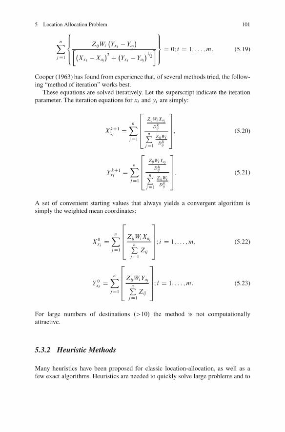
5 Location Allocation Problem 101
nXjD1
8<ˆ:
ZijWi
�Yxi
� Yaj
���Xxi
�Xaj
�2 C �Yxi
� Yaj
�1=2�9>>=>>; D 0I i D 1; : : : ; m: (5.19)
Cooper (1963) has found from experience that, of several methods tried, the follow-ing “method of iteration” works best.
These equations are solved iteratively. Let the superscript indicate the iterationparameter. The iteration equations for xi and yi are simply:
XkC1xi
DnX
jD1
26664
ZijWiXaj
Dkij
nPjD1
ZijWi
Dkij
37775; (5.20)
Y kC1xi
DnX
jD1
26664
ZijWiYaj
Dkij
nPjD1
ZijWi
Dkij
37775: (5.21)
A set of convenient starting values that always yields a convergent algorithm issimply the weighted mean coordinates:
X0xi
DnX
jD1
26664ZijWiXaj
nPjD1
Zij
37775I i D 1; : : : ; m; (5.22)
Y 0xiD
nXjD1
26664ZijWiYaj
nPjD1
Zij
37775I i D 1; : : : ; m: (5.23)
For large numbers of destinations .>10/ the method is not computationallyattractive.
5.3.2 Heuristic Methods
Many heuristics have been proposed for classic location-allocation, as well as afew exact algorithms. Heuristics are needed to quickly solve large problems and to
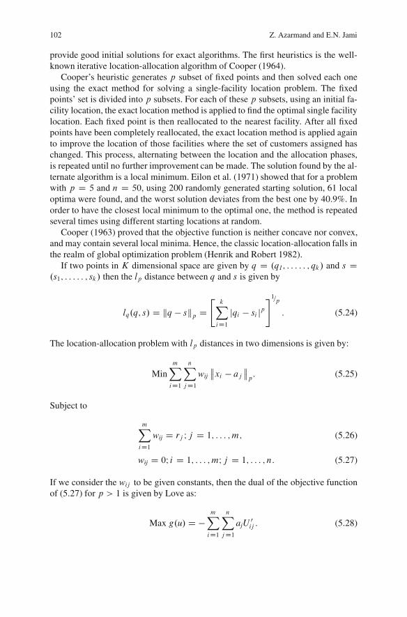
102 Z. Azarmand and E.N. Jami
provide good initial solutions for exact algorithms. The first heuristics is the well-known iterative location-allocation algorithm of Cooper (1964).
Cooper’s heuristic generates p subset of fixed points and then solved each oneusing the exact method for solving a single-facility location problem. The fixedpoints’ set is divided into p subsets. For each of these p subsets, using an initial fa-cility location, the exact location method is applied to find the optimal single facilitylocation. Each fixed point is then reallocated to the nearest facility. After all fixedpoints have been completely reallocated, the exact location method is applied againto improve the location of those facilities where the set of customers assigned haschanged. This process, alternating between the location and the allocation phases,is repeated until no further improvement can be made. The solution found by the al-ternate algorithm is a local minimum. Eilon et al. (1971) showed that for a problemwith p D 5 and n D 50, using 200 randomly generated starting solution, 61 localoptima were found, and the worst solution deviates from the best one by 40.9%. Inorder to have the closest local minimum to the optimal one, the method is repeatedseveral times using different starting locations at random.
Cooper (1963) proved that the objective function is neither concave nor convex,and may contain several local minima. Hence, the classic location-allocation falls inthe realm of global optimization problem (Henrik and Robert 1982).
If two points in K dimensional space are given by q D .q1; : : : : : ; qk/ and s D.s1; : : : : : ; sk/ then the lp distance between q and s is given by
lq.q; s/ D kq � skp D"
kXiD1
jqi � si jp#1=p
: (5.24)
The location-allocation problem with lp distances in two dimensions is given by:
MinmXiD1
nXjD1
wij
��xi � aj��p: (5.25)
Subject to
mXiD1
wij D rj I j D 1; : : : ; m; (5.26)
wij D 0I i D 1; : : : ; mI j D 1; : : : ; n: (5.27)
If we consider the wij to be given constants, then the dual of the objective functionof (5.27) for p > 1 is given by Love as:
Max g.u/ D �mXiD1
nXjD1
ajU0ij : (5.28)
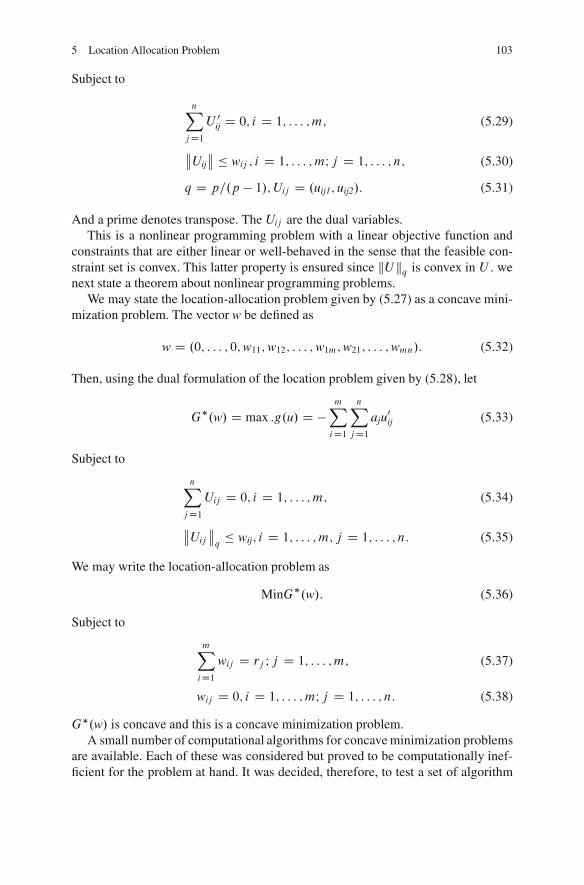
5 Location Allocation Problem 103
Subject to
nXjD1
U 0ij D 0; i D 1; : : : ; m; (5.29)
��Uij
�� � wij ; i D 1; : : : ; mI j D 1; : : : ; n; (5.30)
q D p=.p � 1/; Uij D .uij1; uij2/: (5.31)
And a prime denotes transpose. The Uij are the dual variables.This is a nonlinear programming problem with a linear objective function and
constraints that are either linear or well-behaved in the sense that the feasible con-straint set is convex. This latter property is ensured since kU kq is convex in U . wenext state a theorem about nonlinear programming problems.
We may state the location-allocation problem given by (5.27) as a concave mini-mization problem. The vector w be defined as
w D .0; : : : ; 0;w11;w12; : : : ;w1m;w21; : : : ;wmn/: (5.32)
Then, using the dual formulation of the location problem given by (5.28), let
G�.w/ D max :g.u/ D �mXiD1
nXjD1
aju0ij (5.33)
Subject to
nXjD1
Uij D 0; i D 1; : : : ; m; (5.34)
��Uij��q � wij; i D 1; : : : ; m; j D 1; : : : ; n: (5.35)
We may write the location-allocation problem as
MinG�.w/: (5.36)
Subject to
mXiD1
wij D rj I j D 1; : : : ; m; (5.37)
wij D 0; i D 1; : : : ; mI j D 1; : : : ; n: (5.38)
G�.w/ is concave and this is a concave minimization problem.A small number of computational algorithms for concave minimization problems
are available. Each of these was considered but proved to be computationally inef-ficient for the problem at hand. It was decided, therefore, to test a set of algorithm
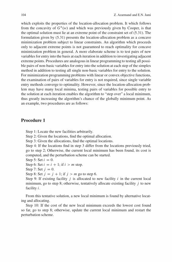
104 Z. Azarmand and E.N. Jami
which exploits the properties of the location-allocation problem. It which followsfrom the concavity of G�.w/ and which was previously given by Cooper, is thatthe optimal solution must lie at an extreme point of the constraint set of (5.31). Theformulation given by (5.31) presents the location-allocation problem as a concaveminimization problem subject to linear constraints. An algorithm which proceedsonly to adjacent extreme points is not guaranteed to reach optimality for concaveminimization problem in general. A more elaborate scheme is to test pairs of newvariables for entry into the basis at each iteration in addition to investigating adjacentextreme points. Procedures are analogous in linear programming to testing all possi-ble pairs of non-basic variables for entry into the solution at each step of the simplexmethod in addition to testing all single non-basic variables for entry to the solution.For minimization programming problems with linear or convex objective functions,the examination of pairs of variables for entry is not required, since single variableentry methods converge to optimality. However, since the location-allocation prob-lem may have many local minima, testing pairs of variables for possible entry tothe solution at each iteration enables the algorithm to “step over” a local minimum,thus greatly increasing the algorithm’s chance of the globally minimum point. Asan example, two procedures are as follows:
Procedure 1
Step 1: Locate the new facilities arbitrarily.Step 2: Given the locations, find the optimal allocation.Step 3: Given the allocations, find the optimal locations.Step 4: If the locations find in step 3 differ from the locations previously tried,go to step 2; Otherwise, the current local minimum has been found, its cost iscomputed, and the perturbation scheme can be started.Step 5: Set i D 0.Step 6: Set i D i C 1; if i > m stop.Step 7: Set j D 0.Step 8: Set j D j C 1; if j > m go to step 6.Step 9: If existing facility j is allocated to new facility i in the current localminimum, go to step 8; otherwise, tentatively allocate existing facility j to newfacility i .
From this tentative solution, a new local minimum is found by alternative locat-ing and allocating.
Step 10: If the cost of the new local minimum exceeds the lowest cost foundso far, go to step 8; otherwise, update the current local minimum and restart theperturbation scheme.
5 Location Allocation Problem 105
Procedure 2
Step 1: Locate the new facilities arbitrarily.Step 2: Given the locations, find the optimal allocations.Step 3: Given the allocations, find the optimal locations.Step 4: If the locations find in step 3 differ from the locations previously tried,go to step 2; Otherwise, the current local minimum has been found, its cost iscomputed, and the perturbation scheme can be started.Step 5: Set i D 0.Step 6: Set i D i C 1; if i > m stop.Step 7: Set j D 0.Step 8: Set j D j C 1; if j > m go to step 6.Step 9: If existing facility j1 is allocated to new facility i in the current localminimum, go to step 11.Step 10: Set j2 D j1.Step 11: Set j2 D j2 C 1; if j2 > n go to step 8.Step 12: If existing facility j2 is allocated to new facility i in the current localminimum, go to step 11; otherwise, tentatively allocate existing facility j1 and j2to new facility i .
From this tentative solution, a new local minimum is found by alternative locat-ing and allocating.
Step 13: If the cost of the new local minimum exceeds the lowest cost foundso far, go to step 11; otherwise, update the current local minimum and restart theperturbation scheme.
In 102 test problems for which the optimal solutions are known, two of algo-rithms achieved the exact optimum solutions in all cases.
5.3.3 Metaheuristic Methods (Salhi and Gamal 2003)
Location-allocation problem is NP-hard problem, metaheuristic methods have beenshown to the best way to tackle larger NP-hard problems. Meta-heuristic such assimulated annealing, Tabu search, genetic algorithm (GA), variable neighborhoodsearch, and ant systems increase the chance of avoiding local optimally.
5.4 Case Study
In this section we will introduce some real-world case studies related to location-allocation problems.
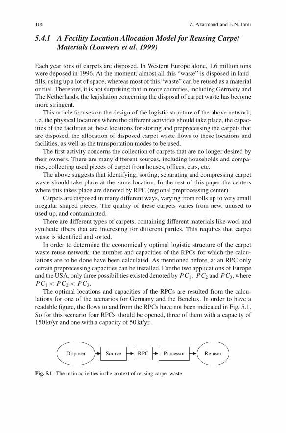
106 Z. Azarmand and E.N. Jami
5.4.1 A Facility Location Allocation Model for Reusing CarpetMaterials (Louwers et al. 1999)
Each year tons of carpets are disposed. In Western Europe alone, 1.6 million tonswere deposed in 1996. At the moment, almost all this “waste” is disposed in land-fills, using up a lot of space, whereas most of this “waste” can be reused as a materialor fuel. Therefore, it is not surprising that in more countries, including Germany andThe Netherlands, the legislation concerning the disposal of carpet waste has becomemore stringent.
This article focuses on the design of the logistic structure of the above network,i.e. the physical locations where the different activities should take place, the capac-ities of the facilities at these locations for storing and preprocessing the carpets thatare disposed, the allocation of disposed carpet waste flows to these locations andfacilities, as well as the transportation modes to be used.
The first activity concerns the collection of carpets that are no longer desired bytheir owners. There are many different sources, including households and compa-nies, collecting used pieces of carpet from houses, offices, cars, etc.
The above suggests that identifying, sorting, separating and compressing carpetwaste should take place at the same location. In the rest of this paper the centerswhere this takes place are denoted by RPC (regional preprocessing center).
Carpets are disposed in many different ways, varying from rolls up to very smallirregular shaped pieces. The quality of these carpets varies from new, unused toused-up, and contaminated.
There are different types of carpets, containing different materials like wool andsynthetic fibers that are interesting for different parties. This requires that carpetwaste is identified and sorted.
In order to determine the economically optimal logistic structure of the carpetwaste reuse network, the number and capacities of the RPCs for which the calcu-lations are to be done have been calculated. As mentioned before, at an RPC onlycertain preprocessing capacities can be installed. For the two applications of Europeand the USA, only three possibilities existed denoted byPC1; PC2 andPC3, wherePC1 < PC2 < PC3.
The optimal locations and capacities of the RPCs are resulted from the calcu-lations for one of the scenarios for Germany and the Benelux. In order to have areadable figure, the flows to and from the RPCs have not been indicated in Fig. 5.1.So for this scenario four RPCs should be opened, three of them with a capacity of150 kt/yr and one with a capacity of 50 kt/yr.
Disposer Re-userProcessorSource RPC
Fig. 5.1 The main activities in the context of reusing carpet waste
5 Location Allocation Problem 107
5.4.2 A New Organ Transplantation Location-Allocation Policy(Bruni et al. 2006)
In this part they propose a location model for the optimal organization of transplantsystem. Instead of simulation approach, which is typical when facing many healthcare applications, their approach is distinctively based on a mathematical program-ming formulation of the relevant problem. The allocation of transplantable organsacross regions with the objective of attaining regional equity in health care is theaim of this part.
The allocation of scarce donated organs is both an increasingly complex clinicaland social problem, as well as a challenging example of mathematical programmingproblem formulation. The process leading to donor identification, consent, organprocurement and allocation continue to dominate debates and efforts in the fieldof transplantation. A huge storage of donors remains while the number of patientsneeding organ transplantation increases.
The problem of long waiting times for transplant candidates and the continualgrowth in waiting list size underscores a simple reality: supply of organs does notmeet the need. This evidence has produced substantial debate about the mechanismsfor allocation of organs to potential recipients, with issues of fairness, efficiency andregional versus national interests.
The following discussion focuses on the key issues that are most relevant for thepurposes of their study:
� The factors considered in the development of an organ allocation policy� The design of an equitable transplant system
As far as the design of the transplant system is concerned, we have to take intoaccount the spatial distribution of some organizations (referred as OPO – OrganProcurement Organization), that play a crucial role in the design of a fair and equi-table transplant system.
The transplantation is performed on condition that the recipients reach the trans-plant hospital in the reasonable time. Therefore, once the organ is allocated, theaccess of the transplant service can be measured in terms of distance to the nearestor time taken to travel to the health facility. The probability of the waiting list inwhich the patient is registered, this size is influenced by the location of the OPOswithin the national area.
Our contribution is placed in this respect. In particular, we propose a mixedinteger linear programming model to face the problem of transplant system orga-nization. The proposed model can be used to analyze simultaneously:
� The location problem of OPOs and referring donor hospital and transplant centers� The districting problem� The waiting lists balancing problem
These issues have a crucial role for the fairness and the equity of the transplant inthe transplant system.
108 Z. Azarmand and E.N. Jami
The goal of an efficient and fair transplant system is to allocate organs in anequitable and timely fashion. A fair and efficient transplant system should guaranteethe greatest survival rate, for patients and for organs used.
When donor organs become available after an individual dies, an organ procure-ment organization (OPO) takes the organs into custody. The OPO then matchesthe donor organs with the appropriate transplant patients, by gathering informationabout the donor organs.
The elapsed time between removal and implantation is critical for the organ be-cause they cannot be used if they have been waiting more than an upper bound timeknown to clinician as “cold-ischemia time”. The time spent in the transplant processhas two components.
For the organ, the first segment of travel time is between the explanation and thearrival to the transplant center. The second segment of waiting refers to the timespent by the potential host traveling to the transplant center.
They design and formulate transplant location allocation model (TRALOCmodel for short); TRALOC is clearly not able to fully capture the complexity of thetransplant system. Nevertheless, the assumptions they made are quite general andallow an elegant and easy formulation. They make clear that the objective of theirstudy is to make the appropriate simplifications that lead to a tractable model.
With the aim to asses and validate TRALOC model. They applied it to the Italytransplant network. The national area is divided into 20 regions and 105 provinces.In particular each province represents a demand node and, therefore, the problem isa 105 node network.
To solve this model different values of p are being tested based on the mini-mum required amount, where p is the number of OPOs that should be established.By determining the number of new facilities, the NP-hard problem changes to NP-complete problem, then Lingo 6 is applied to solve it. Finally decision makers andpolicy makers were offered the results in order to choose the optimum form accord-ing to their own point of view.
References
Badri MA (1999) Combining the analytic hierarchy process and goal programming for globalfacility location-allocation problem. Int J Prod Econ 62:237–248
Brimberg J, Mladenovic N (1996) Solving the continuous Location-Allocation problem with tabusearch. Stud Locational Ann 8:23–32
Brimberg J, Hansen P, Mladenovic N, Taillard ED (2000) Improvements and comparison of heuris-tics for solving the uncapacitated multi source Weber problem. Oper Res 48:444–460
Bruni M, Conforti D, Sicilia N, Trotta S (2006) A new organ transplantation Location-Allocationpolicy: A case study of Italy. Health Care Manage Sci 9:125–142
Cooper L (1963) Location-Allocation problems. Oper Res 11(3):331–343Cooper L (1964) Heuristic methods for location-allocation problems. SIAM Rev 6(1):37–53Eilon S, Watson-Gandy CDT, Christofides N (1971) Distribution Management. New York, HafnerErnst AT, Krishnamoorthy M (1999) Solution algorithms for the capacitated single allocation hub
location problem. Ann Oper Res 86:141–159
5 Location Allocation Problem 109
Gong D, Gen M, Yamazaki G, Xu W (1997) Hybrid evolutionary method for capacitated location-allocation problem. Comput Ind Eng 33:577–580
Hakimi S (1964) Optimum distribution of switching centers in a communication network and somerelated graph theoretic problems. Oper Res 13:462–475
Hansen P, Jaumard B, Taillard E (1998) Heuristic solution of the multi source Weber problem as ap-median problem. Oper Res Lett 22:55–62
Henrik J, Robert FL (1982) Properties and solution methods for large location-allocation problems.J Oper Res Soc 33(5):443–452
Kuenne RE, Soland RM (1972) Exact and approximate solutions to the multi source Weber prob-lem. Math Program 3:193–209
Louwers D, Kip BJ, Peters E, Souren F, Flapper SDP (1999) A facility location-allocation modelfor reusing carpet materials. Comput Ind Eng 36:855–869
Murray AT, Church RL (1996) Applying simulated annealing to location-planning models.J Heuristics 2:31–53
Ohlemuller M (1997) Tabu search for large location-allocation problems. J Oper Res Soc48(7):745–750
Scaparra MP, Scutella MG (2001) Facilities, locations, customers: Building blocks of locationmodels: A survey. Technical report TR-01–18, Computer Science Department, University ofPisa, Italy
Salhi S, Gamal MDH (2003) A Genetic algorithm based approach for the uncapacitated continuouslocation–allocation problem. Ann Oper Res 123:203–222
Zhou J, Liu B (2003) New stochastic models for capacitated location-allocation problem. ComputInd Eng 45:111–125
Chapter 6Quadratic Assignment Problem
Masoumeh Bayat and Mahdieh Sedghi
The quadratic assignment problem (QAP) in location Theory is the problem oflocating facilities the cost of placing a facility depends on the distances from otherfacilities and also the interaction with other facilities. QAP was introduced byKoopmans and Beckman in 1957 who were trying to model a facilities locationproblem.
It is possible to formulate some classic problems of combinatorial optimization,such as the traveling salesman, maximum clique and graph partitioning prob-lems as a QAP. The QAP belongs to the class of NP-complete problems andis considered one of the most difficult combinatorial optimization problems. Ex-act solution strategies for the QAP have been unsuccessful for large problem(approximatelyN � 25).
In Fig. 6.1 the QAP search trends and tendencies in about 50 years is shown(Hahn et al. 2007). Figure 6.1 shows the distribution of QAP publications with re-spect to the categories: applications, theory and algorithms.
Figure 6.2 distributes the number of articles by 5-year periods since 1957, foreach period, the work is also classified according to the same categories of Fig. 6.1.Figure 6.2 shows that an explosion of interest in theory and algorithm developmentoccurred in the period from 1992 to the present.
Figure 6.3 shows a steady increase in interest in the QAP in recent years.Figure 6.4, which covers the recent years, shows that the interest in algorithms
continues to be very strong, with a cyclical trend in theoretical developments. Ap-plications continue to be of interest, but to a lesser extent. It is noteworthy that thereis recently a growing interest in applications to communication link design and tothe optimization of communications networks.
As a first example for introducing the problem we describe the problem of as-signing facilities to locations in an office. Let have four facilities that each facility isdesignated to exactly one location and vice-versa. Our problem is to find a minimumcost allocation of facilities into locations taking the costs as the sum of all possi-ble distance-flow products. For example in Fig. 6.5 an assignment � D .3; 2; 4; 1/
is shown:
R.Z. Farahani and M. Hekmatfar (eds.), Facility Location: Concepts, Models, 111Algorithms and Case Studies, Contributions to Management Science,DOI 10.1007/978-3-7908-2151-2 6, c� Physica-Verlag Heidelberg 2009
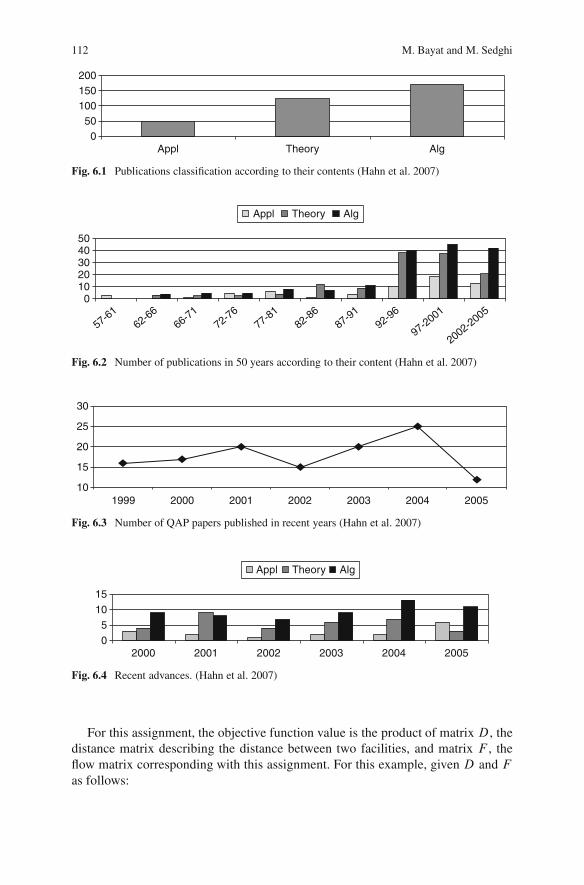
112 M. Bayat and M. Sedghi
050
100150200
Appl Theory Alg
Fig. 6.1 Publications classification according to their contents (Hahn et al. 2007)
01020304050
57-6162-66
66-7172-76
77-8182-86
87-9192-96
97-2001
2002-2005
Appl Theory Alg
Fig. 6.2 Number of publications in 50 years according to their content (Hahn et al. 2007)
10
15
20
25
30
1999 2000 2001 2002 2003 2004 2005
Fig. 6.3 Number of QAP papers published in recent years (Hahn et al. 2007)
0
5
10
15
2000 2001 2002 2003 2004 2005
Appl Theory Alg
Fig. 6.4 Recent advances. (Hahn et al. 2007)
For this assignment, the objective function value is the product of matrix D, thedistance matrix describing the distance between two facilities, and matrix F , theflow matrix corresponding with this assignment. For this example, given D and Fas follows:
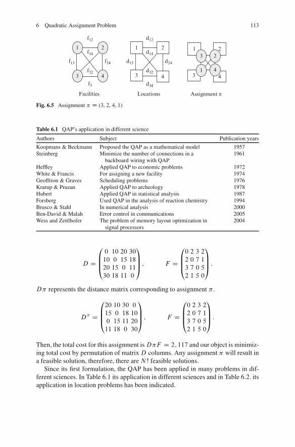
6 Quadratic Assignment Problem 113
2 1
f24
f12
f3
f13
f141
f3243
d12
d24d13
d34
d141
d3243
2
3 41
2
4
3
Facilities Locations Assignment π
2
Fig. 6.5 Assignment � D (3, 2, 4, 1)
Table 6.1 QAP’s application in different science
Authors Subject Publication years
Koopmans & Beckmann Proposed the QAP as a mathematical model 1957Steinberg Minimize the number of connections in a
backboard wiring with QAP1961
Heffley Applied QAP to economic problems 1972White & Francis For assigning a new facility 1974Geoffrion & Graves Scheduling problems 1976Krarup & Pruzan Applied QAP to archeology 1978Hubert Applied QAP in statistical analysis 1987Forsberg Used QAP in the analysis of reaction chemistry 1994Brusco & Stahl In numerical analysis 2000Ben-David & Malah Error control in communications 2005Wess and Zeitlhofer The problem of memory layout optimization in
signal processors2004
D D
0BB@0 10 20 30
10 0 15 18
20 15 0 11
30 18 11 0
1CCA ; F D
0BB@0 2 3 2
2 0 7 1
3 7 0 5
2 1 5 0
1CCA :
D� represents the distance matrix corresponding to assignment � .
D� D
0BB@20 10 30 0
15 0 18 10
0 15 11 20
11 18 0 30
1CCA ; F D
0BB@0 2 3 2
2 0 7 1
3 7 0 5
2 1 5 0
1CCA :
Then, the total cost for this assignment isD�F D 2; 117 and our object is minimiz-ing total cost by permutation of matrixD columns. Any assignment � will result ina feasible solution, therefore, there are NŠ feasible solutions.
Since its first formulation, the QAP has been applied in many problems in dif-ferent sciences. In Table 6.1 its application in different sciences and in Table 6.2. itsapplication in location problems has been indicated.
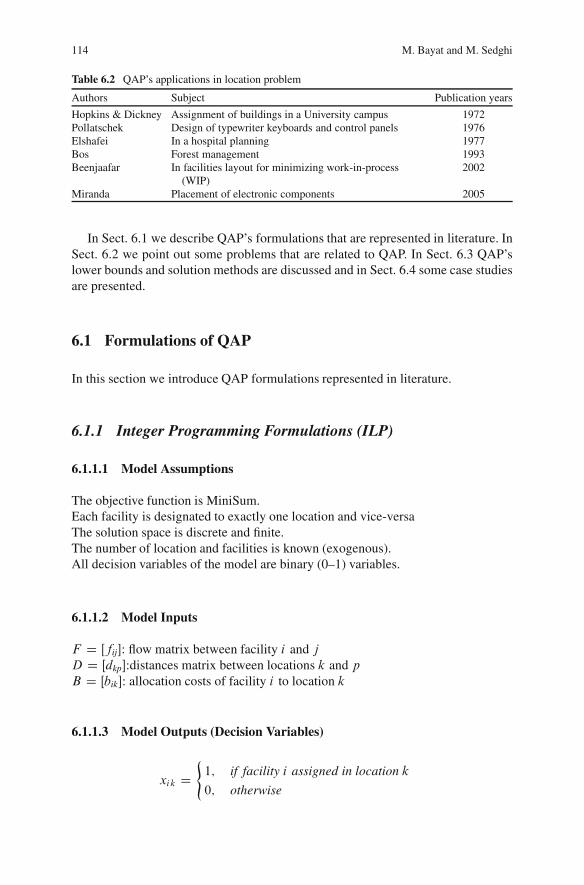
114 M. Bayat and M. Sedghi
Table 6.2 QAP’s applications in location problem
Authors Subject Publication years
Hopkins & Dickney Assignment of buildings in a University campus 1972Pollatschek Design of typewriter keyboards and control panels 1976Elshafei In a hospital planning 1977Bos Forest management 1993Beenjaafar In facilities layout for minimizing work-in-process
(WIP)2002
Miranda Placement of electronic components 2005
In Sect. 6.1 we describe QAP’s formulations that are represented in literature. InSect. 6.2 we point out some problems that are related to QAP. In Sect. 6.3 QAP’slower bounds and solution methods are discussed and in Sect. 6.4 some case studiesare presented.
6.1 Formulations of QAP
In this section we introduce QAP formulations represented in literature.
6.1.1 Integer Programming Formulations (ILP)
6.1.1.1 Model Assumptions
The objective function is MiniSum.Each facility is designated to exactly one location and vice-versaThe solution space is discrete and finite.The number of location and facilities is known (exogenous).All decision variables of the model are binary (0–1) variables.
6.1.1.2 Model Inputs
F D Œfij: flow matrix between facility i and jD D Œdkp:distances matrix between locations k and pB D Œbik: allocation costs of facility i to location k
6.1.1.3 Model Outputs (Decision Variables)
xik D(1; if facility i assigned in location k
0; otherwise
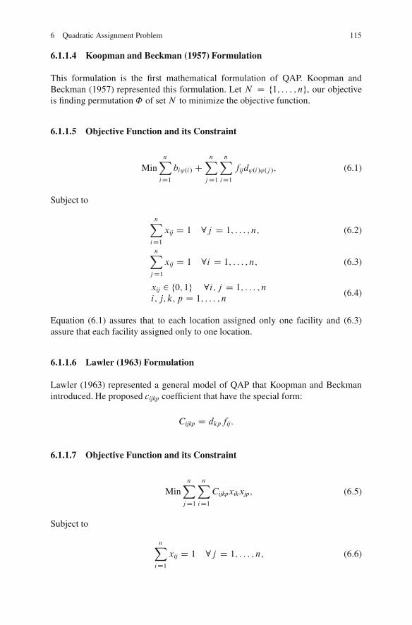
6 Quadratic Assignment Problem 115
6.1.1.4 Koopman and Beckman (1957) Formulation
This formulation is the first mathematical formulation of QAP. Koopman andBeckman (1957) represented this formulation. Let N D f1; : : : ; ng, our objectiveis finding permutation ˚ of set N to minimize the objective function.
6.1.1.5 Objective Function and its Constraint
MinnXiD1
bi'.i/ CnX
jD1
nXiD1
fijd'.i/'.j /; (6.1)
Subject to
nXiD1
xij D 1 8j D 1; : : : ; n; (6.2)
nXjD1
xij D 1 8i D 1; : : : ; n; (6.3)
xij 2 f0; 1g 8i; j D 1; : : : ; n
i; j; k; p D 1; : : : ; n(6.4)
Equation (6.1) assures that to each location assigned only one facility and (6.3)assure that each facility assigned only to one location.
6.1.1.6 Lawler (1963) Formulation
Lawler (1963) represented a general model of QAP that Koopman and Beckmanintroduced. He proposed cijkp coefficient that have the special form:
Cijkp D dkpfij:
6.1.1.7 Objective Function and its Constraint
MinnX
jD1
nXiD1
Cijkpxikxjp; (6.5)
Subject to
nXiD1
xij D 1 8j D 1; : : : ; n; (6.6)
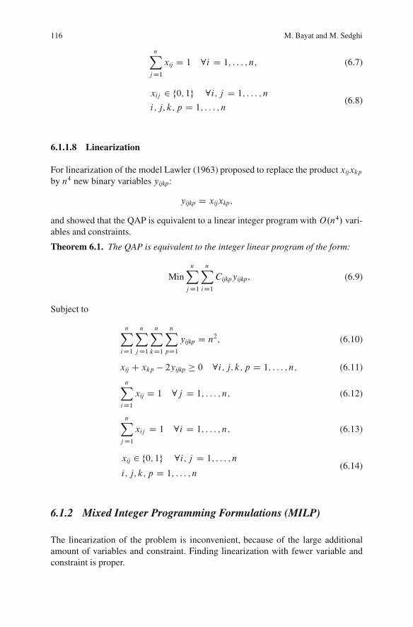
116 M. Bayat and M. Sedghi
nXjD1
xij D 1 8i D 1; : : : ; n; (6.7)
xij 2 f0; 1g 8i; j D 1; : : : ; n
i; j; k; p D 1; : : : ; n(6.8)
6.1.1.8 Linearization
For linearization of the model Lawler (1963) proposed to replace the product xijxkpby n4 new binary variables yijkp:
yijkp D xijxkp;
and showed that the QAP is equivalent to a linear integer program with O.n4/ vari-ables and constraints.
Theorem 6.1. The QAP is equivalent to the integer linear program of the form:
MinnX
jD1
nXiD1
Cijkpyijkp; (6.9)
Subject to
nXiD1
nXjD1
nXkD1
nXpD1
yijkp D n2; (6.10)
xij C xkp � 2yijkp � 0 8i; j; k; p D 1; : : : ; n; (6.11)
nXiD1
xij D 1 8j D 1; : : : ; n; (6.12)
nXjD1
xij D 1 8i D 1; : : : ; n; (6.13)
xij 2 f0; 1g 8i; j D 1; : : : ; n
i; j; k; p D 1; : : : ; n(6.14)
6.1.2 Mixed Integer Programming Formulations (MILP)
The linearization of the problem is inconvenient, because of the large additionalamount of variables and constraint. Finding linearization with fewer variable andconstraint is proper.
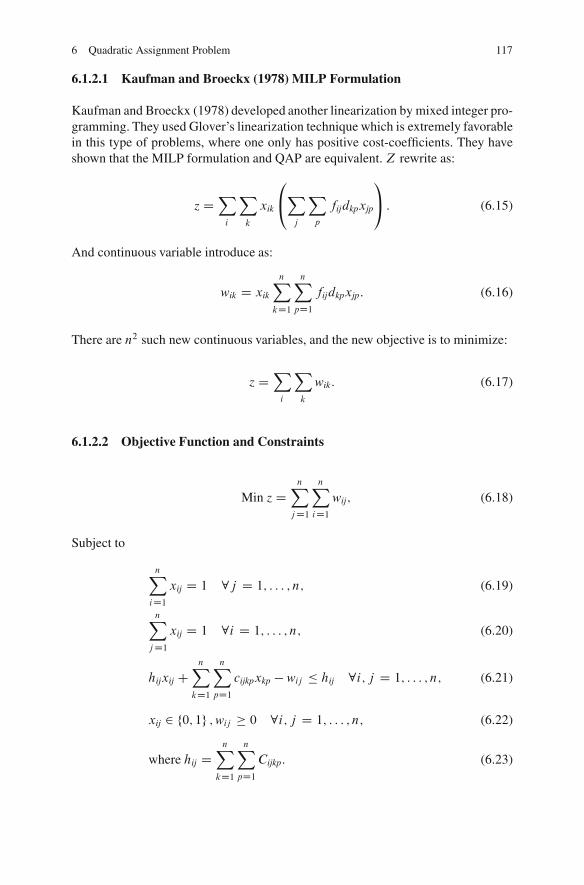
6 Quadratic Assignment Problem 117
6.1.2.1 Kaufman and Broeckx (1978) MILP Formulation
Kaufman and Broeckx (1978) developed another linearization by mixed integer pro-gramming. They used Glover’s linearization technique which is extremely favorablein this type of problems, where one only has positive cost-coefficients. They haveshown that the MILP formulation and QAP are equivalent.Z rewrite as:
z DXi
Xk
xik
0@X
j
Xp
fijdkpxjp
1A : (6.15)
And continuous variable introduce as:
wik D xik
nXkD1
nXpD1
fijdkpxjp: (6.16)
There are n2 such new continuous variables, and the new objective is to minimize:
z DXi
Xk
wik: (6.17)
6.1.2.2 Objective Function and Constraints
Min z DnX
jD1
nXiD1
wij; (6.18)
Subject to
nXiD1
xij D 1 8j D 1; : : : ; n; (6.19)
nXjD1
xij D 1 8i D 1; : : : ; n; (6.20)
hijxij CnX
kD1
nXpD1
cijkpxkp � wij � hij 8i; j D 1; : : : ; n; (6.21)
xij 2 f0; 1g ;wij � 0 8i; j D 1; : : : ; n; (6.22)
where hij DnX
kD1
nXpD1
Cijkp: (6.23)
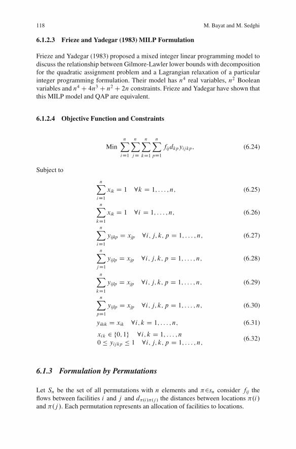
118 M. Bayat and M. Sedghi
6.1.2.3 Frieze and Yadegar (1983) MILP Formulation
Frieze and Yadegar (1983) proposed a mixed integer linear programming model todiscuss the relationship between Gilmore-Lawler lower bounds with decompositionfor the quadratic assignment problem and a Lagrangian relaxation of a particularinteger programming formulation. Their model has n4 real variables, n2 Booleanvariables and n4 C 4n3 C n2 C 2n constraints. Frieze and Yadegar have shown thatthis MILP model and QAP are equivalent.
6.1.2.4 Objective Function and Constraints
MinnXiD1
nXjD
nXkD1
nXpD1
fijdkpyijkp; (6.24)
Subject to
nXiD1
xik D 1 8k D 1; : : : ; n; (6.25)
nXkD1
xik D 1 8i D 1; : : : ; n; (6.26)
nXiD1
yijkp D xjp 8i; j; k; p D 1; : : : ; n; (6.27)
nXjD1
yijlp D xjp 8i; j; k; p D 1; : : : ; n; (6.28)
nXkD1
yijlp D xjp 8i; j; k; p D 1; : : : ; n; (6.29)
nXpD1
yijlp D xjp 8i; j; k; p D 1; : : : ; n; (6.30)
yikik D xik 8i; k D 1; : : : ; n; (6.31)
xik 2 f0; 1g 8i; k D 1; : : : ; n
0 � yijkp � 1 8i; j; k; p D 1; : : : ; n;(6.32)
6.1.3 Formulation by Permutations
Let Sn be the set of all permutations with n elements and �2sn consider fij theflows between facilities i and j and d�.i/�.j / the distances between locations �.i/and �.j /. Each permutation represents an allocation of facilities to locations.
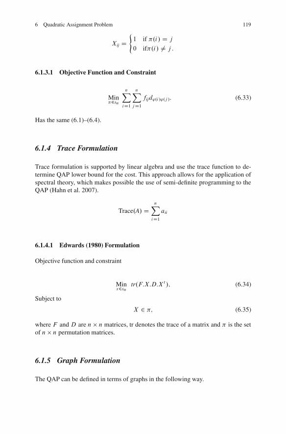
6 Quadratic Assignment Problem 119
Xij D(1 if �.i/ D j
0 if�.i/ ¤ j :
6.1.3.1 Objective Function and Constraint
Min�2sn
nXiD1
nXjD1
fijd'.i/'.j /: (6.33)
Has the same (6.1)–(6.4).
6.1.4 Trace Formulation
Trace formulation is supported by linear algebra and use the trace function to de-termine QAP lower bound for the cost. This approach allows for the application ofspectral theory, which makes possible the use of semi-definite programming to theQAP (Hahn et al. 2007).
Trace.A/ DnXiD1
aii
6.1.4.1 Edwards (1980) Formulation
Objective function and constraint
Minx2sn
tr.F:X:D:Xt /; (6.34)
Subject to
X 2 �; (6.35)
where F and D are n n matrices, tr denotes the trace of a matrix and � is the setof n n permutation matrices.
6.1.5 Graph Formulation
The QAP can be defined in terms of graphs in the following way.
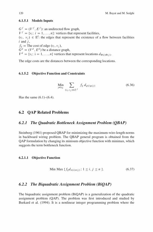
120 M. Bayat and M. Sedghi
6.1.5.1 Models Inputs
Gf D .V f ; Ef /: an undirected flow graph,V f D fvi I i D 1; : : : ; ng: vertices that represent facilities,.vi ; vj / 2 Ef: the edges that represent the existence of a flow between facilitiesi and j ,fij D The cost of edge .vi ; vj /,Gd D .V d ; Ed/ be a distance graph,V d D fvi I i D 1; : : : ; ng vertices that represent locations d˚.i/˚.j /.
The edge costs are the distances between the corresponding locations.
6.1.5.2 Objective Function and Constraints
Min�2sn
X.vi ;vj /2Ef
fij d'.i/'.j / (6.36)
Has the same (6.1)–(6.4).
6.2 QAP Related Problems
6.2.1 The Quadratic Bottleneck Assignment Problem (QBAP)
Steinberg (1961) proposed QBAP for minimizing the maximum-wire-length normsin backboard wiring problem. The QBAP general program is obtained from theQAP formulation by changing its minisum objective function with minimax, whichsuggests the term bottleneck function.
6.2.1.1 Objective Function
Min Max ffijd�.i/�.j / I 1 � i; j � n g: (6.37)
6.2.2 The Biquadratic Assignment Problem (BiQAP)
The biquadratic assignment problem (BiQAP) is a generalization of the quadraticassignment problem (QAP). The problem was first introduced and studied byBurkard et al. (1994). It is a nonlinear integer programming problem where the
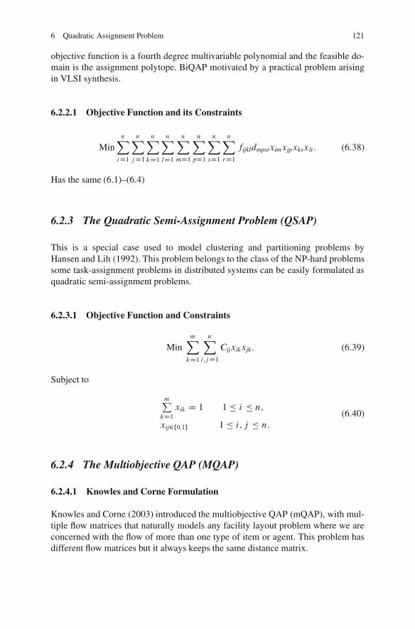
6 Quadratic Assignment Problem 121
objective function is a fourth degree multivariable polynomial and the feasible do-main is the assignment polytope. BiQAP motivated by a practical problem arisingin VLSI synthesis.
6.2.2.1 Objective Function and its Constraints
MinnXiD1
nXjD1
nXkD1
nXlD1
nXmD1
nXpD1
nXsD1
nXrD1
fijkldmpstximxjpxksxlt : (6.38)
Has the same (6.1)–(6.4)
6.2.3 The Quadratic Semi-Assignment Problem (QSAP)
This is a special case used to model clustering and partitioning problems byHansen and Lih (1992). This problem belongs to the class of the NP-hard problemssome task-assignment problems in distributed systems can be easily formulated asquadratic semi-assignment problems.
6.2.3.1 Objective Function and Constraints
MinmXkD1
nXi;jD1
Cijxikxjk: (6.39)
Subject to
mPkD1
xik D 1 1 � i � n;
xij2f0;1g 1 � i; j � n:
(6.40)
6.2.4 The Multiobjective QAP (MQAP)
6.2.4.1 Knowles and Corne Formulation
Knowles and Corne (2003) introduced the multiobjective QAP (mQAP), with mul-tiple flow matrices that naturally models any facility layout problem where we areconcerned with the flow of more than one type of item or agent. This problem hasdifferent flow matrices but it always keeps the same distance matrix.
122 M. Bayat and M. Sedghi
6.2.4.2 Objective Function and its Constraints
Min�2sn
C.�/ D ˚C1.�/; : : : ; Cm.�/
�; (6.41)
where Ck.�/ DXX
fijd�.i/�.j /;8k D 1; : : : ; m: (6.42)
Has the same (6.1)–(6.4).
6.2.4.3 Hamacher Formulation
Hamacher et al. (2003) introduced a different formulation of a multiobjective QAPthat considers different matrices of flows and distances for modeling problems foundin facility layout for social institutions.
Min
0BBBBB@
nPi;j;k;lD1
fikdjlxijxkl
:::nP
i;j;k;lD1fQ
ik dQkl xijxkl
1CCCCCA ; (6.43)
where the problem is to find assignment x as:
xij D(1; if facility i assigned in location j
0; otherwise:
Has the same (6.1)–(6.4).
6.2.5 The Quadratic Three-Dimensional Assignment Problem(Q3AP)
Pierskalla (1967a, b) introduced the quadratic three-dimensional assignment prob-lem (Q3AP) in a technical memorandum. The Q3AP is an extension of the QAPthat can be represented as a three-dimensional assignment problem.
6.2.5.1 Objective Function and Constraints
Where I; J and P are disjoint sets of constraints
6 Quadratic Assignment Problem 123
Min
8<ˆ:
nPiD1
nPjD1
nPpD1
bijpxijpCnPiD1
nPjD1
nPpD1
nPk D 1
k ¤ i
nPn D 1
n ¤ j
nPq D 1
q ¤ p
Cijpknqxijpxknq
9>>>>=>>>>;;
(6.44)
where x 2 I \ J \ P; x binary
I D8<:x � 0 W
nXjD1
nXpD1
xijp D 1 for i D 1; : : : ; n
9=; ; (6.45)
J D8<:x � 0 W
nXiD1
nXpD1
xijp D 1 for j D 1; : : : ; n
9=; ; (6.46)
P D8<:x � 0 W
nXiD1
nXjD1
xijp D 1 for p D 1; : : : ; n
9=; : (6.47)
6.2.6 The Generalized Quadratic Assignment Problem (GQAP)
Lee and Ma (2004) indicated that the GQAP had been proposed by them in 1991which is a generalized problem of the QAP in that there is no restriction that onelocation can accommodate only single equipment. This problem arises in many realworld applications such as facility location problem and logistics network design.
6.2.6.1 Model Inputs
M : a set of equipments .D f1; 2; : : : ; mg/,N : a set of locations .D f1; 2; : : : ; ng/,si : space requirement of equipment i ,Sk: total available space at location k,cik : the cost of installing equipment i at location k,qij : the flow volume from equipment i to j in the planning horizon,dkh: the distance between location k and h .D dhk/,v: the travel cost per unit distance and per unit flow volume.
6.2.6.2 Model Outputs (Decision Variables)
xik D(1; if equipment i is assigned to location k;
0; otherwise:
124 M. Bayat and M. Sedghi
6.2.6.3 Assumptions
Just to avoid trivial cases, we will assume:
(a) There is no single location that is big enough to hold all the equipments or:
Xi2M si > Sk 8k 2 N:
(b) There is no equipment which is too big to be assigned to any location or:
Sk � maxi si ; 8k 2 N
(c) All the locations are distinctive or:
dij ¤ 0; 8j ¤ h 2 N
(d) The distance between locations is symmetric.
6.2.6.4 Objective Function and its Constraints
MinmXjD1
nXkD1
cikxik C
mXiD1
mXjD1
nXkD1
nXhD1
qijdkhxikxjh; (6.48)
Subject to
nXkD1
xik D 1; 8i 2 f1; : : : ; mg ; (6.49)
mXiD1
sixik � Sk; 8k 2 f1; : : : ; ng ; (6.50)
xik 2 f 0; 1 g ; 8i; k: (6.51)
6.2.7 Stochastic QAP (SQAP)
SQAP is basically a network design problem, whenever there is a need to assignactivities to the nodes of a network in order to minimize congestion; the SQAPis an appropriate model of the problem. In SQAP we have distance matrix andP matrix that is the probability of having interaction between facility i and j(Smith and Li 2001).
6 Quadratic Assignment Problem 125
6.3 Solution Techniques
The methods used in combinatorial optimization problems can be either exact,heuristic or metaheuristic shown in Fig. 6.6. The most frequently used strategiesare branch-and-bound or dynamic programming general methods and also there area number of heuristic techniques using different conceptions. In what follows, wediscuss about computational complexity and both approaches and bring their mostimportant references.
6.3.1 Computational Complexity
In fact, the QAP belongs to the class of computationally hard problems known asNP complete. The proof that the QAP is indeed NP-complete was first shown bySahni and Gonzales (1976) and they also proved that any routine that finds evenan ©-approximate solution is also NP-complete, thus making the QAP among the“hardest of the hard” of all combinatorial optimization problems. Belonging to thisclass of problems suggests that an algorithm which solves the problem to optimalityin polynomial time is unlikely to exist. Therefore, to practically solve the QAP onehas to apply heuristic algorithms which find very high quality solutions in shortcomputation time.
6.3.2 Lower Bounds
Lower bounds are useful for measuring heuristic search worst-case solutions quality,and are an essential component in the construction of Branch and Bound (B&B)methods for achieving optimal solutions. We are trying to derive bound that is notbeing hard to compute, can easily be evaluated for subsets of the problem whichoccur after some branching, and finally is tight. There are many different proposalsfor deriving bounds. In the following we briefly survey bounds for QAP problem.
0255075
100
Exact MetahuresticHeuristic
Fig. 6.6 Publications: solution techniques (Hahn et al. 2007)
126 M. Bayat and M. Sedghi
6.3.2.1 The Gilmore and Lawler Lower Bound (GLB)
The Gilmore–Lawler bound (GLB) which was proposed by Gilmore (1962) andLawler (1963) is one of the best-known lower bounds for the small QAP’s problem.It is easy to compute, but it deteriorates fast by increasing in the size of the problem.
GLB D LAP.F / � QAP:
This bounding technique is combinatorial in nature and requires the solution ofa LAP for a Koopman–Beckmann problem that can be computed in O.n3/ time(Anstreicher 2003). Several authors proposed different approaches to improve theGLB, Frieze and Yadegar (1983) proposed GLB with decomposition, Assad and Xu(1985) proposed the AX bound that is obtained iteratively, where n2C1 assignmentof size n are solved in each iteration. Hence, the running time to compute isO.kn5/where k is the number of iterations.
6.3.2.2 Bounds Based on LP and Dual-LP
Frieze and Yadegar (1983), discuss the relationship between GLB with decompo-sition and a Lagrangian relaxation of a mixed integer programming formulation(6.24)–(6.32).
Drezner (1995) proved that the optimal solution for a MILP-formulation is alower bound for the corresponding QAP that is at least as good as the classicalGilmore-Lawler lower bound. Adams and Johnson (1994) develop a dual ascentprocedure for approximating the dual of the MILP relaxation and proved that eachdual solution of the linear programming is also a lower bound for the QAP. Thesebounds are quite expensive to compute and can only be applied to problems ofdimension n � 30.
6.3.2.3 Eigenvalue Related Bounds (EVB)
Finke et al. (1987) proposed Eigenvalue bounds which are based on the trace formu-lation of QAP. The basic idea to derive this bound consists in minimizing objectivefunction of trace formulation over orthogonal rather than just permutation matrices.
Let �1; �2; : : : ; �n be the eigenvalues of the symmetric matrix F and let�1; �2; : : : ; �n be the eigenvalue of the symmetric matrix D. since F and D aresymmetric, the eigenvalues are real and we can assume the ordering
�1 � �2 � : : : � �n and �1 � �2 � : : : �n:
For all permutation ˚
nXiD1
�i�i �nXiD1
nXjD1
fijd'.i/'.j / �nXiD1
�i�n�i : (6.52)
6 Quadratic Assignment Problem 127
Hadley et al. (1992a) consider also the case of non-symmetric QAPs and develop forthem eigenvalue bounds by means of Hermitian matrices. These bounds have goodquality in comparison to Gilmore–Lawler-like bounds; however, they are expensivein terms of computation time and deteriorate quickly when lower levels of a branchand bound tree are searched. The simple EVB is too weak to be computationallyuseful, but several schemes for improving the bound have been considered. Hadleyet al. (1992b) proposed improved eigenvalue bound which have been derived fromthe projected QAP (PD). EVD and PD both requireO.n3/ computing time.
6.3.2.4 Bounds Based on Reformulations
Reformulation linearization technique (RLT) is designed to generate a hierarchyof linear programming (LP) relaxations leading from the ordinary continuous re-laxation to the convex hull representation for mixed-integer 0–1 programmingproblems (Sherali and Adams 1990). Sherali et al. (2000) proposed reduced re-formulation linearization technique to improve RLT. Adams et al. (2007) calculatebounds using a level-2 reformulation linearization technique (2-RLT) that providessharp and tight lower bounds.
6.3.2.5 Variance Reduction Bounds
Initially proposed by Li et al. (1994a), these bounds are based on reduction schemesand are defined from the variance of F and D matrices. These bounds, when usedin a branch-and-bound algorithm, take less computational time and generally ob-tain better performance than GLB. They show more efficiency when the flow anddistance matrices have high variances (Hahn et al. 2007).
6.3.2.6 Semi-Definite Programming and Reformulation–LinearizationBounds
Semi-definite programming (SDP) has proven to be very successful in provid-ing tight relaxations for hard combinatorial problems. SDP relaxations for thequadratic assignment problem (QAP) are derived using the dual of the (homog-enized) Lagrangian dual of appropriate equivalent representations of QAP (Zhaoet al. 1998).
Anstreicher (2001) compares SDP relaxations and eigenvalue bounds;Anstreicher and Brixius (2001) describe a new convex quadratic programmingbound for the QAP. The new bound dominates the well-known projected eigen-value bound, and appears to be competitive with existing bounds in the trade-offbetween bound quality and computational effort.
Burer and Vandenbussche (2006) applied Lagrangian relaxation on a lift-and-project QAP relaxation, following the ideas in Lova’sz and Schrijver (1991), thus
128 M. Bayat and M. Sedghi
obtaining very tight SDP bounds. A report, by Rendl and Sotirov (2003), discussesa very good semi-definite programming (SDP) lower bound for the QAP. In 2003,when the report was written, it reported the tightest lower bounds for a large numberof QAPLIB instances.
Hahn et al. (2007) indicated that according to the research of Povh and Rendl in2006, the strongest relaxation (R3) from Rendl and Sotirov (2003) and the relaxationfrom Burer and Vandenbussche (2006) are actually the same The differing lowerbound values in the two papers are due to the fact that Rendl and Sotirov use thebundle method, which gives only underestimates of the true bound, while Burer andVandenbussche are able to compute this bound more accurately (Hahn et al. 2007).
6.3.3 Exact Algorithms
The different methods used to achieve a global optimum for the QAP includebranch-and-bound, cutting planes or combinations of these methods, like branch-and-cut and dynamic programming. These algorithms are time consuming for largescale problem.
6.3.3.1 Branch-and-Bound
Among all three methods Branch-and-bound are the most known and used algo-rithms. There are several references concerning QAP branch-and-bound algorithms:
The first two branches and bound algorithms were developed by Gilmore (1962)and Lawler (1963) which assign single facilities to single locations. The main dif-ference between two algorithms is in computing the lower bounds. Land (1963) andGavett and Plyter (1966) proposed a algorithm which assign pairs of facilities topairs of locations. Graves and Whinston (1970) and Lawler (1963) developed pro-cedure which assign one unassigned facility to vacant location. Bazaraa and Kirca(1983) proposed the algorithm eliminates “mirror image” branches, thus reducingthe search space. Mans et al. (1995) applied a parallel depth first search branchand bound algorithm for the quadratic assignment problem. Hahn and Grant (1998)presented a new branch-and-bound algorithm for solving the quadratic assignmentproblem (QAP). The algorithm is based on a dual procedure (DP) similar to theHungarian method for solving the linear assignment problem. Hahn et al. (1998)applied a branch-and-bound algorithm for the quadratic assignment problem basedon the Hungarian method.
6.3.3.2 Cutting Plane
Cutting plane methods introduced by Bazaraa and Sherali (1980), initially, did notpresent satisfactory results. The employed technique is not widely used so far, but
6 Quadratic Assignment Problem 129
good quality solutions for QAP cases are being presented. The slow convergenceof this method makes it proper only for small instances. There are some referencespresented as follows:
Burkard and Bonniger (1983) which improved a cutting plane method tosolve the QAP, Kaufman and Broeckx (1978), Bazaraa and Sherali (1982),Miranda et al. (2005).
6.3.3.3 Branch-and-Cut
The branch-and-cut technique, a variation proposed by Padberg and Rinaldi (1991),appears to be an alternative cutting strategy that exploits the polytope defined bythe feasible solutions of the problem. Its main advantage over cutting planes is thatthe cuts are associated with the polypore’s facets. Cuts associated with facets aremore effective than the ones produced by cutting planes, so the convergence to anoptimal solution is accelerated. The dearth of knowledge about the QAP polytope isthe reason why polyhedral cutting planes are not widely used for this problem, andalso Padberg and Rinaldi (1991), Kaibel (1998), Junger and Kaibel (2000, 2001a, b),Blanchard et al. (2003).
6.3.3.4 Dynamic Programming
Dynamic programming is a technique used for QAP special cases where the flowmatrix is the adjacency matrix of a tree.
Christofides and Benavent (1989) studied this case using a MILP approach to therelaxed problem. It was then solved with a dynamic programming algorithm, takingadvantage of the polynomial complexity of the instances.
6.3.4 Heuristic Algorithms
Heuristic algorithms do not guarantee optimality of the best solution obtained and isa procedure dedicated to search good quality solutions. So, all approximate methodsare included in this category.
Heuristic procedures include the following categories: constructive, limited enu-meration, improvement methods and simulated approach.
6.3.4.1 Constructive Method
Gilmore (1962) introduced a constructive method that completes a permutation(i.e., feasible solution) at each iteration of the algorithm. There are some references
130 M. Bayat and M. Sedghi
in this field: Armour and Buffa (1963), Buffa et al. (1964), Tansel and Bilen (1998),Burkard et al. (1991), Arkin et al. (2001), Gutin and Yeo (2002), Yu and Sarker(2003).
6.3.4.2 Enumerative Methods
Enumeration can guarantee that the obtained solution is optimum only if they can goto the end of the enumerative process. Nissen and Paul (1995) applied the thresholdaccepting technique to the QAP. Burkard and Bonniger (1983), West (1983).
6.3.4.3 Improvement Methods
Improvement methods correspond to local search algorithms. Most of the QAPheuristics are in this category. White (1993) proposed a new approach, where theactual data are relaxed by embedding them in a data space that satisfies an ex-tension of the metric triangle property. Arora et al. (2002) proposed a randomizedprocedure for rounding fractional perfect assignments to integral assignments anda also Heider (1973), Mirchandani and Obata (1979), Bruijs (1984), Pardalos et al.(1993), Burkard and Cela (1995), Li and Smith (1995), Anderson (1996), Talbi et al.(1998a), Deineko and Woeginger (2000), Misevicius (2000a), Mills et al. (2003).
6.3.5 Metaheuristic Algorithms
They are characterized by the definition of a priori strategies adapted to the problemstructure. Several of these techniques are based on some form of simulation of anatural process studied within another field of knowledge (metaphors) so they havetwo important categories “metaheuristics based on natural process metaphors” and“metaheuristics based directly on theoretical and experimental considerations”.
6.3.5.1 Metaheuristics Based on Natural Process Metaphors
This kind of algorithm; categorizes to simulated annealing, genetic algorithm,scatter search algorithm, ant colony optimization (ACO) and neural networks andMarkov chains.
6.3.5.2 Simulated Annealing Algorithm
Burkard and Rendl (1984) proposed one of the first applications of simulated an-nealing to the QAP and Wilhelm and Ward (1987) presented the new equilibriumcomponents for it. Yip and Pao (1994) applied the new technique, called guidedevolutionary simulated annealing (GESA) to QAP, there is also Bos (1993a, b).
6 Quadratic Assignment Problem 131
A metaheuristic closely related to SA, was also applied to QAP by Nissen andPaul (1995). Abreu et al. (1999) applied the technique by trying to reduce the num-ber of inversions associated to the problem solution, together with the cost reduction.Misevicius (2000b, 2003) propose a modified simulated annealing algorithm for theQAP-M-SA-QAP and tested the algorithm on a number of instances from the libraryof the QAP instances (QAPLIB) and also Bos (1993a, b), Burkard and Cela (1995),Peng et al. (1996), Mavridou and Pardalos (1997), Chiang and Chiang (1998), Tianet al. (1996 and 1999), Siu and Chang (2002), Baykasoglu (2004).
6.3.5.3 Genetic Algorithm
The GA can be good in order to find a “quite” good but non-optimal solution in afast way. However since we are not sure of the convergence of the algorithm towarda defined value, this algorithm is not usable.
Drezner (2005a) presented a two-phase genetic algorithm and also Tavakkoli-Moghaddain and Shayan (1998), Gong et al. (1999), Drezner and Marcoulides(2003), El-Baz (2004), Wang and Okazaki (2005).
6.3.5.4 Scatter Search Algorithm
Glover (1977) introduced in a heuristic study of integer linear programming prob-lems. Application of scatter search to the QAP can be found in Cung et al. (1997).
6.3.5.5 Ant Colony Optimization (ACO)
Maniezzo and Colorni (1999) first applied the ACO to the QAP. Stutzle and Dorigo(1999) proposed a simple “2-opt” local search with ACO for QAP. Gambardellaet al. (1999) show ant colony as a competitive meta heuristic, mainly for instancesthat have few good solutions close to each other. Middendorf et al. (2002) proposed anew ACO algorithm called s-m-p-Ant and experimented it on instances of the QAP.Solimanpur et al. (2004)solved the inter-cell layout problem and flow between thecells which is modeled as a quadratic assignment problem (QAP), by ACO, thereare some more references Colorni et al. (1996), Stutzle and Holgez (2000), Talbiet al. (2001), Ying and Liao (2004), Acan (2005).
6.3.5.6 Neural Networks and Markov Chains
This algorithm is structurally different from metaheuristics, they are also based ona nature metaphor and they have been applied to the QAP by: Ishii and Sato (1998)applied constrained neural approaches to QAP.
132 M. Bayat and M. Sedghi
Tsuchiya et al. (1996) applied proposed algorithm to QAPLIB.Bousonocalzon and Manning (1995) proposed the Hopfield neural network as a
method for solving the QAP. Uwate et al. (2004) performance of chaos and burstnoises injected on the Hopfield neural network for quadratic assignment problems,and there are some more references listed below: Obuchi et al. (1996), Rossin et al.(1999), Nishiyama et al. (2001), Hasegawa et al. (2002).
6.3.5.7 Metaheuristics Based Directly on Theoretical and ExperimentalConsiderations
This kind of algorithm; categorizes to Tabu search, GRASP, VNS and hybrid algo-rithms.
6.3.5.8 Tabu Search
Tabu search is a local search algorithm that was introduced by Glover (1989a, b) tofind good quality solutions for integer programming problems.
Despite the inconvenience of depending on the size of the tabu list and theway this list is managed, the performances of those algorithms show them asbeing very efficient strategies for the QAP, as analyzed by Taillard (1991) andBattiti and Tecchiolli (1994). In Skorin-Kapov (1990) a TS application is used tosolve QAPs. The method, called Tabu-navigation, uses swap moves (i.e., the ex-change in the location of two objects) to search the solution space. Taillard (1991)applied robust tabu search for the quadratic assignment problem and also Taillard(1991) developed a TS procedure with less complexity for QAP with incorporatesa quick update for the moves in the candidate list at every iteration, this procedureallows the complete evaluation of the swap neighborhood.
Chakrapani and Skorin-Kapov (1993) applied a dynamically changing tabulist sizes, aspiration criterion and long term memory, tabu search for QAP,Skorin-Kapov (1994) also implemented dynamic tabu list sizes for their algorithm.Drezner (2005b) extended concentric tabu for the quadratic assignment problem.
6.3.5.9 GRASP
Li et al. (1994b) presented a GRASP for QAPLIB. Mavridou et al. (1998) pro-posed GRASP for the biquadratic assignment problem. Pitsoulis (2001) presentedGRASPs for solving the following NP-hard nonlinear QAP and also biquadraticassignment problem (BiQAP). Fleurent and Glover (1999) indicate that memorybased medications improve the solution quality of GRASP for solving the QAP.Rangel et al. (2000) introduced new GRASP uses a criterion to accept or reject
6 Quadratic Assignment Problem 133
a given initial solution, thus trying to avoid potentially fruitless searches. Oliveiraet al. (2004) built a GRASP using the path-relinking strategy, which looks for im-provements along the paths joining pairs of good solutions.
6.3.5.10 VNS
This method was introduced by Mladenovic and Hansen (1997). In Gambardellaet al. (1999), three VNS strategies are proposed for the QAP. One of them is asearch over variable neighborhood, according to the basic paradigm. The other twoare hybrids in combination with some of the previously described methods.
6.3.5.11 Hybrid Algorithms
Usually, there are combinations of two or more metaheuristic algorithm. Most ofthe time hybrid algorithm produces better solution for the same problem than singlealgorithm. Some references are listed below:
Fleurent and Ferland (1994) applied a new hybrid procedure that combinesgenetic operators to existing heuristic, local search and tabu search to solve thequadratic assignment problem (QAP). Li et al. (1994a, b) proposed genetic algo-rithm for the QAP which incorporates the construction phase of the GRASP togenerate the initial population. Battiti and Tecchiolli (1994), Bland and Dawson(1994), Chiang and Chiang (1998) use tabu search with simulated annealing.
Bolte and Thonemann (1996) presented a combination of simulated annealingand genetic algorithm. Dorigo et al. (1997) presented HAS-QAP, an hybrid antcolony system coupled with a local search, applied to the quadratic assignment prob-lem. HAS-QAP is compared with some of the best heuristics available for the QAP:two taboo search versions, that is, robust and reactive taboo search, a hybrid geneticalgorithm, and simulated annealing. Ahuja et al. (2000), Drezner (2003) introduceda genetic algorithm incorporates many greedy principles in its design and, hencerefer to it as a greedy genetic algorithm. Youssef et al. (2003) use tabu search, sim-ulated annealing and fuzzy logic together. Balakrishnan et al. (2003) used GATS,a hybrid algorithm that considers a possible planning horizon, which combines ge-netic with tabu search and is designed to obtain all global optima.
Misevicius (2003) propose a modified simulated annealing algorithm for theQAP-M-SA-QAP combined with a tabu search. Misevicius (2004) introduced newresults for the quadratic assignment problem used an improved hybrid genetic pro-cedure. Dunker et al. (2004) combined dynamic programming with evolutionarycomputation for solving a dynamic facility layout problem.Tseng and Liang pro-pose (2005) a hybrid metaheuristic called ANGEL to solve QAP. ANGEL combinesthe ant colony optimization (ACO), the genetic algorithm (GA) and a local searchmethod (LS).
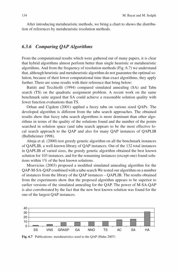
134 M. Bayat and M. Sedghi
After introducing metaheuristic methods, we bring a chart to shows the distribu-tion of references by metaheuristic resolution methods.
6.3.6 Comparing QAP Algorithms
From the computational results which were gathered out of many papers, it is clearthat hybrid algorithms almost perform better than single heuristic or metaheuristicalgorithms. And from the frequency of resolution methods (Fig. 6.7) we understandthat, although heuristic and metaheuristic algorithm do not guarantee the optimal so-lution, because of their lower computational time than exact algorithms, they applyfurther. There are some results with their reference that bring below:
Battiti and Tecchiolli (1994) compared simulated annealing (SA) and Tabusearch (TS) on the quadratic assignment problem. A recent work on the samebenchmark suite argued that SA could achieve a reasonable solution quality withfewer function evaluations than TS.
Orhan and Cigdem (2001) applied a fuzzy tabu on various sized QAPs. Thedeveloped algorithm is different from the tabu search approaches. The obtainedresults show that fuzzy tabu search algorithms is more dominant than other algo-rithms in terms of the quality of the solutions found and the number of the pointssearched in solution space (and tabu search appears to be the most effective lo-cal search approach to the QAP and also for many QAP instances of QAPLIB(Bullnheimer 1998).
Ahuja et al. (2000) test greedy genetic algorithm on all the benchmark instancesof QAPLIB, a well-known library of QAP instances. Out of the 132 total instancesin QAPLIB of varied sizes, the greedy genetic algorithm obtained the best knownsolution for 103 instances, and for the remaining instances (except one) found solu-tions within 1% of the best known solutions.
Misevicius (2003) proposed a modified simulated annealing algorithm for theQAP-M-SA-QAP combined with a tabu search We tested our algorithm on a numberof instances from the library of the QAP instances – QAPLIB. The results obtainedfrom the experiments show that the proposed algorithm appears to be superior toearlier versions of the simulated annealing for the QAP. The power of M-SA-QAPis also corroborated by the fact that the new best known solution was found for theone of the largest QAP instances.
010203040
SS VNS GRASP GA NNO TS AC SA HA
Fig. 6.7 Publications: metaheuristics used to the QAP (Hahn 2007)
6 Quadratic Assignment Problem 135
Tseng and Liang (2005) applied hybrid metaheuristic called ANGEL combinesthe ant colony optimization (ACO), the genetic algorithm (GA) and a local searchmethod (LS) to QAP. Over a hundred instances of QAP benchmarks were testedand the results show that ANGEL is able to obtain the optimal solution with a highsuccess rate of 90%.
Gambardella et al. (1999), in this paper presents HAS-QAP, an hybrid ant colonysystem coupled with a local search, applied to the quadratic assignment problem.HAS-QAP is compared with some of the best heuristics available for the QAP:two tabu search versions, that is, robust and reactive tabu search, an hybrid geneticalgorithm, and simulated annealing. Experimental results show that HAS-QAP andthe hybrid genetic algorithm are the best performing on real world, irregular andstructured problems.
Merz and Freisleben (1999) investigated Memetic algorithm (MA) on a set ofproblem instances containing between 25 and 100 facilities/locations. The resultsindicate that the proposed MA is able to produce high quality solutions quickly.A comparison of the MA with some of the currently best alternative approaches-reactive tabu search, robust tabu search and the fast ant colony system-demonstratesthat the MA outperforms its competitors on all studied problem instances of practi-cal interest.
Tsutsui (2007) applied the cunning ant system (CAS) and ACO to QAP, the resultshowed promising performance of CAS on QAP.
6.4 Case Study
In this section we introduce some case study in real world concerning with QAP.
6.4.1 Hospital Layout as a Quadratic Assignment Problem(Elshafei 1977)
The problem of locating hospital departments so as to minimize the total distancetraveled by patients can be formulated as a quadratic assignment problem. The hos-pital concerned (the Ahmed Maher Hospital) is located in a rather densely populatedpart of Cairo. It is composed of six major departments: out-patient, in-patient, dentalresearch, accident and emergency, physiotherapy and housekeeping and mainte-nance, each department occupying a separate building. The out-patient departmentis more overcrowded with the average daily number of patients now exceeding 700people and patients having to move among the 17 clinics in the department. The lo-cations of the clinics relative to each other has been criticized for causing too muchtraveling for patients and for causing bottlenecks and serious delays. It was thereforedecided to improvement in the layout of the department to reduce the total distancetraveled by patients and hence in the frequency of bottlenecks and congestions.
136 M. Bayat and M. Sedghi
The cost of the original layout is 13,973,298 the cost of the best solution obtainedis 11,281,887, so we obtain approximately the total 19.2% decreasing in distance.The full solution required 136 seconds CPU time on an IBM 360140, the initialsolution being obtained after 44 s CPU time so the remaining 92 s being taken bypart B. The initial solution was 16.4% better than the original layout, a further 2.8%improvement being obtained from part B.
6.4.2 Backboard Wiring Problem (Steinberg 1961)
In 1961, Leon Steinberg’s paper described a backboard wiring problem (SWP)that concerns the placement of computer components so as to minimize the totalamount of wiring required to connect them. In the particular instance considered bySteinberg 34 components with a total of 2,625 interconnections are to be placed on abackboard with 36 open positions. To formulate the wiring problem mathematicallyit is convenient to add two Dummy components with no connections to any othersso that the numbers of components and locations are both nD 36 so for showingthe answer he considered a 6 6 rectangle that each pieces shows the location ofthe components. After solving the problem with branch- and bound algorithm theresult shows that PB and the related QPB perform very poorly and the performanceof GLB is reasonable, and although the dual LP and polyhedral bounds are betterthe computational cost of these bounds is many orders of magnitude higher than thatof GLB. The computation to obtain TDB is also much greater than that required forPB or GLB.
6.4.3 Minimizing WIP Inventories (Benjaafar 2002)
Benjaaafar (2002) use the model to introduce a formulation of the facility layoutdesign problem where the objective is to minimize work-in-process (WIP) theyshow that layouts obtained using a WIP-based formulation can be very differentfrom those obtained using the conventional quadratic assignment problem (QAP)formulation. For example, a QAP-optimal layout can be WIP-infeasible. In gen-eral, they show that WIP is not monotonic in material-handling travel distances soit is possible to reduce overall distances between departments but increase WIP,Furthermore, they find that the relative desirability of a layout can be affected bychanges in material-handling capacity even when travel distances remain the same.After solving this problem with branch- and bound algorithm layout that minimizepf (probability of full handling), does not necessarily minimize pe (probability ofempty handling) and we can have a layout with similar pf but different pe so QAPmodel does not guarantee to be feasible.
6 Quadratic Assignment Problem 137
6.4.4 Zoning in Forest (Bos 1993)
Bos (1993), proposed Zoning the Waterbloem a national forest in southern ofNetherlands, where less than 10% covered by forest, and formulate as QAP so itcan take apart of land quality, management goals and interaction between environ-ment of the forest for assigning a particular grid to particular use. Waterbloem ispresented by 84 grids and its environment is 80 grids and four utility identify:
1. Timber production2. Nature conservation3. Recreation4. Timber production & dispersed recreation
Other area is assign as 5 – residential area, 6 – forest, 7 – agriculture or 8 – road.QAP model solved using simulated annealing method with different weighted
the table of interaction between uses and the results of problem are available in thereferenced article.
6.4.5 Computer Motherboard Design Problem (Miranda 2005)
The model have N electronic components and N location and the goal is minimizethe distance between components so to control the temperature put all heat resourcecomponent together and call it hot – spot and determine the optimal placement.Miranda for solving the electronic motherboard design problem described it as aquadratic assignment problem with additional linear costs and solves it by Benderdecomposition heuristic algorithm. At the end they find that QAP model designproduce lower temperature (there are some picture in the reference article).
References
Abreu NMM, Querido TM, Boaventura-Netto PO (1999) RedInv- SA: A simulated annealing forthe quadratic assignment problem. RAIRO Oper Res 33(3):249–273
Acan A (2005) An external partial permutations memory for ant colony optimization. Lect NotesComput Sci 3448:1–11
Adams WP, Johnson TA (1994) Improved linear programming-based lower bounds for the quad-ratic assignment problem. In: Pardalos PM, Wolkowicz H (eds) Quadratic assignment andrelated problems, DIMACS Series in Discrete Math Theor Comput Sci, AMS, Rhode Island16:43–75
Adams WP, Guignard M, Hahn PM, Hightower WL (2007) A level-2 reformulation-linearizationtechnique bound for the quadratic assignment problem. Eur J Oper Res 180(3):983–996
Ahuja R, Orlin JB, Tiwari A (2000) A greedy genetic algorithm for the quadratic assignmentproblem. Comput Oper Res 27(10):917–934
Anderson EJ (1996) Theory and methodology: Mechanisms for local search. Eur J Oper Res88:139–151
138 M. Bayat and M. Sedghi
Anstreicher KM (2001) Eigenvalue bounds versus semidefinite relaxations for the quadratic as-signment problem. SIAM J Optimiz 11(1):254–265
Anstreicher KM (2003) Recent advances in the solution of quadratic assignment problems. MathProgram 97(1–2):27–42
Anstreicher KM, Brixius NW (2001) A new bound for the quadratic assignment problem based onconvex quadratic programming. Math Program 89(3):341–357
Arkin EM, Hassin R, Sviridenko M (2001) Approximating the maximum quadratic assignmentproblem. Inf Process Lett 77(1):13–16
Armour GC, Buffa ES (1963) Heuristic algorithm and simulation approach to relative location offacilities. Manage Sci 9(2):294–309
Arora S, Frieze A, Kaplan H (2002) A new rounding procedure for the assignment problem withapplications to dense graph arrangement problems. Math Program 92(1):1–36
Assad AA, Xu W (1985) On lower bounds for a class of quadratic f0,1g programs. Oper Res Lett4(4):175–180
Balakrishnan J, Cheng CH, Conway DG, Lau CM (2003) A hybrid genetic algorithm for the dy-namic plant layout problem. Int J Prod Econ 86(2):107–120
Battiti R, Tecchiolli G (1994) Simulated annealing and tabu search in the long run: A comparisonon QAP tasks. Comput Math Appl 28(6):1–8
Baykasoglu A (2004) A metaheuristic algorithm to solve quadratic assignment formulations of cellformation problems without presetting number of cells. J Intell Manuf 15(6):753–759
Bazaraa MS, Sherali HD (1980) Benders’ partitioning scheme applied to a new formulation of thequadratic assignment problem. Naval Res Logist Quart 27:29–41
Bazaraa MS, Sherali HD (1982) On the use of exact and heuristic cutting plane methods for thequadratic assignment problem. J Oper Res Soc 33:991–1003
Bazaraa MS, Kirca O (1983) A branch- and -bound based heuristic for solving the quadraticassignment problem. Naval Res Logist Quart 30:287–304
Ben-David G, Malah D (2005) Bounds on the performance of vector-quantizers under channelerrors. IEEE Trans Inf Theor 51(6):2227–2235
Benjaafar S (2002) Modeling and analysis of congestion in the design of facility layouts. ManageSci 48(5):679–704
Blanchard A, Elloumi S, Faye A, Wicker N (2003) A cutting algorithm of the quadratic assignmentproblem. INFO 41(1):35–49
Bland JA, Dawson GP (1994) Large- scale layout of facilities using a heuristic hybrid algorithm.Appl Math Model 18(9):500–503
Bolte A, Thonemann UW (1996) Optimizing simulated annealing schedules with genetic program-ming. Eur J Oper Res 92(2):402–416
Bos J (1993a) A quadratic assignment problem solved by simulated annealing. J Environ Manage37(2):127–145
Bos J (1993b) Zoning in forest management: a quadratic assignment problem solved by simulatedannealing. J Environ Manage 37:127–145
Bousonocalzon C, Manning MRW (1995) The Hopfield neural-network applied to the quadraticassignment problem. Neural Comput Appl 3(2):64–72
Bruijs PA (1984) On the quality of heuristic solutions to a 19 � 19 quadratic assignment problem.Eur J Oper Res 17:21–30
Brusco MJ, Stahl S (2000) Using quadratic assignment methods to generate initial permutationsfor least-squares unidimensional scaling of symmetric proximity matrices. J Classification17-(2):197–223
Buffa ES, Armour GC, Vollmann TE (1964) Allocating facilities with CRAFT. Harvard Bus Rev42(2):136–158
Bullnheimer B (1998) An examination – scheduling model to maximize students’ study time. LectNotes Comput Sci 1408:78–91
Burer S, Vandenbussche D (2006) Solving lift-and-project relaxations of binary integer programs.SIAM J Optimiz 16:726–750
6 Quadratic Assignment Problem 139
Burkard RE, Bonniger T (1983) A heuristic for quadratic Boolean programs with applications toquadratic assignment problems. Eur J Oper Res 13:374–386
Burkard RE, Rendl F (1984) A thermodynamically motivated simulation procedure for combina-torial optimization problems. Eur J Oper Res 17(2):169–174
Burkard RE, Cela E (1995) Heuristics for biquadratic assignment problems and their computationalcomparison. Eur J Oper Res 83(2):283–300
Burkard RE, Karisch S, Rendl F (1991) QAPLIB – A quadratic assignment problem library.Eur J Oper Res 55:115–119
Burkard RE, Cela E, Klinz B (1994) On the biquadratic assignment problem. In: Pardalos PM,Wolkowicz H (eds) Quadratic assignment and related problems, DIMACS series on discretemathematics and theoretical computer science, vol 16, AMS, Providence, RI, pp 117–146
Chakrapani J, Skorin- Kapov J (1993) Massively parallel tabu search for the quadratic assignmentproblem. Ann Oper Res 41(1–4):327–342
Chiang WC, Chiang C (1998) Intelligent local search strategies for solving facility layout problemswith the quadratic assignment problem formulation. Eur J Oper Res 106(2–3):457–488
Christofides N, Benavent E (1989) An exact algorithm for the quadratic assignment problem. OperRes 37(5):760–768
Colorni A, Dorigo M, Maffioli F, Maniezzo V, Righini G, Trubian M (1996) Heuristics from naturefor hard combinatorial optimization problems. Int Trans Oper Res 3(1):1–21
Cung VD, Mautor T, Michelon P, Tavares A (1997) A scatter search based approach for thequadratic assignment problem. In: Proceedings of IEEE International Conference on Evolu-tionary Computation, pp 165–169
Deineko VG, Woeginger GJ (2000) A study of exponential neighborhoods for the traveling salesmaproblem and for the quadratic assignment problem. Math Program, Ser A 78:519–542
Dorigo M, Gambardella LM, Tailard ED (1997) Ant colonies for Q A P, Technical Report, IDSIA, 4Drezner Z (1995) Lower bounds based on linear programming for the quadratic assignment prob-
lem. Computat Optimiz Appl 4(2):159–165Drezner Z (2005a) Compounded genetic algorithms for the quadratic assignment problem. Oper
Res Lett 33(5):475–480Drezner Z (2005b) The extended concentric tabu for the quadratic assignment problem. Eur J Oper
Res 160:416–422Drezner Z, Marcoulides GA (2003) A distance-based selection ofparents in genetic algorithms. In:
Resende MGC, de Sousa JP (eds). Metaheuristics: Computer decision-making, combinatorialoptimization book series. Kluwer, Dordecht, pp 257–278
Dunker T, Radons G, Westkamper E (2004) Combining evolutionary computation and dynamicprogramming for solving a dynamic facility layout problem. Eur J Oper Res 165(1):55–69
Edwards CS (1980) A branch and bound algorithm for the Koopmans–Beckmann quadratic as-signment problem. Math Program Study 13:35–52
El-Baz MA (2004) A genetic algorithm for facility layout problems of different manufacturingenvironments. Comput Ind Eng 47(2–3):233–246
Elshafei A (1977) Hospital layout as a quadratic assignment problem. Oper Res Quart 28(1):167–179
Finke G, Burkard RE, Rendl F (1987) Quadratic assignment problems. Ann Discrete Math 31:61–82
Fleurent C, Ferland JA (1994) Genetic hybrids for the quadratic assignment problem. In: PardalosPMM, Wolkowicz H (eds). Quadratic assignment and related problems. DIMACS Series inDiscrete Math Theor Comput Sci, vol. 16. AMS, Rhode Island, pp 173–187
Fleurent C, Glover F (1999) Improved constructive multistart strategies of quadratic assignmentproblem using adaptive memory. INFORMS J Comput 11:189–203
Forsberg JH, Delaney RM, Zhao Q, Harakas G, Chandran R (1994) Analyzing lanthanide-includedshifts in the NMR spectra of lanthanide (III) complexes derived from 1,4,7,10-tetrakis (N,N-diethylacetamido)-1,4,7,10-tetraazacyclododecane. Inorg Chem 34:3705–3715
Francis RL, White JA (1974) Facility layout and location: An analytical approach. Prentice-Hall,Englewood Cliffs, NJ
140 M. Bayat and M. Sedghi
Frieze A.M, Yadegar J (1983) On the quadratic assignment problem. Discrete Appl Math 5:89–98Gambardella LM, Taillard D, Dorigo M (1999) Ant colonies for the QAP. J Oper Res Soc
50:167–176Gavett JW, Plyter NV (1966) The optimal assignment of facilities to locations by branch- and-
bound. Oper Res 14:210–232Geoffrion AM, Graves GW (1976) Scheduling parallel production lines with changeover costs:
Practical applications of a quadratic assignment/LP approach. Oper Res 24:595–610Gilmore PC (1962) Optimal and suboptimal algorithms for the quadratic assignment problem.
SIAM J Appl Math 10:305–313Glover F (1977) Heuristics for integer programming using surrogate constraints. Decis Sci
8:156–166Glover F (1989a) Tabu search – Part I. ORSA J Comput 1:190–206Glover F (1989b) Tabu search – Part II. ORSA J Comput 2:4–32Gong D, Yamazaki G, Gen M, Xu W (1999) A genetic algorithm method for one-dimensional
machine location problems. Int J Prod Econ 60–61:337–342Graves GW, Whinston AB (1970) An algorithm for the quadratic assignment problem. Manage Sci
17(7):453–471Gutin G, Yeo A (2002) Polynomial approximation algorithms for TSP and QAP with a factorial
domination number. Discrete Appl Math 119(1–2):107–116Hadley SW, Rendl F, Wolkowicz H (1992a) Nonsymmetric quadratic assignment problems and the
Hoffman–Wielandt inequality. Linear Algebra Appl 58:109–124Hadley SW, Rendl F, Wolkowicz H (1992b) A new lower bound via projection for the quadratic
assignment problem. Math Oper Res 17:727–739Hahn P, Grant T (1998) Lower bounds for the quadratic assignment problem based upon a dual
formulation. Oper Res 46(6):912–922Hahn P, Grant T, Hall N (1998) A branch-and-bound algorithm for the quadratic assignment prob-
lem based on the Hungarian method. Eur J Oper Res 108:629–640Hahn P, Loiola EM, de Abreu NMM, Boaventura-Netto PO, Querido T (2007) A survey for the
quadratic assignment problem. Eur J Oper Res 176:657–690Hamacher H, Nickel S, Tenfelde-Podehl D (2003) Facilities layout for social institutions. In: Oper-
ation Research Proceedings 2001, Selected papers of the international conference on operationsresearch (OR2001). Springer-Verlag, Berlin, pp 229–236
Hansen P, Lih KW (1992) Improved algorithms for partitioning problems in parallel, pipelined,and distributed computing. IEEE Trans Comput 41(6):769–771
Hasegawa M, Ikeguchi T, Aihara K, Itoh K (2002) A nove chaotic search for quadratic assignmentproblems. Eur J Oper Res 139(3):543–556
Heffley DR (1972) The quadratic assignment problem: A note. Econometrica 40(6):1155–1163Heider CH (1973) An N- step, 2- variable search algorithm for the component placement problem.
Naval Res Logist Quart 20:699–724Hubert L (1987) Assignment methods in combinatorial data analysis. Statistics: textbooks and
monographs series, vol 73. Marcel Dekker, New YorkIshii S, Sato M (1998) Constrained neural approaches to quadratic assignment problems. Neural
Netw 11(6):1073–1082Junger M, Kaibel V (2000) On the SQAP-polytope. SIAM J Optimiz 11(2):444–463Junger M, Kaibel V (2001a) The QAP-polytope and the star transformation. Discrete Appl Math
111(3):283–306Junger M, Kaibel V (2001b) Box- inequalities for quadratic assignment polytopes. Math Program
91:75–97Kaibel V (1998) Polyhedral combinatorics of quadratic assignment problems with less objects than
locations. Lecture Notes Comput Sci 1412:409–422Kaufman L, Broeckx F (1978)An algorithm for the quadratic assignment problem using
Benders’decomposition, Eur J Oper Res 2:204–211
6 Quadratic Assignment Problem 141
Knowles J, Corne DW (2003) Instance generators and test suites for the multiobjective quadraticassignment problem. In: Evolutionary multi-criterion optimization (EMO 2003) Second Inter-national Conference, Portugal, Proceedings. Berlin, Springer-Verlag, LNCS, pp 295–310
Koopmans TC, Beckmann MJ (1957) Assignment problems and the location of economic activi-ties. Econometrica 25:53–76
Krarup J, Pruzan PM (1978) Computer-aided layout design. Math Program Study 9:75–94Land AM (1963) A problem of assignment with interrelated costs. Oper Res Quart 14:185–198Lawler EL (1963) The quadratic assignment problem. Manage Sci 9:586–599Lee CG, Ma Z (2004) The generalized quadratic assignment problem. Research Report, Depart-
ment of mechanical and industrial engineering, University of Toronto, CanadaLi WJ, Smith JM (1995) An algorithm for quadratic assignment problems. Eur J Oper Res
81:205–216Li Y, Pardalos PM, Ramakrishnan KG, Resende MGC (1994a) Lower bounds for the quadratic
assignment problem. Oper Res 50:387–410Li Y, Pardalos PM, Resende, MGC (1994b) A greedy randomized adaptive search procedure for
the quadratic assignment problem. In: Pardalos PM, Wolkowicz H (eds), Quadratic assignmentand related problems, DIMACS series in Discrete Math Theor Comput Sci, vol. 16. AMS,Rhode Island, pp 237–261
Lova’sz L, Schrijver A (1991) Cones of matrices and set-functions, and 0–1 optimization. SIAM JOptimiz 1:166–190
Maniezzo V, Colorni A (1999) The ant system applied to the quadratic assign ment problem. KnowlData Eng 11(5):769–778
Mans B, Mautor T, Roucairol C (1995) A parallel depth first search branch and bound algorithmfor the quadratic assignment problem. Eur J Oper Res 81:617–628
Mavridou T, Pardalos PM (1997) Simulated annealing and genetic algorithms for the facility layoutproblem: A survey. Computat Optimiz Appl 7:111–126
Mavridou T, Pardalos PM, Pitsoulis LS, Resende MGC (1998) A GRASP for the biquadratic as-signment problem. Eur J Oper Res 105(3):613–621
Merz P, Freisleben B (1999) A comparison of mimetic algorithms, tabu search, and ant coloniesfor the quadratic assignment problem. In: Proceedings of the 1999 International Congress ofEvolutionary Computation (CEC’99). IEEE Press, New York, pp 2063–2070
Middendorf M, Reischle F, Schmeck H (2002) Multi colony ant algorithms. J Heuristics8(3):305–320
Mills P, Tsang E, Ford J (2003) Applying an extended guided local search to the quadratic assign-ment problem. Ann Oper Res 118(1–4):121–135
Miranda G, Luna HPL, Mateus GR, Ferreira RPM (2005) A performance guarantees heuristicfor electronic components placement problems including thermal effects. Comput Oper Res32:2937–2957
Mirchandani PB, Obata T (1979) Algorithms for a class of quadratic assignment problems. Pre-sented at the Joint ORSA/TIMS National Meeting, New Orleans
Misevicius A (2000a) An intensive search algorithm for the quadratic assignment problem. Infor-matica 11:145–162
Misevicius A (2000b)A new improved simulated annealing algorithm for the quadratic assignmentproblem. Inf Technol Contr 17:29–38
Misevicius A (2003) A modified simulated annealing algorithm for the quadratic assignment prob-lem. Informatica 14(4):497–514
Misevicius A (2004) An improved hybrid genetic algorithm: New results for the quadratic assign-ment problem. Knowl-Based Syst 17(2–4):65–73
Mladenovic N, Hansen P (1997) Variable neighborhood search. Comput Oper Res 24:1097–1100Nishiyama T, Tsuchiya K, Tsujita K (2001) A Markov chain Monte Carlo algorithm for the
quadratic assignment problem based on replicator equations. Lecture Notes Comput Sci2130:148–155
Nissen V, Paul H (1995) A modification of threshold accepting and its application to the quadraticassignment problem. OR Spektrum 17(2–3):205–210
142 M. Bayat and M. Sedghi
Obuchi Y, Masui H, Ohki M (1996) Weighted parallel problem solving by optimization networks.Neural Netw 9(2):357–366
Oliveira CAS, Pardalos MP, Resende MGG (2004) GRASP with path relinking for the quadraticassignment problem. In: Experimental and efficient algorithms, Third International Workshop(WEA 2004), Brazil, LNCS 3059. Springer, Berlin, pp 356–368
Orhan T, Cigdem A (2001) A fuzzy Tabu search approach for the plant layout problemPadberg MW, Rinaldi G (1991) A branch-and-cut algorithm for the resolution of large-scale sym-
metric traveling salesman problems. SIAM Rev 33:60–100Pardalos P M, Murthy K A, Harrison TP (1993) A computational comparison of local search
heuristics for solving quadratic assignment problems. Information 4(1–2):172–187Peng T, Huanchen W, Dongme Z (1996) Simulated annealing for the quadratic assignment prob-
lem: A further study. Comput Ind Eng 31(3–4):925–928Pierskalla WP (1967a) The tri-substitution method for the three-multidimensional assignment
problem. Can Oper Res Soc J 5(2):71–81Pierskalla WF (1967b) The multi-dimensional assignment problem. Technical Memorandum No.
93, Operations Research Department, CASE Institute of Technology, Available on line at:http://www.anderson.ucla.edu/faculty/william.pierskalla/Chronological Bank/Research andPublication Chro.html#Mathematical, State September 1967
Pitsoulis LS, Pardalos PM, Hearn DW (2001) Approximate solutions to the turbine balancing prob-lem. Eur J Oper Res 130m(1):147–155
Pollatschek MA, Gershoni N, Radday YT (1976) Optimization of the typewriter keyboard by sim-ulation. Angewandte Informatik 17:438–439
Rangel M C, Abreu NMM, Boaventura-Netto PO (2000) GRASP in the QAP: an acceptance boundfor initial solutions (in Portuguese). Pesquisa Operacional 20(1):45–58
Rendl F, Sotirov R (2003) Bounds for the quadratic assignment problem using the bundle method.Accepted for publication in Math. Program. B, and will appear in the special issue dedi-cated to Jos Sturm, First available in 2003 as a Technical Report, Department of Mathematics,University of Klagenfurt
Rossin DF, Springer MC, Klein BD (1999) New complexity measures for the facility layoutproblem: An empirical stud using traditional and neural network analysis. Comput Ind Eng36(3):585–602
Sahni S, Gonzales T (1976) P-complete approximation problems. J Assoc Comput Mach 23: 555–565
Siu F, Chang RKC (2002) Effectiveness of optimal node assignments in wavelength division mul-tiplexing networks with fixed regular virtual topogies. Comput Netw 38(1):61–74
Sherali HD, Adams WP (1990) A hierarchy of relaxations between the continuous and convex hullrepresentations for zero-one programming problems. SIAM J Disc Math 3:411–430
Sherali HD, Adams WP, Smith JC (2000) Reduced first-level representations via the reformulation-linearization technique: results, counterexamples, and computations. Discrete Appl Math101:247–267
Skorin-Kapov J (1990) Tabu search applied to the quadratic assignment problem. ORSA J Comput2(1):33–45
Skorin-Kapov J (1994) Extensions of a tabu search adaptation to the quadratic assignment problem.J Comput Oper Res 21(8):855–865
Smith M, Li W (2001) Quadratic assignment problems and M/G/C/C/ state dependent networkflows. J Comb Optimiz 5:421–443
Solimanpur M, Vrat P, Shankaz R (2004) Ant colony optimization algorithm to the inter- cell layoutproblem in cellular manufacturing. Eur J Oper Res 157(3):592–606
Steinberg L (1961) The backboard wiring problem: a placement algorithm. SIAM Rev 3:37–50Stutzle T, Dorigo M (1999) ACO algorithms for the quadratic assignment problem. In: Corne D,
Dorigo M, Glover F (eds). New Ideas Optimiz. McGraw-Hill, New York, pp 33–55Stutzle T, Holgez H (2000) Max-Min ant system. Future Gener Comput Syst 16(8):889–914Taillard E (1991) Robust taboo search for the quadratic assignment problem. Parallel Comput
17:443–455
6 Quadratic Assignment Problem 143
Talbi EG, Hafidi Z, Kebbal D, Geib JM (1998a) A fault-tolerant parallel heuristic for assignmentproblems. Future Generation Comput Syst 14(5–6):425–438
Talbi EG, Roux O, Fonlupt C, Robillard D (2001) Parallel ant colonies for the quadratic assignmentproblem. Future Generation Comput Syst 17(4):441–449
Tansel BC, Bilen C (1998) Move based heuristics for the unidirectional loop network layout prob-lem. Eur J Oper Res 108(1):36–48
Tavakkoli-Moghaddain R, Shayan E (1998) Facilities layout design by genetic algorithms. ComputInd Eng 35(3–4):527–530
Tian P, Wang HC, Zhang DM (1996) Simulated annealing for the quadratic assignment problem:A further study. Comput Ind Eng 31(3–4):925–928
Tian P, Ma J, Zhang DM (1999) Application of the simulated annealing algorithm to the com-binatorial optimization problem with permutation property: An investigation of generationmechanism. Eur J Oper Res 118(1):81–94
Tseng LY, Liang SC (2005) A hybrid metaheuristic for the quadratic assignment problem. ComputOptimiz Appl 34:85–113
Tsuchiya K, Bharitkar S, Takefuji Y (1996) A neural network approach to facility layout problems.Eur J Oper Res 89(3):556–563
Tsutsui S (2007) Cunning ant system for quadratic assignment problem with local search andparallelization. Lecture Notes Comput Sci. Springer, Berlin, pp 269–278
Uwate Y, Nishio Y, Ushida A (2004) Markov chain modeling of intermittency chaos and its appli-cation to Hopfield NN. IEICE Trans Fundam Electron Commun Comput Sci E87A(4):774–779
Wang RL, Okazaki K (2005) Solving facility layout problem using an improved genetic algorithm.IEICE Trans Fundam Electron Commun Comput Sci E88A(2):606–610
Wess B, Zeitlhofer T (2004) On the phase coupling problem between data memory layout genera-tion and address pointer assignment. Lecture Notes Comput Sci 3199:152–166
West DH (1983) Algorithm 608: Approximate solution of the quadratic assignment problem. ACMTrans Math Softw 9:461–466
White DJ (1993) A parametric-based heuristic program for the quadratic assignment problem.Nava Res Logist 40(4):553–568
Wilhelm MR, Ward TL (1987) Solving quadratic assignment problems by simulated annealing.IEEE Trans 19:107–119
Ying KC, Liao CJ (2004) An ant colony system for permutation flow- shop sequencing. ComputOper Res 31(5):791–801
Yip PPC, Pao YH (1994) A guided evolutionary simulated annealing approach to the quadraticassignment problem. IEEE Trans Syst Man Cybernet 24(9):1383–1387
Youssef H, Sait SM, Ali H (2003) Fuzzy simulated evolution algorithm for VLSI cell placement.Comput Ind Eng 44(2):227–247
Yu J, Sarker BR (2003) Directional decomposition heuristic for a linear machine – cell locationproblem. Eur J Oper Res 149(1):142–184
Zhao Q, Karisch SE, Rendl F, Wolkowicz H (1998) Semidefinite programming relaxations for thequadratic assignment problem. J Comb Optimiz 2:71–109
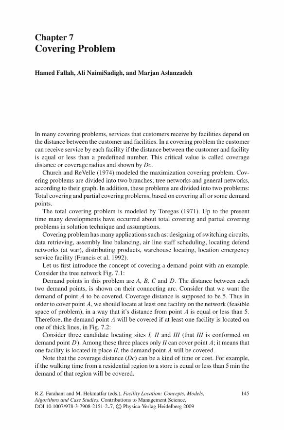
Chapter 7Covering Problem
Hamed Fallah, Ali NaimiSadigh, and Marjan Aslanzadeh
In many covering problems, services that customers receive by facilities depend onthe distance between the customer and facilities. In a covering problem the customercan receive service by each facility if the distance between the customer and facilityis equal or less than a predefined number. This critical value is called coveragedistance or coverage radius and shown by Dc.
Church and ReVelle (1974) modeled the maximization covering problem. Cov-ering problems are divided into two branches; tree networks and general networks,according to their graph. In addition, these problems are divided into two problems:Total covering and partial covering problems, based on covering all or some demandpoints.
The total covering problem is modeled by Toregas (1971). Up to the presenttime many developments have occurred about total covering and partial coveringproblems in solution technique and assumptions.
Covering problem has many applications such as: designing of switching circuits,data retrieving, assembly line balancing, air line staff scheduling, locating defendnetworks (at war), distributing products, warehouse locating, location emergencyservice facility (Francis et al. 1992).
Let us first introduce the concept of covering a demand point with an example.Consider the tree network Fig. 7.1:
Demand points in this problem are A, B, C and D. The distance between eachtwo demand points, is shown on their connecting arc. Consider that we want thedemand of point A to be covered. Coverage distance is supposed to be 5. Thus inorder to cover pointA, we should locate at least one facility on the network (feasiblespace of problem), in a way that it’s distance from point A is equal or less than 5.Therefore, the demand point A will be covered if at least one facility is located onone of thick lines, in Fig. 7.2:
Consider three candidate locating sites I, II and III (that III is conformed ondemand pointD). Among these three places only II can cover pointA; it means thatone facility is located in place II, the demand point A will be covered.
Note that the coverage distance (Dc) can be a kind of time or cost. For example,if the walking time from a residential region to a store is equal or less than 5 min thedemand of that region will be covered.
R.Z. Farahani and M. Hekmatfar (eds.), Facility Location: Concepts, Models, 145Algorithms and Case Studies, Contributions to Management Science,DOI 10.1007/978-3-7908-2151-2 7, c� Physica-Verlag Heidelberg 2009
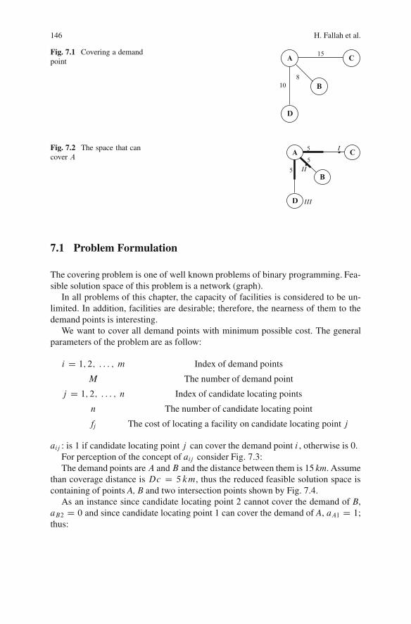
146 H. Fallah et al.
Fig. 7.1 Covering a demandpoint A C
B
D
108
15
Fig. 7.2 The space that cancover A
A C
B
D
5 I
5II5
III
7.1 Problem Formulation
The covering problem is one of well known problems of binary programming. Fea-sible solution space of this problem is a network (graph).
In all problems of this chapter, the capacity of facilities is considered to be un-limited. In addition, facilities are desirable; therefore, the nearness of them to thedemand points is interesting.
We want to cover all demand points with minimum possible cost. The generalparameters of the problem are as follow:
i D 1; 2; : : : ; m Index of demand points
M The number of demand point
j D 1; 2; : : : ; n Index of candidate locating points
n The number of candidate locating point
fj The cost of locating a facility on candidate locating point j
aij : is 1 if candidate locating point j can cover the demand point i , otherwise is 0.For perception of the concept of aij consider Fig. 7.3:The demand points areA andB and the distance between them is 15 km. Assume
than coverage distance is Dc D 5 km, thus the reduced feasible solution space iscontaining of points A, B and two intersection points shown by Fig. 7.4.
As an instance since candidate locating point 2 cannot cover the demand of B,aB2 D 0 and since candidate locating point 1 can cover the demand of A, aA1 D 1;thus:
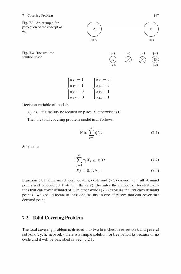
7 Covering Problem 147
Fig. 7.3 An example forperception of the concept ofaij
A B
i=A i=B
Fig. 7.4 The reducedsolution space
A B
i=A i=B
j=1 j=2 j=3 j=4
8<ˆ:aA1 D 1
aA2 D 1
aB1 D 0
aB2 D 0
8<ˆ:aA3 D 0
aA4 D 0
aB3 D 1
aB4 D 1
Decision variable of model:
Xj : is 1 if a facility be located on place j , otherwise is 0
Thus the total covering problem model is as follows:
MinnX
jD1fjXj ; (7.1)
Subject to
nXjD1
aijXj � 1I 8i ; (7.2)
Xj D 0; 1I 8j: (7.3)
Equation (7.1) minimized total locating costs and (7.2) ensures that all demandpoints will be covered. Note that the (7.2) illustrates the number of located facil-ities that can cover demand of i . In other words (7.2) explains that for each demandpoint i . We should locate at least one facility in one of places that can cover thatdemand point.
7.2 Total Covering Problem
The total covering problem is divided into two branches: Tree network and generalnetwork (cyclic network), there is a simple solution for tree networks because of nocycle and it will be described in Sect. 7.2.1.

148 H. Fallah et al.
Fig. 7.5 Example of generalnetwork
B
A
C
A
B
C
DCDC
DCDC
DCDC
Reduced solutionspace
A
B
C
Fig. 7.6 Reducing solution space from continuous space to set points (Daskin 1995)
The general networks (Cyclic networks), are networks that there are more thanone rout between some or all of their nodes.
These networks have a closed loop as their name implies. Consider networkbelow:
In Fig. 7.5 the demand points are A, B, C, the coverage distance is Dc and thefeasible solution space of this problem is the set of points of network.
It seems very difficult to determine the location of facilities and to enter themto the mathematical model as quantities. It is proved that instead of all points ofnetwork (Daskin 1995) we can consider a reduced solution space including demandpoints and intersection points. Intersection points are points that their distance fromat least one of demand points is exactly equal to coverage distance. As we can seein Fig. 7.6 the solution space is reduced from a continuous space to a set of ninecandidate locating points.
Thus all of covering problems have finite candidate locating points (that are al-ways demand points) or we can reduce their space to discreet solution space, so inthis chapter we consider the solution space to be discreet.
If the cost of locating is equal in different places, we have
fj D 1I j D 1; : : : ; n; (7.4)
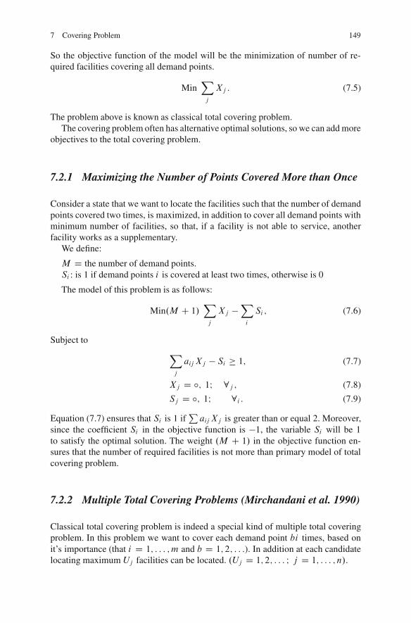
7 Covering Problem 149
So the objective function of the model will be the minimization of number of re-quired facilities covering all demand points.
MinXj
Xj : (7.5)
The problem above is known as classical total covering problem.The covering problem often has alternative optimal solutions, so we can add more
objectives to the total covering problem.
7.2.1 Maximizing the Number of Points Covered More than Once
Consider a state that we want to locate the facilities such that the number of demandpoints covered two times, is maximized, in addition to cover all demand points withminimum number of facilities, so that, if a facility is not able to service, anotherfacility works as a supplementary.
We define:
M D the number of demand points.Si : is 1 if demand points i is covered at least two times, otherwise is 0
The model of this problem is as follows:
Min.M C 1/Xj
Xj �Xi
Si ; (7.6)
Subject to Xj
aijXj � Si � 1; (7.7)
Xj D ı; 1I 8j ; (7.8)
Sj D ı; 1I 8i : (7.9)
Equation (7.7) ensures that Si is 1 ifPaijXj is greater than or equal 2. Moreover,
since the coefficient Si in the objective function is �1, the variable Si will be 1to satisfy the optimal solution. The weight .M C 1/ in the objective function en-sures that the number of required facilities is not more than primary model of totalcovering problem.
7.2.2 Multiple Total Covering Problems (Mirchandani et al. 1990)
Classical total covering problem is indeed a special kind of multiple total coveringproblem. In this problem we want to cover each demand point bi times, based onit’s importance (that i D 1; : : : ; m and b D 1; 2; : : :). In addition at each candidatelocating maximum Uj facilities can be located. .Uj D 1; 2; : : : I j D 1; : : : ; n/:
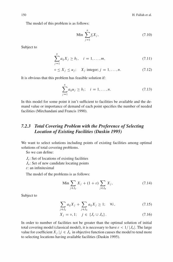
150 H. Fallah et al.
The model of this problem is as follows:
MinnX
jD1fjXj ; (7.10)
Subject to
nXjD1
aijXj � bi ; i D 1; : : : ; m; (7.11)
ı � Xj � uj I Xj integerI j D 1; : : : ; n: (7.12)
It is obvious that this problem has feasible solution if:
nXjD1
aijuj � bi I i D 1; : : : ; n: (7.13)
In this model for some point it isn’t sufficient to facilities be available and the de-mand value or importance of demand of each point specifies the number of neededfacilities (Mirchandani and Francis 1990).
7.2.3 Total Covering Problem with the Preference of SelectingLocation of Existing Facilities (Daskin 1995)
We want to select solutions including points of existing facilities among optimalsolutions of total covering problems.
So we can define:
Je : Set of locations of existing facilitiesJn: Set of new candidate locating points": an infinitesimal
The model of the problems is as follows:
MinXj2Je
Xj C .1C "/Xj2Jn
Xj ; (7.14)
Subject to Xj2Je
aijXj CXj2Jn
aijXj � 1I 8i ; (7.15)
Xj D ı; 1I j 2 fJe [ Jng : (7.16)
In order to number of facilities not be greater than the optimal solution of initialtotal covering model (classical model), it is necessary to have " < 1= jJnj. The largevalue for coefficientXj jj 2 Jn in objective function causes the model to tend moreto selecting locations having available facilities (Daskin 1995).
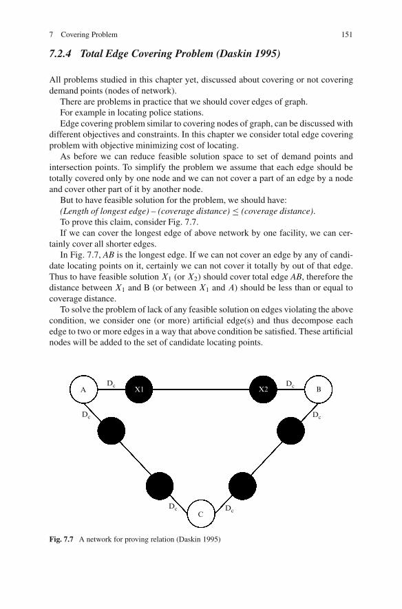
7 Covering Problem 151
7.2.4 Total Edge Covering Problem (Daskin 1995)
All problems studied in this chapter yet, discussed about covering or not coveringdemand points (nodes of network).
There are problems in practice that we should cover edges of graph.For example in locating police stations.Edge covering problem similar to covering nodes of graph, can be discussed with
different objectives and constraints. In this chapter we consider total edge coveringproblem with objective minimizing cost of locating.
As before we can reduce feasible solution space to set of demand points andintersection points. To simplify the problem we assume that each edge should betotally covered only by one node and we can not cover a part of an edge by a nodeand cover other part of it by another node.
But to have feasible solution for the problem, we should have:(Length of longest edge) – (coverage distance) � (coverage distance).To prove this claim, consider Fig. 7.7.If we can cover the longest edge of above network by one facility, we can cer-
tainly cover all shorter edges.In Fig. 7.7, AB is the longest edge. If we can not cover an edge by any of candi-
date locating points on it, certainly we can not cover it totally by out of that edge.Thus to have feasible solution X1 (or X2) should cover total edge AB, therefore thedistance between X1 and B (or between X1 and A) should be less than or equal tocoverage distance.
To solve the problem of lack of any feasible solution on edges violating the abovecondition, we consider one (or more) artificial edge(s) and thus decompose eachedge to two or more edges in a way that above condition be satisfied. These artificialnodes will be added to the set of candidate locating points.
A B
C
Dc
Dc
Dc Dc
Dc
DcX2X1
Fig. 7.7 A network for proving relation (Daskin 1995)
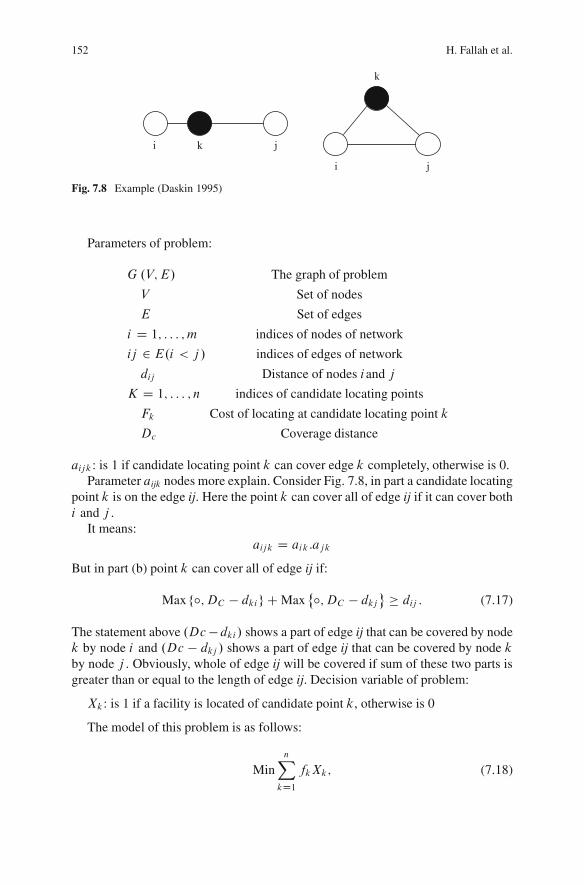
152 H. Fallah et al.
i k j
i j
k
Fig. 7.8 Example (Daskin 1995)
Parameters of problem:
G .V;E/ The graph of problem
V Set of nodes
E Set of edges
i D 1; : : : ; m indices of nodes of network
ij 2 E.i < j / indices of edges of network
dij Distance of nodes iand j
K D 1; : : : ; n indices of candidate locating points
Fk Cost of locating at candidate locating point k
Dc Coverage distance
aijk : is 1 if candidate locating point k can cover edge k completely, otherwise is 0.Parameter aijk nodes more explain. Consider Fig. 7.8, in part a candidate locating
point k is on the edge ij. Here the point k can cover all of edge ij if it can cover bothi and j .
It means:aijk D aik:ajk
But in part (b) point k can cover all of edge ij if:
Max fı;DC � dkig C Max˚ı;DC � dkj
� � dij : (7.17)
The statement above .Dc�dki / shows a part of edge ij that can be covered by nodek by node i and .Dc � dkj / shows a part of edge ij that can be covered by node kby node j . Obviously, whole of edge ij will be covered if sum of these two parts isgreater than or equal to the length of edge ij. Decision variable of problem:
Xk : is 1 if a facility is located of candidate point k, otherwise is 0
The model of this problem is as follows:
MinnX
kD1fkXk; (7.18)
7 Covering Problem 153
Subject to
nXkD1
aijkXj � 1I 8ij 2 EI i < j ; (7.19)
Xj D 0; 1: (7.20)
As we can see, the model is similar to the total covering model and the only differ-ence is in computing coefficients of coverage matrix .aijk/ (Daskin 1995).
7.2.5 Notes on Total Covering Problems
7.2.5.1 Total Covering Problem with Fuzzy Matrix of Coverage Coefficients(Chiang et al. 2005)
There are problems in practice that we can not exactly talk about covering a demandpoint by a candidate locating location.
In other words, the possibility of covering demand point i by facility j , that isshown by �j .i/ has a value which belongs to interval [0,1].
The objective is that with minimum cost of locating facilities the possibility ofcovering each demand point is greater than or equal to a predefined value ˛.
Thus the primary model of the problem is as follows:
MinnX
jD1CjXj; (7.21)
Subject to
1 �nY
jD1.1 � �j .i/ Xj / � ˛I i D 1; : : : ; m; (7.22)
Xj 2 f0; 1g : (7.23)
That Cj is the cost of locating a facility at point j W.j D 1; 2 : : : n/.Chiang et al. (2005) proved that we can transform the (7.21) of above model to
the following linear model:
Subject to
nXjD1
�� ln.1 � �j .i//�Xj � � ln.1 � ˛/I i D 1; : : : ; m; (7.24)
Note that in this model we don’t consider ˛ D 1 and ı < ˛ < 1 (Chiang et al. 2005).
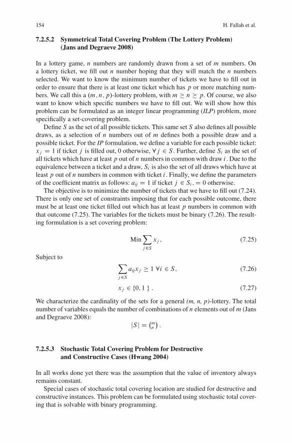
154 H. Fallah et al.
7.2.5.2 Symmetrical Total Covering Problem (The Lottery Problem)(Jans and Degraeve 2008)
In a lottery game, n numbers are randomly drawn from a set of m numbers. Ona lottery ticket, we fill out n number hoping that they will match the n numbersselected. We want to know the minimum number of tickets we have to fill out inorder to ensure that there is at least one ticket which has p or more matching num-bers. We call this a .m; n; p/-lottery problem, with m � n � p. Of course, we alsowant to know which specific numbers we have to fill out. We will show how thisproblem can be formulated as an integer linear programming (ILP) problem, morespecifically a set-covering problem.
Define S as the set of all possible tickets. This same set S also defines all possibledraws, as a selection of n numbers out of m defines both a possible draw and apossible ticket. For the IP formulation, we define a variable for each possible ticket:xj D 1 if ticket j is filled out, 0 otherwise, 8j 2 S . Further, define Si as the set ofall tickets which have at least p out of n numbers in common with draw i . Due to theequivalence between a ticket and a draw, Si is also the set of all draws which have atleast p out of n numbers in common with ticket i . Finally, we define the parametersof the coefficient matrix as follows: aij D 1 if ticket j 2 Si ;D 0 otherwise.
The objective is to minimize the number of tickets that we have to fill out (7.24).There is only one set of constraints imposing that for each possible outcome, theremust be at least one ticket filled out which has at least p numbers in common withthat outcome (7.25). The variables for the tickets must be binary (7.26). The result-ing formulation is a set covering problem:
MinXj2S
xj ; (7.25)
Subject to Xj2S
aijxj � 1 8i 2 S; (7.26)
xj 2 f0; 1 g : (7.27)
We characterize the cardinality of the sets for a general (m, n, p)-lottery. The totalnumber of variables equals the number of combinations of n elements out ofm (Jansand Degraeve 2008):
jS j D �mn
�:
7.2.5.3 Stochastic Total Covering Problem for Destructiveand Constructive Cases (Hwang 2004)
In all works done yet there was the assumption that the value of inventory alwaysremains constant.
Special cases of stochastic total covering location are studied for destructive andconstructive instances. This problem can be formulated using stochastic total cover-ing that is solvable with binary programming.
7 Covering Problem 155
Objective: minimizing the number of storing facilities in a set of discreet points.Constraint: probability of covering each point should not be less than a critical
value.Presumptions:
� Passing time causes improvement or decay in inventory� Distances can be of any type
Decision variable: Xj
Xj : is 1 if a facility is located at point j, otherwise is 0
Parameter:
Fij: Sum of transportation costs in each period and costs of constructive or de-structiveAi : Service level needed for demand point iri : Critical value of probability of covering demand point i
The small model is as follows (Hwang 2004):
MinnP
jD1xj ; (7.28)
Subject to
nPjD1
aijxj � 1 8i D 1; : : : ; m; (7.29)
xj D f0; 1g 8j D 1; : : : ; n; (7.30)
aij D(1 if p.Fij � Ai/ � ri
0 Otherwise: (7.31)
7.3 Partial Covering Problem
Total covering problem can not cover all location problems in real world, becausein many problems budget constraints and other constraints do not let us cover allpoints. For example, consider that we need four facilities to cover all demand pointsbut budget constraint does not let us locate more than three facilities, thus coveringproblem doesn’t have feasible solution.
On the other hand, the total covering problem considers all demand points simi-larly regardless of their demand. For example in a total covering problem, satisfyinga demand point that has 10 units demand, has the same importance with satisfyinga demand point that has 1,000 units demand.
To confront such problems, another covering problem is proposed that calledpartial covering problem. In this part we will introduce some samples of it.
156 H. Fallah et al.
7.3.1 Minimizing Costs Arisen from Not Covering Demand Points(Mirchandani and Francis 1990)
In this problem, maximum number of facilities is limited and equal to P . In otherwords the problem is exogenous and Pi is penalty cost of not covering demandpoint i . In addition consider the number of demand points is m and the number ofcandidate locating points is n.
Decision variables of problem are:
Xj : is 1 if a facility is located at j , otherwise is 0Zi : is 1 if the demand point i is not satisfied, otherwise is 0
The model of this problem is as follows:
MinmXiD1
piZi ; (7.32)
Subject tonX
jD1aijXj CZi � 1 I i D 1; : : : ; m; (7.33)
nXjD1
Xj � P ; (7.34)
Xj 2 f0; 1gI j D 1; : : : ; n; (7.35)
Zi 2 f0; 1g I i D 1; : : : ; m: (7.36)
Assumption above the objective of this model is to minimize total penalty costsof points that their demand is not satisfied. Equation (7.32) ensures that Zi is 1 ifPaijXj is zero; it means that their demand is not satisfied. Equation (7.33) ensures
that the number of facilities can not be more than P .If costs of locating facilities at different points are different, it means we haveFj D the cost of locating a facility at candidate point j .We can replace constraint of the number of facilities represented by (7.33) with
capital constraint as follows:nX
jD1FjXj � C : (7.37)
C is minimum capital to locate facilities (Mirchandani and Francis 1990).
7.3.2 Minimizing Costs of Locating Facilities and Costs Arisenfrom Not Covering Demand Points
In this condition, there is no limitation to number of facilities (or maximum budgetof locating facilities), in other words the problem is endogenous.
7 Covering Problem 157
The objective is to minimize sum of locating costs and penalty costs arisen fromnot covering demand points.
Model of this problem is as follows:
MinnX
jD1FjXj C
mXiD1
piZi ; (7.38)
Subject to
nXjD1
aijXj CZi � 1 I i D 1; : : : ; m; (7.39)
Xj 2 f0; 1g I j D 1; : : : ; n; (7.40)
Zi 2 f0; 1g I j D 1; : : : ; m: (7.41)
Fj is cost of locating a facility at point j and Pi is penalty of not covering demandpoint i in (7.37). Equation (7.38) ensures that Zi is 1 if
PaijXj is zero, it means
that demand point i is not covered.
7.3.3 Maximum Covering Location Problems (Bermanet al. 2003)
One of most famous partial covering problem is maximum covering location prob-lem.
This problem proposed by Church and ReVelle (1974), they limited candidatelocating points to the nodes in network (Berman et al. 2003).
The objective of this problem is to maximize total satisfied demands. In thisproblem, maximum number of facilities is limited (the problem is exogenous).
The model is as follows:
MaxXi
hiZi ; (7.42)
Subject to
Zi �Xj
aijXj I 8i ; (7.43)
Xj
Xj � P ; (7.44)
Xj D 0; 1I 8j; (7.45)
Zi D 0; 1I 8i: (7.46)
Equation (7.42) states that we want to minimize total demands of satisfied demandpoints. hi is demand point i and Zi is one if demand of point i is covered.
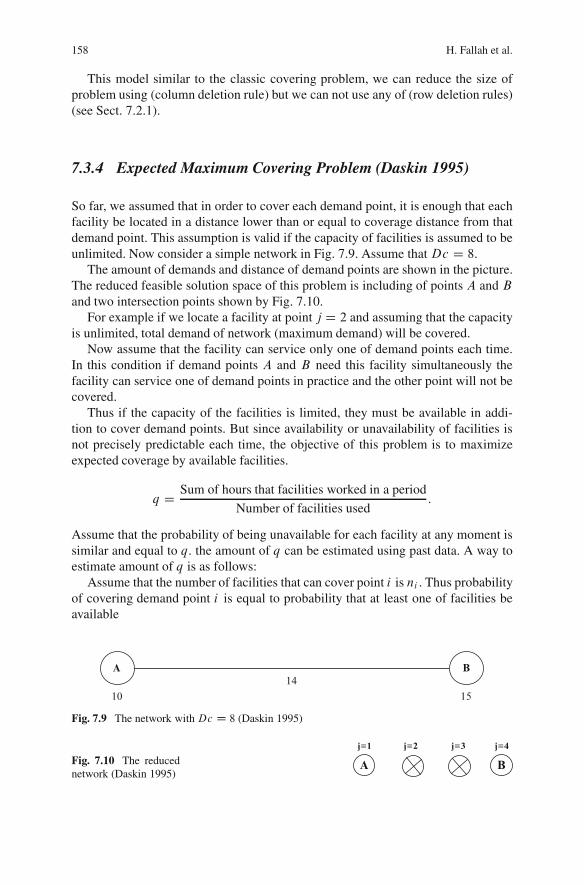
158 H. Fallah et al.
This model similar to the classic covering problem, we can reduce the size ofproblem using (column deletion rule) but we can not use any of (row deletion rules)(see Sect. 7.2.1).
7.3.4 Expected Maximum Covering Problem (Daskin 1995)
So far, we assumed that in order to cover each demand point, it is enough that eachfacility be located in a distance lower than or equal to coverage distance from thatdemand point. This assumption is valid if the capacity of facilities is assumed to beunlimited. Now consider a simple network in Fig. 7.9. Assume that Dc D 8.
The amount of demands and distance of demand points are shown in the picture.The reduced feasible solution space of this problem is including of points A and Band two intersection points shown by Fig. 7.10.
For example if we locate a facility at point j D 2 and assuming that the capacityis unlimited, total demand of network (maximum demand) will be covered.
Now assume that the facility can service only one of demand points each time.In this condition if demand points A and B need this facility simultaneously thefacility can service one of demand points in practice and the other point will not becovered.
Thus if the capacity of the facilities is limited, they must be available in addi-tion to cover demand points. But since availability or unavailability of facilities isnot precisely predictable each time, the objective of this problem is to maximizeexpected coverage by available facilities.
q D Sum of hours that facilities worked in a period
Number of facilities used:
Assume that the probability of being unavailable for each facility at any moment issimilar and equal to q. the amount of q can be estimated using past data. A way toestimate amount of q is as follows:
Assume that the number of facilities that can cover point i is ni . Thus probabilityof covering demand point i is equal to probability that at least one of facilities beavailable
10
A B
15
14
Fig. 7.9 The network withDc D 8 (Daskin 1995)
Fig. 7.10 The reducednetwork (Daskin 1995)
A B
j=1 j=2 j=3 j=4
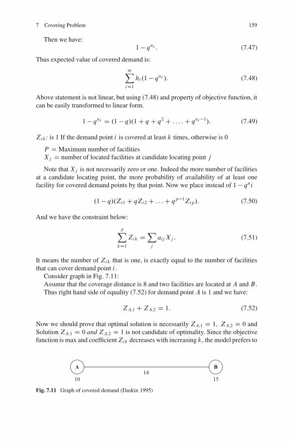
7 Covering Problem 159
Then we have:1 � qni : (7.47)
Thus expected value of covered demand is:
mXiD1
hi .1 � qni /: (7.48)
Above statement is not linear, but using (7.48) and property of objective function, itcan be easily transformed to linear form.
1� qni D .1 � q/.1C q C q2 C : : : :C qni �1/: (7.49)
Zik : is 1 If the demand point i is covered at least k times, otherwise is 0
P D Maximum number of facilitiesXj D number of located facilities at candidate locating point j
Note that Xj is not necessarily zero or one. Indeed the more number of facilitiesat a candidate locating point, the more probability of availability of at least onefacility for covered demand points by that point. Now we place instead of 1 � qni
.1 � q/.Zi1 C qZi2 C : : :C qp�1Zip/: (7.50)
And we have the constraint below:
pXkD1
Zik DXj
aij Xj : (7.51)
It means the number of Zik that is one, is exactly equal to the number of facilitiesthat can cover demand point i .
Consider graph in Fig. 7.11:Assume that the coverage distance is 8 and two facilities are located at A and B .Thus right hand side of equality (7.52) for demand point A is 1 and we have:
ZA;1 CZA;2 D 1: (7.52)
Now we should prove that optimal solution is necessarily ZA;1 D 1; ZA;2 D 0 andSolution ZA;1 D 0 and ZA;2 D 1 is not candidate of optimality. Since the objectivefunction is max and coefficientZik decreases with increasing k, the model prefers to
10
A B
1514
Fig. 7.11 Graph of covered demand (Daskin 1995)
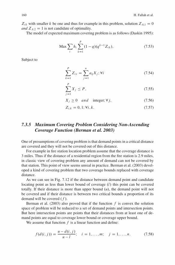
160 H. Fallah et al.
Zik with smaller k be one and thus for example in this problem, solution ZA;1 D 0
and ZA:2 D 1 is not candidate of optimality.The model of expected maximum covering problem is as follows (Daskin 1995):
MaxXi
hi
PXkD1
.1 � q/.qk�1Zik/; (7.53)
Subject to
PXkD1
Zix DnX
jD1aijXj I 8i (7.54)
PXjD1
Xj � P ; (7.55)
Xj � 0 and integerI 8j; (7.56)
Zi;k D 0; 1I 8i; k: (7.57)
7.3.5 Maximum Covering Problem Considering Non-AscendingCoverage Function (Berman et al. 2003)
One of presumptions of covering problem is that demand points in a critical distanceare covered and they will not be covered out of this distance.
For example in fire station location problem assume that the coverage distance is3 miles. Thus if the distance of a residential region from the fire station is 2.9 miles,in classic view of covering problem any amount of demand can not be covered bythat station. This point of view seems unreal in practice. Berman et al. (2003) devel-oped a kind of covering problem that two coverage bounds replaced with coveragedistance.
As we can see in Fig. 7.12 if the distance between demand point and candidatelocating point as less than lower bound of coverage .l/ this point can be coveredtotally. If their distance is more than upper bound .u/, the demand point will notbe covered and if their distance is between two critical bounds a proportion of itsdemand will be covered .f /.
Berman et al. (2003) also proved that if the function f is convex the solutionspace of problem will be reduced to a set of demand points and intersection points.But here intersection points are points that their distances from at least one of de-mand points are equal to coverage lower bound or coverage upper bound.
We assume that function f is a linear function and define:
f .d.i; j // D u � d.i; j /u � l I i D 1; : : : ; mI j D 1; : : : ; n: (7.58)
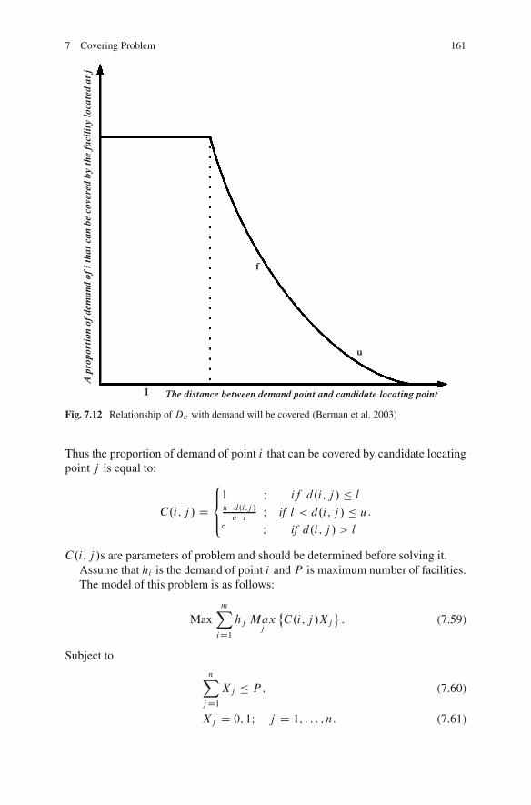
7 Covering Problem 161
A p
ropo
rtio
n of
dem
and
of i
that
can
be
cove
red
by t
he f
acil
ity
loca
ted
at j
The distance between demand point and candidate locating pointI
f
u
Fig. 7.12 Relationship of Dc with demand will be covered (Berman et al. 2003)
Thus the proportion of demand of point i that can be covered by candidate locatingpoint j is equal to:
C.i; j / D
8<:1 I if d.i; j / � lu�d.i;j /
u�l I if l < d.i; j / � uı I if d.i; j / > l
:
C.i; j /s are parameters of problem and should be determined before solving it.Assume that hi is the demand of point i and P is maximum number of facilities.The model of this problem is as follows:
MaxmXiD1
hj Maxj
˚C.i; j /Xj
�: (7.59)
Subject to
nXjD1
Xj � P ; (7.60)
Xj D 0; 1I j D 1; : : : ; n: (7.61)
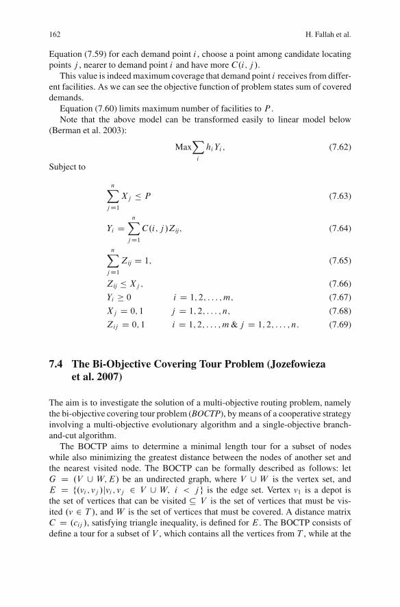
162 H. Fallah et al.
Equation (7.59) for each demand point i , choose a point among candidate locatingpoints j , nearer to demand point i and have more C.i; j /.
This value is indeed maximum coverage that demand point i receives from differ-ent facilities. As we can see the objective function of problem states sum of covereddemands.
Equation (7.60) limits maximum number of facilities to P .Note that the above model can be transformed easily to linear model below
(Berman et al. 2003):
MaxXi
hiYi ; (7.62)
Subject to
nXjD1
Xj � P (7.63)
Yi DnX
jD1C.i; j /Zij; (7.64)
nXjD1
Zij D 1; (7.65)
Zij � Xj ; (7.66)
Yi � 0 i D 1; 2; : : : ; m; (7.67)
Xj D 0; 1 j D 1; 2; : : : ; n; (7.68)
Zij D 0; 1 i D 1; 2; : : : ; m& j D 1; 2; : : : ; n: (7.69)
7.4 The Bi-Objective Covering Tour Problem (Jozefowiezaet al. 2007)
The aim is to investigate the solution of a multi-objective routing problem, namelythe bi-objective covering tour problem (BOCTP), by means of a cooperative strategyinvolving a multi-objective evolutionary algorithm and a single-objective branch-and-cut algorithm.
The BOCTP aims to determine a minimal length tour for a subset of nodeswhile also minimizing the greatest distance between the nodes of another set andthe nearest visited node. The BOCTP can be formally described as follows: letG D .V [ W;E/ be an undirected graph, where V [ W is the vertex set, andE D f.vi ; vj /jvi ; vj 2 V [ W; i < j g is the edge set. Vertex v1 is a depot isthe set of vertices that can be visited � V is the set of vertices that must be vis-ited .v 2 T /, and W is the set of vertices that must be covered. A distance matrixC D .cij /, satisfying triangle inequality, is defined for E . The BOCTP consists ofdefine a tour for a subset of V , which contains all the vertices from T , while at the
7 Covering Problem 163
same time optimizing the following two objectives: .a/ the minimization of the tourlength and .b/ the minimization of the cover. The cover of a solution is defined asthe greatest distance between a node w 2 W , and the nearest visited node v 2 V .
One generic application of the CTP involves designing a tour in a network whosevertices represent.
Points that can be visited, and from which the places that are not on the tour canbe easily reached.
For instance, Toregas et al. (1971) have used the CTP to model the determinationof a tour for a mobile.
Medical facility in an area of Ghana, where every village cannot be reached(Jozefowieza et al. 2007).
7.5 A Fuzzy Multi Objective Covering Based Vehicle LocationModel for Emergency Services (Araz et al. 2007)
Timeliness is one of the most important objectives that reflect the quality of emer-gency services such as ambulance and firefighting systems. To provide timeliness,system administrators may increase the number of service vehicles available. Un-fortunately, increasing the number of vehicles is generally impossible due to capitalconstraints. In such a case, the efficient deployment of emergency service vehiclesbecomes a crucial issue. The objectives considered in the model are maximiza-tion of the population covered by one vehicle, maximization of the population withbackup coverage and increasing the service level by minimizing the total travel dis-tance from locations at a distance bigger than a pre specified distance standard forall zones.
The model addresses the issue of determining the best base locations for a lim-ited number of vehicles so that the service level objectives are optimized. Three ofthe important surrogates that reflect the quality of emergency service systems areconsidered as objectives in the model:
� Maximization of the population covered by one vehicle� Maximization of the population with backup coverage and� Minimization of the total travel distance from locations at a distance bigger than
a pre specified distance standard for all zones.
The proposed model allows the incorporation of decision maker’s imprecise as-piration levels for the goals by means of FGP approach.
Timeliness can be measured in many ways such as:
� Minimization of the total or average time to serve all emergency calls;� Minimization of the maximum travel time to any single call;� Maximization of area coverage (ensures that as many zones in the area as possible
is covered within S minutes of travel)� Maximization of call coverage (ensures that as many calls in the area as possible
is covered within minutes of travel).
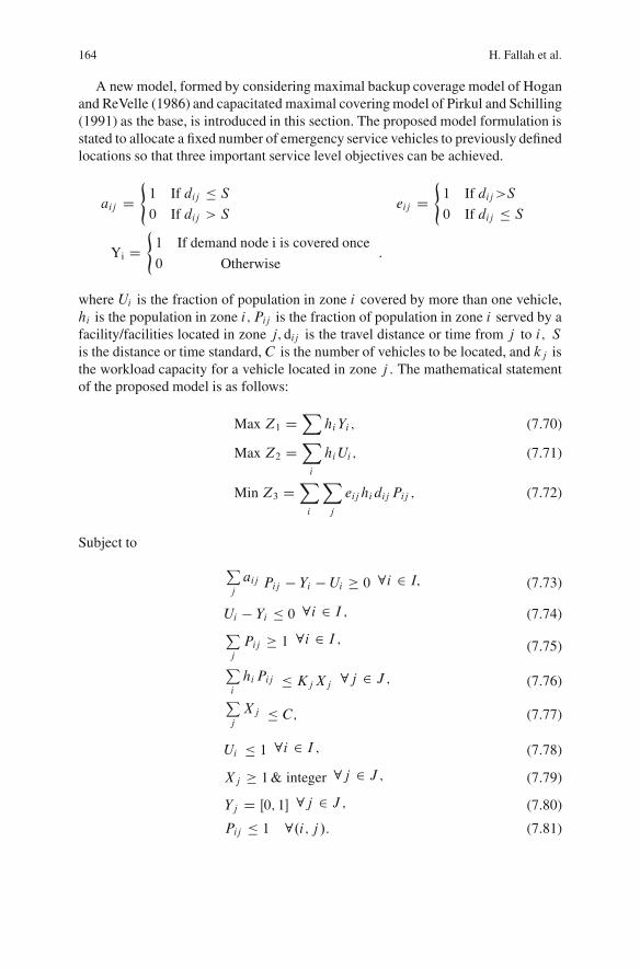
164 H. Fallah et al.
A new model, formed by considering maximal backup coverage model of Hoganand ReVelle (1986) and capacitated maximal covering model of Pirkul and Schilling(1991) as the base, is introduced in this section. The proposed model formulation isstated to allocate a fixed number of emergency service vehicles to previously definedlocations so that three important service level objectives can be achieved.
aij D(1 If dij � S
0 If dij > Seij D
(1 If dij>S
0 If dij � S
Yi D(1 If demand node i is covered once
0 Otherwise:
where Ui is the fraction of population in zone i covered by more than one vehicle,hi is the population in zone i; Pij is the fraction of population in zone i served by afacility/facilities located in zone j; dij is the travel distance or time from j to i; Sis the distance or time standard, C is the number of vehicles to be located, and kj isthe workload capacity for a vehicle located in zone j . The mathematical statementof the proposed model is as follows:
Max Z1 DX
hiYi ; (7.70)
Max Z2 DXi
hiUi ; (7.71)
Min Z3 DXi
Xj
eij hidijPij ; (7.72)
Subject to
Pj
aij Pij � Yi � Ui � 0 8i 2 I; (7.73)
Ui � Yi � 0 8i 2 I ; (7.74)Pj
Pij � 1 8i 2 I ; (7.75)Pi
hiPij � KjXj 8j 2 J ; (7.76)Pj
Xj � C; (7.77)
Ui � 1 8i 2 I ; (7.78)
Xj � 1& integer 8j 2 J ; (7.79)
Yj D Œ0; 1 8j 2 J ; (7.80)
Pij � 1 8.i; j /: (7.81)
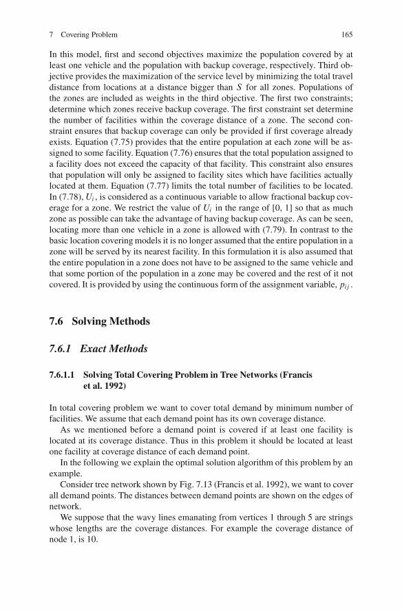
7 Covering Problem 165
In this model, first and second objectives maximize the population covered by atleast one vehicle and the population with backup coverage, respectively. Third ob-jective provides the maximization of the service level by minimizing the total traveldistance from locations at a distance bigger than S for all zones. Populations ofthe zones are included as weights in the third objective. The first two constraints;determine which zones receive backup coverage. The first constraint set determinethe number of facilities within the coverage distance of a zone. The second con-straint ensures that backup coverage can only be provided if first coverage alreadyexists. Equation (7.75) provides that the entire population at each zone will be as-signed to some facility. Equation (7.76) ensures that the total population assigned toa facility does not exceed the capacity of that facility. This constraint also ensuresthat population will only be assigned to facility sites which have facilities actuallylocated at them. Equation (7.77) limits the total number of facilities to be located.In (7.78), Ui , is considered as a continuous variable to allow fractional backup cov-erage for a zone. We restrict the value of Ui in the range of [0, 1] so that as muchzone as possible can take the advantage of having backup coverage. As can be seen,locating more than one vehicle in a zone is allowed with (7.79). In contrast to thebasic location covering models it is no longer assumed that the entire population in azone will be served by its nearest facility. In this formulation it is also assumed thatthe entire population in a zone does not have to be assigned to the same vehicle andthat some portion of the population in a zone may be covered and the rest of it notcovered. It is provided by using the continuous form of the assignment variable, pij .
7.6 Solving Methods
7.6.1 Exact Methods
7.6.1.1 Solving Total Covering Problem in Tree Networks (Franciset al. 1992)
In total covering problem we want to cover total demand by minimum number offacilities. We assume that each demand point has its own coverage distance.
As we mentioned before a demand point is covered if at least one facility islocated at its coverage distance. Thus in this problem it should be located at leastone facility at coverage distance of each demand point.
In the following we explain the optimal solution algorithm of this problem by anexample.
Consider tree network shown by Fig. 7.13 (Francis et al. 1992), we want to coverall demand points. The distances between demand points are shown on the edges ofnetwork.
We suppose that the wavy lines emanating from vertices 1 through 5 are stringswhose lengths are the coverage distances. For example the coverage distance ofnode 1, is 10.
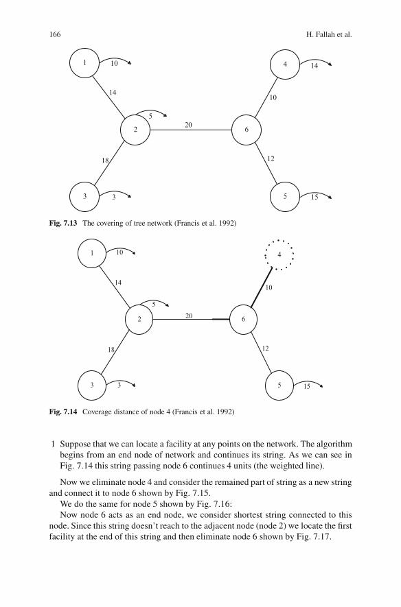
166 H. Fallah et al.
1
5
4
62
3
10
14
5
18
3
20
15
12
10
14
Fig. 7.13 The covering of tree network (Francis et al. 1992)
1
5
4
62
3
10
14
5
18
3
20
15
12
10
Fig. 7.14 Coverage distance of node 4 (Francis et al. 1992)
1 Suppose that we can locate a facility at any points on the network. The algorithmbegins from an end node of network and continues its string. As we can see inFig. 7.14 this string passing node 6 continues 4 units (the weighted line).
Now we eliminate node 4 and consider the remained part of string as a new stringand connect it to node 6 shown by Fig. 7.15.
We do the same for node 5 shown by Fig. 7.16:Now node 6 acts as an end node, we consider shortest string connected to this
node. Since this string doesn’t reach to the adjacent node (node 2) we locate the firstfacility at the end of this string and then eliminate node 6 shown by Fig. 7.17.
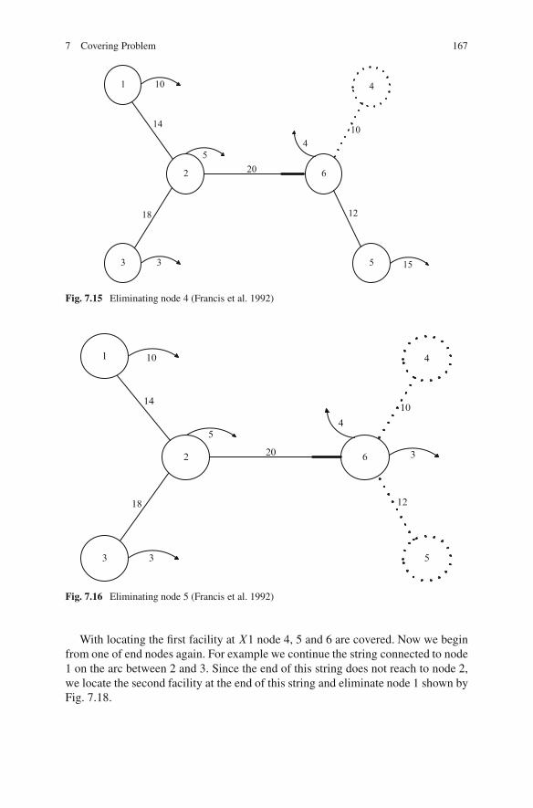
7 Covering Problem 167
1
5
4
62
3
10
14
5
18
3
20
15
12
104
Fig. 7.15 Eliminating node 4 (Francis et al. 1992)
1
5
4
62
3
10
14
5
18
3
20 3
12
10
4
Fig. 7.16 Eliminating node 5 (Francis et al. 1992)
With locating the first facility at X1 node 4, 5 and 6 are covered. Now we beginfrom one of end nodes again. For example we continue the string connected to node1 on the arc between 2 and 3. Since the end of this string does not reach to node 2,we locate the second facility at the end of this string and eliminate node 1 shown byFig. 7.18.
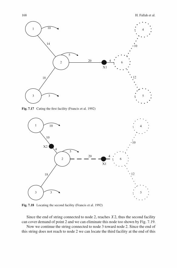
168 H. Fallah et al.
1
5
4
62
3
10
14
5
18
3
20
12
10
4
X1
Fig. 7.17 Cating the first facility (Francis et al. 1992)
1
5
4
62
3
10
10
5
18
3
20
12
10
4
X1
4X2
Fig. 7.18 Locating the second facility (Francis et al. 1992)
Since the end of string connected to node 2, reachesX2, thus the second facilitycan cover demand of point 2 and we can eliminate this node too shown by Fig. 7.19.
Now we continue the string connected to node 3 toward node 2. Since the end ofthis string does not reach to node 2 we can locate the third facility at the end of this
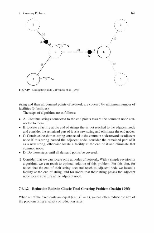
7 Covering Problem 169
1
5
4
62
3
10
5
18
3
20
12
10
4
X1
4X2
Fig. 7.19 Eliminating node 2 (Francis et al. 1992)
string and then all demand points of network are covered by minimum number offacilities (3 facilities).
The steps of algorithm are as follows:
� A: Continue strings connected to the end points toward the common node con-nected to them.
� B: Locate a facility at the end of strings that is not reached to the adjacent nodeand consider the remained part of it as a new string and eliminate the end nodes.
� C: Continue the shortest string connected to the common node toward its adjacentnode if this string passed the adjacent node, consider the remained part of itas a new string, otherwise locate a facility at the end of it and eliminate thatcommon node.
� D: Do these steps until all demand points be covered.
2 Consider that we can locate only at nodes of network. With a simple revision inalgorithm, we can reach to optimal solution of this problem. For this aim, fornodes that the end of their string does not reach to adjacent node we locate afacility at the end of string, and for nodes that their string passes the adjacentnode locate a facility at the adjacent node.
7.6.1.2 Reduction Rules in Classic Total Covering Problem (Daskin 1995)
When all of the fixed costs are equal (i.e., fj D 1), we can often reduce the size ofthe problem using a variety of reduction rules.
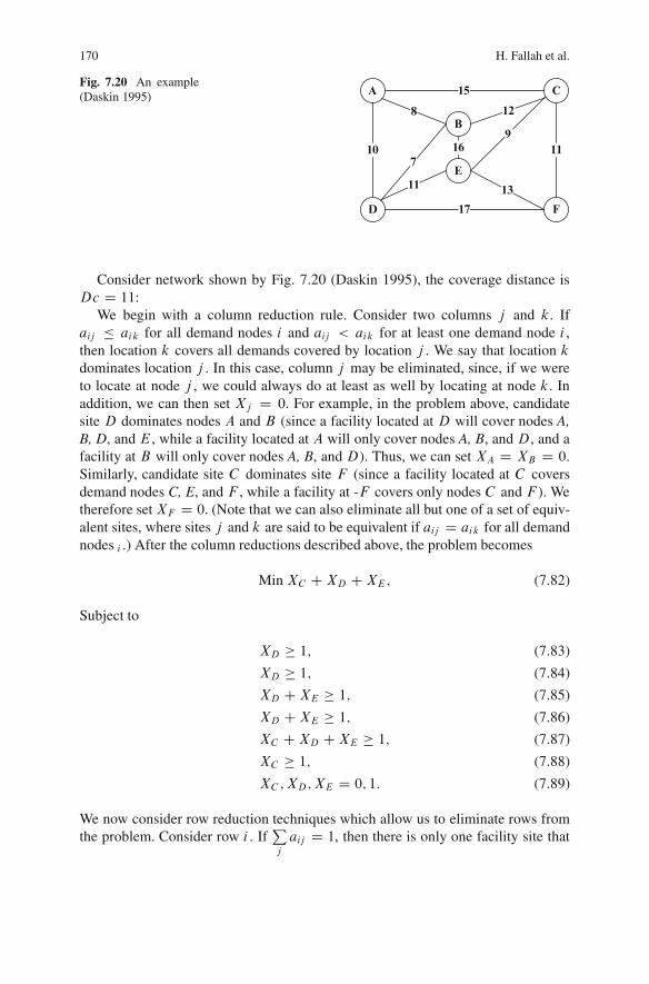
170 H. Fallah et al.
Fig. 7.20 An example(Daskin 1995) A
10
D
E
B
C
F
15
17
11167
8
11
9
12
13
Consider network shown by Fig. 7.20 (Daskin 1995), the coverage distance isDc D 11:
We begin with a column reduction rule. Consider two columns j and k. Ifaij � aik for all demand nodes i and aij < aik for at least one demand node i ,then location k covers all demands covered by location j . We say that location kdominates location j . In this case, column j may be eliminated, since, if we wereto locate at node j , we could always do at least as well by locating at node k. Inaddition, we can then set Xj D 0. For example, in the problem above, candidatesite D dominates nodes A and B (since a facility located at D will cover nodes A,B, D, and E , while a facility located at A will only cover nodes A, B, and D, and afacility at B will only cover nodes A, B, and D). Thus, we can set XA D XB D 0.Similarly, candidate site C dominates site F (since a facility located at C coversdemand nodes C, E, and F , while a facility at -F covers only nodes C and F ). Wetherefore set XF D 0. (Note that we can also eliminate all but one of a set of equiv-alent sites, where sites j and k are said to be equivalent if aij D aik for all demandnodes i .) After the column reductions described above, the problem becomes
Min XC CXD CXE; (7.82)
Subject to
XD � 1; (7.83)
XD � 1; (7.84)
XD CXE � 1; (7.85)
XD CXE � 1; (7.86)
XC CXD CXE � 1; (7.87)
XC � 1; (7.88)
XC ;XD;XE D 0; 1: (7.89)
We now consider row reduction techniques which allow us to eliminate rows fromthe problem. Consider row i . If
Pj
aij D 1, then there is only one facility site that
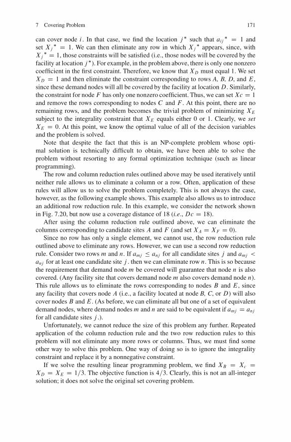
7 Covering Problem 171
can cover node i . In that case, we find the location j � such that aij � D 1 andset Xj � D 1. We can then eliminate any row in which Xj � appears, since, withXj
� D 1, those constraints will be satisfied (i.e., those nodes will be covered by thefacility at location j �). For example, in the problem above, there is only one nonzerocoefficient in the first constraint. Therefore, we know that XD must equal 1. We setXD D 1 and then eliminate the constraint corresponding to rows A, B, D, and E ,since these demand nodes will all be covered by the facility at locationD. Similarly,the constraint for nodeF has only one nonzero coefficient. Thus, we can setXc D 1
and remove the rows corresponding to nodes C and F . At this point, there are noremaining rows, and the problem becomes the trivial problem of minimizing XEsubject to the integrality constraint that XE equals either 0 or 1. Clearly, we setXE D 0. At this point, we know the optimal value of all of the decision variablesand the problem is solved.
Note that despite the fact that this is an NP-complete problem whose opti-mal solution is technically difficult to obtain, we have been able to solve theproblem without resorting to any formal optimization technique (such as linearprogramming).
The row and column reduction rules outlined above may be used iteratively untilneither rule allows us to eliminate a column or a row. Often, application of theserules will allow us to solve the problem completely. This is not always the case,however, as the following example shows. This example also allows us to introducean additional row reduction rule. In this example, we consider the network shownin Fig. 7.20, but now use a coverage distance of 18 (i.e.,Dc D 18).
After using the column reduction rule outlined above, we can eliminate thecolumns corresponding to candidate sites A and F (and set XA D XF D 0).
Since no row has only a single element, we cannot use, the row reduction ruleoutlined above to eliminate any rows. However, we can use a second row reductionrule. Consider two rows m and n. If amj � anj for all candidate sites j and amj <anj for at least one candidate site j . then we can eliminate row n. This is so becausethe requirement that demand node m be covered will guarantee that node n is alsocovered. (Any facility site that covers demand nodem also covers demand node n).This rule allows us to eliminate the rows corresponding to nodes B and E , sinceany facility that covers node A (i.e., a facility located at node B, C, or D) will alsocover nodesB andE . (As before, we can eliminate all but one of a set of equivalentdemand nodes, where demand nodesm and n are said to be equivalent if amj D anjfor all candidate sites j .).
Unfortunately, we cannot reduce the size of this problem any further. Repeatedapplication of the column reduction rule and the two row reduction rules to thisproblem will not eliminate any more rows or columns. Thus, we must find someother way to solve this problem. One way of doing so is to ignore the integralityconstraint and replace it by a nonnegative constraint.
If we solve the resulting linear programming problem, we find XB D Xc DXD D XE D 1=3. The objective function is 4=3. Clearly, this is not an all-integersolution; it does not solve the original set covering problem.
172 H. Fallah et al.
7.6.1.3 The Branch and Bound Method (Daskin 1995)
To ensure that we obtain an all-integer solution, additional techniques will generallybe required. One approach is to use branch and bound.
After reducing the problem size using above rules, we can solve the model us-ing optimal solving methods such as branch and bound or Balas algorithm (Daskin1995).
7.6.2 Heuristic Methods
7.6.2.1 The Greedy Adding Algorithm (Daskin 1995)
This algorithm and its variants may be used to solve (at least approximately) a largenumber of other location problems. The algorithm is known as a greedy algorithmsince it does what is best at each step of the algorithm without looking ahead to seehow the current decisions will impact on later decisions and alternatives.
If we were to locate only one facility (i.e., P D 1), we could solve the problemoptimally by simply evaluating how many demands each candidate site covers (can-didate site j covers
Pi aijhi demands) and selecting the site that covers the most
demands (Daskin 1995).
7.6.2.2 Lagrangian Relaxation (Daskin 1995)
Lagrangian relaxation is an approach to solving difficult problems (such as integerprogramming problems). The approach outlined below is cast in terms of solving amaximization problem. The approach involves the following general steps:
1. Relax one or more constraints by multiplying the constraint(s) by Lagrange mul-tiplier(s) and bringing the constraint(s) into the objective function.
2. Solve the resulting relaxed problem to find the optimal values of the originaldecision variables (in the relaxed problem)
3. (Optional) Use the resulting decision variables from the solution to the relaxedproblem found in step 2 to find a feasible solution to the original problem.
4. Use the solution obtained in step 2 to compute an upper bound on the best valueof the objective function.
5. Examine the solution obtained in step 2 and determine which of the relaxed con-straints are violated. Use some method to modify the Lagrange multipliers insuch a way that the violated constraints are less likely to be violated on the sub-sequent iteration. After new Lagrange multipliers have been identified, return tostep 2 (Daskin 1995).
7 Covering Problem 173
7.6.3 Metaheuristic Methods
7.6.3.1 Grasp Algorithm (Bautista and Pereira 2006)
The GRASP metaheuristic is a random iterative optimization procedure. Thismetaheuristic has been used to solve diverse problems of optimization, includ-ing scheduling, route design, logic, location, graphs, assignment, manufacturing,transport, and telecommunications problems, among others.
Each iteration in the metaheuristic is made up of two phases: a constructive anda local search phase. During the constructive phase, the algorithm uses a random-ized greedy heuristic to obtain an initial solution to the problem. This is based onmodified greedy procedures, where the greedy rule is substituted by a random se-lection among a limited list of candidates showing the best values for the greedyselection rule.
On the other hand, the local search phase permits exploration of the gener-ated solution neighborhood in an attempt to find higher-quality solutions. Afterlocal search, the best solution found during this phase is compared to the best-knownsolution, and substitutes it if the objective value is better than the previously known.Once a stopping criterion is met, the best solution obtained during the procedure isreturned.
In order to solve an optimization problem by means of a GRASP procedure, it isnecessary to define at least the following elements integrated in the heuristics:
� The randomized constructive procedure used during this procedure,� The neighborhood of the solution and the procedure to investigate it,� The stopping criterion usually associated to a maximum number of iterations.
One of the major advantages of the GRASP metaheuristic is how easy this generalscheme may be adapted to the solution of particular problems. GRASP requires fewparameters, basically the stopping criterion, associated to the maximum numberof iterations, and a rule to construct the restricted candidate list (RCL) during theconstructive phase (Bautista and Pereira 2006).
7.7 Case Study
7.7.1 Combination of MCDM and Covering Techniques(Farahani and Asgari 2007)
In this paper, locating some warehouses as distribution centers (DCs) in a real-worldmilitary logistics system will be Investigated. There are two objectives: finding theleast number of DCs and locating them in the best possible locations. The first objec-tive implies the minimum cost of locating the facilities and the latter expresses thequality of the DCs locations, which is evaluated by studying the value of appropriate
174 H. Fallah et al.
attributes affecting the quality of a location. Quality of a location depends on anumber of attributes; so the value of each location is determined by using multiattribute decision making models, by considering the feasible alternatives, the re-lated attributes and their weights according to decision maker’s (DM) point of view.Then, regarding the obtained values and the minimum number of DCs, the two ob-jective functions are formed. Constraints imposed on these two objectives cover allcenters, which must be supported by the DCs. Using multiple objective decisionmaking techniques, the locations of DCs are determined. In the final phase, we usea simple set partitioning model to assign each supported center to only one of thelocated DCs.
The supply chain is composed of three types of facilities:
� Origins;� Supportive centers;� Supported centers.
The objective functions and the constraints of the problem are as follows:
Objective function 1: Maximizing the utility of the selected locations. Utility ofa potential point depends on 23 attributes that will be explained later.Objective function 2: Minimizing the number of supportive centers.Constraint 1: All of the supported centers must be covered (coverage criteria willbe presented later) by supportive centers.Constraint 2: Each of the supported centers must be supported by one and onlyone of the located supportive centers.Phase 1. Determining all attributes that influence the utility of a location.Phase 2. In this phase, we use all possible alternatives as initial inputs of ourprocess.Phase 3. Using MADM techniques to assess the quality of the locations Normally.Phase 4. Using a multiple objective set covering model to find the best locations.Covering problems hold a central place in location theory. In these problems, weare given a set of demand points and a set of potential sites for locating facilities.A demand point is said to be covered by a facility if it lies within a pre-specifieddistance of that facility.
Set covering model is as follows (Francis et al. 1992; Daskin 1995; Mirchandaniand Francis 1990):
Min Z DmXiD1
Xi ; (7.90)
Subject to
mXiD1
aikXi � 1I k D 1; 2; : : : ; n; (7.91)
Xi 2 f0; 1g I i D 1; 2; : : : ; m; (7.92)
7 Covering Problem 175
xi is a binary variable that is equal to one if the feasible alternative i (a potential lo-cation for supportive centers) is suitable for locating supportive centers; otherwise itis equal to 0. Equation (7.90) ensures that the minimum number of supportive cen-ters are located. Equation (7.90) ensures that all of the supported centers are covered.In this expression A D Œaki is called covering matrix; aki is equal to 1 if a poten-tial supportive center located in location i.xi D 1/ is able to cover the supportedcenter located in location k. Generating a covering matrix A D Œaki is based on afactor called critical distance. Critical distance is the maximum time or distance thata supportive center can serve. Covering models focus on the worst-case behavior ofthe system (Daskin 1995). In our problem, we have used critical distances equal to8, 12 or 24 h. Here, there are a number of 233 supported centers. We have designeda modified set covering model with two objective functions as follows (Model 0):
Min Z1 D33XiD1
xi ; (7.93)
Max Z2 D33XiD1
cixi ; (7.94)
Subject to
33XiD1
aki xi � 1I k D 1; : : : ; 233 (7.95)
xi 2 f0; 1g i D 1; : : : ; 33; (7.96)
where ci has been already defined as output of Phase 3. Equation (7.93) is similarto (7.90). Equation (7.94) maximizes the quality of the selected facilities. Equa-tion (7.95) is similar to (7.90). In this problem, it can be considered three scenariosas follows:
Scenario 0 (Model 0): The problem is solved for the first time and no supportivecenter already exists. In this case, the model is the same as Model 0.Scenario 1 (Model 1): There already exist some active supportive centers (ex-isting facilities) and all of these supportive centers must carry on operating. Inthis case, we treat the location of these existing facilities as new locations. But inPhase 4 we use Model 1 instead ofModel 0 in which we have added the following constraints:xi D 1
8i 2 ˚ set of existing facilities gScenario 2 (Model 2): There already exist some active supportive centers (exist-ing facilities) and we try to keep them active if possible. In this case, we considerthe location of these existing facilities as new locations. However, in Phase 4 weuse Model 2 instead of Model 0 in which we have used the following objectivefunction instead of (7.93):
176 H. Fallah et al.
Where n1 shows the number of existing supportive centers and .n � n1/ showsthe number of new supportive centers. " is a parameter that tries to increase the co-efficient of binary variables of the new facilities; this forces the objective function touse existing facilities as much as possible. Our computational results and sensitivityanalysis show that " D 2=n is an appropriate value in this case.
References
Araz C, Hasan S, Irem O (2007) A fuzzy multi objective covering-based vehicle location modelfor emergency services. Comput Oper Res 34:705–726
Bautista J, Pereira J (2006) A GRASP algorithm to solve the unicost set covering problem. ComputOper Res 34(10):3162–3173
Berman O, Krass D, Drezner Z (2003) The gradual covering decay location problem on a network.Eur J Oper Res 151(3):474–480
Chiang CI, Hwang MJ, Liu YH (2005) An alternative formulation for certain fuzzy set-coveringproblems. Math Comput Model 42:363–365
Church R, ReVelle C (1974) the maximal covering location problem. Papers Region Sci Assoc32:101–118
Daskin MS (1995) Network and discrete location: Models, algorithms, and applications. Wiley,New York
Farahani R, Asgari N (2007) Combination of MCDM and covering techniques in a hierarchicalmodel for facility location: A case study. Eur J Oper Res 176(3):1839–1858
Francis RL, McGinnis LF, White JA (1992) Facility layout and location: An analytical approach.Prentice Hall, Englewood Cliffs, NJ
Hogan K, ReVelle C (1986) Concepts and applications of backup coverage. Manage Sci 32:1434–1444
Hwang HS (2004) A stochastic set-covering location model for both ameliorating and deterioratingitems. Comput Ind Eng 46:313–319
Jans R, Degraeve Z (2008) A note on a symmetrical set covering problem: the lottery problem. EurJ Oper Res 186(1):104–110
Jozefowieza N, Semetb F, Talbia EG (2007) The bi-objective covering tour problem. Comput OperRes 34:1929–1942
Mirchandani PB, Francis RL (1990) Discrete location theory. Wiley, New YorkPirkul H, Schilling DA (1991) The maximal covering location problem with capacities on total
workload. Manage Sci 37:233–248.Toregas C, Swain R, ReVelle C, Bergman L (1971) The location of emergency service facilities.
Oper Res 19:1363–1373
Chapter 8Median Location Problem
Masoomeh Jamshidi
The median problem is considered as the main problems identified with the location-allocation problems (see Chap. 5). These problems are intended to find the medianpoints among the candidate points, so that the sum of costs can be minimizedthrough this target function. These kinds of problems include the establishment ofthe public services including schools, hospitals, firefighting, Ambulance, technicalaudit stations of cars, and etc. The target function in the median problems is of theminisum kind. In fact in these problems we try to quantify the sum of distances(costs).
We call the first algorithm to be considered the Chinese algorithm. Apparently,the problem that motivated the development of the Chinese algorithm was thelocation of a threshing floor, used to separate the wheat from the chaff after a wheatharvest. In this case the tree network represents a road network, with the verticesbeing the location of wheat fields. The weight for each vertex represents the amountof wheat to be transported to and from the field and the threshing floor. Locating thethreshing floor at the 1-median causes the total cost of transporting the wheat to andfrom the threshing floor to be minimized (Francis et al. 1992).
In median problems, there is the location finding in the kind of network or graph.The discussion of median problems is focused on graph theory and cannot be beyondthe network or graph.
Fermat (seventeenth century) proposed one problem in order to minimize thesum of distances. In this problem, one rectangular was considered (three points onthe plane) and the aim was to find a point among three points, so that the sumof distances among the chosen point could be minimized through three angles ofthe rectangular. The problem was developed by Alfred Weber and again was in-troduced in twentieth century. In this problem, Weber called them as the clientsdemand through applying the weight on the angles points of rectangular, and calledthe median point as the servicing point. He defined the servicing point among threepointof clients demand, so that the sum of distances can be minimized. This problemis called as the first problem of the location-Allocation (see Chap. 5). Later theproblem proposed by Weber was introduced for multiple servicing states (multiplefacilities) and developed more than three points. The problem introduced by Weberwas connection problem. N can be achieved through choosing the median pointson apexes points of the graph or the nodes of network. This problem was quite
R.Z. Farahani and M. Hekmatfar (eds.), Facility Location: Concepts, Models, 177Algorithms and Case Studies, Contributions to Management Science,DOI 10.1007/978-3-7908-2151-2 8, c� Physica-Verlag Heidelberg 2009
178 M. Jamshidi
similar to the candidate of the correlated problem proposed by Weber. Again theproblem was developed by Hakimi (1964), and through application of the weighton the graph, he began to find the P point on it in order to minimize the sum of theweighted distance from the points.
8.1 Classification
8.1.1 1-Median
The median problems are intended to find the location of one facility on the network,so that the total cost can be minimum.
8.1.2 P-Median
The P-median problems it is a disconnected problem and we can choose the candi-date points through it.
8.1.3 An Example
Now, with an example, we want showing that how we can change continues prob-lem to discrete problem and find feasible solution. Assume in the city we wantto find some location for change store. This problem is a continuous problem. Forchanging this problem into a discrete problem, we can divide the city into smaller re-gions. These regions can be municipal regions or any other region. In every region,we determine the demand for chain stores. If we divide the city into five regions,the continuous map of city with its demands will be changed into a problem withfive demand points. Determining the center of every region and putting whole ofthe demand on that point, the problem changes into network. For determining thecenter of every region we can use the weight of every region, for example the centerof region can be in the east or west of region of course the location of facility is onlyon nodes. Consequently, we face with discrete network. Figure 8.1 is the schematicrepresentation of this network.
In this network, the nodes are considered among two points of supply. The supplycan be in one of the following forms:
� Static demand. That is the demand defined in a fixed or definite form� Probable demand. The demand which involves a variable with a gravity function� Dynamic demand. The demand of network (defined in a function of time.
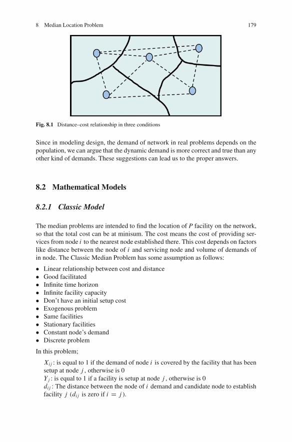
8 Median Location Problem 179
Fig. 8.1 Distance–cost relationship in three conditions
Since in modeling design, the demand of network in real problems depends on thepopulation, we can argue that the dynamic demand is more correct and true than anyother kind of demands. These suggestions can lead us to the proper answers.
8.2 Mathematical Models
8.2.1 Classic Model
The median problems are intended to find the location of P facility on the network,so that the total cost can be at minisum. The cost means the cost of providing ser-vices from node i to the nearest node established there. This cost depends on factorslike distance between the node of i and servicing node and volume of demands ofin node. The Classic Median Problem has some assumption as follows:
� Linear relationship between cost and distance� Good facilitated� Infinite time horizon� Infinite facility capacity� Don’t have an initial setup cost� Exogenous problem� Same facilities� Stationary facilities� Constant node’s demand� Discrete problem
In this problem;
Xij : is equal to 1 if the demand of node i is covered by the facility that has beensetup at node j , otherwise is 0Yj : is equal to 1 if a facility is setup at node j , otherwise is 0dij : The distance between the node of i demand and candidate node to establishfacility j (dij is zero if i D j ).
180 M. Jamshidi
P : The number of facilities to be establishedhi : Demand of i noden: Number of nodes
This model was proposed by ReVelle and Swain (1970);
MinXi
Xj
hidijXij i; j D 1; 2; :::; n: (8.1)
Subject to
Xj
Xij D 1 8i; (8.2)
Xj
Yj D P ; (8.3)
Xij � Yj 8i; j; (8.4)
Xij ; Yj 2 f0; 1g 8i; j: (8.5)
In this problem, the aim is to minimize the total cost needed to satisfy the needsof nodes (to minimize sum of demand-distance). Equation (8.2) states that alldemands should and each node is serviced by just one facility (demand limitation).Equation (8.3) states that there is an endogenous problem and proves the exact Pestablishment. Equations (8.4) states that open facilities can meet the demands. Thusthe demand of i node can be provided with facility established in j node .Xij D 1/
through one facility in j node .Yj D 1/.
8.2.2 Capacitated Plant Location Problem Model (CPLPM)
In this part, we introduce the capacitated plant location problem (CPLP) with mul-tiple facilities in the same site (CPLPM), a special case of the classical CPLP whereseveral facilities can be opened in the same site. Applications of the CPLPM arise ina number of contexts, such as the location of polling stations. Although the CPLPMcan be modeled and solved as a standard CPLP, this approach usually performsvery poorly. CPLP is a classical combinatorial optimization problem (Bramel et al.1998). This location problem is of utmost importance for many public and privateorganizations and its aim is determining a set of capacitated facilities (warehouses,plants, polling stations, etc.) in such a way that the sum of facility construction costsand transportation costs is minimized. Unlike other problem we allow multiple fa-cilities in the same site. The CPLP is strongly NP-hard (Mirchandani and Francis1990) and has been extensively studied in clustering and location theory. As a result,an overabundance of solution approaches has been proposed in the past decades.Exact algorithms have been developed, among others, by Christo Edes and Beasley(1983), Leung and Magnanti (1989), whereas heuristics have been investigated by
8 Median Location Problem 181
Van Roy (1985), Beasley (1988), ChristoEdes and Beasley (1983), GeoIrion andMcBride (1978), Guinard and Kim (1987), Jacobsen (1983), Khumawala (1974).A systematic comparison of heuristics and relaxations for the capacitated plant lo-cation problem is provided by Cornuejols et al. (1991) Based on both a theoreticalanalysis and extensive computational results; they suggest the use of a Lagrangianheuristic to solve large instances of the CPLP.
In this problem;
U : The set of potential facilities,V : The set of customers,dj : The demand of customer j .j 2 V /, where dj > 0,qi : The capacity of facility i .i 2 U /, where qi > 0,cij : The cost of supplying all the demand of customer j .j 2 V / from facilityi .i 2 U /,fi : The fixed cost associated with opening facility i .i 2 U /, where fi > 0,p: The desired number of open facilities (also referred to as medians),yi : A binary decision variable, which takes the value 1, if facility i .i 2 U / isopen, 0 otherwise,xij : A continuous decision variable, corresponding to the fraction of the demandof customer j .j 2 V / supplied from facility i .i 2 U /.
Then CPLP can be formulated as a mixed integer linear programming problem asfollows:
.CPLP/ MinXi2U
Xj2V
cij xi CXi2U
fiyi : (8.6)
Subject to
Xi2U
xij D 1; i 2 V; (8.7)
Xj2V
dj xij � qiyi; i 2 U; (8.8)
Xi2U
yi D p; (8.9)
xij � 0; i 2 U; j 2 V; (8.10)
yi 2 f0; 1g; i 2 U: (8.11)
The objective function (8.6) expresses the minimization of the total costs.Equations (8.7) ensure that the demand of each customer is satisfied. Equations (8.8)establish the connection between .xij / and .yi / variables. They state that no cus-tomer can be supplied from a closed facility and the total demand supplied from eachopen facility does not exceed the capacity of the facility. Equation (8.9) establishesthat the number of open facilities is p. Equations (8.10) provide lower bounds on the.xij / variables. It is worth noting that (8.7)–(8.10) imply xij � 1 .i 2 U I j 2 V /.Finally, (8.11) are the integrality constraints.
182 M. Jamshidi
In the CPLPM, U represents a set of areas where facilities can be located. Suchset is partitioned into n nonempty U1‘ : : : ’Un, each corresponding to a site whereone or more areas are available. Consequently fi D f 0
i , if i I i 2 UK .k 2f1; : : : ; ng/, and Cij D C 0
ij if i 2 UK .k 2 f1; : : : ; ng/ and j; j 0 2 V .
8.2.3 Capacitated P-median Problem (Lorenaa 2004)
If no fixed costs are associated to the potential facilities, then the CPLP is called thecapacitated p-median problem (CPMP).
Where N D f1; : : : ; ng is the index set of entities to allocate and also of possiblemedians with xij D 1 if entity i is allocated to median j , and xij D 0, otherwise;xjj D 1 if median j is selected and xjj D 0, otherwise.
The CPMP model can be formulated in two ways. The first is the following binaryinteger-programming problem (P ):
MinXi2N
Xj2N
cij xij : (8.12)
Subject to Xi2N
xij D 1; i 2 N; (8.13)
Xj2N
xjj D P; (8.14)
Xi2N
dixjj � qixjj; j 2 N; (8.15)
xij 2 f0; 1g; i 2 N; j 2 N: (8.16)
Equations (8.13)–(8.14) impose that each entity is allocated to only one median.Equations (8.15) imposes that a total median capacity must be respected, and (8.16)provide the integer conditions.
The CPMP problem can also be modeled as the following set partitioning prob-lem with a cardinality constraint (SPP).This is the formulation found in Minoux. Thesame formulation can be obtained from the problem P by applying the Dantzing–Wolfe decomposition.
Where S D fS1; S2; : : :; Smg, is a set of subsets of N ;A D Œaik n�m, is a matrix with
aik D(1 if i 2 SK0
0 otherwise:
.SPP/ MinmXkD1
ckxk: (8.17)
8 Median Location Problem 183
Subject to
mXkD1
Akxk D 1; (8.18)
mXkD1
xk D P ; (8.19)
xij 2 f0; 1g: (8.20)
Equations (8.12)–(8.13) are conserved and respectively updated to (18) and (20),according the Dantzig–Wolfe decomposition process.
If S is the set of all subsets of N , the formulation can give an optimal solutionto the CPMP. However, the number of subsets may be huge, and a partial set ofcolumns can be considered instead.
The SPP defined above is also known as the restricted master problem in thecolumn generation context.
8.3 Solution Techniques
Some kinds of solution for solving the p-median problems are as follows:
� Exact methods� Heuristic algorithm� Metaheuristic algorithm
The complete accounting, heuristic and met heuristic algorithm are one of the firsttechnique that are used them for solving the median problem.
Teitz and Bart (1968) proposed two innovated algorithm to solve the P -medianproblems through studying the complete number algorithm of Hakimi. This al-gorithm is based on choosing a primary series of nodes and then exchanging itsmembers with other nodes of the network in order to improve the target function.Jarvinen et al. (1972) proposed a branch and bound algorithm to solve P -medianproblem. Meanwhile, Egbo, Samelson and colleagues proposed a branch and boundalgorithm used to determine its limit through method of logerangean reparation(Narula et al. 1968). Neebe (1978) defined the transportation P -median problem inwhich the number of supply points was limited to P . Also he proposed a branch andbound algorithm for this problem in which the logerangean reparation method wasused to determine its limit. Kariv and Hakimi (1979) proved to find the P -median ina network was to find NP-Hard, and to determine 1-median for a tree was possibleinO.n2/ stage. Galvao (1980) determined the dual form of P -median problem, andobtained a low limit for the problem using the solution by an innovative method.This limit has been used in a branch and bound algorithm and applied to solve theproblems with 30 nodes and desirable P numbers.
184 M. Jamshidi
8.3.1 Lemma
The Weber’s problem was developed by Hakimi (1964), and through application ofthe weight on the graph, he began to find the P point on it in order to minimizethe sum of the weighted distance from the points. To solve the problem, there wasno limitation far the places of the points, and they could be placed in any points ofthe graph. Though the points were not located exactly on the apexes in the resultedsolutions, Hakimi (1964) showed that there could be always a series apexes P tominimize the target functions. Thus, through the constraint of finding the solutionjust on the apexes, again Hakimi (1964) considered this disconnected problem asthe candidate of Weber’s problem. In the median problems, the solution consistingof the apexed P is called the P -median. Also, these problems are to be studied anddefined just over the graph or networks. Hakimi (1964) generalized the concept of1-median to multi-median. He used the concept to determine how to distribute theswitching centers in the Tele-communication network. Later the P -median prob-lems were considered as the inseparable part of the location theory and were calledas a main problem.
8.3.2 Solving 1-Median Problem Algorithm on Tree(Goldman 1971)
� Put for all nodes Ohi D hi
� Choice one node beside the i if it is Ohi �Phi
2, put the facility in the node and go
to step 3.� Otherwise add Wi to wk . k is the only node that it has intersection with insidei node.
� Calculate the objective function.
In the algorithm, time of solving the algorithm increases by developing the num-ber of nodes linearly, because any node will consider its application just one timeO.n2p2/. Kariv and Hakimi (1979) submitted one algorithm for finding the placeof facility P on a tree networks with (n)nodes.
According to previous, without considering the type of network that can be a treenetwork or general, if at least half of the application of all network appear on a node,we can get at least one best solution by putting facility on that node. In tree network,we will lead to getting place of best facility through using the node on top of thetree and mixing those with other connected nodes. This subject is not possible ingeneral networks. For better understanding of this subject consider Fig. 8.2. Thesedifferent conditions that all tree nodes can be placed on best settlement are changedaccording to the length of relating vectors.
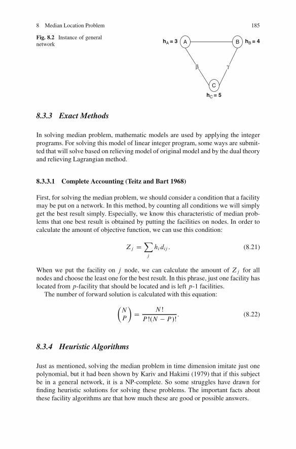
8 Median Location Problem 185
Fig. 8.2 Instance of generalnetwork AhA = 3 hB = 4
hC = 5
B
C
β γ
8.3.3 Exact Methods
In solving median problem, mathematic models are used by applying the integerprograms. For solving this model of linear integer program, some ways are submit-ted that will solve based on relieving model of original model and by the dual theoryand relieving Lagrangian method.
8.3.3.1 Complete Accounting (Teitz and Bart 1968)
First, for solving the median problem, we should consider a condition that a facilitymay be put on a network. In this method, by counting all conditions we will simplyget the best result simply. Especially, we know this characteristic of median prob-lems that one best result is obtained by putting the facilities on nodes. In order tocalculate the amount of objective function, we can use this condition:
Zj DXj
hidij : (8.21)
When we put the facility on j node, we can calculate the amount of Zj for allnodes and choose the least one for the best result. In this phrase, just one facility haslocated from p-facility that should be located and is left p-1 facilities.
The number of forward solution is calculated with this equation:
�N
P
�D NŠ
P Š.N � P/Š: (8.22)
8.3.4 Heuristic Algorithms
Just as mentioned, solving the median problem in time dimension imitate just onepolynomial, but it had been shown by Kariv and Hakimi (1979) that if this subjectbe in a general network, it is a NP-complete. So some struggles have drawn forfinding heuristic solutions for solving these problems. The important facts aboutthese facility algorithms are that how much these are good or possible answers.
186 M. Jamshidi
Although these algorithms result in real world problems very well, they don notguarantee achieving the optimum or approximating it. In solving some problems,these solutions may be optimum or near the best. In other cases, these solution maybe very far. The first Heuristic algorithm for solving the median problems:
� Greedy-adding algorithm� Alternate algorithm� Vertex substitutions algorithm
According to these tree algorithms, innumerable algorithms and new techniques aremade for solving the median problems that are based on those three algorithms.From these three basic algorithms, the vertex substitution algorithm is more generalin comparison to the other two algorithms and up to the present time, it was oneof the mostly used algorithms for solving median problems. Another heuristic al-gorithm is the branch and bound algorithm. (Heuristic branch and bound algorithmis not the same as one of the linear-program problems techniques named branchand bound.)
According to a classification, algorithms are classified into two groups of replymaker algorithms and recovering reply algorithms.
Myopic algorithm is one of the reply maker algorithms. This algorithm tries toget one primary and possible solution for median problems. The algorithm is similarto Greedy adding algorithm that is applied for maximum covering problems.
Both exchange and neighborhood search algorithms are kinds of recovering replyalgorithm. These algorithms are not able to get the primary reply for problems, butthey use them to improve reply that how got from maker algorithms. Two algorithmsare similar to both Greedy adding and maximum heuristic algorithms for maximumcovering and substitution problems. When Lagrangian discounting method is usedbesides one or more heuristic algorithm that will be introduced this section, theywill get the best or near the best reply.
8.3.5 Metaheuristic Algorithms
Meta heuristic algorithms for solving the median problem:
� Genetic algorithm� Concentration algorithm� Neural network� Tabu search algorithm� Simulated annealing
In recent decades metaheuristic algorithms are submitted for solving these kinds ofproblems. Among these algorithms we can mention the genetic algorithm, neighbor-hood search algorithm, tabu search algorithm, concentration algorithm, simulatedannealing algorithm and neural network. Also there are some other algorithms forobtaining one reply with acceptable quality.
8 Median Location Problem 187
Metaheuristic methods are usually used for too many nodes (100, 200, 300, 400,500, 600, 700, 800 and 900).
8.4 Comparison of Methods
In this section, all achieved results that have been concluded from a 12-nodesnetwork are mentioned. Here there is no solution way and just we consider theircomparisons results.
� The solutions that have been achieved by using the myopic algorithms, in themost cases, appears almost in 30% error of amount of Lagrange objective func-tion.
� In each stage, all solution that has been achieved from exchange algorithmsmethod is always for the each number of facilities better than solution by us-ing the neighborhood search algorithms.
� It is better in some situations that neighborhood search algorithms applied aftersetting each facility at network in each stage, and in some other situations, it isbetter to apply the neighborhood search algorithms after setting all facilities.
� We should consider that when the number of settled facilities will be averagefigure, the differences between all achieved results differ from various algorithmstogether and with Lagrange algorithm method.
� When the number of the settled facilities is few, it seams that all algorithms workbetter. For instance, when the number of the settled facilities is more, all resultsthat have been achieved from algorithms are so good and algorithms work sowell. But when the number of the settled facilities is neither few nor more, theproblem is so difficult.
� Exchange algorithm is the best method for this network, considering that ex-changing appears after putting all facilities by using the myopic algorithm.
8.5 Studying Statically the Methods for Solutions of MedianProblem (Reese 2005)
The aim here is to study the methods used to solve the median problems and theyears of proposing them which were classified for 1963–2005 periods. The follow-ing factors were selected among other sources:
� Those focused directly on median problems,� Those involved minisum target function,� Those which define median problems on the graph or network,� Sum of answers limited to searching on nodes,� Those that did not have primary cost of establishment,� Those belonging to median problems with limited capacity or unlimited facilities.
188 M. Jamshidi
Also we avoided the resources with one of the following conditions:
� They had minimax target function,� Study establishment of median problems in a connected space,� There was a probable state demand or cost,� There was a multi-purpose target function,� Considering dislocation of facilities in a time horizon.
The following classification obtained considering the proposed solutions.
8.5.1 Classification of Solving Methods by Period
The number of presented paper in this area before 1970 were 7, between 1970 and1974 were 9, between 1975 and 1979 were 12, between 1980 and 1984 were 9,between 1985 and 1989 were 6, between 1990 and 1994 were 11, between 1995 and1999 were 24 and between 2000 and 2005 the number of paper have the remarkablegrowth so that it reaches 42 paper.
It should also be noted that the methods obtained and used in the last 10 yearsare so higher than the methods used in 1963–1994.
8.5.2 Classification of Different Solving Methods
According to the researches between 1965 and 2005 the LP Relaxation was usedmore than other methods, after that respectively Vertex substitution, approximationalgorithm, genetic algorithm (GA), IP formulation were used, graph theory and sur-rogate relaxation are in the same level, and other methods were assigned less thanfive cases.
8.6 Case Study
In this section we will introduce some real-world case studies related to p-medianproblem:
8.6.1 Post Center Locations (Alba and Dominquez 2006)
In Australia in order to determine ten post centers among 200 centers, 10-medianproblem formulated and finally ten cities including Sidney, Melborn and Adlid, etc.were selected as post centers.
8 Median Location Problem 189
8.6.2 Entrance Exam Facilities (Correa et al. 2004)
PARANA State University (UFPR) in Curitiba in Brazil used the median P modelto determine the location of facilities concerning M.A entrance exam in 2001. Theaim was to appropriate 19,710 candidate students to the facilities located nearer totheir homes as possible.
It was determined that 26 facilities needed to meet the demands of 19,710students among 43 candidate facilities. Finally the number of candidate solutionsshould be 421 billion. �
43
26
�D 421; 171; 648; 758:
The problem was solved by a genetic algorithm.
8.6.3 Polling Station Location (Ghiani et al. 2002)
Polling station location problem in Italy: Number of polling stations was deter-mined according to the number of resident voters in five Italian municipalities (data:November 2000).
This study of the CPLPM was motivated by a polling station location problemin an Italian municipality. In Italy, the following binding obligations must be takeninto account:
� The number of polling stations is fixed for each municipality and calculated ac-cording to the number of resident voters the number of voters assigned to eachpolling station may not exceed given lower and upper bounds;
� The suitability of the potential sites is established by specific safety measures onthe accessibility and typology of the buildings (for example, in some countries,only public buildings, such as schools, are eligible).
8.6.3.1 Formulating the Problem as a CPLPM
U : The set of areas where polling stations can be located.P : Number of polling stations to be activated.V : The set of streets having at least one resident voterdj : The number of voters in street j .j 2 V /, where dj > 0.qi : The upper limit on the total number of voters assigned to a polling stationlocated in area i .i 2 U /I qi may be the same for all areas, i.e.
qi D q DXj2V
dj
pI i 2 U: (8.23)
190 M. Jamshidi
cij : The transportation cost incurred if all voters resident in street j .j 2 V / areassigned to a polling station in area i .i 2 U /I cij can be chosen, for simplicity,equal to dj
�Sij j , where Sij is the walking distance between area i and the “cen-tre of gravity” of street j; fi D f , for all areas. Consequently, the contribution ofthe fixed costs to the objective function (6) can be excluded.
8.6.3.2 Computational Results
As far as the experimental phase is concerned, we have solved first the problemof the optimal location of polling stations in the municipality of Castrovillari. Townlocated in Southern Italy with a population, dated back to November 2000, of 15,709voters, located in 351 different streets spread in a wide area. The solution actuallyadopted by the local government is based on the assignment of all voters residentin the same street to the same polling station, chosen among the nearest ones. As aresult, the walking distance covered by all voters is about 10,731 km, and the numberof voters for each polling station was reported. It was observed that, with respect tothe ideal capacity, the fourth polling station has 18% of voters less, whereas the 18thpolling station has 21% of voters more. The feasible solution found by the heuristicis well balanced and has a cost 37.6% less than that of the solution currently adoptedby the municipality of Castrovillari. Computational results show that the averagedeviation of the heuristic solution over the lower bound is less than 2%.
References
Alba E, Dominquez E (2006) Comparative analysis of modern optimization tools for the p-medianproblem. Stat Comput 16:251–260
Beasley JE (1988) An algorithm for solving large capacitated warehouse location problems EurJ Oper Res 33:314–325
Bramel J, Simchi-Levi D (1998) The logic of logistics. Springer-Verlag, New YorkChristoEdes N, Beasley JE (1983) Extensions to a lagrangian relaxation approach for the capacitate
warehouse location problem Eur J Oper Res 12:19–28Cornuejols G, Sridharan R, Thizy JM (1991) A comparison of heuristics and relaxations for the
capacitated plant location problem Eur J Oper Res 50:280–297Correa ES, Steiner MTA, Freitas AA, Carnieri C (2004) Genetic algorithm for solving a capacitated
p-median problem. Numer Algorithms 35:373–388Francis RL, McGinnis LF, White JA (1992) Facility layout and location: An analytical approach.
Prentice Hall, Englewood Cliffs, NJGalvao RD (1980) A dual-bounded algorithm for the p-median problem. J Oper Res 28(5):
1112–1121GeoIrion AM, McBride R (1978) Lagrangian relaxation applied to capacitated facility location
problem AIIE Trans 1:40–47Ghiani G, Guerriero F, Musmanno R (2002) The capacitated plant location problem with multipli
facilities in the same site. Eur J Oper Res 29:1903–1912Goldman AJ (1971) Optimal center location in simple networks. Trans Sci 5:212–221Guinard M, Kim S (1987) A strong lagrangian relaxation for capacitated plant location problems
Math Program 39:215–528
8 Median Location Problem 191
Hakimi SL (1964) Optimum locations of switching centers and the absolute centers and Mediansof a graph. Eur J Oper Res 12(3):450–459
Hakimi SL (1965) Optimum distribution of switching centers in a communication network andsome related graph theoretic problems. Eur J Oper Res 13(3):462–475
Jacobsen SK (1983) Heuristics for the capacitated plant location model Eur J Oper Res 12:253–261Jarvinen P, Rajala J, Sinervo V (1972) A branch-and-bound algorithm for seeking the p median.
Eur J Oper Res 20(1):173–178Kariv O, Hakimi SL (1979) An algorithmic approach to network location problems. II. The
p-medians. SIAM J Appl Math 37(3):539–560Khumawala BM (1974) An efficient heuristic procedure for the capacitated warehouse location
problem Nav Res Logist Quart 21:609–623Leung JM, Magnanti TL (1989) Valid inequalities and facets of the capacitated plan location prob-
lem Math Program 44:271–291Lorenaa L, Senneb E (2004) A column generation approach to capacitated p-median problems
Oper Res 31:863–876Mirchandani PB, Francis RL (1990) Discrete location theory. Wiley, New YorkNarula SC, Ogbu UI, Samuelsson HM (1968) An algorithm for the p-Median problem. Eur J Oper
Res 16(5):955–961Neebe AW (1978) A branch and bound algorithm for the p-median transportation problem. J Oper
Res Soc 29:989–995Reese J (2005) Methods for solving the p-median problem: An annotated bibliography. Technical
report, Department of Mathematics, Trinity UniversityReVelle C, Swain R (1970) Central facilities location. Geograph Anal 2:30–42Teitz MB, Bart P (1968) Heuristic methods for estimating the generalized vertex median of a
weighted graph. Eur J Oper Res 16(5):955–961Van Roy TJ (1985) A cross decomposition algorithm for capacitated facility location. Eur J Oper
Res 34:145–63
Chapter 9Center Problem
Maryam Biazaran and Bahareh SeyediNezhad
In the covering problems, the attempt is to determine the location of the minimumnumber of facilities necessary to cover all demand nodes. In this type of problems,the coverage distance is an exogenous data. But sometimes the number of facilitiesneeded to cover all demand nodes with a predefined coverage distance may be quitelarge. In order to overcome this, the maximum covering location problem has beendiscussed. In this model, the objective is to maximize the number of covered demandnodes with a fixed number of facilities. In other words, we relaxed the total coveragerequirement (Daskin 1995).
A different strategy is discussed in this chapter. Now, instead of asking the modelto minimize the number of facilities with a given coverage distance, we will ask themodel to minimize the coverage distance with a given number of facilities, whilemaintaining the coverage of all demand nodes. This model is introduced underthe title of p-center problem which is in fact a minimax problem. In this model, theobjective is to find locations of p facilities so that all demands are covered andthe maximum distance between a demand node and the nearest facility (coveragedistance) is minimized. It can be said that we have relaxed the coverage distance(Daskin 1995).
In the p-center model, each demand point has a weight. These weights may havedifferent interpretations such as time per unit distance, cost per unit distance orloss per unit distance (Daskin 1995). So the problem would be seeking a center tominimize a maximum time, cost or loss. In other words, the concern is about theworst case and we want to make it as good as possible (Francis et al. 1992).
For example, assume that we need to establish a number of fire stations in atown. If the time to reach the scene from facility j to demand node i is dij , then thisamount must not be greater than minutes. Therefore, we are looking to providedij <for each node i and a closest facility j . If we are to cover all the points, we needcertain number of facilities. To evaluate the number of facilities needed, one needsto solve a set covering problem. Now assume that there is a budget constraint andwe can not establish enough fire stations, then there are two ways of approaching theproblem. One is to cover maximum points; in this case you are facing a maximumcovering problem. The second approach is to cover all of demand nodes, but throughincreasing the radius of coverage distance. Evaluation of the minimum increase in
R.Z. Farahani and M. Hekmatfar (eds.), Facility Location: Concepts, Models, 193Algorithms and Case Studies, Contributions to Management Science,DOI 10.1007/978-3-7908-2151-2 9, c� Physica-Verlag Heidelberg 2009
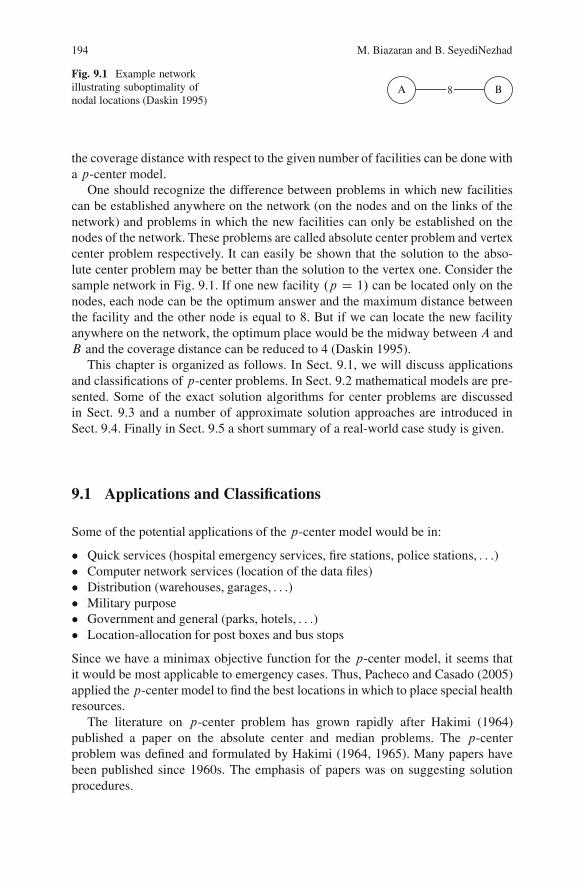
194 M. Biazaran and B. SeyediNezhad
Fig. 9.1 Example networkillustrating suboptimality ofnodal locations (Daskin 1995)
A B8
the coverage distance with respect to the given number of facilities can be done witha p-center model.
One should recognize the difference between problems in which new facilitiescan be established anywhere on the network (on the nodes and on the links of thenetwork) and problems in which the new facilities can only be established on thenodes of the network. These problems are called absolute center problem and vertexcenter problem respectively. It can easily be shown that the solution to the abso-lute center problem may be better than the solution to the vertex one. Consider thesample network in Fig. 9.1. If one new facility .p D 1/ can be located only on thenodes, each node can be the optimum answer and the maximum distance betweenthe facility and the other node is equal to 8. But if we can locate the new facilityanywhere on the network, the optimum place would be the midway between A andB and the coverage distance can be reduced to 4 (Daskin 1995).
This chapter is organized as follows. In Sect. 9.1, we will discuss applicationsand classifications of p-center problems. In Sect. 9.2 mathematical models are pre-sented. Some of the exact solution algorithms for center problems are discussedin Sect. 9.3 and a number of approximate solution approaches are introduced inSect. 9.4. Finally in Sect. 9.5 a short summary of a real-world case study is given.
9.1 Applications and Classifications
Some of the potential applications of the p-center model would be in:
� Quick services (hospital emergency services, fire stations, police stations, : : :)� Computer network services (location of the data files)� Distribution (warehouses, garages, : : :)� Military purpose� Government and general (parks, hotels, : : :)� Location-allocation for post boxes and bus stops
Since we have a minimax objective function for the p-center model, it seems thatit would be most applicable to emergency cases. Thus, Pacheco and Casado (2005)applied the p-center model to find the best locations in which to place special healthresources.
The literature on p-center problem has grown rapidly after Hakimi (1964)published a paper on the absolute center and median problems. The p-centerproblem was defined and formulated by Hakimi (1964, 1965). Many papers havebeen published since 1960s. The emphasis of papers was on suggesting solutionprocedures.
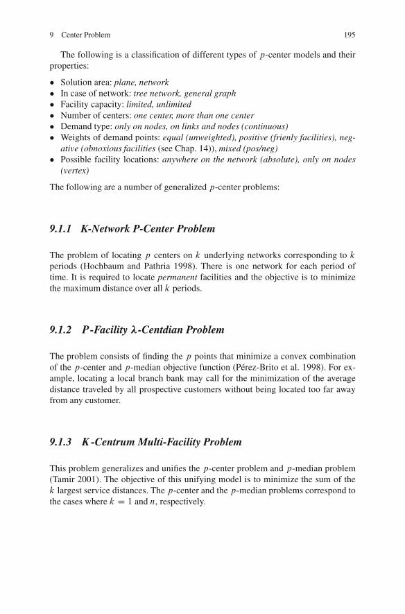
9 Center Problem 195
The following is a classification of different types of p-center models and theirproperties:
� Solution area: plane, network� In case of network: tree network, general graph� Facility capacity: limited, unlimited� Number of centers: one center, more than one center� Demand type: only on nodes, on links and nodes (continuous)� Weights of demand points: equal (unweighted), positive (frienly facilities), neg-
ative (obnoxious facilities (see Chap. 14)), mixed (pos/neg)� Possible facility locations: anywhere on the network (absolute), only on nodes
(vertex)
The following are a number of generalized p-center problems:
9.1.1 K-Network P-Center Problem
The problem of locating p centers on k underlying networks corresponding to kperiods (Hochbaum and Pathria 1998). There is one network for each period oftime. It is required to locate permanent facilities and the objective is to minimizethe maximum distance over all k periods.
9.1.2 P-Facility �-Centdian Problem
The problem consists of finding the p points that minimize a convex combinationof the p-center and p-median objective function (Perez-Brito et al. 1998). For ex-ample, locating a local branch bank may call for the minimization of the averagedistance traveled by all prospective customers without being located too far awayfrom any customer.
9.1.3 K -Centrum Multi-Facility Problem
This problem generalizes and unifies the p-center problem and p-median problem(Tamir 2001). The objective of this unifying model is to minimize the sum of thek largest service distances. The p-center and the p-median problems correspond tothe cases where k D 1 and n, respectively.
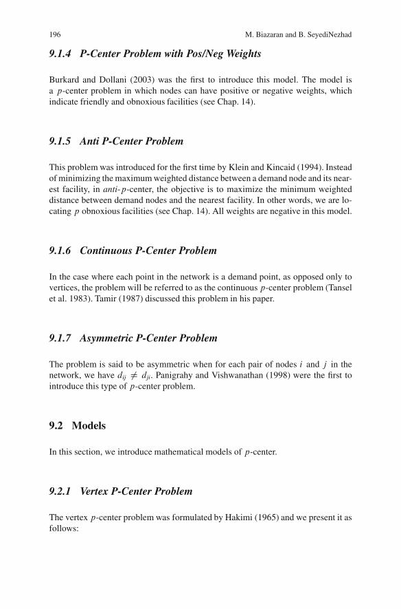
196 M. Biazaran and B. SeyediNezhad
9.1.4 P-Center Problem with Pos/Neg Weights
Burkard and Dollani (2003) was the first to introduce this model. The model isa p-center problem in which nodes can have positive or negative weights, whichindicate friendly and obnoxious facilities (see Chap. 14).
9.1.5 Anti P-Center Problem
This problem was introduced for the first time by Klein and Kincaid (1994). Insteadof minimizing the maximum weighted distance between a demand node and its near-est facility, in anti-p-center, the objective is to maximize the minimum weighteddistance between demand nodes and the nearest facility. In other words, we are lo-cating p obnoxious facilities (see Chap. 14). All weights are negative in this model.
9.1.6 Continuous P-Center Problem
In the case where each point in the network is a demand point, as opposed only tovertices, the problem will be referred to as the continuous p-center problem (Tanselet al. 1983). Tamir (1987) discussed this problem in his paper.
9.1.7 Asymmetric P-Center Problem
The problem is said to be asymmetric when for each pair of nodes i and j in thenetwork, we have dij ¤ dji. Panigrahy and Vishwanathan (1998) were the first tointroduce this type of p-center problem.
9.2 Models
In this section, we introduce mathematical models of p-center.
9.2.1 Vertex P-Center Problem
The vertex p-center problem was formulated by Hakimi (1965) and we present it asfollows:
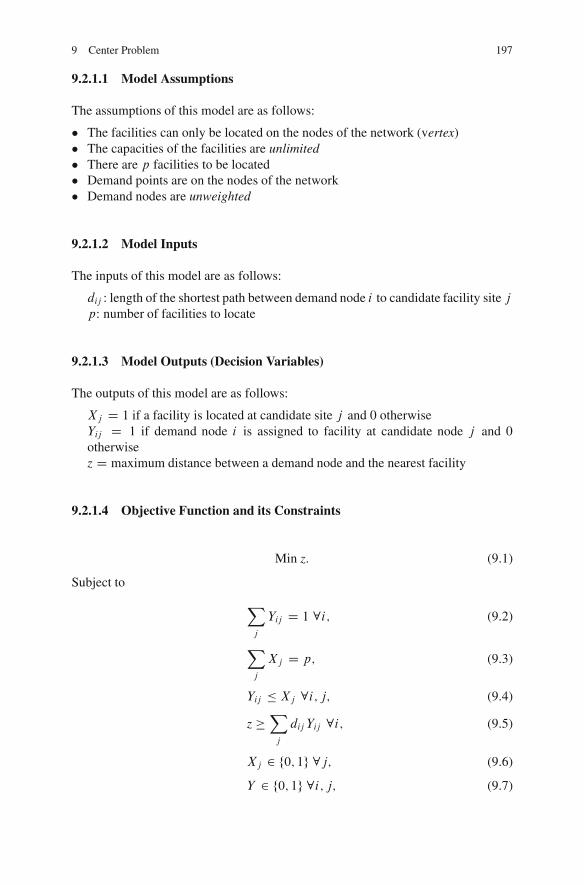
9 Center Problem 197
9.2.1.1 Model Assumptions
The assumptions of this model are as follows:
� The facilities can only be located on the nodes of the network (vertex)� The capacities of the facilities are unlimited� There are p facilities to be located� Demand points are on the nodes of the network� Demand nodes are unweighted
9.2.1.2 Model Inputs
The inputs of this model are as follows:
dij : length of the shortest path between demand node i to candidate facility site jp: number of facilities to locate
9.2.1.3 Model Outputs (Decision Variables)
The outputs of this model are as follows:
Xj D 1 if a facility is located at candidate site j and 0 otherwiseYij D 1 if demand node i is assigned to facility at candidate node j and 0otherwisez D maximum distance between a demand node and the nearest facility
9.2.1.4 Objective Function and its Constraints
Min z: (9.1)
Subject to
Xj
Yij D 1 8i; (9.2)
Xj
Xj D p; (9.3)
Yij � Xj 8i; j; (9.4)
z �Xj
dij Yij 8i; (9.5)
Xj 2 f0; 1g 8j; (9.6)
Y 2 f0; 1g 8i; j; (9.7)
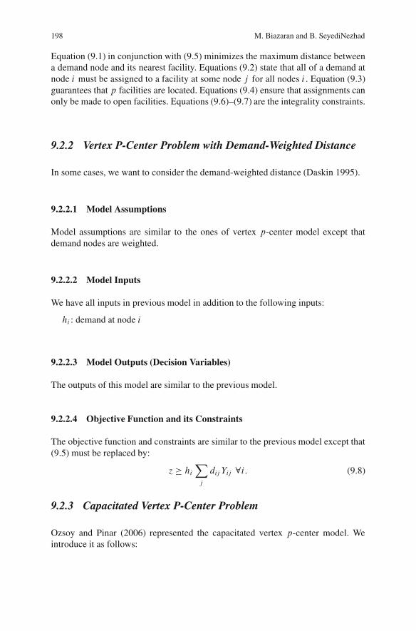
198 M. Biazaran and B. SeyediNezhad
Equation (9.1) in conjunction with (9.5) minimizes the maximum distance betweena demand node and its nearest facility. Equations (9.2) state that all of a demand atnode i must be assigned to a facility at some node j for all nodes i . Equation (9.3)guarantees that p facilities are located. Equations (9.4) ensure that assignments canonly be made to open facilities. Equations (9.6)–(9.7) are the integrality constraints.
9.2.2 Vertex P-Center Problem with Demand-Weighted Distance
In some cases, we want to consider the demand-weighted distance (Daskin 1995).
9.2.2.1 Model Assumptions
Model assumptions are similar to the ones of vertex p-center model except thatdemand nodes are weighted.
9.2.2.2 Model Inputs
We have all inputs in previous model in addition to the following inputs:
hi : demand at node i
9.2.2.3 Model Outputs (Decision Variables)
The outputs of this model are similar to the previous model.
9.2.2.4 Objective Function and its Constraints
The objective function and constraints are similar to the previous model except that(9.5) must be replaced by:
z � hiXj
dij Yij 8i: (9.8)
9.2.3 Capacitated Vertex P-Center Problem
Ozsoy and Pinar (2006) represented the capacitated vertex p-center model. Weintroduce it as follows:
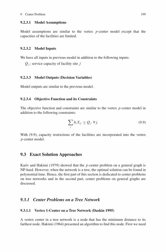
9 Center Problem 199
9.2.3.1 Model Assumptions
Model assumptions are similar to the vertex p-center model except that thecapacities of the facilities are limited.
9.2.3.2 Model Inputs
We have all inputs in previous model in addition to the following inputs:
Qj : service capacity of facility site j
9.2.3.3 Model Outputs (Decision Variables)
Model outputs are similar to the previous model.
9.2.3.4 Objective Function and its Constraints
The objective function and constraints are similar to the vertex p-center model inaddition to the following constraints:
Xi
hiYij � Qj 8j: (9.9)
With (9.9), capacity restrictions of the facilities are incorporated into the vertexp-center model.
9.3 Exact Solution Approaches
Kariv and Hakimi (1979) showed that the p-center problem on a general graph isNP-hard. However, when the network is a tree, the optimal solution can be found inpolynomial time. Hence, the first part of this section is dedicated to center problemson tree networks and in the second part, center problems on general graphs arediscussed.
9.3.1 Center Problems on a Tree Network
9.3.1.1 Vertex 1-Center on a Tree Network (Daskin 1995)
A vertex center in a tree network is a node that has the minimum distance to itsfarthest node. Hakimi (1964) presented an algorithm to find this node. First we need
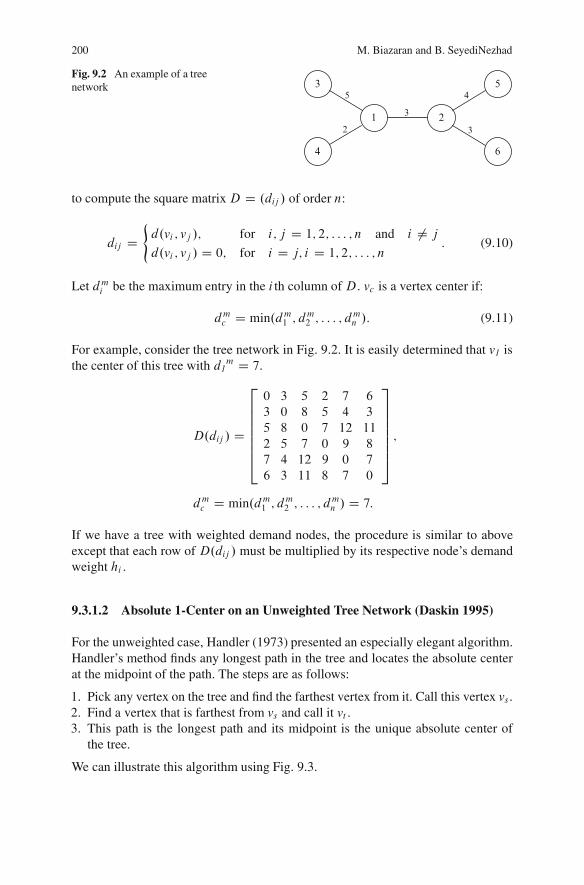
200 M. Biazaran and B. SeyediNezhad
Fig. 9.2 An example of a treenetwork
1 2
3
4
5
6
5
3
3 2
4
to compute the square matrixD D .dij / of order n:
dij D(d.vi ; vj /; for i; j D 1; 2; : : : ; n and i ¤ j
d.vi ; vj / D 0; for i D j; i D 1; 2; : : : ; n: (9.10)
Let dmi be the maximum entry in the i th column of D. vc is a vertex center if:
dmc D min.dm1 ; dm2 ; : : : ; d
mn /: (9.11)
For example, consider the tree network in Fig. 9.2. It is easily determined that v1 isthe center of this tree with d1
m D 7.
D.dij / D
26666664
0 3 5 2 7 6
3 0 8 5 4 3
5 8 0 7 12 11
2 5 7 0 9 8
7 4 12 9 0 7
6 3 11 8 7 0
37777775;
dmc D min.dm1 ; dm2 ; : : : ; d
mn / D 7:
If we have a tree with weighted demand nodes, the procedure is similar to aboveexcept that each row of D.dij / must be multiplied by its respective node’s demandweight hi .
9.3.1.2 Absolute 1-Center on an Unweighted Tree Network (Daskin 1995)
For the unweighted case, Handler (1973) presented an especially elegant algorithm.Handler’s method finds any longest path in the tree and locates the absolute centerat the midpoint of the path. The steps are as follows:
1. Pick any vertex on the tree and find the farthest vertex from it. Call this vertex vs .2. Find a vertex that is farthest from vs and call it vt .3. This path is the longest path and its midpoint is the unique absolute center of
the tree.
We can illustrate this algorithm using Fig. 9.3.
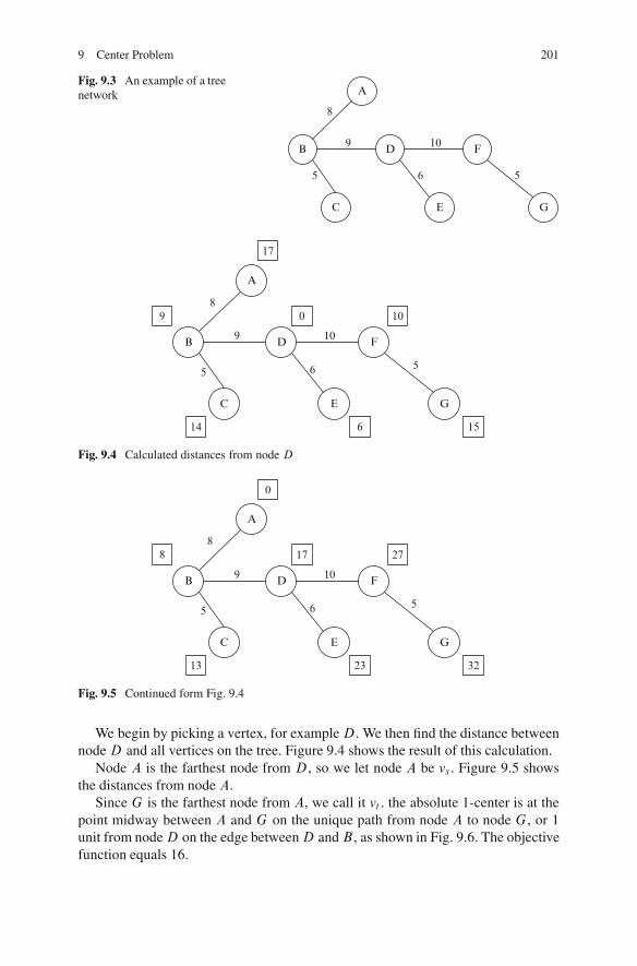
9 Center Problem 201
Fig. 9.3 An example of a treenetwork A
C
B
E
D F
G
9
8
5 6
10
5
A
C
B
E
D F
G
9
8
5 6
10
5
17
0 10
15614
9
Fig. 9.4 Calculated distances from node D
A
C
B
E
D F
G
9
8
5 6
10
5
0
17 27
322313
8
Fig. 9.5 Continued form Fig. 9.4
We begin by picking a vertex, for exampleD. We then find the distance betweennodeD and all vertices on the tree. Figure 9.4 shows the result of this calculation.
Node A is the farthest node from D, so we let node A be vs . Figure 9.5 showsthe distances from node A.
Since G is the farthest node from A, we call it vt . the absolute 1-center is at thepoint midway between A and G on the unique path from node A to node G, or 1unit from nodeD on the edge betweenD andB , as shown in Fig. 9.6. The objectivefunction equals 16.
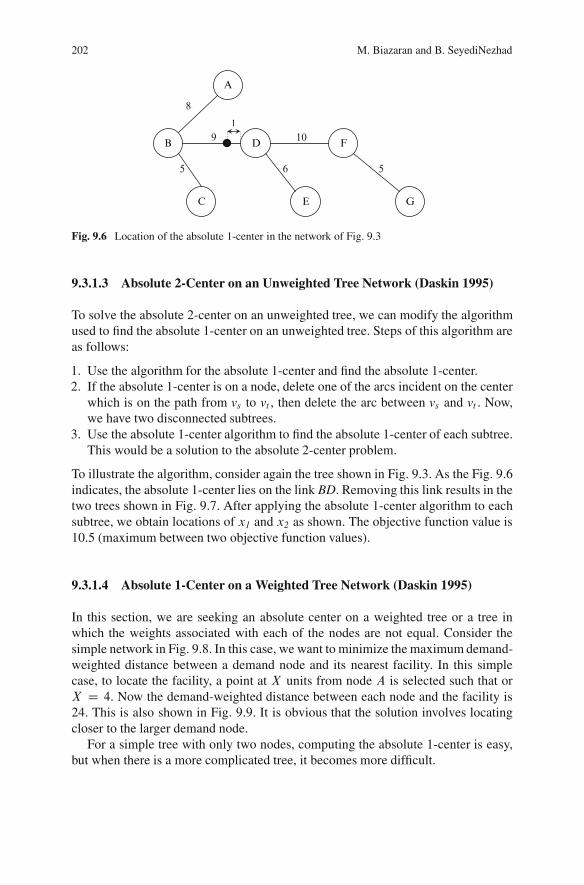
202 M. Biazaran and B. SeyediNezhad
A
C
B
E
D F
G
9
8
5 6
10
5
1
Fig. 9.6 Location of the absolute 1-center in the network of Fig. 9.3
9.3.1.3 Absolute 2-Center on an Unweighted Tree Network (Daskin 1995)
To solve the absolute 2-center on an unweighted tree, we can modify the algorithmused to find the absolute 1-center on an unweighted tree. Steps of this algorithm areas follows:
1. Use the algorithm for the absolute 1-center and find the absolute 1-center.2. If the absolute 1-center is on a node, delete one of the arcs incident on the center
which is on the path from vs to vt , then delete the arc between vs and vt . Now,we have two disconnected subtrees.
3. Use the absolute 1-center algorithm to find the absolute 1-center of each subtree.This would be a solution to the absolute 2-center problem.
To illustrate the algorithm, consider again the tree shown in Fig. 9.3. As the Fig. 9.6indicates, the absolute 1-center lies on the link BD. Removing this link results in thetwo trees shown in Fig. 9.7. After applying the absolute 1-center algorithm to eachsubtree, we obtain locations of x1 and x2 as shown. The objective function value is10.5 (maximum between two objective function values).
9.3.1.4 Absolute 1-Center on a Weighted Tree Network (Daskin 1995)
In this section, we are seeking an absolute center on a weighted tree or a tree inwhich the weights associated with each of the nodes are not equal. Consider thesimple network in Fig. 9.8. In this case, we want to minimize the maximum demand-weighted distance between a demand node and its nearest facility. In this simplecase, to locate the facility, a point at X units from node A is selected such that orX D 4. Now the demand-weighted distance between each node and the facility is24. This is also shown in Fig. 9.9. It is obvious that the solution involves locatingcloser to the larger demand node.
For a simple tree with only two nodes, computing the absolute 1-center is easy,but when there is a more complicated tree, it becomes more difficult.
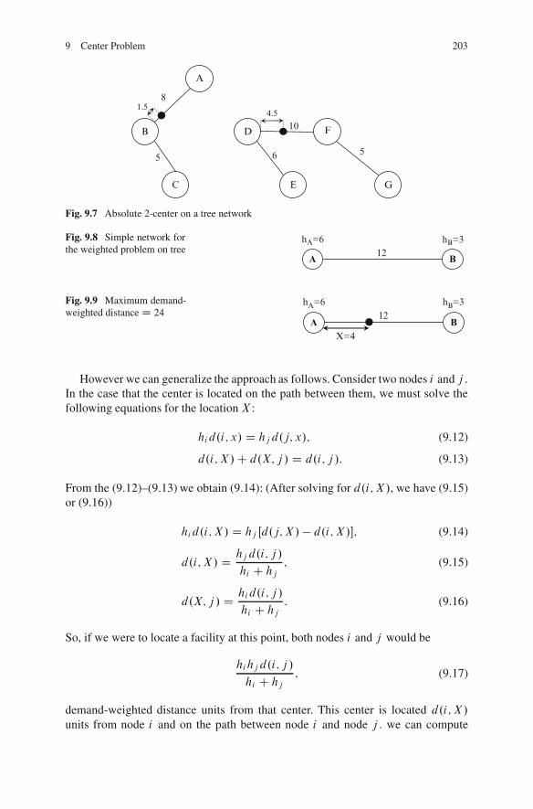
9 Center Problem 203
A
C
B
E
D F
G
8
5 6
10
5
4.51.5
Fig. 9.7 Absolute 2-center on a tree network
Fig. 9.8 Simple network forthe weighted problem on tree
A B12
hA=6 hB=3
Fig. 9.9 Maximum demand-weighted distance D 24
A B12
X=4
hB=3 hA=6
However we can generalize the approach as follows. Consider two nodes i and j .In the case that the center is located on the path between them, we must solve thefollowing equations for the location X :
hid.i; x/ D hj d.j; x/; (9.12)
d.i; X/C d.X; j / D d.i; j /: (9.13)
From the (9.12)–(9.13) we obtain (9.14): (After solving for d.i; X/, we have (9.15)or (9.16))
hid.i; X/ D hj Œd.j;X/ � d.i; X/; (9.14)
d.i; X/ D hj d.i; j /
hi C hj; (9.15)
d.X; j / D hid.i; j /
hi C hj: (9.16)
So, if we were to locate a facility at this point, both nodes i and j would be
hihj d.i; j /
hi C hj; (9.17)
demand-weighted distance units from that center. This center is located d.i; X/units from node i and on the path between node i and node j . we can compute
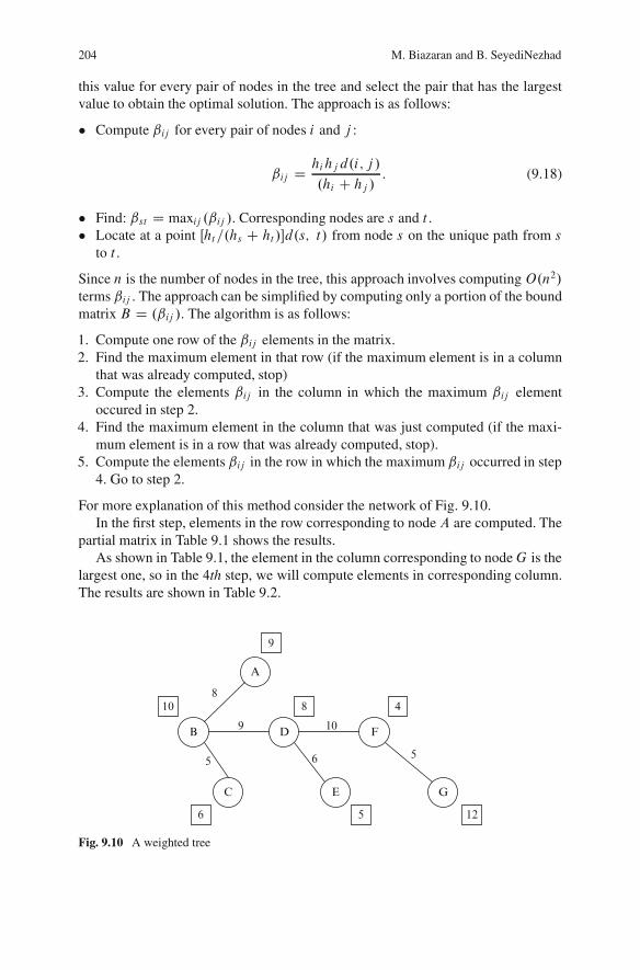
204 M. Biazaran and B. SeyediNezhad
this value for every pair of nodes in the tree and select the pair that has the largestvalue to obtain the optimal solution. The approach is as follows:
� Compute ˇij for every pair of nodes i and j :
ˇij D hihj d.i; j /
.hi C hj /: (9.18)
� Find: ˇst D maxij .ˇij /. Corresponding nodes are s and t .� Locate at a point Œht =.hs C ht /d.s; t/ from node s on the unique path from s
to t .
Since n is the number of nodes in the tree, this approach involves computingO.n2/terms ˇij . The approach can be simplified by computing only a portion of the boundmatrix B D .ˇij /. The algorithm is as follows:
1. Compute one row of the ˇij elements in the matrix.2. Find the maximum element in that row (if the maximum element is in a column
that was already computed, stop)3. Compute the elements ˇij in the column in which the maximum ˇij element
occured in step 2.4. Find the maximum element in the column that was just computed (if the maxi-
mum element is in a row that was already computed, stop).5. Compute the elements ˇij in the row in which the maximum ˇij occurred in step
4. Go to step 2.
For more explanation of this method consider the network of Fig. 9.10.In the first step, elements in the row corresponding to node A are computed. The
partial matrix in Table 9.1 shows the results.As shown in Table 9.1, the element in the column corresponding to nodeG is the
largest one, so in the 4th step, we will compute elements in corresponding column.The results are shown in Table 9.2.
A
C
B
E
D F
G
9
8
5 6
10
5
9
8 4
1256
10
Fig. 9.10 A weighted tree
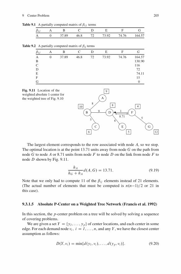
9 Center Problem 205
Table 9.1 A partially computed matrix of ˇij terms
ˇij A B C D E F G
A 0 37.89 46.8 72 73.92 74.76 164.57
Table 9.2 A partially computed matrix of ˇij terms
ˇij A B C D E F G
A 0 37.89 46.8 72 73.92 74.76 164:57
B 130:90
C 116
D 72
E 74:11
F 15
G 0
Fig. 9.11 Location of theweighted absolute 1-center forthe weighted tree of Fig. 9.10 A
C
B
E
D F
G
9
8
5 6
1
5
9
8 4
1256
10
8.71
The largest element corresponds to the row associated with node A, so we stop.The optimal location is at the point 13.71 units away from nodeG on the path fromnode G to node A or 8.71 units from node F to nodeD on the link from node F tonodeD shown by Fig. 9.11.
hA
hG C hAd.A;G/ D 13:71: (9.19)
Note that we only had to compute 11 of the ˇij elements instead of 21 elements.(The actual number of elements that must be computed is n.n�1/=2 or 21 inthis case).
9.3.1.5 Absolute P-Center on a Weighted Tree Network (Francis et al. 1992)
In this section, the p-center problem on a tree will be solved by solving a sequenceof covering problems.
We are given a set Y D fy1; : : : ; ypg of center locations, and each center in someedge. For each demand node vi ; i D 1; : : : ; n, and any Y , we have the closest centerassumption as follows:
D.Y; vi / D minfd.y1; vi /; : : : ; d.yp; vi /g: (9.20)
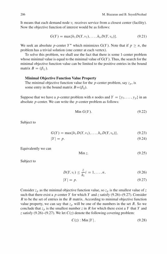
206 M. Biazaran and B. SeyediNezhad
It means that each demand node vi receives service from a closest center (facility).Now the objective function of interest would be as follows:
G.Y / D maxfh1D.Y; v1/; : : : ; hnD.Y; vn/g: (9.21)
We seek an absolute p-center Y � which minimizes G.Y /. Note that if p � n, theproblem has a trivial solution (one center at each vertex).
To solve this problem, we shall use the fact that there is some 1-center problemwhose minimal value is equal to the minimal value of G.Y /. Thus, the search for theminimal objective function value can be limited to the positive entries in the boundmatrix B D .ˇij /.
Minimal Objective Function Value PropertyThe minimal objective function value for the p-center problem, say zp , issome entry in the bound matrix BD.ˇij/.
Suppose that we have a p-center problem with n nodes and Y D fy1; : : : ; ypg in anabsolute p-center. We can write the p-center problem as follows:
Min G.Y /: (9.22)
Subject to
G.Y / D maxfh1D.Y; v1/; : : : ; hnD.Y; vn/g; (9.23)
jY j D p: (9.24)
Equivalently we canMin z: (9.25)
Subject to
D.Y; vi / � z
hii D 1; : : : ; n; (9.26)
jY j D p: (9.27)
Consider zp as the minimal objective function value, so zp is the smallest value of zsuch that there exist a p-center Y for which Y and z satisfy (9.26)–(9.27). ConsiderR to be the set of entries in the B matrix. According to minimal objective functionvalue property, we can say that zp will be one of the numbers in the set R. So weconclude that zp is the smallest number z in R for which there exist a Y that Y andz satisfy (9.26)–(9.27). We let C.z/ denote the following covering problem:
C.z/ W Min jY j : (9.28)
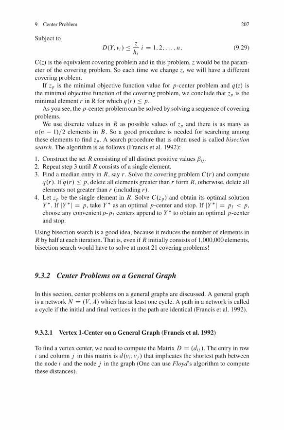
9 Center Problem 207
Subject to
D.Y; vi / � z
hii D 1; 2; : : : ; n; (9.29)
C.z/ is the equivalent covering problem and in this problem, z would be the param-eter of the covering problem. So each time we change z, we will have a differentcovering problem.
If zp is the minimal objective function value for p-center problem and q.z/ isthe minimal objective function of the covering problem, we conclude that zp is theminimal element r in R for which q.r/ � p.
As you see, thep-center problem can be solved by solving a sequence of coveringproblems.
We use discrete values in R as possible values of zp and there is as many asn.n � 1/=2 elements in B . So a good procedure is needed for searching amongthese elements to find zp . A search procedure that is often used is called bisectionsearch. The algorithm is as follows (Francis et al. 1992):
1. Construct the set R consisting of all distinct positive values ˇij .2. Repeat step 3 until R consists of a single element.3. Find a median entry in R, say r . Solve the covering problem C.r/ and computeq.r/. If q.r/ � p, delete all elements greater than r formR, otherwise, delete allelements not greater than r (including r).
4. Let zp be the single element in R. Solve C.zp/ and obtain its optimal solutionY �. If jY �j D p, take Y � as an optimal p-center and stop. If jY �j D p1 < p,choose any convenient p-p1 centers append to Y � to obtain an optimal p-centerand stop.
Using bisection search is a good idea, because it reduces the number of elements inR by half at each iteration. That is, even ifR initially consists of 1,000,000 elements,bisection search would have to solve at most 21 covering problems!
9.3.2 Center Problems on a General Graph
In this section, center problems on a general graphs are discussed. A general graphis a network N D .V; A/ which has at least one cycle. A path in a network is calleda cycle if the initial and final vertices in the path are identical (Francis et al. 1992).
9.3.2.1 Vertex 1-Center on a General Graph (Francis et al. 1992)
To find a vertex center, we need to compute the Matrix D D .dij /. The entry in rowi and column j in this matrix is d.vi ; vj / that implicates the shortest path betweenthe node i and the node j in the graph (One can use Floyd’s algorithm to computethese distances).
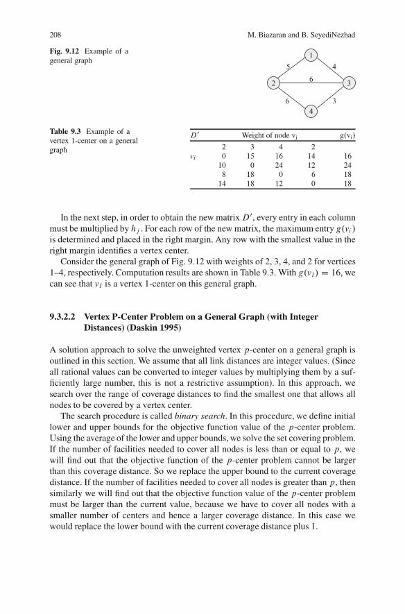
208 M. Biazaran and B. SeyediNezhad
Fig. 9.12 Example of ageneral graph
2
4
3
1
5
6
6
4
3
Table 9.3 Example of avertex 1-center on a generalgraph
D0 Weight of node vj g.vi/
2 3 4 2
vi 0 15 16 14 1610 0 24 12 248 18 0 6 1814 18 12 0 18
In the next step, in order to obtain the new matrixD0, every entry in each columnmust be multiplied by hj . For each row of the new matrix, the maximum entry g.vi /is determined and placed in the right margin. Any row with the smallest value in theright margin identifies a vertex center.
Consider the general graph of Fig. 9.12 with weights of 2, 3, 4, and 2 for vertices1–4, respectively. Computation results are shown in Table 9.3. With g.v1/ D 16, wecan see that v1 is a vertex 1-center on this general graph.
9.3.2.2 Vertex P-Center Problem on a General Graph (with IntegerDistances) (Daskin 1995)
A solution approach to solve the unweighted vertex p-center on a general graph isoutlined in this section. We assume that all link distances are integer values. (Sinceall rational values can be converted to integer values by multiplying them by a suf-ficiently large number, this is not a restrictive assumption). In this approach, wesearch over the range of coverage distances to find the smallest one that allows allnodes to be covered by a vertex center.
The search procedure is called binary search. In this procedure, we define initiallower and upper bounds for the objective function value of the p-center problem.Using the average of the lower and upper bounds, we solve the set covering problem.If the number of facilities needed to cover all nodes is less than or equal to p, wewill find out that the objective function of the p-center problem cannot be largerthan this coverage distance. So we replace the upper bound to the current coveragedistance. If the number of facilities needed to cover all nodes is greater than p, thensimilarly we will find out that the objective function value of the p-center problemmust be larger than the current value, because we have to cover all nodes with asmaller number of centers and hence a larger coverage distance. In this case wewould replace the lower bound with the current coverage distance plus 1.
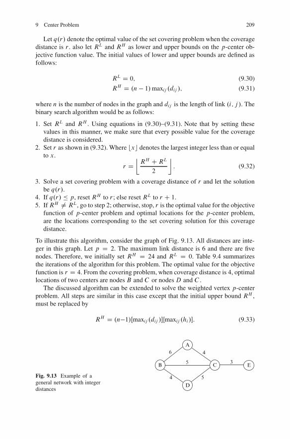
9 Center Problem 209
Let q.r/ denote the optimal value of the set covering problem when the coveragedistance is r . also let RL and RH as lower and upper bounds on the p-center ob-jective function value. The initial values of lower and upper bounds are defined asfollows:
RL D 0; (9.30)
RH D .n � 1/maxij .dij /; (9.31)
where n is the number of nodes in the graph and dij is the length of link .i; j /. Thebinary search algorithm would be as follows:
1. Set RL and RH . Using equations in (9.30)–(9.31). Note that by setting thesevalues in this manner, we make sure that every possible value for the coveragedistance is considered.
2. Set r as shown in (9.32). Where bxc denotes the largest integer less than or equalto x.
r D�RH CRL
2
�: (9.32)
3. Solve a set covering problem with a coverage distance of r and let the solutionbe q.r/.
4. If q.r/ � p, reset RH to r ; else reset RL to r C 1.5. IfRH ¤ RL, go to step 2; otherwise, stop, r is the optimal value for the objective
function of p-center problem and optimal locations for the p-center problem,are the locations corresponding to the set covering solution for this coveragedistance.
To illustrate this algorithm, consider the graph of Fig. 9.13. All distances are inte-ger in this graph. Let p D 2. The maximum link distance is 6 and there are fivenodes. Therefore, we initially set RH D 24 and RL D 0. Table 9.4 summarizesthe iterations of the algorithm for this problem. The optimal value for the objectivefunction is r D 4. From the covering problem, when coverage distance is 4, optimallocations of two centers are nodes B and C or nodesD and C .
The discussed algorithm can be extended to solve the weighted vertex p-centerproblem. All steps are similar in this case except that the initial upper bound RH ,must be replaced by
RH D .n�1/Œmaxij .dij /Œmaxij .hi /: (9.33)
Fig. 9.13 Example of ageneral network with integerdistances
A
B C
D
E
6
5
5
4
4
3
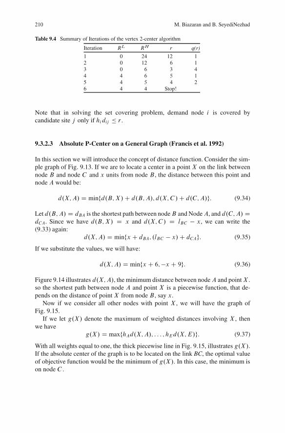
210 M. Biazaran and B. SeyediNezhad
Table 9.4 Summary of Iterations of the vertex 2-center algorithm
Iteration RL RH r q(r)
1 0 24 12 12 0 12 6 13 0 6 3 44 4 6 5 15 4 5 4 26 4 4 Stop!
Note that in solving the set covering problem, demand node i is covered bycandidate site j only if hidij � r .
9.3.2.3 Absolute P-Center on a General Graph (Francis et al. 1992)
In this section we will introduce the concept of distance function. Consider the sim-ple graph of Fig. 9.13. If we are to locate a center in a point X on the link betweennode B and node C and x units from node B , the distance between this point andnode A would be:
d.X;A/ D minfd.B;X/C d.B;A/; d.X;C /C d.C;A/g: (9.34)
Let d.B;A/ D dBA is the shortest path between nodeB and NodeA, and d.C;A/ DdCA. Since we have d.B;X/ D x and d.X;C / D lBC � x, we can write the(9.33) again:
d.X;A/ D minfx C dBA; .lBC � x/C dCAg: (9.35)
If we substitute the values, we will have:
d.X;A/ D minfx C 6;�x C 9g: (9.36)
Figure 9.14 illustrates d.X;A/, the minimum distance between nodeA and pointX .so the shortest path between node A and point X is a piecewise function, that de-pends on the distance of pointX from node B , say x.
Now if we consider all other nodes with point X , we will have the graph ofFig. 9.15.
If we let g.X/ denote the maximum of weighted distances involving X , thenwe have
g.X/ D maxfhAd.X;A/; : : : ; hEd.X;E/g: (9.37)
With all weights equal to one, the thick piecewise line in Fig. 9.15, illustrates g.X/.If the absolute center of the graph is to be located on the link BC, the optimal valueof objective function would be the minimum of g.X/. In this case, the minimum ison node C .
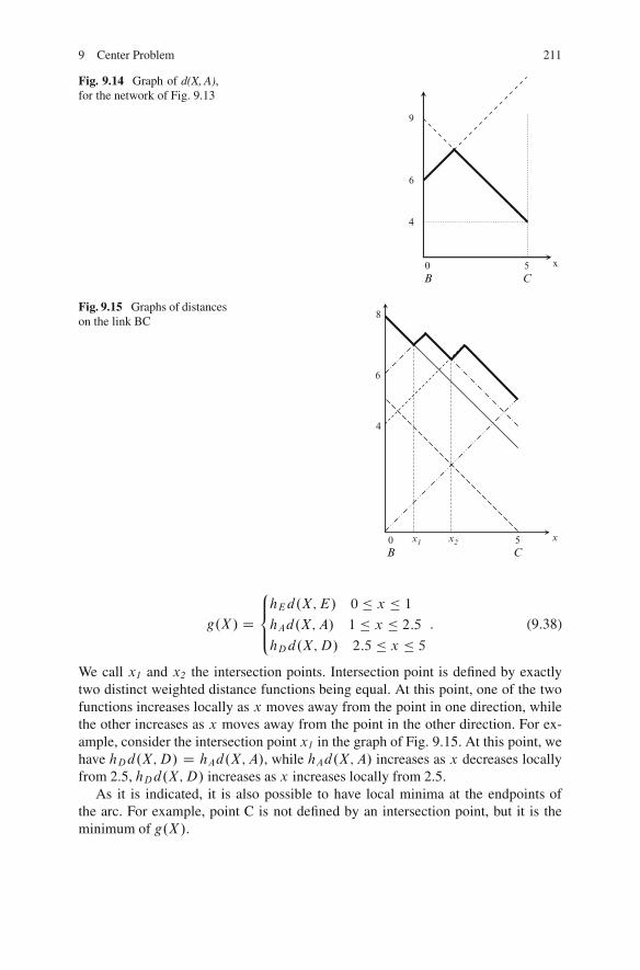
9 Center Problem 211
Fig. 9.14 Graph of d(X, A),for the network of Fig. 9.13
5 C
0 B
6
4
9
x
Fig. 9.15 Graphs of distanceson the link BC
5 C
0 B
6
x
4
8
x1 x2
g.X/ D
8<:hEd.X;E/ 0 � x � 1
hAd.X;A/ 1 � x � 2:5
hDd.X;D/ 2:5 � x � 5
: (9.38)
We call x1 and x2 the intersection points. Intersection point is defined by exactlytwo distinct weighted distance functions being equal. At this point, one of the twofunctions increases locally as x moves away from the point in one direction, whilethe other increases as x moves away from the point in the other direction. For ex-ample, consider the intersection point x1 in the graph of Fig. 9.15. At this point, wehave hDd.X;D/ D hAd.X;A/, while hAd.X;A/ increases as x decreases locallyfrom 2.5, hDd.X;D/ increases as x increases locally from 2.5.
As it is indicated, it is also possible to have local minima at the endpoints ofthe arc. For example, point C is not defined by an intersection point, but it is theminimum of g.X/.
212 M. Biazaran and B. SeyediNezhad
Now after this introduction, we conclude that to find the absolute center in anetwork, we have to find all intersection points on every arc and choose the onewith minimum distance to all other nodes and also evaluate g.vi / at every vertexand finally choose the best point among all intersection points and vertices.
Consider the p-center problem, in which X D fx1; : : : ; xpg is a collection ofcenters. We letD.X; vi / be the distance between vertex vi and a closest center inX ,so the objective would be to find an absolute p-center X� that minimizes:
G.X/ D maxfh1D.X; v1/; : : : ; hnD.X; vn/g: (9.39)
The VIP property for the p-center problem is the following:
Vertex and Intersection Point (VIP) PropertyThere exists at least one absolute p-center for which each center is at a vertex oran intersection point. Thus it is sufficient to consider only vertex and intersectionpoint locations in order to find an absolute p-center.This property reduces the p-center problem with infinite number of points to beconsidered to a problem with a finite number of points to be considered.
Although now we have a finite set of potential center locations, it would be possiblyvery large. To improve our enumeration approach, we will avoid enumeration ofintersection points on some arcs. If we have a current best trial solution, X 0, withfunction value g.X 0/. If we know a number bpq so that g.X/ � bpq for all X inarc Œvp; vq�, and also bpq > g.X 0/, no location on the Œvp; vq� can be an absolutecenter.
Arc Exclusion-Bounding Propertybipq D min fhid.vp; vi /; hid.vq; vi /gbpq D max fbipq: i D 1; : : : ; ngIf bpq>g.X 0/, no point in arc Œvp; vq� is an absolute 1-center.
9.3.2.4 Formulating the P-Center Problem (Francis et al. 1992)
Now that we have limited the solution of absolute p-center to a finite set of potentialcenter locations using VIP and Arc exclusion-bounding properties, we can formu-late the p-center problem. In this case, there is binary decision for every potentiallocation to include it in the p-center or not. Define Q D fq1; q2; : : : ; qm/ to be theset of all potential center location. First n members of Q correspond to vertices ofthe graph.
We associate each intersection point qk with a bound value bk , that is simplythe weighted distance from on of the two vertices used to define the intersectionpoint. For example, consider the intersection point x1 in Sect. 3.2.3. x1 is defined byvertices A and E , so the bound value for x1 is 7.
9 Center Problem 213
Decision variables:
� xj D 1 if a center is located at qj and 0 otherwise
Now the p-center problem can be formulated as follows:
Min zp: (9.40)
Subject to
zp � minfhidij jj 2 .X/gi D 1; : : : ; n; (9.41)
Xj
xj � p; (9.42)
xj 2 f0; 1gj D 1; : : : ; m: (9.43)
The set .X/ in (9.41) is the set of potential center locations that are used in thesolution. This is a mathematical statement of the p-center problem, but there is nodirect solution procedure for it. But the indirect approach is used to solve this prob-lem and consists of solving a sequence of related covering problems. In Sect. 3.2.5,we will discuss the relationship between p-center problem and covering problem.
9.3.2.5 Relationship Between P-Center Problem and Covering Problem(Francis et al. 1992)
We used covering problem to solve center problems earlier in this chapter. Now inthis section, we will discuss the relationship between them in general.
Suppose that .z�; X�/ is the optimal solution to p-center problem. Coveringproblem is as follows:
Decision variables:
� aij D 1 if hidij � z and 0 otherwise
CP.z/ W Minimize p DXj
xj (9.44)
Subject to
Xj
aij xj � 1 i D 1; : : : ; n; (9.45)
xj 2 f0; 1gj D 1; : : : ; m: (9.46)
Now suppose that z1 and z� are specific values for parameter z, and the optimalsolution to CP.z1/ is .p1; X1/. The relationship between two problems is as follows,offered without proof:
1. If .z�; X�/ is a solution to p-center problem, then .p;X�/ solves CP.z�/
214 M. Biazaran and B. SeyediNezhad
2. If .z�; X�/ is a solution to p-center problem and .p1; X1/ solves CP.z1/, then:
(a) If p1 > p, then z1 < z�.(b) If p1 � p, then z1 � z�.
To explain these claims, part 1 states that if we knew the z�, we could use CP.z�/ todetermine X�. Part 2 states that if we can guess a value z1 for z�, and solve CP.z1/,in case (a), we obtain a lower bound on z� and in case (b), we obtain a feasiblesolution or an upper bound on z�. Earlier in this chapter we had a similar discussionon this, for vertex p-center on a general graph with integer distances.
9.4 Approximate Solution Approaches
Kariv and Hakimi (1979) showed that the p-center problem on a general graph isNP-hard. In this section, some of the approximate solution approaches suggestedfor solving p-center problem are discussed.
Many heuristic and metaheuristic solution approaches were designed for thep-center problem in recent years; here we will mention some of them.
� Pallottino et al. (2002) represented a local search heuristic for the capacitatedvertex p-center.
� Bespamyatnikh et al. (2002) represented a polynomial time algorithm forp-center problem on circular arc graphs.
� Burkard and Dollani (2003) represented a number of algorithms with low com-putational complextity for p-center problem with pos/neg weights on trees andgeneral graphs.
� Caruso et al. (2003) represented four algorithms that solve p-center problems.Two exact algorithms and two heuristics. All these methods are based on solvinga sequence of set covering problems. Two heuristics can solve problems up to900 nodes in a few seconds.
� Hochbaum and Pathria (1997) represented approximation algorithms for twoclosely related problems p-SetSupplier and p-SetCenter.
� Khuller et al. (2000) represented polynomial time approximation algorithm tosolve the fault tolerant p-center problem in which every vertex must have at least˛ centers close to it.
� Khuller and Sussmann (2000) represented an approximation algorithm for thecapacitated p-center problem.
� Panigrahy and Vishwanathan (1998) represented an approximation algorithm forthe asymmetric p-center. The authors repeatedly employed a greedy set coveringalgorithm.
� Pelegrin and Canovas (1998) presented new versions of seed point algorithms.In these algorithms, the first step is to generate p points for the p-center prob-lem and then generating a partition of the demand points. They proposed a newassignment rule based on partitions.
9 Center Problem 215
� Andersson et al. (1998) represented an approximation algorithm based on de-mand point aggregation method.
� Dyer and Frieze (1985) presented a greedy algorithm in which the first center ischosen at random. This variant of greedy is called Greedy Plus (GrP).
� Drezner (1984) represented two heuristic algorithms for the p-center problem.These heuristics resemble algorithms for other location-allocation problems.
� Hochbaum and Shmoys (1985) represented a 2-approximation heuristic for thep-center problem.
� Hassin et al. (2003) introduced a local search strategy in which solutions arecompared lexicographically rather than by their worst coordinate. They appliedthis approach to p-center problem.
� Mladenovic et al. (2003) suggested metaheuristic approaches for the first timeas a means for solving p-center problems. They represented a basic VariableNeighborhood search and two Tabu search metaheuristics and a multi-start localsearch for the p-center problem.
� Bozkaya and Tansel (1998) proposed a spanning tree approach for the absolutep-center problem on cyclic networks (general graphs). The approach was moti-vated by the fact that the problem is NP-hard on general networks but solvable inpolynomial time on trees.
� Pacheco and Casado (2005) proposed a metaheuristic procedure based on thescatter search approach for solving p-center problem. The procedure incorpo-rates procedures based on different strategies such as local search, GRASP andpath relinking. The aim was solving problems with real data.
� Cheng et al. (2007) modeled the network of p-center problem as an intervalgraph whose edges all have unit lengths and provide a polynomial time al-gorithm to solve the problem under the assumption that the endpoints of theintervals are sorted.
9.5 Case Study
In this section we introduce a real-world case study related to p-center problems.
9.5.1 A Health Resource Case (Pacheco and Casado 2005)
In Pacheco and Casado (2005) a real health resource allocation problem was sur-veyed in Burgos, a rural area in the north of Spain. As mentioned in their paper,the authorities have limited budget, hence less than ten facilities considered to belocated. With dispersed population in this area, it was essential to design a methodto provide good solutions with a low number of facilities.
Real data in this case refer to the estimation of diabetes cases in that area. Fourhundred and fifty two locations with at least one known case of diabetes were takeninto account within the area and 152 of these locations were considered suitable forthe project.
216 M. Biazaran and B. SeyediNezhad
They dealt with two problems, first one was minimizing the maximum distancebetween users and facilities (p-center) and the second one was minimizing the pop-ulation further away from its closest available facility than a previously fixed time(maximum covering).
References
Andersson G, Francis RL, Normak T, Rayco MB (1998) Aggregation method experimentation forlarge-scale network location problems. Location Sci 6:25–39
Bespamyatnikh S, Bhattacharya B, Keil M, Kirkpathrick D, Segal M (2002) Efficient algorithmsfor centers and medians in interval and circular-arc graphs. Networks 39(3):144–152
Bozkaya B, Tansel B (1998) A spanning tree approach to the absolute p-center problem. LocationSci 6:83–107
Burkard RE, Dollani H (2003) Center problems with pos/neg weights on trees. Eur J Oper Res145:483–495
Caruso C, Colorni A, Aloi L (2003) Dominant an algorithm for the p-center problem. Eur J OperRes 149:53–64
Cheng TCE, Kang L, Ng CT (2007) An improved algorithm for the p-center problem on intervalgraphs with unit lengths. Comput Oper Res 34:2215–2222
Daskin MS (1995) Network and discrete location: Models, algorithms, and applications. Wiley,New York
Dyer ME, Frieze AM (1985) A simple heuristic for the p-center problem. Oper Res Lett 3:285–288Drezner Z (1984) The p-center problem: heuristics and optimal algorithms. J Oper Res Soc 35:
741–748Francis RL, McGinnis LF Jr, White JA (1992), Facility layout and location: An analytical approach.
Prentice-Hall, Englewood Cliffs, NJHakimi SL (1964) Optimum location of switching centers and the absolute centers and medians of
a graph. Oper Res 12:450–459Hakimi SL (1965) Optimum location of switching centers in a communications network and some
related graph theoretic problems. Oper Res 13:462–475Handler GY (1973) Minimax location of a facility in an undirected tree graph. Transport Sci 7:
287–293Hassin R, Levin A, Morad D (2003) Lexicographic local search and the p-center problem. Eur J
Oper Res 151:265–279Hochbaum DS, Pathria A (1997) Generalized p-center problems: Complexity results and approxi-
mation algorithms. Eur J Oper Res 100(3):594–607Hochbaum DS, Pathria A (1998) Locating centers in a dynamically changing network, and related
problems. Location Sci 6:243–256Hochbaum DS, Shmoys DB (1985) A best possible heuristic for the k-center problem. Math Oper
Res 10(2):180–184Kariv O, Hakami SL (1979) An algorithmic approach to network location problems. Part I: the
p-center problem. SIAM J Appl Math 37:513–538Khuller S, Sussmann YJ (2000) The capacitated K-center problem. SIAM J Discrete Math 13:403–
418Khuller S, Pless R, Sussmann Y (2000) Fault tolerant K-center problems. Theor Comput Sci
242:237–245Klein CM, Kincaid RK (1994) The discrete anti-p-center problem. Transport Sci 28:77–79Mladenovic N, Labbe’M, Hansen P (2003) Solving the p-center problem with tabu search and
variable neighborhood search. Networks 42:48–64
9 Center Problem 217
Ozsoy FA, Pinar MC (2006) An exact algorithm for the capacitated vertex p-center problem. Com-put Oper Res 33:1420–1436
Pacheco JA, Casado S (2005) Solving two location models with few facilities by using a hybridheuristic: a real health resources case. Comput Oper Res 32(12):3075–3091
Pallottino S, Scappara MP, Scutella MG (2002) Large scale local search heuristics for the capaci-tated vertex p-center problem. Networks 43(4):241–255
Panigrahy R, Vishwanathan S (1998) An O(log� n) Approximation algorithm for the asymmetricp-center problem. J Algorithms 27:259–268
Pelegrin B, Canovas A (1998) A new assignment rule to improve seed points algorithms for thecontinuous k-center problem. Eur J Oper Res 104:366–374
Perez-Brito D, Moreno-Perez JA, Rodriguez-Martin I (1998) The 2-facility centdian network prob-lem. Location Sci 6:369–381
Tamir A (1987) On the solution value of the continuous p-center location problem on a graph.Math Oper Res 12(2):340–349
Tamir A (2001) The k-centrum multi-facility location problem. Discrete Appl Math 109:293–307Tansel BC, Francis RL, Lowe TJ (1983) Location on networks: A survey. Part I: The p-center and
p-median problems. Manage Sci 29(4):482–497
Chapter 10Hierarchical Location Problem
Sara Bastani and Narges Kazemzadeh
In the basic models presented in previous chapters, it is assumed that there was onlyone type of facility being located. As the systems that provide services/productsusually consist of two or more levels of facilities, we discuss hierarchical facilitysystems in this chapter.
Many facility systems are hierarchical in nature. These facilities are usually hier-archical in terms of the types of services they provide. For example, the health caredelivery system consists of local clinics, hospitals and medical centers (Fig. 10.1). Inthis system a local clinic provides basic health care and diagnostic services. A hos-pital provides out-patient surgery in addition to those provided by a local clinic; anda medical center provides out-patient surgery and a full range of in-patient services.As another example of a hierarchical system, consider a solid waste disposal system.The solid waste is collected from the source of solid waste and shipped to transferstations or landfill stations by trucks. Other examples of a hierarchical system are:education system, postal system, banking system and production–distribution sys-tem (Narula 1986; Daskin 1995).
In the examples above, facilities cannot be located independently at each level.Thus, there is a need to consider them as a hierarchical system.
In this chapter, location-routing problem, which is confused with the hierarchicallocation problem, is not discussed. In the location-routing problem, the locationsof the primary facilities and the demand points are fixed and given; the objec-tive is to locate intermediate facilities and design tours originating at the primaryfacilities to serve the secondary facilities and tours emanating from secondary fa-cilities to serve the demand points. The location-routing problem is presented inChap. 18.
This chapter is organized as follows. In Sect. 10.1, we give a definition about hi-erarchical location problem, its applications and classifications. In Sects. 10.2–10.5mathematical models for the problem are given. We present solution methods inSect. 10.3. We conclude the chapter with some case studies in Sect. 10.4.
R.Z. Farahani and M. Hekmatfar (eds.), Facility Location: Concepts, Models, 219Algorithms and Case Studies, Contributions to Management Science,DOI 10.1007/978-3-7908-2151-2 10, c� Physica-Verlag Heidelberg 2009
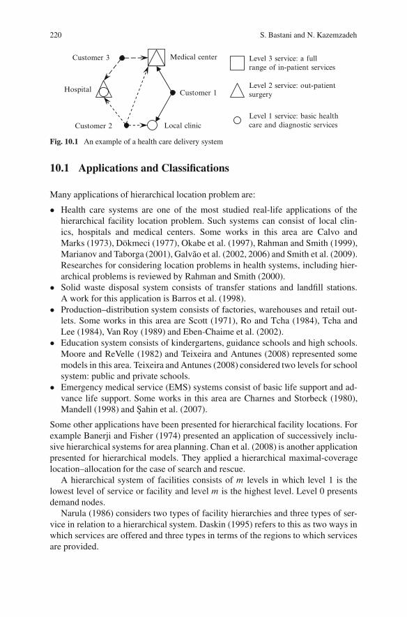
220 S. Bastani and N. Kazemzadeh
Level 3 service: a fullrange of in-patient services
Level 2 service: out-patientsurgery
Customer 2
Medical center
Customer 1
Customer 3
Local clinic
Hospital
Level 1 service: basic healthcare and diagnostic services
Fig. 10.1 An example of a health care delivery system
10.1 Applications and Classifications
Many applications of hierarchical location problem are:
� Health care systems are one of the most studied real-life applications of thehierarchical facility location problem. Such systems can consist of local clin-ics, hospitals and medical centers. Some works in this area are Calvo andMarks (1973), Dokmeci (1977), Okabe et al. (1997), Rahman and Smith (1999),Marianov and Taborga (2001), Galvao et al. (2002, 2006) and Smith et al. (2009).Researches for considering location problems in health systems, including hier-archical problems is reviewed by Rahman and Smith (2000).
� Solid waste disposal system consists of transfer stations and landfill stations.A work for this application is Barros et al. (1998).
� Production–distribution system consists of factories, warehouses and retail out-lets. Some works in this area are Scott (1971), Ro and Tcha (1984), Tcha andLee (1984), Van Roy (1989) and Eben-Chaime et al. (2002).
� Education system consists of kindergartens, guidance schools and high schools.Moore and ReVelle (1982) and Teixeira and Antunes (2008) represented somemodels in this area. Teixeira and Antunes (2008) considered two levels for schoolsystem: public and private schools.
� Emergency medical service (EMS) systems consist of basic life support and ad-vance life support. Some works in this area are Charnes and Storbeck (1980),Mandell (1998) and Sahin et al. (2007).
Some other applications have been presented for hierarchical facility locations. Forexample Banerji and Fisher (1974) presented an application of successively inclu-sive hierarchical systems for area planning. Chan et al. (2008) is another applicationpresented for hierarchical models. They applied a hierarchical maximal-coveragelocation–allocation for the case of search and rescue.
A hierarchical system of facilities consists of m levels in which level 1 is thelowest level of service or facility and level m is the highest level. Level 0 presentsdemand nodes.
Narula (1986) considers two types of facility hierarchies and three types of ser-vice in relation to a hierarchical system. Daskin (1995) refers to this as two ways inwhich services are offered and three types in terms of the regions to which servicesare provided.
10 Hierarchical Location Problem 221
� In a successively inclusive facility hierarchy, a facility at level k .k D 1; : : : ; m/provides services 1 through k.
– A successively inclusive facility hierarchy is said to have a locally inclusiveservice hierarchy if a level k facility .k D 1; : : : ; m/ at location j offers ser-vices of level 1; : : : ; k only to demands at location j and only level k servicesto demands at location i ¤ j .
– A successively inclusive facility hierarchy is said to have a successively in-clusive service hierarchy, Daskin (1995) refers to this as globally inclusiveservice hierarchy, when a level k facility .k D 1; : : : ; m/ at location j pro-vides level 1; : : : ; k services to all demand nodes.
� In a successively exclusive facility hierarchy, a facility level k .k D 1; : : : ; m/provides only services of level k.
– A successively exclusive facility hierarchy is said to have a successively ex-clusive service hierarchy if a level k facility at location j provides type kservices to all demand nodes.
Narula (1984) considers two types of flow discipline. The flow is integrated whenit can be from any lower-level facility to any higher-level facility. The flow is dis-criminating if it is from any lower-level facility k to the next higher-level facilityk C 1.
Sahin and Sural (2007) classify the hierarchical location problem with respect toflow pattern, service variety, spatial configuration, objective, horizontal interactionsand capacity limits on facilities.
� Flow pattern refers to demand flow through levels of a hierarchical system. In asingle-flow pattern, demand begins at level 0, passes through all levels, and finallyends at the highest level; or vice versa. In a multi-flow pattern, demand begins andends at any level k .kD 1; : : : ; m/. Flow pattern is similar to the flow disciplinedescribed in Narula (1984). We can consider flow pattern in a referral or non-referral system. In a referral system, lower-level facility refers a proportion ofcustomers to the higher-level facility.
� Service variety specifies the service availability at the levels of hierarchy. Nestedand non-nested features, respectively resembles Narula’s successively inclusiveand exclusive systems.
� Spatial configuration refers to the coherency of a hierarchical system. A coherenthierarchical system is one in which all customers of the same low level facilityare also customers of the same high level facility.
� For locating facilities in hierarchical location problem models, three types ofobjectives are considered: median, fixed charge, and covering objectives.
Teixeira and Antunes (2008) consider three types of spatial pattern according towhich demands are assigned to facilities: closest assignment, single assignment andpath assignment. In closest assignment, a demand node is assigned to the closestfacility located. In single assignment, a demand node is assigned only to one facil-ity located. In path assignment, when a given facility is located at location j , all
222 S. Bastani and N. Kazemzadeh
demands near the path travelled by the customers to reach the facility are also as-signed to it. In following Sects. 10.2–10.5, we introduce categories of hierarchicallocation models presented and developed as mathematical models.
10.2 Flow-Based Hierarchical Location Problem
Aardal et al. (1999) considers flow-based formulation with fixed-charge objective inwhich allocations is represented by a variable that is more common to network flowmodels and establishes flow from one level of the hierarchy to another. Sahin andSural (2007) present this model with median objective.
10.2.1 Flow-Based Formulation for Single-Flow Systems (Sahinand Sural 2007)
Sahin and Sural (2007) consider a two-level single-flow system, in which flow be-gins from demand node, passes a level 1 facility and ends at a level 2 facility.
10.2.1.1 Model Assumptions
Model assumptions of this model are as follows:
� The objective function is MiniSum.� The solution space is discrete and finite.� The formulation represents a two-level, single-flow, non-nested, non-coherent,
capacitated system.� The number of facilities at each level is known (exogenous model).
10.2.1.2 Model Inputs
Model inputs of this model are as follows:
cjj 0 : unit cost of flow between facilities level 2 at candidate location j 0 and level1 at candidate location jcij : unit cost of flow between level 1 facility at candidate location j and demandnode at idi : the amount of demand at node iMj 0 : the capacity of level 2 facility at candidate location j 0Mj : the capacity of level 1 facility at candidate location jp0: the number of level 2 facilities to be locatedp: the number of level 1 facilities to be located
10 Hierarchical Location Problem 223
10.2.1.3 Model Outputs (Decision Variables)
Model outputs of this model are as follows:
xj 0 D 1 if level 2 facility located at j 0, zero otherwiseyj D 1 if level 1 facility located at j , zero otherwisevjj 0 : amount of flow between level 2 facility at location j 0 and level 1 facility atlocation juij : amount of flow between level 1 facility at location j and demand at location i
10.2.1.4 Objective Function and its Constraints
The objective function of this model and its related constraints are as follows:
MinXi
Xj
uij cij CXj
Xj 0
vjj 0cjj 0 : (10.1)
Subject to Xj
uij D di 8 i; (10.2)
Xj 0
vjj 0 DXi
uij 8 j; (10.3)
Xi
uij � Mjyj 8 j; (10.4)
Xj 0
vjj 0 � Mixi 8 j 0; (10.5)
Xj
yj D p; (10.6)
Xj 0
xj 0 D p0; (10.7)
uij � 0 8 i; j; (10.8)
vjj 0 � 0 8 j; j 0; (10.9)
yj D 0; 1 8 j; (10.10)
xj 0 D 0; 1 8 j 0: (10.11)
Equation (10.1) minimizes the total demand-weighted distance from demand nodesto level 1 facilities and from level 1 facilities to level 2 facilities. Equations (10.2)ensure that the total demand of a node is completely satisfied by level 1facilities. Equations (10.3) ensure that the demand referred to a level 2 facil-ity by a level 1 facility is equivalent to the total demand of that level 1 facility.
224 S. Bastani and N. Kazemzadeh
Equations (10.4)–(10.5) are for facility capacities. Equations (10.6)–(10.7) locatethe required numbers of level 1 and 2 facilities, respectively. Equations (10.8)–(10.9) are non-negativity; (10.10)–(10.11) are integrality constraints.
10.2.2 Flow-Based Formulation for Multi-Flow Systems (Sahinand Sural 2007)
Sahin and Sural (2007) consider a two-level multi-flow, nested system, in whichdemand at location i is provided either directly or via a level 1 facility for its level 2demands and can be served by a level 2 facility for its both level 1 and 2 demands.Since facilities are capacitated, a portion of level 1 demand is provided by a level 1facility and the remaining portion by a level 2 facility. The same model can be seenin Narula and Ogbu (1985).
10.2.2.1 Model Assumptions
The assumptions of this model are similar to previous model except that there is thefollowing difference:
� The formulation represents a two-level, multi-flow, nested, non-coherent, capac-itated system.
10.2.2.2 Model Inputs
Model inputs are similar to previous model in addition to the following parameter:
cij 0 : unit cost of flow between level 2 facility at candidate location j 0 and demandnode at i
10.2.2.3 Model Outputs (Decision Variables)
Model outputs are similar to previous model in addition to the following decisionvariable:
wij 0 : amount of flow between level 2 facility at location j 0 and demand at loca-tion i
10.2.2.4 Objective Function and its Constraints
The objective function is similar to previous model in addition to the following term:Xi
Xj 0
wij 0cij 0 : (10.12)
10 Hierarchical Location Problem 225
The differences between the constraints of this model and previous model are asfollows:
� Equations (10.2) and (10.5) are omitted.� The following constraints are added to the formulation:
Xj
uij CXj 0
wij 0 D di 8 i; (10.13)
Xj 0
vjj 0 CXi
wij 0 � Mixi 8 j 0; (10.14)
wij 0 � 0 8 i; j 0: (10.15)
Equation (10.12) in the objective function minimizes the total demand-weighteddistance from demand nodes to level 2 facilities. Equations (10.13) replace(10.2) for which the first-level demand can be assigned to either level facility.Equations (10.14) replace (10.5) for which a level 2 facility capacity can be utilizedeither by the second-level demand at a node or the referred demand from level 1.Equations (10.15) are non-negativity.
10.3 Median-Based Hierarchical Location Problem(Daskin 1995)
Mirchandani (1987) presents a generalized median-based hierarchical locationmodel which allows various allocation schemes. Daskin (1995) represents median-based formulations in which demand at location i is assigned to a set of facilitiesone from each level.
10.3.1 Median-Based Formulation for Globally Inclusive ServiceHierarchies
A model for a successively inclusive facility hierarchy operating under a globallyinclusive service hierarchy is formulated by Daskin (1995).
10.3.1.1 Model Assumptions
Model assumptions of this model are as follows:
� The objective function is MiniSum.� The solution space is discrete and finite.� The formulation represents a successively inclusive facility hierarchy operating
under a globally inclusive service hierarchy.� The number of facilities at each level is known (exogenous model).
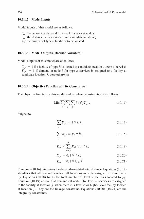
226 S. Bastani and N. Kazemzadeh
10.3.1.2 Model Inputs
Model inputs of this model are as follows:
hik : the amount of demand for type k services at node idij : the distance between node i and candidate location jpk : the number of type k facilities to be located
10.3.1.3 Model Outputs (Decision Variables)
Model outputs of this model are as follows:
Xjk D 1 if a facility of type k is located at candidate location j , zero otherwiseYijk D 1 if demand at node i for type k services is assigned to a facility atcandidate location j , zero otherwise
10.3.1.4 Objective Function and its Constraints
The objective function of this model and its related constraints are as follows:
MinXi
Xj
Xk
hikdij Yijk: (10.16)
Subject to
Xj
Yijk D 1 8 i; k; (10.17)
Xj
Xjk D pk 8 k; (10.18)
Yijk �mXhDk
Xjh 8 i; j; k; (10.19)
Xjk D 0; 1 8 j; k; (10.20)
Yijk D 0; 1 8 i; j; k: (10.21)
Equations (10.16) minimizes the demand-weighted total distance. Equations (10.17)stipulates that all demand levels at all locations must be assigned to some facil-ity. Equation (10.18) limits the total number of level k facilities located to pk .Equation (10.19) ensure that demands at node i for level k services are assignedto the facility at location j when there is a level k or higher level facility locatedat location j . They are the linkage constrains. Equations (10.20)–(10.21) are theintegrality constraints.
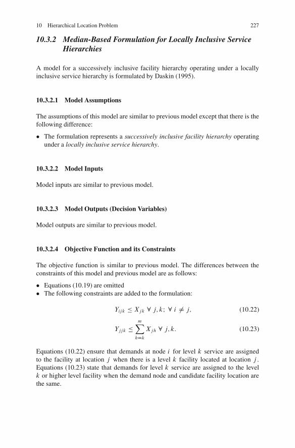
10 Hierarchical Location Problem 227
10.3.2 Median-Based Formulation for Locally Inclusive ServiceHierarchies
A model for a successively inclusive facility hierarchy operating under a locallyinclusive service hierarchy is formulated by Daskin (1995).
10.3.2.1 Model Assumptions
The assumptions of this model are similar to previous model except that there is thefollowing difference:
� The formulation represents a successively inclusive facility hierarchy operatingunder a locally inclusive service hierarchy.
10.3.2.2 Model Inputs
Model inputs are similar to previous model.
10.3.2.3 Model Outputs (Decision Variables)
Model outputs are similar to previous model.
10.3.2.4 Objective Function and its Constraints
The objective function is similar to previous model. The differences between theconstraints of this model and previous model are as follows:
� Equations (10.19) are omitted� The following constraints are added to the formulation:
Yijk � Xjk 8 j; kI 8 i ¤ j; (10.22)
Yjjk �mXhDk
Xjh 8 j; k: (10.23)
Equations (10.22) ensure that demands at node i for level k service are assignedto the facility at location j when there is a level k facility located at location j .Equations (10.23) state that demands for level k service are assigned to the levelk or higher level facility when the demand node and candidate facility location arethe same.
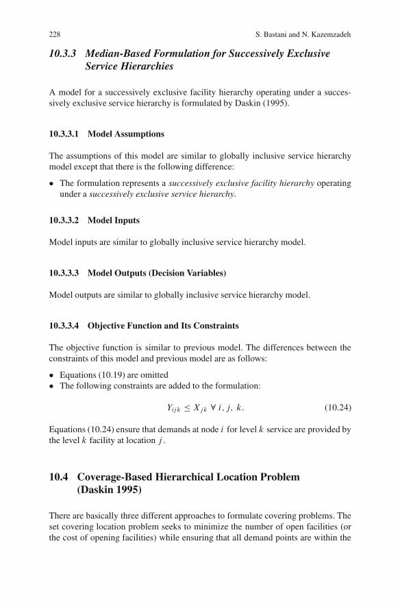
228 S. Bastani and N. Kazemzadeh
10.3.3 Median-Based Formulation for Successively ExclusiveService Hierarchies
A model for a successively exclusive facility hierarchy operating under a succes-sively exclusive service hierarchy is formulated by Daskin (1995).
10.3.3.1 Model Assumptions
The assumptions of this model are similar to globally inclusive service hierarchymodel except that there is the following difference:
� The formulation represents a successively exclusive facility hierarchy operatingunder a successively exclusive service hierarchy.
10.3.3.2 Model Inputs
Model inputs are similar to globally inclusive service hierarchy model.
10.3.3.3 Model Outputs (Decision Variables)
Model outputs are similar to globally inclusive service hierarchy model.
10.3.3.4 Objective Function and Its Constraints
The objective function is similar to previous model. The differences between theconstraints of this model and previous model are as follows:
� Equations (10.19) are omitted� The following constraints are added to the formulation:
Yijk � Xjk 8 i; j; k: (10.24)
Equations (10.24) ensure that demands at node i for level k service are provided bythe level k facility at location j .
10.4 Coverage-Based Hierarchical Location Problem(Daskin 1995)
There are basically three different approaches to formulate covering problems. Theset covering location problem seeks to minimize the number of open facilities (orthe cost of opening facilities) while ensuring that all demand points are within the
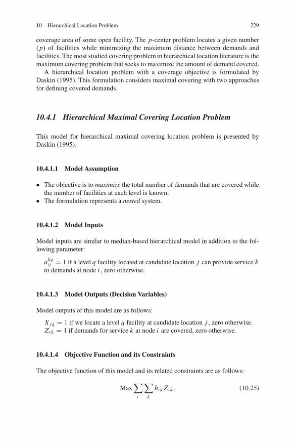
10 Hierarchical Location Problem 229
coverage area of some open facility. The p-center problem locates a given number.p/ of facilities while minimizing the maximum distance between demands andfacilities. The most studied covering problem in hierarchical location literature is themaximum covering problem that seeks to maximize the amount of demand covered.
A hierarchical location problem with a coverage objective is formulated byDaskin (1995). This formulation considers maximal covering with two approachesfor defining covered demands.
10.4.1 Hierarchical Maximal Covering Location Problem
This model for hierarchical maximal covering location problem is presented byDaskin (1995).
10.4.1.1 Model Assumption
� The objective is to maximize the total number of demands that are covered whilethe number of facilities at each level is known.
� The formulation represents a nested system.
10.4.1.2 Model Inputs
Model inputs are similar to median-based hierarchical model in addition to the fol-lowing parameter:
akqij D 1 if a level q facility located at candidate location j can provide service k
to demands at node i , zero otherwise.
10.4.1.3 Model Outputs (Decision Variables)
Model outputs of this model are as follows:
Xjq D 1 if we locate a level q facility at candidate location j , zero otherwise.Zik D 1 if demands for service k at node i are covered, zero otherwise.
10.4.1.4 Objective Function and its Constraints
The objective function of this model and its related constraints are as follows:
MaxXi
Xk
hikZik: (10.25)
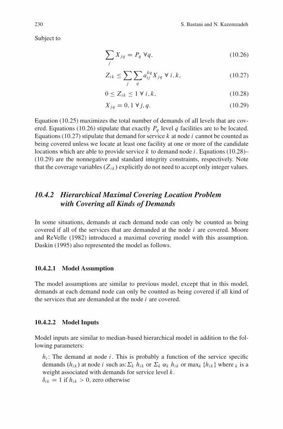
230 S. Bastani and N. Kazemzadeh
Subject to
Xj
Xjq D Pq 8q; (10.26)
Zik �Xj
Xq
akqij Xjq 8 i; k; (10.27)
0 � Zik � 1 8 i; k; (10.28)
Xjq D 0; 1 8j; q: (10.29)
Equation (10.25) maximizes the total number of demands of all levels that are cov-ered. Equations (10.26) stipulate that exactly Pq level q facilities are to be located.Equations (10.27) stipulate that demand for service k at node i cannot be counted asbeing covered unless we locate at least one facility at one or more of the candidatelocations which are able to provide service k to demand node i . Equations (10.28)–(10.29) are the nonnegative and standard integrity constraints, respectively. Notethat the coverage variables .Zik/ explicitly do not need to accept only integer values.
10.4.2 Hierarchical Maximal Covering Location Problemwith Covering all Kinds of Demands
In some situations, demands at each demand node can only be counted as beingcovered if all of the services that are demanded at the node i are covered. Mooreand ReVelle (1982) introduced a maximal covering model with this assumption.Daskin (1995) also represented the model as follows.
10.4.2.1 Model Assumption
The model assumptions are similar to previous model, except that in this model,demands at each demand node can only be counted as being covered if all kind ofthe services that are demanded at the node i are covered.
10.4.2.2 Model Inputs
Model inputs are similar to median-based hierarchical model in addition to the fol-lowing parameters:
hi : The demand at node i . This is probably a function of the service specificdemands .hik/ at node i such as:˙k hik or ˙k ˛k hik or maxk fhikg where k is aweight associated with demands for service level k.ıik D 1 if hik > 0, zero otherwise
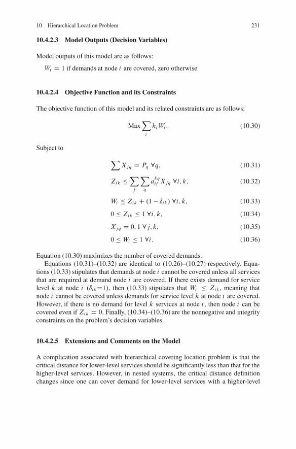
10 Hierarchical Location Problem 231
10.4.2.3 Model Outputs (Decision Variables)
Model outputs of this model are as follows:
Wi D 1 if demands at node i are covered, zero otherwise
10.4.2.4 Objective Function and its Constraints
The objective function of this model and its related constraints are as follows:
MaxXi
hiWi : (10.30)
Subject to
XXjq D Pq 8q; (10.31)
Zik �Xj
Xq
akqij Xjq 8i; k; (10.32)
Wi � Zik C .1 � ıik/ 8i; k; (10.33)
0 � Zik � 1 8i; k; (10.34)
Xjq D 0; 1 8j; k; (10.35)
0 � Wi � 1 8i: (10.36)
Equation (10.30) maximizes the number of covered demands.Equations (10.31)–(10.32) are identical to (10.26)–(10.27) respectively. Equa-
tions (10.33) stipulates that demands at node i cannot be covered unless all servicesthat are required at demand node i are covered. If there exists demand for servicelevel k at node i .ıikD1/, then (10.33) stipulates that Wi � Zik , meaning thatnode i cannot be covered unless demands for service level k at node i are covered.However, if there is no demand for level k services at node i , then node i can becovered even if Zik D 0. Finally, (10.34)–(10.36) are the nonnegative and integrityconstraints on the problem’s decision variables.
10.4.2.5 Extensions and Comments on the Model
A complication associated with hierarchical covering location problem is that thecritical distance for lower-level services should be significantly less than that for thehigher-level services. However, in nested systems, the critical distance definitionchanges since one can cover demand for lower-level services with a higher-level
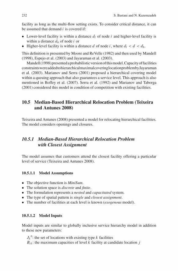
232 S. Bastani and N. Kazemzadeh
facility as long as the multi-flow setting exists. To consider critical distance, it canbe assumed that demand i is covered if:
� Lower-level facility is within a distance dl of node i and higher-level facility iswithin a distance dh of node i or
� Higher-level facility is within a distance d of node i , where dl < d < dh.
This definition is presented by Moore and ReVelle (1982) and then used by Mandell(1998), Espejo et al. (2003) and Jayaraman et al. (2003).
Mandell(1998)presentedaprobabilisticversionofthismodel.CapacityoffacilitiesconstraintswereaddedtohierarchicalmaximalcoveringlocationproblembyJayaramanet al. (2003). Marianov and Serra (2001) proposed a hierarchical covering modelwithin a queuing approach that also guarantees a service level. This approach is alsomentioned in Boffey et al. (2007). Serra et al. (1992) and Marianov and Taborga(2001) considered this model in condition of competition with existing facilities.
10.5 Median-Based Hierarchical Relocation Problem (Teixeiraand Antunes 2008)
Teixeira and Antunes (2008) presented a model for relocating hierarchical facilities.The model considers openings and closures.
10.5.1 Median-Based Hierarchical Relocation Problemwith Closest Assignment
The model assumes that customers attend the closest facility offering a particularlevel of service (Teixeira and Antunes 2008).
10.5.1.1 Model Assumptions
� The objective function is MiniSum.� The solution space is discrete and finite.� The formulation represents a nested and capacitated system.� The type of spatial pattern is single and closest assignment.� The number of facilities at each level is known (exogenous model).
10.5.1.2 Model Inputs
Model inputs are similar to globally inclusive service hierarchy model in additionto these new parameters:
Jk0: the set of locations with existing type k facilities
Bik : the maximum capacities of level k facility at candidate location j
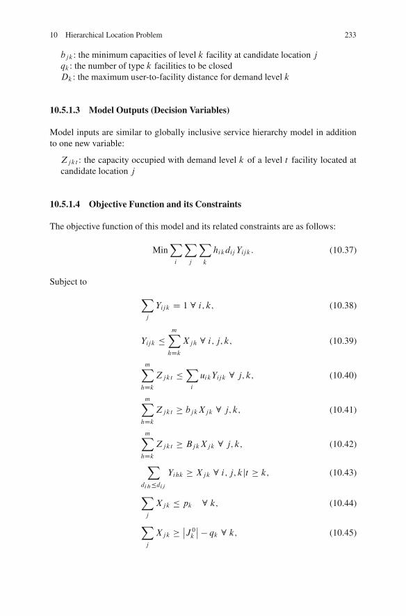
10 Hierarchical Location Problem 233
bjk : the minimum capacities of level k facility at candidate location jqk : the number of type k facilities to be closedDk : the maximum user-to-facility distance for demand level k
10.5.1.3 Model Outputs (Decision Variables)
Model inputs are similar to globally inclusive service hierarchy model in additionto one new variable:
Zjkt : the capacity occupied with demand level k of a level t facility located atcandidate location j
10.5.1.4 Objective Function and its Constraints
The objective function of this model and its related constraints are as follows:
MinXi
Xj
Xk
hikdij Yijk: (10.37)
Subject to
Xj
Yijk D 1 8 i; k; (10.38)
Yijk �mXhDk
Xjh 8 i; j; k; (10.39)
mXhDk
Zjkt �Xi
uikYijk 8 j; k; (10.40)
mXhDk
Zjkt � bjkXjk 8 j; k; (10.41)
mXhDk
Zjkt � BjkXjk 8 j; k; (10.42)
Xdih�dij
Yihk � Xjk 8 i; j; kjt � k; (10.43)
Xj
Xjk � pk 8 k; (10.44)
Xj
Xjk � ˇJ 0kˇ � qk 8 k; (10.45)
234 S. Bastani and N. Kazemzadeh
Yijk D 0 8 i; j; kjdij � Dk; (10.46)
Xjk D 0; 1 8 j; k; (10.47)
Yijk D 0; 1 8 i; j; k; (10.48)
Yjkt � 0 8 j; k; t: (10.49)
Equations (10.38) ensure that all demands of all levels from all nodes are satisfied.Equations (10.39) impose that a given level of demand can only be satisfied by afacility of equal or higher level. Equations (10.40) define capacity variables Zjktby stating that the demand of each level assigned to a node has to be served bysome facility of equal or higher level located there. Equations (10.41)–(10.42) im-pose maximum and minimum limits on capacity, according to facility type. Closestassignment Equations (10.43) are written separately per demand level and state thateach demand level must be assigned to the closest facility of equal or higher level.Equations (10.44)–(10.45) limit the number of new facilities to be opened and ex-isting facilities to be closed. Equations (10.46) limit the maximum travel distancebetween demand nodes and facilities. Finally, Equations (10.47)–(10.49) define de-cision variables and enforce single assignment.
10.5.2 Median-Based Hierarchical Relocation Problem with PathAssignment
The model assumes that when a given facility is located at location j , all demandsnear the path travelled by the customers to reach the facility are also assigned to it(Teixeira and Antunes 2008).
10.5.2.1 Model Assumptions
The assumptions of this model are similar to previous model except that there is thefollowing difference:
� The type of spatial pattern is single and path assignment.
10.5.2.2 Model Inputs
Model inputs are similar to previous model in addition to one new parameter:
jPij j: the cardinality of the subset of demand nodes that are near the shortest pathfrom v to j
10 Hierarchical Location Problem 235
10.5.2.3 Model Outputs (Decision Variables)
Model outputs are similar to previous model.
10.5.2.4 Objective Function and its Constraints
The objective function of this model and its related constraints are as follows:
� Equations (10.43) are omitted� The following constraints are added to the formulation:
Xh
Yhjk � ˇPij ˇ � Yijk 8 i; j; k : (10.50)
In (10.50) the assignments of different levels are independent, while in (10.43) thelocation of higher-level facilities influences lower-level assignments.
10.6 Solving Algorithms for Hierarchical Location Problem
Many algorithms are represented to solve different types of hierarchical facility lo-cation problems. Similar to single-level location problems, Lagrangian relaxations,specialized branch and bound procedures and conventional heuristic methods aredeveloped for hierarchical location problems. Also a group of studies developingcombinatorial approximation algorithms have appeared in recent years. We re-view the related literatures of solving algorithms for hierarchical facility locationproblems.
� Scott (1971) presented a heuristic algorithm for the hierarchical location–allocation problem. The algorithm involves a steady movement from a highvalue of the objective function, to progressively lower values, and this is ac-complished through a series of iterative stages each of which seeks out a locallyoptimal solution.
� Dokmeci (1977) used a heuristic method. In this method at first an ideal the-oretic solution is obtained from the heuristic procedure. Then by repeating theforegoing heuristic and adjustment procedures for each level, the environmen-tally adjusted optimal locations of the facilities are obtained.
� Moore and ReVelle (1982) used relaxed linear programming, supplemented bybranch and bound where necessary, to solve the integer programming prob-lem which is extension of the 2-level hierarchical maximal covering locationproblem.
� Considering the hierarchical maximum covering location problem presentedby Moore and ReVelle (1982), Espejo et al. (2003) defined a combinedLagrangian–surrogate (L–S) relaxation which reduces to a 0–1 knapsack
236 S. Bastani and N. Kazemzadeh
problem. A Lagrangian and a surrogate relaxation of the problem, which areparticular cases of (L–S) relaxation, are also discussed. Then they developed asubgradient-based heuristic using the proposed relaxations to solve this problem.
� Tcha and Lee (1984) represented a branch and bound algorithm for the multi-level uncapacitated facility location problem. In this method, the dual basedscheme of “dual ascent procedure” is applied. Also the convergence rate to anoptimal solution for this branch and bound algorithm has been further acceler-ated by employing two other devices, node simplification procedure and primaldescent procedure.
� For the two-level uncapacitated facility location problem with some side con-straints. Ro and Tcha (1984) proposed a branch and bound solution procedure,employing a set of new devices for lower bounds and simplifications which areobtained by exploiting the submodularity of the objective function and the specialstructure of the side-constraints.
� Narula and Ogbu (1985) developed the Lagrangian relaxation of the uncapac-itated 2-hierarchical location–allocation problem and proposed a subgradientoptimization procedure to solve it.
� Hodgson (1986) solved the nested hierarchical location–allocation problem withallocations based on facility size by employing a heuristic method which allowsall levels to be located simultaneously. He reformulated the model based uponthe Reilly law of retail gravitation, because of the difficulties encountered withthe traditional inverse square Reilly law, using a negative exponential allocationrule which has been a popular way of overcoming the inability to model tripsover short distances.
� Van Roy (1989) used standard features and techniques for solving linearprogramming (LP) and mixed integer programming (MIP) problems with animproved formulation based on pre- and post-processing of the problem anddynamic cut generation procedures for speed up the solution of MIP problems.
� Okabe et al. (1997) used the optimization procedure with two steps for a systemof successively inclusive hierarchical facilities. The first step optimizes a systemof exclusive hierarchical facilities by an analytical method. Using this optimal so-lution, the second step optimizes a system of successively inclusive hierarchicalfacilities by a computational search method.
� Barros et al. (1998) represented a heuristic method based on linear relaxation.� Aardal (1998) presented some classes of inequalities to strengthen the linear re-
laxation for obtaining a good lower bound on the optimal solution in branchand bound.
� Aardal et al. (1999) developed a randomized algorithm for the hierarchical fa-cility location problem. The algorithm is a randomized rounding procedure thatuse an optimal solution of a linear programming relaxation and its dual to makea random choice of facilities to be opened.
� Goncharov and Kochetov (2000) presented a probabilistic Tabu search algorithmfor multi stage uncapacitated facility location problem.
� Marianov and Taborga (2001) proposed a heuristic algorithm to solvetheir model.
10 Hierarchical Location Problem 237
� A simple dual ascent method for the hierarchical facility location problem ispresented by Bumb and Kern (2001). The algorithm is deterministic and basedon the primal-dual technique.
� Bumb (2001) presented a 0.47-approximation algorithm for the maximizationversion of the two level uncapacitated facility location problem. For the analysisof this algorithm the assumption that there are only two levels of facilities isessential. The generalization of the algorithm to the case when the facilities arelocated on k levels, with k > 2, makes the analysis of the algorithm much moredifficult.
� For the nested hierarchical queuing covering location problem, Marianov andSerra (2001) offered a bi-level heuristic with two phases. A construction phaseusing a greedy adding procedure with random substitution (GRASP) and animprovement phase by using a vertex-substitution heuristic and a tabu searchprocedure.
� Eben-Chaime et al. (2002) proposed a heuristic solution schemes and lowerbounds on objective values for capacitated location–allocation problem on a line.
� Galvao et al. (2002) represented Lagrangian-based decomposition of the hierar-chical location problem and proposed three heuristic methods to solve this model:a 3 p-median heuristic which consists of successively locating each level servicesand then applying a vertex substitution algorithm, a Lagrangian heuristic whichuses a subgradient optimization algorithm, and a modified Lagrangian heuristic.
� Galvao et al. (2006) used a Lagrangian heuristic for capacitated version of theirprevious model presented in Galvao et al. (2002).
� A Lagrangian relaxation methodology coupled with a heuristic was employed byJayaraman et al. (2003) for hierarchical maximal covering location problem.
� Ageev et al. (2004) presented improved combinatorial approximation algorithmsfor the k-level facility location problem. In this research they applied path re-duction and greedy for an approximation algorithm. Also they represented arecursive path reduction Algorithm for approximate this problem.
� A quasi-greedy algorithm for approximating the classical uncapacitated two-level facility location problem is presented by Zhang (2006).
� A hybrid multistart heuristic for the uncapacitated facility location problemwas presented by Resende and Werneck (2006). Their method has two phases.The first is a multistart routine with intensification using a process called path-relinking. The second phase is post-optimization.
� Ignacio et al. (2008) presented a two-level hierarchical model for the locationof concentrators and routers in computers networks. They used Lagrangian re-laxation to provide lower bounds for the problem. A tabu search meta-heuristicis then developed to provide approximate solutions. A feasible solution of goodquality is obtained by the TS algorithm.
� Chan et al. (2008) presented a nonlinear model for generalized search-and-rescueproblem. This problem is modeled using a multiobjective linear integer program(MOLIP), which is an approximation of a highly nonlinear integer program.As a solution algorithm, the MOLIP is converted to a two-stage network-flow
238 S. Bastani and N. Kazemzadeh
formulation that reduces the number of explicitly enumerated integer variables.Non-inferior solutions of the MOLIP are evaluated by a value function, whichidentifies solutions that are similar to the more accurate nonlinear model.
10.7 Case Study
In this section we will introduce some real-world case studies related to hierarchicallocation problems.
10.7.1 A Hierarchical Model for the Location of MaternityFacilities in the Municipality of Rio de Janeiro(Galvao et al. 2002 and 2006)
Galvao et al. (2002) represented a 3-level hierarchical model that addresses the lo-cation of levels of facilities associated with maternal and perinatal care in Rio deJaneiro including basic units, maternity homes and neonatal clinics.
Since the overall aim is to develop a location model that aids health care au-thorities to reduce the perinatal mortality rate in the municipality, good access tofacilities is needed. Therefore the model seeks to optimize the surrogate objectiveof total distance travelled by mothers-to-be. By the description of the different typesof facility, they developed a successively inclusive model. Some other assumptionsare considered for this model.
The model is solved for real 1995 data of the municipality of Rio de Janeiro.Also results are given for available problems, for networks ranging from 10 to 400vertices.
Galvao et al. (2006) completed their model by adding some form of capacityconstraints, which are needed especially in the higher, resource intensive level ofthe hierarchy. This model is solved exactly for a small problem and approximatelyfor the 152-vertex Rio de Janeiro data.
10.7.2 Locational Analysis for Regionalization of Turkish RedCrescent Blood Services (Sahin et al. 2007)
Sahin et al. (2007) represented the location problem of the blood services of TurkishRed Crescent (TRC) at a regional level to increase the countrywide service level ofthe blood services, which is an integral part of the national health care system. Theydeveloped location–allocation models to solve the problems of regionalization basedon a hierarchical structure.
10 Hierarchical Location Problem 239
The problem was considered as a 2-level hierarchical system in which the re-gional blood centers (RBCs) are the upper-level facilities whereas the blood centers,blood stations, and mobile units are the lower-level facilities.
The entire problem was decomposed into three stages. In Stage 1 they formulateda 2-level hierarchical pq-median problem in which the locations of the regionalcenters, the allocation of blood centers to the regional centers together with theirservice-referral levels, and the allocation of demand points to the blood centerswere determined. A hierarchical set covering problem was formulated in Stage 2to increase the service level. This second sub-problem finds the minimum numberof blood stations such that every demand point is covered by at least one facil-ity within a given maximal service distance or time. To help increase the servicelevel even further, an integer programming model was formulated as the third sub-problem in Stage 3 to determine the fleet size for the mobile units in each region.
10.7.3 School Network Planning in Coimbra, Portugal (Teixeiraand Antunes 2008)
Teixeira and Antunes (2008) presented a study on the redeployment of Coimbra’sprimary school network in Portugal. Three objectives were pursued by the educa-tion authorities. Three scenarios for the redeployment of the school network wereconsidered. First, they solved median-based hierarchical relocation problem withclosest assignment constraints. For this model, no feasible solutions could be foundfor any one of the three scenarios. The solutions were obtained for the three sce-narios using median-based hierarchical relocation problem with path assignmentconstraints.
References
Aardal K (1998) Reformulation of capacitated facility location problems: how redundant informa-tion can help. Ann Oper Res 82:289–308
Aardal K, Chudak FA, Shmoys DB (1999) A 3-approximation algorithm for the k-level uncapaci-tated facility location problem. Inf Process Lett 72:161–167
Ageev A, Ye YY, Zhang JW (2004) Improved combinatorial approximation algorithms for thek-level facility location problem. SIAM J Discrete Math 18(1):207–217
Banerji S, Fisher HB (1974) Hierarchical location analysis for integrated area planning rural inIndia. Papers Sci Assoc 33:177–194
Barros AI, Dekker R, Scholten V (1998) A two-level network for recycling sand: a case study. EurJ Oper Res 110(3):199–214
Boffey B, Galvao RD, Espejo L (2007) A review of congestion models in the location of facilitieswith immobile servers. Eur J Oper Res 178:643–662
Bumb A (2001) An approximation algorithm for the maximization version of the two level unca-pacitated facility location problem. Oper Res Lett 29:155–161
240 S. Bastani and N. Kazemzadeh
Bumb AF, Kern W (2001) A simple dual ascent algorithm for the multilevel facility location prob-lem. Lecture notes in computer science 2129. Springer, Berlin, pp 55–62
Calvo AB, Marks DH (1973) Location of health care facilities: an analytical approach. Socio-EconPlan Sci 7:407–422
Chan Y, Mahan JM, Chrissis JW, Drake DA, Wang D (2008) Hierarchical maximal coverage loca-tion allocation: Case of generalized search-and-rescue. Comput Oper Res 35:1886–1904
Charnes A, Storbeck J (1980) A goal programming model for the siting of multilevel EMS systems.Socio-Econ Plan Sci 14:155–161
Daskin MS (1995) Network and discrete location: Models, algorithms, and applications. Wiley,New York
Dokmeci VF (1977) A quantitative model to plan regional health facility systems. Manage Sci24(4):411–419
Eben-Chaime M, Mehrez A, Markovich G (2002) Capacitated location–allocation problems on aline. Comput Oper Res 29:459–470
Espejo LGA, Galvao RD, Boffey B (2003) Dual-based heuristics for a hierarchical covering loca-tion problem. Comput Oper Res 30:165–180
Galvao RD, Espejo LGA, Boffey B (2002) A hierarchical model for the location of perinatal facil-ities in the municipality of Rio de Janeiro. Eur J Oper Res 138:495–517
Galvao RD, Espejo LGA, Boffey B (2006) Load balancing and capacity constraints in a hierarchi-cal location model. Eur J Oper Res 172:631–646
Goncharov E, Kochetov Y (2000) Probabilistic tabu search algorithm for the multi-stage uncapac-itated facility location problem. Operations research proceedings. Springer, Berlin, pp 65–70
Hodgson MJ (1986) A hierarchical location–allocation model with allocations based on facilitysize. Ann Oper Res 6:273–289
Ignacio AAV, Filho VJMF, Galvao RD (2008) Lower and upper bounds for a two-level hierarchicallocation problem in computer networks. Comput Oper Res 35:1982–1998
Jayaraman V, Gupta R, Pirkul H (2003) Selecting hierarchical facilities in a service-operationsenvironment. Eur J Oper Res 147:613–628
Mandell MB (1998) Covering models for two-tiered emergency medical services systems. Loca-tion Sci 6:355–368
Marianov V, Serra D (2001) Hierarchical location allocation models for congested system. Eur JOper Res 135:195–208
Marianov V, Taborga P (2001) Optimal location of public health centers which provide free andpaid services. J Oper Res Soc 52(4):391–400
Mirchandani PB (1987) Technical note: generalized hierarchical facility locations. Transport Sci21(2):123–125
Moore GC, ReVelle C (1982) The hierarchical service location problem. Manage Sci 28(7):775–780
Narula SC (1984) Hierarchical location–allocation problems: A classification scheme. Eur J OperRes 5:93–99
Narula SC (1986) Minisum hierarchical location–allocation problems on a network: A survey. AnnOper Res 6:257–272
Narula SC, Ogbu UI (1985) Lagrangian relaxation and decomposition in an uncapacitated2-hierarchical location–allocation problem. Comput Oper Res 12(2):169–180
Okabe A, Okunuki K, Suzuki T (1997) A computational method for optimizing the hierarchy andspatial configuration of successively inclusive facilities on a continuous plane. Location Sci5(4):255–268
Rahman SU, Smith DK (1999) Deployment of rural health facilities in a developing country. J OperRes Soc 50(9):892–902
Rahman SU, Smith DK (2000) Use of location–allocation models in health service developmentplanning in developing nations. Eur J Oper Res 123(3):437–452
Resende MGC, Werneck RF (2006) A hybrid multistart heuristic for the uncapacitated facilitylocation problem. Eur J Oper Res 174:54–68
10 Hierarchical Location Problem 241
Ro H, Tcha DW (1984) A branch and bound algorithm for the two-level uncapacitated facilitylocation problem with some side constraints. Eur J Oper Res 18:349–358
Sahin G, Sural H (2007) A review of hierarchical facility location models. Comput Oper Res34:2310–2331
Sahin G, Sural H, Meral S (2007) Locational analysis for regionalization of Turkish Red Crescentblood services. Comput Oper Res 34:692–704
Scott AJ (1971) Operational analysis of nodal hierarchies in network systems. Oper Res Quart22:25–36
Serra D, Marianov V, ReVelle C (1992) The maximum-capture hierarchical location problem. EurJ Oper Res 62:363–371
Smith HK, Harper PR, Potts CN, Thyle A (2009) Planning sustainable community health schemesin rural areas of developing countries. Eur J Oper Res 193: 768–777
Tcha DW, Lee B (1984) A branch-and-bound algorithm for the multi-level uncapacitated facilitylocation problem. Eur J Oper Res 18:35–43
Teixeira JC, Antunes AP (2008) A hierarchical location model for public facility planning. Eur JOper Res 185:92–104
Van Roy TJ (1989) Multi-level production and distribution planning with transportation fleet opti-mization. Manage Sci 35(12):1443–53
Zhang J (2006) Approximating the two-level facility location problem via a quasi-greedy approach.Math Program 108(1):159–176
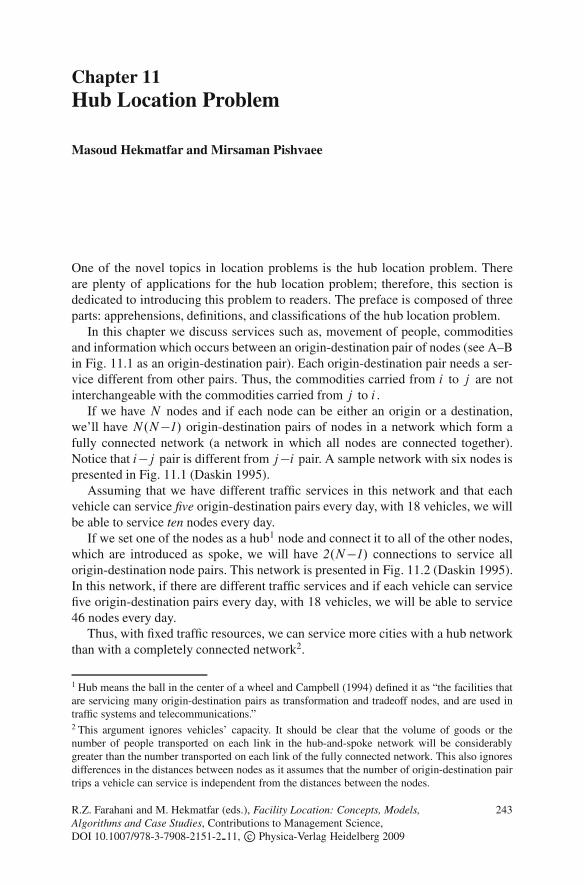
Chapter 11Hub Location Problem
Masoud Hekmatfar and Mirsaman Pishvaee
One of the novel topics in location problems is the hub location problem. Thereare plenty of applications for the hub location problem; therefore, this section isdedicated to introducing this problem to readers. The preface is composed of threeparts: apprehensions, definitions, and classifications of the hub location problem.
In this chapter we discuss services such as, movement of people, commoditiesand information which occurs between an origin-destination pair of nodes (see A–Bin Fig. 11.1 as an origin-destination pair). Each origin-destination pair needs a ser-vice different from other pairs. Thus, the commodities carried from i to j are notinterchangeable with the commodities carried from j to i .
If we have N nodes and if each node can be either an origin or a destination,we’ll have N.N�1/ origin-destination pairs of nodes in a network which form afully connected network (a network in which all nodes are connected together).Notice that i�j pair is different from j�i pair. A sample network with six nodes ispresented in Fig. 11.1 (Daskin 1995).
Assuming that we have different traffic services in this network and that eachvehicle can service five origin-destination pairs every day, with 18 vehicles, we willbe able to service ten nodes every day.
If we set one of the nodes as a hub1 node and connect it to all of the other nodes,which are introduced as spoke, we will have 2.N�1/ connections to service allorigin-destination node pairs. This network is presented in Fig. 11.2 (Daskin 1995).In this network, if there are different traffic services and if each vehicle can servicefive origin-destination pairs every day, with 18 vehicles, we will be able to service46 nodes every day.
Thus, with fixed traffic resources, we can service more cities with a hub networkthan with a completely connected network2.
1 Hub means the ball in the center of a wheel and Campbell (1994) defined it as “the facilities thatare servicing many origin-destination pairs as transformation and tradeoff nodes, and are used intraffic systems and telecommunications.”2 This argument ignores vehicles’ capacity. It should be clear that the volume of goods or thenumber of people transported on each link in the hub-and-spoke network will be considerablygreater than the number transported on each link of the fully connected network. This also ignoresdifferences in the distances between nodes as it assumes that the number of origin-destination pairtrips a vehicle can service is independent from the distances between the nodes.
R.Z. Farahani and M. Hekmatfar (eds.), Facility Location: Concepts, Models, 243Algorithms and Case Studies, Contributions to Management Science,DOI 10.1007/978-3-7908-2151-2 11, c� Physica-Verlag Heidelberg 2009
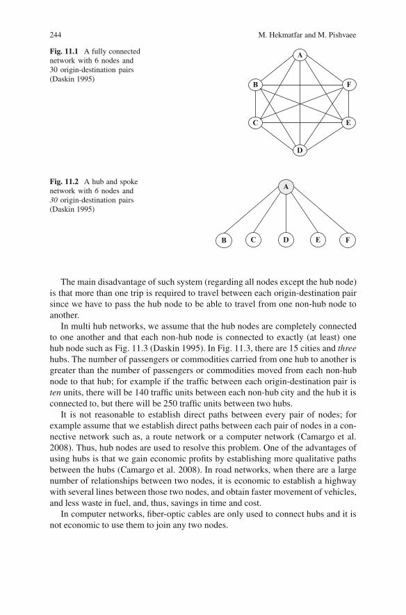
244 M. Hekmatfar and M. Pishvaee
Fig. 11.1 A fully connectednetwork with 6 nodes and30 origin-destination pairs(Daskin 1995)
B
C
D
E
F
A
Fig. 11.2 A hub and spokenetwork with 6 nodes and30 origin-destination pairs(Daskin 1995)
A
B C D E F
The main disadvantage of such system (regarding all nodes except the hub node)is that more than one trip is required to travel between each origin-destination pairsince we have to pass the hub node to be able to travel from one non-hub node toanother.
In multi hub networks, we assume that the hub nodes are completely connectedto one another and that each non-hub node is connected to exactly (at least) onehub node such as Fig. 11.3 (Daskin 1995). In Fig. 11.3, there are 15 cities and threehubs. The number of passengers or commodities carried from one hub to another isgreater than the number of passengers or commodities moved from each non-hubnode to that hub; for example if the traffic between each origin-destination pair isten units, there will be 140 traffic units between each non-hub city and the hub it isconnected to, but there will be 250 traffic units between two hubs.
It is not reasonable to establish direct paths between every pair of nodes; forexample assume that we establish direct paths between each pair of nodes in a con-nective network such as, a route network or a computer network (Camargo et al.2008). Thus, hub nodes are used to resolve this problem. One of the advantages ofusing hubs is that we gain economic profits by establishing more qualitative pathsbetween the hubs (Camargo et al. 2008). In road networks, when there are a largenumber of relationships between two nodes, it is economic to establish a highwaywith several lines between those two nodes, and obtain faster movement of vehicles,and less waste in fuel, and, thus, savings in time and cost.
In computer networks, fiber-optic cables are only used to connect hubs and it isnot economic to use them to join any two nodes.
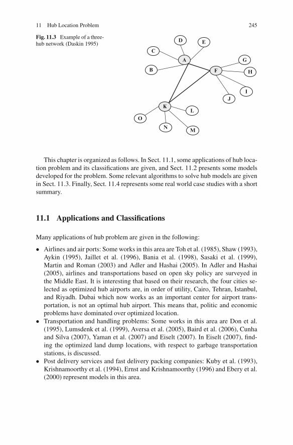
11 Hub Location Problem 245
Fig. 11.3 Example of a three-hub network (Daskin 1995)
A
D E
G
H
IJ
L
MN
O
K
B
C
F
This chapter is organized as follows. In Sect. 11.1, some applications of hub loca-tion problem and its classifications are given, and Sect. 11.2 presents some modelsdeveloped for the problem. Some relevant algorithms to solve hub models are givenin Sect. 11.3. Finally, Sect. 11.4 represents some real world case studies with a shortsummary.
11.1 Applications and Classifications
Many applications of hub problem are given in the following:
� Airlines and air ports: Some works in this area are Toh et al. (1985), Shaw (1993),Aykin (1995), Jaillet et al. (1996), Bania et al. (1998), Sasaki et al. (1999),Martin and Roman (2003) and Adler and Hashai (2005). In Adler and Hashai(2005), airlines and transportations based on open sky policy are surveyed inthe Middle East. It is interesting that based on their research, the four cities se-lected as optimized hub airports are, in order of utility, Cairo, Tehran, Istanbul,and Riyadh. Dubai which now works as an important center for airport trans-portation, is not an optimal hub airport. This means that, politic and economicproblems have dominated over optimized location.
� Transportation and handling problems: Some works in this area are Don et al.(1995), Lumsdenk et al. (1999), Aversa et al. (2005), Baird et al. (2006), Cunhaand Silva (2007), Yaman et al. (2007) and Eiselt (2007). In Eiselt (2007), find-ing the optimized land dump locations, with respect to garbage transportationstations, is discussed.
� Post delivery services and fast delivery packing companies: Kuby et al. (1993),Krishnamoorthy et al. (1994), Ernst and Krishnamoorthy (1996) and Ebery et al.(2000) represent models in this area.
246 M. Hekmatfar and M. Pishvaee
� Telecommunication systems and massage delivery networks: Some works in thisarea are Lee et al. (1996) and Klincewicz (1998).
� Emergency services: Hakimi (1964) and Berman et al. (2007) represented modelsin emergency services. Berman et al. (2007) discussed the location of a hub forrescue helicopters.
� Chain stores in supply chain (like Wall-Mart): A work in this area is Campbellet al. (2002).
� Productive companies in basis transportation correctly: Every assembly plantprobably wants to find an optimized solution for its material storage and handlingsuch that each production facility can receive its required materials effectively.
Some practical examples of hub problems are as follows:
� A classical example is Hungarian railway system with Budapest as its hub.� Two huge American airlines based in Atlanta and Chicago, use hub networks.� Dubai airport is a hub for many flights in the Middle East.
The hub location problem has a short history. The first paper on hub location prob-lem was published by Toh et al. (1985). This paper was on the application of hublocation problem in airlines and airports. Although Hakimi (1964) first published apaper on hub location, since next paper on this topic was not published until twodecades later, it is assumed that the hub location problem has been first discussedin 1980s.
O’Kelly (1987) developed hub location models. He had an important role in de-veloping the first modeling of hub problems (O’Kelly 1987, 1992). Later, Campbell(1994) played a major role in completing hub modeling. His papers are among themost important papers on types of hub modeling (Campbell 1994, 1996). Also,some authors played important roles in improving this topic (Aykin 1994, 1995;Klincewicz 1991, 1992).
Many papers have been published on hub location problem so far (since1980s).Daskin (1995) has written a book on “Network and Discrete location” and only abrief section of this book is dedicated to hub location. Figure 11.4 shows that thenumber of papers has increased in recent years. The number of published paperson hubs shows a significant increase in 1996, which is presumably the time whenthe modeling of hub problems has reached maturity. The emphasis of papers was onmodeling in the early years, on optimizing and completing the models in the follow-ing years, and, finally, on solution methods in recent years. Thus, hub location prob-lem is a rather new topic and a good area for research and development activities.
A classification of different types of hub problems and their properties is repre-sented as follows:
� Area solution: discrete, continual� Objective function: MiniMax, MiniSum� Determination of the number of hubs: exogenous, endogenous� Number of hubs: one hub, more than one hub� Hub capacity: unlimited (uncapacitated), limited
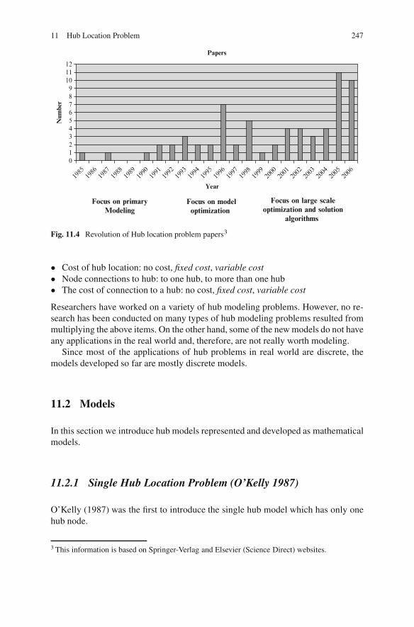
11 Hub Location Problem 247
Focus on primaryModeling
Focus on modeloptimization
Focus on large scaleoptimization and solution
algorithms
Papers
0123456789
101112
2006
2005
2004
2003
2002
2001
2000
1999
1998
1997
1996
1995
1994
1993
1992
1991
1990
1989
1988
1987
1986
1985
Year
Num
ber
Fig. 11.4 Revolution of Hub location problem papers3
� Cost of hub location: no cost, fixed cost, variable cost� Node connections to hub: to one hub, to more than one hub� The cost of connection to a hub: no cost, fixed cost, variable cost
Researchers have worked on a variety of hub modeling problems. However, no re-search has been conducted on many types of hub modeling problems resulted frommultiplying the above items. On the other hand, some of the new models do not haveany applications in the real world and, therefore, are not really worth modeling.
Since most of the applications of hub problems in real world are discrete, themodels developed so far are mostly discrete models.
11.2 Models
In this section we introduce hub models represented and developed as mathematicalmodels.
11.2.1 Single Hub Location Problem (O’Kelly 1987)
O’Kelly (1987) was the first to introduce the single hub model which has only onehub node.
3 This information is based on Springer-Verlag and Elsevier (Science Direct) websites.
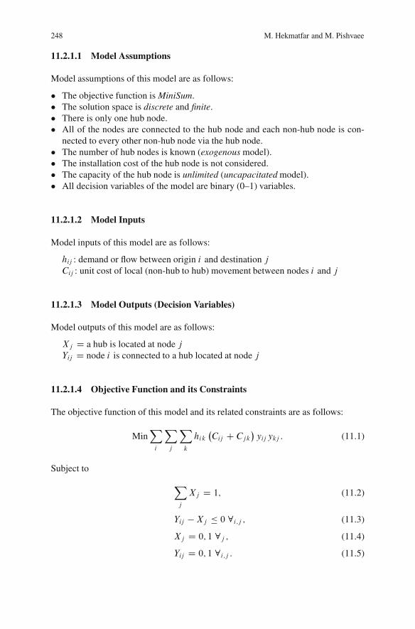
248 M. Hekmatfar and M. Pishvaee
11.2.1.1 Model Assumptions
Model assumptions of this model are as follows:
� The objective function is MiniSum.� The solution space is discrete and finite.� There is only one hub node.� All of the nodes are connected to the hub node and each non-hub node is con-
nected to every other non-hub node via the hub node.� The number of hub nodes is known (exogenous model).� The installation cost of the hub node is not considered.� The capacity of the hub node is unlimited (uncapacitated model).� All decision variables of the model are binary (0–1) variables.
11.2.1.2 Model Inputs
Model inputs of this model are as follows:
hij : demand or flow between origin i and destination jCij : unit cost of local (non-hub to hub) movement between nodes i and j
11.2.1.3 Model Outputs (Decision Variables)
Model outputs of this model are as follows:
Xj D a hub is located at node jYij D node i is connected to a hub located at node j
11.2.1.4 Objective Function and its Constraints
The objective function of this model and its related constraints are as follows:
MinXi
Xj
Xk
hik�Cij C Cjk
�yij ykj : (11.1)
Subject to
Xj
Xj D 1; (11.2)
Yij �Xj � 0 8i;j ; (11.3)
Xj D 0; 1 8j ; (11.4)
Yij D 0; 1 8i;j : (11.5)
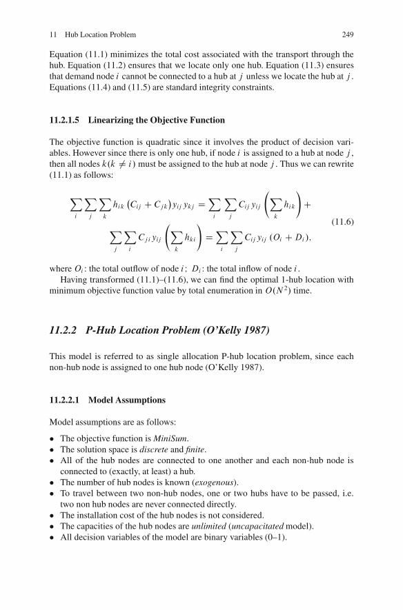
11 Hub Location Problem 249
Equation (11.1) minimizes the total cost associated with the transport through thehub. Equation (11.2) ensures that we locate only one hub. Equation (11.3) ensuresthat demand node i cannot be connected to a hub at j unless we locate the hub at j .Equations (11.4) and (11.5) are standard integrity constraints.
11.2.1.5 Linearizing the Objective Function
The objective function is quadratic since it involves the product of decision vari-ables. However since there is only one hub, if node i is assigned to a hub at node j ,then all nodes k.k ¤ i/ must be assigned to the hub at node j . Thus we can rewrite(11.1) as follows:
Xi
Xj
Xk
hik�Cij C Cjk
�yij ykj D
Xi
Xj
Cij yij
Xk
hik
!C
Xj
Xi
Cj iyij
Xk
hki
!DXi
Xj
Cij yij .Oi CDi/;
(11.6)
whereOi : the total outflow of node i I Di : the total inflow of node i .Having transformed (11.1)–(11.6), we can find the optimal 1-hub location with
minimum objective function value by total enumeration in O.N2/ time.
11.2.2 P-Hub Location Problem (O’Kelly 1987)
This model is referred to as single allocation P-hub location problem, since eachnon-hub node is assigned to one hub node (O’Kelly 1987).
11.2.2.1 Model Assumptions
Model assumptions are as follows:
� The objective function is MiniSum.� The solution space is discrete and finite.� All of the hub nodes are connected to one another and each non-hub node is
connected to (exactly, at least) a hub.� The number of hub nodes is known (exogenous).� To travel between two non-hub nodes, one or two hubs have to be passed, i.e.
two non hub nodes are never connected directly.� The installation cost of the hub nodes is not considered.� The capacities of the hub nodes are unlimited (uncapacitated model).� All decision variables of the model are binary variables (0–1).
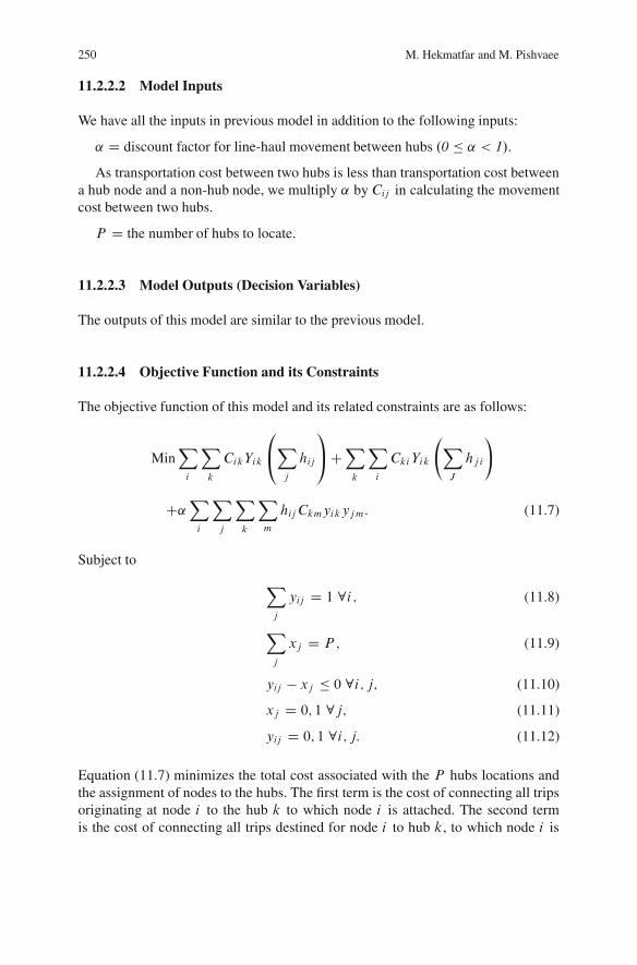
250 M. Hekmatfar and M. Pishvaee
11.2.2.2 Model Inputs
We have all the inputs in previous model in addition to the following inputs:
˛ D discount factor for line-haul movement between hubs .0 � ˛ < 1/.
As transportation cost between two hubs is less than transportation cost betweena hub node and a non-hub node, we multiply ˛ by Cij in calculating the movementcost between two hubs.
P D the number of hubs to locate.
11.2.2.3 Model Outputs (Decision Variables)
The outputs of this model are similar to the previous model.
11.2.2.4 Objective Function and its Constraints
The objective function of this model and its related constraints are as follows:
MinXi
Xk
CikYik
0@X
j
hij
1AC
Xk
Xi
CkiYik
XJ
hj i
!
C˛Xi
Xj
Xk
Xm
hij Ckmyikyjm: (11.7)
Subject to
Xj
yij D 1 8i ; (11.8)
Xj
xj D P ; (11.9)
yij � xj � 0 8i; j; (11.10)
xj D 0; 1 8j; (11.11)
yij D 0; 1 8i; j: (11.12)
Equation (11.7) minimizes the total cost associated with the P hubs locations andthe assignment of nodes to the hubs. The first term is the cost of connecting all tripsoriginating at node i to the hub k to which node i is attached. The second termis the cost of connecting all trips destined for node i to hub k, to which node i is
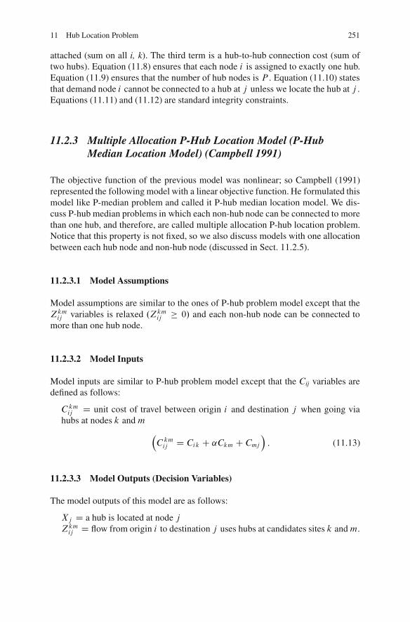
11 Hub Location Problem 251
attached (sum on all i, k). The third term is a hub-to-hub connection cost (sum oftwo hubs). Equation (11.8) ensures that each node i is assigned to exactly one hub.Equation (11.9) ensures that the number of hub nodes is P . Equation (11.10) statesthat demand node i cannot be connected to a hub at j unless we locate the hub at j .Equations (11.11) and (11.12) are standard integrity constraints.
11.2.3 Multiple Allocation P-Hub Location Model (P-HubMedian Location Model) (Campbell 1991)
The objective function of the previous model was nonlinear; so Campbell (1991)represented the following model with a linear objective function. He formulated thismodel like P-median problem and called it P-hub median location model. We dis-cuss P-hub median problems in which each non-hub node can be connected to morethan one hub, and therefore, are called multiple allocation P-hub location problem.Notice that this property is not fixed, so we also discuss models with one allocationbetween each hub node and non-hub node (discussed in Sect. 11.2.5).
11.2.3.1 Model Assumptions
Model assumptions are similar to the ones of P-hub problem model except that theZkmij variables is relaxed .Zkm
ij � 0/ and each non-hub node can be connected tomore than one hub node.
11.2.3.2 Model Inputs
Model inputs are similar to P-hub problem model except that the Cij variables aredefined as follows:
Ckmij D unit cost of travel between origin i and destination j when going via
hubs at nodes k and m Ckmij D Cik C ˛Ckm C Cmj
: (11.13)
11.2.3.3 Model Outputs (Decision Variables)
The model outputs of this model are as follows:
Xj D a hub is located at node jZkmij D flow from origin i to destination j uses hubs at candidates sites k andm.
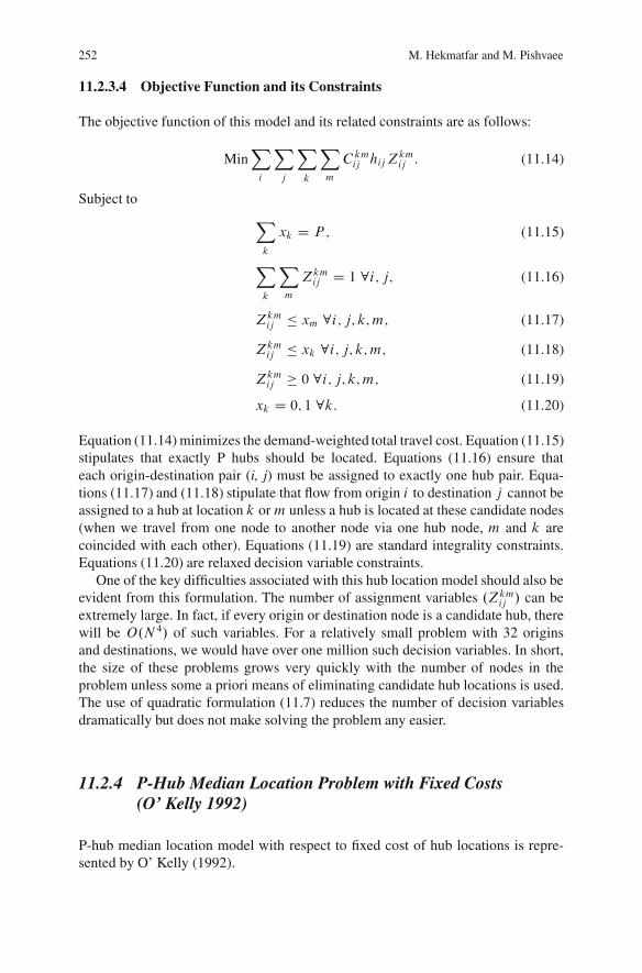
252 M. Hekmatfar and M. Pishvaee
11.2.3.4 Objective Function and its Constraints
The objective function of this model and its related constraints are as follows:
MinXi
Xj
Xk
Xm
C kmij hijZ
kmij : (11.14)
Subject to Xk
xk D P ; (11.15)
Xk
Xm
Zkmij D 1 8i; j; (11.16)
Zkmij � xm 8i; j; k;m; (11.17)
Zkmij � xk 8i; j; k;m; (11.18)
Zkmij � 0 8i; j; k;m; (11.19)
xk D 0; 1 8k: (11.20)
Equation (11.14) minimizes the demand-weighted total travel cost. Equation (11.15)stipulates that exactly P hubs should be located. Equations (11.16) ensure thateach origin-destination pair (i, j) must be assigned to exactly one hub pair. Equa-tions (11.17) and (11.18) stipulate that flow from origin i to destination j cannot beassigned to a hub at location k orm unless a hub is located at these candidate nodes(when we travel from one node to another node via one hub node, m and k arecoincided with each other). Equations (11.19) are standard integrality constraints.Equations (11.20) are relaxed decision variable constraints.
One of the key difficulties associated with this hub location model should also beevident from this formulation. The number of assignment variables .Zkm
ij / can beextremely large. In fact, if every origin or destination node is a candidate hub, therewill be O.N4/ of such variables. For a relatively small problem with 32 originsand destinations, we would have over one million such decision variables. In short,the size of these problems grows very quickly with the number of nodes in theproblem unless some a priori means of eliminating candidate hub locations is used.The use of quadratic formulation (11.7) reduces the number of decision variablesdramatically but does not make solving the problem any easier.
11.2.4 P-Hub Median Location Problem with Fixed Costs(O’ Kelly 1992)
P-hub median location model with respect to fixed cost of hub locations is repre-sented by O’ Kelly (1992).
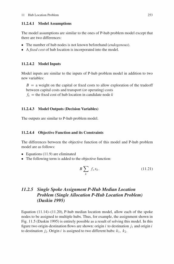
11 Hub Location Problem 253
11.2.4.1 Model Assumptions
The model assumptions are similar to the ones of P-hub problem model except thatthere are two differences:
� The number of hub nodes is not known beforehand (endogenous).� A fixed cost of hub location is incorporated into the model.
11.2.4.2 Model Inputs
Model inputs are similar to the inputs of P-hub problem model in addition to twonew variables:
B D a weight on the capital or fixed costs to allow exploration of the tradeoffbetween capital costs and transport (or operating) costsfk D the fixed cost of hub location in candidate node k
11.2.4.3 Model Outputs (Decision Variables)
The outputs are similar to P-hub problem model.
11.2.4.4 Objective Function and its Constraints
The differences between the objective function of this model and P-hub problemmodel are as follows:
� Equations (11.9) are eliminated� The following term is added to the objective function:
BXk
fxxk: (11.21)
11.2.5 Single Spoke Assignment P-Hub Median LocationProblem (Single Allocation P-Hub Location Problem)(Daskin 1995)
Equation (11.14)–(11.20), P-hub median location model, allow each of the spokenodes to be assigned to multiple hubs. Thus, for example, the assignment shown inFig. 11.5 (Daskin 1995) is entirely possible as a result of solving this model. In thisfigure two origin-destination flows are shown: origin i to destination j1 and origin ito destination j2. Origin i is assigned to two different hubs: k1; k2.
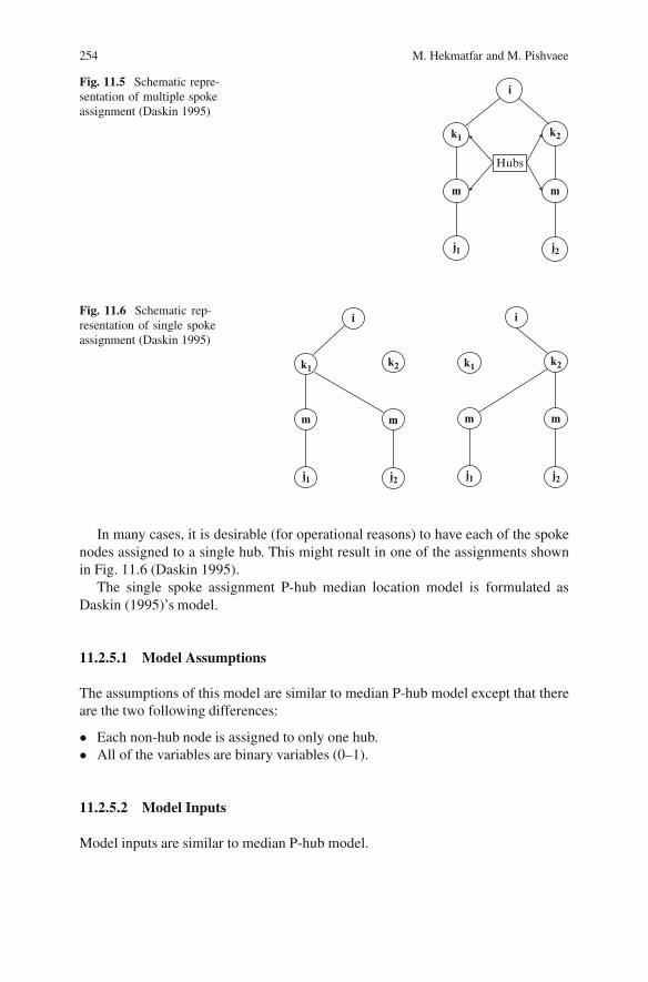
254 M. Hekmatfar and M. Pishvaee
Fig. 11.5 Schematic repre-sentation of multiple spokeassignment (Daskin 1995)
m m
Hubs
j1 j2
k2k1
i
Fig. 11.6 Schematic rep-resentation of single spokeassignment (Daskin 1995)
m m m m
k1 k1k2
i i
k2
j1 j1j2 j2
In many cases, it is desirable (for operational reasons) to have each of the spokenodes assigned to a single hub. This might result in one of the assignments shownin Fig. 11.6 (Daskin 1995).
The single spoke assignment P-hub median location model is formulated asDaskin (1995)’s model.
11.2.5.1 Model Assumptions
The assumptions of this model are similar to median P-hub model except that thereare the two following differences:
� Each non-hub node is assigned to only one hub.� All of the variables are binary variables (0–1).
11.2.5.2 Model Inputs
Model inputs are similar to median P-hub model.
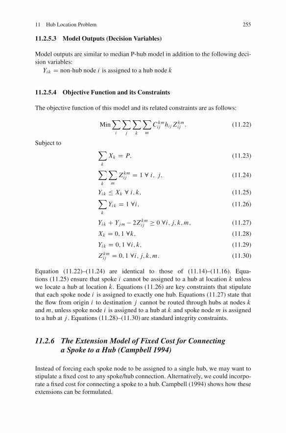
11 Hub Location Problem 255
11.2.5.3 Model Outputs (Decision Variables)
Model outputs are similar to median P-hub model in addition to the following deci-sion variables:Yik D non-hub node i is assigned to a hub node k
11.2.5.4 Objective Function and its Constraints
The objective function of this model and its related constraints are as follows:
MinXi
Xj
Xk
Xm
C kmij hijZ
kmij : (11.22)
Subject to Xk
Xk D P; (11.23)
Xk
Xm
Zkmij D 1 8 i; j; (11.24)
Yik � Xk 8 i; k; (11.25)Xk
Yik D 1 8i; (11.26)
Yik C Yjm � 2Zkmij � 0 8i; j; k;m; (11.27)
Xk D 0; 1 8k; (11.28)
Yik D 0; 1 8i; k; (11.29)
Zkmij D 0; 1 8i; j; k;m: (11.30)
Equation (11.22)–(11.24) are identical to those of (11.14)–(11.16). Equa-tions (11.25) ensure that spoke i cannot be assigned to a hub at location k unlesswe locate a hub at location k. Equations (11.26) are key constraints that stipulatethat each spoke node i is assigned to exactly one hub. Equations (11.27) state thatthe flow from origin i to destination j cannot be routed through hubs at nodes kand m, unless spoke node i is assigned to a hub at k and spoke node m is assignedto a hub at j . Equations (11.28)–(11.30) are standard integrity constraints.
11.2.6 The Extension Model of Fixed Cost for Connectinga Spoke to a Hub (Campbell 1994)
Instead of forcing each spoke node to be assigned to a single hub, we may want tostipulate a fixed cost to any spoke/hub connection. Alternatively, we could incorpo-rate a fixed cost for connecting a spoke to a hub. Campbell (1994) shows how theseextensions can be formulated.
256 M. Hekmatfar and M. Pishvaee
11.2.6.1 Model Assumptions
The assumptions of this model are similar to median P-hub model except that thereis a fixed cost for connecting a spoke to a hub.
11.2.6.2 Model Inputs
Model inputs are similar to median P-hub model in addition to the followingparameter:
gik : the fixed cost of connecting spoke node i to a hub at candidate location k.
11.2.6.3 Model Outputs (Decision Variables)
Model outputs are similar to single allocation median P-hub model.
11.2.6.4 Objective Function and its Constraints
The objective function is similar to median P-hub model in addition to thefollowing term: X
i
Xk
gikYik: (11.31)
11.2.7 Minimum Value Flow on any Spoke/Hub ConnectionProblem (Campbell 1994)
Instead of forcing each spoke node to be assigned to a single hub, we may wantto stipulate that the flow along any spoke/hub connection exceed some minimumvalue. Campbell (1994) represented this model, which is similar to single allocationP-hub location problem.
11.2.7.1 Model Assumptions
The assumptions of this model are similar to median P-hub model except that thereis a minimum flow for each spoke/hub connection.
11.2.7.2 Model Inputs
Model inputs are similar to median P-hub model in addition to the followingparameter:
lik : the minimum flow between spoke i and hub k.
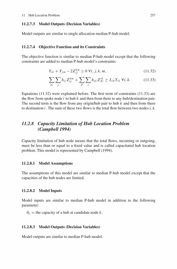
11 Hub Location Problem 257
11.2.7.3 Model Outputs (Decision Variables)
Model outputs are similar to single allocation median P-hub model.
11.2.7.4 Objective Function and its Constraints
The objective function is similar to median P-hub model except that the followingconstraints are added to median P-hub model’s constraints:
Yik C Yjm � 2Zkmij � 0 8i; j; k;m; (11.32)X
m
Xj
hijZkmij C
XP
Xs
hpiZskP i � LikYik 8i; k: (11.33)
Equations (11.32) were explained before. The first term of constraints (11.33) arethe flow from spoke node i to hub k and then from there to any hub/destination pair.The second term is the flow from any origin/hub pair to hub k and then from thereto destination i . The sum of these two flows is the total flow between two nodes i, k.
11.2.8 Capacity Limitation of Hub Location Problem(Campbell 1994)
Capacity limitation of hub node means that the total flows, incoming or outgoing,must be less than or equal to a fixed value and is called capacitated hub locationproblem. This model is represented by Campbell (1994).
11.2.8.1 Model Assumptions
The assumptions of this model are similar to median P-hub model except that thecapacities of the hub nodes are limited.
11.2.8.2 Model Inputs
Model inputs are similar to median P-hub model in addition to the followingparameter:
k D the capacity of a hub at candidate node k.
11.2.8.3 Model Outputs (Decision Variables)
Model outputs are similar to median P-hub model.
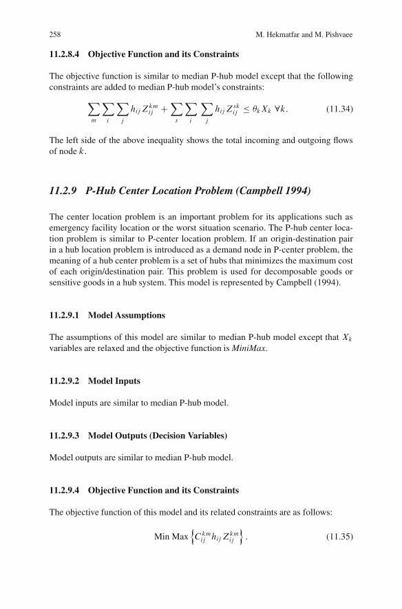
258 M. Hekmatfar and M. Pishvaee
11.2.8.4 Objective Function and its Constraints
The objective function is similar to median P-hub model except that the followingconstraints are added to median P-hub model’s constraints:X
m
Xi
Xj
hijZkmij C
Xs
Xi
Xj
hijZskij � kXk 8k: (11.34)
The left side of the above inequality shows the total incoming and outgoing flowsof node k.
11.2.9 P-Hub Center Location Problem (Campbell 1994)
The center location problem is an important problem for its applications such asemergency facility location or the worst situation scenario. The P-hub center loca-tion problem is similar to P-center location problem. If an origin-destination pairin a hub location problem is introduced as a demand node in P-center problem, themeaning of a hub center problem is a set of hubs that minimizes the maximum costof each origin/destination pair. This problem is used for decomposable goods orsensitive goods in a hub system. This model is represented by Campbell (1994).
11.2.9.1 Model Assumptions
The assumptions of this model are similar to median P-hub model except that Xkvariables are relaxed and the objective function is MiniMax.
11.2.9.2 Model Inputs
Model inputs are similar to median P-hub model.
11.2.9.3 Model Outputs (Decision Variables)
Model outputs are similar to median P-hub model.
11.2.9.4 Objective Function and its Constraints
The objective function of this model and its related constraints are as follows:
Min MaxnCkmij hijZ
kmij
o: (11.35)
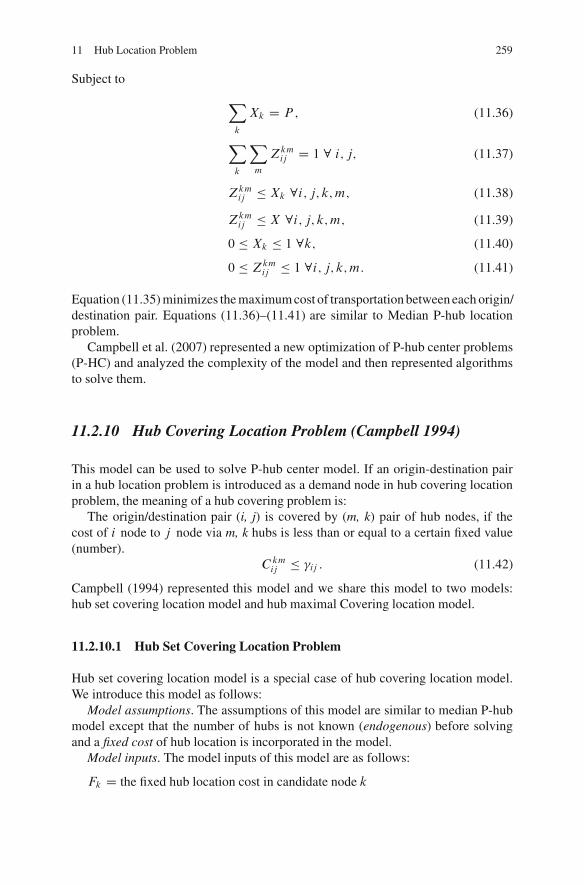
11 Hub Location Problem 259
Subject to
Xk
Xk D P ; (11.36)
Xk
Xm
Zkmij D 1 8 i; j; (11.37)
Zkmij � Xk 8i; j; k;m; (11.38)
Zkmij � X 8i; j; k;m; (11.39)
0 � Xk � 1 8k; (11.40)
0 � Zkmij � 1 8i; j; k;m: (11.41)
Equation (11.35) minimizes the maximum cost of transportation between each origin/destination pair. Equations (11.36)–(11.41) are similar to Median P-hub locationproblem.
Campbell et al. (2007) represented a new optimization of P-hub center problems(P-HC) and analyzed the complexity of the model and then represented algorithmsto solve them.
11.2.10 Hub Covering Location Problem (Campbell 1994)
This model can be used to solve P-hub center model. If an origin-destination pairin a hub location problem is introduced as a demand node in hub covering locationproblem, the meaning of a hub covering problem is:
The origin/destination pair (i, j) is covered by (m, k) pair of hub nodes, if thecost of i node to j node via m, k hubs is less than or equal to a certain fixed value(number).
Ckmij � �ij : (11.42)
Campbell (1994) represented this model and we share this model to two models:hub set covering location model and hub maximal Covering location model.
11.2.10.1 Hub Set Covering Location Problem
Hub set covering location model is a special case of hub covering location model.We introduce this model as follows:
Model assumptions. The assumptions of this model are similar to median P-hubmodel except that the number of hubs is not known (endogenous) before solvingand a fixed cost of hub location is incorporated in the model.
Model inputs. The model inputs of this model are as follows:
Fk D the fixed hub location cost in candidate node k
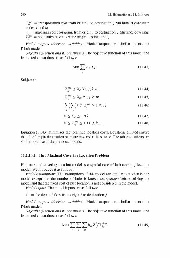
260 M. Hekmatfar and M. Pishvaee
Ckmij D transportation cost from origin i to destination j via hubs at candidate
nodes k and m�ij D maximum cost for going from origin i to destination j (distance covering)V kmij D node hubs m, k cover the origin-destination i, j
Model outputs (decision variables): Model outputs are similar to medianP-hub model.
Objective function and its constraints. The objective function of this model andits related constraints are as follows:
MinXk
FKXK: (11.43)
Subject to
Zkmij � Xk 8i; j; k;m; (11.44)
Zkmij � Xm 8i; j; k;m; (11.45)Xk
Xm
V kmij Zkm
ij � 1 8i; j; (11.46)
0 � Xk � 1 8k; (11.47)
0 � Zkmij � 1 8i; j; k;m: (11.48)
Equation (11.43) minimizes the total hub location costs. Equations (11.46) ensurethat all of origin-destination pairs are covered at least once. The other equations aresimilar to those of the previous models.
11.2.10.2 Hub Maximal Covering Location Problem
Hub maximal covering location model is a special case of hub covering locationmodel. We introduce it as follows:
Model assumptions. The assumptions of this model are similar to median P-hubmodel except that the number of hubs is known (exogenous) before solving themodel and that the fixed cost of hub location is not considered in the model.
Model inputs. The model inputs are as follows:
hij D the demand flow from origin i to destination j
Model outputs (decision variables). Model outputs are similar to medianP-hub model.
Objective function and its constraints. The objective function of this model andits related constraints are as follows:
MaxXi
Xj
Xm
hijZkmij V
kmij : (11.49)
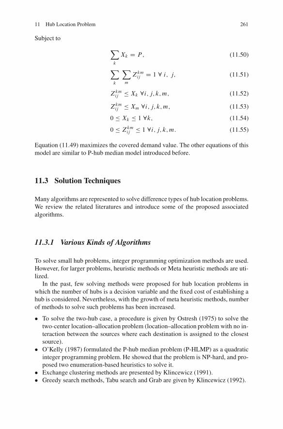
11 Hub Location Problem 261
Subject to
Xk
Xk D P ; (11.50)
Xk
Xm
Zkmij D 1 8 i; j; (11.51)
Zkmij � Xk 8i; j; k;m; (11.52)
Zkmij � Xm 8i; j; k;m; (11.53)
0 � Xk � 1 8k; (11.54)
0 � Zkmij � 1 8i; j; k;m: (11.55)
Equation (11.49) maximizes the covered demand value. The other equations of thismodel are similar to P-hub median model introduced before.
11.3 Solution Techniques
Many algorithms are represented to solve difference types of hub location problems.We review the related literatures and introduce some of the proposed associatedalgorithms.
11.3.1 Various Kinds of Algorithms
To solve small hub problems, integer programming optimization methods are used.However, for larger problems, heuristic methods or Meta heuristic methods are uti-lized.
In the past, few solving methods were proposed for hub location problems inwhich the number of hubs is a decision variable and the fixed cost of establishing ahub is considered. Nevertheless, with the growth of meta heuristic methods, numberof methods to solve such problems has been increased.
� To solve the two-hub case, a procedure is given by Ostresh (1975) to solve thetwo-center location–allocation problem (location–allocation problem with no in-teraction between the sources where each destination is assigned to the closestsource).
� O’Kelly (1987) formulated the P-hub median problem (P-HLMP) as a quadraticinteger programming problem. He showed that the problem is NP-hard, and pro-posed two enumeration-based heuristics to solve it.
� Exchange clustering methods are presented by Klincewicz (1991).� Greedy search methods, Tabu search and Grab are given by Klincewicz (1992).
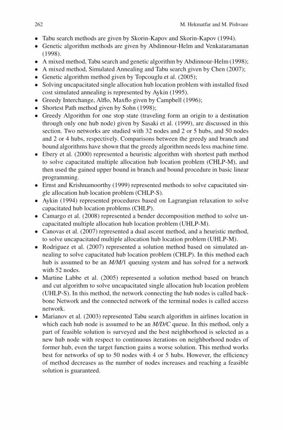
262 M. Hekmatfar and M. Pishvaee
� Tabu search methods are given by Skorin-Kapov and Skorin-Kapov (1994).� Genetic algorithm methods are given by Abdinnour-Helm and Venkataramanan
(1998).� A mixed method, Tabu search and genetic algorithm by Abdinnour-Helm (1998);� A mixed method, Simulated Annealing and Tabu search given by Chen (2007);� Genetic algorithm method given by Topcouglu et al. (2005);� Solving uncapacitated single allocation hub location problem with installed fixed
cost simulated annealing is represented by Aykin (1995).� Greedy Interchange, Alflo, Maxflo given by Campbell (1996);� Shortest Path method given by Sohn (1998);� Greedy Algorithm for one stop state (traveling form an origin to a destination
through only one hub node) given by Sasaki et al. (1999), are discussed in thissection. Two networks are studied with 32 nodes and 2 or 5 hubs, and 50 nodesand 2 or 4 hubs, respectively. Comparisons between the greedy and branch andbound algorithms have shown that the greedy algorithm needs less machine time.
� Ebery et al. (2000) represented a heuristic algorithm with shortest path methodto solve capacitated multiple allocation hub location problem (CHLP-M), andthen used the gained upper bound in branch and bound procedure in basic linearprogramming.
� Ernst and Krishnamoorthy (1999) represented methods to solve capacitated sin-gle allocation hub location problem (CHLP-S).
� Aykin (1994) represented procedures based on Lagrangian relaxation to solvecapacitated hub location problems (CHLP).
� Camargo et al. (2008) represented a bender decomposition method to solve un-capacitated multiple allocation hub location problem (UHLP-M).
� Canovas et al. (2007) represented a dual ascent method, and a heuristic method,to solve uncapacitated multiple allocation hub location problem (UHLP-M).
� Rodriguez et al. (2007) represented a solution method based on simulated an-nealing to solve capacitated hub location problem (CHLP). In this method eachhub is assumed to be an M/M/1 queuing system and has solved for a networkwith 52 nodes.
� Martine Labbe et al. (2005) represented a solution method based on branchand cut algorithm to solve uncapacitated single allocation hub location problem(UHLP-S). In this method, the network connecting the hub nodes is called back-bone Network and the connected network of the terminal nodes is called accessnetwork.
� Marianov et al. (2003) represented Tabu search algorithm in airlines location inwhich each hub node is assumed to be an M/D/C queue. In this method, only apart of feasible solution is surveyed and the best neighborhood is selected as anew hub node with respect to continuous iterations on neighborhood nodes offormer hub, even the target function gains a worse solution. This method worksbest for networks of up to 50 nodes with 4 or 5 hubs. However, the efficiencyof method decreases as the number of nodes increases and reaching a feasiblesolution is guaranteed.
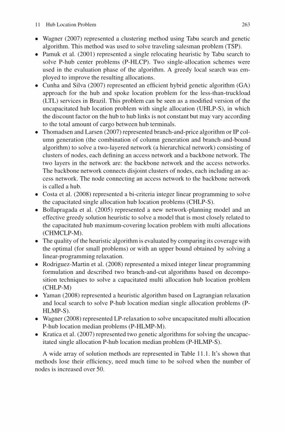
11 Hub Location Problem 263
� Wagner (2007) represented a clustering method using Tabu search and geneticalgorithm. This method was used to solve traveling salesman problem (TSP).
� Pamuk et al. (2001) represented a single relocating heuristic by Tabu search tosolve P-hub center problems (P-HLCP). Two single-allocation schemes wereused in the evaluation phase of the algorithm. A greedy local search was em-ployed to improve the resulting allocations.
� Cunha and Silva (2007) represented an efficient hybrid genetic algorithm (GA)approach for the hub and spoke location problem for the less-than-truckload(LTL) services in Brazil. This problem can be seen as a modified version of theuncapacitated hub location problem with single allocation (UHLP-S), in whichthe discount factor on the hub to hub links is not constant but may vary accordingto the total amount of cargo between hub terminals.
� Thomadsen and Larsen (2007) represented branch-and-price algorithm or IP col-umn generation (the combination of column generation and branch-and-boundalgorithm) to solve a two-layered network (a hierarchical network) consisting ofclusters of nodes, each defining an access network and a backbone network. Thetwo layers in the network are: the backbone network and the access networks.The backbone network connects disjoint clusters of nodes, each including an ac-cess network. The node connecting an access network to the backbone networkis called a hub.
� Costa et al. (2008) represented a bi-criteria integer linear programming to solvethe capacitated single allocation hub location problems (CHLP-S).
� Bollapragada et al. (2005) represented a new network-planning model and aneffective greedy solution heuristic to solve a model that is most closely related tothe capacitated hub maximum-covering location problem with multi allocations(CHMCLP-M).
� The quality of the heuristic algorithm is evaluated by comparing its coverage withthe optimal (for small problems) or with an upper bound obtained by solving alinear-programming relaxation.
� Rodriguez-Martin et al. (2008) represented a mixed integer linear programmingformulation and described two branch-and-cut algorithms based on decompo-sition techniques to solve a capacitated multi allocation hub location problem(CHLP-M)
� Yaman (2008) represented a heuristic algorithm based on Lagrangian relaxationand local search to solve P-hub location median single allocation problems (P-HLMP-S).
� Wagner (2008) represented LP-relaxation to solve uncapacitated multi allocationP-hub location median problems (P-HLMP-M).
� Kratica et al. (2007) represented two genetic algorithms for solving the uncapac-itated single allocation P-hub location median problem (P-HLMP-S).
A wide array of solution methods are represented in Table 11.1. It’s shown thatmethods lose their efficiency, need much time to be solved when the number ofnodes is increased over 50.
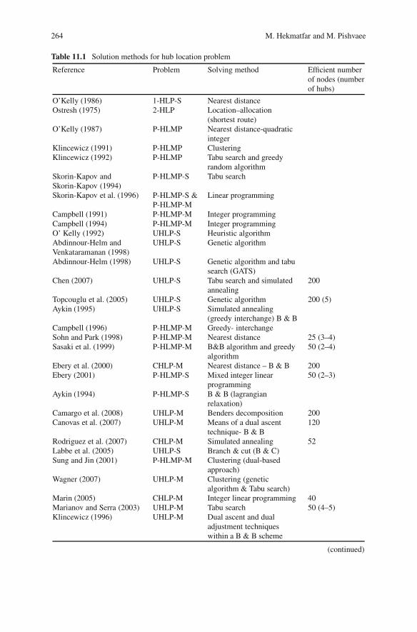
264 M. Hekmatfar and M. Pishvaee
Table 11.1 Solution methods for hub location problem
Reference Problem Solving method Efficient numberof nodes (numberof hubs)
O’Kelly (1986) 1-HLP-S Nearest distanceOstresh (1975) 2-HLP Location–allocation
(shortest route)O’Kelly (1987) P-HLMP Nearest distance-quadratic
integerKlincewicz (1991) P-HLMP ClusteringKlincewicz (1992) P-HLMP Tabu search and greedy
random algorithmSkorin-Kapov andSkorin-Kapov (1994)
P-HLMP-S Tabu search
Skorin-Kapov et al. (1996) P-HLMP-S &P-HLMP-M
Linear programming
Campbell (1991) P-HLMP-M Integer programmingCampbell (1994) P-HLMP-M Integer programmingO’ Kelly (1992) UHLP-S Heuristic algorithmAbdinnour-Helm andVenkataramanan (1998)
UHLP-S Genetic algorithm
Abdinnour-Helm (1998) UHLP-S Genetic algorithm and tabusearch (GATS)
Chen (2007) UHLP-S Tabu search and simulatedannealing
200
Topcouglu et al. (2005) UHLP-S Genetic algorithm 200 (5)Aykin (1995) UHLP-S Simulated annealing
(greedy interchange) B & BCampbell (1996) P-HLMP-M Greedy- interchangeSohn and Park (1998) P-HLMP-M Nearest distance 25 (3–4)Sasaki et al. (1999) P-HLMP-M B&B algorithm and greedy
algorithm50 (2–4)
Ebery et al. (2000) CHLP-M Nearest distance – B & B 200Ebery (2001) P-HLMP-S Mixed integer linear
programming50 (2–3)
Aykin (1994) P-HLMP-S B & B (lagrangianrelaxation)
Camargo et al. (2008) UHLP-M Benders decomposition 200Canovas et al. (2007) UHLP-M Means of a dual ascent
technique- B & B120
Rodriguez et al. (2007) CHLP-M Simulated annealing 52Labbe et al. (2005) UHLP-S Branch & cut (B & C)Sung and Jin (2001) P-HLMP-M Clustering (dual-based
approach)Wagner (2007) UHLP-M Clustering (genetic
algorithm & Tabu search)Marin (2005) CHLP-M Integer linear programming 40Marianov and Serra (2003) UHLP-M Tabu search 50 (4–5)Klincewicz (1996) UHLP-M Dual ascent and dual
adjustment techniqueswithin a B & B scheme
(continued)
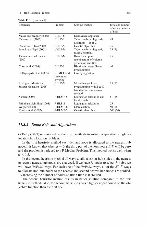
11 Hub Location Problem 265
Table 11.1 (continued)
Reference Problem Solving method Efficient numberof nodes (numberof hubs)
Mayer and Wagner (2002) UHLP-M Dual ascent approachYaman et al. (2007) CHLP-S Tabu search (with greedy
algorithm) – B & C49
Cunha and Silva (2007) UHLP-S Genetic algorithm 25Pamuk and Sepil (2001) UHLP-M Tabu search (with greedy
local algorithm)25 (5)
Thomadsen and Larsen(2007)
UHLP-M Branch and price(combination of columngeneration and B & B)
25
Costa et al. (2008) CHLP-S Bi-criteria integer linearprogramming
40
Bollapragada et al. (2005) CHMCLP-M(maximumcovering)
Greedy algorithm
Rodriguez-Martin andSalazar-Gonzalez (2008)
CHLP-M Mixed integer linearprogramming with B & Cbased on decompositionmethod
25 (10)
Yaman (2008) P-HLMP-S Lagrangian relaxation andlocal search
81 (25)
Pirkul and Schilling (1998) P-HLP-S Lagrangian relaxation 25Wagner (2008) P-HLMP-M LP relaxation 50 (5)Kratica et al. (2007) P-HLMP-S Genetic algorithm 200 (20)
11.3.2 Some Relevant Algorithms
O’Kelly (1987) represented two heuristic methods to solve uncapacitated single al-location hub location problem.
In the first heuristic method each demand node is allocated to the nearest hubnode. It is known that when ˛ D 0, the third part of the nonlinear (11.7) will be zeroand the problem is reduced to a P-Median Problem. This method works well when˛ < 0:5.
In the second heuristic method all ways to allocate non-hub nodes to the nearestor second nearest hub nodes are analyzed. If we haveN nodes to select P hubs, wewill have N!/P!.N! ways. For each one of the N!/P!.N! ways, all of the 2N–P waysto allocate non-hub nodes to the nearest and second nearest hub nodes are studied.By increasing the number of nodes solution time is increased.
The second heuristic method results in better solution compared to the firstheuristic method. Also, the second heuristic gives a tighter upper bound on the ob-jective function than the first one.
266 M. Hekmatfar and M. Pishvaee
11.3.2.1 Greedy Heuristic Algorithm
Greedy algorithm was first presented by Sasaki et al. (1999) to solve the 1-stop un-capacitated multiple allocation hub location problem. One stop means that to travelbetween each origin-destination pair, we have to pass only one hub node. The ap-plication of this method is for small networks such as Japan inner airlines network.
11.3.2.2 Genetic Algorithm
Topcuoglu et al. (2005) represented this algorithm to solve uncapacitated singleallocation hub location problem with fixed cost of location.
A genetic algorithm (GA) is a search algorithm for finding the near-optimal so-lutions in large spaces, which is inspired from population genetics. The general ideawas introduced by Holland (1975). Genetic algorithms have been applied to a largeset of problems in various fields in the literature.
Two example sources for detailed information on GA are the books written byGoldberg (1989) and Mitchell (1998).
11.3.2.3 Benders Decomposition Method
Camargo et al. (2008) represented this method based on an old algorithm in 1962which proposed a partitioning method for solving mixed linear and nonlinear inte-ger programming problems. Camargo et al. (2008) defined a relaxation algorithmfor solving a problem through partitioning it into two simpler problems: an integerproblem, known as MP, and a linear problem, known as SP.
The MP is a relaxed version of the original problem with a set of integer variablesand its associated constraints, while SP is the original problem with the values ofthe integer variables temporarily fixed by the MP.
The algorithm solves each one of the two simpler problems iteratively, one at atime. At each iteration, a new constraint, known as Benders cut, is added to the MP.This new constraint is originated by the dual problem of the SP. The algorithm goeson until the objective function value of the optimal solution to the MP is equal tothat of the SP, when it stops obtaining the optimal solution of the original mixedinteger problem.
11.4 Case Study
In this section we will introduce some real-world case studies related to hub locationproblems.
11 Hub Location Problem 267
11.4.1 The Policy of Open Skies in the Middle East(Adler and Hashai 2005)
In Adler and Hashai (2005), airlines and transportations based on open sky policywere surveyed in the Middle East.
Conclusions drawn from this investigation may enable both researchers and pol-icy makers to develop a greater understanding of the social welfare impacts ofderegulation in the regional air-transport industry and the economic benefits to in-dividual air carriers, countries and passengers alike, once peace restraints in theregion. This analysis had led to the conclusion that the increase in both leisure andbusiness air traffic due to the reduction in violence in the Middle East may lead toan increase of 51% in inter-country passenger flow under the assumption of dereg-ulation of the regional air-transport industry.
It is interesting that based on their research the four cities selected as optimizedhub airports are, in order of utility, Cairo, Tehran, Istanbul, and Riyadh. Dubai whichnow works as an important center for airport transportation, is not an optimal hubairport. This means that, politic and economic problems have dominated over opti-mized location.
11.4.2 A Hub Port in the East Coast of South America (Aversaet al. 2005)
Aversa et al. (2005) formulated a mixed planning model for selecting a hub port,from eleven ports servicing to transportation demands, in the east coast of SouthAmerica.
It was recommended that minimisation of transport costs, is often given un-warranted significance, usually by “awkward” river ports, such as Antwerp andHamburg, while the importance of port costs, in these ports, is at the same timepurposely downplayed.
In this research many ports were researched such as, ports in Brazil, Argentinaand Uruguay. Their model consists of 3,883 variables and 4,225 constraints. Aftersolving the model, port Santos, Brazil was chosen as the hub port.
11.4.3 A Hub Model in Brunswick, Canada (Eiselt 2007)
Eiselt (2007) represented an application of location models to the siting of landfills.The landfill and transfer station location problem was formulated similar to a hublocation problem. The problem included a parameter that measures the discountfactor of the transportation between transfer stations and landfills in comparison tothe unit transportation cost between customers and transfer stations.
268 M. Hekmatfar and M. Pishvaee
The Province of New Brunswick was used to compare optimized facility loca-tions with facility locations that had been chosen by the planners. In order to makesuch comparison, the major towns and villages were chosen on the basis of the sta-tistical data available from the latest census. The result of the calculations was that,the optimized solutions were between 10 and 40% less costly as compared to theobserved solutions. Still, the optimized locations of the landfills were quite closeto those found in the optimization runs. The only exception was a case in whichthe planners deviated from their plan due to public opposition. Their first choice oflocation also appeared in some of the optimized runs. Some additional optimizationwas also performed on a smaller subset of the 93 points which were the basis of theoptimization reported above.
11.4.4 A Hub/Spoke Network in Brazil (Cunha and Silva 2007)
Cunha and Silva (2007) represented the problem of configuring hub-and-spoke net-works for trucking companies that operate less-than-truckload services in Brazil.The problem consists of determining the number of consolidation terminals (alsoknown as hubs), their locations and the assignment of the spokes to the hubs, aim-ing to minimize the total cost, which is composed of fixed and variable costs.
References
Abdinnour-Helm S (1998) A hybrid heuristic for the uncapacitated hub location problem. Eur JOper Res 106:489–99
Abdinnour-Helm S, Venkataramanan MA (1998) Solution approaches to hub location problems.Ann Oper Res 78:31–50
Adler N, Hashai N (2005) Effect of open skies in the Middle East region. Transport Res39:878–894
Aversa R, Botter RC, Haralambides HE, Yoshizaki HTY (2005)A mixed integer programmingmodel on the location of a hub port in the East Coast of South America. Maritime Econ Lo-gist 7:1–18
Aykin T (1994) Lagrangian relaxation based approaches to capacitated hub-and-spoke networkdesign problem. Eur J Oper Res 79:501–523
Aykin T (1995) Networking policies for hub-and-spoke systems with application to the air trans-portation system. Transport Sci 29(3):201–221
Baird AJ (2006) Optimizing the Container transshipment hub location in northern Europe. J Trans-port Geograph 14(3):195–214
Bania N, Bauer P, Zlatoper TU (1998) Air passenger service: A taxonomy of route network, hublocation, and competition. Logist Transport Rev 34:53–74
Berman O, Drezner Z, Wesolowsky G (2007) The transfer point location problem. Eur J Oper Res179(3):978–989
Bollapragada R, Camm J, Rao US, Wu J (2005) A two-phase greedy algorithm to locate andallocate hubs for fixed-wireless broad bound access. Oper Res Lett 33:134–142
Camargo RS, Miranda Jr G, Luna HP (2008) Benders decomposition for the uncapacitated multipleallocation hub location problem. Comput Oper Res 35(4):1047–1064
11 Hub Location Problem 269
Campbell JF (1991) Hub location problems and the p-hub median problem. Center for Businessand Industrial Studies, University of Missouri, St. Louis, MO
Campbell JF (1994) Integer programming formulations of discrete hub location problems. EurJ Oper Res 72:387–405
Campbell JF (1996) Hub location and P-hub median problem. Oper Res 44(6):923–935Campbell JF, Ernst A, Krishnamoorthy M (2002) Hub location problems. In: Drezner Z,
Hammacher H (eds) Facility location: applications and theory. Berlin, SpringerCampbell AM, Lowe TJ, Zhang L (2007) The P-hub center allocation problem. Eur J Oper Res
176(2):819–835Canovas L, Garcia S, Marin A (2007) Solving the uncapacitated multiple allocation hub location
problem by means of a dual-ascent technique. Eur J Oper Res 179:990–1007Chen JF (2007) A hybrid heuristic for the uncapacitated single allocation hub location problem.
Omega 35(2):211–220Costa MG, Captivo ME, Climaco J (2008) Capacitated single allocation hub location problem-A
bi-criteria approach. Comput Oper Res 35(11):3671–3695Cunha CB, Silva MR (2007) A genetic algorithm for the problem of configuring a hub-and-spoke
network for a LTL trucking company in Brazil. Eur J Oper Res 179:747–758Daskin MS (1995) Network and discrete location: Models, algorithms, and applications. Wiley,
New YorkDon T, Harit S, English JR, Whicker G (1995) Hub and spoke networks in truckload trucking:
configuration testing and operational concerns. Logist Transport 31:209–237Ebery J (2001) Solving large single allocation p-hub problems with two or three hubs: Eur J Oper
Res 128:447–458Ebery J, Krishnamoorty M, Ernst A, Boland N (2000) The capacitated multiple allocation hub
location problem: formulation and algorithms. Eur J Oper Res 120:614–631Eiselt HA (2007) Locating landfills – optimization vs. reality. Eur J Oper Res 179(3): 1040–1049Ernst A, Krishnamoorthy M (1996) Efficient algorithms for the uncapaciterted single allocation
P-hub median problem. Location Sci 4:139–154Ernst A, Krishnamoorthy M (1999) Solution algorithms for the capacitated Single allocation hub
location problem. Ann Oper Res 86:141–159Goldberg DE (1989) Genetic algorithms in search, optimization and machine learning. Addison-
Wesley, Reading, MAHakimi SL (1964) Optimum location of switching centers and the absolute centers and medians of
a graph. Oper Res 12:450–459Holland JH (1975) Adaptation in natural and artificial systems. University of Michigan Press,
MichiganJaillet P, Song G, Yu G (1996) Airline network design and hub location problems. Location Sci
4(3):195–212Klincewicz JG (1991) Heuristics for the P-hub location problem. Eur J Oper Res 53:25–37Klincewicz JG (1992) Avoiding local optima in the P-hub location problem using tabu search and
grasp. Ann Oper Res 40:283–302Klincewicz JG (1996) A dual algorithm for the uncapacitated hub location problem. Location Sci
4(3):173–184Klincewicz JG (1998) Hub location in backbone tributary network design: A review. Location Sci
6:307–335Kratica J, Stanimirovic Z, Tosic D, Filipovic V (2007) Two genetic algorithms for solving the
uncapacitated single allocation p-hub median problem. Eur J Oper Res 182:15–28Krishnamoorthy M, Mills G, Sier D (1994) Strategic configuration of the mail processing net-
work: location–allocation modeling-stage 1, CSIRO, Technical Report DMS-C94/9 Divisionof Mathematics and statistics CSIRO, Australia
Kuby MJ, Gray RG (1993) Hub network design problem with stoppers and feeders: Case of federalexpress. Transport Res 27:1–12
Labbe M, Yaman H, Gourdin E (2005) A branch and cut algorithm for hub location problems withsingle assignment 102:371–405
270 M. Hekmatfar and M. Pishvaee
Lee Y, Lim B, Park J (1996) A hub location problem in designing digital data service networks:Lagrangian relaxation approach. Location Sci 4:183–194
Lumsdenk, Dallari F, Ruggeri R (1999) Improving the efficiency of the hub and spoke system forthe SKF European distribution network. Int J Phys Distrib Logist Manage 29:50–64
Marianov V, Serra D (2003) Location models for airline hubs behaving as M/D/c queues. ComputOper Res 30:983–1003
Marin A (2005) Formulating and solving splittable capacitated multiple allocation hub locationproblems. Comput Oper Res 32:3093–3109
Martin JC, Roman C (2003) Hub location in the South-Atlantic airline market: A spatial competi-tion game. Transport Res A: Policy Pract 37(10):865–888
Mayer G, Wagner B (2002) Hub Locator: an exact solution method for the multiple allocation hublocation problem. Comput Oper Res 29:715–39
Mitchell M (1998) An introduction to genetic algorithms. MIT Press, Cambridge, MAO’Kelly ME (1986) The location of interacting hub facilities, Transport Sci 20:92–106O’Kelly ME (1987) A quadratic integer program for the location of interacting hub facilities. Eur
J Oper Res 32:393–404O’ Kelly ME (1992) Hub facility location with fixed costs. Papers in Regional Science 71:292–306Ostresh LMJr (1975) An efficient algorithm for solving the two center location – allocation prob-
lem. J Region Sci 15:209–216Pamuk FS, Sepil C (2001) A solution to the hub center problem via a single-relocation algorithm
with Tabu search. IIE Trans 33:399–411Pirkul H, Schilling DA (1998) An efficient procedure for designing single allocation hub and spoke
systems. Manage Sci 44(12):235–242Rodriguez V, Alvarez MJ, Barcos L (2007) Hub location under capacity constraints. Transport Res
Part E: Logist Transport Rev 43:495–505Rodriguez-Martin I, Salazar-Gonzalez JJ (2008) Solving a capacitated hub location problem. Eur
J Oper Res 184(2):468–479Sasaki M, Suzuki A, Drezner Z (1999) On the selection of hub airports for an airline hub-and-spoke
system. Comput Oper Res 26:1411–1422Shaw SL (1993) Hub structures of major US passenger airline. J Transport Geograph 1(1):47–58Skorin-Kapov D, Skorin-Kapov J (1994) On Tabu search for the location of interacting hub facili-
ties, Eur J Oper Res 73:502–509Skorin-Kapov D, Skorin-Kapov J, O’Kelly M (1996) Tight linear programming relaxations of
uncapacitated p-hub median problems. Proc Natl Decis Sci Conf, Boston 94:582–593Sohn J, Park S (1998) Efficient solution procedure and reduced size formulation for P-hub location
problem. Eur J Oper Res 108:118–126Sung CS, Jin HW (2001) Dual-based approach for a hub network design problem under non-
restrictive policy. Eur J Oper Res 132:88–105Thomadsen T, Larsen J (2007) A hub location problem with fully interconnected backbone and
access networks. Comput Oper Res 34:2520–2531Toh RS, Higgins RC (1985) The impact of hub and spoke network centralization and route
monopoly on domestic airline profitability. Transport J 24:16–27Topcuoglu H, Corut F, Ermis M, Yilmaz G (2005) Solving the uncapacitated hub location using
genetic algorithms. Comput Oper Res 32:467–984Wagner B (2007) An exact solution procedure for a cluster hub location problem, Eur J Oper Res
178:391–401Wagner B (2008) A note on location of hubs in a competitive environment. Eur J Oper Res
184(1):57–62Yaman H (2008) Star P-hub median problem with modular arc capacities. Comput Oper Res
35(9):3009–3019Yaman H, Kara BY, Tansel BC (2007) The latest arrival hub location problem for cargo delivery
systems with stopovers. Transport Res B 41:906–919
Chapter 12Competitive Location Problem
Mohammad Javad Karimifar, Mohammad Khalighi Sikarudi,Esmaeel Moradi, and Morteza Bidkhori
A large part of location theory in operational research has been built around the(mostly implicit) modeling assumption of a spatial monopoly: the facility to be lo-cated offers a unique product or service and is the single player in the part of themarket that is considered. Most situations in practice do not fit such models and theneed arises to incorporate competition with other players. This has long been under-stood by economists who have studied competition, including its spatial aspects, forsome 70 years.
A location model is said to be about competitive facilities when it explicitly in-corporates the fact that other facilities are already (or will be) present in the marketand that the new facilities will have to compete with them for its (their) marketshare. The apparent simplicity of this statement hides several implicit and explicitnotions which have to be made more precise before a clear and well-defined modelarises.
This chapter is organized as follows. In Sect. 12.1, we consider literatures, def-initions and classifications of competitive location problem. Section 12.2 presentssome models with continuous and discrete space developed for the problem, andalso some relevant algorithms to solve these models are given in this section. Finally,Sect. 12.3 represents some real world case studies with a short summary.
12.1 Applications and Classifications
Hotelling’s work (Hotelling 1929) on two terms competing in a linear market (withconsumers distributed uniformly along the line) set the foundations of what is todaythe burgeoning field of competitive location.
During the late thirties and early forties, several papers using the same spatial rep-resentation as Hotelling but modifying some of the economic assumptions appearedin the economic literature (Hoover 1936; Lerner and Singer 1937; Smithies 1941).
R.Z. Farahani and M. Hekmatfar (eds.), Facility Location: Concepts, Models, 271Algorithms and Case Studies, Contributions to Management Science,DOI 10.1007/978-3-7908-2151-2 12, c� Physica-Verlag Heidelberg 2009
272 M.J. Karimifar et al.
There followed several decades of stagnation in the contribution of new insightsin the field of competitive location in linear markets have been past.
Since the late seventies however, a myriad of different models have appearedin the literature of spatial economics and industrial organization (Gabszewicz andThisse 1991).
Parallel to the development of this body of literature, a new field on location mod-eling was growing in the late sixties and seventies at a fast rate, namely facility loca-tion analysis. This field of research, coming basically from the fields of operationsresearch, regional science and geography, dealt with the problem of locating newfacilities in a spatial market in order to optimize one or several geographical and/oreconomic criteria. These criteria included overall distance minimization and trans-port and manufacturing cost minimization. The literature in facility location analysisis extensive: good sources of references can be found in Chhajed et al. (1993). Al-though most of these models used more realistic spatial representations than the line,such as networks and planes, most of them dealt exclusively with non-competitivesituations, and little attention was paid to the characterization of market equilibrium.
From the late seventies, considerations on the interaction between competingfacilities in discrete space have been developed following several different ap-proaches. An extensive bibliographic survey with over 100 citations on competitivelocation can be found in Eiselt et al. (1993).
One of the first questions that is addressed by several authors is whether or nota set of locations in the vertices of a network exist that will ensure a Nash equilib-rium, that is, a position where neither firms have incentives to move. Wendell andMcKelvey (1981) considered the location of two competitive firms with one servereach and tried to and a situation where a firm would capture at least 50% of themarket regardless of the location of its competitor. Results showed that there wasnot a general strategy for the firm that would ensure this capture if locations wererestricted to vertices of the network. Hakimi (1986) also analyzed extensively theproblem of competitive location on vertices and proved that, under certain mathe-matical conditions such as concave transportation costs functions, that there exists aset of optimal locations on the vertices of the network.
A similar problem was studied by Lederer and Thisse (1990). Their problem notonly looked at the specification of a site but also at the setting of a delivered price.They formulated the problem as a two stage game, where in the first stage bothfirms choose locations and in the second stage them simultaneously set deliveryprice schedules, and the result is that there is sub-game perfect Nash equilibrium. AsHakimi (1992) did, they also proved that if firm’s transport costs are strictly concave,then the set of locally choices of the firm is reduced to the vertices of the network.As a consequence, the location problem can be reduced to a 2-median problem ifsocial costs are minimized. A similar result was obtained by Hakimi et al. (1992).
The problem of two firms competing in a spatial market has also been studiedin the case where the market is represented by a tree. Eiselt et al. (1993) provedthat in such a case there is not a sub-game perfect Nash equilibrium if both pricesand locations are to be determined. Eiselt et al. (1993) extended the problem to thelocation of three facilities in a tree. They found that the existence of equilibrium
12 Competitive Location Problem 273
depended on the distribution of the demand in the geographical space in question.In both models, firms were allowed to locate on the edges of the network.
The game-theoretical models presented so far restrict themselves to the locationof firms with one facility each that compete against each other.
Tobin and Friesz (1986) examined the case of a profit-maximizing firm that en-tered a market with several plants. They considered price and production effects onthe market, since the increase in the overall production level from the opening ofnew plants in a spatial market stimulates reactions in the competitors. These reac-tions might a fact not only production levels, but also prices and locations.
Tobin and Friesz developed two models: (1) spatial price equilibrium modelwhich determines equilibrium in prices and production levels for a given numberof firms and (2) a Cournot–Nash oligopolistic model in which a few profit maximiz-ing firms compete in spatially separated markets. They used both models to analyzethe case of an entering firm that is going to open several new plants in spatially sep-arated markets, and knows that its policy will have impact on market prices. Sinceprofits depend on location and price-levels and these depend on the reaction of thecompetitors, it is not possible to use a standard plant location model. To tackle theproblem, they used sensitivity analysis on variation inequalities to relate changes inproduction to changes in price to obtain optimal locations. The model was solvedusing a heuristic procedure where in the first step a spatial competitive equilibriummodel was obtained and, in the second step, a sensitivity analysis of profit to pro-duction changes was performed to select locations and production levels likely tomaximize total profits.
This model was generalized by Friesz et al. (1989) to allow the entering firm todetermine not only production levels and the sites of its plants, Due to the mathe-matical complexity of these models, Miller et al. (1992) developed several heuristicmethods to tackle the problem using the approach of variation inequalities.
Price-location modeling has been studied in a non-competitive model by Hanjoulet al. (1990). They develop three incapacitated plant location models where differentalternative spatial price policies are considered.
Another body of literature on competitive location deals with the sitting of retailconvenience stores. This type of store is characterized by (1) a limited and verysimilar product offering across outlets, (2) similar store image across firms, and (3)similar prices. Therefore, location is a major determinant of success.
Ghosh and Craig (1984) considered the location of several retail facilities by twoservers. The problem is to locate retail facilities in a competitive market knowingthat a competing firm will also enter this market. They used a MiniMax approach,where the entering firm maximizes its profit given the best location of the competi-tor. The firm’s objective is to maximize the net present value of its investment overa long-term planning horizon. The model did not allow location at the same site forboth firms and therefore did not examine the issue of ties. Ghosh and Craig used aheuristic algorithm to obtain solutions. The algorithm is as follows: for each possibleset of locations of firm, the best sitting strategy is found for firm B. The final resultis the set of locations where Firm A’s objective maximum given the best reactivelocation strategy of its competitor. A Teitz and Bart hill climbing heuristic was used
274 M.J. Karimifar et al.
to determine the sites for both firms. The model is adapted to examine other strate-gies such as preemption, i.e., the identification of locations that are robust againstcompetitive action. In a similar model, Dobson and Karmarkar (1987) introducedthe notion of stability in the location of retail outlets by two profit maximizing firmsin a competitive market.
Most competitive decision location models in discrete space assume that con-sumers patronize the closest shop. Karkazis (1989) considered two criteria thatcustomers may use to decide which shop to patronize: a level criterion based onthe preferences of a customer on the size of the facility and a distance criterionbased on closeness to the store. He developed a model that would determine the lo-cation and number of servers to enter the market when there are other firms alreadyoperating in the market by maximizing the profit subject to a budget constraint.
Another model that examines competition among retail stores in a spatial marketwas developed by ReVelle (1986). The maximum capture problem (MAXCAP) hasformed the foundation of a series of models. These models The MAXCAP model,based on the classical maximal location covering problem of Church and ReVelle(1974), consists of the location of servers by an entering firm so as to maximize itsmarket share capture in a market in which competitor servers are already in posi-tion. Eiselt and Laporte (1989a, b) modified the MAXCAP formulation to includeattraction parameters based on gravity models and Voronoi diagrams. ReVelle andSerra (1991) extended the formulation to allow relocation of existing servers as wellas the location of new servers.
The MAXCAP model has also been adapted to consider facilities that are hierar-chical in nature and where there is competition at each level of the hierarchy (Serraet al. 1992).
Regarding Medianoid of Network, as what Hakami says that only about the equalsituation of MAXCAP, as discussed by ReVelle, is different.
Those individuals who have in the recent years also very much studied in thisconnection, have been Drezner, Eiselt, Laporte, Choedhury, Koval, Wesolowsky,Benati, Berman, Freisz, Tobin and Miller.
From the year 1997 onwards, the number of articles increased very much and thepeak period in these years, was the year 2000.
The recent years’ have focused towards the expansion of applications and as-sumptions and to cite an example, in an article written by Aboolian et al. (2006)three objects have been followed. The first one being, is the number of facilities thatmust be located and the second one is the location of such facilities and the last onewhich quietly differs from the other articles, is the facility terms, from the point ofsize, type and volume of services given, etc.
12.1.1 Game Theories (Winston and Wayne 1995)
Game theories or competitive strategies, are mathematical theories, in which com-petitive opportunities have been noticed. This viewpoint is advantageous, when two
12 Competitive Location Problem 275
or more individuals or organizations with specific objects, who have tried to takedecisions and the decision of anyone of them, effect others’ decisions. (This theorydoes not show the playing of implementation of the game but in fact, shows thedescription of methods and principles of selection of the games).
This theory has been mentioned by Mr. Phone Newman and whose theory, takinginto consideration the base of MiniMax, each competitor, acts in such a manner inorder to reduce his maximum losses into minimum.
Regarding this theory, many examples can be given, such as playing of two play-ers in a chess game, competition between members of parliament and competitionof trading companies for safeguarding their shares in the market. The peculiaritiesof competitive games are:
� The number of participants or competitors is limited.� The participant has a limited list of those activities that can be implemented and
it’s possible that such a list may not be the same for all.� Each participant is aware of the possible selections made by others but does not
know which one would be selected by them.� A game can only be considered as over, when each participant would have imple-
mented any one of his selected games. (on assumption that all the games wouldbe played at the same time).
� Any actions taken by anyone of the individual participants, has an advantage forhim and which could be either positive or negative.
� The advantage that each participant would have does not depend only upon hisown actions but also depends on the actions of others.
In this theory, it’s necessary that explanation for some of the parameters are studied,some of which are as under:
� Game. Actions taken between two or more participants and which has eitherprofit or loss for him.
� Player. Each participant or competitor is called a player in the game.� Strategy. Rules have been set earlier already, based on which, the player while
playing, takes decision about his own actions from the list of his own (actions).� Pure strategy. Rule for taking decision for permanent selection, is a special
action.� Impure strategy. Is a decision that is taken from the pure strategies, with fixed
probabilities.� Zero total game. Game of N player, in which the total advantages are zero.� Optimal strategy. Is a strategy in which the value of Minimax is equal to
MaxiMin.
As already shown in the last explanation, in this theory, we can arrive at an optimalresult, when the value of MiniMax (that is, maximum loss is turned into minimum)equal to value of MaxiMin (that is, minimum advantage is turned into maximum).
Accordingly, in view of the initial explanations and definitions regarding gametheories, we shall continue in subsequent sections, by continuing with facilitylocations.
276 M.J. Karimifar et al.
Some of studies of game theory deals with situations where there are only twodecision makers (or players), but there are the situations with n (where n>2) play-ers. For more details about game theory see Winston and Wayne (1995).
12.1.2 Static Competition
The simplest competitive models arise when competition is assumed to be alreadypresent in the market. The whereabouts and characteristics of this competition areknown in advance and assumed to be fixed. Such models correspond to a short termview: they are based on the assumption that the time and/or effort/cost needed forthe competition to react is sufficiently long to harvest the main benefits of the newfacility. These models also form the basis on which more complex models may bebuilt. These kind of static situations are discussed in more detail in the remainder ofthis part.
12.1.3 Competition with Foresight
The situation becomes quite different when a virgin market is entered in the knowl-edge that other competing actors will enter it soon afterwards.
It will, then, be necessary to make decisions with foresight about this compe-tition, which itself will enter a market where competition is already present. Theensuing Stackelberg type models, where each evaluation of the main objectiveinvolves the solution of the competitor’s nontrivial optimization model, quickly be-come extremely complex. We enter here the realm of sequential models, which wererecently extensively surveyed in (Eiselt and Laporte 1996a, b).
12.1.4 Dynamic Models and Competitive Equilibrium
Existing competition will most probably alter its strategy when it loses part of oreven all of its market shares to a newcomer, implying that the competitive en-vironment changes. This leads to dynamic models which aim at describing theaction/reaction cycles of the competing actors.
One of the traditional questions in this respect is the possible (in) existence ofequilibrium situations, dear to economists, to which such a system might evolve. Itis in fact this point of view that forms the root of competitive location theory thanksto the seminal paper of Hotelling (1929). This large area of research has been mostoften surveyed, see e.g. (Eiselt and Laporte 1989a, b, 1996a, b) and will not bediscussed here.
12 Competitive Location Problem 277
12.1.5 Point vs. Regional Demand
Where does demand originate? Is it discrete, i.e., concentrated in a finite set of pointsor rather continuously dispersed over a region? In both cases a precise descriptionis needed of its spatial distribution.
In case of point demand its volume, be it expressed in terms of quantity, fre-quency and/or currency (then sometimes called “buying power” at each demandpoint should be given. For regional demand this is described by a continuous spatialdistribution, often assumed to be uniform.
It may be argued that in principle individual customers form a discrete set, soshould be described by a point distribution. However, there are usually too manyindividuals involved and their location in space is not fixed in time, hence a contin-uous distribution might also be necessary and/or adequate. Observe, however, thatregional demand typically has meaning only in a continuous or network environ-ment (see below).
Next, it must be determined whether demand is elastic or inelastic with respectto quality. In other words, does the volume of demand, depend on the (conditionsof) supply or may it be considered as fixed.
This will largely be determined by the product type. It is customary to considerdemand for essential goods, such as bread, to be inelastic (within time-periods dur-ing which populations may be considered as constant), as opposed to inessentialgoods, e.g., luxury, for which demand may be highly supply/price sensitive.
Demand may also vary independently of the supply, due to the inevitable un-certainties in the market’s description, or due to inherent randomness, e.g., weathereffects. Such situations then are patronizing by stochastic demand. For models ofthis type we refer to (Drezner and Drezner 1996; Peeters 1997).
12.1.6 Patronizing Behavior
In order to be able to determine the market share of a facility it is necessary todescribe in a precise manner which part of the demand will be captured by each ofthe competing facilities. This involves the way customers behave when making thechoice which of several facilities to patronize.
It is generally considered that each customer feels some attraction towards eachof the competing facilities. It is the way these attraction forces determine the actualpatronizing choice which leads to two quite different types of customer behaviormodels.
This choice is deterministic when the full demand of each customer is served bythe facility to which it is mostly attracted. This conceptually simple patronizing ruleis the most common one in the literature. Basically it assumes that as long as thesupply side remains unchanged customers will always patronize one and the samefacility.
278 M.J. Karimifar et al.
The deterministic rule stated above does not clarify what happens in the case ofties, in other words when a customer feels equally and maximally attracted towardsseveral facilities, including a new one. Several tie resolution rules may be consid-ered: either the demand is (equally?) split over all tied facilities, or it goes fullytowards the new facility, or may stick to the competing facilities.
A deterministic choice rule does not allow for the “changing mood” of customers.The choice is probabilistic when each customer splits its volume of demand overthe different facilities, with probabilities determined some way by the attraction felttowards each facility. At present this seems to be the only alternative proposed tothe deterministic “all or nothing” rule.
12.1.7 Attraction Function
The attraction function describes how a customer’s attraction (also often called util-ity, particularly in economics) towards a facility is obtained. In location theory it isalways assumed that some notion of distance between customer and facility plays acrucial role in this attraction.
Typically, attraction will decrease with distance and the attraction function de-scribes in what precise way. In case all competing facilities, existing and new, areuniform, i.e., apart from their site they are further indistinguishable in the sense thatthey offer exactly comparable, and thus substitutable, products and services at thesame prices, the distance will be the sole determinant in the attraction.
It may be observed that in this case it is usually considered that only determin-istic behavior applies. In many cases, however, facilities are multiform, i.e., theydo differ in other aspects than the mere site where they are located, and customerswill take these differences into account in the way they feel attracted to them. Thesedifferences should then be incorporated into the attraction function as additional pa-rameters on top of the distance. There are basically two standard ways in which thismay be done.
In Economics it is often considered that the product’s observed price primarilydetermines the customer’s choice. A notion of attraction in such a setting is thereforefully price based. In the traditional mill pricing system the price actually paid forthe product is given at the facility, but the customer should travel to the facility andits travel cost, determined by the distance of travel, should be included in the fullobserved price. Typically this leads to additive attraction functions.
Apart from distance, one may consider the price as just one of several ingredi-ents in the overall attraction process, in which other features like floor area, numberof cashing counters, product mix, publicity, etc. also play an important role. Allthese properties (excluding distance) may be summarized into a single measure forwhich the unattractive word “attractiveness” has been used, and which we prefer tosimply call the quality. In this context one usually finds proposalsfor multiplicative
12 Competitive Location Problem 279
attraction functions. Note that this type of attraction function has recently been crit-icized since it might imply that a choice of facility may change during the triptowards the facility.
12.1.8 Decision Space
In competitive location models one finds back the three traditional spatial settingsof location theory: discrete space, a network, and continuous space. Observe that acomplete description of space should also include the distance measure used.
In discrete space there is only a (relatively small) finite list of candidate sites andthe market is always assumed to consist of point demand. Distances may then inprinciple be obtained in a very precise way including all possible special featuresnecessary for an adequate description of reality.
Indeed the full set of demand (candidate) facility site pairs is fully known andfinite. The central difficulty in practice resides in the amount of data to be collected.In network environment both demand and facilities may lie anywhere along theedges of the network. The nodes of the network are just the points where edgesmeet. Since travel is assumed to be restricted to the network, distance is typicallycalculated as shortest path distance. Location of new facilities might be further re-stricted to only part of the network, as defined by a set of edge segments.
It should be observed that the term network location is often used in a morerestrictive sense, where only nodes of the network are candidate sites. In our termi-nology such problems are considered as discrete problems, and the network settingis only used in order to obtain a standard way to calculate distances by shortest paths.
On the other hand, theoretical developments in network setting most often leadto the identification (and efficient construction) of finite sets of points which areguaranteed to contain at least one or all optimal sites for the location problem athand. Such localization theorems then allow reducing the original network locationproblem to a discrete one by restricting the search for optimal sites to this “finitedominating set”, thereby generating the situation described in previous paragraph.Similar discrimination results often appear in continuous setting too.
Continuous space refers to a location space determined by a coordinate systemin which in principle any real coordinate values are admissible.
One-dimensional space is equivalent to the simplest possible network: a linearsegment (or line), a very popular setting for competitive equilibrium studies in virtueof its simplicity. Other settings are of course the geographical space fucoids as a two-dimensional plane or possibly a sphere. Applications in e.g., product positioningmay involve even higher dimensional settings.
In continuous space it is necessary to specify the type of distance which is used.Classically this will often be the patronizing distance, but many other distance mea-sures may be considered, like LP .1 � p � C1/ of which the rectangular (orManhattan) distance .p D 1/ and Euclidean distance .p D 2/ are special instances,
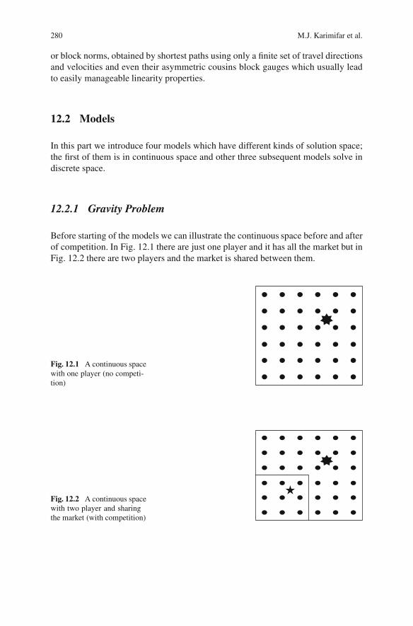
280 M.J. Karimifar et al.
or block norms, obtained by shortest paths using only a finite set of travel directionsand velocities and even their asymmetric cousins block gauges which usually leadto easily manageable linearity properties.
12.2 Models
In this part we introduce four models which have different kinds of solution space;the first of them is in continuous space and other three subsequent models solve indiscrete space.
12.2.1 Gravity Problem
Before starting of the models we can illustrate the continuous space before and afterof competition. In Fig. 12.1 there are just one player and it has all the market but inFig. 12.2 there are two players and the market is shared between them.
Fig. 12.1 A continuous spacewith one player (no competi-tion)
Fig. 12.2 A continuous spacewith two player and sharingthe market (with competition)
12 Competitive Location Problem 281
12.2.1.1 Model Assumptions
Model assumptions of this model are as follows:
� Existing competition is known and fixed.� Customers’ patronize the most attracting facility with their full demand, i.e., “the
winner gets it all” principle.� The probability that a customer patronizes a facility is proportional to its attrac-
tiveness and inversely proportional to a power of the distance to it.� When p new facilities are opened in an area, the total market share T attracted
by these facilities and by those already part of the franchise.� This model finds the best location for new facilities whose individual measures
of attractiveness are known.
12.2.1.2 Model Inputs (Indexes and Sets)
Model inputs of this model are as follows:
i: be the sub index of demand pointj: be the sub index of existing facilitiesm: be the set of new facilities
12.2.1.3 Model Outputs (Decision Variables)
Model outputs of this model are as follows:
.xm; ym/: the location of new facility m, form D 1; : : : ; p
12.2.1.4 Parameters
Parameters of this model are as follows:
n: the number of demand points (each demand point represents a small areaaround it).ai ; bi /: the location of demand point i D 1; : : : ; n
Bi : the available buying power at demand point i for i D 1; : : : ; n
K: the number of existing competing facilitiesC: the number of existing facilities which are part of one’s own chainP: the number of new facility to be locating in the area.xm � ym/ D p
.xm � ai /2 C .ym � bi /2 : the distance between demand pointi and new facility m. i D 1; : : : ; nI m D 1; : : : ; p
Ej : the measure of attractiveness of existing facility j for j D 1; : : : ; k
Am: the measure of attractiveness of existing facility m form D 1; : : : ; p
�: the power to which the distance is raised
282 M.J. Karimifar et al.
12.2.1.5 Objective Function and its Constraints
The objective function of this model as follows:
T DnXiD1
Bi
pPmD1
Am
d�i.xm; ym/
CcP
jD1Ej
d�ij
pPmD1
Am
d�i.xm; ym/
CkP
jD1Ej
d�ij
: (12.1)
The objective is to find the best location in the plane that maximizes the total marketshare captured T using (12.1).
A sequence of algebraic manipulations (Drezner 1995) leads to a somewhat sim-pler minimization problem, one of minimizing the total buying power not attractedby the chain.
F DnXiD1
Bi
kPjDcC1
Ej
d�ij
pPmD1
Am
d�i.xm; ym/
CkP
jD1Ej
d�ij
: (12.2)
The total sums for existing facilities are constants. Let
Gi D Bi
kXjDcC1
Ej
d�ij; Hi D
kXjD1
Ej
d�ij: (12.3)
These definitions lead to:
Min W
8<ˆ:F D
nXiD1
Gi
Hi CpP
mD1Am
d�i.xm; ym/
9>>=>>; : (12.4)
12.2.1.6 Solution Gravity Problem
� Algorithm 1
Randomly generate p sites for the p new facilities.Perform Weisfeld iteration for each of the facilities while holding the other rooted
in their places (Drezner 1995).After all p facilities were relocated one by one in step 2, calculate the changes
in their locations. If the location changes are less than a perspective ", terminate thealgorithm.
The following are two practical approaches to solving (12.4) (Drezner 1995):
12 Competitive Location Problem 283
� The AMPL approach
Instead of pursuing a specialized algorithm for the solution of these problems,standard non-linear programming codes available for the solution of non-linear pro-gramming problems like (Drezner 1995) can be used. The student version of AMPL(Drezner 1995) was used to solve this problem. Since these standard programs as-sume that the objective function is convex, one still needs to resolve the problem re-peatedly with various starting points and select the best solution for implementation.Also, the no convexity of the objective function may cause difficulties in the solutionprocedure itself. The AMPL modeling program is quite easy to write, is very shortand compact, and is easy to follow. The full program is given in (Drezner 1995).
� The excel approach
Spreadsheet software now incorporates optimization capabilities. The “solver”option in Excel can be used to solve. In Excel 4.0, this option is found under “for-mula”. A spread sheet is built to calculate the objective function, and the solverprovides the optimal solution with the calculated market share at the point. Sincethe problem is not convex, the procedure has to be repeated using many randomlygenerated starting location and the best solution is selected for implementation.
12.2.2 The Maximum Capture Problem Model (MAXCAP)(Serra and ReVelle 1995)
12.2.2.1 Model Assumptions
Model assumptions of this model are as follows:
� Existing competition is known and fixed.� Customers’ patronize the most attracting facility with their full demand, i.e., “the
winner gets it all” principle.� This model leads to combinatorial optimization models similar to covering, as
exhaustively reviewed in.
12.2.2.2 Model Inputs (Indexes and Sets)
Model inputs of this model are as follows:
� i; I : be the sub index and set of demand points� pi : set of sites s which i would patronize if a new facility would be opened there� Ti : set of sites for i tied with the currently patronized competitor’s facility
12.2.2.3 Model Outputs (Decision Variables)
Model outputs of this model are as follows:
yi : the fully captured for izi : the tied with a competitor for i
284 M.J. Karimifar et al.
12.2.2.4 Parameters
Parameters of this model are as follows:
wi : the demand of customer for i 2 Ixs : the facility be opened at s
12.2.2.5 Objective Function and its Constraints
The objective function of this model and its related constraints are as follows:
MaxXi2I
wi yi CXi2I
wi2
zi : (12.5)
Subject to
Yi �Xs2pi
xs .i 2 I / ; (12.6)
Zi �Xs2Ti
xs .i 2 I / ; (12.7)
Yi CZi � 1 .i 2 I /; (12.8)Xs2S
xs � P ; (12.9)
Yi ; Zi 2 f0; 1g xs 2 f0; 1g : (12.10)
12.2.2.6 Solution Maximum Capture Problem
Discrete models without split demand lead to the maximal covering type locationmodel introduced in (Church and ReVelle 1974). This is a simplified version ofthe maximal capture problem given above, in which all tie sets ti are empty, andtherefore without the auxiliary tie variables zi . Typically, these models will havemany optimal solutions, a feature which is troublesome for standard exact searchbranch and bound methods, but makes heuristic approaches particularly appealing.A recent proposal (Benati and Laporte 1995) for solving large-scale models of thistype consists of a Tabu search method.
Since in network and continuous setting ties appear whenever a site is chosenwhich is exactly at break-even distance from the demand point, the deterministic al-location rule inevitably leads to discontinuity of the capture function at such points,and previous rule of even split enhances this. Without split one at least retains semi-continuity. Two extreme situations without split demand may now be considered.
12 Competitive Location Problem 285
First there is conservatism, stating that in case of tie with a new facility; cus-tomers will go on patronizing the existing facility they patronized before. This is therule followed in (Hakimi 1990) introducing the NP-hard .r; xp/ medianoid prob-lem: find r sites on a network maximizing the total weight of demand vertices lyingcloser (in terms of shortest paths) to one of them than to any of the competitors xp .
Second, the opposite assumption of novelty orientation, i.e., in case of tie the newfacility gets all demand (Hanjoul and Thill 1987), gives rise to closed captured mar-kets, a feature of particular importance in the next section. With this tie-resolutionrule there corresponds to each demand point a (closed) subset of the location spaceof all sites for the new facility(ies) that would capture that demand. In other words,we have a collection of subsets, each related to a given demand volume. For a par-ticular site the total captured demand is then obtained by summation of the volumesof all sets it lies in. Maximizing the captured demand now means finding (a point in)a no void intersection of such sets corresponding to the highest total volume. In theEuclidean plane these sets are circular balls and it is easy to show that optimal solu-tions will always exist among all intersection points of two of the boundary circles,an easily enumerated finite set of candidates. Dresdner (Drezner 1981) shows howto do this efficiently for a single facility, while (Mehrez and Stulman 1982) suggesta dynamic programming approach for the multi facility version.
These types of model have also been advocated in marketing studies for brandpositioning and even in political science, see (Schmalensee and Thisse 1988). Inthe first case, product characteristics are taken as coordinates in a feature space,consumer groups having a common ideal brand-description represent demand, andattraction towards a brand is expressed by way of the (Euclidean) distance betweenthe points representing the ideal and the real brand. This leads to ball intersectionproblems in higher dimensions, which turn out to be NP-hard when dimension ispart of the input, but polynomial in fixed dimension. Several solution approacheshave been developed recently, all relying on geometric construction and evaluationof a finite dominating set.
12.2.3 The Maximum Capture Problem with Price Model(PMAXCAP) (Serra and ReVelle 1998)
We will introduce the max capture model with price which is a kind of location anddesign problem that contains the price of the product in its output.
12.2.3.1 Model Assumptions
Model assumptions of this model are as follows:
� Existing competition is known and fixed.� Customers’ patronize the most attracting facility with their full demand, i.e., “the
winner gets it all” principle.
286 M.J. Karimifar et al.
� The space is discrete and is defined by a connected graph. On each vertex ofthe graph there is a demand whit a distinct size, the set of local markets that arelocated on the vertices of the graph.
� The consumer’s decision on patronizing a store is based on transportation costsand price. Consumers always go the outlet with the lowest total price, regardlessof its ownership.
� There is an existing firm (from now on, Firm B) operating with q outlets. A newfirm (Firm A) wishes to enter and establish p servers. (The product sold in thisindustry is homogeneous).
� Suppose the demand is elastic then the demand of local market i is a functionof the market’s characteristics and the price customer faces and is denoted asDi.…i/.Thus it could be said thatDi.pCtdib/ is the demand for the local marketi; shopping at its closest outlet. Therefore, the demand function for each localmarket i for Firm A is defined as follows: if bAi is the closest Firm A’s server toi and bBi the closest Firm B’s server, then:
DAi .�
A; �B/ D(Di.�
A/ if pA C tdibAi< pB C tdibB
i
0 if pA C tdibAi
� pB C tdibBi
: (12.11)
� Equation (12.11) is, Firm A will capture the demand of local market i if the totalprice …A
i (mill price plus transport costs) faced by consumers is lower than thetotal price …B
i that defined the in the same way for B . Assume that productionentails for each outlet a fixed set-up cost fj , and a constant marginal cost v, perunit. Thus the total cost for each outlet is given by fj C vs . s is the number ofproducts in this facility. S is the number of products in this facility. If jA is theset of actual outlet locations .J A � J /, then profits for firm A can be written asfollows: YA D .pA � v/
XDAi .�
A; �B/ �Xj2JA
fj : (12.12)
� Equation (12.12) for firm A is determining jA and pA to maximize profits. Thisprofit also depends on other model parameters such as the location and prices ofthe competitor firm and the demand function of consumers among others.
12.2.3.2 Model Inputs (Indexes and Sets)
Model inputs of this model are as follows:
i,I: be the sub index and the set of local markets that are located on the verticesof the graphj, J: be the sub index and set of potential locations for Firm A’s outlets.JB : be the set of actual locations of the outlets of Firm B.
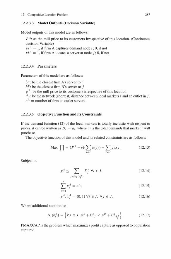
12 Competitive Location Problem 287
12.2.3.3 Model Outputs (Decision Variable)
Model outputs of this model are as follows:
PA: as the mill price to its customers irrespective of this location. (Continuousdecision Variable)yiA D 1, if firm A captures demand node i ; 0, if notxiA D 1, if firm A locates a server at node j ; 0, if not
12.2.3.4 Parameters
Parameters of this model are as follows:
bAi : be the closest firm A’s server to ibBi : be the closest firm B’s server to jpB : be the mill price to its customers irrespective of this locationdij : be the network (shortest) distance between local markets i and an outlet in j .nA D number of firm an outlet servers
12.2.3.5 Objective Function and its Constraints
If the demand function (12) of the local markets is totally inelastic with respect toprices, it can be written asDi D ai , where ai is the total demands that market i willpurchase.
The objective function of this model and its related constraints are as follows:
MaxY
D .PA � v/.Xi2I
aiyj /�Xj2J
fj xj : (12.13)
Subject to
yAi �X
j2NI .bBi/
XAj 8i 2 I; (12.14)
nXjD1
xAj D nA; (12.15)
yAi ; xAj D .0; 1/ 8i 2 I; 8j 2 J: (12.16)
Where additional notation is:
Ni.bBi / D
n8j 2 J; pA C tdij < p
B C tdibBi
o: (12.17)
PMAXCAP is the problem which maximizes profit capture as opposed to populationcaptured.
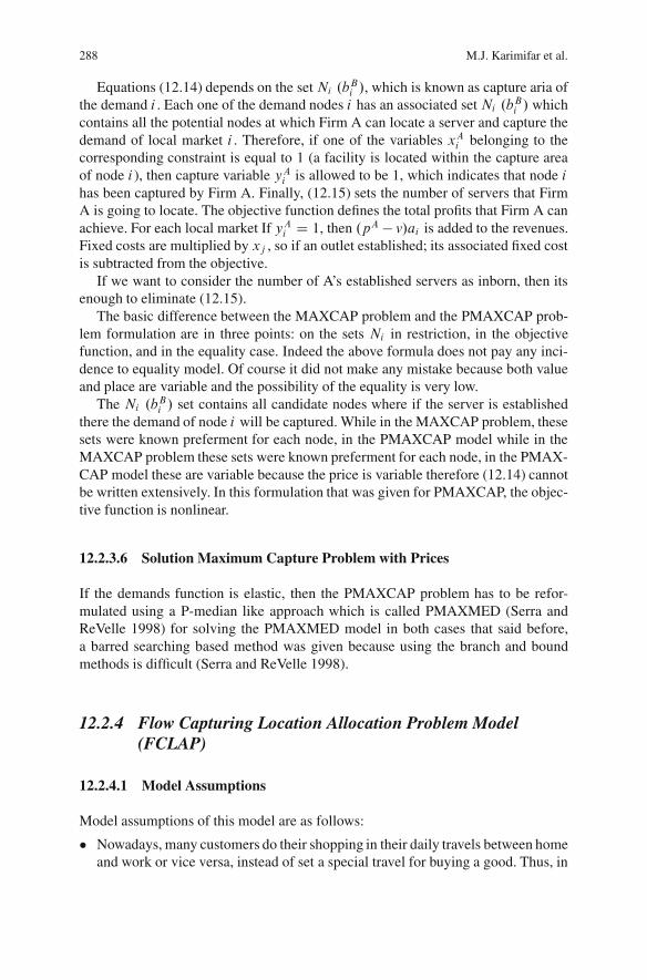
288 M.J. Karimifar et al.
Equations (12.14) depends on the set Ni .bBi /, which is known as capture aria ofthe demand i . Each one of the demand nodes i has an associated set Ni .bBi / whichcontains all the potential nodes at which Firm A can locate a server and capture thedemand of local market i . Therefore, if one of the variables xAi belonging to thecorresponding constraint is equal to 1 (a facility is located within the capture areaof node i ), then capture variable yAi is allowed to be 1, which indicates that node ihas been captured by Firm A. Finally, (12.15) sets the number of servers that FirmA is going to locate. The objective function defines the total profits that Firm A canachieve. For each local market If yAi D 1, then .pA � v/ai is added to the revenues.Fixed costs are multiplied by xj , so if an outlet established; its associated fixed costis subtracted from the objective.
If we want to consider the number of A’s established servers as inborn, then itsenough to eliminate (12.15).
The basic difference between the MAXCAP problem and the PMAXCAP prob-lem formulation are in three points: on the sets Ni in restriction, in the objectivefunction, and in the equality case. Indeed the above formula does not pay any inci-dence to equality model. Of course it did not make any mistake because both valueand place are variable and the possibility of the equality is very low.
The Ni .bBi / set contains all candidate nodes where if the server is establishedthere the demand of node i will be captured. While in the MAXCAP problem, thesesets were known preferment for each node, in the PMAXCAP model while in theMAXCAP problem these sets were known preferment for each node, in the PMAX-CAP model these are variable because the price is variable therefore (12.14) cannotbe written extensively. In this formulation that was given for PMAXCAP, the objec-tive function is nonlinear.
12.2.3.6 Solution Maximum Capture Problem with Prices
If the demands function is elastic, then the PMAXCAP problem has to be refor-mulated using a P-median like approach which is called PMAXMED (Serra andReVelle 1998) for solving the PMAXMED model in both cases that said before,a barred searching based method was given because using the branch and boundmethods is difficult (Serra and ReVelle 1998).
12.2.4 Flow Capturing Location Allocation Problem Model(FCLAP)
12.2.4.1 Model Assumptions
Model assumptions of this model are as follows:
� Nowadays, many customers do their shopping in their daily travels between homeand work or vice versa, instead of set a special travel for buying a good. Thus, in
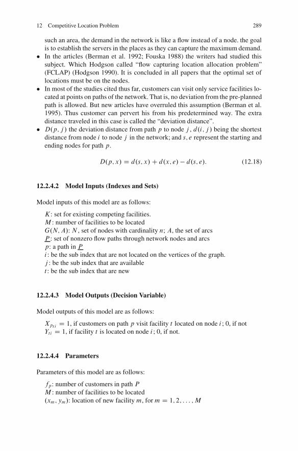
12 Competitive Location Problem 289
such an area, the demand in the network is like a flow instead of a node. the goalis to establish the servers in the places as they can capture the maximum demand.
� In the articles (Berman et al. 1992; Fouska 1988) the writers had studied thissubject. Which Hodgson called “flow capturing location allocation problem”(FCLAP) (Hodgson 1990). It is concluded in all papers that the optimal set oflocations must be on the nodes.
� In most of the studies cited thus far, customers can visit only service facilities lo-cated at points on paths of the network. That is, no deviation from the pre-plannedpath is allowed. But new articles have overruled this assumption (Berman et al.1995). Thus customer can pervert his from his predetermined way. The extradistance traveled in this case is called the “deviation distance”.
� D.p; j / the deviation distance from path p to node j , d.i; j / being the shortestdistance from node i to node j in the network; and s; e represent the starting andending nodes for path p.
D.p; x/ D d.s; x/C d.x; e/ � d.s; e/: (12.18)
12.2.4.2 Model Inputs (Indexes and Sets)
Model inputs of this model are as follows:
K: set for existing competing facilities.M : number of facilities to be locatedG.N;A/: N , set of nodes with cardinality n; A, the set of arcsP : set of nonzero flow paths through network nodes and arcsp: a path in Pi : be the sub index that are not located on the vertices of the graph.j : be the sub index that are availablet : be the sub index that are new
12.2.4.3 Model Outputs (Decision Variable)
Model outputs of this model are as follows:
XptiD 1, if customers on path p visit facility t located on node i ; 0, if not
Yti D 1, if facility t is located on node i ; 0, if not.
12.2.4.4 Parameters
Parameters of this model are as follows:
fp: number of customers in path PM : number of facilities to be located.xm; ym/: location of new facility m, form D 1; 2; : : : ;M
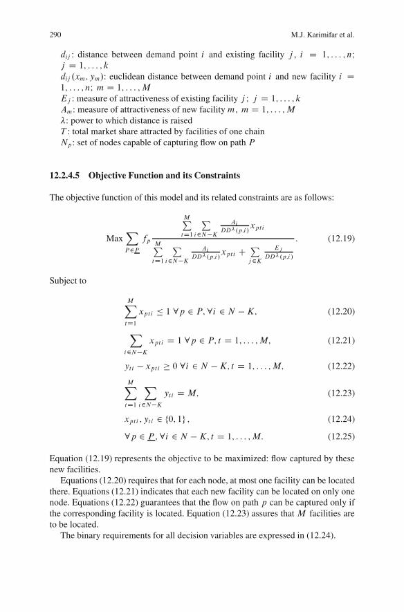
290 M.J. Karimifar et al.
dij : distance between demand point i and existing facility j , i D 1; : : : ; nIj D 1; : : : ; k
dij .xm; ym/: euclidean distance between demand point i and new facility i D1; : : : ; nI m D 1; : : : ;M
Ej : measure of attractiveness of existing facility j I j D 1; : : : ; k
Am: measure of attractiveness of new facility m; m D 1; : : : ;M
�: power to which distance is raisedT : total market share attracted by facilities of one chainNp: set of nodes capable of capturing flow on path P
12.2.4.5 Objective Function and its Constraints
The objective function of this model and its related constraints are as follows:
MaxXP2P
fp
MPtD1
Pi2N�K
Ai
DD�.p;i/xpti
MPtD1
Pi2N�K
Ai
DD�.p;i/xpti C P
j2KEj
DD�.p;i/
: (12.19)
Subject to
MXtD1
xpti � 1 8p 2 P;8i 2 N �K; (12.20)
Xi2N�K
xpti D 1 8p 2 P; t D 1; : : : ;M; (12.21)
yti � xpti � 0 8i 2 N �K; t D 1; : : : ;M; (12.22)
MXtD1
Xi2N�K
yti D M; (12.23)
xpti ; yti 2 f0; 1g ; (12.24)
8p 2 P ;8i 2 N �K; t D 1; : : : ;M: (12.25)
Equation (12.19) represents the objective to be maximized: flow captured by thesenew facilities.
Equations (12.20) requires that for each node, at most one facility can be locatedthere. Equations (12.21) indicates that each new facility can be located on only onenode. Equations (12.22) guarantees that the flow on path p can be captured only ifthe corresponding facility is located. Equation (12.23) assures that M facilities areto be located.
The binary requirements for all decision variables are expressed in (12.24).
12 Competitive Location Problem 291
12.2.4.6 Solution Flow Capturing Location Allocation Problem
Upon model is nonlinear which might make problems in the calculation phase. Wuand Lin (2003) had changed this model to liner, based on the method presented byWu (1997), but the result will not always redound to simplicity. Also those man hadpresented an inventive method for solving the model base on a greedily procedurewhich is too similar to what Berman et al. (Berman et al. 1995; Berman and Krass1998) had developed for FCLAP problem.
12.3 Case Study
In this section we will introduce some real-world case studies related to Competitivelocation problems.
12.3.1 A Case in Toronto (Aboolian et al. 2006)
A company would like to enter the metropolitan Toronto market by locating oneor several supermarket-type retail facilities there. There are two choices for facilitydesigns: a regular facility, with approximately 15,000 square feet of retail space, anda large facility with approximately 45,000 square feet of retail space. These valueswere chosen based on data from the Food Marketing Institute which lists 15,000square feet as the size of a typical supermarket and 40,000–50,000 square feet asthe size of a superstore. The budget that the company has allocated for the Torontoexpansion is sufficient to locate one large facility or up to three regular facilitiesanywhere in the city.
In this case, the following competitive situation is assumed: a competitor provid-ing similar service has already entered the Toronto market, using the same facilitydesign alternatives. For the competitor, the same two choices regarding the numberand sizes of the facilities are considered: one large or three small. For each combi-nation of values of problem parameters described below, optimal locations for thecompetitor’s facilities is selected. The company now has to decide on the locationand sizes of its own facilities given the existing locations of competitive facilities.
The network that is used corresponded to the geography of metropolitan Toronto.The lease costs for retail real estate vary significantly throughout the city, the costdata per square foot is used from the April 2004 Commercial Reality Watch reportproduced by the Toronto Real Estate Board. Since each node of network representsan area that can contain multiple facilities, own and competitive facilities are al-lowed to be co-located within the same nodes.
The problem described above is analyzed under three values for demand elastic-ity parameter, which represent respectively very high elasticity, moderate elasticity,and low elasticity; three values for the size sensitivity parameter, which represent,
292 M.J. Karimifar et al.
respectively, very high sensitivity, moderate sensitivity, and low sensitivity; and twovalues for the distance sensitivity, which represent respectively, high and moderatevalues. Aboolian et al. (2006) wanted to see the extent to which the optimal loca-tion and sizing decisions depend on the problem parameters and on the sizes andlocations of pre-existing competitive facilities.
The following conclusions can be made based on the results of the case study inToronto:
� It is always optimal to locate three regular facilities when either the size sensitiv-ity is small, or size sensitivity is moderate and distance sensitivity is high.
� When distance and size sensitivities are both moderate, three regular facilitiesare also preferred, except when demand is very elastic, in which case one largefacility performs better.
� When size sensitivity is high, one large facility is generally optimal, except whendistance sensitivity is high and demand is not very elastic.
� The optimal sizes of own facilities appear to depend only on problem parametersthe sizes/number of competitive facilities do not seem to affect own design de-cisions. However the locations of own facilities are certainly influenced by both,the number and locations of competitive facilities, as well as by the problemparameters.
� When demand is very elastic, co-locations are very common i.e., one or moreof own facilities are located in the same FSAs as the competitive facilities, wecan loosely interpret these as shopping mall solutions. On the other hand, whendemand elasticity is low, co-location never happens owns facilities tend to belocated away from the competitive ones.
12.3.2 A Case in Yuanlin Taiwan (Wu and Lin 2003)
The decision objective for service providers is to find the optimal locations for suchservice facilities to Maximize the number of customers “captured”. This sort ofproblem is usually called a “flow capturing location allocation problem” (FCLAP),that in the earlier seasons of this book is discussed. In this article a mathemati-cal model and heuristic solving method is developed based on the greedy solvingmethod, and this solving method in the instance study of real networks in Yuanlin,Changhua which was accomplished in Taiwan is surveyed.
Yuanlin is a township in Changhua County, Central Taiwan with an approximatearea of 33 W 72 km2 and a 1998 population of 126,395.
A newly established retail chain is planning to enter the local convenience-storemarket and locate a number of new stores in Yuanlin. For this analysis, The House-hold Registration Office of Yuanlin provided data such as geographical zoning, andthe population of each zone from a 1998 update.
In this analysis, there is a network with 39 nodes and 1482 paths and severalassumptions made in this analysis are described as follows: These criteria consist ofproduct mix (c1), price (c2), interior layout and design (c3), personnel (c4), overall
12 Competitive Location Problem 293
cleanliness (c5), floor space (c6), traffic congestion in the surrounding area (c7),and frequency of promotional sales (c8). Information regarding the location andattractiveness score is gathered for each existing store.
The greedy heuristic and the enumeration method developed are used for solvingthis authentic network. The results enumeration approaches are nodes 19, 27, 3 andthe results greedy approach summarized are nodes 8, 27, 19. The deviation from theoptimal of the greedy heuristic is 5.73%, with 7.141 s taken, which is more than 340times faster than the 2,484.658 s required by the enumeration method are.
References
Aboolian R, Berman O, Krass D (2006) Competitive facility location and design problem. EurJ Oper Res 182:40–62
Benati S, Laporte G (1995) Tabu search algorithms for .rjXp/ medianoid and .rjp/ centroid prob-lems. Location Sci 2:193–204
Berman O, Krass D (1998) Flow intercepting spatial interaction model: A new approach to optimallocation of competitive facilities. Location Sci 6:41–65
Berman O, Larson RC, Fouska N (1992) Optimal location of discretionary service facilities. Trans-port Sci 26:201–221
Berman O, Bertsimas D, Larson RC (1995) Locating discretionary service facilities II: maximizingmarket, minimizing inconvenience. Oper Res 43:623–632
Chhajed D, Francis RL, Lowe TJ (1993) Contributions of operations research to location analysis.Location Sci 1(4):263–287
Church R, ReVelle C (1974) The maximal covering location problem. Papers of the RegionalScience Association 32:101–118
Dobson G, Karmarkar US (1987) Competitive location on a network. Oper Res 35(4):565–574Drezner Z (1981) On a modified one-center problem. Manage Sci 27:848–851Drezner T (1995) Competitive location problem in the plane, In: Drezner Z (ed) Facility location:
A survey of application and methods. Springer, BerlinDrezner T, Drezner Z (1996) Competitive facilities: Market share and location with random utility.
J Region Sci 36:1–15Eiselt HA, Laporte G (1989a) Competitive spatial models. Eur J Oper Res 39:231–242Eiselt HA, Laporte G (1989b) The maximum capture problem on a weighted network. J Region
Sci 29:433–439Eiselt HA, Laporte G (1996a) Equilibrium results in competitive location models. Middle East
Forum 1:63–92Eiselt HA, Laporte G (1996b) Sequential location problems. Eur J Oper Res 96:217–223Eiselt HA, Laporte G, Thisse JF (1993) Competitive location models: A framework and bibliogra-
phy. Transport Sci 27(1):44–54Fouska N (1988) Optimal location of discretionary service facilities, MS Thesis, Operation
Research Center. MIT, Cambridge, MA, USAFriesz T, Tobin L, Miller T (1989) Existence theory for spatially competitive network facility
location models. Ann Oper Res 18:267–276Gabszewicz J, Thisse JF (1991) Location. In: Auman R, Hart S (eds) Handbook of game theory
with economic applications. North-Holland, AmsterdamGhosh A, Craig CS (1984) A location-allocation model for facility planning in a competitive envi-
ronment. Geograph Anals 20:39–51Hakimi SL (1986) p-median theorems for competitive location. Ann Oper Res 5:79–88Hakimi SL (1990) Locations with spatial interactions: Competitive locations and games. In:
Francis RL, Mirchandani PB (eds) Discrete location theory. Wiley, New York, pp 439–447
294 M.J. Karimifar et al.
Hakimi SL, Labbe M, Schmeichel E (1992) The Voronoi partition of a network and its implicationsin location theory. ORSA J Comput 4:412–417
Hanjoul P, Thill JC (1987) Elements of planar analysis in spatial competition. Region Sci UrbanEcon 17:423–439
Hanjoul P, Hansen P, Peeters D, Thisse JF (1990) Uncapacitated plant location under alternativespatial policies. Manage Sci 36(1):41–57
Hodgson J (1990) A flow-capturing location-allocation model. Geograph Anal 22:270–279Hoover E (1936) Spatial price discrimination. Rev Econ Stud 4:182–191Hotelling H (1929) Stability in competition. Econ J 39:41–57Karkazis J (1989) Facilities location in a competitive environment: A promethee based multiple
criteria analysis. Eur J Oper Res 42:294–304Lederer P, Thisse JF (1990) Competitive location on networks under delivery pricing. Oper Res
Lett 9:147–153Lerner A, Singer HV (1937) Some notes on duopoly and spatial competition. J Political Econ
39:145–186Mehrez A, Stulman A (1982) The maximal covering location problem with facility placement on
the entire plane. J Region Sci 22:361–365Miller T, Friesz TL, Tobin RL (1992) Heuristic algorithms for delivered price spatially competitive
network facility location problems. Ann Oper Res 34:177–202Peeters PH (1997) Static competitive location models on networks. Master’s thesis, Vrije Univer-
siteit Brussel, Brussels, Belgium, pp 65ReVelle C (1986) The maximum capture or sphere of in influence problem: Hotelling revisited on
a network. J Region Sci 26(2):343–357ReVelle C, Serra D (1991) The maximum capture problem including relocation. Inf Oper Res
29(2):130–138Schmalensee R, Thisse JF (1988) Perceptual maps and the optimal location of new products: An
integrative essay. Int J Res Market 5:225–24Serra D, ReVelle C (1995) Competitive location in discrete space. In: Drezner Z (ed) Facility
location: a survey of applications and methods. Springer, Berlin, pp 367–386Serra D, ReVelle C (1998) Competitive location and pricing on networks. J Econ Lit Classif C61,
R32, L81, R12Serra D, Marianov V, ReVelle C (1992) The hierarchical maximum capture problem. Eur J Oper
Res 62(3):58–69Smithies A (1941) Optimum location in spatial competition. J Political Econ 49:423–439Tobin R, Friesz TL (1986) Spatial competition facility location models: Definition, formulation
and solution approach. Ann Oper Res 6:47–74Wendell R, McKelvey RD (1981) New perspectives in competitive location theory. Eur J Oper Res
6:174–182Winston, Wayne L (1995) Introduction to mathematical programming, 2nd ed. Duxbury Press,
North Scituate, MAWu TH (1997) A note on a global approach for general 0–1 fractional programming. Eur J Oper
Res 101:220–223Wu TH, Lin JN (2003) Solving the competitive discretionary service facility location problem. Eur
J Oper Res 144:366–37
Chapter 13Warehouse Location Problem
Zeinab Bagherpoor, Shaghayegh Parhizi, Mahtab Hoseininia,Nooshin Heidari, and Reza Ghasemi Yaghin
Finding the optimal location for industrial facilities has always been of a crucialimportance and priority from geographers’ and economists’ view point. Althougheconomics play the main role in presenting location theories by resorting to its theo-ries, geographers, with their focus on locative and spatial changes leading to naturalphenomenon, have also had a share in complimenting these location theories andfinding optimal points to locate industrial activities location. From this point ofview, materials, market and other manufacturing factors have not been concentratedin one point, and their spatial separation necessitates traveling distances which, inturn, brings about costs. That is why optimal industrial location is also a part ofgeographical studies.
By location theories, we mean “a series of principals with resorting to which,the optimal location of industrial activities is determined (point conjoining on themost benefit)”. The history of location theories goes back to nineteenth century inGermany. The first industrial location theory was presented by Shuffle in 1878 A.D.He was successful in applying the gravity model in the way industries are located:
Mij D PiPj �Dij�2; (13.1)
where P&D represent population and distances, respectively. In this way, industriesare located adjacent to huge cities as a response to demand and market factors.
The most dominating principle in finding the optimal location is based on thebasis of the least cost. Lanhart is another scientist in this field who represented histheory in 1882. According to his reasoning, the position of industries depends on thesignificant factor of transportation. In other words, the ideal point for locating indus-try is a point where the total transportation cost, including material, final productsand fuel, are at minimum.
At the mercy of myriad business, logistics and government initiatives, includingjust in time production, quick response, research on quality, enhanced customersatisfaction, operators’ safety, and environmental protection, warehouse operationshave been and are continuously revolutionized (Tompkins et al. 1996). Warehousescan play each of the following roles in a distribution network:
� They can be used as a balance and storage point because of the differencebetween the time scheduling and manufacturing demand. For this reason, the
R.Z. Farahani and M. Hekmatfar (eds.), Facility Location: Concepts, Models, 295Algorithms and Case Studies, Contributions to Management Science,DOI 10.1007/978-3-7908-2151-2 13, c� Physica-Verlag Heidelberg 2009
296 Z. Bagherpoor et al.
warehouses are usually located at the manufacturing point. Complete pallets flowin and out. Warehouses whose role is limited to this can have monthly and sea-sonal demands until progressing to the next step in distribution.
� They can be utilized for storing and commixing outputs coming from differentmanufacturing points in one company or more companies, before being send tothe customers. This part usually responses to the weekly or monthly orders.
� They can be dispersed to reach the shortest transportation distances to be able toquickly respond to the customer’s demand. Items are often chosen individuallyand similar items can be sent daily.
If possible, two or more of these roles must be consolidated in the same warehouses.Today’s changes have necessitated this consolidation to make inputs accessible andto decrease transportation costs. Small items with great value and unpredictabledemands, in particular, are often distributed from a single source through a globalnetwork (Tompkins et al. 1996).
13.1 Classifications
A classification of different types of warehouse location problems is represented asfollows:
� Area solution: discrete, continual� Warehouse installation cost: Fixed installation cost, Without fixed installation
cost� Determination of the number of warehouses: exogenous, endogenous� Determination of the number of products: Single product, Multiple product� Determination of number of periods: singe period and multi period.� Warehouse capacity: unlimited capacity, Limited capacity� Constraint on relationship between warehouses and customer: In some models,
customer’s demand could be served by any number of warehouses but in othersthere are constraints on relationship between customers and warehouses and eachwarehouse can serve only a limited number of customers.
The purpose of these problems is to minimize the total cost of locating warehousesin candidate points and allocating customers to the warehouses in each period. Theseproblems also make clear assumptions about costs. The curve in Fig. 13.1 indicatesthe required cost to build facilities as a function of output quantity and the curve inFig. 13.2 indicates the incurred transportation costs as a function of shipment size(in fact, transportation costs increase with the size of shipment). It may be difficultto estimate the cost items. We may also encounter questions such as “How longdoes a period last?”, “How many periods should be considered?”, and “How muchare the administering costs of the warehouse?”. Such questions can be examined inthe special problem.
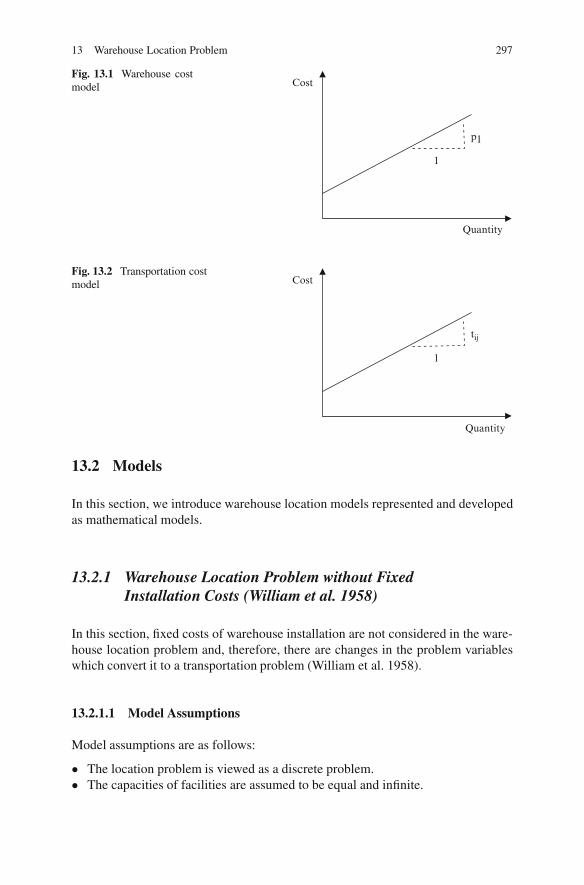
13 Warehouse Location Problem 297
Fig. 13.1 Warehouse costmodel
1
p1
Quantity
Cost
Fig. 13.2 Transportation costmodel
1
tij
Quantity
Cost
13.2 Models
In this section, we introduce warehouse location models represented and developedas mathematical models.
13.2.1 Warehouse Location Problem without FixedInstallation Costs (William et al. 1958)
In this section, fixed costs of warehouse installation are not considered in the ware-house location problem and, therefore, there are changes in the problem variableswhich convert it to a transportation problem (William et al. 1958).
13.2.1.1 Model Assumptions
Model assumptions are as follows:
� The location problem is viewed as a discrete problem.� The capacities of facilities are assumed to be equal and infinite.
298 Z. Bagherpoor et al.
� Transportation costs are an increasing function of shipment sizes.� The number of warehouses should not be more than the number of candidate
points.� Each customer’s demand should be estimated and customers should be allocated
to the warehouses.
13.2.1.2 Model Inputs
i : factory .i D 1; 2; : : : ; m/j : warehouse .j D 1; 2; : : : ; n/k: retailer .k D 1; 2; : : : ; qCijk : cost of the shipment (from factory i to retailer k through warehouse j )including the relevant inventory costQi : quantity shipped from factory iRj : capacity of warehouse jSk : quantity required at destination k
13.2.1.3 Model Outputs (Decision Variables)
Xijk : quantity shipped from factory i via warehouse j to retailer kAijk : amount of inventory remained in warehouse j from the flow Xijk
13.2.1.4 Objective Function and its Constraints
The problem is to minimize the total delivery costs, i.e., to minimize the following:
Min Z DXi;j;k
Cijk�Xijk
�; (13.2)
Subject to
Xjk
Xijk D Qi i D 1; 2; : : : ; m; (13.3)
Xi;k
Aijk�Xijk
� � Rj j D 1; 2; : : : ; n; (13.4)
Xi;j
Xijk D Sk k D 1; 2; : : : ; q: (13.5)
Equation (13.3): all goods must be shipped out of the factoryEquation (13.4): no warehouse capacity can be exceededEquation (13.5): all customers’ demands must be met
13 Warehouse Location Problem 299
The resemblance to the standard transportation problem is obvious and there areonly three differences:
(a) The possible nonlinearity of (13.2)(b) The presence of the warehouse-capacity (13.4)(c) The need for a three subscript notation for the variables Xijk (three dimen-
sional X variables) resulting from the necessity of routing each flow through awarehouse.
Of course, a nonlinear objective function is not necessarily ruled out for the trans-portation problem, and can be ignored. The warehouse capacity limitations in theproblem, can be also be ignored because a firm never ends up renting more thana small fraction of the public warehouse space available at any location.
Elimination of difference (c), i.e., the three-subscript notation, becomes a trivialmatter because of the following rule: An optimal (least cost) solution will involveshipment of all goods that go from factory i� to destination k� via that (those)warehouse (s) j � for which Ci�j�k� D Min jC 0
i�jk�
In the other ways, it will always pay to make any shipment via the warehousethat offers the lowest delivery cost. The solution of the program is now simple.
For each factory-destination combination, i� � k�, select a value j � for which(13.5) is satisfied. This can be done by simple inspection of the Cijk data. Wecan now revise our notation by letting Xi�j�k� D X 0
i�k� ; Ci�j�k� D C 0i�k�
(since in an optimal solution all otherXi�jk� ’s will be equal zero). Substituting thisnotation in (13.2), (13.4), and (13.5) will obviously leave us with a standard trans-portation problem whose optimum solution can be found by the standard methods.
13.2.2 Warehouse Location Problem with Fixed Costof Establishment (Akinc and Khumawala 1977)
All assumptions in this problem are similar to the previous case; the only differenceis the fixed cost of location.
13.2.2.1 Model Inputs
k: customer .k D 1; 2; : : : ; q/
j : candidate points .j D 1; 2; : : : ; n/
fj : cost of locating a warehouse in point jrk : customer’s demandvkj : the cost of shipment to customer k from point j for each unit
ckj D vkj C rk;
where usually q >n.
300 Z. Bagherpoor et al.
13.2.2.2 Model Outputs (Decision Variables)
xkj : a fraction of rk which is transported from j to customer kyi : Will be equal one if the candidate point j is selected, otherwise it will beequal to zero.
13.2.2.3 Objective Function and its Constraints
The warehouse location model is formulated as a mix integer programming prob-lem, as follows:
Min Z DnX
jD1fj yj C
nXjD1
qXkD1
ckj xkj ; (13.6)
Subject to
nXjD1
xkj D 1I k D 1; : : : ; q ; (13.7)
�xkj C yj � 0; (13.8)
0 � xkj � 1; (13.9)
yj 2 f0; 1g : (13.10)
Notice that rk�xkj is the amount transported from point j to customer k (xkj is afraction of rk which is transported from point j to customer k).
Equation (13.7) insure that a customer’s demand is satisfied and that the maxi-mum quantity of xkj is equal to 1. Equation (13.8) insure that a warehouse in pointj serves customer k if a warehouse has been located in that point.
This formulation shows that WLP is, in fact, a special type of n-Median in whichthe number of facilities is ignored.
13.2.2.4 The Other Way of Formulation
In this section, another WLP formulation is presented which is discussed in the lastsection. Here, by adding up of (13.8) over k, the mentioned WLP is converted to thefollowing problem:
Min z0 DnX
jD1fj yj C
nXjD1
qXkD1
ckj xkj .WLP0/; (13.11)
Subject to nXjD1
xkj D 1; k D 1; : : : ; q; (13.12)
13 Warehouse Location Problem 301
qXkD1
xkj � qyj � 0; j D 1; : : : ; n; (13.13)
0 � xkj � 1; k D 1; : : : ; qI j D 1; : : : ; n; (13.14)
yj 2 f0; 1g : (13.15)
Both problems have the same optimal solution. However, they have different re-laxations. In fact, WLP’ can be solved through scanning, since the followingequation holds:
qXkD1
xkj� D qy�
j : (13.16)
Reducing yj � results in the objective function value to reduce as well. Therefore,the constraints of yj � can be solved and replaced in the objective function:
MinnX
jD1
qXkD1
.fj
qC ckj /xkj ; (13.17)
Subject to
nXjD1
xkj D 1; k D 1; : : : ; q; (13.18)
0 � xkj � 1; k D 1; ::; qI j D 1; ::; n: (13.19)
By this WLP compact method, the warehouse with the least fj =q C ckj is chosen.The relaxation of WLP’ presents a weak low bound for the WLP and it is not clearhow it can be used to solve WLP.
Therefore, mathematical models with less number of constraints are not neces-sarily better. For warehouse location models, the extended model of �xkj Cyj � 0is preferred to the following compact model:
qXkD1
xkj � qyj � 0: (13.20)
Even if it increases the size of the model (WLP is called strong LP, and WLP’ iscalled weak LP) (Akinc and Khumawala 1977).
13.2.3 Capacitated Warehouse Location Problem withConstraints in Customers Being Serviced (Nagy 2004)
In the pervious models, a customer’s demand could be served by any number ofwarehouses, but in this model there is a constraint on the warehouses, and, therefore,
302 Z. Bagherpoor et al.
each warehouse can serve only a limited number of customers and each customermust be supplied by exactly one open warehouse. The objective is to determine whichwarehouses to open, and the allocation of the customers to the opened warehouses,such that the sum of the maintenance and supply costs is minimized (Nagy 2004).
13.2.3.1 Model Inputs
k: is the number of customerj : is the number of warehousesckj : is a table containing the cost associated to the supplycf : is the fixed costCapacityj : the max number of stores that it can supply
13.2.3.2 Model Outputs (Decision Variables)
Oj : is a vector of Booleans indicating what warehouses have been opened.Skj : is a matrix of Booleans indicating if customer k is supplied by warehouse j
13.2.3.3 Objective Function and its Constraints
MinXk;j
Skj ckj C cfXj
Oj ; (13.21)
Subject to Xj
Skj D 1; 8k; (13.22)
Xk
Skj � Capacityj ; 8j; (13.23)
Xk
Skj � Oj ; 8k; j : (13.24)
Equation (13.22) insure that a customer must be supplied by exactly one warehouse.Equation (13.23) insure that each warehouse has a fixed capacity. Equation (13.24)insure that a customer can be supplied only by an open warehouse (Nagy 2004).
13.2.4 Single Stage Capacitated Warehouse Location Model(Sharma and Berry 2007)
In this section, new formulations and relaxations of the single stage capacitatedwarehouse location problem (SSCWLP) are described.
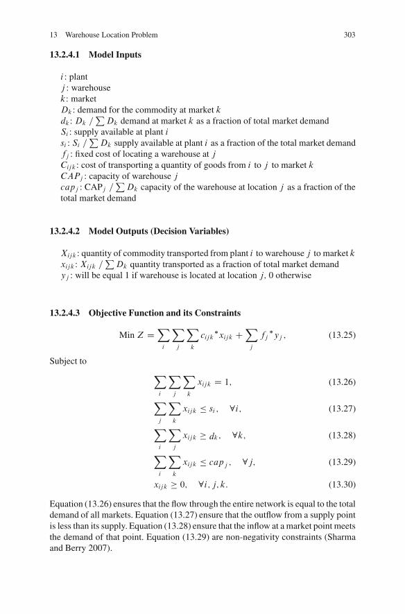
13 Warehouse Location Problem 303
13.2.4.1 Model Inputs
i : plantj : warehousek: marketDk : demand for the commodity at market kdk : Dk =
PDk demand at market k as a fraction of total market demand
Si : supply available at plant isi : Si =
PDk supply available at plant i as a fraction of the total market demand
fj : fixed cost of locating a warehouse at jCijk : cost of transporting a quantity of goods from i to j to market kCAPj : capacity of warehouse jcapj : CAPj =
PDk capacity of the warehouse at location j as a fraction of the
total market demand
13.2.4.2 Model Outputs (Decision Variables)
Xijk : quantity of commodity transported from plant i to warehouse j to market kxijk : Xijk =
PDk quantity transported as a fraction of total market demand
yj : will be equal 1 if warehouse is located at location j; 0 otherwise
13.2.4.3 Objective Function and its Constraints
Min Z DXi
Xj
Xk
cijk�xijk C
Xj
fj�yj ; (13.25)
Subject to Xi
Xj
Xk
xijk D 1; (13.26)
Xj
Xk
xijk � si ; 8i; (13.27)
Xi
Xj
xijk � dk; 8k; (13.28)
Xi
Xk
xijk � capj ; 8j; (13.29)
xijk � 0; 8i; j; k: (13.30)
Equation (13.26) ensures that the flow through the entire network is equal to the totaldemand of all markets. Equation (13.27) ensure that the outflow from a supply pointis less than its supply. Equation (13.28) ensure that the inflow at a market point meetsthe demand of that point. Equation (13.29) are non-negativity constraints (Sharmaand Berry 2007).
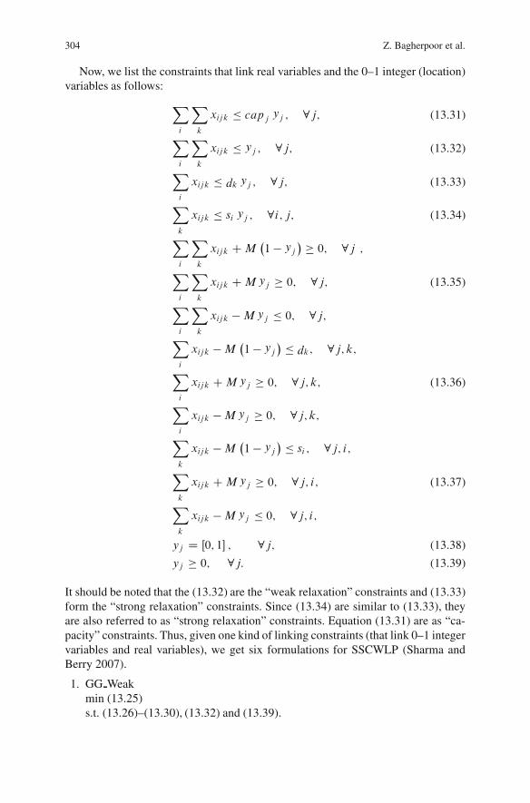
304 Z. Bagherpoor et al.
Now, we list the constraints that link real variables and the 0–1 integer (location)variables as follows: X
i
Xk
xijk � capj yj ; 8j; (13.31)
Xi
Xk
xijk � yj ; 8j; (13.32)
Xi
xijk � dk yj ; 8j; (13.33)
Xk
xijk � si yj ; 8i; j; (13.34)
Xi
Xk
xijk CM�1 � yj
� � 0; 8j ;Xi
Xk
xijk CMyj � 0; 8j; (13.35)
Xi
Xk
xijk �Myj � 0; 8j;Xi
xijk �M �1 � yj
� � dk; 8j; k;Xi
xijk CMyj � 0; 8j; k; (13.36)
Xi
xijk �Myj � 0; 8j; k;Xk
xijk �M �1 � yj
� � si ; 8j; i;Xk
xijk CMyj � 0; 8j; i; (13.37)
Xk
xijk �Myj � 0; 8j; i;
yj D Œ0; 1 ; 8j; (13.38)
yj � 0; 8j: (13.39)
It should be noted that the (13.32) are the “weak relaxation” constraints and (13.33)form the “strong relaxation” constraints. Since (13.34) are similar to (13.33), theyare also referred to as “strong relaxation” constraints. Equation (13.31) are as “ca-pacity” constraints. Thus, given one kind of linking constraints (that link 0–1 integervariables and real variables), we get six formulations for SSCWLP (Sharma andBerry 2007).
1. GG Weakmin (13.25)s.t. (13.26)–(13.30), (13.32) and (13.39).
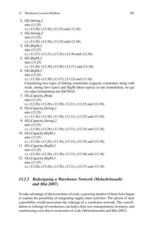
13 Warehouse Location Problem 305
2. GG Strong 1min (13.25)s.t. (13.26)–(13.30), (13.33) and (13.38).
3. GG Strong 2min (13.25)s.t. (13.26)–(13.30), (13.35) and (13.36).
4. GG BigM 1min (13.25)s.t. (13.27)–(13.31), (13.35)–(13.36) and (13.38).
5. GG BigM 2min (13.25)s.t. (13.26)–(13.30), (13.36)–(13.37), and (13.38).
6. GG BigM 3min (13.25)s.t. (13.26)–(13.30), (13.37), (13.33) and (13.38).Considering two types of linking constraints (capacity constraints along withweak, strong (two types) and BigM (three types)) in one formulation, we getsix other formulations for SSCWLP.
7. GG Capacity Weakmin (13.25)s.t. (13.26)–(13.28), (13.30), (13.31), (13.32) and (13.38).
8. GG Capacity Strong 1min (13.25)s.t. (13.26)–(13.28), (13.30), (13.31), (13.33) and (13.38).
9. GG Capacity Strong 2min (13.25)s.t. (13.26)–(13.28), (13.30), (13.31), (13.34) and (13.38).
10. GG Capacity BigM 1min (13.25)s.t. (13.26)–(13.28), (13.30), (13.31), (13.35) and (13.38).
11. GG Capacity BigM 2min (13.25)s.t. (13.26)–(13.28), (13.30), (13.31), (13.36) and (13.38).
12. GG Capacity BigM 3min (13.25)s.t. (13.26)–(13.28), (13.30), (13.31), (13.37) and (13.38).
13.2.5 Redesigning a Warehouse Network (Melachrinoudisand Min 2007)
To take advantage of the economies of scale, a growing number of firms have begunto explore the possibility of integrating supply chain activities. The advent of sucha possibility would necessitate the redesign of a warehouse network. The consoli-dation or redesign of warehouses can help a firm save transportation, inventory, andwarehousing costs due to economies of scale (Melachrinoudis and Min 2007).
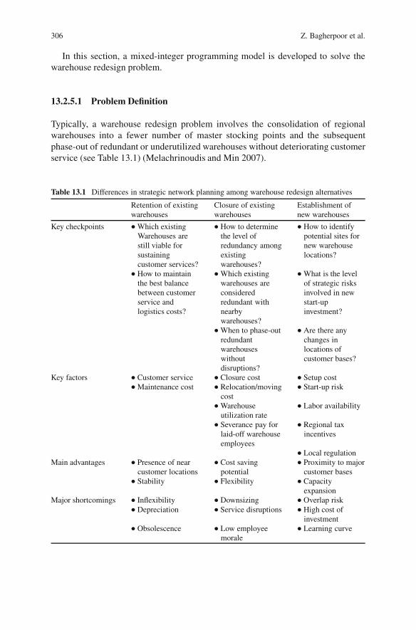
306 Z. Bagherpoor et al.
In this section, a mixed-integer programming model is developed to solve thewarehouse redesign problem.
13.2.5.1 Problem Definition
Typically, a warehouse redesign problem involves the consolidation of regionalwarehouses into a fewer number of master stocking points and the subsequentphase-out of redundant or underutilized warehouses without deteriorating customerservice (see Table 13.1) (Melachrinoudis and Min 2007).
Table 13.1 Differences in strategic network planning among warehouse redesign alternatives
Retention of existingwarehouses
Closure of existingwarehouses
Establishment ofnew warehouses
Key checkpoints Which existingWarehouses arestill viable forsustainingcustomer services?
How to determinethe level ofredundancy amongexistingwarehouses?
How to identifypotential sites fornew warehouselocations?
How to maintainthe best balancebetween customerservice andlogistics costs?
Which existingwarehouses areconsideredredundant withnearbywarehouses?
What is the levelof strategic risksinvolved in newstart-upinvestment?
When to phase-outredundantwarehouseswithoutdisruptions?
Are there anychanges inlocations ofcustomer bases?
Key factors Customer service Closure cost Setup cost Maintenance cost Relocation/moving
cost Start-up risk
Warehouseutilization rate
Labor availability
Severance pay forlaid-off warehouseemployees
Regional taxincentives
Local regulationMain advantages Presence of near
customer locations Cost saving
potential Proximity to major
customer bases Stability Flexibility Capacity
expansionMajor shortcomings Inflexibility Downsizing Overlap risk
Depreciation Service disruptions High cost ofinvestment
Obsolescence Low employeemorale
Learning curve
13 Warehouse Location Problem 307
13.2.5.2 Model Assumptions
1. The warehouses are owned by the company (private).2. When a warehouse is consolidated into another warehouse, its whole capacity is
relocated.3. The restructuring plan covers a planning horizon within which no substantial
changes are likely in the customer demands and in the transportation infrastruc-ture.
4. Although the company distributes its products in various quantities, customerorders are aggregated into a single product.
13.2.5.3 Model Inputs
i : index for manufacturing plants i ,k: index for customers; k 2 K ,j : index for existing warehouses and new candidate sites for relocation and con-solidation; j 2 A,sets: A D E [N I .j; l/ 2 .E A/E: set of existing warehousesN : set of new candidate sites for relocation and consolidation.Vij : Unit production cost (including storage cost) at manufacturing plant i plusunit transshipment cost between manufacturing plant i and warehouse jSjk : Unit warehousing cost at warehouse j and unit transportation cost betweenwarehouse j and customer krlj : Cost of moving and relocating unit capacity l to consolidated site j .l¤j /cj : Throughput capacity of existing warehouse jqi : Production capacity of manufacturing plant idk : Demand of customer kfcj : Cost per unit capacity of warehouse jfmj : Fixed cost of maintaining warehouse j , excluding capacity costfsj : Cost savings resulting from the closure of existing warehouse jtjk : Truck delivery time (in hours) from warehouse j to customer k� : Maximum of customer access time (in hours) from serving warehouses
C.j / D fkjtjk � �g; (13.40)
D.k/ D fj jtjk � τg: (13.41)
13.2.5.4 Model Outputs (Decision Variables)
Xjk : Volume of products shipped from warehouse j to customer kYij : Volume of products supplied by plant i to warehouse j
308 Z. Bagherpoor et al.
zjl will be equal to 1 if capacity of warehouse j , is relocated to site l , or ifexisting warehouse j remains open and otherwise it will be equal to 0wj will be equal to 1 if a new warehouse established at site j and otherwise itwill be equal to 0
13.2.5.5 Objective Function and its Constraints
MinPi2I
Pj2A
vij yij C Pj2A
Pk2C.j /
sjk xjk C Pl2E
Pj2A
rlj zlj C Pj2A
f cj
Pl2E
cl zlj
C Pj2E
f mj
zjj C Pj2N
f mj wj � P
l2E
"f sl
1 � P
j2Azlj
!C f m
l
Pfj2E;j¤lg
zlj
#;
(13.42)
Subject to Xj2A
yij � qi 8i 2 I; (13.43)
Xi2I
yij DXk2C.j /
xjk 8j 2 A; (13.44)
Xk2C.j /
xjk �Xl2E
cl xlj 8j 2 A; (13.45)
Xj2D.k/
xjk D dk 8k 2 K; (13.46)
Xl2E
zlj � jEj zjj 8j 2 E; (13.47)
Xl2E
zlj � jEj wj 8j 2 N; (13.48)
Xj2A
zlj � 1 8l 2 E; (13.49)
xjk � 0 8j 2 A; k 2 K; (13.50)yij � 0 8i 2 I; j 2 A; (13.51)
zlj ;wj 2 f0; 1g 8l 2 E; j 2 A: (13.52)
Equation (13.42) minimizes total supply chain costs comprised of production, trans-portation, warehousing, and relocation costs, while maximizing the cost savings re-sulting from the closure or consolidation of redundant warehouses. Equation (13.43)assure that the total volume of products shipped to warehouses do not exceed thecapacity of the manufacturing plant supplying those products. Equation (13.44) in-sure that the total volume of products supplied by the manufacturing plant to eachwarehouse matches the total volume of products shipped from that warehouse to
13 Warehouse Location Problem 309
its customers. In other words, inbound shipping volume for each warehouse mustbe equal to its outbound shipping volume. Equation (13.45) insure that the totalvolume of products shipped to customers can not exceed the throughput capac-ity (after consolidation) of the warehouse serving them. Equation (13.46) ensurethat the customer demand is satisfied. Equation (13.47) state that the current re-sources (i.e., capacity) of an existing warehouse can not be consolidated into anotherexisting warehouse, unless such a consolidated warehouse remains open. Equa-tion (13.48) state that the capacity of an existing warehouse cannot be relocated toa new site, unless a warehouse is established at the new site. Equation (13.49) con-sider various options for an existing warehouse j . These options include: keepingthe warehouse open .zjj D 1/, consolidating its capacity into another existing ware-house j 2 E; j ¤ l.zlj D 1/, relocating its capacity to a new site i 2 N.zlj D 1/,or closing the existing warehouse l
�zlj D 0 8i 2 A�. Equations (13.50)–(13.51) as-
sure the non negativity of decision variables xjk; yij . Equation (13.52) state that zi land wj are zero-one variables (Melachrinoudis and Min 2007).
13.3 Solution Methods
To solve small WLPs, integer programming optimization methods are used. How-ever, for larger problems, heuristic methods or Meta heuristic methods are utilized.
13.3.1 Exact Solution Methods
The UWLP has attracted considerable attention in mathematical programming.Khumawala (1972) developed a branch and bound algorithm for uncapacitatedwarehouse location problems. Akinc and Khumawala (1977) developed a branchand bound algorithm for capacitated warehouse location problems. Also basedon dual and primal–dual approaches branch and bound algorithms were devel-oped (Erlenkotter 1978; Korkel 1989). Dual-based and primal–dual algorithms arevery effective for the UWLP on the OR Library benchmarks. However, they expe-rience significant difficulties and exhibit exponential behavior on the M� instances(Kratica et al. 2001). These instances stimulate real situations, have a large num-ber of suboptimal solutions, and exhibit a strong tension between transportationand fixed costs, which makes it difficult to eliminate many warehouses early in thesearch (Michel and Hentenryck 2004).
Lagrangian relaxation is a well known technique for calculating lower boundsin branch and bound algorithms. In order to solve CWLP, Geoffrion and Graves(1974), Geoffrion and Nauss (1977), and Christofides and Beasley (1983) have useda Lagrangian relaxation of the demand constraints.
Baker (1986) proposed another Lagrangian relaxation for the demand constraintsto obtain lower band. In order to converge to optimal set of multiplier, he proposed
310 Z. Bagherpoor et al.
a heuristic algorithm. The computational result shows that the algorithm based onpartial dual approach has performed well and generally produced results which areas good as, or better than those of the previously accepted based on a Lagrangianrelaxation of demand constraints.
Beasley (1988) presented a lower bound for the capacitated warehouse locationproblem based upon Lagrangian relaxation of a mixed-integer formulation of theproblem. Feasible solution exclusion constraints are used together with problem re-duction tests derived from both the original problem and the Lagrangian relaxation.By incorporating the lower bound and the reduction tests into a tree search proce-dure solving problems involving up to 500 potential warehouse locations and 1,000customers is possible.
Subgradient optimization is a popular method of finding a good set of multi-pliers for use in Lagrangian relaxation. Baker and Sheasby (1999) developed amodel for obtaining faster convergence. The method was developed within a studyof the generalised assignment problem (GAP) and its application to vehicle routing.The method was applied to benchmark capacitated warehouse location problems(CWLPs).
Lee (1993) presented an algorithm for solving multi products capacitated ware-house location problem based on cross-decomposition, to reduce the computationaldifficulty by incorporating Benders decomposition and Lagrangian relaxation. Thealgorithm solves problems of practical sizes in acceptable times.
Sweeny and Tatham (1976) presented a mixed integer programming formula-tion for the single period warehouse location model with a dynamic programmingprocedure for finding the optimal sequence of configurations over multiple periods.
Kelly and Marucheck (1984) proposed an algorithm for dynamic WLP. First, themodel is simplified and then a partial optimal solution is obtained through iterativeexaminations by both upper and lower bounds on savings realized if a site is openedin a given time period. A complete optimal solution is obtained by solving the re-duced model with Benders’ decomposition procedure. The optimal solution is thentested to determine which time periods contain tentative decisions that may be af-fected by post-horizon data. The relationship between the lower (or upper) boundsutilized in the model simplification time period is analyzed.
Dupont (2008) presented a branch and bound algorithm for a facility locationproblem with concave site dependent costs.
Sharma et al. (2007) presented new formulations and relaxations for single stagecapacitated warehouse location problem. In this paper different formulations andrelaxations were compared with each other.
13.3.2 Heuristic and Metaheuristic Methods
Because of the nature of many warehouse location problems, the exact methods cannot be used to solve them, so heuristic & Meta heuristic methods can be used.
Genetic algorithms have been shown to be very successful on the UWLP. In aseries of papers spanning over several, Kratica et al. (2001) have shown that genetic
13 Warehouse Location Problem 311
algorithms find optimal solutions on the OR Library and the M� instances (wheneverthe optimal solutions are known) with high frequencies and very good efficiency.Their final algorithm uses clever implementation techniques such as caching andbit vectors to avoid recomputing the objective function which is quite costly onlarge-scale problems. Also, the speed-up of the genetic algorithm over mathemati-cal programming approaches increases exponentially with problem size on the M �instances.
Various heuristic search algorithms have also been proposed but have been lesssuccessful. Alves and Almedia (1992) presented simulated annealing algorithmswhich produce high-quality solutions but are quite expensive in computation times(Michel and Hentenryck 2004).
Al-Sultan and Al-Fawzan (1999) presented a tabu-search algorithm. The algo-rithm generates 5n neighbors at each iteration and moves to the best neighbor whichis not tabu and improves the current value of the objective function. Each of these it-erations takes significant computing time, which limits the applicability of the algo-rithm. Michel and Hentenryck (2004) presented another tabu search algorithm. Thealgorithm uses a linear neighborhood and essentially takesO.m log n/ time per iter-ation. It finds optimal solutions on the OR Library and theM � instances (wheneverthe optimal solution is known) with high frequencies. It also outperforms the state ofthe-art genetic algorithm of Kratica et al. (2001), both in efficiency and robustness.
Kuehn and Hamburger (1963) and Whitaker (1985) presented Greedy- Bumpand Shift (Interchange) heuristics algorithms. In the Greedy process, warehousesare located at the most economical positions, one at a time, until no additional ware-houses can be added without increasing the total cost. In the Bump process, thosewarehouses that became uneconomical as a result of the placement of subsequentwarehouses are eliminated. In the Shift process, a warehouse is shifted to anotherpotential location in the same territory if the relocation causes a reduction of thetotal cost.
Heras and Larrosa (2006) analyzed the effect of heuristic orders at three levels ofincreasing overhead: (a) compute the order prior to search and keep it fixed duringthe whole solving process (this is called a static order), (b) compute the order atevery search node using current sub problem information (this is called a dynamicorder) and iii) compute a sequence of different orders at every search node andsequentially enforce the local consistency for each one (this is called dynamic re-ordering).They performed experiments in three different problems: Max-SAT, Max-CSP and warehouse location problems. They did not find an alternative better thanthe rest for all the instances.
Lee (1996) proposed an optimal solution algorithm based on the cross decompo-sition method for multi type capacitated distribution center location problem. Thecross decomposition method can be applied to solve this problem because both theprimal and dual sub problems are relatively easy to solve and both sub problemsquickly converge. Tight lower and upper bounds can be obtained in just a few iter-ations of the proposed algorithm. This algorithm can be used as a heuristic whichproduces not just a feasible solution but also a confidence interval to measure thequality of the solution. The algorithm was implemented in FORTRAN.
312 Z. Bagherpoor et al.
13.4 Case Study
In this section, we describe some applications of the warehouse location problem inreal world.
13.4.1 Redesigning a Warehouse Network(Melachrinoudis and Min 2007)
The model which was described in the last section is a case study of a firm whichplans to redesign its warehouse network and reduce its total logistics costs. Betahas its main manufacturing plant in Terre Haute, Indiana, and currently operates21 warehouses to serve a total of 281 customers scattered around the United Statesand Canada. The warehouse consolidation problem (WCP) facing Beta differs fromthe classical warehouse location problem in that the former is primarily concernedwith determining which existing warehouses to keep open, which new warehousesto establish, and which warehouses to phase-out among the existing locations,whereas the latter is primarily concerned with selecting the optimal site amongthe alternatives of new locations. In this problem, 25 warehouse locations, includ-ing 4 candidate sites were existed. The target problem was solved and analyzed byLINGO optimization software.
Out of the 281 customers, only four have non-unique warehouse assignments andeach one of those four customers receives partial demand allocations from exactlytwo warehouses.
13.4.2 Warehouse Location Problems for Air Freight Forwarders(Wan et al. 1998)
The move of Hong Kong International Airport from the city centre to a suburbanarea in July 1998 provided sufficient capacity to meet the increasing demand ofpassenger and air-cargo flows in Hong Kong in the foreseeable future. However, themove has had adverse side effects such as causing the readjustment of many existingsystems and creating many imminent strategic problems. One of such problems isthe warehouse location of freight forwarders: They have to decide whether theyshould locate their warehouses in the new airport, in current locations, or in newlocations somewhere in the city.
In this case, air freight forwarders had then been facing the decision on whetherthey should (1) move their warehouses to the new airport, (2) stay in the currentlocations, (3) move the warehouses to new locations in the city, (4) keep the currentwarehouses and add an additional one in Chek Lap Kok (CLK), and (5) move thecurrent warehouses to new locations in city and add one in CLK.
13 Warehouse Location Problem 313
With the special structure of a toll bridge for the (CLK) airport, this problemis in exactly the same form as the one-median location problem on a tree networkby using a decomposition approach. The problem can be solved by the Chinesealgorithm or its modified version, the majority algorithm.
References
Akinc U, Khumawala BM (1977) An efficient branch and bound algorithm for the capacitatedwarehouse location problem. Manage Sci 23(6):585–594
Alves ML, Almedia MT (1992) Simulated annealing algorithm for simple plant location problems.Revista Investigacao Operationanl 12
Al-Sultan KS, Al-Fawzan MA (1999) A tabu search approach to the uncapacitated facility locationproblem Ann Oper Res 86:91–103
Baker BM (1986) A partial dual algorithm for the capacitated warehouse location problem. Eur JOper Res 23:48–56
Baker BM, Sheasby J (1999) Accelerating the convergence of subgradient optimization. Eur J OperRes 117:136–144
Beasley JE (1988) An algorithm for solving large capacitated warehouse location problems. Eur JOper Res 33:314–323
Christofides N, Beasley JE (1983) Extensions to a Lagrangian relaxation approach for the capaci-tated warehouse location problem. Eur J Oper Res 12:19–28
Dupont L (2008) Branch and bound algorithm for a facility location problem with concave sitedependent costs. International Journal of Production Economics 112(1):245–254
Erlenkotter D (1978) A dual-based procedure for uncapacitated facility location. Eur J Oper Res26(6):992–1009
Geoffrion AM, Graves GV (1974) Multicommodity distribution system design by benders decom-position. Manage Sci 20(5):882–844
Geoffrion AM, Nauss R (1977) Parametric and postoptimality analysis in integer linear program-ming. Manage Sci 23(5):453–466
Heras F, Larrosa J (2006) Intelligent variable orderings and re-orderingsin DAC-based solvers forWCSP. J Heuristics 12:287–306
Kelly DL, Marucheck AS (1984) Planning horizon results for the dynamic warehouse locationproblem. J Oper Manage 4(3):279–294
Khumawala BM (1972) An efficient branch and bound algorithm for the warehouse location prob-lem. Manage Sci 18(12):585–594
Korkel M (1989) On the exact solution of large-scale simple plant location problems. Eur J OperRes 39:157–173
Kratica J, Tosic D, Filipovic V, Ljubic I (2001) Solving the simple plant location problem bygenetic algorithm. Oper Res 35:127–142
Kuehn A, Hamburger MJ (1963) A heuristic program for locating warehouses. Manage Sci9:643–666
Lee CY (1993) The multi product warehouse location problem: Applying a decomposition algo-rithm. Int J Phys Distrib Logist Manage 23(6):3–13
Lee CY (1996) An algorithm for a two-staged distribution system with various types of distributioncenters. INFOR 34(2):105–117
Melachrinoudis E, Min H (2007) Redesigning a warehouse network. Eur J Oper Res 176:210–229Michel L, Hentenryck PV (2004) A simple tabu search for warehouse location. Eur J Oper Res
157:576–591Nagy T (2004), Warehouse location problem. Available online at http://www.freehackers.org
314 Z. Bagherpoor et al.
Nuass RM (1978) An improved algorithm for the capacitated facility location problem. J Oper ResSoc 29(12):1195–1201
Sharma RRK, Berry V (2007) Developing new formulations and relaxations of single stage capac-itated warehouse location problem (SSCWLP): Empirical investigation for assessing; relativestrengths and computational effort. Eur J Oper Res 177:803–812
Sweeny DJ, Tatham RL (1976) An improved long-run model for multiple warehouse location.Manage Sci 7:748–758
Tompkins JA, White JA, Bozer YA, Frazelle EH, Tanchoco JMA, Trevino J (1996) Facility plan-ning, 2nd ed. Wiley, New York
Wan YW, Raymond K, Cheung, Liu J, Judy H, Tong (1998) Warehouse location problems forair freight forwarders: A challenge created by the airport relocation. J Air Transport Manage4:201–207
Whitaker RA (1985) Some add-drop and drop-add interchange heuristics for non-linear warehouselocation. J Oper Res Soc 36:61–70
William J, Baumol, Wolfe P (1958) A warehouse-location problem. Oper Res 6:252–263
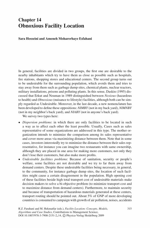
Chapter 14Obnoxious Facility Location
Sara Hosseini and Ameneh Moharerhaye Esfahani
In general, facilities are divided in two groups, the first one are desirable to thenearby inhabitants which try to have them as close as possible such as hospitals,fire stations, shopping stores and educational centers. The second group turns outto be undesirable for the surrounding population, which avoids them and tries tostay away from them such as garbage dump sites, chemical plants, nuclear reactors,military installations, prisons and polluting plants. In this sense, Daskin (1995) dis-cussed that Erkut and Neuman in 1989 distinguished between Noxious (hazardousto health) and Obnoxious (nuisance to lifestyle) facilities, although both can be sim-ply regarded as Undesirable. Moreover, in the last decade, a new nomenclature hasbeen developed to define these oppositions: NIMBY (not in my back yard), NIMNBY(not in my neighbor’s back yard), and NIABY (not in anyone’s back yard).
We survey two types here:
� Dispersion problems: in which there are only facilities to be located in sucha way as to affect each other the least possible. Usually, Cases such as salesrepresentative of some organizations are addressed in this type. The mother or-ganization intends to minimize the comparison among its sales representativeand cover more areas via maximizing distance between them. Note that in somecases, investors interestedly try to minimize the distance between their sales rep-resentative, for instance you can imagine two restaurants with same ownership,although they are placed in one area for making more customers, not only theydon’t lose their customers, but also make more profits.
� Undesirable facilities problems: Because of sanitation, security or people’swelfare, some facilities are not desirable and we try to far them away fromdemand centers. Despite these undesirable facilities being necessary, in general,to the community, for instance garbage dump sites, the location of such facil-ities might cause a certain disagreement in the population. High opening costof these facilities beside high total transport cost of undesirable materials makedecision makers to solve a bi-objective problem (to minimize transport cost andto maximize distance from demand centers). Furthermore, to maintain securityand because of transportation of hazardous materials generated at these centers,transport routing should be pointed out. About 5% of GNP of more developingcountries is consumed to campaign with growth of air pollution, noises, accidents
R.Z. Farahani and M. Hekmatfar (eds.), Facility Location: Concepts, Models, 315Algorithms and Case Studies, Contributions to Management Science,DOI 10.1007/978-3-7908-2151-2 14, c� Physica-Verlag Heidelberg 2009
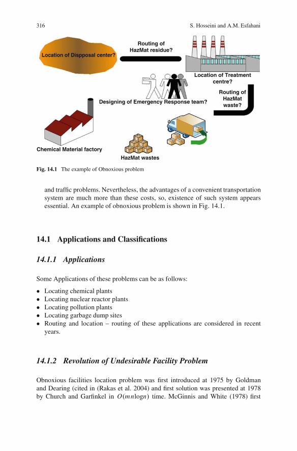
316 S. Hosseini and A.M. Esfahani
HazMat wastes
Designing of Emergency Response team?
Location of Dispposal center?
Routing ofHazMat residue?
Routing ofHazMatwaste?
Location of Treatmentcentre?
Chemical Material factory
Fig. 14.1 The example of Obnoxious problem
and traffic problems. Nevertheless, the advantages of a convenient transportationsystem are much more than these costs, so, existence of such system appearsessential. An example of obnoxious problem is shown in Fig. 14.1.
14.1 Applications and Classifications
14.1.1 Applications
Some Applications of these problems can be as follows:
� Locating chemical plants� Locating nuclear reactor plants� Locating pollution plants� Locating garbage dump sites� Routing and location – routing of these applications are considered in recent
years.
14.1.2 Revolution of Undesirable Facility Problem
Obnoxious facilities location problem was first introduced at 1975 by Goldmanand Dearing (cited in (Rakas et al. 2004) and first solution was presented at 1978by Church and Garfinkel in O.mnlogn/ time. McGinnis and White (1978) first
14 Obnoxious Facility Location 317
introduced a bicriteria problem, using the minisum–minimax criteria. Drezner andWesolowsky (1983) first introduced the rectilinear maximin problem for locatingan obnoxious facility. Ting devised a linear time algorithm for the 1-maxisumproblem on tree networks at 1984. Mehrez et al. (1986) suggested an improve-ment of previous algorithm, based on bounds, which reduced the size of model.Batta and Chiu (1988) present a hazardous material transportation model on a net-work in which sum of distances of container within a threshold limit from demandcenters, is minimized. Ratick and White (1988) develop a multiobjective model,minimizing costs and people’s repulsion simultaneously. In this case Wayman andKuby (1994) present a model with three objectives: Minimization of risk andcost and maximization of equity. Gopalan et al. (1990) model the equity of theHazMat transport risk and present a heuristic solution. At 1995, Melachrinoudisand Smith extended an algorithm with “m” edges and “n” nodes as obnoxiousfacilities, assuming Euclidean spatial distances. But that was not the end of re-searches and different types of these problems with various assumptions werereviewed at those years. Marianov and ReVelle (1998) model a linear vehicle rout-ing problem, minimizing cost and risk simultaneously. Erkut and Verter (1998)model transport risk completely and review various methods. Rogers (1998) pro-pose a model to minimize the global repulsion of the inhabitants of the region.Results show that insecurity of region is the most important reason for nega-tive reaction of people. Giannikos (1998) use the goal-programming techniquefor obnoxious facility location-routing problem. In 1999, Melachrinoudis devel-oped a bicriteria location model for locating a new semi-obnoxious1 facility inan existing layout which is solved by an adaptation of the Fourier–Motzkin elim-ination method. Zagrafos and samara presented a methodological framework fordeveloping a decision support system (DSS) for hazardous materials emergencyresponse operations (Erkut and Alp 2007). Cases such as Routing emergency re-sponse teams and evacuation of region from people and cars were considered inthis paper. Fernandez et al. (2000) address a continuous location within a givengeographical region of an undesirable facility considering environmental aspects.Akgun et al. (2000) review cases which decision maker seeks for various trans-port routes. Zhang et al. (2000) devise a routing hazardous materials algorithm,using GIS2 technique and a Gaussian Plume model for their dispersion model.One of its applications is to transport urban hazardous wastes. Katz et al. (2002)propose a maximin model for multi-facility location. Here the distance betweeneach facility and demand centers should be considered beside distances amongfacilities.
Cappanera et al. (2004) addressed the problem of simultaneously locating ob-noxious facilities and routing obnoxious materials between a set of built-up areasand the facilities. Rakas et al. (2004) propose a multiobjective model with fuzzydata for the location of undesirable facilities. Castillo (2004) reviewed the issuesrelated to hazmat transportation risks and discussed the modeling tool available for
1 These facilities service to demand points; nevertheless, they are undesirable for them.2 Geographic information system
318 S. Hosseini and A.M. Esfahani
routing problem of hazardous materials. Also, a route optimization model is devel-oped as a decision support tool. Rodriguez et al. (2006) considered Euclidean traveldistances for obnoxious facilities location problem. Colebrook et al. (2005) havedeveloped a new bound and a new O(mn) algorithm to solve the network maxianproblem. Erkut and Ingolfsson (2005) formulated the tree design problem as an in-teger programming problem aiming at trade off between cost and risk. Dıaz-Banezet al. (2005) computed shortest paths for transportation of hazardous material incontinuous spaces. They proposed an approximate algorithm based on the bisectionmethod and reduced the optimization problem to a decision problem, where oneneeds to compute the shortest path such that the minimum distance to the demandpoints is not smaller than a certain amount r . Pisinger (2006) present an exact algo-rithm for finding a number of fast upper bounds for P -dispersion problems in whichthese bounds can be derived inO.n/ time. Bell (2006) considered mixed rout strate-gies for the risk-averse shipment of hazardous materials. He believes, for repeatedshipments on the arc with unknown incident probabilities, the safest strategy is touse a mix of routes.
Berman et al. (2007) extended an optimum model for designing emergency re-sponse networks for hazardous materials transportation that would be applicable forlarge-scale problems.
Alumur and Kara (2007) develop a comprehensive multi objective model for thehazardous waste location-routing problem that covers various problems of this field.For exact solving in a case study, GIS technique and CPLEX software were used.Akgun et al. (2007) consider effects of weather systems on HazMat transportation.They introduced weather system effects as circle areas with different probabilitieson accident rate, speed, delays and others. They use time dependent shortest pathproblem in form of an exact model and four heuristic models. They concluded insuch weather systems accident rates can be double. Carotenuto et al. (2007) modela hazmat shipment routing and scheduling problem. They develop a tabu searchalgorithm to assign a minimum and equitable risk route to each hazmat shipmentand schedule these shipments on the assigned routes.
14.1.3 Classification of Undesirable Facility Problems
� Area solution: Discrete, Continual� Number of Objective function: Multiobjective, Single objective� Category: Location, Routing, Location-Routing� Determine the number of nodes: Exogenous, Endogenous� Facility capacity: Unlimited, Limited� Technology assignment: non-assignment, assignment� Number of type of hazardous waste: one type, more than one type
14 Obnoxious Facility Location 319
14.2 Models
14.2.1 Dispersion Problem (Daskin 1995)
In this problem, suppose that there are some candidate centers for installation fa-cilities. The purpose is to find P points for locating in order that maximize theminimum distance between located facilities. In other word, the decision makerknows the number of locatable facilities and candidate centers then, he tries to se-lect set of points that maximize the minimum distance between them.
14.2.1.1 Model Assumptions
� The problem is investigated on the discrete network and nodes are representativeof candidate points.
� This network is general or it’s possible to have loops.� The facilities often are general. In other word, investor (government) focuses on
keeping away facilities from population centers. In these cases, environmentalcosts and some other ones are more important than installation costs.
� The numbers of facilities are predetermined.� All of facilities are obnoxious and should be kept away from population centers.� All of facilities are similar and all of services are equal too.� The installation cost is not considered.� The facilities replacement is not considered.� All of parameters are deterministic.� The problem is formulated in static form. It means that, the problem’s inputs are
not dependent to time.
14.2.1.2 Model Inputs
dij: it is distance between i and jM : it is large elected digit and it is often larger than the maximum distancebetween candidate pointsP : the number of facility to locateD: the minimum distance between facilities
14.2.1.3 Model Outputs (Decision variables)
Xj : 1 if facility is installed in node j ; 0 otherwise
320 S. Hosseini and A.M. Esfahani
14.2.1.4 Objective Function and its Constraints
Max D (14.1)
Subject toXj
Xj D P (14.2)
D � dijC.M � dij/:.1 �Xi/C.M � dij/:.1 � Xj / 8j I 8i j: (14.3)
Xj 2 f0; 1g 8j (14.4)
Equation (14.1) maximizes the minimum distance between facilities. Equation(14.2) represents that number of located facilities, should be P .
Equation (14.2) determines the minimum distance along distance between eachpair of facilities and finally the third constraint shows that Xj is 0, 1 variable.
To achieve better perception of (14.2), consider the following explanations:
� If Xi D Xj D 1 (install facility in node i; j ), so D � dij and it means thatthe minimum distance between each pair of facilities can’t be more than fromdistance between facilities, certainly it is obvious.
� If Xi D 0; Xj D 1 or Xi D 1; Xj D 0 means that, only one facility is locatedin node i; j .
� So, (14.2) will be D � M . It’s clear because M is more than all of coupledistances.
� Now, consider the case that Xi D 0;Xj D 0. In this case, (14.2) will be M �Maxi; j fdijg and, it’s reasonable too.
Researchers didn’t focus much on relationship between dispersion models andother models. As one example in this case, we can refer to Kuby (1987). He hasillustrated the relationship between P -Dispersion and (P -1) Center.
14.2.2 Undesirable Facility Location Problem (Daskin 1995)
Locating some facilities such as fire stations and shopping centers, are consideredin recent decades. For example in locating a shopping center, we know that it shouldbe near and available to population centers. But it’s so important that, we consider inlocating factors such as decreasing noise, heavy traffic in that center, related crimesand people’s tranquility of mind. These factors make problem more complex. Theinvestigated model in this section is P -Median transformed model and for the rea-son that facilities are undesirable, the objective function is maximization. In Medianproblems because of desirability of facilities such as hospitals and fire stations, the
14 Obnoxious Facility Location 321
objective function is minimization. But in Maxisum models, the subject is locatingfacilities such as incinerators that, decision maker attend to far it from demand cen-ters. Of course, it is obvious that we can’t eliminate transportation cost.
14.2.2.1 Model Inputs
P : the number of facilities should be located
14.2.2.2 Model Outputs (Decision Variables)
hi : demand of node iDistance between demand nodes i and candidate place j dij:Xj : 1 if facility is located at node j ; 0 otherwiseYij: 1 if demand of node i was provided by located facility at node j ; 0 otherwise
14.2.2.3 Objective Function and its Constraints
MaxXi
Xj
hidijyij; (14.5)
Xj
Yijij D 1 8i; (14.6)
Xj
Xj ij D P; (14.7)
Yij � Xj 8i; j; (14.8)
Xj D 0; 1 8j; (14.9)
Yij D 0; 1 8i; j: (14.10)
Equation (14.5) minimizes the weighted sum of demands and distances.The (14.6) represent that demands of all nodes should responded by just one
facility. The (14.7) considers the number of all facilities equal P . Equation (14.8)ensures that if any facility is located at node j , demand of this node should re-sponded by itself. Equations (14.9) and (14.10) are integer limitations.
Example 14.1 was illustrated that the above model in reality doesn’t express na-ture of mentioned problem.
14.2.2.4 Example 14.1
A,B,C,D are demand centers, digits in boxes are demand amount of each place andon the line numbers represent distance between places that are connected with line
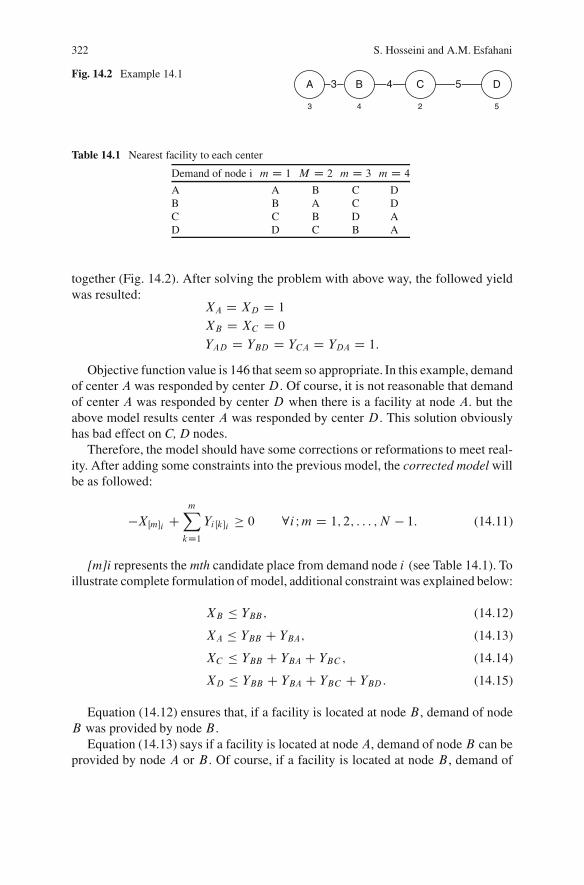
322 S. Hosseini and A.M. Esfahani
Fig. 14.2 Example 14.1A 3
3 4 2 5
B 4 C 5 D
Table 14.1 Nearest facility to each center
Demand of node i m D 1 M D 2 m D 3 m D 4
A A B C DB B A C DC C B D AD D C B A
together (Fig. 14.2). After solving the problem with above way, the followed yieldwas resulted:
XA D XD D 1
XB D XC D 0
YAD D YBD D YCA D YDA D 1:
Objective function value is 146 that seem so appropriate. In this example, demandof center A was responded by centerD. Of course, it is not reasonable that demandof center A was responded by center D when there is a facility at node A. but theabove model results center A was responded by center D. This solution obviouslyhas bad effect on C, D nodes.
Therefore, the model should have some corrections or reformations to meet real-ity. After adding some constraints into the previous model, the corrected model willbe as followed:
�XŒmi CmXkD1
YiŒki � 0 8i Im D 1; 2; : : : ; N � 1: (14.11)
[m]i represents the mth candidate place from demand node i (see Table 14.1). Toillustrate complete formulation of model, additional constraint was explained below:
XB � YBB; (14.12)
XA � YBB C YBA; (14.13)
XC � YBB C YBA C YBC ; (14.14)
XD � YBB C YBA C YBC C YBD: (14.15)
Equation (14.12) ensures that, if a facility is located at node B , demand of nodeB was provided by node B .
Equation (14.13) says if a facility is located at node A, demand of node B can beprovided by node A or B . Of course, if a facility is located at node B , demand of
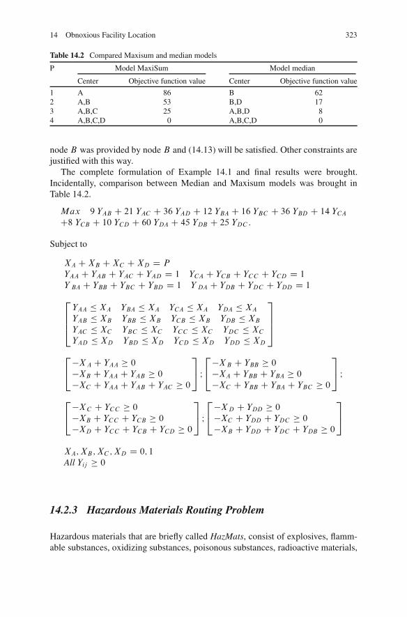
14 Obnoxious Facility Location 323
Table 14.2 Compared Maxisum and median models
P Model MaxiSum Model median
Center Objective function value Center Objective function value
1 A 86 B 622 A,B 53 B,D 173 A,B,C 25 A,B,D 84 A,B,C,D 0 A,B,C,D 0
node B was provided by node B and (14.13) will be satisfied. Other constraints arejustified with this way.
The complete formulation of Example 14.1 and final results were brought.Incidentally, comparison between Median and Maxisum models was brought inTable 14.2.
Max 9 YAB C 21 YAC C 36 YAD C 12 YBA C 16 YBC C 36 YBD C 14 YCAC8 YCB C 10 YCD C 60 YDA C 45 YDB C 25 YDC :
Subject to
XA CXB CXC CXD D P
YAA C YAB C YAC C YAD D 1 YCA C YCB C YCC C YCD D 1
Y BA C YBB C YBC C YBD D 1 Y DA C YDB C YDC C YDD D 1
2664YAA � XA YBA � XA YCA � XA YDA � XAYAB � XB YBB � XB YCB � XB YDB � XBYAC � XC YBC � XC YCC � XC YDC � XCYAD � XD YBD � XD YCD � XD YDD � XD
3775
24�XA C YAA � 0
�XB C YAA C YAB � 0
�XC C YAA C YAB C YAC � 0
35 I24�XB C YBB � 0
�XA C YBB C YBA � 0
�XC C YBB C YBA C YBC � 0
35 I
24�XC C YCC � 0
�XB C YCC C YCB � 0
�XD C YCC C YCB C YCD � 0
35 I24�XD C YDD � 0
�XC C YDD C YDC � 0
�XB C YDD C YDC C YDB � 0
35
XA;XB;XC ;XD D 0; 1
All Yij � 0
14.2.3 Hazardous Materials Routing Problem
Hazardous materials that are briefly called HazMats, consist of explosives, flamm-able substances, oxidizing substances, poisonous substances, radioactive materials,
324 S. Hosseini and A.M. Esfahani
infected materials, corrosives and hazardous wastes (Erkut and Verter 1995). Basi-cally these materials are used in many facilities and processes in the industry such aspetroleum refineries, chemical plants and nuclear reactors or hospital’s wastes. Dueto the nature of hazmats, many risks related to production, storage and transporta-tion of these materials could arise. In the case of transporting hazmats, the selectionof routes considering economic and risk issues is a very important problem andneeds to an integrated transport and risk management. Therefore, the term “optimalroutes” means the route that best fulfils the objectives by the stakeholders associatedwith transporting and distributing of HazMats within the study area.
It’s not possible to completely avoid risks, nevertheless risk management activi-ties such as mitigation and prevention would be useful. These activities are reviewedas two groups: proactives and reactives. Some cases such as driver training, restric-tion of driving hours and container specifications are considered in proactives andsome cases such as firefighting, emergency response and evacuation of region frominhabitants and cars are of reactives.
To understand its importance, we mention some examples of transportingHazMats:
� Every year, approximately, 4 billions shipments of these materials are trans-ported, in other word, 20% of traveling trucks (one in every five) in USA carryHazMats.
� The difference between the transportation of HazMats and any other ones is, inthis case any accident may cause serious damages for people, animals and plants.
� In 1976, as the explosion of a small chemical plant in small city of Seveso andreleased Dioxin, 190 persons damaged seriously and thousands of birds werekilled.
� Afghanistan, 1982, the explosion of a truck, carrying gasoline, in a tunnel killed2,700 persons.
� India, 1984, the Methil-Iso-Cianate leakage in Bhopal area, killed 400 persons.
Annually, about 2.5 million tons of garbage are generated in Tehran that man-agement cost of these huge volumes is 600 billion rials. It is evident that applyinga quick and efficient transportation system is one of the most important ways forreduction of such costs. From other hand, management of hospital-garbage is oneof the most important problems that exist in our country.
Basically, routing of HazMats is done by governments, also because of high sen-sitivity of society toward these accidents, fixed costs of opening facilities are not beconsidered in most of these models, in contrast, risk and equity assessment meth-ods are always be considered. Routing of HazMat is as important as locating them,because these two issues are relevant to each other strictly. In recent decades, re-searchers had more studies in this matter.
One of the recent research studies was published by Akgun et al. (2007) in-vestigated HazMat routing problem with weather systems considerations. Weathersystem effects on accident probability, speed, time duration, risk and cost relatedto HazMat transportations. For example it can lead to change routs, reduce speed,delaying shipment, increase parking times and other issues. Due to the dynamic
14 Obnoxious Facility Location 325
nature of weather system and hence the time varying nature of the weights on linksin the transportation network, time-dependent shortest paths problems (TDSPP)should be considered. TDSPP was first introduced by Cook and Halsey with usingfinite departure times from every node to the destination. TDSPP approach wasdeveloped continuously after that. For example, Ziliakopoulos and Mahmassaniintroduced an algorithm that calculates the TDSP’s from all nodes to the destina-tion for every time step over a given time horizon. Cia et al., Erkut and Alp andNozik researches were focused on TDSPP. Akgun et al. (2007) focused on the ef-fect of weather systems on hazmat routing. They characterized the time dependentattributes of a link due to movement of the weather system. They aimed to finda least risk path for hazmat transportation under variable weather system. Theyapplied one exact model for routing, Time-dependent shortest Path problem, andfour heuristic model such as k-shortest path heuristic (KPATH), dissimilar pathheuristic (DISSIM), Iterative weather system heuristic (IWS) and finally Myopicshortest path heuristic (MYOPIC). They compared exact model with heuristics andheuristics with each others too. They consider a circle area for weather system thatcan move by time and weights that in some methods were constant and in someothers were inconstant.
14.2.3.1 Risk Evaluation for Hazardous Waste Transportation
Risk management activities could result in an accurate assessment of the risks andtherefore it would be possible to create strategies for reduction of risk level to itslowest level. We have expanded models with different conditions in subject of riskevaluation. Erkut and Verter (1998) suggested much evaluation risk models. Thesimplest model in this category yields the product of the accident consequences, theprobability of a hazardous waste accident, activity volume.
Risk D accident consequences probability of a hazardous
waste accident activity volume:
Generally, the accident consequences are measured by population exposure andthe accident probability depends on material type and rout nature. In practice, therout is divided to equal segments (k/m or mile) then; the consequences probabilityis calculated for all segments by population exposure in accident place.
In this equation assumed that, if an accident happens at centerA, people are influ-enced in circle with radius of R. The assumed radius is considered 0–7 km and theconsequences accident is measured through the Worst-case. It means that withoutconsidering geographical, climate and topography conditions, all exposure peoplein assumed circle will perish. Other developed way for calculating the consequencesaccident, presented by Raj and Glikman who discussed about effects of wind and airinstability in the consequences accident in 1991 (see Fig. 14.3). It made the modelso complex, but so similar to reality.
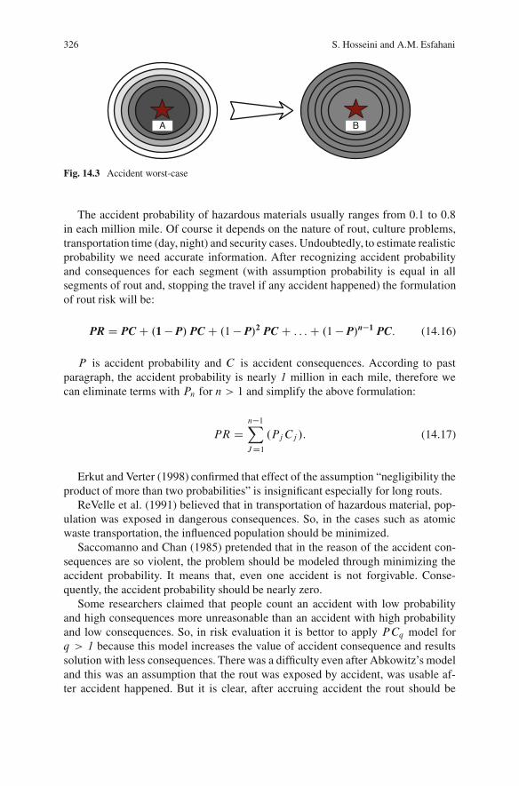
326 S. Hosseini and A.M. Esfahani
A B
Fig. 14.3 Accident worst-case
The accident probability of hazardous materials usually ranges from 0.1 to 0.8in each million mile. Of course it depends on the nature of rout, culture problems,transportation time (day, night) and security cases. Undoubtedly, to estimate realisticprobability we need accurate information. After recognizing accident probabilityand consequences for each segment (with assumption probability is equal in allsegments of rout and, stopping the travel if any accident happened) the formulationof rout risk will be:
PR D PC C .1 � P/ PC C .1 � P/2 PC C : : :C .1 � P/n�1 PC: (14.16)
P is accident probability and C is accident consequences. According to pastparagraph, the accident probability is nearly 1 million in each mile, therefore wecan eliminate terms with Pn for n > 1 and simplify the above formulation:
PR Dn�1XJD1
.PjCj /: (14.17)
Erkut and Verter (1998) confirmed that effect of the assumption “negligibility theproduct of more than two probabilities” is insignificant especially for long routs.
ReVelle et al. (1991) believed that in transportation of hazardous material, pop-ulation was exposed in dangerous consequences. So, in the cases such as atomicwaste transportation, the influenced population should be minimized.
Saccomanno and Chan (1985) pretended that in the reason of the accident con-sequences are so violent, the problem should be modeled through minimizing theaccident probability. It means that, even one accident is not forgivable. Conse-quently, the accident probability should be nearly zero.
Some researchers claimed that people count an accident with low probabilityand high consequences more unreasonable than an accident with high probabilityand low consequences. So, in risk evaluation it is bettor to apply PCq model forq > 1 because this model increases the value of accident consequence and resultssolution with less consequences. There was a difficulty even after Abkowitz’s modeland this was an assumption that the rout was exposed by accident, was usable af-ter accident happened. But it is clear, after accruing accident the rout should be
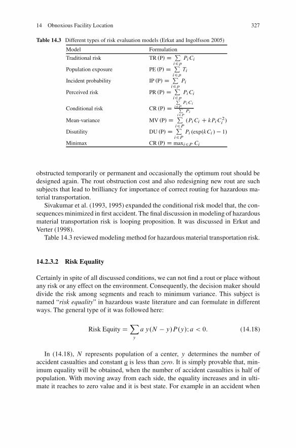
14 Obnoxious Facility Location 327
Table 14.3 Different types of risk evaluation models (Erkut and Ingolfsson 2005)
Model Formulation
Traditional risk TR .P/ D Pi2p
PiCi
Population exposure PE .P/ D Pi2p
Ti
Incident probability IP .P/ D Pi2p
Pi
Perceived risk PR .P/ D Pi2p
PiCi
Conditional risk CR .P/ DP
i2P
Pi CiPi2P
Pi
Mean-variance MV .P/ D Pi2P
.PiCi C kPiC2i/
Disutility DU .P/ D Pi2P
Pi .exp.kCi /� 1/
Minimax CR .P/ D maxi2P Ci
obstructed temporarily or permanent and occasionally the optimum rout should bedesigned again. The rout obstruction cost and also redesigning new rout are suchsubjects that lead to brilliancy for importance of correct routing for hazardous ma-terial transportation.
Sivakumar et al. (1993, 1995) expanded the conditional risk model that, the con-sequences minimized in first accident. The final discussion in modeling of hazardousmaterial transportation risk is looping proposition. It was discussed in Erkut andVerter (1998).
Table 14.3 reviewed modeling method for hazardous material transportation risk.
14.2.3.2 Risk Equality
Certainly in spite of all discussed conditions, we can not find a rout or place withoutany risk or any effect on the environment. Consequently, the decision maker shoulddivide the risk among segments and reach to minimum variance. This subject isnamed “risk equality” in hazardous waste literature and can formulate in differentways. The general type of it was followed here:
Risk Equity DXy
a y.N � y/P.y/I a < 0: (14.18)
In (14.18), N represents population of a center, y determines the number ofaccident casualties and constant a is less than zero. It is simply provable that, min-imum equality will be obtained, when the number of accident casualties is half ofpopulation. With moving away from each side, the equality increases and in ulti-mate it reaches to zero value and it is best state. For example in an accident when
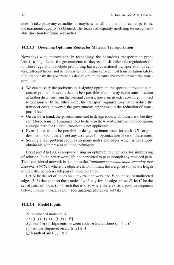
328 S. Hosseini and A.M. Esfahani
doesn’t take place any casualties or maybe when all population of center perishes,the maximum equality is obtained. The fuzzy risk equality modeling seems remark-able direction for future researches.
14.2.3.3 Designing Optimum Routes for Material Transportation
Nowadays with improvement in technology, the hazardous transportation prob-lem is as significant for governments as they establish inflexible regulations forit. These regulations include prohibiting hazardous material transportation in cen-ters, different times, and beneficiaries’ commitment for at most transportation safety.Simultaneously the governments design optimum routs and monitor material trans-portation.
� We can classify the problems in designing optimum transportation routs that in-creases problem. It seems that the best possible solution may be the transportationat farther distances from the demand centers; however, its extra costs are imposedto consumers. In the other word, the transport organizations try to reduce thetransport costs, however, the governments emphasize to the reduction of trans-port risks.
� On the other hand, the governments tend to design routs with lowest risk, but theycan’t force transport organizations to drive in these routs, furthermore, designinga unique path for HazMat transport is not applicable.
� Even if that would be possible to design optimum routs for each OD (origin-destination) pair, there’s not any assurance for optimization of set of these routs.
� Solving a real problem requires so many nodes and edges which is not simplyobtainable with present solution techniques.
Erkut and Alp (2007) proposed using an optimum tree network for simplifyingof solution. In the better word; it’s not permitted to pass through any replaced path.Their considered network is similar to the “optimum communication spanning treenetwork” (OCST), where the objective is to minimize the weighted sum of the lengthof the paths between each pair of nodes on a tree.
Let N be the set of nodes on a city road network and E be the set of undirectededges .i; j / that connect these nodes. Let i < j for the edges in set E . let C be theset of pairs of nodes .u; v/ such that u < v, where there exists a positive shipmentbetween nodes u (origin) and v (destination). Moreover, let take:
14.2.3.4 Model Inputs
N : number of nodes in NA: f.i; j /; .j; i/ W .i; j / 2 EgSuv: number of shipments between nodes u and v where .u; v/ 2 Crij: risk per shipment on arc .i; j / 2 Alij: length of arc .i; j / 2 A
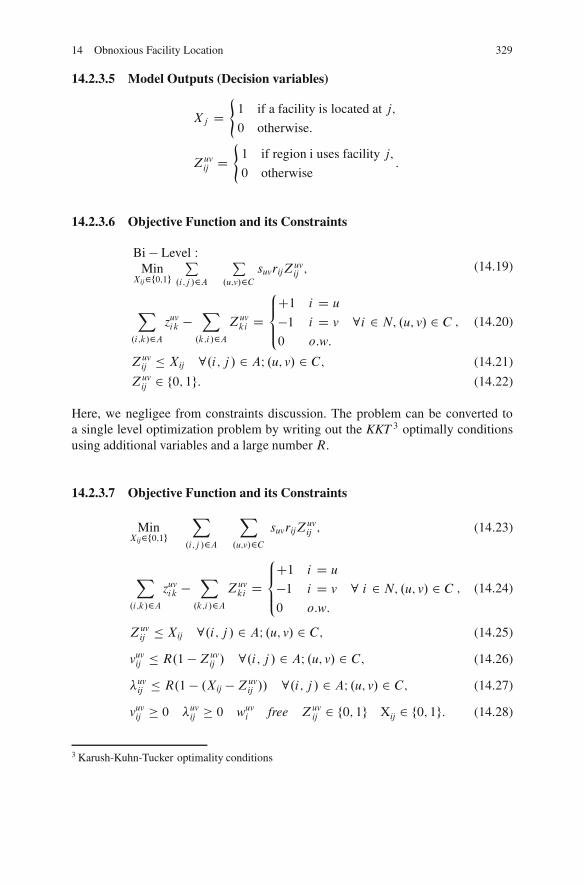
14 Obnoxious Facility Location 329
14.2.3.5 Model Outputs (Decision variables)
Xj D(1 if a facility is located at j;
0 otherwise:
Zuvij D
(1 if region i uses facility j;
0 otherwise:
14.2.3.6 Objective Function and its Constraints
Bi � Level WMin
Xij2f0;1gP
.i;j /2AP
.u;v/2CsuvrijZ
uvij ; (14.19)
X.i;k/2A
zuvik �
X.k;i/2A
Zuvki D
8<:
C1 i D u
�1 i D v 8i 2 N; .u; v/ 2 C0 o:w:
; (14.20)
Zuvij � Xij 8.i; j / 2 AI .u; v/ 2 C; (14.21)
Zuvij 2 f0; 1g: (14.22)
Here, we negligee from constraints discussion. The problem can be converted toa single level optimization problem by writing out the KKT 3 optimally conditionsusing additional variables and a large number R.
14.2.3.7 Objective Function and its Constraints
MinXij2f0;1g
X.i;j /2A
X.u;v/2C
suvrijZuvij ; (14.23)
X.i;k/2A
zuvik �
X.k;i/2A
Zuvki D
8<:
C1 i D u
�1 i D v 8 i 2 N; .u; v/ 2 C0 o:w:
; (14.24)
Zuvij � Xij 8.i; j / 2 AI .u; v/ 2 C; (14.25)
vuvij � R.1 �Zuv
ij / 8.i; j / 2 AI .u; v/ 2 C; (14.26)
�uvij � R.1 � .Xij �Zuv
ij // 8.i; j / 2 AI .u; v/ 2 C; (14.27)
vuvij � 0 �uv
ij � 0 wuvi free Zuv
ij 2 f0; 1g Xij 2 f0; 1g: (14.28)
3 Karush-Kuhn-Tucker optimality conditions
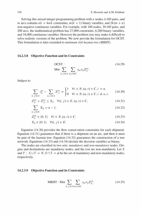
330 S. Hosseini and A.M. Esfahani
Solving this mixed integer programming problem with n nodes, k OD pairs, andm arcs contains nk C 4mk constraints, m.k C 1/ binary variables, and 2k.mC n/
non-negative continuous variables. For example, with 100 nodes, 30 OD pairs, and200 arcs, the mathematical problem has 27,000 constraints, 6,200 binary variables,and 18,000 continuous variables. However the problem size may make it difficult tosolve realistic versions of the problem. We now provide the formulation for OCST.This formulation is later extended to minimum risk hazmat tree (MRHT).
14.2.3.8 Objective Function and its Constraints
OCST W (14.29)
MinX.i;j /2A
X.u;v/2C
suvrijZuvij :
Subject to
X.i;j /2A
zuvij �
X.j;i/2A
Zuvj i D
(1 8i 2 N; .u; v/ 2 C; i D u:
0 8i 2 N; .u; v/ 2 C; i ¤ u; v:(14.30)
Zuvij CZuv
j i � Xij 8.i; j / 2 E; .u; v/ 2 C; (14.31)X.i;j /2E
Xij D n � 1; (14.32)
Zuvij 2 f0; 1g 8i 2 N; .u; v/ 2 C: (14.33)
Xij 2 f0; 1g 8.i; j / 2 E: (14.34)
Equation (14.30) provides the flow conservation constraints for each shipment.Equation (14.31) guarantees that if there is a shipment on an arc, and then it mustbe part of the hazmat tree. Equation (14.32) guarantees the construction of a treenetwork. Equations (14.33) and (14.34) declare the decision variables as binary.
The nodes are classified in two sets: mandatory and non-mandatory nodes. Ori-gins and destinations are mandatory nodes, and the rest are non-mandatory. Let Sand T W S [T D N;S \T D � be the set of mandatory and non-mandatory nodes,respectively.
14.2.3.9 Objective Function and its Constraints
MRHT W MinX.i;j /2A
X.u;v/2C
suvrijZuvij : (14.35)
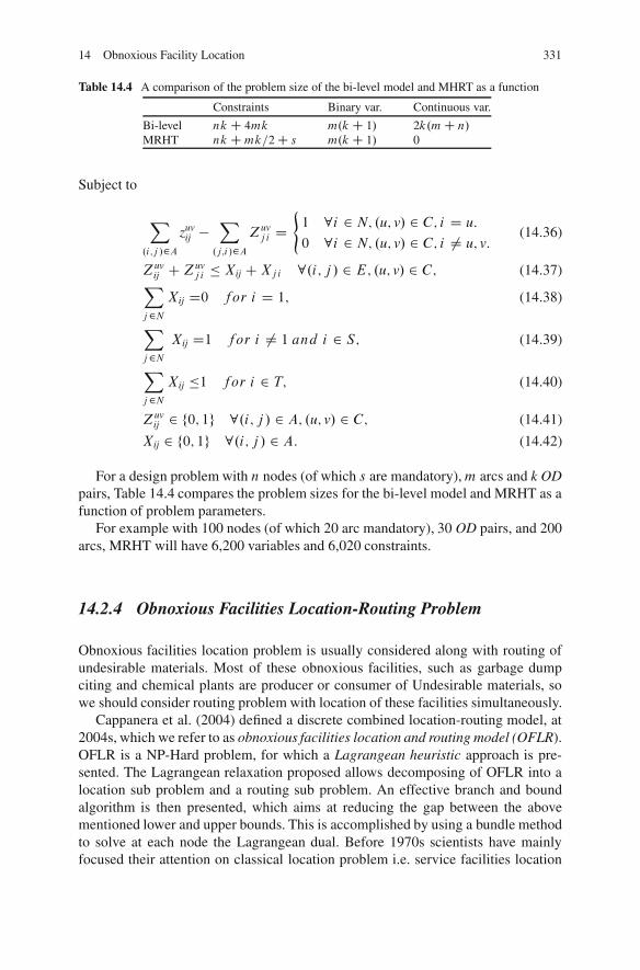
14 Obnoxious Facility Location 331
Table 14.4 A comparison of the problem size of the bi-level model and MHRT as a function
Constraints Binary var. Continuous var.
Bi-level nk C 4mk m.k C 1/ 2k.mC n/
MRHT nk Cmk=2C s m.k C 1/ 0
Subject to
X.i;j /2A
zuvij �
X.j;i/2A
Zuvj i D
(1 8i 2 N; .u; v/ 2 C; i D u:
0 8i 2 N; .u; v/ 2 C; i ¤ u; v:(14.36)
Zuvij CZuv
j i � Xij CXji 8.i; j / 2 E; .u; v/ 2 C; (14.37)Xj2N
Xij D0 for i D 1; (14.38)
Xj2N
Xij D1 for i ¤ 1 and i 2 S; (14.39)
Xj2N
Xij �1 for i 2 T; (14.40)
Zuvij 2 f0; 1g 8.i; j / 2 A; .u; v/ 2 C; (14.41)
Xij 2 f0; 1g 8.i; j / 2 A: (14.42)
For a design problem with n nodes (of which s are mandatory),m arcs and k ODpairs, Table 14.4 compares the problem sizes for the bi-level model and MRHT as afunction of problem parameters.
For example with 100 nodes (of which 20 arc mandatory), 30 OD pairs, and 200arcs, MRHT will have 6,200 variables and 6,020 constraints.
14.2.4 Obnoxious Facilities Location-Routing Problem
Obnoxious facilities location problem is usually considered along with routing ofundesirable materials. Most of these obnoxious facilities, such as garbage dumpciting and chemical plants are producer or consumer of Undesirable materials, sowe should consider routing problem with location of these facilities simultaneously.
Cappanera et al. (2004) defined a discrete combined location-routing model, at2004s, which we refer to as obnoxious facilities location and routing model (OFLR).OFLR is a NP-Hard problem, for which a Lagrangean heuristic approach is pre-sented. The Lagrangean relaxation proposed allows decomposing of OFLR into alocation sub problem and a routing sub problem. An effective branch and boundalgorithm is then presented, which aims at reducing the gap between the abovementioned lower and upper bounds. This is accomplished by using a bundle methodto solve at each node the Lagrangean dual. Before 1970s scientists have mainlyfocused their attention on classical location problem i.e. service facilities location
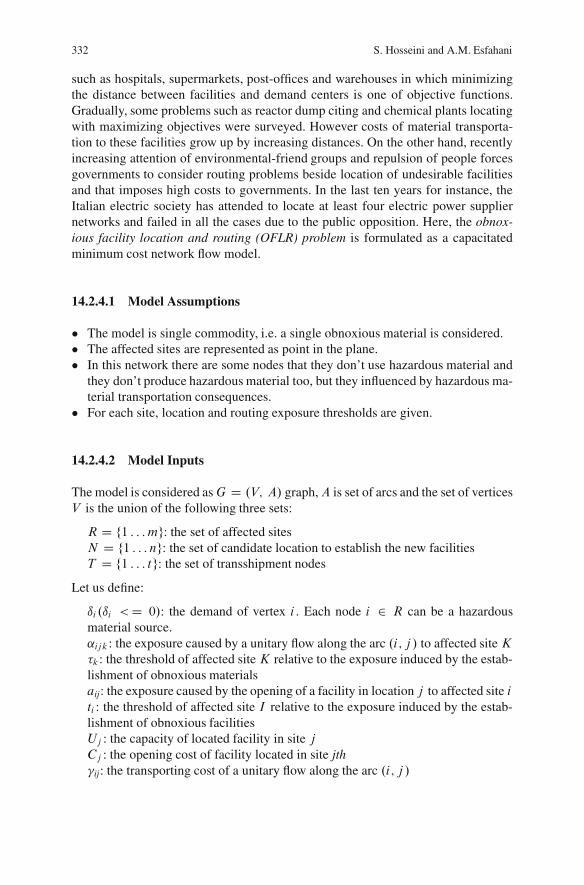
332 S. Hosseini and A.M. Esfahani
such as hospitals, supermarkets, post-offices and warehouses in which minimizingthe distance between facilities and demand centers is one of objective functions.Gradually, some problems such as reactor dump citing and chemical plants locatingwith maximizing objectives were surveyed. However costs of material transporta-tion to these facilities grow up by increasing distances. On the other hand, recentlyincreasing attention of environmental-friend groups and repulsion of people forcesgovernments to consider routing problems beside location of undesirable facilitiesand that imposes high costs to governments. In the last ten years for instance, theItalian electric society has attended to locate at least four electric power suppliernetworks and failed in all the cases due to the public opposition. Here, the obnox-ious facility location and routing (OFLR) problem is formulated as a capacitatedminimum cost network flow model.
14.2.4.1 Model Assumptions
� The model is single commodity, i.e. a single obnoxious material is considered.� The affected sites are represented as point in the plane.� In this network there are some nodes that they don’t use hazardous material and
they don’t produce hazardous material too, but they influenced by hazardous ma-terial transportation consequences.
� For each site, location and routing exposure thresholds are given.
14.2.4.2 Model Inputs
The model is considered asG D .V; A/ graph,A is set of arcs and the set of verticesV is the union of the following three sets:
R D f1 : : : mg: the set of affected sitesN D f1 : : : ng: the set of candidate location to establish the new facilitiesT D f1 : : : tg: the set of transshipment nodes
Let us define:
ıi .ıi <D 0/: the demand of vertex i . Each node i 2 R can be a hazardousmaterial source.˛ijk : the exposure caused by a unitary flow along the arc .i; j / to affected site K�k : the threshold of affected site K relative to the exposure induced by the estab-lishment of obnoxious materialsaij: the exposure caused by the opening of a facility in location j to affected site iti : the threshold of affected site I relative to the exposure induced by the estab-lishment of obnoxious facilitiesUj : the capacity of located facility in site jCj : the opening cost of facility located in site jth�ij: the transporting cost of a unitary flow along the arc .i; j /
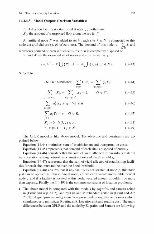
14 Obnoxious Facility Location 333
14.2.4.3 Model Outputs (Decision Variables)
Yj : 1 if a new facility is established at node j ; 0 otherwiseXij: the amount of transported flow along the arc .i; j /
An artificial node P was added to set V , each site j 2 N is connected to thisnode via artificial arc .j; p/ of zero cost. The demand of this node is � P
i2<ıi and
represents demand of each influenced site i 2 R is completely disposed of.V 0 and A0 are the extended set of nodes and arcs respectively,
i:e: V 0 D V[
fP g; A0 D A[
f.j; p/ W j 2 N g: (14.43)
Subject to
OFLR W MINIMIZEXj2N
CjYj CX
.i;j /2A�ijXij; (14.44)
Xj W.j;i/2A0
Xji�X
j W.i;j /2A0
Xij D ıi 8i 2 V 0; (14.45)
X.i;j /2A
˛kijXij � �k 8k 2 R; (14.46)
Xj2N
aijYj � ti 8i 2 R; (14.47)
Xij � 0 8.i; j / 2 A; (14.48)
Yj 2 f0; 1g 8j 2 N: (14.49)
The OFLR model is like above model. The objective and constraints are ex-plained below:
Equation (14.44) minimizes sum of establishment and transportation costs.Equation (14.45) represents that demand of each site is disposed of entirely.Equation (14.46) considers that the sum of yield affected of hazardous material
transportation among network arcs, must not exceed the threshold �k .Equation (14.47) represents that the sum of yield affected of establishing facili-
ties for each site, must not be over the fixed threshold.Equation (14.48) ensures that if any facility is not located at node j , this node
just can be applied as transshipment node, i.e. we can’t vacate undesirable flow atnode j and if a facility is located at this node, vacated amount shouldn’t be morethan capacity. Finally the (14.49) is the common constraint of location problems.
� The above model is compared with the models by zagrafos and samara (citedin (Erkut and Alp 2007)) and by List and Mirchandani (cited in (Erkut and Alp2007)). A goal programming model was presented by zagrafos and samara whichsimultaneously minimizes Routing risk, Location risk and routing cost. The maindifferences between OFLR and the model by Zografos and Samara are following:
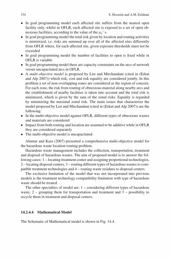
334 S. Hosseini and A.M. Esfahani
� In goal programming model each affected site suffers from the nearest openfacility only, whilst in OFLR, each affected site is exposed to a set of open ob-noxious facilities, according to the value of the aij’ s.
� In goal programming model the total risk given by location and routing activitiesis minimized, i.e. risks are summed up over all of the affected sites differentlyfrom OFLR where, for each affected site, given exposure thresholds must not beexceeded
� In goal programming model the number of facilities to open is fixed while inOFLR is variable
� In goal programming model there are capacity constraints on the arcs of networkversus uncapacitated arcs in OFLR.
� A multi-objective model is proposed by List and Mirchandani (cited in (Erkutand Alp 2007)) which risk, cost and risk equality are considered jointly. In thisproblem a set of non-overlapping zones are considered as the region of concern.For each zone, the risk from routing of obnoxious material along nearby arcs andthe establishment of nearby facilities is taken into account and the total risk isminimized, which is given by the sum of the zonal risks. Equality is regardedby minimizing the maximal zonal risk. The main issues that characterize themodel proposed by List and Mirchandani (cited in (Erkut and Alp 2007)) are thefollowing:
� In the multi-objective model against OFLR, different types of obnoxious wastesand materials are considered
� Impact from both routing and location are assumed to be additive while in OFLRthey are considered separately
� The multi-objective model is uncapacitated.
Alumur and Kara (2007) presented a comprehensive multi-objective model forthe hazardous waste location-routing problem.
Hazardous waste management includes the collection, transportation, treatmentand disposal of hazardous wastes. The aim of proposed model is to answer the fol-lowing cases: 1 – locating treatment center and assigning proportional technologies,2 – locating disposal centers, 3 – routing different types of hazardous wastes to com-patible treatment technologies and 4 – routing waste residues to disposal centers.
The exclusive limitation of the model that was not incorporated into previousmodels is the treatment technology compatibility limitation with type of hazardouswaste should be treated.
The other specialties of model are: 1 – considering different types of hazardouswaste, 2 – grouping them for transportation and treatment and 3 – possibility torecycle them in treatment and disposal centers.
14.2.4.4 Mathematical Model
The Schematic of Mathematical model is shown in Fig. 14.4.
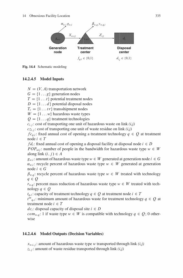
14 Obnoxious Facility Location 335
gw,i yw,q,i di
aw,i gw,i
Xw,i,j Zi,j
bw,q yw,q,i
fq,i ∈ {0,1} dzi ∈ {0,1}
Generationnode
Treatmentcenter
Disposalcenter
Fig. 14.4 Schematic modeling
14.2.4.5 Model Inputs
N D .V; A/ transportation networkG D f1 : : : gg generation nodesT D f1 : : : tg potential treatment nodesD D f1 : : : d g potential disposal nodesTr D f1 : : : t rg transshipment nodesW D f1 : : :wg hazardous waste typesQ D f1 : : : qg treatment technologiesci;j : cost of transporting one unit of hazardous waste on link (i,j)czi;j : cost of transporting one unit of waste residue on link (i,j)fcq;i : fixed annual cost of opening a treatment technology q 2 Q at treatmentnode i 2 Tfdi : fixed annual cost of opening a disposal facility at disposal node i 2 DPOPwij : number of people in the bandwidth for hazardous waste type w 2 W
along link .i; j / 2 Agw;i : amount of hazardous waste type w 2 W generated at generation node i 2 G˛w;i : recycle percent of hazardous waste type w 2 W generated at generationnode i 2 Gˇw;q : recycle percent of hazardous waste type w 2 W treated with technologyq 2 Qrw;q: percent mass reduction of hazardous waste type w 2 W treated with tech-nology q 2 Qtq;i : capacity of treatment technology q 2 Q at treatment node i 2 Ttmq;i : minimum amount of hazardous waste for treatment technology q 2 Q attreatment node i 2 Tdci : disposal capacity of disposal site i 2 Dcomw;q: 1 if waste type w 2 W is compatible with technology q 2 Q; 0 other-wise
14.2.4.6 Model Outputs (Decision Variables)
xw;i;j : amount of hazardous waste type w transported through link (i,j)zi;j : amount of waste residue transported through link (i,j)
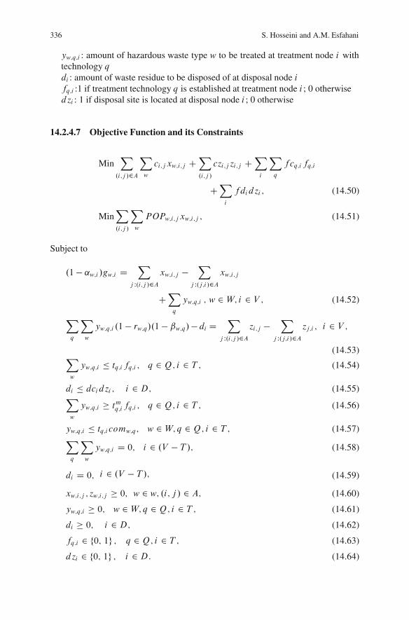
336 S. Hosseini and A.M. Esfahani
yw;q;i : amount of hazardous waste type w to be treated at treatment node i withtechnology qdi : amount of waste residue to be disposed of at disposal node ifq;i :1 if treatment technology q is established at treatment node i ; 0 otherwised zi : 1 if disposal site is located at disposal node i ; 0 otherwise
14.2.4.7 Objective Function and its Constraints
MinX
.i;j /2A
Xw
ci;j xw;i;j CX.i;j /
czi;j zi;j CXi
Xq
fcq;i fq;i
CXi
fdid zi ; (14.50)
MinX.i;j /
Xw
POPw;i;j xw;i;j ; (14.51)
Subject to
.1� ˛w;i /gw;i DX
j W.i;j /2Axw;i;j �
Xj W.j;i/2A
xw;i;j
CXq
yw;q;i ; w 2 W; i 2 V ; (14.52)
Xq
Xw
yw;q;i .1� rw;q/.1 � ˇw;q/� di DX
j W.i;j /2Azi;j �
Xj W.j;i/2A
zj;i ; i 2 V ;
(14.53)Xw
yw;q;i � tq;i fq;i ; q 2 Q; i 2 T ; (14.54)
di � dcid zi ; i 2 D; (14.55)Xw
yw;q;i � tmq;i fq;i ; q 2 Q; i 2 T ; (14.56)
yw;q;i � tq;i comw;q; w 2 W; q 2 Q; i 2 T ; (14.57)Xq
Xw
yw;q;i D 0; i 2 .V � T /; (14.58)
di D 0; i 2 .V � T /; (14.59)
xw;i;j ; zw;i;j � 0; w 2 w; .i; j / 2 A; (14.60)
yw;q;i � 0; w 2 W; q 2 Q; i 2 T ; (14.61)
di � 0; i 2 D; (14.62)
fq:i 2 f0; 1g ; q 2 Q; i 2 T ; (14.63)
d zi 2 f0; 1g ; i 2 D: (14.64)
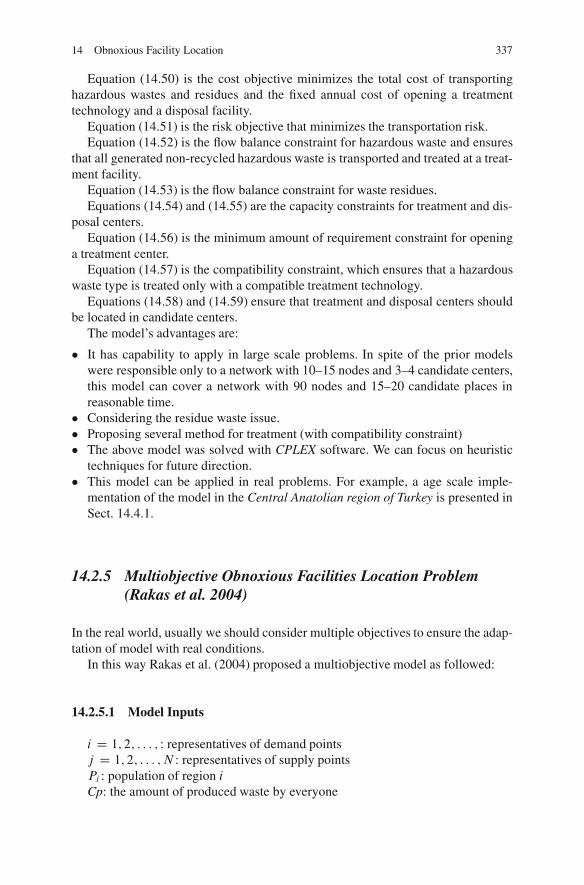
14 Obnoxious Facility Location 337
Equation (14.50) is the cost objective minimizes the total cost of transportinghazardous wastes and residues and the fixed annual cost of opening a treatmenttechnology and a disposal facility.
Equation (14.51) is the risk objective that minimizes the transportation risk.Equation (14.52) is the flow balance constraint for hazardous waste and ensures
that all generated non-recycled hazardous waste is transported and treated at a treat-ment facility.
Equation (14.53) is the flow balance constraint for waste residues.Equations (14.54) and (14.55) are the capacity constraints for treatment and dis-
posal centers.Equation (14.56) is the minimum amount of requirement constraint for opening
a treatment center.Equation (14.57) is the compatibility constraint, which ensures that a hazardous
waste type is treated only with a compatible treatment technology.Equations (14.58) and (14.59) ensure that treatment and disposal centers should
be located in candidate centers.The model’s advantages are:
� It has capability to apply in large scale problems. In spite of the prior modelswere responsible only to a network with 10–15 nodes and 3–4 candidate centers,this model can cover a network with 90 nodes and 15–20 candidate places inreasonable time.
� Considering the residue waste issue.� Proposing several method for treatment (with compatibility constraint)� The above model was solved with CPLEX software. We can focus on heuristic
techniques for future direction.� This model can be applied in real problems. For example, a age scale imple-
mentation of the model in the Central Anatolian region of Turkey is presented inSect. 14.4.1.
14.2.5 Multiobjective Obnoxious Facilities Location Problem(Rakas et al. 2004)
In the real world, usually we should consider multiple objectives to ensure the adap-tation of model with real conditions.
In this way Rakas et al. (2004) proposed a multiobjective model as followed:
14.2.5.1 Model Inputs
i D 1; 2; : : : ; : representatives of demand pointsj D 1; 2; : : : ; N : representatives of supply pointsPi : population of region iCp: the amount of produced waste by everyone
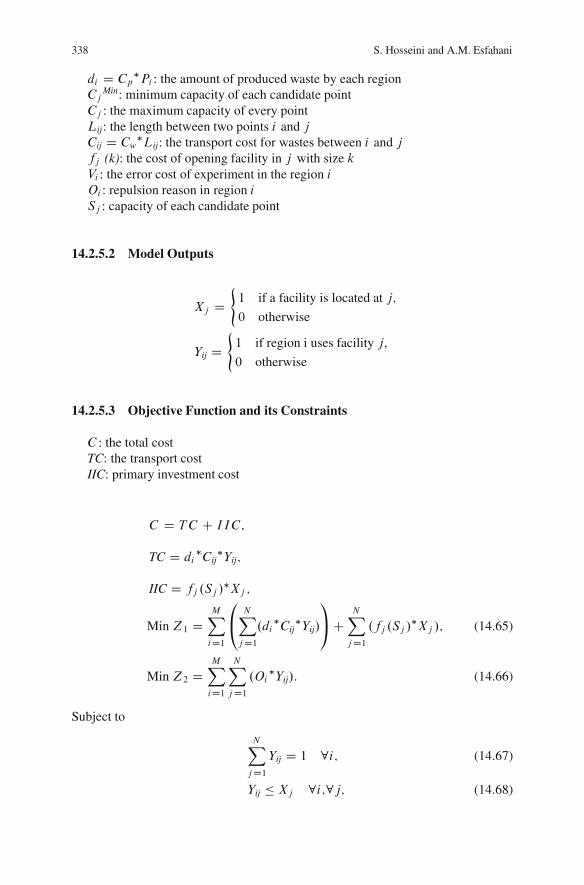
338 S. Hosseini and A.M. Esfahani
di D Cp�Pi : the amount of produced waste by each region
CjMin: minimum capacity of each candidate point
Cj : the maximum capacity of every pointLij: the length between two points i and jCij D Cw
�Lij: the transport cost for wastes between i and jfj (k): the cost of opening facility in j with size kVi : the error cost of experiment in the region iOi : repulsion reason in region iSj : capacity of each candidate point
14.2.5.2 Model Outputs
Xj D(1 if a facility is located at j;
0 otherwise
Yij D(1 if region i uses facility j;
0 otherwise
14.2.5.3 Objective Function and its Constraints
C : the total costTC: the transport costIIC: primary investment cost
C D TC C IIC;
TC D di�Cij
�Yij;
IIC D fj .Sj /�Xj ;
Min Z1 DMXiD1
0@ NXjD1
.di�Cij
�Yij/
1AC
NXjD1
.fj .Sj /�Xj /; (14.65)
Min Z2 DMXiD1
NXjD1
.Oi�Yij/: (14.66)
Subject to
NXjD1
Yij D 1 8i; (14.67)
Yij � Xj 8i;8j; (14.68)
14 Obnoxious Facility Location 339
MXiD1
.d i�Yij/ � Sj 8j ; (14.69)
CMinj � Sj � CMax
j 8j: (14.70)
Equation (14.65) minimizes sum of opening and transportation cost and (14.66)minimizes the people opposition. Equation (14.67) declares each region is coveredby only one facility. Equation (14.68) shows that region i can use facility j only ifone facility is located in j . Equation (14.69) is capacity constraint of each candidatepoint and (14.70) proposes the capacity of every point between two limits.
For solving this continuous model, two models are solved separately and Z1Opt ;Z2
Opt are obtained. Then using weighting method, two objective functions are in-tegrated and following model is solved:
Min Z3 D Weight 1� Z1
ZOpt1
C Weight 2� Z2
ZOpt2
: (14.71)
Because of uncertainty in data estimation, required data are solved as fuzzy datathat are described in (Rakas et al. 2004) in detail.
14.3 Solutions and Techniques
In this section we review some researches in obnoxious facility location field focus-ing on solutions and techniques.
� Melachrinoudis (1999) developed a bicriteria location model for locating a newsemi-obnoxious facility in an existing layout which is solved by an adaptation ofthe Fourier–Motzkin elimination method
� Zhang et al. (2000) devise a routing hazardous materials algorithm, using GIStechnique and a Gaussian Plume model for their dispersion model
� Akgun et al. (2000) to find dissimilar paths for transporting HazMat, solved thecapacitated flow problem:
– Iterative penalty method(IPM)– Minimax method– Gateway shortest path (GSP) method
By increasing the size of problem, calculations volume rises up strongly. Theyused GIS method as a facilator to test different network roads. Finally they pro-posed a P -Dispersion problem and solved it with constructing a candidate set mof K-shortest paths.
� Kara et al. (2003) present two path- selection algorithms for hazmat transportproblems with selection of a minimum risk path. One of the proposed proceduresis a modified version of shortest path algorithm and the other is an adaptation ofa link-labeling algorithm developed for urban transportation.
340 S. Hosseini and A.M. Esfahani
� Cappanera et al. (2004) proposed a Lagrangean heuristic approach allows to de-compose obnoxious facility location routing (OFLR) into a location subproblemand routing subproblem. Then, an effective branch and bound algorithm was of-fered for reduction of the gap between lower and upper bounds.
� Colebrook et al. (2005) presented a new bound for the undesirable 1-medianproblem (Maxian) on networks. they proposed an undesirable center and medianmodels and implemented Multicriteria-anti-cent-dian problem (MACDP). Theycreated a heuristic algorithm for MACDP.
� Dıaz-Banez et al. (2005) for solving the obnoxious short path problem in contin-uous spaces presented an approximate algorithm based on the bisection method.They transformed optimization problem into decision problem and could provideefficient algorithm. They proposed:
– A general method of voroni diagram with daguare geometry– Shortest path avoiding obstacles
� Erkut et al. (2005) formulated the tree design problem as an integer program-ming problem aiming at trade off between cost and risk. They developed a simpleheuristic to expand the solution of the tree design problem by adding node seg-ments.
� Erkut and Alp (2007) formulate the tree design problem for hazardous materialsroutes in and through a major population center as an integer programming modelwith an objective of minimizing the total transport risk. They propose the use ofa new model for finding a minimum risk hazmat tree called Optimum Communi-cation Steiner Tree. Then a construction heuristic that adds paths incrementallyand permits local authorities to balance between risk and cost was developed.
� Zhang et al. (2005) proposed a new model that is a variant of the vehicle rout-ing problem with time windows (VRPTW) by adding load upper bounds on theroad segments. The objective is to find a schedule to guarantee the safety of allvehicles. They propose a sophisticated Tabu search heuristic with novel neigh-borhood operators such as dynamic penalty mechanism to obtain good solutions.
� Zhang et al. (2005) used a heuristic algorithm based on greedy to solve a mul-tiobjective approach (analysing cost minimization, potential risk minimizationand risk equity maximization) to assist decision makers in analysing combinedlocation/routing decisions involving hazmats.
� Dadkar et al. (2008) Identified geographically diverse routes for the transporta-tion of hazardous materials by applying k-shortest path algorithm with stochasticobjective and varying over time. They also implemented Mixed Integer Program-ming.
� Erkut and Gzara (2008) develop and test a heuristic for a bilevel network designproblem for hazmat transportation that finds stable solutions. This heuristic ex-ploits the network flow structure at both levels to overwhelm the difficulty andinstability of the bilevel integer programming model.
� Pisinger (2006) present an exact algorithm for finding a number of fast upperbounds for P-dispersion problems in which these bounds can be derived in O.n/time.
14 Obnoxious Facility Location 341
� Bell (2006) considered mixed rout strategies for the Risk-Averse shipment ofhazardous materials. A minimax problem was formulated to determine the safestset of routs and safest share of traffic between these routs. A simple heuristicbased on a shortest path algorithm and the method of successive averages is pro-posed. Connections to game theory can be seen in the nature of the solution.
� Yapicioglu et al. (2007) offer a new model for the semi obnoxious facility loca-tion problem composed of a weighted minisum function for transportation costand a distance- based piecewise function for the obnoxious effects of the facility.They devise a single objective particle swarm optimizer (PSO) and a bi-objectivePSO to solve this problem.
� Carotenuto et al. (2007) For finding minimum and equitable risk routes forHazMat shipment present a mathematical model and solved with Lagrangian re-laxation and two heuristic algorithms based on the Yen’s k-shortest path:
– Greedy algorithm (GD)– Randomized Greedy algorithm (RGD)
� Carotenuto et al. (2007) implemented a Tabu Search algorithm for scheduling androuting of HazMat transportation. They focus on scheduling to decrease trafficvolume of HazMat transportation as well as on a network road.
14.4 Case Study
14.4.1 Obnoxious Facility Location and Routing in AnatolianRegion of Turkey (Alumur and Kara 2007)
In Central Anatolian region of Turkey, there are 184 administrative districts. Thepopulation of districts ranges from 3,700 to 77,000 people. It assumed that the dis-tricts with a population more than 25,000 produce hazardous waste.
The data on the amount of hazardous waste produced by each districts in Turkeyare not available presently. So, assumed that the amount of hazardous waste gen-erated by each district is proportional to the population times the industrial activitylevel of the district. The GIS system is applied in collecting geographical informa-tion. In this region three types of hazardous waste are generated and two treatmentmethods are determined. The first type waste can be incinerated, the second type issuitable for chemical treatment, and the third type can be treated by both incinera-tion and chemical process. The proposed model assumed that treatment and disposalcenters can be located at the same nodes. The candidate point’s selection is so im-portant because of cost considerations. So that, the model was considered in twoconditions: A: 15 candidate places, B: 20 candidate places. After solving the prob-lem with CPLEX resulted that final answers are not mainly different. Therefore, inthe reason of economic considerations the 15 candidate place state was selected.
342 S. Hosseini and A.M. Esfahani
14.4.2 Designing Emergency Response Network for HazardousMaterials Transportation (Berman et al. 2007)
In addition to government’s policies for decreasing HazMats accidents, detrimentaleffects of these accidents are such that we should consider various alternatives forlocating, routing and improving of emergency teams performance to reduce theseconsequences. Critical factor is quick arrival of emergency teams at the accidentsite. Arrival time, itself, is related to selected paths and location of teams, thereforesuch designs are essential to consider.
In this way, Berman et al. (2007), proposed a maximal arc-covering model foroptimal design of such networks. Their model improves solution capability relativeto previous models by adding some binary variables. Moreover, they developed agreedy heuristic to solve their model efficiently.The advantages of new formula-tion are:
� Reducing the number of variables,� Reducing time of solution,� Compatibility with existing software and large scale problems,� Proposed model is explicit and easy to understand,� The new model constitutes a basis for an efficient heuristic.
Proposed model was efficiently applied for emergency response infrastructurefor gasoline incidents on the highway networks of Quebec and Ontario in Canada.They derived the model parameters from a GIS-based representation of the twoprovinces. This application shows the possibility of a significant improvement in re-sponse capability via relocation of the existing stations. Also, a noticeable decreasein the threshold time of coverage for gasoline incidents is considered.
14.4.3 Locating Waste Pipelines to Minimize their Impacton Marine Environment (Ceceres et al. 2007)
Ceceres et al. (2007), suggested a methodology for locating waste pipelines tominimize their impact on marine environment. A waste pipeline, as an undesir-able facility, is to be located in a coastal region. The coastal fringe is the territorywhere marine, air and terrestrial environments interrelate. Here very diverse andfragile ecosystems coexist, although subjected in many cases to increasing degrada-tion due to industrial and urban developments disrespectful to the environment.
Pasidonia oceanica (Linnaeus) Delile is a plant with leaves, flowers and fruit,similar to those plants which live in forests and gardens, but which lives in the seabetween the surface and a depth of 50 m.
It is endemic to the Mediterranean Sea and, by providing the principal source ofoxygenation of the Mediterranean Sea; it is its most important ecosystem. Due toits ecological role, this sea-grass is a protected species in Spain and in France. Here
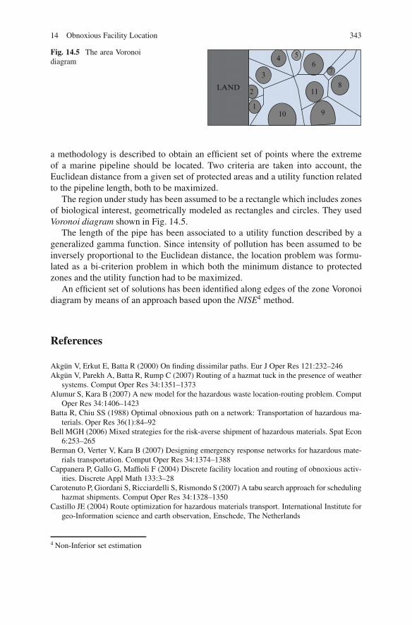
14 Obnoxious Facility Location 343
Fig. 14.5 The area Voronoidiagram
10
2
1
3
4 56
11
9
8
7
LAND
a methodology is described to obtain an efficient set of points where the extremeof a marine pipeline should be located. Two criteria are taken into account, theEuclidean distance from a given set of protected areas and a utility function relatedto the pipeline length, both to be maximized.
The region under study has been assumed to be a rectangle which includes zonesof biological interest, geometrically modeled as rectangles and circles. They usedVoronoi diagram shown in Fig. 14.5.
The length of the pipe has been associated to a utility function described by ageneralized gamma function. Since intensity of pollution has been assumed to beinversely proportional to the Euclidean distance, the location problem was formu-lated as a bi-criterion problem in which both the minimum distance to protectedzones and the utility function had to be maximized.
An efficient set of solutions has been identified along edges of the zone Voronoidiagram by means of an approach based upon the NISE4 method.
References
Akgun V, Erkut E, Batta R (2000) On finding dissimilar paths. Eur J Oper Res 121:232–246Akgun V, Parekh A, Batta R, Rump C (2007) Routing of a hazmat tuck in the presence of weather
systems. Comput Oper Res 34:1351–1373Alumur S, Kara B (2007) A new model for the hazardous waste location-routing problem. Comput
Oper Res 34:1406–1423Batta R, Chiu SS (1988) Optimal obnoxious path on a network: Transportation of hazardous ma-
terials. Oper Res 36(1):84–92Bell MGH (2006) Mixed strategies for the risk-averse shipment of hazardous materials. Spat Econ
6:253–265Berman O, Verter V, Kara B (2007) Designing emergency response networks for hazardous mate-
rials transportation. Comput Oper Res 34:1374–1388Cappanera P, Gallo G, Maffioli F (2004) Discrete facility location and routing of obnoxious activ-
ities. Discrete Appl Math 133:3–28Carotenuto P, Giordani S, Ricciardelli S, Rismondo S (2007) A tabu search approach for scheduling
hazmat shipments. Comput Oper Res 34:1328–1350Castillo JE (2004) Route optimization for hazardous materials transport. International Institute for
geo-Information science and earth observation, Enschede, The Netherlands
4 Non-Inferior set estimation
344 S. Hosseini and A.M. Esfahani
Ceceres T, A.Mesa J, Ortega F (2007) Locating waste pipelines to minimize their impact on marineenvironment. Eur J Oper Res 179(3):1143–1159
Colebrook M, Guti J, Sicilia J (2005) A new bound and an O (mn) algorithm for the undesirable1-median problem (Maxian) on networks. Comput Oper Res 32:309–325
Dadkar Y, Jones D, Nozick L (2008) Identifying geographically diverse routes for the trans-portation of hazardous materials. Transportation Research Part E: Logistics and TransportationReview 44(3):333–349
Daskin MS (1995) Network and discrete location: models, algorithms and applications. Wiley,New York
Dıaz-Banez JM, Gomez F, Toussaint GT (2005) Computing shortest paths for transportation ofhazardous materials in continuous spaces. J Food Eng 70:293–298
Drezner Z, Wesolowsky GO (1983) Location of an obnoxious facility with rectangular distances.J Reg Sci 23:241–248
Erkut E, Verter V (1995) Hazardous Materials Logistics. Springer Series in Oper Res, Chapter 20Erkut E, Verter V (1998) Modeling of transport risk for hazardous material. Oper Res 46(5):
625–642Erkut E, Alp O (2007) Designing a network for hazardous materials shipments. Comput Oper Res
34(5):1389–1405Erkut E, Gzara F (2008) Solving the hazmat transport network design problem. Comput Oper Res
35(7):2234–2247Erkut E, Ingolfsson A (2005) Transport risk models for hazardous materials: revisited. Oper Res
Lett 33:81–89Fernandez J, Fernandez P, Pelegrin B (2000) A continuous location model for siting a non-noxious
undesirable facility within a geographical region. Eur J Oper Res 121:259–274Giannikos I (1998) A multi-objective programming model for locating treatment sites and routing
hazardous wastes. Eur J Oper Res 104:333–342Gopalan R, Kolluri KS, Batta R, Karwan MH (1990) Modeling equity of risk in the transportation
of hazardous materials. Oper Res 38(6):961–973Kara BY, Erkut E, Verter V (2003) Accurate calculation of hazardous materials transport risks.
Oper Res Lett 31:285–292Katz MJ, Kedem K, Segal M (2002) Improved algorithms for placing undesirable facilities. Com-
put Oper Res 29:1859–1872Kuby MJ (1987) Programming models for facility dispersion: the p-dispersion and maxisum dis-
persion problems. Geographical Analysis 19:315–329Marianov V, ReVelle C (1998) Linear, no-approximated models for optimal routing in hazardous
environments. J Operl Res Society 48:157–164McGinnis LF, White JA (1978) A single facility rectilinear location problem with multiple criteria.
Transport Sci 12:217–231Mehrez A, Sinuany-Stern Z, Stulman A (1986) An enhancement of the Drezner–Wesolowsky
algorithm for single facility location with maximin of rectilinear distance. J Oper Res Soc37:971–977
Melachrinoudi E (1999) Bicriteria location of a semi-obnoxious facility. Comput Oper Res 37:581–593
Pisinger D (2006) Upper bounds and exact algorithms for p-dispersion problems. Comput OperRes 33:1380–1398
Rakas J, Teodorovic D, Kim T (2004) Multi-objective modeling for determining location of unde-sirable facilities. Transport Re D9:125–138
Ratick S, White A (1988) A risk sharing model for locating noxious facilities. Environment Plan165–179
ReVelle C, Cohon J, Shobrys D (1991) Simultaneous siting and routing in the disposal of hazardouswastes. Transportation Science 25(2):138–145
Rogers GO (1998) Sitting potentially hazardous facilities: What factors impact perceived and ac-ceptable risk? Landsc Urban Plan 39:265–281
14 Obnoxious Facility Location 345
Rodriguez JJ, Garcia GC, Munoz Perez J Merida Casermeiroa E (2006) A general model for theundesirable single facility location problem. Oper Res Lett 34(4):427–436
Saccomanno FF, Chan A (1985) Economic evaluation of routing strategies for hazardous roadshipments. Transp. Res. Record 1020:12–18
Sivakumar R, Batta R, Karwan MH (1993) A network- based model for transporting extremelyhazardous materials. Oper Res Lett 13(2):85–93
Sivakumar R, Batta R, Karwan MH (1995) A multiple route conditional risk model for transportinghazardous materials. INFOR 33:20–33
Wayman MM, Kuby M (1994) Proactive optimization: General framework and a case study usinga toxic waste location model with technology choice. International symposium on locationaldecisions, ISOLDE VI, Lesvos and Chios, Greece
Yapicioglu H, Smith AE, Dozier G (2007) Solving the semi- obnoxious facility location problemusing bi-objective particle swarm. Eur J Oper Res 177:733–749
Zhang J, Hodgson J, Erkut E (2000) Using GIS to assess the risk of hazardous materials transportin networks. Eur J Oper Res 121:316–329
Zhang L, Guo S, Zhu Y, Lim A (2005) A tabu search algorithm for the safe transportation ofhazardous materials. Proceedings of the ACM symposium on Applied computing, SESSION:Evolutionary computation and optimization (ECO), pp 940–946
Zografos KG, Androutsopoulos KN (2004) A heuristic algorithm for solving hazardous materialsdistribution problems. Eur J Oper Res 152:507–519
Zografos KG, Vasilakis GM, Giannouli IM (2000) Methodological framework for develop-ing decision support system (DSS) for hazardous materials emergency response operations.J Hazardous Mater 71:503–521
Chapter 15Dynamic Facility Location Problem
Reza Zanjirani Farahani, Maryam Abedian, and Sara Sharahi
Facility location is a strategic management decision. This decision is usually made,however, with respect to the current parameters (like weights) which represent pop-ulation, infrastructure, service requirements and others (Drezner 1995; Francis andLowe 1992; Mirchandani and Francis 1990). Much of the research published onlocation theory is drawn from the models such as single/multi facility location, cov-ering,P -median,P -center problems, and their applications and extensions. Solvingmany of these problems can be extremely difficult. Thus, it is not surprising that somuch work has focused on statistic and deterministic problem formulations. Whilesuch formulations are reasonable research topics, they do not capture many of thecharacteristics of real-world location problems.
The strategic nature of facility location problems requires that any reasonablemodel consider some aspects of future uncertainty. Since the investment requiredby location or relocation facilities is usually large, facilities are expected to remainoperable for an extended time period (Owen and Daskin 1998). Thus, the problemof facility location truly involves an extended planning horizon. Decision makersmust not only select robust locations which will effectively serve changing demandover time, but must also consider the timing of facility expansions and relocationsin the long term (Daskin et al. 1992).
It is generally true of facilities that they are expected to serve over a long periodof time. During this time, many of the “constants” of the problem, such as demandsand distribution costs, are likely to change. It is also generally true that relocationcannot be accomplished without cost (Wesolowsky 1973). Thus, decision makersmust select sites that will not simply perform well according to the current systemstate, but that will continue to be profitable for the facility’s lifetime (Owen andDaskin 1998). Considering the fact that changes in static problem parameters canbe forecasted, optimization requires the balance between the benefits of plannedlocation changes and their costs (Wesolowsky 1973).
There are two different types of dynamic facility location Problems: Locationand Location–Relocation. These two types are different in the following ways:
� In a time-dependent location problem, the decision maker selects a site which isprofitable for a defined time horizon.
� In location–relocation problem, the decision maker selects a primary location,relocation or development times and the facility’s location after relocation.
R.Z. Farahani and M. Hekmatfar (eds.), Facility Location: Concepts, Models, 347Algorithms and Case Studies, Contributions to Management Science,DOI 10.1007/978-3-7908-2151-2 15, c� Physica-Verlag Heidelberg 2009
348 R.Z. Farahani et al.
In the remainder of this chapter, first, some classifications of time-dependant facilitylocation problems will be presented. Then, some of the related mathematical mod-els will be reviewed. Next, some lemmas and solution techniques will briefly bepresented. And finally, some real-world case studies will be introduced.
15.1 Classifications
Facility location problems can be divided into static and dynamic problems, Thesecan also be further classified on the basis of different criteria. This section providesa brief description of different classifications of dynamic facility problem.
� Cause of change. The first and the most important way for the classification ofdynamic facility location problem is based on the cause of change and uncer-tainty. According to this criterion, dynamic facility location problems are dividedinto two categories (Owen and Daskin 1998):
– Uncertainty related to planning for future conditions, and– Uncertainty due to the limited knowledge of model input parameters.
Note that in the first category, although there are changes in the conditions, theyare deterministic and time-dependent. In other words, the pattern of changes is dis-tinctive and deterministic. In the second category, although the pattern of changesmay be distinctive, it is not deterministic and time dependent, rather, it is stochastic(Rosental et al. 1978).
� Denoting the weight of facility parameter by “Wi”, deterministic and stochasticchanges can be classified as follows:
– Deterministic changes can be further classified based on whether or not:
1. “Wi” changes in each period of time horizon but it is fixed and distinctive inevery period.
2. The weight parameter, “Wi”, is a function of time, say wi .t/.
Stochastic changes can be classified into three types where:
1. “Wi” has a probabilistic distribution with fixed parameters.2. “Wi” has a probabilistic distribution with variable parameters where the parame-
ters are functions of time.3. There is no information about the alteration of the parameters and the weight of
the facility.
� Dependency variable: Time-dependent weights, Distance-dependent weights.This chapter is mainly dedicated to time-dependent weights. However, someworks such as the one by Huang et al. (1990) consider the weights as a functionof distance between the new facility and the existing facilities; this applicationcan be found in marketing area.
15 Dynamic Facility Location Problem 349
� The number of relocations: Single relocation, Multiple relocation. In the firstcategory, there is only one relocation (Emamizadeh and Z.-Farahani 1997a, b)whereas in the second category the location of the new facility is allowed tochange several times during the time horizon, i.e. n changes are allowed duringthe time span.
� Classification by the number of relocating facilities (Owen and Daskin 1998;Chand 1988): Single facility, Multiple facility. In the first category, only onefacility can be relocated whereas in the second, more than one facility can beconsidered for relocating (Scott 1971).
� Classification by the Relocation Time: Discrete, Continuous. In the first category,relocation can take place only at pre-determined points (Wesolowsky 1973) oftime whereas in the second category, relocation can take virtually any time in thedefined time horizon (Drezner and Wesolowsky 1991).
� Time horizon: Finite, Infinite. Daskin et al. (1992) acknowledge that the difficultyin solving dynamic facility location problems arises from the uncertainty sur-rounding future conditions. Even establishing an appropriate time horizon lengthis a non-trivial problem which is ignored in most formulations. They argue thatthe best way to mange uncertainty is postponing decision making as much aspossible, collecting information and improving forecasts as time advances. Sincethe first period decisions are the ones to be implemented immediately, the au-thors claim that the goal of dynamic location planning should not be to determinelocations and/or relocations for the entire horizon, but to find an optimal or near-optimal first period solution for the problem over an infinite horizon.
15.2 Mathematical Formulations
15.2.1 Static Model (Wesolowsky 1973)
Perhaps the best known of static location models is the generalized Weber problem.The problem requires the location of a facility among m destinations. Costs areassumed to be proportional to distances. Location is achieved by solving:
MinmXiD1
wi :di .x; y/ (15.1)
where:
di .x; y/: is the distance between the facility to be located at .x; y/ and destina-tion i located at .ai ; bi /:wi : is a constant transforming distances into costs.
To simplify notation in the succeeding section, model (15.1) is set in commonnotation.
350 R.Z. Farahani et al.
MinXm
iD1 fi .x; y/: (15.2)
The static model given in (15.2) is now extended to a model with a planning hori-zon of r time periods. This means that the demands, costs and destination locationsare forecasted for r time periods in advance, and the optimal planned location of thefacility in each period must be found. Consider the following problem:
MinrP
kD1
mkPiD1
fki .xk; yk/CrP
kD2Ck:zk;
zk D 0 if dk;k�1 D 0:
(15.3)
where:
mk : is the number of destinations in period k.fki .xk; yk/: is the present value of the cost of shipping from the facility at.xk; yk/ in period k to destination i:Ck : is the cost of moving at the beginning of period k.dk�1; k : the distance the facility is moved at the beginning of period k.
The above model makes the following assumptions:
� Each term fkd .xk; yk/ is adjusted to represent its present value at time 0. It canalso be adjusted by a factor reflecting confidence in the forecast.
� Each “moving” cost Ck is independent from the distance the facility is to bemoved and is also independent from the number of periods it will remain at thenew location (Wesolowsky 1973).
15.2.2 Dynamic P-Median Model (Owen and Daskin 1998)
We will examine the P -median problem under the scenario planning approach.
15.2.2.1 Model Inputs
k: index of possible scenarioshik : demand at node i under scenario kdijk : distance from node i to facility site j under scenario kOvk : optimal P -median solution value for scenario kqk : scenario probability for scenario k.
15.2.2.2 Decision Variables
Yijk D 1 if demand node i is assigned to facility j under scenario k, otherwise is 0Xj D 1 if facility site j locates at potential, otherwise is 0
15 Dynamic Facility Location Problem 351
The regret associated with scenario k is, thus, given by:
Rk D vk � Ovk;where vk the value of the demand is weighted total distance (i.e., the P -medianobjective value) under the compromise locations
vk DX
i
Xjhik:dijk:Yijk:
15.2.2.3 Objective Function and its Constraints
The expected regret problem can thus be formulated as follows:
MinimiseXk
qkRk; (15.4)
Xj
Xj D p; (15.5)
Xj
Yijk D 1 8i; k; (15.6)
Yijk � Xj � 0 8i; j; k; (15.7)
Rk �Xi
Xj
.hikd ijkYijk � OVk/ D 0 8k; (15.8)
Xj D f0; 1g 8j; (15.9)
Yijk D f0; 1g 8i; j; k: (15.10)
The objective function minimizes the expected regret, with regret defined in(15.8). The remaining constraints are the scenario planning equivalents to the stan-dard P-median constraints.
Note that the locations are common to all scenarios and must be determinedbefore knowing which scenario is realized. The demand assignments, however,are scenario-specific. In essence, they are the result of optimizing the assignmentsconditional to the chosen sites after we know which scenario is realized. This formu-lation requires the decision maker to input probability values qk for each scenario,values which must be typically estimated. To avoid making such estimates, we caninstead minimize the maximum regret across all scenarios. This objective is moreconservative, and is formulated with the same constraints as above, but with thefollowing objective function:
Min Max Rkk
: (15.11)
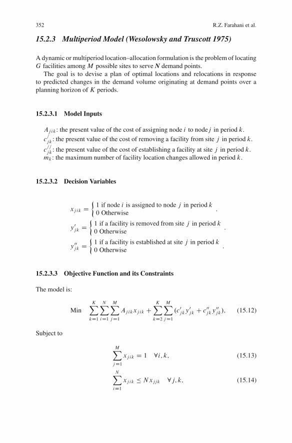
352 R.Z. Farahani et al.
15.2.3 Multiperiod Model (Wesolowsky and Truscott 1975)
A dynamic or multiperiod location–allocation formulation is the problem of locatingG facilities amongM possible sites to serve N demand points.
The goal is to devise a plan of optimal locations and relocations in responseto predicted changes in the demand volume originating at demand points over aplanning horizon ofK periods.
15.2.3.1 Model Inputs
Ajik: the present value of the cost of assigning node i to nodej in period k:
c=
jk : the present value of the cost of removing a facility from site j in period k:
c==
jk : the present value of the cost of establishing a facility at site j in period k:mk : the maximum number of facility location changes allowed in period k:
15.2.3.2 Decision Variables
xj ik D�1 if node i is assigned to node j in period k0 Otherwise
:
y0jk D
�1 if a facility is removed from site j in period k0 Otherwise
:
y00jk D
�1 if a facility is established at site j in period k0 Otherwise
:
15.2.3.3 Objective Function and its Constraints
The model is:
MinKXkD1
NXiD1
MXjD1
Aj ikxj ik CKXkD2
MXjD1
.c0jky
0jk C c00
jky00jk/; (15.12)
Subject to
MXjD1
xj ik D 1 8i; k; (15.13)
NXiD1
xj ik � Nxjjk 8j; k; (15.14)
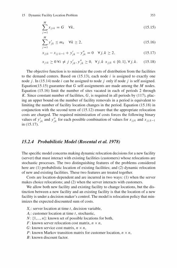
15 Dynamic Facility Location Problem 353
MXjD1
xj ik D G 8k; (15.15)
MXjD1
y0jk � mk 8k � 2; (15.16)
xjjk � xjj k�1 C y0jk � y00
jk D 0 8j; k � 2; (15.17)
xj ik � 08i ¤ j y0jk; y
00jk � 0; 8j; k xjjk 2 f0; 1g;8j; k: (15.18)
The objective function is to minimize the costs of distribution from the facilitiesto the demand centers. Based on (15.13), each node i is assigned to exactly onenode j . In (15.14) node i can be assigned to node j only if node j is self assigned.Equation(15.15) guarantee that G self-assignments are made among the M nodes.Equation (15.16) limit the number of sites vacated in each of periods 2 throughK . Since constant number of facilities, G, is required in all periods by (117), plac-ing an upper bound on the number of facility removals in a period is equivalent tolimiting the number of facility location changes in the period. Equation (15.18) inconjunction with the second term of (15.12) ensure that the appropriate relocationcosts are charged. The required minimization of costs forces the following binaryvalues of y0
jk and y00jk for each possible combination of values for xjjk and xjj;k�1
in (15.17).
15.2.4 Probabilistic Model (Rosental et al. 1978)
The specific model concerns making dynamic relocation decisions for a new facility(server) that must interact with existing facilities (customers) whose relocations arestochastic processes. The two distinguishing features of the problems consideredhere are (1) probabilistic location of existing facilities; and (2) dynamic relocationof new and existing facilities. These two features are treated together.
Costs are location-dependent and are incurred in two ways: (1) when the servermakes choice relocations; and (2) when the server interacts with customers.
We allow both new facility and existing facility to change locations, but the dis-tinction between a new facility and an existing facility is that the location of a newfacility is under a decision maker’s control. The model is relocation policy that min-imizes the expected discounted sum of costs.
Xt : server location at time t , decision variable,At : customer location at time t , stochastic,N : f1,..., ng: known set of possible locations for both,F : known server relocation cost matrix, n � n,G: known service cost matrix, n � n,P : known Markov transition matrix for customer location, n � n,B: known discount factor.
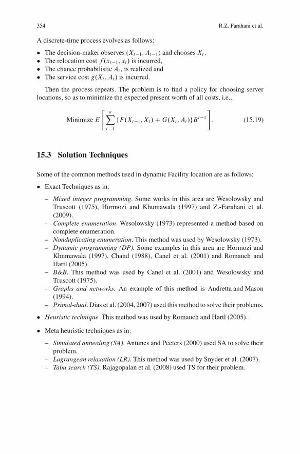
354 R.Z. Farahani et al.
A discrete-time process evolves as follows:
� The decision-maker observes (Xt�1; At�1) and choosesXt ,� The relocation cost f .xt�1; xt / is incurred,� The chance probabilisticAt , is realized and� The service cost g.Xt ; At / is incurred.
Then the process repeats. The problem is to find a policy for choosing serverlocations, so as to minimize the expected present worth of all costs, i.e.,
Minimize E
"aXtD1
fF.Xt�1; Xt /CG.Xt ; At /gBt�1#: (15.19)
15.3 Solution Techniques
Some of the common methods used in dynamic Facility location are as follows:
� Exact Techniques as in:
– Mixed integer programming. Some works in this area are Wesolowsky andTruscott (1975), Hormozi and Khumawala (1997) and Z.-Farahani et al.(2009).
– Complete enumeration. Wesolowsky (1973) represented a method based oncomplete enumeration.
– Nonduplicating enumeration. This method was used by Wesolowsky (1973).– Dynamic programming (DP). Some examples in this area are Hormozi and
Khumawala (1997), Chand (1988), Canel et al. (2001) and Romauch andHartl (2005).
– B&B. This method was used by Canel et al. (2001) and Wesolowsky andTruscott (1975).
– Graphs and networks. An example of this method is Andretta and Mason(1994).
– Primal-dual. Dias et al. (2004, 2007) used this method to solve their problems.
� Heuristic technique. This method was used by Romauch and Hartl (2005).
� Meta heuristic techniques as in:
– Simulated annealing (SA). Antunes and Peeters (2000) used SA to solve theirproblem.
– Lagrangean relaxation (LR). This method was used by Snyder et al. (2007).– Tabu search (TS). Rajagopalan et al. (2008) used TS for their problem.
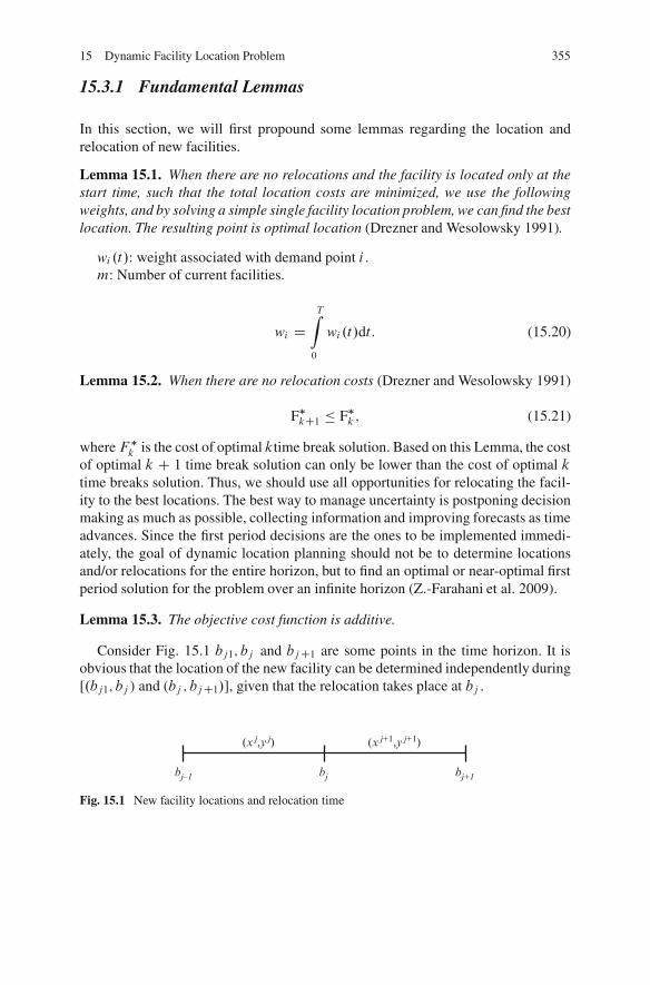
15 Dynamic Facility Location Problem 355
15.3.1 Fundamental Lemmas
In this section, we will first propound some lemmas regarding the location andrelocation of new facilities.
Lemma 15.1. When there are no relocations and the facility is located only at thestart time, such that the total location costs are minimized, we use the followingweights, and by solving a simple single facility location problem, we can find the bestlocation. The resulting point is optimal location (Drezner and Wesolowsky 1991).
wi .t/: weight associated with demand point i .m: Number of current facilities.
wi DTZ0
wi .t/dt: (15.20)
Lemma 15.2. When there are no relocation costs (Drezner and Wesolowsky 1991)
F�kC1 � F�
k ; (15.21)
whereF �k is the cost of optimal ktime break solution. Based on this Lemma, the cost
of optimal k C 1 time break solution can only be lower than the cost of optimal ktime breaks solution. Thus, we should use all opportunities for relocating the facil-ity to the best locations. The best way to manage uncertainty is postponing decisionmaking as much as possible, collecting information and improving forecasts as timeadvances. Since the first period decisions are the ones to be implemented immedi-ately, the goal of dynamic location planning should not be to determine locationsand/or relocations for the entire horizon, but to find an optimal or near-optimal firstperiod solution for the problem over an infinite horizon (Z.-Farahani et al. 2009).
Lemma 15.3. The objective cost function is additive.
Consider Fig. 15.1 bj1; bj and bjC1 are some points in the time horizon. It isobvious that the location of the new facility can be determined independently during[.bj1; bj ) and (bj ; bjC1/], given that the relocation takes place at bj .
bj–1 bj bj+1
(x j,y j) (x j+1,y j+1)
Fig. 15.1 New facility locations and relocation time
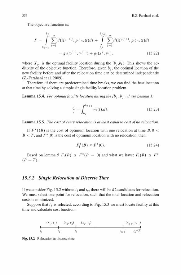
356 R.Z. Farahani et al.
The objective function is:
F DbjZ
bj �1
mXiD1
d.Xj�1;j ; pi /wi .t/dt Cbj C1Zbj
mXiD1
d.Xj;jC1; pi /wi .t/dt
D g1.xj�1; yj�1/C g2.x
j ; yj /; (15.22)
where Xjk is the optimal facility location during the [bj ,bk/. This shows the ad-ditivity of the objective function. Therefore, given bj , the optimal location of thenew facility before and after the relocation time can be determined independently(Z.-Farahani et al. 2009).
Therefore, if there are predetermined time breaks, we can find the best locationat that time by solving a simple single facility location problem.
Lemma 15.4. For optimal facility location during the [bj , bjC1] use Lemma 1:
jwi
DZ bj C1
bj
wi .t/:dt : (15.23)
Lemma 15.5. The cost of every relocation is at least equal to cost of no relocation.
If F �1.B/ is the cost of optimum location with one relocation at time B; 0 <B < T , and F �.0/ is the cost of optimum location with no relocation, then:
F �1 .B/ � F �.0/: (15.24)
Based on lemma 5 F1.B/ � F �.B D 0/ and what we have: F1.B/ � F �.B D T /.
15.3.2 Single Relocation at Discrete Time
If we consider Fig. 15.2 without t1 and tn, there will be Qn2 candidates for relocation.We must select one point for relocation, such that the total location and relocationcosts is minimized.
Suppose that tj is selected, according to Fig. 15.3 we must locate facility at thistime and calculate cost function.
(x1, y1)
t1 t2 t3 tn–1 tn=T
(x2, y2) (x3, y3) (xn–1, yn–1)
Fig. 15.2 Relocation at discrete time
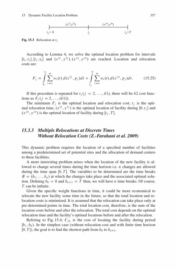
15 Dynamic Facility Location Problem 357
t1= 0 tj tn=T
(x1j,y1j) (x jn,y jn)
Fig. 15.3 Relocation at tj
According to Lemma 4, we solve the optimal location problem for intervalsŒt1; tj ; Œtj ; tn and .x1j ; y1j /; .xjn; yjn/ are reached. Location and relocationcosts are:
Fj DtjZ0
mXiD1
wi .t/:d.x1j ; pj /dt C
TZtj
mXiD1
wi .t/:d.xjn; pj /dt: (15.25)
If this procedure is repeated for tj .j D 2; : : ::; Qn1/, there will be Qn2 cost func-tions as Fj .j D 2; : : :; . Qn1//.
The minimum Fj is the optimal location and relocation cost, tj is the opti-mal relocation time, .x1j ; y1j / is the optimal location of facility during Œ0; tj and.xjn; yjn/ is the optimal location of facility during Œtj ; T .
15.3.3 Multiple Relocations at Discrete TimesWithout Relocation Costs (Z.-Farahani et al. 2009)
This dynamic problem requires the location of a specified number of facilitiesamong a predetermined set of potential sites and the allocation of demand centersto these facilities.
A more interesting problem arises when the location of the new facility is al-lowed to change several times during the time horizon i.e. n changes are allowedduring the time span Œ0; T . The variables to be determined are the time breaksB D .b1; : : :; bn/ at which the changes take place and the associated optimal solu-tion. Defining b0 D 0 and bnC1 D T then, we will have n time breaks. Of course,T can be infinite.
Given the specific weight functions in time, it could be more economical torelocate the new facility some time in the future, so that the total location and re-location costs is minimized. It is assumed that the relocation can take place only atpre-determined points in time. The total location cost, therefore, is the sum of thelocation costs before and after the relocation. The total cost depends on the optimalrelocation time and the facility’s optimal locations before and after the relocation.
Refering to Fig. 15.4; Cjk is the cost of locating the facility during periodŒbj ; bk/. In the simplest case (without relocation cost and with finite time horizonŒ0; T ), the goal is to find the shortest path from b0 to bnC1.
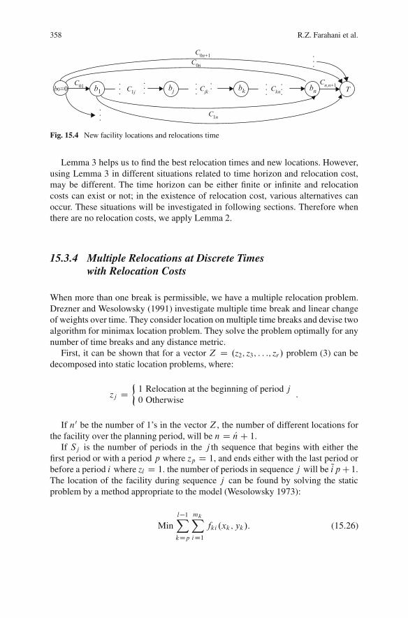
358 R.Z. Farahani et al.
.
.
.
.
.
.
b1 bj bk bn TC1j Cjk
C0n+1
C0n
C1n
Ckn
Cn,n+1...
.
. ...
.
.
. ...
.
.
.C01 b0=0
Fig. 15.4 New facility locations and relocations time
Lemma 3 helps us to find the best relocation times and new locations. However,using Lemma 3 in different situations related to time horizon and relocation cost,may be different. The time horizon can be either finite or infinite and relocationcosts can exist or not; in the existence of relocation cost, various alternatives canoccur. These situations will be investigated in following sections. Therefore whenthere are no relocation costs, we apply Lemma 2.
15.3.4 Multiple Relocations at Discrete Timeswith Relocation Costs
When more than one break is permissible, we have a multiple relocation problem.Drezner and Wesolowsky (1991) investigate multiple time break and linear changeof weights over time. They consider location on multiple time breaks and devise twoalgorithm for minimax location problem. They solve the problem optimally for anynumber of time breaks and any distance metric.
First, it can be shown that for a vector Z D .z2; z3; : : :; zr / problem (3) can bedecomposed into static location problems, where:
zj D�1 Relocation at the beginning of period j0 Otherwise
:
If n0 be the number of 1’s in the vector Z, the number of different locations forthe facility over the planning period, will be n D KnC 1.
If Sj is the number of periods in the j th sequence that begins with either thefirst period or with a period p where zp D 1, and ends either with the last period orbefore a period i where zl D 1. the number of periods in sequence j will be QipC1.The location of the facility during sequence j can be found by solving the staticproblem by a method appropriate to the model (Wesolowsky 1973):
Minl�1XkDp
mkXiD1
fki .xk; yk/: (15.26)
15 Dynamic Facility Location Problem 359
Hence, for any vector Z, the solution of n static problems will specify the suc-cessive optimal locations. The optimal solution to the original problem (3) can nowbe found by evaluating the cost of the location patterns for every possible Z vector(Wesolowsky 1973).
15.3.5 Complete Enumeration
The optimal solution to the problem (15.3) can now be found by evaluating the costof the location patterns for every possible Z vector. There are 2r�1 such vectorsand each vector requires the solution of .Qr1/=2C 1 static problems on the average.Hence, the total number of static problems that must be solved is 2Qr1Œ1C .Qr1/=2.
r�1PiD0
.i C 1/
�r � 1
i
�D
r�1PiD0
i:
�r � 1i
�C
r�1PiD0
�r � 1i
�
D .r � 1/:2r�2 C 2r�1 D 2r�1:�r�12
C 1� : (15.27)
This total enumeration may be feasible for a small r but it is not necessary, sincethere exists a much more efficient way of obtaining a solution (Wesolowsky 1973).
15.3.6 Non-Duplicating Enumeration
Reflection on the above described enumeration procedure yields the followingobservation. Once a move is specified by theZ vector, subsequent succeeding loca-tions are independent of the previous one. This leads to the conclusion that many ofthe static problems solved in the process of the total enumeration of the Z vectorsare identical a better method of enumeration, one that avoids the recalculation ofstatic problems.
In this method, one begins the evaluation at the r th period. If there is a move atthe beginning of the r th period, Cj .1/, the sum of the cost of the static problem andthe moving cost Cr , can be calculated. Similarly, in the r t1th period,Cs.1; 1/ can befound by adding the sum of the costs of the static problem in the r t1th period andthe change cost Crt1 to Cs.1/.
Also Cs.1; 0/ can be found by adding the cost of the static problem in the lasttwo periods to the change cost Cr�1.
One can thus evaluate the cost of the 2r�1 vectors Z without duplicating thecalculation of any static problems. It turns out that this enumeration method callsfor the solution of 2Qr1 static problems (Wesolowsky 1973).
360 R.Z. Farahani et al.
15.3.7 Incomplete DP
Noted that there is no need to evaluate all of the branches. At each stage, as oneproceeds from the last period to the first, only those branches where c; is not greaterthan the stage minimum need be kept. The saving in the number of static problemsthat needs to be evaluated is considerable. If one chooses only one of the branchesin the case where a tie exists at any stage, the total number of static problems to beevaluated is r.r C 1/=2 (Wesolowsky 1973).
1C 2C 3C r D r.r C 1/=2: (15.28)
15.3.8 An Especial BIP
There are some points for relocation and we must select some of them, so that thetotal cost is minimized. For example, we calculate the cost of the policy that thereare two relocations at time 3 and 4.
f13 DmPiD1
wi .t/:d.x13; pi / t 2 Œt1; t3/
f34 DmPiD1
wi .t/:d.x34; pi / t 2 Œt3; t4/
f46 DmPiD1
wi .t/:d.x46; pi / t 2 Œt4; t6/
: (15.29)
The total cost of this policy is:
F DZ t3
t1
f13dt CZ t4
t3
f34dt CZ t6
t4
f46dt: (15.30)
This policy can be shown with binary variable: Z13 D Z34 D Z46 D 1. We pro-pose a binary integer programming (BIP) model composed of six steps (Z.-Farahaniet al. 2009).
Step 1 There are Qn2 time candidates for relocation. Adding t1 D 0 and tn D T
as relocation points yields the total of n points. The interval [0,T ] is divided into Qn1subintervals. There are m demand points. Calculate:
jwi
Dtj C1Ztj
wi .t/dt j D 1; :::; n � 1 i D 1; :::; m (15.31)
15 Dynamic Facility Location Problem 361
Step 2 Definejkwi
W
jkwi
DtkZtj
wi .t/dt k D j C 1; :::; n j D 1; 2; :::; n � 1 i D 1; 2; :::; m j < k:
(15.32)
For every demand point i; Calculate the value ofjkwi
for all values of j and k. This
generates the integrated weight associated with the i th demand point for the locationof the facility during the time interval Œtj ; tk/:
Step 3 For each interval [bj , bk/, find the optimal location of the facility (xjk ,
yjk/. By the value ofjkwi
and the coordinates of the existing facilities (ai ; bi /, the
optimal solution for facility location is used.Step 4 If the new facility has the same location during the time interval [tj , tk/,
calculate Cjk, the location cost, using the following relationship:
Cjk DmXiD1
wjki : d.jk
X:Pi /; (15.33)
where d.Xjk; pi / is the distance between the optimal location of the new facilityand demand point i for Œtj ; tk/ and Xjk is calculated in step 3.
Step 5 Using the cost coefficients in step 4, the following model is used to findthe optimal relocation times:mj
: number of existing facilities
jwi
: the weight associated with demand point i in period jwi .t/: the weight associated with demand point i at time tjkwi
: the integrated weight associated with the i th demand point during the time
interval of [tj , tk/:.xjk; yjk/: the optimal location of the new facility during the time interval of
Œtj ; tk/:
Sj : is the relocation cost at time j .d.Xjk; pi /: the distance between the new facility and i th demand point during
the time interval of [tj , tk/:Zjk : binary variable equal to 1 if the current relocation takes place at tj and the
next one at tk , and is 0 otherwise.
Min F Dn�1XjD1
nXkDjC1
Cjk:Zjk Cn�1XjD2
nXkDjC1
SjZjk; (15.34)
nXkD2
Z1k D 1; (15.35)
362 R.Z. Farahani et al.
k�1XjD1
Zjk DnX
lDkC1Zkl 8k D 2; : : : ; n � 1; (15.36)
n�1XjD1
Zjn D 1 8j; k; (15.37)
Zjk D 0; 1 8j; k: (15.38)
This is a binary integer programming (BIP) model with n constraints and n.nC1/=2variables.
Equation (15.35) ensures that the relocation decision starts at time t1 D 0.Equation (15.36) enforce the consideration of the next relocation time exactly
after the last relocation time.Equation (15.37) guarantee that the decision making will continue to the end of
planning horizon, T . The BIP model can be solved using optimization software suchas LINGO and CPLEX.
The solution to this BIP model yields the times for relocation. The facility loca-tion for each time interval is found in step 3. The total cost of this policy is F .
Step 6 After solving the model, the following solution is obtained:Z1b D Zbc D : : : D Zst D Ztn D 1 and all the other variable are equal to 0.
So t1; tb; : : :; tc ; ts; tt are relocation times and .xtn; ytn/,(xst ; yst /,. . . ,.xbc; ybc/,.x1b; y1b/ are the locations of the new facilities after relocation. The total cost ofthis policy is F .
In this model there are no constraints on the number of relocations. The maxi-mum number of possible relocations is:
N Dn�1XjD1
nXkDjC1
Zjk: (15.39)
If we wish to limit this number to L, the following constraint is added to model.
n�1XjD1
nXkDjC1
Zjk � L: (15.40)
15.3.8.1 Location Dependent Relocation Cost
Another situation closer to real world applications is the case in which relocationcost depends on the location of the facility; i.e. the facility relocation cost at thetime tj is Sj .X D x; y/ instead of Sj , where X D .x; y/ is the location of facility.For instance, one major part of the cost for locating facility is the price of land. Priceof land for locating a facility will differ from one location to another.
In this model, we solve the problem similar to the procedure described in thepervious section. The only difference is that the cost of the best location during[tj ,tk/ will be the minimum of the function:
15 Dynamic Facility Location Problem 363
Cjk D Sj .X/CmXiD1
wjki d.Xjk; pi /: (15.41)
This means that the second term of the objective function is not independent ofthe first term.
If Sj .X D x; y/ is differentiable, the minimum of Cjk could be calculated di-rectly. When squared Euclidean distances are used, Cjk is differentiable and thereis no need to use Hyper approximation procedure (HAP) for the calculation of theoptimal Cjk (Z.-Farahani et al. 2009).
15.3.8.2 Relocation Cost Depend on the Location of FacilityBefore and After Relocation
Sometimes, relocation cost at the time tj depends on the location of facility beforeand after tj . In practical cases, there are situations in which the cost of relocating to acloser location is lower than relocating to a farther location. For example, in mobilefacilities, the relocation cost will be a function of distance between the location offacility before and after relocation time. In this case the objective function is:
Cjk D u.tj / d.Xhj ; Xjk/CmXiD1
wjki d.Xjk; pi /: (15.42)
where th is the last relocation point before tj , d.Xhj ; Xjk/ is the distance be-tween the location of facility before tj .Xhj / and after tj .Xhk/. In addition, u.tj / isthe unit distance cost for relocating a facility from its location to another new loca-tion, at the time tj . In this case, Lemma 3 is not satisfied and the objective functionis not additive.
For a finite time horizon, we propose to perform complete enumeration and findall of feasible paths from t0 to tnC1. When n is large we must resort to heuristicalgorithms. For each feasible solution, we should calculate the objective functionand select the minimum. The number of these feasible paths can be calculated withrespect to the number of relocations (0, 1, 2) as follows:
1C�n
1
�C�n
2
�C : : :C
�n
n
�D 2n: (15.43)
For solving the objective function of each feasible path, note that if both d.Xjk; pi /
and d.Xhj ; Xjk/ are rectilinear distance, we can solve an equivalent LP substitutingthe absolute function with new variables and constraints. If both d.Xjk; pi / andd.Xhj ; Xjk/ are squared Euclidean distance, the objective function is differentiableand the problem can easily be solved. If the type of distances related to d.Xjk; pi /
and d.Xhj ; Xjk/ is different or both are Euclidean, we can use the HAP (Francisand Lowe 1992).
364 R.Z. Farahani et al.
15.3.9 Relocation at Continues Times
As it was noted, relocation can take place only at pre-determined points in time or,at any point in the time horizon. In this section, first, we will propound a lemmaand then we will study the facility location–relocation problem with linear timedependent weights.
Roll Theorem (Leithold 1976). If f .x/ is continuous in [0,T ] and differentiablein (0,T ) and if f .a/ D f .b/, then there is a c such that a < c < b and f .c/ D 0.
Suppose that there are no candidate times for relocation, and relocation can takeplace at any point in the time horizon [0,T ]. Therefore, time break (B/ enters thecost objective function. The cost objective function will be:
F.B; x1; y1; x2; y2/ DBZ0
mXiD1
wi .t/:d.X1; pi /:dt CTZB
mXiD1
wi .t/:d.X2; pi /:dt;
(15.44)where 0 < B < T .Given a distinct time break .B/, other variables are calculated, and for every B
there is only one point (x1; y1/ and (x2; y2/. In other words, (x1; y1/ and (x2; y2/functions of B).
x1 D f1.B/ y1 D f2 .B/ x2 D f3 .B/ y2 D f4 .B/: (15.45)
According to (15.44) and (15.45), the cost function is:
F.B; x1; y1; x2; y2/ D F.B; f1.B/; f2.B/; f3.B/; f4.B//: (15.46)
Relation (15.46) shows that the cost function is function of time break and wecan use F as F.B/ according to (15.44):
F.B D 0/ D F.B D T /: (15.47)
The approximate rectilinear distance is (Francis and Lowe 1992):
jx � ai j C jy � bi j Dp.x � ai /2 C "C
p.y � bi /2 C ": (15.48)
Using this approximation, the cost function of (15.47) is continuous in [0, T ] andderivable in (0, T ).
According to Roll Theorem, there is at least one B , such that 0 < B < T and isan extreme point for cost function.
It is important to note that the weights, wi .t/; cannot be negative in the [0; T ].For the linear weights the following holds:
ui � 0; vi � �uiT: (15.49)
15 Dynamic Facility Location Problem 365
For single relocation, linear weight function is put in the cost function (15.44):
BZ0
mXiD1
wi .t/:d.X1; pi /:dt CTZB
mXiD1
wi .t/:d.X2; pi /:dt D
BZ0
mXiD1
d.X1; pi /:.ui C vi :t/:dt CTZB
mXiD1
d.X2; pi /:.ui C vi :t/:dt: (15.50)
Integration and sigma are replaced:
mXiD1
BZ:
d.X1; pi /:.ui C vi :t/:dt CmXiD1
TZB
d.X2; pi /:.ui C vi :t/:dt D
mXiD1
d.X1; pi /:.ui :t C 1
2vi :t
2/
ˇˇB0 C
mXiD1
d.X2; pi /:.ui :t C 1
2vi :t
2/
ˇˇTB D
mXiD1
d.X1; pi /:.ui :B C 1
2vi :B
2/CmXiD1
d.X2; pi /:.ui :.T � B/
C1
2vi :.T
2 � B2//: (15.51)
For approximate rectilinear function, (15.51) will be differentiable and concaveand, therefore, we will have:
@F
@BD @
@B
*mXiD1
d.X1; pi /:.ui :B C 1
2vi :B
2/
+
C @
@B
*mXiD1
d.X2; pi /:.ui :.T � B/C 1
2vi :.T
2 � B2//
+: (15.52)
Integration and sigma are replaced:
@F
@BD
mXiD1
@
@B
�d.X1; pi /:.ui :BC 1
2vi :B
2/
�C
mXiD1
@
@Bhd.X2; pi /:.ui :.T � B/i
C1
2vi :.T
2 � B2// DmXiD1
d.X1; pi /:.ui C vi :B/
CmXiD1
d.X2; pi /:.�ui � vi :B/ (15.53)
DmXiD1
d.X1; pi /:.ui C vi :B/ �mXiD1
d.X2; pi /:.ui C vi :B/:
366 R.Z. Farahani et al.
In the optimal point (15.53) must be equal to zero:
mXiD1
hd.X1; pi /:.ui C vi :B/ � d.X2; pi /:.ui C vi :B/i
D 0 )mXiD1
h.uiCvi :B/.d.X1; pi /� d.X2; pi //i
D 0 )mXiD1
ui :.d.X1; pi / � d.X2; pi //
�mXiD1
viB:.d.X1; pi / � d.X2; pi // D 0: (15.54)
Therefore, B will be equal to:
B D �
mPiD1
ui :.d.X1; pi / � d.X2; pi //mPiD1
viB:.d.X1; pi / � d.X2; pi//: (15.55)
Note that to make sure that B is at minimum, the second derivation must bepositive.
@2F
@B2> 0
@2F
@B2D @
@B
�@F
@B
�D
@
@B
mXiD1
d.X1; pi /:.ui C vi :B/ �mXiD1
d.X2; pi /:.ui C vi :B/
!)
@2F
@B2D
mXiD1
vi :.d.X1; pi / � d.X2; pi// > 0: (15.56)
According to lemmas 3 and 4, if the relocation times are determined then:
w.1/i DBZ0
.ui C vi t /:dt Dui tC 1
2vi t
2
ˇˇB0 D uiB C 1
2viB
2
w.2/i DTZB
.ui C vi t /:dt Dui tC 1
2vi t
2
ˇˇTB D ui .T �B/C 1
2vi .T
2�B2/: (15.57)
Therefore, using w.1/i we can solve facility location problem and obtain the lo-cation of the facility before relocation, (x1; y1/, then using w.2/i , the location offacility after relocation .x1; y1/ is reached.
15 Dynamic Facility Location Problem 367
Obviously, doing these calculations with hand, particularly for large problems,is very difficult. However, nowadays, with the technological advances, doing thiscalculation with computer is not so difficult and time consuming. Thus, in this sub-section, we present an algorithm that obtains optimal point in this problem.
15.3.10 Iterative Algorithm for Obtaining Optimal Solution
In this algorithm, first an optional B in interval [0, T ] is selected, and w.1/i and w.2/iare calculated using (15.57). Then, .x1; y1/ and .x2; y2/ are calculated through solv-ing the two obtained location problems based on w.1/i and w.2/i . Next, by substitutingthese four variables in (15.55), a new B value is obtained. All the mentioned stepsare repeated using this new B . It can be shown by Roll theorem that these iterationsconverge to a B point.
Not that (15.56) must be satisfied in order to have the F function minimizedfor the given B value, otherwise, we cannot claim that the obtained B minimizesF . Even if (15.56) is satisfied, there is no proof that the obtained point is globalminimum. To solve this problem, repeat the algorithm with differentBs as a startingpoint. Therefore, if a local minimum exists, we can obtain global minimum.
As it was explained before, the steps of the global minimum algorithm for theobtained break time and optimal location are as fallows:
Step 1 Generate a reasonable number for search steps. The smaller this value, themore accurate and the slower the algorithm, and vice versa. Set count D 0; k D 1,F � D 1. Enter coordinates of the existing facilities, linear functions parameters(ui ; vi ), and permissible errors.
Step 2 Set count D count C step if count � T then go to step 10 else go to nextstep.
Step 3 Set Bk1 D count.Step 4 As described before and by considering Bk1, calculate values of
.xk�11 ; yk�1
1 / and .xk�12 ; yk�1
2 /.Step 5 calculate the result of (15.55) as follows:
Bk D �
mPiD1
ui :.d.Xk�11 ; pi / � d.Xk�1
2 ; pi //
mPiD1
viB:.d.Xk�11 ; pi / � d.Xk�1
2 ; pi //
: (15.58)
Step 6 IfˇBk � Bk�1ˇ > ı then set k D k C 1 and go to step 4 else go to the
next step.Step 7 calculate the result of (15.56) as follows:
mXiD1
vi :.d.Xk�11 ; pi / � d.Xk�1
2 ; pi //: (15.59)
If this value is negative then set k D 1 and go to step 2 else go to the next step.
368 R.Z. Farahani et al.
Step 8 calculate the cost using the following equation:
F DmPiD1
.d.Xk�11 ; pi / � d.Xk�1
2 ; pi //:.ui :Bk C 12vi :Bk2/
CmPiD1
d.Xk�12 ; pi /:.ui :T C 1
2vi :T 2//:
(15.60)
Step 9 If F < F � then set F � D F;B� D Bk; .x�1 ; y
�1 / D .xk�1
1 ; yk�11 /;
.x�2 ; y
�2 / D .xk�1
2 ; yk�12 /; k D 1 and go to step 2 else without changes go to step 2
Step 10 B�; .x�1 ; y
�1 /; .x
�2 ; y
�2 / and F � are optimal solutions.
Note that there is also another approach for solving single relocation and multirelocation time-independent problems that interested readers are referred to Owenand Daskin (1998) for detailed information.
15.3.11 Static Stochastic Techniques
The dynamic models described in the previous sections attempt to locate facil-ities assuming that input parameters are known values or vary deterministicallyover time.
In stochastic location problems, any number of system parameters might be takenas uncertain. Stochastic location problems can be broken down into probabilisticapproach and the scenario planning approach (Owen and Daskin (1998).
15.3.11.1 Probabilistic Approach
Sometimes, we examine models which capture the stochastic aspects of facility lo-cation through explicit consideration of the probability distributions associated withmodeled random quantities.
These distributions can be incorporated into standard mathematical programs, orin a queuing framework (Owen and Daskin 1998).
15.3.11.2 Scenario Planning Approach
Scenario planning is a method in which decision makers capture uncertainty byspecifying a number of possible future states. The objective is to find solutionswhich perform well under all scenarios. In some applications, scenario planning re-places forecasting as a way to evaluate trends and potential changes in the businessenvironment. Firms can thus develop strategic responses to a range of environmental
15 Dynamic Facility Location Problem 369
changes, more adequately preparing themselves for the uncertain future. Under suchcircumstances, scenarios are qualitative descriptions of plausible future states, de-rived from the present state with consideration of potential major industry events. Inother applications, scenario planning is used as a tool for formulating and solvingspecific operational problems (Owen and Daskin 1998).
The goal of scenario planning is to specify a set of scenarios, which representthe possible realizations of unknown problem parameters and to consider the rangeof scenarios in determining a compromise (robust) location solution (Owen andDaskin 1998). There are at least three approaches to incorporating scenario planninginto location modeling:
� Optimizing the expected performance over all scenarios,� Optimizing the worst-case performance, and� Minimizing the expected or worst-case regret across all scenarios. (Owen and
Daskin 1998).
Scenario planning approach, though invaluable in dealing with conditions wherethere is uncertainty about input parameter information, has two disadvantages:
� Defining scenario and assigning probabilities to them is difficult� Because of the high calculation efforts required, the number of evaluated scenar-
ios are kept low and therefore, the future condition is restricted (might not berealistic enough) (Snyder 2006).
The regret associated with a scenario is calculated by comparing the performanceof the optimal locations for the scenario (had planners known for certain that thescenario would be realized) with the performance of the compromise locations whenthe scenario is realized. (Owen and Daskin 1998)
In other words, by extent of loss, also referred to as “opportunity loss” it is meantwhat the decision maker pays for performing under the conditions of not knowingabout the occurrence of a scenario as compared with his/her performance in thecompromise locations when the scenario has already realized (Snyder 2006).
Thus, using a regret-based objective allows us to evaluate robust solution alter-natives with respect to the optimal solution obtained under data certainty.
One should use this measure in objectives which:
� Require assessment of scenario realization probabilities, and� Assume that all scenarios are of equal probability.
15.4 Case Study
In this section, we will introduce some case studies related to Dynamic Facilitylocation problems.
370 R.Z. Farahani et al.
15.4.1 A Dynamic Model for School Network Planning (Antunesand Peeters 2000)
This case study describes a dynamic multi-period optimization model that has beenused in Portugal to formulate planning proposals for the evolution of several schoolnetworks.The solution to this problem gives information about where and when newschools should be built, what their sizes should be, which schools should be keptopen and which ones should be closed. Additionally, for the schools which remainopen, it identifies which schools should maintain the same size and which should beresized, becoming larger or smaller.
This model considers the following features:
� Over the planning horizon, each site will not change its state more than once;� Both setup and operation costs have a component dependent on capacity and a
component dependent on attendance; and� Facility size is limited to pre-defined standards, expressed in terms of an archi-
tectural module, for instance, a given number of classrooms.
The objective function of this model minimizes the total discounted (socio-economic) costs of a set of facilities. Facility costs are divided into three parts:fixed costs; capacity-variable costs proportional to the number of modules; andattendance-variable costs proportional to the number of users, a significant part ofwhich will normally consist of transport costs.
The approaches that had been used to solve this model are as following:
� Branch and bound (B&B), but this method is unsuccessful to solve a few10 10 3 .centers sites periods/ problems.
� Dual-based and LR exact methods. However, this kind of method would hardlybe successful in the current case.
� The “myopic” and “panoramic” approaches (heuristics). These methods in thepresence of severe capacity inadequacy and important demand decreases thesituation encountered in many Portuguese regions when the expansion of ele-mentary education was decided didn’t have successful function.
� SA: For 50 problems in 17, SA was unable to find the optimum B&B solution.Moreover, in all these 17 problems, it came quite close to it, as the differencewas always smaller than 1%. In the remaining 33 problems, SA behaved at leastas efficiently as B&B.
15.4.2 A Multiperiod Set Covering for Dynamic Redeploymentof Ambulances (Rajagopalan et al. 2008)
The dynamic available coverage location model was formulated to determine theminimum number of ambulances and their locations for each time cluster in whichsignificant changes in demand pattern take place while meeting coverage require-ments with a predetermined reliability.
15 Dynamic Facility Location Problem 371
A straightforward search algorithm was developed to determine the minimumnumber of servers to provide the coverage and availability requirements. The algo-rithm starts with an estimated fleet size for the first time interval, which is calleda reactive Tabu search (RTS) algorithm. A look-ahead procedure (LAP) within theRTS was used to compute server specific busy probabilities and the resulting cov-erage. Results showed that the RTS with LAP takes them very close to number ofservers required to satisfy the coverage constraint generally 2–3 times faster thanthe algorithm without LAP.
15.4.3 A Multi-period Model for Combat Logistics (Gue 2003)
In the past, logistics support for amphibious warfare has depended on a large, land-based infrastructure, with trucks accomplishing most of the distribution. New warfighting concepts for the US Marine Corps emphasize small, highly-mobile forcessupported instead from the sea. The goal of logistics planners is to support theseforces with as little inventory on land as possible. But the best distribution systemdepends on a number of operational levers.
For better conception, this study has considered a sea base containing combatand support units. Each combat unit is required to reach a particular set of objectiveson land; support units are positioned to provide supplies as needed. Combat unitsconsume food, water, ammunition, and fuel during each time period. Quantities mayvary depending on the intensity of conflict or other concerns. Supply units are free todeploy, move, and to build up and deplete inventories as necessary to meet demand.A fleet of vehicles is available to transport combat units to objectives or intermediatepoints, to move entire supply units, or to transport supplies between units. Naturally,vehicle types are constrained to transport only between feasible origin–destinationpairs. The problem is to determine the locations of supply units for each time periodand the shipments of each commodity between units, such that there is as little land-based inventory as possible.
In this case a multi-period, facility location and multi-commodity flow model isformulated as a mixed integer program. The battle space is modeled as a networkof two types of nodes, combat and supply nodes. In model, it is assumed that thecombat nodes are given in a battle plan and that supply units may not occupy them.And also that intelligence could provide a set of candidate locations for supply units.The objective is to minimize the total inventory of land-based support units, in keep-ing with the primary purpose of sea-based logistics. Decisions in the model are, foreach time period, the locations of support units, inventories held by the units, andthe amounts shipped between units.
Two limitations of this model are:
� Transportation capacity is modeled in units of lb mile, the model could proposea solution that is impossible to implement in practice.
� A solution could also require more transporters than are available.
372 R.Z. Farahani et al.
References
Andretta G, Mason FM (1994) A not on a perfect forward procedure for a single facility dynamiclocation/relocation problem. Oper Res Lett 15:81–83
Antunes A, Peeters D (2000) A dynamic optimization model for school network planning. SocioEcon Plan Sci 34(2):101–120
Canel C, Khumawala B, Law J, Loh A (2001) An algorithm for the capacitated, multi-commoditymulti-period facility location problem. Comput Oper Res 28:411–427
Chand S (1988) Decision/forecast horizon results for a single facility dynamic location/relocationproblem. Oper Res Lett 7(5):247–251
Daskin MS, Hopp WJ, Medina B (1992) Forecast horizon and dynamic facility location planning.Ann Oper Res 40:125–151
Dias J, Captivo E, Climaco J (2004) Dynamic multi-level capacitated and uncapacitated locationproblems: an approach using primal-dual heuristics. Inesc-Coimbra Research Report 26
Dias J, Captivo E, Climaco J (2007) Efficient primal-dual heuristic for a dynamic location problem.J Comput Oper Res 34:1800–1823
Drezner Z (1995) Facility location: a survey of applications and methods. Springer, New YorkDrezner Z, Wesolowsky GP (1991) Facility location when demand is time dependent. Naval Res
Logist 38:763–777Emamizadeh B, Z-Farahani R (1997a) Facility location and relocation in global manufacturing
strategy. Paper presented at the FAIM conference, Middlesbrough, EnglandEmamizadeh B, Z-Farahani R (1997b) Facility location and relocation with time-dependent
weight. Paper presented at the DSI Conference, Sidney, AustraliaFrancis RL, McGinnis LF, White JA (1992) Facility layout and location: an analytical approach,
2nd edn. Prentice Hall, Englewood Cliffs, NJGue k (2003) A dynamic distribution model for combat logistics. Comput Oper Res 30:367–381Hormozi AM, Khumawala BM (1997) An improved algorithm for solving a multi-period facility
location problem. IIE Trans 28:105–114Huang WV, Batta R, Babu AJG (1990) Relocation-promotion problem with Euclidean distance.
Eur J Oper Res 46:61–72Leithold L (1976) The calculus with analytic geometry, 3rd edn. Harper & Row, New YorkMirchandani PB, Francis RL (1990) Discrete location theory. Wiley, New YorkOwen S, Daskin M (1998) Strategic facility location: a review. Eur J Oper Res 111:423–447Rajagopalan H, Saydamb C, Xiaoc J (2008) A multiperiod set covering location model for dynamic
redeployment of ambulances. Comput Oper Res 35:814–826Romauch M, Hartl RFH (2005) Dynamic facility location with stochastic demands. Lecture notes
in computer science (Stochastic algorithms: foundations and applications), vol 3777Rosental R, White J, Young D (1978) Stochastic dynamic location analysis. Manage Sci
124(6):645–653Scott AJ (1971) Dynamic location–allocation systems: some basic planning strategies. Environ
Plan 3:73–82Snyder LV (2006) Facility location under uncertainty: a review. IIE Trans 38(7):547Snyder LV, Daskin MS, Teo CP (2007) The stochastic location model with risk pooling. Eur J Oper
Res 179:1221–1238Wesolowsky GO (1973) Dynamic facility location. Manage Sci 19(11):1241–1248Wesolowsky GO, Truscott WG (1975) The multiperiod location–allocation problem with reloca-
tion of facilities. Manage Sci 22(1):57–65Z.-Farahani R, Drezner Z, Asgari N (2009) Single facility location and relocation problem with
time-dependent weights and discrete planning horizon. Ann Oper Res 167(1):353–368
Chapter 16Multi-Criteria Location Problem
Masoud Hekmatfar and Maryam SteadieSeifi
Decision-making is the process of selecting a possible subset of decisions fromall the available alternatives (feasible space). We introduced many decision-makingmodels including one objective function, so far. Almost there are many criteria forjudging the optimality of decision. In this situation, we will be faced with the multi-criteria decision-making (MCDM). There are many methods to solve the MCDMproblems, but all of them are common in some factors that are as follows (Hwangand Masud 1979; Hwang and Yoon 1981):
� Multiple objectives/attributes� Conflict among criteria� Incomparable units� Design or selection: solutions to these problems consist of two classes, one of
them designs the best alternative and the second one selects the best solutionamong the specified finite alternatives
The MCDM is classified into two categories:
� The multi-objective decision-making (MODM), and� The multi-attribute decision-making (MADM)
First, briefly, we define some prevalent important terms used in this area (Hwangand Masud 1979; Hwang and Yoon 1981):
� Criteria: Criteria are standards of judgment or rules to test acceptability� Goal: Goals are a priori levels of aspiration that are determined by decision mak-
ers (DMs) with explicit term� Objective: Objectives are the directions that increase the inspiration of DMs
(Maybe it seems that the two recent terms have a common meaning, while ob-jectives give the desired direction, goals give a desired level to achieve.)
� Optimal solution: Optimal solution is one which results in maximum value ofeach of the objective functions. Because of the conflicting objectives, this solu-tion will not usually exist
� Efficient solution (Nondominated solution): Qx is an efficient solution if there ex-ists no other feasible solution that will yield an improvement in one objectivewithout causing a reduction in at least one other objective
R.Z. Farahani and M. Hekmatfar (eds.), Facility Location: Concepts, Models, 373Algorithms and Case Studies, Contributions to Management Science,DOI 10.1007/978-3-7908-2151-2 16, c� Physica-Verlag Heidelberg 2009
374 M. Hekmatfar and M. SteadieSeifi
� Preferred solution: A preferred solution is selected by DM from efficientsolutions
� Satisfing solution: A Satisfing solution Satisfies a minimum acceptable level forall attributes of the problem
The MCDM comprises some general techniques that can be used in many types ofapplication including facilities location.
The remainder of this chapter will first present some classifications, objectivefunctions and mathematical models of MCLPs. Next, solution techniques will bebriefly reviewed. Finally, in Sect. 16.3 some real-world case studies will be intro-duced.
16.1 Applications and Classifications
Multi-criteria analysis of location problems has received considerable attentionwithin the scope of continuous and network models in recent years. There are sev-eral problems that are accepted as classical ones:
� The point-objective problem (Wendell and Hurter 1973; Hansen et al. 1980;Pelegrin and Fernandez 1988; Carrizosa et al. 1993)
� The continuous multi-criteria min–sum facility location problem (FLP)(Hamacher et al. 1996; Puerto and Fernandez 1999)
� The network multi-criteria median location problem (Hamacher and Nickel 1998;Wendell et al. 1977)
So far, multi-criteria analysis of discrete location models has attracted less attention.Several authors have dealt with problems and applications of multi-criteria decisionanalysis in this field. For instance,
� Ross and Soland (1980) worked on multi-activity multi-facility problems andproposed an interactive solution method to compute non-dominated solutions tocompare and choose from
� Lee et al. (1981) studied an application of integer goal programming for facilitylocation with multiple competing objectives
� Solanki (1991) applies an approximation scheme to generate a set of non-dominated solutions to a bi-objective location problem
� Ogryczak (1999) looks for symmetrically efficient location patterns in a multi-criteria discrete location problem
In general, none of the above papers focuses on the complete determination of thewhole set of non-dominated solutions. The only exception is the paper by Rossand Soland (1980) that gives a theoretical characterization but does not exploit itsalgorithmic possibilities.
16 Multi-Criteria Location Problem 375
16.2 Models
Although location problems have a long history, we can assume that the modernlocation has been started from Weber research on one vehicle location problem withthe objective function based on minimizing the total rectilinear distances. This trendwas continued up to 1960s, minimizing the total distances (min–sum).
In 1960s, Hakimi (1964) represented a new kind of problems, minimizing themaximal distance (min–max). In this decade, many operation researchers workedon location problems (Eiselt and Laporte 1995).
In the mid 1970s, it seems that the topic of obnoxious location problem wasrepresented by some researchers such as Goldman and also Church and Granfinkelfor the first time (Eiselt and Laporte 1995). Maybe we can assume that after comingup of this topic in multi-objective problems, the MCDM techniques were started tobe used to solve the MCDM problems.
Since the aim of this section is FLPs from objective functions point of view, inthe following sections we try to represent the main classification of objective func-tions, conflicting of contradictory objectives and at last some case study of locationproblems.
We concentrate to display these problems and their classifications based on theirobjective functions.
16.2.1 Private and Public Facilities
Problems that are naturally multi-objectives are generally discussed in public fa-cilities, semi-noxious facilities and desirable facilities. Cohon (1978) representedMCLPs in a separate section. He divided FLPs into two main classes:
� Facility location in private sections� Facility location in public sector
In the first group, problems have almost only one objective and the main purposeis almost minimizing the cost of construction, production and transportation, or thepurpose is maximizing the profit earned from constructing the facility. This kind ofproblems is located in class of classic location problems.
In the second group, problems that are efficient in governments’ final decision-making (directly or indirectly), are divided into three classes:
� Facilities with ordinary services� Facilities with emergency services� Facilities with undesirable effect
In ordinary services like libraries, hygienic clinics etc., the purpose usually consistsof the maximizing of service to more people.
376 M. Hekmatfar and M. SteadieSeifi
In emergency services like fire stations the purpose is usually consisted of maxi-mizing the minimal covering.
In undesirable facilities, there is an undesirable facility like a place for repulsingrefuses, wastes, etc., and the purpose is consisted of minimizing the effect of thisarea on the residents near it.
It seems that the Cohon’s (1978) classification has some problems and it can bepossible to represent better classification. We represent some of them in later parts.
In public sectors, the main problem is the lack of proper criteria and their differ-ent natures. For example in a fire station location problem, there are two conflictingobjectives, one of them is consisted of minimizing the cost of facility and the otherone is consisted of preserving the human life. so how the human life can be evalu-ated?
In Cohon (1978), two location problems are represented, emergency serviceslocation problem (construction of a fire station in Baltimore) and power generationlocation problem in a power station. Readers can refer to Cohon (1978) for moredetails.
16.2.2 Balancing Objective Functions
A group of objective functions are discussed in public facility and services and thepurpose is consisted of maximizing the equity and balanced services among users.These problems are introduced as fairness functions, balancing functions and equityfunctions.
Displaying the value of equity is varied in different problems, but it can be pos-sible to generate a new class of objective functions based on a development frommin–sum functions and a statistic view.
In prevalent min–sum functions, it is easy to show that minimizing the totaldistances of demand points from facility is statistically equal to minimizing the av-erage of distances with assuming one facility and locating in one dimension. (seeEq. 16.1).
min WnXiD1
.xi �L/ D n
nPiD1
.xi �L/n
! n �d (16.1)
where L is the situation of facility.We can assume some other functions like the total squared distance of demands
from facility or cubical distance of demands.From statistics point of view, the total distances (first torque) are related to av-
erage distances, total squared distances (second torque) are related to variance ofdistances, and cubical distances (third torque) are related to scale of symmetry forpoint distribution around facility location place. In other words, by minimizing thesecond torque we can obtain a set of solutions in which the distance oscillation ofdemand points from the facility location are minimized.
16 Multi-Criteria Location Problem 377
With minimizing the total cubical distances, the set of solutions will finally haveless asymmetry. It means that there is not anyone who lives very close or very farfrom the facility.
Balancing objective functions can reach a better solution in dealing with publicFLPs and if we see these three functions simultaneously, it will be necessary to usetechniques of multi-objective programming (Eiselt and Laporte 1995).
16.2.3 Pull, Push and Pull–Push Objectives
The various types of facilities from customer point of view were represented byEiselt and Laporte (1995) as follows:
� Desirable� Undesirable� Partly desirable� Partly undesirable� Indifferent
According to an acceptable classification which was represented by Krarupet al. (2002), Curtin and Church (2003), and Eiselt and Laporte (1995), objec-tive functions are divided into two main classes: Pull and Push. The combinationof these two classes is introduced as pull–push term and is a major topic in multi-objective real problems.
Another kind of classifications is related to service distribution and establishmentof equity which is represented as balancing objective by Eiselt and Laporte (1995).
Pull Objectives The classic location problems, desirable facilities and generallyolder location problems have pull objective functions. For example, it is tried to min-imize the distance between production plants and consuming markets which yieldedminimizing the cost of transportation, maximizing the availability of customers andincreasing part of the market.
The classic pull-objective functions are generally divided into four classes:P-median (min–sum), P-center (min–max), UFLP1 (min–sum) and QAP (min–sum).
Push Objectives Most of the undesirable location problems such as obnoxiousand noxious and also dispersion models have push objective functions. It means thatin these problems the purpose is consisted of decreasing the noxious effect of facilityon demand points. Since in most cases the noxious effect has an inverse relation withthe distance, the purpose of these problems is consisted of maximizing the distancebetween facility and demand points. A complete survey of these problems has beenrepresented by Curtin and Church (2003).
Erkut and Neuman (1990) made a comparison of dispersion models and dividedthem into four main classes: P-dispersion (max–min–min), P-defense (max–sum–
1 Uncapacitated Facility Location Problem
378 M. Hekmatfar and M. SteadieSeifi
min), Anti-hub (max–min–sum) and Maxi-sum dispersion/P-maxian (max–sum–sum). It can be seen that they employed a three-syllable naming convention forobjective functions with maximizing aim to distinguish between different types ofdispersion. Using this convention, the first syllabus for each model was “Max” de-noting that all models attempt to maximize the amount of dispersion among selectedfacility sites. Both the second and third syllables were either “sum” or “min”. In thesecond syllable, a “sum” operator indicates a concern for overall system perfor-mance while a “min” operator indicates a concern for worst-case performance (hereleast distance). The third syllable is again either “sum” or “min”, and it refers towhich facility interactions comprise the minimum distance to be considered by theformulation. When the “min” operator is employed, the objective function is onlyforced by the minimum distance between any two facilities in a given solution. The“sum” operator indicates that the distances from each facility to all other facilitieswill force the objective function.
Push–Pull Objectives As it was indicated in the previous sections, in most of thereal problems, simultaneously there are some conflicted objectives. It means that ob-jective functions are combined with desirable and undesirable effects. It is noticedthat these problems deal with interference of government like municipal, ecologi-cal organization, etc. as an example of these conflicted objectives, assume that thepurpose is consisted of both increasing the distance between production plants andresidential places and also increasing the cost of transportation, decreasing the at-traction of professions, etc.
There is a clear example about these types of problems. In establishing a super-store or a sport club, the purpose of investors is decreasing the distance betweentheir buildings and residential places to attract more customers, but residents preferto live not too far and not too close to these facilities. Such problems are introducedwith terms like “close but not too close” and “never in my back yard”. These classesof problems had not been surveyed until 1970s.
A complete review about discrete location problems with push–pull objectives isrepresented by Krarup et al. (2002).
As it has been mentioned in previous sections, there is a classification of classi-cal location problems with pull-objectives and desirable facilities:P -median, UFLP,QAP with min–sum objective function and P -center with min–max objective func-tion. In QAP demand points and facilities are the same things and the demand isequal to material flow or information between facilities.
Also there is a classification of classical location problems with push-objectives:The first group is consisted of undesirable facilities which have noxious effect onhealth like chemical wastes and obnoxious effect on environment like the noise ofsports clubs. The second group is consisted of dispersion models (Erkut and Neu-man 1990) which there are classically undesirable effects between their facilities.
Krarup et al. (2002) represented that there is a famous problem, apparently firstformulated in the early 1600s by Fermat, together with kind of a companion problemtermed complementary problem (ComP). For a given triangle, Fermat asks for afourth point such that the sum of its Euclidean distances, each weighted by C1, to
16 Multi-Criteria Location Problem 379
the three given points is minimized. ComP differs from Fermat in that the weightassociated with one of these points is �1 instead of C1.
It can be possible to divide push–pull problems into two major groups:
� Problems that only inter-facility interactions are considered, some being desir-able, and some undesirable, this group is called a semi-dispersion model. Thereare some cases in this group such as: QAP with undesirable effect, quadraticknapsack problem that a number of facilities may be established at some pre-defined locations and then undesirable effect will be occurred, P -defense-sumproblem and P -dispersion (Krarup et al. 2002)
� Problems that involve a set of demand points which pull the facilities towardsthem, whereas the undesirable part will be concerned with another set of subjectswhich push the facilities away. These problems are modeled as bi-objective withthe attractions and the repulsions as two quite opposing objectives, each of whichmight still be multi-objective (Krarup et al. 2002)
The strategies that are used to solve these bi-objective problems are summarizedas follows:
� Treat the bi-objective problem as really bi-objective and derive (approximationsto) the Pareto-set
� Fix a bound on the obnoxious effects as a (set of) constraint(s) and optimizethe desirable objective. This leads to standard pull objectives with additionalrestrictions
� Fix a bound for the desirable objective part and optimize the undesirable objec-tive. This leads to standard push objectives with an additional constraint
� Combine the push and pull objectives into a single objective
16.2.4 Mathematical Models
In this section, some multi-objective problems with their mathematic models whichKrarup et al. (2002) called them general push–pull will be represented. First, thereare some remarks, which are represented as follows:
� The type of modeling has a major effect on final solution. It means that the styleof exhibition in an undesirable effect (as you can see in following sections) willbe affected on type of the objective function (the problem will be single objectiveor multiple objective)
� The type of objective functions is usually very different between desirable ef-fect and undesirable effect. For example in a network problem, assume that thepurpose is consisted of establishing a plant which pollutes the air. In one part ofobjective function with desirable effect, we can use shortest route method on thenetwork to represent objective function with minimizing the transportation costs.In another part of objective function with undesirable effect (e.g. air pollution),we should use Euclidean distance to represent objective function, therefore the
380 M. Hekmatfar and M. SteadieSeifi
problem will be NP-hard and we can not use the network properties to find theoptimal solution
� Objectives with distance measuring unit are ascending functions in desirable ef-fect and are descending functions in the undesirable effect with a negative (toonegative) slope in minimal covering. Since one of the purposes of multi-objectivefunctions is consisted of conflicting between objectives, it is necessary to usetechniques of multiple objective functions to solve location problems (e.g. push–pull objectives)
16.2.4.1 Push–Pull Models
These models consider FLPs in which a set of individuals are specified, which arenegatively (potentially) affected by the facilities. All the models considered are NP-hard to solve and thus the solution techniques must rely on some kind of enumerativemethods. Heuristic approaches may also be applied for the solution of large-sizeinstances (Krarup et al. 2002).
UFLPs with Additive Noxious Effects: The UFLP has some assumptions asfollows:
� Finite set I of demand points (users)� Finite set J of candidate points for demands (users)� Each demand point (user) uses a certain facility� Facilities are uncapacitated� The number of facilities are exogenous� Costs include variable cost of customer services and fixed cost fj , the cost of
establishing the facility in j th point
In this problem, the set k is consisted of a set of points such as candidate points anddemand points. akj express the noxious effect of facility j on point k.
The initial model is formulated as follows:
minZ W0@Xi2I
Xj2J
cij yij CX
fj xj
1AC
0@Xk2K
Xj2J
akj xj
1A (16.2)
Subject to
Xj2I
yij D 1; i 2 I (16.3)
yij � xj ; i 2 I; j 2 J; (16.4)
xj 2 f0; 1g; yij 2 f0; 1g; i 2 I j 2 J: (16.5)
16 Multi-Criteria Location Problem 381
If we change the model like Qfj D fj C Pk2K
akj , then the model will be converted
to a UFLP standard model facility with single objective. We can see the importanceof modeling in such problems.
UFLPs with Minimal Covering as Noxious Effects: In several situations, how-ever, it is not reasonable to assume that the obnoxious effects are additive. Forexample, the facilities poison the subsoil water, every affected subject in some pre-defined radius will have to connect to the public water supply instead of using itsown pump.
If pollution occurs in a certain radius, after that the other facilities do not havea noxious effect in that area. In other words, pollution occurs by establishing onefacility and increasing in the number of facilities has not any effect on that.
Therefore, the cost of undesirable effect is constant and does not depend on thenumber of facilities located close to the subject. Since this is an obnoxious effectof minimal covering type, we obtain a different model which may be formulated asfollows:
minZ
0@Xi2J
Xj2J
cij yij CXj2J
fj xj
1AC
Xk2K
akzk (16.6)
Subject to
Xj2I
yij D 1; i 2 I (16.7)
yij � xij i 2 I; j 2 J; (16.8)
xj � zk; j 2 Ck; k 2 K; (16.9)
xj 2 f0; 1g; yij ; zk 2 f0; 1g; i 2 I; j 2 J; k 2 K: (16.10)
where the variable zk here is used to indicate whether subject k is affected by anyfacility or not.
If a facility is established around Ck from point k, it will be resulted in zk D 1
and ak � 0.This problem will be solved by a bi-objective problem with minsum–minsum
objective function. The represented method to solve this problem is approximationof Pareto-set and finally comparing and selecting by the DM (Krarup et al. 2002).
Another more stringent push objective is the worst-case like maxmin type, whereone wants to minimize the maximal effect any subject feels from any of the facilities.When this objective is considered next to the minsum pull objective of the UFLP,another bi-objective model arises.
As before, we use akj to express the noxious effect of a facility at site j onsubject k. Introducing Qaj D maxk2K akj and an auxiliary variable z for the secondobjective, we arrive at the linear, bi-objective MIP formulation:
minXX
cij yij CX
fj xj
(16.11)
382 M. Hekmatfar and M. SteadieSeifi
min z (16.12)
Subject toXyij D 1; i 2 I (16.13)
yij � xj ; i 2 I; j 2 J; (16.14)
xj 2 f0; 1g; yij ; zk 2 f0; 1g; i 2 I; j 2 J; k 2 K: (16.15)
Since undesirable facility problems have multi-objective functions in real world,there are many case studies in the new topic of location science. Therefore, we willintroduce some literature review of multi-objectives briefly.
Rakas et al. (2004) represented a multi-objective model for undesirable facilitiesbased on fuzzy programming.
Erkut and Neuman (1989) displayed the necessity of using multi-objectives inundesirable FLPs. They added that the weakness of single objective problems hasbeen emphasized in location science like repulsion place of urban wastes.
ReVelle (2000) has emphasized the importance of equity functions in undesir-able FLPs. When wastes are generated by residents of an area, it is not fair toconsider just negative effects of wastes on this area; therefore we should use themulti-objective models.
Ratick and White (1988) developed a three-objective for undesirable FLPs.Erkut and Tansel (1992) expanded the Ratick and White (1988) models and
solved the problem under condition of facilities with variable capacity by enumer-ating the possible solutions for possible capacities. This method is useful only forsmall size problems.
Wayman and Kuby (1994) represented a three-objective model for undesirableFLPs. They assumed the following objectives:
Minimizing the fixed cost and transportation cost, minimizing the risk and mini-mizing the inequity.
Rahman and Kuby (1995) developed a multi-objective model for locating a fa-cility to transport wastes. They represented a bi-objective model with minimizingthe installation cost and minimizing the public opposition as their objectives. Thepublic opposition is a descending function from distance to residential places.
Giannikos (1998) represented a goal programming model for locating and car-rying the dangerous wastes by transportation networks. In this model, it is not onlyassumed to minimize the operation costs and the total available risks, but also it isassumed to consider the distribution of risk and the desirability among populatedcenters.
Berman et al. (2000) developed a multi-objective location routing problem (LRP)on the network.
Berman and Drezner (2000) represented a bi-objective to find the best point onthe network to establish a dangerous waste repulsion center.
It was a brief review of undesirable FLPs and it needs more research to findfurther subjects in this area.
16 Multi-Criteria Location Problem 383
16.2.4.2 The MCLP on the Network
Hamacher et al. (1996, 1998, 2002) surveyed MCLP on the network in different sit-uations such as models with desirable effect and semi-noxious effect. Their modelsare usually consisted of single objective function but multiple weighted vectors (thefirst group of MCLPs). The results of their researches are consisted of representinga set of solution algorithms with polynomials under states of set-pareto and lexicog-raphy solution. Most of the proofs are based on a trick series and graph theory.
A review of solved problems in this area, their solution codes, complexity ofthese problems can be found in their papers. Readers can refer to Hamacher et al.(1996, 1998, 2002) to find more related subjects. In the followings, MCLP on thenetwork based on properties and final solution can be seen in brief:
� On the network, graph without any direction, distance node to node, functionmin–sum, lexicography solution (final solution on the node)
� On the network, graph without any direction, distance node to allocation point,function min–sum, lexicography solution (final solution on the node)
� Graph with direction, distance node to node and node to allocation point, functionmin–sum, lexicography solution (final solution on the node)
� Graph without any direction and with direction, distance node to node, paretosolution (final solution on the node)
� Graph without any direction, distance node to allocation point, pareto solution(final solution on the node and vectors)
� Graph with direction, distance node to allocation point, pareto solution (finalsolution on the node) and
� Graph without any direction and with direction, function min–sum with respectto desirable and undesirable effects (final solution on the node)
� There are some complicated algorithms with anti-center objective function thatare represented by Hamacher et al. (1996, 1998, 2002), too
16.3 Solution Techniques
16.3.1 The MCDM Techniques
Naturally, these techniques include both the MADM and the MODM techniques.
16.3.1.1 The MADM Techniques
The distinguishing feature of the MADM problems is that there are usually a lim-ited number of predetermined alternatives. These alternatives satisfy each objectivein a specified level and the DM selects the best solution (or solutions) among
384 M. Hekmatfar and M. SteadieSeifi
all alternatives according to the priority of each objective and the interaction be-tween them. There are many techniques, which are used to tackle the MADMproblems. The most popular ones are as follows: dominant, maximin, maximax,conjunctive method, disjunctive method, lexicographic method, elimination by as-pects, permutation method, linear assignment method, simple additive weighting(SAW), hierarchical additive weighting, ELECTRE, TOPSIS, hierarchical trade-offs, LINMAP, interactive SAW method and MDS with ideal point (Hwang andYoon 1981).
16.3.1.2 The MODM Techniques
In the MODM problems the purpose is to design the best alternative by consideringthe various interactions within the design constraints which best satisfy the DM byway of attaining some acceptable levels of a set of some objectives. The MODMproblems have various components, but the common characteristics of them are asfollows:
� A set of quantifiable and quality objectives� A set of well defined constraints� A process of obtaining some tradeoff information
There are many techniques, which are used to tackle the MODM problems. Themost popular ones are as follows: global criterion method, utility function, metricL-P methods, bounded objective method, lexicographic method, goal programming,goal attainment method, method of Geoffrion, interactive GP, surrogate worth trade-off, method of satisfactory goals, method of Zionts-Wallenius, STEM and relatedmethod, SEMOPS and SIGMOP method, method of displaced ideal, GPSTEMmethod, method of Steuer, parametric method, C-constraint method and adaptivesearch method (Hwang and Lin 1987; Hwang and Masud 1979; Szidarovszkyet al. 1986; Ulungu and Teghem 1994; Zionts 1979).
However, in solving the MODM problems, without respect to the used technique,investigating the following general steps is needed:
� Conflicting Objectives: It is in the nature of the MODM problems to have con-flicting objectives
� Efficient Solution: An ideal solution to a MODM problem is one that results inthe optimum value of each of the objective functions simultaneously. An efficientsolution (Ulungu and Teghem 1994) (also known as non-inferior solution or non-dominated solution) is one in which no one objective function can be improvedwithout a simultaneous detriment to the other objectives
� A preferred Solution: A preferred solution (also known as the best solution) isan efficient solution, which is chosen by the DM as the final decision. We haveused some of simple MODM methods and some sensibility analysis to choose apreferred solution
16 Multi-Criteria Location Problem 385
16.3.2 Metaheuristics for the MODM
Various approaches have been utilized to solve multi objective optimization prob-lems. In general, these approaches can be divided into three categories. The ap-proaches in first category, which is named classical, such as weighted sum approachattempt to convert the multi objective problem into a single objective problemand optimize new single objective problem (Hajela and Lin 1992; Murata andIshibuchi 1995). Optimizing this single objective problem yields a single solution;but the DMs need diverse options in the real condition. In addition, some classicalapproaches require knowing the optimal solution of each objective; acquiring thisinformation about problem is expensive and time consuming. Their dependency tochosen weights, special in the case of non deterministic situation, is another faultof these approaches. Therefore, determination of these weights is really difficult.The second category of approaches includes those act based on Pareto optimal. Inthis case, a set of solutions are acquired when the problem is solved. These ap-proaches, often, utilize evolutionary algorithms to solve multi objective problemwhich are more complicated than those that can be solved by deterministic opti-mization approaches like linear programming. So, these approaches, due to utilizingevolutionary algorithms, require little information about the problem in additionto yield a set of solutions. Some of these approaches are MOGA2 (Fonseca andFleming 1993), NSGA3 (Srinivas and Deb 1994) and NSGA II4 (Deb et al. 2002).Nevertheless, there are some approaches which neither convert the multi objectiveinto single objective nor act based on Pareto optimal. These approaches are settledin the third category. Some of these approaches are: Vector Evaluated Genetic Al-gorithm (Schaffer 1985), Lexicographic Ordering, Weight Min–Max Method andDistance Method.
16.3.3 Multi-Objective Combinatorial Optimization
Nowadays, multi-objective combinatorial optimization (MOCO) (see Ehrgott andGandibleux 2000; Ulungu and Teghem 1994) provides an adequate frameworkto tackle various types of discrete multi-criteria problems. Within this emergentresearch area several methods are known to handle different problems such asdynamic programming enumeration (Villarreal and Karwan (1981), for a method-ological description; Klamroth and Wiecek (2000), for a recent application to knap-sack problems) and implicit enumeration (Zionts and Wallenius 1980; Zionts 1979;Klein and Hannan 1982; Rasmussen 1986; Ramesh et al. 1986). Another approachbased on labeling algorithms can be seen in Captivo et al. (2000). It is worthnoting that most of MOCO problems are NP-hard and intractable (Ehrgott and
2 Multi Objective Genetic Algorithm3 Non-dominate Sorting Genetic Algorithm4 Fast Non-dominate Sorting Genetic Algorithm
386 M. Hekmatfar and M. SteadieSeifi
Gandibleux 2000, for further details). Even in most of the cases where the single-objective problem is polynomially solvable, the multi-objective version becomesNP-hard. This is the case of spanning tree problems and min-cost flow problems,among others. In the case of uncapacitated plant location problem, the single-objective version is already NP-hard (Krarup and Pruzan 1983). This ensures thatthe multi-objective formulation is not solvable in polynomial time. In this context,when time and efficiency become real issues, different alternatives can be used to ap-proximate the Pareto optimal set. One of them is the use of general-purpose MOCOheuristics (Gandibleux et al. 2000). Another possibility is designing “ad hoc” meth-ods based on one of the following strategies:
� Computing the supported non-dominated solutions� Performing a partial enumeration of the solutions space
Obviously, the second strategy does not guarantee the non-dominated character ofall the generated solutions since we only consider the solutions obtained during thepartial search. Nevertheless the reduction in computation time can be remarkable.
16.4 Case Study
In this section we will introduce some real-world case studies related to MCLP.
16.4.1 LRP (Lin and kwok 2006)
In this paper an integrated logistic system are surveyed, where decisions on loca-tion of depot, vehicle routing and assignment of routes to vehicles are consideredsimultaneously. Total cost and workload balance are common criteria influencingdecision-making. Literature on LRPs addressed the location and vehicle routing de-cisions with a common assumption of assigning one route to one vehicle. However,the cost of acquiring vehicles (and crew) is often more significant than the routingcost. This notion of assigning several routes to a vehicle during the routing pro-cedure is explored in their integrated model. Meta heuristics of tabu search andsimulated annealing are applied on real data and simulated data, to compare theirperformances under two versions: simultaneous or sequential routes assignment tovehicles. Results show that the simultaneous versions have advantage over the se-quential versions in problems where routes are capacity-constrained.
Logistics operations often involve sending out staff from their offices or depotsto customers in various areas to perform on-site tasks. There are several decisionsto be considered as follows:
� Selecting the depot locations� Scheduling routes from selected depots to customers� Assigning routes to vehicles/crew
16 Multi-Criteria Location Problem 387
These decisions are often inter-dependent and each change has influenced otherdecisions.
The total cost is an obvious and primary concern of management. This includesthe fixed cost of selected depots, traveling cost of the routes and cost of vehicles andcrew.
This paper examined the integrated model on the total cost and workload balancecriteria that are important to both management and operational staff.
LRP consists of two sub problems:
� FLP� Vehicle Routing Problem
Both of them are shown to be NP-hard.In the MCDM problems, after establishing the location of depots and delivery
routes for vehicles, demands of customers will be satisfied and management willreach its purposes.
Readers can refer to Lin and Kwok (2006) to find further subjects about structureof used algorithms.
16.4.2 Facility Layout (Chiang et al. 2006)
Most of researches have been managed on the facility layout problem, much of itbased on the QAP formulation. The QAP objective is to minimize the transportationcost which expressed as the product of the quantity of workflow and the distancetraveled.
In addition of the common purpose to minimize the transportation costs, the focusof this research is also consisted of minimizing the intersections between transporta-tion routes. This problem is used in production lines of plants and traffic problems,because of the increasing number of intersections, it will derive more queues andmore delays in transportation.
To illustrate the effect of conducting a layout analysis that fails to account forworkflow interference, they consider an eight-department example with the work-flow matrix. The solution to this problem using traditional layout analyses (QAP issolved using Euclidean distances) is provided. This layout arrangement minimizesthe total distance traveled.
Chiang et al. (2006) modeled workflow interference in facility layout design as aquadratic assignment problem, and developed a branch-and-bound procedure and atabu search heuristic to solve the problem.
In this paper, to solve the problem, first the problem is separated into two certainproblems which their objective functions are consisted of minimizing the product oftraveled distance and the number of transportations and minimizing the number ofintersections among routes respectively.
The first problem can be expressed as a QAP and the second problem will beconverted to QAP after adding some constraints to the original model.
388 M. Hekmatfar and M. SteadieSeifi
16.4.3 Fire Station Locations
Location of fire stations is an important factor in its fire protection capability. Yanget al. (2007) aim to determine the optimal location of fire station facilities. Theproposed method is the combination of a fuzzy multi-objective programming anda genetic algorithm. The fuzzy multiple objectives are converted to a single unifiedmin–max goal, which makes it easy to apply a genetic algorithm for the problemsolving. Compared with the existing methods of fire station location this approachhas three distinguishing features:
� Considering fuzzy nature of a DM in the location optimization model� Fully considering the demands for the facilities from the areas with various fire
risk categories� Being more understandable and practical to DM
The case study was based on the data collected from the Derbyshire fire and rescueservice and tried to illustrate the application of the method for the optimization offire station locations.
Determination of where to locate fire stations and how many fire stations to havein a given area is the most important decision faced by any Chief Fire Officer. Theoptimum solution is deduced to minimize the sum of losses from fire and the costof providing the service. The fire station location problems have multi-objectivefunctions which are NP-hard.
Multiple objectives often conflict with each other and require multi-objective ap-proaches. Tzeng and Chen (1999) considered three objectives in the optimal locationof airport fire stations:
� Minimizing the total setup cost of fire stations and total loss cost of an incident� Minimizing the longest distance from the fire stations to any incident point� Minimizing the longest distance from any fire station to the high-risk area
Badri et al. (1998) considered 11 objectives in a general MODM for locating firestations.
� Minimize fixed cost� Minimize total annual operating cost� Maximize service of those areas that have most probability based on number of
forecasted accidents� Minimize average distance travelled from station to accident sites� Minimize maximum distance travelled from station to accident sites� Minimize average time travelled from station to accident sites� Minimize maximum time travelled from station to accident sites� Attain the number of fire stations required� Minimize service overlaps of fire stations� Attain the favored condition of areas� Minimize locating where water availability could be a problem
16 Multi-Criteria Location Problem 389
The main concept of multi-objective problems based on fuzzy approach is consistedof finding the highest level of availability among conflicting constraints. Two com-mon goals usually used in many emergency-location (ambulance, fire station etc.)related studies:
� To minimize the fixed cost and the total loss cost of incidents� To minimize the distance from the fire station to any incident site
Tzeng and Chen (1999) represented an approach for the first objective, to obtain theoptimal number of fire stations, and they use a fuzzy multi-objective model forthe second objective to address the recommendation made by the Home Office onthe time limits for attendance at incident sites.
16.4.4 The 2-Facility Centdian Network Problem (Perez-Britoet al. 1998)
The P-facility centdian network problem consists of finding the P points that mini-mize a convex combination of the P -center and P -median objective functions. Thevertices and local centers constitute a dominating set for the 1-facility centdian.
In this paper, the problem of selecting several points of a network is considered inorder to minimize a function that is distance dependent with respect to given pointsof the network. The median and the center problems are two well-known problemswith numerous possible applications.
In many real world problems, the objective to be optimized in a model is a com-bination of (possibly conflicting) goals. For example, when locating a fire station,there may be two objectives as follows:
� To minimize the distance between stations and farthest potential customer� To minimize the distance between stations and majority of customers
The first function is a center problem and the second one is a median problem. It isreasonable, because to locate the fire station centers, the purpose consisted of bothminimizing the distance between center and the farthest potential incident point(center problem) and minimizing the distance between center and the most denselypopulated point (median problem).
Halpern (1978) represented this multi-objective approach for locating a facil-ity on a network (who coined the term centdian for this problem). Hakimi (1964)demonstrated that the set of vertices (nodes) is a finite dominating set for theP -median problem. Moreno (1985) proved that the set of vertices and local cen-ters (points, in the internal of the edges, which have equal distance and balancedwith respect to two vertices) is a finite dominating set for the P -center problem.Halpern (1978) proved that the set of vertices and local centers of the network is afinite dominating set for the single facility centdian problem. Hooker et al. (1991)considered a theoretical result that extended the finite dominating sets of the sin-gle facility problems to the corresponding P-facility problems, and applied it to the
390 M. Hekmatfar and M. SteadieSeifi
P-facility centdian problem. It is not reasonable; therefore a counterexample hasbeen given by Perez-Brito et al. (1998). In this paper finally an optimal solutionconsisting of vertices and local centers is presented as a set of final solution forsolving the 2-centdian on the network. It also presented a solution procedure for anetwork that improves the complexity of the exhaustive search in the dominatingset. It also provided a very efficient algorithm that solves the 2-centdian on a treenetwork with complexityO.n2/.
16.4.5 Military Logistics (Z-Farahani and Asgari 2007)
The case of this research relates to the MCDM (including the MADM and theMODM) and set covering problem. In this paper, it is represented to locate somewarehouses as distribution centers in a real-world military logistics system. Thisstudy looks for finding the least number of distribution centers and locating them inthe best possible locations. The objectives of the problem are as follows:
� Maximizing the utility of the selected locations. Utility of a potential point de-pends on 23 attributes
� Minimizing the number of supportive centers
The first objective deduced the minimum cost of locating the facilities and the lat-ter expresses the quality of the distribution centers locations, which is evaluated bystudying the value of appropriate attributes affecting the quality of a location. Qual-ity of a warehouse location depends on a number of attributes; so the value of eachlocation is determined by using the MADM methods (hereby, TOPSIS). Then, re-garding the obtained values and the minimum number of distribution centers, thetwo objective functions are formed. Constraints imposed on these two objectivescover all centers, which must be supported by the distribution centers. Using theMODM techniques (hereby, utility function), the locations of distribution centersare determined. In the final phase, a simple set partitioning model is represented toassign each supported center to only one of the located distribution centers.
16.4.6 A Paper Recycling System (Pati et al. 2008)
Since reducing and reutilizing waste being defined as one of the requirements forsubstantial development, the reverse logistic concept of a supply chain has beenused to optimize the recycling system of the paper industry of India.
There are five levels of facilities in this reverse distribution network: customer,dealer, godown owner, supplier and the manufacturer. Also, there are two varietiesof wastepaper. Based on the requirements of the problem, the goals/objectives are:
1. Minimizing the reverse logistics cost (minimizing the positive deviation from theplanned budget)
16 Multi-Criteria Location Problem 391
2. Minimizing the quantity on non-relevant wastepaper in the reverse distributionnetwork (minimizing the positive deviation from the maximum limit of non-relevant wastepaper target)
3. Maximizing the wastepaper collection at source (minimizing the negative devia-tion from the minimum desired waste collection)
A mixed integer goal programming (MIGP) model has been proposed for this FLPin which these objectives are lexicographically minimized and the Pareto inefficientor dominated solutions are produced, based on six priority structures CWN,CNW,NCW, NWC, WCN and WNC where C, N and W represent each of above objectivesrespectively.
Afterwards, the Pareto optimality of the solution is detected by constructing anew achievement function from non-weighted deviational variables and is comparedwith the initial optimal solution. The new achievement objective is to maximize thesum of deviational variables which are not present in the achievement function ofthe MIGP model.
In conclusion, for each priority, the network sub-entities to be closed or openedare determined along with the associated route and quantity of flow for differentvarieties of papers in this multi-item, multi-echelon and multi-facility network.
References
Badri MA, Mortagy AK, Alsayed CA (1998) A multi-objective model for locating fire stations.Eur J Oper Res 110(2):243–260
Berman O, Drezner Z (2000) A note on the location of an obnoxious facility on a network. Eur JOper Res 120:215–217
Berman O, Drezner Z, Wesolowsky G (2000) Routing and location on a network with hazardousthreats. J Oper Res Soc 51:1093–1099
Captivo ME, Climaco J, Figueira J, Martins E. Santos JL (2000) Solving multiple criteria knapsackproblems using labeling algorithms. Paper presented at IO2000, Setubal
Carrizosa E, Conde E, Fernandez FR, Puerto J (1993) Efficiency in Euclidean constrained locationproblems. Oper Res Lett 14(5):291–295
Chiang WC, Kouvelis P, Urban TL (2006) Single- and multi-objective facility layout with work-flow interference considerations. Eur J Oper Res 174:1414–1426
Cohon JL (1978) Multiobjective programming and planning. In: Mathematics in science and engi-neering. vol 140 Academic, NY
Curtin KM, Church RL (2003) A family of location models for multiple-type discrete dispersion.Geogr Anal 38:248–270
Deb K, Pratap A, Agarwal S, Meyarivan T (2002) A fast and elitist multi objective genetic algo-rithm. NSGA-II”, IEEE Trans Evol Comput 6(2):182–197
Ehrgott M, Gandibleux X (2000) An annotated bibliography of multicriteria combinatorial opti-mization OR-Spectr 22(4) 425–460
Eiselt HA, Laporte G (1995) Objectives in location problems, in facility location. In: Drezner Z(ed) A survey of application and methods Springer, NY, pp 151–180
Erkut E, Neuman S (1989) Analytical models for locating undesirable facilities. Eur J Oper Res40:275–291
Erkut E, Neuman S (1990) Comparison of four models for dispersing facilities. INFOR29(2):68–86
392 M. Hekmatfar and M. SteadieSeifi
Erkut E, Neuman S (1992) A multi-objective model for locating undesirable facilities. Ann OperRes 40:209–227
Fonseca CM, Fleming PJ (1993) Multi objective genetic algorithms. In: IEE colloquium on geneticalgorithms for control systems engineering vol 130, London, May
Gandibleux X, Jaszkiewicz A, Freville A, Slowinski R (2000) Multiobjective metaheuristicsJ Heurist 6(3):291–431
Giannikos I (1998) A multi-objective programming model for locating treatment sites and routinghazardous wastes. Eur J Oper Res 104:333–342
Hajela P, Lin CY (1992) Genetic search strategies in multi criterion optimal design. Struct Optim4(2):99–107
Hakimi SL (1964) Optimum locations of switching center and the absolute center and medians ofa graph. Oper Res 12:450–459
Halpern J (1978) Finding minimal center median convex combination (centdian) of a graph.Manage Sci 24(5):535–544
Hamacher HW, Nickel S (1996) Multicriteria planar location problems. Eur J Oper Res 94:66–86Hamacher HW, Labbe M, Nickel S (1998) Multicriteria network location problems with sum ob-
jective. Networks 33:79–92Hamacher HW, Labbe M, Nickel S (2002) Multicriteria semi-obnoxious network location prob-
lems (MSNLP) with sum and center objectives. Ann Oper Res 110:33–53Hansen P, Perreur J, Thisse JF (1980) Location theory, dominance and convexity: some further
results. Oper Res 28:1241–1250Hooker JN, Garfinkel RS, Chen CK (1991) Finite dominating sets for network location problems.
Oper Res 39(1):100–118Hwang CL, Lin ML (1987) Group decision-making under multiple criteria. Springer, New YorkHwang CL, Masud ASM (1979) Multiple objective decision-making. Springer, New YorkHwang CL, Yoon K (1981) Multiple attribute decision-making. Springer, New YorkKlamroth K, Wiecek M (2000) Dynamic programming approach to the multiple criteria knapsack
problem. Naval Res Logist 47:57–76Klein D, Hannan E (1982) An algorithm for the multiple objective integer linear programming
problem. Eur J Oper Res 9:378–385Krarup J, Pruzan PM (1983) The simple plant location problem: survey and synthesis. Eur J Oper
Res 12:36–81Krarup J, Pisingera D, Plastriab F (2002) Discrete location problems with push–pull objectives.
Discrete Appl Math 123:363–378Lee SM, Green GI, Kim C (1981) A multiple criteria model for the location-allocation problem.
Comput Oper Res 8:1–8Lin CKY, Kwok RCW (2006) Multi-objective meta heuristics for a location-routing problem with
multiple use of vehicles on real data and simulated data. Eur J Oper Res 175:1833–1849Moreno JA (1985) A correction to the definition of local center. Eur J Oper Res 20:382–385Murata T, Ishibuchi H (1995) MOGA: multi-objective genetic algorithms. In: Proceedings of the
IEEE international conference on evolutionary computation, Perth, WA, IEEE, Australia, 29November–1 December
Ogryczak W (1999) On the distribution approach to location problems. Comput Ind Eng37:595–612
Pati RK, Vrat P, Kumar P (2008) A goal programming model for paper recycling system. Omega36:405–417
Pelegrin B, Fernandez FR (1988) Determination of efficient points in multiple objective locationproblems. Naval Res Logist Quart 35:697–705
Perez-Brito D, Moreno-Perez JA, Rodriguez-Martin I (1998) The 2-facility centdian networkproblem. Location Sci 6:369–381
Puerto J, Fernandez FR (1999) Multicriteria mini-sum facility location problems. J MulticriteriaDecision Anal 8:268–280
Rahman M, Kuby M (1995) A multi-objective model for locating solid-waste transfer facilitiesusing an empirical opposition function. INFOR 33:34–49
16 Multi-Criteria Location Problem 393
Rakas J, Teodorovic D, Kim T (2004) Multi-objective modeling for determining location ofundesirable facilities. Transp Res Pt 9:125–138
Ramesh R, Zionts S, Karwan M (1986) A class of practical interactive branch and bounds algo-rithms for multicriteria integer programming. Eur J Oper Res 26:161–172
Rasmussen LM (1986) Zero-one programming with multiple criteria. Eur J Oper Res 26:83–95Ratick, White A (1988) A risk-sharing model for locating noxious facilities. Environ Plan
15:165–179ReVelle C (2000) Research challenges in environmental management. Eur J Oper Res 121:218–231Ross GT, Soland RM (1980) A multicriteria approach to location of public facilities. Eur J Oper
Res 4:307–321Schaffer JD (1985) Multiple objective optimization with vector evaluated genetic algorithms. In:
Proceedings of the international conference on genetic algorithm and their applicationsSolanki R (1991) Generating the noninferior set in mixed biobjective linear programs: an applica-
tion to a location problem. Comput Oper Res 18:1–15Srinivas N, Deb K (1994) Multi objective optimization using non dominated sorting in genetic
algorithms. J Evol Comput 2(3):221–48Szidarovszky F, Gershon ME, Duchstein L (1986) Techniques for multi-objective decision-making
in systems management. Elsevier, AmsterdamTzeng GH, Chen YW (1999) The optimal location of airport fire stations: a fuzzy multi-objective
programming and revised genetic algorithm approach. Transport Plan Technol 23:37–55Ulungu EL, Teghem J (1994) Multi-objective combinatorial optimization problems: a survey.
J Multi-criteria Decisions Anal 3:83–104Villarreal B, Karwan MH (1981) Multicriteria integer programming: a (hybrid) dynamic program-
ming recursive approach. Math Program 21:204–233Wayman MM, Kuby M (1994) Proactive optimization: general framework and a case study us-
ing a toxic waste location model with technology choice. Paper presented at the internationalsymposium on locational decisions, ISOLDE VI, Lesvos and Chios, Greece
Wendell RE, Hurter AP (1973) Location theory, dominance and convexity. Oper Res 21:314–320Wendell RE, Hurter AP Jr, Lowe TJ (1977) Efficient points in location problems. AIIE Trans
9(3):238–246Yang L, Jones BF, Yang SH (2007) A fuzzy multi-objective programming for optimization of fire
station locations through genetic algorithms. Eur J Oper Res 181:903–915Z.-Farahani R, Asgari N (2007) Combination of MCDM and covering techniques in a hierarchical
model for facility location: a case study. Eur J Oper Res 176:1839–1858Zionts S (1979) A survey of multiple criteria integer programming methods. Ann Discrete Math
5:389–398Zionts S, Wallenius J (1980) Identifying efficient vectors: some theory and computational results.
Oper Res 23:785–793
Chapter 17Location-Routing Problem
Anahita Hassanzadeh, Leyla Mohseninezhad, Ali Tirdad,Faraz Dadgostari, and Hossein Zolfagharinia
The aim of this chapter is to survey the state of the art in location-routing. Thelocation-routing problem (LRP) is a research area within location analysis, with thedistinguishing property of paying special attention to underlying issues of vehiclerouting.
Since the Vehicle-Routing Problem (VRP), which is a complex problem itself,is known as a basic component of LRPs, the main concepts of VRP are introducedin the first section. In the second section, the definition, applications and classifica-tions of LRP are discussed. The next section is dedicated to the LRP models andintroduces some basic mathematical models of this field. Solution techniques arepresented in the fourth section. Finally, three case studies regarding applications ofLRP in real world are briefly reviewed.
17.1 An Introduction to VRP
Since LRPs are extensions of classical VRPs, here we provide a brief introductionto VRP including its definition, major applications and classification.
17.1.1 Definition of VRP
The VRP is one of the most studied among the combinatorial optimization prob-lems, due both to its practical relevance and to its considerable difficulty. The VRPis concerned with the determination of the optimal routes used by a fleet of vehicles,based on one or more depots, to serve a set of customers.
Typical applications of this problem are, for instance, solid waste collection,street cleaning, school bus routing, dial-a-ride systems, transportation of handi-capped persons, routing of salespeople, and of maintenance units.
R.Z. Farahani and M. Hekmatfar (eds.), Facility Location: Concepts, Models, 395Algorithms and Case Studies, Contributions to Management Science,DOI 10.1007/978-3-7908-2151-2 17, c� Physica-Verlag Heidelberg 2009
396 A. Hassanzadeh et al.
The distribution of goods, in a given time period, concern the service of a set ofcustomers by a set of vehicles, which are located in one or more depots, are operatedby a set of crews (drivers), and perform their movements by using an appropriateroad network. In particular, the solution of a VRP calls for the determination of aset of routes, each performed by a single vehicle that starts and ends at its own de-pot, such that all the requirements of the customers are fulfilled, all the operationalconstraints are satisfied, and the global transportation cost is minimized. Here, wedescribe the typical characteristics of the routing and scheduling problems by con-sidering their main components (road networks, customers, depots, vehicles, anddrivers), the different operational constraints that can be imposed on the construc-tion of routes, and the possible objectives to be achieved in the optimization process.
The road networks, used for the transportation of goods, is generally describedthrough a graph, whose arcs represent the road sections and whose vertices corre-spond to the road junctions and to the depot and customer locations. The arcs (andconsequently the corresponding graphs) can be directed or undirected, dependingon whether they can be traversed in only one direction (for instance, because of thepresence of one-way streets, typical of urban or motorway networks) or in both di-rections, respectively. Each arc is associated with a cost, which generally representsits length, and a travel time, which is possibly dependent on the vehicle type or onthe period during which the arc is traversed.
Typical characteristics of customers are:
� Vertex of the road graph in which the customer is located� Amount of goods (demand), possibly of different types, which must be delivered
or collected at the customer� Periods of the day (time windows) during which the customer can be served (for
instance, because of specific periods during which the customer is open or thelocation can be reached, due to traffic limitations)
� Time required to deliver or collect the goods at the customer location (unloadingor loading times, respectively), possibly dependent on the vehicle type
� Subset of the available vehicles that can be used to serve the customer (forinstance, because of possible access limitations or loading and unloading require-ments)
Sometimes, it is not possible to fully satisfy the demand of each customer. In thesecases, the amounts to be delivered or collected can be reduced, or a subset ofcustomers can be left unserved. To deal with these situations, different prioritiesassociated with the partial or total lack of service, can be assigned to the customers.
The routes performed to serve customers start and end at one or more depots,and are located at the vertices of the road graph. Each depot is characterized bythe number and types of vehicles associated with it and by the global amount ofgoods it can deal with. In some real-world applications, the customers are a prioripartitioned among the depots, and the vehicles have to return to their home depotat the end of each route. In these cases, the overall VRP can be decomposed intoseveral independent problems, each associated with a different depot.
17 Location-Routing Problem 397
Transportation of goods is performed by using a fleet of vehicles whose compo-sition and size can be fixed or can be defined according to the requirements of thecustomers. Typical characteristics of the vehicles are:
� Home depot of the vehicle, and the possibility to end service at a depot other thanthe home one
� Capacity of the vehicle, expressed as the maximum weight, or volume, or numberof pallets, the vehicle can load
� Possible subdivision of the vehicle into compartments; each characterized by itscapacity and by the types of goods that can be carried
� Devices available for the loading and unloading operations;� Subset of arcs of the road graph which can be traversed by the vehicle� Costs associated with utilization of the vehicle (per distance unit, per time unit,
per route, etc.)
Drivers operating the vehicles must satisfy several constraints laid down by unioncontracts and company regulations (for instance, working periods during the day,number and duration of breaks during service, maximum duration of driving peri-ods, overtime). In the following, the constraints imposed on drivers are imbedded inthose associated with the corresponding vehicles.
The routes must satisfy several operational constraints, which depend on thenature of the transported goods, on the quality of the service level, and on the char-acteristics of the customers and the vehicles. Some typical constraints are thefollowing: along each route, the current load of the associated vehicle can not exceedthe vehicle capacity; the customers served in a route can require only the deliveryor the collection of goods; or both possibilities can exist; and customers can beserved only within their time windows and the working periods of the drivers as-sociated with the vehicles visiting them. Precedence constraints can be imposed onthe order in which the customers served in a route are visited. One type of prece-dence constraint requires that a given customer be served in the same route servinga given set of other customers and that the customer must be visited before (or after)the customers belonging to the associated subset. This is the case, for instance, ofthe so-called pickup and delivery problems, wherein the routes can perform both thecollection and the delivery of routes, and the goods collected from the pickupcustomers must be carried to the corresponding delivery customers by the samevehicle.
Another type of the precedence constraints impose that if customers by differenttypes are served in the same route, the order in which customers are visited is fixed.This situation arises, for instance, for the so-called VRP with back hauls, whereinagain, the routes can perform both the collection and the delivery of goods, butconstraints associated with the loading and unloading operations, and the difficultyin rearranging the load of the vehicle along the route, mean that all deliveries mustbe performed before the collections (Toth and Vigo 2002).
398 A. Hassanzadeh et al.
17.1.2 The Traveling Salesman Problem
There exist a few exact methods formed to solve LRPs, and most of them are rep-resented in recent years. These algorithms are usually on the based on the linearinteger models in the VRPs, which include the locating dimension, too. Hence, itis useful to have an overview of an exact method that is considered in the field ofVRPs.
The first integer linear programming formulation for the Traveling SalesmanProblem (TSP) belongs to Dantzig and Fulkerson (1954).
Define:
N D f1; 2; :::; ng a set of nodes .points customers or cities/
C D .cij /; .i; j 2 I [ J / W a distance matrix .undefined if i; j 2 I /
xij: a 0–1 variable equal to 1 if and only if edge .i; j / is chosen in the optimalsolution. xij only need to be defined if i j . Here and elsewhere, xij must beinterpreted as xij whenever i � j .
The problem is then toMinimize
Xi;j2J
cij xij (17.1)
Subject to Xi k
xik CXk j
xkj D 2 .k 2 N/ (17.2)
Xi;j2S
xij � 1
2�.S/� 1 .S � N I 2 � jS j � n � 2/ (17.3)
xij D 0; 1 .i 2 I / (17.4)
In this formulation, (17.2) are degree constrains: they specify the degree of eachnode. Equation (17.3) are subtour elimination constrains: they prevent the forma-tion of subtours over proper subsets of N. Equation (17.4) are integrality constrains(Laporte et al. 1988).
17.1.3 A Classification of Capacitated VRP
Here we concentrate on the basic version of the VRP, the Capacitated VRP (CVRP).In the CVRP, all the customers correspond to deliveries and the demand are deter-ministic, known in advance, and may not be split. The vehicles are identical andbased on a single central depot, and only the capacity restrictions for the vehiclesare imposed. The objective is to minimize the total cost to serve all the customers(Toth and Vigo 2002).
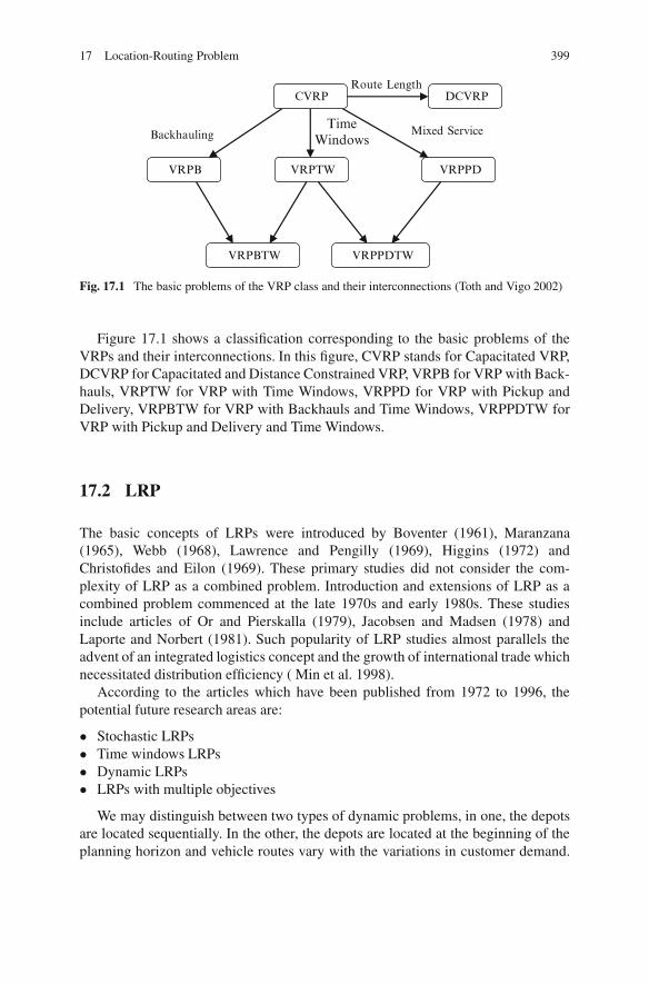
17 Location-Routing Problem 399
TimeWindows
VRPPD
Mixed ServiceBackhauling
Route Length
VRPB VRPTW
DCVRP
VRPPDTWVRPBTW
CVRP
Fig. 17.1 The basic problems of the VRP class and their interconnections (Toth and Vigo 2002)
Figure 17.1 shows a classification corresponding to the basic problems of theVRPs and their interconnections. In this figure, CVRP stands for Capacitated VRP,DCVRP for Capacitated and Distance Constrained VRP, VRPB for VRP with Back-hauls, VRPTW for VRP with Time Windows, VRPPD for VRP with Pickup andDelivery, VRPBTW for VRP with Backhauls and Time Windows, VRPPDTW forVRP with Pickup and Delivery and Time Windows.
17.2 LRP
The basic concepts of LRPs were introduced by Boventer (1961), Maranzana(1965), Webb (1968), Lawrence and Pengilly (1969), Higgins (1972) andChristofides and Eilon (1969). These primary studies did not consider the com-plexity of LRP as a combined problem. Introduction and extensions of LRP as acombined problem commenced at the late 1970s and early 1980s. These studiesinclude articles of Or and Pierskalla (1979), Jacobsen and Madsen (1978) andLaporte and Norbert (1981). Such popularity of LRP studies almost parallels theadvent of an integrated logistics concept and the growth of international trade whichnecessitated distribution efficiency ( Min et al. 1998).
According to the articles which have been published from 1972 to 1996, thepotential future research areas are:
� Stochastic LRPs� Time windows LRPs� Dynamic LRPs� LRPs with multiple objectives
We may distinguish between two types of dynamic problems, in one, the depotsare located sequentially. In the other, the depots are located at the beginning of theplanning horizon and vehicle routes vary with the variations in customer demand.
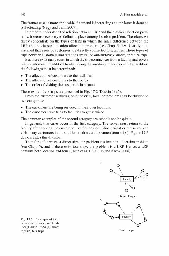
400 A. Hassanzadeh et al.
The former case is more applicable if demand is increasing and the latter if demandis fluctuating (Nagy and Salhi 2007).
In order to understand the relation between LRP and the classical location prob-lems, it seems necessary to define its place among location problem. Therefore, wefirstly concentrate on the types of trips in which the main difference between theLRP and the classical location-allocation problem (see Chap. 5) lies. Usually, it isassumed that users or customers are directly connected to facilities. These types oftrips between customers and facilities are called out-and-back, direct, or return trips.
But there exist many cases in which the trip commences from a facility and coversmany customers. In addition to identifying the number and location of the facilities,the followings must be determined:
� The allocation of customers to the facilities� The allocation of customers to the routes� The order of visiting the customers in a route
These two kinds of trips are presented in Fig. 17.2 (Daskin 1995).From the customer servicing point of view, location problems can be divided to
two categories:
� The customers are being serviced in their own locations� The customers take trips to facilities to get serviced
The common examples of the second category are schools and hospitals.In general, two cases occur in the first category. The server must return to the
facility after serving the customer, like fire engines (direct trips) or the server canvisit many customers in a tour, like repairers and postmen (tour trips). Figure 17.3demonstrates this division.
Therefore, if there exist direct trips, the problem is a location-allocation problem(see Chap. 5), and if there exist tour trips, the problem is a LRP. Hence, a LRPcontains both location and tours ( Min et al. 1998; Lin and Kwok 2006).
Fig. 17.2 Two types of tripsbetween customers and facil-ities (Daskin 1995) (a) directtrips (b) tour trips
Direct Trips
a
b
Tour Trips
Facility
Facility
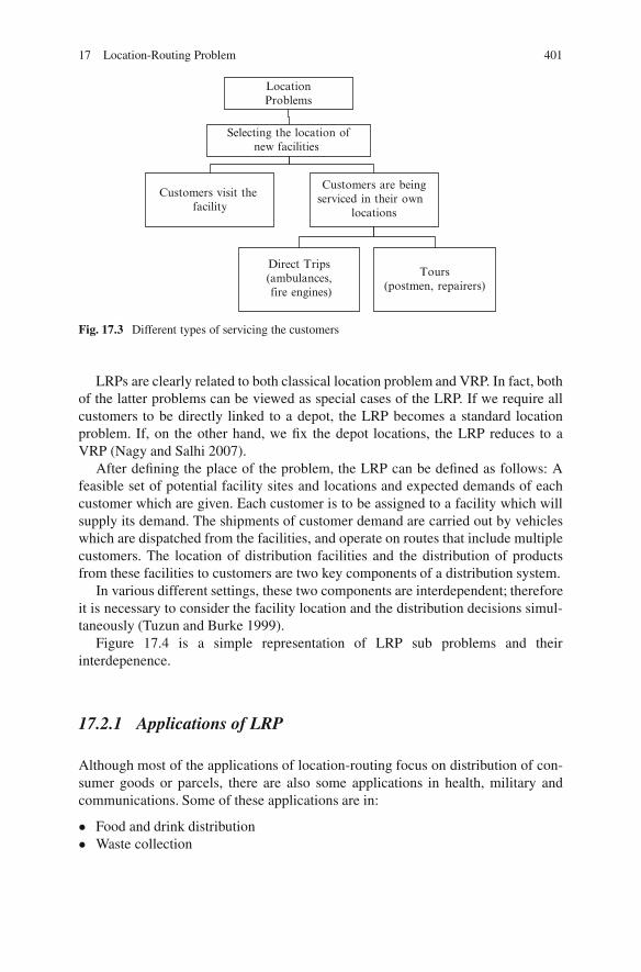
17 Location-Routing Problem 401
LocationProblems
Selecting the location ofnew facilities
Customers visit the facility
Customers are beingserviced in their own
locations
Tours(postmen, repairers)
Direct Trips(ambulances, fire engines)
Fig. 17.3 Different types of servicing the customers
LRPs are clearly related to both classical location problem and VRP. In fact, bothof the latter problems can be viewed as special cases of the LRP. If we require allcustomers to be directly linked to a depot, the LRP becomes a standard locationproblem. If, on the other hand, we fix the depot locations, the LRP reduces to aVRP (Nagy and Salhi 2007).
After defining the place of the problem, the LRP can be defined as follows: Afeasible set of potential facility sites and locations and expected demands of eachcustomer which are given. Each customer is to be assigned to a facility which willsupply its demand. The shipments of customer demand are carried out by vehicleswhich are dispatched from the facilities, and operate on routes that include multiplecustomers. The location of distribution facilities and the distribution of productsfrom these facilities to customers are two key components of a distribution system.
In various different settings, these two components are interdependent; thereforeit is necessary to consider the facility location and the distribution decisions simul-taneously (Tuzun and Burke 1999).
Figure 17.4 is a simple representation of LRP sub problems and theirinterdepenence.
17.2.1 Applications of LRP
Although most of the applications of location-routing focus on distribution of con-sumer goods or parcels, there are also some applications in health, military andcommunications. Some of these applications are in:
� Food and drink distribution� Waste collection
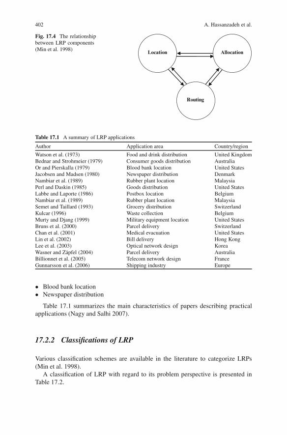
402 A. Hassanzadeh et al.
Fig. 17.4 The relationshipbetween LRP components(Min et al. 1998) Location
Routing
Allocation
Table 17.1 A summary of LRP applications
Author Application area Country/region
Watson et al. (1973) Food and drink distribution United KingdomBednar and Strohmeier (1979) Consumer goods distribution AustraliaOr and Pierskalla (1979) Blood bank location United StatesJacobsen and Madsen (1980) Newspaper distribution DenmarkNambiar et al. (1989) Rubber plant location MalaysiaPerl and Daskin (1985) Goods distribution United StatesLabbe and Laporte (1986) Postbox location BelgiumNambiar et al. (1989) Rubber plant location MalaysiaSemet and Taillard (1993) Grocery distribution SwitzerlandKulcar (1996) Waste collection BelgiumMurty and Djang (1999) Military equipment location United StatesBruns et al. (2000) Parcel delivery SwitzerlandChan et al. (2001) Medical evacuation United StatesLin et al. (2002) Bill delivery Hong KongLee et al. (2003) Optical network design KoreaWasner and Zapfel (2004) Parcel delivery AustraliaBillionnet et al. (2005) Telecom network design FranceGunnarsson et al. (2006) Shipping industry Europe
� Blood bank location� Newspaper distribution
Table 17.1 summarizes the main characteristics of papers describing practicalapplications (Nagy and Salhi 2007).
17.2.2 Classifications of LRP
Various classification schemes are available in the literature to categorize LRPs(Min et al. 1998).
A classification of LRP with regard to its problem perspective is presented inTable 17.2.
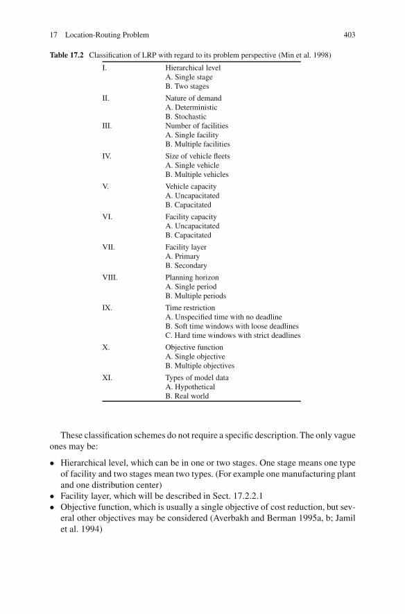
17 Location-Routing Problem 403
Table 17.2 Classification of LRP with regard to its problem perspective (Min et al. 1998)
I. Hierarchical levelA. Single stageB. Two stages
II. Nature of demandA. DeterministicB. Stochastic
III. Number of facilitiesA. Single facilityB. Multiple facilities
IV. Size of vehicle fleetsA. Single vehicleB. Multiple vehicles
V. Vehicle capacityA. UncapacitatedB. Capacitated
VI. Facility capacityA. UncapacitatedB. Capacitated
VII. Facility layerA. PrimaryB. Secondary
VIII. Planning horizonA. Single periodB. Multiple periods
IX. Time restrictionA. Unspecified time with no deadlineB. Soft time windows with loose deadlinesC. Hard time windows with strict deadlines
X. Objective functionA. Single objectiveB. Multiple objectives
XI. Types of model dataA. HypotheticalB. Real world
These classification schemes do not require a specific description. The only vagueones may be:
� Hierarchical level, which can be in one or two stages. One stage means one typeof facility and two stages mean two types. (For example one manufacturing plantand one distribution center)
� Facility layer, which will be described in Sect. 17.2.2.1� Objective function, which is usually a single objective of cost reduction, but sev-
eral other objectives may be considered (Averbakh and Berman 1995a, b; Jamilet al. 1994)
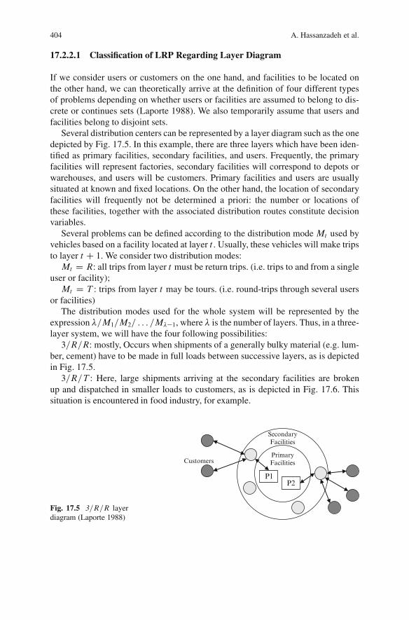
404 A. Hassanzadeh et al.
17.2.2.1 Classification of LRP Regarding Layer Diagram
If we consider users or customers on the one hand, and facilities to be located onthe other hand, we can theoretically arrive at the definition of four different typesof problems depending on whether users or facilities are assumed to belong to dis-crete or continues sets (Laporte 1988). We also temporarily assume that users andfacilities belong to disjoint sets.
Several distribution centers can be represented by a layer diagram such as the onedepicted by Fig. 17.5. In this example, there are three layers which have been iden-tified as primary facilities, secondary facilities, and users. Frequently, the primaryfacilities will represent factories, secondary facilities will correspond to depots orwarehouses, and users will be customers. Primary facilities and users are usuallysituated at known and fixed locations. On the other hand, the location of secondaryfacilities will frequently not be determined a priori: the number or locations ofthese facilities, together with the associated distribution routes constitute decisionvariables.
Several problems can be defined according to the distribution mode Mt used byvehicles based on a facility located at layer t . Usually, these vehicles will make tripsto layer t C 1. We consider two distribution modes:Mt D R: all trips from layer t must be return trips. (i.e. trips to and from a single
user or facility);Mt D T : trips from layer t may be tours. (i.e. round-trips through several users
or facilities)The distribution modes used for the whole system will be represented by the
expression �=M1=M2= : : : =M��1, where � is the number of layers. Thus, in a three-layer system, we will have the four following possibilities:3=R=R: mostly, Occurs when shipments of a generally bulky material (e.g. lum-
ber, cement) have to be made in full loads between successive layers, as is depictedin Fig. 17.5.3=R=T : Here, large shipments arriving at the secondary facilities are broken
up and dispatched in smaller loads to customers, as is depicted in Fig. 17.6. Thissituation is encountered in food industry, for example.
Fig. 17.5 3=R=R layerdiagram (Laporte 1988)
P2P1
PrimaryFacilities
SecondaryFacilities
Customers
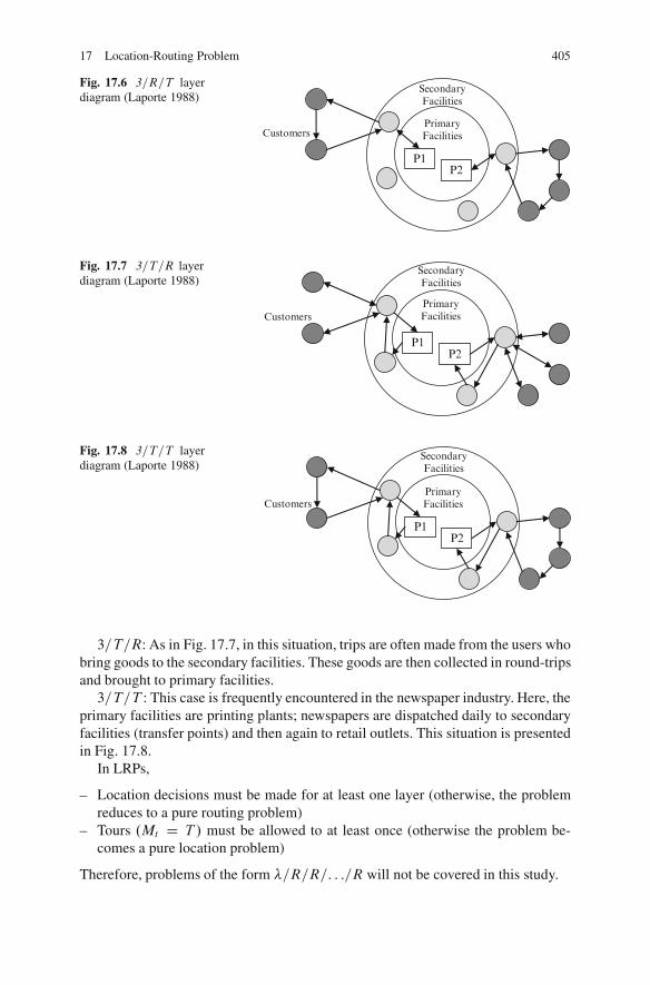
17 Location-Routing Problem 405
Fig. 17.6 3=R=T layerdiagram (Laporte 1988)
P2P1
PrimaryFacilities
SecondaryFacilities
Customers
Fig. 17.7 3=T=R layerdiagram (Laporte 1988)
Customers
P2P1
PrimaryFacilities
SecondaryFacilities
Fig. 17.8 3=T=T layerdiagram (Laporte 1988)
Customers
P2P1
PrimaryFacilities
SecondaryFacilities
3=T=R: As in Fig. 17.7, in this situation, trips are often made from the users whobring goods to the secondary facilities. These goods are then collected in round-tripsand brought to primary facilities.3=T=T : This case is frequently encountered in the newspaper industry. Here, the
primary facilities are printing plants; newspapers are dispatched daily to secondaryfacilities (transfer points) and then again to retail outlets. This situation is presentedin Fig. 17.8.
In LRPs,
– Location decisions must be made for at least one layer (otherwise, the problemreduces to a pure routing problem)
– Tours .Mt D T / must be allowed to at least once (otherwise the problem be-comes a pure location problem)
Therefore, problems of the form �=R=R=: : :=R will not be covered in this study.
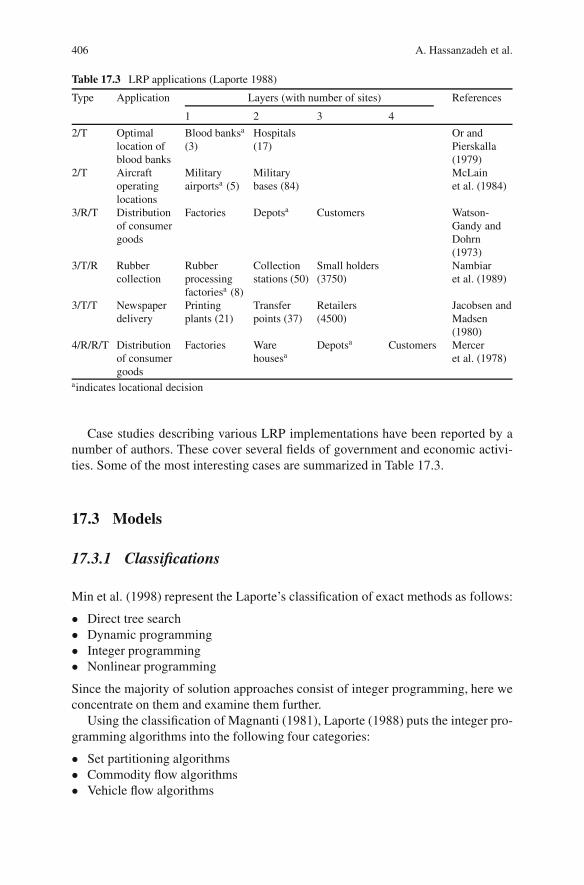
406 A. Hassanzadeh et al.
Table 17.3 LRP applications (Laporte 1988)
Type Application Layers (with number of sites) References
1 2 3 4
2/T Optimallocation ofblood banks
Blood banksa
(3)Hospitals(17)
Or andPierskalla(1979)
2/T Aircraftoperatinglocations
Militaryairportsa (5)
Militarybases (84)
McLainet al. (1984)
3/R/T Distributionof consumergoods
Factories Depotsa Customers Watson-Gandy andDohrn(1973)
3/T/R Rubbercollection
Rubberprocessingfactoriesa (8)
Collectionstations (50)
Small holders(3750)
Nambiaret al. (1989)
3/T/T Newspaperdelivery
Printingplants (21)
Transferpoints (37)
Retailers(4500)
Jacobsen andMadsen(1980)
4/R/R/T Distributionof consumergoods
Factories Warehousesa
Depotsa Customers Merceret al. (1978)
aindicates locational decision
Case studies describing various LRP implementations have been reported by anumber of authors. These cover several fields of government and economic activi-ties. Some of the most interesting cases are summarized in Table 17.3.
17.3 Models
17.3.1 Classifications
Min et al. (1998) represent the Laporte’s classification of exact methods as follows:
� Direct tree search� Dynamic programming� Integer programming� Nonlinear programming
Since the majority of solution approaches consist of integer programming, here weconcentrate on them and examine them further.
Using the classification of Magnanti (1981), Laporte (1988) puts the integer pro-gramming algorithms into the following four categories:
� Set partitioning algorithms� Commodity flow algorithms� Vehicle flow algorithms
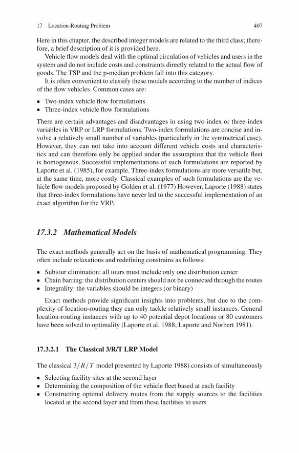
17 Location-Routing Problem 407
Here in this chapter, the described integer models are related to the third class; there-fore, a brief description of it is provided here.
Vehicle flow models deal with the optimal circulation of vehicles and users in thesystem and do not include costs and constraints directly related to the actual flow ofgoods. The TSP and the p-median problem fall into this category.
It is often convenient to classify these models according to the number of indicesof the flow vehicles. Common cases are:
� Two-index vehicle flow formulations� Three-index vehicle flow formulations
There are certain advantages and disadvantages in using two-index or three-indexvariables in VRP or LRP formulations. Two-index formulations are concise and in-volve a relatively small number of variables (particularly in the symmetrical case).However, they can not take into account different vehicle costs and characteris-tics and can therefore only be applied under the assumption that the vehicle fleetis homogenous. Successful implementations of such formulations are reported byLaporte et al. (1985), for example. Three-index formulations are more versatile but,at the same time, more costly. Classical examples of such formulations are the ve-hicle flow models proposed by Golden et al. (1977) However, Laporte (1988) statesthat three-index formulations have never led to the successful implementation of anexact algorithm for the VRP.
17.3.2 Mathematical Models
The exact methods generally act on the basis of mathematical programming. Theyoften include relaxations and redefining constrains as follows:
� Subtour elimination: all tours must include only one distribution center� Chain barring: the distribution centers should not be connected through the routes� Integrality: the variables should be integers (or binary)
Exact methods provide significant insights into problems, but due to the com-plexity of location-routing they can only tackle relatively small instances. Generallocation-routing instances with up to 40 potential depot locations or 80 customershave been solved to optimality (Laporte et al. 1988; Laporte and Norbert 1981).
17.3.2.1 The Classical 3/R/T LRP Model
The classical 3=R=T model presented by Laporte 1988) consists of simultaneously
� Selecting facility sites at the second layer� Determining the composition of the vehicle fleet based at each facility� Constructing optimal delivery routes from the supply sources to the facilities
located at the second layer and from these facilities to users
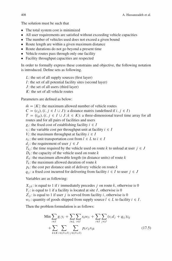
408 A. Hassanzadeh et al.
The solution must be such that
� The total system cost is minimized� All user requirements are satisfied without exceeding vehicle capacities� The number of vehicles used does not exceed a given bound� Route length are within a given maximum distance� Route durations do not go beyond a present time� Vehicle routes pass through only one facility� Facility throughput capacities are respected
In order to formally express these constrains and objective, the following notationis introduced. Define sets as following.
L: the set of all supply sources (first layer)I : the set of all potential facility sites (second layer)J : the set of all users (third layer)K: the set of all vehicle routes
Parameters are defined as below:
Nm D jKj: the maximum allowed number of vehicle routesC D .cij/; .i; j 2 I [ J /: a distance matrix (undefined if i; j 2 I )T D .tijk/; .i; j 2 I [ J I k 2 K/: a three-dimensional travel time array for allroutes and for all pairs of facilities and usersgi : the fixed cost of establishing facility i 2 Ivi : the variable cost per throughput unit at facility i 2 IVi : the maximum throughput at facility i 2 Isli : the unit transportation cost from l 2 L to i 2 Idj : the requirement of user j 2 JTkj : the time required by the vehicle used on route k to unload at user j 2 JDk : the capacity of the vehicle used on route kEk : the maximum allowable length (in distance units) of route kTk : the maximum allowed duration of route kpk : the cost per distance unit of delivery vehicle on route kqij : a fixed cost incurred for delivering from facility i 2 I to user j 2 JVariables are as following:
Xijk : is equal to 1 if i immediately precedes j on route k, otherwise is 0Yj : is equal to 1 if a facility is located at site I , otherwise is 0Zij : is equal to 1 if user j is served from facility i , otherwise is 0wli : quantity of goods shipped from supply source l 2 L to facility i 2 I .
Then the problem formulation is as follows:
MinXi2I
gi yi CXl2L
Xi2I
sliwli CXi2I
Xj2J
.vi dj C qij /zij
CXk2K
Xi2.I[J /
Xj2.I[J /
pkcijxijk (17.5)
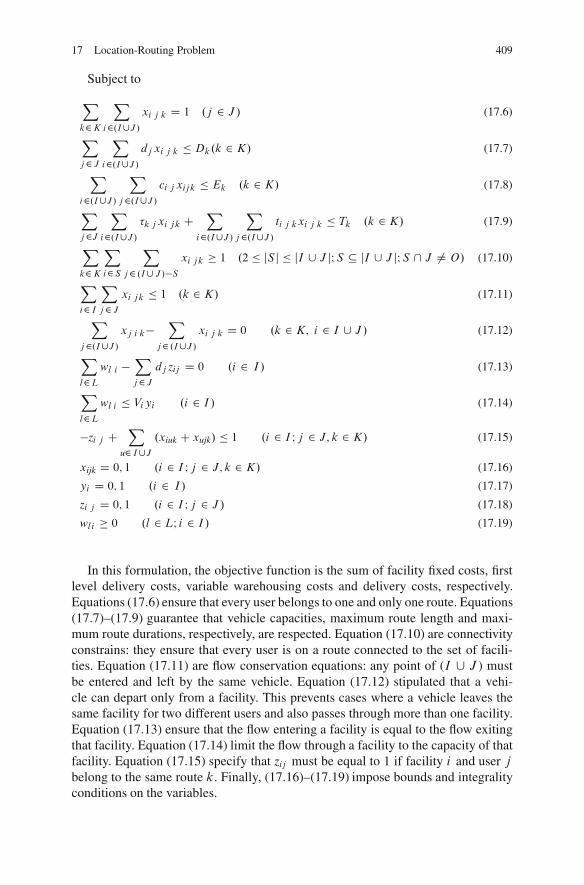
17 Location-Routing Problem 409
Subject to
Xk2K
Xi2.I[J /
xi j k D 1 .j 2 J / (17.6)
Xj2J
Xi2.I[J /
dj xi j k � Dk.k 2 K/ (17.7)
Xi2.I[J /
Xj2.I[J /
ci j xijk � Ek .k 2 K/ (17.8)
Xj2J
Xi2.I[J /
�k j xi jk CX
i2.I[J /
Xj2.I[J /
ti j kxi j k � Tk .k 2 K/ (17.9)
Xk2K
Xi2S
Xj2 .I[J /�S
xi jk � 1 .2 � jS j � jI [ J jIS � jI [ J jIS \ J ¤ O/ (17.10)
Xi2 I
Xj2J
xi jk � 1 .k 2 K/ (17.11)
Xj2.I[J /
xj i k�X
j2 .I[J /xi j k D 0 .k 2 K; i 2 I [ J / (17.12)
Xl2L
wl i �Xj2J
dj zij D 0 .i 2 I / (17.13)
Xl2L
wl i � Viyi .i 2 I / (17.14)
�zi j CX
u2 I[J.xiuk C xujk/ � 1 .i 2 I I j 2 J; k 2 K/ (17.15)
xijk D 0; 1 .i 2 I I j 2 J; k 2 K/ (17.16)
yi D 0; 1 .i 2 I / (17.17)
zi j D 0; 1 .i 2 I I j 2 J / (17.18)
wli � 0 .l 2 LI i 2 I / (17.19)
In this formulation, the objective function is the sum of facility fixed costs, firstlevel delivery costs, variable warehousing costs and delivery costs, respectively.Equations (17.6) ensure that every user belongs to one and only one route. Equations(17.7)–(17.9) guarantee that vehicle capacities, maximum route length and maxi-mum route durations, respectively, are respected. Equation (17.10) are connectivityconstrains: they ensure that every user is on a route connected to the set of facili-ties. Equation (17.11) are flow conservation equations: any point of (I [ J ) mustbe entered and left by the same vehicle. Equation (17.12) stipulated that a vehi-cle can depart only from a facility. This prevents cases where a vehicle leaves thesame facility for two different users and also passes through more than one facility.Equation (17.13) ensure that the flow entering a facility is equal to the flow exitingthat facility. Equation (17.14) limit the flow through a facility to the capacity of thatfacility. Equation (17.15) specify that zij must be equal to 1 if facility i and user jbelong to the same route k. Finally, (17.16)–(17.19) impose bounds and integralityconditions on the variables.
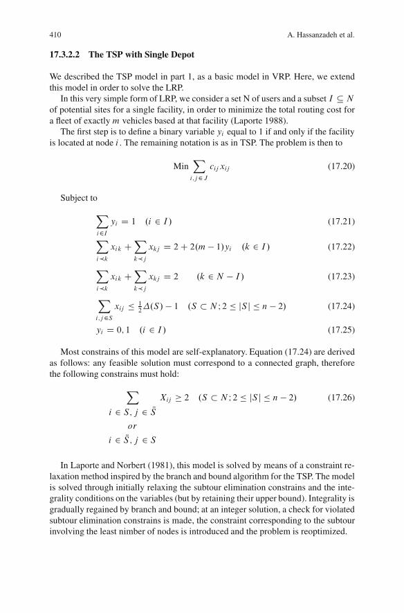
410 A. Hassanzadeh et al.
17.3.2.2 The TSP with Single Depot
We described the TSP model in part 1, as a basic model in VRP. Here, we extendthis model in order to solve the LRP.
In this very simple form of LRP, we consider a set N of users and a subset I � N
of potential sites for a single facility, in order to minimize the total routing cost fora fleet of exactlym vehicles based at that facility (Laporte 1988).
The first step is to define a binary variable yi equal to 1 if and only if the facilityis located at node i . The remaining notation is as in TSP. The problem is then to
MinXi;j2J
cij xij (17.20)
Subject to
Xi2I
yi D 1 .i 2 I / (17.21)
Xik
xik CXkj
xkj D 2C 2.m� 1/yi .k 2 I / (17.22)
Xik
xik CXkj
xkj D 2 .k 2 N � I / (17.23)
Xi;j2S
xij � 12�.S/� 1 .S � N I 2 � jS j � n � 2/ (17.24)
yi D 0; 1 .i 2 I / (17.25)
Most constrains of this model are self-explanatory. Equation (17.24) are derivedas follows: any feasible solution must correspond to a connected graph, thereforethe following constrains must hold:
Xi 2 S; j 2 NS
or
i 2 NS; j 2 S
Xij � 2 .S � N I 2 � jS j � n � 2/ (17.26)
In Laporte and Norbert (1981), this model is solved by means of a constraint re-laxation method inspired by the branch and bound algorithm for the TSP. The modelis solved through initially relaxing the subtour elimination constrains and the inte-grality conditions on the variables (but by retaining their upper bound). Integrality isgradually regained by branch and bound; at an integer solution, a check for violatedsubtour elimination constrains is made, the constraint corresponding to the subtourinvolving the least nimber of nodes is introduced and the problem is reoptimized.
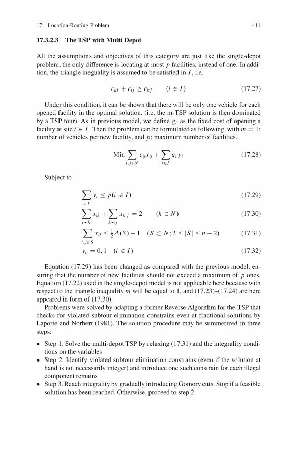
17 Location-Routing Problem 411
17.3.2.3 The TSP with Multi Depot
All the assumptions and objectives of this category are just like the single-depotproblem, the only difference is locating at most p facilities, instead of one. In addi-tion, the triangle ineguality is assumed to be satisfied in I , i.e.
cki C cij � ckj .i 2 I / (17.27)
Under this condition, it can be shown that there will be only one vehicle for eachopened facility in the optimal solution. (i.e. the m-TSP solution is then dominatedby a TSP tour). As in previous model, we define gi as the fixed cost of opening afacility at site i 2 I . Then the problem can be formulated as following, withm D 1:number of vehicles per new facility, and p: maximum number of facilities.
MinXi;j"N
cijxij CXi2I
giyi (17.28)
Subject to
Xi" I
yi � p.i 2 I / (17.29)
Xik
xik CXkj
xk j D 2 .k 2 N/ (17.30)
Xi;j" S
xij � 12�.S/� 1 .S � N I 2 � jS j � n � 2/ (17.31)
yi D 0; 1 .i 2 I / (17.32)
Equation (17.29) has been changed as compared with the previous model, en-suring that the number of new facilities should not exceed a maximum of p ones.Equation (17.22) used in the single-depot model is not applicable here because withrespect to the triangle inequality m will be equal to 1, and (17.23)–(17.24) are hereappeared in form of (17.30).
Problems were solved by adapting a former Reverse Algorithm for the TSP thatchecks for violated subtour elimination constrains even at fractional solutions byLaporte and Norbert (1981). The solution procedure may be summerized in threesteps:
� Step 1. Solve the multi-depot TSP by relaxing (17.31) and the integrality condi-tions on the variables
� Step 2. Identify violated subtour elimination constrains (even if the solution athand is not necessarily integer) and introduce one such constrain for each illegalcomponent remains
� Step 3. Reach integrality by gradually introducing Gomory cuts. Stop if a feasiblesolution has been reached. Otherwise, proceed to step 2
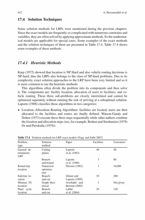
412 A. Hassanzadeh et al.
17.4 Solution Techniques
Some solution methods for LRPs were mentioned during the previous chapters.Since the exact models are frequently so complicated with numerous constrains andvariables, they are often solved by applying approximate methods. So the mathemat-ical models are applicable for special cases. Some examples of the exact methodsand the solution techniques of them are presented in Table 17.4. Table 17.4 showssome examples of these methods.
17.4.1 Heuristic Methods
Karp (1972) showed that location is NP Hard and also vehicle routing decisions isNP-hard, thus the LRPs also belongs to the class of NP-hard problems. Due to itscomplexity, exact solution approaches to the LRP have been very limited and so itis more common to use the heuristic methods.
This algorithms often divide the problem into its components and then solveit. The components are: facility location; allocation of users to facilities; and ve-hicle routing. These three sub-problems are closely interrelated and cannot beoptimized seperately without running the risk of arriving at a suboptimal solution.Laporte (1988) classifies these algorithms in two categories:
� Location–Allocation–Routing Algorithms: facilities are located, users are thenallocated to the facilities and routes are finally defined. Watson-Gandy andDohrn (1973) execute these three steps sequentially while other authors combinethe location and allocation steps (see, for example, Bedner and Strohmeier (1979)Or and Pierskalla (1979))
Table 17.4 Solution methods for LRP exact models (Nagy and Salhi 2007)
Problemtype
Solutionmethod
Paper Facilities Customers
General de-terministicLRP
Cuttingplanes
Laporteet al. (1983)
40 40
Branch-and-bound
Laporteet al. (1988)
3 80
Round-triplocation
Numericaloptimisa-tion
Drezner (1982) 1 10,000
Eulerian lo-cation
Branch-and-cut
Ghiani andLaporte (1999)
50 200
Minmax TSlocation
Graph theo-retical
Averbakh andBerman (2002)
1 Not given
Plant cyclelocation
Branch-and-cut
Labbeet al. (2004)
30 120
17 Location-Routing Problem 413
� Allocation–Routing–Location: the allocation and routing steps are often simulta-neous: sets of routes are first constructed, assuming all facilities “open”; locationsare then selected by dropping various facilities from the system and updatingthe location and routing decisions. The SAV-DROP heuristic of Jacobsen andMadsen (1980) and the algorithm of Srikar and Srivastava (1984) constitute ex-amples of these algorithms
Although this classification is applicable for many heuristic algorithms, not all theheuristic algorithms can be categorized into them. For example, the algorithm pro-posed by Nambiar et al. (1989). did not contain the allocation phase.
Also Nagy and Salhi (2007), have divided the heuristic methods as below:
1. Clustering-based method2. Iterative method3. Hierarchical method
17.4.2 Metaheuristic Methods
One recent development in the solution of combinatorial problems is the introduc-tion of metaheuristics such as tabu search, genetic algorithms, simulated annealing,and neural networks (Tuzun and Burke 1999).
All of these metaheuristics aim to search the solution space more electively thanconventional approaches using deferent strategies. They show great promise in solu-tion of difficult combinatorial problems such as the LRP. Among these, TS exploresthe solution space by moving from a solution to its best neighbor, even if this resultsin a deterioration of the objective function value. This strategy allows the search tomove out of the local optima and explore other regions of the solution space (seeGlover 1995; Glover et al. 1993, for overviews of TS).
17.5 Case Study
17.5.1 Bill Delivery Services (Lin et al. 2002)
In this research, a local case of integrated facility location and distribution plan-ning problem is described. Distribution of bills to customers is a major issue toa telecommunication service company in Hong Kong that serves a large customerbase of business and residential customers. The customer region is divided to 31housing states and four potential depots. This problem is constrained by operatingconstraints such as:
� Daily working hours� Capacity of a vehicle� The capacity of a potential depot
414 A. Hassanzadeh et al.
There is no time window constraint as customers need not be present during thedelivery. If multiple routes could be assigned to a vehicle without exceeding thestaff working hours, further cost reduction could be achieved.
Considering the above interdependent decisions, the basic questions to addressare: given a set of demand nodes (target housing estates) and a set of potential facil-ities (delivery depot sites), where should the facilities be established? How shouldroutes be formed from a facility and what is the routing sequence to the demandnodes such that all demand nodes are served? What is the smaller number of vehi-cles (vehicle fleet size) to be used for a given set of established routes? The primaryobjective of the above location, routing and loading problems is to minimize thesum of facility costs, staff costs, vehicle rental and operating costs.
For solving the problem, based on five different subproblems, the solutions andCPU time of five algorithms TA, SA, (TA, SA), (SA, TA), and branch and boundare calculated and finally the (TA, SA) algorithm is applied to the actual problem.The solution demonstrates that with two depots and 11 routes, the whole customerscan be serviced while the costs are minimized.
17.5.2 Contaminated Waste Disposal (Caballero et al. 2007)
This work presents a model to find the best location for up to two incineration plantsshared between several preestablished locations in Andalusia (Spain) that will beused to dispose solid animal waste and simultaneously find the best routes to trans-port the waste from each slaughterhouse to the plants opened. Thus, we are dealingwith a location (deciding which plants should be opened) routing (designing theroutes to transport the waste from the slaughterhouses) problem.
When evaluating potential locations for the new plants, different factors shouldbe considered; therefore, a multi-objective problem does exist. Five different objec-tives are formulated while taking into account two major aspects:
� Economic objectives (start-up, maintenance, and transport costs)� Social objectives (social rejection by towns on the truck routes, maximum risk as
an equity criterion, and the negative implications for towns close to the plant)
In the application, we face a problem with six possible locations (where at mostwe can choose two of them), 93 clients to serve, five objectives to optimize, andconstraints on truck capacity and on the duration of the route.
To solve this problem, the researchers have adapted a metaheuristic formulti-objective combinatorial optimization problems based on tabu search, themulti-objective metaheuristic using an adaptative memory procedure method. Thisadaptation consists of some specific neighborhood definitions inspired by the move-ments used for a similar problem in the literature, a single-objective LRP withcapacitated vehicles. The solution presents a set of efficient solutions consideringthe five objectives to the decision maker.
17 Location-Routing Problem 415
17.5.3 Logistics System (Lin and Kwok 2006)
This paper addresses an integrated logistic system where decisions on locationof depot, vehicle routing and assignment of routes to vehicles are considered si-multaneously. Total cost and workload balance are common criteria influencingdecision-making. Metaheuristics of tabu search and simulated annealing on real dataand simulated data are applied, to compare their performances under two versions:simultaneous or sequential routes assignment to vehicles. A new statistical proce-dure is proposed to compare two algorithms on the strength of their multi-objectivesolutions.
This research has the following contributions:
� A multi-objective LRP integrated with the routes assignment decisions is consid-ered, and real instances from a local delivery service are used
� Certain methods to estimate unavailable data are proposed: the use of GIS toestimate the travel times and a regression method to estimate the on-site service(delivery) time
� A new statistical procedure based on the hypothesis testing of difference betweentwo population proportions (Z-test) is proposed, in order to compare the relativenon-dominance of multi-objective solutions between tabu search and simulatedannealing
� The effect of allowing multiple use of vehicles in the routes formation stage withthe sequential approach of routing before assignment is examined
References
Averbakh I, Berman O (1995a) Probabilistic sales-delivery man and sales-delivery facility locationproblems on a tree. Transport Sci 29:184–197
Averbakh I, Berman O (1995b) Routing and location-routing p-delivery men problems on a path.Transport Sci 28:162–166
Averbakh I, Berman O (2002) Minmax p-traveling salesmen location problems on a tree. Ann OperRes 110:55–62
Bender V, Strohmeier E (1979) Largerstandorto imierung und Fuhrparkeinsatzplanung in derkonsumguter-industrie. Zen Sconrift Fur Oper Res 23:89–104
Billionnet A, Elloumi S, Grouz-Djerbi L (2005) Designing radio-mobile access networks based onsynchronous digital hierarchy rings. Comput Oper Res 32:379–394
Boventer V (1961) The relationship between transportation costs and location rent in transportationproblems. J Regional Sci 3:27–40
Bruns A, Klose A, Stahly P (2000) Restructuring of Swiss parcel delivery services. OR Spektrum22:285–302
Caballero R, Gonzalez M, Guerrero FM, Molina J, Paralera C (2007) Solving a multiobjectivelocation routing problem with a metaheuristic based on tabu search. Application to a real casein Andalusia. Eur J Oper Res 177(3):1751–1763
Chan Y, Carter WB, Burnes MD (2001) A multiple-depot, multiple-vehicle, location-routing prob-lem with stochastically processed demands. Comput Oper Res 28:803–826
Christofides N, Eilon S (1969) An algorithm for the vehicle dispatching problem. Oper Res Quart20:309–318
416 A. Hassanzadeh et al.
Dantzig GB, Fulkerson DR (1954) Minimizing the number of tankers to meet a fixed schedule.Nav Res Logist Q 1:217–222
Daskin MS (1995) Network and discrete location: Models, algorithms, and applications. Wiley,New York
Drezner Z (1982) Fast algorithms for the round trip location problem. IIE Trans 14:243–248Ghiani G, Laporte G (1999) Eulerian location problems. Networks 34:291–302Glover F (1995) Tabu search fundamentals and uses. Technical paper, University of Colorado,
Boulder, COGlover F, Taillard E, De Werra D (1993) A user’s guide to tabu search. Ann Oper Res 41:3–28Golden BL, Magnanti TL, Nguyen HQ (1997) Implementing vehicle routing algorithms. Networks
7:113–148Gunnarsson H, Ronnqvist M, Carlsson D (2006) A combined terminal location and ship routing
problem. J Oper Res Soc 57:928–938Higgins JC (1972) On the merits of simple models in distribution planning. Int J Phys Distrib
2:144–148Jacobsen SK, Madsen OBG (1978) On the location of transfer points in a two-level newspaper de-
livery system – a case study. Presented at the international symposium on locational decisions,24–28
Jacobsen SK, Madsen OBG (1980) A comparative study of heuristics for a two-level routing-location problem. Eur J Oper Res 5:378–387
Jamil M, Batta R, Malon DM (1994) The traveling repairperson home base location problem.Transp Sci 28:150–161
Karp R (1972) Reducibility among combinatorial problems. Plenum, New York, pp 85–104Kulcar T (1996) Optimizing solid waste collection in Brussels. Eur J Oper Res 90:26–44Labbe M, Rodrıguez-Martın I, Salazar-Gonzalez JJ (2004) A branch-and-cut algorithm for the
plant-cycle location problem. J Oper Res Soc 55:513–520Laporte G (1988) Location-routing problems. In: Methods and studies. North-Holland,
Amsterdam, pp 163–198Laporte G, Norbert Y (1981) An exact algorithm for minimizing routing and operating costs in
depot location. Eur J Oper Res 6:224–226Laporte G, Nobert Y, Pelletier P (1983) Hamiltonian location problems. Eur J Oper Res 12:82–89Laporte G, Nobert Y, Desrochers M (1985) Optimal routing under capacity and distance restric-
tions. Oper Res 33:1050–1073Laporte G, Nobert Y, Taillefer S (1988) Solving a family of multi-depot vehicle routing and
location-routing problems. Transp Sci 22:161–172Lawrence RM, Pengilly PJ (1969) The number and location of depots required for handling prod-
ucts for distribution to retail stores in South-East England. Oper Res Quart 20:23–32Lee Y, Kim S-I, Lee S, Kang K (2003) A location-routing problem in designing optical internet
access with WDM systems. Photon Netw Commun 6:151–160Lin CKY, Chow CK, Chen A (2002) A location-routing-loading problem for bill delivery services.
Comput Ind Eng 43:5–25Lin CKY, Kwok RCW (2006) Multi-objective metaheuristics for a location-routing problem with
multiple use of vehicles on real data and simulated data. Eur J Oper Res 175:1833–1849Magnanti TL (1981) Combinatorial optimization and vehicle fleet planning: perspectives and
prospect. Networks 11:179–214Maranzana FE (1965) On the location of supply points to minimize transport costs. Oper Res Quart
15:261–270McLain DR, Durchholz ML, Wilborn WB (1984) U.S.A.F. EDSA routing and operating location
selection study. Report XPSR84–3, Operations Research Division, Directorate of Studies andAnalysis
Mercer A, Canley MF, Rand GK (1978) Operational distribution research. Taylor and Francis,London
Min H, Jayaraman V, Srivastava R (1998) Combined location-routing problems: a synthesis andfuture research directions. Eur J Oper Res 108:1–15
17 Location-Routing Problem 417
Murty KG, Djang PA (1999) The U.S. army national guard’s mobile training simulators locationand routing problem. Oper Res 47:175–182
Nagy G, Salhi S (2007) Location-routing: issues, models and methods. Oper Res 177:649–672Nambiar JM, Gelders LF, Van Wassenhove LN (1989) Plant location and vehicle routing in the
Malaysian rubber smallholder sector: a case study. Eur J Oper Res 38:14–26Or I, Pierskalla WP (1979) A transportation, location-allocation model for regional blood banking.
AIIE Trans 11:86–95Perl J, Daskin MS (1985) A warehouse location-routing problem. Transp Res 5:381–396Semet F, Taillard E (1993) Solving real-life vehicle routing problems efficiently using tabu search.
Ann Oper Res 41:469–488Srikar B, Srivastava R (1984) Solution methodology for location routing problem. In: ORSA/TIMS
conferenceToth P, Vigo D (2002) An overview of vehicle routing problems. In: Toth P, Vigo D (eds) The ve-
hicle routing problem. pp 1–26, Society for Industrial and Applied Mathematics, PhiladelphiaTuzun D, Burke LI (1999) A two-phase tabu search approach to the location routing problem. Eur
J Oper Res 116:87–99Wasner M, Zapfel G (2004) An integrated multi-depot hub location vehicle routing model for
network planning of parcel service. Int J Prod Econ 90:403–419Watson-Gandy CDT, Dohrn PJ (1973) Depot location with van salesmen – a practical approach.
Omega 11:321–329Webb MHJ (1968) Cost functions in the location of depots for multiple-delivery journeys. Oper
Res Quar 19:11–320
Chapter 18Storage System Layout
Javad Behnamian and Babak Eghtedari
A warehouse consists of a number of parallel aisles. The items are stored on bothsides of the aisles. Order pickers are assumed to be able to traverse the aisles inboth directions and to change direction within the aisles. Their major roles in-clude: buffering the material flow along the supply chain to accommodate variabilitycaused by factors such as product seasonality and/or batching in production andtransportation; consolidation of products from various suppliers for combined de-livery to customers; and value-added-processing such as kitting, pricing, labeling,and product customization.
Usually the items in a warehouse exhibit varying characteristics with respectto dimensions, weight, demand, and other properties. It is natural to apply certainstorage and retrieval strategies depending upon the product families or individualproducts within families. Products need to be put into storage locations before theycan be picked to fulfill customer orders. A storage policy is considered optimal ifit minimizes the average time required to store and retrieve a unit load while satis-fying the various constraints placed upon the system. A storage assignment policyis a set of rules which determines where the unit loads of different products willbe located in a warehouse. With regard to storing unit loads, two major classes ofstorage policies can be distinguished (Koster et al. 2007; Goetschalckx and Ratliff1990; Van den Berg et al. 1999) in other word, The storage location assignmentproblem (SLAP) is to assign incoming products to storage locations in storagedepartments/zones in order to reduce material handling cost and improve spaceutilization. Different warehouse departments might use different SLAP policies de-pending on the department-specific SKU profiles and storage technology (Gu 2005).
A basic rule in assigning products to storage locations is storing “better” prod-ucts in the “better” locations in the order picking system. A “the most desirablelocations” is a location, which provides faster and more ergonomic access to theproduct stored.
The definition of “the most desirable locations” depends on the system as well asthe travel pattern. For example, if traversal routing policy is used for traveling in aconventional multi-parallel-aisle system, the desirability of locations are measuredin terms of aisles where the most desirable locations are in the aisle that is closestto the I/O point (This leads to the so-called organ pipe storage location assignment)(Gu et al. 2007).
R.Z. Farahani and M. Hekmatfar (eds.), Facility Location: Concepts, Models, 419Algorithms and Case Studies, Contributions to Management Science,DOI 10.1007/978-3-7908-2151-2 18, c� Physica-Verlag Heidelberg 2009
420 J. Behnamian and B. Eghtedari
A measure of “goodness” of an item could have been the frequency with whichit is requested. If an item is requested frequently, it is logical to keep that itemin an easily accessible location. But if the item is too heavy, it may be too muchtime consuming to replenish that item to that favored location. Another measure of“goodness” for an item is occupying smaller space. On the other hand if an item isrequested very infrequently, it is not necessary at all to assign it to a favored position,just because it occupies little space. If that practice were followed, the “best” loca-tions could be filled with lots of small products that are not really requested much.
Another basic rule in assigning products to storage locations is taking thedimensions into consideration. Cube matching of the items with the storage lo-cations is essential to eliminate space inefficiencies. Shelf dimensions should bespacious enough to allow easy picking, but tight enough to avoid unused space.Here is a bad usage of shelf space vs. good usage.
An effective storage location assignment policy may reduce the mean travel timesfor storage/retrieval and order-picking. Also, by distributing the activities evenlyover the warehouse subsystems, congestion may be reduced and activities may bebalanced better among subsystems, thus increasing the throughput capacity (Vanden Berg et al. 1999).
18.1 Assumptions and Classifications
The storage system considered here contains multiple products with stores andretrieves performed in a single-command mode1 (i.e., there is only one store orone retrieve on each round trip). Most of the concepts extend in a straight forwardmanner to the dual-command mode (i.e., a store and a retrieve on each round trip).Although there is the potential for more efficient storage using a dual-commandmode, the single-command mode continues to be widely used. This is primarilybecause of the additional coordination required to unload one truck and simultane-ously load another.
We assume that all products in the system are stored and moved in unit loads. Wealso assume that each unit load requires the same space and that the expected cost ofstoring or retrieving a unit load from a storage location is independent of which unitis stored in that location. This assumption allows computation of the expected travelcost for each location before any storage assignment has been made (Goetschalckxand Ratliff 1990).
1 In a single-command cycle either a storage or a retrieval is performed between two consecutivevisits of the input and output station. In a dual-command cycle the S=R machine consecutivelyperforms storage, travels empty to a retrieval location and performs retrieval. The empty travelbetween the storage and retrieval location is referred to as interleaving travel (Van den Berget al. 1999).
18 Storage System Layout 421
The physical location where arriving items will be stored Subject to performancecriteria and constraints such as:
1. Storage capacity and efficiency2. Picker capacity and efficiency based on the picker cycle time3. Response time4. The compatibility between products and storage locations and the compatibility
between products5. Item retrieval policy such as FIFO (first-in, first-out), LIFO (last-in, first-out),
BFIFO (batch first-in, first-out). When using the BFIFO policy, items that arrivedin the same replenishment batch are considered to be equivalent.
In typical warehouse operations, the physical storage infrastructure and its charac-teristics are known when planning the storage location assignment. The availabilityof storage locations is always known in automated warehouses and often known inmechanized warehouses (Gu 2005).
Trade-offs inevitably occur between throughput and storage space in designingstorage systems. The term throughput is used as a measure of the number of storagesand retrievals performed per time period. It can be expressed directly as a rate (e.g.,320 storages per 8-h day). Alternatively it can be given inversely in terms of thetime required to perform storage (e.g., 1.5 min per storage). Space is a measure ofthe static nature of storage. Throughput however is a measure of the activity or thedynamic nature of storage; it represents the flow occurring in storage.
The size of the storage system depends on a number of parameters and variables.For example, the size of the storage system is influenced by storage, throughput, andcost parameters. The decision variables that influence the size of storage include thestorage methods and the storage layout.
The material characteristics and inventory profile establish the storage andthroughput parameters. Included in the former are the characteristics that influencethe way material is stored, handled, and controlled. The material characteristics ofinterest include size, weight, shape, value, shelf life, stack ability, toxicity, flamma-bility, explosiveness; and environmental requirements, among others. The inventoryprofile includes both the amount of each product stored over time and the in-put/output functions that generate the activity requirements for storing and retrievingmaterial.
The input/output functions will depend on; the mission of the storage system. Asan example, consider a distribution center for finished goods produced at variouscompany-owned manufacturing plants. If a push system is used, the productionplants push inventory to the distribution center and the input function will be de-termined by the production schedules at the plants. The output or demand functionmight be represented by a forecasting equation developed for the marketing depart-ment. The cumulative differences in the input and output functions will determinethe storage requirements in the distribution center over time.
Among the cost parameters that influence the size of the storage system are thecosts of providing storage vs. the costs of not providing storage. The former includes
422 J. Behnamian and B. Eghtedari
the costs of providing storage internally vs. leasing space or contracting with a pub-lic warehouse to provide the storage space. The costs of providing storage spaceinclude the costs associated with space, personnel, and equipment resources.
The cost of not providing storage reflects the impact of a space shortage andincludes the cost of lost business, goodwill costs, and the cost to the total businessdue to inadequate space.
The storage method used includes the specification of the unit load and/or con-tainer to be stored, handled, and controlled, as well as the storage/retrieval device,storage equipment, and other material handling equipment. A number of alternativemethods exist for storing and retrieving material, including manually storing itemson shelving, storing unit loads in pallet rack with lift trucks, storing unit loads inpallet rack with automated storage/retrieval machines, and manually storing smallparts in carousel conveyors. Material can be moved to/from storage manually ormechanically via conveyors and industrial trucks, or automatically via automaticguided vehicles and automated monorails, among others.
The storage system layout includes the height, length, and width of storage, thelocation of the individual items in storage, and the location and configuration of anyrequired support functions. Both the storage capacity and the throughput capacityof the storage system will be influenced by the layout used.
In this chapter we consider the layout of the storage system. However, to ac-complish our objective, it will be necessary to determine the size of the storagerequirement. Storage size depends on the number of storage locations required; inturn, the number of storage locations depends on the storage location policy used.
The storage location assignment problem (SLAP) is formally defined as follows:
� Information on the storage area, including its physical configuration and storagelayout.
� Information on the storage locations, including their availability, physical dimen-sions, and location.
� Information on the set of items to be stored, including their physical dimensions,demand, quantity, arrival and departure times.
The storage assignment problem can be divided into three classes depending on theamount of information known about the arrival and departure of the products storedin the warehouse:
1. Product information,2. Item information3. No information.
Different operational policies exist for each of these classes, and their implemen-tation and performance have been discussed extensively in the literature. Most ofthe research has focused on unit-load warehouses. Of course, these SLAP policiescan be applied to non unit-load warehouses as well, but it is usually much moredifficult to provide analytical results because of the complexity of computing theassociated material handling times and cost involved in a non unit-load warehouse(for example when batching and routing are used) (Gu 2005).
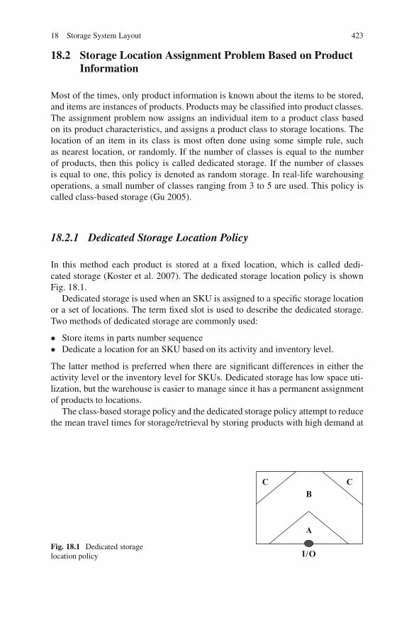
18 Storage System Layout 423
18.2 Storage Location Assignment Problem Based on ProductInformation
Most of the times, only product information is known about the items to be stored,and items are instances of products. Products may be classified into product classes.The assignment problem now assigns an individual item to a product class basedon its product characteristics, and assigns a product class to storage locations. Thelocation of an item in its class is most often done using some simple rule, suchas nearest location, or randomly. If the number of classes is equal to the numberof products, then this policy is called dedicated storage. If the number of classesis equal to one, this policy is denoted as random storage. In real-life warehousingoperations, a small number of classes ranging from 3 to 5 are used. This policy iscalled class-based storage (Gu 2005).
18.2.1 Dedicated Storage Location Policy
In this method each product is stored at a fixed location, which is called dedi-cated storage (Koster et al. 2007). The dedicated storage location policy is shownFig. 18.1.
Dedicated storage is used when an SKU is assigned to a specific storage locationor a set of locations. The term fixed slot is used to describe the dedicated storage.Two methods of dedicated storage are commonly used:
� Store items in parts number sequence� Dedicate a location for an SKU based on its activity and inventory level.
The latter method is preferred when there are significant differences in either theactivity level or the inventory level for SKUs. Dedicated storage has low space uti-lization, but the warehouse is easier to manage since it has a permanent assignmentof products to locations.
The class-based storage policy and the dedicated storage policy attempt to reducethe mean travel times for storage/retrieval by storing products with high demand at
Fig. 18.1 Dedicated storagelocation policy
A
BCC
I/O
424 J. Behnamian and B. Eghtedari
locations that are easily accessible (Van den Berg et al. 1999). This method requiresmore storage space than class-based storage since sufficient storage locations haveto be reserved for the maximum inventory of each product, and therefore increaseswarehouse space cost and material handling cost. On the other hand, dedicated stor-age has the advantage that the controlling of the warehouse is very simple, sinceitems of a product will always be stored in the same locations and sufficient spaceis always available for all of the items in replenishment batches. The simplicityadvantage is decreasing in importance because the introduction of information tech-nologies such as WMS, bar coding, and radio frequency tags provides a real-timeaccurate inventory map of the warehouse. The advantages of robustness and sim-plicity of dedicated storage must be traded off against the increased required storagespace and material handling cost (Gu 2005).
A disadvantage of dedicated storage is that a location is reserved even for prod-ucts that are out of stock. Moreover, for every product sufficient space has to bereserved such that the maximum inventory level can be stored. Thus, the space uti-lization is lowest among all storage policies. An advantage is that order pickersbecome familiar with product locations. In retail warehouses, often the product-to-location assignment matches the layout of the stores. This can save work in thestores, because the products are logically grouped. Finally, dedicated storage can behelpful if products have different weights. Heavy products have to be on the bottomof the pallet and light products on top. By storing products in order of weight androuting the order pickers accordingly, a good stacking sequence is obtained withoutadditional effort. Dedicated storage can be applied in pick areas, with a bulk area forreplenishment that may have, for example, random storage. In this way, the advan-tages of dedicated storage still hold, but the disadvantages are only minor becausededicated storage is applied only to a small area (Koster et al. 2007).
Kallina and Lynn (1976) discussed the implementation of the COI rule in prac-tice. The COI rule is easy to implement and has the intuitive appeal of locatingcompact, fast-moving items in readily accessible locations. Furthermore, the COIrule is proved to be optimal for dedicated storage when the following assumptionsare satisfied:
1. The objective is to minimize the long-term average order picking cost.2. The travel cost depends only on locations. Examples that do not satisfy this
assumption include the case when the travel cost is item dependent or whenthere are multiple I/O points, and products have different probability of mov-ing from/to the I/O points, i.e., it does not satisfy the factoring assumption asdefined in Mallette and Francis (1972).
3. When dual or multi-command order picking is used, there is no dependence be-tween the picked items in the same picking tour.
4. Certain routing policies are assumed for multi-command order picking, e.g.,Jarvis and McDowell (1991) assume using the traversal routing policy for theconventional multi-aisle order picking system.
5. There are no compatibility constraints that limit the storage location assignment,e.g., certain items must and/or cannot be put together (Gu 2005).
18 Storage System Layout 425
18.2.1.1 Space Requirements
With dedicated storage, products are assigned to specific locations. Also, one andonly one product is assigned to a storage location. Hence the number of storage lo-cations assigned to a product must be capable of satisfying the maximum storagerequirement for the product. With multiproduct storage, the storage space requiredequals the sum of the maximum storage requirements for each of the products(Francis et al. 1992).
18.2.1.2 Sizing on the Basis of Service Levels
One approach that can be used to size storage under dedicated storage conditionsis a service-level approach. Specifically, when demand for storage is a randomvariable, storage capacity can be determined on the basis of the probability of ashortage of space. With dedicated storage, Qj storage sots are assigned t producti for i D 1; : : : ; n. Therefore, the probability of there bring a sufficient number ofstorage positions for product i is simply the probability of storage demand beingless than or equal toQj . Thus the probability is given by the cumulative distributionfunction Fj (Qj ).
If the storage demands for the various products are statistically independent, theprobability of there being one or more shortages 0 storage space is given by
Pr .1 or more shortages/ D 1 � Pr .no shortages/ : (18.1)
Since the terms on the right-hand side of (18.2) are the cumulative probabilities,(18.2) can be expressed as
Pr .no shortages/ DnY
jD1pr ; (18.2)
Pr .no shortages/ DnY
jD1Fj .Qj /: (18.3)
Therefore, on substituting (18.3) in (18.1), we obtain
Pr .1 or more shortages/ D 1�nY
jD1Fj .Qj /: (18.4)
18.2.1.3 Sizing on the Basis of Costs
The previous analysis of space requirements for dedicated storage was based en-tirely on, service-level considerations. Under deterministic conditions, the size
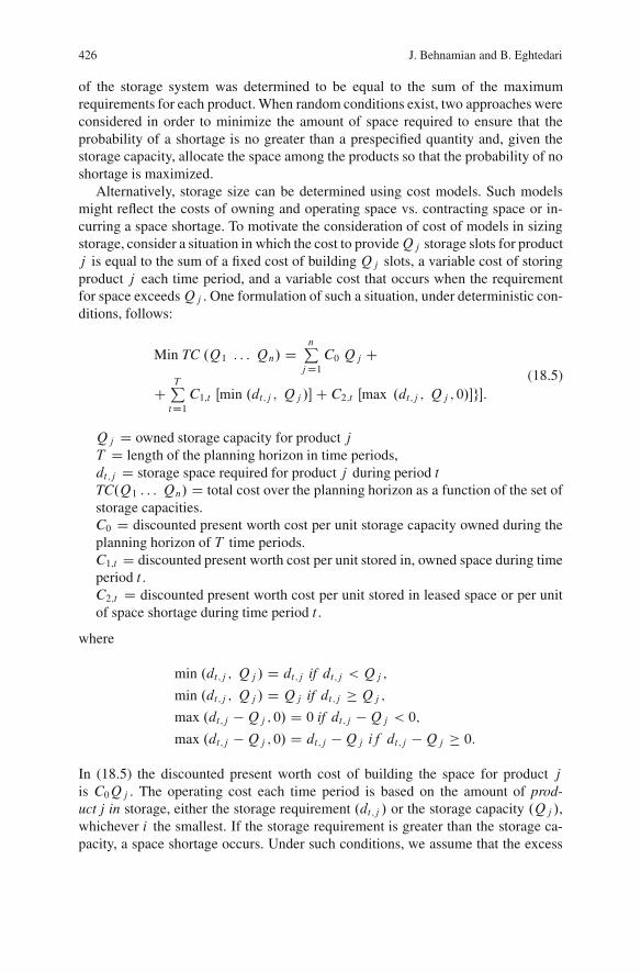
426 J. Behnamian and B. Eghtedari
of the storage system was determined to be equal to the sum of the maximumrequirements for each product. When random conditions exist, two approaches wereconsidered in order to minimize the amount of space required to ensure that theprobability of a shortage is no greater than a prespecified quantity and, given thestorage capacity, allocate the space among the products so that the probability of noshortage is maximized.
Alternatively, storage size can be determined using cost models. Such modelsmight reflect the costs of owning and operating space vs. contracting space or in-curring a space shortage. To motivate the consideration of cost of models in sizingstorage, consider a situation in which the cost to provideQj storage slots for productj is equal to the sum of a fixed cost of building Qj slots, a variable cost of storingproduct j each time period, and a variable cost that occurs when the requirementfor space exceedsQj . One formulation of such a situation, under deterministic con-ditions, follows:
Min TC .Q1 : : : Qn/ DnP
jD1C0 Qj C
CTPtD1
C1;t Œmin .dt;j ; Qj /C C2;t Œmax .dt;j ; Qj ; 0/g:(18.5)
Qj D owned storage capacity for product jT D length of the planning horizon in time periods,dt;j D storage space required for product j during period tTC.Q1 : : : Qn/ D total cost over the planning horizon as a function of the set ofstorage capacities.C0 D discounted present worth cost per unit storage capacity owned during theplanning horizon of T time periods.C1;t D discounted present worth cost per unit stored in, owned space during timeperiod t .C2;t D discounted present worth cost per unit stored in leased space or per unitof space shortage during time period t .
where
min .dt;j ; Qj / D dt;j if dt;j < Qj ;
min .dt;j ; Qj / D Qj if dt;j � Qj ;
max .dt;j �Qj ; 0/ D 0 if dt;j �Qj < 0;
max .dt;j �Qj ; 0/ D dt;j �Qj if dt;j �Qj � 0:
In (18.5) the discounted present worth cost of building the space for product jis C0Qj . The operating cost each time period is based on the amount of prod-uct j in storage, either the storage requirement .dt;j / or the storage capacity .Qj /,whichever i the smallest. If the storage requirement is greater than the storage ca-pacity, a space shortage occurs. Under such conditions, we assume that the excess
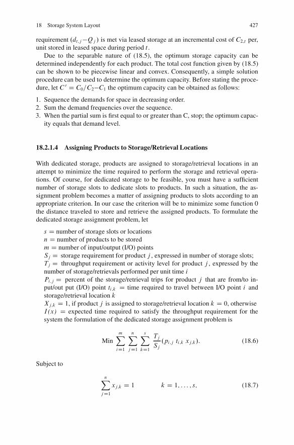
18 Storage System Layout 427
requirement .dt;j�Qj / is met via leased storage at an incremental cost of C2;t per,unit stored in leased space during period t .
Due to the separable nature of (18.5), the optimum storage capacity can bedetermined independently for each product. The total cost function given by (18.5)can be shown to be piecewise linear and convex. Consequently, a simple solutionprocedure can be used to determine the optimum capacity. Before stating the proce-dure, let C 0 D C0=C2�C1 the optimum capacity can be obtained as follows:
1. Sequence the demands for space in decreasing order.2. Sum the demand frequencies over the sequence.3. When the partial sum is first equal to or greater than C, stop; the optimum capac-
ity equals that demand level.
18.2.1.4 Assigning Products to Storage/Retrieval Locations
With dedicated storage, products are assigned to storage/retrieval locations in anattempt to minimize the time required to perform the storage and retrieval opera-tions. Of course, for dedicated storage to be feasible, you must have a sufficientnumber of storage slots to dedicate slots to products. In such a situation, the as-signment problem becomes a matter of assigning products to slots according to anappropriate criterion. In our case the criterion will be to minimize some function 0the distance traveled to store and retrieve the assigned products. To formulate thededicated storage assignment problem, let
s D number of storage slots or locationsn D number of products to be storedm D number of input/output (I/O) pointsSj D storage requirement for product j , expressed in number of storage slots;Tj D throughput requirement or activity level for product j , expressed by thenumber of storage/retrievals performed per unit time iPi;j D percent of the storage/retrieval trips for product j that are from/to in-put/out put (I/O) point ti;k D time required to travel between I/O point i andstorage/retrieval location kXj;k D 1, if product j is assigned to storage/retrieval location k D 0, otherwiseI (x) D expected time required to satisfy the throughput requirement for thesystem the formulation of the dedicated storage assignment problem is
MinmXiD1
nXjD1
sXkD1
Tj
Sj.pi;j ti;k xj;k/: (18.6)
Subject to
nXjD1
xj;k D 1 k D 1; : : : ; s; (18.7)
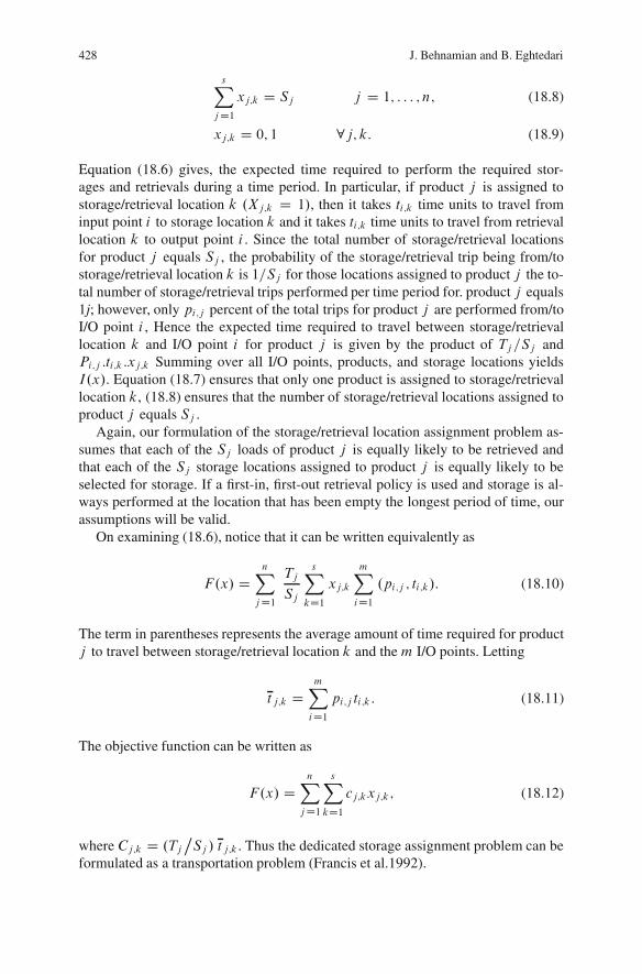
428 J. Behnamian and B. Eghtedari
sXjD1
xj;k D Sj j D 1; : : : ; n; (18.8)
xj;k D 0; 1 8j; k: (18.9)
Equation (18.6) gives, the expected time required to perform the required stor-ages and retrievals during a time period. In particular, if product j is assigned tostorage/retrieval location k .Xj;k D 1/, then it takes ti;k time units to travel frominput point i to storage location k and it takes ti;k time units to travel from retrievallocation k to output point i . Since the total number of storage/retrieval locationsfor product j equals Sj , the probability of the storage/retrieval trip being from/tostorage/retrieval location k is 1=Sj for those locations assigned to product j the to-tal number of storage/retrieval trips performed per time period for. product j equals1j; however, only pi;j percent of the total trips for product j are performed from/toI/O point i , Hence the expected time required to travel between storage/retrievallocation k and I/O point i for product j is given by the product of Tj =Sj andPi;j :ti;k :xj;k Summing over all I/O points, products, and storage locations yieldsI.x/. Equation (18.7) ensures that only one product is assigned to storage/retrievallocation k, (18.8) ensures that the number of storage/retrieval locations assigned toproduct j equals Sj .
Again, our formulation of the storage/retrieval location assignment problem as-sumes that each of the Sj loads of product j is equally likely to be retrieved andthat each of the Sj storage locations assigned to product j is equally likely to beselected for storage. If a first-in, first-out retrieval policy is used and storage is al-ways performed at the location that has been empty the longest period of time, ourassumptions will be valid.
On examining (18.6), notice that it can be written equivalently as
F.x/ DnX
jD1
Tj
Sj
sXkD1
xj;k
mXiD1
.pi;j ; ti;k/: (18.10)
The term in parentheses represents the average amount of time required for productj to travel between storage/retrieval location k and the m I/O points. Letting
t j;k DmXiD1
pi;j ti;k: (18.11)
The objective function can be written as
F.x/ DnX
jD1
sXkD1
cj;kxj;k; (18.12)
where Cj;k D .TjıSj / tj;k . Thus the dedicated storage assignment problem can be
formulated as a transportation problem (Francis et al.1992).
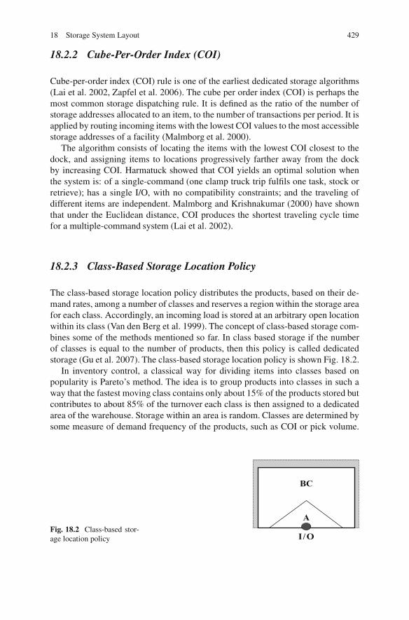
18 Storage System Layout 429
18.2.2 Cube-Per-Order Index (COI)
Cube-per-order index (COI) rule is one of the earliest dedicated storage algorithms(Lai et al. 2002, Zapfel et al. 2006). The cube per order index (COI) is perhaps themost common storage dispatching rule. It is defined as the ratio of the number ofstorage addresses allocated to an item, to the number of transactions per period. It isapplied by routing incoming items with the lowest COI values to the most accessiblestorage addresses of a facility (Malmborg et al. 2000).
The algorithm consists of locating the items with the lowest COI closest to thedock, and assigning items to locations progressively farther away from the dockby increasing COI. Harmatuck showed that COI yields an optimal solution whenthe system is: of a single-command (one clamp truck trip fulfils one task, stock orretrieve); has a single I/O, with no compatibility constraints; and the traveling ofdifferent items are independent. Malmborg and Krishnakumar (2000) have shownthat under the Euclidean distance, COI produces the shortest traveling cycle timefor a multiple-command system (Lai et al. 2002).
18.2.3 Class-Based Storage Location Policy
The class-based storage location policy distributes the products, based on their de-mand rates, among a number of classes and reserves a region within the storage areafor each class. Accordingly, an incoming load is stored at an arbitrary open locationwithin its class (Van den Berg et al. 1999). The concept of class-based storage com-bines some of the methods mentioned so far. In class based storage if the numberof classes is equal to the number of products, then this policy is called dedicatedstorage (Gu et al. 2007). The class-based storage location policy is shown Fig. 18.2.
In inventory control, a classical way for dividing items into classes based onpopularity is Pareto’s method. The idea is to group products into classes in such away that the fastest moving class contains only about 15% of the products stored butcontributes to about 85% of the turnover each class is then assigned to a dedicatedarea of the warehouse. Storage within an area is random. Classes are determined bysome measure of demand frequency of the products, such as COI or pick volume.
Fig. 18.2 Class-based stor-age location policy I /O
A
BC
430 J. Behnamian and B. Eghtedari
Fast moving items are generally called A-items. The next fastest moving categoryof products is called B-items, and so on. Often the number of classes is restricted tothree, although in some cases more classes can give additional gains with respect totravel times (Koster et al. 2007).
This storage policy in the literature seems to be a compromise between the dedi-cated and the randomized storage policies. It divides products into classes based ontheir turnover ratio. The class with the highest ratio is located closest to the I/O. Theimplementation of class based storage (i.e., the number of classes, the assignment ofproducts to classes, and the storage locations for each class) has significant impacton the required storage space and the material handling cost in a warehouse (Guet al. 2007).The implementation of class-based storage (i.e., the number of classes,the assignment of products to classes, and the storage locations for each class) hassignificant impact on the required storage pace and the material handling cost in awarehouse. Research on this problem has been largely focused on AS/RS, especiallysingle-command AS/RS.
18.2.3.1 Criteria for Assigning a Product (Class) to Storage Locations
Different criteria can be used to assign a product (class) to storage locations. Thethree most frequently used criteria are (Gu 2005):
1. Popularity (defined as the number of storage/retrieval operations per unit timeperiod). For the popularity policy, product classes are ranked by decreasing pop-ularity and the classes with the highest popularity are assigned the most desirablelocations.
2. Maximum inventory (defined as the maximum warehouse space allocated to aproduct class). For the maximum inventory policy, product classes are ranked byincreasing maximum inventory and the classes with the lowest maximum inven-tory are assigned the most desirable locations.
3. Cube-per-order index (COI, which is defined as the ratio of the retrieval opera-tions per unit time/ maximum allocated storage space to the number of storage).The COI policy takes into consideration both a SKU’s popularity and its storagespace requirement. Product classes are ranked by increasing COI value and theclasses with the high COI are stored in the most desirable locations.
The implementation of the above policies depends on the types of warehouse sys-tems and, therefore there may be have different variations in that, for example:
1. If storage space is measured in units (e.g., shelves and bays), each unit can betreated as an individual product by appropriately apportioning demand. This ismost commonly used in unit load warehouses and sometimes in less-than-unit-load warehouses. Since each unit load occupies the same amount of storagespace, the popularity policy based on the apportioned popularity is essentiallythe same as the COI policy. However, it is different from the popularity policywithout apportioning. For example, suppose that product A has three unit loadsand a popularity of three picks per day, and product B has one unit load and apopularity of two picks a day. The popularity policy without apportioning will
18 Storage System Layout 431
rank product A ahead of product B. On the other hand, if product A is treatedas three products (denoted as A1, A2, and A3), each of them will have an ap-portioned popularity of 1 pick per day. So the popularity policy based on theapportioned popularity will now rank product B ahead of product A1, A2, andA3, which can be easily verified to be equivalent to the COI policy.
2. The definition of “the most desirable locations” depends on the system as well asthe travel pattern. For example, if traversal routing policy is used for traveling ina conventional multi-parallel-aisle system, the desirability of locations are mea-sured in terms of aisles where the most desirable locations are in the aisle thatis closest to the I/O point. This leads to the so-called organ pipe storage locationassignment.
3. The above three policies are simple and flexible enough to be implemented indifferent warehouse systems. Among them, the COI policy has been the mostcomprehensively studied one. The COI policy was first described without a proofof its optimality.
18.2.3.2 Assigning a Product (Class) to Storage Locations Basedon Popularity
Model parameters:
Qk D Number of storage locations requested at any single operational period forthe storage of SKU i
S D Quantity of storage at any single operational period for the storage of SKU iR D Quantity of retrieval at any single operational period for the storage ofSKU i
Storage policy: calculate S=R ratio
� If S=R < 1: locate nearer to receiving� If S=R > 1: locate nearer to shipping� If S=R D 1: does not matter
18.2.4 Class-Based Dedicated Storage Location Policy (COI)
As a compromise between dedicated storage and randomized storage, class-based,dedicated storage is frequently used. With class-based dedicated storage, productsare divided into three, four, or five classes based on their throughput .T /-to-storage(S ) ratios. The relatively few fast movers are categorized as class 1 products, nextare class 2 products, and then class 3 products, and so on. Dedicated storage is usedfor the classes and randomized storage is used within a class.
It should be noted that the entire discussion of dedicated storage given inSect. 18.2.1 applies to class-based dedicated storage, if, instead of dealing with;products, one deals with classes of products. For this reason, our class-based dedi-cated storage treatment focuses on the formation of classes of products.
432 J. Behnamian and B. Eghtedari
18.2.4.1 Model for Class-Based Storage Location
Van den Berg (1999) presents a polynomial time dynamic programming algorithmthat partitions products and locations into classes such that the mean single com-mand cycle time is minimized. The algorithm works under any demand curve, anytravel time metric, any warehouse layout and any positions of the input station andoutput station. We use the following notation:
Qi D independent random variables representing the number of unit-loads pre-sent of product i at an arbitrary epoch,Pk D set of products in class k D 1; 2; : : : ; K . Due to the demand and supplyprocesses the inventory level fluctuates. We estimate the storage space require-ment such that the storage space in every class suffices for at least a fraction0<˛ <1 of the time. In other words, the probability of a stock overflow is lessthan 1˛-. Let Qk be a random variable representing the inventory level of classk at an arbitrary epoch, i.e.
Qk DXi2Pk
Qi: (18.13)
Now, we want to find the smallest size Sku for the class-region of class k such that
P.Qk � Sk/ � ˛: (18.14)
Let tj in denote the travel time between the input station and location j and let tj out
denote the travel time between the output station and location j .Every stored unit-load is retrieved some time later, so that over a long time period
half of the single command cycles are storages and half are retrievals.Accordingly, the mean single command cycle time to location j 2 L equals:
1
2.2t inj C 2tout
j / D .t inj C toutj /: (18.15)
The single command cycle time, E.SC/, is defined as
E.SC/ DkX
kD1
Pi2Pk
E.Di/Pi2P
E.Di/:X .t inj C tout
j /
jLkj ; (18.16)
where Lk denotes the set of storage locations of class k. The First factor representsthe probability that a request concerns class k. The second factor represents themean travel time to a location in class k.
In order to minimize the expected single command cycle time, we assign theproducts i that constitute the largest demand per reserved space and the locationsj with the smallest .tj in C tj
out / to the First class and we assign the products ithat constitute the next largest demand per reserved space and the locations j with
18 Storage System Layout 433
the next smallest .tj in C tjout / to the second class, and so on. Accordingly, the
locations are ranked according to non-decreasing .tj in C tjout / and the products are
ranked according to nonincreasing demand per reserved space. We define gk.p; l/as the contribution of classes 1; 2; : : : ; k to (18.16) when products 1; 2; : : : ; p andstorage locations 1; 2; : : : ; l are distributed among these classes such that gk.p; l/is minimal. Then gk.p; l/ satisfies
gk.p; l/ D min 1�i�p;1�j�lnhjC1;liC1;p C gk�1.i; j /
o; (18.17)
where hiC1; pjC1;l denotes the contribution to (18.16) if the products iC1; : : : :; pand the locations j C 1; : : : ; l form one class k. Recalling that the number of loca-tions required in each class is determined by (18.15) the values gk.p; l/ are foundby iteratively solving the dynamic programming (18.17) Each gk.p; l/ correspondsto an optimal solution of the sub problem with k classes and the First p products andthe First l storage locations when ranked as indicated before. We may use the algo-rithm to determine the optimal class-partition for 1; 2; : : : ; k classes. Subsequently,the number of classes among 1; 2; : : : ; k may be selected that constitutes an accept-able mean travel time and space requirement (Van den Berg et al. 1999).
Research on this problem has been largely focused on AS/RS, especially singlecommand AS/RS. Hausman et al. (1976) show that for single-command AS/RS withthe Chebyshev metric, the ideal shape of storage regions is L-shaped. For such sys-tems, the problem reduces to determining the number and boundaries of the classes.Explicit analytical solutions for the class boundaries can be derived for the casewith 2 or 3 classes, as shown by Hausman et al. (1976), Kouvelis and Papanicolaou(1995), and Eynan and Rosenblatt (1994). For the general n-class case, Rosenblattand Eynan (1989) and Eynan and Rosenblatt (1994) suggest a one-dimensionalsearch procedure to find the optimal boundaries. The implementation of class-basedstorage in multi-command AS/RS is discussed in Guenov and Raeside (1992).
18.2.5 Full Turn-over Based Storage
For the turnover policy, products are ranked by the ratio of their demand rate dividedby their maximum inventory. Products with the highest turnover are stored in themost desirable locations. The turnover policy is the most comprehensively studiedone in the literature.
This policy distributes products over the storage area according to their turnover.The products with the highest sales rates are located at the easiest accessible loca-tions, usually near the depot. Slow moving products are located somewhere towardsthe back of the warehouse. An early storage policy of this type is the cube-per-order index (COI) rule, A practical implementation of full turnover policies wouldbe easiest if combined with dedicated storage (Koster et al. 2007). It is applicablewhen space requirements for individual items are identical and, like the COI, hasthe objective of maximizing throughput capacity (Malmborg et al. 2000). Gu (2005)
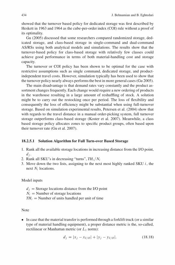
434 J. Behnamian and B. Eghtedari
showed that the turnover based policy for dedicated storage was first described byHeskett in 1963 and 1964 as the cube-per-order index (COI) rule without a proof ofits optimality.
Gu (2005) discussed that some researchers compared randomized storage, ded-icated storage, and class-based storage in single-command and dual-commandAS/RSs using both analytical models and simulations. The results show that theturnover-based policy for class-based storage with relatively few classes couldachieve good performance in terms of both material-handling cost and storagecapacity.
The turnover or COI policy has been shown to be optimal for the case withrestrictive assumptions such as single command, dedicated storage, and product-independent travel costs. However, simulation typically has been used to show thatthe turnover policy nearly always performs the best in more general cases (Gu 2005).
The main disadvantage is that demand rates vary constantly and the product as-sortment changes frequently. Each change would require a new ordering of productsin the warehouse resulting in a large amount of reshuffling of stock. A solutionmight be to carry out the restocking once per period. The loss of flexibility andconsequently the loss of efficiency might be substantial when using full-turnoverstorage. Based on simulation experimental results, Petersen et al. (2004) show thatwith regards to the travel distance in a manual order-picking system, full turnoverstorage outperforms class-based storage (Koster et al. 2007). Meanwhile, a classbased storage policy allocates zones to specific product groups, often based upontheir turnover rate (Gu et al. 2007).
18.2.5.1 Solution Algorithm for Full Turn-over Based Storage
1. Rank all the available storage locations in increasing distance from the I/O point,dj .
2. Rank all SKU’s in decreasing “turns”, THi =Ni3. Move down the two lists, assigning to the next most highly ranked SKU i , the
next Ni locations.
Model inputs
dj D Storage locations distance from the I/O pointNi D Number of storage locationsTHi D Number of units handled per unit of time
Note
� In case that the material transfer is performed through a forklift truck (or a similartype of material handling equipment), a proper distance metric is the, so-called,rectilinear or Manhattan metric (or L1 norm):
dj D jxj � xI=O j C jyj � yI=O j: (18.18)
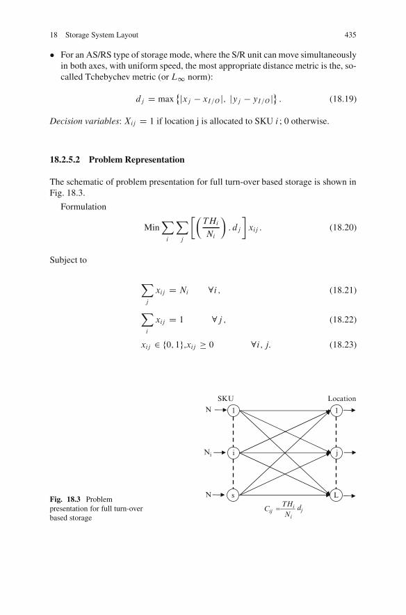
18 Storage System Layout 435
� For an AS/RS type of storage mode, where the S/R unit can move simultaneouslyin both axes, with uniform speed, the most appropriate distance metric is the, so-called Tchebychev metric (or L1 norm):
dj D max˚jxj � xI=O j; jyj � yI=O j� : (18.19)
Decision variables: Xij D 1 if location j is allocated to SKU i ; 0 otherwise.
18.2.5.2 Problem Representation
The schematic of problem presentation for full turn-over based storage is shown inFig. 18.3.
Formulation
MinXi
Xj
��THi
Ni
�: dj
�xij : (18.20)
Subject to
Xj
xij D Ni 8i ; (18.21)
Xi
xij D 1 8j ; (18.22)
xij 2 f0; 1g;xij � 0 8i; j: (18.23)
Fig. 18.3 Problempresentation for full turn-overbased storage
1
i
s
N
Ni
N
SKU Location
1
j
LTHiCij = Ni
dj
436 J. Behnamian and B. Eghtedari
Remarks
� The previous problem representation corresponds to a balanced transportationproblem: Implicitly it has been assumed that: L D P
i
Ni
� For the problem to be feasible, in general, it must hold that: L � Pi
Ni
18.3 Storage Location Assignment ProblemBased on Item Information (SLAP/II)
In the SLAP/II problem, it is assumed that complete information is known about thearrival and departure time of the individual items. It is very unlikely that informationon individual items will be available in typical warehousing operations, but it maybe available in the case of short term planning of container ports or airport gates(Gu 2005).
1. Assignment problem and vector assignment problem2. Shared storage policies for balanced input and output (Goetschalckx and Ratliff
1990)3. Duration-of-stay storage policy4. Shared storage policies for unbalanced input and output (Goetschalckx and
Ratliff 1990)
� Static shared storage policies� Adaptive shared storage policies
18.3.1 Assignment Problem and Vector Assignment Problem
The resulting problem is a specially structured assignment problem (AP), whereitems are assigned to storage locations. The special structure derives from the prop-erty that two items can occupy the same storage location, provided that they do notoccupy it at the same time. This problem has been called the vector assignmentproblem (VAP), since the occupation is no longer expressed as a single binary sta-tus variable but as a vector over the different time periods (Goetschalckx 1998).The optimal solution of this problem for typical warehousing operations is compu-tationally impractical because of the very large problem instances. The problem isof interest to academic research in warehouse operations because it provides a costlower bound or performance upper bound. An example of a heuristic SLAP/II policyis the duration-of-stay (DOS) policy of Goetschalckx and Ratliff (1990).
18 Storage System Layout 437
18.3.2 Shared Storage Policies
Shared storage policies allow for more flexible use of space than that allowed bydedicated storage policies. This provides the potential both to reduce the maximum-effective storage area and to better utilize the more desirable storage locations. Bothof these factors reduce average travel time.
The biggest disadvantage of shared storage is the increased data and computa-tional requirements to keep track of where each retrieved load is located and todetermine where each received load should be stored. Using dedicated storage sys-tems. A location will always be used to store the same product and the picker can“learn” where each product is stored (Goetschalckx and Ratliff 1990).
Dedicated storage policies require the warehouse to be large enough to store themaximum inventories of all products simultaneously. If shared storage is allowedand if products are not replenished simultaneously, then total storage requirementsvary over time depending on how the material input and output are distributed overtime. The required rack size is equal to the maximum number of locations duringthe planning horizon used by the storage policy. The ideal situation occurs when theinput and output flows are balanced. That is, arrival of each unit of new stock occursjust at the time when an old unit is removed from the system. For this ideal case,the warehouse need only be large enough to hold the sum of the average productinventories.
Turnover rate is a product characteristic since all unit loads of the same producthave the same turnover rate. The time in storage or “duration-of-stay” for differentunits of the same product is a unit characteristic since it may differ among differentunit loads of the same product. To illustrate this difference, assume that a replen-ishment batch of units of a product has just arrived and there is no inventory of theproduct already in storage. The first unit retrieved will stay the length of one demandinterarrival time. The last unit retrieved will stay, on the average, the length of thedemand interarrival time multiplied by the batch size of the product. It is shown inSect. 3.2.1 that a duration-of-stay-based policy is optimal under an assumption ofperfectly balanced inputs and outputs.
18.3.2.1 Optimal Shared Storage Policy for a Perfectly Balanced System
A system is balanced if for every period t , the number of arriving units is equal tothe number of departing units. In a balanced system there is never an empty locationat the end of any period and there is always an open location available for an arrivingunit. In this case the warehouse is of minimal size and is equal to the sun1 of averageinventories of all products.
A system is perfectly, balanced if for any period t , the number of departing unitsthat have duration of stay of p is equal to the number of arriving units that have aDOS of p for all p. The number of units arriving in period t with a DOS of y willbe denoted by np.t/. The system is then perfectly balanced if for all p and t thefollowing relationship holds: np.t/ D np.t C p/.
438 J. Behnamian and B. Eghtedari
For a balanced system the aggregate input flow is equal to the aggregate outputflow. For a perfectly balanced system the input flow is equal to the output flowfor each class of units that have the same DOS. Hence perfectly balanced impliesbalanced, but not the reverse.
For a perfectly balanced system, let zp be the total number of units arriving duringany p consecutive time periods that have a DOS equal top. Then zp equals to thenumber’s of slots in the warehouse required for storing units which have DOS equaltop, since the units arriving at time periodpC1will exactly replace the units arrivedat time period one. Note, from the definition of the perfectly balanced system, thatzp is constant over time. For a perfectly balanced system the expression for zp is
Zp DpXiD1
np.i/: (18.24)
The following theorem provides a procedure for determining an optimal shared stor-age policy for a perfectly balanced system
Theorem 18.1. A shared storage policy which minimizes both travel time andrequired storage space for a perfectly balanced system is to allocate for eachp D 1; 2; : : : the zp , unallocated storage locations having the smallest travel timeto unit loads with DOS equal to p.
18.3.3 Duration-of-Stay Storage Policy
In an attempt to reduce the storage space requirement for dedicated storage, somewarehouse managers use a variation of dedicated storage in which the assignmentof products to spaces is managed carefully. In particular, over time, different prod-ucts use the same storage slot, albeit only one product occupies the slot when it isoccupied. The location policy used is here referred to as shared storage.
To motivate our consideration of shared storage, consider the arrival of 100 palletloads of a particular fast mover product to be stored in pallet rack. Pallet loads willbe retrieved and shipped at a rate of five pallet loads per day over a 20-day period.With randomized storage, 100 empty storage slots are randomly selected for theproduct; no recognition is given to the fact that the product is a fast mover.
With dedicated storage, on the other hand, at least 100 empty slots must beavailable among the premium locations assigned to the fast-mover product. If ran-domized storage is used, each time a pallet load is removed from storage, the slotis available for use by the next product requiring storage. However, with dedicatedstorage, each removal of a pallet from storage creates an empty slot that will notpossibly be filled until, at the earliest, the arrival of the next shipment of the sameproduct. Shared storage recognizes that while the product might be considered tobe a fast mover, each pallet load stays in storage different lengths of time. Depend-ing on the amount of the product in inventory at the time the shipment arrives, it ispossible that five pallet loads will be in storage for only 1 day, whereas five other
18 Storage System Layout 439
pallet loads within the same shipment will be in storage for 20 days. From the per-spective of the storage positions in the warehouse, five pallet loads appear to besuper fast movers; the remaining pallet loads are viewed as being less fast, perhapseven medium or slow movers. Shared storage recognizes and takes advantage of theinherent differences in lengths of time that individual pallet loads remain in storage(Francis et al. 1992).
An example of a heuristic SLAP/II policy is the duration-of-stay policy ofGoetschalckx and Ratliff (1990). In DOS-based storage policies, the expected DOSof the i th unit of a SKU with replenishment lot size Q is i=� for i D 1; 2 : : : Q,where � is the demand rate of that SKU.
DOS D i=�: (18.25)
Then the items of all the different products having the shortest DOS are assigned tothe closest locations. Hence, the items of a single replenishment batch of a singleproduct are not stored together in the warehouse. Under some unrealistic assump-tions on the scheduling and size of product replenishments, it can be shown thatthe DOS storage policy is optimal for both materials handling effort and requiredstorage capacity. In practice, DOS-based policies are difficult to implement sinceit requires the tracking and management of each stored unit in the warehouse. Alsothe performance of DOS-based policies depends greatly on factors such as the skew-ness of demands, balance of input and output flows, inventory control policies, andthe detailed implementations. Kulturel et al. (1999) compared class-based storageand DOS-based storage using simulation and showed that the former consistentlyoutperforms the latter in practical settings.
Goetschalckx and Ratliff (1990) and Thonemann and Brandeau (1998) theoret-ically showed that DOS-based storage policies are the most promising policy interms of minimizing traveling costs. In practice, DOS-based policies are difficult toimplement since they require the tracking and management of each stored unit in thewarehouse. Also, the performance of DOS-based policies depends greatly on fac-tors such as the skewness of demands, balance of input and output flows, inventorycontrol policies, and the detailed implementations (Gu 2005).
18.3.3.1 Space Requirements
The storage space requirements for shared storage range from that required for ran-domized storage to that required for dedicated storage, depending on the amountof information available regarding the inventory levels over time for each product.As noted above, the distinction between shared storage and randomized storage isthat the former involves total specificity regarding the storage locations for products,whereas with the latter, the locations depend solely on the mergence of empty slotswithin the warehouse. Shared storage and dedicated storage differ due to the dis-tinction made by the former regarding the time that each load of a product spends,formally the shared storage policy. Relatively little experience has been gained inapplying the policy to large-scale problems optimally; furthermore, as will be seen,
440 J. Behnamian and B. Eghtedari
it is not immediately obvious how one might go about making optimum locationdecisions for large-scale applications. We present the policy because (a) multipleproducts sharing storage space is quite common in some industries, and (b) its fea-tures are sufficiently attractive to warrant our further attention. Since the materialmight be of less interest to those interested in tried and true storage policies, thissection may be omitted without jeopardizing an understanding of the remainingmaterial in the chapter (Francis et al.1992).
In storage; dedicated storage assigns the total replenishment lot of a product toa number of storage positions based on the average time spent in storage for thereplenishment lot.
A situation that naturally suggests the use of shared storage is a production linethat is used to produce multiple products. Since products are produced sequen-tially rather than simultaneously, inventory replenishments are distributed over time.A beverage bottling line is an example of the type of situation we have in mind; otherexamples include production lines for paint, bleach, and industrial chemicals.
In each case cited, the same production equipment is used to produce differentpackage sizes of the same product, as well as different products. A new setup orchangeover is required between the production of different sizes or products Henceit is not possible for the inventory levels of the various sizes and products producedon the same production line to be increasing at the same time. While one productis being produced, the inventory levels of the other products are decreasing. Not allproducts can be at their maximum inventory levels simultaneously. Hence the use iof dedicated storage would result in some empty storage slots, existing at all times.
18.3.4 Shared Storage Policies for Unbalanced Input and Output
A perfectly balanced system is a much idealized situation which is unlikely to occurin real storage systems. However, the analysis of the perfectly balanced systemsprovides:
1. A bound on how much improvement can be expected from the use of sharedstorage policies, and
2. Insights which allow development of attractive heuristics for more realistic situ-ations.
Shared storage policies for systems which are not perfectly balanced need to be dis-tinguished in terms of when information is available to make the storage decisions.We will define static storage policies as those where all the information affecting thestorage and retrieval decision is available at the beginning of the planning period.In this case, all assignments of items to locations can be made prior to the begin-ning of the planning horizon. We define adaptive policies as those using informationwhich becomes available during the planning period to influence the storage and re-trieval decisions. Based on the knowledge gained from the perfectly balanced case,we develop heuristics for both static and adaptive policies and then compare them(Goetschalckx and Ratliff 1990).
18 Storage System Layout 441
18.3.5 Static Shared Storage Policies
First consider a static system where we know the arrival and departure time of eachitem during the planning horizon. From the results we conclude that for all sharedstorage systems that satisfy the travel independence condition, any storage policythat relies only on the ranking of the travel times to the locations (and not on theiractual value) is optimal if and only if it simultaneously maximizes the number ofitems stored in the first, first two, : : : , first N locations. This is a very restrictivecondition and thus finding optimal policies based only on the ranking of the storagelocations will most likely be restricted to special cases. Goetschalckx (1992) showsthat solving the optimal storage policy will require a prohibitive computational effortin a warehousing setting. However, if we know the exact arrival and departure timeof each unit during the planning horizon (i.e., the system is static), then an efficientheuristic (GREEDY) can be formulated.
GREEDY is based on the fact that we can efficiently maximize the number ofunits stored in the first location. Given the assignment of units to the first location,we can maximize the number of units stored in the second location. In general, giventhe assignment of units to the first locations we can maximize the number of unitsstored in location nC1. To accomplish this we first order all the units, which will bestored during the planning horizon, by nondecreasing departure time. If there are anyties, then they are broken by ordering the units by nondecreasing arrival time. Thistie-breaker fills up early locations as much as possible, thereby increasing flexibilityfor later decisions. The storage locations are ordered by nondecreasing travel time.We then assign the units in order to the open location with the smallest travel time.
The computational effort required by GREEDY is small, since it requires onlya sort of the locations and a sort of the items. The effort is of the order ofO.K log .K//C O.N log .N // where K is the number of units stored during theplanning horizon and N is the number of slots in the warehouse (Goetschalckx andRatliff 1990).
18.3.6 Adaptive Shared Storage Policies
Most real life storage systems are adaptive systems, because complete and perfectinformation is not available at the beginning of the planning horizon. Most of thetime, the only information available is with regard to average material flow and, insome cases, what is arriving during the next period. The policy developed in thissection involves establishment of classes within the warehouse based on averagearrivals and departures of items with different durations of stay. This can be viewedas a variation of the Hausman et al. (1976) class based storage concept, but with theclasses based on unit duration of stay rather than product turnover rate.
Let np.t/ be the number of units with DOS equal to p which arrives in period t .Let Nnp be the average number of items arriving in a period with DOS equal to p. For
442 J. Behnamian and B. Eghtedari
a perfectly balanced system Nnp is equal to zp=p. Hence, for those items with DOSequal top, we define a zone of size p Nnp which is exactly the right size each period.
For systems which are not perfectly balanced, some periods have np.t/ differentfrom the number of open locations in the zone of size p Nnp . Hence, a zone of sizepi & is too large for some periods and too small for other periods. One approachto handling this variation is to establish the zones in exactly the same fashion as forthe perfectly balanced case. That is, let zp D p Nnp be the zone size for items withDOS equal to p. Then for p D 1; 2 : : : reserve the z, remaining locations with thesmallest travel time for items with DOS equal to y.
There are two difficulties with this approach which must be overcome. The firstis that z, may not be an integer number of slots since p Nnp is not necessarily integer.This can be handled by rounding z, to the nearest integer. When z, is small therelative impact of this rounding is greater than when z, is larger. For example ifz1 D 1:5 the zone size could double, based on which way z1 value is rounded. Analternative is to aggregate items into a class until the z, for the aggregate class can berounded without large relative Impact. It is shown that for that case the increase inaverage distance traveled which results from combining two adjacent DOS classesis n2pC=2 where c is the slot width. This result indicates that the impact of combin-ing classes is strongly affected by the number of items arriving in a class, but notby the DOS itself. Hence, we would be more inclined to combine DOS classes withsmall np .
The second difficulty occurs when an item arrives with DOS equal to p and thezone allocated for items with DOS equal to p is full. It seems logical to assign theitem either to the nearest zone higher than p with an open location or the nearestzone lower than p with an open location. To better understand the impact of puttingan item in a zone different from its own, consider the following situation. Supposethat one slot in a zone corresponding to DOS equal to p is always used for itemswith DOS equal to q and one slot in a zone corresponding to DOS equal to q isalways used for items with DOS equal to p. Further, assume that both slots remainfull. Let tp and tq , be the average travel time to zones p and q respectively.
If the slots had been used for the correct items, then the expected travel timewould have been tp=p C tp=q. By interchanging the slot usage, the expected traveltime becomes tp=p C tp=q which is an increase of
.q � p/.tq � tp/ıpq: (18.26)
From this we see that the impact of interchange becomes less a p and q get larger(i.e., the penalty for placing an item in the wrong zone decreases with increasingduration of stay).
For the computation experiments discussed in the next section, the zones forthe dynamic shared storage policy were determined by the following ADAPTIVEalgorithm with cumulative rounding. The average time between two demands for anitem of product i is denoted by diti .
18 Storage System Layout 443
18.3.6.1 Adaptive Algorithm
1. For each duration of stay p donp D 0: (18.27)
For each item k D 1 : : : qi in replenishment batch of produce i do
P D k:d in: (18.28)
np D np C 1=.qi :diti /: (18.29)
2. for each duration of stay p do
zp D np:p: (18.30)
Cumulative remainder D 0, prev bound D 0, zone D 0.
3. for each duration of stay p do
Cumulative remainder D cumulative remainder CzpIf cumulative remainder> 1 then,Zone D zone C 1,Zone size (zone) D round to integer (cumulative remainder),Lower dos (zone) D prev bound C1,Upper dos (zone) D p,Cumulative remainder D cumulative remainder – zone size (zone),Prev bound D p.
In step 1 of the algorithm the average number of items arriving for each durationof stay is computed, based on the fact that during qiditi , time periods one item be-longing to product i with duration of stay p will arrive in the system. In step 2the required zone size zp is computed for each duration of stay and the bookkeep-ing variables for step three are initialized. In step 3 of the algorithm, for each dosthe required zone size is added to the cumulative remainder, until the cumulativeremainder is larger than one location.
Then, the new zone is set equal to the cumulative remainder size rounded tothe nearest integer and the DOS bounds for this new zone are set. The size of thisnew zone is then subtracted from the cumulative remainder. This is consistent withthe properties that zones with large zn’s and corresponding large zn’s should notbe combined and zones with small zn’s can be combined without incoming a largepenalty. It also solves the problem on how to round the fractional zone sizes tointeger numbers.
Once the zones are determined, ADAPTIVE executes in the same way as theoptimal policy. At the time of its arrival, the DOS of every unit is estimated andthat unit is stored in its corresponding zone. If that zone is full, the unit is stored inthe open location with the smallest value for expression (Goetschalckx and Ratliff1990).
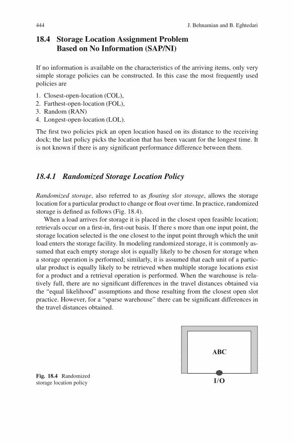
444 J. Behnamian and B. Eghtedari
18.4 Storage Location Assignment ProblemBased on No Information (SAP/NI)
If no information is available on the characteristics of the arriving items, only verysimple storage policies can be constructed. In this case the most frequently usedpolicies are
1. Closest-open-location (COL),2. Farthest-open-location (FOL),3. Random (RAN)4. Longest-open-location (LOL).
The first two policies pick an open location based on its distance to the receivingdock; the last policy picks the location that has been vacant for the longest time. Itis not known if there is any significant performance difference between them.
18.4.1 Randomized Storage Location Policy
Randomized storage, also referred to as floating slot storage, allows the storagelocation for a particular product to change or float over time. In practice, randomizedstorage is defined as follows (Fig. 18.4).
When a load arrives for storage it is placed in the closest open feasible location;retrievals occur on a first-in, first-out basis. If there s more than one input point, thestorage location selected is the one closest to the input point through which the unitload enters the storage facility. In modeling randomized storage, it is commonly as-sumed that each empty storage slot is equally likely to be chosen for storage whena storage operation is performed; similarly, it is assumed that each unit of a partic-ular product is equally likely to be retrieved when multiple storage locations existfor a product and a retrieval operation is performed. When the warehouse is rela-tively full, there are no significant differences in the travel distances obtained viathe “equal likelihood” assumptions and those resulting from the closest open slotpractice. However, for a “sparse warehouse” there can be significant differences inthe travel distances obtained.
Fig. 18.4 Randomizedstorage location policy
ABC
I/O
18 Storage System Layout 445
The random storage policy will only work in a computer-controlled environment(Malmborg et al. 2000). If the order pickers can themselves choose the locationfor storage we would probably get a system known as closest open location stor-age. The first empty location that is encountered by the employee will be used tostore the products. This, typically, leads to a warehouse where racks are full aroundthe depot and gradually more empty towards the back (if there is excess capacity).Hausman et al. (1976) argue that closest open location storage and random storagehave a similar performance if products are moved by full pallets only (Koster et al.2007). Closest open location refers to the placement of stored items in the closestavailable address to minimize expected cycle times in randomized storage systems(Malmborg et al. 2000).
18.4.1.1 Space Requirements
With randomized storage, products can be stored in any available storage slot Hence,the storage space requirements will equal the maximum of the aggregate storage.requirements for the products.
We have considered two approaches in sizing a storage facility determining theminimum size that satisfies; service-level objective (expressed as a probability of aspace shortage), and determining the size on the basis of trade-offs in the costs ofproviding space vs. having insufficient space. In this section, both approaches areconsidered in sizing a storage facility for randomized storage.
Due to the dynamic conditions that typically exist in the replenishment of prod-ucts it is very difficult to exactly predict the storage requirement for randomizedstorage. For this reason, storage capacity levels are sometimes established by treat-ing inventory levels of the products as random variables (Francis et al. 1992).
18.4.1.2 Sizing Randomized Storage Based on “Service Level” Requirements
Q D max number of storage locations requested at any single operational period(a random variable)
Pk D Pr .Q D k/; k D 0; 1; 2 : : : .Probability mass function for Q/; (18.31)
F.k/ D Pr .Qk/ DX
jD0:::kpj .Cumulative distribution function for Q/: (18.32)
Problem formulation. Find the smallest number of locationsN , which will satisfy arequested service level s for storage availability, i.e.,
min N: (18.33)
446 J. Behnamian and B. Eghtedari
Subject to
F.N/ � s; (18.34)
N � 0: (18.35)
SolutionN D min fk W
XjD0;:::;k
pj � sg: (18.36)
18.5 Comparing Storage Policies
� The class-based storage location policy and the dedicated storage location policyattempt to reduce the mean travel times for storage/retrieval by storing productswith high demand at locations that are easily accessible (Van den Berg et al.1999).
� Dedicated storage requires more space than randomized storage. If an out-of-stock condition exists for a given SKU, the empty slot continues to remain“active” with dedicated storage; whereas, it would not be the case with random-ized storage. If multiple slots are assigned for a given SKU, as the inventory leveldecreases, the number of empty slots will increase (Koster et al. 2007).
� Comparing dedicated storage with random storage, the former has the advantageof locating fast moving and compact SKUs close to the I/O points, and there-fore is beneficial for efficient material handling. However, it also requires morestorage space since sufficient storage locations must be reserved for the maxi-mum inventory of each product. In class-based storage, additional decisions areto determine the number of classes and to assign products to classes (Gu et al.2007).
� Dedicated storage policies require that a particular storage location be reservedfor units of a single product during the entire planning horizon. Shared storagepolicies allow the successive storage of units of different products in the samelocation (Goetschalckx and Ratliff 1990).
18.6 Family Grouping
All storage assignment policies discussed so far have not entailed possible relationsbetween products. For example, customers may tend to order a certain product to-gether with another product. In this case, it may be interesting to locate these twoproducts close to each other. An example of this is called family-grouping, wheresimilar products are located in the same region of the storage area. Clearly, group-ing of products can be combined with some of the previously mentioned storagepolicies. For example, it is possible to use class-based storage and simultaneously
18 Storage System Layout 447
group related items. However, the decision in which class to locate the products hasto depend on a combination of the properties of all products in the group. Roll andRosenblatt (1983) compare the space requirements for the random and grouped stor-age for a port warehouse and show that the grouped storage assignment increasesspace requirements compared to random storage assignment. Rosenblatt and Roll(1984) set up a model for warehousing costs, taking the effect of space require-ments into account. To apply family grouping, the statistical correlation betweenitems (e.g. frequency at which they appear together in an order, should be knownor at least be predictable. In the literature, two types of family grouping are men-tioned. The first method is called the complementary-based method, which containstwo major phases. In the first phase, it clusters the items into groups based on ameasure of strength of joint demand (“complementary”).
In the second phase, it locates the items within one cluster as close to each otheras possible (Wascher 2004). Rosenwein (1994) shows that the clustering problemcan be formulated as a p-median problem. For finding the position of clusters, Liu(1999) suggests that the item type with the largest demand should be assigned to thelocation closest to the depot (volume-based strategy), while Lee (1992) proposesto take into account also the space requirement (COI-based strategy). The secondtype of family-grouping method is called the contact based method. This method issimilar to the complementary method, except it uses contact frequencies to clusteritems into groups. For a given (optimal) routing solution, a contact frequency be-tween item type i and item type j is defined as the number of times that an orderpicker picks either item type I directly after item type j , or item type j directlyafter item type i . However, the routing decision is dependent on the location of theitem types, which demonstrates the strong interrelationship between item locationand routing. Due to the fact that finding a joint optimal solution for both problems isnot a realistic approach, at least not for problem instances of the size encountered inpractice, contact-based solution methods alternate between the two problem types(Koster et al. 2007). The contact-based method is considered, for example, in VanOudheusden et al. (1988).
18.7 Continuous Warehouse Layout
In this section we assume that the set of storage locations can be represented ad-equately as “continuous” planar region, a set of positive area, rather than a set ofdiscrete locations. The reasons for studying continuous warehouse layout are three-fold. First, results from continuous formulations can provide insights concerning theunderlying discrete problem. Second, many storage problems involve such a largenumber of storage locations that a continuous representation is quite appropriate.Third, the continuous problem may be easier to solve than the corresponding dis-crete problem.
448 J. Behnamian and B. Eghtedari
18.7.1 Storage Region Configuration
Perhaps after some reflection it should be; apparent that the shape of the continuousstorage region for a product can be defined by a contour line. In this chapter applythese concepts in defining the boundaries of storage regions within a warehouse. Inthis chapter we let the existing facilities be the source (input) and destination output)points for travel to/from storage; the percentage of travel between storage and theI/O points represent the weights between existing and new facilities By definition,a contour line encloses all points having an expected distance raveled less than orequal to the value of the contour line; we call the set of such points a level set orcontour set. In this chapter we will be interested in constructing level sets of a givenarea in defining the storage regions to be used in a warehouse.
A storage region defined by a level set of area A will have an expected distanceless than or equal to the expected distance for any other set of equal area. Based onthe use of contour lines to define storage regions, the problem of determining storageconfigurations for continuous warehouse layouts reduces to a geometry problem.
18.8 Dynamic Storage Location Assignment Problems(Gu 2005)
The version of the SLAP problem studied in the literature is most often static, i.e.,it assumes that the incoming and outgoing material flow patterns are stationary overthe planning horizon. In reality, the material flow changes dynamically due to factorssuch as seasonality and the life cycles of products. Therefore, the storage locationassignment should be adjusted to reflect changing material flow requirements. Onepossibility is to relocate those items whose expected retrieval rate has increased (de-creased) closer to (farther from) the I/O point. Such relocations are only beneficialwhen the expected saving in order picking outweighs the corresponding relocationcost. Therefore, decisions must be made carefully concerning which set of itemsto be relocated, where to relocate them, and how to schedule the relocations. An-other type of relocation might take place as a result of the uncertainty in incomingshipments. For example, Roll and Rosenblatt (1987) describes the situation whenthe storage area is divided into separate zones and any incoming shipment must bestored within a single zone. It might happen that none of the zones has sufficientspace to accommodate an incoming shipment. In such cases, it is advisable to freesome space in a certain zone to accommodate the incoming shipment by shiftingsome stored products in that zone to other zones (Gu 2005).
18.9 Case Study
This section lists some real industrial case studies, which not only provide appli-cations of the various design and operation methods in practical contexts, but more
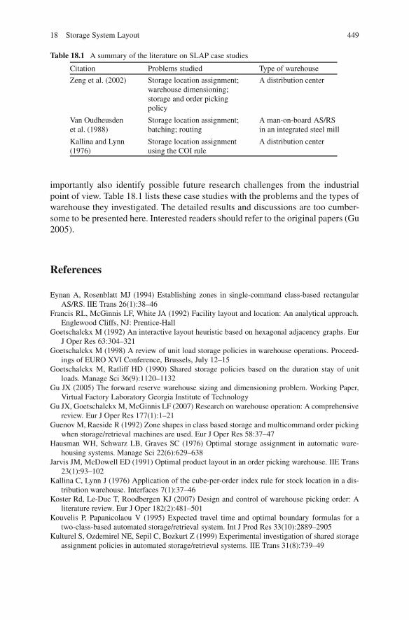
18 Storage System Layout 449
Table 18.1 A summary of the literature on SLAP case studies
Citation Problems studied Type of warehouse
Zeng et al. (2002) Storage location assignment;warehouse dimensioning;storage and order pickingpolicy
A distribution center
Van Oudheusdenet al. (1988)
Storage location assignment;batching; routing
A man-on-board AS/RSin an integrated steel mill
Kallina and Lynn(1976)
Storage location assignmentusing the COI rule
A distribution center
importantly also identify possible future research challenges from the industrialpoint of view. Table 18.1 lists these case studies with the problems and the types ofwarehouse they investigated. The detailed results and discussions are too cumber-some to be presented here. Interested readers should refer to the original papers (Gu2005).
References
Eynan A, Rosenblatt MJ (1994) Establishing zones in single-command class-based rectangularAS/RS. IIE Trans 26(1):38–46
Francis RL, McGinnis LF, White JA (1992) Facility layout and location: An analytical approach.Englewood Cliffs, NJ: Prentice-Hall
Goetschalckx M (1992) An interactive layout heuristic based on hexagonal adjacency graphs. EurJ Oper Res 63:304–321
Goetschalckx M (1998) A review of unit load storage policies in warehouse operations. Proceed-ings of EURO XVI Conference, Brussels, July 12–15
Goetschalckx M, Ratliff HD (1990) Shared storage policies based on the duration stay of unitloads. Manage Sci 36(9):1120–1132
Gu JX (2005) The forward reserve warehouse sizing and dimensioning problem. Working Paper,Virtual Factory Laboratory Georgia Institute of Technology
Gu JX, Goetschalckx M, McGinnis LF (2007) Research on warehouse operation: A comprehensivereview. Eur J Oper Res 177(1):1–21
Guenov M, Raeside R (1992) Zone shapes in class based storage and multicommand order pickingwhen storage/retrieval machines are used. Eur J Oper Res 58:37–47
Hausman WH, Schwarz LB, Graves SC (1976) Optimal storage assignment in automatic ware-housing systems. Manage Sci 22(6):629–638
Jarvis JM, McDowell ED (1991) Optimal product layout in an order picking warehouse. IIE Trans23(1):93–102
Kallina C, Lynn J (1976) Application of the cube-per-order index rule for stock location in a dis-tribution warehouse. Interfaces 7(1):37–46
Koster Rd, Le-Duc T, Roodbergen KJ (2007) Design and control of warehouse picking order: Aliterature review. Eur J Oper 182(2):481–501
Kouvelis P, Papanicolaou V (1995) Expected travel time and optimal boundary formulas for atwo-class-based automated storage/retrieval system. Int J Prod Res 33(10):2889–2905
Kulturel S, Ozdemirel NE, Sepil C, Bozkurt Z (1999) Experimental investigation of shared storageassignment policies in automated storage/retrieval systems. IIE Trans 31(8):739–49
450 J. Behnamian and B. Eghtedari
Lai KK, Xue J, Zhang G (2002) Layout design for a paper reel warehouse: A two-stage heuristicapproach. Int J Prod Econ 75:231–243
Lee MK (1992) A storage assignment policy in a man-on-board automated storage/retrieval sys-tem. Int J Prod Res 30(10):2281–2292
Liu CM (1999) Clustering techniques for stock location and order-picking in a distribution center.Comp Oper Res 26:989–1002
Mallette AJ, Francis, RL (1972) A generalized assignment approach to optimal facility layout.AIIE Trans 4(2):144–147
Malmborg CJ, Al-Tassan K (2000) An integrated performance model for order picking systemswith randomized storage. Appl Math Model 24(2):95–111
Petersen CG, Aase G (2004) A comparison of picking, storage, and routing policies in manualorder picking. Int J Prod Econ 92:11–19
Roll Y, Rosenblatt MJ (1983) Random versus grouped storage policies and their effect on ware-house capacity. Mater Flow 1:199–205
Roll Y, Rosenblatt MJ (1987) Shifting in warehouses. Mater Flow 4:147–157Rosenblatt MJ, Eynan A (1989) Deriving the optimal boundaries for class-based automatic storage/
retrieval systems. Manage Sci 35(12):1519–1524Rosenblatt MJ, Roll Y (1984) Warehouse design with storage policy considerations. Int J Prod Res
22(5):809–821Rosenwein MB (1994) An application of cluster analysis to the problem of locating items within a
warehouse. IIE Trans 26(1):101–103Thonemann UW, Brandeau ML (1998) Optimal storage assignment policies for automated storage
and retrieval systems with stochastic demands. Manage Sci 44(1):142–148Van Oudheusden DL, Tzen YJ, Ko HT (1988) Improving storage and order picking in a person-
on-board AS/R system: a case study. Eng Costs Prod Econ 13:273–283Van den Berg JP, Zijm WHM (1999) Models for warehouse management: Classification and ex-
amples. Int J Prod Econ 59:519–528Wascher G (2004) Order picking: A survey of planning problems and methods. In: Supply Chain
Management and Reverse Logistics, pp 323–347Zapfel G, Wasner M (2006) Warehouse sequencing in the steel supply chain as a generalized job
shop model. Int J Prod Econ 104:482–501Zeng AZ, Mahan M, Fluet N (2002) Designing an efficient warehouse layout to facilitate the order-
filling process: an industrial distributor’s experience. Prod Invent Manage J 43(3):83–88
Chapter 19Location-Inventory Problem
Mohamadreza Kaviani
Traditionally, logistics analysts have divided decision levels into strategic, tacticaland operational (Miranda and Garrido 2006). There are also three important de-cisions within a supply chain: facilities location decisions; inventory managementdecisions; and distribution decisions (Shen and Qi 2007). For example, in a distribu-tion network, we could mention location of Distribution centers (DCs) as a strategicdecision, distribution decisions as a tactical decision and inventory service level as atactical or operational decision. Often, for modeling purposes, these levels are con-sidered separately. And this may conduce to make non-optimal decisions, since inreality there is interaction between the different levels (Miranda and Garrido 2006).For example, most well-studied location models do not consider inventory costs, andshipment costs are estimated by direct shipping. Although one may argue that tacti-cal inventory replenishment decisions and shipment schemes are not at the strategiclevel, and we should not consider them in the strategic planning phase, however,failure to take the related inventory and shipment costs into consideration when de-ciding the locations of facilities can lead to sub-optimality, since strategic locationdecisions have a big impact on inventory and shipment costs (Shen and Qi 2007). Onthe other hand firms would like to consider cost and service levels simultaneously. Itis good to have many DCs, since this reduces the cost of transporting product to cus-tomers (/retailers) and will provide better service. Also, it is good to have few DCs,since this reduces the cost of holding inventory via pooling effects, and reduces thefixed costs associated with operating DCs via economies of scale (Erlebacher andMeller 2000).
Nozick and Turnquist (1998) discussed that in 1997, Thomas provided the datathat show total logistics costs (inventory plus transportation) in the U.S. declinedfrom about 13% of Gross Domestic Product (GDP) in 1985, to about 10.5% in 1993,largely as a result of increasing emphasis on controlling inventories throughout thesupply chain. “However, since 1993, logistics costs (as a percentage of GDP) havebeen essentially constant. The “easy” cost reductions have been made, and furtherimprovements will require more effective tools” (Nozick and Turnquist 1998).
Nozick and Turnquist (2001) also discussed that in 1997, Thomas provided in-ventory and freight transportation costs for the US economy in 1985, and throughthe 1990s. “Freight transportation costs have been nearly constant (at about 6%
R.Z. Farahani and M. Hekmatfar (eds.), Facility Location: Concepts, Models, 451Algorithms and Case Studies, Contributions to Management Science,DOI 10.1007/978-3-7908-2151-2 19, c� Physica-Verlag Heidelberg 2009
452 M. Kaviani
of Gross National Product) over the entire period of the data. Inventory costs fellsignificantly between 1985 and 1992, as companies implemented just-in-time sys-tems and the economy grew steadily. However, since 1992 there has been almost nochange in inventory costs, and total physical distribution costs seem to have reacheda plateau” (Nozick and Turnquist 2001).
On the basis of the above, managing inventory has become a major challengefor firms as they simultaneously try to reduce costs and improve customer servicein today’s increasingly competitive business environment (Daskin et al. 2002). Thegoal of cost reduction is to provide motivation for centralization of inventories. Onthe other hand, the goal of customer responsiveness is to provide motivation for hav-ing goods as near to the final consumer as possible. Thus, there is a basic conflictbetween these objectives, and locating DCs is a critical decision in finding an effec-tive balance between them (Nozick and Turnquist 2001). Many companies face thestrategic decision of deciding on the number of DCs, their location, and which cus-tomers they serve. One objective for a company facing this decision is to maintainacceptable service while minimizing the fixed costs of operating the DCs, inven-tory holding costs at the DCs, and transportation costs between plants and DCs, andDCs and customers (Erlebacher and Meller 2000). Inventory theory literature tendsto focus on finding optimal inventory replenishment strategies at the DCs and theretailer outlets. This work usually assumes that the number and locations of the DCsare given. On the other hand, location theory tends to focus on developing modelsfor determining the number of DCs and their locations, as well as the DC-retailerassignments. This work usually includes fixed facility setup costs and transportationcosts, but the operational inventory and shortage costs are typically ignored (Daskinet al. 2002).
The location-inventory problem is presented bellow. A set of suppliers and cus-tomers are spatially dispersed in a geographical region. Typically, the customersface stochastic demand for an array of products offered by the suppliers (Mirandaand Garrido 2008). We consider a three-tiered system consisting of one or moresuppliers, DCs and customers shown in Fig. 19.1. We assume that the locations ofthe suppliers and the customers are known and that the suppliers have infinite ca-pacity at least from the perspective of the system being modeled. The problem isto determine the optimal number of DCs, their locations, the customers assigned toeach DC, and the optimal ordering policy at the DCs (Daskin et al. 2002).
For example, consider a blood bank that supplied roughly 30 hospitals in thegreater Chicago area. Our focus was on the production and distribution of platelets,the most expensive and most perishable of all blood products. If a unit of plateletsis not used within 5 days of the time it is produced from whole blood, it must bedestroyed. The demand for platelets is highly variable as they are needed in onlya limited number of medical contexts. The hospitals supplied by the blood bankcollectively owned the blood bank and set prices. As a result they could return aunit of platelets up to the time it outdated and not be charged for it. Thus, therewas little incentive to manage inventories in an efficient manner. Many of the largerhospitals ordered almost twice the number of platelet units that they used each yearresulting in the need to destroy thousands of units of this expensive blood product.
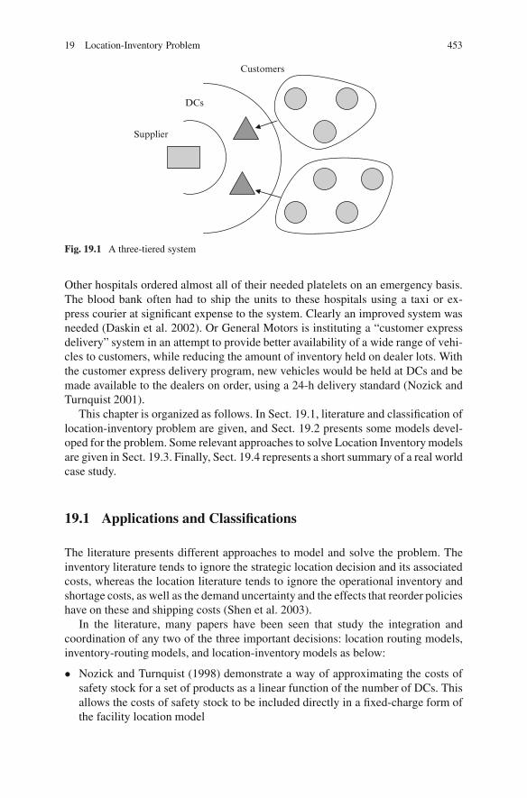
19 Location-Inventory Problem 453
Supplier
DCs
Customers
Fig. 19.1 A three-tiered system
Other hospitals ordered almost all of their needed platelets on an emergency basis.The blood bank often had to ship the units to these hospitals using a taxi or ex-press courier at significant expense to the system. Clearly an improved system wasneeded (Daskin et al. 2002). Or General Motors is instituting a “customer expressdelivery” system in an attempt to provide better availability of a wide range of vehi-cles to customers, while reducing the amount of inventory held on dealer lots. Withthe customer express delivery program, new vehicles would be held at DCs and bemade available to the dealers on order, using a 24-h delivery standard (Nozick andTurnquist 2001).
This chapter is organized as follows. In Sect. 19.1, literature and classification oflocation-inventory problem are given, and Sect. 19.2 presents some models devel-oped for the problem. Some relevant approaches to solve Location Inventory modelsare given in Sect. 19.3. Finally, Sect. 19.4 represents a short summary of a real worldcase study.
19.1 Applications and Classifications
The literature presents different approaches to model and solve the problem. Theinventory literature tends to ignore the strategic location decision and its associatedcosts, whereas the location literature tends to ignore the operational inventory andshortage costs, as well as the demand uncertainty and the effects that reorder policieshave on these and shipping costs (Shen et al. 2003).
In the literature, many papers have been seen that study the integration andcoordination of any two of the three important decisions: location routing models,inventory-routing models, and location-inventory models as below:
� Nozick and Turnquist (1998) demonstrate a way of approximating the costs ofsafety stock for a set of products as a linear function of the number of DCs. Thisallows the costs of safety stock to be included directly in a fixed-charge form ofthe facility location model
454 M. Kaviani
� Erlebacher and Meller (2000) formulate a highly nonlinear integer location-inventory model. They attack the problem by using a continuous approximationas well as a number of constructions and bounding heuristics
� Daskin et al. (2002) and Shen et al. (2003) studied the joint location-inventorymodel in which location, shipment and nonlinear safety stock inventory costs areincluded in the same model. They developed an integrated approach to determinethe number of DCs to establish, the location of the DCs, and the magnitude ofinventory to maintain at each center
� Shen et al. (2003) derived a cross-level model to analyze decisions about in-ventory control and facility location, specially suited to urban settings, wherethe storage space is scarce and the vehicles’ capacity is usually restricted. Bothconditions, on the one hand make the problem difficult to solve optimally, onthe other hand make it more realistic and useful in practice. Shen et al. (2003)reformulate the problem as a Set Covering Problem, which is then solvedthrough a hybrid heuristic mixing columns generation and branch and boundmethods. While Daskin et al. (2002) apply Lagrangian relaxation to solve thisproblem
� Miranda and Garrido (2006) present a simultaneous nonlinear-mixed integermodel of inventory control and facility location decisions, which considers twonovel capacity constraints. The first constraint states a maximum lot size for theincoming orders to each warehouse, and the second constraint is a stochasticbound to inventory capacity. This model is NP-hard and presents nonlinear termsin the objective function and a nonlinear constraint
� Snyder et al. (2007) present a stochastic version of the location model with riskpooling that optimizes location, inventory, and allocation decisions under randomparameters. The goal of their model is to find solutions that minimize the totalcost (including location, transportation, and inventory costs) of the system acrossall scenarios. The location model explicitly handles the economies of scale andrisk-pooling effects that result from consolidating inventory sites. They presenta Lagrangian-relaxation–based exact algorithm for the model. The Lagrangiansub problem is a non-linear integer program, but it can be solved by a low-orderpolynomial algorithm
� Shen and Qi (2007) formulated a nonlinear integer programming model to mini-mize the total cost that includes location costs and inventory costs at the DCs, anddistribution costs in the supply chain, for which they propose a Lagrangian relax-ation based solution algorithm. By exploring the structure of the problem, theyfind a low-order polynomial algorithm for the nonlinear integer programmingproblem that must be solved in solving the Lagrangian relaxation sub-problems
� Miranda and Garrido (2008) developed an efficient heuristic to solve a jointlocation–distribution–inventory model for a three layered supply chain. Thesolution approach is based on Lagrangian relaxation, improved with validityconstraints derived from the finite set of all possible combinations of mean de-mand and variance. The optimal solution’s lower bound is found through theoptimal solution of the dual problem
19 Location-Inventory Problem 455
A classification of different types of location inventory problems and their propertiesis represented as follows:
� Area solution: Discrete, Continual� Objective function: MiniMax, MiniSum� Variables: integer, mixed integer� Determine the number of DCs: Exogenous, Endogenous� DC capacity: Unlimited, Limited� Cost of DC location: No cost, fixed cost, Variable cost� Solution methods: Exact, Heuristic, Meta heuristic
19.2 Models
In this section, we introduce location-inventory models represented and developedas mathematical models.
19.2.1 Model of Shen et al. (2003)
The first model that is present here is easy to understand. Shen et al. (2003) assumethat location costs are incurred when DCs are established. Line-haul transporta-tion costs are incurred for shipments from the single supplier to the DCs. Localtransportation costs are incurred in moving the goods from the DC to the retailers.Inventory costs are incurred at each DC and consist of the carrying cost for the av-erage inventory used over a period of time, as well as safety stock inventory thatis carried to protect against stock outs that might result from the uncertain retailerdemand. Inventory costs are also incurred at each retailer.
19.2.1.1 Model Inputs
Model inputs of this model are as follows:
�i : Mean (yearly) demand at retailer i , for each i 2 I�2i : Variance of (daily) demand at retailer i , for each i 2 Ifi : fixed (annual) cost of locating a regional DC (RDC) at retailer j , for eachj 2 Ivj .x/ : cost to ship x units from the main supplier (the plant) to a RDC locatedat retailer j , for each j 2 Idij : cost per unit to ship from retailer j to retailer i , for each i 2 I and j 2 I˛ : Desired percentage of retailer’s orders satisfiedˇ : Weight factor associated with the transportation cost
456 M. Kaviani
: Weight factor associated with the inventory costz˛ : Standard normal deviate such that P.z � z˛/ D ˛
h : Inventory holding cost per unit of product per yearwj .x/ : Total annual cost of working inventory held at DC j if the expected dailydemand at j is x for each j 2 IFj : fixed cost of placing an order at DC j , for each j 2 IL : lead time in days
19.2.1.2 Model Outputs (Decision Variables)
Model outputs of this model are as follows:
Xj D 1, if retailer j is selected as a DC location, and 0 otherwise for each j 2 IYij D 1, if retailer i is served by a DC based at retailer j , and 0 otherwise foreach i 2 I and each j 2 I
19.2.1.3 Objective Function and its Constraints
The objective function of this model and its related constraints are as follows:
MinXj
(fjXj C ˇ
Xi
�idij Yij C wj
Xi
�iYij
!Chz˛
sXi
�2i Yij
9=;(19.1)
Subject to
Xj
Yij D 1 8i (19.2)
Yij � Xj 8i; j (19.3)
Yij 2 f0; 1g 8i; j (19.4)
Xj 2 f0; 1g 8j (19.5)
Equation (19.1) minimizes the weighted sum of the following four costs: thefixed cost of locating facilities, the shipping cost from the DCs to the non-DC retail-ers, the expected working inventory cost, and the safety stock costs. Equation (19.2)ensures that each retailer is assigned to exactly one DC. Equation (19.3) states thatretailers can only be assigned to candidate sites that are selected as DCs. Equations(19.4) and (19.5) are standard integrity constraints.
19 Location-Inventory Problem 457
19.2.2 Model of Nozick and Turnquist (1998)
Assume that there are n retail outlets assigned to the DC, each with a Poisson de-mand process whose mean rate is �i where 1 � i � n. Each time an item isdemanded at a retail outlet, a replacement is ordered immediately from the DC.Therefore, the demand at the DC is Poisson with a mean rate:
ƒ DXi
�i (19.6)
Assume that the DC has a total of s items either in inventory or on order, and itorders from the plant each time an item is sent to a retail outlet. We will define �and �2 to be the mean and variance of the delivery time of a product from the plantto the DC once an order is placed. Then the performance measures for the singleDC and assigned retail outlets are the same as those for an M/G/s queue with anarrival rate of ƒ, a mean and variance for the service time distribution of � and �2,respectively, and s servers.
The stock out rate is the percentage of demand that can not be satisfied fromon-hand inventory. In the queuing system representation, this is analogous to theprobability that when a customer enters the system, a server is not available (i.e.wait time, denoted by W, is greater than zero). The probability of waiting (stock out),P.W � 0/ in an M/G/s queue can be approximated quite accurately by P.W � 0/
in an M/M/s queue.They use two equations to approximate r D P.W � 0/ for two conditions to find
the minimum inventory necessary for a given stock out rate.If there is a constant total expected demand across all retail outlets, the total
safety stock required is related to the number of DCs used. Consider a product withan expected demand of 800 units per year. Furthermore, assume that this expecteddemand is divided equally among N DCs. Based on these assumptions; they pro-vided a histogram for this case that shows the safety stock necessary for variousnumbers of DCs, given a stock out rate of 5%, and the predicted safety stock basedon a linear regression model:
Safety stock D a C bN D 22C 1:8N
where N D number of DCs.
19.2.2.1 Model Inputs
Model inputs of this model are as follows:
fj : fixed cost of locating a facility at candidate site jhi : demand at location idij : distance from demand location i to candidate site j˛ : cost per unit distance per unit demand
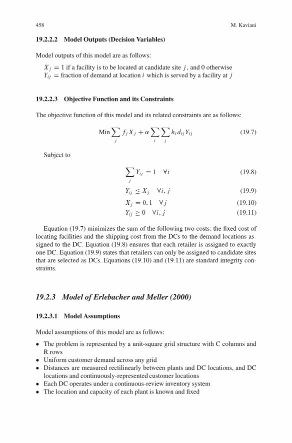
458 M. Kaviani
19.2.2.2 Model Outputs (Decision Variables)
Model outputs of this model are as follows:
Xj D 1 if a facility is to be located at candidate site j , and 0 otherwiseYij D fraction of demand at location i which is served by a facility at j
19.2.2.3 Objective Function and its Constraints
The objective function of this model and its related constraints are as follows:
MinXj
fjXj C ˛Xi
Xj
hidij Yij (19.7)
Subject to
Xj
Yij D 1 8i (19.8)
Yij � Xj 8i; j (19.9)
Xj D 0; 1 8j (19.10)
Yij � 0 8i; j (19.11)
Equation (19.7) minimizes the sum of the following two costs: the fixed cost oflocating facilities and the shipping cost from the DCs to the demand locations as-signed to the DC. Equation (19.8) ensures that each retailer is assigned to exactlyone DC. Equation (19.9) states that retailers can only be assigned to candidate sitesthat are selected as DCs. Equations (19.10) and (19.11) are standard integrity con-straints.
19.2.3 Model of Erlebacher and Meller (2000)
19.2.3.1 Model Assumptions
Model assumptions of this model are as follows:
� The problem is represented by a unit-square grid structure with C columns andR rows
� Uniform customer demand across any grid� Distances are measured rectilinearly between plants and DC locations, and DC
locations and continuously-represented customer locations� Each DC operates under a continuous-review inventory system� The location and capacity of each plant is known and fixed
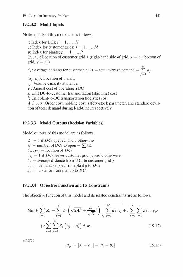
19 Location-Inventory Problem 459
19.2.3.2 Model Inputs
Model inputs of this model are as follows:
i : Index for DCs; i D 1; : : :; N
j : Index for customer grids; j D 1; : : :;M
p: Index for plants; p D 1; : : :; P
.cj ; rj /: Location of customer grid j (right-hand side of grid, x D cj ; bottom ofgrid, y D rj /
dj : Average demand for customer j ; D D total average demand DMPjD1
dj
.ap; bp/: Location of plant pvp: Volume capacity at plant pF : Annual cost of operating a DCs: Unit DC-to-customer transportation (shipping) costl : Unit plant-to-DC transportation (logistic) costA; h; z; � : Order cost, holding cost, safety-stock parameter, and standard devia-tion of total demand during lead-time, respectively
19.2.3.3 Model Outputs (Decision Variables)
Model outputs of this model are as follows:
Zi D 1 if DCi opened, and 0 otherwiseN D number of DCs to open D P
iZi.xi ; yi / D location of DCiwij D 1 if DCi serves customer grid j , and 0 otherwisetip D average distance fromDCi to customer grid jupi D demand shipped from plant p to DCiqpi D distance from plant p to DCi
19.2.3.4 Objective Function and Its Constraints
The objective function of this model and its related constraints are as follows:
Min FrXiD1
Zi CrXiD1
Zi
�p2AhC z�p
Dh
�vuut MXjD1
djwij C l
pXpD1
rXiD1
Ziupiqpi
CsrXiD1
MXjD1
Zi
txij C t
yij
djwij (19.12)
where:qpi D ˇ
xi � apˇC ˇ
yi � bpˇ
(19.13)
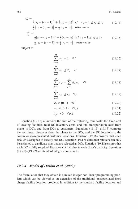
460 M. Kaviani
txij D12Œxi � .cj � 1/2 C 1
2.cj � xi /2I if cj � 1 � xi � cj
12
ˇxi � .cj � 1/ˇC 1
2
ˇcj � xi
ˇ I otherwise
(19.14)
tyij D
12Œyi � .rj � 1/2 C 1
2.rj � yi /
2I if rj � 1 � yi � rj12
ˇyi � .rj � 1/
ˇC 12
ˇrj � yi
ˇ I otherwise
(19.15)
Subject to
MXiD1
wij D 1 8j (19.16)
MXjD1
wij � Zi 8i (19.17)
PXpD1
upi DMXjD1
djwij 8i (19.18)
rXjD1
upi � vp 8p (19.19)
Zi 2 f0; 1g 8i (19.20)
wij 2 f0; 1g 8i; j (19.21)
upi � 0 8p; i (19.22)
Equation (19.12) minimizes the sum of the following four costs: the fixed costof locating facilities, total DC inventory costs, and total transportation costs fromplants to DCs, and from DCs to customers. Equations (19.13)–(19.15) computethe rectilinear distances from the plants to the DCs, and the DC locations to thecontinuously-represented customer locations. Equation (19.16) ensures that eachretailer is assigned to exactly one DC. Equation (19.17) states that retailers can onlybe assigned to candidate sites that are selected as DCs. Equation (19.18) ensures thateach DC is fully supplied. Equation (19.19) checks each plant’s capacity. Equations(19.20)–(19.22) are standard integrity constraints.
19.2.4 Model of Daskin et al. (2002)
The formulation that they obtain is a mixed integer non-linear programming prob-lem which can be viewed as an extension of the traditional uncapacitated fixedcharge facility location problem. In addition to the standard facility location and
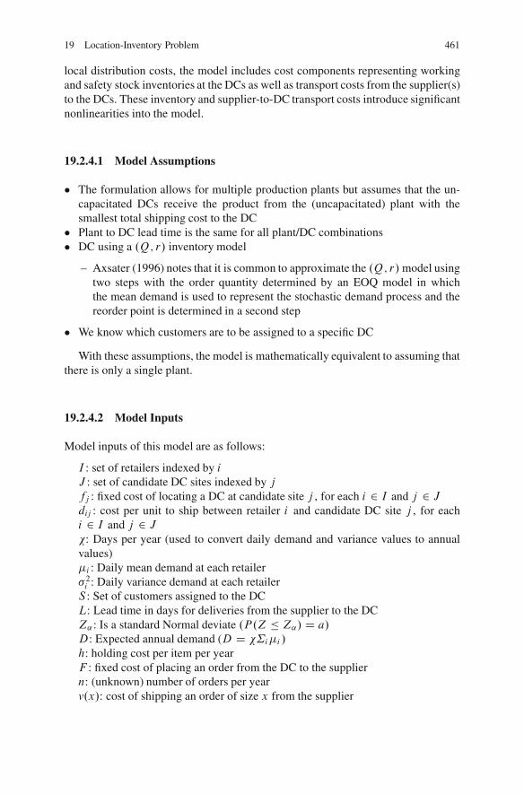
19 Location-Inventory Problem 461
local distribution costs, the model includes cost components representing workingand safety stock inventories at the DCs as well as transport costs from the supplier(s)to the DCs. These inventory and supplier-to-DC transport costs introduce significantnonlinearities into the model.
19.2.4.1 Model Assumptions
� The formulation allows for multiple production plants but assumes that the un-capacitated DCs receive the product from the (uncapacitated) plant with thesmallest total shipping cost to the DC
� Plant to DC lead time is the same for all plant/DC combinations� DC using a .Q; r/ inventory model
– Axsater (1996) notes that it is common to approximate the .Q; r/model usingtwo steps with the order quantity determined by an EOQ model in whichthe mean demand is used to represent the stochastic demand process and thereorder point is determined in a second step
� We know which customers are to be assigned to a specific DC
With these assumptions, the model is mathematically equivalent to assuming thatthere is only a single plant.
19.2.4.2 Model Inputs
Model inputs of this model are as follows:
I : set of retailers indexed by iJ : set of candidate DC sites indexed by jfj : fixed cost of locating a DC at candidate site j , for each i 2 I and j 2 Jdij : cost per unit to ship between retailer i and candidate DC site j , for eachi 2 I and j 2 J�: Days per year (used to convert daily demand and variance values to annualvalues)�i : Daily mean demand at each retailer�2i : Daily variance demand at each retailerS : Set of customers assigned to the DCL: Lead time in days for deliveries from the supplier to the DCZ˛ : Is a standard Normal deviate .P.Z � Z˛/ D a/
D: Expected annual demand (D D �˙i�i /
h: holding cost per item per yearF : fixed cost of placing an order from the DC to the suppliern: (unknown) number of orders per yearv.x/: cost of shipping an order of size x from the supplier
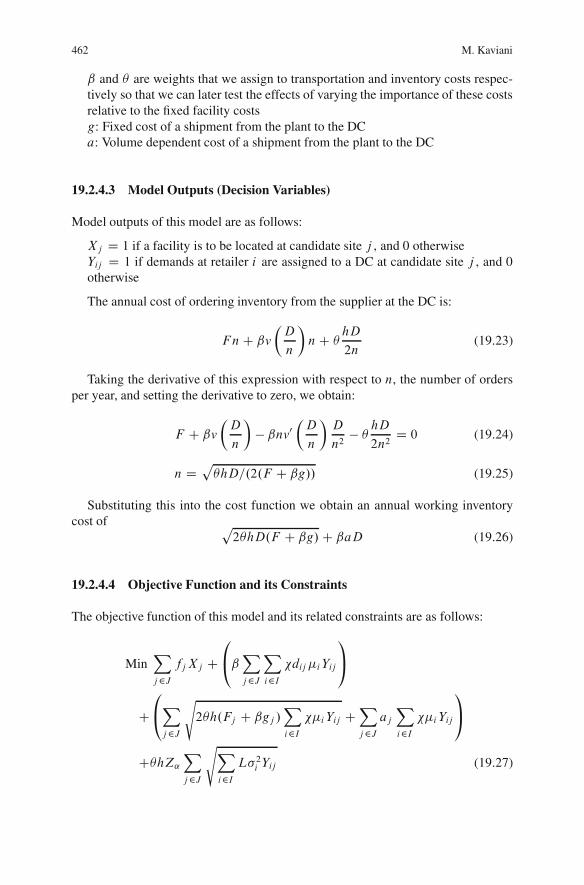
462 M. Kaviani
ˇ and are weights that we assign to transportation and inventory costs respec-tively so that we can later test the effects of varying the importance of these costsrelative to the fixed facility costsg: Fixed cost of a shipment from the plant to the DCa: Volume dependent cost of a shipment from the plant to the DC
19.2.4.3 Model Outputs (Decision Variables)
Model outputs of this model are as follows:
Xj D 1 if a facility is to be located at candidate site j , and 0 otherwiseYij D 1 if demands at retailer i are assigned to a DC at candidate site j , and 0otherwise
The annual cost of ordering inventory from the supplier at the DC is:
FnC ˇv
�D
n
�nC
hD
2n(19.23)
Taking the derivative of this expression with respect to n, the number of ordersper year, and setting the derivative to zero, we obtain:
F C ˇv
�D
n
�� ˇnv0
�D
n
�D
n2� hD
2n2D 0 (19.24)
n DphD=.2.F C ˇg// (19.25)
Substituting this into the cost function we obtain an annual working inventorycost of p
2hD.F C ˇg/C ˇaD (19.26)
19.2.4.4 Objective Function and its Constraints
The objective function of this model and its related constraints are as follows:
MinXj2J
fjXj C0@ˇX
j2J
Xi2I
�dij �iYij
1A
C0@Xj2J
s2h.Fj C ˇgj /
Xi2I
��iYij CXj2J
ajXi2I
��iYij
1A
ChZ˛Xj2J
sXi2I
L�2i Yij (19.27)
19 Location-Inventory Problem 463
Subject to
Xj2J
Yij D 1 8i (19.28)
Yij � Xj 8i; j (19.29)
Xj 2 f0; 1g 8j (19.30)
Yij 2 f0; 1g 8i; j (19.31)
Equation (19.27) minimizes the sum of the following four costs: the fixed cost oflocating facilities, local delivery cost, total working inventory cost, and the safetystock inventory cost. Equation (19.28) ensures that each retailer is assigned to ex-actly one DC. Equation (19.29) states that retailers can only be assigned to candidatesites that are selected as DCs. Equations (19.30) and (19.31) are standard integrityconstraints.
19.2.5 Model of Shen and Qi (2007)
They propose a supply chain design model, which considers the impacts of thestrategic facility location decisions on the tactical inventory and shipment decisionsin a three-tiered supply chain. They assume that each customer has uncertain de-mand that follows a certain probability distribution. They assume that the customersare uniformly scattered in a connected area. Several DCs will be opened and eachDC is served directly by the supplier and distributes products to customers. Eachcustomer will order at the beginning of the period, the DC combines the ordersfrom different customers and order from the supplier. The number and locations ofDCs are not given a priori. They assume that at every DC, there is a delivery truckwith fixed capacity. A key problem is that the demand that is seen by each DC is afunction of the demands at the customers assigned to that DC, which is a functionof the assignment of customers to the DC. They assume the transportation costs andthe inventory costs exhibit economies of scale under which the average unit costdecreases as the total volume of activity increases. This realistic assumption willresult in several nonlinear terms in the formulation.
19.2.5.1 Model Assumptions
� The customers are uniformly scattered in a connected region, S� The area of S is A� The customer demands are independent and follow Normal distributions
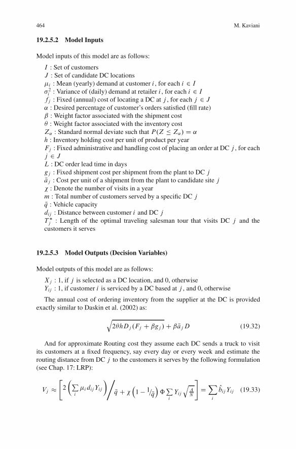
464 M. Kaviani
19.2.5.2 Model Inputs
Model inputs of this model are as follows:
I : Set of customersJ : Set of candidate DC locations�i : Mean (yearly) demand at customer i , for each i 2 I�2i : Variance of (daily) demand at retailer i , for each i 2 Ifj : Fixed (annual) cost of locating a DC at j , for each j 2 J˛ : Desired percentage of customer’s orders satisfied (fill rate)ˇ : Weight factor associated with the shipment cost : Weight factor associated with the inventory costZ˛ : Standard normal deviate such that P.Z � Z˛/ D ˛
h : Inventory holding cost per unit of product per yearFj : Fixed administrative and handling cost of placing an order at DC j , for eachj 2 JL : DC order lead time in daysgj : Fixed shipment cost per shipment from the plant to DC jNaj : Cost per unit of a shipment from the plant to candidate site j� : Denote the number of visits in a yearm : Total number of customers served by a specific DC jNq : Vehicle capacitydij : Distance between customer i and DC jT �j : Length of the optimal traveling salesman tour that visits DC j and the
customers it serves
19.2.5.3 Model Outputs (Decision Variables)
Model outputs of this model are as follows:
Xj : 1, if j is selected as a DC location, and 0, otherwiseYij : 1, if customer i is serviced by a DC based at j , and 0, otherwise
The annual cost of ordering inventory from the supplier at the DC is providedexactly similar to Daskin et al. (2002) as:
q2hDj .Fj C ˇgj /C ˇ NajD (19.32)
And for approximate Routing cost they assume each DC sends a truck to visitits customers at a fixed frequency, say every day or every week and estimate therouting distance from DC j to the customers it serves by the following formulation(see Chap. 17: LRP):
Vj �"2
�Pi
�idij Yij
�,Nq C �
1 � 1=Nq
ˆPi
Yij
qAN
#DXi
Obij Yij (19.33)
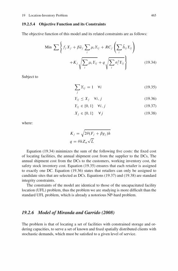
19 Location-Inventory Problem 465
19.2.5.4 Objective Function and its Constraints
The objective function of this model and its related constraints are as follows:
MinX(
fjXj C ˇ NajXi
�iYij CRCj
Xi
Obij Yij!
CKj
sXi
�iYij C q
sXi
�2i Yij
9=; (19.34)
Subject to
Xj
Yij D 1 8i (19.35)
Yij � Xj 8i; j (19.36)
Yij 2 f0; 1g 8i; j (19.37)
Xj 2 f0; 1g 8j (19.38)
where:
Kj Dq2.Fj C ˇgj /h
q D hZ˛pL
Equation (19.34) minimizes the sum of the following five costs: the fixed costof locating facilities, the annual shipment cost from the supplier to the DCs, Theannual shipment cost from the DCs to the customers, working inventory cost, thesafety stock inventory cost. Equation (19.35) ensures that each retailer is assignedto exactly one DC. Equation (19.36) states that retailers can only be assigned tocandidate sites that are selected as DCs. Equations (19.37) and (19.38) are standardintegrity constraints.
The constraints of the model are identical to those of the uncapacitated facilitylocation (UFL) problem, thus the problem we are studying is more difficult than thestandard UFL problem, which is already a notorious NP-hard problem.
19.2.6 Model of Miranda and Garrido (2008)
The problem is that of locating a set of facilities with constrained storage and or-dering capacities, to serve a set of known and fixed spatially distributed clients withstochastic demands, which must be satisfied to a given level of service.
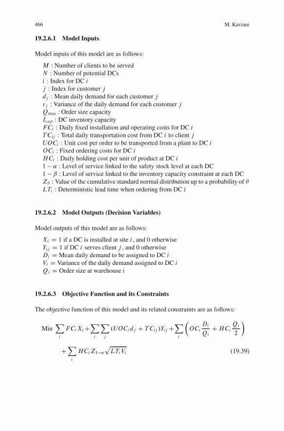
466 M. Kaviani
19.2.6.1 Model Inputs
Model inputs of this model are as follows:
M : Number of clients to be servedN : Number of potential DCsi : Index for DC ij : Index for customer jdj : Mean daily demand for each customer jvj : Variance of the daily demand for each customer jQmax : Order size capacityIcap : DC inventory capacityFCi : Daily fixed installation and operating costs for DC iT Cij : Total daily transportation cost from DC i to client jUOCi : Unit cost per order to be transported from a plant to DC iOCi : Fixed ordering costs for DC iHCi : Daily holding cost per unit of product at DC i1 � ˛ : Level of service linked to the safety stock level at each DC1 � ˇ : Level of service linked to the inventory capacity constraint at each DCZ : Value of the cumulative standard normal distribution up to a probability of LTi : Deterministic lead time when ordering from DC i
19.2.6.2 Model Outputs (Decision Variables)
Model outputs of this model are as follows:
Xi D 1 if a DC is installed at site i , and 0 otherwiseYij D 1 if DC i serves client j , and 0 otherwiseDi D Mean daily demand to be assigned to DC iVi D Variance of the daily demand assigned to DC iQi D Order size at warehouse i
19.2.6.3 Objective Function and its Constraints
The objective function of this model and its related constraints are as follows:
MinXi
FCiXiCXi
Xj
.UOCidj C TCij /Yij CXi
�OCi
Di
Qi
CHCiQi
2
�
CXi
HCiZ1�˛pLTiVi (19.39)
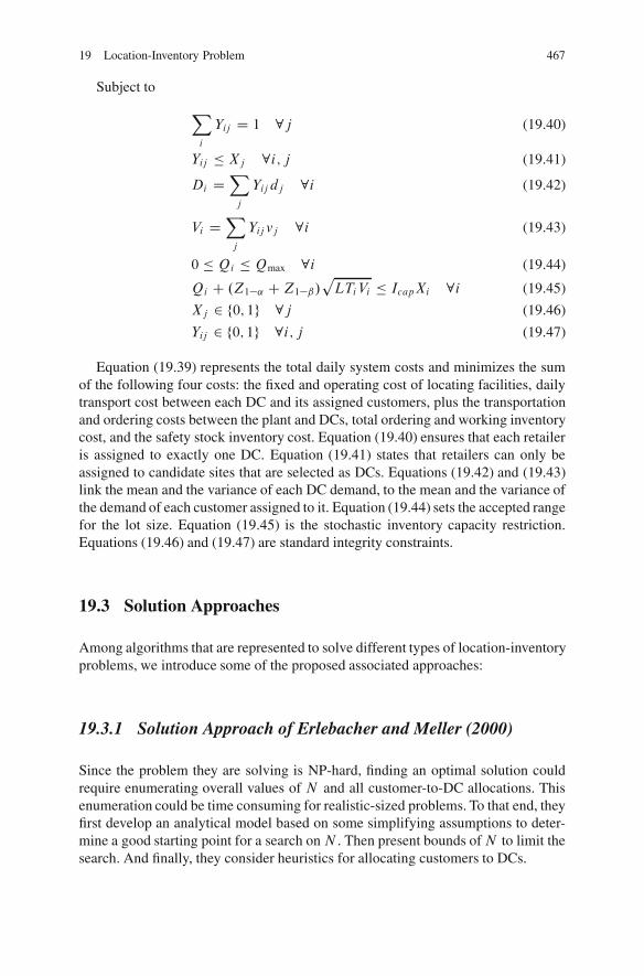
19 Location-Inventory Problem 467
Subject to
Xi
Yij D 1 8j (19.40)
Yij � Xj 8i; j (19.41)
Di DXj
Yij dj 8i (19.42)
Vi DXj
Yij vj 8i (19.43)
0 � Qi � Qmax 8i (19.44)
Qi C .Z1�˛ CZ1�ˇ/pLTiVi � IcapXi 8i (19.45)
Xj 2 f0; 1g 8j (19.46)
Yij 2 f0; 1g 8i; j (19.47)
Equation (19.39) represents the total daily system costs and minimizes the sumof the following four costs: the fixed and operating cost of locating facilities, dailytransport cost between each DC and its assigned customers, plus the transportationand ordering costs between the plant and DCs, total ordering and working inventorycost, and the safety stock inventory cost. Equation (19.40) ensures that each retaileris assigned to exactly one DC. Equation (19.41) states that retailers can only beassigned to candidate sites that are selected as DCs. Equations (19.42) and (19.43)link the mean and the variance of each DC demand, to the mean and the variance ofthe demand of each customer assigned to it. Equation (19.44) sets the accepted rangefor the lot size. Equation (19.45) is the stochastic inventory capacity restriction.Equations (19.46) and (19.47) are standard integrity constraints.
19.3 Solution Approaches
Among algorithms that are represented to solve different types of location-inventoryproblems, we introduce some of the proposed associated approaches:
19.3.1 Solution Approach of Erlebacher and Meller (2000)
Since the problem they are solving is NP-hard, finding an optimal solution couldrequire enumerating overall values of N and all customer-to-DC allocations. Thisenumeration could be time consuming for realistic-sized problems. To that end, theyfirst develop an analytical model based on some simplifying assumptions to deter-mine a good starting point for a search on N . Then present bounds ofN to limit thesearch. And finally, they consider heuristics for allocating customers to DCs.
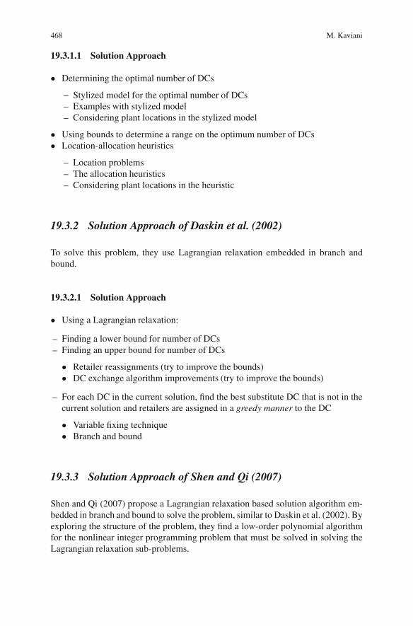
468 M. Kaviani
19.3.1.1 Solution Approach
� Determining the optimal number of DCs
– Stylized model for the optimal number of DCs– Examples with stylized model– Considering plant locations in the stylized model
� Using bounds to determine a range on the optimum number of DCs� Location-allocation heuristics
– Location problems– The allocation heuristics– Considering plant locations in the heuristic
19.3.2 Solution Approach of Daskin et al. (2002)
To solve this problem, they use Lagrangian relaxation embedded in branch andbound.
19.3.2.1 Solution Approach
� Using a Lagrangian relaxation:
– Finding a lower bound for number of DCs– Finding an upper bound for number of DCs
� Retailer reassignments (try to improve the bounds)� DC exchange algorithm improvements (try to improve the bounds)
– For each DC in the current solution, find the best substitute DC that is not in thecurrent solution and retailers are assigned in a greedy manner to the DC
� Variable fixing technique� Branch and bound
19.3.3 Solution Approach of Shen and Qi (2007)
Shen and Qi (2007) propose a Lagrangian relaxation based solution algorithm em-bedded in branch and bound to solve the problem, similar to Daskin et al. (2002). Byexploring the structure of the problem, they find a low-order polynomial algorithmfor the nonlinear integer programming problem that must be solved in solving theLagrangian relaxation sub-problems.
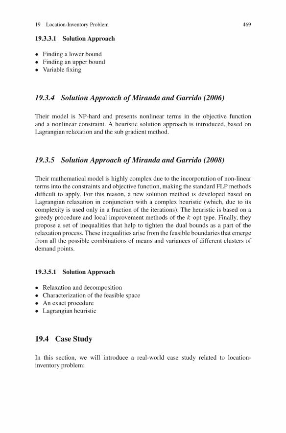
19 Location-Inventory Problem 469
19.3.3.1 Solution Approach
� Finding a lower bound� Finding an upper bound� Variable fixing
19.3.4 Solution Approach of Miranda and Garrido (2006)
Their model is NP-hard and presents nonlinear terms in the objective functionand a nonlinear constraint. A heuristic solution approach is introduced, based onLagrangian relaxation and the sub gradient method.
19.3.5 Solution Approach of Miranda and Garrido (2008)
Their mathematical model is highly complex due to the incorporation of non-linearterms into the constraints and objective function, making the standard FLP methodsdifficult to apply. For this reason, a new solution method is developed based onLagrangian relaxation in conjunction with a complex heuristic (which, due to itscomplexity is used only in a fraction of the iterations). The heuristic is based on agreedy procedure and local improvement methods of the k-opt type. Finally, theypropose a set of inequalities that help to tighten the dual bounds as a part of therelaxation process. These inequalities arise from the feasible boundaries that emergefrom all the possible combinations of means and variances of different clusters ofdemand points.
19.3.5.1 Solution Approach
� Relaxation and decomposition� Characterization of the feasible space� An exact procedure� Lagrangian heuristic
19.4 Case Study
In this section, we will introduce a real-world case study related to location-inventory problem:
470 M. Kaviani
19.4.1 Distribution System for Finished Automobiles in US(Nozick and Turnquist 1998)
Consider a distribution system for finished automobiles. The current distributionsystem for finished automobiles relies on large networks of independent dealers toprovide the inventory of vehicles from which customers choose. Dealers order newvehicles from the manufacturer in the models and colors. These orders typicallyrequire 6–12 weeks to fill and make up the dealer stock. But most customers areunwilling to wait about 6–12 weeks for a vehicle, so most vehicles are sold out ofthe finished vehicle inventory held on dealer lots. The system of relying on dealersto maintain separate pools of inventory is costly because dealers are forced to main-tain a large inventory of cars. As an illustration of the magnitude of inventory costsin the auto industry, consider that in a typical year about 15 million new cars andlight trucks are sold in the U.S., and the average value of those vehicles, is about$18,500. If the average dealer holds 60 days’ inventory, total on-hand inventory isapproximately 2.5 million vehicles, representing an investment of over $46 billion.If inventory carrying costs are about 22% of inventory value, then dealer stock gen-erates annual inventory holding costs on the order of $10 billion.
One alternative method of managing this inventory is through a series of RDCswhich would hold most of the inventory and dealers served by a given RDC andwould have access to its entire inventory.
The questions of how many RDCs are necessary, and where should they be lo-cated, are critical to the success of the venture.
This example will focus on identifying how many RDCs are necessary and wherethey should be located in order to minimize transportation, fixed facility, and inven-tory costs for new vehicles. In this case study the manufacturer serves demandsacross the continental U.S., organized into 698 demand areas. For the purposes ofthis analysis, the demand within each of the demand areas is assumed to occur atthe centroid of the demand area.
The fixed-charge model yields a recommendation of 23 RDCs, also determinesthe assignment of demand areas to RDCs, and gives an indication (using line thick-ness) of the volume of demand allocated to each RDC.
They also illustrate the sensitivity of this solution to changes in the per-RDCfixed-charge coefficient. It is important to notice that within a range of ˙10%, thenumber of RDC’s recommended does not change.
References
Axsater S (1996) Using the deterministic EOQ formula in stochastic inventory control. ManageSci 42:830–834
Daskin MS, Coullard CR, Shen ZM (2002) An inventory-location model: formulation, solutionalgorithm and computational results. Ann Oper Res 110:83–106
19 Location-Inventory Problem 471
Erlebacher SJ, Meller RD (2000) The interaction of location and inventory in designing distributionsystems. IIE Trans 32:155–166
Miranda PA, Garrido RA (2006) A simultaneous inventory control and facility location model withstochastic capacity constraints. Netw Spat Econ 6:39–53
Miranda PA, Garrido RA (2008) Valid inequalities for Lagrangian relaxation in an inventory loca-tion problem with stochastic capacity. Transport Res E 44:47–65
Nozick LK, Turnquist MA (1998) Integrating inventory impacts into a fixed-charge model forlocating distribution centers. Transport Res E-Log 34(3):173–186
Nozick LK, Turnquist MA (2001) Inventory, transportation, service quality and the location ofdistribution centers of distribution centers. Eur J Oper Res 129:362–371
Shen ZM, Qi L (2007) Incorporating inventory and routing costs in strategic location models. EurJ Oper Res 179:372–389
Shen ZM, Coullard C, Daskin MS (2003) A joint location-inventory model. Transport Sci37(1):40–55
Snyder LV, Daskin MS, Teo CP (2007) The stochastic location model with risk pooling. Eur J OperRes 179:1221–1238
Chapter 20Facility Location in Supply Chain
Meysam Alizadeh
A supply chain (SC) is the network of facilities and activities that performs thefunction of product development, procurement of material from vendors, the move-ment of materials between facilities, the manufacturing of products, the distributionof finished goods to customers, and after-market support for sustainment (Mabertand Venkataramanan 1998). The supply chain not only includes the manufacturerand suppliers, but also transporters, warehouses, retailers, and customer themselves.Within each organization, the supply chain include, but not limited to, new prod-uct development, marketing, operations, distribution, finance, and customer service(Chopra 2003).
A supply chain is dynamic and involves the constant flow of information, prod-uct, and funds between different stages. A typical supply chain may involve a varietyof stages. These supply chain stages include:
� Customers� Retailers� Wholesalers/distributors� Manufacturers� Component/raw material suppliers
SC systems can be studied and analyzed from several viewpoints. Yet there arethree major perspectives of SC systems: (a) “material flow”, (b) “information flow”,and (c) “buyer-seller relations” (Fazel Zarandi et al. 2002). The objective of everysupply chain is to maximize the overall value generated. Supply chain managementinvolves the management of flows between and among stages in a supply chain tomaximize totally supply chain profitability (Chopra 2003).
20.1 Design Phases in Supply Chain
Successful supply chain management requires many decisions relating to the flowof information, product, and funds. These decisions fall into three categories or
R.Z. Farahani and M. Hekmatfar (eds.), Facility Location: Concepts, Models, 473Algorithms and Case Studies, Contributions to Management Science,DOI 10.1007/978-3-7908-2151-2 20, c� Physica-Verlag Heidelberg 2009
474 M. Alizadeh
phases, depending on the frequency of each decision and the time frame over whicha decision phase has an impact:
1. Supply chain strategy or design;2. Supply chain planning or tactical level; and3. Supply chain operations.
In the supply chain design phase, strategic decisions, such as facility location andtechnology selection decisions play major roles. While the supply chain configura-tion is determined, the focus shifts to decisions at the tactical and operational levels,such as inventory control and distribution decisions. The five major supply chaindrivers include:
� Production: what, how, and when to produce;� Inventory: how much to make and how much to store;� Location: where best to do what activities;� Transportation: how and when to move product;� Information: the basis for making these decisions.
Facility location may be the most critical and most difficult of the decisions neededto realize an efficiency supply chain. Transportation, inventory, and informationsharing decisions can be readily re-optimized in response to changes in the under-lying conditions of the supply chain; but facility location decisions are often fixedand difficult to change even in the intermediate term.
Therefore, the facility location decision is a strategic decision in supply chainmanagement and play a crucial role in the logistics activities involved in SCM.
20.2 Network Design in Supply Chain
20.2.1 The Role of Network Design in the Supply Chain
Supply chain network design decisions include the location of manufacturing, stor-age, or transportation-related facilities and the allocation of capacity and roles toeach facility. Supply chain network design decisions are classified as follows:
1. Facility role: what role should each facility play? What processes are performedat each facility?
2. Facility location: where should facilities be located?3. Capacity allocation: how much capacity should be allocated to each facility?4. Market and supply allocation: what market should each facility serve?
Which supply sources should feed each facility?All network design decisions affect each other and must be made taking this fact
into consideration.
20 Facility Location in Supply Chain 475
Facility location decisions have a long-term impact on a supply chain’s perfor-mance because it is very expensive to shut down a facility or move it to a differentlocation. A good location decisions can help a supply chain to be responsive whilekeeping its costs low.
20.2.2 Factors Influencing Network Design Decisions
There are seven factors that influence network design decisions in supply chains:
� Strategic factors,� Technological factors,� Macroeconomic factors,� Political factors,� Infrastructure factors,� Competitive factors, and� Operational factors.
In the next section we discuss models for making facility location and capacityallocation decisions during Phase II and IV.
20.3 Classical Models
Managers use network design models in two different situations. First, these modelsare used to decide on locations where facilities will be established and the capacityto be assigned to each facility. Second, these models are used to assign currentdemand to the available facilities and identify lanes along which product will betransported. The following information must be available before the design decisioncan be made:
� Location of supply sources and markets,� Location of potential facility sites,� Demand forecast by market,� Facility, labor, and material costs by site,� Transportation costs between each pair of sites,� Inventory costs by site as well as a function of quantity,� Sale price of product in different regions,� Taxes and tariffs as product is moved between locations,� Desired response time and other service factors.
Given this information, either gravity or network optimization models may be usedto design the network.
476 M. Alizadeh
In this section, we review several traditional facility location models,beginningwith the classical fixed charge location model. We then show how the model can beextended to incorporate additional facets of the supply chain design problem.
20.3.1 Fixed Charge Facility Location Problem (Daskinet al. 2005)
This problem is a classical location problem and forms the basis of many locationmodels that have been used in supply chain design. The problem can be stated sim-ply as follows. We are given a set of customer locations with known demands and aset of candidate facility locations. If we select to locate a facility at a candidate site,we incur a known fixed location cost. There is a known unit shipment cost betweeneach candidate site and each customer location. The problem is to find the locationsof the facilities and the shipment pattern between the facilities and the customers tominimize the combined facility location and shipment costs subject to a requirementthat all customer demands be met (Daskin et al. 2005).
Specifically, we introduce the following notation:
20.3.1.1 Model Inputs
I : Set of customer locations, indexed by iJ : Set of candidate facility locations, indexed by jhi : demand at customer location i 2 Ifi : fixed cost of locating a facility at candidate site j 2 Jcij : unit cost of shipment between candidate facility site j 2 J and customerlocation i 2 I
20.3.1.2 Model Outputs (Decision Variables)
Xj D�1; if we locate at candidate site j 2 J0 if not
;
Yij : Fraction of the demand at customer location i 2 I that is served by a facility atsite j 2 J .
20.3.1.3 Objective Function and its Constraints
The problem is then formulated as the following integer program (Balinski 1965):
Min †j2JfjXj C†j2J†i2I hi cijYij: (20.1)
20 Facility Location in Supply Chain 477
Subject to
†j2J Yij D 1 i 2 I: (20.2)
Yij �Xj � 0 i 2 I I j 2 J; (20.3)
Xj 2 f0; 1g j 2 J; (20.4)
Yij � 0 i 2 I I j 2 J: (20.5)
The objective function (20.1) minimizes the total cost (fixed facility location C ship-ment) of setting up and operating the network. Equation (20.2) stipulates that eachdemand node is fully assigned. Equation (20.3) states that a demand node cannotbe assigned to a facility unless we open that facility. Equation (20.4) enforces thateach candidate site is either open or closed and (20.5) are a simple non-negativityequations.
20.3.2 Uncapacitated Facility Location Model with SingleSourcing
The formulation given in previous section assumes that facilities have unlimitedcapacity; the problem is sometimes referred to as the uncapacitated fixed chargelocation problem. It is well known that at least one solution to this problem involvesassigning all of the demand at each customer location i 2 I fully to the nearestopen facility site j 2 J (Daskin et al. 2005). in other words, Yij 2 f0; 1g. Manyfirms insist on or strongly prefer such single sourcing solutions as they make themanagement of the supply chain considerably simpler.
20.3.3 Capacitated Facility Location Model
One natural extension of the problem is to consider capacitated facilities. If welet bj be the maximum demand that can be assigned to a facility at candidate sitej 2 J (20.1)–(20.5) can be extended to incorporate facility capacities by includingthe following additional equation (Daskin et al. 2005):
†i2IhiYij � bjXj � 0 j 2 J: (20.6)
Equation (20.6) limits the total assigned demand at facility j 2 J to a maximumof bj . From the perspective of the integer programming problem, this constraintsobviates the need for (20.3) since any solution that satisfies (20.5) and (20.6) willalso satisfy (20.3).
For fixed values of the facility location variables, Xj , the optimal values of theassignment variables can be found by solving a traditional transportation problem.
478 M. Alizadeh
The embedded transportation problem is most easily recognized if we replace hiYij by Zij , the quantity shipped from distribution center j to customer i . Thetransportation problem for fixed facility locations is then (Daskin et al. 2005):
Min †i2I†j2J cijZij: (20.7)
Subject to
Xj2J
Zij D hi i 2 I; (20.8)
Xi2I Zij � bjXj j 2 J; (20.9)
Zij � 0 i 2 I I j 2 J; (20.10)
where we denote the fixed (known) values of location variables by OX .The solution to the transportation problem (20.7)–(20.10) may involve fractional
assignments of customers to facilities. This means that the addition of (20.6) will notautomatically satisfy the single sourcing condition. To restore the single sourcingcondition, we can replace the fractional definition of the assignment variables by abinary one:
Yij D
8<:1; if demands at customer site i are served by facility at
candidate site j
0; if not
The problem becomes considerably more difficult to solve since there are now farmore integer variables.
Daskin and Jones (1993) observed that, in many practical contexts, the num-ber of customers is significantly greater than the number of distribution centersthat will be sited. As such, each customer represents a small fraction of the to-tal capacity of the distribution center to which it is assigned. Also, if the singlesourcing requirement is relaxed, the number of multiply sourced customers is lessthan or equal to the number of distribution centers minus one. Thus, relatively fewcustomers will be multiply-sourced in most contexts. They further noted that ware-house capacities, when measured in terms of annual throughput as is commonlydone, are rarely known with great precision, as they depend on many factors, in-cluding the number of inventory turns as the warehouse. They therefore proposed aprocedure for addressing the single sourcing problem that involves (20.1) ignoringthe single sourcing constraint and solving the transportation problem, (20.2) usingduality to find alternate optima to the transportation problem that require fewer cus-tomers to be multiply sourced, and (20.3) allowing small violations of the capacityconstraints to identify solutions that satisfy the single sourcing requirement.
20 Facility Location in Supply Chain 479
20.3.4 Locating Plants and Distribution Centers with MultipleCommodity
In a classic paper, Geoffrion and Graves (1974) extend the traditional fixed chargefacility location problem to include shipments from plants to distribution centersand multiple commodities. They introduce the following additional notation:
20.3.4.1 Model Inputs
K: Set of plant locations, indexed by kL: Set of commodities, indexed by lDli : demand for commodity l 2 L at customer i 2 ISlk : supply of commodity l 2 L at plant k 2 KVj ; Vj : minimum and maximum annual throughput allowed at distribution cen-ter j 2 JVj : variable unit cost of throughput at candidate site j 2 Jclkji: unit cost of producing and shipping commodity l 2 L between plant k 2 K ,candidate facility site j 2 J and customer location i 2 I
20.3.4.2 Model Outputs (Decision Variables)
Yij D
8<:1; if demands at customer site i are served by facility at
candidate site j
0; if not
Zlkji D quantity of commodity l 2 L shipped between plant k 2 K , candidatefacility site j 2 J and customer location i 2 I
20.3.4.3 Objective Function and its Constraints
The problem is then formulated as the following (Geoffrion and Graves 1974):
Min †j2JfjXj C†j2J vj .†i2l†l2LDliYij /C†l2L†k2K†j2I†i2IClkjiZlkji:
(20.11)
Subject to
†j2J†i2IZlkji � Slk k 2 KI 1 2 L; (20.12)Xk2K
Zlkji D DliYij 1 2 LI j 2 J I i 2 J ; (20.13)
480 M. AlizadehXj2J
Yij D 1 i 2 I; (20.14)
VjXj �X
DliYij � VjXj j 2 J; (20.15)
Xj 2 f0; 1g j 2 J; (20.16)
Yij 2 f0; 1g i 2 I I j 2 J; (20.17)
Zlkj i � 0 i 2 I I j 2 J I k 2 KI 1 2 L: (20.18)
The objective function (20.11) minimizes the total fixed and variable costs of thesupply chain network. Equation (20.12) states that the total amount of commod-ity l 2L shipped from plant k 2K cannot exceed the capacity of the plant toproduce that commodity. Equation (20.13) says that the amount of commodityl 2L shipped to customer i 2 I via distribution center (DC) j 2J must equal toamount of that commodity produce at all plants that is destined for that customerand shipped via that DC. Equation (20.14) is the now-familiar single-sourcing con-straint. Equation (20.15) imposes lower and upper on the throughput processed ateach distribution center that is used.
20.4 Integrated Decision Making Models
As Shen (2007) discussed in his paper, in the literature, we have seen many pa-pers that study the integration and coordination of any two of the three importantsupply chain decisions. He review these papers based on the following three cate-gories: (1) location/routing (LR) models; (2) inventory/routing (IR) models; and (3)location/inventory (LI) models.
20.4.1 Integrated Location-Routing Models (LR)
An important limitation of the fixed charge location model, and even a multi-echelon, multi-commodity extension of Geoffrion and Graves, is the assumptionthat full truckload quantities are shipped from a distribution center to a customer(Daskin et al. 2005). In many contexts, shipments are made in less-than-truckload(LTL) quantities from a facility to customers along a multiple-stop route. In the caseof full truckload quantities, the cost of delivery is independent of the other deliver-ies made, whereas in the case of LTL quantities, the cost of delivery depends on theother customers on the route and the sequence in which customers are visited. Dur-ing the past three decades, a sizeable body of literature has developed on integratedlocation/routing models.
Integrated location/routing problems combine three components of supply chaindesign: facility location, customer allocation to facilities and vehicle routing.Laporte (1998) reviews early work on location routing problems; he summarizes
20 Facility Location in Supply Chain 481
the different types of formulations, solution algorithms and computational resultsof work published prior to 1988. More recently, Min et al. (1998) develop a hierar-chical taxonomy and classification scheme that they is used to review the existinglocation routing literature. They categorize papers in terms of problem charac-teristics and solution methodology. One means of classification is the number oflayers of facilities. Typically, three-layer problems include flows from plants todistribution centers to customers, while two-layer problems focus on flows fromdistribution centers to customers.
Like three-layer formulation of Perl, two-layer location routing formulations(e.g., Laporte et al. 1998) usually are based on integer linear programming formu-lations for the vehicle routing problem (VRP). Flow formulations of the VRP areoften classified according to the number of indices of the flow variable. The size andstructure of these formulations make them difficult to solve using standard integerprogramming or network optimization techniques. Motivated by the successful im-plementation of exact algorithms for set-partitioning-based routing models, Berger(1997) formulates a two-layer location/routing problem, she formulates the routesin terms of paths, where a delivery vehicle may not be required to return to the dis-tribution center after the final delivery is made. In the latter case, the time to returnfrom the last customer to the distribution center is much less important than the timefrom the facility to the last customer. Thee is a recent study from Chan et al. (2001),in which they apply the three-dimensional space-filling curve. More recent literaturereview can be found in Nagy and Salhi (2007).
20.4.2 Integrated Inventory-Routing Models (IR)
There are four characteristics associated with IR models: demands; fleet size, i.e.,the number of available vehicles, which is limited or unlimited; length of the plan-ning horizon; and number of demand points visited on a vehicle trip.
Kleywegt et al. (2002) provide an excellent survey and classification of IR mod-els using the above four categories plus a fifth category on the research contributionof the models. More recent literature review can be found in Kleywegt et al. (2002)and Adelman (2003).
20.4.3 Integrated Location-Inventory Models (LI)
The fixed charge location problem ignores the inventory impacts of facility locationdecisions; it deals only with the tradeoff between facility costs, which increase withthe number of facilities, and the average travel cost, which decreases approximatelyas the square root of the number of facilities located (call it N ). Baumol and Wolfe(1958) recognized the contribution of inventory to distribution costs. Eppen (1979)argued that safety stock costs also increase as the square root of N .
482 M. Alizadeh
While the contribution of inventory to distribution costs has been recognized,many papers study the location, inventory, and distribution coordination issues, butmost of these papers either ignore the inventory costs, or approximate the nonlinearcosts with linear functions. Recently there are a few papers that consider nonlinearcost terms in their models. Erlebacher and Meller (2000) formulate a non-linear in-teger location/inventory model. Shen et al. (2003), Daskin et al. (2001) propose thejoint location/inventory in which location, shipment and nonlinear safety stock in-ventory costs are included in the same model. They develop an integrated approachto determine the number of DCs to establish, the location of the DCs, and the mag-nitude of inventory to maintain at each center.
All of the models that will be reviewed in the remainder of this chapter are builton the basic model described in the next section.
20.5 Basic Model Formulation
Shen (2007) considers the design of a three-tiered supply chain system consistingof one or more suppliers, DCs, and retailers. Each retailer has uncertain demand.The problem is to determine how many DCs to locate, where to locate them, whichretailers to assign to each DC, how often to reorder at the DC and what level ofsafety stock to maintain, so as to minimize total cost, while ensuring a specifiedlevel of service.
20.5.1 Model Inputs
I : set of retailersJ : set of candidateDC location�i : mean (daily) demand at retailer i , for each i 2 I�i2: variance of (daily) demand at retailer i , for each i 2 I
fj : fixed (annual) cost of locating a DC at j , for each j 2 Jdij : cost of shipping a unit from DCj to retailer i , for each i 2 I and j 2 J˛: desired percentage of retailer orders satisfied (fill rate)ˇ: weight factor associated with the shipment cost : weight factor associated with the inventory costh: inventory holding cost per unit of product per yearFj : fixed administrative and handling cost of placing an order at DCj , for eachj 2 JL: DC order lead time in daysgi : fixed shipment cost per shipment from the supplier to DCj
Naj : cost per unit of a shipment from the supplier to DCj
�: a constant used to convert daily demand into annual demand
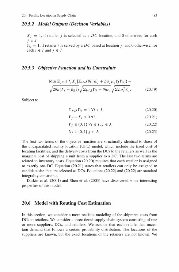
20 Facility Location in Supply Chain 483
20.5.2 Model Outputs (Decision Variables)
Xj D 1, if retailer j is selected as a DC location, and 0 otherwise, for eachj 2 JYij D 1, if retailer i is served by a DC based at location j , and 0 otherwise, foreach i 2 I and j 2 J
20.5.3 Objective Function and its Constraints
Min †j2J ffjXj Œ†i2a.ˇ�idij C ˇaj�j /χYij g Cq2h.Fj C ˇgj /
q†�i�Yij C hzα
q†L�2i Yij : (20.19)
Subject to
†j2J Yij D 1 8i 2 I; (20.20)
Yij �Xi � 0 8i; (20.21)
Yij 2 f0; 1g 8i 2 I; j 2 J; (20.22)
Xj 2 f0; 1g j 2 J: (20.23)
The first two terms of the objective function are structurally identical to those ofthe uncapacitated facility location (UFL) model, which include the fixed cost oflocating facilities, and the delivery costs from the DCs to the retailers as well as themarginal cost of shipping a unit from a supplier to a DC. The last two terms arerelated to inventory costs. Equation (20.20) requires that each retailer is assignedto exactly one DC. Equation (20.21) states that retailers can only be assigned tocandidate site that are selected as DCs. Equations (20.22) and (20.22) are standardintegrality constraints.
Daskin et al. (2001) and Shen et al. (2003) have discovered some interestingproperties of this model.
20.6 Model with Routing Cost Estimation
In this section, we consider a more realistic modeling of the shipment costs fromDCs to retailers. We consider a three-tiered supply chain system consisting of oneor more suppliers, DCs, and retailers. We assume that each retailer has uncer-tain demand that follows a certain probability distribution. The locations of thesuppliers are known, but the exact locations of the retailers are not known. We
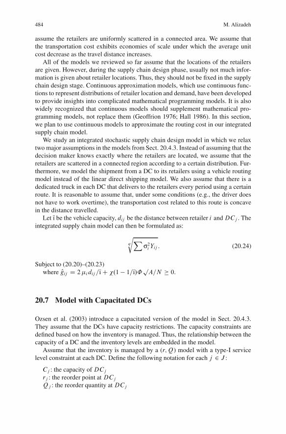
484 M. Alizadeh
assume the retailers are uniformly scattered in a connected area. We assume thatthe transportation cost exhibits economies of scale under which the average unitcost decrease as the travel distance increases.
All of the models we reviewed so far assume that the locations of the retailersare given. However, during the supply chain design phase, usually not much infor-mation is given about retailer locations. Thus, they should not be fixed in the supplychain design stage. Continuous approximation models, which use continuous func-tions to represent distributions of retailer location and demand, have been developedto provide insights into complicated mathematical programming models. It is alsowidely recognized that continuous models should supplement mathematical pro-gramming models, not replace them (Geoffrion 1976; Hall 1986). In this section,we plan to use continuous models to approximate the routing cost in our integratedsupply chain model.
We study an integrated stochastic supply chain design model in which we relaxtwo major assumptions in the models from Sect. 20.4.3. Instead of assuming that thedecision maker knows exactly where the retailers are located, we assume that theretailers are scattered in a connected region according to a certain distribution. Fur-thermore, we model the shipment from a DC to its retailers using a vehicle routingmodel instead of the linear direct shipping model. We also assume that there is adedicated truck in each DC that delivers to the retailers every period using a certainroute. It is reasonable to assume that, under some conditions (e.g., the driver doesnot have to work overtime), the transportation cost related to this route is concavein the distance travelled.
Let Nı be the vehicle capacity, dij be the distance between retailer i andDCj . Theintegrated supply chain model can then be formulated as:
q
rXσ2i Yij : (20.24)
Subject to (20.20)–(20.23)where Ogij D 2�idij =Nı C �.1 � 1=Nı/˚p
A=N � 0.
20.7 Model with Capacitated DCs
Ozsen et al. (2003) introduce a capacitated version of the model in Sect. 20.4.3.They assume that the DCs have capacity restrictions. The capacity constraints aredefined based on how the inventory is managed. Thus, the relationship between thecapacity of a DC and the inventory levels are embedded in the model.
Assume that the inventory is managed by a (r;Q) model with a type-I servicelevel constraint at each DC. Define the following notation for each j 2 J :
Cj : the capacity of DCjrj : the reorder point at DCjQj : the reorder quantity at DCj
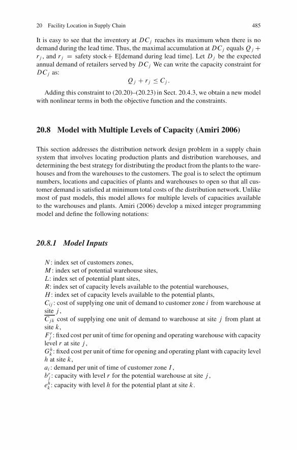
20 Facility Location in Supply Chain 485
It is easy to see that the inventory at DCj reaches its maximum when there is nodemand during the lead time. Thus, the maximal accumulation atDCj equalsQj Crj , and rj D safety stockC E[demand during lead time]. Let Dj be the expectedannual demand of retailers served by DCj We can write the capacity constraint forDCj as:
Qj C rj � Cj :
Adding this constraint to (20.20)–(20.23) in Sect. 20.4.3, we obtain a new modelwith nonlinear terms in both the objective function and the constraints.
20.8 Model with Multiple Levels of Capacity (Amiri 2006)
This section addresses the distribution network design problem in a supply chainsystem that involves locating production plants and distribution warehouses, anddetermining the best strategy for distributing the product from the plants to the ware-houses and from the warehouses to the customers. The goal is to select the optimumnumbers, locations and capacities of plants and warehouses to open so that all cus-tomer demand is satisfied at minimum total costs of the distribution network. Unlikemost of past models, this model allows for multiple levels of capacities availableto the warehouses and plants. Amiri (2006) develop a mixed integer programmingmodel and define the following notations:
20.8.1 Model Inputs
N : index set of customers zones,M : index set of potential warehouse sites,L: index set of potential plant sites,R: index set of capacity levels available to the potential warehouses,H : index set of capacity levels available to the potential plants,Cij : cost of supplying one unit of demand to customer zone i from warehouse atsite j ,Cjk cost of supplying one unit of demand to warehouse at site j from plant atsite k,F rj : fixed cost per unit of time for opening and operating warehouse with capacity
level r at site j ,Ghk : fixed cost per unit of time for opening and operating plant with capacity level
h at site k,ai : demand per unit of time of customer zone I ,brj : capacity with level r for the potential warehouse at site j ,
ehk : capacity with level h for the potential plant at site k.
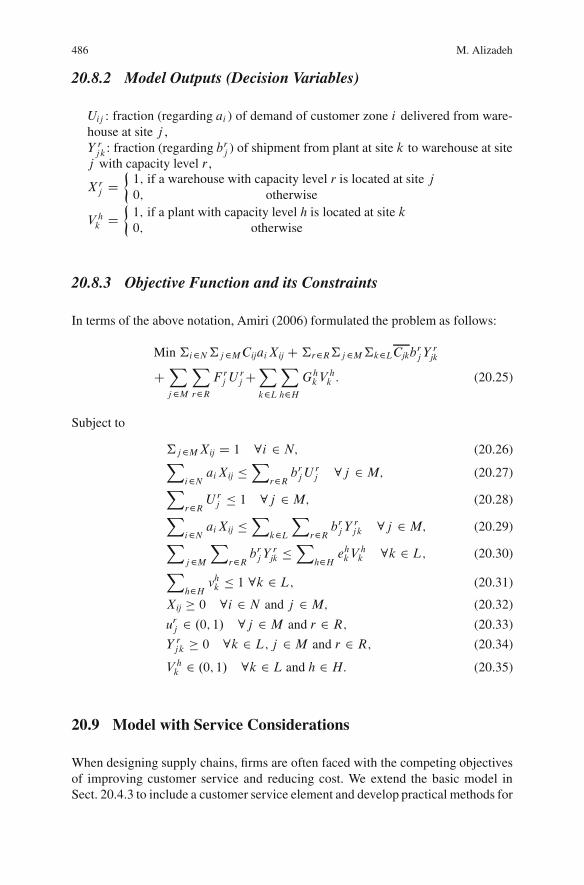
486 M. Alizadeh
20.8.2 Model Outputs (Decision Variables)
Uij : fraction (regarding ai ) of demand of customer zone i delivered from ware-house at site j ,Y rjk : fraction (regarding brj ) of shipment from plant at site k to warehouse at sitej with capacity level r ,
Xrj D
�1; if a warehouse with capacity level r is located at site j0; otherwise
V hk D
�1; if a plant with capacity level h is located at site k0; otherwise
20.8.3 Objective Function and its Constraints
In terms of the above notation, Amiri (2006) formulated the problem as follows:
Min †i2N†j2MCijaiXij C†r2R†j2M†k2LCjkbrj Y
rjk
CXj2M
Xr2R
F rj U
rj C
Xk2L
Xh2H
GhkV
hk : (20.25)
Subject to
†j2MXij D 1 8i 2 N; (20.26)Xi2N aiXij �
Xr2R b
rj U
rj 8j 2 M; (20.27)X
r2R Urj � 1 8j 2 M; (20.28)X
i2N aiXij �X
k2LX
r2R brj Y
rjk 8j 2 M; (20.29)X
j2MX
r2R brj Y
rjk �
Xh2H e
hkV
hk 8k 2 L; (20.30)X
h2H vhk � 1 8k 2 L; (20.31)
Xij � 0 8i 2 N and j 2 M; (20.32)
urj 2 .0; 1/ 8j 2 M and r 2 R; (20.33)
Y rjk � 0 8k 2 L; j 2 M and r 2 R; (20.34)
V hk 2 .0; 1/ 8k 2 L and h 2 H: (20.35)
20.9 Model with Service Considerations
When designing supply chains, firms are often faced with the competing objectivesof improving customer service and reducing cost. We extend the basic model inSect. 20.4.3 to include a customer service element and develop practical methods for
20 Facility Location in Supply Chain 487
quick and meaningful evaluation of cost/service tradeoffs. Service is measured bythe fraction of all demands that are located within an exogenously specified distanceof the assigned DC.
Ross and Soland (1980), in one of the earliest papers on multi-objective locationproblems, argue that practical problems involving the location of public facilitiesshould be modeled as multi-objective problems. Cost and service are the typicalobjectives, although there exist several distinct objectives in each of those twocategories: fixed investment cost, fixed operating cost, variable operating cost, to-tal operating cost, and total discounted cost are all reasonable cost objectives toconsider; and both demand served and response time (or distance traveled) areappropriate objectives for service measurement. They treat such multi-objectiveproblems in the framework of a model for selecting a subset of M sites wherepublic facilities are established to serve client groups located at N distinct points.For a review of other multi-objective location models, we refer the reader to Shen(2005).
Model (20.20)–(20.23) in Sect. 20.4.3 captures important facility location, trans-portation and inventory costs. Some retailers may be served very well, in the sensethat they are located very close to the DCs to which they are assigned, while otherretailers may be served very poorly by this criterion. The maximal covering locationproblem (Church and ReVelle 1974) maximizes the number of customers that can becovered by a fixed number of facilities. Customer i is covered if node i is assignedto a facility that is within dc of node i , where dc is the coverage distance. Insteadof maximizing covered demand volume, for fixed total demand, we can minimizethe uncovered demand volume. In a manner similar to Daskin (1995), we can thenformulate a model that simultaneously minimizes the fixed costs of the facilities anda weighted sum of the uncovered demand volume as follows:
MinX
j2J fjXj CX
j2JX
i2IOdij Yij : (20.36)
Subject to (20.20)–(20.23)Where W is the weight on the uncovered demand volume andUij D��i , if dij >
dc , and 0, if not.This model is structurally identical to basic model. The only difference is that
we penalize all assignments of demand nodes to DCs that are more than dc awayfrom the DC. By varying the weight W on uncovered demand volume, we can traceout an approximation to the set of non-inferior solutions to the tradeoff betweenlocation-inventory costs and customer responsiveness. Altiparmak et al. (2006)presented mixed-integer non-linear programming model for multi-objective opti-mization of SCN. They considered three objectives: (1) minimization of total costcomprised of fixed costs of plants and distribution centers (DCs), inbound and out-bound distribution costs, (2) maximization of customer services that can be renderedto customers in terms of acceptable delivery time (coverage), and (3) maximizationof capacity utilization balance for DCs (i.e., equity on utilization ratios). To dealwith multi-objective and enable the decision maker to evaluate a greater numberof alternative solutions, two different weight approaches were implemented in theproposed GA.
488 M. Alizadeh
20.10 Profit Maximizing Model with Demand Choice Flexibility
Minimizing total cost has been the primitive objective in most of the supply chainnetwork design models. These models typically require that every customer’s de-mand has to be satisfied. However, for a profit-maximizing business, it may notalways be optimal to satisfy all potential demands, especially if the additional costis higher than the additional revenue associated with servicing these customers.Furthermore, if the company is facing competition, sometimes it might be moreprofitable to lose some potential customers to competitors since the cost of main-taining these customers can be prohibitively high. Most supply chain related costs,such as location, transportation, and inventory related costs of an item depend ontotal demand volume, and no clear method exists for determining a customer’s prof-itability a priori, based solely on the characteristics of this customer. Shen addressesthis problem by proposing a profit-maximizing supply chain design model in whicha company can choose whether to satisfy a customer’s demand.
The literature on integrating cost-minimizing supply chain network design mod-els with profit-maximizing microeconomic theory is limited. Hansen et al. (1987)and Hansen et al. (1995) provide surveys on profit-maximizing location models.
Zhang (2001) considers a profit-maximizing location model, where a firm needsto decide where to locate a single DC to serve the customers and to set the pricefor its product, so as to maximize its total profit. He shows that under certain as-sumptions on the complexity counts, a special case of this problem can be solved inpolynomial time. However, he does not consider any cost related terms in his model,not even the DC location costs.
Another location model is proposed by Meyerson (2001), where he considers aprofit earning facility location problem for a given set of demand points, and the de-cision maker needs to open some facilities such that every demand may be satisfiedfrom a local facility and the total profit is maximized. Instead of incurring a cost,opening a facility can gain a certain profit which is a function of the amount of de-mand the facility satisfies. Since this profit-earning problem is NP-hard, Meyersondevelops an approximation algorithm that is based on linear program rounding.
Demand choice flexibility in inventory models is proposed by Geunes et al.(2004). Their models address economic ordering decisions when a producer canchoose whether to satisfy multiple markets. They assume the per unit revenue fromserving a specific customaries exogenously given, not a decision variable. Further-more, their models are pure inventory models; supply chain design related decisions,such as location decisions, are absent from the models.
Shen (2006) considers not only location decisions and customer-DC assignmentdecisions, but also production and inventory related decisions within a supply chainnetwork. It is assumed that after production, the product is shipped to several DCs,and then from DCs to each customer the company has decided to serve. Contraryto Meyerson’s model, assumes opening a facility incurs a certain cost, however, byserving the customers assigned to this facility, a certain amount of profit will begained, which is also a function of the total demand served by the facility.
20 Facility Location in Supply Chain 489
The profit-maximizing supply chain network design problem can be described asfollowing: Given a production site o, a set I of customers and a set J of candidateDC locations, the decision maker wants to determine (a) the number and locations ofthe DCs, (b) the assignments of customers to DCs, (c) the inventory replenishmentstrategy at each DC, and (d) the sale price of the product at each region, so thatthe total profit is maximized. The profit is equal to the revenue minus the total cost,which includes the DC location cost, inventory holding cost at DCs, and deliverycost to DCs.
To model this problem, we define the following additional notation:
fj .x/ (annual) cost of locating and operating a DC at j , for each j 2 J . it is aconcave function of the annual demand x flowing through DCj
K: fixed cost of delivering product from the production site to a DCdoj : distance from the production site o to DCj , j 2 Jdij : distance from the DCj to customer i , for i 2 I; j 2 Jc.doj / delivery cost per unit from the production site o to DCj it has the follow-ing structure:
C.doj / D
8<ˆ:c1; if 0 < doj < d1c2; d1 < doj < d2
: : : ;
ct ; dt�1 < doj < dt
:
It is typically assumed that c1 < c2 < : : : < ct
pj : sale price per unit at the region served by DCj
ui : customer i ’s reserve price g.dij / delivery cost per unit charged to customerif delivery is made from DCj . it has the following structure:
g.dij / D
8<ˆ:
v1; if 0 < dij < d1
v2; d1 < dij < d2
: : : ;
vt ; dt�1 < dij < dt
:
it is typically assumed that v1 � v2 � : : : � vt
Shen (2006) assumes the company will lose a customer if the price a customerhas to pay is higher than the customer’s reserve price, i.e., if ui < pj C g.dij/. Hedefines
Ri.pi C dij / D(pj C g.dij /� c.doj /; pj C g.dij/ � ui
0; pj C g.dij/ > ui:
Shen (2006) formulates the decision problem as a set-covering model, and present abranch-and-price algorithm to solve this model. To solve the resulting pricing prob-lem, it suffices to find, for every DCj 2 J , a maximum-reduced-cost set R�
j � I ,
490 M. Alizadeh
that uses j as the designated DC. Thus, the pricing problem reduces to finding R�j
for each j 2 J . To find R�j , the following integer programming problem must be
solved:
MinX
i2S aiYij �r2kh
Xi2S �iYi � hZ˛
rXi2S �
2i Yi�fj
Xi2S �iYi
:
(20.37)
Subject to
Yi 2 f0; 1g; 8i 2 S; S � �: (20.38)
20.11 Model with Multiple Commodities
Nowadays, retailers carry thousands of different products and the amount of datainvolved in a supply chain design model can be overwhelming. It is not necessary,and may not be possible, to account for all distinct products in the strategic supplychain design phase. Aggregated information at the product category level should beused instead (Simchi-Levi et al. 2000).
Shen (2007) states that Warszawski and Peer (1973) and Warszawski (1973)are among the first to study the multi-commodity location problem. These modelsconsider fixed location costs and linear transportation costs, and assume that eachwarehouse can be assigned at most one commodity.
Geoffrion and Graves (1974) consider the capacitated version of the multi-commodity location problem in which they impose capacity constraints on thesuppliers and the DCs. They also assume that each customer must be served with allthe products it requires from a single DC or directly from a supplier.
Shen (2005) multi-commodity supply chain design model can be stated as fol-lows: We are given a set of alternative facility locations, a set of retailers, a set ofdifferent products, and a certain activity whose cost can be modeled using a concavefunction. The objective is to design a supply chain system that can serve outside de-mand at minimum cost.
Shen (2007) use the following additional notation:
L: set of commodities;It : set of retailers that have demand for commodity l 2 L�il : mean annual demand from retailer i for commodity l .
Decision variables
Xj D 1, if j is selected as facility location, and 0 otherwise, for each j 2 JYijl D 1, if the demand for commodity l of retailer i is served by j , and 0otherwise, for each i 2 I; j 2 J; l 2 L
20 Facility Location in Supply Chain 491
With this notation, Shen (2005) formulates the problem as follows:
MinX
j2JnfjXj C
Xl2L
hXi2l .dijl�il/Yijl CGjl
Xi2l �ilYijl
io:
(20.39)
Subject to
Xj2J Yijl D 1; 8i 2 I; l 2 L; (20.40)
Yijl � Xj � 0 8i 2 I; j 2 J; l 2 L; (20.41)
Yijl 2 f0; 1g:8i 2 I; j 2 J; l 2 L; (20.42)
Xj 2 f0; 1g:8j 2 J: (20.43)
20.12 Model with Unreliable Supply
A supply chain network is a complex system in which there are many uncertainties,such as demands from the customers and delivery reliability. Because most supplychain design decisions (e.g., facility location) are irreversible, it is critical to takethese uncertainties into account.
As Shen (2007) discussed, Qi and Shen consider the multi-period problem thatin each period, multiple retailers order a specific product from a supplier, and thesupplier ships the product to some intermediate facilities selected from a set of can-didate locations. However, the amount of final product delivered on time to a retailermay not be exactly the amount this retailer requests from the supplier, because of thequality issues resulting from different production/assembly capabilities in differentfacilities, mistakes made during the assembly/packaging operations, the weather orother factors that may impact the on-time delivery from facilities to retailers. Thus,the decision maker needs to take this unreliability issue into consideration whendesigning the supply chain.
As Snyder and Daskin (2007) surveyed, a more formal review of this body of lit-erature is presented by Snyder et al. (2006). Owen and Daskin (1998), Daskin et al.(2005), and Snyder (2006) all provide reviews of stochastic location models (gen-erally considering uncertainty in demand, rather than disruptions to facilities). SeeBirge and Louveaux (1997) or Higle (2005) for an introduction to general stochas-tic programming techniques. Snyder and Daskin (2005) introduce several models,based on classical facility location problems, in which facilities may fail with agiven probability. They minimize a weighted sum of two objectives, one of whichis a classical objective (ignoring disruptions) and the other is the expected cost af-ter accounting for disruptions. Customers are assigned to several facilities, one ofwhich is the “primary” facility that serves it under normal circumstances, one ofwhich serves it if the primary facility fails, and so on.
492 M. Alizadeh
As Snyder and Daskin (2007) survived in their paper, Church and Scaparra(2005) and Scaparra and Church (2005, 2006) consider the fortification, rather thandesign, of facilities – that is, the network is assumed to exist and the firm hasresources to prevent disruptions at some of them, thus partially fortifying the net-work. Their model finds the best facilities to fortify assuming that an interdictorwill attempt to cause worst-case losses for the firm by disrupting a fixed number ofthe un-fortified facilities. Similarly, Daskin et al. (2005) allow the firm to choosewhether each facility opened is reliable or unreliable; reliable facilities come at ahigher cost.
20.12.1 Model Inputs
Based on basic model that discussed in Sect. 20.4.3, Qi and Shen define the follow-ing additional notation for this problem:
c: purchasing price from the supplier per unit of product�: number of periods per yearRj : the reliability coefficient associated with facility j , j 2 J , which is a randomvariable between 0 and 1. Let j D E.Rj / and �2j D Var (Rj )pi : retail price at retailer i per unit of product, i 2 I�i : penalty cost of lost good will at retailer i per unit of product, i 2 Ivi : salvage value at retailer i per unit of product, i 2 I
20.12.2 Model Outputs (Decision Variables)
Xj D�1; facility j 2 J is open0; otherwise
,
Qij : order quantity at facility j 2 J from retailer i 2 I in each period.
20.12.3 Objective Function and its Constraints
Qi and Shen assume that the per-unit purchase and transportation costs are basedon the quantity ordered, not the quantity actually received by the retailers. Based onthis assumption, they formulate the following integrated model:
Min �X
j2J
�fjXj C c�
Xi2I Qij C aj �
Xi2I Qij CKJ
rXi2I Qij
C�X
i2I Ti .Q/ D �.Q/�X
j2J fjXj : (20.44)
20 Facility Location in Supply Chain 493
Subject to
1� e�ˇQij � Xj i 2 I; j 2 J; (20.45)
Qij � 0 i 2 I; j 2 J; (20.46)
Xj 2 f0; 1g j 2 J: (20.47)
The objective function maximizes the expected annual profit of the entire systemincluding all facilities and retailers. The first term represents the facility locationcost for opening facilities and the second term is the annual purchasing cost fromthe supplier. The third and fourth term represent the working inventory cost andthe safety stock cost associated with each facility. The last term is profit earned atretailers. Equation (20.45) requires that retailers can only order from open facilities.An exponential function is used to formulate this restriction because of the quickconvergence property of the exponential function. The positive constant ˇ is used toexpedite the convergence.
20.13 Model with Facility Failures (Snyder 2003)
Once a set of facilities has been built, one or more of them may from time to timebecome unavailable, for example, due to inclement weather, labor actions, naturaldisasters, or changes in ownership. These facility “failures” may result in excessivetransportation costs as customers previously served by these facilities must now beserved by more distant ones. In this section, we discuss models for choosing facil-ity locations to minimize fixed and transportation costs while also hedging againstfailures within the system. The goal is to choose facility locations that are both in-expensive and reliable.
The models discussed in this section are based on the fixed charge location prob-lem; they address the tradeoff between operating cost (fixed location costs andday-to-day transportation cost, the classical fixed charge problem objective) andfailure cost (the transportation cost that results after a facility has failed). The firstmodel considers the maximum failure cost that can occur when a single facility fails,while the second model considers the expected failure cost given a fixed probabilityof failure.
In addition to the notation defined earlier, let
Yijk D
8<:1; if facility j 2 J serves as the primary facility and facility
k 2 J serves as the secondary facility for customer i 2 I0; if not
And let V be a desired upper bound on the failure cost that may result if a facilityfails.
494 M. Alizadeh
20.13.1 Objective Function and its Constraints
Snyder (2003) formulates the maximum-failure-cost reliability problem as follows:
MinX
j2J fjXj CX
i2IX
j2JX
k2J hi cijYijk: (20.48)
Subject to
Xj2J
Xk2J Yijk D 1 8i 2 I ; (20.49)
Xk2J Yijk � Xj 8i 2 I;8j 2 J; (20.50)
Yijk � Xk 8i 2 I;8j 2 J;8k 2 J; (20.51)Xi2IX
j2JX
k2J hi cijYijkCX
i2IX
k2J hi cijYijk �V 8j 2 J ; (20.52)
Yijj D 0 8i 2 I;8j 2 J; (20.53)
Xj 2 f0; 1g 8j 2 J; (20.54)
Yijk � f0; 1g 8i 2 I;8j 2 J;8k 2 J: (20.55)
The objective function sums the fixed cost and transportation cost to customers fromtheir primary facilities. Equation (20.49) requires each customer to be assigned toone primary and one backup facility. Equation (20.50) and (20.51) prevent a cus-tomer from being assigned to a primary or a backup facility, respectively, that hasnot been opened. Equation (20.52) is the reliability constraint and requires the fail-ure cost for facility j to be no greater than V . The first summation computes thecost of serving each customer from its primary facility if its primary facility is notj , while the second summation computes the cost of serving customers assigned toj as their primary facility from their backup facilities. Equation (20.53) requires acustomer’s primary facility to be different from its backup facility, and (20.54) and(20.55) are standard integrality and non-negativity constraints. This model can besolved for small instances using an off-the-shelf IP solver, but larger instances mustbe solved heuristically.
The expected-failure-cost reliability model (Snyder and Daskin 2003) assumesthat multiple facilities may fail simultaneously, each with a given probability q offailing. In this case, a single backup facility is insufficient, since a customer’s pri-mary and backup facilities may both fail. Therefore, we define:
Yijr D(1; if facility j 2 J serves as the level � r facility for customer i 2 I0; if not
:
A “level-r” assignment is one for which there are r closer facilities that are open.If r D 0, this is a primary assignment; otherwise it is a backup assignment. The
20 Facility Location in Supply Chain 495
objective is to minimize a weighted sum of the operating cost (the fixed chargelocation problem objective) and the expected failure cost, given by
Xi2I
Xj2J
jJ j�1XrD0
hi cij qr .1 � q/Yijr :
Each customer i is served by its level-r facility (call it j ) if the r closer facilitieshave failed (this occurs with probability qr) and if j itself has not failed (this occurswith probability 1 � q). The full model is omitted here.
20.14 Planning Under Uncertainty (Snyder et al. 2007)
Long-term strategic decisions like those involving facility locations are always madein an uncertain environment. However, classical facility location models like thefixed charge location problem treat data as though they were known and determinis-tic, even though ignoring data uncertainty can result in highly sub-optimal solutions.Unfortunately, as Vidal and Goetschalckx (2000) discussed in their paper, criticalparameters such as customer demands, prices, and resource capacities are quite un-certain. Moreover, the arrival of regional economic alliances, for instance the AsianPacific Economic Alliance and the European Union, have prompted many corpora-tions to move more and more towards global supply chains, and therefore to becomeexposed to risk factors such as exchange rates, reliability of transportation channels,and transfer prices.
Daskin et al. (2003) said that most approaches to decision making under uncer-tainty fall into one of two categories: stochastic programming or robust optimiza-tion. In stochastic programming, the uncertain parameters are described by discretescenarios, each with a given probability of occurrence; the objective is to minimizethe expected cost. In robust optimization, parameters may be described either bydiscrete scenarios or by continuous ranges; no probability information is known,however, and the objective is typically to minimize the worst-case cost or regret.
According Daskin et al. (2003), Sheppard (1974) was one of the first authorsto propose a stochastic approach to facility location. He suggests selecting facilitylocations to minimize the expected cost, though he does not discuss the issue atlength. Weaver and Church (1983) and Mirchandani et al. (1985) present a multi-scenario version of the P-median problem. Their model can be translated into thecontext of the fixed charge location problem as follows. Let S be a set of scenarios.Each scenario s 2S has probability of occurring and specifies a realization of ran-dom demands and travel costs. Location decisions must be made now, before it isknown which scenario will occur. However, customers may be assigned to facilitiesafter the scenario is known. Other stochastic facility location models include thoseof Louveaux (1986), Franga and Luna (1982), Berman and LeBlanc (1984), Carsonand Batta (1990), and Jornsten and Bjorndal (1994).
496 M. Alizadeh
The earlier models assume the decision maker knows the demand parameters.That is, the mean �i and the standard deviation �i of retailer i ’s demand areknown parameters. Snyder et al. (2007) present a stochastic version of the modelin Sect. 20.4.3 that explicitly handles parameter uncertainty by allowing parametersto be described by discrete scenarios, each with a specified probability of occur-rence. The goal is to choose DC locations, assign retailers to DCs, and set inventorylevels at DCs to minimize the total system wide cost. To model this problem, Snyderet al. (2007) define the following additional notation:
20.14.1 Model Inputs
� S : set of scenarios, indexed by s,� �is : mean daily demand at retailer i in scenario s, for i 2 I; s 2 S ,� dijs: per-unit cost to ship from DCj to retailer i in scenario s, for i 2 I; j 2 J ,� qs : probability that scenario s occurs, for s 2 S .
20.14.2 Model Outputs (Decision Variables)
� xj D 1, if j is selected as a facility location, and 0 otherwise, for each j 2 J ,� yijs D 1, if retailer i 2 I is served by DCj j 2 J in scenario s 2 S , and 0
otherwise.
20.14.3 Objective Function and its Constraints
Xs2S
Xj2J
nfjXj C
Xi2I ˇ��is.dijs C aj /Yijs
CKj
rXi2I �isYijs C q
rXi2I Lj �
2i Yijs
: (20.56)
Subject to
Pj2J Yijs D 1; 8i 2 I; s 2 S; (20.57)
Yijs � Xj � 0 8i 2 I; j 2 J; s 2 S ; (20.58)
Yijs 2 f0; 1g 8i 2 I; j 2 J; s 2 S ; (20.59)
Xi 2 f0; 1g 8j 2 J ; (20.60)
where q D hz˛ .
20 Facility Location in Supply Chain 497
20.15 Solution Techniques
A number of solution approaches have been proposed for the supply chain designmodels. We review the related literatures.
� To solve the uncapacitated fixed charge location model, Maranzana (1964) pro-posed a neighborhood search improvement algorithm for the closely relatedp-median problem that exploits the ease in finding optimal solutions to 1-medianproblem: it partitions the customers by facility and then finds the optimal loca-tion within each partition. If any facility changes, the algorithm repartitions thecustomers and continues until no improvement in the solution can be found.
� Teitz and Bart (1968) proposed an exchange or “swap” algorithm for the P-median problem that can also be extended to the fixed charge facility locationproblem.
� Hensen and Mladenovic (1997) proposed a variable neighborhood search algo-rithm for the P-median problem that can also be used for the fixed charge locationproblem.
� Heuristics that be applied to the P-median problem will not perform well forfixed charge facility location problem if the starting number of facilities is sub-optimal. Thus, we should apply more sophisticated heuristics to the problem.Al-Sultan and Al-Fawzan (1999) applied tabu search to the uncapacitated fixedcharge location problem.
� Daskin (1995) review the use of Lagrangian relaxation algorithms in solving theuncapacitated fixed location problem.
� When embedded in branch and bound, Lagrangian relaxation can be used to solvethe fixed charge location problem optimally (Geoffrion 1974).
� Daskin et al. apply Benders decomposition to locating plants and distributioncenters simultaneously with multiple commodities after noting that, if the loca-tion and assignment variables are fixed, the remaining problem breaks down intojLj transportation problems, one for each commodity.
� Shen et al. (2003) outline a column generation approach to solve the basic modelthat presented in Sect. 20.4.3. Daskin et al. (2001) proposes a Lagrangian relax-ation approach for the same problem.
� To solve the model with routing cost estimation, Shen and Qi (2004) developa Lagrangian relaxation based solution algorithm. By exploiting the structure ofthe problem, they find anO.jI j2 log.jI j// time algorithm for the similar problemthat must be solved in the Lagrangian relaxation subproblems.
� Ozsen et al. (2003) apply a Lagrangian relaxation solution algorithm to solvethe capacitated DCs problems that presented in Sect. 20.4.4. The Lagrangiansubproblem is also a non-linear integer program, and they propose an efficientalgorithm for the continuous relaxation of this problem.
� Amiri (2006) studied the designing a distribution network in a supply chain sys-tem with allow for multiple levels of capacities available to the warehouses andplants. He develop a mix integer programming model and present a Lagrangianbased solution procedure for the problem.
498 M. Alizadeh
� Two solution approaches was presented by Shen and Daskin (2005) for the modelwith service consideration, one based on the weighting method and the otherbased on genetic algorithms. The genetic algorithm performs very well comparedto the weighting method, and it is the only feasible approach for large-sized prob-lem instances, since the weighting method requires excessive computational timein such cases.
� A branch-and-price algorithm, a variant of branch-and-bound in which the nodesare processed by solving linear-programming relaxation via column-generation,was presented by Shen (2006) to solve the profit maximizing model with demandchoice flexibility.
� Shen (2005) proposes Lagrangian relaxation embedded in a branch and boundalgorithm to solve the model with multiple commodities.
� Yeh (2005) present a hybrid heuristic algorithm for the multistage supply chainnetwork problem (MSCN). The proposed algorithm employs a simple greedymethod and a hybrid local search method combining the XP, RP and IP to solvethe MSCN. From the computation experiments, both the speed in finding thesolution and the quality of the obtained solutions were good enough to solve thelarger MSCN problem.
� Yeh (2006) has also proposed a memetic algorithm (MA) which is a combinationof GA, greedy heuristic, and local search methods for the same problem. Theauthor has extensively investigated the performance of the MA on the randomlygenerated problems.
� Romeijn et al. (2007) proposed a framework for the two-echelon supply chaindesign problem that incorporates location decisions as well as location-specifictransportation cost and two-echelon inventory costs. Their approach is to formu-late the problem as a set-covering model. They propose to solve this problemusing column generation to deal with the fact that the number of variables(columns) in this formulation is exponentially large.
� Altiparmak et al. (2006) propose a new solution procedure based on genetic algo-rithms to find the set of Pareto-optimal solutions for multi-objective SCN designproblem. To deal with multi-objective and enable the decision maker for evalu-ating a greater number of alternative solutions, two different weight approachesare implemented in the proposed solution procedure.
� Altiparmak et al. (2007) presents a solution procedure based on steady-stategenetic algorithms (ssGA) with a new encoding structure for the design of asingle-source, multi-product, multi-stage SCN. The effectiveness of the ssGAhas been investigated by comparing its results with those obtained by CPLEX,Lagrangian heuristic, hybrid GA and simulated annealing on a set of SCN designproblems with different sizes.
� Hinojosa et al. (2008) formulating the problem that deal with a facility locationproblem where they build new facilities or close down already existing facili-ties at two different distribution levels over a given time horizon. In addition,they allow carrying over stock in warehouses between consecutive periods. Theypropose a Lagrangian approach which relaxes the constraints connecting the dis-tribution levels. A procedure is developed to solve the resulting, independent
20 Facility Location in Supply Chain 499
subproblems and, based on this solution, to construct a feasible solution for theoriginal problem.
� Jayaraman and Pirkul (2001) have developed a heuristic approach based onLagrangean relaxation for the single-source, multi-product, multi-stage SCN de-sign problem. Another heuristic approach based on Lagrangean relaxation andsimulated annealing has been developed by Syam (2002) for a multi-source,multi-product, multi-location framework.
� Jang et al. (2002) have presented a combined model of network design and pro-duction/distribution planning for a SCN. While they have used a Lagrangianheuristic for the design of SCN, a genetic algorithm (GA) has been proposedfor integrated production and distribution planning problem.
� Syarif et al. (2002) have developed a spanning tree-based GA approach for themulti-source, single-product, multi-stage SCN design problem based on Prufernumbers.
� Jayaraman and Ross (2003) have also proposed a heuristic approach based onsimulated annealing for the designing of distribution network and managementin supply chain environment.
� Shen (2007) states that Qi and Shen propose an algorithm based on the bisectionsearch and the outer approximate algorithm. They show that their algorithm ismore efficient that the outer approximation algorithm when being applied to themodel with unreliable supply.
� To solve the model with parameter uncertainty, Snyder et al. (2007) presenta Lagrangian-relaxation based solution algorithm. They show the Lagrangiansubproblem is non-linear integer program, but it can be solved by a low-orderpolynomial algorithm. They present qualitative and quantitative computationalresults on problems with up to 150 nodes and nine scenarios, and describe bothalgorithm performance and solution behavior as key parameters change.
Solution methods discussed above are outlined in Table 20.1. This table shows thatthe use of heuristics and meta-heuristics based solution algorithms increase in re-cently papers.
20.16 Case Study
In this section we will introduce two real-world case studies related to supply chaindesign problems.
20.16.1 An Industrial Case in Supply Chain Designand Multilevel Planning in US (Sousa et al. 2008)
Souse et al. (2007) address a case study, inspired by a real agrochemicals supplychain, with two main objectives, structured in two stages. In the first stage they
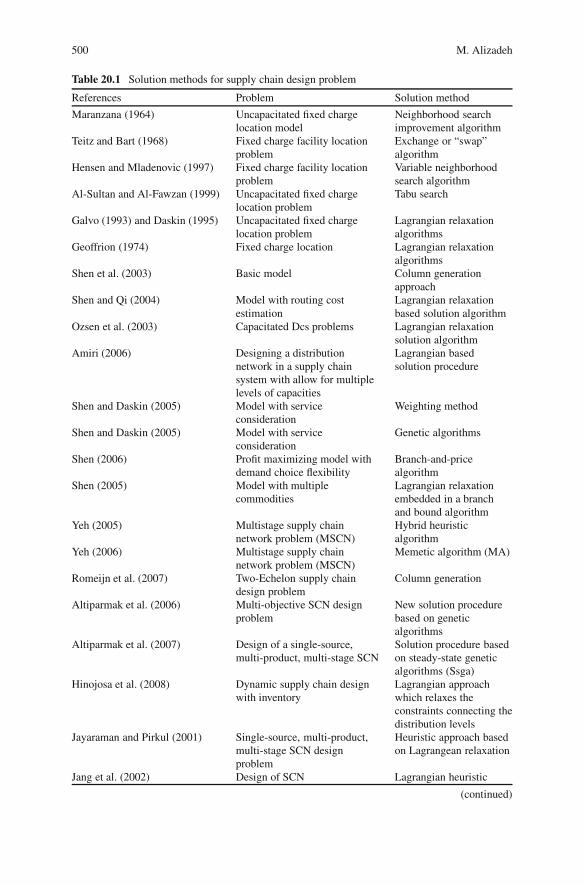
500 M. Alizadeh
Table 20.1 Solution methods for supply chain design problem
References Problem Solution method
Maranzana (1964) Uncapacitated fixed chargelocation model
Neighborhood searchimprovement algorithm
Teitz and Bart (1968) Fixed charge facility locationproblem
Exchange or “swap”algorithm
Hensen and Mladenovic (1997) Fixed charge facility locationproblem
Variable neighborhoodsearch algorithm
Al-Sultan and Al-Fawzan (1999) Uncapacitated fixed chargelocation problem
Tabu search
Galvo (1993) and Daskin (1995) Uncapacitated fixed chargelocation problem
Lagrangian relaxationalgorithms
Geoffrion (1974) Fixed charge location Lagrangian relaxationalgorithms
Shen et al. (2003) Basic model Column generationapproach
Shen and Qi (2004) Model with routing costestimation
Lagrangian relaxationbased solution algorithm
Ozsen et al. (2003) Capacitated Dcs problems Lagrangian relaxationsolution algorithm
Amiri (2006) Designing a distributionnetwork in a supply chainsystem with allow for multiplelevels of capacities
Lagrangian basedsolution procedure
Shen and Daskin (2005) Model with serviceconsideration
Weighting method
Shen and Daskin (2005) Model with serviceconsideration
Genetic algorithms
Shen (2006) Profit maximizing model withdemand choice flexibility
Branch-and-pricealgorithm
Shen (2005) Model with multiplecommodities
Lagrangian relaxationembedded in a branchand bound algorithm
Yeh (2005) Multistage supply chainnetwork problem (MSCN)
Hybrid heuristicalgorithm
Yeh (2006) Multistage supply chainnetwork problem (MSCN)
Memetic algorithm (MA)
Romeijn et al. (2007) Two-Echelon supply chaindesign problem
Column generation
Altiparmak et al. (2006) Multi-objective SCN designproblem
New solution procedurebased on geneticalgorithms
Altiparmak et al. (2007) Design of a single-source,multi-product, multi-stage SCN
Solution procedure basedon steady-state geneticalgorithms (Ssga)
Hinojosa et al. (2008) Dynamic supply chain designwith inventory
Lagrangian approachwhich relaxes theconstraints connecting thedistribution levels
Jayaraman and Pirkul (2001) Single-source, multi-product,multi-stage SCN designproblem
Heuristic approach basedon Lagrangean relaxation
Jang et al. (2002) Design of SCN Lagrangian heuristic
(continued)
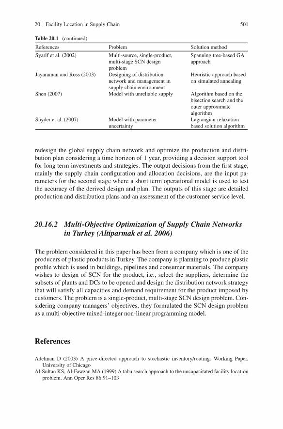
20 Facility Location in Supply Chain 501
Table 20.1 (continued)
References Problem Solution method
Syarif et al. (2002) Multi-source, single-product,multi-stage SCN designproblem
Spanning tree-based GAapproach
Jayaraman and Ross (2003) Designing of distributionnetwork and management insupply chain environment
Heuristic approach basedon simulated annealing
Shen (2007) Model with unreliable supply Algorithm based on thebisection search and theouter approximatealgorithm
Snyder et al. (2007) Model with parameteruncertainty
Lagrangian-relaxationbased solution algorithm
redesign the global supply chain network and optimize the production and distri-bution plan considering a time horizon of 1 year, providing a decision support toolfor long term investments and strategies. The output decisions from the first stage,mainly the supply chain configuration and allocation decisions, are the input pa-rameters for the second stage where a short term operational model is used to testthe accuracy of the derived design and plan. The outputs of this stage are detailedproduction and distribution plans and an assessment of the customer service level.
20.16.2 Multi-Objective Optimization of Supply Chain Networksin Turkey (Altiparmak et al. 2006)
The problem considered in this paper has been from a company which is one of theproducers of plastic products in Turkey. The company is planning to produce plasticprofile which is used in buildings, pipelines and consumer materials. The companywishes to design of SCN for the product, i.e., select the suppliers, determine thesubsets of plants and DCs to be opened and design the distribution network strategythat will satisfy all capacities and demand requirement for the product imposed bycustomers. The problem is a single-product, multi-stage SCN design problem. Con-sidering company managers’ objectives, they formulated the SCN design problemas a multi-objective mixed-integer non-linear programming model.
References
Adelman D (2003) A price-directed approach to stochastic inventory/routing. Working Paper,University of Chicago
Al-Sultan KS, Al-Fawzan MA (1999) A tabu search approach to the uncapacitated facility locationproblem. Ann Oper Res 86:91–103
502 M. Alizadeh
Altiparmak F, Gen M, Lin L, Paskoy T (2006) A genetic algorithm approach for multi-objectiveoptimization of supply chain networks. Comput Ind Eng 51:197–216
Altiparmak F Gen M, Lin L, Karaoglan I (2007) A steady-state genetic algorithm for multi-productsupply chain network design. Comput Ind Eng, in press, Corrected Proof, Available online2 June 2007
Amiri A (2006) Designing a distribution network in a supply chain system: Formulation and effi-cient solution procedure. Eur J Oper Res 171:567–576
Balinski ML (1965) Integer programming: Methods, uses, computation. Manage Sci 12:253–313Baumol WJ, Wolfe P (1958) A warehouse-location problem. Oper Res 6:252–263Berger RT (1997) Location-routing models for distribution system design. Ph.D. Dissertation,
Department of Industrial Engineering and Management Sciences, Northwestern University,Evanston, IL
Birge JR, Louveaux F (1997) Introduction to stochastic programming. Springer-Verlag, New YorkCarson, YM, Batta Y (1990) Locating an ambulance on the Amherst Campus of the State
University of New York at Buffalo. Interfaces 20(5):43–49Chan Y, Carter WB, Burnes MD (2001) A Multiple-depot, multiple-vehicle, location-routing prob-
lem with stochastically processed demands. Comput Oper Res 28:803–826Chopra S (2003) Supply chain management: Strategy, planning, and operation. Prentice-Hall, IndiaChurch RL, ReVelle CS (1974) The maximal covering location problem. Papers Region Sci Assoc
32:101–118Daskin MS (1995) Network and discrete location: Models, algorithms, and applications. Wiley,
New YorkDaskin MS, Jones PC (1993) A new approach to solving applied location/allocation problems.
Microcomput Civil Eng 8:409–421Daskin M, Coullard C, Shen ZJ (2001) An inventory-location model: Formulation, solution algo-
rithm and computational results. Ann Oper Res 110:83–106Daskin MS, Snyder LV, Berter RT (2003) Facility location in supply chain design, forthcoming in
logistics systems. In: Langevin A, Riopel D (eds) Design and optimization. Kluwer, DordechtDaskin MS, Snyder LV, Berger RT (2005) Facility location in supply chain design. In: Langevin
A, Riopel D (eds) Logistics systems: Design and operation. Springer, New York, pp 39–66Eppen G (1979) Effects of centralization on expected costs in a multi-location newsboy problem.
Manage Sci 25(5):498–501Erlebacher SJ, Meller RD (2000) The interaction of location and inventory in designing distribution
systems. HE Trans 32:155–166Fazel Zarandi MH, Turksen IB, Saghiri S (2002) Supply chain: crisp and fuzzy aspects. Int J Appl
Math Comput Sci 12(3)423–435Franga PM, Luna HPL (1982) Solving stochastic transportation-location problems by generalized
Benders decomposition. Transport Sci 16:113–126Geoffrio AM (1974) Lagrangian relaxation for integer programming. Math Program Study 2:
82–114Geoffrion AM (1976) The purpose of mathematical programming is insight, not numbers. Inter-
faces 7:81–92Geoffrion AM, Graves GW (1974) Multicommodity distribution system design by Benders de-
composition. Manage Sci 20(5):822–844Geunes J, Shen ZJ, Romeijn HE (2004) Economic ordering decisions with market choice flexibil-
ity. Naval Res Logist 51:117–136Hall RW (1986) Discrete models/continuous models. Omega, Int J Mgmt Sci 14:213–220Hansen P, Labbe M, Peeters D, Thisse JF (1987) Facility location analysis. Fundam Pure Appl
Econ 22:1–70Hansen P, Peeters D, Thisse JF (1995) The profit-maximizing weber problem. Location Sci 3:
67–85Higle JL (2005) Stochastic programming: Optimization when uncertainty matters. In: Greenberg
HJ (ed) TutORials in operations research. INFORMS, Baltimore, pp 30–53
20 Facility Location in Supply Chain 503
Hinojosaa Y, Kalcsicsb J, Nickelc S, Puertod J, Veltene S (2008) Dynamic supply chain designwith inventory. Comput Oper Res 35:373–391
Jang YJ, Jang SY, Chang BM, Park (2002) A combined model of network design and production/distribution planning for a supply network. Comput Ind Eng 43:263–281
Jayaraman V, Pirkul H (2001) Planning and coordination of production and distribution facilitiesfor multiple commodities. Eur J Oper Res 133:394–408
Jayaraman V, Ross A (2003) A simulated annealing methodology to distribution network designand management. Eur J Oper Res 144:629–645
Jornsten K, Bjorndal M (1994) Dynamic location under uncertainty. Stud Region Urban Plan3:163–184
Kleywegt A, Nori VS, Savelsbergh MWP (2002) Dynamic programming approximations for astochastic inventory routing problem. Working Paper, Georgia Inst. of Technology
Laporte G (1998) Location-routing problems. In: Golden BL, Assad AA (eds) Vehicle routing:methods and studies. North-Holland, Amsterdam, Holland, pp 163–197
Louveaux FV (1986) Discrete stochastic location models. Ann Oper Res 6:23–34Mabert VA, Venkataramanan MA (1998) Special research focus on supply chain linkages:
Challenges for design and management in the 21st century. Dec Sci 29(3):537–552Maranzana FE (1964) On the location of supply points to minimize transport costs. Oper Res Quart
15:261–270Meyerson A (2001) Profit-earning facility location. STOC 2001, Hersonissos, Crete, GreeceMin H, Jayaraman V, Srivastava R (1998) Combined location-routing problems: a synthesis and
future research directions. Eur J Oper Res 108:1–15Mirchandani PB, Oudjit A, Wong RT (1985) Multidimensional extensions and a nested dual ap-
proach for the m-median problem. Eur J Oper Res 21:121–137Nagy G, Salhi S (2007) Location-routing: Issues, models and methods. Eur J Oper Res 177:
649–672Owen SH, Daskin MS (1998) Strategic facility location: A review. Eur J Oper Res 111:423–447Ozsen L, Daskin MS, Coullard CR (2003) Capacitated facility location model with risk pooling.
Networks, SubmittedRomeijn HE, Shu J, Teo CP (2007) Designing two-echelon supply networks. Eur J Oper Res
178:449–462Ross GT, Soland RM (1980) A multicriteria approach to location of public facilities. Eur J Oper
Res 4:307–321Shen ZJ (2005) Multi-commodity supply chain design problem. IIE Trans 37:753–762Shen ZJ (2006) Aprofit-maximizing supply chain network design model with demand choice flex-
ibility. Oper Res Lett 34:673–682Shen ZJ (2007) Integrated supply chain design models: A survey and future research directions.
J Ind Manage Optimiz 3(1):1–27Shen ZJ, Daskin M (2005) Trade-offs between customer service and cost in integrated supply chain
design. M& SOM 7:188–207Shen ZJ, Qi L (2004) Incorporating inventory and routing costs in strategic location models. To
appear in Eur J Oper ResShen ZJ, Coullard C, Daskin M (2003) A joint location-inventory model. Transport Sci 37:40–55Sheppard ES (1974) A conceptual framework for dynamic location-allocation analysis. Environ
Plan 6:547–564Simchi-Levi D, Kaminsky P, Simchi-Levi E (2000) Designing and managing the supply chain.
Irwin McGraw-Hill, New YorkSnyder LV (2003) Supply chain robustness and reliability: Models and algorithms. PhD Dis-
sertation, Department of Industrial Engineering and Management Sciences, NorthwesternUniversity, Ewantson, IL 60208
Snyder LV (2006) Facility location under uncertainty: A review. IIE Trans 38:537–554Snyder LV, Daskin MS (2005) Reliability models for facility location: The expected failure cost
case. Transport Sci 39:400–416
504 M. Alizadeh
Snyder LV, Daskin MS (2007) Models for reliable supply chain network design. Critical Infras-tructure, Murray AT, Grubesic TH. Springer, Berlin, pp 257–289
Snyder LV, Scaparra MP, Daskin ML, Church RC (2006) Planning for disruptions in supplychain networks. In: Greenberg HJ (ed) Tutorials in operations research. INFORMS, Baltimore,forthcoming
Snyder LV, Daskin MS, Teo CP (2007) The stochastic location model with risk pooling. Eur J OperRes 179(3):1221–1238
Sousa R, Shah N, Papageorgiou LG (2008) Supply chain design and multilevel planning: Anindustrial case. Comput Chem Eng 32(11):2643–2663
Syam SS (2002) A model and methodologies for the location problem with logistical components.Comput Oper Res 29:1173–1193
Syarif A, Yun Y, Gen M (2002) Study on multi-stage logistics chain network: A spanning tree-based genetic algorithm approach. Comput Ind Eng 43:299–314
Teitz MB, Bart P (1968) Heuristic methods for estimating the generalized vertex median of aweighted graph. Oper Res 16:955–961
Vidal CJ. Goetschalckx M (2000) Modeling the effect of uncertainties on global logistics systems.J Bus Logist 21(1):95–120
Warszawski A (1973) Multi-dimensional location problems. Oper Res Quart 24:165–179Warszawski A, Peer S (1973) Optimizing the location of facilities on a building site. Oper Res
Quart 24:35–44Weaver, JR, Church RL (1983) Computational procedures for location problems on stochastic
networks. Transport Sci 17:168–180Yeh WC (2005) A hybrid heuristic algorithm for the multistage supply chain network problem. Int
J Adv Manuf Technol 26:675–685Yeh WC (2006) An efficient memetic algorithm for multi-stage supply chain network problem. Int
J Adv Manufact Technol 29(7–8):803–813Zhang S (2001) On a profit maximizing location model. Ann Oper Res 103:251–260
Chapter 21Classification of Location Models and LocationSoftwares
Sajedeh Tafazzoli and Marzieh Mozafari
According to the importance and advantages of classification, the first section ofthis chapter is dedicated to some presented classifications of location models, whichhelp in having more disciplined understanding of location models. In the secondsection, some location softwares will be introduced briefly.
21.1 Classification of Location Models
Nowadays, with the increasing development of science in all branches, need fora systematic arrangement or proposing a classification scheme for easy access toscientific researches seems necessary. Location science is a branch of optimizationscience, which formally introduce by Alfred Weber in 1909. It has been growing sorapidly for years that now without a systematic classification of models, continuingthe procedure of researches would be so difficult. Therefore, several efforts in clas-sifying location models have been made that, some of them will be mentioned inthis section.
21.1.1 Taxonomy vs. Classification Scheme
Classification scheme and taxonomy are two terms often used interchangeably.Though there may be subtle differences in different examples. These two terms areconsidered as follows:
Taxonomy is a classification of similar objects or concepts into a group, basedon their separating characteristics. For example in location models based on “topo-logical structure” criteria, location problems can be classified into three categories,planar (continuous), discrete and network. Taxonomy could be presented by propos-ing few criteria and classifying the concepts based on them.
Classification scheme is a more general term, an arrangement or division of ob-jects into groups based on characteristics common between the objects. The aim of
R.Z. Farahani and M. Hekmatfar (eds.), Facility Location: Concepts, Models, 505Algorithms and Case Studies, Contributions to Management Science,DOI 10.1007/978-3-7908-2151-2 21, c� Physica-Verlag Heidelberg 2009
506 S. Tafazzoli and M. Mozafari
a classification scheme which makes it different from taxonomy is to encompass thewhole subject. But in taxonomy, it is not necessary to cover the whole subject. Re-garding, the comprehensiveness of a classification scheme, it is used for encodingdata which could have many benefits. Some of the advantages of using a classifica-tion scheme are mentioned below:
� Lets a user to find an object in a large collection quickly� Makes detecting duplicate objects easier� Present a meaning for an object, which may not be conveyed by its name or
definition� Makes concise problem statement, as opposed to verbal ambiguous descriptions� Makes data encoding and information retrieval in bibliographical information
system and software libraries simple� Facilitate referencing in literature� Provides a scheme of defined models and help in detecting models which could
be worked on by researchers� Assists in assigning a predefined model to a real problem
21.1.2 Taxonomy
21.1.2.1 Taxonomy of Francis and White (1974)
One of the first taxonomies presented for layout and location problems, is the clas-sification of Francis and White. In this classification six major elements considered:(1) New facility characteristics, (2) existing facility location, (3) new and existingfacility interaction, (4) solution space characteristics (5) distance measure, and (6)objective (Fig. 21.1).
21.1.2.2 Taxonomy of Tansel et al. (1983)
Tansel et al. (1983) present a tree structure as a conceptual framework for theirsurvey of network location models. In this taxonomy, models are classified intopoint-location or path-location models, which are shown in Fig. 21.2.
21.1.2.3 Taxonomy of Brandeau and Chiu (1989)
Brandeau and Chiu (1989) present a taxonomy of location models based on threecriteria, objective, decision variable(s) and system parameters in a table format(Table 21.1). This taxonomy was made according to more than 50 different prob-lem types.
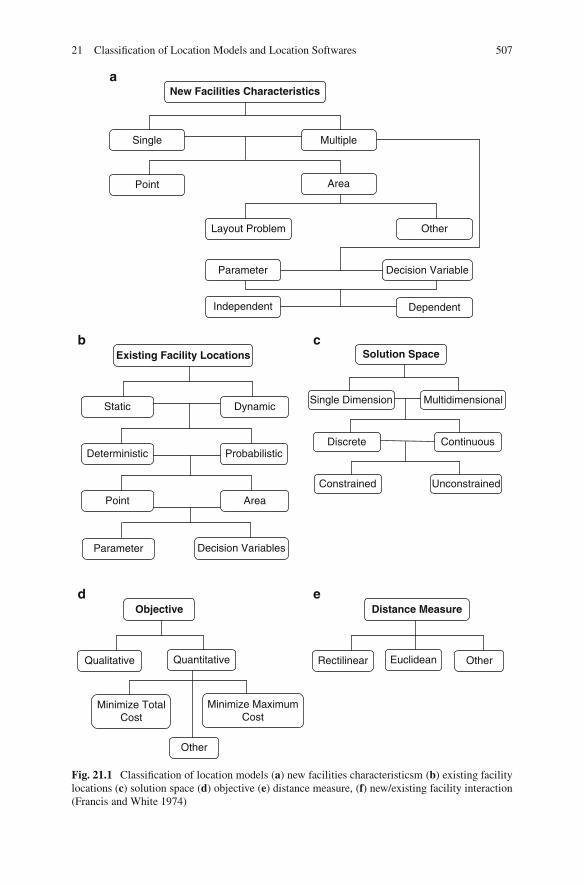
21 Classification of Location Models and Location Softwares 507
a
b c
d eDistance Measure
Rectilinear OtherEuclidean
Objective
Qualitative
Minimize TotalCost
Quantitative
Minimize MaximumCost
Other
Solution Space
Single Dimension Multidimensional
Discrete Continuous
Constrained Unconstrained
Existing Facility Locations
Static Dynamic
Deterministic Probabilistic
Point Area
Parameter Decision Variables
New Facilities Characteristics
Single Multiple
Point Area
Layout Problem Other
Parameter Decision Variable
Independent Dependent
Fig. 21.1 Classification of location models (a) new facilities characteristicsm (b) existing facilitylocations (c) solution space (d) objective (e) distance measure, (f) new/existing facility interaction(Francis and White 1974)
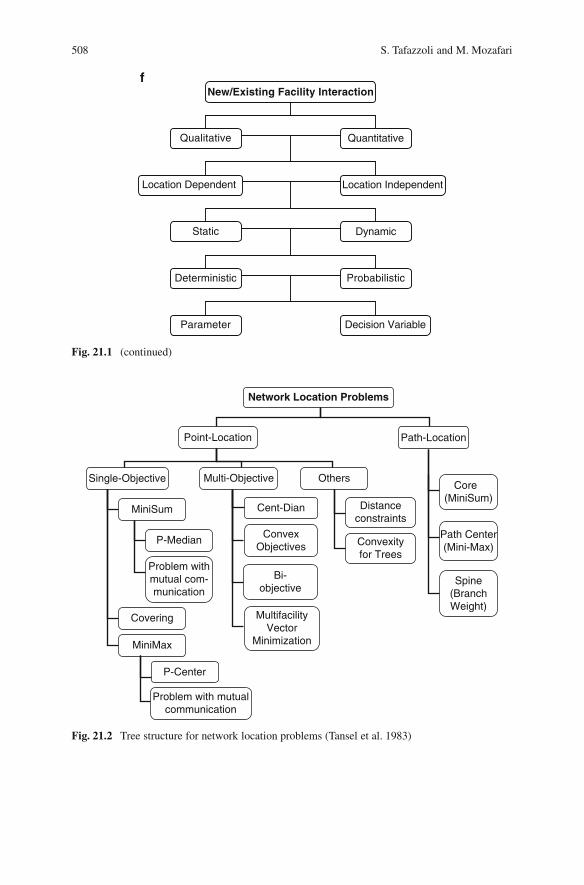
508 S. Tafazzoli and M. Mozafari
New/Existing Facility Interactionf
Qualitative Quantitative
Location Dependent Location Independent
Static Dynamic
Deterministic Probabilistic
Parameter Decision Variable
Fig. 21.1 (continued)
Network Location Problems
Point-Location Path-Location
Single-Objective Multi-Objective OthersCore
(MiniSum)
Path Center(Mini-Max)
Spine(BranchWeight)
Distanceconstraints
Convexityfor Trees
MultifacilityVector
Minimization
Bi-objective
ConvexObjectives
Cent-Dian
Problem with mutualcommunication
P-Center
MiniMax
Covering
Problem withmutual com-munication
P-Median
MiniSum
Fig. 21.2 Tree structure for network location problems (Tansel et al. 1983)
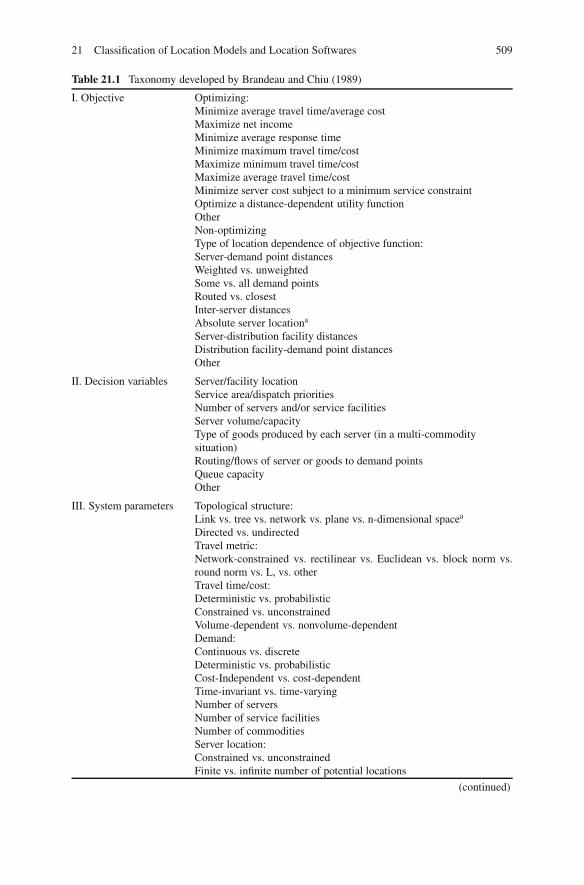
21 Classification of Location Models and Location Softwares 509
Table 21.1 Taxonomy developed by Brandeau and Chiu (1989)
I. Objective Optimizing:Minimize average travel time/average costMaximize net incomeMinimize average response timeMinimize maximum travel time/costMaximize minimum travel time/costMaximize average travel time/costMinimize server cost subject to a minimum service constraintOptimize a distance-dependent utility functionOtherNon-optimizingType of location dependence of objective function:Server-demand point distancesWeighted vs. unweightedSome vs. all demand pointsRouted vs. closestInter-server distancesAbsolute server locationa
Server-distribution facility distancesDistribution facility-demand point distancesOther
II. Decision variables Server/facility locationService area/dispatch prioritiesNumber of servers and/or service facilitiesServer volume/capacityType of goods produced by each server (in a multi-commoditysituation)Routing/flows of server or goods to demand pointsQueue capacityOther
III. System parameters Topological structure:Link vs. tree vs. network vs. plane vs. n-dimensional spacea
Directed vs. undirectedTravel metric:Network-constrained vs. rectilinear vs. Euclidean vs. block norm vs.round norm vs. L, vs. otherTravel time/cost:Deterministic vs. probabilisticConstrained vs. unconstrainedVolume-dependent vs. nonvolume-dependentDemand:Continuous vs. discreteDeterministic vs. probabilisticCost-Independent vs. cost-dependentTime-invariant vs. time-varyingNumber of serversNumber of service facilitiesNumber of commoditiesServer location:Constrained vs. unconstrainedFinite vs. infinite number of potential locations
(continued)
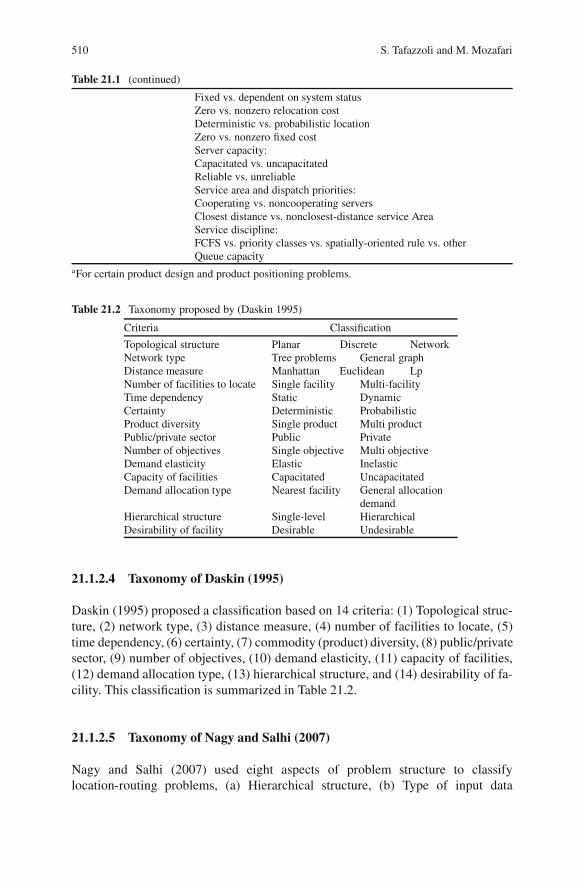
510 S. Tafazzoli and M. Mozafari
Table 21.1 (continued)
Fixed vs. dependent on system statusZero vs. nonzero relocation costDeterministic vs. probabilistic locationZero vs. nonzero fixed costServer capacity:Capacitated vs. uncapacitatedReliable vs. unreliableService area and dispatch priorities:Cooperating vs. noncooperating serversClosest distance vs. nonclosest-distance service AreaService discipline:FCFS vs. priority classes vs. spatially-oriented rule vs. otherQueue capacity
aFor certain product design and product positioning problems.
Table 21.2 Taxonomy proposed by (Daskin 1995)
Criteria Classification
Topological structure Planar Discrete NetworkNetwork type Tree problems General graphDistance measure Manhattan Euclidean LpNumber of facilities to locate Single facility Multi-facilityTime dependency Static DynamicCertainty Deterministic ProbabilisticProduct diversity Single product Multi productPublic/private sector Public PrivateNumber of objectives Single objective Multi objectiveDemand elasticity Elastic InelasticCapacity of facilities Capacitated UncapacitatedDemand allocation type Nearest facility General allocation
demandHierarchical structure Single-level HierarchicalDesirability of facility Desirable Undesirable
21.1.2.4 Taxonomy of Daskin (1995)
Daskin (1995) proposed a classification based on 14 criteria: (1) Topological struc-ture, (2) network type, (3) distance measure, (4) number of facilities to locate, (5)time dependency, (6) certainty, (7) commodity (product) diversity, (8) public/privatesector, (9) number of objectives, (10) demand elasticity, (11) capacity of facilities,(12) demand allocation type, (13) hierarchical structure, and (14) desirability of fa-cility. This classification is summarized in Table 21.2.
21.1.2.5 Taxonomy of Nagy and Salhi (2007)
Nagy and Salhi (2007) used eight aspects of problem structure to classifylocation-routing problems, (a) Hierarchical structure, (b) Type of input data
21 Classification of Location Models and Location Softwares 511
(deterministic/stochastic), (c) Planning period (single/multi-period), (d) Solutionmethod (exact/heuristic), (e) Objective function, (f) Solution space, (g) Number ofdepots (single/multiple), (h) Number and types of vehicles (homogeneous/ hetero-geneous), and (i) Route structure.
21.1.2.6 Taxonomy of ReVelle et al. (2008)
ReVelle et al. (2008) provided a brief taxonomy of broad field of facility locationmodeling in a bibliography in two branches of discrete location science (1) medianand plant location models and (2) center and covering models. In this taxonomy,location models are classified into four categories:
1. Analytic models are based on large simplifying assumptions (fixed cost of locat-ing a facility dependent of where it will locate, demand uniformly distributed,etc). Despite valuable insight which this class of models provides, they cannot beused for real decision-making purposes
2. Continuous models assume that facilities can be located anywhere in service area,while demands are often taken as being at discrete locations
3. Network models assume that topological structure of the location model is anetwork composed of lines and nodes. Much of the literature in this area is con-cerned with finding special structures that can be exploited to derive low-orderpolynomial time algorithms
4. Discrete models assume that the set of demands and candidate location for fa-cilities are discrete. These problems often formulate in integer or mix-integerprogramming that most of them are NP-hard on general network
In addition of these classifications, location models can also be distinguished basedon other attributes (Klose and Drexl 2004; Jia et al. 2007)
21.1.3 Classification Schemes
In several branches of optimization, classification schemes have been proposed andused by authors successfully (schemes in scheduling (Graham et al. 1979) and queu-ing theory (Kendall 1951)). Classification schemes are also proposed in locationscience that few of them will be mentioned here.
21.1.3.1 Classification Scheme of Handler and Mirchandani (1979)
The first classification scheme was proposed by Handler and Mirchandani (1979).They suggested a 4-position scheme which is applicable to network location modelswith objective functions of the center type.
512 S. Tafazzoli and M. Mozafari
Pos1/Pos2/Pos3/Pos4Position 1: information about the new facilitiesPosition 2: information about existing facilitiesPosition 3: number of new facilitiesPosition 4: network type
21.1.3.2 Classification Scheme of Eiselt et al. (1993)
Eiselt et al. (1993) suggested a 5-position scheme for classifying competitive loca-tion models (those based on a game-theory approach).
Pos1/Pos2/Pos3/Pos4/Pos5Position 1: information about the decision space (linear segment, line, circle,
bounded subset of m-dimensional real space, m-dimensional real space, network,tree)
Position 2: number of players (specified number, any arbitrary fixed number,markets with free entry)
Position 3: a description of the pricing policy (mill pricing, uniform deliveredpricing, perfect spatial discriminatory pricing)
Position 4: rules of the game under consideration (Cournot-Nash equilibrium,subgame perfect Nash equilibrium, Stackelberg equilibrium)
Position 5: behavior of the customers (minimization of distance, minimization ofa deterministic or random utility)
21.1.3.3 Classification Scheme of Carrizosa et al. (1995)
Carrizosa et al. (1995) presented a 6-position scheme for classifying planar modelswhere both demand rates and service times are given by a probability distribution.
21.1.3.4 Classification Scheme of Hamacher and Nickel (1998)
Hamacher and Nickel (1998) proposed a 5-position classification scheme for lo-cation models that covers not only classes of specific location models, as in thereferences above, but also covers all of them in a single scheme. Furthermore, thisscheme can describe models which are not of the classical type and problems whichhave not been solved yet. The classification scheme has been in use since 1992 andhas been proven to be helpful in research, software development, classroom teach-ing, and for overview articles. The software library, Library of location algorithms(LoLA) has been developed (Hamacher et al. 1996) based on this classificationscheme. The classification scheme consists of the following five positions:
Pos1/Pos2/Pos3/Pos4/Pos5,where position 1 contains information about the number and type of new facilities.Position 2 indicates type of the location model with respect to the decision space.
21 Classification of Location Models and Location Softwares 513
Position 3 describes the particulars of the specific location model, such as infor-mation about the feasible solutions, capacity restrictions, etc. In position 4, relationbetween new and existing facilities is defined by a distance function or by assignedcosts. In position 5 a description of the objective function is given.
A list of symbols is available for each position that covers a large variety oflocation models. In Table 21.3, some examples of these symbols, according to thethree main areas of location theory (i.e. continuous location, network location anddiscrete location) is given.
If there are not any special assumptions in a position, this is indicated by �. Forexample, a � in position 5 means that any objective function are looked or the � inposition 3 means that standard assumptions for the model described in the remainingfour positions hold. It is assumed by default that weights are non-negative and theobjective function is to be minimized. If these assumptions do not hold this has tobe stated respectively in positions 3 and 5.
In the following, some examples from the literature are given that indicate theability of the 5-position classification scheme to describe various kinds of loca-tion models. Of course the 5-position classification scheme cannot represent thecomplete contents of a paper, but it can reflect the major particulars of the modelsinvestigated.
� Brandeau (1992): 1=P=queue=lP=P
prob
� Erkut and Tansel (1992): 1=T=wm W f .:/=d.V;G/=†� Eiselt and Laporte (1993): 3=T=:=d.V;G/=˙comp
� Mirchandani et al (1996): #=D=F D line; cap=:=†cov
� Burkard et al. (2000): P=G=wm >< 0=d.V;G/=†� Klamroth (2004):1=P=BC=l2;BC
=f convex� Gomes et al. (2007):N=P=alloc=l2=†� Colebrook and Sicilia (2007):1=G=:=d.V;G/=Q� CDpar
21.2 Facility Location Softwares
In previous chapters, many models and algorithms have been discussed for solvingdifferent facility location problems. Of course, in large real world problems, it is im-possible to implement these algorithms manually. In this point computer programsor special software come into play.
Some of the major facility location software is introduced in this section. Al-though they cannot cover all of the facility location models, they are still underdevelopment.
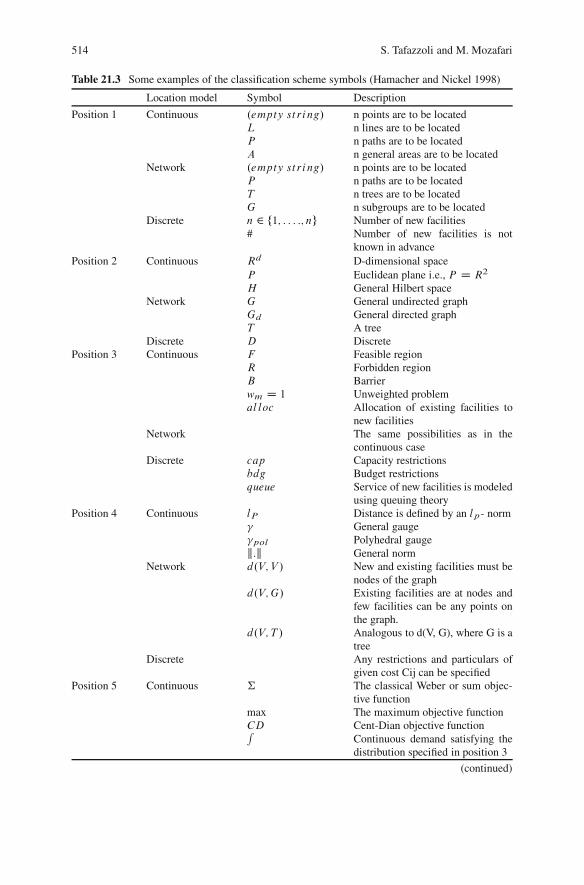
514 S. Tafazzoli and M. Mozafari
Table 21.3 Some examples of the classification scheme symbols (Hamacher and Nickel 1998)
Location model Symbol Description
Position 1 Continuous .empty st ring/ n points are to be locatedL n lines are to be locatedP n paths are to be locatedA n general areas are to be located
Network .empty st ring/ n points are to be locatedP n paths are to be locatedT n trees are to be locatedG n subgroups are to be located
Discrete n 2 f1; : : : :; ng Number of new facilities# Number of new facilities is not
known in advancePosition 2 Continuous Rd D-dimensional space
P Euclidean plane i.e., P D R2
H General Hilbert spaceNetwork G General undirected graph
Gd General directed graphT A tree
Discrete D DiscretePosition 3 Continuous F Feasible region
R Forbidden regionB Barrierwm D 1 Unweighted problemal loc Allocation of existing facilities to
new facilitiesNetwork The same possibilities as in the
continuous caseDiscrete cap Capacity restrictions
bdg Budget restrictionsqueue Service of new facilities is modeled
using queuing theoryPosition 4 Continuous lP Distance is defined by an lp- norm
� General gauge�pol Polyhedral gaugek:k General norm
Network d.V; V / New and existing facilities must benodes of the graph
d.V;G/ Existing facilities are at nodes andfew facilities can be any points onthe graph.
d.V; T / Analogous to d(V, G), where G is atree
Discrete Any restrictions and particulars ofgiven cost Cij can be specified
Position 5 Continuous † The classical Weber or sum objec-tive function
max The maximum objective functionCD Cent-Dian objective functionR
Continuous demand satisfying thedistribution specified in position 3
(continued)
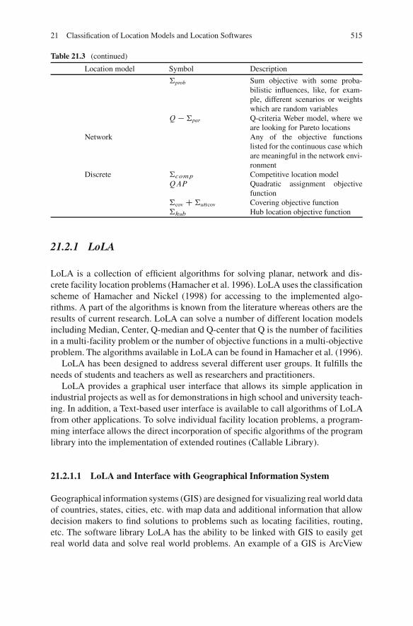
21 Classification of Location Models and Location Softwares 515
Table 21.3 (continued)
Location model Symbol Description
†prob Sum objective with some proba-bilistic influences, like, for exam-ple, different scenarios or weightswhich are random variables
Q �†par Q-criteria Weber model, where weare looking for Pareto locations
Network Any of the objective functionslisted for the continuous case whichare meaningful in the network envi-ronment
Discrete †comp Competitive location modelQAP Quadratic assignment objective
function†cov C†uncov Covering objective function†hub Hub location objective function
21.2.1 LoLA
LoLA is a collection of efficient algorithms for solving planar, network and dis-crete facility location problems (Hamacher et al. 1996). LoLA uses the classificationscheme of Hamacher and Nickel (1998) for accessing to the implemented algo-rithms. A part of the algorithms is known from the literature whereas others are theresults of current research. LoLA can solve a number of different location modelsincluding Median, Center, Q-median and Q-center that Q is the number of facilitiesin a multi-facility problem or the number of objective functions in a multi-objectiveproblem. The algorithms available in LoLA can be found in Hamacher et al. (1996).
LoLA has been designed to address several different user groups. It fulfills theneeds of students and teachers as well as researchers and practitioners.
LoLA provides a graphical user interface that allows its simple application inindustrial projects as well as for demonstrations in high school and university teach-ing. In addition, a Text-based user interface is available to call algorithms of LoLAfrom other applications. To solve individual facility location problems, a program-ming interface allows the direct incorporation of specific algorithms of the programlibrary into the implementation of extended routines (Callable Library).
21.2.1.1 LoLA and Interface with Geographical Information System
Geographical information systems (GIS) are designed for visualizing real world dataof countries, states, cities, etc. with map data and additional information that allowdecision makers to find solutions to problems such as locating facilities, routing,etc. The software library LoLA has the ability to be linked with GIS to easily getreal world data and solve real world problems. An example of a GIS is ArcView
516 S. Tafazzoli and M. Mozafari
GIS using script language called Avenue. This language has been implemented tocombine ArcView GIS with LoLA (Bender et al. 2002).
Via LoLA ArcView R� Link it is possible to read data out of the ArcView GISdatabase and convert them into a LoLA input file, then call LoLA Libraries to solvethe model and finally monitor the results and get the solution back to ArcView GIS.
21.2.1.2 LoLA Example
Here a simple example (from software package) is used to illustrate the ideas in-volved and the basic data required in LoLA.
Consider uncapacitated facility location (UFL) problem, by choosing the char-acteristics of 5-position classification scheme from software menus, LoLA exhibitthe classification by symbols, #=D= � = � =† (Pos1: Number of facilities to locatedetermine by model, Pos2: Discrete solution space, Pos3: No special conditions inmodel, Pos4: Metric define by cost matrix as input, Pos5: Sum (median) objectivefunction).
Input format of this discrete location model contains information about:
� Demand point (x; y; b; n) where x and y are coordinates, b is the customer de-mand and n is the facility name, for example: 54.00 15.00 5,000 [Palermo]
� Cost matrix (n n matrix defines travel or transport cost or time from facility ito j ).
This model is solved for a UFL problem to identify the cities in Italy from which toservice demand of customer sites in a total of 39 cities (supply point must be placedon demand points).
The optimal result consists of:
� The number and location of supply points (opt1 is Lucca and opt2 is Viterbo,Fig. 21.3)
� objective function value� and allocation of demand points to each supply point (Fig. 21.3)
21.2.2 SITATION
SITATION (Daskin 2002) is a facility location software that accompanies Daskin’stext (Network and discrete location: models, algorithms, and applications). The SI-TATION software now solves a number of different discrete and network facilitylocation problems including:
� P-median� P-center� Set covering� Maximal covering
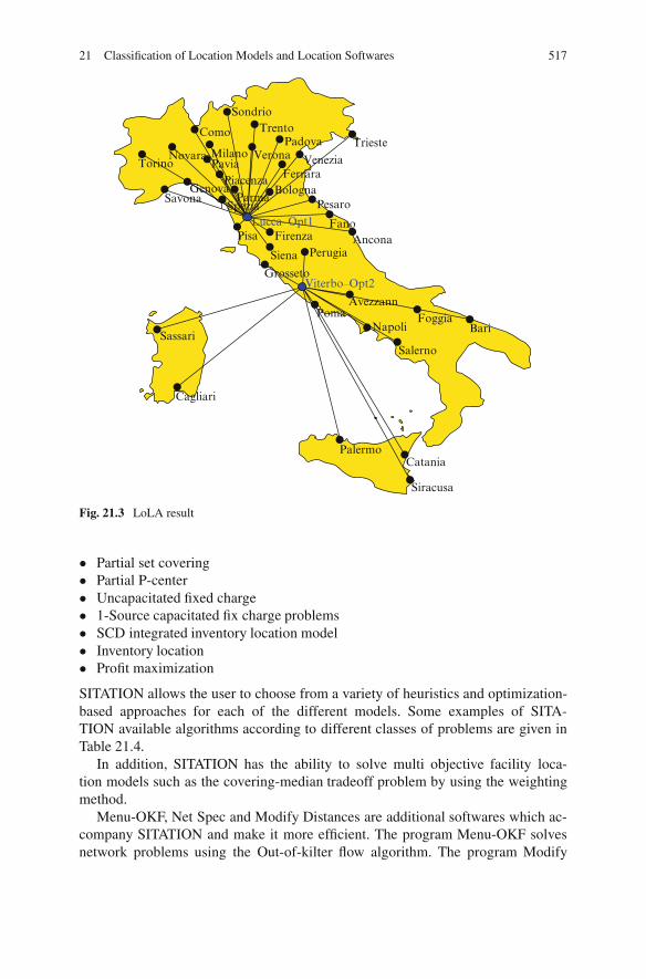
21 Classification of Location Models and Location Softwares 517
Sassari
Cagliari
Catania
Salerno
BariFoggiaPoma
Avezzann
Perugia
Grosseto
Siena
Spezia
Firenza AnconaFano
PesaroBologna
Pisa
ParmaSavonaGenova
NovaraTorino Pavia
Milano
Como
SondrioTrento
Padova
VeneziaFerrara
Verona
Piacenza
Lucca–Opt1
Viterbo–Opt2
Napoli
Siracusa
Palermo
Trieste
Fig. 21.3 LoLA result
� Partial set covering� Partial P-center� Uncapacitated fixed charge� 1-Source capacitated fix charge problems� SCD integrated inventory location model� Inventory location� Profit maximization
SITATION allows the user to choose from a variety of heuristics and optimization-based approaches for each of the different models. Some examples of SITA-TION available algorithms according to different classes of problems are given inTable 21.4.
In addition, SITATION has the ability to solve multi objective facility loca-tion models such as the covering-median tradeoff problem by using the weightingmethod.
Menu-OKF, Net Spec and Modify Distances are additional softwares which ac-company SITATION and make it more efficient. The program Menu-OKF solvesnetwork problems using the Out-of-kilter flow algorithm. The program Modify
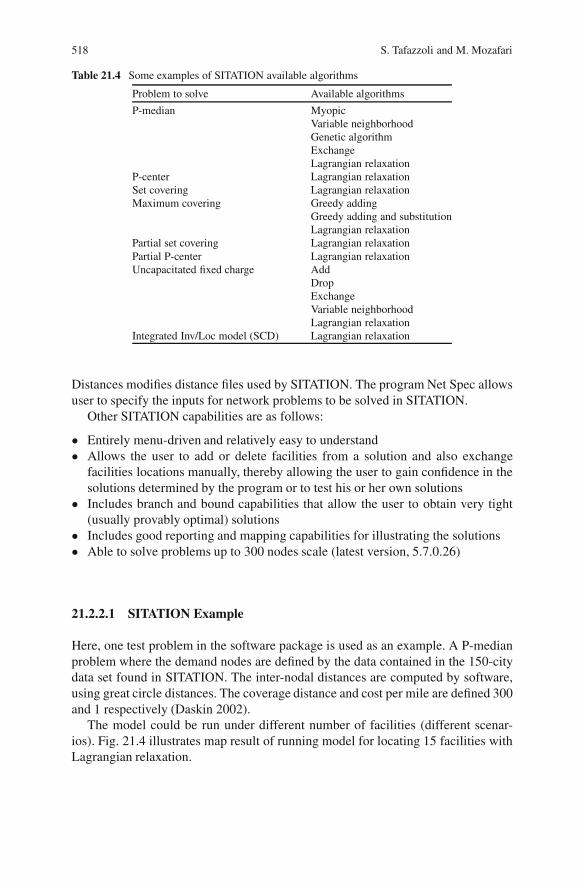
518 S. Tafazzoli and M. Mozafari
Table 21.4 Some examples of SITATION available algorithms
Problem to solve Available algorithms
P-median MyopicVariable neighborhoodGenetic algorithmExchangeLagrangian relaxation
P-center Lagrangian relaxationSet covering Lagrangian relaxationMaximum covering Greedy adding
Greedy adding and substitutionLagrangian relaxation
Partial set covering Lagrangian relaxationPartial P-center Lagrangian relaxationUncapacitated fixed charge Add
DropExchangeVariable neighborhoodLagrangian relaxation
Integrated Inv/Loc model (SCD) Lagrangian relaxation
Distances modifies distance files used by SITATION. The program Net Spec allowsuser to specify the inputs for network problems to be solved in SITATION.
Other SITATION capabilities are as follows:
� Entirely menu-driven and relatively easy to understand� Allows the user to add or delete facilities from a solution and also exchange
facilities locations manually, thereby allowing the user to gain confidence in thesolutions determined by the program or to test his or her own solutions
� Includes branch and bound capabilities that allow the user to obtain very tight(usually provably optimal) solutions
� Includes good reporting and mapping capabilities for illustrating the solutions� Able to solve problems up to 300 nodes scale (latest version, 5.7.0.26)
21.2.2.1 SITATION Example
Here, one test problem in the software package is used as an example. A P-medianproblem where the demand nodes are defined by the data contained in the 150-citydata set found in SITATION. The inter-nodal distances are computed by software,using great circle distances. The coverage distance and cost per mile are defined 300and 1 respectively (Daskin 2002).
The model could be run under different number of facilities (different scenar-ios). Fig. 21.4 illustrates map result of running model for locating 15 facilities withLagrangian relaxation.
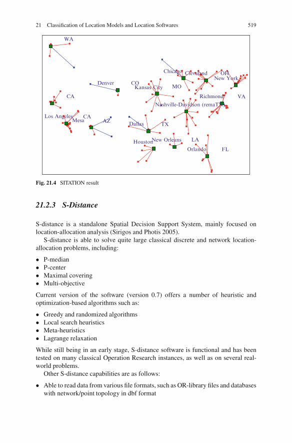
21 Classification of Location Models and Location Softwares 519
Denver
Dallas TX
HoustonNew Orleans
Orlando FL
LA
CA
CAAZ
WA
Los AngelesMesa
Kansas City MO
Chicago Cleveland OHNew York
Richmond VA
Nashville-Davidson (remaTN)
CO
Fig. 21.4 SITATION result
21.2.3 S-Distance
S-distance is a standalone Spatial Decision Support System, mainly focused onlocation-allocation analysis (Sirigos and Photis 2005).
S-distance is able to solve quite large classical discrete and network location-allocation problems, including:
� P-median� P-center� Maximal covering� Multi-objective
Current version of the software (version 0.7) offers a number of heuristic andoptimization-based algorithms such as:
� Greedy and randomized algorithms� Local search heuristics� Meta-heuristics� Lagrange relaxation
While still being in an early stage, S-distance software is functional and has beentested on many classical Operation Research instances, as well as on several real-world problems.
Other S-distance capabilities are as follows:
� Able to read data from various file formats, such as OR-library files and databaseswith network/point topology in dbf format
520 S. Tafazzoli and M. Mozafari
� Provides all Pairs Shortest Paths calculation using Dijkstra’s (2-ary heap) orFloyd’s algorithms, for network problems
� Incorporate an interactive solution process within a simplified GIS framework� Allows the user straight-forward creation and evaluation of different solutions
both numerically and graphically
21.2.4 Other Facility Location Softwares
There is some other facility location software specialized on solving a specific prob-lem and limited more in their functionalities than the three software introducedabove. Some examples are given in the following:
� RLP is a program package for solving restricted 1-facility location problems in auser friendly environment (Nickel and Hamacher 1992)
� Optimal locating air polluting facilities is a general modeling system to evaluateand optimize the location of an air polluting facility (Fliege 2001)
� Jure Mihelic’s K-center algorithms is a program for solving k-Center locationproblems (Mihelic 2004)
� Minimum enclosing circle applet is a program package for solving the MinimalEnclosing Circle problem (Eliosoff and Unger 1998). It is useful for planning thelocation of a shared facility
� Excel template for facility location includes model for center-of-gravity methodfor locating distribution centers
� GAMBINI is a small GIS-utility which calculates draws and exports multiplica-tive weighted Voronoi diagrams (Tiefelsdorf and Boots 1997). A point locationdata structure can be built on top of the Voronoi diagram in order to find theobject that is nearest to a given point
� Mathematical programming softwares such as CPLEX, LINGO, LINDO andGAMS which are useful when having mathematical models for facility locationproblems
References
Bender T, Hennes H, Kalcsics J, Melo MT, Nickel S (2002) Location software and interface withGIS and supply chain management. In: Drezner Z, Hammacher H (eds) Facility location: ap-plications and theory. Berlin, Springer
Brandeau ML (1992) Characterization of the stochastic median queue trajectory in a plane withgeneralized distances. Oper Res 40(2):331–341
Brandeau ML, Chiu SS (1989) An overview of representative problems in location research. Man-age Scie 35:645–674
Burkard RE, Cela E, Dollani H (2000) 2-Medians in trees with pos/neg weights. Discrete ApplMath 105:51–71
21 Classification of Location Models and Location Softwares 521
Carrizosa EJ, Conde E, Munoz M, Puerto J (1995) The generalized weber problem with expecteddistances. RAIRO 29:35–57
Colebrook M, Sicilia J (2007) A polynomial algorithm for the multicriteria cent-dian locationproblem. Eur J Oper Res 179:1008–1024
Daskin MS (1995) Network and discrete location: models, algorithms, and applications. WileyInterscience, NY
Daskin MS (2002) SITATION-facility location software. Department of Industrial Engineer-ing and Management Sciences, Northwestern University, Evanston, IL. http://users.iems.northwestern.edu/�msdaskin/
Eiselt HA, Laporte G (1993) The existence of equilibria in the 3-facility Hotelling model in a tree.Transport Sci 27(1):39–43
Eiselt HA, Laporte G, Thisse JF (1993) Competitive location models: a framework and bibliogra-phy. Transport Sci 27:44–54
Eliosoff J, Unger R (1998). MEC – minimum enclosing circle applet. http://www.cs.mcgill.ca/�cs507/projects/1998/jacob/welcome.html
Erkut E, Tansel BC (1992) On parametric medians of trees. Transport Sci 26(2):149–156Fliege J (2001) OLAF – a general modeling system to evaluate and optimize the location of an air
polluting facility. OR Spektrum 23:117–136Francis RL, White JA (1974) Facility layout and location: an analytical approach. Prentice-Hall,
Englewood CliffsGomes H, Ribeiro AB, Lobo V (2007) Location model for CCA-treated wood waste remediation
units using GIS and clustering methods. Environ Model Softw 22:1788–1795Graham RE, Lawler EL, Lenstra JK, Rinnoy Kan AHG (1979) Optimization and approximation in
deterministic sequencing and scheduling: a survey. Ann Discrete Math 4:287–326Hamacher HW, Nickel S (1998) Classification of location models. Location Sci. 6:229–242Hamacher HW, Klamroth K, Nickel S, Schoebel A (1996) Library of location algorithms. Univer-
sity of Kaiserslautern. http://www.mathematik.uni-kl.de/lola/Handler GY, Mirchandani PB (1979) Location on networks theory and algorithms. MIT Press,
CambridgeJia H, Ordonez F, Dessouky M (2007) A modeling framework for facility location of medical
services for large-scale emergencies. IIE Trans 39:41–55Kendall D (1951) Some problems in the theory of queues. J R Stat Soc 13:151–153Klamroth K (2004) Algebraic properties of location problems with one circular barrier. Eur J Oper
Res 154:20–35Klose A, Drexl A (2004) Facility location models for distribution system design. Eur J Oper Res
162:4–29Mihelic J (2004) Jure Mihelic k-center algorithms. Department of Computer and Information Sci-
ence, University of LjubljanaMirchandani P, Kohli R, Tamir A (1996) Capacitated location problems on a line. Transport Sci
30(1):75–80Nagy G, Salhi S (2007) Location-routing: issues, models and methods. Eur J Oper Res
177:649–672Nickel S, Hamacher HW (1992) RLP: a program package for solving restricted 1-facility location
problems in a user friendly environment. Eur J Oper Res 62:116–117ReVelle CS, Eiselt HA, Daskin MS (2008) A bibliography for some fundamental problem cate-
gories in discrete location science. Eur J Oper Res 184:817–848Sirigos S, Photis YN (2005) S-distance software. Department of Planning and Regional Develop-
ment (DPRD), University of Thessaly, GreeceTansel BC, Francis RL, Lowe TJ (1983) Location on networks: a survey. Part I: the p-center and
p-median problems. Manage Sci 29:482–497Tiefelsdorf M, Boots B (1997) GAMBINI multiplicative weighted voronoi diagrams. http://www.
wlu.ca/wwwgeog/special/download/gambini.htm
Chapter 22Demand Point Aggregation Analysisfor Location Models
Ali NaimiSadigh and Hamed Fallah
When selecting locations for facilities, such as hospitals, fire stations schools, ware-houses and retail outlets, one has to take into account the demand for the serviceprovided by the facility. In many instances, such facilities serve a large number of in-dividuals, and it may not be realistic to model each individual as a separate demandpoint (DP). To reduce the problem size to a manageable one, an analyst is usu-ally forced to aggregate the demand (population) data by representing a collectionof individuals as one DP. While this is a practical solution, it perturbs the originalproblem and may introduce errors to subsequent analysis (Erkut and Bozkaya 1999).
Many location problems can be formulated as minimizing some location objec-tive function subject to upper bounds on other location constraint functions. Whensuch functions are sub additive and no decreasing in the distances, worst-case DPaggregation error bounds are known. It is shown how to solve a relaxation and arestriction of the aggregated problem in such a way as to obtain lower and upperbounds on the optimal value of the original problem (Francis et al. 2002).
Location problems often involve finding locations of new facilities that provideservices of some kind to existing facilities, also called DPs. When such problemstake place in urban contexts, each private residence can be a DP. Thus there canbe too many DPs to be modeled individually, and aggregation of the DPs becomesnecessary; indeed, sometimes only aggregated data is available. This aggregationcreates a more tractable model, but also introduces model error.
It is naturally of interest to examine how much error is introduced, and the effectof the level of aggregation upon the error. Essentially the modeler is faced with atradeoff: less model accuracy for more model tractability, or vice versa.
Hillsman and Rhoda (1978) were perhaps the first to study errors associated withDP aggregation for the K-median problem. Their classification of aggregation errorswas further studied by Current and Schilling (1987), Erkut and Bozkaya (1999) andZhao and Batta (1999). Plastria (2001), in an effort to reduce aggregation error,further refined the Hillsman–Rhoda error classification, and made a strong case forusing the centroid of each aggregation group as the representative point for the groupin the reduced K-median problem. Current and Schilling (1987) considered errorsdue to aggregation for the (discrete) covering problem.
Methods for reducing DP aggregation error have been proposed by Currentand Schilling (1987), Bowerman et al. (1999), and Hodgson and Neuman (1993).
R.Z. Farahani and M. Hekmatfar (eds.), Facility Location: Concepts, Models, 523Algorithms and Case Studies, Contributions to Management Science,DOI 10.1007/978-3-7908-2151-2 22, c� Physica-Verlag Heidelberg 2009
524 A. NaimiSadigh and H. Fallah
General background discussions on DP aggregation and resulting errors can befound in Zhao and Batta (1999, 2000) and Plastria (2001).
Zhao and Batta (2000) point out that there is another kind of aggregation error;it is perhaps less obvious but often occurs. Due to budgetary constraints, only asubset of the set of all possible feasible solutions may be considered. For example,potential location sites of interest may be enumerated in a list. Sites might be addedto the list with more resources to consider sites of interest, additional. This approachis usually viewed as solving a restriction of the actual problem, but it can also beviewed as a “solution space” aggregation, since a large collection of potential sitesis, in effect, aggregated into a smaller collection. Zhao and Batta (1999, 2000) alsogive a general background discussion of DP aggregation, as do Francis et al. (2002).
22.1 Applications
22.1.1 P-Median Problem
A network location model is defined with respect to a connected graph and a setof weighted DPs on the graph; generally, p new facilities are to be established toservice these DPs. The problem of optimally locating the p new facilities so that thesum of the weighted network distances between the DPs and their respective closestnew facilities is smallest is called the p-median problem (Andersson et al. 1998).
The p-median model is arguably the most popular model in the facility loca-tion literature dealing with multiple facilities. Given n DPs in some space (such asEuclidean plane or road network), the goal of the model is to locate p service facil-ities, and allocate the n DPs to these service facilities such as to minimize the totaldistance to be traveled for service. It is possible to solve medium-sized instances(n D 200) of this problem optimally. Furthermore, efficient heuristics are availableto solve larger instances of the problem (n D 1; 000) to near optimality.
Unfortunately, for most realistic instances of the facility location problem, thenumber of DPs is much larger. For example, if we wish to locate facilities (suchas retail outlets, post offices, or bank machines) in a city, then each resident is apotential DP. Given that the population of many large cities exceeds one million, theneed for some aggregation becomes apparent (Erkut and Bozkaya 1999).
22.1.2 P-Center Problem
A model frequently proposed for locating emergency service facilities is thep-center model. Its solution recommends locations for such facilities to mini-mize the maximum time (or distance) in order to respond to an emergency at someDP. In an urban context, there could be millions of possible emergency DPs. Thus,it is common to aggregate DPs.
22 Demand Point Aggregation Analysis for Location Models 525
Location models are generally NP-hard. Furthermore, real-world location prob-lems are often large in scale, and are not solvable to optimality within reasonabletime and effort. Thus, in practice, approximate representations of problems are cre-ated by means of DP aggregation (Rayco et al. 1999).
22.1.3 Covering Problem
Covering models measure effectiveness through assessment of whether demand canreceive service from located facilities (Church and ReVelle 1974). The key conceptin these models is the acceptable proximity or coverage. Usually a maximum value,known as the service standard, is preset with respect to either distance or traveltime, though the latter can be converted to a distance measure. Demand is said to besuitably served if it can be reached by any facility within this maximum coveragestandard. For example, fire department response time should be less than 6 min toan accident or structure fire after a call for service has been received (Tong andMurray 2006).
22.2 Aggregation Errors
22.2.1 Spatial Aggregation Demand
Spatial aggregation of demand units is a common technique used in the solutionof LA models. As mentioned previously, many location problems, including thep-median problem, are NP-hard. Spatial aggregation of the demand units resultsin a reduction of the size of these problems to make them computationally moretractable.
The aggregation process reduces the number of distinct demand units so thatthe m unaggregated demand units indexed by U are aggregated to q < m aggre-gated demand units indexed by the set A D f1; : : :; qg with the demand of eachunaggregated demand unit assigned to its respective aggregated demand unit. Moreprecisely, if the set Uj identifies the unaggregated demand units that are associatedwith aggregated demand unit j�A then the total demand of this aggregated demandunit is given by:
! DXi2Uj
wi j 2 A (22.1)
fU .X/ DXi2U
wiD.X; ui / (22.2)
526 A. NaimiSadigh and H. Fallah
In this way, the function f given in (22.2) can be approximated by:
fA.X/ DXj2A
!jD.X; aj / (22.3)
Where aj is the j th aggregated demand unit and D.X; aj / is a measure of thedistance between aj and the element of X that serves the corresponding demand.Different approximations results by varying the way in which aj and D(X, aj ),j�A, are defined. In any case, solving the p-median problem defined by (22.3) iscomputationally more attractive than solving the one defined by (22.2) simply be-cause q < m. In what follows, we will use the terms basic spatial unit (BSU) andaggregated spatial unit (ASU) to distinguish between unaggregated and aggregateddemand units, respectively. This process of demand aggregation can induce errorsin the evaluation of the cost of a solution to the p-median problem. This error arisessince, in general, the cost of a given solution is different when evaluated using theASUs and the BSUs. The total error caused by the aggregation process for a givensolution NX � S with
ˇ NX ˇ D p is given by:
fA. NX/ � fU . NX/ (22.4)
Hillsman and Rhoda (1978) categorized this error into three different sourceswith two different causes: error due to incorrect distance estimation (SourceA and B) and error caused by misallocating BSUs (Source C). Source A errorsarise since the demand weighted distance from an ASU to a candidate facility siteis not equal to the demand weighted distances between the corresponding BSUsand the same site. Source B errors are a special case of source A errors and occurwhen a potential facility site is at the same position as an ASU. For a given solutionNX � S with
ˇ NX ˇ D p the total source A and B aggregation error is given by:
fA. NX/ � fA;U . NX/
Where for X � S ,
fA;U .X/ DXi2A
Xj2Uj
wj d.X.ai /; uj // (22.5)
Source B errors result in the cost of a solution, underestimating its actual cost,while sourceA errors can result in either underestimation or overestimation. SourceC errors occur because all demand in an ASU is allocated to a single facility eventhough some of the corresponding BSUs may be closer to a different facility. For agiven solution NX � S with
ˇ NX ˇ D p the total source C error can be calculated as:
fA;U . NX/ � fA. NX/
Source C errors result in the cost of the solution to the aggregated problem over-estimating the actual cost of the solution.
22 Demand Point Aggregation Analysis for Location Models 527
Hillsman and Rhoda (1978) examined aggregation error for uniformly distributeddemand in three different configurations and calculated aggregation errors of up to8%. On different data sets, Current and Schilling (1987) discovered aggregationerrors of over 20%.
The discussion so far has concentrated on the total error in the objective functioncaused by aggregation. However, Goodchild (1979) noted that “aggregation tendsto produce much more dramatic effects on facility locations than on the value ofthe objective function” and Bach (1981) further pointed out that ‘the level of ag-gregation exerts a strong influence on the optimal location patterns as well as onthe values of the location criteria. Casillas (1987) clarified this notion by distin-guishing two classes of errors that aggregation causes in the solution of p-medianproblems.
The first is cost estimate error defined as the difference between the estimatedcost of the solution using the aggregated data and the true objective cost calculatedusing the unaggregated data. The other is optimality error which is the differencebetween the actual costs of the solution found using the aggregated data and the costof the solution found using the unaggregated data. If we define:
X�A D argX minfA.X/
as the optimal solution to the p-median problem using the ASUs and
X�U D argX minfU .X/
As the corresponding optimal solution found using the BSUs, then the corre-sponding relative cost estimate error is:
ECE D ŒfA.X�A/� fU .X
�A/=fU .X
�A/ (22.6)
While the corresponding relative optimality error is:
EO D ŒfU .X�A/ � fU .X�
U /=fU .X�U / (22.7)
Note that the cost estimate error ECE D fA.X�A/ � fU .X
�A/ is identical to the
total aggregation error defined in (22.4) when X D X�A (Bowerman et al. 1999).
22.2.2 Methods for Reducing Aggregation Errors
22.2.2.1 P-Median Models
The effects of aggregation on the solution of facility location models have beenrecognized by many authors. For example, Rushton (1989) stated that the “opti-mum locations must be sensitive, to an important degree, at some level of spatial
528 A. NaimiSadigh and H. Fallah
aggregation of data. We do not know how to identify this level in advance forany given application”. Goodchild (1979) also identified the importance of aggre-gation but further noted that the “effects of aggregation are unique to particularsolutions, and therefore no general rules of aggregation can be found”. In a re-cent study, Fotheringham et al. (1995) found that solutions to the p-median problemwere highly sensitive to both level of aggregation and the definitions of the ASUsand that these “results therefore question the reliability of any locational recommen-dations from a location-allocation model when aggregate demand data are used”.However, in a similar study, Murray and Gottsegen (1997) found that a “certainamount of spatial stability [was] in fact present” in the locational configuration ofthe p-median solutions and that the error percentage remained relatively low.
Francis and Lowe (1992) also recognized that “too much aggregation can destroythe accuracy of a location model”. Furthermore, they validated Goodchild’s (1979)claim of there being “no general rules of aggregation” by establishing that the pro-cess of determining an aggregation scheme with minimum worst-case error is anNP-hard problem. Nevertheless, Francis and Lowe (1992) proposed a method fordetermining an aggregation scheme that bounds the level of aggregation error. Theirmethod involves finding a feasible solution to an associated covering problem. Theseresults were further developed as a row–column aggregation scheme for p-medianmodels using rectilinear distances (1996).
Both the effects of aggregation error and the difficulty in finding general ag-gregation schemes have caused researchers to develop methods for reducing theseerrors. For example, Mirchandani and Reilly (1986) proposed a method to reducesource A and B errors for zonal or polygon-based problems. The travel distancewas decomposed into two components: from a facility to a zone, and the inter-zonaltravel distance. These two components were then combined to obtain an improvedestimate of the distance from a facility site to a demand zone.
Current and Schilling (1987) introduced a weighting scheme to eliminate sourceA and source B errors. Their method is based on preventing the loss of locationalinformation during the aggregation process. In their method, the demand weighteddistance between ASU aj and a potential facility site sk 2S is replaced by the de-mand weighted distance of the BSUs associated with the ASU and the site so that:
!j d.sk; aj / DXi2Uj
wi d.sk; ui / (22.8)
where!j is defined as in (22.2). Current and Schilling (1987) tested their method onseveral different data sets, and found that on these data sets their method reduced themagnitude of both the cost estimate error and the optimality error. For these sam-ple problems, their method reduced the average cost estimate error from between�11:8% and �16:4% to between 1.7% and 2.0% and the average optimality errorfrom between 1.3% and 1.7% to between 0.4% and 1.0%. However, their methoddoes not consider source C errors because it adjusts the distances before the prob-lem is solved. Since source C errors depend on the facility locations selected in thesolution, these errors cannot be reduced by their method.
22 Demand Point Aggregation Analysis for Location Models 529
Hodgson and Neuman (1993) proposed a method for reducing source C errors inzonal problems, that is, in problems where the demand is distributed over polygonsreferred to as demand polygons. Their method involves finding Thiessen or Voronoipolygons with the selected set of facilities as control points. Thiessen polygons havethe property that every point in a polygon is closer to that polygon’s control pointthan it is to any other control point (1992). These polygons are then topologicallyoverlaid on the set of demand polygons. Source C error arises wherever any demandpolygon spans more than one Thiessen polygon. The area of each demand polygonis partitioned into zero or more source C error polygons and a complementarypolygon where demand is allocated to the correct facility. The Thiessen demanddisaggregation method computes the centroid of the error and complementary poly-gons and assigns them to the nearest facility (Bowerman et al. 1999).
22.2.2.2 The Demand Partitioning Method for Reducing Aggregation Error
None of the currently available methods reported in the literature for reducing ag-gregation errors consider all three sources of error. In this section, an iterativemethod for reducing aggregation errors in p-median problems that addresses allthree sources of errors by combining Current and Schilling’s (1987) method forhandling source A and B errors and Hodgson and Neuman’s (1993) idea of parti-tioning the ASUs (or in their case, demand zones) to eliminate source C error isintroduced.
The demand partitioning heuristic is an iterative procedure for reducing aggre-gation error. This procedure is based on applying Current and Schilling’s (1987)weighting method and solving the aggregated p-median problem. The ASUs arethen partitioned according to the selected facility sites to form a new set of ASUsso that source C error in the original aggregated problem is eliminated. These newASUs are then used to define a new aggregated p-median problem and the processis repeated until the problem is solved without cost estimate error.
Recall that the weighting method for eliminating source A and B aggregationerrors is based on calculating the demand weighted distances between an ASU anda facility as the demand weighted sum of the distances between the BSUs aggregatedto that ASU and that facility.
However, this procedure does nothing to eliminate source C errors, which can besignificant for some problems.
The source C errors are reduced through a partitioning procedure. In a man-ner similar to the Hodgson and Neuman’s (1993) Thiessen demand disaggregationprocedure, the total level of source C errors can be calculated by assigning eachBSU to the nearest facility in the current p-median solution. This calculation givesthe true cost of the solution and eliminates all cost estimate errors for the original so-lution. This assignment of BSUs to facilities was then used to partition each existingASU into one or more new ASUs.
However, the solution found with the original ASUs may not be optimal for theproblem defined with the new set of ASUs. The weighting and partitioning steps can
530 A. NaimiSadigh and H. Fallah
be repeated on this new set of ASUs. This suggests an iterative demand partitioningprocedure for eliminating all aggregation errors from the solution of an aggregatedproblem.
Given U , the set of BSUs; A, the set of ASUs; and Uj ¤ ¿; j 2 A the indicesof BSUs aggregated to ASUj , the demand partitioning method can be described asfollows:
Initialize: Set the iteration count l D 1. Set A.1/ D A and U .1/j D Uj ; j 2 A
Demand weighting: For each sk�S calculate
d.sk; a.1/j / D
Xi2U .1/
j
wi d.sk; ui /=Xi2U .1/
j
wi for all j�A.1/
Using these distances eliminates source A and source B errors.Heuristic p-median solution: For A D A.l/ findDefining via the current set of ASUs and the distances calculated in step 2. The
corresponding value of the objective function is given by:
fA.X�/ D
Xj2A
!j d.X�.aj /; aj / D
Xj2A
Xi2Uj
wi d.X�.aj /; ui /
where !j D !.l/j ; Uj D U
.l/j ; and aj D a
.l/j for all j�A, are defined in terms
of the current ASUs. This calculation contains only source C errors and thereforeoverestimates fU .X�/.
Set X�.l/ D X�.
Terminate: Stop if l > 1 and X�.l/ D X�
.l�1/. This step is ignored for the firstiteration and otherwise terminates the procedure if the current solution is identicalto the solution from the previous iteration. We know that there is no source C errorin the value of fA.l/.X�
.l�1// therefore if X�.l/ D X�
.l�1/ then there is no aggregationerror in the solution X�
.l/.
Repartition: For each j�A.l/ partition U .l/j , a current ASU, into one or more new
ASUs as follows:Assign each BSU in U .l/
j to the facility in the current p-median solution that isclosest to it. The BSUs in each nonempty assignment comprise a new and uniqueASU. Define A.lC1/ to be the index set of the new ASUs.
This step repartitions the BSUs into a new set of ASUs indexed by A.lC1/ so asto eliminate source C error. All the BSUs in a new ASU were, in the previouslyiteration, aggregated to the same ASU and are allocated to the same facility in thecurrent p-median solution. Conversely, any BSUs that were in the same ASU inthe previous iteration and that are in different ASUs after repartitioning must beassigned to different facilities in the current p-median solution.
Terminate: Stop ifˇA.lC1/
ˇ D ˇA.l/
ˇ. If the number of new ASUs after reparti-
tioning is the same as before repartitioning then the procedure terminates. Since allBSUs in each new ASU were members of a common ASU in the previous iteration,having the same number of ASUs implies that there were no incorrectly allocatedBSUs.
22 Demand Point Aggregation Analysis for Location Models 531
Demand weighting: For each sk�S calculate the distances between potentialfacility sites sk and the new ASUs using:
d.sk; a.lC1/j / D
Xi2U .lC1/
j
wi d.sk; ui /=X
i2U .lC1/
j
wi for all j"A.lC1/
Since all BSUs in a new ASU are closest to the same facility in the currentp-median solution we know that:
fA.X�/ D
Xj2A
!jD.X�; aj / D
Xi2U
wiD.X�; ui / D fU .X
�/
where A D A.lC1/, X�.l/ D X�, and !j D !
.lC1/j and aj D a
.lC1/j for all j�A.
Since fA.X�/ D fU .X�/ the solution X�
.l/ D X� has no aggregation error for the
ASU partitions indexed by A.lC1/.Iterate: Increment l . Go to step 3.This iterative procedure will always terminate since the maximum possible num-
ber of ASUs is equal to the number of BSUs and the procedure terminates if thenumber of ASUs do not increase over iteration (step 6). Thus the maximum possi-ble number of iterations is m�q where q is the number of initial ASUs. In practice,far less iteration is commonly required.
After the procedure terminates at iteration l�, the final solution X�.l�/ D X� is
the solution of the p-median problem defined by A� D A.l�/ and S with no cost
estimate errors, i.e., fA�.X�/ D fU .X�/. This procedure electively reduces the cost
estimate error to zero for the solution of a particular aggregated p-median problem.There is, of course, no guarantee that the solution to this problem is the same as thesolution to the unaggregated p-median problem.
Computational effort in both distances weighting (steps 2 and 7) and partitioning(step 5)
Increases only linearly with the number of BSUs for the following reasons:
(a) Demand weighting: Current and Schilling (1987) weighting method requiresthe calculation of the demand weighted distance between each ASU and eachpotential facility site. Assuming that the distances between the BSUs and thefacility sites are pre-calculated, these distances are calculated as the demandweighted sum of the BSUs aggregated to an ASU and since the ASUs partitionthe BSUs, it takes O(mn)operations, where n is the number of potential facilitysites, to calculate these distances.
(b) Partitioning: Since each BSU must be assigned to the nearest of p facilitysites this assignment requires O(mp) operations. Identifying the new nonemptyASUs then requires O.m/ plus O.q.l/p/ operations, where q.l/ is the num-ber of ASUs in iteration l . Since m � q.l/ this partitioning requires O.mp/operations.
532 A. NaimiSadigh and H. Fallah
Thus both procedures scale well to problems with a large number of BSUs. Con-sequently, the overall computational effort is dominated by whatever heuristic isused for solving the p-median problem.
An assumption for this algorithm is that there is an initial partitioning of theBSUs into ASUs.
Often, when using real-world data sets, there is a natural partitioning of the BSUsthrough the use of existing political boundaries such as districts, counties, or areas.This is the approach that is used for the sample data as outlined in the next section.However, other methods have been suggested to partition the BSUs. Casillas (1987)randomly selected BSUs as the reference centers for the ASUs.
Each BSU was then aggregated to its nearest reference center. Current andSchilling (1987) used both visual inspection and solving a p-median problem toselect the reference centers. Finally, as mentioned above, Francis and Lowe (1992)proposed finding a feasible solution to a covering problem as a method to determinethe reference centers (Bowerman et al. 1999).
22.3 Computational Approach
In this first phase–strategy, our “row–column” DP aggregation procedures involvepartitioning the DPs according to a grid imposed over the demand region (Franciset al. 1996; Rayco et al. 1997). The widths of rows and columns in each grid areadjusted by these algorithms to reflect the DP structure. This initial partitioningprovides a coarse aggregation structure. In our earlier work, we used a rectilinearl-median or l-center as the aggregate DP for each grid cell. There is no guaranteethat this aggregate DP will be on the network. Further, our earlier work was basedonly on rectilinear distances, not network distances. Therefore, in this paper, to findthe aggregate DP in each cell, we carry out a second “fine-tuning” step – tactics –which involves the optimal solution of network location problems on the graph subnetworks induced by the grid partitioning. The location found in each sub network,an l-median or l-center, determines the aggregate DP that replaces all DPs in thesub network. Once we place the aggregate DPs on the network, we go through aMonte Carlo sampling phase, to compute network distances and estimate variouserror values of interest.
Consider the “strategy” step for the p-median model. The grid, with c columnsand r rows, is obtained for the p-median problem by solving a c-median problem onthe x-axis projection of the DPs, and an r-median problem on the y-axis projectionof the DPs; see Francis et al. (1996). Next consider the “tactics” step. Each grid cellinduces a sub network whose largest component’s optimal l-median is designatedas an aggregate DP. Finally, as an optional step, each DP can be “assigned” anaggregate point closest to it; this mapping is given by the Voronoi partition (Hakimiet al. 1992) of the entire network with respect to the DP set.
The aggregate DP set for the p-center model is found in a similar manner, withcertain modifications. The grid is constructed by solving a pair of one-dimensional
22 Demand Point Aggregation Analysis for Location Models 533
c- or r-center problems defined with respect to the projections onto the coordinateaxes of the images, under a transformation, of the DPs; see Rayco et al. (1997). Thistransformation results in a 45ı rotation of the demand data space. The aggregateDPs for each grid cell, furthermore, are given by the optimal network l-centers ofthe largest cell-induced subnetwork components.
The projected median problems on the line are solvable in O..c C r/e/ time us-ing the Hassin and Tamir (1991) algorithm. The one-dimensional center problemsare solvable in O.e log e/ time using a modification of the algorithm by Meggidoet al. (1981) for thep-center problem in trees. Let n D jV j andm D jEj be the num-ber of vertices and edges, respectively, of the network. The splitting of the graph intosubnetworks requires O.e log cr/ effort, and the optimal solution of the l-medianor l-center problems on the subnetworks appears, for typical street networks, tohave an average-case complexity ofO.m2=cr/ (Andersson and Normark 1995). Fi-nally, the Voronoi partition of a graph may be found, using the algorithm by Hakimiet al. (1992), in O.e C n log m/ time. We use the Voronoi partition to computenearest network distances between DPs (aggregated or not) and new facility loca-tions when computing f .X/ and f ‘.X/
The aggregate set so obtained may define the relevant approximating problem.Alternatively, it may serve to initialize an iterative location-allocation procedure,
which is the adaptation to networks of the well-known planar location approachof Cooper (1963); see also Maranzana (1964). This procedure, however, is com-putationally intensive, as each iteration requires the solution of network locationproblems. The location-allocation procedure locates each aggregate DP (Andersonet al. 1998).
References
Andersson G, Normark T (1995) Aggregation methods for large-scale location problems on net-works. Master’s Thesis, Royal Institute of Technology, Stockholm, Sweden
Andersson G, Francis RL, Normark T, Rayco MB (1998) Aggregation method experimentation forlarge scale network location problems. Location Sci 6:25–39
Bach L (1981) The problem of aggregation and distance for analyses of accessibility and accessopportunity in location-allocation models. Environ Plan 13(9):55–78
Bowerman RL, Calamai PH, Brent HG (1999) The demand partitioning method for reducing ag-gregation errors in p-median problems. Comput Oper Res 26:1097–1111
Casillas PA (1987) Data aggregation and the p-median problem in continuous space. In: Ghosh A,Rushton G (eds) Spatial analysis and location-allocation models. Van Nostrand Reinhold, NY
Church R, ReVelle C (1974) The maximal covering location problem. Pap Reg Sci Assoc32:101–118
Cooper L (1963) Location-allocation problems. Oper Res 11:331–344Current JR, Schilling DA (1987) Elimination of source A and B errors in p-median problems.
Geogr Anal 19:95–110Erkut E, Bozkaya B (1999) Analysis of aggregation errors for the p-median problem. Comput Oper
Res 26:1075–1096Fotheringham AS, Densham PJ, Curtis A (1995) The zone definition problem in location-allocation
modeling. Geogr Anal 27:60–77
534 A. NaimiSadigh and H. Fallah
Francis RL, Lowe TJ (1992) On worst-case aggregation analysis for network location problems.Ann Oper Res 40:229–246
Francis RL, Lowe TJ, Rayco MB (1996) Row–column aggregation for rectilinear distance p-median problems. Transport Sci 30(2):160–174
Francis RL, Lowe TJ, Tamir A, Emir-Farinas H (2002) A framework for demand point and solutionspace aggregation analysis for location models. Eur J Oper Res 159:574–585
Goodchild MF (1979) The aggregation problem in location allocation. Geogr Anal 11:240–255Hakimi SL, Labbe M, Schmeichel E (1992) The voronoi partition of a network and its implications
in location theory. ORSA J Comp 4:412–417Hassin R, Tamir A (1991) Improved complexity bounds for location problems on the real line. OR
Lett 10:395–402Hillsman EL, Rhoda R (1978) Errors in measuring distances from populations to service centers.
Ann Regional Sci 12:74–88Hodgson MJ, Neuman S (1993) A GIS approach to eliminating source C aggregation error in
p-median models. Location Sci 1:155–170Maranzana FE (1964) On the location of supply points to minimize transport costs. Oper Res Quart
15:216–270Meggido N, Tamir A, Zemel E, Chandrasekaran R (1981) An O(n log2 n) algorithm for the kth
longest path in a tree with applications to location problems. SIAM J Computing 102:238–337Mirchandani PB, Reilly JM (1986) Spatial nodes in discrete location problems. Ann Oper Res
6:203–222Murray AT, Gottsegen JM (1997) The influuence of data aggregation on the stability of p-median
location model solutions. Geogr Anal 29:200–213Plastria F (2001) On the choice of aggregation points for continuous p-median problems: a case
for the gravity center. TOP 9:217–242Rayco MB, Francis RL, Lowe TJ (1997) Error-bound driven demand point aggregation for the
rectilinear distance p-center model. Location Sci 4:213–235Rayco MB, Francis RL, Tamir A (1999) A p-center grid-positioning aggregation procedure. Com-
put Oper Res 26:1113–1124Rushton G (1989) Application of location models. Ann Oper Res 18:25–42Tong D, Murray AT (2006) Geographical information science to enhance location coverage mod-
eling. UCGIS Summer Assembly, Vancouver, Washington, USAZhao P, Batta R (1999) Analysis of centroid aggregation for the Euclidean distance p-median prob-
lem. Eur J Oper Res 113:147–168Zhao P, Batta R (2000) An aggregation approach to solving the network p-median problem with
link demands. Networks 36:233–241
Appendix: Metaheuristic Methods
Zohre Khoban and Saeed Ghadimi
Combinatorial optimization (CO) is the process of finding the optimal solution forproblems with a region of feasible solutions. Applications of CO are numerousin fields of industry and economy, such as routing, scheduling, packing, location,transportation, telecommunications, financial services, etc. While much progresshas been made in finding exact solutions to some combinatorial optimization prob-lem (COP) such as dynamic programming, many hard COP are still to be solvedexactly and require heuristic methods. Moreover, reaching “optimal solutions” is inmany cases meaningless, so another aim of heuristic methods is quickly producinggood-quality solutions, without necessarily providing any guarantee for reaching theoptimal solution (Resende and De Souse 2004). Metaheuristics are high level pro-cedures that coordinate simple heuristics such as local search, to find solutions thatare of better quality in comparison to those found by the simple heuristics alone.One of the most important reason of using metaheuristics is to escape from localoptimum that heuristics most of the times get trapped in. One of the main goals inany metaheuristic method is to create a balance between intensified and diversifiedsearch. Some well-known metaheuristics are: greedy randomized adaptive searchprocedure (Glover et al. 2003), scatter search (Glover 1999), variable neighbour-hood search (Glover et al. 2003), harmony search (Geem et al. 2001), particle swarmoptimization (Eberhart and Shi 2001), simulated annealing, genetic algorithms, tabuSearch, ant colony optimization and also their hybrids. Hybrids are metaheuristicswith one or more additional heuristic modules or combination of two metaheuristicsfor example TS and GA (Glover et al. 1995) which are more efficient in comparison.In the following sections we describe some of the metaheuristic methods in detail.
Genetic Algorithm
Genetic algorithm (GA) which was first suggested by John Holland (1975) is anevolutionary strategy. The basic mechanism in GA is that of Darwinian evolution:good traits survive and mix to form new while the bad traits are eliminated from thepopulation.
535
536 Z. Khoban and S. Ghadimi
GA is a population based algorithm which starts with an initial population as thefirst generation which most of the time selected randomly. Each individual solutionin the population that is called chromosome is a set of linked features and eachfeature in one chromosome is named a gene. If one chromosome results in a betterresult of fitness function which is considered for each problem, it is fit to surviveand a new generation is created in every iteration by updating the population, usingsome genetic operations which make some changes in the survivors.
Fitness function: The fitness of each chromosome is evaluated by a function anda value is assigned to each chromosome. The fitness function is the only componentof the algorithm that is generally problem specific. Operators have important rolesin GA. The more important ones are:
Selection: The members of the new population are selected based on their fitness.There are many ways of selection varying in complexity. Low selectivity accepts alarge number of solutions, high selectivity allows a few or one to be dominated,however a balance needs to be reached in order to prevent the solution from be-coming trapped in a local optimum. One simple selection method is roulette wheelselection in which more fit members of the population have a higher chance of beingselected.
Crossover: This is the most important reproduction genetic operator. The childof two selected chromosomes in last step gets its features from a random selectionof its parents features. Again there are many kinds of crossover, such as one-pointcrossover which first selects a location to cut the two parents. A new chromosomeis then created by copying the first part of the first chromosome, into a bit string,followed by a copy of the last part of the second chromosome into the same bitstring. The remaining, un-copied parts of the chromosomes are also copied into asecond new chromosome.
Mutation: This would involve making a random change to one of the genes onthe string of one chromosome, done randomly by a given probability.
The result of these operations (selection, crossover and mutation) is a new gen-eration of population, the same size we start with. There are various types ofchromosome’s strings such as bit strings, real numbers, permutations of element,lists of rules, and etc.
The Simple Genetic Algorithm
1. Initialize an initial population mostly in a random way.2. Select individuals for reproduction.3. Generate a new generation by the genetic operations.4. Insert children into population and update the population.5. If the stopping criteria are satisfied, stop the algorithm, otherwise, return to
step 2
Appendix: Metaheuristic Methods 537
Some of GA’s applications are parametrization (Al-Duwaish 1999), job-shopscheduling (Cheng et al. 1999), vehicle routing (Tong et al. 2004), time series pre-diction (Hansen et al. 1999), and chance constrained problem (Poojari and Varghese2008).
Tabu Search
Tabu search (TS) was first produced by Fred Glover (1986), the basic ideas havealso been sketched by Hansen (1986) and additional efforts of formalization arereported by Werra and Hertz (1989). Many good examples and applications of TSwith a collection of references could be found in a book by Glover and Languna(1993). The convergence of TS was proved by Hanafi (2000). TS is a neighborhoodsearch with an iterative procedure. In each iteration k, from a current solution i goesto a next solution j which is searched among the solutions in the neighborhood setN.i; k/ of current solution i . in addition to N.i; k/, there are at least three morecomponents in a simple TS as below:
1. Evaluation function f(i): Evaluation function which is the problem specification,evaluates the value for each solution.
2. Tabu list: TS has two kinds of memories, short term and long term, the shortterm prevents to selecting identical solutions in limited number of consecutiveiterations by saving last moves in a selection named tabu list T .i/ and forbidsmoves that might lead to recently visited solutions.
3. Long term memory: The value f .i�/ of the best solution i* visited so far issaved in the long term memory and updated when a better solution is found, soit prevents to getting trapped in local optimum by jumping to the best currentsolution when its necessary.
Two Important Concepts
Intensification: Sometimes the search process propend to intensify the search insome region of S, because iteration by iteration the solutions become better in thisarea, so for giving a high priority to the solutions near the current one, it is possi-ble to introduce an additional term in the evaluation function which will penalizesolutions far from this region.
Diversification: Sometimes it is fruitful to diversify the solutions by leaving thecurrent region and exploring another area of S, because continuing the search in thisregion is not very satisfactory for evaluation function; so for giving a high priority tothe solutions far from the current one, it is possible to introduce an additional termin the evaluation function that will penalize solutions which are close to the presentone (Hertz et al. 1995).
538 Z. Khoban and S. Ghadimi
By using intensification and diversification the evaluation function changes asbelow:f ‘ D f C Penalty of Intensification + Penalty of Diversification.Aspiration criteria A(i): Aspiration criteria is an additional precaution which is
taken to avoid missing good solutions. Sometimes a solution in spite of belongingto the tabu list, is better than any solution so far seen; so we would allow the tabuclassification of this solution to be overridden and consider the solution admissibleto be visited.
A Simple Tabu Search Algorithm
1. Choose an initial solution i in S . Set i� D i and k D 0.2. Set k D k C 1 and generate N.i; k/ by considering T .i/ and A.i/.3. Choose the best j in N.i; k/ as a new solution.4. Set i D j
5. If f .i/ < f .i�/ then set i� D i .6. Update tabu list and aspiration criteria.7. If a stopping condition is met, then stop. Else go to Step 2.
By using some immediate stopping conditions of TS have been introduced byHertz et al. (1995). Some of TS’s applications are graph coloring (Hertz and Werra1987), maximum independent set (Friden et al.1990), course scheduling (Hertz1992), multicommodity location/allocation (Crainic et al. 1993), job shop schedul-ing (Ponnambalam et al. 2000), quadratic assignment problem (Misevicius 2005).
Ant Colony Optimization
Ant colony optimization (ACO) is a paradigm for designing metaheuristic algo-rithms for combinatorial optimization problems. The first algorithm which can beclassified within this framework was presented in 1991 (Dorigo et al. 1991) and,since then, many diverse variants of the basic principle have been reported in theliterature. The inspiring source of ACO is the pheromone trail laying and followingbehavior of real ants which use pheromones as a communication medium. Analo-gous to the biological example, ACO is based on the indirect communication of acolony of simple agents, called (artificial) ants, mediated by (artificial) pheromonetrails. The pheromone trails in ACO serve as a distributed numerical informationwhich the ants use to probabilistically construct solutions to the problem beingsolved and which the ants adapt during the algorithm’s execution to reflect theirsearch experience. The essential trait of ACO algorithms is the combination of apriori information about the structure of a promising solution with a posteriori in-formation about the structure of previously obtained good solutions.
Appendix: Metaheuristic Methods 539
The ACO metaheuristic: After initialization, the metaheuristic iterates over threephases: at each iteration, a number of solutions are constructed by the ants; thesesolutions are then improved through a local search (this step is optional), and finallythe pheromone is updated. The following is a more detailed description of the threephases (Dorigo et al. 2006).
Construct ant solutions: A set of some artificial ants constructs solutions fromelements of a finite set of available solution components. A solution constructionstarts from an empty partial solution. At each construction step, the partial solutionis extended by adding a feasible solution component from the set of its neighbor-hood.
The choice of a solution component from neighborhood set is guided by astochastic mechanism, which is biased by the pheromone associated with each ofits elements. The rule for the stochastic choice of solution components vary acrossdifferent ACO algorithms.
Apply local search: Once solutions have been constructed, and before updatingthe pheromone, it is common to improve the solutions obtained by the ants througha local search. This phase, which is highly problem-specific, is optional although itis usually included in state-of-the-art ACO algorithms.
Update pheromones: The aim of the pheromone update is to increase thepheromone values associated with good or promising solutions, and to decreasethose that are associated with bad ones. Usually, this is achieved (a) by decreasingall the pheromone values through pheromone evaporation, and (b) by increasing thepheromone levels associated with a chosen set of good solutions.
Several ACO algorithms have been proposed in the literature. Some of them arethe original ant system (Dorigo et al. 1991), MAX-MIN ant system (St¨utzle andHoos 2000) and ant colony system (Dorigo and Gambardella 1997). Some of ACO’sapplications are traveling salesman problem (Stutzle and Hoos 1997), Quadratic as-signment (Maniezzo et al. 1994) Scheduling problems (Merkle et al. 2002), vehiclerouting (Gambardella et al. 1999) and graph coloring (Costa and Hertz 1997).
Simulated Annealing
Simulated annealing (SA) is a random-search technique which exploits an analogybetween the way in which a metal cools and freezes into a minimum energy crys-talline structure (the annealing process) and the search for a minimum in a moregeneral system; it forms the basis of an optimization technique for combinatorialand other problems. SA was developed in 1983 to deal with highly nonlinear prob-lems. SA approaches the global maximization problem similar to using a bouncingball that can bounce over mountains from valley to valley. It begins at a high “tem-perature” which enables the ball to make very high bounces, which enables it tobounce over any mountain to access any valley, given enough bounces. As the tem-perature declines the ball cannot bounce so high, and it can also settle to becometrapped in relatively small ranges of valleys. A generating distribution generates
540 Z. Khoban and S. Ghadimi
possible valleys or states to be explored. An acceptance distribution is also defined,which depends on the difference between the function value of the present generatedvalley to be explored and the last saved lowest valley. The acceptance distributiondecides probabilistically whether to stay in a new lower valley or to bounce out ofit. All the generating and acceptance distributions depend on the temperature. It hasbeen proved that by carefully controlling the rate of cooling of the temperature, SAcan find the global optimum. However, this requires infinite time. Fast annealingand very fast simulated reannealing (VFSR) or adaptive simulated annealing (ASA)are each in turn exponentially faster and overcome this problem.
As pointed above (Wang and Zheng 2001), SA is able to converge to the optimumvalue, but it could be very expensive to get a desired solution in terms of computa-tional time. For that reason, SA has been improved through hybridizing it with othermethods such as the genetic algorithms (Huang et al. 2001) or by parallelising thealgorithm (Bevilacqua 2002). The evolutionary simulated annealing algorithm wasdeveloped to contribute to the progress in this direction. It offers an evolutionaryprocess in which a shorter SA algorithm is substituted for the genetic operators ofcrossover and mutation to evolve a population of solutions. The SA algorithm isso compact that one can easily use it in any evolutionary process, where SA canmanipulate the solutions selected from the population. This makes ESA easily im-plementable in various environments and together with different methods.
Neural Networks
Neural nets have gone through two major development periods – the early 1960sand the mid 1980s. They were a key development in the field of machine learning.Artificial neural networks were inspired by biological findings relating to the behav-ior of the brain as a network of units called neurons. The human brain is estimatedto have around ten billion neurons each connected on average to 10,000 other neu-rons. Each neuron receives signals through synapses that control the effects of thesignal on the neuron. These synaptic connections are believed to play a key role inthe behavior of the brain. Neural networks have emerged as a field of study withinartificial intelligence (AI) and engineering via the collaborative efforts of engineers,physicists, mathematicians, computer scientists, and neuroscientists. Although thestrands of research are many, there is a basic underlying focus on pattern recognitionand pattern generation (Widrow et al. 1988), embedded within an overall focus onnetwork architectures. Many neural network methods can be viewed as generaliza-tions of classical pattern-oriented techniques in statistics and the engineering areasof signal processing, system identification, optimization, and control theory. Thereare also ties to parallel processing, VLSI design, and numerical analysis. A neuralnetwork is first and foremost a graph, with patterns represented in terms of numer-ical values attached to the nodes of the graph and transformations between patternsachieved via simple message-passing algorithms. Certain nodes in the graph aregenerally distinguished as being input nodes or output nodes, and the graph as a
Appendix: Metaheuristic Methods 541
whole can be viewed as a representation of a multivariate function linking inputsto outputs. Numerical values (weights) are attached to the links of the graph, pa-rameterizing the input/output function and allowing it to be adjusted via a learningalgorithm. One of the most applied learning algorithms is the backpropagation algo-rithm. The backpropagation algorithm cycles through two distinct passes, a forwardpass followed by a backward pass through the layers of the network. The algorithmalternates between these passes several times as it scans the training data. Typically,the training data has to be scanned several times before the networks “learns” tomake good classifications (Krose and Smagt 1996).
Forward pass: Computation of the outputs of all neurons in the network. Thealgorithm starts with the first hidden layer using as input values the independentvariables of a case (often called an exemplar in the machine learning community)from the training data set. The neuron outputs are computed for all neurons in thefirst hidden layer by performing the relevant sum and activation function evalua-tions. These outputs are the inputs for neurons in the second hidden layer. Again therelevant sum and activation function calculations are performed to compute the out-puts of second layer neurons. This continues layer by layer until we reach the outputlayer and compute the outputs for this layer. These output values constitute the neu-ral net’s guess at the value of the dependent variable.
Backward pass: Propagation of error and adjustment of weights.This phase begins with the computation of error at each neuron in the output
layer. These errors are used to adjust the weights of the connections between thelast-but-one layer of the network and the output layer. The process is repeated forthe connections between nodes in the last hidden layer and the last-but-one hiddenlayer. The backward propagation of weight adjustments along these lines continuesuntil we reach the input layer. At this time we have a new set of weights on whichwe can make a new forward pass when presented with a training data observation.
References
Al-Duwaish HN (1999) Parameterization and compensation of friction forces using GA. Ind ApplConf Rec 1999 IEEE :653–655
Bevilacqua A (2002) A methodological approach to parallel simulated annealing on an SMP Sys-tem. Journal of Parallel and Distributed Computing 62(10):1548–1570
Cheng R, Gen M, Tsujimura Y (1999) A tutorial survey of job-shop scheduling problems usinggenetic algorithms, part II: hybrid genetic search strategies. Comput Ind Eng 36:343–364
Costa D, Hertz A (1997) Ants can colour graphs. J Oper Res Soc 48:295–305Crainic TG, Gendreau M, Soriano P, Toulouse M (1993) A tabu search procedure for multicom-
modity loction/allocation with balancing requirements. Ann Oper Res 41(4):359–383De Werra D, Hertz A (1989) Tabu search techniques: A tutorial and an application to neural net-
works OR Spektrum, pp 131–141Dorigo M, Gambardella LN (1997) Ant colonies for the traveling salesman problem. cBioSystems
43(2):73–81Dorigo M, Maniezzo M, Colorni A (1991) The ant system: an autocatalytic optimizing process.
Technical Report TR91–016, Politecnico di Milano
542 Z. Khoban and S. Ghadimi
Dorigo M, Birattari M, St¨utzle T (2006) Ant colony optimization artificial ants as a computationalintelligence technique. IRIDIA–Technical report series: TR/IRIDIA/2006–023
Eberhart RC, Shi Y (2001) Particle swarm optimization developments application and resources.Proc Congress Evol Comput 1:81–86
Friden C, Hertz A, De Werra D (1990) TABARIS: an exact algorithm based on tabu search forfinding a maximum independent set in a graph. Comput Oper Res 17:437–445
Gambardella LM, Taillard E, Dorigo M (1999) Ant colonies for the quadratic assignment problem.J Oper Res Soc 50:167–176
Geem Z W, Kim JH, Loganathan GV (2001) A new heuristic optimization algorithm: HarmonySearch, Simulation. Soc Model Simul Int 76(2):60–68
Glover F (1986) Future paths for integer programming and links to artificial intelligence. ComputOper Res 13:533–549
Glover F (1999) Scatter search and path relinking. New ideas in optimization. Wiley, New YorkGlover F, Languna M (1993) In: Reeves C (ed) Tabu search modern heuristic techniques for com-
binatorial problems. Blackwell, Oxford, pp 70–141Glover F, Taillard E, De Werra D (1993) A users guide to tabu search. Ann Oper Res 41:3–28Glover F, Kelly JP, Laguna M (1995) Genetic algorithms and tabu search: Hybrids for optimization.
Comput Oper Res 22(1):111–134Glover F, Kochenberger G, Gary A (2003) Handbook of metaheuristics. International Series in
Operations Research & Management Science, vol. 57, Kluwer Academic Publishers, BostonHanafi S (2000) On the convergence of tabu search. J Heurist 7(1):47–58Hansen P (1986) The steepest ascent mildest descent heuristic for combinatorial programming,
Presented at the Congress on Numerical Methods in Combinatorial Optimization, Capri, ItalyHansen JV, McDonald JB, Nelson RD (1999) Time series prediction with genetic-algorithm de-
signed neural networks. Computat Intell 15(3):171–184Hertz A (1992) Finding a feasible course schedule using tabu search. Discrete Appl Math
35:255–270Hertz A, De Werra D (1987) Using tabu search techniques for graph coloring. Computing
39(4):345–351Hertz A, Taillard E, de Werra D (1995) A tutorial on tabu search. Proceedings of Giornate di
Lavoro AIRO 95:13–24Holland JH (1975) Adaptation in natural and artificial systems. The University of Michigan Press,
The MIT Press, LondonHuang HC, Pan JS, Lu ZM, Sun SH, Hang HM (2001) Vector quantization based on genetic sim-
ulated annealing. Signal Process 81:1513–1523Krose B, V-Smagt P (1996) An introduction to neural networks, 8th edn. The University of
AmsterdamManiezzo V, Colorni A, Dorigo M (1994) The ant system applied to the quadratic assignment
problem. Technical report IRIDIA/94–28, IRIDIA, Universite Libre de Bruxelles, BelgiumMerkle D, Middendorf M, Schmeck H (2002) Ant colony optimization for resource-constrained
project scheduling. IEEE Trans Evol Comput 6(4):333–346Misevicius A (2005) A tabu search algorithm for the quadratic assignment problem. Computat
Optimiz Appl 30(1):95–111Ponnambalam SG, Aravindan P, Rajesh SV (2000) A tabu search algorithm for job shop schedul-
ing. Int J Advanced Manuf Technol 16(10):765–771Poojari CA, Varghese B (2008) GA based technique for solving chance constrained problems. Eur
J Oper Res 185:1128–1154Resende MGC, De Sousa JP, Viana A (2004) Metaheuristics computer decision making. Kluwer,
DordechtStutzle T, Hoos HH (1997) The max-min ant system and local search for the traveling salesman
problem. In: T. Back et al. (eds) Proceedings of the 1997 IEEE International Conference onEvolutionary Computation (ICEC’97). IEEE Press, Piscataway, NJ, pp 309–314
Stutzle T, Hoos HH (2000) max-min ant system. Fut Gen Comput Syst 16(8):889–914
Appendix: Metaheuristic Methods 543
Tong Z, Ning L, Debao S (2004) Genetic algorithm for vehicle routing problem with time windowwith uncertain vehicle number. Intelligent Control and Automation. WCICA 2004. Fifth WorldCongress 4(15–19):2846–2849
Wang L, Zheng DZ (2001) An effective hybrid optimization strategy for job-shop scheduling prob-lems. Comp Oper Res 28(6):585–596
Widrow B, Winter RG, Baxter RA (1988) Layered neural nets for pattern recognition. IEEE TransAcoust Speech Signal Process 36(7):1109–1117

Index
.Q; r/ inventory model, 461
aggregation, 215Aisle Distance, 8algorithm
Weiszfeld, 85Allocation, 249
Multiple, 251Single, 249
Ant Colony Optimization, 538pheromone, 538
Arc Exclusion-Bounding Property, 212
back haul, 397Big-O notation, 22binary search, 208, 209bisection search, 207Block Distance, 9bound matrix, 204, 206
Centrum, 195Class-based dedicated storage location policy,
431class-based storage location policy, 429, 446Classification, 505Classification scheme, 505Classified on facilities, 94Classified on the demand, 94Classified on the physical space, or locations,
94Combinatorial optimization, 535Competitive Location Problem, 271
Attraction Function, 278Competition with Foresight, 276Decision Space, 279Flow Capturing Location Allocation
Problem, 288
Game Theories, 274Gravity Problem, 280Maximum Capture Problem, 283Patronizing Behavior, 277Point vs. Regional Demand, 277Static Competition, 276The Maximum Capture Problem with
Price, 285Complexity Classes, 28
Class NP , 29Class NP -Hard, 34Class P , 28NP -complete, 31
Complexity Theory, 19Computation models, 19
Deterministic Turing Machine (DTM), 19non-deterministic turing machine (NTM),
19Oracle machine models, 19
Computational complexity theory, 19conflicting objectives, 384Continuous space models, 94Contour lines, 74Cooks theorem, 31
P D NP Problem, 31Satisfiability problem, 25
Covering models, 525covering problems, 145
coverage distance, 145Partial Covering, 145Total Covering, 145
Cube-per-order index, 429customer has to be covered by only one
facility, 96customers, 93
Decision Problems, 25Dedicated Storage Location Policy, 423, 446demand partitioning, 529
545
546 Index
demand point, 523aggregation, 523error, 523
Dependency Variable, 348Distance-dependent weight, 348Time-dependent weight, 348
depot, 396Designing optimum routes, 328
MRHT, 330OCST, 328
Deterministic change, 348Discrete space models, 94distance function, 6, 210Distance Matrix, 8distribution cost, 452distribution network, 451
customer, 452Distribution Centers, 451supplier, 452
Duration-of-Stay storage policy, 438dynamic facility location problem, 347
Dynamic P -median Model, 350Location, 347Location–Relocation, 347multiperiod location–allocation, 352Probabilistic Model, 353static location model, 349
Edge covering, 151ellipses, 74endogenous, 253, 259Exogenous, 179, 193, 248, 249, 260
facilities, 93facility hierarchy, 221
successively exclusive, 221successively inclusive, 221
Facility location problem, 348dynamic, 348static, 348
facility’s opening cost, 97Family grouping, 446Fixed Charge Facility Location
Problem, 476flow discipline, 221
discriminating, 221integrated, 221
flow pattern, 221single-flow, 221
Floyd’s algorithm, 207Full Turn-over based storage, 433, 434
Gauges Measures, 10General LA model, 95general networks, 148Genetic algorithm, 266, 535
Crossover, 536Fitness Function, 536Mutation, 536selection for reproduction, 536
Grasp Algorithm, 173gravity problem, 73greedy, 215
Plus (GrP), 215
Hamming Distance, 12HAP, 85Hausdorff Distance, 13hierarchical, 219Hilbert Curve, 11hub, 243, 244
capacitated, 257Center, 258Covering, 259discount factor, 250, 263Maximal Covering, 260Median, 251–253Set Covering, 259single, 247
hyperboloid approximationprocedure, 85
Integrated Decision Making Models, 480Intersection point, 211Inventory cost, 298, 452
lead time, 456Order cost, 459safety stock, 453
Lagrangian relaxation, 172, 454less-than-truckload (LTL), 480Levenshtein Distance, 12Location-allocation, 93, 261locations, 93logistics cost, 451Lower Bound, 125
Bounds based on reformulations, 127Eigenvalue Related Bounds, 126Gilmore and Lawler lower bound, 126Semi-definite programming, 127Variance reduction bounds, 127
LRP, 399, 401Allocation–Routing–Location, 413layer diagram, 404
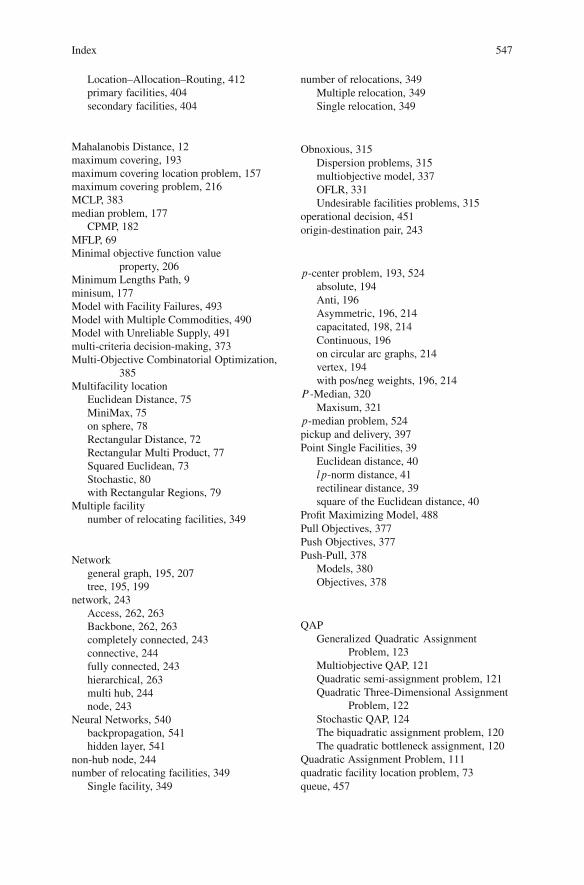
Index 547
Location–Allocation–Routing, 412primary facilities, 404secondary facilities, 404
Mahalanobis Distance, 12maximum covering, 193maximum covering location problem, 157maximum covering problem, 216MCLP, 383median problem, 177
CPMP, 182MFLP, 69Minimal objective function value
property, 206Minimum Lengths Path, 9minisum, 177Model with Facility Failures, 493Model with Multiple Commodities, 490Model with Unreliable Supply, 491multi-criteria decision-making, 373Multi-Objective Combinatorial Optimization,
385Multifacility location
Euclidean Distance, 75MiniMax, 75on sphere, 78Rectangular Distance, 72Rectangular Multi Product, 77Squared Euclidean, 73Stochastic, 80with Rectangular Regions, 79
Multiple facilitynumber of relocating facilities, 349
Networkgeneral graph, 195, 207tree, 195, 199
network, 243Access, 262, 263Backbone, 262, 263completely connected, 243connective, 244fully connected, 243hierarchical, 263multi hub, 244node, 243
Neural Networks, 540backpropagation, 541hidden layer, 541
non-hub node, 244number of relocating facilities, 349
Single facility, 349
number of relocations, 349Multiple relocation, 349Single relocation, 349
Obnoxious, 315Dispersion problems, 315multiobjective model, 337OFLR, 331Undesirable facilities problems, 315
operational decision, 451origin-destination pair, 243
p-center problem, 193, 524absolute, 194Anti, 196Asymmetric, 196, 214capacitated, 198, 214Continuous, 196on circular arc graphs, 214vertex, 194with pos/neg weights, 196, 214
P -Median, 320Maxisum, 321
p-median problem, 524pickup and delivery, 397Point Single Facilities, 39
Euclidean distance, 40lp-norm distance, 41rectilinear distance, 39square of the Euclidean distance, 40
Profit Maximizing Model, 488Pull Objectives, 377Push Objectives, 377Push-Pull, 378
Models, 380Objectives, 378
QAPGeneralized Quadratic Assignment
Problem, 123Multiobjective QAP, 121Quadratic semi-assignment problem, 121Quadratic Three-Dimensional Assignment
Problem, 122Stochastic QAP, 124The biquadratic assignment problem, 120The quadratic bottleneck assignment, 120
Quadratic Assignment Problem, 111quadratic facility location problem, 73queue, 457
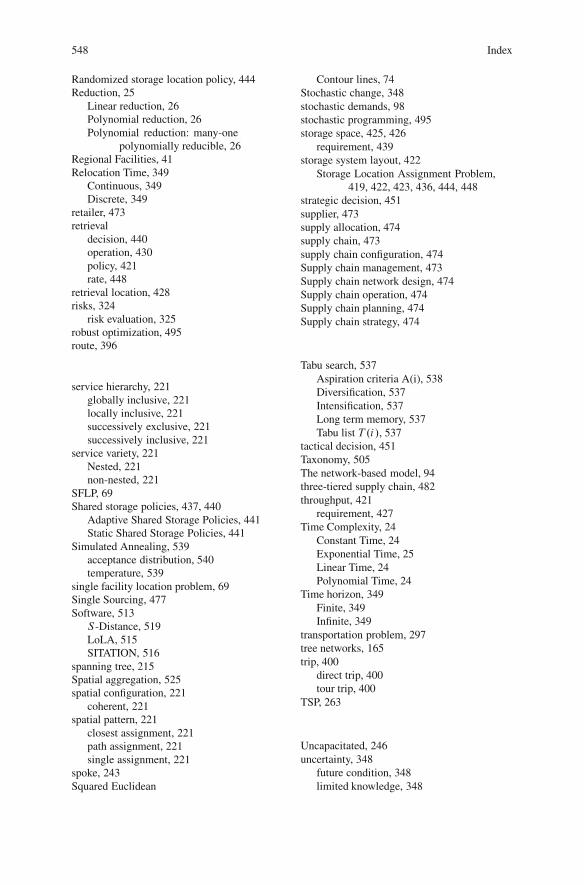
548 Index
Randomized storage location policy, 444Reduction, 25
Linear reduction, 26Polynomial reduction, 26Polynomial reduction: many-one
polynomially reducible, 26Regional Facilities, 41Relocation Time, 349
Continuous, 349Discrete, 349
retailer, 473retrieval
decision, 440operation, 430policy, 421rate, 448
retrieval location, 428risks, 324
risk evaluation, 325robust optimization, 495route, 396
service hierarchy, 221globally inclusive, 221locally inclusive, 221successively exclusive, 221successively inclusive, 221
service variety, 221Nested, 221non-nested, 221
SFLP, 69Shared storage policies, 437, 440
Adaptive Shared Storage Policies, 441Static Shared Storage Policies, 441
Simulated Annealing, 539acceptance distribution, 540temperature, 539
single facility location problem, 69Single Sourcing, 477Software, 513S-Distance, 519LoLA, 515SITATION, 516
spanning tree, 215Spatial aggregation, 525spatial configuration, 221
coherent, 221spatial pattern, 221
closest assignment, 221path assignment, 221single assignment, 221
spoke, 243Squared Euclidean
Contour lines, 74Stochastic change, 348stochastic demands, 98stochastic programming, 495storage space, 425, 426
requirement, 439storage system layout, 422
Storage Location Assignment Problem,419, 422, 423, 436, 444, 448
strategic decision, 451supplier, 473supply allocation, 474supply chain, 473supply chain configuration, 474Supply chain management, 473Supply chain network design, 474Supply chain operation, 474Supply chain planning, 474Supply chain strategy, 474
Tabu search, 537Aspiration criteria A(i), 538Diversification, 537Intensification, 537Long term memory, 537Tabu list T .i/, 537
tactical decision, 451Taxonomy, 505The network-based model, 94three-tiered supply chain, 482throughput, 421
requirement, 427Time Complexity, 24
Constant Time, 24Exponential Time, 25Linear Time, 24Polynomial Time, 24
Time horizon, 349Finite, 349Infinite, 349
transportation problem, 297tree networks, 165trip, 400
direct trip, 400tour trip, 400
TSP, 263
Uncapacitated, 246uncertainty, 348
future condition, 348limited knowledge, 348
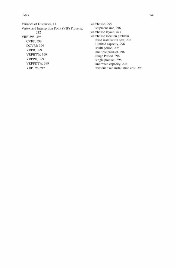
Index 549
Variance of Distances, 11Vertex and Intersection Point (VIP) Property,
212VRP, 395, 398
CVRP, 398DCVRP, 399VRPB, 399VRPBTW, 399VRPPD, 399VRPPDTW, 399VRPTW, 399
warehouse, 295shipment size, 296
warehouse layout, 447warehouse location problem
fixed installation cost, 296Limited capacity, 296Multi period, 296multiple product, 296Singe Period, 296single product, 296unlimited capacity, 296without fixed installation cost, 296
Copyright © 2022 FDOKUMEN