A New Capacitated Vehicle Routing Problem with Split Service for Minimizing Fleet Cost by Simulated...

ARTICLE IN PRESS

Journal of the Franklin Institute 344 (2007) 406–425

0016-0032/$3

doi:10.1016/j

�CorrespoE-mail ad

mkah@amer1American

www.elsevier.com/locate/jfranklin

A New Capacitated Vehicle Routing Problemwith Split Service for Minimizing Fleet Cost

by Simulated Annealing

R. Tavakkoli-Moghaddama,�, N. Safaeib,M.M.O. Kahc,1, M. Rabbania

aDepartment of Industrial Engineering, Faculty of Engineering, University of Tehran,

P.O. Box 11365/4563, Tehran, IranbDepartment of Industrial Engineering, Iran University of Science and Technology, Iran

cSchool of Information Technology & Communication Lamido Zubairu Way, Abti-American University of Nigeria,

P.M.B. 250, Yola, Adamawa State, Nigeria

Received 11 December 2005; accepted 12 December 2005

Abstract

We address a capacitated vehicle routing problem (CVRP) in which the demand of a node can be

split on several vehicles celled split services by assuming heterogeneous fixed fleet. The objective is to

minimize the fleet cost and total distance traveled. The fleet cost is dependent on the number of

vehicles used and the total unused capacity. In most practical cases, especially in urban

transportation, several vehicles transiting on a demand point occurs. Thus, the split services can

aid to minimize the number of used vehicles by maximizing the capacity utilization. This paper

presents a mix-integer linear model of a CVRP with split services and heterogeneous fleet. This model

is then solved by using a simulated annealing (SA) method. Our analysis suggests that the proposed

model enables users to establish routes to serve all given customers using the minimum number of

vehicles and maximum capacity. Our proposed method can also find very good solutions in a

reasonable amount of time. To illustrate these solutions further, a number of test problems in small

and large sizes are solved and computational results are reported in the paper.

r 2006 The Franklin Institute. Published by Elsevier Ltd. All rights reserved.

Keywords: Vehicle routing problem; Split services; Mix-integer programming; Simulated annealing

0.00 r 2006 The Franklin Institute. Published by Elsevier Ltd. All rights reserved.

.jfranklin.2005.12.002

nding author. Tel.:+982188021067; fax: +982188013102.

dresses: [email protected] (R. Tavakkoli-Moghaddam), [email protected] (N. Safaei),

ican.edu (M.M.O. Kah), [email protected] (M. Rabbani).

University, Washington, DC.

www.elsevier.com/locate/jfranklin

ARTICLE IN PRESSR. Tavakkoli-Moghaddam et al. / Journal of the Franklin Institute 344 (2007) 406–425 407

1. Introduction

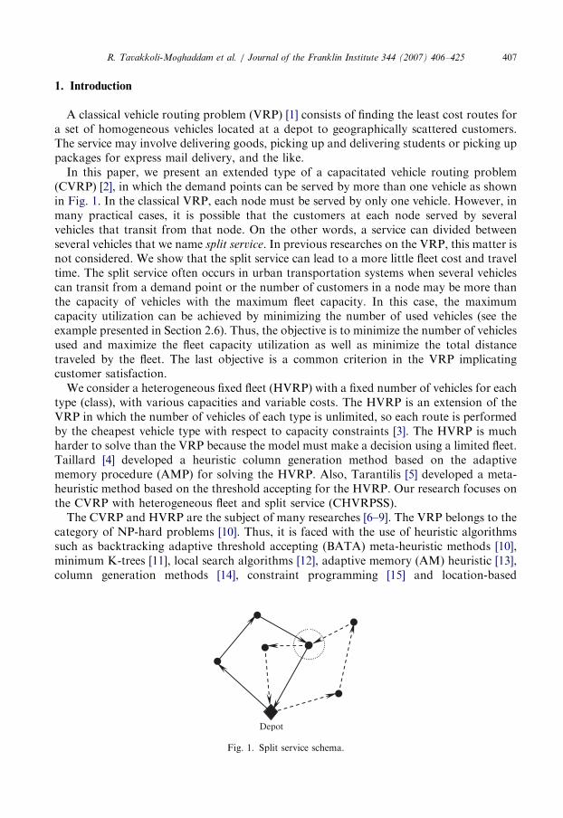
A classical vehicle routing problem (VRP) [1] consists of finding the least cost routes fora set of homogeneous vehicles located at a depot to geographically scattered customers.The service may involve delivering goods, picking up and delivering students or picking uppackages for express mail delivery, and the like.

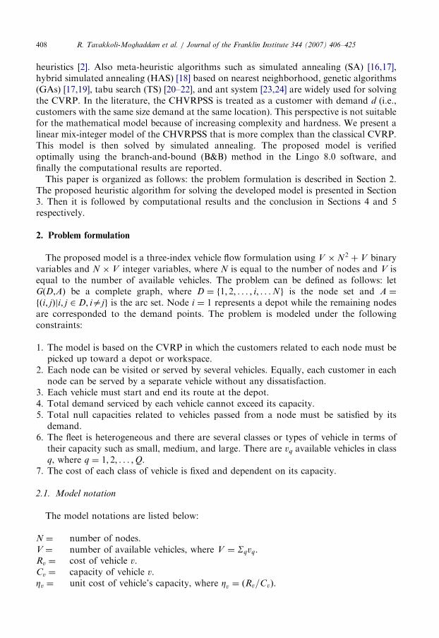
In this paper, we present an extended type of a capacitated vehicle routing problem(CVRP) [2], in which the demand points can be served by more than one vehicle as shownin Fig. 1. In the classical VRP, each node must be served by only one vehicle. However, inmany practical cases, it is possible that the customers at each node served by severalvehicles that transit from that node. On the other words, a service can divided betweenseveral vehicles that we name split service. In previous researches on the VRP, this matter isnot considered. We show that the split service can lead to a more little fleet cost and traveltime. The split service often occurs in urban transportation systems when several vehiclescan transit from a demand point or the number of customers in a node may be more thanthe capacity of vehicles with the maximum fleet capacity. In this case, the maximumcapacity utilization can be achieved by minimizing the number of used vehicles (see theexample presented in Section 2.6). Thus, the objective is to minimize the number of vehiclesused and maximize the fleet capacity utilization as well as minimize the total distancetraveled by the fleet. The last objective is a common criterion in the VRP implicatingcustomer satisfaction.

We consider a heterogeneous fixed fleet (HVRP) with a fixed number of vehicles for eachtype (class), with various capacities and variable costs. The HVRP is an extension of theVRP in which the number of vehicles of each type is unlimited, so each route is performedby the cheapest vehicle type with respect to capacity constraints [3]. The HVRP is muchharder to solve than the VRP because the model must make a decision using a limited fleet.Taillard [4] developed a heuristic column generation method based on the adaptivememory procedure (AMP) for solving the HVRP. Also, Tarantilis [5] developed a meta-heuristic method based on the threshold accepting for the HVRP. Our research focuses onthe CVRP with heterogeneous fleet and split service (CHVRPSS).

The CVRP and HVRP are the subject of many researches [6–9]. The VRP belongs to thecategory of NP-hard problems [10]. Thus, it is faced with the use of heuristic algorithmssuch as backtracking adaptive threshold accepting (BATA) meta-heuristic methods [10],minimum K-trees [11], local search algorithms [12], adaptive memory (AM) heuristic [13],column generation methods [14], constraint programming [15] and location-based

Depot

Fig. 1. Split service schema.

ARTICLE IN PRESSR. Tavakkoli-Moghaddam et al. / Journal of the Franklin Institute 344 (2007) 406–425408

heuristics [2]. Also meta-heuristic algorithms such as simulated annealing (SA) [16,17],hybrid simulated annealing (HAS) [18] based on nearest neighborhood, genetic algorithms(GAs) [17,19], tabu search (TS) [20–22], and ant system [23,24] are widely used for solvingthe CVRP. In the literature, the CHVRPSS is treated as a customer with demand d (i.e.,customers with the same size demand at the same location). This perspective is not suitablefor the mathematical model because of increasing complexity and hardness. We present alinear mix-integer model of the CHVRPSS that is more complex than the classical CVRP.This model is then solved by simulated annealing. The proposed model is verifiedoptimally using the branch-and-bound (B&B) method in the Lingo 8.0 software, andfinally the computational results are reported.This paper is organized as follows: the problem formulation is described in Section 2.

The proposed heuristic algorithm for solving the developed model is presented in Section3. Then it is followed by computational results and the conclusion in Sections 4 and 5respectively.

2. Problem formulation

The proposed model is a three-index vehicle flow formulation using V �N2 þ V binaryvariables and N � V integer variables, where N is equal to the number of nodes and V isequal to the number of available vehicles. The problem can be defined as follows: letG(D,A) be a complete graph, where D ¼ f1; 2; . . . ; i; . . .Ng is the node set and A ¼

fði; jÞji; j 2 D; iajg is the arc set. Node i ¼ 1 represents a depot while the remaining nodesare corresponded to the demand points. The problem is modeled under the followingconstraints:

1.
The model is based on the CVRP in which the customers related to each node must bepicked up toward a depot or workspace.
2.
Each node can be visited or served by several vehicles. Equally, each customer in eachnode can be served by a separate vehicle without any dissatisfaction.
3.
Each vehicle must start and end its route at the depot. 4. Total demand serviced by each vehicle cannot exceed its capacity. 5. Total null capacities related to vehicles passed from a node must be satisfied by its
demand.
6. The fleet is heterogeneous and there are several classes or types of vehicle in terms of
their capacity such as small, medium, and large. There are vq available vehicles in classq, where q ¼ 1; 2; . . . ;Q.

7.
The cost of each class of vehicle is fixed and dependent on its capacity.
2.1. Model notation

The model notations are listed below:

N ¼ number of nodes.V ¼ number of available vehicles, where V ¼ Sqvq.Rv ¼ cost of vehicle v.Cv ¼ capacity of vehicle v.Zv ¼ unit cost of vehicle’s capacity, where Zv ¼ ðRv=CvÞ.


lij ¼ length of arc ði; jÞ 2 A, where l11 ¼ 0, lijalji and for each i41, lii b N.p ¼ unit cost of travel by each vehicle type.di ¼ number of customers or demand in node i, where d1 ¼ 0.S ¼ arbitrary subset of set V.r(S) ¼ minimum number of vehicles needed to serve set S.M ¼ arbitrary large number, say M b N

2.2. Decision variables

Also, the decision variables are as follows:

xvij ¼

1 if arc i; jð Þ 2 A is traversed by vehicle v;

0 otherwise:

�

zv ¼1 if vehicle v is used;

0 otherwise:

�

nvj ¼ number of customers served in node j by vehicle v:

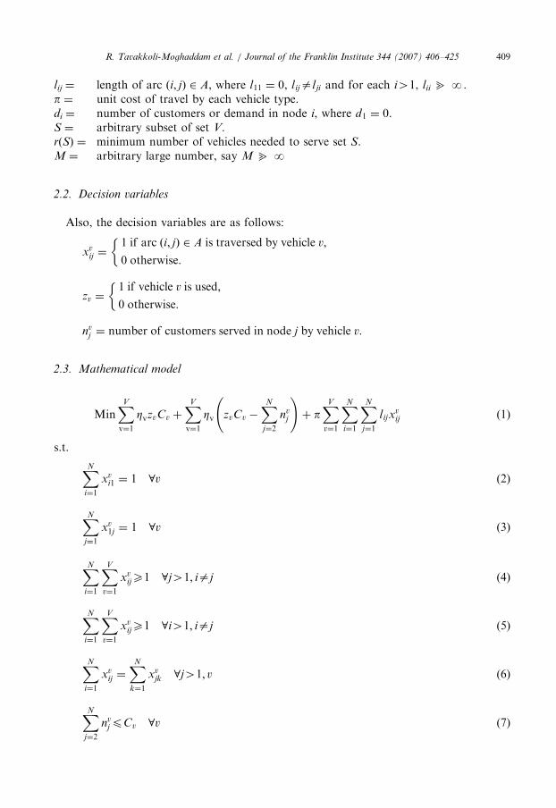
2.3. Mathematical model

MinXV

v¼1

ZvzvCv þXV

v¼1

Zv zvCv �XN

j¼2

nvj

!þ p

XV

v¼1

XN

i¼1

XN

j¼1

lijxvij (1)

s.t.

XN

i¼1

xvi1 ¼ 1 8v (2)

XN

j¼1

xv1j ¼ 1 8v (3)

XN

i¼1

XV

v¼1

xvijX1 8j41; iaj (4)

XN

i¼1

XV

v¼1

xvijX1 8i41; iaj (5)

XN

i¼1

xvij ¼

XN

k¼1

xvjk 8j41; v (6)

XN

j¼2

nvjpCv 8v (7)


XV

v¼1

nvj ¼ dj 8j41 (8)

nvj pM �

XN

i¼1

xvij 8j41; v (9)

zv ¼ 1� xv11 8v (10)

zvXxvij 8v; i41; j (11)

XV

v¼1

Xi2S

XjeS

xvijp Sj j � r Sð Þ 8S � A� 1f g;Sa+ (12)

zv;xvij 2 0; 1f g; nv

j 2 Nþ 8v; i; j.

Eq. (1) presents the objective function aimed at minimizing the fleet cost and totaldistance traveled by the fleet. The first term of the objective function is equal to the totalcost of used vehicles. The second term of the objective function is equal to the cost ofunused capacities in the fleet. This term persuades vehicles to split services and uses theirnull capacity. The third term is equal to the cost of total distance traveled by the fleet. Thisterm restricts the number of nodes visited by each vehicle or minimizes the travel time.Also, the third term can restrict the extra split services. This term can be a criterion formaximizing customer satisfaction. The proposed objective function trades off betweenfleet cost and customer satisfaction. Constraints (2) and (3) impose that the start andend of a route for each vehicle must be the depot. Constraints (4) to (6) impose that atleast one vehicle enters and leaves each node and then serves it. Constraint (7) assuresthat the vehicles’ capacity is not exceeded. Constraint (8) guarantees that vehiclestransited cover the demand in each node. Constraint (9) allows vehicles to serve nodestransited. Constraints (10) and (11) determine the vehicles that are used. The proposedstrategy for eliminating unused vehicles is discussed in Section 2.5. Constraint (12),which is named sub-tour elimination constraints (SECs), ensures that the sub-tours areeliminated.

2.4. Complexity analysis

Comparing the proposed model (CHVRPSS) and a bi-criteria model of the commonCVRP with heterogeneous fixed feet, a number of differences emerge. The objectivefunction in Eq. (1) must be changed into Eq. (13).

MinXV

v¼1

ZvzvCv þ pXV

v¼1

XN

i¼1

XN

j¼1

lijxvij . (13)

Also, constraint (4) and (5) must be expressed to equality as shown in Eqs. (14) and (15).The constraint (7) must be changed as Eq. (16) and constraints (8) and (9) must be


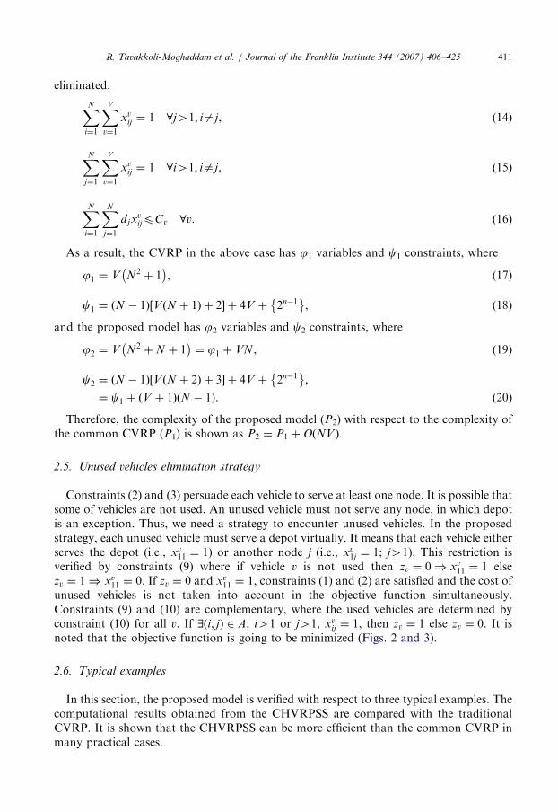
eliminated.

XN

i¼1

XV

v¼1

xvij ¼ 1 8j41; iaj, (14)

XN

j¼1

XV

v¼1

xvij ¼ 1 8i41; iaj, (15)

XN

i¼1

XN

j¼1

djxvijpCv 8v. (16)

As a result, the CVRP in the above case has j1 variables and c1 constraints, where

j1 ¼ V N2 þ 1� �

, (17)

c1 ¼ N � 1ð Þ V N þ 1ð Þ þ 2½ � þ 4V þ 2n�1� �

, (18)

and the proposed model has j2 variables and c2 constraints, where

j2 ¼ V N2 þN þ 1� �

¼ j1 þ VN, (19)

c2 ¼ N � 1ð Þ V N þ 2ð Þ þ 3½ � þ 4V þ 2n�1� �

,

¼ c1 þ V þ 1ð Þ N � 1ð Þ. ð20Þ

Therefore, the complexity of the proposed model (P2) with respect to the complexity ofthe common CVRP (P1) is shown as P2 ¼ P1 þOðNV Þ.

2.5. Unused vehicles elimination strategy

Constraints (2) and (3) persuade each vehicle to serve at least one node. It is possible thatsome of vehicles are not used. An unused vehicle must not serve any node, in which depotis an exception. Thus, we need a strategy to encounter unused vehicles. In the proposedstrategy, each unused vehicle must serve a depot virtually. It means that each vehicle eitherserves the depot (i.e., xv

11 ¼ 1) or another node j (i.e., xv1j ¼ 1; j41). This restriction is

verified by constraints (9) where if vehicle v is not used then zv ¼ 0) xv11 ¼ 1 else

zv ¼ 1) xv11 ¼ 0. If zv ¼ 0 and xv

11 ¼ 1, constraints (1) and (2) are satisfied and the cost ofunused vehicles is not taken into account in the objective function simultaneously.Constraints (9) and (10) are complementary, where the used vehicles are determined byconstraint (10) for all v. If 9ði; jÞ 2 A; i41 or j41, xv

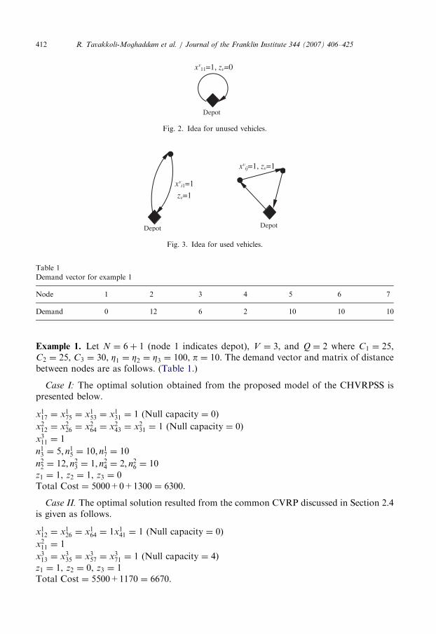
ij ¼ 1, then zv ¼ 1 else zv ¼ 0. It isnoted that the objective function is going to be minimized (Figs. 2 and 3).

2.6. Typical examples

In this section, the proposed model is verified with respect to three typical examples. Thecomputational results obtained from the CHVRPSS are compared with the traditionalCVRP. It is shown that the CHVRPSS can be more efficient than the common CVRP inmany practical cases.

ARTICLE IN PRESS

Depot

x 11=1, zvv =0

Fig. 2. Idea for unused vehicles.

Depot

x ij=1, zvv =1

Depot

x i1=1

zv

v

=1

Fig. 3. Idea for used vehicles.

Table 1

Demand vector for example 1

Node 1 2 3 4 5 6 7

Demand 0 12 6 2 10 10 10

R. Tavakkoli-Moghaddam et al. / Journal of the Franklin Institute 344 (2007) 406–425412

Example 1. Let N ¼ 6þ 1 (node 1 indicates depot), V ¼ 3, and Q ¼ 2 where C1 ¼ 25,C2 ¼ 25, C3 ¼ 30, Z1 ¼ Z2 ¼ Z3 ¼ 100, p ¼ 10. The demand vector and matrix of distancebetween nodes are as follows. (Table 1.)

Case I: The optimal solution obtained from the proposed model of the CHVRPSS ispresented below.

x117 ¼ x1

75 ¼ x153 ¼ x1

31 ¼ 1 (Null capacity ¼ 0)

x212 ¼ x2

26 ¼ x264 ¼ x2

43 ¼ x231 ¼ 1 (Null capacity ¼ 0)

x311 ¼ 1

n13 ¼ 5; n1

5 ¼ 10; n17 ¼ 10

n22 ¼ 12; n2

3 ¼ 1; n24 ¼ 2; n2

6 ¼ 10

z1 ¼ 1, z2 ¼ 1, z3 ¼ 0Total Cost ¼ 5000+0+1300 ¼ 6300.

Case II. The optimal solution resulted from the common CVRP discussed in Section 2.4is given as follows.

x112 ¼ x1

26 ¼ x164 ¼ 1x1


x211 ¼ 1

x313 ¼ x3

35 ¼ x357 ¼ x3


z1 ¼ 1, z2 ¼ 0, z3 ¼ 1Total Cost ¼ 5500+1170 ¼ 6670.

ARTICLE IN PRESS

Table 2


Node 1 2 3 4 5 6 7

Demand 0 8 8 8 8 8 9

Table 3

Distance matrix for example 1

1 2 3 4 5 6 7

1 0 16 20 18 24 24 13

2 N 24 15 33 13 28

3 N 11 10 21 19

4 N 21 10 24

5 N 31 17

6 N 33

7 N

R. Tavakkoli-Moghaddam et al. / Journal of the Franklin Institute 344 (2007) 406–425 413

According to results obtained, the total cost in case I is less than the total cost in case II.In case I, node 3 is served by both vehicles 1 and 2 where vehicle 1 serves five customersand vehicle 2 serves one customer in node 3. The reason is that the second term of theobjective function forces vehicle 2 for at the maximum utilization of its capacity (e.g., thecost of unused capacity is equal to zero). Thus, vehicle 3 is not used (z3 ¼ 0) and the fleetcost is less that one in case II. In case II, vehicle 3 is used instead of vehicle 2 (z2 ¼ 0,z3 ¼ 1) and has four null capacities. Consequently, the fleet cost is more than the fleet costin case I (i.e., 550045000). In contrast, in case II, the cost of total distance traveled by fleetis less than the cost in case I (1170o1300). The reason is that the split service causesincreasing in total distance traveled by vehicle 2 in case I.

Example 2. Consider example 1 with Q ¼ 3 where C1 ¼ 20, C2 ¼ 30, C3 ¼ 40. Thedemand vector is shown in Table 2 and the distances matrix is illustrated in Table 3.

Case I. The optimal solution obtained from the proposed model of the CHVRPSS is asfollows.

x114 ¼ x1

46 ¼ x162 ¼ x1


x214 ¼ x2

43 ¼ x235 ¼ x2

57 ¼ x271 ¼ 1 (Null capacity ¼ 1)

x311 ¼ 1

n14 ¼ 4; n1

6 ¼ 8; n12 ¼ 8

n24 ¼ 4; n2

3 ¼ 8; n25 ¼ 8; n2

7 ¼ 9

z1 ¼ 1, z2 ¼ 1, z3 ¼ 0Total Cost ¼ 5000+100+1260 ¼ 6360$.

Case II. The optimal solution resulted from the common CVRP discussed in Section 2.4is given as follows.

x117 ¼ x1


x211 ¼ 1

ARTICLE IN PRESS

5

3

64

7

1

2

v2

v1

Fig. 4. Optimal routes for case I in example 2.

5

3

64

7

1

2

v1

v3

Fig. 5. Optimal routes for case II in example 2.


x315 ¼ x3

53 ¼ x334 ¼ x3

46 ¼ x362 ¼ x3


z1 ¼ 1, z2 ¼ 0, z3 ¼ 1Total Cost ¼ 6000+1100 ¼ 7100$.

In example 2 and case I, node 4 is served by both vehicles 1 and 2 as shown in Fig. 4.Vehicle 2 has a null capacity in the optimal solution (n2

4 þ n23 þ n2

5 þ n27 ¼ 29o30) incurring

a cost that is equal to 100 whereas vehicle 1 is full. The optimal routes related to case II(common CVRP) is shown in Fig. 5.

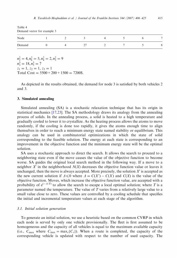
Example 3. The number of customers in a typical node (node 3 given in Table 4) is morethan the capacity of the vehicle with the maximum capacity of the fleet. Consequently, thisexample can not be solved by the common CVRP. Let Q ¼ 3 where C1 ¼ 10, C2 ¼ 20,C3 ¼ 25, Z1 ¼ Z2 ¼ Z3 ¼ 100, p ¼ 10. The demand vector is shown in Table 4 and thedistances matrix is illustrated in Table 3. The number of customers in node 3 is equal to 27that is more than the capacity of vehicle with the maximum capacity (C3 ¼ 25).

The optimal solution obtained from the proposed model of the CHVRPSS is given asfollows.

x117 ¼ x1


x212 ¼ x2

26 ¼ x264 ¼ x2

43 ¼ x231 ¼ 1 (Null capacity ¼ 0)

x313 ¼ x3

35 ¼ x351 ¼ 1 (Null capacity ¼ 0)

n17 ¼ 8

ARTICLE IN PRESS

Table 4


Node 1 2 3 4 5 6 7

Demand 0 4 27 2 7 5 8


n22 ¼ 4; n2

6 ¼ 5; n24 ¼ 2; n2

3 ¼ 9

n33 ¼ 18; n3

5 ¼ 7

z1 ¼ 1, z2 ¼ 1, z3 ¼ 1Total Cost ¼ 5500+200+1500 ¼ 7200$.

As depicted in the results obtained, the demand for node 3 is satisfied by both vehicles 2and 3.

3. Simulated annealing

Simulated annealing (SA) is a stochastic relaxation technique that has its origin instatistical mechanics [17,23]. The SA methodology draws its analogy from the annealingprocess of solids. In the annealing process, a solid is heated to a high temperature andgradually cooled to lower it to crystallize. As the heating process allows the atoms to moverandomly, if the cooling is done too rapidly, it gives the atoms enough time to alignthemselves in order to reach a minimum energy state named stability or equilibrium. Thisanalogy can be used in combinatorial optimizations in which the state of solidcorresponding to the feasible solution. The energy at each state is corresponding to animprovement in the objective function and the minimum energy state will be the optimalsolution.

SA uses a stochastic approach to direct the search. It allows the search to proceed to aneighboring state even if the move causes the value of the objective function to becomeworse. SA guides the original local search method in the following way. If a move to aneighbor X0 in the neighborhood N(X) decreases the objective function value or leaves itunchanged, then the move is always accepted. More precisely, the solution X0 is accepted asthe new current solution if Dp0 where D ¼ CðX 0Þ � CðX Þ and C(X) is the value of theobjective function. Moves, which increase the objective function value, are accepted with aprobability of e(�D/T) to allow the search to escape a local optimal solution; where T is aparameter named the temperature. The value of T varies from a relatively large value to asmall value close to zero. These values are controlled by a cooling schedule that specifiesthe initial and incremental temperature values at each stage of the algorithm.

3.1. Initial solution generation

To generate an initial solution, we use a heuristic based on the common CVRP in whicheach node is served by only one vehicle provisionally. The fleet is first assumed to behomogeneous and the capacity of all vehicles is equal to the maximum available capacity(i.e., Cmax where Cmax ¼ maxvfCvg). When a route is completed, the capacity of thecorresponding vehicle is updated with respect to the number of used capacity. The


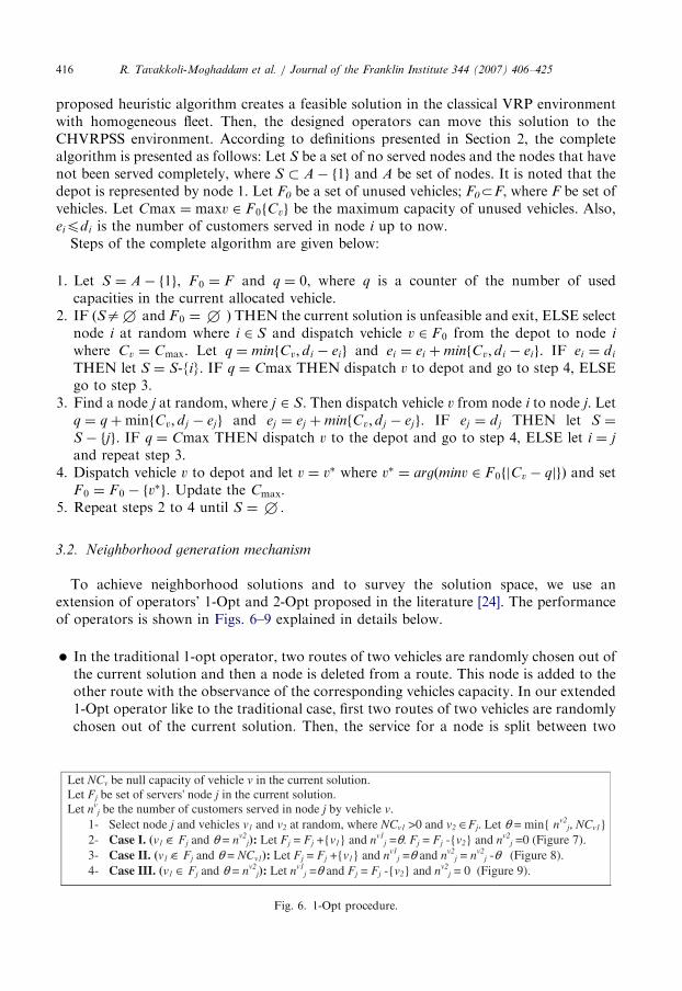
proposed heuristic algorithm creates a feasible solution in the classical VRP environmentwith homogeneous fleet. Then, the designed operators can move this solution to theCHVRPSS environment. According to definitions presented in Section 2, the completealgorithm is presented as follows: Let S be a set of no served nodes and the nodes that havenot been served completely, where S � A� f1g and A be set of nodes. It is noted that thedepot is represented by node 1. Let F0 be a set of unused vehicles; F0CF, where F be set ofvehicles. Let Cmax ¼ maxv 2 F0fCvg be the maximum capacity of unused vehicles. Also,eipdi is the number of customers served in node i up to now.Steps of the complete algorithm are given below:

1.

LLL

Let S ¼ A� f1g, F0 ¼ F and q ¼ 0, where q is a counter of the number of usedcapacities in the current allocated vehicle.

2.
IF (Sa+ and F 0 ¼+ ) THEN the current solution is unfeasible and exit, ELSE selectnode i at random where i 2 S and dispatch vehicle v 2 F0 from the depot to node i
where Cv ¼ Cmax. Let q ¼ minfCv; di � eig and ei ¼ ei þminfCv; di � eig. IF ei ¼ di

THEN let S ¼ S-{i}. IF q ¼ Cmax THEN dispatch v to depot and go to step 4, ELSEgo to step 3.

3.
Find a node j at random, where j 2 S. Then dispatch vehicle v from node i to node j. Letq ¼ qþminfCv; dj � ejg and ej ¼ ej þminfCv; dj � ejg. IF ej ¼ dj THEN let S ¼
S � fjg. IF q ¼ Cmax THEN dispatch v to the depot and go to step 4, ELSE let i ¼ j

and repeat step 3.
4. Dispatch vehicle v to depot and let v ¼ v� where v� ¼ argðminv 2 F 0fjCv � qjgÞ and set
F0 ¼ F0 � fv�g. Update the Cmax.

5.
Repeat steps 2 to 4 until S ¼+.
3.2. Neighborhood generation mechanism

To achieve neighborhood solutions and to survey the solution space, we use anextension of operators’ 1-Opt and 2-Opt proposed in the literature [24]. The performanceof operators is shown in Figs. 6–9 explained in details below.

�
In the traditional 1-opt operator, two routes of two vehicles are randomly chosen out ofthe current solution and then a node is deleted from a route. This node is added to theother route with the observance of the corresponding vehicles capacity. In our extended1-Opt operator like to the traditional case, first two routes of two vehicles are randomlychosen out of the current solution. Then, the service for a node is split between two
et NCv be null capacity of vehicle v in the current solution. et Fj be set of servers' node j in the current solution. et nv

j be the number of customers served in node j by vehicle v. 1- Select node j and vehicles v1 and v2 at random, where NCv1 >0 and v2 ∈ Fj. Let θ = min{ nv2

j, NCv1} 2- Case I. (v1 ∈ Fj and θ = nv2

j): Let Fj = Fj +{v1} and nv1j =θ . Fj = Fj -{v2} and nv2

j =0 (Figure 7). 3- Case II. (v1 ∈ Fj and θ = NCv1): Let Fj = Fj +{v1} and nv1

j =θ and nv2j = nv2

j -θ (Figure 8). 4- Case III. (v1 ∈ Fj and θ = nv2

j): Let nv1j =θ and Fj = Fj -{v2} and nv2

j = 0 (Figure 9).

Fig. 6. 1-Opt procedure.

ARTICLE IN PRESS

Fig. 7. 1-Opt implementation (classical case).

Fig. 8. 1-Opt implementation (split service).

Fig. 9. 1-Opt implementation (inverse split service).

Fig. 10. 2-Opt implementation.


corresponding vehicles or transferred to a new vehicle with the observance of its nullcapacity. This operator may lead to the removal or addition of a vehicle from/to the listof node’s servers. The complete algorithm of the proposed 1-Opt is presented in Fig. 6.Figs. 7–9 depict profiles of the extended 1-Opt operator.
� In 2-Opt operator, two routes belonging to two vehicles are randomly chosen from the
current solution and then two nodes out of the two routes are exchanged with eachother with the observance of corresponding vehicles capacity as shown in Fig. 10.

3.3. Simulated annealing implementation

The SA algorithm has two inside and outside loops. The inside loop controls inachieving the equilibrium in the current temperature and outside loop controls the rate of

ARTICLE IN PRESS

Set T0, Tf, EL and MTT. r = 0 ,Xbest = ∅ Generate X0 by the proposed algorithm in Section 3.1. Xbest = X0

Do (Out Side loop) n = 0 Do (In Side loop)

Select an operator (1-Opt or 2-Opt) randomly and execute on Xn (Operator

n newX X→ ). Δ C = C(Xnew) - C(Xn) If Δ C < 0 Then Xbest = Xnew and set n = n +1 and Xn = Xnew

Else Generate y → U(0,1) randomly and Set z = EXP(-Δ C/Tr )

If y < z Then n = n +1 and Xn = Xnew

End if Loop While( n < EL) r = r + 1 Tr = Tr-1 - α ⋅ Tr-1

Loop While ( r < MTT and Tr > 0 ) Print Xbest

Fig. 11. SA algorithm.


the decrease in temperature. The SA parameters are as follows:

EL (Epoch Length): Number of the accepted solution in each temperature for achievingthe equilibrium.

MTT: Maximum number of consecutive temperature trails.T0: Initial temperature.a: Rate of decreasing temperature (cooling schedule).X: A feasible solution.C(X): The value of the objective function in terms of X.n: Counter for the number of the accepted solution in each temperature.r: Counter for number of consecutive temperature trails, where Tr is equal to

temperature in iteration r.

The steps of the SA algorithm are shown in Fig. 11.

4. Computational Results

In this section, the proposed model is solved by the SA approach and the computationalresults are reported. As shown, the CHVRPSS with the heterogeneous fixed fleet is veryhard and cannot be solved optimality within a reasonable time, except for small-sizedinstances. Thus, it is required to compare the SA solution with a lower-bound (LB)solution for large-sized problems. The LB solution is calculated by a traveling salesmanproblem (TSP) based on the procedure shown in Fig. 12. As shown earlier in Section 2.6,

ARTICLE IN PRESS

1- Let D = Σ idi be the total demand in all nodes. 2- Let the fleet be only a vehicle with capacity D. 3- Solve a TSP for the given problem. 4- LB = η D + π Q where Q is equal to the total

distance traveled by a salesman.

Fig. 12. LB procedure.

Table 5

SA parameter settings

EL MTT Tf a 1-opt rate 2-opt rate

100 100 0 0.99 0.5 0.5


we have optimality verified the proposed model by three typical examples. Also, in thissection to compare SA solutions with optimal ones, we solved five small-sized instances bythe Lingo software according to Table 6. The CPU times is corresponded to an Intels

Celerons mobile 1.3GHz processor. For simplicity, we assume that the unit cost of thecapacity for all vehicle is constant and equal to Z ¼ Zv 8v. Also, it is assumed that the fleetconsists of three classes of vehicles as small (20 persons), medium (30 persons), and large(40 persons) sizes. The distance between nodes is randomly generated at uniform ininterval [1,100] similar to Table 3. The SA parameters set experimentally in advanceaccording to Table 5. In Table 6, SA and optimal solutions are compared in terms of theirCPU time and objective function value (OFV).

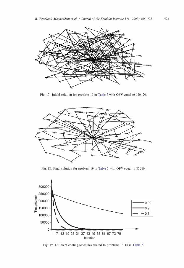
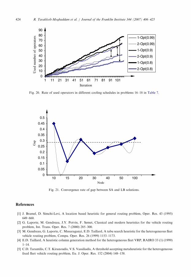
The terms of objective function are separated in columns ‘‘Term 1’’, ‘‘Term 2’’, and‘‘Term 3’’. The total demand in all nodes is shown in column ‘‘D’’ and the total capacity ofthe fleet is shown in column ‘‘TC’’. In the worst case, the OFV gap between SA andoptimal solutions is equal to 5.5% when TC ¼ D. The computational results show that theSA with the proposed operators can reach the optimal solution within a reasonable time atnine times out of ten. The comparison between SA and LB solutions is shown in Table 7 interms of the OFV, CPU time, and cooling schedule (a) for the large-sized problem. Thevalues of cooling schedule considered in three cases are very slow (a ¼ 0:99), slow(a ¼ 0:9), and rapid (a ¼ 0:8). An instance of different cooling schedules related toproblems 11 to 13 (50 node) in Table 7 is shown in Fig. 17. Also, the rate of used operatorsis shown in columns ‘‘1-Opt’’ and ‘‘2-Opt’’. With respect to obtained results, the proposed1-Opt is more efficient than 2-Opt whereby the proportion used of 1-Opt to 2-Opt is nearlyequal to 2 when increasing the dimension. This issue is shown in Fig. 18 for a typicalinstance. Figs. 13–16 show the solutions obtained from the SA algorithm for someinstances given in Table 7. Also, Figs. 17 and 18 depict the initial (zero time) and finalsolutions obtained by SA related to problem 19 given in Table 7. The final solution isfound about 3 hours (Fig. 19.). Above figures imply the improvement of solutions duringSA process for a large-sized problem (Fig. 20). The final solution that is found about3 hours improved 27.14 with respect to the initial solution. As depicted in Fig. 21, theconvergence rate of the gap between SA and LB solutions is nearly equal to 25%.

ARTICLE IN PRESS

Table 7

SA solutions for large-sized problems

Test problem SA

No. N a TC D LB OFV CPU time (S) 1-Opt 2-Opt Gap (%)

1 10 0.99 50 38 5400 7820 9.2 8 4 45

2 10 0.9 50 38 5400 7820 12.7 7 6 45

3 10 0.8 50 38 5400 7820 2.2 11 2 45

4 15 0.99 90 86 10800 11800 74.6 18 8 9

5 15 0.9 90 86 10800 11830 4.47 14 7 1

6 15 0.8 90 86 10800 12110 6.3 23 8 12

7 20 0.99 180 112 14330 18810 297 19 6 31

8 20 0.9 180 112 14330 18790 150 28 12 31

9 20 0.8 180 112 14330 18820 81 29 5 31

10 30 0.99 160 148 19590 23120 848 33 18 18

11 30 0.9 160 148 19590 23250 300 38 30 19

12 30 0.8 160 148 19590 23250 86 30 25 19

13 40 0.99 240 225 26630 32810 2876 47 47 23

14 40 0.9 240 225 26630 32830 1104 45 50 23

15 40 0.8 240 225 26630 33150 331 63 35 24

16 50 0.99 320 282 34340 43540 6509 76 59 27

17 50 0.9 320 282 34340 44980 1990 64 42 31

18 50 0.8 320 282 34340 43680 965 78 30 27

19 100 0.8 600 581 66490 87510 10162 149 115 32

Table 6

Comparison between optimal and SA solutions (an instance with 6 nodes)

Test Problem Optimal solution (B&B) SA Solution Gap (%)

No. N V TC D OFV Term 1 Term 2 Term 3 CPU

time (S)

OFV Term 1 Term 2 Term 3 1-Opt 2-Opt CPU

time (S)

1 6 2 50 46 6590 5000 400 1190 11 6590 5000 400 1190 5 2 2.7 0

2 6 3 70 70 8340 7000 0 1340 13 8800 7000 0 1800 0 1 0.8 5.5

3 6 2 60 57 7530 6000 300 1230 31 7530 6000 300 1230 2 0 0.2 0

4 6 3 70 70 8440 7000 0 1440 34 8550 7000 0 1550 0 0 0.1 1.3

5 6 3 70 68 8500 7000 200 1300 692 8500 7000 200 1300 4 2 24 0

Average gap 1.36


5. Conclusions

This paper presents a special type of the CVRP consisting of the CVRP with HVRP andsplit service named CHVRPSS, in which the demand of each node can be split betweenseveral vehicles. This issue can occur in an urban transportation system when severalvehicles must be passed by a node or station. Also, it is possible that the demand in somestations is more than the maximum capacity in the fleet. We add a new term to theobjective function to maximize the capacity utilization. This term forces vehicles for the

ARTICLE IN PRESS

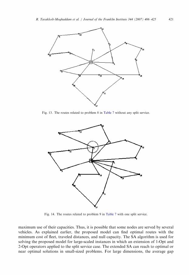
Fig. 13. The routes related to problem 8 in Table 7 without any split service.

Fig. 14. The routes related to problem 9 in Table 7 with one split service.


maximum use of their capacities. Thus, it is possible that some nodes are served by severalvehicles. As explained earlier, the proposed model can find optimal routes with theminimum cost of fleet, traveled distances, and null capacity. The SA algorithm is used forsolving the proposed model for large-scaled instances in which an extension of 1-Opt and2-Opt operators applied to the split service case. The extended SA can reach to optimal ornear optimal solutions in small-sized problems. For large dimensions, the average gap

ARTICLE IN PRESS

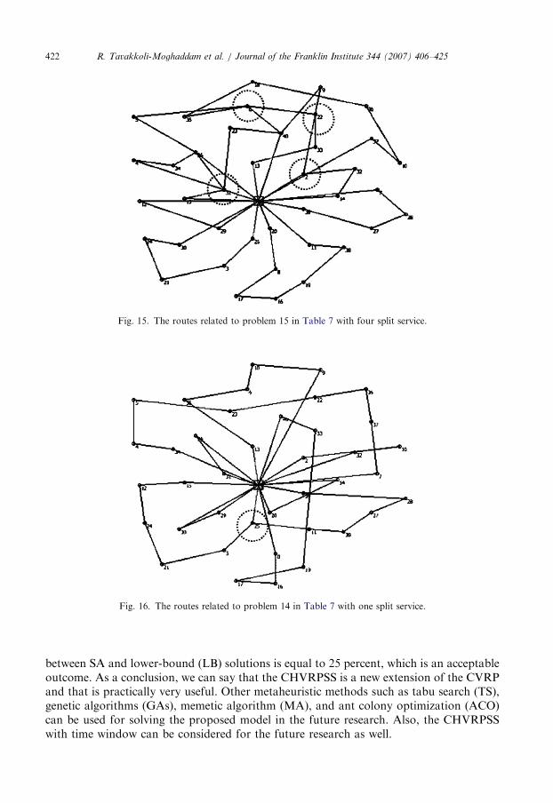
Fig. 15. The routes related to problem 15 in Table 7 with four split service.

Fig. 16. The routes related to problem 14 in Table 7 with one split service.


between SA and lower-bound (LB) solutions is equal to 25 percent, which is an acceptableoutcome. As a conclusion, we can say that the CHVRPSS is a new extension of the CVRPand that is practically very useful. Other metaheuristic methods such as tabu search (TS),genetic algorithms (GAs), memetic algorithm (MA), and ant colony optimization (ACO)can be used for solving the proposed model in the future research. Also, the CHVRPSSwith time window can be considered for the future research as well.

ARTICLE IN PRESS

Fig. 17. Initial solution for problem 19 in Table 7 with OFV equal to 120 120.

Fig. 18. Final solution for problem 19 in Table 7 with OFV equal to 87 510.

0

50000

100000

150000

200000

250000

300000

1 7 13 19 25 31 37 43 49 55 61 67 73 79

0.99

0.9

0.8

Tem

pera

ture

Iteration

Fig. 19. Different cooling schedules related to problems 16–18 in Table 7.


ARTICLE IN PRESS

0

1020

3040

5060

7080

90

1 11 21 31 41 51 61 71 81 91 101

1-Opt(0.99)

2-Opt(0.99)

1-Opt(0.9)

2-Opt(0.9)

1-Opt(0.8)

2-Opt(0.8)

Use

d nu

mbe

r of

ope

rato

rs

Iteration

Fig. 20. Rate of used operators in different cooling schedules in problems 16–18 in Table 7.

0

0.05

0.1

0.15

0.2

0.25

0.3

0.35

0.4

0.45

0.5

10 15 20 30 40 50 100

Gap

Node

Fig. 21. Convergence rate of gap between SA and LB solutions.


References

[1] J. Bramel, D. Simchi-Levi, A location based heuristic for general routing problem, Oper. Res. 43 (1995)

649–660.

[2] G. Laporte, M. Gendreau, J.Y. Potvin, F. Semet, Classical and modern heuristics for the vehicle routing

problem, Int. Trans. Oper. Res. 7 (2000) 285–300.

[3] M. Gendreau, G. Laporte, C. Musaraganyi, E.D. Taillard, A tabu search heuristic for the heterogeneous fleet

vehicle routing problem, Compu. Oper. Res. 26 (1999) 1153–1173.

[4] E.D. Taillard, A heuristic column generation method for the heterogeneous fleet VRP, RAIRO 33 (1) (1999)

1–14.

[5] C.D. Tarantilis, C.T. Kiranoudis, V.S. Vassiliadis, A threshold accepting metaheuristic for the heterogeneous

fixed fleet vehicle routing problem, Eu. J. Oper. Res. 152 (2004) 148–158.


[6] W.C. Chiang, R. Russell, Simulated annealing meta-heuristics for the vehicle routing problem with time

windows, An. Oper. Res. 93 (1996) 3–27.

[7] K.F. Doerner, M. Gronalt, R.F. Hartl, M. Reimann, C. Strauss, M. Stummer, Savings ants for the vehicle

routing problem, in: S. Cagnoni, et al. (Eds.), Applications of Evolutionary Computing, Springer, Berlin,

2002.

[8] G. Dueck, T. Scheuer, Threshold accepting: a general purpose optimization algorithm appearing superior to

simulated annealing, J. Compu. Phys. 90 (1) (1990) 161–175.

[9] M.L. Fisher, Optimal solution of vehicle routing problems using minimum K-trees, Oper. Res. 42 (1994)

626–642.

[10] M. Gendreau, A. Hertz, G. Laporte, A tabu search heuristic for the vehicle routing problem, Manag. Sci. 40

(1994) 1276–1290.

[11] M. Gendreau, G. Laporte, C. Musaraganyi, E.D. Taillard, A tabu search heuristic for the heterogeneous fleet

vehicle routing problem, Compu. Oper. Res. 26 (1999) 1153–1173.

[12] M. Gendreau, G. Laporte, J.Y. Potvin, Local search algorithms for the vehicle routing problem, in:

J.K. Lenstra, E.H.L. Aarts (Eds.), Local Search Algorithms, Wiley, Chichester, 1995.

[13] B. Golden, G. Laporte, E. Taillard, An adaptive memory heuristic for a class of vehicle routing problems

with minmax objective, Compu. Oper. Res. 24 (1999) 445–452.

[14] S. Kirkpatrick, J.R. Gelatt, M. Vecchi, Optimization by simulated annealing, Science 220 (1983) 671–680.

[15] C. Koulamas, S. Antony, R. Jaen, A survey of simulated annealing applications to operations research

problems, Omega 22 (1) (1994) 41–56.

[16] J.K. Lenstra, A. Rinnooy Kan, Complexity of vehicle routing and scheduling problems, Networks 11 (1981)

221–227.

[17] E.D. Taillard, A heuristic column generation method for the heterogeneous fleet VRP, RAIRO 33 (1) (1999)

1–4.

[18] R. Tavakkoli-Moghaddam, N. Safaei, Y. Gholipour, A hybrid simulated annealing for capacitated vehicle

routing problems with the independent route length, Appl. Math. Computation, in press, doi:10.1016/

j.amc.2005.09.040.

[19] J.K. Potvin, S. Bengio, A genetic approach to the vehicle routing problem with time windows, Publication

CRT-953, Centre de recherche sur les transports, University of Montreal, 1994.

[20] M. Reimann, M. Stummer, K. Doerner, A savings based ant system for the vehicle routing problem, in:

W.B. Langdon, et al. (Eds.), Proceedings of the Genetic and Evolutionary Computation Conference

(GECCO 2002), San Francisco, 2002.

[21] F. Semet, E.D. Taillard, Solving real-life vehicle routing problems efficiently using taboo search, An. Oper.

Res. 41 (1993) 469–488.

[22] P. Shaw, Using constraint programming and local search methods to solve vehicle routing problems, in: M.

Maher, J.E. Puget (Eds.), Principles and practice of constraint programming—Proceedings of the Fourth

International Conference, Pisa, Italy, Springer, Berlin, 1998, pp. 417–431.

[23] C.D. Tarantilis, C.T. Kiranoudis, V.S. Vassiliadis, A backtracking adaptive threshold accepting meta-

heuristic method for the vehicle routing problem, Systems Analysis Modeling Simulation 42 (5) (1994)

631–664.

[24] C.D. Tarantilis, V.S. Kiranoudis, V.S. Vassiliadis, A threshold accepting meta-heuristic for the

heterogeneous fixed fleet vehicle routing problem, Eur. J. Oper. Res. 152 (2004) 148–158.

dx.doi.org/10.1016/j.amc.2005.09.040

dx.doi.org/10.1016/j.amc.2005.09.040

A New Capacitated Vehicle Routing Problem with Split Service for Minimizing Fleet Cost by Simulated...

Documents

Transcript of A New Capacitated Vehicle Routing Problem with Split Service for Minimizing Fleet Cost by Simulated...