Minimizing Average Flow Time on Related Machines

Naveen Garg Amit Kumar

Dept. of Computer Science and Engg.

IIT Delhi, New Delhi – 110016

email : naveen,amitk@cse.iitd.ac.in

November 3, 2005

Abstract

We give the first on-line poly-logarithmic competitve algorithm for minimizing average flowtime with preemption on related machines, i.e., when machines can have different speeds. Thisalso yields the first poly-logarithmic polynomial time approximation algorithm for this problem.More specifically, we give an O(log2 P · log S)-competitive algorithm, where P is the ratio ofthe biggest and the smallest processing time of a job, and S is the ratio of the highest and thesmallest speed of a machine. Our algorithm also has the nice property that it is non-migratory.The scheduling algorithm is based on the concept of making jobs wait for a long enough timebefore scheduling them on slow machines.

1 Introduction

We consider the problem of scheduling jobs that arrive over time in multiprocessor environments.This is a fundamental scheduling problem and has many applications, e.g., servicing requestsin web servers. The goal of a scheduling algorithm is to process jobs on the machines so thatsome measure of performance is optimized. Perhaps the most natural measure is the averageflow time of the jobs. Flow time of a job is defined as the difference of its completion time andits release time, i.e., the time it spends in the system.

This problem has received considerable attention in the recent past[2] [10], [1]. All of theseworks make the assumption that the machines are identical, i.e., they have the same speed. Butit is very natural to expect that in a heterogenous processing environment different machineswill have different processing power, and hence different speeds. In this paper, we consider theproblem of scheduling jobs on machines with different speeds, which is also referred to as relatedmachines in the scheduling literature. We allow for jobs to be preempted. Indeed, the problemturns out to be intractable if we do not allow preemption. Kellerer et. al. [9] showed that theproblem of minimizing average flow time without preemption has no online algorithm with o(n)competitive ratio even on a single machine. They also showed that it is hard to get a polynomialtime O(n1/2−ε)-approximation algorithm for this problem. So preemption is a standard, andmuch needed, assumption when minimising flow time.

In the standard notation of Graham et. al. [7], we consider the problem Q|rj , pmtn|∑

j Fj .We give the first poly-logarithmic competitive algorithm for minimizing average flow time onrelated machines. More specifically, we give an O(log2 P · log S)-competitive algorithm, whereP is the ratio of the biggest and the smallest processing time of a job, and S is the ratio ofthe highest and the smallest speed of a machine. This is also the first polynomial time poly-logarithmic approximation algorithm for this problem. Despite its similarity to the special casewhen machines are identical, this problem is much more difficult since we also have to worryabout the processing times of jobs. Our algorithm is also non-migratory, i.e., it processes ajob on only one machine. This is a desirable feature in many applications because moving jobsacross machines may have many overheads.Related Work The problem of minimizing average flow time (with preemption) on identicalparallel machines has received much attention in the past few years. Leonardi and Raz [10]showed that the Shortest Remaining Processing Time (SRPT) algorithm has a competitiveratio of O(log(min( n

m , P ))), where n is the number of jobs, and m is the number of machines. Amatching lower bound on the competitive ratio of any on-line (randomized) algorithm for thisproblem was also shown by the same authors. Awerbuch et. al. [2] gave a non-migratory versionof SRPT with competitive ratio of O(log(min(n, P ))). Chekuri et. al.[5] gave a non-migratoryalgorithm with competitive ratio of O(log(min( n

m , P ))). One of the merits of their algorithmwas a much simpler analysis of the competitive ratio. Instead of preferring jobs according totheir remaining processing times, their algorithm divides jobs into classes when they arrive. Ajob goes to class k if its processing time is between 2k−1 and 2k. The scheduling algorithmnow prefers jobs of smaller class irrespective of the remaining processing time. We also use thisnotion of classes of jobs in our algorithm. Azar and Avrahami[1] gave a non-migratory algorithmwith immediate dispatch, i.e., a job is sent to a machine as soon as it arrives. Their algorithmtries to balance the load assigned to each machine for each class of jobs. Their algorithm alsohas the competitive ratio of O(log(min( n

m , P ))). It is also interesting to note that these are alsothe best known results in the off-line setting of this problem.

Kalyanasundaram and Pruhs[8] introduced the resource augmentation model where the al-gorithm is allowed extra resources when compared with the optimal off-line algorithm. Theseextra resources can be either extra machines or extra speed. For minimizing average flow timeon identical parallel machines, Phillips et. al. [11] showed that we can get an optimal algorithmif we are given twice the speed as compared to the optimal algorithm. In the case of singlemachine scheduling, Bechheti et. al.[4] showed that we can get O(1/ε)-competitive algorithmsif we are give (1 + ε) times more resources. Bansal and Pruhs[3] extended this result to a va-riety of natural scheduling algorithms and to Lp norms of flow times of jobs as well. In case

1

of identical parallel machines, Chekuri et. al.[6] gave simple scheduling algorithms which areO(1/ε3)-competitive with (1 + ε) resource augmentation.Our Techniques A natural algorithm to try here would be SRPT. We feel that it will bevery difficult to analyze this algorithm in case of related machines. Further SRPT is migratory.Non-migratory versions of SRPT can be shown to have bad competitive ratios. To illustrate theideas involved, consider the following example. There is one fast machine, and plenty of slowmachines. Suppose many jobs arrive at the same time. If we distribute these jobs to all theavailable machines, then their processing times will be very high. So at each time step, we needto be selective about which machines we shall use for processing. Ideas based on distributingjobs in proportion to speeds of machines as used by Azar and Avrahami[1] can also be shownto have problems.

Our idea of selecting machines is the following. A job is assigned to a machine only if ithas waited for time which is proportional to its processing time on this machine. The intuitionshould be clear – if a job is going to a slow machine, then it can afford to wait longer before itis sent to the machine. Hopefully in this waiting period, a faster machine might become free inwhich case we shall be able to process it in smaller time. We also use the notion of class of jobsas introduced by Chekuri et. al.[5] which allows machines to have a preference ordering overjobs. We feel that this idea of delaying jobs even if a machine is available is new.

As mentioned earlier, the first challenge is to bound the processing time of our algorithm.In fact a bulk of our paper is about this. The basic idea used is the following – if a job is sent toa very slow machine, then it must have waited long. But then most of this time, our algorithmwould have kept the fast machines busy. Since we are keeping fast machines busy, the optimumalso can not do much better. But converting this idea into a proof requires several technicalsteps.

The second step is of course to bound the flow time of the jobs. Previous works on boundingflow time of jobs in the case of identical machines achieve this in the following way – consider atime t. It can be shown that there is a time t′ such that at t′, our algorithm and the optimumalgorithm are in a very similar state and all our machines are busy during (t′, t). This wouldthen imply that at time t also, our algorithm and the optimum algorithm are in a similar state.But we can not use this idea because we would never be able to keep all machines busy (somemachines can be very slow). So we have to define a sequence of time steps like t′ for each timeand make clever use of geometric scaling to show that the flow time is bounded.

2 Problem Definition and Notations

We consider the on-line problem of minimizing total flow time for related machines. Each job jhas a processing requirement of pj and a release date of rj . There are m machines, numberedfrom 1 to m. The machines can have different speeds, and the processing time of a job j on amachine is pj divided by the speed of the machine. The slowness of machine is the reciprocal ofits speed. It will be easier to deal with slowness, and so we shall use slowness instead of speedin the foregoing discussion. Let si denote the slowness of machine i. So the time taken by jobj to process on machine i is pj · si. Assume that the machines have been numbered so thats1 ≤ s2 ≤ · · · ≤ sm. We shall assume without loss of generality that processing time, releasedates, and slowness are integers. We shall use the term volume of a set of jobs for denoting theirprocessing time on a unit speed machine.

Let A be a scheduling algorithm. The completion time of a job j in A is denoted byCA

j . The flow time of j in A is defined as FAj = CA

j − rj . Our goal is to find an on-linescheduling algorithm which minimizes the total flow time of jobs. Let O denote the optimaloff-line scheduling algorithm.

We now develop some notations. Let P denote the ratio of the largest to the smallestprocessing times of the jobs, and S be the ratio of the largest to the smallest slowness of themachines. For ease of notation, we assume that the smallest processing requirement of any jobis 1, and the smallest slowness of a machine is 1. Let α and β be suitable chosen large enough

2

constants. We divide the jobs and the machines into classes. A job j is said to be in class k ifpj ∈ [αk−1, αk) and a machine i is said to be in class l if si ∈ [βl−1, βl). Note that there areO(log P ) classes for jobs and O(log S) classes for machines. Given a schedule A, we say that ajob j is active at time t in A if rj ≤ t but j has not finished processing by time t in A.

3 Scheduling Algorithm

We now describe the scheduling algorithm. The underlying idea of the algorithm is the following— if we send a job j to machine i, we make sure that it waits for at least pj · si units of time(which is its processing time on machine i). Intuitively, the extra waiting time can be chargedto its processing time. Of course, we still need to make sure that the processing time does notblow up in this process.

The algorithm maintains a central pool of jobs. When a new job gets released, it first goesto the central pool and waits there to get assigned to a machine. Let W (t) denote the set ofjobs in the central pool at time t. Our algorithm will assign each job to a unique machine — ifa job j gets assigned to a machine i, then j will get processed by machine i only. Let Ai(t) bethe set of active jobs at time t which have been assigned to machine i. We shall maintain theinvariant that Ai(t) contains at most one job of each class. So |Ai(t)| ≤ log P .

We say that a job j ∈ W (t) of class k is mature for a machine i of class l at time t, if ithas waited for at least αk · βl time in the central pool, i.e., t − rj ≥ αk · βl. For any time t, wedefine a total order ≺ on the jobs in W (t) as follows – j ≺ j′ if either (i) class(j) < class(j′), or(ii) class(j) = class(j′) and rj > rj′ (in case class(j) = class(j′) and rj = rj′ we can order themarbitrarily).

Now we describe the actual details of the algorithm. Initially, at time 0, Ai(0) is empty foreach machine. At each time t, the algorithm considers machines in the order 1, 2, . . . , m (recallthat the machines have been arranged in the ascending order of their slowness). Let us describethe algorithm when it considers machine i. Let Mi(t) be the jobs in W (t) which are maturefor machine i at time t. Let j ∈ Mi(t) be the smallest job according to the total order ≺. Ifclass(j) < class(j′) for all jobs j′ ∈ Ai(t), then we assign j to machine i (i.e., we delete j fromW (t) and add it to Ai(t)).

Once the algorithm has considered all the machines at time t, each machine i processes thejob of smallest class in Ai(t) at time t. This completes the description of our algorithm. Itis also easy to see that the machines need to perform the above steps for only a polynomialnumber of time steps t (i.e., when a job finishes or matures for a class of machines).

We remark that both the conditions in the definition of ≺ are necessary. The condition (i)is clear because it prefers smaller jobs. Condition (ii) makes sure that we make old jobs waitlonger so that they can mature for slower machines. It is easy to construct examples where ifwe do not obey condition (ii) then slow machines will never get used and so we will incur veryhigh flow time.

4 Analysis

We now show that the flow time incurred by our algorithm is within poly-logarithmic factor ofthat of the optimal algorithm. The outline of the proof is as follows. We first argue that thetotal processing time incurred by our algorithm is not too large. Once we have shown this, wecan charge the waiting time of all the jobs in Ai(t) for all machines i and time t to the totalprocessing time. After this, we show that the total waiting time of the jobs in the central poolis also bounded by poly-logarithmic factor times the optimum’s flow time.

Let A denote our algorithm. For a job j, define the dispatch time dAj of j in A as the timeat which it is assigned to a machine. For a job j and class l of machines, let tM (j, l) denote thetime at which j matures for machines of class l, i.e., tM (j, l) = rj + αkβl, where k is the class ofjob j. Let FA denote the total flow time of our algorithm. For a job j let PA

j denote the timeit takes to process job j in A (i.e., the processing time of j in A). Similarly, for a set of jobs

3

jq

3

jq+1

0

Iq

jq

2

Iq−1

rq

0d

q

0= t

q

e

dq

2

rq

1d

q

3

rq

2

rq

3

jq

0

l

l

l − 1

l − 2

1

jq

1

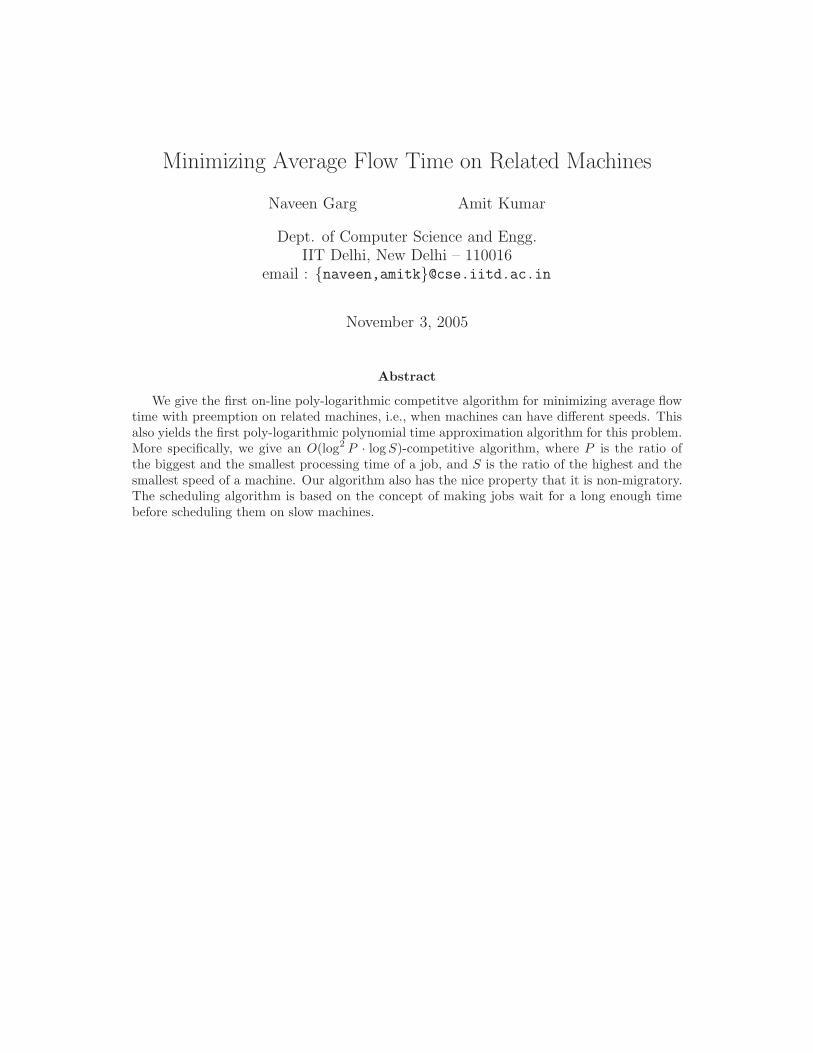
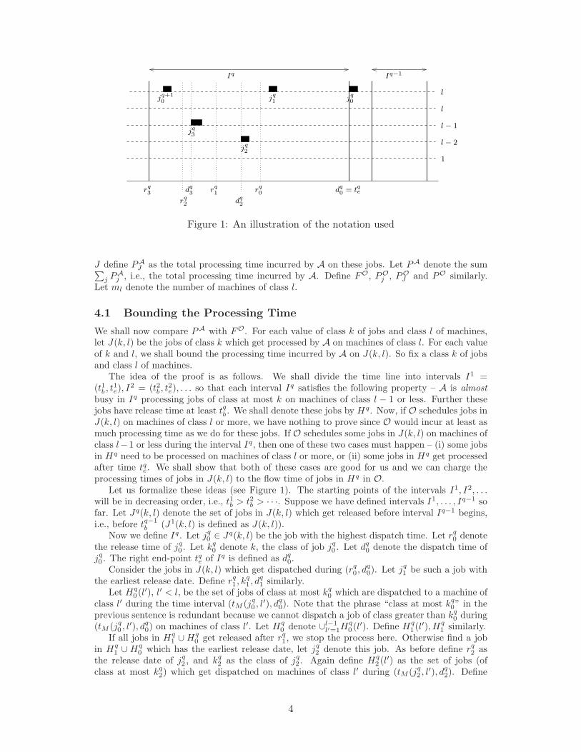
Figure 1: An illustration of the notation used

J define PAJ as the total processing time incurred by A on these jobs. Let PA denote the sum

∑

j PAj , i.e., the total processing time incurred by A. Define FO, PO

j , POJ and PO similarly.

Let ml denote the number of machines of class l.

4.1 Bounding the Processing Time

We shall now compare PA with FO. For each value of class k of jobs and class l of machines,let J(k, l) be the jobs of class k which get processed by A on machines of class l. For each valueof k and l, we shall bound the processing time incurred by A on J(k, l). So fix a class k of jobsand class l of machines.

The idea of the proof is as follows. We shall divide the time line into intervals I1 =(t1b , t

1e), I

2 = (t2b , t2e), . . . so that each interval Iq satisfies the following property – A is almost

busy in Iq processing jobs of class at most k on machines of class l − 1 or less. Further thesejobs have release time at least tqb . We shall denote these jobs by Hq. Now, if O schedules jobs inJ(k, l) on machines of class l or more, we have nothing to prove since O would incur at least asmuch processing time as we do for these jobs. If O schedules some jobs in J(k, l) on machines ofclass l−1 or less during the interval Iq, then one of these two cases must happen – (i) some jobsin Hq need to be processed on machines of class l or more, or (ii) some jobs in Hq get processedafter time tqe. We shall show that both of these cases are good for us and we can charge theprocessing times of jobs in J(k, l) to the flow time of jobs in Hq in O.

Let us formalize these ideas (see Figure 1). The starting points of the intervals I1, I2, . . .will be in decreasing order, i.e., t1b > t2b > · · ·. Suppose we have defined intervals I1, . . . , Iq−1 sofar. Let Jq(k, l) denote the set of jobs in J(k, l) which get released before interval Iq−1 begins,i.e., before tq−1

b (J1(k, l) is defined as J(k, l)).Now we define Iq. Let jq

0 ∈ Jq(k, l) be the job with the highest dispatch time. Let rq0 denote

the release time of jq0 . Let kq

0 denote k, the class of job jq0 . Let dq

0 denote the dispatch time ofjq0 . The right end-point tqe of Iq is defined as dq

0.Consider the jobs in J(k, l) which get dispatched during (rq

0 , dq0). Let jq

1 be such a job withthe earliest release date. Define rq

1, kq1 , d

q1 similarly.

Let Hq0 (l′), l′ < l, be the set of jobs of class at most kq

0 which are dispatched to a machine ofclass l′ during the time interval (tM (jq

0 , l′), dq0). Note that the phrase “class at most kq

0” in theprevious sentence is redundant because we cannot dispatch a job of class greater than kq

0 during(tM (jq

0 , l′), dq0) on machines of class l′. Let Hq

0 denote ∪l−1l′=1H

q0 (l′). Define Hq

1 (l′), Hq1 similarly.

If all jobs in Hq1 ∪ Hq

0 get released after rq1, we stop the process here. Otherwise find a job

in Hq1 ∪ Hq

0 which has the earliest release date, let jq2 denote this job. As before define rq

2 asthe release date of jq

2 , and kq2 as the class of jq

2 . Again define Hq2 (l′) as the set of jobs (of

class at most kq2) which get dispatched on machines of class l′ during (tM (jq

2 , l′), dq2). Define

4

Hq2 analogously. So now assume we have defined jq

0 , jq1 , . . . , jq

i and Hq0 , Hq

1 , . . . , Hqi , i ≥ 2. If all

jobs in Hqi are released after rq

i , then we stop the process. Otherwise, define jqi+1 as the job in

Hqi with the earliest release date. Define Hq

i+1 in a similar manner (see Figure 1). We remarkthat the first two steps of this process differ from the subsequent steps. This we will see later isrequierd to ensure that the intervals do not overlap too much. The following simple observationshows that this process will stop.

Claim 4.1 For i ≥ 2, kqi < kq

i−1.

Proof. Consider a job j ∈ Hqi−1(l

′). If class(j) = class(jqi−1), then A prefers j over jq

i−1. So,release time of j must be at least rq

i−1. Thus, class of jqi must be less than that of jq

i−1.

Suppose this process stops after uq steps. Define the beginning of Iq, i.e., tqb as rquq

.

This completes our description of Iq. Let Hq denote ∪iHqi . We are now ready to show that

interval Iq is sufficiently long, and that for a large fraction of this time, all machines of classless than l are processing jobs of class less than k which are released in this interval itself. Thiswould be valuable in later arguing that O could not have scheduked jobs of J(k, l) on the lowerclass machines and thereby incurred small processing time.

Lemma 4.2 Length of the interval Iq is at least αkβl.

Proof. Indeed, job jq0 must wait for at least αkβl amount of time before being dispatched to a

machine of class l. So tqe − tqs ≥ dq0 − rq

0 ≥ αkβl.

Lemma 4.3 Hq consists of jobs of class at most k and all jobs in Hq are released after tqb .

Proof. The first statement is clear from the definition of Hq. Let us look at Hqi . As argued in

proof of Claim 4.1 all jobs of class kqi in Hq

i are released after rqi . If all jobs of class less than kq

i

in Hqi are released after rq

i , then we are done. Otherwise, all such jobs are released after rqi+1

(after rq2 if i = 0). This completes the proof of the lemma.

Lemma 4.4 A machine of class l′ < l processes jobs of Hq for at least |Iq| − 6 · αkβl′ amountof time during Iq.

Proof. Let us fix a machine i of class l′ < l. Let us consider the interval (rqp, dq

p). Job jqp

matures for i at time tM (jqp , l′). So machine i must be busy during (tM (jq

p , l′), dqp), otherwise we

could have dispatched jqp earlier. We now want to argue that machine i is mainly busy during

this interval processing jobs from Hq.Let j be a job which is processed by i during (tM (jq

p, l′), dqp). We have already noted that j

can be of class at most kqp. If j gets dispatched after tM (jq

p , l′), then by definition it belongs toHq. If j gets dispatched before tM (jq

p , l′), it must belong to Ai(t′). But Ai(t

′) can contain atmost one job of each class. So the total processing time taken by jobs of Ai(t

′) during (t′, dp) is

at most βl′ · (α + α2 + · · · + αkqp) ≤ 3/2 · αkq

pβl′ .So during (rq

p, dqp), i processes jobs from Hq except perhaps for a period of length (tM (jq

p, l′)−

rqp)+3/2 ·αkq

pβl′ = 5/2 ·αkqpβl′ . Since ∪p(r

qp, dp) covers Iq, the amount of time i does not process

jobs from Hq is at most 5/2 · βl′(αk + αk + · · · + 1), which proves the lemma.

We would like to charge the processing time for jobs in J(k, l) in our solution to the flowtime of jobs in Hq in O. But to do this we require that the sets Hq be disjoint. We next provethat this is almost true.

Lemma 4.5 For any q, Iq and Iq+2 are disjoint. Hence Hq and Hq+2 are also disjoint.

Proof. Recall that Jq+1(k, l) is the set of jobs in J(k, l) which get released before tqb . Howeversome of these jobs may get dispatched after tqb and hence Iq and Iq+1 can intersect.

Consider some job j ∈ Jq+1(k, l) is dispatched during Iq. Now, observe that jq+10 is released

before tqb (by definition of Jq+1(k, l)) and dispatched after j. So, j gets dispatched in (rq0 , d

q0).

5

This means that release date of jq+11 must be before release date of j. But tq+1

b ≤ rq+11 and so,

j is released after tq+1b . But then j /∈ Jq+2(k, l). So all jobs in Jq+2(k, l) get dispatched before

Iq begins, which implies that Iq and Iq+2 are disjoint.

Consider an interval Iq. Let Dq(k, l) denote the jobs in J(k, l) which get released after tqbbut dispatched before tqe. It is easy to see that Dq(k, l) is a superset of Jq(k, l)− Jq+1(k, l). So∪qD

q(k, l) covers all of J(k, l).Now we would like to charge the processing time of jobs in Dq(k, l) to the flow time incurred

by O on the jobs in Hq. Before we do this, let us first show that O incurs significant amount offlow time processing the jobs in Hq. This is proved in the technical theorem below whose proofwe defer to the appendix.

Theorem 4.6 Consider a time interval I = (tb, te) of length T . Suppose there exists a set ofjobs JI such that every job j ∈ JI is of class at most k and is released after tb. Further Adispatches all the jobs in JI during I and only on machines of class less than l. Further, eachmachine i of class l′ < l satisfies the following condition : machine i processes jobs from JI forat least T − 6 · αk · βl′ amount of time. Assuming T ≥ αk · βl, the flow time FO

JIincurred by O

on the jobs in JI is at least Ω(

PAJI

)

.

Substituting tb = tqb , te = tqe, I = Iq, T = |Iq|, JI = Hq in the statement of Theorem 4.6 andusing Lemmas 4.2, 4.3, 4.4, we get

PAHq ≤ O(FO

Hq ). (1)

We are now ready to prove the main theorem of this section.

Theorem 4.7 The processing time incurred by A on Dq(k, l), namely PADq(k,l), is O(FO

Hq +

FODq(k,l)).

Proof. Let V denote the volume of Dq(k, l). By Lemma 4.4, machines of class l′ do not processjobs from Hq for at most 6 ·αkβl′ units of time during Iq. This period translates to a job-volumeof at most 6β · αk. If V is sufficiently small then it can be charged to the processing time (orequivalently the flow time in O) of the jobs in Hq.

Lemma 4.8 If V ≤ c · β · αk(m0 + . . . + ml−1) where c is a constant, then PADq(k,l) is O(FO

Hq ).

Proof. The processing time incurred by A on Dq(k, l) is at most βlV = O(αkβl+1 · (m0 + . . . +ml−1)). Now, Lemmas 4.2 and 4.4 imply that machines of class l′ < l process jobs from Hq forat least αkβl/2 amount of time. So PA

Hq is at least αkβl(m0 + . . . + ml−1)/2. Using equation(1), we get the result.

So from now on we shall assume that V ≥ c ·β ·αk+1(m0 + . . .+ml−1) for a sufficiently largeconstant c. We deal with easy cases first :

Lemma 4.9 In each of the following cases PADq(k,l) is O(FO

Dq(k,l) + FOHq ) :

(i) At least V/2 volume of Dq(k, l) is processed on machines of class at least l by O.

(ii) At least V/4 volume of Dq(k, l) is finished by O after time tqe − αkβl/2.

(iii) At least V/8 volume of Hq is processed by O on machines of class l or more.

Proof. Note that PADq(k,l) is at most V βl. If (i) happens, O pays at least V/2 · βl−1 amount of

processing time for Dq(k, l) and so we are done. Suppose case (ii) occurs. All jobs in Dq(k, l)get dispatched by time tqe. So they must get released before tqe − αkβl. So at least 1/4 volumeof these jobs wait for at least αkβl/2 amount of time in O. This means that FO

Dq(k,l) is at least

V/8 · βl, because each job has size at most αk. This again implies the lemma. Case (iii) issimilar to case (i).

6

So we can assume that none of the cases in Lemma 4.9 occur. Now, consider a time t betweentqe − αkβl/2 and tqe. Let us look at machines of class 1 to l − 1. O finishes at least V/4 volumeof Dq(k, l) on these machines before time t. Further, at most V/8 volume of Hq goes out fromthese machines to machines of higher class. The volume that corresponds to time slots in whichthese machines do not process jobs of Hq in A is at most V/16 (for a sufficiently large constantc). So, at least V/16 amount of volume of Hq must be waiting in O at time t. So the total flowtime incurred by O on Hq is at least V/(16αk) ·αkβl/2 which again is Ω(V βl). This proves thetheorem.

Combining the above theorem with Lemma 4.5, we get

Corollary 4.10 PAJ(k,l) is O(FO), and so PA is O(log S log P · FO).

4.2 Bounding the flow time

We now show that the average flow time incurred by our algorithm is within poly-logarithmicfactor of that incurred by the optimal solution. We shall say that a job j is waiting at time t inA if it is in the central pool at time t in A and has been released before time t.

Let V A≤k(t) denote the volume of jobs of class at most k which are waiting at time t in A.

Define V O≤k as the remaining volume of jobs of class at most k which are active at time t in O.

Note the slight difference in the definitions for A and O — in case of A, we are counting onlythose jobs which are in the central pool, while in O we are counting all active jobs. Our goalis to show that for all values of k,

∑

t V A≤k(t) is bounded from above by

∑

t V O≤k(t) plus small

additive factors, i.e., O(αk · (PO + PA)). Once we have this, the desired result will follow fromstandard calculations.

Let us develop some more notation. xA(t) will denote the number of machines busy at timet in A. Define xO(t) similarly. xO

l (t) denotes the number of machines of class l busy at timet in O. PO

l (t1, t2) will denote the total amount of processing time incurred by machines ofclass l during the time period (t1, t2) by O. Define PA

l (t1, t2) similarly. Recall that ml denotesthe number of machines of class l. Define m≤l as the number of machines of class at most l.Similarly define m<l. Let m(l1,l2) denote the number of machines of class between l1 and l2(inclusive of l1 and l2).

Given a class k of jobs and time t, let Jk(t) be the set of jobs of class at most k which arewaiting at time t in A. Let jk(t) ∈ Jk(t) be the job with the earliest release date. Let rk(t)denote the release date of job jk(t), and ck(t) denote the class of jk(t). Let lk(t) denote thelargest l such that jk(t) has matured for machines of class l at time t. In other words, lk(t) isthe highest value of l such that tM (j, l) ≤ t. Observe that all machines of class lk(t) or less mustbe busy processing jobs of class at most ck(t) at time t, otherwise our algorithm should havedispatched j by time t. Our proof will use the following lemma.

Lemma 4.11 For any class k of jobs and time t,

V A≤k(t)−V O

≤k(t) ≤ 2·β·αck(t)·m≤(lk(t)−1)+V A≤(ck(t)−1)(rk(t))−V O

≤(ck(t)−1)(rk(t))+∑

l≥lk(t)

POl (rk(t), t)

βl−1.

Proof. Let V A denote the volume of jobs of class at most k which are processed by A onmachines of class lk(t) − 1 or less during (rk(t), t). Define UA as the volume of jobs of class atmost k which are processed by A on machines of class lk(t) or more during (rk(t), t). Define V O

and UO similarly. Clearly, V A≤k(t)−V O

≤k(t) = V A≤k(rk(t))−V O

≤k(rk(t))+(V O−V A)+(UO−UA).

Let us look at V O − V A first. Any machine of class l′ ≤ lk(t) − 1 is busy in A during(tM (jk(t), l′), t) processing jobs of class at most ck(t). The amount of volume O can process on

such machines during (rk(t), tM (jk(t), l′)) is at most ml′ ·αck(t)βl′

βl′−1 , which is at most ml′ ·β ·αck(t).

So we get V O − V A ≤ m≤(lk(t)−1) · β · αck(t).

7

Let us now consider V A≤k(rk(t)) − V O

≤k(rk(t)). Let us consider jobs of class ck(t) or morewhich are waiting at time rk(t) in A (so they were released before rk(t)). By our definition ofjk(t), all such jobs must be processed by time t in A. If l′ ≤ lk(t)−1, then such jobs can be doneon machines of class l′ only during (tM (jk(t), l′), t). So again we can show that the total volumeof such jobs is at most m≤(lk(t)−1) · β · αck(t) + UA. Thus we get V A

≤k(rk(t)) − V O≤k(rk(t)) ≤

m≤(lk(t)−1) ·β ·αck(t) +UA +V A(≤ck(t)−1)(rk(t))−V O

≤(ck(t)−1)(rk(t)), because V O≤(ck(t)−1)(rk(t)) ≤

V O≤k(rk(t)).

Finally note that UO is at most∑

l≥lk(t)PO

l (rk(t),t)βl−1 . Combining everything, we get the result.

The rest of the proof is really about unraveling the expression in the lemma above. Toillustrate the ideas involved, let us try to prove the special case for jobs of class 1 only. The

lemma above implies that V A≤1(t)−V O

≤1(t) ≤ 2 ·β ·m≤(l1(t)−1)+∑

l≥l1(t)PO

l (r1(t),t)

βl−1 . We are really

interested in∑

t(VA≤1(t) − V O

≤1(t)). Now, the sum∑

t m≤(l1(t)−1) is not a problem because we

know that at time t all machines of class l1(t) or less must be busy in A. So, xA(t) ≥ m≤(l1(t)−1).So∑

t m≤(l1(t)−1) is at most∑

t xA(t), which is the total processing time of A. It is little tricky

to bound the second term. We shall write∑

l≥l1(t)PO

l (r1(t),t)βl−1 as

∑

l≥l1(t)

∑tt′=r1(t)

xOl (t′)βl−1 . We

can think of this as saying that at time time t′, r1(t) ≤ t′ ≤ t, we are charging 1/βl−1 amountto each machine of class l which is busy at time t′ in O. Note that here l is at least l1(t).

Now we consider∑

t

∑

l≥l1(t)

∑tt′=r1(t)

xOl (t′)

βl−1 . For a fixed time t′ and a machine i of class l

which is busy at time t′ in O, let us see for how many times t we charge to i. We charge to iat time t′ if t′ lies in the interval (r1(t), t), and l ≥ l1(t). Suppose this happens. We claim thatt − t′ has to be at most αβl+1. Indeed otherwise t − r1(t) ≥ αβl+1 and so j1(t) has maturedfor machines of class l + 1 as well. But then l < l1(t). So the total amount of charge machine igets at time t′ is at most αβl+1 · 1/βl−1 = O(1). Thus, the total sum turns out to be at most aconstant times the total processing time of O.

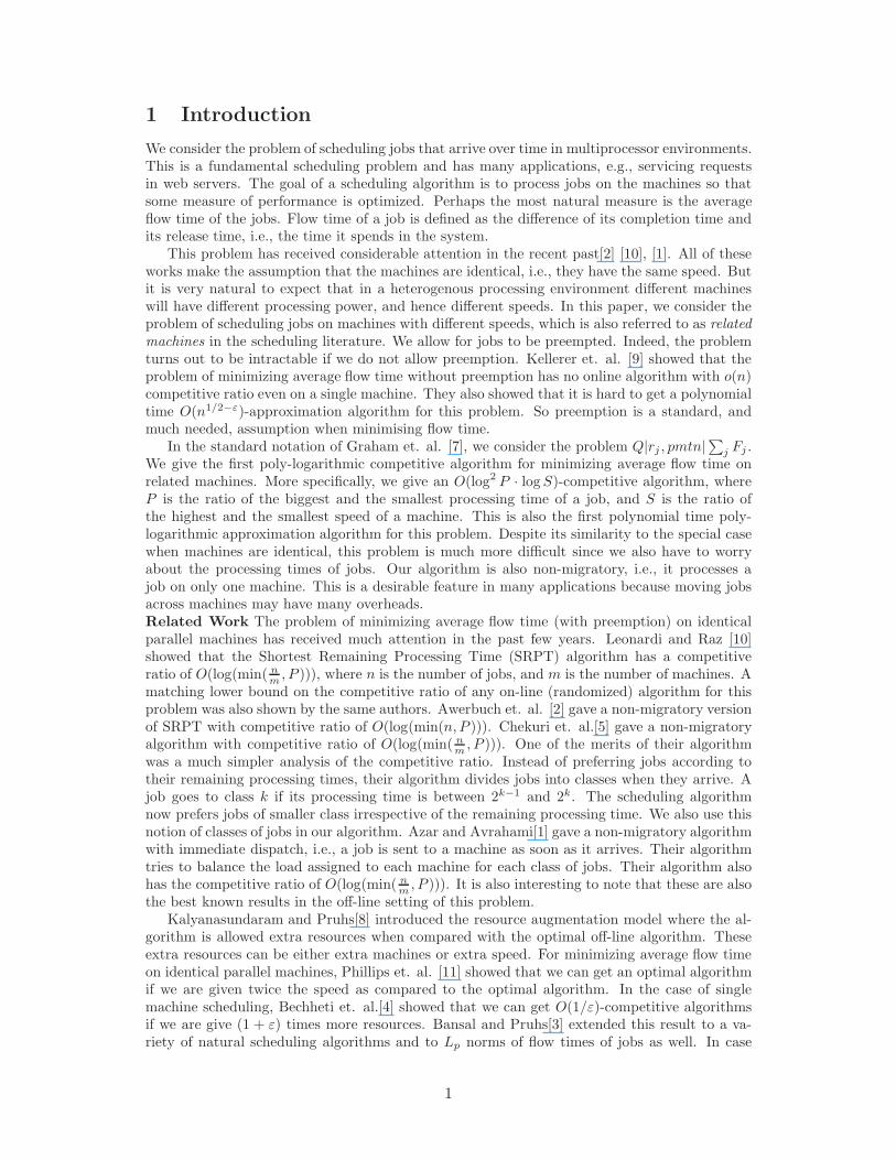
Let us now try to prove this for the general case. We build some notation first. Fix a time tand class k. We shall define a sequence of times t0, t1, · · · and a sequence of jobs j0(t), j1(t), . . .associated with this sequence of times. ci(t) shall denote the class of the job ji(t). Let us seehow we define this sequence. First of all t0 = t, and j0(t) is the job jk(t) (as defined above).Recall the definition of jk(t) – it is the job with the earliest release date among all jobs of classat most k which are waiting at time t in A. Note that c0(t), the class of this job, can be lessthan k. Now suppose we have defined t0, . . . , ti and j0(t), . . . , ji(t), i ≥ 0. ti+1 is the releasedate of ji(t). ji+1(t) is defined as the job jci(t)−1(t

i+1), i.e., the job with the earliest releasedate among all jobs of class less than ci(t) waiting at time ti+1 in A. We shall also definea sequence of classes of machines l0(t), l1(t), . . . in the following manner – li(t) is the highestclass l of machines such that job ji(t) has matured for machines of class l at time ti. Figure 2illustrates these definitions. The vertical line at time ti denotes li(t) – the height of this line isproportional to li(t).

We note the following simple fact.

Claim 4.12 βli(t) · αci(t) ≤ ti − ti+1 ≤ βli(t)+1 · αci(t).

Proof. Indeed ti+1 is the release date of ji(t) and ji(t) matures for machines of class li(t) attime ti, but not for machines of class li+1(t) at time ti.

The statement in Lemma 4.11 can be unrolled iteratively to give the following inequality :

V A≤k(t) − V O

≤k(t) ≤ 2 · β ·(

αc0(t) · m<l0(t) + αc1(t) · m<l1(t) + · · ·)

+

∑

l≥l0(t)

POl (t1, t0)

βl−1+∑

l≥l1(t)

POl (t2, t1)

βl−1+ · · ·

(2)

8

ttttt 1 0234

lllll

0123

4

t 5

5l

t 6

rjjjrrrrrjjjjj 012345

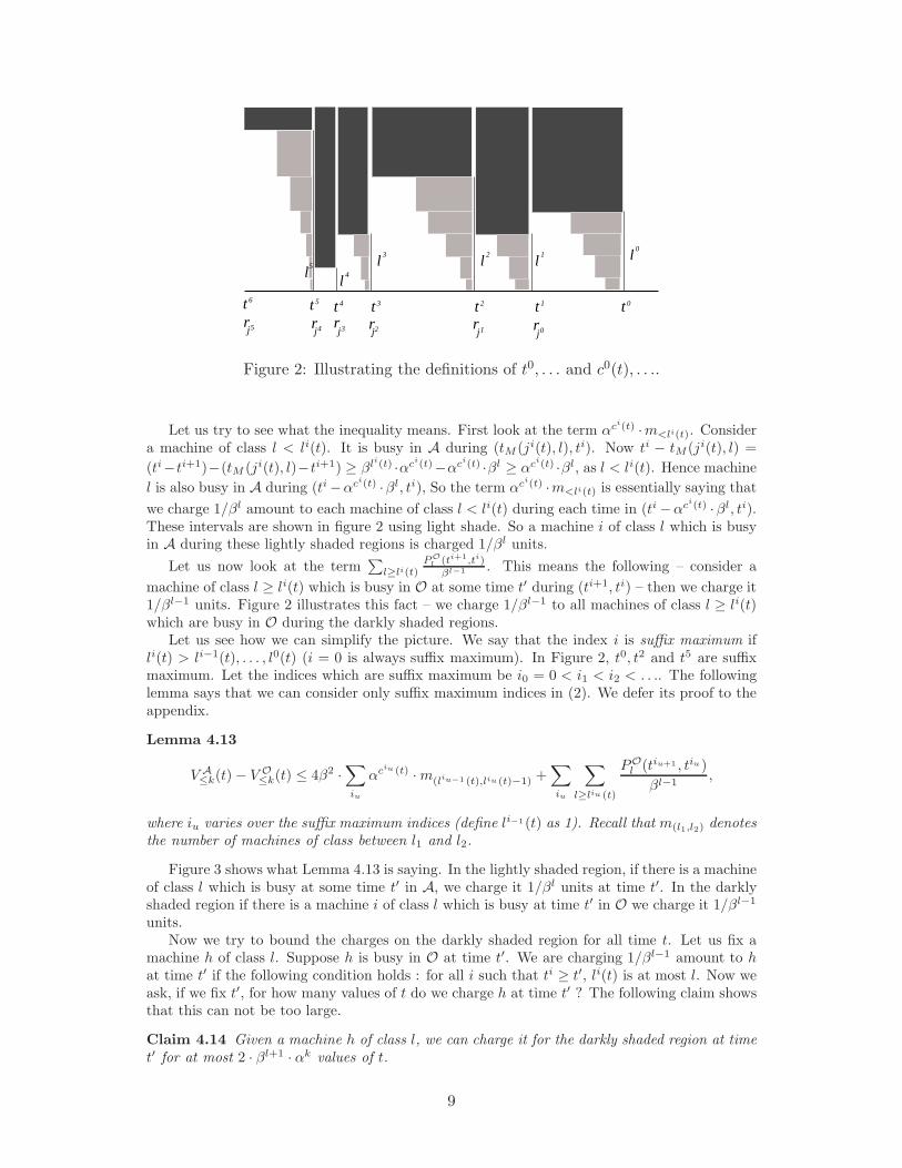
Figure 2: Illustrating the definitions of t0, . . . and c0(t), . . ..

Let us try to see what the inequality means. First look at the term αci(t) ·m<li(t). Considera machine of class l < li(t). It is busy in A during (tM (ji(t), l), ti). Now ti − tM (ji(t), l) =

(ti−ti+1)−(tM (ji(t), l)−ti+1) ≥ βli(t) ·αci(t)−αci(t) ·βl ≥ αci(t) ·βl, as l < li(t). Hence machine

l is also busy in A during (ti −αci(t) ·βl, ti), So the term αci(t) ·m<li(t) is essentially saying that

we charge 1/βl amount to each machine of class l < li(t) during each time in (ti −αci(t) ·βl, ti).These intervals are shown in figure 2 using light shade. So a machine i of class l which is busyin A during these lightly shaded regions is charged 1/βl units.

Let us now look at the term∑

l≥li(t)PO

l (ti+1,ti)βl−1 . This means the following – consider a

machine of class l ≥ li(t) which is busy in O at some time t′ during (ti+1, ti) – then we charge it1/βl−1 units. Figure 2 illustrates this fact – we charge 1/βl−1 to all machines of class l ≥ li(t)which are busy in O during the darkly shaded regions.

Let us see how we can simplify the picture. We say that the index i is suffix maximum ifli(t) > li−1(t), . . . , l0(t) (i = 0 is always suffix maximum). In Figure 2, t0, t2 and t5 are suffixmaximum. Let the indices which are suffix maximum be i0 = 0 < i1 < i2 < . . .. The followinglemma says that we can consider only suffix maximum indices in (2). We defer its proof to theappendix.

Lemma 4.13

V A≤k(t) − V O

≤k(t) ≤ 4β2 ·∑

iu

αciu (t) · m(liu−1 (t),liu (t)−1) +∑

iu

∑

l≥liu (t)

POl (tiu+1 , tiu)

βl−1,

where iu varies over the suffix maximum indices (define li−1(t) as 1). Recall that m(l1,l2) denotesthe number of machines of class between l1 and l2.

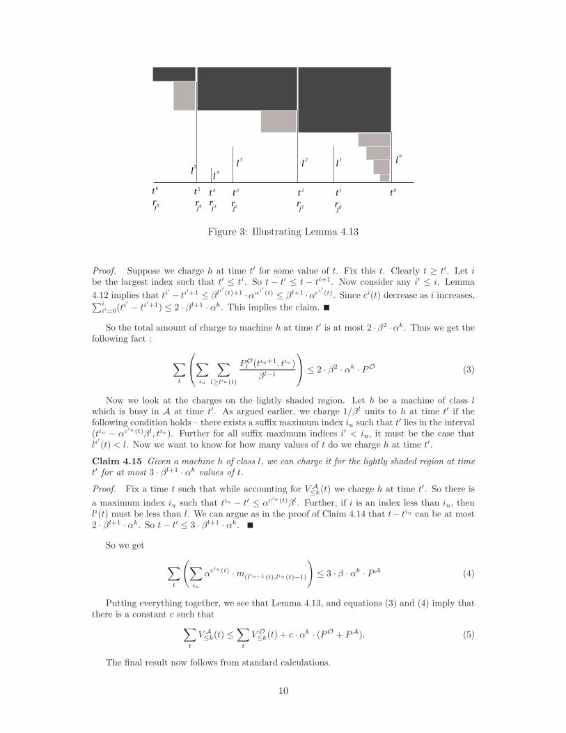
Figure 3 shows what Lemma 4.13 is saying. In the lightly shaded region, if there is a machineof class l which is busy at some time t′ in A, we charge it 1/βl units at time t′. In the darklyshaded region if there is a machine i of class l which is busy at time t′ in O we charge it 1/βl−1

units.Now we try to bound the charges on the darkly shaded region for all time t. Let us fix a

machine h of class l. Suppose h is busy in O at time t′. We are charging 1/βl−1 amount to hat time t′ if the following condition holds : for all i such that ti ≥ t′, li(t) is at most l. Now weask, if we fix t′, for how many values of t do we charge h at time t′ ? The following claim showsthat this can not be too large.

Claim 4.14 Given a machine h of class l, we can charge it for the darkly shaded region at timet′ for at most 2 · βl+1 · αk values of t.

9

ttttt 1 0234

lllll

0123

4

t 5

5l

t 6

rjjjrrrrrjjjjj 012345

Figure 3: Illustrating Lemma 4.13

Proof. Suppose we charge h at time t′ for some value of t. Fix this t. Clearly t ≥ t′. Let ibe the largest index such that t′ ≤ ti. So t − t′ ≤ t − ti+1. Now consider any i′ ≤ i. Lemma

4.12 implies that ti′

− ti′+1 ≤ βli

′(t)+1 ·ααi′ (t) ≤ βl+1 ·αci′ (t). Since ci(t) decrease as i increases,

∑ii′=0(t

i′ − ti′+1) ≤ 2 · βl+1 · αk. This implies the claim.

So the total amount of charge to machine h at time t′ is at most 2 · β2 ·αk. Thus we get thefollowing fact :

∑

t

∑

iu

∑

l≥liu (t)

POl (tiu+1, tiu)

βl−1

≤ 2 · β2 · αk · PO (3)

Now we look at the charges on the lightly shaded region. Let h be a machine of class lwhich is busy in A at time t′. As argued earlier, we charge 1/βl units to h at time t′ if thefollowing condition holds – there exists a suffix maximum index iu such that t′ lies in the interval(tiu − αciu (t)βl, tiu). Further for all suffix maximum indices i′ < iu, it must be the case thatli

′

(t) < l. Now we want to know for how many values of t do we charge h at time t′.

Claim 4.15 Given a machine h of class l, we can charge it for the lightly shaded region at timet′ for at most 3 · βl+1 · αk values of t.

Proof. Fix a time t such that while accounting for V A≤k(t) we charge h at time t′. So there is

a maximum index iu such that tiu − t′ ≤ αciu (t)βl. Further, if i is an index less than iu, thenli(t) must be less than l. We can argue as in the proof of Claim 4.14 that t− tiu can be at most2 · βl+1 · αk. So t − t′ ≤ 3 · βl+1 · αk.

So we get

∑

t

(

∑

iu

αciu (t) · m(liu−1 (t),liu (t)−1)

)

≤ 3 · β · αk · PA (4)

Putting everything together, we see that Lemma 4.13, and equations (3) and (4) imply thatthere is a constant c such that

∑

t

V A≤k(t) ≤

∑

t

V O≤k(t) + c · αk · (PO + PA). (5)

The final result now follows from standard calculations.

10

Theorem 4.16 FA is O(log S · log2 P · FO).

Proof. We have already bounded the processing time of A. Once a job gets dispatched to amachine i, its waiting time can be charged to the processing done by i. Since at any time t,there are at most log P active jobs dispatched to a machine, the total waiting time of jobs aftertheir dispatch time is at most O(log P · PA). So we just need to bound the time for which jobsare waiting in the central pool.

Let nAk (t) be the number of jobs of class k waiting in the central pool at time t in our

algorithm. Let nOk (t) be the number of jobs of class k which are active at time t in O (note

the difference in the definitions of the two quantities). Since jobs waiting in the central pool

in A have not been processed at all, it is easy to see that nAk (t) ≤

V A≤k(t)

αk . Further, V O≤k(t) ≤

αknOk (t) + · · · + αnO

1 (t). Combining these observations with equation (5), we get for all valuesof k,

∑

t

nAk (t) ≤

∑

t

(

nOk (t) +

nOk−1(t)

α+ · · · +

nO1 (t)

αk−1

)

+ c · (PO + PA).

We know that total flow time of a schedule is equal to the sum over all time t of the numberof active jobs at time t in the schedule. So adding the equation above for all values of k andusing Corollary 4.10 implies the theorem.

5 Open Problems

We leave open the problem of finding an online algorithm for this problem whose competitiveratio is independent of the speed of the machines.

References

[1] N. Avrahami and Y. Azar. Minimizing total flow time and total completion time withimmediate dispatching. In Proc. 15th Symp. on Parallel Algorithms and Architectures(SPAA), pages 11–18. ACM, 2003.

[2] Baruch Awerbuch, Yossi Azar, Stefano Leonardi, and Oded Regev. Minimizing the flowtime without migration. In ACM Symposium on Theory of Computing, pages 198–205,1999.

[3] N. Bansal and K. Pruhs. Server scheduling in the l p norm: A rising tide lifts all boats. InACM Symposium on Theory of Computing, pages 242–250, 2003.

[4] Luca Becchetti, Stefano Leonardi, Alberto Marchetti-Spaccamela, and Kirk R. Pruhs. On-line weighted flow time and deadline scheduling. Lecture Notes in Computer Science,2129:36–47, 2001.

[5] C. Chekuri, S. Khanna, and A. Zhu. Algorithms for weighted flow time. In ACM Symposiumon Theory of Computing, pages 84–93. ACM, 2001.

[6] Chandra Chekuri, Ashish Goel, Sanjeev Khanna, and Amit Kumar. Multi-processorscheduling to minimize flow time with epsilon resource augmentation. In ACM Sympo-sium on Theory of Computing, pages 363–372, 2004.

[7] R. L. Graham, E. L. Lawler, J. K. Lenstra, and A. H. G. Rinnooy Kan. Optimization andapproximation in deterministic sequencing and scheduling : a survey. Ann. Discrete Math.,5:287–326, 1979.

[8] Bala Kalyanasundaram and Kirk Pruhs. Speed is as powerful as clairvoyance. In IEEESymposium on Foundations of Computer Science, pages 214–221, 1995.

[9] Hans Kellerer, Thomas Tautenhahn, and Gerhard J. Woeginger. Approximability andnonapproximability results for minimizing total flow time on a single machine. In ACMSymposium on Theory of Cmputing, pages 418–426, 1996.

11

[10] Stefano Leonardi and Danny Raz. Approximating total flow time on parallel machines. InACM Symposium on Theory of Computing, pages 110–119, 1997.

[11] C. A. Phillips, C. Stein, E. Torng, and J. Wein. Optimal time-critical scheduling via resourceaugmentation. In ACM Symposium on Theory of Computing, pages 140–149, 1997.

Appendix

Proof of Theorem 4.6. Let M ′ denote the set of machines of class less than l. First observethat the processing time incurred by A on JI is at most twice of |M ′| ·T (the factor twice comesbecause there may be some jobs which are dispatched during I but finish later — there can beat most one such job for a given class and a given machine). So we will be done if we can showthat FO

JIis Ω(|M ′| · T ).

Let V be the volume of jobs in JI which are done by O on machines of class l or more. If

V ≥ |M ′|·Tβl+1 , then we are done because then the processing time incurred by O on JI is at least

V · βl. So we will assume in the rest of the proof that V ≤ |M ′|·Tβl+1 .

Let i be a machine of class less than l. We shall say that i is good is i processes jobs fromJI for at least T/4 units of time during I in the optimal solution O. Otherwise we say that i

is bad. Let G denote the set of good machines. If |G| ≥ |M ′|β , then we are done again, because

POJI

is at least |G| · T/4. Let B denote the set of bad machines.So we can assume that the number of good machines is at most 1/β fraction of the number

of machines of class less than l. Now consider a time t in the interval (tb + T/2, te).

Claim 5.1 At time t, at least αk|M ′| volume of jobs from JI is waiting in O.

Proof. Let V1 denote the volume of jobs from JI which is done by A during (tb, t). Let V2

denote the volume of jobs from JI which is done by O on machines of class less than l during(tb, t). Recall that for a machine i, si denotes the slowness of i.

Since a machine i of class l′ < l does not perform jobs from JI for at most 6αkβl′ amount of

time during I, we see that V1 ≥∑

i∈M ′t−tb−6αk·βci

si, where ci denotes the class of i. Let us look

at V2 now. In O all bad machines do not process jobs from JI for at least 3T/4 units of timeduring I. So they do not process jobs from JI for at least T/4 units of time during (tb, tb +T/2).

So V2 ≤∑

i∈M ′(t−tb)

si−∑

i∈BT4si

.

This shows that V1 − V2 ≥∑

i∈BT4si

−∑

i∈M ′6αkβci

si. For a bad machine i, T/4− 6αkβci ≥

T/8, since ci ≤ l − 1 (assuming β is large enough). So, we can see that this difference isat least

∑

i∈BT8si

−∑

i/∈B 6αkβ. Since T ≥ βl · αk, we see that this difference is at leastT

βl−1 (|B|/8 − 6|G|), which is at least T |M ′|10βl−1 , because we have assumed that |B| is larger than

|G| by a sufficiently high constant factor. Recall that V is the volume of jobs in JI which isdone by O on machines of class l or more. Clearly, the volume of jobs from JI which is waiting

at time t in O is at least V1 − V2 − V . But V is at most T |M ′|βl+1 . Hence the volume waiting at

time t is at least T |M ′|βl . This proves the lemma.

Since each job in JI is of size at most αk, we see that at least Ω(|M ′|) jobs are waiting attime t. Summing over all values of t in the range (tb + T/2, te) implies the theorem.

Proof of Lemma 4.13. Consider an i, iu+1 < i ≤ iu. Then li(t) ≤ liu(t), otherwise we

should have another suffix maximal index between iu+1 and iu. So∑iu+1−1

i=iuαci(t) · m<li(t) ≤

m<liu (t) ·∑iu−1

i=iuαci(t) ≤ 2·m<liu (t) ·α

ciu (t). So we get∑

i αci(t) ·m<li(t) ≤ 2·∑

ium<liu (t) ·α

ciu (t).

12

Now we consider the sum∑

i

∑

l≥li(t)PO

l (ti+1,ti)

βl−1 . Fix an i, iu+1 < i ≤ iu. Using Claim 4.12,

we see that POl (ti+1, ti) ≤ ml · β

li(t)+1 · αci(t). So we get

∑

l≥li(t)

POl (ti+1, ti)

βl−1≤

∑

l≥liu (t)

POl (ti+1, ti)

βl−1+

liu (t)−1∑

l=li(t)

ml · βli(t)+1 · αci(t)

βl−1

Now the second term on the right hand side above is at most β2 · m<liu (t)αci(t). So we get

iu+1−1∑

i=iu

∑

l≥li(t)

POl (ti+1, ti)

βl−1≤

∑

l≥liu (t)

POl (tiu+1 , tiu)

βl−1+ 2β2αciu (t)m<liu (t),

because αci(t) scales down geometrically as i increases.Finally note that

∑

iuαciu (t)m<liu (t) is at most twice of

∑

iuαciu (t) · m(liu−1 (t),liu (t)−1),

because αci(t) scale down geometrically. This proves the lemma (using (2)).

13