Ugo Gianazza(∗), Giuseppe Savare(∗∗)(∗∗∗)

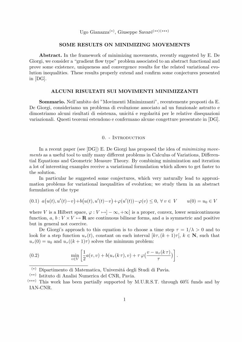
SOME RESULTS ON MINIMIZING MOVEMENTS

Abstract. In the framework of minimizing movements, recently suggested by E. DeGiorgi, we consider a “gradient flow type” problem associated to an abstract functional andprove some existence, uniqueness and convergence results for the related variational evo-lution inequalities. These results properly extend and confirm some conjectures presentedin [DG].

ALCUNI RISULTATI SUI MOVIMENTI MINIMIZZANTI

Sommario. Nell’ambito dei ”Movimenti Minimizzanti”, recentemente proposti da E.De Giorgi, consideriamo un problema di evoluzione associato ad un funzionale astratto edimostriamo alcuni risultati di esistenza, unicita e regolarita per le relative disequazionivariazionali. Questi teoremi estendono e confermano alcune congetture presentate in [DG].

0. - Introduction

In a recent paper (see [DG]) E. De Giorgi has proposed the idea of minimizing move-ments as a useful tool to unify many different problems in Calculus of Variations, Differen-tial Equations and Geometric Measure Theory. By combining minimization and iterationa lot of interesting examples receive a variational formulation which allows to get faster tothe solution.

In particular he suggested some conjectures, which very naturally lead to approxi-mation problems for variational inequalities of evolution; we study them in an abstractformulation of the type

(0.1) a(u(t), u′(t)−v

)+b

(u(t), u′(t)−v

)+ϕ(u′(t))−ϕ(v) ≤ 0, ∀ v ∈ V u(0) = u0 ∈ V

where V is a Hilbert space, ϕ : V 7→]−∞,+∞] is a proper, convex, lower semicontinuousfunction, a, b : V ×V 7→ R are continuous bilinear forms, and a is symmetric and positivebut in general not coercive.

De Giorgi’s approach to this equation is to choose a time step τ = 1/λ > 0 and tolook for a step function uτ (t), constant on each interval [kτ, (k + 1)τ [, k ∈ N, such thatuτ (0) = u0 and uτ ((k + 1)τ) solves the minimum problem:

(0.2) minv∈V

[12a(v, v) + b(uτ (k τ), v) + τ ϕ

(v − uτ (k τ)τ

)].

(∗) Dipartimento di Matematica, Universita degli Studi di Pavia.(∗∗) Istituto di Analisi Numerica del CNR, Pavia.

(∗∗∗) This work has been partially supported by M.U.R.S.T. through 60% funds and byIAN-CNR.

1

If

(0.3) ∃ limτ→0

uτ (t) = u(t), in V, ∀ t ∈ [0,+∞[

we call u a minimizing movement associated to the functional (0.2) and the equation (0.1).Under suitable hypotheses on V, a, ϕ we prove some existence, uniqueness and conver-

gence results from which De Giorgi’s conjectures can be obtained as a special case.Equations of this kind have been largely studied in these last years; just to quote a

few examples, in [DL] and [Br2] a non zero datum f(t) is considered while in [CV] and[Co] a double nonlinearity is studied and a fairly complete list of works on the argumentis given.

It doesn’t seem, however, that anything like we did already exists in the literature,due to the lack of coerciveness of the bilinear form a, to the unboundedness of ϕ and aboveall to the strong pointwise estimate required by (0.2).

We mainly use maximal monotone operators theory and convex analysis, whose tec-niques are developped for example in [Bar], [Br1] and [ET] and to which we refer foradditional related material. On the other hand the stability and convergence estimates aretypical of the abstract numerical analysis of parabolic variational inequalities and they aredevelopped for a different problem in [Ba].

All these results have been previously announced in a joint note with M. Gobbino[GGS], where further bibliographical references on the subject can be found.

In the first paragraph we discuss the problem and present our results in theorems 1–3;the proofs are given in the following sections.

We’d like to thank professor L. Ambrosio for suggesting us this argument of researchand professor F. Brezzi for his support.

2

1. - General definitions and statement of the results

In the following R will be the extended real line (R = R⋃−∞,+∞). Let S be a

topological space. In [DG] De Giorgi proposed the following

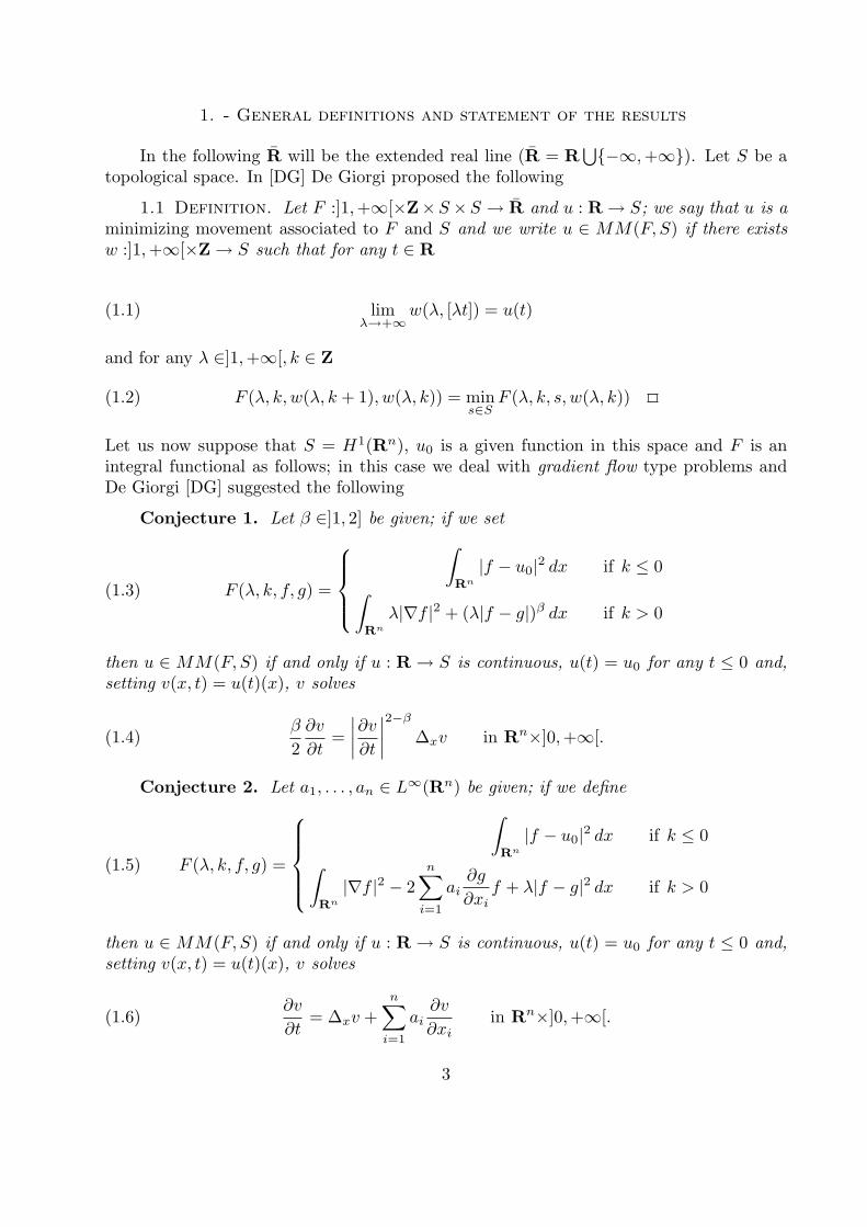
1.1 Definition. Let F :]1,+∞[×Z×S ×S → R and u : R → S; we say that u is aminimizing movement associated to F and S and we write u ∈ MM(F, S) if there existsw :]1,+∞[×Z → S such that for any t ∈ R

(1.1) limλ→+∞

w(λ, [λt]) = u(t)

and for any λ ∈]1,+∞[, k ∈ Z

(1.2) F (λ, k, w(λ, k + 1), w(λ, k)) = mins∈S

F (λ, k, s, w(λ, k))

Let us now suppose that S = H1(Rn), u0 is a given function in this space and F is anintegral functional as follows; in this case we deal with gradient flow type problems andDe Giorgi [DG] suggested the following

Conjecture 1. Let β ∈]1, 2] be given; if we set

(1.3) F (λ, k, f, g) =

∫Rn

|f − u0|2 dx if k ≤ 0∫Rn

λ|∇f |2 + (λ|f − g|)β dx if k > 0

then u ∈ MM(F, S) if and only if u : R → S is continuous, u(t) = u0 for any t ≤ 0 and,setting v(x, t) = u(t)(x), v solves

(1.4)β

2∂v

∂t=

∣∣∣∣∂v∂t∣∣∣∣2−β ∆xv in Rn×]0,+∞[.

Conjecture 2. Let a1, . . . , an ∈ L∞(Rn) be given; if we define

(1.5) F (λ, k, f, g) =

∫Rn

|f − u0|2 dx if k ≤ 0∫Rn

|∇f |2 − 2n∑i=1

ai∂g

∂xif + λ|f − g|2 dx if k > 0

then u ∈ MM(F, S) if and only if u : R → S is continuous, u(t) = u0 for any t ≤ 0 and,setting v(x, t) = u(t)(x), v solves

(1.6)∂v

∂t= ∆xv +

n∑i=1

ai∂v

∂xiin Rn×]0,+∞[.

3

Conjecture 3. If we put

(1.7) F (λ, k, f, g) =

∫Rn

|f − u0|2 dx if k ≤ 0∫Rn

|∇f |2 + λ|f − g|2 dx if k > 0, f ≥ g

+∞ otherwise

then u ∈ MM(F, S) if and only if u : R → S is continuous, u(t) = u0 for any t ≤ 0 and,setting v(x, t) = u(t)(x), v solves

(1.8)∂v

∂t= (∆xv)+ in Rn×]0,+∞[.

1.2 Remark. In the above stated conjectures it must be explained what is the weaksense in which equations (1.4) and (1.8) have to be understood.

1.3 Remark. The above written (1.3), (1.5), (1.7) can all be seen as generalizationof the basic functional

(1.9) F (λ, k, f, g) =

∫Rn

|f − u0|2 dx if k ≤ 0∫Rn

|∇f |2 + λ|f − g|2 dx if k > 0

Let us observe that in these cases it is sufficient to study the limit (1.1) for t ≥ 0.Actually all these conjectures naturally fit into a more general and abstract framework.

Precisely we consider

(1.10)

V Hilbert space with norm ‖ · ‖V ′ its dual, < ·, · > the duality pairing

(1.11)

ϕ : V → R ∪ +∞ proper, lower semicontinuous, convexD(ϕ) its domain, ∂ϕ its subdifferential, ϕ∗ its conjugate (1)

(1) Let us recall that D(ϕ) = v ∈ V : ϕ(v) < +∞ 6= ∅ and that ∀v ∈ V, w ∈ V ′

w ∈ ∂ϕ(v) ⇔ < w, z − v >≤ ϕ(z)− ϕ(v) ∀z ∈ V

ϕ∗ : V ′ 7→ R is a proper l.s.c. convex function defined by

ϕ∗(w) = supv∈V

< w, v > −ϕ(v), ∀w ∈ V ′

4

(1.12)

a(·, ·), b(·, ·) : V × V → R continuous bilinear formsto which the linear continuous operators A,B : V → V ′ are associated (2)

Moreover, a(·, ·) is symmetric and the associated quadratic form, which we e by a(·), ispositive:

a(u, v) = a(v, u); a(u) = a(u, u) ≥ 0 ∀u, v ∈ V.

We can then think to the following problem

Problem P. Let u0 ∈ V be given and consider

(1.13) F (λ, k, v, w) =

‖v − u0‖ if k ≤ 012a(v, v) + b(v, w) +

1λϕ[λ(v − w)] otherwise.

We want to find conditions on a, b, ϕ, u0 such that there exists a unique u : R → V withu ∈ MM(F, V ) and

(1.14)

u ∈ C0(R, V ) ∩ACloc(]0,+∞[;V )u(t) ≡ u0 ∀t ≤ 00 ∈ Au+Bu+ ∂ϕ(u′) a.e. in ]0,+∞[.

Let us start and consider the case with

(1.15) b ≡ 0

If the form a(·, ·) is coercive on V , that is, if it satisfies

(1.16) ∃α > 0 : ∀u ∈ V a(u, u) ≥ α‖u‖2,

then Problem P has a very general answer. As a matter of fact we have the following

Theorem 1. Under hypotheses (1.15) and (1.16), if (3)

(1.17) −Au0 ∈ D(ϕ∗)V ′

(2) As it is usual, ∀u, v ∈ V

< Au, v >= a(u, v) ≤Ma ‖u‖ ‖v‖; < Bu, v >= b(u, v).

(3) ∃!u ∈MM(F, V ) even if this condition is not satisfied; the solution u still verifies thedifferential inclusion but it is not continuous at t = 0; in fact we have limt→0+ u(t) = u+

0

and −u+0 is the projection of u0 on the convex A−1

(D(ϕ∗)

)with respect to the scalar

product defined by a(·, ·).

5

Problem P admits a solution u that satisfies (1.14) and

(1.18) u ∈W 1,+∞loc (]0,+∞[;V ).

Moreover, if we define ϕ as the function v 7→ ϕ(−v), u is the solution to

(1.19)

u(0) = u0

u′ + ∂ϕ∗ (Au) 3 0 a.e. in ]0,+∞[

and belongs to MM(F ∗, V ), where

(1.20) F ∗(λ, k, v, w) =

‖v − u0‖ if k ≤ 0

λ

2a(v − w, v − w) + ϕ∗(Av) otherwise.

1.4 Remark. The minimization of functionals F, F ∗ given by (1.13) and (1.20) leadsto backward Euler scheme for the approximation of (1.14) and (1.19) respectively; this lastcase, in particular, is deeply developped in [Br 2] in a slightly different framework and ourproof is an easy consequence of that theory. On the other hand, using the same proceduresas in section 3 and 4 we could give a direct proof of this result, which would be more relatedto the minimizing movement idea; we restricted ourselves to the results which seem to benew.

1.5 Remark. Let us substitute Rn with a bounded domain Ω and choose S = V =H1

0 (Ω) in conjecture 1. We define

(1.21) a(u, v) =∫

Ω

(∇u,∇v) dx, ϕ(u) =12

∫Ω

|u|β dx, β ∈]1,+∞[.

ThenAu = −∆u, ∂ϕ(u) =

β

2|u|β−2u

andD(ϕ∗) = Lβ

′(Ω) → H−1(Ω),

1β

+1β′

= 1

where the inclusion is dense. It is easy to see that condition (1.17) is satisfied for anychoice of u0.

1.6 Remark. An analogous work can be done with conjecture 3 once we put

(1.22) ϕ(u) =12

∫Ω

|u|2 dx+ Iu≥0, Iu≥0 =

0 if u ≥ 0 a.e.

+∞ otherwise.

Under these hypotheses u satisfies the variational inequality∫Ω

∂u

∂t

(∂u

∂t− v

)+

∫Ω

(∇u,∇

(∂u∂t− v

))≤ 0, ∀v ∈ H1

0 (Ω), v ≥ 0 in Ω a.e. in ]0,+∞[.

6

If a(·, ·) is not coercive (which is the case of our conjectures), the situation is morecomplicated. We will suppose that a uniformly convex Banach space W is given, which iscompatible with V in the sense that(1.23)

V and W are both continuously embedded in a Hausdorff topological vector space TV ∩W is dense in V and in W (4)

Moreover we assume that (5)

(1.24) ∃l, αl > 0 :√a(u, u) + l‖u‖W ≥ αl‖u‖V , ∀u ∈ V ∩W

ϕ is linked to W in the following sense:

(1.25)

∃β ∈]1,+∞[, ∃ψ : V ∩W 7→ R ∪ +∞ proper, convex, l.s.c.

ϕ(u) = ‖u‖βW + ψ(u), ∀u ∈ V ∩W.

We have now

Theorem 2. Under the preceding hypotheses (1.15), (1.23)–(1.25), ∀u0 ∈ V ProblemP has a unique solution u. Moreover, ∀T > 0,

(1.26)

u ∈W 1,β

loc (]0,+∞[;V ), u′ ∈ Lβ(0, T ;W )

ϕ∗(−Au), ψ(u′) ∈ L1(0, T )

and u satisfies also (1.19).

1.7 Remark. If ψ satisfies:

(1.27) 0 ∈ D(ψ), ψ(v) ≥ 0, ∀ v ∈ D(ψ)

the previous result holds for T = +∞ and the proof is sligthly easier. In this case ϕ∗

satisfies (1.27), too.

1.8 Remark. Let us choose W = Lβ(Rn), with β ∈]1, 2], ψ = 0 and consequently

a(u, v) =∫Rn

(∇u,∇v) dx, ϕ(u) =12

∫Rn

|u|β dx.

We are dealing with conjecture 1 and our hypotheses are trivially satisfied. In this case

−∆u ∈ Lβ′(Rn×]0,+∞[), and

∂u

∂t∈ Lβ(Rn×]0,+∞[)

(4) This in particular implies that V ′ and W ′ can be continuously and densely imbeddedinto (V ∩W )′, which will coincide with their sum.(5) As a(·, ·) is positive, this is the same as

∀ε > 0 ∃αε > 0 :√a(u, u) + ε‖u‖W ≥ αε‖u‖V , ∀u ∈ V ∩W.

7

1.9 Remark. As in the previous case, let us choose

W = Lβ(Rn), ψ = IK , K = u ≥ 0, ϕ(u) =1β

∫Rn

|u|β dx+ ψ(u)

then conjecture 3 follows from the abstract theory for β = 2; moreover, denoting byM(Rn)the topological vector space of Radon measures on Rn, we have

D(ϕ∗) = v ∈ H−1(Rn) ∩M(Rn) : v− ∈ Lβ′(Rn)

ϕ∗(u) =1β′

∫Rn

|u−|β′dx, ∂ϕ∗(u) = −(u−)β

′−1.

For a.e. t, ∆u is a measure whose positive part is in Lβ′(Rn) and u satisfies

∂u

∂t= [(∆u)+]β

′−1

1.10 Remark. (Neumann’s problem) As in Remark 1.5 we choose V = H1(Ω) andu is the solution to

β

2|u′|β−2u′ = ∆u in Ω×]0,+∞[

∂u∂n = 0 on ∂Ω×]0 +∞[u = u0 on Ω× 0.

As ∆u belongs to Lβ′(Ω) the Neumann condition makes sense.

Finally, let us consider b 6≡ 0; we will suppose that

(1.28)

W = H is a Hilbert space and V is continuously densely imbedded in H,b can be extended to a continuous bilinear form on V ×H 7→ R, that is

∃Mb > 0 : b(u, v) ≤Mb ‖u‖V ‖v‖H , ∀u, v ∈ V ϕ(u) =12‖u‖2H + ψ(u)

Theorem 3. Problem P admits a unique solution u, which belongs also to H1(0, T ;H)∀T > 0.

1.11 Remark. We end up with conjecture 2 if we suppose that ψ ≡ 0, H = L2(Rn)and

b(u, v) =n∑i=1

∫Rn

ai∂u

∂xiv dx

8

2. - Proof of theorem 1

2.1 Lemma. For any v ∈ V there exists a unique w = σ(λ, v) ∈ V such that

(2.1)12a(w,w) +

1λϕ(λ(w − v)) = min

z∈V[12a(z, z) +

1λϕ(λ(z − v))]

and w solves the following variational inequality

(2.2) a(w,w − z) +1λϕ(λ(w − v))− 1

λϕ(λ(z − v)) ≤ 0 ∀z ∈ V.

Moreover w also solves

(2.3) λa(w − v, w − z) + ϕ∗(Aw)− ϕ∗(Az) ≤ 0 ∀z ∈ V

and the dual problem

(2.4)λ

2a(w − v, w − v) + ϕ∗(Aw) = min

z∈V[λ

2a(z − v, z − v) + ϕ∗(Az)].

Proof The first two relations are obvious since we are looking for the minimum of thesum of convex functions, one of which is coercive and Frechet-differentiable (see [V], [L]).If we define z = λ(z − v) we can rewrite (2.2) in this way

(2.5) a(w, λ(w − v)− z) + ϕ(λ(w − v))− ϕ(z) ≤ 0 ∀z ∈ V ;

that is:−Aw ∈ ∂ϕ(λ(w − v))

Recalling that ∂ϕ∗ is the inverse operator of ∂ϕ (see [Br2], [Bar]) we get:

(2.6) λ(w − v) ∈ ∂ϕ∗(−Aw) = −∂ϕ∗(Aw)

that is (2.3) and (2.4).

2.2 Remark. By (2.6) the function w = σ(λ, v) satisfies:

(2.7) w +1λ∂ϕ∗(Aw) 3 v;

the multivalued operator V 3 v 7→ ∂ϕ∗ A ⊂ V is then maximal and monotone, when Vis endowed with the scalar product a(·, ·). It is also easy to verify that we are dealing withthe subdifferential of the conjugate function of ϕ once we identify V and V ′ through a. Itsresolvent is given by

(2.8) Jτv = σ(1τ, v), V 7→ V

9

We can then finally come to the proof of theorem 1; if we apply the theory developpedin [Br2] we can see immediately that

(2.9)

u′ + ∂ϕ∗(Au) 3 0 a.e. in ]0,+∞[

u(0) = u0

has a unique solution u in C0([0,+∞[;V ) ∩ W 1,+∞loc (]0,+∞[;V ) if −Au0 ∈ D(ϕ∗)

V ′

.Moreover, thanks to the exponential formula we have

(2.10) u(t) = limn→+∞

(·+ t

n∂ϕ∗(A · ))−nu0 = lim

n→+∞Jnt/nu0 ∀t > 0

uniformly on the compact subsets of [0,+∞[. If we now define w(λ, k) as in (1.2) we have

(2.11) w(λ, k) = u0 if k ≤ 0

(2.12) w(λ, k + 1) = σ(λ,w(λ, k)) = J 1λw(λ, k) = Jk+1

1λ

u0.

Choosing 1/λ = t/n, it follows that, ∀t > 0,

(2.13) limn→+∞

w(n

t, n) = u(t) ∀t > 0

uniformly on the compact subsets of ]0,+∞[. Finally, (1.1) is a direct consequence of thefollowing

2.3 Lemma. Let (S, d) be a metric space and w : [0,+∞[×N → S a function suchthat

∃ limn→+∞

w(n

t, n) = u(t)

uniformly on the compact subsets of ]0,+∞[. If u(t) is continuous, then

limλ→+∞

w(λ, [λt]) = u(t) ∀t > 0.

Proof It is enough to observe that

(2.14) | [λt]λ− t| ≤ 1

λ

and

(2.15) d(w(λ, [λt]), u(t)) ≤ d(w(λ, [λt]), u([λt]λ

)) + d(u([λt]λ

), u(t))

10

3. - Proof of theorem 2

We make a slight change in the notations, using the same as in [Ba]. We put

(3.1) τ =1λ∈ ]0, 1[, ukτ = w(1/τ, k) ∈ V.

We have already seen that ukτ is the sequence such that

(3.2) ukτ ≡ u0 for k ≤ 0

(3.3)

δkτ =ukτ − uk−1

τ

τ∈ D(ϕ)

a(ukτ , δkτ − v) + ϕ(δkτ )− ϕ(v) ≤ 0 ∀v ∈ V k ≥ 1

(3.4)

Aukτ ∈ D(ϕ∗)

< δkτ , Aukτ − v > +ϕ∗(Aukτ )− ϕ∗(v) ≤ 0 ∀v ∈ V ′ k ≥ 1

where this last relation is the dual of the previous one. Let us now divide R into theintervals Ikτ = [τ(k − 1), τk[ and consider the function uτ piecewise constant whose valuein Ikτ is uk−1

τ . Our aim is to show that

(3.5) limτ→0+

uτ (t) = u(t) in V ∀t ≥ 0

and that u(t) satisfies (1.14). It is convenient to divide the proof in different steps:1) Stability estimates in suitable functional spaces on the bounded intervals ]0, T [, T > 0.2) Stationary estimates for the singular perturbation problem (3.3) when τ goes to zero.3) Cauchy estimate with respect to the seminorm induced by a.4) Passage to the limit for a subsequence through weak compactness and further rein-

forcement of the convergence thanks to the uniform reflexivity of W .5) Uniqueness of the solution to (1.14) and therefore existence of the limit (3.5).

Step 1: stability estimates.

Let us fix T > 0 and choose N ∈ N such that T ∈ INτ . It is also useful to considerthe piecewise linear function uτ such that:

(3.6) uτ (kτ) = ukτ ; uτ (t) =(t/τ − (k − 1)

)ukτ + (k − t/τ)uk−1

τ , on Ikτ

We then have

11

3.1 Theorem. There exist constants C0, C1 > 0, independent from τ , such that

(3.7) ‖uτ‖L∞(0,T ;V ) ≤ ‖uτ‖L∞(0,T ;V ) ≤ C0

(3.8) ‖u′τ‖Lβ(0,T ;W ) ≤ C1

(3.9)

∫ T

0

ψ(u′τ (t)) dt∫ T

0

ϕ∗(Auτ (t+ τ)) dt

≤ 12a(u0).

Moreover, if (1.27) holds true, then we can choose C1 = 12a(u0).

Proof Since in general

w ∈ ∂ϕ(v) ⇒ (w, v) = ϕ(v) + ϕ∗(w)

we observe that

(3.10) < Aukτ , δkτ > +‖δkτ ‖

βW + ψ(δkτ ) + ϕ∗(Aukτ ) = 0.

Adding up for k = 1 . . . m ≤ N(6)

(3.11)12a(umτ ) +

τ2

2

m∑k=1

a(δkτ ) + τm∑k=1

[‖δkτ ‖

βW + ψ(δkτ ) + ϕ∗(Aukτ )

]=

12a(u0).

Recalling that u′τ (t) ≡ δkτ on Ikτ , (3.9) follows immediately.We already observed that (1.27) implies

(3.12) ϕ∗(v) ≥ 0, ∀ v ∈ V ′

and consequently (3.8); since

(3.13) τm∑k=1

‖δkτ ‖βW ≥ 1

(T + τ)β

β′‖umτ − u0‖βW

via (1.24) we get also (3.7).

(6) We often use the elementary equality:

a(v, v − w) =12[a(v) + a(v − w)− a(w)

]

12

Otherwise we recall that convex lower semicontinuous functions are bounded frombelow by affine functions

(3.14)

∃ξψ ∈ V ′ +W ′, ξϕ∗ ∈ V, η ∈ R :ψ(v) ≥ − < ξψ, v > −ηϕ∗(v) ≥ − < ξϕ∗ , v > −η

.

Therefore

(3.15)

12a(umτ ) +

τ2

2

m∑k=1

a(δkτ ) + τm∑k=1

‖δkτ ‖βW ≤

≤ 12a(u0)+ < ξψ, u

mτ − u0 > +τ

m∑k=1

< ξϕ∗ , Aukτ > +2(τm) η ≤

≤ 12a(u0) + ‖ξψ‖V ′+W ′ · ‖umτ − u0‖V ∩W + (T + τ)[a(ξϕ∗) + 2η] +

τ

4

m∑k=1

a(ukτ )

By (3.13) there exists a constant C > 0 such that

12a(umτ ) + τ

m∑k=1

‖δkτ ‖βW ≤ C[1 + τ

m∑k=1

a(ukτ )].

From here we obtain the uniform boundedness of a(umτ ) (it is a discrete version of Gronwalllemma) and (3.8), (3.7).

To go to the limit in the weak sense we need to control a(u′τ ). This is done precisely by

3.2 Theorem. ∃C2 > 0 independent of τ such that

(3.16)∫ T

0

ta(u′τ (t)) dt ≤ C2.

Proof It is enough to choose v = Auk−1τ , k ≥ 2 in (3.4); if we multiply for kτ and sum

from 2 up to N we have:

(3.17) τN∑k=2

kτ a(δkτ ) + τN∑k=2

[kϕ∗(Aukτ )− (k − 1)ϕ∗(Auk−1

τ )]− τ

N∑k=2

ϕ∗(Auk−1τ ) ≤ 0

from which

τN∑k=2

kτ a(δkτ ) +Nτ ϕ∗(AuNτ )− τϕ∗(Au1τ ) ≤ τ

N−1∑k=1

ϕ∗(Aukτ )

Summing (3.11) written with m = 1 we have

τN∑k=1

kτ a(δkτ ) ≤ τN−1∑k=2

ϕ∗(Aukτ ) + a(u0)− τψ(δ1τ )−Nτϕ∗(AuNτ ) ≤ C2

from which we obtain (3.16).

13

3.3 Lemma. The sequences

(3.18) k 7→ a(δkτ ); k 7→ ϕ∗(Aukτ ) k ≥ 1

are not increasing.

Proof In (3.3) we choose v = δk−1τ and in the one relative to the preceding step we choose

v = δkτ ; summing up we get

(3.19) a(δkτ , δkτ − δk−1

τ ) ≤ 0

and this is precisely the first relation; for the second one it is sufficient to choose v = Auk−1τ

in (3.4).

3.4 Corollary. As a simple consequence

(3.20) a(u′τ (t)) ≤2C2

t2, ∀t ≤ T

Step 2: stationary estimates.

3.5 Lemma. We have

(3.21) limτ→0+

‖u1τ − u0‖W + a(u1

τ − u0) = 0; limτ→0

τ ϕ∗(Au1τ ) = 0.

Proof From (3.8) we immediately obtain

(3.22) ‖u1τ − u0‖βW ≤ C1 τ

β−1 → 0 when τ → 0+;

moreover, since u1τ is bounded in V , compatibility requires that u1

τ u0 in V . If we write(3.11) with m = 1 we can see that

(3.23) lim supτ→0+

a(u1τ ) ≤ a(u0)

and taking into account the positivity of a we have

limτ→0+

a(u1τ − u0) = 0.

Finally, from (3.11) we have:

τϕ∗(Au1τ ) ≤

12[a(u0)− a(u1

τ )]+ < ξψ, u1τ − u0 > +τ η

obtaining the second of (3.21).

14

3.6 Corollary. We have

(3.24) limτ→0+

a(uk+1τ − ukτ ) = 0

uniformly with respect to k.

Proof It is immediate if we combine the previous result with lemma 3.3.

3.7 Corollary. We find

(3.25)

limτ→0+

supt>0

a(uτ (t+ τ)− uτ (t))

limτ→0+

supt>0

a(uτ (t)− uτ (t))

limτ→0+

supt>0

a(uτ (t+ τ)− uτ (t))

= 0

Step 3: Cauchy estimate.

3.8 Theorem. We have

(3.26) limτ,ρ→0+

supt∈[0,T ]

a(uτ (t)− uρ(t)) = 0.

with T = +∞ if (1.27) holds.

Proof It follows from the following lemma:

3.9 Lemma. Let `τ (t) be the τ−periodic function that is equal to t/τ in [0, τ [ andUτ , Uτ the τ−translated functions:

(3.27) Uτ (t) = uτ (t+ τ), Uτ (t) = uτ (t+ τ)

then Uτ satisfies the inequality

(3.28) a(U ′τ , Uτ − v) + ϕ∗(AUτ )− ϕ∗(Av) ≤ (1− `τ )[ϕ∗(AUτ )− ϕ∗(AUτ (t+ τ))].

We choose in (3.28) v = Uρ; changing the role of τ and ρ, summing up and integratingbetween 0 and t, we obtain in the left hand member the difference:

12a(Uτ (t)− Uρ(t))−

12a(Uτ (0)− Uρ(0))

while in the right hand member, due to the τ−periodicity of `τ (t):∫ τ

0

(1−`τ )[ϕ∗(AUτ (t))−ϕ∗(AUτ (T+t))

]dt+

∫ ρ

0

(1−`ρ)[ϕ∗(AUρ(t))−ϕ∗(AUρ(T+t))

]dt

so that:

a(Uτ (t)− Uρ(t)) ≤ a(u1τ − u1

ρ) + τϕ∗(Au1τ ) + ρϕ∗(Au1

ρ) + 2C0 (τ + ρ)(‖Aξϕ∗‖∗ + η)

By lemma 3.5 and its corollary we deduce (3.26).

15

Proof of Lemma 3.9 Let us observe that

(3.29) uτ (t) = `τ (t)uτ (t+ τ) + (1− `τ (t))uτ (t)

(3.30) uτ (t+ τ)− uτ (t) = τ(1− `τ (t))u′τ (t)

with 0 ≤ `τ (t) ≤ 1. Now, thanks to (3.4) we have

(3.31) < u′τ (t), Auτ (t+ τ)− v > +ϕ∗(Auτ (t+ τ))− ϕ∗(v) ≤ 0 ∀v ∈ V ′

and consequently

(3.32)a(u′τ (t), uτ (t)− v) + ϕ∗(Auτ (t))− ϕ∗(Av) ≤

≤ a(u′τ (t), uτ (t)− uτ (t+ τ)) + ϕ∗(Auτ (t))− ϕ∗(Auτ (t+ τ)).

Thanks to (3.30)

a(u′τ (t), uτ (t)− uτ (t+ τ)) = −τ(1− `τ )a(u′τ ) ≤ 0

while, due to convexity,

(3.33) ϕ∗(Auτ (t)) ≤ (1− `τ )ϕ∗(Auτ (t)) + `τ ϕ∗(Auτ (t+ τ)).

Taking account of these two inequalities in (3.32), we obtain (3.28).

Step 4: passage to the limit.

The previous estimates allow us to prove

3.10 Theorem. There exists a subsequence τn with τn 0 and a function

u ∈ C0([0, T ];V ) ∩W 1,βloc (]0, T ];V )

such that

(3.34) uτn(t) u(t) in V, ∀t ∈ [0, T ] lim

n→+∞supt∈[0,T ]

a(uτn(t)− u(t)) = 0.

Moreover u′(t) ∈ Lβ(0, T ;W ) while ψ(u′(t)) and ϕ∗(Au(t)) are in L1(0, T ) and u satisfies

(3.35) u′(t) + ∂ϕ∗(Au(t)) 3 0, u(0) = u0.

Proof The proof is standard: once we extract a subsequence τn such that uτnweak∗-

converges to u in L∞(0, T ;V ) and u′τn u′ in Lβ(0, T ;W ) and in Lβloc(]0, T ];V ), it is

immediate to verify that

(3.36) uτn(t) u(t) in V ∀t ∈ [0, T ]

16

and that

(3.37) limn→+∞

supt∈[0,T ]

a(uτn(t)− u(t)) = 0.

thanks to the lower semicontinuity of the quadratic form a(·).It follows that also Uτn uniformly converges to u in the seminorm induced by a and

therefore

(3.38) Auτn → Au in L∞(0, T ;V ′) (7)

Since by (3.31)

(3.39) u′τn+ ∂ϕ∗(Auτn

) 3 0 a.e. in ]0, T [

the inclusion is still true for u:

(3.40) u′(t) + ∂ϕ∗(Au) 3 0 a.e. in ]0, T [.

We still have to check the continuity in 0; on one hand it is easy to see that

a(u(ε)− u0) = a(u(ε)− uτ (ε)) ∀τ > ε.

In fact, if we choose nε = maxk : τk > ε, nε grows to infinity when ε goes to 0 andtherefore

limε→0+

a(u(ε)− u0) = limε→0+

a(u(ε)− uτnε(ε)) ≤ lim

ε→0+supt∈[0,1]

a(u(t)− uτnε(t)) = 0.

On the other hand

‖u(ε)− u0‖W ≤ lim infn→+∞

‖uτn(ε)− u0‖W ≤ Cε1

β′

and we are done.

As a matter of fact the convergence is actually stronger. At this regard we have

(7) Observe that the Schwartz inequality applied to a gives:

‖Av‖∗ = sup‖w‖=1

< Av,w >≤ sup‖w‖=1

√a(v)

√a(w) ≤Ma

√a(v)

17

3.11 Theorem. Let τn and u be as in the previous proposition. Then

(3.41) u′τn→ u′ in Lβ(0, T ;W ).

In particularlim

n→+∞uτn(t) = u(t) in V

uniformly with respect to t on any bounded interval.

Proof From (3.40) we get

(3.42) a(u′(t), u(t)) + ϕ∗(Au(t)) + ϕ(u′(t)) = 0 a.e. in ]0,+∞[

while from (3.39) we have

(3.43) a(u′τ (t), uτ (t)) + ϕ∗(AUτ (t)) + ϕ(u′τ (t)) ≤ 0.

Let us now integrate from 0 to T (8); we find

(3.44)12a(u(T )) +

∫ T

0

ϕ∗(Au(t)) dt+∫ T

0

[‖u′(t)‖βW + ψ(u′(t))] dt =12a(u0)

and

(3.45)12a(uτn

(T )) +∫ T

0

ϕ∗(AUτn(t)) dt+

∫ T

0

[‖u′τn(t)‖βW + ψ(u′τn

(t))] dt ≤ 12a(u0).

Passing to the limit for τn → 0 we have

lim supn→+∞

∫ T

0

[ϕ(AUτn(t)) + ‖u′τn(t)‖βW + ψ(u′τn

(t))] dt ≤

(3.46) ≤∫ T

0

[ϕ∗(Au(t)) + ‖u′(t)‖βW + ψ(u′(t))] dt.

On the other hand the three functions ϕ∗, ‖·‖βW and ψ are lower semicontinuous. Therefore

(3.47) limn→+∞

∫ T

0

‖u′τn(t)‖βW dt =

∫ T

0

‖u′(t)‖βW dt.

As Lβ(0, T ;W ) is uniformly convex (9),

u′τn→ u′ in Lβ(0, T ;W )

Step 5: uniqueness of the solution.

(8) Thanks to (3.40) we integrate from ε > 0 to T and then we let ε go to zero, using thecontinuity of u in W .(9) For the uniform convexity of Lβ(W ) with W uniformly convex, see [D].

18

Since uτ (t) = uτ (τ [ tτ ]) we also have uτn(t) → u(t). To be sure of the convergence of thewhole family uτ we must prove the uniqueness of the limit.

3.12 Proposition. Let u1, u2 ∈ C0([0,+∞[;V )∩ACloc(]0,+∞[;V ) be two solutionsof the Cauchy problem

Au+ ∂ϕ(u′) 3 0u(0) = u0

.

If ϕ is strictly convex, then u1 ≡ u2.

Proof Usually, thanks to the monotonicity, we obtain that t 7→ a(u1(t) − u2(t)) is notincreasing, so that

a(u1(t)− u2(t)) ≡ 0.

Moreover, if u′1 6= u′2, then for the strict monotonicity of the subdifferential we should have

a(u1(T )− u2(T )) < a(u1(ε)− u2(ε)) = 0

for some 0 < ε < T which is absurd. It follows that u′1 = u′2 and, for the Cauchy condition,u1 ≡ u2.

19

4. - Proof of Theorem 3

We repeat faster the previuos sequence, enhancing all the changes that are to be madeand underlining the specific difficulties of this case.With regard to the notation, we will identify H with its dual so that we have the followingcontinuous and dense inclusions:

(4.1) V → H ≡ H ′ → V ′;

in this way the scalar product (·, ·) of H may be extended to the duality between V andV ′, which we will denote with the same symbol. Finally, | · | will be the norm in H.

The sequence ukτ satisfies now the inequalities (k ≥ 1)

(4.2)

δkτ ∈ D(ψ)

(δkτ +Aukτ +Buk−1τ , δkτ − v) + ψ(δkτ )− ψ(v) ≤ 0

(4.3)

δkτ +Aukτ +Buk−1

τ ∈ D(ψ∗)

(δkτ , δkτ +Aukτ +Buk−1

τ − v) + ψ∗(δkτ +Aukτ +Buk−1τ )− ψ∗(v) ≤ 0

and also

(4.4) (δkτ , δkτ +Aukτ +Buk−1

τ ) + ψ∗(δkτ +Aukτ +Buk−1τ ) + ψ(δkτ ) = 0.

As for the stability estimates we have

4.1 Theorem. ∃C > 0 independent from τ such that

(4.5) ‖uτ‖L∞(0,T ;V ) ≤ ‖uτ‖L∞(0,T ;V ) ≤ C

(4.6) ‖u′τ‖L2(0,T ;H) ≤ C

(4.7)∫ T

0

ψ(u′τ (t)) dt ≤ C

(4.8)∫ T

0

ψ∗(u′(t) +Auτ (t+ τ) +Buτ (t)) dt ≤ C

(4.9)∫ T

0

ta(u′τ (t)) dt ≤ C

20

Proof We work as in the previous paragraph and we obtain from (4.4)

(4.10)

τm∑k=1

(|δkτ |2H +

τ

2a(δkτ )

)+

12a(umτ ) ≤

≤ 12a(u0) + 2mτη+(ξψ + ξψ∗ , u

mτ − u0) + τ

m∑k=1

b(uk−1τ , δkτ + ξψ∗) + a(ukτ , ξψ∗).

We get to (4.5) thanks to Gronwall lemma and to the boundedness of the form b in V ×Hthat leads to the following estimate

τm∑k=1

b(uk−1τ , δkτ + ξψ∗) ≤

12τ

m∑k=1

|δkτ |2 +mτ

2|ξψ∗ |

2 +M2b

2τm−1∑k=0

‖ukτ‖2.

(4.6), (4.7) and (4.8) are immediate and (4.9) comes in a similar way from theorem 3.2.

The stationary estimates are evaluated as in the case of theorem 1.6. In fact

4.2 Lemma. It results

(4.11) limτ→0+

‖u1τ − u0‖ = 0;

(4.12) limτ→0+

τψ∗(δ1τ +Au1τ +Bu0) = 0

It is more delicate the following

4.3 Proposition. It exists a constant C > 0, indipendent from τ such that

(4.13) supt∈[0,T ]

‖uτ (t)− uτ (t+ τ)‖V ≤ C ‖u1τ − u0‖

(4.14)∫ T

0

|u′τ (t)− u′τ (t+ τ)|2H ≤ C‖u1τ − u0‖2

Proof If we work as in Lemma 3.3 we have(δkτ − δk−1

τ , δkτ − δk−1τ + τAδkτ + τBδk−1

τ

)≤ 0;

summing to each member the quantity τ(δkτ , δkτ − δk−1

τ ) and dividing by τ we get:

(4.15)

1τ|δkτ − δk−1

τ |2 +12

[a(δkτ ) + |δkτ |2

]≤

≤ 12

[a(δk−1

τ ) + |δk−1τ |2

]− b(δk−1

τ , δkτ − δk−1τ ) + (δkτ , δ

kτ − δk−1

τ ) ≤

≤ 12

[a(δk−1

τ ) + |δk−1τ |2

]+

12τ|δkτ − δk−1

τ |2 + τ[M2b ‖δk−1

τ ‖2 + |δkτ |2].

21

If we definexkτ = a(ukτ − uk−1

τ ) + |ukτ − uk−1τ |2 ≥ α‖ukτ − uk−1

τ ‖2

summing up (4.15) from k = 2 to m we obtain

xmτ ≤ x1τ + Cτ

m∑k=1

xkτ

from whichxmτ ≤ x1

τ · eC(T+τ)

Weak coercivity of a assures (4.13) and (4.14) consequently follows from (4.15).

Before coming to the wanted convergence, let us define a new function uτ (t) that interpo-lates the sequence ukτ quadratically:

(4.16) uτ (t) =12uτ (t+ τ) +

12[`τ (t)uτ (t+ τ) + (1− `τ (t))u(t)]

with

(4.17) u′τ (t) =u′τ (t+ τ)− u′τ (t)

τ= `τ u

′τ (t+ τ) + (1− `τ )u′τ (t)

Thanks to proposition 4.3 we can see easily that the families uτ , uτ and uτ have the samelimit points in L∞(0, T ;V )∩H1(0, T ;H) just like their translated versions Uτ , Uτ and Uτ(see (3.27)).

Let us set for semplicity

(4.18) Vτ = U ′τ +AUτ +Buτ ; Vτ = U ′τ +AUτ +Buτ

Argueing as in lemma 3.9 we have:

4.4 Lemma. For every v ∈ D(ψ∗) it holds:

(4.19)

(U ′τ , U

′τ +AUτ +Buτ − v

)+ ψ∗(Vτ )− ψ∗(v) ≤

≤ (1− `τ )[ψ∗(Vτ )− ψ∗(Vτ (t+ τ))

]+ b(uτ − uτ , U

′τ ) + (U ′τ , U

′τ − U ′τ )

4.5 Lemma. ∀τ, ρ > 0, s ∈ [0, T ] we have

(4.20)

∫ s

0

|U ′τ (t)− U ′ρ(t)|2 dt+ a(Uτ (s)− Uρ(s)) ≤

≤ a(u1τ − u1

ρ) + E2τ (0, s) + E2

ρ(0, s) +∫ s

0

b(uτ (t)− uρ(t), U ′τ (t)− U ′ρ(t)) dt

where:limτ→0+

Eτ (0, s) = 0 uniformly for s ∈ [0, T ]

22

Proof Let us choose v = Vρ in (4.19); by usual calculations we obtain:∫ s

0

[(U ′τ , U

′τ − U ′ρ) + a(U ′τ , Uτ − Uρ)

]dt+

∫ s

0

ψ∗(Vτ )− ψ∗(Vρ) dt ≤

≤∫ s

0

(1− `τ )

[ψ∗(Vτ )− ψ∗(Vτ (t+ τ))

]+

12

[|U ′τ |2 − |U ′τ |2

]dt+

+∫ s

0

Mb ‖uτ − uτ‖ |U ′τ |+

12|U ′τ − U ′τ |2 +

14|U ′τ − U ′ρ|2 − b(uτ − uρ, U

′τ )

dt

Changing the role of τ and ρ and summing up, we obtain (4.20) with:

E2τ (0, s) =∫ s+τ

s

|U ′τ |2 − 2ψ∗(Vτ )

dt+

∫ s

0

|U ′τ − U ′τ |2 + 2Mb ‖uτ − uτ‖ |U ′τ |

dt+ τψ∗(Vτ (0))

By a further application of Gronwall lemma we conclude:

4.6 Corollary. uτ and uτ are Cauchy’s families in C0([0, T ];V )∩H1(0, T ;H),for every T > 0.

23

5. - References.

[Ba] Baiocchi C. - Discretization of Evolution Variational Inequalities - Progress in Non-linear Differential Equations and their Applications. Birkhauser Boston Inc. (1988), 59-92.

[Bar] Barbu V. - Nonlinear semigroups and differential equations in Banach spaces -Noordhoff International Publishing, Leyden (1976).

[Br 1] Brezis H. - Problemes unilateraux - J. Math. Pures Appl., 57 (1972), 1-168.

[Br 2] Brezis H. - Operateurs Maximaux Monotones et semi-groupes de contractions dansles espaces de Hilbert - North-Holland Mathematics Studies 5, North-Holland PublishingCompany, Amsterdam-London, (1973).

[Co] Colli P. - On some doubly nonlinear evolution equations in Banach spaces - Japan J.Indust. Appl. Math., 9 (1992), 181-203.

[CV] Colli P., Visintin A. - On a class of doubly nonlinear evolution equation - Comm.Partial Differential Equations, 15 (1990), 737-756.

[D] Day M. M. - Some more uniformly convex spaces - Bull. A.M.S., 47, 6, (1941), 506-509.

[DG] De Giorgi E. - New problems on minimizing movements - Boundary Value Problemsfor PDE and Applications. Ed. C. Baiocchi and J. L. Lions, Masson (1993), 81-98.

[DL] Duvaut G., Lions J.L. - Inequalities in mechanics and physics - Springer-Verlag,Berlin (1976).

[ET] Ekeland I., Temam R. - Analyse convexe et problemes variationnels- Dunod Gauthier-Villars, Paris, (1974).

[GGS] Gianazza U., Gobbino M., Savaree G. - Evolution Problems and Minimizing Move-ments - IAN Preprint 899, (1993).

[L] Lions J.L. - Quelques methodes de resolution des problemes aux limites non lineaires- Dunod Gauthier-Villars, Paris, (1969).

[V] Vainberg M. M. - Variational Methods for the Study of Nonlinear Operators - Holden-Day Inc., San Francisco - London - Amsterdam, (1964).

24