Near-Optimal Methods for MinimizingStar-Convex Functions and Beyond

Oliver Hinder Aaron Sidford Nimit S. SohoniStanford University

ohinder, sidford, nims@stanford.edu

April 12, 2022

Abstract

In this paper, we provide near-optimal accelerated first-order methods for minimizing abroad class of smooth nonconvex functions that are unimodal on all lines through a minimizer.This function class, which we call the class of smooth quasar-convex functions, is parameterizedby a constant γ ∈ (0, 1]: γ = 1 encompasses the classes of smooth convex and star-convexfunctions, and smaller values of γ indicate that the function can be “more nonconvex.” Wedevelop a variant of accelerated gradient descent that computes an ε-approximate minimizer ofa smooth γ-quasar-convex function with at most O(γ−1ε−1/2 log(γ−1ε−1)) total function andgradient evaluations. We also derive a lower bound of Ω(γ−1ε−1/2) on the worst-case number ofgradient evaluations required by any deterministic first-order method, showing that, up to alogarithmic factor, no deterministic first-order method can improve upon ours.

1 Introduction

Acceleration [42, 44] is a powerful tool for improving the performance of first-order optimizationmethods. Accelerated gradient descent (AGD) obtains asymptotically optimal runtimes for smoothconvex minimization. Furthermore, acceleration has been used to obtain improved rates for stochasticoptimization [31, 2, 25, 57, 58], coordinate descent methods [46, 20, 27, 51], proximal methods[22, 36, 38], and higher-order optimization [10, 23, 30]. Acceleration has also been successful in awide variety of practical applications, such as image deblurring [7] and neural network training [53].In addition, there has been extensive work giving alternative interpretations of acceleration [3, 9, 52].

More recently, acceleration techniques have been applied to speed up the computation of ε-stationarypoints (points where the gradient has norm at most ε) of smooth nonconvex functions [1, 11, 12].In particular, while gradient descent’s O(ε−2) rate for finding ε-stationary points of nonconvexfunctions with Lipschitz gradients is optimal among first-order methods, if higher-order smoothnessassumptions are made accelerated methods can improve this to O(ε−5/3 log(ε−1)) [11]. Further, [14]shows that under the same assumptions, any dimension-free deterministic first-order method requiresat least Ω(ε−8/5) iterations to compute an ε-stationary point in the worst case. These bounds are

1

arX

iv:1

906.

1198

5v2

[m

ath.

OC

] 1

0 A

pr 2

022

significantly worse than the corresponding O(ε−1/2) bound that AGD achieves for smooth convexfunctions.

Still, in practice it is often possible to find approximate stationary points, and even approximateglobal minimizers, of nonconvex functions faster than these lower bounds suggest. This performancegap stems from the fairly weak assumptions underpinning these generic bounds. For example,[14, 13] only assume Lipschitz continuity of the gradient and some higher-order derivatives. However,functions minimized in practice often admit significantly more structure, even if they are not convex.For example, under suitable assumptions on their inputs, several popular nonconvex optimizationproblems, including matrix completion, deep learning, and phase retrieval, display “convexity-like”properties, e.g. that all local minimizers are global [6, 24]. Much more research is needed tocharacterize structured sets of functions for which minimizers can be efficiently found; our work is astep in this direction.

The class of “structured” nonconvex functions that we focus on in this work is the class of functionswe term quasar-convex. Informally, quasar-convex functions are unimodal on all lines that passthrough a global minimizer. This function class is parameterized by a constant γ ∈ (0, 1], whereγ = 1 implies the function is star-convex [47] (itself a generalization of convexity), and smaller valuesof γ indicate the function can be “even more nonconvex.”1 We produce an algorithm that, given asmooth γ-quasar-convex function, uses O(γ−1ε−1/2 log(γ−1ε−1)) function and gradient queries tofind an ε-optimal point. Additionally, we provide nearly matching query complexity lower bounds ofΩ(γ−1ε−1/2) for any deterministic first-order method applied to this function class. Minimizationon this function class has been studied previously [26, 48]; our bounds more precisely characterizeits complexity.

Basic notation. Throughout this paper, we use ‖·‖ to denote the Euclidean norm (i.e. ‖·‖2). Wesay that a function f : Rn → R is L-smooth, or L-Lipschitz differentiable, if ‖∇f(x)−∇f(y)‖ ≤L ‖x− y‖ for all x, y ∈ Rn. (We say a function is smooth if it is L-smooth for some L ∈ [0,∞).)We denote a minimizer of f by x∗, and we say that a point x is “ε-optimal” or an “ε-minimizer” iff(x) ≤ f(x∗) + ε. We use ‘log’ to denote the natural logarithm and log+(·) to denote maxlog(·), 1.

1.1 Quasar-Convexity: Definition, Motivation, and Prior Work

In this work, we improve upon the state-of-the-art complexity of first-order minimization of quasar-convex functions,2 which are defined as follows.

Definition 1 Let γ ∈ (0, 1] and let x∗ be a minimizer of the differentiable function f : Rn → R.The function f is γ-quasar-convex with respect to x∗ if for all x ∈ Rn,

∇f(x∗) ≥ f(x) +1

γ∇f(x)>(x∗ − x). (1)

1An example of a practical problem that is quasar-convex but not star-convex is the objective for learning linear dy-namical systems (under certain conditions) [29]. We present numerical experiments for this problem in Appendix B.

2The concept of quasar-convexity was first introduced by [29], who refer to it as ‘weak quasi-convexity’. Weintroduce the term ‘quasar-convexity’ because we believe it is linguistically clearer. In particular, ‘weak quasi-convexity’is a misnomer because it does not subsume quasi-convexity. Moreover, using this terminology, strong quasar-convexitywould be confusingly termed ‘strong weak quasi-convexity.’

2

Further, for µ ≥ 0, the function f is (γ, µ)-strongly quasar-convex3 (or (γ, µ)-quasar-convex forshort) if for all x ∈ Rn,

f(x∗) ≥ f(x) +1

γ∇f(x)>(x∗ − x) +

µ

2‖x∗ − x‖2 . (2)

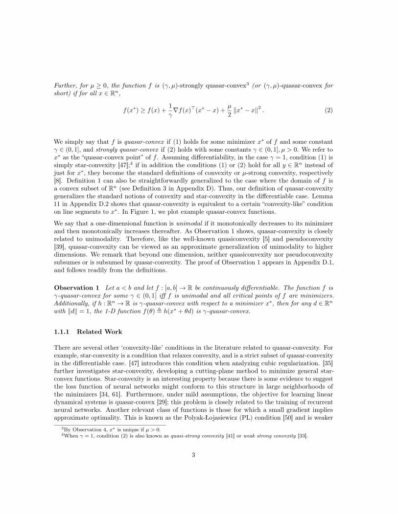
We simply say that f is quasar-convex if (1) holds for some minimizer x∗ of f and some constantγ ∈ (0, 1], and strongly quasar-convex if (2) holds with some constants γ ∈ (0, 1], µ > 0. We refer tox∗ as the “quasar-convex point” of f . Assuming differentiability, in the case γ = 1, condition (1) issimply star-convexity [47];4 if in addition the conditions (1) or (2) hold for all y ∈ Rn instead ofjust for x∗, they become the standard definitions of convexity or µ-strong convexity, respectively[8]. Definition 1 can also be straightforwardly generalized to the case where the domain of f isa convex subset of Rn (see Definition 3 in Appendix D). Thus, our definition of quasar-convexitygeneralizes the standard notions of convexity and star-convexity in the differentiable case. Lemma11 in Appendix D.2 shows that quasar-convexity is equivalent to a certain “convexity-like” conditionon line segments to x∗. In Figure 1, we plot example quasar-convex functions.

We say that a one-dimensional function is unimodal if it monotonically decreases to its minimizerand then monotonically increases thereafter. As Observation 1 shows, quasar-convexity is closelyrelated to unimodality. Therefore, like the well-known quasiconvexity [5] and pseudoconvexity[39], quasar-convexity can be viewed as an approximate generalization of unimodality to higherdimensions. We remark that beyond one dimension, neither quasiconvexity nor pseudoconvexitysubsumes or is subsumed by quasar-convexity. The proof of Observation 1 appears in Appendix D.1,and follows readily from the definitions.

Observation 1 Let a < b and let f : [a, b]→ R be continuously differentiable. The function f isγ-quasar-convex for some γ ∈ (0, 1] iff f is unimodal and all critical points of f are minimizers.Additionally, if h : Rn → R is γ-quasar-convex with respect to a minimizer x∗, then for any d ∈ Rnwith ‖d‖ = 1, the 1-D function f(θ) , h(x∗ + θd) is γ-quasar-convex.

1.1.1 Related Work

There are several other ‘convexity-like’ conditions in the literature related to quasar-convexity. Forexample, star-convexity is a condition that relaxes convexity, and is a strict subset of quasar-convexityin the differentiable case. [47] introduces this condition when analyzing cubic regularization. [35]further investigates star-convexity, developing a cutting-plane method to minimize general star-convex functions. Star-convexity is an interesting property because there is some evidence to suggestthe loss function of neural networks might conform to this structure in large neighborhoods ofthe minimizers [34, 61]. Furthermore, under mild assumptions, the objective for learning lineardynamical systems is quasar-convex [29]; this problem is closely related to the training of recurrentneural networks. Another relevant class of functions is those for which a small gradient impliesapproximate optimality. This is known as the Polyak-Łojasiewicz (PL) condition [50] and is weaker

3By Observation 4, x∗ is unique if µ > 0.4When γ = 1, condition (2) is also known as quasi-strong convexity [41] or weak strong convexity [33].

3

Figure 1: Examples of quasar-convex functions. [Left: f(x) =(x2 + 1

8

)1/6 (quasar-convex withγ = 1

2 ).Middle: f(x, y) = x2y2 (star-convex). The rightmost function is described in Appendix D.3.]

than strong quasar-convexity [26]. For linear residual networks, the PL condition holds in largeregions of parameter space [28]. In addition to pseudoconvexity, quasiconvexity, star-convexity,and the PL condition, other relaxations of convexity or strong convexity include invexity [16],semiconvexity [55], quasi-strong convexity [41], restricted strong convexity [59], one-point convexity[37], variational coherence [62], the quadratic growth condition [4], and the error bound property[19]. A more thorough discussion is provided in Appendix A.1.

We are not the first to study acceleration on quasar-convex functions; recent work by [26] and [48]shows how to achieve accelerated rates for minimizing quasar-convex functions. For a function thatis L-smooth and γ-quasar-convex with respect to a minimizer x∗, with initial distance to x∗ boundedby R, the algorithm of [26] yields an ε-optimal point in O(γ−1L1/2Rε−1/2) iterations, while thealgorithm of [48] does so in O(γ−3/2L1/2Rε−1/2) iterations. For convex functions (which have γ = 1),these bounds match the iteration bounds achieved by AGD [44], but use a different oracle model.In particular, to achieve these iteration bounds, the method in [26] relies on a low-dimensionalsubspace optimization method within each iteration, while [48] uses a one-dimensional line searchover the function value in each iteration, as well as a restart criterion that requires knowledge of thetrue optimal function value.5 However, quasar-convex functions are not necessarily unimodal alongthe arbitrary low-dimensional regions or line segments being searched over. Therefore, even findingan approximate minimizer within these subregions may be computationally expensive, makingeach iteration potentially costly; by contrast, our methods only require a function and gradient

5We discuss [48] in more detail in Appendix A.2.

4

oracle. In addition, neither paper provides lower bounds nor studies the “strongly quasar-convex”regime. Independently, recent work by [60] uses a differential equation discretization to approachthe accelerated O(κ1/2 log(ε−1)) rate for minimization of smooth strongly quasar-convex functionsin a neighborhood of the optimum, in the special case γ = 1.6 Similarly, in the γ = 1 case,geometric descent [9] achieves O(κ1/2 log(ε−1)) running times in terms of the number of calls toa one-dimensional line search oracle (although, as previously noted, the number of function andgradient evaluations required may still be large).7

1.2 Summary of Results

For functions that are L-smooth and γ-quasar-convex, we provide an algorithm which finds anε-optimal solution in O(γ−1L1/2Rε−1/2) iterations (where, as before, R is an upper bound on theinitial distance to the quasar-convex point x∗). Our iteration bound is the same as that of [26], anda factor of γ1/2 better than the O(γ−3/2L1/2Rε−1/2) bound of [48]. Additionally, we are the first toprovide bounds on the total number of function and gradient evaluations required; our algorithmuses O(γ−1L1/2Rε−1/2 log(γ−1ε−1)) evaluations to find a ε-optimal solution.

We also provide an algorithm for L-smooth, (γ, µ)-strongly quasar-convex functions; our algorithmuses O(γ−1κ1/2 log(γ−1ε−1)) iterations and O(γ−1κ1/2 log(γ−1κ) log(γ−1ε−1)) total function andgradient evaluations to find an ε-optimal point, where κ , L/µ (κ is typically referred to as thecondition number). For constant γ, this matches accelerated gradient descent’s bound for smoothstrongly convex functions, up to a logarithmic factor.

The key idea behind our algorithm is to take a close look at which essential invariants need tohold during the momentum step of AGD, and use this insight to carefully redesign the algorithmto accelerate on general smooth quasar-convex functions. By observing how the function behavesalong the line segment between current iterates x(k) and v(k), we show that for any smooth quasar-convex function, there always exists a point y(k) along this segment with the properties needed foracceleration. Furthermore, we show that an efficient binary search can be used to find such a point,even without the assumption of convexity along the segment.

To complement our upper bounds, we provide lower bounds of Ω(γ−1L1/2Rε−1/2) for the number ofgradient evaluations that any deterministic first-order method requires to find an ε-minimizer of aquasar-convex function. This shows that up to logarithmic factors, our lower and upper boundsare tight. Our lower bounds extend the techniques from [14] to the class of smooth quasar-convexfunctions, allowing an almost exact characterization of the complexity of minimizing these functions.

Paper outline. In Section 2, we provide a general framework for accelerating the minimization ofsmooth quasar-convex functions. In Section 3, we apply our framework to develop specific algorithmstailored to both quasar-convex and strongly quasar-convex functions. In Section 4, we provide lowerbounds to show that the upper bounds for quasar-convex minimization of Section 3 are tight up tologarithmic factors. Full proofs, additional results, and numerical experiments are in the Appendix.

6κ = L/µ denotes the condition number of an L-smooth (γ, µ)-strongly quasar-convex function.7Although this result is not explicitly stated in the literature, upon careful inspection of the analysis in [9] it

can be observed that the µ-strong convexity requirement in [9] may be relaxed to the requirement of (1, µ)-strongquasar-convexity, with no changes to the algorithm necessary.

5

2 Quasar-Convex Minimization Framework

In this section, we provide and analyze a general algorithmic template for accelerated minimizationof smooth quasar-convex functions. In Section 3.1 we show how to leverage this framework to achieveaccelerated rates for minimizing strongly quasar-convex functions, and in Section 3.2 we show howto achieve accelerated rates for minimizing non-strongly quasar-convex functions (i.e. when µ = 0).For simplicity, we assume the domain is Rn.

Our algorithm (Algorithm 1) is a simple generalization of accelerated gradient descent (AGD).Indeed, standard AGD can be written in the form of Algorithm 1, for particular choices of theparameters α(k), β(k), η(k). Given a differentiable function f ∈ Rn → R with smoothness parameterL > 0 and initial point x(0) = v(0) ∈ Rn, the algorithm iteratively computes points x(k), v(k) ∈ Rnof improving “quality.” However, it is challenging to argue that Algorithm 1 actually performsoptimally without the assumption of convexity. The crux of circumventing convexity is to show thatthere exists a way to efficiently compute the momentum parameter α(k) to yield convergence at thedesired rate. In this section, we provide general tools for analyzing this algorithm; in Section 3,we leverage this analysis with specific choices of the parameters α(k), β, and η(k) to derive ourfully-specified accelerated schemes for both quasar-convex and strongly quasar-convex functions.

Algorithm 1: General AGD FrameworkInput: L-smooth function f : Rn → R, initial point x(0) ∈ Rn, number of iterations K

Sequences α(k)K−1k=0 , β(k)K−1

k=0 , L(k)K−1k=0 , η(k)K−1

k=0 are defined by the particularalgorithm instance, where α(k) ∈ [0, 1], β(k) ∈ [0, 1], L(k) ∈ (0, 2L), η(k) ≥ γ

L(k) .

1 Set v(0) = x(0)

2 for k = 0, 1, 2, . . . ,K − 1 do3 Set y(k) = α(k)x(k) + (1− α(k))v(k)

4 Set x(k+1) = y(k) − 1L(k)∇f(y(k)) # L(k) computed s.t. f(x(k+1)) ≤ f(y(k))− 1

2L(k)

∥∥∥∇f(y(k))∥∥∥2

5 Set v(k+1) = β(k)v(k) + (1− β(k))y(k) − η(k)∇f(y(k))

end6 return x(K)

We first define notation that will be used throughout Sections 2 and 3:

Definition 2 Let ε(k) , f(x(k))− f(x∗), ε(k)y , f(y(k))− f(x∗), r(k) ,

∥∥v(k) − x∗∥∥2,

r(k)y ,

∥∥y(k) − x∗∥∥2, Q(k) , β(k)

(2η(k)α(k)∇f(y(k))>(x(k) − v(k))− (α(k))2(1− β(k))

∥∥x(k) − v(k)∥∥2).

In the remainder of this section, we analyze Algorithm 1. We assume that f is L-smooth and (γ, µ)strongly quasar-convex (possibly with µ = 0) with respect to a minimizer x∗. First, we use Lemma 1to bound how much the function error of x(k) and the distance from v(k) to x∗ decrease at eachiteration.

Lemma 1 (One Step Framework Analysis) Suppose f is L-smooth and (γ, µ)-quasar-convexwith respect to a minimizer x∗. Then, in each iteration k ≥ 0 of Algorithm 1 applied to f , it is the

6

case that

2(η(k))2L(k)ε(k+1) + r(k+1) ≤ β(k)r(k) +[(1− β(k))− γµη(k)

]r(k)y + 2η(k)

[L(k)η(k) − γ

]ε(k)y +Q(k).

Proof Let z(k) , β(k)v(k) + (1− β(k))y(k). Since v(k+1) = z(k) − η(k)∇f(y(k)), direct algebraicmanipulation yields that

r(k+1) =∥∥∥v(k+1) − x∗

∥∥∥2

=∥∥∥z(k) − x∗ − η(k)∇f(y(k))

∥∥∥2

=∥∥∥z(k) − x∗

∥∥∥2

+ 2η(k)∇f(y(k))>(x∗ − z(k)) + (η(k))2∥∥∥∇f(y(k))

∥∥∥2

. (3)

Using the definitions of z(k) and y(k), we have∥∥∥z(k) − x∗∥∥∥2

= β(k)∥∥∥v(k) − x∗

∥∥∥2

+ (1− β(k))∥∥∥y(k) − x∗

∥∥∥2

− β(k)(1− β(k))∥∥∥v(k) − y(k)

∥∥∥2

= β(k)r(k) + (1− β(k))r(k)y − β(k)(1− β(k))(α(k))2

∥∥∥v(k) − x(k)∥∥∥2

. (4)

Further, since v(k) = y(k)+α(k)(v(k)−x(k)) and z(k) = β(k)v(k)+(1−β(k))y(k) = y(k)+α(k)β(k)(v(k)−x(k)), it follows that

∇f(y(k))>(x∗ − z(k)) = ∇f(y(k))>(x∗ − y(k)) + α(k)β(k)∇f(y(k))>(x(k) − v(k)) . (5)

Since (γ, µ)-strong quasar-convexity of f implies −ε(k)y ≥ 1

γ∇f(y(k))>(x∗ − y(k)) + µ2 r

(k)y and the

definition of x(k+1) and L(k) implies 0 ≤∥∥∇f(y(k))

∥∥2 ≤ 2L(k)[ε(k)y − ε(k+1)], combining with (3), (4),

and (5) yields the result.

Note that L(k) in Line 3 of Algorithm 1 can be set to the Lipschitz constant L if it is known;otherwise, it can be efficiently computed to make f(x(k)) = f(y(k) − 1

L(k)∇f(y(k))) ≤ f(y(k)) −1

2L(k)

∥∥∇f(y(k))∥∥2

and L(k) ∈ (0, 2L) hold using backtracking line search. See Lemma 9 (Ap-pendix C.1) for more details.

Lemma 1 provides our main bound on how the error ε(k) changes between successive iterations of Al-gorithm 1. The key step necessary to apply this lemma is to relate f(y(k)) and ∇f(y(k))>(x(k) − v(k))to f(x(k)), in order to bound Q(k). In the standard analysis of accelerated gradient descent, convexityis used to obtain such a connection.8 In our algorithms, we instead perform binary search to computethe momentum parameter α(k) for which the necessary relationship holds without assuming convexity.The following lemma shows that there always exists a setting of α(k) that satisfies the necessaryrelationship.

Lemma 2 (Existence of “Good” α) Let f : Rn → R be differentiable and let x, v ∈ Rn. Forα ∈ R define yα , αx+ (1− α)v. For any c ≥ 0 there exists α ∈ [0, 1] such that

α∇f(yα)>(x− v) ≤ c [f(x)− f(yα)] . (6)8See Appendix C.4.1 for more details.

7

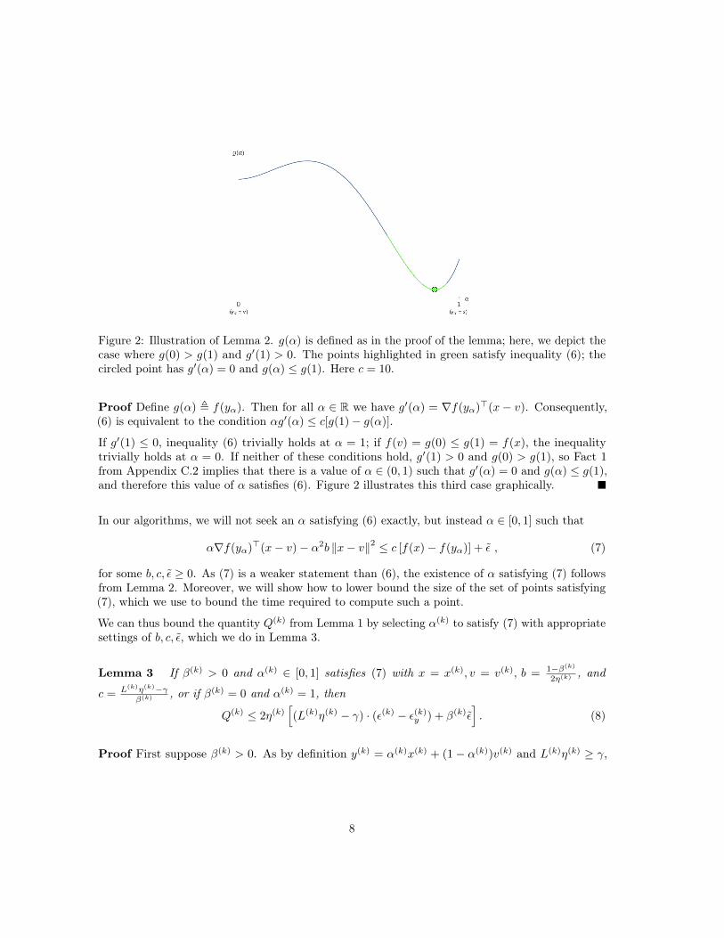
Figure 2: Illustration of Lemma 2. g(α) is defined as in the proof of the lemma; here, we depict thecase where g(0) > g(1) and g′(1) > 0. The points highlighted in green satisfy inequality (6); thecircled point has g′(α) = 0 and g(α) ≤ g(1). Here c = 10.

Proof Define g(α) , f(yα). Then for all α ∈ R we have g′(α) = ∇f(yα)>(x− v). Consequently,(6) is equivalent to the condition αg′(α) ≤ c[g(1)− g(α)].

If g′(1) ≤ 0, inequality (6) trivially holds at α = 1; if f(v) = g(0) ≤ g(1) = f(x), the inequalitytrivially holds at α = 0. If neither of these conditions hold, g′(1) > 0 and g(0) > g(1), so Fact 1from Appendix C.2 implies that there is a value of α ∈ (0, 1) such that g′(α) = 0 and g(α) ≤ g(1),and therefore this value of α satisfies (6). Figure 2 illustrates this third case graphically.

In our algorithms, we will not seek an α satisfying (6) exactly, but instead α ∈ [0, 1] such that

α∇f(yα)>(x− v)− α2b ‖x− v‖2 ≤ c [f(x)− f(yα)] + ε , (7)

for some b, c, ε ≥ 0. As (7) is a weaker statement than (6), the existence of α satisfying (7) followsfrom Lemma 2. Moreover, we will show how to lower bound the size of the set of points satisfying(7), which we use to bound the time required to compute such a point.

We can thus bound the quantity Q(k) from Lemma 1 by selecting α(k) to satisfy (7) with appropriatesettings of b, c, ε, which we do in Lemma 3.

Lemma 3 If β(k) > 0 and α(k) ∈ [0, 1] satisfies (7) with x = x(k), v = v(k), b = 1−β(k)

2η(k) , and

c = L(k)η(k)−γβ(k) , or if β(k) = 0 and α(k) = 1, then

Q(k) ≤ 2η(k)[(L(k)η(k) − γ) · (ε(k) − ε(k)

y ) + β(k)ε]. (8)

Proof First suppose β(k) > 0. As by definition y(k) = α(k)x(k) + (1− α(k))v(k) and L(k)η(k) ≥ γ,

8

applying (7) yields

Q(k) = 2β(k)η(k)

(α(k)∇f(y(k))>(x(k) − v(k))−

(α(k)

)2 (1− β(k))∥∥x(k) − v(k)

∥∥2

2η(k)

)

≤ 2β(k)η(k)

(L(k)η(k) − γ

β(k)[f(x(k))− f(y(k))] + ε

)= 2η(k)

([L(k)η(k) − γ] · [ε(k) − ε(k)

y ] + β(k)ε).

Alternatively, suppose β(k) = 0. Then Q(k) = 0 as well; if we select α(k) = 1, then y(k) = x(k) and(8) trivially holds for any ε, as ε(k)

y = ε(k).

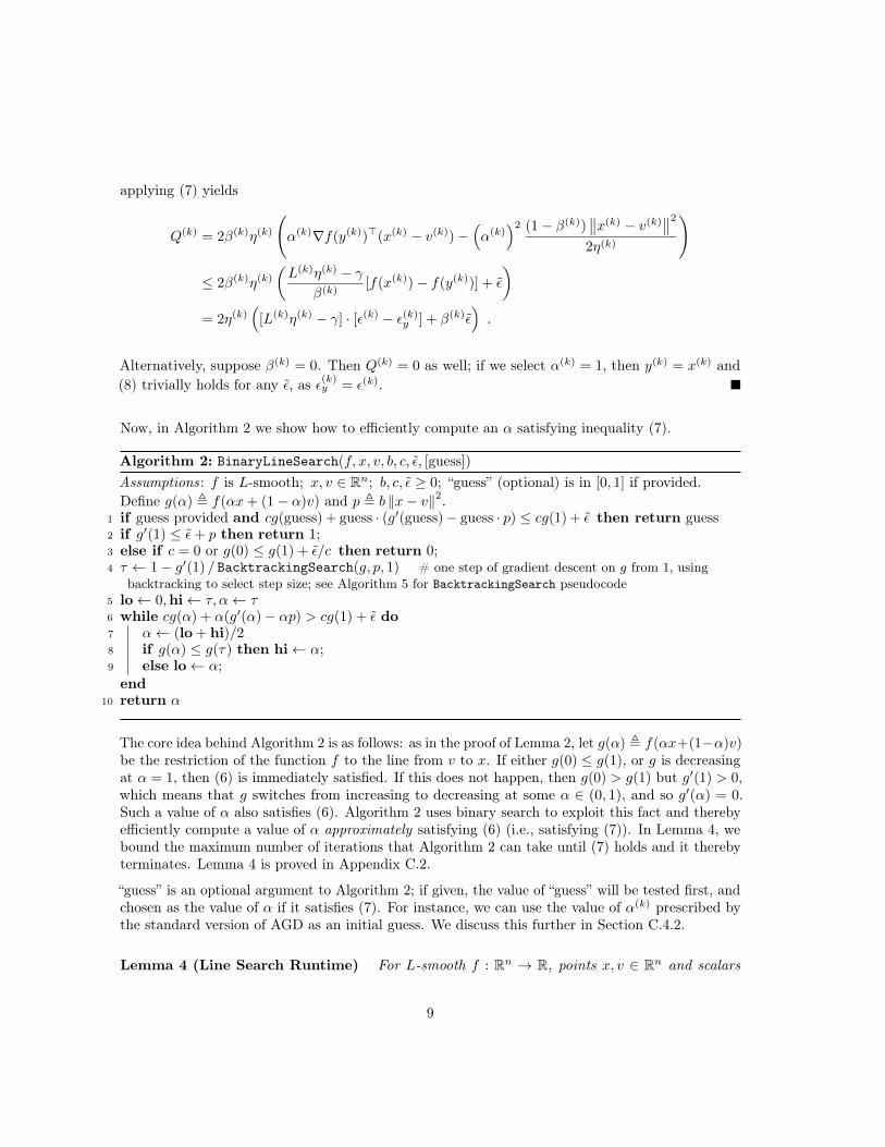
Now, in Algorithm 2 we show how to efficiently compute an α satisfying inequality (7).

Algorithm 2: BinaryLineSearch(f, x, v, b, c, ε, [guess])Assumptions: f is L-smooth; x, v ∈ Rn; b, c, ε ≥ 0; “guess” (optional) is in [0, 1] if provided.Define g(α) , f(αx+ (1− α)v) and p , b ‖x− v‖2.

1 if guess provided and cg(guess) + guess · (g′(guess)− guess · p) ≤ cg(1) + ε then return guess2 if g′(1) ≤ ε+ p then return 1;3 else if c = 0 or g(0) ≤ g(1) + ε/c then return 0;4 τ ← 1− g′(1) / BacktrackingSearch(g, p, 1) # one step of gradient descent on g from 1, using

backtracking to select step size; see Algorithm 5 for BacktrackingSearch pseudocode5 lo← 0,hi← τ, α← τ6 while cg(α) + α(g′(α)− αp) > cg(1) + ε do7 α← (lo + hi)/28 if g(α) ≤ g(τ) then hi← α;9 else lo← α;end

10 return α

The core idea behind Algorithm 2 is as follows: as in the proof of Lemma 2, let g(α) , f(αx+(1−α)v)be the restriction of the function f to the line from v to x. If either g(0) ≤ g(1), or g is decreasingat α = 1, then (6) is immediately satisfied. If this does not happen, then g(0) > g(1) but g′(1) > 0,which means that g switches from increasing to decreasing at some α ∈ (0, 1), and so g′(α) = 0.Such a value of α also satisfies (6). Algorithm 2 uses binary search to exploit this fact and therebyefficiently compute a value of α approximately satisfying (6) (i.e., satisfying (7)). In Lemma 4, webound the maximum number of iterations that Algorithm 2 can take until (7) holds and it therebyterminates. Lemma 4 is proved in Appendix C.2.

“guess” is an optional argument to Algorithm 2; if given, the value of “guess” will be tested first, andchosen as the value of α if it satisfies (7). For instance, we can use the value of α(k) prescribed bythe standard version of AGD as an initial guess. We discuss this further in Section C.4.2.

Lemma 4 (Line Search Runtime) For L-smooth f : Rn → R, points x, v ∈ Rn and scalars

9

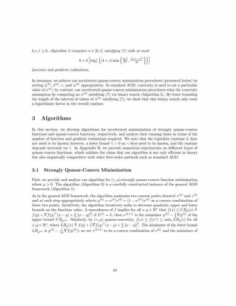
b, c, ε ≥ 0, Algorithm 2 computes α ∈ [0, 1] satisfying (7) with at most

8 + 3⌈log+

2

((4 + c) min

2L3

b3 ,L‖x−v‖2

2ε

)⌉function and gradient evaluations.

In summary, we achieve our accelerated quasar-convex minimization procedures (presented below) bysetting η(k), β(k), ε, and α(k) appropriately. In standard AGD, convexity is used to set a particularvalue of α(k); by contrast, our accelerated quasar-convex minimization procedures relax the convexityassumption by computing an α(k) satisfying (7) via binary search (Algorithm 2). By lower boundingthe length of the interval of values of α(k) satisfying (7), we show that this binary search only costsa logarithmic factor in the overall runtime.

3 Algorithms

In this section, we develop algorithms for accelerated minimization of strongly quasar-convexfunctions and quasar-convex functions, respectively, and analyze their running times in terms of thenumber of function and gradient evaluations required. We note that the Lipschitz constant L doesnot need to be known; however, a lower bound γ > 0 on γ does need to be known, and the runtimedepends inversely on γ. In Appendix B, we provide numerical experiments on different types ofquasar-convex functions, which validate the claim that our algorithm is not only efficient in theorybut also empirically competitive with other first-order methods such as standard AGD.

3.1 Strongly Quasar-Convex Minimization

First, we provide and analyze our algorithm for (γ, µ)-strongly quasar-convex function minimization,where µ > 0. The algorithm (Algorithm 3) is a carefully constructed instance of the general AGDframework (Algorithm 1).

As in the general AGD framework, the algorithm maintains two current points denoted x(k) and v(k)

and at each step appropriately selects y(k) = α(k)x(k) + (1− α(k))v(k) as a convex combination ofthese two points. Intuitively, the algorithm iteratively seeks to decrease quadratic upper and lowerbounds on the function value. L-smoothness of f implies for all x, y ∈ Rn that f(x) ≤ UBy(x) ,f(y) +∇f(y)>(x− y) + L

2 ‖x− y‖2; if L(k) = L, then x(k+1) is the minimizer y(k) − 1

L∇y(k) of the

upper bound UBy(k) . Similarly, by (γ, µ) quasar-convexity, f(x) ≥ f(x∗) ≥ minz LBy(z) for allx, y ∈ Rn, where LBy(x) , f(y) + 1

γ∇f(y)>(x− y) + µ2 ‖x− y‖

2. The minimizer of the lower boundLBy(k) is y(k) − 1

γµ∇f(y(k)); we set v(k+1) to be a convex combination of v(k) and the minimizer of

10

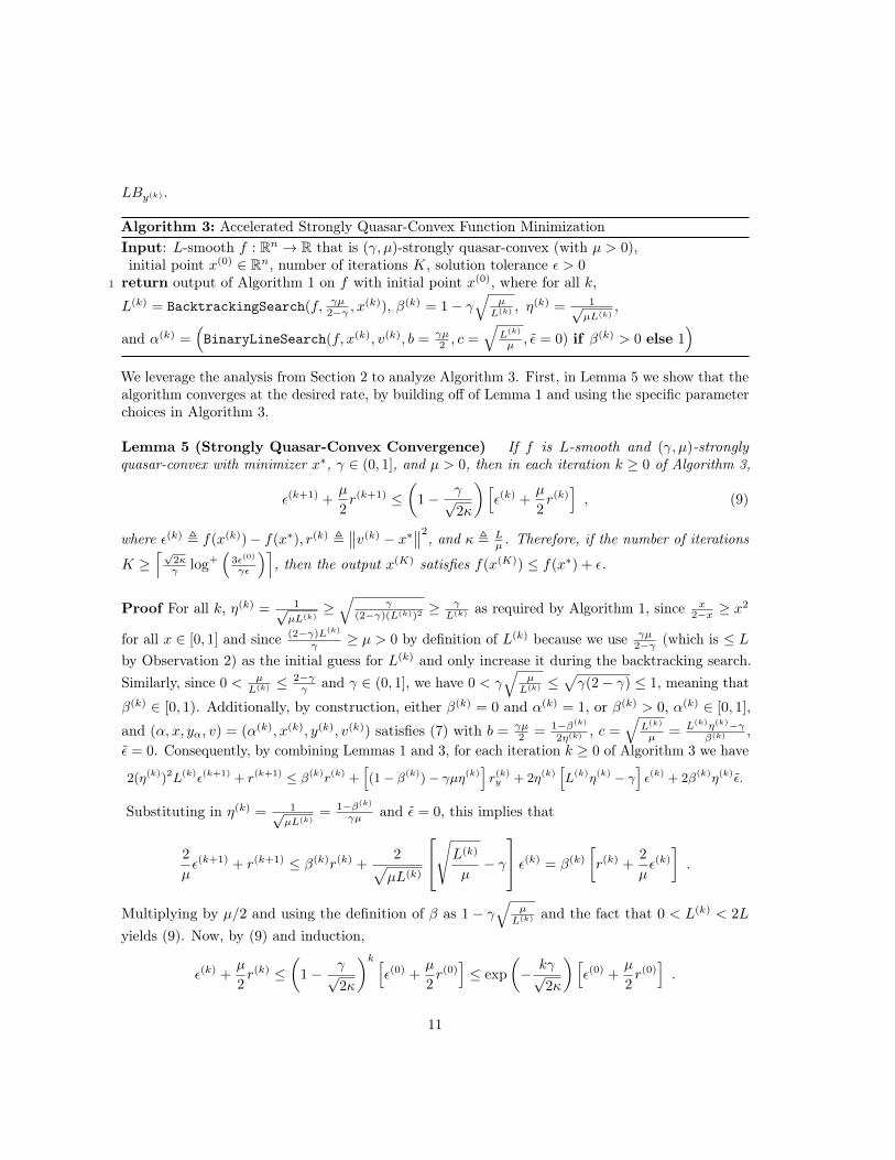
LBy(k) .

Algorithm 3: Accelerated Strongly Quasar-Convex Function MinimizationInput: L-smooth f : Rn → R that is (γ, µ)-strongly quasar-convex (with µ > 0),initial point x(0) ∈ Rn, number of iterations K, solution tolerance ε > 0

1 return output of Algorithm 1 on f with initial point x(0), where for all k,

L(k) = BacktrackingSearch(f, γµ2−γ , x

(k)), β(k) = 1− γ√

µL(k) , η(k) = 1√

µL(k),

and α(k) =(BinaryLineSearch(f, x(k), v(k), b = γµ

2 , c =√

L(k)

µ , ε = 0) if β(k) > 0 else 1)

We leverage the analysis from Section 2 to analyze Algorithm 3. First, in Lemma 5 we show that thealgorithm converges at the desired rate, by building off of Lemma 1 and using the specific parameterchoices in Algorithm 3.

Lemma 5 (Strongly Quasar-Convex Convergence) If f is L-smooth and (γ, µ)-stronglyquasar-convex with minimizer x∗, γ ∈ (0, 1], and µ > 0, then in each iteration k ≥ 0 of Algorithm 3,

ε(k+1) +µ

2r(k+1) ≤

(1− γ√

2κ

)[ε(k) +

µ

2r(k)

], (9)

where ε(k) , f(x(k))− f(x∗), r(k) ,∥∥v(k) − x∗

∥∥2, and κ , L

µ . Therefore, if the number of iterations

K ≥⌈√

2κγ log+

(3ε(0)

γε

)⌉, then the output x(K) satisfies f(x(K)) ≤ f(x∗) + ε.

Proof For all k, η(k) = 1√µL(k)

≥√

γ(2−γ)(L(k))2 ≥ γ

L(k) as required by Algorithm 1, since x2−x ≥ x

2

for all x ∈ [0, 1] and since (2−γ)L(k)

γ ≥ µ > 0 by definition of L(k) because we use γµ2−γ (which is ≤ L

by Observation 2) as the initial guess for L(k) and only increase it during the backtracking search.Similarly, since 0 < µ

L(k) ≤ 2−γγ and γ ∈ (0, 1], we have 0 < γ

√µL(k) ≤

√γ(2− γ) ≤ 1, meaning that

β(k) ∈ [0, 1). Additionally, by construction, either β(k) = 0 and α(k) = 1, or β(k) > 0, α(k) ∈ [0, 1],

and (α, x, yα, v) = (α(k), x(k), y(k), v(k)) satisfies (7) with b = γµ2 = 1−β(k)

2η(k) , c =√

L(k)

µ = L(k)η(k)−γβ(k) ,

ε = 0. Consequently, by combining Lemmas 1 and 3, for each iteration k ≥ 0 of Algorithm 3 we have

2(η(k))2L(k)ε(k+1) + r(k+1) ≤ β(k)r(k) +[(1− β(k))− γµη(k)

]r(k)y + 2η(k)

[L(k)η(k) − γ

]ε(k) + 2β(k)η(k)ε.

Substituting in η(k) = 1√µL(k)

= 1−β(k)

γµ and ε = 0, this implies that

2

µε(k+1) + r(k+1) ≤ β(k)r(k) +

2õL(k)

√L(k)

µ− γ

ε(k) = β(k)

[r(k) +

2

µε(k)

].

Multiplying by µ/2 and using the definition of β as 1− γ√

µL(k) and the fact that 0 < L(k) < 2L

yields (9). Now, by (9) and induction,

ε(k) +µ

2r(k) ≤

(1− γ√

2κ

)k [ε(0) +

µ

2r(0)]≤ exp

(− kγ√

2κ

)[ε(0) +

µ

2r(0)].

11

Therefore, whenever k ≥√

2κγ log+

(ε(0)+µ

2 r(0)

ε

)we have ε(k) = f(x(k)) − f(x∗) ≤ ε, as r(k) ≥ 0

always. By Corollary 1, 2ε(0)

γ ≥ µ2 r

(0), so it suffices to run k ≥⌈√

2κγ log+

(3ε(0)

γε

)⌉iterations.

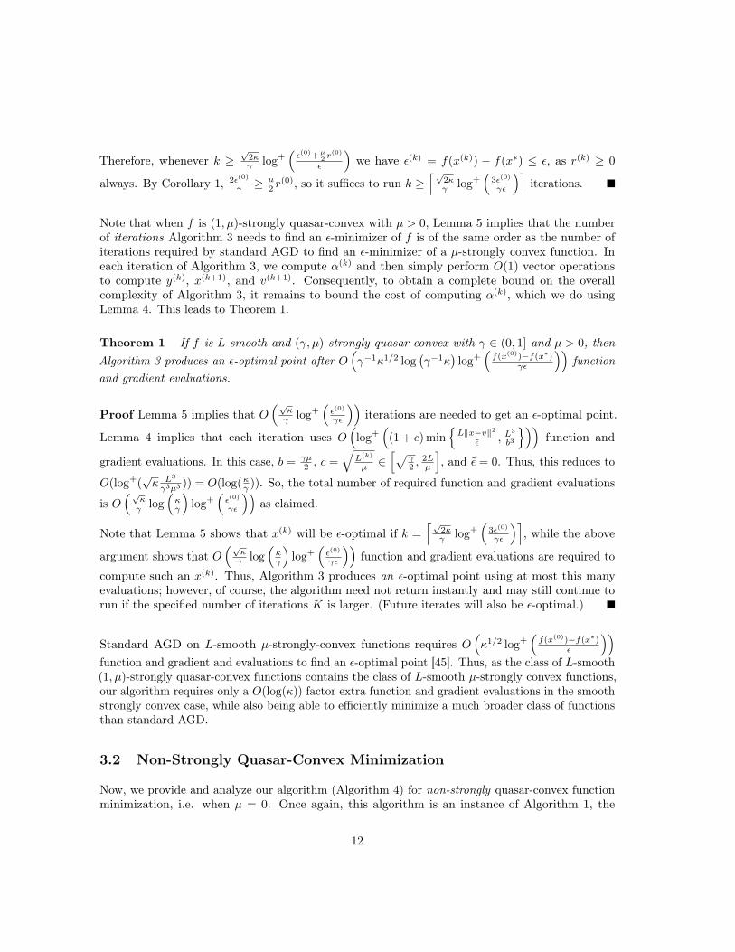
Note that when f is (1, µ)-strongly quasar-convex with µ > 0, Lemma 5 implies that the numberof iterations Algorithm 3 needs to find an ε-minimizer of f is of the same order as the number ofiterations required by standard AGD to find an ε-minimizer of a µ-strongly convex function. Ineach iteration of Algorithm 3, we compute α(k) and then simply perform O(1) vector operationsto compute y(k), x(k+1), and v(k+1). Consequently, to obtain a complete bound on the overallcomplexity of Algorithm 3, it remains to bound the cost of computing α(k), which we do usingLemma 4. This leads to Theorem 1.

Theorem 1 If f is L-smooth and (γ, µ)-strongly quasar-convex with γ ∈ (0, 1] and µ > 0, thenAlgorithm 3 produces an ε-optimal point after O

(γ−1κ1/2 log

(γ−1κ

)log+

(f(x(0))−f(x∗)

γε

))function

and gradient evaluations.

Proof Lemma 5 implies that O(√

κγ log+

(ε(0)

γε

))iterations are needed to get an ε-optimal point.

Lemma 4 implies that each iteration uses O(

log+(

(1 + c) minL‖x−v‖2

ε , L3

b3

))function and

gradient evaluations. In this case, b = γµ2 , c =

√L(k)

µ ∈[√

γ2 ,

2Lµ

], and ε = 0. Thus, this reduces to

O(log+(√κ L3

γ3µ3 )) = O(log(κγ )). So, the total number of required function and gradient evaluations

is O(√

κγ log

(κγ

)log+

(ε(0)

γε

))as claimed.

Note that Lemma 5 shows that x(k) will be ε-optimal if k =⌈√

2κγ log+

(3ε(0)

γε

)⌉, while the above

argument shows that O(√

κγ log

(κγ

)log+

(ε(0)

γε

))function and gradient evaluations are required to

compute such an x(k). Thus, Algorithm 3 produces an ε-optimal point using at most this manyevaluations; however, of course, the algorithm need not return instantly and may still continue torun if the specified number of iterations K is larger. (Future iterates will also be ε-optimal.)

Standard AGD on L-smooth µ-strongly-convex functions requires O(κ1/2 log+

(f(x(0))−f(x∗)

ε

))function and gradient and evaluations to find an ε-optimal point [45]. Thus, as the class of L-smooth(1, µ)-strongly quasar-convex functions contains the class of L-smooth µ-strongly convex functions,our algorithm requires only a O(log(κ)) factor extra function and gradient evaluations in the smoothstrongly convex case, while also being able to efficiently minimize a much broader class of functionsthan standard AGD.

3.2 Non-Strongly Quasar-Convex Minimization

Now, we provide and analyze our algorithm (Algorithm 4) for non-strongly quasar-convex functionminimization, i.e. when µ = 0. Once again, this algorithm is an instance of Algorithm 1, the

12

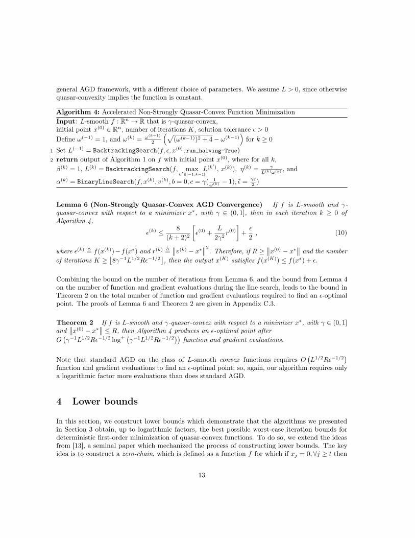
general AGD framework, with a different choice of parameters. We assume L > 0, since otherwisequasar-convexity implies the function is constant.

Algorithm 4: Accelerated Non-Strongly Quasar-Convex Function MinimizationInput: L-smooth f : Rn → R that is γ-quasar-convex,initial point x(0) ∈ Rn, number of iterations K, solution tolerance ε > 0

Define ω(−1) = 1, and ω(k) = ω(k−1)

2

(√(ω(k−1))2 + 4− ω(k−1)

)for k ≥ 0

1 Set L(−1) = BacktrackingSearch(f, ε, x(0), run_halving=True)

2 return output of Algorithm 1 on f with initial point x(0), where for all k,β(k) = 1, L(k) = BacktrackingSearch(f, max

k′∈[−1,k−1]

L(k′), x(k)), η(k) = γL(k)ω(k) , and

α(k) = BinaryLineSearch(f, x(k), v(k), b = 0, c = γ( 1ω(k) − 1), ε = γε

2 )

Lemma 6 (Non-Strongly Quasar-Convex AGD Convergence) If f is L-smooth and γ-quasar-convex with respect to a minimizer x∗, with γ ∈ (0, 1], then in each iteration k ≥ 0 ofAlgorithm 4,

ε(k) ≤ 8

(k + 2)2

[ε(0) +

L

2γ2r(0)

]+ε

2, (10)

where ε(k) , f(x(k))−f(x∗) and r(k) ,∥∥v(k) − x∗

∥∥2. Therefore, if R ≥

∥∥x(0) − x∗∥∥ and the number

of iterations K ≥⌊8γ−1L1/2Rε−1/2

⌋, then the output x(K) satisfies f(x(K)) ≤ f(x∗) + ε.

Combining the bound on the number of iterations from Lemma 6, and the bound from Lemma 4on the number of function and gradient evaluations during the line search, leads to the bound inTheorem 2 on the total number of function and gradient evaluations required to find an ε-optimalpoint. The proofs of Lemma 6 and Theorem 2 are given in Appendix C.3.

Theorem 2 If f is L-smooth and γ-quasar-convex with respect to a minimizer x∗, with γ ∈ (0, 1]and

∥∥x(0) − x∗∥∥ ≤ R, then Algorithm 4 produces an ε-optimal point after

O(γ−1L1/2Rε−1/2 log+

(γ−1L1/2Rε−1/2

))function and gradient evaluations.

Note that standard AGD on the class of L-smooth convex functions requires O(L1/2Rε−1/2

)function and gradient evaluations to find an ε-optimal point; so, again, our algorithm requires onlya logarithmic factor more evaluations than does standard AGD.

4 Lower bounds

In this section, we construct lower bounds which demonstrate that the algorithms we presentedin Section 3 obtain, up to logarithmic factors, the best possible worst-case iteration bounds fordeterministic first-order minimization of quasar-convex functions. To do so, we extend the ideasfrom [13], a seminal paper which mechanized the process of constructing lower bounds. The keyidea is to construct a zero-chain, which is defined as a function f for which if xj = 0,∀j ≥ t then

13

∂f(x)∂xt+1

= 0. On these zero-chains, one can provide lower bounds for a particular class of methodsknown as first-order zero-respecting (FOZR) algorithms, which are algorithms that only query thegradient at points x(t) with x(t)

i 6= 0 if there exists some j < t with ∇if(x(j)) 6= 0. Examples ofFOZR algorithms include gradient descent, accelerated gradient descent, and nonlinear conjugategradient [21]. It is relatively easy to form lower bounds for FOZR algorithms applied to zero-chains,because one can prove that if the initial point is x(0) = 0, then x(T ) has at most T nonzeros [13,Observation 1]. The particular zero-chain we use to derive our lower bounds is

fT,σ(x) , q(x) + σ

T∑i=1

Υ(xi) ,

where

Υ(θ) , 120

∫ θ

1

t2(t− 1)

1 + t2dt

q(x) ,1

4(x1 − 1)2 +

1

4

T−1∑i=1

(xi − xi+1)2.

This function fT,σ is similar to the function fT,µ,r of [14]. However, the lower bound proof isdifferent because the primary challenge is to show fT,σ is quasar-convex, rather than showingthat

∥∥∇fT,σ(x)∥∥ ≥ ε for all x with xT = 0. Our main lemma shows that this function is in fact

1100T

√σ-quasar-convex.

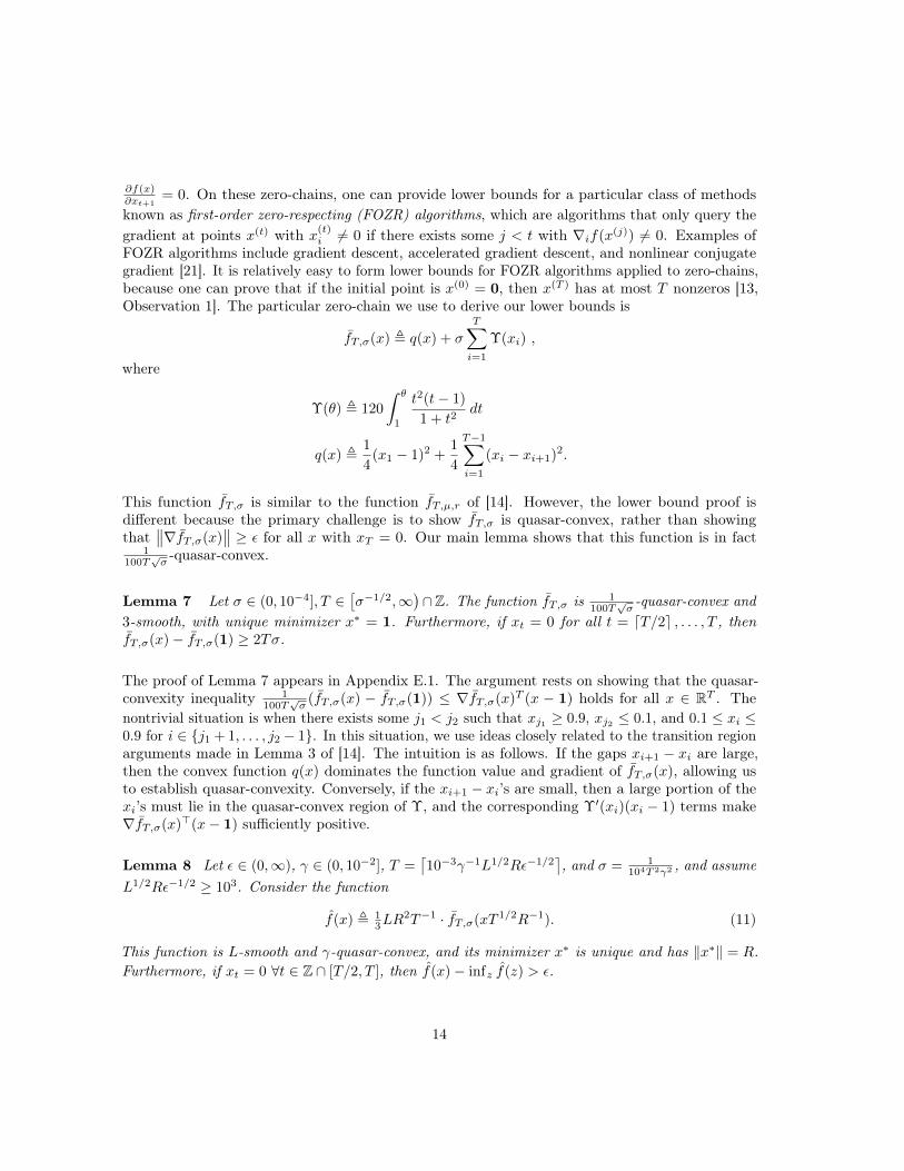
Lemma 7 Let σ ∈ (0, 10−4], T ∈[σ−1/2,∞

)∩Z. The function fT,σ is 1

100T√σ-quasar-convex and

3-smooth, with unique minimizer x∗ = 1. Furthermore, if xt = 0 for all t = dT/2e , . . . , T , thenfT,σ(x)− fT,σ(1) ≥ 2Tσ.

The proof of Lemma 7 appears in Appendix E.1. The argument rests on showing that the quasar-convexity inequality 1

100T√σ

(fT,σ(x) − fT,σ(1)) ≤ ∇fT,σ(x)T (x − 1) holds for all x ∈ RT . Thenontrivial situation is when there exists some j1 < j2 such that xj1 ≥ 0.9, xj2 ≤ 0.1, and 0.1 ≤ xi ≤0.9 for i ∈ j1 + 1, . . . , j2 − 1. In this situation, we use ideas closely related to the transition regionarguments made in Lemma 3 of [14]. The intuition is as follows. If the gaps xi+1 − xi are large,then the convex function q(x) dominates the function value and gradient of fT,σ(x), allowing usto establish quasar-convexity. Conversely, if the xi+1 − xi’s are small, then a large portion of thexi’s must lie in the quasar-convex region of Υ, and the corresponding Υ′(xi)(xi − 1) terms make∇fT,σ(x)>(x− 1) sufficiently positive.

Lemma 8 Let ε ∈ (0,∞), γ ∈ (0, 10−2], T =⌈10−3γ−1L1/2Rε−1/2

⌉, and σ = 1

104T 2γ2 , and assumeL1/2Rε−1/2 ≥ 103. Consider the function

f(x) , 13LR

2T−1 · fT,σ(xT 1/2R−1). (11)

This function is L-smooth and γ-quasar-convex, and its minimizer x∗ is unique and has ‖x∗‖ = R.Furthermore, if xt = 0 ∀t ∈ Z ∩ [T/2, T ], then f(x)− infz f(z) > ε.

14

The proof of Lemma 8 appears in Appendix E.1. Combining Lemma 8 with Observation 1 from [13]yields a lower bound for first-order zero-respecting algorithms, and an extension of this lower boundto the class of all deterministic first-order methods. This leads to Theorem 3, whose proof appearsin Appendix E.2.

Theorem 3 Let ε, R, L ∈ (0,∞), γ ∈ (0, 1], and assume L1/2Rε−1/2 ≥ 1. Let F denote the set ofL-smooth functions that are γ-quasar-convex with respect to some point with Euclidean norm lessthan or equal to R. Then, given any deterministic first-order method, there exists a function f ∈ Fsuch that the method requires at least Ω(γ−1L1/2Rε−1/2) gradient evaluations to find an ε-optimalpoint of f .

Theorem 3 demonstrates that the upper bound for our algorithm for quasar-convex minimization istight within logarithmic factors. We note that by reduction (Remark 4), one can prove a lower boundof Ω(γ−1κ1/2) for strongly quasar-convex functions; thus, our algorithm for strongly quasar-convexminimization is also optimal within logarithmic factors.

Although the construction of our lower bounds is similar to that of [14], there are importantdifferences between our lower bounds and theirs. First, the assumptions differ significantly; weassume quasar-convexity and Lipschitz continuity of the first derivative, while [14] assumes Lipschitzcontinuity of the first three derivatives. Next, the bounds in [13, 14] apply to finding ε-stationarypoints, rather than ε-optimal points. In addition, our lower and upper bounds only differ bylogarithmic factors, whereas there is a gap of O(ε−1/15) between the lower bound of Ω(ε−8/5) givenby [14] and the best known corresponding upper bound of O(ε−5/3 log(ε−1)) [11]. Finally, we requirext = 0 for all t > T/2 to guarantee f(x) − infz f(z) > ε, whereas [13, 14] only need xT = 0 toguarantee

∥∥∥∇f(x)∥∥∥ > ε.

5 Conclusion

In this work, we introduce a generalization of star-convexity called quasar-convexity and provideinsight into the structure of quasar-convex functions. We show how to obtain a near-optimalaccelerated rate for the minimization of any smooth function in this broad class, using a simple butnovel binary search technique. In addition, we provide nearly matching theoretical lower bounds forthe performance of any first-order method on this function class. Interesting topics for future researchare to further understand the prevalence of quasar-convexity in problems of practical interest, andto develop new accelerated methods for other structured classes of nonconvex problems.

15

Acknowledgements

The work of Aaron Sidford was supported by NSF CAREER Award CCF-1844855.

References[1] Naman Agarwal, Zeyuan Allen-Zhu, Brian Bullins, Elad Hazan, and Tengyu Ma. Finding approximate

local minima faster than gradient descent. In Symposium on Theory of Computing (STOC), pages1195–1199. ACM, 2017.

[2] Zeyuan Allen-Zhu. Katyusha: The first direct acceleration of stochastic gradient methods. Journal ofMachine Learning Research, 18(1):8194–8244, 2017.

[3] Zeyuan Allen-Zhu and Lorenzo Orecchia. Linear coupling: An ultimate unification of gradient andmirror descent. In Innovations in Theoretical Computer Science (ITCS), pages 1–22, 2017.

[4] Mihai Anitescu. Degenerate nonlinear programming with a quadratic growth condition. SIAM Journalon Optimization, 10(4):1116–1135, 2000.

[5] Kenneth Arrow and Alain Enthoven. Quasi-concave programming. Econometrica, 16(5):779–800, 1961.

[6] Peter Bartlett, David Helmbold, and Philip Long. Gradient descent with identity initialization efficientlylearns positive-definite linear transformations by deep residual networks. Neural Computation, 31(3):477–502, 2019.

[7] Amir Beck and Marc Teboulle. A fast iterative shrinkage-thresholding algorithm for linear inverseproblems. SIAM Journal on Imaging Sciences, 2(1):183–202, 2009.

[8] Stephen Boyd and Lieven Vandenberghe. Convex Optimization. Cambridge University Press, 2004.

[9] Sébastien Bubeck, Yin Tat Lee, and Mohit Singh. A geometric alternative to Nesterov’s acceleratedgradient descent. arXiv preprint arXiv:1506.08187, 2015.

[10] Sébastien Bubeck, Qijia Jiang, Yin Tat Lee, Yuanzhi Li, and Aaron Sidford. Near-optimal method forhighly smooth convex optimization. In Conference on Learning Theory (COLT), pages 492–507, 2019.

[11] Yair Carmon, John Duchi, Oliver Hinder, and Aaron Sidford. Convex until proven guilty: Dimension-freeacceleration of gradient descent on non-convex functions. In International Conference on MachineLearning (ICML), pages 654–663, 2017.

[12] Yair Carmon, John Duchi, Oliver Hinder, and Aaron Sidford. Accelerated methods for nonconvexoptimization. SIAM Journal on Optimization, 28(2):1751–1772, 2018.

[13] Yair Carmon, John Duchi, Oliver Hinder, and Aaron Sidford. Lower bounds for finding stationarypoints I. Mathematical Programming, pages 1–50, 2019.

[14] Yair Carmon, John Duchi, Oliver Hinder, and Aaron Sidford. Lower bounds for finding stationarypoints II: First-order methods. Mathematical Programming, 2019.

[15] Chih-Chung Chang and Chih-Jen Lin. LIBSVM: A library for support vector machines. ACMTransactions on Intelligent Systems and Technology, 2:27:1–27:27, 2011. Software available at http://www.csie.ntu.edu.tw/~cjlin/libsvm.

16

[16] Bruce Craven and Barney Glover. Invex functions and duality. Journal of the Australian MathematicalSociety, 39(1):1–20, 1985.

[17] Cong Dang and Guanghui Lan. On the convergence properties of non-Euclidean extragradient methodsfor variational inequalities with generalized monotone operators. Computational Optimization andApplications, 60:277–310, 2015.

[18] Dheeru Dua and Casey Graff. UCI machine learning repository, 2017. http://archive.ics.uci.edu/ml.

[19] Marian Fabian, René Henrion, Alexander Kruger, and Jiří Outrata. Error bounds: Necessary andsufficient conditions. Set-Valued and Variational Analysis, 18(2):121–149, 2010.

[20] Olivier Fercoq and Peter Richtárik. Accelerated, parallel, and proximal coordinate descent. SIAMJournal on Optimization, 25(4):1997–2023, 2015.

[21] Roger Fletcher and Colin Reeves. Function minimization by conjugate gradients. The ComputerJournal, 7(2):149–154, 1964.

[22] Roy Frostig, Rong Ge, Sham Kakade, and Aaron Sidford. Un-regularizing: approximate proximalpoint and faster stochastic algorithms for empirical risk minimization. In International Conference onMachine Learning (ICML), pages 2540–2548, 2015.

[23] Alexander Gasnikov, Pavel Dvurechensky, Eduard Gorbunov, Evgeniya Vorontsova, Daniil Se-likhanovych, and César Uribe. The global rate of convergence for optimal tensor methods in smoothconvex optimization. Computer Research and Modeling, 10(6):737–753, 2018.

[24] Rong Ge, Jason Lee, and Tengyu Ma. Matrix completion has no spurious local minimum. In Advancesin Neural Information Processing Systems (NeurIPS), pages 2973–2981, 2016.

[25] Saeed Ghadimi and Guanghui Lan. Accelerated gradient methods for nonconvex nonlinear and stochasticprogramming. Mathematical Programming, 156(1-2):59–99, 2016.

[26] Sergey Guminov and Alexander Gasnikov. Accelerated methods for α-weakly-quasi-convex problems.arXiv preprint arXiv:1710.00797, 2017.

[27] Filip Hanzely and Peter Richtárik. Accelerated coordinate descent with arbitrary sampling and bestrates for minibatches. In International Conference on Artificial Intelligence and Statistics (AISTATS),pages 304–312, 2019.

[28] Moritz Hardt and Tengyu Ma. Identity matters in deep learning. In International Conference onLearning Representations (ICLR), 2017.

[29] Moritz Hardt, Tengyu Ma, and Benjamin Recht. Gradient descent learns linear dynamical systems.Journal of Machine Learning Research, 19(29):1–44, 2018.

[30] Bo Jiang, Haoyue Wang, and Shuzhong Zhang. An optimal high-order tensor method for convexoptimization. In Conference on Learning Theory (COLT), pages 1799–1801, 2019.

[31] Rie Johnson and Tong Zhang. Accelerating stochastic gradient descent using predictive variancereduction. In Advances in Neural Information Processing Systems (NeurIPS), pages 315–323, 2013.

[32] Pooria Joulani, András György, and Csaba Szepesvári. A modular analysis of adaptive (non-)convexoptimization: Optimism, composite objectives, and variational bounds. In International Conference onAlgorithmic Learning Theory (ALT), 2017.

17

[33] Hamed Karimi, Julie Nutini, and Mark Schmidt. Linear convergence of gradient and proximal-gradientmethods under the Polyak-Łojasiewicz condition. In Joint European Conference on Machine Learningand Knowledge Discovery in Databases (ECML-PKDD), pages 795–811. Springer, 2016.

[34] Robert Kleinberg, Yuanzhi Li, and Yang Yuan. An alternative view: When does SGD escape localminima? In International Conference on Machine Learning (ICML), pages 2698–2707, 2018.

[35] Jasper Lee and Paul Valiant. Optimizing star-convex functions. In Symposium on Foundations ofComputer Science (FOCS), pages 603–614. IEEE, 2016.

[36] Huan Li and Zhouchen Lin. Accelerated proximal gradient methods for nonconvex programming. InAdvances in Neural Information Processing Systems (NeurIPS), pages 379–387, 2015.

[37] Yuanzhi Li and Yang Yuan. Convergence analysis of two-layer neural networks with ReLU activation.In Advances in Neural Information Processing Systems (NeurIPS), pages 597–607, 2017.

[38] Hongzhou Lin, Julien Mairal, and Zaid Harchaoui. A universal catalyst for first-order optimization. InAdvances in Neural Information Processing Systems (NeurIPS), pages 3384–3392, 2015.

[39] Olvi Mangasarian. Pseudo-convex functions. Journal of the Society for Industrial and AppliedMathematics Series A Control, 3(2):281–290, 1965.

[40] James Munkres. Topology. Pearson, 1975.

[41] Ion Necoara, Yurii Nesterov, and François Glineur. Linear convergence of first order methods fornon-strongly convex optimization. Mathematical Programming, 175(1):69–107, 2019.

[42] Arkadi Nemirovski. Orth-method for smooth convex optimization. Izvestia AN SSSR, Ser. Tekhnich-eskaya Kibernetika, 2, 1982.

[43] Arkadi Nemirovski and David Yudin. Problem Complexity and Method Efficiency in Optimization.Wiley, 1983.

[44] Yurii Nesterov. A method of solving a convex programming problem with convergence rate O(1/k2).Soviet Mathematics Doklady, 27(2):372–376, 1983.

[45] Yurii Nesterov. Introductory Lectures on Convex Optimization. Kluwer Academic Publishers, 2004.

[46] Yurii Nesterov. Efficiency of coordinate descent methods on huge-scale optimization problems. SIAMJournal on Optimization, 22(2):341–362, 2012.

[47] Yurii Nesterov and Boris Polyak. Cubic regularization of Newton method and its global performance.Mathematical Programming, 108(1):177–205, 2006.

[48] Yurii Nesterov, Alexander Gasnikov, Sergey Guminov, and Pavel Dvurechensky. Primal-dual acceleratedgradient descent with line search for convex and nonconvex optimization problems. Proceedings of theRussian Academy of Sciences (RAS), 485(1):15–18, 2019.

[49] Adam Paszke, Sam Gross, Soumith Chintala, Gregory Chanan, Edward Yang, Zachary DeVito, ZemingLin, Alban Desmaison, Luca Antiga, and Adam Lerer. Automatic differentiation in PyTorch. InAdvances in Neural Information Processing Systems (NeurIPS) - Autodiff Workshop, 2017.

[50] Boris Polyak. Gradient methods for minimizing functionals. Zhurnal Vychislitel’noi Matematiki iMatematicheskoi Fiziki, 3(4):643–653, 1963.

18

[51] Shai Shalev-Shwartz and Tong Zhang. Accelerated proximal stochastic dual coordinate ascent forregularized loss minimization. In International Conference on Machine Learning (ICML), pages 64–72,2014.

[52] Weijie Su, Stephen Boyd, and Emmanuel Candès. A differential equation for modeling Nesterov’saccelerated gradient method: Theory and insights. In Advances in Neural Information ProcessingSystems (NeurIPS), pages 2510–2518, 2014.

[53] Ilya Sutskever, James Martens, George Dahl, and Geoffrey Hinton. On the importance of initializationand momentum in deep learning. In International Conference on Machine Learning (ICML), pages1139–1147, 2013.

[54] Alexander Tyurin. Mirror version of similar triangles method for constrained optimization problems.arXiv preprint arXiv:1705.09809, 2017.

[55] Huynh Van Ngai and Jean-Paul Penot. Approximately convex functions and approximately monotonicoperators. Nonlinear Analysis: Theory, Methods & Applications, 66(3):547–564, 2007.

[56] Jean-Philippe Vial. Strong and weak convexity of sets and functions. Mathematics of OperationsResearch, 8(2):231–259, 1983.

[57] Blake Woodworth and Nati Srebro. Tight complexity bounds for optimizing composite objectives. InAdvances in Neural Information Processing Systems (NeurIPS), pages 3639–3647, 2016.

[58] Peng Xu, Bryan He, Christopher De Sa, Ioannis Mitliagkas, and Christopher Ré. Accelerated stochasticpower iteration. In International Conference on Artificial Intelligence and Statistics (AISTATS), pages58–67, 2018.

[59] Hui Zhang and Wotao Yin. Gradient methods for convex minimization: better rates under weakerconditions. arXiv preprint arXiv:1303.4645, 2013.

[60] Jingzhao Zhang, Suvrit Sra, and Ali Jadbabaie. Acceleration in first order quasi-strongly convexoptimization by ODE discretization. In IEEE Conference on Decision and Control (CDC), 2019.

[61] Yi Zhou, Junjie Yang, Huishuai Zhang, Yingbin Liang, and Vahid Tarokh. SGD converges to globalminimum in deep learning via star-convex path. In International Conference on Learning Representations(ICLR), 2019.

[62] Zhengyuan Zhou, Panayotis Mertikopoulos, Nicholas Bambos, Stephen Boyd, and Peter Glynn. Stochas-tic mirror descent in variationally coherent optimization problems. In Advances in Neural InformationProcessing Systems (NeurIPS), pages 7040–7049, 2017.

19

A Extended Related Work

A.1 Related Function Classes to Quasar-Convexity

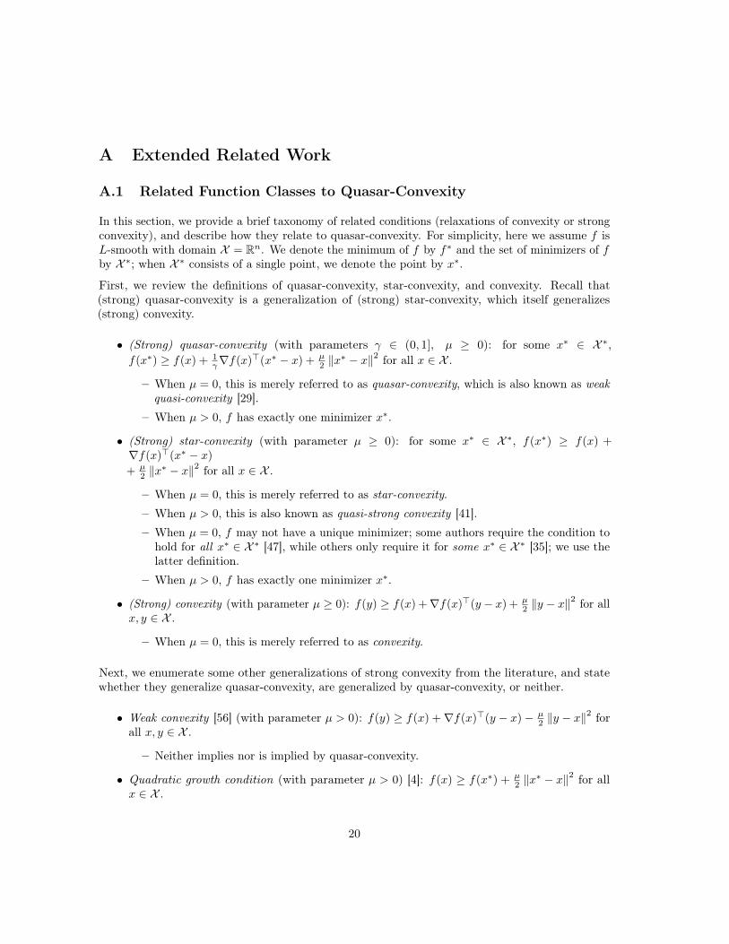
In this section, we provide a brief taxonomy of related conditions (relaxations of convexity or strongconvexity), and describe how they relate to quasar-convexity. For simplicity, here we assume f isL-smooth with domain X = Rn. We denote the minimum of f by f∗ and the set of minimizers of fby X ∗; when X ∗ consists of a single point, we denote the point by x∗.

First, we review the definitions of quasar-convexity, star-convexity, and convexity. Recall that(strong) quasar-convexity is a generalization of (strong) star-convexity, which itself generalizes(strong) convexity.

• (Strong) quasar-convexity (with parameters γ ∈ (0, 1], µ ≥ 0): for some x∗ ∈ X ∗,f(x∗) ≥ f(x) + 1

γ∇f(x)>(x∗ − x) + µ2 ‖x

∗ − x‖2 for all x ∈ X .

– When µ = 0, this is merely referred to as quasar-convexity, which is also known as weakquasi-convexity [29].

– When µ > 0, f has exactly one minimizer x∗.

• (Strong) star-convexity (with parameter µ ≥ 0): for some x∗ ∈ X ∗, f(x∗) ≥ f(x) +∇f(x)>(x∗ − x)

+ µ2 ‖x

∗ − x‖2 for all x ∈ X .

– When µ = 0, this is merely referred to as star-convexity.

– When µ > 0, this is also known as quasi-strong convexity [41].

– When µ = 0, f may not have a unique minimizer; some authors require the condition tohold for all x∗ ∈ X ∗ [47], while others only require it for some x∗ ∈ X ∗ [35]; we use thelatter definition.

– When µ > 0, f has exactly one minimizer x∗.

• (Strong) convexity (with parameter µ ≥ 0): f(y) ≥ f(x) +∇f(x)>(y − x) + µ2 ‖y − x‖

2 for allx, y ∈ X .

– When µ = 0, this is merely referred to as convexity.

Next, we enumerate some other generalizations of strong convexity from the literature, and statewhether they generalize quasar-convexity, are generalized by quasar-convexity, or neither.

• Weak convexity [56] (with parameter µ > 0): f(y) ≥ f(x) +∇f(x)>(y − x)− µ2 ‖y − x‖

2 forall x, y ∈ X .

– Neither implies nor is implied by quasar-convexity.

• Quadratic growth condition (with parameter µ > 0) [4]: f(x) ≥ f(x∗) + µ2 ‖x

∗ − x‖2 for allx ∈ X .

20

– Neither implies nor is implied by quasar-convexity.

• Restricted secant condition (with parameter µ > 0) [59]: 0 ≥ ∇f(x)>(x∗ − x) + µ2 ‖x

∗ − x‖2for all x ∈ X .

– Implied by (γ, µγ )-strong quasar-convexity (for any choice of γ ∈ (0, 1]).

• One-point strong convexity (with parameter µ > 0) [37]: for some y ∈ X , 0 ≥ ∇f(x)>(y −x) + µ

2 ‖y − x‖2 for all x ∈ X .

– This is a generalization of the restricted secant property (which is one-point strongconvexity in the special case y = x∗), and is therefore likewise implied by strong quasar-convexity.

• Variational coherence [62]: 0 ≥ ∇f(x)>(x∗ − x) for all x ∈ X , x∗ ∈ X ∗, with equality iffx ∈ X ∗.

– Implied by strong quasar-convexity (for any µ > 0 and γ ∈ (0, 1]). The closely relatedweaker condition “for some x∗ ∈ X ∗, 0 ≥ ∇f(x)>(x∗ − x) for all x ∈ X , with equalityiff x ∈ X ∗” is implied by quasar-convexity (for any µ ≥ 0, γ ∈ (0, 1]). In fact, the setof functions satisfying this condition is the limiting set of the class of γ-quasar-convexfunctions as γ → 0; this is the set of differentiable functions with star-convex sublevelsets.

• Polyak-Łojasiewicz condition [50] (with parameter µ > 0): 12 ‖∇f(x)‖2 ≥ µ(f(x)− f∗) for all

x ∈ X .

– This is implied by the restricted secant property [33], and therefore by strong quasar-convexity.

• Quasiconvexity [5]: f(λx+ (1− λ)y) ≤ maxf(x), f(y) for all x, y ∈ X and λ ∈ [0, 1].

– Neither implies nor is implied by quasar-convexity. (However, the set of differentiablequasiconvex functions is contained in the limiting set of the the class of γ-quasar-convexfunctions as γ → 0.)

• Pseudoconvexity [39]: f(y) ≥ f(x) for all x, y ∈ X such that ∇f(x) · (y − x) ≥ 0.

– Neither implies nor is implied by quasar-convexity.

• Invexity [16]: x ∈ X ∗ for all x ∈ X such that ∇f(x) = 0.

– Implied by quasar-convexity (for any µ ≥ 0, γ ∈ (0, 1]).

A.2 Comparison to Nesterov et al. (2018)

As discussed in Section 1.1.1, both our method (Algorithm 4) and Algorithm 2 of [48] minimizeγ-quasar-convex functions at accelerated rates. Compared to the method in [48], our algorithmattains a better runtime bound by a factor of γ1/2, and does not require the optimal function value

21

to be known. Meanwhile, the method of [48] can handle functions that are L-smooth (where L neednot be known) with respect to more general norms (not necessarily Euclidean). The algorithmsthemselves are quite similar (in the case of γ-quasar-convex functions that are L-smooth withrespect to the Euclidean norm), as both are generalizations of standard AGD. However, unlike[48], our algorithm does not rely on any restarts. Furthermore, while both algorithms conducta one-dimensional minimization between current iterates x(k) and v(k) in each iteration, we usethe insight that this can actually be done via a carefully implemented binary search to do thisefficiently.

B Numerical Experiments

We first consider optimizing a “hard function” - an example of the type of function used to constructthe lower bound in Theorem 2. This function class is parameterized by σ and the dimension T ; wedenote these functions by fT,σ (see Appendix 4 for the definition). We compare our method to othercommonly used first-order methods: gradient descent (GD), [standard] accelerated gradient descent(AGD), nonlinear conjugate gradients (CG), and the limited-memory BFGS (L-BFGS) algorithm.(Out of all these algorithms, only our method and GD offer theoretical guarantees for quasar-convexfunction minimization.)

We next evaluate our algorithm on real-world tasks: we use our algorithm to train a support vectormachine (SVM) on the nine LIBSVM UCI binary classification datasets [15] (which are derived fromthe UCI “Adult” datasets [18]). The SVM loss function we use is a smoothed version of the hingeloss: f(x) =

∑ni=1 φα(1− bia>i x), where ai ∈ Rd, bi = ±1 are given by the training data (the ai’s

are the covariates and the bi’s are the labels), and φα(t) = 0 for t ≤ 0, t2

2 for t ∈ [0, 1], and tα−1α + 1

2

for t ≥ 1. When α = 1, φα = t2

2 for all t ≥ 0, and thus φα and f are convex. For all α ∈ (0, 1], φαis smooth and α-quasar-convex. Line searches for this function are inexpensive, as the quantitiesbia>i x need only be calculated once per outer loop iteration. Results are given in Table 1.

Finally, we evaluate on the problem of learning linear dynamical systems, which was shown to bequasar-convex (under certain assumptions) by [29]. In this problem, we are given observations(xt, yt)Ti=1 generated by the time-invariant linear system ht+1 = Aht + Bxt; yt = Cht + Dxt,where xt, yt ∈ R; ht ∈ Rn is the hidden state at time t; and Θ = (A,B,C,D) are the (unknown)parameters of the system. Informally, we seek to learn Θ to minimize 1

T

∑Ti=1(yt − yt)2, where

ht+1 = Aht + Bxt; yt = Cht + Dxt, and h0 = 0. When parameterized in controllable canonicalform, this problem was shown to be quasar-convex on a subset of the domain near the optimumin [29]. We describe this problem and our experimental approach in more detail in Appendix B.1.Representative plots are given in Figure 3. Despite the nonconvexity, AGD performs quite wellon this problem. Nonetheless, we observe that our method is competitive with AGD in terms ofiteration count; we use more function evaluations due to the line search, but gradient evaluations areabout twice as expensive in this setting, and the line search can also be parallelized. The design ofbetter heuristics to speed up our method is an interesting question for future empirical investigation.

In all experiments, we use adaptive step sizes for our method, as well as GD and AGD, as in practiceL may not be known a priori. We do not use an initial guess for the line search.

22

↓ Function / Algorithm → Ours (Alg. 4) Gradient Descent (GD) Standard AGD Nonlinear CG L-BFGSfT,σ (σ = 10−1, T = 102; ε = 10−4) 422; 1,451 336; 738 272; 869 312; 1,599 354; 1,778fT,σ : (σ = 10−4, T = 103; ε = 10−6) 12,057; 55,357 18,607; 40,684 3,891; 12,399 1,251; 3,647 1,093; 6,554fT,σ : (σ = 10−6, T = 103; ε = 10−8) 17,135; 167,447 275,572; 602,561 55,623; 177,247 10,007; 30,023 2,079; 12,476

LIBSVM UCI (α = 1; ε = 10−4) 0.92; +0.017% 4.65; +0.036% — 0.46; +0.001% 0.29; +0.010%LIBSVM UCI (α = 0.5; ε = 10−4) 1.32; +0.016% 4.78; +0.033% — 0.48; +0.001% 0.30; +0.011%

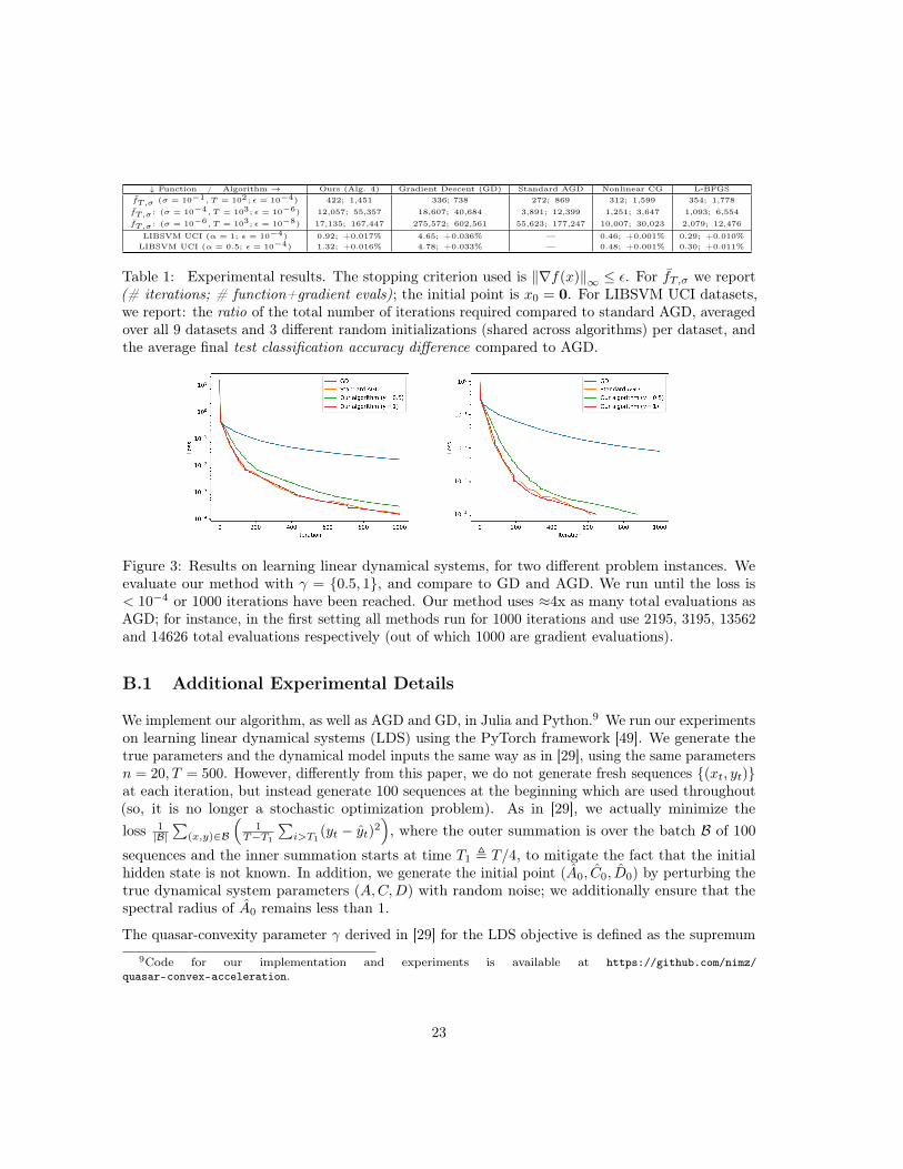
Table 1: Experimental results. The stopping criterion used is ‖∇f(x)‖∞ ≤ ε. For fT,σ we report(# iterations; # function+gradient evals); the initial point is x0 = 0. For LIBSVM UCI datasets,we report: the ratio of the total number of iterations required compared to standard AGD, averagedover all 9 datasets and 3 different random initializations (shared across algorithms) per dataset, andthe average final test classification accuracy difference compared to AGD.

Figure 3: Results on learning linear dynamical systems, for two different problem instances. Weevaluate our method with γ = 0.5, 1, and compare to GD and AGD. We run until the loss is< 10−4 or 1000 iterations have been reached. Our method uses ≈4x as many total evaluations asAGD; for instance, in the first setting all methods run for 1000 iterations and use 2195, 3195, 13562and 14626 total evaluations respectively (out of which 1000 are gradient evaluations).

B.1 Additional Experimental Details

We implement our algorithm, as well as AGD and GD, in Julia and Python.9 We run our experimentson learning linear dynamical systems (LDS) using the PyTorch framework [49]. We generate thetrue parameters and the dynamical model inputs the same way as in [29], using the same parametersn = 20, T = 500. However, differently from this paper, we do not generate fresh sequences (xt, yt)at each iteration, but instead generate 100 sequences at the beginning which are used throughout(so, it is no longer a stochastic optimization problem). As in [29], we actually minimize theloss 1

|B|∑

(x,y)∈B

(1

T−T1

∑i>T1

(yt − yt)2), where the outer summation is over the batch B of 100

sequences and the inner summation starts at time T1 , T/4, to mitigate the fact that the initialhidden state is not known. In addition, we generate the initial point (A0, C0, D0) by perturbing thetrue dynamical system parameters (A,C,D) with random noise; we additionally ensure that thespectral radius of A0 remains less than 1.

The quasar-convexity parameter γ derived in [29] for the LDS objective is defined as the supremum9Code for our implementation and experiments is available at https://github.com/nimz/

quasar-convex-acceleration.

23

of the real part of a ratio of two degree-n univariate polynomials over the complex unit circle.Therefore, it is difficult to calculate in practice. We instead simply evaluate different values of γ inour experiments; we find that, while the choice of γ does affect performance somewhat, our methoddoes not break down even if the “wrong” choice is used.

[29] presented two better-performing alternatives to fixed-stepsize SGD: SGD with gradient clippingor projected SGD. By contrast, as we use an adaptive step size, there is no need to clip gradients;in addition, we find projection to be unnecessary as the initial iterate we generate already hasρ(A0) < 1 by construction.

In the LDS experiments, we use forward difference to approximate the 1D gradients in the linesearch, since full gradient evaluations require backpropagation and are thus more expensive thanfunction evaluations in this case; we do not find this to incur significant numerical error.

For the adaptive step sizes, we use a standard scheme in which the step size at iteration k > 0 [whichwe denote 1

L(k) ] is initialized to the previous step size 1L(k−1) times a fixed value ζ1 ≥ 1, and then

multiplied by a fixed value ζ2 ∈ (0, 1) until it is small enough so that the function value decrease issufficient,10 where ζ1, ζ2 are constant hyperparameters. (This slightly generalizes Algorithm 5, whichsimply sets ζ2 = 1/2.) In all experiments for GD, AGD, and our method, we used ζ1 = 1.1, ζ2 = 0.6,and L(0) = 1 (these values were only coarsely tuned; the algorithms are fairly insensitive to themwhen reasonable settings are used).

C Algorithm Analysis

Here, we provide omitted proofs and details for Sections 2-3.

C.1 Backtracking Step Size Search Analysis

In Algorithm 5 (analyzed in Lemma 9), we show how to efficiently compute an L(k) such thatf(y(k) − 1

L(k)∇f(y(k))) ≤ f(y(k))− 12L(k)

∥∥∇f(y(k))∥∥2

holds in Line 3 of Algorithm 1, even when thetrue Lipschitz constant L is unknown. This is done using standard backtracking line search; we pro-vide the details of the algorithm and analysis for completeness (Algorithm 5). [Note that run_halvingmeans we halve L repeatedly as long as the descent inequality is satisfied—corresponding to doubling

10Specifically, for GD, we decrease the step size 1L(k) until the criterion f(x(k+1)) ≤ f(x(k))− 1

2L(k) ||∇f(x(k))||2

is satisfied; for AGD and our method, the criterion is f(x(k+1)) ≤ f(y(k)) − 12L(k) ||∇f(y(k)||2. These criteria are

guaranteed to hold when L(k) ≥ L.

24

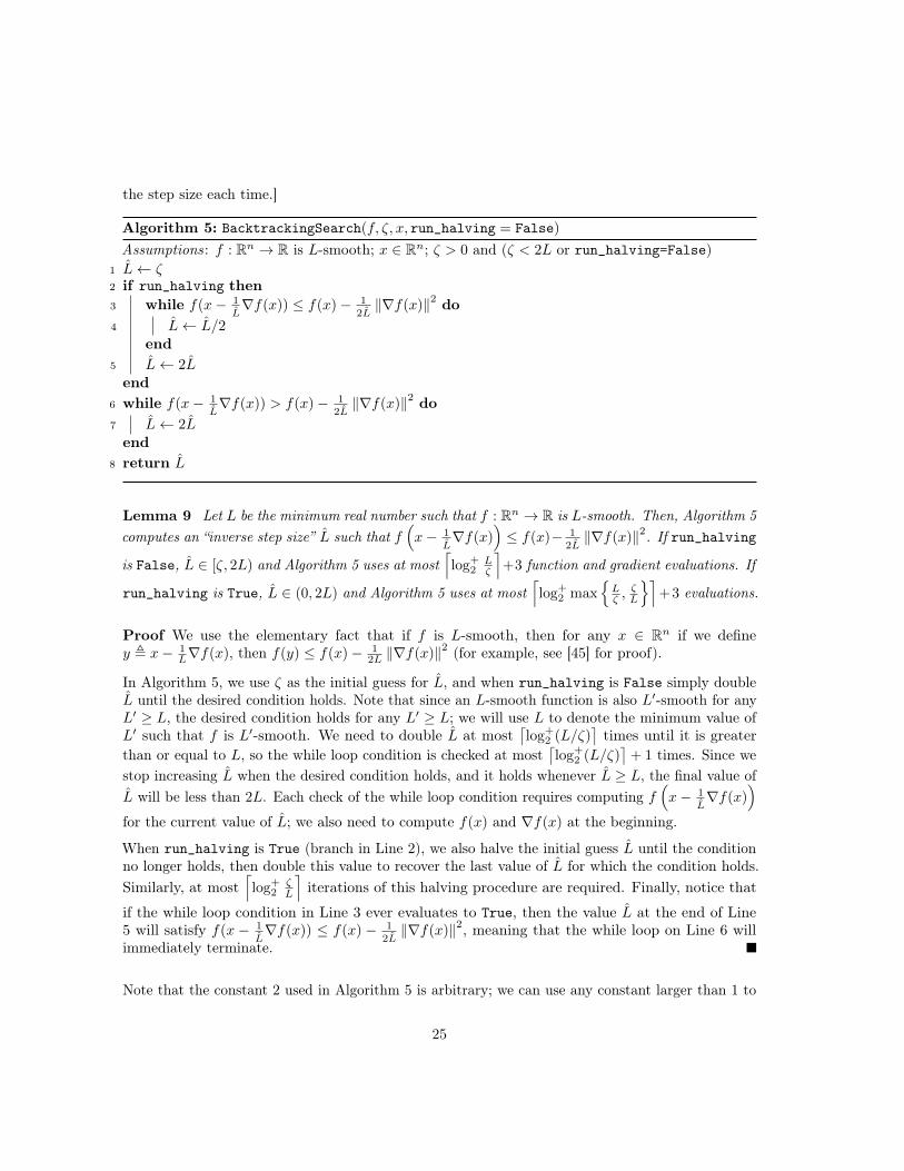
the step size each time.]

Algorithm 5: BacktrackingSearch(f, ζ, x, run_halving = False)

Assumptions: f : Rn → R is L-smooth; x ∈ Rn; ζ > 0 and (ζ < 2L or run_halving=False)1 L← ζ2 if run_halving then3 while f(x− 1

L∇f(x)) ≤ f(x)− 1

2L‖∇f(x)‖2 do

4 L← L/2end

5 L← 2Lend

6 while f(x− 1L∇f(x)) > f(x)− 1

2L‖∇f(x)‖2 do

7 L← 2Lend

8 return L

Lemma 9 Let L be the minimum real number such that f : Rn → R is L-smooth. Then, Algorithm 5computes an “inverse step size” L such that f

(x− 1

L∇f(x)

)≤ f(x)− 1

2L‖∇f(x)‖2. If run_halving

is False, L ∈ [ζ, 2L) and Algorithm 5 uses at most⌈log+

2Lζ

⌉+3 function and gradient evaluations. If

run_halving is True, L ∈ (0, 2L) and Algorithm 5 uses at most⌈log+

2 maxLζ ,

ζL

⌉+3 evaluations.

Proof We use the elementary fact that if f is L-smooth, then for any x ∈ Rn if we definey , x− 1

L∇f(x), then f(y) ≤ f(x)− 12L ‖∇f(x)‖2 (for example, see [45] for proof).

In Algorithm 5, we use ζ as the initial guess for L, and when run_halving is False simply doubleL until the desired condition holds. Note that since an L-smooth function is also L′-smooth for anyL′ ≥ L, the desired condition holds for any L′ ≥ L; we will use L to denote the minimum value ofL′ such that f is L′-smooth. We need to double L at most

⌈log+

2 (L/ζ)⌉times until it is greater

than or equal to L, so the while loop condition is checked at most⌈log+

2 (L/ζ)⌉

+ 1 times. Since westop increasing L when the desired condition holds, and it holds whenever L ≥ L, the final value ofL will be less than 2L. Each check of the while loop condition requires computing f

(x− 1

L∇f(x)

)for the current value of L; we also need to compute f(x) and ∇f(x) at the beginning.

When run_halving is True (branch in Line 2), we also halve the initial guess L until the conditionno longer holds, then double this value to recover the last value of L for which the condition holds.Similarly, at most

⌈log+

2ζL

⌉iterations of this halving procedure are required. Finally, notice that

if the while loop condition in Line 3 ever evaluates to True, then the value L at the end of Line5 will satisfy f(x − 1

L∇f(x)) ≤ f(x) − 1

2L‖∇f(x)‖2, meaning that the while loop on Line 6 will

immediately terminate.

Note that the constant 2 used in Algorithm 5 is arbitrary; we can use any constant larger than 1 to

25

multiplicatively increase L each time, which merely changes both the runtime and the final upperbound on L by a constant factor. The term “backtracking” is used because increasing L correspondsto decreasing the “step size.”

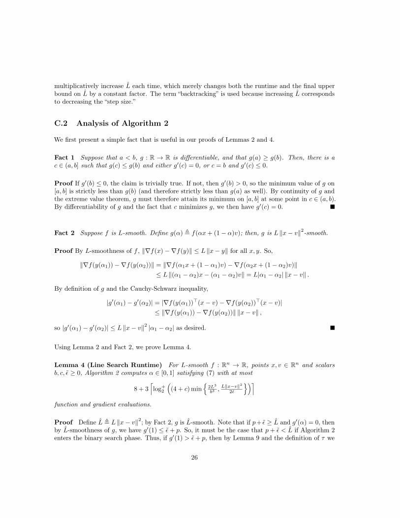
C.2 Analysis of Algorithm 2

We first present a simple fact that is useful in our proofs of Lemmas 2 and 4.

Fact 1 Suppose that a < b, g : R → R is differentiable, and that g(a) ≥ g(b). Then, there is ac ∈ (a, b] such that g(c) ≤ g(b) and either g′(c) = 0, or c = b and g′(c) ≤ 0.

Proof If g′(b) ≤ 0, the claim is trivially true. If not, then g′(b) > 0, so the minimum value of g on[a, b] is strictly less than g(b) (and therefore strictly less than g(a) as well). By continuity of g andthe extreme value theorem, g must therefore attain its minimum on [a, b] at some point in c ∈ (a, b).By differentiability of g and the fact that c minimizes g, we then have g′(c) = 0.

Fact 2 Suppose f is L-smooth. Define g(α) , f(αx+ (1− α)v); then, g is L ‖x− v‖2-smooth.

Proof By L-smoothness of f , ‖∇f(x)−∇f(y)‖ ≤ L ‖x− y‖ for all x, y. So,

‖∇f(y(α1))−∇f(y(α2))‖ = ‖∇f(α1x+ (1− α1)v)−∇f(α2x+ (1− α2)v)‖≤ L ‖(α1 − α2)x− (α1 − α2)v‖ = L|α1 − α2| ‖x− v‖ .

By definition of g and the Cauchy-Schwarz inequality,

|g′(α1)− g′(α2)| = |∇f(y(α1))>(x− v)−∇f(y(α2))>(x− v)|≤ ‖∇f(y(α1))−∇f(y(α2))‖ ‖x− v‖ ,

so |g′(α1)− g′(α2)| ≤ L ‖x− v‖2 |α1 − α2| as desired.

Using Lemma 2 and Fact 2, we prove Lemma 4.

Lemma 4 (Line Search Runtime) For L-smooth f : Rn → R, points x, v ∈ Rn and scalarsb, c, ε ≥ 0, Algorithm 2 computes α ∈ [0, 1] satisfying (7) with at most

8 + 3⌈log+

2

((4 + c) min

2L3

b3 ,L‖x−v‖2

2ε

)⌉function and gradient evaluations.

Proof Define L , L ‖x− v‖2; by Fact 2, g is L-smooth. Note that if p+ ε ≥ L and g′(α) = 0, thenby L-smoothness of g, we have g′(1) ≤ ε+ p. So, it must be the case that p+ ε < L if Algorithm 2enters the binary search phase. Thus, if g′(1) > ε+ p, then by Lemma 9 and the definition of τ we

26

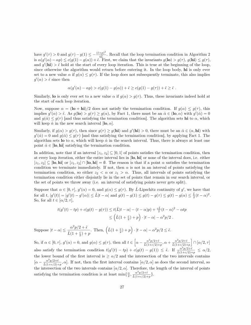
have g′(τ) > 0 and g(τ)−g(1) ≤ − (ε+p)2

4L. Recall that the loop termination condition in Algorithm 2

is α(g′(α)− αp) ≤ c(g(1)− g(α)) + ε. First, we claim that the invariants g(lo) > g(τ), g(hi) ≤ g(τ),and g′(hi) > ε hold at the start of every loop iteration. This is true at the beginning of the loop,since otherwise the algorithm would return before entering it. In the loop body, hi is only everset to a new value α if g(α) ≤ g(τ). If the loop does not subsequently terminate, this also impliesg′(α) > ε since then

α(g′(α)− αp) > c(g(1)− g(α)) + ε ≥ c(g(1)− g(τ)) + ε ≥ ε .

Similarly, lo is only ever set to a new value α if g(α) > g(τ). Thus, these invariants indeed hold atthe start of each loop iteration.

Now, suppose α = (lo + hi)/2 does not satisfy the termination condition. If g(α) ≤ g(τ), thisimplies g′(α) > ε. As g(lo) > g(τ) ≥ g(α), by Fact 1, there must be an α ∈ (lo, α) with g′(α) = 0and g(α) ≤ g(τ) [and thus satisfying the termination condition]. The algorithm sets hi to α, whichwill keep α in the new search interval [lo, α].

Similarly, if g(α) > g(τ), then since g(τ) ≥ g(hi) and g′(hi) > 0, there must be an α ∈ (α,hi) withg′(α) = 0 and g(α) ≤ g(τ) [and thus satisfying the termination condition], by applying Fact 1. Thealgorithm sets lo to α, which will keep α in the search interval. Thus, there is always at least onepoint α ∈ [lo,hi] satisfying the termination condition.

In addition, note that if an interval [z1, z2] ⊆ [0, 1] of points satisfies the termination condition, thenat every loop iteration, either the entire interval lies in [lo,hi] or none of the interval does, i.e. either[z1, z2] ⊆ [lo,hi] or [z1, z2] ∩ [lo,hi] = ∅. The reason is that if a point α satisfies the terminationcondition we terminate immediately. If not, then α is not in an interval of points satisfying thetermination condition, so either z2 < α or z1 > α. Thus, all intervals of points satisfying thetermination condition either disjointly lie in the set of points that remain in our search interval, orthe set of points we throw away (i.e. an interval of satisfying points never gets split).

Suppose that α ∈ [0, τ ], g′(α) = 0, and g(α) ≤ g(τ). By L-Lipschitz continuity of g′, we have thatfor all t, |g′(t)| = |g′(t)− g′(α)| ≤ L|t− α| and g(t)− g(1) ≤ g(t)− g(τ) ≤ g(t)− g(α) ≤ L

2 (t− α)2.So, for all t ∈ [α/2, τ ],

t(g′(t)− tp) + c(g(t)− g(τ)) ≤ t(L|t− α| − (t− α)p) + cL2 (t− α)2 − αtp

≤(L(1 + c

2 ) + p)· |t− α| − α2p/2 .

Suppose |t− α| ≤ α2p/2 + ε

L(1 + c2 ) + p

. Then,(L(1 + c

2 ) + p)· |t− α| − α2p/2 ≤ ε.

So, if α ∈ [0, τ ], g′(α) = 0, and g(α) ≤ g(τ), then all t ∈[α− α2p/2+ε

L(1+c/2)+p, α+ α2p/2+ε

L(1+c/2)+p

]∩ [α/2, τ ]

also satisfy the termination condition t(g′(t) − tp) + c(g(t) − g(1)) ≤ ε. If α2p/2+ε

L(1+c/2)+p≤ α/2,

the lower bound of the first interval is ≥ α/2 and the intersection of the two intervals contains[α− α2p/2+ε

L(1+c/2)+p, α]. If not, then the first interval contains [α/2, α] as does the second interval, so

the intersection of the two intervals contains [α/2, α]. Therefore, the length of the interval of pointssatisfying the termination condition is at least minα2 ,

α2p/2+ε

L(1+c/2)+p.

27

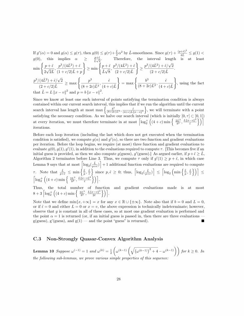
If g′(α) = 0 and g(α) ≤ g(τ), then g(0) ≤ g(τ)+ L2 α

2 by L-smoothness. Since g(τ) + (p+ε)2

4L≤ g(1) <

g(0), this implies α ≥ p+ε

L√

2. Therefore, the interval length is at least

min

p+ ε

2√

2L,p3/(4L2) + ε

(1 + c/2)L+ p

≥ min

p+ ε

L√

8,p3/(4L2) + ε

(2 + c/2)L

≥ p3/(4L2) + ε/

√2

(2 + c/2)L.

p3/(4L2) + ε/√

2

(2 + c/2)L≥ max

p3

(8 + 2c)L3,

ε

(4 + c)L

= max

b3

(8 + 2c)L3,

ε

(4 + c)L

, using the fact

that L = L ‖x− v‖2 and p = b ‖x− v‖2.

Since we know at least one such interval of points satisfying the termination condition is alwayscontained within our current search interval, this implies that if we run the algorithm until the currentsearch interval has length at most max

b3

(8+2c)L3 ,ε

(4+c)L‖x−v‖2

, we will terminate with a point

satisfying the necessary condition. As we halve our search interval (which is initially [0, τ ] ⊂ [0, 1])at every iteration, we must therefore terminate in at most

⌈log+

2

((4 + c) min

2L3

b3 ,L‖x−v‖2

ε

)⌉iterations.

Before each loop iteration (including the last which does not get executed when the terminationcondition is satisfied), we compute g(α) and g′(α), so there are two function and gradient evaluationsper iteration. Before the loop begins, we require (at most) three function and gradient evaluations toevaluate g(0), g(1), g′(1), in addition to the evaluations required to compute τ . [This becomes five if aninitial guess is provided, as then we also compute g(guess), g′(guess).] As argued earlier, if p+ ε ≥ L,Algorithm 2 terminates before Line 3. Thus, we compute τ only if g′(1) ≥ p + ε, in which caseLemma 9 says that at most

⌈log2( L

p+ε )⌉

+ 1 additional function evaluations are required to compute

τ . Note that Lp+ε ≤ min

Lp ,

Lε

since p, ε ≥ 0; thus,

⌈log2( L

p+ε )⌉≤⌈log2

(min

Lp ,

Lε

)⌉≤⌈

log+2

((4 + c) min

2L3

b3 ,L‖x−v‖2

ε

)⌉.

Thus, the total number of function and gradient evaluations made is at most8 + 3

⌈log+

2

((4 + c) min

2L3

b3 ,L‖x−v‖2

2ε

)⌉.

Note that we define minx,+∞ = x for any x ∈ R ∪ ±∞. Note also that if b = 0 and L = 0,or if ε = 0 and either L = 0 or x = v, the above expression is technically indeterminate; however,observe that g is constant in all of these cases, so at most one gradient evaluation is performed andthe point α = 1 is returned (or, if an initial guess is passed in, then there are three evaluations —g(guess), g’(guess), and g(1) — and the point “guess” is returned).

C.3 Non-Strongly Quasar-Convex Algorithm Analysis

Lemma 10 Suppose ω(−1) = 1 and ω(k) = 12

(ω(k−1)

(√(ω(k−1)

)2+ 4− ω(k−1)

))for k ≥ 0. In

the following sub-lemmas, we prove various simple properties of this sequence:

28

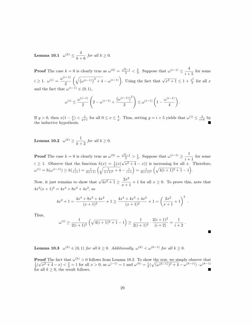
Lemma 10.1 ω(k) ≤ 4

k + 6for all k ≥ 0.

Proof The case k = 0 is clearly true as ω(0) =√

5−12 < 2

3 . Suppose that ω(i−1) ≤ 4

i+ 5for some

i ≥ 1. ω(i) =ω(i−1)

2

(√(ω(i−1)

)2+ 4− ω(i−1)

). Using the fact that

√x2 + 1 ≤ 1 + x2

2 for all x

and the fact that ω(i−1) ∈ (0, 1),

ω(i) ≤ ω(i−1)

2

(2− ω(i−1) +

(ω(i−1)

)22

)≤ ω(i−1)

(1− ω(i−1)

4

).

If y > 0, then x(1− x4 ) < 4

y+1 for all 0 ≤ x ≤ 4y . Thus, setting y = i+ 5 yields that ω(i) ≤ 4

i+6 bythe inductive hypothesis.

Lemma 10.2 ω(k) ≥ 1

k + 2for all k ≥ 0.

Proof The case k = 0 is clearly true as ω(0) =√

5−12 > 1

2 . Suppose that ω(i−1) ≥ 1

i+ 1for some

i ≥ 1. Observe that the function h(x) = 12 (x(√x2 + 4 − x)) is increasing for all x. Therefore,

ω(i) = h(ω(i−1)) ≥ h( 1i+1 ) = 1

2(i+1)

(√1

(i+1)2 + 4− 1i+1

)= 1

2(i+1)2

(√4(i+ 1)2 + 1− 1

).

Now, it just remains to show that√

4x2 + 1 ≥ 2x2

x+ 1+ 1 for all x ≥ 0. To prove this, note that

4x2(x+ 1)2 = 4x4 + 8x3 + 4x2, so

4x2 + 1 =4x4 + 8x3 + 4x2

(x+ 1)2+ 1 ≥ 4x4 + 4x3 + 4x2

(x+ 1)2+ 1 =

(2x2

x+ 1+ 1

)2

.

Thus,

ω(i) ≥ 1

2(i+ 1)2

(√4(i+ 1)2 + 1− 1

)≥ 1

2(i+ 1)2· 2(i+ 1)2

(i+ 2)=

1

i+ 2.

Lemma 10.3 ω(k) ∈ (0, 1) for all k ≥ 0. Additionally, ω(k) < ω(k−1) for all k ≥ 0.

Proof The fact that ω(k) > 0 follows from Lemma 10.2. To show the rest, we simply observe that12 (√x2 + 4− x) < 2

2 = 1 for all x > 0; as ω(−1) = 1 and ω(k) = 12 (√

(ω(k−1))2 + 4− ω(k−1)) · ω(k−1)

for all k ≥ 0, the result follows.

29

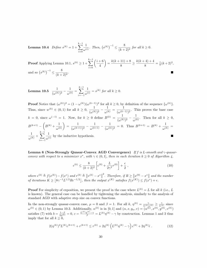
Lemma 10.4 Define s(k) = 1 +

k−1∑i=0

1

ω(i). Then,

(s(k)

)−1 ≤ 8

(k + 2)2for all k ≥ 0.

Proof Applying Lemma 10.1, s(k) ≥ 1 +

k−1∑i=0

(i+ 6

4

)=k(k + 11) + 8

8≥ k(k + 4) + 4

8= 1

8 (k + 2)2,

and so(s(k)

)−1 ≤ 8

(k + 2)2.

Lemma 10.51

(ω(k))2− 1

ω(k)=

k−1∑i=−1

1

ω(i)= s(k) for all k ≥ 0.

Proof Notice that (ω(k))2 = (1− ω(k))(ω(k−1))2 for all k ≥ 0, by definition of the sequence ω(k).Thus, since w(k) ∈ (0, 1) for all k ≥ 0,

1

(ω(k))2− 1

ω(k)=

1

(ω(k−1))2. This proves the base case

k = 0, since ω(−1) = 1. Now, for k ≥ 0 define B(k) =1

(ω(k))2− 1

ω(k). Then for all k ≥ 0,

B(k+1) −(B(k) +

1

ω(k)

)=

1

(ω(k+1))2− 1

ω(k+1)− 1

(ω(k))2= 0. Thus B(k+1) = B(k) +

1

ω(k)=

1

ω(k)+

k−1∑i=−1

1

ω(i)by the inductive hypothesis.

Lemma 6 (Non-Strongly Quasar-Convex AGD Convergence) If f is L-smooth and γ-quasar-convex with respect to a minimizer x∗, with γ ∈ (0, 1], then in each iteration k ≥ 0 of Algorithm 4,

ε(k) ≤ 8

(k + 2)2

[ε(0) +

L

2γ2r(0)

]+ε

2, (10)

where ε(k) , f(x(k))−f(x∗) and r(k) ,∥∥v(k) − x∗

∥∥2. Therefore, if R ≥

∥∥x(0) − x∗∥∥ and the number

of iterations K ≥⌊8γ−1L1/2Rε−1/2

⌋, then the output x(K) satisfies f(x(K)) ≤ f(x∗) + ε.

Proof For simplicity of exposition, we present the proof in the case where L(k) = L for all k (i.e., Lis known). The general case can be handled by tightening the analysis, similarly to the analysis ofstandard AGD with adaptive step size on convex functions.

In the non-strongly quasar-convex case, µ = 0 and β = 1. For all k, η(k) = γL(k)ω(k) ≥ γ

L(k) sinceω(k) ∈ (0, 1) by Lemma 10.3. Additionally, α(k) is in [0, 1] and (α, x, yα, v) = (α(k), x(k), y(k), v(k))

satisfies (7) with b = 1−β2η(k) = 0, c = L(k)η(k)−γ

β = L(k)η(k) − γ by construction. Lemmas 1 and 3 thusimply that for all k ≥ 0,

2(η(k))2L(k)ε(k+1) + r(k+1) ≤ r(k) + 2η(k)(L(k)η(k) − γ

)ε(k) + 2η(k)ε . (12)

30

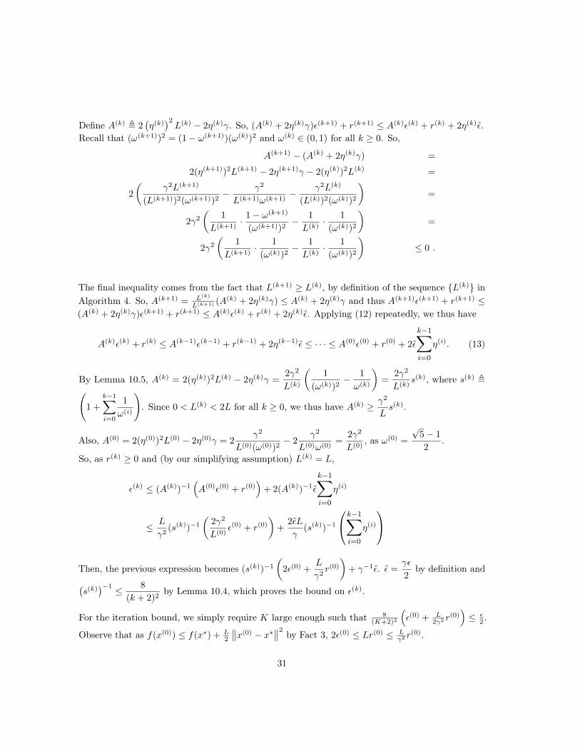
Define A(k) , 2(η(k)

)2L(k) − 2η(k)γ. So, (A(k) + 2η(k)γ)ε(k+1) + r(k+1) ≤ A(k)ε(k) + r(k) + 2η(k)ε.

Recall that (ω(k+1))2 = (1− ω(k+1))(ω(k))2 and ω(k) ∈ (0, 1) for all k ≥ 0. So,

A(k+1) − (A(k) + 2η(k)γ) =

2(η(k+1))2L(k+1) − 2η(k+1)γ − 2(η(k))2L(k) =

2

(γ2L(k+1)

(L(k+1))2(ω(k+1))2− γ2

L(k+1)ω(k+1)− γ2L(k)

(L(k))2(ω(k))2

)=

2γ2

(1

L(k+1)· 1− ω(k+1)

(ω(k+1))2− 1

L(k)· 1

(ω(k))2

)=

2γ2

(1

L(k+1)· 1

(ω(k))2− 1

L(k)· 1

(ω(k))2

)≤ 0 .

The final inequality comes from the fact that L(k+1) ≥ L(k), by definition of the sequence L(k) inAlgorithm 4. So, A(k+1) = L(k)

L(k+1) (A(k) + 2η(k)γ) ≤ A(k) + 2η(k)γ and thus A(k+1)ε(k+1) + r(k+1) ≤(A(k) + 2η(k)γ)ε(k+1) + r(k+1) ≤ A(k)ε(k) + r(k) + 2η(k)ε. Applying (12) repeatedly, we thus have

A(k)ε(k) + r(k) ≤ A(k−1)ε(k−1) + r(k−1) + 2η(k−1)ε ≤ · · · ≤ A(0)ε(0) + r(0) + 2ε

k−1∑i=0

η(i). (13)

By Lemma 10.5, A(k) = 2(η(k))2L(k) − 2η(k)γ =2γ2

L(k)

(1

(ω(k))2− 1

ω(k)

)=

2γ2

L(k)s(k), where s(k) ,(

1 +

k−1∑i=0

1

ω(i)

). Since 0 < L(k) < 2L for all k ≥ 0, we thus have A(k) ≥ γ2

Ls(k).

Also, A(0) = 2(η(0))2L(0) − 2η(0)γ = 2γ2

L(0)(ω(0))2− 2

γ2

L(0)ω(0)=

2γ2

L(0), as ω(0) =

√5− 1

2.

So, as r(k) ≥ 0 and (by our simplifying assumption) L(k) = L,

ε(k) ≤ (A(k))−1(A(0)ε(0) + r(0)

)+ 2(A(k))−1ε

k−1∑i=0

η(i)

≤ L

γ2(s(k))−1

(2γ2

L(0)ε(0) + r(0)

)+

2εL

γ(s(k))−1

k−1∑i=0

η(i)

Then, the previous expression becomes (s(k))−1

(2ε(0) +

L

γ2r(0)

)+ γ−1ε. ε =

γε

2by definition and(

s(k))−1 ≤ 8

(k + 2)2by Lemma 10.4, which proves the bound on ε(k).

For the iteration bound, we simply require K large enough such that 8(K+2)2

(ε(0) + L

2γ2 r(0))≤ ε

2 .

Observe that as f(x(0)) ≤ f(x∗) + L2

∥∥x(0) − x∗∥∥2

by Fact 3, 2ε(0) ≤ Lr(0) ≤ Lγ2 r

(0).

31

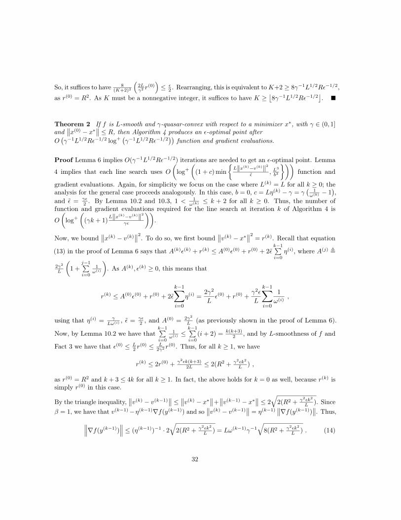
So, it suffices to have 8(K+2)2

(2Lγ2 r

(0))≤ ε

2 . Rearranging, this is equivalent toK+2 ≥ 8γ−1L1/2Rε−1/2,

as r(0) = R2. As K must be a nonnegative integer, it suffices to have K ≥⌊8γ−1L1/2Rε−1/2

⌋.

Theorem 2 If f is L-smooth and γ-quasar-convex with respect to a minimizer x∗, with γ ∈ (0, 1]and

∥∥x(0) − x∗∥∥ ≤ R, then Algorithm 4 produces an ε-optimal point after

O(γ−1L1/2Rε−1/2 log+

(γ−1L1/2Rε−1/2

))function and gradient evaluations.

Proof Lemma 6 implies O(γ−1L1/2Rε−1/2) iterations are needed to get an ε-optimal point. Lemma

4 implies that each line search uses O(

log+

((1 + c) min

L‖x(k)−v(k)‖2

ε , L3

b3

))function and

gradient evaluations. Again, for simplicity we focus on the case where L(k) = L for all k ≥ 0; theanalysis for the general case proceeds analogously. In this case, b = 0, c = Lη(k) − γ = γ

(1

ω(k) − 1),

and ε = γε2 . By Lemma 10.2 and 10.3, 1 < 1

ω(k) ≤ k + 2 for all k ≥ 0. Thus, the number offunction and gradient evaluations required for the line search at iteration k of Algorithm 4 is

O

(log+

((γk + 1)

L‖x(k)−v(k)‖2γε

)).

Now, we bound∥∥x(k) − v(k)

∥∥2. To do so, we first bound

∥∥v(k) − x∗∥∥2

= r(k). Recall that equation

(13) in the proof of Lemma 6 says that A(k)ε(k) + r(k) ≤ A(0)ε(0) + r(0) + 2εk−1∑i=0

η(i), where A(j) ,

2γ2

L

(1 +

j−1∑i=0

1ω(i)

). As A(k), ε(k) ≥ 0, this means that

r(k) ≤ A(0)ε(0) + r(0) + 2ε

k−1∑i=0

η(i) =2γ2

Lε(0) + r(0) +

γ2ε

L

k−1∑i=0

1

ω(i),

using that η(i) = γLω(i) , ε = γε

2 , and A(0) = 2γ2

L (as previously shown in the proof of Lemma 6).

Now, by Lemma 10.2 we have thatk−1∑i=0

1ω(i) ≤

k−1∑i=0

(i+ 2) = k(k+3)2 , and by L-smoothness of f and

Fact 3 we have that ε(0) ≤ L2 r

(0) ≤ L2γ2 r

(0). Thus, for all k ≥ 1, we have

r(k) ≤ 2r(0) + γ2εk(k+3)2L ≤ 2(R2 + γ2εk2

L ) ,

as r(0) = R2 and k + 3 ≤ 4k for all k ≥ 1. In fact, the above holds for k = 0 as well, because r(k) issimply r(0) in this case.

By the triangle inequality,∥∥v(k) − v(k−1)

∥∥ ≤ ∥∥v(k) − x∗∥∥+∥∥v(k−1) − x∗

∥∥ ≤ 2

√2(R2 + γ2εk2

L ). Sinceβ = 1, we have that v(k−1)−η(k−1)∇f(y(k−1)) and so

∥∥v(k) − v(k−1)∥∥ = η(k−1)

∥∥∇f(y(k−1))∥∥. Thus,∥∥∥∇f(y(k−1))

∥∥∥ ≤ (η(k−1))−1 · 2√

2(R2 + γ2εk2

L ) = Lω(k−1)γ−1

√8(R2 + γ2εk2

L ) . (14)

32

Now, by definition of x(k), v(k), and y(k−1),

x(k) − v(k) = y(k−1) − 1L∇f(y(k−1))− v(k)

= α(k−1)x(k−1) + (1− α(k−1))v(k−1) − 1L∇f(y(k−1))− v(k)

= α(k−1)x(k−1) + (1− α(k−1))v(k−1) − 1L∇f(y(k−1))−

(v(k−1) − η(k−1)∇f(y(k−1))

)= α(k−1)(x(k−1) − v(k−1)) + (η(k−1) − 1

L )∇f(y(k−1)) .

Therefore, ∥∥∥x(k) − v(k)∥∥∥ ≤ α(k−1)

∥∥∥x(k−1) − v(k−1)∥∥∥+

∣∣∣η(k−1) − 1L

∣∣∣ · ∥∥∥∇f(y(k−1))∥∥∥

≤∥∥∥x(k−1) − v(k−1)

∥∥∥+(η(k−1) + 1

L

)·∥∥∥∇f(y(k−1))

∥∥∥≤∥∥∥x(k−1) − v(k−1)

∥∥∥+ 2Lω(k−1) ·

∥∥∥∇f(y(k−1))∥∥∥

≤∥∥∥x(k−1) − v(k−1)

∥∥∥+ γ−1

√32(R2 + γ2εk2

L )

≤∥∥∥x(k−1) − v(k−1)

∥∥∥+√

32γ−1(R+ γk

√εL

),

where the first inequality is the triangle inequality, the third inequality uses that η(k−1) = γLω(k−1)

and that γ, ω(k−1) ∈ (0, 1], the fourth inequality uses (14), and the final inequality uses that√a+ b ≤

√a+√b for any a, b ≥ 0.

As this holds for all k ≥ 1, we have by induction that for all k ≥ 0,

∥∥∥x(k) − v(k)∥∥∥ ≤ ∥∥∥x(0) − v(0)

∥∥∥+

k∑j=1

√32γ−1

(R+ γj

√εL

)=√

32γ−1

k∑j=1

(R+ γj

√εL

),

since x(0) = v(0). Simplification yields∥∥x(k) − v(k)

∥∥ ≤ √32kγ−1R+√

8k(k + 1)√

εL . For all k ≥ 1,

it is the case that k + 1 ≤ 2k, so∥∥x(k) − v(k)

∥∥ ≤ √32(kγ−1R+ k2

√εL

); this inequality holds for

k = 0 as well, as∥∥x(0) − v(0)

∥∥ = 0 in this case.

Suppose k ≤⌊4γ−1L1/2Rε−1/2

⌋. Then∥∥∥x(k) − v(k)

∥∥∥ ≤ √32(

4γ−1L1/2Rε−1/2 · γ−1R+ 16γ−2LR2ε−1 ·√

εL

)= 80

√2 · γ−2L1/2R2ε−1/2 .

Recall that the line search at iteration k requires O(

log+

((γk + 1)

L‖x(k)−v(k)‖2γε

))function and

gradient evaluations. (γk + 1)L‖x(k)−v(k)‖2

γε ≤ (4L1/2Rε−1/2 + 1) · 12800(γ−5L2R4ε−2). Therefore,each line search indeed requires O

(log+

(γ−1L1/2Rε−1/2

))function and gradient evaluations.

As the number of iterations k is O(γ−1L1/2Rε−1/2), the total number of function and gradientevaluations required is thus O

(γ−1L1/2Rε−1/2 log+

(γ−1L1/2Rε−1/2

)), as claimed.

33

As in the strongly convex case, the algorithm may continue to run if the specified number of iterationsK is larger; however, this theorem combined with Lemma 6 shows that x(k) will be ε-optimal ifk =

⌊4γ−1L1/2Rε−1/2

⌋, and this x(k) will be produced using

O(γ−1L1/2Rε−1/2 log+

(γ−1L1/2Rε−1/2

))function and gradient evaluations. (Future iterates x(k′)

with k′ >⌊4γ−1L1/2Rε−1/2

⌋will also be ε-optimal.)

Remark 1 If f is L-smooth and γ-quasar-convex with γ ∈ (0, 1] and∥∥x(0) − x∗

∥∥ ≤ R, then gradientdescent with step size 1

L returns a point x with f(x) ≤ f(x∗) + ε after O(γ−1LR2ε−1

)function and

gradient evaluations.

Proof See Theorem 1 in [26].

C.4 Comparisons with Standard AGD

We have described how our algorithms relate to standard (convex) AGD. We briefly comment onthe difference between the analysis of our algorithms and that of standard AGD, and on the use ofa line search “initial guess” inspired by the setting of α(k) in standard AGD.

C.4.1 Analysis

Concretely, a key step in the proof of convergence of algorithms that extend Algorithm 1 (includingour algorithms as well as standard AGD) is to bound Q(k); this bound is then combined withLemma 1 to get the final convergence bound. In standard AGD, we bound Q(k) by setting α(k) to aspecific predetermined value. For instance, in the non-strongly convex case (where β = 1), α(k) is set

such thatα(k)

1− α(k)= L(k)η(k) − 1.11 We then have Q(k) = 2η(k) · α(k)

1− α(k)∇f(y(k))>(x(k) − y(k)) =

2η(k)(L(k)η(k) − 1)∇f(y(k))>(x(k) − y(k)), and then we use convexity to obtain that Q(k) ≤2η(k)(L(k)η(k) − 1)(f(x(k))− f(y(k))) = 2η(k)(L(k)η(k) − 1)(ε(k) − ε(k)

y ). By contrast, for our algo-rithms, we bound Q(k) using Lemma 3.

C.4.2 Line Search Initial Guess

In special cases, specifying an “initial guess” for α in the binary line search (Algorithm 2) canspeed up our algorithms, by allowing the line search to be circumvented a large portion of thetime. For instance, at each step k we can use the α(k) prescribed by the standard version of AGD

as a guess: this value is√L(k)/µ

1+√L(k)/µ

in the strongly convex case (Algorithm 3), and 1− ω(k) in the

non-strongly convex case (Algorithm 4). Thus, when f is convex or strongly convex (and thus γ = 1),our respective algorithms using the initial guess are equivalent to standard AGD (as described in

11As η(k) = 1L(k)ω(k) , this implies that α(k) = 1− ω(k).

34

[45]), since this initial guess always satisfies the necessary condition (7) by convexity [in fact, itsatisfies the stronger (6)] and will thus be chosen as the value of α(k). Moreover, even when f isnonconvex, checking this initial guess costs at most one extra function and gradient evaluationeach per invocation of Algorithm 2. So, when γ = 1 we can interpret the overall algorithm as a“robustified” version of standard AGD—each iteration is identical to that of standard AGD unlessa “convexity violation” between x(k) and v(k) is detected, in which case we fall back to the binarysearch.

C.4.3 Analysis Techniques

We remark that our analysis can also be recast in the framework of estimate sequences (for instance,following [45]), by generalizing the analysis for standard AGD. The analysis presented in this workis an adaptation of a somewhat different style of analysis of standard AGD, based on analyzingthe one-step decrease in the more general potential function presented in Lemma 1. Indeed, asmentioned, the standard AGD algorithms for both convex and strongly convex minimization arealso specific instances of the framework presented in Algorithm 1.

D The Structure of Quasar-Convex Functions

In this section, we prove various properties of quasar-convex functions. First, we state a slightlymore general definition of quasar-convexity on a convex domain.

Definition 3 Let X ⊆ Rn be convex. Furthermore, suppose that either X is open or n = 1. Letγ ∈ (0, 1] and let x∗ ∈ X be a minimizer of the differentiable function f : X → R. The function f isγ-quasar-convex on X with respect to x∗ if for all x ∈ X ,

f(x∗) ≥ f(x) +1

γ∇f(x)>(x∗ − x).

Suppose also µ ≥ 0. The function f is (γ, µ)-strongly quasar-convex on X if for all x ∈ X ,

f(x∗) ≥ f(x) +1

γ∇f(x)>(x∗ − x) +

µ

2‖x∗ − x‖2 .

If X is of the form [a, b] ⊆ R, then ∇f(a) and ∇f(b) here denote limh→0+

f(a+h)−f(a)h and lim

h→0−

f(b+h)−f(b)h ,

respectively. Differentiability simply means that ∇f(x) exists for all x ∈ X .

Definition 3 is exactly the same as Definition 1 if the domain X = Rn. We remark that it is possibleto generalize Definition 3 even further to the case where X is a star-convex set with star center x∗.

D.1 Proof of Observation 1

Observation 1 Let a < b and let f : [a, b]→ R be continuously differentiable. The function f isγ-quasar-convex for some γ ∈ (0, 1] iff f is unimodal and all critical points of f are minimizers.

35

Additionally, if h : Rn → R is γ-quasar-convex with respect to a minimizer x∗, then for any d ∈ Rnwith ‖d‖ = 1, the 1-D function f(θ) , h(x∗ + θd) is γ-quasar-convex.

Proof First, we prove that if f is continuously differentiable and unimodal with nonzero derivativeexcept at minimizers, then f is γ-quasar-convex for some γ > 0.

Let x∗ be a minimizer of f on [a, b], and let x ∈ [a, b] be arbitrary. Define gx(t) = f((1− t)x∗ + tx).By unimodality of f , gx is differentiable and increasing on [0, 1], so g′x(t) ≥ 0 for t ∈ [0, 1], and

f(x)− f(x∗) = gx(1)− gx(0) =

1∫0

g′x(t) dt .

Also, g′x(1) = f ′(x)(x−x∗) 6= 0 by assumption for all x with f(x) > f(x∗). Note that if f(x) = f(x∗),then gx(t) is constant on [0, 1] by unimodality and so g′x(t) = 0 for all t ∈ [0, 1].

Define Cx∗ = supx∈[a,b]

supt∈[0,1]

g′x(t)

g′x(1), where we define the inner supremum to be 1 if f(x) = f(x∗). By

continuity of each g′x over [0, 1] and the fact that g′x(1) > 0 for all x ∈ [a, b] with f(x) > f(x∗),supt∈[0,1]

g′x(t)g′x(1) is a continuous function of x. Thus as the outer supremum is over the compact

interval [a, b], Cx∗ indeed exists; note that Cx∗ ∈ [1,∞).

For any x ∈ [a, b] with f(x) > f(x∗), we thus havef(x)− f(x∗)

f ′(x)(x− x∗)=

∫ 1

0g′x(t) dt

g′x(1)≤ Cx∗ , meaning

f(x∗) ≥ f(x)+Cx∗(f′(x)(x∗−x)). This also holds for all x such that f(x) = f(x∗), as either x = x∗

or f ′(x) = 0 in these cases. Thus, f is 1Cx∗

quasar-convex on [a, b] with respect to x∗. Finally,if we define Cmax = max

x∗∈argminx∈[a,b] f(x)Cx∗ , we have that f is 1

Cmaxquasar-convex on [a, b] where

1Cmax

∈ (0, 1] is a constant depending only on f , a, and b. This completes the proof.

Now, we prove the other direction (which is much simpler). Suppose that f : [a, b] → R isdifferentiable and quasar-convex for some γ ∈ (0, 1]. Then 1

γ f′(x)(x− x∗) ≥ f(x)− f(x∗) ≥ 0. If x

is not a minimizer of f , then the last inequality is strict; otherwise, either x ∈ a, b or f ′(x) = 0. Inother words, assuming x is not a minimizer, when x < x∗ [i.e. to the left of x∗], f ′ < 0 and so f isstrictly decreasing, while when x > x∗ [i.e. to the right of x∗], f ′ > 0 and so f is strictly increasing.This implies that f is unimodal.

Finally, suppose h : Rn → R is γ-quasar-convex with respect to a minimizer x∗, suppose d ∈ Rn has‖d‖ = 1, and define f(θ) , h(x∗ + θd). Note that f ′(θ) = d>∇h(x∗ + θd) and that θ = 0 minimizesf . By γ-quasar-convexity of h with respect to x∗, we have for all θ ∈ R that

f(0) = h(x∗) ≥ h(x∗ + θd) + 1γ∇h(x∗ + θd)>(x∗ − (x∗ + θd)) = f(θ) + 1

γ f′(θ)(0− θ) ,

meaning that f is γ-quasar-convex.

36

D.2 Characterizations of Quasar-Convexity

Lemma 11 Let f : X → R be differentiable with a minimizer x∗ ∈ X , where the domain X ⊆ Rnis open and convex.12 Then, the following two statements:

f(tx∗ + (1− t)x) + t

(1− t

2− γ

)γµ

2‖x∗ − x‖2 ≤ γtf(x∗) + (1− γt)f(x) ∀x ∈ X , t ∈ [0, 1] (15)

f(x∗) ≥ f(x) +1

γ∇f(x)>(x∗ − x) +

µ

2‖x∗ − x‖2 ∀x ∈ X (16)

are equivalent for all µ ≥ 0, γ ∈ (0, 1].

Proof First, we prove that (16) implies (15).

Suppose (16) holds and µ = 0. Let x ∈ X be arbitrary and for all t ∈ [0, 1] let xt , (1− t)x∗ + txand let g(t) , f(xt)− f(x∗). Since g′(t) = ∇f(xt)

>(x− x∗) and x∗ − xt = −t(x∗ − x), substitutingthese equalities into (16) yields that g(t) ≤ t

γ g′(t) for all t ∈ [0, 1].

Rearranging, we see that the inequality in (15) [for fixed x] is equivalent to the condition thatg(t) ≤ `(t) for all t ∈ [0, 1], where `(t) , (1− γ(1− t))g(1). We proceed by contradiction: supposethat for some α ∈ [0, 1] it is the case that g(α) > `(α). Note that α > 0 necessarily. Let β be theminimum element of the set t ∈ [α, 1] : g(t) = `(t). Since g(1) = `(1), such a β exists with α < β.Consequently, for all t ∈ (α, β) we have g(t) ≥ `(t) and so∫ β

α

g′(t) dt = g(β)− g(α) < `(β)− `(α) = γ(β − α)g(1) (17)

and

(β − α)g(1) =

∫ β

α

`(t)

1− γ(1− t)dt ≤

∫ β

α

g(t)

1− γ(1− t)dt . (18)

Combining (17) and (18) and using that g(t) ≤ tγ g′(t), we have

∫ β

α

[1

t− 1

1− γ(1− t)

]g(t) dt ≤

∫ β

α

g′(t)

γdt−

∫ β

α

g(t)

1− γ(1− t)dt < 0

As g(t) = f(xt) − f(x∗) ≥ 0 and 1/t ≥ 1/(1 − γ(1 − t)) for all t ∈ [α, β] ⊂ (0, 1], we have acontradiction.

Now, suppose µ > 0. Define h(x) , f(x) − γµ

2(2− γ)‖x∗ − x‖2. Observe that h(x∗) = f(x∗),

∇h(x) = ∇f(x)− γµ

2− γ(x− x∗), and ∇h(x)>(x∗ − x) = ∇f(x)>(x∗ − x) +

γµ

2− γ‖x∗ − x‖2. Thus,

12We remark that this lemma still holds if X is open and star-convex with star center x∗, or if X is any subintervalof R.

37

by algebraic simplification and then application of (16) by assumption,

h(x) +1

γ∇h(x)>(x∗ − x) = f(x)− γµ

2(2− γ)‖x∗ − x‖2 +

1

γ∇f(x)>(x∗ − x) +

µ

2− γ‖x∗ − x‖2

= f(x) +1

γ∇f(x)>(x∗ − x) +

µ

2‖x∗ − x‖2

(− γ

2− γ+

2

2− γ

)= f(x) +

1

γ∇f(x)>(x∗ − x) +

µ

2‖x∗ − x‖2

≤ f(x∗) = h(x∗) .

As we earlier showed that (16) implies (15) in the µ = 0 case, we have that

h(tx∗ + (1− t)x) ≤ γth(x∗) + (1− γt)h(x) .

Substituting in the definition of h:

f(tx∗ + (1− t)x)− γµ

2(2− γ)‖x∗ − tx∗ − (1− t)x‖2

≤ γtf(x∗) + (1− γt)f(x)− (1− γt) γµ

2(2− γ)‖x∗ − x‖2 .

Rearranging terms and simplifying yields

f(tx∗ + (1− t)x) +γµ

2(2− γ)

((1− γt) ‖x∗ − x‖2 − (1− t)2 ‖x∗ − x‖2

)≤ γtf(x∗) + (1− γt)f(x) .

Finally, (1− γt)− (1− t)2 = t((2− γ)− t), which gives the desired result.

Now, we prove that (15) implies (16).

This time, define g(t) , f(tx∗ + (1 − t)x). For t ∈ [0, 1), g′(t) = ∇f(tx∗ + (1 − t)x)>(x∗ − x).

By assumption, g(t) + t

(1− t

2− γ

)γµ

2‖x∗ − x‖2 ≤ γtg(1) + (1 − γt)g(0) for all t ∈ [0, 1], so

g(1) ≥ g(0) +g(t)− g(0)

γt+

(1− t

2− γ

)µ

2‖x∗ − x‖2 for all t ∈ (0, 1]. Taking the limit as t ↓ 0

yields f(x∗) = g(1) ≥ g(0) +1

γg′(0) +

µ

2‖x∗ − x‖2 = f(x) +

1

γ∇f(x)>(x∗ − x) +

µ

2‖x∗ − x‖2.

Remark 1 A modified version of Lemma 11 holds if x∗ is replaced with any point x ∈ X , whereeither γ = 1 or (15) and (16) hold for all x ∈ X with f(x) ≥ f(x). If f satisfies either of theseequivalent properties, we then say that f is “(γ, µ)-strongly quasar-convex with respect to x.”

Remark 2 Using Remark 1, we can show that even if x is not a minimizer of the function f ,Algorithms 3 and 4 can still be applied to efficiently finding a point that has an objective value ofat most f(x) + ε; the respective runtime bounds are the same, and the proofs remain essentiallyunchanged.

38

Note that when γ = 1, µ = 0, and (15) is required to hold for all minimizers of f , it becomes thestandard definition of star-convexity [47].

Corollary 1 If f is (γ, µ)-strongly quasar-convex with minimizer x∗, then

f(x) ≥ f(x∗) +γµ

2(2− γ)‖x∗ − x‖2 , ∀x

Proof Plug in t = 1 to (15) to get

f(x∗) +

(1− 1

2− γ

)γµ

2‖x∗ − x‖2 ≤ γf(x∗) + (1− γ)f(x) .

Simplifying yields

f(x) ≥ f(x∗) +

(1− 1

2− γ

)γµ

2(1− γ)‖x∗ − x‖2 = f(x∗) +

γµ

2(2− γ)‖x∗ − x‖2 .

Fact 3 If f : X → R is L-smooth, x∗ is a minimizer of f , and the domain X ⊆ Rn is open andstar-convex with star center x∗, then f(y) ≤ f(x∗) + L

2 ‖y − x∗‖2 for all y ∈ X .

Proof This is a simple and well-known fact that is true of any L-smooth function (whether or notit is quasar-convex); for completeness, we provide the proof.

Define g(t) , f((1− t)x∗ + ty), for t ∈ [0, 1]. So, g′(t) = ∇f((1− t)x∗ + ty)>(y− x∗), g(0) = f(x∗),and g(1) = f(y). Since g′(0) = 0 and f is L-smooth, ‖∇f((1− t)x∗ + ty)‖ ≤ L ‖(1− t)x∗ + ty − x∗‖ =

Lt ‖y − x∗‖. So, g′(t) ≤ |g′(t)| ≤ Lt ‖y − x∗‖2, and thus f(y) = g(1) =

1∫0

g′(t) dt + g(0) ≤

1∫0

Lt ‖y − x∗‖2 dt+ g(0) = L2 ‖y − x

∗‖2 + f(x∗).

Observation 2 If f is (γ, µ)-strongly quasar-convex, then f is not L-smooth for any L < γµ2−γ .

Proof If f is (γ, µ)-strongly quasar-convex, Corollary 1 says that f(x) ≥ f(x∗) + γµ2(2−γ) ‖x

∗ − x‖2

for all x. If f is L-smooth, Fact 3 says that f(x) ≤ f(x∗) + L2 ‖x

∗ − x‖2 for all x.

Thus, if f is (γ, µ)-strongly quasar-convex and L-smooth, we have γµ2(2−γ) ‖x

∗ − x‖2 ≤ L2 ‖x

∗ − x‖2

for all x, which means that we must have L ≥ γµ2−γ .

39

Observation 3 If f is γ-quasar convex, the set of its minimizers is star-convex.

Proof Recall that a set S is termed star-convex (with star center x0) if there exists an x0 ∈ S suchthat for all x ∈ S and t ∈ [0, 1], it is the case that tx0 + (1− t)x ∈ S [40].

Suppose f : X → R is γ-quasar-convex with respect to a minimizer x∗ ∈ X , where X is convex.Suppose y ∈ X also minimizes f . Then for any t ∈ [0, 1], equation (15) implies that f(tx∗+(1−t)y) ≤γtf(x∗) + (1 − γt)f(y) = γtf(x∗) + (1 − γt)f(x∗) = f(x∗). So, tx∗ + (1 − t)y is in X and alsominimizes f . Thus, the set of minimizers of f is star-convex, with star center x∗.

Observation 4 If f is (γ, µ)-strongly quasar-convex with µ > 0, f has a unique minimizer.

Proof By Corollary 1, f(x) > f(x∗) if µ > 0 and x 6= x∗, implying that x minimizes f iff x = x∗.

Observation 5 Suppose f is differentiable and (γ, µ)-strongly quasar-convex. Then f is also(θγ, µ/θ)-strongly quasar-convex for any θ ∈ (0, 1].

Proof (γ, µ)-strong quasar-convexity states that 0 ≥ f(x∗)−f(x) ≥ 1γ∇f(x)>(x∗−x)+ µ

2 ‖x∗ − x‖2

for some x∗ and all x in the domain of f . Multiplying by 1θ − 1 ≥ 0, it follows that

f(x∗) ≥ f(x) + 1γ∇f(x)>(x∗ − x) + µ

2 ‖x− x∗‖2 ≥ f(x) + 1

γθ∇f(x)>(x∗ − x) + µ2θ ‖x

∗ − x‖2.

Note that any (γ, µ)-strongly quasar-convex function is also (γ, µ)-strongly quasar-convex for anyµ ∈ [0, µ]. Thus, the restriction γ ∈ (0, 1] in the definition of quasar-convexity may be made withoutany loss of generality compared to the restriction γ > 0.

Observation 6 The parameter γ is a dimensionless quantity, in the sense that if f is γ-quasar-convex on Rn, the function g(x) , a · f(bx) is also γ-quasar-convex on Rn, for any a ≥ 0, b ∈ R.

Proof If a or b is 0, then g is constant so the claim is trivial. Now suppose a, b 6= 0. Let x∗ denotethe quasar-convex point of f . Observe that as x∗ minimizes f , x∗/b minimizes g. By (15), for allx ∈ Rn we have

1ag((tx∗ + (1− t)x)/b) = f(tx∗ + (1− t)x)

≤ γtf(x∗) + (1− γt)f(x)

= γt · 1ag(x∗/b) + (1− γt) · 1

ag(x/b) .

Multiplying by a, we have g(t(x∗/b) + (1 − t)(x/b)) ≤ γtg(x∗/b) + (1 − γt)g(x/b) for all x ∈ Rn.Since x/b can take on any value in Rn, this means that g is γ-quasar-convex with respect to x∗/b.

40

D.3 Construction of Quasar-Convex Functions

We now briefly describe some basic “building blocks” and closure properties of the family of quasar-convex functions, inspired by the analogous discussion for star-convex functions in Appendix A of[35]. (Recall also that star-convex functions, such as the examples in [35], are quasar-convex withγ = 1.)

1. Suppose f : Rn → R is (γ, µ)-quasar-convex with respect to x∗ = 0. Let a ≥ 0, c ∈ R be scalars,M ∈ Rm×n, and b ∈ Rm. Then g(x) = a · f(M(x+ b)) + c is (γ, µ · σ2

min(M))-quasar-convex,where σmin(M) denotes the smallest singular value of M.

• Proof : It is easy to see that adding the constant c does not affect the quasar-convexityproperties, and that g(x − b) has the same quasar-convexity properties as g(x); so,by Observation 6, it suffices to prove the claim for a = 1, b = 0, c = 0. We havef(0) ≥ f(x) − 1

γ∇f(x)>x + µ2 ‖x‖

2 for all x ∈ Rn, by (γ, µ)-quasar-convexity of fwith respect to x∗ = 0. So g(0) = f(0) ≥ f(My) − 1

γ∇f(My)>(My) + µ2 ‖My‖2 =

f(My) − 1γM∇f(My)>y + µ

2 ‖My‖2 ≥ f(My) − 1γM∇f(My)>y +

µσ2min(M)

2 ‖y‖2 =

g(y) + 1γ∇g(y)>(0− y) +

µσ2min(M)

2 ‖0− y‖2 for all y ∈ Rm, which proves the claim.

2. If f, g are (γ1, µ1) and (γ2, µ2) quasar-convex respectively with respect to the same minimizerx∗, then h(x) = f(x) + g(x) is (minγ1, γ2, µ1 + µ2) quasar-convex with respect to the sameminimizer x∗.

• Proof : h(x∗) = f(x∗) + g(x∗) ≥ f(x) + 1γ1∇f(x)>(x∗ − x) + µ1

2 ‖x∗ − x‖2 + g(x) +

1γ2∇g(x)>(x∗ − x) + µ1

2 ‖x∗ − x‖2 = h(x) + µ1+µ2

2 ‖x∗ − x‖2 + 1γ1∇f(x)>(x∗ − x) +

1γ2∇g(x)>(x∗ − x) ≥ h(x) + µ1+µ2

2 ‖x∗ − x‖2 + 1minγ1,γ2 (∇f(x) +∇g(x))>(x∗ − x) as

desired, since ∇f(x)>(x∗ − x) ≤ f(x∗)− f(x) ≤ 0 and similarly ∇g(x)>(x∗ − x) ≤ 0.

3. Suppose f, g are γ-quasar-convex with respect to the same point x∗, and f(x∗) = g(x∗) = 0.Then h(x) = f(x)g(x) is also γ-quasar-convex with respect to x∗.

• Proof : Using Lemma 11 and the fact that f, g are nonnegative, h(tx∗ + (1 − t)x) =f(tx∗ + (1− t)x)g(tx∗ + (1− t)x) ≤ (1− γt)f(x) · (1− γt)g(x) = (1 + (γt)2 − 2γt)h(x)for all t ∈ [0, 1]. As γt ∈ [0, 1], (γt)2 ≤ γt, so (1 + (γt)2 − 2γt)h(x) ≤ (1 − γt)h(x) bynonnegativity of h. Applying Lemma 11 yields the result.

4. Let X be a bounded star-convex set with C1 boundary and star center x∗ = 0. Let f : R→ Rbe γ-quasar-convex with respect to the point 0, with f(0) = 0, and let g(x) be an arbitrary C1

nonnegative function defined on the boundary of X . For each point x 6= x∗ ∈ X , let P (x) bethe (unique) intersection of the boundary of X with the ray from x∗ to x, and let P (x∗) = x∗.Then the function h(x) = f(‖x‖) · g (P (x)) is nonnegative, C1, and γ-quasar-convex on Xwith respect to x∗ = 0. (Note: The rightmost function plotted in Figure 1 was constructed inthis manner, where X is the unit circle [so P (x) = x

‖x‖ ], f(x) = x2

1+x2 , and g was a randomlygenerated linear combination of exponentiated high-frequency trigonometric functions.)

41

• Proof : Nonnegativity of f and g implies that of h. The properties of X imply thatlimx→0

h(x) = 0 = h(0), so the fact that f, g ∈ C1 implies that h is also C1. Also, for anyx 6= x∗ and any t ∈ [0, 1), h(tx∗+(1−t)x) = h((1−t)x) = f(‖(1− t)x‖) ·g(P ((1−t)x)) =f(t · 0 + (1 − t) · ‖x‖) · g(P (x)) ≤ (1 − γt)f(‖x‖) · g(P (x)) = (1 − γt)h(x) = γth(x∗) +(1− γt)h(x). To obtain the preceding inequalities, we used Lemma 11 for f , and the factthat P (tx) = P (x) for any t ∈ (0, 1], since the ray from x∗ to tx also passes through x.Finally, it is trivially true that h(tx∗ + (1− t)x) ≤ γth(x∗) + (1− γt)h(x) when x = x∗

or when t = 1, so applying Lemma 11 yields the result.

E Lower Bound Proofs

In this section, we use 0 to denote a vector with all entries equal to 0, and 1 to denote a vector withall entries equal to 1.

E.1 Proof of Lemma 8

Before we prove Lemma 8, we prove two useful results related to the properties of q and Υ. Forconvenience, these functions are restated below:

Υ(θ) , 120

∫ θ

1

t2(t− 1)

1 + t2dt

q(x) ,1

4(x1 − 1)2 +

1

4

T−1∑i=1

(xi − xi+1)2.

Observation 7 q is convex and 2-smooth with minimizer x∗ = 1. Also, for any 1 ≤ j1 < j2 ≤ T ,

q(x) =1

2∇q(x)>(x− x∗) ≥ max

1

4(x1 − 1)2,

(xj1 − xj2)2

4(j2 − j1)

.

Proof Convexity and 2-smoothness of q follow from definitions. It is easy to see that q is alwaysnonnegative and q(1) = 0, so 1 minimizes q. In fact 1 is the unique minimizer, since q is strictlypositive for all nonconstant vectors and all vectors with x1 6= 1.

Notice that as q is a convex quadratic, q(x) = 12 (x−x∗)>∇2q(x)(x−x∗) where ∇2q(x) is a constant

matrix. Therefore ∇q(x) = ∇2q(x)(x− x∗). It follows that q(x) = 12∇q(x)>(x− x∗).

By definition q(x) ≥ 14 (x1−1)2. Furthermore, 1

j2−j1∑j2i=j1

(xi−xi+1)2 ≥(

1j2−j1

∑j2i=j1

(xi − xi+1))2

=(xj1−xj2 )2

(j2−j1)2 , where the inequality uses that the expectation of the square of a random variable isgreater than the square of its expectation. The result follows.

Properties of Υ that we will use are listed below.

42

Lemma 12 The function Υ satisfies the following.

1. Υ′(0) = Υ′(1) = 0.

2. For all θ ≤ 1, Υ′(θ) ≤ 0, and for all θ ≥ 1, Υ′(θ) ≥ 0.

3. For all θ ∈ R we have Υ(θ) ≥ Υ(1) = 0, and Υ(0) ≤ 10.

4. Υ′(θ) < −1 for all θ ∈ (−∞,−0.1] ∪ [0.1, 0.9].

5. Υ is 180-smooth.

6. For all θ ∈ R we have Υ(θ) ≤ min30θ4 − 40θ3 + 10, 60(θ − 1)2, and Υ(0) ≥ 5.

7. For all θ 6∈ (−0.1, 0.1) we have 40(θ − 1)Υ′(θ) ≥ Υ(θ).

Proof Properties 1-4 were proved in [14, Lemma 2].

Property 5. |Υ′′(θ)| = 120∣∣∣ θ(θ3+3θ−2)

(1+θ2)2

∣∣∣ ≤ 120 · 32 = 180 for all θ ∈ R. Thus, for any θ1, θ2 ∈ R,

|Υ′(θ1)−Υ′(θ2)| ≤ maxθ∈[θ1,θ2]

|Υ′′(θ)| · |θ1 − θ2| ≤ 180|θ1 − θ2|.

Property 6. We have Υ(0) = 120∫ 1

0t2(1−t)

1+t2 dt ≥ 120∫ 1

0t2(1−t)

2 dt = 1202·12 = 5. For all θ ∈ R we have

Υ(θ) = 120∫ θ

1t2(t−1)

1+t2 dt ≤ 120∫ θ

1t2(t−1) dt = 120((θ4/4+θ3/3)−(1/4−1/3)) = 30θ4−40θ3+10. In

addition, since t2

1+t2 ≤ 1 for all t, we have for all θ ∈ R that Υ(θ) ≤ 120∫ θ

1(t− 1) dt = 120(θ− 1)2/2.

Property 7. If θ ∈ (∞,−1.0] ∪ [1.0,∞) then θ2

1+θ2 ≥ 12 , so by property 6 we have

Υ(θ) + 40(1− θ)Υ′(θ) ≤ 60(θ − 1)2 − 40 · 120θ2(θ − 1)2

1 + θ2

≤ 60(θ − 1)2 − 40 · 60(θ − 1)2

= −60 · 39(θ − 1)2

≤ 0.

Alternatively, if θ ∈ [−1.0,−0.1] ∪ [0.1, 1.0] then 11+θ2 ≥ 1

2 , so by property 6 we have

Υ(θ) + 40(1− θ)Υ′(θ) ≤ 10 + 30θ4 − 40θ3 − 40 · 120θ2(θ − 1)2

1 + θ2

≤ 10(1 + θ2

(3θ2 − 4θ − 240(θ − 1)2

))= 10

(1− 237θ4 + 476θ3 − 240θ2

)= 10P (θ) ,

where we define P (θ) , 1−237θ4 +476θ3−240θ2. Observe that P ′(θ) = −12θ(40− 119θ + 79θ2) hasexactly three roots: at θ = 0, θ = 1 and θ = 40/79. Furthermore, at θ = 1, θ = 40/79 and θ = 0.1 wehave P (θ) ≤ 0, which implies P (θ) ≤ 0 for θ ∈ [0.1, 1]. We conclude that Υ(θ) + 40(1− θ)Υ′(θ) ≤ 0

43

for θ ∈ [0.1, 1]. In addition, P (θ) is negative while P ′(θ) is positive for θ = −0.1, which means thatP (θ) and thus Υ(θ) + 40(1− θ)Υ′(θ) are also negative on [−1.0,−0.1].

In order to prove Lemma 8, we first prove an “unscaled version” in Lemma 7. This is the criticaland most difficult part of the proof of the result; some intuition is provided in Section 4.

Lemma 7 Let σ ∈ (0, 10−4], T ∈[σ−1/2,∞

)∩ Z. The function fT,σ is 1

100T√σ-quasar-convex and

3-smooth, with unique minimizer x∗ = 1. Furthermore, if xt = 0 for all t = dT/2e , . . . , T , thenfT,σ(x)− fT,σ(1) ≥ 2Tσ.

Proof Since σ ∈ (0, 10−4], Υ is 180-smooth, and q is 2-smooth, we deduce fT,σ is 3-smooth. ByObservation 7 and Lemma 12.3 we deduce fT,σ(1) = 0 < fT,σ(x) for all x 6= 1. Therefore, x∗ = 1 isthe unique minimizer of fT,σ.

Now, we will show fT,σ is 1100T

√σ-quasar-convex, i.e. that ∇fT,σ(x)>(x− 1) ≥ fT,σ(x)−fT,σ(1)

100T√σ

forall x ∈ RT . Define

A , i : xi ∈ (−∞,−0.1] ∪ (0.9,∞)B , i : xi ∈ (−0.1, 0.1)C , i : xi ∈ [0.1, 0.9].

First, we derive two useful inequalities. By Observation 7 and the fact that Υ′(xi) ≤ 0 for i ∈ B,

∇fT,σ(x)>(x− 1) = ∇q(x)>(x− 1) + σ∑

i∈A∪B∪C

(xi − 1)Υ′(xi)

≥ 2q(x) + σ∑i∈A∪C

(xi − 1)Υ′(xi) . (19)

By Lemma 12.2 and 12.6 we deduce∑i∈B∪C Υ(xi) ≤ |B ∪ C|Υ(−0.1) ≤ 11T , so it follows that

fT,σ(x) ≤ q(x) + 11Tσ + σ∑i∈AΥ(xi), and therefore using T ≥ σ−1/2 and nonnegativity of Υ and

q, we have

fT,σ(x)− fT,σ(1)

100T√σ

=fT,σ(x)

100T√σ

≤ 11Tσ

100T√σ

+σ

100T√σ

∑i∈A

Υ(xi) +1

100T√σq(x)

≤ 11

100σ1/2 +

σ

100

∑i∈A

Υ(xi) +1

100q(x)

≤ 11

100σ1/2 +

σ

40

∑i∈A

Υ(xi) + q(x) (20)

We now consider three possible cases for the values of x.

44

1. Consider the case that x1 6∈ [0.9, 1.1]. We have

∇fT,σ(x)>(x− 1) ≥ 2q(x) +σ

40

∑i∈A∪C

Υ(xi)

≥ 0.12

4+ q(x) +

σ

40

∑i∈A∪C

Υ(xi)

=1√

104σ·√σ

4+

σ

40

∑i∈A∪C

Υ(xi) + q(x)

≥√σ

4+

σ

40

∑i∈A∪C

Υ(xi) + q(x)

≥ fT,σ(x)− fT,σ(1)

100T√σ

where the first inequality uses (19) and Lemma 12.7, the second inequality uses Observation 7and x1 6∈ [0.9, 1.1], the penultimate inequality uses σ ∈ (0, 10−6] ⊂ (0, 10−4], and the finalinequality uses (20) and nonnegativity of Υ.

2. Consider the case that B = ∅. By Lemma 12.7 and convexity of q(x),

∇fT,σ(x)>(x− 1) = ∇q(x)>(x− 1) + σ∑i∈A∪C

(xi − 1)Υ′(xi)

≥ q(x)− q(1) +σ

40

∑i∈A∪C

Υ(xi)

=1

40

q(x) + σ

T∑i=1

Υ(xi)

− fT,σ(1) +39

40q(x)

≥ fT,σ(x)− fT,σ(1)

40

≥ fT,σ(x)− fT,σ(1)

100T√σ

.

3. Suppose cases 1-2 do not hold, i.e., x1 ∈ [0.9, 1.1] and B 6= ∅. Then there exist some m ≥ 1 andj ∈ 1, . . . , T −m such that xj ≥ 0.9, xj+m ≤ 0.1, and xi ∈ C for all i ∈ j+1, . . . , j+m−1.

45

Then,

∇fT,σ(x)>(x− 1) ≥ q(x) + σ∑i∈A∪C

(xi − 1)Υ′(xi) + q(x)

≥ 0.82

4m+ σ

∑i∈C

(xi − 1)Υ′(xi) + σ∑i∈A

(xi − 1)Υ′(xi) + q(x)

≥ 0.82

4m+ 0.1σ(m− 2) +

σ

40

∑i∈A

Υ(xi) + q(x)

≥ 0.16√1.6

σ1/2 +σ

40

∑i∈A

Υ(xi) + q(x)

≥ fT,σ(x)− fT,σ(1)

100T√σ

where the the first inequality holds by (19), the second inequality uses Observation 7, thethird inequality uses Lemma 12.4 and 12.7, the fourth inequality uses that m =

√1.6σ−0.5 ≥ 2

minimizes the previous expression, and the final inequality uses (20) [and the fact that0.16/

√1.6 > 0.11].

Finally, suppose xt = 0 for all t = dT/2e , . . . , T . Then we have fT,σ(x) − fT,σ(1) = fT,σ(x) ≥σ dT/2eΥ(0) ≥ 2Tσ, where the first inequality uses that Υ ≥ 0 and q ≥ 0, and the last inequalityuses that T ≥ 1 and Υ(0) ≥ 5.

With Lemma 7 in hand, we are able to establish Lemma 8 which is a scaled version of Lemma 7.

Lemma 8 Let ε ∈ (0,∞), γ ∈ (0, 10−2], T =⌈10−3γ−1L1/2Rε−1/2

⌉, and σ = 1

104T 2γ2 , and assumeL1/2Rε−1/2 ≥ 103. Consider the function

f(x) , 13LR

2T−1 · fT,σ(xT 1/2R−1). (11)

This function is L-smooth and γ-quasar-convex, and its minimizer x∗ is unique and has ‖x∗‖ = R.Furthermore, if xt = 0 ∀t ∈ Z ∩ [T/2, T ], then f(x)− infz f(z) > ε.

Proof We have σ−1/2 = 102Tγ ≤ T and σ = 1104T 2γ2 ≤ 1

(L1/2Rε−1/2)2 ≤ 10−6, so fT,σ satisfies theconditions of Lemma 7.

Let us verify the properties of f . The optimum of fT,σ is 1, but after this rescaling it becomesx∗ = R√

T1, for which ‖x∗‖ = R. For all x, y ∈ RT , by 3-smoothness of fT,σ we have∥∥∥∇f(x)−∇f(y)

∥∥∥ = 13 (LR2T−1) · (T 1/2R−1)

∥∥∥∇fT,σ(xT 1/2R−1)−∇fT,σ(yT 1/2R−1)∥∥∥

≤ (LR2T−1) · (T 1/2R−1)2 ‖x− y‖= L ‖x− y‖ .

46

Therefore f is L-smooth. By the definition of σ we have 1100T

√σ

= γ, so fT,σ is γ-quasar-convex.

As quasar-convexity is invariant to scaling (Observation 6), we deduce that f is γ-quasar-convex aswell. Finally, given x(k)

t = 0 for t = dT/2e , . . . , T , we have

f(x(k))− infzf(z) ≥ 2Tσ · LR

2

3T= 2

3LR2σ = 2

3 (10−2γ−1L1/2RT−1)2 ≥ 503 ε,

where the first transition uses Lemma 7, the third transition uses that σ = 1104T 2γ2 , and the last transi-

tion uses that T =⌈10−3γ−1L1/2Rε−1/2

⌉≤ 2 · 10−3γ−1L1/2Rε−1/2 since 10−3γ−1(L1/2Rε−1/2) ≥ 1.

E.2 Proof of Theorem 3

Before proving Theorem 3 we recap definitions that were originally provided in [13].

Definition 4 A function f is a first-order zero-chain if for every x ∈ Rn,

xi = 0 ∀i ≥ t ⇒ ∇if(x) = 0 ∀i > t.

Definition 5 An algorithm is a first-order zero-respecting algorithm (FOZRA) if, for all i ∈1, . . . , n, its iterates x(0), x(1), ... ∈ Rn satisfy

∇if(x(k)) = 0 ∀k ≤ t ⇒ x(t+1)i = 0

for all i ∈ 1, . . . , n.

Definition 6 An algorithm A is a first-order deterministic algorithm (FODA) if there exists asequence of functions Ak such the algorithm’s iterates satisfy

x(k+1) = Ak(x(0), . . . , x(k),∇f(x(0)), . . . ,∇f(x(k)))

for all k ∈ N, input functions f , and starting points x(0).

Observation 8 Consider ε > 0, a function class F , and K ∈ N. If f : Rn → R satisfies

1. f is a first-order zero-chain,

2. f belongs to the function class F , i.e. f ∈ F , and

3. f(x)− infz f(z) ≥ ε for every x such that xt = 0 for all t ∈ K,K + 1, . . . , n;

then it takes at least K iterations for any FOZRA to find an ε-optimal solution of f .

Proof Cosmetic modification of the proof of Observation 2 in [13].

47

Theorem 3 Let ε, R, L ∈ (0,∞), γ ∈ (0, 1], and assume L1/2Rε−1/2 ≥ 1. Let F denote the set ofL-smooth functions that are γ-quasar-convex with respect to some point with Euclidean norm lessthan or equal to R. Then, given any deterministic first-order method, there exists a function f ∈ Fsuch that the method requires at least Ω(γ−1L1/2Rε−1/2) gradient evaluations to find an ε-optimalpoint of f .

Proof Applying Lemma 8 and Observation 8 implies this result for any first-order zero-respectingmethod. Applying Proposition 1 from [13], which states that lower bounds for first-order zero-respecting methods also apply to deterministic first-order methods, gives the result.

E.3 Lower Bounds via Reduction

Remark 3 If we have an algorithm that can approximately minimize a strongly quasar-convexfunction, we can use it to approximately minimize a quasar-convex function.

Proof This follows from the fact that if f is γ-quasar-convex with respect to a minimizer x∗,then the function gε(x) = f(x) + ε

2

∥∥x− x(0)∥∥2

is (γ, ε)-strongly quasar-convex with respect tox∗ (recall this terminology from Remark 1). Note that x∗ is not necessarily a minimizer of gε,but gε(x∗) ≤ f(x∗) + εR2/2, where R =

∥∥x(0) − x∗∥∥. Therefore, if we obtain a point x with

gε(x) ≤ infx g(x) + εR2/2, then f(x) ≤ gε(x) ≤ gε(x∗) + ε/2 ≤ f(x∗) + εR2.

Remark 4 Given any deterministic first-order method, there exists an L-smooth, (γ, µ)-stronglyquasar-convex function such that the method requires at least Ω(maxγ−1L1/2µ−1/2,γ−1L1/2µ−1/2 log+(ε−1)) gradient evaluations to find an ε-optimal point of f .

Proof Suppose there was a deterministic first-order method for minimizing L-smooth (γ, µ)-stronglyquasar-convex functions which required o(γ−1κ−1/2) gradient evaluations to find an ε-minimizer,where κ = L

µ . Let f be an L-smooth function that is γ-quasar-convex with respect to a minimizer x∗,let ε > 0, and let R =

∥∥x(0) − x∗∥∥. Then, the function gε/R2 is (L+ ε

R2 )-smooth and (γ, εR2 )-strongly

quasar-convex with respect to x∗ as shown in Remark 3, so the condition number of gε/R2 isκ = 1 + LR2

ε . Thus, we could apply the method to find an ε2R2 -minimizer of gε/R2 , and it would do

so using o(γ−1⌈L1/2Rε−1/2

⌉) gradient evaluations. But an ε

2R2 -minimizer of gε/R2 is an ε-minimizerof f , as argued in Remark 3; thus, this violates the lower bound on the complexity of minimizingquasar-convex functions shown in Theorem 3.

To prove the second part of the lower bound, we first note that any (γ, µ)-quasar-convex quadratic isalso (1, ( 2

γ − 1)−1µ)-quasar-convex and thus (1, γµ2 )-quasar-convex, and in fact γµ2 -strongly convex ;

this follows from definitions. Thus, direct application of the Ω((L/µ)1/2 log+(ε−1)) lower boundon the complexity of finding an ε-minimizer of an L-smooth µ-strongly convex quadratic with adeterministic first-order method [43, Chapter 7] yields a lower bound of Ω(γ−1/2(L/µ)1/2 log+(ε−1))on the complexity of first-order minimization of L-smooth (γ, µ)-quasar-convex functions.

48