HAL Id: tel-03394466https://tel.archives-ouvertes.fr/tel-03394466

Submitted on 22 Oct 2021

HAL is a multi-disciplinary open accessarchive for the deposit and dissemination of sci-entific research documents, whether they are pub-lished or not. The documents may come fromteaching and research institutions in France orabroad, or from public or private research centers.

L’archive ouverte pluridisciplinaire HAL, estdestinée au dépôt et à la diffusion de documentsscientifiques de niveau recherche, publiés ou non,émanant des établissements d’enseignement et derecherche français ou étrangers, des laboratoirespublics ou privés.

Convex and online optimization : applications toscheduling and selection problems

Victor Verdugo

To cite this version:Victor Verdugo. Convex and online optimization : applications to scheduling and selection problems.Data Structures and Algorithms [cs.DS]. Université Paris sciences et lettres; Universidad de Chile,2018. English. NNT : 2018PSLEE079. tel-03394466

COMPOSITION DU JURY :

M. Jose Correa Universidad de Chile, Directeur de thèse

M. Christoph Dürr Sorbonne Université, Rapporteur

M. Samuel Fiorini Université libre de Bruxelles, Rapporteur et membre du jury

M. Rida LarakiUniversité Paris Dauphine, Membre du jury

Mme. Claire Mathieu École normale supérieure et Collège de France, Directrice de thèse

Mme. Nicole Megow Universität Bremen, Membre du jury

M. Tobias Mömke Universität Bremen, Membre du jury

Mme. Alantha Newman Université Grenoble Alpes, Membre du jury

M. Fernando Ordóñez Universidad de Chile, Membre du jury

Soutenue par Victor Verdugo le 13 Juin 2018 h

THÈSE DE DOCTORAT

de l’Université de recherche Paris Sciences et Lettres  PSL Research University

Préparée dans le cadre d’une cotutelle entre École normale supérieure et l’Universidad de Chile

Dirigée par Jose Correa et Claire Mathieu

Ecole doctorale n°386 École Doctorale de Sciences Mathématiques de Paris Centre

Spécialité Informatique

Convex and Online Optimization: Applications to Scheduling and Selection Problems

Optimisation convexe et en ligne: applications aux problèmes de planification et de sélection

Acknowledgments

First of all, I’m really grateful to my advisors, Claire Mathieu and Jose Correa, for allyour support, guidance and patience, for those inspiring conversations about researchand life. I’ve learned a lot from you these years about how to do research, and I’msure I will keep learning from you in the future. Thank you!

I thank Christoph Durr and Samuel Fiorini for carefully reviewing this work, andyour helpful comments. I also thank to Rida Laraki, Nicole Megow, Tobias Momke,Alantha Newman and Fernando Ordonez for being part of the jury.

I had the chance to share with two very inspiring group of people, at Talgo ENSand the Acgo UChile. I thank Eric Colin de Verdiere, Hang Zhou, Zenthao Li andVincent Cohen-Addad for all those conversations about research and french. Manythanks to Frederik Mallmann-Trenn, for all the nice moments and also for being a greatcollaborator. I learned a lot about randomness and algorithms working together.

I thank Bastian Bahamondes, Carlos Bonet, Antoine Hochart, Ruben Hoeksma,Tim Oosterwijk, Kevin Schewior, Marc Schroder, Andreas Tonnis and Andreas Wiesefor the really nice research environment, the nice conversations at lunch or coffee, andalso for our research meetings at Pepperland. Thanks to my office mates Andres Cristi,Patricio Foncea, Dana Pizarro and Raimundo Saona for all the inspiring conversationsand collaboration. Thanks to Fabio Botler, for the friendship and advice, for thepatience to understand my basic portuguese, and for sharing your knowledge aboutgraph theory with me. I also thank the great people at the DSI, specially to AndreaCanales, Alvaro Brunel, Carlos Casorran, Javier Ledezma and Dana Pizarro. Thankyou all!

I thank Varun Kanade for all the advice and support, for your collaboration and forsharing your insight and knowledge in theoretical computer science. I thank MonaldoMastrolilli for hosting me in IDSIA twice, where I also worked with Adam Kurpisz, forsharing all your expertise and knowledge about convex hierarchies. I thank AlbertoMarchetti-Spaccamela for hosting me in Sapienza, to work on real time scheduling. Ithank Jannik Matuschke for hosting me in Tor Vergata, and also in TU Munich, I reallyenjoyed and learned a lot from our research meetings about flows and combinatorialproblems. I thank Tobias Momke for hosting me at Max Planck Institute, to work onthe traveling salesman problem.

I thank Jose Soto for guiding me through online selection problems, for sharing allyour expertise in combinatorial optimization, and also for your advice and support.

I thank Jose Verschae for the support over these years, since I started my master

i

thesis. For sharing your knowledge on approximation and online problems, and forthe motivation to work and learn together about algebra and optimization. We stillhave a lot to learn!

I thank Mario Bravo, Roberto Cominetti and Cristobal Guzman for all the greatconversations about math, research and teaching.

Thanks to Fernanda Melis and Linda Valdes for all your help.My special thanks to Victor Bucarey, for being such a great friend, for all the

support over these years, for our conversations about life, football, music and research;Muchas gracias tocayo! Also my special thanks to Sebastian Reyes Riffo, for all thesupport and friendship, for hosting me every recent time I’ve been in Paris, and forsharing this great experience that is living far from home.

Thanks to all the amazing people and friends, Nacho, Nico, Niko, Mati, Javi,Geraldine, Joce, Felipe S., Marıa Angelica, Daniel, Karl, Vito, Camila, Seba H., SebaZ., Alvaro, Felipe G., sorry if I forgot someone!

Finally, thanks to my parents, Victor and Marta, to my brother Bastian, mysister Estefanıa and my niece Pascuala, you have been always a tremendous support.Muchas gracias por todo!

Contents

I Convex Optimization: Applications to Scheduling 11

1 Introduction 131.1 The Configuration Linear Program . . . . . . . . . . . . . . . . . . . . 141.2 Convex Hierarchies . . . . . . . . . . . . . . . . . . . . . . . . . . . . . 151.3 Lower bounds . . . . . . . . . . . . . . . . . . . . . . . . . . . . . . . . 171.4 Upper bound . . . . . . . . . . . . . . . . . . . . . . . . . . . . . . . . 18

2 The hard instances 212.1 Integrality gap for clp: Proof of Theorem 1(i) . . . . . . . . . . . . . . 23

3 Sherali-Adams (SA) Hierarchy 253.1 Machine Decomposition Lemma . . . . . . . . . . . . . . . . . . . . . . 263.2 Integrality gap for SA: Proof of Theorem 1(ii) . . . . . . . . . . . . . . 29

4 Lovasz-Schrijver (LS+) Hierarchy 334.1 Integrality gap of LS+: Proof of Theorem 1(iii) . . . . . . . . . . . . . . 344.2 The protection matrices are PSD . . . . . . . . . . . . . . . . . . . . . 36

5 Break symmetries to approximate 415.1 Group invariant sets . . . . . . . . . . . . . . . . . . . . . . . . . . . . 415.2 Symmetry breaking inequalities . . . . . . . . . . . . . . . . . . . . . . 425.3 The Lasserre/SoS (Las) Hierarchy . . . . . . . . . . . . . . . . . . . . . 455.4 Balanced partitionings . . . . . . . . . . . . . . . . . . . . . . . . . . . 465.5 An approximation scheme for Scheduling . . . . . . . . . . . . . . . . . 475.6 Proof of Theorem 6 . . . . . . . . . . . . . . . . . . . . . . . . . . . . . 49

II Online Optimization: Selection Problems 57

6 Introduction 596.1 Ordinal MSP versus Utility MSP . . . . . . . . . . . . . . . . . . . . . 606.2 Our results and techniques . . . . . . . . . . . . . . . . . . . . . . . . . 616.3 Organization . . . . . . . . . . . . . . . . . . . . . . . . . . . . . . . . 646.4 Preliminaries . . . . . . . . . . . . . . . . . . . . . . . . . . . . . . . . 656.5 Measures of competitiveness: Ordinal MSP . . . . . . . . . . . . . . . . 67

iii

7 Protect to be competitive 71

8 Matroids with small forbidden sets 758.1 Transversal matroids and Gammoids . . . . . . . . . . . . . . . . . . . 758.2 Matroidal Graph Packings . . . . . . . . . . . . . . . . . . . . . . . . . 798.3 Graphic and Hypergraphic Matroids . . . . . . . . . . . . . . . . . . . 828.4 Column Sparse Representable Matroids . . . . . . . . . . . . . . . . . . 848.5 Laminar Matroids and Semiplanar Gammoids . . . . . . . . . . . . . . 86

9 Algorithm for Uniform Matroids 97

10 Algorithms for general matroids 10110.1 Ordinal/Probability: Proof of Theorem 9 . . . . . . . . . . . . . . . . . 10210.2 Comparison between ordinal measures . . . . . . . . . . . . . . . . . . 107

General Introduction

The difficulty of solving a combinatorial optimization problem comes in many differentways. Sometimes, the input is totally available but the number of possible solutionsis so large that looking for a good one requires a lot of effort. In other situationsthe problem is the opposite: Finding a good solution is not hard but the input isonly partially revealed. Over the years, techniques have been developed in differentcontexts that help to attack the situations above. Nevertheless, they are usually veryadapted to the particular problem at hand, or the instances that are to be solved. Arethere unified approaches to find good solutions in these many situations?

Figure 1: Dantzig, Fulkerson and Johnson in 1954, introduced the cutting planesapproach to find a tour passing through Washington DC and the other states. Sincethen, it is a unifying and successful tool for tackling large scale problems.

Input is known, problems are hard! In practical situations, usually the instancesand restrictions over the search space are complicated, and a first step is to simplifyreality and model it. For the last part, a tool that is widely used nowadays andthat has become a unifying approach is linear programming. The goal is to find a

1

way in which the solutions of the combinatorial problem can be mapped to solutionssatisfying some linear inequalities, and their performance is measured using a linearobjective. Once a model has been found, the second step is to solve the linear program.Since the introduction of the simplex method by Dantzig in 1947 [29], obtaining asolution became practical in many contexts, and it was used intensively those yearsin operations research and economics, to mention a few. This development coincidedwith the growing of the practical necessities of finding good solutions to large problems,and with a progressive advance in the computational technologies. Today, there is anextremely rich body of methods for solving linear programs very accurately, with areasonable computational cost, and very fast. It is now part of the toolbox in machinelearning, combinatorial optimization, economics and decision making in general.

x1

x2

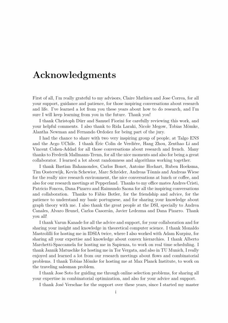
Figure 2: By introducing a Chvatal-Gomory cut, one improves the integrality gap byremoving basic feasible solutions that are fractional. The constraint x2 Æ 4 is validfor every integer feasible solution.

So when the question of solving a linear program is well understood, one goes backto the first step: The model. The picture becomes less clear at this point becausethe way a model is constructed depends heavily on the point of view adopted by whodesigned it. That is, very different models can answer the same question, but what ismore important, they have direct implications over the second step: Solving. Whereasmodel A can be solved rapidly, model B can exhibit a poor performance in terms ofaccuracy and solving time. The situation turns down to be more dramatic when thesearch space is restricted to integer values, that is integer programming. In general,solving an integer program is an NP-hard problem, so the classic and very successfulapproach is to relax the search space and look for a fractional solution. How muchdo we lose in this step? We quantify this in the so-called integrality gap, that is, theratio between the best integral solution and the best fractional solution.

At the moment of suggesting a model there are two important aspects to consider:

Contents Contents

The size and the integrality gap. The first question can be measured easily, but thesecond aspect is far from being easy to estimate. The ideal model is one of reasonablesize and very good integrality gap, but in most of the cases one of them should beresigned to attain the other. Many methods have been suggested the last decades toimprove the integrality gap of a model and one of the most popular is the cutting planesapproach, from the seminal work of Dantzig, Fulkerson and Johnson [28]. There, onelooks for better integrality gaps by introducing new constraints that are valid for everyinteger solution. Chvatal in 1973 [27] showed a particular way of constructing theseconstraints that eventually provide a full description of the convex hull of the integersolutions. Many state-of-the-art solvers already include these methods at the momentof solving an integer program.

2x1 + 2x2 Ø 1,

x21 = x1,

x22 = x2.

2x1 + 2y1,2 Ø x1,

2x2 + 2y1,2 Ø x2,

2x2 ≠ 2y1,2 Ø 1 ≠ x1,

2x1 ≠ 2y1,2 Ø 1 ≠ x2,

x1 + x2 ≠ y1,2 Æ 1,

minx1, x2 Ø y1,2,

x1, x2, y1,2 Ø 0.

x1

x2

Figure 3: The set (x1, x2) œ 0, 12 : 2x1 + 2x2 Ø 1 can be relaxed using linear pro-gramming. This region K0 includes fractional basic feasible solutions such as (1/2, 0)and (0, 1/2). By adding new variables simulating the possible products between thevariables and introducing new constraints, one obtains a larger program, but is easy tosolve. Furthermore, the projection K1 over the original space it is strictly containedin K0. This approach was introduced by Sherali & Adams [95]. By combining thefirst, third and fifth constraint at the right one can show that 2x1 + 5x2/3 Ø 1 holds,which cuts the point (0, 1/2).

Another way to gradually improve the integrality gap is the lift & project approach.The idea is to introduce many new variables in order to be able of including morecomplicated constraints that are valid for every integer solution. One obtains a pro-gram in a higher dimensional space, and then goes back by projecting to the variable

3

space of the original program. By doing this it is possible to simulate non-linear con-straints, at the cost of incrementing the size. Eventually, by repeating this step manytimes it is possible to reach the convex hull of the integer solutions. The programsobtained from these methods are also based on semidefinite programming, which is ageneralization of the linear case and can be solved efficiently. Recently these methodshave attracted a lot of interest in the theoretical computer science community, sinceit provides a candidate for unifying many of the existing optimal algorithms. We referto the survey of Barak and Steurer for an overview and some open problems [14].

Both of these methods are guaranteed to improve the integrality gap, but due tocomputational limitations it is not possible to apply them for many steps. Therefore,the key question is: How fast the integrality gap decreases? We try to answer thisquestion in Part I in the particular case of a scheduling problem, which is among themost fundamental and studied combinatorial problems.

Problems are easy, input is unknown! In contrast to before, there are many combi-natorial problems that are relatively simple to solve, but the difficulty relies on theavailability of input data. This can be really problematic especially when decisionshave to be made over time. We then say that the input is revealed online.

Consider the following situation. A logistics company needs to hire a data scientistto develop new technologies in their operations area. Some candidates are shortlistedto be interviewed, but due to time constraints, the time windows between them arenot so short. Assuming that when an offer is made the interviewing process is finished,the question is: Who to offer? This is an online selection problem.

sample size

probability

10030 40

1e

Figure 4: There are a 100 candidates. The decision maker interviews s candidateswithout making any offer, this is the sampling phase. After the sampling phase, thedecision maker selects the best candidate seen so far. With probability ¥ ≠ s

100ln

1

s100

2

the selected candidate is the best among the hundred. This probability is maximizedat s = 37 ¥ 100/e.

Sometimes at the moment of revealing an element it is also revealed a weight orreward, but more often the decision maker ranks the elements seen so far. The second

Contents Contents

ingredient is the order in which the elements are revealed. When the order is chosenuniformly at random, the problem is widely known as the secretary problem. It isneither clear when the problem was stated for the first time nor who solved it. Theproblem appeared in the February 1960 column of Scientific American, but Cayley andeven Kepler already thought about similar questions. It was Lindley [75] in 1961 whoseems to be the first in publishing a solution in a scientific journal but posteriorly theresults were extended and studied profoundly in the optimization community, optimalcontrol, probability and in the last decade, algorithms.

The key algorithmic question is then how to construct simple and provably goodstopping rules. Observe that under full knowledge, which is the offline setting, theoptimal solution is just to pick the best element. If the selection constraints are morecomplicated, say, selecting at most three instead of only one, the offline problem is stillvery simple. In fact, one can see that if the selection is restricted to what is known asmatroid, the optimal solution for the offline setting is given by the greedy algorithm.The Kruskal algorithm for finding minimum spanning trees is just an implementationof the greedy algorithm for a very particular matroid.

The answer to the hiring problem is the following: Interview about the 37% of thecandidates without making any offer, and then make an offer to best candidate seenso far. With probability close to 0.37 the decision maker will pick the best candidateamong every. The ratio between the best we could have done offline versus what wedo online is called the competitiveness of the algorithm. Then the question is thefollowing: Is it possible to find simple algorithms with good competitiveness for theselection problem, under combinatorial constraints, that guarantee every element inthe optimal solution to be picked with good probability? We study this question inPart II, when the selection is restricted to matroid constraints.

Contributions of this Thesis

In the first part of this thesis we study the problem of scheduling identical machines tominimize the makespan. In the scheduling literature it is usually referred as PÎCmax.This problem has been studied extensively from an algorithmic point of view. Inparticular, a polynomial time approximation scheme1 exists for this problem, whichis based on rounding the instance to decrease the combinatorics and then running adynamic program. The question we try to answer is the following:

Q1: Is it possible to match the best approximation factors by applying lift &project methods over a known relaxation to reduce the integrality gap?

We show that applying these methods over the natural linear program relaxationsfor this problem does not help to reduce the integrality gap. More specifically, the

1For every Á > 0, there is an algorithm that computes a solution with cost at most (1 + Á)opt,where opt is the cost of the optimal solution in a minimization problem. The running time of thealgorithm is polynomial in the input size.

5

problem is modeled as an assignment problem for which its integrality gap is knownto be 2. We answer the question negatively.

A1(≠): Even if we apply lift & project to construct linear or semidefinite programsof exponential size, the integrality gap is not less than 1.0009.

We remark that the constant in the lower bound has not been optimized, and probablycan be improved, but it is good enough for the exposition of the result. This answer,although informative, it is a bit unsatisfactory since we know this problem is easyfrom an approximation point of view. A very particular feature of the case when themachines are identical is that the relaxations we obtain are all symmetric respect tothe action of a group: If we permute machines, we obtain other feasible schedule withthe same makespan. In practice and also in theory, this is known to be harmful atthe moment of optimizing. Then, the approach we consider is the following. Beforeapplying lift & project, we break the machine symmetries of the ground linear programby introducing constraints. We show that in this case we are able to reduce theintegrality gap, and matching the best known approximation factors.

A1(+): If we apply lift & project after breaking machine symmetries, we canobtain relaxations of polynomial size and with integrality gap arbitrarily close toone.

In the second part of this thesis we study the secretary problem when the selectionis constrained to a matroid. Usually, the problem is studied under the existence of aweight associated to every element, and the performance of an algorithm is measuredin terms of the expected weight of the algorithm selection. For many matroid fam-ilies there are algorithms with constant competitiveness, but it remains as an openquestion whether the same can be attained for any matroid. We introduce a notionof competitiveness that does not assume the existence of weights, but rather assumesthe ability to rank the elements seen so far at every time step. The secretary problemwas originally stated in this framework, but most of the subsequent work focusedon the weighted version. Our goal is to maximize the probability for which any ele-ment in the optimal solution is selected by the algorithm, that is a stronger notion ofcompetitiveness.

Q2: Can we design algorithms with good competitiveness for the secretary prob-lem for this stronger notion?

We answer this question positively for many matroid families, by showing algorithmsthat match or beat the best known competitiveness in the weaker weighted notion.Furthermore, we develop a general framework for designing algorithms with constantprobability competitiveness. We also design algorithms for general matroids in thethe stronger notion.

A2: There is a general framework that yields O(1) probability competitivenessfor many matroid families.

Contents Contents

The first chapter of each Part I and II provide a deeper introduction and a formalexposition of the results obtained.

7

Publications of the Author

[1] Jose Correa, Patricio Foncea, Dana Pizarro, and Victor Verdugo. From pricingto prophets, and back! Submitted, 2017.

[2] Jose Soto, Abner Turkieltaub and Victor Verdugo. Strong Algorithms forthe Ordinal Matroid Secretary Problem. In Proceedings of the Twenty-NinthAnnual ACM-SIAM Symposium on Discrete Algorithms, SODA 2018.

[3] Sanjoy Baruah, Vincenzo Bonifaci, Alberto Marchetti-Spaccamela and VictorVerdugo. A scheduling model inspired by control theory. In Proceedings ofthe 25th International Conference on Real-Time Networks and Systems, RTNS2017.

[4] Varun Kanade, Frederik Mallmann-Trenn and Victor Verdugo. How Large IsYour Graph? 31st International Symposium on Distributed Computing, DISC2017.

[5] Frederik Mallmann-Trenn, Claire Mathieu and Victor Verdugo. Skyline Com-putation with Noisy Comparisons. CoRR, abs/1710.02058, 2017.

[6] Jose Correa, Victor Verdugo and Jose Verschae. Splitting versus setup trade-offs for scheduling to minimize weighted completion time. Operations ResearchLetters, 2016.

[7] Adam Kurpisz, Monaldo Mastrolilli, Claire Mathieu, Tobias Momke, VictorVerdugo and Andreas Wiese. Semidefinite and Linear Programming Integral-ity Gaps for Scheduling Identical Machines. Mathematical Programming. Apreliminary version appeared in Integer Programming and Combinatorial Opti-mization, IPCO 2016.

[8] Jose Correa, Alberto Marchetti-Spaccamela, Jannik Matuschke, Leen Stougie,Ola Svensson, Victor Verdugo and Jose Verschae. Strong LP formulations forscheduling splittable jobs on unrelated machines. Mathematical Programming,2015. A preliminary version appeared in Integer Programming and Combinato-rial Optimization, IPCO 2014.

[9] Frans Schalekamp, Rene Sitters, Suzanne van der Ster, Leen Stougie, VictorVerdugo and Anke van Zuylen. Split scheduling with uniform setup times.Journal of Scheduling, 2015.

9

Part I

Convex Optimization: Applicationsto Scheduling

11

Chapter 1

Introduction

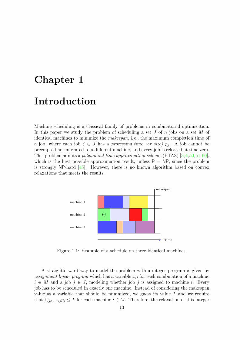
Machine scheduling is a classical family of problems in combinatorial optimization.In this paper we study the problem of scheduling a set J of n jobs on a set M ofidentical machines to minimize the makespan, i. e., the maximum completion time ofa job, where each job j œ J has a processing time (or size) pj. A job cannot bepreempted nor migrated to a different machine, and every job is released at time zero.This problem admits a polynomial-time approximation scheme (PTAS) [3,4,50,51,60],which is the best possible approximation result, unless P = NP, since the problemis strongly NP-hard [45]. However, there is no known algorithm based on convexrelaxations that meets the results.

pj

makespan

machine 1

machine 2

machine 3

Time

Figure 1.1: Example of a schedule on three identical machines.

A straightforward way to model the problem with a integer program is given byassignment linear program which has a variable xij for each combination of a machinei œ M and a job j œ J , modeling whether job j is assigned to machine i. Everyjob has to be scheduled in exactly one machine. Instead of considering the makespanvalue as a variable that should be minimized, we guess its value T and we requirethat

q

jœJ xijpj Æ T for each machine i œ M . Therefore, the relaxation of this integer

13

program, denoted by [assign(T )], is given by

ÿ

iœM

xij = 1 for all j œ J,

ÿ

jœJ

xijpj Æ T for all i œ M,

xij Ø 0 for all i œ M, for all j œ J.

1.1 The Configuration Linear Program

The assignment LP is dominated by the configuration linear program, or configurationLP for short, which is, to the best of our knowledge, the strongest relaxation forthe problem studied in the literature [100]. Given a value T > 0, a configurationcorresponds to a multiset of processing times such that its total sum does not exceedT , i. e., it is a feasible assignment for a machine when the makespan is equal to T .The multiplicity function m(p, C) indicates the number of times that the processingtime p appears in the multiset C. The load of a configuration C is just the totalprocessing time, that is,

q

pœpj :jœJ m(p, C) · p. Given T , let C denote the set of allfeasible configurations, that is, with load at most T . Observe that the definition interms of multisets makes sense since we are working in a setting of identical machines.

For each combination of a machine i œ M and a configuration C œ C, the con-figuration LP has a variable yiC that models whether machine i is scheduled withjobs according to configuration C. Letting np denote the number of jobs in J withprocessing time p, we can write the linear program relaxation, clp(T ), given by

ÿ

CœC

yiC = 1 for all i œ M , (1.1)

ÿ

iœM

ÿ

CœC

m(p, C)yiC = np for all p œ pj : j œ J, (1.2)

yiC Ø 0 for all i œ M, for all C œ C. (1.3)

We remark that in another common definition [100], a configuration is a subset, notof processing times but of jobs. We can solve that linear program to an arbitraryaccuracy in polynomial time [100] and similarly our linear program above.

3 3 1 4

T = 13

Figure 1.2: Machine scheduled according to a configuration C with makespan T = 13,with m(3, C) = 2, m(1, C) = 1 and m(4, C) = 1. The load of the configuration is2 · 3 + 1 · 1 + 1 · 4 = 11.

1.2. Convex Hierarchies Chapter 1

Integrality gap. Recall the configuration LP, clp(T ), does not have an objective func-tion and instead we seek to determine the smallest value T for which it is feasible. Inthis context, given an integer program that models the problem of scheduling identicalmachines and with T a fixed value of the makespan, we say that K(T ) is a convexrelaxation if it is a convex set that contains every integer feasible solution. We definethe integrality gap to be the value supIœI Cmax(I)/T ú(I) over all scheduling instancesI, where Cmax(I) is the optimal makespan of the scheduling instance I and T ú(I) isthe minimum value T such that K(T ) is feasible.

With the additional constraint that T Ø maxjœJ pj, the assignment LP relaxationhas an integrality gap of 2. This can be shown using the analysis of the list schedulingalgorithm, see e. g., [102]. On the other hand, a lower bound of 2 ≠ 1/|M | can beeasily shown for an instance with |M | + 1 jobs of unit size. Naturally, the integralitygap of the configuration LP is as well upper bounded by 2, since it dominates theassignment LP. One of the first results we show is that the configuration LP has anthe integrality gap which is at least 1.0009 (Chapter 2). For the more general unrelatedmachines scheduling problem, the formulation where configurations are jobs sets hasan integrality gap equal to 2 [100].

1.2 Convex Hierarchies

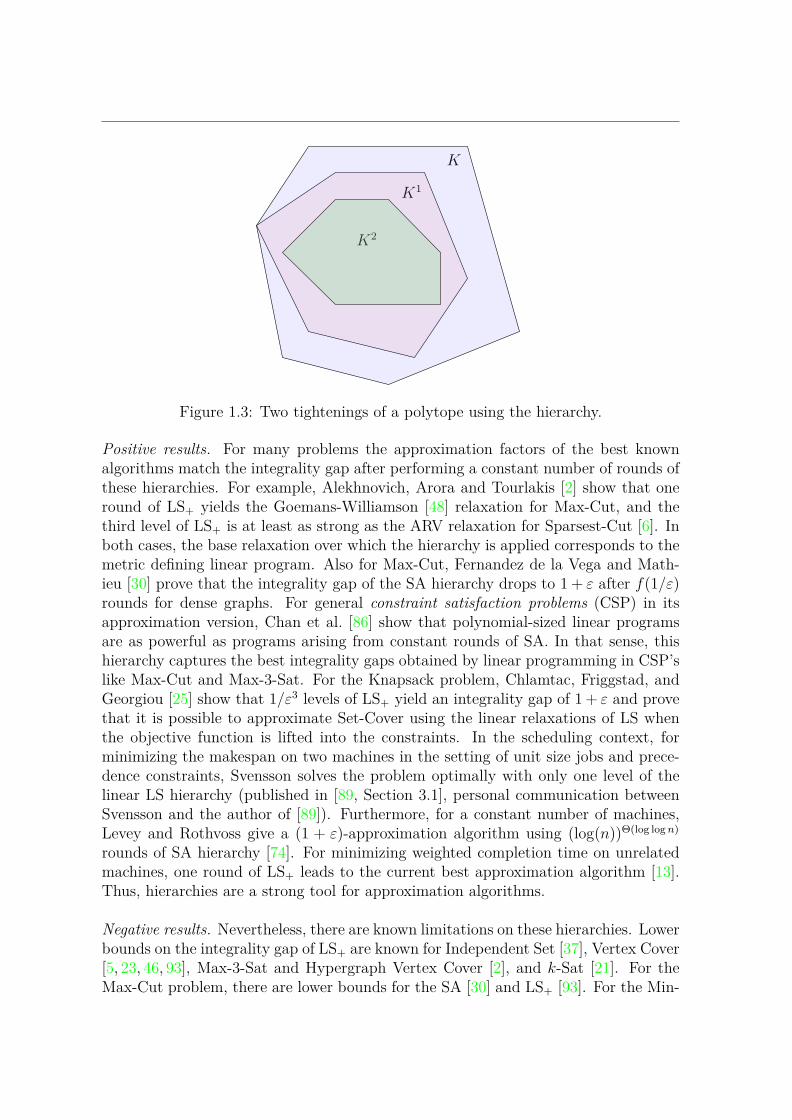
An interesting question is whether other convex relaxations have better integralitygaps. Convex hierarchies, parameterized by a number of levels, rounds or steps, aresystematic approaches to gradually tightening the ground relaxation, at the cost ofincreased running time in solving the relaxation. As a consequence, they are goodcandidates for designing approximation algorithms based on rounding a solution ob-tained from these relaxations. Given a polytope K ™ [0, 1]n, all these approachesproduce a family of convex relaxations K1, K2, . . . , Kn satisfying that

K = K0 ´ K1 ´ K2 ´ · · · ´ Kn≠1 ´ Kn = conv(K fl 0, 1n).

Popular among these methods are the Sherali-Adams (SA) hierarchy [95] (Chap-ter 3) the Lovasz-Schrijver hierarchy (LS) and its semidefinite (LS+) counterpart [78],(Chapter 4) and the Lasserre/Sum-Of-Squares (Las) hierarchy [72, 88] (Chapter 5),which is the strongest of the three. The level r relaxations are known to be solvablein time nO(r), where n is the number of variables, provided some assumptions overthe ground polytope. In particular, when r is constant, the complexity of solving therelaxation becomes polynomial on the program size. This is relevant when looking foran approximation algorithm based on this relaxation. For a comparison between themand their algorithmic implications we refer to [26,73,89]. In some settings, for exam-ple the Independent Set problem in sparse graphs [12], a hierarchy obtained from SAstrenghtened with semidefinite constraints at the first level has also been considered.

15

K

K1

K2

Figure 1.3: Two tightenings of a polytope using the hierarchy.

Positive results. For many problems the approximation factors of the best knownalgorithms match the integrality gap after performing a constant number of rounds ofthese hierarchies. For example, Alekhnovich, Arora and Tourlakis [2] show that oneround of LS+ yields the Goemans-Williamson [48] relaxation for Max-Cut, and thethird level of LS+ is at least as strong as the ARV relaxation for Sparsest-Cut [6]. Inboth cases, the base relaxation over which the hierarchy is applied corresponds to themetric defining linear program. Also for Max-Cut, Fernandez de la Vega and Math-ieu [30] prove that the integrality gap of the SA hierarchy drops to 1 + Á after f(1/Á)rounds for dense graphs. For general constraint satisfaction problems (CSP) in itsapproximation version, Chan et al. [86] show that polynomial-sized linear programsare as powerful as programs arising from constant rounds of SA. In that sense, thishierarchy captures the best integrality gaps obtained by linear programming in CSP’slike Max-Cut and Max-3-Sat. For the Knapsack problem, Chlamtac, Friggstad, andGeorgiou [25] show that 1/Á3 levels of LS+ yield an integrality gap of 1 + Á and provethat it is possible to approximate Set-Cover using the linear relaxations of LS whenthe objective function is lifted into the constraints. In the scheduling context, forminimizing the makespan on two machines in the setting of unit size jobs and prece-dence constraints, Svensson solves the problem optimally with only one level of thelinear LS hierarchy (published in [89, Section 3.1], personal communication betweenSvensson and the author of [89]). Furthermore, for a constant number of machines,Levey and Rothvoss give a (1 + Á)-approximation algorithm using (log(n))Θ(log log n)

rounds of SA hierarchy [74]. For minimizing weighted completion time on unrelatedmachines, one round of LS+ leads to the current best approximation algorithm [13].Thus, hierarchies are a strong tool for approximation algorithms.

Negative results. Nevertheless, there are known limitations on these hierarchies. Lowerbounds on the integrality gap of LS+ are known for Independent Set [37], Vertex Cover[5, 23, 46, 93], Max-3-Sat and Hypergraph Vertex Cover [2], and k-Sat [21]. For theMax-Cut problem, there are lower bounds for the SA [30] and LS+ [93]. For the Min-

1.3. Lower bounds Chapter 1

Sum scheduling problem (i. e., scheduling with job dependent cost functions on onemachine) the integrality gap is unbounded even after O(

Ôn) rounds of Lasserre [69].

In particular, that holds for the problem of minimizing the number of tardy jobs eventhough that problem is solvable in polynomial time, thus SDP hierarchies sometimesfail to reduce the integrality gap even on easy problems.

1.3 Lower bounds

One of the questions we try to answer in this work is the following: Is it possible toobtain a polynomial time (1 + ‘)-approximation algorithm based on directly applyingthe SA or the LS+ hierarchy over the configuration LP? This would match the bestknown polynomial time approximation factor known. We answer this question in thenegative. We prove that even after Ω(n) rounds of SA or LS+ to the configurationLP, where n is the number of jobs in the instance, the integrality gap of the resultingrelaxation is still at least 1 + 1/1023. Since the configuration LP dominates theassignment LP, our result also holds if we apply Ω(n) rounds of SA or LS+ to theassignment LP.

Theorem 1. Consider the problem of scheduling identical machines to minimize themakespan, PÎCmax. For each n œ N there exists an instance with n jobs such that:

(i) the configuration LP has an integrality gap of at least 1024/1023.

(ii) after applying r = Ω(n) rounds of the SA hierarchy to the configuration LP theobtained relaxation has an integrality gap of at least 1024/1023.

(iii) after applying r = Ω(n) rounds of the LS+ hierarchy to the configuration LP theobtained relaxation has an integrality gap of at least 1024/1023.1

Therefore, the SA and the LS+ hierarchies do not yield the best possible approx-imation algorithms when applied over the configuration LP. Namely, suppose thereexists r œ N such that the r level of the SA hierarchy has an integrality gap of atmost 1+Á, with Á < 1/1023. In particular, that holds as well for the hard instances ofTheorem 1 and r = Ω(n). We remark that for the hierarchies studied in Theorem 1,a number of rounds equal to the number of variables in clp(T ) suffice to bring theintegrality gap down to exactly one, although this number is in general exponentiallylarge in the input size. Nevertheless, we also prove in Chapter 3 that a number ofrounds equal to number of machines suffices to reduce the integrality gap to one, whenthe SA hierarchy is applied over the configuration LP. This comes as a consequenceof a stronger decomposition lemma, that relies on the structure of the configurationlinear program.

1In general, the SA and LS+ hierarchies are incomparable, so (iii) does not follow directly from(ii). The linear counterpart of Lovasz-Schrijver, the LS hierarchy, is weaker than SA and thereforethe result follows in that case from (ii).

17

We prove Theorem 1 by defining a family of instances IkkœN constructed fromthe Petersen graph (see Figure 2.3). The size of instance Ik, given by the number ofmachines and jobs, is Θ(k) and the number of jobs is Θ(k) as well. In Chapter 2 weprovide an explicit construction of the hard instances and we prove that the configu-ration LP is feasible for T = 1023 while the integral optimum has a makespan of atleast 1024. In Chapter 3, we show for each instance Ik that we can define a fractionalsolution that is feasible for the polytope obtained by applying Ω(k) rounds of SA tothe configuration LP parametrized by T = 1023. Finally, in Chapter 4 we prove thesame for the semidefinite relaxations obtained with the LS+ hierarchy, and we studythe matrices arising in the lower bound proof.

1.4 Upper bound

The assignment and configuration LP’s have in common the fact that we can permutethe machines, and the solutions obtained remain feasible. The sets satisfying thisproperty are said to be invariant under the action of some permutation group. In thecase of these polytopes, the symmetric group of size equal to the number of machinesis acting over the feasible solutions. The same holds for the relaxations obtained fromapplying SA and LS+ over the configuration LP. This is a key fact when reducingthe dimensionality of the matrices certifying the feasible solutions in Chapter 4. Theresults shown in Theorem 1 suggest that symmetric relaxations do not seem to be goodcandidates for obtaining small integrality gaps for the scheduling problem. Therefore,the question we study is the following: Is it possible to obtain a polynomial sized linearor semidefinite relaxation with an integrality gap of (1 + Á) that is not invariant forthe machine symmetries? This time, we provide a positive answer. Below we state,informally, the main theorem which is proven in Chapter 5.

Theorem 2. For every Á > 0, there exists a non-machine symmetric polynomial sizedsemidefinite relaxation with an integrality gap of at most (1 + Á), for the problem ofscheduling to minimize the makespan.

The theorem is based on introducing a formulation that breaks the symmetries inthe assignment LP by adding new constraints. They enforce a very particular struc-ture over any feasible solution of the formulation that should respect a lexicographicorder over the machine configurations induced by any feasible integer solution. Ontop of the relaxation obtained from adding the aforementioned constraints, we applythe Lasserre/SoS hierarchy. In Chapter 5 we provide a full proof of the theorem, andalso a direct application of it: A polynomial time approximation scheme based onsolving the semidefinite relaxation.

Practice. The presence of symmetries in the formulations is known to be harmful andthe literature about how to deal with them is large. Most of them focus on how toadd constraints that break the symmetries, or how to modify the divide and conquerbranching techniques in order to avoid unnecessary computations by approaches such

1.4. Upper bound Chapter 1

as perturbation of the numeric values defining the program and variables fixing [80,81, 84]. Particular interest have attracted partitioning problems such as scheduling,packing, coloring and clustering. One way of removing the symmetries of a formulationis to consider decompositions such as Dantzig-Wolfe, where all the structure of apartition is hidden and the goal is to find how many times such a structure appearson a solution. In fact, the configuration LP can be seen as an intermediate stepbetween the assignment LP and its Dantzig-Wolfe decomposition. This approach hasproven to be successful in practice for many situations including the above mentionedproblems in transportation, routing and coloring [16,31,83,99].

x1

x2

x1

x2

Figure 1.4: The polytope in R2 at the left is invariant under the action of permuting

variables, that is, every time (x1, x2) is feasible, then (x2, x1) is also feasible.

Extended formulations. Similar results to Theorem 1 can be found in the contextof extended formulations, that is, a convex set on a higher dimensional space thatcoincides with the original one when projected to the initial variables space. Remark-able are the results of Yannakakis [103] that neither the matching polytope nor theTSP polytope have symmetric linear extended formulation of subexponential size. Re-cently, this results were extended also for non symmetric linear extended formulationsby Fiorini et al. [42] in the case of TSP and by Rothvoss [90] for matching. The samenegative result follows if one consider semidefinite formulations, since Braun et al. [19]showed that any symmetric semidefinite program for matching has exponential size.They also show that every symmetric relaxation of polynomial size nk for asymmetricTSP is not stronger than an O(k) level Lasserre/SoS relaxation.

Symmetry breaking constraints. The way we obtain improvements in the gap at Theo-rem 2 is by adding constraints on top of the initial symmetric relaxation, which is theassignment polytope in this case, in order to obtain a program that is not invariant.The result would also follow if we consider initially the configuration LP, since onecan show that the Lasserre/SoS hierarchy over the assignment LP at certain level isstronger than the configuration LP, provided some assumptions over the instances.The idea behind all these approaches is to remove parts of the feasible region thatprovide no extra information in terms of objective value and solution structure. De-

19

pending on the problem and the particular group action, different sets of symmetrybreaking inequalities have been considered. For partitioning problems there are waysof enforcing an order over the solutions and then guaranteeing that only one solu-tion per orbit is considered [43, 44, 59]. Following the same lines, in the particularcase of scheduling there is a way of ensuring that exactly one representative per orbitis selected by intersecting the original partitioning polytope with the so called or-bitope [61]. They provide a linear description of the orbitope that is of exponentialsize, but it can be separated efficiently. For an extensive treatment we refer to theexcellent survey of Margot [82].

Relaxation for the

minimum makespan

scheduling problem

Configuration

Linear Program

Hard instances for which

the configuration LP has an

integrality gap of at least

1 + 1/1023 (Chapter 2)

From the Petersen graph

to Scheduling instances

Instances remain hard

for SA (Chapter 3)

Instances remain hard

for the semidefinite

LS+ (Chapter 4)

Block-symmetric matrices

and dimensionality reduction

Break symmetries in the

assignment LP and apply

Lasserre/SoS (Chapter 5)

Lexicographic schedules

over machine configurations

Figure 1.5: Organization of Part I.

Chapter 2

The hard instances

In this chapter we show that the configuration LP described by constraints (1.1) and(1.2) has an integrality gap of at least 1024/1023. To this end, for each k œ N wedefine an instance Ik that is inspired by the Petersen graph G = (V, E) (see Figure 2.1)with vertex set V = 0, 1, . . . , 9. We first have to introduce a family of multigraphsobtained from G.

For each k œ N, we construct a multigraph Gk = (V, Ek) with vertex set equalto V and the set of edges Ek is defined as follows: For each edge u, v œ E of thePetersen graph G, we have a multiset E(u, v) with k copies of the edge u, v. Theset Ek is just the multiset obtained from the union of all these multisets, that is,Ek = fiu,vœEE(u, v). In particular we have that G1 = G, the Petersen graph.

0

1

23

4

5

6

78

9

0

1

23

4

5

6

78

9

Figure 2.1: On the left, the Petersen graph G1. On the right, the mutigraph G3

obtained from considering 3 copies of each edge in the Petersen graph.

The scheduling instances. In the instance Ik we have a job je for every e œ Ek, whichis the set of edges in the multigraph Gk. Thus Ik has 15k jobs. Let e œ Ek be suchthat e œ E(u, v), that is, e is an edge between nodes u and v. The processing timeof je is pje

= 2u + 2v. We define the set of machines for Ik to be [3k] = 1, . . . , 3k.Observe that every subset of edges F ™ Ek induces a multiset CF of job-sizes as

follows: For every u, v œ E and p = 2u + 2v, we have m(p, CF ) = |F fl E(u, v)|.In words, for every possible processing time, we check how many copies of the corre-sponding edge in G are in F , and this number is the multiplicity of the processing time

21

in the multiset CF . If the load of CF is at most T , we say that CF is the configurationinduced by F . We remark that this mapping is not injective, since different subsetsof edges may induce the same processing times multiplicities and therefore the sameconfiguration.

0

1

23

4

5

6

78

9

Figure 2.2: The edges in purple induce the configuration 20 + 24, 20 + 24, 24 + 29, 29 +26, 23 +28 and the orange edges induce the configuration 20 +24, 24 +23, 23 +28, 29 +27, 22 + 21. The first has a load of 1402 and the second has a load of 951.

Matching configurations. The Petersen graph G has exactly six perfect matchings—1, . . . , —6. We have that the sum of the job sizes in a perfect matching —¸ is

ÿ

eœ—¸

pje=

9ÿ

u=0

2u deg—¸(u) = 1023,

since deg—¸(u) = 1 for every node u œ V . Therefore, —¸ induces a configuration C¸

with load 1023 in the following way: C¸ = 2u + 2v : u, v œ —¸, that is, for everyedge e œ —¸ we have in C¸ one copy of a job with processing time pje

defined as above.The configurations set C— = C1, . . . , C6 are called matching configurations.

It can be checked easily that is not possible to find a partition of the edges inthe Petersen graph such that every part is a perfect matching, i. e., there is no 1-factorization of the Petersen graph. This property is a key ingredient for proving thelower bounds on the integrality gaps of the different relaxations we consider for thescheduling problem. We extend the definition of 1-factorization to multigraphs in thenatural way. In the following lemma we show an infinite sequence of multigraphs inGkkœN for which there is no 1-factorization.

2.1. Integrality gap for clp: Proof of Theorem 1(i) Chapter 2

0

1

23

45

6

78

9

0

1

23

45

6

78

9

0

1

23

45

6

78

9

0

1

23

45

6

78

9

0

1

23

45

6

78

9

0

1

23

4

5

6

78

9

Figure 2.3: The Petersen graph and its six perfect matchings (coloured edges). Ob-serve that the blue matchings are isomorphic.

Lemma 1. For every odd k œ N, there is no 1-factorization of the multigraph Gk.

Proof. Let —6 be the perfect matching of the Petersen graph consisting of the fiveedges 0, 5, 1, 6, 2, 7, 3, 8 and 4, 9, called spokes (last matching at Figure2.3). Suppose there exists a 1-factorization of Gk, and let Ê6 be the number of timesthat the perfect matching —6 appears in the 1-factorization. In particular, the size ofthe 1-factorization is 3k, since there are 15k edges in Gk and every perfect matchinghas exactly 5 edges.

Each spoke, which appears in exactly one other perfect matching in —1, . . . , —5,must be contained in exactly k perfect matchings of the 1-factorization. Therefore, forall j œ [5], the perfect matching —j appears k ≠ Ê6 times in the 1-factorization. Thus,in total the size of the 1-factorization is 5(k ≠ Ê6) + Ê6 = 5k ≠ 4Ê6. However, thatsum equals 3k, and so Ê6 = k/2. Since k is odd and Ê6 an integer, the contradictionfollows.

2.1 Integrality gap for clp: Proof of Theorem 1(i)

In this section we prove that the integrality gap of the configuration LP is at least1024/1023. In fact, we prove a stronger statement: For every k œ N, the gap of theconfiguration LP at instance Ik is at least 1024/1023. Given Ik, we proceed in twosteps: We first prove that the configuration LP with T = 1023 is feasible for Ik, andsecondly we prove that the makespan of Ik is at least 1024.

Lemma 2. For every k œ N, the configuration linear program for T = 1023 is feasibleat instance Ik.

Proof. We define a fractional solution that is supported only by matching configura-tions: For every machine i œ [3k] and each ¸ œ 1, 2, . . . , 6 we set yiC¸

= 1/6. For

23

every machine i œ [3k] and every configuration C œ C \ C— we set yiC = 0. The set ofmachine constraints (1.1) at clp(T ) is clearly satisfied, since for every i œ [3k] we have

ÿ

CœC

yiC =6

ÿ

¸=1

yiC¸= 6 · 1/6 = 1.

For the set of job-size constraints (1.2), recall that for every e = u, v œ E and p =2u + 2v, in Ik we have that np = k. The Petersen graph is such that there are exactlytwo perfect matchings —

p1 , —

p2 containing e, and therefore m(p, Cp

1 ) = m(p, Cp2 ) = 1,

where Cp1 and Cp

2 are the matching configurations induced by —p1 and —

p2 , respectively.

Thus, we get

3kÿ

i=1

ÿ

CœC

m(p, C)yiC =3kÿ

i=1

(yiCp1

+ yiCp2) = 3k · (1/6 + 1/6) = k,

and so y is feasible.

Lemma 3. For every odd k œ N, the optimal makespan for Ik is at least 1024.

Proof. We first show that the optimal makespan is at least 1023. The total size of thejobs in the instance is equal to

ÿ

eœEk

pje=

9ÿ

u=0

2u degGk(u) = 1023 · 3k,

since degGk(u) = 3k for every u œ 0, . . . , 9. There are 3k machines, so if we had a

schedule with makespan strictly less than 1023 it would imply that the total load isstrictly less than 3k ·1023, which is a contradiction. In particular, the optimal integralmakespan for Ik is at least 1023.

Suppose that the optimal makespan is equal to 1023. By the argument above, itimplies that every machine is scheduled with a configuration of load equal to 1023.Let C be a configuration with load equal to 1023, and let F ™ Ek such that C is theconfiguration induced by F .

Claim 4. The set F is a perfect matching in Gk.

In particular, C is a matching configuration. Since every job has to be assigned tosome machine, the schedule is induced by a partition of the edges in Ek where everypart is a perfect matching, i. e., a 1-factorization of Gk. However, this is not possible,since by Lemma 1 there is no 1-factorization of Gk when k is odd. Therefore, we havea contradiction and we conclude that the optimal makespan is at least 1024.

Proof of Claim 4 in Lemma 3. The load of configuration C is

1023 =9

ÿ

u=0

2u degF (u) = degF (0) + 29

ÿ

u=1

2u≠1 degF (u).

In particular, the last equality implies that degF (0) is odd. By induction on u itmust be that for every u œ 0, . . . , 9, degF (u) is odd. Since the sum does not exceed1023 =

q9u=0 2u, it follows that degF (u) = 1 for every u œ 0, . . . , 9 and so F is a

perfect matching in Gk.

Chapter 3

Sherali-Adams (SA) Hierarchy

Convex hierarchies provide a way of obtaining gradually stronger relaxations for aninteger program. In order to design approximation algorithms based on them it iscrucial to understand how fast the gap decreases. In this chapter we study relaxationsobtained from the Sherali-Adams (SA) hierarchy over the configuration LP, and weprove that the hard instances shown in Chapter 2 remain hard even after a linearnumber of rounds of the SA hierarchy.

The SA hierarchy is based on linear programming and basically works by addingnew variables and constraints to a linear program in a higher dimensional space andthen projecting back to the original variables space. We introduce the relaxationsobtained by applying the hierarchy over the configuration LP in a self-contained way,that is equivalent to the approach in the original work of Sherali & Adams [95]. Werevisit and/or introduce the necessary properties for our purposes.

In the configuration LP, clp(T ), the variables set is M ◊ C. The level r Sherali-Adams relaxation, SAr(clp(T )), is a polytope in [0, 1]Pr+1(M◊C) where Pr+1(M ◊ C) =A ™ M ◊ C : |A| Æ r + 1. It is defined by the following set of constraints:

ÿ

CœC

yHfi(i,C) = yH for all i œ M , for all H œ Pr(M ◊ C), (3.1)

ÿ

iœM

ÿ

CœC

m(p, C)yHfi(i,C) = npyH for all p œ pj : j œ J, for all H œ Pr(M ◊ C),

(3.2)

yH Ø 0 for all H œ Pr+1(M ◊ C), (3.3)

yÿ = 1. (3.4)

We denote by SArproj(clp(T )) the projection in R

M◊C of the polytope above. Theproperties summarized in the lemma below are common to most of the hierarchiesconsidered in the literature. For the sake of completeness, we show a self-containedproof in the context of the configuration LP.

Lemma 5. Let r œ N. For every scheduling instance and every T > 0, the followingholds:

(i) clp(T ) fl 0, 1M◊C ™ SArproj(clp(T )).

25

(ii) SAr+1proj(clp(T )) ™ SAr

proj(clp(T )).

(iii) Let y œ SAr(clp(T )). If K œ Pr+1(M ◊ C) and H ™ K, then yK Æ yH .

The first property shows that SA provides relaxations of the integer solutions ofthe configuration LP. The second property guarantees that at every step we obtain arelaxation at least as strong than the previous one. Finally, the third property revealssome consistency on the relaxation values. In order to gain intuition, it is useful tothink off the value yK as the probability that every variable in K is set to one.

Proof of Lemma 5. Consider a scheduling instance and T > 0.

(i) Let z œ clp(T ) fl 0, 1M◊C. For every non-empty H œ Pr+1(M ◊ C) we setyH =

r

(i,C)œH ziC , and yÿ = 1. Clearly, the set of constraints in (3.3) and (3.4)are satisfied. Fix a set H œ Pr+1(M ◊ C). For every i œ M we have that

ÿ

CœC

yHfi(i,C) ≠ yH = yH

A

ÿ

CœC

ziC ≠ 1

B

.

Since z œ clp(T ) it follows thatq

CœC ziC ≠ 1 = 0 and therefore the machineconstraints in (3.1) are all satisfied. Analogously, for every p œ pj : j œ J,

ÿ

iœM

ÿ

CœC

m(p, C)yHfi(i,C) ≠ npyH = yH

A

ÿ

iœM

ÿ

CœC

m(p, C)ziC ≠ np

B

,

and since z œ clp(T ) we haveq

iœM

q

CœC m(p, C)ziC ≠ np = 0. Therefore, thejob-size constraints (3.2) are satisfied.

(ii) Let y œ SAr+1(clp(T )). By definition of the relaxation at level r + 1, y satisfiesevery constraint at level r and therefore the restriction of y to Pr+1(M ◊ C) isfeasible for SAr(clp(T )). Since every singleton in M ◊C belongs to Pr+1(M ◊C),the lemma follows.

(iii) It is enough to prove it when K = H fi (i, R) for some machine i œ M andsome configuration R œ C. Since y Ø 0, the machine constraints (3.1) imply that

yH =ÿ

CœC

yHfi(i,C) Ø yHfi(i,R) = yK .

3.1 Machine Decomposition Lemma

Given a polytope, the minimum number of rounds that are necessary to guarantee theconvergence to the convex hull of the integer solutions is known as rank of the hierarchy[7, 21, 24, 73]. In general, the rank of a polytope in [0, 1]E in the Sherali-Adamshierarchy is upper bounded by |E| (see e. g. [95]). In this case, |E| = |M ◊ C| = m|C|,which is exponentially large on the input size. Instead we get an upper bound on therank of the configuration LP which is linear in the input size.

3.1. Machine Decomposition Lemma Chapter 3

Theorem 3. For every scheduling instance with m machines and every T > 0,

SAmproj(clp(T )) = conv

1

clp(T ) fl 0, 1M◊C2

.

The theorem above is a direct consequence of a lemma we state next. It reliesheavily on the structure of the configuration LP. It can also be proved in terms of thestronger Lasserre/SoS hierarchy by means of the Decomposition Theorem [62], butwe show that the relaxations obtained from the Sherali-Adams hierarchy are strongenough to get the desired bound on the rank.

Lemma 6. Let r œ N and S ™ M be a subset of machines with r Ø |S|. Then,

SArproj(clp(T )) ™ conv

1

SAr≠|S|proj (clp(T )) fl 0, 1S◊C

2

.

In words, the lemma says that we can decompose a solution at level r into a convexcombination of solutions at level r ≠ |S| and all of them are integral at the variablesfor the machines in S. When the number of machines is fixed, i. e., not part of theinput, we obtain the following direct corollary from Theorem 6.

Corollary 7. Consider the problem of scheduling identical machines to minimize themakespan with a fixed number of machines equal to m. Then, the m = O(1) level ofthe SA hierarchy over the configuration LP has an integrality gap equal to 1.

Proof of Theorem 3. The convexity of the set SAmproj(clp(T )) and Lemma 5(i) imply

that SAmproj(clp(T )) ´ conv

3

clp(T ) fl 0, 1M◊C

4

. The other inclusion comes from

applying Lemma 6 with S = M and r = m.

Given r œ N, we prove Lemma 6 by induction on the cardinality of S. Beforeproceeding with the proof we need to introduce a technical lemma about the relax-ations obtained from Sherali-Adams over the configuration LP. Let y œ SAr(clp(T ))and consider a single machine i œ M . If y(i,C) œ (0, 1) for some configuration C, wesay that y is fractional at machine i, otherwise we say that y is integral at machine i.For every C œ C such that y(i,C) œ (0, 1), consider the vector defined by

y(i, C)H =yHfi(i,C)

y(i,C)

for every H œ Pr(M◊C). Observe that constraints (3.1) guarantee thatq

CœC y(i,C) =1. Furthermore,

y =ÿ

CœC:y(i,C)œ(0,1)

y(i,C)y(i, C),

and therefore y is a convex combination of the vectors in y(i, C) : C œ C, y(i,C) œ(0, 1). The vector y(i, C) is said to be the conditioning of y at (i, C). The followinglemma is the key for the inductive step.

27

Lemma 8. Suppose that y is fractional at machine i œ M . Then, for every C œ Csuch that y(i,C) œ (0, 1), we have y(i, C) œ SAr≠1(clp(T )) and y(i, C) is integral atmachine i.

Proof. Observe that y(i, C)(i,C) = y(i,C)fi(i,C)/y(i,C) = 1. The feasibility ofy(i, C) in clp(T ) implies that y(i, C) is integral at machine i.

Now we have to verify that y(i, C) satisfies the constraint at the level r ≠ 1. LetH œ Pr≠1(M ◊ C) and consider a machine ¸ œ M . We have that |H fi (i, C)| Æ r,so from the feasibility of y at level r we obtain that

ÿ

RœC

y(i, C)Hfi(¸,R) =1

y(i,C)

ÿ

RœC

yHfi(¸,R)fi(i,C) =yHfi(i,C)

y(i,C)

= y(i, C)H ,

and thus the machine constraints (3.1) are satisfied. Consider a job size p œ pj : j œJ. Analogously as before, from the feasibility of y at level r we have that

ÿ

¸œM

ÿ

RœC

m(p, R)y(i, C)Hfi(¸,R) =1

y(i,C)

ÿ

¸œM

ÿ

RœC

m(p, R)yHfi(¸,R)fi(i,C)

= np

yHfi(i,C)

y(i,C)

= npy(i, C)H ,

and then the job-size constraints (3.2) are satisfied. The non-negativity of y(i, C) isclear and y(i, C)ÿ = yÿfi(i,C)/y(i,C) = 1. That finishes the proof.

In particular, this implies Lemma 6 when S = i and since it does not dependon i, it holds true for every S ™ M of cardinality one. Observe that if y was integralat machine i then the lemma follows by the nested property at Lemma 5(ii). Anotherimportant property of the conditioning is the following: If the vector y was integralat some machine ¸, then after conditioning the vector obtained remains integral atmachine ¸. To check this, suppose that y(¸,S) = 1. It is enough to check thaty(i, C)(¸,R) = 0 for every R ”= S, since the machine constraints (3.1) imply theny(i, C)(¸,S) = 1. By Lemma 5(iii), we have that

y(i, C)(¸,R) =y(¸,R)fi(i,C)

y(i,C)

Æ y(¸,R)

y(i,C)

= 0.

Proof of Lemma 6. In the following assume r Ø 2. Let S ™ M of cardinality at least2 and y œ SAr(clp(T )). Consider the set S = S \ ¸ for some ¸ œ S. By induction,

there exists a family of vectors y◊◊œΘ ™ SAr≠|S|(clp(T )) = SAr≠|S|+1(clp(T )) suchthat y can obtained as a convex combination of them, and for every ◊ œ Θ the vectory◊ is integral at every machine in S.

In the following we prove that for every ◊ œ Θ, the vector y◊ restricted toPr≠|S|+1(M ◊C) can be obtained as a convex combination of vectors in SAr≠|S|(clp(T ))and they are all integral at every machine in S fi ¸ = S. For that end we make useof our technical Lemma 8. As explained before, if y◊ is integral at machine ¸ then weare done. Suppose then that y◊ is fractional at machine ¸ and consider the family of

3.2. Integrality gap for SA: Proof of Theorem 1(ii) Chapter 3

vectors y◊(¸, C) : C œ C, y◊(¸,C) œ (0, 1) as defined before. By Lemma 8, they are

all in SA(r≠|S|+1)≠1(clp(T )) = SAr≠|S|(clp(T )) and they are all integral at machine ¸.Since the vector y◊ was integral at S, the vectors obtained from conditioning remainintegral there and therefore they are all integral at S, which concludes the proof.

3.2 Integrality gap for SA: Proof of Theorem 1(ii)

We show that for the family of instances IkkœN defined in Section 2.1, if we applyO(k) rounds of the Sherali-Adams hierachy to the configuration LP for T = 1023, thenthe resulting relaxation is feasible. Thus, after Ω(k) rounds of SA the configurationLP still has an integrality gap of at least 1024/1023 for an instance with Θ(k) jobsand machines.

We can observe that the configuration LP computes a set of edges in a completebipartite graph with vertex sets M and C. The edges are selected such that each nodein M is incident to at most one selected edge. More specifically, consider the completedirected bipartite graph with vertex sets M and C, which is identified with M ◊ C.We say that F ™ M ◊ C is an M-matching if |C œ C : (i, C) œ F| = degF (i) Æ 1.We say that i œ M is incident to F if degF (i) = 1. The notation extends if theconfigurations set is not C but a subset of it.

M Cy œ clp(T )

Figure 3.1: Feasible schedule given by an integral solution of the configuration LP.Example with five machines, three of them in the same configuration. The degree ofevery machine node is exactly one, as specified by the constraints (1.1).

In the following we consider the family of instances Ik : k œ N, k is odd as inSection 2.1 and T = 1023. For any set S, let P(S) be the power set of S. We define

29

a solution to SAr(clp(T )) for T = 1023. To this end, we need to provide a value yA

for each set A œ Pr+1(M ◊ C). These values are given by the following function: Let„ : P(M ◊ C—) æ R be such that

„(A) =1

(3k)|A|

Ÿ

jœ[6]

(k/2)degA(Cj)

if A is an M -matching, and zero otherwise, where (x)0 = 1 and (x)a = x(x≠1) · · · (x≠a + 1) if a Ø 1 is integer positive. This is called the lower factorial function. Toget some understanding about how the „ works, it could be useful to think on aprobabilistic interpretation that is formalized in the lemma below: Suppose we knowthat a set A is chosen (i.e., we condition on this), then the conditional probabilitythat a pair (i, Cj) is chosen equals (k/2 ≠ degA(Cj))/(3k ≠ |A|) when A fi (i, Cj) isan M -matching.

Lemma 9. Let A ™ M ◊ C— be an M-matching of size at most 3k ≠ 1. If i œ M isnot incident to A, then for every j œ [6],

„(A fi (i, Cj)) = „(A)k/2 ≠ degA(Cj)

3k ≠ |A|.

Proof. Given that i is not incident to A, we have |Afi(i, Cj)| = |A|+1. Furthermore,for ¸ ”= j we have that degAfi(i,Cj)(C¸) = degA(C¸) and degAfi(i,Cj)(Cj) = degA(Cj)+1.

We are ready now to define our solution to SAr(clp(T )). It is the vector y„ œR

Pr+1(M◊C) defined such that y„A = „(A) if A is an M -matching in M ◊ C—, and zero

otherwise.

Lemma 10. For every odd k, y„ is a feasible solution in SAr(clp(T )) for the instanceIk when r = Âk/2Ê and T = 1023.

We note that in the proof above, the projection of y„ onto the space of the configu-ration LP is exactly the fractional solution from Lemma 2. The proof of Theorem 1(ii)now follows directly from the lemma above.

Proof of Theorem 1(ii). Let k be such that n = 15k + ¸ where k is the greatest oddinteger such that 15k Æ n. The theorem follows by considering the instance Ik asdefined before, T = 1023 and r = Âk/2Ê.

Proof of Lemma 10. The non-negativity follows by checking that the lower factorialin the definition of „ remains non-negative for r = Âk/2Ê. It is also clear from thedefinition that y„

ÿ = „(ÿ) = 1.We next prove that y„ satisfies the machine constraints (3.1) in SAr(clp). If i is

a machine incident to H, then all terms in the left-hand summation are 0 except for

3.2. Integrality gap for SA: Proof of Theorem 1(ii) Chapter 3

the unique pair (i, C) that belongs to H, so the sum equals y„H . If i is not incident to

H, then by Lemma 9 we have

ÿ

CœC

y„Hfi(i,C) =

„(H)

3k ≠ |H|

6ÿ

j=1

(k/2 ≠ degH(Cj)) = „(H) = y„H ,

since 6 · k/2 = 3k andq6

j=1 degH(Cj) = |H|. Finally we prove that y„ satisfies the setof constraints (3.2) for every processing time. Fix p and H. Since y„ is supported bysix configurations, we have

ÿ

iœM

ÿ

CœC

m(p, C)y„Hfi(i,C) =

ÿ

iœM

6ÿ

j=1

m(p, Cj)„(H fi (i, Cj)).

There are exactly two configurations Cp1 , Cp

2 œ C— such that m(p, Cp1 ) = m(p, Cp

2 ) = 1,and for the others it is zero, so

6ÿ

j=1

m(p, Cj)„(H fi (i, Cj)) = „(H fi (i, Cp1 )) + „(H fi (i, Cp

2 )).

Let fiM(H) = i œ M : degH(i) = 1 be the subset of machines incident to H. Wesplit the sum over i œ M into two parts, i œ fiM(H) and i /œ fiM(H). For the firstpart,

ÿ

iœfiM (H)

(„(H fi (i, Cp1 )) + „(H fi (i, Cp

2 ))) = „(H)(degH(Cp1 ) + degH(Cp

2 ))

since „(H fi (i, Cp1 )) is either „(H) or 0 depending on whether (i, Cp

1 ) œ H, and thesame holds for Cp

2 . For the second part, using Lemma 9 we have that for ¸ œ 1, 2,

ÿ

i/œfiM (H)

„(H fi (i, Cp¸ )) =

„(H)

3k ≠ |H|

ÿ

i/œfiM (H)

(k/2 ≠ degH(Cp¸ ))

= „(H)(k/2 ≠ degH(Cp¸ )),

since |H \ fiM(H)| = 3k ≠ |H|. Thanks to cancellations, we get precisely what wewant,

ÿ

iœM

ÿ

CœC

m(p, C)y„Hfi(i,C) =

ÿ

¸œ1,2

„(H)(degH(Cp¸ ) + k/2 ≠ degH(Cp

¸ ))

= k · „(H) = npy„H .

31

Chapter 4

Lovasz-Schrijver (LS+) Hierarchy

In contrast to the last chapter, we introduce the Lovasz-Schrijver hierarchy in a generalcontext. This is due to the simplicity behind the construction of the relaxations. Inwhat follows, if y = (a, x) œ R ◊ R

d, we denote yÿ = a and yi = xi for all i œ [d].Consider the operator N+ on the family of convex cones in R◊R

d defined as follows.Let R ™ R ◊ R

d be a convex cone. Then, y œ N+(R) if and only if there exists asymmetric matrix Y ™ R

(d+1)◊(d+1) such that

(i) y = Y eÿ = diag(Y ),

(ii) for all i œ [d], Y ei, Y (eÿ ≠ ei) œ R,

(iii) Y is positive semidefinite,

where ei denotes the vector with a one in the i-th entry and zero elsewhere. A matrixY satisfying the conditions above is sometimes called in the literature the protectionmatrix of y. The following property comes directly from the definition of the operator.

Proposition 11. Let R be a convex cone. Then, N+(R) is a convex cone andN+(R) ™ R.

Proof. Let y, z œ N+(R) and ⁄, µ œ R+. It is enough to show that ⁄y + µz œ N+(R).Let Y and Z be protection matrices for y and z respectively. Then, ⁄Y + µZ is aprotection matrix for ⁄y + µz. Conditions (i) and (ii) come from the linearity of diagand the matrix product. Since the set of symmetric positive semidefinite matrices isa convex cone, the condition (iii) follows as well.

Now we prove the second property. Let y œ N+(R). In particular, Y e1, Y (eÿ≠e1) œR. Since R is a convex cone, it follows that Y e1 + Y (eÿ ≠ e1) = Y eÿ = y by condition(i), and therefore y œ R.

Given a polytope P ™ [0, 1]d, let Q = (a, x) œ R+◊P : x/a œ P ™ R+◊Rd be the

lifted convex cone of P . The level r relaxation of the LS+ hierarchy, N r+(Q) ™ R◊R

d, isdefined recursively as follows: N0

+(Q) = Q and N r+(Q) = N+(N r≠1

+ (Q)). Proposition11 guarantees the recursive definition is well defined ant it defines a nested family.Furthermore, the family is guaranteed to converge to the cone spanned by the integervectors at Q at level d [78, Theorem 1.4].

33

4.1 Integrality gap of LS+: Proof of Theorem 1(iii)

To prove the integrality gap for LS+ we follow an inductive argument. We start fromthe configuration LP, clp(T ), and we denote by Qk the lifted convex cone of clp(T )for instance Ik and T = 1023. For simplicity, we sometimes use the notation iC forthe ordered pair (i, C), as it is usually done for directed graphs.

Let A be an M -matching in M ◊C—, as defined in Section 3.2. The partial scheduley(A) œ R

M◊C is the vector such that for every i œ M and j œ 1, 2, . . . , 6, y(A)iCj=

„(A fi (i, Cj))/„(A), and zero otherwise. Below is the key Lemma that implies themain theorem. We postpone its proof to the end of the next section.

Lemma 12. Let k be an odd integer and r Æ Âk/2Ê. Then, for every M-matching Aof cardinality Âk/2Ê ≠ r in M ◊ C—, we have y(A) œ N r

+(Qk).

Proof of Theorem 1(iii). Let k be such that n = 15k + ¸ where k is the greatest oddinteger such that 15k Æ n. Consider instance Ik defined in Section 2.1, T = 1023 andr = Âk/2Ê. By Lemma 31, for A = ÿ we obtain y(ÿ) œ N r

+(Qk).

C2

C1

C1machine 1

machine 2

machine 3

machine 4

...

machine 9

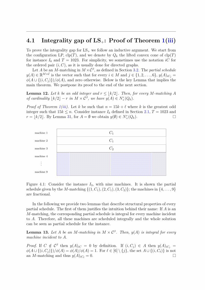
Figure 4.1: Consider the instance I3, with nine machines. It is shown the partialschedule given by the M -matching (1, C1), (2, C1), (3, C2); the machines in 4, . . . , 9are fractional.

In the following we provide two lemmas that describe structural properties of everypartial schedule. The first of them justifies the intuition behind their name: If A is anM -matching, the corresponding partial schedule is integral for every machine incidentto A. Therefore, all these machines are scheduled integrally and the whole solutioncan be seen as partial schedule for the instance.

Lemma 13. Let A be an M-matching in M ◊ C—. Then, y(A) is integral for everymachine incident to A.

Proof. If C /œ C— then y(A)iC = 0 by definition. If (i, Cj) œ A then y(A)iCj=

„(A fi (i, Cj))/„(A) = „(A)/„(A) = 1. For ¸ œ [6] \ j, the set A fi (i, C¸) is notan M -matching and thus y(A)iC¸

= 0.

4.1. Integrality gap of LS+: Proof of Theorem 1(iii) Chapter 4

The second lemma below provides the base case for the induction in the proofof Lemma 31 and complements the lemma above: The partial schedules are indeedfeasible solutions for the configuration LP.

Lemma 14. Let A be an M-matching in M ◊ C— of cardinality at most Âk/2Ê. Then,y(A) œ clp(T ).

Proof. We note that y(A)iC = y„Afi(i,C)/y„

A, and then the feasibility of y(A) in clp(T )

is implied by the feasibility of y„ in SAr(clp(T )), for r = Âk/2Ê.

The protection matrices. Given A an M -matching of M ◊C— and the respective partialschedule y(A), let Y (A) be the real symmetric matrix with rows and columns indexedin ÿ fi (M ◊ C), such that its principal submatrix indexed by ÿ fi (M ◊ C—) equals

A

1 y(A)€

y(A) Z(A)

B

,

where Z(A)iCj ,¸Ch= „(Afi(i, Cj), (¸, Ch))/„(A). All the other entries of the matrix

Y (A) are equal to zero. The matrix Y (A) provides the protection matrix we need inthe proof of the key Lemma. Condition (i) in the definition of the protection matrixis guaranteed by construction. To check that condition (ii) is satisfied we require thefollowing lemma.

Lemma 15. Let A be an M-matching in M ◊ C— and i a non-incident machine toA. Then,

q6j=1 Y (A)eiCj

= Y (A)eÿ.

Finally, condition (iii) is the more technical condition to be checked. It requiresthe use of algebraic tools and a series of operations to reduce the dimensionality ofthe problem. We postpone the proof of Theorem 4 to Section 4.2. We then proveLemma 15 and posteriorly we are ready to prove the key Lemma.

Theorem 4. For every M-matching A in M ◊ C— such that |A| Æ Âk/2Ê, the matrixY (A) is positive semidefinite.

Proof of Lemma 15. Let S be the index of a row of Y (A). If S /œ ÿfi (M ◊C—) thenthat row is identically zero, so the equality is satisfied. Otherwise,

e€S

6ÿ

j=1

Y (A)eiCj=

1

„(A)

6ÿ

j=1

„(A fi (i, Cj) fi S).

If A fi S is not an M -matching then „(A fi S fi i, Cj) = 0 for all i and j œ [6], ande€

S Y (A)eÿ = „(A fi S) = 0, so the equality is satisfied. If A fi S is an M -matching,then

1

„(A)

6ÿ

j=1

„(A fi (i, Cj) fi S) =„(A fi S)

„(A)

6ÿ

j=1

„(A fi S fi (i, Cj))

„(A fi S)

= e€S Y (A)eÿ

6ÿ

j=1

y„AfiSfi(i,Cj)

y„AfiS

= e€S Y (A)eÿ,

35

since y„ is a feasible solution for the SA hierarchy and threfore the summation aboveis equal to 1 due to the machine constraints (3.1).

Proof of Lemma 31. We proceed by induction in r. For r = 0 this is implied byLemma 14, so now suppose that it holds for r = t. Let y(A) be a partial scheduleof A of cardinality Âk/2Ê ≠ t ≠ 1. We prove that the matrix Y (A) is a protectionmatrix for y(A). It is symmetric by definition, and Y (A)eÿ = (1, diag(Y (A))) =(1, y(A)), so condition (i) is satisfied. Thanks to Theorem 4 the matrix Y (A) ispositive semidefinite, that is condition (iii).

It remains to check that condition (ii) is fulfilled. Let (i, C) be such that y(A)iC œ(0, 1). In particular, by Lemma 13 we have (i, C) /œ A and C œ C—. We claim thatY (A)eiC/y(A)iC is equal to (1, y(Afi(i, C))). If S indexes a row not in M ◊C— thenthe respective entry in both vectors is zero, so the equality is satisfied. Otherwise,

e€S Y (A)eiC

y(A)iC

=„(A fi (i, C) fi S)

„(A fi (i, C))= y(A fi (i, C))S.

The cardinality of the M -matching A fi (i, C) is equal to |A| + 1 = Âk/2Ê ≠ t, andtherefore by induction we have that Y (A)eiC/y(A)iC = (1, y(Afi(i, C))) œ N t

+(Qk).Now we prove that the vectors Y (A)(eÿ ≠ eiC)/(1 ≠ y(A)iC) are feasible for N t

+(Qk).By Lemma 15 we have that for every ¸ œ 1, 2, . . . , 6,

Y (A)(eÿ ≠ eiC¸)

1 ≠ y(A)iC¸

=ÿ

jœ[6]\¸

A

y(A)iCjq

jœ[6]\¸ y(A)iCj

B

y(A fi (i, Cj)),

and then Y (A)(eÿ≠eiC¸)/(1≠y(A)iC¸

) is a convex combination of the partial schedulesy(A fi (i, Cj)) : j œ [6] \ ¸ µ N t

+(Qk), concluding the induction.

4.2 The protection matrices are PSD

In this section we provide a full proof of Theorem 4. To prove that Y (A) is a positivesemidefinite matrix we perform several transformations of the original matrix thatpreserve the property of being positive semidefinite or not. We start with a shortsummary of the proof.

Proof scheme. First, we remove all those zero columns and rows. Then, Y (A) ispositive semidefinite if and only if its principal submatrix indexed by ÿ fi (M ◊C—) is positive semidefinite. We construct the matrix Cov(A) by taking the Schur’sComplement of Y (A) with respect to the entry (ÿ, ÿ).

The resulting matrix is positive semidefinite if and only if Y (A) is positive semidef-inite. After removing null rows and columns in Cov(A) we obtain a new matrix,Cov+(A), which can be written using tensor products as I ¢ Q + (J ≠ I) ¢ W , withQ, W œ R

6◊6, W = –Q for some – œ (≠1, 0) and I, J being the identity and the all-ones matrix, respectively. By applying a lemma about block matrices in [49], Y (A) ispositive semidefinite if and only if W is positive semidefinite.

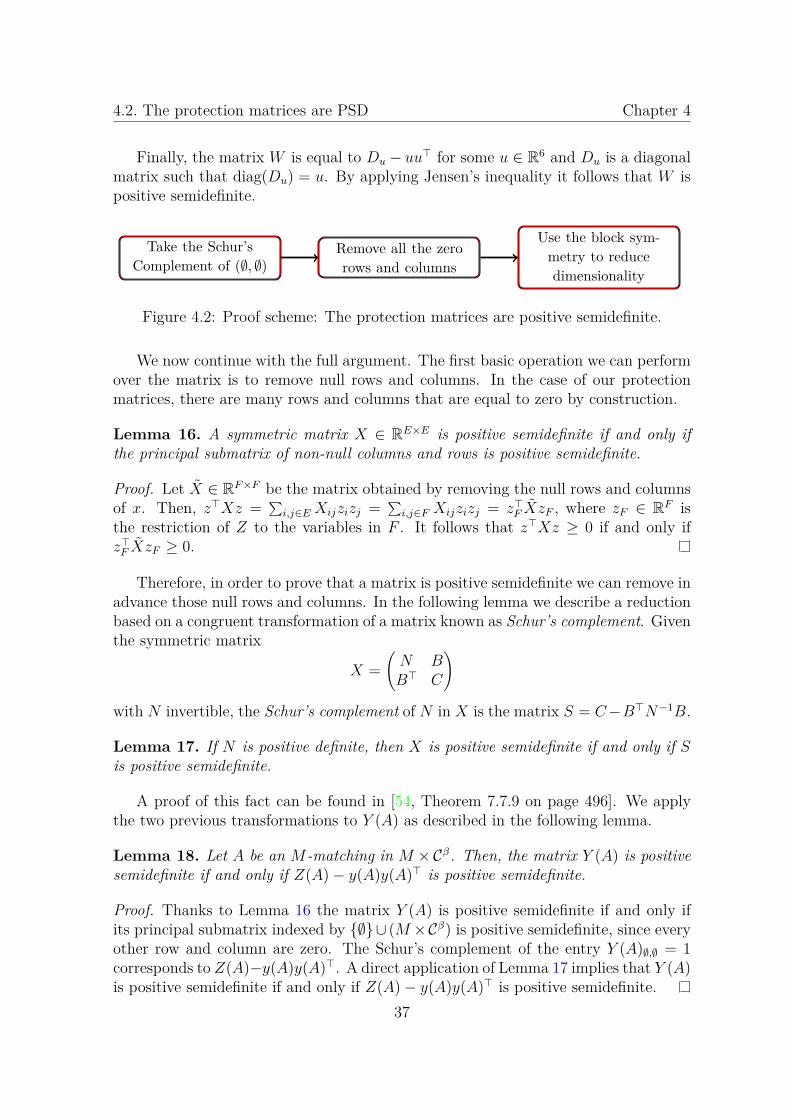
4.2. The protection matrices are PSD Chapter 4

Finally, the matrix W is equal to Du ≠ uu€ for some u œ R6 and Du is a diagonal

matrix such that diag(Du) = u. By applying Jensen’s inequality it follows that W ispositive semidefinite.

Take the Schur’s

Complement of (ÿ, ÿ)Remove all the zero

rows and columns

Use the block sym-

metry to reduce

dimensionality

Figure 4.2: Proof scheme: The protection matrices are positive semidefinite.

We now continue with the full argument. The first basic operation we can performover the matrix is to remove null rows and columns. In the case of our protectionmatrices, there are many rows and columns that are equal to zero by construction.

Lemma 16. A symmetric matrix X œ RE◊E is positive semidefinite if and only if

the principal submatrix of non-null columns and rows is positive semidefinite.

Proof. Let X œ RF ◊F be the matrix obtained by removing the null rows and columns

of x. Then, z€Xz =q

i,jœE Xijzizj =q

i,jœF Xijzizj = z€F XzF , where zF œ R

F isthe restriction of Z to the variables in F . It follows that z€Xz Ø 0 if and only ifz€

F XzF Ø 0.

Therefore, in order to prove that a matrix is positive semidefinite we can remove inadvance those null rows and columns. In the following lemma we describe a reductionbased on a congruent transformation of a matrix known as Schur’s complement. Giventhe symmetric matrix

X =

A

N BB€ C

B

with N invertible, the Schur’s complement of N in X is the matrix S = C ≠B€N≠1B.

Lemma 17. If N is positive definite, then X is positive semidefinite if and only if Sis positive semidefinite.

A proof of this fact can be found in [54, Theorem 7.7.9 on page 496]. We applythe two previous transformations to Y (A) as described in the following lemma.

Lemma 18. Let A be an M-matching in M ◊ C—. Then, the matrix Y (A) is positivesemidefinite if and only if Z(A) ≠ y(A)y(A)€ is positive semidefinite.

Proof. Thanks to Lemma 16 the matrix Y (A) is positive semidefinite if and only ifits principal submatrix indexed by ÿ fi (M ◊ C—) is positive semidefinite, since everyother row and column are zero. The Schur’s complement of the entry Y (A)ÿ,ÿ = 1corresponds to Z(A)≠y(A)y(A)€. A direct application of Lemma 17 implies that Y (A)is positive semidefinite if and only if Z(A) ≠ y(A)y(A)€ is positive semidefinite.

37

Further removals. We denote by Cov(A) the matrix Z(A)≠y(A)y(A)€, the covariancematrix of y(A). In the proof of Lemma 18 we removed first all those null rows andcolumns in Y (A). In fact, in the new matrix Cov(A) there are null rows and columnsthat can be removed of the matrix, so we can perform this operation again. Recall thatfiM(A) is the set of machines incident to A, and let Cov+(A) be the principal submatrixof Cov(A) obtained by removing every row and column indexed by E(fiM(A)) =(i, Cj) : i œ fiM(A), j œ 1, 2, . . . , 6.

Lemma 19. Let A be an M-matching in M ◊C—. Then, Y (A) is positive semidefiniteif and only if Cov+(A) is positive semidefinite.

Proof. We prove that for every (i, Cj) œ E(fiM(A)), Cov(A)eiCj= 0. By expanding,

e€¸Ck

Cov(A)eiCj=

1

„(A)„(A fi (¸, Ck), (i, Cj)) ≠ y(A)iCj

y(A)¸Ck.

By Lemma 13, if i is a machine incident to A we have y(A)iCj= 1(i,Cj)œA, and by

the definition of the function „ we have that it is supported over M -matchings only.Then, „(A fi (¸, Ck), (i, Cj)) = „(A fi (¸, Ck))1(i,Cj)œA, and

e€¸Ck

Cov(A)eiCj=

A

1

„(A)„(A fi (¸, Ck)) ≠ y(A)¸Ck

B

1(i,Cj)œA = 0,

because of the definition of the partial schedule y(A). The Lemma follows by a directapplication of Lemma 16.

Note that if machine i is not incident to A, the values y(A)iCj: j œ [6] do not

depend on the machine, but only on A. This motivates the definition of the vector‹(A) œ R

6 such that

‹(A)j =k/2 ≠ degA(Cj)

3k ≠ |A|,

for every j œ 1, 2, . . . , 6. If y(A) is a partial schedule, for every machine incident toA the entries yiCj

are in 0, 1, which is in total 3|A| entries. This is why Cov+(A) hasa very particular structure: If we order the rows and columns according to machines,a block structure appears. To properly define this we require some notation. LetU œ R

p◊q and T œ Rr◊s. Then, the tensor product between U and T , U ¢ T , is the

matrixQ

c

c

a

U11T . . . U1qT...

. . ....

Up1T . . . UpqT

R

d

d

b

œ Rpr◊qs.

Proposition 20. Let A, B, C, D four matrices such that the products AC and BDare well defined. Then, the following holds:

(i) (A ¢ B)(C ¢ D) = AC ¢ BD.

(ii) (A ¢ B)€ = A€ ¢ B€.

4.2. The protection matrices are PSD Chapter 4

A proof of (i) can be found at [53, Lemma 4.2.10 on page 244] and (ii) is directfrom the definition. The fractional part of y(A) corresponds to 1 ¢ ‹(A), where 1 isthe vector in R

3k≠|A| with every entry equal to 1. Furthermore, the value Z(A)iCj ,¸C¸=

“(A)j¸ is independent of the machines when i, ¸ are not incident to A,

“(A)j¸ =

Y

_

_

_

_

_

_

]

_

_

_

_

_

_

[

(k/2 ≠ degA(j))(k/2 ≠ degA(¸))

(3k ≠ |A|)(3k ≠ |A| ≠ 1)if j ”= ¸,

(k/2 ≠ degA(j))(k/2 ≠ degA(j) ≠ 1)

(3k ≠ |A|)(3k ≠ |A| ≠ 1)if j = ¸.

Then, we can fully express the matrix Cov+(A) in terms of tensor products involving“(A) and ‹(A)

I ¢ D‹(A) + (J ≠ I) ¢ “(A) ≠ (1 ¢ ‹(A))(1 ¢ ‹(A))€, (4.1)

where I is the 3k ≠ |A| dimensional identity matrix, J is the 3k ≠ |A| dimensionalall-ones matrix and D‹(A) œ R

6◊6 is such that D‹(A)jj = ‹(A)j for j œ 1, . . . , 6,and D‹(A)jh = 0 when j ”= h. The key consequence is that we can reduce the task ofproving that Y (A) is positive semidefinite to prove the same for matrices of constantdimension.

Block matrices. We say that a matrix X œ Rrn◊rn belongs to the (r, n)-block symmetry

set, Symnr , if there exist matrices D, E œ R

r◊r such that X = I ¢ D + (J ≠ I) ¢ E.For example, when n = 3,

X =

Q

c

a

D E EE D EE E D

R

d

b .

The following lemma characterizes the set of positive semidefinite matrices in Symnr .

Lemma 21 ([49]). Let X = I ¢ D + (J ≠ I) ¢ E œ Symnr . Then, X is positive

semidefinite if and only if i) D ≠ E is positive semidefinite and ii) D + (n ≠ 1)E ispositive semidefinite.

As a consequence, we reduce the dimensionality of the problem to r. In particular,Cov+(A) belongs to Sym

3k≠|A|6 and therefore the task now is to check that two matrices

of constant dimension are positive semidefinite.

Lemma 22. For every M-matching A in M ◊ C—, the covariance matrix Cov+(A)

belongs to Sym3k≠|A|6 and it is equal to

I ¢ ∆(A) ≠ (J ≠ I) ¢ 1

3k ≠ |A| ≠ 1∆(A),

where ∆(A) = D‹(A) ≠ ‹(A)‹(A)€.

39

Proof. We check first that Cov(A)+ œ Sym3k≠|A|6 . By Proposition 20, we have

(1 ¢ ‹(A))(1 ¢ ‹(A))€ = (1 ¢ ‹(A))1

1€ ¢ ‹(A)€2

= J ¢ ‹(A)‹(A)€.

Replacing this in the expression in 4.1 we get

Cov+(A) = I ¢ D‹(A) + (J ≠ I) ¢ “(A) ≠ J ¢ ‹(A)‹(A)€

= I ¢1

D‹(A) ≠ ‹(A)‹(A)€2

+ (J ≠ I) ¢1

“(A) ≠ ‹(A)‹(A)€2

= I ¢ ∆(A) + (J ≠ I) ¢1

“(A) ≠ ‹(A)‹(A)€2

,

so it remains to check that “(A) ≠ ‹(A)‹(A)€ = ≠1/(3k ≠ |A| ≠ 1) · ∆(A). Considertwo configurations Cj ”= C¸. Then, the non-diagonal entry (j, ¸) is equal to

“(A)j¸ ≠ ‹(A)j‹(A)¸ =(k/2 ≠ degA(j))(k/2 ≠ degA(¸))

(3k ≠ |A|)(3k ≠ |A| ≠ 1)≠ ‹(A)j‹(A)¸

=

A

3k ≠ |A|

3k ≠ |A| ≠ 1≠ 1

B

‹(A)j‹(A)¸ = ≠ 1

3k ≠ |A| ≠ 1∆(A)j¸.

For a diagonal element, we have

“(A)jj ≠ ‹(A)2j =

(k/2 ≠ degA(j))(k/2 ≠ degA(j) ≠ 1)

(3k ≠ |A|)(3k ≠ |A| ≠ 1)≠ ‹(A)2

j

=3k ≠ |A|

3k ≠ |A| ≠ 1

A

‹(A)2j ≠ 1

3k ≠ |A|‹(A)j

B

≠ ‹(A)2j

= ≠ 1

3k ≠ |A| ≠ 1(‹(A)j ≠ ‹(A)2

j) = ≠ 1

3k ≠ |A| ≠ 1∆(A)jj.

In addition with Lemma 21 we have the ingredients to prove that Cov+(A) is apositive semidefinite matrix when |A| Æ Âk/2Ê.

Proof of Theorem 4. By Lemma 22, Cov+(A) œ Sym3k≠|A|6 and then we can apply

Lemma 21. Therefore, the matrix Cov+(A) is positive semidefinite if and only if i)

∆(A) ≠ 13k≠|A|≠1

∆(A) = 3k≠|A|3k≠|A|≠1

∆(A) is positive semidefinite, and ii) ∆(A) ≠ (3k ≠|A| ≠ 1) · 1

3k≠|A|≠1∆(A) = 0 is positive semidefinite. The last condition is trivially

satisfied, and then Cov+(A) is positive semidefinite if and only if ∆(A) is positivesemidefinite. Given any vector x œ R

6, we have

x€∆(A)x =

6ÿ

j=1

‹(A)jx2j ≠

Q

a

6ÿ

j=1

‹(A)jxj

R

b

2

.

The vector ‹(A) œ R6 is non-negative if |A| Æ Âk/2Ê. As it satisfies that ΋(A)Î1 = 1,

by applying Jensen’s inequality with the function „(w) = w2 the latter expression isnon-negative for every x œ R

6. Then, Cov+(A) is positive semidefinite, and thanks toLemma 19 we conclude that Y (A) is positive semidefinite.

Chapter 5

Break symmetries to approximate

A natural source of symmetry in our problem comes from the fact that the machinesare identical: Given a schedule, we obtain other schedules with the same makespanby permuting the assignment over the machines. A second source of symmetry in theproblem arises from permuting jobs with the same processing time.

The symmetric nature of the combinatorial problem does not directly imply thata formulation is symmetric, but most of the time the natural formulations reflect thesymmetries as well. This is the case for the two formulations considered so far in thiswork, the assignment LP and the configuration LP. In what follows we introduce thenecessary algebraic tools for this chapter and formalize all these notions.

5.1 Group invariant sets

Given a set of variables D, we denote by GL(RD) the set of invertible matrices inR

D◊D. For a group G, we say that Φ : G æ GL(RD) is a matrix representation overR

D if Φ is a G-homomorphism, that is, for every g, h œ G we have Φ(g)Φ(h) = Φ(gh).A polytope K ™ R

D is said to be G-invariant if for every g œ G and x œ K,Φ(g)x œ K. We say that G induces an action over K, by the function fl : G ◊ K æ Ksuch that fl(g, x) = Φ(g)x.

A group of particular interest is the symmetric group of order d, denoted by Sd. Itcorresponds to the set of permutations over 1, . . . , d and the composition as product.This group has a matrix representation P over Rd given by the permutation matrices:For every ¸, k œ 1, . . . , d, let P (‡)¸k = 1 if and only if ‡(¸) = k.

Q

c

c

c

c

c

c

a

0 1 0 0 01 0 0 0 00 0 0 1 00 0 1 0 00 0 0 0 1

R

d

d

d

d

d

d

b

Figure 5.1: Permutation matrix of ‡ = (12)(34)(5).

41

It is not hard to check that for every scheduling instance and every T > 0, theassignment polytope is Sm-invariant, where the set of machines is M = 1, . . . , m.In this case, the variables are indexed by the set M ◊ J and the representation of Sm

over RM◊J is constructed as follows: Given ‡ œ Sm, define Φ(‡) = P (‡) ¢ I, where

I is the identity matrix in RJ◊J . The fact that Φ is a matrix representation follows

using the properties in Proposition 20: For every ‡, fi œ Sm,

Φ(‡)Φ(fi) = (P (‡) ¢ I)(P (fi) ¢ I) = P (‡)P (fi) ¢ I2 = P (‡fi) ¢ I = Φ(‡fi).

Let ‡ œ Sm and x œ assign(T ). For every j œ J , we haveÿ

iœM

(Φ(‡)x)ij =ÿ

iœM

x‡(i)j =ÿ

iœM

xij = 1,

since ‡ is a permutation of M . Therefore, every job constraint remains the same whenpermuting machines. Now given i œ 1, . . . , m, we have

ÿ

jœJ

(Φ(‡)x)ijpj =ÿ

jœJ

x‡(i)jpj Æ T,

since the last corresponds to the machine constraint for ‡(i). Observe that havingevery right hand side in the machine constraint equal to T is relevant to check theinvariance. If we had different machine availabilities then is not clear that the programremains invariant using the same representation. Then we should allow the group toact also over the coefficients in the linear functions defining the polytope.

1

2

3

1

2

3

Figure 5.2: Schedule of an instance with three machines and five jobs. Effect of thepermutation ‡ = (13) in the solution.

We can also observe that Sm is acting over the configuration LP. The representationof the permutation group is constructed in a very similar way, as well as checking thatclp(T ) is Sm-invariant. Scheduling identical machines belongs to a larger class ofpartitioning problems. The common feature of all these problems is to have a set ofelements that are to be partitioned in subsets, each of them meeting some constraints.In this case, we look for a partition of the jobs, where every part satisfies a packingconstraint.

5.2 Symmetry breaking inequalities

Recall that in the configuration LP we look for an assignment of machines to the set ofconfigurations C. For example, in the hard instances obtained from the Petersen graph

5.2. Symmetry breaking inequalities Chapter 5

in Chapter 2 (see Figure 2.1) the number of configurations for T = 1023 is equal to six,so every feasible schedule should have many machines scheduled according to the sameconfiguration. In what follows, we introduce a set of constraints that guarantee everyinteger solution in the polytope to obey a specific order on the configurations over themachines. Recall that the set of machine is the set M = 1, . . . , m. Therefore, if weknew that a machine ¸ is scheduled according to a given configuration C, it shouldbe that every machine smaller (larger) than ¸ is scheduled respecting the order onthe configurations set. This is a way of breaking the machine symmetries since we arerestricting the set of possible assignments.

We need some notation before introducing the symmetry breaking constraints.Suppose we have a partitioning J of the job set J into s parts, J = J1, . . . , Js.In principle, the partition is arbitrary. An example of such a partition is given inthe following way. Suppose the job sizes are ordered from largest to smallest, that isp1 > p2 > · · · > ps where s = |pj : j œ J| is the number of different job sizes. Then,we could define the partition such that Jq = j œ J : pj = pq for every q œ [s], andwe call it the job-sizes partition.

In this context, a configuration C is a multiset of elements in 1, . . . , s. Recallthat for every q œ 1, . . . , s, the multiplicity of q in C, m(q, C), is the number oftimes that pq appears repeated in C. For example, if s = 3 and C = 1, 1, 1, 2,we have m(1, C) = 3, m(2, C) = 1 and m(3, C) = 0. We denote by C the set of allconfigurations. Observe that it coincides with the configuration notion introduced inChapter 1 if we consider the job-sizes partition.

We say that a configuration C is lexicographically larger than S, and we denoteC >lex S, if there exists q œ [s] such that m(¸, C) = m(¸, S) for all ¸ < q and m(q, C) >m(q, S). Following the example with s = 3, the configuration C = 1, 1, 1, 2, 2 islexicographically larger than S = 1, 1, 1, 2, 3 since m(1, C) = m(1, S) = 3 andm(2, C) = 2 > m(2, S) = 1.

Given a positive integer number B, consider the polytope assign(B, T ) given by

assign(T ) flm≠1‹

i=1

Y

]

[

x œ RM◊J :

sÿ

q=1

Bs≠qÿ

jœJq

1

xij ≠ x(i+1)j

2

Ø 0

Z

^

\

.

Sometimes, to avoid confusion we use the notation assign(J, B, T ) to emphasize thatwe are considering the polytope for the jobs set J . We also remark that the symmetrybreaking constraints depend on the partitioning of J . Given a subset of jobs K µ Jsuch that

q

jœK pj Æ T , we denote by conf(K) the configuration such that for everyq œ 1, . . . , s, m(q, conf(K)) = |KflJq|. We then say that conf(K) is the configurationinduced by K and we denote by C the set of all possible configurations induced in thisway. Observe that >lex defines a total order over C.

In the following we show that for sufficiently large, but polynomially sized B, everyinteger solution in the polytope obeys the lexicographic order on configurations overthe machines. More specifically, given a feasible integer solution x œ assign(T ), forevery machine i œ M let Ci(x) œ C be the configuration defined by the number ofjobs for each possible part that are scheduled in i according to x, that is, for everyq œ 1, . . . , s, m(q, Ci(x)) =

q

jœJqxij.

43

Theorem 5. There exists B = O(|J |2) such that for every integer solution x œassign(B, T ), Ci(x) Ølex Ci+1(x) for every machine i œ M \ m.

In general, the polytope above is not Sm-invariant, but it is a valid formulationfor the problem of finding a schedule with makespan at most T . More specifically, weshow that if there is a schedule with makespan at most T , then there is an integersolution in assign(B, T ).

Lemma 23. Suppose there is an integer solution in assign(T ). Then, there existsB = O(|J |2) for which there is an integer solution in assign(B, T ).

We prove the theorem statements above by introducing an intermediate resultconnecting the lexicographic order over the configurations and the symmetry breakingconstraints shown above. Given B œ N, let LB : C æ R be the function such that forevery configuration C œ C,

LB(C) =s

ÿ

q=1

Bs≠qm(q, C).

Recall that the lexicographic order over the configurations induces a total order overC. We show that exists a polynomially sized value of B for which LB is a strictlyincreasing function, that is, if C <lex S then LB(C) < LB(S). Using this result wethen prove Theorem 5.

Lemma 24. Let B > 2s maxqœ[s] |Jq|. Then, LB is strictly increasing.

Proof of Theorem 5. Fix a machine i œ M \ m. Since x is an integer solution inassign(B, T ), we have Ci(x), Ci+1(x) œ C. The symmetry breaking constraints impliesthat

0 Æs

ÿ

q=1

Bs≠q (m(q, Ci(x)) ≠ m(q, Ci+1(x))) = LB(Ci(x)) ≠ LB(Ci+1(x)).

Applying Lemma 24 for B = 1 + 2s maxqœ[s] |Jq| = O(|J |2) it holds that LB is strictlyincreasing and therefore Ci(x) Ølex Ci+1(x).

Proof of Lemma 23. Consider an integer solution x œ assign(T ). Since the lexico-graphic relation defines a total order over C, there exists a permutation ‡ œ Sm suchthat C‡(i)(x) Ølex C‡(i+1)(x) for every i œ M \ m. Consider the new schedule xobtained by permuting the solution according to ‡, that is, xij = x‡(i)j for every(i, j) œ M ◊ J . Then, for every i œ M \ m it follows that

sÿ

q=1

Bs≠qÿ

jœJq

1

xij ≠ x(i+1)j

2

=s

ÿ

q=1

Bs≠q1

m(q, C‡(i)(x)) ≠ m(q, C‡(i+1)(x))2

= LB(C‡(i)(x)) ≠ LB(C‡(i+1)(x)) Ø 0,

where the last inequality holds by Lemma 24. We conclude that x œ assign(B, T ).

5.3. The Lasserre/SoS (Las) Hierarchy Chapter 5

We recall that having B of polynomial input size is relevant at the moment of solv-ing the linear program assign(B, T ). In particular, the input size is O(|J |2 · log(Bs)) =O(poly(|J |)), and so in can be solved in time O(poly(|J |)) using, for example, theKarmakar algorithm or the Ellipsoid method [94, Chapter 15]. In what follows, weuse a superscript over the configurations to indicate its lexicographic order, that is,C1 > C2 > C3 > · · · > C |C|.

Proof of Lemma 24. Consider two configurations C, S œ C such that C >lex S. Let qbe the smallest in 1, . . . , s integer such that the multiplicities of the configurationsare different, that is, m(¸, C) = m(¸, S) for every ¸ < q. For the sake of contradictionsuppose that m(q, C) < m(q, S). In particular, every term up to max0, q ≠ 1 inthe summation defining LB(C) ≠ LB(S) is equal to zero. By upper bounding thesummation from mins, q + 1 we obtain that

sÿ

q=mins,q+1

Bs≠q (m(q, C) ≠ m(q, S)) Æs

ÿ

q=mins,q+1

Bs≠q (|m(q, C)| + |m(q, S)|)

Æs

ÿ

q=mins,q+1

Bs≠q · 2|Jq|

<

A

2s maxqœ[s]

|Jq|

B

Bs≠q≠1 Æ B · Bs≠q≠1,

and since m(q, S) ≠ m(q, C) Ø 1 it follows that

sÿ

q=q

Bs≠q (m(q, C) ≠ m(q, S)) < Bs≠q + Bs≠q (m(q, C) ≠ m(q, S))

< Bs≠q (1 + m(q, C) ≠ m(q, S)) < 0,

yielding to the contradiction.

5.3 The Lasserre/SoS (Las) Hierarchy

The Lasserre/SoS hierarchy is the strongest lift & project operator among the onesconsidered in this work, that is Sherali-Adams (SA) and Lovasz-Schrijver (LS+). Be-fore introducing the relaxations obtained from the hierarchy, we require some nota-tion about moment matrices, that play a role in what follows. Then we introducethe hierarchy in a self-contained way. Given a set E be a set and r œ N, recallthat Pr(E) = A ™ E : |A| Æ r. For a vector z œ R

P2r(E), the r-moment matrix,Mr(z) œ R

Pr(E)◊Pr(E), is such that for every U, V œ Pr(E), Mr(z)U,V = zUfiV . Observethat this matrix is symmetric. We consider an operation ı called the shift productbetween a vector z œ R

Pr(E) and a vector a œ RP1(E) such that for all U œ Pr(E),

(a ı z)U =ÿ

eœE

aexUfie ≠ aÿxU ,

45

recalling that ae = ae for simplicity when e is a singleton. Given a schedulinginstance and T > 0, for every i œ M let packi œ R

P1(M◊J) be such that packiÿ = T ,

packi¸j = ≠pj if ¸ = i and zero otherwise. Similarly, for every i œ M \ m let

breaki œ RP1(M◊J) be such that

breaki¸j =

Y

_

_

]

_

_

[

Bs≠q if ¸ = i and j œ Jq, for all q œ 1, . . . , s,

≠Bs≠q if ¸ = i + 1 and j œ Jq, for all q œ 1, . . . , s,

0 otherwise.

The level r Lasserre/SoS relaxation, Lasr(assign(B, T )), is an SDP in [0, 1]P2r+2(M◊J),

ÿ

iœM

xIfi(i,j) ≠ xI = 0 for all j œ J, for all I œ P2r+1(M ◊ J), (5.1)

Mr(packi ı x) ≤ 0 for all i œ M, (5.2)

Mr(breaki ı x) ≤ 0 for all i œ M \ m, (5.3)

Mr+1(x) ≤ 0, (5.4)

xÿ = 1. (5.5)

5.4 Balanced partitionings

Observe that Las0(assign(B, T )) is at least as strong as assign(B, T ). In this sectionwe study the integrality gap of the SDP relaxations obtained from the Lasserre/SoShierarchy. More specifically, we show that after a small number of rounds that dependson the configurations set C, and therefore on the partitioning J , the integrality gapcan be arbitrarily close to one. Recall that whereas the total number of jobs canbe large, the number of configurations could be small and therefore we obtain betterbounds. We say a partitioning J is –-balanced, with – Ø 1, if for every K, H ™ Jsuch that conf(K) = conf(H),

ÿ

jœK

pj Æ –ÿ

jœH

pj.

Other parameter that plays a key role is the maximum number of jobs that can bescheduled in the same machine with makespan at most T , that is,

⁄ = max

Y

]

[

|K| :ÿ

jœK

pj Æ T

Z

^

\

.

For example, if we knew that pj Ø T/3 for every j œ J , then ⁄ Æ 3. The followingis the main result of this chapter: Given a balanced partitioning of J and its inducedconfigurations C, there is a level of the hierarchy for which its feasibility implies theexistence of an integral solution with a makespan close to T . Provided that B ischosen accordingly to Lemma 5, it gives us a schedule respecting the lexicographicorder of configurations over the machines.

5.5. An approximation scheme for Scheduling Chapter 5

Theorem 6. Consider a scheduling instance, T > 0 and an –-balanced partition-ing of the set J . Suppose the ⁄|C| = ·(C) level of the Lasserre/SoS hierarchy overassign(B, T ) is feasible, that is,

Las·(C)(assign(B, T )) ”= ÿ.

Then, there exists a schedule, xlex œ assign(B, –T )fl0, 1M◊J , that is, with makespanat most –T . Furthermore, it can be found in time |J |O(·(C)).

The value ·(C) = ⁄|C| can be improved, but this is good enough for this exposition.If we go back to the hard instances shown in Chapter 2, we observe that for T = 1023there is a constant number of configurations for all the instances IkkœN if we considerthe job-sizes partition, since there are only 15 different job sizes. Furthermore, sincethe smallest job size in the instances is 33, we have that ⁄ Æ 1023/33 = 31. Recallthat for T = 1023 there is no feasible schedule for the instance and the job-sizespartition is 1-balanced. Therefore, for every k œ N, there is an O(1) level Lasserrerelaxation for T = 1023 which is equal to the empty set.

An important observation is that we assume the number of machines m to begreater than ·(C), since otherwise the theorem follows by a direct application ofTheorem 3 in Chapter 3. The proof of this theorem follows in a slightly similar wayto that of the Machine Decomposition Lemma (see Chapter 3, Lemma 6). There,the argument was based on an induction over the number of machines that are to beintegral. We leave the full proof of Theorem 6 to Section 5.6, and in the followingsection we show how to obtain a polynomial time approximation scheme as corollaryof the main theorem.

5.5 An approximation scheme for Scheduling

An idea that has been frequently exploited for designing approximation schemes inscheduling and packing problems is to split the instances into long jobs and short jobs.Then, each sub-instance is solved or approximated by using suitable techniques, andmerged afterwards in order to provide a solution for the original problem. Roundingthe numeric values of the instances plays a key role in this approaches since it allows toreduce the underlying combinatorics. In particular, it allows exhaustive enumerationin some cases.

We provide an approximation scheme that uses the idea of splitting the instanceinto long and short jobs, but we do not round the numeric values. In what follows,given Á > 0, we say that a job j œ J is long if pj Ø ÁT , and it is short otherwise. Thesubset of long jobs is denoted by Jlong and the short jobs are Jshort = J \ Jlong. Weconsider a partitioning that simulates the rounding by grouping jobs with a similarprocessing time. More specifically, for every q œ 1, . . . , (1 ≠ Á)/Á2, let

Jq =;

j œ Jlong :3

1

Á+ q

4

Á2T > pj Ø3

1

Á+ q ≠ 1

4

Á2T<

,

47

and we call this the Á-partitioning of the long jobs. We show next that this partitioningis arbitrarily close to being 1-balanced, and therefore we can try to schedule long jobsusing the main theorem.

Lemma 25. For every Á > 0, the Á-partitioning is (1 + Á)-balanced.

Proof. Consider K, H ™ J such that conf(K) = conf(H) = C for the Á-partitioning J .In particular, for every q œ 1, . . . , |J | we have that |K fl Jq| = m(q, C) = |H fl Jq|,and so there exists a bijection Ïq : K fl Jq æ H fl Jq. Furthermore, for any pair ofjobs j, ¸ œ Jq it holds

pj

p¸

Æ1

1Á

+ q2

Á2T1

1Á

+ q ≠ 12

Á2TÆ

1Á

+ 11Á

= 1 + Á,

since the function (1Á

+ q)/(1Á

+ q ≠ 1) is strictly decreasing in [1, +Œ). Therefore,for every q œ 1, . . . , |J | it holds that

q

jœKflJqpj Æ (1 + Á)

q

jœKflJqpÏq(j) = (1 +

Á)q

jœHflJqpj, and we conclude that

ÿ

jœK

pj =|J |ÿ

q=1

ÿ

jœKflJq

pj Æ (1 + Á)|J |ÿ

q=1

ÿ

jœHflJq

pj = (1 + Á)ÿ

jœH

pj.

Given Á > 0, consider assign(B, T ) obtained from the partitioning above and Bchosen according to Lemma 24. Then, using a binary search like procedure we lookfor the smallest T such that the level ·(C) relaxation of the Lasserre/SoS hierarchyis feasible for the long jobs. Invoking Theorem 6 we then obtain a schedule forthe long jobs. The short jobs are scheduled then using the classic list schedulingalgorithm [102].

Algorithm 1

Input: A scheduling instance and T Ø 1/mq

jœJ pj.Output: A schedule with makespan at most (1 + Á)T if there exists a schedule for

Jlong with makespan at most T ; infeasible otherwise.1: For all (i, j) œ M ◊ J , initialize xij Ω 0.2: Consider the (Á/2)-partitioning of Jlong and B = 1 + 42≠Á

Á2 |Jlong|.

3: if Las·(C)(assign(Jlong, B, T )) ”= ÿ then4: construct the Lex-schedule xlex of Jlong; for all (i, j) œ M ◊ Jlong, xij Ω xlex

ij .5: while Jshort ”= ÿ do6: Pick k œ Jshort, and let i œ M such that i œ argmin¸ œ M :

q

jœJ pjx¸j,7: update xik Ω 1 and Jshort Ω Jshort \ k.

8: Return x.9: else return infeasible.

Theorem 7. If Las·(C)(assign(Jlong, B, T )) ”= ÿ, then Algorithm 2 returns a schedulewith makespan at most (1 + Á)T .

5.6. Proof of Theorem 6 Chapter 5

Proof. Thanks to Theorem 6, if Las·(C)(assign(Jlong, B, T )) ”= ÿ, then xlex is an integralschedule for Jlong with makespan at most T . In this case, jobs in Jshort are assignedaccording to the list scheduling algorithm, for which we include the analysis onlyfor completeness. Let k œ Jshort and let i œ M such that xik = 1. Since T >1/m

q

jœJ\k pj, it follows that T >q

jœJ pjxij since this value is minimized at i œ M .Therefore, the load of machine i after scheduling job k is upper bounded by

pk +ÿ

jœJ :xij=1

pj <Á

2T +

3

1 +Á

2

4

T = (1 + Á)T.

The approximation scheme works as follows. We perform a binary search procedureto find the smallest integer value of T such that Las·(C)(assign(B, T )) ”= ÿ. To dothis it is enough to consider the lower bound 1/m

q

jœJ pj on the optimal makespan,and the upper bound Á1/m

q

jœJ pjË + maxjœJ pj. For such value of T , thanks toTheorem 7 we obtain a schedule with makespan at most (1 + Á)T . In particular,Las·(C)(assign(Jlong, B, Cmax)) ”= ÿ and therefore the makespan of this schedule is atmost (1 + Á)T Æ (1 + Á)Cmax.

Regarding the running time, observe that the smallest job size in Jlong is (Á/2)T ,so we have ⁄ Æ 2/Á. The size of C can also be upper bounded by (1 + 2/Á)4/Á2

, sincenot more than 2/Á jobs can be allocated to single machine and the size of the partitionis less than 4/Á2. Since the running time of the algorithm is dominated by findinga feasible solution at level ·(C) < 2

Á(1 + 2

Á)4Á≠2

of the Lasserre/SoS relaxation, thealgorithm runs in polynomial time.

5.6 Proof of Theorem 6

Preliminaries. Before proceeding with the proof we need to introduce some proper-ties that are satisfied by the relaxations obtained from the Lasserre/SoS hierarchy.Similarly to the SA and LS+ hierarchies, we also have convergence in this case to theinteger hull. In the following, we show a structural lemma that shows this propertyas a corollary, but more crucially, a property that in general is not satisfied by weakerhierarchies, known as the Decomposition Theorem [62]. We make an exposition thatis self-contained and we include the proof of these results in the context of the as-signment polytope. The following properties are very simple and they will be usefulthroughout the section.

Proposition 26. Let x œ Lasr(assign(B, T )). Then, the following holds:

i) For every I œ Pr+1(M ◊ J), xI œ [0, 1].

ii) If L œ Pr+1(M ◊ J) and I ™ L, then xL Æ xI .

Proof. To check i) it is enough to consider the principal submatrix of Mr+1(x) givenby the entries ÿ and I. Since it is positive semidefinite as well, the determinant isnon-negative, that is xI(1 ≠ xI) Ø 0 and then xI œ [0, 1]. To check ii) it is enough

49

to consider the principal submatrix of Mr+1(x) given by the entries I and L. This ispositive semidefinite, and so its determinant is non-negative. Since xIfiL = xL it holdsthat xL(xI ≠ xL) Ø 0, thus xL Æ xI .

Given x œ Lasr(assign(B, T )), the extension of x, ext(x), is the vector with entriesin P(M ◊ J) such that ext(x)I = 0 if |I| > 2r + 2 and ext(x)I = xI otherwise. Givena machine i œ M and a subset of jobs K ™ J , let x(i, K) be a vector with entries inP2(r≠|K|)+2(M ◊ J) such that

x(i, K)I =ÿ

H™J :K™H

(≠1)|H\K|ext(x)Ifi(i◊H),

for every I œ P2(r≠|K|)+2(M ◊ J). The following property is usually called the Mobiusinversion in the moment matrices literature, or inclusion-exclusion in the probabilitycontext.

Lemma 27. Let x œ Lasr(assign(B, T )) and i œ M . Then, x =q

K™J x(i, K).

Proof. Let I œ P2r+2(M ◊J). By substituting, parameterizing in H\K and reorderingthe summation it follows that

ÿ

K™J

x(i, K)I =ÿ

K™J

ÿ

H™J :K™H

(≠1)|H\K|ext(x)Ifi(i◊H)

=ÿ

H™J

ÿ

R™J :R™H

(≠1)|R|ext(x)Ifi(i◊H)

=ÿ

H™J

ext(x)Ifi(i◊H)

ÿ

R™J :R™H

(≠1)|R|.

Observe that if H ”= ÿ, then the last term of the summation is equal to zero. Therefore,the summation above is equal to ext(x)Ifi(i◊ÿ) = xI .

An important observation is that the equality above says that xÿ =q

K™J x(i, K)ÿ

and xÿ = 1, therefore

x =ÿ

K™J

x(i, K) =ÿ

K™J :x(i,K)ÿ>0

x(i, K)ÿ ·

A

x(i, K)

x(i, K)ÿ

B

,

so x is a convex combination of the vectors xC(i, K) : K ™ J and x(i, K)ÿ > 0 wherexC(i, K) = x(i, K)/x(i, K)ÿ. An important observation is that the vector xC(i, K) isintegral for machine i: If j œ K, it follows that

x(i, K)ij =ÿ

H™J :K™H

(≠1)|H\K|ext(x)(i,j)fi(i◊H)

=ÿ

H™J :K™H

(≠1)|H\K|ext(x)ÿfi(i◊H) = x(i, K)ÿ,

5.6. Proof of Theorem 6 Chapter 5

and therefore xC(i, K)ij = 1. Now, given j /œ K, we split the summation betweenthose sets that contain K fi j and those that do not. Therefore,

x(i, K)ij =ÿ

H™J :K™H

(≠1)|H\K|ext(x)(i,j)fi(i◊H)

=ÿ

H™J\j:K™H

((≠1)|H\K| + (≠1)|H\K|+1)ext(x)i◊(Hfij) = 0.

In the following we state the Decomposition Theorem [62] adapted to our purposes,which is a structural property of the Lasserre/SoS hierarchy that makes it strongerthan others. We include its proof for the sake of completeness, although it follows thesame lines than [62] and it could be skipped.

Theorem 8. Let x œ Lasr(assign(B, T )) for some r Ø ⁄. Then, for every machinei œ M and K ™ J such that x(i, K)ÿ > 0, we have xC(i, K) œ Lasr≠⁄(assign(B, T )).Furthermore, xC(i, K)ij = 1 for every j œ K and zero otherwise.

Proof of Theorem 8. It remains to show that xC(i, K) œ Lasr≠⁄(assign(B, T )). Infact, we show a stronger result: For every i œ M and K ™ J , if x(i, K)ÿ > 0 thenxC(i, K) œ Lasr≠|K|(assign(B, T )). In particular, the constraints (5.2) at level r = 0imply that K induces a configuration, Ci(xC(i, K)) œ C, and therefore |K| Æ ⁄.

The constraint (5.5) is clearly satisfied. We now check that constraint (5.4) issatisfied, that is, Mr≠|K|+1(xC(i, K)) ≤ 0. Since Mr+1(x) ≤ 0, there exist a family ofvectors –I : I œ Pr+1(M ◊ J) such that for every U, V œ Pr+1(M ◊ J), xUfiV =È–U , –V Í. Consider the vector –C(i, K) with entries in Pr≠|K|+1(M ◊ J) such that

–C(i, K)I =1

Ò

x(i, K)ÿ

ÿ

H™J :K™H

(≠1)|H\K|–Ifi(i◊H).

We show that for every U, V œ Pr≠|K|+1, xC(i, K)UfiV = È–C(i, K)U , –C(i, K)V Í andthat implies constraint (5.4) is satisfied.

x(i, K)ÿ · È–C(i, K)U , –C(i, K)V Í=

ÿ

H™J :K™H

ÿ

G™J :K™G

(≠1)|H\K|+|G\K|È–Ufi(i◊H), –V fi(i◊G)Í

=ÿ

H™J :K™H

(≠1)|H\K|ÿ

G™J :K™G

(≠1)|G\K|xUfiV fi(i◊H)fi(i◊G).

Observe that |U | Æ r ≠ |K| + 1 and |V | Æ r ≠ |K| + 1, and therefore every term inthe summation above is well defined. Consider H ”= K and and element h œ H \ K.Then, the second summation is equal to

ÿ

G™J :Kfih™G

((≠1)|G\K| + (≠1)|G\K|+1)xUfiV fi(i◊H)fiG = 0,

and therefore in the summation above it only remains the term for H = K, that is,ÿ

G:K™G

(≠1)|G\K|xUfiV fi(i◊K)fi(i◊G)

=ÿ

G:K™G

(≠1)|G\K|xUfiV fi(i◊G) = x(i, K)UfiV ,

51

since GfiK = G. To check the constraints (5.1), we have that given I œ P2r+1(M ◊J),ÿ

¸œM

x(i, K)Ifi(¸,j) =ÿ

¸œM

ÿ

H™J :K™H

(≠1)|H\K|ext(x)Ifi(¸,j)fi(i◊H)

=ÿ

H™J :K™H

(≠1)|H\K|ÿ

¸œM

ext(x)Ifi(¸,j)fi(i◊H)

=ÿ

H™J :K™H

(≠1)|H\K|ext(x)Ifi(i◊H) = x(i, K)I ,

since ext(x) satisfies the constraint (5.5) for I as well. Finally, it remains to checkconstraints (5.2) and (5.3). Let fl be any vector in packi, breaki : i œ M \ m fipackm. Since Mr(fl ı x) ≤ 0, there exists a family of vectors —I : I œ Pr(M ◊ J)such that for every U, V œ Pr(M ◊ J), (fl ı x)UfiV = È—U , —V Í. Let —C(i, K) be thevector with entries in Pr≠|K|(M ◊ J) such that

—C(i, K)I =1

Ò

x(i, K)ÿ

ÿ

H™J :K™H

(≠1)|H\K|—Ifi(i◊H).

We show next that for every U, V œ Pr≠|K|, (flıxC(i, K))UfiV = È—C(i, K)U , —C(i, K)V Íand that implies constraint (5.4) is satisfied. First, observe that

x(i, K)ÿ · È—C(i, K)U , —C(i, K)V Í=

ÿ

H:K™H

(≠1)|H\K|ÿ

G:K™G

(≠1)|G\K|(fl ı x)UfiV fi(i◊H)fi(i◊G).

We have that |U | Æ r ≠ |K| and |V | Æ r ≠ |K|, and therefore every term in thesummation above is well defined. As we showed before, in the summation above itonly remains the term for H = K. Therefore,

ÿ

G:K™G

(≠1)|G\K|(fl ı x)UfiV fi(i◊(KfiG)) =ÿ

G:K™G

(≠1)|G\K|(fl ı x)UfiV fi(i◊G)

= (fl ı x(i, K))UfiV ,

and we conclude using that fl ı x(i, K) = x(i, K)ÿ · (fl ı xC(i, K)).

Other relevant property is that if the vector x was integral at some machine, thenit remains integral for a vector in the convex combination of the decomposition.

Proposition 28. Suppose that x œ Lasr(assign(B, T )) with r Ø ⁄, and it is integralat machine h. Let K ™ J with xC(i, K)ÿ > 0. Then, xC(i, K)hj = xhj œ 0, 1 for allj œ J .

Proof. Let j œ J such that xhj = 0. Observe every term in the summation definingxC(i, K)hj contains (h, j), and then by Proposition 26 they are all zero. It followsthat xC(i, K)hj = 0. On the other hand, if xhj = 1, since

q

¸œM x¸j = 1 it follows thatx¸j = for every ¸ ”= h. By using the argument above and since xC(i, K) œ assign(B, T )by Theorem 8, it follows that xC(i, K)¸j = 0 for every ¸ ”= h and therefore xC(i, K)hj =1 ≠ q

¸œM xC(i, K)¸j = 1.

5.6. Proof of Theorem 6 Chapter 5

Constructing the schedule. The proof of Theorem 6 follows in a constructive way. Weiteratively call the Decomposition Theorem 8 and obtain, in that way, many machinesthat are integral. If we start from a high enough level of the hierarchy, we get at theend a solution that is feasible for assign(B, T ), and therefore, the configurations ofthe integral machines have to obey the lexicographic order. We then show how toextend the schedule to the rest of the machines using those configurations and provethis schedule to be feasible.

The algorithm consist of two phases. In Phase 1, we use the solution obtainedfrom high enough level of the hierarchy to find the last machine which is fractionallyscheduled according to configuration C1 using the Decomposition Theorem, and picksuch a vector obtained from the convex combination. We then proceed by finding thelast machine scheduled fractionally according to C2, and so on. We end up with asolution that is integral for all these machines, and it respects the lexicographic orderover the configurations. In Phase 2, we construct the schedule for the rest of themachines and jobs that have not been assigned yet. We call the schedule obtainedin this way the lexicographic schedule, xlex. Below we provide the pseudocode of theconstruction, and then we prove it outputs a feasible schedule.

Algorithm 2

Input: A solution x œ Las·(C)(assign(B, T )).Output: A schedule xlex with makespan at most T .

1: For all (i, j) œ M ◊ J , initialize xlexij Ω 0, ¸ Ω 0 and y0 Ω x.

2: Û Phase 1: Inducing integrality of certain machines.3: for ¸ = 1 to |C| do4: Let M ¸ = i œ M : exists K ™ J with y¸(i, K)ÿ > 0 and conf(K) = C¸.5: if M ¸ ”= ÿ then6: let i¸ = max M ¸ and K¸ ™ J such that conf(K¸) = C¸ and y¸(i¸, K¸)ÿ > 0,7: for every j œ K¸ let xlex

i¸j Ω 1,

8: y¸+1 Ω y¸C(i¸, K¸).

9: else i¸ = Œ10: Reset ¸ Ω 1, i0 = 0.11: Û Phase 2: Extending the above solution greedily.12: for ¸ = 1 to |C| do13: if i¸ < Œ then14: for maxiq : 0 Æ q < ¸, iq < Œ < i < i¸ do15: let Ki ™ J \ j œ J : exists i œ M with xlex

ij = 1 where conf(Ki) = C¸;16: for every j œ Ki, let xlex

ij Ω 1.

17: Return xlex.

Lemma 29. Let x œ Lasr(assign(B, T )) for r Ø ⁄, and i, h œ M with i < h. Supposethat x is integral for machine h. Then, for every I such that x(i, I)ÿ > 0, we haveconf(I) Ølex Ch(x).

Proof. Let I ™ J with xC(i, I)ÿ > 0. By Theorem 8 we have that xC(i, I) œ53

assign(B, T ), xC(i, I)ij œ 0, 1 for all j œ J and conf(I) = Ci(xC(i, I)). In par-ticular, from the symmetry breaking constraints it follows that LB(Ci(xC(i, I))) ØLB(Ch(x)), since by Proposition 28 the vector xC(i, I) remains integral at h and inthe same configuration than x. The function LB is strictly increasing, and thereforeconf(I) = Ci(xC(i, I)) Ølex Ch(x).

Observe that it is guaranteed by the algorithm that machine m is integral at theend of Phase 1. In the following, we prove that at the end of every iteration of Phase1, the machines between other two that have been induced to be integral by using thedecomposition are all fractionally scheduled according to the same configuration. Inparticular, it guarantees that the greedy approach of Phase 2 works.

Lemma 30. Let ¸ œ 1, . . . , |C|. For every i œ M such that i¸ = maxiq : 0 Æ q <¸, iq < Œ < i Æ i¸ and every q œ 1, . . . , s,

q

jœJqy¸

ij = m(q, C¸).

Proof. Let i œ M be a machine such that i¸ < i Æ i¸. By Lemma 29, for every K ™ Jsuch that y¸(i, K)ÿ > 0 it holds that conf(K) Ølex C¸, but we show next that they areall equalities. Suppose there exists K ™ J such that Ct = conf(K) >lex C¸ for somet < ¸. That would imply that i Æ it < Œ, contradicting that i¸ < i. By Lemma 27,for every q œ 1, . . . , s it holds that

ÿ

jœJq

y¸ij =

ÿ

jœJq

ÿ

K™J :y¸(i,K)ÿ>0

y¸(i, K)ÿ · yC(i, K)ij

=ÿ

K™J :y¸(i,K)ÿ>0

y¸(i, K)ÿ

ÿ

jœJq

yC(i, K)ij

=ÿ

K™J :y¸(i,K)ÿ>0

y¸(i, K)ÿ · m(q, C¸) = y¸ÿ · m(q, C¸) = m(q, C¸).

Proof of Theorem 6. For every ¸ œ 1, . . . , |C|, let N ¸ = i œ M : i¸ < i < i¸.Observe that some of these sets could be equal to the ÿ. Thanks to Lemma 30, at theend of Phase 1 we obtain a solution y|C| satisfying every constraint of assign(B, T ), it

is integral for every machine in M \ fi|C|¸=1N

¸ and every machine in N ¸ is fractionallyscheduled according to configuration C¸, for all ¸ œ 1, . . . , |C|. We now see how weconstruct a schedule with makespan at most – · T for the jobs that have not beenscheduled in Phase 1, and using only the machines in M = fi|C|

¸=1N¸.

Left J be all the jobs that have not been scheduled in Phase 1. Consider thebipartite graph with nodes given by the jobs J on one side, and the other side arethe set of nodes R = M ◊ 1, . . . , s. There is an edge between j œ J and (i, q) œ R

if y|C|ij > 0 and j œ Jq. We consider a transportation problem where the offer of

every node in J is exactly 1, and the demand of a node (i, q) is equal to m(q, C¸) ifi œ N ¸. By construction the total offer equals to total demand and y|C| is a fractionalsolution to this problem. Therefore, since this is a feasible transportation problem,the integrality of the flow formulation implies that exists an integral solution and away of implementing Phase 2.

5.6. Proof of Theorem 6 Chapter 5

Given ¸ œ 1, . . . , |C| with i¸ < Œ, in Phase 2 we have that every machine i œ N ¸

is such that conf(Ki) = C¸ = conf(K), where Ki are the jobs scheduled to i in xlex,and K the jobs scheduled to i¸. The partitioning of the jobs is –-balanced, so we havethat

ÿ

jœJ

pjxlexij =

ÿ

jœKi

pj Æ –ÿ

jœK

pj = –ÿ

jœJ

pjxlexi¸j Æ –T,

since the load at machine i¸ is guaranteed to be at most T thanks to Phase 1. Thatconcludes the proof.

55

Part II

Online Optimization: SelectionProblems

57

Chapter 6

Introduction

In the classical secretary problem (see, e.g., [41] for a survey) an employer wants toselect exactly one out of n secretaries arriving in random order. After each arrival,the employer learns the relative merits of the new candidate (i.e., he can comparethe candidate with previous ones but no numerical quantity is revealed), and mustreject or accept immediately. Lindley [75] and Dynkin [35] show that the strategy ofsampling 1/e ¥ 0.37 fraction of the candidates and then selecting the first record has aprobability of at least 1/e ¥ 0.37 of selecting the best candidate and that no algorithmcan beat this constant. During the last decade, generalizations of this problem haveattracted the attention of researchers, specially due to applications in online auctionsand online mechanism design.

Arguably one the most natural extension is the generalized secretary problemby Babaioff et al. [11]. In their setting, a set R of candidates of known size is pre-sented to an algorithm on uniform random order. On arrival, each element r revealsits hidden weight w(r) and the algorithm must irrevocably decide whether to selectit or not while preserving the independence of the set of selected elements on a givenindependence system1 (R, I). The objective is to maximize the total weight of theselected independent set. Mainly motivated by applications and by the richness oftheir structural properties, Babaioff et al. focuses on the case in which (R, I) is amatroid, 2, where this problem takes the name of Matroid Secretary Problem (MSP).In the following, an – utility-competitive algorithm is one that returns an independentset whose expected weight is at least 1/– times the weight of an optimum independentset.

Babaioff et al. posts the well-known, and still open, Matroid Secretary Conjecturewhich in its weak form states that there must be a constant competitive algorithmfor the MSP on any matroid, and on its strong form, claims that the constant is e.They also provide a Threshold Price Algorithm (TPA) achieving an O(log fl) utility-competitive ratio on matroids of rank fl. Better algorithms have improved this ratio

1An independence system is a pair (R, I) where R is finite, and I is a nonempty family of subsetsof R that is closed under inclusion. The sets in I are called independent sets.

2A matroid is an independence system (R, I) satisfying the next augmentation property: wheneverX, Y œ I, and |X| < |Y |, there must be an element r œ Y \ X such that X + r œ I.

59

to O(Ô

log fl) by Chakraborty and Lachish [22] and later to the current best ratio ofO(log log fl) by Lachish [70] and independently by Feldman et al. [39].

The generalized secretary problem has also been studied on non-matroidal systemssuch as knapsack [10], online matchings on graphs and hypergraphs [32,64,68] and LPpackings [65]. Babaioff et al. [11] show that for general independence systems everyalgorithm on n elements must be Ω(log n/ log log n) utility-competitive and Rubinstein[91] provides an O(log n log fl) competitive algorithm. Many works consider alternativeobjective functions, such as minimum sum of ranks [1], time discounted variants [9],convex costs under knapsack type restrictions [15] and submodular objectives [17,38,40]. Another rich line of research focuses on relaxing the random order condition andthe power of the adversary setting the weights. There are O(1) competitive algorithmsfor the MSP on the random order and assignment model [96], on the adversarial orderrandom assignment model [87, 96] and on the free order model [56]. Non-uniformarrival orders have also been considered [63]. Related to this line of research is thedesign of order-oblivious algorithms, which can sample a constant fraction of theelements but afterwards, the arrival order may be arbitrary; and results related toprophet inequality settings on which the weight of each element is a random variablewith known distribution but the arrival order is adversarial, see [8, 34,67,92].

6.1 Ordinal MSP versus Utility MSP

A common requirement for the mentioned algorithms for the MSP on general matroidsis that they require to use numerical weights: they all treat elements with similarweights more or less equivalently. In contrast, in the definition of the classical secretaryproblem, the decisions made by an algorithm only rely on the ordinal preferencesbetween candidates. This is a very natural condition as for many applications it isdifficult to determine (for instance, via an interview) a numerical weight representingeach candidate, but it is often simple to compare any two of them. For this reason werestrict our study to the ordinal MSP in which the decision maker can only compareseen elements. This is, it can check which element is higher in an underlying hiddentotal order º. In particular, the algorithm cannot really compute the weight of a set.

However, matroids have the following extremely nice feature: it is possible to finda maximum weight independent set using only ordinal information by greedily con-structing an independent set using the order º. The set OPT found this way is theunique lexicographically3 maximum independent of the matroid. So it is quite naturalto ask what can be done without numerical weights in the secretary setting. In orderto measure the performance of an algorithm we introduce three notions of compet-itiveness for the ordinal MSP. We say that an algorithm is – ordinal-competitive iffor every nonnegative weight function compatible with the total order, the expectedweight of the output independent set ALG is at least 1/– the weight of OPT. Itis – intersection-competitive if the expected fraction of elements in OPT that is in-

3A set A = a1, . . . , ak ™ R is lexicographically larger than a set B = b1, . . . , bk ™ R of thesame size, with respect to the order º on A fi B if ai º bi for the first i on which ai and bi differ.

6.2. Our results and techniques Chapter 6

cluded into ALG is at least 1/–, and it is – probability-competitive if for every elementr œ OPT, the probability that r is included into ALG is at least 1/–. It is not hardto see that any – ordinal-competitive algorithm is also – competitive in the classi-cal (utility) sense and also that any – probability-competitive algorithm is also –

competitive in every other setting. All the mentioned algorithms [11, 22, 39, 70] forthe standard or utility MSP do not work in the ordinal model, and so the existenceof an –-utility competitive algorithm does not imply the existence of an – probabil-ity/intersection/ordinal competitive algorithm. To the authors’ knowledge the onlyknown algorithms for ordinal MSP on general matroids (apart from the trivial O(fl)probability-competitive that selects the top independent singleton using a classicalsecretary algorithm) are Bateni et al.’s O(log2 fl) ordinal-competitive algorithm [17](which also works for submodular objective functions) and Soto’s variant of TPA [96]which is O(log fl) ordinal-competitive.

Hoefer and Kodric [52] study the ordinal secretary problem obtaining constantordinal-competitive algorithms for bipartite matching, general packing LP and inde-pendent sets with bounded local independence number. They also show that Feldmanand Zenklusen’s reduction [40] from submodular to linear MSP works in the ordinalmodel.

MSP on specific matroids. An extensive amount of work has been done on the lastdecade on the MSP on specific matroid classes including unitary [18, 20, 35, 47, 75],uniform [10,66], transversal [11, 32,68], graphic [9, 11, 68], cographic [96], regular andMFMC [33], k-column sparse [96] and laminar matroids [55,56,79]. Even though thealgorithms are stated for the utility MSP, many of the proofs work directly on eitherthe ordinal MSP under ordinal or even probability competitiveness. We include inTable 6.1 a summary of all known results together with the improved bounds obtainedin this paper.

6.2 Our results and techniques

We first formalize our new competitiveness notions for ordinal MSP and study theirinterrelations. We say that a performance notion is stronger than another if any algo-rithm that is – competitive for the former is also – competitive for the latter. Underthis definition, we show that probability is stronger than ordinal and intersection, andthat ordinal is stronger than utility.

We first focus on developing a powerful technique to define strong algorithms forthe MSP on many classes of matroids. Informally (see the exact definition in Chapter7), we say that an algorithm has forbidden set of size k if it samples without selectings ≥ Bin(n, p) elements and the following condition holds. Suppose that an element rú

of OPT arrives in a position t > s and let Rt be the set of elements that arrived on orbefore time t. For each time step i between s + 1 and t ≠ 1 there is a random set Fi ofat most k forbidden elements such that if for every i, the element arriving at time i isnot forbidden (i ”œ Fi) then rú is sure to be selected. The following is the key lemma

61

Matroid Class Previous guarantees New algorithms(u,o,p competitive) p-approx ref. forb.

Transversal o: 16 [32], 8 [68], e [64] e Alg. 3 1

µ exch. gammoids u: O(µ2) [68], eµ [64] µµ/(µ≠1) Alg. 4 µ(type of hypermatching)

Matching matroids - 4 Alg. 5 2

µ exch. matroid packings - µµ/(µ≠1) Alg. 5 µ

Graphic o: 16 [11], 3e [9], 2e [68] 4 Alg, 6 2

Hypergraphic - 4 Alg, 6 2

k-sparse matroids o: ke [96] kk/(k≠1) Alg. 7 k

k-framed matroids - kk/(k≠1) Alg. 7 k

Semiplanar gammoids - 44/3 Alg. 8 4

Laminar o: 177.77 [55] 3Ô

3 ¥ 5.196 Alg. 9 3

o: 3Ô

3e ¥ 14.12 [56]p: 9.6 [79]

Uniform U(n, fl) p: e [10] 1 + O(

log fl/fl) Alg. 10 -o: 1 + O(

1/fl)

Cographic p: 3e [96] - - -

Regular, MFMC o: 9e [33] - - -

Table 6.1: State-of-the-art competitive ratios for all known matroid classes, including ourresults.

that shows why algorithms with small forbidden sets are useful for the MSP.

Lemma 31 (Key Lemma). By setting the right sampling probability p = p(k), everyalgorithm with forbidden sets of size k is –(k) probability-competitive, where

(p(k), –(k)) =

Y

]

[

(1/e, e) if k = 1,

(k≠ 1k≠1 , k

kk≠1 ) if k Ø 2.

Obtaining algorithms with small forbidden sets is simple for many matroid classes.In fact, it is easy to see that the variant of the standard classical secretary algorithmwhich samples s ≥ Bin(n, p) elements and then selects the first element better thanthe best sampled element, has forbidden sets of size 1. Suppose that the maximumelement rú arrives at time t > s and denote by x the second best element among thosethat have arrived up to time t. If x does not arrive at any time between s + 1 andt ≠ 1 then for sure, x will be used as threshold and thus rú will be selected. In theabove notation, all forbidden sets Fi are equal to the singleton x. Using the keylemma, by setting p = 1/e, this algorithm is e competitive.

We provide new algorithms that beat the state of the art guarantees for transver-sal, graphic, k-sparse and laminar matroids. We also provide new algorithms forother classes of matroids such as matching matroids, certain matroidal graph pack-ings (which generalize matching matroids), hypergraphic matroids, k-framed matroids(which generalize k-sparse matroids), semiplanar gammoids and low exchangeability

6.2. Our results and techniques Chapter 6

gammoids. As an interesting side result, we revisit Kleinberg’s 1 + O(fl≠1/2) ordinal-competitive algorithm. We show that its probability-competitiveness is bounded awayfrom 1 and propose an algorithm that achieves a probability-competitive ratio of

1 + O(Ò

log fl/fl). Our new results for specific classes of matroids are summarized inTable 6.1, which, for completeness includes all matroid classes ever studied on theMSP, even those for which we couldn’t improve the state of the art. In the referenceswithin the table u, o and p stand for utility, ordinal and probability competitivenessrespectively.

Kesselheim et al.’s algorithm for online bipartite matching [64] uses a techniquevery similar to that in the previous lemma to compute the expected weight contribu-tion of the k-th arriving vertex, which is enough to prove asymptotically e + O(1/n)utility-competitiveness for online bipartite matchings. In fact, for transversal ma-troids, this yields to an e + O(1/n) ordinal-competitive algorithm. But their analysisdoes not imply any guarantee on the probability notion. In the next section we showby using a different analysis, that their algorithm has forbidden sets of size 1 and soit is actually e probability-competitive (always, not just asymptotically).

We obtain as well results for the ordinal MSP on general matroids. For the weakintersection notion one can show that exists a ln(2/e) intersection-competitive algo-rithm for the MSP using a greedy variant. More interestingly, we show that in theordinal notion we can match the factor attained for the weaker utility variant. Forthe stronger probability notion we do not attain the same competitiveness ratio.

Theorem 9. There exist an O(log log fl) ordinal-competitive algorithm and an O(log fl)probability competitive algorithm for the MSP.

Even though Theorem 17 is attained by a very simple algorithm, we note thatstandard ideas such as thresholding do not work for the intersection notion since ele-ments outside OPT that are higher than actual elements from OPT do not contributeto the objective. The algorithms mentioned in Theorem 9 are based on the recentO(log log fl) utility-competitive algorithm by Feldman et al. [39]. Their algorithmsamples a fraction of the elements so as to classify most of the non-sampled ones intoh = O(log fl) weight classes consisting off elements whose weights are off by at mosta factor of 2. They implement a clever random strategy to group consecutive weightclasses together into buckets, each one containing roughly the same random number ofweight classes. On each bucket they define a single random matroid with the propertythat if one picks an independent set from each one of these matroids, their union isindependent in the original one. Their algorithm then selects a greedy independentset on each bucket matroid and outputs their union. Due to the random bucketing,the expected number of elements selected on each weight class is at least Ω(1/ log h)times the number of elements that OPT selects from the same class. This means thatthe global algorithm is actually O(log h) = O(log log fl) utility-competitive.

In the ordinal setting we cannot implement this idea in the same way, since basi-cally we do not have any weights. However, we can still partition the elements of thematroid into ordered layers. The idea is to select a collection of thresholds obtainedfrom the optimum of a sample, and use them as separators to induce the layers. This

63

motivates the definition of the Layered-MSP (see Section 10.1). For both ordinal andprobability competitiveness we provide a reduction from the Layered-MSP to the or-dinal MSP. For the ordinal notion, we select as thresholds a geometrically decreasing(in value order) subset of the sample optimum, so we can partition the matroid intoh = O(log fl) layers. For the probability notion we use all the elements of the sampleoptimum as thresholds. The crucial result in this part is that our reduction allowsto go from any g(h) competitive algorithm for the Layered-MSP to a g(O(1 + log h))ordinal-competitive algorithm, and to a g(O(h)) probability-competitive algorithm.In particular, by applying Feldman et al.’s algorithm, interpreting these layers asweight classes, we get an O(log log fl) ordinal-competitive algorithm and an O(log fl)probability-competitive algorithm for the original matroid.

6.3 Organization

In Section 6.4 we recall some definitions, fix some notation and formally describe theperformance guarantees for the ordinal MSP, studying their relations. In Chapter 7we prove our key lemma for algorithms with small forbidden sets. We then in Chapter8 show how devise simple algorithms for all the matroid classes mentioned using theforbidden sets technique. The competitiveness ratios are summarized in Table 6.1. InChapter 9 we show an asymptotically 1 probability-competitive algorithm for uniformmatroids. Finally, in Chapter 10 we describe our new algorithms for general matroidsby proving Theorem 9 and we study the relations between the different competitivenessnotions.

General framework

for probability-

competitiveness (Chapter 7)

Forbidden sets:

Backward analysis

Applications of the frame-

work for different matroid

families (Chapter 8)

Finding small forbidden sets

Asymptotically 1 probability-

competitiveness for uniform

matroids (Chapter 9)

Kleinberg’s algorithm

Algorithms for general

MSP (Chapter 10)

Layered matroids and

Feldman et al.’s algorithm

Figure 6.1: Organization of Part II.

6.4. Preliminaries Chapter 6

6.4 Preliminaries

Recall that given a ground set R, a matroid (R, I) is an ordered pair where I ™ P(R)is non-empty and it satisfies the following two conditions:

(M1) if I œ I and I Õ ™ I, then I Õ œ I,

(M2) if I1 and I2 are in I and |I1| < |I2|, then there is an element e œ I2 \ I1 suchthat I1 fi e œ I.

Every family satisfying condition (M1) is called an independence system. The con-dition (M2) is known as the augmentation axiom. A set in I that is a maximalindependent set for the inclusion is called a base. To make notation lighter, we use +and ≠ for the union and difference of a set with a single element respectively. Thatis, Q + r ≠ e = (Q fi r) \ e. By the augmentation axiom is clear that every basehas the same cardinality and this number is called the rank of a matroid. There is anstronger statement than (M2) which is called the strong basis exchange: For every pairof bases X, Y œ I and for all x œ X \Y , there exist y œ Y \X such that X ≠x+y œ Iand Y ≠ y + x œ I. That is, there exists a way of swaping x with an element y thatpreserves the independence of both sets.

Example 1. Given a set R and k œ N, such that |R| Ø k, consider I = F ™ R :|R| Æ k, that is, every subset of cardinality at most k. This is called the k-uniformmatroid of R and its bases are the subsets of R with cardinality exactly equal to k.

Example 2. Given a graph G = (V, E), consider I to be the set of all subsets of edgesX ™ E such that (V, X) is a forest. The pair (E, I) is called the graphic matroid ofG, and its bases are the maximal forests in G. In particular, when G is connected,the bases are the subsets of edges forming a spanning tree of G.

Example 3. Given a matrix A œ RL◊R, consider I to be the set of subsets X ™ R such

that the columns indexed by X are linearly independent in RL. The pair (R, I) is

called the linear matroid of A. In particular, every graphic matroid can be representedby considering the linear matroid obtained from the adjacency matrix of G. We willgo back later in this part to this notion of matroid representation.

The matroids we consider are ordered, i. e., there is a. strict total order º over theground set R = r1, . . . , rn and we denote it by M = (R, I, º). We call º the valueorder and say that r1 is the highest valued element, r2 is the second one, and so on,then r1 º r2 º · · · º rn. The elements of I are ordered according to the lexicographicorder induced by º.

There are many combinatorial problems that can be modeled as an ordered ma-troid, and the following is a classic example. Given a graph G, suppose we have a totalorder over the edges and we look for the lexicographically maximum spanning tree.This problem can be solved by running the greedy Kruskal’s algorithm. Usually the

65

problem is posed considering weights over the edges instead of an order. In that case,one looks for a spanning tree of maximum weight, which is not necessarily unique.We say that a nonnegative weight function w : E æ R+ is compatible with the valueorder if the following holds: For every i, j œ [n], if ri º rj then w(ri) Ø w(rj).

· · ·

r1 º r2 º r3 º r4 · · · rm≠1 º rm

Figure 6.2: The optimal lexicographic base (red elements) can be found by the greedyalgorithm feeded with elements from highest to smallest in the order. An element isselected as long as it preserves the independence.

In terms of matroids, the problem above is to find the lexicographically optimumbase of the graphic matroid of G, and naturally, the same question can be formulatedfor a general matroid. The greedy algorithm solves this problem: From the highest tosmallest element, select an element and add it to the current solution if this union isan independent set. By matroid properties, for every subset Q ™ R, there is a uniquelexicographically optimum base OPT(Q) obtained by applying the greedy algorithmin the order º, over the set Q. Note that for every compatible weight function theset OPT = OPT(E) is a maximum weight independent set. We reserve the use ofsuperscripts k œ N on a set Q to denote the subset of the highest mink, |Q| valuedelements of Q. In particular Rk and OPTk denote the set of the top k elements of thematroid and of OPT respectively. We also reserve n and fl to denote the number ofelements of R and its rank respectively.

The definition of rank extends for subsets of R, that is, the rank of Q ™ R isthe cardinality of its bases, fl(Q) = max|I| : I œ I, I ™ Q, and the span of Qis span(Q) = r œ R : fl(Q + r) = fl(Q). In matroids, OPT has the property ofimproving any subset in the following sense.

Lemma 32. Let Q ™ R. Then, OPT fl Q ™ OPT(Q).

Proof of Lemma 32. Let r = rk be an element of OPTflQ. Since rk is selected by theGreedy algorithm we have that r ”œ span(Rk≠1). But then r ”œ span(Rk≠1 fl Q) andso it is also selected by the Greedy algorithm applied only on the set Q. Therefore,r œ OPT(Q).

In the (utility/ordinal) MSP, the elements of a (nonnegatively weighted/orderedmatroid) are presented in uniform random order to an online algorithm that does notknow a priori the (weights/value order) of unrevealed elements. At any moment, thealgorithm can (view the weight of/compare in the total order) any pair of revealedelement. When a new element r is presented, the algorithm must decide whether toadd r to the solution and this decision is permanent. The algorithm must guarantee

6.5. Measures of competitiveness: Ordinal MSP Chapter 6

that the set of selected elements is at all times independent4 in the matroid. Theobjective of the algorithm is to return a set ALG as close as OPT as possible accordingto certain competitiveness metric.

Recall that the algorithm considered for the MSP have access to the elements in anonline and uniformly at random fashion. We denote by r1 the first element arriving, r2

the second, and so on. In general, Rt = r1, r2, . . . , rt is the set of elements arrivingup to time t.

6.5 Measures of competitiveness: Ordinal MSP

Recall that an algorithm for the utility MSP returning a set ALG is – Ø 1 utility-competitive if

E[w(ALG)] Ø w(OPT)/–. (6.1)

We introduce three measures of competitiveness for the ordinal MSP. Recall that thealgorithm only learns ordinal information about the elements but it cannot accessnumerical weights. In this sense, they are closer to the classical secretary problemthan the utility variant (for a discussion about this aspect in the original secretaryproblem, see [41]).

Since the weight function remains completely hidden for the algorithm, the firstmeasure of competitiveness we consider is the following. An algorithm is – ordinal-competitive if for every weight function w compatible with the value order, condition(6.1) holds. An equivalent characterization of competitiveness is obtained by thefollowing lemma.

Lemma 33. An algorithm is – Ø 1 ordinal-competitive if and only if for every k œ [n],

E|ALG fl Rk| Ø |OPT fl Rk|/–. (6.2)

Proof. Consider an – ordinal-competitive algorithm returning a set ALG and let k œ[n]. Define the weight function w(r) = 1 if r œ Rk and zero otherwise, which iscompatible with the value order. Then, E[|ALG fl Rk|] = E[w(ALG)] Ø 1

–w(OPT) =

1–|OPT fl Rk|. Now suppose that (6.2) holds. Then, for any compatible function w,

and defining w(rn+1) := 0,

E[w(ALG)] =n

ÿ

k=1

(w(rk) ≠ w(rk+1)) · E[|ALG fl Rk|]

Øn

ÿ

k=1

(w(rk) ≠ w(rk+1)) ·1

–|OPT fl Rk| =

1

–w(OPT).

4For particular classes of matroids, we may assume that M is known beforehand by the algorithm,or alternatively that it is discovered by the algorithm via an independence oracle that allows it totest any subset of revealed elements. In any case, it is a standard assumption that the algorithm atleast know the number of elements n in the matroid.

67

In the second measure we consider, we want to make sure that every element ofthe optimum is part of the output with large probability. We say that an algorithmis – Ø 1 probability-competitive if for every e œ OPT,

Pr(e œ ALG) Ø 1/–. (6.3)

Finally, in the third measure we want to maximize the number of elements in theoptimum that the algorithm outputs. We say an algorithm is – Ø 1 intersection-competitive if

E[|OPT fl ALG|] Ø |OPT|/–. (6.4)

Relation between variants. The ordinal and probability measures are in fact strongerthan the standard utility notion. That is, any – ordinal/probability-competitive al-gorithm yields to an – utility-competitive algorithm. Furthermore, the probability isthe strongest of them all.

Lemma 34. If an algorithm is – ordinal-competitive then it is – utility-competitive.If an algorithm is – probability-competitive then it is also – ordinal, utility andintersection-competitive.

Proof of Lemma 34. If an algorithm is – ordinal-competitive then by definition it is– utility-competitive. Now consider an – probability-competitive algorithm returninga set ALG. For any k œ [n], we have E[|ALG fl Rk|] Ø E[|ALG fl OPT fl Rk|] =q

rœOPTflRk Pr(r œ ALG) Ø |OPTflRk|–

. which means that the algorithm is – ordinal-competitive, and therefore, it is also – utility-competitive. To see that the algorithmis also – intersection-competitive we note that

E[|ALG fl OPT|] =ÿ

eœOPT

Pr(e œ ALG) Ø |OPT|

–.

Probability Ordinal Utility

Intersection

Figure 6.3: The probability notion is the strongest. The intersection notion is incom-parable to the ordinal one.

We provide in Chapter 10 a comparison between the different competitiveness mea-sures. An algorithm for the utility variant, which recall is able to use the elements’weights, may not be adapted to the ordinal MSP, since in this model it can not use anyweight information. In other words, the existence of an – utility-competitive for a ma-troid (or matroid class) does not imply the existence of an –-competitive algorithm forany of the other three measures. It is worth noting that the intersection-competitive

6.5. Measures of competitiveness: Ordinal MSP Chapter 6

measure is incomparable with the other measures. It is not hard to find fixed fami-lies of instances for which a given algorithm is almost 1 intersection-competitive buthas unbounded utility/ordinal/probability-competitiveness. There are also examplesachieving almost 1 ordinal-competitiveness but unbounded intersection-competitiveratio.

69

Chapter 7

Protect to be competitive

In this chapter we introduce and describe a technique we call forbidden sets, thatallows us to analyze algorithms for the ordinal MSP. Thanks to this technique wedevise algorithms for many matroid classes previously studied in the context of MSPand to other matroids that have not been studied in this context. Furthermore,our results improve upon the best known competitive ratios for almost all studiedmatroid classes, and we study them in details in Chapter 8. Recall that |R| = n, andfor t œ [n], rt is the random element arriving at time t, and Rt is the random set ofelements arriving at or before time t.

Definition 35. An algorithm has forbidden sets of size k if it has the followingproperties.

1. (Correctness) The algorithm returns an independent set ALG.2. (Sampling property) It chooses a sample size s at random from Bin(n, p) for

some fixed sampling probability p, and it does not accept any element from thefirst s arriving ones.

3. (k-forbidden property) For every triple (X, Y, rú) with Y ™ R, rú œ OPT(Y )and X ™ Y ≠ rú, one can define a set F(X, Y, rú) ™ X of at most k forbiddenelements of X such that the following condition holds. Let t Ø s + 1 be a fixedtime. If rt œ OPT(Rt) and for every j œ s + 1, . . . , t ≠ 1, rj ”œ F(Rj, Rt, rt)then rt is selected by the algorithm.

To better understand the k-forbidden property suppose that a fixed element rú œOPT arrives at step t Ø s + 1, that is rt = rú. Note that the set Rt≠1 of elementsarriving before rt is a random subset of size t ≠ 1 of R ≠ rt, and no matter the choiceof Rt≠1, rú is always part of OPT(Rt) = OPT(Rt≠1 + rt). Inductively, for j = t ≠ 1down to j = 1, once Rj is specified, rj is a uniform random element of Rj, and Rj≠1

is defined as Rj ≠ rj. Moreover, this choice is independent of the previous randomexperiments (i.e., the choices of rj+1, . . . , rt≠1, Rt≠1). The k-forbidden property (3.)says that if for every j œ s + 1, . . . , t ≠ 1 element rj is not a forbidden elementin F(Rj, Rt, rt) then rú is guaranteed to be selected by the algorithm. Designingalgorithms with small forbidden sets is the key to achieve constant competitiveness asour key Lemma (that we restate below) shows.

71

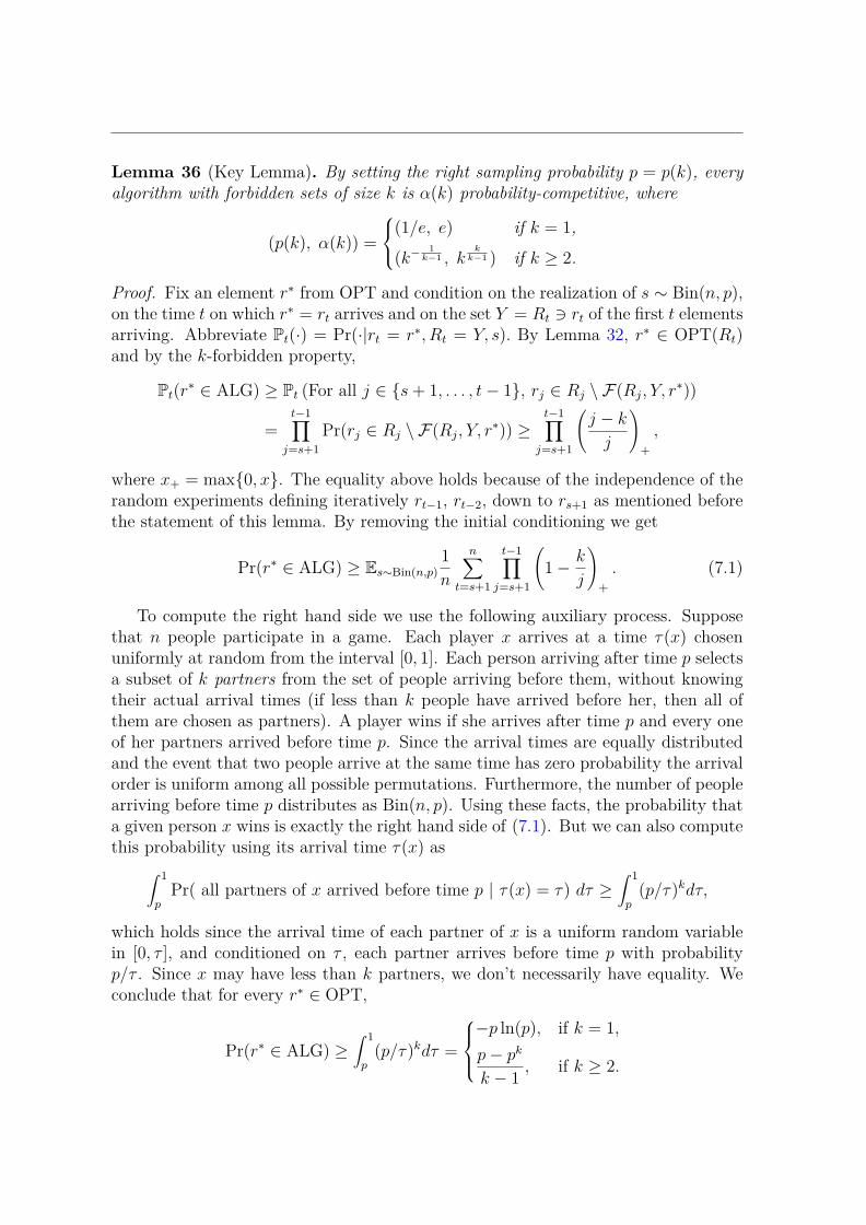
Lemma 36 (Key Lemma). By setting the right sampling probability p = p(k), everyalgorithm with forbidden sets of size k is –(k) probability-competitive, where

(p(k), –(k)) =

Y

]

[

(1/e, e) if k = 1,

(k≠ 1k≠1 , k

kk≠1 ) if k Ø 2.

Proof. Fix an element rú from OPT and condition on the realization of s ≥ Bin(n, p),on the time t on which rú = rt arrives and on the set Y = Rt – rt of the first t elementsarriving. Abbreviate Pt(·) = Pr(·|rt = rú, Rt = Y, s). By Lemma 32, rú œ OPT(Rt)and by the k-forbidden property,

Pt(rú œ ALG) Ø Pt (For all j œ s + 1, . . . , t ≠ 1, rj œ Rj \ F(Rj, Y, rú))

=t≠1Ÿ

j=s+1

Pr(rj œ Rj \ F(Rj, Y, rú)) Øt≠1Ÿ

j=s+1

A

j ≠ k

j

B

+

,

where x+ = max0, x. The equality above holds because of the independence of therandom experiments defining iteratively rt≠1, rt≠2, down to rs+1 as mentioned beforethe statement of this lemma. By removing the initial conditioning we get

Pr(rú œ ALG) Ø Es≥Bin(n,p)1

n

nÿ

t=s+1

t≠1Ÿ

j=s+1

A

1 ≠ k

j

B

+

. (7.1)

To compute the right hand side we use the following auxiliary process. Supposethat n people participate in a game. Each player x arrives at a time ·(x) chosenuniformly at random from the interval [0, 1]. Each person arriving after time p selectsa subset of k partners from the set of people arriving before them, without knowingtheir actual arrival times (if less than k people have arrived before her, then all ofthem are chosen as partners). A player wins if she arrives after time p and every oneof her partners arrived before time p. Since the arrival times are equally distributedand the event that two people arrive at the same time has zero probability the arrivalorder is uniform among all possible permutations. Furthermore, the number of peoplearriving before time p distributes as Bin(n, p). Using these facts, the probability thata given person x wins is exactly the right hand side of (7.1). But we can also computethis probability using its arrival time ·(x) as

⁄ 1

pPr( all partners of x arrived before time p | ·(x) = ·) d· Ø

⁄ 1

p(p/·)kd·,

which holds since the arrival time of each partner of x is a uniform random variablein [0, · ], and conditioned on · , each partner arrives before time p with probabilityp/· . Since x may have less than k partners, we don’t necessarily have equality. Weconclude that for every rú œ OPT,

Pr(rú œ ALG) Ø⁄ 1

p(p/·)kd· =

Y

_

]

_

[

≠p ln(p), if k = 1,

p ≠ pk

k ≠ 1, if k Ø 2.

Chapter 7

By optimizing the value of p as a function of k, we obtain that the probability ofrú œ ALG is 1/–(k), with –(k) as in the statement of the lemma and the probabilityachieving it is p = p(k).

The idea of analyzing an algorithm as a series of stochastically independent ex-periments which defines the reverse arrival sequence appears very early in the historyof the secretary problem. One can prove that the algorithm for the classical secretaryproblem, that samples s ≥ Bin(n, p(1)) elements and then selects the first elementbetter than all the sampled ones, is e probability-competitive. In fact, it has forbid-den sets of size 1. In our notation, for each (X, Y, rú) with rú the maximum elementof Y and X ™ Y ≠ rú, define the forbidden set F(X, Y, rú) as the singleton OPT(X).The 1-forbidden condition states that if the element rt arriving at time t is a record,that is, rt œ OPT(Rt), and if for every time j œ s + 1, . . . , t ≠ 1, rj ”œ OPT(Rj) (i.e.,the j-th arriving element is not a record), then rt will be chosen by the algorithm.Since all forbidden sets have size at most 1, setting the sampling probability to bep(1) = 1/e guarantees the probability-competitive ratio of –(1) = e.

edcba

321

Figure 7.1: Given a bipartite graph, in the transversal matroid a set of nodes on thebottom side is independent if there exists a matching covering them. The thick edgesa, 3, b, 1, c, 2 form a matching providing a witness for a, b, c.

Independence witness. It turns out that for many matroid classes there is a combi-natorial object that acts as certificate for testing independence. That is, a set X isindependent on a given matroid if and only if each element r œ X can be mapped toan object (e.g., an edge covering r, a path ending in r, a subgraph covering r, etc.) rsuch that the set X = r : r œ X satisfies a combinatorial property (e.g., a matchingcovering X, a collection of edge/node disjoint paths connecting X with some source,a collection of disjoint subgraphs covering X). We call X a witness for the indepen-dence of X. A set X may have multiple witnesses, but we will always assume thatthere is a canonical witness, witness(X), that can be computed by the algorithm andfurthermore, the choice of the witness cannot depend on the set of elements seen sofar nor on its arrival order. The fact that the witnesses do not depend on the arrivalorder makes them amenable to the analysis by the reverse arrival sequence analysisabove, which in turn, will help us to devise algorithms with constant-size forbiddensets.

73

Chapter 8

Matroids with small forbidden sets

In this chapter we show how to apply the forbidden sets technique to devise algorithmsfor different matroid families. The goal is to find algorithms having small forbiddensets. In particular, if an algorithm has constant size forbidden sets then this imme-diately implies that it is O(1) probability-competitive. We show this in many cases,such as transversal, graphic and laminar matroids. Other matroid families are con-sidered, and we obtain probability-competitive algorithms for all of them, beating thebest known ratios even for the weaker utility variant.

8.1 Transversal matroids and Gammoids

Let G = (L fi R, F ) be a bipartite graph with independent set L and R, where theelements of R are called the terminals of G. The transversal matroid T [G] associatedto G is the matroid with ground set R whose independent sets are those X ™ R thatcan be covered by a matching in G. We call G the transversal presentation of T [G].

edcba

321 L

R

Figure 8.1: Presentation of a transversal matroid with terminals R = a, b, c, d, e.The sets a, b, c and a, d, e are bases.

Let G = (V, E) be a digraph and two subsets S, R ™ V called sources and terminalsrespectively, not necessarily disjoint. The gammoid, Γ(G, S, R), is the matroid over

75

R, where X ™ R is independent if X is linked to S, that is, if there are node-disjointdirected paths from S and ending on each element of X. We say that (G, S, R) is thegammoid presentation of the matroid. Note that transversal matroids can be seen asgammoids by declaring all the non-terminals as sources and directing the arcs in thetransversal presentation from sources to terminals.

In the Transversal MSP, a transversal presentation G for an unknown orderedmatroid M = T [G] is either revealed at the beginning of the process, or it is re-vealed online in the following way. Initially, the algorithm only knows the number ofterminals. The terminals in R arrive in random order and whenever r œ R arrives,it reveals its ordinal value information and the set of its neighbors in G, which isa subset of L. In the gammoid MSP, a gammoid presentation (G, S, R) for an un-known gammoid is either revealed at the beginning or it is revealed online as elementsfrom R arrive: When a terminal r œ R arrives, all possible S-r paths are revealed.At that time, the algorithm has access to the subgraph Gt ™ G only containing thearcs belonging to every possible S-Rt path and can test whether a vertex is in S or not.

Exchangeability parameter for gammoids. Let us define a parameter to control thecompetitiveness of our algorithm for the gammoid MSP. Let X be an independent setand let Q be a path linking a terminal r œ R \ X outside X to S. The exchangeabilityµ of the presentation (G, S, R) is the maximum number of paths that Q intersects ina collection of S-X paths. The intuition behind is the following: in order to include Qinto the collection of paths while keeping disjointness we have to remove or exchangeat least µ paths from the collection. For instance, if we define the diameter d of thegammoid presentation as the maximum number of nodes in any source-terminal path,then µ is at most d. If furthermore the terminals are sinks, that is out-degree 0, thenµ is at most d ≠ 1, since paths ending at different terminals cannot intersect on aterminal.

Remark 37. This is the case for transversal matroids: their diameter in the gam-moid presentation is 2 and their exchangeability is 1. For our results, we assume thealgorithm also knows an upper bound µ for the exchangeability parameter, and in thiscase we call the problem µ-gammoid MSP or bounded exchangeability gammoid MSP.

Most of the known algorithms for transversal MSP [11, 32, 68] work with ordi-nal information. The best algorithm so far, by Kesselheim et al. [64] achieves anasymptotically optimal utility-competitive ratio of e + O(1/n) for the more general(non-matroidal) vertex-at-a-time bipartite online matching problem, in which edgesincident to the same arriving vertex may have different weights and the objective isto select a matching of maximum total weight. For the specific case of transversalmatroid this algorithm can be implemented in the ordinal model, meaning that ise + O(1/n) ordinal-competitive. Interestingly, for the broader bipartite matchingscase, Kesselheim’s algorithm does not work in the ordinal model, but the previousalgorithm by Korula and Pal [68] does, achieving 8 ordinal-competitiveness. A recent

8.1. Transversal matroids and Gammoids Chapter 8

result by Hoefer and Kodric [52] improves this factor to 2e ordinal-competiive for bi-partite matchings.

a b c d e

1

2 3 S

R

Figure 8.2: Presentation of a gammoid with terminals R = a, b, c, d, e and sourcesS = 1, 2, 3. The sets a, b, e and a, b, d are bases. The diameter of this gammoidpresentation is 4, then the exchangeability µ is at most 3.

The µ-gammoid MSP problem is a special case of the (non-matroidal) hypergraphvertex-at-a-time matching (HVM) with edges of size at most µ + 1 studied by Ko-rula and Pal [68] and later by Kesselheim et al.’s [64] online hypermatching problem(see the discussion in those papers for precise definitions). They achieve O(µ2) andeµ utility-competitiveness respectively. Below we propose an algorithm for the µ-gammoid MSP that has forbidden sets of size µ. Provided we know µ upfront we get an–(µ) probability-competitive algorithm. Note that for µ Ø 2, –(µ) = µ1+1/(µ≠1) < eµ,so our guarantee strictly improves on that of previous algorithms for HVM and hy-permatching, on the special case of µ-gammoids.

Our algorithms. We use the convention that for every vertex v covered by somematching M , M(v) denotes the vertex matched with v in M . Furthermore, for everyindependent set X ™ R, we select canonically a witness matching MX := witness(X)that covers X. In the case of gammoids, for any set P of node-disjoint paths linkingsome set X to S, and for every v œ X, P(v) denotes the unique path in P linking vto S. We also say that P covers a vertex u if u is in the union of the vertices of allpaths in P . Furthermore, for every independent set X ™ R, we canonically select afixed collection of node-disjoint S-X directed paths PX := witness(X) linking X to

77

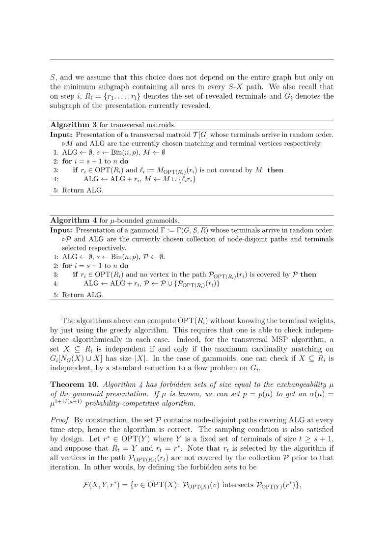
S, and we assume that this choice does not depend on the entire graph but only onthe minimum subgraph containing all arcs in every S-X path. We also recall thaton step i, Ri = r1, . . . , ri denotes the set of revealed terminals and Gi denotes thesubgraph of the presentation currently revealed.

Algorithm 3 for transversal matroids.

Input: Presentation of a transversal matroid T [G] whose terminals arrive in random order.ÛM and ALG are the currently chosen matching and terminal vertices respectively.

1: ALG Ω ÿ, s Ω Bin(n, p), M Ω ÿ2: for i = s + 1 to n do3: if ri œ OPT(Ri) and ¸i := MOPT(Ri)(ri) is not covered by M then4: ALG Ω ALG + ri, M Ω M fi ¸iri

5: Return ALG.

Algorithm 4 for µ-bounded gammoids.

Input: Presentation of a gammoid Γ := Γ(G, S, R) whose terminals arrive in random order.ÛP and ALG are the currently chosen collection of node-disjoint paths and terminalsselected respectively.

1: ALG Ω ÿ, s Ω Bin(n, p), P Ω ÿ.2: for i = s + 1 to n do3: if ri œ OPT(Ri) and no vertex in the path POPT(Ri)(ri) is covered by P then4: ALG Ω ALG + ri, P Ω P fi POPT(Ri)(ri)

5: Return ALG.

The algorithms above can compute OPT(Ri) without knowing the terminal weights,by just using the greedy algorithm. This requires that one is able to check indepen-dence algorithmically in each case. Indeed, for the transversal MSP algorithm, aset X ™ Ri is independent if and only if the maximum cardinality matching onGi[NG(X) fi X] has size |X|. In the case of gammoids, one can check if X ™ Ri isindependent, by a standard reduction to a flow problem on Gi.

Theorem 10. Algorithm 4 has forbidden sets of size equal to the exchangeability µof the gammoid presentation. If µ is known, we can set p = p(µ) to get an –(µ) =µ1+1/(µ≠1) probability-competitive algorithm.

Proof. By construction, the set P contains node-disjoint paths covering ALG at everytime step, hence the algorithm is correct. The sampling condition is also satisfiedby design. Let rú œ OPT(Y ) where Y is a fixed set of terminals of size t Ø s + 1,and suppose that Rt = Y and rt = rú. Note that rt is selected by the algorithm ifall vertices in the path POPT(Rt)(rt) are not covered by the collection P prior to thatiteration. In other words, by defining the forbidden sets to be

F(X, Y, rú) = v œ OPT(X) : POPT(X)(v) intersects POPT(Y )(rú),

8.2. Matroidal Graph Packings Chapter 8

the element rt is selected if rj ”œ F(Rj, Rt, rt) for all j œ s + 1, . . . , t ≠ 1. Bydefinition, each forbidden set has size at most µ.

Algorithm 3 is essentially Algorithm 4 applied over the gammoid presentation ofthe transversal matroid T [G]. Together with Remark 37, it follows the result for thetransversal MSP.

Theorem 11. Algorithm 3 has forbidden sets of size 1, and therefore, by choosingp = 1/e, it is an (optimal) e probability-competitive for transversal matroids.

We remark that every constant utility-competitive algorithm so far known fortransversal MSP requires to learn a bipartite presentation online. It is an open problemto find constant competitive algorithms for transversal matroids that only access thematroid via an independence oracle.

8.2 Matroidal Graph Packings

Let H be a finite set of graphs. An H-packing of a host graph G = (V, E) is a collectionQ = Hii=1...k of node-disjoint subgraphs of G such that each H œ Q is isomorphic tosome graph in H. A vertex in G is said to be covered by Q if it belongs to some graphof Q. Let R ™ V be a set of vertices called terminals and consider the independencesystem M(R, G, H) over R whose independent sets are all X ™ R for which thereis an H-packing covering X in G. We say that H is matroidal if M(V (G), G, H)defines a matroid for every graph G. Note that in this case, if M(R, G, H) is therestriction of M(V (G), G, H) to a subset R, then it is also a matroid. We call everysuch M(R, G, H) a graph packing matroid.

a

b

cd

e

f

g

hi

j

Figure 8.3: The Petersen graph (V, E). In the matching matroid M(V, G, K2), theset a, g, d is independent since it is covered by the matching a, g, g, b, c, d.

79

Matroidal families. For an extensive treatment see Loebl and Poljak [76], Janata [58]and the references therein. In the following examples, Kn denotes the complete graphon n vertices and Sn denotes the star with n legs. If H = K1 then M(V, G, H) isthe free matroid over V where all sets are independent. If H = K2 then M(V, G, H)is the matching matroid of G, whose independent sets are all vertex sets that can becovered by a matching. If for some k the family H = S1, S2, . . . , Sk is a sequentialset of stars, then M(V, G, H) is matroidal. It is, in fact, the matroid union of manymatching matroids. The family M(V, G, H) is also matroidal if H = K2, H whereH is either a factor-critical graph or a 1-propeller.1 For most known matroidal classesthere are polynomial time algorithms available to check independence. This is thecase for all classes above. Observe that transversal matroids are instances of matchingmatroids restricted to one side of the bipartition of the host graph.

As we did for gammoids, we also define an exchangeability parameter µ to controlthe competitiveness of our algorithm. Consider an H-packing Q of G, and a subgraphH ™ G from the class H covering a terminal r œ R that is not covered by Q. Theexchangeability µ of M(R, G, H) is the maximum number of terminals over all suchQ and H that would become uncovered if we removed all graphs from Q that intersectH, namely,

µ := max

Y

]

[

ÿ

HÕœQ : V (H)flV (HÕ) ”=ÿ

|V (H Õ) fl R| : H covers a terminal not covered by Q

Z

^

\

.

This parameter may be complicated to compute but there is a simple upper bound:let h be the maximum number of vertices of a graph from H. Then the worst possiblesituation occurs when Q contains only graphs of size h, and H is also a graph of size hintersecting every graph in Q on exactly one vertex (different from r). In this case, allgraphs from Q must be removed, so the number of newly uncovered vertices becomesh · (h ≠ 1). This means that µ Æ h(h ≠ 1).

In the H-Packing MSP, the algorithm receives a collection H of graphs. A hostgraph G = (V, E) with terminals R ™ V is either revealed at the beginning or it isrevealed online as elements from R arrive: when a terminal r œ R arrives, all possibleedges that belong to a graph H ™ G with r œ V (H) with H œ H (via isomorphism)are revealed. More precisely, let Rt denote the set of terminals revealed up to time t.At that time the algorithm has access to the subgraph Gt ™ G induced by all verticesbelonging to every possible subgraph H ™ G, with H œ H that intersects Rt. Thealgorithm can also test whether a vertex is a terminal or not. We also assume thatan upper bound µ for the exchangeability parameter is available, and in this case wecall the problem bounded H-packing MSP. Analogously to previous sections, for everyindependent X we select a canonical packing QX := witness(X) that does not dependon the arrival order.

In the description of the algorithm we use the convention that for every H-packingQ of a set X, and for every v œ V covered by Q, Q(v) denotes the unique graph in Q

1A factor-critical graph is one such that H ≠ x admits a perfect matching for all x œ V (H). A1-propeller is a graph having a leaf r, and a vertex c such that for every x œ V (H) ≠ c, H ≠ x admitsa perfect matching.

8.2. Matroidal Graph Packings Chapter 8

covering v. We also recall that on step i, Ri = r1, . . . , ri denotes the set of revealedterminals and Gi denotes the subgraph of the presentation currently revealed.

Algorithm 5 for µ bounded H-packing matroids.

Input: A matroidal family H and a host graph G = (V, E) whose terminals R ™ V arrivein random order.

Û Q and ALG are the currently chosen H-packing and terminals selected respectively.1: ALG Ω ÿ, s Ω Bin(n, p), Q Ω ÿ.2: for i = s + 1 to n do3: if ri œ OPT(Ri) and ri is already covered by Q. then4: ALG Ω ALG + ri.5: else if ri œ OPT(Ri) and Q fi QOPT(Ri)(ri) is an H-packing. then6: ALG Ω ALG + ri, Q Ω Q fi QOPT(Ri)(ri).

7: Return ALG.

The algorithm can compute OPT(Ri) without knowing the terminal weights, byapplying the greedy algorithm for M(R, G, H).

Theorem 12. Algorithm 5 has forbidden sets of size equal to the exchangeability µof the H-presentation. If µ is known beforehand, we can set p = p(µ) to obtainan –(µ) = µ1+1/(µ≠1) probability-competitive algorithm for µ-bounded graph packingmatroids.

Proof. Correctness and the sampling condition for forbidden sets are satisfied by de-sign. Now let rú œ OPT(Y ) where Y is a fixed set of terminals of size t Ø s + 1, andsuppose that Rt = Y and rt = rú. Terminal rt is selected by the algorithm if eitherQ already covers it on arrival, or if all vertices in the graph QOPT(Rt)(rt) were notcovered by graphs in Q prior to that iteration. In any case by defining as forbiddensets

F(X, Y, rú) = v œ OPT(X) : V (QOPT(X)(v)) intersects V (QOPT(Y )(rú)) \ rú,

we have that rt is selected if rj ”œ F(Rj, Rt, rt) for all j œ s + 1, . . . , t ≠ 1. Bydefinition, each forbidden set has size at most µ.

We remark that the competitiveness achievable by an algorithm heavily dependson the way the matroid is presented. For instance, consider a matching matroidM with host graph G = (V, E). Note that the exchangeability of this matroid isµ Æ 2(2 ≠ 1) = 2. If the graph is presented online then we can use the previousalgorithm to obtain an –(2) = 4 probability-competitive algorithm. If on the otherhand the graph is presented upfront, then we can use the fact that every matchingmatroid is transversal [36] to construct a transversal presentation of M and thenapply our e probability-competitive algorithm using that presentation.

81

8.3 Graphic and Hypergraphic Matroids

The graphic matroid M[G] = (R, I) associated to a graph G = (V, R) is the one whoseindependent sets are all the subsets of edges X ™ R such that (V, X) is a forest. Thehypergraphic matroid M[G] associated to a hypergraph G = (V, R), whose edges maybe incident to any number of vertices, is the matroid over R whose independent setsX ™ R are those, for which one can canonically choose for every r œ X an edgedenoted by edge(r, X) = u(r)v(r) in KV = (V,

1

V2

2

) with both endpoints in r in such

a way that all edge(r, X), for r œ X are different, and the collection edge(X) =edge(r, X) : r œ X is a forest [77]. If all the edges of the hypergraph have size 1 or2 we are back in the graphic case.

One can check that the hypergraphic matroid M[G] = (R, I) is the matroid

induced from the graphic matroid M[KV ] via the bipartite graph (R fi1

V2

2

, E) with

ef œ E if f ™ e. In other words, X is independent in the hypergraphic matroid M[G]if edge(X) is independent in the graphic matroid M[KV ]. Moreover, if G is alreadya graph, edge(X) = X and edge(r, X) = r for all r œ X.

a

c

d

b

e

f

g

h

i

j

k a

c

d

b

e

f

g

h

i

j

k

Figure 8.4: Canonical orientation (at the right) of the forest at the left.

In the graphic MSP/hypergraphic MSP we assume that the underlying graph orhypergraph G of a matroid M[G] is either revealed at the beginning or revealed onlinein the natural way: we learn edges as they arrive. Let X ™ R be an independent set.By orienting each connected component of the forest edge(X) from an arbitrary root,we obtain a canonical orientation arc(X) of edge(X) (for convenience, we denote byarc(e, X) the oriented version of edge(e, X)) with indegree deg≠

arc(X)(v) Æ 1 for everyvertex v. The converse is almost true in the following sense. If A is a set of arcs(maybe including loops) such that deg≠

A(v) Æ 1 for every vertex then the underlyinggraph is not necessarily a forest in KV , but a pseudoforest: every connected compo-nent contains at most 1 cycle, which is directed. In fact, the edge sets of pseudoforestof a given graph J are exactly the independent set of the so called bicircular matroidof J . This matroid is transversal with presentation H, where V (H) = V (J) fi E(J)and ve œ E(H) if and only if e is incident to v. This is the starting point for ouralgorithm for graphic matroids.

The algorithm. The plan is to only consider edges that belong to the current optimum.Furthermore, if we select an edge, then we orient it and include it into an arc set Awith the property that each vertex has maximum in-degree 1. Instead of using a

8.3. Graphic and Hypergraphic Matroids Chapter 8

random orientation (as in the algorithms by Korula and Pal [68] or Soto [96]), atevery step we use the canonical orientation of the current optimum forest. In orderto avoid closing a cycle we also impose that an arc (u, v) can not be added to A ifdeg≠

A(u) = 1 or deg≠A(v) = 1. The same algorithm works on hypergraphic matroids

if we replace each independent set X on the hypergraphic matroid by its associatedforest edge(X). We also recall that on step i, Ri = r1, . . . , ri denotes the set ofrevealed edges. The algorithm is fully described below.

Algorithm 6 for graphic or hypergraphic matroids.

Input: A hypergraphic matroid M[G] with underlying hypergraph G = (V, R), whose edgesarrive in random order.

Û ALG and A are the currently selected independent set and the orientation of itsassociated forest.

1: ALG Ω ÿ, s Ω Bin(n, p), A Ω ÿ.2: for i = s + 1 to n do3: if ri œ OPT(Ri) then4: Let ai = (ui, vi) be the canonical orientation of edge(ri, OPT(Ri)).5: if deg≠

A(ui) = 0 = deg≠A(vi) then

6: ALG Ω ALG + ri, A Ω A + ai

7: Return ALG.

Theorem 13. Algorithm 6 has forbidden sets of size 2. By setting p = p(2) = 1/2,we get an –(2) = 4 probability-competitive algorithm for both graphic and hypergraphicmatroids.

Proof. We first prove that the edge set A obtained from A by removing its orientationis acyclic. Suppose by contradiction that at the end of some step i, A contains for thefirst time a set C such that its unoriented version C is an undirected cycle. Since this isthe first time a cycle appears, ri must be selected and ai = (ui, vi) must be contained inC. Since ai is included in A, we know that after its inclusion, deg≠

A(vi) = deg≠C(vi) = 1

(before its inclusion, the indegree of vi was 0) and that deg≠A(ui) = deg≠

C(ui) = 0. Butsince C is a cycle the outdegree of ui is deg+

C(ui) = 2 ≠ deg≠C(ui) = 2. But then, there

must be another vertex x in C with indegree 2. This cannot happen because at everymoment the indegree of each vertex is at most 1.

The proof above guarantees correctness of the algorithm: for the graphic case,we have A = ALG and for the hypergraphic case, each edge ri of ALG is mappedto edge(ri, OPT(Ri)) œ A which form a forest. In both cases we conclude ALG isindependent.

Since the sampling condition is satisfied by design, we only need to prove the2-forbidden condition. Let rú œ OPT(Y ) where Y is an arbitrary set of t Ø s + 1edges, and suppose that Rt = Y and rt = rú. The algorithm would then define anarc at = (ut, vt) and will proceed to add rt to ALG provided that no arc aj = (uj, vj)considered before has head vj equal to ut or vt. In other words, by defining

F(X, Y, rú) =Ó

f œ OPT(X) : arc(f,OPT(X)) is not orientedtowards any endpoint of edge(rú,OPT(Y ))

Ô

83

then rt is selected if rj ”œ F(Rj, Rt, rt) for all j œ s + 1, . . . , t ≠ 1. Moreover,since each arc set arc(OPT(X)) = arc(f, OPT(X)) : f œ OPT(X) has maximumindegree 1, there are at most 2 arcs in arc(OPT(X)) oriented towards an endpoint ofedge(rú, OPT(Y )). So each forbidden set has size at most 2.

8.4 Column Sparse Representable Matroids

An interesting way to generalize graphic matroids is via their matrix representation.We say that a matroid M is represented by a m ◊ n matrix M with coefficients ina field F if we can bijectively map the elements of its ground set to the columns ofM in such a way that the independent sets of M are in correspondence with the setsof columns that are linearly independent in F

m. Graphic matroids are representableby their adjacency matrix interpreted in GF (2). In fact they can be represented inany field. Matroids that have this property are called regular. Note that each graphicmatroid is representable by a very sparse matroid: each column has only 2 non-zeroelements.

Following [96] we say that a matroid is k column sparse representable if it admitsa representation whose columns have at most k nonzero entries each. These matroidsinclude many known classes such as graphic matroids (k = 2), rigidity matroids[101] on dimension d (k = 2d) and more generally matroids arising from rigiditytheory from d-uniform hypergraphs. These matroids are called (k, ¸)-sparse matroids(where 0 Æ ¸ Æ kd ≠ 1), and they are, using our notation, kd column sparse [97].Interesting cases include generic bar-joint framework rigidity in the plane [71], whichare characterized by (2, 3)-sparse matroids in dimension d = 2 (they are 4 columnsparse) and generic body-bar framework rigidity in R

d which are characterized by

(1

d+12

2

,1

d+12

2

)-sparse matroids [98] (they are d1

d+12

2

column sparse).

S

W

W

W

W

U

a,b a,c a,d b,c b,d c,d

a 1 1 1 0 0 0b 1 0 0 1 1 0

c 0 1 0 1 0 1

d 0 0 1 0 1 1

T

X

X

X

X

V

a

b

c d

Figure 8.5: Representation of the graphic matroid in the graph K4. The columnsrepresenting the tree a, b, a, c, c, d are linearly independent.

Let M be a matroid with k sparse representation M and let X be an indepen-dent set of columns. It is easy to show (see e.g., [96]) that we can select one nonzerocoordinate from each column in X such that no two selected entries lie on the same

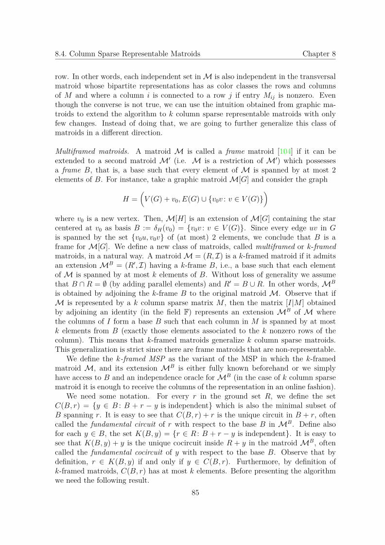
8.4. Column Sparse Representable Matroids Chapter 8

row. In other words, each independent set in M is also independent in the transversalmatroid whose bipartite representations has as color classes the rows and columnsof M and where a column i is connected to a row j if entry Mij is nonzero. Eventhough the converse is not true, we can use the intuition obtained from graphic ma-troids to extend the algorithm to k column sparse representable matroids with onlyfew changes. Instead of doing that, we are going to further generalize this class ofmatroids in a different direction.

Multiframed matroids. A matroid M is called a frame matroid [104] if it can beextended to a second matroid MÕ (i.e. M is a restriction of MÕ) which possessesa frame B, that is, a base such that every element of M is spanned by at most 2elements of B. For instance, take a graphic matroid M[G] and consider the graph

H =3

V (G) + v0, E(G) fi v0v : v œ V (G)4

where v0 is a new vertex. Then, M[H] is an extension of M[G] containing the starcentered at v0 as basis B := ”H(v0) = v0v : v œ V (G). Since every edge uv in Gis spanned by the set v0u, v0v of (at most) 2 elements, we conclude that B is aframe for M[G]. We define a new class of matroids, called multiframed or k-framedmatroids, in a natural way. A matroid M = (R, I) is a k-framed matroid if it admitsan extension MB = (RÕ, I) having a k-frame B, i.e., a base such that each elementof M is spanned by at most k elements of B. Without loss of generality we assumethat B fl R = ÿ (by adding parallel elements) and RÕ = B fi R. In other words, MB

is obtained by adjoining the k-frame B to the original matroid M. Observe that ifM is represented by a k column sparse matrix M , then the matrix [I|M ] obtainedby adjoining an identity (in the field F) represents an extension MB of M wherethe columns of I form a base B such that each column in M is spanned by at mostk elements from B (exactly those elements associated to the k nonzero rows of thecolumn). This means that k-framed matroids generalize k column sparse matroids.This generalization is strict since there are frame matroids that are non-representable.

We define the k-framed MSP as the variant of the MSP in which the k-framedmatroid M, and its extension MB is either fully known beforehand or we simplyhave access to B and an independence oracle for MB (in the case of k column sparsematroid it is enough to receive the columns of the representation in an online fashion).

We need some notation. For every r in the ground set R, we define the setC(B, r) = y œ B : B + r ≠ y is independent which is also the minimal subset ofB spanning r. It is easy to see that C(B, r) + r is the unique circuit in B + r, oftencalled the fundamental circuit of r with respect to the base B in MB. Define alsofor each y œ B, the set K(B, y) = r œ R : B + r ≠ y is independent. It is easy tosee that K(B, y) + y is the unique cocircuit inside R + y in the matroid MB, oftencalled the fundamental cocircuit of y with respect to the base B. Observe that bydefinition, r œ K(B, y) if and only if y œ C(B, r). Furthermore, by definition ofk-framed matroids, C(B, r) has at most k elements. Before presenting the algorithmwe need the following result.

85

Lemma 38. Let X be an independent set of a k-framed matroid M with k-frame B.There is a (canonical) injection fiX : X æ B such that B + x ≠ fiX(x) is independentfor all x œ X.

Proof. Extend X to a base X Õ of MÕ. By the strong basis exchange axiom there is abijection fi : X Õ æ B such that B + x ≠ fi(x) is a base for all x œ X Õ. The restrictionof fi to X yields the desired injection.

Algorithm 7 for k-framed matroids.

Input: A k-frame matroid M, with independence oracle access to MB and to B. Theelements of M arrive in random order.

Û ALG is the set currently selected and BÕ is the set of elements of the frame B thathave been marked.

1: ALG Ω ÿ, s Ω Bin(n, p), BÕ Ω ÿ.2: for i = s + 1 to n do3: if ri œ OPT(Ri) and C(B, ri) fl BÕ = ÿ then4: ALG Ω ALG + ri, BÕ Ω BÕ + fiOP T (Ri)(ri)

5: Return ALG.

Theorem 14. Algorithm 7 has forbidden sets of size k. By setting p = p(k), we getan –(k) probability-competitive algorithm for k-framed matroids.

Proof. Suppose that the algorithm is not correct, and let Z = ri(1), ri(2), . . . , ri(¸)be a circuit in ALG with s + 1 Æ i(1) Æ i(2) Æ · · · Æ i(¸). When ri(1) arrived, y :=fiOPT(Ri(1))(ri(1)) œ C(B, ri(1)) was marked. Furthermore, our algorithm guaranteesthat for every element ri œ ALG with i > i(1), y ”œ C(B, ri). In particular, y œC(B, ri(j)) if and only if j = 1, or equivalently, K(B, y)flZ = ri(1). But this impliesthat the circuit Z and the cocircuit K := K(B, y) + y intersect only in one element,which cannot happen in a matroid. Therefore, the algorithm is correct.

Since the sampling condition is satisfied by design, we only need to prove thek-forbidden condition. Let rú œ OPT(Y ) where Y is an arbitrary set of t Ø s + 1elements, and suppose that Rt = Y and rt = rú. The algorithm accepts rú if and only ifno element of C(B, rt) was marked before. Let y œ C(B, rt) be an arbitrary element.A sufficient condition for y not being marked at step j is that fiOPT(Rj)(rj) ”= y.Therefore, if we define the forbidden sets

F(X, Y, rú) = f œ OPT(X) : fiOPT(X)(f) œ C(B, rú)

it is clear that rt is selected if rj ”œ F(Rj, Rt, rú) for all j œ s+1, . . . , t≠1. Moreover,since fiOPT(X) is injective we conclude that |F(X, Y, rú)| Æ |C(B, rú)| Æ k.

8.5 Laminar Matroids and Semiplanar Gammoids

In this section we define special classes of gammoids amenable for our techniques.An arc-capacitated gammoid (ACG) M[N ] is defined by a directed network N =

8.5. Laminar Matroids and Semiplanar Gammoids Chapter 8

(G, o, R, c) where G = (V, E) is a digraph, o œ V is a single source, R ™ V \ o is acollection of terminals and c : E æ Z

+ is a strictly positive integer capacity functionon the arcs of G. The ground set of M[N ] is R and every set J ™ R is independent ifand only if there exist an o-R flow on N satisfying the capacity constraints on the arcsand where each j œ J receives one unit of flow. Without loss of generality we assumethat every terminal is reachable from o via a directed path. It is easy to see thatACGs are equivalent to gammoids without loops, but they are more closely related totransportation or distribution applications.

A semiplanar gammoid is an ACG whose digraph G admits a semiplanar drawing,which is a planar drawing where all terminals are on the x-axis, the source node ison the positive y-axis, and the rest of the graph (arcs and nodes) are strictly abovethe x-axis, in a way that they do not touch the infinite ray starting upwards from thesource node. It is easy to see that G admits a semiplanar drawing if and only if itis planar and all the terminals and the source are contained in the same face (whichcould be a cycle, a tree or more generally, a pseudoforest).

Laminar Matroids. An important example of semiplanar gammoids are laminar ma-troids. A collection L of non-empty subsets of a finite set of terminals R is calledlaminar if for every L, H œ L, L fl H œ L, H, ÿ. The laminar matroid M[R, L, c],where L is a laminar family over R and c : L æ Z

+ is a positive integer capacityfunction on the sets of L, is the matroid with ground set R and whose independentsets are those X ™ R for which the number of elements that X contains in any setof the laminar family does not exceed its capacity, i.e. |X fl L| Æ c(L). Observethat, since c is positive, every singleton is independent. Furthermore, without loss ofgenerality we assume that R œ L (with c(R) equal to the rank of the matroid) andthat all singletons are in L (with c(r) = 1 for each r œ R). Adding those sets doesnot destroy laminarity.

b c d ea f g h

Figure 8.6: Laminar family.

The Hasse diagram of the containment order of L forms a tree T Õ where every setin L is a child of the smallest set in L that strictly contains it. Note that the leavesof T Õ are in bijection with the terminals, and that the root (unique maximum) vR

represents R. Consider the directed graph G obtained by adding an auxiliary vertexo to T Õ connected to vR and orienting the tree away from o. If we put o on the uppersemiaxis, draw G with all arcs pointing downwards, and assign capacities to each arcequal to the capacity of the laminar set associated to the arc’s head, then we obtaina semiplanar representation of M[R, L, c]. Furthermore, the terminals in R appear in

87

the x-axis in the left-to-right order induced by the drawing of the tree.

Semiplanar drawings and neighbours. In what follows we fix a semiplanar drawingG of a semiplanar gammoid M[N ]. We identify R with the set [n] by labeling theterminals from left to right as they appear in the x-axis. For convenience in the restof the presentation, we add to G two auxiliary nodes on the x-axis, 0 and n+1, where0 is located to the left of 1, and n + 1 is located to the right of n, together with thearcs o0 and o(n + 1). Observe that by our assumptions on the drawing, it is possibleto add those arcs without destroying semiplanarity.

For any set J ™ [n] and any y œ J fi 0, n + 1, we denote by LeftJ(y) the closestelement to y in J fi0 that is located strictly to its left (understanding LeftJ(0) = 0).Similarly, we denote by RightJ(y) the first element in J fi n + 1 located to the rightof y (understanding RightJ(n + 1) = n + 1). For y œ [n] \ J , we call LeftJ+y(y) andRightJ+y(y) its left and right neighbors in J (note that they maybe equal to 0 or n+1and thus are not necessarily elements of J).

Ancestors, tree-order and representatives. In the future we will map each terminaloutside an independent set J to one or more of its neighbors in J . For the case inwhich G is a tree (i.e., for laminar matroids) we want to consistently assign eachelement to just one of them. We do this as follows. For every pair of nodes x, y in G,let xGy be the unique undirected x-y path in G. We say that x is an ancestor of y(and y is a descendant of x) if oGy contains oGx; in that case we denote x ˆ y (andy ı x). Note that (V, ı) is a partial order, and in fact, it is a join-semilattice wherex ‚ y is the lowest common ancestor of x and y. Note that by our drawing choice, forany i œ [j, jÕ] ™ [0, n + 1] we have i ı j ‚ jÕ. In particular, if [j, jÕ] ™ [k, kÕ] ™ [0, n + 1]then j ‚ jÕ ı k ‚ kÕ.

For every nonempty set J ™ [n], and for every terminal y œ [n], we define itsrepresentantive fiJ(y) in J such that

fiJ(y) =

Y

_

_

]

_

_

[

y if y œ J ,

LeftJ+y(y) if y œ [n] \ J and y ‚ LeftJ+y(y) @ y ‚ RightJ+y(y),

RightJ+y(y) if y œ [n] \ J and y ‚ LeftJ+y(y) ˆ y ‚ RightJ+y(y).

This element is well defined since for all y œ [n] \ J , both y ‚ LeftJ+y(y) andy ‚ RightJ+y(y) belong to oGy and so one is an ancestor of the other. Observethat fiJ(y) is never equal to 0 (because then o = 0 ‚ y @ RightJ+y(y) ‚ y which is acontradiction as o is the root), nor n+1 (because then o = (n+1)‚y ı LeftJ+y(y)‚y ıvR @ o). In particular, fiJ(y) œ LeftJ+y(y), y, RightJ+y(y) fl J . A graphical wayto understand the definition of the representative of an element y outside J is thefollowing: let j and jÕ be the left and right neighbors of y in J respectively and calloGj and oGjÕ the left and right paths respectively. The representative of y is its leftneighbor (respectively, its right neighbor) if and only if by starting from y and walkingup on G against its orientation, the first path hit is the left path (respectively theright path). In case of a tie, the representative is the right neighbor (see Figure 8.7).

8.5. Laminar Matroids and Semiplanar Gammoids Chapter 8

1 1513 14876540 18112 3 169 10 12 17

22

3

2

4

2 2

3

5

Figure 8.7: Semiplanar drawing of a laminar matroid with ground set [17]. Nonunit arccapacities are shown. Below we show the partition (fiJ(j))jœJ induced by the independentset J = 3, 5, 10, 13, 15.

We claim also that for every j œ J , the set of elements to its right having j asrepresentative is an interval of the form [j, k] with k < RightJ(j). Indeed, this is trueif RightJ(j) = n + 1. Suppose now that jÕ := RightJ(j) Æ n, and that the claimdoes not hold. Then, there must be two consecutive terminals i, i + 1 œ [j, jÕ] withfiJ(i + 1) = j and fiJ(i) = jÕ. But then, we get the following contradiction:

(i + 1) ‚ jÕ ı i ‚ jÕ ı i ‚ j ı (i + 1) ‚ j @ (i + 1) ‚ jÕ

where the first inequality holds since [i+1, jÕ] ™ [i, jÕ], the second, by the definition offiJ(i), the third since [j, i] ™ [j, i + 1] and the fourth by definition of fiJ(i + 1). Sinceevery element in (j, jÕ) either has j or jÕ as representative, we conclude, in fact, thatthe entire set fi≠1

J (j) of elements with j as representative is an interval of terminalsenclosing j but strictly contained in [LeftJ(j), RightJ(j)]. In other words (fiJ(j))jœJ

is a partition of [n] into |J | intervals.

The algorithms. In what follows we describe our algorithms for semiplanar gammoidsand laminar matroids. Apart from some special case occurring when the sample isempty, our algorithms are extremely simple. Each one computes the optimal solutionOPT(Rs) of the sample and leave their elements unmarked. When a terminal ri that ispart of the current optimum arrives, it checks if the (closest neighbors / representative)of ri in OPT(Rs) (are / is) unmarked. If so, it marks (them / it) and selects ri aspart of the solution.

89

Algorithm 8 for semiplanar gammoids.

Input: An semiplanar gammoid with a fixed semiplanar drawing1: ALG Ω ÿ, s Ω Bin(n, p),2: if s = 0 then3: ALG Ω r14: else B Ω ÿ.5: for i = s + 1 to n do6: if ri œ OPT(Ri), LeftOPT(Rs)+ri

(ri) ”œ B and RightOPT(Rs)+ri(ri) ”œ B then

7: ALG Ω ALG + ri, andB Ω B fi LeftOPT(Rs)+ri

(ri), RightOPT(Rs)+ri(ri)

8: Return ALG.

Algorithm 9 for laminar matroids.

Input: A laminar matroid with a fixed semiplanar drawing1: ALG Ω ÿ, s Ω Bin(n, p),2: if s = 0 then3: ALG Ω r14: else B Ω ÿ.5: for i = s + 1 to n do6: if ri œ OPT(Ri) and fiOPT(Rs)(ri) ”œ B then7: ALG Ω ALG + ri, and

B Ω B fi fiOPT(Rs)(ri).

8: Return ALG.

Theorem 15. Algorithm 8 has forbidden sets of size 4. By setting p = p(4) =3

Ò

1/4 we get an –(4) = 44/3 ¥ 6.3496 probability-competitive algorithm for semiplanarACGs.

The previous result applied to laminar matroids already beat the best guaranteesknown for that class (9.6 [79] and 3

Ô3e [56, 57]). But we can do better for laminar

matroids since for those, there is a unique path from the source to each terminal.

Theorem 16. Algorithm 9 has forbidden sets of size 3. By setting p = p(3) =Ò

1/3

we get an –(3) = 3Ô

3 probability-competitive algorithm for laminar matroids.

We observe that this algorithm is very similar to the 3Ô

3e competitive algorithmof Jaillet et al. [56, 57]. Note that the partition of the terminals given by fiOPT(Rs)

induces a unitary partition matroid P Õ. After the sample, Algorithm 9 simply selectson each part, the first arriving element that is part of the current optimum. It canbe shown that the partition matroid P Õ we define is the same as the one definedin [57, Section 3.2]. The main algorithmic difference is that in [57], the authors usethe algorithm for the classic secretary problem to select one terminal on each partthat has constant probability of being the largest element. Instead, we select the first

8.5. Laminar Matroids and Semiplanar Gammoids Chapter 8

arriving element on each part that is part of the optimum at the time of arrival. Thissmall change makes the competitive ratio of our algorithm e times smaller than theirs,but the analysis is more involved. To prove Theorems 15 and 16 we need to developsome extra tools.

For every nonempty independent set J ™ [n] in the semiplanar gammoid M[N ] wechose an arbitrary but fixed integral o-J flow fJ satisfying the arc capacity constraintsand saturating J . Define the unit capacity network N1(J) = (G1(J), o, R, 1), whereG1(J) is obtained from G by splitting each arc uv with fJ(uv) Ø 2 into fJ(uv) parallelarcs (we keep all arcs uv with fJ(uv) œ 0, 1, we also keep the arcs o0 and o(n + 1)).We do this in such a way that G1(J) is still semiplanar. The matroid M[N1(J)] isthe unit capacity semiplanar gammoid associated to J .

Observe that every path in G1(J) corresponds canonically to an unsplitted pathin G going through the same nodes. Furthermore, every arc-disjoint collection P ofo-R paths in G1(J) can be regarded, by unsplitting parallel arcs, as an o-R flow f onG such that each arc e œ E(G), satisfies f(e) Æ fJ(e) Æ c(e). Therefore, we have thefollowing important lemma.

Lemma 39. Any independent set in M[N1(J)] is also independent in the originalmatroid M[N ].

We say that two paths P and Q in the drawing of a graph cross if P enters Q onthe left, shares zero or more arcs with Q and then exits Q on the right, or viceversa.A collection of paths is mutually noncrossing if no pair of them cross.2 The o-Jflow fJ in the network N can be mapped to an o-J flow f 1

J in N1(J) in a naturalway. By applying flow-decomposition on f 1

J we get a collection P kkœJ of arc-disjointpaths. Define also P 0 and P n+1 as the paths consisting of a single arc o0 and o(n+1)respectively. By a standard planar uncrossing argument, we can assume that all pathsin P kkœJfi0,n+1 are mutually noncrossing (but they can still share internal nodes,in fact all paths P k with k œ J contain o and vR, see Figure 8.8). For j œ J + 0, calljÕ = RightJ+0(j) and define the collection of arcs Aj ™ E(G1(J)) as those that aredrawn in the closed planar region Rj bounded by P j, P jÕ

and the x-axis. Since pathsP kkœJfi0,n+1 form a topological star whose tips are in the x-axis we conclude thatRkkœJ+0 is a division of the region bounded by P 0, P n+1 and the x-axis, and thusAkkœJ+0 is a covering of all arcs in G1(J). In fact, if 1 Æ jÕ ”= n + 1, then every arcof P jÕ

belongs to pieces Aj and AjÕ

, while each arc in G1(J) \ P kkœJ belongs to asingle piece of the covering. Furthermore, the only terminals contained in region Rj

are those in [j, jÕ].

Lemma 40. Let y œ [n] \ J , and j = LeftJ+y(y), jÕ = RightJ+y y be its neighborsin J . Then there is a directed o-y path DJ(y) in G1(J) whose arc set is completely

2An alternative way to understand this definition is to imagine that in the drawing nodes andarcs have positive area (they are circles and thick lines). A drawing of a path is any continuous non-self-intersecting curve drawn inside the union of all circles and thick lines associated to the nodesand arcs of P visiting them in the correct order. A collection of paths are mutually noncrossing ifwe can find drawings such that no pair of them intersects. Note that two noncrossing paths can stillshare arcs and nodes.

91

1 12116540 1492 3 137 8 10

3

2

1 12116540 1492 3 137 8 10

Figure 8.8: On the left, a flow fJ associated to the independent set J = 1, 4, 6, 11 ona semiplanar gammoid M[N ] with ground set R = [13] (0 and 14 are auxiliary nodes). Onthe right, M[N1(J)] and the partition of the drawing into regions R0, R1, R4, R6 and R11

induced by the paths P jjœJfi0,14. The regions R0, R4 and R11 are shaded.

8.5. Laminar Matroids and Semiplanar Gammoids Chapter 8

contained in Aj. Furthermore, DJ(y) can be chosen so that it arcs-intersects at mostone path P in (P k)kœJ . In the semiplanar case, P must be one of P j and P jÕ

, and inthe laminar case, P = P fiJ (¸).

Proof. Note that y œ [j, jÕ] is in the planar region Rj. Since y is reachable from o inG, there is a path Q from o to y in G1(J). Let v be the last vertex in Q contained inthe vertices of P j and P jÕ

(v maybe in one or both paths), say v is in P œ P j, P jÕ

.By concatenating the initial piece of P from o to v and the final piece of Q from v toy we get a path DJ(y) that is completely contained in Aj and that intersects the arcsof at most one path in Pj, PjÕ.

Consider the same situation in the laminar case. All arcs in P j, P jÕ

and Q aresplitted versions of arcs in oGj, oGjÕ and oGy respectively. The vertex v definedabove satisfies v = y ‚ j ‚ jÕ. If y ‚ j @ y ‚ jÕ then v = y ‚ j, fiJ(y) = j and we canconstruct DJ(y) avoiding all arcs in P jÕ

by selecting P = P j in the previous argument.Analogously, if y ‚ jÕ ı y ‚ j then v = y ‚ jÕ, fiJ(y) = jÕ, and we can choose DJ(¸) toavoid P j by setting P = P jÕ

.

Lemma 41. Let J ™ [n] be a nonempty independent set in M[N ] and I ™ [n] \ J .Consider the following properties.

(P1) For every x, y œ I with x ”= y,

LeftJ+x(x), RightJ+x(x) fl LeftJ+y(y), RightJ+y(y) = ÿ.

(P2) M[N ] is laminar and for every x, y œ I, fiJ(x) ”= fiJ(y).

If either (P1) or (P2) holds then I is independent in M[N1(J)]

Proof. Suppose that (P1) is satisfied. Then for every pair of distinct x, y œ I, thepaths DJ(x) and DJ(y) constructed in Lemma 40 must lie on non-consecutive (andhence disjoint) regions in RkkœJ+0. Therefore the paths DJ(z)zœI are mutuallyarc-disjoint from which we conclude that I is an independent set in M[N1(J)].

Suppose now that (P2) is satisfied. Let x < y be distinct terminals in I. We claimthat the paths DJ(x) and DJ(y) are arc disjoint. If x and y belong to different regionsthen the only possibility for them to share an arc is that x is in Rj, y œ RjÕ with jÕ =RightJ(j), and both share arcs in P jÕ

. But then, by Lemma 40, fiJ(x) = fiJ(y) = jÕ

which is a contradiction.If x and y are in the same region Rj, then x, y œ [j, jÕ] with j = LeftJ+x(x) =

LeftJ+y(y) and jÕ = RightJ+x(x) = RightJ+y(y) œ J + (n + 1). Since the function fiJ

partitions [n] into intervals and x < y, we must have fiJ(x) = j, fiJ(y) = jÕ. Supposenow that DJ(x) and DJ(y) had an arc a in common and let w be its head. Since DJ(x)and DJ(y) are split versions of oGx and oGy we get that w ˆ x‚y. Since w and x‚jare both in oGx, one is an ancestor of the other. Note that w cannot be an ancestor ofx ‚ j since above the latter DJ(x) coincides with P j which is arc-disjoint from DJ(y)by Lemma 40 (and a is a common arc). It follows that x ‚ j A w ˆ x ‚ y ˆ y, andthus, x ‚ j ˆ y ‚ j. But since fiJ(y) = jÕ we have y ‚ j ˆ y ‚ jÕ and we conclude that

93

x ‚ j ˆ y ‚ jÕ ˆ jÕ. From the last expression we get x ‚ j ˆ x ‚ jÕ which contradictsthe fact that fiJ(x) = j.

We have thus shown that all paths (DJ(z))zœI are arc-disjoint, thence I is inde-pendent in M[N1(J)].

Now we are ready to define the forbidden sets of sizes at most 4 and 3 respectivelyfor Algorithms 8 and 9. For (X, rú) with rú œ [n], X ™ [n] \ rú define the setF4(X, rú) given by

LeftX(LeftX+rú(rú)), LeftX+rú(rú), RightX+rú(rú), RightX(RightX+rú(rú)),

and I4(X, rú) = [LeftX(LeftX+rú(rú)), RightX(RightX+rú(rú))]. The set F4(X, rú) con-tains the 2 closest terminals to the left of rú in X and the 2 closest terminals to itsright. I4(X, rú) is the enclosing interval containing F4(X, rú). Similarly, for the caseof laminar matroids, define

F3(X, rú) = LeftX(fiX(rú)), fiX(rú), RightX(fiX(rú))

I3(X, rú) = [LeftX(fiX(rú)), RightX(fiX(rú))].

where F3(X, rú) consists of the representative of rú in X and its two neighbors, andI3(X, rú) is its enclosing interval. We need one last technical lemma to analize thealgorithms performance.

Lemma 42. Let X and rú as above, and let x œ X.

(a) If x œ F4(X, rú) then I4(X, rú) ™ I4(X ≠ x, rú).

(b) If x ”œ F4(X, rú) then F4(X, rú) = F4(X ≠ x, rú) and I4(X, rú) = I4(X ≠ x, rú).

If the matroid is laminar, the following properties also hold

(c) If x œ F3(X, rú) then I3(X, rú) ™ I3(X ≠ x, rú).

(d) If x ”œ F3(X, rú) then F3(X, rú) = F3(X ≠ x, rú) and I3(X, rú) = I3(X ≠ x, rú).

Proof of Lemma 42.

Part (a): Let F4(X, rú) = a, b, c, d from left to right (note that near the borderswe could have a = b or c = d), in particular a Æ b Æ rú Æ c Æ d. Denote bya≠ = LeftX(a) and d+ = RightX(d).

(i) If x œ a, b then F4(X ≠ x, rú) = (F4(X, rú) ≠ x) + a≠ and so I4(X, rú) =[a, d] ™ [a≠, d] = I4(X ≠ x, rú).

(ii) If x œ c, d then F4(X ≠ x, rú) = (F4(X, rú) ≠ x) + d+ and so I4(X, rú) =[a, d] ™ [a, d+] = I4(X ≠ x, rú).

8.5. Laminar Matroids and Semiplanar Gammoids Chapter 8

Part (b): Direct.For parts (c) and (d) let F3(X, rú) = a, b, c from left to right (in particular

b = fiX(rú), note that we could be in the cases a = b = 0 or b = c = n + 1). Denoteby a≠ = LeftX(a) and c+ = RightX(c).Part (c): We have many possibilities to analyze.

(i) If x = b, then the closest neighbors of rú in X ≠ x are a and c. In particularfiX≠x(rú) is either a or c. In both cases, I3(X, rú) = [a, c] ™ I3(X ≠ x, rú).

(ii) If x = a ”= b and rú œ [b, c], then b and c are still the closest neighbors of rú

in X ≠ x, and in particular, the representative in X ≠ x is the same as that inX, i.e., fiX≠x(rú) = b. Note that since we removed a, LeftX≠x(b) = a≠ and so,I3(X, rú) = [a, c] ™ [a≠, c] = I3(X ≠ x, rú)

(iii) The case x = c ”= b and rú œ [a, b] is analogous to the previous one

(iv) If x = a ”= b, and rú œ [a, b], then the closest neighbors of rú in X ≠ x are a≠

and b. We have that rú ‚ b ı rú ‚ a ı rú ‚ a≠ where the first inequality holdssince fiX(rú) = b and the second one since [a, r] ™ [a≠, rú]. We conclude thatfiX≠x(rú) = b. In particular I3(X, rú) = [a, c] ™ [a≠, c] = I3(X ≠ x, rú).

(v) If x = c ”= b and rú œ [b, c] then the closest neighbors of rú in X ≠ x are b andc+. We have that rú ‚ b @ rú ‚ c ı rú ‚ c+ where the first inequality holdssince fiX(rú) = b and the second holds since [rú, c] ™ [rú, c+]. We conclude thatfiX≠x(rú) = b. In particular I3(X, rú) = [a, c] ™ [a, c+] = I3(X ≠ x, rú).

Part (d): Since x ”œ F3(X, rú) the neighbors of rú in X ≠x are the same as those in X,it follows that fiX≠x(rú) = fiX(rú) = b, LeftX≠x(b) = a, RightX≠x(b) = c. ThereforeF3(X ≠ x, rú) = F3(X, rú) and I3(X ≠ x, rú) = I3(X, rú).

Now we are ready to prove the guarantees for Algorithms 8 and 9.

Proofs of Theorems 15 and 16. For both algorithms, if s = 0 then |ALG| = 1 andso it is independent. In the following assume that s Ø 1. Line 6 in the algorithmsguarantees that the set ALG satisfies the conditions of Lemma 41, hence ALG isindependent in M[N1(J)], and by Lemma 39, ALG is independent in the originalmatroid. This proves correctness. Since the sampling condition holds by construc-tion, we only need to check the forbidden property. For the rest of the proof, defineF(X, rú) = Fi(X, rú), I(X, rú) = Ii(X, rú) where i = 4 on the semiplanar case, andi = 3 for the laminar case. We will show that the sets F(X, Y, rú) := F(X, rú) fl [n]are forbidden sets of size at most 4 for Algorithm 8 and of size 3 for Algorithm 9.

Let rú œ OPT(Y ) where Y is an arbitrary set of t Ø s + 1 elements, and supposethat Rt = Y and rt = rú. Assume now that the condition

for every i œ s + 1, . . . , t ≠ 1, ri ”œ F(OPT(Ri), rt), (ı)

95

holds. We have to show that rt = rú is chosen by the algorithm.

Claim. The intervals I(OPT(Ri), rú) are non-decreasing in i, namely, for all i Æ t≠2,

I(OPT(Ri), rú) ™ I(OPT(Ri+1), rú).

Indeed, let i Æ t ≠ 2. If OPT(Ri) = OPT(Ri+1) then the claim is trivial, so assumeotherwise. In particular, we have ri+1 œ OPT(Ri+1) \ OPT(Ri). To simplify notation,let A = OPT(Ri+1) and AÕ = A ≠ ri+1. By condition (ı), ri+1 ”œ F(A, rú), and thenby Lemma 42 using X = A,

F(A, rú) = F(AÕ, rú) and I(A, rú) = I(AÕ, rú). (8.1)

By the matroid exchange axiom we have two cases: either OPT(Ri) = AÕ orOPT(Ri) = AÕ + r for some r ”= ri+1. In the first case we have by (8.1) thatI(OPT(Ri), rú) = I(AÕ, rú) = I(A, rú) = I(OPT(Ri+1), rú), which ends the proof,and so we focus on the the second case. If r œ F(AÕ + r, r), then by (8.1) and Lemma42 applied to X = AÕ + r, we have I(OPT(Ri), rú) = I(AÕ + r, rú) ™ I(AÕ, rú) =I(A, rú) = I(OPT(Ri+1), rú). On the other hand, if r ”œ F(AÕ + r, r), then, againby Lemma 42 and and (8.1) we have I(OPT(Ri), rú) = I(AÕ + r, rú) = I(AÕ, rú) =I(A, rú) = I(OPT(Ri+1), rú). This concludes the proof of the claim.

We show how to finish the proof using the claim. Suppose that ri is selected bythe algorithm for some i œ s + 1, . . . , t ≠ 1. By (ı) and the claim we deduce thatri ”œ I(OPT(Ri), rú) ´ I(OPT(Rs), rú). In particular ri is far away from rú:

(a) In the semiplanar case, there are at least 2 terminals of the set OPT(Rs) be-tween rú and ri. In particular, LeftOPT(Rs)+ri

(ri), RightOPT(Rs)+ri(ri) and

LeftOPT(Rs)+rú(rú), RightOPT(Rs)+rú(rú) do not intersect and so, at iterationi, neither LeftOPT(Rs)+rú(rú) nor RightOPT(Rs)+rú(rú) are added into B.

(b) In the laminar case, there is at least one terminal of the set OPT(Rs) betweenfiOPT(Rs)(r

ú) and ri. In particular, fiOPT(Rs)(ri) ”= fiOPT(Rs)(rú), and so, at itera-

tion i, fiOPT(Rs)(rú) is not added into B.

Since the statements above are satisfied for every i Æ t ≠ 1, we conclude that attime t, rt = rú satisfies the conditions in line 6 of the algorithms, and so it is selected.This concludes the proof that Algorithms 8 and 9 have forbidden sets of sizes 4 and3 respectively.

Chapter 9

Algorithm for Uniform Matroids

We devise a variant of Kleinberg’s algorithm [66] for uniform matroids whose proba-bility competitiveness tends to 1 as the rank fl goes to infinity. Kleinberg’s algorithmis better described when both the rank fl = 2k and the number of elements n = 2N

are powers of 2. It was originally presented in a recursive manner, but it is illustrativeto describe it without using recursion.

Kleinberg’s algorithm. For every i œ N, let Ii be the interval of the first n/2i elements.Then the intervals Jk := Ik, Jk≠1 := Ik≠1 \Ik, . . . , J1 := I1 \I2 and J0 = I0 \I1 partitionthe ground set R. The algorithm treats each interval in J0, J1, . . . , Jk separately.For 0 Æ i Æ k ≠ 1, it selects at most bi = fl/2i+1 elements from Ji and at most one ele-ment from Jk, so that in total at most fl elements are selected. The way the algorithmselects an element or not is determined by a threshold for each interval. Namely, itselects the first arriving element from Jk and for i œ 0, 1, . . . , k ≠ 1, the algorithmuses as threshold in the interval Ji the (fl/2i)-th highest element seen strictly beforethe interval, i.e., the (fl/2i)-th element of Ii+1. It selects every element better thanthis threshold until the budget bi of the interval is depleted, ignoring all the elementsarriving later in this interval.

The probability-ratio of Kleinberg’s algorithm is at least 4/3. Kleinberg [66] shows that

the previous algorithm is guaranteed to obtain an expected fraction 1≠O(Ò

1/fl) of the

optimum weight, which in our notation means to be 1/(1 ≠ O(Ò

1/fl)) = 1 + O(Ò

1/fl)utility-competitive. This guarantee also holds for the ordinal notion since the al-gorithm does not need weights. However, as we show next, its probability com-petitiveness is bounded away from 1. Since J0 and I1 have the same cardinality,with probability tending to 1/4 as fl goes to infinity, we simultaneously have that|I1 fl Rfl≠1| < |J0 fl Rfl≠1| and rfl œ J0. Given that, the threshold for J0, which is thefl/2-th element of I1, will be attained by an element of Rfl≠1 which is strictly betterthan rfl. Thus, rfl will not be selected. Therefore, the algorithm selects rfl (which isin OPT) with probability at most 1 ≠ 1/4 = 3/4.

97

An asymptotically 1 probability-competitive algorithm. The next algorithm is a simplemodification of Kleinberg’s, which we write in a continuous setting. Every elementis associated with a uniform random variable with support [0, 1). It is useful for thispart to imagine [0, 1) as a time interval, and identify the realization of the uniformrandom variable as the arrival time of the element. For each j œ N, let Ij be theinterval [0, 2≠j) and Jj = [2≠j≠1, 2≠j) to be its second half. The sequence JjjœN

partitions the interval [0, 1). For convenience, let Kj = [2≠j≠1, 2≠j≠1(2 ≠ 4Áj)) be theleft (1 ≠ 4Áj) fraction of the interval Jj, for some parameter Áj, depending on fl, to bechosen later.

Algorithm 10 for uniform matroids.

Input: A uniform matroid U(n, fl) with ground set R and rank fl.1: Get a sample of size n, independently and uniformly at random from [0, 1). Sort

it from smallest to largest as t1 < t2 < · · · < tn. Thus ti is interpreted as thearrival time of ri.

2: ALG Ω ÿ3: for i = 1 to n do4: Compute the index j such that ti œ Jj = [2≠j≠1, 2≠j).5: Compute the threshold fj equal to the Á(1

2)j+1(1 + Áj)flË-th highest element in

Ri with arrival time in Ij+1 = [0, 2≠j≠1).6: if less than (1

2)j+1fl elements with arrival in Jj have been selected and ri º fj

then7: ALG Ω ALG + ri

8: Return ALG.

0 · · · 0.25 0.5 1I0

I1 J0

I2 J1

I3 J2

...

Figure 9.1: Definition of the sets Ij and Jj

Theorem 43. Algorithm 10 is 1 + O(Ò

log fl/fl) probability-competitive.

By going from utility to probability we incur in a factor ofÔ

log fl on the error prob-ability. It remains open whether we can achieve Kleinberg’s utility-competitiveness of

1 + O(Ò

1/fl) for the stronger probability notion.

Chapter 9

Proof of Theorem 43. Since the algorithm selects at most (1/2)j+1fl elements frominterval Jj, in total at most

q

jœN(1/2)j+1fl = fl elements are included into ALG.Therefore, the algorithm is correct. Since the matroid is uniform of rank fl, theoptimal base is OPT = r1, r2, . . . , rfl. Let rú = rk œ OPT, for some k œ 1, . . . , fl.In what follows, let j be an integer such that 0 Æ j Æ Â1

2log(fl/96)Ê := jú and let

Áj =Ò

12 · 2j ln fl/fl. We first find a lower bound on the probability that rú is selected,given that its arrival time is in Jj.

For each ri œ R ≠ rú, let X(j)i and Y

(j)i be the indicator variables that the arrival

time of ri is in Ij+1 and Kj respectively. Let ‡(fj) be the global ranking of thecomputed threshold fj, that is, r‡(fj) = fj. Consider the following three events,

ÿ

iœ[fl+1]\k

X(j)i <

(1 + Áj)

2j+1fl,

ÿ

iœ

ËÏ

1+Áj

1≠Ájfl

Ì

+1

È

\k

X(j)i Ø 1 + Áj

2j+1fl,

ÿ

iœ

ËÏ

1+Áj

1≠Ájfl

Ì

+1

È

\k

Y(j)

i <1

2j+1fl,

that we call U1, U2 and U3 respectively. Consider a fourth event, U4, that is tk œ Kj

where tk is the arrival time of rk. We claim that provided tk œ Jj, the intersection ofthese four events guarantees that rú is selected by the algorithm. Conditional on theevent that tk œ Jj, event U1 fl U2 implies that fl + 1 < ‡(fj) Æ Á(1 + Áj)fl/(1 ≠ Áj)Ë + 1and rú º fj. Event U2 fl U3 implies that the number of elements strictly higher thanthe threshold fj and arriving on interval Kj is strictly less than (1

2)j+1fl. In particular,

this implies that the algorithm has not selected enough elements in the interval Jj.Therefore, conditional on the event that tk œ Jj, the event U1 fl U2 fl U3 fl U4 impliesthat rú œ ALG. Calling Ui to the negation of event Ui, by union bound and notingthat events from 1 to 3 are independent of the arrival time of rú = rk, we havePr(rk ”œ ALG | tk œ Jj) Æ q4

i=1 Pr(Ui | tk œ Jj) = Pr(U1) + Pr(U2) + Pr(U3) + 4Áj.

The random variables X(j)i iœ[n]\k are independently and identically Bernoulli

distributed of parameter equal to the length of Ij+1, that is 2≠j≠1. Similarly, the ran-

dom variables Y(j)

i iœ[n]\k are independently and identically Bernoulli distributedof parameter equal to the length of Kj that is (1 ≠ 4Áj)2

≠j≠1. In the following weupper bound the probabilities in the sum above by using the Chernoff bound [85, p.64-66, Theorems 4.4 and 4.5], then

Pr(U1) Æ exp3

≠Á2j

32≠j≠1fl

4

= exp3

≠12 · 2j ln fl

3fl2≠j≠1fl

4

= exp3

≠2 ln fl

4

Æ 1

fl.

Let µX and µY be the expected sums of the random variables X(j)i , and respectively

Y(j)

i , for i œËÏ

1+Áj

1≠Ájfl

Ì

+ 1È

\ k. We have µX =Ï

1+Áj

1≠Ájfl

Ì 1

12

2j+1 Ø 1+Áj

1≠Áj· fl

2j+1 . The

choice of j guarantees that 1/fl < ‘j < 1/8, and therefore

µY =

G

1 + Áj

1 ≠ Áj

fl

H

1 ≠ 4Áj

2j+1Æ

A

1 + Áj

1 ≠ Áj

+ Áj

B

fl ·1 ≠ 4Áj

2j+1

Æ (1 ≠ 4Áj)(1 + 2Áj)

1 ≠ Áj

fl

2j+1Æ 1

1 + Áj

·fl

2j+1,

99

where in the last inequality we used that Áj < 1/8. By Chernoff bound on events U2

and U3, we obtain

Pr(U2) Æ Pr

A

ÿ

i

X(j)i < µX(1 ≠ Áj)

B

Æ exp3

≠Á2j

2µX

4

Æ exp3

≠12 · 2j ln fl

2fl·

1 + Áj

1 ≠ Áj

·fl

2j+1

4

Æ 1

fl,

Pr(U3) Æ Pr

A

ÿ

i

Y(j)

i Ø µY (1 + Áj)

B

Æ exp3

≠Á2j

3µY

4

Æ exp3

≠12 · 2j ln fl

3fl·

1 + Áj

1 ≠ Áj

·(1 ≠ 4Áj)fl

2j+1

4

Æ 1

fl.

Putting all together, it follows that

Pr(rk ”œ ALG) =ÿ

j>jú

Pr(rk ”œ ALG|tk œ Jj)1

2j+1+

jú

ÿ

j=0

Pr(rk ”œ ALG|tk œ Jj)1

2j+1

Æÿ

j>jú

1

2j+1+

ÿ

jØ0

A

3

fl+ 4Áj

B

1

2j+1=

1

2jú+1+

A

3

fl+ 4

Û

12 ln fl

fl

ÿ

jØ0

2j/2

2j+1

B

,

which is O1Ò

1fl

+ 1fl

+Ò

log fl

fl

2

= O1Ò

log fl

fl

2

. Then, the algorithm is (1≠O(Ò

log fl

fl))≠1 =

(1 + O(Ò

log fl/fl)) probability-competitive.

Chapter 10

Algorithms for general matroids

In this section we provide algorithms for general matroids in the different competitive-ness notions we consider in this work. We first show an O(1)-intersection competitivealgorithm and then we proceed with ordinal/probability notions. Our algorithm forthe intersection notion works as follows. We first sample s elements, where s is cho-sen appropriately later. After that, we select an element as long as it is part of theoptimum of the subset of elements seen so far, and it preserves the independence ofthe current solution. Recall that we denote by Ri = r1, r2, . . . , ri the first i elementsseen by the algorithm.

Algorithm 11 Improving Greedy

Input: Matroid M(R, I) in random order r1, r2, . . . , rn, and a fixed integer s œ1, . . . n.

1: ALG Ω ÿ2: for i = s + 1 to n do3: if ri œ OPT(Ri) and ALG + ri œ I then4: ALG Ω ALG + ri.

5: Return ALG.

Theorem 17. Algorithm 11 is ln(e/2) intersection-competitive for the general MSP.

The idea of only considering elements that belong to the current optimum is notnew. Ma et al. [79] consider an algorithm that after sampling a fraction of the elements,selects an element as long as it belongs to the current offline optimum, and they provethis to be 9.6 utility-competitive (and the analysis holds for probability as well) forlaminar matroids. The same algorithm was suggested by Babaioff et al. [11], and theyshowed how this algorithm fails to be even constant utility-competitive. In contrast,we show this algorithm to be O(1) intersection-competitive.

Lemma 44. Let B = ri : ri œ OPT(Ri), i œ s + 1, . . . , n. Then E[|B|] =(Hn ≠ Hs)fl, where Hj denotes the j-th harmonic number.

101

Proof. For every i œ [n] if we condition the set Ri to be some fixed set F œ1

Ri

2

, wehave

Pr(ri œ OPT(Ri)|Ri = F ) = Pr(ri œ OPT(F )) Æ fl

i.

Therefore, by linearity of expectation we conclude that

E[|B|] =n

ÿ

i=s+1

Pr(ri œ OPT(Ri)) Æn

ÿ

i=s+1

fl

i= (Hn ≠ Hs)fl.

Proof of Theorem 17. We study the competitiveness of the algorithm when the samplesize is s, and then we optimize over this value to conclude the theorem. For any randomordering, |ALG| = fl(R \ Rs) Ø fl(OPT \ Rs) = |OPT \ Rs|. Therefore,

E[|ALG fl OPT|] Ø E[|ALG|] + E[|OPT \ Rs|] ≠ E[|ALG fi (OPT \ Rs)|]

Ø 2E[|OPT \ Rs|] ≠ E[|ALG fi (OPT \ Rs)|].

Furthermore, ALG fi (OPT \ Rs) ™ B, where B is the set defined in Lemma 44. Sincethe elements arrive in uniform random order, for r œ OPT we have that Pr(r /œ Rs) =(n ≠ s)/n = 1 ≠ s/n. Therefore, the right hand side of the previous inequality is atleast

2E[|OPT \ Rs|] ≠ E[|B|] = 23

1 ≠ s

n

4

fl ≠ (Hn ≠ Hs)fl

Ø3

2 ≠ 2s

n≠

⁄ n

s

1

xdx

4

fl =3

2 ≠ 2s

n+ ln(s/n)

4

fl.

This quantity is maximized in s = n/2. So, by assuming n even (which can be doneby adding an extra dummy element if n is odd), and setting the algorithm for s = n/2,we obtain

E[|ALG fl OPT|] Ø fl(1 ≠ ln(2)) = |OPT|/ ln(e/2).

The same holds if we modify the algorithm by choosing a random sample size ofexpected value n/2, that is, s ≥ Bin(n, 1/2).

10.1 Ordinal/Probability: Proof of Theorem 9

We introduce a variant of the MSP that helps us to leverage existing algorithms forthe utility version of the MSP, in order to get competitive algorithms for the ordinaland probability variants. We need a concept similar to the aided sample-based MSPintroduced by Feldman et al . [39].

In the Layered-MSP the input is a tuple (M, F, C, º) where M = (R, I, º) is atotally ordered matroid, C = c1, c2, . . . , ck is a finite set with C fl R = ÿ, º is atotal order over R fi C with c1 º c2 º · · · º ck, and F is a random subset of R inwhich every element is present with probability 1/2. The set C defines a partitionof R in the following way. We call C0 = r œ R : r º c1 the highest layer and

10.1. Ordinal/Probability: Proof of Theorem 9 Chapter 10

Ck = r œ R : ck º r the lowest layer. For j œ 1, . . . , k ≠1, the j-th layer is the setCj = r œ R : cj º r º cj+1. By construction, the layers C0, C1, . . . , Ck inducedby C form a partition of R. In the following we call a tuple (M, F, C, º) a layeredmatroid.

An algorithm for the Layered-MSP first sees F but is unable to select any of itselements. The rest of the elements of M arrive in uniform random order. At time stept, the algorithm can get the full value order in Rt by using only ordinal information,it can use an independence oracle to test any subset of Rt and it can also checkmembership of any element to each layer induced by C. We say that an algorithmfor the Layered-MSP is –-competitive if it returns an independent set ALG œ I, andfor each j œ 0, 1, . . . , |C|, E[|ALG fl Cj|] Ø 1

–|OPT fl Cj|, where the expectation is

taken both over the distribution of F and the internal algorithm randomness.

Theorem 45 (Feldman et al., [39, Corollary 4.1]). There exists an 8Álog(|C|+1)+1Ë-competitive algorithm for the Layered-MSP.

For the sake of completeness we include the mentioned algorithm for Layered-MSPof Feldman et al. We remark that the algorithm was introduced in the context of theutility version. Nevertheless, the result above follows in the absence of weights.

Algorithm 12 (Feldman et al. [39]) for Layered-MSP

Input: A layered matroid (M, F, C, º)1: Let · be a uniformly at random number from 0, 1, . . . , Álog(|C| + 1)Ë.2: Let ∆ be a uniformly at random number from 0, 1, . . . , 2· ≠ 1.

3: Let B = B1, B2, . . . , BÁ(∆+|C|)/2· Ë where Bi =tmin|C|,2· i≠∆

j=max0,2· (i≠1)≠∆+1 Cj.4: With probability 1/2, set H = odd(|C|) or even(|C|) otherwise.5: For each i œ H let Ti Ω ÿ.6: for each element in r œ R \ F do7: Let i be such that r œ Bi.8: if i œ H and r œ Ni and Ti + r œ Ii then9: Ti Ω Ti + r.

10: Return ALG = fiiœHTi.

About the algorithm of Feldman et al. We denote by odd(k) and even(k) the odd andeven numbers, respectively, in the set 0, 1, . . . , k. The set Ii is the independent setsfamily of a matroid Mi = (Ni, Ii) defined as follows. Let BØi = fijœi,...,Á(∆+|C|)/2· ËBj.The matroid M1 is obtained from M by contracting 1 F flBØ2 and then restricting2 toB1. For i > 1, Mi is obtained from M by contracting F fl BØi+1 and then restrictingit to Bi fl span(F fl BØi≠1).

1The contraction of M = (R, I) by Q, M/Q, has ground set R ≠ Q and a set I is independent iffl(I fi Q) ≠ fl(Q) = |I|.

2The restriction of M = (R, I) to Q, M|Q, has ground set Q and a set I is independent if I œ Iand I ™ Q.

103

From Layered-MSP to ordinal MSP. The main result of this section corresponds tothe lemma below, which is a reduction between the ordinal MSP and the versionintroduced in this section, the Layered MSP. In particular, it allows us to designordinal/probability-competitive algorithms as long as we have a competitive algorithmfor the Layered MSP. Theorem 9 follows directly using this lemma, and the rest ofthis section is devoted to prove the lemma.

Lemma 46. Suppose there exists a g(|C|)-competitive algorithm for the Layered-MSP,where g is a non-decreasing function. Then,

(i) there exists an O(g(1 + log fl)) ordinal-competitive algorithm for the MSP, and

(ii) there exists an O(g(1 + fl)) probability-competitive algorithm for the MSP.

Proof of Theorem 9. We observe that g(x) = 8Álog(x + 1) + 1Ë is non-decreasing, sowe can apply Lemma 46 using Algorithm 12 and Theorem 45.

In the following, let Alayer be a g(|C|)-competitive algorithm for the layered-MSP.Our algorithm for Lemma 46 (i), depicted as Algorithm 13, first gets a sample from Rwith expected size n/2, and constructs a partition C using the optimum of the sample.By sampling a set F over the remaining elements it feeds Alayer with a layered matroid.

Algorithm 13 O(g(1 + log fl)) ordinal-competitive algorithm

Input: Matroid M(R, I, º) in random order r1, r2, . . . , rn.1: Let s ≥ Bin(n, 1/2) and compute OPT(Rs) = s(1), . . . , s(¸), where s(1) º

s(2) º · · · º s(¸).2: Let C = s(1), s(2), s(4), . . . , s(2k≠1), where k = Âlog ¸Ê + 1.3: Let t ≥ Bin(n ≠ s, 1/2) and let F = rs+1, . . . , rs+t be the next t elements from

R \ Rs.4: Return ALG = Alayer(M|R\Rs

, F, C, º).

Proof of Lemma 46 (i). Let OPT = f(1), . . . , f(fl) be such that f(1) º f(2) º· · · º f(fl). Consider the function T : N æ N given by T (0) = 0, T (i) = |r œR : r º f(i)| if i œ [1, fl] and T (i) = n if i > fl. In particular, for i œ [1, fl], T (i) isthe number of elements in M that are at least as high as the i-th element of OPT,so f(i) = rT (i). Observe that for all k such that T (i) Æ k < T (i + 1) we have|OPT fl Rk| = i. In the following we study the expected number of elements from Rk

that the algorithm selects, so we can conclude using Lemma 33. If T (0) Æ k < T (1)it holds E[|ALG fl Rk|] = 0 = |OPT fl Rk|, so this case is done.

Let k œ N be such that T (1) Æ k < T (8). Let f be the highest non-loop elementin the value order with f(1) º f . With probability at least 1/4, it holds that f(1) œR \ Rs and f œ Rs. In this case, f œ OPT(Rs), since f(1) = s(1), and the onlynon-loop element of C0 is f(1). Thus, C0 = f(1) = OPT(R \ Rs) fl C0. Therefore,

Pr(C0 = f(1)) Ø Pr(f(1) œ R \ Rs, f œ Rs) Ø 1/4.

10.1. Ordinal/Probability: Proof of Theorem 9 Chapter 10

Since g is non-decreasing and |C| Æ 1+log ¸ Æ 1+log fl, Algorithm Alayer is g(1+log fl)-competitive. Furthermore, the event C0 = f(1) depends only on steps 1 and 2 ofthe algorithm before executing Alayer. It follows that

Pr(f(1) œ ALG) Ø 1

4Pr(f(1) œ ALG|C0 = f(1)) =

1

4E[|ALG fl C0| | C0 = f(1)]

Ø 1

4g(1 + log fl)E[|OPT(R \ Rs) fl C0| |C0 = f(1)] =

1

4g(1 + log fl).

Since |OPT fl Rk| Æ 8, we conclude in this case that

E[|ALG fl Rk|] Ø Pr(f(1) œ ALG) Ø 1

4g(1 + log fl)Ø 1

32g(1 + log fl)|OPT fl Rk|.

Let j Ø 3 and k be such that T (2j) Æ k < T (2j+1). We denote q = 2j≠3. LetAj be the event where |f(1), . . . , f(2q) fl R \ Rs| Ø q and Bj is the event where|f(2q + 1), . . . , f(6q) fl Rs| Ø 2q. We have that Pr(Aj fl Bj) Ø 1/4, since in ouralgorithm the probability for an element to be sampled equals the probability of notbeing sampled. Observe that any subset of elements strictly better than f(t) has rankat most t ≠ 1, and therefore f(2q) ≤ s(2q). If Bj holds, then s(2j≠2) = s(2q) ≤ f(6q).Since f(6q) ≤ f(8q) = f(2j), it follows that

j≠3€

i=0

Ci ™ r œ R \ Rs : r ≤ f(2j) = RT (2j) fl R \ Rs.

This implies that

E[|ALG fl Rk|] Ø 1

4E

5

|ALG fl RT (2j)|-

-

-

-

Aj fl Bj

6

Ø 1

4E

5-

-

-

-

ALG flj≠3€

i=0

Ci

-

-

-

-

-

-

-

-

Aj fl Bj

6

.

Furthermore, if Aj holds, then

-

-

-

-

OPT(R \ Rs) flj≠3€

i=0

Ci

-

-

-

-

= |f œ OPT fl R \ Rs : f ≤ s(2q)|

Ø |f œ OPT fl R \ Rs : f ≤ f(2q)| Ø q.

Since g is non-decreasing and |C| Æ 1+log ¸ Æ 1+log fl, Algorithm Alayer is g(1+log fl)-competitive. Since events Aj and Bj depend only on the sampling at line 1 of thealgorithm (before executing Alayer) and by using linearity of the expectation and theobservation above we have that

1

4E

5-

-

-

-

ALG flj≠3€

i=0

Ci

-

-

-

-

-

-

-

-

Aj fl Bj

6

Ø 1

4g(1 + log fl)E

5-

-

-

-

OPT(R \ Rs) flj≠3€

i=0

Ci

-

-

-

-

-

-

-

-

Aj fl Bj

6

Ø 1

4g(1 + log fl)q Ø 1

64g(1 + log fl)|OPT fl Rk|,

where the last inequality holds since |OPT fl Rk| Æ 2j+1 = 16q. By using Lemma 33we conclude that the algorithm is O(g(1 + log fl)) ordinal-competitive.

105

Algorithm 14 O(g(1 + fl)) probability-competitive algorithm

Input: Matroid M(R, I, º) in random order r1, r2, . . . , rn.1: Let s ≥ Bin(n, 1/2) and compute OPT(Rs) = s(1), . . . , s(¸), where s(1) º

s(2) º · · · º s(¸).2: Let t ≥ Bin(n ≠ s, 1/2) and let F = rs+1, . . . , rs+t be the next t elements from

R \ Rs.3: Return ALG = Alayer(M|R+

s, F fl R+

s , OPT(Rs), º), where R+s = r œ R \ Rs : r œ

OPT(Rs + r).

To prove Lemma 46 (ii), consider Algorithm 14 depicted above. Before the analysis,it will be useful to consider the next process. Let (Xt)tœN be a sequence of Bernoulliindependent random variables such that Pr(Xt = 0) = Pr(Xt = 1) = 1/2 for everyt œ N. We create two sets V, W ™ R iteratively using the following procedure.

Algorithm 15 Coupling procedure

Input: Matroid M(R, I, º).1: Initialize V Ω ÿ, W Ω ÿ and ◊ Ω 0.2: for i = 1 to n do3: if ri œ OPT(V + ri) then4: ◊ Ω ◊ + 1 and Y◊ = Xi.5: if Y◊ = 0 then6: V Ω V + ri

7: else W Ω W + ri.

The value ◊ represents a counter on the elements that improve over the current setV . When the counter is updated, we say that the element considered on that iterationis assigned coin Y◊.

Lemma 47. (V, W ) has the same distribution as (OPT(Rs), R+s ) in Algorithm 14.

Proof. Let (Vi, Wi)ni=1 be the states of the coupling process at the end of each iteration.

Let Z = ri : Xi = 0. Observe that Z and the sample Rs of Algorithm 14 have thesame distribution. Since the coupling procedure checks from highest to lowest element,it follows that Vi = OPT(ZflRi) for every i œ 1, . . . , n, and therefore Vn = OPT(Z).To conclude the lemma it suffices to check that Wn = r œ R \ Z : r œ OPT(Z + r).In fact, it can be proven by induction that

Wi = r œ Ri \ Z : r œ OPT(Vi + r)

for every i œ 1, . . . , n, and the lemma follows, since Rn = R and Vn = OPT(Z).

Proof of Lemma 46 (ii). Thanks to Lemma 47 we assume that (OPT(Rs), R+s ) is gen-

erated by the process described in Algorithm 15. In what follows, fix f(j) = rT (j) œOPT. We know that at step T (j) of the coupling procedure, f(j) œ OPT(Rs + f(j))no matter the trajectory of (Xi)iœN. Let ◊ be such that rT (j) is assigned coin Y◊,

10.2. Comparison between ordinal measures Chapter 10

that is, Y◊ = XT (j). Then, with probability at least 1/8, the event E defined asY◊≠1 = Y◊+1 = 0 and Y◊ = 1, holds. If E happens, let s(h) be the element of OPT(Rs)who was assigned coin Y◊≠1. In particular, the element s(h + 1) is assigned coin Y◊+1.Thus,

Ch = r œ R+s : s(h) º r º s(h + 1) = f(j) = OPT(R+

s ) fl Ch.

Therefore by using that the occurrence of E is decided before executing Alayer whichis g(1 + ¸) Æ g(1 + fl) competitive, we get that

Pr(f(j) œ ALG) Ø 1

8Pr(f(j) œ ALG|E)

=1

8E[|ALG fl Ch||E ] Ø 1

8g(1 + fl)E[|OPT(R+

s ) fl Ch||E ] =1

8g(1 + fl),

and we conclude that Algorithm 14 is O(g(1 + fl)) probability-competitive.

10.2 Comparison between ordinal measures

In this section we discuss about some incomparability results for the competitivenessmeasures previously introduced. We show that an algorithm that is utility-competitiveis not necessarily competitive for the rest of the measures. In particular, we providean instance where the O(log fl) utility-competitive algorithm by Babaioff, Immorlicaand Kleinberg [11] has a poor competitiveness for the other three. Regarding thenotions of the ordinal MSP, we show that the intersection and the ordinal measuresare incomparable. More specifically, we show the existence of an algorithm and aninstance where it is arbitrarily close to 1 intersection-competitive, but have an un-bounded ordinal/probability-competitiveness. And on the other hand, we also showthe existence of an algorithm and an instance where it is arbitrarily close to 1 ordinal-competitive, but has an unbounded intersection/probability-competitiveness. Recallthat probability is the strongest in the sense that it implies competitiveness for all theother measures considered (see Lemma 34).

In the utility variant, the weight w(r) of an element is revealed to the algorithmwhen arrived. Suppose for simplicity that the rank fl of the matroid is known3 and thatthe weights the algorithm sees are all different. In the above mentioned algorithm,called by the authors the Threshold Price Algorithm (TPA), it is taken a sample Rs ofs ≥ Bin(n, 1/2) elements4 and it records the top weight wú of a non-loop5 element seenin Rs. It chooses uniformly at random a number · in the set 0, 1, 2, . . . , Álog2 flË, andthen it selects greedily any non-sampled element whose weight is at least T = wú/2· .

Theorem 48 (Babaioff et al. [11]). The algorithm TPA is O(log fl) utility-competitive.

3This assumption can be removed by using standard arguments; we can set fl equal to twice therank of the sampled part.

4The original analysis uses half of n, but the analysis gets simpler if one uses Bin(n, 1/2) sinceone can assume that each element is in the sample with probability 1/2 independent of the rest.

5A loop in a matroid is an element that belongs to no basis.

107

We show in this section that TPA is Ω(fl)-competitive in the intersection, ordinaland probability measures. We first revisit the proof by [11] for the O(log fl) utility-competitiveness of TPA.

Proof of Theorem 48. Let OPT = f(1), . . . , f(fl) be the optimal base such thatw1 > w2 > · · · > wfl, where wi = w(f(i)) for each i œ 1, . . . , fl. Suppose thatf(1) /œ Rs. Then, if the second non-loop element of the matroid is sampled and if· = 0, the element f(1) will be selected in the second phase of TPA. Hence Pr(f(1) œALG) Ø 1/4 · 1/(Álog flË + 1) = Ω(1/ log fl).

Let B = i œ 2, . . . , fl : wi Ø w1/fl, and let Ei be the event where f(1) œ Rs

and wi/2 < T Æ wi. For each i œ B, we have log(w1/wi) < log fl and thereforePr(Ei) = 1/2 · Pr(· = Álog(w1/wi)Ë) = Ω(1/ log fl). The random order assumptionimplies that in expectation (i ≠ 1)/2 Ø i/4 elements in f(2), . . . , f(i) are non-sampled, hence the expected rank of the matroid restricted to non-sampled elementsof weight at least wi = w(f(i)) is Ω(i). Therefore, given i œ B and conditioned onEi, the algorithm selects Ω(i) elements of value at least wi/2. It follows that for eachi œ B,

E[|ALG fl r : w(r) Ø wi/2|] Ø Pr(Ei)E[|ALG fl r : w(r) Ø wi/2||Ei] = Ω

A

i

log fl

B

.

In addition, observe that the elements in OPT \ f(i) : i œ B fi 1 have totalweight less than w1(fl ≠ |B| ≠ 1)/fl < w1, and therefore 2

q

iœBfi1 wi Ø w(OPT).Putting all together, we have that the expected weight of the output is

E[w(ALG)] Ø 1

2

flÿ

i=1

(wi ≠ wi+1)E[|ALG fl r : w(r) Ø wi/2|]

= Ω

A

1

log fl

B

ÿ

iœBfi1

(wi ≠ wi+1) · i

= Ω

A

1

log fl

B

ÿ

iœBfi1

wi = Ω

A

1

log fl

B

w(OPT).

We study in the following the competitiveness of TPA for the ordinal measures.Since probability is the strongest (Lemma 34), it is enough to check that TPA is Ω(fl)ordinal and intersection competitive. Let R = r1, . . . , rn with n = 2fl3. Consider thelaminar family Rn/2, R, where Rn/2 = r1, . . . , rn/2, and take the laminar matroid(R, I) where a set I œ I is independent if |I fl Rn/2| Æ 1 and |I| Æ fl. In particular,the matroid rank is fl. Given Á > 0, the weights are given by w(ri) = 8 ≠ Ái fori œ 1, . . . n/2, and w(ri) = 7 ≠ Ái for i œ n/2 + 1, . . . , n.

Observe that the optimal basis is given by OPT = r1, rn/2+1, . . . , rn/2+fl≠1. If werun TPA on this instance, with probability p = 1 ≠ 2≠n/2 the top weight wú in thesample is from Rn/2, and thus, 7 < wú < 8. Let E be this event. No matter the valueof T , the algorithm always select at most fl elements in the non-sampled part, and

10.2. Comparison between ordinal measures Chapter 10

therefore

E[|ALG fl OPT|] = (1 ≠ 2≠n/2)E[|ALG fl OPT||E ] + 2≠n/2E[|ALG fl OPT||E ]

Æ E[|ALG fl OPT||E ] + fl · 2≠fl3 Æ E[|ALG fl OPT||E ] + 1.

Conditional on E , we have that either T > 7 or T < 4. In the first case, TPA willselect at most one element, which would come from Rn/2, and so |ALG fl OPT| Æ 1.Otherwise, if T < 4, the algorithm will select at most one element from Rn/2 andat most the first fl non-sampled elements from R \ Rn/2. The expected number ofelements in rn/2+1, . . . , rn/2+fl≠1 appearing in rs+1, . . . , rs+fl, that is the first fl ele-ments appearing after the sample, is (fl≠1)fl/n < 1. It follows that E[|ALGflOPT||E ]is upper bounded by 2, and therefore E[|ALG fl OPT|] Æ 3. The discussion aboveimplies as well that E[|ALG fl Rn/2+fl≠1|] Æ 3, and then TPA is Ω(fl) intersection andordinal competitive. The conclusion for the ordinal case follows by using the charac-terization for ordinal competitiveness in Lemma 33.

Ordinal and intersection notions. We show in the following that there is no competi-tiveness dominance between the intersection and the ordinal notions. Let m and M betwo positive integers. Consider R = r1, r2, . . . , r(M+1)m and let L be the partitionof R given by

L =m€

i=1

ri fiM€

j=1

rjm+1, . . . , r(j+1)m.

In particular, we consider the partition matroid Mm,M = (R, I) where I œ I if|I fl L| Æ 1 for every L œ L. The matroid rank is m + M . The algorithm we chooseis greedy: we initialize ALG Ω ÿ, and when an element r arrives it is selected ifALG + r œ I.

Proposition 49. Suppose M Ø m2. Then, the greedy algorithm over instance Mm,M

is (1 + 1/m) ordinal-competitive and Ω(m) intersection-competitive.

In fact, the ordinal competitiveness holds no matter what the value of M is. Weadjust the value of M in order to get a poor competitiveness for the intersectionnotion.

Proof of Proposition 49. The optimal base of Mm,M is the highest element of eachpart in L, that is,

OPT = r1, r2, . . . , rm fi rjm+1 : j œ 1, . . . , M.

In particular, we have

|OPT fl Rk| =

Y

]

[

k if k œ 1, . . . , m,

m + j if k œ jm + 1, . . . , (j + 1)m and j œ 1, . . . , M.

Observe that an element r œ Q, with Q œ L, is selected by the algorithm if andonly if r is the first element of Q that arrives. Therefore, Pr(ri œ ALG) = 1 if

109

i œ 1, . . . , m and Pr(ri œ ALG) = 1/m if i œ m + 1, . . . , (m + 1)m. It follows thatE[|ALG fl Rk|] = k if k œ 1, . . . , m. If k > m, then

E[|ALG fl Rk|] =m

ÿ

i=1

Pr(ri œ ALG) +k

ÿ

i=m+1

Pr(ri œ ALG) = m +1

m(k ≠ m).

Thus, when k œ 1, . . . , m, we have |OPT fl Rk|/E[|ALG fl Rk|] = 1. Supposek = jm + r with j Ø 1 and 0 Æ r Æ m. Then,

|OPT fl Rk|

E[|ALG fl Rk|]=

m + j

m + 1m

(k ≠ m)

= 1 +m ≠ r

m2 + mj + r ≠ mÆ 1 +

1

m + j ≠ 1Æ 1

m,

and thus the greedy algorithm is (1+1/m) ordinal-competitive for Mm,M . In the firstinequality we used that „(x) = (m ≠ x)/(m2 + mj + x ≠ m) is a decreasing functionin the interval [0, m]. Observe that the competitiveness result holds no matter thevalue of M . It remains to study the intersection competitiveness. By the observationsabove, we have that

|OPT|

E[|ALG fl OPT|]=

m + M

m + 1m

· MØ m + m2

m + mØ m

2,

and so the algorithm is at least Ω(m) intersection-competitive.

Although not mentioned explicitly in the proof, since Pr(ri œ ALG) = 1/m fori > m it follows that the algorithm is m probability competitive for Mm,M , andfor every M . In the following we construct an instance for which the intersectioncompetitiveness is close to 1, but the ordinal competitiveness is poor. Let m be apositive integer and R = r1, . . . , r2m≠1. Consider the partition L given by

L =Ó

r1, . . . , rm, rm+1, rm+2, . . . , r2m≠1Ô

.

Let Nm = (R, I) be the partition matroid where I œ I if |I fl L| Æ 1 for every L œ L.The matroid rank is m.

Proposition 50. The greedy algorithm over instance Nm is (1 + 1/m) intersection-competitive and Ω(m) ordinal-competitive.

Proof. An element r œ Q, with Q œ L, is selected by the algorithm if and only if r isthe first element of Q that arrives. Therefore, Pr(ri œ ALG) = 1/m if i œ 1, . . . , mand Pr(ri œ ALG) = 1 if i œ m+1, . . . , 2m≠1. Since OPT = r1, rm+1, . . . , r2m≠1,

|OPT fl R1|

E[|ALG fl R1|]=

1

Pr(r1 œ ALG)= m,

hence the algorithm is Ω(m) ordinal-competitive. Finally, we have

|OPT|

E|ALG fl OPT|=

m

1/m + m ≠ 1Æ 1 +

1

m,

and so the greedy algorithm is (1 + 1/m) intersection-competitive over Nm.

Concluding Remarks

In this thesis we studied applications to scheduling and online selection problemthrough general frameworks. For scheduling, we considered relaxations obtained fromperforming lift & project steps. We proved that if we apply these techniques directlyover the assignment formulations known for the problem, then they fail to reducethe integrality gap even when the size of the relaxations is exponentially large onthe input size. All the relaxations above mentioned are symmetric with respect tomachine permutations, so we go back one step in our approach, and before applyinglift & project we break the machine symmetries. It turns out that in this way we getarbitrarily close to one integrality gaps, and the relaxations are of polynomial size.We summarize below the main message of this part.

Lift & project methods are powerful tools for obtaining relaxations with goodintegrality gaps, but they have be applied to the right model. Symmetries areharmful, so, we suggest an operator that break symmetires, lift & project.

We believe that understanding the interaction between the action of a group over aformulation and its effect at the moment of using hierarchies should be understoodbetter. In particular, it opens the way to combine techniques that look for symmetriesin a formulation (they are not always evidently present as in the scheduling problem),break them and then strengthening the model.

In the second part of the thesis we considered the matroid secretary problemunder a strong notion of competitiveness. We provide a general tool that allows toobtain O(1) competitiveness for many matroid families. Furthermore, we obtainedprobability competitiveness for general matroids, and in a weaker notion we matchedthe best known for the classic weighted secretary problem.

We develop a framework to analize algorithms by studying the size of the forbiddensets and the competitiveness attained is a function of this parameter. The smallerthe size of the forbidden sets, the better the competitiveness.

In particular, the existence of an algorithm with forbidden sets of size one for everymatroid would prove the strong MSP conjecture. It is an interesting question whetherthis approach can be applied to obtain good competitive ratios in non-matroidal set-tings. In our analysis we require an optimality condition that is necessary for matroids,but we do not know if it is sufficient.

111

Bibliography

[1] M. Ajtai, N. Megiddo, and O. Waarts. Improved Algorithms and Analysis forSecretary Problems and Generalizations. SIAM Journal on Discrete Mathemat-ics, 14(1):1–27, 2001.

[2] M. Alekhnovich, S. Arora, and I. Tourlakis. Towards strong nonapproximabilityresults in the Lovasz-Schrijver hierarchy. In STOC, pages 294–303, 2005.

[3] N. Alon, Y. Azar, G. J. Woeginger, and T. Yadid. Approximation schemes forscheduling. In SODA, pages 493–500, 1997.

[4] N. Alon, Y. Azar, G. J. Woeginger, and T. Yadid. Approximation schemes forscheduling on parallel machines. Journal of Scheduling, 1(1):55–66, 1998.

[5] S. Arora, B. Bollobas, L. Lovasz, and I. Tourlakis. Proving integrality gapswithout knowing the linear program. Theory of Computing, 2:19–51, 2006.

[6] S. Arora, S. Rao, and U. Vazirani. Expander flows, geometric embeddings andgraph partitioning. Journal of the ACM, 56(2):5, 2009.

[7] A. Atserias and E. Maneva. Sherali–adams relaxations and indistinguishabilityin counting logics. SIAM Journal on Computing, (1):112–137, 2013.

[8] P. D. Azar, R. Kleinberg, and S. M. Weinberg. Prophet inequalities with limitedinformation. In Proc. of SODA 2014, pages 1358–1377, 2014.

[9] M. Babaioff, M. Dinitz, A. Gupta, N. Immorlica, and K. Talwar. SecretaryProblems: Weights and Discounts. In Proc. of SODA 2009, pages 1245–1254,2009.

[10] M. Babaioff, N. Immorlica, D. Kempe, and R. Kleinberg. A knapsack secretaryproblem with applications. In Proc. of APPROX-RANDOM 2007, volume 4627of LNCS, pages 16–28, 2007.

[11] M. Babaioff, N. Immorlica, and R. Kleinberg. Matroids, secretary problems,and online mechanisms. In Proc. of SODA 2007, pages 434–443, 2007.

[12] N. Bansal. Approximating independent sets in sparse graphs. In SODA, pages1–8, 2015.

113

[13] N. Bansal, A. Srinivasan, and O. Svensson. Lift-and-round to improve weightedcompletion time on unrelated machines. CoRR, abs/1511.07826, 2015.

[14] B. Barak and D. Steurer. Sum-of-squares proofs and the quest toward optimalalgorithms. arXiv preprint arXiv:1404.5236, 2014.

[15] S. Barman, S. Umboh, S. Chawla, and D. L. Malec. Secretary problems withconvex costs. In Proc. of ICALP 2012, volume 7391 of LNCS, pages 75–87,2012.

[16] C. Barnhart, E. L. Johnson, G. L. Nemhauser, M. W. Savelsbergh, and P. H.Vance. Branch-and-price: Column generation for solving huge integer programs.Operations research, 46(3):316–329, 1998.

[17] M. Bateni, M. Hajiaghayi, and M. Zadimoghaddam. Submodular secretaryproblem and extensions. ACM Transactions on Algorithms, 9(4):1–23, 2013.

[18] M. Beckmann. Dynamic programming and the secretary problem. Computers& Mathematics with Applications, 19(11):25–28, 1990.

[19] G. Braun, J. Brown-Cohen, A. Huq, S. Pokutta, P. Raghavendra, A. Roy,B. Weitz, and D. Zink. The matching problem has no small symmetric sdp.Mathematical Programming, 165(2):643–662, 2017.

[20] F. T. Bruss. Sum the odds to one and stop. The Annals of Probability,28(3):1384–1391, 2000.

[21] J. Buresh-Oppenheim, N. Galesi, S. Hoory, A. Magen, and T. Pitassi. Rankbounds and integrality gaps for cutting planes procedures. Theory of Computing,2:65–90, 2006.

[22] S. Chakraborty and O. Lachish. Improved Competitive Ratio for the MatroidSecretary Problem. In Proc. of SODA 2012, pages 1702–1712, 2012.

[23] M. Charikar. On semidefinite programming relaxations for graph coloring andvertex cover. In SODA, pages 616–620, 2002.

[24] K. H. Cheung. Computation of the lasserre ranks of some polytopes. Mathe-matics of Operations Research, (1):88–94, 2007.

[25] E. Chlamtac, Z. Friggstad, and K. Georgiou. Lift-and-project methods for setcover and knapsack. In Algorithms and Data Structures, pages 256–267. 2013.

[26] E. Chlamtac and M. Tulsiani. Convex relaxations and integrality gaps. InHandbook on semidefinite, conic and polynomial optimization, pages 139–169.Springer, 2012.

[27] V. Chvatal. Edmonds polytopes and a hierarchy of combinatorial problems.Discrete mathematics, pages 305–337, 1973.

Bibliography Bibliography

[28] G. Dantzig, R. Fulkerson, and S. Johnson. Solution of a large-scale traveling-salesman problem. Journal of the operations research society of America,2(4):393–410, 1954.

[29] G. B. Dantzig. Origins of the simplex method. ACM, 1990.

[30] W. F. de la Vega and C. Mathieu. Linear programming relaxations of maxcut.In SODA, pages 53–61, 2007.

[31] M. Desrochers and F. Soumis. A column generation approach to the urbantransit crew scheduling problem. Transportation Science, 23(1):1–13, 1989.

[32] N. B. Dimitrov and C. G. Plaxton. Competitive Weighted Matching in Transver-sal Matroids. Algorithmica, 62(1-2):333–348, 2012.

[33] M. Dinitz and G. Kortsarz. Matroid Secretary for Regular and DecomposableMatroids. SIAM Journal on Computing, 43(5):1807–1830, 2014.

[34] P. Dutting and R. Kleinberg. Polymatroid prophet inequalities. In Proc. of ESA2015, volume 9294 of LNCS, pages 437–449, 2015.

[35] E. B. Dynkin. The optimum choice of the instant for stopping a Markov process.Soviet Math. Dokl, 4:627–629, 1963.

[36] J. Edmonds and D. Fulkerson. Transversals and matroid partition. Journalof Research of the National Bureau of Standards Section B Mathematics andMathematical Physics, 69B(3):147–153, 1965.

[37] U. Feige and R. Krauthgamer. The probable value of the Lovasz–Schrijver relax-ations for maximum independent set. SIAM Journal on Computing, 32:345–370,2003.

[38] M. Feldman, J. Naor, and R. Schwartz. Improved competitive ratios for submod-ular secretary problems (extended abstract). In APPROX-RANDOM, volume6845 of LNCS, pages 218–229, 2011.

[39] M. Feldman, O. Svensson, and R. Zenklusen. A Simple O (log log(rank)) -Competitive Algorithm for the Matroid Secretary Problem. In Proc. of SODA2015, pages 1189–1201, 2015.

[40] M. Feldman and R. Zenklusen. The submodular secretary problem goes linear.In Proc. of FOCS 2015, pages 486–505, 2015.

[41] T. S. Ferguson. Who Solved the Secretary Problem? Statistical Science,4(3):282–289, 1989.

115

[42] S. Fiorini, S. Massar, S. Pokutta, H. R. Tiwary, and R. De Wolf. Linear vs.semidefinite extended formulations: exponential separation and strong lowerbounds. In Proceedings of the forty-fourth annual ACM symposium on Theoryof computing, pages 95–106. ACM, 2012.

[43] P. Flener, A. Frisch, B. Hnich, Z. Kiziltan, I. Miguel, J. Pearson, and T. Walsh.Symmetry in matrix models. In Proceedings of SymCon, volume 1. Citeseer,2001.

[44] P. Flener, A. M. Frisch, B. Hnich, Z. Kiziltan, I. Miguel, J. Pearson, andT. Walsh. Breaking row and column symmetries in matrix models. In In-ternational Conference on Principles and Practice of Constraint Programming,pages 462–477. Springer, 2002.

[45] M. Garey and D. Johnson. “Strong” NP-completeness results: motivation, ex-amples, and implications. Journal of the ACM, 25:499–508, 1978.

[46] K. Georgiou, A. Magen, T. Pitassi, and I. Tourlakis. Integrality gaps of 2-o(1) for vertex cover SDPs in the Lovasz–Schrijver hierarchy. SIAM Journal onComputing, 39:3553–3570, 2010.

[47] J. P. Gilbert and F. Mosteller. Recognizing the Maximum of a Sequence. Journalof the American Statistical Association, 61(313):35, 1966.

[48] M. Goemans and D. Williamson. Improved approximation algorithms for max-imum cut and satisfiability problems using semidefinite programming. Journalof the ACM, 42:1115–1145, 1995.

[49] N. Gvozdenovic and M. Laurent. The operator  for the chromatic number ofa graph. SIAM Journal on Optimization, 19:572–591, 2008.

[50] D. Hochbaum. Approximation algorithms for NP-hard problems. PWS Publish-ing Co., 1996.

[51] D. Hochbaum and D. Shmoys. Using dual approximation algorithms for schedul-ing problems theoretical and practical results. Journal of the ACM, 34:144–162,1987.

[52] M. Hoefer and B. Kodric. Combinatorial Secretary Problems with Ordinal In-formation. In I. Chatzigiannakis, P. Indyk, F. Kuhn, and A. Muscholl, edi-tors, Proc. of ICALP 2017, volume 80 of Leibniz International Proceedings inInformatics (LIPIcs), pages 133:1–133:14, Dagstuhl, Germany, 2017. SchlossDagstuhl–Leibniz-Zentrum fuer Informatik.

[53] R. A. Horn and C. R. Johnson. Topics in Matrix Analysis. Cambridge UniversityPress, 1994.

Bibliography Bibliography

[54] R. A. Horn and C. R. Johnson. Matrix analysis. Cambridge university press,2012.

[55] S. Im and Y. Wang. Secretary Problems: Laminar Matroid and Interval Schedul-ing. In Proc. of SODA 2011, pages 1265–1274, 2011.

[56] P. Jaillet, J. A. Soto, and R. Zenklusen. Advances on Matroid Secretary Prob-lems: Free Order Model and Laminar Case. In Proc. of IPCO 2013, volume7801 of LNCS, pages 254–265, 2013.

[57] P. Jaillet, J. A. Soto, and R. Zenklusen. Advances on Matroid Secretary Prob-lems: Free Order Model and Laminar Case (Full version). http://arxiv.org/

abs/1207.1333v2, 2014.

[58] M. Janata. Matroids induced by packing subgraphs. SIAM J. Discrete Math.,18(3):525–541, 2005.

[59] R. Jans. Solving lot-sizing problems on parallel identical machines usingsymmetry-breaking constraints. INFORMS Journal on Computing, 21(1):123–136, 2009.

[60] K. Jansen. An eptas for scheduling jobs on uniform processors: using an milprelaxation with a constant number of integral variables. SIAM Journal on Dis-crete Mathematics, 24(2):457–485, 2010.

[61] V. Kaibel and M. Pfetsch. Packing and partitioning orbitopes. MathematicalProgramming, 114(1):1–36, 2008.

[62] A. Karlin, C. Mathieu, and C. Nguyen. Integrality gaps of linear and semi-definite programming relaxations for knapsack. In IPCO, pages 301–314. 2011.

[63] T. Kesselheim, R. Kleinberg, and R. Niazadeh. Secretary Problems with Non-Uniform Arrival Order. In Proc. of STOC 2015, pages 879–888, 2015.

[64] T. Kesselheim, K. Radke, A. Tonnis, and B. Vocking. An Optimal OnlineAlgorithm for Weighted Bipartite Matching and Extensions to CombinatorialAuctions. In Proc. of ESA 2013, volume 8125 of LNCS, pages 589–600, 2013.

[65] T. Kesselheim, K. Radke, A. Tonnis, and B. Vocking. Primal beats dual ononline packing LPs in the random-order model. In Proc. of STOC 2014, pages303–312, 2014.

[66] R. Kleinberg. A Multiple-Choice Secretary Algorithm with Applications to On-line Auctions. In Proc. of SODA 2005, pages 630–631, 2005.

[67] R. Kleinberg and S. M. Weinberg. Matroid prophet inequalities. In Proc. ofSTOC 2012, pages 123–136, 2012.

117

[68] N. Korula and M. Pal. Algorithms for Secretary Problems on Graphs andHypergraphs. In Proc. of ICALP 2009, volume 5556 of LNCS, pages 508–520,2009.

[69] A. Kurpisz, S. Leppanen, and M. Mastrolilli. A Lasserre lower bound for themin-sum single machine scheduling problem. In Algorithms–ESA 2015, pages853–864. 2015.

[70] O. Lachish. O(log log Rank) Competitive Ratio for the Matroid Secretary Prob-lem. In Proc. of FOCS, pages 326–335, 2014.

[71] G. Laman. On graphs and rigidity of plane skeletal structures. Journal ofEngineering Mathematics, 4(4):331–340, 1970.

[72] J. Lasserre. Global optimization with polynomials and the problem of moments.SIAM Journal on Optimization, 11:796–817, 2001.

[73] M. Laurent. A comparison of the Sherali-Adams, Lovasz-Schrijver, and Lasserrerelaxations for 0-1 programming. Mathematics of Operations Research, 28:470–496, 2003.

[74] E. Levey and T. Rothvoss. A Lasserre-based (1+Á)-approximation for Pm|pj =1, prec|Cmax. CoRR, abs/1509.07808, 2015.

[75] D. V. Lindley. Dynamic Programming and Decision Theory. Applied Statistics,10(1):39–51, 1961.

[76] M. Loebl and S. Poljak. On matroids induced by packing subgraphs. Journalof Combinatorial Theory, Series B, 44(3):338–354, 1988.

[77] M. Lorea. Hypergraphes et matroıdes. Cahiers Centre Etud. Rech. Oper, 17:289–291, 1975.

[78] L. Lovasz and A. Schrijver. Cones of matrices and set-functions and 0-1 opti-mization. SIAM Journal on Optimization, 1:166–190, 1991.

[79] T. Ma, B. Tang, and Y. Wang. The Simulated Greedy Algorithm for Sev-eral Submodular Matroid Secretary Problems. Theory of Computing Systems,58(4):681–706, 2016.

[80] F. Margot. Exploiting orbits in symmetric ilp. Mathematical Programming,98(1-3):3–21, 2003.

[81] F. Margot. Symmetric ilp: Coloring and small integers. Discrete Optimization,4(1):40–62, 2007.

[82] F. Margot. Symmetry in integer linear programming. In 50 Years of IntegerProgramming 1958-2008, pages 647–686. Springer, 2010.

Bibliography Bibliography

[83] A. Mehrotra and M. A. Trick. A column generation approach for graph coloring.informs Journal on Computing, 8(4):344–354, 1996.

[84] I. Mendez-Dıaz and P. Zabala. A branch-and-cut algorithm for graph coloring.Discrete Applied Mathematics, 154(5):826–847, 2006.

[85] M. Mitzenmacher and E. Upfal. Probability and computing: Randomized algo-rithms and probabilistic analysis. Cambridge University Press, 2005.

[86] S. C. On, J. Lee, P. Raghavendra, and D. Steurer. Approximate constraintsatisfaction requires large lp relaxations. In FOCS, pages 350–359. IEEE, 2013.

[87] S. Oveis Gharan and J. Vondrak. On Variants of the Matroid Secretary Problem.Algorithmica, 67(4):472–497, 2013.

[88] P. Parrilo. Semidefinite programming relaxations for semialgebraic problems.Mathematical programming, 96:293–320, 2003.

[89] T. Rothvoß. The lasserre hierarchy in approximation algorithms. Lecture notesfor the MAPSP, 2013.

[90] T. Rothvoß. The matching polytope has exponential extension complexity. Jour-nal of the ACM (JACM), 64(6):41, 2017.

[91] A. Rubinstein. Beyond matroids: secretary problem and prophet inequality withgeneral constraints. In Proc. of STOC 2016, pages 324–332, 2016.

[92] A. Rubinstein and S. Singla. Combinatorial prophet inequalities. In Proc. ofSODA 2017, pages 1671–1687. SIAM, 2017.

[93] G. Schoenebeck, L. Trevisan, and M. Tulsiani. Tight integrality gaps for Lovasz-Schrijver LP relaxations of vertex cover and max cut. In Proceedings of thethirty-ninth annual ACM symposium on Theory of computing, pages 302–310,2007.

[94] A. Schrijver. Theory of linear and integer programming. John Wiley & Sons,1998.

[95] H. Sherali and W. Adams. A hierarchy of relaxations between the continuousand convex hull representations for zero-one programming problems. SIAMJournal on Discrete Mathematics, 3:411–430, 1990.

[96] J. A. Soto. Matroid Secretary Problem in the Random-Assignment Model. SIAMJournal on Computing, 42(1):178–211, 2013.

[97] I. Streinu and L. Theran. Natural realizations of sparsity matroids. Ars Math-ematica Contemporanea, 4(1):141–151, 2011.

119

[98] T. S. Tay. Rigidity of multi-graphs. I. Linking rigid bodies in n-space. Journalof Combinatorial Theory, Series B, 36(1):95–112, 1984.

[99] P. H. Vance, C. Barnhart, E. L. Johnson, and G. L. Nemhauser. Solving binarycutting stock problems by column generation and branch-and-bound. Compu-tational optimization and applications, 3(2):111–130, 1994.

[100] J. Verschae and A. Wiese. On the configuration-LP for scheduling on unrelatedmachines. Journal of Scheduling, 17:371–383, 2014.

[101] W. Whiteley. Some matroids from discrete applied geometry. ContemporaryMathematics, 197:171–311, 1996.

[102] D. Williamson and D. Shmoys. The design of approximation algorithms. Cam-bridge University Press, 2011.

[103] M. Yannakakis. Expressing combinatorial optimization problems by linear pro-grams. Journal of Computer and System Sciences, 43(3):441–466, 1991.

[104] T. Zaslavsky. Frame Matroids and Biased Graphs. European Journal of Com-binatorics, 15(3):303–307, 1994.

Résumé

L'optimisation convexe a été un outil puissant

pour concevoir des algorithmes. Dans la

pratique est largement utilisé dans des

domaines tels que la recherche opérationnelle

et l'apprentissage automatique, mais aussi

dans de nombreux problèmes combinatoires

fondamentaux, ils cèdent aux algorithmes

d'approximations les mieux connues

fournissant des garanties inconditionnelles sur

la qualité de la solution. Dans la première

partie de ce travail, nous étudions l'effet de la

construction de relaxations convexes sur un

problème d'emballage, basé sur l'application de

méthodes de levage et de projet. Nous

montrons une faiblesse de ces relaxations

lorsqu'elles sont obtenues à partir des

formulations naturelles de ce problème, en

montrant l'impossibilité de réduire l'écart même

lorsque ces relaxations sont très importantes.

Nous fournissons un moyen de combiner des

procédures de rupture de symétrie et des

méthodes de levage et de projet pour obtenir

des écarts arbitraires.

Dans la deuxième partie de cette thèse, nous

étudions les problèmes de sélection en ligne,

c'est-à-dire que les éléments arrivent dans le

temps et nous devons en sélectionner certains

irrévocablement pour répondre à certaines

contraintes combinatoires, mais aussi pour

maximiser la qualité de la sélection.

Habituellement, cette qualité est mesurée en

termes de poids, mais nous considérons une

variante plus forte dans laquelle les poids ne

sont pas nécessairement connus en raison de

la disponibilité de l'information. Au lieu de cela,

tant que nous pouvons classer les éléments,

nous pouvons fournir un cadre général pour

obtenir des algorithmes d'approximation avec

de bons ratios compétitifs dans de nombreux

contextes.

Mots Clés

Programmation linéaire, Programmation semi-

définie, Ordonnancement, Selection en ligne,

Algorithmes d’approximation.

Abstract

Convex optimization has been a powerful tool

for designing algorithms. In practice is a widely

used in areas such as operations research and

machine learning, but also in many

fundamental combinatorial problems they yield

to the best know approximations algorithms

providing unconditional guarantees over the

solution quality. In the first part of this work we

study the effect of constructing convex

relaxations to a packing problem, based on

applying lift & project methods. We exhibit a

weakness of this relaxations when they are

obtained from the natural formulations of this

problem, by showing the impossibility of

reducing the gap even when this relaxations

are very large. We provide a way of combining

symmetry breaking procedures and lift & project

methods to obtain arbitrarily good gaps.

In the second part of this thesis we study online

selection problems, that is, elements arrive

over time and we have to select some of them,

irrevocably, in order to meet some

combinatorial constraints, but also trying to

maximize the quality of the selection. Usually

this quality in measured in terms of weight, but

we consider a stronger variant in which weights

are not necessarily known because of

information availability. Instead, as long as we

can rank the elements, we can provide a

general framework to obtain approximation

algorithms with good competitive ratios in many

contexts.

Keywords

Linear Programming, Semidefinite

programming, Scheduling, Online Selection,

Approximation algorithms.