A parallel matching algorithm for convex bipartite graphs and applications to scheduling

JOURNAL OF PARALLEL AND DISTRIBUTED COMPUTING 1, 185-205 (1984)

A Parallel Matching Algorithm for Convex Bipartite Graphs and Applications to Scheduling*

ELIEZER DEKEL+ AND SARTAJ SAHNI

Department of Computer Science, University of Minnesota, Minneapolis, Minnesota 55455

An efficient parallel algorithm to obtain maximum matchings in convex bipartite graphs is developed. This algorithm can be used to obtain efficient parallel algorithms for several scheduling problems. Some examples are: job scheduling with release times and deadlines; scheduling to minimize maximum cost; and preemptive scheduling to minimize maximum completion time.

1. INTR~DUC~~N

A convex bipartite graph G is a triple (A, B, E). A = {a,, u2, . . . , un} and B = {bl, bz, . . , b,} are disjoint sets of vertices. E is the edge set. E satisfies the following properties:

(1) If (i, 1) is an edge of E, then either i E A and j E B or i E B and j E A; i.e., no edge joins two vertices in A or two in B.

(2) If (ai, bj) E E and (ai, bj+k) E E, then (ai, bj+q) E E, 1 5 4 < k. Property (1) above is the bipartite property while property (2) is the con-

vexity property. An example of a convex bipartite graph is shown in Fig. 1.1. F C E is a matching in the convex bipartite graph G = (A, B, E) iff no two edges in F have a common endpoint. F 1 = {(a,, b2), (Q, b3), (us, b,)} is a matching in the graph of Fig. 1.1 while F2 = {(a,, b,), (a,, b2), (u2, b,)} is not. F is a maximum curdinulity matching (or simply a maximum matching) in G iff (a) P is a matching and (b) G contains no matching H such that IHI ’ IFI (IHI = number of edges in H). The matching depicted by solid lines in Fig. 1.1 is a maximum matching in that graph.

In what follows, we shall find it convenient to have an alternate representation of convex bipartite graphs. It is clear that every convex bipartite graph

*This research was supported in part by the Office of Naval Research under contract NOOO14-80-C-0650.

tCurrent address: Mathematical Sciences Program, University of Texas at Dallas, Rich- ardson, Texas 75080.

185 0743-7315184 $3.00

Copyright 0 1984 by Academic F’ress, Inc. All rights of reproduction in any form reserved.

186 DEKEL AND SAHNI

A B

al

a2

a3 O

a4

a5 F

bl

b2

b3

FIG. 1.1. A convex bipartite graph.

G = (A, B, E), A = {a,, . . . , a,}, B = {b,, . . . , b,} is uniquely represented by the set of triples:

T = {(i, s;, hi) 1 1 5 i 5 n}

Si = min{j( (Ui, bj) E E}

hi = max{jI (Ui, bj) E E}.

In the triple representation, we explicitly record the smallest (Si) and highest (hi) index vertices to which each ai is connected. For the example of Fig. 1.1, we have T = ((1, 1, 2), (2, 3, 3), (3, 0, O>, (4, 3, 3), (5, 1, 3)).

As an example of the use of matchings in convex bipartite graphs, consider the problem of scheduling a set J of n unit time jobs to minimize the number of tardy jobs. In this problem, we are given a set, of n jobs. Job i has a release time ri and a due time di. It requires one unit of processing. We assume that Ti and di are natural numbers. A subset F of J is a feasible subset iff every job in F can be scheduled on one machine in such a way that no job is scheduled before its release time or after its due time. A feasible subset F is a maximum feasible subset iff there is no feasible subset MAXM of J such that 1 Q 1 > 1 J I.

A maximum feasible subset F can be found by transforming the problem into a maximum matching problem on a convex bipartite graph. Without loss of generality, we may assume that min {T;} = 0; Ti < & 1 I i 5 n; and max {d;} 5 n. The convex bipartite graph corresponding to J is given by the triple set T = {(i, sip hi) I si = rip hi = di - 1). Figure 1.2 shows an example of a job set and the corresponding convex bipartite graph G. Vertex i of A represents job i while vertex i in B simply represents the time slot [i, i + 11. There is an edge from job i to time slot [j, j + l] iff ri 5 j < die Hence, every matching in G represents a feasible subset of J. Also, corresponding to every feasible subset of J there is a matching in G. Clearly, a maximum cardinality feasible subset of J can be easily obtained from a maximum matching of G. In addition, a maximum matching also provides the time slots in which the jobs should be scheduled.

PARALLEL MATCHING ALGORITHM FOR CONVEX BIPARTITE GRAPHS 187

ri=s. 1 di=hi+ 1

6

FIGURE 1.2

We shall see several other examples of the application of matchings in convex bipartite graphs in later sections.

Glover [5] has obtained a rather simple algorithm to find a maximum matching in a convex bipartite graph G = (A, B, E). Let hi = max {j 1 (ai, bj) E E}, 1 5 i 5 1 A I. Glover’s algorithm considers the vertices in B one by one starting at bi. We first determine the set R of remaining vertices in A to which the vertex bj currently being considered is connected. Let 4 be such that a, E R and h, = minapER {h,}. Vertex bj is matched to a, and a4 deleted from the graph. The next vertex in B is now considered. Observe that Glover’s algorithm is essentially the same as that suggested by Jackson [6].

A straightforward implementation of Glover’s algorithm has complexity 0 (mn). When m is 0 (log log n), a more efficient implementation results from the use of the fast priority queues of van Emde Boas [4, 81. The resulting implementation has complexity O(m + II log log n). The fastest sequential algorithm known for the matching problem is due to Lipski and Preparata [8]. It differs from Glover’s algorithm in that it examines the vertices of A one by one rather than those of B. This algorithm has complexity O(n + mA(m)), where A (a) is the inverse of the Ackermann’s function and is a very slowly growing function.

In this paper, we are primarily concerned with parallel algorithms. In Section 2, we obtain a parallel algorithm for maximum matchings in convex bipartite graphs. In Section 3, we use this parallel algorithm to obtain efficient parallel algorithms for three scheduling problems. All our analyses will assume the availability of as many processing elements (PEs) as needed. This is in keeping with much of the research done on parallel algorithms. In practice, of course, only k processors (for some fixed k) will be available. Our analyses are easily modified for this case. It will be apparent that if our algorithm has time complexity t(n) using g(n) PEs, then with k PEs (k < g(n)), its complexity will be t(n)g(n)/k.

188 DEKEL AND SAHNI

The parallel computer model used is the shared memory model (SMM). This is an example of a single instruction stream-multiple data stream (SIMD) computer. In a SMM computer, there are p PEs. Each PE is capable of performing the standard arithmetic and logical operations. The PEs are indexed 0, 1, . . . , p - 1 and an individual PE may be referenced as in PE(I’). Each PE knows its index and has some local memory. In addition, there is a global memory to which every PE has access. The PEs are syn- chronized and operate under the control of a single instruction stream. An enable/disable mask may be used to select a subset of the PEs that are to perform an instruction. Only the enabled PEs will perform the instruction. Disabled PEs remain idle. All enabled PEs execute the same instruction. The set of enabled PEs may change from instruction to instruction.

If two PEs attempt to simultaneously read the same word of the shared memory, a read con&t occurs. If two PEs attempt to simultaneously write into the same word of the shared memory, a write conjlict occurs. Throughout this paper, we shall assume that read and write conflicts are prohibited.

The reader is referred to [2] for a list of references dealing with graph algorithms, matrix algorithms, sorting, scheduling, etc., on a SMM computer .

2. PARALLEL MATCHING IN CONVEX BIPARTITE GRAPHS

In Section 1, we showed that every instance of the problem of scheduling jobs to minimize the number of tardy jobs could be transformed into an equivalent instance of the maximum matching in a convex bipartite graph problem. It should be evident that the reverse is also true. Hence, the two problems are isomorphic. A parallel algorithm for a special case of the job scheduling formulation was obtained by us in [ 11. In this special case, it was assumed that all jobs have the same release time. This corresponds to the case when the convex bipartite graphs are of the form T = {(i, Si, hi) 1 1 5 i 5 n} and Si = C, 1 5 i 5 n for some C.

We shall now proceed to show how the solution for the special case described above can be used to solve the general case when all the ri’S are not the same. This will be done using the binary tree method described by Dekel and Sahni [2]. Rather than specify the new algorithm formally, we shall describe how it works by means of an example.

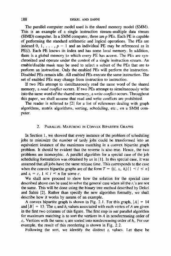
A convex bipartite graph is shown in Fig. 2.1. For this graph, 1 A 1 = 14 and 1 B 1 = 13. The Si and hi values associated with each vertex of A are given in the first two columns of this figure. The first step in our parallel algorithm for maximum matching is to sort the vertices in A in nondecreasing order of Si. Vertices with the same si are sorted into nondecreasing order of hi. For our example, the result of this reordering is shown in Fig. 2.2.

Following the sort, we identify the distinct si values. Let these be

PARALLEL MATCHING ALGORITHM FOR CONVEX BIPARTITE GRAPHS 189 S i hi A B

4

1

1

1

4

4

1

9

9

12

9

4

12

12

8

4

3

4

10

4

2

11

10

13

13

11

13

12

1 1

2 2

3 3

4 4

5 5

6 6

7 7

9

10 10

11 11

12 12

FIGURE 2.1

RI, R2, . . . , &. Assume that R, < R2 < . * . -C Rk, Let Rk+, = max{hi} + l.Forourexample,k = 4andR(l : k + 1) = (1,4,9, 12, 14).

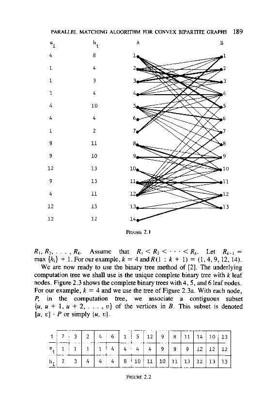
We are now ready to use the binary tree method of [2]. The underlying computation tree we shall use is the unique complete binary tree with k leaf nodes. Figure 2.3 shows the complete binary trees with 4,5, and 6 leaf nodes. For our example, k = 4 and we use the tree of Figure 2.3a. With each node, P, in the computation tree, we associate a contiguous subset {u,u+1,24+2 )...) u} of the vertices in B. This subset is denoted [u, u] - P or simply [u, u].

i - s

i -

hi -

FIGURE 2.2

190 DEKEL AND SAHNI

A (a) (b)

FIG. 2.3. Complete binary trees: (a) 4 leaves; (b) 5 leaves; (c) 6 leaves.

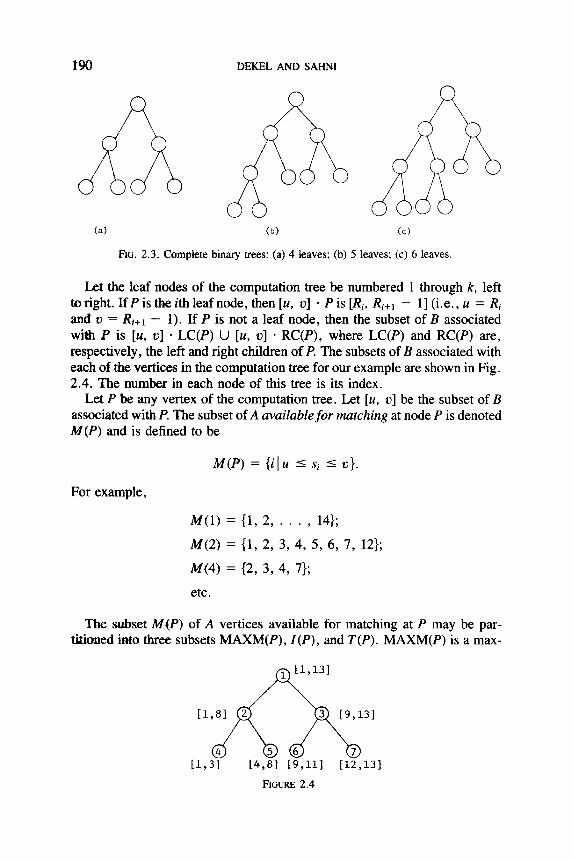
Let the leaf nodes of the computation tree be numbered 1 through k, left to right. IfP is the ith leaf node, then [u, U] * P is [Pi, Ri+r - l] (i.e., u = Ri Uld 1) = Ri+l - 1). If P is not a leaf node, then the subset of B associated with P is [u, u] . LC(P) U [u, v] * RC(P), where LC(P) and RC(P) are, respectively, the left and right children of P The subsets of B associated with each of the vertices in the computation tree for our example are shown in Fig. 2.4. The number in each node of this tree is its index.

Let P be any vertex of the computation tree. Let [u, u] be the subset of B associated with P The subset of A available for matching at node P is denoted M(P) and is defined to be

For example,

M(P) = {i 1 U I Si 5 U}.

M(1) = (1, 2, . . . , 14);

M(2) = (1, 2, 3, 4, 5, 6, 7, 12);

M(4) = 12, 3, 4, 71;

etc.

The subset M(P) of A vertices available for matching at P may be par- titioned into three subsets MAXM(P), Z(P), and T(P). MAXM(P) is a max-

1 El,131

[I,81 2

A

3 19,131

[1,3;1 &I $,lll 11:,131

FIGURE 2.4

PARALLEL MATCHING ALGORITHM FOR CONVEX BIPARTITE GRAPHS 19 1

s i h’ i 4 8

1 4

1 3

1 4

4 8

4 4

1 2

4 8

A’ B’

10 01 20 02

30 03

40 04

50 05

60 06 70 07

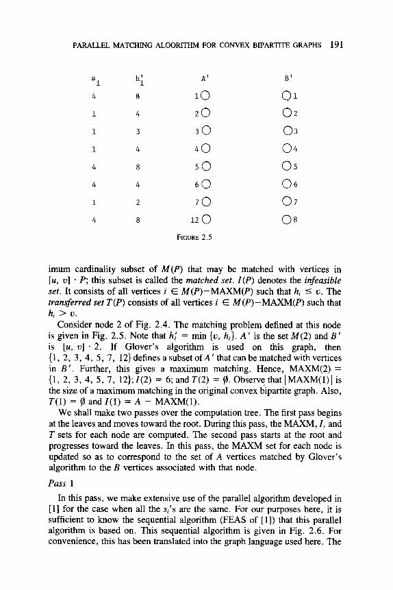
12 0 08 FIGURE 2.5

imum cardinality subset of M(P) that may be matched with vertices in [u, U] * P; this subset is called the matched set. Z(P) denotes the infeasible set. It consists of all vertices i E M(P)-MAXM(P) such that hi 5 v. The transferred set T(P) consists of all vertices i E M(P)-MAXM(P) such that hi > 1).

Consider node 2 of Fig. 2.4. The matching problem defined at this node is given in Fig. 2.5. Note that h,! = min {u, hi}. A’ is the set M(2) and B’ is [u, u] * 2. If Glover’s algorithm is used on this graph, then { 1, 2, 3, 4, 5, 7, 12) defines a subset of A ’ that can be matched with vertices in B ‘. Further, this gives a maximum matching. Hence, MAXM(2) = (1, 2, 3, 4, 5, 7, 12); Z(2) = 6; and T(2) = 9. Observe that 1 MAXM(l) 1 is the size of a maximum matching in the original convex bipartite graph. Also, Z-(l) = fl and Z(1) = A - MAXM(l).

We shall make two passes over the computation tree. The first pass begins at the leaves and moves toward the root. During this pass, the MAXM, I, and T sets for each node are computed. The second pass starts at the root and progresses toward the leaves. In this pass, the MAXM set for each node is updated so as to correspond to the set of A vertices matched by Glover’s algorithm to the B vertices associated with that node.

Pass 1

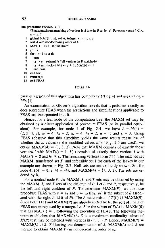
In this pass, we make extensive use of the parallel algorithm developed in [I] for the case when all the sI’s are the same. For our purposes here, it is sufficient to know the sequential algorithm (FEAS of [l]) that this parallel algorithm is based on. This sequential algorithm is given in Fig. 2.6. For convenience, this has been translated into the graph language used here. The

192 DEKEL AND SAHNI

Line prucedure FEAS(n, u. u) //Find a maximum matching of vertices in A into the B set [u, 01. For every vertex i E A, si = U./l

1 global MAT(1 : n); set A; integer n, u, u, i, j 2 sort A into nondecreasing order of h, 3 MAT(1 : n) + O//initialize// 4 j+u 5 for i c 1 to n do 6 ease

8 9

10 11 12

:j > v : return(j) //all vertices in B matched// :j I hi : //select ill j +- j + 1, MAT(i) + 1 end case

end for return(j) end FEAS

RGURE 2.6

parallel version of this algorithm has complexity O(log n) and uses n/log n PEs [l].

An examination of Glover’s algorithm reveals that it performs exactly as does procedure FEAS when the restrictions and simplifications applicable to FEAS are incorporated into it.

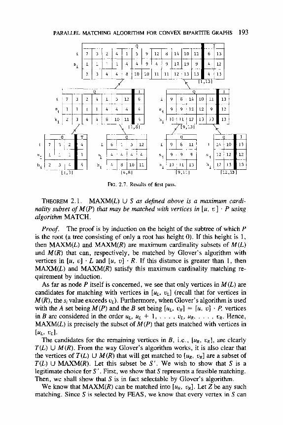
Hence, for a leaf node of the computation tree, the MAXM set may be obtained by a direct application of procedure FEAS (or its parallel equivalent). For example, for node 4 of Fig. 2.4, we have A = M(4) = (2, 3, 4, 7); h2 = 4; h3 = 3; h4 = 4; h7 = 2; u = 1; and o = 3. Using FEAS (observe that this algorithm yields the same results regardless of whether the hi values or the modified values hl of Fig. 2.5 are used), we obtain MAXM(4) = (7, 3, 2). Note that MAXM consists of exactly those vertices i with MAT(i) = 1. I( ) consists of exactly those vertices i with MAT(i) = @ and hi - -= ~1. The remaining vertices form T( ). The matched set MAXM, transferred set T, and infeasible set I for each of the leaves in our example are shown in Fig. 2.7. Null sets are not explicitly shown. So, for node 4,Z(4) = 8; T(4) = (4); and MAXM(4) = (7, 3, 2). The sets are ordered by hi.

For a nonleaf node P, the MAXM, I, and T sets may be obtained by using the MAXM, I, and T sets of the children of P. Let L and R, respectively, be the left and right children of P. To determine MAXM(P), we first use procedure FEAS with u = UR and 2) = uR ([UR, uR] is the subset of B associated with the right child R of P). The A set consists of T(L) U MAXM(R). Since both T(L) and MAXM(R) are already sorted by hi, the sort of line 2 of FEAS can be replaced by a merge. Let S be the subset of T(L) U MAXM(R) that has MAT( ) = 1 following the execution of FEAS. The following theorem establishes that MAXM(L) U S is a maximum cardinality subset of M(P) that may be matched with vertices in [u, u] * Z? Hence, MAXM(P) = MAXM(L) U S. Following the determination of S, MAXM(L) and S are merged to obtain MAXM(P) in nondecreasing order of hi.


====I 'i

[I,3

Q 3 2 4 1 5 12 6

111444 4

Lb.81

i

'i

h. 1 [V,lll

i 14 10

'i EL-

12 12

hi 12 13

[=,I

I

13 1 12

13

31

FIG. 2.7. Results of first pass.

THEOREM 2.1. MAXM(L) U S as dejned above is a maximum cardinality subset of M(P) that may be matched with vertices in [u, V] * P using algorithm MATCH.

Proof. The proof is by induction on the height of the subtree of which P is the root (a tree consisting of only a root has height 0). If this height is 1, then MAXM(L) and MAXM(R) are maximum cardinality subsets of M(L) and M(R) that can, respectively, be matched by Glover’s algorithm with vertices in [u, u] * L and [u, V] * R. If this distance is greater than 1, then MAXM(L) and MAXM(R) satisfy this maximum cardinality matching requirement by induction.

As far as node P itself is concerned, we see that only vertices in M(L) are candidates for matching with vertices in [U L, 0~1 (recall that for vertices in M(R), the si value exceeds Q). Furthermore, when Glover’s algorithm is used with the A set being M(P) and the B set being [uL, v~] = [u, ~1 * P, vertices in B are considered in the order uL, uL + 1, . . . , q, &, . . . , OR. Hence, MAXM(L) is precisely the subset of M(P) that gets matched with vertices in [UL, ULI.

The candidates for the remaining vertices in B, i.e., [UR, vR] , are clearly Z’(L) U M(R). From the way Glover’s algorithm works, it is also clear that the vertices of T(L) U M(R) that will get matched to [uR, vR] are a subset of T(L) U MAXM(R). Let this subset be S ‘. We wish to show that S is a legitimate choice for S ‘. First, we show that S represents a feasible matching. Then, we shall show that S is in fact selectable by Glover’s algorithm.

We know that MAXM(R) can be matched into [UR, ~1. Let Z be any such matching. Since S is selected by FEAS, we know that every vertex in S can

194 DEKEL AND SAHNI

be paired with a distinct vertex in [U R, uR] in a such a way that no vertex j in S is paired with a vertex with index greater than hj. Consider a pairing W that meets this condition. Now suppose that some vertex j in S is paired with a vertex 4 in [us, u,J with index less than Sj. Clearly, j must be a member of MAXM(R) (as all vertices in T(L) have an s value less than uR). Suppose that j is matched to j, in Z. So, 4 < ji. If j, is free in W, then the pairing of j in W may be changed from q to ji. If j, is not free, then suppose it is matched to j,. From the restriction on W, it follows that q < j, 5 hi,. If j, E T(L), then j, may be paired with q and j with j, (since q < j,, Sj2 < q < hj,). If j2 E MAXM(R), then suppose that j2 is matched to j3 in Z. It is easy to see that j3 # ji. If q = j3 or j3 is free in W then we may pair j with j, and j, with j,. If q is in the interval [Sj,, hj,], then we may pairj with j, and j2 with q. If q is not in this interval, then since q < hj2, q < Sj2 5 j,. Note that the condition q < j,i+i is preserved. This is needed in case jzi+z E T(L). NOW, let j, be the vertex paired with j, in W. It should be clear that we can continue in this way and modify W so that j is paired with j,, j, with j,, j, with j5, etc. In the new pairing, there is one fewer vertex of S that is paired with a vertex with a smaller s value.

Repeating the above construction several times, W can be transformed into a matching such that every vertex j E S is matched to a vertex q in [uR, uR] such that Sj 5 q 5 hja Hence, S represents a feasible matching.

Let S ’ (as defined earlier) be the subset of MAXM(R) U T(L) matched by Glover’s algorithm to the vertex set [Us, uR]. We shall now proceed to show that S is a valid choice for S ’ . Let Z be any matching of MAXM(R) into [uR, uR]. Let Y be a matching of S ’ in which all vertices in MAXM(R) fl S ’ are matched to the same vertex in [uR, u,J as in the matching Z. Let W be a corresponding matching for S. The existence of the matchings Y and W is a consequence of the construction used to show the feasibility of S.

From the definition of S ‘, it follows that S ’ @ S. Also, from the working of FEAS, it follows that S c S ’ . Let j E S be a vertex with least hj such that j e S ’ . If no such j exists, then S = S ’ . Assume that j is matched to q in W. If q is free in Y, then S’ cannot be of maximum cardinality. So, let p E 3’ be matched to q in Y. By definition of Y and W p $ S. Also, from the order in which FEAS considers vertices, hp 2 hj (as otherwise, FEAS would consider p before j and select p for S). Hence, S ’ U {j} - {p} is also a subset selectable by Glover’s algorithm. (Since hp 2 hj, by ensuring j < p, Glover’s algorithm will be forced to match j before p.) S’ U {j} - {p} agrees with S in one place more than does S ‘.

By repeating this interchange process, S ’ may be transformed into S with the result that S is also a maximum cardinality subset of MAXM(R) U T(L) that is selectable by Glover’s algorithm for matching in [uR, ~~1.

Hence, MAXM(L) U S is a maximum cardinality subset of M(P) selectable by Glover’s algorithm for matching in [u, u] * P n

Once MAXM(P) is known, T(P) and Z(P) are easily computed. Actually,

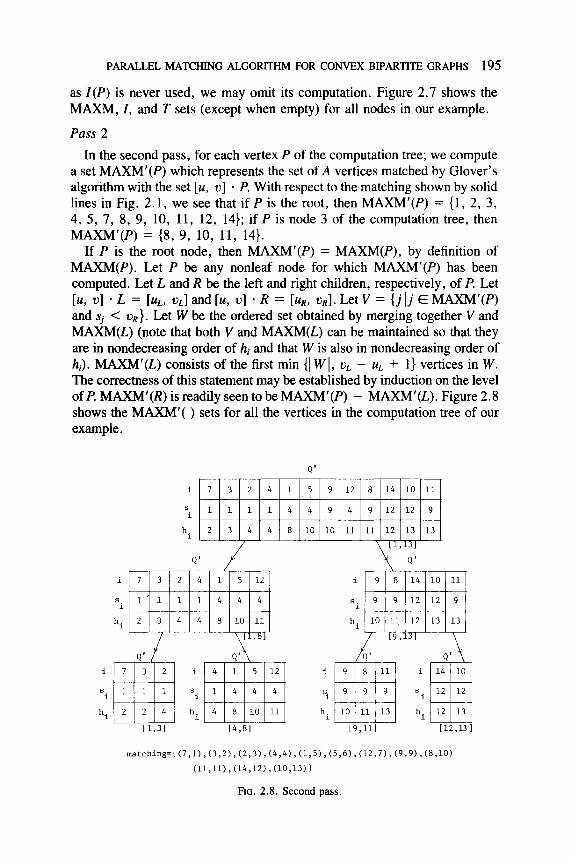
In the second pass, for each vertex P of the computation tree; we compute a set MAXM’(P) which represents the set of A vertices matched by Glover’s algorithm with the set [u, u] . P With respect to the matching shown by solid lines in Fig. 2.1, we see that if P is the root, then MAXM’(P) = (1, 2, 3, 4, 5, 7, 8, 9, 10, 11, 12, 14); if P is node 3 of the computation tree, then MAXM’(P) = (8, 9, 10, 11, 14).

If P is the root node, then MAXM’(P) = MAXM(P), by definition of MAXM(P). Let P be any nonleaf node for which MAXM’(P) has been computed. Let L and R be the left and right children, respectively, of P. Let [u, u] * L = [UL, UJ and [u, u] . R = [uR, uJ. Let V = {jlj E MAXM’(P) and Sj < 2)R). Let W be the ordered set obtained by merging together V and MAXM(L) (note that both V and MAXM(L) can be maintained so that they are in nondecreasing order of hi and that W is also in nondecreasing order of hi). MAXM’(L) consists of the first min (1 W 1, uL - uL + 1) vertices in W. The correctness of this statement may be established by induction on the level of P MAXM’(R) is readily seen to be MAXM’(P) - MAXM’(L). Figure 2.8 shows the MAXM’( ) sets for all the vertices in the computation tree of our example.

Q’

i

s i

h. 1


as I(P) is never used, we may omit its computation. Figure 2.7 shows the MAXM, I, and T sets (except when empty) for all nodes in our example.

Pass 2

i

s i

h. 1 [I,31 [4,81 [9,111 [12,Ul

matching=i(7,1),(3,2),(2,3),(4,4),(1,5),(5,6),(12,7),(9,9),(8,10)

(11,11),(14,12~,~10,13~1

FIG. 2.8. Second pass.

196 DEKEL AND SAHNI

From the MAXM’( ) sets of the leaves, the matching is easily obtained. If P is a leaf, and [u, V] * P = [a, b], then the first vertex in MAXM’(P) is matched with a, the second with a + 1, etc. (note that MAXM’(P) is in nondecreasing order of hi). The matching for our example is also given in Fig. 2.8. Complexity Analysis

The initial ordering of A by si and within Si by hi can be done in 0 (log’ n) time using n/2 PEs [ 11, 121. During the first pass, the computation of MAXM( ) requires the use of FEAS and a merge. The use of FEAS (without the sort) takes O(log n) time and requires O(lM(P) I/logIM(P) I) PEs [l]. The merge at node P takes O(log n) time with [M(P) l/2 PEs. Since MAXM can be computed in parallel for all nodes on the same level of the computation tree, O(log n) time is needed per level. The total time for the first pass is O(log’ n) and n/2 PEs are needed. Pass 2 requires only some merging per node. The total cost of this pass is also O(log’ n) and n/2 PEs suffice.

Hence, the overall complexity of our parallel algorithm for maximum matching in convex bipartite graphs is 0 (log’ n). The PE requirement is O(n).

Another complexity measure often computed for parallel algorithms is the effectiveness of processor utilization (EPU) (see [ 1, 2, 141). For any problem P and parallel algorithm A, this is defined as follows:

EPU(P, A) = complexity of fastest “known” sequential algorithm for P

complexity of A * number of PEs used by A ’

For our algorithm, we have an EPU that is fl((n + mA(m))/(log’ n * n)) (recall that m = I B I).

3. APPLICATIONS TO SCHEDULING

We have already seen one application of matchings in convex bipartite graphs to scheduling. This application was to a problem that is actually isomorphic to the matching problem: viz., find the maximum number of unit time jobs from J = {(ri, di) I 1 - ’ - < I < n, r; and di are natural numbers} that can be scheduled on a single machine such that no job is scheduled before its release time ri or after its due time d,. In this section, we shall look at three other scheduling problems that can be solved in an efficient manner using the parallel matching algorithm developed in previous section.

3.1 Scheduling to Minimize the Maximum Cost In this problem, we are given n unit time jobs. Associated with each job

is a release time r; (which is a natural number) and a nondecreasing cost


function ci( ), 1 I i I n. Let S = (s,, s2, . . . , s,) be a one-machine schedule for the n jobs. Si denotes the start time of job i. Let 4; be as defined below:

i

Ci (Si) Si L ri 4i =

CQ Si < ri.

The cost of S is defined to be max {qi}. We wish to find a schedule with minimum cost.

As pointed out by Rinnooy Kan [ 131, this problem may be solved by first determining the finish time of a minimum finish time schedule for the n jobs. If the n jobs are already in nondecreasing order of release times ri, then a minimum finish time schedule has start times Si given by

Sl = l-1

Si = max {Ti, Si-1 + l}. (3.1)

This equation is a special case of Eq. (6.1) of [l] and so we may use algorithm PADMIS of [l] to obtain the Si’s. The finish time, C *, of a minimum finish time schedule for the n jobs is S, + 1.

For simplicity, let us assume that rl = 0. Once C* has been computed, a schedule that has minimum cost may be obtained by constructing the convex bipartite graph, G, with A = (1, 2, . . . , n} and B = (0, 1, . . . , C * - 1). There is an edge from i in A to j in B iff j 2 ri. (A represents the jobs andj E B represents the time slot [j, j + 11.) A cost ci(j) is associated with edge (i, j).

From our choice of C *, it follows that the graph just constructed has a maximum matching M of size n. Every such matching defines a feasible schedule. A matching for which the maximum edge cost is minimum defines the optimal matching for our scheduling problem.

As suggested by Rinnooy Kan [ 131, this matching can be obtained by performing a binary search on the O(n2) edge costs in G. At each iteration of this binary search, all edges with cost greater than c are deleted from G and a maximum matching in the resulting convex bipartite graph G ’ found. If this matching is of size less than n, then there is no matching in G with maximum edge cost no more than c; otherwise there is. The time complexity of Rinnooy Kan’s scheme is readily seen to be O(nA(n) log n).

Complexity Analysis The initial sort by release times can be done in 0 (log2 n) time using 0 (n)

PEs [ 121. C * can be found in 0 (log n) time using n PEs and the algorithm of [ 11. Each iteration of the binary search requires the construction of G ’ and the solution of a matching problem. The first of these can be done in 0 (log2 n) time using 0 (n2/log2 n) PEs. The second task takes 0 (log’ n) time and 0 (n)

198 DEKEL AND SAHNI

PEs. The total time needed to determine the matching with minimum cost is therefore O(log3 n) and the number of PEs needed is 0 (n2/logz n). Hence, the overall complexity of the parallel scheduling algorithm is 0 (log3 n). The number of PEs used is 0 (n 2/log2 n). The EPU of our parallel algorithm is l&4(n) log n/(log3 n * n2/log2 n)) = R(A(n)/n).

3.2. Job Sequencing with Release Times and Deadlines

Once again, each job has a processing requirement that is one unit. How- ever, this time there is a release time rj, deadline di, and weight wi associated with job i. The r,‘s and d;‘s are natural numbers. No job may be scheduled before its release time. We are interested in obtaining a maximum weight subset of the n jobs such that all jobs in this subset can be scheduled on a single machine in such a manner that none starts before its release time or finishes after its deadline.

This problem can be solved efficiently by a sequential greedy algorithm. Jobs are considered in nonincreasing order of the weights. If the job, i, currently being considered can be scheduled together with all the others so far scheduled such that no job violates its release time or deadline, then job i is in the optimal schedule. Otherwise, it is not. The sequential complexity of this algorithm is O(n*) [7].

For the parallel algorithm, we resort to a convex bipartite graph formulation. The A set represents the n jobs; so, 1 A ) = n. The B set represents time slots. Let a = min {ri} and b = max {di}. B = {a, a + 1, . . , b - l}. In the convex bipartite graph corresponding to the scheduling problem, there is an edge from i in A toj E B iff ri 5 j < di. The weight of each edge incident on vertex i E A is wi. We wish to find a matching M for which the sum of edge weights is maximum.

Our parallel algorithm for this is based on the greedy sequential algorithm for job sequencing with release times and deadlines, Define the binary relation R on the weights wi as follows:

wiRwj iff Wi < Wj or (wi = wj and i > j).

Let Gi be the convex bipartite graph obtained from G by deleting all edges with weight wj such that Wj R Wi. Clearly, the following determines whether or not i is in the maximum weight matching:

(a) Determine the size of the maximum cardinality matching in Gi. Let this be si.

(b) Delete all edges incident on vertex i E A of Gi. Determine the size of the maximum cardinality matching in the new graph. Let this be s ‘i.

(c) i is in the maximum weight matching iff si = s: + 1. So, each vertex can determine, in parallel, whether or not it is in the

maximum weight matching. To avoid read conflicts, we need to make n copies of the graph G. This can be done in O(log n) time using O(n2) PEs.


To see this, observe that as G is a convex bipartite graph, it can be represented in 0 (n) space. So, n PEs can make one copy of G in 0 (n) time. Next, 2n PEs are used to make a copy of each of these copies. Now we have four copies of G. At step log n, n*/2 PEs make one copy of each of the existing n/2 copies in O(1) time. Gi can be constructed in O(1) time using O(n) PEs per vertex i. Then, steps (a), (b), and (c) above can be performed in O(log’ n) time using a total to O(n’) PEs. (Note that only pass 1 of the parallel convex matching algorithm need be executed.) The total time needed to determine the subset of A in the maximum weight matching is therefore 0 (log2 n).

Once we have obtained the above subset of A, the actual matching can be determined by deleting from G all vertices that are not in this subset. A maximum cardinality matching on the resulting graph yields the desired matching with maximum weight. This corresponds to an optimal schedule for the scheduling problem. It takes an additional O(log* n) time to determine this matching.

The complexity of the parallel algorithm is O(log’ n) and its EPU is a(n*/(log* n * n*)) = fi(l/log2 n).

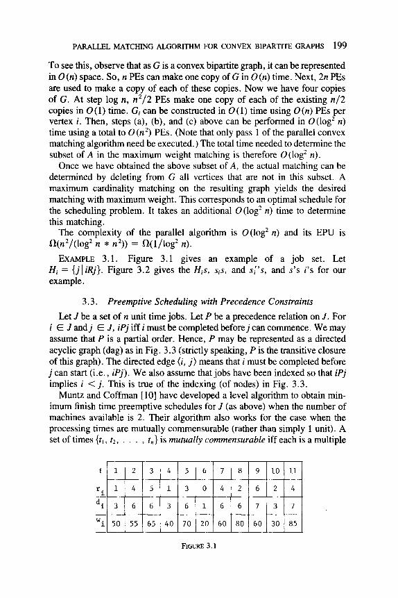
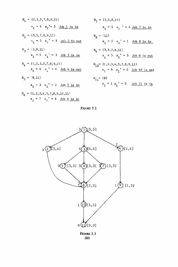
EXAMPLE 3.1. Figure 3.1 gives an example of a job set. Let Hi = {j] iRj}. Figure 3.2 gives the His, SiS, and sl’s, and S’S i’s for our example.

3.3. Preemptive Scheduling with Precedence Constraints

Let J be a set of n unit time jobs. Let P be a precedence relation on J. For i E J andj E J, iPj iff i must be completed before j can commence. We may assume that P is a partial order. Hence, P may be represented as a directed acyclic graph (dag) as in Fig. 3.3 (strictly speaking, P is the transitive closure of this graph). The directed edge (i, j) means that i must be completed before j can start (i.e., iPj). We also assume that jobs have been indexed so that iPj implies i < j. This is true of the indexing (of nodes) in Fig. 3.3.

Muntz and Coffman [lo] have developed a level algorithm to obtain minimum finish time preemptive schedules for J (as above) when the number of machines available is 2. Their algorithm also works for the case when the processing times are mutually commensurable (rather than simply 1 unit). A set of times {tl, t2, . . . , t,,} is mutually commensurable iff each is a multiple

i -

r. c - W. I. -

Hl = {2,3,5,7,8,9,11} H7 = I3,5,8,111

s. 1 = 6 si'= 5 Job 1 is in si=5 s. I. ' = 4 Job 7 is in

H2 = {3,5,7,8,9,11} H8 = ill} S. 1 =5 sir=5 Job2isout S. 1 =2 si'= 1 Job 8 is in

H3 = {5,8,111 Hg = {3,5,7,8,111 S. 1 =4 si'= 3 Job 3 is in S

i =5 si'= 5 Job 9 is out

H4 = 11,2,3,5,7,8,9,11> HlO= I1,2,3,4,5,7,8,9,111

si =6 sit= 6 Job 4 is out s. = 6 1 s.'=6 JoblOisout 1

H5 = 18,11}

si =3 si'= 2 Job 5 is in

H6 = {1,2,3,4,5,7,8,9,10,11}

si = 7 s.'=6 Job6isin 1

Hll= I01

'i = 1 Si' = 0 Job 11 is in

FIGURE 3.2

[2,41

[I,31


procedure SCH L + maximum level Si t all jobs in J with level = i, 0 5 i 5 L for k +- L to 1 do

if ) Sk) = 1 then find the largest j such that j < k and Sj contains a job all of whose predecessors are in &, .!?-,, . , Sk+, If no such j exists then exit endif. Let q be this value of j and let r be the job in S, with the above property S, +- S, - {r}; Sk + Sk U {r}

endif endfor preemptively schedule the jobs in each Si using McNaughton’s rule [9]. Jobs in S, precede those in S,-,

end SCH

FIG. 3.4. The Muntz-Coffman Algorithm.

of some number W. In the case of mutually commensurable times, each job is broken into a chain of jobs each requiring w units of processing. In this section, we shall deal directly only with the case of unit time tasks.

Let G be the dag representation of the precedence relation P. A node in G is terminal iff its out-degree is 0. The level of a node in G is the length of the longest path from 0 to any terminal node. All terminal nodes have level 0. In Fig. 3.3, the number outside each node is its level.

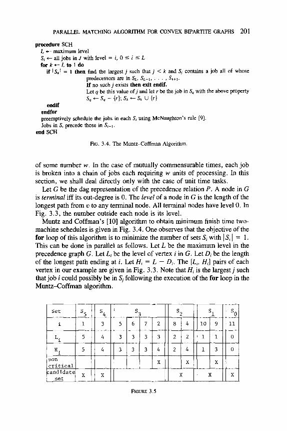
Muntz and Coffman’s [lo] algorithm to obtain minimum finish time two- machine schedules is given in Fig. 3.4. One observes that the objective of the for loop of this algorithm is to minimize the number of sets Sj with 1 Si 1 = 1. This can be done in parallel as follows. Let L be the maximum level in the precedence graph G. Let Li be the level of vertex i in G. Let Di be the length of the longest path ending at i. Let Hi = L - Di. The [Li, Hi] pairs of each vertex in our example are given in Fig. 3.3. Note that iY< is the largest j such that job i could possibly be in Sj following the execution of the for loop in the Muntz-Coffman algorithm.

Hi 5 4 3334 24 13 0

non critical X X X

candidate x set X X X X

FIGURE 3.5

202

A

DEKEL AND SAHNI

B new index

2 l 5 0

4

*

4 1

9 2 3

1 4

0 5

FIG. 3.6. Convex bipartite graph.

A job i is said to be critical iff Li = Hi. Only noncritical jobs are candidates for displacement to other sets. Also, only those sets Si that initially have exactly one critical job are candiates to receive a new job during the for loop. Note that every Si must have at least one critical job. In Fig. 3.5, the noncritical jobs have been marked with an X. Sets that are candidates to receive a new job have also been marked with an X. Double vertical lines mark set boundaries.

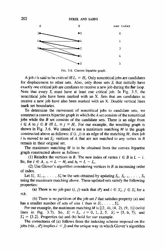
To determine the movement of noncritical jobs to candidate sets, we construct a convex bipartite graph in which the A set consists of the noncritical jobs while the B set consists of the candidate sets. There is an edge from i E A to j E B iff Li I j 5 Hi. For our example, the resulting graph is shown in Fig. 3.6. We intend to use a maximum matching M in the graph constructed above as follows: if (i, j) is an edge of the matching M, then job i is moved to set Sj; vertices of A that are not matched to any vertex in B remain in their original set.

The maximum matching M is to be obtained from the convex bipartite graph constructed above as follows:

(1) Reindex the vertices in B. The new index of vertex i E B is L - i. SO, for i E A, Si = L - Hi and hi = L - L;.

(2) Use Glover’s algorithm considering vertices in B in increasing order of index.

Lets;, St-,, . . . ) Sh be the sets obtained by updating S,, S,-, , . . . , So using the maximum matching above. These updated sets satisfy the following properties:

(a) There is no job pair (i, j) such that iPj and i E ,SL, j E Si for a sb.

(b) There is no partition of the job set J that satisfies property (a) and has a smaller number of sets of size 1 than in ,Yt, . . . , S&

For our example, the maximum matching M is ((2, 4), (4, 2), (9, 1)) (solid lines in Fig. 3.7). So, S,! = Sip i = 0, 1, 2, 5. S; = (5, 6, 7); and S; = (3.2). Properties (a) and (b) hold for our example.

The correctness of (a) follows from the indexing scheme imposed on the jobs (viz., iPj implies i < j) and the unique way in which Glover’s algorithm


1

2

3

4

5

7

8

9

FIGURE 3.7

works. Suppose that statement (a) is incorrect. Then, there exists a job pair (i, j) such that iPj and i E Si, j E SL and a I b. Since no such job pair exists in S,, . . . , SO, it must be the case that job j is noncritical and is matched to b (old indexing) in M (as only noncritical jobs can change sets and no job moves to a set of smaller index). From the definition of L and H and the knowledge that iPj, it follows that H; 2 L;, Hj 2 Lj, Li > Lj, and Hi > Hj. If job i is critical, then it is the case that Li > Hi. SO, job j cannot possibly be matched to a set b with A 5 b. Hence, we may assume that i is also noncritical. Again, if i is not matched in M, then a > b as for a to be less than or equal to b, it must be the case that Li < Hj. But since Li > Lj, hi < hj and i must get matched to b before j can (see Glover’s alogrithm). Hence, i and j must both be matched in M. i is matched to a and j to b. Hence, a f b. If a < b then vertex b is considered before a (as its new index is L-b < L-u). Since iPb, it must be the case that Hi 2 b 2 L;. Also, L, 1 Lj implies that h, < hi. Hence, Glover’s algorithm will match i to b and not j to b.

The truth of property (b) is established using the following reasoning. If i E B is such that no vertex of A is matched to i in M, then ( Sl) = 1. To see this, observe that Si has exactly one critical job. Every noncritical job in Si is a candidate for matching with i E B. Thus, if no job is matched with i, then all these noncritical jobs are matched elsewhere and ) SlI = 1. It is readily seen that if i E B is matched in M, then 1 S[ ) > 1. Hence, the number of sets of size 1 is minimized when a maximum matching is used.

Complexity Analysis

The steps in our parallel preemptive scheduling algorithm are: (l)DetermineLiandHi, 15 i 5 n (2) Mark the noncritical jobs

204 DEKEL AND SAHNI

(3) Mark the candidate sets (4) Construct the convex bipartite graph (5) Find the maximum matching M (6) Reassign matched jobs to their new sets (7) Schedule jobs in the same set using McNaughton’s rule.

Step 1 I can be performed in O(log2 n) time using the critical path algorithm developed by Dekel, Nassimi, and Sahni [3]. This algorithm uses O(n3/log n) PEs. The noncritical jobs can be identified in 0( 1) time using n PEs. The sets S,, . . . , S, may be obtained in O(log n) time by sorting on L;. This requires O(n2) PEs. The candidate sets can be marked in O(log n) time and the resulting convex bipartite graph may be constructed in an additional 0 (1) time using II’ PEs. The matching requires 0 (log2 n) time and 0 (n) PEs while the reassigning takes 0 (1) time. A parallel implementation of McNaughton’s rule appears in [ 11. This has complexity 0 (log n) and uses O(n/log n) PEs.

Hence, the overall complexity of our seven-step parallel algorithm for preemptive scheduling is 0 (log2 n). The number of PEs used is 0 (n 3/lag n). Since the fastest sequential algorithm known for this problem (i.e., the Muntz-Coffman algorithm) has complexity 0 (n 2), the EPU of our parallel algorithm is 0 (n2/(log2 n * n3/log n)) = 0 (1 /(n log n)).

4. CONCLUSIONS

We have developed fast parallel algorithms for several versions of the matching problem for convex bipartite graphs. In Section 2, we explicitly considered the maximum cardinality matching problem. In Sections 3.1 and 3.2, we considered the problems of obtaining a maximum matching that minimized the maximum weight edge used as well as one that maximized the total weight of the used edges. Both these problems were discussed in con- nection with the scheduling problems in which they naturally arose. Finally, the maximum cardinality matching algorithm was again used to solve the preemptive scheduling problem of Section 3.3 efficiently.

This paper has further enhanced the utility of the binary tree method of Dekel and Sahni [2] for the design of parallel algorithms. It should also be pointed out that while all of our complexity analyses have assumed the availability of as many PEs as needed, our algorithms can be used when fewer PEs are available. The complexity of each algorithm will increase by no more than the shortfall in PEs. So if only half the number of PEs is available, then the time needed will at most double (except for a possible constant increase in overhead).

REFERENCES 1. Dekel, E., and Sahni, S. Parallel scheduling algorithms. aper. Res. 31, 1 (1983), 24-49.

2. Dekel, E., and Sahni, S. Binary trees and parallel scheduling algorithms. IEEE Trans. Compur. C-32, 3 (March 1983), 307-315.


3. Dekel, E., Nassimi, D., and Sahni, S. Parallel matrix and graph algorithms. SICOMP 10, 4 (Nov. 1981), 657-675.

4. Emde Boas, P. van. Preserving order in a forest in less than logarithmic time and linear space. Inform. Process. Letr. 6 (1977), 80-82.

5. Glover, F. Maximum matching in a convex bipartite graph. Naval Res. Logist. Quart. 14 (1967), 313-316.

6. Jackson, J. R. Scheduling a production line to minimize maximum tardiness. Research Rep. 43, Management Science Research Project, University of California, Los Angeles, 1955.

7. Lageweg, B. J., and Lawler, E. L. Private communication. Cited in Lenstra, J. K. Sequencing by Enumerative Methods. Mathematisch Centrum, Amsterdam, 1976, p. 22.

8. Lipski, W., Jr., and Preparata, F. P. Efficient algorithms for finding maximum matchings in convex bipartite graphs and related problems. Actu Inform. 15 (1981), 329-346.

9. McNaughton, R. Sequencing with deadlines and loss functions. Management Sci. 6 (1959), l-12.

10. Muntz, R. R., and Coffman, E. G., Jr. Optimal preemtive scheduling on two-processor systems. IEEE Trans. Comput. C-18 (1969) 1014-1020.

11. Nassimi, D., and Sahni S. Bitonic sort on a mesh connected parallel computer. IEEE Truns Comput. C-28, 1 (Jan. 1979), 2-7.

12. Preparata, F. P. New parallel-sorting schemes. IEEE Trans. Comput. C-27,7 (July 1978), 669-673.

13. Rinnooy Kan, A. H. G. Machine scheduling problems, class$ication complexity, and computation. Nijhoff, The Hague, 1976.

14. Savage, C., Parallel algorithms for graph theoretic problems. Ph.D. thesis, University of Illinois, Urbana, Aug. 1978.

A parallel matching algorithm for convex bipartite graphs and applications to scheduling

Documents

Transcript of A parallel matching algorithm for convex bipartite graphs and applications to scheduling