Non-convex Global Optimization on Convex Domains

Saebamirahmadi.blogspot.com 2014©

1

Non-convex Global Optimization on Box-constrained Domains

Saeb AmirAhmadi Chomachar

Ph. D. Student

Department of Mechanical Engineering

Faculty of Engineering and Technology

The University of Guilan, Rasht, Iran

P. O. BOX 3756

Tel: +98-939-469-7639

Email: [email protected].

mailto:[email protected]


2

Abstract:

Presented here is a global optimization algorithm to solve n-dimensional box-constrained non-convex

global optimization problems. The algorithm is referred to as Multi-Point Moving Grid (MPMG)

method. It is of derivative-free type and does not require an initial guess or initialization procedure.

The method is always convergent to the global solution as long as the objective function is Lipschitz

continuous along with the first order and second order optimality conditions are satisfied. With

increase in dimension size the computational cost of the method linearly grows which shows the

method is efficient. The method is as well accurate to the largest extent. Global optimization is often

NP-hard when the dimension of problem is high. Deterministic global optimization methods yield

accurate results but are quite expensive in cost when problem is high-dimensional. On the other hand,

stochastic methods are efficient and fast but they do not guarantee the accuracy of the solution found.

However, MPMG search method developed in this study is simultaneously efficient and accurate. The

efficiency and accuracy of the method is shown through numerical exercise and by a concise

mathematical proof. The method is successfully capable to accurately and efficiently spot on the global

optimizer for an exponential function with 3000 dimensions. Also a purportedly NP-hard quadratic

programming problem is easily solved by the MPMG method. Several other high-dimensional multi-

modal bench-mark functions available in the existing literature are successfully examined and treated

by the method. For low dimensional problems and on an ordinary PC the solution is a fraction of a

second away from a click and also for high dimensional problems the solution is not far away. The

convergence rate is linear with a 0.5 asymptotic error constant. It is noteworthy that the method was

confirmed to solve ‘non-convex global optimization on convex domains' and a future paper is

supposed to be developed on this title.

1. Introduction

Mathematical analysis is a blessing ability of all living objects, in whose brains the analyses are

performed to enable them to lead a better life. Any living creature knows how to solve mathematical

problems for their particular issues. For example, one knows how to play card game to heighten the

chance of win and spider knows how to weave its web for the best probability of catching its prey.

There are many other examples that clarify the performance of mathematical analyses by living

creatures as a fish that evades in perpendicular direction to line of sight of a sea hunter.

Optimization problems, as a class of these mathematical problems that occur in our daily life, are

routinely solved in our mind. For example any living object knows that the straight line connecting

two points A and B is the path of minimum distance passing through those points and this is confirmed

by congenital logic in one’s healthy mind. So the concepts of optimization problems are not bizarre

for the mind of ordinary people who have had no exposure to formal mathematics and this is what

makes this field of research more tangible from a theoretical aspect and also conceptually less abstract.

Solving optimization problems are an unavoidable part of our daily life, and at its highest level,

the most optimum strategies are planned that lead to achieve the most valued goals. Optimization

theory is utilized to solve a wide range of problems, from Econometrics to applied sciences.

Studying optimization problems dates back to antiquity whilst Euclid in 300 B.C. studied minimal

distance from a point to a line and proved that in rectangles with constant perimeter, the maximum

area is inscribed by the squares.


3

Global optimization is a very important research subject in optimization field. It is in fact the

methodology of finding the decision or design variables that extremize a multi-variable function on a

certain domain of solution.

Global optimization belongs to the class of NP-complete problems and are typically quite difficult

to be solved exactly. Deterministic methods provide accurate solutions to GO problems as long as the

dimension size is low. On the other hand, stochastic methods provide the solution for high-dimensional

GO problems but they do not guarantee the accuracy of the solution found. Although there is a great

enthusiasm and thirst for a method that is simultaneously efficient and accurate in solving GO

problems, but such a method has not been developed in the existing literature yet. Fortunately, the

author of this paper believes the global optimization algorithm named; Multi-Point Moving Grid

(MPMG) method developed in this study, satiates the thirst of researchers for such universal method.

Many real-world applications can be formulated as global optimization problems. Although

finding the optimum solution of such problems is a daunting job, it is very worthwhile to be

challenged.

In a text-book by Floudas [1], he presented the application of global optimization to problems in

chemical engineering. Needless to say that global optimization is not only restricted to solve problems

in chemical engineering and it has also widespread applications in all branches of engineering,

sciences and applied sciences. Hence it is understood why global optimization has attracted lots of

attention from researches in the field. In another paper, Floudas [2] reviewed the advances in the

application of global optimization to design and control of chemical process systems. Numerous

bench-mark functions in local and global optimization with engineering interest were presented in a

handbook published in 1999 (Floudas & Pardalos [3]).

The fastest optimization algorithms are useful to locate only local optimizers. Global optimization

usually refers to non-convex global optimization, however, global convex optimization has attracted

an interest from scientists recently and is a field of research. Convex and non-convex global

optimization are the terms originated from the mathematical character of the objective function whose

optimum solutions are sought. Convex optimization corresponds to the global optimization of

objective functions which are convex. Meanwhile, convexity is a mathematical character attributed to

functions or regions which satisfy convexity definition that is a mathematical inequality. The convex

optimization methods that have recently attracted many researchers are not actually very robust. These

methods are applicable to find the global minimum for a class of functions that are convex, where the

global minimizer (or maximizer) is the only minimum (or maximum) that exists. This is what makes

the convex optimization methods to be hardly viewed as robust. Global optimization theories are not

in an advanced level of development if not calling it rudimentary.

Optimization methods are basically divided into derivative methods and derivative-free

methods. In derivative-free methods the domain of solution is directly investigated to locate the global

optimizer or local optimizers. This is sometimes very costly and time-consuming. In these methods, it

is not necessary to know the derivative values and the direction of the gradient vector of the functions

whose optimum values are sought. Examples of derivative-free methods in optimization are multilevel

coordinate search, genetic algorithms, bee colony, ant colony, particle swarm and simulated annealing.

The derivative-methods such as steepest descent utilize the direction of the gradient vector of the

functions to approach an optimizer, usually a local one.

In this paper a global optimization method is developed that has none of the negative characters

of the methods developed in the existing literature such as high computational cost or low accuracy.

In fact the method developed in this paper, is of low computational cost as stochastic methods and is

accurate as deterministic methods.

It should be noticed that a mature and healthy human mind develops very perfect optimum

strategies in the most intricate conditions. To the belief of the author of this paper, approaching


4

deterministic problems through stochastic means, as refers to several optimization techniques, does

not seem a good idea. The author believes that, a perfect deterministic solution always exist for an

associated deterministic problem. The human beings are intellectually much stronger than to yield to

the tenacity and difficulty of the so-called NP-hard optimization problems and this study would

optimistically prove this. There are numerous text books for mathematical optimization [4-31]. Several

global optimization algorithms are applicable to find the global optimum of the objective function

provided its analytical properties such as the Lipschitz constant is known. This information is often

unavailable, hence, these methods are not robust and reliable for many of the problems.

This paper presents a method to solve n-dimensional non-convex global optimization on box-

constrained domains. These problems are visited in many real-world applications. The method is

named Multi-Point Moving Grid (MPMG) search method. It is of multi-level coordinate search type

and provides the solution to a general class of GO problems. The method is convergent to the optimal

solution as long as the objective function is Lipschitz continuous and also first order together with

second order optimality conditions are satisfied.

In the present work, the optimizer is efficiently found with probability one and with high

accuracy. MPMG search method is either capable to solve ‘non-convex global optimization on convex

domains’ and the mathematical proof is left for a future paper that is supposed to be developed on this

title.

In the remaining, first preliminaries are presented and then Multi-Point Moving Grid (MPMG)

search is described. After that the analysis and simulation results are presented.

2. Preliminaries

Box constrained global optimization has a wide range of applications in engineering design [32-

48]. Global optimization methods provide the global optimum of multi-modal functions which have

numerous local optima. Many methods and techniques are developed in the existing literature related

to global optimization, however, how to solve such problems efficiently is still a problem with great

challenges. In the last decades, some deterministic methods (such as the filled function method [49-

58]) has attracted much interest in the field of global optimization.

In many optimization problems, the existence of several local optimizers poses a challenge for

classical optimization methods to find the global optimizer. In better words, the classical methods are

inclined to get entrapped in local optimizers before reaching out for the global optimizer.

Multi-point Moving Grid (MPMG) method developed in this study has in one place all the

positive characters of all other methods and has none of the negative characters of them. The MPMG

method developed here has a potential to simultaneously replace both stochastic and deterministic

approaches in global optimization.

A general constrained optimization problem is formulized as:

(2.1)

.

n n

'min' F(x) x Ix

F : R R; I R

F(x) is said to be globally optimized at the point *

x if the followings hold true:

(2.2) *F(x ) F(x) : x I ,

And:


5

(2.3) *F(x ) F(x) : x I ,

The former for global minimization problem and the latter for global maximization problem. *

x is the

optimum solution.

In this study, the domain of solution is assumed to be a set product of closed intervals in Rn or in other

words a hypercube, mathematically given as:

(2.4) . L U n n L UI = [x x ] = x R x x x

Figure 1 The area; I, in 2-d Cartesian frame.

An important analytical property of a function F (x), defined already, is the Lipschitz continuity. Given

two metric spaces X(X,d ) and

Y(Y,d ) , where Xd denotes the metric on the set X and Yd is

the metric on the set Y (for example Yd (x,y) = x - y ), then the function F(x) is called Lipschitz

continuous if a real constant L 0 exists, such that for all 1 2x ,x in the domain of solution, the

following holds true:

(2.5) Y 1 2 X 1 2

d (F(x ),F(x )) Ld (x ,x ) ,

A minimum of L is referred to as the Lipschitz constant for the function F(x). The inequality is trivially

satisfied if x1=x2.

Convexity is another fundamental concept in optimization. Convex optimization methods are utilized

to find the global optimum values for convex functions. A convex function F (x) is such that for any

couple of points, 1 2x ,x in the domain of solution, the following holds true in the space1nR

(2.6) , [ ] . n

1 2 1 2F(αx +(1-α)x ) αF(x )+(1-α)F(x ) α 0 1

For a concave function the inequality sign in (2.6) should be inverted.


6

Multilevel coordinate search is a derivative-free method that performs the search directly on

candidate points in domain of solution and evaluates function values at these points to reach the global

optimizer while there is no need for any information on the function’s gradient. The paper developed

by H. Waultraud and N. Arnold [59], elaborates a type of this method that has many restrictions such

as good initialization procedure. The MPMG method developed in this paper is typically viewed as a

critically modified multi-level coordinate search method.

The MPMG method is robust, efficient and accurate and is based on a simple mathematical

logic. It is in fact a multilevel coordinate search method, at every level of which, the best

approximation is updated and the error bound is continually decreased. There is no restricting

assumption on the convexity of the functions that are to be optimized (the function may be convex or

non-convex and the only restriction is for the objective function to be Lipschitz continuous). At every

level of the method, the problem is transformed into finding the optimizer in only a number of (2n+1)

engaged candidate points, where n is the dimensionality of the problem. The method is authenticated

by a precise mathematical proof and also by numerical simulations. The algorithm proceeds iteratively

searching the optimal point among 2n+1 equally-spaced points which belong to the neighborhood of

the best solution found in the previous iteration. The time needed to perform the function evaluation

in 2n+1 points grows linearly in n (with O(n)) when n goes to infinity, therefore the algorithm is fairly

computationally economical.

3. Analysis

Weierstrass theorem states that a function; F (x), that is continuous on a nonempty feasible set

S (a closed and bounded set), has a global minimum in S.

In the current study it is assumed that F (x) is continuous and regular on domain of solution,

therefore a minimizer as *x exists in I that satisfies (2.2). At every level ‘s’ the set of optimum design

variables is given by the n-vector notified by s,optx that is the center of equally spaced points which

are the candidates for the next level of search.

The process of finding the global optimizer is formulized as a multilevel process. At the first level the

optimizer is the mid-point of domain of solution:

(3.1) 1, opt midpointx = x .

midpointx is the center-point (mid-point) of the domain of solution I, that is a hypercube formed

as the Cartesian product of closed intervals.

At every level; s, the optimization problem is tantamount to finding the optimizer in only a

number of (2n+1) points where n is the dimension of I. For a 2-D domain of solution, the engaged

points and the graphical illustration of the MPMG method is given by Fig. 2.


7

Figure 2 the critical grid-points engaged at level s and the geometry of the problem for a typical 2-D

domain of solution.

3.1. Necessary and Sufficient condition for the convergence of the MPMG method

The distance between the candidate points engaged at every level s, is given as:

(3.2) ,i i nsi sis

u - vd = ;i = 1,2,...,n;d R ,n

2

Where is the set of natural numbers. n is the dimensionality of the problem and *x is the global

minimizer hence satisfies the following inequality:

(3.3) , [ ] ,L U L U

A

* n * n n nF(x ) F(αx + (1- α)x ) α 0 1 ,x R ,x R ,x R

where:

(3.4)

(3.5)

,Lx = inf(I)

.Ux = sup(I)


8

s,optx is the minimizer spotted on at level ‘s’ and it is the center of a number of 2n+1 next level

candidate grid-points which are generated at equal spaces of ds.

In this study, the functions whose optimum values are sought are Lipschitz continuous with

respect to the 2-norm, however the Lipschitz constant; L, is not to be necessarily known. Based on the

knowledge from (2.5) it should hold true that:

(3.6)

If Xd demonstrate the Euclidean norm then based on the assumptions of the problem the

following holds true:

(3.7)

d(x,y)=x-y and 2

. notifies the Euclidean norm briefly shown by . .

Based on the problem assumptions the followings hold true

(3.8) ,B *s,optF(x ) - F(x ) 0 A

(3.9) ,B *s,optF(x ) - F(x ) 0 A

where B= s,optF(x ) and A is notified in (3.3).

Any Lipschitz continuous function is certainly convex on a class of sub-domains; Iconvex, and

is as well certainly concave on another class of sub-domains; the complement set; Iconcave. Notice

that the members of Iconvex and Iconcave might be a mixture of points and sub-intervals in I, also

might include the null set. Therefore the following inequality holds true over the whole domain of

solution; I, with a mild hypotheses. Based on the definition of convexity and concavity the right-hand-

side of the inequality (3.3) is decomposed, hence the following holds true:

(3.10)

Tconvex is the set of points in [0 1]n which is associated to a class of sub-intevals in I on which the

function is convex and Tconcave is the set of points (or class of sub-intervals) in [0 1]n associated

with the set of points in I on which the function is concave. When α spans [0 1]n the whole domain

of solution is spanned. Without any disregard of mathematical logic, it holds true to cross-over the

place of L

x and U

x in (3.3), hence (3.9) becomes:

(3.11) ,

H

* U Ls,opt s,optF(x ) - F(x ) F(x ) -αF(x ) - (1-α)F(x )

inequalities (3.10) and (3.11) are added to yield:

.* *Y s,opt X s,optd (F(x ),F(x )) Ld (x ,x )

.* *s,opt 2 s, opt s 2

d(F(x ),F(x )) Ld (x ,x ) = L d

, .U

G

n* Ls,opt s,opt concave convexF(x ) - F(x ) F(x ) αF(x ) (1-α)F(x ) α T T T = 0 1


9

(3.12) 2 ( ) .

W= G+H

* U Ls,opt s,opt

1F(x ) - F(x ) 0 ( F(x ) - (2α -1) F(x ) F(x ) )

2

The right hand side of the inequality 3.12; the expression W, is placed between the two expressions of

the inequality (3.7) to enforce both (3.12) and (3.7) to hold true (this is the imposition of Lipschiz

continuity of the objective function and simultaneously guarantee of convergence to the optimal

solution), mathematically expressed as:

(3.13) 0.5 , * U Ls,opt s,opt sF(x ) -F(x ) 0 F(x ) α - F(x ) F(x ) L d

(3.14) 0.5 , * * U Ls,opt sF(x ) -F(x ) 0 ΔF+F(x ) α - F(x ) F(x ) L d

(3.15) 4 5 .*s,opt 1 2 3 sF(x ) - F(x ) 0 E E E E E L d

4 5, , , and1 2 3E E E E E are given in Appendix. It is assumed that the objective function is a cost

function which is positive on domain of solution, whereas, this is a mild assumption and might be

loosen through an alternative mathematical formulation for the proof. The function is Lipschitz

continuous and this yields:

(3.16) .U LF(x ) F(x ) = L u - v

Mathematical expansion of F at *x gives:

(3.17) ,* T *1ΔF = J(x )(±d) + d H(x )d +H.O.T

2

H.O.T notifies the higher order terms in the expansion given in (3.17). J is the Jacobian and is given

simply by:

(3.18) .* *J(x ) = F(x )

H is the Hessian matrix, and downward del is the gradient symbol. Therefore it is true to write:

(3.19) , * T *1ΔF = F(x )d + d H(x )d + H.O.T

2

Where:

(3.20) 2T * *

max sd H(x )d λ (H(x )) d

Based on the first order optimality condition which is also the MPMG’s assumption, it is known that:

(3.21) 0. *F(x )d

Because the objective function is assumed to be continuous and regular on the domain of solution the

following limit exists and based on (3.15) and (3.19-21), we have:


10

(3.22)

11 2

.

s

s s

s*max

d 0(s ) d 0(s )s s

u - vL( α - 0.5 )

d L( α - 0.5 )λ (H(x )) lim lim

d d

This yields:

(3.23) . *maxλ (H(x ))

Based on second order optimality condition H (x*) is positive definite, therefore its eigenvalues are

positive. It means that:

(3.24) 0 .*maxλ (H(x ))

Hence the convergence criteria is broken to (3.25) as long as the objective function is Lipschitz

continuous:

(3.25) 0 .*maxλ (H(x ))

Which is the case ever happens for a Lipschitz continuous function. Based on the preceding analysis

the MPMG method is convergent to the global solution for any Lipschitz continuous function as long

as first order and second order optimality conditions are met and the function is regular.

To study the convergence we have:

(3.26)

For a sufficiently large value of ‘h’ not the infinity:

(3.27)

es is the error value at level s. If h→∞ then:

(3.28) .

*s, opt

sLim x - x = 0

And this is considered as the uniform convergence of discrete optimizer sequence; s, optx , to the

continuous global optimizer;*

x . Another convergence study is presented through the following

formulation and based on (3.2):

(3. 29) .

*s

s+1 s+1

s+1*sss

x - x e 2 1Lim = = =

2e 2x - x

This shows unity order of convergence to zero and a 0.5 asymptotic error constant. It means the method

is linearly convergent to zero with a 0.5 convergence rate.

.

*s, opt s

s sLim x - x Lim d

.

s hss h s h

u - vLim d = Lim ε

2


11

3.2. Numerical Simulations and Applications of the MPMG method

A computer code was developed in the MATLABTM software environment to investigate the

performance of the global optimization method (named MPMG) developed in this study. Based on PC

simulations, the MPMG proved to be robust, efficient and accurate. In contrast to several other

methods that are vulnerable to get stuck to local optimizers, the MPMG developed in this study is

robustly capable to locate the global optimizer for any Lipschitz continuous function as long as the

first order and second order optimality conditions are met. The global optimizers for the test functions

are simply a click away for low-dimensional problems, while MATLABTM genetic algorithms (GA

subroutine) failed (it hanged up!!!). There is no requirement for an initial guess or an initialization

procedure. By MPMG the domain of solution is continually split and the error bound is continually

decreased. Based on this idea, the method is not sensitive to the hugeness of domain of solution and it

is available for the largest box-constrained domains corresponding to certain optimization problems.

In case of multiple global optimizers (weak global optimum) such as in sine waves, one of the global

optimizers in the considered domain is spotted on by the MPMG strategy. In the follow, the 3-D

functions whose optimum values were sought are given in correspondence to their computer

illustrations. The estimates of the optimum variables are marked by white points converged to the

exact values. Through the numerical illustrations, there would be no doubt even for a cynical observer

that the MPMG is robust, accurate and efficient. In addition to box-constrained domains, MPMG

search method is available for problems with convex domain of solution, and the proof will be

presented in a future paper. Numerical simulations are presented for global optimization of high-

dimensional multimodal functions including quadratic programming and linear programming as well

as several other cases. The CPU of the PC on which the simulations were performed was a Core 2

Duo, 3.40 GHz with 2.00 GB of RAM. It should be added that for numerical simulation of the MPMG

method for functions with over 3000 variables the PC warned the lack of memory. Hence, for these

cases simulations were performed on a superior computer whose CPU characteristics were informed

in the relevant sections in the following. In the upcoming sections Ni is the number of iterations and

N is the dimension of the GO problem. The method was successfully capable to accurately and

efficiently spot on the global optimizers for an exponential function and quadratic programming with

3000 dimensions. Also it efficiently yielded accurate solutions to high-dimensional multi-modal test

functions available in the existing literature. For low dimensional problems the solution is a fraction

of a second away from a click and also for high dimensional problems the solution is not far away.

‘x*’ is the known solution and ‘x*predicted’ is the solution revealed by the MPMG method. For 2-D

functions, x and y are the coordinates whose range of variation is given correspondingly. Convergence

plots are given in the following section.

#1- Goldstein–Price function:

2 2 2

2 2 2

( , ) (1 ( 1) (19 14 3 14 6 3 ))

(30 (2 3 ) (18 32 12 48 36 27 )); 2 , 5

F x y x y x x y xy y

x y x x y xy y x y

(0, 1) 3 minF F


12

Figure 3 Goldstein-Price function and the estimated minimizers converged to the exact value of (x=0,

y= -1)

#2- a highly oscillatory function

2 2

2 2

sin( )( , ) ; 2 , 5.5

x yF x y x y

x y

Figure 4 the weak global maximum estimated by MPMG in an strongly edgy and volatile environment

#3- Ackley’s function


13

1 2 1

1 1

0.02 cos 2

20 20

N N

i i

i i

N x N x

F e e e

Ni=10

N=1000

1000

qx [0 25]

x*=[0 0 0 0…0]

x*predicted=[0 0 0 0…0]

F(x*predicted)=-8.8818×10-16

runtime=1200seconds

#4- Rastrigin’s function

2

1

10cos(2 ) 10N

i

i

ixxF

Ni=5

N=1000

1000

qx [0 1]

x*= x*predicted =[0 0 0 0…0]

F(x*predicted)=0

Runtime=1010 seconds

#5- Shekel Function

42 1 4

1 1

( ( ) ) ; 5; [0 10]m

q qp p q

p q

F x C m x

1(1, 2, 2, 4, 4,6,3,7,5,5)

10

4.0 1.0 8.0 6.0 3.0 2.0 5.0 8.0 6.0 7.0

4.0 1.0 8.0 6.0 7.0 9.0 3.0 1.0 2.0 3.0

4.0 1.0 8.0 6.0 3.0 2.0 5.0 8.0 6.0 7.0

4.0 1.0 8.0 6.0 7.0 9.0 3.0 1.0 2.0 3.0

C

x*=[4, 4, 4, 4] F(x*)=-10.1532

x*predicted=[3.9990, 3.9990, 3.9990, 3.9990] F(x*predicted)=-10.5314

runtime=0.064340 (a fraction of a second)


14

#6- Griewank function

2 1000

1 1

1cos( ) 1; [0 600] ;N 1000

4000

NNq

q q

q q

xF x x

q

; Ni=20

x*=[0 0 0 0 0 … 0] F(x*)=0

x*predicted=[0 0 0 0 0… 0] F(x*predicted)=0

runtime= 200 seconds

# 7- Evtushenko function (ref. [13])

62

1

1[ sin(2 ( )]

6 5q

q

qF x

6[0 1]x

x*=[0.55 0.35 0.15 0.95 0.75 0.55] F(x*)= -1

x*predicted=[0.5498 0.3496 1.1504 0.9502 0.7500 0.5498] F(x*predicted)=-1.0000

runtime= 1.27 seconds

Figure 5 Convergence plot for the Evtushenko function in 6 dimensions

# 8- Csendes’ function

206

1

1(2 sin( ))q

q q

F xx

Ni=10

1 2 3 4 5 6 7 8 9 10-1

-0.9

-0.8

-0.7

-0.6

-0.5

-0.4

-0.3

Number of iterations

Function o

ptim

um

valu

es a

t each level

convergence study for the Evtushenko function in 6 variables


15

N=20

20x [0 2]

x*=[0 0 0 0 … 0] F(x*)=0

x*predicted=[0.0054 0.0054 0 .0054 … 0.0054] F(x*predicted)=6.0643*10-13


# 9- Michaelwicz’s function

2

22

1

qsin( ) sin( )

m

q

q

q

xF x

2[0 ]x

m=10

N=2

Ni=10

x*=[2.20319 1.57049] F (x*)= -1.8013

x*predicted=[2.2028 1.5708]

F(x*predicted)= -1.8013

runtime=0.015368 second

# 10-a- Exponential function

3000

1F

2q

q

-0.5 x

-e

3000x [0 1]

Ni=10;

x*=[0 0 0 0 0 0 0 0 ... 0] F(x*)= -1

x*predicted=[0 0 0 0 0 … 0] F(x*predicted)= -1

CPU characteristics: Intel Core i 5, 4 GB RAM



16

Figure 6 Convergence study for the exponential function based on various dimensionality.

# 10-b- Exponential function

21500

1

( )

; 11500

q qx c

q

qcF

q

-0.5

-e

15 00x [0 1]

Ni=12;

xq*= qc F(x*)= -1

x*predicted=[0.9993 0.9988 0.9988 0.9973 0.9966 0.9961 0.9954 0.9946 0.9939 0.9934

……………… 0.0112 0.0107 0.0010 0.0093 0.0085 0.0081 0.0073 0.0066….. 0.0061

0.0049 0.0039 0.0034 0.0027 0.0020 0.0012 0.0007 0]

F(x*predicted)= -1.0000

CPU#1


1 2 3 4 5 6 7 8 9 10-1

-0.9

-0.8

-0.7

-0.6

-0.5

-0.4

-0.3

-0.2

-0.1

0


Function o

ptim

um

valu

es a

t each level

Convergence study for the exponential function based on various dimension size

100 dimensions

50 dimensions

30 dimensions

20 dimensions

10 dimensions


17

Figure 7 Convergence plot for the exponential function in 1500 dimensions

# 11- Quadratic Function (Quadratic programming)

CPU characteristics: Intel Core i5, 4 GB RAM

30002

1

( )q q

q

F x c

3000x [0 1]

N=3000

Ni=10

runtime = 27364 seconds

min=2.3842*10-4

* 13000

... 0.5049 0.5049 0.5049 0.5039 0.5039 0.5039

* 1.0000 0.9990 0.99

...............0.500

90 0.9990 0.9980 0.9980 0.9980 0

0 0.5000 0.5000 ... 0.003

.

9

9971 ..

0.0029 0.0029 ...

0.0020 0.0020 0.0

.

020 0.

q q

x predict

c

d

qx

e

0010 0.0010 0.0010 0 0

0 2 4 6 8 10 12-1

-0.9

-0.8

-0.7

-0.6

-0.5

-0.4

-0.3

-0.2

-0.1

0Convergence plot for exponential function with 1500 decision variables

Number of iterations Ni

Obje

ctive f

unction's

optim

um

valu

es a

t each ite

ration


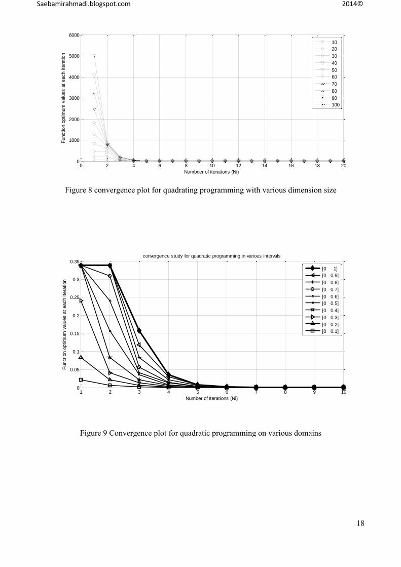
18

Figure 8 convergence plot for quadrating programming with various dimension size

Figure 9 Convergence plot for quadratic programming on various domains

0 2 4 6 8 10 12 14 16 18 200

1000

2000

3000

4000

5000

6000

Numbeer of iterations (Ni)

Function o

ptim

um

valu

es a

t each ite

ration

10

20

30

40

50

60

70

80

90

100

1 2 3 4 5 6 7 8 9 100

0.05

0.1

0.15

0.2

0.25

0.3

0.35convergence study for quadratic programming in various intervals

Number of Iterations (Ni)

Function o

ptim

um

valu

es a

t each ite

ration

[0 1]

[0 0.9]

[0 0.8]

[0 0.7]

[0 0.6]

[0 0.5]

[0 0.4]

[0 0.3]

[0 0.2]

[0 0.1]


19

Figure 10 convergence plot for quadratic programming in 3000 dimensions

#-12- Linear programming

Min {b x , * * 1000[x 40 40]i ix x }

*

ix known

N=1000

Ni=10

x*(Known)= x*predicted = 2.9322, 2.9322,…

F(x*predicted)= -1.4600e+08

b= -1.2738e+02, 1.0898e+02, -2.2530e+03 …

Runtime=3054.09 seconds

1 2 3 4 5 6 7 8 9 100

10

20

30

40

50

60

70

Number of iterations (Ni)

Function o

ptim

um

valu

es a

t each ite

ration

Convergence study for quadratic programming in 3000 dimensions


20

Figure 11 Convergence plot for linear programming in 500 dimensions

4. Conclusions

A global optimization algorithm, named MPMG (Multi-Point Moving Grid) method was developed

which by simulation and a concise mathematical proof was shown to be simultaneously efficient and

accurate. The method is valid as long as the objective function is Lipschitz continuous and first order

as well as second order optimality conditions are met. The computational cost associated with the

method linearly grows with increase in dimension size. This is much economical than any other

deterministic GO algorithms that their computational cost usually exponentially grows with increase

in dimension size. Several highly multi-modal bench-mark functions were efficiently and accurately

treated by the method. Quadratic programming and also exponential bench-mark function with 3000

decision variables were also examined by the method and an accurate solution were efficiently found

for the corresponding problems. It is noteworthy that the method was confirmed to solve ‘non-convex

global optimization on convex domains’ and a future paper is supposed to be developed on this title.

The MPMG algorithm, synchronized the good characters of stochastic and deterministic methods in

one place. The algorithm fills the vacant place of a most wanted global optimization method which is

desired to be simultaneously efficient and accurate.

Biography

Saeb AmirAhmadi Chomachar was born on July 1984, in Rasht, Iran. He is currently a PhD candidate

in Mechanical Engineering (Dynamics, Vibrations, and Controls) at the University of Guilan, Rasht,

Iran. He received an M.Sc. in Aerospace Engineering (Flight Mechanics) from the Center of

Excellence in Flight Dynamics and Controls at the Aerospace Engineering Department of the

AmirKabir University of Technology (AUT), Tehran, Iran, 2011. As well he holds a B.Sc. in

Mechanical Engineering (Mechanics of Solids) from the University of Guilan, Rasht, Iran, 2007. He

is serving as a reviewer for the IEEE (Aerospace and Electronic Systems, Transactions on), and the

AIAA (Journal of Guidance, Control and Dynamics). As well he served as a reviewer for ASME-

IMECE-2012. His research interest lies in the area of development of novel mathematical theories. As

well he is interested in research fields of flight dynamics and controls in general and particularly the

Aeroservoelasticity. He is the author of several popular online publications.

1 2 3 4 5 6 7 8 9 10-1.5

-1.4

-1.3

-1.2

-1.1

-1

-0.9

-0.8

-0.7x 10

8


Function o

ptim

um

valu

es a

t each level

Convergence study for linear programming in 500 dimensions


21

REFERENCES

[1] Floudas, C. A. Deterministic global optimization: Theory, methods and applications. Nonconvex

optimization and its applications. Kluwer Academic Publishers, (2000).

[2] Floudas, C. A. Global optimization in design and control of chemical process systems. Journal of

Process Control, 10, 125, (2000).

[3] Floudas, C. A., Pardalos, P. M., Adjiman, C. S., Esposito,W. R., Gumus¸, Z. H., Harding, S. T.,

Klepeis, J. L., Meyer, C., & Schweiger, C. A. Handbook of test problems in local and global

optimization. Kluwer Academic Publishers, (1999).

[4] Bard, J. F. Practical bilevel optimization. Nonconvex optimization and its applications. Kluwer

Academic Publishers, (1998).

[5] Horst, R., Pardalos, P. M., & Thoai, N. V. Introduction to global optimization. Nonconvex

optimization and its applications. Kluwer Academic Publishers, (2000).

[6] Sherali, H. D., & Adams, W. P. A reformulation–linearization technique for solving discrete and

continuous nonconvex problems. Nonconvex optimization and its applications. Kluwer Academic

Publishers, (1999).

[7] Tawarmalani, M.,&Sahinidis, N.V. Semidefinite relaxations of fractional programs via novel

convexification techniques. Journal of Global Optimization, (2001), 20, 137–158.

[8] Tuy, H. Convex analysis and global optimization. Nonconvex optimization and its applications.

Kluwer Academic Publishers.) (1998).

[9] Zabinsky, Z. B. Stochastic adaptive search for global optimization. Nonconvex optimization and

its applications. Kluwer Academic Publishers.). (2003).

[10] Neumaier, A. Complete search in continuous global optimization and constraint satisfaction. In

A. Iserles (Ed.), Acta Numerica (Vol. 13, pp. 271–369). Cambridge University Press, (2004).

[11] J. Jahn, Introduction to the Theory of Nonlinear Optimization, 3rd Edition, Springer-Verlag

Berlin Heidelberg, (2007).

[12] Z. Michalewicz, Genetic algorithms + data structures = evolution programs, 3rd ed., Springer,

Berlin (1996).

[13] J. S. Arora, Introduction to Optimum Design, Second Edition, Elsevier Academic Press (2004).

[14] A. Ben-Tal, L. El Ghaoui, A. Nemirovski, Robust Optimization, Princeton University Press

(2009).

[15] D. Bertsekas, Convex Analysis and Optimization, Athena Scientific (2003).

[16] I. M Bomze, T. Csendes, R. Horst, and P. M. Pardalos, Developments in Global optimization.

Dordrecht, Netherlands: Kluwer, (1997).

[17] J. Borwein AND A. Lewis, Convex Analysis and Nonlinear Optimization, Springer (2000)

[18] S. P. Boyd AND L. Andenberghe, Convex Optimization. Cambridge University, (2004)

[19] E. K. P. Chong, S. H. Zak, An Introduction to Optimization, Wiley (2011).

[20] N. Christofides, Combinatorial optimization, Wiley (1979)

[21] M Clerc, Particle Swarm Optimization, John Wiley & Sons, Jan (2010).

[22] K. Deb, Optimization for Engineering Design: Algorithms and Examples, PHI Learning Pvt. Ltd.

(2004).

[23] P. E. Gill, W. Murray, M. H. Wright, Practical optimization, Academic Press (1981).

[24] O. Güler, Foundations of Optimization in Finite Dimensions, Springer (2010).

[25] E. R. Hansen, Global optimization using interval analysis, Dekker, New York (1992).

[26] R. Horst, H. Tuy, Global optimization, deterministic approaches, 3rd ed. (2010), Springer, Berlin.

[27] B. Korte, J. Vygen, Combinatorial Optimization: Theory and Algorithms, Springer (2005).

[28] Y. Nesterov, Yurii. Introductory Lectures on Convex Optimization, Kluwer Academic Publishers

(2004).

[29] J. Nocedal AND S. Wright, Numerical Optimization (Springer Series in Operations Research and

Financial Engineering) 2nd edition (2006).

[30] G. C. Onwubolu, B. V. Babu, New Optimization Techniques in Engineering, Springer, (2004).

[31] A. Ruszczyński. Nonlinear Optimization. Princeton University Press (2006).

http://www.google.com/search?tbo=p&tbm=bks&q=inauthor:%22Aharon+Ben-Tal%22

http://www.google.com/search?tbo=p&tbm=bks&q=inauthor:%22Laurent+El+Ghaoui%22

http://www.google.com/search?tbo=p&tbm=bks&q=inauthor:%22Arkadi+Nemirovski%22

http://en.wikipedia.org/wiki/Dimitri_Bertsekas

http://www.amazon.com/exec/obidos/ASIN/0792343514/ref=nosim/weisstein-20

http://www.amazon.com/exec/obidos/ASIN/0792343514/ref=nosim/weisstein-20

http://www.stanford.edu/~boyd/cvxbook/bv_cvxbook.pdf

http://www.google.com/search?tbo=p&tbm=bks&q=inauthor:%22Edwin+K.+P.+Chong%22

http://www.google.com/search?tbo=p&tbm=bks&q=inauthor:%22Stanislaw+H.+Zak%22

http://www.google.com/search?tbo=p&tbm=bks&q=inauthor:%22Maurice+Clerc%22

http://www.google.com/search?tbo=p&tbm=bks&q=inauthor:%22Kalyanmoy+Deb%22

http://www.google.com/search?tbo=p&tbm=bks&q=inauthor:%22Philip+E.+Gill%22

http://www.google.com/search?tbo=p&tbm=bks&q=inauthor:%22Walter+Murray%22

http://www.google.com/search?tbo=p&tbm=bks&q=inauthor:%22Margaret+H.+Wright%22

http://www.google.com/search?tbo=p&tbm=bks&q=inauthor:%22Osman+G%C3%BCler%22

http://www.google.com/search?tbo=p&tbm=bks&q=inauthor:%22Bernhard+Korte%22

http://www.google.com/search?tbo=p&tbm=bks&q=inauthor:%22Jens+Vygen%22

http://www.amazon.com/Jorge-Nocedal/e/B001H6Q8P2/ref=ntt_athr_dp_pel_1

http://www.amazon.com/s/ref=ntt_athr_dp_sr_2?_encoding=UTF8&field-author=Stephen%20Wright&ie=UTF8&search-alias=books&sort=relevancerank

http://www.google.com/search?tbo=p&tbm=bks&q=inauthor:%22Godfrey+C.+Onwubolu%22

http://www.google.com/search?tbo=p&tbm=bks&q=inauthor:%22B.+V.+Babu%22


22

[32] J. J. Moré and G. Toraldo, On the solution of large quadratic programming problems with bound

constraints, SIAM J. Optim., 1 (1991), pp. 93–113. New York, 1984.

[33] R. Glowinski, Numerical Methods for Nonlinear Variational Problems, Springer-Verlag, Berlin,

New York, (1984).

[34] E. G. Birgin, I. Chambouleyron, and J. M. Mart´ınez, Estimation of the optical constants and the

thickness of thin films using unconstrained optimization, J. Comput. Phys., 151 (1999), pp. 862–880.

[35] P. G. Ciarlet, The Finite Element Method for Elliptic Problems, North–Holland, Amsterdam,

(1978).

[36] E. G. Birgin, R. Biloti, M. Tygel, and L. T. Santos, Restricted optimization: A clue to a fast and

accurate implementation of the common reflection surface stack method, J. Appl. Geophys., 42 (1999),

pp. 143–155.

[37] W. Glunt, T. L. Hayden, and M. Raydan, Molecular conformations from distance matrices, J.

Comput. Chem., 14 (1993), pp. 114–120.

[38] A. R. Conn, N. I. M. Gould, and Ph. L. Toint, Global convergence of a class of trust region

algorithms for optimization with simple bounds, SIAM J. Numer. Anal., 25 (1988), pp. 433–460.

[39] Z. Dostál, A. Friedlander, and S. A. Santos, Solution of coercive and semicoercive contact

problems by FETI domain decomposition, Contemp. Math., 218 (1998), pp. 82–93.

[40] Z. Dostál, A. Friedlander, and S. A. Santos, Augmented Lagrangians with adaptive precision

control for quadratic programming with simple bounds and equality constraints, SIAM J. Optim., 13

(2003), pp. 1120–1140.

[41] F. Facchinei and S. Lucidi, A class of penalty functions for optimization problems with bound

constraints, Optimization, 26 (1992), pp. 239–259.

[42] A. Friedlander, J. M. Mart´ınez, and S. A. Santos, A new trust region algorithm for bound

constrained minimization, Appl. Math. Optim., 30 (1994), pp. 235–266.

[43] W. W. Hager, Dual techniques for constrained optimization, J. Optim. Theory Appl., 55 (1987),

pp. 37–71.

[44] W. W. Hager, Analysis and implementation of a dual algorithm for constrained optimization, J.

Optim. Theory Appl., 79 (1993), pp. 427–462.

[45] J. M. Mart´ınez, BOX-QUACAN and the implementation of augmented Lagrangian algorithms

for minimization with inequality constraints, J. Comput. Appl. Math., 19 (2000), pp. 31–56.

[46] W. W. Hager, Dual techniques for constrained optimization, J. Optim. Theory Appl., 55 (1987),

pp. 37–71.

[47] W. W. Hager, Analysis and implementation of a dual algorithm for constrained optimization, J.

Optim. Theory Appl., 79 (1993), pp. 427–462.

[48] J. M. Mart´ınez, BOX-QUACAN and the implementation of augmented Lagrangian algorithms

for minimization with inequality constraints, J. Comput. Appl. Math., 19 (2000), pp. 31–56.

[49] R.P. Ge, A filled function method for finding a global minimizer of a function of several variables,

Math. Program. 46 (1990) pp.191–204.

[50] R.P. Ge, C.B. Huang, A continuous approach to nonlinear integer programming, Appl. Math.

Comput. Vol 34 (1989) pp.39–60

[51] R.P. Ge, Y.F. Qin, A class of filled functions for finding a global minimizer of a function of

several variables, J. Optim. Theory Appl. 54 (2) (1987) pp.241–252.

[52] X. Liu, A computable filled function used for global optimization, Appl. Math. Comput. 126

(2002) pp. 271–278.

[53] X. Liu, Finding global minima with a computable filled function, J. Global Optim. 19 (2001)

pp.151–161.

[54] X. Liu, W. Xu, A new filled function applied to global optimization, Comput. Operat. Res. 31

(2004) pp.61–80.

[55] S. Lucid, V. Piccialli, New classes of globally convexized filled functions for global optimization,

J. Global Optim. 24 (2002) pp.219–236.

[56] Y.L. Shang, L.S. Zhang, A filled function method for finding a global minimizer on global integer

optimization, J. Comput. Appl.

Math. 181 (2005) pp.200–210.


23

[57] Z. Xu, H. Huang, P. Pardalos, C. Xu, Filled functions for unstrained global optimization, J. Global

Optim. 20 (2001) pp.49–65.

[58] W.X. Zhu, A class of filled functions for box constrained continuous global optimization, Appl.

Math. Comput. 169 (2006) pp.129–145.

[59] H. Waultraud AND N. Arnold, Global optimization by multilevel coordinate search, Kluwer

Academic Publishers, Netherlands, (1998).

Appendix.

0.5 * U L1E ΔF F(x ) α - F(x ) F(x )

0.5 * U L2E = ΔF+F(x ) α - F(x ) F(x )

0.5 0.5 * U L * U L3E = ΔF + F(x ) α - F(x ) F(x ) ΔF + F(x ) α - F(x ) F(x )

4 3 , 0.5s opt U LE E = ΔF + ΔF F(x ) α - F(x ) F(x )

5 2 0.5 U LE = ΔF α - F(x ) F(x )

Non-convex Global Optimization on Convex Domains

Documents

Transcript of Non-convex Global Optimization on Convex Domains