1

Convex Optimization-based Beamforming: From Receive

to Transmit and Network Designs

Accepted for publication in IEEE Signal Processing Magazine

c© 2010 IEEE. Personal use of this material is permitted. However, permission to reprint/republish this material for

advertising or promotional purposes or for creating new collective works for resale or redistribution to servers or lists,

or to reuse any copyrighted component of this work in other works must be obtained from the IEEE.

ALEX B. GERSHMAN, NICHOLAS D. SIDIROPOULOS, SHAHRAM

SHAHBAZPANAHI, MATS BENGTSSON, AND BJORN OTTERSTEN

Stockholm 2010

IR–EE–SB 2010:007

1

Convex Optimization-based Beamforming: From

Receive to Transmit and Network DesignsAlex B. Gershman, Nicholas D. Sidiropoulos, Shahram Shahbazpanahi, Mats Bengtsson, and Bjorn Ottersten

Abstract—In this article, an overview of advanced convexoptimization approaches to multi-sensor beamforming is pre-sented, and connections are drawn between different types ofoptimization-based beamformers that apply to a broad class ofreceive, transmit, and network beamformer design problems. It isdemonstrated that convex optimization provides an indispensableset of tools for beamforming, enabling rigorous formulationand effective solution of both longstanding and emerging designproblems.

I. INTRODUCTION

Beamforming is a versatile and powerful approach to re-

ceive, transmit, or relay signals-of-interest in a spatially selec-

tive way in the presence of interference and noise. Receive

beamforming is a classic yet continuously developing field

that has a rich history of theoretical research and practical

applications to radar, sonar, communications, microphone ar-

ray speech/audio processing, biomedicine, radio astronomy,

seismology and other areas [1]. In the last decade, there has

been renewed interest in beamforming driven by applications

in wireless communications, where multi-antenna techniques

have emerged as one of the key technologies to accommodate

the explosive growth of the number of users and rapidly

increasing demands for new high data-rate services.

Recently, there has been significant progress in the field

of receive beamforming facilitated by convex optimization.

Motivated by the fact that the traditional adaptive beam-

forming techniques such as minimum variance beamforming

A. B. Gershman is the corresponding author. He is with with theCommunication Systems Group, Institute of Telecommunications, DarmstadtUniversity of Technology, Merckstr. 25, D-64283 Darmstadt, Germany, e-mail: gershman@nt.tu-darmstadt.de, phone: +49 6151 162813, fax:+49 6151 162913. N. D. Sidiropoulos is with the Department of Elec-tronic and Computer Engineering, Technical University of Crete, Chania73100, Greece; e-mail: nikos@telecom.tuc.gr, phone: +30 2821037227, fax: +30 28210 37542. S. Shahbazpanahi is with the Faculty ofEngineering and Applied Science, University of Ontario Institute of Tech-nology, 2000 Simcoe Street North, Oshawa, Ontario, L1H 7K4, Canada;e-mail: shahram.shahbazpanahi@uoit.ca, phone: +1 905 7213111(ext. 2842), fax: +1 905 7213370. M. Bengtsson and B. Ottersten are withthe School of Electrical Engineering, Royal Institute of Technology, SE-10044 Stockholm, Sweden; e-mails: mats.bengtsson@ee.kth.se andbjorn.ottersten@ee.kth.se, phone +46 8790 8463, fax: +46 87907260. B. Ottersten is also with securityandtrust.lu at the University of Luxem-bourg. The work of A. B. Gershman was supported in parts by the EuropeanResearch Council (ERC) Advanced Investigator Grants program under Grant227477-ROSE and German Research Foundation (DFG) under Grant GE1881/4-1. The work of S. Shahbazpanahi was supported by the NationalScience and Engineering Research Council of Canada (NSERC) under theDiscovery Grants program. The work of N. D. Sidiropoulos was supportedby ARL-ERO contract W911NF-09-1-0004. The work of M. Bengtsson wassupported by the Swedish Research Council (VR). The work of B. Otterstenhas received funding from the European Research Council under the EuropeanCommunity’s Seventh Framework Programme (FP7/2007-2013) / ERC grantagreement no 228044.

lack robustness against even small mismatches in the desired

signal steering vector [2]-[3], several authors proposed robust

techniques that are based on the concept of worst-case per-

formance optimization; see [4]-[11] and references therein.

One distinguishing feature of this line of work is that, using

convex optimization theory, seemingly complex robust design

problems formulated in [4]-[11] have been recast into tractable

convex forms and efficiently solved using interior point algo-

rithms or other appropriate numerical techniques. Beyond the

deterministic worst-case robust beamformer designs of [4]-

[11], there has been a recent trend to alternatively use less

conservative probabilistically-constrained designs [12] which

employ convex optimization to solve the resulting chance

programming problems. Moreover, both the worst-case and

probabilistically-constrained beamforming approaches have

been extended to the case of designing multi-user receivers

for space-time coded multiple-input multiple-output (MIMO)

communication systems [13]-[14].

Transmit beamforming is a relatively young and dynam-

ically developing research field. Classical beamforming is

matched to a single steering vector of interest (or, in the case

of robust beamforming, a “ball” of steering vectors around

the “nominal” one) and its goal is to ensure that the inner

product of the beamforming weight vector and the steering

vector of interest is large, while the inner product of the

beamforming weight vector and all other steering vectors

is small (to mitigate interference). This paradigm applies to

both receive beamforming and unicast transmit beamforming

towards a single receiver. A related but different case is that of

multi-user transmit beamforming, which arises in the cellular

multi-user downlink when the transmitter is equipped with

multiple transmit antennas. In this case, multiple transmit

beamforming weight vectors are used to carry different co-

channel unicast transmissions, each meant to reach the receiver

of one user. These vectors are then jointly designed to balance

the interference between different transmissions. The weight

vector designed for a given user should have a large inner

product with the steering vector of this user, and small

inner products with the steering vectors of all other users.

This concept was pioneered in [15]-[16] where several early

downlink beamforming techniques have been developed in the

context of voice services in a cellular mobile radio network

where, from the operator’s perspective, the system should

provide an acceptable quality-of-service (QoS) to each user

and serve as many users as possible, while radiating as low

power as possible. An important step forward followed in [17],

where convex optimization methods were used to solve the

problems of [15]-[16] and their robust worst-case optimization

2

based extensions. As the robust designs of [17] are based

on several approximations and can be shown to be overly-

conservative, recent follow-up work has pursued less conser-

vative robust designs based on convex optimization [18]-[19].

To provide more flexibility than that of worst-case designs,

outage probability-constrained downlink beamformers based

on chance programming have also been recently developed

[20], [21], [22].

What if we wish to transmit common information to many

users? The traditional way of doing this is (semi-) blind, in the

sense that it assumes little if anything regarding the steering

vectors or even the spatial distribution of users listening to

the transmission at any given time. In traditional radio and

TV broadcasting, for example, the signal is emitted either

isotropically or with a fixed beampattern to cover a service

area. There are many reasons for this, including the fact that

analog receivers were passive devices incapable of provid-

ing feedback to the transmitting station. In modern digital

wireless networks, particularly those based on subscription or

offering location-aware services, we often have some level

of channel state information (CSI) at the transmitter. This

can be exploited to boost network reach, coverage, quality of

service, and spectral efficiency; and minimize interference to

other systems (thus facilitating co-habitation, as in cognitive

radio). This is the premise of a recent line of work (starting

with [23] and [24]) on multicast beamforming using convex

optimization tools. Multicast beamforming is now part of

the current UMTS-LTE / EMBMS draft for next-generation

cellular wireless services [25], [26]. Similar ideas are currently

making their way through fixed wireless and local distribution

standardization committees, and are likely to influence media

distribution to wireless hand-held devices.

Information-theoretic analysis of the relay channel [39] and

multiple-relay networks [40] has paved the way for more

practical network cooperation schemes. Network beamforming

is a rapidly emerging area that belongs to the general field of

cooperative communications [27]. The key idea of network

beamforming is to use a “virtual array” of relay nodes that

retransmit properly weighted signals from the source to the

destination [28], thereby exploiting cooperation diversity. In

the simplest setting, a distributed network beamformer uses

an adaptive complex-valued weighting of the received signal,

similar to the so-called amplify-and-forward protocol. More

advanced types of relay processing (e.g., based on the decode-

and-forward strategy) are also possible. An interesting fea-

ture of network beamforming is that it can be interpreted

as a certain combination of receive and transmit strategies.

However, the main difference between the concept of network

beamforming and the more traditional concepts of receive and

transmit beamforming is that the relays can hardly exchange

information about their received signals, so that beamforming

is performed in a distributed fashion. There has been a

rapidly growing activity in this area over the last two years.

Following [28], a number of new concepts and methods have

been proposed, see [29]-[38] and references therein. These

include multi-user and bi-directional extensions of the original

approach of [28] and new beamforming strategies such as a

filter-and-forward approach [33], [34]. Convex optimization

techniques have been extensively used in these works to obtain

computationally attractive (exact or approximate) solutions to

originally difficult design problems.

The main goal of this paper is to present a system-

atic overview of the current state of the art of advanced

optimization-based beamforming, and to explore interrela-

tionships between different types of beamformers that apply

to a broad class of practically important receive, transmit,

and network beamforming problems. While the focus of this

article is on applications in wireless communications, several

designs considered here are also applicable in quite different

application contexts, such as MIMO radar.

The remainder of this paper is organized as follows. Sec-

tions II, III and IV are devoted to the receive, transmit, and

network beamforming problems, respectively. In Section V,

conclusions are drawn and future research directions are

briefly discussed.

Notation: Uppercase and lowercase bold letters denote

matrices and vectors, respectively. E{·}, Tr(·), (·)T , and (·)H

stand for the statistical expectation, trace of a matrix, trans-

pose, and Hermitian transpose, respectively. I is the identity

matrix. ‖ · ‖ denotes the Euclidean norm of a vector or the

Frobenius norm of a matrix. ⊙ denotes the Schur-Hadamard

(element-wise) matrix or vector product, diag(a) stands for

a diagonal matrix whose diagonal entries are the elements of

vector a, and λmax(·) stands for the principal eigenvalue of a

matrix.

II. RECEIVE BEAMFORMING

The output signal of a narrowband receive beamformer can

be written as

x(t) = wHy(t)

where w is the N × 1 vector of beamformer complex weight

coefficients, y(t) is the N×1 complex snapshot vector of array

observations, and N is the number of antenna array sensors.

The array observation vector can be modeled as

y(t) = s(t) + n(t)

where s(t) and n(t) are the desired signal and the interference-

plus-noise components of y(t), respectively. In the point signal

source case, s(t) = s(t)as where s(t) and as are the desired

signal waveform and its steering vector (spatial signature),

respectively.

If as and the true array covariance matrix R ,

E{y(t)yH(t)} are perfectly known, then the optimal weight

vector can be straightforwardly obtained by means of maxi-

mizing the signal-to-interference-plus-noise ratio (SINR) [1],

see Fig. 1. In the finite sample case, the true array covari-

ance matrix is unavailable and, therefore, its sample estimate

R = 1J

∑Jt=1 y(t)yH(t) = 1

J YYH is used instead of R

where Y , [y(1), . . . ,y(J)] is the beamformer training data

matrix and J is the number of snapshots available. Then,

the optimal weight vector can be approximately computed by

solving the following convex problem [1]-[3]

minw

wHRw s.t. wHas = 1. (1)

3

Desiredsignal

Interferer 1

Interferer 2

Fig. 1. Illustration of receive adaptive beamforming: Polar plot of adaptedbeampattern. The beamformer output SINR is maximized by means ofenhancing the desired signal by the beampattern mainlobe and rejecting theinterferers by beampattern nulls.

The solution to (1) can be expressed in the following

familiar closed form [1]:

w = βR−1as (2)

where the scalar β = (aHs R−1as)

−1 does not affect the

beamformer output SINR. The beamformer in (2) is usually

referred to as the sample matrix inversion (SMI) based mini-

mum variance (MV) technique.

The fact that the sample array covariance matrix R is

used instead of R in (1) is known to dramatically affect the

performance of (2) as compared to the optimal beamformer

in the case when the desired signal component is present

in the training samples [2], [3]. Note that the latter case is

typical for multi-antenna wireless communications and passive

source localization. Such a performance degradation caused by

signal cancellation is commonly termed as signal self-nulling.

It becomes especially strong in practical scenarios, when the

knowledge of as is imperfect as well [3].

One of the most popular ad hoc approaches to improve

the robustness of the SMI-based MV technique and to avoid

signal self-nulling is the diagonal loading (DL) method [2],

[41] whose key idea is to regularize the solution of (1) by

adding the quadratic penalty term γwHw to the objective

function, where γ is a preselected DL factor. The resulting

loaded SMI (LSMI) beamformer amounts to replacing the

sample covariance matrix R in (2) by its diagonally loaded

counterpart, γI + R.

The main shortcoming of the traditional DL approach is that

there is no easy and reliable way of choosing the DL factor

γ. Note that any fixed choice of γ can be only suboptimal,

because the optimal choice of γ is known to be scenario-

dependent [2], [4]. To avoid the aforementioned drawbacks of

the standard DL technique, more theoretically rigorous robust

MV beamforming algorithms have been recently proposed in

[4]-[8] based on worst-case designs.

The key idea of the beamformer developed in [4] and,

independently, in [7], is to explicitly model the steering vector

uncertainty as δ , as − as where as and as are the actual

and presumed signal steering vectors, respectively; and to

assume that the Euclidean norm of δ is upper-bounded by

a known constant ε. This corresponds to the case of spherical

uncertainty; a more general ellipsoidal uncertainty model has

been considered in [7] and [8].

The essence of the approach of [4] is to add robustness

to the standard MV beamforming problem (1) by using the

distortionless response constraint which must be satisfied for

all mismatched signal steering vectors in the given spherical

uncertainty set. With such a constraint, robust MV beamformer

design has been formulated in [4] as the following optimiza-

tion problem:

minw

wHRw s.t. |wH(as + δ)| ≥ 1 ∀ ‖δ‖ ≤ ε. (3)

Note that the constraint in (3) warrants that the distortionless

response will be maintained in the worst case, i.e., for the

particular choice of δ which corresponds to the smallest value

of |wH(as+δ)| provided that ‖δ‖ ≤ ε. Towards converting (3)

to convex form, it has been shown in [4] that, for reasonably

small size of the uncertainty region, ε ≤ |wHas|/‖w‖,

min‖δ‖≤ε

|wH(as + δ)| = |wHas| − ε‖w‖. (4)

Using (4) and taking into account that the objective function in

(3) remains unchanged when w undergoes an arbitrary phase

rotation, it has been shown in [4] that (3) can be converted to

the following convex form:

minw

wHRw s.t. wHas ≥ ε‖w‖ + 1 (5)

where the constraint in (5) also implicitly constrains wHas to

be real-valued and positive. The problem in (5) belongs to the

class of second-order cone programming (SOCP) problems

that can be easily solved (with complexity comparable to

that of the SMI-based MV beamformer) using standard and

highly efficient convex optimization software [42]-[43] or,

alternatively, using Newton-type algorithms [7], [8], [44]. It

can be proved [4] that the constraint in (5) is active, i.e., it is

satisfied with equality. Interestingly, the robust design in (5)

admits an adaptive DL interpretation; see our first insert to

appreciate this link.

4

Adaptive DL interpretation of the robust beamformer (5). Taking into accountthat the constraint in (5) is active and using the Lagrange multiplier method, thesolution of (5) can be found by minimizing the Lagrangian function [8]

L(w, λ) = wH

Rw − λ(wH

as − ε‖w‖ − 1)

where λ is the Lagrange multiplier. Computing the gradient of L(w, λ) andequating it to zero yields

Rw + λεw

‖w‖= λas. (6)

Since rescaling the weight vector by an arbitrary constant does not affect theoutput SINR, (6) can be transformed to

(

R +ε

‖w‖I

)

w = as (7)

where, for the sake of simplicity, the same notation w is used for the rescaledweight vector as for the original one in (6).

From (7), it can be seen that the robust beamformer (5) belongs to the class of

adaptive DL techniques because its DL factor ε/‖w‖ depends on ‖w‖ and,

therefore, is scenario-dependent. In contrast to the fixed DL approach, such

adaptive diagonal loading optimally matches the DL factor to the radius ε of

the uncertainty sphere.

Extensions of worst-case beamformer designs: One useful

extension of the robust beamformer (5) has been developed in

[6]. In this work, a more general case is considered where,

apart from the steering vector mismatch, there is a nonsta-

tionarity of the beamformer training data. This nonstationarity

is characterized in [6] by the matrix ∆ which models the

mismatch in the data matrix Y, and it is proposed to combine

the robustness against interference nonstationarity and steering

vector errors using the ideas similar to that of [4] and [7].

Correspondingly, the objective function in (3) can be modified

as

max‖∆‖≤η

‖(Y + ∆)Hw‖2

where η is some known upper bound on the matrix ∆.

It has been shown in [6] that the resulting modified problem

can be converted to the following convex form:

minw

‖YHw‖ + η‖w‖ s.t. wHas ≥ ε‖w‖ + 1. (8)

Note that, similar to (5), the problem in (8) belongs to the

class of SOCP problems and, hence, it can be easily solved.

Another useful extension of the approach of [4] and [7]

has been developed in [12]. The authors of [12] argue that,

although the worst-case beamformer designs are known to

result in quite robust techniques, they might be overly con-

servative because the actual worst operational conditions may

occur in practice with a very low (or even zero) probability.

This motivated the authors of [12] to develop an alternative

approach to robust beamforming that provides the robustness

only against “likely” spatial signature errors. Using this phi-

losophy, the probabilistically constrained counterpart of the

problem (3) can be written as [12]

minw

wHRw s.t. Pr{|wH(as + δ)| ≥ 1} > p (9)

where δ is assumed to be a random mismatch vector drawn

from some known distribution, Pr{·} is the probability oper-

ator whose explicit form can be obtained from the statistical

assumptions on the steering vector errors, and p is some pre-

selected probability threshold. In contrast to the deterministic

constraint used in (3) (that requires the distortionless response

to be maintained for all norm-bounded mismatch vectors in

the uncertainty sphere), the soft (probabilistic) constraint in

(9) maintains the distortionless response only for the mismatch

vectors δ whose probability is sufficiently high, while ignoring

the values of δ which are unlikely to occur. Therefore, the

constraint in (9) can be interpreted as an outage probability

constraint maintaining this probability (pout = 1 − p) low.

It has been shown in [12] that for both circularly symmetric

Gaussian and for the worst-case distribution1 of the steering

vector mismatch, the chance programming problem in (9)

can be tightly approximated by means of deterministic SOCP

problems. Interestingly, the latter problems are mathematically

quite similar to (5). However, an important advantage of the

probability-constrained beamformers of [12] with respect to

their worst-case counterparts of [4] and [7] is that the former

beamformers enable to explicitly quantify the parameters of

the uncertainty region in terms of the beamformer outage

probability. This streamlines the choice of ε.

Further convex optimization-based extensions of the robust

beamformers discussed in this section have been recently

proposed. In [9], a semidefinite programming (SDP) approach

has been developed to extend the beamformers of [4] and [7]

to a more general (than the spherical and ellipsoidal) class

of uncertainty models. Several broadband generalizations of

[4] have been proposed in [10] and [11]. Extensions of the

approaches of [4] and [12] to the problem of designing robust

multi-user MIMO receivers have been developed in [13] and

[14], respectively.

Before moving on, it is instructive to summarize three

different approaches towards beamforming under uncertainty,

using the relatively simple case of receive beamforming as an

example: see our second insert.

Beamforming under uncertainty:

• Worst-case design:

minw

wH

Rw s.t. |wH

(as + δ)| ≥ 1 ∀ ‖δ‖ ≤ ε.

• Probabilistic design:

minw

wH

Rw s.t. Pr{|wH

(as + δ)| ≥ 1} > p

Interpretation: in a long sequence of “trials” (i.i.d. draws of δ), acceptableperformance is guaranteed in p × 100% of cases; signal outage happens withprobability (at the rate of) less than 1 − p.• Expectation-based design:

minw

wH

Rw s.t. E{|wH

(as + δ)|} ≥ t

The latter only requires knowledge of the second-order statistics (instead ofthe distribution) of h := as + δ, which is convenient. The flip side is that thisformulation offers no outage performance guarantee in general. For this reason,expectation-based design is the “last resort” way of dealing with uncertainty.

III. TRANSMIT BEAMFORMING

A. Downlink Beamforming

For notational convenience, we consider a single base

station equipped with N antennas, transmitting individual

narrowband data streams to a set of M users, each having a

single antenna. Note that all results in this section generalize

1The worst-case distribution (for given covariance) of the mismatch vec-tor turns out to be discrete. This result entails an intermediate restriction(strengthening) of the outage constraint, see [12] for details.

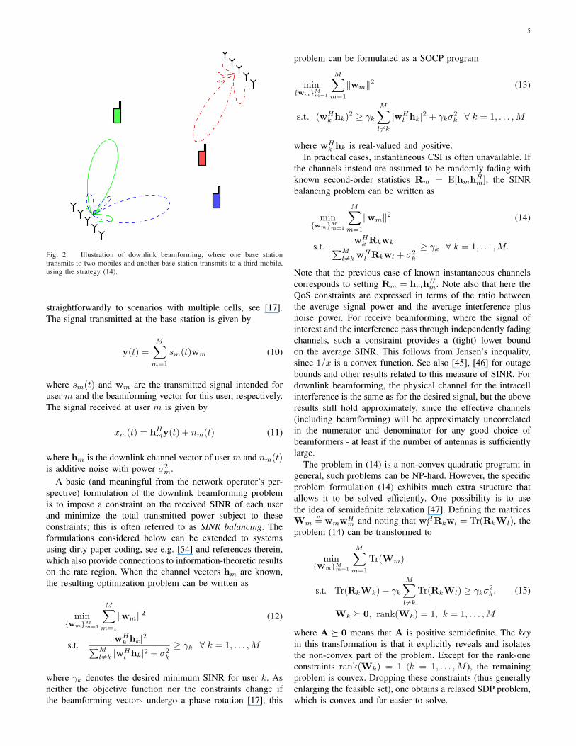
5

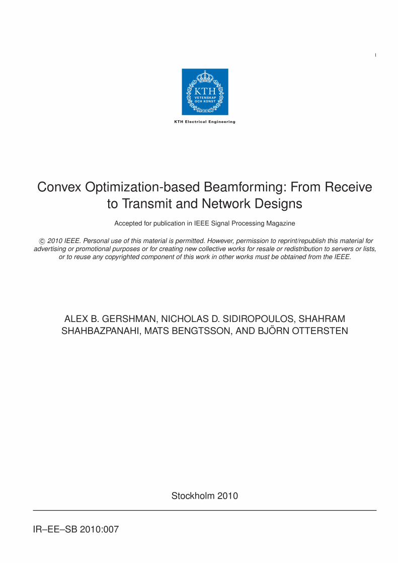
Fig. 2. Illustration of downlink beamforming, where one base stationtransmits to two mobiles and another base station transmits to a third mobile,using the strategy (14).

straightforwardly to scenarios with multiple cells, see [17].

The signal transmitted at the base station is given by

y(t) =

M∑

m=1

sm(t)wm (10)

where sm(t) and wm are the transmitted signal intended for

user m and the beamforming vector for this user, respectively.

The signal received at user m is given by

xm(t) = hHmy(t) + nm(t) (11)

where hm is the downlink channel vector of user m and nm(t)is additive noise with power σ2

m.

A basic (and meaningful from the network operator’s per-

spective) formulation of the downlink beamforming problem

is to impose a constraint on the received SINR of each user

and minimize the total transmitted power subject to these

constraints; this is often referred to as SINR balancing. The

formulations considered below can be extended to systems

using dirty paper coding, see e.g. [54] and references therein,

which also provide connections to information-theoretic results

on the rate region. When the channel vectors hm are known,

the resulting optimization problem can be written as

min{wm}M

m=1

M∑

m=1

‖wm‖2 (12)

s.t.|wH

k hk|2∑M

l 6=k |wHl hk|2 + σ2

k

≥ γk ∀ k = 1, . . . ,M

where γk denotes the desired minimum SINR for user k. As

neither the objective function nor the constraints change if

the beamforming vectors undergo a phase rotation [17], this

problem can be formulated as a SOCP program

min{wm}M

m=1

M∑

m=1

‖wm‖2 (13)

s.t. (wHk hk)2 ≥ γk

M∑

l 6=k

|wHl hk|2 + γkσ2

k ∀ k = 1, . . . , M

where wHk hk is real-valued and positive.

In practical cases, instantaneous CSI is often unavailable. If

the channels instead are assumed to be randomly fading with

known second-order statistics Rm = E[hmhHm], the SINR

balancing problem can be written as

min{wm}M

m=1

M∑

m=1

‖wm‖2 (14)

s.t.wH

k Rkwk∑M

l 6=k wHl Rkwl + σ2

k

≥ γk ∀ k = 1, . . . , M.

Note that the previous case of known instantaneous channels

corresponds to setting Rm = hmhHm. Note also that here the

QoS constraints are expressed in terms of the ratio between

the average signal power and the average interference plus

noise power. For receive beamforming, where the signal of

interest and the interference pass through independently fading

channels, such a constraint provides a (tight) lower bound

on the average SINR. This follows from Jensen’s inequality,

since 1/x is a convex function. See also [45], [46] for outage

bounds and other results related to this measure of SINR. For

downlink beamforming, the physical channel for the intracell

interference is the same as for the desired signal, but the above

results still hold approximately, since the effective channels

(including beamforming) will be approximately uncorrelated

in the numerator and denominator for any good choice of

beamformers - at least if the number of antennas is sufficiently

large.

The problem in (14) is a non-convex quadratic program; in

general, such problems can be NP-hard. However, the specific

problem formulation (14) exhibits much extra structure that

allows it to be solved efficiently. One possibility is to use

the idea of semidefinite relaxation [47]. Defining the matrices

Wm , wmwHm and noting that wH

l Rkwl = Tr(RkWl), the

problem (14) can be transformed to

min{Wm}M

m=1

M∑

m=1

Tr(Wm)

s.t. Tr(RkWk) − γk

M∑

l 6=k

Tr(RkWl) ≥ γkσ2k, (15)

Wk º 0, rank(Wk) = 1, k = 1, . . . ,M

where A º 0 means that A is positive semidefinite. The key

in this transformation is that it explicitly reveals and isolates

the non-convex part of the problem. Except for the rank-one

constraints rank(Wk) = 1 (k = 1, . . . , M ), the remaining

problem is convex. Dropping these constraints (thus generally

enlarging the feasible set), one obtains a relaxed SDP problem,

which is convex and far easier to solve.

6

There are at least three possible interpretations of this

semidefinite relaxation

• With the rank constraints rank(Wk) = 1, (15) is com-

pletely equivalent to (14). This problem can become a

relaxed version of (14) only when the matrices Wk are

allowed to have any rank.

• It can be shown that the semidefinite relaxation of (15)

is the Lagrange dual of the Lagrange dual of (14).

• If we allow the beamforming vectors to be randomly

time-varying with covariance matrix Wk = E[wkwHk ],

the optimal choice of Wk is given by the semidefinite

relaxation of (15). One possible practical implementation

of such a scheme is to use a space-time code with the

corresponding transmit covariance matrix.

For general non-convex quadratic programs, semidefinite re-

laxation can only be used to obtain a lower bound on the

optimal objective function and possibly determine an ap-

proximate solution to the original problem, such as in the

multicast beamforming problem described below. However,

in the specific case of (15) with dropped rank constraints,

it turns out that the ostensible relaxation is not a relaxation,

i.e., the “relaxed” problem is exactly equivalent to the original

problem. In other words, it can be shown that the solution

to (15) with dropped rank constraints always yields rank-

one matrices Wk, which directly provides the solution to

(14) using Wk = wkwHk . In optimization terminology, this

result shows that strong duality holds for problem (14), i.e.,

that the dual of (14) has the same optimal objective as the

primal problem. This result is not so surprising, considering

that there are also several other algorithms available to solve

problem (14), see [15], [48]. These algorithms are not based

on the convex reformulation of (15) but rather on rewriting

the problem into an equivalent virtual uplink problem, that

can be solved using fixed point iterations [49]. See the special

insert on the connection between Lagrange duality and virtual

uplink. From practical experience, the algorithm in [48] is

preferable compared to the semidefinite reformulation in terms

of computational speed, at least so long as (15) with dropped

rank constraints is solved using general purpose SDP software

like [42].

Further modifications and extensions: Several modifica-

tions and extensions have been proposed to the SINR bal-

ancing problem (14). For multi-cell scenarios, the problem

can be extended to not only find the jointly optimal set

of transmit beamformers, but also to determine to which

base station each user should be assigned to. Surprisingly

enough, this mixed combinatorial and non-convex quadratic

problem can be solved easily, see [50], [51]. The trick is

to conceptually view all the base stations as a single virtual

base station that jointly transmits to all users, and solve the

corresponding beamforming problem. By making the channel

covariance matrices for the virtual base station block-diagonal,

the solution will not benefit from using coherent transmission

from several base stations (in contrast to so-called coherent

coordinated multi-point transmission schemes that recently

have been proposed for use in IMT-advanced), and it can

be shown that the optimal beamforming vectors will only be

non-zero in a sub-vector corresponding to one of the base

stations. One proof is based on the simple observation that

the corresponding optimal matrices Wk in the semidefinite

reformulation will be both block-diagonal and rank-one, which

is only possible if only one of the blocks is non-zero. An

alternative is to exploit the virtual uplink formulation and

use general results from the theory of standard interference

functions [49]. Algorithmically, this conceptual idea can be

implemented with a computational complexity that is only

K times larger than in the case with a given base station

assignment, where K is the number of base stations.

Connection between Lagrange duality and virtual uplink. Introducing thedual variables qk for the constraints in (14), the Lagrangian can be written as

L(wk, qk) =

M∑

m=1

‖wm‖2−

M∑

k=1

qk

wHk

Rk

γk

wk −M∑

l6=k

wHl Rkwl − σ

2

k

and minimizing with respect to wk results in the dual problem

max{qk}

M∑

k=1

qkσ2

k s.t. I−qkRk

γk

+

M∑

n 6=k

qnRn º 0, ∀ k = 1, . . . , M. (16)

From the definition of positive definiteness, the constraints holds if and only if

uH(∑ M

n6=k qnRn + I−qkRk

γk)u ≥ 0 for all vectors u, i.e. (16) can be written

as

max{qk}

M∑

k=1

qkσ2

k s.t. maxuk

uHk qkRkuk

uHk

(∑

Mn6=k qnRn + I)uk

≤ γk, ∀ k = 1, . . . , M.

(17)

For a given fixed set of uk, it is easy to see that the optimal qk is the uniqueset of values where all constraints are fulfilled with equality. In particular, thisequivalence must hold for the uk that maximize each constraint, so the solutionto (17) is given by the fixed point of

maxuk

uHk qkRkuk

uHk

(∑

Mn 6=k qnRn + I)uk

= γk, ∀ k = 1, . . . , M. (18)

The so-called virtual uplink problem associated with (14) is given by

min{qk,uk}

M∑

k=1

qkσ2

k s.t.uH

k qkRkuk

uHk

(∑

Mn6=k qnRn + I)uk

≥ γk, ∀ k = 1, . . . , M

(19)

where qk and uk can be interpreted as transmit powers and receive beamform-ers, respectively, in this virtual uplink beamforming problem. A similar argumentshows that the optimum is given by the fixed point of (18). From the so-calledcomplementarity conditions, it can be seen that the optimal uk will only differfrom the optimal wk in (14) by a scaling. From standard convexity theory [52],the dual of (16), i.e., (15) with dropped rank constraints has the same optimalobjective as (16), which means that the proofs in [17] and [48] that (19) and (14)

are equivalent also show the equivalence to (15) with dropped rank constraints.See also [54] for further discussions on these connections.Note that replacing the objective function in (19) by

∑ Mk=1

qk will not affectthe optimal uk. It is common to first normalize all channels corresponding toσ2

k = 1 to get a more esthetic formulation of the virtual uplink problem (19).

An alternative to the SINR balancing formulation is to

consider the converse problem, namely to maximize the SINR

of each user subject to a constraint on the available transmit

power. Unfortunately, to our knowledge, there is no convex

formulation of the resulting optimization problem, which

however can still be solved very efficiently using the virtual

uplink formulation and a fixed-point iteration, see [48]. An

alternative solution using quasi-convexity is described in [53].

An advantage of the semidefinite relaxation technique is

that it is very easy to add more constraints to the problem

formulation. For example, the transmit power of the individual

antenna elements can be constrained, see [17]. As long as

the corresponding constraints on the matrices Wk are linear

(or convex), the problem can be solved efficiently. However,

there are in general no guarantees that strong duality holds

7

(i.e., that the optimal matrices Wk are rank-one) when ad-

ditional convex constraints are included. Strong duality has

been proven only for certain special cases. For example, in-

dividual power constraints per antenna are considered in [54],

where an efficient algorithm based on a generalization of

the virtual uplink duality is developed. In [55] it is shown

that an indefinite constraint of the form wHk Ckwk = 0 or

wHk Ckwk ≥ 0 can be added for each user, where the matrices

Ck are indefinite Hermitian matrices, and strong duality still

holds for the resulting optimization problem. Such constraints

may, for example, be used to enforce solutions with increased

path diversity in CDMA scenarios, or to constrain the relative

power transmitted to surrounding cells. This result has recently

been generalized in [56], where both aforementioned types of

indefinite constraints and so-called soft-shaping interference

constraints of the form∑M

m=1 wHmSkmwm ≤ τk with positive

semidefinite matrices Skm are considered. It is shown that

the semidefinite relaxation of the corresponding optimization

problems has a rank-one solution in a certain number of cases,

for example when there are up to two indefinite constraints for

each user, or when there are up to two soft-shaping constraints

for the system. The proofs are constructive, showing how a

given high-rank solution can be converted into a solution with

lower rank, under certain conditions.

Just as for the receive beamforming problem, many papers

have been devoted to robust extensions that can cope with un-

certainties in the channel knowledge, due to estimation errors,

feedback quantization or delays between channel estimation

and the actual transmission, for example. Most references

consider worst-case strategies given bounds on the errors.

Errors in the channel covariance matrices are considered in

[17] and [19] where the true covariance matrix is modeled as

Rm+∆m with a known bound ‖∆m‖ ≤ εm on the error term.

Replacing the numerator and denominator in (14) by a lower

and upper bound, respectively, as proposed in [17], results in

a kind of diagonal loading of the matrix Rk in the numerator

and denominator of the constraints in (14). Unfortunately, this

approach is very conservative and the resulting optimization

problem often does not even have a feasible solution. A

less conservative approach is proposed in [19], wherein the

worst-case matrix ∆m for each constraint is found by solving

the dual problem, and the resulting beamforming problem is

solved using the semidefinite relaxation technique. Numerical

experiments in [19] indicate that the obtained solution is

always rank-one, but no proof of this empirical observation

is available. An alternative outage probability based approach

is proposed in [20], where the matrices ∆m are assumed to be

Gaussian distributed and the SINR constraints are required to

hold with a certain probability. Again, semidefinite relaxation

is used to solve the problem and the numerical results in [20]

indicate that the solution always is rank-one.

Robustness against uncertainties in the channel vectors hm

has been considered in [18], [57], and [58] using a QoS

constraint expressed in terms of the MSE instead of SINR.

For exactly known channel vectors, such an MSE constraint is

equivalent to an SINR constraint. For partial CSI, on the other

hand, MSE constraints provide a conservative lower bound on

the SINR, as shown in [18]. Stochastic error models have also

10

20

30

30

210

60

240

90

270

120

300

150

330

180 0

++

++

++

+

+++

++

Fig. 3. Illustration of multicast beamforming: Polar plot of a multicasttransmit beampattern. Multicast subscriber locations are denoted by redcrosses. Unlike receive beamforming or single-user transmit beamforming,the multicast beampattern comprises multiple lobes, each generally servinga group of users. Unlike multi-user transmit beamforming that uses multiplebeampatterns, each carrying a different unicast stream, here a single beampat-tern that carries a common information stream is used. Notice that the lobeserving the lower-left group has higher peak magnitude, to compensate for ahigher path loss experienced by distant users.

been considered where the channel vector uncertainties are

assumed to be Gaussian distributed. In [57], the average MSE

is optimized subject to a constraint on the total transmitted

power, whereas in [21], a pre-specified outage level on the

MSE is used.

B. Multicast Beamforming

Consider a base station or wireless access point that uses

N antennas to transmit common information to a pool of

M users, each equipped with a single receive antenna. This

problem statement corresponds to the case of single-group

multicast (or, equivalently, broadcast) beamforming. Let hm

be the N ×1 complex downlink channel vector of user m and

w be the N × 1 complex beamforming vector. The objective

is to design w in such a way that the inner product of w

and each hm (m = 1, . . . , M ) is large, while the norm

of w is small. This philosophy is rather different from the

robust receive or unicast transmit beamforming paradigms,

because the different hm’s need not be clustered in a small

neighborhood and the resulting adapted transmit beampattern

has multiple mainlobes; see Fig 3.

Formally, such a design may be stated as the following

optimization problem [23]:

minw

‖w‖2 s.t. |wHhm|2 ≥ σ2mγm ∀ m = 1, . . . , M (20)

where σ2m is the additive noise power at user m, and γm is

the desired signal-to-noise power ratio (SNR) at user m. The

right-hand side of each inequality in (20) can be absorbed

in hm, yielding |wH hm|2 ≥ 1 with hm , hm/√

σ2mγm.

8

Dropping the tilde sign for brevity yields the following QoS

formulation:

minw

‖w‖2 s.t. |wHhm|2 ≥ 1 ∀ m = 1, . . . , M. (21)

Note that this formulation has a certain similarity to (12) as

in both cases the total transmit power is minimized subject to

QoS constraints. However, contrary to (12), a single weight

vector is used in (21).

An alternative formulation to the one in (21) arises from

an information theory standpoint. Intuitively, if one transmits

a single information-bearing signal to be decoded by a group

of users, the attainable information rate that can be decoded

by all interested users is determined by the weakest link, i.e.,

the user with the smallest SNR. This suggests the following

“democratic” max-min-fair formulation:

maxw

minm∈{1,...,M}

|wHhm|2 s.t. ‖w‖2 ≤ P

where P is an upper bound on the allowable transmission

power. Without loss of generality, we may absorb P in the

channel vectors and henceforth set P = 1. It is also easy to

see that an optimal solution will use all available power, hence

we may replace the power inequality with equality.

It is important to note that beamforming does not generally

attain the multicast channel capacity – this may require a

higher-rank transmit covariance. The capacity-attaining strat-

egy, however, is often impractical for a number of reasons, in-

cluding the complexity of multi-stream Shannon (de-)coding,

and incompatibility with existing and emerging standards.

Beamforming, on the other hand, is simple to implement and

often attains a significant fraction of multicast capacity [24].

Interestingly, it can be shown that the QoS and the max-

min-fair formulations of multicast beamforming are equivalent

up to scaling [24], and the scaling constant can be easily de-

termined. Furthermore, multicast beamformer design naturally

yields the optimal information-theoretic transmission strategy

as a by-product, as we will see in the sequel.

How difficult is the multicast beamforming problem? It is

certainly clean-cut, and easy in the case of a single user: by

virtue of the Cauchy-Schwartz inequality, an optimal solution

is simply a scaled version of the user’s steering vector. When

we add more users, the situation becomes less clear. At this

point, it is instructive to turn to the QoS formulation to gain

insight. Notice that the quadratic constraints |wHhm|2 ≥ 1are non-convex. This implies that we are dealing with a non-

convex optimization problem, as first clue. Going one step

further, let us visualize the structure of the feasible set in

the QoS formulation. Towards this end, we will consider the

special case where all vectors are real-valued and N = 2. Fig.

4 illustrates the intricate structure of the “playing field” in this

simplified scenario – and the picture is not pretty. Whereas we

could perhaps characterize the potentially interesting vertices

when M is small, this seems daunting for large M . It has

been shown in [24] that the multicast beamforming problem

is in fact NP-hard for M ≥ N ; it contains the partition

problem as a special case. In plain words, this means that

we have to give up hope of exactly solving an arbitrary

problem instance at reasonable complexity. This motivates

−5 −4 −3 −2 −1 0 1 2 3 4 5

−5

−4

−3

−2

−1

0

1

2

3

4

5

feasible

infeasible

−5 0 5

−5

−4

−3

−2

−1

0

1

2

3

4

5

Fig. 4. Peeking through shattered glass: Geometry of the feasible set in thereal-valued two-dimensional case (N = 2 transmit antennas; w and {hi}

M

i=1

are real-valued). Top panel: M = 4; bottom panel: M = 40. The axescorrespond to the elements of w. Every constraint (wT

hi)2 ≥ 1 excludes

a strip perpendicular to hi and passing through the origin. The non-convexfeasible set is shown in blue, while the infeasible set is shown in red. Noticethat both are symmetric with respect to reflection (changing the sign of bothelements of w). Since the norm of w is also invariant with respect to changeof sign, there are two optimal solutions for w, indicated by the yellow circles.As the number of users/constraints (M ) increases, the glass tends to shatterin a larger number of smaller pieces that are further away from the origin, asillustrated in the bottom panel.

the pursuit of approximate solutions which can approach

optimal performance at moderate complexity. Towards this

end, a convex approximation strategy based on semidefinite

relaxation is considered next.

Using |wHhm|2 = Tr(wwHhmhHm) and defining Rm ,

hmhHm, we may recast the max-min fair problem as follows:

maxw

minm∈{1,...,M}

Tr(wwHRm) s.t. Tr(wwH) = 1. (22)

By change of variable X , wwH , we may further restate (22)

as

maxX

minm∈{1,...,M}

Tr(XRm)

s.t. Tr(X) = 1, X º 0, rank(X) = 1. (23)

Following the idea of semidefinite relaxation, we can drop the

non-convex rank constraint rank(X) = 1 to approximate (23)

by an SDP problem. Notice that this relaxation “restores” up

to full covariance rank, yielding the capacity-optimal transmit

9

covariance [24], [59] (cf. first-principles definition of multicast

capacity, using Tr(XRm) = Tr(XhmhHm) = hH

mXhm, and

monotonicity of log(·)).

Once the relaxed problem is solved, the only direct claim

one can make is that the resulting objective topt is no less than

the optimal max-min value of the original NP-hard problem

(since by dropping a constraint we expanded the feasible set).

In many (but not all) cases, it turns out that the associated

Xopt is rank-one, which means that our relaxation was not a

relaxation after all (see also the earlier discussion for downlink

beamforming). If Xopt is rank-one, then we can find wopt for

the original problem simply by taking the principal component

of Xopt. When Xopt has higher rank, there is more work to be

done in “rounding” Xopt to a rank-one matrix – simply taking

the principal component is not the best strategy. The prevailing

rounding strategy is based on randomization: drawing i.i.d.

random vectors from a zero-mean multivariate Gaussian of

covariance Xopt and picking the best one. Details can be found

in [24]. Note that randomization can be theoretically justified

in this context – it is possible to bound the gap to the optimal

solution of the original NP-hard problem. On this issue, see

[47], [60], [61].

At the end of the day, one is interested in how well the over-

all relaxation-randomization algorithm works in practice. The

answer is that it works very well [24], although, for the case

of a single-group multicast, there are now better and simpler

algorithms available as a result of considerable follow-up work

[62], [63]. The power of convex optimization/approximation

lies in its generality; for example, it can handle the case of

multiple (interfering) multicast groups [64]-[66], additional

convex constraints, etc.

Further extensions: Robust multicast beamforming has been

dealt with in [64]. Bridging the ground between multi-user

downlink and multicast beamforming, the general case of

multiple interfering multicast groups has been studied in

[62], [65], [66], and cross-layer multicast beamforming and

admission control in [62]. Instead of (exact or approximate)

instantaneous CSI, it is possible to use long-term average

CSI in the form of estimated channel correlation matrices

Rm, albeit only average QoS guarantees can be offered in

this case. Going one step further, [67] considered the case

when the only information available for the channel vectors is

their prior distribution. This is naturally modeled as a mixture

distribution – e.g., a Gaussian mixture comprising components

centered at different locations and with varying spread. Such

a model can capture subscriber clustering in malls, campuses,

or other urban “hotspots”. In this case, similarly to the receive

and downlink beamforming techniques of [12] and [20], the

pertinent design criterion is the beamformer outage probability.

While outage probability minimization also turns out to be NP-

hard, an effective approximation is again possible [67]. It is

worth noting that this last approach is particularly appealing

in practice, because the mixture model can be built using

historical data and/or field measurements around local points

of interest.

Source

Destination

f1

g1

Relay 1

f2

g2Relay 2

f3

g3

Relay 3

fN

gN

Relay N

Fig. 5. A relay network.

IV. RELAY NETWORK BEAMFORMING

Let us now consider a wireless network which consists of a

source, a destination, and N relay nodes as shown in Fig. 5.

Assume that due to the poor quality of the channel between the

source and destination, they cannot communicate directly with

each other, but the destination cooperates with the N single-

antenna relay nodes to receive the information transmitted by

the source node and retransmitted by the relays. We use fi

and gi to denote the channel complex coefficients between the

source and the ith relay and between the ith relay and destina-

tion, respectively. In earlier network beamformer designs [28],

is has been assumed that the instantaneous CSI is perfectly

known at the destination or relays. However, this assumption

is often violated in practical scenarios with randomly fading

channels. To avoid the need to know instantaneous CSI, fi

and gi can be modeled as random variables [29], and it can

be assumed that their joint second-order statistics are known

at the destination node which uses this knowledge to compute

the relay complex weight coefficients and feed them back to

the relay nodes. Alternatively, such second-order CSI may be

available at the relay nodes rather than destination. In the latter

case, each relay has to compute its own weight coefficient.

During the first step of a two-step amplify-and-forward

protocol, the source transmits the signal√

P0s to the relays,

where s is the information symbol, P0 is the source transmit

power, and without loss of generality it is assumed that

E{|s|2} = 1. The received signal at the ith relay is given

by

xi =√

P0 fi s + νi (24)

where νi is the noise at the ith relay whose variance is known

to be σ2ν . In the second step, the ith relay transmits yi which

is an amplified and phase-steered version of its received signal

and can be written as

yi = wixi . (25)

Here, wi is the complex relay beamforming weight that is used

by the ith relay to adjust the phase and the amplitude of the

corresponding signal.

Interestingly, network beamforming can be viewed as a

certain combination of receive and transmit beamforming

as the same weights are used for the signal reception and

10

transmission. Moreover, network beamforming is distributed

as each relay node knows only its own received signal, and

does not know the signals received by the other relay nodes.

The signal received by the destination is given by

z =r∑

i=1

giyi + n (26)

where n is the receiver noise whose variance σ2n is known.

Using (24) and (25), we can rewrite (26) as

z =√

P0

r∑

i=1

wifi gis

︸ ︷︷ ︸

signal component

+

r∑

i=1

wigiνi + n

︸ ︷︷ ︸

total noise, nT

. (27)

To optimally calculate the relay weight coefficients, the des-

tination SNR has to be maximized subject to some power

constraints. To illustrate the application of convex optimization

to this problem, let us consider the individual relay power

constraints. Then, the following optimization problem has to

be solved:

maxw

SNR s.t. Pi ≤ Pi ∀ i = 1, . . . , N (28)

where Pi and Pi are, respectively, the actual and maximum

allowable transmit powers of the ith relay. As in (14), we

use the ratio of expected signal power to expected noise

power as a measure of SNR. In [29], it has been shown

that this is given by wHRwσ2

n+wHQwand Pi = Dii|wi|2 where

w , [w1, . . . , wN ]T , f , [f1, . . . , fN ]T , g , [g1, . . . , gN ]T ,

Q , σ2νE{ggH}, R , P0E{(f ⊙ g)(f ⊙ g)H}, D ,

P0 diag([E{|f1|2}, . . . ,E{|fN |2}]

)+ σ2

νI, and Dii is the ithdiagonal entry of D.

Hence, the problem in (28) can be rewritten as

maxw

wHRw

σ2n + wHQw

s.t. Dii|wi|2 ≤ Pi ∀ i = 1, . . . , N.

Defining X , wwH , this optimization problem can be

rewritten as

maxX

Tr(RX)

σ2n + Tr(QX)

s.t. DiiXii ≤ Pi ∀ i = 1, . . . , N ; rank(X) = 1, X º 0

where Xii is the ith diagonal entry of X. Following the idea of

semidefinite relaxation and dropping the non-convex rank-one

constraint, the latter problem can be relaxed as

maxX,t

t

s.t. Tr (X(R − tQ)) ≥ σ2nt, (29)

Xii ≤ Pi/Dii ∀ i = 1, . . . , N ; X º 0.

Note that, for any fixed value of t the set of feasible X in (29)

is convex; it follows that the optimization problem in (29) is

quasiconvex.

Solving (29), one can obtain the maximum achievable SNR

(which is the maximum value of t, denoted as tmax). To solve

(29), the following key observation [52] has been used in [29].

If, for some given SNR value t, the convex feasibility problem

find X

s.t. tr (X(R − tQ)) ≥ σ2nt, (30)

Xii ≤ Pi/Dii ∀ i = 1, . . . , N ; X º 0

is feasible, then tmax ≥ t. Conversely, if (30) is not feasible,

then tmax < t. Based on this observation, one can check

whether the optimal value tmax of the quasiconvex problem

(29) is smaller or greater than any given value t. In [29], it has

been proposed to use a simple bisection algorithm for solving

(29), where (30) has to be solved at each step of this algorithm.

Let us start with some preselected interval [tl tu] which is

known to contain the optimal value tmax, the problem (30) is

then solved at the midpoint t = (tl + tu)/2. If (30) is feasible

for this value of t, then tl = t is set; otherwise tu = t is chosen.

This procedure is repeated until the difference between tu and

tl is smaller than some preselected threshold δ.

Numerical examples in [29] have shown that, similar to the

case of downlink beamforming, the so-obtained solution Xopt

is always rank-one and, therefore, no randomization is needed

to obtain the beamforming weight vector. However, no proof

of this empirical observation is available in [29].

Summary of network beamforming algorithm.

Step 1: Properly set the initial values of tl and tu.Step 2: Set t := (tl + tu)/2 and solve (30).Step 3: If (30) is feasible, then tl := t; otherwise tu := t.Step 4: If tu − tl < δ, then go to Step 5; otherwise go to Step 2.Step 5: Find the weight vector from the principal eigenvector of the resultingmatrix Xopt.

One suitable choice of the initial values of tl and tu is

0 and SNRmax(Pmax), respectively, where SNRmax(Pmax)is the maximum achievable SNR under the total relay power

budget Pmax =∑N

i=1 Pi. It has been shown in [29] that

SNRmax(Pmax) = Pmaxλmax(G) (31)

where G , (σ2nI + PmaxD

−1/2QD−1/2)−1D−1/2RD−1/2.

The results of [28] and [29] are applicable only when the

relays are fully synchronized at the symbol level and when the

source-to-relay and relay-to-destination channels are frequency

flat. When these channels are frequency selective or the time

synchronization between the relays is poor, the signal replicas

passed through different relays and/or channel paths will arrive

to the destination node with different delays. This will result

in inter-symbol-interference (ISI).

To combat such ISI, two different approaches have been

presented in the literature. In [33]-[34], a filter-and-forward

protocol has been introduced for frequency selective relay

networks, and several related network beamforming techniques

have been developed. In these techniques, the relays deploy

finite impulse response (FIR) filters to compensate for the

effect of source-to-relay and relay-to-destination channels; that

is, the burden of mitigating ISI is put on the shoulders of

the relay nodes. One of these techniques can be viewed as

an extension of (29) because it is based on maximizing the

destination QoS (measured in terms of SINR) subject to the

individual relay power constraints. The latter technique is

also based on a combination of bisection search and convex

feasibility problem-solving.

11

Another beamforming approach developed in [35] for asyn-

chronous but flat-fading relay networks, suggests the relay

processing to be simple (i.e., to follow the amplify-and-

forward protocol), while the source and destination nodes carry

the main burden of mitigating ISI. Viewing an asynchronous

flat-fading relay network as an artificial multipath channel

(where each channel path corresponds to one particular relay),

the authors of [35] use the orthogonal frequency division

multiplexing (OFDM) scheme at the source and destination

nodes to deal with this artificial multipath channel.

Convex optimization has also found its application to

multi-user (i.e., multiple-source, multiple-destination) network

beamforming techniques. In [30], a network of relays is used to

establish communication between multiple source destination

pairs. The relays amplify and phase adjust the signal they

receive from all transmitting sources by multiplying it with

a complex beamforming weight. To obtain the optimal value

of beamforming weights, the total relay transmit power is

minimized subject to QoS constraints on the received SINRs

at the destinations. It is then shown that using semidefinite

relaxation, this power minimization problem can be turned into

a convex SDP problem. In light of the results of [68], when

the number source-destination pairs is less than or equal to 3,

the semidefinite relaxation approach is always guaranteed to

have a rank-one solution, and therefore, in this case it is not

a relaxation but exact transformation of the original problem

(note here some similarity to the downlink beamforming case,

where the resulting solution after semidefinite relaxation yields

rank-one matrices as well).

Considering the same problem as considered in [30], the

authors of [36] use additional constraints to enforce the signals

received by the destinations be all in-phase. This will turn

the aforementioned constrained total relay power minimization

problem into an SOCP problem. As SOCP problems can be

solved with much lower computational complexity than SDP

problems, the approach of [36] to peer-to-peer network beam-

forming is computationally less expensive than that of [30].

The price for this computational complexity improvement is a

small increase in the relay transmitted power.

Convex optimization has also proven instrumental in ap-

plication to the design of beamformers for two-way (bi-

directional) relay networks. Such beamformers have been

developed in [32] for three-node two-way networks with one

multi-antenna relay node and two single-antenna transceivers,

and in [31] and [38] for multiple-node two-way networks

with all single-antenna nodes involving two transceivers and

multiple relays.

V. CONCLUSIONS AND FUTURE DIRECTIONS

In this paper, we have presented an overview of the current

state of the art of advanced optimization-based beamform-

ing with application to the receive, transmit and network

beamformer design problems. Connections have been drawn

between different types of optimization-based beamformers,

and it has been demonstrated that convex optimization is an

indispensable toolbox for beamformer designs.

Promising future research directions include beamformer

designs for frequency-selective scenarios; incorporating prac-

tical communications engineering aspects, such as synchro-

nization, modulation, and coding; and real-time beamformer

weight optimization to account for time-selective fading and

other sources of temporal variation in the operational envi-

ronment. Robustness issues will likely remain high in the

research agenda, in light of erroneous / delayed / quan-

tized CSI encountered in practical systems. This is especially

true for network beamforming which is still in its infancy.

Computationally efficient implementations of beamforming

techniques are critical for applications of beamforming in

practical systems, and it can be foreseen that this field will

keep benefiting from advances in convex optimization theory -

including relevant work towards real-time convex optimization

[69].

REFERENCES

[1] H. L. Van Trees, Optimum Array Processing, Wiley, NY, 2002.[2] H. Cox, R. M. Zeskind, and M. H. Owen, “Robust adaptive beamform-

ing,” IEEE Trans. Acoust., Speech, Signal Processing, vol. 35, pp. 1365-1376, Oct. 1987.

[3] A. B. Gershman, “Robust adaptive beamforming in sensor arrays,”AEU – Int. J. Electronics and Communications, vol. 53, pp. 305-314,Dec. 1999.

[4] S. Vorobyov, A. B. Gershman, and Z.-Q. Luo, “Robust adaptivebeamforming using worst-case performance optimization: A solution tothe signal mismatch problem,” IEEE Trans. Signal Process., vol. 51,pp. 313-324, Feb. 2003.

[5] S. Shahbazpanahi, A. B. Gershman, Z.-Q. Luo, and K. M. Wong,“Robust adaptive beamforming for general-rank signal models,” IEEE

Transactions on Signal Processing, vol. 51, pp. 2257-2269, Sept. 2003.[6] S. A. Vorobyov, A. B. Gershman, Z-Q. Luo, and N. Ma, “Adaptive

beamforming with joint robustness against mismatched signal steeringvector and interference nonstationarity,” IEEE Signal Process. Lett.,vol. 11, pp. 108-111, Feb. 2004.

[7] R. G. Lorenz and S. P. Boyd, “Robust minimum variance beamforming,”IEEE Trans. Signal Process., vol. 53, pp. 1684-1696, May 2005.

[8] Robust Adaptive Beamforming, J. Li and P. Stoica (Eds), John Wiley &Sons, Hoboken, NJ, 2006.

[9] S-J. Kim, A. Magnani, A. Mutapcic, S. P. Boyd, and Z-Q. Luo, “Robustbeamforming via worst-case SINR maximization,” IEEE Trans. Signal

Process., vol. 56, pp. 1539-1547, Apr. 2008.[10] A. El-Keyi, T. Kirubarajan, and A. B. Gershman, “Wideband ro-

bust beamforming based on worst-case performance optimization,” inProc. IEEE SSP Workshop, Bordeaux, France, July 2005, pp. 265-270.

[11] M. Rubsamen, A. El-Keyi, A. B. Gershman, and T. Kirubarajan, “Robustbroadband adaptive beamforming using convex optimization,” chapterin Convex Optimization in Signal Processing and Communications,D. Palomar and Y. C. Eldar, Editors, Cambridge Univ. Press, to appear.

[12] S. Vorobyov, H. Chen, and A. B. Gershman, “On the relationshipbetween robust minimum variance beamformers with probabilistic andworst-case distortionless response constraints,” IEEE Trans. Signal Pro-

cess., vol. 56, pp. 5719-5724, Nov. 2008.[13] Y. Rong, S. Shahbazpanahi, and A. B. Gershman, “Robust linear

receivers for space-time block coded multi-access MIMO systems withimperfect channel state information,” IEEE Trans. Signal Process.,vol. 53, pp. 3081-3090, Aug. 2005.

[14] Y. Rong, S. A. Vorobyov, and A. B. Gershman, “Robust linear receiversfor multi-access space-time block coded MIMO systems: A probabilis-tically constrained approach,” IEEE J. Sel. Areas Commun., vol. 24,pp. 1560-1570, Aug. 2006.

[15] F. Rashid-Farrokhi, K. J. R. Liu, and L. Tassiulas, “Transmit beamform-ing and power control for cellular wireless systems,” IEEE J. Sel. Areas

Commun., vol. 16, pp. 1437-1450, Oct. 1998.[16] C. Farsakh and J. A. Nossek, “Spatial covariance-based downlink be-

ramforming in an SDMA mobile radio system,” IEEE Trans. Commun.,vol. 46, pp. 1497-1506, Nov. 1998.

[17] M. Bengtsson and B. Ottersten, “Optimal and suboptimal transmitbeamforming,” in Handbook of Antennas in Wireless Communications,L. Godara, Editor, CRC Press, 2001.

[18] N. Vucic and H. Boche, “Robust QoS-constrained optimization of down-link multiuser MISO systems,” IEEE Trans. Signal Process., vol. 57,pp. 714-725, Feb. 2009.

12

[19] I. Wajid, Y. C. Eldar, and A. B. Gershman, “Robust downlink beam-forming using covariance channel state information,” Proc. ICASSP’09,Taipei, Taiwan, April 2009.

[20] B. K. Chalise, S. Shahbazpanahi, A. Czylwik, and A. B. Gershman, “Ro-bust downlink beamforming based on outage probability specifications,”IEEE Trans. Wireless Commun., vol. 6, pp. 3498-3503, Oct. 2007.

[21] N. Vucic and H. Boche, “A tractable method for chance-constrainedpower control in downlink multiuser MISO systems with channeluncertainty,” IEEE Signal Process. Lett., vol. 16, pp. 346-349, May 2009.

[22] M.B. Shenouda and T.N. Davidson, “Probabilistically-constrained ap-proaches to the design of the multiple antenna downlink,” in Proc. 42nd

Asilomar Conference on Signals, Systems and Computers, pp. 1120-1124, 26-29 Oct. 2008.

[23] N. D. Sidiropoulos and T. N. Davidson, “Broadcasting with channelstate information,” in Proc. IEEE SAM Workshop, Sitges, Spain, July2004, pp. 489493.

[24] N.D. Sidiropoulos, T.N. Davidson, Z.-Q. Luo, “Transmit beamformingfor physical layer multicasting,” IEEE Trans. Signal Process., vol. 54,no. 6, part 1, pp. 2239-2251, June 2006.

[25] Motorola Inc., “Long term evolution (LTE): A technical overview,” Tech-nical White Paper, http://business.motorola.com/experiencelte/pdf/LTE%20Technical%20Overview.pdf

[26] A. Lozano, “Long-term transmit beamforming for wireless multicast-ing,” in Proc. ICASSP’07, April 2007, Honolulu, Hawaii.

[27] J. N. Laneman, D. N. C. Tse, and G. W. Wornell, “Cooperative diversityin wireless networks: Efficient protocols and outage behavior,” IEEE

Trans. Inform. Theory, vol. 50, pp. 3062-3080, Dec. 2004.[28] Y. Jing and H. Jafarkhani, “Network beamforming using re-

lays with perfect channel information,” Proc. ICASSP’07, vol. 3,pp. 473-476, Honolulu, HI, April 2007; the full paper available athttp://arxiv.org/pdf/0804.1117v1.

[29] V. Havary-Nassab, S. Shahbazpanahi, A. Grami, and Z.-Q. Luo, “Dis-tributed beamforming for relay networks based on second-order statisticsof the channel state information,” IEEE Trans. Signal Process., vol. 56,pp. 4306-4316, Sept. 2008.

[30] S. Fazeli-Dehkordy, S. Shahbazpanahi, and S. Gazor, “Multiple peer-to-peer communications using a network of relays,” IEEE Trans. Signal

Process., vol. 57, pp. 3053-3062, Aug. 2009.[31] V. Havary-Nassab, S. Shahbazpanahi, and A. Grami, “Optimal net-

work beamforming for bi-directional relay networks,” Proc. ICASSP’09,Taipei, Taiwan, April 2009.

[32] Y.-C. Liang and R. Zhang, “Optimal analogue relaying with multi-antennas for physical layer network coding,” Prof. ICC’08, Bejing,China, May 2008, pp. 3893-3897.

[33] H. Chen, A. B. Gershman, and S. Shahbazpanahi, “Filter-and-forwarddistributed beamforming for relay networks in frequency selective fadingchannels,” Proc. ICASSP’09, Taipei, Taiwan, April 2009

[34] H. Chen, A. B. Gershman, and S. Shahbazpanahi, “Filter-and-forwarddistributed beamforming in relay networks with frequency selectivefading,” IEEE Trans. Signal Process., to appear.

[35] A. Abdelkader, S. Shahbazpanahi, and A. B. Gershman, “Joint sub-carrier power loading and distributed beamforming in OFDM-basedasynchronous relay networks,” IEEE CAMSAP’09, Aruba, Dec. 2009,to appear.

[36] H. Chen, A. B. Gershman, and S. Shahbazpanahi, “Distributed peer-to-peer beamforming for multiuser relay networks,” Proc. ICASSP’09,Taipei, Taiwan, April 2009.

[37] J. Joung and A. H. Sayed, “Power allocation for beamforming relaynetworks under channel uncertainties,” in Proc. Globecom’09, Honolulu,Hawaii, December 2009, to appear.

[38] S. Shahbazpanahi, “A semi-closed-form solution to optimal decentral-ized beamforming for two-way relay networks,” IEEE CAMSAP’09,Aruba, Dec. 2009, to appear.

[39] T. Cover and A.E. Gamal, “Capacity theorems for the relay channel,”IEEE Trans. Inform. Theory, vol. 25, pp. 572-584, Sep. 1979.

[40] M. Gastpar and M. Vetterli, “On the capacity of large Gaussian relaynetworks,” IEEE Trans. Inform. Theory, vol. 51, pp. 765-779, March2005.

[41] Y. I. Abramovich, “Controlled method for adaptive optimization offilters using the criterion of maximum SNR,” Radio Engineering and

Electronic Physics, vol. 26, pp. 87-95, March 1981.[42] J. F. Sturm, “Using SeDuMi 1.02, a MATLAB toolbox for optimization

over symmetric cones,” Optim. Meth. Software, vol. 11-12, pp. 625-653,Aug. 1999; awailable at http://sedumi.ie.lehigh.edu/.

[43] M. Grant, S. Boyd, and Y. Y. Ye, “CVX: MATLABsoftware for disciplined convex programming,” available athttp://www.stanford.edu/boyd/cvx/V.1.0RC3, Feb. 2007.

[44] J. Li, P. Stoica, and Z. Wang, “On robust Capon beamforming anddiagonal loading,” IEEE Trans. Signal Process., vol. 51, pp. 1702-1715,July 2003.

[45] S. Kandukuri and S. Boyd. “Optimal power control in interference-limited fading wireless channels with outage-probability specifications,”IEEE Trans. Wireless Comm., vol. 1, no. 1, pp. 46–55, Jan. 2002.

[46] M. Bengtsson and B. Ottersten, “Signal waveform estimation from arraydata in angular spread environment,” in Proc. 30th Asilomar Conf. Sig.,

Syst., Comput., Nov. 1996, pp. 355–359.

[47] Z.-Q. Luo, W.-K. Ma, M.-C. So, Y. Ye, and S. Zhang, “Nonconvexquadratic optimization, semidefinite relaxation, and applications,” IEEE

Signal Processing Magazine, this issue.

[48] M. Schubert and H. Boche, “Solution of the multiuser down-link beamforming problem with individual SINR constraints,” IEEE

Trans. Veh. Technology, vol. 53, pp. 18-28, Jan. 2004.

[49] R. D. Yates, “A framework for uplink power control in cellular radiosystems,” IEEE J. Sel. Areas Commun., vol. 13, no. 7, pp. 1341-1347,Sep. 1995.

[50] M. Bengtsson, “Jointly optimal downlink beamforming and base stationassignment,” in Proc. ICASSP’01, Salt Lake City, UT, May 2001, vol. V,pp. 2961-2964.

[51] R. Stridh, M. Bengtsson, and B. Ottersten, “System evaluation ofoptimal downlink beamforming with congestion control in wirelesscommunication,” IEEE Trans. Wireless Commun., vol. 5, pp. 743-751,Apr. 2006.

[52] S. Boyd and L. Vandenberghe, Convex Optimization, Cambridge Uni-versity Press, 2004.

[53] A. Wiesel, Y. C. Eldar, and S. S. (Shitz), “Linear precoding via conicoptimization for fixed MIMO receivers,” IEEE Trans. Signal Process.,vol. 54, pp. 161-176, Jan. 2006.

[54] W. Yu and T. Lan, “Transmitter optimization for the multi-antennadownlink with per-antenna power constraints,” IEEE Trans. Signal

Process., vol. 55, pp. 2646-2660, June 2007.

[55] D. Hammarwall, M. Bengtsson, and B. Ottersten, “Downlink beamform-ing with indefinite shaping constraints,” IEEE Trans. Signal Process.,vol. 54, pp. 3566-3580, Sep. 2006.

[56] Y. Huang and D. P. Palomar, “Rank-constrained separable semidefiniteprogram with applications to optimal beamforming,” IEEE Trans. Signal

Processing, to appear.

[57] M. B. Shenouda and T. N. Davidson, “On the design of lineartransceivers for multiuser systems with channel uncertainty,” IEEE

J. Sel. Areas Commun., vol. 26, pp. 1015-1024, Aug. 2008.

[58] M. B. Shenouda and T. N. Davidson, “Nonlinear and linear broadcastingwith QoS requirements: Tractable approaches for bounded channeluncertainties,” IEEE Trans. Signal Processing, vol. 57, pp. 1936-1947,May 2009.

[59] N. Jindal, Z.-Q. Luo, “Capacity limits of multiple antenna multicast,”in Proc. IEEE Int. Symposium Inf. Theory, July 2006, Seattle, WA,pp. 1841-1845.

[60] Z.-Q. Luo, N. D. Sidiropoulos, P. Tseng, S. Zhang, “Approximationbounds for quadratic optimization with homogeneous quadratic con-straints,” SIAM J. Optimization, vol. 18, no. 1, pp. 1-28, Feb. 2007.

[61] T.-H. Chang, Z.-Q. Luo, C.-Y. Chi, “Approximation bounds for semidef-inite relaxation of max-min-fair multicast transmit beamforming prob-lem,” IEEE Trans. Signal Process., vol. 56, pp. 3932-3943, Aug. 2008.

[62] E. Matskani, N. D. Sidiropoulos, Z.-Q. Luo, and L. Tassiulas, “Effi-cient batch and adaptive approximation algorithms for joint multicastbeamforming and admission control, IEEE Trans. Signal Process., toappear.

[63] A. Abdelkader, A.B. Gershman, N.D. Sidiropoulos, “Multiple-antennamulticasting using channel orthogonalization and local refinement,”submitted to IEEE Trans. Signal Process., July 2009.

[64] E. Karipidis, N.D. Sidiropoulos, Z.-Q. Luo, “Convex transmit beam-forming for downlink multicasting to multiple co-channel groups,” inProc. ICASSP’06, May 2006, Toulouse, France.

[65] E. Karipidis, N. D. Sidiropoulos, Z.-Q. Luo, “Far-field multicast beam-forming for uniform linear antenna arrays,” IEEE Trans. Signal Process.,vol. 55, pp. 4916-4927, Oct. 2007.

[66] E. Karipidis, N. D. Sidiropoulos, Z.-Q. Luo, “Quality of service andmax-min-fair transmit beamforming to multiple co-channel multicastgroups,” IEEE Trans. Signal Process., vol. 56, pp. 1268-1279, March2008.

[67] V. Ntranos, N. D. Sidiropoulos, and L. Tassiulas, “On multicast beam-forming for minimum outage,” IEEE Trans. on Wireless Communica-

tions, vol. 8, pp. 3172-3181, June 2009.

13

[68] Y. Huang and S. Zhang, “Complex matrix decomposition and quadraticprogramming,” Mathematics of Operation Research, vol. 32, pp. 758–768, Aug. 2007.

[69] J. Mattingley, S. Boyd, “Real-Time Convex Optimization in SignalProcessing,” IEEE Signal Processing Magazine, this issue.

Alex B. Gershman received his Diploma and Ph.D. degrees

in Radiophysics and Electronics from the Nizhny Novgorod

State University, Russia, in 1984 and 1990, respectively. Since

2005, he is a Professor at Darmstadt University of Technology,

Germany. He has co-authored papers that received two IEEE

Signal Processing Society (SPS) Best Paper Awards in 2004

and 2005, and the IEEE Aerospace and Electronic Systems

Society (AESS) Barry Carlton Award in 2006. Prof. Gershman

served as Editor-in-Chief for the IEEE SIGNAL PROCESSING

LETTERS (2006–2008), and as Chair of the Sensor Array and

Multichannel Processing Technical Committee of the IEEE

SPS (2007–2008). He is a Fellow of the IEEE.

Nicholas D. Sidiropoulos graduated from the Aristotelian

University of Thessaloniki, Greece, and received his Ph.D.

in Electrical Engineering from the University of Maryland, in

1992. He was Assistant Professor at the University of Virginia,

and Associate Professor at the University of Minnesota. Since

2002, he is a Professor at the Technical University of Crete

– Greece. He received the IEEE Signal Processing Society

(SPS) Best Paper Award in 2001 and 2007, has served as SPS

Distinguished Lecturer (2008-2009), and as Chair of the Signal

Processing for Communications and Networking Technical

Committee of the IEEE SPS. Prof. Sidiropoulos is a Fellow

of IEEE.

Shahram Shahbazpanahi received his B.S., M.S., and PhD.

degrees all in Electrical Engineering, from Sharif University of

Technology, Tehran, Iran 1992, 1994, and 2001, respectively.

Since 2005, he is an Assistant Professor at the University of

Ontario Institute of Technology, Oshawa, Ontario, Canada. He

serves as Associate Editor for both the IEEE TRANSACTIONS

ON SIGNAL PROCESSING and the IEEE SIGNAL PROCESS-

ING LETTERS. He is a member of the Sensor Array and

Multichannel Processing Technical Committee of the IEEE

Signal Processing Society.

Mats Bengtsson received the M.S. degree Linkoping Univer-

sity, Linkoping, Sweden, in 1991 and the Ph.D. degrees from

the Royal Institute of Technology (KTH), Stockholm, Sweden,

in 2000. From 1991 to 1995, he was with Ericsson Telecom

AB Karlstad. He currently holds a position as Associate

Professor in the Signal Processing Laboratory of the School of

Electrical Engineering at KTH. He serves as Associate Editor

for the IEEE TRANSACTIONS ON SIGNAL PROCESSING.

Bjorn Ottersten received the M.S. degree from Linkoping

University, Linkoping, Sweden, in 1986 and his Ph.D. in

1989 from Stanford University, Stanford, CA. Since 1991 he

is a Professor at the Royal Institute of Technology (KTH),

Stockholm. From 2004 to 2008 he was dean of the School of

Electrical Engineering at KTH and from 1992 to 2004 he was

head of the department for Signals, Sensors, and Systems at

KTH. Dr. Ottersten is also Director of securityandtrust.lu at

the University of Luxembourg since 2009. He has co-authored

papers that received the IEEE Signal Processing Society

Best Paper Award in 1993, 2001, and 2006. Dr. Ottersten is

currently Editor-in-Chief of EURASIP SIGNAL PROCESSING

JOURNAL. He is a Fellow of the IEEE and EURASIP.