Beamforming and power control for interference reduction in wireless communications using particle...

Int. J. Electron. Commun. (AEÜ) 64 (2010) 489–502

www.elsevier.de/aeue

Beamforming and power control for interference reduction in wirelesscommunications using particle swarm optimization

Majid Khodier∗, Gameel Saleh

Department of Electrical Engineering, Jordan University of Science and Technology, P.O. Box 3030, Irbid 22110, Jordan

Received 7 October 2008; accepted 4 March 2009

Abstract

We consider joint beamforming (BF) and power control to minimize cochannel interference in a CDMA wireless uplink,where an antenna array of different geometries receives from single-antenna wireless users. The problem is to find theoptimum beamforming weight vector and the minimum transmission power of each terminal such that the quality of service(QoS) requirements of the users are fulfilled and the so-called near–far effect is alleviated. This will increase the channelcapacity and further prolongs the battery lives of the mobile terminals. The particle swarm optimization method is used todetermine the optimum beamforming weight vector and the minimum transmission power of each terminal. Uniform linearand circular array geometries are considered, with and without correlated shadow fading. Simulation results illustrate theadvantage of using BF jointly with power control and the robustness of the optimization technique used.� 2009 Elsevier GmbH. All rights reserved.

Keywords: CDMA; Power control; Beamforming; Particle swarm optimization; Antenna array

1. Introduction

In DS-CDMA systems, the cross correlation of differentspreading codes given to users is not zero in practice due tothe multipath propagation and incomplete orthogonality ofthe pseudonoise codes between different users. Therefore,the receiver sees the other users’ signals as interference, andthe more users in the system the more interference is gen-erated. Although increasing the signal power of a mobileuser will increase its SNR, unfortunately, such increase intransmission power will cause interference on other neigh-borhood terminals. Power control (PC) and antenna arraybeamforming (BF) are essential radio resource managementmethods in CDMA cellular communication systems, wherecochannel interference is the primary capacity-limiting fac-tor. The problem is then to steer a beam toward the userof interest and nulls to others, and to find the minimum

∗ Corresponding author. Tel.: +96227201000; fax: +96227201074.E-mail address: [email protected] (M. Khodier).

1434-8411/$ - see front matter � 2009 Elsevier GmbH. All rights reserved.doi:10.1016/j.aeue.2009.03.010

transmission powers such that the quality of service (QoS)requirements of the users are fulfilled and the so-callednear–far effect is alleviated. This will increase the channelcapacity and prolong the battery lives of the mobile ter-minals and even of the base stations. The basic papers onthe joint BF and PC problem are found in [1,2]. The jointreceiving BF and PC algorithm, which is presented in [1],involves iterating the BF and PC steps alternately. The con-vergence and optimality of the solution of this algorithm isproved in [2]. In the transmit BF and PC algorithm, a virtualuplink BF scheme with virtual centralized PC is appliedwith centralized PC [1]. A similar approach for joint uplinkBF and PC with additional joint multi-user detection waspresented in [3]. In [4], joint transmission BF, PC, and datarate allocation is discussed. An adaptive QoS application tothe joint BF and PC systems is introduced in [5]. Feasibilityresults related to the joint problem in single-cell CDMAsystems are presented in [6]. This paper uses the parti-cle swarm optimization (PSO) method [7–11] to optimizejointly and in iterative way both the beamforming weight

http://www.elsevier.de/aeue

mailto:[email protected]

490 M. Khodier, G. Saleh / Int. J. Electron. Commun. (AEÜ) 64 (2010) 489–502

S1

S2

W11

W12

W13

W1Ny1

Combiner 1

Antennaelement 1

Antennaelement 2

Antennaelement 3

Antennaelement N

W21

W22

W23

W2Ny2

Combiner 2

WM1

WM2

WM3

WMNyM

Combiner M

.

.

.

.

.

.

SM

.

.

.

...

...

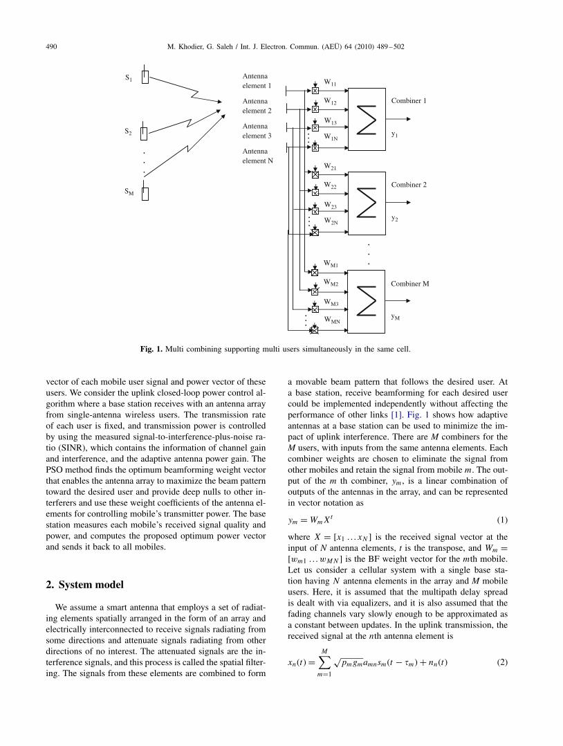
Fig. 1. Multi combining supporting multi users simultaneously in the same cell.

vector of each mobile user signal and power vector of theseusers. We consider the uplink closed-loop power control al-gorithm where a base station receives with an antenna arrayfrom single-antenna wireless users. The transmission rateof each user is fixed, and transmission power is controlledby using the measured signal-to-interference-plus-noise ra-tio (SINR), which contains the information of channel gainand interference, and the adaptive antenna power gain. ThePSO method finds the optimum beamforming weight vectorthat enables the antenna array to maximize the beam patterntoward the desired user and provide deep nulls to other in-terferers and use these weight coefficients of the antenna el-ements for controlling mobile’s transmitter power. The basestation measures each mobile’s received signal quality andpower, and computes the proposed optimum power vectorand sends it back to all mobiles.

2. System model

We assume a smart antenna that employs a set of radiat-ing elements spatially arranged in the form of an array andelectrically interconnected to receive signals radiating fromsome directions and attenuate signals radiating from otherdirections of no interest. The attenuated signals are the in-terference signals, and this process is called the spatial filter-ing. The signals from these elements are combined to form

a movable beam pattern that follows the desired user. Ata base station, receive beamforming for each desired usercould be implemented independently without affecting theperformance of other links [1]. Fig. 1 shows how adaptiveantennas at a base station can be used to minimize the im-pact of uplink interference. There are M combiners for theM users, with inputs from the same antenna elements. Eachcombiner weights are chosen to eliminate the signal fromother mobiles and retain the signal from mobile m. The out-put of the m th combiner, ym , is a linear combination ofoutputs of the antennas in the array, and can be representedin vector notation as

ym = Wm Xt (1)

where X = [x1 . . . xN ] is the received signal vector at theinput of N antenna elements, t is the transpose, and Wm =[wm1 . . . wM N ] is the BF weight vector for the mth mobile.Let us consider a cellular system with a single base sta-tion having N antenna elements in the array and M mobileusers. Here, it is assumed that the multipath delay spreadis dealt with via equalizers, and it is also assumed that thefading channels vary slowly enough to be approximated asa constant between updates. In the uplink transmission, thereceived signal at the nth antenna element is

xn(t) =M∑

m=1

√pm gmamnsm(t − �m) + nn(t) (2)

M. Khodier, G. Saleh / Int. J. Electron. Commun. (AEÜ) 64 (2010) 489–502 491

where sm is the transmitted signal from user m, �m is thecorresponding time delay, gm is the path loss and fadingbetween the user and the base station, nn is the thermalnoise at the input of the n th antenna element, pm is thetransmission power of the m th transmitter and amn is themn element of the steering matrix A which represents theantenna array response (or spatial signature) of the m thmobile to the n th antenna element. The m th column of thesteering matrix A, am , is given by

am=

⎡⎢⎢⎣

1e− j2(�/�)(x2 cos(�m ) sin(�m )+y2 sin(�m ) sin(�m )+z2 cos(�m )

...

e− j2(�/�)(xN cos(�m ) sin(�m )+yN sin(�m ) sin(�m )+zN cos(�m )

⎤⎥⎥⎦

(3)

where (�m, �m) is the direction of arrival (DoA) of mobilesignal m to the antenna array, and (�, �) are the elevationand azimuth angles, respectively. The elevation angle is mea-sured from the z-axis; i.e., the horizontal plane correspondsto �=�/2. The wavelength of the signal is �, and xn , yn andzn are the distances in the x, y, and z directions from the nth antenna element to the reference element 1 (located at theorigin) [12]. In this paper, the distance between any two ad-jacent elements is fixed to �/2. The problem of beamformingis to maximize the SINR for specific link, i.e., minimizingthe interference at receiver of that link. To minimize the in-terference we minimize the variance or average power at theoutput of beamformer subject to maintaining unity gain atthe direction of the signal [2]. The SINR level at the outputof the mth combiner in the uplink can be calculated using[2]:

�m=Lgm pm |W H

m am |2∑Mj=1j � m

g j p j |W Hm a j |2+�2|Wm |2 , 1 � m � M (4)

where �2 is the variance of the noise, H is hermitian trans-pose, and L is the processing gain of CDMA systems, whichis the ratio between the bandwidth and the bit rate. The goalof BF is to find the weight vector Wm that minimizes theinterference (denominator of Eq. (4) subject to a unity gainat the direction of interest, i.e., Wmam = 1. In this paper, anull steering BF is used where number of antenna elementsshould be comparable with the number of users and DoA ofall users should be known, here the DoAs are estimated as auniform random variable. The null steering BF simply max-imizes the signal towards the desired user and introducesnull towards the interferers. Different weight vector are ob-tained for different users. The optimum weight vector foreach user can be computed using the PSO method, alongwith the optimum transmitter power vector.

3. The particle swarm optimization method

The PSO is a robust stochastic evolutionary computa-tion technique based on the movement and intelligence of

swarms, and was introduced in 1995 by Kennedy and Eber-hart [7]. In comparison with other stochastic evolutionaryalgorithms like genetic algorithm (GA), PSO has fewer com-plicated operations, fewer defining parameters, and gener-ally fewer lines of code, including the fact that the basicalgorithm is very easy to understand and implement. Be-cause of these advantages, the PSO has received increasingattention in recent years. As an evolutionary algorithm, thePSO algorithm depends on the social interaction between in-dependent agents, here called particles, during their searchfor the optimum solution using the concept of fitness. Themain steps of the PSO algorithm are discussed below. Af-ter defining the solution space and the fitness function, thePSO algorithm starts by randomly initializing the positionand velocity of each particle in the swarm. The i th particlein the swarm is assigned a position and a velocity vectorsas follows:

Xi = [xi1 xi2 . . . xi N ] (5)

Vi = [vi1 vi2 . . . vi N ] (6)

where N represents the number of parameters need to beoptimized, like the transmission powers of the MS’s in thecell, 1 � i � M , and M is the number of particles (agents)in the swarm (population size). It has been found that rela-tively small population size can sufficiently explore a solu-tion space while avoiding excessive fitness evaluations andless computational time. Parametric studies have found thata population size of about 30 is optimal for many problems,and even smaller population sizes of around 10–20 particleshave been effective for engineering problems. In this paper,we selected it to be 20 particles in the swarm (by trial anderror). Each particle’s position vector represents a possiblesolution to the optimization problem (for example the min-imum powers we need to find, or may represent the elec-tric phase, amplitude, or space between the elements of theantenna array). Each position vector is scored to obtain ascalar fitness (cost) function based on how well it solves theproblem. These particles then fly through the N-dimensionalproblem space subject to both deterministic and stochas-tic update rules to new positions, which are subsequentlyscored. The velocity of each particle depends on the distanceof the current position to the positions that resulted in goodfitness values. To update the velocity matrix, each particle re-members its own personal best position that it has ever found(called its local best) and each particle also knows the bestposition found by any particle in the swarm (called the globalbest). The personal best position vector defines the positionat which each particle attained its best fitness value up tothe present iteration

Pi = [pi1 pi2 . . . pi N ] (7)

The global best position vector defines the position in thesolution space at which the best fitness value was achieved


Fig. 2. Particle swarm optimization as modeled by a swarm ofbees searching for flowers [8].

by all particles, and is defined by

G = [g1 g2 . . . gN ] (8)

This process can be visualized as a swarm of bees in a field[8] as in Fig. 2. Their goal is to find the location with thehighest density of flowers. Without any knowledge of thefield a priori, the bees begin in random locations with ran-dom velocities looking for flowers. Each bee can rememberthe locations where it found the most flowers, and somehowknows the locations where the other bees found an abun-dance of flowers. Torn between returning to the locationwhere it had personally found the most flowers, or explor-ing the location reported by others to have the most flowers,the ambivalent bee accelerates in both directions altering itstrajectory to fly somewhere between the two points. Alongthe way, a bee might find a place with a higher concentra-tion of flowers than it had found previously. It would thenbe drawn to this new location as well as the location of themost flowers found by the whole swarm. Occasionally, onebee may fly over a place with more flowers than had beenencountered by any bee in the swarm. The whole swarmwould then be drawn toward that location in additional totheir own personal discovery. In this way, the bees explorethe field. Constantly, they are checking the territory theyfly over against previously encountered locations of highestconcentration hoping to find the absolute highest concentra-tion of flowers. Eventually, the bees’ flight leads them to theone place in the field with the highest concentration of flow-ers. Soon, all the bees swarm around this point. Unable tofind any points of higher flower concentration, they are con-tinually drawn back to the highest flower concentration. InFig. 2, dashed lines trace the paths of our imaginary agents,and the solid arrows show the two components of their ve-locity vector. The first bee here has found a personal bestlocation, and one component of his velocity vector pointsto that position. The other vector points to the global bestposition, which was found by the second bee. Finally, thethird bee shows that although a particle may not have found

a useful personal best, it still is drawn to the same globalbest position.

All the information needed by the PSO algorithm is con-tained in X, V, P, and G. These vectors are updated such thateach particle takes the path of a damped oscillatory move-ment toward its personal best and the global best positions.To achieve this, the velocity of each particle is updated ac-cording to

vtin = wvt−1

in + c1U1(ptin − xt−1

in ) + c2U2(gtn − xt−1

in ) (9)

where the superscripts t and t − 1 refer to the time index ofthe current and the previous iterations, U1 and U2 are twodifferent uniformly distributed random numbers in the inter-val [0,1]. The parameters c1 and c2 are scaling factors thatdetermine the relative “pull” of local and global best. Pre-vious work has shown that a value of 2.0 is a good choicefor both parameters. The parameter w is a number, calledthe “inertia weight,” in the range [0,1], which specifies theweight by which the particle’s current velocity depends onits previous velocity and how far the particle is from its per-sonal best and global best positions. Numerical experimentshave shown that the PSO algorithm converges faster if w islinearly damped with iterations starting at 0.9 and decreas-ing linearly to 0.4 at the last iteration. Such damping willslow down the velocity of the particles as they get closerto the global best position, and therefore enhancing conver-gence speed of the PSO algorithm. The damping of w withtime step t is given as follows:

w(t) = wmax − wmax − wmin

tmaxt (10)

where tmax is the maximum number of iterations, and wmax

and wmin selected to be 0.9 and 0.4, respectively. The up-dated velocity is ultimately subject to a restricted predeter-mined value vmax , beyond which the velocity should notexceed to keep the particles in the solution space as follows:

i f (abs(vnew) >vmax ), vnew = vmax

abs(vnew)vnew (11)

The position vector is updated according to

Xti = Xt−1

i + V ti (12)

The PSO algorithm, like other evolutionary algorithms, usesthe concept of fitness to guide the particles during theirsearch for the optimum position vector in the N -dimensionalspace. The fitness defines how well the position vector ofeach particle satisfies the requirements of the optimizationproblem. The particle’s position vector that resulted in thebest fitness is chosen as the global best position vector,and this information is passed to all other particles to usein adjusting their velocity and position vectors accordingly.The main steps of the PSO algorithm are illustrated in theflowchart shown in Fig. 3, and more details about the PSOmethod, various versions, parameter selection, implemen-tation, and some applications can be found in [7–11]. The


Fig. 3. Flowchart of the PSO algorithm. The termination conditioncan be the number of iterations, the convergence of the swarm, orthe achievement of a particular goal fitness value.

standard PSO algorithm as explained above can be summa-rized in the following steps:

1. Initialize the position and velocity vectors of the particlesrandomly in the solution space.

2. Use the current position vector of each particle to eval-uate the fitness function.

3. Compare the particle’s fitness value with the particle’spersonal best position, denoted by pbest. If the currentvalue is better than pbest, then replace pbest by the cur-rent value, and the particle’s position vector by the cur-rent position vector.

4. Compare the current fitness value with the global previ-ous best value, denoted by gbest. If the current value isbetter than gbest, then set gbest and the global best posi-tion vector to the current value and position, respectively.

5. Update the particle’s velocity and position.6. Repeat starting from step (2) until a stopping criterion

is met: a good fitness value or a maximum number ofiterations.

4. Array factor and fitness functions

4.1. Computation of array factor

The array factor for linear antenna array of N isotropic-elements equally spaced along the x-axis, with the first ele-ment located at the origin (i.e., xn=(n−1)�/2, yn=0, zn=0)

is given by [12]:

AF(�, In, n) =N∑

n=1

wne jkxn cos(�)

=N∑

n=1

Ine j[(n−1)�� cos(�)+n ] (13)

where: k = 2�/� is the wave number, wn = Ine jn is thecomplex BF weight of element n, In is the electric excitedamplitude weight of element n (will be assumed 1 hereafter),n is the electric excited phase weight of element n (to beobtained by PSO), N is the total number of elements in thearray, � is the incident azimuth direction of arrival, whilethe elevation DoA is assumed as � = �/2 for all users.

Circular antenna array of N antenna elements uniformlyspaced on a circle of radius r0 in the x.y plane is alsoconsidered. The elements in the circular antenna array arealso taken to be isotropic sources; so the radiation patternof this array can be described by its array factor. In the x.yplane, the array factor for the uniform circular antenna arrayis given by [12]:

AF(�, In, n) =N∑

n=1

Ine j[kr0 cos(�−�n )+n ] (14)

where

kr0 = 2�

�r0 =

N∑n=1

dn (15)

�n = 2��∑n

i=1di

kr0(16)

In the above equations, dn represents the arc separation (interms of wavelength) between element n and element n − 1,and �n is the angular position of the n th element in the x.yplane. The magnitude squared of the array factor representsthe antenna power gain in (4): |AF |2 = |W H

m am |2.

4.2. Fitness functions

(A) Power control without BF: It is obvious from (4)that controlling the powers of the users amounts to directlycontrolling the QoS, which is a pre-specified target SINRvalue (�th). Without BF, the SINR of the m th user becomes

�m = Lgm pm∑M

j=1j � m

g j p j + �2, 1 � m � M (17)

A maximum power level usually limits the transmitted powerof mobile m, pmax

m :

0 < pm � pmaxm , 1 � m � M (18)

The objective here is to find a nonnegative power vector P =[p1 . . . pM ] which satisfies the maximum power constraint


Fig. 4. Normalized array factor magnitude versus azimuth angles for 30 users taken the first user as a desired user with DoA = 30◦.

in (18) and maximizes the fitness function F expressed as[13]:

F = 1

M

M∑m=1

F Em + 1

M

M∑m=1

F Em F P

m + F H (19)

where F Em is a threshold function defined for user m by

F Em =

{1, �m � �th0 otherwise

(20)

This part of the objective function maximizes the numberof users who have their SINRs above the minimum requiredvalue and hence ensures a sufficient quality of service. Sincelow mobile transmitter power means little interference toothers and longer battery life, the power objective compo-nent F P

m gives credit to solutions that utilize low power andpunishes others using high levels, and is defined as

F Pm = 1 − pm

pmaxm

(21)

The reason for multiplying by F Em is to prevent those users

who have failed to reach the target SINR from contributingto the objective score. The last component of the objectivefunction, F H , encourages the solution whose received powercomponents divergence is not far away from its mean value,and is defined by [13]:

F H ={

1 − 5�p

P̄, �p � 0.2 P̄

0 otherwise(22)

where P̄ and �p are the average and the standard deviationof the received power vector, respectively.

(B) Power control with BF: For power control with BF,the goal is to solve the following problem:

min

(M∑

m=1

pm

)

s.t. �m � �th (23)

where �th is the threshold SINR, selected to be 5dB. Thetransmitted power of mobile m is usually limited and con-strained by Eq. (23) and by a maximum power level pmax

mas in Eq. (18).

(C) Null steering BF: The fitness function in this case ischosen as

Fm = max

⎛⎜⎜⎝abs

⎡⎢⎢⎣|AF(�m)| −

M∑j=1j � m

|AF(� j )|

⎤⎥⎥⎦⎞⎟⎟⎠ (24)

Maximizing the fitness function above means maximizingthe output power toward the desired user at �m and minimiz-ing the total power in the direction of other users (interferingsignals) at � j by imposing deep nulls in these directions. Itshould be mentioned that null steering is achieved by opti-mizing only the phase shift, n , of each antenna element inthe array. As an illustration, we examined the ability of PSOto steer a beam with a maximum gain toward a desired userand nulls toward the interferers. In the simulation, we have30 users and hence we have 30 DoAs. A linear antenna ar-ray of 60 elements was used, and the desired signal makesan azimuth angle of 30◦ while the other 29 signals are con-sidered interferers with DoAs that differ by 5◦ only after the


Fig. 5. Optimum excited phases for the 60 antenna elements.

Fig. 6. Optimum excited phases for the 60 antenna elements.

desired one (i.e., with 35◦, 40◦, . . . , 175◦). The resulting ar-ray factor is shown in Fig. 4, where it is clear that the PSOalgorithm has the ability to place a peak toward the desireduser and deep nulls toward the other users (interferers). Forthe user with DoA=30◦ as a desired one, the optimum phaseshift of each element is shown in Fig. 5 (blue line) whilethe phase shifts for the last user who has a DoA = 175◦are represented in the same figure with the red line. In the

same way, different phase shifts are obtained for the otherusers.

In summary, the goal of the joint BF and SINR-basedpower control is to choose a pair of the BF weight vector Wm

and transmission power vector P such that each user’s SINRcan satisfy the SINR requirement, while the total poweris minimized. The PSO is used to optimize both the BFweight vector of each mobile user signal and power vector of


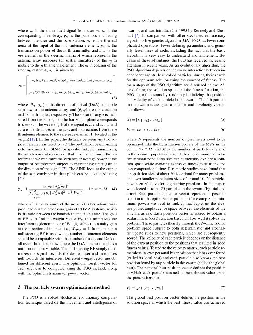
Fig. 7. Average received SINR versus the number of mobile users.

Fig. 8. Outage probability versus the number of mobile users.

these users. This can be realized using the following iterativealgorithm:

1. Choose an initial power vector and a random BF weightvector.

2. Use the PSO to find the BF weight vector of each userusing the null steering beamformer.

3. Use the result in step 2 to optimize the power vector andcompute the SINR of each user according to Eq. (4).

4. Iteratively update the steps (2) and (3) until the algo-rithm converges to an optimum BF weight and powervectors.

5. Simulation environment

A single-cell CDMA system with different number ofusers is considered, and the BS situated at the cell center


Fig. 9. Average transmitted power versus iterations with and without BF.

Fig. 10. Average received SINR against iterations with and without BF.

whose radius is 200m, and mobile users distributed ran-domly over the cell and their directions randomly chosen atinitialization. Uniform linear and circular antenna array ge-ometries are used in the simulations. The DoAs are estimatedas random variables uniformly distributed in the interval [0�]. The attenuation of a radio signal can be modeled as aproduct of two effects, namely path loss and shadowing asgiven by

gm = Dm × Sm (25)

where Dm is the large-scale distance-dependent attenuationin the average signal power. Based on studies in [14,15], awidely accepted model for path loss (or path gain) Dm isdescribed as

Dm = B

dm

(26)

where B is a constant depending on the antenna proper-ties, transmission wavelength, and the environment (rural,suburban, urban), assumed 1 in this paper, and dm is the


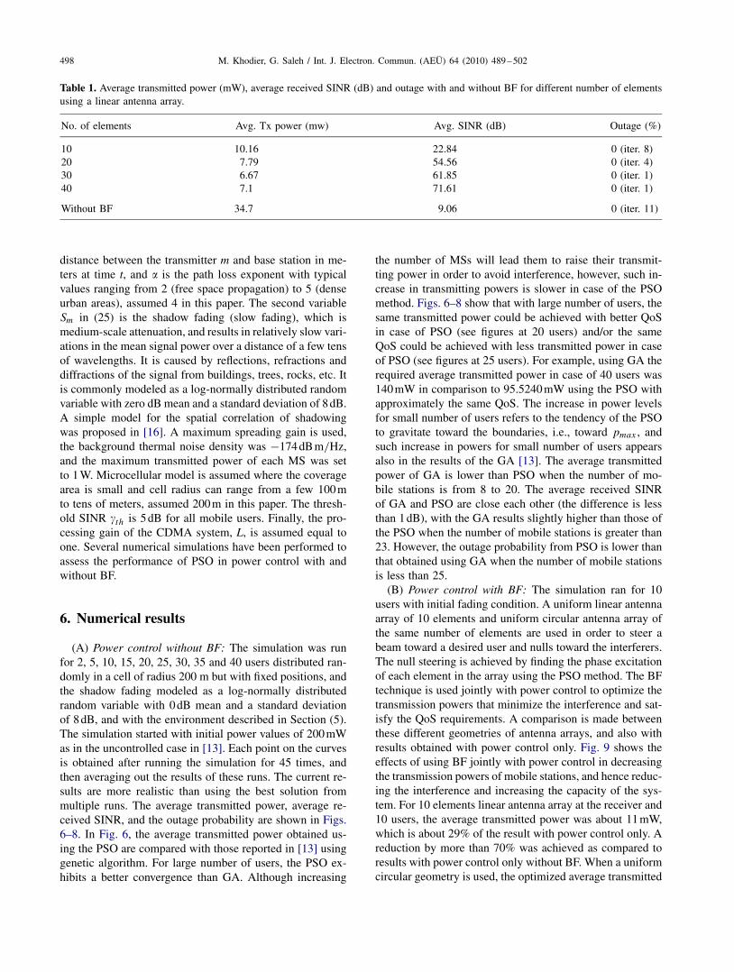
Table 1. Average transmitted power (mW), average received SINR (dB) and outage with and without BF for different number of elementsusing a linear antenna array.

No. of elements Avg. Tx power (mw) Avg. SINR (dB) Outage (%)

10 10.16 22.84 0 (iter. 8)20 7.79 54.56 0 (iter. 4)30 6.67 61.85 0 (iter. 1)40 7.1 71.61 0 (iter. 1)

Without BF 34.7 9.06 0 (iter. 11)

distance between the transmitter m and base station in me-ters at time t, and is the path loss exponent with typicalvalues ranging from 2 (free space propagation) to 5 (denseurban areas), assumed 4 in this paper. The second variableSm in (25) is the shadow fading (slow fading), which ismedium-scale attenuation, and results in relatively slow vari-ations in the mean signal power over a distance of a few tensof wavelengths. It is caused by reflections, refractions anddiffractions of the signal from buildings, trees, rocks, etc. Itis commonly modeled as a log-normally distributed randomvariable with zero dB mean and a standard deviation of 8dB.A simple model for the spatial correlation of shadowingwas proposed in [16]. A maximum spreading gain is used,the background thermal noise density was −174 dBm/Hz,and the maximum transmitted power of each MS was setto 1W. Microcellular model is assumed where the coveragearea is small and cell radius can range from a few 100mto tens of meters, assumed 200m in this paper. The thresh-old SINR �th is 5dB for all mobile users. Finally, the pro-cessing gain of the CDMA system, L, is assumed equal toone. Several numerical simulations have been performed toassess the performance of PSO in power control with andwithout BF.

6. Numerical results

(A) Power control without BF: The simulation was runfor 2, 5, 10, 15, 20, 25, 30, 35 and 40 users distributed ran-domly in a cell of radius 200 m but with fixed positions, andthe shadow fading modeled as a log-normally distributedrandom variable with 0dB mean and a standard deviationof 8dB, and with the environment described in Section (5).The simulation started with initial power values of 200mWas in the uncontrolled case in [13]. Each point on the curvesis obtained after running the simulation for 45 times, andthen averaging out the results of these runs. The current re-sults are more realistic than using the best solution frommultiple runs. The average transmitted power, average re-ceived SINR, and the outage probability are shown in Figs.6–8. In Fig. 6, the average transmitted power obtained us-ing the PSO are compared with those reported in [13] usinggenetic algorithm. For large number of users, the PSO ex-hibits a better convergence than GA. Although increasing

the number of MSs will lead them to raise their transmit-ting power in order to avoid interference, however, such in-crease in transmitting powers is slower in case of the PSOmethod. Figs. 6–8 show that with large number of users, thesame transmitted power could be achieved with better QoSin case of PSO (see figures at 20 users) and/or the sameQoS could be achieved with less transmitted power in caseof PSO (see figures at 25 users). For example, using GA therequired average transmitted power in case of 40 users was140mW in comparison to 95.5240mW using the PSO withapproximately the same QoS. The increase in power levelsfor small number of users refers to the tendency of the PSOto gravitate toward the boundaries, i.e., toward pmax , andsuch increase in powers for small number of users appearsalso in the results of the GA [13]. The average transmittedpower of GA is lower than PSO when the number of mo-bile stations is from 8 to 20. The average received SINRof GA and PSO are close each other (the difference is lessthan 1dB), with the GA results slightly higher than those ofthe PSO when the number of mobile stations is greater than23. However, the outage probability from PSO is lower thanthat obtained using GA when the number of mobile stationsis less than 25.

(B) Power control with BF: The simulation ran for 10users with initial fading condition. A uniform linear antennaarray of 10 elements and uniform circular antenna array ofthe same number of elements are used in order to steer abeam toward a desired user and nulls toward the interferers.The null steering is achieved by finding the phase excitationof each element in the array using the PSO method. The BFtechnique is used jointly with power control to optimize thetransmission powers that minimize the interference and sat-isfy the QoS requirements. A comparison is made betweenthese different geometries of antenna arrays, and also withresults obtained with power control only. Fig. 9 shows theeffects of using BF jointly with power control in decreasingthe transmission powers of mobile stations, and hence reduc-ing the interference and increasing the capacity of the sys-tem. For 10 elements linear antenna array at the receiver and10 users, the average transmitted power was about 11mW,which is about 29% of the result with power control only. Areduction by more than 70% was achieved as compared toresults with power control only without BF. When a uniformcircular geometry is used, the optimized average transmitted


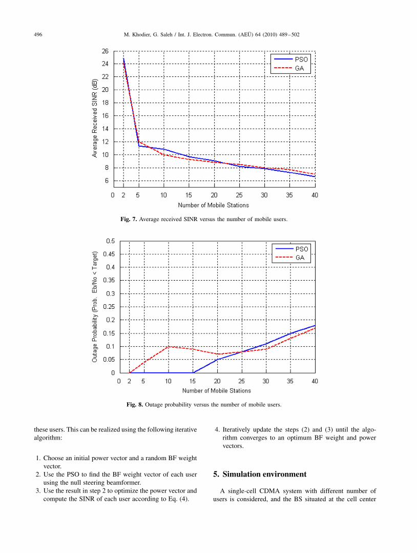
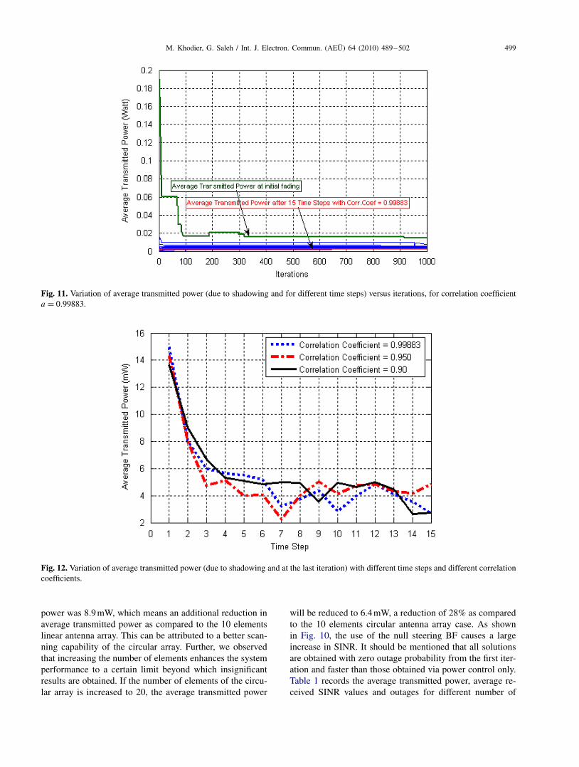
Fig. 11. Variation of average transmitted power (due to shadowing and for different time steps) versus iterations, for correlation coefficienta = 0.99883.

Fig. 12. Variation of average transmitted power (due to shadowing and at the last iteration) with different time steps and different correlationcoefficients.

power was 8.9mW, which means an additional reduction inaverage transmitted power as compared to the 10 elementslinear antenna array. This can be attributed to a better scan-ning capability of the circular array. Further, we observedthat increasing the number of elements enhances the systemperformance to a certain limit beyond which insignificantresults are obtained. If the number of elements of the circu-lar array is increased to 20, the average transmitted power

will be reduced to 6.4mW, a reduction of 28% as comparedto the 10 elements circular antenna array case. As shownin Fig. 10, the use of the null steering BF causes a largeincrease in SINR. It should be mentioned that all solutionsare obtained with zero outage probability from the first iter-ation and faster than those obtained via power control only.Table 1 records the average transmitted power, average re-ceived SINR values and outages for different number of


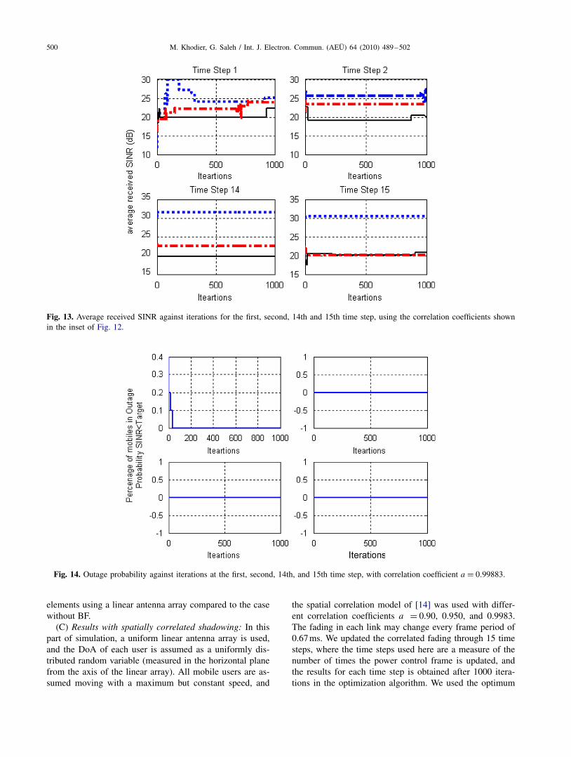
Fig. 13. Average received SINR against iterations for the first, second, 14th and 15th time step, using the correlation coefficients shownin the inset of Fig. 12.

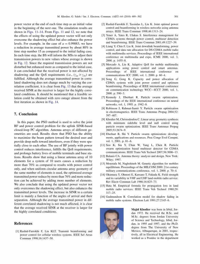
Fig. 14. Outage probability against iterations at the first, second, 14th, and 15th time step, with correlation coefficient a = 0.99883.

elements using a linear antenna array compared to the casewithout BF.

(C) Results with spatially correlated shadowing: In thispart of simulation, a uniform linear antenna array is used,and the DoA of each user is assumed as a uniformly dis-tributed random variable (measured in the horizontal planefrom the axis of the linear array). All mobile users are as-sumed moving with a maximum but constant speed, and

the spatial correlation model of [14] was used with differ-ent correlation coefficients a = 0.90, 0.950, and 0.9983.The fading in each link may change every frame period of0.67ms. We updated the correlated fading through 15 timesteps, where the time steps used here are a measure of thenumber of times the power control frame is updated, andthe results for each time step is obtained after 1000 itera-tions in the optimization algorithm. We used the optimum


power vector at the end of each time step as an initial valuein the beginning of the next one. The simulation results areshown in Figs. 11–14. From Figs. 11 and 12, we note thatthe effects of using the updated power vector will not onlyovercome the shadowing effect but also enhance the powerlevels. For example, in the case of a = 0.99883, we havea reduction in average transmitted power by about 80% intime step number 15 as compared to the initial fading case.In each time step, the BS will inform the MSs to adjust theirtransmission powers to new values whose average is shownin Fig. 12. Since the required transmission powers are notdisturbed but enhanced more as compared to the initial case,it can concluded that the received power is not affected byshadowing and the QoS requirements (i.e., (�m � �th) arefulfilled. Although the average transmitted power in corre-lated shadowing does not change much by varying the cor-relation coefficient, it is clear from Fig. 13 that the averagereceived SINR at the receiver is larger for the highly corre-lated conditions. It should be mentioned that a feasible so-lution could be obtained with zero outage almost from thefirst iteration as shown in Fig. 14.

7. Conclusion

In this paper, the PSO method is used to solve the jointBF and power control problem for the uplink SINR-basedclosed-loop PC algorithm. Antenna arrays of different ge-ometries are used. Results show that PSO has the abilityto maximize the beam pattern toward the desired user andprovide deep nulls toward interferers, even if they were spa-tially close to each other. The use of BF jointly with powercontrol reduces interference, fulfills the QoS requirements,and prolongs battery lives of mobile terminals and base sta-tions. Results show that using a linear antenna array of 10elements for a system of 10 users causes a reduction bymore than 70% as compared to results with power controlonly, and when uniform circular antenna array geometry ofthe same number of elements is used, the optimized averagetransmitted power reduce by more than 76% and more reduc-tion can be achieved by adding more number of elements.We also conclude that using the updated power vector notonly overcomes the shadowing effect, but also enhances thetransmitted power levels. The increase in SINR to a certainlimit is mainly a function of the angles of arrival and theirseparation. Although the average transmitted power in dif-ferent correlated shadowing is not much affected, it is clearthat the average received SINR at the receiver is larger forthe highly correlated conditions.

References

[1] Rashid-Farrokhi F, Liu KLT. Transmit beamforming andpower control for cellular wireless systems. IEEE Sel AreasCommun 1998;16:1437–50.

[2] Rashid-Farrokhi F, Tassiulas L, Liu K. Joint optimal powercontrol and beamforming in wireless networks using antennaarrays. IEEE Trans Commun 1998;46:1313–24.

[3] Yener A, Yates R, Ulukus S. Interference management forCDMA systems through power control, multiuser detectionand beamforming. IEEE Trans Commun 2001;49:1227–39.

[4] Liang Y, Chin F, Liu K. Joint downlink beamforming, powercontrol, and data rate allocation for DS-CDMA mobile radiowith multimedia services. Proceedings of IEEE internationalconference on multimedia and expo, ICME 2000, vol. 3,2000. p. 1455–8.

[5] Mercado A, Liu K. Adaptive QoS for mobile multimediaapplications using power control and smart antennas.Proceedings of IEEE international conference oncommunications ICC 2000, vol. 1, 2000. p. 60–4.

[6] Song G, Gong K. Capacity and power allocation ofCDMA systems with joint power control and optimumbeamforming. Proceedings of IEEE international conferenceon communication technology WCC—ICCT 2000, vol. 1,2000. p. 590–3.

[7] Kennedy J, Eberhart R. Particle swarm optimization.Proceedings of the IEEE international conference on neuralnetworks, vol. 1, 1995. p. 1942–8.

[8] Robinson J, Rahmat-Samii Y. Particle swarm optimizationin electromagnetics. IEEE Trans Antennas Propag 2004;52:397–407.

[9] Khodier M, Christodoulou C. Linear array geometry synthesiswith minimum sidelobe level and null control usingparticle swarm optimization. IEEE Trans Antennas Propag2005;53:2674–9.

[10] Eberhart R, Shi Y. Particle swarm optimization: develop-ments, applications and resources. Proc Congr Evol Comput,vol. 1, 2001. p. 81–6.

[11] Soo K, Siu Y, Chan W, Yang L, Chen R. Particleswarm optimization based multiuser detector for CDMAcommunications. IEEE Trans Veh Technol 2007;56:3006–13.

[12] Balanis CA. Antenna theory: analysis and design. New York:Wiley; 1997.

[13] Moustafa M, Naghshineh M. Genetic algorithm for mobilesequilibrium. Proceedings of the MILCOM 2000: 21st centurymilitary communications conference, vol. 1, 2000. p. 70–4.

[14] Okumura Y, Ohmori E, Kawano T, Fukuda K. Field strengthand its variability in VHF and UHF land-mobile radio service.Rev Electr Commun Lab 1986;16:825–73.

[15] Hata M. Empirical formula for propagation loss in landmobile radio services. IEEE Trans Veh Technol 1980;29:317–25.

[16] Gudmundson R. Correlation model for shadow fading inmobile radio systems. Electron Lett 1991;27:2145–6.

Majid Khodier was born in Irbid, Jor-dan 1972. He received the B.Sc. andM.Sc. degrees from Jordan Universityof Science and Technology, Irbid, Jor-dan, in 1995 and 1997, and the Ph.D.degree from The University of NewMexico, Albuquerque, in 2001, respec-tively, all in Electrical Engineering. Heworked as a Postdoc in the department


of electrical engineering at The University of New Mexico wherehe performed research in the areas of RF/photonic antennas forwireless communications, and modeling of MEMS switches formulti-band antenna applications. In September of 2002, he joinedthe department of electrical engineering at Jordan University ofScience and Technology as an assistant professor. In February2008, he became an associate professor. His research interests arein the areas of numerical techniques in electromagnetics, model-ing of passive and active microwave components and circuits, ap-plications of MEMS in antennas, and RF/photonic antenna appli-cations in broadband wireless communications, and optimizationmethods. He published numerous papers in international journalsand refereed conferences. His article entitled “Linear array ge-ometry synthesis with minimum sidelobe level and null controlusing particle swarm optimization” published in “IEEE Transac-tions on Antennas and Propagation 53 (8)” in August, 2005 hasbeen recently identified by Thomson Essential Science Indicatorsto be one of the most cited papers in the research area of “ParticleSwarm Optimization.” Dr Khodier is listed in Marquis who’s whoin science and engineering, who’s who in the world, and is a se-nior member of the IEEE.

Gameel Saleh received the B.S. andM.S. degrees in electrical engineeringfrom Aden University, Yemen, andJordan University of Science and Tech-nology, Jordan, in 2001 and 2008,respectively. In 2002, he joined theDepartment of Electronics and Com-munications Engineering, Aden Uni-versity, Yemen. His fields of interestinclude radio resource management,optimization techniques and self orga-nized MIMO systems.

Beamforming and power control for interference reduction in wireless communications using particle...

Documents

Transcript of Beamforming and power control for interference reduction in wireless communications using particle...