FBMC Prototype Filter Design via Convex Optimization - arXiv

arX

iv:1

810.

1171

7v1

[ee

ss.S

P] 2

7 O

ct 2

018

1

FBMC Prototype Filter Design via Convex

Optimization

Ricardo Tadashi Kobayashi and Taufik Abrão

Abstract

In this work, we propose a prototype filter design for Filter Bank MultiCarrier (FBMC) systems

based on convex optimization, aiming superior spectrum features while maintaining a high symbol

reconstruction quality. Initially, the proposed design is written as a non-convex Quadratically Constrained

Quadratic Programming (QCQP), which is relaxed into a convex QCQP guided by a line search. Through

the resulting problem, we design three prototype filters: Type-I, II and III. In particular, the Type-II filter

shows a slightly better performance than the classical Mirabasi-Martin design, while Type-I and III filters

offer a much more contained spectrum than most of the prototype filters suitable for FBMC applications.

Furthermore, numerical results corroborate the effectiveness of the designed filters as the proposed filters

offer fast decay and contained spectrum while not jeopardizing symbol reconstruction in practice.

Index Terms

Prototype filters, filter bank multicarrier, FBMC design, quadratic programming, convex optimiza-

tion.

I. INTRODUCTION

Thanks to its simple, yet elegant, implementation and ability to deal with highly selective chan-

nels, Orthogonal Frequency-Division Multiplexing (OFDM) has become the standard waveform

for many contemporary telecommunication systems, including 802.11 for local area networks,

802.16 for Wimax and 4G LTE systems [1]. However, OFDM presents drawbacks that may be

unbearable for 5G and future wireless systems. First, OFDM relies on Cyclic-Prefix (CP) to

simplify equalization, which reduces the spectral efficiency. Furthermore, OFDM signal deploys

R. T. Kobayashi and T. Abrão are with the Department of Electrical Engineering (DEEL), State University of Londrina (UEL),

Londrina, PR, Brazil (email: [email protected], [email protected]).

October 30, 2018 DRAFT

http://arxiv.org/abs/1810.11717v1

2

a rectangular envelope, leading to a spectrum with high sidelobes (-13 dB), comprising its

neighboring bands. Finally, OFDM relies strictly on its orthogonality, hence random access

channel and multi-cell scenarios may prevent its proper operation.

More recently, an outstanding effort has been spent towards the research on 5G communication

systems, which envisions applications such as Tactile Internet, Internet of Things and gigabit

connectivity [2]. Generally speaking, these applications require scalability, robustness, flexibility,

low latency, and improved spectral/energy efficiencies, which will not be attained exclusively

through OFDM. Therefore, a paradigm shift on radio access is required to comply the stringent

requirements of 5G. In this context, some waveform alternatives have been proposed as 5G

candidates, to name a few: FBMC, Universal Filtered MultiCarrier (UFMC), Filtered OFDM

and Generalized Frequency-Division Multiplexing (GFDM) [3].

In special, FBMC waveform is regarded as a strong candidate for 5G and other wireless

systems to come. By using non-rectangular pulse shaping, FBMC generates a lower Out-of-

Band (OoB) energy emission. Another interesting feature is the ability of FBMC to deal with

InterSymbol Interference (ISI) without relying on CP, making it more efficient than OFDM. Also,

FBMC requirements on time/frequency synchronization are more relaxed than other multicarrier

schemes [4]. Yet another important aspect of FBMC is its compatibility with massive-MIMO

systems [5]: one of the main technologies to drive 5G [6]. Indeed, given such promising aspects,

FBMC waveform was selected as a candidate waveform on METIS project [7] and as the main

choice for PHYDIAS project [8]. Notice, however, that providing a full and detailed comparison

between FBMC and OFDM is out of the scope of this work. In fact, works such as [5], [9]–[11]

offer a rich comparison between FBMC and OFDM schemes.

Despite offering many advantages, FBMC still presents some issues to be addressed. Due to

its dependence on orthogonality in the real field, many algorithms used in other multicarrier

systems need to be adapted for FBMC. As a result, traditional pilot aided channel estimation

cannot be proceed as in OFDM, since pilots are prone to imaginary interference at the receiver

[12], [13]. Furthermore, PAPR reduction techniques need to be adapted for FBMC, e.g., Tone

Reservation method [14], [15].

Another concern that emerges while designing an FBMC system is the choice of the prototype

filter. For example, when adapting themselves for opportunistic spectrum sharing, cognitive radios

should minimize OoB emission in order to avoid interfering with other bands [16]. Although

being less vulnerable to time/frequency channel dispersion, FBMC signals are still prone to such


3

effects [17]. Thus, well localized filters in time and frequency are desirable. Another aspect to

be taken into account is the reconstruction capabilities offered by the filter, as FBMC systems

operate under an intrinsic interference floor dictated by the prototype filter.

From this perspective, this work proposes a prototype filter design based on convex optimiza-

tion which aims for the power minimization of the OoB pulse energy, constrained to a maximum

tolerable self-interference level and a fast spectrum decay. Initially, the design is modeled as an

optimization problem in the standard form, which is, unfortunately, a non-convex QCQP. To

circumvent such an issue, we propose a relaxation which leads to a convex QCQP guided by a

line search. In the sequel, we test our methodology by designing three prototype filters. Numerical

results show that the three proposed filters can provide both proper symbol reconstruction and

a very desirable spectral response, making them an exciting option to be deployed in FBMC

systems to come.

The contribution of this work is fourfold:

• A detailed formulation of the optimization problem prototype filter;

• The proposition of a relaxation that leads to a convex problem;

• Design methodology of three filters with superior spectrum features and symbol reconstruc-

tion capabilities compatible with the operation of FBMC systems;

• A fair comparison between the proposed prototype filters and other popular choices.

The remainder of the paper is organized as follows. In Section II, a brief description on FBMC

systems is provided. In order to establish a methodology for comparing different prototype filters,

Section III presents some figures of merit to evaluate the performance provided by prototype

filters from different perspectives. Section IV makes a quick survey on popular prototype filters

in FBMC systems, which are used for comparison along the numerical results. In Section V,

the proposed prototype filter design is presented and discussed. Numerical results are presented

in Section VI and Section VII offers the conclusions and final remarks of the work.

Notation: Vectors are denoted by lower case bold letters and matrices are denoted by upper

case bold letters. A−1, AT and ‖A‖p are the inverse, the transpose and the p-norm of A,

respectively. Also, I denotes the identity matrix and [A]i,k is the entry for the ith row and

kth column of A. Furthermore, ρ(A) is the set of eigenvalues of A, ρmax(A) is the largest

eigenvalue of A and ρmin(A) is the smallest eigenvalue of A. Re {z} and Im {z} are the real

part and imaginary part of z, receptively, and j =√−1. ⌈x⌉ smallest integer greater than or equal

to x and ⌊x⌋ the largest integer that is less than or equal to x. Finally, E [·] is the expectation


4

operator and 〈a[k] |b[k]〉 is the inner product of a[k] and b[k].

II. FBMC MULTIPLEXING

An FBMC signal consists of a set of staggered Pulse Amplitude Modulation (PAM) symbols

multiplexed along M subcarriers using a particular filtering, which enables features like low OoB

emission. Differently from OFDM, the FBMC symbol interval is shorter than its duration, which

compensates the amount of data multiplexed, as two staggered PAM symbols are transmitted

instead of one Quadrature Amplitude Modulation (QAM) or Phase-shift keying (PSK) symbol.

In order to ensure a better orthogonality between different symbols, a suitable phase shift is

introduced into each PAM symbol and a well designed filter is also required.

At the critical sampling rate, the multiplexed FBMC signal can be expressed as [13, eq. (1)]

s[k] =∞∑

n=−∞

M−1∑

m=0

am,npm,n[k], (1)

where am,n is the nth PAM symbol of the mth subcarrier and pm,n[k] is the pulse shape used

by such a symbol. In particular,

pm,n[k] = p

[

k − nM2

]

ej(2πM

mk+φm,n), (2)

where p[k] is the prototype filter, k = k − (Lp − 1)/2 and φm,n is the phase shift introduced

into am,n. The prototype filter is truncated to Lp samples and typical values are KM − 1, KM

and KM + 1, where K is referred as the overlapping factor. Noticeably, the distance between

adjacent subcarriers is 1/M , while the signaling interval is M/2, i.e., half the amount of samples

used in OFDM. Hence, an FBMC symbol introduces interference to its neighborhood, which

must be addressed in order to enable the symbol reconstruction at the receiver. In this sense,

the phase shift ejφm,n is introduced to minimize the interference between adjacent symbols. The

most common choice used to phase-shift PAM symbols [8], [18] is

ejφm,n = ejπ2(m+n), (3)

which makes adjacent symbols to be phase-shifted by π/2 and will be used throughout this

work.


5

A. Symbol Reconstruction

Since PAM symbols are deployed to convey information, one may retrieve the symbol am0,n0

by taking the real part of the projection of pm0,n0[k] onto the multiplexed signal s[k], i.e.,

am0,n0 = Re {〈s[k] |pm0,n0[k]〉} . (4)

Unfortunately, the set of sequences {pm,n[k]} is not orthogonal, even considering an appropriate

phase-shift and the real part operator. Differently from OFDM, adjacent FBMC symbols overlap

as the filter length is larger than the signaling interval, i.e., Lp > M/2. Thus, the estimated

symbol is composed by the symbol itself and its associated interference:

am0,n0 = am0,n0 +∑

n 6=n0m6=m0

am,nRe {〈pm,n[k] |pm0,n0 [k]〉} . (5)

Hence, an appropriate prototype filter should be employed in order to enable reconstruction at

the receiver, since it introduces a self-interference according to eq. (5).

B. FBMC Transmultiplexer Scheme

Fig. 1 presents a complete FBMC transmultiplexer schematic. In this representation, PAM

symbols from different subchannels are phase shifted, expanded at a rate of M/2, pulse-shaped

by their respective subcarrier filter

pm[k] = p[k]ej 2πM

m(

k−Lp−1

2

)

(6)

and combined to form the multiplexed signal s[k]. At the receiver side, the delay ∆β ensures

the causality of the scheme, while the latency ∆α arises at the estimated symbols. The relation

between ∆α and ∆β is given by

Lp − 1 =M

2∆α −∆β, (7)

as demonstrated in [18, sec. II.C]. Since ∆α and ∆β are non-negative integers, it is easy to verify

that a longer prototype filter introduces a higher latency at the output of the transmultiplexer.

Thus, it is desirable to deploy filters with a low overlapping factor in order reduce the latency.

However, desirable spectrum and reconstructions features usually come at the expense of longer

prototype filters.


6

a0,n ×

ejφ0,n

↑ M2

p0[k]

a1,n ×

ejφ1,n

↑ M2

p1[k]

aM−1,n ×

ejφM−1,n

↑ M2

pM−1[k]

+ z−∆β

s[k]

p0[k] ↓ M2

×

e−jφ0,n−∆α

a0,n−∆α

p1[k] ↓ M2

×

e−jφ1,n−∆α

a1,n−∆α

pM−1[k] ↓ M2

×

e−jφM−1,n−∆α

aM−1,n−∆α

← Transmitter Receiver →

Synthesis Filter Bank Analysis Filter Bank

Figure 1. FBMC Transmultiplexer

III. FIGURES OF MERIT FOR PROTOTYPE FILTERS

In this section, we present some figures of merit to evaluate the performance of prototype filters

from different perspectives, which can be deployed to design or select the most suitable filter for

a given application. The figures of merit herein presented suitably characterize prototype filters

according to their spectrum leakage, time-frequency localization, and reconstruction capabilities,

as shown in the sequel.

A. Signal-to-Interference Ratio

According to eq. (4), the prototype filter impacts the symbol estimation at the receiver side.

Hence, considering the scenario depicted in Fig. 1, the estimated symbols experience an Signal-

to-Interference Ratio (SIR) expressed by

SIR =1

M−1∑

m=0

∞∑

n=−∞

Re {〈pm,n[k] |pm0,n0[k]〉}2, (8)

which can be used to quantize the symbol reconstruction quality. Typically, prototype filters are

designed to provide an SIR level of dozens of dBs, e.g., [19, tab. I]. Indeed, there are some

other alternatives such as the maximum distortion parameter [18, eq. (44)] and the prototype

filter noise floor [20, eq. (4)], which describe the self-interference of the prototype filter similarly

to eq. (8).


7

B. In and Out-of-Band Energy

Another concern that arises when designing prototype filters for multicarrier applications is the

amount of energy emitted outside the passband. Low OoB energy emission ensures high energy

efficiency and low interference to adjacent bands, which are desirable features a Cognitive Radio

must comply when adapting itself for an opportunistic spectrum usage [16].

The energy contained within the frequency range |ω| ≤ ωc can be defined as

E(ωc) =1

2π

∫ ωc

−ωc

∣

∣P (ejω)∣

∣

2dω, (9)

where P (ejω) is the Discrete-Time Fourier Transform (DTFT) of p[k]. Typically, ωc is set to

1/M as it is the subcarrier frequency separation.

More conveniently, eq. (9) may be expressed in matrix form, by defining the vector

p =[

p[0] p[1] · · · p[Lp − 1]]T

(10)

and the entries of the matrix Γ(ωc) as [21, eq. (3.2.18)]

[Γ(ωc)]k,l =ωc

πsinc

[

(k − l)ωc

π

]

. (11)

Thus, the In-Band (IB) energy can be evaluated through

E(ωc) = pTΓ(ωc)p, (12)

while, the total energy of the filter can be expressed as

E(π) = pTp (13)

and the energy outside the frequency range |ω| ≤ ωc, or OoB energy, is evaluated by

E(ωc) = pT [I− Γ(ωc)]p. (14)

C. Maximum Sidelobe Level

As suggested by the name, the Maximum Sidelobe Level (MSL) measures the ratio between

the maximum sidelobe of |P (ejω)|2 and the main lobe level. The MSL can be defined as

MSL =maxω∈W

∣

∣P (ejω)∣

∣

2

|P (ej0)|2, (15)

where

W =

{

ω ∈ R

∣

∣

∣

∣

ω > 0,d

dω|P (ejω)|2 = 0

}

. (16)

Notice that the MSL describes the interference generated by p[k] to adjacent bands.


8

D. Heisenberg Factor

As a significant amount of telecommunication systems operates under large delay and/or

Doppler spreads, their pulse shaping is expected to be well localized in order to deal with such

a harsh environment. Hence, it is highly desirable to deploy a prototype filter with low time and

frequency spreading, which are defined respectively as

D2k =

∞∑

k=−∞

k2 |p[k]|2 (17)

and

D2ν =

∫ 1/2

−1/2

ν2∣

∣P (ej2πν)∣

∣

2dν. (18)

Unfortunately, a prototype filter cannot be designed to achieve an arbitrary time-frequency

localization, as time and frequency spreadings are conflicting goals. Indeed, this statement is

known as the Heisenberg Uncertainty Principle, described by the inequality

0 ≤ ξ ≤ 1, (19)

where

ξ =1

4πDkDν

, (20)

which is referred as the Heisenberg parameter. Notice that well located pulses can achieve close

to unit ξ, while poorly located pulses may achieve near null values of ξ.

IV. PROTOTYPE FILTERS

This section provides a brief background on some prototype filter options for FBMC systems.

In particular, the most popular prototype filter choices are the Extended Gaussian Function

(EGF), Martin-Mirabbasi and the Optimal Finite Duration Pulses (OFDP), due to their remarkable

features and simplicity. Nevertheless, other less popular options include the windowed based

prototype filter [8, eq. (34)], the Hermite filter introduced in [22, eq. (16)] and the classical

Square-Root Raised Cosine (SRRC) [11, eq. (24)]. Moreover, there are still some more recent

developments in this field, which include the works [23] and [24].

As this paper does not aim to provide a full survey on prototype filters, this section offers a

brief background on the EGF, Martin-Mirabbasi and the OFDP prototype filters, which are the

best candidates for FBMC systems to come [25, sec. 7.2.1.1]. In fact, there are already some

works that provide a rich discussion on prototype filters, e.g., [26].


9

A. Extended Gaussian Function

Originally, the EGF was generated using the Isotropic Orthogonal Transform Algorithm (IOTA)

[27, eq. (25)]

Oax(t) =x(t)

∑∞−∞ |x(t− ai)|

2 (21)

on a Gaussian function with a spreading factor α, i.e., gα(t) = (2α)1/4e−παt2 . Hence, the

continuous EGF is defined as

p(t) = F−1Oτ0FOν0gα(t), (22)

where F is the Fourier transform operator, τ0 is the signaling interval and ν0 is the subcarrier

spacing, which must comply τ0ν0 = 1/2 for FBMC systems. In order to obtain the discrete

version of an EGF, one can sample it properly. Fortunately, an analytic expression for (22) is

provided in [28, eq. (7)].

As the IOTA aims to make EGF pulses orthogonal, they are expected to provide a high

quality symbol reconstruction. In fact, SIR level provided by an EGF can be adjusted by tuning

the spread factor α, where the SIR is proportional to α, as can be observed in [28, fig. 3].

However, by increasing α, the EGF pulse becomes shorter in time and, thus, a higher frequency

dispersion is expected.

B. Mirabbasi-Martin

To ensure fast spectrum decay throughout the stopband region, the Mirabbasi-Martin prototype

filter [19] focuses on minimizing the discontinuity in their boundaries, while maintaining good

reconstruction features for multicarrier applications and ensuring a smooth pulse variation. This

design uses the frequency sampling technique, where the filter weights are actually samples of

the frequency response of the prototype filter.

Due to its fast spectrum decay and good performance for data reconstruction, Mirabbasi-

Martin prototype is the main choice for the Phydias project [8], which aims to enable FBMC

applications in wireless systems to come. Indeed, some authors refer such a filter, for K = 4,

as the PHYDIAS filter.

The Mirabbasi-Martin prototype filter can be written as the following discrete low-pass filter:

p[k] =

k0 + 2K−1∑

i=1

ki cos

(

2πi

KMk

)

, 0 ≤ k ≤ Lp − 1

0, otherwise

(23)

where kℓ are the filter weights which are available in [19, tab. I].


10

C. Prolate Filter and Discrete Slepian Sequences

The Prolate filter is a classic design that aims to maximize the energy within its passband

region. This design can be compactly expressed as

ψψψ0,ωs = argmax pHΓ(ωs)p

s.t. pHp = 1

. (24)

Since Γ(ωs) is symmetric, a straightforward solution comes by recalling the Rayleigh-Ritz

Theorem [29, theo. 4.4.2], which guarantees the solution of (24) to be the eigenvector associated

to the largest eigenvalue of Γ(ωs). By denoting γ0 ≥ γ1 ≥ · · · ≥ γLp−1 > 0 the eigenvalues of

Γ(ωs), and ψψψi,ωs the eigenvector associated to γi, the solution of (24) is

ψψψ0,ωs =[

ψ0,ωs [0] ψ0,ωs [1] · · · ψ0,ωs [Lp − 1]]T

. (25)

Physically, γi represents the normalized energy of ψi[k] within |ω| ≤ ωc, thus

0 ≤ γi ≤ 1. (26)

Consequently, the sequence ψ0,ωs [k] is the most selective filter for the problem stated in eq. (24).

It is also noteworthy mentioning that, the remaining filters ψi,ωs[k] are local solutions, possessing

less energy within their passband than ψ0,ωs[k]. Indeed, {ψi,ωs [k]}i is also known as the Discrete

Prolate Spheroidal Sequences (DPSS) or the Slepian series [30]. Interestingly, the Slepian series

is a good choice to interpolate smooth functions [31, tab. 2], making it suitable for low OoB

emission applications.

D. Optimal Finite Duration Pulse

As stated previously, the Prolate design is optimal in terms of minimizing the energy outside

the passband. However, (near) perfect reconstruction requirements are not taken into account in

this design. From this perspective, the OFDP deploys the Slepian series to provide a filter design

with low OoB emission and a good symbol reconstruction capability. The OFDP can be written

as

p[k] =∑

i

α2iψ2i,2π/M [k], (27)

where the coefficients α2i can be found in [32, tab. I]. Since the IB energy of ψ2i, i.e., γ2i, decays

rapidly as can be observed in [30, fig. 3,4], truncation is acceptable for solving the problem.


11

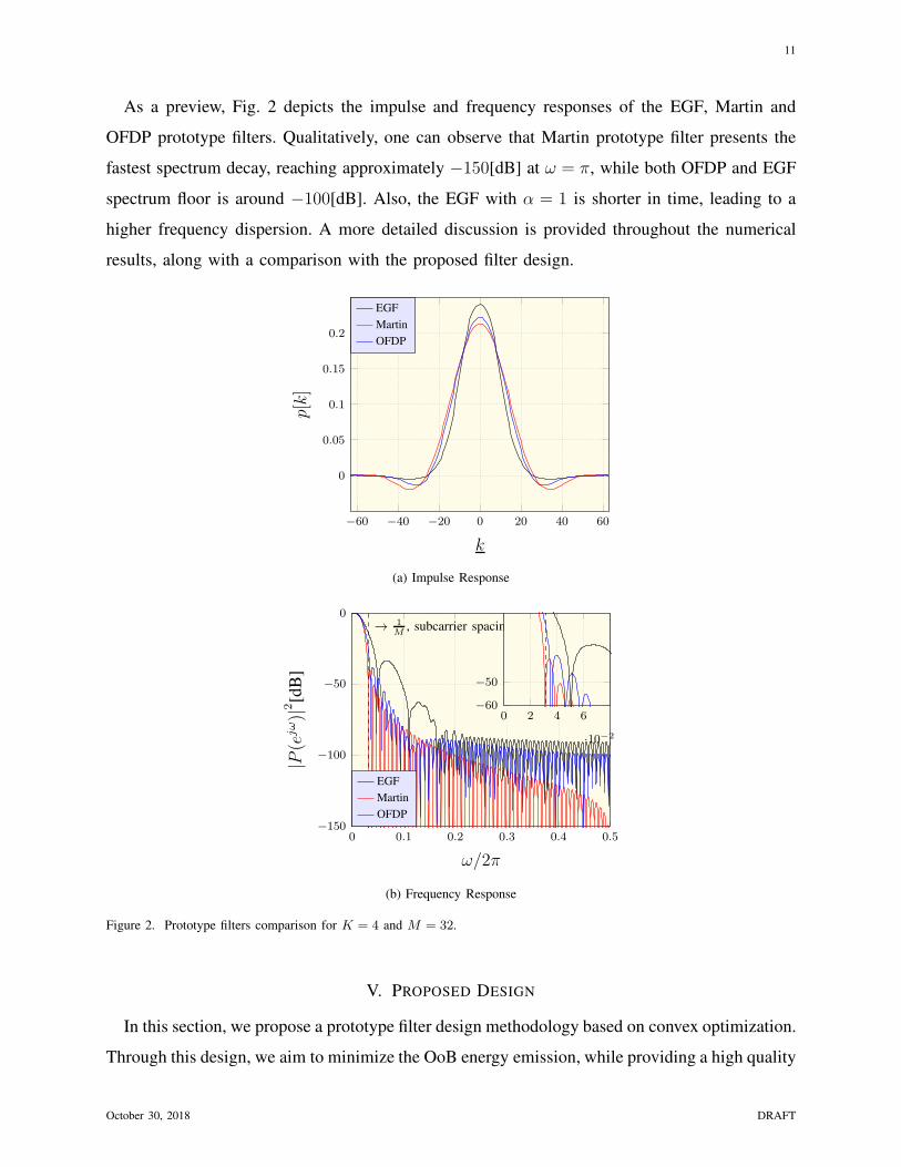
As a preview, Fig. 2 depicts the impulse and frequency responses of the EGF, Martin and

OFDP prototype filters. Qualitatively, one can observe that Martin prototype filter presents the

fastest spectrum decay, reaching approximately −150[dB] at ω = π, while both OFDP and EGF

spectrum floor is around −100[dB]. Also, the EGF with α = 1 is shorter in time, leading to a

higher frequency dispersion. A more detailed discussion is provided throughout the numerical

results, along with a comparison with the proposed filter design.

−60 −40 −20 0 20 40 60

0

0.05

0.1

0.15

0.2

k

p[k]

EGF

Martin

OFDP

(a) Impulse Response

0 0.1 0.2 0.3 0.4 0.5−150

−100

−50

0→ 1

M, subcarrier spacing

ω/2π

|P(e

jω)|2

[dB

]

EGF

Martin

OFDP

0 2 4 6

·10−2

−50

−60

(b) Frequency Response

Figure 2. Prototype filters comparison for K = 4 and M = 32.

V. PROPOSED DESIGN

In this section, we propose a prototype filter design methodology based on convex optimization.

Through this design, we aim to minimize the OoB energy emission, while providing a high quality


12

symbol reconstruction and maintaining a fast spectrum decay. The description of the proposed

design begins by defining the filter expression as a linear transformation. In the sequence, we

provide the objective function expression, i.e., the OoB energy. Furthermore, we present a full

discussion on the FBMC interference elements, which is be used to ensure a high SIR prototype

filter. The constraints required to achieve a prototype filter with fast spectrum decay are also

offered. Finally, we cast the complete problem as a non-convex QCQP, which on its turn is

relaxed into a convex QCQP guided by a line search. Since our design depends on convex

optimization, we present the design itself alongside with all the convexity proofs. This choice

is made aiming to favor the comprehension of both the deployed optimization method and the

related convexity issues.

A. Filter Expression

In order to model the prototype filter, let us define the matrix

F =[

f0 f2 · · · fN−1

]

. (28)

to be an aggregation of N sequences, where

fi =[

fi[0] fi[1] · · · fi[Lp − 1]]T

(29)

is a vector with unitary norm ‖fi‖2 = 1. Hence, let us express the prototype as the linear

transformation

p = Fc, (30)

where

c =[

c0 c2 · · · cN−1

]T

(31)

are the coefficients to be optimized.

Throughout this paper, we consider two families to be deployed as fi[k]1. First, we consider

fi[k] as the DPSS, i.e.,

fi[k] = ψ2i,ωs [k]. (32)

As an alternative, a family of cosine sequences can also be deployed:

fi[k] =

1√KM + 1

, i = 0

√

2

KM + 2cos

(

2πi

KMk

)

, i = 1, · · ·N − 1

. (33)

1One can deploy other sequences as long as they are (near) orthogonal, symmetrical around (Lp − 1)/2.


13

Notice that, large values of N may increase the OoB frequency content or make the last entries

of c very small. Thus, since N < Lp, the number of optimization variables is considerably

reduced.

B. Energy Expression

Combining eq. (14) and (30), one may rewrite the energy concentrated within the stopband

region as

E(ωc) = cT[

ILp − Γ(ωc)]

c

= cTQ0c(34)

which is an appropriate choice as it is a quadratic convex function, given Q0 is a positive

semidefinite matrix. A more straightforward, yet informal, way of proofing that Q0 is positive

semidefinite is by recalling that E(ωc) is an energy measurement, i.e., a non-negative value.

Thus, if E(ωc) is non-negative, Q0 is positive semidefinite. Since Q0 is positive semidefinite,

eq. (34) is convex [33, sec. 1].

C. FBMC Interference Elements

As observed in eq. (5), the quality of the symbol reconstruction depends on the prototype

filter, which needs to be designed to provide low distortion levels and enable near-perfect

reconstruction. To simplify the representation of the interference for our problem, let us define

ǫm,n = Re {〈pm,n[k] |p0,0[k]〉}

= cos (φm,n)

∞∑

k=−∞

p

[

k − nM2

]

p[k] cos

(

2π

Mmk

)

(35)

as the distortion or interference introduced by the symbol am,n into the symbol a0,0.

Based on (35), five straightforward properties can be listed:

i ǫ0,0 represents the pulse energy;

ii ǫm,n is an even sequence concerning the index n, i.e., ǫm,n = ǫm,−n;

iii ǫm,n is odd circular symmetric concerning the index m, i.e., ǫm,n = −ǫM−m,n, for 1 ≤ m ≤M/2− 1;

iv ǫm,n = 0 for |n| >⌈

Lp

M/2

⌉

− 1, since the prototype filter is finite;

v ǫm,n = 0 case m+ n is odd, given the cosine term.


14

Thus, taking into account properties ii, iii and iv, let us define

E =

(m,n)

∣

∣

∣

∣

∣

∣

∣

∣

∣

∣

∣

∣

0 ≤ m ≤ M/2

0 ≤ n ≤⌈

Lp−1M/2

⌉

− 1

m+ n even

m+ n 6= 0

(36)

to be the set of distortion elements ǫm,n which are not strictly null, but can assume a negligible

values depending on the prototype filter design. Given the symmetry of ǫm,n, we omitted the

redundant elements in order to propose an efficient optimization problem.

1) Matrix Form: In order to model the interference elements ǫm,n in matrix form, two matrices

need to be defined. First,

[Πn]i,j =

1, j = i+ nM/2

0, otherwise

(37)

are the entries of the nilpotent matrix Πn, responsible for shifting the sequence p[k] by nM/2

samples. The second matrix, Σm, incorporates the cosine term of the summation of eq. (35) and

is defined as

Σm = diag

{

cos

(

2π

Mmk

)}

k=0,1,··· ,Lp−1

. (38)

Initially, we can rewrite eq. (35) in matrix form:

ǫm,n = pT cos(φm,n)ΣmΠnp

= pTQ(0)m,np.

(39)

Notice that, since Σm is diagonal and Πn is nilpotent, Q(0)m,n is also nilpotent for n 6= 0.

Conversely, case n = 0, the eigenvalues of Q(0)m,n lies on the diagonal of Σm, as Σm is diagonal

and Π0 = ILp . Thus, Q(0)m,n is not a set of positive semidefinite matrices making ǫm,n to be a

non-convex set.

For convenience, ǫm,n can be expressed using Hermitian symmetric matrices. Thus, by noting

that ǫm,−n = pT(

Q(0)m,n

)T

p and ǫm,−n = ǫm,n, eq. (35) can be expressed as

ǫm,n =1

2pT

[

Q(0)m,n +

(

Q(0)m,n

)T]

p

= pTQ(1)m,np.

(40)


15

Since Q(1)m,n is a Hermitian matrix, it yields real eigenvalues. Unfortunately, to our knowledge,

the exact eigenvalues of Q(1)m,n, given n 6= 0, cannot be tracked analytically. However, one can

observe that ∣

∣

∣

∣

∣

∑

ℓ

[

Q(1)m,n

]

i,ℓ

∣

∣

∣

∣

∣

≤ 1, i 6= ℓ. (41)

Hence, the Gershgorin Theorem [29, Theorem 6.1.1] guarantees that the eigenvalues are inside

the interval

ρ(

Q(1)m,n

)

∈ [−1, 1] (42)

In terms of the coefficients ci, the interference element ǫm,n can be written as

ǫm,n = cTFTQ(1)m,nFc

= cTQ(2)m,nc.

(43)

Again, Q(2)m,n is Hermitian and with eigenvalues that are not analytically traceable. Nevertheless,

one can also realize that ρ(

Q(2)m,n

)

∈ [−1, 1], by analyzing the numerical radius of Q(2)m,n.

2) Self-Interference Constraints: In order to manage the self-interference level generated by

the prototype filter, the proposed problem is constrained to a maximum interference level of ǫ0

|ǫm,n| =∣

∣cTQ(2)m,nc

∣

∣ ≤ ǫ0, (m,n) ∈ E . (44)

Notice that the absolute value must be taken, since ǫm,n can assume both real and negative

values. Alas, the constraint presented in (44) is non-convex since +Q(2)m,n and −Q(2)

m,n cannot be

positive semidefinite simultaneously.

3) Eigenvalues Shift: The eigenvalues of Q(2)m,n can be manipulated by adding the term

δcTFTFc and subtracting δ from eq. (44), leading to

cT[

+Q(2)m,n + δFTF

]

c− δ ≤ ǫ0

cT[

−Q(2)m,n + δFTF

]

c− δ ≤ ǫ0

, (m,n) ∈ E , (45)

which is valid if and only if the energy of the prototype filter is unitary, i.e., ‖p‖22 = cTFTFc = 1.

In order to provide a more compact notation, let us rewrite eq. (45) as

cTQ(3a)m,nc ≤ ǫ0 + δ

cTQ(3b)m,nc ≤ ǫ0 + δ

, (46)

Considering the eigenvalues of Q(2)m,n and that both FTF and Q

(2)m,n are Hermitian, one can

easily observe that

ρ(

Q(3a)m,n

)

∈[

δρmin

(

FTF)

− 1, δρmax

(

FTF)

+ 1]

(47)


16

by recalling the Weyl’s Inequality. A particular case takes place if F is orthonormal, where

ρ(

Q(3a)m,n

)

∈ [δ − 1, δ + 1] , (48)

which is the case if F is a Slepian basis, i.e., eq. (32). However, if F is composed by a cosine

sequences, as the ones in eq. (33), such matrix is only near orthogonal, making the eigenvalues

of FTF very close to the unit. Hence, there exists a non-negative value of δ which makes all the

eigenvalues of Q(3a)m,n positive, making this matrix positive semidefinite. Similarly, we can also

conclude that Q(3b)m,n is also positive definite for a given value of δ. Hence, both entries of eq.

(46) are convex, as both Q(3a)m,n and Q

(3b)m,n are positive semidefinite [34].

D. Spectrum Decay

As practical FBMC systems deploy windowed pulses, spectrum decay may stagnate, specially

if the boundaries of the prototype filter are not null. Thus, the samples at the boundaries of the

prototype filter should assume values as low as possible to ensure a fast spectrum decay. In this

sense, let us define

p[k] = cTuk, (49)

where

uk =[

f0[k] f1[k] · · · fN−1[k]]T

. (50)

Thus, the boundaries of the prototype filter are constrained by

∣

∣cTuk

∣

∣ ≤ u0, k ∈ K, (51)

where K is the set of indexes of the boundaries samples we wish to limit to a maximum level

u0. Since the prototype filter is symmetrical, i.e., p[k] = p[Lp − 1 − k], one does not need to

constraint the amplitude of the pulse from both sides.


17

E. Resulting Optimization Problem

By taking eq. (34) as the objective function and eqs. (46) and (51) as constraints, the resulting

problem can be written:

c∗ = argmin cTQ0c

s.t. cTQ(3a)m,nc ≤ ǫ0 + δ, (m,n) ∈ E

cTQ(3b)m,nc ≤ ǫ0 + δ, (m,n) ∈ E

∣

∣uTk c

∣

∣ ≤ u0, k ∈ K

cTFTFc = 1

(52)

Unfortunately, the problem posed in (52) is non-convex as the energy equality constraint is

quadratic instead of affine [34].

F. Convex QCQP Relaxation

As an alternative to circumvent the non-convexity of eq. (52), let us propose a relaxation in

order to obtain a convex QCQP. First, consider the norm inequality

‖c‖2 ≤ ‖c‖1 ≤√N ‖c‖2 . (53)

One can observe that there is a value of ζ such as

‖c‖2 =‖c‖1ζ

. (54)

By analyzing (53), one can observe that eq. (53) is valid for

1 ≤ ζ ≤√N (55)

Taking the previous observation, we propose exchanging the norm-2 equality constraint by a

norm-1 equality‖c‖1ζ

=1Tc

ζ, (56)

where 1 is a vector of ones. Notice that, eq. (56) holds if ci ≥ 0, which can be obtained by a

proper choice of F. As a rule of thumb, fi[k] is chosen to be symmetrical around (Lp − 1)/2,

i.e.,

[F]ℓ,i = [F]Lp+1−ℓ,i , 1 ≤ ℓ ≤⌊

Lp

2

⌋

, (57)


18

where fi[k] = [F]k+1,i for 0 ≤ k ≤ Lp − 1. Also, the central sample of fi must be positive:

[F]⌈Lp2

⌉

,i> 0 (58)

Such features can be observed, for example, in Martin prototype filter, OFDP and Hermite

designs if their respective functions are properly scaled.

Therefore, a relaxed QCQP can be cast from eq. (52) and (56):

c(ζ) = argmin cTQ0c

s.t. cTQ(3a)m,nc ≤ ǫ0 + δ, (m,n) ∈ E

cTQ(3b)m,nc ≤ ǫ0 + δ, (m,n) ∈ E

∣

∣uTk c

∣

∣ ≤ u0, k ∈ K

1Tc

ζ= 1

c ≥ 0.

(59)

The convexity of (59) can be guaranteed as the Hessian of both the objective function and the

constraints are positive semidefinite, and, also, the equality constraint are affine [35]. Neverthe-

less, one must first track the value of ζ∗, for which ‖p‖2 is as close as possible to the unity,

leading to a near optimal solution. In this sense, the associated line search problem

ζ∗ = argmin∣

∣1− cT (ζ)FTFc(ζ)∣

∣

2

s.t. 1 ≤ ζ ≤√N

(60)

can be performed to track the optimal value of ζ . One can observe that the line search posed in

(60) requires the solution/evaluation of eq. (59). Also, the objective function of (60) must reach

very small values to satisfy ‖p‖2 = 1. Hence, once ζ∗ is found, the relaxed solution

c∗ = c(ζ∗) (61)

is established.

VI. NUMERICAL RESULTS

In this section, we offer the numerical results to corroborate the effectiveness of the proposed

filter design methodology. First, we define the optimization setup for three proposed prototype

filters. After that, we provide a brief explanation on the tools deployed to solve the proposed

optimization problem. Finally, we offer a performance comparison between the filters obtained

through the proposed methodology versus the EGF, OFDP and Martin prototype filters.


19

A. Optimization Setup

In order to exemplify the effectiveness of the proposed design, we solve (60) using three

different configurations referred hereafter as Type-I, Type-II and Type-III prototype filters. All

the three set of parameters are summarized in Table I. It is noteworthy mentioning that we choose

an overlapping factor K = 4, as it enables achieving filters with a high performance for both

SIR and spectrum measurements. Furthermore, M = 32 was chosen to enable a better spectrum

visualization. However, we must highlight at this point that the proposed design is also capable

of handling other values of M .

Table I

OPTIMIZATION PARAMETERS SETUP FOR THE PROPOSED METHOD CONSIDERING K = 4, M = 32 AND Lp = KM + 1

Parameter Type-I Type-II Type-III

N 2K K + 1 K + 1

ωc2πM

KN

2πM

KN

2πM

ǫ0 2 · 10−4 8 · 10−5 2 · 10−4

u0 10−12 10−12 10−12

K {0, 1} {0} {0, 1}

δ 2 2 2

fi[k] eq. (32) eq. (33) eq. (33)

Type-I configuration deploys 2K DPSS with a passband of ωs = 2π/M to build the prototype

filter, reasonably stringent interference tolerance ǫ0 and near null border samples. On the other

hand, Type-II and Type-III filters are built through the summation K + 1 cosines. Type-II

imposes a higher reconstruction constraint, while Type-III focuses on a very fast spectrum decay.

Furthermore, we set δ = 2 as it can easily make Q(3a)m,n and Q

(3b)m,n positive semidefinite, according

to eq. (47). Concerning ωc, it is noteworthy mentioning that such a parameter is set around 2π/M ,

given the subcarrier bandwidth and separation. For Type-II and III, we set a more stringent ωc

to reduce the spectrum level within adjacent subcarriers.

The solution for the proposed design with the configurations described in Table I takes two

phases. First, the master problem (60) is solved by using the Golden search, whereas the slave

problem (59) was solved through MOSEK 8.0. For this class of problem, MOSEK casts the

original QCQP as a Second-Order Cone Program (SOCP), which is solved by the interior-point


20

algorithm described in [36]. In order to achieve an easier implementation, (60) was parsed into

MATLAB using the modeling language CVX. The solution of the proposed problem, i.e., the

weights of the filters are provided at the Appendix, where some additional observations are

offered.

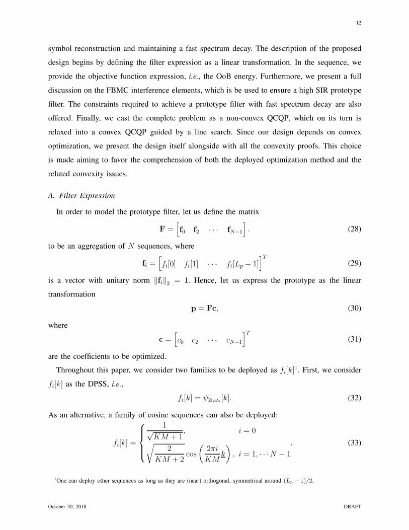
B. Prototype Filter Performance Analysis

In Fig. 3, one can observe both the impulse and frequency responses of the prototype filters

obtained via the proposed problem. As for the impulse response, all prototype filters are very

similar. Nevertheless, the frequency response of Type-I, Type-II and Type-III are very distin-

guishable, besides presenting small sidelobes and fast spectrum decay. In particular, Type-I and

Type-III presented a very expressive spectrum decay, compared with Type-II. But by promoting

a comparison among Type-I, Type-II, Type-III, EGF, OFDP, and Martin prototype filters, one

concludes that the proposed pulses achieved a superior spectrum decay with small sidelobes.

Indeed, one may also observe that Type-II and Martin filter are very similar, but the former

presented smaller sidelobes.

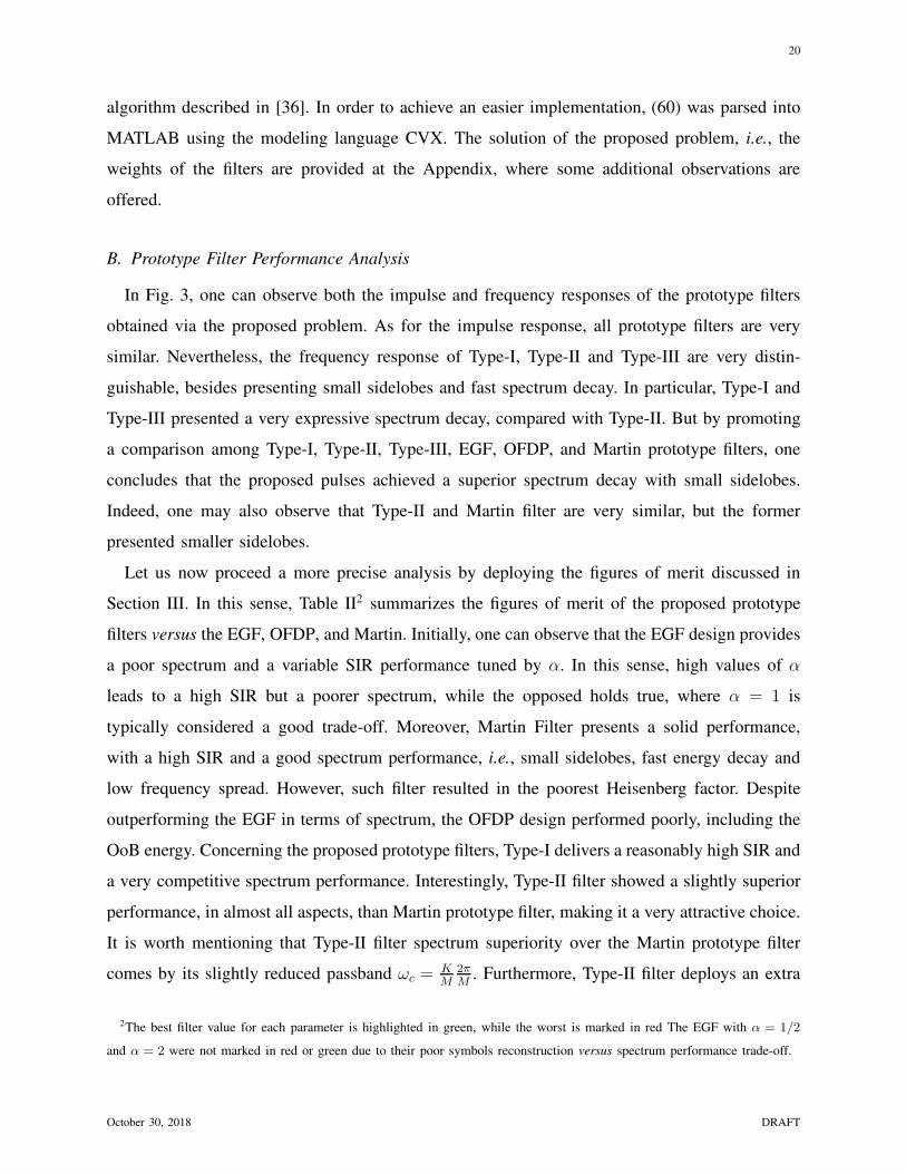
Let us now proceed a more precise analysis by deploying the figures of merit discussed in

Section III. In this sense, Table II2 summarizes the figures of merit of the proposed prototype

filters versus the EGF, OFDP, and Martin. Initially, one can observe that the EGF design provides

a poor spectrum and a variable SIR performance tuned by α. In this sense, high values of α

leads to a high SIR but a poorer spectrum, while the opposed holds true, where α = 1 is

typically considered a good trade-off. Moreover, Martin Filter presents a solid performance,

with a high SIR and a good spectrum performance, i.e., small sidelobes, fast energy decay and

low frequency spread. However, such filter resulted in the poorest Heisenberg factor. Despite

outperforming the EGF in terms of spectrum, the OFDP design performed poorly, including the

OoB energy. Concerning the proposed prototype filters, Type-I delivers a reasonably high SIR and

a very competitive spectrum performance. Interestingly, Type-II filter showed a slightly superior

performance, in almost all aspects, than Martin prototype filter, making it a very attractive choice.

It is worth mentioning that Type-II filter spectrum superiority over the Martin prototype filter

comes by its slightly reduced passband ωc =KM

2πM

. Furthermore, Type-II filter deploys an extra

2The best filter value for each parameter is highlighted in green, while the worst is marked in red The EGF with α = 1/2

and α = 2 were not marked in red or green due to their poor symbols reconstruction versus spectrum performance trade-off.


21

Table II

PROTOTYPE FILTERS COMPARISON CONSIDERING K = 4, M = 32 AND Lp = KM + 1.

Prototype Filter SIR[dB] MSL[dB] Dk Dν ξ E(

2πM

)

[dB] E(

4πM

)

[dB]

EGF (α = 1/2) 33.73 −58.21 8.964 0.0101 0.878 −33.95 −48.81

EGF (α = 2) 114.48 −21.38 5.163 0.0176 0.874 −12.46 −20.67

EGF (α = 1) 60.49 −33.80 6.457 0.0126 0.976 −19.69 −33.50

Martin 65.23 −39.86 8.784 0.0102 0.884 −45.61 −70.60

OFDP 59.86 −38.33 7.842 0.0109 0.933 −35.45 −62.29

Type-I 52.74 −43.63 8.230 0.0106 0.915 −42.30 −82.96

Type-II 68.09 −47.68 8.568 0.0103 0.897 −50.09 −72.93

Type-III 51.25 −58.73 7.877 0.0108 0.935 −35.20 −100.57

tone (N = K + 1) when compared with the Martin filter (K tones), improving the symbol

reconstruction. Finally, Type-III presented a similar SIR performance to Type-I and the smallest

MSL. However, the OoB energy E(2π/M) is among the highest.

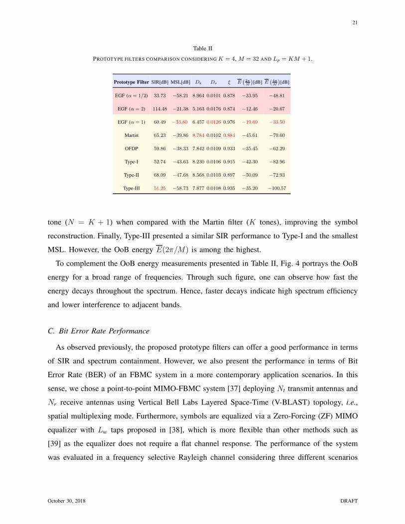
To complement the OoB energy measurements presented in Table II, Fig. 4 portrays the OoB

energy for a broad range of frequencies. Through such figure, one can observe how fast the

energy decays throughout the spectrum. Hence, faster decays indicate high spectrum efficiency

and lower interference to adjacent bands.

C. Bit Error Rate Performance

As observed previously, the proposed prototype filters can offer a good performance in terms

of SIR and spectrum containment. However, we also present the performance in terms of Bit

Error Rate (BER) of an FBMC system in a more contemporary application scenarios. In this

sense, we chose a point-to-point MIMO-FBMC system [37] deploying Nt transmit antennas and

Nr receive antennas using Vertical Bell Labs Layered Space-Time (V-BLAST) topology, i.e.,

spatial multiplexing mode. Furthermore, symbols are equalized via a Zero-Forcing (ZF) MIMO

equalizer with Lw taps proposed in [38], which is more flexible than other methods such as

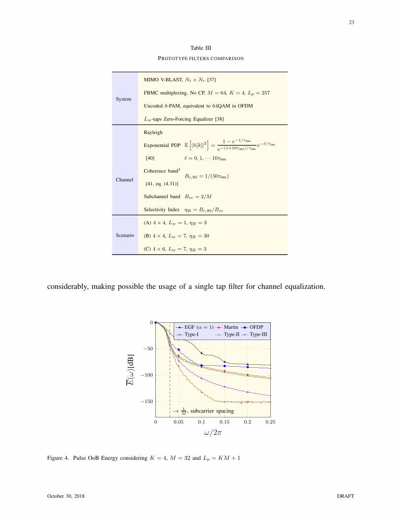
[39] as the equalizer does not require a flat channel response. The performance of the system

was evaluated in a frequency selective Rayleigh channel considering three different scenarios


22

described in Table III. Notice that the radio channel of Scenarios (A) and (C) are reasonably

frequency selective, whereas Scenario (A) can be considered frequency flat per subcarrier.

Fig. 5 depicts the BER performance for all configurations and a wide normalized Signal-to-

Noise Ratio (SNR) (Eb/N0) range. Observing the results for Scenario (A), we can conclude that

even a 7 taps equalization was unable to compensate the channel properly under a high SNR

regime, introducing a BER floor. Yet in this configuration, we can also observe that the BER

floor level is proportional to Dν , where, for example, the EGF filter performed poorly due to

its higher frequency dispersion. For Scenario (B), all filters performed similarly in the analyzed

Eb/N0 range. Hence, despite differences in terms of the measured SIR, the proposed prototype

filters seems to be suitable in practical scenario. For Scenario (C), diversity improved the BER

−60 −40 −20 0 20 40 60

0

0.05

0.1

0.15

0.2

k

p[k]

Type-I

Type-II

Type-III

(a) Impulse Response

0 0.1 0.2 0.3 0.4 0.5

−200

−150

−100

−50

0→ 1

M, subcarrier spacing

ω/2π

|P(e

jω)|2

[dB

]

Type-I

Type-II

Type-III

0 2 4 6

·10−2

−50

−60

−70

(b) Frequency Response

Figure 3. Type-I, II and III pulses for K = 4, M = 32 and Lp = KM + 1


23

Table III

PROTOTYPE FILTERS COMPARISON

MIMO V-BLAST, Nt ×Nr [37]

FBMC multiplexing, No CP, M = 64, K = 4, Lp = 257

Uncoded 8-PAM, equivalent to 64QAM in OFDM

System

Lw-taps Zero-Forcing Equalizer [38]

Channel

Rayleigh

Exponential PDP

[40]

E

[

|h[k]|2]

=1− e−1/τrms

e−(1+10τrms)/τrmse−ℓ/τrms

ℓ = 0, 1, · · · 10τrms

Coherence band3

[41, eq. (4.31)]

Bc,90 = 1/(50τrms)

Subchannel band Bsc = 2/M

Selectivity Index ηB = Bc,90/Bsc

(A) 4× 4, Lw = 1, ηB = 3

(B) 4× 4, Lw = 7, ηB = 30Scenario

(C) 4× 6, Lw = 7, ηB = 3

considerably, making possible the usage of a single tap filter for channel equalization.

0 0.05 0.1 0.15 0.2 0.25

−150

−100

−50

0

→ 1M

, subcarrier spacing

ω/2π

E(ω

)[d

B]

EGF (α = 1) Martin OFDP

Type-I Type-II Type-III

Figure 4. Pulse OoB Energy considering K = 4, M = 32 and Lp = KM + 1


24

0 10 20 30 40 50 60

10−5

10−4

10−3

10−2

10−1

A

BC

Eb/N0[dB]

BE

REGF (α = 1) Martin OFDP

Type-I Type-II Type-III

Figure 5. BER performance for different prototype filter choices.

At this point, it is noteworthy mentioning that the BER floor can be established in two cases.

The first case is the BER floor generated due to the subcarrier frequency selectivity which

took place in Scenario (A). The other BER floor level is dictated by the self-interference of the

prototype filter, which can be measured using the SIR parameter. In Scenario (A), one could lower

the BER floor level by increasing the number of subcarriers or, conversely, by deploying a longer

equalizer. However, such BER floor never surpasses the one dictated by the self-interference of

the prototype filter.

Despite possessing different SIR levels, all the prototype filters presented similar BER per-

formance in each analyzed scenario, as depicted in Fig. 5. Performance differences in Scenario

(B) and (C) should arise only in higher SNR level, which would require a much more de-

manding computational resources. However, filters with extremely high SIR levels may not

be required as systems typically do not operate in a SNR level around 70 − 100[dB], where

self-interference should take place. Despite Type-I and Type-III possessing lower SIR levels,

they do not introduce noticeable performance losses in the presented SNR range, which covers

most practical application scenarios. Thus, the keypoint of this analysis is to demonstrate that

the proposed prototype filters impose no symbol reconstruction drawbacks, while offering a

considerable spectrum improvement, making them an interesting choice for current and future

applications.


25

VII. CONCLUSIONS AND FINAL REMARKS

Throughout this paper, we proposed a prototype filter design framework capable of providing

high symbol reconstruction performance and desirable spectral features. The main difference

between the proposed design methodology and other available options is its solution method

based on convex optimization. In this sense, we were able to write such a complex design

into a convex QCQP problem guided by a line search, which benefits from powerful available

optimization tools. As a result, we proposed three prototype filters. The Type-I and Type-III

filters presented very fast spectrum decays, with the MSL ranging from −45 to −58[dB] and

reasonably high SIR values. On the other hand, the Type-II filter demonstrated to be slightly

superior, in almost all aspects, then the Mirabbasi-Martin design, which is a standard choice

for FBMC systems. Thus, the proposed design methodology showed to be both flexible and

effective, given the superior spectrum performance achieved by the proposed prototype filters.

REFERENCES

[1] T. Hwang, C. Yang, G. Wu, S. Li, and G. Y. Li, “OFDM and Its Wireless Applications: A Survey,” IEEE Transactions

on Vehicular Technology, vol. 58, no. 4, pp. 1673–1694, May 2009.

[2] H. Freeman and A. Dutta, “5G Perspective [The President’s Page],” IEEE Communications Magazine, vol. 54, no. 5, pp.

4–5, May 2016.

[3] G. Wunder, P. Jung, M. Kasparick, T. Wild, F. Schaich, Y. Chen, S. T. Brink, I. Gaspar, N. Michailow, A. Festag,

L. Mendes, N. Cassiau, D. Ktenas, M. Dryjanski, S. Pietrzyk, B. Eged, P. Vago, and F. Wiedmann, “5GNOW: Non-

Orthogonal, Asynchronous Waveforms for Future Mobile Applications,” IEEE Communications Magazine, vol. 52, no. 2,

pp. 97–105, February 2014.

[4] N. Cassiau, D. Ktenas, and J. B. Dore, “Time and Frequency Synchronization for CoMP with FBMC,” in ISWCS 2013;

The Tenth International Symposium on Wireless Communication Systems, Aug 2013, pp. 1–5.

[5] A. Farhang, N. Marchetti, F. Figueiredo, and J. P. Miranda, “Massive MIMO and Waveform Design for 5th Generation

Wireless Communication Systems,” in 1st International Conference on 5G for Ubiquitous Connectivity, Nov 2014, pp.

70–75.

[6] F. Boccardi, R. W. Heath, A. Lozano, T. L. Marzetta, and P. Popovski, “Five Disruptive Technology Directions for 5G,”

IEEE Communications Magazine, vol. 52, no. 2, pp. 74–80, February 2014.

[7] M. Schellmann, “Mobile and Wireless Communications Enablers for the Twenty-twenty Information Society (METIS),”

Tech. Rep. ICT-317669-METIS/D2.4 Proposed, Feb 2015.

[8] A. Viholainen, M. Bellanger, and M. Huchard, “PHYDYAS 007 - PHYsical layer for DYnamic AccesS and Cognitive

Radio,” Tech. Rep. ICT-211887, Jan 2009.

[9] J. Fang, Z. You, I. T. Lu, J. Li, and R. Yang, “Comparisons of Filter Bank Multicarrier Systems,” in 2013 IEEE Long

Island Systems, Applications and Technology Conference (LISAT). New York, USA: IEEE, 2013, pp. 1–6.

[10] D. S. Waldhauser, L. G. Baltar, and J. A. Nossek, “Comparison of Filter Bank Based Multicarrier Systems with OFDM,”

in Apccas 2006 - 2006 IEEE Asia Pacific Conference on Circuits and Systems, 2006, pp. 976–979.


26

[11] B. Farhang-Boroujeny, “OFDM Versus Filter Bank Multicarrier,” IEEE Signal Processing Magazine, vol. 28, no. 3, pp.

92–112, May 2011.

[12] C. Lele, R. Legouable, and P. Siohan, “Channel Estimation with Scattered Pilots in OFDM/OQAM,” in 2008 IEEE 9th

Workshop on Signal Processing Advances in Wireless Communications, July 2008, pp. 286–290.

[13] W. Cui, D. Qu, T. Jiang, and B. Farhang-Boroujeny, “Coded Auxiliary Pilots for Channel Estimation in FBMC-OQAM

Systems,” IEEE Transactions on Vehicular Technology, vol. 65, no. 5, pp. 2936–2946, May 2016.

[14] Y. Rahmatallah and S. Mohan, “Peak-To-Average Power Ratio Reduction in OFDM Systems: A Survey And Taxonomy,”

Communications Surveys & Tutorials, IEEE, vol. 15, no. 4, pp. 1567–1592, 2013.

[15] S. S. K. C. Bulusu, H. Shaiek, and D. Roviras, “Reduction of PAPR of FBMC-OQAM Systems by Dispersive Tone

Reservation Technique,” in 2015 International Symposium on Wireless Communication Systems (ISWCS), Aug 2015, pp.

561–565.

[16] R. Kumar and A. Tyagi, “Computationally Efficient Mask-Compliant Spectral Precoder for OFDM Cognitive Radio,” IEEE

Transactions on Cognitive Communications and Networking, vol. 2, no. 1, pp. 15–23, March 2016.

[17] L. Zhang, P. Xiao, A. Zafar, A. u. Quddus, and R. Tafazolli, “FBMC System: An Insight Into Doubly Dispersive Channel

Impact,” IEEE Transactions on Vehicular Technology, vol. 66, no. 5, pp. 3942–3956, May 2017.

[18] P. Siohan, C. Siclet, and N. Lacaille, “Analysis and Design of OFDM/OQAM Systems Based on Filterbank Theory,” IEEE

Transactions on Signal Processing, vol. 50, no. 5, pp. 1170–1183, 2002.

[19] S. Mirabbasi and K. Martin, “Overlapped Complex-Modulated Transmultiplexer Filters with Simplified Design and Superior

Stopbands,” IEEE Transactions on Circuits and Systems II: Analog and Digital Signal Processing, vol. 50, no. 8, pp. 456–

469, Aug 2003.

[20] M. G. Bellanger, “Specification and Design of a Prototype Filter for Filter Bank Based Multicarrier Transmission,” in 2001

IEEE International Conference on Acoustics, Speech, and Signal Processing. Proceedings (Cat. No.01CH37221), vol. 4,

2001, pp. 2417–2420 vol.4.

[21] P. P. Vaidyanathan, Multirate Systems and Filter Banks. Upper Saddle River, NJ, USA: Prentice-Hall, Inc., 1993.

[22] R. Haas and J.-C. Belfiore, “A Time-Frequency Well-localized Pulse for Multiple Carrier Transmission,” Wireless Personal

Communications, vol. 5, no. 1, pp. 1–18, Jul 1997.

[23] J. A. Prakash and G. R. Reddy, “Efficient Prototype Filter Design for Filter Bank Multicarrier (FBMC) System Based on

Ambiguity Function Analysis of Hermite polynomials,” in 2013 International Mutli-Conference on Automation, Computing,

Communication, Control and Compressed Sensing (iMac4s), March 2013, pp. 580–585.

[24] A. Aminjavaheri, A. Farhang, L. E. Doyle, and B. Farhang-Boroujeny, “Prototype Filter Design for FBMC in Massive

MIMO Channels,” in 2017 IEEE International Conference on Communications (ICC), May 2017, pp. 1–6.

[25] M. Dohler and T. Nakamura, 5G Mobile and Wireless Communications Technology, A. Osseiran, J. F. Monserrat, and

P. Marsch, Eds. Cambridge University Press, 2016.

[26] A. Sahin, I. Guvenc, and H. Arslan, “A Survey on Multicarrier Communications: Prototype Filters, Lattice Structures, and

Implementation Aspects,” IEEE Communications Surveys Tutorials, vol. 16, no. 3, pp. 1312–1338, Third 2014.

[27] B. L. Floch, M. Alard, and C. Berrou, “Coded Orthogonal Frequency Dvision Multiplex [TV Broadcasting],” Proceedings

of the IEEE, vol. 83, no. 6, pp. 982–996, Jun 1995.

[28] P. Siohan and C. Roche, “Cosine-Modulated Filterbanks Based on Extended Gaussian Functions,” IEEE Transactions on

Signal Processing, vol. 48, no. 11, pp. 3052–3061, 2000.

[29] R. A. Horn and C. R. Johnson, Matrix Analysis. New York, USA: Cambridge University Press, 1985.

[30] D. Slepian, “Prolate Spheroidal Wave Functions, Fourier analysis, and Uncertainty V: The Discrete Case,” The Bell System

Technical Journal, vol. 57, no. 5, pp. 1371–1430, May 1978.


27

[31] I. C.Moore and M. Cada, “Prolate spheroidal wave functions, fourier analysis, and uncertainty v: the discrete case,” Prolate

Spheroidal Wave functions, an Introduction to the Slepian Series and its Properties, vol. 16, no. 3, pp. 208–230, Mar 2004.

[32] A. Vahlin and N. Holte, “Optimal Finite Duration Pulses for OFDM,” in Global Telecommunications Conference, 1994,

1994, pp. 258–262.

[33] C. Lu, S.-C. Fang, Q. Jin, Z. Wang, and W. Xing, “KKT Solution and Conic Relaxation for Solving Quadratically

Constrained Quadratic Programming Problems,” SIAM Journal on Optimization, vol. 21, no. 4, pp. 1475–1490, Dec 2011.

[34] S. Boyd and L. Vandenberghe, Convex Optimization. New York, NY, USA: Cambridge University Press, 2004.

[35] Z. q. Luo, W. k. Ma, A. M. c. So, Y. Ye, and S. Zhang, “Semidefinite Relaxation of Quadratic Optimization Problems,”

IEEE Signal Processing Magazine, vol. 27, no. 3, pp. 20–34, May 2010.

[36] E. Andersen, C. Roos, and T. Terlaky, “On implementing a primal-dual interior-point method for conic quadratic

optimization,” Mathematical Programming, vol. 95, no. 2, pp. 249–277, Feb 2003.

[37] F. Rottenberg, X. Mestre, F. Horlin, and J. Louveaux, “Single-Tap Precoders and Decoders for Multiuser MIMO FBMC-

OQAM Under Strong Channel Frequency Selectivity,” IEEE Transactions on Signal Processing, vol. 65, no. 3, pp. 587–600,

Feb 2017.

[38] T. Ihalainen, A. Ikhlef, J. Louveaux, and M. Renfors, “Channel Equalization for Multi-Antenna FBMC/OQAM Receivers,”

IEEE Transactions on Vehicular Technology, vol. 60, no. 5, pp. 2070–2085, Jun 2011.

[39] C. W. Chen and F. Maehara, “An Enhanced MMSE Subchannel Decision Feedback Equalizer with ICI Suppression for

FBMC/OQAM Systems,” in 2017 International Conference on Computing, Networking and Communications (ICNC), Jan

2017, pp. 1041–1045.

[40] N. Chayat, “Tentative Criteria for Comparison of Modulation Methods,” IEEE, Tech. Rep., 1997.

[41] J. R. Hampton, Introduction to MIMO Communications, 1st ed. New York, USA: Cambridge University Press, 2014.

APPENDIX

PROTOTYPE FILTER WEIGHTS

The weights of the proposed prototype filter are presented in Table IV.

Table IV

FILTER WEIGHTS FOR TYPE-I, TYPE-II AND TYPE-III CONFIGURATIONS WITH K = 4, M = 32, Lp = KM + 1

ci Type-I Type-II Type-III

c0 9.179317816790 · 10−1 5.016511380872 · 10−1 4.993086025524 · 10−1

c1 3.802162534407 · 10−1 6.897038048179 · 10−1 6.777473126670 · 10−1

c2 1.077526750194 · 10−1 5.039449735142 · 10−1 5.037266848356 · 10−1

c3 2.456277538185 · 10−2 1.795258480584 · 10−1 2.213401597940 · 10−1

c4 4.639914990515 · 10−3 9.191524770412 · 10−3 4.093046350246 · 10−2

c5 1.306778847145 · 10−3 − −

c6 1.577770437750 · 10−3 − −

c7 3.721905313771 · 10−4 − −

In particular, if F is taken as a cosine basis (Type-II and Type-III) scaling the number of

subcarriers for a given overlapping factor K is an easier task due to the frequency sampling


28

feature of such basis. In this sense, even if the coefficients provided in Table IV are derived for

a specific value of M , one can still scale the prototype filter for larger values of M . This can

be achieve by correctly scaling the frequency components via

p[k] =

N−1∑

i=0

c′i cos

(

2π

KMik

)

, (62)

where

c′i =

1, i = 0√

2Lp

Lp + 1

cic0, otherwise

. (63)

ACKNOWLEDGMENTS

This work was supported in part by the National Council for Scientific and Technological

Development (CNPq) of Brazil under grants 404079/2016-4 and 304066/2015-0, in part by

CAPES-Brazil (PhD scholarship), and in part by Londrina State University, Parana State Gov-

ernment (UEL).


29

RICARDO TADASHI KOBAYASHI Received the B.Tech. and Master degree, both in Electrical Engi-

neering from the State University of Londrina, Londrina, Brazil in 2014 and 2016, respectively. Currently,

he is with State University of Londrina as a P.hD. student working toward his Doctorate EE degree. His

research interests lie in communications and signal processing, including MIMO detection techniques,

equalization for multicarrier systems, optimization aspects of communications, convex optimization, cog-

nitive radio techniques and filter design for multicarrier applications.

TAUFIK ABRÃO (IEEE-SM’12, SM-SBrT) received the B.S., M.Sc., and Ph.D. degrees in electrical

engineering from the Polytechnic School of the University of São Paulo, Brazil, in 1992, 1996, and 2001,

respectively. Since March 1997, he has been with the Communications Group, Department of Electrical

Engineering, Londrina State University, Londrina, Brazil, where he is currently an Associate Professor of

Communications Engineering and the head of the Telecommunication and Signal Processing Group. He

has been a Guest Researcher in the Connectivity Group at Aalborg University, DK (July-Oct. 2018). In

2012, he was an Academic Visitor with the Communications, Signal Processing, and Control Research Group, University of

Southampton, Southampton, U.K. From 2007 to 2008 he was a Postdoctoral Researcher with the Department of Signal Theory

and Communications, Polytechnic University of Catalonia (TSC/UPC), Barcelona, Spain. He has participated in several projects

funded by government agencies and industrial companies. He has supervised 24 M.Sc., four Ph.D. students, and two postdocs.

He has co-authored 11 book chapters on mobile radio communications He is involved in editorial board activities of six journals

in the wireless communication area, and he has served as TCP member in several symposium and conferences. He has been

served as an Editor for the IEEE Communications Surveys & Tutorials since 2013, IET Journal of Engineering since 2014,

and IEEE Access since 2016 and Transactions on Emerging Telecommunications Technologies (ETT-Wiley) since 2018. He

is a senior member of IEEE and SBrT-Brazil. His current research interests include communications and signal processing,

especially in massive MIMO multiuser detection and estimation, ultra-reliable low latency communications (URLLC), machine-

type communication (MTC), resource allocation, as well as heuristic and convex optimization aspects of 4G and 5G wireless

systems. He has co-authored +240 research papers published in specialized/international journals and conferences.


FBMC Prototype Filter Design via Convex Optimization - arXiv

Documents

Transcript of FBMC Prototype Filter Design via Convex Optimization - arXiv