Supereulerian graphs, hamiltonicity of graphs and several ...
161
-
Upload
khangminh22 -
Category
Documents
-
view
0 -
download
0
Transcript of Supereulerian graphs, hamiltonicity of graphs and several ...

No d'ordre:
THÈSE
Présentée pour obtenir
LE GRADE DE DOCTEUR EN SCIENCES
DE L'UNIVERSITÉ PARIS-SUD
ÉCOLE DOCTORALE: Informatique
Spécialité: Informatique
par
Weihua YANG
Supereulerian graphs, hamiltonicity of graphs
and several extremal problems in graphs
pour une soutenance en 27 Septembre 2013
Composition du jury :
M. Hao Li (Directeur de thèse)
Mme. Lianzhu Zhang (Président du jury)
M. Xiaofeng Guo (Examinateurs)
M. Yannis Manoussakis (Examinateurs)
M. Zden¥k Ryjá£ek (Rapporteur)
Mme. Guiying Yan (Rapporteur)

Thèse préparée au
Département de Informatique d'Orsay
Laboratoire de Informatique (CNRS UMR 8623), Bât. 650
Université Paris-Sud
91,405 Orsay CEDEX

Dedication
This thesis is dedicated to my family, especially, my parents and my wife. All I
have and will accomplish are only possible due to their love and sacrifices.
I


Contents
Resume en Francais 1
English Abstract 3
Chapter 1 Introduction 5
§1.1 Basic definitions and notation . . . . . . . . . . . . . . . . . . . . . 5
§1.2 Supereulerian graphs . . . . . . . . . . . . . . . . . . . . . . . . . 9
§1.2.1 Basic definitions and backgrounds . . . . . . . . . . . . . . 9
§1.2.2 Main results on supereulerian graphs . . . . . . . . . . . . . 18
§1.3 Hamiltonian line graphs . . . . . . . . . . . . . . . . . . . . . . . . 20
§1.3.1 Definitions and backgrounds . . . . . . . . . . . . . . . . . 20
§1.3.2 Main results . . . . . . . . . . . . . . . . . . . . . . . . . . 26
§1.4 Fault-tolerant hamiltonian laceability of Cayley graphs generated
by transposition trees . . . . . . . . . . . . . . . . . . . . . . . . . . 27
§1.4.1 Basic definitions and background . . . . . . . . . . . . . . . 27
§1.4.2 Main results . . . . . . . . . . . . . . . . . . . . . . . . . . 29
§1.5 Several extremal problems . . . . . . . . . . . . . . . . . . . . . . . 30
Chapter 2 Supereulerian graphs 33
§2.1 A note on supereulerian graphs in terms of a given small matching
number . . . . . . . . . . . . . . . . . . . . . . . . . . . . . . . . . 33
§2.2 On spanning trail in terms of degree sum condition . . . . . . . . . 37
§2.3 Collapsible graphs in terms of edge-degree conditions . . . . . . . . 45
§2.4 Open problems . . . . . . . . . . . . . . . . . . . . . . . . . . . . . 53
Chapter 3 Hamiltonian line graphs 55
I

CONTENTS
§3.1 Collapsible graphs, and 3-connected and essentially 11-connected
line graphs . . . . . . . . . . . . . . . . . . . . . . . . . . . . . . . . 55
§3.1.1 Collapsible graphs and hamiltonicity of line graphs . . . . . 55
§3.1.2 3-connected and essentially 11-connected line graphs . . . . 57
§3.2 3-connected and essentially 10-connected line graphs . . . . . . . . 62
§3.3 3-connected and essentially 4-connected line graphs . . . . . . . . . 69
§3.4 Open problems . . . . . . . . . . . . . . . . . . . . . . . . . . . . . 72
Chapter 4 Fault-tolerant hamiltonicity of Cayley graphs generated
by transposition trees 73
§4.1 Fault-tolerant hamiltonian laceability of Cayley graphs generated
by transposition trees . . . . . . . . . . . . . . . . . . . . . . . . . . 73
§4.1.1 Johnson graphs and cartesian product . . . . . . . . . . . . 75
§4.1.2 Gn is (n − 3)-edge fault tolerant hamiltonian laceable if
D(TB) < 4 . . . . . . . . . . . . . . . . . . . . . . . . . . . . 80
§4.1.3 Gn is (n − 3)-edge fault tolerant hamiltonian laceable if
D(TB) ≥ 4 . . . . . . . . . . . . . . . . . . . . . . . . . . . . 85
§4.2 Fault-tolerant bipancyclicity of Cayley graphs generated by trans-
position generating trees . . . . . . . . . . . . . . . . . . . . . . . . 91
Chapter 5 Several extremal graph problems 98
§5.1 Subgraph of hypercubes, extra-edge connectivity of hypercubes and
folded hypercubes . . . . . . . . . . . . . . . . . . . . . . . . . . . . 98
§5.1.1 Subgraph of hypercubes . . . . . . . . . . . . . . . . . . . . 98
§5.1.2 Extra-edge connectivity of hypercubes . . . . . . . . . . . . 103
§5.1.3 Extra-edge connectivity of folded hypercubes . . . . . . . . 105
§5.2 The minimum size of graphs under a given edge-degree condition . 113
II

CONTENTS
§5.2.1 Minimum restricted (2δ + k − 2)-edge connected graph for
k ∈ 0, 1, 2 . . . . . . . . . . . . . . . . . . . . . . . . . . . 117
§5.3 The minimum size of graphs under Ore-conditon . . . . . . . . . . 124
§5.4 Open problems . . . . . . . . . . . . . . . . . . . . . . . . . . . . . 126
Chapter 6 Future research 128
§6.1 Supereulerian problem . . . . . . . . . . . . . . . . . . . . . . . . . 128
§6.2 Hamiltonian line graphs . . . . . . . . . . . . . . . . . . . . . . . . 129
§6.3 Fault-tolerant Hamiltonicity of Cayley graphs generated by trans-
position trees . . . . . . . . . . . . . . . . . . . . . . . . . . . . . . 130
§6.4 Extremal problems . . . . . . . . . . . . . . . . . . . . . . . . . . . 130
Bibliography 132
Papers included in the thesis 147
Published and Submitted Papers 149
Acknowledgements 154
III

Resume
Dans cette these, nous concentrons sur les sujets suivants: super-eulerien
graphe, hamiltonien ligne graphes, le tolerants aux pannes hamiltonien laceabilite
de Cayley graphe genere par des transposition arbres et plusieurs problemes extremaux
concernant la (minimum et/ou maximum) taille des graphes qui ont la meme pro-
priete.
Cette these comprend six chapitres. Le premier chapitre introduit des definitions
et indique la conclusion des resultats principaux de cette these, et dans le dernier
chapitre, nous introduisons la recherche de furture de la these. Les travaux princi-
paux sont montres dans les chapitres 2-5 comme suit:
Dans le chapitre 2, nous explorons les conditions pour qu’un graphe soit super-
eulerien.
Dans la section 1, nous prouvons que si pour tous les arcs xy ∈ E(G), d(x) +
d(y) ≥ n− 1 − p(n), alors G est collapsible sauf quelques bien definis graphes qui
ont la propriete p(n) = 0 quand n est impair et p(n) = 1 quand n est pair. Comme
corollaire, nous pourrions obtenir un caracterisation des graphes dont tous ces arcs
satisfaisons d(x) + d(y) ≥ n− 1 − p(n).
Dans la section 2, nous caracterisons des graphes dont le degree minimum
est au moins de 2 et le nombre de matching est au plus de 3. Utilisant cette
caracterisation, nous renforcons les resultats de [93] et mentionnons une conjecture
avec la papier d’avant.
Dans la section 3 de la Chapitre 2, nous concentrons sur la conjecture propose
par Chen and Lai [Conjecture 8.6 of [33]] que tous les graphes est pliable. Nous
trouvons les conditions suffisantes pour que un graphe de 3-arcs connectes soit
pliable.
Dans le chapitre 3, nous considerons surtout l’hamiltonien de 3-connecte ligne
graphe.
Dans la premiere section de Chapitre 3, nous presentons plusieurs condi-
tions pour que un ligne graphe soit hamiltonien. En particulier, nous montrons
que chaque 3-connecte, essentiellement 11-connecte ligne graphe est hamiltonien-
connecte. Cela renforce le resultat dans [91].
1

French Abstract
Dans la seconde section de Chapitre 3, nous montrons que chaque 3-connecte,
essentiellement 10-connecte ligne graphe est hamiltonien-connecte.
Dans la troisieme section de Chapitre 3, nous montrons que 3-connecte, es-
sentiellement 4-connecte ligne graphe venant d’un graphe qui comprend au plus 9
sommets de degre 3 est hamiltonien. En plus, si un graphe G a 10 sommets de
degre 3 et son ligne graphe n’est pas hamiltonien, G peut contractile a le graphe
de Peterson.
Dans le chapitre 4, nous considerons arc tolerants aux pannes hamiltonicite
de Cayley graphe genere par transposition arbre. Nous montrons d’abord que pour
tous F ⊆ E(Cay(B : Sn)), si |F | ≤ n− 3 et n ≥ 4, il existe un hamiltonien graphe
dans Cay(B : Sn)−F entre tous les paires de sommets qui sont dans les differents
partite ensembles. De plus, nous renforcons le resultat figurant ci-dessus dans la
seconde section montrant que Cay(Sn, B)−F est bipancyclique si Cay(Sn, B) n’est
pas un star graphe, n ≥ 4 et |F | ≤ n− 3.
Dans le chapitre 5, nous considerons plusieurs problemes extremaux concer-
nant la taille des graphes.
Dans la section 1 de Chapitre 5, nous bornons la taille de sous-graphe provoque
par m sommets de hypercubes (n-cubes). Nous montrons que un sous-graphe
provoque par m (indique m pars∑
i=0
2ti, t0 = [log2m] et ti = [log2(m−i−1∑
r=0
2tr)]
pour i ≥ 1) sommets d’un hypercube as∑
i=0
ti2ti−1 +
s∑
i=0
i · 2ti arcs au plus. Pour
ses applications, nous determinons la m-extra arc-connectivite des hypercubes pour
m ≤ 2[ n2] et la g-extra-arc-connectivite (λg(FQn)) d’un hypercube FQn pour g ≤ n.
Dans la section 2 de Chapitre 5, nous etudions partiellement la taille minimale
d’un graphe savant son degre minimum et son degre d’arc. Pour une application,
nous caracterisons quelques arc-connectes graphes limites savants leur arc nombre
minimum.
Dans la section 3 de Chapitre 5, nous considerons la taille minimale des graphes
satisfaisants la Ore-condition.
Mots Cles: Super-eulerien graphe, Hamiltonien cycle, Ligne graphe, Conjecture
de Thomassen, Hypercube, Arc-connectivite, La theorie de graphe extremal.
2

Abstract
In this thesis, we focus on the following topics: supereulerian graphs, hamilto-
nian line graphs, fault-tolerant hamiltonian laceability of Cayley graphs generated
by transposition trees, and several extremal problems on the (minimum and/or
maximum) size of graphs under a given graph property.
The thesis includes six chapters. The first one is to introduce definitions and
summary the main results of the thesis, and in the last chapter we introduce the
furture research of the thesis. The main studies in Chapters 2 - 5 are as follows.
In Chapter 2, we explore conditions for a graph to be supereulerian.
In Section 1, we characterize the graphs with minimum degree at least 2 and
matching number at most 3. By using the characterization, we strengthen the
result in [93] and we also address a conjecture in the paper.
In Section 2 of Chapter 2, we prove that if d(x) + d(y) ≥ n − 1 − p(n) for
any edge xy ∈ E(G), then G is collapsible except for several special graphs, where
p(n) = 0 for n even and p(n) = 1 for n odd. As a corollary, a characterization
for graphs satisfying d(x) + d(y) ≥ n − 1 − p(n) for any edge xy ∈ E(G) to be
supereulerian is obtained. This result extends the result in [21].
In Section 3 of Chapter 2, we focus on a conjecture posed by Chen and
Lai [Conjecture 8.6 of [33]] that every 3-edge connected and essentially 6-edge
connected graph is collapsible. We find a kind of sufficient conditions for a 3-edge
connected graph to be collapsible.
In Chapter 3, we mainly consider the hamiltonicity of 3-connected line graphs.
In the first section of Chapter 3, we give several conditions for a line graph to
be hamiltonian, especially we show that every 3-connected, essentially 11-connected
line graph is hamilton-connected which strengthens the result in [91].
In the second section of Chapter 3, we show that every 3-connected, essentially
10-connected line graph is hamiltonian-connected.
In the third section of Chapter 3, we show that 3-connected, essentially 4-
connected line graph of a graph with at most 9 vertices of degree 3 is hamiltonian.
3

English Abstract
Moreover, if G has 10 vertices of degree 3 and its line graph is not hamiltonian,
then G can be contractible to the Petersen graph.
In Chapter 4, we consider edge fault-tolerant hamiltonicity of Cayley graphs
generated by transposition trees. We first show that for any F ⊆ E(Cay(B : Sn)),
if |F | ≤ n− 3 and n ≥ 4, then there exists a hamiltonian path in Cay(B : Sn)−F
between every pair of vertices which are in different partite sets. Furthermore, we
strengthen the above result in the second section by showing that Cay(Sn, B)−F
is bipancyclic if Cay(Sn, B) is not a star graph, n ≥ 4 and |F | ≤ n− 3.
In Chapter 5, we consider several extremal problems on the size of graphs.
In Section 1 of Chapter 5, we bounds the size of the subgraph induced by
m vertices of hypercubes. We show that a subgraph induced by m (denote m
bys∑
i=0
2ti , t0 = [log2m] and ti = [log2(m−i−1∑
r=0
2tr)] for i ≥ 1) vertices of an n-
cube (hypercube) has at mosts∑
i=0
ti2ti−1 +
s∑
i=0
i · 2ti edges. As its applications, we
determine the m-extra edge-connectivity of hypercubes for m ≤ 2[ n2] and g-extra-
edge-connectivity (λg(FQn)) of the folded hypercube FQn for g ≤ n.
In Section 2 of Chapter 5, we partially study the minimum size of graphs
with a given minimum degree and a given edge degree. As an application, we
characterize some kinds of restricted edge connected graphs with minimum edge
number.
In Section 3 of Chapter 5, we consider the minimum size of graphs satisfying
Ore-condition.
Keywords: Supereulerian graph, Hamiltonian cycle, Line graph, Thomassen’s
conjecture, Hypercube, Edge-connectivity, Extremal graph theory.
4

Chapter 1 Introduction
Graph theory is a very popular and interesting area of discrete mathematics.
The earliest known paper on graph theory was given by E. Euler (1736), which
told about the seven bridges of konigsberg. In the recent decades, graph theory
has developed very fast. There are many well-known problems on graph theory, e.g.,
Hamiltonian problem, four-color problem, Chinese postman problem, the optimal
assignment problem etc.. Moreover, graph theory has wide applications to practical
problems, such as chemistry, biology, computer science, communication networks.
This thesis focus on the following topics: supereulerian graphs, hamiltonian
line graphs, fault-tolerant hamiltonian laceability of Cayley graphs generated by
transposition trees, several extremal problems to determine the (minimum and/or
maximum) size of graphs under a given graph property.
In this chapter, we give a short but relatively complete introduction. In the
first section, some basic definitions and notation are given. In the second section
we review the classic results on supereulerian graph and introduce our works on
this topic. In the third section we review the classic results on hamiltonian line
graphs and introduce our works on this topic. In the fourth section we introduce
fault-tolerant hamiltonian laceability of Cayley graphs generated by transposition
trees. Next, we introduce the main works on several extremal problems.
§1.1 Basic definitions and notation
A graph G is an ordered triple (V (G), E(G), ψG) consisting of a nonempty
set V (G) of vertices, a set E(G), disjoint from V (G), of edges, and an incidence
function ψG that associates with each edge of G an unordered pair of (not neces-
sarily distinct) vertices of G. If e is an edge and u and v are vertices such that
ψG(e) = uv, then e is said to join u and v; the vertices u and v are called the ends
of e.
The ends of an edge are said to be incident with the edge, and vice versa.
Two vertices which are incident with a common edge are adjacent, as are two edges
which are incident with a common vertex. An edge with identical ends is called a
loop, and an edge with distinct ends a link.
5
Chapter 1 Introduction
A graph is simple if it has no loops and no two of its links join the same pair
of vertices. A non-simple graph is called multigraph.
A graph H is a subgraph of G (written H ⊆ G) if V (H) ⊆ V (G), E(H) ⊆E(G), and ψH is the restriction of ψG to E(H). When H ⊆ G but H 6= G, we call
H a proper subgraph of G. If H is a subgraph of G, G is a supergraph of H . A
spanning subgraph of G is a subgraph H with V (H) = V (G).
By deleting fromG all loops and, for every pair of adjacent vertices, all but one
link joining them, we obtain a simple spanning subgraph of G, called the underlying
simple graph of G.
Suppose that V ′ is a nonempty subset of V (G). The subgraph of G whose
vertex set is V ′ and whose edge set is the set of those edges of G that have both
ends in V ′ is called the subgraph of G induced by V ′ and is denoted by G[V ′]; we
say that G[V ′] is an induced subgraph of G. The induced subgraph G[V (G) \ V ′] is
denoted by G− V ′. If V ′ = v, we write G− v for G− v.
Now suppose that E ′ is a nonempty subset of E(G). The subgraph of G whose
vertex set is the set of ends of edges in E ′ and whose edge set is E ′ is called the
subgraph of G induced by E ′ and is denoted by G[E ′]; G[E ′] is an edge-induced
subgraph of G. The spanning subgraph of G with edge set E(G) \ E ′ is written
simply as G−E ′. The graph obtained from G by adding a set of edges E ′ is denoted
by G+E ′. If E ′ = e, we write G− e and G+ e instead of G−e and G+ e.
Let G1 and G2 be subgraph of G. We say that G1 and G2 are disjoint if they
have no vertex in common, and edge-disjoint if they have no edge in common. The
union G1 ∪ G2 of G1 and G2 is the subgraph with vertex set V (G1) ∪ V (G2) and
edge set E(G1)∪E(G2); if G1 and G2 are disjoint, we sometimes denote their union
by G1 +G2.
The degree dG(v) (If no confusion arises, simplified as d(v). The same for
other notation in the following.) of a vertex v in G is the number of edges of G
incident with v, each loop counting as two edges. We denote δ(G) and ∆(G) the
minimum and maximum degrees, respectively, of vertices of G.
A walk in G is a finite non-null sequence W = v0e1v1e2v2 · · · ekvk, whose terms
are alternately vertices and edges, such that, for 1 ≤ i ≤ k, the ends of ei are vi−1
6
§1.1 Basic definitions and notation
and vi. We say that W is a walk from v0 to vk, or a (v0, vk)-walk. The vertices
v0 and vk are called the origin and terminus of W , respectively, and v1, . . . , vk−1
its internal vertices. The integer k is the length of W . In a simple graph, a walk
v0e1v1e2v2 · · · ekvk can be specified simply by v0v1 · · · vk. If the edges e1, . . . , ek of
a walk W are distinct, W is called a trail. If, in addition, the vertices v0, v1, . . . , vk
are distinct, W is called a path. Usually, denote the section vivi+1 · · · vj of the path
P = v0v1 · · · vk by P [vi, vj ].
A walk is closed if it has positive length and its origin and terminus are the
same. A closed trail whose origin and internal vertices are distinct is a circuit ;
and a closed path is a cycle. Similarly, we shall introduce eulerian trail (circuit),
spanning (closed) trail, dominating trail (circuit), hamiltonian path (cycle), etc.
in next section. We sometimes use the term ‘path’ or ‘cycle’ to denote a graph
corresponding to a path or cycle.
Two vertices u and v of G are said to be connected if there is a (u, v)-path
in G. Connection is an equivalence relation on the vertex set V (G). Thus there is
a partition of V (G) into nonempty subsets V1, V2, . . . , Vw such that two vertices u
and v are connected if and only if both u and v belong to the same set Vi. The
subgraphs G[V1], G[V2], . . . , G[Vw] are called the components of G. If G has exactly
one component, G is connected ; otherwise, G is disconnected.
An acyclic graph is one that contains no cycle. A tree is a connected acyclic
graph. A spanning tree of G is a spanning subgraph of G that is tree.
A vertex cut of G is a subset V ′ of V (G) such that G− V ′ is disconnected. If
the vertex cut V ′ has only one vertex v, then call v as a cut vertex. A k-vertex
cut is a vertex cut of k elements. If G has at least one pair of distinct nonadjacent
vertices, the connectivity κ(G) of G is the minimum k for which G has a k-vertex
cut; otherwise, we define κ(G) to be |V (G)| − 1. G is said to be k-connected if
κ(G) ≥ k.
Similarly, an edge-cut of G is a subset E ′ of E(G) such that G−E ′ is discon-
nected. If the edge-cut E ′ = e, then call e as a cut-edge or bridge. A k-edge-cut
is an edge-cut of k elements. Define the edge-connectivity λ(G) of G to be the
minimum k for which G has a k-edge-cut. G is said to be k-edge-connected if
λ(G) ≥ k.
7

Chapter 1 Introduction
A vertex cut X (edge-cut) of G is essential if G−X has at least two non-trivial
components. For an integer k > 0, a graph G is essentially k-connected (essentially
k-edge-connected) if G does not have an essential vertex cut X (essential edge
cut) with |X| < k. In particular, the essential edge-connectivity of G, denote by
λ′(G), is the minimum cardinality over all essential edge-cut of G. Furthermore,
an edge set F is said to be an m-restricted edge cut of a connected graph G if
G− F is disconnected and each component of G− F contains at least m vertices.
Let m-restricted edge-connectivity (λm(G)) be the minimum size of all m-restricted
edge-cut.
In this thesis, we mainly consider simple graphs. Sometimes, we also use some
properties of multigraphs. We conclude this section by introducing some special
classes of graphs.
A simple graph in which each pair of distinct vertices is joined by an edge is
called a complete graph. A bipartite graph is one whose vertex set can be partitioned
into two subsets X and Y , so that each edge has one end in X and one end in Y ;
such a partition (X, Y ) is called a bipartition of graph. A complete bipartite graph
is a simple bipartite graph with bipartition (X, Y ) in which each vertex of X is
joined to each vertex of Y ; if |X| = m and |Y | = n, such a graph is denoted by
Km,n. A k-partite graph is one whose vertex set can be partitioned into k subsets
so that no edges has both ends in any one subset; a complete k-partite graph is one
that is simple and in which each vertex is joined to every vertex that is not in the
same subset.
The line graph of a graph G, denoted by L(G), has E(G) as its vertex set,
where two vertices in L(G) are adjacent if and only if the corresponding edges in
G have at least one vertex in common. From the definition of a line graph, if L(G)
is not a complete graph, then a subset X ⊆ V (L(G)) is a vertex cut of L(G) if and
only if X is an essential edge-cut of G.
The complete bipartite graph K1,n is called a star, and the K1,3 is called a
claw. A graph is claw-free if it contains no claw as its induced subgraph. Line
graphs are claw-free.
The n-dimensional hypercube is the graph whose vertices are the ordered n-
tuples of 0’s and 1’s, two vertices being joined if and only if they differ in exactly
8

§1.2 Supereulerian graphs
one coordinate.
Let G be a finite group and X ⊂ G, the Cayley graph of G with respect to
X is the graph Cay(G, X) with vertex set G in which g and gx are joined by
an undirected edge for every g ∈ G and x ∈ X. If g and gx are joined by an
undirected edge, then, we think of the edge (g, gx) as being labeled x. The more
detailed properties for Cayley graphs will be given in Section 4.
§1.2 Supereulerian graphs
We organize this section as follows. We first introduce basic definitions and
several related results on this topic. And then we introduce our main results on
this topic.
§1.2.1 Basic definitions and backgrounds
An eulerian trail is a trail in a graph which visits every edge exactly once.
Similarly, an eulerian circuit or eulerian closed trail is an eulerian trail which starts
and ends on the same vertex. They were first discussed by Leonhard Euler while
solving the famous Seven Bridges of Koigsberg problem in 1736. The problem was
rather simple – the town of Konigsberg consists of two islands and seven bridges.
Is it possible, by beginning anywhere and ending anywhere, to walk through the
town by crossing all seven bridges but not crossing any bridge twice?
Fig. 1.1: The seven bridges and their graph.
9
Chapter 1 Introduction
A vertex is odd if its degree is odd and even if its degree is even. A graph is
even if each of its vertices is even. A graph is eulerian if it is connected and even.
Theorem 1.2.1 ([52]) An eulerian trail exists in a connected graph if and only if
there are either no odd vertices or two odd vertices.
Later, several equivalent theorems were obtained, as follows.
Theorem 1.2.2 If G is not a trivial graph, then these are equivalent.
(a) G has a closed trail use each edge exactly once.
(b) G is eulerian.
(c) G is an edge disjoint union of cycles.
(d) The number of the sets of edges of G, each of which is contained in a
spanning tree of G, is odd.
(e) Every edge of G lies on an odd number of cycles.
Results (a) and (b) are equivalent due to C. Hierholzer [70] in 1873. Conditions
(c), (d), and (e), respectively, were due to Veblen [135], Shank [122], and Mckee’s
modification of Toida’s theorem [128]. For the more detailed survey we refer to
[25].
We call a graphs supereulerian if it has a spanning eulerian subgraph. Mo-
tivated by the Chinese Postman Problem, Boesch et al. [13] proposed the su-
pereulerian graph problem: determine when a graph has a spanning eulerian sub-
graph. They indicated that this might be a difficult problem. Pulleyblank [119]
showed that such a decision problem, even when restricted to planar graphs, is NP-
complete. We refer the readers to [25, 33] for the supereulerian graph problem. So
a natural problem is what conditions can guarantee a graph to be supereulerian?
F. Jaeger in [80] reported the following well-known theorems.
Theorem 1.2.3 ([80]) Let G be a graph and F ⊂ E(G). There is an even sub-
graph H of G with edges F if and only if F contains no bonds (minimal edge-cuts)
of G of odd cardinality.
10
§1.2 Supereulerian graphs
Theorem 1.2.4 ([80]) If a graph contains two edge-disjoint spanning trees, then
it is supereulerian.
Tutte [134] and Nash-Williams [113] characterized the maximum number of
edge-disjoint spanning trees in a given graph, which implies the following.
Theorem 1.2.5 Every 2k-edge-connected graph contains k-edge-disjoint spanning
trees.
The following corollary due to Jaeger [80] is clear.
Theorem 1.2.6 ([80]) Every 4-edge-connected graph is supereulerian.
We note that a graph with cut-edge is not supereulerian. The rest of the
supereulerian problems focus on 3-edge-connected graphs and 2-edge-connected
graphs. To explore the graphs with no two edge-disjoint trees, Catlin in [26] es-
tablished a reduction method which was used to prove a lot of new results in this
topic. We first introduce his method below.
For a graph G, let O(G) denote the set of odd degree vertices of G. Given a
subset R of V (G), a subgraph Γ of G is called an R-subgraph if both O(Γ) = R and
G−E(Γ) is connected. A graph G is collapsible if for any even subset R of V (G),
G has an R-subgraph. Note that when R = ∅, a spanning connected subgraph H
with O(H) = ∅ is a spanning eulerian subgraph of G. Thus every collapsible graph
is supereulerian. Catlin [26] showed that any graph G has a unique subgraph H
such that every component of H is a maximally connected collapsible subgraph
of G and every non-trivial connected collapsible subgraph of G is contained in a
component of H . For a subgraph H of G, the graph G/H is obtained from G by
identifying the two ends of each edge in H and then deleting the resulting loops.
The contraction G/H is called the reduction of G if H is the maximal collapsible
subgraph of G, i.e. there is no non-trivial collapsible subgraph in G/H . A graph
G is reduced if it is the reduction of itself. Let F (G) denote the minimum number
of edges that must be added to G so that the resulting graph has two edge-disjoint
spanning trees. The following summarizes some of the previous results concerning
collapsible graphs.
11
Chapter 1 Introduction
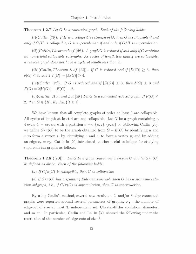
Theorem 1.2.7 Let G be a connected graph. Each of the following holds.
(i)(Catlin [26]). If H is a collapsible subgraph of G, then G is collapsible if and
only if G/H is collapsible; G is supereulerian if and only if G/H is supereulerian.
(ii)(Catlin, Theorem 5 of [26]). A graph G is reduced if and only if G contains
no non-trivial collapsible subgraphs. As cycles of length less than 4 are collapsible,
a reduced graph does not have a cycle of length less than 4.
(iii)(Catlin, Theorem 8 of [26]). If G is reduced and if |E(G)| ≥ 3, then
δ(G) ≤ 3, and 2|V (G)| − |E(G)| ≥ 4.
(iv)(Catlin [26]). If G is reduced and if |E(G)| ≥ 3, then δ(G) ≤ 3 and
F (G) = 2|V (G)| − |E(G)| − 2.
(v)(Catlin, Han and Lai [29]) Let G be a connected reduced graph. If F (G) ≤2, then G ∈ K1, K2, K2,t(t ≥ 1).
We have known that all complete graphs of order at least 3 are collapsible.
All cycles of length at least 4 are not collapsible. Let G be a graph containing a
4-cycle C = uvzwu with a partition π =< u, z, v, w >. Following Catlin [20],
we define G/π(C) to be the graph obtained from G − E(C) by identifying u and
z to form a vertex x, by identifying v and w to form a vertex y, and by adding
an edge eπ = xy. Catlin in [20] introduced another useful technique for studying
supereulerian graphs as follows.
Theorem 1.2.8 ([20]) . Let G be a graph containing a 4-cycle C and let G/π(C)
be defined as above. Each of the following holds:
(a) If G/π(C) is collapsible, then G is collapsible;
(b) If G/π(C) has a spanning Eulerian subgraph, then G has a spanning eule-
rian subgraph, i.e., if G/π(C) is supereulerian, then G is supereulerian.
By using Catlin’s method, several new results on 2- and/or 3-edge-connected
graphs were reported around several parameters of graphs, e.g., the number of
edge-cut of size at most 3, independent set, Chvatal-Erdos condition, diameter,
and so on. In particular, Catlin and Lai in [30] showed the following under the
restriction of the number of edge-cuts of size 3.
12

§1.2 Supereulerian graphs
Theorem 1.2.9 ([30]) A 3-edge-connected graph with at most 10 edge-cuts of size
3 is either supereulerian, or it is contractible to the Petersen graph.
Later, Li and Lai in [97] improved the result above by showing the following.
Theorem 1.2.10 ([97]) A 3-edge-connected graph with at most 11 edge-cuts of
size 3 is either supereulerian, or it is contractible to the Petersen graph.
Note that there are two reduced snarks of order 18. So 17 is best possible in
the two theorems above. We conjecture A 3-edge-connected with at most 17 edge-
cuts of size 3 is either supereulerian, or it is contractible to the Petersen graph.
This problem is open. In fact, the theorems above are closely related to one kind
of problems on supereulerian graphs. We discuss it below.
A minimum edge-cut of a graph G is called a bond of G. For two integers
l > 0 and k ≥ 0, let C(l, k) denote the family of 2-edge-connected graphs such
that a graph G ∈ C(l, k) if and only if for every bond S ⊂ E(G) with S ≤ 3,
each component of G−S has order at least (|V (G)| − k)/l. Catlin and Li [32] first
investigated the characterization of supereulerian graphs in the family of C(5, 0),
and they showed the following.
Theorem 1.2.11 ([32]) Every graph in C(5, 0) is either supereulerian or can be
contracted to K2,3.
Later, Broersma and Xiong [15] improve the result above.
Theorem 1.2.12 ([15]) If G ∈ C(5, 2) and |V (G)| ≥ 13, then G is either su-
pereulerian, or G can be contracted to one of K2,3 and K2,5.
Li et al. [96] continued the research and proved the following results concerning
the characterization of supereulerian graphs in a C(6, 0), as follows.
Theorem 1.2.13 ([96]) If G ∈ C(6, 0), then G is either supereulerian, or can
be contracted to K2,3, K2,5 or K ′2,3, where K ′
2,3 is the graph obtained from K2,3 by
replacing an edge e ∈ E(K2,3) with a path of length 2.
13

Chapter 1 Introduction
Similarly, Li et al. [98] reported a similar characterization on C(6, 5). One
may note that the expectations in the results above are 2-edge-connected. So, we
naturally ask what will happen if we restrict our research on the 3-edge-connected
graphs. Chen [34] showed that a 3-edge-connected graph of order at most 13 is
either supereulerian, or can be contracted to the Petersen graph. One may naturally
conjecture a 3-edge-connected graph in C(l, 0), l ≤ 13 is either supereulerian, or
can be contracted to the Petersen graph. In fact, we conjecture a 3-edge-connected
graph in C(l, 0), l ≤ 17 is either supereulerian, or can be contracted to the Petersen
graph. For the studies of the problems, we refer to [34, 99, 114]
Theorem 1.2.14 ([34]) Let G be a 3-edge-connected graph. If G ∈ C(10, 0), then
G is either supereulerian, or can be contracted to the Petersen graph.
Niu et al. [114] improved the result above as follows.
Theorem 1.2.15 ([114]) Let G be a 3-edge-connected graph with order at least
11k. If G ∈ C(10, k), then is either supereulerian, or can be contracted to the
Petersen graph.
Recently, Li et al. showed the following.
Theorem 1.2.16 ([34]) Let G be a 3-edge-connected graph. If G ∈ C(12, 0), then
G is either supereulerian, or can be contracted to the Petersen graph.
Overall, the study of the supereulerian problem on C(l, k) of 2- and/or 3-edge-
connected graphs is still not complete. We shall list them as one of our further
research topics.
We turn to another parameter–independent set of graphs. We first introduce
a result due to Benhocine et al. [8].
Theorem 1.2.17 ([8]) Let G be a 2-edge-connected graph on n ≥ 3 vertices. If
d(u) + d(v) ≥ 2n+ 3
3
whenever uv 6∈ E(G), then G has a spanning closed trail.
14

§1.2 Supereulerian graphs
Later, Catlin [27] and Chen [37] weakened the restriction as follows.
Theorem 1.2.18 ([27, 37]) Let G be a 2-edge-connected graph with order n and
girth g ∈ 3, 4. If n is sufficiently large and if
d(u) + d(v) ≥ 2
g − 2(n
5− 4 + g)
whenever uv 6∈ E(G), then G has a spanning closed trail.
Veldman weakened the condition above in [136] as follows.
Theorem 1.2.19 ([136]) Let G be a connected graph with order n ≥ 5. If
d(u) + d(v) + d(w) ≥ n− 1
for any 3-independent set u, v, w, then G has a spanning trail (possibly open).
The theorem above implies a spanning trail, may be not eulerian trail. So
we would like to know what such kind conditions can guarantee an eulerian trail.
Catlin [28] reported the following.
Theorem 1.2.20 ([28]) Let G be a 2-edge-connected graph with order n. If
d(u) + d(v) + d(w) ≥ n+ 1
for any 3-independent set u, v, w, then exactly one of the following holds:
(a) G is collapsible;
(b) G ∈ C4, C5, K2,3, Ga, where Ga is a well defined graph of 6 vertices.
Besides, Chen and Xue [39] weakened the sum of the 3-independent set above
to n− 2 for spanning trail and n− 5 for dominating trail.
In [36], Chen weakened the condition in Theorem 1.2.18 by using 3-independent
set as follows.
15
Chapter 1 Introduction
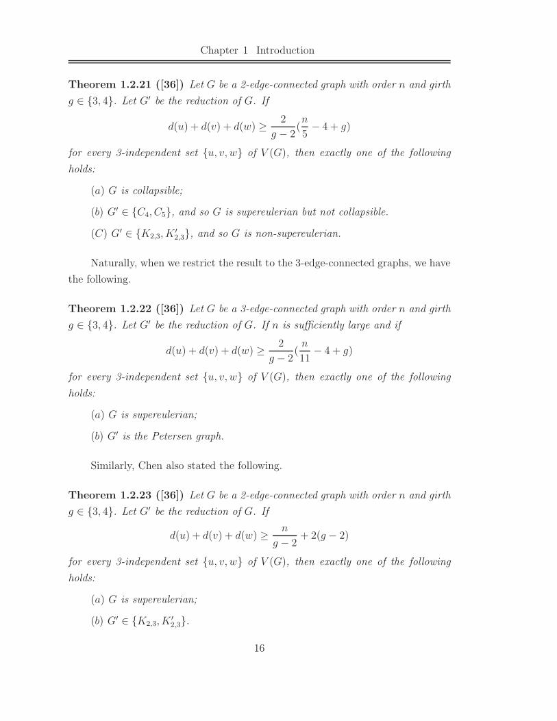
Theorem 1.2.21 ([36]) Let G be a 2-edge-connected graph with order n and girth
g ∈ 3, 4. Let G′ be the reduction of G. If
d(u) + d(v) + d(w) ≥ 2
g − 2(n
5− 4 + g)
for every 3-independent set u, v, w of V (G), then exactly one of the following
holds:
(a) G is collapsible;
(b) G′ ∈ C4, C5, and so G is supereulerian but not collapsible.
(C) G′ ∈ K2,3, K′2,3, and so G is non-supereulerian.
Naturally, when we restrict the result to the 3-edge-connected graphs, we have
the following.
Theorem 1.2.22 ([36]) Let G be a 3-edge-connected graph with order n and girth
g ∈ 3, 4. Let G′ be the reduction of G. If n is sufficiently large and if
d(u) + d(v) + d(w) ≥ 2
g − 2(n
11− 4 + g)
for every 3-independent set u, v, w of V (G), then exactly one of the following
holds:
(a) G is supereulerian;
(b) G′ is the Petersen graph.
Similarly, Chen also stated the following.
Theorem 1.2.23 ([36]) Let G be a 2-edge-connected graph with order n and girth
g ∈ 3, 4. Let G′ be the reduction of G. If
d(u) + d(v) + d(w) ≥ n
g − 2+ 2(g − 2)
for every 3-independent set u, v, w of V (G), then exactly one of the following
holds:
(a) G is supereulerian;
(b) G′ ∈ K2,3, K′2,3.
16

§1.2 Supereulerian graphs
Theorem 1.2.24 ([36]) Let G be a 3-edge-connected graph with order n and girth
g ∈ 3, 4. Let G′ be the reduction of G. If n is sufficiently large and if
d(u) + d(v) + d(w) ≥ 3
g − 2(n
14− 4 + g)
for every 3-independent set u, v, w of V (G), then exactly one of the following
holds:
(a) G is supereulerian;
(b) G′ is the Petersen graph.
In [36], Chen also obtained a bound of matching number of the reduction of a
graph. Similarly, Chen and Lai [35] bounded the matching number of the reduced
graphs. The reduction of graphs of diameter 2 were characterized in [87]. Recently,
Han et al. [65] studied supereulerian problem under the Chvatal-erdos condition.
They showed that the graphs satisfying Chvatal-erdos condition are supereulerian
but several well defined exceptions. Note that the supereulerian problem is NP-
compiete. So, exploring conditions for a graph to be supereulerian is an interesting
problem. In Chapter 2, we obtain several such conditions on matching number,
edge-degree, and 3-restricted edge-connectivity. The main results will be intro-
duced in the next subsection.
A dominating closed trail (DCT for short) is a closed trail T such that every
edge has at least one end vertex on T . The following theorem turns the hamiltonian
cycle (the definition will be introduced in the next section) of a line graph to the
closed trail of its root graph.
Theorem 1.2.25 (Harary and Nash-Williams [66]) Let G be a graph not a
star. Then L(G) is hamiltonian if and only if G has a dominating closed trail.
Note that a spanning eulerian subgraph of a graph G is a dominating closed
trail of G. Thus, the results on supereulerian graphs always imply the correspond-
ing results on line graphs.
In this thesis, two conjectures on supereulerian graphs of Chen and Lai will
be mentioned and several partial results on them will be obtained in Chapters 2
and 3 below.
17
Chapter 1 Introduction
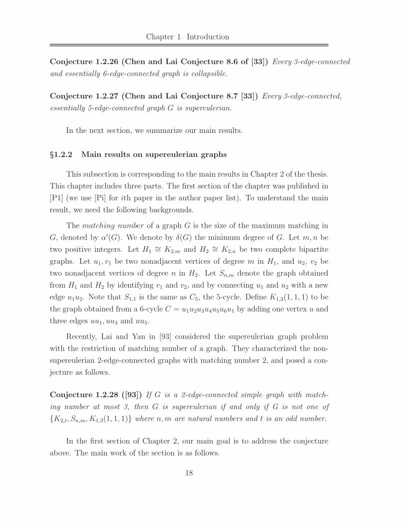
Conjecture 1.2.26 (Chen and Lai Conjecture 8.6 of [33]) Every 3-edge-connected
and essentially 6-edge-connected graph is collapsible.
Conjecture 1.2.27 (Chen and Lai Conjecture 8.7 [33]) Every 3-edge-connected,
essentially 5-edge-connected graph G is supereulerian.
In the next section, we summarize our main results.
§1.2.2 Main results on supereulerian graphs
This subsection is corresponding to the main results in Chapter 2 of the thesis.
This chapter includes three parts. The first section of the chapter was published in
[P1] (we use [Pi] for ith paper in the author paper list). To understand the main
result, we need the following backgrounds.
The matching number of a graph G is the size of the maximum matching in
G, denoted by α′(G). We denote by δ(G) the minimum degree of G. Let m,n be
two positive integers. Let H1∼= K2,m and H2
∼= K2,n be two complete bipartite
graphs. Let u1, v1 be two nonadjacent vertices of degree m in H1, and u2, v2 be
two nonadjacent vertices of degree n in H2. Let Sn,m denote the graph obtained
from H1 and H2 by identifying v1 and v2, and by connecting u1 and u2 with a new
edge u1u2. Note that S1,1 is the same as C5, the 5-cycle. Define K1,3(1, 1, 1) to be
the graph obtained from a 6-cycle C = u1u2u3u4u5u6u1 by adding one vertex u and
three edges uu1, uu3 and uu5.
Recently, Lai and Yan in [93] considered the supereulerian graph problem
with the restriction of matching number of a graph. They characterized the non-
supereulerian 2-edge-connected graphs with matching number 2, and posed a con-
jecture as follows.
Conjecture 1.2.28 ([93]) If G is a 2-edge-connected simple graph with match-
ing number at most 3, then G is supereulerian if and only if G is not one of
K2,t, Sn,m, K1,3(1, 1, 1) where n,m are natural numbers and t is an odd number.
In the first section of Chapter 2, our main goal is to address the conjecture
above. The main work of the section is as follows.
18

§1.2 Supereulerian graphs
We characterize the graphs with a given small matching number. We charac-
terize the graphs with minimum degree at least 2 and matching number at most
3. The characterization when the matching number is at most 2 strengthens the
result of Lai and Yan’s that characterized the non-supereulerian 2-edge-connected
graphs with matching at most 2; The characterization of the graphs with matching
number at most 3 addresses the conjecture of Lai and Yan in [93].
We next introduce the main result of the second section in Chapter 2, which
was published in [P2]. The main work of this section is to find spanning trail in
the graphs satisfying d(x) + d(y) ≥ n − 1 − p(n) for each edge xy ∈ E(G), where
p(n) = 0 for n even and p(n) = 1 for n odd, as follows.
Let G be a graph with n ≥ 4 vertices. Catlin in [21] showed that if d(x) +
d(y) ≥ n for each edge xy ∈ E(G), then G has a spanning trail except for several
defined graphs. In this work we obtain a similar result that if d(x) + d(y) ≥n − 1 − p(n) for each edge xy ∈ E(G), then G is collapsible except for several
special graphs, which strengthens the result of Catlin’s, where p(n) = 0 for n even
and p(n) = 1 for n odd. As corollaries, a characterization for graphs satisfying
d(x)+d(y) ≥ n−1−p(n) for each edge xy ∈ E(G) to be supereulerian is obtained.
In the third section, we consider the Conjectures 1.2.26 and 1.2.27 under a
restriction to 3-restricted edge connectivity of graphs. The results were published
in [P3]. The main works are as follows.
For e = uv ∈ E(G), define d(e) = d(u) + d(v) − 2 the edge degree of e,
and ξ(G) = mind(e) : e ∈ E(G). Denote by λm(G) the m-restricted edge-
connectivity of G (λ3(G)), and denote Di(G) the set of vertices of degree i. In
this part, we prove that a 3-edge-connected graph with ξ(G) ≥ 7, and λ3(G) ≥ 7
is collapsible; a 3-edge-connected simple graph with ξ(G) ≥ 7, and λ3(G) ≥ 6 is
collapsible; a 3-edge-connected graph with ξ(G) ≥ 6, λ2(G) ≥ 4, and λ3(G) ≥ 6
with at most 24 vertices of degree 3 is collapsible; a 3-edge-connected simple graph
with ξ(G) ≥ 6, and λ3(G) ≥ 5 with at most 24 vertices of degree 3 is collapsible;
a 3-edge-connected graph with ξ(G) ≥ 5, and λ2(G) ≥ 4 with at most 9 vertices of
degree 3 is collapsible. As a corollary, we show that a 4-connected line graph L(G)
with minimum degree at least 5 and |D3(G)| ≤ 9 is Hamiltonian.
19

Chapter 1 Introduction
§1.3 Hamiltonian line graphs
§1.3.1 Definitions and backgrounds
A hamiltonian path or traceable path is a path that visits each vertex exactly
once. A graph that contains a hamiltonian path is called a traceable graph. A graph
is hamiltonian− connected if for every pair of vertices there is a hamiltonian path
between the two vertices. A graph that contains a hamiltonian cycle is called a
hamiltonian graph.
The hamiltonian problem, determining when a graph contains a spanning
cycle, has long been fundamental in Graph Theory. Hamiltonian paths and cycles
are named after William Rowan Hamilton who invented the Icosian Game. In
1856, Hamilton invented a mathematical game, the Icosian Game, consisting of a
dodecahedron. Each of its twenty vertices was labeled with the name of a city and
the problems was to find a hamiltonian cycle in this dodecahedron graph, to make
a Voyage around the world.
The hamiltonian problem (graph theory) has been studied widely as one of
the most important problems in graph theory. Determining whether hamiltonian
cycles exist in graphs is NP-complete. Therefore it is natural and very interesting
to study sufficient conditions for hamiltonicity.
On the hamiltonian problem, one may find many well known theorems in any
graph theory textbook. So it is not necessary and impossible to give a detailed
survey in this thesis. In particular, Li recently in [102] surveyed the results due to
Dirac’s theorem which started a new approach to develop sufficient conditions on
degrees for a graph to be hamiltonian; For the survey on the hamiltonian problem
on Cayley graphs, we refer to [140] by Witte and Gallian; Gould gave two nice sur-
veys in [63, 64] in which contains many problems on generalizations of hamiltonian
problem; Bauer et al. [7] gave a survey which focus on the toughness of graphs
and the hamiltonian problem. We suggest the readers to refer to the surveys for
different topics of the hamiltonian problem [9, 12, 112].
One of the important topics in hamiltonian graph theory is the hamiltonicity
of claw-free graphs (i.e., a graph is called claw-free if it contain no induced claw,
20

§1.3 Hamiltonian line graphs
K1,3). Before we introduce our main results, we start by presenting a conjecture
by Matthews and Sumner, as follows.
Conjecture 1.3.1 (Matthews and Sumner [109]) Every 4-connected claw-free
graph is hamiltonian.
It is well known that every line graph is claw-free. Thomassen in 1986 posed
the following conjecture:
Conjecture 1.3.2 (Thomassen [125]) Every 4-connected line graph is hamilto-
nian.
The line graph transformation is probably the most interesting of all graph
transformations, and it is certainly the most widely studied. Much of this activity
was stimulated by Ore’s discussion of line graphs, and problems about them, in
[116]. The line graph concept is quite natural, and has been introduced in several
ways, see Whitney [139]. In the third chapter of this thesis we only concentrate on
the hamiltonian line graphs.
Note that Conjecture 1.3.1 is stronger that Conjecture 1.3.2 since line graphs
are claw-free. Herbert Fleischner asked whether they are equivalent? To answer
the question, Ryjacek introduced a closure operation (It is based on adding edges
without destroying the (non)hamiltonicity (similar to the Bondy-Chvatal closure
for graphs with nonadjacent pairs with high degree sums). The edges are added
by looking at a vertex v and the subgraph of G induced by N(v) (neighborhood of
v in G). If G[N(v)] is connected and not a complete graph, all edges are added to
turn G[N(v)] into a complete graph. This procedure is repeated in the new graph,
etc., until it is impossible to add any more edges. The resulting graph is called the
closure of G, or simply R−closure of G, denoted by cl(G). By using the R-closure,
Ryjacek [120] reported the following.
Theorem 1.3.3 ([120]) Let G be a claw-free graph. Then
(1) the closure cl(G) is uniquely determined;
(2) cl(G) is hamiltonian if and only if G is hamiltonian;
(3) cl(G) is the line graph of a triangle-free graph.
21
Chapter 1 Introduction
In fact, Conjectures 1.3.1 and 1.3.2 are also equivalent to several other con-
jectures. Recall Theorem 1.2.25, one can see that Conjectures 1.3.1 and 1.3.2 are
equivalent to the following.
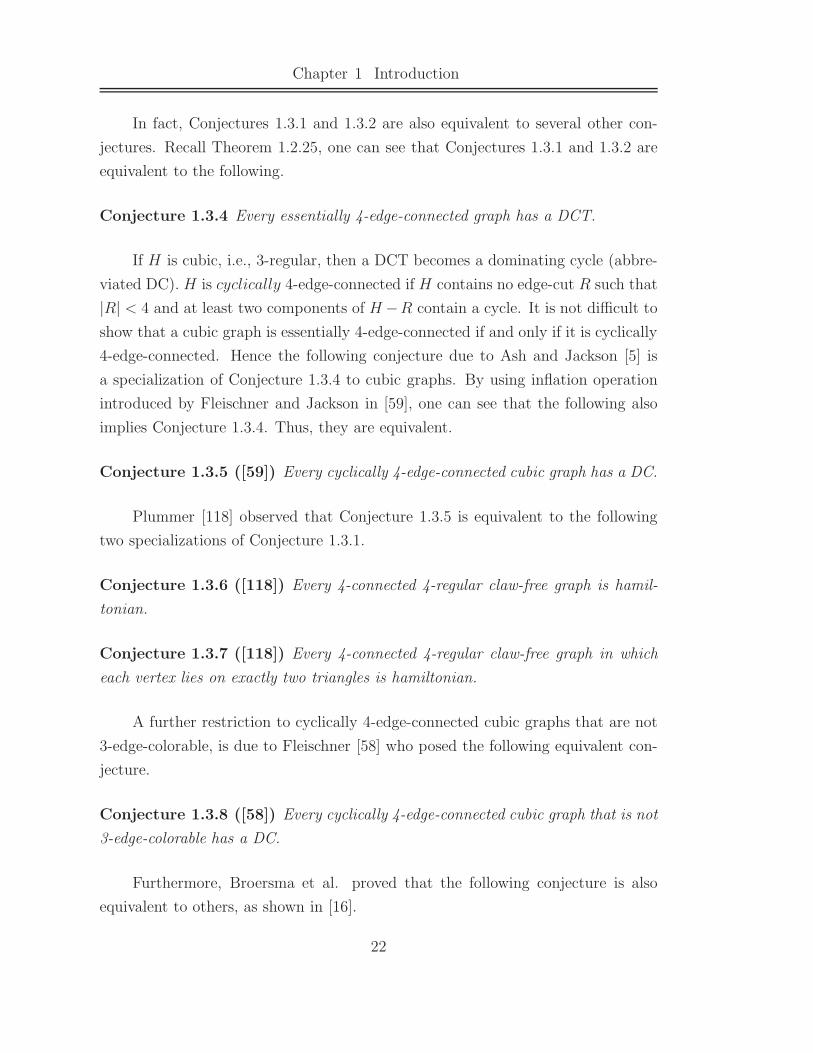
Conjecture 1.3.4 Every essentially 4-edge-connected graph has a DCT.
If H is cubic, i.e., 3-regular, then a DCT becomes a dominating cycle (abbre-
viated DC). H is cyclically 4-edge-connected if H contains no edge-cut R such that
|R| < 4 and at least two components of H−R contain a cycle. It is not difficult to
show that a cubic graph is essentially 4-edge-connected if and only if it is cyclically
4-edge-connected. Hence the following conjecture due to Ash and Jackson [5] is
a specialization of Conjecture 1.3.4 to cubic graphs. By using inflation operation
introduced by Fleischner and Jackson in [59], one can see that the following also
implies Conjecture 1.3.4. Thus, they are equivalent.
Conjecture 1.3.5 ([59]) Every cyclically 4-edge-connected cubic graph has a DC.
Plummer [118] observed that Conjecture 1.3.5 is equivalent to the following
two specializations of Conjecture 1.3.1.
Conjecture 1.3.6 ([118]) Every 4-connected 4-regular claw-free graph is hamil-
tonian.
Conjecture 1.3.7 ([118]) Every 4-connected 4-regular claw-free graph in which
each vertex lies on exactly two triangles is hamiltonian.
A further restriction to cyclically 4-edge-connected cubic graphs that are not
3-edge-colorable, is due to Fleischner [58] who posed the following equivalent con-
jecture.
Conjecture 1.3.8 ([58]) Every cyclically 4-edge-connected cubic graph that is not
3-edge-colorable has a DC.
Furthermore, Broersma et al. proved that the following conjecture is also
equivalent to others, as shown in [16].
22

§1.3 Hamiltonian line graphs
Conjecture 1.3.9 ([16]) Every snark has a dominating cycle.
For Conjecture 1.3.2, the first nice result was due to Zhan [159], as follows.
Theorem 1.3.10 ([159]) Every 7-connected line graph is hamiltonian-connected.
By using R-closure, Ryjacek proved the following.
Theorem 1.3.11 ([120]) Every 7-connected claw-free graph is hamiltonian.
Very recently, an important progress towards the conjectures was obtained by
Kaiser and Vrana [81] in which the following theorem is listed:
Theorem 1.3.12 ([81]) Every 5-connected line graph with minimum degree at
least 6 is hamiltonian.
So we clearly have:
Corollary 1.3.13 Every 6-connected line graph is hamiltonian.
Using Ryjacek’s line graph closure, the following corollary is obtained:
Corollary 1.3.14 ([81]) Every 5-connected claw-free graph G with minimum de-
gree at least 6 is hamiltonian.
The above theorems are based on the restriction of high connectivity. Several
authors considered Conjecture 1.3.2 under the restriction of the number of vertices
of degree 3 in G. For example, Chen et al. in [38] reported that every 4-connected
line graph L(G) with D3(G) = ∅ is hamiltonian. Li in [101] proved that every 6-
connected claw-free graph with at most 33 vertices of degree 6 is hamiltonian. LetG
be a 6-connected line graph. Hu, Tian and Wei in [79] showed that if d6(G) ≤ 29 or
G[D6(G)] contains at most 5 vertex disjoint K4’s, then G is hamiltonian-connected.
Let G be a 6-connected claw-free graph. Hu, Tian and Wei in [78] showed that
if d6(G) ≤ 44 or G[D6(G)] contains at most 8 vertex disjoint K4’s, then G is
23

Chapter 1 Introduction
hamiltonian. Let G be a 6-connected line graph. Zhan in [160] showed that if
either d6(G) ≤ 74, or d6(G) ≤ 54 or G[D6(G)] contains at most 5 vertex disjoint
K4’s, then G is hamiltonian.
We now turn to the 4-connected line (claw-free) graphs. Lai [88] considered
the line graph of planar graphs as follows.
Theorem 1.3.15 ([88]) Every 4-connected line graph of a planar graph is hamil-
tonian.
Kriesell [85] considered the line graph of claw-free graphs as follows.
Theorem 1.3.16 ([85]) All 4-connected line graphs of claw-free graphs are hamiltonian-
connected.
Lai et al. improved the result above to the following.
Theorem 1.3.17 ([89]) Every 4-connected line graph of a quasi claw-free graph
is hamilton- connected.
Another topic on hamiltonicity of 4-connected line graphs is due to the re-
striction of forbidden subgraphs. A graph is called H-free if it contains no H as its
induced subgraph. The forbidden subgraphs involving in hamiltionian line (claw-
free) graph theme includes: Zk (denote a graph obtained from the disjoint union
of a Pk+1 and a 3-cycle K3 by identifying one endvertex of Pk+1 with one vertex of
K3.), the generalized bull (denote by Bs,t, to be the graph obtained by attaching
each of some two distinct vertices of a triangle to an end vertex of one of two
vertex-disjoint paths of orders s and t.), net (denoted by Ns1,s2,s3, to be the graph
obtained by identifying each vertex of a K3 with an end vertex of three disjoint
paths Ps1+1, Ps2+1, Ps3+1, respectively.) and so on. We refer to [63, 64] for the old
results on this topic. We next summary several recently results on this topic.
In 1999, Brousek, Ryjacek and Favaron proved the following.
Theorem 1.3.18 ([18]) Every 3-connected claw-free and Z4-free graph is hamil-
tonian.
24
§1.3 Hamiltonian line graphs
Later, Lai et al. [92] improved the result above by the following.
Theorem 1.3.19 ([92]) Every 3-connected claw-free and Z8-free graph is hamil-
tonian.
In [92], Lai et al. posed a conjecture which was addressed by Fujisawa [61].
Theorem 1.3.20 Every 3-connected claw-free and Z9-free graph G is hamiltonian
unless G is the line graph of Q∗, where Q∗ denote the graph obtained from the
Petersen graph by adding one pendant edge to each vertex.
Fujisawa with the other author Chiba [41] generalized the result above to
3-connected Bs,9−s-free and claw free graphs.
Theorem 1.3.21 ([41]) Every 3-connected Bs,9−s-free line graph is hamiltonian
for 1 ≤ s ≤ 4.
Very recently, Xiong et al. [142] considered claw-free graphs as follows (we
state part of the original results, the complete results include the discussion for
Bs,9−s-free claw-free graphs, and the discussion for Ns1,s2,s3-free graph claw-free
graphs when si > 0, s1 + s2 + s3 = 10).
Theorem 1.3.22 ([142]) Every 3-connected claw-free and Ns1,s2,s3-free graph G
is hamiltonian for si > 0, s1 + s2 + s3 ≤ 9.
Luczak and F. Pfender [106] showed that every P11-free claw free 3-connected
graph is hamiltonian. The result was improved to P12-free by Ma et al. [107].
So far, several different topics are mentioned on hamiltonian problem of line
graph (i.e., claw-free graph). The following one lead to our research in this thesis.
Lai et al in [91] considered the following problem:
Question 1 For 3-connected line graphs, can high essential connectivity guarantee
the existence of a hamiltonian cycle ?
25
Chapter 1 Introduction
They proved the following theorem:
Theorem 1.3.23 (Lai et al. [91]) Every 3-connected, essentially 11-connected line
graph is hamiltonian.
In Chapter 3, we consider what is the minimum integer k such that every
3-connected, essentially k-connected line graph is hamiltonian. In the next section,
we summary our main results in Chapter 3.
§1.3.2 Main results
To discuss the main results of the third chapter, several new notations are
needed. Esfahanian in [51] proved that if a connected graph G with |V (G)| ≥ 4
is not a star K1,n−1, then λ′(G) exists and λ′(G) ≤ ξ(G). Thus, an essentially
k-edge connected graph has edge-degree at least k. Denote Di(G) and di(G) the
set of vertices of degree i and |Di(G)|, respectively. If no confusion arises, we
directly use Di and di for Di(G) and di(G), respectively. For a subgraph A ⊆ G,
v ∈ V (G), NG(v) denotes the set of the neighbors of v in G and NG(A) denotes
the set (⋃
v∈V (A)NG(v)) \ V (A). If no confusion arises, we use an edge uv for a
subgraph with three elements of u, v, uv. Denote G[X] the subgraph induced by
the vertex set X of V (G).
The main results of Chapter 3 includes three parts. In the first section of
Chapter 3, we consider the hamiltonian-connectedness of 3-connected and essen-
tially 11-connected line graphs. The result of this part was published in [P4]. The
main results are as follows.
(1) Every 3-edge-connected, essentially 6-edge-connected graph with edge-
degree at least 7 is collapsible. (2) Every 3-edge-connected, essentially 5-edge-
connected graph with edge-degree at least 6 and at most 24 vertices of degree 3
is collapsible which implies that 5-connected line graph with minimum degree at
least 6 of a graph with at most 24 vertices of degree 3 is hamiltonian. (3) Every
3-connected, essentially 11-connected line graph is hamiltonian-connected which
strengthens the result in [Every 3-connected, essentially 11-connected line graph is
Hamiltonian, Journal of Combinatorial Theory, Series B 96 (2006) 571-576] by Lai
et al. (4) Every 7-connected line graph is Hamiltonian-connected which is proved
26

§1.4 Fault-tolerant hamiltonian laceability of Cayley graphs generated bytransposition trees
by a method different from Zhan’s. By using the multigraph closure introduced by
Ryjacek and Vrana which turns a claw-free graph into the line graph of a multi-
graph while preserving its hamiltonian-connectedness, the results (3) and (4) can
be extended to claw-free graphs.
In the second section of Chapter 3, we show that every 3-connected, essen-
tially 10-connected line graph is hamiltonian-connected. Using the line closure
introduced by Ryjacek, we have that every 3-connected, essentially 10-connected
claw-free graph is hamiltonian. The result of this part was published in [P5].
In the third section of Chapter 3, we consider the hamiltonicity of 3-connected
and essentially 4-connected line graphs. The result of this part was published in
[P6]. The main results are as follows.
We show the conjecture (every 3-connected, essentially 4-connected line graph
is hamiltonian) posed by Lai et al is not true and there is an infinite family of
counterexamples; we show that 3-connected, essentially 4-connected line graph of
a graph with at most 9 vertices of degree 3 is hamiltonian; examples show that all
conditions are sharp. Moreover, if G has 10 vertices of degree 3 and L(G) is not
hamiltonian, then G can be contracted to the Petersen graph.
§1.4 Fault-tolerant hamiltonian laceability of Cayley
graphs generated by transposition trees
§1.4.1 Basic definitions and background
We would like to avoid the related topic of fault-tolerant hamiltonicity of
general graphs. The main research in this part is due to the stimulation of several
studies of computer scientists. As the Cayley graph is widely applied in the design
of networks, several families of Cayley graphs have been received much attention.
Cayley graphs generated by transposition trees is one of important families.
The interconnection network of a communication or distributed computer sys-
tem is usually modeled by a (directed) graph in which the vertices represent the
switching elements or processors and communication links are represented by (di-
rected) edges. Clearly, properties of the (directed) graph determine how efficiently
27

Chapter 1 Introduction
the system can run. Thus, the ones hope a graph has higher connectivity which in-
creases the fault tolerance, smaller diameter which reduces the transmission delay,
symmetry (vertex-and edge-transitivity) which reduce design and operation costs,
recursive structure which simplifies design scheme. Another desired property is
hamiltonicity of a graph which are widely applied to design computer algorithm,
for example, broadcasting algorithms, gossiping algorithms and sorting algorithms.
Let Sn denote the symmetric group on 1, · · · , n, (p1p2 · · · pn) denote the per-
mutation
1 2 · · ·n
p1p2 · · · pn
, and (ij) denote the permutation
1 2 · · · i · · · j · · ·n
1 2 · · · j · · · i · · ·n
(it is obtained by exchanging the ith and jth objects of
1 2 · · ·n
1 2 · · ·n
) which is
called a transposition. It is easy to see that (p1 · · · pi · · ·pj · · · pn)(ij) = (p1 · · · pj · · · pi · · · pn).
Let B be a minimal generating set of Sn. If the minimal generating set B is a set of
transpositions of Sn is called minimal transposition generating set. In this paper,
we always assume the minimal generating set is minimal transposition generating
set. For the convenience of discussion, we describe the the minimal transposition
generating set B of Sn by a transpositon generating graph, written TB, where the
vertex set of TB is 1, 2, · · · , n, the edge set is (ij)|(ij) ∈ B. Note that B is a
minimal transposition generating set of Sn, it can be seen that TB is a tree which
is called transposition generating tree, see [62] for the details.
Cayley graph Cay(Sn, B) is called Cayley graph grenerated by transposition
generating tree if B is a minimal transposition generating set of Sn. It is well
known that the Cayley graph Cay(Sn, B) is called star graph and bubble-sort
graph if TB∼= K1,n−1 and TB
∼= Pn (Pn is a path with n vertices), respectively.
For a bipartite graph G, Wong introduced the following definition in [141]. A
bipartite graph G is hamiltonian laceable if there is a hamiltonian path between
every pair of vertices which are in different partite sets [141].
Since edge faults may happen when a network is put in use, it is significant
to consider faulty networks. So, fault-tolerance ability is a very important factor
of interconnection networks [76].
28

§1.4 Fault-tolerant hamiltonian laceability of Cayley graphs generated bytransposition trees
A bipartite graph G is k-edge fault tolerant hamiltonian laceable if G − F
is hamiltonian laceable for any F ⊆ E(G) with |F | ≤ k, where set F is called
fault edge set, edges of F are called fault edges, and edges of E(G) − F are
called fault-free edges. A graph G is pancyclic if it contains cycles of all length
l, 3 ≤ l ≤ |V (G)|, see [82] for the details. We say that G is vertex-pancyclic if,
for each vertex v of G and for every integer l with 3 ≤ l ≤ n, there is an l-cycle
that contains v. Furthermore, a graph is called edge-pancyclic if every edge lies
on an l-cycle for every 3 ≤ l ≤ n. Since bipartite graphs have no odd cycle, a
bipartite graph G is called bipancyclic if it contains cycles of all even length from 4
to |V (G)|. For bipartite graphs, vertex-bipancyclicity and edge-bipancyclicity are
defined similarly. A bipartite graph G is called k-edge fault-tolerant bipancyclic if
G− F remains bipancyclic for any set F of edges with |F | ≤ k, where F is called
a fault edge set of the fault edge.
Hamiltonicity of graphs with fault edges have been studied by many authors,
for examples, the works on hypercubes can be found in [4, 77, 129, 130], the works
on star graphs and bubble-sort graphs can be found in [3, 60, 73, 100, 82, 131], the
works on alternating group graphs and butterfly graphs can be found in [132, 141]
etc..
In particular, Li et al. [100] and Araki et al. [3] showed that the n-dimensional
star graph and n-dimensional bubble-sort graph are (n − 3)-edge fault tolerant
hamiltonian laceable, respectively. A common generalization of star graphs and
bubble-sort graphs are studied in [2, 40, 62, 84, 127, 150], which is the class of
Cayley graphs generated by transition trees. Motivated by the proofs of [3, 100],
we consider edge fault-tolerant hamiltonicity of Cayley graphs generated by trans-
position trees.
In Chapter 4, we consider edge fault-tolerant hamiltonicity of Cayley graphs
generated by transposition trees. We summary our main results in Chapter 4 as
follows.
§1.4.2 Main results
The main results of Chapter 4 includes two parts. The result of the first
section of Chapter 4 was published in [P7], in which we show that for any F ⊆
29
Chapter 1 Introduction
E(Cay(B : Sn)), if |F | ≤ n− 3 and n ≥ 4, then there exists a hamiltonian path in
Cay(B : Sn) − F between every pair of vertices which are in different partite sets.
The result is optimal with respect to the number of edge faults.
The second section of Chapter 4 is included in a manuscript [P8]. In this sec-
tion we strengthen the above result by showing that Cay(Sn, B)−F is bipancyclic
if Cay(Sn, B) is not a star graph, n ≥ 4 and |F | ≤ n− 3.
§1.5 Several extremal problems
Determining the minimum and/or maximum size of graphs with some given
property is a classical problem in extremal graph theory. In Chapter 5, we con-
sider several such problems of graphs. In particular, the hypercube (n-cube) is
an interesting combinatorial structure, and there are many interesting conjectures
on hypercubes. We would like to mention two conjectures due to Erdos. In [47],
he conjectured the maximum size (ex(Qn, C4)) of subgraphs of an n-cube with
no 4-cycle is (12
+ o(1))e(Qn) (note that e(Qn) = n2n−1 = |E(Qn)|). The con-
jecture stimulates many authors to study such problems. The best upper bound,
(0.6226+o(1))n2n−1, is due to Thomason and Wagner [126], while Brass, Harborth
and Nienborg [14] showed 12(n+
√n)2n−1 ≤ ex(Qn, C4), when n is a positive integer
power of 4, and 12(n+ 0.9
√n)2n−1 ≤ ex(Qn, C4) for all n ≥ 9.
Furthermore, several authors generalized the problem to Cl for l ≥ 6. Define
cl := limn→∞ ex(Qn, Cl)/e(Qn). It is known that 1/3 ≥ c6 < 0.3941 by Conder
[44], c4k = 0 for any integer k ≥ 2 by Chung [42] and c4k+2 ≤ 1√2
for k ≥ 1 by
Axenovich and Martin [6].
The other conjecture posed by Erdos and Guy [48] is the crossing number of
the hypercube cr(Qn) satisfying lim cr(Qn)4n = 5
32. The recently progress we refer to
[108] by Madej and [53] by Faria.
Some other similar problems on hypercubes we refer to [6, 126] and we refer
to [56, 83, 138, 155, 156, 157] for the studies related to the structure of hypercubes.
We omit the detailed survey for these problems, as the topic is not the main focus
of this thesis.
We shall consider the following extremal problem on n-cubes: How many edges
30

§1.5 Several extremal problems
can a subgraph of hypercube of m vertices contain in an n-cube have? In Section
1, we show that a subgraph induced by m (denote m bys∑
i=0
2ti , t0 = [log2m] and
ti = [log2(m−i−1∑
r=0
2tr)] for i ≥ 1) vertices of an n-dimensional hypercube has at
mosts∑
i=0
ti2ti−1 +
s∑
i=0
i · 2ti edges.
As its applications, we determine the m-extra edge-connectivity (m-restricted
edge-connectivity) of hypercubes for m ≤ 2[ n2], and m-extra-edge-connectivity
(λm(FQn)) of the folded hypercube FQn for m ≤ n. The results on hypercubes
was published in [P9]. In particular, the result on folded hypercubes will appear
in [P10], in which we generalize the main result in [On reliability of the folded
hypercubes. Information Sciences 177 (2007) 1782-1788.] on the 3-extra edge-
connectivity of folded hypercubes. and it also implies the results in [On Extra
Connectivity and Extra Edge Connectivity Measures of Folded Hypercubes, IEEE
Transactions on Computers, Jan. 2013 DOI.10.1109/TC.2013.10.] on the 4-extra
edge-connectivity of folded hypercubes.
In Section 2, we consider what is the minimum size of graphs with a given
order n, a given minimum degree δ and a given minimum edge-degree 2δ + k − 2?
In this thesis (results are included in [P11]), we partially answer the question for
k = 0, 1, 2 and characterize the corresponding extremal graphs.
As an application, we characterize some kinds of restricted edge-connected
graphs with minimum edge number. In fact, characterizing the extremal graphs
with the given connectivity is a classical topic in graph theory. For example, In [45],
Cozzens and Wu studied the minimum critically k-edge connected graph (a k-edge
connected graph is critical if λ(G − v) < k for any vertex v ∈ V (G)). In [110],
Maurer and Slater defined the k-edge♯-connectivity which is the other version of
restricted edge connectivity and characterized the cases k = 1, 2, 3. Later, Peroche
and Virlouvet gave some partial results on the cases k = 4, 5. Recently, Hong et
al [72] showed that the minimally restricted k-edge connected graph is λ′-optimal
( A restricted k-edge connected G is called minimally restricted k-edge connected if
λ′(G− e) < k for any edge e.). Here, we give some partial results on the minimum
restricted edge connected graphs.
In Section 3, we consider the minimum size of graphs satisfying Ore condition,
31

Chapter 1 Introduction
which is included in [P12].
32

Chapter 2 Supereulerian graphs
§2.1 A note on supereulerian graphs in terms of a given
small matching number
The matching number of a graph G is the size of the maximum matching in
G, denoted by α′(G). We denote by δ(G) the minimum degree of G. Let m,n be
two positive integers. Let H1∼= K2,m and H2
∼= K2,n be two complete bipartite
graphs. Let u1, v1 be two nonadjacent vertices of degree m in H1, and u2, v2 be
two nonadjacent vertices of degree n in H2. Let Sn,m denote the graph obtained
from H1 and H2 by identifying v1 and v2, and by connecting u1 and u2 with a new
edge u1u2. Note that S1,1 is the same as C5, the 5-cycle. Define K1,3(1, 1, 1) to be
the graph obtained from a 6-cycle C = u1u2u3u4u5u6u1 by adding one vertex u and
three edges uu1, uu3 and uu5.
Recently, Lai and Yan in [93] considered supereulerian graph problem with the
restriction of matching number of a graph and posed two conjectures as follows.
Conjecture 2.1.1 If G is a 2-edge-connected simple graph with matching number
at most 3, then G is supereulerian if and only if G is not one of K2,t, Sn,m, K1,3(1, 1, 1)where n,m are natural numbers and t is an odd number
Conjecture 2.1.2 If G is a 3-edge-connected simple graph with matching number
at most 5, then G is supereulerian if and only if G is not contractible to the Petersen
graph.
In [1], An and Xiong pointed that the second conjecture is a corollary of a
result in Chen [35] and they also pointed that the first conjecture is not true by
giving some counterexamples. They revised the first conjecture as a new conjecture
in [1], but the revision is not complete yet. We do not list it here, see [1].
In this note we first obtain a characterization for graphs with minimum degree
2 and matching number at most 2 that strengthens the result of Lai and Yan
in [93] (the main result in [93] is that every 2-edge-connected graph with α′(G) ≤ 2
is supereulerian if and only if G is not K2,t for some odd number t); Similarly,
33

Chapter 2 Supereulerian graphs
a characterization of the graphs with minimum degree at least 2 and matching
number at most 3 is obtained which addresses the problem raised by Conjecture 1.
We first consider the characterization of graphs with minimum degree at least
2 and matching number at most 2.
In this section we characterize the graphs with minimum degree 2 and match-
ing number at most 2. For a graph G, a cycle of G is called dominating cycle if the
cycle contains at least one endvertex of any edge of G.
Theorem 2.1.3 Let G be a graph with minimum degree at least 2 and maximum
matching number at most 2. Then G ∈ 1 = G : δ(G) ≥ 2 and |V (G)| ≤5 ∪ K2,t ∪ K ′
2,t, where K ′2,t is obtained from K2,t by adding an edge between
the two vertices of degree t.
Proof. Suppose C is the longest cycle of G with length l. If l ≤ 3, then by
δ(G) ≥ 2 and α′(G) ≤ 2 we clearly have either G ∼= K3 or G isomorphic to the
hourglass, where the hourglass is a graph obtained from K5 by removing the edges
of a C4. Thus, G ∈ 1. Note that α′(G) ≤ 2, then l ≤ 5.
Case 1. l = 5.
We claim that C is a dominating cycle of G, since other cases will induce
α′(G) ≥ 3. Note that G is connected. If V (G − C) 6= ∅, the case will induce a
matching of size 3. Thus, |V (G)| = 5 and then G ∈ G : δ(G) ≥ 2 and |V (G)| ≤5 ⊆ 1.
Case 2. l = 4.
Suppose C = x1x2x3x4x1. Clearly, C is a dominating cycle, since otherwise it
will induce α′(G) ≥ 3. If V (G) = V (C), then G ∈ 1. Otherwise, let v ∈ V (G−C).
Since δ(G) ≥ 2, v has exactly two neighbors in V (C) (otherwise will induces a cycle
of length 5). Since α′(G) ≤ 2, all the vertices in V (G−C) have the same neighbors
in V (C). So we clearly have either G ∼= K2,t or G ∼= K ′2,t.
Lemma 2.1.4 A graph G with δ(G) ≥ 2 and |V (G)| ≤ 5 is either supereulerian
or G = K2,3. Moreover, K2,t is supereulerian if t is an even number, and non-
supereulerian otherwise.
34

§2.1 A note on supereulerian graphs in terms of a given small matching number
Proof. It is easy to obtain the first part by considering its longest cycle. The
second part is obvious.
Corollary 2.1.5 (Theorem 2 [93]) If G is a 2-edge-connected simple graph with
matching number at most 2, then G is supereulerian if and only if G is not K2,t
for some odd number t.
Proof. By the Observation 2.1.4, the corollary holds sinceK ′2,t is supereulerian.
In the following, we consider the graphs with matching number at most 3.
We first introduce some special graphs as follows.
S ,m S ,m S ,m’ ’’1 11
x
x x
xx
x
x
x
x
x
x
xx
x x
1
1
2
34
5
1
2
34
5
1
2
34
5
Fig. 2.1: The case n = 1x
x
xx
x
x
x
xx
x
x
x
x
x
x
x1
2
34
5
1
2
3
5
1
2
34
4
5
6
S S Cn m, n m 6(k;s,t,r),’
Fig. 2.2: The case m ≥ n ≥ 2
The following four graphs below are the simple variants of Sn.m: S∗1,m =
S1,m + x1x3, S′∗1,m = S ′
1,m + x1x3, S′′∗1,m = S ′
1,m + x1x3, S′′n,m = S ′
n,m + x1x4. Sim-
ilarly, C6(k; s, t) contains the following three variants that obtained by adding
edges x1x3, x1x3, x3x5 and x1x3, x3x5, x5x1, respectively. We use C to de-
note the set of C6(k; s, t, r) and its three variants mentioned above. Let S =
S1,m, S′1,m, S
′′1,m, S
∗1,m, S
′∗1,m, S
′′∗1,m, Sn,m, S
′n,m, S
′′n,m, K2,t, K
′2,t
35

Chapter 2 Supereulerian graphs
Theorem 2.1.6 Let G be a graph with minimum degree 2 and matching number
at most 3. Then G is in 2 = G : |V (G)| ≤ 7 ∪ S ∪ C.
Proof. Suppose C is the longest cycle of G with length l. Similarly as in
Theorem 4, we have |V (G)| = 7 if l = 7 and thus G ∈ 2.
If l = 3, then G ∈ K3, H,H′, H ′′, where H denotes the hourglass, H ′, H ′′
denote the two different graphs obtained from a hourglass and a triangle by iden-
tifying a vertex of a hourglass and a vertex of a triangle. Each of the cases implies
|V (G)| ≤ 7 and then G ∈ 2. Thus we may assume l ≥ 4.
Case 1. l = 6
Let C = x1x2x3x4x5x6x1 be a longest cycle of G. Clearly, C is a dominating
cycle of G. Suppose V (G − C) 6= ∅. Since α′(G) ≤ 3 and l = 6, at most one of
the two endvertices of an edge ab ∈ E(C) has neighbors in V (G − C). Thus at
most three pairwise nonadjacent vertices of V (C) have neighbors in V (G−C) and
assume that they are x1, x3, x5. Suppose there are k vertices of V (G−C) such that
each of them is only adjacent to vertices of x1, x3, x5. In this case, it is easy to see
that G ∈ C.
Case 2. l = 5
Let C = x1x2x3x4x5x1 be a longest cycle of G. Note that l = 5 and δ(G) ≥ 2.
Then if C is not a dominating cycle of G, then G is the graph obtained from a cycle
C5 (a cycle of length 5) and a triangle by identifying a vertex of the C5 and a vertex
of triangle and adding some edges on the C5. In this case, we have |V (G)| ≤ 7.
Suppose C is a dominating cycle of G. It is easy to see that G contains a Sn,m as
a subgraph for some m,n. If m ≥ n ≥ 2, then G ∈ Sn,m, S′n,m, S
′′n,m. If n = 1,
then G ∈ S1,m, S′1,m, S
′′1,m, see Fig. 2.3.
Case 3. l = 4
Let C = x1x2x3x4x1 be a longest cycle of G. Similarly, if C is not a dominating
cycle, then |V (G)| ≤ 7. If C is a dominating cycle, we have G ∼= K2,t or G ∼= K ′2,t
for some integer t.
Note that S∗1,m, S
′∗1,m, S
′′∗1,m, and S ′′
n,m are supereulerian. If G ∼= C6(k; s, t, r),
k = 1, s, t, r ≥ 1 and the parities of s, t, r are the same, then G is not supereulerian.
36

§2.2 On spanning trail in terms of degree sum condition
In fact, G has 4 vertices of odd degree and only one edge can be removed. So G is
not supereulerian. If k ≥ 2, the k−1 vertices of degree 3 can be used to adjust the
parities of s, t, r such that one of them is different from others, then the resulting
is supereulerian clearly. So we have the following theorem.
Theorem 2.1.7 Let G be a graph with minimum degree 2 and α′(G) ≤ 3. Then
G is not supereulerian if and only if one of the following holds:
(1) If G ∼= Sn,m, m ≥ n ≥ 1, then one of n,m is an even number;
(2) If G ∈ S ′1,m, S
′′1,m, then m is even number;
(3) If G ∼= S ′n,m, m ≥ n ≥ 2, then x4 is a vertex of odd degree.
(4) If G ∼= C6(k; s, t, r), then k = 0 or 1. Moreover, if k = 1, then the parities
of s, t, r are the same; If k = 0, then s, t, r are different.
Proof. We only prove the necessity. We first claim that a graph G 6∈ S ∪ Cwith at most 7 vertices and δ(G) ≥ 2 is supereulerian. In fact, the claim is easily
obtained by considering the longest cycle of G. Thus we assume |V (G)| ≥ 8.
By Theorem 2.1.6 and the discussion above, (1), (2), (3), (4) are easy to obtain by
consider the parities of n,m, s, t, r.
Remark. Theorem 2.1.7 implies Conjecture 2.1.1 is not complete and one can
revise it easily by using the theorem above.
§2.2 On spanning trail in terms of degree sum condition
Catlin in [21] showed the following:
Theorem 2.2.1 (Catlin [21]) Let G be a connected graph on n vertices and let
u, v ∈ V (G). If
d(x) + d(y) ≥ n (2.2.1)
for each edge xy ∈ E(G), then exactly one of the following holds:
(i) G has a spanning (u, v)-trail.
37

Chapter 2 Supereulerian graphs
(ii) d(z) = 1 for some vertex z 6∈ u, v.
(iii) G = K2,n−2, u = v and n is odd.
(iv) G = K2,n−2, u 6= v, uv ∈ E(G), n is even, and d(u) = d(v) = n− 2.
(v) u = v, and u is the only vertex with degree 1 in G.
The following stronger result modifies Catlin’s theorem above:
Theorem 2.2.2 Let G be a connected graph of order n ≥ 4 and G satisfies (2.2.1)
for every edge of G. Then exactly one of the following holds:
(i) G is collapsible.
(ii) The reduction of G is K1,t−1 for t ≥ 3 such that all of the vertices of degree
1 are trivial and they have the same neighbor in G, t ≤ n2. Moreover, if t = 2, then
G− v is collapsible for a vertex v in the K2.
(iii) G is K2,n−2.
By the definition of the collapsible graph, Theorem 2.2.2 implies Theorem 2.2.1.
Theorem 2.2.2 implies a previous result by using Harary and Nash-Williams’s
theorem (we recall the theorem below).
Theorem 2.2.3 (Harary and Nash-Williams [66]) Let G be a graph with at
least 4 vertices. The line graph L(G) is hamiltonian if and only if G has a closed
trail that contains at least one vertex of each edge of G.
Note that every graph in K2,n−2, K1,n−1 has a closed trail that contains at
least one vertex of each edge of G. Then by Theorem 2.2.2 we have:
Theorem 2.2.4 (Brualdi and Shanny [19]) Let G be a connected graph with
n ≥ 4 vertices. If G satisfies (2.2.1) for every edge of G, then L(G) is hamiltonian.
Theorem 2.2.4 was improved by Clark in [43] as follows:
38

§2.2 On spanning trail in terms of degree sum condition
Theorem 2.2.5 (Clark [43]) Let G be a connected graph on n ≥ 6 vertices, and
let p(n) = 0 for n even and p(n) = 1 for n odd. If each edge of G satisfies
d(x) + d(y) ≥ n− 1 − p(n), (2.2.2)
then L(G) is hamiltonian.
Motivated by Theorem 2.2.5, Catlin in [21] considered replacing the condition
(2.2.1) in Theorem 2.2.1 by (2.2.2), and classified the two exceptional cases that
can arise. The following gives an analagous result for the collapsibility of graphs.
Theorem 2.2.6 Let G be a connected graph of order n ≥ 4 and let p(n) = 0 for n
even and p(n) = 1 for n odd. If each edge of G satisfies (2.2.2), then exactly one
of the following holds:
(i) G is collapsible.
(ii) The reduction of G is K1,t−1 for t ≥ 3 such that all of the vertices of degree
1 are trivial and they have the same neighbor in G, t ≤ n2. Moreover, if t = 2, then
G− v is collapsible for some vertex v in the K2.
(iii) G is in C5, G7, G′7, K1,n−1, K2,n−2, K
′2,n−3, where K ′
2,n−3 is obtained from
K2,n−3 by adding a pendant edge on one of the vertices of degree n− 3, and G7, G′7
are the graphs shown in Fig.2.1.
The following example shows that the condition (2.2.2) in Theorem 2.2.6 is
sharp: Let G be a graph of order n ≥ 6, such that G has a bridge e and G − e
consisting of two complete graphs of order ⌊n2⌋, ⌈n
2⌉ respectively. Clearly, if n
is even, then d(x) + d(y) ≥ n − 2 for each edge of G, and if n is odd, then
d(x) + d(y) ≥ n− 3. However, the reduction G′ of G is K2 and each vertices of G′
is non-trivial. This violates Theorem 2.2.6.
Note that every graph of G7, G′7, K2,n−2, k
′2,n−3, K1,n−1 has a closed trail that
contains at least one vertex of each edge of G. By the definition of a collapsible
graph and Theorem 2.2.3, Theorem 2.2.6 implies Theorem 2.2.5. By Theorem 2.2.6
and the definition of a collapsible graph, we also have the following, which is similar
to Theorem 2.2.1.
39

Chapter 2 Supereulerian graphs
Corollary 2.2.7 Let G be a connected graph on n vertices and let u, v ∈ V (G). If
d(x) + d(y) ≥ n− 1 − p(n) (2.2.3)
for each edge xy ∈ E(G) and p(n) defined as above, then exactly one of the following
holds:
(i) G has a spanning (u, v)-trail.
(ii) G ∈ G7, G′7, K1,n−1, K
′2,n−2 or the reduction of G is K1,t−1 for some
integer t ≥ 2.
(iii) G = K2,n−2, u = v and n is odd.
(iv) G = K2,n−2, u 6= v, uv ∈ E(G), n is even, and d(u) = d(v) = n− 2.
G7 G7’
Fig. 2.3:
Assume H is a collapsible subgraph of G. It is easy to see that if a vertex
y ∈ V (G−H) and |N(y)∩ V (H)| ≥ 2, then the subgraph induced by y ∪ V (H)
is collapsible. We denote by ξ(G) the value mind(x)+ d(y) : xy ∈ E(G) and call
d(x) + d(y) the edge degree-sum of xy.
Lemma 2.2.8 Let G be a graph on n vertices satisfying ξ(G) ≥ n − 1. Suppose
G′ is the reduction of G. Then ξ(G′) ≥ |V (G′)| − 1.
Proof. Assume that u is a non-trivial vertex of G′, i.e. it is the contraction
of a maximal collapsible connected subgraph H . We call H the preimage of u and
denote PM(u) = H . It is sufficient to consider the edges that are incident to u in
G/PM(u) and the others are clear. Assume that yu ∈ E(G/PM(u)). Then there
40

§2.2 On spanning trail in terms of degree sum condition
is a vertex x ∈ V (PM(u)) such that xy ∈ E(G). Note that the neighbors of x out
of PM(u) are also neighbors of u in G′. Then by d(x) + d(y) ≥ n− 1 we have
dG/PM(u)(u) + dG/PM(u)(y) ≥ d(x) − (|PM(u)|) + 1 + d(y)
≥ n− |PM(u)| + 1 − 1
= |G/PM(u)| − 1
The assertion follows from inequality (5.3.2).
Lemma 2.2.9 Let G be a graph on n vertices satisfying ξ(G) ≥ n − 1. Suppose
G′ is of order t, G′ is the reduction of G and G 6= G′. Then G′ 6∈ K2,t−2, K′2,t−3
for t ≥ 4.
Proof. We only give the proof for the case G 6= K2,t−2 as the other case is similar.
By way of contradiction assume K2,t−2 is the reduction of G. Let v1, · · · , vt−2 be
the vertices of degree 2 and u, v be the vertices of degree t− 2 in G′. If vi is non-
trivial for some i, we let G∗ be the graph obtained by replacing vi by PM(vi) and
replacing the edges uvi, vvi by edges ux, vy, whenever x (y) in PM(vi) is adjacent
to a vertex in PM(u) in G. Assume |V (G∗)| = n′. Note that if n′ ≥ t + 2, then
dG∗(v)+dG∗(vj) = t < n′−1 in G∗, a contradiction (by Lemma 2.2.8). Thus, every
vertex of degree 2 is trivial. Similarly, u, v are also trivial. We complete the proof.
Similar to Lemmas 2.2.8,2.2.9, we also have:
Lemma 2.2.10 Let G be a graph on n vertices satisfying ξ(G) ≥ n − 2. Suppose
G′ is the reduction of G. Then ξ(G′) ≥ |V (G′)| − 2.
Lemma 2.2.11 Let G be a graph on n vertices satisfying ξ(G) ≥ n − 2. Suppose
G′ (of order t) is the reduction of G and G 6= G′. Then G′ 6∈ K2,t−2, K′2,t−3
for t ≥ 5 if and only if G 6∈ G7, G′7, where K ′
2,t−3 defined as in Theorem 2.2.6.
Moreover, if G ∈ G7, G′7, then t = 5 and G′ = K2,3.
Corollary 2.2.12 Let G be a graph on n vertices satisfying ξ(G) ≥ n− 1 − p(n).
Suppose G′ of order t is the reduction of G and G 6= G′. Then G′ 6∈ K2,t−2, K′2,t−3
for t ≥ 6.
41

Chapter 2 Supereulerian graphs
Lemma 2.2.13 Let G be a graph on n vertices satisfying ξ(G) ≥ n − 1 − p(n).
Suppose G′ is the reduction of G. Then G′ contains at most one non-trivial vertex.
Proof. Let G be a graph on n vertices satisfying ξ(G) ≥ n−1−p(n). Suppose
G′ is the reduction of G and G 6= G′. We shall show that G′ contains at most one
non-trivial vertex.
If there is a bridge e = xy in G′ such that both x and y are non-trivial,
then e implies a bridge e′ = x′y′ ∈ E(G) of G. We denote by G1, G2 the two
components of G − e′. Since x, y are non-trivial, Gi contains an edge xiyi such
that x′, y′ 6∈ xi, yi. It is easy to find a contradiction by computing the edge
degree-sum of xiyi. So we assume G′ contains no such bridge from now on. Thus
n ≥ 7 if G′ contains at least two non-trivial vertices.
If G′ contains at least three non-trivial vertices u1, u2, u3, then there is an
edge e = xy ∈ E(G) such that x ∈ V (PM(ui)) for some i ∈ 1, 2, 3 and y 6∈V (PM(u1) ∪ PM(u2) ∪ PM(u3)). Without loss of generality we may assume x ∈V (PM(u3)). Let ni = |PM(ui)| and s = |V (G− ∪PM(ui))|. Note that x, y have
at most two neighbors in PM(u1) ∪ PM(u2) and x, y have no common neighbor.
We compute the edge degree-sum of e = xy: d(e) ≤ |V (G − ∪PM(ui)) − y| +|V (PM(u3))−x|+ |NPM(u1)∪PM(u2)(x, y)|+ |x, y| ≤ s− 1+n3 − 1+2+2 =
s + n3 + 2 = n− n1 − n2 + 2 < n− 2, a contradiction. Thus, G′ has at most two
non-trivial vertices.
Assume G′ contains two non-trivial vertices u1, u2. If G′ contains a trivial edge
xy (i.e. x, y are both trivial), it is easy to find a contradiction by computing the
edge degree-sum of xy. So G′ contains no trivial edge. Thus, each of the vertices in
V (G)− V (PM(u1)∪PM(u2)) has degree at most 2 and then the degree of vertex
in N(V (G)− V (PM(u1)∪PM(u2))) is at least n− 1− p(n)− 2 (in fact, n− 3 for
n even and n− 4 for n odd).
Case 1. There is a vertex of degree 1 in G′.
If ui is a vertex of degree 1 in G′ for some i, (without loss of generality) say
u1. Then there is a vertex of degree 2 in V (G − PM(u1) ∪ PM(u2)), say x. Let
y1 ∈ V (PM(u1)), y2 ∈ V (PM(u2)) be two vertices such that xy1, xy2 ∈ E(G).
So |PM(u1)| ≥ |NG(y1) ∪ y1 − x| ≥ n − 1 − p(n) − d(x) − 1 = n − 4 −
42

§2.2 On spanning trail in terms of degree sum condition
p(n), |V (G − PM(u1) − x)| ≥ |NG(y2) ∪ y2 − x| ≥ n − 4 − p(n), and then
n ≥ |NG(y1) ∪ y1| + |NG(y2) ∪ y2| + |x| ≥ 2(n − 4) + 1 for n even and
n ≥ 2(n− 5) + 1 for n odd. That is, n ≤ 6 for n even and n ≤ 9 for n odd. Recall
that n ≥ 7. Then n is odd and n ≤ 9. If n = 7, then PM(ui) = K3. It is easy
to find a contradiction by computing the edge degree-sum of an edge in PM(ui)
which is not incident to x. Similarly, if n = 9, it is easy to find a contradiction.
Assume that there is a trivial vertex x of degree 1 and assume xu1 ∈ E(G′)
and xy ∈ E(G). Note that u2 is non-trivial. It is easy to see that there is an edge
x1u2 ∈ E(G′) such that x1 6∈ u1, u2, x1u1, x1u2 ∈ E(G′) and then there is a vertex
y1 in PM(u2) such that x1y1 ∈ E(G). Since |PM(u1)| ≥ 3 and x1u1 ∈ E(G′),
d(x1)+d(y1) ≤ n−4+1 = n−3 (note that |(N(x1)∪N(y1))∩(V (PM(u1))∪x)| ≤ 1
and x1, y1 have no common neighbor.), a contradiction.
Case 2. Each trivial vertex of G′ has degree 2.
In this case, G′ = K2,t−2 for some t. A contradiction of this case follows from
Lemma 2.2.11 since G7, G′7 contain exactly one non-trivial vertex.
Therefore, the claim holds.
Lemma 2.2.14 (Catlin [24]) The graphs K3,3 and K3,3−e are collapsible, where
K3,3 − e is the graph obtained by removing an edge from K3,3.
Similar to Lemma 2.2.9, we have the following:
Lemma 2.2.15 Let G 6∈ G7, G′7 be a graph of n vertices and ξ(G) ≥ n−1−p(n).
Suppose G′ is the reduction of G and G′ 6= G. Then G′ is K1,t−1 for some integer
t.
Proof. Let u be the only non-trivial vertex of G′. It suffices to show that G′
contains no trivial edge. By way of contradiction we assume that xy ∈ E(G′) is
trivial and let xu ∈ E(G′).
If n is even, then ξ(G) ≥ n − 1 and thus |V (G′)| ≥ n − 1. It is impossible
since |PM(u)| ≥ 3.
If n is odd, then ξ(G) ≥ n−2 and thus |V (G′)| ≥ n−2. Therefore, PM(u) =
K3, d(x)+d(y) = n−2 and V (G−PM(u)−x, y) ∈ N(x, y). Let S = V (G′−
43
Chapter 2 Supereulerian graphs
u, x, y) = y1, · · · , yn−5 and let NG′(y) = y1, · · · , yk. Note that |V (G′)| = n−2
and dG′(x) + dG′(y) = n − 2. Then NG′(yi) = NG′(x) − y for i = 1, · · · , k(yyi, i = 1, · · · , k are all trivial). So G′ = Kd(x),d(y). By Lemma 2.2.14, we have
either d(x) ≤ 2 or d(y) ≤ 2. Note that G′ = K2,n−4, contradicts to Lemma 2.2.11.
This implies that G′ = K1,t−1 for some t. We complete the proof.
Lemma 2.2.16 Let G be a reduced graph on n ≥ 5 vertices satisfying ξ(G) ≥n− 1 − p(n). Then G is in C5, K1,n−1, K2,n−2, K
′2,n−3.
Proof. Similarly, assume that G is reduced and |V (G)| ≥ 3. By Theo-
rem 1.2.7, we have |E(G)| ≤ 2n − 4 and δ(G) ≤ 3. So we may distinguish the
following three cases for n even, or odd:
Case 1. n is even.
Note that p(n) = 0 and ξ(G) ≥ n− 1 in this case.
Subcase 1.1. δ(G) = 3.
Let d(u) = 3 andN(u) = u1, u2, u3. SinceG contains no triangle, u1, u2, u3is independent. Note that n is even and d(u) + d(ui) ≥ n − 1. Then, |E(G)| ≥3(n− 4) > 2n− 4 for n > 8. Therefore, n ≤ 8. If n = 6, then G = K3,3, but K3,3
is collapsible, a contradiction. Thus n = 8 and then 12 = 3(n − 4) ≤ |E(G)| ≤2n − 4 = 12. Thus d(ui) = 4. It is easy to see that G is a bipartite graph and G
contains a subgraph isomorphic to K3,3 − e, a contradiction.
Subcase 1.2. δ(G) = 2.
Similarly, let d(u) = 2 and N(u) = u1, u2. Note that d(ui) ≥ n − 3 and
u1, u2 is independent. If one of u1, u2 has degree n− 2, then G = K2,n−2. If not,
d(u1) = d(u2) = n − 3, it can be seen that G contains a subgraph isomorphic to
K3,3 − e for n ≥ 6.
Subcase 1.3. δ(G) = 1.
Let S = v1, v2, · · · , vs 6= ∅ be the set of vertices of degree 1. We first claim
that the neighbor of the s vertices v1, · · · , vs are the same since otherwise this
implies |E(G)| > 2n− 4. Denote the common neighbor by u. If d(u) = n− 1, then
G is K1,n−1 since G contains no triangle. If not, there is a vertex w 6∈ N(u), and let
44

§2.3 Collapsible graphs in terms of edge-degree conditions
wv ∈ E(G) for some vertex v in N(u) − S. Clearly, d(v) = 2. Since ξ(G) ≥ n− 1
and G contains no triangle, we have d(w) ≥ n− 3, that is, G = K ′2,n−3.
Case 2. n is odd.
Subcase 2.1. δ(G) = 3.
Assume that d(u) = 3 and N(u) = u1, u2, u3. Note that ξ(G) ≥ n− 2 and
|E(G)| ≤ 2n−4. On the one hand, 3(n−5) ≤ |E(G)| ≤ 2n−4 implies n ≤ 11; On
the other hand 3n+12
≤∑
x∈V (G) d(x)
2= |E(G)| ≤ 2n−4 implies n ≥ 9. If n = 9, then
3n+12
= 2n−4 = |E(G)| and then there is an edge having edge degree-sum 6 < n−2,
a contradiction. Thus, n = 11. Note that 3n+12
= 17 ≤ |E(G)| ≤ 2n− 4 = 18. It is
easy to see that there is an edge that has edge degree-sum 6, a contradiction.
Subcase 2.2. δ(G) = 2.
Assume that d(u) = 2 and N(u) = u1, u2. Note that ξ(G) ≥ n − 2. Then
d(ui) ≥ n − 4. A simple argument shows that G ∈ C5, K2,n−2, or G contains
K3,3 − e as a subgraph which implies a contradiction.
Subcase 2.3. δ(G) = 1.
Assume that d(u) = 1 and N(u1) = u1. If d(u1) = n− 1, then G = K1,n−1.
A simple argument shows that if d(u1) = n− 2, then G = K ′2,n−3
Proofs of Theorems 2.2.6 and 2.2.2. By Lemmas 2.2.11,2.2.15,2.2.16, Theo-
rem 2.2.6 holds. Note that G7, G′7, K
′2,n−3 and C5 violate condition (2.2.1). Then
Theorem 2.2.6 implies Theorem 2.2.2.
§2.3 Collapsible graphs in terms of edge-degree conditions
Clearly, a minimal essential edge-cut is 2-restricted edge cut, and a 2-restricted
edge cut is an essential edge-cut. So the essential edge-connectivity equals the 2-
restricted edge-connectivity for a graph G. Esfahanian in [51] proved that if a
connected graph G with |V (G)| ≥ 4 is not a star K1,n−1, then λ2(G) exists and
λ2(G) ≤ ξ(G). Thus, an essentially k-edge connected graph has edge-degree at
least k.
Corresponding to the 3-restricted edge-cut, we define P2-edge-cuts. An edge
45

Chapter 2 Supereulerian graphs
cut F of G is a P2-edge-cut of G if at least two components of G− F contain P2,
where P2 denote a path with three vertices. Clearly, a minimal P2-edge-cut of G is a
3-restricted edge-cut of G, and a 3-restricted edge-cut of G is a P2-edge-cut of G. It
is not difficult to see that a P2-edge-cut of G implies a 3-restricted edge-cut. Thus,
the size of a P2-edge-cut of G is not less than the 3-restricted edge-connectivity of
G.
Denote Di(G) the set of vertices of degree i and let di(G) = |Di(G)|, respec-
tively. If there is no confusion, we use Di and di for Di(G) and di(G), respectively.
For a subgraph A ⊆ G, v ∈ V (G), NG(v) denotes the set of the neighbors of v in
G and NG(A) denotes the set (⋃
v∈V (A)NG(v)) \ V (A). If no confusion, we use an
edge uv for a subgraph whose vertex set is u, v and edge set uv. Denote G[X]
the subgraph induced by the vertex set X of V (G).
This section considers the following conjecture.
Conjecture 2.3.1 (Chen and Lai Conjecture 8.6 of [33]) Every 3-edge-connected
and essentially 6-edge connected graph G is collapsible.
Let G be a connected and essentially 3-edge-connected graph such that L(G)
is not a complete graph. The core of this graph G, denoted by G0, is obtained by
deleting all the vertices of degree 1 and contracting exactly one edge xy or yz for
each path xyz in G with dG(y) = 2.
Lemma 2.3.2 (Shao [123]) Let G be an essentially 3-edge-connected graph G.
(i) G0 is uniquely defined, and λ(G0) ≥ 3.
(ii) If G0 is supereulerian, then L(G) is Hamiltonian.
In the following lemma, the graph considered may have loops. Note that a
loop is an edge with two same endpoints. For a graph G and u ∈ V (G), denote
EG(u) the set of edges incident with u in G. When the graph G is understood from
the context, we write Eu for EG(u) simply. When a graph G is understood from
the context, we use δ and n for δ(G) and |V (G)|, respectively.
Lemma 2.3.3 Let G be a graph with minimum degree δ ≥ 3, ξ(G) ≥ 2δ + k −2 and k ≥ 1. Then |E(G)| ≥ 2n+ δ2+(k−4)δ−2k
δ+kdδ.
46

§2.3 Collapsible graphs in terms of edge-degree conditions
Proof. Let N(G) = NG(Dδ), T (G) = V (G) \ (N ∪Dδ) (or simply, we use N and
T for N(G) and T (G)). Note that G is a graph with ξ(G) ≥ 2δ − 1, then Dδ is
an independent set of G and the degree of the vertices in N is at least δ + k, the
vertices in T is at least δ + 1. We prove this claim by induction on |T |.
We first let |T | = ∅. The degree of the vertex in N is at least δ + k. If
|N | > δδ+k
dδ, we have
|E(G)| =
∑idi
2≥ δdδ
2+δ + k
2|N | =
δ + k
2n− k
2dδ
= 2n +δ + k − 4
2n− k
2dδ
= 2n +δ + k − 4
2(dδ + |N |) − k
2dδ
= 2n +δ − 4
2dδ +
δ + k − 4
2|N |
≥ 2n +δ − 4
2dδ +
δ + k − 4
2
δ
δ + kdδ
= 2n +(δ − 4)(δ + k) + δ(δ + k − 4)
2(δ + k)dδ
= 2n +δ2 + (k − 4)δ − 2k
δ + kdδ.
If |N | ≤ δδ+k
dδ, we have
|E(G)| ≥ δdδ = 2n+ δdδ − 2n
= 2n+ δdδ − 2(δ + |N |) = 2n+ δdδ − 2|N |
= 2n+ (δ + 2)dδ −2δ
δ + kdδ
= 2n+δ2 + (k − 4)δ − 2k
δ + kdδ.
Now, we assume |T | = 1 and T = u. Clearly, d(u) ≥ δ + 1 ≥ 4. We first
suppose d(u) = 2s for some s ≥ 2. Assume that there is l loops on u and let 2s =
2l+2t. Now, we delete the l loops of u and label the 2t neighbors corresponding the
2t edges naturally. Denote the 2t neighbors by N ′(u) = u1, u2, · · · , u2t (it is not a
set if G[u∪N(u)] contains some multi-edges), that is, N ′(u) contains v k times if
47

Chapter 2 Supereulerian graphs
there is k edges between u and v. We construct a graph G′ by (i) : deleting vertex
u and edges uui, i = 1, 2, · · · , 2t; (ii) : adding new edges u1u2, u3u4, · · · , u2t−1u2t.
It can be seen that Dδ(G) = Dδ(G′), V (G′) = V (G) \ u, E(G′) = (E(G) \ Eu) ∪
u1u2, u3u4, · · · , u2t−1u2t. Hence, |V (G′)| = |V (G)| − 1, |E(G′)| = |E(G)| − d(u)2
,
ξ(G′) ≥ 2δ + k − 2. Note that the set T (G′) is ∅, then we have |E(G′)| ≥ 2(n −1) + δ2+(k−4)δ−2k
δ+kdδ. Therefore,
|E(G)| = |E(G′)| + d(u)
2
≥ 2|V (G′)| + δ2 + (k − 4)δ − 2k
δ + kdδ +
d(u)
2
= 2(|V (G)| − 1) +δ2 + (k − 4)δ − 2k
δ + kdδ +
d(u)
2
= 2|V (G)| + δ2 + (k − 4)δ − 2k
δ + kdδ + (
d(u)
2− 2)
≥ 2|V (G)| + δ2 + (k − 4)δ − 2k
δ + kdδ.
Next, we suppose u ∈ T with l loops, d(u) = 2s + 1 and 2s + 1 = 2l + 2t + 1 for
some s ≥ 2 and N(u) = u1, u2, · · · , u2t+1. Let u′ ∈ N , we first construct G′ by
adding a new edge uu′. Now, u is in the T (G′) and dG′(u) ≥ 6 is even. Similarly,
we construct a new graph G′′ such that T (G′′) is empty. Note thatdG′ (u)
2≥ 3, then
|E(G′)| = |E(G′′)| + dG′(u)
2
≥ 2|V (G′′)| + δ2 + (k − 4)δ − 2k
δ + kdδ +
dG′(u)
2
= 2(|V (G′)| − 1) +δ2 + (k − 4)δ − 2k
δ + kdδ +
dG′(u)
2
= 2|V (G)| + δ2 + (k − 4)δ − 2k
δ + kdδ + (
dG′(u)
2− 2)
≥ 2|V (G′)| + δ2 + (k − 4)δ − 2k
δ + kdδ + 1.
Thus, |E(G)| = |E(G′)| − 1 ≥ 2|V (G)| + δ2+(k−4)δ−2kδ+k
dδ.
Assume that the claim holds for 1 ≤ |T | < m and |T | = m ≥ 2 in the
following. Take a vertex u ∈ T such that d(u) = mind(v)|v ∈ T. Clearly, by the
argument above, if d(u) is even, then, the claim holds by constructing a new graph
48

§2.3 Collapsible graphs in terms of edge-degree conditions
G′ (similar to the case when |T | = 1, i.e. G′ is constructed by deleting the vertex
u, l + t edges, and adding t new edges) with |T | = m − 1 and then by induction.
Assume d(u) is odd. Similar to the case when |T | = 1. We first construct a new
graph G′ by adding a new edge as the case |T | = 1. It can be seen that dG′(u) is
even and dG′(u) ≥ 6. Then we construct a new graph G′′ similar to that of |T | = 1,
by induction and the argument similar to that of (4), the claim holds. We complete
the proof of the claim.
In this paper, we only need the following three special cases of Lemma 3.1:
Corollary 2.3.4 Let G is a graph with δ(G) ≥ 3, ξ(G) ≥ 7. Then |E(G)| ≥2|V (G)|.
Corollary 2.3.5 Let G be a graph with δ(G) ≥ 3, ξ(G) ≥ 6. Then |E(G)| ≥2|V (G)| − d3
5.
Corollary 2.3.6 Let G be a graph with δ(G) ≥ 3, ξ(G) ≥ 5. Then |E(G)| ≥2|V (G)| − d3
2.
Let G′ be the reduction of G. Note that contraction do not decrease the edge
connectivity of G, then G′ is either a k-edge connected graph or a trivial graph
if G is k-edge connected. Assume that G′ is the reduction of a 3-edge-connected
graph and non-trivial. It follows from Theorem 1.2.7 and G′ is 3-edge connected
that F (G′) ≥ 3. Then by Theorem 1.2.7, we have |E(G′)| ≤ 2|V (G′)| − 5.
A subgraph of G is called a 2-path or a P2 subgraph of G if it is isomorphic
to a K1,2 or a 2-cycle. An edge cut X of G is a 2-path-edge-cut of G if at least two
components of G−X contain 2-paths. Clearly, a P2-edge-cut of a graph G is also
a 2-path-edge-cut of G. By the definition of a line graph, for a graph G, if L(G)
is not a complete graph, then L(G) is essentially k-connected if and only if G does
not have a 2-path-edge-cut with size less than k. Since G0 is a contraction of G,
every P2-edge-cut of G0 is also a P2-edge-cut of G.
Lemma 2.3.7 (Lai et al Lemma 2.3 of [91]) Let k > 2 be an integer, and let
G be a connected and essentially 3-edge-connected graph. If L(G) is essentially
k-connected, then every 2-path-edge-cut of G0 has size at least k.
49

Chapter 2 Supereulerian graphs
We call a vertex of G′ non-trivial if the vertex is obtained by contracting a
collapsible subgraph of G0, and trivial, otherwise. Assume that k ≥ 3 is an integer,
and G is a 3-edge-connected and essentially k-edge-connected graph. Thus G0 has
no non-trivial vertex of degree i such that 3 ≤ i < k.
Lemma 2.3.8 Let G be a reduced 3-edge-connected non-trivial graph. Then d3 ≥10.
Proof. Since F (G′) ≥ 3, we have
4|V (G)| − 10 ≥ 2|E(G)| =∑
idi ≥ 3d3 + 4(|V (G)| − d3) = 4|V (G)| − d3.
Thus, d3 ≥ 10.
If V1 and V2 are two disjoint subsets of V (G), then [V1, V2]G denotes the set
of edges in G with one end in V1 and the other end in V2. When the graph G
is understood from the context, we also omit the subscript G and write [V1, V2]
for [V1, V2]G. If H1 and H2 are two vertex disjoint subgraphs of G, then we write
[H1, H2] for [V (H1), V (H2)]. Assume that u is a non-trivial vertex of G′, and it
is obtained by contracting a maximal connected collapsible subgraph H of G. We
call H the preimage of u and let PM(u) = H . If a subgraph X of G′ is obtained
by contracting some maximal connected collapsible subgraph U of G. We call U
the preimage of X and let PM(X) = U . In particular, we call X non-trivial if
X 6∼= U .
Theorem 2.3.9 A 3-edge-connected graph with ξ(G) ≥ 7, and λ3(G) ≥ 7 is col-
lapsible.
Proof. Let G be a 3-edge-connected graph with ξ(G) ≥ 7, and λ3(G) ≥ 7 and G′
be the reduction of G. By way of contradiction, suppose that G′ is non-trivial. Note
that F (G′) ≥ 3 and thus |E(G′)| ≤ 2|V (G′)|−5, then we can obtain a contradiction
by Corollary 2.3.4 if ξ(G′) ≥ 7. So we next show that the edge degree of G′ is at
least 7.
Suppose that there is an edge e = uv with d(e) < 7 in G′. By Theorem 1.2.7
and Lemma 2.3.8, it is easy to see that G′ − u, v contains a component having
50
§2.3 Collapsible graphs in terms of edge-degree conditions
at least three vertices. Note that the edge degree of uv is less than 7, then uv is
clearly non-trivial. Thus, [PM(uv), PM(G′ − u, v)]G is a P2-edge-cut of G, but
its size is less than 7, a contradiction. We complete the proof.
Note that a simple graph contains no 2-cycle, then each non-trivial collapsible
connected subgraph of a graph having at least three vertices. If we consider the
simple graph, the condition of Theorem 2.3.9 can be weaken slightly.
Theorem 2.3.10 A 3-edge-connected simple graph with ξ(G) ≥ 7, and λ3(G) ≥ 6
is collapsible.
Proof. Let G be a 3-edge-connected simple graph with ξ(G) ≥ 7, and λ3(G) ≥ 6
and G′ is the reduction of G. By way of contradiction, suppose that G′ is non-
trivial. Note that F (G′) ≥ 3 and thus |E(G′)| ≤ 2|V (G′)| − 5, then we can obtain
a contradiction by Corollary 2.3.4 if ξ(G′) ≥ 7. So we show that the edge degree
of G′ is at least 7. Not that G is 3-edge connected and so is G′, then it is sufficient
to show that the contraction does not product new vertices of degree less than 6.
By Theorem 1.2.7, G′ − u contains a component with at least three ver-
tices, for any vertex u ∈ V (G′). Suppose that u ∈ V (G′) is a vertex obtained by
contracting a maximal connected collapsible subgraph H of G. If u is non-trivial,
then |V (PM(u))| ≥ 3 sine G is simple graph. Then [PM(u), PM(G′ − u)] is a
P2-edge-cut of G. If dG′(u) < 6, then we get a P2-edge-cut whose size is less than
6, a contradiction. That is, the edge degree of G′ is at least 7. We complete the
proof.
By Lemma 2.3.2 and Theorem 2.3.9, we have
Corollary 2.3.11 (Zhan [159]) A 7-connected line graph is Hamiltonian.
By a very similar proof to that of Theorems 2.3.9 and 2.3.10, we obtain the
following theorem.
Theorem 2.3.12 A 3-edge-connected graph with ξ(G) ≥ 6, λ2(G) ≥ 4, and λ3(G) ≥6 with at most 24 vertices of degree 3 is collapsible.
51

Chapter 2 Supereulerian graphs
Proof. Let G be a 3-edge-connected graph with ξ(G) ≥ 6, λ2(G) ≥ 4, and
λ3(G) ≥ 6 and at most 24 vertices of degree 3, and G′ be the reduction of G.
By an argument similar to that of Theorem 4.3, one can see that the edge
degree of G′ is at least 6. In fact, suppose that there is an edge e = uv with
d(e) < 6 in G′. By Theorem 1.2.7 and Lemma 2.3.8, it is easy to see that G′−u, vcontains a component having at least three vertices. Note that the edge degree of
uv is less that 6, then uv is clearly non-trivial. Thus, [PM(uv), PM(G′−u, v)]Gis a P2-edge-cut of G, but its size is less that 6, a contradiction.
Note that λ2(G) ≥ 4, then G′ clearly contains no non-trivial vertex of de-
gree 3, that is, |D3(G′)| ≤ |D3(G)| . By Corollary 2.3.5, we have |E(G′)| ≥
2|V (G′)| − |D3(G′)|5
. If |D3(G′)| ≤ |D3(G)| ≤ 24, then |E(G′)| ≥ 2|V (G′)| −
|D3(G′)|5
≥ 2|V (G)| − 4 (note that the number of edges is an integer) which contra-
dicts |E(G′)| ≤ 2|V (G′)| − 5. Thus, the claim holds.
Similar to Theorem 2.3.10, we have the following theorem:
Theorem 2.3.13 A 3-edge-connected simple graph with ξ(G) ≥ 6, and λ3(G) ≥ 5
with at most 24 vertices of degree 3 is collapsible.
Proof. The proof is similar to that of Theorem 2.3.10. Let G be a 3-edge-
connected simple graph with ξ(G) ≥ 6, and λ3(G) ≥ 5, at most 24 vertices of
degree 3, and G′ is the reduction of G. By way of contradiction, suppose that G′ is
non-trivial. Note that F (G′) ≥ 3 and thus |E(G′)| ≤ 2|V (G′)| − 5, then we obtain
a contradiction by by an argument similar to that of Theorem 2.3.13 if ξ(G′) ≥ 6.
So we show that the edge degree of G′ is at least 6. Not that G is 3-edge-connected
and so is G′, then it is sufficient to show that the contraction does not product a
new vertex of degree less than 5.
By Theorem 1.2.7, G′ − u contains a component with at least three ver-
tices, for any vertex u ∈ V (G′). Suppose that u ∈ V (G′) is a vertex obtained by
contracting a maximal connected collapsible subgraph H of G. If u is non-trivial,
then |V (PM(u))| ≥ 3 since G is simple graph. Then [PM(u), PM(G′ − u)] is
a P2-edge-cut of G. If dG′(u) < 6, then we get a is a P2-edge-cut less than 6, a
contradiction. Thus, the edge degree of G′ is at least 6. We complete the proof.
By Theorem 2.3.13, we have the following corollary:
52

§2.4 Open problems
Corollary 2.3.14 (Yang et al [149]) For a 5-connected line graph L(G) with
minimum degree at least 6, if G is simple and |D3(G)| ≤ 24, them L(G) is Hamil-
tonian.
Similarly as above, we list the following results without proof.
Theorem 2.3.15 A 3-edge-connected graph with ξ(G) ≥ 5, and λ2(G) ≥ 4 with at
most 9 vertices of degree 3 is collapsible.
§2.4 Open problems
In Section 3 above, we consider the 3-edge connected graphs with a given edge
degree and the restriction on λ3. One may naturally ask the following.
Conjecture 2.4.1 If G is a 3-edge-connected, essentially 4-edge-connected graph
with ξ(G) ≥ 9, then G has a spanning eulerian subgraph.
Lai et al. in [90] studied the question, but the proof is not complete. So the
question is still open.
According the current results on the supereulerian 3-edge connected graphs,
one can see that the studies essentially depends on the assumption of few edge-cuts
of size 3 (in other word, the graph considered almost contains two edge disjoint
trees, i.e., F is small), for example, the results in [15, 30]. For more information on
supereulerian graph, we refer to the survey [25] By Catlin. Catlin in [25] conjectured
the following.
Conjecture 2.4.2 A 3-edge-connected simple graph with at most 17 vertices is
either supereulerian, or it is contractible to the Petersen graph.
Moreover, Catlin and Lai in [30] showed that a 3-edge-connected with at most
10 edge cuts of size 3 is either supereulerian, or it is contractible to the Petersen
graph. We naturally give the following conjecture.
Conjecture 2.4.3 A 3-edge-connected with at most 17 edge cuts of size 3 is either
supereulerian, or it is contractible to the Petersen graph.
53

Chapter 2 Supereulerian graphs
Note that there are two reduced snarks of order 18. So 17 is best possible.
So far, only a few results to consider 3-edge connected graphs whose reduction
with many vertices of degree 3 (in other word, F is large.). Note that the description
here is not very exact. So there is still a big gap to completely characterize the
non-supereulerian 3-edge connected graphs.
Catlin in [23] showed that if a graph with F (G) ≤ 2k + 1, then either G
contains a spanning subgraph with at most 2k vertices of odd degree, or G can be
contracted to a tree of order 2k + 2 whose vertices all have odd degree. What will
happen if a 3-edge connected graph with large F ? Note a 3-regular graph is either
supereulerian or it is a snark.
Conjecture 2.4.4 Let G be a 3-edge-connected reduced graph with F (G) = k.
Then G is either supereulerian, or G is contractible to a snark of order at most k.
Fleischner and Jacson in [57] established an equivalent relation between cycli-
cally 4-edge connected graphs and 3-regular graphs for considering the dominating
trail. We ask the following.
Question 2 Is there an equivalent relation between 3-edge connected graph and
3-regular graphs on the supereulerian problem?
54

Chapter 3 Hamiltonian line graphs
§3.1 Collapsible graphs, and 3-connected and essentially
11-connected line graphs
§3.1.1 Collapsible graphs and hamiltonicity of line graphs
In the following lemma, the graph considered may have loops. Noticing that
a loop is an edge with two same endpoints. For a graph G and u ∈ V (G), denote
EG(u) the set of edges incident with u in G. When the graph G is understood from
the context, we write Eu for EG(u) simply. By using Lemma 2.3.3, we have the
following.
Lemma 3.1.1 Let G be a graph with δ(G) ≥ 3, ξ(G) ≥ 6. Then |E(G)| ≥2|V (G)| − d3
5.
Let G′ be the reduction of G. Note that contraction can not decrease the edge
connectivity of G, then G′ is either a k-edge connected graph or a trivial graph if G
is k-edge connected. Assume that G′ is the reduction of a 3-edge connected graph
and non-trivial. It follows from Theorem 1.2.7 and G′ being 3-edge connected that
F (G′) ≥ 3. Then by Theorem 1.2.7, we have |E(G′)| ≤ 2|V (G′)| − 5.
We call a vertex of G′ non-trivial if the vertex is obtained by contracting
a collapsible subgraph of G, and trivial, otherwise. Assume that G is a 3-edge
connected, essentially k ≥ 4-edge connected graph. It is easy to see thatG′ contains
no non-trivial vertex of degree i such that 3 ≤ i < k (otherwise, an essentially edge
cut of G with size less than k is found).
Theorem 3.1.2 A 3-edge connected, essentially 5-edge connected graph with edge-
degree at least 6 and at most 24 vertices of degree 3 is collapsible.
Proof. Let G be a 3-edge connected, essentially 5-edge connected graph with edge-
degree 6 and at most 24 vertices of degree 3, andG′ be the reduction ofG. Note that
G is essentially 5-edge connected, then the contraction can not product new vertex
of degree 3 or 4 by Theorem 1.2.7 (suppose u is vertex obtained by contracting
55

Chapter 3 Hamiltonian line graphs
a non-trivial maximal collapsible connected subgraph of G and dG′(u) < 5. By
Theorem 1.2.7, G′ − u contains at least one non-trivial component. It is not
difficult to see that G contains an essential edge-cut with size less than than 5,
a contradiction), that is, |D3(G′)| ≤ |D3(G)| and G′ is 3-edge connected graph
with edge-degree 6. By Lemma 3.1, we have |E(G′)| ≥ 2|V (G′)| − |D3(G′)|5
, that
is, |E(G′)| ≥ 2|V (G′)| − |D3(G′)|5
≥ 2|V (G′)| − 4 which contradicts with |E(G′)| ≤2|V (G′)| − 5. Thus, we complete the proof.
Note that a 3-edge connected, essentially 6-edge connected graph has edge-
degree at least 6, then we have the following two corollaries which are the partial
results of Conjecture 1.2.26 and Conjecture 1.2.27, respectively:
Corollary 3.1.3 A 3-edge connected, essentially 5-edge connected graph with edge-
degree at least 6 and at most 24 vertices of degree 3 is supereulerian.
Corollary 3.1.4 A 3-edge connected, essentially 6-edge connected graph with at
most 24 vertices of degree 3 is collapsible.
For a graph G, if L(G) is k ≥ 3-connected, then G is essentially k-edge con-
nected. Clearly, the core of G is 3-edge connected and essentially k-edge connected.
Clearly, if the minimum degree of L(G) is k, then the edge degree of G is at least
k. Thus, by Lemma 2.3.2 and Theorem 3.1.2, we have the following corollaries:
Corollary 3.1.5 A 5-connected line graph with minimum degree at least 6 of a
graph with at most 24 vertices of degree 3 is hamiltonian.
From the proof above, it can be seen that Lemma 2.3.3 plays a key role.
Similarly, we pose the following lemma for considering the 3-edge connected graphs
with ξ(G) ≥ 7. The proof of the following is very similar to that of Lemma 2.3.3,
we leave the complete proof to readers and only point the part which is different
from the proof of Lemma 2.3.3.
Lemma 3.1.6 Assume that G is a graph with δ(G) ≥ 3, ξ(G) ≥ 7. Then |E(G)| ≥2|V (G)|.
56
§3.1 Collapsible graphs, and 3-connected and essentially 11-connected line graphs
Proof. By leting k = 3 in Lemma 2.3.3, one can see the claim.
By Lemma 3.1.6, and the similar argument to that of the proof of Theo-
rem 3.1.2, we have the following theorem which is another partial result of Con-
jecture 1.2.27. Note that Lemma 7 in [79] implies a stronger result: Every 3-edge
connected essentially 6-edge-connected graph with edge-degree at least 7 has 2 edge
disjoint spanning trees (also 44 edges edge-degree 6 are allowed), which also implies
the following.
Theorem 3.1.7 A 3-edge connected, essentially 6-edge connected graph with edge-
degree at least 7 is collapsible.
Similarly as Corollary 3.1.3, we have the following corollary which is posed by
Chen and Lai [33].
Corollary 3.1.8 (Chen and Lai Theorem 7.3 of [33]) A 3-edge connected, es-
sentially 7-edge connected graph is collapsible.
By Lemma 2.3.2 and Theorem 3.1.7, we give a weaker result (than the result
of [79]):
Corollary 3.1.9 A 6-connected line graph with minimum degree at least 7 is hamil-
tonian.
By Corollary 3.1.9, the following corollary is clear.
Corollary 3.1.10 (Zhan [159]; Chen and Lai Theorem 7.2 of [33]) A 7-connected
line graph is hamiltonian.
§3.1.2 3-connected and essentially 11-connected line graphs
Lemma 3.1.11 (Lai et al Theorem 2.3 (iii) [94]) If G is collapsible, then for
any pair of vertices u, v ∈ V (G), G has a spanning (u, v)-trail.
A dominating (e1, e2)-trail of G is an (e1, e2)-trail T of G such that every edge
of G is incident with an internal vertex of T .
57

Chapter 3 Hamiltonian line graphs
Lemma 3.1.12 (Lai et al Proposition 2.2. [94]) Let G be a graph with |E(G)| ≥3. Then L(G) is hamiltonian connected if and only if for any pair of edges e1, e2 ∈E(G) has a dominating (e1, e2)-trail.
For a graph G and any pair of edges e1, e2 ∈ E(G), let G(e1, e2) denote the
graph obtained from G by subdividing both e1 and e2, and denote the new vertices
by v(e1) and v(e2). Thus V (G(e1, e2)) − V (G) = v(e1), v(e2). The following
lemma is obtained by Lai et al by combining the definition of collapsible and
Lemma 2.9 of [94]; Combining Lemmas 3.1.11 and 3.1.12, Zhan also stated the
following lemma in (4.3) of [160].
Lemma 3.1.13 (Lai et al Lemma 2.9 [94], Zhan 4.3 of [160]) Assume that G0
is the core of G. If G0(e1, e2) is collapsible, then L(G) is hamiltonian-connected.
A subgraph of G isomorphic to a K1,2 or a 2-cycle is called a 2-path or a P2
subgraph of G. An edge cut X of G is a P2-edge cut of G if at least two components
of G−X contain 2-paths. By the definition of a line graph, for a graph G, if L(G)
is not a complete graph, then L(G) is essentially k-connected if and only if G does
not have a P2-edge cut with size less than k. Since the core G0 is obtained from
G by contractions (deleting a pendant edge is equivalent to contracting the same
edge), every P2-edge-cut of G0 is also a P2-edge-cut of G. Hence, the following
lemma is easy:
Lemma 3.1.14 (Lai et al Lemma 2.3 of [91]) Let k > 2 be an integer, and
let G be a connected, essentially 3-edge connected graph. If L(G) is essentially
k-connected, then every P2-edge cut of G0 has size at least k.
If V1, V2 are two disjoint subsets of V (G), then [V1, V2]G denotes the set of
edges in G with one end in V1 and the other end in V2. When the graph G is
understood from the context, we also omit the subscript G and write [V1, V2] for
[V1, V2]G. If H1, H2 are two vertex disjoint subgraphs of G, then we also write
[H1, H2] for [V (H1), V (H2)].
58
§3.1 Collapsible graphs, and 3-connected and essentially 11-connected line graphs
Lemma 3.1.15 (Lai et al Lemma 3.1 of [91]) Let G be graph such L(G) is
3-connected and essentially 11-connected, and G′ be the reduction of G0. For
each u, v, w ∈ V (G′) such that P = uvw is a 2-path in G′, the edge cut X =
[u, v, w, V (G′) \ u, v, w]G′ is a P2-edge cut of G′ and |X| ≥ 11.
Recall that f(x) = x−4x
and l(u) = f(d(u)) defined in [91]. The following
lemma is an useful property of f(x).
Lemma 3.1.16 (Lai et al Lemma 3.3 of [91]) Each of the following holds.
(i) f(x) is an increasing function.
(ii) If d(u) ≥ k, then l(u) ≥ f(k).
Lemma 3.1.17 Let G be a graph such that L(G) is 3-connected and essentially
11-connected. Then G0(e1, e2) is collapsible.
Proof. Assume that G0 is the core of G. Clearly, any P2-edge cut of G0 has
size at least 11. Let G′ be the reduction of G0(e1, e2). If G′ is trivial, then, by
Lemma 4.3, the assertion holds. By contradiction, suppose G′ is non-trivial. Let
v ∈ D3, NG′(v) = v1, v2, v3, and let s = |NG′(v) ∩ D2(G′)|. We first show some
claims as follows.
Claim 1. F (G′) ≥ 3.
Assume F (G′) ≤ 2. By Theorem 1.2.7, G′ is a K2,t. It is easy to find an edge
cut of G0 of size 2, which contradicts to that G0 is 3-edge connected. So the claim
holds.
By Theorem 1.2.7, we have |E(G′)| ≤ 2|V (G)| − 5.
Recall that we call a vertex of G′ non-trivial if the vertex is obtained by
contracting a non-trivial collapsible subgraph of G0(e1, e2), and trivial, otherwise.
Assume that u is a non-trivial vertex of G′, and it is the contraction of a maxi-
mal collapsible connected subgraph H . We call H the preimage of u and denote
PM(u) = H .
Claim 2. Let xyz be a P2 of G′ and mindG′(x), dG′(y), dG′(z) ≥ 3. Then
[G0[PM(x)∪PM(y)∪PM(z)], G0−G0[PM(x)∪PM(y)∪PM(z)]]G0 is a P2-edge
cut of G0.
59

Chapter 3 Hamiltonian line graphs
Note that the degree ( in G′ ) of the vertex in x, y, z is at least 3 and G′
contains at most two vertices of degree 2, then it is easy to find a P2 without
vertex of degree 2 in G′ − x, y, z (Note that G′ contains no cycles of lengths
3 and 2, then NG′(x) ∪ NG′(y) ∪ NG′(z) \ x, y, z contains at least 4 vertices of
G′ − x, y, z. Since there are at most two of NG′(x) ∪NG′(y) ∪NG′(z) \ x, y, zwith degree 2, a simple argument shows that G′ − x, y, z contains a P2 clearly.).
Thus, [G0[PM(x) ∪ PM(y)∪ PM(z)], G0 −G0[PM(x) ∪ PM(y)∪ PM(z)]]G0 is a
P2-edge cut of G0.
Claim 3. Let v ∈ D3(G′), NG′(v) = v1, v2, v3. For any two vertices vi, vj ∈
NG′(v) \D2(G′), dG′(vi) + dG′(vj) ≥ 12 for i 6= j hold.
By Claim 2., this claim is clear.
Claim 4. Each component of G′[D3(G′)] contains at most two vertices.
Suppose that there is a component in G′[D3(G′)] contains a P2, say xyz. By
Claim 2, [G0[PM(x) ∪ PM(y) ∪ PM(z)], G0 − G0[PM(x) ∪ PM(y) ∪ PM(z)]]G0
is a P2-edge cut of G0 with size less than 11, a contradiction.
Claim 5. Suppose that v ∈ D3(G′) is an isolated vertex of G′[D3(G
′)] and NG′(v)∩D2(G
′) = ∅. Then l(v1) + l(v2) + l(v3) ≥ 1.
By Lemma 3.1.16 and Claim 3, this claim is clear.
Claim 6. Suppose that v, w ∈ D3(G′) and vw ∈ E(G′) and N(vw) ∩D2(G
′) = ∅.If v1, v2 are the vertices adjacent to v in G′ different from w and v3, v4 are the
vertices adjacent to w in G′ different from v, then (I) v1, v2, v3, v4 are mutually
distinct vertices, and (II) both l(v1) + l(v2) ≥ 1 and l(v3) + l(v4) ≥ 1.
By Theorem 1.2.7, (I) is clearly true. By Lemma 3.1.16 and Claim 3, this
claim is clear.
We now turn to prove Lemma 3.1.17. We first assume thatNG′(v)∩D2(G′) = ∅
for all v ∈ D3(G′). By Claims 5 and 6, we have the following inequality.
d3 =∑
v∈D31 ≤ ∑
v∈D3
∑
uv∈E,u 6∈D3l(u) =
∑
i≥4
∑
u∈Di
∑
uv∈E,v∈D3l(u)
≤ ∑
i≥4
∑
u∈Dii · f(i) =
∑
i≥4
∑
u∈Di(i− 4) =
∑
i≥4(i− 4) · di.
60

§3.1 Collapsible graphs, and 3-connected and essentially 11-connected line graphs
Now assume NG′(D2(G′)) ∩ D3(G
′) 6= ∅. Notice that |D2(G′)| ≤ 2. It is not
difficult to see that at most 4 vertices of degree 3 do not satisfy Claims 5 and 6.
Assume that S is the set of the vertices in NG′(D2(G′))∩D3(G
′) and the vertices in
D3(G′) such that one of its neighbor is in NG′(D2(G
′)) ∩D3(G′). Assume |S| = t.
We claim that NG′(S) ∩ D3(G′) = ∅ and |S| ≤ 4. In fact, suppose by the way
of contradiction that NG′(S) ∩ D3(G′) 6= ∅ and let x ∈ NG′(S) ∩ D3(G
′). By the
definition of S, there are two vertices y, z ∈ S such that xy ∈ E(G′) and yz is a
connected component of G′[D3(G′)]. By Claim 2 and Lemma 3.1.15, we induce a
contradiction (note that the degree of each vertex of x, y, z is 3, this fact contradicts
that [G0[PM(x)∪PM(y)∪PM(z)], G0−G0[PM(x)∪PM(y)∪PM(z)]]G0 should
be a P2-edge-cut of G0 by Claim 2) and thus NG′(S)∩D3(G′) = ∅. By an argument
similar to the proof of Claim 2, we have |S| ≤ 4. If |S| ≥ 5, by|D2(G′)| ≤ 2, we can
find x, y and z which satisfy the conditions of Claim 2.
Then, we have
d3 = t+∑
v∈D3\S 1 ≤ t+∑
v∈D3\S∑
uv∈E,u 6∈D3\S l(u) = t+∑
i≥4
∑
u∈Di
∑
uv∈E,v∈D3\S l(u)
≤ t+∑
i≥4
∑
u∈Dii · f(i) = t+
∑
i≥4
∑
u∈Di(i− 4) = t+
∑
i≥4(i− 4) · di
≤ 4 +∑
i≥4(i− 4) · di.
On the other hand, by Claim 1, we have
10 ≤ 2(2|V (G′)| − |E(G′)|) = 4|V (G′)| − 2|E(G′)| = 4|V (G′)| −∑
i
idi
=∑
i
(4 − i)di = (4 − 2)d2 +∑
i≥3
(4 − i)di ≤ 4 + d3 −∑
i≥4
(i− 4)di
≤ 4 + 4 = 8,
a contradiction. Thus, G′ = K1 and G0(e1, e2) is collapsible.
By Lemmas 3.1.13 and 3.1.17, we have the following theorem.
Theorem 3.1.18 Every 3-connected, essentially 11-connected line graph is hamiltonian-
connected.
61

Chapter 3 Hamiltonian line graphs
Next, we consider the hamiltonicity of 7-connected line graph. If L(G) is
7-connected, then G is essentially 7-edge connected and G0 is 3-edge connected, es-
sentially 7-edge connected. By an argument very similar to that of Theorems 3.1.17
and 3.1.18 (moreover, it is easier than the argument of 3.1.17 and 3.1.18), we have
the following theorems:
Lemma 3.1.19 Let G be 3-connected, essentially 7-edge connected graph. Then
G0(e1, e2) is collapsible.
Thus, by Lemma 3.1.13, we have
Theorem 3.1.20 Every 7-connected line graph is hamiltonian-connected.
In [121], Ryjacek and Vrana introduced a closure named multigraph closure
which turns a claw-free graph into the line graph of a multigraph while preserving
its hamiltonian-connectedness. Using Theorem 9 in [121], Theorem 3.1.18 can be
extended to claw-free graphs.
Corollary 3.1.21 Every 3-connected, essentially 11-connected claw-free graph is
hamiltonian-connected.
§3.2 3-connected and essentially 10-connected line graphs
We first recall several definitions. Let G be an essentially 3-edge-connected
graph such that L(G) is not a complete graph. In this section, the core of this
graph G, denoted by G0, is obtained by deleting all the vertices of degree at most 3
adjacent to at most one vertex (together with the incident edges), and contracting
exactly one edge xy or yz for each path xyz in G with dG(y) = 2.
Lemma 3.2.1 ([159]) Let G be an essentially 3-edge-connected graph G. Then
the core G0 of G satisfies the following.
(i) G0 is uniquely defined and δ(G) ≥ 3;
(ii) V (G0) is a dominating set of G;
62

§3.2 3-connected and essentially 10-connected line graphs
(iii) If G0 contains an eulerian spanning trail T , then T is a dominating trail
of G;
(iv) If G0 is spanning trailable, then G is dominating trailable;
(v) If G0 is spanning trailable, then L(G) is hamiltonian-connected.
Theorem 3.2.2 (Nash-Williams and Tutte [113, 134]) A finite graph G can
be decomposable into n connected factors if and only if
|S| ≥ n(ω(G− S) − 1)
for each subset S of the edge set E(G).
We shall prove the following theorem by using Theorem 3.2.2.
Theorem 3.2.3 The core of an essentially 3-edge connected and conditional-P2
10-edge connected graph contains two edge-disjoint spanning trees.
Proof. Let S be a subset of E(G0) and let G1, · · · , Gω be the components of G0−S.
To prove the core G0 of an essentially 3-edge connected and conditional-P2 10-edge
connected graph G contains two edge-disjoint spanning trees, it is sufficient to show
that
|S| ≥ 2(ω(G0 − S) − 1) = 2(ω − 1)
for each subset S of the edge set E(G0) by Theorem 3.2.2.
Let m(Gi) denote the number of edges exactly one of its endpoints in V (Gi).
If ω ≤ 5, it is easy to show that |S| ≥ 8 and then (1) is true. We assume ω ≥ 6 in
the following arguments. Assume Ga is a component with m(Ga) = 3 in G0−S (in
fact, such component is consisting of a single vertex of degree 3 since δ(G0) ≥ 3 and
P2-λ(G0) ≥ 10) and Gb is a component in G0 −S which contains a vertex adjacent
to a vertex of Ga. If G0 −V (Ga ∪Gb) contains a P2, then Gb is either a component
with m(Gb) ≥ 9, or a component consisting of a single vertex since P2-λ(G0) ≥ 10.
If there is a component Gb in G0 − S such that G0 − V (Ga ∪Gb) contains no P2,
then (1) holds clearly (hints, this case implies that G0 − V (Ga ∪ Gb) is consisting
of some isolated vertices and isolated edges, and each of them satisfies m(Gi) ≥ 3,
63

Chapter 3 Hamiltonian line graphs
thus |S| ≥ 3(ω − 1)). So we may assume G0 − V (Ga ∪ Gb) contains a P2 for any
pair of components Ga, Gb.
By the argument above, we assume that G1, · · · , Gs1, · · · , Gs2, · · · , Gs3, · · · , Gω
denote all the components of G0 − S, where G1, · · · , Gs1 are the components con-
sisting of a single vertex of degree 3 in G0, Gs1+1, · · · , Gs2 (if they exists) are
the components consisting of a single vertex of degree either 4 or 5 and each of
them is adjacent to a vertex of a component in G1, · · · , Gs1; Gs2+1, · · · , Gs3 (if
they exists) are the components such that m(Gi) ≥ 6 for i = s2 + 1, · · · , s3 and
each of them containing a vertex is adjacent to a vertex in some components of
G1, · · · , Gs1, Gs3+1, · · · , Gω (if they exists) are the remaining components of G0−S(note m(Gi) ≥ 4, i = s3 + 1, · · · , ω).
Let G be a graph with minimum degree δ ≥ 3, T (G) = NG(D3(G)) and
R(G) = V (G) −D3(G) − T (G). To prove Theorem 11, a new claim is needed.
Claim 1. Let G be a graph with minimum degree δ ≥ 3. If dG(e) ≥ 7 for any edge
e ∈ E(G[D3(G)∪T (G)]) and dG(v) ≥ 4 for any v ∈ R(G), then |E(G)| ≥ 2|V (G)|.
The detailed proof of Claim 1 can be found in Appendix.
Now we prove Theorem 11 by using Claim 1. We denote by G0/Gi the graph
obtained by contracting Gi, i.e. identify the two ends of each edge in Gi and then
deleting the resulting loops. Let G′ be the graph obtained from G0 by contracting
all the subgraphs Gi, i ∈ 1, · · · , ω. Denote by vGithe vertex obtained by con-
tracting Gi. Clearly, |S| = |E(G′)| and ω(G0 − S) = |V (G′)|. Note that if s2 = s1,
then |E(G′)| ≥ 2|V (G′)| by Claim 1, that is, |S| ≥ ω(G0 −S). We are done. So we
assume s2 6= s1 from now no.
Note that each component of Gs1+1, · · · , Gs2 is a single vertex and is adjacent
to at most one vertex in G1, · · · , Gs1 since otherwise induces a P2-edge cut with
size no more than 8, a contraction. Let Ga, Gb be two components of G0 − S and
a ∈ 1, · · · , s1, b ∈ s1 + 1, · · · , s2. Note that Gb is single vertex and there is
a vertex of degree 3 is adjacent to Gb. Let v = Ga, u = Gb and uv ∈ S,
where dG0(v) = 3. It is not difficult to see that if G0 − v ∪ u ∪ Gt, for any
Gt that contains a vertex adjacent to at east one of u or v, contains a P2, then
m(v∪u∪Gt) ≥ 10; if not, it is easy to see that (1) holds, we are done. Thus we
64

§3.2 3-connected and essentially 10-connected line graphs
always assume m(v ∪ u ∪Gt) ≥ 10, that is, m(Gt) ≥ 6 and then dG′(vGt) ≥ 6.
Assume NG0(u) = v, u1, u2, u3 and ui ∈ V (Gai), i = 1, 2, 3 (may ai = aj , i 6= j).
Now we define two operations for removing the vertices of degree 4 and 5 in
T (G′).
(O1): Assume that vGb∈ T (G′) is a vertex of degree 4 in G′ and vGb
vGa, vGb
vGa1,
vGbvGa2
, vGbvGa3
∈ E(G′) (the multiedge is allowed in our argument). Remove ver-
tex vGb, the edges vGb
vGa, vGb
vGa1, vGb
vGa2, vGb
vGa3and add new edges vGa
vGa1, vGa2
vGa3
(The loop is allowed), see Fig.3.1.
Fig. 3.1: O1
(O2): Assume that vGb∈ T (G′) is a vertex of degree 5 in G′ and vGb
vGa, vGb
vGa1,
vGbvGa2
, vGbvGa3
, vGbvGa4
∈ E(G′). Remove vertex vGb, the edges vGb
vGa, vGb
vGa1,
vGbvGa2
, vGbvGa3
, vGbvGa4
and add new edges vGavGa1
, vGa2vGa3
, vGa4vGa4
(vGa4vGa4
denotes a loop on vertex vGa4), see Fig.3.2.
Apply operations O1 (or O2) on a graph G and denote the resulting graph by
G∗. By the definitions of O1 and O2, we have that if |E(G∗)| ≥ 2|V (G∗)|, then
|E(G)| ≥ 2|V (G)|.
Apply the operations O1 and O2 to the vertices of degree 4 and 5 in T (G′) and
denote the resulting graph by G∗. Note that if |E(G∗)| ≥ 2|V (G∗)|, then inequality
(1) holds. Since m(Gai) ≥ 6, we have dG′(vGai
) ≥ 6. Thus, |E(G∗)| ≥ 2|V (G∗)| by
Claim 1. We complete the proof.
By the definition of the core, we have the following corollary.
65

Chapter 3 Hamiltonian line graphs
Fig. 3.2: O2
Theorem 3.2.4 (Catlin and Lai [31]) Let G be a graph and let e1, e2 ∈ E(G).
If G has two edge-disjoint spanning trees, then exactly one of the following holds:
(a) G has a spanning (e1, e2)-trail.
(b) e1, e2 is an edge-cut of G.
Theorem 3.2.5 The core G0 of an essentially 3-edge connected and conditional-P2
10-edge connected graph G is spanning trailable.
Proof. By Theorem 5.2.1, G0 contains two edge-disjoint trees. By Theorem 3.2.4,
it is sufficient to show that G0 is 3-edge connected (no edge-cut is consisting of two
edges). Note that G is essentially 3-edge connected, then G0 is 3-connected by the
definition of the core. Then, we complete the proof.
Combining Lemma 3.2.1 with Theorem 3.2.5, we have the following.
Corollary 3.2.6 Every 3-connected, essentially 10-connected line graph is hamiltonian-
connected.
Using the multigraph closure introduced by Ryjacek [121], we have the follow-
ing corollary.
Corollary 3.2.7 Every 3-connected, essentially 10-connected claw-free graph is
hamiltonian-connected.
66

§3.2 3-connected and essentially 10-connected line graphs
Appendix Proof of Claim 1.
Claim 1. Let G be a graph with minimum degree δ ≥ 3. If dG(e) ≥ 7 for any edge
e ∈ E(G[D3(G)∪T (G)]) and dG(v) ≥ 4 for any v ∈ R(G), then |E(G)| ≥ 2|V (G)|.
Proof. Note that if a component of G has no vertex of degree 3, then the com-
ponent satisfies the inequality. So we assume that each of the components of G
contains some vertices of degree 3. Let T = NG(D3), R = V \ (N ∪D3). Note that
dG(e) ≥ 7 for any edge e ∈ E(G[D3(G) ∪ T (G)]) and dG(v) ≥ 4 for any v ∈ R(G),
then D3 is an independent set of G and the degree of the vertices in T is at least
6, the vertices in R is at least 4. We prove this claim by induction on |R|.
We first let |R| = ∅, then each of the vertices in T has degree at least 6. If
|T | > 12d3, we have
|E(G)| =
∑idi
2≥ 3d3
2+
6(|V (G)| − d3)
2= 2|V (G)| − 3
2d3 + |V (G)|
= 2|V (G)| − 3
2d3 + d3 + |T |
> 2|V (G)| − 3
2d3 + d3 +
1
2d3
= 2|V (G)|.
Thus, we may assume |T | ≤ 12d3. It is easy to see that
|E(G)| ≥ 3d3 = 2d3 + d3
≥ 2(d3 + |T |)= 2|V (G)|.
Now, we assume |R| = 1, that is, R = u for some vertex v. Clearly,
d(u) ≥ 4. We first suppose d(u) = 2k for some k ≥ 2. Assume that there is l
loops on u and let 2k = 2l + 2t. Now, we delete the l loops of u and label the
2t neighbors corresponding the 2t edges naturally. Denote the 2t neighbors by
N ′(u) = u1, u2, · · · , u2t (it is not a set if G[u ∪ N(u)] contains some multi-
edges), that is, N ′(u) contains v k times if there is k edges between u and v. We
construct a graph G′ by (i) : deleting vertex u and edges uui, i = 1, 2, · · · , 2t;
67

Chapter 3 Hamiltonian line graphs
(ii) : adding new edges u1u2, u3u4, · · · , u2t−1u2t. It can be seen that D3(G) =
D3(G′), V (G′) = V (G) \ u, E(G′) = (E(G) \ Eu) ∪ u1u2, u3u4, · · · , u2k−1u2k.
Hence, |V (G′)| = |V (G)| − 1, |E(G′)| = |E(G)| − d(u)2
. Note that the set R(G′)
is ∅ and G′ satisfies the conditions of Claim 1, then we have |E(G′)| ≥ 2|V (G′)|.Therefore,
|E(G)| = |E(G′)| + d(u)
2
≥ 2|V (G′)| + d(u)
2= 2(|V (G)| − 1) +
d(u)
2
= 2|V (G)| + (d(u)
2− 2)
≥ 2|V (G)|.
Next, we suppose u ∈ R with l loops, d(u) = 2k + 1 and 2k + 1 = 2l + 2t + 1
for some k ≥ 2 and similarly N ′(u) = u1, u2, · · · , u2t+1. Let u′ ∈ T , we first
construct G′ by adding an new edge uu′. Now, u is in the R(G′) and dG′(u) ≥ 6
is even. Similarly as above, we construct a new graph G′′ such that the R(G′′) is
empty. Note thatdG′ (u)
2≥ 3, then
|E(G′)| = |E(G′′)| + dG′(u)
2
≥ 2|V (G′′)| + dG′(u)
2= 2(|V (G′)| − 1) +
dG′(u)
2
= 2|V (G)| + (dG′(u)
2− 2)
≥ 2|V (G′)| + 1.
Thus, |E(G)| = |E(G′)| − 1 ≥ 2|V (G)|.
Assume that the claim holds for 1 ≤ |R| < m and |R| = m ≥ 2 in the
following. Note that each of the components of G contains some vertex of degree 3,
then there is a vertex u in R which is adjacent to some vertex of R. Clearly, by the
argument above, if d(u) = 2l + 2t is even, then, the claim holds by constructing a
new graph G′ (similarly as the case when |R| = 1, i.e. G′ is constructed by deleting
a vertex u, l + t edges, and adding t new edges) with |R| = m − 1 and then by
induction, we are done. Assume d(u) is odd. Similarly as the case when |R| = 1.
It can be seen that dG′(u) is even and dG′(u) ≥ 6. Then we construct a new graph
68
§3.3 3-connected and essentially 4-connected line graphs
G′′ similar to that of |R| = 1, by induction and the argument similar to that of (5),
the claim holds. We complete the proof of the claim.
§3.3 3-connected and essentially 4-connected line graphs
Let G′ be the reduction of G. Note that contraction do not decrease the edge
connectivity of G, then G′ is either a k-edge connected graph or a trivial graph if G
is k-edge connected. Assume that G is the reduction of a 3-edge connected graph
and non-trivial. It follows from Theorem 1.2.7 (iv) and G′ is 3-edge connected that
F (G′) ≥ 3. Then by Theorem 1.2.7 (iii), we have |E(G′)| ≤ 2|V (G′)| − 5. Denote
Di(G) and di(G) the set of vertices of degree i and |Di(G)|, respectively. For
X ⊂ V (G), denote [X, V (G) \X] the set of the edge one endpoint contained in X
and the other one contained in V (G)\X. Moreover, we also use [G[X], G[V (G)\X]]
for the set [X, V (G) \X] if no confusion, where G[X] denote the subgraph induced
by vertex set X.
Lemma 3.3.1 Let G be a reduced 3-edge connected non-trivial graph. Then d3 ≥10.
Proof. Since F (G′) ≥ 3, we have
4|V (G)| − 10 ≥ 2|E(G)| =∑
idi ≥ 3d3 + 4(|V (G)| − d3) = 4|V (G)| − d3.
Thus, d3 ≥ 10.
A subgraph of G isomorphic to a K1,2 or a 2-cycle is called a 2-path or a P2
subgraph of G. An edge cut X of G is a P2-edge-cut of G if at least two components
of G−X contain 2-paths. By the definition of a line graph, for a graph G, if L(G)
is not a complete graph, then L(G) is essentially k-connected if and only if G does
not have a P2-edge-cut with size less than k. Since the core G0 is obtained from
G by contractions (deleting a pendant edge is equivalent to contracting the same
edge), every P2-edge-cut of G0 is also a P2-edge-cut of G.
Lemma 3.3.2 Let G be a 3-edge connected graph. If L(G) is essentially 4-connected,
then L(G) is 4-connected.
69

Chapter 3 Hamiltonian line graphs
Proof. Since G is 3-edge connected, the minimum degree of G is at least 3. Thus,
the minimum degree of L(G) is at least 4. Noticing that L(G) is essentially 4-
connected. Thus, there is no vertex cut with less than 4 vertices, that is, L(G) is
4-connected.
Corollary 3.3.3 Let G be a 3-edge connected graph. If L(G) is essentially 4-
connected, then G is essentially 4-edge connected.
Lemma 3.3.4 Let G be a 3-edge connected graph with at most 9 vertices of degree
3. If L(G) is essentially 4-connected, then G is collapsible.
Proof. Let G′ be the reduction of G. If G′ is trivial, we are done. Assume, G′ is
non-trivial. Note that G contains at most 9 vertices of degree 3, by Lemma 3.1,
then there is a non-trivial vertex of degree 3 in G′, say u. Note that L(G) is
essentially 4-connected, by Theorem 1.2.7 (ii) and Lemma 3.1, u can not be the
reduction of a subgraph with more than two vertices (otherwise, the vertices of
L(G) induced by the edges in [PM(u), PM(G− u)] is an essential cut of L(G)
containing three vertices, which contradicts that L(G) is essentially 4-connected).
Thus, u is the reduction of a subgraph with order 2 and at least two multiple edges.
By Theorem 1.2.7, [PM(u), PM(G−u)] is an essential edge-cut of G with three
edges which contradict with Corollary 3.3. Thus, G is collapsible.
Note that Petersen graph is not collapsible, then we clearly have that all
conditions of Lemma 3.4 are sharp.
Theorem 3.3.5 Let L(G) be a 3-connected, essentially 4-connected line graph of
a graph. If d3(G) ≤ 9, then L(G) is hamiltonian. Moreover, if G has 10 vertices
of degree 3 and L(G) is not hamiltonian, then the reduction of G0 is the Petersen
graph.
Proof. Let G be a graph with at most 9 vertices of degree 3 such that L(G) is
3-connected, essentially 4-connected. Then by Lemma 2.2, the core of G is 3-edge
connected with at most 9 vertices of degree 3. By Lemma 3.3.4, the core of G is
collapsible. By Lemma 2.2, L(G) is hamiltonian.
70

§3.3 3-connected and essentially 4-connected line graphs
Suppose that G has 10 vertices of degree 3 and L(G) is not hamiltonian. Note
that G0 is 3-edge connected and essentially 4-edge connected. By Lemma3.3.1,
G0 contains10 vertices of degree 3, then G0 contains exactly 10 edge-cut of size 3.
Then the reduction of G0 is the Petersen graph (this due to a theorem in [30] by
Catlin and Lai that any 3-edge-connected graph with at most 10 edge cuts of size
3 either has a spanning closed trail or it is contractible to the Petersen graph).
Concluding remarks. We shall show that all conditions of Theorem 3.5 are
sharp.
We first show that the condition “3-connected” is sharp by the following ex-
ample. Let u, v be the vertices of degree 2k+3 in K2,2k+3. Denote K ′2,2k+3 the graph
obtained by subdividing all adjacent edges of u. Clearly, L(K ′2,2k+3) is 2-connected,
essentially 2k + 3-connected, but it is not hamiltonian.
Second, let P ′ be the graph obtained by subdividing each edge of the Petersen
graph exactly once. We add at least two pendant edges on each vertex of degree
3 in P ′, and denote the resulting graph by P ′′. Clearly, L(P ′′) a is a 3-connected,
essentially 3-connected graph without a hamiltonian cycle, then the condition “es-
sentially 4-connected” is sharp.
Third, an example shows that the condition “d3(G) ≤ 9” in Theorem 5.1.13 is
sharp: Petersen graph P has a perfect matching M with five edges. We construct
a new graph P ′ by subdividing the five edges in M . Clearly, the resulting graph P ′
contains no dominating circuit (the dominating circuit of P ′ implies a hamiltonian
cycle of P ). Thus, L(P ′) is not hamiltonian. It is not difficult to see that L(P ′) is
3-connected, essentially 4-connected (this example is a special case of the following
counterexamples, see the detailed proof below).
We will construct an infinite family of counterexamples for Conjecture 1.3.
Two known results are needed.
Lemma 3.3.6 (Fleischner and Jackson Corollary 1 [54]) A cubic graph is cycli-
cally 4-edge connected if and only if it is essentially 4-edge connected.
Theorem 3.3.7 (Petersen’s Theorem, Corollary 5.4 [11]) Any bridgeless cu-
bic graph has a perfect matching.
71
Chapter 3 Hamiltonian line graphs
An infinite family of counterexamples: Let G be a snark. Noticing that G
has a perfect matching M . We construct a new graph G′ by subdividing the edges
in M i.e. replace each edge of M by a path of length 2. Note that G is clearly
non-hamiltonian (otherwise, it will be of class one), then G′ has no dominating
circuits. Therefore L(G′) is not hamiltonian. By Lemma 3.3.6, then L(G′) is
3-connected, essentially 4-connected (otherwise, L(G′) is 3-connected, essentially
3-connected, an essential-cut with three vertices of L(G′) induces an essential edge-
cut of G by contracting one of the edge of each P2 added by the subdivision, where
a contraction of an edge is obtained by identifying the two ends of and deleting the
resulting loops.).
§3.4 Open problems
Based on the results above, we naturally ask the following question.
Question 3 What is the minimum integer k such that every 3-connected line
graphs, essentially k-connected line graph has a hamiltonian cycle? The problem
is still open. By the above remark, we have 5 ≤ k ≤ 11. In particular, the next
candidate will be k = 5.
Question 4 What is the minimum integer k such that every 3-connected line
graphs, essentially k-connected line graph is hamiltonian connected if and only if it
is hamiltonian?
Question 5 In Theorem 3.3.5, we show that if G has 10 vertices of degree 3 and
L(G) is not hamiltonian, then the reduction of G0 is the Petersen graph. It is
natural to ask what is the maximum t such that G has t vertices of degree 3 and
L(G) is not hamiltonian, then the reduction of G0 is the Petersen graph.
72
Chapter 4 Fault-tolerant hamiltonicity of
Cayley graphs generated by transposition trees
We refer to the book [62] for notations and terminologies not described this
chapter.
§4.1 Fault-tolerant hamiltonian laceability of Cayley
graphs generated by transposition trees
Recall the definitions for Cayley graphs. Cay(Sn, B) is said to be Cayley graph
grenerated by transposition tree if B is a minimal transposition generating set of
Sn. In particular, Cay(Sn, B) is called star graph, written STn, and bubble-sort
graph, written BSn, if TB∼= K1,n−1 and TB
∼= Pn (Pn is a path with n vertices),
respectively.
It is convenient to denote Cay(Sn, B) by Gn when no confusion arise. For any
bipartite graph G, we use V0(G) and V1(G) to denote the two different partite sets
of G, respectively.
Let x be a permutation. The ith position of x is denoted by x[i]. For ex-
ample, given x = 4312 ∈ V (G4), then, x[1] = 4, x[2] = 3, x[3] = 1 and x[4] = 2,
respectively. Therefore, x| x[n] = i = p1p2 · · ·pn−1i| p1p2 · · · pn−1 range over all
permutations on 1, 2, · · · , i−1, i+1, · · · , n. The following property present that
the label of the vertex set of a transpositions tree TB does not affect the structural
property of the Cayley graph generated by TB.
Lemma 4.1.1 ([62]) Let B1 and B2 be two minimal transpositions generating sets
of Sn. Then Cay(Sn, B1) ∼= Cay(Sn, B2) if and only if TB1∼= TB2 .
The following useful structural properties of Gn can be found in [40, 84, 150].
Lemma 4.1.2 If n is a leaf of TB, then Gn can be decomposed into n disjoint copies
of Gn−1, say Gn(1), Gn(2), · · · , Gn(n), where Gn(i) is a subgraph of Gn induced by
vertex set x| x[n] = i.
73

Chapter 4 Fault-tolerant hamiltonicity of Cayley graphs generated bytransposition trees
We say that the decomposition is induced by the leaf n. In the following,
unless stated otherwise, we always assume that n is a leaf of TB and (n − 1, n) is
a pendant edge in TB. Sometimes, we need a special decomposition by some other
leaf in TB, for example, if a decomposition is induced by leaf j, then Gn(k) is the
subgraph of Gn induced by vertex set x| x[j] = k.
Note that (p1 · · · pi · · · pj · · ·pn)(ij) = (p1 · · · pj · · · pi · · ·pn). Let x be a ver-
tex of Gn(i), unless stated otherwise, we call the vertex x′ = x((n − 1)n)) the
outgoing neighbor of x and (x, x′) the outgoing edge of x.
Lemma 4.1.3 (1) There are (n − 2)! edges between Gn(i) and Gn(j) for i, j =
1, 2, · · · , n, i 6= j. We use Ei,j to denote the set formed by such (n − 2)! edges
between Gn(i) and Gn(j).
(2) Ei,j is an independent edge set of Gn for any two distinct integers i, j.
(3) Half of the end vertices of the edges of Ei,j contained in V (Gn(i)) are in
V0(Gn(i)) and the other (n−2)!2
end vertices contained in V (Gn(i)) are in V1(Gn(i)).
(4) The outgoing neighbors of x and y are contained in different subgraphs STn(i),
if x and y are adjacent in V (STn(j)).
Note that n− 3 < (n−2)!2
for n ≥ 5, then we have the following observation by
Lemma 4.1.3.
Lemma 4.1.4 Let F be a fault edge set of Gn. If |F | ≤ n − 3 and n ≥ 5, then
there exists x ∈ V0(Gn(i)), y ∈ V1(Gn(i)), w ∈ V1(Gn(j)), z ∈ V0(Gn(j)) such that
(x, w), (y, z) ∈ Ei,j − F for i 6= j.
For any s ∈ B, we think of the edge (g, gs) as being labeled s. An edge
e = (x, y) is a pair-edge if x[n − 1] = y[n − 1] and x[n] = y[n]. So an edge with
label (ij) is a pair-edge if and only if i, j ∩ n − 1, n = ∅. For a pair-edge
e, e[n − 1] and e[n] denote the (n − 1)th and nth coordinates of two ends of e,
respectively. Clearly, if a pair-edge e = (x, y) is in Gn(i) with e[n− 1] = j, then x′
and y′ are both in Gn(j), and x′ is adjacent to y′, where x′ and y′ are the outgoing
neighbors of x and y, respectively. Furthermore, the pair-edge e′ = (x′, y′) of Gn(j)
is called the coupled pair-edge of e, see [82] for the details.
74

§4.1 Fault-tolerant hamiltonian laceability of Cayley graphs generated bytransposition trees
Li et al. in [100] and Araki and Kikuchi in [3] reported the following results
on STn and BSn.
Lemma 4.1.5 ([100]) Let x ∈ V0(BSn), y ∈ V1(BSn) and e ∈ E(BSn) such that
e 6= (x, y)1. If n ≥ 4, then BSn has a hamiltonian path from x to y containing e.
Lemma 4.1.6 ([3]) Let e = (u, v) ∈ E(BSn) and x ∈ V (BSn)− u, v. If n ≥ 4,
then BSn − u, v has a hamiltonian path starting from x.
Theorem 4.1.7 ([3],[100]) Star graphs STn and bubble-sort graphs BSn are (n−3)-edge fault tolerant hamiltonian laceable for n ≥ 4.
Theorem 4.1.8 ([127]) Cayley graphs Gn are hamiltonian laceable for n ≥ 4.
§4.1.1 Johnson graphs and cartesian product
We shall introduce a well known graph family, namely Jonson graphs J(v, k, k−1), and a useful relation between J(v, k, k − 1) and Cay(Sn, B).
Let v, k, and i be fixed positive integers with v ≥ k ≥ i, and let Ω be a fixed
set of size v. The vertices of J(v, k, i) are the subsets of Ω with size k, and two
vertices are adjacent if their intersection has size i.
By definition, J(v, k, i) has(
vk
)vertices, and it is a
(ki
)(v−kk−i
)-regular graph. For
v ≥ 2k, the graphs J(v, k, k− 1) are known as the Johnson graph and the graphs
J(v, k, 0) are known as the Kneser graphs. In particular, J(5, 2, 0) is known as
the Petersen graph. For the graphs J(v, k, i), we suggest readers to refer to [62]
for the details. The graphs J(5, 2, 1) and J(6, 3, 2) are given in Fig. 4.1 and Fig.
4.2.
A graph G is vertex(resp. edge) transitive if its automorphism group act
transitively on V (G)(resp. E(G). That is, for any two distinct vertices of G
there exists an automorphism mapping one to the other. A connected graph G
is distance transitive if given any two ordered pairs of vertices 〈u, u′〉 and 〈v, v′〉such that d(u, u′) = d(v, v′), there is an automorphism g of G such that g(u) = u′
1we mean that either x and y are nonadjacent, or edges e and (x, y) are different edges.
75
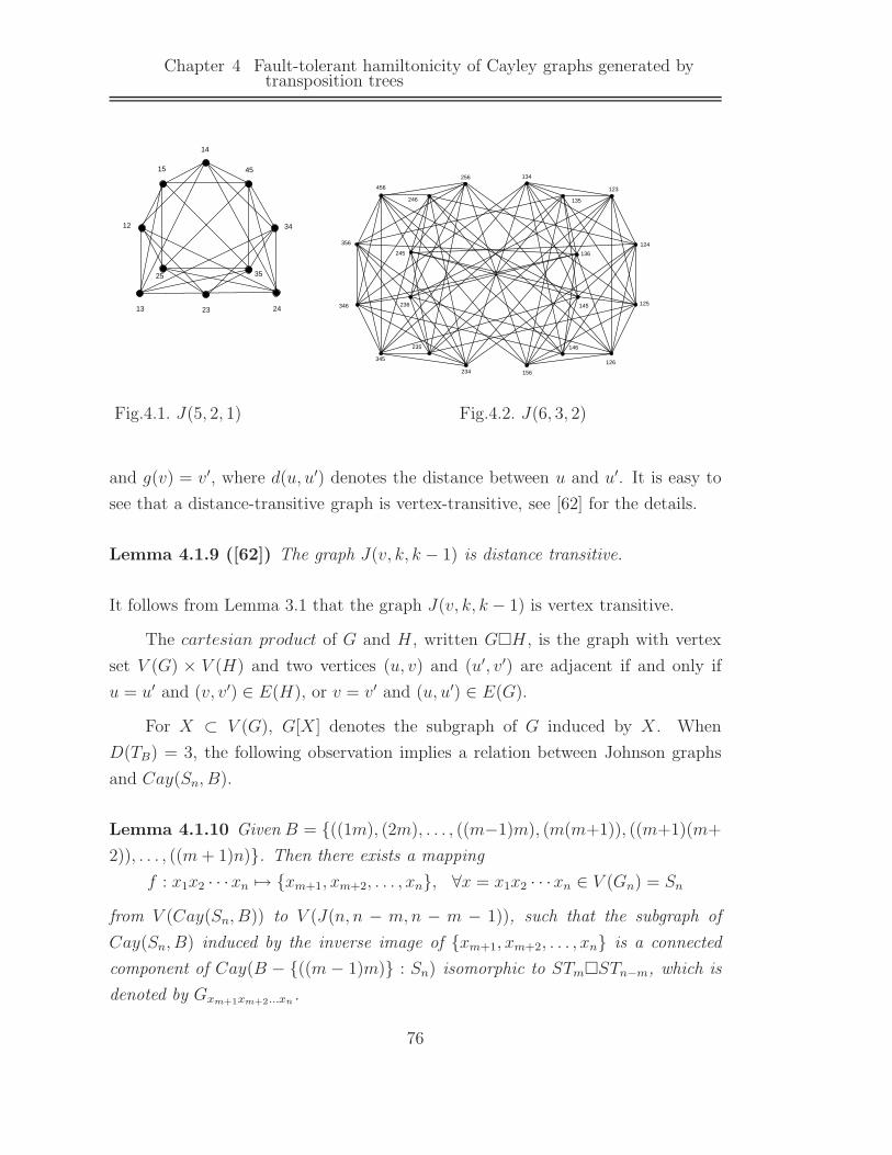
Chapter 4 Fault-tolerant hamiltonicity of Cayley graphs generated bytransposition trees
14
45
34
242313
12
15
25 35
123
124
125
126
156234
345
346
356
456
256 134
136
145
146
135
235
236
245
246
Fig.4.1. J(5, 2, 1) Fig.4.2. J(6, 3, 2)
and g(v) = v′, where d(u, u′) denotes the distance between u and u′. It is easy to
see that a distance-transitive graph is vertex-transitive, see [62] for the details.
Lemma 4.1.9 ([62]) The graph J(v, k, k − 1) is distance transitive.
It follows from Lemma 3.1 that the graph J(v, k, k − 1) is vertex transitive.
The cartesian product of G and H , written GH , is the graph with vertex
set V (G) × V (H) and two vertices (u, v) and (u′, v′) are adjacent if and only if
u = u′ and (v, v′) ∈ E(H), or v = v′ and (u, u′) ∈ E(G).
For X ⊂ V (G), G[X] denotes the subgraph of G induced by X. When
D(TB) = 3, the following observation implies a relation between Johnson graphs
and Cay(Sn, B).
Lemma 4.1.10 Given B = ((1m), (2m), . . . , ((m−1)m), (m(m+1)), ((m+1)(m+
2)), . . . , ((m+ 1)n). Then there exists a mapping
f : x1x2 · · ·xn 7→ xm+1, xm+2, . . . , xn, ∀x = x1x2 · · ·xn ∈ V (Gn) = Sn
from V (Cay(Sn, B)) to V (J(n, n − m,n − m − 1)), such that the subgraph of
Cay(Sn, B) induced by the inverse image of xm+1, xm+2, . . . , xn is a connected
component of Cay(B − ((m − 1)m) : Sn) isomorphic to STmSTn−m, which is
denoted by Gxm+1xm+2...xn.
76

§4.1 Fault-tolerant hamiltonian laceability of Cayley graphs generated bytransposition trees
Lemma 4.1.11 There exists a hamiltonian path between any two vertices in J(5, 2, 1)−F for any F ⊆ E(J(5, 2, 1)) with |F | ≤ 2.
Proof. It is easy to see that D(J(5, 2, 1)) = 2. Let F be an edge set of
J(5, 2, 1) with |F | ≤ 2. By Lemma 4.1.9, it is sufficient to show that there exists
hamiltonian paths between 13 and 24, and between 35 and 45 in J(5, 2, 1) − F .
We first show that there is hamiltonian path between 13 and 24 in J(5, 2, 1)−F . Note that P1 = (13, 14, 34, 23, 12, 15, 45, 35, 25, 24) and P2 = (13, 34, 45, 14, 15,
35, 23, 25, 12, 24) are two edge-disjoint hamiltonian paths between 13 and 24, then
there is nothing to do if one of them contains no fault edge. Supposes each of
them contains an edge of F . Note that P3 = (13, 23, 34, 35, 45, 25, 15, 12, 14, 24) is
another hamiltonian path between 13 and 24 in J(5, 2, 1), and P3∩P2 = ∅, P3∩P1 =
(23, 34), (35, 45), (15, 12). If P3 contains no fault edge, we are done. If not, P3
contains a fault edge e, then e ∈ (23, 34), (35, 45), (15, 12) since |F | ≤ 2. Clearly,
P4 = (13, 23, 12, 14, 34, 35, 25, 15, 45, 24) is a hamiltonian path between 13 and 24
in J(5, 2, 1) − E(P2) − (23, 34), (35, 45), (15, 12). That is, there is a fault-free
hamiltonian path between 13 and 24 in J(5, 2, 1) − F .
Similarly, we can find a hamiltonian path between 35 and 45 in J(5, 2, 1)−F .
We complete the proof.
Lemma 4.1.12 There exists a hamiltonian path between any two vertices in J(6, 3, 2)−F for any F ⊆ E(J(6, 3, 2)) with |F | ≤ 2.
Proof. It is easy to see that D(J(6, 3, 2)) = 3. Let F be an edge set of
J(6, 3, 2) with |F | ≤ 2. By Lemma 4.1.9, it is sufficient to show that there exists
hamiltonian paths between 123 and 456, 123 and 256, and 123 and 234 in J(6, 3, 2)−F .
For the vertices 123 and 456, we can find three edge-disjoint hamiltonian paths
as follows: P1 = (123, 134, 146, 126, 124, 245, 145, 125, 235, 135, 156, 136, 236, 246, 256, 356,
345, 234, 346, 456), P2 = (123, 124, 125, 126, 156, 145, 146, 136, 135, 134, 234, 246, 245, 256,
236, 235, 345, 346, 356, 456), P3 = (123, 125, 135, 145, 134, 136, 126, 256, 156, 146, 346,
246, 124, 234, 236, 356, 235, 245, 345, 456). Thus, there is a hamiltonian path be-
tween 123 and 456 in J(6, 3, 2) − F , since |F | ≤ 2.
77

Chapter 4 Fault-tolerant hamiltonicity of Cayley graphs generated bytransposition trees
The other two cases are very similar to that of the case above.
A hamiltonian cycle C is called triangle-v hamiltonian cycle if the two neigh-
bors w, z of v on C are adjacent in G, denoted by Cv. Using the similar method of
Lemma 4.1.11, we have the following two lemmas.
Lemma 4.1.13 There exists a triangle-v hamiltonian cycle Cv in J(5, 2, 1) − F
for any v ∈ V (J(5, 2, 1)) and F ⊆ E(J(5, 2, 1)) with |F | ≤ 2.
Lemma 4.1.14 There exists a triangle-v hamiltonian cycle Cv in J(6, 3, 2) − F
for any v ∈ V (J(6, 3, 2)) and F ⊆ E(J(6, 3, 2)) with |F | ≤ 3.
Let Cn denote the cycle of length n and Kn denote the complete graph with
n vertices, respectively. It is not difficult to see that C6K2 and C6C6 are both
vertex transitive and edge transitive bipartite graphs. The proof of Lemma 4.1.15
below is easy. So we omit the detailed proof of Lemma 4.1.15.
Lemma 4.1.15 Suppose that x ∈ V0(C6K2), y ∈ V1(C6K2), e ∈ E(C6K2)
and e 6= (x, y). Then there is a hamiltonian path between x and y containing e in
C6K2.
Proof. Note that C6K2 is vertex transitive. We fix a vertex x and prove
the claim by finding the hamiltonian path containing the given edge between the
following four pairs of vertices: x and yi, i = 1, 2, 3, 4 such that d(x, yi) = i. It is
not difficult to prove the result by constructing a hamiltonian path between x and
yi containing any given edge.
Lemma 4.1.16 Suppose x ∈ V0(C6C6), y ∈ V1(C6C6), e ∈ E(C6C6) and e 6=(x, y). Then there is a hamiltonian path between x and y containing e.
Proof. Note that C6C6 contains three vertex disjoint copies of C6K2, say
H1, H2 and H3, such that there exists a matching Mi,j between V (Hi) and V (Hj)
which matches the vertices of a cycle C6 in Hi to the vertices of a cycle C6 in Hj
for i 6= j. Let x ∈ V0(Hi) and y ∈ V1(Hj). Since C6C6 is edge transitive, without
loss of generality we may assume e ∈ E(H1).
78
§4.1 Fault-tolerant hamiltonian laceability of Cayley graphs generated bytransposition trees
Case 1. i = j = 1.
By Lemma 3.6, there exists a hamiltonian path P1 in H1 between x and y
containing e. Pick f = (u, v) ∈ E(P1) such that (u, u′), (v, v′) ∈ M1,2 (or M1,3),
where u′ and v′ are the matched vertices of u and v by M1,2 (or M1,3). Clearly,
f ′ = (u′, v′) ∈ E(C6C6). Call f ′ = (u′, v′) the matched edge of f . Without
loss of generality, assume that f ′ ∈ E(H2). Similarly, take g = (w, z) ∈ E(H2)
and g′ = (w′, z′) ∈ E(H3) such that g 6= f ′ and g′ is the matched edge of g. By
Lemma 4.1.15, there exists a hamiltonian path P2 in H2 between u′ and v′ contain-
ing f ′ and a hamiltonian path P3 in H3 between w′ and z′. Thus, a hamiltonian
path between x and y containing e is obtained from P1 − f, P2 − f ′ − g, P3 − g′ and
edges (u, u′), (v, v′), (w,w′), (z, z′).
Case 2. i = 1 or j = 1.
By the symmetry of H1, H2 and H3, it is sufficient to consider the case i = 1
and j = 3. Take u ∈ V1(H1), u′ ∈ V0(H2), v ∈ V1(H2), v
′ ∈ V0(H3) such that e 6=(x, u) and (u, u′), (v, v′) ∈ E(C6C6). By Lemma 3.6, there exists a hamiltonian
path P1 in H1 between x and u containing e, a hamiltonian path P2 in H2 between
u′ and v, a hamiltonian path P3 in H3 from v′ to y. Thus, a hamiltonian path
in C6C6 between x and y containing e is formed by paths P1, P2, P3 and edges
(u, u′), (v, v′).
Case 3. i = j 6= 1.
Without loss of generality, we assume i = 3. It is not difficult to see that
there exists f = (u, v) ∈ E(H1), f′ = (u′, v′) ∈ E(H2), g = (z, w) ∈ E(H2) and
g′ = (z′, w′) ∈ E(H3) such that e 6= f, g 6= f ′, and both f and g are matched by
f ′ and g′, respectively. By Lemma 4.1.15, there exists a hamiltonian path P1 in
H1 between u and v containing e, a hamiltonian path P2 in H2 between z and w
containing f ′, a hamiltonian path P3 in H3 between x and y containing g′. Thus,
an expected hamiltonian path is obtained from path P1, P2 − f ′, P3 − g′ and edges
(u, u′), (v, v′), (w,w′), (z, z′).
Case 4. i, j 6= 1 and i 6= j.
Similarly as the argument of Case 2, we complete the proof.
79
Chapter 4 Fault-tolerant hamiltonicity of Cayley graphs generated bytransposition trees
§4.1.2 Gn is (n−3)-edge fault tolerant hamiltonian laceable if D(TB) < 4
Let H1 and H2 be two subgraphs of a bipartite graph H , and let F ⊆ E(H)
be a fault edge set. We say that H1 and H2 have property P with respect to F
if there exists the vertices x1 ∈ V0(H1), y1 ∈ V1(H1), x2 ∈ V1(H2) and y2 ∈ V0(H2)
such that (x1, x2), (y1, y2) ∈ E(H) − F .
Lemma 4.1.17 Let H = (V0
⋃V1, E) be a bipartite graph with fault edge set
F , and Hi, i = 1, 2, · · · , m, be the subgraphs of H such that V0(H)⋃V1(H) =
V (H1)⋃V (H2)
⋃ · · ·⋃V (Hm), V (Hi)⋂V (Hj) = ∅ for i 6= j. Suppose x ∈
V0(Hi), y ∈ V1(Hj), i 6= j, and i1, i2, · · · , im is a sequence of 1, 2, · · · , m such
that i1 = i, im = j. If Hir and Hir+1 have property P with respect to F for each
r, 1 ≤ r ≤ m − 1, and Hir − F is hamiltonian laceable for 1 ≤ r ≤ m, then there
exists a hamiltonian path in H between x and y.
Proof. By the definition of property P, the lemma is clearly true.
We have the following corollary by the above lemma.
Corollary 4.1.18 Let S ⊆ 1, 2, . . . , n and F ⊆ E(Gn) with |F | ≤ n − 3. For
any x ∈ V0(Gn(i)), y ∈ V1(Gn(j)), i, j ∈ S, i 6= j, if n ≥ 5 and Gn(k) − F
is hamiltonian laceable for each k ∈ S, then there exists a hamiltonian path in
Gn[⋃
i∈S V (Gn(i))] − F between x and y.
Note that ST2∼= K2 and ST3
∼= C6, then it is easy to see thatCay((13), (23) :
S5) is the disjoint union of twenty cycles of length 6, and Cay((13), (23), (45) : S5)
is formed by ten subgraphs that each of them is isomorphic to C6K2.
Lemma 4.1.19 Suppose B = (13), (23), (34), (45) and F ⊆ E(Cay(B : S5)).
If |F | ≤ 2 and all edges of F have the same label (34), then Cay(B, S5) − F is
hamiltonian laceable.
Proof. Let f(x1x2 · · ·x5) = x4, x5 be the mapping from V (Cay(B : S5)) to
V (J(5, 2, 1)) in Lemma 4.1.10. Thus, the subgraph induced by the inverse image
of x4, x5 is a connected component of Cay(B−(34) : S5), written Gx4x5 , which
80

§4.1 Fault-tolerant hamiltonian laceability of Cayley graphs generated bytransposition trees
is isomorphic to ST3ST2 (C6K2). Furthermore, there are exactly two edges
between Gx4x5 and Gy4y5 if |x4, x5⋂y4, y5| = 1. In fact, we assume x5 = y5,
then (x1x2y4x4x5, x1x2x4y4y5) and (x2x1y4x4x5, x2x1x4y4y5) are such two edges
between Gx4x5 and Gy4y5 . Moreover, the two ends in Gx4x5 (or Gy4y5) of the above
two edges are in different partite sets of Cay(B, S5). That is, Gx4x5 and Gy4y5 have
the property P with respect to F .
For J(5, 2, 1), we call edge (x4, x5, y4, y5) fault edge of J(5, 2, 1), if there
exists some fault edges between V (Gx4x5) and V (Gy4y5) in G5. Since |F | ≤ 2,
J(5, 2, 1) has at most two fault edges. Denote by F ′ the fault edge set of J(5, 2, 1).
Now, we prove that Cay(B : S5)−F is hamiltonian laceable. Let x ∈ V0(Gx4x5)
and y ∈ V1(Gy4y5). Consider the following two cases.
Case 1. x4, x5 = y4, y5.
In this case, there exists a triangle-x4, x5 hamiltonian cycle Cx4,x5 in J(5, 2, 1)−F ′ by Lemma 4.1.13. For convenience, we assume that Cx4,x5 = (U1, U2, · · · , U10, U1),
where U1 = x4, x5. It is not difficult to see that there exists an edge e = (u, v)
in Gx4x5 such that e 6= (x, y), and (u, w), (v, z) ∈ E(Cay(B : S5)), where w ∈ GU2
and z ∈ GU10 , (for example, if U2 = x4, t5 and U10 = x4, z5, where x5, t5 and
z5 are three distinct integers. Thus, at least one of (t5x2z5x4x5, z5x2t5x4x5) and
(t5x2z5x5x4, z5x2t5x5x4) with label (13) is an such edge in Gx4x5. Similarly, the
other cases is easy to obtained). By the definition of fault edge of J(5, 2, 1), (u, w)
and (v, z) are fault-free. By Lemma 4.1.15, there is a hamiltonian path P1 in Gx4x5
between x and y containing edge (u, v). By the definition of fault edge of J(5, 2, 1)
and Lemma 4.1.17, there exists a path P2 between z and w containing all vertices
of GUi, 2 ≤ i ≤ 10. Hence, a hamiltonian path in Cay(B : S5)−F is obtained from
P1 − e, P2, and edges (u, w) and (v, z).
Case 2. x4, x5 6= y4, y5.
By Lemma 4.1.11, there is a hamiltonian path in Cay(B : S5) − F between
x4, x5 and y4, y5. Furthermore, by definition of fault edge of J(5, 2, 1) and
Lemma 4.1.17, there exists a hamiltonian path P in Cay(B : S5) − F between x
and y.
81

Chapter 4 Fault-tolerant hamiltonicity of Cayley graphs generated bytransposition trees
Lemma 4.1.20 Suppose that B = ((13), (23), (34), (45), (46) and F ∈ E(Cay(B :
S6)). If |F | ≤ 3 and all edges of F have label (34), then Cay(B : S6) is hamiltonian
laceable.
Proof.Let x ∈ V0(Cay(B : S6)), y ∈ V1(Cay(B : S6)). We next show that
there exists a hamiltonian path in Cay(B : S6) − F between x and y.
Similarly as the proof of Lemma 4.1.15, let f be the mapping from V (Cay(B :
S6)) to V (J(6, 3, 2)) in Lemma 4.1.10.
We definite the fault edge of J(6, 3, 2) distinguishing the following two cases:
when x, y ∈ V (Gx4x5x6) for some set x4, x5, x6, we call edge (w4, w5, w6, z4, z5, z6)fault edge of J(6, 3, 2) if there exists fault edge between V (Gw4w5w6) and V (Gz4z5z6);
when x ∈ Gx4x5x6 , y ∈ Gy4y5y6 satisfying x4, x5, x6 6= y4, y5, y6, we call edge
(w4, w5, w6, z4, z5, z6) fault edge of J(6, 3, 2) if there exists at least two fault
edges between V (Gw4w5w6) and V (Gz4z5z6).
It is easy to see there is exactly four edges between Gx4x5x6 and Gy4y5y6 if
|x4, x5, x6 ∩ y4, y5, y6| = 2. By a similar argument as Lemma 4.1.19, this
lemma follows from Lemma 4.1.12, 4.1.14, and 4.1.16.
Lemma 4.1.21 Let F ⊆ E(STn+1) such that each edge of F has label (n(n+ 1)).
If |F | ≤ 2n− 3 and n ≥ 4, then STn+1 − F is a hamiltonian laceable.
Proof. Assume x ∈ V0(STn+1(i1)), y ∈ V1(STn+1(i2)). Since each edge of F
has label (n(n+1)), E(STn+1(i))∩F = ∅. Thus STn+1(i) ∼= STn, i = 1, 2, · · · , n+1,
is hamiltonian laceable. We prove this lemma by distinguishing the following two
cases.
Case 1. i1 6= i2. Note that there are (n+1−2)!2
edges between V0(STn+1(i)) and
V1(STn+1(j)), and (n+1−2)!2
edges between V1(STn+1(i)) and V0(STn+1(j)) if i 6= j
by Lemma 4.1.3. Since 2n− 3 < 2 · (n+1−2)!2
for n ≥ 4, at most one pair elements of
STn+1(i)| i = 1, 2, · · · , n+1 has no property P with respect to F . So there exists
a sequence STn+1(j1), STn+1(j2), · · · , STn+1(jn+1) of STn+1(i) | i = 1, 2, · · · , n+1such that i1 = j1, i2 = jn+1 and STn+1(k) and STn+1(k + 1) have property Pwith respect to F , where, 1 ≤ k ≤ n. By Lemma 4.1.17, there exists a fault-free
hamiltonian path in STn+1 − F between x and y.
82

§4.1 Fault-tolerant hamiltonian laceability of Cayley graphs generated bytransposition trees
Case 2. i1 = i2.
Without loss of generality, assume i1 = i2 = 1, and let P1 be a hamiltonian
path of STn+1(i1) between x and y. Since P1 has length n! − 1, there exists a
matching in STn+1(i1) containing ⌊n!−12
⌋ edges of P1. Since ⌊n!−12
⌋ > 2n − 3 for
n ≥ 4 and all fault edges are outgoing edges, by the pigeonhole principle, we can
pick an edge (u, v) ∈ E(P1) such that u, v are incident to no fault edge. Let u′ and v′
be the outgoing neighbors of u and v, respectively, and assume v′ ∈ V1(STn+1(j2))
and u′ ∈ V0(STn+1(jn+1)) (j2 6= jn+1 by Lemma 4.1.3). Without loss of generality,
assume P1 = (x, · · · , u, v, · · · , y).
If there exists a sequence STn+1(j2), STn+1(j3), · · · , STn+1(jn+1) of STn+1(j) | j =
2, · · · , n+1 such that STn+1(k) and STn+1(k+1) have property P with respect to F ,
where k = 2, · · · , n. By Lemma 4.1.17, there exists a hamiltonian path P2 between
u′ and v′ in STn+1[⋃
2≤i≤n+1 V (STn+1(i))]. Thus, xP1uu′P2v
′vP1y is a hamiltonian
path in STn+1 − F between x and y.
Otherwise, there exists no sequence STn+1(j2), STn+1(j3), · · · , STn+1(jn+1) of
STn+1(j), j = 2, · · · , n+1 such that STn+1(k) and STn+1(k+1) have property Pwith respect to F , where k = 2, · · · , n. It only happens when n = 4 and at least 3
fault edges between ST5(j3) and ST5(j4) (otherwise, there exists such a sequence).
But, |Ej3j4| = 6 and |F | ≤ 5, So, at least one edge e = (w,w′) in Ej3j4 is fault-
free. Without loss of generality, assume w ∈ V0(ST5(j3)) and w′ ∈ V1(ST5(j4)).
Since |F − Ej3j4 | ≤ 2, each pair of ST5(j) | j = 2, 3, 4, 5, other than ST5(j3) and
ST5(j4), has property P with respect to F . Thus, by Lemma 4.1.17, there exists
a hamiltonian path P2 in ST5[V (ST5(j2)) ∪ V (ST5(j3))] − F between v′ and w, a
hamiltonian path P3 in ST5[V (ST5(j4))∪V (ST5(j5))]−F between u′ and w′. So a
desired hamiltonian path in ST5 −F is obtained from path Pi, i = 1, 2, 3 and edges
(u, u′), (v, v′), (w,w′).
Lemma 4.1.22 Let F ⊆ E(Gn) such that each edge of F has label (lk). If
D(TB) = 3, |F | ≤ (n − 3), and neither l nor k is a leaf of TB, then Gn − F
is hamiltonian laceable.
Proof. Since D(TB) = 3 and neither l nor k is a leaf of TB, either 2dTB(l) ≥ n
or 2dTB(k) ≥ n. Without loss of generality, assume that dTB
(l) = m ≥ n/2.
83

Chapter 4 Fault-tolerant hamiltonicity of Cayley graphs generated bytransposition trees
Furthermore, set l = m, k = m + 1, NTB(m) = 1, 2, · · · , m − 1, m + 1 and
NTB(m+1) = m,m+2, · · · , n. If n = 4, then G4
∼= BS4 follows from D(TB) = 3
and the result holds by Theorem 2.1. Suppose n ≥ 5, then m ≥ 3 by D(TB) = 3.
If m = 3, then n = 5, 6 follows from dTB(m) = m ≥ n/2. Therefore, the result
holds for m = 3 by Lemmas 4.1.19 and 4.1.20. Suppose m ≥ 4 in the following
argument.
By induction on n−m. Clearly, n−m ≥ 2. Let x ∈ V0(Gn(i1)), y ∈ V1(Gn(i2)).
It is suffices to show that there exists a hamiltonian path in Gn −F between x and
y. Let Gn(1), Gn(2), . . . , Gn(n) be the decomposition induced by leaf n (edge (m+
1, n)). If n −m = 2, then Gn(i) ∼= STm+1. Since n − 3 ≤ 2m − 3, Gn(i) − F is
hamiltonian laceable for each i by Lemma 4.1.21. It is easy to check that Gn − F
is hamiltonian laceable by considering either i1 6= i2 or i1 = i2, and we omit it.
Suppose that this lemma holds for n − m < k, k ≥ 2. It is not different to
present that this lemma holds for n−m = k by induction on n−m, and we omit
it.
Theorem 4.1.23 Cayley graphs Gn are (n − 3)-edge fault tolerant hamiltonian
laceable for n ≥ 4 if D(TB) ≤ 3.
Proof. If D(TB) = 2, then the result is true by Theorem 4.1.7. Thus, suppose
D(TB) = 3. By induction on n. If n = 4, then G4∼= SB4 and the result holds
by Theorem 4.1.7. We assume that the result holds for Gn−1, and prove that the
result holds for Gn. If there exists no fault edge of F with label (l, k) such that
dTB(l) = 1 or dTB
(k) = 1, then the result holds by Lemma 4.1.22.
If not, that is, there exists some fault edges of F with label (lk) such that
dTB(l) = 1 or dTB
(k) = 1. Without loss of generality, we assume l = n − 1, k = n
and dTB(n) = 1. Let Gn(1), Gn(2), . . . , Gn(n) be the decomposition induced by
leaf n. Since at least one of F is outgoing edge, |E(Gn(i))⋂F | ≤ n − 4 for
each i. Hence Gn(i) − F is hamiltonian laceable by induction hypothesis. For
x ∈ V0(Gn(i1)), y ∈ V1(Gn(i2)), it is suffices to show that there exists a hamiltonian
path in Gn − F between x and y.
If i1 6= i2. There exists a hamiltonian path in Gn − F between x and y by
Lemma 4.1.18. Otherwise, that is, i1 = i2. Let P1 be a hamiltonian path P1
84

§4.1 Fault-tolerant hamiltonian laceability of Cayley graphs generated bytransposition trees
between x and y in Gn(i1) − F . By Lemma 4.1.2, Gn(i1) contains n − 1 copes
of Gn−2. Thus P1 contains at least n − 2 edges with label (r(n − 1)), where one
of r and (n − 1) is a leaf of TB − n. Since |F | ≤ n − 3 and edges with the same
label are nonadjacent, by the pigeonhole principle, at least one edge, say e = (u, v),
of such n − 2 edges is adjacent to no fault edge with label ((n − 1)n). Let both
u′ and v′ be the outgoing neighbors of u and v, respectively. Since (u, v) has
label (r(n − 1)), u′, v′ are in distinct subgraphs Gn(jk), say Gn(j2), Gn(jn)). By
Lemma 4.1.17, Gn[⋃
2≤k≤n V (Gn(jk))] − F has a hamiltonian path P2 between u′
and v′. Therefore, a desired hamiltonian path is obtained from paths P1 − e, P2
and edges (u, u′), (v, v′).
§4.1.3 Gn is (n−3)-edge fault tolerant hamiltonian laceable if D(TB) ≥ 4
In this section, we first show that if n ≥ 5 and D(TB) ≥ 3, then there exists a
particular decomposition by some leaf of TB. This decomposition is the key of all
the following results.
Lemma 4.1.24 For arbitrary e ∈ E(Gn), if n ≥ 5 and D(TB) ≥ 3, then there
exists a decomposition of Gn induced by some leaf m of TB such that D(TB−m) ≥ 3
and e is no outgoing edge.
Proof. First, if D(TB) ≥ 4, let P be a longest path in TB with ends i, j, and
let both i′ and j′ be neighbors of i and j on P , respectively. If e has no label (ii′),
then the decomposition induced by leaf i is a desired decomposition.
Next, suppose D(TB) = 3. Since n ≥ 5, TB has at least three leaves, and
at least two leaves have a common neighbor in TB. we may assume that i, j have
common neighbor k. If e has no label (ik), then the decomposition induced by leaf
i is a desired decomposition.
Lemma 4.1.25 Let x ∈ V0(Gn), y ∈ V1(Gn) and e ∈ E(Gn) such that e 6= (x, y).
If D(TB) ≥ 3 and n ≥ 4, then there exists a hamiltonian path in Gn between x and
y containing e .
Proof. If n = 4, thenG4∼= BS4 and the result holds by Lemma 4.1.5. When n ≥ 5,
by Lemma 4.1.24, we can assume that ((n− 1)n) is a pendent edge, and that the
85

Chapter 4 Fault-tolerant hamiltonicity of Cayley graphs generated bytransposition trees
decomposition induced by leaf n satisfies e ∈ E(Gn(k)) and D(TB − n) ≥ 3. First,
suppose that the result holds for Gn−1 and let x ∈ V0(Gn(i1)) and y ∈ V1(Gn(i2)).
It is easy to check that the result holds for Gn by considering the following four
cases: (1) i1 = i2 = k; (2) i1 = k and i1 6= i2; (3) i1 = i2 and k 6= i1 and (4) i1, i2
and k are pairwise distinct.
Corollary 4.1.26 Let e = (u, v) ∈ E(Gn) and x ∈ V (Gn). If n ≥ 4 and D(TB) ≥3, then Gn − u, v has a hamiltonian path starting from x.
Proof. Without loss of generality, assume x ∈ V0(Gn) and v ∈ V1(Gn). Thus, there
exists a hamiltonian path P in Gn between x and v containing e. So P − u, v is
a desired path.
Recall that for arbitrary x ∈ V (Gn(i)), unless stated otherwise, we call the
vertex x′ = x((n−1)n)) the outgoing neighbor of x and (x, x′) the outgoing edge of
x. Moreover, for arbitrary pair-edge e, we use e′ to denote the coupled pair-edge.
Lemma 4.1.27 Let F ⊆ E(Gn), S ⊆ 1, 2, · · · , n with n ≥ 5, and let Gn(1),
Gn(2), · · · , Gn(n) be the decomposition induced by a leaf n of TB satisfying D(TB−n) ≥ 3. For arbitrary path P of Gn − F , if
(1). V (P )⋂V (Gn(i)) = ∅, i ∈ S;
(2). there exists an edge (u, v) ∈ E(P ) such that u[n − 1], v[n − 1] ∈ S and the
outgoing edges of u and v are fault-free; and
(3). F⋂E(Gn[
⋃
i∈S V (Gn(i))]) = ∅.Then P can be extended to a path P ∗ in Gn such that P ∗ contains all edges of P −eand all vertices of Gn(i), i ∈ S.
Proof. Since D(TB − n) ≥ 3, Lemma 4.1.25 holds for Gn(i) satisfying F ∩E(Gn(i)) = ∅. Assume u′ ∈ Gn(i1), v
′ ∈ Gn(i2). If |S| = 1, then the result follows
from Theorem 2.2. Suppose |S| ≥ 2. If i1 6= i2, then the result follows from
Observation 4.1.
Otherwise i1 = i2. When |S| = 2, we set S = i1, j. We can choose e =
(w, z) ∈ E(Gn(i1)) such that e 6= (u′, v′), and w′, z′ are both inGn(j) sinceD(TB) ≥D(TB − n) ≥ 3. By Lemma 4.1.25, there exists a hamiltonian path P1 in Gn(i1)
86

§4.1 Fault-tolerant hamiltonian laceability of Cayley graphs generated bytransposition trees
between x and y containing e, a hamiltonian path P2 in Gn(j) between w′ and z′.
Thus a desired path P ∗ is obtained from paths P − (u, v), P1 − e, P2 and edges
(u, u′), (v, v′), (z, z′), (w,w′).
When |S| > 2, then we can choose e = (w, z) ∈ E(Gn(i1)) such that w′ ∈V (Gn(i3)), and z′ ∈ V (Gn(i4)), where i3, i4 ∈ S and i3 6= i4. (It is not difficult to see
that there does exist a such edge since D(TB) ≥ 3, for example, if (r(n− 1)) ∈ B,
then (w1 · · ·wr−1i3wr+1 · · ·wn−3i4i1, w1 · · ·wr−1i4wr+1 · · ·wn−3i3i1) is a such edge
with label (r(n − 1))). Clearly e 6= (u′, v′) since they have different outgoing
edges. By Lemma 4.1.25, there exists a hamiltonian path P in Gn(i1) between
u′ and v′ containing e. By Lemma 4.1.17, there exists a hamiltonian path P2 in
Gn[⋃
i∈S−i1 V (Gn(i)] between w′ and z′. So, an desired path P ∗ is obtained from
paths P − (u, v), P1 − e, P2 and edges (u, u′), (v, v′), (z, z′), (w,w′).
Theorem 4.1.28 Cayley graphs Gn are (n − 3)-edge fault tolerant hamiltonian
laceable for n ≥ 5 if D(TB) ≥ 4.
Proof. By induction on n. If n = 5, then G5∼= BS5 and BS5 is (5 − 3)-edges
fault-tolerant hamiltonian laceable follows from D(TB) ≥ 4 and Theorem 4.1.7. We
suppose that Gn−1 is (n − 4)-edges fault tolerant hamiltonian laceable for n ≥ 6,
and next present that this theorem holds for Gn. Let F ∈ E(Gn) with |F | ≤ n−3.
If there exists a edge e ∈ F with label (lk) such that either dTB(l) = 1 or
dTB(k) = 1. Without loss of generality, assume that dTB
(k) = 1, k = n, l = n− 1.
Hence, |E(Gn(i))⋂F | ≤ n−4 for all i ∈ 1, 2, · · · , n. If D(TB−n) ≥ 4, Gn(i)−F
is hamiltonian laceable by induction hypothesis. If not, that is, D(TB − n) = 3
since D(TB) ≥ 4. Thus Gn(i)−F is hamiltonian laceable by Theorem 4.1.23. It is
easy to check that the result holds in this case, and we omit it.
If there exists no edge e in F with label (lk) such that either dTB(l) = 1 or
dTB(k) = 1. Suppose |F | = n − 3 (add edges to F if necessary). If TB is a path,
then this case holds by Theorem 4.1.7. Thus we suppose that TB is not a path.
We have the following claim.
Claim. If TB is not a path, then there exists a decompositionGn(1), Gn(2), . . . , Gn(n)
of Gn such that at least two fault edges with the same label are pair-edges.
87

Chapter 4 Fault-tolerant hamiltonicity of Cayley graphs generated bytransposition trees
Proof of Claim 1. Since TB is not a path, it has at least three leaves. But no
edge e ∈ F has label (lk) such that either dTB(l) = 1 or dTB
(k) = 1, fault edges
occupy at most n−4 labels. Since |F | .= n−3, by the pigeonhole principle, at least
two fault pair-edges have the common label, say (i, j). Clearly, there exists a leaf,
without loss of generality, say n, such that n is not incident to the edge (i, j) in
TB. The decomposition Gn(1), Gn(2), . . . , Gn(n) of Gn induced by leaf n satisfies
the requirement of this claim. This complete the proof of claim 1.
Assume that n has neighbor n − 1 in TB. Since D(TB) ≥ 4, D(TB − n) ≥ 3.
Therefore, Lemmas 4.1.25 and 4.1.27 hold for Gn(i) with F ∩ E(Gn(i)) = ∅. We
suppose that |F ⋂E(Gn(i))| = n− 3 for some i in the following. (Otherwise, that
is, |F ⋂E(Gn(i))| ≤ n − 4 for all i ∈ 1, 2, · · · , n, this case is easily checked and
omitted.) Since F ⊆ E(Gn(i)), Lemmas 4.1.25 and 4.1.27 hold for Gn(j), j 6= i.
It is suffices to show that for any two vertices x and y with different partite
sets, there exits a hamiltonian path in Gn − F between x and y. Assume x ∈V0(Gn(i1)), y ∈ V1(Gn(i2)), and consider the following four cases.
Case 1. i1 = i2 = i.
Suppose that Gn(i) − F has a hamiltonian path P between x and y. Clearly,
we can pick an edge e = (u, v) of P such that u[n−1], v[n−1] 6= i. By Lemma 5.2,
P can be extended to a hamiltonian path P ∗ in Gn − F between x and y.
Next, suppose that Gn(i) − F has no hamiltonian path from x to y. Pick
f = (w, z) ∈ F such that f 6= (x, y), and let F ′ = F − f . Thus Gn(i) − F ′ has a
hamiltonian path P between x and y by induction hypothesis. Clearly, f ∈ E(P ).
Thus P can be extended to a hamiltonian path P ∗ in Gn − F between x and y by
Lemma 4.1.27.
Case 2. i1 = i and i1 6= i2.
Suppose that Gn(i)−F has a hamiltonian path P1 between x and some vertex
v. If v′ ∈ V0(Gn(i2)). Pick e = (w, z) ∈ E(Gn(i2)) such that w[n − 1], z[n − 1] 6∈i, i2. By Lemma 4.1.25, there exists a hamiltonian path P2 in Gn(i2) between
v′ and y containing e . By Lemma 4.1.27, (x, P1, v, v′, P2, y) can be extended to
a hamiltonian path in Gn − F between x and y. If v′ 6∈ V0(Gn(i2)), then, by
88
§4.1 Fault-tolerant hamiltonian laceability of Cayley graphs generated bytransposition trees
Lemma 4.1.18, there exists a hamiltonian path P2 in Gn − Gn(i) − F between v′
and y. Hence a desired hamiltonian path is obtained from P1, P2 and edge (v, v′).
We next suppose that Gn(i) − F has no hamiltonian path starting from x.
If there exists a pair-edge f = (u, v) ∈ F such that f [n − 1] 6= i2. Choose
z ∈ V1(Gn(i)) such that f 6= (x, z) and z′ ∈ V0(Gn(i2)). Let F ′ = F − f . By
induction hypothesis, Gn(i) − F ′ has a hamiltonian path P1 between x and z.
Clearly, f ∈ E(P1). By Theorem 4.1.8, Gn(i2) has a hamiltonian path P2 between
z′ and y. By Lemma 4.1.27, (x, P1, z, z′, P2, y) can be extended to a hamiltonian
path in Gn − F between x and y.
If not, that is, there exists no pair-edge f ∈ F such that f [n − 1] 6= i2. By
Claim 1, at least two fault pair-edges have the common label. So we can find a
pair-edge f = (u, v) ∈ F such that neither u nor v has y as the outgoing neighbor.
Let F ′ = F − f and the coupled pair-edge of f is f ′ = (u′, v′) ∈ E(Gn(i2)). By
Lemma 4.1.26, Gn(i2)−u′, v′ has a hamiltonian path P2 starting from y to some
vertex, say z.
If z′ ∈ V1(Gn(i)), then Gn(i) − F ′ has a hamiltonian path P1 between x
and z′ by induction hypothesis. Clearly, f ∈ E(P1). Without loss of generality,
assume that P1 = (x, · · · , v, u, · · · , z′). Pick an edge e = (s, t) ∈ E(P1) such that
s[n− 1], t[n− 1] 6∈ i, i2. (In fact, let s be a vertex in Gn(i) different from x, u, v
and z′ such that s[n − 1] 6= i2. Clearly at least one of two incident edges of s on
P1 is a such edge since two incident edges of s on P1 have different labels.) By
Lemma 4.1.27, (x, · · · , v, v′, u′, u, · · · , z′, z, P2, y) can be extended to a hamiltonian
path in Gn − F between x and y. If z′ 6∈ V1(Gn(i)), then we may assume that
z′ ∈ V1(Gn(i3)), i3 6∈ i, i2. Choose w ∈ V1(Gn(i)) such that f 6= (x, w) and
w′ ∈ V0(Gn(i4)), where i4 6∈ i, i2, i3. Let P1 be a hamiltonian path in Gn(i) − F ′
between x and w. Clearly, f ∈ E(P1). By Lemma 4.1.18, Gn − Gn(i) − Gn(i2)
has a hamiltonian path P3 between w′ and z′. Hence a desired hamiltonian path
is obtained from P1 − f, P2, P3 and edges (u, u′), (v, v′), (u′, v′), (w,w′) and (z, z′).
Case 3. i1 = i2 6= i.
If there exists a pair-edge f = (u, v) ∈ F such that its coupled pair-edge f ′ =
(u′, v′) ∈ E(Gn(i1)) and f ′ 6= (x, y). By Lemma 4.1.25, Gn(i1) has a hamiltonian
89
Chapter 4 Fault-tolerant hamiltonicity of Cayley graphs generated bytransposition trees
path P1 between x and y containing f ′. Without loss of generality, assume P1 =
(x, · · · , u′, v′, · · · , y). By induction hypothesis, Gn(i) − F has a hamiltonian path
P2 between u and v. Clearly, we can pick an edge e = (w, z) of P2 such that
w[n− 1], z[n− 1] 6∈ i, i1, then by Lemma 4.1.27, (x, · · · , u′, u, P2, v, v′, · · · , y) can
be extended to a hamiltonian path in Gn − F between x and y.
If not, that is, there exists no pair-edge f = (u, v) ∈ F such that its coupled
pair-edge f ′ = (u′, v′) ∈ E(Gn(i1)), and f ′ 6= (x, y). We have the following claim.
Claim There exists a pair-edge f = (u, v) ∈ F such that its coupled pair-edge
f ′ = (u′, v′) ∈ E(Gn(i3)), i3 6∈ i1, i.
Proof of Claim 2. By Claim 1, at least two fault pair-edges have the common label,
say f1 and f2. First, clearly, f1[n − 1], f2[n − 1] 6= i since f1, f2 ∈ E(Gn(i)). If
f1[n−1] 6= i1, we are done. Thus, suppose f1[n−1] = i1 and f1 = (x, y)(Otherwise,
that is, f1[n− 1] = i1 and f1 6= (x, y), which contradicts the hypothesis that there
exists a pair-edge f = (u, v) ∈ F such that its coupled pair-edge f ′ = (u′, v′) ∈E(Gn(i3)), i3 6∈ i1, i). We say f2[n − 1] 6= i1. Otherwise, that is, f2[n − 1] = i1.
Since f1 and f2 have the common label and f1 = (x, y), we know f2 6= (x, y), which
contradicts the hypothesis that there exists a pair-edge f = (u, v) ∈ F such that
its coupled pair-edge f ′ = (u′, v′) ∈ E(Gn(i3)), i3 6∈ i1, i). This complete the
proof of this claim.
By Claim 2, we can pick a pair-edge f = (u, v) ∈ F such that its coupled pair-
edge f ′ = (u′, v′) ∈ E(Gn(i3)), i3 6∈ i1, i. By induction hypothesis, Gn(i)−F has
a hamiltonian path P1 from u to v. It is not different to construct a hamiltonian
path P2 in Gn −Gn(i) between x and y containing f ′. Thus, a desired hamiltonian
path in Gn − F is obtained from paths P1, P2 and edges (u, u′), (v, v′).
Case 4. i1, i2 and i are pairwise distinct.
If there exists a pair-edge f = (u, v) ∈ F such that its coupled pair-edge
f ′ = (u′, v′) ∈ E(Gn(i3)), i3 6∈ i1, i2. Choose z ∈ V1(Gn(i1)), w ∈ V0(Gn(i2)) such
that z′ ∈ V0(Gn(i3)), w′ ∈ V1(Gn(i3)). Furthermore, pick e = (s, t) ∈ E(Gn(i2))
such that e 6= (y, w), s[n − 1], t[n − 1] 6∈ i, i1, i2, i3. By Theorem 4.1.8, Gn(i1)
has a hamiltonian path P1 between x and z. By Lemma 4.1.20, there exists a
hamiltonian path P2 in Gn(i2) between y and w containing e, a hamiltonian path
90

§4.2 Fault-tolerant bipancyclicity of Cayley graphs generated by transpositiongenerating trees
P3 in Gn(i3) between w′ and z′ containing f ′. By induction hypothesis, there
exists a fault-free hamiltonian path P4 in Gn(i) − F between u and v. With-
out loss of generality, assume P3 = (w′, · · · , u′, v′, · · · , z′). By Lemma 4.1.27,
(x, P1, z, z′, · · · , v′, v, P4, u, u
′, · · · , w′, w, P2, y) can be extended to a hamiltonian
path in Gn − F between x and y.
If not, that is, for any pair-edge f ∈ F , its coupled pair-edge f ′ is contained
in either Gn(i1) or Gn(i2). By the symmetry of i1 and i2, we may assume that
f = (u, v) is a fault pair-edge and its coupled pair-edge f ′ = (u′, v′) ∈ E(Gn(i1)).
Choose a vertex z ∈ V1(Gn(i1)) such that f ′ 6= (x, z) and z′ ∈ V0(Gn(i3)), where
i3 6∈ i, i1, i2. By Lemma 4.1.25, Gn(i1) has a hamiltonian path P1 between x and
z containing f ′. Without loss of generality, assume P1 = (x, · · · , u′, v′, · · · , z). By
induction hypothesis, Gn(i) − F has a hamiltonian path P2 between u and v. By
Lemma 4.1.18, Gn − Gn(i) −Gn(i1) has a hamiltonian path P3 between z′ and y.
Hence (x, · · · , u′, u, P2, v, v′, · · · , z, z′, P3, y) is a hamiltonian path in Gn−F between
x and y.
By this all possibilities have been exhausted and the proof is thus complete.
Combining Theorem 4.1.23 with Theorem 4.1.28, we have the following main
result.
Theorem 4.1.29 Cayley graphs Gn are (n − 3)-edge fault tolerant hamiltonian
laceable for n ≥ 4.
Note that Gn is n− 1-regular. Thus the number of edge faults is sharp.
§4.2 Fault-tolerant bipancyclicity of Cayley graphs
generated by transposition generating trees
Fault-tolerant pancyclicity of popular networks have been studied, such as
star graphs [133], bubble-sort graphs [82], Mobius cubes [75, 147] and crossed
cubes [76, 77]. In this section, we consider edge fault-tolerant bipancyclicity of
Cayley graphs generated by transposition generating trees. For the other studies
91

Chapter 4 Fault-tolerant hamiltonicity of Cayley graphs generated bytransposition trees
on Cayley graphs generated by transposition generating trees, we suggest readers
to refer to [2, 3, 40, 60, 62, 73, 82, 84, 100, 127, 131, 151, 150].
We recall several notations related this section. Unless stated otherwise, we
assume TB is a tree and use Gn to denote the Cayley graph Cay(Sn, B). Thus,
each vertex of Gn is a permutation of Sn. We use V0(Gn) to denote the set of
all odd permutations of Sn and V1(Gn) the set of all even permutations of Sn,
respectively. Clearly, V (Gn) = V0(Gn)⋃V1(Gn) and Gn is bipartite graph with
partite sets V0(Gn) and V1(Gn). We use STn and BSn to denote the n-dimensional
star graph and n-dimensional bubble-sort graph, respectively.
By Lemma 4.1.1 in the last section, we have that the label of the vertex set
of a transpositions generating tree T does not affect the structural property of the
Cayley graph generated by T . We call the decomposition of Lemma ?? is induced
by the leaf n. Unless stated otherwise, we always assume that (n−1, n) is a pendant
edge of TB in the following. Let x be a vertex of Gn(i). Sometimes, we may use
other leaf to obtain some special decomposition, for example, if a decomposition
is induced by j, then Gn(k) is the subgraph induced by vertex set x| x[j] = k.We call the vertex x′ = x((n − 1)n)) the outgoing neighbor of x and (x, x′) the
outgoing edge of x. For convenience, we denote V0(Gn)⋂V (Gn(i)) by V0(Gn(i)),
V1(Gn)⋂V (Gn(i)) by V1(Gn(i)), respectively.
A transposition generating tree TB is called a double-star if it contains exactly
one non-pendant edge. Assume that (ij) is the non-pendant edge of TB. The
following observation is easy to obtain.
Lemma 4.2.1 Assume that n ≥ 5 and D(TB) ≥ 3. Then there exists a decompo-
sition of Gn induced by some leaf j such that D(TB − j) ≥ 3. Furthermore, if TB
is a double-star, we can get a decomposition of Gn induced by a pedant edge (ij)
such that there exists another integer j′ and (ij′) is also a pedant edge of TB.
Lemma 4.2.2 ([104]) Let F be a edge set of Gn and n ≥ 4, |F | ≤ n − 3. Then
Gn − F is hamiltonian laceable.
Combining Lemma 4.1.4 with the main results of the last section, we give the
following corollary without proof.
92

§4.2 Fault-tolerant bipancyclicity of Cayley graphs generated by transpositiongenerating trees
Corollary 4.2.3 Let Gn(i1), · · · , Gn(is) be s subgraph of Gn(i), i = 1, · · · , n, F be
an edge set and x ∈ V (Gn(i1)), y ∈ V (Gn(is) be two vertex of different partite sets
of Gn . If F ≤ n − 4, then there is a path of length s(n − 1)! in Gn[V (Gn(i1)) ∪· · · ∪ V (Gn(is))] between x and y.
Lemma 4.2.4 ([124]) The Cayley graph Gn is vertex-bipancyclic if and only if
Gn is not a star graph.
Lemma 4.2.5 ([124]) For any two edges of Cayley graph Gn, if n ≥ 3, then there
is a hamiltonian cycle of Gn containing them.
Lemma 4.2.6 ([124]) For n ≥ 3, every edge of Gn lies on an even cycle of length
l for every 6 ≤ l ≤ n!.
Lemma 4.2.7 ([62]) Let T be a set of transpositions from Sym(n) and let g and h
be elements of T . If the transposition generating graph of T contains no triangles,
then g and h have exactly one common neighbor in Cay(Sym(n),T ) if gh 6= hg,
and exactly two common neighbors otherwise.
Clearly, for any two distinct transpositions (ij) and (kl), (ij)(kl) = (kl)(ij)
if and only if i, j ∩ k, l = ∅. It is not difficult to see that if C4 = v1v2v3v4 is
a 4-cycle of Γn, then there must exist two transpositions (ij) and (kl) such that
i, j ∩ k, l = ∅ and v2 = v1(ij), v3 = v2(kl), v4 = v3(ij) = v1(kl). In fact,
there exists an automorphism of Gn, say ψ ∈ Aut(Gn), such that ψ(v1) = id
since Gn is vertex transitive, furthermore, C ′4 = ψ(v1v2v3v4) is also a 4−cycle of
Γn. Let g = ψ(v2), h = ψ(v4), clearly, g and h are two transpositions of T . By
lemma 2.1, we have that gh = hg since they have two common neighbors. That is,
(ij) = ψ−1(g), (kl) = ψ−1(h).
By the above argument, we have the following corollary.
Corollary 4.2.8 A cycle uvxy is a 4-cycle of Gn such that edge (u, v) with label
(ij) and edge (v, x) with label (st) if and only if (x, y) has label (ij), edges (u, y)
has label (st), and s, t ∩ i, j = ∅.
93

Chapter 4 Fault-tolerant hamiltonicity of Cayley graphs generated bytransposition trees
Thus, the edge with label (ij) of the Cayley graph generated by a double-star
with non-pendant edge (i, j) is not contained in a 4-cycle, that is, the Cayley graph
generated by a double-star is not edge-bipancyclic. In [124], the following lemma
is reported.
Lemma 4.2.9 ([124]) If a tree TB is neither a star nor a double-star, the Cayley
graph Cay(Sn, B) is edge-bipancyclic.
Lemma 4.2.10 ([82]) BSn is (n− 3)-edge fault-tolerant bipancyclic for n ≥ 4.
Note that the girth of star graph is 6. Xu et al. in [144] reported the following
theorem.
Theorem 4.2.11 ([144]) For any edge set F of STn with |F | ≤ n − 3 and any
edge e of STn − F , there exists a cycle of an arbitrary even length from 6 to n! in
STn − F containing e provide n ≥ 3.
Theorem 4.2.12 Gn is (n − 3)-edge fault-tolerant bipancyclic if Gn is not star
graph.
Proof By induction on n. If n = 4, then Gn∼= BSn and the result follows
from Lemma 4.2.10 directly. Let F be a faulty edge set with |F | ≤ n − 3. Note
that Gn is not star graph, then by Lemma 4.2.1 there exists a decomposition of Gn
such that each Gn(i), i = 1, 2, · · · , n is not (n− 1)-dimensional star graph if n ≥ 5.
Without loss of generality we assume the above decomposition is induced by leaf
n and (n − 1, n) is a pedant edge of TB. By Lemma 4.2.1, we can assume that
(j, n− 1) is another pedant edge of TB and e = (x, y) is an edge of Gn with label
(j(n − 1)). Thus, we have that the outgong neighbors of x and y are in different
subgraphs of Gn(1), · · · , Gn(n). For n ≥ 5, we can assume that the result holds for
Gn(i). Let Fi = F ∩ E(Gn(i)). Since |F | ≤ n− 3, there is a subgraph Gn(k) such
that Fk = ∅. Let l be any even integer such that 4 ≤ l ≤ n! and let l = q(n−1)!+r,
where 0 ≤ q ≤ n − 1 and 0 < r ≤ (n− 1)!. We next construct a cycle of length l
in Gn − F .
94

§4.2 Fault-tolerant bipancyclicity of Cayley graphs generated by transpositiongenerating trees
Case 1. |Fi| ≤ n− 4 for all i.
In this case, we have that Gn(i) − Fi is bipancyclic by induction.
Subcase 1.1 q ≥ 2.
Since there are (n−1)!2
edges with label (j(n− 1)) in Gn(k) and (n−1)!4
> n− 3
for n ≥ 5, there exists an edge ek = (uk, vk) is not adjacent to any fault edge.
Assume that the outgoing neighbors u′k and v′k of uk and vk are in Gn(i1) and
Gn(iq−1), respectively. If q = 2 and since (n−2)!2
> n − 3, then there exists an
fault-free edge f = (ui1 , u′iq−1
) such that u′k and ui1 are in different partite sets. By
Lemma 4.2.2, there exists two hamiltonian cycle Ci1 and Ciq−1 in Gn(i1)−Fi1 and
Gn(iq−1)−Fiq−1 . By Lemma 2.5 and Lemma 4.2.1, we can take a cycle C ′ of length
r containing ek if r ≥ 4. Thus there are a cycle of length l formed by Ci1 , Ciq−1 and
C ′. If q ≥ 3, then we choose other q− 3 subgraphs of Gn(1), · · · , Gn(n), except for
Gn(i1), Gn(i2), Gn(k), say, Gn(i2), · · · , Gn(iq−2). Similarly, there exists fault-free
edges (ui2, u′i2), · · · , (uiq−2, u
′iq−2
) such that u′ij and uij are in different partite sets
of Gn(ij). By an argument similar to above, we have a cycle of length l if r ≥ 4.
Clearly, if r = 2, then the cycle of length l is also obtained by above the edge ek
and other q cycles of length (n− 1)!.
Subcase 1.2 q ≤ 1.
If q = 0, then the result is clearly true by Lemma 4.2.4.
We next assume that q = 1. Note that D(TB) ≥ 3, then there exists a pedant
edge (s, t) of TB such that s, t∩ n− 1, n = ∅. Since there are (n−2)!2
edges with
label (st) and (n−2)!2
> n− 3, there exists an edge e∗k = (u∗k, v∗k) with label (st) such
that e∗k is not adjacent any fault edge. It is not difficult to see that the outgoing
neighbors u∗k′ and v∗k
′ of u∗k and v∗k are in a same subgraph of Gn(1), · · · , Gn(n), say,
Gn(i∗). By Lemma 4.2.2, there exists a hamiltonian cycle Ci∗ of Gn(i∗) between
u∗k′ and v∗k
′. By an argument similar to that of Subcase 1.1, a cycle of length l is
obtained by Ci∗ and a cycle of length r or an edge of Gn(k).
Case 2. |Fi| = n− 3 for some integer i.
Without loss of generality we assume that i = 1 and let G∗n = Gn[V (Gn(2) ∪
· · · ∪ V (Gn(n))]. Note that D(TB − (n − 1, n)) ≥ 3, then we can see that there
95
Chapter 4 Fault-tolerant hamiltonicity of Cayley graphs generated bytransposition trees
exists and pedant edge (s, t) of TB such that s, t ∩ n − 1, n = ∅. Let (u2, v2)
be an edge of Gn(2) with label (st) and u2[n− 1] = v2[n− 1] = 3 (such edge exists,
for example, let u2 = x1 · · ·xn−332 be a vertex of Gn(2), then (u2, u2(st)) is a such
edge of Gn(2)). We can see that the outgoing neighbors u′2, v′2 of u2, v2 are in Gn(3)
and u2, v2, v′2, u
′2 induce a 4-cycle of Gn be Corollary 2.1. Similarly, we can take
an edge (ui, vi) with label (st) in Gn(i) such that the outgong neighbors u′i, v′i of
ui, vi are in Gn(i + 1) for i = 2, · · · , n − 1. Thus, we can see that there exists a
hamiltonian cycle of Gn(i) containing edges (ui, vi) and (u′i, v′i) by Lemma 2.10.
By an argument similar to that of Subcase 1.1, we can see that there is a cycle of
length l in G∗n if 4 ≤ l ≤ (n− 1)(n− 1)!.
Next, we show the existence of cycles of length l for (n−1)(n−1)!+2 ≤ l ≤ n!.
Assume that l = (n− 1)(n− 1)! + r If there exists a fault edge with label (st) such
that s, t ∩ n − 1, n = ∅, say e1 = (u1, v1), then the outgoing neighbors u′1, v′1
of u1, v1 are in a same subgraph Gn(i2). We look the edge e1 a fault free edge
temporarily. By Lemma 4.2.2, we have that there is a hamiltonian path P1 of
Gn(1) between u1 and v1. Thus, P1, u′1 and u′2 form a cycle of length (n− 1)! + 2.
By an argument similar to that of above paragraph, we can construct an sequence
of u′1, v′1, ui2, vi2, u′i2, v′i2 , ui3, vi3, · · · , u′in−1, v′in−1
, uin, vin and take a cycle (or
an edge) of length r in Gn(in). Thus, a cycle of length l is obtained clearly by
above argument.
We next assume that each fault edge has label (j(n−1)) for some j. Note that
D(TB) ≥ 3, then there exists a pedant edge (s, t) of TB such that n−1 6∈ s, t and
t is a leaf of TB. Note that no fault edge has label (st). Thus, the leaf t induces a
decomposition of Gn, say G′n(i), i = 1, 2, · · · , n. If G′
n(i) is not isomorphic to star
graph, then we can construct a cycle of length l by an argument similar to above
paragraph (let F ′i = G′
n(i) ∩ F . If |Fi| ≤ n − 4, then by Case 1 the result is true;
if |Fk| = n − 3 for some k, then the result is obtained by an argument similar to
that of above paragraph).
We next assume that each subgraph G′n(i) is isomorphic to (n−1)-dimensional
star graph. Let F ′i = G′
n(i)∩F . Then |F ′i | ≤ n−3. We omit the proof of the case of
each |Fi| ≤ n−4 for all i (see Case 1). Assume that Fk = n−3 for some k. Look a
fault edge ek = (uk, vk) the fault free edge temporarily. By Theorem 4.2.11, there
96

§4.2 Fault-tolerant bipancyclicity of Cayley graphs generated by transpositiongenerating trees
exists a cycle of an arbitrary even length from 6 to n! in G′n(k)−Fk containing ek.
Note that there is no fault edge out of G′n(k). It is not difficult to see that we can
construct a cycle of length l for (n − 1)(n − 1)! + 6 ≤ l = q(n − 1)! + r ≤ n! by
taking a r-cycle in G′n(k) containing ek and a special (n − 1)!-cycle in each other
subgraph G′n(i), i 6= k. If l = (n− 1)(n− 1)! + 2, then we can construct a cycle by
taking an edge ek = (uk, vk) of G′n(k) − F , the outgoing edges of uk, vk and a path
of length (n − 1)(n − 1)! of Gn − G′n(k) between u′k and v′k (if u′k and v′k are in a
same subgraph, then by an the similar argument to above paragraph we have the
(n − 1)(n − 1)!-path; if u′k and v′k are in the distinct subgraphs, then the path is
also obtained by Corollary 4.2.3). Note that (n − 1)!/4 > n − 3 for n ≥ 5, then
there exists a path of length 4 in G′n(k) − F , say P . Assume the ends of P are
uk, vk. If l = (n − 1)(n − 1)! + 4, then we can construct a cycle by taking a path
of length 4, the outgoing edges of uk, vk and another path of length (n− 1)(n− 1)!
between uk and vk in Gn −G′n(k).
97

Chapter 5 Several extremal graph problems
§5.1 Subgraph of hypercubes, extra-edge connectivity of
hypercubes and folded hypercubes
§5.1.1 Subgraph of hypercubes
In this part we shall determine the maximum size of an induced subgraph of
a vertex set with a given size. As an application, we determine a kind of edge-
connectivity (extra edge-connectivity) of hypercubes in Section 3.
Let m be an integer and m =s∑
i=0
2ti be the decomposition of m such that
t0 = log2m, and ti = [log2(m−i−1∑
r=0
2tr)] for i ≥ 1. Suppose X is a vertex set
of Qn of size m. We denote by exm
2the maximum size of the subgraph (of Qn)
induced by m vertices, i.e., exm = max2|E(Qn[X])| : X ⊂ V (Qn) and |X| = m,is the maximum possible sum of the degrees of the vertices in the subgraph (of
Qn) induced by m vertices. In particular, for an integer i ∈ 1, 2, · · · , n, we may
express Qn as D0 ⊕ D1 such that D0 and D1 are the two (n − 1)-subcubes of Qn
induced by the vertices with the ith coordinate 0 and 1 respectively. We will use
decomposition Qn = D0 ⊕D1 directly without explanation on its coordinate if no
confusion arises. Sometimes we also use X i−10Xn−i and X i−11Xn−i to denote D0
and D1, where X ∈ Z2.
Theorem 5.1.1 Let X be a vertex set of Qn with size m. Then exm =s∑
i=0
ti2ti +
s∑
i=0
2 · i · 2ti.
Proof. We first claim that exm ≥s∑
i=0
ti2ti +
s∑
i=0
2 · i · 2ti . It is sufficient
to show that there is a subgraph G1 in Qn such that |V (G1)| = m, |E(G1)| =
12(
s∑
i=0
ti2ti +
s∑
i=0
2 · i · 2ti). We pack G1 as follows.
Take s+ 1 ti-dimensional subcubes for i = 0, · · · , s as follows:
98

§5.1 Subgraph of hypercubes, extra-edge connectivity of hypercubes and foldedhypercubes
Q0 : X1 · · ·Xt0︸ ︷︷ ︸
t0
0 · · ·0
Q1 : X1 · · ·Xt1︸ ︷︷ ︸
t1
0 · · · 0
︸ ︷︷ ︸
t0
10 · · ·0
Q2 : X1 · · ·Xt2︸ ︷︷ ︸
t2
0 · · · 0
︸ ︷︷ ︸
t1
10 · · ·010 · · ·0
· · ·
Note that Q0 is given and Qi is taken from a ti−1-dimensional subcube which is
obtained from Qi−1 by changing the 0 of (ti−1+1)th-coordinate of Qi−1 to 1. Define
G1 = Qn[V (Q0) ∪ · · · ∪ V (Qs)]. For convenience sake we define f(m) =s∑
i=0
ti2ti +
s∑
i=0
2 · i · 2ti . It is not difficult to count the number of edges of G1 by considering
the edges within Qi’s (12
s∑
i=0
ti2ti) and the edges between Qi’s (1
2
s∑
i=0
2 · i · 2ti). Thus,
the claim holds, i.e., exm ≥ f(m) =s∑
i=0
ti2ti +
s∑
i=0
2 · i · 2ti .
We next show that exm ≤ f(m) by induction on n, equivalently, exm = f(m).
Assume X is a vertex set such that 2|E(Qn[X])| = exm. By the definition and
the property of hypercubes, we can check the equality directly for n = 2, 3. So we
assume n ≥ 4. Denote X ∩ D0, X ∩ D1 by X0, X1, respectively. Without loss of
generality, we let mi = |Xi|, i = 0, 1 and suppose m0 =s0∑
i=0
2t0i ≤ m1 =s1∑
i=0
2t1i . By
induction, if m0 = 0, then exm ≤ f(m), then we may assume m0 > 0 from now on.
Case 1. Assume s = 0, i.e., m = 2t0 .
If t00 = t0 − 1, then m0 = m1 = 2t0−1. In this case, exm = 2|E(Qn[X])| ≤2|E(Qn[X0])|+2|E(Qn[X1])|+2m0 ≤ exm0 +exm1 +2m0 = f(m0)+f(m1)+2m0 =
(t0 − 1)2t0−1 + (t0 − 1)2t0−1 + 2t0 = f(m) (To understand the inequality clearly,
we give two notes: 1. There are at most m0 edges between D0[X0] and D1[X1]; 2.
The symbols exm0 and exm1 are restricted in D0 and D1, i.e., one can look them
as exm0 |D0 and exm1 |D1 . The similar context will be omitted from now on). So we
may assume t00 < t0 − 1 and t10 = t0 − 1.
99

Chapter 5 Several extremal graph problems
Claim: f(m0) + f(m1) + 2m0 ≤ f(m) when m = 2t0 = m0 + m1 and m1 >
m0 > 0, and f(m0)+f(m1)+2m0 = f(m) when m = 2t0 = m0 +m1 and m1 = m0.
One can check the second part of the claim directly. So we only prove the first
part.
Note that m0 + m1 = 2t0 . Suppose m0 =s0∑
i=0
2t0i and m1 =s1∑
i=0
2t1i . It can be
seen that t0s0 = t1s1 and
t00, t01, · · · , t0(s0−1), t10, · · · , t1(s1−1) = t0 − 1, t0 − 2, · · · , t0s0 + 1 (2)
(In fact, one can see this recursively. Note that m1 > m0, hence t10 = t0 − 1.
Clearly, m1 − 2t0−1 + m0 = 2t0−1. Let m′1 = m1 − 2t0−1, m′
0 = m0. If m′1 >
m′0, then t11 = t0 − 2; If m′
0 > m′1, then t00 = t0 − 2; If m′
0 = m′1, then
t11 = t00 = t0 − 2. Since 2t0 is finite, one can find that t0s0 = t1s1 . Clearly,
|t00, t01, · · · , t0(s0−1), t10, · · · , t1(s1−1)| = |t0 − 1, t0 − 2, · · · , t0s0 + 1| = s0 + s1).
We put the two expressions (m0 =s0∑
i=0
2t0i and m1 =s1∑
i=0
2t1i) together as follow:
m0 +m1 = 2t0 =t0−1∑
l=t0s0+1
2l + 2t0s0 + 2t0s1
= 2t0−1 + · · ·+ 2t0−j + · · ·+ 2t0s0+1 + 2t0s0 + 2t0s0 (3)
(Note that (3) contains exactly (s0 + 1) + (s1 + 1) terms). Note that
f(2t0) = t02t0
= (t0 −1)2t0−1 +[(t0 −2)2t0−2 +2 · 2t0−2]+ · · ·+[(t0 − i)2t0−i +2 · (i−1) · 2t0−i] (4)
+ · · ·+ [(t0s0)2t0s0 + 2 · (t0 − t0s0 − 1) · 2t0s0 ] + [(t0s0)2
t0s0 + 2 · (t0 − t0s0) · 2t0s0 ]
(Recall the construction of the subgraph G1 at the beginning of the proof, one
can understand this equality by letting G1 be the t0-dimensional subcube. In fact,
the equality (4) also follows from the definition of f(m) and the expression of
m). By (2), for any term 2t0i in m0 =s0∑
i=0
2t0i , there is a term 2t0−j in (3) such
that t0 − j = t0i, and hence there is a term [(t0 − j)2t0−j + 2 · (j − 1) · 2t0−j ]
in (4) corresponding to the term. We write (t0 − j)2t0−j + 2 · (j − 1) · 2t0−j =
t0i2t0i + 2 · i · 2t0i + 2 · (j − 1 − i) · 2t0i . Since m1 > m0, we have j − 2 ≥ i (for
100
§5.1 Subgraph of hypercubes, extra-edge connectivity of hypercubes and foldedhypercubes
example, t0 − 2 ≥ t00 and hence j = 2, i = 0, j − 2 = 0 ≥ i = 0.). This impliess0∑
i=0
2 · (j−1− i) ·2t0i ≥s0∑
i=0
2 · ·2t0i = 2m0. Thus f(m0)+f(m1)+2m0 ≤ f(m) when
m = 2t0 = m0 +m1 and m1 > m0 > 0. The claim holds.
By induction, we have exm0 + exm1 = f(m0) + f(m1). Since f(m0) + f(m1) +
2m0 ≤ f(m), we have exm ≤ exm0 + exm1 + 2m0 = f(m0) + f(m1) + 2m0 ≤ f(m)
for m0 ≥ 0.
Case 2. Assume s > 0.
We prove this case recursively. We define the following two operations:
(O1). If t10 > t00, let T 1 ⊂ X1 be a subset of X1 such that |T 1| = 2t10 , and let
X1 = X\T 1, X10 = X0, X
11 = X1\T 1, and m1 = m−|T 1|, m1
0 = m0, m11 = m1−|T 1|.
We first claim f(m) ≥ f(m1) + 2 minm1, 2t10+ t102t10 . In fact, we prove the
claim by considering the following two subcases: 2t10 is a term of the expression
m =s∑
i=0
2ti, and the other.
If 2t10 is a term of the expression m =s∑
i=0
2ti, then either t10 = t0 or t10 = t1 =
t0 − 1 (Note that m1 ≥ m2
and s > 0. Then m1 > 2t0−1 and hence t10 ≥ t0 − 1.).
If t10 = t0, then f(m1) =s∑
i=1
ti2ti +
s∑
i=1
2 · (i − 1) · 2ti is obtained from f(m) =
s∑
i=0
ti2ti +
s∑
i=0
2 · i · 2ti by removing t02t0 + 2(2t1 + · · · + 2ts) = t02
t0 + 2m1, that is,
f(m) = f(m1) + 2m1 + t02t10 ; If t10 = t0 − 1, then f(m1) is obtained from f(m) by
removing t12t1 + 2(2t1 + · · ·+ 2ts), that is, f(m) ≥ f(m1) + 2 · 2t10 + t102
t10 .
If 2t10 is not a term of the expression m =s∑
i=0
2ti , then t10 = t0−1 > t1. In this
case, one can see f(m) = (t10 +1)2t10+1 +s∑
i=1
ti2ti +
s∑
i=1
2 · i ·2ti and f(m1) = t102t10 +
s∑
i=1
ti2ti +
s∑
i=1
2 · i ·2ti. This f(m)−f(m1) = (t10 +1)2t10+1− t102t10 = t102t10 +2t10+1.
Thus, the claim holds.
Note that 2|E(Qn[X])| ≤ 2|E(Qn[X − T 1])|+ 2 minm1, 2t10 + t102t10 . Com-
bining this with f(m) ≥ f(m1) + 2 minm1, 2t10 + t102t10 . It can be seen that
2|E(Qn[X])| ≤ f(m) follows from 2|E(Qn[X − T 1])| = 2|E(Qn[X1])| ≤ f(m1).
(O2). If t10 = t00, let T 1i ⊂ Xi be a subset of Xi such that |T 1
i | = 2t10 = 2t00 ,
101

Chapter 5 Several extremal graph problems
and let T 1 = T 10 ∪ T 1
1 , X1 = X \ T 1, X1
i = Xi \ Ti, and m1 = m− |T 10 | − |T 1
1 |, m1i =
mi − |T 1i |.
Similarly, we note that f(m) ≥ f(m1) + 2 minm1, 2t10+1 + (t10+1)2t10+1 and
2|E(Qn[X])| ≤ 2|E(Qn[X − (T0 ∪ T1)])| + 2 minm1, 2t10+1 + (t10+1)2t10+1. Thus,
2|E(Qn[X])| ≤ f(m) follows from 2|E(Qn[X − T 1])| = 2|E(Qn[X1])| ≤ f(m1).
We repeat (O1) and/or (O2) i times (i ≤ mins0, s1) such that either X i ⊂V (D0) (or V (D1)), or mi = 2l for some integer l (i.e., Case 1 holds). Then we have
2|E(Qn[Xi])| ≤ f(mi) by induction, or by Case 1. This completes the proof.
We point some properties of function exm as follows.
Lemma 5.1.2 Let m =s∑
i=0
2ti be an integer. If s ≤ [n2]−1, then exm+1 ≤ exm +n.
Proof. Note that exm =s∑
i=0
ti2ti +
s∑
i=0
2 · i · 2ti and s ≤ [n2] − 1. Then the
assertion follows from exm+1 − exm = f(m+ 1) − f(m) = 2s+ 2 ≤ n.
Note that hypercube Qn is n-regular and s < [n2] if m < 2[ n
2] − 1. Denote by
EX the set of edges in which each edge contains exactly one end vertex in X. By
the observation above, we have the following.
Corollary 5.1.3 Let X be a subset of V (Qn) with |X| = m. Then EX contains
at least n|X| − exm edges. Moreover, the function e(m) = n|X| − exm is strictly
increasing (respect to m) if m < 2[ n2].
Moreover, note that the hypercube is n-regular, and the size of G1 is at mostexm
2. If m ≤ 2n−2, then one can pick the subgraph G1 in an (n − 2)-dimensional
subcube such that 2|E(G1)| = exm. Thus, we have the following.
Corollary 5.1.4 If m ≤ 2n−2, then (n− 2)m− exm ≥ 0.
In the next two subsections, we apply the result in this section. We consider the
extra edge-connectivity of hypercubes and folded hypercubes.
102
§5.1 Subgraph of hypercubes, extra-edge connectivity of hypercubes and foldedhypercubes
§5.1.2 Extra-edge connectivity of hypercubes
In this section we give an application of Theorem 5.1.1 to determine the m-
extra edge-connectivity of hypercubes which will be defined below.
It is well known that when the underlying topology of an interconnection net-
work is modelled by a connected graph G = (V,E), where V is the set of processors
and E is the set of communication links in the network, the edge-connectivity λ(G)
is an important feature determining reliability and fault tolerance of the network.
It can correctly reflect the fault tolerance of network systems with few processors.
However, it always underestimates the resilience of large networks. There is a dis-
crepancy because the occurrence of events which would disrupt a large network
after a few processor or link failures is highly unlikely. Thus the disruption en-
visaged occurs in a worst case scenario. To overcome this shortcoming, Harary
introduced the concept of conditional (edge-) connectivity [68]. One special case
of the conditional connectivity is the extra (edge-) connectivity [50],[55], which
receives a lot of attention in recent years, and is the focus of this paper.
For a connected graph G, a m-extra edge-cut of G is an edge-cut F of G such
that every component of G − F has at least m vertices. The cardinality of the
minimum m-extra edge-cut of G is the m-extra edge-connectivity of G, denoted by
λm(G). A minimum m-extra edge-cut of G is abbreviated as a λm-cut of G. The
extra edge-connectivity of hypercubes and cube-based graphs have attracted much
attention these years as they are kinds of measures of fault-tolerance of networks,
see for example [50]. For the extra edge-connectivity of cube-based graphs, there
is no general results, several authors reported some results for the special cases
m = 2, 3, 4 of hypercubes and several cube-based networks, see for examples [50,
105, 115, 161, 162]. We shall determine the g-extra edge-connectivity of hypercubes
for m ≤ 2[ n2] by using Theorem 5.1.1.
Lemma 5.1.5 Let F be a λm-cut of Qn such that the smallest component C of
Qn − F contains m ≤ 2n−1 vertices. Then C contains 12exm edges.
Proof. Note that F is a λm-cut. Then Qn − F contains exactly two com-
ponents. Let C be the smaller one. It is sufficient to show that there exists a
103

Chapter 5 Several extremal graph problems
m-extra edge-cut such that the smaller component having m =s∑
i=0
2ti vertices
and 12exm edges (since |E(C)| ≤ 1
2exm edges, the claim holds). By (1) (in the
proof of Theorem 5.1.1), we can pack a connected subgraph G1 in Qn such that
|V (G1)| = m, |E(G1)| = 12exm. We next show that EV (G1) is a m-extra edge-cut
by proving that Qn − V (G1) is connected, where EV (G1) is defined as EX in Corol-
lary 5.1.3. By the definition of Qn and the subgraph G1, it can be seen that there
is a path from 11 · · ·1 to any vertex of Qn − V (G1) by changing 1 to 0 one by one
in the suitable coordinates. We are done.
Since m-extra edge-connectivity of Qn was determined for m = 1, 2, 3, 4 [50,
115, 105, 161], we only consider the case 5 ≤ m ≤ 2[ n2] and then we assume n ≥ 6
below.
Theorem 5.1.6 The m-extra edge-connectivity of Qn is nm− exm for n ≥ 6, m ≤2[ n
2].
Proof. Assume n ≥ 6, m ≤ 2[ n2]. By Lemma 5.1.5, we have λm(Qn) ≤
nm− exm since there is a m-extra edge-cut of size nm− exm. We next show that
λm(Qn) ≥ nm− exm.
Let F be a λm-cut ofQn and C be the smaller component ofQn−F (since F is a
minimal edge-cut, there are exactly two components in Qn−F ). If m ≤ |C| < 2[ n2],
then by Corollary 5.1.3 we have |C| = m and λm(Qn) ≥ nm − exm, that is,
λm(Qn) = nm− exm. We may assume |C| = m∗ =s∑
i=1
2ti ≥ 2[ n2] from now on.
For convenience sake, we assume that n is even. Note that 2n2 − 1 = 2
n2−1 +
2n2−2 + · · · + 21 + 20 and f(2
n2 − 1) = n
2· 2n
2 − n. Then, n(2n2 − 1) − f(2
n2 − 1) =
n2n2 − f(2
n2 ) = n
2· 2n
2 . It is sufficient to show that |EV (C)| ≥ nm∗ − exm∗ ≥ n2· 2n
2
when m∗ ≥ 2n2 . Denote by m′ = m∗ − 2t0 . Clearly, m′ ≤ 2n−2. By Corollary 5.1.4,
it is easy to see the following:
nm∗ − exm∗ = n2t0 + n(2t1 + · · · + 2ts) − t02t0 − (
s∑
i=1
ti2ti +
s∑
i=1
2 · i · 2ti)
= (n− t0)2t0 + (n
s∑
i=1
2ti − (
s∑
i=1
ti2ti +
s∑
i=1
2 · i · 2ti))
104

§5.1 Subgraph of hypercubes, extra-edge connectivity of hypercubes and foldedhypercubes
= (n− t0)2t0 + nm′ − exm′ − 2m′
≥ (n− t0)2t0
= (n− t0) · 2(t0−n2) · 2n
2
Note that n2≤ t0 < n − 1, then we have (n − t0) · 2(t0−n
2) ≥ n
2. So λm(Qn) =
|F | = |EV (C)| ≥ nm− exm ≥ n2· 2n
2 in this case.
If n is odd, the argument is similar. We omit the discussion for this case. We
complete the proof.
Remark. We explain why we do not discuss the m-extra edge-connectivity of Qn
for m > 2n2 . From Theorem 5.1.6, we have λm(Qn) is strict increasing respect to
m when m < 2[ n2], but it is not true when m ≥ 2[ n
2]. In fact, the function λm(Qn)
is dependent on the decomposition of m, for example, λ2
n2(Qn) = λ
2n2 −1
(Qn). To
determine the exact value of m-extra edge-connectivity of Qn, we have to determine
the decomposition for each 2l ≤ m ≤ 2l+1, l = [n2] + 1, · · · , n− 1. So we think it is
imposable to give an exact value for every m, at least by the method posed here.
It is not difficult to see that if F is an edge-cut with size no more than nm−exm
for m ≤ 2[ n2], then Bn − F has two components such that the smaller one is of at
most m vertices. Then we naturally consider the following problem.
Conjecture 5.1.7 Let F be a λm-cut for m ≤ 2[ n2]. Then the smaller component
of Qn − F is isomorphic to the subgraph G1 of m vertices.
To encourage readers to consider this conjecture, we give an evidence below.
Latifi et al. in [95] proved that if H is a subgraph of Qn such that |V (H)| =
2k, |E(H)| = k2k−1, then H is isomorphic to Qk. This implies the following.
Corollary 5.1.8 Let F be a λm-cut for m = 2k, k ≤ [n2]. Then the smaller com-
ponent of Qn − F is isomorphic to Qk.
§5.1.3 Extra-edge connectivity of folded hypercubes
In this part, we shall explore the g-extra edge-connectivity of folded hyper-
cubes for more general g ≤ n.
105
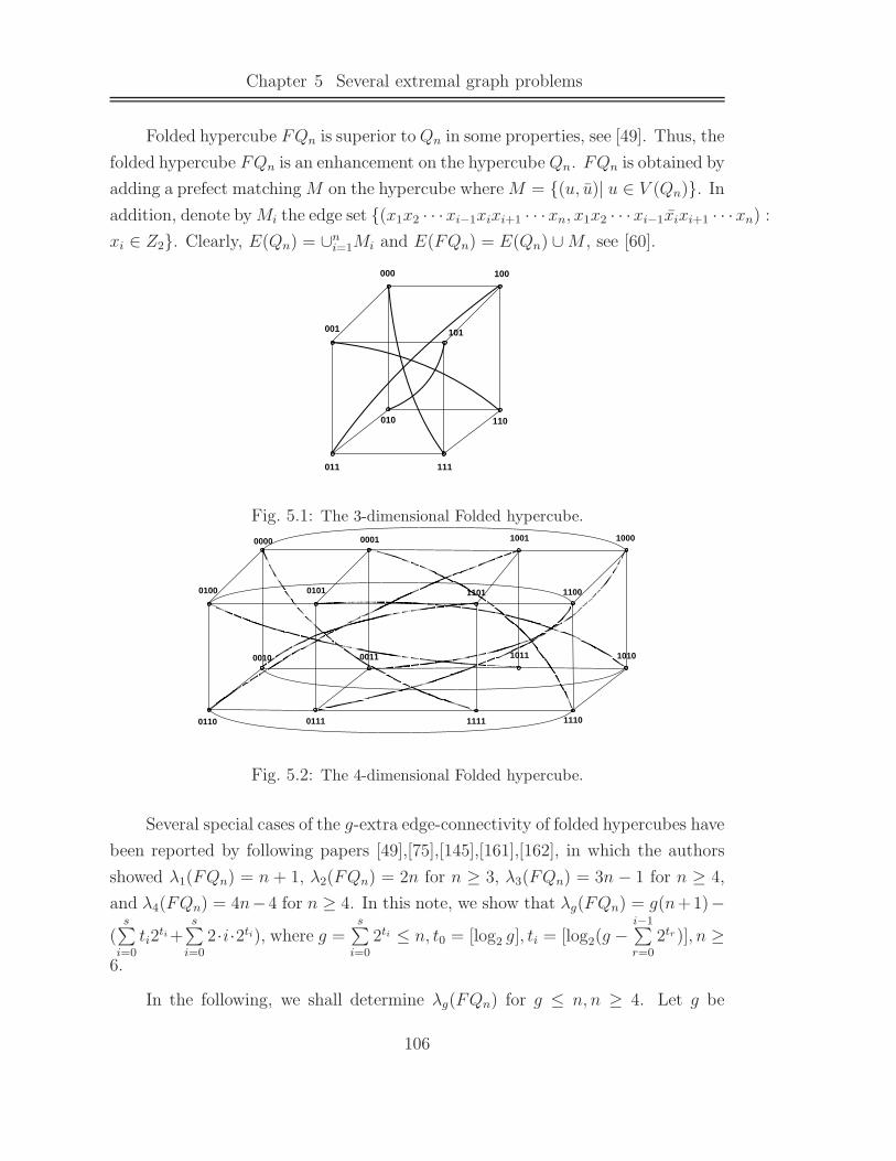
Chapter 5 Several extremal graph problems
Folded hypercube FQn is superior toQn in some properties, see [49]. Thus, the
folded hypercube FQn is an enhancement on the hypercube Qn. FQn is obtained by
adding a prefect matching M on the hypercube where M = (u, u)| u ∈ V (Qn). In
addition, denote byMi the edge set (x1x2 · · ·xi−1xixi+1 · · ·xn, x1x2 · · ·xi−1xixi+1 · · ·xn) :
xi ∈ Z2. Clearly, E(Qn) = ∪ni=1Mi and E(FQn) = E(Qn) ∪M , see [60].
000
001
011
010
100
110
111
101
Fig. 5.1: The 3-dimensional Folded hypercube.
0000 0001
00110010
0100 0101
01110110
1001
1101
1011
1111
1100
1000
1010
1110
Fig. 5.2: The 4-dimensional Folded hypercube.
Several special cases of the g-extra edge-connectivity of folded hypercubes have
been reported by following papers [49],[75],[145],[161],[162], in which the authors
showed λ1(FQn) = n + 1, λ2(FQn) = 2n for n ≥ 3, λ3(FQn) = 3n − 1 for n ≥ 4,
and λ4(FQn) = 4n−4 for n ≥ 4. In this note, we show that λg(FQn) = g(n+1)−(
s∑
i=0
ti2ti +
s∑
i=0
2·i·2ti), where g =s∑
i=0
2ti ≤ n, t0 = [log2 g], ti = [log2(g −i−1∑
r=0
2tr)], n ≥6.
In the following, we shall determine λg(FQn) for g ≤ n, n ≥ 4. Let g be
106

§5.1 Subgraph of hypercubes, extra-edge connectivity of hypercubes and foldedhypercubes
an integer and g =s∑
i=0
2ti be a decomposition of g such that t0 = [log2m], and
ti = [log2(m−i−1∑
r=0
2tr)] for i ≥ 1. For any integer g =s∑
i=0
2ti ≤ 2n−1, we first show
that FQn contains an induced subgraph G1 of order g such that∑
u∈V (G1)
d(u) =
s∑
i=0
ti2ti +
s∑
i=0
2 · i ·2ti . It is sufficient to show that there is a subgraph G1 in Qn such
that |V (G1)| = g, |E(G1)| = 12(
s∑
i=0
ti2ti +
s∑
i=0
2 · i · 2ti), and the subgraph contains
no edges in M . We pack G1 as defined in last section.
It is not difficult to count the number of edges of G1 by considering the edges
within Qi’s and the edges between Qi’s. In fact, each Qi contains 12
s∑
i=0
ti2ti edges,
and it is not difficult to see that each vertex in Qi is adjacent to one vertex in each
of Qi−1, Qi−2, · · · , Q0. Thus, |V (G1)| = g, |E(G1)| = 12(
s∑
i=0
ti2ti +
s∑
i=0
2 · i · 2ti), and
the subgraph contains no edges in M .
Let EV (G1)(FQn) be the set of edges of FQn having exactly one endvertex
in G1 (Unless stated otherwise, we omit the subscript FQn). Then, |EV (G1)| =
g(n+ 1) − (s∑
i=0
ti2ti +
s∑
i=0
2 · i · 2ti).
Lemma 5.1.9 There is a g-extra edge-cut of size g(n+1)− (s∑
i=0
ti2ti +
s∑
i=0
2 · i · 2ti)
for g ≤ 2n−1, i.e., λg ≤ g(n+ 1) − (s∑
i=0
ti2ti +
s∑
i=0
2 · i · 2ti).
Proof. We shall that EV (G1) is a g-extra edge-cut and then the lemma holds.
It is sufficient to show that FQn − EV (G1) − G1 is connected and contains more
than g vertices. Note that |V (G1)| = g ≤ 2n−1 and then FQn − V (G1) contains
at least g vertices. So we only need to show that Qn − V (G1) is connected. By
the definition of Qn, it can be seen that there is a path from 11 · · ·1 to any vertex
of Qn − V (G1) by changing 1 to 0 one by one in the suitable coordinates. We are
done.
Lemma 5.1.10 ([103]) Let X be a vertex set of Qn with sizem. Then 2|E(Qn[X])| ≤s∑
i=0
ti2ti +
s∑
i=0
2 · i · 2ti.
107
Chapter 5 Several extremal graph problems
Lemma 5.1.11 ([60]) FQn −Mi is isomorphic to Qn for all i.
Lemma 5.1.12 Let H be connected subgraph induced by X in FQn.
(i) If |X| ≤ g =s∑
i=0
2ti ≤ n and n ≥ 5, then |E(H)| ≤ 12(
s∑
i=0
ti2ti +
s∑
i=0
2 · i · 2ti).
(ii) If |X| ≥ n + 1, then |EX | ≥ g(n + 1) − (s∑
i=0
ti2ti +
s∑
i=0
2 · i · 2ti) for any
g ≤ n, n ≥ 6.
Proof. We first prove (i). If H contains no edges of M , then by Lemma 5.1.10
the lemma holds. We claim that there exists an integer i such that H contains no
edges of Mi. In fact, if H contains at least an edge of Mi for each i, then we pack
one edge from Mi ∩E(H) for each i and one edge from m. The n+ 1 edges induce
a subgraph H∗ of H . If H∗ contains a cycle, then the cycle contains even number
of edges of Mj if there is one edge of Mj on the cycle. Thus, H∗ is a forest and
then it contains at least n + 1 vertices. This contradicts to g ≤ n. So we may
assume there exists an inter i such that Mi ∩ E(H) = ∅. By Lemma 5.1.11 and
Lemma 5.1.10, we have (i) holds.
We next show that (ii) holds. We suppose n ≥ 8 in this claim and leave the
proof for the cases n = 6, 7 in Appendix.
Let f(g) = (s∑
i=0
ti2ti +
s∑
i=0
2 · i · 2ti). Note that f(g + 1) − f(g) = 2s + 2 and
s < [n2] since g ≤ n (one can obtain the inequalities by simply count, we omit the
details). Then, g(n+ 1) − f(g) is increasing for g ≤ n since 2s+ 2 < n+ 1. Thus,
it is sufficient to show that |EX | ≥ n(n + 1) − f(n).
Note that |EX | = |X|(n + 1) − 2|E(FQn[X])|. Clearly, 2|E(FQn[X]) ≤2|E(FQn−M [X])|+ |X| and then 2|E(FQn−M [X])| ≤ f(|X|) by Lemma 5.1.10.
Thus, |EX | = |X|(n+1)−2|E(FQn[X])| ≥ |X|(n+1)−2|E(FQn−M [X])|−|X| =
|X|n− 2|E(FQn −M [X])| ≥ |X|n− f(|X|).
Consider the expression h(|X|) = (|X|n−f(|X|))−(n(n+1)−f(n)) = (|X|−n−1)n−(f(|X|)−f(n)) for n+2 ≤ |X| < 2[ n
2]. Note that |X|n−f(|X|) is increasing,
then h(|X|) ≥ h(n+ 2). Let n =s∑
i=0
2ti . Then h(n+ 2) = n− (f(n+ 2)− f(n)) =
n−((f(n+2)−f(n+1))+(f(n+1)−f(n))) ≤ n−(2(s+1)+2+2s+2) = n−(4s+6).
It is easily checked that if n ∈ [2j, 2j+1], then s ≤ j. So n− (4s+6) > 0 for n ≥ 25.
108

§5.1 Subgraph of hypercubes, extra-edge connectivity of hypercubes and foldedhypercubes
Moreover, n − (4s + 6) ≥ 0 for 16 = 24 ≤ n ≤ 31 = 25 − 1. Note that if we let
n + 1 =s′∑
i=0
2ti, then
h(n+2) = n−((f(n+2)−f(n+1))+(f(n+1)−f(n))) = n−(2s′+2+2s+2). (1)
By (1), it can be seen that h(n + 2) ≥ 0 for 8 ≤ n ≤ 15. Thus, h(n + 2) ≥ 0 for
n + 2 ≤ |X| < 2[ n2] and then |EX | ≥ n(n + 1) − f(n) for n+ 2 ≤ |X| < 2[ n
2].
Claim 1. Let X be a subset V (Qn) with |X| ≥ 2[ n2]. Then |EX(Qn)| ≥
[n2] · 2[ n
2].
By Lemma 5.1.10, it is sufficient to show that |EX(Qn)| ≥ n|X| − f(|X|) ≥[n2] · 2[ n
2] when |X| ≥ 2[ n
2]. In fact, it is easy to see the following:
n|X| − f(|X|) = n2t0 + n(2t1 + · · ·+ 2ts) − t02t0 − (
s∑
i=1
ti2ti +
s∑
i=1
2 · i · 2ti)
= (n− t0)2t0 + (n
s∑
i=1
2ti − (s∑
i=1
ti2ti +
s∑
i=1
2 · i · 2ti))
> (n− t0)2t0
= (n− t0) · 2(t0−[ n2]) · 2[ n
2]
Note that [n2] ≤ t0 < n− 1, then we have (n− t0) · 2(t0−[ n
2]) ≥ [n
2].
Since FQn−M is isomorphic toQn and |EX | ≥ [n2]·2[ n
2], we have |EX(FQn)| ≥
|EX(Qn)| ≥ [n2] · 2[ n
2]. It is not difficult to see that [n
2] · 2[ n
2] ≥ n(n + 1) − f(n) for
n ≥ 8.
The rest is to show that (ii) holds for |X| = n+1. Note thatH is connected. If
H contains either no edges ofMi for some i, or no edges ofM , then by Lemma 5.1.11
that |EX | ≥ (n + 1)(n + 1) − f(n + 1) > n(n + 1) − f(n) for n ≥ 5 (Note that
f(n + 1) − f(n) = 2s+ 2, the inequality follows from n + 1 > 2s+ 2). So we may
assume that H contains at least one edge of Mi for each i, and contains at least
one edge of M .
Claim 2. H −M is a path.
Take an edge ei from Mi ∩ E(H) for each i. Then the subgraph H∗ of H
induced by e1, · · · , en is a forest. Note that H is of order n+ 1. Then the forest
109

Chapter 5 Several extremal graph problems
is a tree. Since H contains an edge f of M , then H∗ +f contains a cycle (of length
n+ 1). Thus H∗ is a path of length n. Note that the cycle contains no chords (by
definition of FQn). Thus H −M is a path.
So H is a cycle. Thus, |EX | ≥ (n+ 1)(n+ 1)− 2(n+ 1) > n(n+ 1)− f(n) for
n ≥ 5.
Theorem 5.1.13 λg(FQn) = g(n+ 1)− (s∑
i=0
ti2ti +
s∑
i=0
2 · i · 2ti), where n ≥ 6, g =
s∑
i=0
2ti ≤ n, t0 = [log2 g], and ti = [log2(g −i−1∑
r=0
2tr)] for i ≥ 1.
Proof. By Lemma 5.1.9, it is sufficient to show that λg(FQn) ≥ g(n + 1) −(
s∑
i=0
ti2ti +
s∑
i=0
2 · i · 2ti). Let F be a minimum g-extra edge-cut of FQn and C be
the smaller one of the two components in FQn − F (note that FQn − F contains
exactly two components since F is a minimum g-extra edge-cut). We next show
that |F | ≥ g(n+1)−(s∑
i=0
ti2ti +
s∑
i=0
2·i·2ti). If |V (C)| ≤ n, then by Lemma 5.1.12 (i)
we have |F | ≥ |EV (C)| = |V (C)|(n+1)−|E(C)| ≥ g(n+1)− (s∑
i=0
ti2ti +
s∑
i=0
2 · i ·2ti)
and then we are done. If |V (C)| ≥ n+1, then |F | ≥ g(n+1)−(s∑
i=0
ti2ti +
s∑
i=0
2·i·2ti)
by Lemma 5.1.12 (ii). We complete the proof.
Appendix. We shall show that |EX | ≥ g(n+ 1)− (s∑
i=0
ti2ti +
s∑
i=0
2 · i · 2ti) for
n = 6, 7. By Lemma 5.1.12 (i), it is sufficient to show that |EX | ≥ n(n+ 1)− f(n)
for |X| ≥ n + 2, n = 5, 6, 7. By the proof of Lemma 5.1.12 (ii), we have |EX | ≥n(n + 1) − f(n) for |V (C)| = n + 1, n ≥ 5. We may assume |X| ≥ n + 2. Let
z(n) = n(n + 1) − f(n). Then z(6) = 28, z(7) = 38. To show that |EX | ≥n(n + 1) − f(n), we first use an algorithm to exclude several cases. Note that
|EX | ≥ n|X|−f(|X|). We compute the function R(x) = nx−f(x)−z(n) by using
Matlab, where x = |X| =s∑
i=0
2ti and then f(x) =s∑
i=0
ti2ti +
s∑
i=0
2 · i · 2ti .
We list the algorithm as follows.
For n = 6, we have x = 8, R(x) = −4, x = 9, R(x) = 0, x = 10, R(x) =
2, x = 11, R(x) = 4, x = 12, R(x) = 4, x = 13, R(x) = 6, x = 14, R(x) =
6, x = 15, R(x) = 6, x = 16, R(x) = 4, x = 17, R(x) = 8, x = 18, R(x) =
110

§5.1 Subgraph of hypercubes, extra-edge connectivity of hypercubes and foldedhypercubes
Algorithm 1 Input n, z(n); Output x,R(x)1: for x = n + 2 to 2n−1 do
2: Initialize j = 0, s = 0, f(x) = 0;
3: while x > s do
4: tj = [log2(x− s)];
5: s = s + 2tj ;
6: f(x) = f(x) + tj2tj + 2 ∗ j ∗ 2tj ;
7: j = j + 1;
8: end while
9: R(x) = nx− f(x) − z(n);
10: Print x,R(x);11: x = x+ 1;
12: end for
10, x = 19, R(x) = 12, x = 20, R(x) = 12, x = 21, R(x) = 14, x =
22, R(x) = 14, x = 23, R(x) = 14, x = 24, R(x) = 12, x = 25, R(x) =
14, x = 26, R(x) = 14, x = 27, R(x) = 14, x = 28, R(x) = 12, x =
29, R(x) = 12, x = 30, R(x) = 10, x = 31, R(x) = 8, x = 32, R(x) = 4.
For n = 7, we have x = 9, R(x) = −1, x = 10, R(x) = 2, x = 11, R(x) =
5, x = 12, R(x) = 6, x = 13, R(x) = 9, x = 14, R(x) = 10, x = 15, R(x) =
11, x = 16, R(x) = 10, x = 17, R(x) = 15, x = 18, R(x) = 18, x =
19, R(x) = 21, x = 20, R(x) = 22, x = 21, R(x) = 25, x = 22, R(x) =
26, x = 23, R(x) = 27, x = 24, R(x) = 26, x = 25, R(x) = 29, x =
26, R(x) = 30, x = 27, R(x) = 31, x = 28, R(x) = 30, x = 29, R(x) =
31, x = 30, R(x) = 30, x = 31, R(x) = 29, x = 32, R(x) = 26, x =
33, R(x) = 31, x = 34, R(x) = 34, x = 35, R(x) = 37, x = 36, R(x) =
38, x = 37, R(x) = 41, x = 38, R(x) = 42, x = 39, R(x) = 43, x =
40, R(x) = 42, x = 41, R(x) = 45, x = 42, R(x) = 46, x = 43, R(x) =
47, x = 44, R(x) = 46, x = 45, R(x) = 47, x = 46, R(x) = 46, x =
47, R(x) = 45, x = 48, R(x) = 42, x = 49, R(x) = 45, x = 50, R(x) =
46, x = 51, R(x) = 47, x = 52, R(x) = 46, x = 53, R(x) = 47, x =
111

Chapter 5 Several extremal graph problems
54, R(x) = 46, x = 55, R(x) = 45, x = 56, R(x) = 42, x = 57, R(x) =
43, x = 58, R(x) = 42, x = 59, R(x) = 41, x = 60, R(x) = 38, x =
61, R(x) = 37, x = 62, R(x) = 34, x = 63, R(x) = 31, x = 64, R(x) = 26.
Note that R(x) < 0 occurs only when |X| = n + 2, n = 6, 7. We next prove
the assertion for these cases. We suppose |X| = n + 2, n = 6, 7. Note that H is
connected. If H contains either no edges of Mi for some i, or no edges of M , then
by Lemma 5.1.11 that |EX | ≥ (n+1)(n+2)−f(n+2) ≥ n(n+1)−f(n) for n ≥ 5.
So we may assume that H contains at least one edge of Mi for each i, and contains
at least one edge of M . Take an edge ei from Mi ∩ E(H) for each i. Then the
subgraph of H induced by e1, · · · , en is a forest. Note that H is of order n + 2.
Then the forest has exactly two components.
Suppose that there is an edge fi ∈ Mi such that the subgraph H∗ induced
by e1, · · · , en, fi is a tree. Take an edge f from H ∩M , then H∗ + f contains a
cycle (of length n + 1), say C. Clearly, C contains no chords. Note that H∗ − C
is a isolated vertex, say u. Clearly, u is adjacent to at most one vertex on C by
the definition of adjacent relation in FQn. So |E(H)| = n + 2 and then EX =
(n+ 1)|X| − 2|E(H)| = (n + 1)(n+ 2) − 2(n+ 2) > n(n + 1) − f(n) for n = 6, 7.
Suppose that there is no fi inMi between the two components of the forest. So
H−M has exactly two components, say H1 and H2. Let X1 = V (H1), X2 = V (H2)
and x1 = |X1|, x2 = |X2|. Without loss of generality we may assume x1 ≥ x2. If
H [X1] contains some edge in M , then H [X1] is a cycle and H2 is a isolated vertex.
Thus, H is the graph obtained from a cycle of length n + 1 by adding a pendant
edge. Therefore, |E(H)| = n+2 and |EX | > n(n+1)− f(n) for n ≥ 5. So we may
assume x2 ≥ 2. Note that Hi is a subgraph of FQn −M . Then 2|E(Hi)| ≤ f(xi).
Since there is no edges of M in Hi, H contains at most minx1, x2 edges in M . So,
2|E(H)| ≤ f(x1)+f(x2)+2 minx1, x2 < f(x1+x2) (Note that the last inequality
is not difficult to obtain, see the detailed explanations in the proof of the Claim in
Theorem 1 [104]). Thus |EH | ≥ |X|(n+ 1)− f(|X|) = (n+ 1)(n+ 2)− f(n+ 2) >
n(n+ 1) − f(n) for n ≥ 5. We complete the proof.
Conclusions. We emphasize that the result in this part is a successor of the
result in [158], in which we determined the g-extra connectivity of folded hypercubes
FQn for n ≥ 8, g ≤ n− 4.
112
§5.2 The minimum size of graphs under a given edge-degree condition
Note that the assumption g ≤ n and the previous results cannot imply the case
for n = 5, g = 5. Then Theorem 5.1.13 should contain the case n = 5, g = 5 but
it miss the case. By the method posed in this note, we consider R(x) for n = 5.
We have x = 7, R(x) = −3, x = 8, R(x) = −4, x = 9, R(x) = −1, x =
10, R(x) = 0, x = 11, R(x) = 1, x = 12, R(x) = 0, x = 13, R(x) = 1, x =
14, R(x) = 0, x = 15, R(x) = −1, x = 16, R(x) = −4. So we have to discuss
the case |X| = 8, 9, 15, 16 for n = 5. For these cases, we have no simple method to
consider them. If we discuss them by the regular method, then it implies a long
and tedious proof. So we omit the case in this note.
The key problem in this method is to determine the maximum number of
edges of the subgraph induced by a vertex set with a given size. We conjecture
the maximum number of edges of the subgraph induced by m vertices in folded
hypercubes is f(m) for m ≤ 2[ n2].
§5.2 The minimum size of graphs under a given
edge-degree condition
I first note that the main result in this subsection also appeared in my first
Phd thesis in Xiamen University. In that thesis we consider the connectivity of
graphs, in which I use the main results to characterized minimum restricted k-edge
connected graphs for some integer k. Here, I would like to emphasize the extremal
problem on the edge-condition.
Determining the minimum and/or maximum size of graphs with some given
parameters is a classic extremal problem in graph theory, see [10]. In this paper, we
consider the following problem: What is the minimum size of graphs with a given
order n, a given minimum degree δ and a given minimum edge-degree 2δ + k − 2?
We obtain a lower bound for the minimum size of graphs with a given order n, a
given minimum degree δ and a given minimum edge-degree 2δ+k−2. Moreover, we
characterize the extremal graphs for k = 0, 1, 2. As an application, we characterize
some kinds of minimum restricted edge connected graphs.
In the following theorem, the graph considered may have loops (a loop is an
edge with two same endpoints). For a graph G and u ∈ V (G), let EG(u) be the set
113
Chapter 5 Several extremal graph problems
of edges incident with u in G. When the graph G is understood from the context,
we write Eu for EG(u), δ and n for δ(G) and |V (G)|, respectively. Denote by Gn,δ,k
a graph with order n, minimum degree δ, and minimum edge-degree 2δ + k − 2,
and let Gn,δ,k be the set of all Gn,δ,k’s.
Theorem 5.2.1 Let G be a graph with minimum degree δ ≥ 3, ξ(G) ≥ 2δ+ k− 2.
Then |E(G)| ≥ δ2n + δk
2(δ+k)dδ. Moreover, equality holds if and only if dδ = δ+k
2δ+kn
and V (G) = Dδ ∪N(Dδ).
Proof. Let N(G) = NG(Dδ) and T (G) = V \ (N ∪Dδ) (or simply, we use N and
T for N(G) and T (G)). Note that k ≥ 0 and the inequality holds if k = 0. Then
we may assume that G is a graph with ξ(G) ≥ 2δ − 1, i.e. k ≥ 1. Thus, Dδ is an
independent set of G. The degrees of vertices in N are at least δ+k and the degrees
of vertices in T are at least δ + 1. We consider the size of G by distinguishing the
following two cases.
If |N | > δδ+k
dδ, we have
|E(G)| =
∑idi
2≥ δdδ
2+δ + k
2|N | + δ + 1
2|T |
=δdδ
2+δ + k
2|N | + δ + 1
2(n− dδ − |N |)
=δ
2n+
n
2− dδ
2− δ + 1
2|N | + dδ + k
2|N |
=δ
2n+
k − 1
2|N | + δ
2n− dδ
2
>δ
2n+
k − 1
2(
δ
δ + kdδ) +
δ
2n− dδ
2
=δ
2n+
δk
2(δ + k)dδ −
δ
2(δ + k)dδ +
|N | + |T |2
By the assumption, we have |E(G)| ≥ δ2n + δk
2(δ+k)dδ since |N |+|T |
2≥ δ
2(δ+k)dδ.
If |N | ≤ δδ+k
dδ, we have
|E(G)| ≥ δdδ +δ + 1
2|T |
114
§5.2 The minimum size of graphs under a given edge-degree condition
=δ
2dδ +
δ
2δ|N | + δ
2dδ −
δ
2δ|N | + δ + 1
2|T |
=δ
2n+
δ
2dδ −
δ
2|N | + 1
2|T |
≥ δ
2n+
δ
2dδ −
δ
2
δ
δ + kdδ +
1
2|T |
≥ δ
2n+
δk
2(δ + k)dδ
By the Inequality (2), one can see that if |N | < δδ+k
dδ, then |E(G)| > δ2n +
δk2(δ+k)
dδ. Moreover, if the equality holds in Inequality (2), then |T | = 0. Note that
|N | = δδ+k
dδ and |T | = 0 imply that dδ = δ+k2δ+k
n. Thus, the equality holds if and
only if dδ = δ+k2δ+k
n and |N | = δ2δ+k
n. We complete the proof.
We next consider the extremal graphs for k = 0, 1, 2. By Theorem 5.2.1, we
have |E(Gn,δ,k)| ≥ ⌈ δ2n⌉ if k = 0. The following graph Hs,m ∈ Gn,δ,k such that
|E(Hs,m)| = ⌈ δ2n⌉.
For integers s, n, n ≥ s+1, Harary [67] constructed classes of graphs Hs,n that
are minimum s-connected. The graph Hs,n is as follows.
Case 1. s = 2r, r > 0. H2r,n is with vertex set 0, 1, 2, · · · , n − 1 and two
vertices i and j are adjacent if i− r ≤ j ≤ i+ r, where addition is taken modulo n.
Case 2. s = 2r + 1, r > 0.
Case 2.1. n is even. Then H2r+1,n is obtained by adding edges joining vertex
i to vertex i+ n2
for 1 ≤ i < n2
on H2r,n.
Case 2.2. n is odd. H2r+1,n is obtained by adding edges [0, (n−1)2
] and [0, (n+1)2
],
and [i, i+ (n+1)2
] for 1 ≤ i < (n−1)2
on H2r,n.
Clearly, Hδ,n has minimum degree δ and the minimum edge-degree 2δ+0− 2.
In particular, Hδ,n has ⌈ δ2n⌉ edges. A graph G is called almost n-regular if there
is at most one vertex of degree n + 1 and all other vertices have degree n. The
following theorem follows immediately from the argument above.
Theorem 5.2.2 |E(Gn,δ,0)| ≥ ⌈ δ2n⌉ and |E(Gn,δ,0)| = ⌈ δ
2n⌉ if and only if Gn,δ,0 is
an almost δ-regular graph.
From now on, we always assume k = 1, 2 in this section. A bipartite graph is
115

Chapter 5 Several extremal graph problems
called (δ, δ + k)-graph if the degree the vertices in a part are all δ, and vertices in
the other part have degree δ+k. We denote a (δ, δ+k)-graph by G(δ, δ+k). Note
that if a graph Gn,δ,k is a (δ, δ + k)-graph, i.e. dδ = δ+k2δ+k
n, then the equality of
Theorem 5.2.1 holds. By Theorem 5.2.1, we have |E(G(δ, δ + k))| > δ2n + δk
2(δ+k)dδ
if dδ 6= δ+k2δ+k
n, k = 1, 2. That is, |E(Gn,δ,k)| > δ2n + δk
2(δ+k)dδ if Gn,δ,k is not a
(δ, δ + k)-graph for k = 1, 2. Thus, the following holds.
Theorem 5.2.3 If k = 1, 2 and n = (2δ+k)t for some integer t, then |E(Gn,δ,k)| ≥δ2n + δk
2(δ+k)dδ. Moreover, |E(Gn,δ,k)| = δ
2n + δk
2(δ+k)dδ if and only if Gn,δ,k is a
(δ, δ + k)-graph.
Proof. By Theorem 5.2.1, we have |E(G(δ, δ+k))| ≥ δ2n+ δk
2(δ+k)dδ. Note that k ≥
1. Then Dδ(G) is an independent set. Since dδ = δ+k2δ+k
·n and V (G) = Dδ ∪N(Dδ),
we have that each vertex of V (G) − Dδ(G) has degree δ + k and Dδ+k(G) is an
independent set. We complete the proof.
We define the function f(n) for the minimum size of all Gn,δ,k’s. In Theo-
rem 5.2.3, we characterized the extremal graphs for k = 1, 2 and n = (2δ + k)t for
some t. Next, we consider f(n) for k = 1, 2 and n 6= (2δ + k)t for any t.
Lemma 5.2.4 If k = 1, 2, then f(n) + ⌊ δ2⌋ ≤ f(n+ 1).
Proof. Let Gn+1,δ,k be a graph with f(n+1) edges. Take a vertex u of degree δ in
Gn+1,δ,k. Note that there is no loops on u since k 6= 0. Assume that δ is even. Let
N ′(u) = u1, u2, · · · , uδ. We construct a Gn,δ,k with f(n+1)− δ2
edges by deleting
the vertex u and adding δ2
new edges u1u2, u3u4, · · · , uδ−1uδ. If δ is odd, then we
first add a new edge between u and a vertex in D≥δ+k, and then we may construct
a Gn,δ,k with f(n+ 1) − ⌊ δ2⌋ edges. That is, f(n) + ⌊ δ
2⌋ ≤ f(n+ 1).
Lemma 5.2.5 If k = 1, then f(n+ 1) ≤ f(n) + ⌊ δ2⌋ + 1.
Proof. We first assume that δ is even. Let Gn,δ,k be a graph with f(n) edges. We
shall construct a new graph Gn+1,δ,k with f(n) + ⌊ δ2⌋ + 1 edges by adding a new
vertex u, joining an edge between u and a vertex of D≥δ+k(G), and adding δ2
loops
on u. Thus, f(n+ 1) ≤ f(n) + ⌊ δ2⌋ + 1 in this case.
116

§5.2 The minimum size of graphs under a given edge-degree condition
Suppose δ is odd. Let Gn,δ,k be a graph with f(n) edges. We shall construct
a new graph Gn+1,δ,k with f(n) + ⌊ δ2⌋ + 1 edges by adding a new vertex u, joining
an edge between u and vertex of v ∈ D≥δ+k(G), adding ⌊ δ2⌋ loops on u, deleting
an edge vv′ ∈ E(G) and adding a new edge uv′. Thus, f(n+ 1) ≤ f(n) + ⌊ δ2⌋ + 1.
We complete the proof.
Lemma 5.2.6 If k = 2, then f(n+ 1) ≤ f(n) + ⌊ δ2⌋ + 2.
Proof. LetGn,δ,k be a graph with f(n) edges. Similarly as the proof of Lemma 5.2.5,
we construct a new graph Gn+1,δ,k with f(n) + ⌊ δ2⌋+ 2 edges by adding a new ver-
tex u, joining an edge between u and vertex of v ∈ D≥δ+k(G), adding ⌊ δ2⌋ loops
on u, deleting edges vv′, vv′′ ∈ E(G) and adding two new edges uv′, uv′′. Thus,
f(n+ 1) ≤ f(n) + ⌊ δ2⌋ + 2.
Combining the Lemmas above, we have the following.
Theorem 5.2.7 If k = 1, then f(n) + ⌊ δ2⌋ ≤ f(n + 1) ≤ f(n) + ⌊ δ
2⌋ + 1, and if
k = 2, then f(n) + ⌊ δ2⌋ ≤ f(n+ 1) ≤ f(n) + ⌊ δ
2⌋ + 2.
Remark. Assume k = 1. Note that f((2δ + k)(t − 1)) + ⌊ δ2⌋(2δ + k) <
f((2δ + k)t) < f((2δ + k)(t− 1)) + (⌊ δ2⌋ + 1)(2δ + k), then by Theorem 5.2.3 that
the bounds of Theorem 5.2.7 for k = 1 are sharp.
In the next section, we shall characterize some kinds of minimum restricted
edge-connected graphs by applying the Theorems 5.2.2 and 5.2.3.
§5.2.1 Minimum restricted (2δ + k − 2)-edge connected graph for k ∈0, 1, 2
We assume that the graph considered in the section has minimum degree δ.
Esfahanian and Hakimi [51] introduced the concept of restricted edge-connectivity.
The concept of restricted edge-connectivity is also a kind of conditional edge-
connectivity proposed by Harary in [67]. An edge set F a restricted edge-cut of
G if G− F is disconnected and contains no isolated vertices. The minimum cardi-
nality over all restricted edge-cuts is the restricted edge-connectivity of G, denoted
117

Chapter 5 Several extremal graph problems
by λ′(G). If a graph has restricted edge-connectivity k, then the graph is called re-
stricted k-edge-connected. A graph G is called minimum restricted k-edge connected
if G is restricted k-edge connected and no restricted k-edge connected graphs with
the same number of vertices has fewer edges than G. A graph G with λ′(G) = ξ(G)
is called λ′-optimal. Esfahanian in [51] proved that if a connected graph G with
|V (G)| ≥ 4 is not a star K1,n−1, then λ′(G) exists and
λ(G) ≤ λ′(G) ≤ ξ(G). (5.2.1)
By inequality (5.2.12), the minimum edge degree of a restricted 2δ + k − 2-edge
connected graph is at least 2δ + k − 2. For the studies of λ′-optimal graphs, we
suggest the readers to refer to the survey [69].
In this section, we shall characterize minimum restricted 2δ−2-edge connected
graphs by using Theorem 5.2.2, and the minimum restricted 2δ + k − 2-edge con-
nected graphs with order (2δ+ k)t for k = 1, 2 by using Theorem 5.2.3. Note that
if δ = 1 and k = 0, 1, 2, then the minimum restricted 2δ + k − 2-edge connected
graph is clear. Thus, we may assume δ ≥ 2 in the following.
In fact, characterizing the minimum graphs with some given property on the
connectivity of graphs is a classic topic. For example, in [45], Cozzens and Wu
studied the minimum critically k-edge connected graph (a k-edge connected graph
is critical if λ(G − v) < k for any vertex v ∈ V (G)). In [110], Maurer and
Slater defined the k-edge♯-connectivity which is the other version of restricted edge
connectivity and characterized the cases k = 1, 2, 3. Later, Peroche and Virlouvet
gave some partial results on the cases k = 4, 5. Recently, Hong et al [72] showed that
the minimally restricted k-edge connected graph is λ′-optimal ( A restricted k-edge
connected graph G is called minimally restricted k-edge connected if λ′(G− e) < k
for any edge e.). Here, we give some partial results on the minimum restricted edge
connected graphs.
To characterize the minimum restricted 2δ−2-edge connectivity, the following
lemma is needed. We shall give the proof of the following lemma in Section 3.
Lemma 5.2.8 Harary graph Hδ,n is λ′-optimal.
It can be seen that there exists a restricted 2δ− 2-edge connected graph with
118

§5.2 The minimum size of graphs under a given edge-degree condition
size ⌈ δn2⌉ from Lemma 5.2.8. Thus, we have the following characterization for
minimum restricted 2δ − 2-edge connected graph.
Theorem 5.2.9 The minimum restricted 2δ − 2-edge connected graph with mini-
mum degree δ is an almost δ-regular graph.
Let Aut(G) denote the automorphism group of G, i.e., the set of bijective
mappings on its vertices that preserve incidence. For x ∈ V (G), the set g(x) :
g ∈ Aut(G) is an orbit of Aut(G); we abuse the terminology a little to call it
an orbit of G. Let W be a subgroup of the symmetric group over a set S. We
say that W acts transitively on a subset T of S if for any h, l ∈ T , there exists
a permutation ϕ ∈ W with ϕ(h) = l. Clearly, the automorphism group Aut(G)
acts transitively on each orbit of Aut(G). We call a graph G a double-orbit graph if
Aut(G) has at most two orbits. A double-orbit bipartite graph is also called a half
vertex transitive graph. When Aut(G) has exactly two orbits, we denote them as
V1 and V2. Next, we shall construct a double orbit bipartite graph G(V1, V2) with
(2δ + k)t vertices for each integer t.
We denote the vertex set of G(V1, V2) by V1∪V2, and V1 = 0, 1, · · · , (δ+k)t−1 = Z(δ+k)t, V2 = 0, 1, · · · , δt − 1 = Zδt. Add an edge between the vertex i of
V1 and the vertex i + j of V2 for j = 0, 1, · · · , δ − 1 (the addition is taken modulo
δ). Clearly, G(V1, V2) is a double orbit bipartite graph such the vertex of V1 has
degree δ and the vertex in V2 has degree δ + k.
We shall give a characterization for the minimum restricted 2δ + k − 2-edge
connected graph for k = 1, 2. We need the following lemma and we leave its proof
in Section 4.
Lemma 5.2.10 The half vertex transitive graph G(V1, V2) is λ′-optimal.
By Lemma 5.2.10, there exists a restricted 2δ+k−2-edge connected (δ, δ+k)-
graph. Then by Theorem 5.2.3, we have the following theorem.
Theorem 5.2.11 If k = 1, 2 and n = (2δ + k)t for some positive integer t, then
the minimum restricted 2δ + k − 2-edge connected graph with minimum degree δ is
a (δ, δ + k)-graph.
119

Chapter 5 Several extremal graph problems
Proof of Lemma 5.2.8
It is sufficient to show that λ′(Hδ,n) = ξ(Hδ,n) = 2δ− 2, n ≥ 4. We only prove
the case λ′(Hδ,n) = ξ(Hδ,n) = 2δ − 2 for δ = 2k + 1 and n is even, and other two
cases can be shown by the similar arguments (we leave it to the readers). We write
H for Hδ,n for simply.
We call edges (i, i + n2) the diagonal edges and edges (i, i + j) the j-edges.
Clearly, all 1-edges form a cycle, denoted by C = 12 . . . n1. We use Ci,j, Ci,j, Ci,j,
and Ci,j to denote paths i(i+1), . . . , j; (i+1)(i+2), . . . , j; i(i+1), . . . , (j−1), and
(i+1), . . . , (j−1), respectively. For a graph G and two disjoint non-empty subsets
A and B of V (G), we denote by [A,B] the set of edge with one end in A and the
other one in B. We denote by EG(A) the set of edges (in E(G)) with exactly one
end in A. For a subgraph X ⊂ G and e = uv ∈ E(G), we use EG(X) for EG(V (X))
and EG(e) for EG(u, v). Sometimes, we write x for the single vertex set x. For
a subgraph X ⊂ G and a vertex u 6∈ X, we use [u,X] for [u, V (X)]. Moreover,
if A = V \A, then we write ω(A) for [A,A].
Lemma 5.2.12 Hδ,n is λ′-optimal for 4 ≤ n ≤ 7.
Lemma 5.2.13 For any complete graph Km, m ≥ 4, λ′(Km) = 2m− 4.
The proof of Lemma 2.1. For an 1-edge e, it is easy to check that EH(e)
is a restricted edge cut. Therefore, λ′(H) ≤ ξ(H) = 2δ − 2. We shall show
that λ′(H) ≥ ξ(H) = 2δ − 2. Suppose that there exists a restricted edge cut
F, |F | < 2δ−2, such that H−F is disconnected and contains no trivial component.
If there is a component of order 2 ≤ t ≤ 3 in H − F , then we clearly have
|F | ≥ 2δ − 2, a contradiction. Thus we may suppose that each component of
H − F has order at least 4. Let B be a component with minimum order in all the
components of H − F .
Claim 1. |F | > 2δ − 3 for k = 1 and k = n/2 − 1.
Proof of claim 1. Suppose k = 1. If the vertices of B are continuous, that is,
V (B) = x, x+1, . . . , y, then edges (x−1)x, y(y+1), x(x+n/2), . . . , y(y+n/2) ∈F . So |F | ≥ 4 > 2δ−3 = 3, a contradiction. If not, there must be diagonal edge in
B, without loss of generality, we assume that 0(n/2) ∈ E(B), then both C0,n/2 and
120

§5.2 The minimum size of graphs under a given edge-degree condition
Cn/2,0 contain vertices in V (H)\V (B) since B is the smallest component of H−F .
So |E(C0,n/2) ∩ F | ≥ 2 and |E(Cn/2,0) ∩ F | ≥ 2. Thus |F | ≥ 4 > 2δ − 3 = 3.
If k = n/2− 1, then H is a complete graph. It can be seen that |F | > 2δ− 3.
This completes the proof of the claim.
In the following arguments, we suppose that n ≥ 8, 2 ≤ k ≤ n/2− 2 and each
component of H − F has order at least 4. We consider the following two cases.
Case 1. B contains two distinct vertices x and y such that y−x ≡ l(modn), l >
k and V (Cx,y) ∩ V (B) = ∅, or x− y ≡ l(modn), l > k and V (Cy,x) ∩ V (B) = ∅.
Without loss of generality, we assume that y − x ≡ l(modn), l > k and
V (Cx,y) ∩ V (B) = ∅, see Fig. 1. a.
s
s
s
s
s
s
s
s
s
s
s
s
x yx
y
w z
Cx,y Cx,y
x′y′ur
u′r
a b
F ig. 1
Pick w ∈ NB(x) and z ∈ NB(y) such that V (Cw,x) ∩ V (B) = x, w and
|V (Cy,z) ∩ V (B) = y, z (w and z may be the same). We use E ′x, E
′y, E
′w and
E ′z to denote [x, V (Cx,y)], [y, V (Cx,y)], [w, V (Cw,y)]\xw and [z, V (Cx,z)]\yz re-
spectively. By the hypothesis of Case 1 and the rules for picking w and z, we have
E ′x ⊆ F,E ′
y ⊆ F,E ′w ⊆ F and E ′
z ⊆ F . Note that |E ′x| ≥ k, |E ′
y| ≥ k, |E ′w| ≥
k − 1, |E ′z| ≥ k − 1. Set e = xx′, f = yy′ are diagonal edges incident to x, y
respectively. We distinguish the following two subcases.
Case 1.1. e, f 6∈ E(B).
Then, |F | ≥ |E ′x| + |E ′
y| + |E ′w| + |E ′
z| + 2 ≥ 2δ − 2 > 2δ − 3, a contradiction.
Case 1.2. At least one of e, f is contained in B.
Without loss of generality, set that e ∈ E(B) and NH(x′) ∩ V (Cx′,y′) =
121
Chapter 5 Several extremal graph problems
u1, u2, . . . , uk. We claim that for any ur ∈ NH(x′) ∩ V (Cx′,y′), if urx′ 6∈ F ,
that is, ur ∈ V (B), then uru′r ∈ F . Otherwise, it contradicts the fact that
V (Cx,y) ∩ V (B) = ∅, see Fig. 1. b. Similarly, the fact is true for y′. Thus
there exist at least two edges in F except E ′x, E
′y, E
′w and E ′
z. Therefore, |F | ≥|E ′
x| + |E ′y| + |E ′
w| + |E ′z| + 2 ≥ 2δ − 2 > 2δ − 3, a contradiction.
Case 2. For any x ∈ V (B), B contains a vertex in x, x+ 1, . . . , x+ k.
We first suppose n ≥ 4k. Let Hi denote the subgraph of H induced by vertex
set ik, ik+1, . . . , (i+1)k, 0 ≤ i ≤ 3. By the definition of H , we have Hi∼= Kk+1.
Furthermore, we denote F ∩ E(Hi) by Fi. Clearly, Fi is an edge cut of Hi. Since
λ(Hi) = k, we have that |F | ≥ |F0| + |F1| + |F2| + |F3| ≥ 4k = 2δ − 2 > 2δ − 3, a
contradiction.
We next suppose n < 4k. Note that B is the smallest component of H − F ,
then |V (B)| ≤ |V (H)|/2. Thus, there exist two vertices x, x+ 1 ∈ V (H)\V (B). If
k = 2, then B satisfies the condition of Case 1. We assume that k ≥ 3 from now
on.
Since |V (B)| ≥ 4, n < 4k, and H is not a complete graph, there exist two
disjoint cliques G1 and G2 (defined as Hi above, G1∼= G2
∼= Kk+1 and V (G1) ∩V (G2) = ∅), such that |V (B) ∩ V (Gi)| ≥ 2 and |(V (H)\V (B)) ∩ V (Gi)| ≥ 2 for
i = 1, 2. Suppose x, y ∈ V (B∩G1) and F ∩E(Gi) = Fi. Clearly, |Fi| ≥ λ′(Gi) =
2k− 2. If x(x+n/2), y(y+n/2) ∈ F , then |F | ≥ |F1|+ |F2|+ 2 = 2δ− 2 > 2δ− 3,
a contradiction. If not, without loss of generality, we assume that x(x+ n/2) 6∈ F ,
then at least one of the incident edges of vertex (x + n/2) excepting the edges
contained in [x, V (B)\x] is contained in F . Otherwise, |V (B)| ≥ 2k ≥ |V (H)|/2,
this contradicts the hypothesis that B is the smallest component of H − F . The
same fact is true for vertex (y+n/2). Thus |F | ≥ |F1|+ |F2|+2 = 2δ−2 > 2δ−3.
This completes the proof.
Proof of Lemma 5.2.10
A restricted edge cut F of G is called a λ′-cut if |F | = λ′(G). It is easy to see
that for any λ′-cut F , G − F has exactly two connected non-trivial components.
Let A be a proper subset of V . We denote G[A] the subgraph of G induced by
A. If ω(A) is a λ′-cut of G, then A is called a λ′-fragment of G. It is clear that
122
§5.2 The minimum size of graphs under a given edge-degree condition
if A is a λ′-fragment of G, then so is A. Let r(G)=min |A|: A is a λ′-fragment
of G. Obviously, 2 ≤ r(G) ≤ 12|V |. A λ′-fragment B is called a λ′-atom of G if
|B| = r(G).
In [143], Xu proved the following two theorems.
Theorem 5.2.14 ([143]) Let G = (V,E) be a connected graph with at least four
vertices and G ≇ K1,m. Then G is λ′-optimal if and only if r(G) = 2.
Theorem 5.2.15 ([143]) Let G = (V,E) be a connected graph with at least four
vertices and G ≇ K1,m. If G is not λ′-optimal, then any two distinct λ′-atoms of
G are disjoint.
In what follows, we assume that G = G(V1, V2) is a connected half vertex
transitive graph with bipartitions V1 and V2. Assume that each vertex in V1 has
degree d1 and each vertex in V2 has degree d2.
Lemma 5.2.16 Let G = G(V1, V2) be a connected half vertex transitive graph with
n = |V (G)| ≥ 4 and G ≇ K1,n−1. Assume that A is a λ′-atom, Y = G[A] and
Ai = A ∩ Vi (i = 1, 2). If G is not λ′-optimal, then
(i) V (G) is a disjoint union of distinct λ′-atoms,
(ii) Aut(Y ) acts transitively both on A1 and A2.
Proof. (i) Clearly, Ai = A ∩ Vi 6= ∅ (i=1,2). Since Aut(G) acts transitively both
on X1 and X2, each vertex of G lies in a λ′-atom. By Theorem 4.2, we have that
V (G) is a disjoint union of distinct λ′-atoms.
(ii) Since G is half vertex transitive, for any xi1, xi2 ∈ Ai, there exists α ∈Aut(G) such that xi2 = α(xi1). Note that α(A) is also a λ′-atom and α(A)∩A 6= ∅.Then α(A) = A by Theorem 4.2. Clearly, the restriction of α on A induces an
automorphism of Y , which maps xi1 to xi2.
Theorem 5.2.17 Let G = G(V1, V2) be a connected half vertex transitive graph
with n = |V (G)| ≥ 4 and G ≇ K1,n−1. Then G is λ′-optimal.
123

Chapter 5 Several extremal graph problems
Proof. Assume that G is not λ′-optimal. Let A be a λ′-atom of G. Obviously,
Ai = A∩Xi 6= ∅ for i = 1, 2. Suppose that each vertex in V1 has degree d1 and each
vertex in V2 has degree d2. By Lemma 4.3, we have that Y = G[A] is a connected
half vertex transitive graph. Let dG[A](x1i) = k1 for any x1i ∈ A1 and dG[A](x2i) = k2
for any x2i ∈ A2. Thus we have |A1|(d1 − k1) + |A2|(d2 − k2) < ξ(X) = d1 + d2 − 2
which implies (|A1|−1)(d1−k1)+(|A2|−1)(d2−k2) < k1 +k2−2 ≤ |A1|+ |A2|−2,
and then (|A1| − 1)(d1 − k1 − 1) + (|A2| − 1)(d2 − k2 − 1) < 0. Thus, we may
assume (|A1| − 1)(d1 − k1 − 1) < 0 (or (|A2| − 1)(d2 − k2 − 1) < 0). It follows
d1 − k1 − 1 < 0, that is, k1 = d1. By Theorem 4.2, Lemma 4.3 and the half vertex
transitivity of G, we may assume that V (G) =⋃k
i=1 αi(A) (where αi ∈ Aut(G)
for 1 ≤ i ≤ k) such that (1) G[αi(A)] ∼= X[αj(A)] and αi(A) ∩ αj(A) = ∅ for
any distinct i, j ∈ 1, 2, · · · , k, and (2) Xj =⋃k
i=1 αi(Aj) for j = 1, 2. Thus
we have that [αi(A), αj(A)] = ∅ for any distinct i, j ∈ 1, 2, · · · , k, that is, G is
disconnected, a contradiction.
The proof of Lemma 2.3. By Theorem 4.4, the result is clearly true.
§5.3 The minimum size of graphs under Ore-conditon
Ore-conditon is a well known condition in several topics of graph theory.
In this note we consider the minimum size of graphs of order n satisfying Ore-
condition, i.e., the sum of the degrees of two non-adjacent vertices is at least n.
Define On = G : G is of order n and satisfies Ore-condition , exn = min|E(G)| :
G ∈ On. Clearly, any member of On is a connected graph with diameter 2. Let
Gn−12
, n+12
denote the graph obtained by adding n−12
independent edges between a
complete graph Kn−12
and a complete graph Kn+12
, and adding an edge on the
vertex of degree n−12
in the Kn+12
and a vertex in the Kn−12
. We use Vi(G) for
the set of vertices of degrees i in G. Let Gn−32
, n+32
= G : G ∈ On, |Vn−12
(G)| =n−3
2, |Vn+1
2(G)| = n+3
2and G[Vn−1
2(G)] is complete graph Kn−3
2, G[Vn+1
2(G)] is ob-
tained from complete graph Kn+32
by removing n−32
edges.
Theorem 5.3.1 For a given integer n, we have exn = n2
4for the even number n
and exn = n2+34
for the odd number n. Moreover, let G be the graph with minimum
exn edges, then equalities hold if and only if G is a n2-regular graph for even number
124

§5.3 The minimum size of graphs under Ore-conditon
n and either G ∼= Gn−12
, n+12
or G ∈ Gn−32
, n+32
for odd number n.
Proof. Note that the graph is of diameter 2 if it satisfies Ore-condition. The
complete bipartite graph Kn2, n2
satisfies Ore-condition and has exactly n2
4edges for
the even number n; and Gn−12
, n+12
has n2+34
edges. Thus exn ≤ n2
4for the even
number n and exn ≤ n2+34
for the odd number n. We next show the two equalities
hold.
By way of contradiction we assume that exn <n2
4for the even number n and
G be a minimum counterexample. Thus the minimum degree δ of G is less than n2.
Let d(u) = δ. Then the degrees of vertices in N(u) are at least δ and the degrees
of vertices in V (G) − N(u) − u are at least n − δ. Assume k is the number of
edges between N(u) and V (G) −N(u) − u. Thus
|E(G)| ≥ δ + (δ2 − δ − k
2) +
(n− δ − 1)(n− δ) − k
2+ k (5.3.2)
= δ +δ2
2− δ
2+n2
2− nδ +
δ2
2− n
2+δ
2(5.3.3)
= δ2 − (n− 1)δ +n2
2− n
2(5.3.4)
The function f(δ) = δ2−(n−1)δ+ n2
2− n
2is decreasing on the interval [1, n−1].
Since δ ≤ n−22
, f(δ) ≥ f(n−22
) = n2
4, a contradiction. Thus, δ ≥ n
2, that is, exn ≥ n2
4
and then exn = n2
4. We complete the proof for the even number n.
We assume that n is odd, exn <n2+3
4and G be a minimum counterexample.
We fist show that δ ≥ n−12
. By contradiction, we assume δ < n−12
. By an argument
similar to that the case of even number, we have f(δ) ≥ f(n−32
) = n2+34
, a contra-
diction. So δ ≥ n−12
. Let V ′ be the set of the vertices of degree n−12
and V ′′ be the
set of the vertices of degree at least n+12
. Thus
|E(G)| =1
2(∑
v∈V ′
d(v) +∑
v∈V2
d(v))
≥ 1
2(n− 1
2|V ′| + n + 1
2|V ′′|)
=1
2(n− 1
2|V ′| + n + 1
2(n− |V ′|))
=1
2(n(n+ 1)
2− |V ′|)
125

Chapter 5 Several extremal graph problems
Note that G[V ′] is complete and G is connected. Then |V ′| ≤ n−12
. Thus,
we have |E(G)| ≥ n2+14
. Since n is odd, we have |E(G)| ≥ ⌈n2+14
⌉ = n2+34
, a
contradiction. That is, exn = n2+34
for the even number n.
For the even number case, one can see that if G ∈ On, then |E(G)| = exn if
and only if G is a n2-regular graph. We now consider the odd number n. Combining
the argument above, only two cases need to be discussed.
Case 1. There is a vertex u ∈ V (G) such that d(u) = n−32
.
Recall the function f(δ) ≥ f(n−32
) = n2+34
. We have d(v) = n−32
each vertex
v ∈ N(u) since the equalities hold in (5.3.2). Note that the Ore-condition implies
that G[u ∪ N(u)] is a Kn−12
. Thus, there is no edges indecent to u ∪ N(u)
excepting the edges in Kn−12
, this contradict with G is connected.
Case 2. The minimum degree of G is n−12
.
In this case, the equalities in (5.3.5) hold. Thus |V ′| is either equal to n−12
orn−3
2by (5.3.5). Assume |V ′| = n−1
2. It is easy to see that G ∼= Gn−1
2, n+1
2since the
degrees of the vertices in V (G) − u ∪N(u) are equal to n+12
.
Similarly, if |V ′| = n−32
, then G ∈ Gn−32
, n+32
. We complete the proof.
Generally, we want to explore the minimum size of graphs satisfying the sum
of any two non-adjacent vertices at least t < n. Define Otn the set of graphs (order
n) satisfying the sum of degrees of any two non-adjacent vertices at least t < n.
Let extn = min|E(G)| : G ∈ Ot
n. We conjecture the following.
Conjecture 5.3.2 For a given n, we have extn = nt
4if t is even and ext
n =
⌈n(t+1)−(t−1)4
⌉ if t is odd.
§5.4 Open problems
In Section 2 and Section 3, we posed two problems under the degree sum
condition, one is on the degree sum of two adjacent vertices and the other is on
the degree sum of two non-adjacent vertices. Although we obtained some partial
results, there is a gap to the solution of the problems. So the problems we posed,
in some sense, are still open. In particular, characterizing the minimum/minimal
126

§5.4 Open problems
restricted k-edge connected graphs is an interesting problem (itself).
127

Chapter 6 Future research
Note that we have summarized several open problems in the end of Chapter
2 and Chapter 3. Here, we would like to mention several our new studies related
to this thesis which are not included in the thesis. as the extensions and open
problems of the thesis.
§6.1 Supereulerian problem
For the supereulerian problem, we have mentioned several open problems in
Chapter 2. We would like to mention another two kinds of sufficient conditions for
a graph to supereulerian.
In 1972, Chvatal and Erdos showed that the graph G with independence
number α(G) no more than its connectivity κ(G) (i.e. κ(G) ≥ α(G)) is hamiltonian.
This condition stimulates us to consider whether the condition edge-connectivity
(λ(G)) of G no less than matching number (edge independence number) of G α′(G)
can guarantee G containing a spanning closed trail (i.e. G is supereulerian).
We recently show that if λ(G) ≥ α′(G)−1, then G either is supereulerian or is
in a well-defined family of graphs; we weaken the condition κ(G) ≥ α(G)−1 in [65]
to λ(G) ≥ α(G) − 1 and obtain the similar characterization on non-supereulerian
graphs. Moreover, we discuss the graph which contains a dominating trail in terms
of λ(G) ≥ α(G) − 2 (λ(G) ≥ α′(G) − 2).
When we consider the topic above, we posed the following problems:
Question 6 What is the minimum integer t such that a 3-edge connected graph G
satisfying λ(G) ≥ α′(G) − t is neither superian nor the Petersen graph ?
Question 7 Furthermore, what is the minimum integer t such that a 3-edge con-
nected graph G satisfying λ(G) ≥ α′(G) − t contains no dominating trail ?
Question 8 What is the minimum t such that a graph G satisfies λ(G) ≥ 2 and
α′(G) ≤ λ(G) + t, but G contains no dominating trail.
128

§6.2 Hamiltonian line graphs
Question 9 Toughness and the hamiltonicity of graphs is a well known area in
hamiltonian graph theory, see the survey [7]. What conditions can guarantee a
1-tough graph to be supereulerian ?
§6.2 Hamiltonian line graphs
For the hamiltonicity problems of line graphs, Li posed two problems recently
and were solved partially by our team.
It is well known that if a graph G contains a spanning closed trail, then its
line graph L(G) is Hamiltonian. Li asked the following.
Question 10 Whether k spanning closed trails in a graph imply k edge-disjoint
hamiltonian cycles in its line graph?
We partially answer the problem as follows.
Theorem 6.2.1 If a graph G with minimum degree 4k has k edge -disjoint span-
ning closed trails, then its line graph L(G) contains k edge-disjoint Hamilton cycles.
So the Li’s problem is still open. Furthermore, one may weaken the condition
spanning closed trail to the dominating trail. They are two different problems.
So far, a larger number of results on the hamiltonicity of line graphs with
higher connectivity were reported. Li suggested a new idea (exploring the condition
such that removing some edges of a hamiltonian line graph under the condition
preserve the hamiltonicity) and found a condition as follows.
Theorem 6.2.2 Let G be a closed (under R-closure) hamiltonian claw free-graph
with δ(G) ≥ 7, and F be an edge set of G. For any maximal clique Ku, if
dKu−F (x) + dKu−F (y) ≥ 34(|Ku| + 1) for any pair of vertices x, y ∈ V (Ku), then
G− F is hamiltonian.
Question 11 Exploring new conditions similar as the theorem above.
129

Chapter 6 Future research
§6.3 Fault-tolerant Hamiltonicity of Cayley graphs
generated by transposition trees
We have improved the result in Section 1 of Chapter 4 by the following.
Theorem 6.3.1 Let F be a fault edge set of Gn in which each vertex is incident
with two or more fault-free edges. If |F | ≤ 2n− 7, then Gn − F is hamiltonian for
n ≥ 4.
Comparing the studies on star graphs, one may find that there are many gen-
eralizations of hamiltionian problems on this kind of Cayley graphs. For example,
edge-hamiltonicity [154], and so on.
§6.4 Extremal problems
In Section 2 and Section 3 of Chapter 5, we posed two problems under the
degree sum condition, one is on the degree sum of two adjacent vertices and the
other is on the degree sum of two non-adjacent vertices. We have mentioned that
the problems are still open. In this part, we would like to list a new kind of similar
problems which were posed when we consider the connectivity of transitive graphs
in [148]. As the backgrounds aroused the problems is not an area of this thesis, we
do not mention it. We just pose them as extremal problems as follows.
Let Γn,g = G : |V (G)| = n, g(G) ≥ g, Γ∗n,g = G : G is regular and G ∈
Γn,g, Γ∗∗n,g = G : G is bipartite and G ∈ Γ∗
n,g, e(Γn,g) = max|E(G)| : G ∈Γn,g(resp. e(Γ∗
n,g); e(Γ∗∗n,g)), k(Γ
∗n,g) = maxk : k is the regular degree of G,G ∈
Γ∗n,g(resp. k(Γ∗∗
n,g).
Question 12 The relation between e(Γn,g) and e(Γ′n,g), where Γn,g = G : |V (G)| =
n, g(G) ≥ g; Γ′n,g = G : |V (G)| = n, g(G) = g. I conjecture that e(Γn,g)=e(Γ
′n,g).
Question 13 The upper bound and lower bound of e(Γn,g). That is: what is the
maximum size of a graph with order n and g(G) ≥ g?
130

§6.4 Extremal problems
Question 14 Characterizing the extremal graph G such that |E(G)| = e(Γn,g).
Turan’s Theorem implies the best result of Problem 1 and 2 when g = 4. Can we
give a Turan-type result? Even for some small g(=5,6...)?
Question 15 Consider the upper bound the minimum degree of the extremal graph.
Similarly, a graph G is planar, then the minimum degree of G is not more than 5.
Can we give an upper bound fδ(n, g) such that the minimum degree of a graph with
girth g(G) ≥ g and order n cannot more than fδ(n, g)?
Question 16 Consider the upper bound of e(Γ∗n,g), k(Γ
∗n,g) (resp. e(Γ∗∗
n,g), k(Γ∗∗n,g)).
The upper bound of e(Γ∗∗n,g), k(Γ
∗∗n,g) may be is the easiest in above problems.
131

Bibliography
[1] M. An and L. Xiong, Supereulerian graphs, collapsible graphs and matchings,
submitted.
[2] T. Araki, Hyper Hamiltonian laceability of Cayley graphs generated by transpo-
sitions, Networks 48 (2006) 121-124.
[3] T. Araki and Y. Kikuchi, Hamiltonian laceability of bubble-sort graphs with edge
faults, Information Sciences 177 (2007) 2679-2691.
[4] Y. A. Ashir and I. A. Stewart, Fault-tolerant embedding of Hamiltonian circuits
in k-ary n-cube, SIAM Journal on Discrete Mathematics 15 (2002) 317–328.
[5] P. Ash and B. Jackson, Dominating cycles in bipartite graphs. inJ. In: Bondy,
A.,Murty, U.S.R. (eds.) Progress in Graph Theory, pp. 81 87. Academic Press,
New York (1984).
[6] M. Axenovich and R. Martin, a note on short cycles in a hypercube, Discrete
Math. 306 (2006) 2212–2218.
[7] D. Bauer, E.F. Schmeichel, and H.J. Veldman; Some recent results on long cycles
in tough graphs, Proc. 6th Int. on the theory and application of graphs, Kalama-
zoo, (1988) 113-123.
[8] A. Benhocine, L. Clark, N. Kohler, and H.J. Veldman, On circuits and pancyclic
line graphs J. Graph Theory 10 (1986) 411–425.
[9] J.C. Bermond and C. Thomassen, Cycles in digraphs - a survey, J. Graph Theory
5 (1981) 1-43.
[10] B. Bollobas, Extremal Graph Theory. Academic Press, New York, 1978.
[11] J. A. Bondy and U. S. R. Murty, Graph Theory with Applications. Macmillan,
New York, 1976.
132
[12] J.A. Bondy, Hamilton cycles in graphs and digraphs. (Proceedings 9th S.E. Conf.
on Combin., Graph Theory and Computing), Congr. Numer. XXI (1978) 3-28.
[13] F.T. Boesch, C. Suffel, and R. Tindell, The spanning subgraphs of Eulerian
graphs, J. Graph Theory 1 (1977) 79–84.
[14] P. Brass, H. Harborth, and H. Nienborg, On the maximum number of edges in a
C4-free subgraph of Qn, J. Graph Theory 19 (1995) 17–23.
[15] H.J. Broersma and Liming Xiong, A note on minimum degree conditions for
supereulerian graphs, Discrete Applied Mathematics 120 (2002) 35-43.
[16] H.J. Broersma, G. Fijavz, T. Kaiser, R. Kuzel, Z. Ryjacek, and P. Vrana, Con-
tractible subgraphs, Thomassen’s conjecture and the dominating cycle conjecture
for snarks. Discrete Math. 308 (2008) 6064–6077.
[17] H.J. Broersma, Z. Ryja, and P. Vrana, How many conjectures can you stand? A
survey, Graphs and Combinatorics 28 (2012) 57–75.
[18] J. Brousek, Z. Ryjacek, and O. Favaron, Forbidden subgraphs, hamiltonianicity
and closure in claw-free graph, Discrete Math. 196 (1999) 29–50.
[19] R. A. Brualdi and R. F. Shanny, Hamiltonian line graphs, J. Graph Theory 5
(1981) 307-314.
[20] P.A. Catlin, SuperEulerian graphs, collapsible graphs and 4-cycle, Congr. Number
56 (1987) 223–246.
[21] P.A. Catlin, Spanning trail, J. Graph Theory 11 (1987) 161-167.
[22] P.A. Catlin, Double cycle covers and the petersen graph II, Congres. Numer. 76
(1990) 173-181.
[23] P.A. Catlin, Nearly eulerian spanning subgraphs, Ars combinatoria 25 (1988) 115-
124.
133

Bibliography
[24] P.A. Catlin, Supereulerian graphs, collapsible graphs, and four-cycles, Congressus
Numerantium 58 (1988) 233-246.
[25] P. Catlin, Supereulerian graph: a survey, J. Graph Theory 16 (1992) 177-196.
[26] P.A. Catlin, A reduction method to find spanning Eulerian subgraphs, J. Graph
Theory 12 (1988) 29–45.
[27] P.A. Catlin Contractions of graphs with no spanning eulerian subgraphs Combi-
natorica 8 (1988) 313 321.
[28] P.A. Catlin Spanning eulerian subgraphs and matchings Discrete Math. 76 (1989)
95–116.
[29] P.A. Catlin, Z. Han, and H.-J. Lai, Graphs without spanning eulerian subgraphs,
Discrete Math. 160 (1996) 81–91.
[30] P.A. Catlin, Z. Han, and H.-J. Lai, Supereulerian Graphs and the Petersen Graph,
Journal of Combinatorial Theory Series B 66, (1996) 123-139.
[31] P.A. Catlin and H.-J. Lai, Spanning trails joining two given edges, in: Y. Alavi, G.
Chartrand, O.R. Ollermann, A.J. Schwenk (Eds.), Graph Theory, Combinatorics,
and Applications, John Wiley and Sons, Inc., 1991, pp. 207-222.
[32] P.A. Catlin and X.W. Li, Supereulerian graphs of minimum degree at least 4, J.
Adv. Math. 28 (1999) 65–69.
[33] Z.-H. Chen and H.-J. Lai, Reduction techniques for supereulerian graphs and
related topics - an update. Combinatorics and Graph Theory 95, ed. by Ku
Tung-Hsin, World Scientific, Singapore/London (1995) pp.53–69.
[34] Z.-H. Chen, SuperEulerian graphs and the Petersen graph. J. of Comb. Math, and
Comb. Computing 9 (1991) 70–89.
[35] Z.-H. Chen, Collapsible graphs and the matching, J. Graphs Theory 17 (1993)
597–605.
134
[36] Z.-H. Chen, Supereulerian graphs, independent sets, and degree-sum conditions,
Discrete Mathematics 179 (1998) 73–87.
[37] Z.H. Chen, A degree condition for spanning eulerian subgraphs J. Graph Theory
17 (1993) 5–21.
[38] Z.-H. Chen, H.-Y. Lai, H.-J. Lai, and G.Q. Weng, Jacson’s conjecture on wular-
ian subgraphs, in: Combinatorics, Graph Theory, Algorithms and Applications
(Y. Alavi, D. R. Lick, J. Liu, Eds. ) The Proceeding of the Third China-USA
Conference, P. R. China, Beijing, 1993, pp.53–58.
[39] Z.Q. Chen and Y.F. Xue, On spanning trails and dominating trails, preprint.
[40] E. Cheng and L. Liptak, Linearly many faults in Cayley graphs generated by
transposition trees, Information Sciences 177 (2007) 4877-4882.
[41] S. Chiba and J. Fujisawa, Hamiltonicity of 3-connected generalized
bull-free line graphs, http://www.rs.kagu.tus.ac.jp/chiba/forbidden-
subgraph(B %7Bs,t%7D).pdf.
[42] F. Chung, Subgraphs of a hypercube containing no small even cycles, J. Graph
Theory 16 (1992) 273–286.
[43] L. Clark, On hamiltonian line graphs, J. Graph Theory 8 (1984) 303-307.
[44] M. Conder, Hexagon-free subgraphs of hypercubes, J. Graph Theory 17 (1993)
477–479.
[45] Margaret B. Cozzens and Shu-Shih Y. Wu, On Minimum Critically n-Edge-
Connected Graphs, SIAM. J. on Algebraic and Discrete Methods 8 (1987) 659–
669.
[46] P. Erdos, Some of my favorite unsolved problems, A tribute to Paul Erdos, Cam-
bridge Universty press, New York 1990 pp. 467–478.
135

Bibliography
[47] P. Erdos, On some problems in graph theory, combinatorial analysis and combi-
natorial number theory, Graph Theory and Combinatorics (1984) 1–17.
[48] P. Erdos and R.K. Guy, Crossing number problems, Amer. Math. Monthly 80
(1973) 52-58.
[49] A. Ei-Amawy and S. Latifi, Properties and performance of Folded Hypercubes,
IEEE.Trans. on Parallel and Distributed Systems 2 (1991) 31-42.
[50] A. H. Esfahanian, Generalized Measure of Fault Tolerance with Application to
n-cube Networks, IEEE Trans. on Comput. 38 (1989) 1586-1591.
[51] A.H. Esfahanian and S.L. Hakimi, On computing a conditional edge-connectivity
of a graph, Information Processing Letters 27 (1988) 195–199.
[52] L. Euler, Solutio problematis ad geometriam situs pertinentis, Commentarii
Academiae Scientiarum Petropolitanae 8 (1736) 128-140.
[53] L. Faria and C.M.H. de Figueiredo, On Eggleton and Guy’s conjectured upper
bound for the crossing number of the n-cube, Math. Slovaca 50 (2000) 271–287.
[54] H. Fleischner and B. Jackson, A Note Concerning some Conjectures on Cyclically
4-Edge Connected 3-Regular Graphs, Annals of Discrete Mathematics 41 (1989)
171-178.
[55] J. Fabrega and M.A. Fiol, On the extraconnectivity of graphs, Discrete Mathe-
matics 155 (1996) 49-57.
[56] J. Fink, Perfect matching extend to hamiltonian cycles in hypecubes, J. Combin.
Theory Ser. B 97 (2007) 1074–1076.
[57] H. Fleischner and B. Jackson, A note concerning some conjectures on cycli-
cally 4-edge-connected 3-regular graphs ,in: L.D. Andersen, I.T. Jakobsen, C.
Thomassen, B. Toft, P.D. Vestergaard (Eds.), Graph Theory in Memory of G.A.
136
Dirac, Annals of Discrete Math., vol. 41, North-Holland, Amsterdam (1989), pp.
171-177.
[58] H. Fleischner, Cycle decompositions, 2-coverings, removable cycles and the four-
color disease. In: Bondy , J.A., Murty, U.S.R. (eds.) Progress in Graph Theory,
pp. 233 246. Academic Press, New York (1984).
[59] H. Fleischner and B. Jackson, A note concerning some conjectures on cycli-cally
4-edge-connected 3-regular graphs, Annals of Discrete Mathematics 41 (1988)
171–177.
[60] J.S. Fu, Conditional fault-tolerant hamiltonicity of star graphs, Parallel Comput-
ing 33 (2007) 488-496.
[61] J. Fujisawa, Forbidden subgraphs for hamiltonicity of 3-connected claw-free
graphs, Journal of Graph Theory 73 (2013) 146–160.
[62] C. Godsil and G. Royle, Algebraic Graph Theory, Springer-Verlag New York
Berlin Heidelberg, 2004. pp 9, 33, 66-67.
[63] R. J. Gould, Updating the hamiltonian problem–A survey, Journal of Graph The-
ory 15 (1991) 121-157.
[64] R. J. Gould, Advances on the Hamiltonian Problem - A Survey, Graphs and
Combinatorics 19 (2003) 7-52.
[65] L. Han, H-J. Lai, L. Xiong, and H. Yan, The Chvatal-Erdos condition for su-
pereulerian graphs and the Hamiltonian index, Discrete Mathematics 310 (2010)
2082-2090.
[66] F. Harary and J.A. Nash-Williams, On Eulerian and hamiltonian graphs and line
graphs, Canad. Math. Bull. 8 (6) (1965) 701-709.
[67] F. Harary, The maximum connectivity of a graph, Proc. Nat. Acad. Sci. U.S.A.
48 (1962) 1142–1146.
137

Bibliography
[68] F. Harary, Conditional connectivity, Networks 13 (1983) 346-357.
[69] A. Hellwiga and L. Volkmann, Maximally edge-connected and vertex-connected
graphs and digraphs: A survey, Discrete Mathematics 308 (2008) 3265-3296.
[70] C. Hierholzer, Uber die Moglichkeit, einen Linienzug ohne Wiederholung und ohne
Unterbrechung zu umfahren. Mathematische Annalen VI (1873) 30–32.
[71] Y. Hong, Q. Liu, and Z. Zhang, Minimally restricted edge connected graphs,
Applied Mathematics Letters 21 (2008) 820-823.
[72] W.S. Hong and S.Y. Hsieh, Extra edge connectivity of hypercube-like net-
works, International Journal of Parallel, Emergent and Distributed Systems
DOI:10.1080/17445760.2011.650696.
[73] S. Hsieh, G. Chen, and C. Ho, Hamiltonian-laceability of star graphs, Networks
36 (2000) 225-232.
[74] S. Y. Hsieh and C. W. Lee, Conditional edge-fault hamiltonicity of matching
composition networks, IEEE Transactions on Parallel and Distributed Systems
20 (2009) 581-592.
[75] S. Y. Hsieh and C. H. Chen, Pancyclicity on Mobious cubes with maximal edge
faults, Parallel Computing 30 (2004) 407-421.
[76] W. T. Huang, W. k. Chen, and C. H. Chen, On the fault-tolerant pancyclicity
of crossed cubes, in: Proc. of the 9th International Conference on Parallel and
Distributed Systems, 2002, pp. 483–488.
[77] H. S. Hung, J. S. Fu, and G. H. Chen, Fault-free Hamiltonian cycles in crossed
cubes with conditional link faults, Information Sciences 177 (2007) 5664-5674.
[78] Z. Hu, F. Tian, and B. Wei, Some results on paths and cycles in calw-free graphs,
preprint.
138

[79] Z. Hu, F. Tian, and B. Wei, Hamilton connectivity of line graphs and claw-free
graphs, J. Graph Theory 50 (2005) 130–141.
[80] F. Jaeger, Anote on supereulerian graphs, J. Graph Theory 3 (1979) 91-93.
[81] T. Kaiser and P. Vrana, Hamilton cycles in 5-connected line graphs, Submitted
on 20 Sep 2010, arXiv:1009.3754v1.
[82] Y. Kikuchi and T. Araki, Edge-bipancyclicity and edge-fault-tolerant bipancyclic-
ity of bubble-sort graphs, Information Processing Letters 100 (2006) 52-59.
[83] S. Klavzar, Counting hypercubes in hypercubes, Discrete Math. 306 (2006) 2964–
2967.
[84] V. Kompel′makher and V. Liskovets, Sequential generation of arrangements by
means of a basis of transpositions, Kibernetica, 3 (1975) 17-21.
[85] M. Kriesell, All 4-connected line graphs of claw-free graphs are hamiltonian-
connected, J. Combin. Theory Ser. B 82 (2001) 306–315.
[86] R. Kuzel, L. Xiong: Every 4-connected line graph is hamiltonian if and only if it is
hamiltonian connected. In: R. Ku el: Hamiltonian properties of graphs. Ph.D.
Thesis, U.W.B. Pilsen, 2004.
[87] H.-J Lai, Reduced graphs of diameter two, J. Graph Theory 14 (1990) 77–87.
[88] H.-J Lai, Every 4-connected line graph of a planar graph is hamiltonian, Graphs
and Combinatorics 10 (1994) 249–253.
[89] H.-J Lai, Y. Shao, and M. Zhan, Every 4-connected line graph of a quasi claw-free
graph is hamiltonian connected, Discrete Mathematics 308 (2008) 5312–5316.
[90] H.-J. Lai, H. Li, Y. Shao, and M. Zhan, On 3-Edge-Connected Supereulerian
Graphs, Graphs and Combinatorics 27 (2012) 207-214.
139

Bibliography
[91] H.-J. Lai, Y. Shao, H. Wu, and J. Zhou, Every 3-connected, essentially 11-
connected line graph is Hamiltonian, Journal of Combinatorial Theory, Series
B 96 (2006) 571–576.
[92] H-J. Lai, L. Xiong, H. Yan, and J. Yan, Every 3-connected claw-free Z8-free graph
is Hamiltonian, Journal of Graph Theory 64 (2010) 1–11.
[93] H.-J. Lai and H. Yan, SuperEulerian graphs and matchings, Applied Mathematics
Letters 24 (2011) 1867–1869.
[94] H.-J. Lai, Y. Shao, G. Yu, and M. Zhan, Hamiltonian connectedness in 3-
connected line graphs, Discrete Appl. Math. 157 (5) (2009) 982–990.
[95] S. Latifi, M. Hegde, and M. Naraghi-Pour, Conditional connectivity measures for
large multiprocessor systems, IEEE Trans. Comput. 43 (1994) 218–222.
[96] D.X. Li, H.-J. Lai, and M.Q. Zhan, Eulerian subgraphs and Hamilton-connected
line graphs, Discrete Appl. Math. 145 (2005) 422-428.
[97] X.M. Li, D.X. Li, and H.-J. Lai, Supereulerian graphs and the Petersen graph,
Graphs Combin. (submitted).
[98] X.M. Li, D.X. Li, and H.-J. Lai, The supereulerian graphs in the graph family
C(l, k), Discrete Math. 309 (2009) 2937–2942.
[99] X.M. Li, D.X. Li, and H.-J. Lai, On 3-edge-connected supereulerian graphs in
graph family C(l, k), Discrete Mathematics 310 (2010) 2455 2459.
[100] T. Li, Jimmy J. Tan and L. Hsu, Hyper hamiltonian laceablity on edge fault star
graph, Information Science 165 (2004) 59-71.
[101] H. Li, A note on hamiltonian claw-free graphs, Rapport de recherche n0 1022, LRI,
UMR 8623 CNRS-UPS, Bat. 490, Universit de Paris sud, 91405-Orsay, France
1996.
140

[102] H. Li, Generalizations of Dirac s theorem in Hamiltonian graph theory A survey,
Discrete Mathematics, DOI: http://dx.doi.org/10.1016/j.disc.2012.11.025.
[103] H. Li and W. Yang, Bounding the size of the subgraph induced by m vertices and
extra edge-connectivity of hypercubes, Discrete Applied Math. (in press).
[104] H. Li, W. Yang and J. Meng, Fault-tolerant hamiltonian laceability of Cayley
graphs generated by transposition generating trees, Discrete Mathematics 312
(2012) 3087-3095.
[105] H. Lin and J. Meng, Restricted Connectivity of the Line Graph of Hypercube, J.
Xinjiang University 27 (2010) 23–26.
[106] T. Luczak and F. Pfender, Claw-free 3-connected P11-free graphs are Hamiltonian,
J. Graph Theory 47 (2004) 111–121.
[107] X. Ma, H.-J. Lai, W. Xiong, B. Wu, and X. An, Hamiltonicity of 3-connected
claw-free graphs (submitted for publication).
[108] T. Madej, Bounds for the crossing number of the -cube, J. Graph Theory 15
(1991) 81–97.
[109] M.M. Matthews and D.P. Sumner, Hamiltonian results in K1,3-free graphs, J.
Graph Theory 8 (1984) 139–146.
[110] B. Maurer and J. Slater, On k-minimally n-edge connected graphs, Discrete Math-
ematics 24 (1978) 185-195.
[111] T. A. McKee, Recharacterizing Eulerian: Intimations of new duality, Discrete
Mathematics 51 (1984) 237–242.
[112] J. Mitchem and E. Schmeichel, Pancyclic and bypancyclic graphs - a survey.
Graphs and Applications, (Boulder, Colo., 1982), Wiley - Intersci. Pub., Wi-
ley.New York, (1985) 271-287.
141

Bibliography
[113] C.St.J.A. Nash-Williams, Edge disjoint spanning trees of finite graphs, J. London
Math. Sot. 36 (1961) 445-450.
[114] Z.H. Niu and L.M. Xiong, Supereulerianity of k-edge-connected graphs with a
restriction on small bonds, Discrete Appl. Math. 158 (2010) 37–43.
[115] J. Ou, On maximal 3-restricted edge connectivity and reliability analysis ofhyper-
cube networks, Applied Mathematics and Computation 217 (2010) 2602-2607.
[116] O. Ore, Graphs and subgraphs, Trans. Am. Math. Sol. 84(1957) 109-136.
[117] B. Peroche and C. Virlouvet, Minimally 4-edge♯-connected graphs, Discrete Math-
ematics 125 (1994) 289-299.
[118] M.D. Plummer, A note on hamilton cycles in claw-free graphs. Congressus Nu-
merantium 96 (1993) 113–122.
[119] W.R. Pulleyblank, A note on graphs spanned by Eulerian graphs, J. Graph Theory
3 (1979) 309–310.
[120] Z. Ryjacek, On a closure concept in claw-free graphs, J. Combin. Theory Ser. B
70 (1997) 217–224.
[121] Z. Ryjacek and P. Vrana, Line graphs of multigraphs and Hamilton-connectedness
of claw-free graphs, Journal of Graph Theory 66 (2011) 152-173.
[122] H. Shank, Some parity results on binary vector spaces. Ars Combinat. 8 (1979)
107–108.
[123] Y. Shao, Claw-free graphs and line graphs, PhD dissertation, West Virginia Uni-
versity, 2005.
[124] Y. Tanaka, Y. Kikuchi, T. Araki, and Y. Shibata, Bipancyclic properties of Cayley
graphs generated by transpositions, Discrete Mathematics 310 (2010) 748-754.
[125] C. Thomassen, Reflections on graph theory, J. Graph Theory 10 (1986) 309–324.
142

[126] A. Thomason and P. Wagner, Bounding the size of square-free subgraphs of the
hypercube, Discrete Math. 309 (2009) 1730–1735.
[127] M. Tchuente, Generation of permutations by graphical exchanges, ARS Combi-
natria, 14 (1982) 115-122.
[128] S. Toida, Properties of an Euler graph. J. Franklin Inst. 295 (1973) 343–345.
[129] C.H. Tsai, J. Tan, T. Liang, and L. Hsu, Fault-tolerant hamiltonian laceability of
hyper- cubes, Information Processing Letters, 83 (2002) 301-306.
[130] C. H. Tsai, Linear array and ring embeddings in conditional faulty hypercubes,
Theoretical Computer Science, 314 (2004) 431-443.
[131] P. Y. Tsai, J. S. Fu and G. H. Chen, Fault-free longest paths in star networks with
conditional link faults, Theoretical Computer Science, 410(8-10) (2009) 766-775.
[132] P. Y. Tsai, J. S. Fu, and G. H. Chen, Embedding Hamiltonian cycles in alternating
group graphs under conditional fault model, Information Sciences, 179(6) (2009)
851-857.
[133] Y.C. Tseng, S.H. Chang, and J.P. Sheu, Fault-tolerant ring embedding in a star
graph with both link and node failures, IEEE Trans. Parallel and Distributed
Systems 8 (12) (1997) 1185-1195.
[134] W.T. Tutte, On the problems of decomposing a graph into n-connected factors,
J. London Math. Sot. 36 (1961) 231-245.
[135] O. Veblen, An application of modular equations in analysis situs, Ann. of Math.
14 (1912-1913) 86-94.
[136] H.J. Veldman Existence of spanning and dominating trails and circuits J. Graph
Theory 10 (1986) 23–31.
[137] V. G. Vizing, On an estimate of the chromatic class of a p-graph, Diskret. Analiz
3 (1964) 25-30.
143

Bibliography
[138] S. Wagner and M. Wild, Decomposing the hypercube Qn into n isomorphic edge-
disjoint trees, Discrete Math. 312 (2012) 1819–1822.
[139] Whitney, On the abstract properties of linear dependence, Amer. J. Math., 57
(1935) 509-533.
[140] D. Witte, J. A. Gallian, A survey-Hamiltonian cycles in Cayley graphs. Discrete
Math. 51 (1984), 293-304.
[141] S. Wong, Hamiltonian cycles and paths in butterfly graphs, Networks, 26 (1995)
145-150.
[142] X. Wei, H.-J. Lai, X. Ma, K. Wang, and M. Zhang, Hamilton cycles in 3-connected
claw-free and net-free graphs, Discrete Mathematics 313 (2013) 784–795.
[143] J. Xu and K. Xu, On restricted edge connectivity of graphs, Discrete. Math. 258
(2002) 205-214.
[144] M. Xu, X. Hu, and Q. Zhu, Edge-bipancyclicity of star graphs under edge-fault
tolerant, Applied Mathematics and Computation 183 (2006) 972-979.
[145] J.M. Xu, Q. Zhu, X.M. Hou, and T. Zhou, On restricted connectivity and extra
connectivity of hypercubes and foled hypercubes, J. of Shanghai Jiaotong Univ.
10 (2005) 203-207.
[146] J. M. Xu, Q. Zhu, and M. Xu, Fault-tolerant analysis of a class of networks,
Information Processing Letters 103 (2007) 222-226.
[147] M. C. Yang, T. K. Li, J.J.M. Tan and L. H. Hsu, Fault-tolerant pancyclicity of
the Mobius cubes, IEICE Trans. Fundamentals E88-A (2005) 346-352.
[148] W. Yang, Z. Zhang, C. Qin, and X. Guo, On super 2-restricted and 3-restricted
edge-connected vertex transitive graphs, Discrete Mathematics 311 (2011) 2683-
2689.
144

[149] W. Yang, H. Lai, H. Li, and X. Guo, Collapsible Graphs and Hamiltonian Con-
nectivity of Line Graphs, Discrete Applied Mathematics 160 (2012) 1837-1844.
[150] W. Yang, H. Li, and J. Meng, Conditional connectivity of Cayley graphs by
transposition trees, Information Processing Letters 110 (2010) 1027-1030.
[151] W. Yang, H. Li, and J. Meng, A note conditonal fault-tolerant hamiltonicity of
star graphs, J. Study of Math. 43 (2011) 328-334.
[152] W. Yang, L. Xiong, H. Lai, and X. Guo, Hamiltonicity of 3-connected Line Graphs,
Applied Mathematics Letters 25 (2012) 1835-1838..
[153] W. Yang, Y. Tian, H-Z. Li, H. Li, H. Lin, and X. Guo, The minimum size of graphs
with a given minimum degree and a given edge degree, submitted to DAM.
[154] W. Yang and J. Meng, Conditional fault-tolerant hamiltonicity of star graphs,
Journal of Mathematical Study 2010 (4).
[155] W. Yang and J. Meng, Extraconnectivity of Hypercubes, Applied Mathematics
Letters 22 (2009) 887-891.
[156] W. Yang and J. Meng, Extraconnectivity of hypercubes II, Australasian Journal
of Combinatorics 47 (2010) 189-195.
[157] W. Yang and J. Meng, Generalized measures of fault tolerance in hypercube
networks, Applied Mathematics Letters 25 (2012) 1335–1339.
[158] W. Yang and J. Meng, Extra connectivity of folded hypercubes, Ars combinatorics
(2009) in press.
[159] S. Zhan, On Hamiltonian line graphs and connectivity, Discrete Math. 89 (1991)
89–95.
[160] M. Zhan, Hamiltonicity of 6-connected line graphs, Discrete Applied Mathematics
158 (2010) 1971–1975.
145

Bibliography
[161] Q. Zhu and J.M. Xu, On restricted edge connectivity and extra edge connectivity
of hypercubes and foled hypercubes, J. University of Science and Technology of
China 36 (2006) 246-253.
[162] Q. Zhu, J. Xu, X. Hou, M. Xu, On reliability of the folded hypercubes, Information
Sciences 177 (2007) 1782–1788.
[163] Q. Zhu, J.-M. Xu, and M. Lu, Edge fault tolerance analysis of a class of networks,
Appl. Math. Comput. 172 (1) (2006) 111–121.
146

Papers included in the thesis
1. Hao Li, Weihua Yang, Supereulerian graphs and matching, Ars Combinatoria,
accepted in 2012.
2. Hao Li, Weihua Yang, A note on collapsible graph and supereulerian graph,
Discrete Mathematics 312 (2012) 2223-2227.
3. Weihua Yang, Hongjian Lai, Hao Li, Xiaofeng Guo, Collapsible graphs and
hamiltonicity of line graphs, Graph and Combinatorics, DOI: 10.1007/s00373-
012-1280-x.
4. Weihua Yang, Hongjian Lai, Hao Li, Xiaofeng Guo, Collapsible graphs and
hamiltonian connectedness of line graphs, Discrete Applied Mathematics 160
(2012) 1837-1844.
5. Hao Li, Weihua Yang Every 3-connected essentially 10-connected line graph is
hamiltonian connected, Discrete Mathematics 312 (2012) 3670-3674.
6. Weihua Yang, Liming Xiong, Hongjian Lai, Xiaofeng Guo, Hamiltonicity of
3-connected line graphs, Applied Mathematics Letters 25 (2012) 1835-1838.
7. Hengzhe Li, Weihua Yang, Jixiang Meng, Fault-hamiltonicity of Cayley graphs
generated by transposition generating trees, Discrete Mathematics 312 (2012)
3087-3095.
8. Weihua Yang, Hengzhe Li, Hao Li, Weihua He, Fault-tolerant bipancyclicity
of Cayley graphs generated by transposition generating trees, Submitted to
Information Science.
9. Hao Li, Weihua Yang, Bounding the size of the subgraph induced by m vertices
and extra edge-connectivity of hypercubes, Discrete Applied Mathematics DOI.
10.1016/j.dam.2013.04.009.
10. Hao Li, Weihua Yang, On reliability of the folded hypercubes in terms of the
extra edge-connectivity, Submitted to Information Science.
11. Weihua Yang, Hengzhe Li, Yingzhi Tian, Hao Li, Xiaofeng Guo, The minimum
size of graphs with a given minimum degree and a given edge degree, Revised
submission (revision) to Discrete Applied Mathematics
147

Papers included in the thesis
12. Hao Li, Weihua Yang, The minimum size of graphs satisfying Ore condition,
manuscript.
148

Published and submitted Papers during the
course of graduate study
Submitted papers and manuscripts
1. Hao Li, Weihua He, Weihua Yang, Yandong Bai, A Note on Edge-Disjoint
Hamilton Cycles in Line Graphs, prepare to submitted to Discrete Mathematics
2. Hao Li, Weihua Yang, Supereulerian graphs and Chvatal-Erdos condition, pre-
pare to submitted to Discrete Mathematics.
3. Hao Li, Weihua Yang, On reliability of the folded hypercubes in terms of the
extra edge-connectivity, Submitted to Information Science.
4. Hao Li, Weihua Yang, The minimum size of graphs satisfying Ore condition,
manuscript.
5. Weihua Yang, Hengzhe Li, Yingzhi Tian, Hao Li, Xiaofeng Guo, The minimum
size of graphs with a given minimum degree and a given edge degree, Revised
submission to Discrete Applied Mathematics.
6. Weihua Yang, Huiqiu Lin, Chengfu Qin, On the t/k-diagnosability of BC net-
works, submitted to Applied Mathematics and Computation.
7. Weihua Yang, Huiqiu Lin, Chengfu Qin, Meirun Chen, On the cyclic edge-
connectivity of double-orbit graphs, submitted to Utilitas Mathematica.
8. Huiqiu Lin, Jinlong Shu, Baoyindureng Wu, Weihua Yang, Nordhaus-Gaddum-
type theorem for Matching number of graphs when decomposing into k-parts,
submitted to European Journal of Combinatorics.
9. Huifang Miao, Weihua Yang, Strongly Self-Centered Orientation of Complete
k-Partite Graphs, Submitted to Discrete Applied Mathematics.
10. Huiqiu Lin, Weihua Yang, Yingzhi Tian, Juan Liu, On the super restricted edge
connectivity of double-orbit graphs with two orbits of the same size, submitted
to GC.
149

Published and Submitted Papers
11. Weihua Yang, Hengzhe Li, Huiqiu Lin, Weihua He, Fault-tolerant bipancyclic-
ity of Cayley graphs generated by transposition generating trees, Submitted to
Information Science.
12. Mingzu Zhang, Jixiang Meng, Yingzhi Tian, Dawei Feng, Weihua Yang, On
the extra-edge connectivity of BC graphs, submitted to Information Science.
13. Hengzhe Li, Weihua Yang, Jixiang Meng, Fault-hamiltonicity of Cayley graphs
generated by transposition generating trees II, manuscript.
14. Huiqiu Lin, Weihua Yang, Jinlong Shu, On the planarity of path graphs,
manuscript.
Published papers
1. Weihua Yang, Huiqiu Lin, Reliability evaluation of BC networks in terms of the
extra vertex- and edge-connectivity, IEEE Transaction on Computer, accepted
in 2013.
2. Wei Zhuang, Weihua Yang, Lianzhu Zhang, Xiaofeng Guo, Properties of Chip-
firing Games on Complete Graphs, Bulletin of the Malaysian Mathematical Sci-
ences Society, accepted in 2013, http://www.emis.de/journals/BMMSS/pdf/acceptedpapers/2013-
02-068-R1.pdf.
3. Hao Li, Weihua Yang, Bounding the size of the subgraph induced by m vertices
and extra edge-connectivity of hypercubes, Discrete Applied Mathematics DOI.
10.1016/j.dam.2013.04.009.
4. Hao Li, Weihua Yang, A note on collapsible graph and supereulerian graph,
Discrete Mathematics 312 (2012) 2223-2227.
5. Hao Li, Weihua Yang Every 3-connected essentially 10-connected line graph is
hamiltonian connected, Discrete Mathematics 312 (2012) 3670-3674.
6. Hao Li, Weihua Yang, Supereulerian graphs and matching, Ars Combinatoria,
accepted in 2012.
150

Published and Submitted Papers
7. Weihua Yang, Hongjian Lai, Hao Li, Xiaofeng Guo, Collapsible graphs and
hamiltonian connectedness of line graphs, Discrete Applied Mathematics 160
(2012) 1837-1844.
8. Weihua Yang, Liming Xiong, Hongjian Lai, Xiaofeng Guo, Hamiltonicity of
3-connected line graphs, Applied Mathematics Letters 25 (2012) 1835-1838.
9. Weihua Yang, Hongjian Lai, Hao Li, Xiaofeng Guo, Collapsible graphs and
hamiltonicity of line graphs, Graph and Combinatorics, DOI: 10.1007/s00373-
012-1280-x.
10. Hengzhe Li, Weihua Yang, Jixiang Meng, Fault-hamiltonicity of Cayley graphs
generated by transposition generating trees, Discrete Mathematics 312 (2012)
3087-3095.
11. Litao Guo, Weihua Yang, Super connectivity of Kronecker products of split
graphs, powers of cycles, powers of paths and complete graphs, Applied Math-
ematics Letters 26 (2013) 120-123.
12. Weihua Yang, Jixiang Meng, Generalized Measures of Fault Tolerance in Hy-
percube Networks, Applied Mathematics Letters 25 (2012) 1335-1339.
13. Chengfu Qin, Xiaofeng Guo, Weihua Yang, The contractible subgraph of 5-
connected graphs, Czechoslovak Mathematical Journal, accepted in 2012.
14. Huiqiu Lin, Weihua Yang, Jinlong Shu, Distance spectral radius of digraphs
with given connectivity, Discrete Mathematics 312 (2012) 1849-1856.
15. Huiqiu Lin, Weihua Yang, Jixiang Meng, Super restricted edge-connectivity
of regular double-orbit graphs, Applied Mathematics and Computation 218
(2012) 6656–6660.
16. Weihua Yang, Zhao Zhang, Chengfu Qin Xiaofeng Guo, On super 2-restricted
and 3-restricted edge-connected vertex transitive graphs, Discrete Mathematics
311 (2011) 2683-2689.
17. Weihua Yang, Zhao Zhang, Xiaofeng Guo, Eddie Cheng, Laszlo Liptak, On
the edge connectivity of graphs with two orbits of the same size, Discrete
Mathematics (2011) 1768-1777.
151
Published and Submitted Papers
18. Eddie Cheng, Laszlo Liptak, Weihua Yang, Zhao Zhang, Xiaofeng Guo, A
kind of conditional vertex connectivity of Cayley graphs generated by 2-trees,
Information Sciences (2011) 4300-4308.
19. Hengzhe Li, Jixiang Meng, Weihua Yang, 3-Restricted edge and vertex connec-
tivity of Cayley graphs generated by transposition generating trees, Journal of
Xinjiang University 2 (2011) 148-151.
20. Litao Guo, Weihua Yang, Xiaofeng Guo, On a kind of reliability analysis of
networks, Applied Mathematics and Computation 218 (2011) 2711-2715.
21. Huiqiu Lin, Weihua Yang, Hailiang Zhang, Jinlong Shu, Outerplanarity of line
graphs and iterated line graphs, Applied Mathematics Letters 24 (2011) 1214–
217.
22. Wei Zhuang, Weihua Yang, Xiaofeng Guo, On total domination number of
Cartesian product of directed cycles, Ars Combinatoria, accepted in 2011.
23. Wei Zhuang, Weihua Yang, Xiaofeng Guo, Structural Properties of Directed
P2-Path Graphs, Journal of Mathematical Study 44 (2011), 16-21.
24. Weihua Yang, Hengzhe Li, Jixiang Meng, Conditional connectivity of Cayley
graphs by transposition trees, Information Processing Letters 110 (2010) 1027-
1030.
25. Weihua Yang, Hengzhe Li, Xiaofeng Guo, A Kind of Conditional Fault Tol-
erance of (n; k)-star Graphs, Information Processing Letters 110 (2010) 1007-
1011.
26. Weihua Yang, Huiqiu lin, Xiaofeng Guo, On cyclic edge connectivity of regular
graphs with two orbits, Ars Combinatoria, aacepted in 2010.
27. Weihua Yang, Jixang Meng, Conditional fault-tolerant hamiltonicity of star
graphs, Journal of Mathematical Study (4) 2010.
28. Zhao Zhang, Wei Xiong, Weihua Yang, A Kind of Conditional Fault Tolerance
of Alternating Group Graphs, Information Processing Letters 110 (2010) 998-
1002.
152

Published and Submitted Papers
29. Mingyang Fu, Weihua Yang, Jixiang Meng, Extraconnectivity of Cartesian
product of paths, Ars Combinatoria 96 (2010) 515-520.
30. Weihua Yang, Jixiang Meng, Extraconnectivity of hypercubes II, Australasian
Journal of Combinatorics 47 (2010) 189-195.
31. Huiqiu Lin, Weihua Yang, Jixiang Meng, On cyclic edge connectivity of graphs
with two orbits of same size, Journal of Mathematical Study 43 (2010) 233-241.
32. Weihua Yang, Jixiang Meng, Extraconnectivityof hypercubes, Applied Mathe-
matics Letters 22 (2009) 887-891.
33. Weihua Yang, Jixiang Meng, Embeddingconnected double-loop networks with
even cardinality in books, Applied Mathematics Letters 22 (2009) 1458-1461.
34. Hengzhe Li, Weihua Yang, Jixiang Meng, A kind of conditional vertex connec-
tivity of recursive circulants, Ars Combinatoria, accepted in 2009.
35. Huiqiu Lin, Weihua Yang, Jixiang Meng, lambda-optimally regular graphs with
two orbits, Ars Combinatoria, accepted in 2009.
36. Weihua Yang, Jixiang Meng, Extraconnectivity of Folded Hypercubes, Ars
Combinatoria, accepted in 2009.
153

Acknowledgements
I would like to thank my supervisors Professor Hao LI for his helpful sugges-
tions, scholarly stimulation during the past three years. I also would like to thank
my classmates and friends–Jianqiang Cheng, Chen Wang, Weihua He, Yandong
Bai, Qiang Sun, especially Chuan Xu for translating the French abstract of the
thesis, and so on–for their valuable suggestions and friendly help on my life and
my research. I would like to thank my colleagues/cooperators for their valuable
suggestions on my research during my graduate studies at LRI-CNRS (Paris-sud
University).
154