graphs: An efficient tool for constructing symmetric and semisymmetric graphs
Upload
khangminh22Category
view
5download
0
FACULTAD DE FISICA
DEPARTAMENTO DE FISICA
ATOMICA, MOLECULAR Y NUCLEAR
Quantum correlations and graphs
Memoria presentada por
Antonio Jose Lopez Tarrida
para optar al grado de Doctor en Fısica
Sevilla, 30 de junio de 2014


DEPARTAMENTO DE FISICA ATOMICA, MOLECULAR Y NUCLEAR
Facultad de Fısica
Universidad de Sevilla
Quantum correlations and graphs
Memoria presentada al Departamento de Fısica Atomica, Molecular y Nuclear, y a laComision de Doctorado de la Universidad de Sevilla en cumplimiento de los requisitos
para optar al grado de Doctor en Fısica
El Director:
Dr. D. Adan Cabello Quintero
El Tutor:
Dr. D. Joaquın Jose GomezCamacho
El Doctorando:
D. Antonio Jose Lopez Tarrida
Sevilla, 30 de junio de 2014

Requisitos para la MencionInternacional en el Tıtulo de Doctor
La memoria de tesis doctoral que presentamos cumple los siguientes requisitos para la optara la Mencion Internacional en el Tıtulo de Doctor:
• Durante el perıodo de investigacion del Doctorado, el doctorando ha realizado una estanciade investigacion de tres meses fuera de Espana en una institucion de ensenanza superioro centro de investigacion de prestigio realizando trabajos de investigacion directamenterelacionados con su tesis. En concreto, entre el 25 de septiembre y el 23 de diciembre de2011 fue estudiante de doctorado visitante en el grupo de investigacion Kvantinformation& Kvantoptik (KIKO), de la Stockholms Universitet, dirigido por el Prof. Dr. MohamedBourennane y bajo la supervision directa del mismo.
• Parte de la tesis doctoral, al menos el resumen y las conclusiones, se ha redactado en unade las lenguas habituales para la comunicacion cientıfica en su campo de conocimiento,distinta a cualquiera de las lenguas oficiales en Espana (en ingles). La disertacion endefensa de la tesis, igualmente, sera realizada parcial o totalmente en ingles.
• La tesis ha sido informada por un mınimo de dos expertos pertenecientes a alguna insti-tucion de educacion superior o instituto de investigacion no espanol. Han emitido informepositivo acerca de la tesis doctoral y en apoyo de la Mencion Internacional los profesores
– Dr. Jan-Ake Larsson, de la Linkopings Universitet, Suecia.
– Dr. Marcelo Terra-Cunha, de la Universidade Federal de Minas Gerais, Brasil.
• Formara parte del tribunal evaluador de la tesis al menos un experto con tıtulo de Doctorperteneciente a alguna institucion de educacion superior o instituto de investigacion noespanol. Ha confirmado su participacion el Prof. Dr. Otfried Guhne, de la UniversitatSiegen, Alemania.


Agradecimientos
La tesis que hoy concluyo con estas lıneas, cierra una historia que comenzo... con otra tesisdoctoral, alla por los primeros anos 90 del siglo pasado, siendo yo otro yo, mucho mas joven. Traslos cursos de doctorado, aquella tesis, de tematica y naturaleza bien diferentes a esta, quedoabruptamente interrumpida —y finalmente abandonada— antes de tomar cuerpo y densidadpor la inesperada visita de la enfermedad, que me obligo a replantearme mis prioridades. Hoy,dos decadas mas tarde, mas viejo y experimentado aunque no se si mas sabio, tras un felizmatrimonio, dos hijos, dolorosas desapariciones de familiares y amigos queridos, concursos yoposiciones, innumerables horas de trabajo como docente, miles de alumnos, el desempeno deun cargo academico en la universidad, cumplimiento de fechas, presion y estres, reconocimientosy sinsabores, azares y vicisitudes, luces y sombras, cierro una etapa y confıo en abrir otra, nonecesariamente mejor, pero quiza mas plena y mas tranquila.
Es momento de mirar atras con agradecimiento, y tener un recuerdo para aquellas personasque han ayudado en el ultimo lustro, a veces sin saberlo, a que esta tesis haya pasado de ser unaentelequia a materializarse por fin, tras un considerable esfuerzo de comprension y compresion(mas si cabe en alguien tan proclive como el que escribe a dejarse llevar por el frenesı del verbo),en una memoria de poco mas de doscientas paginas que encierran muchos sacrificios. Sin lainfluencia, consejo y apoyo explıcitos o implıcitos de esas personas, el producto final habrıa sidobien distinto, a buen seguro peor: cualquier demerito que aun ası persista en esta memoria esenteramente achacable al autor, y no a sus supervisores, colaboradores, companeros, familiaresy amigos. Cualquier relacion de estos a buen seguro pecara de incompleta, por lo que de entradapido disculpas si alguien se siente postergado u olvidado, esperando con ello que sea indulgentey no me lo tenga en cuenta.
La genesis, desarrollo y materializacion de este trabajo de investigacion no hubieran sidoposibles sin el estımulo de mi director de tesis, companero y amigo, Adan Cabello Quintero. Soyconsciente de que yo, ya entrado en la cuarentena, algo oxidado, con obligaciones academicasy familiares sin cuento y con muy poco tiempo disponible, no encajaba en el modelo idealde estudiante de doctorado full-time recien licenciado que Adan tenıa en mente cuando mepropuso el reto (“Un estudiante de doctorado debe trabajar 24 horas al dıa... Y si no essuficiente, debe trabajar tambien de noche”, Asher Peres. Mensaje enviado por Adan porcorreo-e o por Skype..., varias veces en cinco anos). Le debo gratitud por atreverse, asumir elriesgo y tener paciencia con mis otras obligaciones. Su pasion y entusiasmo contagiosos por laMecanica Cuantica, sus misterios, perplejidades y sorpresas, que me ha transmitido a traves dejugosas discusiones cuyo tiempo hemos robado al poco del que ya disponıamos, han hecho posibleculminar la empresa. Hacerme partıcipe de sus hallazgos y avances en sus trabajos en solitario

4
o con otros autores, permitiendome intervenir en numerosas discusiones aportando mi punto devista, ha sido un regalo enormemente enriquecedor, que de paso me ha brindado la posibilidadde conocer e interaccionar con algunos de los investigadores mas destacados en nuestro campode estudio. Recuerdo en particular, con especial afecto, al Dr. Fabio Sciarrino, de la Universitadi Roma La Sapienza, a quien Adan me presento en la XXXIII Bienal de la RSEF en Santander,en septiembre de 2011, con quien mantuve cordiales e interesantes conversaciones, y que medio buenos consejos ante mi inminente marcha a Estocolmo. Precisamente, la oportunidadde realizar una estancia de investigacion en Estocolmo se concreto gracias a Adan, merced asus contactos y su implicacion personal en las gestiones. Otra ocasion singular que se hizorealidad gracias a Adan fue la asistencia al FQXi Workshop on Quantum Contextuality andSequential Measurements, celebrado en Sevilla en noviembre de 2013. Allı Adan me presentoa investigadores a quienes admiraba por sus trabajos pero a los que no conocıa personalmente:Marek Zukowski, Karl Svozil, Otfried Guhne, Jan-Ake larsson, Matthias Kleinmann, DagomirKaszlikowski, Pawel Kurzynski, Mateus Araujo, entre otros. Todo un privilegio.
Espero, en el balance final, no haberle defraudado en exceso. Yo finalizo mi viaje enriquecidopor tantas memorables experiencias. Por todo ello y mucho mas, gracias de nuevo, Adan.
Quiero manifestar mi agradecimiento a los miembros del Departamento de Fısica Atomica,Molecular y Nuclear de la Facultad de Fısica de la Universidad de Sevilla, tanto a su personaldocente como de administracion y servicios, porque durante el tiempo que compartı con ellosen una primera etapa hace anos (aquel remoto proyecto de tesis...), y recientemente en esteultimo quinquenio de reencuentro, siempre me han dispensado una cordial acogida. Quiero enparticular agradecer su disponibilidad, su atencion y su tiempo a Jose Miguel Arias Carrasco,Director del Departamento, y a Joaquın Jose Gomez Camacho, mi tutor en el programa dedoctorado de Fısica Nuclear, ambos con una agenda muy apretada en la que siempre han hechohueco generosamente cuando he necesitado su consejo y apoyo. Tengo un recuerdo agradecidotambien para Miguel Angel Respaldiza Galisteo, que pudo ser mi director de tesis si la ruedade la fortuna hubiese girado de otra forma, y que presidio en diciembre de 2009 el tribunalevaluador de mi Diploma de Estudios Avanzados en Fısica Nuclear. Y como no, a Pepe Dıaz,siempre tan servicial, por su ayuda en el laboratorio hace anos, y por su interes en como me hanido yendo las cosas ultimamente.
Las fructıferas conversaciones e intercambios “e-epistolares” (por correo-e) con mis cola-boradores en trabajos de investigacion, cuyas coordenadas mentales tanto difieren en algunosaspectos de las mıas para beneficio de todos, me han hecho ponerme al dıa, reciclarme, mo-tivarme, mejorar, profundizar..., ¡y divertirme! Quiero recordar aquı con carino innumerablescharlas mantenidas a lo largo de cuatro anos con Pilar Moreno Martın, companera de doctoradoen el Grupo de Investigacion de Fundamentos de Mecanica Cuantica, en las que compartimosno solo lo meramente cientıfico, sino tambien inquietudes en un terreno mas personal, aquı enSevilla, en Ciudad Real y en Roma. Vaivenes de la vida tras la defensa de su tesis doctoralhan hecho que perdamos el contacto: le deseo lo mejor en sus aspiraciones de futuro. Con LarsEirik Danielsen, de la Universidad de Bergen (Noruega), que trabaja ahora en el ambito pri-vado, he mantenido contacto a distancia: ha sido un admirable colaborador, eficaz y brillante,un autentico especialista, de trato cordial y educado por escrito, y jucio certero. Para mı hasido un autentico privilegio trabajar con el. En cuanto a Jose Ramon Portillo Fernandez, “Jose-Ra”, nuestro matematico residente, especialista en Matematica Discreta y Teorıa de Grafos, que

5
puedo decir: me he sentido en todos estos anos muy identificado con su manera altamente crea-tiva de abordar los problemas, dosificando adecuadamente orden y caos, todo ello con un fino eironico sentido del humor, con el que simpatizo visceralmente. Guardo gran cantidad de correos-e que atestiguan la buena sintonıa y la sinergia positiva de nuestra colaboracion, de la que yo abuen seguro he obtenido mas de lo que haya podido aportarle. Le agradezco especialmente suapoyo y comprension en los momentos grises que, como toda empresa de largo recorrido, tiene larealizacion de una tesis doctoral. Gracias, amigo Jose-Ra, por el animo constante y el optimismomilitante. Un apartado especial merece tambien Carmen Santana, quien desinteresadamente,pues es completamente ajena a nuestro campo de investigacion —aunque por motivos persona-les lo sigue de cerca—, tuvo a bien prestarnos ayuda grafica en uno de nuestros artıculos: a suexperta mano con las herramientas de diseno grafico debemos las figuras 4.1 y 4.2 de esta tesisdoctoral, por las cuales le estamos enormemente agradecidos (de la calidad de su trabajo da feel que la segunda de ellas acabo siendo figura de portada del volumen 45, numero 28, de 20 dejulio de 2012 en la revista Journal of Physics A: Mathematical and Theoretical).
Entre el 25 de septiembre y el 23 de diciembre de 2011 realice una estancia de investigacionde tres meses como estudiante de doctorado visitante en el grupo de investigacion Kvantinfor-mation & Kvantoptik (KIKO), de la Stockholms Universitet, dirigido por el Prof. Dr. MohamedBourennane, bajo la directa supervision de este y de Adan Cabello. Dicha estancia, a la quetanto debe la primera parte de esta tesis doctoral (la ultima, cronologicamente), fue una expe-riencia irrepetible. Separarme tres meses de mi familia, con mis hijos en una edad crıtica enque necesitaban a su padre cerca (aunque Skype haga milagros) fue una apuesta importante,en que mi mujer jugo un papel esencial, al darme la tranquilidad necesaria para poder marchara Estocolmo sin inquietudes. Desde el dıa de mi llegada, el Prof. Bourennane fue simplementeMohamed, un supervisor cercano, cordial, amigable y divertido al par que duro y exigente, queme hizo facil la estancia: se puso completamente a mi disposicion aquel primer lunes en el Al-baNova Universitetscentrum, me presento uno por uno a todos los miembros del grupo, y nocejo hasta que quede perfectamente equipado, conectado e instalado en mi silla en el extremoizquierdo de la mesa corrida de la sala A3001, la de los PhD students, en la tercera planta deledificio, a un tiro de piedra de su despacho. Estoy en deuda de gratitud con el Prof. Bourennanepor su inestimable apoyo y consejo, y por las numerosas discusiones sobre la Mecanica Cuantica,sus fundamentos y aplicaciones, tanto en los muchos almuerzos compartidos con Adan Cabelloy con el en Le Due Fratelli o en el comedor del AlbaNova, como en los encuentros en el acoge-dor seminario con cristalera orientada al oeste, mirando al lago Brunnsviken. En una de esasocasiones, por mediacion de Adan, conocı a Piotr Badziag, y disfrute viendoles a el, a Adan yMohamed discutir, discrepar y debatir los pormenores de un artıculo en ciernes, que a la postreacabarıa presentando las tres desigualdades pentagonales de Bell. Tres temperamentos fuertes,y toda una experiencia.
Quiero dejar constancia de mi agradecimiento a todos los miembros del grupo del Prof.Bourennane, en especial a Hannes Hubel e Isabel Herbauts, que me obsequiaron con su agradablecompanıa y calida conversacion en el almuerzo del primer dıa y en muchas otras ocasiones, yse interesaron por mi situacion en Estocolmo, solventando mis dudas y brindandome su tiempocuando necesite ayuda con tramites o con problemas informaticos de diversa ındole. Tambiena Elias Amselem, brillante investigador, estupendo companero, agradable y gran conversador,con quien mantuve cordial relacion desde el primer momento. Lo mismo puedo decir de Kate

6
Blanchfield y Johan Ahrens, y por identicas razones. Alley Hameedi y Muhamad Sadiq medepararon buenos ratos de camaraderıa: paciente y amablemente, tuvieron a bien ensenarme ellaboratorio y mostrarme en detalle los experimentos que estaban llevando a cabo, y fueron muycordiales y entranables el dıa de mi vuelta a casa. Con el Prof. Ingemar Bengtsson compartı uninteresante almuerzo en un restaurante con comida local, y una aun mas interesante discusion encompanıa de Adan y Kate sobre la desigualdad de Yu-Oh, recien descubierta. He dejado para elfinal al estudiante de master Mojtaba Taslimitehrani, “Mo”: eramos casi siempre los primerosen llegar y los ultimos en irnos. Con el compartı te, inquietudes, charlas reposadas al mediodıay a la caıda temprana de la noche nordica, planes de futuro, sus desvelos con la gravitacioncuantica, y de cuando en cuando parte del recorrido diario de regreso a casa, desde el AlbaNovahasta la estacion de metro de Odengatan. Se que anda ahora por la Chalmers University ofTechnology, en Goteborg: le deseo la mejor de las suertes en su carrera investigadora, y en lavida.
Estocolmo resulto una ciudad acogedora, lo que favorecio que no tuviese que preocuparmede otra cosa que no fuera la investigacion, con algunos momentos de ocio y esparcimiento. Ellofue posible gracias entre otras cosas al propietario del piso en que alquile mi habitacion durantelos tres meses: Carlos Sanz, sudamericano afincado en Suecia desde hace anos, un hombrerespetuoso, afable y servicial, con el que fue muy facil entenderse. Durante el primer mes y mediocompartı piso con un aleman de voz grave y risa resonante, Sascha Tiede, doctor en Quımica quea la sazon estaba realizando un postdoc en la Stockholms Universitet. Recuerdo nıtidamenteel dıa de mi llegada, a las 4 p.m. del 25 de septiembre de 2011: tal como solte la maleta,tras las oportunas formalidades, me agarro del brazo, me metio en el metro de Bergshamra,y me enseno Gamla Stan en una hora y media, llevandome con la lengua fuera, segun el paraaclimatarme a la ciudad cuanto antes. Lo cierto es que fue un buen companero de piso, con elque simpatice desde primera hora, y al que eche de menos a su marcha. Le reemplazo un joveny polıglota cocinero holandes, Cornelis van der Plas (o “Cor”, como le gustaba que le llamaran),cuyo horario era disjunto respecto al mıo, salvo dos dıas en semana, en que departıamos en losdesayunos y acordabamos una mınima coordinacion. Puedo decir que con ambos tuve suerte, yla convivencia fue civilizada. Esta ausencia de problemas domesticos fomento la concentracionen el piso, donde el trabajo y el estudio continuaban hasta bien entrada la noche, preparandola jornada siguiente. En definitiva, guardo de mi estancia en Estocolmo un magnıfico recuerdo.
La estancia de investigacion en el extranjero es uno de los requisitos que deben cumplirsepara que esta tesis pueda optar a la Mencion Internacional en el Tıtulo de Doctor. Otro requisitoindispensable es el informe positivo por parte de dos expertos pertenecientes a alguna institucionde educacion superior o instituto de investigacion extranjero. Debo manifestar mi profundoagradecimiento a los profesores Dr. Jan-Ake Larsson, de la Linkopings Universitet (Suecia), y Dr.Marcelo Terra-Cunha, de la Universidade Federal de Minas Gerais (Brasil), por su amabilidada la hora de ofrecerse para leer el manuscrito de la tesis y emitir el correspondiente informe.Les doy las gracias, no solo por el tono y contenido de los informes, sino por haber hecho unhueco en sus apretadas agendas entre transito, vuelo y congreso, para ocuparse del trabajo deun doctorando acuciado por plazos inminentes que cumplir, que irrumpio en sus programas deactividades alterandolos irremisiblemente.
Ya de vuelta en Sevilla, y prosiguiendo con los reconocimientos, agradezco vivamente amuchos companeros del claustro de profesores de la Escuela Tecnica Superior de Ingenierıa

7
de Edificacion, su interes por saber de mis progresos y su insistencia en que no decayera enmi animo, cuando aun el final estaba lejos. En particular a los mas persistentes en diversasepocas: Jose Marıa Calama Rodrıguez, Antonio Ramırez de Arellano Agudo, Juan Jesus Gomezde Terreros, Enrique Herrero Gil, Amparo Graciani Garcıa, Valeriano Lucas Ruiz, Rosa MarıaDomınguez Caballero y Juan Jesus Martın del Rıo. Retrospectivamente, lo valoro mucho masahora que el final ya se vislumbra.
Me siento especialmente en deuda con todos mis companeros del Departamento de FısicaAplicada II. En la seccion de Arquitectura todos merecen un hueco en estas lıneas: Jose PabloBaltanas, Diego Frustraglia, Rafael Garcıa-Tenorio, Francisco Gascon, Pilar Gentil, Sara Giron,Aureliano Gomez, Guillermo Manjon, Juan Mantero, Jesus Martel, Rafael Morente, FranciscoNieves, Juan Lucas Retamar e Ignacio Vioque, cada uno a su manera ha sido un apoyo y unestımulo durante todo este tiempo. Pero he de destacar singularmente a una gran, excelentepersona: Teofilo Zamarreno Garcıa, siempre dispuesto a interesarse por mis avances, y a darmeconstantemente animos y consejo durante anos, siempre con la palabra justa, siempre tan cer-cano. Quiza no lo sabıas ni lo sospechabas, Teo, pero te estoy muy, muy agradecido.
En cuanto a mis companeros de Fısica Aplicada II en la E. T. S. de Ingenierıa de Edificacion...Estas palabras no pueden hacerles justicia. Sin ellos este trabajo podrıa haber descarrilado porfalta de tiempo, o haberse alargado sine die. Me han cubierto las espaldas en los asuntosdel dıa a dıa siempre que lo he necesitado durante los ultimos dos o tres anos, lo que me hapermitido sacar mas tiempo y concentrarme en esta tarea, y han soportado estoicamente misdigresiones, limıtrofes con la obsesion monomanıaca, acerca de las luces y sombras del trabajo deinvestigacion, y lo han hecho con una sonrisa amable, exenta de diplomacia. Gracias (por ordende antiguedad creciente en el grupo, que no de merito) a Sheila Lopez, Marıa Villa, Manuel Espın,Adan Cabello, Miguel Galindo, Agustın Fernandez, Helena Moreno, Paco Pontiga, LeoncioGarcıa y Martın Munoz. Mi recuerdo mas sentido a nuestro buen Antonio Ramırez Perez, quenos dejo antes de tiempo, y al que a buen seguro le habrıa gustado verme en este trance. Todossois no solo companeros, sino amigos. A cada uno de vosotros debo algo:
Sheila y Marıa, que han aportado aires nuevos al grupo, me han dado valiosısimos consejosde toda ındole, y han hecho que renueve mis energıas y mi ilusion en momentos de desanimo.A las dos, gracias por ese desbordante y contagioso entusiasmo. Espero compartir con vosotrasmuchos anos de amistad, colaboracion y companerismo.
Manuel, en relativamente poco tiempo, se ha convertido en un autentico amigo, merecedorde mi mas absoluta confianza y respeto. Te agradezco tu permanente y desinteresada oferta deapoyo y ayuda, el estar al quite en todo lo que ha ido surgiendo durante la elaboracion de estatesis, y tu aguda perspicacia en todos los problemas que te he consultado.
De Adan..., ya ha quedado dicho todo al principio: solo deseo que sigamos colaborando ydisfrutando, mas si cabe, en la docencia, la investigacion y en el dıa a dıa.
Miguel, con su aparentemente despreocupada manera de tomarse lo que la vida va trayendo,me ha ensenado a desdramatizar ante las adversidades, a asumirlas con naturalidad, y a notomarse a uno mismo demasiado en serio, todo un ejercicio de salud mental y una gran leccionde cara a la redaccion de la memoria de la tesis. Gracias, maestro.
A ti Agustın, amigo fiel y constante, he de agradecerte tu bonhomıa, tu caracter afable, ytu absoluta e incondicional disponibilidad para todo lo que pudiera necesitar. E instarte, conaprecio, a que pongas proa al puerto de su tesis, con buen viento.

8
Helena, mi amiga desde hace mas de veinte anos, siempre esta ahı, siempre tiene tiempoque concederme aun cuando le agobien sus muchas tareas. Gracias por escucharme, aunqueultimamente sea tan pesado y me repita demasiado con mis desvelos sobre la tesis. Gracias porla amistad que compartimos y que ha ido acendrandose con el paso del tiempo.
A Leoncio, entranable amigo al que echamos mucho en falta en el dıa a dıa por su buenhumor contagioso, le agradezco sus sabios consejos, y la leccion continua que nos da con sumanera de enfocar la vida. Sabes bien que todos, de mayores, queremos ser (y haber sido) comotu. Gracias por recordarme, en los agobios de la tesis, cuales eran las autenticas prioridades.
Con Martın, gran amigo en horas bajas, con quien tantas cavilaciones sobre la tesis y sobreun sinfın de temas he compartido antes de su retiro pasajero, mi deuda de gratitud es enorme,imposible de saldar. Te deseo un pronto y feliz restablecimiento, que nos permita compensar eltiempo que se fue en una nueva etapa de mayor densidad vital.
Y Paco... El pasado 31 de enero, con ocasion de una de sus providenciales actuaciones,Adan me dijo por correo-e: “Hablamos poco de ello: Paco es estupendo”. Y llevaba toda larazon. Va siendo hora de que quede consignado por escrito: querido Paco, contigo se rompio elmolde. Creo que todos estamos de acuerdo en que no puede haber mejor companero. Graciasmil, Paco, por tu tiempo, por tu entrega, por tu ayuda, por tu serenidad, por tu capacidad ypor tu pericia puesta al servicio de todos y mıo. Esta tesis serıa muy distinta, lo sabes bien,sin tus atinados consejos sobre los misteriosos caminos del LATEX y otras herramientas, cuandonada parecıa funcionar. Y, por supuesto, tampoco serıa la misma tesis sin los desayunos en quea diario la irrepetible Susana, tu y yo arreglamos el mundo. Susana, la de verbo apasionadoy preciso, mente privilegiada, mil y un intereses y temas de conversacion, consejo oportuno ybuenos sentimientos. En lo practico, le agradezco su sensato punto de vista sobre las vicisitudesque un doctorando atraviesa en la genesis y desarrollo de una tesis doctoral, que ha sido muyvalioso para mı. Pero me quedarıa muy corto limitandome solo a eso: es mucho mas lo quehemos compartido. Sobre todas las cosas he de agradecerle... que sea como es. Gracias, amiga.
Termino con mi cırculo mas ıntimo:
Gracias a todos mis otros amigos, los de fuera del trabajo, y muy singularmente a Alberto(mi amigo mas antiguo) y su mujer Rocıo, y a “los seis magnıficos” de los ultimos veinte anos:Eva y Pepe, Chary y Manolo, Helena y Manuel. Vosotros, quiza sin ser conscientes de ello,habeis jugado un papel muy importante, habeis sido una valvula de escape, un balsamo de lastensiones acumuladas durante la escritura de esta memoria. Me habeis recordado todos estosanos, en jornadas memorables de camaraderıa y eutrapelia, que sı, que es cierto, que hay vidamas alla de la tesis...
Finalmente, gracias a mi familia, la carnal y la extendida:
A Feli, Enrique, Marilo, Luis y Amparo, por preguntar desinteresadamente por mis progresos,y animarme. A mis cunados Pedro y Jorge, por muchas estimulantes conversaciones en torno ala tesis.
Y a mis hermanos: Alicia, Inmaculada, Patricio Luis, Angela y Cristina, que transitanconmigo por la vida desde siempre, por su firme apoyo en esta empresa todos estos anos, susconstantes palabras de animo, y su carino incondicional. No se necesitan mas palabras...
A todos los citados y a los omitidos involuntariamente, muchas gracias.
Los que estan permanentemente en mi pensamiento: mis padres, mi mujer, mis hijos, mimaestro, merecen una dedicatoria aparte...

Dedicatoria
Esta tesis doctoral, esta larga empresa de reflexion y crecimiento interior que tantas horas desueno y vigilia me ha robado, esta dedicada a quienes mas la han sufrido y disfrutado conmigoen todos estos anos. Con vosotros lo celebro:
A mis padres, Antonio y Filli, las personas mas rectas que he conocido nunca, mi modelode conducta en la vida, mi referente etico, mi apoyo incondicional, raıces y savia de mi arbol.Siempre os estare en deuda por vuestro carino y vuestros sacrificios, sin los cuales no serıa posiblehaber llegado hasta aquı. Esta tesis doctoral es tambien vuestra. Os quiero.
A mi esposa Maribel, por ser y estar, hic et nunc, nunc et semper. La bella hechicera detodos los dıas, magia cotidiana que lo hace todo posible. Mi inspiracion, mi reposo, mi balsamo,mi hogar, mi amor, agua, aire y sol de mi arbol. Por sufrirme y entenderme. Por tu entrega.Por todo lo compartido, por todo lo que tu sabes.
Y a mis hijos Antonio Jose y Marıa Celeste, mis tesoros mas preciados, mi ilusion renovadaa diario, mi aventura mas estimulante, mi arco iris tras la tormenta, prometedores frutos de miarbol. Por ser tan comprensivos para su tierna edad cuando comence esta empresa, y entenderque su padre tenıa que robarles un poco de su tiempo para dedicarlo a menesteres mas prosaicos.Y, ahora que han crecido, por haber sabido esperarme con una sonrisa expectante al final delcamino.
Por ultimo, una dedicatoria especial a una persona irrepetible. Cuando empece esta tesisdoctoral, no imaginaba que tendrıa que formularla de esta manera, lamentablemente:
A mi maestro, D. Luis Rey Romero (1935–2009), la primera persona que me hablo de esaextrana disciplina llamada Mecanica Cuantica, en agradecimiento por la pasion que siemprepuso en la docencia y la investigacion. Maestro en el aula y en la vida, tanto en la salud como,especialmente, en la enfermedad que no pudo doblegar su espıritu. Mi amigo. Con admiracion,respeto, y ya desgraciadamente con irreversible nostalgia de los momentos compartidos.
In memoriam.


Contents
Agradecimientos 3
Dedicatoria 9
Requisitos para la Mencion Internacional en el Tıtulo de Doctor 15
Introduccion y resumen 17
Introduction and summary 27
I Exclusivity graphs of non-contextuality inequalities 35
1 Graph-theoretic approach to quantum correlations 37
1.1 Specker’s observation and the exclusivity principle within a general framework ofoperational theories . . . . . . . . . . . . . . . . . . . . . . . . . . . . . . . . . . 37
1.1.1 Preparations and tests . . . . . . . . . . . . . . . . . . . . . . . . . . . . . 38
1.1.2 States and observables . . . . . . . . . . . . . . . . . . . . . . . . . . . . . 38
1.1.3 Joint measurability of observables . . . . . . . . . . . . . . . . . . . . . . 38
1.1.4 Events . . . . . . . . . . . . . . . . . . . . . . . . . . . . . . . . . . . . . . 39
1.1.5 Mutual exclusivity of events . . . . . . . . . . . . . . . . . . . . . . . . . . 39
1.1.6 Specker’s observation and the E principle . . . . . . . . . . . . . . . . . . 40
1.2 Correlations . . . . . . . . . . . . . . . . . . . . . . . . . . . . . . . . . . . . . . . 40
1.2.1 General correlations . . . . . . . . . . . . . . . . . . . . . . . . . . . . . . 41
1.2.2 No-signaling correlations . . . . . . . . . . . . . . . . . . . . . . . . . . . . 43
1.2.3 Local correlations . . . . . . . . . . . . . . . . . . . . . . . . . . . . . . . . 45
1.2.4 Quantum correlations . . . . . . . . . . . . . . . . . . . . . . . . . . . . . 45
1.2.5 Commutativity, no-disturbance and joint measurability . . . . . . . . . . 47
1.3 Quantum contextuality. Non-contextual correlations . . . . . . . . . . . . . . . . 48
1.4 Cabello-Severini-Winter’s graph-theoretic approach to quantum correlations . . . 49
1.4.1 Exclusivity graph of an experiment . . . . . . . . . . . . . . . . . . . . . . 49
1.4.2 Compatibility and exclusivity graphs of a non-contextuality inequality . . 50
1.4.3 Correlations in theories satisfying the exclusivity principle . . . . . . . . . 52

12 CONTENTS
1.4.4 The limits of the correlations in NCHV theories, quantum theory andtheories satisfying the E principle . . . . . . . . . . . . . . . . . . . . . . . 54
1.4.5 The Lovasz number as a physical limit and the set of quantum correlations 551.4.6 Suggested developments and connections to our work . . . . . . . . . . . . 56
1.5 Classification of contextual exclusivity graphs . . . . . . . . . . . . . . . . . . . . 581.5.1 Results . . . . . . . . . . . . . . . . . . . . . . . . . . . . . . . . . . . . . 59
2 Basic exclusivity graphs in quantum correlations 632.1 Introduction . . . . . . . . . . . . . . . . . . . . . . . . . . . . . . . . . . . . . . . 632.2 The exclusivity graph of a non-contextuality inequality . . . . . . . . . . . . . . . 642.3 Basic exclusivity graphs . . . . . . . . . . . . . . . . . . . . . . . . . . . . . . . . 642.4 Basic exclusivity graphs and the dimension of the quantum system . . . . . . . . 672.5 NC inequalities represented by basic exclusivity graphs . . . . . . . . . . . . . . . 682.6 The exclusivity principle enforces the quantum violation of the NC inequalities
represented by basic exclusivity graphs . . . . . . . . . . . . . . . . . . . . . . . . 702.7 Appendix: Basic exclusivity graphs inside the exclusivity graphs of some NC
inequalities . . . . . . . . . . . . . . . . . . . . . . . . . . . . . . . . . . . . . . . 73
3 Quantum fully contextual correlations 753.1 Introduction . . . . . . . . . . . . . . . . . . . . . . . . . . . . . . . . . . . . . . . 753.2 Non-contextual content. Quantum fully contextual correlations . . . . . . . . . . 763.3 Graph approach . . . . . . . . . . . . . . . . . . . . . . . . . . . . . . . . . . . . 77
3.3.1 Quantum fully contextual exclusivity graphs . . . . . . . . . . . . . . . . 783.4 Experimental quantum fully contextual correlations . . . . . . . . . . . . . . . . 79
4 Quantum social networks 834.1 Introduction . . . . . . . . . . . . . . . . . . . . . . . . . . . . . . . . . . . . . . . 844.2 Quantum social networks . . . . . . . . . . . . . . . . . . . . . . . . . . . . . . . 874.3 Social networks with no-better-than-quantum advantage . . . . . . . . . . . . . . 884.4 Final remarks . . . . . . . . . . . . . . . . . . . . . . . . . . . . . . . . . . . . . . 894.5 Appendix . . . . . . . . . . . . . . . . . . . . . . . . . . . . . . . . . . . . . . . . 90
4.5.1 Finding graphs in which QSNs can outperform CSNs . . . . . . . . . . . . 904.5.2 State-independent QSNs . . . . . . . . . . . . . . . . . . . . . . . . . . . . 91
II Graph states: Classification and optimal preparation 93
5 Introduction: Stabilizer formalism and graph states 955.1 Stabilizer formalism . . . . . . . . . . . . . . . . . . . . . . . . . . . . . . . . . . 95
5.1.1 The Pauli group . . . . . . . . . . . . . . . . . . . . . . . . . . . . . . . . 975.1.2 Stabilized states and stabilizing operators . . . . . . . . . . . . . . . . . . 995.1.3 Stabilizers and stabilizer states . . . . . . . . . . . . . . . . . . . . . . . . 1015.1.4 Unitary operations and stabilizer formalism . . . . . . . . . . . . . . . . . 1025.1.5 Measurements in the stabilizer formalism . . . . . . . . . . . . . . . . . . 105
5.2 Graph states . . . . . . . . . . . . . . . . . . . . . . . . . . . . . . . . . . . . . . 108

CONTENTS 13
5.2.1 Definitions . . . . . . . . . . . . . . . . . . . . . . . . . . . . . . . . . . . 109
5.2.2 Graph states as a “theoretical laboratory” for multipartite entanglement . 111
6 Entanglement in eight-qubit graph states 121
6.1 Introduction . . . . . . . . . . . . . . . . . . . . . . . . . . . . . . . . . . . . . . . 121
6.2 Criteria for the classification . . . . . . . . . . . . . . . . . . . . . . . . . . . . . . 122
6.2.1 Minimum number of controlled-Z gates for the preparation . . . . . . . . 122
6.2.2 Schmidt measure . . . . . . . . . . . . . . . . . . . . . . . . . . . . . . . . 123
6.2.3 Rank indexes . . . . . . . . . . . . . . . . . . . . . . . . . . . . . . . . . . 124
6.3 Procedures and results . . . . . . . . . . . . . . . . . . . . . . . . . . . . . . . . . 124
6.3.1 Orbits under local complementation . . . . . . . . . . . . . . . . . . . . . 124
6.3.2 Bounds to the Schmidt measure . . . . . . . . . . . . . . . . . . . . . . . 125
6.4 Final remarks, open problems, and future developments . . . . . . . . . . . . . . 128
7 Compact set of invariants characterizing graph states of up to eight qubits 133
7.1 Introduction and main goal . . . . . . . . . . . . . . . . . . . . . . . . . . . . . . 133
7.2 Basic concepts . . . . . . . . . . . . . . . . . . . . . . . . . . . . . . . . . . . . . 135
7.2.1 Supports and classes of equivalence related to supports . . . . . . . . . . 136
7.2.2 Invariants of Van den Nest, Dehaene, and De Moor . . . . . . . . . . . . . 136
7.3 Results and discussion . . . . . . . . . . . . . . . . . . . . . . . . . . . . . . . . . 139
8 Optimal preparation of graph states 145
8.1 Introduction . . . . . . . . . . . . . . . . . . . . . . . . . . . . . . . . . . . . . . . 145
8.1.1 Graph states: the graph as a blueprint for preparation . . . . . . . . . . . 146
8.1.2 Preparation using only controlled-Z gates . . . . . . . . . . . . . . . . . . 146
8.1.3 Optimum preparation . . . . . . . . . . . . . . . . . . . . . . . . . . . . . 148
8.2 Classification of graph states in terms of entanglement . . . . . . . . . . . . . . . 150
8.3 Optimum representative . . . . . . . . . . . . . . . . . . . . . . . . . . . . . . . . 152
8.4 One-qubit gates . . . . . . . . . . . . . . . . . . . . . . . . . . . . . . . . . . . . . 154
8.5 Example . . . . . . . . . . . . . . . . . . . . . . . . . . . . . . . . . . . . . . . . . 154
8.6 Further developments: Hypergraph states as generalizations of graph states . . . 155
9 Proposed experiment for the quantum “Guess My Number” protocol 159
9.1 Introduction . . . . . . . . . . . . . . . . . . . . . . . . . . . . . . . . . . . . . . . 159
9.1.1 Reduction of communication complexity in a nutshell . . . . . . . . . . . 160
9.2 The original Guess My Number protocol. Experimental requirements . . . . . . . 163
9.3 The modified Guess My Number protocol . . . . . . . . . . . . . . . . . . . . . . 164
9.3.1 Maximum classical probability of winning . . . . . . . . . . . . . . . . . . 165
9.3.2 Best entanglement-assisted strategy . . . . . . . . . . . . . . . . . . . . . 166
9.4 Results and discussion . . . . . . . . . . . . . . . . . . . . . . . . . . . . . . . . . 168
Exclusivity graphs and graph states: What is the connection? 171
A connection between exclusivity graphs and graph states . . . . . . . . . . . . . . . . 171
Conclusiones 175

14 CONTENTS
Conclusions 185
Publications and contributions directly related to the thesis 193Articles published in peer-reviewed journals . . . . . . . . . . . . . . . . . . . . . 193Other contributions . . . . . . . . . . . . . . . . . . . . . . . . . . . . . . . . . . 194
Index of acronyms 197
Bibliography 199


Introduccion y resumen
Esta tesis doctoral trata de diversos aspectos de la teorıa cuantica (TC), que abarcan desdeel campo de los fundamentos de la disciplina (en particular, la busqueda de un conjunto deprincipios que seleccionen y distingan a la TC en el panorama de las teorıas probabilısticasgenerales) hasta el reino de las aplicaciones en informacion y computacion cuanticas.
Todos los problemas que hemos abordado en nuestra investigacion tienen un rasgo distintivocomun: la teorıa de grafos parece ser especialmente adecuada para describirlos y tratarlos. Y nosolo eso: el lenguaje y las herramientas de la teorıa de grafos proporcionan una poderosa y nuevapercepcion que permite arrojar luz sobre tales problemas, y representan ademas un importanteimpulso para futuros desarrollos.
Precisamente, uno de los problemas que tuvimos que plantearnos en esta tesis, desde el primermomento, fue decidir su tıtulo. El alcance de la tesis era demasido amplio como para poderlocomprimir en un tıtulo que fuese significativo, preciso y relativamente corto, y esto explicanuestra eleccion final: Quantum correlations and graphs, es decir, Correlaciones cuanticas ygrafos, una declaracion intencionadamente de amplio espectro y algo vaga con la que intentamoscapturar los principales aspectos de nuestra investigacion, quiza sin exito.
En lo que concierne a la alusion a los grafos en el tıtulo, la principal razon para nuestraconcision es la siguiente: la tesis esta dividida en dos partes en las que los grafos constituyen laherramienta matematica ubicua y versatil sobre la cual hemos basado toda nuestra investigacion.Sin embargo, hemos de hacer notar que los grafos significan cosas muy distintas y juegan papelesbien diferentes en cada parte de la tesis. En la Parte I, que esta dedicada a los grafos deexclusividad de desigualdades no contextuales (NC), los grafos dan cuenta de experimentosen los cuales algunas medidas se llevan a cabo sobre ciertos estados: los vertices de uno detales grafos representan eventos, en tanto que las aristas describen relaciones de exclusividadmutua entre eventos, y sobre la base de dichos grafos nosotros construimos desigualdades NC ycalculamos sus valores lımite a partir de algunos numeros combinatorios propios de los grafos.En la Parte II, que esta dedicada especıficamente a los denominados estados grafo, los grafospor el contrario representan estados cuanticos entrelazados de muchos qubits. El grafo no soloproporciona una ayuda para escribir el generador del estado grafo, sino que tambien sirve porası decir como una plantilla o guıa para su preparacion: los vertices representan qubits, y lasaristas describen subsiguientes operaciones de entrelazamiento cada una de la cuales involucra ados qubits. Todo esto prueba cuan fructıfera y versatil llega a ser la teorıa de grafos cuando seaplica a algunos problemas fundamentales en TC, lo que constituye una de la principales ideasque alientan la tesis.
Entre estas dos partes de la tesis, en apariencia desligadas, hay no obstante una profundaconexion, que se explica con detalle al final de la tesis, en la p. 171. En pocas palabras: hay

18 Introduccion y resumen
una construccion que partiendo de cualquier grafo conexo de tres o mas vertices que describea un estado grafo lleva a un grafo de mayor orden y tamano, siendo este ultimo un grafode exclusividad cuyos vertices representan todos los posibles eventos consistentes con el grupoestabilizador del estado grafo original, y cuyas aristas conectan eventos mutuamente excluyentes.Tal procedimiento transcribe en terminos de teorıa de grafos la conexion existente entre un estadografo y una desigualdad de Bell violada maximamente por la TC.
Otro comentario importante tiene que ver con correlaciones cuanticas, el otro elementoque aparece con concision en el tıtulo: proporcionamos una definicion general de correlacio-nes cuanticas en la Sec. 1.2.4, a la que referimos al lector para mas detalle. Nosotros selec-cionamos dos tipos de correlaciones cuanticas: correlaciones cuanticas proyectivas, y correlacio-nes cuanticas tipo Bell. Debemos enfatizar el hecho de que en la primera parte de esta tesis,a menos que se diga expresamente lo contrario, por correlaciones cuanticas se entendera quese trata de correlaciones cuanticas proyectivas, es decir, correlaciones entre los resultados demedidas conjuntas de observables cuanticos proyectivos. Las razones para esta eleccion se apor-tan en la p. 46. Por otro lado, nuestro principal interes en la segunda parte de la tesis es laclasificacion y preparacion optima de estados grafo. En este caso, las correlaciones cuanticas(en particular, correlaciones cuanticas tipo Bell) aparecen implıcitamente al discutir la conexionexistente entre los grafos de exclusividad, los estados grafo y una clase de desigualdades de Bellviolada maximamente por los estados grafo.
Con todas estas consideraciones en mente, pasamos a continuacion a hacer una descripcionresumida de nuestro trabajo de investigacion. La tesis que presentamos, como ha quedado dicho,esta estructurada en dos partes:
1. La Parte I se titula Grafos de exclusividad de desigualdades no contextuales, yesta organizada en cuatro capıtulos:
• Capıtulo 1: Aproximacion a las correlaciones cuanticas mediante teorıa degrafos.
Este es un capıtulo introductorio, cuyo principal proposito es proporcionar el mınimotrasfondo teorico necesario para discutir los problemas y resultados de la primeraparte de la tesis, ademas de presentar nuestros primeros resultados mas basicos.
Comenzamos en la Sec. 1.1 con una descripcion concisa y autocontenida del marcogeneral de las teorıas operacionales, siguiendo las Refs. [1, 2]. Esta introduccionconcluye con la definicion de exclusividad mutua entre eventos, en terminos opera-cionales. Ello nos permite conectar la observacion de Specker acerca de la mensura-bilidad dos a dos y la mensurabilidad conjunta en TC con el principio de exclusividad(E), es decir, con el hecho de que la suma de las probabilidades de un conjunto deeventos mutuamente excluyentes dos a dos no puede exceder de 1. En la Sec. 1.2pasamos revista a diferentes tipos de correlaciones entre resultados de medidas re-alizadas en un sistema, segun las predicciones de ciertas teorıas fısicas. Seguimoslas Refs. [3, 4, 5] en la discusion de las correlaciones locales, cuanticas, no-signalingand generales. Nos ocupamos de dos tipos de correlaciones cuanticas: proyectivas ytipo Bell, y seguidamente centramos nuestra atencion en las correlaciones cuanticasproyectivas, proporcionando razones para dicha eleccion en la primera parte de la

Introduccion y resumen 19
tesis. En la Sec. 1.3 definimos correlaciones no contextuales, e introducimos el con-cepto de desigualdad NC. La Sec. 1.4 se dedica a presentar la aproximacion a lascorrelaciones cuanticas mediante teorıa de grafos de Cabello-Severini-Winter (CSW),recogida en las Refs. [6, 7], atendiendo especıficamente a dos resultados principalesy varias propuestas de posible desarrollo ulterior de dichos autores, en las cualesse basa nuestra investigacion. Presentamos nuestros primeros resultados basicos enla Sec. 1.5, relativos a la clasificacion de los llamados grafos cuanticos contextuales(QCG), y concluimos resumiendo las conexiones entre esta clasificacion y los proble-mas abordados en capıtulos subsiguientes.
• Capıtulo 2: Grafos de exclusividad basicos en correlaciones cuanticas.
En este capıtulo nos ocupamos de un problema fundamental: entender por que laTC viola unicamente ciertas desigualdades NC, e identificar los principios fısicos queimpiden violaciones mayores que las producidas por la TC.
Utilizamos, como herramienta principal a lo largo del capıtulo, el grafo de exclusivi-dad de una desigualdad NC que ya se ha introducido previamente en la Sec. 1.4.2. Enla Sec. 2.3, presentamos una condicion necesaria para la existencia de correlacionescuanticas contextuales: demostramos que la TC viola unicamente aquellas desigual-dades NC cuyos grafos de exclusividad contienen, como subgrafos inducidos, ciclosimpares de cinco o mas vertices y/o sus complementos. En la Sec. 2.4, mostramosque se puede obtener una cota inferior de la dimension (i. e., del numero de estadosperfectamente distinguibles) del sistema cuantico utilizado para violar la desigual-dad NC mediante la identificacion de subgrafos inducidos en el grafo de exclusividadde la desigualdad NC. El resultado de la Sec. 2.3 sugiere que las desigualdades NCcuyos grafos de exclusividad son o bien un ciclo impar o bien su complemento sonespecialmente importantes para entender la manera en que la TC viola desigualdadesNC. En la Sec. 2.5 mostramos que los ciclos impares son los grafos de exclusividadde una familia bien conocida de desiguladades NC, y que hay tambien una familiade desigualdades NC cuyos grafos de exclusividad son los complementos de los ciclosimpares. Ademas, caracterizamos los valores maximos no contextual y cuantico deestas desigualdades NC y proporcionamos los estados cuanticos y las medidas queconducen a sus violaciones cuanticas maximas. Finalmente, en la Sec. 2.6 presen-tamos algunos resultados que ofrecen evidencias que apoyan la conjetura de que elprincipio E selecciona exactamente la maxima violacion cuantica de la desigualdadesNC discutidas en la Sec. 2.5. Finalizamos el capıtulo con material adicional en laSec. 2.7, en la que presentamos una tabla que cuenta el numero de subgrafos de ex-clusividad basicos inducidos en los grafos de exclusividad de algunas desigualdadesNC y demostraciones de Kochen-Specker (KS) conocidas.
• Capıtulo 3: Correlaciones cuanticas completamente contextuales.
Las correlaciones cuanticas son contextuales. Sin embargo, en general, nada impide laexistencia de correlaciones incluso mas contextuales aun. El proposito del Capıtulo 3es identificar y poner a prueba una desigualdad NC en la cual la violacion cuanticano pueda ser mejorada por ninguna hipotetica teorıa post-cuantica, y utilizarla paraobtener experimentalmente correlaciones en las que la fraccion de correlaciones no

20 Introduccion y resumen
contextuales sea lo mas pequena posible. Tales correlaciones se generan experimen-talmente a partir de los resultados de test secuenciales compatibles realizados sobreun sistema cuantico de cuatro estados codificado en la polarizacion y el camino de unsolo foton.
Para abordar dicho proposito, utilizamos una de las ideas clave del Capıtulo 1 (enparticular, las Secs. 1.4.6 y 1.5.1): la aplicacion de la aproximacion de CSW me-diante teorıa de grafos a las correlaciones cuanticas (Ref. [7]) sobre la base de nuestraclasificacion de los QCG (Ref. [8]) permite disenar experimentos con contextualidadcuantica “a la carta”, mediante la seleccion de grafos con las propiedades deseadas.
El Capıtulo 3 presenta un destacado ejemplo de este programa: utilizamos el en-foque teorico-grafico de CSW a fin de identificar y realizar un experimento con testcuanticos secuenciales y compatibles, que produce correlaciones con la mayor contex-tualidad permitida por la suposicion de no-disturbance (ND) (vease Ec. (1.20)), cuyavalidez se asume tambien para teorıas post-cuanticas. Con ese objetivo, en la Sec. 3.2introducimos en primer lugar una medida de contextualidad de las correlaciones, elllamado contenido no contextual WNC, de modo que el valor WNC = 0 correspondea la contextualidad maxima. A continuacion, mostramos como obtener experimen-talmente cotas superiores medibles de WNC. Mas tarde, en la Sec. 3.3, mostramosen que modo la teorıa de grafos nos permite identificar experimentos en que la cotasuperior de WNC predicha por la TC es igual a cero, y aplicamos ese metodo para se-leccionar un experimento para el cual WNC = 0. Esto implica a su vez utilizar nuestraclasificacion de los QCG para seleccionar un grafo con las propiedades combinatoriasdeseadas, i. e., un grafo cuantico completamente contextual (QFCG). Encontramosque hay unicamente cuatro QFCG con menos de 11 vertices, e identificamos aquelque requiere un sistema cuantico con la dimension mınima necesaria para producir lamaxima violacion cuantica de la desigualdad NC asociada a dicho grafo de exclusivi-dad. Ademas, proporcionamos la desigualdad NC, el estado cuantico y las medidasconducentes a la maxima violacion cuantica. Finalmente, en la Sec. 3.4, describimosy llevamos a cabo el experimento que pone a prueba dicha desigualdad NC, y dis-cutimos los resultados obtenidos, que ponen de manifiesto correlaciones para las queWNC < 0.06.
• Capıtulo 4: Redes sociales cuanticas.
Para cerrar la primera parte de la tesis, este capıtulo propone una interesante apli-cacion de las ideas expuestas en los capıtulos precedentes. Consideramos una tarea deteorıa de la informacion, en concreto la maximizacion de cierta probabilidad prome-dio, para la cual el enfoque de CSW basado en teorıa de grafos constituye un marconatural. Para dicha tarea, la TC no solo supera a las teorıas clasicas, sino que tambienen algunos casos no puede ser mejorada utilizando hipoteticas teorıas post-cuanticas.El aspecto novedoso aquı es que el enfoque se hace mas atractivo al tender un puentecon otra disciplina, la de las ciencias sociales, en la que la teorıa de grafos propor-ciona una herramienta principal en el analisis, y esta conexion abre la posibilidad aposteriores aplicaciones insospechadas.
Enfocamos nuestra atencion en las redes sociales (RS), un objeto de estudio tradi-

Introduccion y resumen 21
cional en las ciencias sociales. Empezamos con la observacion de que, si bien unaRS viene tıpicamente descrita por un grafo en que los vertices representan actores dela red y las aristas representan el resultado de su mutua interaccion, dicho grafo nocaptura la naturaleza de las interacciones ni explica por que un actor esta conectadoo no a otros actores de la RS. Desde esta perspectiva, el grafo da una descripcionincompleta de la RS. El objetivo de este capıtulo es discutir las RS sobre la base delas interacciones generales que pueden dar lugar a ellas.
En la Sec. 4.1 introducimos un enfoque fısico a las RS en que cada actor esta carac-terizado por un test sı-no sobre un sistema fısico. Este enfoque permite considerarRS mas generales (RSG), mas alla de aquellas generadas por interacciones basadas enpropiedades pre-existentes, como ocurre en las RS clasicas (RSC). Tambien ponemosde manifiesto la diferencia entre una RSG y una RSC descritas por el mismo grafo,por medio de una tarea simple para la cual la probabilidad promedio de exito estaacotada superiormente de manera diferente dependiendo de la naturaleza de las inter-acciones que definen la RS. En la Sec. 4.2 introducimos las RS cuanticas (RSQ), comoun ejemplo de RS mas alla de las RSC. En una RSQ, un actor i esta caracterizadopor un test acerca de si el sistema esta o no en un estado cuantico |ψi〉. Nosotrosdemostramos que las RSQ superan a las RSC para la tarea previamente mencionaday en ciertos grafos. Identificamos los mas simples de entre dichos grafos, y mostramosque los grafos en que las RSQ superan a las RSC son cada vez mas frecuentes a medidaque crece el numero de vertices. En la Sec. 4.3 consideramos grafos para los que lasRSQ superan a las RSC, pero ninguna RSG supera a la mejor RSQ, e identificamostodos los grafos con menos de 11 vertices con esa propiedad. Es mas, analizamostambien el hecho de que, mientras que la ventaja cuantica usualmente requiere lapreparacion del sistema en un estado cuantico especıfico, segun crece la complejidadde la red este requerimiento llega a ser innecesario: existen grafos para los cualesla ventaja cuantica es independiente del estado cuantico. Nosotros identificamos elgrafo mas simple de esta clase. El capıtulo finaliza con algunas observaciones acercade las posibles implicaciones practicas de estas ideas, en la Sec. 4.4; y con un breveapendice con detalles tecnicos acerca de las herramientas y procedimientos necesariospara alcanzar nuestros resultados, en la Sec. 4.5.
2. La Parte II lleva por tıtulo Estados grafo: Clasificacion y preparacion optima, yesta estructurada en cinco capıtulos:
• Capıtulo 5: Introduccion: Formalismo de estabilizador y estados grafo.
Es este un capıtulo introductorio, cuyo proposito es proporcionar las definicionesprincipales, y el mınimo trasfondo teorico necesario para sentar las bases para ladiscusion de los resultados de la segunda parte de la tesis. El capıtulo se organiza endos secciones:
La Sec. 5.1 se dedica a introducir el formalismo de estabilizador. Presentamos, enuna forma autocontenida y compacta, algunos conceptos basicos y definiciones juntocon la notacion y las tecnicas que se utilizaran en los siguientes capıtulos. Discuti-mos brevemente el grupo de Pauli, y consideramos estados estabilizados y operadores

22 Introduccion y resumen
estabilizadores, en general; y a continuacion ponemos enfasis especıficamente en losconceptos de estabilizador y generador, y en estados de estabilizador, que seran uti-lizados con profusion mas tarde. Entre las operaciones unitarias destacamos el papelimportante de las operaciones pertenecientes al grupo de Clifford, que seran de muchautilidad cuando mas tarde tratemos con los estados grafo y sus propiedades de entre-lazamiento.
La Sec. 5.2 enfoca la atencion sobre los estados grafo, ejemplos particulares de estadosde estabilizador que constituyen el objeto de estudio en esta parte de nuestra inves-tigacion. Presentamos una lista condensada de posibles aplicaciones de los estadosgrafo en teorıa cuantica de la informacion. Se dan dos definiciones de estado grafoen la Sec. 5.2.1: la primera constituye una receta para la preparacion de un estadografo, que utiliza el grafo correspondiente como una plantilla o modelo. La segundaconstituye una caracterizacion algebraica del generador del estado grafo sobre la basedel propio grafo. En la Sec. 5.2.2 nos ocupamos de los estados grafo entendidos comoun “laboratorio teorico” para el entrelazamiento multipartito, y describimos algunosresultados relevantes obtenidos previamente por otros autores en relacion con el pro-blema general de la clasificacion del entrelazamiento en estados cuanticos puros, queproporcionan el escenario conceptual para nuestras contribuciones. Terminamos laexposicion con un resumen sucinto acerca de la clasificacion de los estados grafo dehasta 7 qubits en clases de equivalencia bajo operaciones locales de Clifford (LC),que fue llevada a cabo por nuestros predecesores Hein, Eisert y Briegel (HEB) enla Ref. [9], la cual puede considerarse el punto de partida de nuestro trabajo sobreestados grafo.
• Capıtulo 6: Entrelazamiento en estados grafo de ocho qubits.
En este capıtulo extendemos hasta ocho qubits la clasificacion de los estados grafode acuerdo a la equivalencia LC llevada a cabo en la Ref. [9], con la que cerramos elcapıtulo precedente.
Van den Nest, Dehaene y De Moor (VDD) encontraron en la Ref. [10] que la aplicacionsucesiva de una transformacion con una descripcion grafica simple es suficiente paragenerar la clase de equivalencia completa de estados grafo bajo operaciones locales uni-tarias (LU) pertenecientes al grupo de Clifford, tambien conocida como orbita. Estatransformacion simple recibe el nombre de complementacion local, transformacionque en definitiva permite generar las orbitas de todos los estados grafo de n qubitsno equivalentes bajo operaciones LC; en particular, las 101 orbitas correspondientesa los estados grafo de 8 qubits, cuya clasificacion es la meta de este capıtulo.
Para establecer un orden entre las clases de equivalencia nosotros utilizamos los crite-rios propuestos en las Refs. [9, 11], es decir, (a) numero de qubits, (b) mınimo numerode puertas controlled-Z necesario para la preparacion, (c) la medida de Schmidt, y(d) los ındices de rango. Estos criterios se introducen y describen en la Sec. 6.2.En la Sec. 6.3 presentamos nuestros resultados: para cada una de estas clases deequivalencia obtenemos un representante que requiere el mınimo numero de puertascontrolled-Z para su preparacion y mınima profundidad de preparacion. Ademas,calculamos la medida de Schmidt para la particion 8-partita, y los rangos de Schmidt

Introduccion y resumen 23
para todas las particiones bipartitas. En la Sec. 6.4 presentamos nuestras conclu-siones y senalamos algunos problemas pendientes, que atanen principalmente a laslimitaciones del uso de los criterios precedentes como etiquetas que distingan de formano ambigua entre cualquier par de clases de equivalencia bajo LC de estados grafo dehasta ocho qubits. Este asunto es abordado en el siguiente capıtulo.
• Capıtulo 7: Conjunto compacto de invariantes que caracteriza a estadosgrafo de hasta ocho qubits.
El conjunto de medidas de entrelazamiento propuesto por HEB en la Ref. [9] paraestados grafo de n qubits falla a la hora de distinguir entre clases de equivalencia bajooperaciones LC (clases LC) que no son equivalentes entre sı, para n ≥ 7. Por tanto,no podemos utilizar estos invariantes para decidir a que clase de entrelazamientopertenece un estado grafo dado. Recıprocamente, si dispusiesemos de un conjunto deinvariantes con esas caracterısticas, entonces podrıamos utilizarlo para etiquetar demanera no ambigua cada una de las clases.
Por otro lado, el conjunto de invariantes propuesto por VDD en la Ref. [12] distingueentre clases no equivalentes, pero contiene demasiados invariantes (mas de 2 × 1036
para n = 7) para ser practico.
En este capıtulo resolvemos el problema de decidir a que clase de entrelazamientopertenece un estado grafo de n ≤ 8 qubits mediante el calculo de algunas propiedadesintrınsecas del estado, por tanto sin necesidad de generar la clase LC completa. LaSec. 7.1 es un resumen condensado de ideas y conceptos que ya se han presentado encapıtulos previos, y que permiten seguir las discusiones subsiguientes. En la Sec. 7.2,por conveniencia, empezamos recordando la definicion de estado grafo a traves de lacaracterizacion algebraica del generador, y repasamos el efecto de la complementacionlocal sobre los operadores de estabilizacion. Luego, en la Sec. 7.2.1, introducimos unnuevo concepto basico del formalismo de estabilizador, a saber, el soporte de un ope-rador de estabilizacion, y las clases de equivalencia relativas a los soportes. Estosconceptos son necesarios en la Sec. 7.2.2, donde analizamos algunos de los resultadosacerca de invariantes propuestos por VDD que seran utiles en nuestra discusion. Enla Sec. 7.3 presentamos y discutimos los resultados de nuestra investigacion: confir-mamos la conjetura formulada en la Ref. [12] de que los invariantes de VVD tipor = 1 son suficientes para distinguir entre las 146 clases de equivalencia LC paraestados grafo de hasta ocho qubits. Ademas, introducimos un nuevo conjunto com-pacto de invariantes relacionado con los propuestos por VDD, los llamados invariantescardinalidad-multiplicidad (C-M), y demostramos que cuatro de tales invariantes C-Mson suficientes para distinguir entre todas las clases LC no equivalentes para estadosgrafo con n ≤ 8 qubits.
• Capıtulo 8: Preparacion optima de estados grafo.
En este capıtulo aprovechamos tanto la clasificacion de los estados grafo en clases deequivalencia LC (Cap. 6) como la identificacion de tales clases sobre la base de unconjunto compacto de invariantes bajo operaciones LC (Cap. 7). Mostramos comopreparar cualquier estado grafo de hasta 12 qubits con: (a) el mınimo numero depuertas controlled-Z, y (b) la mınima profundidad de preparacion. Asumimos en

24 Introduccion y resumen
la preparacion solo puertas de un qubit, y puertas controlled-Z. El metodo explotael hecho de que cualquier estado grafo pertenece a una clase de equivalencia bajooperaciones LC: si uno necesita preparar un estado grafo |G〉 y sabe que dicho es-tado pertenece a una clase especıfica, entonces uno puede preparar |G〉 mediante lapreparacion del estado |G′〉, equivalente bajo operaciones LC, que requiere el menornumero de puertas entrelazadoras y la menor profundidad de preparacion de esaclase LC (Refs. [9, 11, 13]), y a continuacion transformando |G′〉 en |G〉 por medio deoperaciones unitarias de un qubit.
En la Sec. 8.1, por comodidad, recordamos la definicion de estado grafo en la quese usa el grafo como una plantilla o modelo para su preparacion a traves de la apli-cacion de una serie de puertas controlled-Z. Definimos el concepto de profundidadde preparacion, y a continuacion discutimos como el problema de la profundidad depreparacion esta relacionado con un problema clasico en teorıa de grafos, el de ladeterminacion del ındice cromatico o numero cromatico de aristas de un grafo: elmınimo numero de colores requerido para conseguir un coloreado propio de aristasdel grafo.
En la Sec. 8.2, extendemos hasta 12 qubits la clasificacion de los estados grafo deacuerdo con sus propiedades de entrelazamiento (en clases LC), e identificamos cadaclase utilizando para ello unicamente un conjunto reducido de invariantes (invarian-tes C-M). En la Sec. 8.3, proporcionamos un representante de la clase con las dospropiedades (a) y (b), si este existe, o en caso contrario uno con la propiedad (a)y otro con la propiedad (b). Todos estos resultados, que ocupan varios cientos demegabytes, se organizan en dos tablas, una para n < 12 y otra para n = 12, que sepresentan como material suplementario en la Ref. [14]. En la Sec. 8.4 explicamos comoobtener las puertas de un qubit necesarias, y proporcionamos como material suple-mentario en la Ref. [15] un programa de ordenador para, dado el grafo G correspondi-ente al estado grafo que uno desea preparar, generar una secuencia de operaciones decomplementacion local que conecte G con el correspondiente (o los correspondientes)grafo(s) optimo(s). Finalmente, en la Sec. 8.5 ilustramos el metodo completo con unejemplo.
Como material para terminar este capıtulo, hemos anadido la Sec. 8.6, donde dis-cutimos sucintamente una generalizacion de los estados grafo conocida como estadoshipergrafo, de la cual los anteriores constituyen un subconjunto. Tras presentar lasdefiniciones principales, y describir algunos de los resultados mas recientes acerca dela exploracion de las propiedades de entrelazamiento y caracterısticas no clasicas delos estados hipergrafo, senalamos posibles futuras extensiones de nuestras contribu-ciones en relacion con los estados grafo, en particular el analisis de la profundidadde preparacion de un estado hipergrafo dado y su posible procedimiento optimo depreparacion.
• Capıtulo 9: Propuesta experimental para el protocolo cuantico “Guess MyNumber”.
El objetivo de este capıtulo es presentar, de una manera sencilla y directa, un pro-tocolo experimental de reduccion de la complejidad de la comunicacion basado en el

Introduccion y resumen 25
uso de recursos cuanticos, conocido como el protocolo “Guess My Number” (GMN).El punto clave radica en que los participantes en el protocolo GMN comparten unestado cuantico entrelazado, y este estado cuantico es precisamente un estado grafo,el estado Greenberger-Horne-Zeilinger (GHZ) de tres (o de cuatro) qubits.
En los Caps. 6–8 hemos centrado nuestra atencion en los estados grafo desde el puntode vista de la teorıa del entrelazamiento. Tambien hemos presentado resumidamentemuchas de las principales aplicaciones de los estados grafo en teorıa cuantica de lainformacion en la Sec. 5.2. Entre ellas mencionamos la complejidad de la comuni-cacion, para la cual los estados grafo constituyen recursos interesantes y ventajososdebido a su genuino entrelazamiento multipartito.
Comenzamos en la Sec.9.1.1 pasando revista de manera resumida a algunos conceptosbasicos relacionados con la complejidad de la comunicacion, a fin de proporcionar elmınimo trasfondo conceptual necesario. Enfatizamos el hecho de que los estadosgrafo, como otros estados cuanticos entrelazados, constituyen un valioso recurso quepuede ser compartido por los participantes en aquellos escenarios correspondientesal denominado modelo de entrelazamiento de la complejidad de la comunicacion.Nuestro proposito en las siguinetes secciones es presentar en detalle uno de esosescenarios, que involucra un protocolo de comunicacion basado en el juego GMN, conla peculiaridad de que los participantes comparten especıficamente un estado grafo.
Describimos el protocolo original GMN asistido por entrelazamiento para la reduccionde la complejidad de la comunicacion, introducido por Steane y van Dam, en laSec. 9.2, y a continuacion analizamos las dificultades de una realizacion experimentalde dicho protocolo: esta requerirıa producir y detectar estados GHZ de tres qubitscon una eficiencia η > 0.70, lo que a su vez requerirıa detectores de un foton deeficiencia σ > 0.89.
Presentamos nuestra version modificada del protocolo GMN en la Sec. 9.3: pro-ponemos ciertos cambios que hacen que el protocolo GMN modificado sea experi-mentalmente factible. Discutimos seguidamente la mejor estrategia clasica (que im-plica intercambio de bits, utilizando aleatoriedad compartida), la estrategia cuanticaalternativa (intercambio de bits sobre la base del uso ingenioso de un estado grafocompartido), y luego hacemos una comparacion entre sus rendimientos para deter-minar la ventaja cuantica respecto a la variante clasica, a traves del analisis de laprobabilidad de exito en el juego GMN. Finalmente, en la Sec. 9.4, discutimos losrequisitos de eficiencia de deteccion de fotones necesarios para realizar el experimentoen el laboratorio, y realizamos una propuesta experimental concreta para tal experi-mento. En el experimento propuesto, la reduccion cuantica de la complejidad de lacomunicacion multipartita requerirıa una eficiencia η > 0.05, que se puede lograr condetectores con σ > 0.47, para cuatro participantes, y η > 0.17 (σ > 0.55) para tresparticipantes. Concluimos el capıtulo dando cuenta de la subsiguiente realizacion delexperimento por parte de Zhang et al. en la Ref. [16], con los resultados esperados: losparticipantes separados entre sı que comparten el estado (grafo) entrelazado, puedencomputar una funcion de inputs distribuidos mediante el intercambio de menos in-formacion clasica que la requerida utilizando cualquier estrategia clasica.

26 Introduccion y resumen
La tesis termina con una seccion separada en la p. 171, donde explicamos en cierto detallela conexion entre las Partes I y II. En la p. 185 se recoge un resumen con las conclusiones dela tesis. Los artıculos en que se basa esta tesis, junto con otras contribuciones, se relacionanen la p. 193. Por comodidad, se proporciona un ındice con los acronimos mas frecuentementeutilizados a lo largo de la tesis en la p. 197. Finalmente, tras la bibliografıa, presentamos unanexo con los artıculos originales que dan soporte a la tesis.

Introduction and summary
This thesis is concerned with several topics in quantum theory (QT), that range from thefield of the foundations of the discipline (in particular, the quest for a set of principles thatsingle out QT from the landscape of general probabilistic theories) to the realm of applicationsin quantum information and computation.
All the issues we have addressed in our research have a common flavor: graph theory seemsto be perfectly suited to describe and deal with them. And not only this: the language andtools from graph theory provide a powerful insight that sheds light on such issues and representan important boost for future developments.
Incidentally, one of the problems we had to address in this thesis, from the very first moment,was to decide its title. The scope of the thesis was too wide to be captured in a meaningful,precise and relatively short title, and this fact accounts for our final choice: Quantum correlationsand graphs, an intentionally broad-range and somewhat vague declaration with which we try tocapture the main aspects of our research, perhaps unsuccessfully.
Concerning the allusion to graphs in the title, the main reason for our conciseness is this:the thesis is divided into two parts where graphs constitute the ubiquitous and versatile math-ematical tool upon which we have based all our research. However, graphs mean very differentthings and play diverse roles in either part of the thesis. In Part I, which is devoted to exclu-sivity graphs of non-contextuality (NC) inequalities, graphs account for experiments in whichsome measurements are carried out on states: vertices represent events while edges describerelations of mutual exclusivity between events, and on the basis of such graphs we constructNC inequalities and calculate their bounds from some combinatorial numbers specific of thegraphs. In Part II, specifically devoted to graph states, graphs represent entangled multi-qubitquantum states. The graph not only provides an aid to write the generator of a graph state,but also serves as a blueprint for its preparation: vertices represent qubits and edges describesubsequent entangling 2-qubit operations. This proves how fruitful and versatile graph theorybecomes when applied to some fundamental problems in QT, one of the main thrusts of thethesis.
Nevertheless, between these apparently non-linked parts of the thesis there is in fact a pro-found connection, which is explained in detail at the end of the thesis, on p. 171. In a nutshell:there is a construction that maps any connected graph on three or more vertices representinga graph state into a larger graph, which is an exclusivity graph whose vertices represent allpossible events consistent with the stabilizer group of the graph state and where mutually ex-clusive events are adjacent. Such procedure translates into graph-theoretic terms the connectionbetween a graph state and a Bell inequality maximally violated by quantum mechanics.
Another important remark has to do with quantum correlations, the other concise element

28 Introduction and summary
of the title: a general definition of quantum correlations is provided in Sect. 1.2.4, where werefer the reader for further details. We single out two kinds of quantum correlations: projectivequantum correlations and Bell-type quantum correlations. We must emphasize the fact that inthe first part of this thesis, unless otherwise noted, by quantum correlations we mean projectivequantum correlations, i.e., correlations between the outcomes of jointly measurable projectivequantum observables. The reasons for this choice are given on p. 46. On the other hand, themain concern of the second part of the thesis is the classification and optimal preparation ofgraph states. In this case, quantum correlations (in particular, Bell-type quantum correlations)are implicit when we discuss the connection between exclusivity graphs, graph states, and aclass of Bell inequalities maximally violated by graph states.
With these considerations in mind, let us give an outline of our work below. This thesis isstructured as follows:
1. Part I is titled Exclusivity graphs of non-contextuality inequalities, and is organizedin four chapters:
• Chapter 1: Graph-theoretic approach to quantum correlations.
This is an introductory chapter, whose main purpose is to provide the minimumnecessary theoretical background for discussing the problems and results of the firstpart of this thesis, along with our first basic results.
We begin in Sect. 1.1 with a concise and self-contained description of the generalframework of operational theories, following Refs. [1, 2]. This introduction concludeswith the definition of mutual exclusivity of events in operational terms. This allowsus connect Specker’s observation about pairwise and joint measurability in QT withthe exclusivity (E) principle, namely, the fact that the sum of the probabilities ofa set of pairwise exclusive events cannot exceed 1. In Sect. 1.2 we review differentkinds of correlations between outcomes of measurements performed on a system, aspredicted by certain physical theories. We follow Refs. [3, 4, 5] in the discussionof local, quantum, no-signaling and general correlations. We single out two kindsof quantum correlations: projective and Bell-type quantum correlations, and thenfocus the attention on projective quantum correlations, providing reasons for thatchoice throughout the first part of the thesis. In Sect. 1.3 we define non-contextualcorrelations, and introduce the concept of NC inequality. Sect. 1.4 is devoted topresenting the graph-theoretic approach to quantum correlations by Cabello-Severini-Winter (CSW) from Refs. [6, 7], focusing our attention on two main results and severalproposals of further development, on which our research is based. We present ourfirst basic result in Sect. 1.5, the classification of the so-called quantum contextualgraphs (QCGs), and we conclude summarizing the links between this classificationand the problems addressed in the subsequent chapters.
• Chapter 2: Basic exclusivity graphs in quantum correlations.
In this chapter we address a fundamental problem: to understand why QT onlyviolates some NC inequalities and identify the physical principles that prevent higher-than-quantum violations.

Introduction and summary 29
We use, as a main tool throughout the chapter, the exclusivity graph of an NCinequality which was already introduced in Sect. 1.4.2. In Sect. 2.3, we present anecessary condition for the existence of quantum contextual correlations: We provethat QT violates only those NC inequalities whose exclusivity graphs contain, asinduced subgraphs, odd cycles on five or more vertices and/or their complements.In Sect. 2.4, we show that a lower bound of the dimension (i.e., of the number ofperfectly distinguishable states) of the quantum system that is used to violate an NCinequality can be obtained by identifying induced subgraphs in the exclusivity graphof the NC inequality. The result in Sect. 2.3 suggests that NC inequalities whoseexclusivity graph is either an odd cycle or its complement are especially importantfor understanding the way QT violates NC inequalities. In Sect. 2.5, we show that oddcycles are the exclusivity graphs of a well-known family of NC inequalities, and thatthere is also a family of NC inequalities whose exclusivity graphs are the complementsof odd cycles. Moreover, we characterize the maximum non-contextual and quantumvalues of these NC inequalities and also provide the quantum states and measurementsleading to their maximum quantum violation. Finally, in Sect. 2.6 we present someresults that provide evidence supporting the conjecture that the maximum quantumviolation of the NC inequalities discussed in Sect. 2.5 is exactly singled out by theE principle. We finish the chapter with additional material in Sect. 2.7, where wepresent a table that counts the number of induced basic exclusivity subgraphs insidethe exclusivity graphs of some NC inequalities and Kochen-Specker (KS) proofs.
• Chapter 3: Quantum fully contextual correlations.
Quantum correlations are contextual yet, in general, nothing prevents the existenceof even more contextual correlations. The purpose of Chapter 3 is to identify andtest a NC inequality in which the quantum violation cannot be improved by anyhypothetical post-quantum theory, and use it to experimentally obtain correlationsin which the fraction of non-contextual correlations is as small as possible. Suchcorrelations are experimentally generated from the results of sequential compatibletests on a four-state quantum system encoded in the polarization and path of a singlephoton.
For that purpose, we use one of the key ideas of Chapter 1 (in particular, Sects. 1.4.6and 1.5.1): the application of CSW’s graph-theoretic approach in Ref. [7] on the basisof our classification of QCGs in Ref. [8] allows to design experiments with quantumcontextuality on demand, by selecting graphs with the desired properties.
Chapter 3 presents a remarkable example of this programme: we use CSW’S graph-theoretic approach in order to identify and perform an experiment with sequentialquantum compatible tests, which produces correlations with the largest contextualityallowed under the no-disturbance (ND) assumption (1.20), which is assumed to bevalid also for post-quantum theories. For this purpose, in Sect. 3.2 we first introducea measure of contextuality of the correlations, the so-called non-contextual contentWNC, so that WNC = 0 corresponds to the maximum contextuality. Then, we showhow to experimentally obtain testable upper bounds to WNC. Next, in Sect. 3.3, weshow how graph theory allows us to identify experiments in which the upper bound

30 Introduction and summary
to WNC predicted by QT is zero, and apply this method to single out an experimentfor which WNC = 0. This implies using our classification of QCGs to select a graphwith the desired combinatorial properties, i.e., a quantum fully contextual graph(QFCG). There are only four QFCGs with less than 11 vertices, and we identifythe one requiring a quantum system with the minimum dimension needed for themaximum quantum violation of the NC inequality associated to the graph. Moreover,we provide the NC inequality, the quantum state and the measurements leading tothe maximum quantum violation. Finally, in Sect. 3.4, we describe and perform theexperiment testing the NC inequality, and discuss the results obtained, which revealcorrelations in which WNC < 0.06.
• Chapter 4: Quantum social networks.
To close the first part of the thesis, this chapter proposes an appealing application ofthe ideas previously presented in the foregoing chapters. We consider an information-theoretic task, namely, the maximization of certain average probability, for whichCSW’s graph-theoretic approach is a natural framework. For this task, QT not onlyoutperforms classical theories, but also in some cases cannot be improved by usinghypothetical post-quantum theories. The novel point is that the approach is mademore attractive by building a bridge to another discipline, social sciences, in whichgraph theory provides a major tool in the analysis, and this connection opens thepossibility of further unforeseen applications.
We focus our attention on social networks (SNs), a traditional subject of study insocial sciences. We start with the observation that, while a SN is typically describedby a graph in which vertices represent actors and edges represent the result of theirmutual interactions, the graph does not capture the nature of the interactions orexplain why an actor is linked or not to other actors of the SN. From this perspective,the graph gives an incomplete description. The aim of the chapter is to discuss SNson the basis of general interactions which can give rise to them.
In Sect. 4.1, we introduce a physical approach to SNs in which each actor is character-ized by a yes-no test on a physical system. This approach allows us to consider moregeneral SNs (GSNs) beyond those originated by interactions based on pre-existingproperties, as in a classical SN (CSN). We also highlight the difference between aGSN and a CSN described by the same graph, by virtue of a simple task for whichthe average probability of success is upper bounded differently depending on thenature of the interactions defining the SN. In Sect. 4.2 we introduce quantum SNs(QSNs) as an example of SNs beyond CSNs. In a QSN, an actor i is characterizedby a test of whether or not the system is in a quantum state |ψi〉. We show thatQSNs outperform CSNs for the aforementioned task and some graphs. We identifythe simplest of these graphs and show that graphs in which QSNs outperform CSNsare increasingly frequent as the number of vertices increases. In Sect. 4.3 we considergraphs for which QSNs outperform CSNs but no GSN outperforms the best QSN, andidentify all the graphs with less than 11 vertices with that property. Furthermore, weanalyze the fact that, while the quantum advantage usually requires the preparationof the system in a specific quantum state, as the complexity of the network increases

Introduction and summary 31
this requirement becomes unnecessary: there are graphs for which the quantum ad-vantage is independent of the quantum state. We identify the simplest graph of thiskind. The chapter ends with some final remarks about possible practical implicationsof these ideas, in Sect. 4.4; and a brief appendix with technical details relating thetools and procedures needed to achieve our results, in Sect. 4.5.
2. Part II is titled Graph states: Classification and optimal preparation, and is orga-nized in five chapters:
• Chapter 5: Introduction: Stabilizer formalism and graph states.
This is an introductory chapter, whose purpose is to provide the main definitions andminimum necessary theoretical background to pave the way for discussing the resultsof the second part of this thesis. The chapter is organized in two sections:
Sect. 5.1 is devoted to introducing the stabilizer formalism. We present, in a ratherself-contained and compact fashion, some basic concepts and definitions along withthe notation and techniques that will be used in the subsequent chapters. We brieflydescribe the Pauli group, and consider stabilized states and stabilizing operators,in general; and then we put emphasis specifically on the concepts of stabilizer andgenerator, and on stabilizer states, that will be profusely used later. Among unitaryoperations, the important role of the operations belonging to the Clifford group, whichwill be useful when dealing with graph states and their entanglement properties, isalso highlighted.
Sect. 5.2 focuses the attention on graph states, a particular instance of stabilizerstates which constitute the subject of study in this part of our research. We presenta condensed list of possible applications in quantum information theory. Two defini-tions of graph states are given in Sect. 5.2.1: the first is a recipe for the preparationof a graph state, which uses the corresponding graph as a blueprint. The second oneconstitutes an algebraic characterization of the graph state’s generator on the basis ofthe graph. In Sect. 5.2.2 we deal with graph states as a “theoretical laboratory” formultipartite entanglement, and describe some relevant results previously obtained byother authors in relation to the general problem of the classification of entanglementin pure quantum states, which provide the conceptual scenario for our contributions.We finish the exposition with a succinct outline of the classification of graph states ofup to 7 qubits in classes of equivalence under local Clifford (LC) operations carriedout by our predecessors Hein, Eisert and Briegel (HEB) in Ref. [9], which can beconsidered the starting point of our work on graph states.
• Chapter 6: Entanglement in eight-qubit graph states.
In this chapter, we extend up to eight qubits the classification of graph states accord-ing to LC equivalence in Ref. [9] that closed the previous chapter.
Van den Nest, Dehaene, and De Moor (VDD) found that the successive applicationof a transformation with a simple graphical description is sufficient to generate thecomplete equivalence class of graph states under local unitary (LU) operations withinthe Clifford group, also known as orbit, Ref. [10]. This simple transformation is local
32 Introduction and summary
complementation, which allows to generate the orbits of all LC-inequivalent n-qubitgraph states; in particular, the 101 orbits corresponding to 8-qubit graph states,whose classification is the goal of this chapter.
To establish an order between the equivalence classes we use the criteria proposed inRefs. [9, 11], namely, (a) number of qubits, (b) minimum number of controlled-Z gatesneeded for the preparation, (c) the Schmidt measure, and (d) the rank indexes. Thesecriteria are introduced an reviewed in Sect. 6.2. In Sect. 6.3 we present our results:for each of these classes we obtain a representative which requires the minimumnumber of controlled-Z gates for its preparation and minimum preparation depth,and calculate the Schmidt measure for the 8-partite split, and the Schmidt ranksfor all bipartite splits. In Sect. 6.4 we present our conclusions and point out somepending problems, mainly about the limitations in the use of the previous criteria aslabels that distinguish unambiguously among any pair of LC classes of equivalence ofgraph states up to eight qubits. This issue is tackled in the following chapter.
• Chapter 7: Compact set of invariants characterizing graph states of up toeight qubits.
The set of entanglement measures proposed by HEB in Ref. [9] for n-qubit graphstates fails to distinguish between inequivalent classes under LC operations if n ≥ 7.Therefore, we cannot use these invariants for deciding which entanglement class agiven state belongs to. Reciprocally, if we have such a set of invariants, then we canuse it to unambiguously label each of the classes.
On the other hand, the set of invariants proposed by VDD in Ref. [12] distinguishesbetween inequivalent classes, but contains too many invariants (more than 2 × 1036
for n = 7) to be practical.
In this chapter we solve the problem of deciding which entanglement class a graphstate of n ≤ 8 qubits belongs to by calculating some of the state’s intrinsic properties,thus without generating the whole LC class. Sect. 7.1 is a condensed outline ofideas and concepts already presented in foregoing chapters, allowing to follow thesubsequent discussions. In Sect. 7.2, for the sake of convenience, we start recallingthe definition of graph state through the algebraic characterization of the generator,and review the effect of local complementation on the stabilizing operators. Then, inSect. 7.2.1, we introduce a new basic concept of the stabilizer formalism, namely, thesupport of a stabilizing operator, and the classes of equivalence related to supports.This concepts are necessary in Sect. 7.2.2, where we analyze some of the results aboutthe invariants proposed by VDD that will be useful in our discussion. In Sect. 7.3we present and discuss the results of our research: we confirm the conjecture inRef. [12] that VVD’s invariants of type r = 1 are enough for distinguishing betweenthe 146 LC equivalence classes for graph states up to eight qubits. Moreover, weintroduce a new compact set of invariants related to those proposed by VDD, the so-called cardinality-multiplicity (C-M) invariants, and show that four C-M invariantsare enough for distinguishing between all inequivalent classes with n ≤ 8 qubits.
• Chapter 8: Optimal preparation of graph states.
In this chapter we take advantage of both the classification of graph states in LC

Introduction and summary 33
equivalence classes (Chap. 6) and the identification of such classes on the basis of acompact set of LC invariants (Chap. 7). We show how to prepare any graph stateof up to 12 qubits with: (a) the minimum number of controlled-Z gates, and (b) theminimum preparation depth. We assume only one-qubit and controlled-Z gates. Themethod exploits the fact that any graph state belongs to an equivalence class underLC operations: If one needs to prepare a graph state |G〉 and knows that it belongs toone specific class, then one can prepare |G〉 by preparing the LC-equivalent state |G′〉requiring the minimum number of entangling gates and the minimum preparationdepth of that class (Refs. [9, 11, 13]) and then transform |G′〉 into |G〉 by means ofsimple one-qubit unitary operations.
In Sect. 8.1, for convenience, we recall the definition of graph state using the graphas a blueprint for its preparation through the application of a series of controlled-Z gates. We define the concept of preparation depth, and then discuss how thepreparation depth problem is related to an old problem in graph theory, namely,the determination of the chromatic index or edge chromatic number: the minimumnumber of colors required to get a proper edge coloring of the graph.
In Sect. 8.2, we extend up to 12 qubits the classification of graph states accordingto their entanglement properties, and identify each class using only a reduced set ofinvariants (C-M invariants). In Sect. 8.3, we provide a representative of the class withboth properties (a) and (b), if it exists, or, if it does not, one with property (a) andone with property (b). All these results, which occupy several hundreds of megabytes,are organized in two tables, one for n < 12 and one for n = 12, and presented assupplementary material in Ref. [14]. In Sect. 8.4, we explain how to obtain the one-qubit gates needed, and provide as supplementary material a computer program inRef. [15] to, given the graph G corresponding to the state we want to prepare, generatea sequence of local complementations which connect G to the corresponding optimumgraph(s). Finally, in Sect. 8.5, the whole method is illustrated with an example.
As ending material for this chapter, we have added Sect. 8.6, where we succinctly dis-cuss a generalization of graph states known as hypergraph states, of which the formerones constitute a subset. After presenting the main definitions, and describing someof the most recent results about the exploration of the entanglement properties andnonclassical features of hypergraph states, we consider possible future extensions ofour contributions regarding graph states, in particular the analysis of the preparationdepth of a given hypergraph state and its possible optimal preparation procedure.
• Chapter 9: Proposed experiment for the quantum “Guess My Number”protocol.
The goal of this chapter is to present, in a straightforward manner, an experimentalprotocol of reduction of communication complexity based on the use of quantumresources, known as the “Guess My Number” (GMN) protocol. The key point is thatthe participants in the GMN protocol share an entangled quantum state, and thisquantum state is precisely a graph state, the 3-qubit or 4-qubit Greenberger-Horne-Zeilinger (GHZ) state.
In Chaps. 6–8 we have focused our attention on graph states from the point of view

34 Introduction and summary
of the theory of entanglement. We also outlined many of the main applications inquantum information science in Sect. 5.2. Among them, we mentioned communicationcomplexity, for which graph states constitute interesting and advantageous resourcesdue to their genuine multipartite entanglement.
We begin in Sect.9.1.1 with a summarized review of some basic concepts relating com-munication complexity, in order to provide the necessary background. We emphasizethat graph states, like other entangled quantum states, constitute a valuable resourcethat may be shared by the participants in those scenarios corresponding to the entan-glement model of communication complexity. Our purpose in the next sections is topresent in detail one of those scenarios, involving a communication protocol based onthe GMN game, with the peculiarity that the contestants share specifically a graphstate.
We describe the original entanglement-assisted GMN protocol for the reduction ofcommunication complexity, introduced by Steane and van Dam, in Sect. 9.2, andthen analyze the difficulties of an experimental realization of this protocol: it wouldrequire producing and detecting three-qubit GHZ states with an efficiency η > 0.70,which in turn would require single photon detectors of efficiency σ > 0.89.
Our modified version of the GMN protocol is presented in Sect. 9.3: we proposecertain changes that make the modified GMN protocol experimentally feasible. Wediscuss the best classical strategy (exchanging bits and using shared randomness),the alternative quantum strategy (exchanging bits on the basis of a clever use of theshared graph state), and then make a comparison between their yields to determinethe quantum versus classical advantage, through the analysis of the probability ofsuccess in the game. Finally, in Sect. 9.4, we discuss the photon detection efficiencyrequirements needed to perform the experiment in the laboratory, and make a con-crete proposal for such an experiment. In the proposed experiment, the quantumreduction of the multiparty communication complexity would require an efficiencyη > 0.05, achievable with detectors of σ > 0.47, for four parties, and η > 0.17(σ > 0.55) for three parties. In a final remark, we account for the subsequent re-alization of the experiment by Zhang et al. in Ref. [16], with the expected results:the separated parties sharing the entangled (graph) state can compute a functionof distributed inputs by exchanging less classical information than it is required byusing any classical strategy.
The thesis ends with a separate section on p. 171, where we explain in certain detail theconnection between Parts I and II. A summary of conclusions of the thesis is collected on p. 185.The articles this thesis is based on, and other contributions, are listed on p. 193. For the sake ofconvenience, an index of acronyms frequently used throughout the thesis is provided on p. 197.Finally, after the bibliography, we present an addendum of enclosed publications, which supportthe thesis.

Part I
Exclusivity graphs ofnon-contextuality inequalities


Chapter 1
Graph-theoretic approach toquantum correlations
The purpose of this chapter is to provide the minimum necessary theoretical background fordiscussing the results of the first part of this thesis. We will briefly present some basic conceptsand definitions, along with the notation and techniques that will be used in the subsequentchapters. Some relevant results previously obtained by other authors, on which our research isbased, will also be described here. We will finish the exposition with some basic results of ours,and their links to the contents and developments of the following chapters.
We begin in Sect. 1.1 with a concise and self-contained description of the general frameworkof operational theories, following Refs. [1, 2]. This introduction concludes with the definition ofmutual exclusivity of events in operational terms. This allows us connect Specker’s observationabout pairwise and joint measurability in quantum theory (QT) with the exclusivity (E) prin-ciple. In Sect. 1.2 we review different kinds of correlations between outcomes of measurementsperformed on a system, as predicted by certain physical theories. We follow Refs. [3, 4, 5] inthe discussion of local, quantum, no-signaling and general correlations. In Sect. 1.3 we definenon-contextual correlations, and introduce the concept of non-contextuality (NC) inequality.Sect. 1.4 is devoted to presenting the graph-theoretic approach to quantum correlations byCabello-Severini-Winter (CSW) in Refs. [6, 7], focusing our attention on two main results andseveral proposals of further development, on which our research is based. We present our firstbasic result in Sect. 1.5, the classification of the so-called quantum contextual graphs, and weconclude summarizing the links between this classification and the problems addressed in thesubsequent chapters.
1.1 Specker’s observation and the exclusivity principle within ageneral framework of operational theories
In this section, we formulate Specker’s observation about QT (Refs. [17, 18]) and the Eprinciple (Refs. [19, 20, 21]) within a general framework of operational theories and prove thatthe E principle holds in any theory in which Specker’s observation holds.

38 Graph-theoretic approach to quantum correlations
1.1.1 Preparations and tests
Preparations and tests are taken as primitive notions with the following meaning:A preparation is a sequence of unambiguous and reproducible experimental procedures.A test is a preparation followed by a step in which outcome information is supplied to an
observer. This information is not trivial since tests that follow identical preparations may nothave identical outcomes.
An operational theory is one that specifies the probabilities of each possible outcome X ofeach possible test M given each preparation P . We denote these probabilities by p(X|M ;P ).
The presented framework is independent of the interpretation of probability used; the readeris free to use, e.g., frequentist, propensity, or Bayesian interpretations.
1.1.2 States and observables
Two preparations are operationally equivalent if they yield identical outcome probabilitydistributions for either test. Each equivalence class of preparations is called a state. For instance,the state associated with a particular preparation P1 is
ρ1 ≡ P | ∀M : p(X|M ;P ) = p(X|M ;P1). (1.1)
Two tests are operationally equivalent if they yield identical outcome probability distribu-tions for either preparation. Each equivalence class of tests is called an observable. For instance,the observable associated with a particular test M1 is
µ1 ≡ M | ∀P : p(X|M ;P ) = p(X|M1;P ). (1.2)
1.1.3 Joint measurability of observables
Two observables µ1 and µ2 are jointly measurable if there exists an observable µ such that:(i) the outcome set of µ, σ(µ), is the Cartesian product of the outcome sets of µ1 and µ2, i.e.,
σ(µ) ≡ (Xi, Xj) | Xi ∈ σ(µ1), Xj ∈ σ(µ2), (1.3)
and (ii) for all states ρ, the outcome probability distributions for every measurement of µ1 orµ2 are recovered as marginals of the outcome probability distribution of µ, i.e.,
∀ρ, ∀Xi ∈ σ(µ1) :
p(Xi|µ1; ρ) =∑
Xj∈σ(µ2)
p((Xi, Xj)|µ; ρ), (1.4a)
∀ρ, ∀Xj ∈ σ(µ2) :
p(Xj |µ2; ρ) =∑
Xi∈σ(µ1)
p((Xi, Xj)|µ; ρ). (1.4b)
N observables µ1, . . . , µN are jointly measurable if there exists an observable µ such that:(i’) the outcome set of µ is the Cartesian product of the outcome sets of µ1, . . . , µN and (ii’)for all states ρ, the outcome probability distributions for every joint measurement of any subset

1.1 Specker’s observation and the exclusivity principle [...] 39
S ≡ µi|i ∈ I ⊂ µ1, . . . , µN are recovered as marginals of the outcome probability distributionof µ. Denoting by µS an observable associated with a joint measurement of the subset S, itsoutcome set by σ(µS) and one of its outcomes by XS , the condition can be expressed as
∀S, ∀ρ, ∀XS ∈ σ(µS) :
p(XS |µS ; ρ) =∑Xt:t/∈I
p((X1, . . . , XN )|µ; ρ). (1.5)
Joint measurability of a set of observables implies pairwise joint measurability of them (i.e.,joint measurability of any pair of them). The converse is not necessarily true.
A joint probability distribution for N observables µ1, . . . , µN exists if, for all subsets S ≡µi|i ∈ I ⊂ µ1, . . . , µN, for all states ρ and for all XS ∈ σ(µS), where µS is an observableassociated with a joint measurement of S, there exists a probability distribution p(X1, . . . , XN |ρ)such that
p(XS |µS ; ρ) =∑Xt:t/∈I
p(X1, . . . , XN |ρ). (1.6)
If some observables are jointly measurable then there exists a joint probability distributionfor them. The existence of a joint probability distribution for some observables does not implythat they are jointly measurable. The non-existence of a joint probability distribution for someobservables indicates the impossibility of jointly measuring them.
1.1.4 Events
We are interested in a specific type of preparations: those resulting from a test M withoutcome X on a previous preparation P . We denote these preparations by P ′ ≡ X|M ;P .
Two of these preparations are operationally equivalent if they yield identical outcome proba-bility distributions for either subsequent test M ′. Each equivalence class of these preparations iscalled an event. For instance, the event associated with a particular preparation P ′1 ≡ X1|M1;P1
is
ε1 ≡P ′ | ∀M ′ : p(X ′|M ′;P ′) = p(X ′|M ′;P ′1)
. (1.7)
Notice that the term “event”, which is usually restricted to designate the outcome X of testM on preparation P , here designates the state after test M with outcome X on preparationP . The probability of an event is therefore the probability of transforming one state (e.g.,the one associated with P1) into another (e.g., the one associated with P ′1). In a given NCinequality (see Sect. 1.3, and Eq. (1.22)), all probabilities (of events) are probabilities of differenttransformations of the same state.
1.1.5 Mutual exclusivity of events
Two events ε1 and ε2 are mutually exclusive if there exist two jointly measurable observablesµ1, univocally defined for ε1 (i.e., independent of ε2), and µ2, univocally defined for ε2, thatdistinguish between them, i.e., if there exists an observable µ associated with a joint measurement

40 Graph-theoretic approach to quantum correlations
of µ1 and µ2 such that there are X1 ⊂ σ(µ) and X2 ⊂ σ(µ) with X1 ∩X2 = ∅ such that
p(X1|µ; ε1) = 1, (1.8a)
p(X2|µ; ε2) = 1. (1.8b)
The N events of a set E = ε1, . . . , εN are jointly exclusive if there exists a set of N jointlymeasurable observablesM = µ1, . . . , µN that distinguish between the events in any subset ofE .
Joint exclusivity of a set of events implies mutual exclusivity of any pair of them. Theconverse is not necessarily true.
1.1.6 Specker’s observation and the E principle
Specker’s observation. Specker pointed out that, in QT, pairwise joint measurability of a setM of observables implies joint measurability ofM, while in other theories this implication doesnot need to hold (Ref. [17]). Later, Specker conjectured that this is “the fundamental theorem”of QT (watch video in Ref. [18]).
The E principle states that any set of pairwise mutually exclusive events is jointly exclusive.Therefore, from Kolmogorov’s axioms of probability, the sum of their probabilities cannot behigher than 1.
Lemma: In any theory in which pairwise joint measurability of observables implies jointmeasurability of observables, pairwise mutual exclusivity of events implies joint exclusivity ofevents.
Proof: If the events in a set E = ε1, . . . , εN are pairwise exclusive, there exists a set M =µ1, . . . , µN of pairwise jointly measurable observables that permits to distinguish between anytwo events in E . If pairwise joint measurability ofM implies joint measurability ofM, thenMpermits to distinguish between the events in any subset of E .
The converse implication, namely, that in any theory in which pairwise mutual exclusivityimplies joint exclusivity also pairwise joint measurability implies joint measurability, is notnecessarily true.
1.2 Correlations
Any experimental scenario, where some measurements are performed on a physical system,and for which it is desirable to avoid any assumptions regarding the kind of system or the specificway the measurements are implemented, can be rephrased in an more abstract but equivalentway by means of a device-independent or “black-box” (or simply box) formalism: we model thescenario by a black box for which there are some admissible sets of inputs M1,M2, . . . ,Mk,chosen from a set M of possible inputs. By admissible set of inputs we mean settings or mea-surements corresponding to some jointly measurable observables, in the sense of 1.1.3. For eachinput Mj the black box returns an output aj from a set of possible outputs Aj . We can picturethis situation as some experimentalist (or team of experimentalists) in the laboratory pressingappropriate buttons of the box to select the inputs, and then registering the results depictedby some built-in flashing lights or mobile pointers indicating values in a dial. We must remark

1.2 Correlations 41
that not all possible combinations of buttons might, in principle, be pushed, depending on thespecific experiment to be modeled, which is an abstract way to describe the joint measurabilityof observables.
Let us note that this formalism is able to account for more restricted scenarios, those wherea physical system is not viewed as a single entity but as a set of physical subsystems, upon whichseveral parties carry out measurements: in this case the black box is just a collection of black sub-boxes, for each of which the previous description is still valid. The setting chosen by one of theparties in the corresponding sub-box could be constrained or not by the functioning of the sub-box and even by another party’s box’s setting selection, giving rise to sets of admissible inputs.The sub-boxes might be space-like separated, if needed, like in Bell-type scenarios, where n space-like separated parties have access to k measurements each, and each of these measurements hasm possible outcomes (we would assign a sub-box per party, with the appropriate number ofbuttons and lights). In such a case, we admit the parties can choose their settings regardless ofthe other parties’ selection.
The inner functioning of such a box (or sub-boxes) is in principle irrelevant for our pur-poses: no matter how the outputs are produced (either by actual measurements carried outon physical systems or by some rules derived from an unknown theory), we can assume theinner mechanism as inaccessible in practice. That being the case, and considering that theoutcomes can be correlated in an arbitrary fashion, a general way to describe the box’s behav-ior from the viewpoint of these correlations, independently of the physical model, is throughthe joint probability distributions of the resulting outputs, conditioned on the selected inputs,p(a1, a2, . . . , ak|M1,M2, . . . ,Mk), where M1, . . . ,Mk is any admissible set of inputs (note thatfor sets of jointly measurable observables the existence of well defined joint probability distribu-tions is guaranteed, according to 1.1.3).
In the following subsections we will summarize the most relevant types of correlations onthe basis of the properties fulfilled by the corresponding joint probability distributions of theoutcomes generated by such black boxes.
1.2.1 General correlations
Let us consider a physical system modeled by a black box, and let M1, . . . ,MN be ajointly measurable set of inputs. Denote by aj the outcome corresponding to the measurementMj on the physical system.1 Without loss of generality, we will assume that there is only a finitenumber of possible discrete outcomes for Mj . As we have said before, the outcomes obtained canbe arbitrarily correlated, and the joint probability distribution of the outcomes conditioned onthe settings, p(a1, a2, . . . , aN |M1,M2, . . . ,MN ), is an adequate way to describe the correlations.These joint probability distributions must obey the positivity condition
p(a1, a2, . . . , aN |M1,M2, . . . ,MN ) ≥ 0,∀a1, . . . , aN ,∀M1, . . . ,MN , (1.9)
1This is a generalization of an scenario in which there are N parties, each of them possessing a physical system.Party j has a finite set of different observables at disposal, among which he/she can choose one at will. Mj is theobservable (alternatively, the setting) chosen by party j, and aj is the corresponding outcome the party obtainswhen measuring Mj on the physical system.

42 Graph-theoretic approach to quantum correlations
and the normalization condition∑a1,...,aN
p(a1, a2, . . . , aN |M1,M2, . . . ,MN ) = 1, ∀M1, . . . ,MN . (1.10)
The fact that these probabilities cannot be greater than 1 is derived from (1.9) and (1.10).The set of all possible joint probability distributions satisfying the positivity and normal-
ization conditions constitutes a convex set, since convex combinations of them are legitimateprobability distributions too. It is useful to consider these conditioned probability distributionsas points in a large dimensional real space:2 the set of all these points is a convex polytope, thatwe can refer to as the general correlations polytope, G.
In order to deal with more specific types of correlations, it is necessary to consider furtherrestrictions besides conditions (1.9) and (1.10). The procedure usually followed consists ofobtaining marginal probabilities for each setting and outcome from the joint probabilities (bysumming over the outcomes of the other settings), and then introducing constraints upon thesemarginal probabilities motivated by more or less plausible physical considerations. For the sakeof simplicity, let us illustrate this procedure with a simple case:
Imagine two sets of inputs S1 = A1, B1 and S2 = A2, B2 with the following property:the inputs in S1 are not jointly measurable, and the same is true for those in S2; nevertheless,choosing one input from S1 and another input from S2 results in a jointly measurable pair ofinputs (we can visualize S1 and S2 as two switches with only two positions A and B, that canbe manipulated independently). Let us denote an outcome corresponding to Ai (or Bj) by ai(or bj). If we choose the setting A1 from S1, there are two possible jointly measurable pairsinvolving A1, namely A1, A2 and A1, B2, and the marginal probabilities of an outcome a1
for each of the two possible settings from S2 are given by
pA2(a1|A1) =∑a2
p(a1, a2|A1, A2), (1.11a)
pB2(a1|A1) =∑b2
p(a1, b2|A1, B2). (1.11b)
The same can be said for B1 in relation to jointly measurable settings from S2, and likewisefor the marginal probabilities of outcomes corresponding to settings chosen from S2 regardingjointly measurable settings from S1.
Note that, for general correlations (those described by joint probability distributions fulfillingonly (1.9) and (1.10)), the marginal probabilities pA2(a1|A1) and pB2(a1|A1) might be different.In case pA2(a1|A1) 6= pB2(a1|A1), this would imply that the choice of setting in S2 could changethe marginal probability distribution of outcomes of measurements belonging to S1 (and viceversa, by switching the roles of S1 and S2): the term signaling is conventionally used to refer tothis behavior.
It is interesting to note that signaling is often described taking for granted the existenceof two space-like separated parties 1, 2 that can choose freely between two settings fromS1 = A1, B1 and S2 = A2, B2, respectively. In this scenario, space-like separation provides
2For instance, for the N-party scenario mentioned in footnote 1, we need a space of dimension d =∏N
j=1 nMjnaj ,where nMj and naj are, respectively, the number of settings and the number of outcomes per setting for party j.

1.2 Correlations 43
the joint measurability of two observables belonging to different parties: party 1 could signalto party 2 just by selecting different settings from S1 thereby disturbing party 2’s marginalprobability distributions, and vice versa.
Nevertheless, from the point of view of this thesis, the existence of parties and the space-like separation between them are extra assumptions that lead to a specific kind of signaling,namely, super-luminal signaling.3 The former two-party (or multi-party) scenario is nothing buta particular instance of the more general and less constrained framework we are consideringhere, where the only assumption is the joint measurability of certain observables. Therefore,signaling must be understood as the fact that the marginal probability distribution of outcomesof a measurement M might be affected by different possible choices of measurements that canbe jointly performed with M , without presupposing the reason for their joint measurability.
Of course, signaling need not be the case for more restrictive types of correlations, like thosewe deal with in the following subsections.
1.2.2 No-signaling correlations
Once again, consider the previous two sets of inputs S1 = A1, B1 and S2 = A2, B2 withthe same joint-measurability relationships between them. If the marginal probability distribu-tions of outcomes of a measurement belonging to one of the sets do not depend on the choice ofa jointly measurable setting made in the other set, then the correlation between their outcomesis a no-signaling correlation: so to say, both sets cannot signal to each other by means of thechoice of setting, so that no one is able to tell what setting from S2 was chosen and measured (orwhether any measurement at all was performed) by looking at the statistics of the outcomes ofmeasurements from S1, and vice versa. Mathematically, the marginal probabilities pM2(a1|A1)and pM2(b1|B1) are independent of the choice M2 ∈ A2, B2, and analogously for pM1(a2|A2)and pM1(b2|B2) with respect to the choice M1 ∈ A1, B1, namely,
pM2(a1|A1) = p(a1|A1),∀a1,∀M2 ∈ S2, (1.12a)
pM2(b1|B1) = p(b1|B1), ∀b1, ∀M2 ∈ S2, (1.12b)
pM1(a2|A2) = p(a2|A2),∀a2,∀M1 ∈ S1, (1.12c)
pM1(b2|B2) = p(b2|B2),∀b2, ∀M1 ∈ S1. (1.12d)
This is the mathematical content of the so-called no-signaling principle. Let us recall thatour only assumption here is the joint measurability between an observable selected from S1
and another observable selected from S2. When no additional assumptions are made, someauthors (see Ref. [22], v.g.) prefer to denominate this principle as no-disturbance principle,4 and
3With more detail, super-luminal signaling entails a notion of space-time structure, whereas signaling doesnot: we can define the event of measuring an observable as the space-time region comprising the volume in spacewhere the measurement takes place and the interval of time between the choice of setting and the obtention ofthe corresponding outcome. Space-like separation between such measurement events implies that the observerswho perform the measurements are sufficiently distant from each other, and the measurement processes are briefenough so that the measurement events are outside each other’s light cone in any inertial reference frame. Therelativistic principle of constancy of the speed of light in any reference frame entails that no signal carryinginformation can travel faster than light, and hence provides the threshold for super-luminal influences.
4Alternatively, Gleason’s property, like in Ref. [6], since it is the condition underlying Gleason’s theorem.

44 Graph-theoretic approach to quantum correlations
reserve the term “no-signaling” for scenarios in which the sets of measurements S1 and S2 areperformed on space-like separated physical systems. From our point of view, such distinction isunnecessary.
We can generalize the definition of no-signaling correlations to the case in which there areN sets of observables S1, S2, . . . , SN : by hypothesis, let us assume that any collection of Nobservables, one from each set Si, is jointly measurable (although the observables belongingto the same set Si need not be jointly measurable). In case of no-signaling correlations, onecannot signal to a given subset of these sets of observables from the remaining sets by changingthe latter’s selected measurement settings.5 Therefore, the marginal probability distributionsof outcomes of observables for each subset of input sets only depend on the correspondingobservables measured within the subset.
Mathematically, take any subset S1, S2, . . . , Sp, and select the settings A1, A2, . . . , Ap,with Ai ∈ Si, ∀i. Then, the condition that the rest of the sets Sp+1, . . . , SN cannot signal toS1, S2, . . . , Sp by switching their settings implies that, for all outcomes ap+1, . . . , aN :
p(a1, . . . , ap|A1, . . . , AN ) = p(a1, . . . , ap|A1, . . . , Ap). (1.13)
In fact, conditions (1.13) derive from a single statement: from a given set of observables Skone cannot signal to the rest of the sets S1, S2, . . . , Sk−1, Sk+1, . . . , SN by switching betweensettings in Sk. In mathematical terms, following Refs. [3, 4] and adapting the language appro-priately, for each k ∈ 1, . . . , N the marginal probability distribution that is obtained whentracing out set Sk’s outcomes is independent of what observable (Ak, Bk, etcetera) is measuredin Sk. Namely:∑
ak
p(a1, . . . , ak, . . . , aN |A1, . . . , Ak, . . . , AN ) =∑bk
p(a1, . . . , bk, . . . , aN |A1, . . . , Bk, . . . , AN ),
(1.14)for all outcomes a1, . . . , ak−1, ak+1, . . . , aN and all settings A1, . . . , Ak, Bk, . . . , AN . This allowsto define the marginal probability distribution for the N − 1 sets not including set Sk,
p(a1, . . . , ak−1, ak+1, . . . , aN |A1, . . . , Ak−1, Ak+1, . . . , AN ), (1.15)
in a way which does not depend on the settings chosen in Sk, as required.
The set of joint probability distributions arising from no-signaling correlations, consideredas points in the real space, constitutes a convex polytope, the so-called no-signaling polytope,P. The facets of P that follow from the positivity conditions (1.9) can be considered as trivial,whereas those following from the no-signaling requirements (1.14) are non-trivial ones: a pointviolating an inequality describing a non-trivial facet of P would correspond to experimental datawhich cannot be reproduced using only a no-signaling model, implying the necessity of somekind of signaling.
Obviously, P ⊂ G.
5Note again that each set Si of settings could be assigned to a different party j, space-like separated from theothers, although this restriction is not necessary.

1.2 Correlations 45
1.2.3 Local correlations
The set of no-signaling correlations that we have just presented can in turn be dividedinto two types: local and non-local. In the black-box description, local correlations are thosegenerated by a local box, consisting of a collection of sub-boxes that share classical information,i.e., the only resources at disposal are local operations and shared randomness. Usually, eachsub-box is assigned to an observer who locally chooses its settings (for instance, following certainrules on the basis of shared randomness) and obtains the corresponding outcomes (that can becommunicated to other parties by classical means). Consequently, local correlations are thosedescribed by joint probability distributions of the form
p(a1, . . . , aN |A1, . . . , AN ) =∑λ
p(λ)p(a1|A1, λ) · · · p(aN |AN , λ), (1.16)
where λ (sometimes called local hidden variable) is a random variable that stands for the infor-mation shared among the parties; p(λ) is the probability that a particular value of λ occurs, andp(aj |Aj , λ) is the (locally generated) probability that party j outputs aj given that the sharedrandom data was λ and the input was chosen to be Aj .
A model that provides only local correlations is usually called a local hidden-variable (LHV)model. The joint probability distributions that cannot be written similarly to (1.16) correspondto non-local correlations.
When we represent joint probability distributions satisfying (1.16) as points in a real spacewe obtain the set of local correlations, which is a convex polytope, the so-called local polytope,frequently denoted by L. Such local polytope is delimited by two kinds of facets: firstly, trivialfacets described by the positivity conditions (1.9), which are trivial facets of the no-signalingpolytope P as well. Secondly, non-trivial facets corresponding to Bell-type inequalities, whoseviolation by certain point implies that such a point lies outside the local polytope, and thuscorresponds to non-local correlations. The latter facets are not facets of P.
Note that local correlations are no-signaling, since one can define their marginal probabilitydistributions the same way as it was done previously for no-signaling correlations, i.e., like in(1.15). Accordingly, the set-inclusion relationship between the correlation polytopes presentedso far is L ⊂ P ⊂ G.
For a complete review of Bell inequalities, polytopes and related topics, see Ref. [23].
1.2.4 Quantum correlations
Quantum correlations constitute the main subject of this thesis. A precise definition of whatis meant by quantum correlations in our work requires us to introduce some previous concepts:
Without loss of generality, in QT we can represent the state of a quantum system by aunit vector |ψ〉 in a Hilbert space H, and a quantum measurement Ai by a set of orthogonal
projectors Π(Ai)ai ai , where each projector corresponds to an outcome ai, fulfilling Π
(Ai)ai Π
(Aj)aj =
δai,ajΠ(Ai)ai and
∑ai
Π(Ai)ai = 1H. The probability of obtaining outcome ai when measurement Ai
is performed on a system in state |ψ〉 is
p(ai|Ai) = 〈ψ|Π(Ai)ai |ψ〉. (1.17)

46 Graph-theoretic approach to quantum correlations
Notice that, from the point of view of an observer having access only to a subspace HS ofH (i.e., H = HS
⊕H⊥S ), the state is represented by a density operator ρ = trH⊥S
(|ψ〉〈ψ|), where
trH⊥Sdenotes the partial trace over subspace H⊥S , and the measurement Ai is represented by
the positive-operator-valued measure (POVM) elements M (Ai)ai ai , where M
(Ai)ai = ΠSΠ
(Ai)ai ΠS ,
and ΠS is the orthogonal projection taking HS⊕H⊥S to HS .6
Two quantum measurements Ai and Aj are compatible if and only if [Π(Ai)ai ,Π
(Aj)aj ] =
0,∀ai, aj . A set of quantum measurements A1, . . . , AN is compatible if each pair Ai, Ajis compatible. Such a set is called a context.
We define quantum correlations as those that can be written as
p(a1, . . . , aN |A1, . . . , AN ) = 〈ψ|Π(A1)a1 . . .Π(AN )
aN|ψ〉, (1.18)
where |ψ〉 is a quantum state in H, Π(Ai)ai are orthogonal projectors, and A1, . . . , AN is a
context.Two types of quantum correlations are of particular interest:(I) Projective quantum correlations: those for which all quantum measurements Ai are pro-
jective in HS .(II) Bell-type quantum correlations: in this case, the quantum system is composed of N spa-
tially separated subsystems, and the joint Hilbert space is H = (H1⊕H⊥1 )⊗· · ·⊗ (HN
⊕H⊥N ).
Quantum mechanics fulfills the no-signaling principle. Therefore, quantum correlations (1.18)constitute a type of no-signaling correlations: the corresponding marginal probability distribu-tions are defined in the same way as it was done in (1.15) for no-signaling correlations. Takingnow the joint probability distributions (1.18) as points in the real space, the set of quantumcorrelations ends up still being a convex set but with a more subtle geometry, not a polytope(since the number of its extremal points is not finite and, correspondingly, the number of itsbounding halfplanes is infinite): this set is usually named as the quantum set or quantum body,and denoted by Q. Note also that, since the correlations allowed by quantum mechanics can vio-late Bell inequalities, the set Q includes points corresponding to correlations that are non-local.Trivially, the local polytope is a subset of the quantum set.
In a nutshell, the set-inclusion relationship between the general correlations, no-signalingand local polytopes as defined in the previous subsections, and the quantum set we have justintroduced, is the following: L ⊂ Q ⊂ P ⊂ G. Such strict set-inclusion relationship is illustratedin Fig. 1.1.7.
An important remark: in the following sections of this chapter, and also in the rest of thisthesis unless otherwise stated, we will focus on projective quantum correlations. Hereafter, as aconsequence, by quantum correlations we will mean correlations between the outcomes of jointlymeasurable projective quantum observables. Note that these correlations are less restrictive thanBell-type correlations. There are two fundamental reasons for this choice: (i) In Bell-typescenarios (where the emphasis is put on non-locality) it is assumed that experiments involving
6The other way round, any POVM can be understood as a projection-valued measure (PVM), i.e., a set ofmutually orthogonal projections that sum to 1, in an enlarged Hilbert space by virtue of Neumark’s theorem. Seefor instance Ref. [24], Sect. 9.6. Also Ref. [25].
7We encourage the reader to compare his figure with Fig. 1.4, where another set-inclusion relationship isdepicted, for sets of correlations associated to an arbitrary exclusivity graph G.

1.2 Correlations 47
Figure 1.1: Schematic representation of the inclusion relationship among the sets of general (G),no-signaling (P), quantum (Q) and local (L) correlations, as defined in previous subsections. Allof them are polytopes, except for Q, which is in general a convex set but not a polytope. Recallthat L is delimited by trivial facets described by the positivity conditions (1.9), and non-trivialfacets corresponding to Bell-type inequalities. In the figure, the two hyperplanes delimiting Land Q represent Bell inequalities.
space-like separated tests are more fundamental than other types of correlation experiments.Nevertheless, apparently nothing in the rules of QT supports this assumption. In fact, quantumcorrelations can also occur in experiments involving jointly measurable observables in systemsin which no parts can be identified and, consequently, where space-like separation plays no role(Ref. [26]). (ii) The basic quantum correlations (those corresponding to basic exclusivity graphs,see Chap. 2) do not attain their maximum values in Bell-type scenarios, whereas these maximaare achieved in less restricted scenarios, in which parts are not taken into account, and whereonly jointly measurable projective quantum observables are involved. An example can be foundin Ref. [27] (see also Sect. 1.4.5, and footnote 22, on p. 55).
1.2.5 Commutativity, no-disturbance and joint measurability
We will finish this section with a brief comment on the mutual implications between someof the concepts presented so far, specifically with regard to QT. According to Ref. [28], two ofthe main features of QT, in sharp contrast with classical physics, are the impossibility of jointlymeasure some observables and the fact that measurements of different observables usually dis-turb each other, properties that often come along with non-commutativity of the operatorsrepresenting such observables. Strictly speaking, however, no-disturbance (ND), joint measur-ability (JM) and commutativity (COM) are different concepts. Whereas joint measurabilityand no-disturbance can easily be understood in operational terms, as we have seen before,commutativity seems to rely more on the underlying mathematical representation of quantum

48 Graph-theoretic approach to quantum correlations
observables.8 The connections between all these properties are well studied for pairs of generalquantum observables, which are given in terms of POVMs. In general, it is known that
COM⇒ ND⇒ JM, (1.19)
and that the first two implications are strict in the sense that the reverse implications do nothold in general. Nonetheless, if the POVMs are PVMs then all three notions turn out to becoincident with one another. Given that this thesis focuses on projective measurements, we willuse such notions as equivalent and interchangeable, unless noted otherwise.
1.3 Quantum contextuality. Non-contextual correlations
Quantum contextuality (Refs. [17, 29, 30]) refers to the fact that the predictions of quantummechanics cannot be reproduced assuming non-contextuality of results (i.e., that the results arepredefined and independent of other compatible tests) or, equivalently, non-contextual hiddenvariable (NCHV) theories.9 By compatible tests we mean jointly measurable tests, according todefinition of joint measurability in Sect. 1.1.3 (for other definitions of compatibility, see Ref. [24],p. 203; Ref. [31], Sect. 6.3; and also Ref. [32]). In quantum mechanics, two tests representedby self-adjoint operators A and B are compatible when A and B commute.10 This guaranteesthat the quantum predictions for compatible tests are given by a single probability measure ona single probability space. Compatibility implies that the probability p(ai|xi) of obtaining theresult ai for the test xi is independent of other compatible tests x1, . . . , xi−1, xi+1, . . . , xn, i.e.,
p(ai|xi) =∑
a1,...,ai−1,ai+1,...,an
p(a1, . . . , an|x1, . . . , xn), (1.20)
for all sets x1, . . . , xn of compatible tests, and where p(a1, . . . , an|x1, . . . , xn) is the joint probabil-ity of obtaining the results a1, . . . , an for the compatible tests x1, . . . , xn, respectively. Assump-tion (1.20) is formally equivalent to the no-signaling principle (or, alternatively, no-disturbanceprinciple, as some authors refer to the no-signaling principle when it involves compatible tests—like in this case— instead of space-like separated tests; see p. 43).
The assumption of the non-contextuality of results states that the result ai of test xi isthe same regardless of other compatible tests being performed; it only depends of xi and somehidden variables λ. This implies that the correlation among the results of compatible tests canbe expressed as
p(a1, . . . , an|x1, . . . , xn) =∑λ
p(λ)n∏i=1
p(ai|xi, λ), (1.21)
8In Ref. [28], the concept of coexistence of observables is also defined, and its implications regarding commu-tativity, joint measurability and no-disturbance are discussed. We will set it aside, since it will not be necessaryfor our purposes.
9The terms “contextuality” and “contextual” come from context, which is a set of mutually compatible ob-servables.
10Recalling (1.19), commutativity between the self-adjoint operators implies joint-measurability of the ob-servables represented by them. Hence, a context can be defined, alternatively, as a set of jointly-measurableobservables.

1.4 CSW’s graph-theoretic approach to quantum correlations 49
for some common distribution p(λ). Such correlations are called non-contextual correlations.NC inequalities are expressions of the form
S ≡∑
Ta1,...,an,x1,...,xnp(a1, . . . , an|x1, . . . , xn)NC
≤ ΩNC, (1.22)
where Ta1,...,an,x1,...,xn are real numbers andNC
≤ ΩNC denotes that the maximum value of S forany non-contextual correlations [therefore satisfying (1.21)] is ΩNC. Quantum contextuality isexperimentally observed through the violation of NC inequalities (Refs. [33, 34, 35, 36]).
Quantum non-locality (Ref. [37]) is a particular form of quantum contextuality which occurswhen the tests are not only compatible but also space-like separated. In this case, NC inequali-ties are called Bell inequalities (Ref. [37]). In addition to applications such as device-independentquantum key distribution (Refs. [38, 39]) and random number generation (Ref. [40]), which re-quire space-like separation, quantum contextuality also offers advantages in scenarios withoutspace-like separation. Examples are communication complexity (Ref. [41]), parity-oblivious mul-tiplexing (Ref. [42]), zero-error classical communication (Ref. [43]), and quantum cryptographysecure against specific attacks (Refs. [44, 45]).
1.4 Cabello-Severini-Winter’s graph-theoretic approach to quan-tum correlations
The experimental violation of NC inequalities reveals contextual correlations that cannotbe explained with NCHV theories, i.e., theories in which outcomes are predefined and do notdepend on which combination of jointly measurable observables is considered. A novel approachto quantum correlations within this general framework of contextual correlations is presented inRefs. [6, 7]: the main feature of this approach is the use of graphs to characterize correlationsarising in three different classes of theories, namely, NCHV theories, QT, and more general prob-abilistic theories. The first part of this thesis is directly based on this graph-theoretic approach,and develops some of the proposals in Refs. [6, 7]: for instance, the classification of graphsaccording to some of their combinatorial numbers, which consequently provides a classificationof all possible forms of quantum contextuality; or the identification of experimental scenarioswith specific correlations on demand (e.g., fully contextual quantum correlations). The afore-mentioned reasons justify that we dedicate the present section to summarize the fundamentalconcepts that underlie the graph-theoretic approach, and the main results obtained in Refs. [6, 7].
1.4.1 Exclusivity graph of an experiment
Given any correlation experiment, one can associate it with a graph G in which events arerepresented by vertices and pairs of exclusive events11 are represented by adjacent vertices. Wewill refer to G as the exclusivity graph of the experiment.
For example, let us consider the Clauser-Horne-Shimony-Holt (CHSH) experiment, Ref. [46],in which there are four tests A0, B0, A1, and B1, each of them with two possible outcomes: −1
11See the operational definition of mutual exclusivity in 1.1.5. In practice, two events are mutually exclusive ifthey cannot be simultaneously true: at most, one of them can occur.
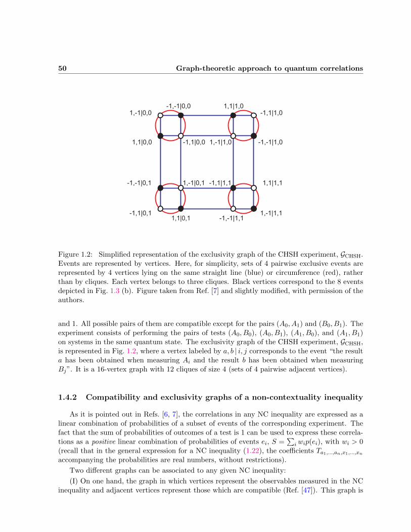
50 Graph-theoretic approach to quantum correlations
1,-1|0,0-1,-1|0,0
1,1|0,0 -1,1|0,0
1,-1|0,1-1,-1|0,1
-1,1|0,11,1|0,1 -1,-1|1,1
1,1|1,0-1,1|1,0
-1,-1|1,01,-1|1,0
-1,1|1,1 1,1|1,1
1,-1|1,1
Figure 1.2: Simplified representation of the exclusivity graph of the CHSH experiment, GCHSH.Events are represented by vertices. Here, for simplicity, sets of 4 pairwise exclusive events arerepresented by 4 vertices lying on the same straight line (blue) or circumference (red), ratherthan by cliques. Each vertex belongs to three cliques. Black vertices correspond to the 8 eventsdepicted in Fig. 1.3 (b). Figure taken from Ref. [7] and slightly modified, with permission of theauthors.
and 1. All possible pairs of them are compatible except for the pairs (A0, A1) and (B0, B1). Theexperiment consists of performing the pairs of tests (A0, B0), (A0, B1), (A1, B0), and (A1, B1)on systems in the same quantum state. The exclusivity graph of the CHSH experiment, GCHSH,is represented in Fig. 1.2, where a vertex labeled by a, b | i, j corresponds to the event “the resulta has been obtained when measuring Ai and the result b has been obtained when measuringBj”. It is a 16-vertex graph with 12 cliques of size 4 (sets of 4 pairwise adjacent vertices).
1.4.2 Compatibility and exclusivity graphs of a non-contextuality inequality
As it is pointed out in Refs. [6, 7], the correlations in any NC inequality are expressed as alinear combination of probabilities of a subset of events of the corresponding experiment. Thefact that the sum of probabilities of outcomes of a test is 1 can be used to express these correla-tions as a positive linear combination of probabilities of events ei, S =
∑iwip(ei), with wi > 0
(recall that in the general expression for a NC inequality (1.22), the coefficients Ta1,...,an,x1,...,xnaccompanying the probabilities are real numbers, without restrictions).
Two different graphs can be associated to any given NC inequality:
(I) On one hand, the graph in which vertices represent the observables measured in the NCinequality and adjacent vertices represent those which are compatible (Ref. [47]). This graph is

1.4 CSW’s graph-theoretic approach to quantum correlations 51
A0
A1
B0B1
1,1|0,0
-1,-1|0,0
1,1|0,1
1,-1|1,1 -1,1|1,1
1,1|1,0
-1,-1|1,0 -1,-1|0,1
(b)(a)
Figure 1.3: (a) The compatibility graph of the local observables in the CHSH experiment. (b)The exclusivity graph GCHSH of the CHSH inequality (1.25).
the so-called compatibility graph. For example, consider the CHSH inequality in Ref. [46],
β = 〈A0B0〉+ 〈A0B1〉+ 〈A1B0〉 − 〈A1B1〉NCHV
≤ 2, (1.23)
where 〈AiBj〉 denotes the mean value of the product of the results of measuring the observables
Ai and Bj , each of them with possible results either −1 or 1, andNCHV
≤ 2 indicates that 2 isthe maximum value for β for NCHV theories. As we have said before, all possible pairs ofobservables in the CHSH experiment are compatible except for the pairs (A0, A1) and (B0, B1).Therefore, the compatibility graph12 is the one depicted in Fig. 1.3 (a).
(II) On the other hand, by taking into account that
± 〈AiBj〉 = 2[p(1,±1 | i, j) + p(−1,∓1 | i, j)]− 1, (1.24)
where p(a, b | i, j) is the probability of the event “the result a has been obtained when measuring
12Remarkably, there is a connection between the compatibility graph of a set of observables and the existenceof a joint probability distribution for them. In Refs. [48, 22] the authors prove that for any set of observableswhose corresponding compatibility graph is a chordal graph (i.e., a graph which does not contain induced cyclesof size greater than 3), there always exists a joint probability distribution reproducing the quantum marginals.They also provide a graph theoretical method to construct such joint probability distribution on the basis of thecompatibility graph. Let us note that the CHSH compatibility graph of Fig. 1.3 (a) is the 4-cycle, C4, which is nota chordal graph: this entails the lack of a joint probability distribution for the set of observables A0, A1, B0, B1,a reason behind the violation of the NC inequality (1.23).

52 Graph-theoretic approach to quantum correlations
Ai and the result b has been obtained when measuring Bj ,” inequality (1.23) can be written as
SCHSH =β
2+ 2 = p(1, 1 | 0, 0) + p(−1,−1 | 0, 0) + p(1, 1 | 0, 1) + p(−1,−1 | 0, 1)
+ p(1, 1 | 1, 0) + p(−1,−1 | 1, 0) + p(1,−1 | 1, 1) + p(−1, 1 | 1, 1)NCHV
≤ 3,
(1.25)
where the left-hand side is now a convex sum of probabilities of events. A new graph can beassociated to the set of events, one in which the vertices represent the events and adjacentvertices represent events that cannot occur simultaneously (i.e., exclusive events). This is theso-called exclusivity graph (see Ref. [6]). For example, the exclusivity graph for the CHSHinequality (1.25), denoted as GCHSH, is depicted in Fig. 1.3 (b). Let us note that the set of 8events appearing in (1.25) constitutes a subset of the 16 events of the whole CHSH experiment(those corresponding to the black vertices in Fig. 1.2): GCHSH is the induced subgraph13 ofGCHSH obtained by removing all but the 8 black vertices.14 GCHSH is isomorphic to the 8-vertexcirculant (1, 4) graph, Ci8(1, 4).
Whereas in the previous CHSH example and in other NC inequalities (like, for instance,Wright’s inequality in Ref. [49]) all probabilities have weight 1, that need not be the case ingeneral: in an arbitrary NC inequality, expressed as a linear combination of probabilities ofevents S =
∑iwip(ei) with wi > 0, each probability p(ei) may have a different weight wi,
and hence the exclusivity graph associated to S will be a vertex-weighted graph15 (G,w), whereG ⊆ G. For such graph, a vertex i ∈ V (G) represents an event ei such that p(ei) is in S,adjacent vertices represent exclusive events, and the vertex weights represent the weights wi ofthe probabilities p(ei).
In the following subsections we present the two main results obtained in Refs. [6, 7] on whichthis part of our thesis is based.
1.4.3 Correlations in theories satisfying the exclusivity principle
Quantum theory (QT) is the most successful scientific theory of all times. However, it is stillnot known how to derive it from fundamental physical principles. Recently, this problem hasbeen addressed from different perspectives. One consists of reconstructing QT from information-theoretic axioms (see Refs. [50, 51, 52, 53, 54, 55]). However, these reconstructions fail to
13An induced subgraph H of a given graph F is obtained by selecting a subset of the vertices of F and theirincident edges in such a way that for any pair of vertices i and j of H, ij is an edge of H if and only if ij isan edge of F . Alternatively, it is a subgraph obtained by deleting a subset of the vertices of F along with theirincident edges.
14Note that taking the 16 events, the normalization of the probabilities, namely,
p(1, 1 | i, j) + p(1,−1 | i, j) + p(−1, 1 | i, j) + p(−1,−1 | i, j) = 1, ∀ i, j = 0, 1, (1.26)
and no-signaling conditions between the pairs (A0, A1) and (B0, B1), namely,
p(a | i) = p(a, 1 | i, j) + p(a,−1 | i, j),∀ a = −1, 1;∀ i, j = 0, 1, (1.27a)
p(b | j) = p(1, b | i, j) + p(−1, b | i, j), ∀ b = −1, 1;∀ i, j = 0, 1, (1.27b)
determine the probabilities of the “white events” given the probabilities of the “black events”.15A vertex-weighted graph (G,w) is a graph G with vertex set V (G) and weight assignment w : V (G)→ R+.

1.4 CSW’s graph-theoretic approach to quantum correlations 53
capture the “physical assumptions that give rise to the theory”, according to Refs. [56, 57].Another approach, initiated by the work of Popescu and Rohrlich in Ref. [58], tries to identifythe principles behind quantum nonlocal correlations (Refs. [59, 60, 61, 62, 63, 64, 65, 66]).Here one problem is that principles such as information causality (Ref. [61]) and macroscopiclocality (Ref. [62]) have been proved to fail to exclude non-quantum correlations in tripartitescenarios (see Refs. [63, 64]). However, the main limitation of this approach is that it renouncesto explain quantum correlations between experiments that are not space-like separated, whilequantum correlations are ubiquitous.
Nothing in the known rules of QT supports the previous supposition according to whichexperiments with space-like separation are more fundamental than other types of correlationexperiments. As pointed out in Refs. [6, 7], a more general approach to account for quantumcorrelations follows from the question of whether there exists a joint probability distribution thatgives the marginal probabilities predicted by QT, which is equivalent to the question of whethera specific set of linear correlation inequalities is satisfied (Bell inequalities, for experiments withspace-like separated tests; and NC inequalities, for more general scenarios).
As we have said before, the experimental violation of NC inequalities reveals contextual cor-relations that cannot be explained by NCHV theories. In this sense, QT is contextual. In orderto account for such contextual quantum correlations, QT is contrasted in Ref. [7] with NCHVtheories and with a general class of theories assigning probabilities to events, namely, probabilis-tic theories satisfying the E principle (see 1.1.6), according to which the sum of probabilitiesof any set of pairwise exclusive events cannot be higher than 1. This class has been previouslyconsidered in Refs. [17, 49]. Specker noticed that classical theories and QT satisfy this principle,but that there are theories that do not (Refs. [17, 1]).
Given an NC inequality S and its pertaining exclusivity graph (G,w), it is convenient todenote by E1 those theories satisfying the E principle applied to the probabilities assigned tothe vertices of G alone (or, as it is usually said, to “one copy of G”). Here, the index 1 in E1 isused to distinguish these theories from those satisfying the E principle applied jointly to G andother independent graphs, Refs. [19, 20, 67, 2] (for instance, by En we would designate theoriessatisfying the E principle applied to the entire set of probabilities assigned independently to thevertices of n copies of a given graph G).
In Refs. [6, 7], the set of correlations obeying E1, denoted by E1(G), is defined as
E1(G) :=
p ∈ R|V |+ :
∑i∈C
pi ≤ 1 for all cliques C
. (1.28)
Moreover, E1(G) is exactly the fractional stable set polytope (or clique-constrained stable setpolytope) of G, QSTAB(G), introduced in Ref. [68].
Let us emphasize that if (G,w) is the exclusivity graph of an NC inequality, then a cliqueC ∈ V (G) corresponds to a set of pairwise exclusive events, and the condition
∑i∈C pi ≤ 1
formulates the E principle (see 1.1.6) applied to one copy of G. For our purposes, the importantassertion is this: correlations obeying E1 also obey the no-signaling principle . In fact, the setof E1-correlations, E1(G), is a proper or strict subset of P(G), the no-signaling polytope16 of
16For the proof of these statements we refer the reader to Ref. [6] (Appendix, [ii]); and also to Ref. [65], where

54 Graph-theoretic approach to quantum correlations
G. We refer the reader to Figs. 1.1 and 1.4 for a pictorial representation of the relationships ofinclusion for the different sets of correlations.
1.4.4 The limits of the correlations in NCHV theories, quantum theory andtheories satisfying the E principle
The exclusivity graph of S can be used to calculate the limits of the correlations in NCHVtheories, QT and theories satisfying E1. Three combinatorial numbers characteristic of (G,w)provide such limits: the independence number, the Lovasz number and the fractional packingnumber. We give the definitions below.
Let (G,w) be a vertex-weighted graph with vertex set V , and wi the weight correspondingto vertex i ∈ V . An independent or stable set of G17 is a set of pairwise nonadjacent vertices ofG. The independence number of (G,w), denoted by α(G,w), is the maximum of
∑iwi taken
over all stable sets of vertices of G (Ref. [69]). When all the vertices have weight 1 (unweightedgraph) the independence number is denoted as α(G), and is equal to the cardinality of thelargest independent set of G (Ref. [70]).
An orthonormal representation (OR) in Rd of a graph G with vertex set V assigns a nonzerounit vector |vi〉 ∈ Rd to each i ∈ V such that 〈vi|vj〉 = 0 for all pairs i, j of nonadjacentvertices. A further unit vector |ψ〉 ∈ Rd, usually called handle (Ref. [71]), is sometimes specifiedtogether with the OR. The definition of OR does not require that different vertices be mappedonto different vectors nor that adjacent vertices be mapped onto nonorthogonal vectors.18 Thecomplement G of a graph G is the graph with vertex set V such that two vertices i, j areadjacent in G if and only if i, j are not adjacent in G. The Lovasz number of (G,w) can bedefined following Refs. [71, 72, 69] as
ϑ(G,w) := max∑i∈V
wi|〈ψ|vi〉|2, (1.29)
where the maximum is taken over all ORs of G and handles in any dimension.The fractional packing number (or fractional stability number) of (G,w) (Refs. [72, 69, 68]),
denoted by α∗(G,w), is defined as
α∗(G,w) := max∑i∈V
wipi, (1.30)
where the maximum is taken over all pi ≥ 0 and for all cliques C of G, under the restriction∑i∈C pi ≤ 1.19
the authors introduce the so-called local orthogonality (LO) principle —which may be seen as the E principlerestricted to Bell scenarios— and prove that, while the set of LO correlations coincides with the set of no-signalingcorrelations in the bipartite case, it is strictly smaller for more than two parties. That is, the LO principle is morerestrictive than the no-signaling principle in the multipartite case. Recall that quantum correlations fulfill the E(or LO, in Bell scenarios) principle.
17Since the adjacency relationship between vertices does not depend on the vertex weight assignment, and forthe sake of simplicity, we omit reference to weights when it is not necessary.
18If these conditions also hold, the OR is called faithful.19Recall that, when (G,w) is the exclusivity graph of an NC inequality, this last restriction imposes that the
sum of the probabilities of any set of pairwise exclusive events in S (such sets correspond to cliques in G) cannotexceed 1, which is the content of the E principle, in 1.1.6.

1.4 CSW’s graph-theoretic approach to quantum correlations 55
The independence number is a lower bound of the Shannon capacity Θ(G) of a graph G(Ref. [68]), whereas the Lovasz number and the fractional packing number are upper bounds ofΘ(G). The comparison between one another gives (Ref. [71])
α(G) ≤ ϑ(G) ≤ α∗(G), (1.31)
and this relationship also holds for the weighted versions of these combinatorial numbers (Ref. [69]).
Result 1 (Ref. [7]): Given S corresponding to a Bell or NC inequality, the maximum valueof S for classical (LHV and NCHV) theories, QT, and theories satisfying E1 is given by
SLHV,NCHV
≤ α(G,w)QT
≤ ϑ(G,w)E1
≤ α∗(G,w), (1.32)
where (G,w) is the exclusivity graph of S.
For example, applying Result 1 to SCHSH (1.25), whose exclusivity graph is the one in Fig 1.3(b), one obtains α(GCHSH) = 3, ϑ(GCHSH) = 2 +
√2, and α∗(GCHSH) = 4, which correspond
to the maximum for LHV (Ref. [46]) and NCHV theories, QT (Ref. [73]), and no-signaling20
theories (Ref. [58]), respectively.
1.4.5 The Lovasz number as a physical limit and the set of quantum corre-lations
Note that ϑ(G,w) might be only an upper bound to the maximum quantum value of Sin cases in which the particular physical settings of the experiment testing S add further con-straints.21 A typical example of this circumstance is a Bell inequality, which is a particularinstance of NC inequality satisfied by LHV theories, where compatible settings are assumed tocorrespond to different space-like separated parties (in a general NC inequality, however, compat-ibility of measurements does not have to follow from the space-like separation of observers). Thisadditional constraint could prevent the maximum quantum value of S from reaching ϑ(G,w).22
In the light of this, a natural question is whether, given G, there is a NC inequality thatreaches ϑ(G).
Result 2 (Ref. [7]): For any graph G, there is always a NC inequality such that the quantummaximum is exactly ϑ(G) and the set of quantum probabilities is exactly the Grotschel-Lovasz-Schrijver theta body TH(G) (Ref. [69]).
The proof, that we transcribe here almost literally, is the following (Ref. [7]): given G,by definition (1.29), there is always an OR of G in Rd, |vi〉, and a handle |ψ〉 such thatϑ(G) =
∑i∈V |〈ψ|vi〉|2 [i.e, an OR of G providing ϑ(G)]. Let D be the minimum dimension d in
20Recall the previous comment about no-signaling correlations and correlations obeying E1, in 1.4.3, p. 53. Fora 2-party Bell scenario, like CHSH, E1 and no-signaling principles define the same set of correlations.
21We have dealt with a similar issue when discussing no-signaling correlations and the rather ad hoc distinctionbetween the no-signaling and no-disturbance principles. See p. 43.
22For example, as we have just mentioned, the maximum quantum value of SCHSH in (1.25) is equal to 2 +√2, which is exactly ϑ(GCHSH) = ϑ[Ci8(1, 4)], and this value is achievable regardless of the possible space-like
separation between measurements Ai and Bj . On the contrary, if G is a pentagon, C5, although there exist NCinequalities for which the maximum quantum value is ϑ(C5) =
√5 (see Refs. [49, 74]), there is no Bell inequality
reaching ϑ(C5) (Ref. [27]).

56 Graph-theoretic approach to quantum correlations
which this OR exists. Then, consider the following positive linear combination of probabilitiesof events:
S =∑i∈V
P (1, 0, . . . , 0|i, i1, . . . , in(i)), (1.33)
where test i is defined as Πi = |vi〉〈vi|, with |vi〉 in the OR, test ij is Πij = |vij 〉〈vij |, with |vij 〉in the OR, and i1, . . . , in(i) is the set of tests corresponding to vertices adjacent to i. Notethat 1, 0, . . . , 0|i, i1, . . . , in(i), which belongs to the same equivalence class as 1|i (see 1.1.4; bothof them are possible realizations of the same event), is a repeatable event with a well-definedprobability, even though i, i1, . . . , in(i) need not be compatible tests.
The important point is that S so defined reaches ϑ(G) when a quantum system is prepared inthe quantum state |ψ〉, and this fact identifies ϑ(G) as a fundamental physical limit for quantumcorrelations.
On the other hand, in QT, the set of probabilities that can be assigned to the vertices of Gby performing tests on a quantum system is
Q(G) :=
(|〈ψ|vi〉|2 : i ∈ V ) : (|vi〉 : i ∈ V ) is an OR of G and |ψ〉 a handle. (1.34)
If the quantum system has dimension greater than or equal to D, then Q(G) is exactly the thetabody TH(G) introduced in Ref. [69] (see Theorem 3.5 in Ref. [69] and Corollary 9.3.22 (c) inRef. [75]).
In other words, given any graph G, there is always a correlation experiment in which thewhole set of quantum probabilities for G can be reached, and TH(G) is such set of physicalcorrelations for G.
Let us note that, according to Refs. [6, 7], and for a given exclusivity graph G, the set-inclusion relationship among the set of quantum correlations Q(G) (that is, the theta bodyTH(G)), the set of classical correlations C(G) (coincident with the stable set polytope or vertexpacking polytope, STAB(G), in Ref. [69]), and the set of correlations obeying the E1 princi-ple, E1(G) (which is exactly the fractional stable set polytope or clique-constrained stable setpolytope, QSTAB(G)), is given by
C(G) ⊆ Q(G) ⊆ E1(G), (1.35)
since STAB(G) ⊆ TH(G) ⊆ QSTAB(G) after Ref. [69]. Such relationship23 is depicted inFig. 1.4, which is inspired in another figure taken from Ref. [76]. Note that in Fig. 1.4 the setsrefer to a particular exclusivity graph G, whereas in Fig. 1.1 the depicted sets of correlationsare general, in the sense that they do not refer to a particular exclusivity graph G, but to everypossible correlations of each type: local, quantum, no-signaling or general.
1.4.6 Suggested developments and connections to our work
As the authors point out, Results 1 and 2 in Ref. [7] would allow to design experiments withquantum contextuality on demand by selecting graphs with the desired relationships between
23The relation of set-inclusion among these sets may be strict or not, depending on the graph G. A directexample: consider a perfect graph, i.e., a graph which does not contain, as induced subgraph, any cycle orcomplement of a cycle with an odd number of vertices equal or greater than five. Then, STAB(G) = TH(G). Infact, it is proven in Ref. [69] that STAB(G) = TH(G) if and only if G is a perfect graph.

1.4 CSW’s graph-theoretic approach to quantum correlations 57
Figure 1.4: Schematic representation of the set-inclusion relationship among the theta bodyTH(G), which is in general a convex set but not a polytope, and the stable set and fractionalstable set polytopes, STAB(G) and QSTAB(G). Note that the set-inclusion relationship amongthese three sets may or may not be strict, depending on the combinatorial numbers characteristicof the graph G.
α(G), ϑ(G) and α∗(G), graphs for which a general method to construct NC inequalities isprovided.
As we emphasize in Chap. 2, any experiment producing quantum contextual correlations canbe associated to an exclusivity graph G for which α(G) < ϑ(G). A graph with this property iscalled there a quantum contextual graph (QCG), whereas one fulfilling α(G) = ϑ(G) is called aquantum noncontextual graph (QNCG). According to Ref. [7], specifically, for every QCG thereis a NC inequality with classical limit given by α(G) and quantum violation given by ϑ(G).
In addition, making use of Results 1 and 2 in Ref. [7], a question such as which are thecorrelations with maximum quantum contextuality can now be addressed, since it can be relatedto the question of which graphs have the maximum ratio ϑ(G)/α(G) for a given number ofvertices. Similarly, all possible forms of quantum contextuality can be classified by classifyinggraphs according to their combinatorial numbers.
We tackle the above-mentioned proposals in Sect. 1.5: a complete classification of QCGs upto 10 vertices is provided, which allows to identify experimental scenarios with correlations ondemand by picking out graphs with the required properties, and classify quantum correlationsthrough the study of their graph combinatorial numbers.
On the other hand, for every G such that α(G) < ϑ(G) = α∗(G), there is a NC inequalityin which the maximum quantum violation cannot be higher without violating the E principle(Ref. [7]). In Chap. 3 we refer to quantum correlations achieving α∗(G) as quantum fully con-textual correlations. Accordingly, we can denominate such a graph as quantum fully contextualgraph (QFCG). Finding the simplest QFCGs is possible once a classification of QCGs with re-spect to their combinatorial numbers is at disposal, by selecting the graphs fulfilling the desiredconstraints. In Sect. 1.5 we identify the four simplest QFCGs on the basis of our classification.

58 Graph-theoretic approach to quantum correlations
Moreover, in Chap. 3 we single out the QFCG for which the violation of the associated NCinequality requires a physical system of lower dimension, and describe the experiment testingsuch NC inequality and revealing experimental fully contextual quantum correlations for thefirst time.
Finally, Result 2 in Ref. [7] suggests that an important question for understanding quan-tum correlations is which is the principle that singles out TH(G) among all possible sets ofprobabilities that can be assigned to the vertices of G. A way to consider such question is to un-derstand why QT only violates some NC inequalities, and to elucidate what physical principlesprevent higher-than-quantum violations. The E principle has recently revealed as one promis-ing candidate to accomplish the goal in Refs. [77, 19, 20, 21]. Our contribution in Ref. [78] tothis fundamental problem is the subject of Chap. 2: we prove that QT only violates those NCinequalities whose exclusivity graphs contain, as induced subgraphs, odd cycles of length fiveor more, and/or their complements. In addition, we show that odd cycles are the exclusivitygraphs of a well-known family of NC inequalities and that there is also a family of NC inequali-ties whose exclusivity graphs are the complements of odd cycles. We characterize the maximumnon-contextual and quantum values of these inequalities, and provide evidence supporting theconjecture that the maximum quantum violation of these inequalities is exactly singled out bythe E principle.
1.5 Classification of contextual exclusivity graphs
As we have asserted in the previous section, quantum contextuality is experimentally ob-served through the violation of NC inequalities. For each NC inequality S(G) formulated interms of a positive linear combination of probabilities of events there is an associated exclusivitygraph G whose independence, Lovasz and fractional packing numbers provide the limits of cor-relations in NCHV theories, QT and theories satisfying the E principle, respectively. By virtueof this graph-theoretic approach, the problem of singling out all NC inequalities with a quantumviolation becomes equivalent to the problem of identifying all QCGs, i.e., those graphs for whichα(G) < ϑ(G). A classification of QCGs is, therefore, a powerful tool to identify experiments ofphysical relevance.
We addressed the elaboration of a classification of QCGs according to their combinatorialnumbers α(G), ϑ(G) and α∗(G). For that purpose, we generated all non-isomorphic simpleconnected graphs with less than 11 vertices using nauty, Ref. [79]. There are 11989764 of them.For each of them we calculated α(G) using Mathematica (Ref. [80]) and ϑ(G) using SeDuMi
(Ref. [81]) and DSDP (Refs. [82, 83]). There are 992398 graphs for which α(G) < ϑ(G). Then,we calculated α∗(G) using Mathematica from the clique-vertex incidence matrix of G obtainedfrom the adjacency matrix of G using MACE (Refs. [84, 85]), an algorithm for enumerating allmaximal cliques.
In addition, we obtained the minimum dimensionality d(G) of the quantum system in whichthe maximum quantum violation of S(G) occurs, or a lower bound of d(G), by identifyingsubgraphs in G which are geometrically impossible in a space of lower dimensionality. Forexample, the simplest impossible graph in dimension d = 1 consists of two non-adjacent vertices;in d = 2, three vertices, one of them adjacent to the other two. From these two impossible graphs,

1.5 Classification of contextual exclusivity graphs 59
one can recursively construct impossible graphs in any dimension d by adding two vertices linkedto all vertices of an impossible graph in d − 2. For example, if a graph contains a square (a4-cycle), then d > 3.24
This procedure results in a list containing G, α(G), ϑ(G), α∗(G) and d(G) [or a lower boundof d(G)]. From this list we filtered out those graphs for which α(G) = ϑ(G), i.e., QNCGs, andkept the remaining graphs (i.e., the QCGs).
In order to organize the resulting information, we also calculated the minimum dimensionalityof a classical system reproducing the exclusivity relationships among events in S(G), i.e., theadjacency relationships in G. Such number is given by a property of G known in graph theoryas the intersection number25 (Ref. [86]) of the complement of G, i(G). For that calculationwe employed a program based on nauty, very-nauty (Refs. [87, 88]). Then, we introduced ameasure of quantumness, given by
Q(G) =ϑ(G)− α(G)
i(G), (1.36)
and a measure of how close the maximun quantum value is from the largest violation allowedby theories satisfying E1, namely,
E(G) =α∗(G)− ϑ(G)
i(G). (1.37)
We then ordered the QCGs attending to the following criteria: (i) n(G) = |V (G)|, (ii) Q(G),(iii) (decreasing) E(G), (iv) d(G), (v) |E(G)| (number of edges of G), (vi) size of the largestclique (subset of pairwise connected vertices), and (vii) number of cliques with the largest size.
1.5.1 Results
An ordered list containing G, α(G), ϑ(G), and α∗(G) for all graphs with less than 11 verticesfor which α(G) < ϑ(G) is provided in Ref. [8]. In Table 1.1, we present the total number ofnon-isomorphic simple connected graphs for a number of vertices ranging from 2 to 10; thenumber of them which are QCGs [α(G) < ϑ(G)], and for the latter, the number of those whichare QFCGs [α(G) < ϑ(G) = α∗(G)]. We can extract some conclusions:
On one hand, there are no QCGs with a number of vertices less than 5. In Fig. 1.5 we presenta sample with the 37 simplest QCGs, those corresponding to a number of vertices ranging from5 to 7, along with data corresponding to the values of α(G), ϑ(G), d(G) or a lower bound of it(in parentheses), and α∗(G), for each graph G. The simplest QCG is the pentagon or 5-cycle,C5, depicted in red in Fig. 1.5, which is the exclusivity graph corresponding to the Wright andKlyachko-Can-Binicioglu-Shumovsky NC inequalities in Refs. [49, 74]. A careful inspection ofthe figure reveals that all the graphs shown in it contain C5 as induced subgraph, with theexception of two: the heptagon (C7) and its complement (C7), both also depicted in red. Thisthree graphs belong to a well-known family in graph theory: the so-called odd holes and odd
24See 2.4 for an application of this argument to the complements of odd cycles. In brief, the graph F obtainedby deleting bd/2c disjoint edges from a d-vertex complete graph Kd is an impossible subgraph in dimension d− 1.
25This number is described in detail on p. 84, in a different context.

60 Graph-theoretic approach to quantum correlations
antiholes (see p. 65 for a definition, and a brief outline of their interest in graph theory). Asubsequent analysis of the QCGs of up to 10 vertices, the scope of our classification, suggeststhat all QCGs might necessarily contain odd holes and/or odd antiholes as induced subgraphs(Ref. [78]). The deep insight encompassed by this fact is the main thrust of Chap. 2, where wedeal with this issue in detail, and give the corresponding proof.
Table 1.1: Number of non-isomorphic simple connected graphs, QCGs and QFCGs with anumber of vertices up to 10.
Vertices Connected graphs QCGs QFCGs
< 5 10 0 05 21 1 06 112 3 07 853 33 08 11117 498 09 261080 16533 010 11716571 975330 4
On the other hand, there is no QFCG with less than 10 vertices. The simplest ones are thefour 10-vertex graphs depicted in Fig. 1.6. Given that for such graphs α(G) < ϑ(G) = α∗(G),there is an NC inequality associated to each of them in which the maximum quantum violationcannot be higher without violating the E principle. Achieving such maximum quantum violationwould reveal, therefore, fully contextual quantum correlations. Graph (c) in Fig. 1.6, which weshall call S3, is the graph corresponding to the simplest NC inequality capable of revealingfully contextual quantum correlations, from the viewpoint of the dimensionality of the requiredquantum system (see Ref. [89]). Graph (d) in Fig. 1.6 is the Johnson graph J(5, 2), which isthe complement of the Petersen graph (a well-known graph in the field of graph theory; seeFig. 4.3 (b)). J(5, 2) is the exclusivity graph corresponding to Cabello’s twin-inequality inRef. [90], which is the simplest NC inequality capable of revealing fully contextual quantumcorrelations, from the viewpoint of the number of experiments (involving yes-no tests) needed.Graphs (a) and (b) are essentially as graph (c) minus one or two edges, and do not outperform(c) nor (d) regarding the number of experiments needed or the dimensionality of the quantumsystem required. Graph S3 and its corresponding NC inequality, and the experiment revealingfully contextual quantum correlations on the basis of them, is the main issue of Chap. 3, towhich we refer the reader for further details.

1.5 Classification of contextual exclusivity graphs 61
No. 1 No. 2 No. 3 No. 4
No. 5 No. 6 No. 7 No. 8 No. 9 No. 10
No. 11 No. 12 No. 13 No. 14 No. 15 No. 16
No. 17 No. 18 No. 19 No. 20 No. 21 No. 22
No. 23 No. 24 No. 25 No. 26 No. 27 No. 28
No. 29 No. 30 No. 31 No. 32 No. 33 No. 34
No. 35 No. 36 No. 37
Figure 1.5: Quantum contextual graphs up to 7 vertices. In red, the pentagon or 5-cycle, C5;the heptagon or 7-cycle, C7; and the complement of the heptagon, C7.

62 Graph-theoretic approach to quantum correlations
79
34 8
610
1
25
(b)
79
34 8
610
1
25
79
34 8
610
1
25
(a)
79
34 8
610
1
25
79
34 8
610
1
25
(c)
79
34 8
610
1
25
79
34 8
610
1
25
(d)
79
34 8
610
1
25
Figure 1.6: The four simplest quantum fully contextual graphs. Graph (c) is S3 (see main text).Graphs (a) and (b) are the same as (c), minus one or two edges. Graph (d) is the Johnson graphJ(5, 2), which is the complement of the Petersen graph.

Chapter 2
Basic exclusivity graphs in quantumcorrelations
In this chapter we present the results obtained in Ref. [78]. Below we provide a brief summary.
Summary: A fundamental problem is to understand why quantum theory only violates someNC inequalities and identify the physical principles that prevent higher-than-quantumviolations. We prove that quantum theory only violates those NC inequalities whoseexclusivity graphs contain, as induced subgraphs, odd cycles of length five or more, and/ortheir complements. In addition, we show that odd cycles are the exclusivity graphs of awell-known family of NC inequalities and that there is also a family of NC inequalitieswhose exclusivity graphs are the complements of odd cycles. We characterize the maximumnon-contextual and quantum values of these inequalities, and provide evidence supportingthe conjecture that the maximum quantum violation of these inequalities is exactly singledout by the E principle.
2.1 Introduction
Quantum contextuality1, namely, the fact that the quantum correlations between the resultsof compatible measurements cannot be reproduced with NCHV theories (Refs. [17, 29, 30]) isbehind a wide spectrum of applications of QT to communication and computation (Refs. [91,42, 92, 41, 93, 45]). Quantum contextual correlations are experimentally detected through theviolation of inequalities satisfied by NCHV models, called NC inequalities (Refs. [94, 74, 95,96]). A fundamental problem is to understand why QT only violates some NC inequalities andidentify the physical principles that prevent higher-than-quantum violations of these inequalities(Refs. [61, 62, 97, 19]).
In this chapter we investigate this problem. We will use, as a main tool throughout thechapter, the exclusivity graph of an NC inequality which was already introduced in Sect. 1.4.2. InSect. 2.3, we present a necessary condition for the existence of quantum contextual correlations:We prove that QT violates only those NC inequalities whose exclusivity graphs contain, as
1See Sect. 1.3 for a accurate definitions of quantum contextuality and NC inequalities.

64 Basic exclusivity graphs in quantum correlations
induced subgraphs, odd cycles on five or more vertices and/or their complements. In Sect. 2.4,we show that a lower bound of the dimension (i.e., of the number of perfectly distinguishablestates) of the quantum system that is used to violate an NC inequality can be obtained byidentifying induced basic exclusivity subgraphs in the exclusivity graph of the NC inequality.
The result in Sect. 2.3 suggests that NC inequalities whose exclusivity graph is either anodd cycle or its complement are especially important for understanding the way QT violates NCinequalities. In Sect. 2.5, we show that each of these types of exclusivity graphs is connected toa family of NC inequalities and provide the quantum states and measurements leading to themaximum quantum violation. Finally, in Sect. 2.6 we present some results that suggest thatthe E principle, namely, that the sum of the probabilities of a set of pairwise exclusive eventscannot exceed 1, explains the maximum quantum violation of all the NC inequalities discussedin Sect. 2.5.
2.2 The exclusivity graph of a non-contextuality inequality
As we pointed out in some detail in Sect. 1.4.2, the correlations in any NC inequality canbe expressed as a linear combination of probabilities of a subset of events of the correspondingexperiment. The fact that the sum of probabilities of outcomes of a test is 1 (normalization con-dition) allows us to express these correlations as a positive linear combination S of probabilitiesof events ei, that is, S =
∑iwip(ei), with wi > 0. The exclusivity graph G of the NC inequality
S is the one in which the vertices represent the events and adjacent vertices represent mutuallyexclusive events (Refs. [6, 7]).
The interest of the exclusivity graph G is that the maximum value of S for NCHV theoriesis exactly given by the independence number of the graph α(G) (which is the maximum numberof pairwise nonadjacent vertices in G), while the maximum value in QT is upper bounded (andfrequently exactly given) by the Lovasz number of the graph ϑ(G) (Refs. [6, 7]). We refer thereader to Sect. 1.4.4 for definitions and a precise formulation of this fact.
The important point is that any experiment producing quantum contextual correlations canbe associated to an exclusivity graph G for which α(G) < ϑ(G). Hereafter, as we previously havedone in Sect. 1.4.6, we will refer to a graph with this property as a quantum contextual graph(abbreviated QCG), and to a graph for which α(G) = ϑ(G) as a quantum non-contextual graph(abbreviated QNCG). We provide a classification of all QCGs up to 10 vertices in Sect. 1.5.
2.3 Basic exclusivity graphs
The following definition is necessary to present out first result: A subgraph H of a graph Gis said to be induced if, for any pair of vertices i and j of H, ij is an edge of H if and only ifij is an edge of G. For example, a graph G has an induced pentagon if it is possible to removefrom G all but five vertices (and their corresponding edges) so that we end up with a pentagonwith no additional edges.
Result 1: The exclusivity graph of any NC inequality violated by QT contains, as inducedsubgraphs, odd cycles on five or more vertices and/or their complements.

2.3 Basic exclusivity graphs 65
This result2 is based on two fundamental results in graph theory: The strong perfect graphtheorem and the (weak) perfect graph theorem. Perfect graphs were introduced in Ref. [98] inconnection to the problem of the zero-error capacity of a noisy channel in Ref. [68]: Shannonobserved that ω(G∗n) = ω(G)n for graphs such that ω(G) = χ(G), which made the problemof characterizing the Shannon capacity of such graphs more tractable [G∗n is the disjunctiveproduct3 of n copies of G, ω(G) is the clique number, and χ(G) is the chromatic number of G; ingeneral, ω(G) ≤ χ(G)]. Berge defined perfect graphs as those graphs G for which ω(H) = χ(H)for each induced subgraph H ⊆ G. Berge observed that all odd cycles Cn with n ≥ 5 (knownin graph theory as “odd holes”) and their complements Cn (known as “odd antiholes”) satisfyω(G) < χ(G). From this result, Berge conjectured that a graph G is perfect if and only if Ghas no odd hole or odd antihole as induced subgraph (strong perfect graph conjecture). Thisconjecture has been recently proven in Ref. [100], and it is now known as the strong perfectgraph theorem. The simplest odd holes and antiholes are illustrated in Fig. 2.1.
The perfect graph conjecture (due also to Berge), which was later proved by Lovasz inRef. [101] and is now known as the (weak) perfect graph theorem, states that if G is a perfectgraph, then its complement, G, is also a perfect graph.
Theorem 1: Let G be the exclusivity graph of an NC inequality. If G is a perfect graph, thenG is a QNCG and, as a consequence, the NC inequality is not violated by QT.
Proof: If G is perfect, then ω(G) = χ(G). On the other hand, according to the sandwichtheorem in Ref. [102], ω(G) ≤ ϑ(G) ≤ χ(G) for any graph G. Hence, G perfect implies ω(G) =ϑ(G) = χ(G). Given that ω(G) = α(G), we obtain α(G) = ϑ(G), i.e., if G is a perfect graph,then G is a QNCG. Applying now the (weak) perfect graph theorem, if G is perfect, then Gis also perfect. Therefore, repeating the previous argument the other way around we concludethat G is a QNCG as well: α(G) = ϑ(G). This finishes the proof.
Corollary 1: If G is a QCG, i.e., if G is the exclusivity graph of an NC inequality violated byQT, then G is not perfect. Consequently, by the strong perfect graph theorem, G must containodd holes and/or odd antiholes as induced subgraphs.
This proves Result 1.Observation 1: A NC inequality not violated by QT may contain an NC inequality violated
by QT. This means that, even if the exclusivity graph of the initial NC inequality is not a QCG,the exclusivity graph of the initial NC inequality may have an induced subgraph that is a QCG.
Observation 2: No odd cycle or complement of an odd cycle has an odd cycle or a complementof an odd cycle as an induced subgraph. This suggests that odd cycles and their complementscould be used as a basis for a decomposition of any exclusivity graph.
Observation 3: The basic exclusivity graphs necessary for quantum contextuality are thesame basic graphs necessary for graph nonperfectness.
2One of the conclusions in Sect. 1.5.1, derived on the basis of the classification of QCGs, is directly connectedto Result 1.
3The disjunctive product of graphs, also known as or product or co-normal product, is defined as follows:given two graphs G = (V (G), E(G)) and H = (V (H), E(H)), the or product G ∗H is a graph such that (i) thevertex set of G∗H is the Cartesian product W = V (G)×V (H); and (ii) any two distinct vertices (u, u′) ∈W and(v, v′) ∈W are adjacent in G∗H if and only if u is adjacent to v in G, or u′ is adjacent to v′ in H. The or productis the complementary product of the well-known strong (normal or AND) product ⊗, and hence their mutual
relationship is G ∗H = (G⊗H). We refer the reader interested in a comprehensive overview about associativeproducts of graphs to Ref. [99].

66 Basic exclusivity graphs in quantum correlations
1
6
11
5
10
49
3
8
2
7
1
2
3
4
5
67
8
9
10
11
6
1
5
9
83
7
2
1
2
3
4
56
7
8
9
4
1
4
7
36
2
5
1
2
3
45
6
7
1
3
52
1
2
34
5
C5
C7
C9
C11
C5
C7
C9
C11
_ _ _ _
4
Figure 2.1: Cj denote the odd cycles on j vertices and Cj their complements. The figure depictsthe cases j = 5, 7, 9, 11. Notice that C5 and C5 are isomorphic.
Proof: A graph G is called almost perfect (Refs. [103, 104]) if there exists at least onevertex v ∈ V (G) such that the graph G − v obtained by deleting v (and its incident edges)is perfect. Trivially, every perfect graph is almost perfect. There are many nonperfect graphswhich are almost perfect. The interesting point is that there are nonperfect graphs for whichthe deletion of any vertex gives rise to a perfect graph: A graph G is minimal (or minimally)imperfect if it is not perfect but every induced subgraph H ⊂ G is perfect [i.e., ω(G) < χ(G) butω(H) = χ(H),∀H ⊂ G, H induced]. Note that, as a consequence of the strong perfect graphtheorem, any nonperfect graph is either an odd hole or an odd antihole, or must contain suchodd holes and/or odd antiholes as induced subgraphs. Hence, the only minimal imperfect graphsare the odd holes and odd antiholes. Moreover, given that every induced subgraph H ⊂ Gm ofa minimal imperfect graph Gm is perfect, then the deletion of an arbitrary vertex v ∈ V (Gm)produces an induced subgraph of Gm which is a perfect graph (Ref. [105]). Therefore, minimalimperfect graphs are not only almost perfect but the only almost-perfect graphs for which almostperfectness does not depend on the vertex choice. That is why odd holes and antiholes are thenecessary basic graphs for nonperfectness: Starting from an arbitrary nonperfect graph, anddeleting vertex by vertex trying to preserve nonperfectness in the subsequent resulting inducedsubgraphs, eventually leads to a minimal imperfect graph. Since minimal imperfect graphs arealso QCGs and all QCGs are nonperfect (Corollary 1), then minimal imperfect graphs are thesimplest ones giving rise to quantum contextuality.

2.4 Basic exclusivity graphs and the dimension of the quantum system 67
2.4 Basic exclusivity graphs and the dimension of the quantumsystem
A distinguishing feature of the complements of the odd cycles is that their presence asinduced subgraphs in an exclusivity graph G provides valuable information about the minimumdimension that a quantum system must have in order to generate events reproducing all therelationships of exclusivity described by G. While any of the relationships of exclusivity in anodd cycle can be reproduced using a quantum three-dimensional system, this is impossible forthe relationships of exclusivity described by the complement of an odd cycle with n ≥ 7 vertices.
Result 2: If an exclusivity graph corresponding to an NC inequality has as an inducedsubgraph a complement of an odd cycle on n ≥ 5 vertices, then the quantum dimension of thesystems whose events reproduce these exclusivity relationships is, at least, b2n/3c.
Proof: A (faithful) OR of G is an assignment of unit vectors |vj〉nj=1 to the vertices of G such
that orthogonal vectors are assigned to the vertices (iff) if they are adjacent.4 Vectors |vj〉nj=1
represent the states of the system after the corresponding events; vectors are orthogonal if (iff)events are exclusive.
Let G be an exclusivity graph containing an odd antihole Cn as induced subgraph. To obtaina lower bound of the dimension d of the quantum system producing events whose exclusivityrelationships are described exactly by G, we can study the constraints imposed by the presenceof Cn. Note that for any two different vertices u, v ∈ Cn, N(u) 6= N(v), where N(i) denotesthe neighborhood of vertex i (see Fig. 2.1). This implies that a faithful OR of G must assigndifferent vectors to u and v. As a consequence, we can lower bound d by identifying subgraphsin Cn which are geometrically impossible in a space of lower dimension, assuming that distinctvertices are assigned distinct vectors. For example, the simplest impossible graph in d = 1consists of two nonadjacent vertices in Cn; in d = 2, three vertices, one of them adjacent to theother two. From these two impossible graphs, one can recursively construct impossible graphsin any d by adding two vertices adjacent to all vertices of an impossible graph in d − 2. Forexample, if Cn contains a square, then d > 3. In brief, the graph F obtained by deleting bd/2cdisjoint edges from a d-vertex complete graph Kd is an impossible subgraph in dimension d− 1of Cn.
To lower bound d, we must consider three cases: (C1) If n = 3m,m ∈ N, take the subgraphF induced in Cn by vertices 1, 2, 4, 5, . . . , 3i + 1, 3i + 2, . . . , 3(m − 1) + 1, 3(m − 1) + 2 (seeFig. 2.1). F is isomorphic to K2m minus m disjoint edges and is, therefore, an impossible graphin d = 2m − 1. Hence, Cn is not faithfully representable in d = 2m − 1 = 2n
3 − 1 = b2n/3c-1.The same holds true for G ⊇ Cn. (C2) If n = 3m + 1,m ∈ N, take the subgraph F inducedin Cn by vertices 1, 2, 4, 5, . . . , 3i + 1, 3i + 2, . . . , 3(m− 1) + 1, 3(m− 1) + 2. F is isomorphicto K2m minus m disjoint edges and is, therefore, an impossible graph in d = 2m − 1. Hence,Cn is not faithfully representable in d = 2m − 1 = 2n−1
3 − 1 = b2n/3c-1. The same holdstrue for G ⊇ Cn. (C3) If n = 3m + 2,m ∈ N, take the subgraph F induced in Cn by vertices1, 2, 4, 5, . . . , 3i+ 1, 3i+ 2, . . . , 3(m− 1) + 1, 3(m− 1) + 2, 3m+ 1. F is isomorphic to K2m+1
minus m disjoint edges and, therefore, it is an impossible graph in d = 2m. Hence, Cn is notfaithfully representable in d = 2m = 2(n−2)
3 = b2n/3c-1. The same holds true for G ⊇ Cn.
4See definition of orthonormal representation of a graph G on p. 54.

68 Basic exclusivity graphs in quantum correlations
2.5 NC inequalities represented by basic exclusivity graphs
Result 3: For any cycle Cn with n odd ≥ 5, there is an NC inequality such that
S(Cn)NCHV
≤ α(Cn)Q
≤ ϑ(Cn), (2.1)
where S(Cn) is a sum of probabilities of events matching the relationships of exclusivity repre-
sented by Cn,Q
≤ ϑ(Cn) indicates that its maximum value in QT is exactly ϑ(Cn), and
α(Cn) =n− 1
2, (2.2a)
ϑ(Cn) =n cos
(πn
)1 + cos
(πn
) (2.2b)
are, respectively, the independence number and the Lovasz number of Cn.Proof. By explicit construction. For any n odd ≥ 5, the events in the following sum of
probabilities of events:
S(Cn) =n∑i=1
P (1, 0|i, i+[n
2
]), (2.3)
where the sum in each event is taken modulo n, and numerating5 the vertices of Cn as in Fig. 2.1,have exactly the relationships of exclusivity represented by Cn.
The fact that the maximum value of S(Cn) for NCHV theories is α(Cn) is proven in Ref. [6].The fact that ϑ(Cn) is not only an upper bound of the maximum quantum value, but a valuethat QT actually reaches can be seen by preparing the system in the quantum state
〈ψ| = (1, 0, 0) (2.4)
and measuring the observables represented by
j = |vj〉〈vj |, (2.5)
where
〈vj | =[cosφ, sinφ cos
(2πj
n
), sinφ sin
(2πj
n
)], (2.6)
with j = 1, . . . , n, cos2 φ = ϑ(Cn)n .
The vectors (2.6) constitute a Lovasz-optimum OR of Cn. An OR is Lovasz optimum if thereis a unit vector |ψ〉, called handle, such that
∑nj=1 |〈vj |ψ〉|2 = ϑ(G). In our case, the handle is
given by Eq. (2.4).Result 4: For any complement of a cycle Cn with n odd ≥ 5, there is an NC inequality such
that
S(Cn)NCHV
≤ α(Cn)Q
≤ ϑ(Cn), (2.7)
5Note that we have chosen this labelling of the events in (2.3) and vertices in Fig. 2.1 in order to match thecompact expression of the vectors (2.6). Needless to say, other labellings are possible, giving rise to different waysto write the NC inequality (2.3). The same can be said about odd antiholes.

2.5 NC inequalities represented by basic exclusivity graphs 69
where
α(Cn) = 2, (2.8a)
ϑ(Cn) =1 + cos
(πn
)cos(πn
) . (2.8b)
Proof. For n = 5, the proof of Result 3 is valid, since C5 and C5 are isomorphic. For any nodd ≥ 7, the events in the following sum of probabilities of events:
S(Cn) =n∑i=1
P (1, 0, . . . , 0|i, i+ 2, . . . , i+ n− 3), (2.9)
where the sum in each event is taken modulo n, and numerating the vertices of Cn as in Fig. 2.1,have all the relationships of exclusivity represented by Cn.
The fact that the maximum value of S(Cn) for NCHV theories is α(Cn) is proven in Ref. [6].The fact that ϑ(Cn) is not only an upper bound of the maximum quantum value, but a valuethat QT actually reaches can be seen by preparing the system in the quantum state
〈ψ| = (1, 0, . . . , 0), (2.10)
and measuring the observables represented by
j = |vj〉〈vj |, (2.11)
where the k-th component of 〈vj |, denoted as vj,k, with6 0 ≤ j ≤ n − 1 and 0 ≤ k ≤ n − 3, isgiven by
vj,0 =
√ϑ(Cn)
n, (2.12a)
vj,2m−1 = Tj,m cos (Rj,m), (2.12b)
vj,2m = Tj,m sin (Rj,m), (2.12c)
where m = 1, 2, . . . , n−32 and
Tj,m = (−1)j(m+1)
√√√√2(
cos (πn) + (−1)m+1 cos[
(m+1)πn
])n cos(πn)
, (2.13a)
Rj,m =j(m+ 1)π
n. (2.13b)
6Note that here, for the sake of convenience, we relabel the observables (2.11) in such a way that, for thecomplements of odd cycles, j = |vj〉〈vj | corresponds to vertex i = j + 1 in Fig. 2.1.

70 Basic exclusivity graphs in quantum correlations
The vectors defined by Eqs. (2.12) and (2.13) constitute a Lovasz-optimum OR7 of Cn withhandle given by Eq. (2.10).
Note that, for every NC inequality presented in this section, the compatibility graph of theobservables is isomorphic to the exclusivity graph of the events. This follows from the fact thatevery observable in these NC inequalities is of the form (2.5) and every event is of the type1, 0, . . . , 0|i, j, . . . , z.
2.6 The exclusivity principle enforces the quantum violation ofthe NC inequalities represented by basic exclusivity graphs
It has been recently proved that the principle that the sum of probabilities of a set of pairwiseexclusive events cannot be higher than 1 (Refs. [17, 6, 49, 18, 19, 65, 107, 77]), i.e., the E principle(see 1.1.6 for details), exactly singles out the maximum quantum value for the NC inequalityassociated to C5 (see Ref. [19]). The LO principle in Ref. [65] may be seen as the E principlerestricted to Bell scenarios (Ref. [107]). Note, however, that while for a given graph G, there
7After some algebraic manipulations, these general expressions for Lovasz-optimum ORs of odd antiholes canbe expressed in a much more compact way. For instance, taking the graph C7, and for the same labeling of thevertices as in Fig. 2.1, and handle 〈ψ| = (1, 0, 0, 0, 0), one can obtain for k = 1, . . . , 7 that
|wk〉 =
cos (φ1)sin (φ1) cos (φ2) cos (φ3)sin (φ1) cos (φ2) sin (φ3)sin (φ1) sin (φ2) cos (φ4)sin (φ1) sin (φ2) sin (φ4)
, (2.14)
with
cos (φ1) =
√1 + cos (π/7)
7 cos (π/7), (2.15a)
cos (φ2) = 2 sin (π/7)
√2 cos (π/7)
−1 + 6 cos (π/7), (2.15b)
φ3 =2π2k
7, (2.15c)
φ4 =2πk
7. (2.15d)
Interestingly, this kind of compact expression for the Lovasz-optimum OR of C7 is related to the fact that thisgraph is what is known in graph theory as a 2-factorable graph: a factor or spanning subgraph of a graph G is asubgraph of G with the same vertex set as G. A k-factor of G is a k-regular factor, and a k-factorization partitionsthe edges of the graph G into disjoint k-factors. Note that a 2-factor is always a spanning cycle (or a collection ofdisjoint cycles that spans the vertex set of G), so that a 2-factorization is a factorization of G in disjoint cycles.It turns out that C7 can be 2-factorized into two disjoint factors isomorphic to C7, each of which span the entireset of vertices, and such that the two of them collectively exhaust the set of edges. Examining and comparing(2.14) with (2.6), we can interpret that the compact expression for the Lovasz-optimum OR of C7 in dimension 5is constructed from two interwoven Lovasz-optimum ORs of C7, each of which spans a subspace of dimension 3.This 2-factorization property is a common feature of odd antiholes, which comes from a necessary and sufficientcondition found by Julius Petersen in 1891 (Ref. [106]), according to which, for k integer, any 2k-regular graph is2-factorable. As a consequence, the same idea applies to odd antiholes of higher orders.

2.6 The exclusivity principle enforces the quantum violation [...] 71
is always an NC inequality for which QT reaches ϑ(G) (Refs. [6, 7]), this is not true if “NCinequality” is replaced by “Bell inequality”, as in Ref. [27] (see 1.4.5).
A natural question, especially important in the light of Result 1, is whether the E principlemay single out the maximum quantum value for the NC inequalities associated to Cn and Cnfor n odd ≥ 7 presented in Sect. 2.5.
Observation 4. “[T]he evidence that the Shannon capacity of odd cycles is extremely closeto the value of the Lovasz theta function” (Ref. [108]) strongly suggests that the E principlesingles out the maximum quantum value for the NC inequalities (2.7). This implies that the Eprinciple also singles out the maximum quantum value for the NC inequalities (2.1). In any case,it is very unlikely that any actual experiment would allow us to distinguish nature’s maximumviolation (assumed to be given by QT) from the maximum value allowed by the E principle.
Proof. Ref. [6] shows that, for a given exclusivity graph G, the maximum value satisfyingthe E principle (applied only to one copy of G) for the sum S(G) of probabilities of events whoserelationships of exclusivity are represented by G is given by the fractional packing number of G,α∗(G,Γ), which is equal to max
∑i∈V (G)wi, where the maximum is taken over all 0 ≤ wi ≤ 1
and for all cliques (subsets of pairwise linked vertices) Cj ∈ Γ, under the restriction∑
i∈Cjwi ≤ 1
(Refs. [68, 109]). When Γ is the set of all cliques of G, then α∗(G,Γ) is also called the Rosenfeldnumber p(G) (Ref. [110]). As shown in Ref. [19], for vertex-transitive graphs8 (such us, e.g.,Cn and Cn), the maximum value of S(G) satisfying the E principle applied to n copies is givenby n√p(G∗n), where G is the exclusivity graph of the NC inequality. Recall that the maximum
quantum value is given by ϑ(G). For C5, p(C5) = 52 and
√p(C5 ∗ C5) = ϑ(C5) =
√5, which
proves that the E principle applied to two copies of C5 singles out the maximum quantum valueof S(C5). The whole process can be summarized in the following expression:
S(C5)NCHV
≤ 2Q, E2
≤√
5E1
≤ 5
2, (2.16)
whereNCHV
≤ 2 indicates that the maximum value for NCHV theories is 2,Q, E2
≤√
5 indicates thatthe maximum value for QT and for theories satisfying the E principle applied to two copies of
C5 is√
5, andE1
≤ 52 indicates that the maximum value for theories satisfying the E principle
applied to one copy of C5 is 52 .
For C7, with n = 1, 2, 3, n√p(C∗n7 ) = 7
2 . Since p(C7) = 72 , this means that, for C7, the E
principle applied to two or three copies of C7 does not tell us more than the E principle appliedto one copy. However, the E principle applied to four copies of C7 leads us to a value closer tothe maximum quantum one. This follows from Ref. [111], where it is proven that
4
√p(C∗47 ) ≤ 7
4√
17≈ 3.4474. (2.17)
The situation is similar for Cn with n odd ≥ 9: the value singled out by the E principle seems toconverge to the maximum quantum one as more copies of Cn are taken into account, but thereis no clear evidence that this actually happens.
8A graph G is vertex transitive if, given any two vertices v and w of G, there exists an automorphism ψ :V (G) −→ V (G) such that ψ(v) = w, i.e., every pair of vertices of G is equivalent under some element of itsautomorphism group.

72 Basic exclusivity graphs in quantum correlations
However, note that odd cycles are sparser than their complements. As a result, when theE principle is applied to multiple copies of complements of odd cycles, the resulting value ap-proaches the maximum quantum one much faster. Consider, for example, C7. From Ref. [112],we obtain that
p(C7) =7
3>
√p(C7
∗2) =
7√10
>3
√p(C7
∗3) =
73√
33. (2.18)
Therefore,
S(C7)NCHV
≤ 2Q
≤ 2.1099E3
≤ 2.1824E2
≤ 2.2136E1
≤ 2.3333. (2.19)
For four copies of C7, only bounds of ω(C7∗4
) are known (see Ref. [113]), but it is clear that thevalue is even closer to the maximum quantum one after considering the fourth copy, since
74√
115≈ 2.1376 ≤ 4
√p(C7
∗4) ≤ 7
4√
108≈ 2.1714. (2.20)
For five copies, the best bounds known (Ref. [113]) are also compatible with a value even closerto the maximum quantum one.
The point is that there is strong evidence (Ref. [108]) that the Shannon capacity of oddcycles, Θ(Cn), is extremely close to their Lovasz number, ϑ(Cn). This is important since
limm→∞
m
√p(Cn
∗m) =
n
limm→∞m
√ω(Cn
∗m)
=n
Θ(Cn)(2.21)
(this holds because Cn and Cn are vertex transitive), which, if Θ(Cn) = ϑ(Cn), would be equalto ϑ(Cn), which is exactly the maximum quantum value for Cn.
If the E principle singles out the maximum quantum value of inequalities (2.7), then it alsosingles out the maximum quantum value of inequalities (2.1). To see it,9 consider one experi-ment testing the inequality (2.7) for a given n, and a completely independent experiment testingthe inequality (2.1) for the same n. Notice that the exclusivity graph of the events defined bytaking one event of the first inequality and the corresponding event of the second inequality isthe complete graph on n vertices, since the exclusivity graphs of the two inequalities are com-plementary. Therefore, the E principle imposes that the sum of the probabilities of the n eventsconstructed this way cannot exceed 1. Take into account that each of these probabilities is theproduct of the probability of the event in the first inequality times the probability of the corre-sponding event in the second inequality, since the corresponding experiments are independent.Assume now that the E principle predicts that the maximum of the first inequality is ϑ(Cn)and that the maximum value of the first inequality is reached when all the probabilities areequal. Assuming that the maximum value of the second inequality is also reached when all theprobabilities are equal, and recalling that ϑ(Cn)ϑ(Cn) = n, we are led to the conclusion thatthe maximum value allowed by the E principle for the second inequality cannot be higher thanϑ(Cn), which is precisely the maximum value in QT.
9We refer the reader to Ref. [21], in particular Result 3 and its proof, which is directly connected to thisassertion and the subsequent argument. In fact it constitutes a generalization: If G is a vertex-transitive graphon n vertices, given the quantum maximum for G, the E principle singles out the quantum maximum for G.

2.7 Appendix: Basic exclusivity graphs inside [...] 73
2.7 Appendix: Basic exclusivity graphs inside the exclusivitygraphs of some NC inequalities
Table 2.1 shows the number of induced basic exclusivity graphs inside some NC inequalitiesand Kochen-Specker (KS) proofs. The absence of induced odd antiholes may explain why theNC inequalities associated to the exclusivity graphs of type (ii) were not pointed out before. Toour knowledge, the first time a type (ii) graph with n ≥ 7 was identified as a QCG is in Ref. [8].
Table 2.1: Number of induced basic exclusivity graphs in some NC inequalities and KS proofs.The column “Graph” gives the standard name in graph theory, “Vertices” indicates its numberof vertices, “Dimension” indicates the minimum dimension of the quantum system needed todefine events with the corresponding exclusivity relationships.
NC inequality/KS proof Graph Vertices Dimension C5 C7 C7 C9 C9
KCBS (Ref. [74]) C5 5 3 1 0 0 0 0CHSH (Ref. [46]) Ci8(1, 4) 8 4 8 0 0 0 0S3 (Refs. [93, 89]) 10 4 10 0 0 0 0KCBS-twin (Ref. [90]) J(5, 2) 10 6 12 0 0 0 0Mermin (Ref. [114]) Complement of Shrikhande 16 8 96 0 0 0 0KS-18 (Refs. [115, 116]) 18 4 144 108 0 12 0YO (Ref. [117]) and its tight version (Ref. [118]) 22 3 288 384 0 0 0KS-24 (Ref. [119]) 24 4 576 576 0 192 0KS-31 (Ref. [24]) 31 3 70 184 0 248 0KS-33 (Ref. [119]) 33 3 72 84 0 128 0


Chapter 3
Quantum fully contextualcorrelations
In this chapter we present the results obtained in Ref. [89]. Below we provide a brief summary.
Summary: Quantum correlations are contextual yet, in general, nothing prevents the existenceof even more contextual correlations. We identify and test an NC inequality in whichthe quantum violation cannot be improved by any hypothetical post-quantum theory,and use it to experimentally obtain correlations in which the fraction of non-contextualcorrelations is less than 0.06. Our correlations are experimentally generated from theresults of sequential compatible tests on a four-state quantum system encoded in thepolarization and path of a single photon.
3.1 Introduction
In this chapter we make use of concepts and results already presented in previous sections ofthis thesis. In particular, we refer the reader to the basic definitions of quantum contextualityand compatibility of tests, and their corresponding mathematical descriptions, which can befound in Sect. 1.3.
As we pointed out in 1.4.6, the application of CSW’s graph-theoretic approach in Ref. [7] onthe basis of a classification of QCGs would allow to design experiments with quantum contextu-ality on demand, by selecting graphs with the desired properties. Such classification is providedin Ref. [8] and described in Sect. 1.5.
This chapter presents a remarkable example of this programme: Our goal is to use the graph-theoretic approach in order to identify and perform an experiment with sequential quantumcompatible tests, which produces correlations with the largest contextuality allowed under theno-disturbance assumption (1.20), which is assumed to be valid also for post-quantum theories.For this purpose, we first introduce a measure of contextuality of the correlations, the non-contextual content WNC, so that WNC = 0 corresponds to the maximum contextuality. Then,we show how to experimentally obtain testable upper bounds to WNC. Next, we show how graphtheory allows us to identify experiments in which the upper bound to WNC predicted by QT

76 Quantum fully contextual correlations
is zero, and apply this method to single out an experiment for which WNC = 0. Finally, weperform this experiment and obtain correlations in which WNC < 0.06.
3.2 Non-contextual content. Quantum fully contextual correla-tions
Every correlation among compatible tests [therefore satisfying (1.20)] can be expressed as
P (a1, . . . , an|x1, . . . , xn) = wNC PNC(a1, . . . , an|x1, . . . , xn)
+ (1− wNC)PC(a1, . . . , an|x1, . . . , xn), (3.1)
where 0 ≤ wNC ≤ 1, and PNC(a1, . . . , an|x1, . . . , xn) can be expressed as (1.21), whereasPC(a1, . . . , an|x1, . . . , xn) satisfies (1.20) but cannot be expressed as (1.21). We define the non-contextual content WNC of the correlations as the maximum value of wNC over all possibledecompositions as (3.1), i.e.,
WNC ≡ maxPNC,PC
wNC. (3.2)
This definition is parallel to the definition of local content introduced in Ref. [120]. In fact, forcorrelations generated through space-like separated tests, the non-contextual content equals thelocal content.
ΩNC, ΩQ, and ΩC will denote, respectively, the maximum value of S [see (1.22)] for non-contextual correlations [i.e., which can be expressed as (1.21)], quantum correlations, and corre-lations satisfying (1.20). Now consider correlations satisfying (1.20) and saturating ΩQ. Then,given a decomposition of such correlations as (3.1), with wNC = WNC, ΩQ can be expressed as
ΩQ =∑
Ta1,...,an,x1,...,xn [WNC PNC(a1, . . . , an|x1, . . . , xn)
+ (1−WNC)PC(a1, . . . , an|x1, . . . , xn)]
= WNC
∑Ta1,...,an,x1,...,xnPNC(a1, . . . , an|x1, . . . , xn)
+ (1−WNC)∑
Ta1,...,an,x1,...,xnPC(a1, . . . , an|x1, . . . , xn). (3.3)
The first sum can be expressed in a non-contextual form, so it is upper bounded by ΩNC. Thesecond sum cannot be expressed in a non-contextual form, so it can only be upper bounded byΩC. Hence, ΩQ ≤ WNC ΩNC + (1 −WNC) ΩC, and, taking into account that ΩNC ≤ ΩQ ≤ ΩC,then
WNC ≤ΩC − ΩQ
ΩC − ΩNC. (3.4)
Any experimental violation Sexp of a NC inequality indicates that ΩC > ΩNC and, therefore,provides an upper bound on WNC, namely WNC ≤ (ΩC − Sexp)/(ΩC − ΩNC). Assuming thatthe maximum Sexp in an ideal experiment is given by ΩQ, to observe correlations with zeronon-contextual content, here called quantum fully contextual correlations, one has to test a NCinequality such that its maximum quantum violation equals its maximum possible violationunder the assumption (1.20), i.e., an inequality for which ΩNC < ΩQ = ΩC.

3.3 Graph approach 77
01|0210|35
010|012111|345
11|0300|03
111|012010|345
01|25
00|14
a a x x1 1... | ...n n
x x1... : settingsn
a a1... : outcomesn
Figure 3.1: Exclusivity graph S3 corresponding to the NC inequality (3.5). Vertices representpropositions. For example, 01|25 means “result 0 is obtained when test 2 is performed, and result1 is obtained when test 5 is performed”. Edges link propositions that cannot be simultaneouslytrue. For example, 01|25 and 01|02 are linked, since in the first proposition the result of test 2is 0, while in the second proposition the result of test 2 is 1.
However, even if ΩQ = ΩC, inherent imperfections of actual experiments will prevent theobservation of WNC = 0. In general, the more complex the experiment to produce the requiredquantum correlations is, the higher the probability that experimental imperfections lead to ahigher upper bound for the non-contextual content. Therefore, the task is to identify the simplestNC inequality violated by QT and such that ΩQ = ΩC.
3.3 Graph approach
Let us recall that, according to Refs. [6, 7], for any graph G there is a NC inequality1
for which ΩNC, ΩQ, and ΩC are given, respectively, by the independence number α(G), theLovasz number ϑ(G), and the fractional packing number α∗(G) of the graph. Therefore, theproblem of identifying the simplest NC inequality violated by QT and such that ΩQ = ΩC
(and consequently, the simplest NC inequality experiment capable of revealing quantum fullycontextual correlations), is equivalent to the problem of singling out the simplest QCG for whichα(G) < ϑ(G) = α∗(G). We refer to a graph with this property as a QFCG.
1Needless to say, following Sect. 1.4.2, and in the spirit of CSW’s graph theoretic approach, by NC inequalitywe refer to a positive linear combination of probabilities of events, and by graph we refer to the correspondingexclusivity graph.

78 Quantum fully contextual correlations
3.3.1 Quantum fully contextual exclusivity graphs
For the purpose of identifying QFCGs, we generated all non-isomorphic graphs with lessthan 11 vertices using nauty (Ref. [79]). There are 11989764 of them. For each of them wecalculated α(G) using Mathematica (Ref. [80]) and ϑ(G) using SeDuMi (Ref. [81]) and DSDP
(Refs. [82, 83]). There are 992398 graphs for which α(G) < ϑ(G). Then, we calculated α∗(G)using Mathematica from the clique-vertex incidence matrix of G obtained from the adjacencymatrix of G using MACE (Refs. [84, 85]), an algorithm for enumerating all maximal cliques. Alist containing G, α(G), ϑ(G), and α∗(G) for all graphs with less than 11 vertices for whichα(G) < ϑ(G) is provided in Ref. [8].
As we already have commented in Sect. 1.5.1, there are only four graphs with less than 11vertices for which α(G) < ϑ(G) = α∗(G); all of them have 10 vertices, and they are depicted inFig. 1.6. Moreover, the minimum dimension of the quantum system needed for the maximumquantum violation is given by the minimum dimension of the orthogonal representation of thecomplement of the graph leading to ϑ(G). Using this, it can be shown that the maximumquantum violation of NC inequalities associated to three of the aforementioned QFCGs requiresquantum systems of dimension higher than four, while only the complement of the graph (a) inFig. 1.6 admits an orthogonal representation in dimension four. For the sake of convenience, weshow this graph in Fig. 3.1. We will denote this graph by S3.
The inequality associated to the graph S3 is constructed by looking for propositions involvingcompatible tests, such that each vertex represents one proposition in the inequality and the edgesonly link propositions that cannot be simultaneously true. Then, the inequality is simply givenby the sum of all the probabilities of the propositions represented in the graph.
For the graph S3, it can be easily seen that the following NC inequality is in one-to-onecorrespondence with the graph:
S ≡P (010|012) + P (111|012) + P (01|02) + P (00|03)
+ P (11|03) + P (00|14) + P (01|25) + P (010|345)
+ P (111|345) + P (10|35)NC
≤ 3,
(3.5)
where P (10|35) is the probability of obtaining result 1 when test 3 is performed and result 0when test 5 is performed. In this case, the coefficients Ta1,...,an,x1,...,xn in (1.22) are all 1. Thenon-contextual bound, ΩNC = 3, can be obtained from the independence number of the graph S3.The maximum quantum violation of inequality (3.5) and its maximum possible violation underthe assumption (1.20) can be obtained from the Lovasz and the fractional packing numbers ofthe graph S3, respectively. This gives
ΩQ = ΩC = 3.5. (3.6)
The maximum quantum violation can be achieved by preparing a four-state quantum system inthe state
|ψ〉 =1√2
(|0〉+ |3〉) , (3.7)
where 〈0| = (1, 0, 0, 0), 〈1| = (0, 1, 0, 0), 〈2| = (0, 0, 1, 0), and 〈3| = (0, 0, 0, 1), and with the tests

3.4 Experimental quantum fully contextual correlations 79
represented by the following tensor products of Pauli matrices σi and the 2×2 identity matrix 1:
0 = σx ⊗ 1, 1 = 1⊗ σz, 2 = σx ⊗ σz,3 = 1⊗ σx, 4 = σz ⊗ 1, 5 = σz ⊗ σx. (3.8)
The results 0 and 1 correspond to the eigenvalues −1 and +1, respectively, of the operators in(3.8). Notice that every probability in (3.5) includes only pairs or trios of mutually compatibletests.
3.4 Experimental quantum fully contextual correlations
The experiment testing the NC inequality (3.5) required two-test sequences [for instance,to obtain P (00|14)], and three-test sequences [for instance, to obtain P (010|012)]. We built sixdevices for the six dichotomic tests defined in (3.8). The sequential tests were performed usingcascade setups (Ref. [36]) like the one shown in Fig. 3.2. We tested inequality (3.5) using thespatial path and polarization of a single photon carrying a four-state quantum system with thefollowing encoding:
|0〉 = |t,H〉, |1〉 = |t, V 〉, |2〉 = |r,H〉, |3〉 = |r, V 〉, (3.9)
where t, r, H, and V denote the transmitted path, reflected path, horizontal, and verticalpolarization of the photon, respectively.
The cascade setup used to implement two sequential tests on a single photon consists of threeparts: state preparation, testing devices, and detectors. The preparation of the polarization-spatial path-encoded single photon state |ψ〉 is achieved using a source of H-polarized singlephotons. This single-photon source consists on an attenuated stabilized narrow bandwidthdiode laser emitting at the wavelength of 780 nm. This laser offers a long coherence length.The two-photon coincidences were set to a negligible level by attenuating the laser to a meanphoton number of 0.06 per time coincidence window. This source is followed by a half-wave plate(HWP) set at 22.5 and a polarizing beam splitter (PBS), allowing the photon to be distributedwith equal probability between the two paths t and r with the right polarization H and V ,respectively (see Fig. 3.2).
Then, the photon in the two paths enters the device for testing x1 through the device’s inputand follows one of the two possible outputs, which correspond to the values +1 and −1. Aftereach of the two outputs we placed a device for testing x2. We used two identical devices fortesting x2. Finally, we placed a single-photon detector (D) at the output of the two devices x2.The same idea is used for sequences of three tests x1, x2, and x3, by adding four devices formeasuring x3 and using eight single photon detectors.
Devices for measuring the six tests defined in (3.8) are given in Fig. 3.3. Measurements1 and 3 are standard polarization measurements using a PBS and a HWP which map thepolarization eigenstate of the operator to |t,H〉 and |r, V 〉. The mapping to the eigenstates oftest 0, namely (|t〉 ± |r〉)/
√2, was accomplished by interfering the two paths in a 50/50 beam
splitter (BS). A wedge (W) is placed in one of the paths to set the phase between both paths (seeFig. 3.3). Tests 2 and 5 are represented by the tensor product of a spatial path and a polarization

80 Quantum fully contextual correlations
(a)
(b)
r
t
D
D
D
D
Source
Figure 3.2: (a) Scheme for sequential tests of x1 and x2. The two possible results of eachtest are assigned the values +1 and −1, and are represented by whichever lamp is flashing. (b)Cascade setup used to implement two sequential tests on a single photon. It consists of threeparts: state preparation, testing devices, and detectors. The preparation part produces thepolarization-spatial path-encoded single photon state |ψ〉. The two outputs of the device fortesting x1 correspond to the two possible results. After each of these two outputs we placed adevice for testing x2. Single photon detectors are placed at each of the four outputs of the twodevices x2 (see the main text for details).
operator so they have a four-dimensional eigenspace. However, since the tests need to be rowwiseand columnwise compatible, only their common eigenstates can be used for distinguishing theeigenvalues. Measurement 4 requires us only to distinguish between paths t and r. We neededto recreate the eigenstates of the performed tests after each mapping and before entering thenext test, since our single-test devices map eigenstates to a fixed spatial path and polarization.
All interferometers in the experimental setup were based on a displaced Sagnac configura-tion. The stability of these interferometers is very high. We obtained visibilities over 99% forphase insensitive interferometers, and ranging between 90% and 95% for phase sensitive interfer-ometers. We used silicon avalanche photodiodes calibrated to have the same detection efficiencyfor single-photon detection. All single counts were registered using an eight-channel coincidencelogic with a time window of 1.7 ns. The raw detection events were gathered in a 10-second timeperiod for each of the six experimental configurations.
The experimental results are presented in Table 3.1. The errors in the results were deducedfrom the standard deviation of 50 samples in the 10-second time period. The main sources ofsystematic errors were the small imperfections in the interferometers and in the overlappingof the light modes and the polarization components. These are the causes of the deviationof the experimental results from the ideal case observed in Table 3.1. The fact that some ofthe experimental results exceeded the corresponding ideal predictions was due to the lack of

3.4 Experimental quantum fully contextual correlations 81
Figure 3.3: Devices for measuring the six tests defined in (3.8). The technique used consistsin mapping the eigenstates of the operator to the two states |t, φ〉 and |r, φ〉, where φ is apolarization state (see the main text for details).
Table 3.1: Experimental results for inequality (3.5). The column “Ideal” refers to the predictionsof QT for an ideal experiment.
Probability Experimental result Ideal
P (010|012) 0.24091± 0.00021 0.25P (111|012) 0.30187± 0.00020 0.25P (01|02) 0.28057± 0.00020 0.25P (00|03) 0.50375± 0.00014 0.5P (11|03) 0.47976± 0.00014 0.5P (00|14) 0.47511± 0.00034 0.5P (01|25) 0.43765± 0.00015 0.5P (010|345) 0.24296± 0.00051 0.25P (111|345) 0.25704± 0.00052 0.25P (10|35) 0.24751± 0.00035 0.25
Ω 3.4671± 0.0010 3.5
perfect compatibility between the sequential tests caused by the non-perfect visibilities of theinterferometers. Ref. [32] explains how to deal with this loophole.
From the results in Table 3.1, we can establish the following experimental upper bound to

82 Quantum fully contextual correlations
the non-contextual content of the correlations:
WNC ≤ 0.0658± 0.0019. (3.10)
This is the lowest experimental bound on the non-contextual content ever reported in any Bellor NC inequalities experiment. The previous lowest experimental upper bound on the non-contextual (local) content was 0.218± 0.014 (see Ref. [121]).
As in most experiments of Bell and NC inequalities with photons, we assumed that the de-tected photons were an unbiased sample of the prepared photons. This assumption is necessary,since the detection efficiency, without taking into account the losses in the setup, was 0.50 (avalue obtained considering that the detection efficiency of the single-photon detectors was 55%and the efficiency of the fiber coupling was 90%). Future experiments using heralded sourcesand single-photon detectors of very high efficiency (Refs. [122, 123]) may close this loophole.Our experiment was intended to be a proof-of-principle experiment to illustrate the power ofthe graph approach in Ref. [6] to single out experiments with properties on demand (in our case,ΩNC < ΩQ = ΩC), and to experimentally observe fully contextual correlations.

Chapter 4
Quantum social networks
In this chapter we present the results obtained in Ref. [124]. Below we provide a briefsummary.
Summary:
We introduce a physical approach to social networks (SNs) in which each actor is charac-terized by a yes-no test on a physical system. This allows us to consider SNs beyond thoseoriginated by interactions based on pre-existing properties, as in a classical SN (CSN). Asan example of SNs beyond CSNs, we introduce quantum SNs (QSNs) in which actor i ischaracterized by a test of whether or not the system is in a quantum state |ψi〉. We showthat QSNs outperform CSNs for a certain task and some graphs. We identify the simplestof these graphs and show that graphs in which QSNs outperform CSNs are increasinglyfrequent as the number of vertices increases. We also discuss more general SNs and identifythe simplest graphs in which QSNs cannot be outperformed.
We start this chapter with a short preamble intended to explain its apparently dissimilargoal when compared with the previous ones.
At first glance, the title does not seem to have any relation with either quantum correlationsor exclusivity graphs, but this impression is far from being true: An appealing approach inthe quest for properties singling out QT from the landscape of general probabilistic theoriescontemplates communication and computational tasks, in which not only does QT outperformclassical theories, but also in some cases cannot be improved by using hypothetical post-quantumtheories. Here, as in previous chapters, we consider post-quantum theories with the only re-quirement that they cannot assign a value larger than 1 to the sum of probabilities of mutuallyexclusive possibilities, i.e., theories which fulfill the E principle.1 As a consequence, the classof tasks we are interested in consists of those requiring one to maximize a sum of probabilitiesof propositions tested on a physical system. There are many examples of tasks belonging tosuch class, ranging from some communication complexity tasks to all NC and Bell inequalities(Refs. [125, 95, 33, 36, 93, 116]). The one we present in this chapter (the maximization of cer-tain average probability) also belongs to this class. Remarkably, for such class of tasks, CSW’s
1See Sect. 1.1.6.

84 Quantum social networks
graph-theoretic approach is a natural framework, through the identification of possibilities (orevents) with vertices of a graph, and mutual exclusivity relationships between pairs of eventswith edges.
The novel point is that we have made an effort to present this task and the correspondingclassical, quantum and post-quantum yields in an attractive way that suggests potential prac-tical applications, maybe even in daily life: for that purpose, we have built a bridge to anotherdiscipline, social sciences, in which graph theory provides a major tool in the analysis, in par-ticular in the field of SNs. A final remark: it is important to draw the reader’s attention to thefact that, for that reason, in this chapter the adjacency relationships among the vertices of thegraphs are reversed with respect to foregoing chapters since we must account for usual (classical)SNs, where links are established on the basis of coincident properties of those who interact, andthis feature must be preserved when one tries to generalize the concept of SN to give rise to aquantum or post-quantum counterpart.
4.1 Introduction
Social networks (SNs) are a traditional subject of study in social sciences (Refs. [126,127, 128]) and may be tackled from many perspectives, including complexity and dynamics(Refs. [129, 130, 131]). Recently, they have attracted much attention after their tremendousgrowth through the internet. A SN is a set of people, “actors”, with a pattern of interactionsbetween them. In principle, there is no restriction on the nature of these interactions. Inpractice, in actual SNs, these interactions are based on relationships or mutual acquaintances(common interests, friendship, kinship,etc). However, to our knowledge, SNs have never beendiscussed on the basis of general interactions which can give rise to them. This is precisely theaim of this work.
A first observation is that, while a SN is typically described by a graph in which verticesrepresent actors and edges represent the result of their mutual interactions, the graph does notcapture the nature of the interactions or explain why actor i is linked or not to other actors.From this perspective, the graph gives an incomplete description.
In order to account for this, we will consider the following, more general, scenario. Werepresent each actor i by a yes-no test Ti on a physical system S initially prepared in a stateρ and with possible outcomes 1 (yes) or 0 (no). Of course, these tests must satisfy some rulesso that actual SNs naturally fit within them. More importantly, these rules must allow us toconsider SNs beyond classical SNs (CSNs), defined as those in which the links between actorsare determined by pre-existing properties of the actors, such as, e.g., their enthusiasm for jazz.
First, let us see how a CSN can be characterized in terms of yes-no tests Ti. In any CSN, itis always possible to identify a minimum set of labels such as “jazz” that describes the presenceor absence of a link between any two actors; each actor’s links are described by the value “yes”or “no” for each of these labels. An example is shown in Fig. 4.1. The size of that minimumset of labels coincides with a property of the underlying graph G, known in graph theory as itsintersection number2 (Ref. [86]), i(G). For example, for the CSN shown in Fig. 4.1, the seven
2The intersection number of a graph G is the minimum cardinality of a set X such that G is the intersectiongraph of a family F of subsets of X , that is, the graph whose vertices represent the sets in F , with two distinct

4.1 Introduction 85
labels which describe the network cannot be reduced to a smaller number since for the underlyinggraph i(G) = 7. Suppose each actor has the complete list of labels with their correspondingvalue “yes” or “no” as in Fig. 4.1. The input physical system S can be a card, and its stateρ is what is written on it, that is, the name of one of the labels. For instance, for the CSN inFig. 4.1, the state ρ may be “jazz”. Then, the outcome of Ti is 1 if actor i has in its list of labels“yes” for jazz, and 0 if it has “no” for jazz. The initial state of the card does not change afterthe test.
In this characterization of a SN, tests Ti naturally fulfil the following rules. (i) Two actorsi and j are linked if and only if there exists some state ρ for which the results of Ti and Tj areboth 1, which simply means that i and j share the pre-existing property described by the labelin ρ. (ii) If a test Ti is repeated on the same state ρ, it will always give the same result, whichsimply means that the actor’s label does not change under the execution of the test. (iii) Forany ρ, the order of the tests is irrelevant, which reflects the symmetry of the interaction.
Note that, as a consequence of rule (i), if for a given ρ the outcome of Ti is 1, then a test Tjin any j which is not linked to i will never give the outcome 1. This means that, for any ρ andany set I of pairwise non-linked actors, the sum of the outputs of the tests Ti over all actors inI is upper bounded by 1. Moreover, this results in a restriction on the possible states ρ. Forinstance, in the previous example, the state “jazz or Oxford” is not allowed. For such a state,the tests Ti and Tj corresponding to two non-linked actors i and j for which the values of thelabels “jazz” and “Oxford” are, respectively, “jazz: yes; Oxford: no” and “jazz: no; Oxford:yes”, would give both the outcome 1, in contradiction with rule (i).
Let us consider now more general SNs (GSNs). We denote by Pρ(a, b|Ti, Tj) the joint prob-ability of obtaining outcome a ∈ 0, 1 when performing Ti on the system S initially preparedin the state ρ, and outcome b ∈ 0, 1 when performing Tj on S in the state ρi resulting fromthe previous test Ti. The tests must obey the following rules, which generalize (i)–(iii): (I)Pρ(1, 1|Ti, Tj) determines the linkage between actors i and j; they are linked if and only if thereexists some ρ such that Pρ(1, 1|Ti, Tj) > 0. (II) For any ρ, Pρ(a, a|Ti, Ti) = Pρ(a|Ti), i.e., whenTi is repeatedly performed on S initially in the state ρ, it always yields the same result. (III)For any ρ, the order of the tests is irrelevant: Pρ(a, b|Ti, Tj) = Pρ(b, a|Tj , Ti).
Note that in a CSN the probabilities Pρ(a|Ti) can take only the values 0 or 1, whereas in aGSN these probabilities can take any values compatible with rules (I)–(III). Moreover, here wewill assume that the state ρ may change according to the results of the tests Ti.
There is a simple task which highlights the difference between a GSN and a CSN describedby the same graph G: the average probability T that, for an actor i chosen at random, the testTi yields the outcome 1. The interesting point is that T is upper bounded differently dependingon the nature of the interactions defining the SN. For the CSN, let us suppose that the card is
vertices linked by an edge if and only if the corresponding sets have a non-empty intersection. Let us note thatthis number coincides with the edge clique cover number, usually denoted as θ′(G) or θE(G), which has a directgraphical interpretation, based on its definition: Let V (G) and E(G) be the sets of vertices and edges of G,respectively. Let C ⊆ V (G) be a clique, and e = (i, j) ∈ E(G) an edge. It is said that C covers e if and only ifi, j ∈ C. An edge clique cover (ECC) of G is a collection C = C1, . . . , CN of cliques of G such that for everyedge e ∈ E(G) there is at least one clique Ce ∈ C that covers e. It is said that C is optimal if there is no otherECC of G, say C′, such that |C′| < |C|. The number of cliques in an optimal ECC is the ECC number θE(G) of G.This number has previously appeared in this thesis on p. 59, regarding the classification of quantum contextualgraphs (QCGs).

86 Quantum social networks
jazzOxfordyogasushichessBachrunning
jazzOxfordyogasushichessBachrunning
jazzOxfordyogasushichessBachrunning
jazzOxfordyogasushichessBachrunning
jazzOxfordyogasushichessBachrunning
jazzOxfordyogasushichessBachrunning
Figure 4.1: A CSN. Each actor is represented by a vertex of a graph and each link by an edge.The characteristic of a CSN is that links can be explained on the basis of pre-existing propertiesof the actors such as whether or not they are jazz enthusiasts, attended Oxford University,practice yoga, like sushi, will participate in a chess tournament, love the music of J. S. Bach orrun four times a week.
in the state ρ (e.g., jazz). Then, for an actor i chosen at random, T = 1n
∑ni=1 Pρ(1|Ti), where
n is the number of actors. The maximum value of T over all possible states ρ is the maximumnumber of actors sharing the value “yes” for a pre-existing property, divided by the number ofactors. This corresponds to ω(G)
n , where ω(G) is the clique number (Ref. [86]) of G, i.e. thenumber of vertices in the largest clique. Given a graph, a clique is a subset of vertices suchthat every pair is linked by an edge. The term “clique” comes from the social sciences, wheresocial cliques are groups of people all of whom know each other (Ref. [132]). In the example ofFig. 4.1, the value of the clique number for the graph is ω(G) = 2. As a consequence, for any
CSN represented by that graph, the maximum of T is ω(G)n = 1
3 .
However, for a GSN described by a graph G, the maximum value for T compatible with
rules (I)–(III) is α∗(G)n , where G denotes the complement of G, which is the graph G on the
same vertices such that two vertices of G are adjacent if and only if they are not adjacent in G,and α∗(G) is the so-called fractional packing number (Ref. [109]) of G, defined as max
∑i∈V wi,
where the maximum is taken for all 0 ≤ wi ≤ 1 and for all cliques cj of G, under the restriction3∑i∈cj wi ≤ 1. In the example of Fig. 4.1, α∗(G) = 5
2 . Hence, the maximum of T satisfying rules
(I)–(III) is 512 >
13 , attainable for instance by taking Pρ(1|Ti) = 1
4 for i = 1, 3 and Pρ(1|Tj) = 12
for j = 2, 4, 5, 6.
Note that the maximum value of T does not change when the outcome 1 is not deterministic,as in a CSN, but occurs with certain probability. In this sense, such “randomized” SNs do notperform better than CSNs.
The interesting point is that, since there are graphs for which ω(G) < α∗(G), then there
3As we said on p. 54, this restriction accounts for the E principle.

4.2 Quantum social networks 87
Figure 4.2: A QSN can be visualized as a CSN in which each actor i has a device to measure aquantum state |ψi〉.
should exist SNs in which T goes beyond the maximum value for CSNs.
4.2 Quantum social networks
We shall introduce now a natural SN for which T may be larger than the maximum for anyCSN represented by the same graph. A quantum SN (QSN) is defined as a SN in which eachactor i is associated with a quantum state |ψi〉. The states are chosen to reflect the graph ofthe network in the following sense: Non-adjacent (adjacent) vertices in the graph correspondto orthogonal (non-orthogonal) states.4 It is always possible to associate quantum states to theactors of any network fulfilling the orthogonality relationships imposed by its graph (Ref. [133]).Reciprocally, any set of quantum states defines a QSN.
A QSN can be constructed from a CSN by assigning to actor i a device to test the quantumstate |ψi〉, as illustrated in Fig. 4.2. The characterization of the QSN in terms of yes-no testsTi satisfying rules (I)–(III) is as follows. Each device receives a system S in a quantum state ρas input, and gives as output either the state |ψi〉 and the outcome 1, or a state orthogonal to|ψi〉 and the outcome 0. These tests are measurements represented in quantum mechanics byrank-1 projectors. Note that projective measurements are the simplest repeatable measurementsin quantum mechanics [in agreement with rule (II)], whereas general measurements representedby POVMs are not repeatable.
In a QSN, T may be larger than the maximum for any CSN represented by the same graph. Ifeach and every actor is provided with the same input state |Ψ〉, according to quantum mechanicsthe probability of getting the outcome 1 when performing Ti for a randomly chosen i is nowT = 1
n
∑ni=1 |〈Ψ|ψi〉|2. Given G, the quantity 1
n max∑n
i=1 |〈Ψ|ψi〉|2, where the maximum istaken over all quantum vectors |Ψ〉 and |ψi〉 and all dimensions, gives the maximum value of Tfor any QSN. This number is equal to ϑ(G)
n , where ϑ(G) is the Lovasz number (Ref. [71]) of G,which can be computed to arbitrary precision by semi-definite programming in polynomial time
4This assignment corresponds to a faithful orthogonal representation of the graph G of the network. Seedefinitions on pp. 54 and 67.

88 Quantum social networks
(see the Appendix, 4.5).
The Lovasz number was introduced as an upper bound of the Shannon capacity of a graph(Ref. [68]), and it is sandwiched between the clique number ω(G) and the chromatic numberχ(G) of a graph (Ref. [102]): ω(G) ≤ ϑ(G) ≤ χ(G). The interesting point is that, for thosegraphs such that ϑ(G) > ω(G), QSNs outperform CSNs.
On the other hand, ϑ(G) is upper bounded by the fractional packing number α∗(G), as was
shown by Lovasz in Ref. [71]. In a nutshell, T and its three upper bounds fulfil TCSN
≤ ω(G)n
QSN
≤ϑ(G)n
GSN
≤ α∗(G)n . For example, for the SNs in Figs. 4.1 and 4.2, one has T
CSN
≤ 13
QSN
≤√
56
GSN
≤ 512 .
These numbers, ω(G) [which is equal to the independence number α(G) of the complementgraph], ϑ(G) and α∗(G) have previously appeared in quantum information, in the discussion ofthe quantum channel version of Shannon’s zero-error capacity problem in Refs. [134, 43], and infoundations of quantum mechanics, in the discussion of NC inequalities, in Ref. [6].
We generated all non-isomorphic connected graphs with less than 11 vertices (more than11 × 106 graphs) and singled out those for which ϑ(G) > ω(G) (as explained in the Appendix,4.5). The graph with less number of vertices such that ϑ(G) > ω(G) is the pentagon, for whichω(G) = 2 and ϑ(G) =
√5, which can be attained using a quantum system of dimension d = 3
[see Fig. 4.3 (a)]. The second simplest graph for which ϑ(G) > ω(G) is the one in Figs. 4.1and 4.2. For a given number of vertices, the number of graphs such that the maximum of Tfor QSNs is larger than for CSNs rapidly increases. The complete list of these graphs with lessthan 11 vertices is provided in the Appendix, 4.5.
Interestingly, the probability that the graph of an arbitrary network with a large numberof actors contains induced graphs in which a QSN outperforms a CSN is almost identity. Thisfollows from a result in graph theory according to which an arbitrarily large graph contains withalmost certainty an induced copy of every graph (Ref. [70]).5 A graph H is said to contain aninduced copy of G when G is a subgraph of H obtained by removing some of the vertices andall the edges incident to these vertices.
Moreover, a stronger result can be proven. The probability that QSNs outperform CSNsfor an arbitrarily large graph is almost identity. This follows from the observation in Ref. [135]that, while for an n-vertex random graph with edges generated with probability 1/2 the valueof ω(G) is almost surely (Ref. [136]) roughly 2 log2 n, the value of ϑ(G) is almost surely o(
√n)
(Ref. [137]).
Once one has identified a graph for which ϑ(G) > ω(G), one can compute the quantum states|Ψ〉 and |ψi〉 of minimum dimensionality dQ providing the optimal quantum solution, the onethat maximizes T . For the simplest graph with quantum advantage these states are in Fig. 4.3(a). The state |Ψ〉 is the initial state of S needed to obtain the maximum quantum advantage.
4.3 Social networks with no-better-than-quantum advantage
Remarkably, there are graphs for which QSNs outperform CSNs but no GSN outperformsthe best QSN: those satisfying ω(G) < ϑ(G) = α∗(G). To single out such graphs is particularlyinteresting because they would allow us to construct the best GSN in a simple way.
5Ibid., proposition 11.3.1.

4.4 Final remarks 89
We identified all the graphs with less than 11 vertices with ω(G) < ϑ(G) = α∗(G). Thereare only four of them. The simplest one is in Fig. 4.3 (b). Its quantum realization requires aquantum system of dimension d = 6 (e.g., a qubit-qutrit system) and ω(G) = 2 and ϑ(G) = 5
2 .The second simplest graph contains the first one, and it is shown in Fig. 4.3 (c). It only requiresa quantum system of dimension d = 4; for this graph ω(G) = 3 and ϑ(G) = 7
2 . The other twographs are the one in Fig. 4.3 (c) with one or two extra edges.
In all the graphs we have explored so far, the quantum advantage requires the preparationof S in a specific quantum state |Ψ〉. However, as the complexity of the network increases thisrequirement becomes unnecessary. This is due to the fact that there are graphs for which thequantum advantage is independent of |Ψ〉; thus any quantum state (pure or mixed, includingmaximally mixed) can be used as initial state for the tests Ti.
As proven in the Appendix (4.5), any set of quantum states |ψi〉 belonging to the class ofthe so-called KS sets (see Refs. [30, 24]) defines a QSN in which the quantum advantage isindependent of the state |Ψ〉. The graph corresponding to the SN associated to the simplestKS set (Ref. [115]) is illustrated in Fig. 4.3 (d). It has ω(G) = 4 and ϑ(G) = 9
2 , requires aquantum system of dimension d = 4, and no GSN can outperform it. Methods to generate KSsets (Refs. [138, 139, 140, 141]) can be used to obtain QSNs with all these features.
4.4 Final remarks
Any actual SN through the internet, like Facebook or Twitter, is complex enough to poten-tially benefit from assigning quantum tests to the actors. An example is the following: supposethat a company wants to sell a product to as many Facebook users as possible. Under the(correct) assumption that Facebook is a CSN, the optimal strategy would be to identify thebiggest subgroup of mutually linked actors, single out their common interest, and then design acommercial targeting this common interest. However, if Facebook were a QSN with exactly thesame links as the actual Facebook, then the company would have a larger positive feedback bylinking its commercial to the results of the quantum tests.
As in a CSN, the vertices of a QSN can be organized in communities or clusters, with manyedges joining vertices of the same cluster and comparatively few edges joining vertices of differentclusters. Given a graph G, community detection might be simpler if the graph represents a QSNrather than a CSN. The reason is that a QSN with a given G requires a (quantum) physicalsystem of dimension (i.e., number of perfectly distinguishable states) dQ = ξ(G), with ξ(G) theorthogonal rank of the complement of G, defined as the minimum d such that there exists anorthogonal representation of G in d dimensions (i.e., a function mapping non-adjacent verticesin G to orthogonal vectors in Cd). However, building a CSN requires a physical system ofdimension dC = i(G) (e.g., for the graph G in Fig. 4.1, there are i(G) = 7 distinguishable statesρ: jazz,. . . , running). We have dQ ≤ dC and, in most cases, dQ < dC . As an example, whilefor the graphs in Fig. 4.3 (a)–(d), dC is 5, 15, 10 and 18; dQ is 3, 6, 4 and 4, respectively. Oncea community is detected, the study of its induced subgraph will tell us whether or not it has aquantum advantage. Note that QSNs with no global quantum advantage can contain inducedsubgraphs (e.g., representing communities) with quantum advantage.
On the experimental side, constructing a simple QSN with advantage over its classical coun-

90 Quantum social networks
terpart is within actual experimental capabilities. The simplest example is a pentagon in whicheach actor has a device for testing the appropriate quantum state.
4.5 Appendix
We explain how we obtained all graphs G with less than 11 vertices for which ϑ(G) > ω(G).We also prove that a set of quantum states belonging to the class of KS sets defines a QSN inwhich the quantum advantage is independent of the state.
4.5.1 Finding graphs in which QSNs can outperform CSNs
To obtain all SNs with less than 11 actors in which the assignment of quantum statescan outperform the corresponding CSNs, we generated all non-isomorphic connected graphsusing nauty (Ref. [79]), and then we calculated ω(G) (using Mathematica, Ref. [80]), ϑ(G)(using SeDuMi, Ref. [81], and also DSDP, Refs. [82, 83]) and α∗(G) (using Mathematica fromthe clique-vertex incidence matrix of G, obtained from the adjacency matrix of G calculatedusing MACE, Refs. [84, 85], for enumerating all maximal cliques). In addition, we obtained theminimum dimensionality ξ(G) of the quantum system in which the maximum quantum versusclassical advantage occurs, or a lower bound of ξ(G), by identifying subgraphs in G which aregeometrically impossible in a space of lower dimensionality. For example, the simplest impossiblegraph in dimension d = 1 consists of two non-linked (non-orthogonal) vertices in G; in d = 2,three vertices, one of them linked to the other two. From these two impossible graphs, one canrecursively construct impossible graphs in any dimension d by adding two vertices linked to allvertices of an impossible graph in d − 2. For example, if G contains a square, then ξ(G) > 3.Finally, we have calculated the minimum dimensionality i(G) needed for a CSN by using aprogram based on nauty, very-nauty (Ref. [87] and Ref. [88]).
Table 4.1 contains the number of non-isomorphic graphs with a given number of vertices,up to 10 vertices; the number of them in which QSNs outperform CSNs, and for the latter, thenumber of those for which no GSN outperforms the best QSN. All non-isomorphic graphs withless than 11 vertices (around 106) in which QSNs outperform CSNs are presented in Ref. [142].
Table 4.1: Number of non-isomorphic graphs with vertices ranging from 5 to 10 correspondingto SNs in which the assignment of quantum states to the actors provides advantage, and numberof them in which the advantage cannot be improved by GSNs.
Vertices Graphs With quantum advantage With no-better-than-quantum advantage
5 21 1 06 112 2 07 853 28 08 11117 456 09 261080 15951 010 11716571 957639 4

4.5 Appendix 91
4.5.2 State-independent QSNs
A KS set in dimension d (Ref. [30]) is a set of rays S in the d-dimensional complex spacesuch that there is no function f : S → 0, 1 satisfying that for all orthonormal bases b ⊆ S,∑
u∈b f(u) = 1.Proposition: For any KS set in dimension d represented by a graph G, ω(G) < ϑ(G) for any
initial state in dimension d.Proof: For an n-ray KS set in dimension d, ϑ(G) = n
d , since ϑ(G) is the same for any initialstate, including the maximally mixed state ρ = 1
d1 (where 1 represents the identity matrix).ω(G) cannot reach this number since, by definition of KS set in dimension d, there is no way toassign 0 or 1 to their elements in such a way that, for every clique of size d in the complementgraph G, which corresponds to a basis b ⊆ S, d − 1 elements are 0 and one is 1. This meansthat the best possible assignment respecting that two non-adjacent vertices in G cannot be both1 includes at least one clique C in G for which 0 is assigned to the d elements. The KS setcan be expanded so that every vector belongs to a clique of size d in G, and the assignmentscan be replicated an integer number m such that mω(G) and mϑ(G) can be expressed as asum of elements grouped in cliques. The contribution of each clique is either 0 or 1. In mϑ(G)all cliques’s contribution is 1, whereas in mω(G) the contribution of the clique C in which theassignment fails is 0.

92 Quantum social networks
25
34
6 7
89
10
1
25
34
6 7
89
10
1
34
1
25
(a)
(b)
(c)
12
6
7
8
910
11
12
13
14
15
16
17
18
3
4
5
(d)
Figure 4.3: Graphs for which QSNs can outperform CSNs. The right side displays the quantumstates |ψi〉 and |Ψ〉 needed for the maximum quantum advantage using a quantum system of thesmallest dimension. (a) is the simplest graph for which QSNs can outperform CSNs. (b) and(c) are the simplest graphs for which QSNs cannot be improved. Graph (c) has the same edgesas graph (b) plus extra ones. (d) is the simplest known graph in which the quantum advantageis independent of |Ψ〉.

Part II
Graph states: Classification andoptimal preparation


Chapter 5
Introduction: Stabilizer formalismand graph states
The purpose of this chapter is to provide the main definitions and minimum necessarytheoretical background that pave the way for discussing the results of the second part of thisthesis. The chapter is organized in two sections:
Sect. 5.1 is devoted to introducing the stabilizer formalism. We present, in a rather self-contained and compact fashion, some basic concepts and definitions along with the notationand techniques that will be used in the subsequent chapters. We put special emphasis on theconcepts of stabilizer and generator, that will be profusely used later, and also in the importantrole of the operations belonging to the Clifford group, which will be useful when dealing withgraph states and their entanglement properties.
Sect. 5.2 focuses the attention on graph states, a particular instance of stabilizer states whichconstitute the subject of study in this part of our research. After giving the definition and acondensed list of possible applications, we deal with graph states as a “theoretical laboratory”for multipartite entanglement, and describe some relevant results previously obtained by otherauthors in relation to the general problem of the classification of entanglement in pure quantumstates, which provide the conceptual scenario for our contributions. We will finish the expositionwith a succinct outline of the classification of graph states of up to 7 qubits in classes of equiv-alence under local Clifford operations carried out by our predecessors Hein, Eisert and Briegelin Ref. [9], which can be considered the starting point of our work on graph states.
5.1 Stabilizer formalism
Graph states constitute a family of multipartite pure entangled states belonging to thebroader family of the so-called stabilizer states. The concept of stabilizer is a key issue in orderto study graph states and present some of our results: this is the main reason why we willdedicate this section to briefly introduce the basics of the stabilizer formalism.
Representing quantum states as linear combinations of basis states can quickly become prolixand even useless for certain problems as the dimension (or the number of subsystems) of the

96 Introduction: Stabilizer formalism and graph states
system increases.1 As an alternative, we could constrain ourselves to studying certain types ofquantum states. An obvious possibility is to limit ourselves to those states that can be writtenas a linear combination of an upper bounded number of basis vectors, but such restriction wouldlead us to put aside most quantum states and therefore to miss many of the interesting featuresof quantum mechanics.
Another more fruitful possibility consists in considering “theoretical laboratories”,2 i.e., spe-cific sets or families of quantum states which capture essential features of the problem we areinterested in, but which are nevertheless relatively easier to understand in their properties —without bounding the dimension of the system—, due to the fact that they admit an economicaldescription, much more compact than that of the state vector. Among those theoretical lab-oratories, stabilizer states (and the associated stabilizer formalism) constitute a conspicuousexample. Another one, to which we will devote further analysis in the next chapters, is the setof graph states, a proper subset of the set of stabilizer states. We develop this issue in somemore detail in Sect. 5.2.2, where we discuss graph states as a theoretical laboratory for the studyof multipartite entanglement.
The stabilizer formalism has proved useful in many applications: for instance, in measurement-based quantum computation (Refs. [144, 145]), in quantum error correction (Ref. [146]), or inquantum secret sharing (Ref. [147]). And also in fundamental problems, such as the studyof quantum entanglement (Refs. [148, 149]), or the stabilizer-state violation of local realism(Ref. [150]). The idea that underlies the stabilizer formalism is that many quantum states canbe more easily described through the operators that stabilize3 them than by the usual statevector description. A pivotal aspect of the stabilizer formalism is the clever use of elements ofgroup theory: in particular, it focuses the attention on a specific class of unitary operators whichhas the structure of a group, the so-called Pauli group, which can be considered as a multi-qubit
1For instance, if we had to carry out the analysis, characterization and classification of the multipartite quantumentanglement, we would find that the number of entanglement classes of equivalence for pure multipartite statesgrows very rapidly as a direct consequence of the exponential increase in the dimension of the correspondingHilbert space.
2This denomination —an apparent oxymoron— is used, v.g., in Ref. [143], regarding the systematic study ofmulti-particle entanglement.
3See Sect. 5.1.2 for the definition.

5.1 Stabilizer formalism 97
extension of the Pauli matrices4 for single qubits.
5.1.1 The Pauli group
The Pauli group Pn on n qubits consists of all 4 × 4n n-fold tensor products of the formM = αMM1
⊗· · ·⊗Mn, where αM ∈ ±1,±ı is an overall phase factor and Mi is either the
2 × 2 identity matrix σ0 = 1 or one of the Pauli matrices X = σx, Y = σy, and Z = σz. Incompact notation, following Ref. [151], Pn = ±1,±i × 1, X, Y, Z⊗n.
As an example, P1, which is the Pauli group on one qubit, is the 16-element set5
P1 ≡ ±I,±iI,±X,±iX,±Y,±iY,±Z,±iZ. (5.11)
Another example: the operator X ⊗ iI ⊗−Z ⊗ iY ⊗−iI ⊗Z ⊗Y is an element of P7 (whichinvolves 4 × 47 = 65536 elements). Note that one can merge all the phases affecting each one-qubit tensor factor into an unique overall phase, and write −iX ⊗ I ⊗Z ⊗ Y ⊗ I ⊗Z ⊗ Y . Andone can even opt for a more compact notation, like −iX1Z3Y4Z6Y7: here, each subindex refersto the qubit onto which the Pauli operator is acting; both identity operators and tensor productsymbols ⊗ are unstated.
Let us recall some basic ideas of group theory. Given that Pn is a group, then it is aset of elements endowed with an associative multiplication operation, satisfying the followingproperties:
1. Pn contains the identity operator, 1⊗ · · · ⊗ 1 = 1⊗n.
4Recall that the Pauli matrices can be expressed in the computational basis |0〉, |1〉 as:
X = σx =
(0 11 0
); Y = σy =
(0 −ii 0
); Z = σz =
(1 00 −1
); 1 = σ0 =
(1 00 1
). (5.1)
The action of the Pauli operators on the states of the computational basis is
X|0〉 = |1〉, (5.2)
X|1〉 = |0〉, (5.3)
Y |0〉 = i|1〉, (5.4)
Y |1〉 = −i|0〉, (5.5)
Z|0〉 = |0〉, (5.6)
Z|1〉 = −|1〉. (5.7)
As a consequence, Pauli’s matrices can be alternatively expressed in Dirac’s notation as:
X = |0〉〈1|+ |1〉〈0|, (5.8)
Y = −i|0〉〈1|+ i|1〉〈0|, (5.9)
Z = |0〉〈0| − |1〉〈1|. (5.10)
5This set has algebraic structure of group under the operation of matrix multiplication: factors ±1,±i arenecessary to guarantee closure under such operation.

98 Introduction: Stabilizer formalism and graph states
2. Closure property, i.e., the product of any two elements of Pn must also be an element of Pn.Multiplying g = g1⊗· · ·⊗gn ∈ Pn and h = h1⊗· · ·⊗hn ∈ Pn, gives gh = g1h1⊗· · ·⊗gnhn,which also belongs to Pn (each single-qubit factor gjhj is a Pauli matrix affected by acoefficient ±1 o ±i).
3. For each element in Pn there is an inverse within Pn: given g = g1 ⊗ · · · ⊗ gn ∈ Pn, theoperator g† = g†1 ⊗ · · · ⊗ g
†n also belongs to Pn (recall that Pauli matrices are Hermitian,
X = X†, Y = Y †, Z = Z†, 1 = 1†). Furthermore, gg† = g1g†1⊗· · ·⊗ gng
†n = 1⊗n, implying
that g† is the inverse of g.
The previous properties are satisfied by any group, regardless of its nature. The followingones are specific of the elements of the Pauli group (Ref. [150]):
• Given that Pauli matrices (except for 1) are traceless, the elements of Pn are also tracelessoperators (with the exception of ±1,±i × 1⊗n).
• Pauli matrices are unitary, and as a consequence the same is true for the elements of Pn.
• The elements of Pn whose overall phases are ±1 are Hermitian, unlike those with overallphases ±i, which are anti Hermitian. Hence, we can partition Pn in two subsets: the firstone consists of all the Hermitian elements g ∈ Pn. These elements fulfill g2 = 1⊗n, andconsequently their eigenvalues are ±1; the second subset consists of all the anti Hermitianelements h ∈ Pn, which satisfy h2 = −1⊗n, and therefore have eigenvalues ±i.
• Any two elements belonging to Pn either commute or anticommute. This property istrivial for P1. Following literally Ref. [150], we can extend it to Pn by defining a functionf(gj , hj) of gj , hj ∈ P1, such that
f(gj , hj) =
0 if gj and hj conmmute,1 if gj and hj anticonmmute.
(5.12)
Note that gjhj = (−1)f(gj ,hj)hjgj . Taking now two elements g = g1 ⊗ · · · ⊗ gn andh = h1⊗· · ·⊗hn in Pn, and evaluating their commutator and anti-commutator, we obtain
[g, h] = gh− hg = hg ((−1)∑n
j=1 f(gj ,hj) − 1), (5.13)
g, h = gh+ hg = hg ((−1)∑n
j=1 f(gj ,hj) + 1). (5.14)
Obviously, g and h either commute or anticommute, depending on the number of pairs ofone-qubit tensor factors (gj , hj) which anticommute. The necessary and sufficient conditionfor g, h ∈ Pn to commute is that
∑nj=1 f(gj , hj) is an even number, which implies that
these elements of Pn must have an even number of elements of P1 that anticommute.
According to group theory, for any group G (v.g., Pn) there exists a subset of elements thatgenerates the entire group. Assuming that the group operation is a multiplication (in case ofadditive groups the definition is similar), we say that a subset γG = g1, . . . , gl ⊆ G generates Gif any element of G can be written as a product of elements of γG. The notation G = 〈g1, . . . , gl〉

5.1 Stabilizer formalism 99
(or G = 〈γG〉) is commonly used to describe this fact. The set γG is called a generating set orgenerator of the group G. Note that the generating set of a group is not necessarily unique.Furthermore, one can always choose a generating set γG in such a way that all its elementsare independent, in the sense that no element of γG is the product of other elements of γG.6
As a consequence, removing dependent elements from a generating set γG does not alter itscapacity to generate the group G, unlike the elimination of any operator gi from an independentgenerating set: this would result in a decrease of the size of the (new) generated group.
5.1.2 Stabilized states and stabilizing operators
The key definition on which the stabilizer formalism is based is the following: we say thata state |ψ〉 is stabilized by some operator A if |ψ〉 is an eigenstate of A with eigenvalue +1,i.e., A|ψ〉 = |ψ〉. The operator A is a stabilizing operator of |ψ〉. For instance, the state|+〉 = 1√
2(|0〉+ |1〉) is the eigenvector of the Pauli operator X with eigenvalue +1, X|+〉 = |+〉,
and consequently it is a state (in fact, the only one) stabilized by X.
We can easily extend this concept to states of higher dimension: if we consider an operatorgiven by the tensor product of two Pauli matrices, then, we find that there are two linearlyindependent states stabilized by such an operator. For example (Ref. [150]), given the operatorX ⊗ X = X1X2, we see that it stabilizes both the state |Φ+〉 = 1√
2(|00〉 + |11〉) and the state
|Ψ+〉 = 1√2(|10〉+ |01〉), i.e., X1X2|Φ+〉 = |Φ+〉, and X1X2|Ψ+〉 = |Ψ+〉.
As we will see later, the denomination stabilizer states on n qubits comes from the fact thatsuch kind of states are stabilized by n-fold tensor products of Pauli matrices. But there arecertain subtle aspects in this generalization that must be clarified:
Recall that we have stated above, on p. 98, that Pn splits into two subsets: first, thesubset of Hermitian elements g ∈ Pn, whose overall phases are ±1, which satisfy g2 = 1⊗n,and have eigenvalues ±1. And second, the subset of anti-Hermitian elements h ∈ Pn, whoseoverall phases are ±i, which satisfy h2 = −1⊗n, and have eigenvalues ±i. According to thedefinitions of stabilized state and stabilizing operator previously given, the eigenvalue of thestabilizing operator A corresponding to the stabilized state |ψ〉 must necessarily be equal to+1. As a consequence, the anti-Hermitian elements of Pn cannot be stabilizing operators of anystate. Therefore, the anti-Hermitian half of the Pauli group Pn is discarded from the stabilizerformalism.7
Moreover, there is another operator belonging to the Pauli group Pn that is also out of thestabilizer formalism: the operator −1⊗n. Here is the reason: if we suppose that this operatorstabilizes some state |ψ〉, then it must fulfill −1⊗n|ψ〉 = |ψ〉 = −|ψ〉, which results in |ψ〉 = 0.This rules −1⊗n out as stabilizing operator for any meaningful state.
According to Ref. [150], let g ∈ Pn be a Hermitian element, and let us consider the operatorgiven by Pg = 1
2(1⊗n + g), where 1⊗n is the identity operator in Pn. Such operator Pg has the
6Or more precisely: given certain coefficients ai ∈ 0, 1, no product of the form ga11 · · · g
akk will be equal to
the identity, unless ai = 0, ∀i.7Alternatively, on a more fundamental level, we demand that stabilizing operators are observables, and hence
Hermitian.

100 Introduction: Stabilizer formalism and graph states
following property:(1
2(1⊗n + g)
)2
=1
4(1⊗n + 2g + g2) =
1
4(1⊗n + 2g + 1
⊗n) =1
2(1⊗n + g), (5.15)
that is, Pg = P 2g , which implies that Pg is a projection operator. It is easy to check that
12(1⊗n + g)|ψ〉 = |ψ〉 for those states |ψ〉 stabilized by g, and 1
2(1⊗n + g)|φ〉 = 0 for the othereigenvectors of g (those corresponding to the eigenvalue −1). From these features we concludethat Pg = 1
2(1⊗n + g) is the projection operator onto the states stabilized by g. These statesconstitute a Hilbert subspace whose dimension, dg can be calculated from the trace of theprojection operator Pg,
dg = tr
[1
2(1⊗n + g)
]=
1
2tr(1⊗n) = 2n−1, (5.16)
where we have used the traceless property tr(g) = 0 fulfilled by any operator of Pn. There-fore, any Hermitian operator of the Pauli group Pn stabilizes exactly 2n−1 linearly independentstates.8
Let us see now what happens when we consider states stabilized by several Pauli operators.For instance, let us take those states stabilized by the operator X1X2. In addition, let usimpose the condition that they are stabilized by Z ⊗ Z = Z1Z2. Then, the only state out ofthe two (|Φ+〉, |Ψ+〉) initially stabilized by X1X2 which is also stabilized by Z1Z2 is |Φ+〉 =
1√2(|00〉+ |11〉).We observe a reduction in the dimension of the Hilbert subspace of stabilized states. In order
to generalize this example, let g, h ∈ Pn be two different Hermitian elements of the Pauli groupof order n such that they commute: then, g and h will have common eigenvectors. To determinethe number of linearly independent states stabilized by both operators at the same time, wecan resort to the corresponding projection operators Pg and Ph onto the subspaces stabilizedby g and h. The intersection of both subspaces is described by PgPh, and its dimension, d(g,h),coincides with the trace of PgPh, namely,
d(g,h) = tr
[1
2(1⊗n + g)
1
2(1⊗n + h)
]= tr
[1
4(1⊗n + g + h+ gh)
]= 2n−2. (5.17)
Again, we have used the traceless property for Pauli operators, tr(g) = tr(h) = 0, and thefact that tr(gh) = 0 since gh ∈ Pn, and g 6= h, by hypothesis. The obvious conclusion is thefollowing: the number of linearly independent states stabilized both by g and by h is 2n−2, andhence the dimension of the stabilized subspace is reduced by half with respect to the initial dgbecause of the introduction of a new commuting stabilizing operator h. The repetition of suchprojection argument leads us to state that
1. a set of k mutually independent9 and commuting n-fold operators of Pn jointly stabilizes2n−k linearly independent states, and
8For instance, the operator X ⊗X ∈ P2 stabilizes two linearly independent states, namely, |Φ+〉 and |Ψ+〉.9Recall footnote 6 on p. 99. The independence property means that no operator can be written as a product
of other operators, up to a sign, and this is equivalent to products of operators being traceless (Ref. [150]).

5.1 Stabilizer formalism 101
2. for each new addition of an independent and commuting operator belonging to Pn to suchset, the dimension of the common stabilized subspace is cut in half.
Another remarkable issue is the following: if a given set of elements of the Pauli group Pnjointly stabilizes a common subspace, then such set constitutes a subgroup10 in Pn. This followsfrom three facts: (i) In case that two given Hermitian operators g, h ∈ Pn stabilize a certainstate |ψ〉, then their product gh ∈ Pn also stabilizes the same state, i.e., g|ψ〉 = |ψ〉, h|ψ〉 =|ψ〉 ⇒ gh|ψ〉 = |ψ〉. (ii) The identity operator 1⊗n stabilizes all states. (iii) The Hermitianelements of Pn are their own inverses (and trivially, they stabilize the same states).
5.1.3 Stabilizers and stabilizer states
Now we can proceed to define on a sound basis the concepts of stabilizer and stabilizer state,along with a summary of key ideas, some of them already presented:
• As we have said before, given a set of k(≤ n) mutually independent and commuting11
operators g1, . . . , gk of the Pauli group Pn, this set stabilizes a total amount of 2n−k
linearly independent states, which collectively constitute a basis of the common vectorspace stabilized by the k operators. Let us denote such stabilized vector space as VS .
• Any other operator h which is obtained by multiplying in all possible ways the k operatorsgi among one another (there are 2k ways to do that) stabilizes VS as well. Moreover, theidentity operator 1⊗n, and the corresponding inverse operators of the gi (themselves) alsostabilize VS . Therefore, the set of all the n-fold Pauli operators that together stabilize thevector space VS has the structure of a group. In particular, it is a subgroup of the Pauligroup Pn, the so-called stabilizer group of VS , or simply stabilizer of VS , denoted by S.
• Therefore, a stabilizer S ⊆ Pn, is defined as an Abelian subgroup of Pn which does notcontain the operator −1⊗n (Ref. [152]). A stabilizer consists of 2k n-qubit Pauli operators,si, i = 1, . . . , 2k, mutually commuting, and all of them Hermitian (with overall phases ±1).
Hence, we can write si = αiM(i)1 ⊗ · · · ⊗M
(i)n ∈ Pn, i = 1, . . . , 2k, for some k ≤ n, where
αi is an overall phase factor, and M(i)j stands for one of the four one-qubit Pauli operators
1, X, Y, Z acting on qubit j. The operators si are called stabilizing operators.
• The set of k independent operators g1, . . . , gk which under multiplication generates thegroup S is the generating set or generator of the stabilizer S. We will denote it by γS =g1, . . . , gk. Following the notation previously introduced on p. 98, we have S = 〈γS〉.Each operator gi is a generating operator. The number of generating operators is thecardinality of the generator, |γS | = k.
• A stabilizer S is completely specified by its generator γS . Nevertheless, the generator isnot unique: note that given two generating operators gi, gj ∈ γS , gi 6= gj , we can alwayssubstitute any of them by their product h = gigj , and the new set γS obtained is agenerator of S as well.
10A subgroup is a subset of group elements that by themselves constitute a group. Consequently, a subgroupsatisfies the group properties on p. 97.
11So that they can be diagonalized simultaneously and, therefore, share a common set of eigenvectors.

102 Introduction: Stabilizer formalism and graph states
• If the cardinality of the generator is |γS | = k, then the cardinality of the correspondingstabilizer is |S| = 2k, and the dimension of the stabilized vector space is dimVS = 2n−k =2n−|γS |. Therefore, the generator provides and economical way to describe not only thestabilizer S, but also the stabilized vector space VS (much more compact than the usualvector state description), which is one of the main advantages of the stabilizer formalism.12
• The case where the number of generating operators, k, equals the number of qubits, n,is special: if |γS | = n, then |S| = 2n, and the dimension of the vector space stabilizedby S is dimVS = 20 = 1. As a consequence, for the set of 2n stabilizing operatorssi ∈ S, there exists an unique common n-qubit eigenstate |ψ〉 with eigenvalue +1, hencefulfilling si|ψ〉 = |ψ〉, ∀i. Such state |ψ〉 is called a stabilizer state,13 since it is the onlystate stabilized by each and every stabilizing operator si ∈ S. Alternatively, we define astabilizer state on n qubits as the simultaneous +1 eigenstate of n independent, commutingelements of the Pauli group Pn.
5.1.4 Unitary operations and stabilizer formalism
For our purposes, it is also useful to make a brief review about the effect of unitary operationson the stabilizer, and the associated dynamics of the stabilized vector subspaces inside the largerHilbert space in which they are immersed.
Let VS be the space of states stabilized by a stabilizer S. Suppose that we apply an arbitraryunitary operation U (i.e., an U such that U †U = UU † = 1) on VS , so that the stabilized states“evolve” under U . Let |ψ〉 ∈ VS be any of such states, and si ∈ S any stabilizing operator.
12An example will suffice: take the following generator
γ(S) ≡
g1 X Z Z X 1
g2 1 X Z Z Xg3 X 1 X Z Zg4 Z X 1 X Z.
(5.18)
This 4 generating operators completely specify the corresponding 24 = 16 operators of the stabilizer S, andconsequently the stabilized vector space VS , whose dimension is dimVS = 2. A basis of VS is, for instance,
|ψ1〉 =1
4(|00000〉+ |10010〉+ |01001〉+ |10100〉+ |01010〉 − |11011〉 − |00110〉 − |11000〉
−|11101〉 − |00011〉 − |11110〉 − |01111〉 − |10001〉 − |01100〉 − |10111〉+ |00101〉), (5.19)
|ψ2〉 =1
4(|11111〉+ |01101〉+ |10110〉+ |01011〉+ |10101〉 − |00100〉 − |11001〉 − |00111〉
−|00010〉 − |11100〉 − |00001〉 − |10000〉 − |01110〉 − |10011〉 − |01000〉+ |11010〉). (5.20)
13We illustrate this point with a simple example taken from Ref. [150]: the state |Φ−〉 = 1√2(|00〉 − |11〉) is the
only state stabilized both by −X1X2 and by Z1Z2. These two operators commute, since there is an even numberone-qubit tensor factors that anticommute [see eq. (5.13)]. On the other hand, the two operators are independent,and therefore, they constitute a generator γS of certain stabilizer S. Since the cardinality of this generator equals2, then the number of operators in the stabilizer is equal to 22 = 4, namely: S = 1⊗ 1,−X ⊗X,Y ⊗ Y,Z ⊗Z.The dimension of the stabilized vector space VS is equal to dimVS = 22−2 = 1. Therefore, there is a unique statewhich is stabilized by S, the aforementioned |Φ−〉 = 1√
2(|00〉 − |11〉), which is a stabilizer state.

5.1 Stabilizer formalism 103
Given that, by definition, si|ψ〉 = |ψ〉, then
U |ψ〉 = Usi|ψ〉 = UsiU†U |ψ〉. (5.21)
According to Eq. (5.21), the transformed state under the action of U , namely U |ψ〉, is stabilizedby the operator UsiU
†. We can extend this result to the entire initial subspace VS , and concludethat the new transformed vector space UVS is stabilized by the group USU † ≡ UsiU † | si ∈S. In other words, we can follow the unitary dynamics of the stabilized states through thecorresponding transformation undergone by the stabilizer.
In addition, if γS = g1, . . . , gk is the generator of S, then USU † = 〈Ug1U†, . . . , UgkU
†〉.That is, to account for the change that U induces on the stabilizer S it suffices to see how Uaffects the generator γS .
As an easy but useful example, let us discuss concisely the case of the one-qubit Hadamardgate H, which can be expressed in the computational basis in matrix form as
H =1√2
(1 11 −1
), (5.22)
or in Dirac’s notation as H = 1√2(|0〉〈0| + |0〉〈1| + |1〉〈0| − |1〉〈1|). The Hadamard gate is a
unitary operation (H† = H−1), to which we can apply what we have said before. A well-knownresult reflects the way Pauli operators are transformed under the action of H, namely
HXH† = Z; HYH† = −Y ; HZH† = X; H1H† = 1. (5.23)
Consequently, if H is applied on a quantum state stabilized by the operator Z (i.e., the state |0〉)then the resulting state (i.e., |+〉) is stabilized by the transformed stabilizing operator, which isprecisely X, as expected. This —apparently naive— result entails one of the main advantagesof the stabilizer formalism, which is evidenced when we apply the same idea to n qubits: letus take the n-qubit state whose stabilizer is S = 〈Z1, Z2, . . . , Zn〉. Such state, on the basisof the one-qubit case that we have just discussed, is |0〉⊗n. If we apply now the Hadamardoperation onto each of the n qubits, i.e., H⊗n, then the stabilizer of the resulting state afterthe transformation is S ′ = 〈X1, X2, . . . , Xn〉, so that the state is |+〉⊗n. The key point is theremarkable economy of such description: the resulting vector state, in its usual expression,requires 2n complex amplitudes to be specified, whereas the alternative description based on thegenerator is linear with n (there are n generating operators, which by themselves completelyspecify the stabilizer, and therefore the stabilized state). This is the main thrust of the stabilizerformalism, as we pointed out at the beginning of this chapter, and also on p. 102.
Of course, the same ideas come into play for other one-qubit unitary operations, like thephase gate S = Ph(π2 ) = |0〉〈0|+ i|1〉〈1|, in matrix form
S =
(1 00 i
), (5.24)
or for unitary operations involving more than one qubit, like for instance the 2-qubit controlled-NOT (C-NOT, XOR or CX) gate,
CX = |0〉〈0| ⊗ 1+ |1〉〈1| ⊗X = |00〉〈00|+ |01〉〈01|+ |10〉〈11|+ |11〉〈10|, (5.25)

104 Introduction: Stabilizer formalism and graph states
or in matrix form
CX =
(1 00 X
)=
1 0 0 00 1 0 00 0 0 10 0 1 0
, (5.26)
which, as it is well-known, in combination with the Hadamard gate can be used to createentanglement (Ref. [152]). The fact that the action of these three gates can be described withinthe stabilizer formalism is interesting since any unitary operation taking elements of Pn toelements of Pn under conjugation can be composed from the Hadamard, C-NOT and phasegates. We refer the interested reader to Ref. [152], Sect. 10.5.2, for further details.
The Clifford group
We must remark that given some n-qubit stabilizer state |ψ〉 and an arbitrary unitary op-erator U , the resulting state U |ψ〉 after the action of U is not, in general, a “Pauli-type”stabilizer state, meaning that the transformed stabilizer under conjugation by U , i.e., USU † =〈Ug1U
†, . . . , UgkU†〉, need not be a subgroup of the Pauli group Pn.14 Noticing this fact makes
particularly interesting (and important) to consider those unitary operations that map elementsof the Pauli group Pn to elements also belonging to Pn under conjugation, and hence, suchthat they apply a “Pauli-type” stabilizer state onto another stabilizer state of the same type.The set of operations which verify this condition is a group, known as the Clifford group, Cn.Unitary operations belonging to the Clifford group are usually called Clifford elements, Cliffordoperations or Clifford unitaries. According to a well-known definition in group theory, thoseoperations that map a group G onto itself under conjugation constitute the so-called normalizerof the group, N(G). Therefore, the Clifford group is the normalizer of the Pauli group, i.e.,
Cn = N(Pn) = U | UPnU † = Pn. (5.27)
The normalizer of the one-qubit Pauli group, N(P1), is the one-qubit Clifford group, C1,whose elements are the one-qubit Clifford operations. It is straightforward to check that thePauli matrices themselves belong to C1: if g and h are two arbitrary Pauli matrices, then thetransformation of h under conjugation with respect to g fulfills ghg† = ± hgg† = ± h, giventhat g and h either commute or anticommute.
The so-called local Clifford (LC) group on n qubits, Cn1 , is the n-fold tensor product of theone-qubit Clifford group C1 with itself. The elements of Cn1 are the LC operators, of the formU =
⊗ni=1 Ui, where Ui ∈ C1.
About the generating set of the one-qubit Clifford group C1, it is shown in Refs. [146, 153, 151]that, disregarding overall phases, C1 is a finite group with 24 elements, all of them obtainableas a product of operators chosen from the set H,S, i.e., the Hadamard and phase unitary
14Recall that, according to the definition on p. 99, if certain quantum state |ψ〉 is an eigenstate with eigenvalue+1 of some operator A, i. e., A|ψ〉 = |ψ〉, then |ψ〉 is stabilized by A, and A is a stabilizing operator for |ψ〉. Notethat nothing in this definition imposes A to be an operator of the Pauli group.

5.1 Stabilizer formalism 105
operations, which also belong to the one-qubit Clifford group.15 In compact notation:
N(P1) = 〈H,S〉. (5.29)
With respect to the Clifford group Cn, the corresponding generator consists of the unitaryone-qubit operations H and S, along with an additional unitary operator (Refs. [146, 153, 151]):although there is some freedom for this choice, the most usual option is the C-NOT gate or,alternatively (and better for our purposes), the controlled-Z gate16 CZ, defined as
CZ = |0〉〈0| ⊗ 1+ |1〉〈1| ⊗ Z = |00〉〈00|+ |01〉〈01|+ |10〉〈10| − |11〉〈11|, (5.30)
or in matrix form
CZ =
(1 00 Z
)=
1 0 0 00 1 0 00 0 1 00 0 0 −1
. (5.31)
Note that one can define two-qubit general controlled unitary operations CU = |0〉〈0| ⊗ 1+|1〉〈1| ⊗ U (of which CZ and CX are two remarkable instances): one of the qubits onto whichCU acts is the so-called control qubit, and the other is the target qubit. If the control qubit isin the state |0〉, 1 is applied to the target qubit. Only when the control qubit is in the state|1〉 is the U operation applied to the target qubit. In general, the action of a general controlledunitary operation is not symmetric under exchange of the dichotomic character control/targetbetween the qubits. That is the case for CX. On the contrary, CZ has the little advantageof being symmetric under control/target exchange, and that is the reason why some authors(Refs. [153, 154, 155, 150], and we among them) prefer it. Anyway, we can write
Cn = N(Pn) = 〈H,S,CX〉 = 〈H,S,CZ〉. (5.32)
5.1.5 Measurements in the stabilizer formalism
Although not fundamental for the purposes of this thesis (in a first reading it may be skipped),for the sake of completeness we will devote a few lines in this subsection to the description ofmeasurements in the stabilizer formalism. We will follow Refs. [152, 150], where we refer theinterested reader for further details. The main motivation is that any quantum operation (think,for instance, in applications such as measurement-based quantum computation, or a quantumerror correction) may be thought of as a unitary operation followed by a projective measurementwhose outcome is ignored (Ref. [24]). Focussing on measurements, we will consider those thatare in a certain sense “natural” in the context of the stabilizer formalism.
15Such belonging to C1 is trivial, given the way H transforms the Pauli matrices under conjugation in Eqs. (5.23),and since
SXS† = Y ; SY S† = −X; SZS† = Z; S1S† = 1. (5.28)
16It is straighforward to check that CX = (1 ⊗ H) CZ (1 ⊗ H), which in the end means that it is possible toreproduce the action of a C-NOT gate by combining one CZ gate and two Hadamard gates on the target qubit.This accounts for the freedom of choice aforementioned.

106 Introduction: Stabilizer formalism and graph states
Let |ψ〉 be a n-qubit stabilizer state, whose stabilizer S is generated by γS = g1, . . . , gn.This implies that dimVS = 1. Let us suppose that we make a measurement of certain observablerepresented by a Hermitian operator M . To exploit the power of the stabilizer formalism, wewould like the post-measurement state to be a stabilizer state as well. In order to satisfy suchrequirement, and given that according to QT the post-measurement state is an eigenstate of M ,then M must be a Hermitian tensor product of Pauli matrices, i.e., a Hermitian element (overallphase ±1) of the Pauli group Pn, namely
M = αMM1 ⊗ . . .⊗Mn, (5.33)
where αM is an overall phase and each Mj is one of the Pauli matrices 1, X, Y, Z acting onqubit j. A measurement of such an operator M is sometimes called a Pauli measurement.
For the sake of simplicity, let us assume that M ∈ Pn with αM = +1 (if αM = −1, thediscussion is almost the same except for a exchange in the probabilities of the two outcomes).Let the state of the physical system of n qubits be the stabilizer state |ψ〉, and suppose we carryout a measurement of M . We are interested in the transformation (if any) undergone by thestabilizer S. There are two possibilities:
• M commutes with all the generating operators g1, . . . , gn of S.
Then, either M or −M is an element of S: taking any gj ∈ γS , we have
gjM |ψ〉 = Mgj |ψ〉 = M |ψ〉, ∀gj ; j = 1, . . . , n. (5.34)
That is, M |ψ〉 ∈ VS . Since dimVS = 1, M |ψ〉 must be a multiple of |ψ〉. On the otherhand M ∈ Pn, and thus M2 = 1⊗n, which leads to M |ψ〉 = ± |ψ〉. I.e, either M or−M belongs to S. Let us assume that M ∈ S (otherwise the discussion is similar): thenM |ψ〉 = |ψ〉, and hence |ψ〉 is an eigenstate of M with eigenvalue +1: the measurementoutcome is +1 with probability one, whereas the measurement does not alter the state, andthe stabilizer remains invariant.
• M anticommutes with at least one of the generating operators g1, . . . , gn of S.
Without loss of generality we can assume that M anticommutes only with certain g ∈ γS ,and commutes with the rest.17 Then, since M2 = 1⊗n (because M ∈ Pn) its eigenvaluesare ±1. Now we can write the projection operator corresponding to the outcomes ±1 of the
measurement of M as Π(±)M = 1
2(1⊗n ±M), and subsequently apply the rules of quantummechanics in order to calculate the probabilities p(±1) of such outcomes, obtaining
p(+1) = tr
(1⊗n +M
2|ψ〉〈ψ|
), (5.36)
p(−1) = tr
(1⊗n −M
2|ψ〉〈ψ|
). (5.37)
17If, for instance, M anticommuted with another generating operator different from g, say gi, we would have
Mggi = −gMgi = ggiM, (5.35)
and therefore M would commute with ggi. Recall that, according to one of the key properties of a stabilizer Slisted on p. 101, the substitution of an element gi of the generator γS by the product gig with another elementg produces a new generator γS of the same stabilizer S. Proceeding with such substitutions, we arrive at thedesired case in which M anticommutes only with g ∈ γS .

5.1 Stabilizer formalism 107
Using the fact that g|ψ〉 = |ψ〉, and also that Mg = −gM :
p(+1) = tr
(1⊗n +M
2g|ψ〉〈ψ|
)= tr
(g1⊗n −M
2|ψ〉〈ψ|
). (5.38)
The trace is invariant under cyclic permutation of a product of operators. On the otherhand, g is a Hermitian operator, i.e., g = g†. Since g|ψ〉 = |ψ〉, then 〈ψ|g = 〈ψ|g† = 〈ψ|.Substituting in Eq. (5.38) and operating:
p(+1) = tr
(g1⊗n −M
2|ψ〉〈ψ|
)= tr
(1⊗n −M
2|ψ〉〈ψ|g
)(5.39)
= tr
(1⊗n −M
2|ψ〉〈ψ|g†
)= tr
(1⊗n −M
2|ψ〉〈ψ|
)= p(−1). (5.40)
And given that p(+1) + p(−1) = 1, we conclude that p(+1) = p(−1) = 1/2.
If the result of measuring M is +1 (this will happen with probability 1/2), then the stateof the system after the measurement, following the rules of quantum mechanics, will be
|ψ(+)〉 =Π
(+)M |ψ〉√p(+1)
=1√2
(1⊗n +M)|ψ〉. (5.41)
Notice that the stabilizer of this state, say S, has a generator obtained from γS =g1, . . . , gn, substituting g —which anticommutes with M— by M itself. In a similarway, if the result of measuring M is −1, the stabilizer S of the post-measurement statewill have a generator obtained from γS substituting g by −M .
In a nutshell, using the stabilizer formalism, the description of the action of measuring aHermitian operator M ∈ Pn (a Pauli measurement) on a stabilizer state |ψ〉 with stabilizer S isthe following:
1. Find a generator γS of S such that at most one generating operator anticommutes withM .
2. If all the generating operators of γS commute with M , then the result of the measurementof M (+1 or −1) will occur with probability one, and both the state |ψ〉 and the stabilizerS will be left invariant.
3. If one generating operator g anticommutes with M , then the state after the measurementof M will have a new stabilizer S whose generator is obtained from γS , replacing g by±M . The outcomes of the measurement (±1) will occur at random.
In any case, the post-measurement state after a Pauli measurement is carried out on astabilizer state is also a stabilizer state.
At this point, we finish our review of the basics of the stabilizer formalism. For additionalissues like the representation of an n-fold tensor product of Pauli matrices as a 2n-dimensionalbinary vector, and the application of this alternative formalism to algebraically describe stabilizerstates, we refer the interested reader to Ref. [150]. It might also be very instructive, in orderto capture the advantages of the stabilizer formalism, to see how it is applied in the contextof quantum codes and quantum error correction. A very suitable approach can be found inRef. [152] (the entire Chap. 10, and more specifically Sect. 10.5.5).

108 Introduction: Stabilizer formalism and graph states
5.2 Graph states
Graph states (see Refs. [9, 11]) are a type of n-qubit pure states that play several fundamentalroles in quantum information theory. In quantum error-correction, the stabilizer codes whichprotect quantum systems from errors (Ref. [156]) can be realized as graph codes (Refs. [157, 158]).In measurement-based (or one-way) quantum computation (Ref. [144]), graph states are theinitial resources consumed during the computation. Moreover, some graph states are universalresources for quantum computation (Ref. [145]). In quantum simulation, graph states allowus to demonstrate fractional braiding statistics of anyons in an exactly solvable spin model(Ref. [159]). Graph states have been used in multipartite purification schemes (Ref. [160]).The Clifford group has been used for entanglement distillation protocols (Ref. [161]). Graphstates naturally lead to Greenberger-Horne-Zeilinger (GHZ) or all-versus-nothing proofs of Bell’stheorem (Refs. [162, 163, 164, 165, 166, 167]), which can be converted into Bell inequalities whichare maximally violated by graph states (Refs. [114, 168, 169, 170, 171, 172]). Some specific graphstates are essential for several quantum communication protocols, including entanglement-basedquantum key distribution (Ref. [91]), teleportation (Ref. [173]), reduction of communicationcomplexity (Ref. [174]), and secret sharing (Refs. [175, 176]).
In addition to all these applications, graph states also play a fundamental role in the theoryof entanglement. For n ≥ 4 qubits, there is an infinite amount of different, inequivalent classes ofn-qubit pure entangled states. The graph state formalism is a useful abstraction which permitsa detailed (although not exhaustive) classification of n-qubit entanglement of n ≥ 4 qubits.Precisely, we will devote the following chapters, where we present the main results of the secondpart of this thesis, to going more deeply into this topic.
For all these reasons, a significant experimental effort is devoted to the creation and testingof graph states of an increasing number of qubits. On one hand, there are experiments of n-qubit n-photon graph states up to n = 6 (Refs. [177, 178, 179, 180, 181]). On the other hand,the combination of two techniques, hyper-entanglement (i.e., entanglement in several degrees offreedom, like polarization and linear momentum) in Refs. [182, 183, 184, 185, 186, 187, 188] andthe sources of 4, 5, and 6-photon entanglement using parametric down-conversion in Refs. [189,190, 191, 192, 193, 178, 194] allows us to create 6-qubit 4-photon graph states (Refs. [195, 196]),8-qubit 4-photon graph states (Ref. [195]), and even 10-qubit 5-photon graph states (Ref. [195]).The use of 4-photon sources for preparing 8-qubit graph states is particularly suitable due to thehigh visibility of the resulting states. Finally, if we restrict ourselves to GHZ states (which canbe considered a specific class of graph states), it has been reported in Ref. [197] the creation ofGHZ states with up to 14 qubits using a string of trapped 40Ca+ ions, where each ion representsa qubit.18
As we have already pointed out at the beginning of this chapter, graph states constitutea special family of stabilizer states, and henceforth we can apply to graph states all the ideaspresented in the previous sections.
18This is, to our knowledge, the current best achievement.

5.2 Graph states 109
5.2.1 Definitions
Summarizing the essentials of Sect. 5.1.3, recall that the stabilizing operators si of a givenstabilizer S commute, so that they can be diagonalized simultaneously and, therefore, share acommon set of eigenvectors that constitute a basis of the vector space VS stabilized by S. Thevector space VS is of dimension 2n−k when the cardinality of the generator γS is |γS | = k. As aconsequence, if |γS | = n (and therefore |S| = 2n), then there exists a unique common eigenstate|ψ〉 on n qubits with eigenvalue 1, such that si|ψ〉 = |ψ〉 for every stabilizing operator si ∈ S.Such a state |ψ〉 is called a stabilizer state because it is the only state that is stabilized (or fixed)by every operator of the stabilizer S.
Given that an n-qubit graph state |G〉 is a specific instance of stabilizer state, the gen-erator of |G〉 consists of k = n generating operators, which provide a compact mathematicalcharacterization of |G〉, as we will remark below.
A n-qubit graph state |G〉 is a pure entangled state associated to a graph G(V,E) consisting ofa set of n vertices V = 1, . . . , n and a set of edges E connecting pairs of vertices, E ⊂ V × V(Refs. [9, 11]). Each vertex represents a qubit. An edge (i, j) ∈ E represents an Ising-typeinteraction between qubits i and j. The graph G provides both a blueprint for preparing |G〉and a mathematical characterization of |G〉 on the basis of the stabilizer formalism:19
(I) The recipe for preparing the state |G〉 is the following (see Figs. 5.1 and 5.2): first prepareeach qubit in the state |+〉 = 1√
2(|0〉+|1〉), i.e., the initial n-qubit state will be |ψ0〉 =
⊗i∈V |+〉i.
Then, for each edge (i, j) ∈ E connecting two qubits i and j, apply a controlled-Z gate betweenthese qubits, i.e., the unitary transformation CZ = |00〉〈00| + |01〉〈01| + |10〉〈10| − |11〉〈11|.According to this,
|G〉 =∏
(i,j)∈E
CZij |+〉⊗n, (5.42)
where CZij stands for a controlled-Z operation between qubits i and j.(II) The alternative mathematical characterization of |G〉, which exploits the stabilizer for-
malism, is the following: the graph state |G〉 associated to the graph G is the unique n-qubitstate which fulfills
gi|G〉 = |G〉, for i = 1, . . . , n, (5.43)
where gi are the generating operators of the stabilizer group of the state, defined as the setsj2
n
j=1 of all products of the generating operators. Specifically, gi is the generating operatorassociated to the vertex i, defined by
gi := Xi
⊗j∈N (i)
Zj , (5.44)
19We must emphasize that graphs associated to graph states are simple, connected and undirected graphs withoutweights, that is, graphs G with the following properties: (1) all the vertices in G are of the same type (all of themrepresented by the same symbol); (2) vertices are not connected to themselves (i.e., graphs without loops); (3)there are no multiple edges between the same set of vertices; (4) any two vertices i and j are connected by a pathin G; (5) there is no weight assignment to the vertices; and (6) edges have no inherent direction. Note that itis also possible to associate a graph to any stabilizer state, but in that case one should consider different typesof nodes or vertices (solid and hollow, and even with signs), and also loops, along with some linkage restrictions.For details, refer to Ref. [150], Sect. 2.3.

110 Introduction: Stabilizer formalism and graph states
initial state interaction pattern graph and graph state
Figure 5.1: Recipe for preparing a 8-qubit graph state, starting from a “blank” state |+〉⊗8
corresponding to a 8-vertex empty graph, and applying a sequence of controlled-Z gates.
Qubit 2
Qubit 1
Qubit 3
Qubit 4
Qubit 5
Qubit 6
Qubit 7
Qubit 8
Figure 5.2: A circuit of preparation for the 8-qubit graph state corresponding to Fig. 5.1, usingcontrolled-Z gates. In the circuit, a qubit (vertex of the graph) is represented by a horizontalwire, and a controlled-Z gate (edge in the graph) by a vertical segment with diamond-shapedends connecting the qubits involved in the operation. Such ends are identical, since controlled-Zgates are symmetric under exchange between control/target qubits.

5.2 Graph states 111
where N (i) is the neighborhood of the vertex i, i.e., the set of those vertices which are connectedto i, and Xi (Zi) denotes the Pauli matrix σx (σz) acting on the ith qubit.20
The equivalence between the two ways, (I) and (II), to account for a graph state followsfrom the next reasoning:21 the initial state, namely, |ψ0〉 = |+〉⊗n, is a stabilizer state whose
generating n-qubit operators belong to the Pauli group Pn and are of the form g(0)i = Xi, for
i = 1, . . . , n. The two-qubit operator CZij is Hermitian (i.e., CZij = CZ†ij), it is symmetric underexchange of control/target qubits, and belongs to the Clifford group Cn (see Sect. 5.1.4), so thatit maps Pn onto itself. As a consequence, the resulting state after the application of a sequenceof controlled-Z gates is also a stabilizer state (in the strict sense of the term, i.e., it is stabilizedby a subgroup of the Pauli group). It is easy to check that, given |ψ0〉 = |+〉⊗n, if one applies acontrolled-Z gate CZij between qubits i and j (corresponding to an edge (i, j) ∈ E of the graph
G), then it will transform the generating operators g(0)i = Xi and g
(0)j = Xj under conjugation
in such a way thatCZij Xi
CZij = XiZj , (5.46)
andCZij Xj
CZij = ZiXj , (5.47)
and will leave the other g(0)k 6=i,j invariant. The reiterated application of this argument to the
sequence of controlled-Z gates following the blueprint provided by the set of edges ofG eventuallyleads to a final state, the graph state |G〉, which is a stabilizer state with the n generators givenby Eq. (5.44), as required.
5.2.2 Graph states as a “theoretical laboratory” for multipartite entangle-ment
Graph states, as we have mentioned in the introduction to Sect. 5.2, play several fundamentalroles in the field of quantum information, not only from a theoretical point of view, but also inthe realm of applications. There is another field in which graph states, the stabilizer formalismon which they are based, and the powerful aid provided by selected elements of graph theory,have proved to be very valuable tools to gain an insight: the theory of entanglement. The study
20A simple example is the 3-qubit linear cluster state |LC3〉, whose associated graph is the 3-vertex linear clusterLC3, consisting of three vertices 1, 2, 3, one of them (say vertex 2) linked to the other two. With such labeling,the stabilizer of |LC3〉 is the following set of 23 = 8 3-qubit Pauli operators:
S(|LC3〉) =
s1 = g1 = X1 Z2 13
s2 = g2 = Z1 X2 Z3
s3 = g3 = 11 Z2 X3
s4 = g1g2 = Y1 Y2 Z3
s5 = g1g3 = X1 12 X3
s6 = g2g3 = Z1 Y2 Y3
s7 = g1g2g3 = − Y1 X2 Y3
s8 = gjgj = 11 12 13,
(5.45)
where the first three of them are the generating operators given by Eq. (5.44).21For the sake of compactness along the argument, the Pauli identity operators acting on qubits not expressly
mentioned remain unstated. For instance, Xi will refer to a n-fold tensor product with σx acting on qubit i, andidentity operators on the other qubits.

112 Introduction: Stabilizer formalism and graph states
and characterization of graph states from the viewpoint of their entanglement properties is,among other things, a direct consequence of the great interest they have raised as a result of themultiple applications and tasks in which they are useful. Nevertheless, at a more fundamentallevel, the set of graph states constitutes an exceptional “theoretical laboratory” for the studyof multipartite entanglement by itself. On one hand, the stabilizer formalism entails a moreeconomical description of graph states (linear in the number of qubits), which allows to setaside the vector state representation: the latter, in case of an n-qubit state, would imply togive account of 2n complex amplitudes in general, and this is the reason why the analysis ofentanglement on the basis of the vector representation becomes unfeasible in practice for arelatively small number of qubits. On the other hand, any graph state has a natural graphicalcounterpart, in the form of a simple, connected, undirected and unweighted graph, completelydetermined by its adjacency matrix: this enables us to resort to a plethora of well-known toolsand results from graph theory in order to go in depth about the characterization of entanglement,whose treatment becomes more transparent, and computationally more manageable.
Due to the fact that most of the main results of the second part of this thesis deal with thistopic, we give below a brief panoramic review of some important results previously obtained byother authors, which constitute the framework for our contributions.
Summary of previous results about classification of multipartite entanglement
1. Two pure states |ψ〉 and |φ〉 are equivalent under local operations assisted by classicalcommunication (LOCC), i.e., they can be obtained with certainty from each other bymeans of LOCC, if and only if they are equivalent under local unitary (LU) operations(Refs. [198, 199]). Therefore, LOCC equivalence equals LU equivalence:
|ψ〉 LOCC7−→ |φ〉 ⇔ |ψ〉 LU7−→ |φ〉. (5.48)
However, as it is pointed out in Ref. [200], and already for bipartite systems, two states |ψ〉and |φ〉 are typically not related by LU operations, and one needs continuous parametersto label all equivalence classes: there are infinitely many of them (Refs. [201, 202]). Asa consequence, in order to carry out a simpler classification of pure states in terms ofentanglement, the relation of equivalence between states must be based on another kind ofconversion between them, different from LOCC. A possibility (Ref. [198]) is to consider theconversion of the states through stochastic local operations and classical communication(SLOCC) instead of LOCC: this means using LOCC but without imposing that the con-version between states has to be attained with certainty. Therefore, it suffices a nonzeroprobability of success for the transformation under LOCC in order to consider that twostates are equivalent.
2. LU operations are a particular instance of SLOCC. Therefore, those states that are equiv-alent under LU are also equivalent under SLOCC (the converse is not necessarily true). Aclassification under SLOCC is a coarse graining of the one based on LU:
|ψ〉 LU7−→ |φ〉 ⇒ |ψ〉 SLOCC7−→ |φ〉. (5.49)

5.2 Graph states 113
We will say that two quantum states have the same entanglement if they are SLOCC equiv-alent. With this relation of equivalence, several authors have carried out the correspondingclassification of n-partite quantum states according to their entanglement properties. Thesimplest situation implies assuming one qubit per party; unfortunately, for n-qubit systemsthe situation becomes involved very soon, for a small number of qubits. In a nutshell:
• For n = 2 there are essentially two classes of equivalence: one of them includesall product states (unentangled). The other one includes all pure entangled states,since any of them can be converted into the Einstein-Podolski-Rosen (EPR) state|Φ+〉 = 1√
2(|00〉+ |11〉) through SLOCC (Refs. [200, 203]).
• For n = 3 there are six classes of equivalence under SLOCC (Ref. [200]). One of themcorresponds to fully separable (therefore unentangled) states, the A − B − C-class.A possible representative state of such class is the state |ψA−B−C〉 = |000〉. Three ofthem correspond to bi-separable states (one class for each bipartition A−BC, B−AC,C − AB), in which the state of the two-qubit part is entangled. As an example, apossible representative state of the A − BC-class is |ψA−BC〉 = 1√
2|0〉(|00〉 + |11〉).
Finally, two of them correspond to genuinely tripartite entangled states: the GHZ-class, whose representative state is the 3-qubit GHZ state |GHZ〉 = 1√
2(|000〉+|111〉),
and the W-class, whose representative state is the 3-qubit W state |W 〉 = 1√3(|100〉+
|010〉+ |001〉).
• For n ≥ 4 the number of classes of equivalence under SLOCC becomes infinite: as itis shown in Ref. [200], the reason is that the number of parameters of a state whichthe parties can modify acting locally through SLOCC grows linearly with n, whereasthe number of parameters required to specify the state grows exponentially with n.Nevertheless, in the case n = 4, the uncountable set of classes can be grouped intonine continuous families, whose representatives can be found in Ref. [204]. A similartreatment to extend the SLOCC classification for states of more than four qubits,or for multipartite systems of qudits of dimension d > 2, remains unknown to ourknowledge.
3. The exponential growth of the complexity of the problem of classifying pure quantum statesaccording to SLOCC equivalence has led to postpone such attempt for arbitrary states, andto focus the attention on specific families of quantum states (“theoretical laboratories”)describable with a relatively small number of parameters when compared with the generalproblem, but whose more economical description nevertheless captures essential features ofthe problem of classifying entanglement, in the hope that this strategy makes it possibleto gain some insight about the general problem. As we said at the beginning of thissection, stabilizer states and graph states constitute appropriate “theoretical laboratories”for such purpose. Any graph state is describable through a simple, connected, undirectedand unweighted graph. Recall that graph states belong to the broader family of stabilizerstates: as we mentioned in footnote 19 on p. 109, it is also possible to associate a morecomplicated kind of graph to any stabilizer state. Interestingly, any stabilizer state |S〉 is

114 Introduction: Stabilizer formalism and graph states
equivalent under local operations belonging to the LC group22 (i.e., unitary operations whichmap the Pauli group onto itself under conjugation) to some —generally non-unique— graphstate |G〉 (Ref. [158]). Consequently, we can restrict our analysis to graph states, sincethe corresponding entanglement classification will account for stabilizer states up to LCoperations.
4. Every two graph states which are equivalent under SLOCC are also equivalent under LUoperations (Ref. [205]). Recall that according to Eq. (5.49), and for any pair of arbitrarypure states, LU equivalence implies SLOCC equivalence. The converse is not true ingeneral, but it is fulfilled by graph states. Hence, given two different graph states |G〉 and|G′〉,
|G〉 SLOCC7−→ |G′〉 ⇐⇒ |G〉 LU7−→ |G′〉. (5.50)
In other words, for graph states SLOCC equivalence and LU equivalence are coincidentnotions, which means that the classification of graph states according to entanglement canbe based on LU equivalence. We can conclude that two n-qubit graph states |G〉 and |G′〉will have the same degree of n-partite entanglement if and only if there exist n unitarytransformations Ui on individual qubits such that |G′〉 =
⊗ni=1 Ui|G〉.
5. In case that the aforementioned one-qubit unitary transformations Ui belong to the one-qubit Clifford group C1 (equivalently, in case that U =
⊗ni=1 Ui belongs to the LC group Cn1 ;
see p. 104 for details), we say that the two graph states |G〉 and |G′〉 are equivalent underLC transformations, or LC equivalent, in brief. In relation to this, there is an importantconjecture, usually referred to as “LU⇔LC”, that poses the question whether LU equiv-alence and LC equivalence coincide for graph states. Note that, trivially, LC equivalenceimplies LU equivalence, since LC operations constitute a subset of LU operations. Thestrong implication, hence, is the converse, LU⇒LC. The triple coincidence of SLOCC,LU and LC equivalence for graph states would make the task of checking whether twogiven graph states are locally equivalent much more efficient, because it would be basedon LC equivalence, yielding an additional advantage: a description of such local equiva-lence of graph states in purely graph theoretic terms would be possible thanks to the localcomplementation rule, that we describe later in item 6 on this list of results.
Unfortunately, the LU⇔LC conjecture is proven false in Ref. [206], where Ji et al. offerexplicit counterexamples of the conjecture. The smallest counterexample Ji et al. havefound corresponds to two 27-qubit graph states whose corresponding graphs are the sameexcept for only one edge, and such that they are LU equivalent but not LC equivalent.23
The same algorithm employed for this finding has generated other counterexamples with35 qubits. Although not proven, Ji et al. in fact “[...] believe that 27 is the smallestpossible size of counterexamples of LU⇔LC.”
Nevertheless, the LU⇔LC conjecture is true for several classes of n qubit graph states:on one hand, numerical results show that LC equivalence coincides with local unitary
22See details about the Clifford group on p. 104.23In fact, they conclude that two LU-equivalent graph states which are not LC equivalent always have associated
graphs that differ only in one edge.

5.2 Graph states 115
equivalence for qubit graph states associated with connected graphs up to n = 7 vertices(see Refs. [9, 11]). On the other hand, LU⇔LC also works for graph states whose stabilizerssatisfy certain conditions24 (Ref. [207]). Moreover, going beyond Ref. [207], the class ofstabilizer states for which LU⇔LC is broadened to include all stabilizer states representedby graphs with cycles of length neither 3 nor 4 in Ref. [208].
We must emphasize that in the second part of this thesis the following assumption is made:deciding whether or not two graph states of n < 27 qubits have the same entanglement isequivalent to deciding whether or not they are LC equivalent. In other words, we assumethat the LU⇔LC conjecture is true for graph states of up to n = 26 qubits, a number ofqubits beyond n = 8 (the one corresponding to the classification we present in Chap. 6)or n = 12 (corresponding to the extended classification we provide in Chap. 8).25
6. According to Ref. [10], it is possible to translate the action of LC operations on graph statesinto transformations on their associated graphs, i.e., to provide transformation rules, statedin purely graph theoretical terms, which completely characterize the evolution of graphstates under LC operations. There is essentially one basic rule, known as local complemen-tation (abbreviated in this thesis26 as LC∗) and described below, the successive applicationof which on a graph G generates the complete equivalence class of the corresponding graphstate |G〉 under local unitary operations within the Clifford group: such LC equivalenceclass of a graph state |G〉 is usually referred to as the LC orbit of |G〉 (or simply, orbit).
Let us note that we can also conform this language of classes of equivalence to the effect ofLC∗ on the associated graph G: we can say that two graphs G and G′ are LC∗ equivalent ifit is possible to transform one in the other by means of a sequence of LC∗ operations. As aconsequence, LC∗ splits the set of graphs into LC∗ classes of equivalence: all those graphsthat can be obtained through reiterative application of LC∗ on a given graph G constitutethe so-called (LC∗) orbit of G. In principle, one can choose any of the graphs of a givenorbit as the representative of such orbit. The choice of a certain graph as representativemay be based on different criteria. As we will see later, we will adopt in our work one inparticular, which entails a clear physical meaning.
Local complementation on a vertex i of a graph G acts as follows: one picks out the vertexi and inverts (complements) the neighborhood N (i) of i; i.e., vertices in the neighborhoodwhich were connected become disconnected and vice versa. Mathematically, denoting an
24According to Ref. [207], this conditions concern a subgroup M(|G〉) in the stabilizer S of a graph state|G〉: M(|G〉) is generated by the so-called minimal elements, i.e., the operators of S with minimal support (seeSect. 7.2.1 for the concept of support). The conditions refer to the fact that the three Pauli operators X, Y andZ must appear in each and every qubit throughout the operators in M(|G〉). If M(|G〉) fulfills this conditions
and |G〉 LU7−→ |G′〉, then |G〉 LC7−→ |G′〉.25We suppose that Ji et al.’s algorithm (Ref. [206]) would have detected counterexamples of such a relatively
small size, in case there were any.26We prefer to use the abbreviation LC∗ in order to avoid confusion: nevertheless, it is usual to abbreviate
local complementation by LC as well, since in the end it is, so to say, the graphical counterpart of LC operationson graph states, expecting that the meaning of the acronym LC will be clear from the context of the discussion:“local Clifford” when applied to graph states, “local complementation” when referred to graphs.

116 Introduction: Stabilizer formalism and graph states
a
b
c
G G’l( )i
Figure 5.3: Local complementation λ(i) on vertex i of the graph G on the left. The neigh-borhood of i (highlighted in the graph in the center), whose adjacency relationship is inverted(complemented) by λ(i), is the set of vertices N (i) = a, b, c. The rest of the edges of G (dashedlines) remains unaltered. The resulting LC∗-equivalent graph G′ is on the right.
LC∗ on vertex i by λ(i),
G = (V,E)λ(i)7−→ G′ = (V,E∆KN (i)), (5.51)
where ∆ stands for the symmetric difference between sets of edges,27 and KN (i) is theset of edges of the complete graph over the vertices of N (i). An example is depicted inFig. 5.3.
The action of LC∗ on vertex i of a graph G can be described in the stabilizer formalism.On the stabilizer28 of |G〉, LC∗ on the qubit i induces the map Y (i) 7→ Z(i), Z(i) 7→ −Y (i)
on the qubit i, and the map X(j) 7→ −Y (j), Y (j) 7→ X(j) on the qubits j ∈ N (i), followingRef. [11]. On the generator, LC∗ on the qubit i maps the generating operators gold
j withj ∈ N (i) to gnew
j gnewi .
Summarizing, we can say that two graph states |G〉 and |G′〉 have the same degree ofentanglement (and hence, belong to the same LC equivalence class —or LU equivalenceclass— or orbit) if there exists a sequence Λ of LC∗ operations transforming the graphs Gand G′ between each other (i.e., if G and G′ belong to the same orbit),
|G〉 ≡LC |G′〉 ⇐⇒ GΛ←→ G′. (5.53)
27Given to sets of edges E ⊂ V × V and F ⊂ V × V connecting vertices of the set V , E∆F is the symmetricdifference between E and F , defined as
E∆F = (E ∪ F )− (E ∩ F ). (5.52)
28For the sake of economy, we use the same labels interchangeably both for qubits and for vertices: in a mildabuse of terminology, the “neighborhood of qubit i” must be understood as the set of qubits j whose associatedvertices —also labeled by j— belong to the neighborhood of vertex i.

5.2 Graph states 117
Previous progress on the classification of graph states according to entanglement
The list of results of other authors that we have just revisited constitute the conceptualframework in which we develop our contributions, collected in the next chapters. In order tocomplete this review, we must briefly discuss another result of importance for us, since it is thestarting point of our research on graph states.
The classification and study of the entanglement properties of graph states have been achieved,up to 7 qubits, by Hein, Eisert, and Briegel (HEB, hereafter) in Ref. [9] (see also Ref. [11]). Thisclassification has been useful to identify new two-observer all-versus-nothing proofs (Ref. [167]),new Bell inequalities (Refs. [171, 172]), and has stimulated the preparation of several graph states(Ref. [195]). In our work, we have extended HEB’s classification up to 8 qubits in Ref. [13] (seeChap. 6), and subsequently up to 12 qubits in Ref. [209] (see Chap. 8).
The number of orbits under local complementation for simple, connected, non-isomorphic29
n-vertex graphs grows very rapidly with the number of vertices, as it is shown in Table 5.1,where data have been taken from Ref. [210] (also available in Ref. [11], p. 55). According to thattable, the total number of LC∗ orbits for graphs with a number of vertices ranging from 2 to 7 is45, and this number coincides with the number of LC equivalence classes for graph states of upto 7 qubits analyzed by HEB from the perspective of their entanglement properties in Ref. [9].
Table 5.1: Number of LC∗ orbits for simple, connected, non-isomorphic graphs, as a function ofthe number of vertices.
Number of vertices Number of LC∗ orbits
1 12 13 14 25 46 117 268 1019 44010 313211 4045712 1274068
In a nutshell, the 45 LC classes of graph states are ordered according to the following criteria:(a) number of qubits, (b) minimum number of controlled-Z gates needed for the preparation,
29Graph isomorphism (i.e., a permutation of the vertices that map neighbored vertices onto neighbored vertices)physically comes up to an exchange of particles. If we focus on examining the question of how the entanglementin a graph state is related to the topology of its underlying graph, graph isomorphic situations are essentiallythe same. Of course, if we excluded graph isomorphisms, as we would do, e.g., if we were interested in quantumcommunication scenarios where the labeling of the qubits and their ”local environment” is relevant, the numberof inequivalent classes of graph states would be considerably larger.

118 Introduction: Stabilizer formalism and graph states
(c) the Schmidt measure, and (d) the rank indexes (they are calculated and tabulated, for eachLC class, in Ref. [9], table II). For the definitions and details we refer the reader to Sect. 6.2.The ordering criteria (c) and (d) refer to entanglement measures30 which are invariant underLC transformations and quantify the entanglement of graph states belonging to each LC orbit.In principle, they should also allow to label and discriminate unambiguously between any pairof different LC orbits.31
Finally, HEB provide a list of simple representatives of each equivalence class, althoughthey do not specify accurately the criterion of simplicity followed for their particular choice. InFig. 5.4, we show for illustrative purposes the simple representative graphs of the 45 LC orbitsof graph states, as they appear in Ref. [9].
We end this introductory chapter with this succinct outline of HEB’s classification of graphstates up to 7 qubits. Now we are ready to address the three main problems of our research ongraph states:
(i) The extension of the classification of graph states in LC equivalence classes up to 8 qubits(Chap. 6).
(ii) The quest for a compact set of LC invariants capable of labeling and distinguishingunambiguously between any pair of LC orbits of graph states of up to 8 qubits (Chap. 7).
(iii) The formulation of an optimal preparation procedure of graph states on the basis of thepreparation depth and the LC equivalence classes; and the extension of the LC classification upto 12 qubits, along with a critical discussion about the effectiveness of the previous compact setof invariants as LC orbit-discriminating quantities (Chap. 8).
Moreover we present, as closing contribution, a practical application of graph states toquantum information theory, namely, to the field of communication complexity: we providean entanglement-assisted experimental protocol of reduction of communication complexity. Inthat protocol, the participants share an entangled state which is precisely a graph state, the3-qubit or 4-qubit GHZ state, respectively, whose associated graphs are the complete graphs K3
or K4, belonging to the LC classes of graph states Nos. 2 and 3 in Refs. [9, 11]. This protocol isan example to additionally motivate the usefulness and importance of graph states in quantuminformation theory (Chap. 9).
30Other entanglement measures to specifically quantify entanglement in pure graph states have been consid-ered afterwards in the scientific literature. For instance, distance-like measurements as the relative entropy ofentanglement or the geometric measure are analyzed for graph states in Ref. [211]. Geometric measure and thecalculation of the closest product states are evaluated in Ref. [212] for up to 8 qubits, and in Ref. [213] for 9, 10and 11 qubits, giving rise to another ordering of the LC orbits.
31We see later, in Chap. 6, that the latter —unambiguous discrimination among LC classes— is not the case;we provide a solution up to 8 qubits in Chap. 7, whose degree of validity up to 12 qubits is discussed in Chap. 8.

5.2 Graph states 119
Figure 5.4: List of representative graphs with up to 7 vertices that are not equivalent underlocal complementation and graph isomorphism, corresponding to the 45 LC equivalence classesof graph states of up to 7 qubits. Figure reproduced from Hein et al. (Ref. [9]).


Chapter 6
Entanglement in eight-qubit graphstates
In this chapter we present the results obtained in Ref. [13]. Below we provide a brief summary.
Summary:
Any 8-qubit graph state belongs to one of the 101 equivalence classes under local unitaryoperations within the Clifford group. For each of these classes we obtain a representativewhich requires the minimum number of controlled-Z gates for its preparation, and calculatethe Schmidt measure for the 8-partite split, and the Schmidt ranks for all bipartite splits.This results into an extension to 8 qubits of the classification of graph states proposed byHein, Eisert, and Briegel [Phys. Rev. A 69, 062311 (2004)].
6.1 Introduction
As we have discussed in Chap. 5, the classification and study of the entanglement propertiesof graph states have been achieved, up to 7 qubits, by HEB in Refs. [9, 11]. The main purposeof this chapter is to extend such classification to 8-qubit graph states.
Recall that up to 7 qubits there are 45 orbits, i.e., classes of graph states that are notequivalent under one-qubit unitary transformations. With 8 qubits, there are 101 new classes ofequivalence (see Table 5.1). For a small n, the number of orbits has been well known for a longtime (see, e.g., Ref. [210]).1 The purpose here is to classify them according to several relevantphysical properties for quantum information theory.
Needless to say, the main object of study in this chapter is the graph state. We refer thereader to Sect. 5.2.1 for the definition of graph state, both as a recipe for its preparation andas an algebraic description on the basis of the stabilizer formalism. Many of the most relevantapplications of graph states in the field of quantum information, along with a summary of the
1There are 995 non-isomorphic connected graphs distributed among the 45 orbits up to 7 vertices, and 11117for the 101 orbits of 8 vertices (Ref. [210]). Note that in this chapter we are only interested in graph statesassociated to connected graphs. In quantum codes, connected graphs correspond to indecomposable quantumcodes (i.e., those that cannot be expressed as the direct sum of two smaller codes).

122 Entanglement in eight-qubit graph states
experimental efforts devoted to the creation and testing of graph states of an increasing numberof qubits can be found in Sect. 5.2, p. 108.
For the purposes of this chapter, the key is local complementation, a simple transformationwhich leaves the entanglement properties of graph states invariant. Summarizing what we havediscussed in the previous chapter, let us recall that two n-qubit states, |φ〉 and |ψ〉 have thesame n-partite entanglement if and only if there are n one-qubit unitary transformations Ui,such that |φ〉 =
⊗ni=1 Ui|ψ〉. If these one-qubit unitary transformations belong to the one-qubit
Clifford group,2 then both states are said to be LC equivalent. Van den Nest, Dehaene, and DeMoor (VDD, hereafter) found that the successive application of a transformation with a simplegraphical description is sufficient to generate the complete equivalence class of graph statesunder local unitary operations within the Clifford group (the so-called orbit, see Ref. [10]). Thissimple transformation is local complementation, by means of which one can generate the orbitsof all LC-inequivalent n-qubit graph states; in particular, the 101 orbits corresponding to 8-qubitgraph states, whose classification is the goal of this chapter.
The definition of local complementation —which is our main classifying tool— and thegraphical description of its action on a given graph have been introduced in Sect. 5.2.2, item 6on p. 115, where we refer the reader.
To establish an order between the equivalence classes we will use the criteria proposed inRefs. [9, 11]. These criteria are introduced in Sect. 6.2. In Sect. 6.3 we present our results. InSect. 6.4 we present the conclusions and point out some pending problems.
6.2 Criteria for the classification
Following HEB, the criteria for ordering the classes are: (a) number of qubits, (b) minimumnumber of controlled-Z gates needed for the preparation, (c) the Schmidt measure, and (d) therank indexes. For instance, class No. 1 is the only one containing two-qubit graph states, classNo. 2 is the only one containing three-qubit graph states (Refs. [9, 11]). Classes No. 3 and No. 4both have n = 4 qubits and require a minimum of |E|=3 controlled-Z gates. However, classNo. 3 has Schmidt measure ES = 1, while class No. 4 has ES = 2.
6.2.1 Minimum number of controlled-Z gates for the preparation
Different members of the same LC class require a different number of controlled-Z gates fortheir preparation starting from the state |+〉 = (|0〉+ |1〉) /
√2 for each qubit. The first criterion
for our classification is the minimum number of controlled-Z gates required for preparing onegraph state within the LC class. This corresponds to the number of edges of the graph with theminimum number of edges within the LC∗ class, |E|. We will provide a representative graphwith the minimum number of edges for each LC class of graph states.
2As a reminder, the one-qubit Clifford group C1 is generated by the Hadamard gate H =(|0〉〈0|+ |0〉〈1|+ |1〉〈0| − |1〉〈1|) /
√2 and the phase gate S = |0〉〈0|+ i|1〉〈1|.

6.2 Criteria for the classification 123
6.2.2 Schmidt measure
The Schmidt measure was introduced by Eisert and Briegel as a tool for quantifying thegenuine multipartite entanglement of quantum systems in Ref. [214] (see also Ref. [215]). Anystate vector |ψ〉 ∈ H(1)⊗ . . .⊗H(N) of a composite quantum system with N components can berepresented as
|ψ〉 =
R∑i=1
ξi|ψ(1)i 〉 ⊗ · · · ⊗ |ψ
(N)i 〉, (6.1)
where ξi ∈ C for i = 1, . . . , R, and |ψ(j)i 〉 ∈ H(j), for j = 1, . . . , N . The Schmidt measure
associated with a state vector |ψ〉 is then defined as
ES(|ψ〉) = log2(r), (6.2)
where r is the minimal number R of terms in the sum of Eq. (6.1) over all linear decompositionsinto product states. In case of a two-component system (N = 2), the minimal number of productterms r is given by the Schmidt rank of the state |ψ〉. Hence, the Schmidt measure could beconsidered a generalization of the Schmidt rank to multipartite quantum systems [see Eq. (6.7)below]. The Schmidt measure can be extended to mixed states by means of a convex roofextension. In this chapter, however, we will deal only with pure states.
Given a graph G = (V,E), a partition of V is any tuple (A1, . . . , AM ) of disjoint subsetsAi ⊂ V , with
⋃Mi=1Ai = V . In case M = 2, we refer to the partition as a bipartition, and denote
it (A,B). We will write
(A1, . . . , AN ) ≤ (B1, . . . , BM ), (6.3)
if (A1, . . . , AN ) is a finer partition than (B1, . . . , BM ), which means that every Ai is containedin some Bj . The latter is then a coarser partition than the former. For any graph G = (V,E),the partitioning where (A1, . . . , AM ) = V such that |Ai| = 1, for every i = 1, . . . ,M , is referredto as the finest partition.
We must point out that ES is nonincreasing under a coarse graining of the partitioning: Iftwo components are merged in order to form a new component, then the Schmidt measure canonly decrease. If we denote the Schmidt measure of a state vector |ψ〉 evaluated with respect to
a partitioning (A1, . . . , AN ) as E(A1,...,AN )S (|ψ〉), meaning that the respective Hilbert spaces are
those of the grains of the partitioning, then the nonincreasing property of ES can be expressedas
E(A1,...,AN )S (|ψ〉) ≥ E(B1,...,BM )
S (|ψ〉), (6.4)
if (A1, . . . , AN ) ≤ (B1, . . . , BM ).Let (A,B) be a bipartition (i.e., A ∪ B = V ;A ∩ B = ∅) of a graph G = (V,E), with
V = 1, . . . , N, and let us denote the adjacency matrix of the graph by Γ, i.e., the symmetricmatrix with elements
Γij =
1, if (i, j) ∈ E,
0, otherwise.(6.5)
When we are dealing with a bipartition, it is useful to label the vertices of the graph so thatA = 1, . . . , p, B = p + 1, . . . , N. Then, we can decompose the adjacency matrix Γ into

124 Entanglement in eight-qubit graph states
submatrices ΓA, ΓB (that represent edges within A and edges within B), and ΓAB (the |A|× |B|off-diagonal submatrix of the adjacency matrix Γ that represents those edges between A andB), (
ΓA ΓABΓTAB ΓB
)= Γ. (6.6)
The Schmidt rank SRA(G) of a graph state |G〉 represented by the graph G = (V,E), withrespect to the bipartition (A,B), is given by the binary rank [i.e., the rank over GF (2)] of thesubmatrix ΓAB,
SRA(G) = rankF2(ΓAB). (6.7)
It follows straightforwardly from the definition that SRA(G) = SRB(G), because the differentbipartitions are fixed by choosing the smaller part, say A, of the bipartition (A,B), which gives2N−1 bipartitions.
6.2.3 Rank indexes
While calculating the Schmidt rank with respect to all possible bipartitions of a given graph,let us count how many times a certain rank occurs in all the bipartite splits, and then classifythis information according to the number of vertices in A, the smaller part of the split underconsideration. There is a compact way to express this information, the so-called rank indexes(Refs. [9, 11]). The rank index for all the bipartite splits with p vertices in the smaller part Ais given by the p-tuple
RIp = (νpp , . . . , νp1) = [νpj ]1j=p, (6.8)
where νpj is the number of times in which SRA(G) = j, with |A| = p, occurs.
6.3 Procedures and results
The main results of the chapter are summarized in Fig. 6.2 and Table 6.1. In the following,we provide details on the calculations leading to these results.
6.3.1 Orbits under local complementation
We have generated all LC∗ orbits for n = 8 and calculated the number of non-isomorphicgraphs in each LC∗ orbit, denoted by |LC|. These numbers are counted up to isomorphism.
In addition, for each orbit, we have calculated a representative with the minimum number ofedges |E|. As representative, we have chosen the one (or one of those) with the minimum numberof edges and the minimum maximum degree (i.e., number of edges incident with a vertex). Thismeans that the graph state associated to this graph requires the minimum number of controlled-Z gates for its preparation, and the minimum preparation depth3 (i.e., its preparation requires
3This particular choice paves the way for Chapter 8, where we show how to prepare any graph state of upto 12 qubits with the minimum number of controlled-Z gates and the minimum preparation depth by means ofone-qubit and controlled-Z gates. We refer the reader to that chapter for the definition of preparation depth andits implications.

6.3 Procedures and results 125
a minimum number of steps; see Ref. [216]). All the representatives of each of the 101 orbits areillustrated in Fig. 6.2. |LC| and |E| are in Table 6.1.
6.3.2 Bounds to the Schmidt measure
It is a well-known fact that for any measure of multiparticle entanglement proposed so far,including the Schmidt measure ES , the computation is exceedingly difficult for general states. Inorder to determine ES , one has to show that a given decomposition in Eq. (6.1) with R terms isminimal. For a general state, the minimization problem involved can be a very difficult problemof numerical analysis, which scales exponentially in the number of parties N as well as in thedegree of entanglement of the state itself. Nevertheless, this task becomes feasible if we restrictour attention to graph states. HEB established several upper and lower bounds for the Schmidtmeasure in graph theoretical terms in Refs. [9, 11]. These bounds make possible to determinethe Schmidt measure for a large number of graphs of practical importance, because in manycases the bounds proposed are easily computable and, remarkably, the upper and lower boundsfrequently coincide.
Pauli persistency and size of the minimal vertex cover
For any graph state |G〉, upper bounds for its Schmidt measure ES(|G〉) are the Paulipersistency PP (G) and the size of the minimal vertex cover V C(G),
ES(|G〉) ≤ PP (G) ≤ V C(G). (6.9)
The Pauli persistency is the minimal number of local Pauli measurements necessary to disen-tangle a graph state. Concerning this question, HEB described graphical transformation ruleswhen local Pauli measurements are applied (Refs. [9, 11]).
A vertex cover is a concept from graph theory: It is any subset V ′ ⊆ V of vertices in a graphG to which any edge of G is incident (see Fig. 6.1). Therefore, the minimal vertex cover of agraph is the smallest one, whose size4 is denoted by V C(G). According to the graphical rulesfor the Pauli measurements, since each σz measurement simply deletes all edges incident to avertex, the size of the minimal vertex cover would equal the Pauli persistency, provided that werestrict the Pauli measurements to σz measurements. Nevertheless, in graphs with many edges,i.e., very connected, a proper combination of σx, σy, and σz measurements could provide a moreefficient disentangling sequence, giving a better upper bound PP (G) for the Schmidt measure.See Refs. [9, 11] for details.
Maximal Schmidt rank
For any graph state |G〉, a lower bound for the Schmidt measure ES(|G〉) is the maximalSchmidt rank,
SRmax(G) ≤ ES(|G〉). (6.10)
4The size of a minimal vertex cover in a graph G is also known as the vertex cover number of G, denotedsometimes as τ(G) or β(G). Interestingly, there is a relation between the vertex cover number τ(G) and theindependence number α(G) (another combinatorial number profusely used in the first part of this thesis), namely,α(G) + τ(G) = |G|, where |G| is the number of vertices of the graph G.

126 Entanglement in eight-qubit graph states
1
8
7
65
4
3
2 1
8
7
65
4
3
2
Figure 6.1: The set of vertices 4, 6, and 8 is the minimal vertex cover of the graph (left). Theset of vertices 3, 5, 7, and 8, is a vertex cover of the graph, but is not minimal, it has size 4(right).
While calculating the Schmidt rank with respect to all possible bipartitions of a given graphG = (V,E), if one maximizes the Schmidt rank over all bipartitions (A,B) of the graph, andtakes into account the nonincreasing property of ES |(G)〉 [see Eq. (6.4)], then one obtains alower bound for the Schmidt measure with respect to the finest partitioning. This lower boundis the maximal Schmidt rank,
SRmax(G) := maxA⊆V
SRA(G). (6.11)
According to the definition of Schmidt rank, the maximal Schmidt rank for any state is, at most,bN2 c, i.e., the largest integer less than or equal to N
2 .
Addition and deletion of edges and vertices
Applying the LC∗ rule does not change the Schmidt measure ES . It is interesting to remarkthat other local changes to the graph, such as the deletion of edges or vertices, have only a limitedeffect on ES . This fact is established by HEB in Ref. [9] in what they call the edge/vertex rule:On one hand, by deleting (or adding) an edge e between two vertices of a graph G the Schmidtmeasure of the resulting graph G′ = G ± e can at most decrease (or increase) by 1. On theother hand, if a vertex v (including all its incident edges) is deleted, the Schmidt measure of theresulting graph G′ = G − v cannot increase, and will at most decrease by one. If ES(|G + e〉)denotes the Schmidt measure of the graph state corresponding to the graph G + e, then theprevious rules can be summarized as
ES(|G+ e〉) ≤ ES(|G〉) + 1, (6.12a)
ES(|G− e〉) ≥ ES(|G〉)− 1, (6.12b)
ES(|G− v〉) ≥ ES(|G〉)− 1. (6.12c)
We have used these rules in two ways: Firstly, as an internal test to check our calculations,comparing pairs of graphs connected by a sequence of addition or deletion of edges/vertices;

6.3 Procedures and results 127
and secondly, as a useful tool that, in some graphs, has enabled us to go from a bounded toa determined value for the Schmidt measure, once again by comparison between a problematicgraph G and a resulting graph G′ (typically obtained by edge or vertex deletion) of a knownSchmidt measure.
Schmidt measure in some special types of graphs
There are some special types of graph states in which lower and upper bounds for the Schmidtmeasure coincide (see Ref. [9]), giving directly a determined value for ES . Since the maximalSchmidt rank for any state can be at most bN2 c, and restricting ourselves to states with coincidentupper and lower bounds to ES , it is true that SRmax(G) = ES(|G〉) = PP (G) = V C(G) ≤ bN2 c.This is the case for GHZ states, and states represented by trees, rings with an even number ofvertices, and clusters. In our work we have used the following results concerning GHZ statesand trees:
(a) The Schmidt measure for any multipartite GHZ state is 1.(b) A tree T is a graph that has no cycles. The Schmidt measure of the corresponding graph
state |T 〉 is the size of its minimal vertex cover: ES(|T 〉) = V C(T ).There is another interesting kind of graphs for our purposes, the so-called 2-colorable graphs.
A graph is said to be 2-colorable when it is possible to perform a proper 2-coloring on it: Thisis a labeling V → 1, 2, such that all connected vertices are associated with a different elementfrom 1, 2, which can be identified with two colors. It is a well-known fact in graph theorythat a necessary and sufficient criterion for a graph to be 2-colorable is that it does not containany cycles of odd length. Mathematicians call these graphs bipartite graphs due to the fact thatthe whole set of vertices can be distributed into two disjoint subsets A and B, such that no twovertices within the same subset are connected, and therefore every edge connects a vertex in Awith a vertex in B.
In Ref. [9], HEB provided lower and upper bounds for the Schmidt measure that could beapplied to graph states represented by 2-colorable graphs:
1
2rankF2(Γ) ≤ ES(|G〉) ≤ b|V |
2c, (6.13)
where Γ is the adjacency matrix of the 2-colorable graph. If Γ is invertible, then
ES(|G〉) = b |V |2c. (6.14)
Besides, HEB pointed out that any graph G which is not 2-colorable can be turned into a 2-colorable one G′ by simply deleting the appropriate vertices on cycles with odd length presentin G. The identification of this graphical action with the effect of a σz measurement on qubitscorresponding to such vertices yields new upper bounds for ES(|G〉):
ES(|G〉) ≤ ES(|G′〉) +M ≤ b|V −M |2
c+M ≤ b|V |+M
2c, (6.15)
where M is the number of removed vertices. We have used these new bounds in some graphs asa tool to check our calculations.

128 Entanglement in eight-qubit graph states
6.4 Final remarks, open problems, and future developments
To sum it all up, we have extended to 8 qubits the classification of the entanglement ofgraph states proposed in Ref. [9] for n < 8 qubits. Notice that for n = 8 we have 101 classes,while for n < 8 there are only 45 classes. For each of these classes we obtain a representativewhich requires the minimum number of controlled-Z gates for its preparation (see Fig. 6.2),and calculate the Schmidt measure for the 8-partite split (which measures the genuine 8-partyentanglement of the class), and the Schmidt ranks for all bipartite splits (see Table 6.1).
This classification has been useful to obtain new all-versus-nothing proofs of Bell’s theorem(Ref. [167]) and new Bell inequalities. Specifically, any 8-qubit graph state belonging to a classwith a representative with 7 edges (i.e., a tree) has a specific type of Bell inequality (Ref. [172]).More generally, it has been helpful to investigate the non-locality (i.e., the non-simulability ofthe predictions of quantum mechanics by means of LHV models) of graph states in Ref. [171].
Extending the classification in Ref. [9] a further step sheds some light on the limitations ofthe method of classification. The criteria used in Ref. [9] to order the classes (see Sect. 6.2)already failed to distinguish all classes in n = 7. For instance, classes No. 40, No. 42, andNo. 43 in Refs. [9, 11] have the same number of qubits, require the same minimum number ofcontrolled-Z gates for the preparation, and have the same Schmidt measure and rank indexes.The same problem occurs between classes No. 110 and No. 111, between classes No. 113 andNo. 114, and between classes No. 116 and No. 117 in our classification (see Table 6.1). FollowingRefs. [9, 11], we have placed the class with lower |LC| in the first place. However, this solutionis not satisfactory, since |LC| is not related to the entanglement properties of the class. On theother hand, VDD have proposed a finite set of invariants that characterizes all classes (Ref. [12]).However, this set has more than 2 × 1036 invariants already for n = 7. We have addressed theproblem of obtaining a minimum set of invariants capable of distinguishing all classes with n ≤ 8qubits in Ref. [217], and this work is the main issue of Chap. 7 of this thesis.
Another weak point in the method is that the precise value of ES is still unknown for someclasses. The good news is that, for most of these classes, the value might be fixed if we knewthe value for the 5-qubit ring cluster state, which is the first graph state in the classificationfor which the value of ES is unknown in Refs. [9, 11]. Unfortunately, we have not made anyprogress in calculating ES for the 5-qubit ring cluster state.5
Table 6.1 shows that there are no 8-qubit graph states with rank indexes RIp = [νpj ]1j=p withνpj 6= 0 if j = p, and νpj = 0 if j < p, i.e., with maximal rank with respect to all bipartite splits,
5There are other entanglement measures to specifically quantify the genuine multipartite entanglement in puregraph states (see footnote 30 on p. 118). Along with the Schmidt measure one can also consider, for instance,the relative entropy of entanglement and the geometric measure: this three quantities are extremely difficult tocompute analytically. Interestingly, Hajdusek and Murao have recently presented in Ref. [211] a more graphicaland intuitive perspective. In their approach they show that the problem of evaluating these three entanglementmeasures in pure graph states can be mapped directly to the well-known problem of identifying the maximumindependent set in graph theory. For a given graph state |G〉, knowing the independence number α(G) of thegraph G corresponds to knowing the upper bound for the three aforementioned entanglement measures, as well aswhether the upper and lower bounds for each of them are equal. Moreover, identifying which qubits comprise themaximum independent set allows them to construct the minimal linear decomposition of |G〉 into product statesas well as its closest separable and closest product state, which allow to calculate the measures. Unfortunately,they are able to evaluate the three entanglement measures only in the case when the lower and upper boundscoincide, which is not the case for the 5-qubit ring cluster state.

6.4 Final remarks, open problems, and future developments 129
i.e., such that entanglement is symmetrically distributed between all parties. These states arerobust against disentanglement by a few measurements. Neither there are 7-qubit graph stateswith this property (Refs. [9, 11]). This makes more interesting the fact that there is a single5-qubit and a single 6-qubit graph state with this property (Refs. [9, 11]).

130 Entanglement in eight-qubit graph states
1
8
7
65
4
3
2
No. 109
1
8
7
65
4
3
2
No. 117
1
8
7
65
4
3
2
No. 133
1
8
7
65
4
3
2
No. 69
1
8
7
65
4
3
2
No. 53
1
8
7
65
4
3
2
No. 125
1
8
7
65
4
3
2
No. 93
4
3
1
8
7
65
2
No. 85
1
8
7
65
4
3
2
No. 61
No. 143
1
8
7
65
4
3
2
No. 100
1
8
7
65
4
3
2
No. 108
1
8
7
65
4
3
2
No. 116
1
8
7
65
4
3
2
No. 140
1
8
7
65
4
3
2
No. 132
1
8
7
65
4
3
2
No. 124
1
8
7
65
4
3
2
No. 68
1
8
7
65
4
3
2
No. 52
1
8
7
65
4
3
2
No. 92
1
8
7
65
4
3
2
No. 84
1
8
7
65
4
3
2
No. 76
1
8
7
65
4
3
2
No. 60
1
8
7
65
4
3
2
No. 107
1
8
7
65
4
3
2
No. 115
1
8
7
65
4
3
2
No. 123
1
8
7
65
4
3
2
No. 139
1
8
7
65
4
3
2
No.131
1
8
7
65
4
3
2
No. 67
1
8
7
65
4
3
2
No. 51
1
8
7
65
4
3
2
No. 91
1
8
7
65
4
3
2
No. 83
1
8
7
65
4
3
2
No. 75
1
8
7
65
4
3
2
No. 59
65
1
8
74
3
2
No. 99
1
8
7
65
4
3
2
No. 98
1
8
7
65
4
3
2
No. 114
1
8
7
65
4
3
2
No. 122
1
8
7
65
4
3
2
No. 138
1
8
7
65
4
3
2
No. 130
1
8
7
65
4
3
2
No. 66
1
8
7
65
4
3
2
No. 50
1
8
7
65
4
3
2
No. 106
1
8
7
65
4
3
2
No. 82
1
8
7
65
4
3
2
No. 74
1
8
7
65
4
3
2
No. 90
1
8
7
65
4
3
2
No. 58
1
8
7
65
4
3
2
No. 146
1
8
7
65
4
3
2
No. 89
1
8
7
65
4
3
2
No. 97
1
8
7
65
4
3
2
No. 113
1
8
7
65
4
3
2
No. 121
1
8
7
65
4
3
2
No. 137
1
8
7
65
4
3
2
No. 129
1
8
7
65
4
3
2
No. 65
1
8
7
65
4
3
2
No. 49
1
8
7
65
4
3
2
No. 105
1
8
7
65
4
3
2
No. 81
65
1
8
74
3
2
No. 73
1
8
7
65
4
3
2
No. 57
1
8
7
65
2
No. 145
4
3
1
8
7
65
4
3
2
No. 88
1
8
7
65
4
3
2
No. 96
1
8
7
65
4
3
2
No. 104
1
8
7
65
4
3
2
No. 112
1
8
7
65
4
3
2
No. 120
1
8
7
65
4
3
2
No. 136
1
8
7
65
4
3
2
No. 64
1
8
7
65
4
3
2
No. 48
1
8
7
65
4
3
2
No. 80
65
1
8
74
3
2
No. 72
1
8
7
65
4
3
2
No. 56
1
8
7
65
4
3
2
No. 144
4
3
1
8
7
65
4
3
2
No. 87
1
8
7
65
4
3
2
No. 95
1
8
7
65
4
3
2
No. 103
1
8
7
65
4
3
2
No. 119
1
8
7
65
4
3
2
No. 135
1
8
7
65
4
3
2
No. 127
1
8
7
65
4
3
2
No. 63
6
4
3
1
8
7
5
2
No. 47
1
8
7
65
4
3
2
No. 79
65
1
8
74
3
2
No. 71
1
8
7
65
4
3
2
No. 55
1
8
7
65
4
3
2
No. 86
1
8
7
65
4
3
2
No. 110
1
8
7
65
4
3
2
No. 118
1
8
7
65
4
3
2
No. 134
1
8
7
65
4
3
2
No. 126
1
8
7
65
4
3
2
No. 62
1
8
7
65
4
3
2
No. 78
65
1
8
74
3
2
No. 70
1
8
7
65
4
3
2
No. 54
65
1
8
74
3
2
No. 94
65
1
8
74
3
2
No. 102
1
8
7
65
4
3
2
No. 46
4
1
8
7
65
3
2
No. 142
No. 141
1
8
7
65
4
3
2
No. 111
1
8
7
65
4
3
2
No. 101
1
8
7
65
4
3
2
No. 77
1
8
7
65
4
3
2
4
1
8
7
65
3
2
4
3
1
8
7
65
2
No. 128
Figure 6.2: Graphs associated to the 101 classes on 8-qubit graph states inequivalent underlocal complementation and graph isomorphism. We have chosen as representative of the classthe one (or one of those) with minimum number of edges and minimum maximum degree (i.e.,number of edges incident with a vertex), which means that it requires the minimum number ofcontrolled-Z gates in the preparation and minimum preparation depth.

6.4 Final remarks, open problems, and future developments 131
Table 6.1: Entanglement of the 101 classes of 8-qubit graph states. No. is the number of theclass; it is assigned attending to |E|, ES , and RIj ; the numbering starts at the point in which theone in Refs. [9, 11] ends. |LC| is the number of nonisomorphic elements of the class. |E| is thenumber of edges of those representatives with the minimum number of edges. ES is the Schmidtmeasure (or its lower and upper bounds). RIj is the rank index with j qubits in the smallerbipartition (i.e., the number of bipartite splits in which a certain rank occurs; ranks appear indecreasing order from left to right). 2-col indicates whether or not a 2-colorable representativeexists.
No. |LC| |E| ES RI4 RI3 RI2 2-col No. |LC| |E| ES RI4 RI3 RI2 2-col46 2 7 1 (0,0,0,35) (0,0,56) (0,28) yes 97 154 8 4 (8,22,4,1) (42,13,1) (27,1) no47 6 7 2 (0,0,20,15) (0,30,26) (12,16) yes 98 542 8 4 (8,22,5,0) (42,14,0) (27,1) no48 6 7 2 (0,0,30,5) (0,45,11) (15,13) yes 99 300 8 4 (12,16,7,0) (44,11,1) (27,1) yes49 16 7 2 (0,0,30,5) (0,45,11) (17,11) yes 100 214 8 4 (14,17,4,0) (48,8,0) (28,0) yes50 4 7 2 (0,0,34,1) (0,48,8) (16,12) yes 101 14 9 3 (0,20,15,0) (24,32,0) (25,3) no51 16 7 2 (0,0,34,1) (0,51,5) (19,9) yes 102 66 9 3 (0,28,7,0) (32,24,0) (25,3) no52 10 7 3 (0,12,16,7) (16,28,12) (20,8) yes 103 66 9 3 (0,30,5,0) (36,20,0) (26,2) yes53 16 7 3 (0,12,22,1) (16,34,6) (20,8) yes 104 6 9 3 (0,32,0,3) (32,24,0) (24,4) yes54 44 7 3 (0,12,22,1) (16,35,5) (21,7) yes 105 57 9 3 < 4 (0,30,5,0) (36,19,1) (25,3) no55 16 7 3 (0,18,14,3) (18,33,5) (21,7) yes 106 28 9 4 (8,18,9,0) (38,18,0) (25,3) no56 44 7 3 (0,18,14,3) (22,29,5) (23,5) yes 107 17 9 4 (8,20,6,1) (32,24,0) (24,4) no57 10 7 3 (0,18,15,2) (18,36,2) (21,7) yes 108 72 9 4 (8,20,7,0) (36,20,0) (25,3) no58 25 7 3 (0,18,16,1) (18,36,2) (22,6) yes 109 87 9 4 (8,20,7,0) (40,16,0) (27,1) no59 44 7 3 (0,18,16,1) (22,31,3) (23,5) yes 110 114 9 4 (8,22,5,0) (40,16,0) (26,2) no60 44 7 3 (0,24,9,2) (24,30,2) (23,5) yes 111 372 9 4 (8,22,5,0) (40,16,0) (26,2) no61 26 7 3 (0,24,10,1) (28,25,3) (23,5) yes 112 70 9 4 (8,24,2,1) (40,16,0) (26,2) no62 120 7 3 (0,24,10,1) (28,26,2) (24,4) yes 113 264 9 4 (8,24,3,0) (44,12,0) (27,1) no63 66 7 3 (0,26,7,2) (30,24,2) (25,3) yes 114 542 9 4 (8,24,3,0) (44,12,0) (27,1) no64 14 7 4 (8,12,12,3) (32,18,6) (24,4) yes 115 156 9 4 (12,18,5,0) (46,9,1) (27,1) no65 25 7 4 (8,12,14,1) (32,20,4) (24,4) yes 116 174 9 4 (12,20,3,0) (46,10,0) (27,1) no66 120 7 4 (8,14,12,1) (34,19,3) (25,3) yes 117 542 9 4 (12,20,3,0) (46,10,0) (27,1) no67 72 7 4 (8,16,10,1) (36,17,3) (25,3) yes 118 262 9 4 (12,20,3,0) (48,8,0) (28,0) no68 172 7 4 (8,18,8,1) (38,16,2) (26,2) yes 119 802 9 4 (14,19,2,0) (50,6,0) (28,0) no69 10 8 2 (0,0,34,1) (0,52,4) (20,8) yes 120 117 9 4 (16,16,3,0) (50,6,0) (28,0) yes70 10 8 2 (0,0,35,0) (0,54,2) (21,7) yes 121 10 10 3 (0,32,2,1) (32,24,0) (24,4) no71 10 8 3 (0,12,22,1) (16,36,4) (20,8) no 122 37 10 3 (0,32,3,0) (40,16,0) (27,1) yes72 21 8 3 (0,12,22,1) (16,36,4) (22,6) no 123 36 10 4 (8,22,5,0) (44,12,0) (26,2) no73 10 8 3 (0,18,17,0) (18,36,2) (21,7) no 124 7 10 4 (8,24,0,3) (32,24,0) (24,4) no74 44 8 3 (0,18,17,0) (22,32,2) (23,5) yes 125 103 10 4 (8,24,3,0) (42,14,0) (26,2) no75 66 8 3 (0,18,17,0) (22,33,1) (24,4) no 126 46 10 4 (8,24,3,0) (44,12,0) (27,1) no76 26 8 3 (0,20,14,1) (24,30,2) (24,4) yes 127 170 10 4 (8,26,1,0) (46,10,0) (27,1) no77 26 8 3 (0,24,10,1) (24,31,1) (23,5) yes 128 74 10 4 (12,20,3,0) (46,10,0) (27,1) yes78 28 8 3 (0,24,10,1) (28,27,1) (23,5) no 129 340 10 4 (12,22,1,0) (48,8,0) (27,1) no79 44 8 3 (0,24,11,0) (28,26,2) (23,5) no 130 254 10 4 (12,22,1,0) (50,6,0) (28,0) no80 132 8 3 (0,24,11,0) (28,27,1) (24,4) no 131 433 10 4 (14,21,0,0) (52,4,0) (28,0) no81 114 8 3 (0,24,11,0) (30,25,1) (25,3) yes 132 476 10 4 (16,18,1,0) (52,4,0) (28,0) no82 72 8 3 (0,26,9,0) (30,26,0) (25,3) no 133 28 10 4 < 5 (12,22,0,1) (48,8,0) (28,0) no83 72 8 3 (0,28,6,1) (32,23,1) (25,3) yes 134 9 11 3 < 4 (0,30,5,0) (40,15,1) (25,3) no84 198 8 3 (0,28,7,0) (34,22,0) (26,2) yes 135 39 11 4 (8,26,1,0) (44,12,0) (26,2) no85 56 8 3 < 4 (0,30,4,1) (34,21,1) (25,3) no 136 46 11 4 (12,20,3,0) (50,6,0) (27,1) no86 28 8 4 (8,16,10,1) (32,22,2) (24,4) no 137 208 11 4 < 5 (16,18,1,0) (52,4,0) (28,0) no87 10 8 4 (8,16,10,1) (32,24,0) (24,4) yes 138 298 11 4 < 5 (18,17,0,0) (54,2,0) (28,0) no88 56 8 4 (8,16,10,1) (36,18,2) (26,2) no 139 24 11 4 < 5 (20,10,5,0) (50,5,1) (27,1) no89 66 8 4 (8,16,11,0) (36,18,2) (25,3) yes 140 267 11 4 < 5 (20,14,1,0) (54,2,0) (28,0) no90 72 8 4 (8,18,9,0) (34,22,0) (25,3) no 141 4 12 4 (28,0,7,0) (56,0,0) (28,0) no91 63 8 4 (8,18,9,0) (36,20,0) (26,2) yes 142 22 12 4 < 5 (14,21,0,0) (56,0,0) (28,0) no92 66 8 4 (8,18,9,0) (38,16,2) (25,3) no 143 46 12 4 < 5 (20,12,3,0) (50,6,0) (27,1) yes93 176 8 4 (8,18,9,0) (38,17,1) (26,2) no 144 28 13 4 (28,4,3,0) (56,0,0) (28,0) no94 76 8 4 (8,20,6,1) (36,19,1) (25,3) no 145 7 13 4 < 5 (16,18,1,0) (56,0,0) (28,0) no95 194 8 4 (8,20,7,0) (38,18,0) (26,2) yes 146 51 13 4 < 5 (24,10,1,0) (56,0,0) (28,0) no96 352 8 4 (8,20,7,0) (40,15,1) (26,2) no


Chapter 7
Compact set of invariantscharacterizing graph states of up toeight qubits
In this chapter we present the results obtained in Ref. [217]. Below we provide a briefsummary.
Summary:
The set of entanglement measures proposed by Hein, Eisert, and Briegel for n-qubit graphstates [Phys. Rev. A 69, 062311 (2004)] fails to distinguish between inequivalent classesunder local Clifford operations if n ≥ 7. On the other hand, the set of invariants proposedby Van den Nest, Dehaene, and De Moor [Phys. Rev. A 72, 014307 (2005)] distinguishesbetween inequivalent classes, but contains too many invariants (more than 2 × 1036 forn = 7) to be practical. Here we solve the problem of deciding which entanglement classa graph state of n ≤ 8 qubits belongs to by calculating some of the state’s intrinsicproperties. We show that four invariants related to those proposed by VDD are enoughfor distinguishing between all inequivalent classes with n ≤ 8 qubits.
7.1 Introduction and main goal
Let us start, for the sake of convenience, with a quick overview of some of the results alreadypresented in Chap. 5. This results are explained in more detail in Sect. 5.2.2:
Graph states play a fundamental role in the study of entanglement. Two quantum stateshave the same entanglement if they are equivalent under SLOCC. For n = 3, there are six classesunder SLOCC (see Ref. [200]). For n ≥ 4 the number of classes under SLOCC is infinite and isspecified by an exponentially increasing number of parameters. However, if we focus on graphstates of n < 27 qubits, then the discussion becomes simpler. On one hand, every two graphstates which are SLOCC equivalent are also equivalent under LU operations (Ref. [205]). Onthe other hand, previous results suggest that, for graph states of n < 27 qubits, the notion ofLU equivalence and LC equivalence coincide. The “LU⇔LC conjecture” states that “every two

134 Compact set of invariants characterizing graph states of up to eight qubits
LU-equivalent stabilizer states must also be LC equivalent.” Ji et al. proved that the LU⇔LCconjecture is false in Ref. [206]. However, the LU⇔LC is true for several classes of n qubit graphstates (Refs. [207, 208]) and the simplest counterexamples to the conjecture are graph statesof n = 27 qubits in Ref. [206]. Indeed, Ji et al. “believe that 27 is the smallest possible sizeof counterexamples of LU⇔LC.” In this part of our research we assume that deciding whetheror not two graph states of n < 27 qubits have the same entanglement is equivalent to decidingwhether or not they are LC equivalent.
The aim of this chapter is to solve the following problem: Given an n-qubit graph statewith n < 9 qubits, decide which entanglement class it belongs to just by examining some of thestate’s intrinsic properties (i.e., without generating the whole LC class). The solution to thisproblem is of practical importance. If one needs to prepare a graph state |G〉 and knows thatit belongs to one specific class, then one can prepare |G〉 by preparing the LC-equivalent state|G′〉 requiring the minimum number of entangling gates and the minimum preparation depth ofthat class (see Refs. [9, 11, 13]) and then transform |G′〉 into |G〉 by means of simple one-qubitunitary operations.1 The problem is that, so far, we do not know a simple set of invariants whichdistinguishes between all classes of entanglement, even for graph states with n ≤ 7 qubits.
In that regard recall that, as we already know from Chap. 6, the classification of graphstates’ entanglement has been achieved, up to n = 7 qubits, by HEB in Refs. [9, 11]. Wehave extended such classification to n = 8 qubits in Ref. [13]. The criteria for ordering theclasses in Refs. [9, 11, 13], for each number of qubits, are based on several quantities: first,the minimum number of two-qubit gates required for the preparation of a member of the class;and second, some entanglement measures, namely, the Schmidt measure for the n-partite split(which measures the genuine n-party entanglement of the class, Ref. [214]), and the Schmidtranks for all bipartite splits (or rank indexes, Refs. [9, 11]). The problem is that this set ofentanglement measures fails to distinguish between inequivalent classes (i.e., between differenttypes of entanglement). There is already an example of this problem for n = 7 in Refs. [9, 11],and the same occurs for n = 8 in Ref. [13] (see details in Sect. 6.4). Therefore, we cannot usethese invariants for deciding which entanglement class a given state belongs to. Reciprocally, ifwe have such a set of invariants, then we can use it to unambiguously label each of the classes.
VDD proposed a finite set of invariants that characterizes all classes (Ref. [12]). However,already for n = 7, this set has more than 2× 1036 invariants which are not explicitly calculatedanywhere, so this set is not useful for classifying a given graph state. Indeed, VDD “believethat [their set of invariants] can be improved —if not for all stabilizer states then at least forsome interesting subclasses of states” (Ref. [12]). Moreover, they state that “it is likely thatonly [some] invariants need to be considered in order to recognize LC equivalence” (Ref. [12]),and that “it is not unlikely that there exist smaller complete lists of invariants which exhibitless redundancies” (Ref. [12]). In this chapter we show that, if n ≤ 8, then four invariants areenough to recognize the type of entanglement (Ref. [217]).
In Sect. 7.2, after outlining or referring to previous ideas allowing to follow the subsequentdiscussions, we introduce a new basic concept of the stabilizer formalism, namely, the supportof a stabilizing operator (Sect. 7.2.1). This concept is necessary in order to review some of the
1This preparation procedure constitutes the issue of Chap. 8, where we take advantage of both the classificationof graph states in LC equivalence classes (Chap. 6) and the identification of such classes on the basis of a compactset of LC invariants (main concern of the current chapter) to achieve optimality in the preparation.

7.2 Basic concepts 135
results about the invariants proposed by VDD that will be useful in our discussion (Sect. 7.2.2).Then, in Sect. 7.3, we present the results of our research, and discuss their implications.
7.2 Basic concepts
In the following, we will take advantage of concepts and notation previously introduced in thisthesis. In particular, we will base our discussion on the stabilizer formalism, since graph statesare a special kind of stabilizer states:2 we refer the reader to Sect. 5.1 for a condensed overview,and more specifically to the notions of Pauli group and generator of a group (Sect. 5.1.1), n-qubitstabilizer and stabilizer states (Sect. 5.1.3).
Of the two possible definitions of graph state, we are interested in this chapter in the algebraiccharacterization in the stabilizer formalism, which has been presented in Sect. 5.2.1, definition(II). Nevertheless, for convenience we recall it here: the graph state |G〉 associated to the graphG is the unique n-qubit state fulfilling
gi|G〉 = |G〉, for i = 1, . . . , n, (7.1)
where gi are the generating operators of the state’s stabilizer group, the latter defined as theset sj2
n
j=1 of all products of the generating operators. The generating operator gi associatedto the vertex i is defined by
gi := X(i)⊗
(i,j)∈EZ(j), (7.2)
where the product is extended to those vertices j which are connected with i and X(i) (Z(i))denotes the Pauli matrix σx (σz) acting on the ith qubit.
As we have seen, VDD found that the successive application of local complementation onthe graph G associated to a graph state |G〉 is enough to generate the complete equivalence classof |G〉 under local unitary operations (orbit of |G〉) within the Clifford group (Ref. [10]). Thedetails and the description of the graphical action of local complementation can be consulted inSect. 5.2.2, item 6. For subsequent purposes we need to remember that, on the stabilizer, localcomplementation on the qubit i induces the map
Y (i) 7→ Z(i), Z(i) 7→ −Y (i) (7.3)
on the qubit i, and the map
X(j) 7→ −Y (j), Y (j) 7→ X(j) (7.4)
on the qubits j connected with i (Ref. [11]).
Finally, using local complementation one can generate the orbits of all LC-inequivalent n-qubit graph states. There are 45 orbits for n ≤ 7 (Refs. [9, 11]) and 101 orbits for n = 8(Ref. [13]).
With these tools, we are ready to introduce the new concept of support of a stabilizingoperator.
2We also know from Chap. 5 that every stabilizer state is equivalent under LC operations to some (generallynon unique) graph state (Ref. [158]).

136 Compact set of invariants characterizing graph states of up to eight qubits
7.2.1 Supports and classes of equivalence related to supports
Let |ψ〉 be a stabilizer state and S(|ψ〉) the corresponding stabilizer. Given a stabilizing
operator si = αiM(i)1
⊗· · ·⊗M
(i)n , its support supp(si) is the set of all j ∈ 1, . . . , n such that
M(i)j differs from the identity 1. Therefore, the support3 of si is the set of the labels of the qubits
on which the action of the Pauli matrices is non trivial (i.e., there is a X, Y , or Z Pauli matrixacting on the qubit). Notice that, according to Eqs. (7.3) and (7.4), the support of a stabilizingoperator is preserved under the maps induced on the stabilizer by local complementation.
Let ω ⊆ 1, . . . , n be the support of a stabilizing operator si, supp(si) = ω. The weight ofthe operator si is the cardinality of its support, |ω|. The identity operator 1
⊗· · ·⊗
1, whichis always present in a stabilizer due to the underlying group structure, fulfills ω = ∅ and,therefore, is of weight zero.
The set of operators si2n
i=1 of a stabilizer S(|ψ〉) of a stabilizer state |ψ〉 can be classifiedinto equivalence classes according to their supports, defining a partition in the stabilizer. Wewill say that two stabilizing operators si and sj of S belong to the same equivalence class [ω] ifthey have the same support ω, i.e., supp(si) = supp(sj) = ω. We denote by Aω(|ψ〉) the numberof elements (stabilizing operators) si ∈ S(|ψ〉) with supp(si) = ω. In other words, Aω(|ψ〉) isthe cardinality of the equivalence class [ω].
Since any graph state |G〉 is a special type of stabilizer state, these definitions can also beapplied to them.
7.2.2 Invariants of Van den Nest, Dehaene, and De Moor
The following theorem is a key result obtained by VDD in Ref. [12] that presents a finite set ofinvariants which characterizes the LC equivalence class of any stabilizer state (i.e., functions thatremain invariant under the action of all LC transformations). We have chosen an adapted for-mulation of the theorem to group multiplication involving Pauli operators [see Eq. (7.5)], slightlydifferent from VDD’s original notation, which is based on the well-known equivalent formulationof the stabilizer formalism in terms of algebra over the field F2 = GF(2), where arithmetic isperformed modulo 2 and each stabilizing operator is identified with a 2n-dimensional binaryindex operator.
Theorem 1. Let |ψ〉 be a stabilizer state on n qubits corresponding to a stabilizer S|ψ〉. Letr ∈ N0 and consider subsets ωk, ωkl ⊆ 1, . . . , n for every k, l ∈ 1, . . . , r, with k < l. DenoteΩ := (ω1, ω2, . . . , ω12, ω13, . . .) and let T Ω
n,r(|ψ〉) be the set consisting of all tuples (s1, . . . , sr) ∈S|ψ〉 × . . .× S|ψ〉 satisfying
supp(sk) = ωk, supp(sksl) = ωkl. (7.5)
Then, (i) |T Ωn,r(|ψ〉)| is LC invariant and (ii) the LC equivalence class of |ψ〉 is completely deter-
mined by the values of all invariants |T Ωn,n(|ψ〉)| (i.e., where r = n).
VDD provide another family of support-related invariants, based on a second theorem withthe same formulation than the one above, except for the substitution of conditions (7.5) by new
3Let us remind the reader that, for a given stabilizer S, the stabilized vector space VS is of dimension 2n−k
when the cardinality of the generator γS is |γS | = k. For simplicity we are assuming k = n in the definition, butthe concept of support we have just introduced can also be applied in case the stabilized space is not of dimensionone, that is, in case that S does not fix a unique state |ψ〉.

7.2 Basic concepts 137
constraintssupp(sk) ⊆ ωk, supp(sksl) ⊆ ωkl. (7.6)
These new LC invariants are the dimensions of certain vector spaces and, in principle, are moremanageable from a computational point of view because they involve the generator matrix ofthe stabilizer and rank calculation. Nevertheless, we will focus our attention on the first familyof invariants, since they suffice to solve the problem we address in this chapter with no extracomputational effort. To resort to the second family would be justified in case we had to useinvariants with a high r value to achieve LC discrimination among graph states up to eightqubits. We refer the reader to Ref. [12] for a proof of Theorem 1 and the extension to the secondfamily of LC invariants.
The invariants of Theorem 1 are the cardinalities of certain subsets T Ωn,r(|ψ〉) of S|ψ〉 · · · S|ψ〉,
which are defined in terms of simple constraints (7.5) on the supports of the stabilizing operators.VDD pointed out that, for r = 1, these invariants count the number of operators in the stabilizerwith a prescribed support. Therefore, fixing r = 1, for every possible support ωk ⊆ 1, . . . , n,there is an invariant
|s ∈ S|ψ〉|supp(s) = ωk|. (7.7)
That is, the invariants for r = 1 are the Aωk(|ψ〉), i.e., the cardinalities of the equivalence classes
[ωk] of the stabilizer. The number of possible supports in a stabilizer of an n-qubit state is equalto 2n and, therefore, there are 2n VDD’s invariants for r = 1. Many of them could be equal tozero. In fact, when dealing specifically with graph states, it can be easily seen that Aωk
(|ψ〉) = 0when referred to supports fulfilling |ωk| = 1 because stabilizing operators of weight 1 are notpresent in the stabilizer of a graph state due to the inherent connectivity of the graphs associatedto the states that rules out isolated vertices.
On the other hand, VDD consider the invariants Aωk(|ψ〉) as “local versions” of the so-called
weight distribution of a stabilizer, a concept frequently used in classical and quantum codingtheory. For r ≥ 2, the new series of invariants involve r-tuples of stabilizing operators and theircorresponding supports and constitute a generalization of the weight distribution. Let us denote
Ad(|ψ〉) =∑
ω,|ω|=d
Aω(|ψ〉), (7.8)
the number of stabilizing operators with weight equal to d. According to this notation, theweight distribution of a stabilizer is the (n+ 1)-tuple
W|ψ〉 = Ad(|ψ〉)nd=0. (7.9)
In principle, W|ψ〉 could be a compact way to present the whole information about theinvariants Aω(|ψ〉), i.e., VDD’s invariants with r = 1. This question will be addressed later.
In order to clarify the content of VDD’s theorem, let us briefly discuss the way it workswhen applied to a particular graph state. We have chosen the three-qubit linear cluster state,|LC3〉, because of its simplicity, combined with a sufficient richness in the stabilizer structure.Table 7.1 shows the stabilizer of |LC3〉 with its eight stabilizing operators, s1, . . . , s8. Threeof them (s1 = g1, s2 = g2, and s3 = g3) constitute a generator. |LC3〉 is a three-qubit graphstate, so there are 23 = 8 possible supports (8 being the number of subsets in the set 1, 2, 3):
∅, 1, 2, 3, 1, 2, 1, 3, 2, 3, 1, 2, 3. (7.10)

138 Compact set of invariants characterizing graph states of up to eight qubits
Table 7.1: Stabilizer and supports for the graph state |LC3〉.
Stabilizing operators Support Weight
XZ1 s1 = g1 1, 2 2ZXZ s2 = g2 1, 2, 3 31ZX s3 = g3 2, 3 2111 s4 = g1g1 ∅ 0Y Y Z s5 = g1g2 1, 2, 3 3X1X s6 = g1g3 1, 3 2ZY Y s7 = g2g3 1, 2, 3 3−Y XY s8 = g1g2g3 1, 2, 3 3
(i) VDD’s invariants for r = 1. In this case, Ω = (ω1). By Ω, we denote each of all thepossible ways to choose a single support ω1, so there are eight choices for Ω, which are thoselisted in Eq. (7.10). Given a particular choice of Ω = (ω1), the set T Ω
n,1(|LC3〉) contains allstabilizing operators s1 for the |LC3〉 fulfilling
supp(s1) = ω1, (7.11)
so, as a matter of fact, T Ωn,1(|LC3〉) is the equivalence class [ω1] associated to the support ω1.
Only five out of the eight possible supports are in fact present in the stabilizer of the state|LC3〉 (see the column “Support” in Table 7.1) and, therefore, we can distinguish between fivenon empty equivalence classes [ω]. According to VDD’s theorem, the LC invariants for r = 1,|T Ωn,1(|LC3〉)|, are the cardinalities Aω(|LC3〉) of such equivalence classes [ω], namely,
A∅(|LC3〉) = 1, (7.12a)
A1(|LC3〉) = 0, (7.12b)
A2(|LC3〉) = 0, (7.12c)
A3(|LC3〉) = 0, (7.12d)
A1,2(|LC3〉) = 1, (7.12e)
A1,3(|LC3〉) = 1, (7.12f)
A2,3(|LC3〉) = 1, (7.12g)
A1,2,3(|LC3〉) = 4. (7.12h)
(ii) VDD’s invariants for r = 2. In this case, Ω = (ω1, ω2;ω12). By Ω we denote each ofall the possible different ways to choose two supports ω1, ω2, and then a third support ω12.Let M = 2n be the number of possible supports and n being the number of qubits. On onehand, there are
(M2
)different combinations of two supports (ω1, ω2), plus M couples of the form
(ω1, ω2 = ω1). On the other hand, there are M possible choices for ω12. As a consequence, there
are M[M +
(M2
)]ways to choose Ω. For n = 3, this number is 288. Given a particular choice

7.3 Results and discussion 139
of Ω = (ω1, ω2;ω12), the set T Ωn,2(|LC3〉) contains all the two-tuples of the stabilizing operators
(s1, s2) of the state |LC3〉 fulfilling
supp(s1) = ω1, supp(s2) = ω2, supp(s1s2) = ω12. (7.13)
Many of these sets T Ωn,2(|LC3〉) could be empty because the stabilizer fails to fulfill any of the
conditions (7.13). The cardinalities of the 288 sets, |T Ωn,2(|LC3〉)|, are the VDD’s invariants that
we are interested in. For instance, if we choose Ω = (ω1, ω2;ω12) such that
ω1 = 1, 2, ω2 = 1, 2, 3, ω12 = 1, 2, 3, (7.14)
then, according to the information in Table 7.1, there is only one operator with support ω1,namely, s1, and four operators with support ω2: s2, s5, s7, and s8. We obtain T Ω
n,2(|LC3〉) =(s1, s2), (s1, s5), (s1, s7), (s1, s8) because these four two-tuples verify conditions (7.13), and thevalue of the corresponding VDD’s invariant is the cardinality of the set, |T Ω
n,2(|LC3〉)| = 4.
Another example. If we choose Ω such that ω1 = 1, 2, ω2 = 2, 3, and ω12 = 1, 2, 3,then the VDD’s invariant is |T Ω
n,2(|LC3〉)| = 0, because the two-tuple (s1, s3) defined by thesupports ω1 and ω2 fulfills s1s3 = s6 and s6 does not match with support ω12.
7.3 Results and discussion
The number of VDD’s invariants for an n-qubit graph state grows very rapidly with r (and,of course, with n). If n = 3, there are eight invariants for r = 1 and 288 invariants for r = 2. Foran eight-qubit graph state, there are 256 invariants for r = 1 and 8421376 for r = 2. Obviously,the problem of calculating all the VDD’s invariants for graph states up to eight qubits becomescompletely unfeasible if there are no restrictions on r. The total number of VDD’s invariants fora given n-qubit graph state, and all possible values of r, is M +
∑nr=2C
′(M, r)C ′(M,P ), whereM = 2n, P =
(r2
), and C ′(M, r) denotes the combinations with repetition of M elements choose
r. For n = 7, this formula gives 2.18× 1036; for n = 8, it gives 1.88× 1053.
How many of them are needed to distinguish between all LC equivalence classes? VDDstated in Ref. [12] that “the LC equivalence class of |ψ〉 is completely determined by the valuesof all invariants |T Ω
n,n(|ψ〉)| (i.e., where r = n)”. However, this number [i.e., C ′(M, r)C ′(M,P )with r = n] is still too large to be practical. For n = 7 is 2.18 × 1036 and for n = 8 is1.88× 1053 (i.e., most of the invariants correspond to the case r = n). We are interested in theminimum value of r that yields a series of invariants sufficient to distinguish between all the146 LC equivalence classes of graph states up to n = 8 qubits. In Ref. [12], the authors pointout that there are examples of equivalence classes in stabilizer states which are characterizedby invariants of small r; for instance, those equivalent to GHZ states. In addition, they remarkthat a characterization based on small r values could be feasible, at least for some interestingsubclasses or subsets of stabilizer states. We have calculated the VDD’s invariants for r = 1 forthe 146 LC equivalence classes of graph states with up to n = 8 qubits. This implies calculatingthe cardinalities Aω(|ψ〉) of the corresponding equivalence classes [ω] of the 146 representativesof the LC equivalence classes, 30060 invariants in total (since there are 1, 1, 2, 4, 11, 26, and 101classes of two-, three-, four-, five-, six-, seven-, and eight-qubit graph states, respectively, and the

140 Compact set of invariants characterizing graph states of up to eight qubits
number of VDD’s invariants with r = 1 is 2n for each class). Our results confirm the conjecturethat invariants with r = 1 are enough for distinguishing between the 146 LC equivalence classesfor graph states up to eight qubits. It is therefore unnecessary to resort to families of VDD’sinvariants |T Ω
n,r(|ψ〉)| with r ≥ 2.
Our goal is not to show the values of these 30060 invariants but to compress all this in-formation and construct simple invariants from it. However, in order to do it properly, somerequirements should be fulfilled. (I) The compacted information must be unambiguous andeasily readable. (II) The compacted information must be LC invariant. (III) The compactedinformation concerning different LC equivalence classes must still distinguish between any ofthem.
Following the comments of VDD in Ref. [12] about considering the invariants Aω(|ψ〉) as“local versions” of the weight distribution W|ψ〉 of a stabilizer, we have calculated W|ψ〉 for the146 LC classes of equivalence, according to definition (7.9). It can easily be seen that, if Aω(|ψ〉)is LC invariant, then W|ψ〉 is also LC invariant and permits a compact way to compress theinformation of the invariants Aω(|ψ〉). Unfortunately, W|ψ〉 is not able to distinguish between anytwo LC classes of equivalence. Table 7.2 shows that the weight distribution fails to distinguishbetween LC classes starting from n = 6. Graph states with labels 13 and 15 in Refs. [9, 11] havethe same weight distribution and this degeneration increases as the number of qubits grows, aswe have checked out calculating W|ψ〉 for all graph states up to eight qubits.
Table 7.2: Weight distribution for graph states up to six qubits.
Graph state A0 A1 A2 A3 A4 A5 A6
1 1 0 32 1 0 3 43 1 0 6 0 94 1 0 2 8 55 1 0 10 0 5 166 1 0 4 6 11 107 1 0 2 8 13 88 1 0 0 10 15 69 1 0 15 0 15 0 3310 1 0 7 8 7 24 1711 1 0 6 0 33 0 2412 1 0 4 8 13 24 1413 1 0 3 8 15 24 1314 1 0 2 8 17 24 1215 1 0 3 8 15 24 1316 1 0 3 0 39 0 2117 1 0 1 8 19 24 1118 1 0 0 8 21 24 1019 1 0 0 0 45 0 18

7.3 Results and discussion 141
Therefore, we must look for a way to compress the information about the invariants Aω(|ψ〉),which satisfies (I)–(III). The fact that the stabilizing operators of a stabilizer can be classified intoequivalence classes according to their supports (equivalence classes [ω]), and that the cardinalitiesof such classes [ω] are the invariants Aω(|ψ〉), leads us to introduce two definitions. Two classes[ω1] and [ω2] are equipotent if and only if both have the same cardinality, i.e., Aω1(|ψ〉) =Aω2(|ψ〉), regardless of whether their stabilizing operators have different weights |ω1| 6= |ω2| ornot. It is clear that the number of equipotent equivalence classes [ω] for a given cardinalityAω(|ψ〉) is LC invariant. We will call it the Aω multiplicity (or Aω potency) and denote it byM(Aω). For instance, if we take a look at the list of invariants Aω(|LC3〉) [see Eqs. (7.12a)–(7.12h)] we find that the value 0 appears three times (so there are three equivalence classes [ω]with that cardinality), and then M(0) = 3. Using this criterion, M(1) = 4 and M(4) = 1 forthe |LC3〉.
If we tabulate the values of Aω(|ψ〉) together with the corresponding values of M(Aω), weobtain a two-index compact information, which is LC invariant and, more importantly, LCdiscriminant, as required. The results are shown in Tables 7.3–7.5.
In Table 7.5 we can see that four numbers are enough to distinguish between all classesof graph states with n = 8 qubits: the multiplicities of the values 0, 1, 3, and 4. Indeed, inTables 7.3 and 7.4 we see that these four numbers are enough to distinguish between all classesof graph states with n ≤ 8 qubits.
Summarizing, we have shown that, to decide which entanglement class a graph state of n ≤ 8qubits belongs to, it is enough to calculate four quantities. These four LC invariants characterizeany LC class of n ≤ 8 qubits.
This result solves a problem raised in the classification of graph states of n ≤ 8 qubits4
developed in Refs. [9, 11, 13]. A compact set of invariants that characterize all inequivalentclasses of graph states with a higher number of qubits can be obtained by applying the samestrategy. This can be done numerically up to n = 12 qubits,5 a number of qubits beyond thepresent experimental capability in the preparation of graph states (Ref. [195]).
We have also shown that the conjecture (Ref. [218]) that the list of LC invariants given inEq. (7.6) is sufficient to characterize the LC equivalence classes of all stabilizer states, which isnot true in general (Ref. [9]), is indeed true for graph states of n ≤ 8 qubits. Moreover, we haveshown that, for graph states of n ≤ 8 qubits, the list of LC invariants given in Eq. (7.7), whichis more restrictive than the list given in Eq. (7.6), is enough. This solves a problem suggested inRef. [12], regarding the possibility of characterizing special subclasses of stabilizer states usingsubfamilies of invariants.
4See Sect. 6.4.5As a matter of fact, this is one of the problems we address in Chap. 8, where the calculation of cardinality-
multiplicity (C-M) invariants Aω(|G〉) — M(Aω) is extended to graph states |G〉 of up to 12 qubits, and whoseeffectiveness as discriminants among any LC classes of graph states is discussed as well.

142 Compact set of invariants characterizing graph states of up to eight qubits
Table 7.3: Invariants for the n-qubit graph states with 3 ≤ n ≤ 6. Notation: valuemultiplicity.The numeration of the classes is the one in Refs. [9, 11].
No. Invariants
1 02, 11, 31
2 03, 14, 41
3 08, 17, 91
4 08, 13, 24, 51
5 015, 116, 161
6 018, 18, 23, 42, 101
7 017, 17, 26, 51, 81
8 015, 111, 35, 61
9 032, 131, 331
10 038, 115, 28, 82, 171
11 041, 116, 46, 241
12 038, 114, 27, 41, 52, 81, 141
13 042, 16, 28, 46, 51, 131
14 037, 112, 28, 34, 62, 121
15 042, 112, 46, 53, 131
16 044, 14, 212, 53, 211
17 034, 118, 26, 31, 54, 111
18 033, 121, 33, 46, 101
19 047, 11, 315, 181

7.3 Results and discussion 143
Table 7.4: Invariants for the seven-qubit graph states. Notation: valuemultiplicity. The numera-tion of the classes is the one in Refs. [9, 11].
No. Invariants
20 063, 164, 641
21 078, 132, 215, 162, 341
22 084, 132, 48, 83, 401
23 077, 131, 215, 83, 171, 261
24 087, 125, 48, 56, 161, 251
25 092, 112, 28, 47, 54, 84, 201
26 087, 116, 214, 47, 81, 102, 281
27 080, 125, 211, 33, 43, 53, 81, 141, 231
28 085, 115, 216, 43, 67, 91, 181
29 087, 112, 215, 49, 53, 131, 221
30 080, 121, 212, 36, 41, 54, 83, 171
31 086, 128, 43, 54, 86, 201
32 089, 112, 216, 44, 54, 82, 321
33 072, 140, 23, 34, 44, 94, 181
34 085, 114, 217, 47, 51, 62, 131, 221
35 079, 125, 212, 42, 56, 83, 171
36 086, 114, 217, 44, 52, 62, 82, 261
37 080, 121, 212, 38, 41, 52, 62, 121, 211
38 074, 132, 28, 33, 45, 75, 161
39 077, 122, 216, 35, 42, 75, 161
40 070, 136, 27, 37, 67, 151
41 078, 122, 214, 35, 43, 54, 111, 201
42 074, 126, 215, 35, 67, 151
43 084, 18, 221, 37, 67, 151
44 078, 124, 23, 315, 46, 101, 191
45 083, 122, 310, 410, 62, 241

144 Compact set of invariants characterizing graph states of up to eight qubits
Table 7.5: Invariants for the eight-qubit graph states. Notation: valuemultiplicity. The numerationof the classes is the one in Ref. [13].
No. Invariants No. Invariants
46 0128, 1127, 1291 97 0163, 144, 217, 314, 45, 54, 72, 106, 221
47 0158, 163, 232, 322, 651 98 0157, 155, 217, 39, 44, 53, 63, 71, 94, 122, 241
48 0173, 164, 415, 163, 841 99 0165, 140, 218, 317, 44, 52, 62, 71, 94, 122, 241
49 0158, 162, 231, 161, 172, 321, 501 100 0152, 159, 216, 38, 412, 98, 211
50 0176, 163, 816, 651 101 0168, 158, 418, 83, 96, 122, 241
51 0176, 156, 47, 58, 87, 321, 441 102 0177, 126, 226, 34, 411, 52, 62, 86, 201, 321
52 0192, 124, 216, 48, 57, 84, 164, 371 103 0174, 120, 240, 39, 64, 72, 82, 124, 271
53 0180, 130, 230, 48, 82, 102, 162, 171, 491 104 0200, 121, 424, 56, 134, 571
54 0163, 154, 222, 38, 84, 92, 181, 241, 421 105 0159, 158, 215, 34, 412, 92, 104, 161, 341
55 0185, 132, 216, 413, 87, 202, 441 106 0193, 119, 215, 312, 612, 91, 123, 541
56 0181, 130, 223, 46, 67, 83, 92, 122, 181, 301 107 0196, 19, 224, 412, 54, 88, 132, 411
57 0191, 132, 29, 416, 106, 161, 661 108 0180, 126, 226, 34, 44, 610, 92, 123, 361
58 0176, 149, 414, 514, 202, 411 109 0164, 140, 228, 32, 48, 54, 61, 72, 106, 221
59 0183, 128, 225, 46, 52, 63, 82, 102, 132, 141, 161, 341 110 0174, 132, 222, 313, 44, 71, 82, 106, 111, 311
60 0179, 132, 225, 49, 63, 83, 101, 142, 201, 381 111 0166, 140, 222, 39, 49, 51, 61, 74, 101, 131, 161, 311
61 0186, 124, 220, 410, 58, 82, 104, 161, 401 112 0168, 131, 232, 39, 48, 51, 72, 134, 311
62 0169, 146, 215, 37, 45, 57, 81, 92, 121, 151, 181, 331 113 0161, 146, 221, 310, 44, 56, 61, 83, 112, 141, 261
63 0175, 127, 231, 34, 46, 62, 87, 91, 142, 261 114 0158, 151, 220, 312, 42, 53, 61, 72, 82, 114, 261
64 0200, 18, 214, 418, 56, 86, 131, 142, 291 115 0164, 140, 228, 32, 47, 56, 87, 141, 261
65 0188, 113, 228, 416, 64, 92, 124, 331 116 0161, 138, 237, 37, 42, 61, 73, 106, 281
66 0181, 120, 226, 38, 48, 63, 74, 81, 103, 161, 281 117 0161, 143, 223, 314, 44, 53, 61, 72, 102, 132, 281
67 0179, 124, 226, 34, 48, 52, 68, 92, 121, 181, 301 118 0155, 155, 212, 316, 49, 98, 211
68 0170, 135, 220, 312, 47, 52, 74, 81, 102, 132, 251 119 0152, 159, 216, 310, 49, 61, 86, 112, 231
69 0180, 154, 48, 57, 164, 172, 371 120 0160, 142, 229, 33, 412, 61, 86, 112, 231
70 0176, 162, 814, 161, 172, 321 121 0192, 125, 424, 56, 88, 411
71 0188, 122, 232, 57, 84, 172, 691 122 0176, 124, 224, 36, 416, 61, 72, 106, 221
72 0148, 184, 28, 37, 84, 174, 351 123 0190, 128, 212, 31, 516, 86, 112, 511
73 0185, 132, 215, 412, 810, 161, 501 124 0200, 15, 232, 56, 88, 134, 411
74 0178, 130, 226, 49, 66, 83, 92, 241, 361 125 0169, 135, 228, 34, 44, 56, 64, 81, 92, 122, 331
75 0166, 154, 214, 46, 57, 84, 91, 142, 171, 291 126 0170, 144, 214, 36, 512, 86, 101, 112, 261
76 0188, 126, 214, 414, 52, 86, 92, 131, 142, 291 127 0161, 148, 219, 36, 49, 54, 76, 101, 161, 281
77 0186, 128, 218, 412, 54, 104, 142, 161, 401 128 0161, 142, 233, 33, 46, 61, 73, 106, 281
78 0191, 124, 222, 41, 58, 87, 142, 601 129 0160, 150, 218, 38, 49, 63, 72, 94, 121, 301
79 0178, 132, 225, 47, 66, 84, 123, 421 130 0156, 152, 219, 39, 410, 61, 86, 112, 231
80 0166, 149, 215, 36, 48, 56, 81, 91, 111, 141, 201, 351 131 0152, 159, 216, 312, 46, 62, 74, 104, 251
81 0156, 170, 23, 34, 415, 92, 101, 134, 281 132 0156, 152, 216, 313, 410, 75, 102, 131, 251
82 0179, 127, 227, 34, 46, 64, 82, 91, 125, 301 133 0148, 169, 212, 32, 416, 98, 211
83 0179, 124, 226, 34, 410, 52, 64, 82, 92, 121, 181, 301 134 0188, 134, 320, 63, 910, 541
84 0165, 149, 214, 36, 410, 76, 81, 102, 132, 251 135 0166, 144, 220, 33, 412, 810, 351
85 0160, 156, 216, 34, 410, 54, 81, 144, 321 136 0191, 130, 23, 33, 412, 715, 101, 481
86 0190, 110, 230, 416, 53, 92, 102, 162, 371 137 0154, 151, 226, 38, 46, 62, 74, 104, 251
87 0200, 19, 216, 424, 52, 134, 571 138 0154, 151, 224, 314, 41, 65, 96, 271
88 0176, 128, 216, 314, 412, 71, 84, 114, 231 139 0183, 112, 231, 310, 510, 66, 123, 301
89 0174, 130, 232, 44, 52, 66, 85, 142, 321 140 0160, 136, 234, 39, 48, 64, 92, 122, 271
90 0175, 124, 233, 34, 410, 62, 74, 81, 162, 341 141 0212, 11, 314, 628, 451
91 0168, 128, 244, 31, 42, 64, 72, 82, 124, 271 142 0184, 143, 628, 451
92 0175, 127, 231, 34, 48, 62, 81, 91, 106, 341 143 0179, 114, 235, 315, 73, 88, 101, 321
93 0170, 133, 226, 39, 44, 52, 66, 71, 91, 122, 151, 271 144 0172, 19, 256, 36, 64, 88, 291
94 0182, 120, 226, 38, 410, 52, 83, 101, 132, 161, 341 145 0188, 137, 32, 628, 451
95 0164, 141, 228, 36, 44, 54, 62, 72, 112, 142, 291 146 0164, 121, 256, 32, 64, 88, 291
96 0167, 140, 223, 37, 45, 55, 71, 84, 112, 141, 291

Chapter 8
Optimal preparation of graph states
In this chapter we present the results obtained in Ref. [209]. Below we provide a briefsummary.
Summary:
We show how to prepare any graph state of up to 12 qubits with: (a) the minimumnumber of controlled-Z gates, and (b) the minimum preparation depth. We assume onlyone-qubit and controlled-Z gates. The method exploits the fact that any graph statebelongs to an equivalence class under local Clifford operations. We extend up to 12 qubitsthe classification of graph states according to their entanglement properties, and identifyeach class using only a reduced set of invariants. For any state, we provide a circuit withboth properties (a) and (b), if it does exist, or, if it does not, one circuit with property(a) and one with property (b), including the explicit one-qubit gates needed.
8.1 Introduction
Building a quantum computer entails isolating atomic-scale systems, except when a con-trolled interaction (e.g., a logic gate) is applied. Isolation must be kept up until a subsequentcontrolled interaction is applied. Any undesirable coupling with the outside disrupts the quan-tum state of the systems and ruins the computation. Due to the enormous difficulties whichkeeping atomic-scale systems isolated and controlled entails, a main limiting factor preventingthe development of quantum computing is the amount of time during which the systems mustbe kept isolated and controlled to achieve the computation. Therefore, the task of reducing thisamount of time is an essential factor in the process of achieving the goal of building a quantumcomputer.
Another limiting factor for quantum computation is the number of entangling gates needed.While one-qubit gates can be built with fidelities higher than 99%, two-qubit entangling gateshardly reach 93%, and this becomes worse for three-qubit gates, etc. Therefore, since one- andtwo-qubit gates are enough for universal quantum computation, it is reasonable to focus oncircuits with only one- and two-qubit gates, and having the least possible number of two-qubitgates.

146 Optimal preparation of graph states
Here we address the problem of preparing an important class of quantum states, namely,graph states, with circuits requiring (a) the minimum number of two-qubit entangling gates,and (b) the minimum preparation depth (i.e., requiring a minimum number of time steps). Weassume that we can implement arbitrary one-qubit gates and one specific two-qubit entanglinggate, the controlled-Z gate. The result can be easily extended to any other specific two-qubitgate.
8.1.1 Graph states: the graph as a blueprint for preparation
The subject of study in this chapter, as in the foregoing two ones, is the graph state. Thereader interested in references about the most relevant applications of graph states in the fieldof quantum information, together with an outline of the experimental efforts devoted to thecreation and testing of graph states of an increasing number of qubits, may find them in Sect.5.2.Likewise, Sect. 5.2.2 deals with the role of graph states in the theory of entanglement. Ourcontributions with respect to this topic are described in Chaps. 6–7, more specifically in Sect. 6.4and Sect. 7.3.
Although two definitions of graph state have already been presented in detail in Sect. 5.2.1,it is convenient for our purposes recalling here definition (I), according to which the graph Gprovides a blueprint for preparing the graph state |G〉. Succinctly, an n-qubit graph state |G〉 is apure state associated with a graph G = (V,E) consisting of a set of n vertices V = 0, . . . , n−1and a set of edges E connecting pairs of vertices, E ⊂ V×V (Refs. [9, 11]). Each vertex representsa qubit, whereas an edge (i, j) ∈ E represents an Ising-type interaction between qubits i andj. To prepare |G〉, one first prepares each qubit in the state |+〉 = 1√
2(|0〉 + |1〉), i.e., the
initial state will be |ψ0〉 =⊗
i∈V |+〉i. Then, for each edge (i, j) ∈ E connecting two qubitsi and j, one applies a controlled-Z gate between these qubits, i.e., the unitary transformationCZ = |00〉〈00|+ |01〉〈01|+ |10〉〈10| − |11〉〈11|.
8.1.2 Preparation using only controlled-Z gates
Let us suppose that we have the state |ψ0〉 =⊗n−1
i=0 |+〉i, and we want to prepare theeight-qubit graph state |G〉 whose graph G is in Fig. 8.1, using only controlled-Z gates. Onepossible way is to follow the preparation procedure suggested by G, taking into account thepossible restrictions in performing two or more controlled-Z gates simultaneously, and optimallydistributing the controlled-Z gates to minimize the number of steps. The preparation depth of|G〉 is the minimum number of time steps required to prepare |G〉 (Ref. [216]).
The state |ψ0〉 corresponds to a graph with n isolated vertices. The total number of edgesin G gives a trivial upper bound to the preparation depth of |G〉, since each controlled-Z gatecan be applied in a time step. To find the minimum number of time steps, we have to explorethe possibility of applying two or more controlled-Z gates in a single time step.
Given a vertex i in G, the neighborhood of i, N (i), is the set of vertices connected to i. Nowlet us suppose that there is more than one element in N (i), i.e., |N (i)| > 1, and let j, k ∈ N (i)be two of the neighbors. Then, to prepare the corresponding graph state |G〉 we must applya controlled-Z gate to entangle qubits i and j, and another one to entangle qubits i and k.Applying a controlled-Z gate between qubits i and j in a certain time step implies that both

8.1 Introduction 147
0
7
6
54
3
2
1
Figure 8.1: Graph corresponding to the 8-qubit graph state we want to prepare. Edges in thesame color represent controlled-Z gates that can be performed in the same time step.
qubits are busy during this entangling interaction. If we focus on qubit i, we have to wait fora further time step to have qubit i free before applying another controlled-Z gate to entangle iand k. Nevertheless, vertex k could be connected to another vertex l 6= i, j in G. If such isthe case, we could in principle take advantage of the same time step we are using to entanglequbits i and j in order to do the same with qubits k and l, because both controlled-Z gates canbe performed in parallel.
Remarkably, the problem of determining the minimum number of time steps with the re-strictions that we have mentioned is related to an old problem in graph theory: given an edge(i, j) in G, let us use a certain color to mark (i, j) and those other edges of G correspondingto controlled-Z gates that can be performed at the same time step than that of (i, j), and usedifferent colors for those edges related to controlled-Z gates that do not fulfill this condition.Since two controlled-Z gates can be performed at the same time step if and only if the fourqubits involved do not coincide, then every edge incident to the same vertex must have a differ-ent color. In graph theory this color configuration is called a proper edge coloring or, to put itmore concisely, the graph is said to be edge-colored. Hence, the preparation depth problem isequivalent to determining the minimum number of colors required to get a proper edge coloringof G. This problem is known as the determination of the chromatic index or edge chromaticnumber χ′(G).
Let us denote by ∆(G) the maximum degree of G (i.e., the maximum number of edgesincident to the same vertex). Vizing’s theorem (Ref. [219]) states that G can be edge-coloredin either ∆(G) or ∆(G) + 1 colors, and not fewer than that. Therefore, χ′(G) is either ∆(G)or ∆(G) + 1. A proof can be found in Ref. [220]. The important point is that χ′(G) gives thepreparation depth of |G〉 (Refs. [216, 221]).
Graphs requiring ∆(G) colors are called class-1 graphs, and those requiring ∆(G) + 1 colorsare called class-2 graphs. For instance, the four-qubit fully connected graph state is representedby a graph of four vertices, six edges, and maximum degree equal to 3: it is a class-1 graph,so that its preparation depth coincides with its maximum degree: 3. On the other hand, thethree-qubit fully connected graph state is represented by a graph of three vertices with three

148 Optimal preparation of graph states
edges and maximum degree equal to 2: it is the smallest class-2 graph and, as a consequence,its preparation depth is also 3.
The graph in Fig. 8.1 is a class-1 graph: it can be edge-colored with ∆(G) = 7 colors (thisnumber corresponds to the degree of vertex 3). Hence, if we use only controlled-Z gates, theminimum preparation depth of the corresponding graph state is 7. For instance, one of theoptimal distributions of the 13 controlled-Z gates is given in the circuit of Fig. 8.2, which hasseven time steps.
1 2 3 4 5 6 7
Qubit 1
Qubit 0
Qubit 2
Qubit 3
Qubit 4
Qubit 5
Qubit 6
Qubit 7
Figure 8.2: A circuit with minimum preparation depth for the graph state corresponding toFig. 8.1, using only controlled-Z gates. In the circuit, a qubit (vertex of the graph) is representedby a horizontal wire, and a controlled-Z gate (edge in the graph) by a vertical segment withdiamond-shaped ends connecting the qubits involved in the operation. Time steps are separatedby vertical dashed lines.
However, if we are allowed to use one-qubit gates, in most cases it is possible to get thedesired graph state with a lower number of two-qubit gates and less preparation depth. Forthat purpose, one has to take into account the degree of entanglement of the state we want toprepare.
8.1.3 Optimum preparation
Let us recall that two graph states have the same degree of entanglement1 if and only ifthey are equivalent under local unitary LU operations (Ref. [205]), so that they belong to the
1This paragraph is a condensed summary of results that we have previously presented in a more extensivelyway in Sect. 5.2.2.

8.1 Introduction 149
same LU equivalence class. Moreover, previous results suggest that, for graph states of up to 26qubits (Ref. [206]), the notions of LU equivalence and LC equivalence coincide and, therefore,entanglement classes are in fact LC equivalence classes (or LC classes, for short). This impliesa remarkable simplification, since it is possible to carry out a graphical description of the actionof LC transformations on graph states (Ref. [10]): the successive application of a simple graphtransformation rule, the so called local complementation, on a certain graph G and on those thatare obtained from G, allows us to generate the whole LC class of |G〉. The entire set of graphsconnected to a given G by a sequence of local complementations is usually referred to as theorbit of G (in correspondence with the LC orbit or LC class of |G〉).
Any of the graph states belonging to a given LC class could be used as a representativefor that orbit, but there is a practical advantage in taking one requiring: (a) the minimumnumber of controlled-Z gates, or (b) the minimum preparation depth of the class. If we canidentify which LC class a given |G〉 belongs to, then we can prepare |G〉 by preparing insteadthe LC-equivalent state |G′〉 requiring (a) and (b), and then transform |G′〉 into |G〉 by means ofsingle-qubit Clifford operations corresponding to a sequence of local complementations carriedout on G′. This last transformation from |G′〉 to |G〉 requires only one additional time step,since the local complementation at vertex a is equivalent (Refs. [9, 11]) to the unitary operation
U τa (G) = exp(−iπ
4σ(a)x
) ∏b∈N (a)
exp(iπ
4σ(b)z
), (8.1)
where σ(a)x is the Pauli matrix σx acting on qubit a, σ
(b)z is the Pauli matrix σz acting on
qubit b, and N (a) is the neighborhood of a. Operations on different qubits commute, andtherefore one can group together a sequence of unitary operations U τa (G) corresponding tolocal complementations into n one-qubit gates Ri (with i = 0, . . . , n − 1), which can be jointlyperformed in a single step.
The preparation procedure of a graph state |G〉 through the optimum LC representative |G′〉provides an advantage in time steps when compared to the standard graph-based controlled-Zprocedure2 when
χ′(G)− χ′(G′) > 1, (8.2)
since the preparation depth for the standard procedure is χ′(G), while the preparation depththrough the optimum LC representative is χ′(G′) + 1, that is, the sum of the preparation depthof the optimum LC representative plus a unit of time corresponding to the one-qubit gates.This means that the preparation depth through the optimum LC representative provides anadvantage for most graph states. For instance, as we will see, for the graph state of Fig. 8.1, theoptimum preparation circuit requires only seven controlled-Z gates and three time steps: savingsix controlled-Z gates and requiring four time steps fewer than in the standard procedure.
However, the preparation through the optimum LC representative requires us to identifywhich LC class |G〉 belongs to. To be practical, this must require us to identify the simplestsignature of the class.
In Sect. 8.2, we classify all LC classes for graph states up to n = 12 qubits. This classificationis based on a reduced set of invariants which allows us to identify which class a given state belongs
2I.e., the one that uses G as a blueprint for the preparation of |G〉, described above.

150 Optimal preparation of graph states
to. In Sect. 8.3, we provide a representative of the class with both properties (a) and (b), if itexists, or, if it does not, one with property (a) and one with property (b). All these results,which occupy several hundreds of megabytes, are organized in two tables, one for n < 12 andone for n = 12, and presented as supplementary material in Ref. [14]. Finally, in Sect. 8.4,we explain how to obtain the one-qubit gates needed, and provide as supplementary materiala computer program in Ref. [15] to, given the graph G corresponding to the state we want toprepare, generate a sequence of local complementations which connect G to the correspondingoptimum graph(s). In Sect. 8.5, the whole method is illustrated with an example.
8.2 Classification of graph states in terms of entanglement
The classification of the entanglement of graph states has been achieved up to n = 7 inRefs. [9, 11], and we have extended it to n = 8 in Ref. [13] (see Chap. 6). There are 45 LCclasses3 for graph states up to seven qubits, and 101 LC classes for eight-qubit graph states,which are ordered according to certain criteria based on several entanglement measures, whichare invariant under LC transformations.
Here we extend the classification up to n = 12. The number of orbits for n ≤ 8 qubits is 146.For n = 9, there are 440 orbits; for n = 10, there are 3 132 orbits; for n = 11, there are 40 457;and, for n = 12, there are 1 274 068. All the information about each LC class is presented assupplementary material in Ref. [14].
For each LC class we give the number of nonisomorphic graphs in the associated LC∗ class(size of the orbit), |LC|. Then, the orbits are classified according to the number of vertices(qubits), |V |; the minimum number of edges of a graph belonging to the class (controlled-Zgates needed for the preparation), |E|; the Schmidt measure, ES (upper and lower bounds aregiven where the exact value is unknown); and for n/2 ≥ i ≥ 2, the rank indexes RIi for bipartitesplits with i vertices in the smallest partition. The classifying labels |V |, |E|, ES , and RIi areapplied in this order. Additionally, we include the information regarding the existence (or not)of a two-colorable graph belonging to the class (a piece of data which is useful, in some cases,to calculate lower and upper bounds for the Schmidt measure).
However, these numbers, which were (almost) enough to identify every class if n ≤ 8, arenot enough to identify every class if n > 8. In other words, the set of entanglement measures forn-qubit graph states used in Refs. [9, 11, 13] failed to distinguish between inequivalent classesunder LC operations if n > 8: different LC classes had coincident values for those entanglementmeasures. In fact, the number of problematic LC classes increases with n. Therefore, usingthese invariants for deciding which entanglement class a given state belongs to is unreliable. Afinite set of invariants that characterizes all classes has been proposed in Ref. [12]. However,already for n = 7, this set has more than 2× 1036 invariants which are not explicitly calculatedanywhere, and hence this set is not useful for classifying a given graph state.
3In this and subsequent sections, as we have done in previous chapters, we use again the abbreviation LC∗
for local complementation on graphs, the graphical counterpart of local Clifford (LC) operations on graph states.Nevertheless, sometimes it is arguable, and the reader may overlook this notation (perhaps unnecessary) whendealing in the same paragraph or argument with LC orbits of graph states and LC∗ orbits of the associated graphs,given that there is a direct correspondence, and the meaning is clear from the context.

8.2 Classification of graph states in terms of entanglement 151
Nevertheless, a compact set of invariants related to those proposed in Ref. [12] is enough todistinguish among all inequivalent LC classes with n ≤ 8 qubits: the 4 two-index invariants calledcardinalities-multiplicities (C-M hereafter) in Ref. [217]. There is a straightforward procedurefor calculating these four invariants using the information contained in the graphs (see Chap. 7).
We have analyzed the utility and limitations of the C-M invariants as LC-class discriminantsfor graph states up to 12 qubits, a question that was left as an open problem in Ref. [217](see Chap. 7, p. 141), where it was conjectured that four of these C-M invariants would beenough to label and discriminate all the LC classes. Our results show that for graph statesof n ≥ 9 qubits the C-M invariants fail to distinguish between inequivalent LC classes: thesmallest counterexample of the conjecture corresponds to a pair of nine-qubit orbits that haveexactly the same entire list of C-M invariants. These are the only problematic orbits for n = 9qubits. As an alternative for discriminating between them, we have calculated the whole list ofVDD invariants of type r = 1 (Ref. [12]) for these two orbits, and once again these invariantscoincide. In order to determine the number of C-M and VDD “problematic” (undistinguishable)orbits, we have extended our calculations up to n = 12 qubits. The ratio pf (n) of the numberof graphs belonging to problematic orbits and the overall number of graphs for each n, gives theprobability that a randomly chosen graph state falls in one of the problematic orbits. The valuesof pf (n) are, fortunately, quite low (see Table 8.1). Therefore, the first step of the procedure ofpreparation, i.e., the identification of the orbit, resorts to C-M invariants (and, sometimes, typer = 1 VDD invariants), and works in most cases. For those rare states whose orbit identificationthrough C-M or VDD (r = 1) invariants is not univocal, one would resort to VDD invariants ofhigher order r (Ref. [12]). However, the computational effort of this task makes this procedureless efficient than simply generating the whole LC∗ orbit of the graph.
Table 8.1: Orbits for which C-M and VDD invariants are not good LC discriminants.
n No. of orbits No. of problematic orbits pf (n)
≤ 8 146 0 09 440 2 0.001221810 3 132 8 0.000699611 40 457 78 0.001192912 1 274 068 472 0.0000949
In the supplementary material (see Ref. [14]), those LC classes which have the same set ofquantities |V |, |E|, ES , RIi are ordered according to the C-M invariants, going from the small-est cardinality (zero) to the biggest one, and increasing the value of the associated multiplicity ofeach cardinality. For those orbits with the same set of quantities |V |, |E|, ES , RIi,C-M invariants,orbits are ordered by the increasing size of the orbit, |LC|. We do not apply any subsequentclassifying criteria, in case there were undistinguishable LC classes left.
C-M invariants are given as an ordered list of multiplicities Mi, for i = 0, . . . , x. Thevalue Mi is the multiplicity of the cardinality i. We do not list all 2n possible multiplicities,but only the multiplicities of cardinalities 0, . . . , x, where x is the smallest number such that

152 Optimal preparation of graph states
all“non-problematic” orbits are distinguished. This may not be the smallest possible set ofC-M invariants. For instance, only the cardinalities 0, 1, 3, 4 are needed for n ≤ 8, but, forsimplicity’s sake, we have included the continuous list 0, 1, 2, 3, 4.
8.3 Optimum representative
We have determined the optimum representatives for all the orbits up to 12 qubits, initiallydefined as one of those with the minimum number of edges in the orbit and, among them, oneof those with the minimum chromatic index. In the supplementary material (Ref. [14]), we haveincluded a column labeled min(|E|, χ′,#) for each LC∗ class, where |E| is the minimum numberof edges in the class, χ′ is the minimum chromatic index of the graphs with |E| edges, and #is the number of nonisomorphic graphs with |E| edges and chromatic index χ′. The value ofχ′ coincides with the preparation depth of those representative states and indicates how muchmore efficient the preparation procedure we are proposing is than the standard one [it is χ′(G′)in Eq. (8.2)].
While carrying out the LC∗ classification, an interesting observation arose: the optimumrepresentative of a certain orbit was determined by the application of two filters to the orbitin a certain order. First, we looked for the graph with the minimum number of edges (whichimplies a minimum number of two-qubit entangling operations), |E|, and second the minimumchromatic index χ′ fixed that |E| (which means a minimum preparation depth given those graphswith |E| edges). However, if we commute the order of the filters, for n ≤ 7 qubits, the result ofthe permutation of the filters gives the same graph, but this is not the case for n > 7. We getthe simplest example of non coincidence between the final optimum representatives for n = 8,where there is only one orbit (LC∗ class number 136) in which the permutation of the filtersdoes not produce the same final graph. There are two graphs in this orbit with |E| = 11 andχ′ = 4, and one graph with χ′ = 3 and |E| = 12 (see Fig. 8.3). For each n ≤ 12, we calculatedthe number of orbits with different final representatives when we applied the filters in differentorder: the ratio of the number of “exceptional” orbits and the entire number of orbits increaseswith n, for n ≥ 9 (Table 8.2).
Table 8.2: Orbits for which a different order of the filters relating the minimum number of edgesand minimum chromatic index produces a non-coincident representative graph.
n # of orbits # of exceptional orbits
≤ 7 45 08 101 19 440 310 3 132 6511 40 457 2 58712 1 274 068 136 518
Moreover, we have included in our tables (see supplementary material Ref. [14]), beside the

8.3 Optimum representative 153
column labeled min(|E|, χ′,#), another column labeled min(χ′, |E|,#), with a 3-tuple of values(χ′, |E|,#), where χ′ is now the minimum chromatic index in the class, |E| is the minimumnumber of edges of the graphs with chromatic index χ′, and # is the number of nonisomorphicgraphs with chromatic index χ′ and |E| edges. Checking the coincidence of χ′ and |E| in bothcolumns directly tells us if a certain orbit is exceptional or not. In case of coincidence, we haveleft the second column blank. From an experimental point of view, the appropriate order for thefilters is something that the experimentalists should elucidate, since it is related to the physicalsubstrate used to implement the qubits, and the resources at their disposal. If minimizing thenumber of two-qubit entangling operations is a critical factor, because the fidelity in performingsuch quantum gates is lower than desirable, then the appropriate order is (|E|, χ′): once thenumber of gates is minimized, then it is the turn of reducing the preparation depth.
1 2 3 4 5
Qubit 1
Qubit 0
Qubit 2
Qubit 3
Qubit 4
Qubit 5
Qubit 6
Qubit 7
R0
R1
R2
R4
R5
R6
R3
R7
0
7
6
54
3
2
1 0
7
6
54
3
2
1
1 2 3 4
Qubit 1
Qubit 0
Qubit 2
Qubit 3
Qubit 4
Qubit 5
Qubit 6
Qubit 7
R’0
R’1
R’2
R’4
R’5
R’6
R’3
R’7
Figure 8.3: Two optimum representatives for LC∗ class number 136 (up). The graph on theleft is obtained by applying over the entire orbit the filter min(|E|, χ′), i.e., first minimizingover |E| and then over χ′, whereas the one on the right is obtained by applying the filtermin(χ′, |E|). Any graph state belonging to LC class number 136 could be prepared by meansof the circuits depicted under those representatives. The circuit on the left prioritizes a lowernumber of entangling gates; the one on the right prioritizes a lower preparation depth. Ri andR′i are one-qubit gates. They are specific for the state of the class 136 we want to prepare.
To complete our results in Ref. [14] we provide, in the two final columns for each LC∗ class,an optimum graph resulting from the filters applied in the order min(|E|, χ′,#), and another

154 Optimal preparation of graph states
one applying the filters as min(χ′, |E|,#) (if it is not coincident with the former; in case ofcoincidence, the second final column is left blank). The edges of the graph are listed, withvertices indexed as 0, . . . , n−1. Moreover, edges are divided in classes (enclosed by parentheses)that define a proper edge-coloring (with χ′ colors). This information is equivalent to providingan optimum circuit [with a number of time steps equal to χ′(G′)] for preparing the optimumrepresentative graph G′ of the class. The graphs and circuits in Fig. 8.3 have been designedaccording to the information in the supplementary material in Ref. [14] for LC∗ class number136.
8.4 One-qubit gates
Assuming that an experimentalist has prepared the optimum representative graph state |G′〉corresponding to the desired state |G〉, he or she needs to know at least one sequence of localcomplementations connecting G′ with G. The length of this LC∗ sequence is not relevant, dueto the possibility of implementation of the corresponding local operations as one-qubit gates inonly one time step, as was already discussed above. However, finding a way in the orbit from|G′〉 to |G〉 is a hard task. To make the entire orbit-based preparation procedure practical,we have designed a computer program that accomplishes this task. Very briefly, it uses theinformation about the graph G related to the state |G〉 that one wishes to obtain. The inputis the information about the edges. The program finds the optimal graph(s) G′ with respectto both the number of edges and chromatic index (these two quantities are also part of theoutput), and provides a sequence of LC∗ mapping G′ onto G (corresponding to LC operationstransforming |G′〉 into |G〉). This computer program is included as supplementary material inRef. [15].
8.5 Example
In order to clarify the whole process, we go back to the graph in Fig. 8.1. As we mentioned,G is a class-1 graph. Therefore, the preparation depth of |G〉 using only controlled-Z gates is7. The orbit-based procedure allows us to reduce significatively the preparation depth and thenumber of controlled-Z gates. It consists of the following steps:
(I) To identify the orbit or LC equivalence class the graph state |G〉 belongs to, we calculatethe C-M invariants (Ref. [217]). The result is: 0170, 135, 312, 47. Therefore, after consultingRef. [14], we conclude that the graph state |G〉 belongs to the LC class number 68.
(II) Also in Ref. [14] we find the optimum representative graph G′: it is the eight-vertex linearcluster LC8 (see Fig. 8.4). Graph LC8 is a class-1 graph, whose maximum degree is ∆(G′) = 2.Hence its preparation depth is 2, which means a remarkable saving in the preparation depthcompared to that of |G〉.
(III) Therefore, it is worth preparing |G〉 by preparing |G′〉 and then applying suitable one-qubit gates. The program in Ref. [15] outputs a sequence of local complementations whichconnects G′ to G. For instance, the sequence of LC∗ operations applied on vertices 6, 7, 4,5, and 2 in graph G′ enables us to obtain G. Denoting the corresponding series of LC oper-ations by τ(G′), we have |G〉 = τ(G′)|G′〉. Applying Eq. (8.1) and re-arranging terms so that

8.6 Further developments: Hypergraph states as generalizations [...] 155
0
7
6
54
3
2
1
Figure 8.4: Graph state LC8, optimum representative of orbit 68.
τ(G′) =∏i∈V Ri, where Ri is a specific gate on qubit i, we obtain that
R0 = exp(iπ
2σ(0)z
), (8.3a)
R1 = exp
(i3π
4σ(1)z
), (8.3b)
R2 = exp(−iπ
4σ(2)x
)exp
(iπ
4σ(2)z
), (8.3c)
R3 = exp(iπ
2σ(3)z
), (8.3d)
R4 = exp(iπ
4σ(4)z
)exp
(−iπ
4σ(4)x
)exp
(iπ
4σ(4)z
), (8.3e)
R5 = exp(−iπ
4σ(5)x
)exp
(iπ
4σ(5)z
), (8.3f)
R6 = exp(iπ
2σ(6)z
)exp
(−iπ
4σ(6)x
), (8.3g)
R7 = exp(iπ
4σ(7)z
)exp
(−iπ
4σ(7)x
). (8.3h)
In addition, the number of controlled-Z gates necessary to get |G〉 is remarkably reduced(six two-qubit gates fewer than in the standard preparation method). The optimum circuit forpreparing |G〉, with a preparation depth equal to 3, is the one in Fig. 8.5.
8.6 Further developments: Hypergraph states as generaliza-tions of graph states
Hitherto, we have considered graph states as a special family of stabilizer states (see Chap. 5).In this ending section, we will devote a few lines to discuss another natural way in which graphstates can be embedded into a more general set of quantum states: quantum hypergraph states.
Graph states can be created in an n-qubit system using only particular two-qubit interactions,implemented for instance as controlled-Z gates. Nevertheless, a strictly larger set of n-qubit

156 Optimal preparation of graph states
1 2 3
Qubit 1
Qubit 0
Qubit 2
Qubit 3
Qubit 4
Qubit 5
Qubit 6
Qubit 7
R0
R1
R2
R4
R5
R6
R3
R7
Figure 8.5: Optimum circuit for preparing the graph state corresponding to Fig. 8.1.
entangled quantum states can be generated considering up to n-qubit interactions of a certainkind among the qubits. This line of thought leads to the introduction of the so-called hypergraphstates (Refs. [222, 223]), which also admit an intuitive graphical representation that serves as apossible blueprint for their preparation, and an algebraic characterization based on the fact thatthey are stabilized by operators which constitute appropriate generalizations of the stabilizingoperators of graph states.
Following Ref. [222], to account for k-qubit interactions (1 ≤ k ≤ n), let us consider a
general controlled-Z gate, denoted by CZ(k)i1i2...ik
, acting on the k qubits labeled by i1i2 . . . ik. By
definition we take CZ(1)i1≡ Zi1 . Algebraically, CZ
(k)i1i2...ik
introduces a minus sign to the inputstate |11 . . . 1〉i1i2...ik , i.e.,
CZ(k)i1i2...ik
|11 . . . 1〉i1i2...ik = −|11 . . . 1〉i1i2...ik , (8.4)
and leaves all the other components of the computational basis unchanged. Hence the actionof the controlled-Z gate is invariant under permutations of the n qubits in the computational
basis, which means that any of the k qubits on which CZ(k)i1i2...ik
acts can be considered as the
target qubit.4 Trivially, the usual 2-qubit controlled-Z gate is just an instance of the general
controlled-Z gate, that is, CZ = CZ(2)i1i2
.
To define the concept of hypergraph state we need a previous definition: a hypergraph G≤n =V,E is a set of n vertices V with a set of hyperedges E of any order k, 1 ≤ k ≤ n. In other
4For consistency in the definitions, it is also assumed in Ref. [222] that CZ(0) ≡ −1.

8.6 Further developments: Hypergraph states as generalizations [...] 157
Qubit 2
Qubit 1
Qubit 3
Qubit 4
Qubit 5
Qubit 6
Qubit 7
Qubit 8
Figure 8.6: Correspondence between a 8-vertex hypergraph (left) and the circuit of preparation ofthe corresponding 8-qubit hypergraph state (right). The hypergraph |G≤8〉 has one 1-hyperedge5, two 2-hyperedges 1, 3 and 3, 4, one 3-hyperedge 6, 7, 8, one 4-hyperedge 1, 2, 3, 4,and one 8-hyperedge 1, 2, 3, 4, 5, 6, 7, 8. Note that in the circuit of preparation there is alocal Z gate acting on qubit 5, whereas the rest of the operations are standard and generalcontrolled-Z gates affecting different sets of qubits. The symbols are self-explained.
words, E is a set of non-empty subsets of V , so a hyperedge can connect any number of vertices(a hyperedge connecting k vertices is called a k-hyperedge).
With the action of the general controlled-Z gate in Eq. (8.4) and the definition of hypergraphat hand, we arrive at the two definitions of hypergraph state:
(I) Given a hypergraphG≤n as a blueprint, the recipe for the preparation of the correspondingquantum hypergraph state |G≤n〉 is the following: Assign to each vertex a qubit, and first prepareeach qubit in the state |+〉 = 1√
2(|0〉 + |1〉), i.e., the initial n-qubit state will be |ψ0〉 = |+〉⊗n.
Then, for each hyperedge, perform a general controlled-Z operation between all connected qubits.Formally, if the qubits i1, i2, . . . , ik are connected by a k-hyperedge, then perform the operationCZ
(k)i1i2...ik
. Eventually, and according to this, the corresponding hypergraph state can be writtenas
|G≤n〉 =
n∏k=1
∏i1,i2,...,ik∈E
CZ(k)i1i2...ik
|+〉⊗n, (8.5)
where i1, i2, . . . , ik ∈ E denotes k vertices which are connected by a k-hyperedge. Notice thatthe product of k = 1, 2, . . . , n accounts for different types (sizes or cardinalities) of hyperedgesin the hypergraph.
We illustrate the correspondence between hypergraphs and hypergraph states with an ex-ample in Fig. 8.6.
(II) The algebraic characterization on the basis of a generalized stabilizer formalism is thefollowing: The hypergraph state |G≤n〉 associated to a given hypergraph G≤n is the unique

158 Optimal preparation of graph states
n-qubit state which fulfills
Ki|G≤n〉 = |G≤n〉, ∀i = 1, 2, . . . , n. (8.6)
For any vertex i, Ki is the correlation operator given by
Ki = Xi ⊗n∏k=1
CZ(k−1)N (i) = Xi ⊗
n∏k=1
∏(i1,i2,...,ik−1)∈N (i)
CZ(k−1)i1i2...ik−1
, (8.7)
where the product over k takes into account all kinds of hyperedges that may appear in G≤n.For any value of k, the neighborhood N (i) of the vertex i is defined as
N (i) = (i1, i2, . . . , ik−1)|i, i1, i2, . . . , ik−1 ∈ E. (8.8)
Different kinds of neighborhoods can obviously appear in this scenario (ranging from singlevertices to k − 1-tuples), depending on the order k of the hyperedges that connect the vertex ito other vertices.
A k-uniform hypergraph is a hypergraph such that all its hyperedges have size k (in otherwords, it is a collection of sets of size k). Therefore, graphs constitute the family of 2-uniformhypergraphs. Accordingly, the set of graph states is the subset of 2-uniform hypergraph states.This fact poses the question whether the classification of graph states in equivalence classesunder LC operations that we have dealt with in Chaps. 5–8 admits an extension for the broaderfamily of hypergraph states. We can give a positive answer: the exploration of the entanglementproperties and nonclassical features of hypergraph states has been carried out very recently inRef. [223]. The authors identify the equivalence classes under LU transformations for hypergraphstates of up to four qubits (providing also simple representatives for each class), as well asimportant classes of five- and six-qubit states, and determine various entanglement propertiesof these classes. They also present general conditions under which the local unitary equivalenceof hypergraph states can simply be decided by considering a finite set of transformations with aclear graph-theoretical interpretation (Pauli operations). Moreover, they consider the questionwhether hypergraph states and their correlations can be used to reveal contradictions withclassical hidden variable theories (thereby extending a previous work in Ref. [165]), and showthat the generalized stabilizer formalism of hypergraph states can be used to derive various NCand Bell inequalities.
A natural extension of our contribution in this chapter, namely, the analysis of the prepa-ration depth of a given hypergraph state |H〉 and its possible optimal preparation procedure,would rely upon the unambiguous identification of the LU equivalence class |H〉 belongs to, theknowledge of the simplest representative hypergraph state |H0〉 of that class, and a sequenceof LU operations (possibly local Pauli operations) connecting both of them. For that purpose,we would resort to elements of graph theory: the chromatic index χ′(H) of a hypergraph H isthe least number of colors needed to color the hyperedges so that no intersecting hyperedges(hyperedges with some common vertices) have the same color. This number is a measure of thepreparation depth of |H〉 since it takes into account the fact that, during the action of a generalcontrolled-Z gate on a set of qubits, all of them are busy (unavailable) for another multi-qubitinteraction. This is a possible issue for future research.

Chapter 9
Proposed experiment for thequantum “Guess My Number”protocol
In this chapter we present the results obtained in Ref. [224]. Below we provide a briefsummary.
Summary:
An experimental realization of the entanglement-assisted “Guess My Number” protocolfor the reduction of communication complexity, introduced by Steane and van Dam, wouldrequire producing and detecting three-qubit GHZ states with an efficiency η > 0.70, whichwould require single photon detectors of efficiency σ > 0.89. We propose a modification ofthe protocol which can be translated into a real experiment using present-day technology.In the proposed experiment, the quantum reduction of the multiparty communicationcomplexity would require an efficiency η > 0.05, achievable with detectors of σ > 0.47, forfour parties, and η > 0.17 (σ > 0.55) for three parties.
9.1 Introduction
In foregoing chapters, we have focused our attention on graph states, an important familyof multipartite quantum states (which includes among its members GHZ and cluster states)useful for applications in quantum information science, some of which have been outlined inSect. 5.2. Such a list of applications was not intended to be exhaustive, but significant in relationto the possible uses of graph states. Among them, we mentioned communication complexity(Ref. [174]), for which graph states constitute interesting and advantageous resources due to theirgenuine multipartite entanglement. The goal of this chapter is to present, in a straightforwardmanner, an experimental protocol of reduction of communication complexity based on the useof quantum resources, known as the “Guess My Number” (GMN) protocol. The key point isthat the participants in the GMN protocol share an entangled quantum state, and this quantumstate is precisely a graph state, the 3-qubit or 4-qubit GHZ state, respectively, whose associated

160 Proposed experiment for the quantum “Guess My Number” protocol
graphs are the complete graphs K3 or K4, belonging to the LC classes of graph states Nos. 2 and3 in Refs. [9, 11]. This protocol will serve as an example to additionally motivate the usefulnessand importance of graph states in quantum information theory.
First of all, we will quickly review some basic concepts relating communication complexity.Then, we will describe the original GMN protocol in Sect. 9.2. In subsequent sections we presentour contributions: first, our modified version of the GMN protocol in Sect. 9.3, and finally ourresults and conclusions in Sect. 9.4.
9.1.1 Reduction of communication complexity in a nutshell
Communication complexity is an abstract model for the paradigm of distributed computation(Ref. [41]). Its main purpose is to study the amount of information, in terms of bits or qubits(quantum communication complexity), that two spatially separated computing devices need toexchange in order to perform some computational task. Andrew Yao in 1979 was the first tointroduce and study the topic of classical communication complexity in Ref. [225]. Yao himself,in 1993, considered how the situation might change if separated devices (or parties, Alice andBob) were allowed to exchange qubits rather than classical bits (Ref. [226]). In principle, thereare apparently convincing reasons to believe that quantum information should not provide anyadvantage when compared with classical communication: Holevo’s theorem (Ref. [227]), a resultabout the classical information capacity of quantum channels, states that, for any classicalmessage, the cost of transmitting it from one party (Alice) to another party (Bob) in terms ofqubits is the same as the cost of transmitting it in terms of classical bits. In other words, ifthe computational task requires transmitting k bits on average, then it also requires k qubits onaverage.1
Notwithstanding, such belief turns out to be incorrect: quantum mechanics can be usedto obtain remarkable advantages for such information/computation tasks. In fact, one of themost impressive applications of quantum resources for information processing is precisely thereduction of the communication complexity required for certain computations (Refs. [174, 229,230, 231, 232]).
Following Ref. [41], in order to understand why quantum information can provide an ad-vantage in communication and, nonetheless, not to contradict Holevo’s theorem, let us considerfirst a communication scenario, the most basic one. Such scenario is illustrated in Fig. 9.1,which is taken also from Ref. [41]: there are two parties, Alice and Bob. Alice receives an inputconsisting of an n-bit string x ∈ 0, 1n, and her task is to transmit it to Bob. She is onlyallowed to send him a message, and with that information at disposal Bob must output x. Inthis so simple scenario it is true that messages based on quantum resources are not more efficientthan classical ones, according to Holevo’s theorem. As a consequence, Alice will have to sendn qubits in order to achieve the task (classically, she would have to send the entire n-bit stringx): quantum information does not provide an advantage.
Nevertheless, the situation with respect to a possible advantage in the use of quantum re-
1To put it another way, and following G. Brassard (Ref. [228]), no more than n bits of expected classicalinformation can be communicated between unentangled parties by the transmission of n qubits. Yao’s originalmodel implicitly assumed that Alice and Bob were not allowed to share prior entanglement in the initializationphase.

9.1 Introduction 161
Alice Bob
n
Figure 9.1: The basic communication scenario (the one underlying Holevo’s theorem). Alicereceives as input an n-bit string x, and then sends a message to Bob, who must output x.Sending a quantum message in not more efficient than sending a classical one, according toHolevo (Ref. [227]). Figure taken from Ref. [41].
sources instead of classical ones is different when one considers a more elaborated communicationscenario for Alice and Bob, with a different computational task: imagine that Bob’s goal is notto output Alice’s n-bit string x (unknown for him), but to determine some information that isa function f(x, y) of x which may depend on other data y (for instance, another n-bit string) atBob’s disposal but unknown for Alice. It is assumed that the form of the function f is knownboth to Alice and to Bob prior to the execution of the information protocol. Obviously, there isa trivial solution for this problem: Alice sends Bob her input x, and Bob subsequently computesf(x, y). Remarkably, in this more involved scenario, quantum information enables Alice andBob to attain the task with less qubit communication than would be required if the protocolwere restricted to convey only classical bit communication. An scenario of the class we have justdescribed, following Ref. [41], is usually referred to as a communication complexity scenario, andis illustrated in Fig. 9.2, which is also taken from Ref. [41].
The issue in classical communication complexity is to evaluate how much classical commu-nication is required to compute the value of the function f(x, y). To accomplish the task, theparties may not only exchange bits, but also use shared or local randomness. In quantum com-munication complexity the parties may instead use quantum resources. There are basically twoapproaches: the quantum communication model (Ref. [226]), in which parties can communicatequbits, and the entanglement model (Ref. [174]), where the parties share entangled states andare allowed to communicate classical bits.2 Interestingly, the entanglement model is connected
2Both models are essentially equivalent if one allows the parties in the quantum communication model toshare entangled states as well, since in that case one qubit in the quantum communication model can be replacedby two bits and one maximally entangled 2-qubit state (an EPR pair, v.g., |Φ+〉 = 1√
2(|0〉|0〉 + |1〉|1〉)) in the
entanglement model, and conversely one bit can be simulated by one qubit (Ref. [41]).

162 Proposed experiment for the quantum “Guess My Number” protocol
Alice Bob
Figure 9.2: The basic communication complexity scenario. Both Alice and Bob receive n-bitstrings, x and y respectively (x unknown to Bob, y unknown to Alice), and their goal is tocompute certain function f(x, y), that will be Bob’s output. For some tasks with this struc-ture, communication based on quantum messages is much more efficient than communicationrestricted to classical messages. The number of qubits can be exponentially smaller than thenumber of bits. Figure taken from Ref. [41].
with fundamental problems: in Ref. [125] it is proven that for every Bell’s inequality, includingthose which are not yet known, there always exists a communication complexity problem, forwhich a protocol assisted by states which violate the inequality (therefore, entangled) is moreefficient than any classical protocol. Violation of Bell’s inequalities is the necessary and sufficientcondition for quantum protocols to beat the classical ones.
In this chapter we are interested precisely in the second approach: Let us suppose that twoor more separated parties need to compute a function of a number of inputs distributed amongthem. Using the best classical strategy, this would require a certain minimum amount of classicalcommunication to be transmitted between the parties. However, if the parties initially sharedsome entangled states, then the amount of classical communication required for the computationwould be a great deal smaller than if no entanglement were present. The quantum advantageusually grows with the number of parties involved (Ref. [229]). Entanglement-assisted reduc-tion of classical communication complexity has numerous potential applications in computernetworks, VLSI circuits, and data structures (Ref. [233]).
Graph states, like other entangled quantum states, constitute a valuable resource that maybe shared by the participants in those scenarios corresponding to the entanglement model ofcommunication complexity. They can provide surprising increases in communication efficiencyin some protocols and tasks, outperforming the best classical yield. Our purpose in the nextsections is to present in detail one of those scenarios, involving a communication protocol basedon the GMN game, with the peculiarity that the contestants share specifically a graph state(in particular, a GHZ state of 3 or 4 qubits). We analyze the difficulties of an experimen-

9.2 The original Guess My Number protocol. Experimental requirements 163
tal realization of the entanglement-assisted GMN protocol for the reduction of communicationcomplexity, and then propose certain changes that make the modified version of the GMN pro-tocol experimentally feasible. We discuss the best classical strategy (exchanging bits and usingshared randomness), the alternative quantum strategy (exchanging bits on the basis of a cleveruse of the shared graph state), and then make a comparison between their yields to determinethe quantum versus classical advantage, through the analysis of the probability of success in thegame. Finally, we discuss the photon detection efficiency requirements needed to perform theexperiment in the laboratory, and make a concrete proposal for such an experiment.
9.2 The original Guess My Number protocol. Experimentalrequirements
A particularly attractive, thought-provoking, and stimulating way to show the quantumadvantage was proposed by Steane and van Dam as a method for always winning the televisioncontest “Guess My Number” in Ref. [232]. A team of three contestants (Alice, Bob, and Charlie),each of them isolated in a booth, is given an integer number n = nA +nB +nC of apples (wherenj = 0, 1/2, 1, or 3/2). One of the contestants must guess whether the number is odd or evenjust by receiving one bit from the other two contestants. The best classical strategy would allowthe contestants to win in 75% of the cases. However, they can win in 100% of the cases if theyinitially share three-qubit GHZ states (Refs. [162, 234]). The same game can be played with fourcontestants and the quantum versus classical advantage is the same: 100% vs 75%. Steane andvan Dam stressed that “A laboratory demonstration of entanglement-enhanced communicationwould be (. . . ) a landmark in quantum physics and quantum information science” (Ref. [232]).So far, however, the requirements for an experimental implementation of the quantum GMNprotocol have impeded further progress. Some progress has been reported on simpler schemesof quantum reduction of classical communication complexity. For instance, Xue et al. presentedan experiment on quantum reduction of two-party communication complexity based on two-qubit entanglement (Ref. [235]). Galvao proposed a protocol requiring only one qubit and adetection efficiency σ > 0.33 (Ref. [236]). More recently, Brukner, Zukowski, and Zeilingerhave introduced a quantum reduction of two-party communication complexity based on theentanglement between two qutrits (Ref. [237]).
The main obstacle for an experimental realization of the quantum GMN protocol is the highdetection efficiency required. The required setup would consist of a source of GHZ states, singlequbit operations, and single qubit detectors. If we define the overall efficiency η as the number ofthree-qubit (or four-qubit) joint detections corresponding to GHZ states, divided by the numberof three-qubit (or four-qubit) systems emitted by the source, then, assuming that when no jointdetection occurs the probability of winning the game is only 1/2, the experimental probabilityof winning the GMN game using GHZ states is
Pexp(η) = η + (1− η)1
2. (9.1)
Therefore, the quantum advantage could be detected if an overall efficiency η > 0.50 could beachieved. In the three-qubit case, the experiment would require threefold coincidences between

164 Proposed experiment for the quantum “Guess My Number” protocol
detectors so that each individual detector should have an efficiency σ = 0.79 (since σ = η1/c, cbeing the number of qubits). Moreover, in order to obtain an experimental quantum probabilityof winning the GMN game 10% higher than the best classical probability, we would need η >0.70, which would require detectors of efficiency σ > 0.89.
Quantum optics provides the best way to produce qubits in a GHZ state and distributethem to various spacetime regions. However, the first experiments producing three-photonpolarization-entangled GHZ states (Refs. [238, 239]) did not satisfy the demands of the GMNprotocol, because only a tiny fraction of the ensemble of photon triplets was detected (Ref. [232]).Further experiments producing four-photon GHZ states (Ref. [240]) yield a fourfold coincidencewith a success probability 4 times higher than that of previous three-photon experiments. More-over, recent experiments (Ref. [241]) report a fourfold coincidence rate 2 orders of magnitudebrighter than in Ref. [240]. We shall show that in the very near future this technology couldallow an experimental demonstration of a quantum reduction of a genuine three or four-partycommunication complexity.
9.3 The modified Guess My Number protocol
In this section, we introduce a modified version of the quantum GMN protocol which isexperimentally feasible with current technology. We shall describe a quantum reduction of three-party (four-party) communication complexity in which the quantum advantage is clear, providedwe can produce three (four) qubits in a GHZ state and detect them all separately with an overallefficiency η > 0.17, which would require detectors of efficiency σ > 0.55 (η > 0.05 and σ > 0.47,for four qubits). The main goal of this proposal is to note that the absence of perfect sourcesand detectors does not prevent us from performing an experimental demonstration of a quantumreduction of a genuine multiparty communication complexity and to stimulate experimental workalong these lines.
The modified GMN game preserves all the essential features of the original game, but includesrules that relax the detection requirements to experimentally show the quantum advantage. Themodified GMN game features one referee (and a fourth contestant in the c = 4 version). Weshall discuss in detail the four-party version of the modified protocol; similar rules apply to thethree-party version. During the game, each of four contestants (Alice, Bob, Charlie, and David)is isolated in a booth. Before the game starts, they can take anything they want with them intothe booths, but once they are in, they will not be able to communicate with each other or withanybody else, save for the referee. Once they are in the booths, the referee distributes amongthem a randomly chosen integer number n of apples in four portions, n = nA + nB + nC + nD,such that nj = 0, 1/2, 1, or 3/2. Then, the referee asks each and everyone whether or not theyare ready to play the game; if all contestants say yes, then the referee asks Bob, Charlie, andDavid to give him a bit. Then, the referee adds (modulo 2) the three bits, and hands the resultover to Alice. The team wins if Alice ascertains whether the total number of distributed applesis even or odd. If any contestant refuses to play the game, then the referee distributes a newnumber n′ = n′A + n′B + n′C + n′D of apples and asks the four contestants again whether or notthey are ready to play the game, etc. If the referee distributes N rounds of apples, then thecontestants are forced to play the game for at least r rounds (hereafter referred as “the played

9.3 The modified Guess My Number protocol 165
Table 9.1: The 19 integer combinations of 0, 1/2, 1, and 3/2, and their corresponding 128 vari-ations. In 64 of them ni + nj + nk + nl is an odd number while in the other 64 it is an evennumber.
ni, nj , nk, nl ni + nj + nk + nl number of variations
0, 0, 0, 0 0 10, 0, 0, 1 1 40, 0, 1/2, 1/2 1 60, 0, 1/2, 3/2 2 120, 0, 1, 1 2 60, 1/2, 1/2, 1 2 121/2, 1/2, 1/2, 1/2 2 10, 0, 3/2, 3/2 3 60, 1/2, 1, 3/2 3 240, 1, 1, 1 3 4
1/2, 1/2, 1/2, 3/2 3 41/2, 1/2, 1, 1 3 60, 1, 3/2, 3/2 4 121/2, 1/2, 3/2, 3/2 4 61/2, 1, 1, 3/2 4 121, 1, 1, 1 4 1
1/2, 3/2, 3/2, 3/2 5 41, 1, 3/2, 3/2 5 6
3/2, 3/2, 3/2, 3/2 6 1
rounds”). The contestants know p = r/N before the game starts. In addition, the referee mustensure that each of the 128 possible variations of apples (see Table 9.1) occurs with the samefrequency in the played rounds.
9.3.1 Maximum classical probability of winning
In the modified GMN game, if the referee forces the contestants to play in r = pN of theN rounds, the contestants can refuse to play between the first and the N − r round, but thenthey are forced to play in the remaining r rounds. If they decide to play without being forcedto do so then, every time they play, they will postpone in one round the moment they have toplay compulsorily. The maximum classical probability of winning is obtained by combining twostrategies. The first one applies in the rounds in which they play without being forced to do so,and can be designed in a way such that the contestants know when they must play and successis guaranteed when they do play (this happens, at best, once in every 32 rounds, on average, ifc = 4, and once in every 8 rounds, on average, if c = 3). The second strategy applies when theyare forced to play. It could be any of the best classical strategies of the original GMN game,giving a probability of success of 3/4 (for instance, each contestant would give the referee a bit

166 Proposed experiment for the quantum “Guess My Number” protocol
value 0 if she/he had received nj = 0 or 1/2, or a bit value 1 if she/he had received nj = 1 or3/2). From all this follows that, for the modified GMN game, the best classical strategies (ofwhich there are several) give the following maximum probability of winning for c = 3 or c = 4contestants being forced to play in at least p of the rounds,
PC(c, p) = limN→∞
(1− µ)N−pN
4pN
pN∑j=0
(j + 3pN)µj
×(N − pN + j − 1
j
)
+N∑
j=pN+1
(1− µ)N−jµj(Nj
) , (9.2)
where
µ =8
22c. (9.3)
For c = 3 and c = 4, this probability is represented as a function of p in Fig. 9.3. In addition,Fig. 9.3 contains numerical simulations of the probability that the team with c = 3 and c = 4wins when using the best classical strategy for games of N = 100 rounds.
Note that, in both cases, if the referee forces the team to play all the rounds, the probabilityof winning by using the best classical strategy is 3/4 while, if the referee forces them to play inat least one of every 100 rounds, then the probability of success using the best classical strategyis approximately 1.
9.3.2 Best entanglement-assisted strategy
Let us now see what the probabilities of winning are when using the best entanglement-assisted strategy. The contestants will always win if they use the following method:
(1) Each contestant carries a qubit belonging to a four-qubit system initially prepared in theGHZ state
|GHZ〉 =1√2
(|0000〉+ |1111〉), (9.4)
where |0000〉 = |0〉 ⊗ |0〉 ⊗ |0〉 ⊗ |0〉, where |0〉 = (1/√
2)(|0〉+ |1〉) and |1〉 = (1/√
2)(|0〉 − |1〉).(2) Each contestant j applies to her/his qubit the rotation
R(nj) = |0〉〈0|+ einjπ|1〉〈1|, (9.5)
where nj is her/his number of apples.(3) Then, each contestant measures her/his qubit in the computational basis |0〉, |1〉.(4) If, due to the inefficiency of the detectors, a contestant does not obtain a result, then
she/he will tell the referee that she/he will not play the game, and the referee will thereforeabort that round. Note that, in the aborted rounds, Alice does not receive any bits from thereferee. If all contestants consent to play that round, then Bob, Charlie, and David will givetheir outcomes to the referee, who will add them up, and give the result to Alice.

9.3 The modified Guess My Number protocol 167
Figure 9.3: Exact and numerical simulations of the probability of the contestants winning themodified GMN game using the best classical strategy, as a function of the minimum percentageof rounds the referee forces them to play, for the three-contestant game (black squares) and four-contestant game (white squares). In the numerical simulations the referee distributes N = 100rounds. The exact probabilities are given by Eq. (9.2). Interestingly, for c = 3 contestantsforced to play in at least p = 0.17 of the rounds, the best classical probability of winning is onlyPC = 0.92. For c = 4 contestants forced to play in at least p = 0.05 of the rounds, the bestclassical probability of winning is only PC = 0.90.
In this case Alice can give the correct answer with probability 1 because state (9.4) has thefollowing property: for any nA + nB + nC + nD integer (where nj = 0, 1/2, 1, or 3/2),
R(nA)⊗R(nB)⊗R(nC)⊗R(nD)|GHZ〉
=
|GHZ〉 if nA + nB + nC + nD is even,
|GHZ⊥〉 if nA + nB + nC + nD is odd,(9.6)
where |GHZ〉 and |GHZ⊥〉 can be reliably distinguished by local measurements in the computa-tional basis:
|GHZ〉 =1
2√
2(|0000〉+ |0011〉+ |0101〉+ |0110〉
+|1001〉+ |1010〉+ |1100〉+ |1111〉), (9.7)
|GHZ⊥〉 =1
2√
2(|0001〉+ |0010〉+ |0100〉+ |0111〉
+|1000〉+ |1011〉+ |1101〉+ |1110〉). (9.8)

168 Proposed experiment for the quantum “Guess My Number” protocol
Table 9.2: Examples of single photon detection efficiency requirements for the modified GMNprotocol. c is the number of parties, PQ−PC is the difference between the quantum and classicalprobabilities of winning, η is the number of joint detections divided by the number of systemsemitted by the source, and σ is the corresponding single photon detection efficiency.
c PQ − PC η σ
3 0.250 1 14 0.250 1 13 > 0.214 > 0.50 > 0.794 > 0.218 > 0.20 > 0.673 > 0.107 > 0.20 > 0.584 > 0.177 > 0.10 > 0.563 > 0.077 > 0.17 > 0.554 > 0.097 > 0.05 > 0.47
9.4 Results and discussion
Assuming that, when all four contestants obtain a result, this corresponds to a GHZ state(i.e., assuming that any error in the preparation is negligible), then having an experimentalefficiency η allows the team to play the modified GMN game with p = η. Now let us go backto the probabilities illustrated in Fig. 9.3. In the first place we shall compare the experimentalrequirements for the original GMN game with three qubits to those of the modified protocol.The most important point is that, while in the original GMN protocol the difference betweenthe quantum and classical probabilities of winning could be detected only if the experimentalsetup has an overall efficiency η > 0.50 (that is, a single qubit detection efficiency σ = 0.79),in the modified protocol the difference between the quantum and classical probabilities canbe detected for almost any efficiency. Moreover, as seen above, to obtain an experimentalquantum probability of winning 10% higher than the best classical probability in the originalGMN protocol, the setup would need to have η > 0.70 (that is, a single qubit detection efficiencyσ > 0.89). However, to obtain a difference between the quantum and classical probabilities ofwinning higher than 7.7% in the modified protocol, the setup would only require η > 0.17 (thatis, detectors of efficiency σ > 0.55). On the other hand, since sources of four-photon GHZstates (9.4) are currently available (Refs. [240, 241]), then it is interesting to note that, for c = 4contestants and an experimental setup with an overall efficiency η > 0.05 (that is, with detectorsof efficiency σ > 0.47), it would be possible to obtain a difference between the quantum andclassical probabilities higher than 9.7%. Photodetectors of σ > 0.47 are currently available.Other examples for different values of σ can be found in Table 9.2. An interesting advantage ofall these experiments is that the expected quantum probabilities are 1, which implies that theerror of the experimental results, given by the standard deviation
√P (1− P )/r, where r is the
number of coincidences (i.e., played rounds), should be very low.
The proposed experiment would consist of a source emitting three (or four) polarization-entangled photons in a GHZ state generated in a parametric-down conversion process (Refs. [240,

9.4 Results and discussion 169
241]), coupled into three (four) single mode optical fibers which distribute the photons to differ-ent regions, where each photon suffers a randomly chosen rotation of the type (9.5), and a linearpolarization measurement (typically the horizontal and vertical states represent the computa-tional basis). If all photons are detected, then two (three) of the contestants send their result tothe referee who adds them up and sends the result to the third (fourth) contestant, who adds itto her result and gives the answer.
To sum up, while testing the advantage of the original quantum GMN protocol involvingthree parties would require detectors of an efficiency at least σ > 0.79 (or σ > 0.89 to obtain anexperimental quantum probability of winning 10% higher than the best classical probability),we have introduced a modified quantum GMN protocol involving three or four parties andpreserving all the essential features of the original one, but with the remarkable property thatthe quantum vs classical advantage is detectable for any σ. To be specific, σ > 0.55 wouldallow us to obtain an experimental quantum probability of winning at least 7.7% higher thanthe best classical probability in the three-party case, and σ > 0.47 would allow us to obtainan experimental quantum probability of winning at least 9.7% higher than the best classicalprobability in the four-party case.
As a final remark, our hope that this proposal stimulated experimental work to detect thequantum reduction of a genuine multiparty communication complexity was made into realityin 2007 by Zhang et al. in Ref. [16]. The authors present an experimental demonstration of amodified version of the entanglement-assisted GMN protocol for the reduction of communica-tion complexity among three separated parties. The parties take advantage of the properties ofthe GHZ state they share. As expected, the results of experimental measurements imply thatthe separated parties can compute a function of distributed inputs by exchanging less classi-cal information than it is required by using any classical strategy. Moreover, the results alsodemonstrate the advantages of entanglement-enhanced communication, which is very close toquantum communication. In Figs. 9.4 and 9.5, reproduced with permission of the authors, weshow the experimental setup and the measurement results of the modified quantum three-partyGMN experiment.

170 Proposed experiment for the quantum “Guess My Number” protocol
GHZ
π
( )j
in
jR n H H e V V= +
( )A
R n
+
-
( )C
R n
( )B
R n
Host
Trig
D1 D2
D4
D3
1
3
2
4
HWPQWP
+
-
B
+
+
-
A
PBSHWP
UV
BBO Delay
Figure 9.4: Diagram of Hefei’s experimental setup for the three-party modified GMN gameusing three-photon entanglement. Reproduced from Zhang et al., Phys. Rev. A 75, 022302(2007), with permission of the authors.
Figure 9.5: Measurement results of Hefei’s quantum three-party GMN experiment, for the32 possible variations. Square dots represent the number of played rounds (corresponding tothe right y axis). The dashed line at 1.0 and the solid line at 0.75 represent the theoreticalmaximum quantum and classical probabilities of winning the modified GMN game, respectively.The histogram (referred to the left y axis) shows the experimental probabilities of winning,which turn out to be significantly higher than the maximum classical probabilities. Reproducedfrom Zhang et al., Phys. Rev. A 75, 022302 (2007), with permission of the authors.

Exclusivity graphs and graph states:What is the connection?
Last but not least, we conclude with a final remark that gives internal coherence to our work.Recall what we said at the beginning of this work, on p. 27: Throughout this thesis, graphshave been the ubiquitous mathematical entity upon which we have based all our research. Thatbeing true, we must highlight the fact that this thesis is divided into two parts where graphsmean very different things and play diverse roles. In the first part, devoted to exclusivity graphsof NC inequalities, graphs account for experiments in which some measurements are carried outon states: vertices represent events while edges describe relations of mutual exclusivity betweenevents, and on the basis of such graphs we construct NC inequalities and calculate their boundsfrom some combinatorial numbers specific of the graphs. In the second part, devoted to graphstates, graphs represent entangled multi-qubit quantum states. The graph not only provides anaid to write the generator of a graph state, but also serves as a blueprint for its preparation:vertices represent qubits (each of them initialized at the state |+〉) and edges describe subsequententangling 2-qubit operations (v.g., controlled-Z gates). This proves how fruitful and versatilegraph theory becomes when applied to some fundamental problems in QT (one of the mainthrusts of the thesis), but at the same time causes us a slight nuisance: the scope of the thesisis too wide to be captured in a meaningful, precise and relatively short title, and this explainswhy we have chosen that of Quantum correlations and graphs, an intentionally broad-range titlewith which we try to cover all the aspects of our research.
Nevertheless, between these apparently non-linked parts of the thesis there is in fact a pro-found connection. So, the question is: Exclusivity graphs and graph states, what is the connec-tion?
Such a question is frequently formulated in workshops and meetings on quantum informationtheory when the topic of exclusivity graphs of NC inequalities is part of the programme, sincemost people in the field usually have acquired prior familiarity with graph states. In the followingwe elucidate the answer to this question succinctly, on the basis of previous results obtained byother authors.
A connection between exclusivity graphs and graph states
(I) The first key result comes from Ref. [165]: any graph state corresponding to a connectedgraph violates local realism, i.e., all graph states feature nonlocal correlations unexplainable

172 Exclusivity graphs and graph states: What is the connection?
a
bc
a
bc
Figure 9.6: Connected subgraphs on 3 vertices of a given graph G that give rise to a violationof local realism by the corresponding graph state |G〉.
with LHV theories. For instance, the non-trivial 2-qubit graph state is LC equivalent to thesinglet state and hence violates the original Bell inequality, Ref. [37]. Moreover, for a connectedgraph state with more than two vertices, any connected subgraph on three vertices yields acontradiction when trying to explain the observed correlations with LHV theories (see Fig. 9.6).
A quick reminder: recall (Sect. 5.2.1) that a graph state |G〉 associated to graph G is theunique common eigenvector to all stabilizing (generating) operators gi, i.e., gi|G〉 = |G〉 for alli ∈ 1, ..., n. Regarding correlations, from a physical point of view, the graph G describes allthe perfect correlations of the state |G〉, since 〈G|gi|G〉 = 1 for all i ∈ 1, ..., n. By consideringthe set of operators that can be obtained from products of generating operators (5.44), oneobtains a commutative group featuring 2n elements, the so-called stabilizer group, defined as
S(G) = sjj=1,...,2n , sj =∏
i∈Ij(G)
gi, (9.9)
where Ij(G) denotes any of the 2n subsets of the vertices of the graph G. All the stabilizingoperators are of the form
si =n⊗j=1
O(i)j , (9.10)
where operators O(i)j ∈ 1,±Xj ,±Yj ,±Zj are one-qubit Pauli operators.
In order to prove that all graph states feature nonlocal correlations (Ref. [165]; see alsoRef. [164], specifically for cluster states of qubits with respect to their nonlocal properties,where it is proven that a GHZ argument always holds for any cluster state), we can proceed togenerate Bell inequalities by adding all elements of the stabilizer group S(G). We eventuallyarrive at the operator
B(G) =
2n∑i=1
si =
2n∑i=1
n⊗j=1
O(i)j . (9.11)
It is then possible to define a Bell inequality based on the above Bell operator, and tocompute its local bound
L(G) = maxLHV|〈B〉| (9.12)

Exclusivity graphs and graph states: What is the connection? 173
Note that the graph state |G〉 reaches the value of 2n (i.e., the algebraic maximum) for Bellinequality (9.12), since si|G〉 = |G〉 for all i ∈ 1, ..., 2n. However, it turns out that L(G) < 2n
for any graph G. Therefore, for all graph states it is possible to construct a Bell inequality,which the graph state itself violates maximally.
Bell inequalities of the type (9.12), in principle, are not optimal in the following sense(Ref. [171]): note that they involve the entire set of 2n stabilizing operators of S(G). Nev-ertheless, for a given graph state associated to a connected graph of n ≥ 3 qubits, if one con-siders the Bell operator involving the whole set of stabilizing operators, then one always havea violation of a Bell inequality (Ref. [165]), but not the maximum one according to a specificmeasure, namely, the ratio D between the quantum value of the Bell operator and its boundin LHV theories (Refs. [165, 171]). Such a violation occurs because that Bell operator containsinside a simpler Bell operator (i.e., involving a smaller number of stabilizing operators) givingthe maximum violation according to D. Moreover, the maximum violation (measured by D) canbe obtained for Bell operators with a different number of terms: in that case, one can choosethe one with the lowest number, since the other inequalities contain this inequality and requiremore measurements, according to Ref. [171].
Anyway, we conclude that for graph states it is always possible to derive Bell inequalitiesmaximally violated by them.
(II) The second key result comes from Ref. [242]: it is possible to transform the Bell op-erator (9.11), which is written as a sum of mean values of stabilizing operators, into a sumof probabilities of events, and then apply CSW’s graph-theoretic approach from Refs. [6, 7] inorder to construct the graph associated with the Bell inequality3 (9.12). The procedure is thefollowing (Ref. [242]):
Let G be a graph on n vertices and |G〉 the corresponding n-qubit graph state. Let S(G) be
the stabilizer group of G. For each si ∈ S(G), with si =⊗n
j=1O(i)j , let wi = |O(i)
j : O(i)j 6= 1|
be the weight4 of si. Let Ei = E(k,i) : k = 1, 2, . . . , 2wi−1 be the set of the events of si, i.e.the measurement outcomes that occur with non-zero probability when the system is in state |G〉and the stabilizing operators si are measured with single-qubit measurements. The set of allevents is E =
⋃i=1,2,...,2n−1 Ei. Hence, two events are exclusive if there exists a j ∈ 1, . . . , n for
which the same single-qubit measurement gives a different outcome. Therefore, the exclusivitygraph of the inequality (9.12) is the graph H(G) in which vertices represent the events in E andedges link pairs of mutually exclusive events.
This method has a remarkable feature: when it is applied to two graphs G1 and G2 belongingto the same orbit under local complementation, it eventually leads to the same exclusivity graphH(G). In other words, there is an unique exclusivity graph H(G) for each LC orbit (andconsequently for each LC class of equivalence of graph states), and one can choose any arbitrarygraph of the orbit as a representative to generate H(G) (for instance, the simplest representativesin the classifications provided in Refs. [9, 11, 13, 209]).
Another important point concerns the characteristics of the exclusivity graph: given an n-qubit graph state |G〉, let H be the exclusivity graph corresponding to its LC orbit. Then, for
3We know from Sect. 1.3 that Bell inequalities are special instances of NC inequalities, in particular, when thetests involved in a NC inequality are not only compatible but also space-like separated.
4See Sect. 7.2.1.

174 Exclusivity graphs and graph states: What is the connection?
n > 2,α(H) < ϑ(H) = α∗(H) = 2n − 1, (9.13)
where α(H), ϑ(H) and α∗(H) are the independence number, the Lovasz number and the frac-tional packing number of H, respectively.5 In other words, the graph G violates the correspond-ing Bell inequality (9.12) up to its algebraic maximum.
Let us recall, from Sect. 1.4.6, that those graphs G fulfilling α(G) < ϑ(G) = α∗(G) are calledQFCGs, and for them there is a NC inequality in which the maximum quantum violation cannotbe higher without violating the E principle, Ref. [7]. Moreover, in Chap. 3 we refer to quantumcorrelations achieving α∗(G) as quantum fully contextual correlations. Finally, it turns out thatexclusivity graphs associated to LC orbits of graph states belong to such noteworthy family ofQFCGs.
A final remark: the foregoing connection between exclusivity graphs and graph states sug-gests a possible generalization that deserves future research. In Sect. 8.6 we have outlined theconcept of hypergraph states. The identification of equivalence classes of hypergraph states un-der LU transformations for up to four qubits, as well as important classes of five- and six-qubitstates has been carried out in Ref. [222]. The question whether hypergraph states and their cor-relations can be used to reveal contradictions with classical hidden variable theories has also beenconsidered, and various NC inequalities and Bell inequalities have been derived in Ref. [222]. Itwould be interesting to generate the corresponding exclusivity graphs and study their properties,in particular their combinatorial numbers: we cannot dismiss the possibility that the results onhypergraph states shed new light on the nature and limits of quantum correlations.
5See definitions in Sect. 1.4.4.

Conclusiones
En esta tesis hemos tratado diversos aspectos de la teorıa cuantica (TC), que comprendentanto problemas de ındole fundamental como aplicada. Todos ellos comparten un rasgo distintivocomun: se trata de problemas adecuados para abordarlos mediante una descripcion basada enconceptos, metodos y herramientas propios de la teorıa de grafos. Tal descripcion proporcionauna capacidad de percepcion adicional en la busqueda de soluciones a los problemas planteados.Nuestros resultados confirman el poder, versatilidad y utilidad del enfoque basado en teorıa degrafos que hemos seguido. Esto se hace patente tanto en la Parte I, donde el principal objeto deinteres es el grafo de exclusividad de una desigualdad no contextual (NC) y la conexion de susnumeros combinatorios caracterısticos con los lımites de las correlaciones clasicas, cuanticas ymas generales; como en la Parte II, donde la atencion se centra primordialmente en los estadosgrafo, su clasificacion de acuerdo con sus propiedades de entrelazamiento, y la formulacion deun procedimiento optimo de preparacion. Y no solo eso: la conexion entre ambas partes de latesis (p. 171) revela nuevos aspectos que a primera vista pasan desapercibidos pero que, una vezdesvelados, dan soporte a la idea ya mencionada: la TC y la teorıa de grafos son disciplinas quese impulsan mutuamente en obvia sinergia.
En lınea con estas consideraciones, y a fin de dar fin a la tesis, presentamos a continuacionel resumen con las conclusiones obtenidas a partir de aquellos capıtulos que corresponden a losresultados innovadores de nuestro trabajo:
• Capıtulo 1
Los Resultados 1 y 2 de la Ref. [7], correspondientes a la aproximacion a las correlacionescuanticas mediante teorıa de grafos de Cabello-Severini-Winter (CSW), permitirıan disenarexperimentos con contextualidad cuantica “a la carta” mediante la seleccion de grafos Gcon las relaciones deseadas entre el numero de independencia α(G), el numero de Lovaszϑ(G) y el numero de empaquetamiento fraccionario α∗(G), grafos para los cuales CSWproporcionan un metodo general para construir desigualdades NC.
Siguiendo la propuesta de CSW, nosotros hemos abordado la elaboracion de la clasificacionde los llamados grafos cuanticos contextuales (QCG), que se definen como aquellos para losque α(G) < ϑ(G). En la Ref. [8] proporcionamos una lista ordenada que contiene G, α(G),ϑ(G), y α∗(G) para todos los grafos de menos de 11 vertices tales que α(G) < ϑ(G). LaTabla 1.1 presenta el numero total de grafos simples conexos no isomorfos para un numerode vertices entre 2 y 10; ademas, el numero de ellos que son QCG [α(G) < ϑ(G)], y paraestos ultimos, el numero de ellos que son grafos cuanticos completamente contextuales[QFCG, es decir, aquellos para los que α(G) < ϑ(G) = α∗(G)].

176 Conclusiones
No existen QCG con un numero de vertices menor que 5. En la Fig. 1.5 presentamosuna muestra con los 37 QCG de menor orden, aquellos correspondientes a un numero devertices entre 5 y 7. El QCG mas simple es el pentagono o 5-ciclo, C5, que es el grafode exclusividad asociado a las desigualdades NC de Wright y Klyachko-Can-Binicioglu-Shumovsky (veanse Refs. [49, 74]). Una cuidadosa inspeccion de la figura revela que todoslos grafos mostrados en ella contienen a C5 como subgrafo inducido, con la excepcionde dos de ellos: el heptagono o 7-ciclo (C7) y su complemento (C7). Estos tres grafospertenecen a una familia bien conocida en teorıa de grafos: los llamados holes y antiholesimpares. Un analisis posterior de los QCG de hasta 10 vertices sugiere que todos los QCGpodrıan contener necesariamente holes y/o antiholes impares como subgrafos inducidos.Resolvemos este problema en la Ref. [78] (y dicha solucion es nuestro principal interes enel Cap. 2).
No hay ningun QFCG con menos de 10 vertices. Los mas simples son los cuatro grafosde 10 vertices que se muestran en la Fig. 1.6. Dado que para tales grafos se tiene queα(G) < ϑ(G) = α∗(G), hay una desigualdad NC asociada a cada uno de ellos en la cualla maxima violacion cuantica no puede ser mayor sin violar el principio de exclusividad(E), es decir, que la suma de las probabilidades de un conjunto de eventos mutuamenteexcluyentes dos a dos no puede ser mayor que 1. Alcanzar tal maxima violacion cuanticarevelarıa, por tanto, correlaciones cuanticas completamente contextuales. El grafo (a) enla Fig. 1.6, llamado por nosotros S3, es el grafo de exclusividad que corresponde a ladesigualdad NC capaz de revelar correlaciones cuanticas completamente contextuales massimple desde el punto de vista de la dimension del sistema cuantico requerido (Ref. [89];veanse tambien las conclusiones del Cap. 3). El grafo (d) en la Fig. 1.6 es el conocido comografo de Johnson, J(5, 2), que es el grafo de exclusividad correspondiente a la desigualdadtwin de Cabello en la Ref. [90]: se trata de la desigualdad NC capaz de revelar correlacionescuanticas completamente contextuales mas simple desde el punto de vista del numero deexperimentos (test sı/no) necesario. Los grafos (b) y (c) son esencialmente como el grafo(a) mas una o dos aristas extra, y no superan a los grafos (a) o (d) en lo referente alnumero de experimentos necesario o la dimension del sistema cuantico requerido.
En consecuencia, finalmente podemos concluir que la clasificacion completa de los QCGde hasta 10 vertices que proporcionamos en la Ref. [8] nos permite identificar escena-rios experimentales con correlaciones “a la carta” mediante la seleccion de grafos con laspropiedades requeridas, y clasificar las correlaciones cuanticas a traves del estudio de losnumeros combinatorios de dichos grafos.
• Capıtulo 2
Hemos demostrado que la TC unicamente viola un tipo particular de desigualdades NC:aquellas cuyos grafos de exclusividad contienen ciertos subgrafos inducidos basicos, losciclos impares con cinco o mas vertices y sus complementos (Resultado 1, p. 64). Tambienhemos demostrado que la presencia de algunos de estos subgrafos proporciona una cotainferior a la dimension mınima que debe tener un sistema cuantico para hacer que ladesigualdad NC correspondiente sea experimentalmente comprobable (Resultado 2, p. 67).
Por otro lado, hemos mostrado que hay una familia de desigualdades NC violada por la

Conclusiones 177
TC cuyos grafos de exclusividad son precisamente los ciclos de orden impar (Resultado 3,p. 68). Este resultado no es nuevo (veanse Refs. [6, 1, 47]). El resultado interesante esque hemos demostrado que existe otra familia de desigualdades NC violadas por la TCcuyos grafos de exclusividad son los complementos de los ciclos de orden impar (Resul-tado 4, p. 68), y ademas hemos descrito como alcanzar el maximo valor cuantico para cadamiembro de esta familia.
Finalmente, hemos aportado evidencias que sugieren que la maxima violacion cuantica delas desigualdades correspondientes a los Resultados 3 y 4 es seleccionada por el principioE. Esto anade nuevos ejemplos a la lista de desigualdades cuyo maximo valor cuantico esseleccionado por dicho principio (vease Ref. [19]). El hecho de que los grafos de exclusividadde estas desigualdades NC basicas estan presentes como subgrafos inducidos en el grafo deexclusividad de cualquier desigualdad NC violada por la TC (Resultado 1) sugiere que elprincipio E puede resultar fundamental para explicar las correlaciones cuanticas.
• Capıtulo 3
Hemos aplicado la aproximacion de CSW a las correlaciones cuanticas mediante teorıade grafos (Refs. [6, 7]) sobre la base de nuestra clasificacion de los QCG proporcionadaen la Ref. [8], con la finalidad de disenar un experimento con contextualidad cuantica “ala carta” mediante la busqueda y seleccion de grafos con las propiedads deseadas. Esteprocedimiento nos ha permitido identificar y despues llevar a cabo un experimento contest cuanticos compatibles y secuenciales, que produce correlaciones con la mayor contex-tualidad permitida bajo la suposicion de no-disturbance (ND) expresada por la Ec. (1.20),que se asume como valida tambien para teorıas post-cuanticas.
Para tal proposito, hemos utilizado nuestra clasificacion de QCG para seleccionar aquelQFCG con menos de 11 vertices (hay solo cuatro grafos de esta clase) que requiriese unsistema cuantico con la mınima dimension necesaria para alcanzar la maxima violacioncuantica de la desigualdad NC asociada a tal grafo. Ademas, hemos proporcionado ladesigualdad NC, el estado cuantico y el conjunto de medidas conducentes a dicha maximaviolacion cuantica.
Asumiendo que los fotones detectados constituyen una muestra representativa y fiel delos emitidos por la fuente, y asumiendo tambien que la compatibilidad de los test secuen-ciales es perfecta, las correlaciones observadas en nuestro experimento exhiben la mayorcontextualidad de la que nunca antes se haya informado en ningun experimento previosobre desigualdades de Bell o desigualdades NC: correlaciones experimentales en las cualesla fracccion de correlaciones no contextuales es menor que 0.06. Se trata, pues, de corre-laciones experimentales que proporcionan una evidencia convincente de la existencia decorrelaciones completamente contextuales (i. e., aquellas sin contenido no contextual) enla naturaleza.
Ademas, con todo ello hemos demostrado la utilidad de la aproximacion de CSW a lascorrelaciones cuanticas basada en teorıa de grafos (Refs. [6, 7]), a la hora de identificarexperimentos con ciertas propiedades deseables. Ello sugiere que desarrollos posterioressegun estas lıneas de trabajo proporcionaran mejores herramientas para identificar y ob-servar fenomenos de especial interes fısico.

178 Conclusiones
• Capıtulo 4
Una red social (RS) suele describirse tıpicamente mediante un grafo en el cual los verticesrepresentan actores de la red y las aristas representan el resultado de su mutua interaccion,pero tal grafo no plasma la naturaleza de las interacciones ni explica por que un actor seconecta o no a otros actores de la RS. Para solventar esa carencia en la descripcion habitual,hemos introducido un enfoque fısico de las RS en el cual cada actor viene caracterizado porun test sı/no realizado sobre un sistema fısico. Este enfoque nos ha permitido considerarRS mas generales (RSG), que van mas alla de las que se originan por interacciones basadasen propiedades preexistentes, como ocurre en una RS clasica (RSC). Hemos confrontadoRSG y RSC descritas por el mismo grafo, y hemos puesto de manifiesto la diferencia entreellas por medio de una tarea simple para la cual los rendimientos correspondientes, medidosa traves de la probabilidad promedio de exito en la tarea, estan acotados superiormentede manera diferente dependiendo de la naturaleza de las interacciones que definen cadatipo de RS.
Hemos introducido tambien las RS cuanticas (RSQ) como un ejemplo de RS mas allade las RSC: hemos demostrado que las RSQ superan a las RSC en la tarea mencionadapreviamente y para ciertos grafos especıficos. Presentamos todos los grafos no isomorfosde menos de 11 vertices (alrededor de 106) para los que las RSQ superan a las RSC enla Ref. [142]. Hemos identificado los grafos mas simples con esta caracterıstica, y hemosdemostrado que los grafos para los cuales las RSQ superan a las RSC son cada vez masfrecuentes a medida que el numero de vertices crece.
Ademas, hemos considerado grafos para los cuales las RSQ superan a las RSC, pero talesque ninguna RSG descrita por uno de tales grafos supera a la mejor RSQ con el mismografo, y hemos identificado todos los grafos de menos de 11 vertices con esa propiedad. LaTabla 4.1 muestra el numero de grafos no isomorfos con un numero dado de vertices, hasta10 vertices; el numero de ellos en que las RSQ superan a las RSC, y para estos ultimos, elnumero de aquellos para los cuales ninguna RSG supera a la mejor RSQ.
Finalmente, hemos considerado grafos para los que la ventaja cuantica es independientedel estado cuantico, y hemos identificado el grafo mas simple de este tipo.
• Capıtulo 5
Al ser este capıtulo una introduccion a la segunda parte de la tesis, consistente en la recopi-lacion de aspectos conceptuales junto con resultados de otros autores, no hay conclusionesasociadas a el.
• Capıtulo 6
Hemos extendido hasta n = 8 qubits la clasificacion del entrelazamiento de los estadosgrafo con n < 8 qubits propuesta por Hein, Eisert y Briegel (HEB) en la Ref. [9]. Paran = 8 hay 101 clases de equivalencia bajo operaciones locales de Clifford (LC), tambienconocidas como clases LC u orbitas, en tanto que para n < 8 hay solo 45 clases LC.
Para cada una de estas clases LC hemos obtenido un representante cuya preparacionrequiere el mınimo numero de puertas controlled-Z y, ademas, la mınima profundidad de

Conclusiones 179
preparacion. Dichos representantes se corresponden con grafos con el mınimo numero dearistas y el mınimo grado maximo (vease la Fig. 6.2). Tambien hemos calculado, para cadaclase LC, la medida de Schmidt para la particion 8-partita (que mide el entrelazamientogenuino 8-partito de la clase LC), y los rangos de Schmidt para todas las particionesbipartitas (Tabla 6.1).
Esta clasificacion ha resultado util para obtener nuevas demostraciones todo-o-nada delteorema de Bell en la Ref. [167], y nuevas desigualdades de Bell. Concretamente, cualquierestado grafo de 8 qubits que pertenezca a una clase LC con un grafo representante de 7aristas (i. e., un arbol) conlleva un tipo especıfico de desigualdad de Bell (Ref. [172]). Demodo mas general, la clasificacion ha sido util para investigar la no localidad (i. e., la noreproducibilidad de las predicciones de la TC por medio de modelos de variables ocultaslocales—modelos LHV por su acronimo en ingles) de los estados grafo en la Ref. [171].
Los criterios utilizados en la Ref. [9] para etiquetar y ordenar las clases LC ya fallaban aldistinguir todas las clases para n = 7. Hemos comprobado que el mismo problema surgecon n = 8, entre las clases No. 110 y No. 111, entre las clases No. 113 y No. 114, y entrelas clases No. 116 y No. 117 de nuestra clasificacion (vease la Tabla 6.1). Por otra parte,Van den Nest, Dehaene y De Moor (VDD) han propuesto en la Ref. [12] un conjunto finitode invariantes que caracteriza todas las clases, pero dicho conjunto contiene demasiadosinvariantes (mas de 2 × 1036 para n = 7) para resultar practico. Este hecho plantea elproblema de obtener un conjunto mınimo de invariantes bajo operaciones LC capaz dedistinguir todas las clases con n ≤ 8 qubits (este es el principal asunto tratado en el Cap. 7de esta tesis).
El valor preciso de la medida de Schmidt ES es todavıa desconocido para algunas clases.Sin embargo, para la mayorıa de estas clases, dicho valor podrıa quedar fijado si se conocierael valor para el estado cluster anular de 5 qubits (correspondiente al grafo pentagonal o5-ciclo), que es el primer estado grafo de la clasificacion para el cual el valor de ES sedesconoce (Refs. [9, 11]). Desafortunadamente, nosotros no hemos hecho ningun progresoen el calculo de ES para dicho estado grafo.
No hay estados grafo de 8 qubits con ındices de rango RIp = [νpj ]1j=p con νpj 6= 0 si j = p,y νpj = 0 si j < p, i. e., con rango maximo con respecto a todas las biparticiones, esdecir, tales que el entrelazamiento este simetricamente distribuido entre todas las partes(Tabla 6.1). Estos estados son robustos contra el desentrelazamiento producido por unaspocas medidas. Tampoco hay estados grafo de 7 qubits con esta propiedad (Refs. [9, 11]).Esto hace mas interesante el hecho de que haya unicamente un estado grafo de 5 qubits yotro de 6 qubits con esta propiedad (Refs. [9, 11]).
• Capıtulo 7
El conjunto de medidas de entrelazamiento propuesto por HEB en la Ref. [9] para estadosgrafo de n qubits falla al distinguir entre clases LC no equivalentes si n ≥ 7 (Ref. [13]).El conjunto de invariantes propuesto por VDD en la Ref. [12] sı distingue entre clases LCno equivalentes, pero contiene demasiados invariantes (mas de 2 × 1036 para n = 7) pararesultar practico.

180 Conclusiones
Hemos resuelto el problema de decidir a que clase de entrelazamiento pertenece un estadografo de n ≤ 8 qubits mediante el calculo de algunas de las propiedades intrınsecas delestado, y por tanto sin generar la clase LC completa.
En primer lugar, hemos confirmado la conjetura formulada en la Ref. [12] de que los in-variantes de VVD de tipo r = 1 son suficientes para distinguir entre las 146 clases deequivalencia bajo operaciones LC para estados grafo de hasta ocho qubits. No obstante,el numero de dichos invariantes para estados grafo de hasta ocho qubits es aun demasiadogrande para propositos practicos (30060 invariantes). Posteriormente, hemos comprobadoque la distribucion de pesos, que constituye una forma compacta de comprimir la in-formacion relativa a los invariantes de VDD de tipo r = 1, no resuelve el problema dedistinguir entre cualesquiera dos clases de equivalencia LC: de hecho, ya no lo hace paraestados grafo de 6 qubits.
A continuacion, hemos introducido un nuevo conjunto compacto de invariantes bajo ope-raciones LC relacionados con los propuestos por VDD, a los que hemos denominado in-variantes cardinalidad-multiplicidad (C-M), y hemos demostrado que basta con cuatroinvariantes C-M para distinguir entre todas las clases LC no equivalentes de estados grafocon n ≤ 8 qubits. Este resultado resuelve el problema surgido en la clasificacion de losestados grafo de n ≤ 8 qubits desarrollada en las Refs. [9, 11, 13].
Tambien hemos demostrado que la conjetura formulada en la Ref. [218], segun la cual lalista de invariantes bajo operaciones LC dados por la Ec. (7.6) es suficiente para caracteri-zar las clases de equivalencia LC de todos los estados de estabilizador, que no es cierta engeneral (Ref. [9]), es de hecho cierta para estados grafo de n ≤ 8 qubits. Ademas hemosdemostrado que para estados grafo de n ≤ 8 qubits, la lista de invariantes bajo operacionesLC que vienen dados por la Ec. (7.7), que es mas restrictiva que la lista de los que vienendados por la Ec. (7.6), es suficiente. Esto resuelve un problema apuntado por VDD en laRef. [12], en relacion con la posibilidad de caracterizar subclases especiales de estados deestabilizador usando subfamilias de invariantes.
Se puede obtener un conjunto compacto de invariantes C-M que caracterice todas las clasesLC no equivalentes para estados grafo con un numero mayor de qubits aplicando la mismaestrategia. Esto puede llevarse a cabo numericamente hasta n = 12, un numero de qubitsmas alla de la actual capacidad experimental de preparacion de estados grafo (Ref. [195]).En este capıtulo, la cuestion tocante a si estos invariantes conservan su eficacia paradiscriminar de manera no ambigua entre diferentes clases LC, queda abierta para futurainvestigacion, y finalmente es resuelta en el Cap. 8.
• Capıtulo 8
Hemos propuesto un procedimiento para la preparacion optima de cualquiera de los mas de1.65×1011 estados grafo de hasta 12 qubits, basado en sus propiedades de entrelazamiento.Aquı por preparacion optima entendemos una preparacion con (a) un numero mınimo depuertas de entrelazamiento y (b) un numero mınimo de pasos o etapas de tiempo, cuandoes posible; o bien, eligiendo entre (a) o (b) en los otros casos. La preferencia dependeradel sistema fısico particular que estemos considerando. Nuestro principal objetivo ha sidoproporcionar en un unico paquete todas las herramientas necesarias para identificar con

Conclusiones 181
rapidez la clase de entrelazamiento a la que pertenece el estado diana, y a continuacionencontrar facilmente el circuito (o los circuitos) optimo(s) correspondiente(s) de puertas deentrelazamiento, y finalmente las puertas de un qubit explıcitas adicionales necesarias parapreparar el estado diana; todo ello a partir de un estado puro producto inicial, y asumiendounicamente puertas de un qubit arbitrarias y puertas controlled-Z, lo que constituye elescenario mas comun para propositos practicos.
Los resultados publicados en la Ref. [209] y presentados en este capıtulo van mas alla de losque se obtienen en las Refs. [9, 11, 13, 217]: la clasificacion en virtud del entrelazamientode una familia muy relevante de estados puros (estados grafo, y por extension, estados deestabilizador) de 9, 10, 11 y 12 qubits. En total, se introducen casi 1.3 × 10⁶ clases deentrelazamiento.
Hemos analizado la utilidad y las limitaciones de los invariantes C-M como discriminantesde las clases LC para estados grafo de hasta 12 qubits, una cuestion que se dejo comoproblema abierto en la Ref. [217] (vease Cap. 7), donde se conjeturaba que cuatro detales invariantes C-M bastarıan para etiquetar y discriminar todas las clases LC. Nuestrosresultados muestran que para estados grafo de n ≥ 9 qubits los invariantes C-M fallanal distinguir entre clases LC no equivalentes: el contraejemplo de menor tamano parala conjetura corresponde a un par de orbitas de nueve qubits que tienen exactamentela misma lista completa de invariantes C-M. Estas son las unicas orbitas problematicaspara n = 9 qubits. Como alternativa para discriminar entre ellas hemos calculado la listacompleta de invariantes de VDD de tipo r = 1 (vease Ref. [12]) para las dos orbitas,y una vez mas estos invariantes coinciden. A fin de determinar el numero de orbitas“problematicas” (indistinguibles) desde el punto de vista de los invariantes C-M y VDD,hemos extendido nuestros calculos hasta n = 12 qubits. La ratio pf (n) entre el numerode grafos pertenecientes a orbitas problematicas y el numero total de grafos para cadavalor de n, da la probabilidad de que un estado grafo escogido al azar caiga en una delas orbitas problematicas. Los valores calculados de pf (n) son, afortunadamente, bastantebajos (vease la Tabla 8.1). Por tanto, el primer paso en el procedimiento de preparacion, i.e., la identificacion de la orbita, recurre a invariantes C-M (y, a veces, a invariantes de VDDtipo r = 1), y funciona en la mayorıa de los casos. Para aquellos casos poco frecuentesen los que la identificacion de la orbita a traves de invariantes C-M o de VDD (r = 1) nofuera unıvoca, uno podrıa recurrir a invariantes de VDD de mayor orden r (Ref. [12]). Sinembargo, el esfuerzo computacional de dicha tarea hace este procedimiento menos eficienteque simplemente generar la orbita LC completa del estado grafo.
Los resultados obtenidos tienen relevancia experimental. Por ejemplo, imaginemos unfısico experimental en el campo de los iones atrapados que quisiera preparar estados grafo.El fısico experimental sabe que puede mantener, v. g., nueve iones (qubits) aislados deinfluencias externas por un perıodo de tiempo dado, y sabe que durante ese tiempo puedellevar a cabo un maximo de m operaciones de entrelazamiento de dos qubits con unaeficiencia por encima de un cierto valor umbral. El fısico experimental quiere saber queclases de estados grafo (que clases de entrelazamiento) son una diana razonable con estosrecursos. Nuestros resultados en este capıtulo le permiten responder a esta cuestion: sim = 8, el puede preparar 47 clases diferentes (las clases 147–193 en la Ref. [14]); si m = 9,

182 Conclusiones
puede preparar 47 + 95 = 142 clases diferentes (las clases 147–288 en la Ref. [14]), etc.Ademas, nuestro trabajo le dice cual es la secuencia optima de laseres (puertas) requeridapara preparar cualquier estado de cada clase.
Y lo que es mas interesante: consideremos que el fısico experimental quiere preparar unestado grafo especıfico de nueve qubits. Nuestra contribucion proporciona el protocoloconocido mas simple para identificar a que clase de entrelazamiento pertenece el estadografo diana, y da el circuito mas simple para prepararlo, donde mas simple significa en lamayorıa de los casos aquel que requiere el mınimo numero de puertas de entrelazamiento dedos qubits y mınimo numero de pasos de computacion; en aquellos casos en que tal circuitono existe, nuestra contribucion proporciona un circuito que requiere el mınimo numero depuertas de entrelazamiento, y tambien otro circuito que requiere mınima profundidad.
• Capıtulo 9
El protocolo original asistido por entrelazamiento para la reduccion de la complejidad de lacomunicacion conocido como “Guess My Number” (GMN), que fue introducido por Steaney van Dam en la Ref. [232], plantea algunas dificultades para su realizacion experimental:requerirıa producir y detectar estados de Greenberger-Horne-Zeilinger (GHZ) de tres qubitscon una eficiencia η > 0.70, lo que a su vez conllevarıa disponer de detectores de un fotoncon eficiencia σ > 0.89.
Hemos elaborado una version modificada del protocolo GMN: los cambios que hemos intro-ducido finalmente hacen que el protocolo GMN modificado sea factible experimentalmente.Discutimos la mejor estrategia clasica (que implica intercambio de bits y uso de aleato-riedad compartida); la estrategia cuantica alternativa (en que se intercambian bits sobre labase de un uso ingenioso de un estado entrelazado compartido por los participantes en elprotocolo, que es ademas un estado grafo); y a continuacion realizamos una comparacionentre sus rendimientos para determinar la ventaja cuantica respecto a la variante clasica,mediante el analisis de la probabilidad de exito en el protocolo (que puede visualizarsecomo un juego).
Nuestros resultados indican que, mientras que la comprobacion de la ventaja del protocolocuantico GMN original con tres participantes precisa de detectores con una eficiencia deal menos σ > 0.79 (o σ > 0.89 para obtener una probabilidad experimental cuantica deexito un 10% mayor que la mejor probabilidad clasica), nuestro protocolo cuantico GMNmodificado con tres o cuatro participantes conserva todas las caracterısticas esenciales deloriginal, pero con la destacable propiedad de que la ventaja cuantica respecto a la varianteclasica es detectable para cualquier σ.
Para ser mas especıficos, una eficiencia σ > 0.55 nos permitirıa obtener una probabilidadexperimental cuantica de exito al menos un 7.7% mayor que la mejor probabilidad clasica,en el caso de tres participantes; y σ > 0.47 nos permitirıa obtener una probabilidadexperimental cuantica de exito al menos un 9.7% mayor que la mejor probabilidad clasica,en el caso de cuatro participantes en el protocolo.
Esta propuesta ha estimulado posterior esfuerzo experimental para la deteccion de la re-duccion cuantica de una complejidad de comunicacion multipartita genuina, lo que final-mente ha llevado a la realizacion del experimento (vease la Ref. [16]), con los resultados

Conclusiones 183
esperados: los participantes en el protocolo cuantico modificado pueden computar unafuncion de inputs distribuidos mediante el intercambio de menos informacion clasica de laque se requerirıa utilizando cualquier estrategia clasica.
Con estas consideraciones, damos fin a las conclusiones de la tesis doctoral.


Conclusions
In this thesis we have dealt with several topics in quantum theory (QT), encompassing bothfundamental and applied issues, all of them sharing a common feature: they are suitable for adescription based on concepts, methods and tools taken from graph theory, and such descriptionprovides additional insight in search of solutions to the problems raised. Our results confirmthe power, versatility and usefulness of the graph-theoretic approach we have followed. Thisis patent both in Part I, where the main subject of interest is the exclusivity graph of a non-contextuality (NC) inequality and the connection of its characteristic combinatorial numberswith the limits of classical, quantum and more general correlations; and in Part II, whereattention is primarily focused on graph states, their classification according to entanglementproperties, and the formulation of an optimal preparation procedure. Moreover, the connectionbetween both parts of the thesis (p. 171) reveals new aspects that at first sight go unnoticedbut, once uncovered, support the aforementioned idea: QT and graph theory are disciplines thatmutually boost each other in obvious synergy.
In line with these considerations, and in order to close this thesis, we present below thesummary of conclusions drawn from those chapters which correspond to innovative results ofour work:
• Chapter 1
According to Cabello-Severini-Winter’s (CSW) graph-theoretic approach to quantum cor-relations, Results 1 and 2 in Ref. [7] would allow to design experiments with quantumcontextuality on demand by selecting graphs G with the desired relationships between theindependence number α(G), the Lovasz number ϑ(G) and the fractional packing numberα∗(G), graphs for which a general method to construct NC inequalities is provided.
Following that suggestion, we have addressed the elaboration of a classification of quantumcontextual graphs (QCGs, for which α(G) < ϑ(G)). An ordered list containing G, α(G),ϑ(G), and α∗(G) for all graphs with less than 11 vertices for which α(G) < ϑ(G) is providedin Ref. [8]. Table 1.1 presents the total number of non-isomorphic simple connected graphsfor a number of vertices ranging from 2 to 10; the number of them which are QCGs[α(G) < ϑ(G)], and for the latter, the number of those which are quantum fully contextualgraphs [QFCGs, fulfilling α(G) < ϑ(G) = α∗(G)].
There are no QCGs with a number of vertices less than 5. In Fig. 1.5 we present a samplewith the 37 simplest QCGs, those corresponding to a number of vertices ranging from 5to 7. The simplest QCG is the pentagon or 5-cycle, C5, which is the exclusivity graph

186 Conclusions
corresponding to the Wright and Klyachko-Can-Binicioglu-Shumovsky NC inequalities (seeRefs. [49, 74]). A careful inspection of the figure reveals that all the graphs shown in itcontain C5 as induced subgraph, with the exception of two: the heptagon or 7-cycle (C7)and its complement (C7). This three graphs belong to a well-known family in graph theory:the so-called odd holes and odd antiholes. A subsequent analysis of the QCGs of up to 10vertices suggests that all QCGs might necessarily contain odd holes and/or odd antiholesas induced subgraphs, Ref. [78] (this issue is our main interest in Chap. 2).
There is no QFCG with less than 10 vertices. The simplest ones are the four 10-vertexgraphs depicted in Fig. 1.6. Given that for such graphs α(G) < ϑ(G) = α∗(G), there isan NC inequality associated to each of them in which the maximum quantum violationcannot be higher without violating the exclusivity (E) principle (namely, that the sumof probabilities of a set of pairwise exclusive events cannot be higher than 1). Achiev-ing such maximum quantum violation would reveal, therefore, fully contextual quantumcorrelations. Graph (a) in Fig. 1.6, called S3, is the graph corresponding to the simplestNC inequality capable of revealing fully contextual quantum correlations, from the view-point of the dimensionality of the required quantum system, Ref. [89] (see conclusions ofChap. 3). Graph (d) in Fig. 1.6 is the Johnson graph J(5, 2), which is the exclusivitygraph corresponding to Cabello’s twin-inequality in Ref. [90], the simplest NC inequalitycapable of revealing fully contextual quantum correlations, from the viewpoint of the num-ber of experiments (yes-no tests) needed. Graphs (b) and (c) are essentially as graph (a)plus one or two extra edges, and do not outperform (a) nor (d) regarding the number ofexperiments needed or the dimensionality of the quantum system required.
Consequently, we finally conclude that the complete classification of QCGs up to 10 verticesprovided in Ref. [8] allows to identify experimental scenarios with correlations on demandby picking out graphs with the required properties, and classify quantum correlationsthrough the study of their graph combinatorial numbers.
• Chapter 2
We have proven that QT only violates a particular kind of NC inequalities: those whoseexclusivity graph contains some basic induced subgraphs, odd cycles with five or morevertices and their complements (Result 1, p. 64). We have also shown that the presence ofsome of these subgraphs provides a lower bound to the minimum dimension that a quan-tum system must have to make the corresponding NC inequality experimentally testable(Result 2, p. 67).
In addition, we have shown that there is a family of NC inequalities violated by QT whoseexclusivity graphs are precisely odd cycles (Result 3, p. 68). This result is not new (seeRefs. [6, 1, 47]). The interesting result is that we have shown that there is another familyof NC inequalities violated by QT whose exclusivity graphs are the complements of oddcycles (Result 4, p. 68). We have described how to reach the maximum quantum value foreach member of this family.
Finally, we have shown evidences that suggest that the maximum quantum violation of theinequalities in Results 3 and 4 are singled out by the E principle. This adds new examplesto the list of inequalities whose maximum quantum value is singled out by this principle

Conclusions 187
(see Ref. [19]). The fact that the exclusivity graphs of these NC inequalities are presentin the exclusivity graph of any NC inequality violated by QT (Result 1) suggests that theE principle may be fundamental for quantum correlations.
• Chapter 3
We have applied CSW’s graph-theoretic approach in Refs. [6, 7] on the basis of our clas-sification in Ref. [8] of QCGs to design an experiment with quantum contextuality ondemand, by selecting graphs with the desired properties. This procedure has allowed us toidentify and perform an experiment with sequential quantum compatible tests, which pro-duces correlations with the largest contextuality allowed under the no-disturbance (ND)assumption (1.20), which is assumed to be valid also for post-quantum theories.
For that purpose, we have used our classification of QCGs to select the QFCG with lessthan 11 vertices (there are only four of them) requiring a quantum system with the mini-mum dimension needed to achieve the maximum quantum violation of the NC inequalityassociated to the graph. Moreover, we have provided the NC inequality, the quantum stateand the measurements leading to the maximum quantum violation.
Assuming that the detected photons are a fair sample of those emitted by the source andassuming that the compatibility of the sequential tests is perfect, the correlations observedin our experiment exhibit the largest contextuality ever reported in any experiment ofBell or NC inequalities (experimental correlations in which the fraction of non-contextualcorrelations is less than 0.06), and provide compelling evidence of the existence of fullycontextual correlations (i.e., those without non-contextual content) in nature.
Moreover, we have demonstrated the usefulness of the approach to quantum correlationsbased on graph theory (Refs. [6, 7]) in identifying experiments with properties on demand.This suggests that further developments along these lines will provide better tools toidentify and observe phenomena of physical interest.
• Chapter 4
A social network (SN) is typically described by a graph in which vertices represent ac-tors and edges represent the result of their mutual interactions, but such graph does notcapture the nature of the interactions or explain why an actor is linked or not to otheractors of the SN. To account for that lack in the usual description, we have introduced aphysical approach to SNs in which each actor is characterized by a yes-no test on a physicalsystem. This approach has allowed us to consider more general SNs (GSNs) beyond thoseoriginated by interactions based on pre-existing properties, as in a classical SN (CSN). Wehave confronted GSN and CSN described by the same graph and evidenced the differencebetween them by means of a simple task for which the corresponding yields, measuredthrough the average probability of success, are upper bounded differently depending onthe nature of the interactions defining the SN.
We have also introduced quantum SNs (QSNs) as an example of SNs beyond CSNs: wehave shown that QSNs outperform CSNs for the aforementioned task and some specificgraphs. All non-isomorphic graphs with less than 11 vertices (around 106) in which QSNsoutperform CSNs are presented in Ref. [142]. We have identified the simplest of these

188 Conclusions
graphs and shown that graphs in which QSNs outperform CSNs are increasingly frequentas the number of vertices increases.
Moreover, we have considered graphs for which QSNs outperform CSNs but no GSNoutperforms the best QSN, and identified all the graphs with less than 11 vertices withthat property. Table 4.1 contains the number of non-isomorphic graphs with a givennumber of vertices, up to 10 vertices; the number of them in which QSNs outperformCSNs, and for the latter, the number of those for which no GSN outperforms the bestQSN.
Finally, we have considered graphs for which the quantum advantage is independent of thequantum state, and identified the simplest graph of this kind.
• Chapter 5
Being this chapter a compilation of conceptual issues and results of other authors, thereare no conclusions associated to this chapter.
• Chapter 6
We have extended to 8 qubits the classification of the entanglement of graph states pro-posed in Ref. [9] for n < 8 qubits. For n = 8 there are 101 local Clifford (LC) classes ofequivalence (orbits), while for n < 8 there are only 45 classes.
For each of these classes we have obtained a representative which requires the minimumnumber of controlled-Z gates for its preparation and, in addition, the minimum preparationdepth. This representatives correspond to graphs with minimum number of edges andminimum maximum degree (Fig. 6.2). We have also calculated for each class the Schmidtmeasure for the 8-partite split (which measures the genuine 8-party entanglement of theclass), and the Schmidt ranks for all bipartite splits (Table 6.1).
This classification has been useful to obtain new all-versus-nothing proofs of Bell’s theoremin Ref. [167] and new Bell inequalities. Specifically, any 8-qubit graph state belonging to aclass with a representative with 7 edges (i.e., a tree) has a specific type of Bell inequality(Ref. [172]). More generally, it has been helpful to investigate the nonlocality (i.e., thenon-simulability of the predictions of quantum mechanics by means of local hidden variable(LHV) models) of graph states in Ref. [171].
The criteria used in Ref. [9] to label and order the classes already failed to distinguishall classes in n = 7. We have checked that the same problem occurs between classesNo. 110 and No. 111, between classes No. 113 and No. 114, and between classes No. 116and No. 117 in our classification (see Table 6.1). On the other hand, Van den Nest,Dehaene, and De Moor (VDD) have proposed a finite set of invariants that characterizesall classes in Ref. [12], but contains too many invariants (more than 2 × 1036 for n = 7)to be practical. This fact poses the problem of obtaining a minimum set of LC invariantscapable of distinguishing all classes with n ≤ 8 qubits (main issue of Chap. 7 of this thesis).
The precise value of the Schmidt measure ES is still unknown for some classes. Never-theless, for most of these classes, the value might be fixed if we knew the value for the5-qubit ring cluster state, which is the first graph state in the classification for which the

Conclusions 189
value of ES is unknown (Refs. [9, 11]). Unfortunately, we have not made any progress incalculating ES for the 5-qubit ring cluster state.
There are no 8-qubit graph states with rank indexes RIp = [νpj ]1j=p with νpj 6= 0 if j = p, andνpj = 0 if j < p, i.e., with maximal rank with respect to all bipartite splits, i.e., such thatentanglement is symmetrically distributed between all parties (Table 6.1). These states arerobust against disentanglement by a few measurements. Neither there are 7-qubit graphstates with this property (Refs. [9, 11]). This makes more interesting the fact that thereis a single 5-qubit and a single 6-qubit graph state with this property (Refs. [9, 11]).
• Chapter 7
The set of entanglement measures proposed by Hein, Eisert and Briegel (HEB) in Ref. [9]for n-qubit graph states fails to distinguish between inequivalent classes under LC opera-tions if n ≥ 7 (Ref. [13]). The set of invariants proposed by VDD in Ref. [12] distinguishesbetween inequivalent classes, but contains too many invariants (more than 2 × 1036 forn = 7) to be practical.
We have solved the problem of deciding which entanglement class a graph state of n ≤ 8qubits belongs to by calculating some of the state’s intrinsic properties, thus withoutgenerating the whole LC class.
First, we have confirmed the conjecture in Ref. [12] that VVD’s invariants of type r = 1are enough for distinguishing between the 146 LC equivalence classes for graph states upto eight qubits. Nevertheless, the number of such invariants for graph states of up to eightqubits is still too large for practical purposes (30060 invariants). Subsequently, we havechecked that the weight distribution, a compact way to compress the information regardingVDD invariants of type r = 1, does not solve the problem of distinguishing between anytwo LC classes of equivalence: it already fails for 6-qubit graph states.
Then, we have introduced a new compact set of LC invariants related to those proposedby VDD, the so-called cardinality-multiplicity (C-M) invariants, and shown that four C-Minvariants are enough for distinguishing between all inequivalent classes with n ≤ 8 qubits.This result solves the problem raised in the classification of graph states of n ≤ 8 qubitsdeveloped in Refs. [9, 11, 13].
We have also shown that the conjecture in Ref. [218] that the list of LC invariants givenin Eq. (7.6) is sufficient to characterize the LC equivalence classes of all stabilizer states,which is not true in general (Ref. [9]), is indeed true for graph states of n ≤ 8 qubits.Moreover, we have shown that, for graph states of n ≤ 8 qubits, the list of LC invariantsgiven in Eq. (7.7), which is more restrictive than the list given in Eq. (7.6), is enough. Thissolves a problem suggested in Ref. [12], regarding the possibility of characterizing specialsubclasses of stabilizer states using subfamilies of invariants.
A compact set of C-M invariants that characterize all inequivalent classes of graph stateswith a higher number of qubits can be obtained by applying the same strategy. This canbe done numerically up to n = 12, a number of qubits beyond the present experimentalcapability in the preparation of graph states (Ref. [195]). The question whether these in-variants keep their effectiveness to unambiguously discriminate among different LC classes

190 Conclusions
is left open for future research (and solved in Chap. 8).
• Chapter 8
We have proposed a procedure for the optimal preparation of any of the more than 1.65×10¹¹ graph states with up to 12 qubits, based on their entanglement properties. Optimalmeans with both (a) a minimum number of entangling gates and (b) a minimum number oftime steps, when possible, or choosing between (a) or (b), in the other cases. The preferencewill depend on the particular physical system we are considering. The main goal has beento provide in a single package all the tools needed to rapidly identify the entanglement classthe target state belongs to, and then easily find the corresponding optimal circuit(s) ofentangling gates, and finally the explicit additional one-qubit gates needed to prepare thetarget, starting with a pure product state and assuming only arbitrary one-qubit gates andcontrolled-Z gates, which constitutes the most common scenario for practical purposes.
The results published in Ref. [209] and presented in this chapter go beyond those inRefs. [9, 11, 13, 217]: the classification of entanglement for a highly relevant family ofqubit pure states (graph states and, by extension, stabilizer states) of 9, 10, 11, and 12qubits. In total, almost 1.3× 10⁶ entanglement classes are introduced.
We have analyzed the utility and limitations of the C-M invariants as LC-class discrim-inants for graph states up to 12 qubits, a question that was left as an open problem inRef. [217] (see Chap. 7), where it was conjectured that four of these C-M invariants wouldbe enough to label and discriminate all the LC classes. Our results show that for graphstates of n ≥ 9 qubits the C-M invariants fail to distinguish between inequivalent LCclasses: the smallest counterexample of the conjecture corresponds to a pair of nine-qubitorbits that have exactly the same entire list of C-M invariants. These are the only prob-lematic orbits for n = 9 qubits. As an alternative for discriminating between them, wehave calculated the whole list of VDD invariants of type r = 1 (see Ref. [12]) for these twoorbits, and once again these invariants coincide. In order to determine the number of C-Mand VDD “problematic” (undistinguishable) orbits, we have extended our calculations upto n = 12 qubits. The ratio pf (n) of the number of graphs belonging to problematic orbitsand the overall number of graphs for each n, gives the probability that a randomly chosengraph state falls in one of the problematic orbits. The values of pf (n) are, fortunately,quite low (see Table 8.1). Therefore, the first step of the procedure of preparation, i.e.,the identification of the orbit, resorts to C-M invariants (and, sometimes, type r = 1VDD invariants), and works in most cases. For those rare states whose orbit identificationthrough C-M or VDD (r = 1) invariants is not univocal, one would resort to VDD invari-ants of higher order r (Ref. [12]). However, the computational effort of this task makesthis procedure less efficient than simply generating the whole LC orbit of the graph state.
The results have experimental relevance. For example, imagine an experimentalist in thefield of trapped ions who wants to prepare graph states. The experimentalist knows that hecan keep, e.g., nine ions (qubits) isolated from external influences for a given period of time,and knows that during this time he can perform a maximum of m two-qubit entanglingoperations with an efficiency above a certain threshold. The experimentalist wants to knowwhich classes of graph states (which classes of entanglement) are a reasonable target with

Conclusions 191
these resources. Our results in this chapter allow him to answer this question: if m = 8,he can prepare 47 different classes (classes 147–193 in Ref. [14]); if m = 9, he can prepare47 + 95 = 142 different classes (classes 147–288 in Ref. [14]), etc. Moreover, our work tellsthe experimentalist which is the optimum sequence of lasers (gates) required for preparingany state of each class.
More interestingly, consider that the experimentalist wants to prepare a specific nine-qubitgraph state. Our contribution provides the simplest known protocol to identify whichentanglement class the target state belongs to, and give the simplest circuit to prepare it,where simplest means in most cases the one requiring the minimum number of entanglinggates and computational steps or, in those cases in which such a circuit does not exist,gives a circuit requiring the minimum number of entangling gates, and a circuit requiringminimum depth.
• Chapter 9
The original entanglement-assisted “Guess My Number” (GMN) protocol for the reductionof communication complexity, introduced by Steane and van Dam in Ref. [232], poses somedifficulties for an experimental realization: it would require producing and detecting three-qubit Greenberger-Horne-Zeilinger (GHZ) states with an efficiency η > 0.70, which in turnwould require single photon detectors of efficiency σ > 0.89.
We have elaborated a modified version of the GMN protocol: the changes we have intro-duced eventually make the modified GMN protocol experimentally feasible. We discussthe best classical strategy (exchanging bits and using shared randomness), the alternativequantum strategy (exchanging bits on the basis of a clever use of the shared entangledstate, which is a graph state), and then make a comparison between their yields to deter-mine the quantum versus classical advantage, through the analysis of the probability ofsuccess in the game.
Our results indicate that while testing the advantage of the original quantum GMN proto-col involving three parties requires detectors of an efficiency at least σ > 0.79 (or σ > 0.89to obtain an experimental quantum probability of winning 10% higher than the best clas-sical probability), our modified quantum GMN protocol involving three or four partiespreserves all the essential features of the original one, but with the remarkable propertythat the quantum vs classical advantage is detectable for any σ.
To be specific, σ > 0.55 would allow us to obtain an experimental quantum probabilityof winning at least 7.7% higher than the best classical probability in the three-party case,and σ > 0.47 would allow us to obtain an experimental quantum probability of winningat least 9.7% higher than the best classical probability in the four-party case.
This proposal has stimulated subsequent experimental work to detect the quantum re-duction of a genuine multiparty communication complexity, which has resulted in therealization of the experiment (see Ref. [16]), with the expected results: the parties in-volved in the modified quantum protocol, can compute a function of distributed inputs byexchanging less classical information than it is required by using any classical strategy.
With this, we put and end to the conclusions of our PhD thesis.


Publications and contributionsdirectly related to the thesis
Articles published in peer-reviewed journals
1. A. Cabello and A. J. Lopez-Tarrida,
Proposed experiment for the quantum “Guess My Number” protocol,
Phys. Rev. A 71, 020301(R) (2005).
2. A. Cabello, A. J. Lopez-Tarrida, P. Moreno, and J. R. Portillo,
Entanglement in eight-qubit graph states
Phys. Lett. A 373, 2219 (2009); ibid. 374, 3991 (2010).
3. A. Cabello, A. J. Lopez-Tarrida, P. Moreno, and J. R. Portillo,
Compact set of invariants characterizing graph states of up to eight qubits
Phys. Rev. A 80, 012102 (2009).
4. A. Cabello, L. E. Danielsen, A. J. Lopez-Tarrida, and J. R. Portillo,
Optimal preparation of graph states
Phys. Rev. A 83, 042314 (2011).
5. A. Cabello, L. E. Danielsen, A. J. Lopez-Tarrida, and J. R. Portillo,
Quantum social networks
J. Phys. A: Math. Theor. 45, 285101 (2012).
6. E. Amselem, L. E. Danielsen, A. J. Lopez-Tarrida, J. R. Portillo, M. Bourennane, and A.Cabello,
Experimental fully contextual correlations
Phys. Rev. Lett. 108, 200405 (2012).
7. A. Cabello, L. E. Danielsen, A. J. Lopez-Tarrida, and J. R. Portillo,
Basic exclusivity graphs in quantum correlations
Phys. Rev. A 88, 032104 (2013).

194 Publications and contributions directly related to the thesis
Other contributions
1. A. Cabello, y A. J. Lopez-Tarrida,
Propuesta experimental para implementar el protocolo cuantico “Guess My Number”
XXX Reunion Bienal de la Real Sociedad Espanola de Fısica (Orense, Espana, septiem-bre de 2005). Libro de actas de la XXX Bienal de la Real Sociedad Espanola de Fısica(Universidad de Vigo, 2005), p. 663.
2. A. Cabello, J. R. Portillo, A. J. Lopez-Tarrida, y P. Moreno,
Entrelazamiento en estados grafo de 8 qubits
I Workshop Matematica Discreta Algarve Andalucıa y VI Encuentros Andaluces de MatematicaDiscreta. Avances en Matematica Discreta en Andalucıa y en El Algarve (Instituto Supe-rior de Engenharia da Universidade Do Algarve, Galaroza, Huelva, Espana, 2009), p. 71.ISBN: 978-972-97073-7-7.
3. A. Cabello, A. J. Lopez-Tarrida, P. Moreno, y J. R. Portillo,
Conjunto compacto de invariantes que permiten caracterizar estados grafo de hasta ochoqubits
XXXII Reunion Bienal de la Real Sociedad Espanola de Fısica (Ciudad Real, Espana, 7-11de septiembre de 2009). M. A. Lopez de la Torre, J. A. de Toro y J. Gonzalez, Libro deactas de la XXXII Bienal de la Real Sociedad Espanola de Fısica (Real Sociedad Espanolade Fısica, Madrid, 2009), p. 540-541.
4. A. Cabello, A. J. Lopez-Tarrida, P. Moreno, and J. R. Portillo,
Compact set of invariants characterizing graph states up to eight qubits
QIPC 2009. International Conference on Quantum Information Processing and Commu-nication (September 21-25, 2009, Rome, Italy). Book of abstracts, p. 39.
5. A. Cabello, J. R. Portillo, A. J. Lopez-Tarrida, and P. Moreno,
Classification of the entanglement properties of eight qubit graph states
JCCGG 2009. The 7th Japan Conference on Computational Geometry and Graphs(Kanazawa, Japan, November 11-13, 2009). Book of abstracts (Japan Advanced Insti-tute of Science and Technology, Kanazawa, 2009), pp. 105-106.
6. A. Cabello, L. E. Danielsen, A. J. Lopez-Tarrida, and J. R. Portillo,
Optimal preparation of quantum graph states
ACCOTA 2010. International Workshop on Combinatorial and Computational Aspects ofOptimization, Topology and Algebra (Playa del Carmen, Quintana Roo, Mexico, 2010).Book of abstracts, pp. 58-59.
7. A. Cabello, L. E. Danielsen, A. J. Lopez-Tarrida, y J. R. Portillo,
Aproximacion mediante grafos a las teorıas clasicas, la mecanica cuantica y las teorıasprobabilısticas generales

Publications and contributions directly related to the thesis 195
XXXIII Reunion Bienal de la Real Sociedad Espanola de Fısica (Santander, Espana. 19-23septiembre 2011). XXXIII Reunion Bienal de la Real Sociedad Espanola de Fısica, Vol. 4,p. 185-186. ISBN: 978-84-86116-40-8.
8. J. R. Portillo, A. Cabello, A. J. Lopez-Tarrida, and L. E. Danielsen,
Quantum Social Networks
ACCOTA 2012. International Workshop on Combinatorial and Computational Aspects ofOptimization, Topology and Algebra (Huatulco, Oaxaca, Mexico, 2012).
9. A. Cabello, L. E. Danielsen, A. J. Lopez-Tarrida, y J. R. Portillo,
Grafos de exclusividad en correlaciones cuanticas
VIII Encuentros Andaluces de Matematica Discreta (IMUS, Universidad de Sevilla, 2013).


Index of acronyms
BS 50/50 beam splitter
C-M Cardinality-multiplicity (invariants)
C-NOT Controlled NOT (gate, operation)
CHSH Clauser-Horne-Shimony-Holt
COM Commutativity
CSN Classical social network
CSW Cabello-Severini-Winter
E Exclusivity (principle)
EPR Einstein-Podolski-Rosen
GHZ Greenberger-Horne-Zeilinger
GMN Guess My Number (protocol)
GSN General social network
HEB Hein-Eisert-Briegel
HWP Half-wave plate
JM Joint measurability
KS Kochen-Specker
LC Local Clifford (equivalence, operation)

198 Index of acronyms
LC∗ Local complementation
LHV Local hidden variables
LO Local Orthogonality (principle)
LOCC Local operations assisted by classical communication
LU Local unitary (equivalence, operation, transformation)
NC Non-contextuality (inequality)
ND No-Disturbance (principle, assumption)
NCHV Non-contextual hidden variables
OR Orthonormal representation
PBS Polarizing beam splitter
POVM Positive-operator-valued measure
PVM Projection-valued measure
QCG Quantum contextual graph
QFCG Quantum fully contextual graph
QNCG Quantum non-contextual graph
QSN Quantum social network
QT Quantum theory
SLOCC Stochastic local operations assisted by classical communication
SN Social network
VDD Van den Nest-Dehaene-De Moor
VLSI Very-large-scale integration

Bibliography
[1] Y.-C. Liang, R. W. Spekkens and H. M. Wiseman, Phys. Rep. 506, 1 (2011). 18, 28, 37,53, 177, 186
[2] M. Nawareg, F. Bisesto, V. D’Ambrosio, E. Amselem, F. Sciarrino, M. Bourennane andA. Cabello, (2013), arXiv:1311.3495. 18, 28, 37, 53
[3] J. Barrett, N. Linden, S. Massar, S. Pironio, S. Popescu and D. Roberts, Phys. Rev. A71, 022101 (2005). 18, 28, 37, 44
[4] L. Masanes, A. Acın and N. Gisin, Phys. Rev. A 73, 012112 (2006). 18, 28, 37, 44
[5] M. P. Seevinck, Parts and holes. An inquiry into quantum and classical correlations, PhDthesis, Utrecht University, 2008, arXiv:0811.1027v3. 18, 28, 37
[6] A. Cabello, S. Severini and A. Winter, (2010), arXiv:1010.2163. 19, 28, 37, 43, 49, 50, 52,53, 56, 64, 68, 69, 70, 71, 77, 82, 88, 173, 177, 186, 187
[7] A. Cabello, S. Severini and A. Winter, Phys. Rev. Lett. 112, 040401 (2014). 19, 20, 28,29, 37, 49, 50, 52, 53, 55, 56, 57, 58, 64, 71, 75, 77, 173, 174, 175, 177, 185, 187
[8] A. Cabello, L. E. Danielsen, A. J. Lopez-Tarrida and J. R. Portillo,http://www.ii.uib.no/˜larsed/quantum graphs/. 20, 29, 59, 73, 75, 78, 175, 176,177, 185, 186, 187
[9] M. Hein, J. Eisert and H. J. Briegel, Phys. Rev. A 69, 062311 (2004). 22, 23, 24, 31, 32,33, 95, 108, 109, 115, 117, 118, 119, 121, 122, 124, 125, 126, 127, 128, 129, 131, 134, 135,140, 141, 142, 143, 146, 149, 150, 160, 173, 178, 179, 180, 181, 188, 189, 190
[10] M. Van den Nest, J. Dehaene and B. D. Moor, Phys. Rev. A 69, 022316 (2004). 22, 31,115, 122, 135, 149
[11] M. Hein, W. Dur, J. Eisert, R. Raussendorf, M. Van den Nest and H. J. Briegel, En-tanglement in graph states and its applications, in Quantum Computers, Algorithms andChaos, 2006, edited by G. Casati, D.L. Shepelyansky, P. Zoller and G. Benenti (IOS Press,Amsterdam, 2006), arXiv:quant-ph/0602096v1. 22, 24, 32, 33, 108, 109, 115, 116, 117,118, 121, 122, 124, 125, 128, 129, 131, 134, 135, 140, 141, 142, 143, 146, 149, 150, 160,173, 179, 180, 181, 189, 190

200 BIBLIOGRAPHY
[12] M. Van den Nest, J. Dehaene and B. D. Moor, Phys. Rev. A 72, 014307 (2005). 23, 32,128, 134, 136, 137, 139, 140, 141, 150, 151, 179, 180, 181, 188, 189, 190
[13] A. Cabello, A. J. Lopez-Tarrida, P. Moreno and J. R. Portillo, Phys. Lett. A 373, 2219(2009); ibid. 374, 3991 (2010). 24, 33, 117, 121, 134, 135, 141, 144, 150, 173, 179, 180,181, 189, 190
[14] A. Cabello, L. E. Danielsen, A. J. Lopez-Tarrida and J. R. Portillo,http://www.ii.uib.no/˜larsed/entanglement/. 24, 33, 150, 151, 152, 153, 154, 181,182, 191
[15] A. Cabello, L. E. Danielsen, A. J. Lopez-Tarrida and J. R. Portillo,http://www.ii.uib.no/˜larsed/entanglement/findoptimal.c. 24, 33, 150, 154
[16] J. Zhang, X.-H. Bao, T.-Y. Chen, T. Yang, A. Cabello and J.-W. Pan, Phys. Rev. A 75,022302 (2007). 25, 34, 169, 182, 191
[17] E. P. Specker, Dialectica 14, 239 (1960). 37, 40, 48, 53, 63, 70
[18] E. P. Specker, 2009, https://vimeo.com/52923835. 37, 40, 70
[19] A. Cabello, Phys. Rev. Lett. 110, 060402 (2013). 37, 53, 58, 63, 70, 71, 177, 187
[20] B. Yan, Phys. Rev. Lett. 110, 260406 (2013). 37, 53, 58
[21] B. Amaral, M. Terra Cunha and A. Cabello, Phys. Rev. A 89, 030101(R) (2014). 37, 58,72
[22] R. Ramanathan, A. Soeda, P. Kurzynski and D. Kaszlikowski, Phys. Rev. Lett. 109,050404 (2012). 43, 51
[23] R. F. Werner and M. M. Wolf, Quant. Inf. Comp. 1 (3), 1 (2001), arXiv:quant-ph/0107093v2. 45
[24] A. Peres, Quantum Theory: Concepts and Methods, (Kluwer, Dordrecht, 1995), p. 203.46, 48, 73, 89, 105
[25] C. Heunen, T. Fritz and M. L. Reyes, Phys. Rev. A 89, 032121 (2014). 46
[26] A. Cabello, Nature 474, 456 (2011). 47
[27] M. Sadiq, P. Badziag, M. Bourennane and A. Cabello, Phys. Rev. A 87, 012128 (2013).47, 55, 71
[28] D. Reeb, D. Reitzner and M. M. Wolf, J. Phys. A: Math. Theor. 46, 462002 (2013). 47,48
[29] J. S. Bell, Rev. Mod. Phys. 38, 447 (1966). 48, 63
[30] S. Kochen and E. P. Specker, J. Math. Mech. 17, 59 (1967). 48, 63, 89, 91

BIBLIOGRAPHY 201
[31] C. J. Isham, Lectures on Quantum Theory. Mathematical and Structural Foundations,(Imperial College Press, London, 1995). 48
[32] O. Guhne, M. Kleinmann, A. Cabello, J.-A. Larsson, G. Kirchmair, F. Zahringer, R. Ger-ritsma and C. F. Roos, Phys. Rev. A 81, 022121 (2010). 48, 81
[33] G. Kirchmair, F. Zahringer, R. Gerritsma, M. Kleinmann, O. Guhne, A. Cabello, R. Blattand C. F. Roos, Nature (London) 460, 494 (2009). 49, 83
[34] M. Michler, H. Weinfurter and M. Zukowski, Phys. Rev. Lett. 84, 5457 (2000). 49
[35] H. Bartosik, J. Klepp, C. Schmitzer, S. Sponar, A. Cabello, H. Rauch and Y. Hasegawa,Phys. Rev. Lett. 103, 040403 (2009). 49
[36] E. Amselem, M. Radmark, M. Bourennane and A. Cabello, Phys. Rev. Lett. 103, 160405(2009). 49, 79, 83
[37] J. S. Bell, Physics 1, 195 (1964). 49, 172
[38] J. Barrett, L. Hardy and A. Kent, Phys. Rev. Lett. 95, 010503 (2005). 49
[39] A. Acın, N. Brunner, N. Gisin, S. Massar, S. Pironio and V. Scarani, Phys. Rev. Lett. 98,230501 (2007). 49
[40] S. Pironio, A. Acın, S. Massar, A. Boyer de la Giroday, D. N. Matsukevich, P. Maunz,S. Olmschenk, D. Hayes, L. Luo, T. A. Manning and C. Monroe, Nature (London) 464,1021 (2010). 49
[41] H. Buhrman, R. Cleve, S. Massar and R. de Wolf, Rev. Mod. Phys. 82, 665 (2010). 49,63, 160, 161, 162
[42] R. W. Spekkens, D. H. Buzacott, A. J. Keehn, B. Toner and G. J. Pryde, Phys. Rev. Lett.102, 010401 (2009). 49, 63
[43] T. S. Cubitt, D. Leung, W. Matthews and A. Winter, Phys. Rev. Lett. 104, 230503(2010). 49, 88
[44] K. Svozil, Bertlmann’s chocolate balls and quantum type cryptography, in Physics andComputation 2010, edited by H. Guerra (University of Azores, Portugal, Ponta Delgada,2010), p. 235, arXiv:0903.0231v2. 49
[45] A. Cabello, V. D’Ambrosio, E. Nagali and F. Sciarrino, Phys. Rev. A 84, 030302(R)(2011). 49, 63
[46] J. F. Clauser, M. A. Horne, A. Shimony and R. A. Holt, Phys. Rev. Lett. 23, 880 (1969).49, 51, 55, 73
[47] M. Araujo, M. T. Quintino, C. Budroni, M. Terra Cunha and A. Cabello, Phys. Rev. A88, 022118 (2013). 50, 177, 186

202 BIBLIOGRAPHY
[48] P. Kurzynski, R. Ramanathan and D. Kaszlikowski, Phys. Rev. Lett. 109, 020404 (2012).51
[49] R. Wright, The state of a pentagon, in Mathematical Foundations of Quantum Mechanics,edited by A. R. Marlow (Academic, San Diego, 1978), p. 255. 52, 53, 55, 59, 70, 176, 186
[50] L. Hardy, (2001), quant-ph/0101012. 52
[51] L. Hardy, (2011), arXiv:1104.2066. 52
[52] B. Dakic and C. Brukner, Quantum theory and beyond: Is entanglement special?, in DeepBeauty. Understanding the Quantum World through Mathematical Innovation, edited byH. Halvorson (Cambridge University Press, New York, 2011), p. 365. 52
[53] L. Masanes and M. P. Muller, New J. Phys. 13, 063001 (2011). 52
[54] G. Chiribella, G. M. D’Ariano and P. Perinotti, Phys. Rev. A 84, 012311 (2011). 52
[55] L. Masanes, M. P. Muller, R. Augusiak and D. Perez-Garcıa, PNAS 110, 16373 (2013).52
[56] C. A. Fuchs and A. Peres, Phys. Today 53(3), 70 (2000). 53
[57] C. A. Fuchs and B. C. Stacey, (2014), arXiv:1401.7254. 53
[58] S. Popescu and D. Rohrlich, Found. Phys. 24, 379 (1994). 53, 55
[59] W. van Dam, Nonlocality and Communication Complexity, PhD thesis, Department ofPhysics, University of Oxford, 2000. 53
[60] W. van Dam, Nat. Comput. 12, 9 (2013). 53
[61] M. Paw lowski, T. Paterek, D. Kaszlikowski, V. Scarani, A. Winter and M. Zukowski,Nature (London) 461, 1101 (2009). 53, 63
[62] M. Navascues and H. Wunderlich, Proc. R. Soc. A 466, 881 (2009). 53, 63
[63] R. Gallego, L. E. Wurflinger, A. Acın and M. Navascues, Phys. Rev. Lett. 107, 210403(2011). 53
[64] T. H. Yang, D. Cavalcanti, M. L. Almeida, C. Teo and V. Scarani, New J. Phys. 14,013061 (2012). 53
[65] T. Fritz, A. B. Sainz, R. Augusiak, J. Bohr Brask, R. Chaves, A. Leverrier and A. Acın,Nature Communications 4, 2263 (2013). 53, 70
[66] M. Navascues, Y. Guryanova, M. J. Hoban and A. Acın, (2014), arXiv:1403.4621. 53
[67] A. Cabello, (2013), arXiv:1303.6523v1. 53
[68] C. E. Shannon, IRE Trans. Inform. Theory 2, 8 (1956). 53, 54, 55, 65, 71, 88

BIBLIOGRAPHY 203
[69] M. Grotschel, L. Lovasz and A. Schrijver, J. of Combinatorial Theory B 40, 330 (1986).54, 55, 56
[70] R. Diestel, Graph Theory, Graduate Texts in Mathematics 173 (Springer, Heidelberg,2010). 54, 88
[71] L. Lovasz, IEEE Trans. Inf. Theory 25, 1 (1979). 54, 55, 87, 88
[72] M. Grotschel, L. Lovasz and A. Schrijver, Combinatorica 1, 169 (1981). 54
[73] B. Cirel’son [Tsirelson], Lett. Math. Phys. 4, 93 (1980). 55
[74] A. A. Klyachko, M. A. Can, S. Binicioglu and A. S. Shumovsky, Phys. Rev. Lett. 101,020403 (2008). 55, 59, 63, 73, 176, 186
[75] M. Grotschel, L. Lovasz and A. Schrijver, Geometric Algorithms and Combinatorial Op-timization (Springer, Berlin, 1988). 56
[76] J. L. Ramırez-Alfonsın and B. A. Reed (Eds.), Perfect graphs, (John Wiley & Sons, 2001).56
[77] A. Cabello, (2012), arXiv:1212.1756. 58, 70
[78] A. Cabello, L. E. Danielsen, A. J. Lopez-Tarrida and J. R. Portillo, Phys. Rev. A 88,032104 (2013). 58, 60, 63, 176, 186
[79] B. D. McKay, nauty User’s Guide (Version 2.4), (Department of Computer Science,Australian National University, Canberra, Australia, 2007). 58, 78, 90
[80] http://www.wolfram.com/mathematica/. 58, 78, 90
[81] http://sedumi.ie.lehigh.edu/. 58, 78, 90
[82] http://www.mcs.anl.gov/hs/software/DSDP/. 58, 78, 90
[83] S. J. Benson, Y. Ye and X. Zhang, SIAM J. Optimiz. 10, 443 (2000). 58, 78, 90
[84] MACE (MAximal Clique Enumerator). 58, 78, 90
[85] K. Makino and T. Uno, New algorithms for enumerating all maximal cliques, in Proceedingsof the 9th Scandinavian Workshop on Algorithm Theory (SWAT 2004), (Springer-Verlag,2004), p. 260. 58, 78, 90
[86] F. Harary, Graph Theory, (Addison-Wesley, Reading, Massachusetts, 1994). 59, 84, 86
[87] K. Briggs, The very nauty Graph Library (Version 1.1). 59, 90
[88] L. T. Kou, L. J. Stockmeyer and C. K. Wong, Commun. ACM 21, 135 (1978). 59, 90
[89] E. Amselem, L. E. Danielsen, A. J. Lopez-Tarrida, J. R. Portillo, M. Bourennane and A.Cabello, Phys. Rev. Lett. 108, 200405 (2012). 60, 73, 75, 176, 186

204 BIBLIOGRAPHY
[90] A. Cabello, Phys. Rev. A 87, 010104(R) (2013). 60, 73, 176, 186
[91] A. K. Ekert, Phys. Rev. Lett. 67, 661 (1991). 63, 108
[92] J. Anders and D. E. Browne, Phys. Rev. Lett. 102, 050502 (2009). 63
[93] E. Nagali, V. D’Ambrosio, F. Sciarrino and A. Cabello, Phys. Rev. Lett. 108, 090501(2012). 63, 73, 83
[94] A. Cabello, S. Filipp, H. Rauch and Y. Hasegawa, Phys. Rev. Lett. 100, 130404 (2008).63
[95] A. Cabello, Phys. Rev. Lett. 101, 210401 (2008). 63, 83
[96] P. Badziag, I. Bengtsson, A. Cabello and I. Pitowsky, Phys. Rev. Lett. 103, 050401 (2009).63
[97] J. Oppenheim and S. Wehner, Science 330, 1072 (2010). 63
[98] C. Berge, Wiss. Z. Martin-Luther Univ. Halle-Wittenberg 10, 114 (1961). 65
[99] R. J. Nowakowski and D. F. Rall, Discussiones Mathematicae Graph Theory 16(1), 53(1996). 65
[100] M. Chudnovsky, N. Robertson, P. Seymour and R. Thomas, Ann. Math. 164, 51 (2006).65
[101] L. Lovasz, Discr. Math. 2, 253 (1972). 65
[102] D. E. Knuth, Electr. J. Comb. 1, A1 (1994). 65, 88
[103] M. W. Padberg, Math. Programming 6, 180 (1974). 66
[104] M. W. Padberg, Linear Algebra Appl. 15, 69 (1976). 66
[105] M. Preissmann and A. Sebo, Some Aspects of Minimal Imperfect Graphs, in PerfectGraphs, edited by B. A. Reed and J. L. Ramırez-Alfonsın (Wiley, Chichester, 2001),p. 185. 66
[106] J. Petersen, Acta Mathematica 15, 193 (1891). 70
[107] J. Henson, (2012), arXiv:1210.5978v3. 70
[108] B. Codenotti, I. Gerace and G. Resta, Ars Combinatoria 66, 243 (2003). 71, 72
[109] E. R. Scheinerman and D. H. Ullman, Fractional Graph Theory, Wiley-Interscience Seriesin Discrete Mathematics and Optimization (John Wiley & Sons, New York, 1997). 71, 86
[110] M. Rosenfeld, Proc. Am. Math. Soc. 18, 315 (1967). 71
[111] T. Bohman and R. Holzman, IEEE Transactions on Information Theory 49, 721 (2003).71

BIBLIOGRAPHY 205
[112] A. Vesel and J. Zerovnik, Discrete Math. 12, 333 (1998). 72
[113] A. Vesel and J. Zerovnik, Inf. Process. Lett. 81, 277 (2002). 72
[114] N. D. Mermin, Phys. Rev. Lett. 65, 1838 (1990). 73, 108
[115] A. Cabello, J. M. Estebaranz and G. Garcıa-Alcaine, Phys. Lett. A 212, 183 (1996). 73,89
[116] V. D’Ambrosio, I. Herbauts, E. Amselem, E. Nagali, M. Bourennane, F. Sciarrino and A.Cabello, Phys. Rev. X 3, 011012 (2013). 73, 83
[117] S. Yu and C. H. Oh, Phys. Rev. Lett. 108, 030402 (2012). 73
[118] M. Kleinmann, C. Budroni, J.-A. Larsson, O. Guhne and A. Cabello, Phys. Rev. Lett.109, 250402 (2012). 73
[119] A. Peres, J. Phys. A 24, L175 (1991). 73
[120] J. Barrett, A. Kent and S. Pironio, Phys. Rev. Lett. 97, 170409 (2006). 76
[121] L. Aolita, R. Gallego, A. Acın, A. Chiuri, G. Vallone, P. Mataloni and A. Cabello, Phys.Rev. A 85, 032107 (2012). 82
[122] A. E. Lita, B. Calkins, L. A. Pellouchoud, A. J. Miller and S. W. Nam, Proc. SPIE Int.Soc. Opt. Eng.7681, 76810D (2010). 82
[123] D. Fukuda, G. Fuji, T. Numata, K. Amemiya, A. Yoshizawa, H. Tsuchida, H. Fujino,H. Ishii, T. Itatani, S. Inoue and T. Zama, Opt. Express 19, 870 (2011). 82
[124] A. Cabello, L. E. Danielsen, A. J. Lopez-Tarrida and J. R. Portillo, J. Phys. A: Math.Theor. 45, 285101 (2012). 83
[125] C. Brukner, M. Zukowski, J.-W. Pan and A. Zeilinger, Phys. Rev. Lett. 92, 127901 (2004).83, 162
[126] J. Scott, Social Network Analysis, (Sage, London, 1991). 84
[127] S. Wasserman and K. Faust, Social Network Analysis: Methods and Applications, (Cam-bridge University Press, Cambridge, 1994). 84
[128] L. C. Freeman, The Development of Social Network Analysis, (Empirical Press, Vancouver,2006). 84
[129] R. Albert and A.-L. Barabasi, Phys. Rev. Lett. 85, 5234 (2000). 84
[130] R. Albert and A.-L. Barabasi, Rev. Mod. Phys. 74, 47 (2002). 84
[131] A.-L. Barabasi, Science 325, 412 (2009). 84
[132] R. D. Luce and A. D. Perry, Psychometrika 14, 95 (1949). 86

206 BIBLIOGRAPHY
[133] L. Lovasz, M. Saks and A. Schrijver, Linear Algebra Appl. 114/115, 439 (1989). 87
[134] R. Duan, S. Severini and A. Winter, IEEE Trans. Inf. Theory 59(2), 1164 (2013). 88
[135] U. Feige and R. Krauthgamer, SIAM J. Comput. 32, 345 (2003). 88
[136] N. Alon and J. H. Spencer, The Probabilistic Method, (Wiley, New York, 2000). 88
[137] F. Juhasz, Combinatorica 2, 153 (1982). 88
[138] J. Zimba and R. Penrose, Stud. Hist. Phil. Sci. 24, 697 (1993). 89
[139] A. Cabello and G. Garcıa-Alcaine, J. Phys. A 29, 1025 (1996). 89
[140] A. Cabello, J. M. Estebaranz and G. Garcıa-Alcaine, Phys. Lett. A 339, 425 (2005). 89
[141] M. Pavicic, J.-P. Merlet, B. D. McKay and N. D. Megill, J. Phys. A 38, 1577 (2005). 89
[142] A. Cabello, L. E. Danielsen, A. J. Lopez-Tarrida and J. R. Portillo,http://www.ii.uib.no/˜larsed/qsn/. 90, 178, 187
[143] M. Aspelmeyer and J. Eisert, Nature 455, 180 (2008). 96
[144] R. Raussendorf and H. J. Briegel, Phys. Rev. Lett. 86, 5188 (2001). 96, 108
[145] M. Van den Nest, A. Miyake, W. Dur and H. J. Briegel, Phys. Rev. Lett. 97, 150504(2006). 96, 108
[146] D. Gottesman, Stabilizer codes and quantum error correction, PhD thesis, CaliforniaInstitute of Technology, 1997, arXiv:quant-ph/9705052v1. 96, 104, 105
[147] R. Cleve, D. Gottesman and H.-K. Lo, Phys. Rev. Lett. 83, 648 (1999). 96
[148] D. Fattal, T. S. Cubitt, Y. Yamamoto, S. Bravyi and I. L. Chuang, (2004), arXiv:quant-ph/0406168v1. 96
[149] G. Wang and M. Ying, Phys. Rev. A 75, 052332 (2007). 96
[150] M. B. Elliott, Stabilizer states and local realism, PhD thesis, University of New Mexico,2008, arXiv:0807.2876v1. 96, 98, 99, 100, 102, 105, 107, 109
[151] B. Eastin, Error channels and the threshold for fault-tolerant quantum computation, PhDthesis, The University of New Mexico, 2007, arXiv:0710.2560v1. 97, 104, 105
[152] M. A. Nielsen and I. L. Chuang, Quantum Computation and Quantum Information,(Cambridge University Press, Cambridge, England, 2000). 101, 104, 105, 107
[153] D. Gottesman, Phys. Rev. A 57, 127 (1998). 104, 105
[154] S. Aaronson and D.Gottesman, Phys. Rev. A 70, 052328 (2004). 105
[155] M. B. Elliott, B. Eastin and C. M. Caves, Phys. Rev. A 77, 042307 (2008). 105

BIBLIOGRAPHY 207
[156] D. Gottesman, Phys. Rev. A 54, 1862 (1996). 108
[157] D. Schlingemann and R. F. Werner, Phys. Rev. A 65, 012308 (2001). 108
[158] D. Schlingemann, Quantum Inf. Comput. 2(4), 307 (2002). 108, 114, 135
[159] Y.-J. Han, R. Raussendorf and L.-M. Duan, Phys. Rev. Lett. 98, 150404 (2007). 108
[160] W. Dur, H. Aschauer and H.-J. Briegel, Phys. Rev. Lett. 91, 107903 (2003). 108
[161] J. Dehaene, M. Van den Nest, B. De Moor and F. Verstraete, Phys. Rev. A 67, 022310(2003). 108
[162] D. Greenberger, M. Horne and A. Zeilinger, Going beyond Bell’s theorem, in Bell’sTheorem, Quantum Theory and Conceptions of the Universe, 1989, edited by M. Kafatos(Kluwer Academic, Dordrecht, Holland, 1989), p. 69, arXiv:0712.0921. 108, 163
[163] D. P. DiVincenzo and A. Peres, Phys. Rev. A 55, 4089 (1997). 108
[164] V. Scarani, A. Acın, E. Schenck and M. Aspelmeyer, Phys. Rev. A 71, 042325 (2005).108, 172
[165] O. Guhne, G. Toth, P. Hyllus and H. J. Briegel, Phys. Rev. Lett. 95, 120405 (2005). 108,158, 171, 172, 173
[166] A. Cabello, Phys. Rev. Lett. 95, 210401 (2005). 108
[167] A. Cabello and P. Moreno, Phys. Rev. Lett. 99, 220402 (2007). 108, 117, 128, 179, 188
[168] M. Ardehali, Phys. Rev. A 46, 5375 (1992). 108
[169] G. Toth, O. Guhne and H. J. Briegel, Phys. Rev. A 73, 022303 (2006). 108
[170] L.-Y. Hsu, Phys. Rev. A 73, 042308 (2006). 108
[171] A. Cabello, O. Guhne and D. Rodrıguez, Phys. Rev. A 77, 062106 (2008). 108, 117, 128,173, 179, 188
[172] O. Guhne and A. Cabello, Phys. Rev. A 77, 032108 (2008). 108, 117, 128, 179, 188
[173] C. H. Bennett, G. Brassard, C. Crepeau, R. Jozsa, A. Peres and W. K. Wootters, Phys.Rev. Lett. 70, 1895 (1993). 108
[174] R. Cleve and H. Buhrman, Phys. Rev. A 56, 1201 (1997). 108, 159, 160, 161
[175] M. Zukowski, A. Zeilinger, M. A. Horne and H. Weinfurter, Acta Phys. Pol. A 93, 187(1998). 108
[176] D. Markham and B. C. Sanders, Phys. Rev. A 78, 042309 (2008). 108
[177] P. Walther, K. J. Resch, T. Rudolph, E. Schenck, H. Weinfurter, V. Vedral, M. Aspelmeyerand A. Zeilinger, Nature (London) 434, 169 (2005). 108

208 BIBLIOGRAPHY
[178] N. Kiesel, C. Schmid, U. Weber, O. Guhne, G. Toth, R. Ursin and H. Weinfurter, Phys.Rev. Lett. 95, 210502 (2005). 108
[179] C.-Y. Lu, X.-Q. Zhou, O. Guhne, W.-B. Gao, J. Zhang, Z.-S. Yuan, A. Goebel, T. Yangand J.-W. Pan, Nat. Phys. 3, 91 (2007). 108
[180] C.-Y. Lu, W.-B. Gao, O. Guhne, X.-Q. Zhou, Z.-B. Chen and J.-W. Pan, Phys. Rev. Lett.102 030502 (2009). 108
[181] J. K. Pachos, W. Wieczorek, C. Schmid, N. Kiesel, R. Pohlner and H. Weinfurter, NewJ. Phys. 11, 083010 (2009). 108
[182] P. G. Kwiat, J. Mod. Opt. 44, 2173 (1997). 108
[183] P. G. Kwiat and H. Weinfurter, Phys. Rev. A 58, R2623(R) (1998). 108
[184] C. Cinelli, M. Barbieri, R. Perris, P. Mataloni and F. De Martini, Phys. Rev. Lett. 95,240405 (2005). 108
[185] T. Yang, Q. Zhang, J. Zhang, J. Yin, Z. Zhao, M. Zukowski, Z.-B. Chen and J.-W. Pan,Phys. Rev. Lett. 95, 240406 (2005). 108
[186] J. T. Barreiro, N. K. Langford, N. A. Peters and P. G. Kwiat, Phys. Rev. Lett. 95, 260501(2005). 108
[187] M. Barbieri, F. De Martini, P. Mataloni, G. Vallone and A. Cabello, Phys. Rev. Lett. 97,140407 (2006). 108
[188] G. Vallone, E. Pomarico, P. Mataloni, F. De Martini and V. Berardi, Phys. Rev. Lett. 98,180502 (2007). 108
[189] H. Weinfurter and M. Zukowski, Phys. Rev. A 64, 010102(R) (2001). 108
[190] M. Eibl, S. Gaertner, M. Bourennane, C. Kurtsiefer, M. Zukowski and H. Weinfurter,Phys. Rev. Lett. 90, 200403 (2003). 108
[191] S. Gaertner, M. Bourennane, M. Eibl, C. Kurtsiefer and H. Weinfurter, Appl. Phys. B77, 803 (2003). 108
[192] M. Bourennane, M. Eibl, S. Gaertner, C. Kurtsiefer, A. Cabello and H. Weinfurter, Phys.Rev. Lett. 92, 107901 (2004). 108
[193] P. Walther, M. Aspelmeyer, K. J. Resch and A. Zeilinger, Phys. Rev. Lett. 95, 020403(2005). 108
[194] S. Gaertner, M. Bourennane, C. Kurtsiefer, A. Cabello and H. Weinfurter, Phys. Rev.Lett. 100, 070504 (2008). 108
[195] W.-B. Gao, C.-Y. Lu, X.-C. Yao, P. Xu, O. Guhne, A. Goebel, Y.-A. Chen, C.-Z. Peng,Z.-B. Chen and J.-W. Pan, Nat. Phys. 6, 331 (2010). 108, 117, 141, 180, 189

BIBLIOGRAPHY 209
[196] W.-B. Gao, X.-C. Yao, P. Xu, O. Guhne, A. Cabello, C.-Y. Lu, Z.-B. Chen and J.-W.Pan, unpublished. 108
[197] T. Monz, P. Schindler, J. T. Barreiro, M. Chwalla, D. Nigg, W. A. Coish, M. Harlander,W. Hansel, M. Hennrich and R. Blatt, Phys. Rev. Lett. 106, 130506 (2011). 108
[198] C. H. Bennett, S. Popescu, D. Rohrlich, J. A. Smolin and A. V. Thapliyal, Phys. Rev. A63, 012307 (2000). 112
[199] G. Vidal, J. Mod. Opt. 47, 355 (2000). 112
[200] W. Dur, G. Vidal and J. I. Cirac, Phys. Rev. A 62, 062314 (2000). 112, 113, 133
[201] N. Linden and S. Popescu, Fortsch. Phys. 46, 567 (1998), arXiv:quant-ph/9711016. 112
[202] J. Kempe, Phys. Rev. A 60, 910 (1999). 112
[203] H.-K. Lo and S. Popescu, Phys. Rev. A 63, 022301 (2001). 113
[204] F. Verstraete, J. Dehaene, B. De Moor and H. Verschelde, Phys. Rev. A 65, 052112 (2002).113
[205] M. Van den Nest, J. Dehaene and B. D. Moor, Local equivalence of stabilizer states, inProceedings of the 16th International Symposium on Mathematical Theory of Networksand Systems (MTNS 2004), (Katholieke Universiteit Leuven, Belgium, 2004). 114, 133,148
[206] Z. Ji, J. Chen, Z. Wei and M. Ying, Quantum Inf. Comput. 10(1&2), 97 (2010). 114, 115,134, 149
[207] M. Van den Nest, J. Dehaene and B. D. Moor, Phys. Rev. A 71, 062323 (2005). 115, 134
[208] B. Zeng, H. Chung, A. W. Cross and I. L. Chuang, Phys. Rev. A 75, 032325 (2007). 115,134
[209] A. Cabello, L. E. Danielsen, A. J. Lopez-Tarrida and J. R. Portillo, Phys. Rev. A 83,042314 (2011). 117, 145, 173, 181, 190
[210] L. E. Danielsen, Database of Self-Dual Quantum Codes,http://www.ii.uib.no/˜larsed/vncorbits/. 117, 121
[211] M. Hajdusek and M. Murao, New J. Phys. 15, 013039 (2013). 118, 128
[212] X.-Y. Chen, J. Phys. B: At. Mol. Opt. Phys. 43(8), 085507 (2010). 118
[213] C. Wang, L. Jiang and L. Wang, J. Appl. Math. Phys. 1, 51 (2013). 118
[214] J. Eisert and H. J. Briegel, Phys. Rev. A 64, 022306 (2001). 123, 134
[215] S. Severini, Phys. Lett. A 356, 99 (2006). 123

210 BIBLIOGRAPHY
[216] M. Mhalla and S. Perdrix, (2004), 8th Workshop Quantum Information Processing,QIP’05, (Boston, January 2005), arXiv:quant-ph/0412071. 125, 146, 147
[217] A. Cabello, A. J. Lopez-Tarrida, P. Moreno and J. R. Portillo, Phys. Rev. A 80, 012102(2009). 128, 133, 134, 151, 154, 181, 190
[218] A. Bouchet, Discrete Math. 114, 75 (1993). 141, 180, 189
[219] V. G. Vizing, Diskret. Analiz. 3, 25 (1964), (in Russian). 147
[220] J. Misra and D. Gries, Inform. Process. Lett. 41, 131 (1992). 147
[221] A. Broadbent and E. Kashefi, Theor. Comput. Sci. 410, 2489 (2009). 147
[222] M. Rossi, M. Huber, D. Bruß and C. Macchiavello, New J. Phys. 15, 113022 (2013). 156,174
[223] O. Guhne, M. Cuquet, F. E. S. Steinhoff, T. Moroder, M. Rossi, D. Bruß, B. Kraus andC. Macchiavello, (2014), arXiv:1404.6492v1. 156, 158
[224] A. Cabello and A. J. Lopez-Tarrida, Phys. Rev. A 71, 020301(R) (2005). 159
[225] A. C.-C. Yao, Some complexity questions related to distributed computing, in Proceedingsof the 11th Annual ACM Symposium on Theory of Computing, STOC’79, (New York,1979). 160
[226] A. C.-C. Yao, Quantum circuit complexity, in Proceedings of the 34th Annual IEEESymposium on Foundations of Computer Science, (Palo Alto, California, 1993). 160, 161
[227] A. S. Holevo, Probl. Peredachi Inf. 9:3, 3 (1973). 160, 161
[228] G. Brassard, (2001), arXiv:quant-ph/0101005v1. 160
[229] H. Buhrman, R. Cleve and A. Wigderson, Quantum vs. classical communication and com-putation, in Proceedings of the 30th Annual ACM Symposium on the Theory of Computing(STOC98), (ACM Press, New York, 1998), p. 63. 160, 162
[230] H. Buhrman, W. van Dam, P. Høyer and A. Tapp, Phys. Rev. A 60, 2737 (1999). 160
[231] R. Raz, Exponential separation of quantum and classical communication complexity, inProceedings of the 31st Annual ACM Symposium on the Theory of Computing (STOC99),1999, (ACM Press, New York, 1999), p. 358. 160
[232] A. M. Steane and W. van Dam, Phys. Today 53 (2), 35 (2000). 160, 163, 164, 182, 191
[233] E. Kushilevitz and N. Nisan, Communication Complexity, (Cambridge University Press,Cambridge, England, 1997). 162
[234] D. M. Greenberger, M. A. Horne, A. Shimony and A. Zeilinger, Am. J. Phys. 58, 1131(1990). 163

BIBLIOGRAPHY 211
[235] P. Xue, Y.-F. Huang, Y.-S. Zhang, C.-F. Li and G.-C. Guo, Phys. Rev. A 64, 032304(2001). 163
[236] E. F. Galvao, Phys. Rev. A 65, 012318 (2002). 163
[237] C. Brukner, M. Zukowski and A. Zeilinger, Phys. Rev. Lett. 89, 197901 (2002). 163
[238] D. Bouwmeester, J.-W. Pan, M. Daniell, H. Weinfurter and A. Zeilinger, Phys. Rev. Lett.82, 1345 (1999). 164
[239] J.-W. Pan, D. Bouwmeester, M. Daniell, H. Weinfurter and A. Zeilinger, Nature (London)403, 515 (2000). 164
[240] J.-W. Pan, M. Daniell, S. Gasparoni, G. Weihs and A. Zeilinger, Phys. Rev. Lett. 86,4435 (2001). 164, 168, 169
[241] Z. Zhao, T. Yang, Y.-A. Chen, A.-N. Zhang, M. Zukowski and J.-W. Pan, Phys. Rev.Lett. 91, 180401 (2003). 164, 168, 169
[242] A. Cabello, M. G. Parker, G. Scarpa and S. Severini, J. Math. Phys. 54, 072202 (2013).173
Copyright © 2022 FDOKUMEN