Arrow ribbon graphs
13
arXiv:1107.3237v2 [math.CO] 13 Sep 2012 ARROW RIBBON GRAPHS ROBERT BRADFORD, CLARK BUTLER, SERGEI CHMUTOV Abstract. We introduce an additional arrow structure on ribbon graphs. We extend the dichromatic polynomial to ribbon graphs with this structure. This extended polynomial satis- fies the contraction-deletion relations and behaves naturally with respect to the partial duality of ribbon graphs. From a virtual link, we construct an arrow ribbon graph whose extended dichromatic polynomial specializes to the arrow polynomial of the virtual link recently intro- duced by H. Dye and L. Kauffman. This result generalizes the classical Thistlethwaite theorem to the arrow polynomial of virtual links. Introduction The classical Thistlethwaite theorem [Th] relates the Jones polynomial V L (t) of an alternating link L to the Tutte polynomial T GL of an appropriate planar graph G L L G L V L (t)= t + t 3 − t 4 = −t 2 (−t −1 − t + t 2 ) T GL (x, y)= y + x + x 2 T GL (−t, −t −1 )= = −t −1 − t + t 2 For non-alternating links Thistlethwaite [Th] imposed an additional structure on planar graphs G L . For every crossing that contradicted the alternating pattern, he assigned a sign “−” to the corresponding edge of G L . Thus he worked with signed graphs. In 1989 L. Kauffman [K2] refor- mulated and reproved the Thistlethwaite theorem by extending the Tutte polynomial to signed graphs. He also extended Thistlethwaite’s contraction-deletion property of the Jones polynomial to the signed Tutte polynomial [Th]. The Thistlethwaite theorem was later generalized to virtual links using ribbon graphs (see [Ch, ChPa, ChVo]), and also using the relative Tutte polynomial of planar graphs [DH]. A relation between these two approaches was later established by two of the authors [BuCh]. Recently, it was observed [DK, Mi] that for virtual links the Jones polynomial can be split into several parts which are invariant under the Reidemeister moves individually. These additional parts do not arise in the case of classical links. The generating function of these parts was called the arrow polynomial in [DK]. We introduce an additional arrow structure on ribbon graphs which is inspired by the arrow structure on virtual links used to formulate the arrow polynomial. This structure enables us to formulate an extension of Thistlethwaite’s theorem analagous to Kauffman’s extension [K2]. We obtain the arrow polynomial as a specialization of an appropriate extension of the Bollobas– Riordan polynomial to ribbon graphs with an arrow structure. This extended polynomial satisfies contraction-deletion relations and behaves well with respect to the partial duality of ribbon graphs [Ch]. An arrow structure is a choice of arrows tangent to the boundaries of the vertex-discs and the edge-ribbons. Particular cases of arrow structure have appeared in the literature before. Under the name arrow presentation it has been used to encode ribbon graphs [Ch, EMM, Mo2, Mo3, Mo4]. 2010 Mathematics Subject Classification. 05C10, 05C31, 57M15, 57M25, 57M27. Key words and phrases. Graphs on surfaces, ribbon graphs, dichromatic polynomial, Bollob´as-Riordan poly- nomial, Tutte polynomial, duality, virtual links, arrow polynomial. 1
Transcript of Arrow ribbon graphs

arX
iv:1
107.
3237
v2 [
mat
h.C
O]
13
Sep
2012
ARROW RIBBON GRAPHS
ROBERT BRADFORD, CLARK BUTLER, SERGEI CHMUTOV
Abstract. We introduce an additional arrow structure on ribbon graphs. We extend thedichromatic polynomial to ribbon graphs with this structure. This extended polynomial satis-
fies the contraction-deletion relations and behaves naturally with respect to the partial dualityof ribbon graphs. From a virtual link, we construct an arrow ribbon graph whose extendeddichromatic polynomial specializes to the arrow polynomial of the virtual link recently intro-duced by H. Dye and L. Kauffman. This result generalizes the classical Thistlethwaite theoremto the arrow polynomial of virtual links.
Introduction
The classical Thistlethwaite theorem [Th] relates the Jones polynomial VL(t) of an alternatinglink L to the Tutte polynomial TGL
of an appropriate planar graph GL
L GLVL(t) = t+ t3 − t4
= −t2(−t−1 − t+ t2)
TGL(x, y) = y + x+ x2
TGL(−t,−t−1) =
= −t−1 − t+ t2
For non-alternating links Thistlethwaite [Th] imposed an additional structure on planar graphsGL. For every crossing that contradicted the alternating pattern, he assigned a sign “−” to thecorresponding edge of GL. Thus he worked with signed graphs. In 1989 L. Kauffman [K2] refor-mulated and reproved the Thistlethwaite theorem by extending the Tutte polynomial to signedgraphs. He also extended Thistlethwaite’s contraction-deletion property of the Jones polynomialto the signed Tutte polynomial [Th].
The Thistlethwaite theorem was later generalized to virtual links using ribbon graphs (see[Ch, ChPa, ChVo]), and also using the relative Tutte polynomial of planar graphs [DH]. Arelation between these two approaches was later established by two of the authors [BuCh].
Recently, it was observed [DK, Mi] that for virtual links the Jones polynomial can be split intoseveral parts which are invariant under the Reidemeister moves individually. These additionalparts do not arise in the case of classical links. The generating function of these parts was calledthe arrow polynomial in [DK].
We introduce an additional arrow structure on ribbon graphs which is inspired by the arrowstructure on virtual links used to formulate the arrow polynomial. This structure enables usto formulate an extension of Thistlethwaite’s theorem analagous to Kauffman’s extension [K2].We obtain the arrow polynomial as a specialization of an appropriate extension of the Bollobas–Riordan polynomial to ribbon graphs with an arrow structure. This extended polynomial satisfiescontraction-deletion relations and behaves well with respect to the partial duality of ribbon graphs[Ch].
An arrow structure is a choice of arrows tangent to the boundaries of the vertex-discs and theedge-ribbons. Particular cases of arrow structure have appeared in the literature before. Under thename arrow presentation it has been used to encode ribbon graphs [Ch, EMM, Mo2, Mo3, Mo4].
2010 Mathematics Subject Classification. 05C10, 05C31, 57M15, 57M25, 57M27.Key words and phrases. Graphs on surfaces, ribbon graphs, dichromatic polynomial, Bollobas-Riordan poly-
nomial, Tutte polynomial, duality, virtual links, arrow polynomial.
1
2 ROBERT BRADFORD, CLARK BUTLER, SERGEI CHMUTOV
A similar structure appeared in the theory of Vassiliev knot invariants [BN] under the namemarked surfaces which came from Penner’s triangulation of the decorated moduli space of Riemannsurfaces [Pe], see also [LZ, Sec.4.4].
This work was done as part of the Summer 2010 undergraduate research working group
http://www.math.ohio-state.edu/~chmutov/wor-gr-su10/wor-gr.htm
“Knots and Graphs” at the Ohio State University. We are grateful to all participants of the groupfor valuable discussions, to the OSU Honors Program Research Fund for the student financialsupport, to Ilya Kofman and Iain Moffatt for useful comments, and to an anonymous referee forvarious suggestions which drastically improved the exposition of the paper.
1. Ribbon graphs and arrow structure
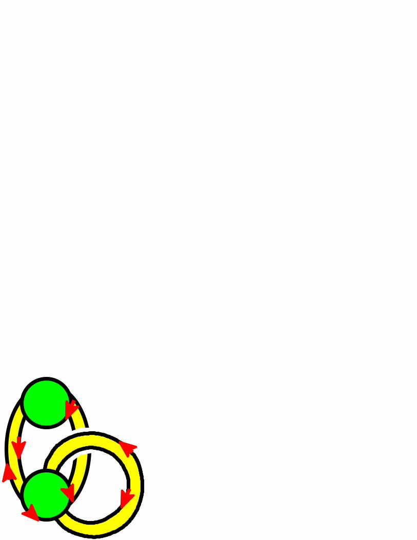
By a ribbon graph we mean an abstract (not necessarily orientable) surface with boundary de-composed into topological discs of two types, vertex-discs and edge-ribbons, satisfying the followingnatural conditions: the vertex-discs and the edge-ribbons intersect by disjoint line segments, eachsuch line segment lies on the boundary of precisely one vertex and precisely one edge, and everyedge contains exactly two such line segments. We refer to [BR, Ch] for precise definitions and to[GT, LZ, MT] for the general notions and terminology of topological graph theory. Ribbon graphsare considered up to homeomorphisms of the underlying surfaces preserving the decomposition.A ribbon graph can be regarded as a regular neighborhood of a graph cellularly embedded intoa surface. Thus the language of ribbon graphs is essentially the same as for cellularly embeddedgraphs. Here are a few examples of ribbon graphs.
1
2
3
=
3
1
23
1
2
Alternatively, a ribbon graph may be given by an arrow presentation (see the third picture). Anarrow presentation consists of a set of disjoint circles together with a collection of arrow markingson these circles. These arrows are labeled in pairs. To obtain a ribbon graph from an arrowpresentation, we glue discs to each of the circles and attach edge ribbons to each pair of arrowsaccording to the orientation of the arrows.
1.1. Arrow structure.
Definition 1.1. An arrow ribbon graph is a ribbon graph together with a set (possibly empty) ofarrows tangent to the boundaries of the (vertex- and edge-) discs of the decomposition. Two arrowgraphs are equivalent if there is a homeomorphism between the corresponding surfaces respectingthe decompositions and the orientations of the arrows.
The endpoints of segments along which the edges are attached to the vertices divide the bound-aries of (vertex- and edge-) discs into arcs.
We will refer to the sides of each edge connecting to the vertices as the attaching arcs. We willrefer to the sides which do not attach to vertices as the free edge arcs. Similarly, we will refer tothose arcs on vertices which are the complement of the attaching arcs as free vertex arcs.
The arrows may be slid along these arcs by an appropriate homeomorphism, but may not beslid over the end-points of the segments, and so may not change the type of arc that it is on.Each arc may contain several arrows.
For example, if there are several arrows on an attaching arc, then only their order on the arcis relevant, not their actual position on the arc. However, they all must be located on the arc andshould not be slid to a free vertex arc or a free edge arc.
An important example of an arrow structure is the arrow structure given by a particular arrowpresentation of a ribbon graph. In this case the arrows all lie on the attaching arcs of the edges.

ARROW RIBBON GRAPHS 3
Each pair of arrows corresponds to a map attaching the corresponding edge ribbon to the vertexdiscs.
1.2. Partial duality. Partial duality of ribbon graphs was introduced in [Ch] under the namegeneralized duality. Dan Archdeacon suggested a more appropriate term, partial duality. Underthis name it was then used in papers [EMM, Mo2, Mo3, Mo4, VT].
For any ribbon graph G, there is a natural dual ribbon graph G∗, also called the Euler-Poincaredual. First we glue a disc, also known as a face, to each boundary component of G, obtaining a
closed surface G without boundary. Then we remove the interior of all vertex-discs of G. Thenewly glued disc-faces will be the vertex-discs of G∗. The edge-ribbons for G∗ will be the sameas for G but now they are attached to the new vertices by the pair of opposite arcs which usedto be free edge arcs in G, and the attaching arcs of the ribbons become free edge arcs. This is aparticular case of the partial duality with respect to the set of all edges of G.
Definition 1.2. Partial duality is duality with respect to a subset D ⊆ E(G) of edges of G.We denote this partially dual graph by GD. It is constructed as follows. Consider the spanningsubgraph FD of G containing all vertices of G and only the edges from the subset D. Regard theboundary components of FD as curves on the surface of G via the inclusion FD → G. Glue a discto G along each connected component of this curve and remove the interior of all vertices of G.Regard these newly glued discs as vertices.
The result GD is easily seen to be a ribbon graph: Each edge in D is now attached to a vertexby the pair of opposite arcs which were free edge arcs in G, while the attaching arcs are now freeedge arcs, since the interiors of the vertices were deleted. The edges of E\D are attached by thesame pair of opposite sides as before.
For arrow ribbon graphs we preserve all of the arrows on the arcs of the edges and vertices. Notehowever that arrows on the free edge arcs of an edge in D will become arrows on the attachingarcs of that edge in GD, and vice versa.
The next table illustrates the partial duality with respect to a single edge.
e G Ge
non loop
α
β
εγδ
αβ
εγ
δ
orientable loop BAα
β
γ
δ
BA
α
βγδ
non-orientable loop BAα
β
γ
δ
A
Bγ
δ
β
α
We label the arrows by letters α, β, γ, δ, ε in order to make clear which arrow goes to which
under the partial duality. The boxes A and B here stand in for the presence of other edges
4 ROBERT BRADFORD, CLARK BUTLER, SERGEI CHMUTOV
which may be attached to the vertex along the dotted arcs. The order of attachment of these
edges in the box
A
is opposite to the one in A .
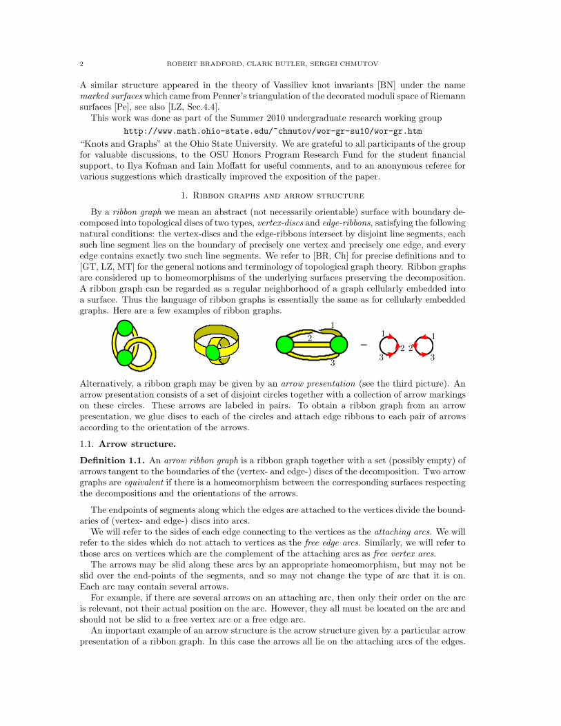
Here are some more examples (the details of partial duality are worked out in [Ch]).
G =
e1 e2
=⇒ Ge2 = =
e1
e2
, Ge1 =e1 e2
G =
e1e2
e3
=⇒ G{e2,e3} =
e1
e2
e3
Properties [Ch].
(a) G∅ = G.(b) GE(G) = G∗.
(c)(GD
)D′
= G(D∪D′)\(D∩D′), in particular
–(GD
)D= G,
– for e 6∈ D, GD∪{e} =(GD
){e}=
(G{e}
)D.
(d) Partial duality preserves orientability.(e) Partial duality preserves the number of connected components.
1.3. Contraction-Deletion.
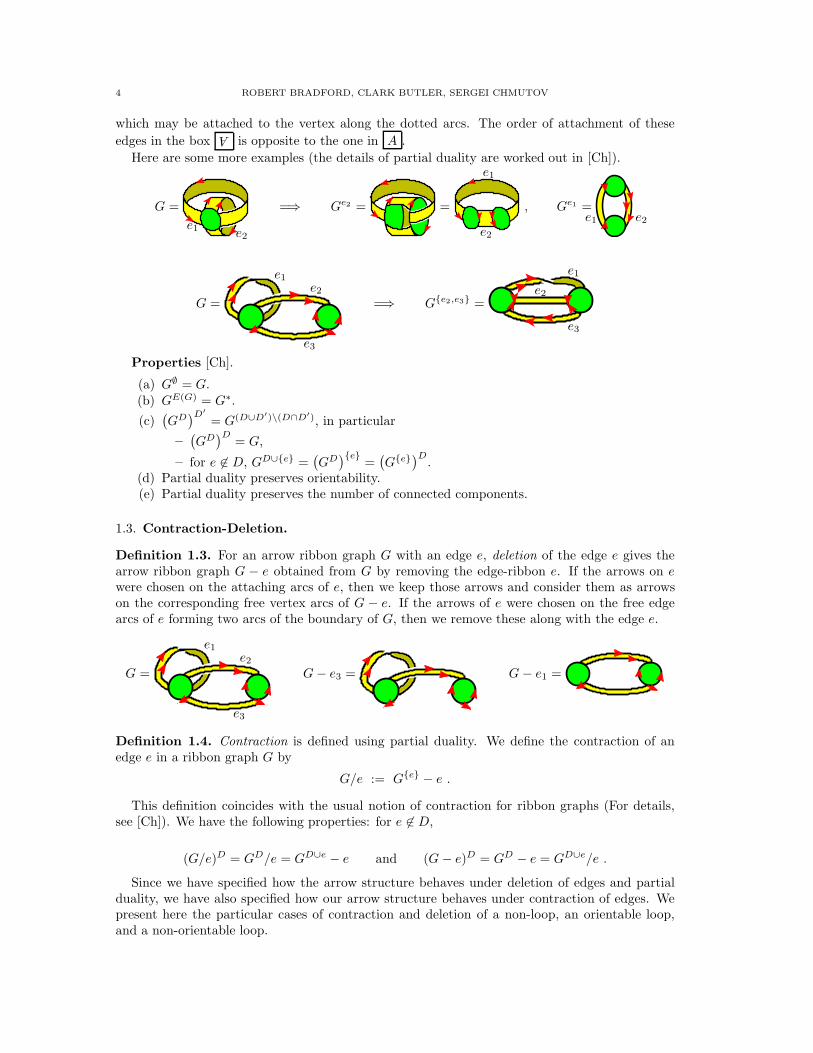
Definition 1.3. For an arrow ribbon graph G with an edge e, deletion of the edge e gives thearrow ribbon graph G − e obtained from G by removing the edge-ribbon e. If the arrows on ewere chosen on the attaching arcs of e, then we keep those arrows and consider them as arrowson the corresponding free vertex arcs of G − e. If the arrows of e were chosen on the free edgearcs of e forming two arcs of the boundary of G, then we remove these along with the edge e.
G =
e1e2
e3
G− e3 = G− e1 =
Definition 1.4. Contraction is defined using partial duality. We define the contraction of anedge e in a ribbon graph G by
G/e := G{e} − e .
This definition coincides with the usual notion of contraction for ribbon graphs (For details,see [Ch]). We have the following properties: for e 6∈ D,
(G/e)D = GD/e = GD∪e − e and (G− e)D = GD − e = GD∪e/e .
Since we have specified how the arrow structure behaves under deletion of edges and partialduality, we have also specified how our arrow structure behaves under contraction of edges. Wepresent here the particular cases of contraction and deletion of a non-loop, an orientable loop,and a non-orientable loop.

ARROW RIBBON GRAPHS 5
e G Ge G− e = Ge/e G/e = Ge − e
non loop
α
β
εγδ
αβ
εγ
δεγδ
αβ
orientable loop BAα
β
γ
δ
BA
α
βγδ BA
αBA βγ
δ
non-orientable loop BAα
β
γ
δ
A
Bγ
δ
β
α
BAα
β
A
Bγ
δ
Here are three more examples.
G =
e1 e2
=⇒ G/e2 =
G =
e1e2
e3
=⇒ G/e3 = G/e1 =
2. Arrow dichromatic polynomial
Tutte’s dichromatic polynomial ZG(a, b), also known as a partition function of the Potts modelin statistical mechanics, was generalized to signed graphs in [K2]. Its multivariable version wasintroduced in [Tr] and used in [Sok]. The multivariable Tutte polynomial also appears as a veryspecial case of Zaslavsky’s colored Tutte polynomial of a matriod [Za] and consequently also ofBollobas and Riordan’s colored Tutte polynomial of graph [BR1]. It can be defined as
ZG(a,b) :=∑
F⊆E(G)
ak(F )∏
e∈F
be ,
The sum runs over all spanning subgraphs of G, which we identify with subsets F of E(G).b := {be} is the set of variables (weights) be corresponding to the edges e of G, and k(F ) denotesthe number of connected components of F .
The multivariable dichromatic polynomial was generalized to ribbon graphs in [Mo1] as
ZG(a,b, c) :=∑
F⊆E(G)
ak(F )(∏
e∈F
be
)cbc(F ) ,

6 ROBERT BRADFORD, CLARK BUTLER, SERGEI CHMUTOV
where bc(F ) is the number of connected components of the boundary of F . Its signed versionfrom [VT] can be obtained by substitution
a = q,
be =
{αe if e is positive,q/αe if e is negative,
and multiplication of the whole polynomial by∏
e∈E(G)
q−1/2αe.
Remark 2.1. The dichromatic polynomial is essentially equivalent to the Tutte polynomial.Its ribbon graph formulation, known as the Bollobas-Riordan polynomial [BR], is equivalent tothe ribbon graph formulation of the dichromatic polynomial in the same way. Similarly, onemay introduce a multivariable Bollobas-Riordan polynomial [Mo1, VT]. Sometimes it is moreconvenient to use a homogeneous, doubly weighted form of it, which can be defined as
(1) BRG(X,Y, Z) :=∑
F⊆E(G)
(∏
e∈F
xe) (∏
e∈E(G)\F
ye) Xr(G)−r(F ) Y n(F ) Zk(F )−bc(F )+n(F ) ,
where r(F ) := |V (G)| − k(F ) is the rank of F , n(F ) := |E(F )| − r(F ) is the nullity of F , andwith each edge e we associate a pair of variables (xe, ye).
Of course, BRG(X,Y, Z) is equivalent to ZG(a,b, c) due to the relation
BRG(X,Y, Z) =( ∏
e∈E(G)
ye
)(Y Z)−v(G)X−k(G)ZG(XY Z2, {xeY Z/ye}, Z
−1) .
A signed version of the Bollobas-Riordan polynomial, which was introduced in [ChPa] and usedin [ChVo, Ch], can be obtained from the multivariable Bollobas-Riordan polynomial by choosingthe weights (x+, y+) (resp. (x−, y−)) of positive (resp. negative) edges to be
x+ := y+ := 1, x− :=
√X
Y, y− :=
√Y
X.
The main combinatorial results of [Ch] about contraction-deletion and partial duality may begeneralized to the doubly weighted Bollobas-Riordan polynomial in a straightforward way.
Definition 2.2. In the presence of an arrow structure we can extend the dichromatic polynomialZG(a,b, c) to the arrow dichromatic polynomial,
AG(a,b, c,K) :=∑
F⊆E(G)
ak(F )(∏
e∈F
be
)cbc(F )
∏
f∈∂(F )
Ki(f) ,
where F is a spanning subgraph ofG which we will also refer to as a state; the parameters k(F ) andbc(F ) are the same as before; and the rightmost product runs over all boundary components f ofF . The variables Ki(f) are assigned to each boundary component f according to the arrangementof arrows along this boundary component. Namely, the subscript i(f) is equal to half of thenumber of arrows along the boundary component f remaining after recursive cancellations of allneighboring pairs of arrows which point in the same direction:
K1 K1/2 K2
We set K0 = 1. Note that whenever the number of arrows is odd on a boundary component, theassociated variable is alwaysK1/2. The arrow dichromatic polynomial is a polynomial in infinitelymany variables a, be, c,K1/2,K1,K2, . . . . However, for a concrete graph G only finitely many K’sappear in AG(a,b, c,K).
ARROW RIBBON GRAPHS 7
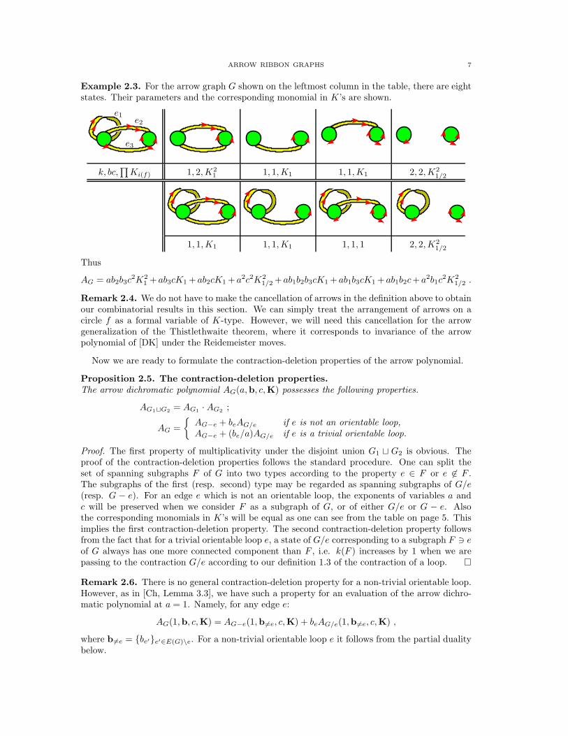
Example 2.3. For the arrow graph G shown on the leftmost column in the table, there are eightstates. Their parameters and the corresponding monomial in K’s are shown.
e1e2
e3
k, bc,∏
Ki(f) 1, 2,K21 1, 1,K1 1, 1,K1 2, 2,K2
1/2
1, 1,K1 1, 1,K1 1, 1, 1 2, 2,K21/2
Thus
AG = ab2b3c2K2
1 + ab3cK1+ ab2cK1+ a2c2K21/2+ ab1b2b3cK1+ ab1b3cK1+ ab1b2c+ a2b1c
2K21/2 .
Remark 2.4. We do not have to make the cancellation of arrows in the definition above to obtainour combinatorial results in this section. We can simply treat the arrangement of arrows on acircle f as a formal variable of K-type. However, we will need this cancellation for the arrowgeneralization of the Thistlethwaite theorem, where it corresponds to invariance of the arrowpolynomial of [DK] under the Reidemeister moves.
Now we are ready to formulate the contraction-deletion properties of the arrow polynomial.
Proposition 2.5. The contraction-deletion properties.The arrow dichromatic polynomial AG(a,b, c,K) possesses the following properties.
AG1⊔G2= AG1
· AG2;
AG =
{AG−e + beAG/e if e is not an orientable loop,
AG−e + (be/a)AG/e if e is a trivial orientable loop.
Proof. The first property of multiplicativity under the disjoint union G1 ⊔ G2 is obvious. Theproof of the contraction-deletion properties follows the standard procedure. One can split theset of spanning subgraphs F of G into two types according to the property e ∈ F or e 6∈ F .The subgraphs of the first (resp. second) type may be regarded as spanning subgraphs of G/e(resp. G − e). For an edge e which is not an orientable loop, the exponents of variables a andc will be preserved when we consider F as a subgraph of G, or of either G/e or G − e. Alsothe corresponding monomials in K’s will be equal as one can see from the table on page 5. Thisimplies the first contraction-deletion property. The second contraction-deletion property followsfrom the fact that for a trivial orientable loop e, a state of G/e corresponding to a subgraph F ∋ eof G always has one more connected component than F , i.e. k(F ) increases by 1 when we arepassing to the contraction G/e according to our definition 1.3 of the contraction of a loop. �
Remark 2.6. There is no general contraction-deletion property for a non-trivial orientable loop.However, as in [Ch, Lemma 3.3], we have such a property for an evaluation of the arrow dichro-matic polynomial at a = 1. Namely, for any edge e:
AG(1,b, c,K) = AG−e(1,b 6=e, c,K) + beAG/e(1,b 6=e, c,K) ,
where b 6=e = {be′}e′∈E(G)\e. For a non-trivial orientable loop e it follows from the partial dualitybelow.
8 ROBERT BRADFORD, CLARK BUTLER, SERGEI CHMUTOV
Proposition 2.7. The partial duality properties.Let D ⊆ E(G) be a subset of edges and G′ := GD be the corresponding partial dual arrow graph.
The evaluation of the arrow dichromatic polynomial at a = 1 satisfies to the equation:
AG(1,b, c,K) =(∏
e∈D
be
)AG′(1,bD, c,K) ,
where the weights bD = {b′e} of edges of G′ are
b′e =
{be if e 6∈ D ,
1/be if e ∈ D .
Proof. The proof is similar to [Ch, Theorem 3.1]. The 1-to-1 correspondence between the spanningsubgraphs F of G and the spanning subgraphs F ′ of G′ is given by the symmetric difference:F ′ = F∆D := (F ∪D) \ (F ∩D).
This correspondence assures that the monomials in weights be are equal to each other for Fand F ′. Indeed,
(∏
e∈D
be
) ∏
e′∈F ′
b′e =(∏
e∈D
be
) ∏
e′∈F\D
be′∏
e′∈D\F
1/be′ =∏
e∈F
be .
The boundary of F coincides with the boundary of F ′ by the construction of the partial duality.Thus the corresponding arrow monomials in c and K’s are also equal to each other. One maycheck this with the table on page 5. �
3. Virtual links
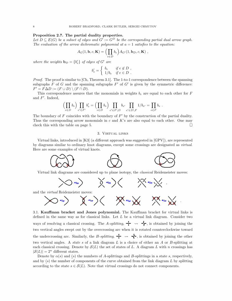
Virtual links, introduced in [K3] (a different approach was suggested in [GPV]), are representedby diagrams similar to ordinary knot diagrams, except some crossings are designated as virtual.Here are some examples of virtual knots.
Virtual link diagrams are considered up to plane isotopy, the classical Reidemeister moves:
,
and the virtual Reidemeister moves:
.
3.1. Kauffman bracket and Jones polynomial. The Kauffman bracket for virtual links isdefined in the same way as for classical links. Let L be a virtual link diagram. Consider two
ways of resolving a classical crossing. The A-splitting, , is obtained by joining the
two vertical angles swept out by the overcrossing arc when it is rotated counterclockwise toward
the undercrossing arc. Similarly, the B-splitting, , is obtained by joining the other
two vertical angles. A state s of a link diagram L is a choice of either an A or B-splitting ateach classical crossing. Denote by S(L) the set of states of L. A diagram L with n crossings has|S(L)| = 2n different states.
Denote by α(s) and (¯s) the numbers of A-splittings and B-splittings in a state s, respectively,
and by (.s) the number of components of the curve obtained from the link diagram L by splitting
according to the state s ∈ S(L). Note that virtual crossings do not connect components.

ARROW RIBBON GRAPHS 9
Definition 3.1. [K1] The Kauffman bracket of a diagram L is a polynomial in three variables A,B, d defined by the formula
[L](A,B, d) :=∑
s∈S(L)
Aα(s) B(¯s)d(.s)−1
.
The Jones polynomial JL(t) is obtained from the Kauffman bracket by a simple substitution:
A = t−1/4, B = t1/4, d = −t1/2 − t−1/2 ;
JL(t) := (−1)w(L)t3w(L)/4[L](t−1/4, t1/4,−t1/2 − t−1/2) ,
where w(L) is the writhe of the diagram L, which is the sum of signs assigned to oriented classicalcrossings according to the rule:
+1 , −1 .
Note that [L] is not a topological invariant of the link; it depends on the link diagram andchanges with Reidemeister moves.
3.2. Dye-Kauffman arrow polynomial [DK]. We can keep more information splitting a clas-sical crossing. Namely, when a splitting does not respect the orientation, we put two arrows onthe branches of the splitting oriented counterclockwise near the crossing:
, .
Thus the state circles are supplied with an arrow structure. With each such circle c we associatethe variable Kc as in Definition 2.2. Then we can define the arrow bracket polynomial as
[L]A(A,B, d) :=∑
s∈S(L)
Aα(s) B(¯s)d(.s)−1
∏
c∈s
Kc .
The standard substitution B := A−1, d := −A2−A−2 gives the normalized Dye-Kauffman arrow
polynomial [DK]:
〈L〉NA := (−A3)−w(L)[L]A(A,A−1,−A2 −A−2) ,
which is an invariant of virtual links. The invariance under the Reidemeister moves follows fromthe rule of cancellation of arrows in Definition 2.2. A remarkable observation of H. Dye andL. Kauffman is that for classical link diagrams, all arrows will cancel, and the K variables thus donot occur in the arrow polynomial. In this case it is essentially equivalent to the Jones polynomial(after the further substitution A = t−1/4).
4. Arrow Thistlethwaite theorem
4.1. From virtual link diagrams to arrow ribbon graphs. With each state s of a virtuallink diagram L we associate an arrow ribbon graph Gs
L. The vertices of GsL are obtained by gluing
discs to the state circles of s. The edges of GsL correspond to the classical crossings of L. Each is
obtained by gluing a small planar band connecting the two opposite arcs of the particular splittingof s. We consider two types of edge-ribbons. If a crossing of L is resolved as an A-splitting in thestate s, we assign +1 to the corresponding edge, if it is resolved as a B-splitting, then we assign−1. We thus get a signed ribbon graph.
The arrow structure assigns two arrows on opposite sides of each edge-ribbon according to theorientation of the plane where the corresponding planar band is located. If a crossing splitting ins respects the orientation of strands, we put two arrows on the free edge arcs of the correspondingsmall planar band induced by the counterclockwise orientation of the plane. If the splitting in s
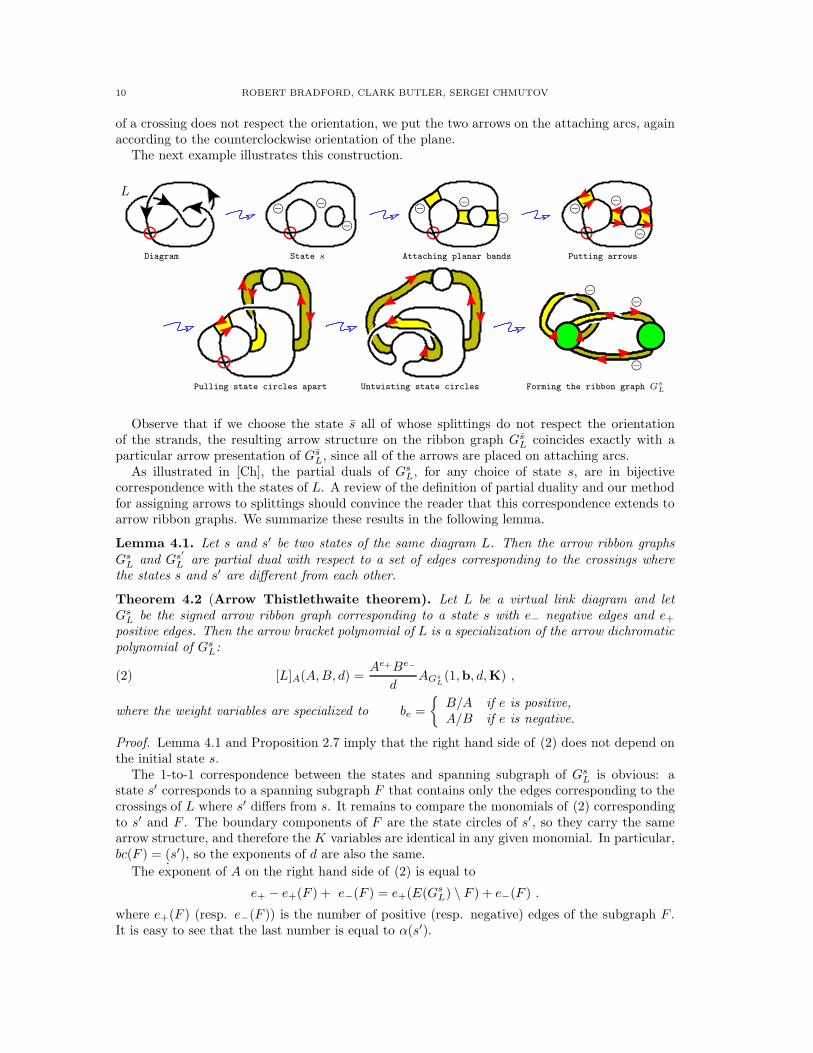
10 ROBERT BRADFORD, CLARK BUTLER, SERGEI CHMUTOV
of a crossing does not respect the orientation, we put the two arrows on the attaching arcs, againaccording to the counterclockwise orientation of the plane.
The next example illustrates this construction.
L
Diagram
❢−❢−
❢−
State s
❢−❢−
❢−
Attaching planar bands
❢−❢−
❢−
Putting arrows
Pulling state circles apart Untwisting state circles
❢−❢−
❢−
Forming the ribbon graph Gs
L
Observe that if we choose the state s all of whose splittings do not respect the orientationof the strands, the resulting arrow structure on the ribbon graph Gs
L coincides exactly with aparticular arrow presentation of Gs
L, since all of the arrows are placed on attaching arcs.As illustrated in [Ch], the partial duals of Gs
L, for any choice of state s, are in bijectivecorrespondence with the states of L. A review of the definition of partial duality and our methodfor assigning arrows to splittings should convince the reader that this correspondence extends toarrow ribbon graphs. We summarize these results in the following lemma.
Lemma 4.1. Let s and s′ be two states of the same diagram L. Then the arrow ribbon graphs
GsL and Gs′
L are partial dual with respect to a set of edges corresponding to the crossings where
the states s and s′ are different from each other.
Theorem 4.2 (Arrow Thistlethwaite theorem). Let L be a virtual link diagram and let
GsL be the signed arrow ribbon graph corresponding to a state s with e− negative edges and e+
positive edges. Then the arrow bracket polynomial of L is a specialization of the arrow dichromatic
polynomial of GsL:
(2) [L]A(A,B, d) =Ae+Be−
dAGs
L(1,b, d,K) ,
where the weight variables are specialized to be =
{B/A if e is positive,
A/B if e is negative.
Proof. Lemma 4.1 and Proposition 2.7 imply that the right hand side of (2) does not depend onthe initial state s.
The 1-to-1 correspondence between the states and spanning subgraph of GsL is obvious: a
state s′ corresponds to a spanning subgraph F that contains only the edges corresponding to thecrossings of L where s′ differs from s. It remains to compare the monomials of (2) correspondingto s′ and F . The boundary components of F are the state circles of s′, so they carry the samearrow structure, and therefore the K variables are identical in any given monomial. In particular,bc(F ) = (.s
′), so the exponents of d are also the same.
The exponent of A on the right hand side of (2) is equal to
e+ − e+(F ) + e−(F ) = e+(E(GsL) \ F ) + e−(F ) .
where e+(F ) (resp. e−(F )) is the number of positive (resp. negative) edges of the subgraph F .It is easy to see that the last number is equal to α(s′).

ARROW RIBBON GRAPHS 11
Finally the exponent of B at the right hand side of (2) is equal to e− + e+(F )− e−(F ) =e−(E(Gs
L) \ F ) + e+(F ) = (¯s′) . �
5. Specializations
It was indicated in [Ch] that the previously known ribbon graph generalizations of the Thistleth-waite theorem from [ChPa, ChVo, DFKLS] can be unified using different states in the constructionof the ribbon graph Gs
L. Here we formulate the corresponding arrow polynomial generalizations.
5.1. All-A-splitting state. If s = sA is a state consisting of all A-splittings, then all the edges ofGs
L are positive. In this case all weight variables will be equal to each other: be = B/A. Theorem4.2 becomes
[L]A(A,B, d) =∑
F⊆E(Gs
L)
Ae(F )Be(F )dbc(F )−1∏
f∈∂(F )
Ki(f) ,
where F := E(GsL) \ F is the complementary set of edges. This equation directly extends the
results of [DFKLS] to the arrow polynomial.
5.2. Seifert state. Let s be the Seifert state where all splittings preserve the orientation of thelink L. Using (1) we can define an arrow version of the Bollobas-Riordan polynomial as
ABRG(X,Y, Z,K) :=∑
F⊆E(G)
(∏
e∈F
xe) (∏
e6∈F
ye)Xr(G)−r(F )Y n(F )Zk(F )−bc(F )+n(F )
∏
f∈∂(F )
Ki(f) .
Substituting x+ = y+ = 1, x− =√X/Y , y− =
√Y/X as in Remark 2.1, we get the signed
unweighted version of the arrow Bollobas-Riordan polynomial
sBRG(X,Y, Z,K) =∑
F⊆E(G)
Xr(G)−r(F )+s(F )Y n(F )−s(F )Zk(F )−bc(F )+n(F )∏
f∈∂(F )
Ki(f) ,
where s(F ) := e−(F )−e−(F )2 . In this case Theorem 4.2 becomes
[L]A(A,B, d) = An(Gs
L)Br(Gs
L)dk(G
s
L)−1sBRGs
L(Ad/B,Bd/A, 1/d,K) ,
which directly extends the results of [ChVo] to the arrow polynomial.
References
[BN] D. Bar-Natan, On the Vassiliev knot invariants, Topology, 34 (1995) 423–472.[BR] B. Bollobas and O. Riordan, A polynomial of graphs on surfaces, Math. Ann. 323 (2002) 81–96.[BR1] B. Bollobas, O. Riordan, A Tutte polynomial for colored graphs, Combinatorics, Probability and Com-
puting 8 (1999) 45–93.[BuCh] C. Butler, S. Chmutov, Bollobas-Riordan and relative Tutte polynomials. Preprint arXiv:
math.CO/1011.0072.[Ch] S. Chmutov, Generalized duality for graphs on surfaces and the signed Bollobas-Riordan polynomial,
Journal of Combinatorial Theory, Ser. B, 99(3) (2009) 617–638. Preprint arXiv:math.CO/0711.3490,[ChPa] S. Chmutov, I. Pak, The Kauffman bracket of virtual links and the Bollobas-
Riordan polynomial, Moscow Mathematical Journal 7(3) (2007) 409–418. Preprint\protect\vrule width0pt\protect\href{http://arxiv.org/abs/math/0609012}{arXiv:math.GT/0609012},
[ChVo] S. Chmutov, J. Voltz, Thistlethwaite’s theorem for virtual links, Journal of Knot Theory and Its Ramifi-cations, 17(10) (2008) 1189–1198. Preprint arXiv:math.GT/0704.1310.
[DFKLS] O. Dasbach, D. Futer, E. Kalfagianni, X.-S. Lin, N. Stoltzfus, The Jones polynomial andgraphs on surfaces, Journal of Combinatorial Theory, Ser.B 98 (2008) 384–399. Preprint\protect\vrule width0pt\protect\href{http://arxiv.org/abs/math/0605571}{arXiv:math.GT/0605571}.
[DH] Y. Diao, G. Hetyei, Relative Tutte polynomials for colored graphs and virtual knot theory, CombinatoricsProbability and Computing 19 (2010) 343–369. Preprint arXiv:math.CO/0909.1301.
[DK] H. Dye, L. Kauffman, Virtual Crossing Number and the Arrow Polynomial, Journal of Knot Theory ItsRamifications 18(10) (2009) 1335-1357. Preprint arXiv:math.GT/0810.3858.
[EMM] J. Ellis-Monaghan, I. Moffatt, Twisted duality for embedded graphs. Trans. Amer. Math. Soc. 364 (2012)1529–1569.
12 ROBERT BRADFORD, CLARK BUTLER, SERGEI CHMUTOV
[GPV] M. Goussarov, M. Polyak and O. Viro, Finite type invariants ofclassical and virtual knots, Topology 39 (2000) 1045–1068. Preprint\protect\vrule width0pt\protect\href{http://arxiv.org/abs/math/9810073}{arXiv:math/9810073}v2 [math.GT].
[GT] J. L. Gross and T. W. Tucker, Topological graph theory, Wiley, NY, 1987.[K1] L. H. Kauffman, New invariants in knot theory, Amer. Math. Monthly 95 (1988) 195–242.[K2] L. H. Kauffman, A Tutte polynomial for signed graphs, Discrete Appl. Math. 25 (1989) 105–127.[K3] L. H. Kauffman, Virtual knot theory, European Journal of Combinatorics 20 (1999) 663–690.[LZ] S. K. Lando, A. K. Zvonkin, Graphs on surfaces and their applications, Springer, 2004.[Mi] Y. Miyazawa, A multi-variable polynomial invariant for virtual knots and links, Journal of Knot Theory
and Its Ramifications, 17(11) (2008) 1311–1326.[Mo1] I. Moffatt, Knot invariants and the Bollobas-Riordan polynomial of embed-
ded graphs, European Journal of Combinatorics 29 (2008) 95–107. Preprint\protect\vrule width0pt\protect\href{http://arxiv.org/abs/math/0605466}{arXiv:math.CO/0605466}.
[Mo2] I. Moffatt, Partial duality and Bollobas and Riordan’s ribbon graph polynomial, Discrete Mathematics310 (2010) 174–183. Preprint arXiv:math.CO/0809.3014.
[Mo3] I. Moffatt, A characterization of partially dual graphs, Journal of Graph Theory 67(3) (2011) 198-217.Preprint arXiv:math.CO/0901.1868.
[Mo4] I. Moffatt, Partial duals of plane graphs, separability and the graphs of knots. PreprintarXiv:math.CO/1007.4219.
[MT] B. Mohar, C. Thomassen, Graphs on Surfaces, The Johns Hopkins University Press, 2001.[Pe] R. Penner, The decorated Teichmuller space of punctured surfaces, Communications in Mathematical
Physics 113(2) (1987) 299–339.
[Sok] A. D. Sokal, The multivariate Tutte polynomial (alias Potts model) for graphsand matroids, in Surveys in Combinatorics 2005, London Math. Soc. Lec-ture Note Ser., 327 Cambridge University Press (2005)173-226. Preprint\protect\vrule width0pt\protect\href{http://arxiv.org/abs/math/0503607}{arXiv:math/0503607}v1 [math.CO].
[Th] M. Thistlethwaite, A spanning tree expansion for the Jones polynomial, Topology 26 (1987) 297–309.[Tr] L. Traldi, A dichromatic polynomial for weighted graphs and link polynomials, Proc. AMS 106 (1989)
279–286.[VT] F. Vignes-Tourneret, The multivariate signed Bollobas-Riordan polynomial, Discrete Math. 309 (2009)
5968–5981. Preprint arXiv:math.CO/0811.1584.[Za] T.Zaslavsky, Strong Tutte functions of matroids and graphs, Trans. Amer. Math. Soc. 334(1) (1992),
317-347.
Department of Mathematics, University of Kansas, 1460 Jayhawk Blvd., Lawrence, Kansas 66045
Department of Mathematics, The Ohio State University, 231 West 18th Avenue, Columbus, OH 43210