Statistically validated networks in bipartite complex systems

Michele Tumminello,1 Salvatore Micciche,1 Fabrizio

Lillo,1, 2 Jyrki Piilo,3 and Rosario N. Mantegna1

1Dipartimento di Fisica e Tecnologie Relative, Universita di Palermo,

viale delle Scienze Ed.18, I-90128 Palermo, Italia

2Santa Fe Institute, 1399 Hyde Park Road, Santa Fe NM 87501, USA

3Turku Centre for Quantum Physics,

Department of Physics and Astronomy,

University of Turku, FI-20014 Turun yliopisto, Finland

1

arX

iv:1

008.

1414

v1 [

phys

ics.

soc-

ph]

8 A

ug 2

010

Many complex systems present an intrinsic bipartite nature and are often de-

scribed and modeled in terms of networks [1–5]. Examples include movies and

actors [1, 2, 4], authors and scientific papers [6–9], email accounts and emails

[10], plants and animals that pollinate them [11, 12]. Bipartite networks are

often very heterogeneous in the number of relationships that the elements of

one set establish with the elements of the other set. When one constructs a pro-

jected network with nodes from only one set, the system heterogeneity makes it

very difficult to identify preferential links between the elements. Here we intro-

duce an unsupervised method to statistically validate each link of the projected

network against a null hypothesis taking into account the heterogeneity of the

system. We apply our method to three different systems, namely the set of

clusters of orthologous genes (COG) in completely sequenced genomes [13, 14],

a set of daily returns of 500 US financial stocks, and the set of world movies of

the IMDb database [15]. In all these systems, both different in size and level

of heterogeneity, we find that our method is able to detect network structures

which are informative about the system and are not simply expression of its

heterogeneity. Specifically, our method (i) identifies the preferential relation-

ships between the elements, (ii) naturally highlights the clustered structure of

investigated systems, and (iii) allows to classify links according to the type of

statistically validated relationships between the connected nodes.

Bipartite networks are composed by two disjoint sets of nodes such that every link con-

nects a node in the first set with a node of the second set. The bipartite network is often

transformed by one-mode projecting, i.e. one creates a network of nodes belonging to one of

the two sets and two nodes are connected when they have at least one common neighboring

node of the other set. Two main and related problems arise in these networks. First, there is

often a large heterogeneity in the node degree of the bipartite network and the information

associated to this heterogeneity is partially lost in the projected network. Second, a link in

a projected network could indicate a preferential relationships between two specific nodes

or could be consistent with the degree of heterogeneity of the system. In this letter we

introduce a statistical method to validate the presence of a link by simultaneously coping

with the heterogeneity of the system.

A bipartite system presents two sources of heterogeneity associated with the two sets. To

2

be specific consider the example of the COG database [13, 14], where one set is composed

by 66 organism’s genomes and the other by 4,873 COGs. The number of COGs in a genome

is heterogeneous, ranging from 362 to 2,243. Similarly, the number of genomes in which a

specific COG is present ranges from 3 to 66. Here we consider the projected network of

genomes. A COGk is a COG present in k = 3, · · · , 66 genomes. In each subset of COGks

we are therefore left only with the heterogeneity of organisms. We identify a preferential

relationship between each pair of organisms by statistically validating the co-occurrence of

COGks against a null hypothesis that takes into account such heterogeneity. Specifically,

given two organisms A and B, let NA be the number of COGks in organism A and NB

the number of COGks in organism B. The total number of COGks is Nk and the observed

number of COGks belonging to both A and B is NAB. Under the null hypothesis of random

co-occurrence, the probability of observing X co-occurrences is given by the hypergeometric

distribution [16]

H(X|Nk, NA, NB) =

(NA

X

)(Nk−NA

NB−X

)(Nk

NB

) . (1)

We can therefore associate a p-value to the observed NAB as p(NAB) = 1 −∑NAB−1X=0 H(X|Nk, NA, NB). It is worth noting that the described null hypothesis directly

takes into account the heterogeneity of organisms with respect to the number of COGs

present in their genome. For each pair of organisms, we separately evaluate the p-value for

each subset of COGk and we count the number of subsets in which the p-value is smaller

than a selected statistical threshold. We accordingly set a link between A and B if the

number of subsets is non vanishing and we use it as the weight of the link. The described

link validation procedure involves multiple hypothesis testing, across organism pairs and

subsets of COGk. Therefore the statistical threshold must be corrected for multiple com-

parisons. The most stringent method to address this problem is the Bonferroni correction

[17]. It is based on the consideration that if one tests Nt either dependent or independent

hypotheses on a set of data, then a conservative way of maintaining the error rate low is

to test each individual hypothesis at a statistical significance level of pt/Nt, where pt is the

chosen statistical threshold (1% in the present study). In our case the number of organ-

isms is No = 66 and we test Nt = 64No(No − 1)/2 hypotheses, equal to the number of

pairs of organisms times the number of subsets of COGk. Thus our Bonferroni threshold

is pb = 0.01 · 2/(64No(No − 1)) ∼= 7.3 × 10−8. We refer to the network obtained by using

3

the Bonferroni threshold as the Bonferroni network. A less stringent correction for multiple

comparisons is the False Discovery Rate (FDR) [18]. The threshold of the FDR correction

linearly increases with the number of tests in which the null hypothesis is rejected. We refer

to the network obtained by using the FDR correction for multiple comparisons as the FDR

network. By construction, the Bonferroni network is a subgraph of the FDR network, which

is a subgraph of the adjacency network.

The Bonferroni network of organisms includes 58 non isolated nodes connected by 216

weighted links (Fig. 1A) and it shows seven connected components, each one having a clear

biological interpretation in terms of organisms’ lineage. The FDR network of organisms

includes all the 66 organisms and the number of weighted links in this network is 369

(Fig. 1B). Thus the entire set is covered and the additional links provides relations among

the groups already observed in the Bonferroni network. Note that the adjacency network of

this system is a complete graph.

It is worth noting that both the Bonferroni and the FDR network display a clear clus-

ter structure and the clusters have a direct biological interpretation in terms of lineages.

Even if the FDR network is completely connected, the application of community detection

algorithms [19], such as Infomap [20], to the statistically validated networks gives a clear

community structure (see Fig. 1). This is not true for the adjacency network and shows

that the statistically validated networks are able to identify the many relevant links inside

communities and the few relevant links between different communities of organisms.

As a second example we consider the collective dynamics of the daily return of Ns = 500

highly capitalized US financial stocks in the period 2001-2003 (748 trading days). The two

sets of the bipartite system are the stocks and the days, and we consider here the projected

network of stocks. The interest in this example is that we (i) generalize our procedure

to complex systems where the elements are monitored by continuous variables, (ii) show

how to simplify the above procedure when the second source of heterogeneity (in the above

example the COG frequency in different organisms) is small, and (iii) show how to classify

links according to the type of relation between the two nodes.

Since we want to identify similarities and differences among stock returns not due to

the global market behavior, we investigate the excess return of each stock i with respect

to the average daily return of all the stocks in our set. The excess return of each stock

i at day t is then converted into a categorical variable with 3 states: up, down, and null.

4

For each stock we introduce a daily varying threshold σi(t) as the average of the absolute

excess return (a measure of local volatility) of stock i over the previous 20 days. State up

(down) is assigned when the excess return of stock i at day t is larger (smaller) than σi(t)

(-σi(t)). The state null is assigned to the remaining days. We study the co-occurrence of

states up and down for each pair of stocks. In this case we can neglect the heterogeneity of

state occurrence in different trading days because the number of up (down) states is only

moderately fluctuating across different days and it has a bell shaped distribution with a

range of fluctuations smaller than one decade for each stock. With this approximation we

can statistically validate the co-occurrence of state A (either up or down) of stock i and

state B (either up or down) of stock j with the following procedure. Let us call NA (NB)

the number of days in which stock i (j) is in the state A (B). Let us call NAB the number of

days when we observe the co-occurrence of state A for stock i and state B for stock j. Under

the null hypothesis of random co-occurrence of state A for stock i and state B for stock j,

the probability of observing X co-occurrences of the investigated states of the two stocks in

T observations is again described by the hypergeometric distribution, H(X|T,NA, NB). As

before we can associate p-value with each pair of investigated stocks for each combination

of the investigated states. We indicate the state up (down) of stock i as iu (id). The

possible combinations are (iu,ju), (iu,jd), (id,ju), and (id,jd). As before the statistical test is

a multiple hypothesis test and therefore either the Bonferroni or FDR correction is necessary.

The Bonferroni threshold is pb = pt/(2Ns(Ns − 1)) where the denominator of the threshold

is the number of considered stock pairs (Ns(Ns − 1)/2) times 4, which is the number of

different co-occurrences investigated. Each pair of stocks is characterized by the set of the

above four combinations which are statistically validated. There are 24 − 1 = 15 possible

cases (relationships) with at least one validation, but we observe only 5 cases: L1 in which

the co-occurrences (iu,ju) and (id,jd) are both validated; L2 in which only the co-occurrence

(id,jd) is validated, L3 in which only the co-occurrence (iu,ju) is validated, L4 in which

either only (iu,jd) or only (id,ju) is validated; and L5 when both the co-occurrence (iu,jd)

and (id,ju) are validated. Note that we put in the same relationship L4 two cases which are

different only for the order in which the two nodes are considered. The set of relationships

L1, L2, and L3 and the associated links describe a coherent movement of the price of the two

stocks, while the set of relationships L4 and L5 describes opposite deviation from the average

market behavior. We can therefore construct networks where the statistically validated links

5

are associated with a label that specifies the type of relationship between the two connected

nodes. This structure is richer than a simple unweighted network, but it is also different

from a weighted network because it describes relationships which cannot be described by

a numerical value only. We address the set of different relationships present between two

nodes of the statistically validated network with the term multi-link.

The Bonferroni network of the system is composed by 349 stocks connected by 2,230

multi-links. The multi-links are of different nature. Specifically, we observe 1,158 L1-links,

494 L2-links, 354 L3-links, 196 L4-links, and 28 L5-links. The largest connected component

of the network includes 273 stocks. There also are 19 smaller connected components of size

ranging from 2 to 15. In Fig. 2 we show the largest connected component of the Bonferroni

network. It presents several regions in which stocks are strongly connected by L1, L2, and

L3 multi-links. These regions are very homogeneous in the economic sector of the stocks.

The connection between different regions is mostly provided by a large number of L4 and

L5 multi-links. This is especially evident for the group of technology stocks (red circles)

for which all except one of the multi-links outgoing from the group are L4 or L5 multi-

links, indicating moderate or strong anti-correlation of technology stocks with the other

groups. The strongest anti-correlation is detected between technology and services stocks

(cyan circles). A partition analysis of the Bonferroni network shows (see Supplementary

Information) that the services stocks, which are anti-correlated with the technology stocks,

mostly belong to the economic sub-sector of Real estate operations. We have also computed

the FDR network of the system. As expected, it includes more stocks (494) and more multi-

links (11,281), since the requirement on the statistical validation is less restrictive. The

FDR network has a single connected component and the fraction of L4 and L5 multi-links

is higher (35.9 %) than in the case of the Bonferroni network (10.0 %).

As before the adjacency network of stocks is a complete graph. On the contrary both the

Bonferroni and the FDR networks display a highly clustered structure with clusters having

a clear economic meaning. The use of Infomap on these statistically validated networks

gives a partition in communities, which are extremely homogeneous by economic sector (see

Supplementary Information). Therefore our method allows to construct networks where (i)

links are statistically validated against a null hypothesis, (ii) multi-links describe qualita-

tively different relationships between pairs of stocks, e.g. both co-movements and opposite

movements occurring between pairs of stocks, and (iii) a very accurate identification of com-

6

munities of stocks is possible. To the best of our knowledge the presence of all these features

is pretty unique and it is not shared by other similarity networks [22] based on topological

constraints [23–25], correlation threshold [26], or validated with bootstrap [27].

The last system we investigate is the bipartite system of movies and actors. We collect

data from the Internet Movie Database (IMDb), which is the largest web repository of

world movies. We consider here the projected network of the 89,605 movies produced in

the period 1990-2008. The set includes movies realized in 169 countries, and at least one

genre is specified for each movie. The number of involved actors is 412,143. We choose this

example because (i) it is a large system, (ii) it has a large heterogeneity both in movies and

in actors, and (iii) it allows a sophisticated cluster characterization analysis based on the

characteristics of the movie, namely genre, language, country, etc..

The actors heterogeneity ranges between 1 and 247 and it is so pronounced that there is

no practical way to eliminate it when constructing statistically validated networks of movies.

The approach of the k-subsets is not feasible due to lack of sufficient statistics. Therefore,

an approximate statistical validation can be performed, by taking into account only the

movies heterogeneity. In the presence of this limitation a number of false positive links can

be expected. In spite of this limitation, the results obtained for the statistically validated

networks are very informative about several aspects of the movie industry.

We construct the statistically validated networks of movies by testing the co-occurrence

of actors in the cast of each movie pair. The null hypothesis we use is again given by the

hypergeometric distribution, which naturally takes into account the heterogeneity due to

the number of actors performing in each movie. Table I shows the severe filtering of nodes

and links that is obtained in the validated networks of movies with respect to the adjacency

network. Only 16% (47%) of the nodes and 1% (7%) of the links of the adjacency network

are statistically validated in the Bonferroni (FDR) network.

A comparison of the degree of movies in the adjacency and FDR networks allows to

clearly distinguish Asian movie industry from the rest of the world movie industry, and

languages within single countries like India (see Fig.3). According to the present state of

the IMDb database, this comparison suggests that the Asian movie industry, and the Indian

movie industry in particular, present a level of variety in their cast formation that is lower

than the variety observed in the western movie industry conditioned to the number of actors

present in the movie casts.

7

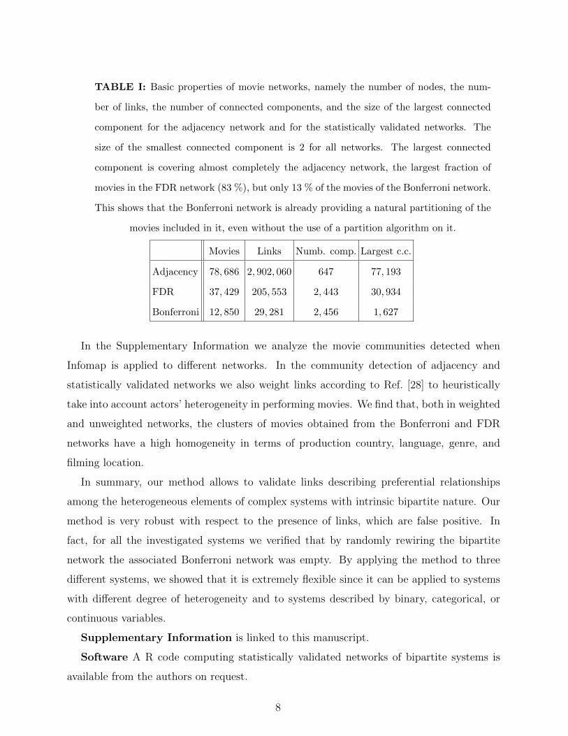
TABLE I: Basic properties of movie networks, namely the number of nodes, the num-

ber of links, the number of connected components, and the size of the largest connected

component for the adjacency network and for the statistically validated networks. The

size of the smallest connected component is 2 for all networks. The largest connected

component is covering almost completely the adjacency network, the largest fraction of

movies in the FDR network (83 %), but only 13 % of the movies of the Bonferroni network.

This shows that the Bonferroni network is already providing a natural partitioning of the

movies included in it, even without the use of a partition algorithm on it.

Movies Links Numb. comp. Largest c.c.

Adjacency 78, 686 2, 902, 060 647 77, 193

FDR 37, 429 205, 553 2, 443 30, 934

Bonferroni 12, 850 29, 281 2, 456 1, 627

In the Supplementary Information we analyze the movie communities detected when

Infomap is applied to different networks. In the community detection of adjacency and

statistically validated networks we also weight links according to Ref. [28] to heuristically

take into account actors’ heterogeneity in performing movies. We find that, both in weighted

and unweighted networks, the clusters of movies obtained from the Bonferroni and FDR

networks have a high homogeneity in terms of production country, language, genre, and

filming location.

In summary, our method allows to validate links describing preferential relationships

among the heterogeneous elements of complex systems with intrinsic bipartite nature. Our

method is very robust with respect to the presence of links, which are false positive. In

fact, for all the investigated systems we verified that by randomly rewiring the bipartite

network the associated Bonferroni network was empty. By applying the method to three

different systems, we showed that it is extremely flexible since it can be applied to systems

with different degree of heterogeneity and to systems described by binary, categorical, or

continuous variables.

Supplementary Information is linked to this manuscript.

Software A R code computing statistically validated networks of bipartite systems is

available from the authors on request.

8

Acknowledgements We thank S. Fortunato and J. Kertesz for fruitful discussions. J.P.

acknowledge financial support by The Magnus Ehrnrooth Foundation and the Vilho, Yrjo,

and Kalle Vaisala Foundation.

[1] Watts, D.J. & Strogatz, S.H. Collective dynamics of small-world networks. Nature 393, 440-

442 (1998).

[2] Barabasi, A.L. & Albert, R. Emergence of scaling in random networks. Science 286, 509-512

(1999).

[3] Newman, M.E.J., Watts, D.J. & Strogatz, S.H. Random graph models of social networks.

Proc. Natl. Acad. Sci. USA 99, 2566-2572 (2002).

[4] Song, C.M., Havlin, S. & Makse, H.A. Self-similarity of complex networks. Nature 433, 392-

395 (2005).

[5] Schweitzer, F., Fagiolo, G., Sornette, D., Vega-Redondo, F., Vespignani, A. & White, D.R.

Economic Networks: The New Challenges. Science 325, 422-425 (2009).

[6] Newman, M.E.J. The structure of scientific collaboration networks. Proc. Natl. Acad. Sci.

USA 98, 404-409 (2001).

[7] Barabasi, A.L, et al. Evolution of the social network of scientific collaborations. Physica A

311, 590-614 (2002).

[8] Guimera, R., Uzzi, B., Spiro, J. & Amaral, L.A.N. Team assembly mechanisms determine

collaboration network structure and team performance. Science 308, 697-702 (2005).

[9] Colizza, V., Flammini, A., Serrano, M.A. & Vespignani, A. Detecting rich-club ordering in

complex networks. Nature Physics 2, 110 - 115 (2006).

[10] McCallum, A., Wang, X.R. & Corrada-Emmanuel, A. Topic and role discovery in social

networks with experiments on enron and academic email. J. Artif. Intell. Res. 30, 249-272

(2007).

[11] Bascompte, J., Jordano, P., Melian, C.J., & Olesen, J.E. The nested assembly of plant-animal

mutualistic networks. Proc. Natl. Acad. Sci. USA 100 9383-9387 (2003).

[12] Reed-Tsochas, F., Uzzi, B. A simple model of bipartite cooperation for ecological and organi-

zational networks. Nature 457, 463-466 (2009).

[13] Tatusov, R.L., Koonin, E.K. & Lipman, D.J. A genomic Perspective of Protein Families.

9

FIG. 1: Bonferroni (Panel A) and FDR (Panel B) networks of the organisms investigated

in the COG database. The shape of the node indicates the super kingdom of the organism:

Archaea (squares), Bacteria (circles), and Eukaryota (triangles). The color of the node

indicates the phylum of the organism. The thickness of the link is related to its weight

and is proportional to the logarithm of the number of COGk validations between the

two connected nodes. Red links are those removed when Infomap [20] is applied and

thus they connect different communities of organisms. The Bonferroni network (Panel A)

presents 7 connected components plus 8 isolated nodes (not shown). The largest connected

component (on the left) is composed of bacteria belonging to the phylum of Proteobacteria.

Subgroups belonging to different classes can also be recognized. In fact, Eco, Ecz, Ecs,

Ype, Hin, Pmu, Vch, Pae and Sty belong the class of Gammaproteobacteria whereas Atu,

Sme, Bme, Ccr, Rpr, Rco and Mlo are Alphaproteobacteria and NmA, Nme and Rso are

Betaproteobacteria. The second connected component is composed by Archaea genomes

belonging to the two phyla of Euryarchaeota (Mth, Mja, Hbs, Tac, Tvo, Pho, Pab, Afu,

Mka, and Mac) and Crenarchaeota (Pya, Sso and Ape). Interestingly Archaea are also

linked to the three unicellular eukaryotes present in the set (Ecu, Sce and Spo) although the

weight of the links of eukariotes with Archaea is markedly smaller than the one observed

for links occurring among Archaea [21]. The FDR network (Panel B) is connected. The

group of Archaea and Eukaryota is clearly distinct from the network region of Bacteria.

10

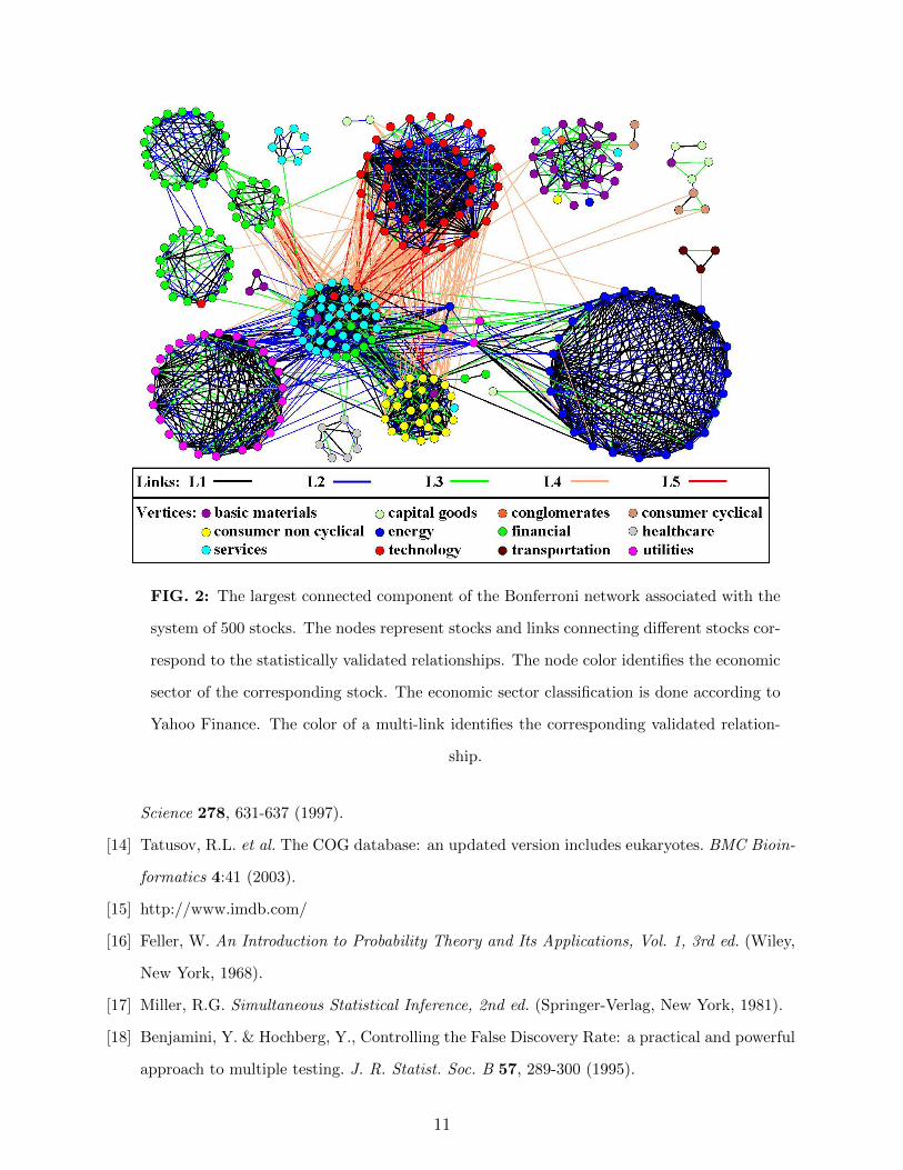
FIG. 2: The largest connected component of the Bonferroni network associated with the

system of 500 stocks. The nodes represent stocks and links connecting different stocks cor-

respond to the statistically validated relationships. The node color identifies the economic

sector of the corresponding stock. The economic sector classification is done according to

Yahoo Finance. The color of a multi-link identifies the corresponding validated relation-

ship.

Science 278, 631-637 (1997).

[14] Tatusov, R.L. et al. The COG database: an updated version includes eukaryotes. BMC Bioin-

formatics 4:41 (2003).

[15] http://www.imdb.com/

[16] Feller, W. An Introduction to Probability Theory and Its Applications, Vol. 1, 3rd ed. (Wiley,

New York, 1968).

[17] Miller, R.G. Simultaneous Statistical Inference, 2nd ed. (Springer-Verlag, New York, 1981).

[18] Benjamini, Y. & Hochberg, Y., Controlling the False Discovery Rate: a practical and powerful

approach to multiple testing. J. R. Statist. Soc. B 57, 289-300 (1995).

11

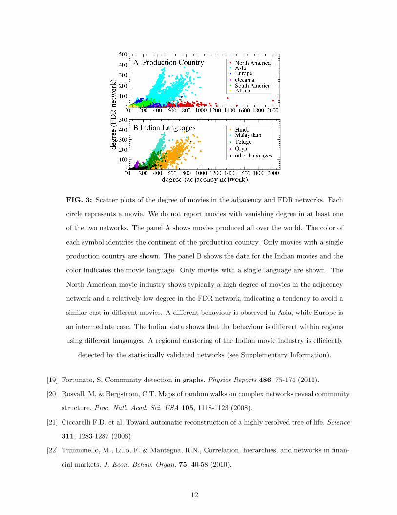
FIG. 3: Scatter plots of the degree of movies in the adjacency and FDR networks. Each

circle represents a movie. We do not report movies with vanishing degree in at least one

of the two networks. The panel A shows movies produced all over the world. The color of

each symbol identifies the continent of the production country. Only movies with a single

production country are shown. The panel B shows the data for the Indian movies and the

color indicates the movie language. Only movies with a single language are shown. The

North American movie industry shows typically a high degree of movies in the adjacency

network and a relatively low degree in the FDR network, indicating a tendency to avoid a

similar cast in different movies. A different behaviour is observed in Asia, while Europe is

an intermediate case. The Indian data shows that the behaviour is different within regions

using different languages. A regional clustering of the Indian movie industry is efficiently

detected by the statistically validated networks (see Supplementary Information).

[19] Fortunato, S. Community detection in graphs. Physics Reports 486, 75-174 (2010).

[20] Rosvall, M. & Bergstrom, C.T. Maps of random walks on complex networks reveal community

structure. Proc. Natl. Acad. Sci. USA 105, 1118-1123 (2008).

[21] Ciccarelli F.D. et al. Toward automatic reconstruction of a highly resolved tree of life. Science

311, 1283-1287 (2006).

[22] Tumminello, M., Lillo, F. & Mantegna, R.N., Correlation, hierarchies, and networks in finan-

cial markets. J. Econ. Behav. Organ. 75, 40-58 (2010).

12

[23] Mantegna R.N. Hierarchical structure in financial markets. Eur. Phys. J. B 11, 193-197 (1999).

[24] Bonanno, G., Caldarelli, G., Lillo, F. & Mantegna, R.N. Topology of correlation-based minimal

spanning trees in real and model markets. Phys. Rev. E 68, 046130 (2003).

[25] Tumminello, M., Aste, T., Di Matteo, T. & Mantegna, R.N. A tool for filtering information

in complex systems. Proc. Natl. Acad. Sci. USA 102, 10421-10426 (2005).

[26] Onnela, J.-P., Chakraborti, A., Kaski, K., Kertesz, J. & Kanto, A. Dynamics of market

correlations: Taxonomy and portfolio analysis. Phys. Rev. E 68, 056110 (2003).

[27] Tumminello, M., Coronnello, C., Lillo, F., Micciche, S. & Mantegna, R.N. Spanning Trees and

bootstrap reliability estimation in correlation based networks. Int. J. Bifurcation Chaos 17,

2319-2329 (2007).

[28] Newman M.E.J. Scientific collaboration networks. II. Shortest paths, weighted networks, and

centrality. Phys. Rev. E 64, 016132 (2001).

13

SUPPLEMENTARY INFORMATION

Statistically validated networks in bipartite complex systems

I. CLUSTER DETECTION AND CHARACTERIZATION

In the present study we perform community detection1,2 on the adjacency and statistically

validated networks, in order to put in evidence the different community structure of these

networks.

We obtain a partition of the vertices of networks by using the Infomap method by Ros-

vall and Bergstrom3. This algorithm is considered one of the best2 available today and it

allows to efficiently investigate both weighted and unweighted networks. The method uses

the probability flow of random walks in the considered network to identify the community

structure of the system. This approach implies that two independent applications of the

method to the same network may produce (typically slightly) different partitions of vertices.

For each investigated network, we run the Infomap 103 times and we select the best partition

according to the minimal “code length”3. The obtained partition depends on whether the

network is weighted or not, and eventually on how weights are selected. Therefore, in the

following we discuss case by case the way in which cluster detection is performed. Once

clusters of elements are detected, there still remains the problem of cluster interpretation.

We address this problem by comparing the partition of the system as produced by the In-

fomap with an a priori classification of the elements of the system. For instance movies can

be characterized by their genre, and stocks can be characterized according to their economic

sector.

A. Cluster characterization

Let us consider a system of N elements and a specific detected cluster C of NC elements to

be characterized. Each element of the system has a certain number of attributes according

1 Girvan, M., & Newman M.E.J., Community structure in social and biological networks Proc. Natl. Acad.

Sci. USA 99, 7821-7826 (2002).2 Fortunato, S., Community detection in graphs. Physics Reports 486, 75-174 (2010).3 Rosvall, M. & Bergstrom, C. T., Maps of random walks on complex networks reveal community structure.

Proc. Natl. Acad. Sci. USA 105, 1118-1123 (2008)

14

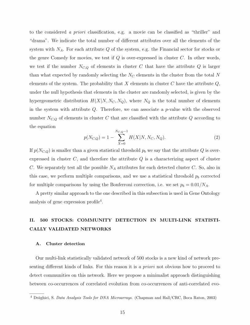
to the considered a priori classification, e.g. a movie can be classified as “thriller” and

“drama”. We indicate the total number of different attributes over all the elements of the

system with NA. For each attribute Q of the system, e.g. the Financial sector for stocks or

the genre Comedy for movies, we test if Q is over-expressed in cluster C. In other words,

we test if the number NC,Q of elements in cluster C that have the attribute Q is larger

than what expected by randomly selecting the NC elements in the cluster from the total N

elements of the system. The probability that X elements in cluster C have the attribute Q,

under the null hypothesis that elements in the cluster are randomly selected, is given by the

hypergeometric distribution H(X|N,NC , NQ), where NQ is the total number of elements

in the system with attribute Q. Therefore, we can associate a p-value with the observed

number NC,Q of elements in cluster C that are classified with the attribute Q according to

the equation

p(NC,Q) = 1−NC,Q−1∑X=0

H(X|N,NC , NQ). (2)

If p(NC,Q) is smaller than a given statistical threshold pb we say that the attribute Q is over-

expressed in cluster C, and therefore the attribute Q is a characterizing aspect of cluster

C. We separately test all the possible NA attributes for each detected cluster C. So, also in

this case, we perform multiple comparisons, and we use a statistical threshold pb corrected

for multiple comparisons by using the Bonferroni correction, i.e. we set pb = 0.01/NA.

A pretty similar approach to the one described in this subsection is used in Gene Ontology

analysis of gene expression profile4.

II. 500 STOCKS: COMMUNITY DETECTION IN MULTI-LINK STATISTI-

CALLY VALIDATED NETWORKS

A. Cluster detection

Our multi-link statistically validated network of 500 stocks is a new kind of network pre-

senting different kinds of links. For this reason it is a priori not obvious how to proceed to

detect communities on this network. Here we propose a minimalist approach distinguishing

between co-occurrences of correlated evolution from co-occurrences of anti-correlated evo-

4 Draghici, S. Data Analysis Tools for DNA Microarrays. (Chapman and Hall/CRC, Boca Raton, 2003)

15

lutions. Our procedure is as follows: in the community search on our network we remove

all the links describing anti-correlated evolutions (L4 and L5), or, equivalently, we weight

them with a zero weight. On the other hand, we weight the remaining links by taking into

account whether the statistical validation of the link is single or twofold. With this choice,

the twofold links L1 have the weight equal to 2, whereas onefold links L2 and L3 have the

weight equal to 1. While our approach is pragmatic and heuristic, we are aware that a more

theoretically based approach partitioning multi-link networks would certainly be useful in

our approach and in the study of many other networks, where links of different nature can

be naturally defined.

B. Cluster characterization

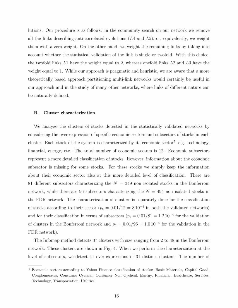
We analyze the clusters of stocks detected in the statistically validated networks by

considering the over-expression of specific economic sectors and subsectors of stocks in each

cluster. Each stock of the system is characterized by its economic sector5, e.g. technology,

financial, energy, etc. The total number of economic sectors is 12. Economic subsectors

represent a more detailed classification of stocks. However, information about the economic

subsector is missing for some stocks. For these stocks we simply keep the information

about their economic sector also at this more detailed level of classification. There are

81 different subsectors characterizing the N = 349 non isolated stocks in the Bonferroni

network, while there are 96 subsectors characterizing the N = 494 non isolated stocks in

the FDR network. The characterization of clusters is separately done for the classification

of stocks according to their sector (pb = 0.01/12 = 8 10−4 in both the validated networks)

and for their classification in terms of subsectors (pb = 0.01/81 = 1.2 10−4 for the validation

of clusters in the Bonferroni network and pb = 0.01/96 = 1.0 10−4 for the validation in the

FDR network).

The Infomap method detects 37 clusters with size ranging from 2 to 48 in the Bonferroni

network. These clusters are shown in Fig. 4. When we perform the characterization at the

level of subsectors, we detect 41 over-expressions of 31 distinct clusters. The number of

5 Economic sectors according to Yahoo Finance classification of stocks: Basic Materials, Capital Good,

Conglomerates, Consumer Cyclical, Consumer Non Cyclical, Energy, Financial, Healthcare, Services,

Technology, Transportation, Utilities.

16

FIG. 4: Clusters of the Bonferroni network of 500 stocks traded in the US equity markets.

The seven clusters on the top row from left to right can be labelled by the over-expressions

of economic subsectors as follows: 1) Services – Real estate operations, 2) Technology –

Communication equipment, Technology – Computer hardware, Technology – Electronic

instruments and control, and Technology – Semiconductors, 3) Consumer – Non-cyclical

food processing, and Consumer – Non-cyclical personal and household products, 4) En-

ergy – Oil and gas integrated, Energy – Oil and gas operations, and Energy – Oil well

services and equipment, 5) Basic materials – Chemical manufacturing, and Basic materi-

als – Chemical plastic and rubber, 6) Utilities –Electric utilities, and Utilities – Natural

gas utilities, and 7) Financial – Insurance life, and Financial – Insurance property and

casualty.

over-expressed subsectors per cluster is therefore 1.32. Most of the clusters are described by

a single economic subsector.

In Fig. 5 we show a color representation of the categorical variables of some of the stocks

included in the Bonferroni network. Specifically, we consider stocks belonging to the 10

largest clusters detected by the Infomap algorithm. In Fig. 5 a green spot indicates a state

up of the excess return whereas a red spot indicates a state down. The state null of the

excess return is represented by a black spot. Vertical blue lines are separating different

17

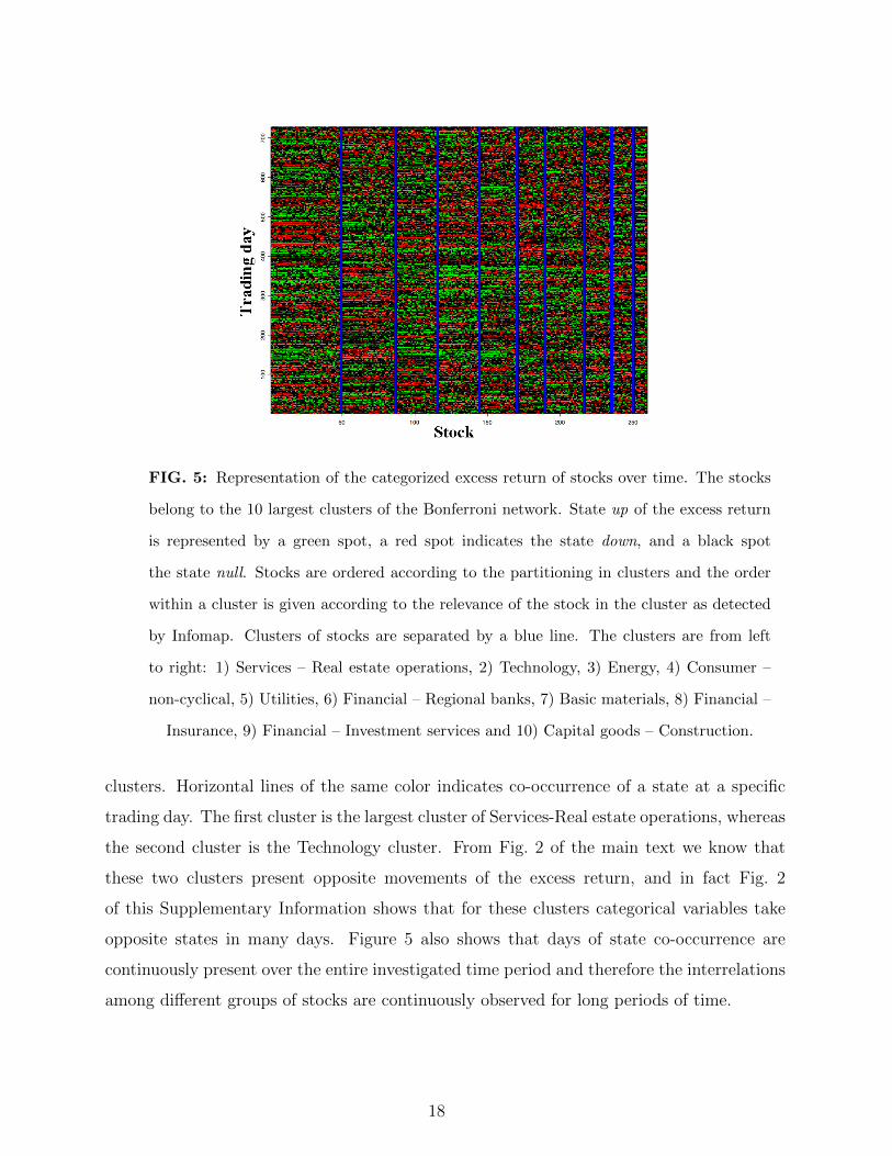
FIG. 5: Representation of the categorized excess return of stocks over time. The stocks

belong to the 10 largest clusters of the Bonferroni network. State up of the excess return

is represented by a green spot, a red spot indicates the state down, and a black spot

the state null. Stocks are ordered according to the partitioning in clusters and the order

within a cluster is given according to the relevance of the stock in the cluster as detected

by Infomap. Clusters of stocks are separated by a blue line. The clusters are from left

to right: 1) Services – Real estate operations, 2) Technology, 3) Energy, 4) Consumer –

non-cyclical, 5) Utilities, 6) Financial – Regional banks, 7) Basic materials, 8) Financial –

Insurance, 9) Financial – Investment services and 10) Capital goods – Construction.

clusters. Horizontal lines of the same color indicates co-occurrence of a state at a specific

trading day. The first cluster is the largest cluster of Services-Real estate operations, whereas

the second cluster is the Technology cluster. From Fig. 2 of the main text we know that

these two clusters present opposite movements of the excess return, and in fact Fig. 2

of this Supplementary Information shows that for these clusters categorical variables take

opposite states in many days. Figure 5 also shows that days of state co-occurrence are

continuously present over the entire investigated time period and therefore the interrelations

among different groups of stocks are continuously observed for long periods of time.

18

III. NETWORK OF MOVIES

The largest component of the adjacency movie network comprises 77,193 movies whereas

the second largest component has only 11 movies. When we apply the Infomap partition-

ing algorithm to the unweighted adjacency movie network we obtain a partitioning of the

network which presents 2,451 distinct clusters. The cluster size decreases smoothly from

the largest value of 13,608 down to the smallest value of 2. We will see in the following

discussion that the partitioning of the network presents a certain degree of informativeness

about the system. In fact the obtained clusters present a certain degree of homogeneity

with respect to the main country of production, the language and some classes of genre of

movies.

The FDR network is characterized by a largest connected component of 30,934 movies.

The Infomap algorithm makes a partition of this and other components of the network into

3,967 clusters whose size is decreasing from 1,478 to 2 movies. Table 1 of the main text

shows that the Bonferroni network does not present a giant connected component. In fact

the largest connected component comprises only 13% of the movies linked in the network.

However, the application of the Infomap algorithm refines the natural partitioning of the

network by detecting 2,782 clusters whose size is ranging from 577 to 2 movies. We also

note that the number of connected components in the Bonferroni network (2,456) is roughly

equal to the number of the Infomap clusters in the adjacency network (2,451).

A. Community detection in weighted movie networks

Our method provides a full control of the statistical validation of links against a random

null hypothesis taking into account the fact that different movies have a different number of

actors. The system also presents a second source of heterogeneity. In fact, different actors

typically play a different number of movies. In our sample the number of movies played by

a single actor is ranging from 1 to 247. As discussed in the main text, we do not have a

rigorous and computationally feasible way to also take into account this second source of

heterogeneity in our statistical validation procedure. We therefore use a heuristic approach,

19

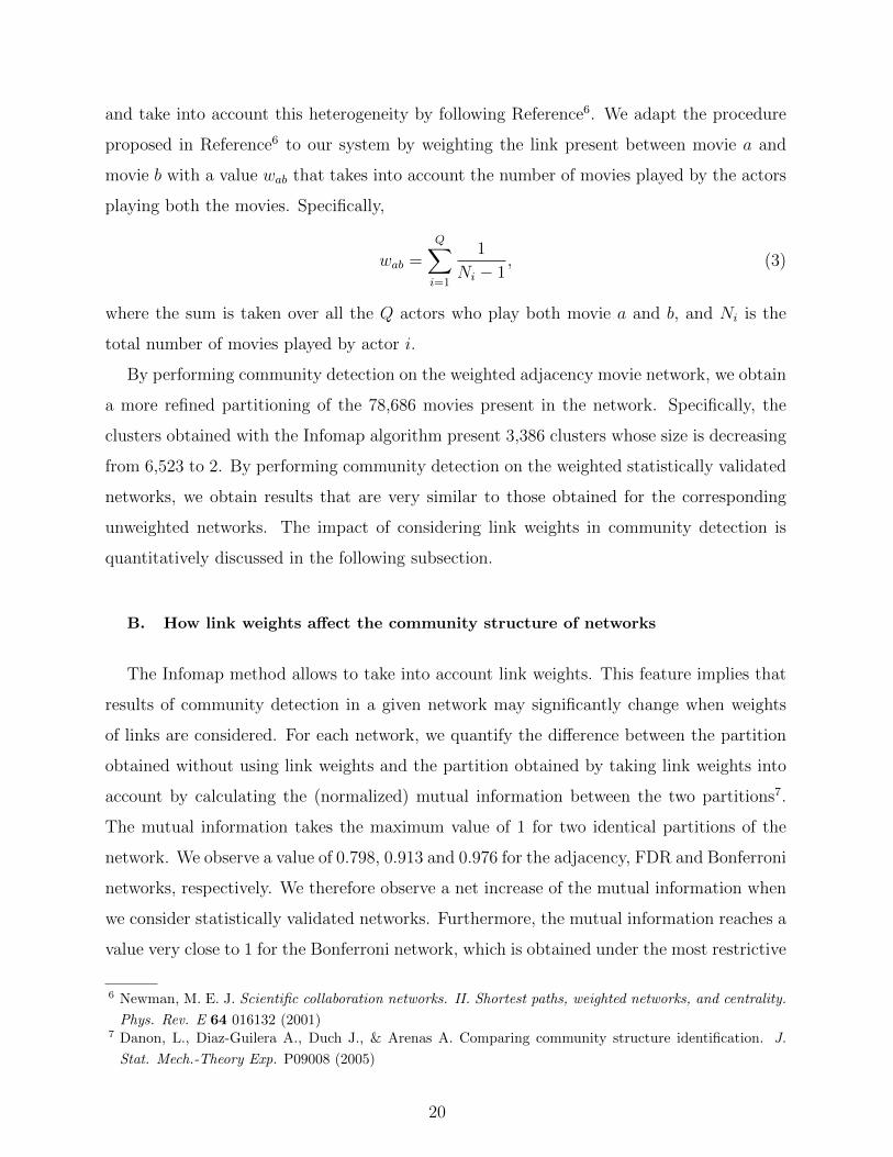
and take into account this heterogeneity by following Reference6. We adapt the procedure

proposed in Reference6 to our system by weighting the link present between movie a and

movie b with a value wab that takes into account the number of movies played by the actors

playing both the movies. Specifically,

wab =

Q∑i=1

1

Ni − 1, (3)

where the sum is taken over all the Q actors who play both movie a and b, and Ni is the

total number of movies played by actor i.

By performing community detection on the weighted adjacency movie network, we obtain

a more refined partitioning of the 78,686 movies present in the network. Specifically, the

clusters obtained with the Infomap algorithm present 3,386 clusters whose size is decreasing

from 6,523 to 2. By performing community detection on the weighted statistically validated

networks, we obtain results that are very similar to those obtained for the corresponding

unweighted networks. The impact of considering link weights in community detection is

quantitatively discussed in the following subsection.

B. How link weights affect the community structure of networks

The Infomap method allows to take into account link weights. This feature implies that

results of community detection in a given network may significantly change when weights

of links are considered. For each network, we quantify the difference between the partition

obtained without using link weights and the partition obtained by taking link weights into

account by calculating the (normalized) mutual information between the two partitions7.

The mutual information takes the maximum value of 1 for two identical partitions of the

network. We observe a value of 0.798, 0.913 and 0.976 for the adjacency, FDR and Bonferroni

networks, respectively. We therefore observe a net increase of the mutual information when

we consider statistically validated networks. Furthermore, the mutual information reaches a

value very close to 1 for the Bonferroni network, which is obtained under the most restrictive

6 Newman, M. E. J. Scientific collaboration networks. II. Shortest paths, weighted networks, and centrality.

Phys. Rev. E 64 016132 (2001)7 Danon, L., Diaz-Guilera A., Duch J., & Arenas A. Comparing community structure identification. J.

Stat. Mech.-Theory Exp. P09008 (2005)

20

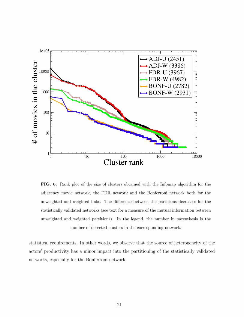
FIG. 6: Rank plot of the size of clusters obtained with the Infomap algorithm for the

adjacency movie network, the FDR network and the Bonferroni network both for the

unweighted and weighted links. The difference between the partitions decreases for the

statistically validated networks (see text for a measure of the mutual information between

unweighted and weighted partitions). In the legend, the number in parenthesis is the

number of detected clusters in the corresponding network.

statistical requirements. In other words, we observe that the source of heterogeneity of the

actors’ productivity has a minor impact into the partitioning of the statistically validated

networks, especially for the Bonferroni network.

21

C. Cluster size and inclusiveness

In the following, we separately discuss the results obtained for the partitioning of the

adjacency, FDR and Bonferroni weighted networks. Results obtained for the Bonferroni

network are rather similar to those obtained for the FDR network. The size profile of the

clusters obtained by partitioning the adjacency, FDR and Bonferroni networks are shown

in Fig. 6, both in the case of unweighted and weighted networks. It is quite clear from

the figure that the cluster size decreases from the largest to the smallest cluster in a pretty

different way for the adjacency networks and the statistically validated networks. In fact,

the FDR and Bonferroni networks present a decay of cluster size versus its rank that is well

approximated by a power-law decay.

In the majority of cases, the clusters detected in the Bonferroni network correspond to

the strongest interconnected parts of larger clusters detected in the FDR network. The

clusters of the FDR network correspond in turn to sets of movies which in large majority

are present in bigger clusters observed in the weighted adjacency network. This general

observation should not be seen as a strict inclusive relation but we wish to point out that a

sort of “typical” inclusiveness is observed for most of the detected clusters.

In the next subsection we describe results about the characterization of clusters in the

different networks.

D. Cluster characterization

We analyze the clusters of movies we obtain for the three different weighted networks,

by considering the over-expression of specific characteristics of the movies contained in each

cluster. By using the information about movies as provided by IMDb, we consider 4 different

classifications of movies. Indeed the IMDb reports for each movie indication about (i)

country or countries of production, (ii) language or languages used in the movie, (iii) movie

genre (or genres) and (iv) location or locations where the movie was shot. Only in a limited

number of cases some of these informations are not available. When this happens we indicate

the missing attribute about the movie as “not available”. We characterize clusters obtained

for all the networks by separately testing the over-expression of each attribute present in

each one of the above mentioned 4 classifications.

22

In different networks we observe a different profile of over-expression. The degree of

specificity is higher for smaller clusters and therefore a higher specificity is observed for the

Bonferroni and for the FDR networks. This is especially true for the genre and the location

classifications. In general, the country and language over-expression is quite specific for most

clusters in the investigated networks. Exceptions are clusters containing movies produced

in former Yugoslavia and Soviet Union. This is due to the fact that during the investigated

period these countries have split into several independent countries.

In Table II we summarize the number of over-expressions observed in the clusters iden-

tified by the Infomap in the weighted networks. We also report in parenthesis the number

of distinct clusters where at least one over-expression has been observed. By comparing the

number of over-expressions with the number of characterized clusters, one can estimate the

average number of over-expressions per cluster. This number decreases, for any considered

classification, when we move from the weighted adjacency network to the weighted FDR net-

work and then to the weighted Bonferroni network (the only exception being observed for

the language characterization when moving from the FDR to the Bonferroni network). For

example, in the case of the genre over-expression, the average number of over-expressions per

cluster is 1.41, 1.34 and 1.33 for the adjacency, FDR and Bonferroni network, respectively.

The decrease is more pronounced for the genre and filming location characterization. This

observation quantitatively indicates a higher specificity in cluster characterization for the

statistically validated networks. In the next section, we comment in detail two specific cases,

in order to illustrate some of the changes of sensitivity and specificity in the over-expression

characterization of clusters in the different weighted networks.

E. Case studies

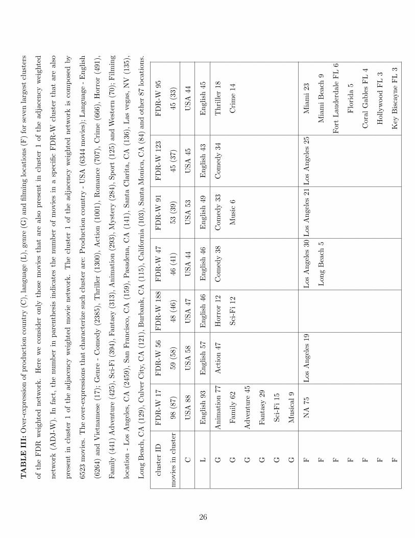
1. Largest cluster of the weighted adjacency network and the overlapping FDR clusters

We discuss the case of the largest cluster observed in the partition of the adjacency

weighted network. This is a cluster of 6,523 movies mainly in English and mainly produced

in the USA. In the caption of Table III, we report the major over-expressions observed

for this cluster. The over-expressed production country is USA and in fact 6,433 movies

of the cluster have been produced or co-produced in that country. The over-expressed

23

TABLE II: Summary of the over-expression of production country, language, genre and

filming location observed in the clusters obtained by performing the Infomap partitioning of

the adjacency weighted movie network (ADJ-W), FDR weighted movie network (FDR-W)

and the Bonferroni weighted movie network (BONF-W). For each of the four considered

classifications, we report the total number of observed over-expressions for each network.

The number in parenthesis is the number of distinct clusters where at least one over-

expression has been observed.

ADJ-W FDR-W BONF-W

movies in all clusters 78,686 37,429 12,850

number of clusters 3,386 4,982 2,931

Production country 1,206 1,944 1,009

over-expression (1,115) (1,816) (960)

Language 601 1,429 819

over-expression (494) (1,297) (729)

Genre 629 715 373

over-expression (445) (533) (281)

Filming location 2,196 1,836 853

over-expression (793) (1,123) (571)

languages are English and Vietnamese. However, it should be noted that the number of

movies filmed in these languages is quite different. In fact there are 6,264 movies where

the language is English and only 17 movies where the language is Vietnamese. The over-

expression of Vietnamese is observed because only 64 movies in Vietnamese are present in

the weighted adjacency network. The genre over-expression involves 14 different genres and

the filming location over-expression involves 97 different locations. The large majority of

filming locations are in California but cities of many other states are also observed.

We observe that 3,600 movies of the above described adjacency network cluster are split

in many clusters of the weighted FDR network. In Table III we report some information

about the seven FDR nework clusters having the largest intersection with the considered

adjacency network cluster. Cluster labels in the figure are those provided by the Infomap.

24

The complete list of clusters and movies for all the networks is available upon request to

the authors. From the Table it is evident that the size of the FDR clusters is more than

one order of magnitude smaller than the size of the adjacency cluster. In other words the

Infomap partitioning of the FDR network is quite refined for USA movies. These clusters

of movies are almost always characterized by USA as production country and English as

language. The genre and filming location over-expression provide the main characterization

of FDR clusters. Table III shows that the FDR cluster 17 is mainly a cluster of animation

movies and, of course, for this cluster no filming location over-expression is observed except

the indication of not available (NA). Cluster 56 is a cluster of action movies and the main

filming location of them is Los Angeles, CA. Clusters 47, 91 and 123 are all clusters of

comedy movies and the over-expressed filming location is again Los Angeles, CA. Cluster 188

is composed by a group of horror movies and a group of science fiction movies, while cluster

95 mainly includes thriller and crime movies. Interestingly, for this last cluster the over-

expressed filming locations are all in Florida. This case study shows that the FDR network

loses in sensitivity with respect to the adjacency network (less movies are involved in the

FDR network) but significantly gains in specificity (clusters in the FDR network are more

homogeneous, especially with respect to the genre and filming location characterization). To

provide a further example of this improvement in specificity it is worth noting that 8 of the

17 movies in Vietnamese language present in the largest cluster of the weighted adjacency

network are found in cluster 775 of the FDR network, which is composed by only 15 movies.

2. A cluster of Indian movies of the weighted adjacency network and the overlapping clusters

of the FDR and Bonferroni networks

The second case study concerns a cluster of Indian movies. The weighted adjacency movie

network presents five large clusters of Indian movies. Here we discuss the properties of the

second largest cluster of these five Indian movies clusters. We do not consider the largest

one, because it is already very homogeneous according to the language: 90% of indian movies

in this cluster are in Hindi. We indicate the selected cluster of Indian movies as cluster 24

of the weighted adjacency network. This cluster consists of 648 movies. In the caption of

Table IV we report all the over-expressions observed for this cluster. The over-expressed

production country is indeed India and over-expressions are also observed for four languages

25

TA

BL

EII

I:O

ver-

exp

ress

ion

ofp

rod

uct

ion

cou

ntr

y(C

),la

ngu

age

(L),

gen

re(G

)an

dfi

lmin

glo

cati

ons

(F)

for

seve

nla

rges

tcl

ust

ers

ofth

eF

DR

wei

ghte

dn

etw

ork.

Her

ew

eco

nsi

der

only

thos

em

ovie

sth

atar

eal

sop

rese

nt

incl

ust

er1

ofth

ead

jace

ncy

wei

ghte

d

net

wor

k(A

DJ-W

).In

fact

,th

enu

mb

erin

par

enth

esis

ind

icat

esth

enu

mb

erof

mov

ies

ina

spec

ific

FD

R-W

clu

ster

that

are

also

pre

sent

incl

ust

er1

ofth

ead

jace

ncy

wei

ghte

dm

ovie

net

wor

k.

Th

ecl

ust

er1

ofth

ead

jace

ncy

wei

ghte

dn

etw

ork

isco

mp

osed

by

6523

mov

ies.

Th

eov

er-e

xp

ress

ion

sth

atch

arac

teri

zesu

chcl

ust

erar

e:P

rod

uct

ion

cou

ntr

y-

US

A(6

344

mov

ies)

;L

angu

age

-E

ngl

ish

(626

4)

and

Vie

tnam

ese

(17)

;G

enre

-C

omed

y(2

385)

,T

hri

ller

(130

0),

Act

ion

(100

1),

Rom

ance

(707

),C

rim

e(6

66),

Hor

ror

(491

),

Fam

ily

(441

)A

dve

ntu

re(4

25)

,S

ci-F

i(3

94),

Fan

tasy

(313

),A

nim

atio

n(2

93),

Myst

ery

(284

),S

por

t(1

25)

and

Wes

tern

(70)

;F

ilm

ing

loca

tion

-L

os

An

gele

s,C

A(2

459),

San

Fra

nci

sco,

CA

(159

),P

asad

ena,

CA

(141

),S

anta

Cla

rita

,C

A(1

36),

Las

vega

s,N

V(1

35),

Lon

gB

each

,C

A(1

29),

Cu

lver

Cit

y,C

A(1

21),

Bu

rban

k,

CA

(115

),C

alif

orn

ia(1

03),

San

taM

onic

a,C

A(8

4)an

dot

her

87lo

cati

ons.

clu

ster

IDF

DR

-W17

FD

R-W

56F

DR

-W18

8F

DR

-W47

FD

R-W

91F

DR

-W12

3F

DR

-W95

mov

ies

incl

ust

er98

(87)

59

(58)

48(4

6)46

(41)

53(3

9)45

(37)

45(3

3)

CU

SA

88U

SA

58U

SA

47U

SA

44U

SA

53U

SA

45U

SA

44

LE

ngl

ish

93

En

gli

sh57

En

glis

h46

En

glis

h46

En

glis

h49

En

glis

h43

En

glis

h45

GA

nim

ati

on

77A

ctio

n47

Hor

ror

12C

omed

y38

Com

edy

33C

omed

y34

Th

rill

er18

GF

amil

y62

Sci

-Fi

12M

usi

c6

Cri

me

14

GA

dve

ntu

re45

GF

anta

sy29

GS

ci-F

i15

GM

usi

cal

9

FN

A75

Los

An

gele

s19

Los

An

gele

s30

Los

An

gele

s21

Los

An

gele

s25

Mia

mi

23

FL

ong

Bea

ch5

Mia

mi

Bea

ch9

FF

ort

Lau

der

dal

eF

L6

FF

lori

da

5

FC

oral

Gab

les

FL

4

FH

olly

wood

FL

3

FK

eyB

isca

yn

eF

L3

26

spoken in India, five distinct movie genres, and eight filming locations. By comparing the

clusters of the weighted FDR network with this cluster of the weighted adjacency network,

we observe a large overlapping of movies. For example, 515 movies of cluster 24 are present

in clusters 5 and 43 of the weighted FDR network. In other words, the Indian cluster 24

detected in the weighted adjacency network splits into two distinct clusters in the weighted

FDR network. The first cluster (cluster 5) comprises movies where the language spoken is

mainly Telugu, whereas the second cluster (cluster 43) mainly comprises movies in Tamil.

The characterization of genre and filming location is more specific than the one observed

for cluster 24 of the adjacency network, but the degree of specificity is not too high (see the

first two columns of Table IV).

A higher degree of specificity is observed when we consider the clusters of the weighted

Bonferroni network. In Table IV, we show the over-expression characterization of the five

largest clusters of Bonferroni network overlapping with cluster 24 of the weighted adjacency

network (last five columns of Table IV). There is a unique language characterization per

cluster at this level. The filming location characterization is poor due to the fact that

this information is often absent for Indian movies recorded in the IMDb. In fact the “not

available” (NA) over-expression is the most frequent one.

In conclusion, we also notice for Indian movies the ability of statistically validated net-

works to describe communities of movies that are smaller but more homogeneous, according

to the considered classifications, with respect to the communities of movies in the adjacency

network.

27

TA

BL

EIV

:O

ver-

exp

ress

ion

ofp

rod

uct

ion

cou

ntr

y(C

),la

ngu

age

(L),

gen

re(G

)an

dfi

lmin

glo

cati

ons

(F)

for

two

larg

est

clu

ster

s

ofF

DR

wei

ghte

dn

etw

ork

an

dfi

ve

larg

est

clu

ster

sof

Bon

ferr

oni

wei

ghte

dn

etw

orks.

Her

ew

eco

nsi

der

the

mov

ies

that

are

also

pre

sent

incl

ust

er24

of

the

ad

jace

ncy

wei

ghte

dm

ovie

net

wor

k.

Infa

ct,

the

nu

mb

erin

par

enth

esis

ind

icat

eth

enum

ber

ofm

ovie

sin

asp

ecifi

cF

DR

-Wor

BO

NF

-Wcl

ust

erth

atar

eal

sop

rese

nt

incl

ust

er24

ofth

ead

jace

ncy

wei

ghte

dm

ovie

net

wor

k.

Th

ecl

ust

er24

ofth

ead

jace

ncy

wei

ghte

dn

etw

ork

isco

mp

osed

by

648

mov

ies.

Th

eov

er-e

xp

ress

ion

sth

atch

arac

teri

zesu

chcl

ust

erar

e:P

rod

uct

ion

cou

ntr

y-

Ind

ia(6

43m

ovie

s);

Lan

guag

e-

Tel

ugu

(438

),T

amil

(196

),H

ind

i(5

2)an

dK

ann

ada

(14)

;G

enre

-D

ram

a(3

12),

Act

ion

(213

),R

om

ance

(180),

Fam

ily

(53)

an

dM

usi

cal

(48)

;F

ilm

ing

loca

tion

-N

otA

vail

able

(515

),H

yd

erab

ad(5

3),

Ch

enn

ai(3

1),

Ind

ia

(17),

An

dh

raP

rad

esh

(8),

Ra

jah

mu

nd

ry(5

),T

amil

Nad

u(4

)an

dV

ikar

abad

(3).

clu

ster

IDF

DR

-W5

FD

R-W

43B

ON

F-W

10B

ON

F-W

13B

ON

F-W

309

BO

NF

-W60

7B

ON

F-W

806

396

(390)

132

(125

)11

1(1

11)

110

(110

)13

(13)

10(1

0)15

(13)

CIn

dia

395

Ind

ia13

2In

dia

111

Ind

ia11

0In

dia

13In

dia

10In

dia

15

LT

elu

gu375

Tam

il12

0T

elu

gu11

1T

elu

gu10

9T

elu

gu12

Tel

ugu

9T

amil

14

LT

amil

15H

ind

i21

LT

elu

gu21

GA

ctio

n132

Rom

ance

52F

amil

y25

Act

ion

47

GR

om

ance

94A

ctio

n48

Mu

sica

l11

Rom

ance

39

GF

amil

y40

Mu

sica

l17

GM

usi

cal

24

FN

A315

NA

99N

A98

NA

78

FH

yd

erab

ad

45C

hen

nai

15H

yd

erab

ad13

FA

nd

hra

Pra

des

h7

Tam

ilN

adu

3A

nd

hra

Pra

des

h5

FR

aja

hm

un

dry

4

28