Can Earthquake Loss Models be Validated Using Field Observations
29
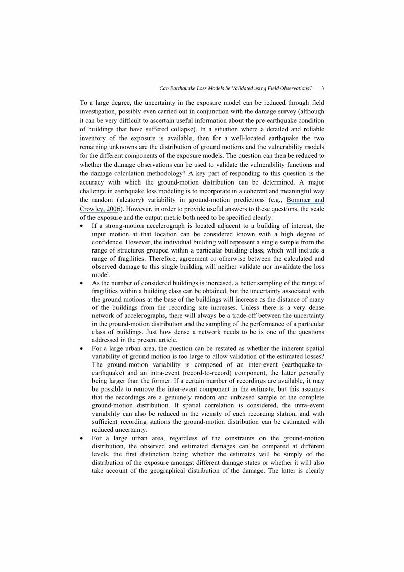
1 Journal of Earthquake Engineering © A. S. Elnashai and N. N. Ambraseys CAN EARTHQUAKE LOSS MODELS BE VALIDATED USING FIELD OBSERVATIONS? HELEN CROWLEY * European Centre for Training and Research in Earthquake Engineering (EUCENTRE),Via Ferrata 1, Pavia, Italy PETER J. STAFFORD and JULIAN J. BOMMER Department of Civil and Environmental Engineering, Imperial College London, London, UK Received (received date) Revised (revised date) Accepted (accepted date) The occurrence of a damaging earthquake provides an opportunity to compare observed and estimated damage, provided that detailed observations of the earthquake effects are made in the field. A question that arises is whether such comparisons can provide the basis for validation of an earthquake loss model. In order to explore this issue, a case study loss model for the northern Marmara region has been set up and the losses have been calculated for various ground-motion fields that arise when different assumptions are made about the ground-motion variability. In particular, the influence of removing the inter-event variability for a scenario earthquake and modeling spatial correlation among ground motions is studied. Further analyses are conducted assuming that a number of accelerograms are available within the region and that knowledge of spatial correlations among ground motions can therefore be used to better predict the motions at sites in the vicinity of the recording stations. The results demonstrate that unless one has a dense network of accelerographs (commensurate with the geographical resolution of exposure), then the variability in the losses cannot be sufficiently reduced to allow validation of the loss model. Keywords: ground-motion variability; spatial correlation; loss assessment; damage data 1. Introduction Earthquake loss models are developed to estimate the losses expected to be suffered by a given city, region or portfolio of insured assets due to either a single earthquake scenario or for a given return period considering the effects of all possible earthquake scenarios. In either case, if collateral earthquake hazards such as surface fault rupture, liquefaction and landslides are not considered, the estimates will be based on four basic elements: a seismicity model, specifying the location, magnitude and, in the case of probabilistic estimates, the frequency of the earthquake scenarios; a ground-motion model, which predicts the amplitude of one or more ground-motion parameters throughout the area of * Address correspondence to H. Crowley, European Centre for Training and Research in Earthquake Engineering (EUCENTRE), Via Ferrata 1, 27100, Pavia, Italy; E-mail: [email protected]
-
Upload
independent -
Category
Documents
-
view
0 -
download
0
Transcript of Can Earthquake Loss Models be Validated Using Field Observations
1
Journal of Earthquake Engineering © A. S. Elnashai and N. N. Ambraseys
CAN EARTHQUAKE LOSS MODELS BE VALIDATED USING FIELD OBSERVATIONS?
HELEN CROWLEY*
European Centre for Training and Research in Earthquake Engineering (EUCENTRE),Via Ferrata 1, Pavia, Italy
PETER J. STAFFORD and JULIAN J. BOMMER Department of Civil and Environmental Engineering,
Imperial College London, London, UK
Received (received date) Revised (revised date)
Accepted (accepted date)
The occurrence of a damaging earthquake provides an opportunity to compare observed and estimated damage, provided that detailed observations of the earthquake effects are made in the field. A question that arises is whether such comparisons can provide the basis for validation of an earthquake loss model. In order to explore this issue, a case study loss model for the northern Marmara region has been set up and the losses have been calculated for various ground-motion fields that arise when different assumptions are made about the ground-motion variability. In particular, the influence of removing the inter-event variability for a scenario earthquake and modeling spatial correlation among ground motions is studied. Further analyses are conducted assuming that a number of accelerograms are available within the region and that knowledge of spatial correlations among ground motions can therefore be used to better predict the motions at sites in the vicinity of the recording stations. The results demonstrate that unless one has a dense network of accelerographs (commensurate with the geographical resolution of exposure), then the variability in the losses cannot be sufficiently reduced to allow validation of the loss model.
Keywords: ground-motion variability; spatial correlation; loss assessment; damage data
1. Introduction
Earthquake loss models are developed to estimate the losses expected to be suffered by a given city, region or portfolio of insured assets due to either a single earthquake scenario or for a given return period considering the effects of all possible earthquake scenarios. In either case, if collateral earthquake hazards such as surface fault rupture, liquefaction and landslides are not considered, the estimates will be based on four basic elements: a seismicity model, specifying the location, magnitude and, in the case of probabilistic estimates, the frequency of the earthquake scenarios; a ground-motion model, which predicts the amplitude of one or more ground-motion parameters throughout the area of
*Address correspondence to H. Crowley, European Centre for Training and Research in Earthquake Engineering (EUCENTRE), Via Ferrata 1, 27100, Pavia, Italy; E-mail: [email protected]
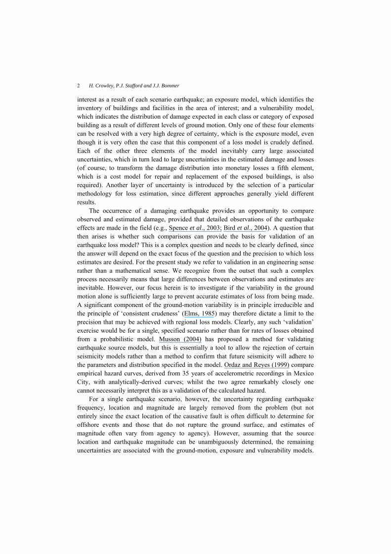
2 H. Crowley, P.J. Stafford and J.J. Bommer interest as a result of each scenario earthquake; an exposure model, which identifies the inventory of buildings and facilities in the area of interest; and a vulnerability model, which indicates the distribution of damage expected in each class or category of exposed building as a result of different levels of ground motion. Only one of these four elements can be resolved with a very high degree of certainty, which is the exposure model, even though it is very often the case that this component of a loss model is crudely defined. Each of the other three elements of the model inevitably carry large associated uncertainties, which in turn lead to large uncertainties in the estimated damage and losses (of course, to transform the damage distribution into monetary losses a fifth element, which is a cost model for repair and replacement of the exposed buildings, is also required). Another layer of uncertainty is introduced by the selection of a particular methodology for loss estimation, since different approaches generally yield different results.
The occurrence of a damaging earthquake provides an opportunity to compare observed and estimated damage, provided that detailed observations of the earthquake effects are made in the field (e.g., Spence et al., 2003; Bird et al., 2004). A question that then arises is whether such comparisons can provide the basis for validation of an earthquake loss model? This is a complex question and needs to be clearly defined, since the answer will depend on the exact focus of the question and the precision to which loss estimates are desired. For the present study we refer to validation in an engineering sense rather than a mathematical sense. We recognize from the outset that such a complex process necessarily means that large differences between observations and estimates are inevitable. However, our focus herein is to investigate if the variability in the ground motion alone is sufficiently large to prevent accurate estimates of loss from being made. A significant component of the ground-motion variability is in principle irreducible and the principle of ‘consistent crudeness’ (Elms, 1985) may therefore dictate a limit to the precision that may be achieved with regional loss models. Clearly, any such ‘validation’ exercise would be for a single, specified scenario rather than for rates of losses obtained from a probabilistic model. Musson (2004) has proposed a method for validating earthquake source models, but this is essentially a tool to allow the rejection of certain seismicity models rather than a method to confirm that future seismicity will adhere to the parameters and distribution specified in the model. Ordaz and Reyes (1999) compare empirical hazard curves, derived from 35 years of accelerometric recordings in Mexico City, with analytically-derived curves; whilst the two agree remarkably closely one cannot necessarily interpret this as a validation of the calculated hazard.
For a single earthquake scenario, however, the uncertainty regarding earthquake frequency, location and magnitude are largely removed from the problem (but not entirely since the exact location of the causative fault is often difficult to determine for offshore events and those that do not rupture the ground surface, and estimates of magnitude often vary from agency to agency). However, assuming that the source location and earthquake magnitude can be unambiguously determined, the remaining uncertainties are associated with the ground-motion, exposure and vulnerability models.
Can Earthquake Loss Models be Validated using Field Observations?
3
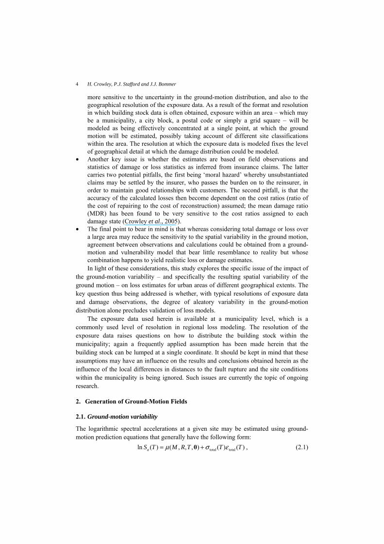
To a large degree, the uncertainty in the exposure model can be reduced through field investigation, possibly even carried out in conjunction with the damage survey (although it can be very difficult to ascertain useful information about the pre-earthquake condition of buildings that have suffered collapse). In a situation where a detailed and reliable inventory of the exposure is available, then for a well-located earthquake the two remaining unknowns are the distribution of ground motions and the vulnerability models for the different components of the exposure models. The question can then be reduced to whether the damage observations can be used to validate the vulnerability functions and the damage calculation methodology? A key part of responding to this question is the accuracy with which the ground-motion distribution can be determined. A major challenge in earthquake loss modeling is to incorporate in a coherent and meaningful way the random (aleatory) variability in ground-motion predictions (e.g., Bommer and Crowley, 2006). However, in order to provide useful answers to these questions, the scale of the exposure and the output metric both need to be specified clearly: • If a strong-motion accelerograph is located adjacent to a building of interest, the
input motion at that location can be considered known with a high degree of confidence. However, the individual building will represent a single sample from the range of structures grouped within a particular building class, which will include a range of fragilities. Therefore, agreement or otherwise between the calculated and observed damage to this single building will neither validate nor invalidate the loss model.
• As the number of considered buildings is increased, a better sampling of the range of fragilities within a building class can be obtained, but the uncertainty associated with the ground motions at the base of the buildings will increase as the distance of many of the buildings from the recording site increases. Unless there is a very dense network of accelerographs, there will always be a trade-off between the uncertainty in the ground-motion distribution and the sampling of the performance of a particular class of buildings. Just how dense a network needs to be is one of the questions addressed in the present article.
• For a large urban area, the question can be restated as whether the inherent spatial variability of ground motion is too large to allow validation of the estimated losses? The ground-motion variability is composed of an inter-event (earthquake-to-earthquake) and an intra-event (record-to-record) component, the latter generally being larger than the former. If a certain number of recordings are available, it may be possible to remove the inter-event component in the estimate, but this assumes that the recordings are a genuinely random and unbiased sample of the complete ground-motion distribution. If spatial correlation is considered, the intra-event variability can also be reduced in the vicinity of each recording station, and with sufficient recording stations the ground-motion distribution can be estimated with reduced uncertainty.
• For a large urban area, regardless of the constraints on the ground-motion distribution, the observed and estimated damages can be compared at different levels, the first distinction being whether the estimates will be simply of the distribution of the exposure amongst different damage states or whether it will also take account of the geographical distribution of the damage. The latter is clearly
4 H. Crowley, P.J. Stafford and J.J. Bommer
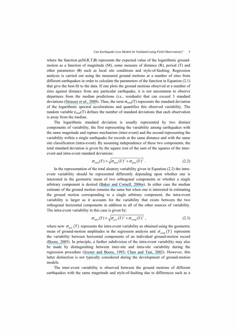
more sensitive to the uncertainty in the ground-motion distribution, and also to the geographical resolution of the exposure data. As a result of the format and resolution in which building stock data is often obtained, exposure within an area – which may be a municipality, a city block, a postal code or simply a grid square – will be modeled as being effectively concentrated at a single point, at which the ground motion will be estimated, possibly taking account of different site classifications within the area. The resolution at which the exposure data is modeled fixes the level of geographical detail at which the damage distribution could be modeled.
• Another key issue is whether the estimates are based on field observations and statistics of damage or loss statistics as inferred from insurance claims. The latter carries two potential pitfalls, the first being ‘moral hazard’ whereby unsubstantiated claims may be settled by the insurer, who passes the burden on to the reinsurer, in order to maintain good relationships with customers. The second pitfall, is that the accuracy of the calculated losses then become dependent on the cost ratios (ratio of the cost of repairing to the cost of reconstruction) assumed; the mean damage ratio (MDR) has been found to be very sensitive to the cost ratios assigned to each damage state (Crowley et al., 2005).
• The final point to bear in mind is that whereas considering total damage or loss over a large area may reduce the sensitivity to the spatial variability in the ground motion, agreement between observations and calculations could be obtained from a ground-motion and vulnerability model that bear little resemblance to reality but whose combination happens to yield realistic loss or damage estimates. In light of these considerations, this study explores the specific issue of the impact of
the ground-motion variability – and specifically the resulting spatial variability of the ground motion – on loss estimates for urban areas of different geographical extents. The key question thus being addressed is whether, with typical resolutions of exposure data and damage observations, the degree of aleatory variability in the ground-motion distribution alone precludes validation of loss models.
The exposure data used herein is available at a municipality level, which is a commonly used level of resolution in regional loss modeling. The resolution of the exposure data raises questions on how to distribute the building stock within the municipality; again a frequently applied assumption has been made herein that the building stock can be lumped at a single coordinate. It should be kept in mind that these assumptions may have an influence on the results and conclusions obtained herein as the influence of the local differences in distances to the fault rupture and the site conditions within the municipality is being ignored. Such issues are currently the topic of ongoing research.
2. Generation of Ground-Motion Fields
2.1. Ground-motion variability
The logarithmic spectral accelerations at a given site may be estimated using ground-motion prediction equations that generally have the following form: total totalln ( ) ( , , , ) ( ) ( )aS T M R T T Tµ σ ε= +θ , (2.1)
Can Earthquake Loss Models be Validated using Field Observations?
5
where the function µ(M,R,T,θ) represents the expected value of the logarithmic ground-motion as a function of magnitude (M), some measure of distance (R), period (T) and other parameters (θ) such as local site conditions and style-of-faulting. Regression analysis is carried out using the measured ground motions at a number of sites from different earthquakes in order to calculate the parameters of the function in Equation (2.1) that give the best-fit to the data. If one plots the ground motions observed at a number of sites against distance from any particular earthquake, it is not uncommon to observe departures from the median predictions (i.e., residuals) that can exceed 3 standard deviations (Strasser et al., 2008). Thus, the term σtotal(T) represents the standard deviation of the logarithmic spectral accelerations and quantifies this observed variability. The random variable εtotal(T) defines the number of standard deviations that each observation is away from the median.
The logarithmic standard deviation is usually represented by two distinct components of variability, the first representing the variability among earthquakes with the same magnitude and rupture mechanism (inter-event) and the second representing the variability within a single earthquake for records at the same distance and with the same site classification (intra-event). By assuming independence of these two components, the total standard deviation is given by the square root of the sum of the squares of the inter-event and intra-event standard deviations:
2 2total inter intra( ) ( ) ( )T T Tσ σ σ= + . (2.2)
In the representation of the total aleatory variability given in Equation (2.2) the intra-event variability should be represented differently depending upon whether one is interested in the geometric mean of two orthogonal components or whether a single arbitrary component is desired (Baker and Cornell, 2006a). In either case the median estimate of the ground motion remains the same but when one is interested in estimating the ground motion corresponding to a single arbitrary component, the intra-event variability is larger as it accounts for the variability that exists between the two orthogonal horizontal components in addition to all of the other sources of variability. The intra-event variability in this case is given by:
2 2intra g.m. comp( ) ( ) ( )T T Tσ σ σ= + , (2.3)
where now ( )g.m. Tσ represents the intra-event variability as obtained using the geometric mean of ground-motion amplitudes in the regression analysis and ( )comp Tσ represents the variability between horizontal components of an individual ground-motion record (Boore, 2005). In principle, a further subdivision of the intra-event variability may also be made by distinguishing between inter-site and intra-site variability during the regression procedure (Joyner and Boore, 1993; Chen and Tsai, 2002). However, this latter distinction is not typically considered during the development of ground-motion models.
The inter-event variability is observed between the ground motions of different earthquakes with the same magnitude and style-of-faulting due to differences such as a
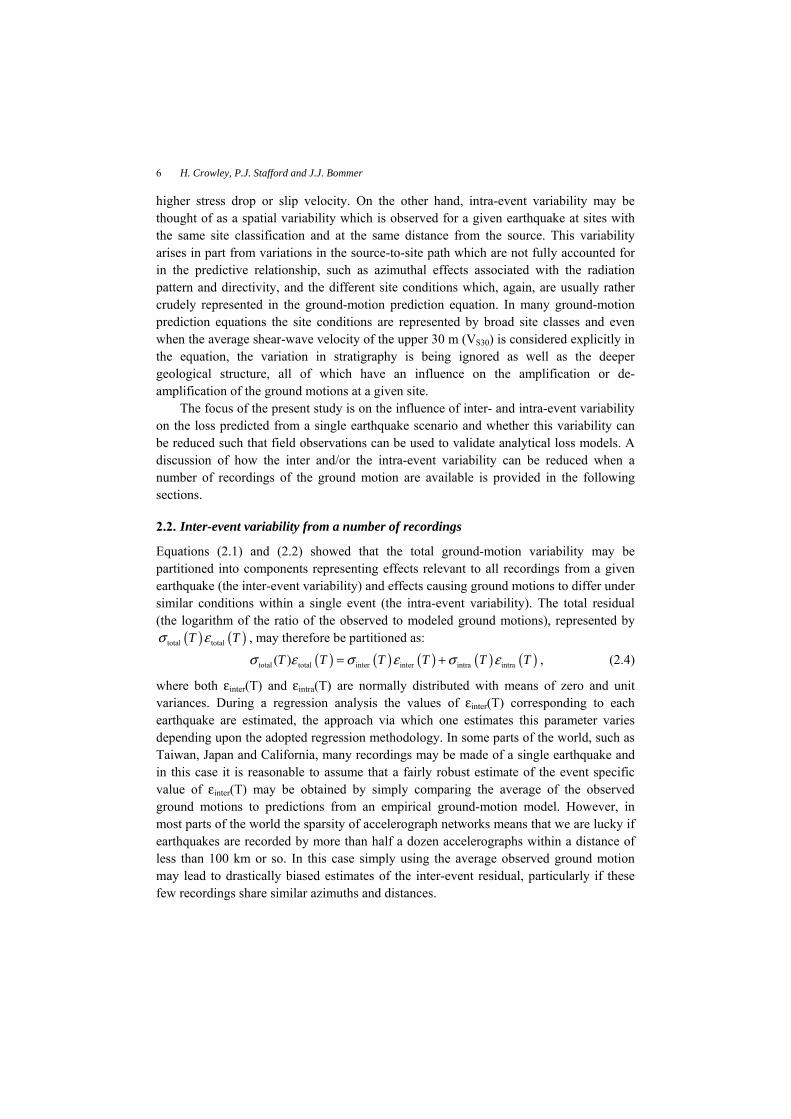
6 H. Crowley, P.J. Stafford and J.J. Bommer higher stress drop or slip velocity. On the other hand, intra-event variability may be thought of as a spatial variability which is observed for a given earthquake at sites with the same site classification and at the same distance from the source. This variability arises in part from variations in the source-to-site path which are not fully accounted for in the predictive relationship, such as azimuthal effects associated with the radiation pattern and directivity, and the different site conditions which, again, are usually rather crudely represented in the ground-motion prediction equation. In many ground-motion prediction equations the site conditions are represented by broad site classes and even when the average shear-wave velocity of the upper 30 m (VS30) is considered explicitly in the equation, the variation in stratigraphy is being ignored as well as the deeper geological structure, all of which have an influence on the amplification or de-amplification of the ground motions at a given site.
The focus of the present study is on the influence of inter- and intra-event variability on the loss predicted from a single earthquake scenario and whether this variability can be reduced such that field observations can be used to validate analytical loss models. A discussion of how the inter and/or the intra-event variability can be reduced when a number of recordings of the ground motion are available is provided in the following sections.
2.2. Inter-event variability from a number of recordings
Equations (2.1) and (2.2) showed that the total ground-motion variability may be partitioned into components representing effects relevant to all recordings from a given earthquake (the inter-event variability) and effects causing ground motions to differ under similar conditions within a single event (the intra-event variability). The total residual (the logarithm of the ratio of the observed to modeled ground motions), represented by
( ) ( )total totalT Tσ ε , may therefore be partitioned as:
( ) ( ) ( ) ( ) ( )total total inter inter intra intra( )T T T T T Tσ ε σ ε σ ε= + , (2.4)
where both εinter(T) and εintra(T) are normally distributed with means of zero and unit variances. During a regression analysis the values of εinter(T) corresponding to each earthquake are estimated, the approach via which one estimates this parameter varies depending upon the adopted regression methodology. In some parts of the world, such as Taiwan, Japan and California, many recordings may be made of a single earthquake and in this case it is reasonable to assume that a fairly robust estimate of the event specific value of εinter(T) may be obtained by simply comparing the average of the observed ground motions to predictions from an empirical ground-motion model. However, in most parts of the world the sparsity of accelerograph networks means that we are lucky if earthquakes are recorded by more than half a dozen accelerographs within a distance of less than 100 km or so. In this case simply using the average observed ground motion may lead to drastically biased estimates of the inter-event residual, particularly if these few recordings share similar azimuths and distances.
Can Earthquake Loss Models be Validated using Field Observations?
7
Bommer and Crowley (2006) have presented a discussion on the treatment of ground-motion variability in loss estimation analyses. The most theoretically robust approach is to use Monte Carlo simulation to generate ground-motion fields by first drawing from the inter-event variability to obtain the value of εinter(T) and then drawing from the intra-event variability for many sites to obtain the εintra(T) terms. This approach allows the total variability to be accounted for in a meaningful way. However, in the present study we are concerned with addressing the question of whether or not a loss estimate may be validated through the use of field observations. Under this scenario it is assumed that we have a suite of observed motions and the proper application of the Bommer and Crowley (2006) approach would therefore be to obtain the inter-event residual directly from the observed ground motions and then sample from the intra-event variability in order to simulate realistic ground-motion fields that are consistent with the observations.
The reduction in ground-motion variability that may be achieved if one has knowledge of the inter-event residual is significant (Anderson and Brune, 1999). The chances of validating a loss model increase markedly if one can reduce the uncertainty associated with creating an estimate of the actual ground-motion field. It is therefore important to try to obtain estimates of this parameter so that the total variability may be reduced. The issue of how to best estimate the inter-event residual given a certain number of records with a particular spatial distribution is a non-trivial issue that is still under investigation. For the purposes of the current work we assume that one may obtain an estimate, provided at least a few records are available, and investigate the impact of modeling ground-motion fields using the reduced variability associated with this condition.
2.3. Macrospatial correlation of ground motions
A further consideration made herein concerns the macrospatial correlation between the ground-motion residuals at pairs of sites due to their proximity. This is a phenomenon whose importance in seismic risk analysis has been recognized for many years (e.g., McGuire, 1988), but which has only recently begun to be modeled due to the increased number of dense arrays of recording stations that have been set up around the world. Macrospatial correlation between the ground-motion residuals at pairs of sites arises because the sites are affected by the same earthquake and thus may be affected by similar azimuthal and directivity effects of the propagating waves, similar geological profiles, etc. Boore et al. (2003) summarize this phenomenon as follows: “The spatial variability in ground motions reduces to zero as the distance between two sites decreases to zero. On the other hand, for a great enough separation distance the spatial correlation of the ground motions reduces to zero and the additional uncertainty reaches that for an individual observation about the overall change of motion with distance (as given, for example, by fitting the data to a function using regression analysis).”
8 H. Crowley, P.J. Stafford and J.J. Bommer
The model proposed in McGuire (1988) for the calculation of the covariance, γ(h,k), of the residuals of peak ground acceleration (PGA) at two sites h and k includes both directivity effects and a distance-dependent term:
2
0[ ( ( , ) / ) ]2 2 2( , ) 2 cos cosγ σ σ σ −= + Θ Θ + r h k re d h k sh k e , (2.5)
where σe2, σd
2 and σs2 are the variances of the residual terms εe (an event term, i.e., inter-
event), εd (a directivity term) and εs (a site term), respectively; Θh and Θk are the azimuths of sites h and k with respect to the rupture†; r(h,k) is the distance between the two sites and r0 is the standard correlation length (the separation distance at which the correlation coefficient is equal to e-1≈0.368).
A recent proposal for the correlation between the residuals of peak ground velocity (PGV) at two sites by Wang and Takada (2005) has the following form:
0( ( , ) / )( , ) r h k rh k eγ −= . (2.6)
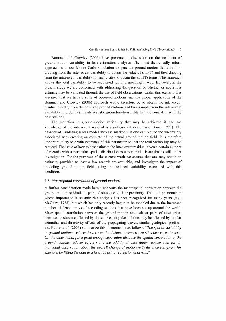
Here, only the intra-event distance-dependence term has been considered and the form is slightly different from the equivalent term in McGuire (1988). Wang and Takada (2005) obtained the ground-motion residuals from hundreds of recordings from six earthquakes in Japan and Taiwan by considering two different attenuation relationships. For each earthquake, they grouped the pairs of sites into bins with separation distance intervals of 4km and calculated the covariance between the ground-motion residuals in each bin for the two ground-motion relationships (Figure 1). The covariance functions for each earthquake and for each ground-motion relationship were found to lead to similar standard correlation lengths (around 20-40km). The uncertainty in the correlation length is nevertheless influenced by many factors such as wave propagation and ground conditions and is thus expected to change for different regions around the world.
r(h,k) r(h,k)
γ(h,
k)
γ(h,
k)
γ = exp(-r(h,k)/27.8) γ = exp(-r(h,k)/27.3)
Fig. 1. Normalised auto-covariance functions for the Chi-Chi earthquake for (a) the Annaka ground-motion relationship and (b) the Midorikawa-Ohtake ground-motion relationship (Wang and Takada, 2005). [Note that the titles of the axes and the equations have been modified in order to use the same terms as McGuire]
† The expression in Equation (2.5) is a suggested form for a model of the covariance. As such, precise definitions of the convention via which azimuths are defined are not provided. However, the definitions would vary with rupture mechanism, e.g., for strike-slip faults azimuths could be defined in a horizontal plane and would be measured with respect to the direction of rupture.
Can Earthquake Loss Models be Validated using Field Observations?
9
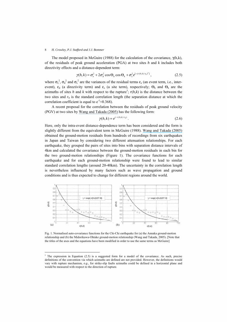
The appendix of Boore et al. (2003) presents a summary of the work carried out by Boore (1997) in which the spatial variability of peak motion from the 1994 Northridge mainshock was studied. The following equation was proposed for the variance of peak ground motions as a function of inter-site spacing:
( ) 22 2( , ) log
11 ,r h k Y indobs F r h kN
σ σ ⎛ ⎞= + ⎡ ⎤⎜ ⎟ ⎣ ⎦⎝ ⎠, (2.7)
( ) ( ), 1 exp 0.6 ,F r h k r h k⎡ ⎤= − −⎡ ⎤⎣ ⎦ ⎣ ⎦ , (2.8)
where σr(h,k)logY is the standard deviation of differences in the logarithm of the peak motion Y, σindobs is the standard deviation of an individual observation about a regression, and N is the number of recordings used in the average of a group of recordings in a small region. F[r(h,k)] is a function that accounts for the spatial correlation of the motion; F takes on values of 0.0 and 1.0 for r(h,k) = 0 and r(h,k) = ∞, respectively. F[r(h,k)] was estimated by Boore (1997) by studying peak ground accelerations from the larger horizontal component of the 1994 Northridge mainshock, supplemented by other studies of spatial variability (Figure 2). The function F(∆) has been transformed herein into the correlation of the residuals of peak motion at pairs of sites, γ(h,k), separated by kilometres, using the following formula:
2
[ 0.6 ( , ) ]( , ) 1 1 r h kh k eγ −⎡ ⎤= − −⎣ ⎦ . (2.9)
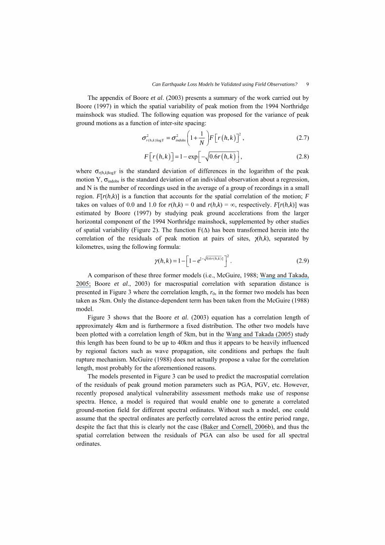
A comparison of these three former models (i.e., McGuire, 1988; Wang and Takada, 2005; Boore et al., 2003) for macrospatial correlation with separation distance is presented in Figure 3 where the correlation length, r0, in the former two models has been taken as 5km. Only the distance-dependent term has been taken from the McGuire (1988) model.
Figure 3 shows that the Boore et al. (2003) equation has a correlation length of approximately 4km and is furthermore a fixed distribution. The other two models have been plotted with a correlation length of 5km, but in the Wang and Takada (2005) study this length has been found to be up to 40km and thus it appears to be heavily influenced by regional factors such as wave propagation, site conditions and perhaps the fault rupture mechanism. McGuire (1988) does not actually propose a value for the correlation length, most probably for the aforementioned reasons.
The models presented in Figure 3 can be used to predict the macrospatial correlation of the residuals of peak ground motion parameters such as PGA, PGV, etc. However, recently proposed analytical vulnerability assessment methods make use of response spectra. Hence, a model is required that would enable one to generate a correlated ground-motion field for different spectral ordinates. Without such a model, one could assume that the spectral ordinates are perfectly correlated across the entire period range, despite the fact that this is clearly not the case (Baker and Cornell, 2006b), and thus the spatial correlation between the residuals of PGA can also be used for all spectral ordinates.
10 H. Crowley, P.J. Stafford and J.J. Bommer
Fig. 2. Standard deviation of difference of log of the larger peak horizontal acceleration as a function of interstation spacing leading to the F[r(h,k)] function (Boore et al., 2003)
Separation Distance, r(h,k) (km)
0 5 10 15 20
Cov
aria
nce,
γ(h
,k)
0.0
0.2
0.4
0.6
0.8
1.0
Boore et al. (2003)Wang & Takada (2005) r0 = 5kmMcGuire (1988) distance-dependent term r0 = 5km
Fig. 3. Comparison of the covariance of the residuals of peak ground motion with separation distance of two sites for the models of Wang and Takada (2005), McGuire (1988) and Boore et al. (2003)
Can Earthquake Loss Models be Validated using Field Observations?
11
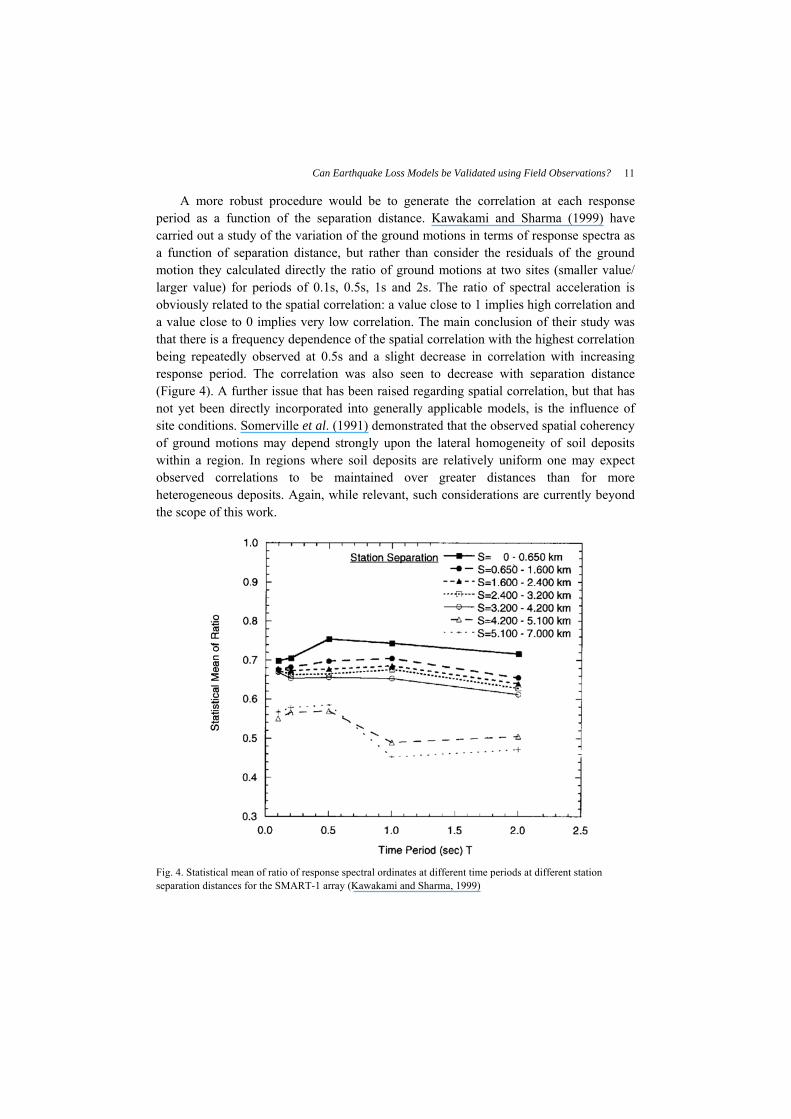
A more robust procedure would be to generate the correlation at each response period as a function of the separation distance. Kawakami and Sharma (1999) have carried out a study of the variation of the ground motions in terms of response spectra as a function of separation distance, but rather than consider the residuals of the ground motion they calculated directly the ratio of ground motions at two sites (smaller value/ larger value) for periods of 0.1s, 0.5s, 1s and 2s. The ratio of spectral acceleration is obviously related to the spatial correlation: a value close to 1 implies high correlation and a value close to 0 implies very low correlation. The main conclusion of their study was that there is a frequency dependence of the spatial correlation with the highest correlation being repeatedly observed at 0.5s and a slight decrease in correlation with increasing response period. The correlation was also seen to decrease with separation distance (Figure 4). A further issue that has been raised regarding spatial correlation, but that has not yet been directly incorporated into generally applicable models, is the influence of site conditions. Somerville et al. (1991) demonstrated that the observed spatial coherency of ground motions may depend strongly upon the lateral homogeneity of soil deposits within a region. In regions where soil deposits are relatively uniform one may expect observed correlations to be maintained over greater distances than for more heterogeneous deposits. Again, while relevant, such considerations are currently beyond the scope of this work.
Fig. 4. Statistical mean of ratio of response spectral ordinates at different time periods at different station separation distances for the SMART-1 array (Kawakami and Sharma, 1999)
12 H. Crowley, P.J. Stafford and J.J. Bommer
Baker and Cornell (2006b) have studied the correlation between the total residuals of spectral ordinates at two different periods, and have proposed a model to predict this correlation. Such a correlation between spectral ordinates can easily be included when generating ground motions at given sites for a given earthquake scenario; however, one issue that needs to be resolved is how this correlation should be considered in combination with the macrospatial correlation of the ground-motion residuals at pairs of sites. Goda and Hong (2007) have recently tackled this problem by modelling the spatial correlation coefficient as a function of both response period and separation distance.
3. The Loss Model
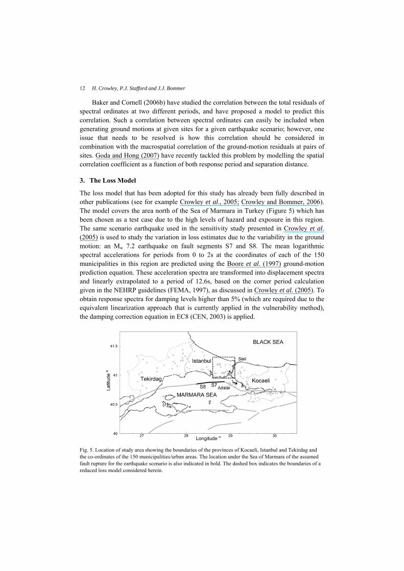
The loss model that has been adopted for this study has already been fully described in other publications (see for example Crowley et al., 2005; Crowley and Bommer, 2006). The model covers the area north of the Sea of Marmara in Turkey (Figure 5) which has been chosen as a test case due to the high levels of hazard and exposure in this region. The same scenario earthquake used in the sensitivity study presented in Crowley et al. (2005) is used to study the variation in loss estimates due to the variability in the ground motion: an Mw 7.2 earthquake on fault segments S7 and S8. The mean logarithmic spectral accelerations for periods from 0 to 2s at the coordinates of each of the 150 municipalities in this region are predicted using the Boore et al. (1997) ground-motion prediction equation. These acceleration spectra are transformed into displacement spectra and linearly extrapolated to a period of 12.6s, based on the corner period calculation given in the NEHRP guidelines (FEMA, 1997), as discussed in Crowley et al. (2005). To obtain response spectra for damping levels higher than 5% (which are required due to the equivalent linearization approach that is currently applied in the vulnerability method), the damping correction equation in EC8 (CEN, 2003) is applied.
Fig. 5. Location of study area showing the boundaries of the provinces of Kocaeli, Istanbul and Tekirdag and the co-ordinates of the 150 municipalities/urban areas. The location under the Sea of Marmara of the assumed fault rupture for the earthquake scenario is also indicated in bold. The dashed box indicates the boundaries of a reduced loss model considered herein.
Can Earthquake Loss Models be Validated using Field Observations?
13
Only reinforced concrete (RC) buildings have been included in the exposure component of the loss calculations. The 2000 Building Census has been used to obtain data on the number of RC buildings with a number of storeys of 1, 2, 3, 4, 5, 6 and 7-9 in each of the 150 municipalities in the study area (Figure 5). The structural characteristics of these buildings have been obtained from a statistical study of Turkish RC buildings from the Marmara Region (Bal et al., 2007). The building stock has been divided into building classes based on the use, age, number of storeys and location leading to a separation between buildings which are ‘good’ and ‘poor’ and those which will have a ‘soft-storey’ or a ‘global’ mechanism: further information on the structural characteristics adopted for each building class are included in Crowley et al. (2005). It is expected that the majority of the building stock in each municipality are concentrated in an urban area close to the town hall. Hence, as the building stock data from the Census is not available at a higher resolution, the exposure data has been assumed to be concentrated at the coordinates of the town hall in each municipality (Figure 5).
The proportion of RC buildings in each class that will exceed the limit states of slight, moderate and extensive damage are calculated using a probabilistic displacement-based approach termed DBELA (Crowley et al., 2004). The displacement capacity and period of vibration of a given building class are estimated from their geometric and material properties and the demand is modeled using a displacement response spectrum, thus allowing a direct comparison between the displacement demand and the displacement capacity. The equivalent linearization procedure is applied in DBELA such that the building class is modeled as a single-degree-of-freedom (SDOF) system which behaves linearly with a secant stiffness and the equivalent viscous damping is modeled by reducing the displacement response spectrum by a factor dependent on the ductility demand on the system (see for example Calvi, 1999). Although DBELA currently uses overdamped elastic spectra to calculate the displacement demand, it may also be calculated from inelastic spectra obtained using the displacement coefficient method (see e.g., ATC, 2005). The variability in the displacement capacity within a group of buildings can be accounted for through Monte Carlo simulation once the mean value, standard deviation and probabilistic distribution of each structural property has been identified. A random population of buildings is generated by taking random draws from the distribution for each structural property (such as storey height, beam length, column depth, etc.). The period and displacement capacity of each building are calculated and the latter is compared with the limit state displacement demand: the number of buildings whose displacement capacity is less than the displacement demand is calculated and thus the proportion of buildings that exceed a given limit state is found. The damage distribution has been converted into the mean damage ratio (MDR) (which relates the cost of repair to the cost of replacement of the building stock) by applying damage ratios to each damage band based on those in HAZUS (FEMA, 2003): 2% for slight damage, 10% for moderate damage, 50% for extensive damage and 100% for complete damage. The uncertainty in the damage-loss conversion ratios has not been considered as this
14 H. Crowley, P.J. Stafford and J.J. Bommer paper deals with the comparison of damage estimates only; the use of the mean damage ratio has been used for simplicity in the presentation of the results.
4. Sensitivity of Loss Model Results to Variability in Ground Motion
Once the mean logarithmic spectral accelerations at each site have been estimated, a random sampling of εinter from a normal distribution with zero mean and unit standard deviation can be made, multiplied by the inter-event standard deviation, and added to the mean logarithmic ground motions at each site. To account for the intra-event variability, a random sampling of εintra is made in a similar manner to the inter-event case at each site of the model. This process is repeated until 1000 random uncorrelated ground-motion fields have been generated. In order to consider the correlation of the εintra values at closely-spaced sites, a correlation (or covariance) matrix is required (as discussed in Sec. 2.3) and this can be calculated based on the distance between pairs of sites and an assumed correlation length. In the current study, the Wang and Takada (2005) macrospatial correlation model has been adopted and thus directivity effects have not been included. It is noted that a single draw of the intra-event variability is made at each site and this draw is assumed to apply across all periods, i.e., it is assumed that the spectral ordinates are fully correlated.
4.1. Uncorrelated ground-motion fields with total variability
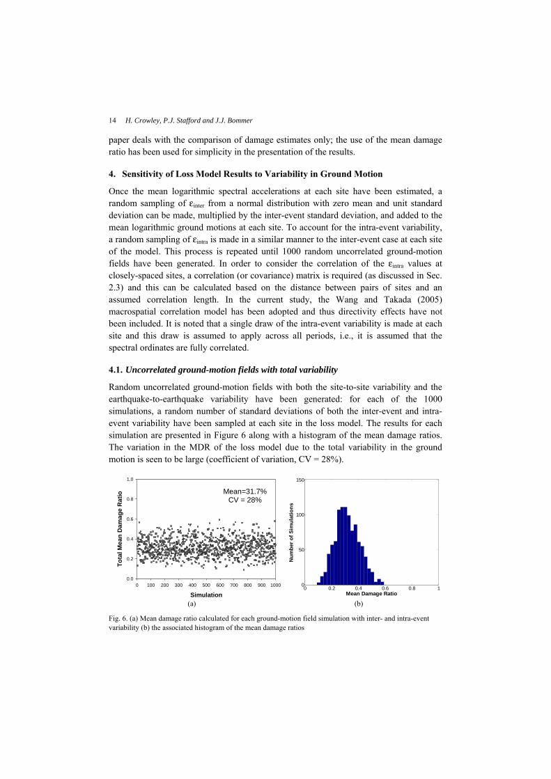
Random uncorrelated ground-motion fields with both the site-to-site variability and the earthquake-to-earthquake variability have been generated: for each of the 1000 simulations, a random number of standard deviations of both the inter-event and intra-event variability have been sampled at each site in the loss model. The results for each simulation are presented in Figure 6 along with a histogram of the mean damage ratios. The variation in the MDR of the loss model due to the total variability in the ground motion is seen to be large (coefficient of variation, CV = 28%).
Simulation0 100 200 300 400 500 600 700 800 900 1000
Tota
l Mea
n D
amag
e R
atio
0.0
0.2
0.4
0.6
0.8
1.0
0 0.2 0.4 0.6 0.8 10
50
100
150
Mean Damage Ratio
Num
ber o
f Sim
ulat
ions
Mean=31.7% CV = 28%
(a) (b)
Fig. 6. (a) Mean damage ratio calculated for each ground-motion field simulation with inter- and intra-event variability (b) the associated histogram of the mean damage ratios
Can Earthquake Loss Models be Validated using Field Observations?
15
4.2. Uncorrelated ground-motion fields with no inter-event variability
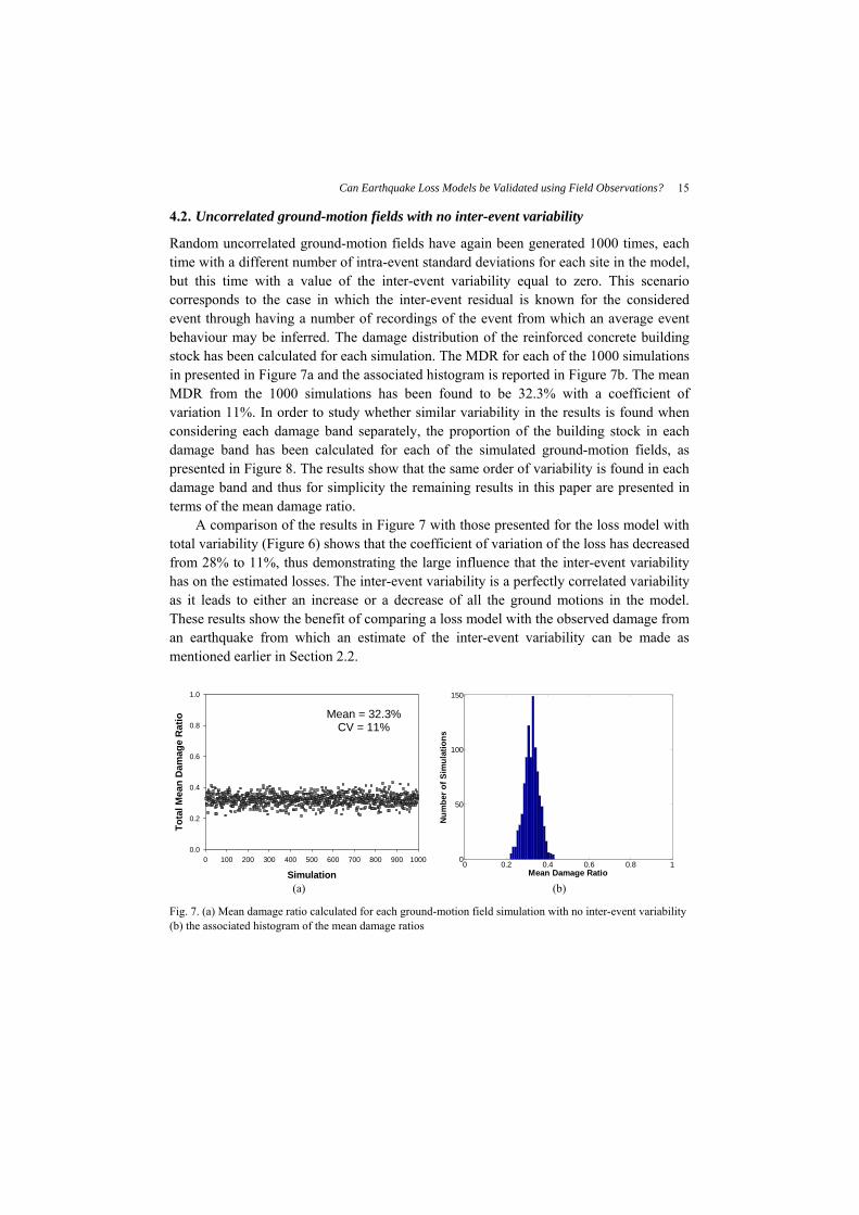
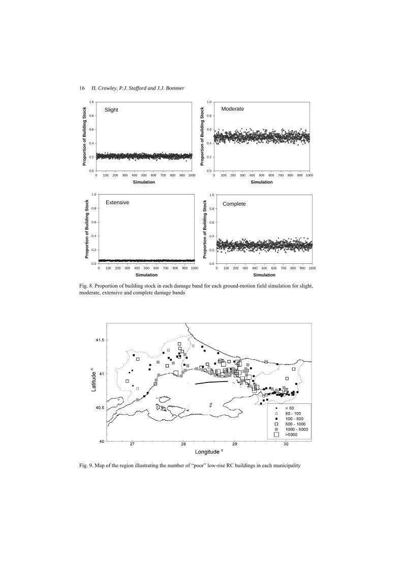
Random uncorrelated ground-motion fields have again been generated 1000 times, each time with a different number of intra-event standard deviations for each site in the model, but this time with a value of the inter-event variability equal to zero. This scenario corresponds to the case in which the inter-event residual is known for the considered event through having a number of recordings of the event from which an average event behaviour may be inferred. The damage distribution of the reinforced concrete building stock has been calculated for each simulation. The MDR for each of the 1000 simulations in presented in Figure 7a and the associated histogram is reported in Figure 7b. The mean MDR from the 1000 simulations has been found to be 32.3% with a coefficient of variation 11%. In order to study whether similar variability in the results is found when considering each damage band separately, the proportion of the building stock in each damage band has been calculated for each of the simulated ground-motion fields, as presented in Figure 8. The results show that the same order of variability is found in each damage band and thus for simplicity the remaining results in this paper are presented in terms of the mean damage ratio.
A comparison of the results in Figure 7 with those presented for the loss model with total variability (Figure 6) shows that the coefficient of variation of the loss has decreased from 28% to 11%, thus demonstrating the large influence that the inter-event variability has on the estimated losses. The inter-event variability is a perfectly correlated variability as it leads to either an increase or a decrease of all the ground motions in the model. These results show the benefit of comparing a loss model with the observed damage from an earthquake from which an estimate of the inter-event variability can be made as mentioned earlier in Section 2.2.
Simulation0 100 200 300 400 500 600 700 800 900 1000
Tota
l Mea
n D
amag
e R
atio
0.0
0.2
0.4
0.6
0.8
1.0
0 0.2 0.4 0.6 0.8 10
50
100
150
Mean Damage Ratio
Num
ber o
f Sim
ulat
ions
Mean = 32.3% CV = 11%
(a) (b)
Fig. 7. (a) Mean damage ratio calculated for each ground-motion field simulation with no inter-event variability (b) the associated histogram of the mean damage ratios
16 H. Crowley, P.J. Stafford and J.J. Bommer
Simulation0 100 200 300 400 500 600 700 800 900 1000
Prop
ortio
n of
Bui
ldin
g St
ock
0.0
0.2
0.4
0.6
0.8
1.0
Simulation0 100 200 300 400 500 600 700 800 900 1000
Prop
ortio
n of
Bui
ldin
g St
ock
0.0
0.2
0.4
0.6
0.8
1.0
Simulation0 100 200 300 400 500 600 700 800 900 1000
Prop
ortio
n of
Bui
ldin
g St
ock
0.0
0.2
0.4
0.6
0.8
1.0
Simulation0 100 200 300 400 500 600 700 800 900 1000
Prop
ortio
n of
Bui
ldin
g St
ock
0.0
0.2
0.4
0.6
0.8
1.0
Slight Moderate
Extensive Complete
Fig. 8. Proportion of building stock in each damage band for each ground-motion field simulation for slight, moderate, extensive and complete damage bands
Fig. 9. Map of the region illustrating the number of “poor” low-rise RC buildings in each municipality
Can Earthquake Loss Models be Validated using Field Observations?
17
Figure 7 and 8 illustrate that when considering the whole loss model, the variability in the ground motion from site to site does not have a particularly large influence on the results. The reason for the low variation in the loss model results from simulation to simulation is most probably due to the log-normal distribution of the ground motions which leads to high ground motions in some areas of the model and lower ground-motions in other areas; the repetition of the scenario is likely to replace the higher ground motions with lower ground motions and vice versa, thus leading to a “smoothing out” of the losses from one simulation to another. This low variation in the ground motions is more likely for this large loss model which is rather homogeneous with respect to the building stock: Figure 9 shows a map illustrating the number of low-rise poor RC buildings in each municipality. As seen from this map, many of the municipalities close to the fault segment, which will have the most influence on the loss results, have a similar number of buildings.
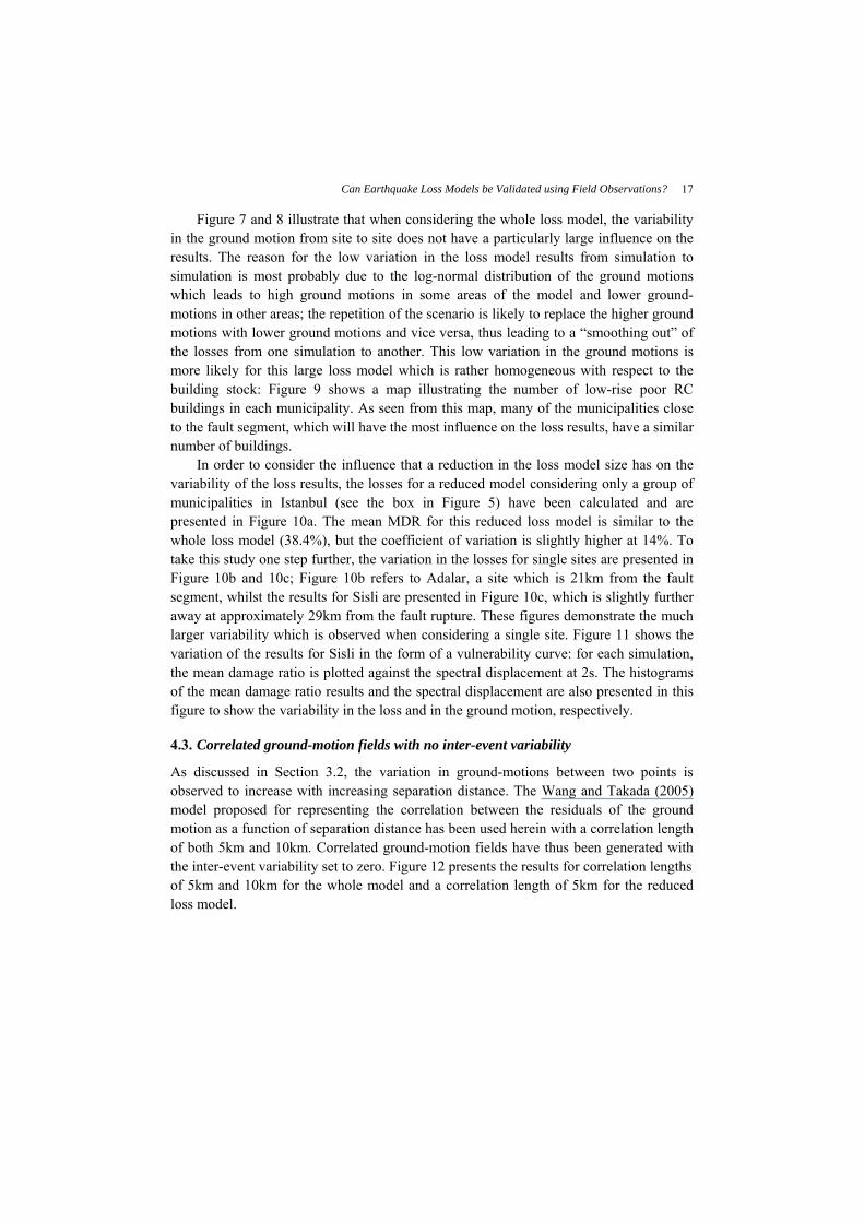
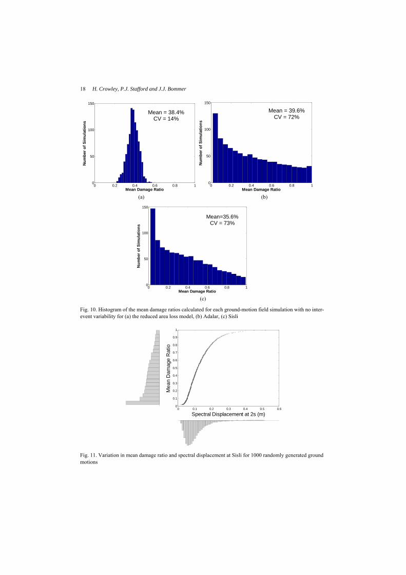
In order to consider the influence that a reduction in the loss model size has on the variability of the loss results, the losses for a reduced model considering only a group of municipalities in Istanbul (see the box in Figure 5) have been calculated and are presented in Figure 10a. The mean MDR for this reduced loss model is similar to the whole loss model (38.4%), but the coefficient of variation is slightly higher at 14%. To take this study one step further, the variation in the losses for single sites are presented in Figure 10b and 10c; Figure 10b refers to Adalar, a site which is 21km from the fault segment, whilst the results for Sisli are presented in Figure 10c, which is slightly further away at approximately 29km from the fault rupture. These figures demonstrate the much larger variability which is observed when considering a single site. Figure 11 shows the variation of the results for Sisli in the form of a vulnerability curve: for each simulation, the mean damage ratio is plotted against the spectral displacement at 2s. The histograms of the mean damage ratio results and the spectral displacement are also presented in this figure to show the variability in the loss and in the ground motion, respectively.
4.3. Correlated ground-motion fields with no inter-event variability
As discussed in Section 3.2, the variation in ground-motions between two points is observed to increase with increasing separation distance. The Wang and Takada (2005) model proposed for representing the correlation between the residuals of the ground motion as a function of separation distance has been used herein with a correlation length of both 5km and 10km. Correlated ground-motion fields have thus been generated with the inter-event variability set to zero. Figure 12 presents the results for correlation lengths of 5km and 10km for the whole model and a correlation length of 5km for the reduced loss model.
18 H. Crowley, P.J. Stafford and J.J. Bommer
0 0.2 0.4 0.6 0.8 10
50
100
150
Mean Damage Ratio
Num
ber o
f Sim
ulat
ions
Mean = 38.4% CV = 14%
0 0.2 0.4 0.6 0.8 10
50
100
150
Mean Damage Ratio
Num
ber o
f Sim
ulat
ions
Mean = 39.6% CV = 72%
(a) (b)
0 0.2 0.4 0.6 0.8 10
50
100
150
Mean Damage Ratio
Num
ber o
f Sim
ulat
ions
Mean=35.6% CV = 73%
(c)
Fig. 10. Histogram of the mean damage ratios calculated for each ground-motion field simulation with no inter-event variability for (a) the reduced area loss model, (b) Adalar, (c) Sisli
0 0.1 0.2 0.3 0.4 0.5 0.60
0.1
0.2
0.3
0.4
0.5
0.6
0.7
0.8
0.9
1
Spectral Displacement at 2s (m)
Mea
n D
amag
e R
atio
Fig. 11. Variation in mean damage ratio and spectral displacement at Sisli for 1000 randomly generated ground motions
Can Earthquake Loss Models be Validated using Field Observations?
19
0 0.2 0.4 0.6 0.8 10
50
100
150
Mean Damage Ratio
Num
ber o
f Sim
ulat
ions
Mean=31.8% CV = 19%
0 0.2 0.4 0.6 0.8 10
50
100
150
Mean Damage Ratio
Num
ber o
f Sim
ulat
ions
Mean=31.8% CV = 27%
(a) (b)
0 0.2 0.4 0.6 0.8 10
50
100
150
Mean Damage Ratio
Num
ber o
f Sim
ulat
ions
Mean=37.6% CV = 25%
(c)
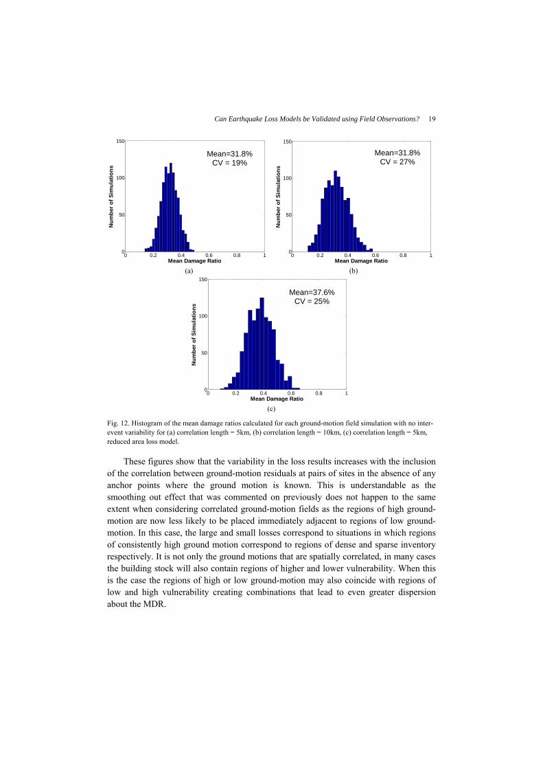
Fig. 12. Histogram of the mean damage ratios calculated for each ground-motion field simulation with no inter-event variability for (a) correlation length = 5km, (b) correlation length = 10km, (c) correlation length = 5km, reduced area loss model.
These figures show that the variability in the loss results increases with the inclusion of the correlation between ground-motion residuals at pairs of sites in the absence of any anchor points where the ground motion is known. This is understandable as the smoothing out effect that was commented on previously does not happen to the same extent when considering correlated ground-motion fields as the regions of high ground-motion are now less likely to be placed immediately adjacent to regions of low ground-motion. In this case, the large and small losses correspond to situations in which regions of consistently high ground motion correspond to regions of dense and sparse inventory respectively. It is not only the ground motions that are spatially correlated, in many cases the building stock will also contain regions of higher and lower vulnerability. When this is the case the regions of high or low ground-motion may also coincide with regions of low and high vulnerability creating combinations that lead to even greater dispersion about the MDR.
20 H. Crowley, P.J. Stafford and J.J. Bommer 4.4. Correlated ground-motion fields with “anchor points”
Despite the interesting conclusions which the previous results present concerning the importance of including spatial correlation for the prediction of future losses, the main focus of the current paper is whether loss models can be validated and thus it is interesting to study whether a number of recordings of a given earthquake can be used to reduce the uncertainty in the predicted loss model results for a given scenario. If, for a given event, recordings are available at a number of sites then knowledge of these ground motions may be used in conjunction with spatial correlation considerations to constrain the ground-motion field for regions in the vicinity of the recording stations. In order to ascertain the real influence of such an additional constraint, sites have been chosen from those in the base model for which the ground motions are assumed to be known; these will henceforth be termed “anchor points”. The problem of generating spatially correlated random fields given knowledge of the ground motion at particular points is not new. Extensive work has been conducted over the last two decades on this matter, with a primary focus being on the prediction of spatially compatible time series or spectra (Vanmarcke and Fenton, 1991; Vanmarcke et al., 1993; Zerva and Zhang, 1997; Liao and Zerva, 2006; Douglas, 2007, among others). For the current study we are concerned only with the correlation of peak values, be they peak ground accelerations or peak responses of a SDOF system; in this case the situation is simplified considerably.
Vanmarcke et al. (1993) have shown how one may obtain the expected values of spatially correlated ground-motion fields conditional upon knowledge of the ground motion(s) at another location(s). More recently, Park et al. (2007) have arrived at the same formulation with the additional feature of also stipulating the conditional variability of the unknown ground motions given knowledge of ground motions at surrounding locations. The method of Park et al. (2007) is adopted and briefly outlined here. The normalized ground-motion residuals at all sites can be regarded as a single realization of a multivariate normal distribution denoted by,
( )MVN ,=ε 0 Σ , (4.1)
where MVN() represents a multivariate normal distribution with a mean of zero over all dimensions, 0 , and a covariance matrix given by Σ ; the vector ε represents the normalized residuals at all of the considered sites. This formulation has been used to generate the ground-motion fields of the previous sections. In the case where spatial correlation is ignored the covariance matrix is diagonal, whereas in the previous section, where spatial correlation was included, the covariance matrix has off-diagonal terms proportional to the assumed spatial correlation.
In order to generate spatially correlated ground-motion fields conditional on the knowledge of ground motions at particular sites, the ground-motions at the k known sites were first generated by assuming that only these sites existed and making a draw from a k-dimensional multivariate distribution of the form in Equation (4.1) and associating these normalized residuals with the expected value of the ground motion at each site. Then, following Park et al. (2007), the conditional ground-motion field was obtained by
Can Earthquake Loss Models be Validated using Field Observations?
21
first re-ordering the sites into groups corresponding to the k known and u unknown locations. The vectors and matrices of Equation (4.1) may then be restructured as,
MVN ,⎛ ⎞⎧ ⎫ ⎧ ⎫ ⎡ ⎤
= ⎜ ⎟⎨ ⎬ ⎨ ⎬ ⎢ ⎥⎩ ⎭ ⎩ ⎭ ⎣ ⎦⎝ ⎠
k k kk ku
u u uk uu
ε 0 Σ Σε 0 Σ Σ
, (4.2)
with the bold subscripts k and u corresponding to the known and unknown elements of the relevant vectors and matrices. Given this partitioning, sets of conditional spatially-correlated normalized residuals may be obtained by drawing from the following conditional u-dimensional multivariate normal distribution:
{ } { }( )1 1MVN ,− −⎡ ⎤= = −⎣ ⎦u k k uk kk k uu uk kk kuε ε ε Σ Σ ε Σ Σ Σ Σ . (4.3)
While the physical interpretation of Equation (4.3) may not be immediately tractable for some, the methodology can easily be explained by way of a simple hypothetical example. Consider two nearby sites for which a normalized ground-motion residual is known at one of the sites. Now assuming that the residual at the known location is positive, it is likely that, if the other site is sufficiently close, the normalized ground-motion residual here will also be positive. Equation (4.3) reflects this intuition by modifying the expected value of the distribution of residuals at the site where the ground motion is unknown. Furthermore, the likely variation of residual values about this expected (positive) value is now reduced to less than the variability that exists given no knowledge, i.e. the variability specified by a ground-motion prediction equation. Again, the modified covariance matrix in Equation (4.3) is appropriately modified to reflect this reduced variability. Within this framework, the vector of simulated normalized residuals
[ ], T= k uε ε ε has an overall mean very close to zero and a standard deviation very close to that of the ground-motion prediction equation yet includes meaningful spatial correlation between points within the overall considered region.
In order to apply the above framework, a number of recording stations have been selected at random, for use as anchor points, from the 150 municipalities in the loss model (Figure 5). The number of anchor points has been gradually increased from 1 to 100 and the random site-selection has been repeated 10 times to study the influence associated with the selection of the anchor points. For each run, the procedure outlined above has been implemented in order to generate 1000 correlated ground-motion fields (considering the intra-event variability only and using a correlation length of 5km), each one being used to calculate the total MDR. The mean, standard deviation and coefficient of variation of the calculated MDRs has been calculated for each of the runs (i.e., for each of the 10 combinations of anchor points, based on a number of recording stations that varies from 1 to 100). The results are presented in Table 1 where it can be seen that the mean loss varies extensively and randomly; this is expected as the mean loss is a function of the ground motions selected at the anchor points. However, the standard deviation and the coefficient of variation are both observed to decrease with increasing numbers of anchor points. These two parameters are also seen to vary rather significantly as a function of the selected anchor points as the proportion of exposure data in these
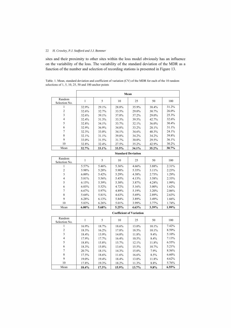
22 H. Crowley, P.J. Stafford and J.J. Bommer sites and their proximity to other sites within the loss model obviously has an influence on the variability of the loss. The variability of the standard deviation of the MDR as a function of the number and selection of recording stations is presented in Figure 13.
Table. 1. Mean, standard deviation and coefficient of variation (CV) of the MDR for each of the 10 random selections of 1, 5, 10, 25, 50 and 100 anchor points
Mean
Random Selection No. 1 5 10 25 50 100
1 32.9% 29.1% 28.8% 35.9% 38.4% 31.2% 2 32.6% 32.7% 33.5% 29.0% 30.7% 26.0% 3 32.6% 39.1% 37.8% 37.2% 29.0% 25.3% 4 32.4% 31.3% 33.3% 39.5% 42.7% 32.6% 5 32.8% 34.1% 33.7% 32.1% 36.0% 30.4% 6 32.9% 36.9% 34.8% 33.2% 28.1% 31.1% 7 32.3% 33.0% 34.1% 34.6% 40.3% 24.1% 8 32.1% 31.1% 39.8% 34.2% 34.2% 39.8% 9 33.0% 31.5% 31.7% 30.0% 29.5% 36.1%
10 32.8% 32.4% 27.5% 35.2% 42.9% 30.2% Mean 32.7% 33.1% 33.5% 34.1% 35.2% 30.7%
Standard Deviation Random
Selection No. 1 5 10 25 50 100
1 5.57% 5.46% 5.36% 4.66% 3.88% 2.31% 2 5.98% 5.28% 5.98% 5.35% 3.11% 2.23% 3 6.00% 5.42% 5.29% 4.38% 2.73% 1.29% 4 5.81% 5.56% 5.45% 4.13% 3.58% 2.33% 5 6.15% 5.39% 5.30% 3.87% 4.24% 1.99% 6 6.03% 5.52% 4.72% 5.16% 3.00% 1.62% 7 6.67% 5.97% 4.89% 5.19% 3.20% 2.06% 8 5.64% 5.81% 4.63% 5.69% 2.89% 2.63% 9 6.28% 6.13% 5.84% 3.89% 3.49% 1.66%
10 5.83% 6.26% 5.01% 3.99% 3.77% 1.74% Mean 6.00% 5.68% 5.25% 4.63% 3.39% 1.99%
Coefficient of Variation
Random Selection No. 1 5 10 25 50 100
1 16.9% 18.7% 18.6% 13.0% 10.1% 7.42% 2 18.3% 16.2% 17.8% 18.5% 10.1% 8.59% 3 18.4% 13.9% 14.0% 11.8% 9.4% 5.10% 4 17.9% 17.7% 16.4% 10.5% 8.4% 7.13% 5 18.8% 15.8% 15.7% 12.1% 11.8% 6.55% 6 18.3% 15.0% 13.6% 15.5% 10.7% 5.21% 7 20.7% 18.1% 14.3% 15.0% 7.9% 8.56% 8 17.5% 18.6% 11.6% 16.6% 8.5% 6.60% 9 19.0% 19.4% 18.4% 13.0% 11.8% 4.62%
10 17.8% 19.3% 18.2% 11.3% 8.8% 5.76% Mean 18.4% 17.3% 15.9% 13.7% 9.8% 6.55%
Can Earthquake Loss Models be Validated using Field Observations?
23
No. of Recording Stations
0 25 50 75 100 125 150
Stan
dard
Dev
iatio
n of
Tot
al M
DR
(%)
0
2
4
6
8
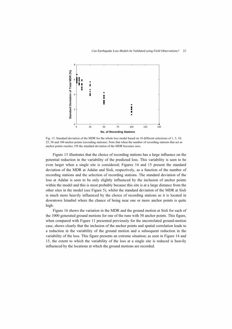
Fig. 13. Standard deviation of the MDR for the whole loss model based on 10 different selections of 1, 5, 10, 25, 50 and 100 anchor points (recording stations). Note that when the number of recording stations that act as anchor points reaches 150 the standard deviation of the MDR becomes zero.
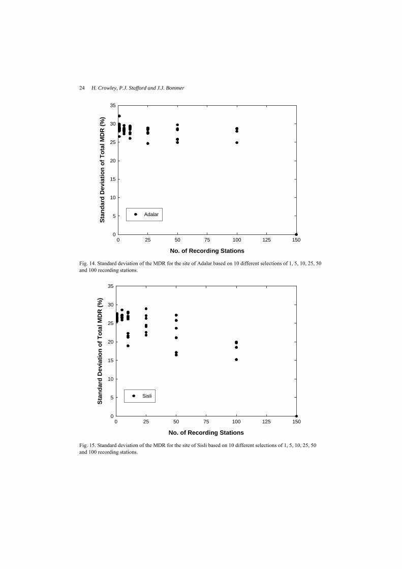
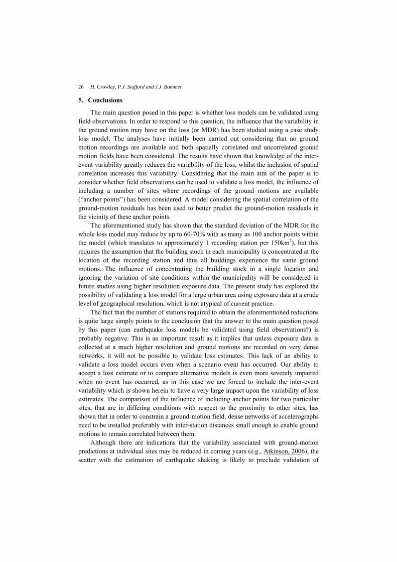
Figure 13 illustrates that the choice of recording stations has a large influence on the potential reduction in the variability of the predicted loss. This variability is seen to be even larger when a single site is considered; Figures 14 and 15 present the standard deviation of the MDR at Adalar and Sisli, respectively, as a function of the number of recording stations and the selection of recording stations. The standard deviation of the loss at Adalar is seen to be only slightly influenced by the inclusion of anchor points within the model and this is most probably because this site is at a large distance from the other sites in the model (see Figure 5), whilst the standard deviation of the MDR at Sisli is much more heavily influenced by the choice of recording stations as it is located in downtown Istanbul where the chance of being near one or more anchor points is quite high.
Figure 16 shows the variation in the MDR and the ground motion at Sisli for each of the 1000 generated ground motions for one of the runs with 50 anchor points. This figure, when compared with Figure 11 presented previously for the uncorrelated ground-motion case, shows clearly that the inclusion of the anchor points and spatial correlation leads to a reduction in the variability of the ground motion and a subsequent reduction in the variability of the loss. This figure presents an extreme situation; as seen in Figure 14 and 15, the extent to which the variability of the loss at a single site is reduced is heavily influenced by the locations at which the ground motions are recorded.
24 H. Crowley, P.J. Stafford and J.J. Bommer
No. of Recording Stations
0 25 50 75 100 125 150
Stan
dard
Dev
iatio
n of
Tot
al M
DR
(%)
0
5
10
15
20
25
30
35
Adalar
Fig. 14. Standard deviation of the MDR for the site of Adalar based on 10 different selections of 1, 5, 10, 25, 50 and 100 recording stations.
No. of Recording Stations
0 25 50 75 100 125 150
Stan
dard
Dev
iatio
n of
Tot
al M
DR
(%)
0
5
10
15
20
25
30
35
Sisli
Fig. 15. Standard deviation of the MDR for the site of Sisli based on 10 different selections of 1, 5, 10, 25, 50 and 100 recording stations.

Can Earthquake Loss Models be Validated using Field Observations?
25
0 0.1 0.2 0.3 0.4 0.5 0.60
0.1
0.2
0.3
0.4
0.5
0.6
0.7
0.8
0.9
1
Spectral Displacement at 2s (m)
Mea
n D
amag
e R
atio
Fig. 16. Variation in mean damage ratio and spectral displacement at Sisli for 1000 randomly generated correlated ground motions based on a loss model with 50 known recording stations.
4.5. Summary
Table 2 presents a summary of the results presented in Sections 4.1 to 4.4 for the whole loss model which shows clearly how the variability in the losses is affected by the removal of the inter-event variability, the inclusion of spatial correlation and the knowledge of the ground motion at a number of anchor points.
Table. 2. Summary of the mean, standard deviation and coefficient of variation of the mean damage ratio obtained for the whole loss model for different simulations of the ground-motion fields
Mean MDR (%) Coefficient of Variation (%)
Standard Deviation (%)
Uncorrelated Fields Inter + Intra-Event Variability 31.7 28 8.88
No Inter-Event Variability 32.3 11 3.55 Correlated Fields, No Inter-Event Variability Correlation length = 5km 31.8 19 6.04 Correlation length = 10km 31.8 27 8.58 Correlated Fields (Correlation length = 5km), No Inter-Event Variability 1 anchor point 32.7 18.4 6.00 5 anchor points 33.1 17.3 5.68 10 anchor points 33.5 15.9 5.25 25 anchor points 34.1 13.7 4.63 50 anchor points 35.2 9.80 3.39 100 anchor points 30.7 6.55 1.99
26 H. Crowley, P.J. Stafford and J.J. Bommer 5. Conclusions
The main question posed in this paper is whether loss models can be validated using field observations. In order to respond to this question, the influence that the variability in the ground motion may have on the loss (or MDR) has been studied using a case study loss model. The analyses have initially been carried out considering that no ground motion recordings are available and both spatially correlated and uncorrelated ground motion fields have been considered. The results have shown that knowledge of the inter-event variability greatly reduces the variability of the loss, whilst the inclusion of spatial correlation increases this variability. Considering that the main aim of the paper is to consider whether field observations can be used to validate a loss model, the influence of including a number of sites where recordings of the ground motions are available (“anchor points”) has been considered. A model considering the spatial correlation of the ground-motion residuals has been used to better predict the ground-motion residuals in the vicinity of these anchor points.
The aforementioned study has shown that the standard deviation of the MDR for the whole loss model may reduce by up to 60-70% with as many as 100 anchor points within the model (which translates to approximately 1 recording station per 150km2), but this requires the assumption that the building stock in each municipality is concentrated at the location of the recording station and thus all buildings experience the same ground motions. The influence of concentrating the building stock in a single location and ignoring the variation of site conditions within the municipality will be considered in future studies using higher resolution exposure data. The present study has explored the possibility of validating a loss model for a large urban area using exposure data at a crude level of geographical resolution, which is not atypical of current practice.
The fact that the number of stations required to obtain the aforementioned reductions is quite large simply points to the conclusion that the answer to the main question posed by this paper (can earthquake loss models be validated using field observations?) is probably negative. This is an important result as it implies that unless exposure data is collected at a much higher resolution and ground motions are recorded on very dense networks, it will not be possible to validate loss estimates. This lack of an ability to validate a loss model occurs even when a scenario event has occurred. Our ability to accept a loss estimate or to compare alternative models is even more severely impaired when no event has occurred, as in this case we are forced to include the inter-event variability which is shown herein to have a very large impact upon the variability of loss estimates. The comparison of the influence of including anchor points for two particular sites, that are in differing conditions with respect to the proximity to other sites, has shown that in order to constrain a ground-motion field, dense networks of accelerographs need to be installed preferably with inter-station distances small enough to enable ground motions to remain correlated between them.
Although there are indications that the variability associated with ground-motion predictions at individual sites may be reduced in coming years (e.g., Atkinson, 2006), the scatter with the estimation of earthquake shaking is likely to preclude validation of
Can Earthquake Loss Models be Validated using Field Observations?
27
earthquake loss models. In the absence of very dense accelerograph networks in urban areas, the level of variability in the ground-motion field of any earthquake event, even where there is good classification of the near-surface geology, will be too high to allow the use of even very detailed damage observations for validation of the estimates obtained from earthquake loss models. Reductions in the aleatory variability of ground-motion models may potentially be achieved by calibrating models to specific local conditions or by constraining empirical models through the use of detailed location-specific seismological models. However, actual validation of a loss model would require a very dense network of strong-motion recording instruments in an urban area and also excellent geographical resolution of the exposure data. This conclusion, however, does not mean that we should not strive to continually produce more reliable and robust estimates of losses, both through the development of improved modeling techniques and the collection of better data on the surface geology, the exposed building stock and the vulnerability characteristics of the buildings under consideration. Using modeling techniques that have a physical, rather than empirical, basis is an important step in this direction, and all studies that lead to refinement of the models for seismic sources and for ground-motion prediction in a given region contribute to the objective of improving loss estimations.
Acknowledgements
Peter Stafford is a fellow of the Willis Research Network and we gratefully acknowledge their continuing financial support. The authors would like to acknowledge the extensive comments of Dr John Douglas and two anonymous reviewers which helped to improve the final version of this paper. The authors are also grateful to many other individuals, who provided data and papers related to the study, including Dr Dave Boore, Dr Jack Baker and Dr Hanping Hong.
References
Abrahamson, N., and Sykora, D. (1993) “Variation of ground motions across individual sites,” Fourth DOE Natural Phenomena Hazards Mitigation Conference, Atlanta, Georgia, 19–22 October, 1993.
Applied Technology Council (2005) “Improvement of Nonlinear Static Seismic Analysis Procedures,” FEMA-440, ATC, California, USA.
Anderson, J.G. and Brune, J.N. (1999) “Probabilistic seismic hazard analysis without the ergodic assumption,” Seismological Research Letters 70, 19-28.
Atkinson, G.M. (2006) “Single-station sigma,” Bulletin of the Seismological Society of America 96(2), 446-455.
Baker, J.W. and Cornell, C.A. (2006a) “Which spectral acceleration are you using?” Earthquake Spectra 22, 293-312.
Baker, J.W. and Cornell, C.A. (2006b) “Correlation of response spectral values for multicomponent ground motions,” Bulletin of the Seismological Society of America 96(1), 215-227.
28 H. Crowley, P.J. Stafford and J.J. Bommer Bal, I.E., Crowley, H., Pinho, R. and Gülay, F.G. (2007) “Structural characteristics of Turkish RC
building stock in Northern Marmara region for loss assessment applications,” ROSE Research Report, 2007/03, IUSS Press, Pavia, Italy.
Bird, J.F., Bommer, J.J., Bray, J. , Sancio, R. and Spence R. (2004) “Comparing loss estimation with observed damage in a zone of ground failure: a study of the 1999 Kocaeli earthquake in Turkey,” Bulletin of Earthquake Engineering 2(3), 329-360.
Bommer, J.J. and Crowley, H. (2006) “The influence of ground motion variability in earthquake loss modelling,” Bulletin of Earthquake Engineering 4(3), 231-248.
Boore, D.M. (1997) “Estimates of average spectral amplitudes at FOAKE sites, Appendix C in An evaluation of methodology for seismic qualification of equipment, cable trays, and ducts in ALWR plants by use of experience data,” K. K. Bandyopadhyay, D. D. Kana, R. P. Kennedy, and A. J. Schiff (Editors), U.S. Nuclear Regulatory Commission NUREG/CR-6464 and Brookhaven National Lab BNL-NUREG- 52500, C-1-C-69.
Boore, D.M. (2005) “Erratum: Seismological Research Letters, Vol. 68, No. 1, pp. 128-153, January/February 1997, Equations for estimating horizontal response spectra and peak acceleration from western north American earthquakes: A summary of recent work, D.M. Boore, W.B. Joyner, and T.E. Fumal” Seismological Research Letters 76, 368-369.
Boore, D. M., Joyner, W.B., and Fumal, T.E. (1997) “Equations for estimating horizontal response spectra and peak acceleration from western North American earthquakes: a summary of recent work,” Seismological Research Letters 68, 128–153.
Boore, D.M., Gibbs, J.F., Joyner, W.B., Tinsley, J.C. and Ponti, D.J. (2003) “Estimated Ground Motion From the 1994 Northridge, California, Earthquake at the Site of the Interstate 10 and La Cienega Boulevard Bridge Collapse, West Los Angeles, California,” Bulletin of Seismological Society of America 93(6), 2737-2751.
Calvi, G.M. (1999) “A displacement-based approach for vulnerability evaluation of classes of buildings,” Journal of Earthquake Engineering 3, 411-438.
CEN - Comite Europeen de Normalisation (2003) “Eurocode 8, Design of Structures for Earthquake Resistance – Part 1: General rules, seismic actions and rules for buildings,” Pr-EN 1998-1. Final Draft. December 2003.
Chen, Y.-H. and Tsai, C.-C.P. (2002) “A new method for estimation of the attenuation relationship with variance components,” Bulletin of the Seismological Society of America 92(5), 1984-1991.
Crowley, H. and Bommer, J.J. (2006) “Modelling seismic hazard in earthquake loss models with spatially distributed exposure,” Bulletin of Earthquake Engineering 4(3), 249-273.
Crowley, H., Pinho, R. and Bommer, J.J. (2004) “A probabilistic displacement-based vulnerability assessment procedure for earthquake loss estimation,” Bulletin of Earthquake Engineering 2, 173-219.
Crowley, H., Bommer, J.J., Pinho, R. and Bird, J.F. (2005) “The impact of epistemic uncertainty on an earthquake loss model,” Earthquake Engineering and Structural Dynamics 34(14), 1635-1685.
Douglas, J. (2007) “Inferred ground motions on Guadeloupe during the 2004 Les Saintes earthquake,” Bulletin of Earthquake Engineering 5, 363-376.
Elms, D.G. (1985) “The principle of consistent crudeness,” Proceedings of the Workshop on Civil Engineering Application of Fuzzy Sets, Purdue University, IN, p.35-44.
FEMA (1997) “1997 NEHRP Recommended Provisions for Seismic Regulations for New Buildings. FEMA 273,” Federal Emergency Management Agency, Washington DC.
FEMA (2003) “HAZUS-MH Technical Manual,” Federal Emergency Management Agency, Washington D.C.
Field, E.H. and Hough, S.E. (1997) “The variability of PSV response spectra across a dense array deployed during the Northridge aftershock sequence,” Earthquake Spectra, 13, 243–257.

Can Earthquake Loss Models be Validated using Field Observations?
29
Goda, K. and Hong, H.P. (2007) “Spatial correlation of peak ground motions and response spectra,” Bulletin of Seismological Society of America, in press.
Joyner, W.B. and Boore, D.M. (1993) “Methods for regression analysis of strong-motion data,” Bulletin of the Seismological Society of America 83(2), 469-487.
Kawakami, H. and Sharma, S. (1999) “Statistical study of spatial variation of response spectrum using free field records of dense strong motion arrays,” Earthquake Engineering and Structural Dynamics 28, 1273-1294.
Kawakami, H., and Mogi, H. (2003) “Analyzing spatial intraevent variability of peak ground accelerations as a function of separation distance,” Bulletin of the Seismological Society of America 93, 1079–1090.
Liao, S. and Zerva, A. (1997) “Physically compliant, conditionally simulated spatially variable seismic ground motions for performance-based design” Earthquake Engineering and Structural Dynamics 35, 891-919.
McCann, M.W., Jr., and Boore, D.M. (1983) “Variability in ground motions: root mean square acceleration and peak acceleration for the 1971 San Fernando, California, earthquake,” Bulletin of the Seismological Society of America 73, 615–632.
McGuire, R.K. (1988) “Seismic risk to lifeline systems: critical variables and sensitivities,” Proceedings of 9th World Conference on Earthquake Engineering Vol. VII, pp. 129-134.
Musson, R.M.W. (2004) “Objective validation of seismic hazard source models,” Proceedings of 13th World Conference on Earthquake Engineering, Vancouver, Canada, paper no. 2492.
Ordaz, M. and Reyes, C. (1999) “Earthquake hazard in Mexico City: observations versus computations,” Bulletin of the Seismological Society of America 89(5), 1379-1383.
Park, J., Bazzurro, P. and Baker, J.W. (2007) “Modelling spatial correlation of ground motion intensity measures for regional seismic hazard and portfolio loss estimation” Proceedings of the 10th International Conference of Application of Statistics and Probability in Civil Engineering (ICASP10), Tokyo, Japan, 8pp.
Somerville, P.G., McLaren, J.P., Sen, M.K. and Helmberger, D.V. (1991) “The influence of site conditions on the spatial incoherence of ground motions,” Structural Safety, 10, 1-13.
Spence, R., Bommer, J.J., del Re, D., Bird, J., Aydinoğlu, N. and Tabuchi, S. (2003) “Comparing loss estimation with observed damage: a study of the 1999 Kocaeli earthquake in Turkey,” Bulletin of Earthquake Engineering 1(1), 83-113.
Strasser, F.O., Bommer, J.J. and Abrahamson, N.A. (2008) “Truncation of the distribution of ground-motion residuals.” Journal of Seismology 12(1), 79-105.
Vanmarcke, E.H. and Fenton, G.A. (1991) “Conditioned simulation of local-fields of earthquake ground motion” Structural Safety 10(1-3), 247-264.
Vanmarcke, E.H., Heredia-Zavoni, E. and Fenton, G.A. (1993) “Conditional simulation of spatially correlated earthquake ground motion” Journal of Engineering Mechanics 119(11), 2333-2352.
Wang, M. and Takada, T. (2005) “Macrospatial correlation model of seismic ground motions,” Earthquake Spectra 21(4), 1137-1156.
Zerva, A. and Zhang, O. (1997) “Correlation patterns in characteristics of spatially variable seismic ground motions” Earthquake Engineering and Structural Dynamics 26, 19-39.