arX

iv:0

710.

1031

v1 [

cond

-mat

.sta

t-m

ech]

4 O

ct 2

007

Thermodynamics of statistically interacting quantum gas in D dimensions

Geoffrey G. Potter,1 Gerhard Muller,1 and Michael Karbach2, 1

1 Department of Physics, University of Rhode Island, Kingston RI 02881, USA2 Bergische Universitat Wuppertal, Fachbereich Mathematik und Naturwissenschaften, D-42097 Wuppertal, Germany

We present the exact thermodynamics (isochores, isotherms, isobars, response functions) of astatistically interacting quantum gas in D dimensions. The results in D = 1 are those of the ther-modynamic Bethe ansatz for the nonlinear Schrodinger model, a gas with repulsive two-body contactpotential. In all dimensions the ideal boson and fermion gases are recovered in the weak-coupling andstrong-coupling limits, respectively. For all nonzero couplings ideal fermion gas behavior emergesfor D ≫ 1 and, in the limit D → ∞, a phase transition occurs at T > 0. Significant deviations fromideal quantum gas behavior are found for intermediate coupling and finite D.

I. INTRODUCTION

The wave of experimental studies that led to the firstobservations of Bose-Einstein condensation (BEC) andthe development of measurement and confinement tech-nologies have renewed strong interest in the statisticalmechanics of interacting quantum gases [1, 2, 3, 4, 5, 6].This line of research can make good use of explicit high-accuracy results from any type of analysis that goes be-yond low-density/high-temperature expansions and be-yond mean-field theory. Of particular interest are resultsfor response functions, the very quantities most directlyamenable to experimental investigations.

Such results can be produced on a rigorous basis forquantum gases with statistical interaction under verygeneral circumstances as shown by Wu [7, 8]. The con-cept of statistical interaction introduced by Haldane [9]has proven to be a very useful methodological device tocapture the statistical mechanical properties of degreesof freedom subject to dynamical interaction. For severalmodel systems in dimension D = 1 the coupling betweendegrees of freedom can be substituted by a generalizedPauli principle with no loss of rigor regarding the ther-modynamic analysis [9, 10, 11, 12, 13].

Whereas an equivalence between dynamical and sta-tistical interaction is not likely to be realized in D > 1(apart from highly contrived scenarios), models of statis-tically interacting degrees of freedom can stand on theirown. Their thermodynamic properties can be analyzedexactly in any dimension D, producing a full and consis-tent account of fluctuations as will be demonstrated inthis work [14]. The exact results emerging from this anal-ysis make it possible to connect features of the statisticalinteraction with features of a corresponding dynamicalinteraction. The systematic study of such connections,in turn, opens the door to the design of (exactly solv-able) models of statistical interaction for the descriptionof thermodynamic phenomena associated with specificaspects of dynamical interaction.

In a previous paper [15] we have established a bench-mark in that regard by exploring the thermodynamicsof an ideal quantum gas with fractional statistics inD dimensions – a thermodynamic generalization of theCalogero-Sutherland (CS) model [16, 17, 18] – taking

advantage of techniques and results reported in previ-ous studies [7, 8, 12, 17, 19, 20, 21, 22, 23, 24, 25, 26,27, 28, 29, 30, 31, 32, 33, 34]. In that case the statisticalinteraction was limited to pairs of particles with identicalmomenta.

Here we relax that constraint and consider a modelsystem, again in D dimensions, with a statistical inter-action that extends to pairs of particles with arbitrarymomenta, a system moreover, whose statistical interac-tion in D = 1 is equivalent to the dynamical interactionof a model that is solvable (beyond thermodynamics) viaBethe ansatz: the nonlinear Schrodinger (NLS) model[35, 36, 37, 38, 39, 40, 41].

In Sec. II we review the concept of statistical interac-tion and its use in statistical mechanics. We introducethe NLS model and the generalization of its thermody-namics to D > 1. In Sec. III we describe the method ofthermodynamic analysis applied to the generalized NLSmodel. In Sec. IV we discuss selected thermodynamicproperties thus calculated. In Sec. V we assess the re-sults in relation to existing benchmarks for ideal quan-tum gases with fractional statistics.

II. STATISTICAL INTERACTION

The statistical interaction of any given model systemis specified by a generalized Pauli principle [9], express-ing how the number of states available to one particle isaffected by the presence of other particles:

∆di.= −

∑

j

gij∆nj . (1)

The indices i, j refer to particle species and the gij arestatistical interaction coefficients. For bosons we havegij = 0 and for fermions gij = δij . Integrating Eq. (1)yields the holding capacity for particles of species i inthe presence of a specific number of particles from eachspecies:

di = Ai −∑

j

gij(nj − δij), (2)

where Ai are statistical capacity constants. The numberof many-particle states composed of ni statistically in-

2

teracting particles is

W (ni) =∏

i

(

di + ni − 1ni

)

. (3)

The three principal specifications of a system of par-ticles subject to a statistical interaction are sets of (i)energies ǫi, (ii) capacity constants Ai, and (iii) interac-tion coefficients gij . The grand potential of such a systemcan be expressed in the form [7]

Ω = −kBT∑

i

Ai ln

[

1 + wi

wi

]

, (4)

where the wi are determined by the nonlinear algebraicequations,

ǫi − µ

kBT= ln(1 + wi) −

∑

j

gji ln

(

1 + wj

wj

)

. (5)

The control variables are T (temperature) and µ (chem-ical potential). The average numbers of particles, 〈ni〉,are related to the wi by the linear equations,

∑

j

(δijwj + gij) 〈nj〉 = Ai. (6)

If gij = giδij then all Eqs. (5) and (6) are decoupledand the statistical interaction reduces to a (fractional)exclusion condition.

A. Application to quantum gas

For a nonrelativistic quantum gas in a box of dimen-sionality D and volume V = LD the aforementioned spec-ifications are encoded in the energy-momentum relationǫ0(k) = |k|2 (in units where ~

2/2m = 1) and in a functiong(k,k′). The grand potential (4) becomes

Ω = −kBT

(

L

2π

)D ∫

dDk ln1 + wk

wk

, (7)

where wk is the solution of the nonlinear integral equa-tion

|k|2 − µ

kBT= ln(1 + wk) −

∫

dDk′ g(k′,k) ln1 + wk′

wk′

. (8)

The particle density in k-space, 〈nk〉, is the solution ofthe linear integral equation

〈nk〉wk +

∫

dDk′ g(k,k′)〈nk′〉 = 1. (9)

The fundamental thermodynamic relations (thermody-namic and caloric equations of state) depend on the so-lutions of (8) and (9) as follows:

pV

kBT=

(

L

2π

)D ∫

dDk ln1 + wk

wk

, (10)

N =

(

L

2π

)D ∫

dDk 〈nk〉, (11)

U =

(

L

2π

)D ∫

dDk |k|2〈nk〉. (12)

If the statistical interaction is of the form g(|k−k′|) then

the solutions of (8) and (9) only depend on the magnitudeof the particle momenta.

B. Nonlinear Schrodinger model

Consider the boson gas in D = 1 with repulsive con-tact interaction of strength c as described by the NLSHamiltonian

H = −N

∑

i=1

∂2

∂x2i

+ 2c∑

j<i

δ(xi − xj). (13)

The thermodynamic Bethe ansatz (TBA) solution [37,38, 39, 40] of the NLS model expresses the grand poten-tial in the form

Ω(T, L, µ) = −kBT

(

L

2π

)∫ +∞

−∞

dk ln(

1 + e−ǫ(k)/kBT)

,

(14)where ǫ(k) is the solution of the Yang-Yang equation [37],

ǫ(k) = k2−µ−kBT

2π

∫ +∞

−∞

dk′K(k−k′) ln(

1 + e−ǫ(k′)/kBT)

(15)with kernel

K(k − k′) =2c

c2 + (k − k′)2. (16)

The particle density 〈nk〉 is the solution, for given ǫ(k),of the Lieb-Liniger equation [35, 37],

〈nk〉[

1 + eǫ(k)/kBT]

= 1 +1

2π

∫ +∞

−∞

dk′ K(k − k′)〈nk′ 〉.(17)

Bernard and Wu [12] showed that this TBA solution isequivalent to the thermodynamics of a statistically inter-acting gas in D = 1 if the following identifications aremade:

wk = eǫ(k)/kBT , (18a)

g(k − k′) = δ(k − k′) − 1

2πK(k − k′). (18b)

C. Generalization of NLS model

The generalized NLS model is a quantum gas in Ddimensions with the statistical interaction expressed bythe kernel

K(k− k′) =

2Γ(D)

πD/2−1Γ(D/2)

cD

[c2 + (k − k′)2]D(19)

3

of the Yang-Yang equation (15) and Lieb-Liniger equa-tion (17) generalized to D ≥ 1 and designed to reproducethe exact thermodynamics of the dynamically interactingNLS model in D = 1. The kernel (19) has the properties

limc→∞

K(k) = 0, (20a)

limc→0

K(k) = 2πδ(k), (20b)∫

dDk K(k) = 2π. (20c)

This model interpolates between the ideal Fermi-Dirac(FD) gas in the strong-coupling limit (c = ∞) and theideal Bose-Einstein (BE) gas in the weak-coupling limit(c = 0) in all dimensions D ≥ 1. In the limit D → ∞ itturns into the ideal FD gas for all c > 0.

For the further analysis of the generalized NLS modelwe reduce Eqs. (8) and (9) into integral equations for thefunctions

ǫ(k).= kBT lnwk, n(k)

.= 〈nk〉, (21)

where k.= |k|. We also introduce scaled quantities

k.=

k√kBT

, c.=

c√kBT

, (22a)

ǫ(k).=

ǫ(k)

kBT, n(k)

.= n(k). (22b)

Equations (15) and (17) thus thermodynamically gener-alized to D ≥ 1 become

ǫ(k) = k2 − ln z −∫ ∞

0

dk′K(k, k′) ln(1 + e−ǫ(k′)), (23)

n(k)[

1 + eǫ(k)]

= 1 +

∫ ∞

0

dk′K(k, k′)n(k′), (24)

with fugacity z = eµ/kBT and reduced kernel

K(k, k′) =2cDΓ(D)[Γ(D/2)]2

× k′D−1(c2 + k2 + k′2)

[c4 + 2c2(k2 + k′2) + (k2 − k′2)2](D+1)/2 . (25)

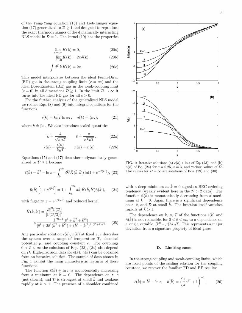
Any particular solution ǫ(k), n(k) at fixed z, c describesthe system over a range of temperature T , chemicalpotential µ, and coupling constant c. For couplings0 < c < ∞ the solutions of Eqs. (23), (24) also dependon D. High-precision data for ǫ(k), n(k) can be obtainedfrom an iterative solution. The sample of data shown inFig. 1 exhibit the main characteristic features of thesefunctions.

The function ǫ(k) + ln z is monotonically increasingfrom a minimum at k = 0. The dependence on z, c(not shown), and D is strongest at small k and weakensrapidly at k > 1. The presence of a shoulder combined

-12

-8

-4

0

4

0 0.5 1 1.5 2

ε- (k- )+ln

(z)

k-

D = 1

2

3

5

∞

(a)

0

4

8

12

16

20

0 0.5 1 1.5 2

n- (k- )

k-

D = 1

2

3

5

∞ (b)

FIG. 1: Iterative solutions (a) ǫ(k) + ln z of Eq. (23), and (b)n(k) of Eq. (24) for c = 0.25, z = 3, and various values of D.The curves for D = ∞ are solutions of Eqs. (29) and (30).

with a deep minimum at k = 0 signals a BEC orderingtendency (weakly evident here in the D > 2 data). Thefunction n(k) is monotonically decreasing from a maxi-mum at k = 0. Again there is a significant dependenceon z, c, and D at small k. The function itself vanishesrapidly at k > 1.

The dependence on k, µ, T of the functions ǫ(k) andn(k) is not reducible, for 0 < c < ∞, to a dependence ona single variable, (k2 −µ)/kBT . This represents a majordeviation from a signature property of ideal gases.

D. Limiting cases

In the strong-coupling and weak-coupling limits, whichare fixed points of the scaling relation for the couplingconstant, we recover the familiar FD and BE results:

ǫ(k) = k2 − ln z, n(k) =

(

1

zek2

+ 1

)−1

, (26)

4

for c = ∞, and

ǫ(k) = ln

(

1

zek2 − 1

)

, n(k) =

(

1

zek2 − 1

)−1

(27)

for c = 0. The D-independence of these functions is an-other signature property of ideal gases, a property upheldin the presence of fractional statistics [15]. The paraboliccurve, ǫ(k) + ln z = k2, may serve as baseline for the so-lutions of (23). It is exact in the strong-coupling limitfor all z > 0, but only for z → 0 in the weak-couplinglimit. For 0 < z < 1 the deviations of ǫ(k) + ln z from k2

and of n(k) from zero are suppressed by factors ∼ e−k2

as k increases. We have noted very similar behavior inthe numerical results for 0 < c < ∞.

In the limit D → ∞ the reduced kernel (25) acquiresa much simpler structure,

limD→∞

K(k, k′) = δ(

k′ −√

k2 + c2)

, (28)

but the c-dependence is retained and (for c > 0) also thestatistical coupling of particles with distinct momenta.Equations (23) and (24), with reduced kernel (28) turninto the implicit functions

ǫ(k) = k2 − ln z − ln

(

1 + e−ǫ

“√k2+c2

”)

, (29)

n(k)[

1 + eǫ(k)]

= 1 + n(√

k2 + c2)

. (30)

The solution of Eq. (29) is

e−ǫ(k) =∞∑

l=0

zl+1e−(l+1)k2

e−c2l(l+1)/2, (31)

and the solution of Eq. (30) is

n(k) =

∞∑

l=0

αlzl+1e−k2(l+1) (32)

with the recursion

αl = e−c2

2 l(l+1) −l

∑

j=1

(

αl−je− c2

2 j(j−1)

−αj−1e− c2

2 ((l−j)(l−j+1)+2j))

. (33)

For c → ∞ Eqs. (26) are recovered, and for c → 0Eqs. (27).

III. THERMODYNAMIC ANALYSIS OF

GENERALIZED NLS MODEL

Exact results for the thermodynamics of the general-ized NLS model in D ≥ 1 and across the range 0 ≤ c ≤ ∞of coupling strengths can now be calculated from the so-lutions ǫ(k) and n(k) of Eqs. (23) and (24), respectively.

A. NLS functions

The fundamental thermodynamic relations (10)–(12)are rewritten in the form

pλDT

kBT= F (D)

p (z, c), (34)

NλDT

V= F

(D)N (z, c)

[

+z

1 − z

]

, (35)

UλDT

V

/D2

kBT = F(D)U (z, c), (36)

where

λT.=

√

h2

2πmkBT

~2/2m=1−→

√

4π

kBT(37)

is the thermal wavelength and the term in (35) enclosedby square-brackets is relevant only if c = 0 and D > 2.The NLS functions in (34)-(36) are defined as follows:

F (D)p (z, c)

.=

2

Γ(D/2)

∫ ∞

0

dk kD−1 ln(

1 + e−ǫ(k))

, (38)

F(D)N (z, c)

.=

2

Γ(D/2)

∫ ∞

0

dk kD−1n(k), (39)

F(D)U (z, c)

.=

2

Γ(D/2 + 1)

∫ ∞

0

dk kD+1n(k), (40)

where the additional dependence of ǫ(k), n(k) on D, c, zis implied.

In the strong-coupling and weak-coupling limits, theNLS functions turn into the familiar FD functions,

fn(z).=

1

Γ(n)

∫ ∞

0

dxxn−1

z−1ex + 1, z ≥ 0, (41)

and BE functions,

gn(z).=

1

Γ(n)

∫ ∞

0

dxxn−1

z−1ex − 1, 0 ≤ z ≤ 1, (42)

respectively:

F (D)p (z,∞) = F

(D)U (z,∞) = fD/2+1(z), (43a)

F(D)N (z,∞) = fD/2(z), (43b)

and

F (D)p (z, 0) = F

(D)U (z, 0) = gD/2+1(z), (44a)

F(D)N (z, 0) = gD/2(z). (44b)

5

Furthermore, for D ≫ 1 fermionic behavior results forany c > 0:

F (D)p (z, c), F

(D)U (z, c)

D≫1 fD/2+1(z), (45a)

F(D)N (z, c)

D≫1 fD/2(z). (45b)

With increasing D the factor kD±1 pushes all significantcontributions to the integrals (38)-(40) toward larger andlarger k, where the deviations of ǫ(k) and n(k) from their(c = ∞)-values (26) become smaller and smaller [42].

A characteristic ideal-gas property is that the depen-dence of the fugacity on the thermodynamic variablesT, V,N is expressible as a function of a single variable,

x.= λT v−1/D, v

.= V/N . (46)

In the Maxwell-Boltzmann (MB) gas we have xD = z,in the FD gas xD = fD/2(z), and in the BE gas xD =gD/2(z). A unique functional relation persists in the caseof fractional statistics [15]. In the generalized NLS model,

however, we have xD = F(D)N (z, c) with a separate T -

dependence contained in c. For ideal quantum gases,including those with fractional statistics, there also existsa unique functional dependence of pV/NkBT on z. Againthis no longer holds in the generalized NLS model, where

we have pV/NkBT = F(D)p (z, c)/F

(D)N (z, c).

B. Reference values

We introduce reference values for the thermodynamicvariables v, T , p based on the thermal wavelength λT andthe MB equation of state pv = kBT in the presentationof our data below:

kBTv =4π

v2/D, pv =

4π

v2/D+1(v = const.) (47)

vT =

(

4π

kBT

)D/2

, pT =(kBT )D/2+1

(4π)D/2(T = const.)

(48)

kBTp = 4π( p

4π

)2

D+2

, vp =

(

4π

p

)D

D+2

(p = const.)

(49)They are especially useful in comparative plots that en-compass the full range of c at finite D.

For the thermodynamic analysis we must adapt theNLS functions to the type of process under consideration.Each function has a different z-dependence at fixed c, de-pending, for example, on whether we consider v = const,T = const, or p = const. To this end we introduce threekinds of reduced coupling constants for use in isochoric,isothermal, and isobaric processes, respectively:

cv.=

c√kBTv

= c

√

T

Tv=

c

x(v = const), (50)

cT.=

c√kBT

= c (T = const), (51)

cp.=

c√

kBTp

= c

√

T

Tp

.=

c

y(p = const), (52)

where x and y are the solutions of

xD = F(D)N (z, cvx), (53)

yD+2 = F (D)p (z, cpy), (54)

respectively.Reference values based on the chemical potential

present themselves as an alternative in some situations.Defining ln z

.= Tv/T in isochoric processes and ln z

.=

Tp/T in isobaric processes, we have

Tv

Tv=

pv

pv=

[

Γ

(D2

+ 1

)]2D

D≫1

D2e

(55)

for v = const, and

Tp

Tp=

vp

vp=

[

Γ

(D2

+ 2

)]2

D+2D≫1

(D2

+ 1

)

1

e(56)

for p = const. The divergence of these ratios of in thelimit D → ∞ has some surprising consequence as will bediscussed in Sec. IV B.

IV. RESULTS

In Ref. [15] we presented a panoramic view of the ther-modynamics of the generalized CS model (ideal quan-tum gas with fractional statistics) in D dimensions. Theemphasis was on the crossover between boson-like andfermion-like features in isochores, isotherms, isobars, re-sponse functions, and the speed of sound as caused by as-pects of the statistical interaction that reflect long-rangeattraction and short-range repulsion.

The generalized NLS model considered here exhibitssome similarities with the generalized CS model regard-ing thermodynamic properties, especially their depen-dence on the coupling constants of the two models. How-ever, there are notable differences, many of which canbe identified as significant deviations from ideal gas be-havior. In our presentation of results we highlight thesedeviations and the role of dimensionality.

A. Isochores, isobars, and isotherms

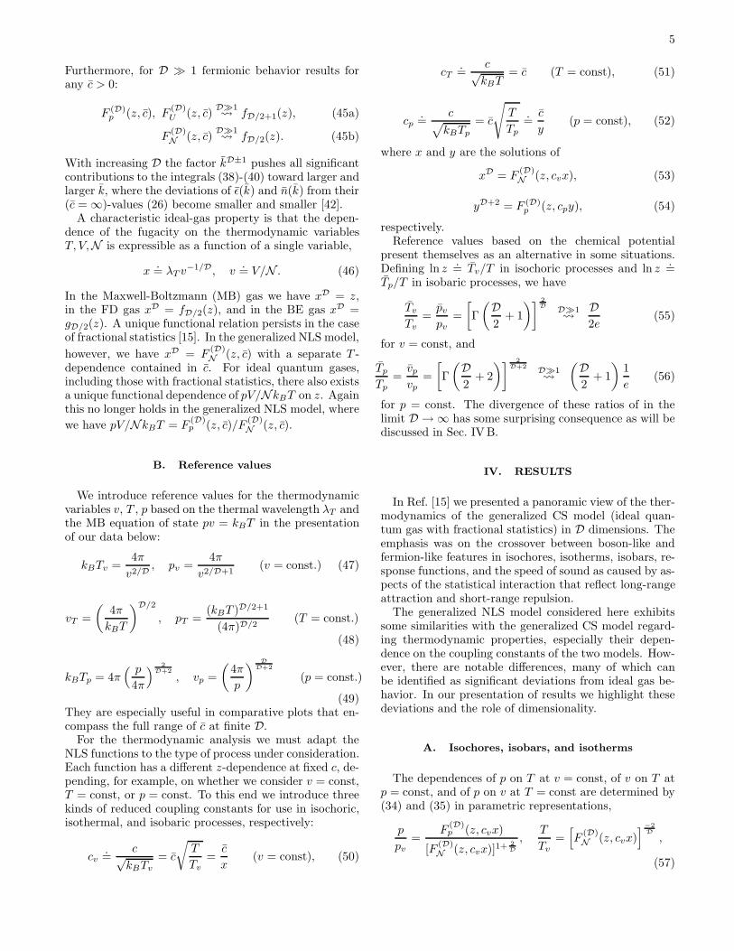
The dependences of p on T at v = const, of v on T atp = const, and of p on v at T = const are determined by(34) and (35) in parametric representations,

p

pv=

F(D)p (z, cvx)

[F(D)N (z, cvx)]1+

2D

,T

Tv=

[

F(D)N (z, cvx)

]−2D

,

(57)

6

v

vp=

[F(D)p (z, cpy)]

DD+2

F(D)N (z, cpy)

,T

Tp=

[

F (D)p (z, cpy)

]

−2D+2

,

(58)

p

pT= F (D)

p (z, cT ),v

vT=

[

F(D)N (z, cT )

]−1

, (59)

respectively, with the fugacity z in the role of the param-eter. Here x and y are the solutions of (53) and (54),respectively.

In Fig. 2 we show isochores, isobars, and isotherms forvarious coupling strengths cv,p,T in D = 3. The vari-ation of the curves between the (weak-coupling) bosonlimit and the (strong-coupling) fermion limit is similarto what was observed in the generalized CS model [15]:the convergence of all curves toward the MB line at highT or large v, and the fanning out at low T or small v.Corresponding plots in other D show similar trends inthe two models.

The shape of the curves for cv,p,T > 0 in Fig. 2 yieldsome insight into the physical interpretation of the sta-tistical interaction. For weak couplings (cv,p,T < 1) thecurves exhibit boson-like features at high T or large vand fermion-like features at low T or small v. Theseobservations translate into a long-range attractive partand a shorter-range repulsive part of the statistical in-teraction. The attractive tail is only present for smallcv,p,T , whereas the repulsive core is conspicuous for allcv,p,T > 0.

Among all the curves only the ones pertaining to theboson limit (cv,p,T = 0) have a singularity. This singular-ity signals the presence of a phase transition, the onset ofBEC. In the D = 3 case shown, the phase transition oc-curs at Tc/Tv ≃ 0.527, pc/pv ≃ 0.271 along the isochore,at Tc/Tp ≃ 0.889, vc/vp ≃ 0.456 along the isobar, and atvc/vT ≃ 0.383, pc/pT ≃ 1.341 along the isotherm.

The bosonic isochore has a singularity at Tc/Tv > 0only in D > 2. In 2 < D ≤ 4 it has a discontinuityin curvature. In D > 4 it becomes a discontinuity inslope. In the limit D → ∞ the bosonic isochore itselfbecomes discontinuous. By contrast, the bosonic isobarhas a singularity at Tc/Tp > 0 in all dimensions D ≥ 1,but with vc/vp > 0 only in D > 2. The bosonic isothermhas a horizontal portion at v/vT < vc/vT in D > 2 (seeRef. [15] for more details on the bosonic curves.)

We have already noted that all three NLS functions(38)-(40) converge toward the corresponding FD func-tions as D → ∞ provided we have c > 0. One reflection ofthis fact in the data for isochores, isobars, and isothermsis that all curves for cv,p,T > 0 move closer together asD increases. They coalesce into the universal curve (iso-chore, isobar, or isotherm) representing the ideal FD gasin D = ∞. Only the bosonic curves at T < Tc or v < vc

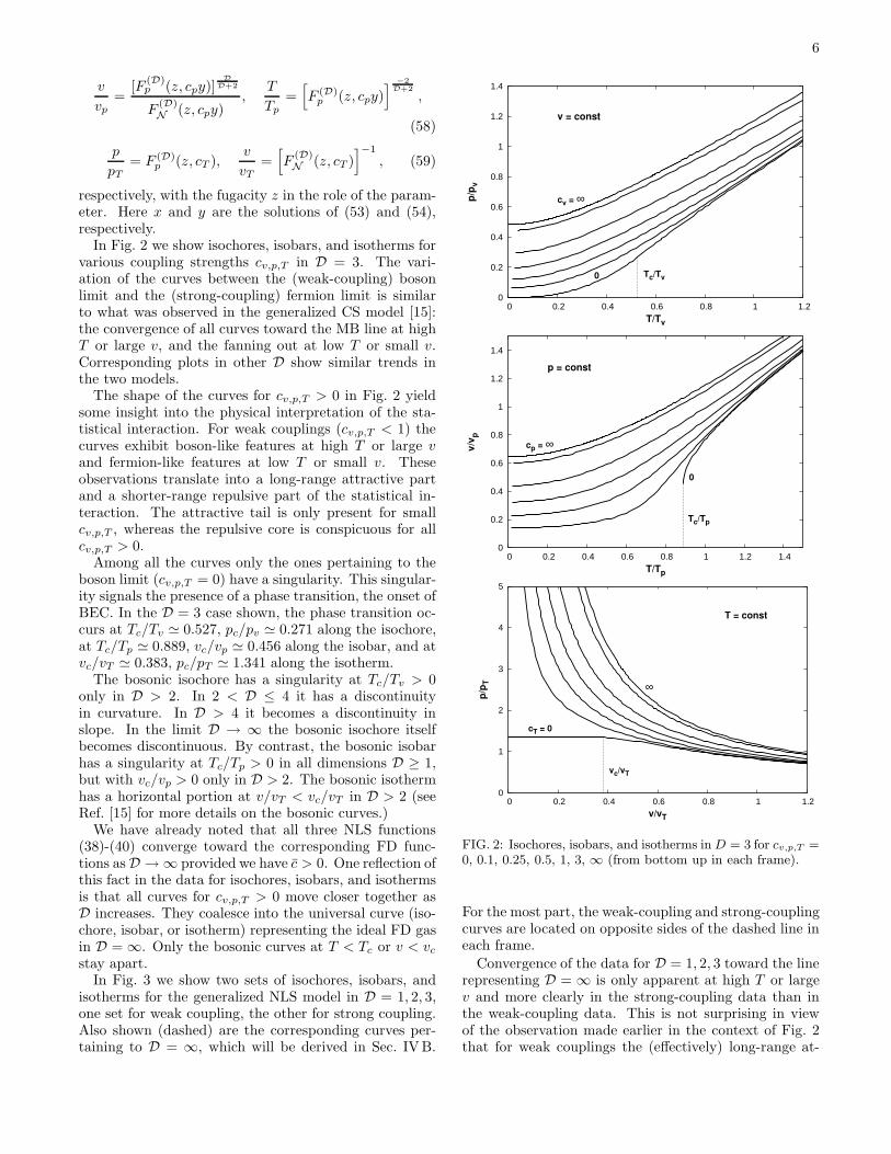
stay apart.In Fig. 3 we show two sets of isochores, isobars, and

isotherms for the generalized NLS model in D = 1, 2, 3,one set for weak coupling, the other for strong coupling.Also shown (dashed) are the corresponding curves per-taining to D = ∞, which will be derived in Sec. IVB.

0

0.2

0.4

0.6

0.8

1

1.2

1.4

0 0.2 0.4 0.6 0.8 1 1.2

p/p

v

T/Tv

0

cv = ∞

v = const

Tc/Tv

0

0.2

0.4

0.6

0.8

1

1.2

1.4

0 0.2 0.4 0.6 0.8 1 1.2 1.4

v/v

p

T/Tp

cp = ∞

0

p = const

Tc/Tp

0

1

2

3

4

5

0 0.2 0.4 0.6 0.8 1 1.2

p/p

T

v/vT

cT = 0

∞

T = const

vc/vT

FIG. 2: Isochores, isobars, and isotherms in D = 3 for cv,p,T =0, 0.1, 0.25, 0.5, 1, 3, ∞ (from bottom up in each frame).

For the most part, the weak-coupling and strong-couplingcurves are located on opposite sides of the dashed line ineach frame.

Convergence of the data for D = 1, 2, 3 toward the linerepresenting D = ∞ is only apparent at high T or largev and more clearly in the strong-coupling data than inthe weak-coupling data. This is not surprising in viewof the observation made earlier in the context of Fig. 2that for weak couplings the (effectively) long-range at-

7

0

0.2

0.4

0.6

0.8

1

0 0.2 0.4 0.6 0.8 1

p/p

v

T/Tv

3 2

1

cv = 0.25

D = 3

2 1

cv = 3

0

0.2

0.4

0.6

0.8

1

0 0.2 0.4 0.6 0.8 1

v/v

p

T/Tp

3

2

1

cp = 0.25

D = 1

2

3

cp = 3

0

1

2

3

4

0 0.2 0.4 0.6 0.8 1

p/p

T

v/vT

1

2

3

cT = 0.25

D = 1

2

3

cT = 3

FIG. 3: Isochores, isobars, and isotherms in D = 1, 2, 3 forcv,p,T = 0.25 and cv,p,T = 3. The dashed lines represent thecurves for D = ∞.

tractive part and short-range repulsive part of the statis-tical interaction are responsible for opposing trends and acrossover between them. However, convergence becomesmanifest in higher D (not shown) as the NLS functionsgradually turn into FD functions first for strong couplingsand then also for weak couplings.

B. Phase transition in D = ∞

It is well known that no phase transition at T > 0 ex-ists for free fermions in D < ∞. No transition is expectedto exist in the generalized NLS model in finite D exceptin the boson limit. However, a curious transition doesemerge in the limit D → ∞, where the generalized NLSmodel with c > 0 effectively turns into an ideal FD gas.

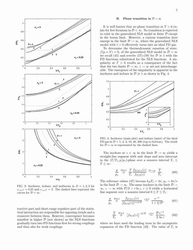
To determine the thermodynamic equation of state,f(p, v, T ) = 0, of the generalized NLS model in D = ∞we recall (45) and rewrite (57)-(59) for D ≫ 1 with theFD functions substituted for the NLS functions. A sin-gularity at T > 0 results as a consequence of the factthat the two limits D → ∞, z → ∞ are not interchange-able. The emergence of the singularity is apparent in theisochores and isobars in D ≫ 1 as shown in Fig. 4.

0

0.2

0.4

0.6

0.8

1

1.2

0 0.2 0.4 0.6 0.8 1

p/p

v

T/Tv

D = 1

300

1

0 1 0

v/v

p

T/Tp

FIG. 4: Isochores (main plot) and isobars (inset) of the idealFD gas in D = 1, 2, 3, 10, 40, 300 (top to bottom). The resultfor D = ∞ is represented by the dashed lines.

The isochore at z < ∞ in the limit D → ∞ yields astraight-line segment with unit slope and zero interceptin the (T/Tv, p/pv)-plane over a nonzero interval Tc ≤T ≤ ∞:

p

pv

D≫1≃ T

Tv

fD/2+1(z)

fD/2(z)

D→∞−→ T

Tv. (60)

The reference values (47) become kBTv = 4π, pv = 4π/vin the limit D → ∞. The same isochore in the limit D →∞, z → ∞ with D/2 = r ln z, r ≥ 0 yields a horizontalline segment over a nonzero interval 0 ≤ T ≤ Tc:

p

pv

D≫1≃ fD/2+1(z)

[fD/2(z)]1+2/D

z≫1

e−1

1 + 2/D , (61)

T

Tv

D≫1≃[

fD/2(z)]−2/D z≫1

D2

e−1

ln z, (62)

where we have used the leading term in the asymptoticexpansion of the FD function [43]. The value of Tc is

8

determined by the intersection point of the two line seg-ments. The equation of state thus reads [44]

pv =

kBT, T > Tc

kBTc, T < Tc; kBTc =

4π

e. (63)

This same universal relation can also be inferred fromEq. (58) for the isobar or from Eq. (59) for the isothermby performing the appropriate limits. All isotherms arehyperbolas, including the transition line at T = Tc. Allthe isochores and isobars consist of two straight-line seg-ments with the singularity at T = Tc as already shownin Fig. 4.

This somewhat unusual phase transition from a fullyintact Fermi sea at T < Tc to an ideal MB gas at T > Tc

results from the conspiracy of two opposing effects, onesuppressing thermal excitations at low T and the otherenhancing them at high T . Both effects grow stronger inhigher dimensions.

We know from (55) that as D increases the referencetemperature Tv becomes smaller and smaller comparedto the Fermi temperature Tv in isochoric processes (con-sidered here for specificity). This suppresses any rise inpressure at sufficiently small but nonzero T/Tv more andmore strongly. In the limit D → ∞, as Tv/Tv → 0, thepressure will remain constant over a non-vanishing in-terval of T/Tv at the value p/pv = e−1 exerted by theperfect Fermi sea.

We also know (e.g. from analogies to microcanonicalensembles) that as D increases the energy density of one-particle states is progressively thinned out inside the sur-face of the Fermi hypersphere except close to the surface.The consequence is that a smaller and smaller amount ofthermal energy is needed to knock out the vast majorityof particles from the Fermi sea. Moreover, the density ofvacancies near the Fermi edge becomes so large that theconstraint on occupancy imposed by the Pauli principleis negligible.

In D ≫ 1, therefore, if T/Tv is raised gradually, no sig-nificant thermal excitations take place initially becauseTv/Tv ≪ 1. The isochore stays flat. Once T has reacheda certain threshold the Fermi sea is emptied quickly be-cause of its shallowness and the abundance of vacanciesclose by. The system thus crosses over from a near per-fectly degenerate Fermi sea to a nearly ideal MB gas ona very short interval of T/Tv as documented in Fig. 4. InD = ∞ this crossover has sharpened into a phase transi-tion. There is no latent heat involved in that transitionand there is no sudden increase in pressure [45].

Note that on the alternative temperature scale Tv theemergent crossover between near perfect Fermi sea andalmost ideal MB gas is pushed to lower and lower valuesof T as D increases, ultimately to T/Tv = 0 for D = ∞.The resultant isochore is then that of the ideal MB gasall the way down.

It is interesting to recall the phase diagram of the idealBE gas in D = ∞ for comparison. The thermodynamicequation of state inferred from the scaled isochores, iso-bars, or isotherms as derived, for example, in Ref. [15]

has the form

pv =

kBT, T > Tc

0, T < Tc; kBTc = 4π. (64)

As in the FD case there are two phases separated by atransition line at constant T . The high-T phase is againan ideal MB gas. The low-T phase is a pure BEC. Thetransition is of first order and occurs at a higher temper-ature than in the FD case. Whereas the FD transitiondisappears in D < ∞, the BE transition persists down toD > 2, but is of second-order in D < ∞ and occurs alonga line in (p, v, T )-space that is no longer an isotherm.

C. Response functions

The three major response functions for a gasof spinless particles are the isochoric heat capacity,Cv

.= N−1(∂U/∂T )v, the isobaric expansivity, αp

.=

v−1(∂v/∂T )p, and the isothermal compressibility, κT.=

−v−1(∂v/∂p)T . For the generalized NLS model we mustevaluate the expressions

Cv

kB=

(D2

4+

D2

)

F(D)U (z, cvx)

F(D)N (z, cvx)

− D2

4

∂∂z F

(D)U (z, cvx)

∂∂z F

(D)N (z, cvx)

,

(65)

Tpαp =Tp

T

[

(D2

+ 1

)

F(D)p (z, cpy) ∂

∂z F(D)N (z, cpy)

F(D)N (z, cpy) ∂

∂z F(D)p (z, cpy)

− D2

]

,

(66)

pT κT =v

vT

∂∂z F

(D)N (z, cT )

∂∂z F

(D)p (z, cT )

, (67)

versus the independent variables T/Tv, T/Tp, v/vT , re-spectively, from (57)-(59).

In Fig. 5 we show the dependence of each responsefunction on the coupling strength in D = 3. Thevariation of the curves between the BE and FD limitsshows some resemblance to that observed in an idealgas with fractional statistics (generalized CS model) [15].All three response functions depend only weakly on thestatistical interaction at high temperature or low den-sity. The dominant trends there reflect MB behavior,Cv = (3/2)kBT , αp = 1/T , κT = v/kBT . Distinctboson-like and fermion-like features and crossovers be-tween them emerge at low temperatures and high densi-ties. The exact analytic behavior of the response func-tions in any D for the FD and BE limits was describedin Ref. [15].

The heat capacity in D = 3 for strong coupling isdominated by fermion-like features at all T , exhibiting amonotonic descent from the MB asymptote as T is low-ered and a linear approach to zero. For weak couplingthe initial increase, the smooth maximum followed by asteep descent is a boson-like feature. The ultimate lin-ear approach to zero signals the crossover to fermion-likebehavior.

9

0

0.5

1

1.5

2

0 0.2 0.4 0.6 0.8 1 1.2

Cv/k

B

T/Tv

0.25

0.5

1

Tc/Tv

cv = 0

∞

0.1

0

1

2

3

4

0 0.2 0.4 0.6 0.8 1 1.2 1.4

Tpα p

T/Tp

cp = 0

∞

Tc/Tp

0

0.5

1

1.5

2

2.5

3

0 0.2 0.4 0.6 0.8 1 1.2 1.4

pTκ T

v/vT

cT = 0

∞

vc/vT

FIG. 5: Isochoric heat capacity, isobaric expansivity, andisothermal compressibility in D = 3 for cv,p,T = 0, 0.1, 0.25,0.5, 1, 3, ∞. The heat-capacity curves for cv = 3, ∞ areunresolved. The dashed lines mark the onset of BEC.

The expansivity in D = 3 depends only weakly on T forstrong coupling and approaches zero linearly as T → 0,which is a characteristic fermion-like behavior. For weakcoupling the pronounced rise in expansivity is a boson-like feature. However, the repulsive core of the statisticalinteraction for c > 0, no matter how weak, prevents theexpansivity from diverging and forces the fermion-like

0

0.1

0.2

0.3

0.4

0.5

0.6

0 0.2 0.4 0.6 0.8 1 1.2

Cv/k

B

T/Tv

cv = 0

∞

D = 1

0

0.2

0.4

0.6

0.8

1

0 0.2 0.4 0.6 0.8 1 1.2

Cv/k

B

T/Tv

0.25

0.51

3

0,∞

D = 2

cv = 0.1

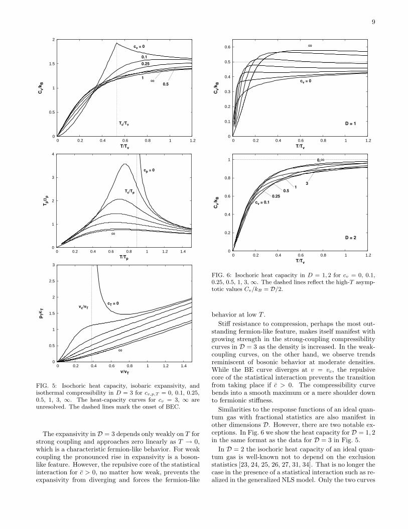
FIG. 6: Isochoric heat capacity in D = 1, 2 for cv = 0, 0.1,0.25, 0.5, 1, 3, ∞. The dashed lines reflect the high-T asymp-totic values Cv/kB = D/2.

behavior at low T .

Stiff resistance to compression, perhaps the most out-standing fermion-like feature, makes itself manifest withgrowing strength in the strong-coupling compressibilitycurves in D = 3 as the density is increased. In the weak-coupling curves, on the other hand, we observe trendsreminiscent of bosonic behavior at moderate densities.While the BE curve diverges at v = vc, the repulsivecore of the statistical interaction prevents the transitionfrom taking place if c > 0. The compressibility curvebends into a smooth maximum or a mere shoulder downto fermionic stiffness.

Similarities to the response functions of an ideal quan-tum gas with fractional statistics are also manifest inother dimensions D. However, there are two notable ex-ceptions. In Fig. 6 we show the heat capacity for D = 1, 2in the same format as the data for D = 3 in Fig. 5.

In D = 2 the isochoric heat capacity of an ideal quan-tum gas is well-known not to depend on the exclusionstatistics [23, 24, 25, 26, 27, 31, 34]. That is no longer thecase in the presence of a statistical interaction such as re-alized in the generalized NLS model. Only the two curves

10

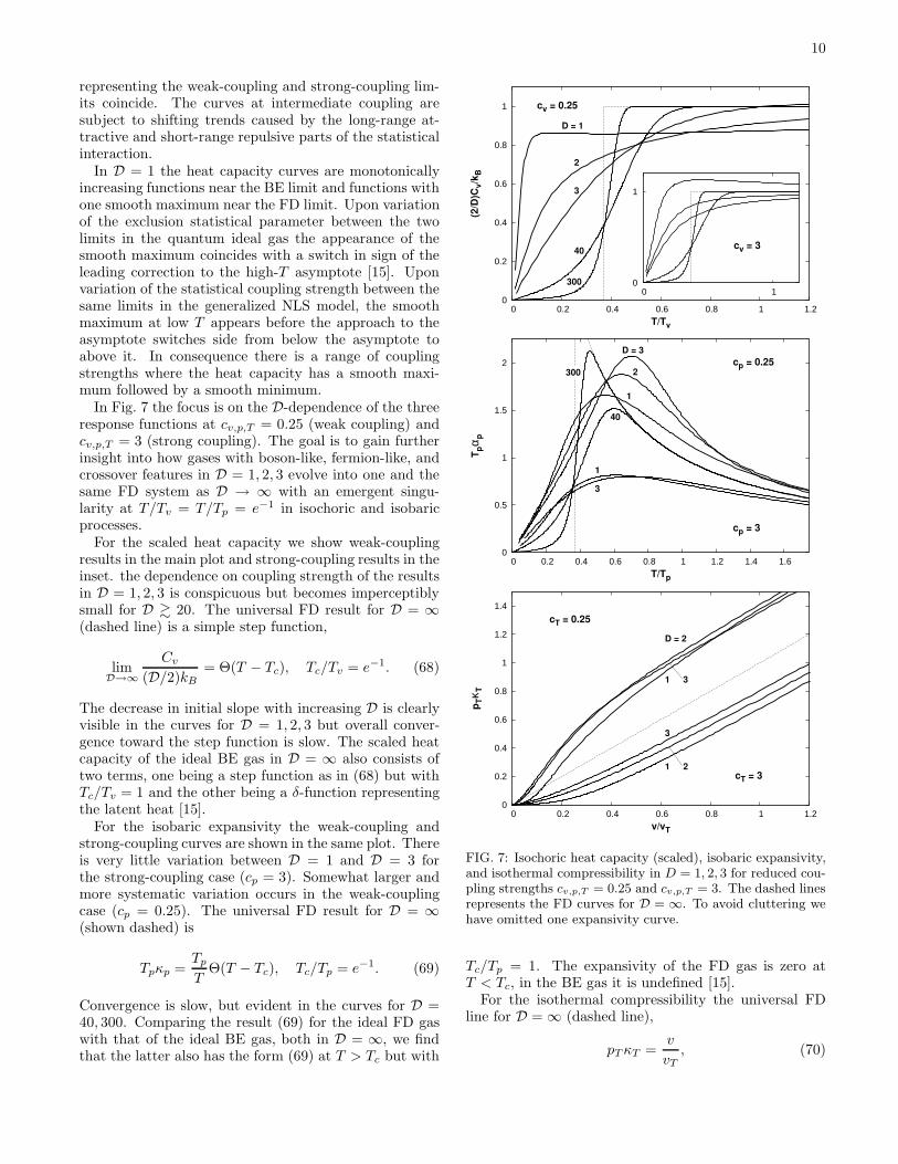
representing the weak-coupling and strong-coupling lim-its coincide. The curves at intermediate coupling aresubject to shifting trends caused by the long-range at-tractive and short-range repulsive parts of the statisticalinteraction.

In D = 1 the heat capacity curves are monotonicallyincreasing functions near the BE limit and functions withone smooth maximum near the FD limit. Upon variationof the exclusion statistical parameter between the twolimits in the quantum ideal gas the appearance of thesmooth maximum coincides with a switch in sign of theleading correction to the high-T asymptote [15]. Uponvariation of the statistical coupling strength between thesame limits in the generalized NLS model, the smoothmaximum at low T appears before the approach to theasymptote switches side from below the asymptote toabove it. In consequence there is a range of couplingstrengths where the heat capacity has a smooth maxi-mum followed by a smooth minimum.

In Fig. 7 the focus is on the D-dependence of the threeresponse functions at cv,p,T = 0.25 (weak coupling) andcv,p,T = 3 (strong coupling). The goal is to gain furtherinsight into how gases with boson-like, fermion-like, andcrossover features in D = 1, 2, 3 evolve into one and thesame FD system as D → ∞ with an emergent singu-larity at T/Tv = T/Tp = e−1 in isochoric and isobaricprocesses.

For the scaled heat capacity we show weak-couplingresults in the main plot and strong-coupling results in theinset. the dependence on coupling strength of the resultsin D = 1, 2, 3 is conspicuous but becomes imperceptiblysmall for D & 20. The universal FD result for D = ∞(dashed line) is a simple step function,

limD→∞

Cv

(D/2)kB= Θ(T − Tc), Tc/Tv = e−1. (68)

The decrease in initial slope with increasing D is clearlyvisible in the curves for D = 1, 2, 3 but overall conver-gence toward the step function is slow. The scaled heatcapacity of the ideal BE gas in D = ∞ also consists oftwo terms, one being a step function as in (68) but withTc/Tv = 1 and the other being a δ-function representingthe latent heat [15].

For the isobaric expansivity the weak-coupling andstrong-coupling curves are shown in the same plot. Thereis very little variation between D = 1 and D = 3 forthe strong-coupling case (cp = 3). Somewhat larger andmore systematic variation occurs in the weak-couplingcase (cp = 0.25). The universal FD result for D = ∞(shown dashed) is

Tpκp =Tp

TΘ(T − Tc), Tc/Tp = e−1. (69)

Convergence is slow, but evident in the curves for D =40, 300. Comparing the result (69) for the ideal FD gaswith that of the ideal BE gas, both in D = ∞, we findthat the latter also has the form (69) at T > Tc but with

0

0.2

0.4

0.6

0.8

1

0 0.2 0.4 0.6 0.8 1 1.2

(2/D

)Cv/k

B

T/Tv

D = 1

2

3

300

cv = 0.25

40

1

0 1 0

cv = 3

0

0.5

1

1.5

2

0 0.2 0.4 0.6 0.8 1 1.2 1.4 1.6

Tpα p

T/Tp

D = 3

2

1

300cp = 0.25

40

1

3

cp = 3

0

0.2

0.4

0.6

0.8

1

1.2

1.4

0 0.2 0.4 0.6 0.8 1 1.2

pTκ T

v/vT

D = 2

1 3

cT = 0.25

3

1 2cT = 3

FIG. 7: Isochoric heat capacity (scaled), isobaric expansivity,and isothermal compressibility in D = 1, 2, 3 for reduced cou-pling strengths cv,p,T = 0.25 and cv,p,T = 3. The dashed linesrepresents the FD curves for D = ∞. To avoid cluttering wehave omitted one expansivity curve.

Tc/Tp = 1. The expansivity of the FD gas is zero atT < Tc, in the BE gas it is undefined [15].

For the isothermal compressibility the universal FDline for D = ∞ (dashed line),

pT κT =v

vT, (70)

11

is indistinguishable from the MB result. The weak-coupling and strong-coupling curves are located on op-posite sides of that line. Convergence is apparent inthe curves for D = 1, 2, 3 in the strong-coupling case(cT = 3) but not in the weak-coupling case (cT = 0.25).The isothermal compressibility of ideal BE gas is also de-scribed by the result (70) but only for v/vT > vc/vT = 1.At v/vT < 1 the bosonic result is infinite [15].

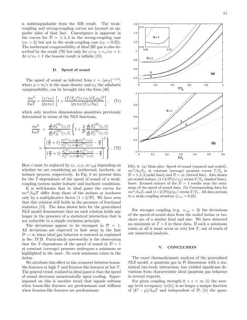
D. Speed of sound

The speed of sound as inferred from c = (ρκS)−1/2,where ρ = m/v is the mass density and κS the adiabaticcompressibility, can be brought into the form [46]

mc2

kBT=

(v/vT )

(pT κT )

[

1 +(T/Tp)

2(v/vT )(Tpαp)2

(pT κT )(Cv/kB)

]

, (71)

which only involves dimensionless quantities previouslydetermined in terms of the NLS functions,

mc2

kBT=

∂∂z F

(D)p (z, c)

∂∂z F

(D)N (z, c)

1 +2

D∂∂z F

(D)p (z, c)

∂∂z F

(D)U (z, c)

×

[

(

D2 + 1

) F (D)p (z,c) ∂

∂zF

(D)N

(z,c)

F(D)N

(z,c) ∂∂z

F(D)p (z,c)

− D2

]2

[

(

D2 + 1

) F(D)U

(z,c) ∂∂z

F(D)N

(z,c)

F(D)N

(z,c) ∂∂z

F(D)U

(z,c)− D

2

]

. (72)

Here c must be replaced by cT , cvx, or cpy depending onwhether we are considering an isothermal, isochoric, orisobaric process, respectively. In Fig. 8 we present datafor the T -dependence of the speed of sound of a weak-coupling system under isobaric and isochoric conditions.

It is well-known that in ideal gases the curves formc2/kBT differ from those of the isobars or isochoresonly by a multiplicative factor (1 + 2/D). We have seenthat this relation still holds in the presence of fractionalstatistics [15]. The data shown here for the generalizedNLS model demonstrate that no such relation holds anylonger in the presence of a statistical interaction that isnot reducible to a simple exclusion principle.

The deviations appear to be strongest in D = 1.All deviations are expected to fade away in the limtD → ∞ when ideal gas behavior is restored as explainedin Sec. IVB. Particularly noteworthy is the observationthat the T -dependence of the speed of sound in D = 1at constant (average) pressure undergoes a minimum ashighlighted in the inset. No such minimum exists in theisobar.

We attribute this effect to the crossover between boson-like features at high T and fermion-like features at low T .The general trend, realized in ideal gases is that the speedof sound decreases monotonically upon cooling. Super-imposed on this is another trend that signals softnesswhen boson-like features are predominant and stiffnesswhen fermion-like features are predominant.

0.4

0.6

0.8

1

1.2

1.4

1.6

0 0.2 0.4 0.6 0.8 1T/Tp

D = 1

2

3(a)

0.77

0.75 0.24 0.06

D = 1

0

0.2

0.4

0.6

0.8

1

0 0.1 0.2 0.3 0.4 0.5 0.6T/Tv

(b)

D = 1

2

3

FIG. 8: (a) Main plot: Speed of sound (squared and scaled),mc2/kBTp, at constant (average) pressure versus T/Tp inD = 1, 2, 3 (solid lines) and D = ∞ (dotted line). Also shownare scaled isobars, (1+2/D)(v/vp) versus T/Tp (dashed lines).Inset: Zoomed extract of the D = 1 results near the mini-mum of the speed of sound data. (b) Corresponding data formc2/kBTv and (1+2/D)(p/pv) versus T/Tv. All data pertainto a weak-coupling situation (cv,p = 0.25).

For stronger coupling (e.g. cv.p = 3) the deviationsof the speed-of-sound data from the scaled isobar or iso-chore are of a similar kind and size. We have detectedno minimum at T > 0 in these data. If such a minimumexists at all it must occur at very low T , out of reach ofour numerical analysis.

V. CONCLUSION

The exact thermodynamic analysis of the generalizedNLS model, a quantum gas in D dimensions with a sta-tistical two-body interaction, has yielded significant de-viations from characteristic ideal quantum gas behaviorin several respects.

For given coupling strength 0 < c < ∞ (i) the aver-age level occupancy 〈n(k)〉 is no longer a unique functionof (k2 − µ)/kBT and independent of D; (ii) the quan-

12

tities pλDT /kBT , NλD

T /V , and (UλDT /V )/(kBTD/2) are

no longer unique functions of the fugacity z; (iii) thetwo quantities pλD

T /kBT and (UλDT /V )/(kBTD/2) are

no longer identical.Among the consequences are (i) that the T -dependence

of the internal energy is no longer of the same shape asthe isochore; (ii) that the quantity pV/NkBT is no longera function of z alone in given D; (iii) that there is nolonger any simple relation between the speed of soundand the isochore or isobar.

In any finite D the statistical interaction of the gener-alized NLS model smoothly interpolates between an idealBE gas in the weak-coupling limit (c = 0) and an idealFD gas in the strong-coupling limit (c = ∞). In the

limit D → ∞ the system behaves like an ideal BE gasfor c = 0 and like an ideal FD gas for c > 0. In D = ∞both quantum gases feature a phase transition at Tc > 0along isochores or isobars. The transition is of first orderin the BE case and of second order in the FD case.

Acknowledgments

Financial support from the DFG SchwerpunktKollektive Quantenzustande in elektronischen 1D

Ubergangsmetallverbindungen (for M.K.) is grate-fully acknowledged. We have greatly benefited fromdiscussions with Prof. A. E. Meyerovich.

[1] C. J. Pethick and H. Smith, Bose-Einstein condensation

in dilute gases (Cambridge University Press, 2002).[2] L. Pitaesvskii and S. Stringari, Bose-Einstein condensa-

tion (Oxford University Press, 2003).[3] M. Greiner, I. Bloch, O. Mandel, T. W. Hansch, and

T. Esslinger, 87, 160405 (2001).[4] A. Gorlitz, et al., Phys. Rev. Lett. 87, 130402 (2001).[5] F. Schreck, L. Kaykovich, K. L. Corwin, G. Ferrari,

T. Bourdel, J. Cubizolles, and C. Salomon, Phys. Rev.Lett. 87, 080403 (2001).

[6] D. S. Petrov, D. M. Gangardt, and G. V. Shlyapnikov,J. Phys. IV France 116, 5 (2004).

[7] Y.-S. Wu, Phys. Rev. Lett. 73, 922 (1994).[8] Y. S. Wu, in New development on integrable systems and

long-ranged interaction models, M. I. Ge and Y. S. Wu,Eds. (World Scientific, Singapore, 1995), p. 159; Y. S.Wu, in Proceedings of the XX international conference

on group theoretical methods in physics, A. Arima, T.Eguchi, and N. Nakanishi, Eds. (World Scientific, Singa-pore, 1995), p. 94.

[9] F. D. M. Haldane, Phys. Rev. Lett. 67, 937 (1991).[10] F. D. M. Haldane, Phys. Rev. Lett. 66, 1529 (1991).[11] F. D. M. Haldane in Correlation effects in low-

dimensional electron systems, A. Okiji and N. Kawakami,Eds., (Springer-Verlag, Heidelberg, 1994).

[12] D. Bernard and Y.-S. Wu, in New developments on

integrable systems and long-ranged interaction models,

(World Scientific, Singapore, 1994).[13] M. Arikawa, M. Karbach, G. Muller, and K. Wiele, J.

Phys. A: Math. Gen. 39, 10623 (2006).[14] An effort with similar goals but different strategy was

reported by B. Sutherland, Phys. Rev. B 56, 4422 (1997).[15] G. G. Potter, G. Muller, and M. Karbach, Phys. Rev. E

75, 061120 (2007).[16] F. Calogero, J. Math. Phys. 12, 419 (1971).[17] B. Sutherland, Phys. Rev. A 4, 2019 (1971).[18] B. Sutherland, Phys. Rev. A 5, 1372 (1972).[19] S. B. Isakov, Int. J. Mod. Phys. 9, 2563 (1994).[20] S. B. Isakov, D. P. Arovas, J. Myrheim, and A. P. Poly-

chronakos, Phys. Lett. A 212, 299 (1996).[21] G. S. Joyce, S. Sarkar, J. Spalek, and K. Byczuk, Phys.

Rev. B 53, 990 (1996).

[22] M. V. N. Murthy and R. Shankar, Phys. Rev. B 60, 6517(1999).

[23] R. M. May, Phys. Rev. 135, A1515 (1964).[24] T. Aoyama, Eur. Phys. J. B 20, 123 (2001).[25] M. H. Lee, Phys. Rev. E 55, 1518 (1997).[26] A. Swarup and B. Cowan, J. Low Temp. Phys. 134, 881

(2004).[27] D.-V. Anghel, J. Phys. A: Math. Gen. 35, 7255 (2002).[28] C. Nayak and F. Wilczek, Phys. Rev. Lett. 73, 2740

(1994).[29] K. Iguchi, Phys. Rev. Lett. 78, 3233 (1997).[30] K. Iguchi, Mod. Phys. Lett. B 11, 765 (1997).[31] K. Iguchi, Int. J. Mod. Phys. B 11, 3551 (1997).[32] K. Iguchi and K. Aomoto, Int. J. Mod. Phys. B 14, 485

(2000).[33] M. V. Medvedev, Phys. Rev. Lett. 78, 4147 (1997).[34] S. Viefers, F. Ravndal, and T. Haugset, Am. J. Phys. 63,

369 (1995).[35] E. Lieb and W. Liniger, Phys. Rev. 130, 1605 (1963).[36] E. H. Lieb, Phys. Rev. 130, 1616 (1963).[37] C. N. Yang and C. P. Yang, J. Math. Phys. 10, 1115

(1969).[38] C. P. Yang, Phys. Rev. 2, 154 (1970).[39] V. E. Korepin, N. M. Bogoliubov, and A. G. Izer-

gin, Quantum Inverse Scattering Method and Correlation

Functions (Cambridge University Press, 1993).[40] M. Takahashi, Thermodynamics of one-dimensional Solv-

able Models (Cambridge University Press, 1999).[41] B. Sutherland, Beautiful models: 70 years of exactly

solved quantum many-body problems (World Scientific,Singapore, 2004).

[42] The same argument applies to the case c = 0 but only forz ≤ 1. Indeed we have f∞(z) = g∞(z) = z for 0 ≤ z ≤ 1.

[43] R. K. Pathria, Statistical mechanics (Pergamon Press,Oxford, 1972).

[44] In D = ∞, pv and kBT become dimensionless under theconvention ~

2/2m = 1 used here.[45] The scaled entropy S/ND rises from zero at T ≥ Tc with

finite slope.[46] For consistency, we must use reference values Tv, Tp, and

vT derived from the first expression (37) for λT in thiscontext.