Applied Thermodynamics: Software Solutions
267
-
Upload
khangminh22 -
Category
Documents
-
view
1 -
download
0
Transcript of Applied Thermodynamics: Software Solutions

2
Dr. M. Thirumaleshwar
Applied Thermodynamics: Software Solutions Part-V (Compressible flow: Isentropic flow – Normal shocks – Fanno flow – Rayleigh flow, and Engine trials)
Download free eBooks at bookboon.com

3
Applied Thermodynamics: Software Solutions: Part-V (Compressible flow: Isentropic flow – Normal shocks – Fanno flow – Rayleigh flow, and Engine trials)1st edition© 2014 Dr. M. Thirumaleshwar & bookboon.comISBN 978-87-403-0767-2
Download free eBooks at bookboon.com

Applied Thermodynamics: Software Solutions: Part-V
4
Contents
Contents
Dedication Part I
Preface Part I
About the Author Part I
About the Software used Part I
To the Student Part I How to use this Book? Part I
1 Gas Power Cycles Part I1.1 Definitions, Statements and Formulas used[1-6]: Part I1.2 Problems on Otto cycle (or, constant volume cycle): Part I1.3 Problems on Diesel cycle (or, constant pressure cycle): Part I1.4 Problems on Dual cycle (or, limited pressure cycle): Part I1.5 Problems on Stirling cycle: Part I1.6 References: Part I
Download free eBooks at bookboon.com
Click on the ad to read more
GET THERE FASTER
Oliver Wyman is a leading global management consulting firm that combines
deep industry knowledge with specialized expertise in strategy, operations, risk
management, organizational transformation, and leadership development. With
offices in 50+ cities across 25 countries, Oliver Wyman works with the CEOs and
executive teams of Global 1000 companies.
An equal opportunity employer.
Some people know precisely where they want to go. Others seek the adventure of discovering uncharted territory. Whatever you want your professional journey to be, you’ll find what you’re looking for at Oliver Wyman.
Discover the world of Oliver Wyman at oliverwyman.com/careers
DISCOVEROUR WORLD

Applied Thermodynamics: Software Solutions: Part-V
5
Contents
2 Cycles for Gas Turbines and Jet propulsion Part II2.1 Definitions, Statements and Formulas used[1-7]: Part II2.2 Problems solved with Mathcad: Part II2.3 Problems solved with EES: Part II2.4 Problems solved with TEST: Part II2.5 References: Part II
3 Vapour Power Cycles Part II3.1 Definitions, Statements and Formulas used[1-7]: Part II3.2 Problems solved with Mathcad: Part II3.4 Problems solved with TEST: Part II3.5 References: Part II
4 Refrigeration Cycles Part III4.1 Definitions, Statements and Formulas used[1-7]: Part III4.1.1 Ideal vapour compression refrigeration cycle: Part III4.2 Problems solved with Mathcad: Part III4.3 Problems solved with DUPREX (free software from DUPONT) [8]: Part III4.4 Problems solved with EES: Part III4.5 Problems solved with TEST: Part III4.6 References: Part III
Download free eBooks at bookboon.com
Click on the ad to read moreClick on the ad to read more

Applied Thermodynamics: Software Solutions: Part-V
6
Contents
5 Air compressors Part III5.1 Definitions, Statements and Formulas used[1-6]: Part III5.2 Problems solved with Mathcad: Part III5.3 Problems solved with EES: Part III5.4 References: Part III
6 Thermodynamic relations Part III6.1 Summary of Thermodynamic relations [1-6]: Part III6.5 References: Part III
7 Psychrometrics Part IV7.1 Definitions, Statements and Formulas used [1-11]: Part IV7.2 Problems solved with Mathcad: Part IV7.3 Problems solved with Psychrometric chart: Part IV7.4 Problems solved with EES: Part IV7.5 Problems solved with TEST: Part IV7.6 References: Part IV
Download free eBooks at bookboon.com
Click on the ad to read moreClick on the ad to read moreClick on the ad to read more
81,000 kmIn the past four years we have drilled
That’s more than twice around the world.
What will you be?
Who are we?We are the world’s leading oilfield services company. Working globally—often in remote and challenging locations—we invent, design, engineer, manufacture, apply, and maintain technology to help customers find and produce oil and gas safely.
Who are we looking for?We offer countless opportunities in the following domains:n Engineering, Research, and Operationsn Geoscience and Petrotechnicaln Commercial and Business
If you are a self-motivated graduate looking for a dynamic career, apply to join our team.
careers.slb.com
Applied Thermodynamics: Software Solutions: Part-V
7
Contents
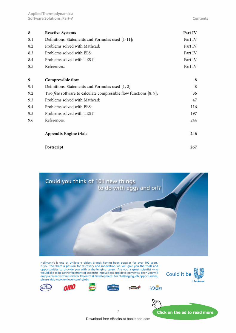
8 Reactive Systems Part IV8.1 Definitions, Statements and Formulas used [1-11]: Part IV8.2 Problems solved with Mathcad: Part IV8.3 Problems solved with EES: Part IV8.4 Problems solved with TEST: Part IV8.5 References: Part IV
9 Compressible flow 89.1 Definitions, Statements and Formulas used [1, 2]: 89.2 Two free software to calculate compressible flow functions [8, 9]: 369.3 Problems solved with Mathcad: 479.4 Problems solved with EES: 1169.5 Problems solved with TEST: 1979.6 References: 244
Appendix Engine trials 246
Postscript 267
Download free eBooks at bookboon.com
Click on the ad to read moreClick on the ad to read moreClick on the ad to read moreClick on the ad to read more
Hellmann’s is one of Unilever’s oldest brands having been popular for over 100 years. If you too share a passion for discovery and innovation we will give you the tools and opportunities to provide you with a challenging career. Are you a great scientist who would like to be at the forefront of scientific innovations and developments? Then you will enjoy a career within Unilever Research & Development. For challenging job opportunities, please visit www.unilever.com/rdjobs.
Could you think of 101 new thingsto do with eggs and oil?

Applied Thermodynamics: Software Solutions: Part-V
8
Compressible flow
9 Compressible flowLearning objectives:
1. In this chapter, ‘Compressible flow’ is dealt with.2. Formulas for stagnation temp, stagnation pressure, property variations in isentropic flow are
compiled first. 3. Then, formulas for property changes during isentropic flow through convergent as well as
Convergent-Divergent (C-D) nozzles, normal shocks, Fanno flow (i.e. adiabatic flow with friction) and frictionless flow through ducts with heat transfer (i.e. Rayleigh flow) are enumerated.
4. Property tables for these cases, which should be useful in calculations, are also given.5. Many useful Functions are written in Mathcad and EES to calculate the property variations
for different cases mentioned above. These Functions make the calculations very easy. Using these Functions all the property variations are tabulated and also the plots are drawn.
6. A large number of Problems from University question papers as well as from standard Text books are solved to demonstrate the use of the Functions written in Mathcad and EES.
7. Convenience of visual solutions using TEST is demonstrated by solving problems on isentropic flow through nozzles and for normal shocks.
8. An Appendix on Engine trials is included, since this topic forms part of the syllabus in some universities.
=========================================================================
9.1 Definitions, Statements and Formulas used [1, 2]:
9.1.1 Stagnation properties:
We have: Enthalpy = Internal energy + flow energy
When P.E. and K.E. are negligible, Enthalpy represents the ‘total energy’.
However, for high speed flows, as in the case of nozzles or jet engines, K.E. is not negligible, and then the enthalpy and K.E. are combined in to a single term called ‘stagnation (or total) enthalpty’ as follows:
where V is the velocity of fluid.
Download free eBooks at bookboon.com

Applied Thermodynamics: Software Solutions: Part-V
9
Compressible flow
For isentropic flow through a duct such as a nozzle, with no change in P.E., we have:
i.e. stagnation enthalpy remains constant.
Stagnation enthalpy represents the enthalpy of a fluid when it is brought to rest adiabatically.
For an ideal gas:
Stagnation pressure (P0): It is the pressure a fluid attains when brought to rest isentropically.
For an ideal gas with constant sp. heats, P0 is related to static pressure by:
And, ratio of stagnation density to static density is given by:
So, energy balance for a steady flow device becomes:
And, for an ideal gas:
Download free eBooks at bookboon.com

Applied Thermodynamics: Software Solutions: Part-V
10
Compressible flow
9.1.2 Speed of sound and Mach Number:
Speed of sound, c is given by:
From this, we get:
Thus, for a given ideal gas, speed of sound is a function of temp alone.
Mach Number (Ma): It is the ratio of actual velocity of the fluid to the speed of sound in the same fluid at the same state.
Flow is called ‘sonic’ when Ma = 1, ‘subsonic’ when Ma < 1, ‘supersonic’ when Ma > 1, and ‘hypersonic’ when Ma >> 1.
9.1.3 One dimensional isentropic flow:
Flow through nozzles, diffusers and turbine blade passages can be approximated as one dimensional isentropic flow and low parameters vary in the direction of flow only.
Variation of fluid velocity with flow area: Starting with continuity equation and applying the energy balance, and using the definition of Mach Number, we get:
In the above, since A and V are positive, we conclude:
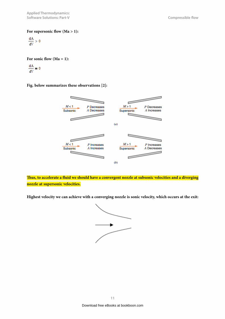
For subsonic flow (Ma < 1):
Download free eBooks at bookboon.com
Applied Thermodynamics: Software Solutions: Part-V
11
Compressible flow
For supersonic flow (Ma > 1):
For sonic flow (Ma = 1):
Fig. below summarizes these observations [2]:
Thus, to accelerate a fluid we should have a convergent nozzle at subsonic velocities and a diverging nozzle at supersonic velocities.
Highest velocity we can achieve with a converging nozzle is sonic velocity, which occurs at the exit:
Download free eBooks at bookboon.com
Applied Thermodynamics: Software Solutions: Part-V
12
Compressible flow
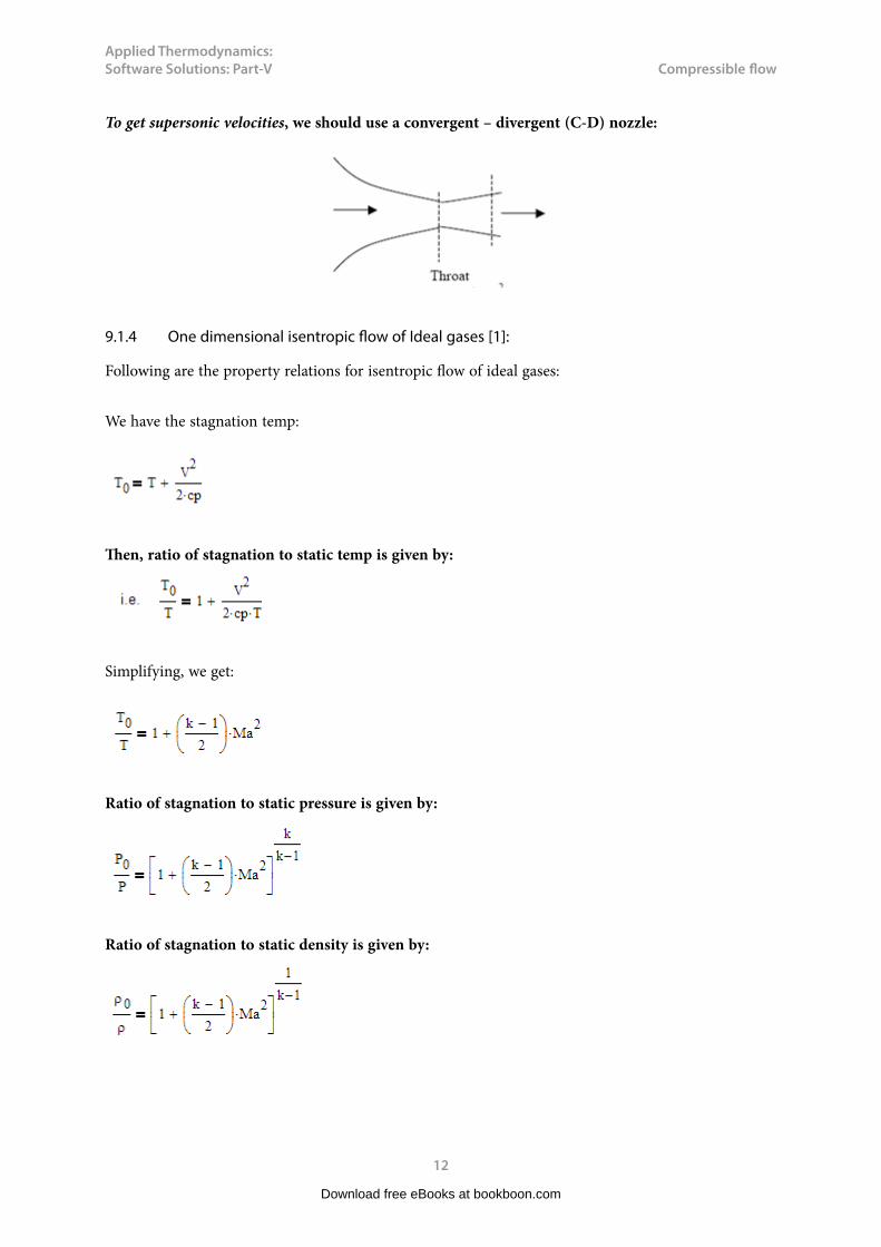
To get supersonic velocities, we should use a convergent – divergent (C-D) nozzle:
9.1.4 One dimensional isentropic flow of Ideal gases [1]:
Following are the property relations for isentropic flow of ideal gases:
We have the stagnation temp:
Then, ratio of stagnation to static temp is given by:
Simplifying, we get:
Ratio of stagnation to static pressure is given by:
Ratio of stagnation to static density is given by:
Download free eBooks at bookboon.com

Applied Thermodynamics: Software Solutions: Part-V
13
Compressible flow
Properties of fluid where Mach No. is 1 (i.e. at the throat) are called ‘critical properties’ and are denoted by asterisk (or star). So, setting Ma = 1 in the above relations, we get the critical ratios:
It is convenient to have following values of critical properties readily available:
Superheated steam: k = 1.3
Hot products of combustion: k = 1.33
Air:k = 1.4
Mono-atomic gases:k = 1.667
0.5457 0.5404 0.5283 0.4871
0.8696 0.8584 0.8333 0.7499
0.6276 0.6295 0.6340 0.6495
Download free eBooks at bookboon.com
Click on the ad to read moreClick on the ad to read moreClick on the ad to read moreClick on the ad to read moreClick on the ad to read more
© Deloitte & Touche LLP and affiliated entities.
360°thinking.
Discover the truth at www.deloitte.ca/careers
© Deloitte & Touche LLP and affiliated entities.
360°thinking.
Discover the truth at www.deloitte.ca/careers
© Deloitte & Touche LLP and affiliated entities.
360°thinking.
Discover the truth at www.deloitte.ca/careers © Deloitte & Touche LLP and affiliated entities.
360°thinking.
Discover the truth at www.deloitte.ca/careers

Applied Thermodynamics: Software Solutions: Part-V
14
Compressible flow
9.1.5 Effect of back pressure on exit velocity, mass flow rate and pressure distribution [1]:
For convergent nozzle: See fig. below[2]:
Since inlet velocity is almost zero, stagnation pressure, P0 and temp T0 are equal to the inlet pressure and temp.
PB is the back pressure, PE is the pressure at the exit plane of the nozzle.
In the above fig:
For curve designated by ‘a’: PB = P0, therefore, there is no flow.
For curve designated by ‘b’: PB < P0, but PB > Pcrit. Now, PE = PB and there is subsonic flow, and at the exit, Mach No. is less than 1.
For curve designated by ‘c’: PB < P0, and PB = Pcrit. Now, PE = PB and there is subsonic flow in the nozzle and at the exit, flow is sonic.
For curve designated by ‘d’: PB < Pcrit, Now, PE remains Pcrit and there is subsonic flow in the nozzle and at the exit, flow is still sonic only. Pressure falls from PE to PB outside the exit. Now, the nozzle is said to be ‘choked’.
Mass flow rate and pressure ratios for the above scheme are shown below:
Download free eBooks at bookboon.com
Applied Thermodynamics: Software Solutions: Part-V
15
Compressible flow
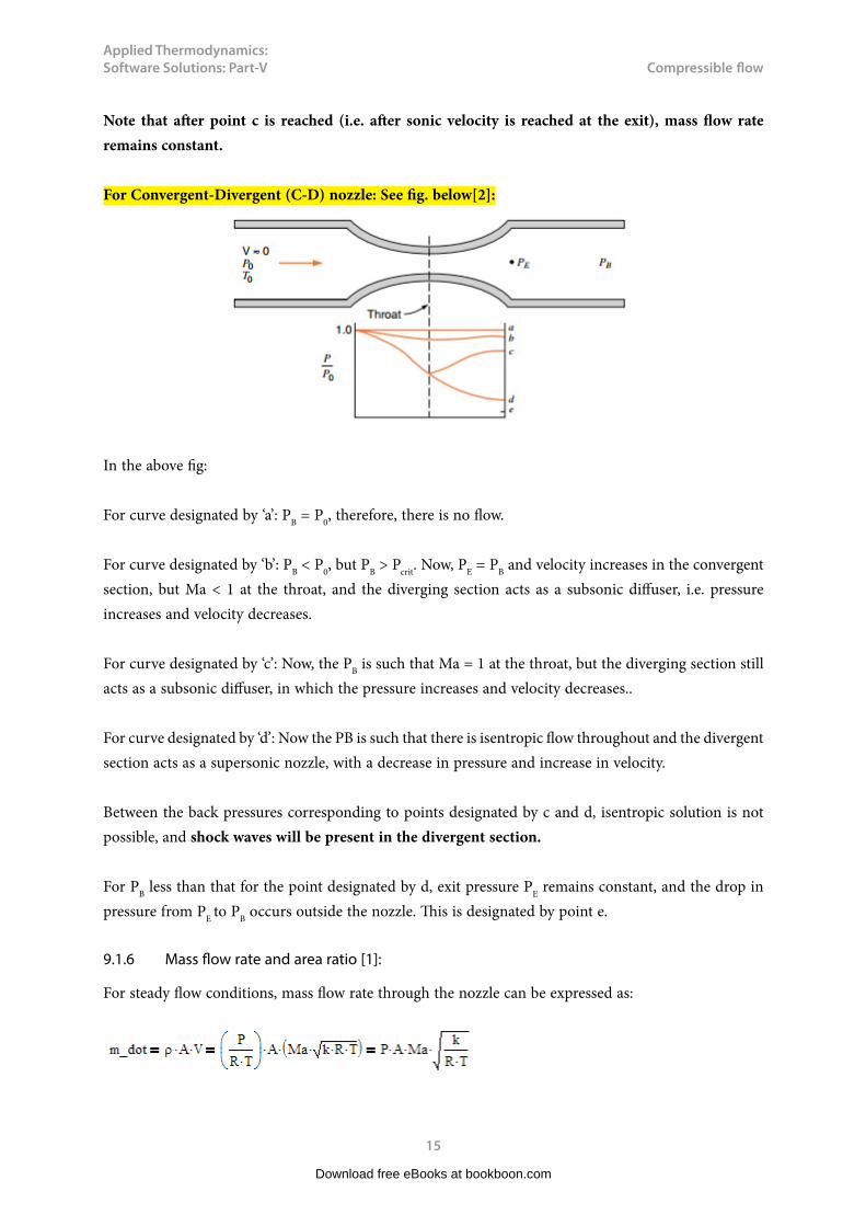
Note that after point c is reached (i.e. after sonic velocity is reached at the exit), mass flow rate remains constant.
For Convergent-Divergent (C-D) nozzle: See fig. below[2]:
In the above fig:
For curve designated by ‘a’: PB = P0, therefore, there is no flow.
For curve designated by ‘b’: PB < P0, but PB > Pcrit. Now, PE = PB and velocity increases in the convergent section, but Ma < 1 at the throat, and the diverging section acts as a subsonic diffuser, i.e. pressure increases and velocity decreases.
For curve designated by ‘c’: Now, the PB is such that Ma = 1 at the throat, but the diverging section still acts as a subsonic diffuser, in which the pressure increases and velocity decreases..
For curve designated by ‘d’: Now the PB is such that there is isentropic flow throughout and the divergent section acts as a supersonic nozzle, with a decrease in pressure and increase in velocity.
Between the back pressures corresponding to points designated by c and d, isentropic solution is not possible, and shock waves will be present in the divergent section.
For PB less than that for the point designated by d, exit pressure PE remains constant, and the drop in pressure from PE to PB occurs outside the nozzle. This is designated by point e.
9.1.6 Mass flow rate and area ratio [1]:
For steady flow conditions, mass flow rate through the nozzle can be expressed as:
Download free eBooks at bookboon.com

Applied Thermodynamics: Software Solutions: Part-V
16
Compressible flow
Now, writing P and T in terms of stagnation pressure and stagnation temp:
Eqn. (A) is valid at any cross-section of nozzle along the length of nozzle.
Max. mass flow rate occurs when the Mach No. is equal to 1, and this occurs at the throat. Denoting the area at the throat by Astar, and substituting Ma = 1 in eqn. (A), we get:
Download free eBooks at bookboon.com
Click on the ad to read moreClick on the ad to read moreClick on the ad to read moreClick on the ad to read moreClick on the ad to read moreClick on the ad to read more

Applied Thermodynamics: Software Solutions: Part-V
17
Compressible flow
From eqn. (A) by eqn. (B), we get:
Area ratio (A/Astar) is the ratio of the area at the point where Mach No. is Ma to the throat area, and (A/Astar) as a function of Mach No. is plotted below[2]:
Note that for a given (A/Astar) there are two values of Ma, one for the subsonic region and the other for the supersonic region.
Also:
From eqn.(B), for an ideal gas with k = 1.4, we get:
Download free eBooks at bookboon.com

Applied Thermodynamics: Software Solutions: Part-V
18
Compressible flow
9.1.7 Impulse Function (F) and A*P ratio[10]:
Both the quantities P.A and r.A.V^2 occur frequently in compressible flow calculations, and both have units of Force. So, they are conveniently expressed together as an important gas dynamic parameter, called Impulse Function, or the wall force function. It is defined as:
Now, at M = 1, we have: F = Fstar.
And, the non-dimensional Impulse Function is:
Second function that occurs frequently in compressible flow calculations is:
Simplified expression for this function is:
Download free eBooks at bookboon.com
Applied Thermodynamics: Software Solutions: Part-V
19
Compressible flow
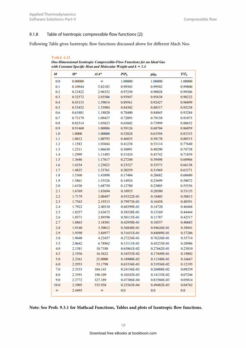
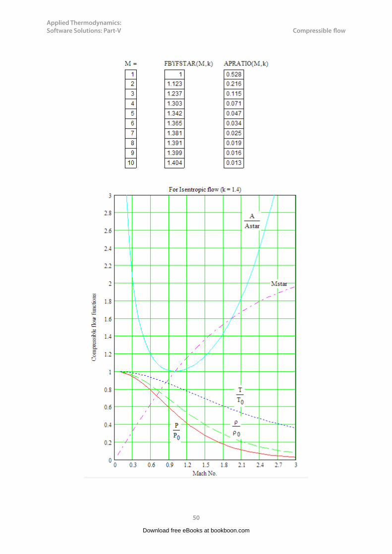
9.1.8 Table of Isentropic compressible flow functions [2]:
Following Table gives Isentropic flow functions discussed above for different Mach Nos.
Note: See Prob. 9.3.1 for Mathcad Functions, Tables and plots of Isentropic flow functions.
Download free eBooks at bookboon.com
Applied Thermodynamics: Software Solutions: Part-V
20
Compressible flow
9.1.9 Normal shocks [2]:
Normal shock occurs in a plane normal to the flow direction. Also, shock occurs only in the divergent portion of the C-D nozzle, since before the shock, the velocity should be supersonic (i.e. Ma > 1). Flow through the shock is highly irreversible, and therefore, can not be approximated as isentropic. Property changes across the shock are of special interest, and are, therefore, tabulated for easy reference.
Denoting the properties upstream of the shock by subscript x and properties downstream of the shock by y, we have:
Download free eBooks at bookboon.com
Click on the ad to read moreClick on the ad to read moreClick on the ad to read moreClick on the ad to read moreClick on the ad to read moreClick on the ad to read moreClick on the ad to read more
������������� ����������������������������������������������� �� ���������������������������
������ ������ ������������������������������ ����������������������!���"���������������
�����#$%����&'())%�*+����������,����������-
.��������������������������������� ��
���������� ���������������� ������������� ���������������������������� �����������
The Wakethe only emission we want to leave behind

Applied Thermodynamics: Software Solutions: Part-V
21
Compressible flow
Combining the conservation of mass and energy equations and plotting on h-s diagram, gives the Fanno line. And, combining the conservation of mass and momentum equations and plotting on h-s diagram, gives the Rayleigh line. Max. entropy points in these lines (i.e. points a and b in the following fig.) correspond to Ma = 1. Upper part of each curve represents subsonic states and the lower part, supersonic.
In the above fig., at the two points of intersection of Fanno and Rayleigh lines, i.e. at x and y, all the three equations are satisfied; x is in the supersonic region and y is in the subsonic region.
Since (sy – sx) > 0, normal shock proceeds from x to y. Thus, velocity changes from supersonic before the shock to subsonic after the shock.
Download free eBooks at bookboon.com

Applied Thermodynamics: Software Solutions: Part-V
22
Compressible flow
9.1.10 Equations governing normal shocks [2]:
From the conservation of energy principle, stagnation enthalpy remains constant across the shock,
i.e. T0x = T0y.
We have:
Therefore, dividing these two equations, we get:
Download free eBooks at bookboon.com
Click on the ad to read moreClick on the ad to read moreClick on the ad to read moreClick on the ad to read moreClick on the ad to read moreClick on the ad to read moreClick on the ad to read moreClick on the ad to read more
CAREERKICKSTARTAn app to keep you in the know
Whether you’re a graduate, school leaver or student, it’s a difficult time to start your career. So here at RBS, we’re providing a helping hand with our new Facebook app. Bringing together the most relevant and useful careers information, we’ve created a one-stop shop designed to help you get on the career ladder – whatever your level of education, degree subject or work experience.
And it’s not just finance-focused either. That’s because it’s not about us. It’s about you. So download the app and you’ll get everything you need to know to kickstart your career.
So what are you waiting for?
Click here to get started.

Applied Thermodynamics: Software Solutions: Part-V
23
Compressible flow
From continuity equation:
In the above, using the equation of state and definition of Mach No., and eqn for sonic velocity c, we get:
Combining eqns (a) and (b), i.e. combining the energy and continuity eqns, we get the eqn for the Fanno line:
Similarly, combining the momentum and continuity equations, we get the eqn for the Rayleigh line:
Combining equations (c) and (d), we get the following eqn relating Mx and My:
Properties across a normal shock change as follows [1]:
After the shock, we have:
P → increases
P0 → decreases
V → decreases
M → decreases
Download free eBooks at bookboon.com

Applied Thermodynamics: Software Solutions: Part-V
24
Compressible flow
T → increases
T0 → remains const.
ρ → increases
s → increases
Ratio of stagnation pressures across a shock (P0y/P0x) is often useful [3]:
Since there is no area change across a shock, we get from eqn C (for A/Astar) and eqn. (f) above:
Download free eBooks at bookboon.com
Click on the ad to read moreClick on the ad to read moreClick on the ad to read moreClick on the ad to read moreClick on the ad to read moreClick on the ad to read moreClick on the ad to read moreClick on the ad to read moreClick on the ad to read more

Applied Thermodynamics: Software Solutions: Part-V
25
Compressible flow
9.1.11 Table below gives the Normal shock functions for an ideal gas with k = 1.4: [Ref:2]
Note: See Prob. 9.3.2 for Mathcad Functions, Tables and plots of Normal shock functions.
Download free eBooks at bookboon.com

Applied Thermodynamics: Software Solutions: Part-V
26
Compressible flow
9.1.12 Nozzle and diffuser coefficients [2]:
Nozzle efficiency (ηN): is defined as:
See the following fig:
Velocity coeff. of Nozzle (CV):
Coeff. of discharge for a Nozzle (CD):
Download free eBooks at bookboon.com

Applied Thermodynamics: Software Solutions: Part-V
27
Compressible flow
Diffuser efficiency (ηD): is defined with respect to the following fig:
In the above fig: 1 and 01 are the actual and stagnation states of fluid entering the diffuser, and 2 and 02 are the actual and stagnation states of fluid leaving the diffuser. Then, diffuser efficiency is defined as:
Download free eBooks at bookboon.com
Click on the ad to read moreClick on the ad to read moreClick on the ad to read moreClick on the ad to read moreClick on the ad to read moreClick on the ad to read moreClick on the ad to read moreClick on the ad to read moreClick on the ad to read moreClick on the ad to read more
AXA Global Graduate Program
Find out more and apply

Applied Thermodynamics: Software Solutions: Part-V
28
Compressible flow
After some manipulation, we get:
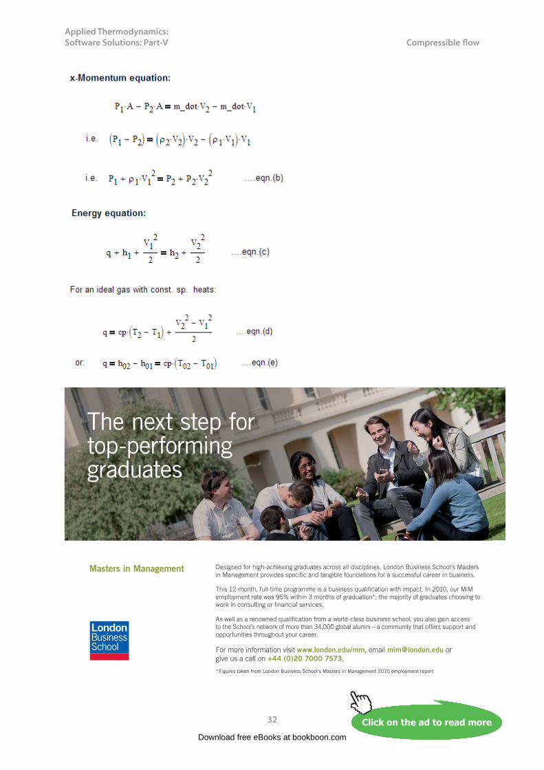
9.1.13 Flow in constant area ducts with Friction – Fanno flow[10]:
Flow in a constant area duct with friction in the absence of work and heat transfer is known as Fanno flow. Flow in gas ducts of aircraft engines, air conditioning systems etc are examples of Fanno flow.
Fanno Flow is specified by: (i) continuity eqn. (ii) Energy eqn. and (iii) const. area, no work and no heat transfer. Also, all sonic properties are constant… p*, rho*, V*, A* etc. Stagnation properties at the sonic state are also const.
Fanno flow is represented as Fanno line in a h-s diagram as explained earlier.
Variation of flow properties in Fanno flow are given by following equations:
Velocity:
Density:
Pressure:
Temperature:
Download free eBooks at bookboon.com
Applied Thermodynamics: Software Solutions: Part-V
29
Compressible flow
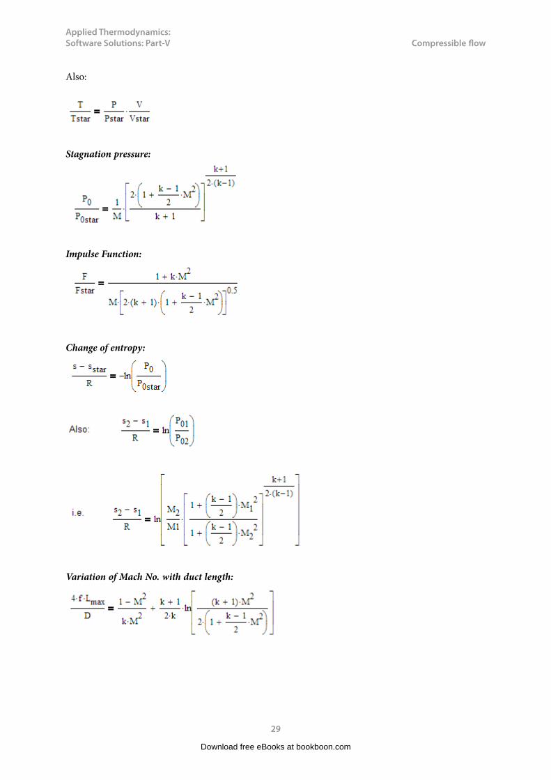
Also:
Stagnation pressure:
Impulse Function:
Change of entropy:
Variation of Mach No. with duct length:
Download free eBooks at bookboon.com

Applied Thermodynamics: Software Solutions: Part-V
30
Compressible flow
9.1.14 Table below gives the Fanno flow functions for an ideal gas with k = 1.4:
Note: See Prob.9.3.4 for Mathcad Functions, Tables and plots of Fanno flow parameters.
For M < 1:
Download free eBooks at bookboon.com

Applied Thermodynamics: Software Solutions: Part-V
31
Compressible flow
For M > 1:
Changes in M, V, P, T, rho and s, with increasing distance are summarized below, for Fanno flow:
dM dV dP dT dρ ds dP_0 dρ_0
M < 1 + + - - - + - -
M > 1 - - + + + + - -
Note: + means: increase; – means: decrease.
Note: From the above Table, observe that ds always increases, and dP_0 and dρ_0 always decrease.
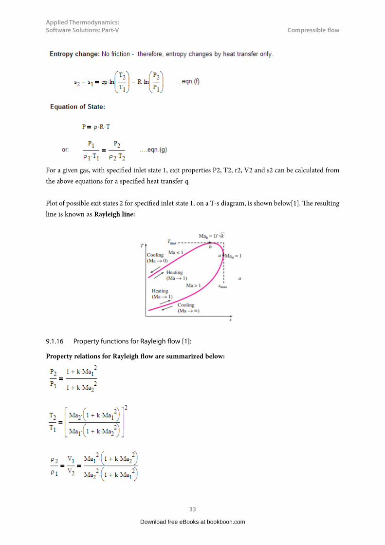
9.1.15 Flow with heat transfer and negligible friction – Rayleigh flow [1]:
Considering the one dimensional flow in a constant area duct, with heat transfer and no friction:
Download free eBooks at bookboon.com
Applied Thermodynamics: Software Solutions: Part-V
32
Compressible flow
Download free eBooks at bookboon.com
Click on the ad to read moreClick on the ad to read moreClick on the ad to read moreClick on the ad to read moreClick on the ad to read moreClick on the ad to read moreClick on the ad to read moreClick on the ad to read moreClick on the ad to read moreClick on the ad to read moreClick on the ad to read more
Designed for high-achieving graduates across all disciplines, London Business School’s Masters in Management provides specific and tangible foundations for a successful career in business.
This 12-month, full-time programme is a business qualification with impact. In 2010, our MiM employment rate was 95% within 3 months of graduation*; the majority of graduates choosing to work in consulting or financial services.
As well as a renowned qualification from a world-class business school, you also gain access to the School’s network of more than 34,000 global alumni – a community that offers support and opportunities throughout your career.
For more information visit www.london.edu/mm, email [email protected] or give us a call on +44 (0)20 7000 7573.
Masters in Management
The next step for top-performing graduates
* Figures taken from London Business School’s Masters in Management 2010 employment report
Applied Thermodynamics: Software Solutions: Part-V
33
Compressible flow
For a given gas, with specified inlet state 1, exit properties P2, T2, r2, V2 and s2 can be calculated from the above equations for a specified heat transfer q.
Plot of possible exit states 2 for specified inlet state 1, on a T-s diagram, is shown below[1]. The resulting line is known as Rayleigh line:
9.1.16 Property functions for Rayleigh flow [1]:
Property relations for Rayleigh flow are summarized below:
Download free eBooks at bookboon.com

Applied Thermodynamics: Software Solutions: Part-V
34
Compressible flow
Denoting sonic condition (at exit, state 2, i.e. Ma2 = 1) by star:
Dimensionless stagnation temp:
Dimensionless stagnation pressure:
Download free eBooks at bookboon.com
Click on the ad to read moreClick on the ad to read moreClick on the ad to read moreClick on the ad to read moreClick on the ad to read moreClick on the ad to read moreClick on the ad to read moreClick on the ad to read moreClick on the ad to read moreClick on the ad to read moreClick on the ad to read moreClick on the ad to read more
Get Internationally Connected at the University of Surrey MA Intercultural Communication with International BusinessMA Communication and International Marketing
MA Intercultural Communication with International Business
Provides you with a critical understanding of communication in contemporary socio-cultural contexts by combining linguistic, cultural/media studies and international business and will prepare you for a wide range of careers.
MA Communication and International Marketing
Equips you with a detailed understanding of communication in contemporary international marketing contexts to enable you to address the market needs of the international business environment.
For further information contact:T: +44 (0)1483 681681E: [email protected]/downloads

Applied Thermodynamics: Software Solutions: Part-V
35
Compressible flow
9.1.17 Rayleigh flow functions for an ideal gas with k = 1.4 are tabulated below
Note: See Prob. 9.3.6 for Mathcad Functions, Tables and plots of Rayleigh flow parameters.
Note: There is a limit on the heat addition in this flow process. Max. possible heat transfer occurs when the end state corresponds to (T0 / T0_star) = 1.
Download free eBooks at bookboon.com

Applied Thermodynamics: Software Solutions: Part-V
36
Compressible flow
For inlet Mach No. M, max. possible heat transfer is given by:
Above expression can be used to find heat transfer required to change the Mach No. from M1 to M2, since (T02/T0star) and (T01/T0star) are functions of M2 and M1.
9.2 Two free software to calculate compressible flow functions [8, 9]:
There are many calculators on-line to calculate compressible flow functions described in earlier sections.
Here, we mention two very useful calculators: (i) VUCALC, a window based calculator, and (ii) a browser based compressible aerodynamic calculator.
Download free eBooks at bookboon.com

Applied Thermodynamics: Software Solutions: Part-V
37
Compressible flow
9.2.1 VUCALC [8]: VuCalc is based on a program of the same name written by Tom Benson of NASA
This is a stand-alone, window based calculator. It does not need installation, i.e. it works from the folder in which it is located.
Opening screen starts with the ‘Help’ tab, and looks as follows:
Note that there are 8 tabs on the top: gamma, isentropic flow, normal shock, oblique shock, std. atmosphere, Rayleigh (flow), Fanno (flow) and Help.
Download free eBooks at bookboon.com

Applied Thermodynamics: Software Solutions: Part-V
38
Compressible flow
• ‘gamma’ tab: allows you to change the value of gamma (or, k in the notation used by us)
• ‘isentropic flow’ tab – for calculations of isentropic flow functions: you can select any one parameter with the radio button as shown below, and click on ‘compute’ to get results:
Download free eBooks at bookboon.com

Applied Thermodynamics: Software Solutions: Part-V
39
Compressible flow
• ‘normal shock’ tab – for calculations of normal shock functions: you can select any one parameter as shown below, and click on ‘compute’ to get results:
Download free eBooks at bookboon.com
Click on the ad to read moreClick on the ad to read moreClick on the ad to read moreClick on the ad to read moreClick on the ad to read moreClick on the ad to read moreClick on the ad to read moreClick on the ad to read moreClick on the ad to read moreClick on the ad to read moreClick on the ad to read moreClick on the ad to read moreClick on the ad to read more
STEP INTO A WORLD OF OPPORTUNITYwww.ecco.com/[email protected]

Applied Thermodynamics: Software Solutions: Part-V
40
Compressible flow
• ‘oblique shock’ tab – for calculations of oblique shock functions: here, there are two inputs: upstream Mach No. is the necessary input, and the other input may be chosen with the radio button as shown below. Click on ‘compute’ to get results:
• ‘standard atmosphere’ tab – computes various parameters for given altitude and Mach No. as shown below:
Download free eBooks at bookboon.com

Applied Thermodynamics: Software Solutions: Part-V
41
Compressible flow
• ‘Rayleigh’ tab – computes various parameters for any one input, chosen with radio button, as shown below:
• ‘Fanno’ tab – computes various parameters for any one input, chosen with radio button, as shown below:
Download free eBooks at bookboon.com

Applied Thermodynamics: Software Solutions: Part-V
42
Compressible flow
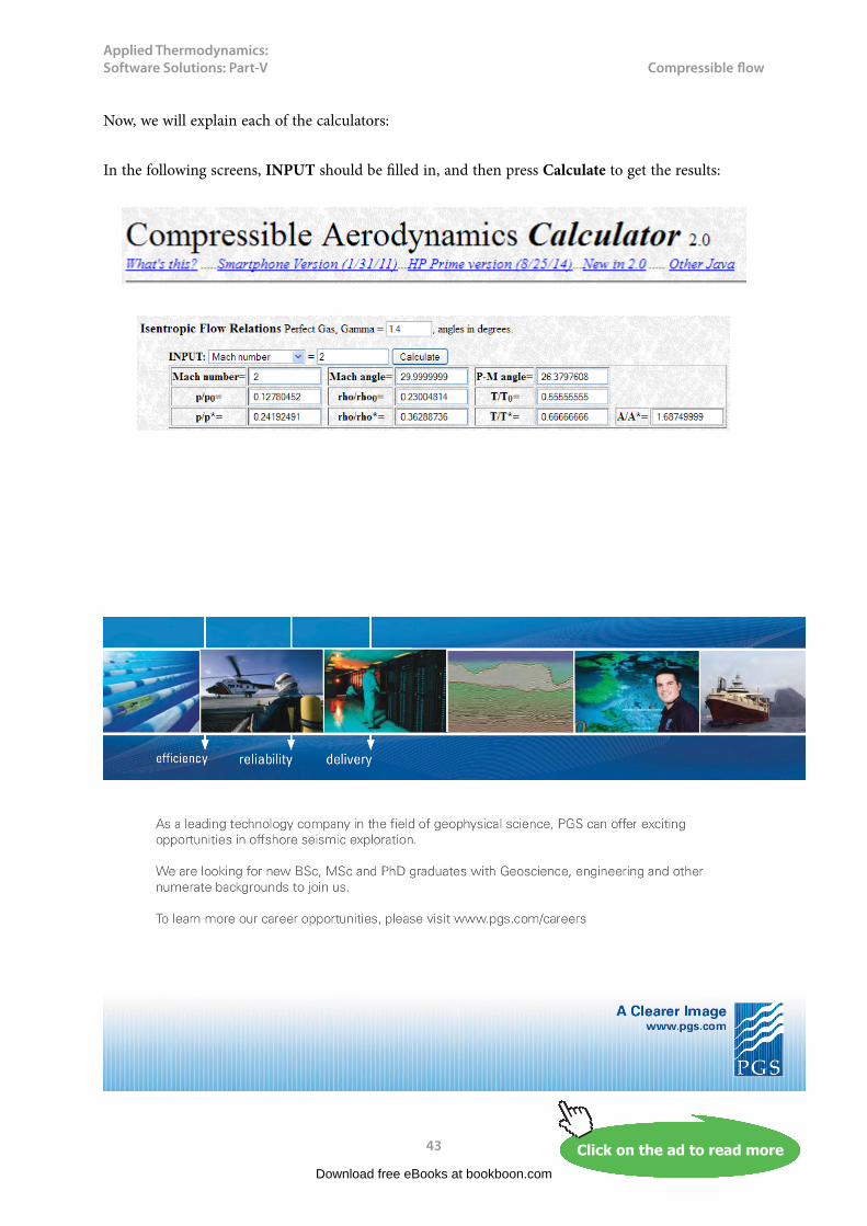
9.2.2 A compressible Aerodynamic calculator based on program by Devenport:
This is a browser based calculator. i.e. you have to save the page once from Internet. Afterwards, you can use it with the web browser, without being connected to Internet.
Here the different calculators are the following:
• Isentropic flow calculator• Normal shock calculator• Oblique shock calculator• Fanno flow calculator, and• Rayleigh flow calculator
All the calculators are on one page, and it looks like this:
Download free eBooks at bookboon.com
Applied Thermodynamics: Software Solutions: Part-V
43
Compressible flow
Now, we will explain each of the calculators:
In the following screens, INPUT should be filled in, and then press Calculate to get the results:
Download free eBooks at bookboon.com
Click on the ad to read moreClick on the ad to read moreClick on the ad to read moreClick on the ad to read moreClick on the ad to read moreClick on the ad to read moreClick on the ad to read moreClick on the ad to read moreClick on the ad to read moreClick on the ad to read moreClick on the ad to read moreClick on the ad to read moreClick on the ad to read moreClick on the ad to read more

Applied Thermodynamics: Software Solutions: Part-V
44
Compressible flow
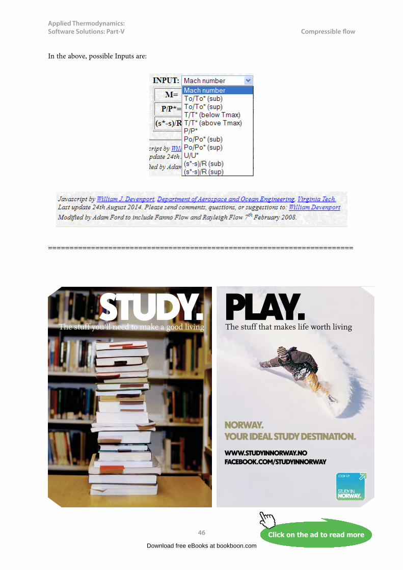
In the above, possible Inputs are:
In the above, again, possible Inputs are:
Download free eBooks at bookboon.com

Applied Thermodynamics: Software Solutions: Part-V
45
Compressible flow
In the above, possible Inputs are:
In the above, possible Inputs are:
Download free eBooks at bookboon.com
Applied Thermodynamics: Software Solutions: Part-V
46
Compressible flow
In the above, possible Inputs are:
=======================================================================
Download free eBooks at bookboon.com
Click on the ad to read moreClick on the ad to read moreClick on the ad to read moreClick on the ad to read moreClick on the ad to read moreClick on the ad to read moreClick on the ad to read moreClick on the ad to read moreClick on the ad to read moreClick on the ad to read moreClick on the ad to read moreClick on the ad to read moreClick on the ad to read moreClick on the ad to read moreClick on the ad to read more
STUDY. PLAY.The stuff you'll need to make a good living The stuff that makes life worth living
NORWAY. YOUR IDEAL STUDY DESTINATION.
WWW.STUDYINNORWAY.NOFACEBOOK.COM/STUDYINNORWAY

Applied Thermodynamics: Software Solutions: Part-V
47
Compressible flow
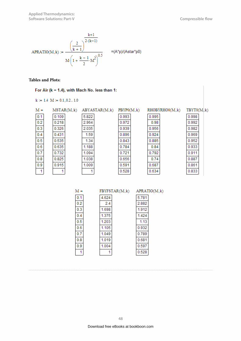
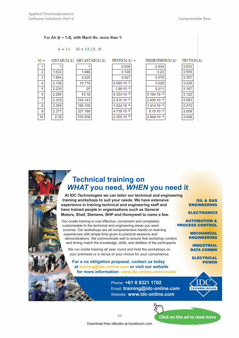
9.3 Problems solved with Mathcad:
Prob.9.3.1 Write Mathcad Functions for one dimensional isentropic flow functions for an ideal gas with
k = 1.4. Also plot these functions against M.
Mathcad Solution:
Fig.Prob.9.3.1 Isentropic flow in a C-D nozzle
Download free eBooks at bookboon.com
Applied Thermodynamics: Software Solutions: Part-V
48
Compressible flow
Tables and Plots:
Download free eBooks at bookboon.com
Applied Thermodynamics: Software Solutions: Part-V
49
Compressible flow
Download free eBooks at bookboon.com
Click on the ad to read moreClick on the ad to read moreClick on the ad to read moreClick on the ad to read moreClick on the ad to read moreClick on the ad to read moreClick on the ad to read moreClick on the ad to read moreClick on the ad to read moreClick on the ad to read moreClick on the ad to read moreClick on the ad to read moreClick on the ad to read moreClick on the ad to read moreClick on the ad to read moreClick on the ad to read more
Technical training on WHAT you need, WHEN you need it
At IDC Technologies we can tailor our technical and engineering training workshops to suit your needs. We have extensive
experience in training technical and engineering staff and have trained people in organisations such as General Motors, Shell, Siemens, BHP and Honeywell to name a few.Our onsite training is cost effective, convenient and completely customisable to the technical and engineering areas you want covered. Our workshops are all comprehensive hands-on learning experiences with ample time given to practical sessions and demonstrations. We communicate well to ensure that workshop content and timing match the knowledge, skills, and abilities of the participants.
We run onsite training all year round and hold the workshops on your premises or a venue of your choice for your convenience.
Phone: +61 8 9321 1702Email: [email protected] Website: www.idc-online.com
INDUSTRIALDATA COMMS
AUTOMATION & PROCESS CONTROL
ELECTRONICS
ELECTRICAL POWER
MECHANICAL ENGINEERING
OIL & GASENGINEERING
For a no obligation proposal, contact us today at [email protected] or visit our website for more information: www.idc-online.com/onsite/
Applied Thermodynamics: Software Solutions: Part-V
50
Compressible flow
Download free eBooks at bookboon.com
Applied Thermodynamics: Software Solutions: Part-V
51
Compressible flow
=======================================================================
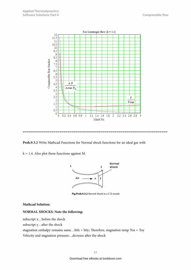
Prob.9.3.2 Write Mathcad Functions for Normal shock functions for an ideal gas with
k = 1.4. Also plot these functions against M.
Fig.Prob.9.3.2 Normal shock in a C-D nozzle
Mathcad Solution:
NORMAL SHOCKS: Note the following:
subscript x…before the shocksubscript y…after the shockstagnation enthalpy remains same…h0x = h0y; Therefore, stagnation temp Tox = ToyVelocity and stagnation pressure…decrease after the shock
Download free eBooks at bookboon.com

Applied Thermodynamics: Software Solutions: Part-V
52
Compressible flow
Static pressure Py, temp.Ty, and density rhoy…increase after the shockMach No. My is always less than 1 after the shockParticularly, the increase of temp. after the shock is of major concern to the Aerospace Engineer.
Increase in entropy after the shock: (sy-sx) = cp.ln(Ty/Tx) – R*ln(Py/Px)
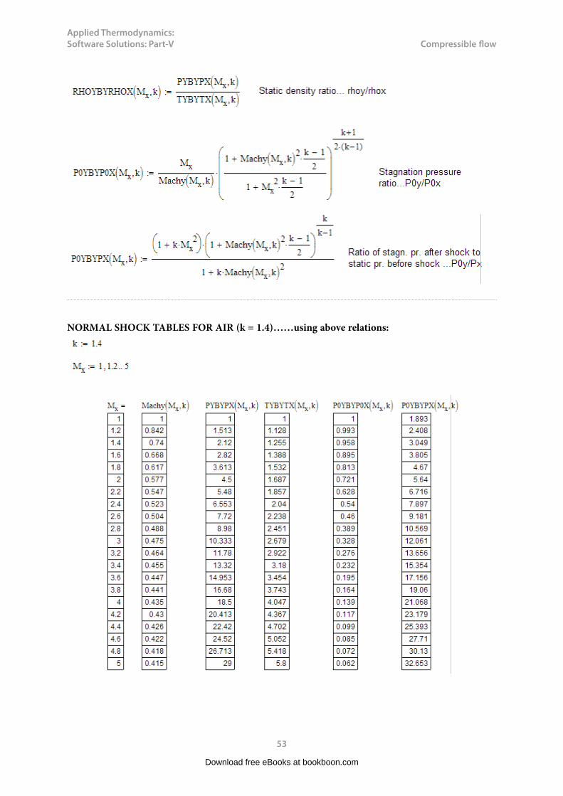
Normal shock Functions:
Download free eBooks at bookboon.com
Click on the ad to read moreClick on the ad to read moreClick on the ad to read moreClick on the ad to read moreClick on the ad to read moreClick on the ad to read moreClick on the ad to read moreClick on the ad to read moreClick on the ad to read moreClick on the ad to read moreClick on the ad to read moreClick on the ad to read moreClick on the ad to read moreClick on the ad to read moreClick on the ad to read moreClick on the ad to read moreClick on the ad to read more
���������� ����� ��������� �������������������������������� �!�" ��#������"��$�%��&��!�"��'����� �(%����������(������ ��%�� ")*+� +���$����� ��"��*������+ ���� ����������� ������ �� ���,���, +��$ ,���-
���," +�� , +��$ ,��
Applied Thermodynamics: Software Solutions: Part-V
53
Compressible flow
NORMAL SHOCK TABLES FOR AIR (k = 1.4)……using above relations:
Download free eBooks at bookboon.com
Applied Thermodynamics: Software Solutions: Part-V
54
Compressible flow
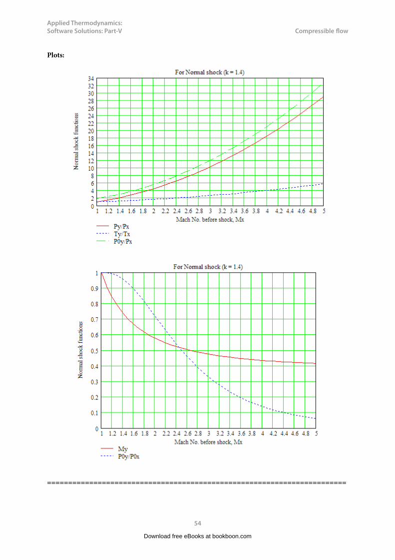
Plots:
=======================================================================
Download free eBooks at bookboon.com

Applied Thermodynamics: Software Solutions: Part-V
55
Compressible flow
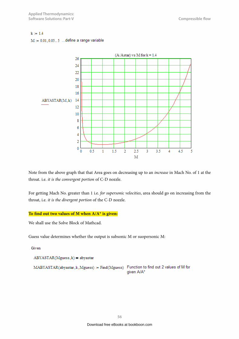
Prob. 9.3.3. Plot the area ratio (A / Astar) against Mach No. M. Write a Mathcad program to find the two values of M, one in the subsonic region, and the other in the supersonic region for a given (A/star).
Fig.Prob.9.3.3 Isentropic flow in a C-D nozzle
Mathcad Solution:
Download free eBooks at bookboon.com
Click on the ad to read moreClick on the ad to read moreClick on the ad to read moreClick on the ad to read moreClick on the ad to read moreClick on the ad to read moreClick on the ad to read moreClick on the ad to read moreClick on the ad to read moreClick on the ad to read moreClick on the ad to read moreClick on the ad to read moreClick on the ad to read moreClick on the ad to read moreClick on the ad to read moreClick on the ad to read moreClick on the ad to read moreClick on the ad to read more
Applied Thermodynamics: Software Solutions: Part-V
56
Compressible flow
Note from the above graph that that Area goes on decreasing up to an increase in Mach No. of 1 at the throat. i.e. it is the convergent portion of C-D nozzle.
For getting Mach No. greater than 1 i.e. for supersonic velocities, area should go on increasing from the throat, i.e. it is the divergent portion of the C-D nozzle.
To find out two values of M when A/A* is given:
We shall use the Solve Block of Mathcad.
Guess value determines whether the output is subsonic M or suopersonic M:
Download free eBooks at bookboon.com
Applied Thermodynamics: Software Solutions: Part-V
57
Compressible flow
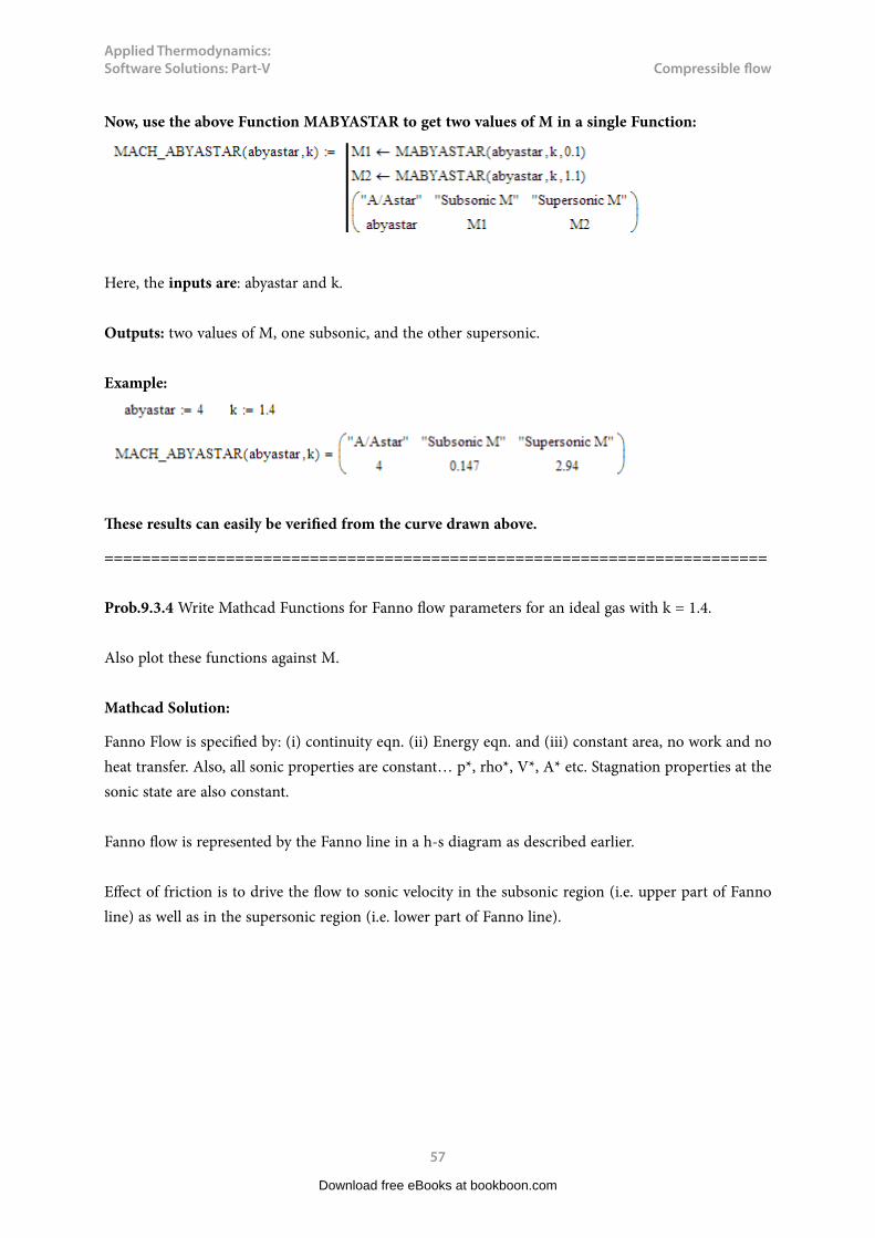
Now, use the above Function MABYASTAR to get two values of M in a single Function:
Here, the inputs are: abyastar and k.
Outputs: two values of M, one subsonic, and the other supersonic.
Example:
These results can easily be verified from the curve drawn above.
=======================================================================
Prob.9.3.4 Write Mathcad Functions for Fanno flow parameters for an ideal gas with k = 1.4.
Also plot these functions against M.
Mathcad Solution:
Fanno Flow is specified by: (i) continuity eqn. (ii) Energy eqn. and (iii) constant area, no work and no heat transfer. Also, all sonic properties are constant… p*, rho*, V*, A* etc. Stagnation properties at the sonic state are also constant.
Fanno flow is represented by the Fanno line in a h-s diagram as described earlier.
Effect of friction is to drive the flow to sonic velocity in the subsonic region (i.e. upper part of Fanno line) as well as in the supersonic region (i.e. lower part of Fanno line).
Download free eBooks at bookboon.com

Applied Thermodynamics: Software Solutions: Part-V
58
Compressible flow
Fig.Prob.9.3.4 Fanno flow (i.e. adiabatic flow with friction).
Following are the Mathcad functions for property calculations:
Then, between any two states x and y, we can write: Py/Px = (Py/P*).(P*/Px)
Download free eBooks at bookboon.com
Click on the ad to read moreClick on the ad to read moreClick on the ad to read moreClick on the ad to read moreClick on the ad to read moreClick on the ad to read moreClick on the ad to read moreClick on the ad to read moreClick on the ad to read moreClick on the ad to read moreClick on the ad to read moreClick on the ad to read moreClick on the ad to read moreClick on the ad to read moreClick on the ad to read moreClick on the ad to read moreClick on the ad to read moreClick on the ad to read moreClick on the ad to read more
DTU, Technical University of Denmark, is ranked as one of the best technical universities in Europe, and offers internationally recognised Master of Science degrees in 39 English-taught programmes.
DTU offers a unique environment where students have hands-on access to cutting edge facilities and work
closely under the expert supervision of top international researchers.
DTU’s central campus is located just north of Copenhagen and life at the University is engaging and vibrant. At DTU, we ensure that your goals and ambitions are met. Tuition is free for EU/EEA citizens.
Visit us at www.dtu.dk
Study at one of Europe’s leading universities

Applied Thermodynamics: Software Solutions: Part-V
59
Compressible flow
(Remember: Darcy friction factor, fD = 4 * fanning friction factor ff)
Download free eBooks at bookboon.com
Applied Thermodynamics: Software Solutions: Part-V
60
Compressible flow
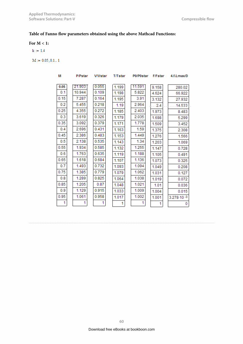
Table of Fanno flow parameters obtained using the above Mathcad Functions:
For M < 1:
Download free eBooks at bookboon.com

Applied Thermodynamics: Software Solutions: Part-V
61
Compressible flow
For M > 1:
Download free eBooks at bookboon.com

Applied Thermodynamics: Software Solutions: Part-V
62
Compressible flow
Now, plot the Fanno flow parameters:
Download free eBooks at bookboon.com
Click on the ad to read moreClick on the ad to read moreClick on the ad to read moreClick on the ad to read moreClick on the ad to read moreClick on the ad to read moreClick on the ad to read moreClick on the ad to read moreClick on the ad to read moreClick on the ad to read moreClick on the ad to read moreClick on the ad to read moreClick on the ad to read moreClick on the ad to read moreClick on the ad to read moreClick on the ad to read moreClick on the ad to read moreClick on the ad to read moreClick on the ad to read moreClick on the ad to read more
Increase your impact with MSM Executive Education
For more information, visit www.msm.nl or contact us at +31 43 38 70 808
or via [email protected] the globally networked management school
For more information, visit www.msm.nl or contact us at +31 43 38 70 808 or via [email protected]
For almost 60 years Maastricht School of Management has been enhancing the management capacity
of professionals and organizations around the world through state-of-the-art management education.
Our broad range of Open Enrollment Executive Programs offers you a unique interactive, stimulating and
multicultural learning experience.
Be prepared for tomorrow’s management challenges and apply today.
Executive Education-170x115-B2.indd 1 18-08-11 15:13

Applied Thermodynamics: Software Solutions: Part-V
63
Compressible flow
=======================================================================
Prob.9.3.5 Determine the length of 15 cm ID commercial steel pipe required to change the flow of air from M = 0.2 to M = 0.4 in Fanno flow.
Fig.Prob.9.3.5 Fanno flow (i.e. adiabatic flow with friction).
Mathcad Solution:
From Moody’s chart, taking into account the roughness factor, Darcy friction factor, fD = 0.015
Download free eBooks at bookboon.com

Applied Thermodynamics: Software Solutions: Part-V
64
Compressible flow
=======================================================================
Prob.9.3.6 Write Mathcad Functions to calculate Rayleigh Flow functions.Plot these functions against Mach No.
Rayleigh flow is frictionless flow with heat transfer.
Fig.Prob.9.3.6 Rayleigh flow
Mathcad Solution:
We have:
Download free eBooks at bookboon.com

Applied Thermodynamics: Software Solutions: Part-V
65
Compressible flow
Download free eBooks at bookboon.com
Click on the ad to read moreClick on the ad to read moreClick on the ad to read moreClick on the ad to read moreClick on the ad to read moreClick on the ad to read moreClick on the ad to read moreClick on the ad to read moreClick on the ad to read moreClick on the ad to read moreClick on the ad to read moreClick on the ad to read moreClick on the ad to read moreClick on the ad to read moreClick on the ad to read moreClick on the ad to read moreClick on the ad to read moreClick on the ad to read moreClick on the ad to read moreClick on the ad to read moreClick on the ad to read more
EXPERIENCE THE POWER OF FULL ENGAGEMENT…
RUN FASTER. RUN LONGER.. RUN EASIER…
READ MORE & PRE-ORDER TODAY WWW.GAITEYE.COM
Challenge the way we run
1349906_A6_4+0.indd 1 22-08-2014 12:56:57

Applied Thermodynamics: Software Solutions: Part-V
66
Compressible flow
Function to find heat transfer, Q when M1 and M2 are known in Rayleigh flow:
Q in J/kg, cp in J/kg.K, T1 in K
Function to find Entropy change, DELTAS, when M1 and M2 are known in Rayleigh flow:
Entropy change in J/kg.K, when T (K), R (J/kg.K)
Download free eBooks at bookboon.com

Applied Thermodynamics: Software Solutions: Part-V
67
Compressible flow
Table of results obtained using the above Mathcad Functions:
Download free eBooks at bookboon.com
Applied Thermodynamics: Software Solutions: Part-V
68
Compressible flow
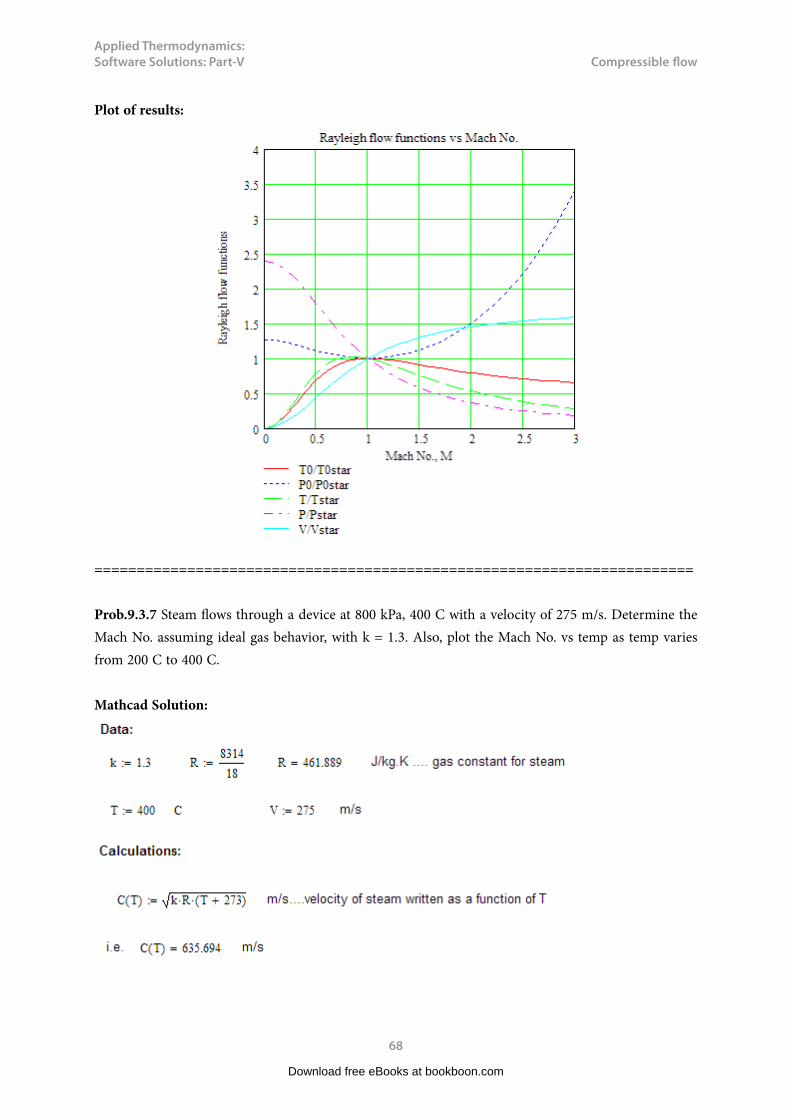
Plot of results:
=======================================================================
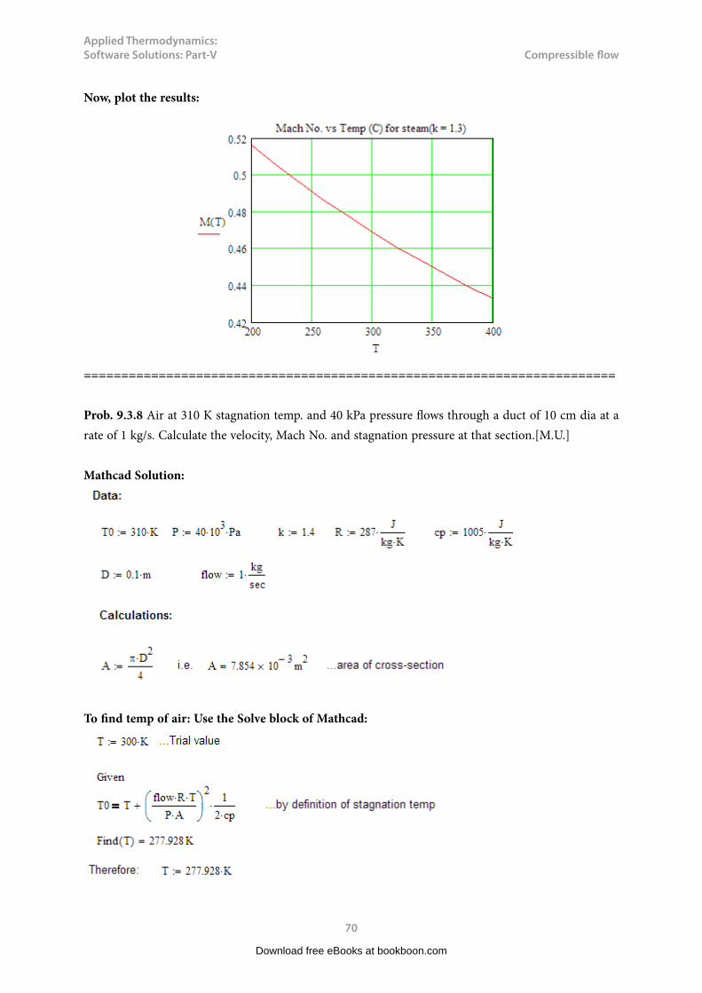
Prob.9.3.7 Steam flows through a device at 800 kPa, 400 C with a velocity of 275 m/s. Determine the Mach No. assuming ideal gas behavior, with k = 1.3. Also, plot the Mach No. vs temp as temp varies from 200 C to 400 C.
Mathcad Solution:
Download free eBooks at bookboon.com

Applied Thermodynamics: Software Solutions: Part-V
69
Compressible flow
Download free eBooks at bookboon.com
Click on the ad to read moreClick on the ad to read moreClick on the ad to read moreClick on the ad to read moreClick on the ad to read moreClick on the ad to read moreClick on the ad to read moreClick on the ad to read moreClick on the ad to read moreClick on the ad to read moreClick on the ad to read moreClick on the ad to read moreClick on the ad to read moreClick on the ad to read moreClick on the ad to read moreClick on the ad to read moreClick on the ad to read moreClick on the ad to read moreClick on the ad to read moreClick on the ad to read moreClick on the ad to read moreClick on the ad to read more
GET THERE FASTER
Oliver Wyman is a leading global management consulting firm that combines
deep industry knowledge with specialized expertise in strategy, operations, risk
management, organizational transformation, and leadership development. With
offices in 50+ cities across 25 countries, Oliver Wyman works with the CEOs and
executive teams of Global 1000 companies.
An equal opportunity employer.
Some people know precisely where they want to go. Others seek the adventure of discovering uncharted territory. Whatever you want your professional journey to be, you’ll find what you’re looking for at Oliver Wyman.
Discover the world of Oliver Wyman at oliverwyman.com/careers
DISCOVEROUR WORLD
Applied Thermodynamics: Software Solutions: Part-V
70
Compressible flow
Now, plot the results:
=======================================================================
Prob. 9.3.8 Air at 310 K stagnation temp. and 40 kPa pressure flows through a duct of 10 cm dia at a rate of 1 kg/s. Calculate the velocity, Mach No. and stagnation pressure at that section.[M.U.]
Mathcad Solution:
To find temp of air: Use the Solve block of Mathcad:
Download free eBooks at bookboon.com
Applied Thermodynamics: Software Solutions: Part-V
71
Compressible flow
=======================================================================
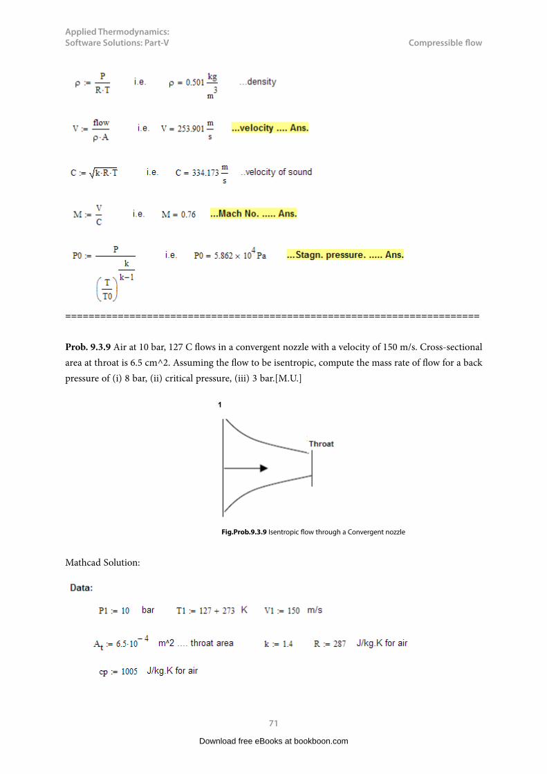
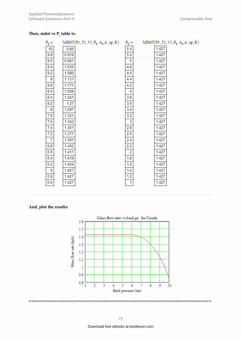
Prob. 9.3.9 Air at 10 bar, 127 C flows in a convergent nozzle with a velocity of 150 m/s. Cross-sectional area at throat is 6.5 cm^2. Assuming the flow to be isentropic, compute the mass rate of flow for a back pressure of (i) 8 bar, (ii) critical pressure, (iii) 3 bar.[M.U.]
Fig.Prob.9.3.9 Isentropic flow through a Convergent nozzle
Mathcad Solution:
Download free eBooks at bookboon.com

Applied Thermodynamics: Software Solutions: Part-V
72
Compressible flow
Always, find the critical pressure first.
Remember: for air, Pstar/P0 = 0.5283, and Tstar/T0 = 0.8333
Download free eBooks at bookboon.com

Applied Thermodynamics: Software Solutions: Part-V
73
Compressible flow
Download free eBooks at bookboon.com
Click on the ad to read moreClick on the ad to read moreClick on the ad to read moreClick on the ad to read moreClick on the ad to read moreClick on the ad to read moreClick on the ad to read moreClick on the ad to read moreClick on the ad to read moreClick on the ad to read moreClick on the ad to read moreClick on the ad to read moreClick on the ad to read moreClick on the ad to read moreClick on the ad to read moreClick on the ad to read moreClick on the ad to read moreClick on the ad to read moreClick on the ad to read moreClick on the ad to read moreClick on the ad to read moreClick on the ad to read moreClick on the ad to read more

Applied Thermodynamics: Software Solutions: Part-V
74
Compressible flow
(b) Plot the mass flow rate vs back pressure:
Write a Mathcad program as shown below:
Here, the Inputs are: P1 (bar), T1 K), V1(m/s), Pt (bar), At (m^2), k (=cp/cv), cp (J/kg.K) and R (J/kg.K).
Output is : mdot (kg/s)
Download free eBooks at bookboon.com
Applied Thermodynamics: Software Solutions: Part-V
75
Compressible flow
Then, mdot vs Pt table is:
And, plot the results:
=======================================================================
Download free eBooks at bookboon.com

Applied Thermodynamics: Software Solutions: Part-V
76
Compressible flow
Prob. 9.3.10 Air at a pressure of 15 bar, temp. 150 C, and velocity 50 m/s, expands in a nozzle isentropically to 1.4 bar pressure. The mass flow rate is 240 kg/min. Determine: (i) cross-sectional areas at inlet, throat and exit (ii) velocity, temp and Mach Nos. at throat and exit. [M.U.]
Fig.Prob.9.3.10 Isentropic flow through a C-D nozzle
Mathcad Solution:
First find the critical pressure, to ascertain if choking occurs:
Download free eBooks at bookboon.com

Applied Thermodynamics: Software Solutions: Part-V
77
Compressible flow
Download free eBooks at bookboon.com
Click on the ad to read moreClick on the ad to read moreClick on the ad to read moreClick on the ad to read moreClick on the ad to read moreClick on the ad to read moreClick on the ad to read moreClick on the ad to read moreClick on the ad to read moreClick on the ad to read moreClick on the ad to read moreClick on the ad to read moreClick on the ad to read moreClick on the ad to read moreClick on the ad to read moreClick on the ad to read moreClick on the ad to read moreClick on the ad to read moreClick on the ad to read moreClick on the ad to read moreClick on the ad to read moreClick on the ad to read moreClick on the ad to read moreClick on the ad to read more
81,000 kmIn the past four years we have drilled
That’s more than twice around the world.
What will you be?
Who are we?We are the world’s leading oilfield services company. Working globally—often in remote and challenging locations—we invent, design, engineer, manufacture, apply, and maintain technology to help customers find and produce oil and gas safely.
Who are we looking for?We offer countless opportunities in the following domains:n Engineering, Research, and Operationsn Geoscience and Petrotechnicaln Commercial and Business
If you are a self-motivated graduate looking for a dynamic career, apply to join our team.
careers.slb.com

Applied Thermodynamics: Software Solutions: Part-V
78
Compressible flow
Or, calculate Astar by continuity eqn. at throat:
=======================================================================
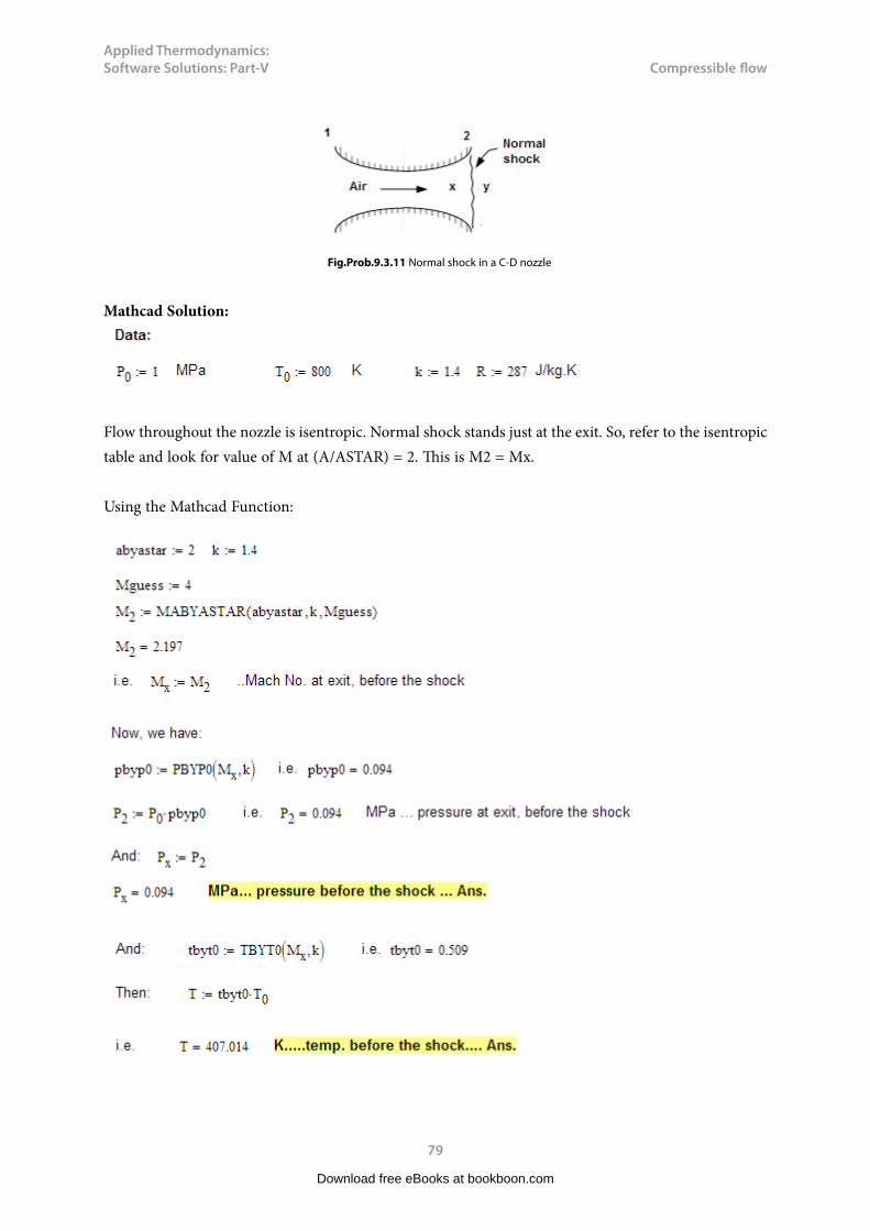
Prob.9.3.11 Air flows in a C-D nozzle having exit area ratio of 2. Stagnation pressure and temp. at entry are 1 MPa and 800 K respectively. Find out the back pressure necessary for a normal shock to appear just at the exit plane of the nozzle. Also find out temp., velocity just upstream of the shock wave.
Download free eBooks at bookboon.com
Applied Thermodynamics: Software Solutions: Part-V
79
Compressible flow
Fig.Prob.9.3.11 Normal shock in a C-D nozzle
Mathcad Solution:
Flow throughout the nozzle is isentropic. Normal shock stands just at the exit. So, refer to the isentropic table and look for value of M at (A/ASTAR) = 2. This is M2 = Mx.
Using the Mathcad Function:
Download free eBooks at bookboon.com
Applied Thermodynamics: Software Solutions: Part-V
80
Compressible flow
Note: Compare the results from Mathcad Functions with those in the Isentropic/Normal shock Tables. Then, you will appreciate the convenience (and accuracy) in using the Mathcad Functions.
=======================================================================
Download free eBooks at bookboon.com
Click on the ad to read moreClick on the ad to read moreClick on the ad to read moreClick on the ad to read moreClick on the ad to read moreClick on the ad to read moreClick on the ad to read moreClick on the ad to read moreClick on the ad to read moreClick on the ad to read moreClick on the ad to read moreClick on the ad to read moreClick on the ad to read moreClick on the ad to read moreClick on the ad to read moreClick on the ad to read moreClick on the ad to read moreClick on the ad to read moreClick on the ad to read moreClick on the ad to read moreClick on the ad to read moreClick on the ad to read moreClick on the ad to read moreClick on the ad to read moreClick on the ad to read more
Hellmann’s is one of Unilever’s oldest brands having been popular for over 100 years. If you too share a passion for discovery and innovation we will give you the tools and opportunities to provide you with a challenging career. Are you a great scientist who would like to be at the forefront of scientific innovations and developments? Then you will enjoy a career within Unilever Research & Development. For challenging job opportunities, please visit www.unilever.com/rdjobs.
Could you think of 101 new thingsto do with eggs and oil?

Applied Thermodynamics: Software Solutions: Part-V
81
Compressible flow
Prob. 9.3.12 In a C-D nozzle, inlet conditions of air are 1000 kPa, 800 K, the velocity being zero. It is required to produce a supersonic flow at 800 m/s, mass flow rate being 5 kg/s. Find throat and exit areas, Mach no. at exit, P and T at throat and exit.[M.U.]
Fig.Prob.9.3.12 Isentropic flow in a C-D nozzle
Mathcad Solution:
Download free eBooks at bookboon.com

Applied Thermodynamics: Software Solutions: Part-V
82
Compressible flow
=======================================================================
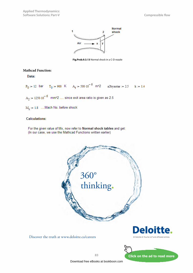
Prob.9.3.13 In a C-D nozzle, air enters with stagnation pressure of 12 bar and temp. 627 C. Normal shock occurs at a section where M = 1.8. Exit area ratio is 2.5. Throat area is 500 mm^2. Find P. T, M, C, V, stagnation pressure loss just downstream of the shock and exit.[M.U.]
Download free eBooks at bookboon.com
Applied Thermodynamics: Software Solutions: Part-V
83
Compressible flow
Fig.Prob.9.3.13 Normal shock in a C-D nozzle
Mathcad Function:
Download free eBooks at bookboon.com
Click on the ad to read moreClick on the ad to read moreClick on the ad to read moreClick on the ad to read moreClick on the ad to read moreClick on the ad to read moreClick on the ad to read moreClick on the ad to read moreClick on the ad to read moreClick on the ad to read moreClick on the ad to read moreClick on the ad to read moreClick on the ad to read moreClick on the ad to read moreClick on the ad to read moreClick on the ad to read moreClick on the ad to read moreClick on the ad to read moreClick on the ad to read moreClick on the ad to read moreClick on the ad to read moreClick on the ad to read moreClick on the ad to read moreClick on the ad to read moreClick on the ad to read moreClick on the ad to read more
© Deloitte & Touche LLP and affiliated entities.
360°thinking.
Discover the truth at www.deloitte.ca/careers
© Deloitte & Touche LLP and affiliated entities.
360°thinking.
Discover the truth at www.deloitte.ca/careers
© Deloitte & Touche LLP and affiliated entities.
360°thinking.
Discover the truth at www.deloitte.ca/careers © Deloitte & Touche LLP and affiliated entities.
360°thinking.
Discover the truth at www.deloitte.ca/careers
Applied Thermodynamics: Software Solutions: Part-V
84
Compressible flow
When M = 1.8, from Isentropic table, get P/Po and T/To:
Download free eBooks at bookboon.com
Applied Thermodynamics: Software Solutions: Part-V
85
Compressible flow
Now, for this value of A2/Astar, refer to Isentropic tables: (We use the Mathcad Functions written earlier):
=======================================================================
Download free eBooks at bookboon.com
Applied Thermodynamics: Software Solutions: Part-V
86
Compressible flow
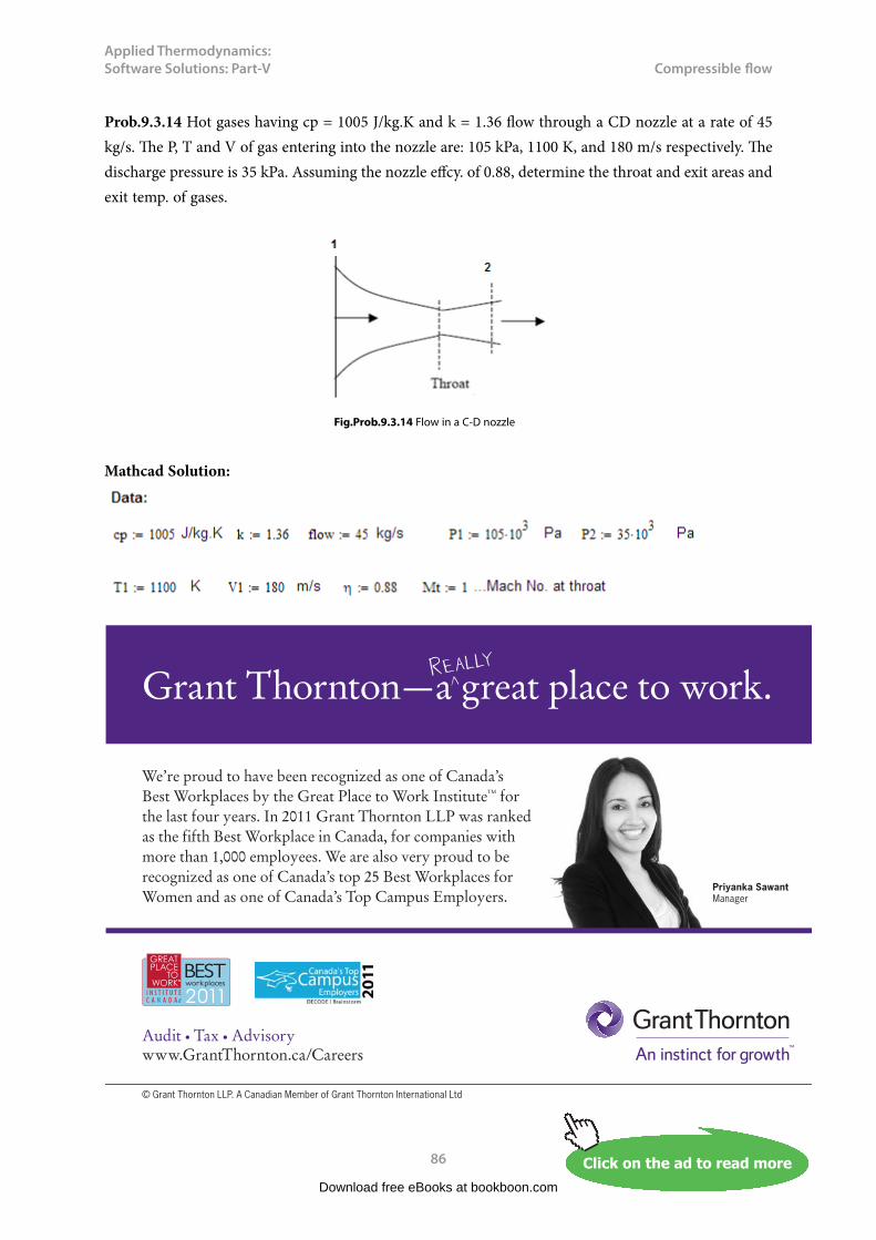
Prob.9.3.14 Hot gases having cp = 1005 J/kg.K and k = 1.36 flow through a CD nozzle at a rate of 45 kg/s. The P, T and V of gas entering into the nozzle are: 105 kPa, 1100 K, and 180 m/s respectively. The discharge pressure is 35 kPa. Assuming the nozzle effcy. of 0.88, determine the throat and exit areas and exit temp. of gases.
Fig.Prob.9.3.14 Flow in a C-D nozzle
Mathcad Solution:
Download free eBooks at bookboon.com
Click on the ad to read moreClick on the ad to read moreClick on the ad to read moreClick on the ad to read moreClick on the ad to read moreClick on the ad to read moreClick on the ad to read moreClick on the ad to read moreClick on the ad to read moreClick on the ad to read moreClick on the ad to read moreClick on the ad to read moreClick on the ad to read moreClick on the ad to read moreClick on the ad to read moreClick on the ad to read moreClick on the ad to read moreClick on the ad to read moreClick on the ad to read moreClick on the ad to read moreClick on the ad to read moreClick on the ad to read moreClick on the ad to read moreClick on the ad to read moreClick on the ad to read moreClick on the ad to read moreClick on the ad to read more

Applied Thermodynamics: Software Solutions: Part-V
87
Compressible flow
Download free eBooks at bookboon.com

Applied Thermodynamics: Software Solutions: Part-V
88
Compressible flow
=======================================================================
Prob. 9.3.15 A C-D duct with a throat area 0.35 times the exit area is supplied with air at a stagnation pressure of 1.5 bar. It discharges into atmosphere with a static pressure of 100 kPa. Assuming that there is normal shock in the divergent part, find: Mach Nos., pressure just upstream and downstream of the shock, loss in stagnation pressure and area ratio at the section where shock occurs. [M.U.]
Fig.Prob.9.3.15 Normal shock in a C-D nozzle
Mathcad Solution:
i.e. A2/At = 1/0.35 = 2.857
Download free eBooks at bookboon.com

Applied Thermodynamics: Software Solutions: Part-V
89
Compressible flow
Calculations:
Flow is isentropic from section 1 to x and then from y to 2.
Since there is a normal shock, flow is choked i.e. sonic velocity at throat.
Then: m *sqrt(T0)/(Astar*P0) = const. i.e. for const. m and T0, Astar*P0 = const.
i.e. A1star*P01 = A2star * P02 or, A1star/A2star = P02/P01
Also, P01 = P0t = P0x and P0y = P02
We can write: A2/At = (A2/A2star) * (A2star/At)
But, (At/A2star) = (At/A1star) * (A1star/A2star) = 1 * (P02/P01)
So, (A2/At) = (A2/A2star) * (P01/P02)
i.e. 2.857 = (A2/A2star) * (1.5/P02) ….(eqn. A)
Let apratio = (A2*P2)/(A2star*P02) …..(eqn. B)
Download free eBooks at bookboon.com
Click on the ad to read moreClick on the ad to read moreClick on the ad to read moreClick on the ad to read moreClick on the ad to read moreClick on the ad to read moreClick on the ad to read moreClick on the ad to read moreClick on the ad to read moreClick on the ad to read moreClick on the ad to read moreClick on the ad to read moreClick on the ad to read moreClick on the ad to read moreClick on the ad to read moreClick on the ad to read moreClick on the ad to read moreClick on the ad to read moreClick on the ad to read moreClick on the ad to read moreClick on the ad to read moreClick on the ad to read moreClick on the ad to read moreClick on the ad to read moreClick on the ad to read moreClick on the ad to read moreClick on the ad to read moreClick on the ad to read more
������������� ����������������������������������������������� �� ���������������������������
������ ������ ������������������������������ ����������������������!���"���������������
�����#$%����&'())%�*+����������,����������-
.��������������������������������� ��
���������� ���������������� ������������� ���������������������������� �����������
The Wakethe only emission we want to leave behind
Applied Thermodynamics: Software Solutions: Part-V
90
Compressible flow
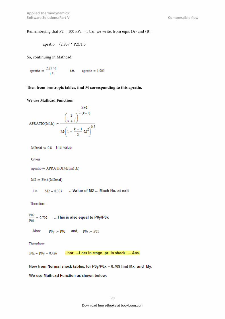
Remembering that P2 = 100 kPa = 1 bar, we write, from eqns (A) and (B):
apratio = (2.857 * P2)/1.5
So, continuing in Mathcad:
Then from isentropic tables, find M corresponding to this apratio.
We use Mathcad Function:
Download free eBooks at bookboon.com

Applied Thermodynamics: Software Solutions: Part-V
91
Compressible flow
=======================================================================
Prob.9.3.16 Air expands adiabatically in a nozzle from initial state of 6 bar, 527 C to a pressure of 2.5 bar. Calculate: (i) mass flow rate if throat dia is 2 cms (ii) velocity at the throat (iii) exit dia [M.U.]
Fig.Prob.9.3.16 Flow in a C-D nozzle
Download free eBooks at bookboon.com

Applied Thermodynamics: Software Solutions: Part-V
92
Compressible flow
Mathcad Solution:
Download free eBooks at bookboon.com
Click on the ad to read moreClick on the ad to read moreClick on the ad to read moreClick on the ad to read moreClick on the ad to read moreClick on the ad to read moreClick on the ad to read moreClick on the ad to read moreClick on the ad to read moreClick on the ad to read moreClick on the ad to read moreClick on the ad to read moreClick on the ad to read moreClick on the ad to read moreClick on the ad to read moreClick on the ad to read moreClick on the ad to read moreClick on the ad to read moreClick on the ad to read moreClick on the ad to read moreClick on the ad to read moreClick on the ad to read moreClick on the ad to read moreClick on the ad to read moreClick on the ad to read moreClick on the ad to read moreClick on the ad to read moreClick on the ad to read moreClick on the ad to read more
CAREERKICKSTARTAn app to keep you in the know
Whether you’re a graduate, school leaver or student, it’s a difficult time to start your career. So here at RBS, we’re providing a helping hand with our new Facebook app. Bringing together the most relevant and useful careers information, we’ve created a one-stop shop designed to help you get on the career ladder – whatever your level of education, degree subject or work experience.
And it’s not just finance-focused either. That’s because it’s not about us. It’s about you. So download the app and you’ll get everything you need to know to kickstart your career.
So what are you waiting for?
Click here to get started.

Applied Thermodynamics: Software Solutions: Part-V
93
Compressible flow
=======================================================================
Download free eBooks at bookboon.com

Applied Thermodynamics: Software Solutions: Part-V
94
Compressible flow
Prob.9.3.17 Consider a C-D nozzle of exit area ratio 3. Air at 5 bar, 127 C flows through the nozzle with a velocity of 200 m/s. If a normal shock stands at the point where Mach No. is 2, find fluid properties at a section just immediately after the shock.[M.U.]
Fig.Prob.9.3.17 Normal shock in a C-D nozzle
Mathcad Solution:
Download free eBooks at bookboon.com
Applied Thermodynamics: Software Solutions: Part-V
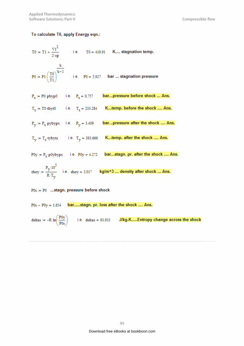
95
Compressible flow
Download free eBooks at bookboon.com

Applied Thermodynamics: Software Solutions: Part-V
96
Compressible flow
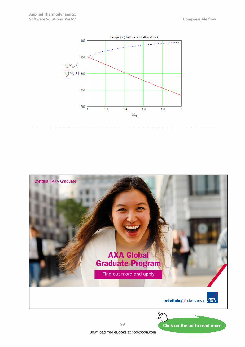
(b) Plot the static and stagn. pressure, temp. before the shock and after the shock against Mx, as Mx varies from 1 to 2:
First write the relevant quantities as functions of Mx:
Download free eBooks at bookboon.com
Click on the ad to read moreClick on the ad to read moreClick on the ad to read moreClick on the ad to read moreClick on the ad to read moreClick on the ad to read moreClick on the ad to read moreClick on the ad to read moreClick on the ad to read moreClick on the ad to read moreClick on the ad to read moreClick on the ad to read moreClick on the ad to read moreClick on the ad to read moreClick on the ad to read moreClick on the ad to read moreClick on the ad to read moreClick on the ad to read moreClick on the ad to read moreClick on the ad to read moreClick on the ad to read moreClick on the ad to read moreClick on the ad to read moreClick on the ad to read moreClick on the ad to read moreClick on the ad to read moreClick on the ad to read moreClick on the ad to read moreClick on the ad to read moreClick on the ad to read more
Applied Thermodynamics: Software Solutions: Part-V
97
Compressible flow
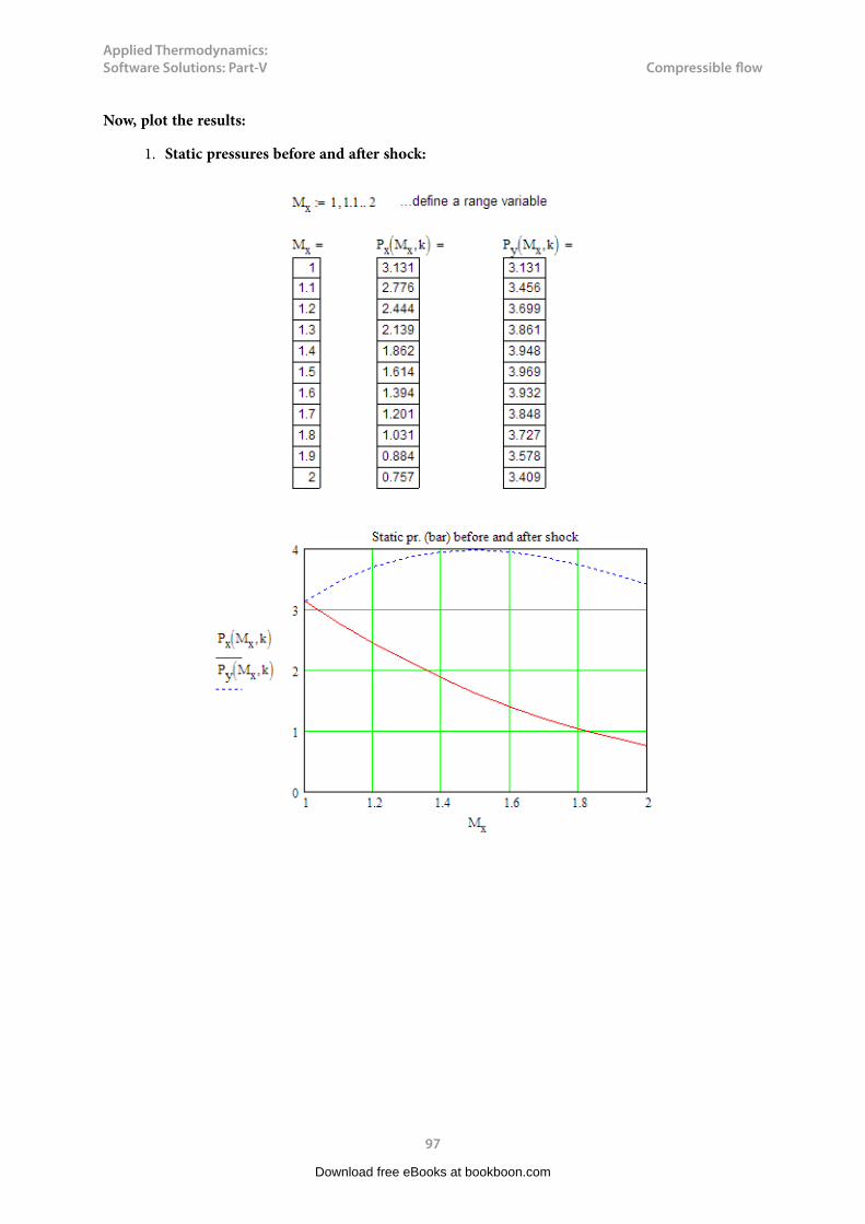
Now, plot the results:
1. Static pressures before and after shock:
Download free eBooks at bookboon.com

Applied Thermodynamics: Software Solutions: Part-V
98
Compressible flow
2. Stagnation pressures before and after shock:
Note: Stagn. Pressure before shock = P0 is constant.
3. Static temps. before and after shock:
Download free eBooks at bookboon.com
Applied Thermodynamics: Software Solutions: Part-V
99
Compressible flow
Download free eBooks at bookboon.com
Click on the ad to read moreClick on the ad to read moreClick on the ad to read moreClick on the ad to read moreClick on the ad to read moreClick on the ad to read moreClick on the ad to read moreClick on the ad to read moreClick on the ad to read moreClick on the ad to read moreClick on the ad to read moreClick on the ad to read moreClick on the ad to read moreClick on the ad to read moreClick on the ad to read moreClick on the ad to read moreClick on the ad to read moreClick on the ad to read moreClick on the ad to read moreClick on the ad to read moreClick on the ad to read moreClick on the ad to read moreClick on the ad to read moreClick on the ad to read moreClick on the ad to read moreClick on the ad to read moreClick on the ad to read moreClick on the ad to read moreClick on the ad to read moreClick on the ad to read moreClick on the ad to read more
AXA Global Graduate Program
Find out more and apply

Applied Thermodynamics: Software Solutions: Part-V
100
Compressible flow
(c) Plot entropy change across the shock against Mx, as Mx varies from 0.4 to 2. What is the inference from the plot?
Note: We know that Normal shock is highly irreversible, and therefore, entropy must increase across the shock.
Download free eBooks at bookboon.com
Applied Thermodynamics: Software Solutions: Part-V
101
Compressible flow
Up to Mach No. = 1, entropy change is –ve, which is impossible. Therefore, for a normal shock to occur, Mach No. before the shock (Mx) must be more than 1. i.e. Normal shock can occur only in a supersonic flow, i.e. in the divergent part of a C-D nozzle.
=======================================================================
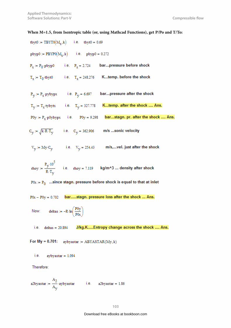
Prob.9.3.18 In a C-D nozzle, air enters with stagnation pressure of 10 bar and temp. 360 K. Exit area ratio is 2.0. Throat area is 500 mm^2. Find stagnation exit pressure, temp, Mach No., stagnation pressure loss just downstream of the shock and exit, when (i) Normal shock occurs at a section where M = 1.5.
(ii) Normal shock stands at the exit plane of nozzle. [M.U.]
Fig.Prob.9.3.18 Normal shock in a C-D nozzle
Mathcad Solution:
Download free eBooks at bookboon.com

Applied Thermodynamics: Software Solutions: Part-V
102
Compressible flow
Download free eBooks at bookboon.com
Click on the ad to read moreClick on the ad to read moreClick on the ad to read moreClick on the ad to read moreClick on the ad to read moreClick on the ad to read moreClick on the ad to read moreClick on the ad to read moreClick on the ad to read moreClick on the ad to read moreClick on the ad to read moreClick on the ad to read moreClick on the ad to read moreClick on the ad to read moreClick on the ad to read moreClick on the ad to read moreClick on the ad to read moreClick on the ad to read moreClick on the ad to read moreClick on the ad to read moreClick on the ad to read moreClick on the ad to read moreClick on the ad to read moreClick on the ad to read moreClick on the ad to read moreClick on the ad to read moreClick on the ad to read moreClick on the ad to read moreClick on the ad to read moreClick on the ad to read moreClick on the ad to read moreClick on the ad to read more
Designed for high-achieving graduates across all disciplines, London Business School’s Masters in Management provides specific and tangible foundations for a successful career in business.
This 12-month, full-time programme is a business qualification with impact. In 2010, our MiM employment rate was 95% within 3 months of graduation*; the majority of graduates choosing to work in consulting or financial services.
As well as a renowned qualification from a world-class business school, you also gain access to the School’s network of more than 34,000 global alumni – a community that offers support and opportunities throughout your career.
For more information visit www.london.edu/mm, email [email protected] or give us a call on +44 (0)20 7000 7573.
Masters in Management
The next step for top-performing graduates
* Figures taken from London Business School’s Masters in Management 2010 employment report
Applied Thermodynamics: Software Solutions: Part-V
103
Compressible flow
When M=1.5, from Isentropic table (or, using Mathcad Functions), get P/Po and T/To:
Download free eBooks at bookboon.com
Applied Thermodynamics: Software Solutions: Part-V
104
Compressible flow
Now, for this value of A2/Astar, refer to Isentropic tables (or, use Mathcad Functions):
(ii) When shock is at exit plane, i.e. A2/Astar = 2:
Now, for this value of A2/Astar, refer to Isentropic tables, or use Mathcad Functions:
Download free eBooks at bookboon.com

Applied Thermodynamics: Software Solutions: Part-V
105
Compressible flow
When M=2.197, from Isentropic table, get P/Po and T/To:
Download free eBooks at bookboon.com
Click on the ad to read moreClick on the ad to read moreClick on the ad to read moreClick on the ad to read moreClick on the ad to read moreClick on the ad to read moreClick on the ad to read moreClick on the ad to read moreClick on the ad to read moreClick on the ad to read moreClick on the ad to read moreClick on the ad to read moreClick on the ad to read moreClick on the ad to read moreClick on the ad to read moreClick on the ad to read moreClick on the ad to read moreClick on the ad to read moreClick on the ad to read moreClick on the ad to read moreClick on the ad to read moreClick on the ad to read moreClick on the ad to read moreClick on the ad to read moreClick on the ad to read moreClick on the ad to read moreClick on the ad to read moreClick on the ad to read moreClick on the ad to read moreClick on the ad to read moreClick on the ad to read moreClick on the ad to read moreClick on the ad to read more
Get Internationally Connected at the University of Surrey MA Intercultural Communication with International BusinessMA Communication and International Marketing
MA Intercultural Communication with International Business
Provides you with a critical understanding of communication in contemporary socio-cultural contexts by combining linguistic, cultural/media studies and international business and will prepare you for a wide range of careers.
MA Communication and International Marketing
Equips you with a detailed understanding of communication in contemporary international marketing contexts to enable you to address the market needs of the international business environment.
For further information contact:T: +44 (0)1483 681681E: [email protected]/downloads
Applied Thermodynamics: Software Solutions: Part-V
106
Compressible flow
=======================================================================
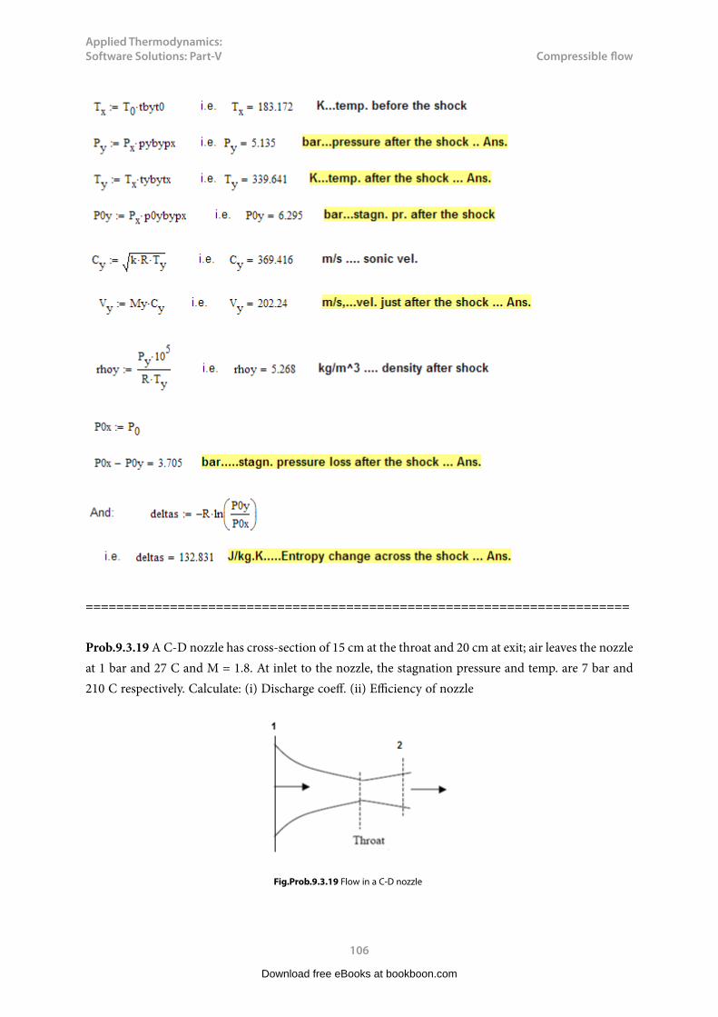
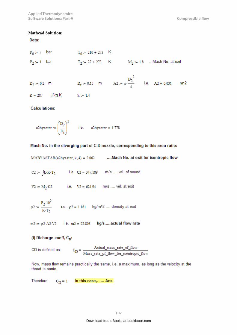
Prob.9.3.19 A C-D nozzle has cross-section of 15 cm at the throat and 20 cm at exit; air leaves the nozzle at 1 bar and 27 C and M = 1.8. At inlet to the nozzle, the stagnation pressure and temp. are 7 bar and 210 C respectively. Calculate: (i) Discharge coeff. (ii) Efficiency of nozzle
Fig.Prob.9.3.19 Flow in a C-D nozzle
Download free eBooks at bookboon.com
Applied Thermodynamics: Software Solutions: Part-V
107
Compressible flow
Mathcad Solution:
Download free eBooks at bookboon.com

Applied Thermodynamics: Software Solutions: Part-V
108
Compressible flow
Download free eBooks at bookboon.com
Click on the ad to read moreClick on the ad to read moreClick on the ad to read moreClick on the ad to read moreClick on the ad to read moreClick on the ad to read moreClick on the ad to read moreClick on the ad to read moreClick on the ad to read moreClick on the ad to read moreClick on the ad to read moreClick on the ad to read moreClick on the ad to read moreClick on the ad to read moreClick on the ad to read moreClick on the ad to read moreClick on the ad to read moreClick on the ad to read moreClick on the ad to read moreClick on the ad to read moreClick on the ad to read moreClick on the ad to read moreClick on the ad to read moreClick on the ad to read moreClick on the ad to read moreClick on the ad to read moreClick on the ad to read moreClick on the ad to read moreClick on the ad to read moreClick on the ad to read moreClick on the ad to read moreClick on the ad to read moreClick on the ad to read moreClick on the ad to read more
STEP INTO A WORLD OF OPPORTUNITYwww.ecco.com/[email protected]
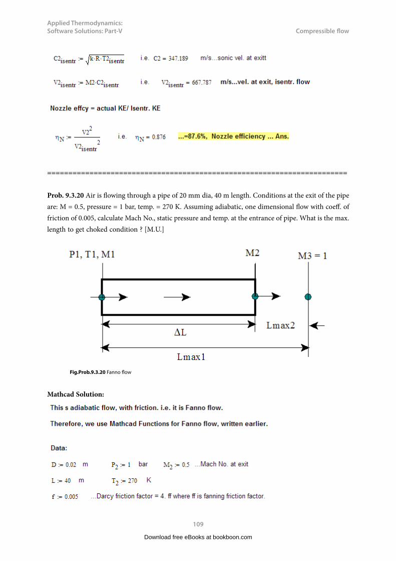
Applied Thermodynamics: Software Solutions: Part-V
109
Compressible flow
=======================================================================
Prob. 9.3.20 Air is flowing through a pipe of 20 mm dia, 40 m length. Conditions at the exit of the pipe are: M = 0.5, pressure = 1 bar, temp. = 270 K. Assuming adiabatic, one dimensional flow with coeff. of friction of 0.005, calculate Mach No., static pressure and temp. at the entrance of pipe. What is the max. length to get choked condition ? [M.U.]
Fig.Prob.9.3.20 Fanno flow
Mathcad Solution:
Download free eBooks at bookboon.com

Applied Thermodynamics: Software Solutions: Part-V
110
Compressible flow
Download free eBooks at bookboon.com

Applied Thermodynamics: Software Solutions: Part-V
111
Compressible flow
=======================================================================
Prob.9.3.21 Air enters a duct of constant area with pressure of 5 bar, temp. 150 C and velocity 100 m/s. Heat transfer to air takes place at constant rate, and pressure at the outlet is 4 bar. There is no work transfer. Assume frictionless flow and calculate exit temp and heat transfer per unit mass flow.[M.U.]
Fig.Prob.9.3.21 Rayleigh flow
Download free eBooks at bookboon.com
Click on the ad to read moreClick on the ad to read moreClick on the ad to read moreClick on the ad to read moreClick on the ad to read moreClick on the ad to read moreClick on the ad to read moreClick on the ad to read moreClick on the ad to read moreClick on the ad to read moreClick on the ad to read moreClick on the ad to read moreClick on the ad to read moreClick on the ad to read moreClick on the ad to read moreClick on the ad to read moreClick on the ad to read moreClick on the ad to read moreClick on the ad to read moreClick on the ad to read moreClick on the ad to read moreClick on the ad to read moreClick on the ad to read moreClick on the ad to read moreClick on the ad to read moreClick on the ad to read moreClick on the ad to read moreClick on the ad to read moreClick on the ad to read moreClick on the ad to read moreClick on the ad to read moreClick on the ad to read moreClick on the ad to read moreClick on the ad to read moreClick on the ad to read more
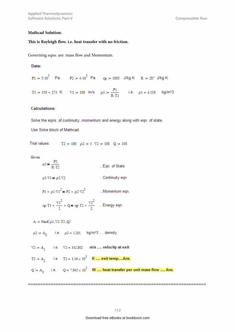
Applied Thermodynamics: Software Solutions: Part-V
112
Compressible flow
Mathcad Solution:
This is Rayleigh flow. i.e. heat transfer with no friction.
Governing eqns. are: mass flow and Momentum.
=======================================================================
Download free eBooks at bookboon.com

Applied Thermodynamics: Software Solutions: Part-V
113
Compressible flow
Prob.9.3.22 Air flows with negligible friction through a 10 cm dia duct at a rate of 2.3 kg/s. Temp and pressure at inlet are: T1 = 450 K and P1 = 200 kPa. Mach No. at exit is M2 = 1. Determine the rate of heat transfer and the pressure drop for this section of duct. [Ref: 1]
Fig.Prob.9.3.22 Rayleigh Flow
Mathcad Solution:
This is Rayleigh flow. i.e. heat transfer with no friction.
Download free eBooks at bookboon.com

Applied Thermodynamics: Software Solutions: Part-V
114
Compressible flow
Download free eBooks at bookboon.com
Click on the ad to read moreClick on the ad to read moreClick on the ad to read moreClick on the ad to read moreClick on the ad to read moreClick on the ad to read moreClick on the ad to read moreClick on the ad to read moreClick on the ad to read moreClick on the ad to read moreClick on the ad to read moreClick on the ad to read moreClick on the ad to read moreClick on the ad to read moreClick on the ad to read moreClick on the ad to read moreClick on the ad to read moreClick on the ad to read moreClick on the ad to read moreClick on the ad to read moreClick on the ad to read moreClick on the ad to read moreClick on the ad to read moreClick on the ad to read moreClick on the ad to read moreClick on the ad to read moreClick on the ad to read moreClick on the ad to read moreClick on the ad to read moreClick on the ad to read moreClick on the ad to read moreClick on the ad to read moreClick on the ad to read moreClick on the ad to read moreClick on the ad to read moreClick on the ad to read more
STUDY. PLAY.The stuff you'll need to make a good living The stuff that makes life worth living
NORWAY. YOUR IDEAL STUDY DESTINATION.
WWW.STUDYINNORWAY.NOFACEBOOK.COM/STUDYINNORWAY
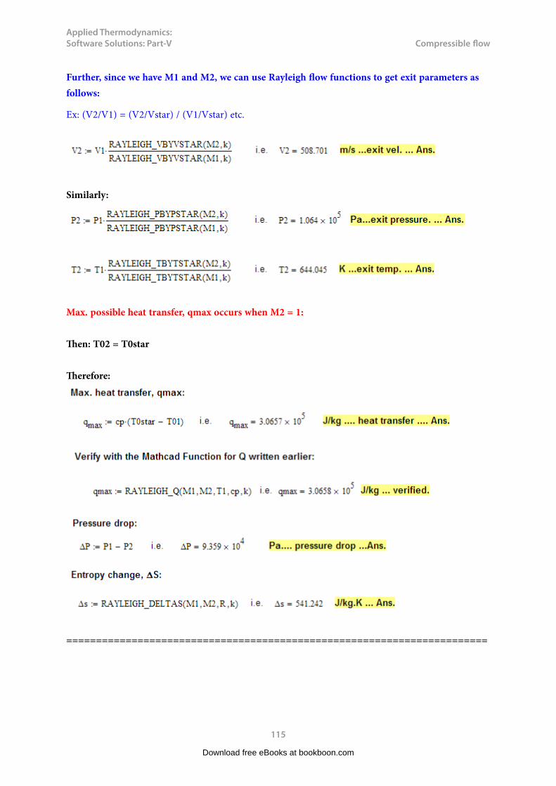
Applied Thermodynamics: Software Solutions: Part-V
115
Compressible flow
Further, since we have M1 and M2, we can use Rayleigh flow functions to get exit parameters as follows:
Ex: (V2/V1) = (V2/Vstar) / (V1/Vstar) etc.
Similarly:
Max. possible heat transfer, qmax occurs when M2 = 1:
Then: T02 = T0star
Therefore:
=======================================================================
Download free eBooks at bookboon.com
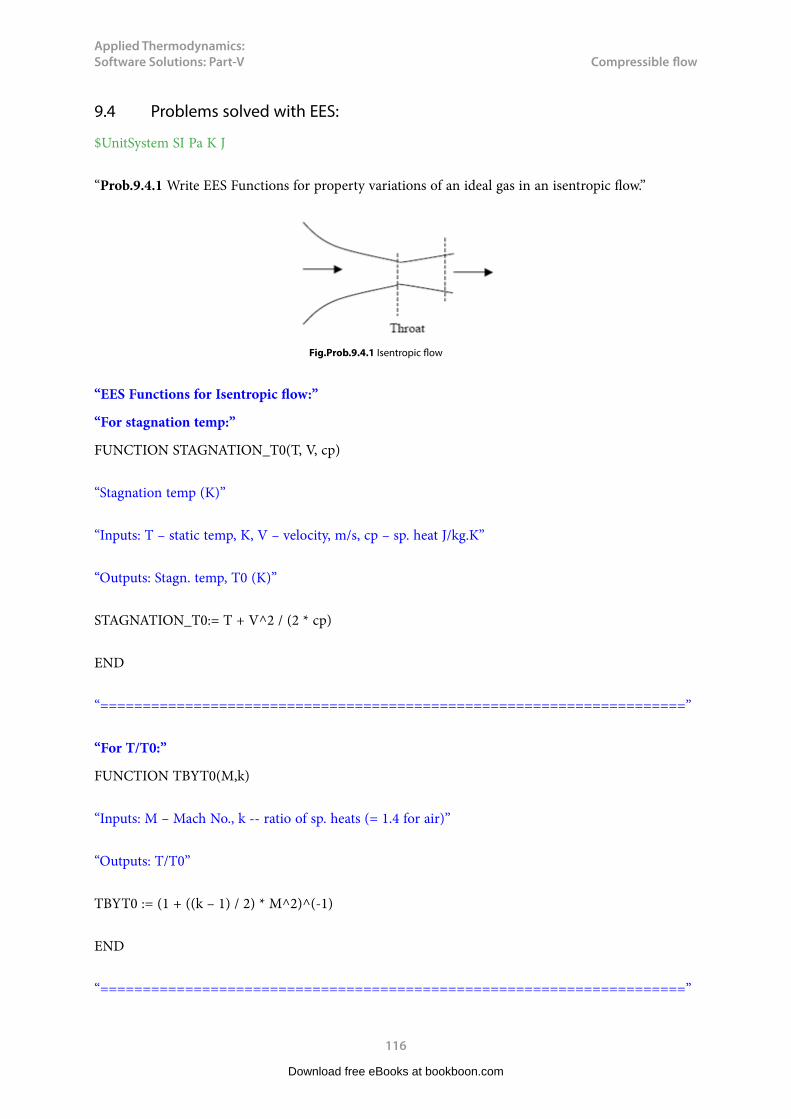
Applied Thermodynamics: Software Solutions: Part-V
116
Compressible flow
9.4 Problems solved with EES:
$UnitSystem SI Pa K J
“Prob.9.4.1 Write EES Functions for property variations of an ideal gas in an isentropic flow.”
Fig.Prob.9.4.1 Isentropic flow
“EES Functions for Isentropic flow:”
“For stagnation temp:”
FUNCTION STAGNATION_T0(T, V, cp)
“Stagnation temp (K)”
“Inputs: T – static temp, K, V – velocity, m/s, cp – sp. heat J/kg.K”
“Outputs: Stagn. temp, T0 (K)”
STAGNATION_T0:= T + V^2 / (2 * cp)
END
“=====================================================================”
“For T/T0:”
FUNCTION TBYT0(M,k)
“Inputs: M – Mach No., k -- ratio of sp. heats (= 1.4 for air)”
“Outputs: T/T0”
TBYT0 := (1 + ((k – 1) / 2) * M^2)^(-1)
END
“=====================================================================”
Download free eBooks at bookboon.com

Applied Thermodynamics: Software Solutions: Part-V
117
Compressible flow
“For P/P0:”
FUNCTION PBYP0(M,k)
“Inputs: M – Mach No., k -- ratio of sp. heats (= 1.4 for air)”
“Outputs: P/P0”
PBYP0 := (1 + ((k – 1) / 2) * M^2)^(-k/(k – 1))
END
“=====================================================================”
“For rho/rho0:”
FUNCTION RHOBYRHO0(M,k)
“Inputs: M – Mach No., k -- ratio of sp. heats (= 1.4 for air)”
“Outputs: rho/rho0”
Download free eBooks at bookboon.com
Click on the ad to read moreClick on the ad to read moreClick on the ad to read moreClick on the ad to read moreClick on the ad to read moreClick on the ad to read moreClick on the ad to read moreClick on the ad to read moreClick on the ad to read moreClick on the ad to read moreClick on the ad to read moreClick on the ad to read moreClick on the ad to read moreClick on the ad to read moreClick on the ad to read moreClick on the ad to read moreClick on the ad to read moreClick on the ad to read moreClick on the ad to read moreClick on the ad to read moreClick on the ad to read moreClick on the ad to read moreClick on the ad to read moreClick on the ad to read moreClick on the ad to read moreClick on the ad to read moreClick on the ad to read moreClick on the ad to read moreClick on the ad to read moreClick on the ad to read moreClick on the ad to read moreClick on the ad to read moreClick on the ad to read moreClick on the ad to read moreClick on the ad to read moreClick on the ad to read moreClick on the ad to read more
Technical training on WHAT you need, WHEN you need it
At IDC Technologies we can tailor our technical and engineering training workshops to suit your needs. We have extensive
experience in training technical and engineering staff and have trained people in organisations such as General Motors, Shell, Siemens, BHP and Honeywell to name a few.Our onsite training is cost effective, convenient and completely customisable to the technical and engineering areas you want covered. Our workshops are all comprehensive hands-on learning experiences with ample time given to practical sessions and demonstrations. We communicate well to ensure that workshop content and timing match the knowledge, skills, and abilities of the participants.
We run onsite training all year round and hold the workshops on your premises or a venue of your choice for your convenience.
Phone: +61 8 9321 1702Email: [email protected] Website: www.idc-online.com
INDUSTRIALDATA COMMS
AUTOMATION & PROCESS CONTROL
ELECTRONICS
ELECTRICAL POWER
MECHANICAL ENGINEERING
OIL & GASENGINEERING
For a no obligation proposal, contact us today at [email protected] or visit our website for more information: www.idc-online.com/onsite/
Applied Thermodynamics: Software Solutions: Part-V
118
Compressible flow
RHOBYRHO0 := (1 + ((k – 1) / 2) * M^2)^(-1/(k – 1))
END
“=====================================================================”
“For Mstar:”
FUNCTION MSTAR(M,k)
“Inputs: M – Mach No., k -- ratio of sp. heats (= 1.4 for air)”
“Outputs: Mstar”
MSTAR := M * sqrt((k + 1) / ( 2 + (k – 1) * m^2))
END
“=====================================================================”
“For A/Astar:”
FUNCTION ABYASTAR(M,k)
“Inputs: M – Mach No., k -- ratio of sp. heats (= 1.4 for air)”
“Outputs: A / Astar”
ABYASTAR := (1/M) * ((2 / (k + 1)) + (k – 1) * M^2/ (k + 1))^ ((k + 1) / (2 * (k – 1)))
END
“=====================================================================”
“For F/Fstar:”
FUNCTION FBYFSTAR(M,k)
“Inputs: M – Mach No., k -- ratio of sp. heats (= 1.4 for air)”
“Outputs: F / Fstar”
Download free eBooks at bookboon.com

Applied Thermodynamics: Software Solutions: Part-V
119
Compressible flow
AA := 1 + k * M^2
BB:= 1 + ((k – 1)/2) * M^2
FBYFSTAR := (1/M) * AA / sqrt(2 * (1 + k) * BB)
END
“=====================================================================”
“For F/Fstar:”
FUNCTION APRATIO(M,k)
“Inputs: M – Mach No., k -- ratio of sp. heats (= 1.4 for air)”
“Outputs: (A * P) / ( Astar * P0)”
AA := (1/M) * ( 2 / (k + 1)) ^ ((k + 1) / (2 * (k – 1)))
BB:= sqrt(1 + ((k – 1)/2) * M^2)
APRATIO :=AA / BB
END
“=====================================================================”
“Prob.9.4.2 Using the EES Functions for property variations of an ideal gas in an isentropic flow, written above, plot the property variations against Mach No.”
EES Solution:
{M = 1}
k = 1.4
Mstar = MSTAR(M,k)
abyastar = ABYASTAR(M,k)
Download free eBooks at bookboon.com
Applied Thermodynamics: Software Solutions: Part-V
120
Compressible flow
tbyt0 = TBYT0(M,k)
pbyp0 = PBYP0(M,k)
rhobyrho0 = RHOBYRHO0(M,k)
fbyfstar = FBYFSTAR(M,k)
apratio = APRATIO(M,k)
Download free eBooks at bookboon.com
Click on the ad to read moreClick on the ad to read moreClick on the ad to read moreClick on the ad to read moreClick on the ad to read moreClick on the ad to read moreClick on the ad to read moreClick on the ad to read moreClick on the ad to read moreClick on the ad to read moreClick on the ad to read moreClick on the ad to read moreClick on the ad to read moreClick on the ad to read moreClick on the ad to read moreClick on the ad to read moreClick on the ad to read moreClick on the ad to read moreClick on the ad to read moreClick on the ad to read moreClick on the ad to read moreClick on the ad to read moreClick on the ad to read moreClick on the ad to read moreClick on the ad to read moreClick on the ad to read moreClick on the ad to read moreClick on the ad to read moreClick on the ad to read moreClick on the ad to read moreClick on the ad to read moreClick on the ad to read moreClick on the ad to read moreClick on the ad to read moreClick on the ad to read moreClick on the ad to read moreClick on the ad to read moreClick on the ad to read more
���������� ����� ��������� �������������������������������� �!�" ��#������"��$�%��&��!�"��'����� �(%����������(������ ��%�� ")*+� +���$����� ��"��*������+ ���� ����������� ������ �� ���,���, +��$ ,���-
���," +�� , +��$ ,��
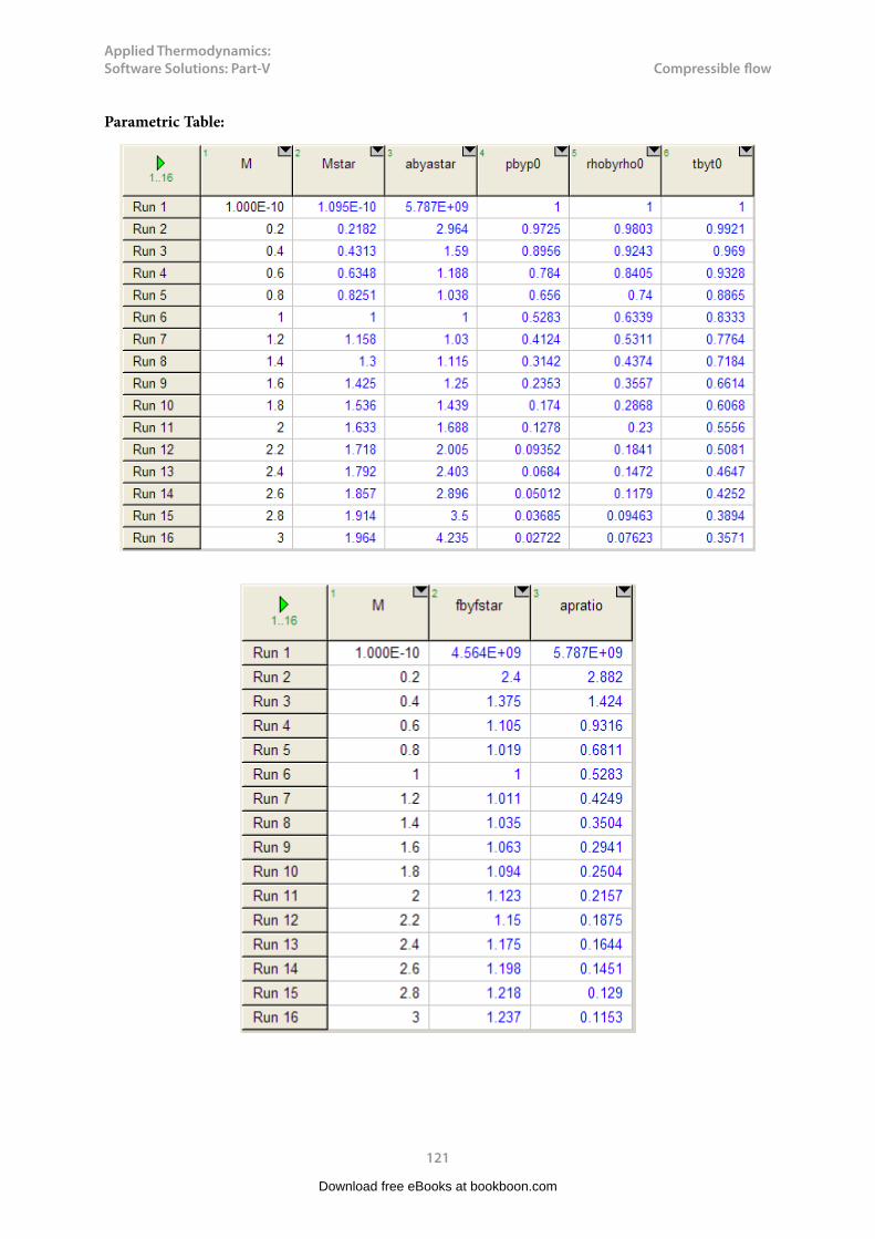
Applied Thermodynamics: Software Solutions: Part-V
121
Compressible flow
Parametric Table:
Download free eBooks at bookboon.com

Applied Thermodynamics: Software Solutions: Part-V
122
Compressible flow
Note: In the above Tables, minimum value for M is shown as 1E-10, since M = 0 will give a ‘Division by zero’ error.
Plots:
Download free eBooks at bookboon.com
Click on the ad to read moreClick on the ad to read moreClick on the ad to read moreClick on the ad to read moreClick on the ad to read moreClick on the ad to read moreClick on the ad to read moreClick on the ad to read moreClick on the ad to read moreClick on the ad to read moreClick on the ad to read moreClick on the ad to read moreClick on the ad to read moreClick on the ad to read moreClick on the ad to read moreClick on the ad to read moreClick on the ad to read moreClick on the ad to read moreClick on the ad to read moreClick on the ad to read moreClick on the ad to read moreClick on the ad to read moreClick on the ad to read moreClick on the ad to read moreClick on the ad to read moreClick on the ad to read moreClick on the ad to read moreClick on the ad to read moreClick on the ad to read moreClick on the ad to read moreClick on the ad to read moreClick on the ad to read moreClick on the ad to read moreClick on the ad to read moreClick on the ad to read moreClick on the ad to read moreClick on the ad to read moreClick on the ad to read moreClick on the ad to read more

Applied Thermodynamics: Software Solutions: Part-V
123
Compressible flow
=======================================================================
“Prob.9.4.3 Write EES Functions for property variations across a normal shock for an ideal gas.”
Fig.Prob.9.4.3 Normal shock
EES Functions:
“For My, Mach No. after shock:”
FUNCTION My(Mx,k)
“Inputs: Mx – Mach No. before shock, k -- ratio of sp. heats (= 1.4 for air)”
“Outputs: My”
AA := (2 / (k – 1)) + Mx^2
BB:= ((2 * k)/(k-1))*Mx^2 -1
Download free eBooks at bookboon.com

Applied Thermodynamics: Software Solutions: Part-V
124
Compressible flow
My := sqrt(AA / BB)
END
“=====================================================================”
“For Py/Px, static pressure ratio:”
FUNCTION PYBYPX(Mx,k)
“Inputs: Mx – Mach No. before shock, k -- ratio of sp. heats (= 1.4 for air)”
“Outputs: Py/Px”
PYBYPX := ((2*k) / (k + 1)) * Mx^2 – (k – 1)/(k + 1)
END
“=====================================================================”
“For Ty/Tx, static temp ratio:”
FUNCTION TYBYTX(Mx,k)
“Inputs: Mx – Mach No. before shock, k -- ratio of sp. heats (= 1.4 for air)”
“Outputs: Ty/Tx”
AA := 1 + ((k – 1)/2) * Mx^2
BB:= ((2 * k) / (k – 1)) * Mx^2 – 1
CC := (1/2) * (k + 1)^2 * Mx^2 / (k – 1)
TYBYTX := AA * BB / CC
END
“=====================================================================”
Download free eBooks at bookboon.com

Applied Thermodynamics: Software Solutions: Part-V
125
Compressible flow
“For rhoy/rhox, densityratio:”
FUNCTION RHOYBYRHOX(Mx,k)
“Inputs: Mx – Mach No. before shock, k -- ratio of sp. heats (= 1.4 for air)”
“Outputs: rhoy/rhox”
RHOYBYRHOX := PYBYPX(Mx, k) / TYBYTX(Mx, k)
END
“=====================================================================”
“For P0y/P0x, stagn. pressure ratio:”
FUNCTION P0YBYP0X(Mx,k)
“Inputs: Mx – Mach No. before shock, k -- ratio of sp. heats (= 1.4 for air)”
Download free eBooks at bookboon.com
Click on the ad to read moreClick on the ad to read moreClick on the ad to read moreClick on the ad to read moreClick on the ad to read moreClick on the ad to read moreClick on the ad to read moreClick on the ad to read moreClick on the ad to read moreClick on the ad to read moreClick on the ad to read moreClick on the ad to read moreClick on the ad to read moreClick on the ad to read moreClick on the ad to read moreClick on the ad to read moreClick on the ad to read moreClick on the ad to read moreClick on the ad to read moreClick on the ad to read moreClick on the ad to read moreClick on the ad to read moreClick on the ad to read moreClick on the ad to read moreClick on the ad to read moreClick on the ad to read moreClick on the ad to read moreClick on the ad to read moreClick on the ad to read moreClick on the ad to read moreClick on the ad to read moreClick on the ad to read moreClick on the ad to read moreClick on the ad to read moreClick on the ad to read moreClick on the ad to read moreClick on the ad to read moreClick on the ad to read moreClick on the ad to read moreClick on the ad to read more
DTU, Technical University of Denmark, is ranked as one of the best technical universities in Europe, and offers internationally recognised Master of Science degrees in 39 English-taught programmes.
DTU offers a unique environment where students have hands-on access to cutting edge facilities and work
closely under the expert supervision of top international researchers.
DTU’s central campus is located just north of Copenhagen and life at the University is engaging and vibrant. At DTU, we ensure that your goals and ambitions are met. Tuition is free for EU/EEA citizens.
Visit us at www.dtu.dk
Study at one of Europe’s leading universities

Applied Thermodynamics: Software Solutions: Part-V
126
Compressible flow
“Outputs: P0y/P0x”
AA := Mx / My(Mx,k)
BB := 1 + (My(Mx,k))^2 * (k – 1)/2
CC:= 1 + Mx^2 * (k – 1)/2
DD := ( k + 1)/ (2 * (k -1))
P0YBYP0X := AA * (BB / CC)^DD
END
“=====================================================================”
“For P0y/Px:”
FUNCTION P0YBYPX(Mx,k)
“Inputs: Mx – Mach No. before shock, k -- ratio of sp. heats (= 1.4 for air)”
“Outputs: P0y/Px”
AA := 1 + k * Mx^2
BB := 1 + k * (My(Mx,k))^2
CC:= 1 + (My(Mx,k))^2 * (k – 1)/2
DD := k /(k – 1)
P0YBYPX := (AA/BB) * CC^DD
END
“=====================================================================”
Download free eBooks at bookboon.com

Applied Thermodynamics: Software Solutions: Part-V
127
Compressible flow
“For entropy change, DELTAS across the shock:”
FUNCTION DELTAS(Mx,R, k)
“Inputs: Mx – Mach No. before shock, k -- ratio of sp. heats (= 1.4 for air)”
“Outputs: DELTAS (J/kg.K) = -R * ln (P0y/P0x).We write: (P0y/P0x) = (P0y/Px) * (Px/P0x)Now, (Px/P0x) is obtained from Isentropic relation since flow from inlet to shock is isentropic
Another relation for DELTAS is DELTS = cp . ln(Ty/Tx) – R . ln(Py/Px)”
AA := P0YBYPX(Mx,k)
BB := PBYP0(Mx,k)
DELTAS := -R * ln(AA * BB)
END
“=====================================================================”
“Prob.9.4.4 Using the EES Functions for property variations across a normal shock in an ideal gas, written above, plot the property variations against Mach No.”
EES Solution:
{Mx = 2}
k = 1.4
My = My(Mx, k)
pybypx = PYBYPX(Mx, k)
rhoybyrhox = RHOYBYRHOX(Mx, k)
tybytx = TYBYTX(Mx, k)
p0ybyp0x = P0YBYP0X(Mx, k)
p0ybypx = P0YBYPX(Mx, k)
Download free eBooks at bookboon.com

Applied Thermodynamics: Software Solutions: Part-V
128
Compressible flow
Parametric Table:
Download free eBooks at bookboon.com
Click on the ad to read moreClick on the ad to read moreClick on the ad to read moreClick on the ad to read moreClick on the ad to read moreClick on the ad to read moreClick on the ad to read moreClick on the ad to read moreClick on the ad to read moreClick on the ad to read moreClick on the ad to read moreClick on the ad to read moreClick on the ad to read moreClick on the ad to read moreClick on the ad to read moreClick on the ad to read moreClick on the ad to read moreClick on the ad to read moreClick on the ad to read moreClick on the ad to read moreClick on the ad to read moreClick on the ad to read moreClick on the ad to read moreClick on the ad to read moreClick on the ad to read moreClick on the ad to read moreClick on the ad to read moreClick on the ad to read moreClick on the ad to read moreClick on the ad to read moreClick on the ad to read moreClick on the ad to read moreClick on the ad to read moreClick on the ad to read moreClick on the ad to read moreClick on the ad to read moreClick on the ad to read moreClick on the ad to read moreClick on the ad to read moreClick on the ad to read moreClick on the ad to read more
Increase your impact with MSM Executive Education
For more information, visit www.msm.nl or contact us at +31 43 38 70 808
or via [email protected] the globally networked management school
For more information, visit www.msm.nl or contact us at +31 43 38 70 808 or via [email protected]
For almost 60 years Maastricht School of Management has been enhancing the management capacity
of professionals and organizations around the world through state-of-the-art management education.
Our broad range of Open Enrollment Executive Programs offers you a unique interactive, stimulating and
multicultural learning experience.
Be prepared for tomorrow’s management challenges and apply today.
Executive Education-170x115-B2.indd 1 18-08-11 15:13

Applied Thermodynamics: Software Solutions: Part-V
129
Compressible flow
Now, plot the results:
=======================================================================
“Prob.9.4.5 Write EES Functions for property variations of an ideal gas in Fanno flow (i.e. adiabatic flow with friction in constant area ducts).”
Fig.Prob.9.4.5 Fanno flow
Download free eBooks at bookboon.com

Applied Thermodynamics: Software Solutions: Part-V
130
Compressible flow
EES Functions:
Here, functions are non-dimensionalised with respect to values at M = 1, denoted by star.Thus, to find velocity ratio between sections 1 and 2 of pipe, we write:
V1/V2 = (V1/Vstar) * (Vstar/V2)
“For V/Vstar : Also, this is equal to: rhostar/rho”
FUNCTION FANNO_VBYVSTAR(M, k)
“Inputs: M – Mach No. k -- ratio of sp. heats (= 1.4 for air)”
“Outputs: V/Vstar”
AA := 2 * (1 + ((k – 1)/2) * M^2)
FANNO_VBYVSTAR := M * sqrt((k + 1) / AA)
END
“=====================================================================”
“For P/Pstar:”
FUNCTION FANNO_PBYPSTAR(M, k)
“Inputs: M – Mach No. k -- ratio of sp. heats (= 1.4 for air)”
“Outputs: P/Pstar”
AA := 2 * (1 + ((k – 1)/2) * M^2)
FANNO_PBYPSTAR := (1/M) * sqrt((k + 1) / AA)
END
“=====================================================================”
Download free eBooks at bookboon.com

Applied Thermodynamics: Software Solutions: Part-V
131
Compressible flow
“For T/Tstar:”
FUNCTION FANNO_TBYTSTAR(M, k)
“Inputs: M – Mach No. k -- ratio of sp. heats (= 1.4 for air)”
“Outputs: T/Tstar”
AA := 2 * (1 + ((k – 1)/2) * M^2)
FANNO_TBYTSTAR := (k + 1) / AA
END
“=====================================================================”
“For P0/P0star:”
FUNCTION FANNO_P0BYP0STAR(M, k)
“Inputs: M – Mach No. ..k -- ratio of sp. heats (= 1.4 for air)”
Download free eBooks at bookboon.com
Click on the ad to read moreClick on the ad to read moreClick on the ad to read moreClick on the ad to read moreClick on the ad to read moreClick on the ad to read moreClick on the ad to read moreClick on the ad to read moreClick on the ad to read moreClick on the ad to read moreClick on the ad to read moreClick on the ad to read moreClick on the ad to read moreClick on the ad to read moreClick on the ad to read moreClick on the ad to read moreClick on the ad to read moreClick on the ad to read moreClick on the ad to read moreClick on the ad to read moreClick on the ad to read moreClick on the ad to read moreClick on the ad to read moreClick on the ad to read moreClick on the ad to read moreClick on the ad to read moreClick on the ad to read moreClick on the ad to read moreClick on the ad to read moreClick on the ad to read moreClick on the ad to read moreClick on the ad to read moreClick on the ad to read moreClick on the ad to read moreClick on the ad to read moreClick on the ad to read moreClick on the ad to read moreClick on the ad to read moreClick on the ad to read moreClick on the ad to read moreClick on the ad to read moreClick on the ad to read more
EXPERIENCE THE POWER OF FULL ENGAGEMENT…
RUN FASTER. RUN LONGER.. RUN EASIER…
READ MORE & PRE-ORDER TODAY WWW.GAITEYE.COM
Challenge the way we run
1349906_A6_4+0.indd 1 22-08-2014 12:56:57

Applied Thermodynamics: Software Solutions: Part-V
132
Compressible flow
“Outputs: P0/P0star”
AA := 2 * (1 + ((k – 1)/2) * M^2)
BB := (k + 1) / ( 2 * (k – 1))
FANNO_P0BYP0STAR := (1/M) * (AA / (k + 1))^BB
END
“=====================================================================”
“For F/Fstar : “
FUNCTION FANNO_FBYFSTAR(M, k)
“Inputs: M – Mach No. k -- ratio of sp. heats (= 1.4 for air)”
“Outputs: F/Fstar”
AA := sqrt (2 * ( k+ 1) * (1 + ((k – 1)/2) * M^2))
BB :=(1 + k * M^2) / M
FANNO_FBYFSTAR := BB / AA
END
“=====================================================================”
“For 4.f.Lmax/D:”
FUNCTION FANNO_FOURFLMAXBYD(M, k)
“Inputs: M – Mach No. k -- ratio of sp. heats (= 1.4 for air)”
“Outputs: 4.f.Lmax/D”
AA :=(1 – M^2) / (k * M^2)
Download free eBooks at bookboon.com

Applied Thermodynamics: Software Solutions: Part-V
133
Compressible flow
BB := (k + 1) / (2 * k)
CC := (k + 1) * M^2
DD := (2 * (1 + ((k – 1)/2) * M^2))
FANNO_FOURFLMAXBYD := AA + BB * ln(CC/DD)
END
“=====================================================================”
“Prob.9.4.6 Plot property variations of an ideal gas with k = 1.4,in Fanno flow against Mach No.”
EES Solution:
{M = 2}
k = 1.4
Download free eBooks at bookboon.com
Click on the ad to read moreClick on the ad to read moreClick on the ad to read moreClick on the ad to read moreClick on the ad to read moreClick on the ad to read moreClick on the ad to read moreClick on the ad to read moreClick on the ad to read moreClick on the ad to read moreClick on the ad to read moreClick on the ad to read moreClick on the ad to read moreClick on the ad to read moreClick on the ad to read moreClick on the ad to read moreClick on the ad to read moreClick on the ad to read moreClick on the ad to read moreClick on the ad to read moreClick on the ad to read moreClick on the ad to read moreClick on the ad to read moreClick on the ad to read moreClick on the ad to read moreClick on the ad to read moreClick on the ad to read moreClick on the ad to read moreClick on the ad to read moreClick on the ad to read moreClick on the ad to read moreClick on the ad to read moreClick on the ad to read moreClick on the ad to read moreClick on the ad to read moreClick on the ad to read moreClick on the ad to read moreClick on the ad to read moreClick on the ad to read moreClick on the ad to read moreClick on the ad to read moreClick on the ad to read moreClick on the ad to read more
GET THERE FASTER
Oliver Wyman is a leading global management consulting firm that combines
deep industry knowledge with specialized expertise in strategy, operations, risk
management, organizational transformation, and leadership development. With
offices in 50+ cities across 25 countries, Oliver Wyman works with the CEOs and
executive teams of Global 1000 companies.
An equal opportunity employer.
Some people know precisely where they want to go. Others seek the adventure of discovering uncharted territory. Whatever you want your professional journey to be, you’ll find what you’re looking for at Oliver Wyman.
Discover the world of Oliver Wyman at oliverwyman.com/careers
DISCOVEROUR WORLD
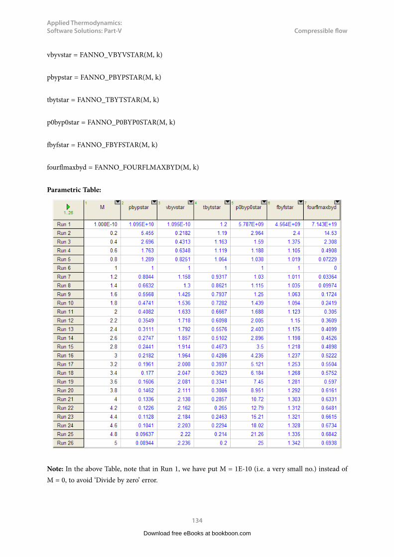
Applied Thermodynamics: Software Solutions: Part-V
134
Compressible flow
vbyvstar = FANNO_VBYVSTAR(M, k)
pbypstar = FANNO_PBYPSTAR(M, k)
tbytstar = FANNO_TBYTSTAR(M, k)
p0byp0star = FANNO_P0BYP0STAR(M, k)
fbyfstar = FANNO_FBYFSTAR(M, k)
fourflmaxbyd = FANNO_FOURFLMAXBYD(M, k)
Parametric Table:
Note: In the above Table, note that in Run 1, we have put M = 1E-10 (i.e. a very small no.) instead of M = 0, to avoid ‘Divide by zero’ error.
Download free eBooks at bookboon.com

Applied Thermodynamics: Software Solutions: Part-V
135
Compressible flow
Now, plot the results:
=======================================================================
Download free eBooks at bookboon.com
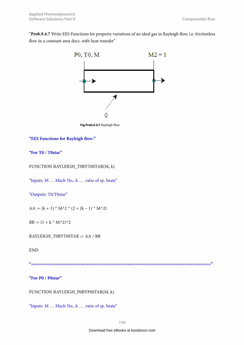
Applied Thermodynamics: Software Solutions: Part-V
136
Compressible flow
“Prob.9.4.7 Write EES Functions for property variations of an ideal gas in Rayleigh flow, i.e. frictionless flow in a constant area duct, with heat transfer”
Fig.Prob.9.4.7 Rayleigh flow
“EES Functions for Rayleigh flow:”
“For T0 / T0star”
FUNCTION RAYLEIGH_T0BYT0STAR(M, k)
“Inputs: M … Mach No., k …. ratio of sp. heats”
“Outputs: T0/T0star”
AA := (k + 1) * M^2 * (2 + (k – 1) * M^2)
BB := (1 + k * M^2)^2
RAYLEIGH_T0BYT0STAR := AA / BB
END
“=====================================================================”
“For P0 / P0star”
FUNCTION RAYLEIGH_P0BYP0STAR(M, k)
“Inputs: M … Mach No., k …. ratio of sp. heats”
Download free eBooks at bookboon.com

Applied Thermodynamics: Software Solutions: Part-V
137
Compressible flow
“Outputs: P0/P0star”
AA := (k + 1) / ( 1 + k * M^2)
BB := ((2 + (k – 1) * M^2) / (k + 1))^(k / (k – 1))
RAYLEIGH_P0BYP0STAR := AA * BB
END
“=====================================================================”
“For T / Tstar”
FUNCTION RAYLEIGH_TBYTSTAR(M, k)
“Inputs: M … Mach No., k …. ratio of sp. heats”
“Outputs: T/Tstar”
Download free eBooks at bookboon.com
Click on the ad to read moreClick on the ad to read moreClick on the ad to read moreClick on the ad to read moreClick on the ad to read moreClick on the ad to read moreClick on the ad to read moreClick on the ad to read moreClick on the ad to read moreClick on the ad to read moreClick on the ad to read moreClick on the ad to read moreClick on the ad to read moreClick on the ad to read moreClick on the ad to read moreClick on the ad to read moreClick on the ad to read moreClick on the ad to read moreClick on the ad to read moreClick on the ad to read moreClick on the ad to read moreClick on the ad to read moreClick on the ad to read moreClick on the ad to read moreClick on the ad to read moreClick on the ad to read moreClick on the ad to read moreClick on the ad to read moreClick on the ad to read moreClick on the ad to read moreClick on the ad to read moreClick on the ad to read moreClick on the ad to read moreClick on the ad to read moreClick on the ad to read moreClick on the ad to read moreClick on the ad to read moreClick on the ad to read moreClick on the ad to read moreClick on the ad to read moreClick on the ad to read moreClick on the ad to read moreClick on the ad to read moreClick on the ad to read more
Applied Thermodynamics: Software Solutions: Part-V
138
Compressible flow
RAYLEIGH_TBYTSTAR := (M * ( 1 + k) / ( 1 + k * M^2))^2
END
“=====================================================================”
“For P / Pstar”
FUNCTION RAYLEIGH_PBYPSTAR(M, k)
“Inputs: M … Mach No., k …. ratio of sp. heats”
“Outputs: P / Pstar”
RAYLEIGH_PBYPSTAR := ( 1 + k) / ( 1 + k * M^2)
END
“=====================================================================”
“For V / Vstar”
FUNCTION RAYLEIGH_VBYVSTAR(M, k)
“Inputs: M … Mach No., k …. ratio of sp. heats”
“Outputs: V / Vstar. Also, note: V/Vstar = rhostar/rho”
RAYLEIGH_VBYVSTAR := ( 1+ k) * M^2/ ( 1 + k * M^2)
END
“=====================================================================”
“For Entropy change: (s2 – s1)”
FUNCTION RAYLEIGH_DELTAS(M1, M2, R, k)
“Inputs: M1, M2 … Mach Nos at inlet and exit of duct., R = gas constant (J/kg.K), k …. ratio of sp. heats”
Download free eBooks at bookboon.com

Applied Thermodynamics: Software Solutions: Part-V
139
Compressible flow
“Outputs: (s2 – s1), J/kg.K “
AA = (M2/ M1)^((2 * k)/(k – 1))
BB = (1+ k * M1^2)/ (1 + k * M2^2)
CC = (k + 1) / (k – 1)
RAYLEIGH_DELTAS := R * ln(AA * BB^CC)
END
“=====================================================================”
“For heat transfer, Q”
FUNCTION RAYLEIGH_Q(M1, M2, cp, T1, k)
“Inputs: M1, M2 … Mach Nos at inlet and exit of duct., T1 = inlet temp (K), cp = sp.heat at const. pressure (J/kg.K), k …. ratio of sp. heats”
“Outputs: Q, J/kg “
AA = M2^2 – M1^2
BB = 2 – 2 * k * M1^2 * M2^2
CC = (k – 1) * (M2^2 + M1^2)
DD = 2 * M1^2 * (1 + k * M2^2)^2
RAYLEIGH_Q := cp * T1 * AA * (BB + CC) / DD
END
“=====================================================================”
Download free eBooks at bookboon.com
Applied Thermodynamics: Software Solutions: Part-V
140
Compressible flow
“Prob.9.4.8 Using the EES Functions for property variations of an ideal gas in Rayleigh flow, plot the Rayleigh flow functions against Mach No.”
EES Solution:
{M = 2}
k = 1.4
t0byt0star = RAYLEIGH_T0BYT0STAR(M, k)
p0byp0star = RAYLEIGH_P0BYP0STAR(M, k)
tbytstar = RAYLEIGH_TBYTSTAR(M, k)
pbypstar = RAYLEIGH_PBYPSTAR(M, k)
vbyvstar = RAYLEIGH_VBYVSTAR(M, k)
Download free eBooks at bookboon.com
Click on the ad to read moreClick on the ad to read moreClick on the ad to read moreClick on the ad to read moreClick on the ad to read moreClick on the ad to read moreClick on the ad to read moreClick on the ad to read moreClick on the ad to read moreClick on the ad to read moreClick on the ad to read moreClick on the ad to read moreClick on the ad to read moreClick on the ad to read moreClick on the ad to read moreClick on the ad to read moreClick on the ad to read moreClick on the ad to read moreClick on the ad to read moreClick on the ad to read moreClick on the ad to read moreClick on the ad to read moreClick on the ad to read moreClick on the ad to read moreClick on the ad to read moreClick on the ad to read moreClick on the ad to read moreClick on the ad to read moreClick on the ad to read moreClick on the ad to read moreClick on the ad to read moreClick on the ad to read moreClick on the ad to read moreClick on the ad to read moreClick on the ad to read moreClick on the ad to read moreClick on the ad to read moreClick on the ad to read moreClick on the ad to read moreClick on the ad to read moreClick on the ad to read moreClick on the ad to read moreClick on the ad to read moreClick on the ad to read moreClick on the ad to read more
81,000 kmIn the past four years we have drilled
That’s more than twice around the world.
What will you be?
Who are we?We are the world’s leading oilfield services company. Working globally—often in remote and challenging locations—we invent, design, engineer, manufacture, apply, and maintain technology to help customers find and produce oil and gas safely.
Who are we looking for?We offer countless opportunities in the following domains:n Engineering, Research, and Operationsn Geoscience and Petrotechnicaln Commercial and Business
If you are a self-motivated graduate looking for a dynamic career, apply to join our team.
careers.slb.com
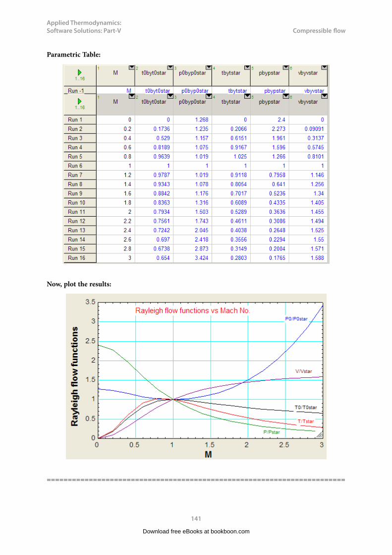
Applied Thermodynamics: Software Solutions: Part-V
141
Compressible flow
Parametric Table:
Now, plot the results:
=======================================================================
Download free eBooks at bookboon.com

Applied Thermodynamics: Software Solutions: Part-V
142
Compressible flow
“Prob.9.4.9 Air at 330 K and 200 kPa enters a duct with a varying flow area. If the Mach No. at the entrance is 0.25, determine the temp, pressure and Mach No. at a location where flow area has reached to 60% of the entrance area. Assume the flow to be steady and isentropic and oxygen to be an ideal gas.”
Fig.Prob.9.4.9 Isentropic flow in a duct of varying area
EES Solution:
“Data:”
“Let 1 refer to entrance and 2 to the required state.”
k = 1.4 “for air”
M1 = 0.25
T1 = 330 “K”
P1 = 200 “kPa”
“Calculations:”
“Use EES functions for property variations in isentropic flow written above:”
“At M1 = 0.25, we have:”
a1byastar = ABYASTAR(M1, k) “…gives A1/Astar”
T1 / T0 = TBYT0(M1, k) “… gives T0”
P1 / P0 = PBYP0(M1, k) “… gives P0”
Download free eBooks at bookboon.com

Applied Thermodynamics: Software Solutions: Part-V
143
Compressible flow
“Now, at the desired location: A2 = 0.6 * A1”
a2bya1 = 0.6 “…by data: A2/A1 = 0.6”
“Therefore: (A2/Astar) = (A2/A1) * (A1 / Astar). Then, we have:”
a2byastar = a2bya1 * a1byastar “…. gives A2/Astar”
“Now, for this a2byastar, from isentropic flow relations, we get:”
a2byastar = ABYASTAR(M2,k) “….finds M2 “
“While finding M2, remember that it should be subsonic, since at the entry, flow is subsonic, and it is a convergent nozzle since area is decreasing.
So, select the guess value as less than 1 for M2, as explained below:”
Download free eBooks at bookboon.com
Click on the ad to read moreClick on the ad to read moreClick on the ad to read moreClick on the ad to read moreClick on the ad to read moreClick on the ad to read moreClick on the ad to read moreClick on the ad to read moreClick on the ad to read moreClick on the ad to read moreClick on the ad to read moreClick on the ad to read moreClick on the ad to read moreClick on the ad to read moreClick on the ad to read moreClick on the ad to read moreClick on the ad to read moreClick on the ad to read moreClick on the ad to read moreClick on the ad to read moreClick on the ad to read moreClick on the ad to read moreClick on the ad to read moreClick on the ad to read moreClick on the ad to read moreClick on the ad to read moreClick on the ad to read moreClick on the ad to read moreClick on the ad to read moreClick on the ad to read moreClick on the ad to read moreClick on the ad to read moreClick on the ad to read moreClick on the ad to read moreClick on the ad to read moreClick on the ad to read moreClick on the ad to read moreClick on the ad to read moreClick on the ad to read moreClick on the ad to read moreClick on the ad to read moreClick on the ad to read moreClick on the ad to read moreClick on the ad to read moreClick on the ad to read moreClick on the ad to read more
Hellmann’s is one of Unilever’s oldest brands having been popular for over 100 years. If you too share a passion for discovery and innovation we will give you the tools and opportunities to provide you with a challenging career. Are you a great scientist who would like to be at the forefront of scientific innovations and developments? Then you will enjoy a career within Unilever Research & Development. For challenging job opportunities, please visit www.unilever.com/rdjobs.
Could you think of 101 new thingsto do with eggs and oil?
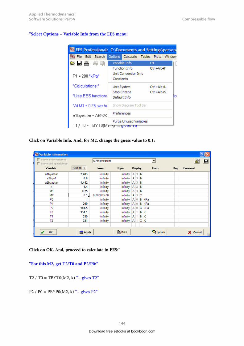
Applied Thermodynamics: Software Solutions: Part-V
144
Compressible flow
“Select Options – Variable Info from the EES menu:
Click on Variable Info. And, for M2, change the guess value to 0.1:
Click on OK. And, proceed to calculate in EES:”
“For this M2, get T2/T0 and P2/P0:”
T2 / T0 = TBYT0(M2, k) “…gives T2”
P2 / P0 = PBYP0(M2, k) “…gives P2”
Download free eBooks at bookboon.com

Applied Thermodynamics: Software Solutions: Part-V
145
Compressible flow
Results:
Thus:
Mach No. at section 2 = M2 = 0.4529 …. Ans.
Pressure at section 2 = P2 = 181.5 kPa … Ans.
Temp. at section 2 = T2 = 321 K … Ans.
=======================================================================
“Prob.9.4.10 A conical diffuser has entry and exit dia of 15 cm and 30 cm respectively. P, T and V of air at entry are 0.69 bar, 340 K and 180 m/s respectively. Determine: (i) exit pressure (ii) exit velocity (iii) force exerted on the diffuser walls. Assume isentropic flow, k = 1.4, cp = 1000 J/kg.K”
Fig.Prob.9.4.10 Isentropic flow in a diffuser
EES Solution:
“Data:”
D1 = 0.15 “m”
D2 = 0.3 “m”
P1 = 0.69 “bar”
T1 = 340 “K”
Download free eBooks at bookboon.com

Applied Thermodynamics: Software Solutions: Part-V
146
Compressible flow
V1 = 180 “m/s”
k = 1.4
cp = 1000 “J/kg.K”
R = 287 “J/kg.K”
“Calculations:”
A1 = pi * D1^2 /4 “m^2 …. inlet area”
A2 = pi * D2^2 /4 “m^2… exit area”
T01 = T1 + V1^2 / (2 * cp) “K… stagn. temp at inlet”
T02 = T01 “..for isentropic flow”
rho1 = (P1 * 10^5) / (R * T1) “m^3 /kg … density at inlet”
“Therefore,T1/T01 can be found out, and for this T1/T01, find M1 etc from isentropic flow functions:”
T1/T01 = TBYT0(M1, k) “…finds M1”
P1/P01 = PBYP0(M1, k) “..finds P01”
P02 = P01 “…for isentropic flow”
A1/A1star = ABYASTAR(M1, k) “…finds A1star”
A2star = A1star”…for isentropic flow”
F1/F1star = FBYFSTAR(M1, k) “…finds F1 for M1”
“When M = 1: pressure is Pstar, Temp is Tstar:”
P1star/P01 = PBYP0(1, k) “…finds P1star”
P2star = P1star
Download free eBooks at bookboon.com

Applied Thermodynamics: Software Solutions: Part-V
147
Compressible flow
T1star/T01 = TBYT0(1, k)”…finds T1star”
F1star = (P1star * 10^5) * A1star * (1 + k) “N”
F2star = F1star
“At the exit: Find (A2/A2star) and then find M2 and other functions corresponding to this (A2/A2star) from isentropic functions:”
A2/A2star = ABYASTAR(M2, k) “… finds M2”
P2/P02 = PBYP0(M2, k) “..finds P2”
F2/F2star = FBYFSTAR(M2, k) “…finds F2 for M2”
T2/T02 = TBYT0(M2, k) “…finds T2”
rho2 = P2 * 10^5 / (R * T2) “..kg/m^3…density at exit”
mass_flow = rho1 * A1 * V1 “kg/s”
Download free eBooks at bookboon.com
Click on the ad to read moreClick on the ad to read moreClick on the ad to read moreClick on the ad to read moreClick on the ad to read moreClick on the ad to read moreClick on the ad to read moreClick on the ad to read moreClick on the ad to read moreClick on the ad to read moreClick on the ad to read moreClick on the ad to read moreClick on the ad to read moreClick on the ad to read moreClick on the ad to read moreClick on the ad to read moreClick on the ad to read moreClick on the ad to read moreClick on the ad to read moreClick on the ad to read moreClick on the ad to read moreClick on the ad to read moreClick on the ad to read moreClick on the ad to read moreClick on the ad to read moreClick on the ad to read moreClick on the ad to read moreClick on the ad to read moreClick on the ad to read moreClick on the ad to read moreClick on the ad to read moreClick on the ad to read moreClick on the ad to read moreClick on the ad to read moreClick on the ad to read moreClick on the ad to read moreClick on the ad to read moreClick on the ad to read moreClick on the ad to read moreClick on the ad to read moreClick on the ad to read moreClick on the ad to read moreClick on the ad to read moreClick on the ad to read moreClick on the ad to read moreClick on the ad to read moreClick on the ad to read more
© Deloitte & Touche LLP and affiliated entities.
360°thinking.
Discover the truth at www.deloitte.ca/careers
© Deloitte & Touche LLP and affiliated entities.
360°thinking.
Discover the truth at www.deloitte.ca/careers
© Deloitte & Touche LLP and affiliated entities.
360°thinking.
Discover the truth at www.deloitte.ca/careers © Deloitte & Touche LLP and affiliated entities.
360°thinking.
Discover the truth at www.deloitte.ca/careers

Applied Thermodynamics: Software Solutions: Part-V
148
Compressible flow
mass_flow = rho2 * A2 * V2 “..finds V2, vel. at exit”
“Force exerted on Diffuser walls = Thrust of the flow in backward direction”
“i.e. Thrust = F2 – F1”
Thrust_on_walls = F2 – F1 “N”
Resuts:
Thus:
Exit pressure = P2 = 0.8056 bar .. Ans.
Exit velocity = V2 = 40.29 m/s …. Ans.
Force exerted on diffuser walls = 4160 N … Ans.
Download free eBooks at bookboon.com
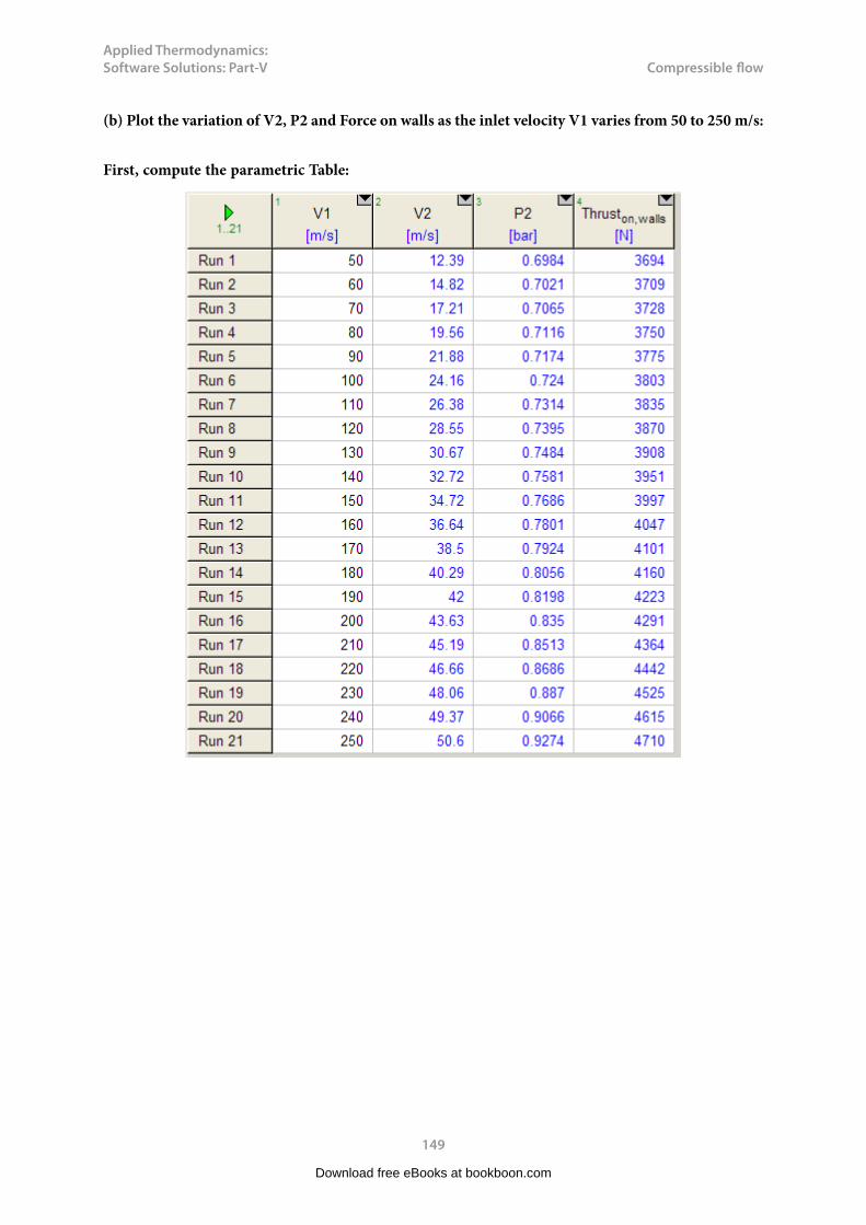
Applied Thermodynamics: Software Solutions: Part-V
149
Compressible flow
(b) Plot the variation of V2, P2 and Force on walls as the inlet velocity V1 varies from 50 to 250 m/s:
First, compute the parametric Table:
Download free eBooks at bookboon.com

Applied Thermodynamics: Software Solutions: Part-V
150
Compressible flow
Now, plot the results:
Download free eBooks at bookboon.com
Click on the ad to read moreClick on the ad to read moreClick on the ad to read moreClick on the ad to read moreClick on the ad to read moreClick on the ad to read moreClick on the ad to read moreClick on the ad to read moreClick on the ad to read moreClick on the ad to read moreClick on the ad to read moreClick on the ad to read moreClick on the ad to read moreClick on the ad to read moreClick on the ad to read moreClick on the ad to read moreClick on the ad to read moreClick on the ad to read moreClick on the ad to read moreClick on the ad to read moreClick on the ad to read moreClick on the ad to read moreClick on the ad to read moreClick on the ad to read moreClick on the ad to read moreClick on the ad to read moreClick on the ad to read moreClick on the ad to read moreClick on the ad to read moreClick on the ad to read moreClick on the ad to read moreClick on the ad to read moreClick on the ad to read moreClick on the ad to read moreClick on the ad to read moreClick on the ad to read moreClick on the ad to read moreClick on the ad to read moreClick on the ad to read moreClick on the ad to read moreClick on the ad to read moreClick on the ad to read moreClick on the ad to read moreClick on the ad to read moreClick on the ad to read moreClick on the ad to read moreClick on the ad to read moreClick on the ad to read more

Applied Thermodynamics: Software Solutions: Part-V
151
Compressible flow
=======================================================================
Download free eBooks at bookboon.com
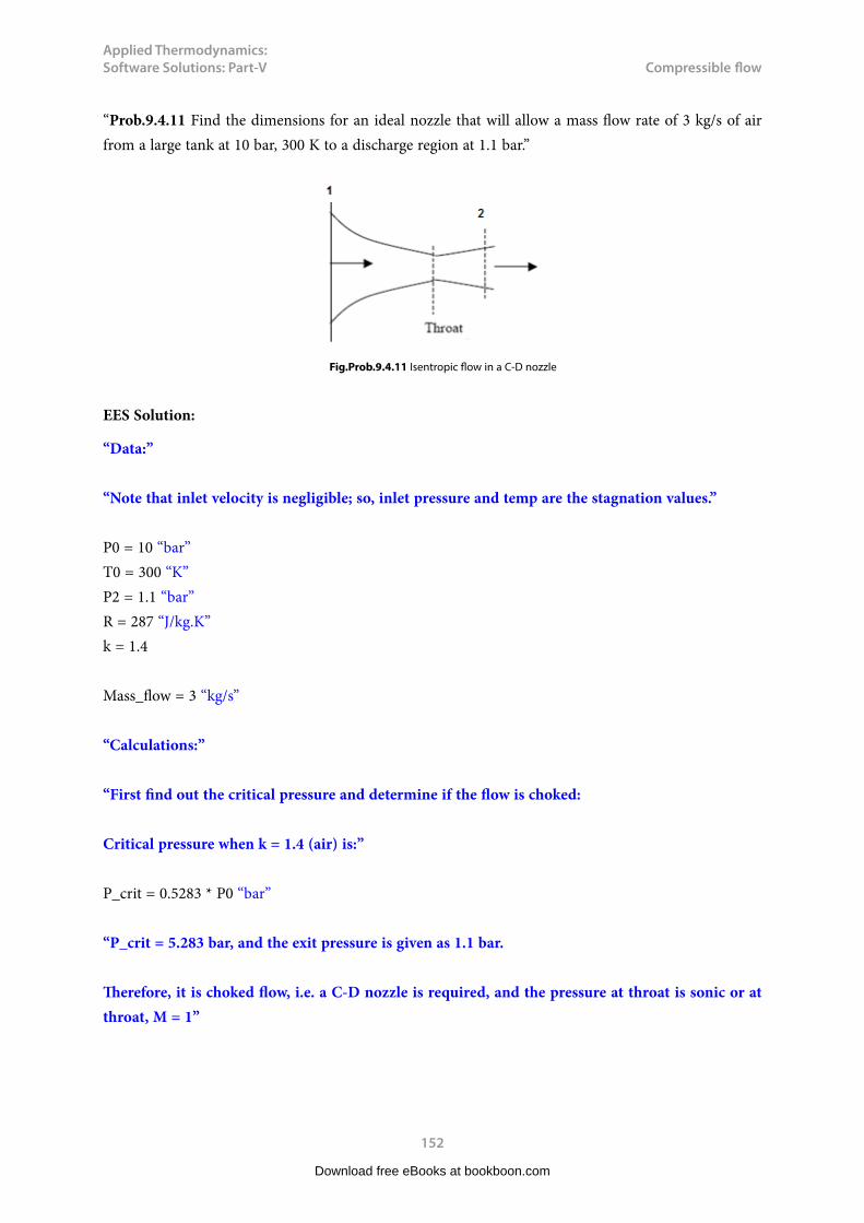
Applied Thermodynamics: Software Solutions: Part-V
152
Compressible flow
“Prob.9.4.11 Find the dimensions for an ideal nozzle that will allow a mass flow rate of 3 kg/s of air from a large tank at 10 bar, 300 K to a discharge region at 1.1 bar.”
Fig.Prob.9.4.11 Isentropic flow in a C-D nozzle
EES Solution:
“Data:”
“Note that inlet velocity is negligible; so, inlet pressure and temp are the stagnation values.”
P0 = 10 “bar”T0 = 300 “K”P2 = 1.1 “bar”R = 287 “J/kg.K”k = 1.4
Mass_flow = 3 “kg/s”
“Calculations:”
“First find out the critical pressure and determine if the flow is choked:
Critical pressure when k = 1.4 (air) is:”
P_crit = 0.5283 * P0 “bar”
“P_crit = 5.283 bar, and the exit pressure is given as 1.1 bar.
Therefore, it is choked flow, i.e. a C-D nozzle is required, and the pressure at throat is sonic or at throat, M = 1”
Download free eBooks at bookboon.com

Applied Thermodynamics: Software Solutions: Part-V
153
Compressible flow
“Then, from isentropic relations:”
P_star = P0 * PBYP0(1, k) “bar…pressure at throat”
T_star = T0 * TBYT0(1, k) “K…temp at throat”
rho_star = rho0 * RHOBYRHO0(1, k) “kg/m^3….density at throat”
rho0 = P0 * 10^5 / (R * T0) “kg/m^3 … density at inlet”
V_star = sqrt(k * R * T_star) “m/s …. vel. at throat = sonic vel.”
Mass_flow = rho_star * A_star * V_star “m^2…finds area at throat, A_star”
“At the exit:”
P2/P0 = PBYP0(M2,k) “..finds M2 for known P2/P0..
Download free eBooks at bookboon.com
Click on the ad to read moreClick on the ad to read moreClick on the ad to read moreClick on the ad to read moreClick on the ad to read moreClick on the ad to read moreClick on the ad to read moreClick on the ad to read moreClick on the ad to read moreClick on the ad to read moreClick on the ad to read moreClick on the ad to read moreClick on the ad to read moreClick on the ad to read moreClick on the ad to read moreClick on the ad to read moreClick on the ad to read moreClick on the ad to read moreClick on the ad to read moreClick on the ad to read moreClick on the ad to read moreClick on the ad to read moreClick on the ad to read moreClick on the ad to read moreClick on the ad to read moreClick on the ad to read moreClick on the ad to read moreClick on the ad to read moreClick on the ad to read moreClick on the ad to read moreClick on the ad to read moreClick on the ad to read moreClick on the ad to read moreClick on the ad to read moreClick on the ad to read moreClick on the ad to read moreClick on the ad to read moreClick on the ad to read moreClick on the ad to read moreClick on the ad to read moreClick on the ad to read moreClick on the ad to read moreClick on the ad to read moreClick on the ad to read moreClick on the ad to read moreClick on the ad to read moreClick on the ad to read moreClick on the ad to read moreClick on the ad to read more
������������� ����������������������������������������������� �� ���������������������������
������ ������ ������������������������������ ����������������������!���"���������������
�����#$%����&'())%�*+����������,����������-
.��������������������������������� ��
���������� ���������������� ������������� ���������������������������� �����������
The Wakethe only emission we want to leave behind
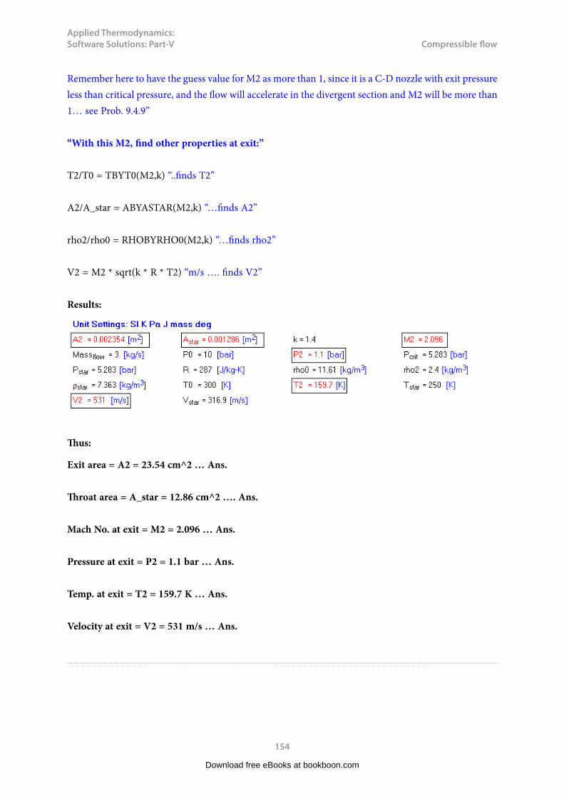
Applied Thermodynamics: Software Solutions: Part-V
154
Compressible flow
Remember here to have the guess value for M2 as more than 1, since it is a C-D nozzle with exit pressure less than critical pressure, and the flow will accelerate in the divergent section and M2 will be more than 1… see Prob. 9.4.9”
“With this M2, find other properties at exit:”
T2/T0 = TBYT0(M2,k) “..finds T2”
A2/A_star = ABYASTAR(M2,k) “…finds A2”
rho2/rho0 = RHOBYRHO0(M2,k) “…finds rho2”
V2 = M2 * sqrt(k * R * T2) “m/s …. finds V2”
Results:
Thus:
Exit area = A2 = 23.54 cm^2 … Ans.
Throat area = A_star = 12.86 cm^2 …. Ans.
Mach No. at exit = M2 = 2.096 … Ans.
Pressure at exit = P2 = 1.1 bar … Ans.
Temp. at exit = T2 = 159.7 K … Ans.
Velocity at exit = V2 = 531 m/s … Ans.
Download free eBooks at bookboon.com

Applied Thermodynamics: Software Solutions: Part-V
155
Compressible flow
(b) Plot the variation of Throat area (Astar) and Exit area (A2), as the mass flow rate varies from 1 kg/s to 4 kg/s:
First, compute the Parametric Table:
Now, plot the results:
Download free eBooks at bookboon.com

Applied Thermodynamics: Software Solutions: Part-V
156
Compressible flow
=======================================================================
Download free eBooks at bookboon.com
Click on the ad to read moreClick on the ad to read moreClick on the ad to read moreClick on the ad to read moreClick on the ad to read moreClick on the ad to read moreClick on the ad to read moreClick on the ad to read moreClick on the ad to read moreClick on the ad to read moreClick on the ad to read moreClick on the ad to read moreClick on the ad to read moreClick on the ad to read moreClick on the ad to read moreClick on the ad to read moreClick on the ad to read moreClick on the ad to read moreClick on the ad to read moreClick on the ad to read moreClick on the ad to read moreClick on the ad to read moreClick on the ad to read moreClick on the ad to read moreClick on the ad to read moreClick on the ad to read moreClick on the ad to read moreClick on the ad to read moreClick on the ad to read moreClick on the ad to read moreClick on the ad to read moreClick on the ad to read moreClick on the ad to read moreClick on the ad to read moreClick on the ad to read moreClick on the ad to read moreClick on the ad to read moreClick on the ad to read moreClick on the ad to read moreClick on the ad to read moreClick on the ad to read moreClick on the ad to read moreClick on the ad to read moreClick on the ad to read moreClick on the ad to read moreClick on the ad to read moreClick on the ad to read moreClick on the ad to read moreClick on the ad to read moreClick on the ad to read more
CAREERKICKSTARTAn app to keep you in the know
Whether you’re a graduate, school leaver or student, it’s a difficult time to start your career. So here at RBS, we’re providing a helping hand with our new Facebook app. Bringing together the most relevant and useful careers information, we’ve created a one-stop shop designed to help you get on the career ladder – whatever your level of education, degree subject or work experience.
And it’s not just finance-focused either. That’s because it’s not about us. It’s about you. So download the app and you’ll get everything you need to know to kickstart your career.
So what are you waiting for?
Click here to get started.
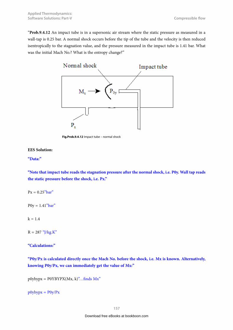
Applied Thermodynamics: Software Solutions: Part-V
157
Compressible flow
“Prob.9.4.12 An impact tube is in a supersonic air stream where the static pressure as measured in a wall-tap is 0.25 bar. A normal shock occurs before the tip of the tube and the velocity is then reduced isentropically to the stagnation value, and the pressure measured in the impact tube is 1.41 bar. What was the initial Mach No.? What is the entropy change?”
Fig.Prob.9.4.12 Impact tube – normal shock
EES Solution:
“Data:”
“Note that impact tube reads the stagnation pressure after the normal shock, i.e. P0y. Wall tap reads the static pressure before the shock, i.e. Px.”
Px = 0.25”bar”
P0y = 1.41”bar”
k = 1.4
R = 287 “J/kg.K”
“Calculations:”
“P0y/Px is calculated directly once the Mach No. before the shock, i.e. Mx is known. Alternatively, knowing P0y/Px, we can immediately get the value of Mx:”
p0ybypx = P0YBYPX(Mx, k)”…finds Mx”
p0ybypx = P0y/Px
Download free eBooks at bookboon.com
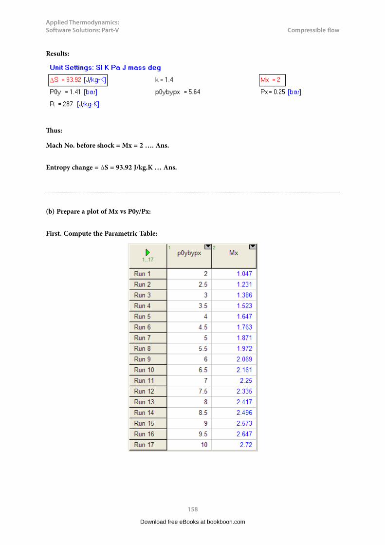
Applied Thermodynamics: Software Solutions: Part-V
158
Compressible flow
Results:
Thus:
Mach No. before shock = Mx = 2 …. Ans.
Entropy change = ΔS = 93.92 J/kg.K … Ans.
(b) Prepare a plot of Mx vs P0y/Px:
First. Compute the Parametric Table:
Download free eBooks at bookboon.com
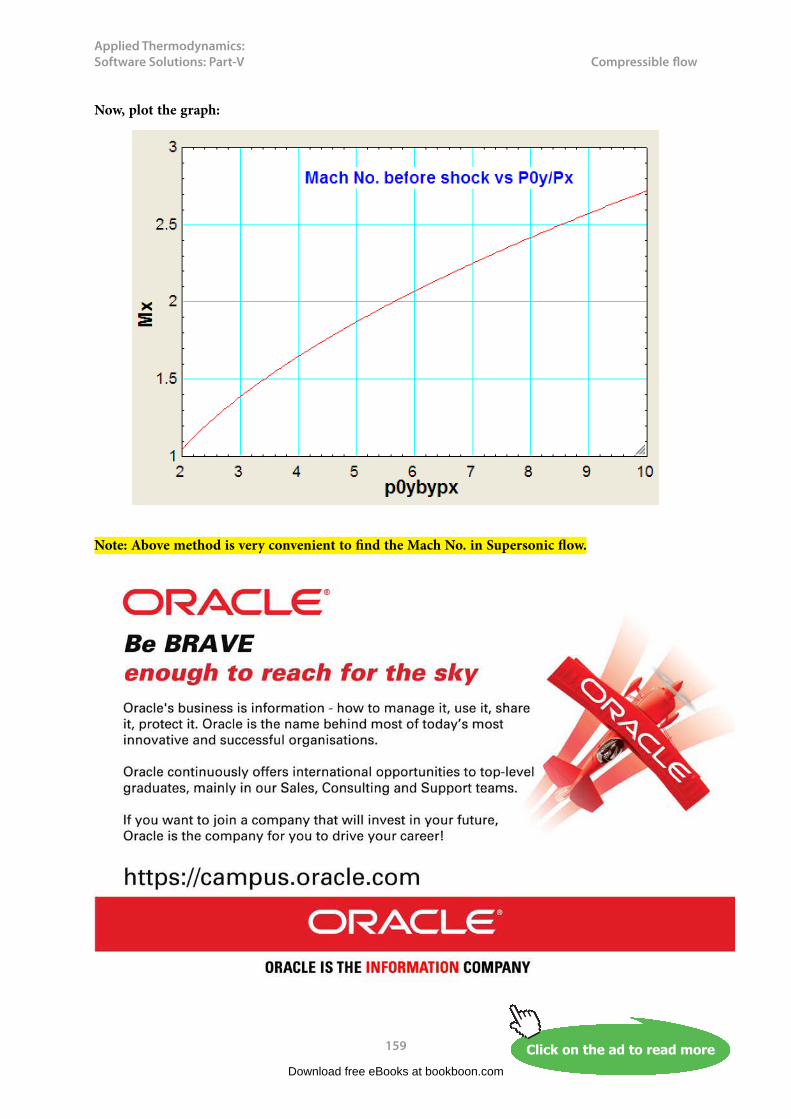
Applied Thermodynamics: Software Solutions: Part-V
159
Compressible flow
Now, plot the graph:
Note: Above method is very convenient to find the Mach No. in Supersonic flow.
Download free eBooks at bookboon.com
Click on the ad to read moreClick on the ad to read moreClick on the ad to read moreClick on the ad to read moreClick on the ad to read moreClick on the ad to read moreClick on the ad to read moreClick on the ad to read moreClick on the ad to read moreClick on the ad to read moreClick on the ad to read moreClick on the ad to read moreClick on the ad to read moreClick on the ad to read moreClick on the ad to read moreClick on the ad to read moreClick on the ad to read moreClick on the ad to read moreClick on the ad to read moreClick on the ad to read moreClick on the ad to read moreClick on the ad to read moreClick on the ad to read moreClick on the ad to read moreClick on the ad to read moreClick on the ad to read moreClick on the ad to read moreClick on the ad to read moreClick on the ad to read moreClick on the ad to read moreClick on the ad to read moreClick on the ad to read moreClick on the ad to read moreClick on the ad to read moreClick on the ad to read moreClick on the ad to read moreClick on the ad to read moreClick on the ad to read moreClick on the ad to read moreClick on the ad to read moreClick on the ad to read moreClick on the ad to read moreClick on the ad to read moreClick on the ad to read moreClick on the ad to read moreClick on the ad to read moreClick on the ad to read moreClick on the ad to read moreClick on the ad to read moreClick on the ad to read moreClick on the ad to read more

Applied Thermodynamics: Software Solutions: Part-V
160
Compressible flow
Position the Impact tube parallel to flow as shown, to ensure a normal shock, measure static and stagnation pressures Px and P0y, and then use the above graph to read the value of Mach No. Mx.
=======================================================================
“Prob.9.4.13 Air enters a nozzle at a pressure of 3.5 MN/m^2 and a temp of 500 C. It leaves at a pressure of 0.7 MN/m^2. air flow rate is 1.3 kg/s and may be considered as isentropic. Determine: (i) throat area (ii) exit area (iii) Mach No. at exit. Take k = 1.4, R = 287 J/kg.K”
Fig.Prob.9.4.13 Isentropic flow in a C-D nozzle
EES Solution:
“Data:”
P0 = 35 “bar … since inlet velocity is not given, taken as negligible”T0 = 773 “K”P2 = 7”bar”R = 287 “J/kg.K”k = 1.4Mass_flow = 1.3 “kg/s”
“Calculations:”
“First find out the critical pressure and determine if the flow is choked:
Critical pressure when k = 1.4 (air) is:”
P_crit = 0.5283 * P0 “bar”
“P_crit = 18.49 bar, and the exit pressure is given as 7 bar.
Therefore, it is choked flow, i.e. a C-D nozzle is required, and the pressure at throat is sonic or at throat, M = 1”
Download free eBooks at bookboon.com

Applied Thermodynamics: Software Solutions: Part-V
161
Compressible flow
“Then, from isentropic relations:”
P_star = P0 * PBYP0(1, k) “bar…pressure at throat”
T_star = T0 * TBYT0(1, k) “K…temp at throat”
rho_star = rho0 * RHOBYRHO0(1, k)”kg/m^3….density at throat”
rho0 = P0 * 10^5 / (R * T0) “kg/m^3 … density at inlet”
V_star = sqrt(k * R * T_star) “m/s …. vel. at throat = sonic vel.”
Mass_flow = rho_star * A_star * V_star “m^2…finds area at throat, A_star”
“At the exit:”
P2/P0 = PBYP0(M2,k) “..finds M2 for known P2/P0”
“With this M2, find other properties at exit:”
T2/T0 = TBYT0(M2,k)”..finds T2”
A2/A_star = ABYASTAR(M2,k)”…finds A2”
rho2/rho0 = RHOBYRHO0(M2,k) “…finds rho2”
V2 = M2 * sqrt(k * R * T2)”m/s …. finds V2”
Results:
Download free eBooks at bookboon.com

Applied Thermodynamics: Software Solutions: Part-V
162
Compressible flow
Thus:
Throat area = Astar = 2.555 cm^2 …. Ans.
Exit area = A2 = 3.438 cm^2 …. Ans.
Exit Mach No. = M2 = 1.709 ….Ans.
Exit velocity = V2 = 756.6 m/s … Ans.
Exit temp = T2 = 488.1 K …. Ans.
Download free eBooks at bookboon.com
Click on the ad to read moreClick on the ad to read moreClick on the ad to read moreClick on the ad to read moreClick on the ad to read moreClick on the ad to read moreClick on the ad to read moreClick on the ad to read moreClick on the ad to read moreClick on the ad to read moreClick on the ad to read moreClick on the ad to read moreClick on the ad to read moreClick on the ad to read moreClick on the ad to read moreClick on the ad to read moreClick on the ad to read moreClick on the ad to read moreClick on the ad to read moreClick on the ad to read moreClick on the ad to read moreClick on the ad to read moreClick on the ad to read moreClick on the ad to read moreClick on the ad to read moreClick on the ad to read moreClick on the ad to read moreClick on the ad to read moreClick on the ad to read moreClick on the ad to read moreClick on the ad to read moreClick on the ad to read moreClick on the ad to read moreClick on the ad to read moreClick on the ad to read moreClick on the ad to read moreClick on the ad to read moreClick on the ad to read moreClick on the ad to read moreClick on the ad to read moreClick on the ad to read moreClick on the ad to read moreClick on the ad to read moreClick on the ad to read moreClick on the ad to read moreClick on the ad to read moreClick on the ad to read moreClick on the ad to read moreClick on the ad to read moreClick on the ad to read moreClick on the ad to read moreClick on the ad to read more
AXA Global Graduate Program
Find out more and apply
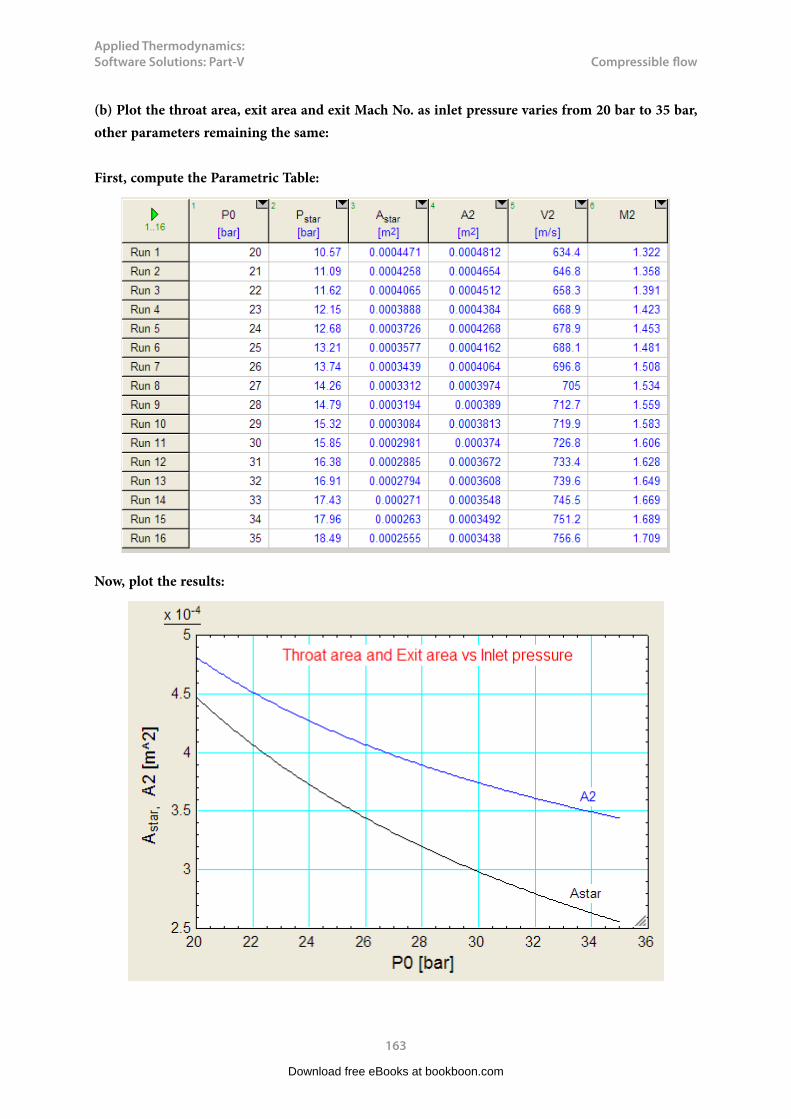
Applied Thermodynamics: Software Solutions: Part-V
163
Compressible flow
(b) Plot the throat area, exit area and exit Mach No. as inlet pressure varies from 20 bar to 35 bar, other parameters remaining the same:
First, compute the Parametric Table:
Now, plot the results:
Download free eBooks at bookboon.com

Applied Thermodynamics: Software Solutions: Part-V
164
Compressible flow
=======================================================================
“Prob.9.4.14 Consider a CD nozzle with throat area = 20 cm^2, exit area = 33.75 cm^2, inlet pressure = 10 bar, inlet temp = 800 K, negligible inlet velocity. Take k = 1.4, R = 287 J/kg.K for air. Determine: mass flow rate, exit pressure and exit Mach No. for following cases:
i. Isentropic flow with M = 0.7 at the throat,ii. Isentropic flow with M = 1 at the throat and diverging portion acting as diffuser,iii. Isentropic flow with M = 1 at the throat and diverging portion acting as nozzle,iv. Isentropic flow through nozzle with a normal shock standing at the exit,v. A normal shock stands in the diverging section where the area is 25 cm^2; elsewhere in the
nozzle, the flow is isentropic.”
Fig.Prob.9.4.14 Isentropic flow in a C-D nozzle
Download free eBooks at bookboon.com
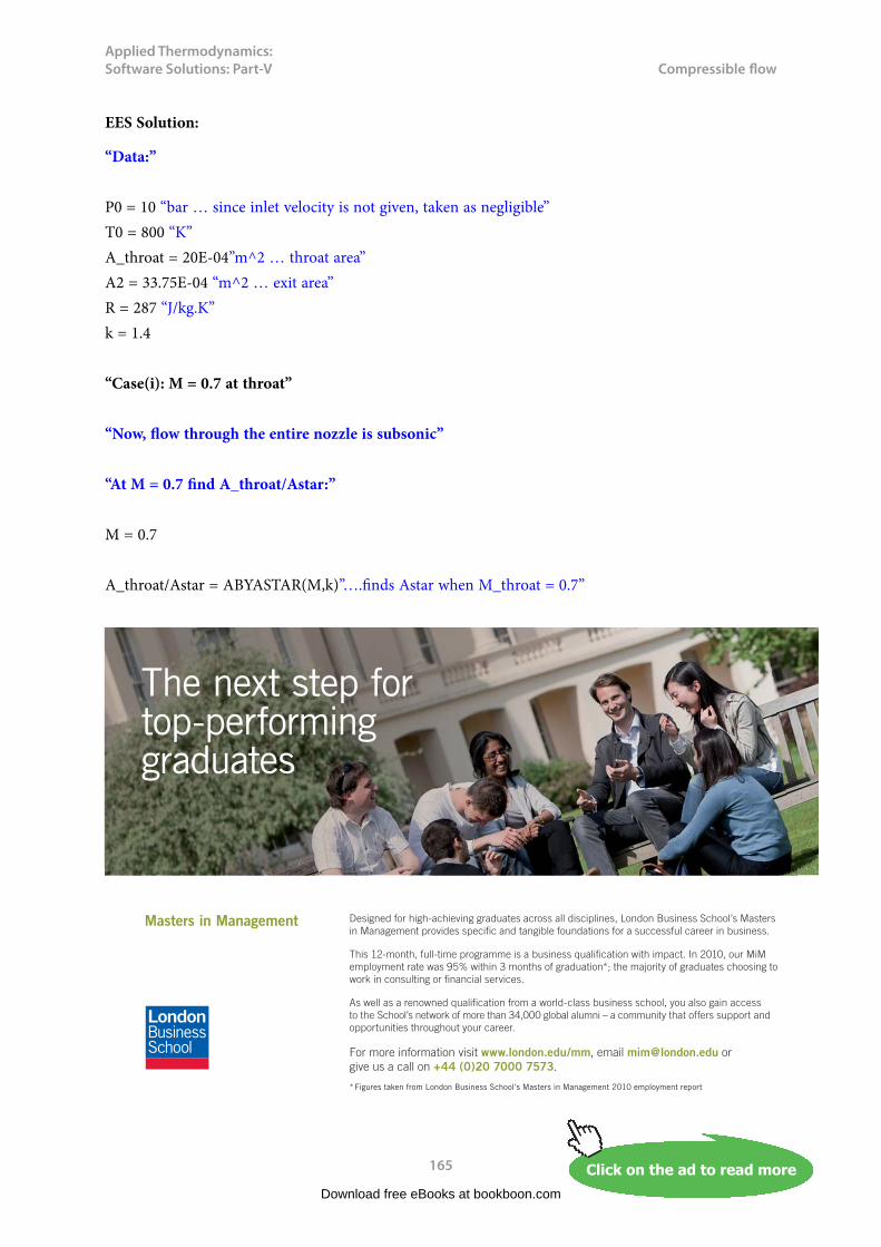
Applied Thermodynamics: Software Solutions: Part-V
165
Compressible flow
EES Solution:
“Data:”
P0 = 10 “bar … since inlet velocity is not given, taken as negligible”T0 = 800 “K”A_throat = 20E-04”m^2 … throat area”A2 = 33.75E-04 “m^2 … exit area”R = 287 “J/kg.K”k = 1.4
“Case(i): M = 0.7 at throat”
“Now, flow through the entire nozzle is subsonic”
“At M = 0.7 find A_throat/Astar:”
M = 0.7
A_throat/Astar = ABYASTAR(M,k)”….finds Astar when M_throat = 0.7”
Download free eBooks at bookboon.com
Click on the ad to read moreClick on the ad to read moreClick on the ad to read moreClick on the ad to read moreClick on the ad to read moreClick on the ad to read moreClick on the ad to read moreClick on the ad to read moreClick on the ad to read moreClick on the ad to read moreClick on the ad to read moreClick on the ad to read moreClick on the ad to read moreClick on the ad to read moreClick on the ad to read moreClick on the ad to read moreClick on the ad to read moreClick on the ad to read moreClick on the ad to read moreClick on the ad to read moreClick on the ad to read moreClick on the ad to read moreClick on the ad to read moreClick on the ad to read moreClick on the ad to read moreClick on the ad to read moreClick on the ad to read moreClick on the ad to read moreClick on the ad to read moreClick on the ad to read moreClick on the ad to read moreClick on the ad to read moreClick on the ad to read moreClick on the ad to read moreClick on the ad to read moreClick on the ad to read moreClick on the ad to read moreClick on the ad to read moreClick on the ad to read moreClick on the ad to read moreClick on the ad to read moreClick on the ad to read moreClick on the ad to read moreClick on the ad to read moreClick on the ad to read moreClick on the ad to read moreClick on the ad to read moreClick on the ad to read moreClick on the ad to read moreClick on the ad to read moreClick on the ad to read moreClick on the ad to read moreClick on the ad to read more
Designed for high-achieving graduates across all disciplines, London Business School’s Masters in Management provides specific and tangible foundations for a successful career in business.
This 12-month, full-time programme is a business qualification with impact. In 2010, our MiM employment rate was 95% within 3 months of graduation*; the majority of graduates choosing to work in consulting or financial services.
As well as a renowned qualification from a world-class business school, you also gain access to the School’s network of more than 34,000 global alumni – a community that offers support and opportunities throughout your career.
For more information visit www.london.edu/mm, email [email protected] or give us a call on +44 (0)20 7000 7573.
Masters in Management
The next step for top-performing graduates
* Figures taken from London Business School’s Masters in Management 2010 employment report
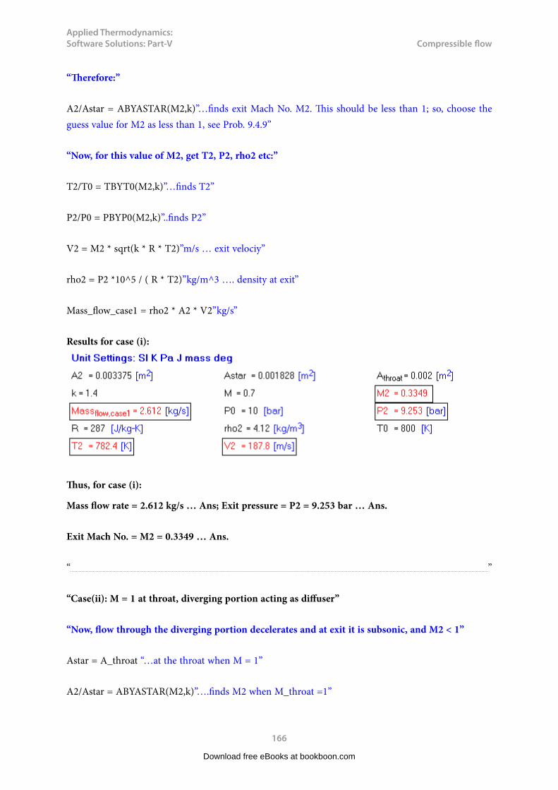
Applied Thermodynamics: Software Solutions: Part-V
166
Compressible flow
“Therefore:”
A2/Astar = ABYASTAR(M2,k)”…finds exit Mach No. M2. This should be less than 1; so, choose the guess value for M2 as less than 1, see Prob. 9.4.9”
“Now, for this value of M2, get T2, P2, rho2 etc:”
T2/T0 = TBYT0(M2,k)”…finds T2”
P2/P0 = PBYP0(M2,k)”..finds P2”
V2 = M2 * sqrt(k * R * T2)”m/s … exit velociy”
rho2 = P2 *10^5 / ( R * T2)”kg/m^3 …. density at exit”
Mass_flow_case1 = rho2 * A2 * V2”kg/s”
Results for case (i):
Thus, for case (i):
Mass flow rate = 2.612 kg/s … Ans; Exit pressure = P2 = 9.253 bar … Ans.
Exit Mach No. = M2 = 0.3349 … Ans.
“ ”
“Case(ii): M = 1 at throat, diverging portion acting as diffuser”
“Now, flow through the diverging portion decelerates and at exit it is subsonic, and M2 < 1”
Astar = A_throat “…at the throat when M = 1”
A2/Astar = ABYASTAR(M2,k)”….finds M2 when M_throat =1”
Download free eBooks at bookboon.com
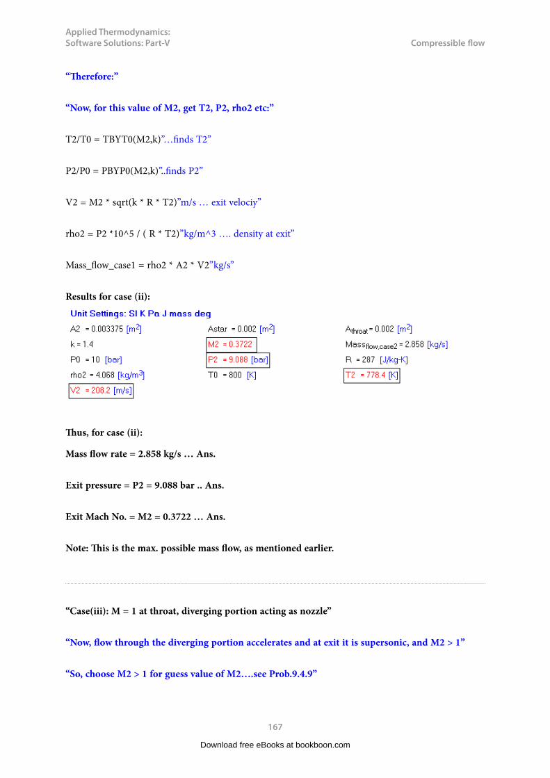
Applied Thermodynamics: Software Solutions: Part-V
167
Compressible flow
“Therefore:”
“Now, for this value of M2, get T2, P2, rho2 etc:”
T2/T0 = TBYT0(M2,k)”…finds T2”
P2/P0 = PBYP0(M2,k)”..finds P2”
V2 = M2 * sqrt(k * R * T2)”m/s … exit velociy”
rho2 = P2 *10^5 / ( R * T2)”kg/m^3 …. density at exit”
Mass_flow_case1 = rho2 * A2 * V2”kg/s”
Results for case (ii):
Thus, for case (ii):
Mass flow rate = 2.858 kg/s … Ans.
Exit pressure = P2 = 9.088 bar .. Ans.
Exit Mach No. = M2 = 0.3722 … Ans.
Note: This is the max. possible mass flow, as mentioned earlier.
“Case(iii): M = 1 at throat, diverging portion acting as nozzle”
“Now, flow through the diverging portion accelerates and at exit it is supersonic, and M2 > 1”
“So, choose M2 > 1 for guess value of M2….see Prob.9.4.9”
Download free eBooks at bookboon.com
Applied Thermodynamics: Software Solutions: Part-V
168
Compressible flow
Astar = A_throat “…at the throat since M = 1 at throat”
A2/Astar = ABYASTAR(M2,k)”….finds M2 when Mthroat =1”
“Therefore:”
“Now, for this value of M2, get T2, P2, rho2 etc:”
T2/T0 = TBYT0(M2,k)”…finds T2”
P2/P0 = PBYP0(M2,k)”..finds P2”
V2 = M2 * sqrt(k * R * T2)”m/s … exit velociy”
rho2 = P2 *10^5 / ( R * T2)”kg/m^3 …. density at exit”
Mass_flow_case3 = rho2 * A2 * V2”kg/s”
Download free eBooks at bookboon.com
Click on the ad to read moreClick on the ad to read moreClick on the ad to read moreClick on the ad to read moreClick on the ad to read moreClick on the ad to read moreClick on the ad to read moreClick on the ad to read moreClick on the ad to read moreClick on the ad to read moreClick on the ad to read moreClick on the ad to read moreClick on the ad to read moreClick on the ad to read moreClick on the ad to read moreClick on the ad to read moreClick on the ad to read moreClick on the ad to read moreClick on the ad to read moreClick on the ad to read moreClick on the ad to read moreClick on the ad to read moreClick on the ad to read moreClick on the ad to read moreClick on the ad to read moreClick on the ad to read moreClick on the ad to read moreClick on the ad to read moreClick on the ad to read moreClick on the ad to read moreClick on the ad to read moreClick on the ad to read moreClick on the ad to read moreClick on the ad to read moreClick on the ad to read moreClick on the ad to read moreClick on the ad to read moreClick on the ad to read moreClick on the ad to read moreClick on the ad to read moreClick on the ad to read moreClick on the ad to read moreClick on the ad to read moreClick on the ad to read moreClick on the ad to read moreClick on the ad to read moreClick on the ad to read moreClick on the ad to read moreClick on the ad to read moreClick on the ad to read moreClick on the ad to read moreClick on the ad to read moreClick on the ad to read moreClick on the ad to read more
Get Internationally Connected at the University of Surrey MA Intercultural Communication with International BusinessMA Communication and International Marketing
MA Intercultural Communication with International Business
Provides you with a critical understanding of communication in contemporary socio-cultural contexts by combining linguistic, cultural/media studies and international business and will prepare you for a wide range of careers.
MA Communication and International Marketing
Equips you with a detailed understanding of communication in contemporary international marketing contexts to enable you to address the market needs of the international business environment.
For further information contact:T: +44 (0)1483 681681E: [email protected]/downloads

Applied Thermodynamics: Software Solutions: Part-V
169
Compressible flow
Results for case (iii):
Thus, for case (iii):
Mass flow rate = 2.858 kg/s … Ans.
Exit pressure = P2 = 1.278 bar .. Ans.
Exit Mach No. = M2 = 2 … Ans.
Note: This is the max. possible mass flow for given geometry and stagn. Pressure and temp.
“ ”
“Case(iv): M = 1 at throat, Normal shock at exit:”
“So, just before the shock, we have Mx = M2 = 2, obtained from case(iii)”
Astar = A_throat “…at the throat since M = 1 at throat”
A2/Astar = ABYASTAR(M2,k)”….finds M2 when Mtroat =1”
Mx = M2
Px = 1.278 “bar = P2 from previous case”
Tx = 444.4 “K = T2 from previous case”
Download free eBooks at bookboon.com
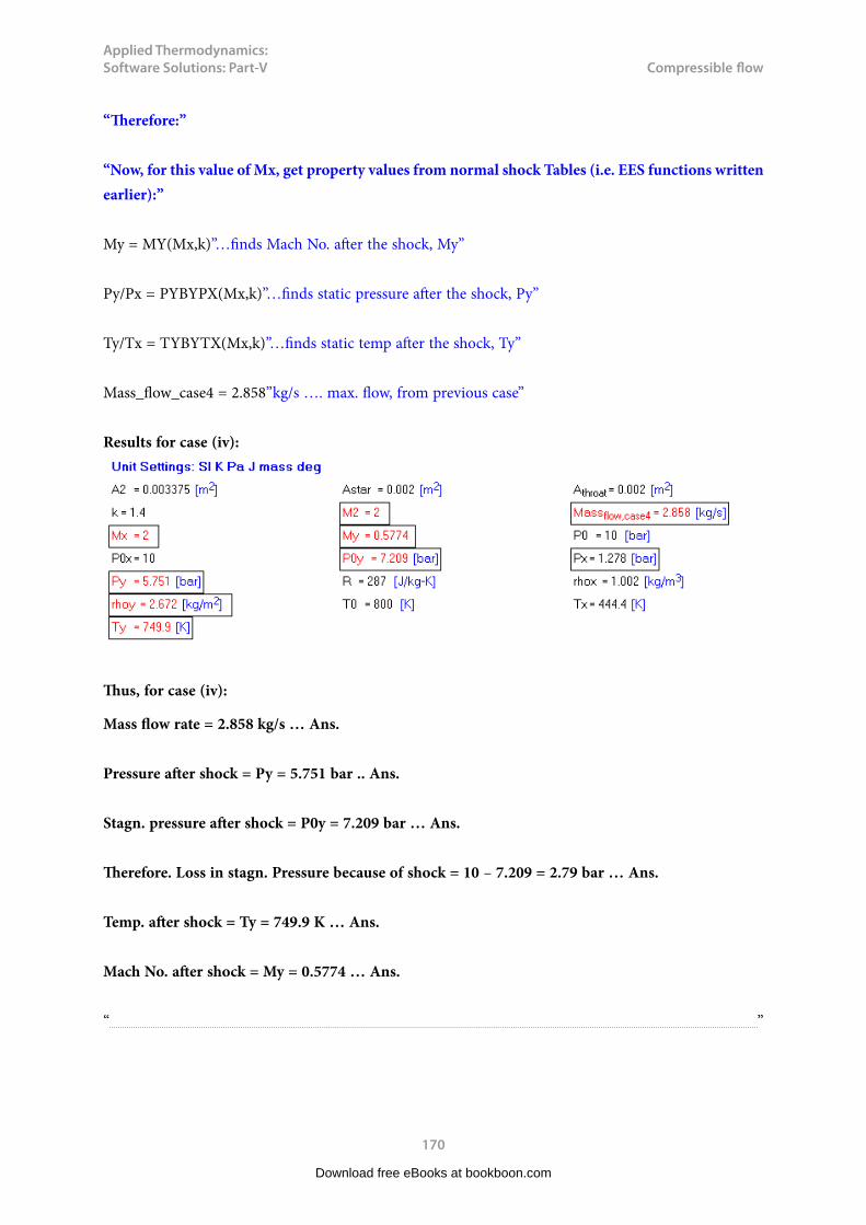
Applied Thermodynamics: Software Solutions: Part-V
170
Compressible flow
“Therefore:”
“Now, for this value of Mx, get property values from normal shock Tables (i.e. EES functions written earlier):”
My = MY(Mx,k)”…finds Mach No. after the shock, My”
Py/Px = PYBYPX(Mx,k)”…finds static pressure after the shock, Py”
Ty/Tx = TYBYTX(Mx,k)”…finds static temp after the shock, Ty”
Mass_flow_case4 = 2.858”kg/s …. max. flow, from previous case”
Results for case (iv):
Thus, for case (iv):
Mass flow rate = 2.858 kg/s … Ans.
Pressure after shock = Py = 5.751 bar .. Ans.
Stagn. pressure after shock = P0y = 7.209 bar … Ans.
Therefore. Loss in stagn. Pressure because of shock = 10 – 7.209 = 2.79 bar … Ans.
Temp. after shock = Ty = 749.9 K … Ans.
Mach No. after shock = My = 0.5774 … Ans.
“ ”
Download free eBooks at bookboon.com

Applied Thermodynamics: Software Solutions: Part-V
171
Compressible flow
“Case(v): M = 1 at throat, Normal shock at at a section where Ax = 25 cm^2:”
“So, Ax / Astar known. For this value of Ax/Astar, get Mx etc from isentropic functions:”
Astar = A_throat “…at the throat… since M = 1 at throat”
Ax = 25E-04”m^2”
Ay = Ax
Ax/Astar = ABYASTAR(Mx,k)”….finds Mx when Ax/Astar is known”
Px = P0 * PBYP0(Mx,k) “bar … finds Px”
Tx = T0 * TBYT0(Mx,k) “K … finds Tx “
Download free eBooks at bookboon.com
Click on the ad to read moreClick on the ad to read moreClick on the ad to read moreClick on the ad to read moreClick on the ad to read moreClick on the ad to read moreClick on the ad to read moreClick on the ad to read moreClick on the ad to read moreClick on the ad to read moreClick on the ad to read moreClick on the ad to read moreClick on the ad to read moreClick on the ad to read moreClick on the ad to read moreClick on the ad to read moreClick on the ad to read moreClick on the ad to read moreClick on the ad to read moreClick on the ad to read moreClick on the ad to read moreClick on the ad to read moreClick on the ad to read moreClick on the ad to read moreClick on the ad to read moreClick on the ad to read moreClick on the ad to read moreClick on the ad to read moreClick on the ad to read moreClick on the ad to read moreClick on the ad to read moreClick on the ad to read moreClick on the ad to read moreClick on the ad to read moreClick on the ad to read moreClick on the ad to read moreClick on the ad to read moreClick on the ad to read moreClick on the ad to read moreClick on the ad to read moreClick on the ad to read moreClick on the ad to read moreClick on the ad to read moreClick on the ad to read moreClick on the ad to read moreClick on the ad to read moreClick on the ad to read moreClick on the ad to read moreClick on the ad to read moreClick on the ad to read moreClick on the ad to read moreClick on the ad to read moreClick on the ad to read moreClick on the ad to read moreClick on the ad to read more
STEP INTO A WORLD OF OPPORTUNITYwww.ecco.com/[email protected]
Applied Thermodynamics: Software Solutions: Part-V
172
Compressible flow
“Therefore:”
My = MY(Mx,k)”…finds Mach No. after the shock, My”
Py/Px = PYBYPX(Mx,k)”…finds static pressure after the shock, Py”
Ty/Tx = TYBYTX(Mx,k)”…finds static temp after the shock, Ty”
rhoy = Py * 10^5 / (R * Ty) “…kg/m^3… density after shock”
rhoy/rhox = RHOYBYRHOX(Mx,k)”…finds rhox, kg/m^3”
P0x = P0 “..isentr. flow up to shock”
P0y/P0x = P0YBYP0x(Mx,k) “..finds P0y”
Mass_flow_case5 = 2.858”kg/s …. max. flow, from previous case”
“After the shock, flow is isentropic up to the exit.
Therefore, use the isentropic functions again:”
AybyAstar = ABYASTAR(My,k)
“Then:”
A2/Aystar = (A2/Ay) * (AybyAstar)
A2/Aystar = ABYASTAR(M2,k)”…finds M2 at exit”
“Now, corresponding to this M2, we have:”
Ty/T0y = TBYT0(My,k)”…finds T0y”
P2/P0y = PBYP0(M2,k)”..finds P2”
T2/T0y = TBYT0(M2,k)”…finds T2”
Stagn_Press_loss = P0x – P0y “bar”
V2 = M2 * sqrt(k * R * T2)”m/s … exit velociy”
Download free eBooks at bookboon.com

Applied Thermodynamics: Software Solutions: Part-V
173
Compressible flow
“Entropy increase in shock:”
DELTAS = DELTAS(Mx,R,k)”J/kg.K”
Results for case (v):
Thus, for case (v):
Mass flow rate = 2.858 kg/s … Ans.
Pressure after shock = Py = 6.635 bar .. Ans.
Stagn pressure after shock = P0y = 8.953 bar … Ans.
Therefore. Loss in stagn. pressure because of shock = (P0x – P0y) = 1.074 bar … Ans.
Temp. after shock = Ty = 734.4 K … Ans.
Mach No. after shock = My = 0.6685 … Ans.
Entropy change across shock = ΔS = 31.74 J/kg.K … Ans.
Exit pressure = P2 = 7.901 bar … Ans.
Exit temp = T2 = 771.9 K …. Ans.
=======================================================================
Download free eBooks at bookboon.com

Applied Thermodynamics: Software Solutions: Part-V
174
Compressible flow
“Prob.9.4.15 Air flows subsonically in an adiabatic 2 cm dia duct. Average friction factor is 0.006. What length of duct is necessary to accelerate the flow from M1 = 0.1 to M2 = 0.5? What additional length will accelerate it to M3 = 1? Assume k = 1.4”
Fig.Prob.9.4.15 Fanno flow
Download free eBooks at bookboon.com
Click on the ad to read moreClick on the ad to read moreClick on the ad to read moreClick on the ad to read moreClick on the ad to read moreClick on the ad to read moreClick on the ad to read moreClick on the ad to read moreClick on the ad to read moreClick on the ad to read moreClick on the ad to read moreClick on the ad to read moreClick on the ad to read moreClick on the ad to read moreClick on the ad to read moreClick on the ad to read moreClick on the ad to read moreClick on the ad to read moreClick on the ad to read moreClick on the ad to read moreClick on the ad to read moreClick on the ad to read moreClick on the ad to read moreClick on the ad to read moreClick on the ad to read moreClick on the ad to read moreClick on the ad to read moreClick on the ad to read moreClick on the ad to read moreClick on the ad to read moreClick on the ad to read moreClick on the ad to read moreClick on the ad to read moreClick on the ad to read moreClick on the ad to read moreClick on the ad to read moreClick on the ad to read moreClick on the ad to read moreClick on the ad to read moreClick on the ad to read moreClick on the ad to read moreClick on the ad to read moreClick on the ad to read moreClick on the ad to read moreClick on the ad to read moreClick on the ad to read moreClick on the ad to read moreClick on the ad to read moreClick on the ad to read moreClick on the ad to read moreClick on the ad to read moreClick on the ad to read moreClick on the ad to read moreClick on the ad to read moreClick on the ad to read moreClick on the ad to read more

Applied Thermodynamics: Software Solutions: Part-V
175
Compressible flow
EES Solution:
“Data:”
d = 0.02”m”
f = 0.006
M1 = 0.1
M2 = 0.5
M3 = 1
k = 1.4
“Calculations:”
“We use the EES Functions written earlier for Fanno flow:”
“At M1 = 0.1, find Lmax1:”
4 * f * Lmax1 /d = FANNO_FOURFLMAXBYD(M1,k) “…finds Lmax1 from the point where M1 = 0.1to the location where M = 1”
“At M2 = 0.5, find Lmax2:”
4 * f * Lmax2 /d = FANNO_FOURFLMAXBYD(M2,k) “…finds Lmax2 from the point where M = 0.5 to the location where M = 1”
“Therefore:”
DELTAL = Lmax1 – Lmax2”m… distance between locations where Mach Nos. are M1 and M2”
Results:
Download free eBooks at bookboon.com
Applied Thermodynamics: Software Solutions: Part-V
176
Compressible flow
Thus:
Distance between locations where Mach Nos. are M1 and M2 = dL = 54.88 m …Ans.
Distance between locations where Mach Nos. are M2 and M3 = Lmax2 = 0.8909 m … Ans.
Note: It takes 54.88 m to accelerate from M1 = 0.1 to M2 = 0.5, but takes only 0.89 m to reach sonic velocity (i.e. M = 1) from the location of M2 = 0.5
=======================================================================
“Prob.9.4.16 In the above problem, assume that at M1 = 0.1, the pressure and temp are: P1 = 600 kPa and T1 = 450 K respectively. At section 2 further downstream, M2 = 0.5. Compute P2, T2, V2 and P02.”
EES Solution:
“Data:”
M1 = 0.1
M2 = 0.5
P1 = 600”kPa”
T1 = 450”K”
k = 1.4
R = 287”J/kg.K”
“Calculations:”
“Find V1 and P01 at section1:”
V1 = M1 * sqrt(k * R * T1)
“From Isentropic functions, at M1 = 0.1:”
P1/P01 = PBYP0(M1,k)”…finds P01, kPa”
Download free eBooks at bookboon.com

Applied Thermodynamics: Software Solutions: Part-V
177
Compressible flow
“Now, use Fanno flow Functions to compute all properties downstream:”
P2/P1 = FANNO_PBYPSTAR(M2,k) / FANNO_PBYPSTAR(M1,k)”…finds P2, kPa”
T2/T1 = FANNO_TBYTSTAR(M2,k) / FANNO_TBYTSTAR(M1,k)”…finds T2, K”
V2/V1 = FANNO_VBYVSTAR(M2,k) / FANNO_VBYVSTAR(M1,k)”…finds V2, m/s”
P02/P01 = FANNO_P0BYP0STAR(M2,k) / FANNO_P0BYP0STAR(M1,k)”…finds P02, kPa”
Results:
Download free eBooks at bookboon.com
Click on the ad to read moreClick on the ad to read moreClick on the ad to read moreClick on the ad to read moreClick on the ad to read moreClick on the ad to read moreClick on the ad to read moreClick on the ad to read moreClick on the ad to read moreClick on the ad to read moreClick on the ad to read moreClick on the ad to read moreClick on the ad to read moreClick on the ad to read moreClick on the ad to read moreClick on the ad to read moreClick on the ad to read moreClick on the ad to read moreClick on the ad to read moreClick on the ad to read moreClick on the ad to read moreClick on the ad to read moreClick on the ad to read moreClick on the ad to read moreClick on the ad to read moreClick on the ad to read moreClick on the ad to read moreClick on the ad to read moreClick on the ad to read moreClick on the ad to read moreClick on the ad to read moreClick on the ad to read moreClick on the ad to read moreClick on the ad to read moreClick on the ad to read moreClick on the ad to read moreClick on the ad to read moreClick on the ad to read moreClick on the ad to read moreClick on the ad to read moreClick on the ad to read moreClick on the ad to read moreClick on the ad to read moreClick on the ad to read moreClick on the ad to read moreClick on the ad to read moreClick on the ad to read moreClick on the ad to read moreClick on the ad to read moreClick on the ad to read moreClick on the ad to read moreClick on the ad to read moreClick on the ad to read moreClick on the ad to read moreClick on the ad to read moreClick on the ad to read moreClick on the ad to read more
STUDY. PLAY.The stuff you'll need to make a good living The stuff that makes life worth living
NORWAY. YOUR IDEAL STUDY DESTINATION.
WWW.STUDYINNORWAY.NOFACEBOOK.COM/STUDYINNORWAY
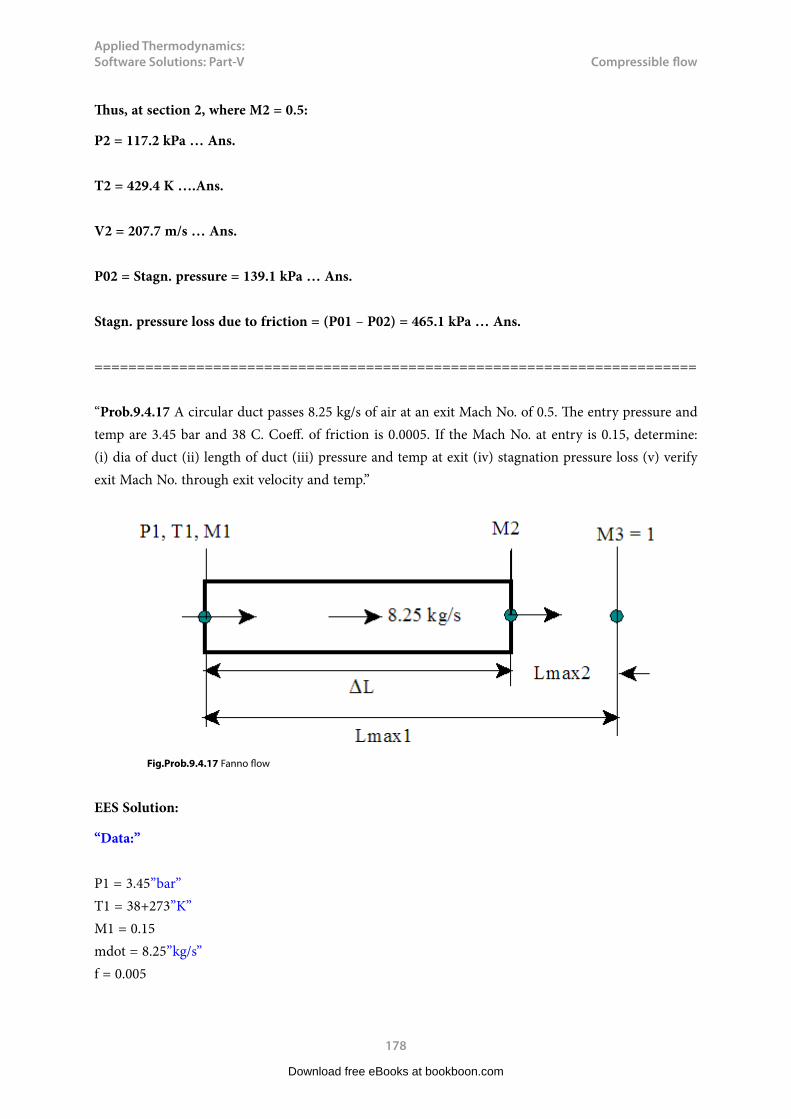
Applied Thermodynamics: Software Solutions: Part-V
178
Compressible flow
Thus, at section 2, where M2 = 0.5:
P2 = 117.2 kPa … Ans.
T2 = 429.4 K ….Ans.
V2 = 207.7 m/s … Ans.
P02 = Stagn. pressure = 139.1 kPa … Ans.
Stagn. pressure loss due to friction = (P01 – P02) = 465.1 kPa … Ans.
=======================================================================
“Prob.9.4.17 A circular duct passes 8.25 kg/s of air at an exit Mach No. of 0.5. The entry pressure and temp are 3.45 bar and 38 C. Coeff. of friction is 0.0005. If the Mach No. at entry is 0.15, determine: (i) dia of duct (ii) length of duct (iii) pressure and temp at exit (iv) stagnation pressure loss (v) verify exit Mach No. through exit velocity and temp.”
Fig.Prob.9.4.17 Fanno flow
EES Solution:
“Data:”
P1 = 3.45”bar”T1 = 38+273”K”M1 = 0.15mdot = 8.25”kg/s”f = 0.005
Download free eBooks at bookboon.com

Applied Thermodynamics: Software Solutions: Part-V
179
Compressible flow
M2 = 0.5k = 1.4R = 287”J/kg.K”
“Calculations:”
rho1 = P1*1E05/(R * T1)”kg/m^3….density at entry”
C1 = sqrt(k * R * T1) “m/s …. sonic velocity at entry”
V1 = M1 * C1 “m/s…velocity at entry”
mdot = rho1 * A1 * V1 “m^2 …. finds area at entry”
A1 = pi * d^2 / 4 “m….finds dia of duct”
“To find P01:”
“From Isentropic Functions:”
P1/P01 = PBYP0(M1,k)”….finds P01, bar”
“At M1 = 0.15, find Lmax1:”
4 * f * Lmax1 /d = FANNO_FOURFLMAXBYD(M1,k) “…finds Lmax1 from the point where M1 = 0.1to the location where M = 1”
“At M2 = 0.5, find Lmax2:”
4 * f * Lmax2 /d = FANNO_FOURFLMAXBYD(M2,k) “…finds Lmax2 from the point where M = 0.5 to the location where M = 1”
“Therefore:”
DELTAL = Lmax1 – Lmax2”m… distance between locations where Mach Nos. are M1 and M2”
“Now, find properties from Fanno flow Functions:”
P2/P1 = FANNO_PBYPSTAR(M2,k) / FANNO_PBYPSTAR(M1,k)”…finds P2, bar”
Download free eBooks at bookboon.com
Applied Thermodynamics: Software Solutions: Part-V
180
Compressible flow
T2/T1 = FANNO_TBYTSTAR(M2,k) / FANNO_TBYTSTAR(M1,k)”…finds T2, K”
V2/V1 = FANNO_VBYVSTAR(M2,k) / FANNO_VBYVSTAR(M1,k)”…finds V2, m/s”
P02/P01 = FANNO_P0BYP0STAR(M2,k) / FANNO_P0BYP0STAR(M1,k)”…finds P02, kPa”
“To verify M2:”
C2 = sqrt(k * R * T2)”m/s …. sonic vel. at exit”
“Therefore, M2_verify:”
M2_verify = V2/C2 “…should be equal to M2”
Download free eBooks at bookboon.com
Click on the ad to read moreClick on the ad to read moreClick on the ad to read moreClick on the ad to read moreClick on the ad to read moreClick on the ad to read moreClick on the ad to read moreClick on the ad to read moreClick on the ad to read moreClick on the ad to read moreClick on the ad to read moreClick on the ad to read moreClick on the ad to read moreClick on the ad to read moreClick on the ad to read moreClick on the ad to read moreClick on the ad to read moreClick on the ad to read moreClick on the ad to read moreClick on the ad to read moreClick on the ad to read moreClick on the ad to read moreClick on the ad to read moreClick on the ad to read moreClick on the ad to read moreClick on the ad to read moreClick on the ad to read moreClick on the ad to read moreClick on the ad to read moreClick on the ad to read moreClick on the ad to read moreClick on the ad to read moreClick on the ad to read moreClick on the ad to read moreClick on the ad to read moreClick on the ad to read moreClick on the ad to read moreClick on the ad to read moreClick on the ad to read moreClick on the ad to read moreClick on the ad to read moreClick on the ad to read moreClick on the ad to read moreClick on the ad to read moreClick on the ad to read moreClick on the ad to read moreClick on the ad to read moreClick on the ad to read moreClick on the ad to read moreClick on the ad to read moreClick on the ad to read moreClick on the ad to read moreClick on the ad to read moreClick on the ad to read moreClick on the ad to read moreClick on the ad to read moreClick on the ad to read moreClick on the ad to read more
Technical training on WHAT you need, WHEN you need it
At IDC Technologies we can tailor our technical and engineering training workshops to suit your needs. We have extensive
experience in training technical and engineering staff and have trained people in organisations such as General Motors, Shell, Siemens, BHP and Honeywell to name a few.Our onsite training is cost effective, convenient and completely customisable to the technical and engineering areas you want covered. Our workshops are all comprehensive hands-on learning experiences with ample time given to practical sessions and demonstrations. We communicate well to ensure that workshop content and timing match the knowledge, skills, and abilities of the participants.
We run onsite training all year round and hold the workshops on your premises or a venue of your choice for your convenience.
Phone: +61 8 9321 1702Email: [email protected] Website: www.idc-online.com
INDUSTRIALDATA COMMS
AUTOMATION & PROCESS CONTROL
ELECTRONICS
ELECTRICAL POWER
MECHANICAL ENGINEERING
OIL & GASENGINEERING
For a no obligation proposal, contact us today at [email protected] or visit our website for more information: www.idc-online.com/onsite/

Applied Thermodynamics: Software Solutions: Part-V
181
Compressible flow
Results:
Thus:
Dia of duct = d = 0.2264 m … Ans.
Length of duct = ΔL = 304.1 m … Ans.
Pressure at exit = P2 = 1.012 bar … Ans.
Temp at exit = T2 = 297.5 K … Ans.
Stagn. pressure loss = (P01 – P02) = 2.304 bar … Ans.
M2 = M2_verify ….verified…Ans.
=======================================================================
“Prob.9.4.18 Air at P0 = 10 bar, T0 = 400 K is supplied to a 50 mm dia pipe. Friction factor = 0.002. If Mach No. changes from 3 at entry to 1 at exit, determine: (i) the length of pipe (ii) mass flow rate.(b) Plot the variation of ΔL and mdot as M1 varies from 1.5 to 3.5, all other parameters remaining the same.”
Fig.Prob.9.4.18 Fanno flow
Download free eBooks at bookboon.com

Applied Thermodynamics: Software Solutions: Part-V
182
Compressible flow
EES Solution:
“Data:”
P0 = 10”bar”T0 = 400”K”M1 = 3 “….Mach No. at entry”M2 = 1 “….Mach No. at exit”d = 0.05”m…dia of pipe”f = 0.002k = 1.4R = 287”J/kg.K”
“Calculations:”
A = pi * d^2 / 4 “m^2 …. cross-sectional area of pipe”
“We shall use EES functions for Fanno flow, written earlier:”
“At M1 =3, find Lmax1:”
4 * f * Lmax1 /d = FANNO_FOURFLMAXBYD(M1,k) “…finds Lmax1 from the point where M1 = 3 to the location where M = 1, i.e. the exit, in the present case”
“Therefore:”
DELTAL = Lmax1”m… Length of pipe, i.e. distance between locations where Mach Nos. are M1 and M2”
“To find mass flow rate, mdot: We have: mdot = rho1 * A * V1:”
“Now, use the Isentropic Functions:”
“At M1 = 3:”
P1/P0 = PBYP0(M1,k)”…finds pressure at inlet, P1(bar)”
T1/T0 = TBYT0(M1,k)”…finds temp at inlet, T1 (K)”
“And:”
rho1 = P1*1E05 / (R * T1)”kg/m^3 …. density at inlet”
Download free eBooks at bookboon.com
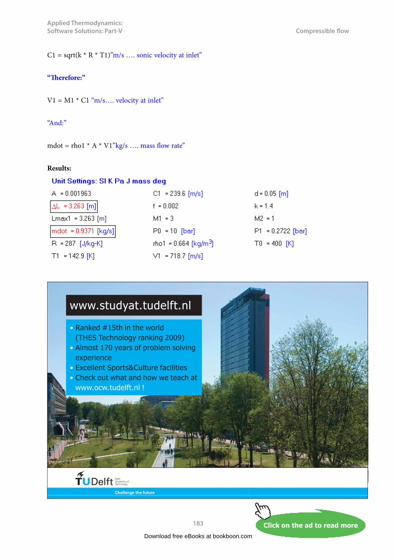
Applied Thermodynamics: Software Solutions: Part-V
183
Compressible flow
C1 = sqrt(k * R * T1)”m/s …. sonic velocity at inlet”
“Therefore:”
V1 = M1 * C1 “m/s…. velocity at inlet”
“And:”
mdot = rho1 * A * V1”kg/s …. mass flow rate”
Results:
Download free eBooks at bookboon.com
Click on the ad to read moreClick on the ad to read moreClick on the ad to read moreClick on the ad to read moreClick on the ad to read moreClick on the ad to read moreClick on the ad to read moreClick on the ad to read moreClick on the ad to read moreClick on the ad to read moreClick on the ad to read moreClick on the ad to read moreClick on the ad to read moreClick on the ad to read moreClick on the ad to read moreClick on the ad to read moreClick on the ad to read moreClick on the ad to read moreClick on the ad to read moreClick on the ad to read moreClick on the ad to read moreClick on the ad to read moreClick on the ad to read moreClick on the ad to read moreClick on the ad to read moreClick on the ad to read moreClick on the ad to read moreClick on the ad to read moreClick on the ad to read moreClick on the ad to read moreClick on the ad to read moreClick on the ad to read moreClick on the ad to read moreClick on the ad to read moreClick on the ad to read moreClick on the ad to read moreClick on the ad to read moreClick on the ad to read moreClick on the ad to read moreClick on the ad to read moreClick on the ad to read moreClick on the ad to read moreClick on the ad to read moreClick on the ad to read moreClick on the ad to read moreClick on the ad to read moreClick on the ad to read moreClick on the ad to read moreClick on the ad to read moreClick on the ad to read moreClick on the ad to read moreClick on the ad to read moreClick on the ad to read moreClick on the ad to read moreClick on the ad to read moreClick on the ad to read moreClick on the ad to read moreClick on the ad to read moreClick on the ad to read more
���������� ����� ��������� �������������������������������� �!�" ��#������"��$�%��&��!�"��'����� �(%����������(������ ��%�� ")*+� +���$����� ��"��*������+ ���� ����������� ������ �� ���,���, +��$ ,���-
���," +�� , +��$ ,��

Applied Thermodynamics: Software Solutions: Part-V
184
Compressible flow
Thus:
Length of pipe = ΔL = 3.263 m … Ans.
Mass flow rate = mdot = 0.9371 kg/s … Ans.
(b) Plot the variation of ΔL and mdot as M1 varies from 1.5 to 3.5, all other parameters remaining the same:
First, compute the Parametric Table:
Download free eBooks at bookboon.com
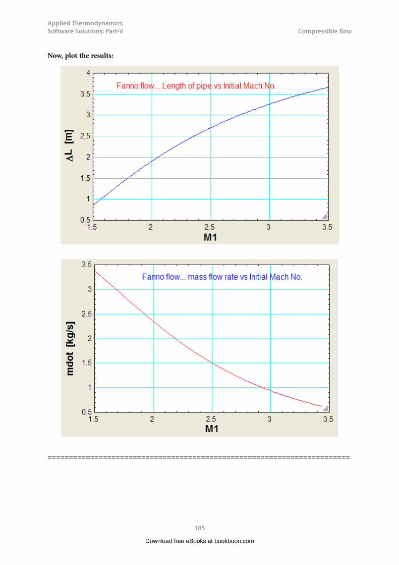
Applied Thermodynamics: Software Solutions: Part-V
185
Compressible flow
Now, plot the results:
=======================================================================
Download free eBooks at bookboon.com

Applied Thermodynamics: Software Solutions: Part-V
186
Compressible flow
“Prob.9.4.19 A fuel-air mixture, approximated as air with k = 1.4, enters a duct combustion chamber at V1 = 75 m/s, P1 = 150 kPa, T1 = 300 K. The heat addition by combustion is 900 kJ/kg. Compute: (i) the exit properties V2, P2, T2, and (ii) the total heat addition which would cause a sonic exit flow.”
Fig.Prob.9.4.19 Rayleigh flow
Download free eBooks at bookboon.com
Click on the ad to read moreClick on the ad to read moreClick on the ad to read moreClick on the ad to read moreClick on the ad to read moreClick on the ad to read moreClick on the ad to read moreClick on the ad to read moreClick on the ad to read moreClick on the ad to read moreClick on the ad to read moreClick on the ad to read moreClick on the ad to read moreClick on the ad to read moreClick on the ad to read moreClick on the ad to read moreClick on the ad to read moreClick on the ad to read moreClick on the ad to read moreClick on the ad to read moreClick on the ad to read moreClick on the ad to read moreClick on the ad to read moreClick on the ad to read moreClick on the ad to read moreClick on the ad to read moreClick on the ad to read moreClick on the ad to read moreClick on the ad to read moreClick on the ad to read moreClick on the ad to read moreClick on the ad to read moreClick on the ad to read moreClick on the ad to read moreClick on the ad to read moreClick on the ad to read moreClick on the ad to read moreClick on the ad to read moreClick on the ad to read moreClick on the ad to read moreClick on the ad to read moreClick on the ad to read moreClick on the ad to read moreClick on the ad to read moreClick on the ad to read moreClick on the ad to read moreClick on the ad to read moreClick on the ad to read moreClick on the ad to read moreClick on the ad to read moreClick on the ad to read moreClick on the ad to read moreClick on the ad to read moreClick on the ad to read moreClick on the ad to read moreClick on the ad to read moreClick on the ad to read moreClick on the ad to read moreClick on the ad to read moreClick on the ad to read more

Applied Thermodynamics: Software Solutions: Part-V
187
Compressible flow
EES Solution:
This is Rayleigh flow:
“Data:”
k = 1.4cp = 1005 “J/kg.K”R = 287”J/kg.K”V1 = 75”m/s”P1 = 150”kPa”T1 = 300”K”q = 9E05”J/kg”
“Calculations:”
T01 = T1 + V1^2/(2 * cp)”K….finds stagn. temp T01 at 1”
“Therefore:”
q = cp * (T02 – T01)”..finds T02(K)”
“Now:”
C1 = sqrt(k * R * T1)”m/s …. sonic velocity at 1”
“Then:”
M1 = V1 / C1”….Mach No. at 1”
“For this M1, find Rayleigh flow parameters using the EES functions for Rayleigh flow written earlier:”
T01/T0star = RAYLEIGH_T0BYT0STAR(M1,k)”….finds T0star”
“At section 2:”
T02/T0star = RAYLEIGH_T0BYT0STAR(M2,k)”…finds M2”
Download free eBooks at bookboon.com
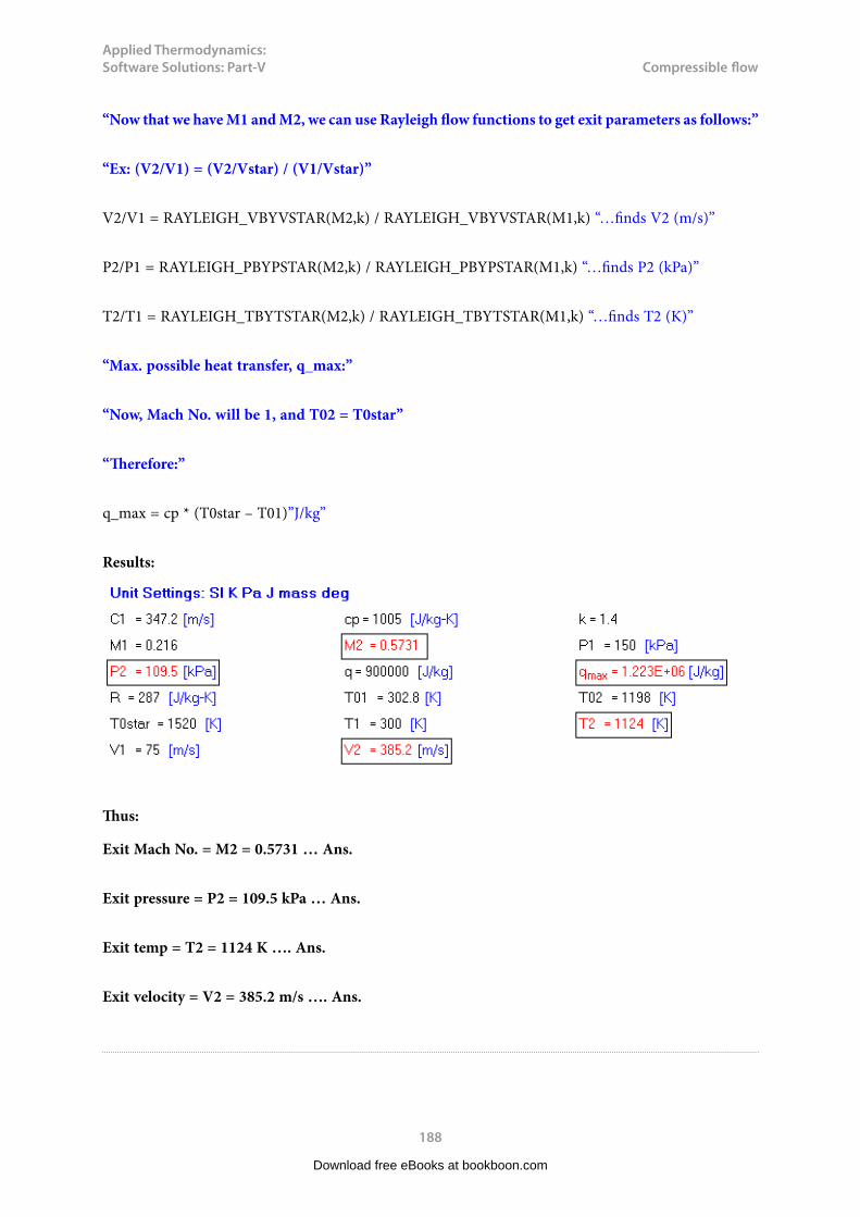
Applied Thermodynamics: Software Solutions: Part-V
188
Compressible flow
“Now that we have M1 and M2, we can use Rayleigh flow functions to get exit parameters as follows:”
“Ex: (V2/V1) = (V2/Vstar) / (V1/Vstar)”
V2/V1 = RAYLEIGH_VBYVSTAR(M2,k) / RAYLEIGH_VBYVSTAR(M1,k) “…finds V2 (m/s)”
P2/P1 = RAYLEIGH_PBYPSTAR(M2,k) / RAYLEIGH_PBYPSTAR(M1,k) “…finds P2 (kPa)”
T2/T1 = RAYLEIGH_TBYTSTAR(M2,k) / RAYLEIGH_TBYTSTAR(M1,k) “…finds T2 (K)”
“Max. possible heat transfer, q_max:”
“Now, Mach No. will be 1, and T02 = T0star”
“Therefore:”
q_max = cp * (T0star – T01)”J/kg”
Results:
Thus:
Exit Mach No. = M2 = 0.5731 … Ans.
Exit pressure = P2 = 109.5 kPa … Ans.
Exit temp = T2 = 1124 K …. Ans.
Exit velocity = V2 = 385.2 m/s …. Ans.
Download free eBooks at bookboon.com

Applied Thermodynamics: Software Solutions: Part-V
189
Compressible flow
(b) If T1 varies from 300 K to 600 K, how do other properties, including the max. possible heat transfer change?
First, compute the Parametric Table:
Download free eBooks at bookboon.com
Click on the ad to read moreClick on the ad to read moreClick on the ad to read moreClick on the ad to read moreClick on the ad to read moreClick on the ad to read moreClick on the ad to read moreClick on the ad to read moreClick on the ad to read moreClick on the ad to read moreClick on the ad to read moreClick on the ad to read moreClick on the ad to read moreClick on the ad to read moreClick on the ad to read moreClick on the ad to read moreClick on the ad to read moreClick on the ad to read moreClick on the ad to read moreClick on the ad to read moreClick on the ad to read moreClick on the ad to read moreClick on the ad to read moreClick on the ad to read moreClick on the ad to read moreClick on the ad to read moreClick on the ad to read moreClick on the ad to read moreClick on the ad to read moreClick on the ad to read moreClick on the ad to read moreClick on the ad to read moreClick on the ad to read moreClick on the ad to read moreClick on the ad to read moreClick on the ad to read moreClick on the ad to read moreClick on the ad to read moreClick on the ad to read moreClick on the ad to read moreClick on the ad to read moreClick on the ad to read moreClick on the ad to read moreClick on the ad to read moreClick on the ad to read moreClick on the ad to read moreClick on the ad to read moreClick on the ad to read moreClick on the ad to read moreClick on the ad to read moreClick on the ad to read moreClick on the ad to read moreClick on the ad to read moreClick on the ad to read moreClick on the ad to read moreClick on the ad to read moreClick on the ad to read moreClick on the ad to read moreClick on the ad to read moreClick on the ad to read moreClick on the ad to read more
DTU, Technical University of Denmark, is ranked as one of the best technical universities in Europe, and offers internationally recognised Master of Science degrees in 39 English-taught programmes.
DTU offers a unique environment where students have hands-on access to cutting edge facilities and work
closely under the expert supervision of top international researchers.
DTU’s central campus is located just north of Copenhagen and life at the University is engaging and vibrant. At DTU, we ensure that your goals and ambitions are met. Tuition is free for EU/EEA citizens.
Visit us at www.dtu.dk
Study at one of Europe’s leading universities
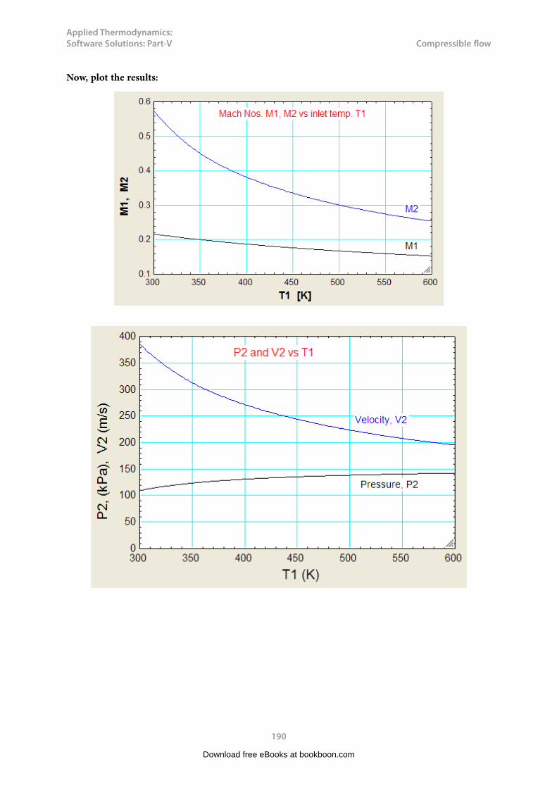
Applied Thermodynamics: Software Solutions: Part-V
190
Compressible flow
Now, plot the results:
Download free eBooks at bookboon.com
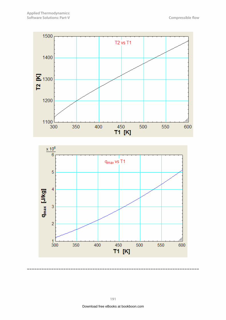
Applied Thermodynamics: Software Solutions: Part-V
191
Compressible flow
=======================================================================
Download free eBooks at bookboon.com
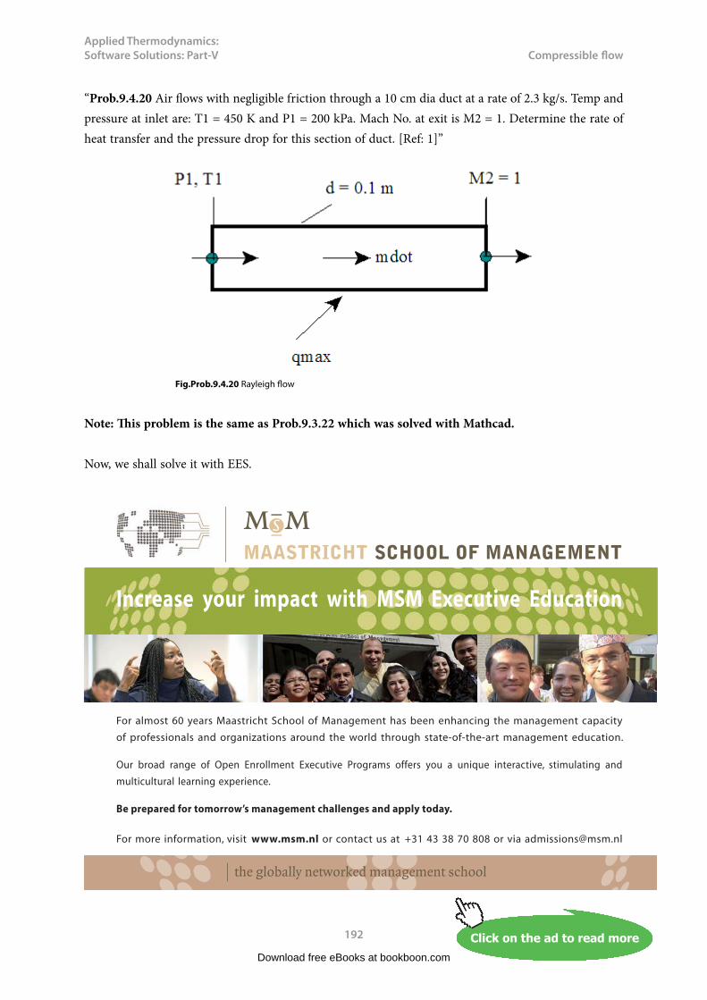
Applied Thermodynamics: Software Solutions: Part-V
192
Compressible flow
“Prob.9.4.20 Air flows with negligible friction through a 10 cm dia duct at a rate of 2.3 kg/s. Temp and pressure at inlet are: T1 = 450 K and P1 = 200 kPa. Mach No. at exit is M2 = 1. Determine the rate of heat transfer and the pressure drop for this section of duct. [Ref: 1]”
Fig.Prob.9.4.20 Rayleigh flow
Note: This problem is the same as Prob.9.3.22 which was solved with Mathcad.
Now, we shall solve it with EES.
Download free eBooks at bookboon.com
Click on the ad to read moreClick on the ad to read moreClick on the ad to read moreClick on the ad to read moreClick on the ad to read moreClick on the ad to read moreClick on the ad to read moreClick on the ad to read moreClick on the ad to read moreClick on the ad to read moreClick on the ad to read moreClick on the ad to read moreClick on the ad to read moreClick on the ad to read moreClick on the ad to read moreClick on the ad to read moreClick on the ad to read moreClick on the ad to read moreClick on the ad to read moreClick on the ad to read moreClick on the ad to read moreClick on the ad to read moreClick on the ad to read moreClick on the ad to read moreClick on the ad to read moreClick on the ad to read moreClick on the ad to read moreClick on the ad to read moreClick on the ad to read moreClick on the ad to read moreClick on the ad to read moreClick on the ad to read moreClick on the ad to read moreClick on the ad to read moreClick on the ad to read moreClick on the ad to read moreClick on the ad to read moreClick on the ad to read moreClick on the ad to read moreClick on the ad to read moreClick on the ad to read moreClick on the ad to read moreClick on the ad to read moreClick on the ad to read moreClick on the ad to read moreClick on the ad to read moreClick on the ad to read moreClick on the ad to read moreClick on the ad to read moreClick on the ad to read moreClick on the ad to read moreClick on the ad to read moreClick on the ad to read moreClick on the ad to read moreClick on the ad to read moreClick on the ad to read moreClick on the ad to read moreClick on the ad to read moreClick on the ad to read moreClick on the ad to read moreClick on the ad to read moreClick on the ad to read more
Increase your impact with MSM Executive Education
For more information, visit www.msm.nl or contact us at +31 43 38 70 808
or via [email protected] the globally networked management school
For more information, visit www.msm.nl or contact us at +31 43 38 70 808 or via [email protected]
For almost 60 years Maastricht School of Management has been enhancing the management capacity
of professionals and organizations around the world through state-of-the-art management education.
Our broad range of Open Enrollment Executive Programs offers you a unique interactive, stimulating and
multicultural learning experience.
Be prepared for tomorrow’s management challenges and apply today.
Executive Education-170x115-B2.indd 1 18-08-11 15:13

Applied Thermodynamics: Software Solutions: Part-V
193
Compressible flow
EES Solution:
This is Rayleigh flow.
“Data:”
k = 1.4cp = 1005 “J/kg.K”R = 287”J/kg.K”d = 0.1”m…dia of duct”P1 = 200”kPa”T1 = 450”K”mdot = 2.3”kg/s”M2 = 1”..Mach No. at exit”
“Calculations:”
A = pi * d^2 / 4 “m^2 …. cross-sectional area of duct”
rho1 = P1*1000 / (R * T1)”kg/m^3…density at inlet”
mdot = rho1 * A * V1”…finds inlet velocity, V1 (m/s)”
C1 = sqrt(k * R * T1)”m/s …. sonic velocity at inlet”
T01 = T1 + V1^2/(2 * cp)”K….finds stagn. temp T01 at 1”
“Therefore:”
M1 = V1 / C1 “…Mach No. at inlet”
“And:”
T01/T0star = RAYLEIGH_T0BYT0STAR(M1,k)”….finds T0star”
“Now that we have M1 and M2, we can use Rayleigh flow functions to get exit parameters as follows:”
“Ex: (V2/V1) = (V2/Vstar) / (V1/Vstar) … etc.”
V2/V1 = RAYLEIGH_VBYVSTAR(M2,k) / RAYLEIGH_VBYVSTAR(M1,k) “…finds V2 (m/s)”
Download free eBooks at bookboon.com

Applied Thermodynamics: Software Solutions: Part-V
194
Compressible flow
P2/P1 = RAYLEIGH_PBYPSTAR(M2,k) / RAYLEIGH_PBYPSTAR(M1,k) “…finds P2 (kPa)”
T2/T1 = RAYLEIGH_TBYTSTAR(M2,k) / RAYLEIGH_TBYTSTAR(M1,k) “…finds T2 (K)”
“Max. possible heat transfer, qmax when M2 = 1:”
“Then: T02 = T0star”
“Therefore:”
q_max = cp * (T0star – T01)”J/kg”
“Pressure drop:”
DELTAP = (P1 – P2) “kPa”
“Entropy change:”
DELTAS = RAYLEIGH_DELTAS(M1, M2, R, k) “..using the EES Function written earlier”
“Verify the heat transfer qmax using the EES Function for Q written earlier:”
qmax2 = RAYLEIGH_Q(M1, M2, cp, T1, k)
Results:
Download free eBooks at bookboon.com

Applied Thermodynamics: Software Solutions: Part-V
195
Compressible flow
Thus:
At the inlet: M1 = 0.4447 … Ans.
At the exit: M2 = 1, P2 = 106.4 kPa, V2 = 508.7 m/s, T2 = 644 K … Ans.
Pressure drop = ΔP = 93.59 kPa … Ans.
Heat transfer = qmax = 306572 J/kg … Ans.
Entropy change = Δs = 541.2 J/kg.K … Ans.
qmax2 = 306579 J/kg … using the EES Function written earlier…should be equal to qmax ,… verified.
=======================================================================
“Prob.9.4.21 Heat is added to air flowing in a duct until it is choked, and the amount of heat added is 600 kJ/kg. The exit temp is 1000 K. Calculate the temp and Mach No. at entry. [Ref: 11]”
Download free eBooks at bookboon.com
Click on the ad to read moreClick on the ad to read moreClick on the ad to read moreClick on the ad to read moreClick on the ad to read moreClick on the ad to read moreClick on the ad to read moreClick on the ad to read moreClick on the ad to read moreClick on the ad to read moreClick on the ad to read moreClick on the ad to read moreClick on the ad to read moreClick on the ad to read moreClick on the ad to read moreClick on the ad to read moreClick on the ad to read moreClick on the ad to read moreClick on the ad to read moreClick on the ad to read moreClick on the ad to read moreClick on the ad to read moreClick on the ad to read moreClick on the ad to read moreClick on the ad to read moreClick on the ad to read moreClick on the ad to read moreClick on the ad to read moreClick on the ad to read moreClick on the ad to read moreClick on the ad to read moreClick on the ad to read moreClick on the ad to read moreClick on the ad to read moreClick on the ad to read moreClick on the ad to read moreClick on the ad to read moreClick on the ad to read moreClick on the ad to read moreClick on the ad to read moreClick on the ad to read moreClick on the ad to read moreClick on the ad to read moreClick on the ad to read moreClick on the ad to read moreClick on the ad to read moreClick on the ad to read moreClick on the ad to read moreClick on the ad to read moreClick on the ad to read moreClick on the ad to read moreClick on the ad to read moreClick on the ad to read moreClick on the ad to read moreClick on the ad to read moreClick on the ad to read moreClick on the ad to read moreClick on the ad to read moreClick on the ad to read moreClick on the ad to read moreClick on the ad to read moreClick on the ad to read moreClick on the ad to read more
EXPERIENCE THE POWER OF FULL ENGAGEMENT…
RUN FASTER. RUN LONGER.. RUN EASIER…
READ MORE & PRE-ORDER TODAY WWW.GAITEYE.COM
Challenge the way we run
1349906_A6_4+0.indd 1 22-08-2014 12:56:57
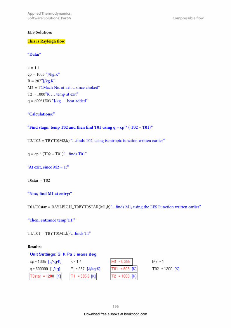
Applied Thermodynamics: Software Solutions: Part-V
196
Compressible flow
EES Solution:
This is Rayleigh flow.
“Data:”
k = 1.4cp = 1005 “J/kg.K”R = 287”J/kg.K”M2 = 1”..Mach No. at exit .. since choked”T2 = 1000”K … temp at exit”q = 600*1E03 “J/kg … heat added”
“Calculations:”
“Find stagn. temp T02 and then find T01 using q = cp * ( T02 – T01)”
T2/T02 = TBYT0(M2,k) “…finds T02..using isentropic function written earlier”
q = cp * (T02 – T01)”…finds T01”
“At exit, since M2 = 1:”
T0star = T02
“Now, find M1 at entry:”
T01/T0star = RAYLEIGH_T0BYT0STAR(M1,k)”…finds M1, using the EES Function written earlier”
“Then, entrance temp T1:”
T1/T01 = TBYT0(M1,k)”…finds T1”
Results:
Download free eBooks at bookboon.com

Applied Thermodynamics: Software Solutions: Part-V
197
Compressible flow
Thus:
Temp at entry = T1 = 585.6 K …. Ans.
Mach No. at entry = M1 = 0.385 … Ans.
Note: See the ease with which these complicated eqns are solved with EES Functions. No need to refer to Rayleigh Tables and interpolate.
=======================================================================
9.5 Problems solved with TEST:
Like other calculators (or ‘daemons’) in TEST, Gas Dynamics calculator is very easy and convenient to use.
It is assumed that you have already done free registration at the web-site www.thermofluids.net.
Now, as you go to www.thermofluids.net, you are asked to enter your email address and the password. On supplying that information, the opening screen with a personal greeting appears. Click on ‘TESTCalcs’ on the Menu bar at the bottom of the window. We get the TESTCalcs tree, from which you can choose the ‘Gas Dynamics’ calculator, at the right hand bottom corner, as shown below:
Download free eBooks at bookboon.com

Applied Thermodynamics: Software Solutions: Part-V
198
Compressible flow
Hovering the mouse pointer over the ‘Gas Dynamics’ gives the following explanatory window:
Download free eBooks at bookboon.com
Click on the ad to read moreClick on the ad to read moreClick on the ad to read moreClick on the ad to read moreClick on the ad to read moreClick on the ad to read moreClick on the ad to read moreClick on the ad to read moreClick on the ad to read moreClick on the ad to read moreClick on the ad to read moreClick on the ad to read moreClick on the ad to read moreClick on the ad to read moreClick on the ad to read moreClick on the ad to read moreClick on the ad to read moreClick on the ad to read moreClick on the ad to read moreClick on the ad to read moreClick on the ad to read moreClick on the ad to read moreClick on the ad to read moreClick on the ad to read moreClick on the ad to read moreClick on the ad to read moreClick on the ad to read moreClick on the ad to read moreClick on the ad to read moreClick on the ad to read moreClick on the ad to read moreClick on the ad to read moreClick on the ad to read moreClick on the ad to read moreClick on the ad to read moreClick on the ad to read moreClick on the ad to read moreClick on the ad to read moreClick on the ad to read moreClick on the ad to read moreClick on the ad to read moreClick on the ad to read moreClick on the ad to read moreClick on the ad to read moreClick on the ad to read moreClick on the ad to read moreClick on the ad to read moreClick on the ad to read moreClick on the ad to read moreClick on the ad to read moreClick on the ad to read moreClick on the ad to read moreClick on the ad to read moreClick on the ad to read moreClick on the ad to read moreClick on the ad to read moreClick on the ad to read moreClick on the ad to read moreClick on the ad to read moreClick on the ad to read moreClick on the ad to read moreClick on the ad to read moreClick on the ad to read moreClick on the ad to read more
GET THERE FASTER
Oliver Wyman is a leading global management consulting firm that combines
deep industry knowledge with specialized expertise in strategy, operations, risk
management, organizational transformation, and leadership development. With
offices in 50+ cities across 25 countries, Oliver Wyman works with the CEOs and
executive teams of Global 1000 companies.
An equal opportunity employer.
Some people know precisely where they want to go. Others seek the adventure of discovering uncharted territory. Whatever you want your professional journey to be, you’ll find what you’re looking for at Oliver Wyman.
Discover the world of Oliver Wyman at oliverwyman.com/careers
DISCOVEROUR WORLD

Applied Thermodynamics: Software Solutions: Part-V
199
Compressible flow
Click on ‘Gas Dynamics’, and the following window appears:
Note from the above screen print that there are 4 tabs: State Panel, Device Panel, Table Panel and I/O Panel. By default, State Panel is selected.
Click on ‘Device Panel’ tab, and we get:
Download free eBooks at bookboon.com
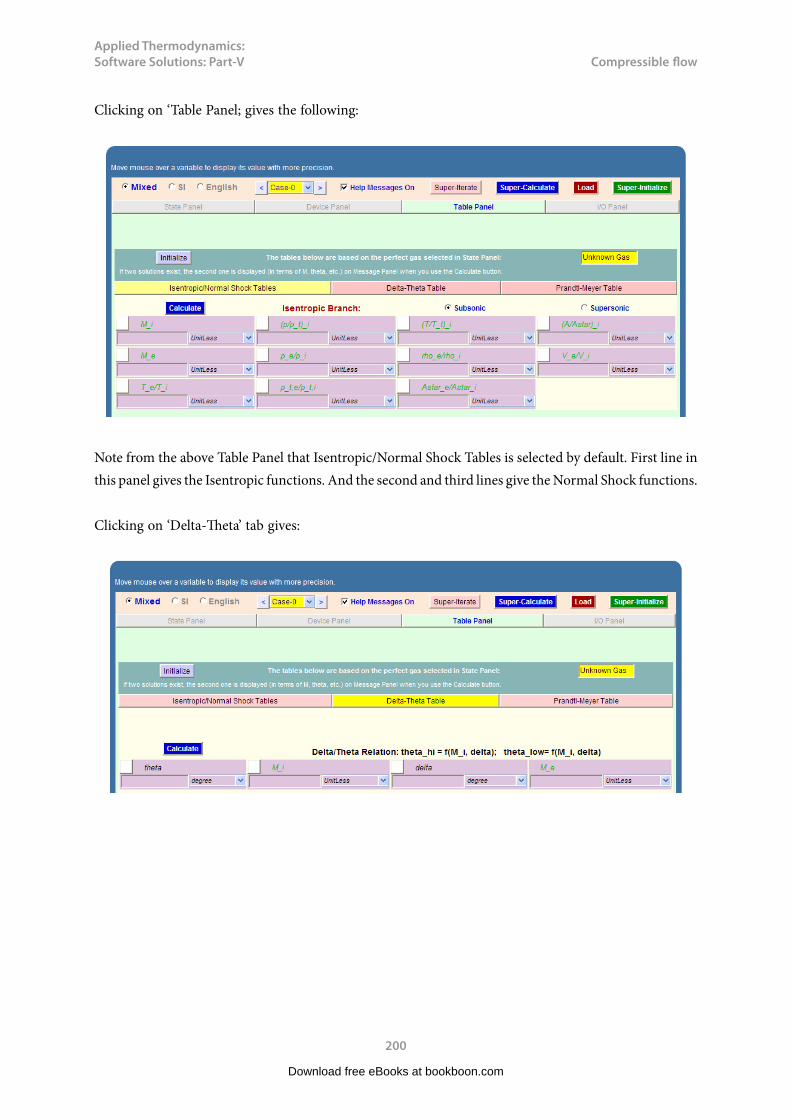
Applied Thermodynamics: Software Solutions: Part-V
200
Compressible flow
Clicking on ‘Table Panel; gives the following:
Note from the above Table Panel that Isentropic/Normal Shock Tables is selected by default. First line in this panel gives the Isentropic functions. And the second and third lines give the Normal Shock functions.
Clicking on ‘Delta-Theta’ tab gives:
Download free eBooks at bookboon.com

Applied Thermodynamics: Software Solutions: Part-V
201
Compressible flow
And, clicking on Prandtl – Mayer Table gives:
With this brief introduction to Gas Dynamics calculator, let us solve a few problems in TEST:
Prob.9.5.1 An airplane is flying at a speed of 920 km/h at an altitude of 10 km where the temp is -50 C. Determine if the speed of this airplane is subsonic or supersonic. [Ref: 1]
Download free eBooks at bookboon.com
Click on the ad to read moreClick on the ad to read moreClick on the ad to read moreClick on the ad to read moreClick on the ad to read moreClick on the ad to read moreClick on the ad to read moreClick on the ad to read moreClick on the ad to read moreClick on the ad to read moreClick on the ad to read moreClick on the ad to read moreClick on the ad to read moreClick on the ad to read moreClick on the ad to read moreClick on the ad to read moreClick on the ad to read moreClick on the ad to read moreClick on the ad to read moreClick on the ad to read moreClick on the ad to read moreClick on the ad to read moreClick on the ad to read moreClick on the ad to read moreClick on the ad to read moreClick on the ad to read moreClick on the ad to read moreClick on the ad to read moreClick on the ad to read moreClick on the ad to read moreClick on the ad to read moreClick on the ad to read moreClick on the ad to read moreClick on the ad to read moreClick on the ad to read moreClick on the ad to read moreClick on the ad to read moreClick on the ad to read moreClick on the ad to read moreClick on the ad to read moreClick on the ad to read moreClick on the ad to read moreClick on the ad to read moreClick on the ad to read moreClick on the ad to read moreClick on the ad to read moreClick on the ad to read moreClick on the ad to read moreClick on the ad to read moreClick on the ad to read moreClick on the ad to read moreClick on the ad to read moreClick on the ad to read moreClick on the ad to read moreClick on the ad to read moreClick on the ad to read moreClick on the ad to read moreClick on the ad to read moreClick on the ad to read moreClick on the ad to read moreClick on the ad to read moreClick on the ad to read moreClick on the ad to read moreClick on the ad to read moreClick on the ad to read more

Applied Thermodynamics: Software Solutions: Part-V
202
Compressible flow
TEST Solution:
From the Thermodynamic Tables in Text books, pressure at an altitude of 10 km is read as: 26.5 kPa.
Go to Gas Dynamics calculator (as already explained). Choose air as the substance. In the State Panel, for State 1: enter p1, T1 and Vel1 as shown. Hit Enter (or click on Calculate). We get:
Thus:
Mach No. = Mach1 = 0.8533.
Therefore, speed of the airplane is subsonic…. Ans.
Note that other properties such as density (rho1), sp. volume (v1), enthalpy (h1), stagnation (or total) temp (T_t1), stagnation pressure (p_t1) etc are also available in the same panel.
=======================================================================
Prob.9.5.2 Calculate the critical temp, pressure, and density of (i) air at 200 kPa, 100 C, and 250 m/s, and (ii) helium at 200 kPa, 40 C and 300 m/s. [Ref: 1]
Download free eBooks at bookboon.com

Applied Thermodynamics: Software Solutions: Part-V
203
Compressible flow
TEST Solution:
i. For Air:
Go to Gas Dynamics calculator. In the State Panel, select Air as working substance. Enter values of p1, T1 and Vel1 as shown. Hit Enter. We get:
Now, critical properties refer to M = 1. So, go to State 2, and for Isentropicflow, enter: p_t2 = p_t1, T_t2 = T_t1, and M = 1, and hit Enter. We get:
Thus:
#critical pressure = p2 = 139.85 kPa … Ans.
#critical temp = 2 = 336.91 K .. Ans.
#critical density = rho2 = 1.4464 kg/m^3 … Ans.
Download free eBooks at bookboon.com
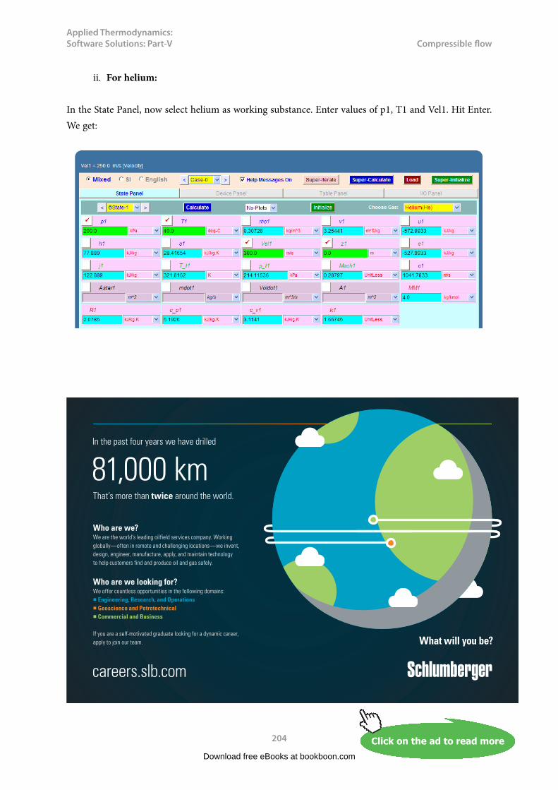
Applied Thermodynamics: Software Solutions: Part-V
204
Compressible flow
ii. For helium:
In the State Panel, now select helium as working substance. Enter values of p1, T1 and Vel1. Hit Enter. We get:
Download free eBooks at bookboon.com
Click on the ad to read moreClick on the ad to read moreClick on the ad to read moreClick on the ad to read moreClick on the ad to read moreClick on the ad to read moreClick on the ad to read moreClick on the ad to read moreClick on the ad to read moreClick on the ad to read moreClick on the ad to read moreClick on the ad to read moreClick on the ad to read moreClick on the ad to read moreClick on the ad to read moreClick on the ad to read moreClick on the ad to read moreClick on the ad to read moreClick on the ad to read moreClick on the ad to read moreClick on the ad to read moreClick on the ad to read moreClick on the ad to read moreClick on the ad to read moreClick on the ad to read moreClick on the ad to read moreClick on the ad to read moreClick on the ad to read moreClick on the ad to read moreClick on the ad to read moreClick on the ad to read moreClick on the ad to read moreClick on the ad to read moreClick on the ad to read moreClick on the ad to read moreClick on the ad to read moreClick on the ad to read moreClick on the ad to read moreClick on the ad to read moreClick on the ad to read moreClick on the ad to read moreClick on the ad to read moreClick on the ad to read moreClick on the ad to read moreClick on the ad to read moreClick on the ad to read moreClick on the ad to read moreClick on the ad to read moreClick on the ad to read moreClick on the ad to read moreClick on the ad to read moreClick on the ad to read moreClick on the ad to read moreClick on the ad to read moreClick on the ad to read moreClick on the ad to read moreClick on the ad to read moreClick on the ad to read moreClick on the ad to read moreClick on the ad to read moreClick on the ad to read moreClick on the ad to read moreClick on the ad to read moreClick on the ad to read moreClick on the ad to read moreClick on the ad to read more
81,000 kmIn the past four years we have drilled
That’s more than twice around the world.
What will you be?
Who are we?We are the world’s leading oilfield services company. Working globally—often in remote and challenging locations—we invent, design, engineer, manufacture, apply, and maintain technology to help customers find and produce oil and gas safely.
Who are we looking for?We offer countless opportunities in the following domains:n Engineering, Research, and Operationsn Geoscience and Petrotechnicaln Commercial and Business
If you are a self-motivated graduate looking for a dynamic career, apply to join our team.
careers.slb.com
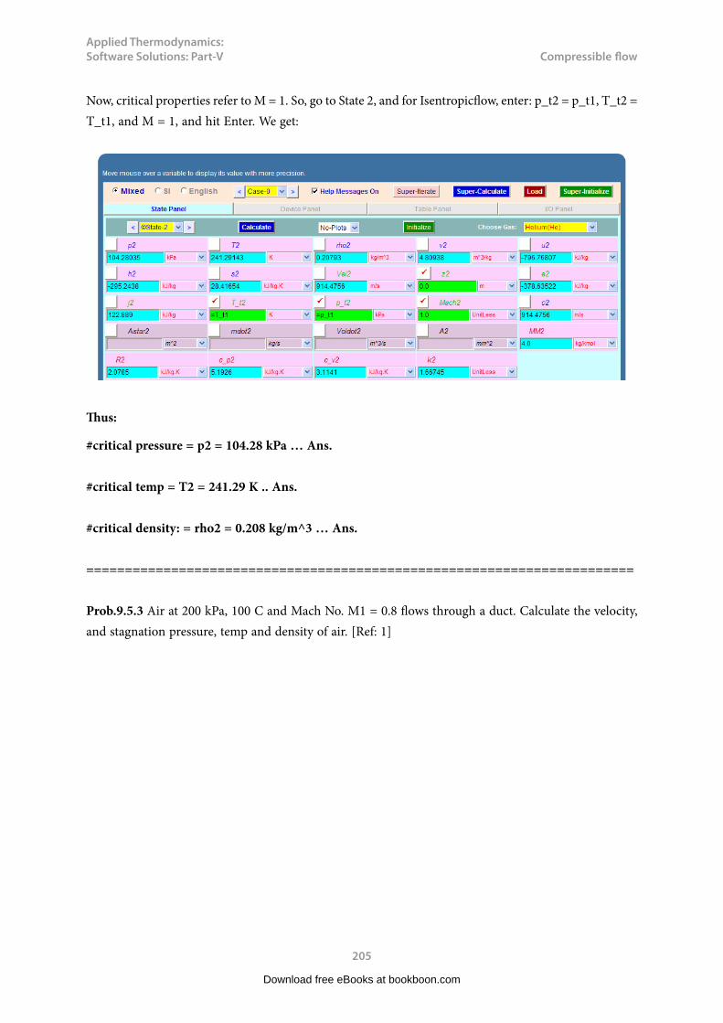
Applied Thermodynamics: Software Solutions: Part-V
205
Compressible flow
Now, critical properties refer to M = 1. So, go to State 2, and for Isentropicflow, enter: p_t2 = p_t1, T_t2 = T_t1, and M = 1, and hit Enter. We get:
Thus:
#critical pressure = p2 = 104.28 kPa … Ans.
#critical temp = T2 = 241.29 K .. Ans.
#critical density: = rho2 = 0.208 kg/m^3 … Ans.
=======================================================================
Prob.9.5.3 Air at 200 kPa, 100 C and Mach No. M1 = 0.8 flows through a duct. Calculate the velocity, and stagnation pressure, temp and density of air. [Ref: 1]
Download free eBooks at bookboon.com

Applied Thermodynamics: Software Solutions: Part-V
206
Compressible flow
TEST Solution:
Go to Gas Dynamics calculator. In the State Panel, select Air as working substance. Enter values of p1, T1 and Mach1 as shown. Hit Enter. We get:
We note the results:
Velocity, Vel1 = 309.727 m/s … Ans.
Stagn. pressure = p_t1 = 304.85 kPa … Ans.
Stagn. temp = T_t1 = 420.88 K … Ans.
Density = rho1 = 1.8676 kg/m^3 … Ans.
=======================================================================
Prob.9.5.4 Air is contained in a reservoir at 5 MPa, 21 C and flows out at a rate of 1 kg/s through a tube. At a particular location the static pressure is measured as 3 MPa. Neglect the velocity at the reservoir and assuming isentropic flow, calculate the Mach No., velocity and area at that location. [Ref: 11]
TEST Solution:
Since velocity is negligible at reservoir, P1 and T1 are: stagn. pressure and stagn. temp. Let the reservoir be designated by state 1.
At the given location, say state 2, P2 is known. For isentropic flow, use the condition that stagn. pressure and stagn. temp remain constant, i.e. p_t1 = p_t2 , and T_t1 = T_t2.
Download free eBooks at bookboon.com
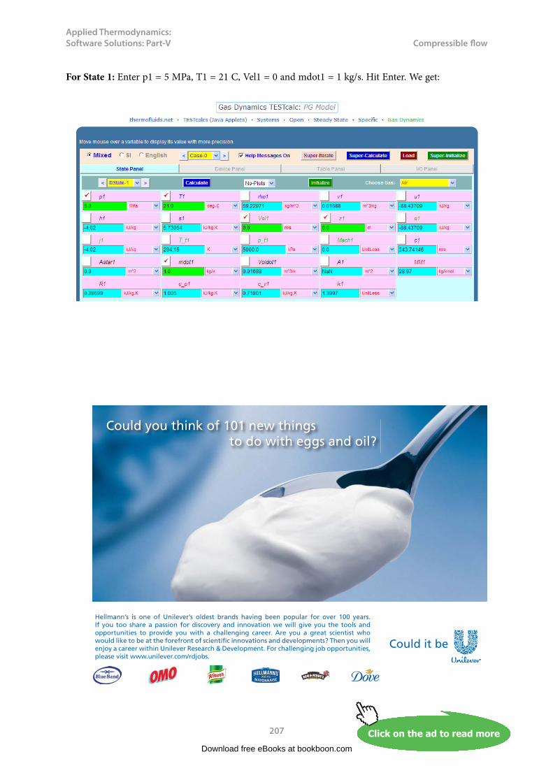
Applied Thermodynamics: Software Solutions: Part-V
207
Compressible flow
For State 1: Enter p1 = 5 MPa, T1 = 21 C, Vel1 = 0 and mdot1 = 1 kg/s. Hit Enter. We get:
Download free eBooks at bookboon.com
Click on the ad to read moreClick on the ad to read moreClick on the ad to read moreClick on the ad to read moreClick on the ad to read moreClick on the ad to read moreClick on the ad to read moreClick on the ad to read moreClick on the ad to read moreClick on the ad to read moreClick on the ad to read moreClick on the ad to read moreClick on the ad to read moreClick on the ad to read moreClick on the ad to read moreClick on the ad to read moreClick on the ad to read moreClick on the ad to read moreClick on the ad to read moreClick on the ad to read moreClick on the ad to read moreClick on the ad to read moreClick on the ad to read moreClick on the ad to read moreClick on the ad to read moreClick on the ad to read moreClick on the ad to read moreClick on the ad to read moreClick on the ad to read moreClick on the ad to read moreClick on the ad to read moreClick on the ad to read moreClick on the ad to read moreClick on the ad to read moreClick on the ad to read moreClick on the ad to read moreClick on the ad to read moreClick on the ad to read moreClick on the ad to read moreClick on the ad to read moreClick on the ad to read moreClick on the ad to read moreClick on the ad to read moreClick on the ad to read moreClick on the ad to read moreClick on the ad to read moreClick on the ad to read moreClick on the ad to read moreClick on the ad to read moreClick on the ad to read moreClick on the ad to read moreClick on the ad to read moreClick on the ad to read moreClick on the ad to read moreClick on the ad to read moreClick on the ad to read moreClick on the ad to read moreClick on the ad to read moreClick on the ad to read moreClick on the ad to read moreClick on the ad to read moreClick on the ad to read moreClick on the ad to read moreClick on the ad to read moreClick on the ad to read moreClick on the ad to read moreClick on the ad to read more
Hellmann’s is one of Unilever’s oldest brands having been popular for over 100 years. If you too share a passion for discovery and innovation we will give you the tools and opportunities to provide you with a challenging career. Are you a great scientist who would like to be at the forefront of scientific innovations and developments? Then you will enjoy a career within Unilever Research & Development. For challenging job opportunities, please visit www.unilever.com/rdjobs.
Could you think of 101 new thingsto do with eggs and oil?
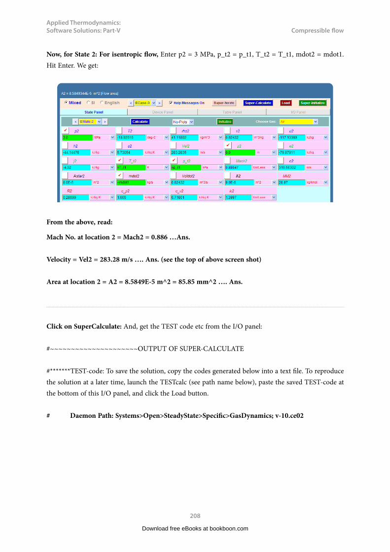
Applied Thermodynamics: Software Solutions: Part-V
208
Compressible flow
Now, for State 2: For isentropic flow, Enter p2 = 3 MPa, p_t2 = p_t1, T_t2 = T_t1, mdot2 = mdot1. Hit Enter. We get:
From the above, read:
Mach No. at location 2 = Mach2 = 0.886 …Ans.
Velocity = Vel2 = 283.28 m/s …. Ans. (see the top of above screen shot)
Area at location 2 = A2 = 8.5849E-5 m^2 = 85.85 mm^2 …. Ans.
Click on SuperCalculate: And, get the TEST code etc from the I/O panel:
#~~~~~~~~~~~~~~~~~~~~~OUTPUT OF SUPER-CALCULATE
#*******TEST-code: To save the solution, copy the codes generated below into a text file. To reproduce the solution at a later time, launch the TESTcalc (see path name below), paste the saved TEST-code at the bottom of this I/O panel, and click the Load button.
# Daemon Path: Systems>Open>SteadyState>Specific>GasDynamics; v-10.ce02
Download free eBooks at bookboon.com

Applied Thermodynamics: Software Solutions: Part-V
209
Compressible flow
#––––––––––Start of TEST-code –––––––––––––––––––––––––––––––––––-
States {
State-1: Air;
Given: { p1= 5.0 MPa; T1= 21.0 deg-C; Vel1= 0.0 m/s; z1= 0.0 m; mdot1= 1.0 kg/s; }
State-2: Air;
Given: { p2= 3.0 MPa; z2= 0.0 m; T_t2= “T_t1” K; p_t2= “p_t1” kPa; mdot2= “mdot1” kg/s; }
}
#–––––––––––End of TEST-code –––––––––––––––––––––––––––––––––––
#––––Property spreadsheet starts:
=======================================================================
Prob.9.5.5 A convergent nozzle has an exit area of 500 mm^2. Air enters the nozzle with a stagnation pressure of 1000 kPa and a stagnation temp of 360 K. Determine the mass rate of flow for back pressures of 800 kPa, 528 kPa, and 300 kPa, assuming isentropic flow. [Ref: 2]
Fig.Prob.9.5.5 Isentropic flow in a convergent nozzle
Download free eBooks at bookboon.com

Applied Thermodynamics: Software Solutions: Part-V
210
Compressible flow
TEST Solution:
Remember that in a convergent nozzle, maximum possible Mach No. is 1, and it occurs at the throat.
At that time, M = 1, and the pressure is critical pressure Pstar, and the temp is critical temp Tstar, and the mass flow rate is maximum. If the back pressure is further decreased below the critical pressure, it has no effect on mass flow, and it remains constant.
Also, we have for air (k = 1.4), Tstar/T0 = 0.833, Pstar/P0 = 0.5283
Go to Gas Dynamics calculator. In the State Panel, select Air as working substance.
Download free eBooks at bookboon.com
Click on the ad to read moreClick on the ad to read moreClick on the ad to read moreClick on the ad to read moreClick on the ad to read moreClick on the ad to read moreClick on the ad to read moreClick on the ad to read moreClick on the ad to read moreClick on the ad to read moreClick on the ad to read moreClick on the ad to read moreClick on the ad to read moreClick on the ad to read moreClick on the ad to read moreClick on the ad to read moreClick on the ad to read moreClick on the ad to read moreClick on the ad to read moreClick on the ad to read moreClick on the ad to read moreClick on the ad to read moreClick on the ad to read moreClick on the ad to read moreClick on the ad to read moreClick on the ad to read moreClick on the ad to read moreClick on the ad to read moreClick on the ad to read moreClick on the ad to read moreClick on the ad to read moreClick on the ad to read moreClick on the ad to read moreClick on the ad to read moreClick on the ad to read moreClick on the ad to read moreClick on the ad to read moreClick on the ad to read moreClick on the ad to read moreClick on the ad to read moreClick on the ad to read moreClick on the ad to read moreClick on the ad to read moreClick on the ad to read moreClick on the ad to read moreClick on the ad to read moreClick on the ad to read moreClick on the ad to read moreClick on the ad to read moreClick on the ad to read moreClick on the ad to read moreClick on the ad to read moreClick on the ad to read moreClick on the ad to read moreClick on the ad to read moreClick on the ad to read moreClick on the ad to read moreClick on the ad to read moreClick on the ad to read moreClick on the ad to read moreClick on the ad to read moreClick on the ad to read moreClick on the ad to read moreClick on the ad to read moreClick on the ad to read moreClick on the ad to read moreClick on the ad to read moreClick on the ad to read more
© Deloitte & Touche LLP and affiliated entities.
360°thinking.
Discover the truth at www.deloitte.ca/careers
© Deloitte & Touche LLP and affiliated entities.
360°thinking.
Discover the truth at www.deloitte.ca/careers
© Deloitte & Touche LLP and affiliated entities.
360°thinking.
Discover the truth at www.deloitte.ca/careers © Deloitte & Touche LLP and affiliated entities.
360°thinking.
Discover the truth at www.deloitte.ca/careers

Applied Thermodynamics: Software Solutions: Part-V
211
Compressible flow
1. For State 1: Enter p_t1 = 1000 kPa, T_t1 = 360 K, and hit Enter. We get:
2. Case (i): At the throat, let the state be 2. Then, for isentropic flow, use the condition that stagnation pressure and stagn. temp remain constant, i.e. p_t1 = p_t2 , and T_t1 = T_t2. In addition, for state 2, also enter p2 = 800 kPa, and hit Enter. We get:
Thus: Mach No. at throat = Mach2 = 0.57378, and Mass flow rate = mdot2 = 0.872 kg/s … Ans.
Download free eBooks at bookboon.com

Applied Thermodynamics: Software Solutions: Part-V
212
Compressible flow
3. Case(ii): Back pressure = 538 kPa. Let this be designated by State 3.
For State 3, we enter: p3 = 528 kPa, T_t3 = T_t1, p_t3 = p_t1, A3 = A2, and hit Enter. We get:
We see that: Mach3 = 1 and, mass flow = mdot3 = 1.065 kg/s. ….Ans.
Note that this is the max. possible flow rate for this convergent nozzle.
4. Case (iii): Back pressure = 300 kPa. This is less than the critical pressure of 528 kPa;
So, there is no effect on mass flow and it remains constant at 1.065 kg/s … Ans.
=======================================================================
Prob.9.5.6 A C_D nozzle has an exit area to throat area ratio of 2. Air enters the nozzle with a stagnation pressure of 1000 kPa and stagnation temp of 360 K. The throat area is 500 mm^2. Determine the mass rate of flow, exit pressure, exit temp, exit Mach No, and exit velocity for the following conditions: (i) sonic velocity at the throat, diverging section acting as a nozzle (ii) sonic velocity at the throat, diverging section acting as a diffuser. [Ref: 2]
Fig.Prob.9.5.6 Isentropic flow in a C-D nozzle
Download free eBooks at bookboon.com

Applied Thermodynamics: Software Solutions: Part-V
213
Compressible flow
TEST Solution:
Remember that in a C-D nozzle: when the back pressure is equal to or less than the ‘critical pressure’ (i.e. pressure corresponding to M = 1 at throat), the flow is maximum. Supersonic velocity occurs only in the divergent section of C-D nozzle, which acts as a nozzle accelerating the flow. If the back pressure is less than the critical pressure, divergent section acts as a diffuser and the flow decelerates, i.e. Mach No. reduces.
Go to Gas Dynamics calculator. In the State Panel, select Air as working substance.
Download free eBooks at bookboon.com
Click on the ad to read moreClick on the ad to read moreClick on the ad to read moreClick on the ad to read moreClick on the ad to read moreClick on the ad to read moreClick on the ad to read moreClick on the ad to read moreClick on the ad to read moreClick on the ad to read moreClick on the ad to read moreClick on the ad to read moreClick on the ad to read moreClick on the ad to read moreClick on the ad to read moreClick on the ad to read moreClick on the ad to read moreClick on the ad to read moreClick on the ad to read moreClick on the ad to read moreClick on the ad to read moreClick on the ad to read moreClick on the ad to read moreClick on the ad to read moreClick on the ad to read moreClick on the ad to read moreClick on the ad to read moreClick on the ad to read moreClick on the ad to read moreClick on the ad to read moreClick on the ad to read moreClick on the ad to read moreClick on the ad to read moreClick on the ad to read moreClick on the ad to read moreClick on the ad to read moreClick on the ad to read moreClick on the ad to read moreClick on the ad to read moreClick on the ad to read moreClick on the ad to read moreClick on the ad to read moreClick on the ad to read moreClick on the ad to read moreClick on the ad to read moreClick on the ad to read moreClick on the ad to read moreClick on the ad to read moreClick on the ad to read moreClick on the ad to read moreClick on the ad to read moreClick on the ad to read moreClick on the ad to read moreClick on the ad to read moreClick on the ad to read moreClick on the ad to read moreClick on the ad to read moreClick on the ad to read moreClick on the ad to read moreClick on the ad to read moreClick on the ad to read moreClick on the ad to read moreClick on the ad to read moreClick on the ad to read moreClick on the ad to read moreClick on the ad to read moreClick on the ad to read moreClick on the ad to read moreClick on the ad to read more
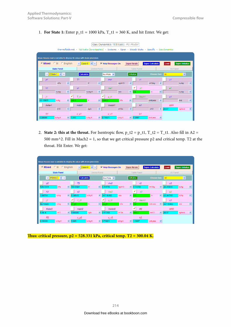
Applied Thermodynamics: Software Solutions: Part-V
214
Compressible flow
1. For State 1: Enter p_t1 = 1000 kPa, T_t1 = 360 K, and hit Enter. We get:
2. State 2: this at the throat. For Isentropic flow, p_t2 = p_t1, T_t2 = T_t1. Also fill in A2 = 500 mm^2. Fill in Mach2 = 1, so that we get critical pressure p2 and critical temp. T2 at the throat. Hit Enter. We get:
Thus: critical pressure, p2 = 528.331 kPa, critical temp. T2 = 300.04 K.
Download free eBooks at bookboon.com

Applied Thermodynamics: Software Solutions: Part-V
215
Compressible flow
3. Case (i): When diverging portion acts as a nozzle: i.e. flow accelerates, and is supersonic at exit.
First, let us get the Mach No. at exit. Go to Tables Panel, and first row gives Isentropic Functions. Now that we know (A2/Astar) from data, fill in (A/Astar) in the Table, Choose Supersonic radio button, since we know that flow is supersonic. (This is important.) And hit Enter. We get:
We see from the above screen shot that Mach No. at exit is M_i = 2.197.
Now, go to State 3. Fill in this Mach No as Mach3 = 2.19697, A3 = 1000 mm^2 (since area ratio is 2), and p_t3 = p_t1 and T_t3 = T_t1 as shown. Hit Enter. We get:
Download free eBooks at bookboon.com

Applied Thermodynamics: Software Solutions: Part-V
216
Compressible flow
Thus:
At exit: Mach3 = 2.19697, p3 = 93.968 kPa, T3 = 183.24 K, Velocity = Vel3 = 596.05 m/s … Ans.
And, mass flow rate = mdot3 = 1.065 kg/s … Ans.
4. Case (ii): When diverging portion acts as diffuser: i.e. flow decelerates, and is subsonic at exit.
Now, the Mach No. at exit will be less than 1 since flow will be subsonic.To get the Mach No. at exit, again go to Tables Panel where the first row gives Isentropic Functions. fill in (A/Astar) in the Table, choose Subsonic radio button, since we know that flow is subsonic. (This is important.) And hit Enter. We get:
We see from the above that Mach No. at exit is M_i = 0.30591.
Now, go to State 4. Fill in this Mach No as Mach4 = 0.30591, A4 = 1000 mm^2 (since area ratio is 2), and p_t4 = p_t1 and T_t4 = T_t1 as shown. Hit Enter. We get:
Download free eBooks at bookboon.com
Applied Thermodynamics: Software Solutions: Part-V
217
Compressible flow
Thus:
At exit: Mach4 = 0.30592, p4 = 937.17 kPa, T4 = 353.39 K, Velocity = Vel4 = 115.26 m/s … Ans.
And, mass flow rate = mdot4 = 1.065 kg/s … Ans.
5. Click on SuperCalculate and get the TEST code etc from the I/O Panel:
#~~~~~~~~~~~~~~~~~~~~~OUTPUT OF SUPER-CALCULATE
# Daemon Path: Systems>Open>SteadyState>Specific>GasDynamics; v-10.ce02
#
#––––––––––Start of TEST-code –––––––––––––––––––––––––––––––––––-
States {
State-1: Air;
Given: { z1= 0.0 m; T_t1= 360.0 K; p_t1= 1000.0 kPa; }
Download free eBooks at bookboon.com
Click on the ad to read moreClick on the ad to read moreClick on the ad to read moreClick on the ad to read moreClick on the ad to read moreClick on the ad to read moreClick on the ad to read moreClick on the ad to read moreClick on the ad to read moreClick on the ad to read moreClick on the ad to read moreClick on the ad to read moreClick on the ad to read moreClick on the ad to read moreClick on the ad to read moreClick on the ad to read moreClick on the ad to read moreClick on the ad to read moreClick on the ad to read moreClick on the ad to read moreClick on the ad to read moreClick on the ad to read moreClick on the ad to read moreClick on the ad to read moreClick on the ad to read moreClick on the ad to read moreClick on the ad to read moreClick on the ad to read moreClick on the ad to read moreClick on the ad to read moreClick on the ad to read moreClick on the ad to read moreClick on the ad to read moreClick on the ad to read moreClick on the ad to read moreClick on the ad to read moreClick on the ad to read moreClick on the ad to read moreClick on the ad to read moreClick on the ad to read moreClick on the ad to read moreClick on the ad to read moreClick on the ad to read moreClick on the ad to read moreClick on the ad to read moreClick on the ad to read moreClick on the ad to read moreClick on the ad to read moreClick on the ad to read moreClick on the ad to read moreClick on the ad to read moreClick on the ad to read moreClick on the ad to read moreClick on the ad to read moreClick on the ad to read moreClick on the ad to read moreClick on the ad to read moreClick on the ad to read moreClick on the ad to read moreClick on the ad to read moreClick on the ad to read moreClick on the ad to read moreClick on the ad to read moreClick on the ad to read moreClick on the ad to read moreClick on the ad to read moreClick on the ad to read moreClick on the ad to read moreClick on the ad to read moreClick on the ad to read more
������������� ����������������������������������������������� �� ���������������������������
������ ������ ������������������������������ ����������������������!���"���������������
�����#$%����&'())%�*+����������,����������-
.��������������������������������� ��
���������� ���������������� ������������� ���������������������������� �����������
The Wakethe only emission we want to leave behind
Applied Thermodynamics: Software Solutions: Part-V
218
Compressible flow
State-2: Air;
Given: { z2= 0.0 m; T_t2= “T_t1” K; p_t2= “p_t1” kPa; Mach2= 1.0 UnitLess; A2= 500.0 mm^2; }
State-3: Air;
Given: { z3= 0.0 m; T_t3= “T_t1” K; p_t3= “p_t1” kPa; Mach3= 2.19697 UnitLess; A3= 1000.0 mm^2; }
State-4: Air;
Given: { z4= 0.0 m; T_t4= “T_t1” K; p_t4= “p_t1” kPa; Mach4= 0.30592 UnitLess; A4= 1000.0 mm^2; }
}
#–––––––––––End of TEST-code –––––––––––––––––––––––––––––––––––
=======================================================================
Prob.9.5.7 At a certain point A in a tube, the Mach No. is 2, static temp is 250 K and static pressure is 200 kPa. Find out the Mach No. and static temp at a point B downstream where static pressure is 150 kPa. Assume isentropic flow and the fluid is air. [Ref: 11]
TEST Solution:
Remember that in isentropic flow, stagnation temp and stagnation pressure remain constant.
Go to Gas Dynamics calculator. In the State Panel, select Air as working substance.
Download free eBooks at bookboon.com

Applied Thermodynamics: Software Solutions: Part-V
219
Compressible flow
1. For State 1: Enter p1 = 200 kPa, T1 = 250 K, Mach1 = 2, and hit Enter. We get:
2. Now, for State 2: Enter p2 = 150 kPa, p_t2 = p_t1, T_t2 = T_t1, and hit Enter. We get:
Then, we see that:
Mach No. at State 2 = Mach2 = 2.184 …Ans.
Static temp. at State 2 = T2 = 230.283 K … Ans.
Download free eBooks at bookboon.com
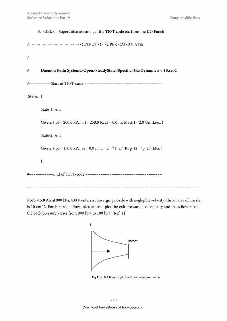
Applied Thermodynamics: Software Solutions: Part-V
220
Compressible flow
3. Click on SuperCalculate and get the TEST code etc from the I/O Panel:
#~~~~~~~~~~~~~~~~~~~~~OUTPUT OF SUPER-CALCULATE:
#
# Daemon Path: Systems>Open>SteadyState>Specific>GasDynamics; v-10.ce02
#––––––––––Start of TEST-code –––––––––––––––––––––––––––––––––––-
States {
State-1: Air;
Given: { p1= 200.0 kPa; T1= 250.0 K; z1= 0.0 m; Mach1= 2.0 UnitLess; }
State-2: Air;
Given: { p2= 150.0 kPa; z2= 0.0 m; T_t2= “T_t1” K; p_t2= “p_t1” kPa; }
}
#–––––––––––End of TEST-code –––––––––––––––––––––––––––––––––––
=======================================================================
Prob.9.5.8 Air at 900 kPa, 400 K enters a converging nozzle with negligible velocity. Throat area of nozzle is 10 cm^2. For isentropic flow, calculate and plot the exit pressure, exit velocity and mass flow rate as the back pressure varies from 900 kPa to 100 kPa. [Ref: 1]
Fig.Prob.9.5.8 Isentropic flow in a convergent nozzle
Download free eBooks at bookboon.com

Applied Thermodynamics: Software Solutions: Part-V
221
Compressible flow
TEST Solution:
Again, remember that in isentropic flow, stagnation temp and stagnation pressure remain constant.
Go to Gas Dynamics calculator. In the State Panel, select Air as working substance.
1. For State 1: Enter p1 = 900 kPa, T1 = 400 K, Vel1 = 0, and hit Enter. We get:
Observe from the above that stagn. pressure p_t1 and stagn. temp T_t1 are calculated.
Download free eBooks at bookboon.com
Click on the ad to read moreClick on the ad to read moreClick on the ad to read moreClick on the ad to read moreClick on the ad to read moreClick on the ad to read moreClick on the ad to read moreClick on the ad to read moreClick on the ad to read moreClick on the ad to read moreClick on the ad to read moreClick on the ad to read moreClick on the ad to read moreClick on the ad to read moreClick on the ad to read moreClick on the ad to read moreClick on the ad to read moreClick on the ad to read moreClick on the ad to read moreClick on the ad to read moreClick on the ad to read moreClick on the ad to read moreClick on the ad to read moreClick on the ad to read moreClick on the ad to read moreClick on the ad to read moreClick on the ad to read moreClick on the ad to read moreClick on the ad to read moreClick on the ad to read moreClick on the ad to read moreClick on the ad to read moreClick on the ad to read moreClick on the ad to read moreClick on the ad to read moreClick on the ad to read moreClick on the ad to read moreClick on the ad to read moreClick on the ad to read moreClick on the ad to read moreClick on the ad to read moreClick on the ad to read moreClick on the ad to read moreClick on the ad to read moreClick on the ad to read moreClick on the ad to read moreClick on the ad to read moreClick on the ad to read moreClick on the ad to read moreClick on the ad to read moreClick on the ad to read moreClick on the ad to read moreClick on the ad to read moreClick on the ad to read moreClick on the ad to read moreClick on the ad to read moreClick on the ad to read moreClick on the ad to read moreClick on the ad to read moreClick on the ad to read moreClick on the ad to read moreClick on the ad to read moreClick on the ad to read moreClick on the ad to read moreClick on the ad to read moreClick on the ad to read moreClick on the ad to read moreClick on the ad to read moreClick on the ad to read moreClick on the ad to read moreClick on the ad to read more
CAREERKICKSTARTAn app to keep you in the know
Whether you’re a graduate, school leaver or student, it’s a difficult time to start your career. So here at RBS, we’re providing a helping hand with our new Facebook app. Bringing together the most relevant and useful careers information, we’ve created a one-stop shop designed to help you get on the career ladder – whatever your level of education, degree subject or work experience.
And it’s not just finance-focused either. That’s because it’s not about us. It’s about you. So download the app and you’ll get everything you need to know to kickstart your career.
So what are you waiting for?
Click here to get started.
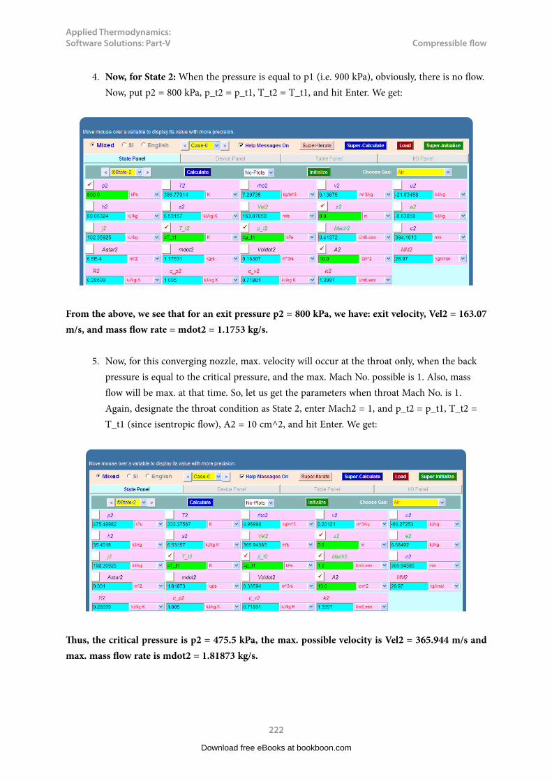
Applied Thermodynamics: Software Solutions: Part-V
222
Compressible flow
4. Now, for State 2: When the pressure is equal to p1 (i.e. 900 kPa), obviously, there is no flow. Now, put p2 = 800 kPa, p_t2 = p_t1, T_t2 = T_t1, and hit Enter. We get:
From the above, we see that for an exit pressure p2 = 800 kPa, we have: exit velocity, Vel2 = 163.07 m/s, and mass flow rate = mdot2 = 1.1753 kg/s.
5. Now, for this converging nozzle, max. velocity will occur at the throat only, when the back pressure is equal to the critical pressure, and the max. Mach No. possible is 1. Also, mass flow will be max. at that time. So, let us get the parameters when throat Mach No. is 1. Again, designate the throat condition as State 2, enter Mach2 = 1, and p_t2 = p_t1, T_t2 = T_t1 (since isentropic flow), A2 = 10 cm^2, and hit Enter. We get:
Thus, the critical pressure is p2 = 475.5 kPa, the max. possible velocity is Vel2 = 365.944 m/s and max. mass flow rate is mdot2 = 1.81873 kg/s.
Download free eBooks at bookboon.com

Applied Thermodynamics: Software Solutions: Part-V
223
Compressible flow
As the back pressure is decreased below the critical pressure of 475.5 kPa, exit pressure remains constant at the critical pressure, and the exit velocity and mass flow rate also remain constant.
6. To plot Exit velocity and mass flow rate against the back pressure: It is quite easy. All that we have to do is go to State 2, and change the value of p2 to the desired value, and click on Calculate (or, hit Enter). Immediately, all other calculations for State 2 are updated. Note the results in a Tabular form for different values of p2 as shown below:
Back pressure ( = P2), kPa Mach No. Exit Velocity (m/s) Mass flow rate (kg/s)
900 0 0 0
800 0.414 163.07 1.175
700 0.61 235.96 1.546
600 0.784 296.48 1.74
500 0.956 352.47 1.816
475.5 1.0 365.944 1.8187
400 1.0 365.944 1.8187
300 1.0 365.944 1.8187
200 1.0 365.944 1.8187
100 1.0 365.944 1.8187
Now, plot the results in EXCEL:
Download free eBooks at bookboon.com
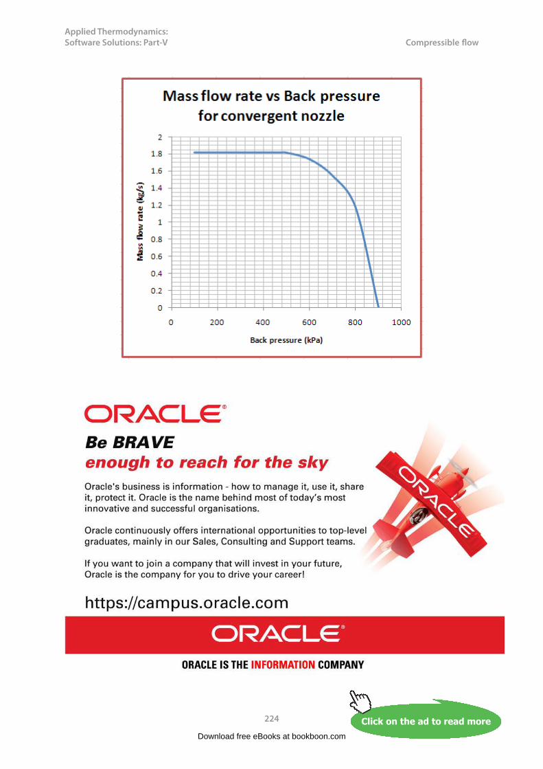
Applied Thermodynamics: Software Solutions: Part-V
224
Compressible flow
Download free eBooks at bookboon.com
Click on the ad to read moreClick on the ad to read moreClick on the ad to read moreClick on the ad to read moreClick on the ad to read moreClick on the ad to read moreClick on the ad to read moreClick on the ad to read moreClick on the ad to read moreClick on the ad to read moreClick on the ad to read moreClick on the ad to read moreClick on the ad to read moreClick on the ad to read moreClick on the ad to read moreClick on the ad to read moreClick on the ad to read moreClick on the ad to read moreClick on the ad to read moreClick on the ad to read moreClick on the ad to read moreClick on the ad to read moreClick on the ad to read moreClick on the ad to read moreClick on the ad to read moreClick on the ad to read moreClick on the ad to read moreClick on the ad to read moreClick on the ad to read moreClick on the ad to read moreClick on the ad to read moreClick on the ad to read moreClick on the ad to read moreClick on the ad to read moreClick on the ad to read moreClick on the ad to read moreClick on the ad to read moreClick on the ad to read moreClick on the ad to read moreClick on the ad to read moreClick on the ad to read moreClick on the ad to read moreClick on the ad to read moreClick on the ad to read moreClick on the ad to read moreClick on the ad to read moreClick on the ad to read moreClick on the ad to read moreClick on the ad to read moreClick on the ad to read moreClick on the ad to read moreClick on the ad to read moreClick on the ad to read moreClick on the ad to read moreClick on the ad to read moreClick on the ad to read moreClick on the ad to read moreClick on the ad to read moreClick on the ad to read moreClick on the ad to read moreClick on the ad to read moreClick on the ad to read moreClick on the ad to read moreClick on the ad to read moreClick on the ad to read moreClick on the ad to read moreClick on the ad to read moreClick on the ad to read moreClick on the ad to read moreClick on the ad to read moreClick on the ad to read moreClick on the ad to read more

Applied Thermodynamics: Software Solutions: Part-V
225
Compressible flow
7. Click on SuperCalculate and get the TEST code etc from the I/O Panel:
~~~~~~~~~~~~~~~~~~~~~OUTPUT OF SUPER-CALCULATE :
# Daemon Path: Systems>Open>SteadyState>Specific>GasDynamics; v-10.ce02
#––––––––––Start of TEST-code –––––––––––––––––––––––––––––––––––-
States {
State-1: Air;
Given: { p1= 900.0 kPa; T1= 400.0 K; Vel1= 0.0 m/s; z1= 0.0 m; }
State-2: Air;
Given: { p2= 800.0 kPa; z2= 0.0 m; T_t2= “T_t1” K; p_t2= “p_t1” kPa; A2= 10.0 cm^2; }
}
#–––––––––––End of TEST-code –––––––––––––––––––––––––––––––––––
=======================================================================
Prob.9.5.9 Air enters a normal shock at 18 kPa, 205 K and 740 m/s. Calculate the stagnation pressure and Mach No. upstream of the shock, as well as the pressure, temp, velocity, Mach No. and stagnation pressure downstream of the shock. Also, find the entropy change across the shock. [Ref: 1]
Fig.Prob.9.5.9 Normal shock
TEST Solution:
Again, remember that up to the shock, the flow is isentropic, and after the shock also, flow is isentropic. Stagnation temp remains constant across the shock, but stagn. pressure drops.
Download free eBooks at bookboon.com

Applied Thermodynamics: Software Solutions: Part-V
226
Compressible flow
1. Go to Gas Dynamics calculator. In the State Panel, select Air as working substance. Enter the parameters before the shock, viz. p1, T1 and Vel1 as shown. Hit Enter. We get:
Note that stagn. pressure p_t1 = 347.57 kPa, Mach1 = 2.5787, entropy before shock = s1 = 6.98247 kJ/kg.K
2. Now, Mach1 = 2.5787 is the Mach No. before the shock. To get properties after the shock, go to Table Panel. Enter M_i = 2.5787 and hit Enter. We get:
Note from the above that first row gives isentropic functions and second and third rows give Normal shock functions. So, Mach No. after shock = M_e = 0.50567 and other property ratios are also available in lines 2 and 3. We use these ratios to get properties after shock.
Download free eBooks at bookboon.com

Applied Thermodynamics: Software Solutions: Part-V
227
Compressible flow
3. Properties after shock are designated by State 2: Enter T2 = 2.21574 * T1, Vel2 = 0.29189 * Vel1 and p_t2 = 0.46808 * p_t1, using the property ratios obtained in the Shock Table above. Hit Enter. We get:
Thus:
Vel2 = 215.999 m/s, p_t2 = 162.69 kPa, T2 = 454.23 K, Mach2 = 0.50567, entropy after shock = s2 = 7.20033 kJ/kg.K … Ans.
Download free eBooks at bookboon.com
Click on the ad to read moreClick on the ad to read moreClick on the ad to read moreClick on the ad to read moreClick on the ad to read moreClick on the ad to read moreClick on the ad to read moreClick on the ad to read moreClick on the ad to read moreClick on the ad to read moreClick on the ad to read moreClick on the ad to read moreClick on the ad to read moreClick on the ad to read moreClick on the ad to read moreClick on the ad to read moreClick on the ad to read moreClick on the ad to read moreClick on the ad to read moreClick on the ad to read moreClick on the ad to read moreClick on the ad to read moreClick on the ad to read moreClick on the ad to read moreClick on the ad to read moreClick on the ad to read moreClick on the ad to read moreClick on the ad to read moreClick on the ad to read moreClick on the ad to read moreClick on the ad to read moreClick on the ad to read moreClick on the ad to read moreClick on the ad to read moreClick on the ad to read moreClick on the ad to read moreClick on the ad to read moreClick on the ad to read moreClick on the ad to read moreClick on the ad to read moreClick on the ad to read moreClick on the ad to read moreClick on the ad to read moreClick on the ad to read moreClick on the ad to read moreClick on the ad to read moreClick on the ad to read moreClick on the ad to read moreClick on the ad to read moreClick on the ad to read moreClick on the ad to read moreClick on the ad to read moreClick on the ad to read moreClick on the ad to read moreClick on the ad to read moreClick on the ad to read moreClick on the ad to read moreClick on the ad to read moreClick on the ad to read moreClick on the ad to read moreClick on the ad to read moreClick on the ad to read moreClick on the ad to read moreClick on the ad to read moreClick on the ad to read moreClick on the ad to read moreClick on the ad to read moreClick on the ad to read moreClick on the ad to read moreClick on the ad to read moreClick on the ad to read moreClick on the ad to read moreClick on the ad to read more
AXA Global Graduate Program
Find out more and apply

Applied Thermodynamics: Software Solutions: Part-V
228
Compressible flow
And, entropy change across the shock = (s2 – s1) = 0.21786 kJ/kg.K = 217.86 J/kg.K .. Ans.
4. Click on SuperCalculate and get TEST code etc from the I/O Panel:
#~~~~~~~~~~~~~~~~~~~~~OUTPUT OF SUPER-CALCULATE:
# Daemon Path: Systems>Open>SteadyState>Specific>GasDynamics; v-10.ce02
#––––––––––Start of TEST-code –––––––––––––––––––––––––––––––––––-
States {
State-1: Air;
Given: { p1= 18.0 kPa; T1= 205.0 K; Vel1= 740.0 m/s; z1= 0.0 m; }
State-2: Air;
Given: { T2= “2.21574*T1” K; Vel2= “0.29189*Vel1” m/s; z2= 0.0 m; p_t2= “0.46808*p_t1” kPa; }
}
#–––––––––––End of TEST-code –––––––––––––––––––––––––––––––––––
=======================================================================
Prob.9.5.10. Air enters a C-D nozzle of supersonic wind tunnel at 1 MPa, 300 K with a low velocity. If a normal shock wave occurs at the exit plane of the nozzle at M = 2.4, determine the P, T, Mach No., Vel, and stagnation pressure after the shock. [Ref: 1]
Fig.Prob.9.5.10 Normal shock
Download free eBooks at bookboon.com

Applied Thermodynamics: Software Solutions: Part-V
229
Compressible flow
TEST Solution:
Again, remember that up to the shock, the flow is isentropic, and after the shock also, flow is isentropic. Stagnation temp remains constant across the shock, but stagn. pressure drops.
1. Go to Gas Dynamics calculator. In the State Panel, select Air as working substance. Enter the parameters before the shock, viz. p1, T1 and Vel1 as shown. Hit Enter. We get:
2. Go to the Table Panel to get properties before and after the shock. Enter M_i = 2.4 and hit Enter. We get:
Download free eBooks at bookboon.com

Applied Thermodynamics: Software Solutions: Part-V
230
Compressible flow
In the above Table, in the first row, we have property ratios for isentropic conditions. They are used below to get properties before shock:
3. And, designating the State as 2 as the state before the shock, enter p2, T2 and Mach2 as shown. Hit Enter. We get:
Download free eBooks at bookboon.com
Click on the ad to read moreClick on the ad to read moreClick on the ad to read moreClick on the ad to read moreClick on the ad to read moreClick on the ad to read moreClick on the ad to read moreClick on the ad to read moreClick on the ad to read moreClick on the ad to read moreClick on the ad to read moreClick on the ad to read moreClick on the ad to read moreClick on the ad to read moreClick on the ad to read moreClick on the ad to read moreClick on the ad to read moreClick on the ad to read moreClick on the ad to read moreClick on the ad to read moreClick on the ad to read moreClick on the ad to read moreClick on the ad to read moreClick on the ad to read moreClick on the ad to read moreClick on the ad to read moreClick on the ad to read moreClick on the ad to read moreClick on the ad to read moreClick on the ad to read moreClick on the ad to read moreClick on the ad to read moreClick on the ad to read moreClick on the ad to read moreClick on the ad to read moreClick on the ad to read moreClick on the ad to read moreClick on the ad to read moreClick on the ad to read moreClick on the ad to read moreClick on the ad to read moreClick on the ad to read moreClick on the ad to read moreClick on the ad to read moreClick on the ad to read moreClick on the ad to read moreClick on the ad to read moreClick on the ad to read moreClick on the ad to read moreClick on the ad to read moreClick on the ad to read moreClick on the ad to read moreClick on the ad to read moreClick on the ad to read moreClick on the ad to read moreClick on the ad to read moreClick on the ad to read moreClick on the ad to read moreClick on the ad to read moreClick on the ad to read moreClick on the ad to read moreClick on the ad to read moreClick on the ad to read moreClick on the ad to read moreClick on the ad to read moreClick on the ad to read moreClick on the ad to read moreClick on the ad to read moreClick on the ad to read moreClick on the ad to read moreClick on the ad to read moreClick on the ad to read moreClick on the ad to read moreClick on the ad to read more
Designed for high-achieving graduates across all disciplines, London Business School’s Masters in Management provides specific and tangible foundations for a successful career in business.
This 12-month, full-time programme is a business qualification with impact. In 2010, our MiM employment rate was 95% within 3 months of graduation*; the majority of graduates choosing to work in consulting or financial services.
As well as a renowned qualification from a world-class business school, you also gain access to the School’s network of more than 34,000 global alumni – a community that offers support and opportunities throughout your career.
For more information visit www.london.edu/mm, email [email protected] or give us a call on +44 (0)20 7000 7573.
Masters in Management
The next step for top-performing graduates
* Figures taken from London Business School’s Masters in Management 2010 employment report

Applied Thermodynamics: Software Solutions: Part-V
231
Compressible flow
4. Properties after shock are designated as State 3, and we use the property ratios in second and third rows of the above Table. Using these ratios, enter p_t3, Vel3 and Mach3 as shown below. Hit Enter. We get:
Thus: After the shock:
Pressure, p3 = 448.21 kPa, Temp. T3 = 284.46 K, Mach3 = 0.523, Velocity, Vel3 = 176.8 m/s, and stagn. pressure p_t3 = 540.06 kPa …Ans.
5. Click on SuperCalculate and get TEST code etc from the I/O Panel:
#~~~~~~~~~~~~~~~~~~~~~OUTPUT OF SUPER-CALCULATE:
# Daemon Path: Systems>Open>SteadyState>Specific>GasDynamics; v-10.ce02
#––––––––––Start of TEST-code –––––––––––––––––––––––––––––––––––-
States {
State-1: Air;
Given: { p1= 1000.0 kPa; T1= 300.0 K; Vel1= 0.0 m/s; z1= 0.0 m; }
State-2: Air;
Given: { p2= “0.0684*p_t1” kPa; T2= “0.46487*T_t1” K; z2= 0.0 m; Mach2= 2.4 UnitLess; }
Download free eBooks at bookboon.com

Applied Thermodynamics: Software Solutions: Part-V
232
Compressible flow
State-3: Air;
Given: { Vel3= “0.31126*Vel2” m/s; z3= 0.0 m; p_t3= “0.54004*p_t2” kPa; Mach3= 0.52306 UnitLess; }
}
#–––––––––––End of TEST-code –––––––––––––––––––––––––––––––––––
=======================================================================
Prob.9.5.11. Air enters a C-D nozzle at low velocity at 2 MPa and 100 C. If the exit area of nozzle is 3.5 times the throat area, what must be the back pressure to produce a normal shock at the exit plane of the nozzle? [Ref: 1]
Fig.Prob.9.5.11 Normal shock
TEST Solution:
Following are the steps:
1. Go to Gas Dynamics calculator. In the State Panel, select Air as working substance. Enter the parameters of flow, viz. p1, T1 and Vel1=0, as shown. Hit Enter. We get:
Download free eBooks at bookboon.com

Applied Thermodynamics: Software Solutions: Part-V
233
Compressible flow
2. Go to the Table Panel to get properties before and after the shock. Enter A/Astar = 3.5 and hit Enter. We get:
In the above Table, in the first row, we have property ratios for isentropic conditions. Second and third rows give property ratios for normal shock.
Download free eBooks at bookboon.com
Click on the ad to read moreClick on the ad to read moreClick on the ad to read moreClick on the ad to read moreClick on the ad to read moreClick on the ad to read moreClick on the ad to read moreClick on the ad to read moreClick on the ad to read moreClick on the ad to read moreClick on the ad to read moreClick on the ad to read moreClick on the ad to read moreClick on the ad to read moreClick on the ad to read moreClick on the ad to read moreClick on the ad to read moreClick on the ad to read moreClick on the ad to read moreClick on the ad to read moreClick on the ad to read moreClick on the ad to read moreClick on the ad to read moreClick on the ad to read moreClick on the ad to read moreClick on the ad to read moreClick on the ad to read moreClick on the ad to read moreClick on the ad to read moreClick on the ad to read moreClick on the ad to read moreClick on the ad to read moreClick on the ad to read moreClick on the ad to read moreClick on the ad to read moreClick on the ad to read moreClick on the ad to read moreClick on the ad to read moreClick on the ad to read moreClick on the ad to read moreClick on the ad to read moreClick on the ad to read moreClick on the ad to read moreClick on the ad to read moreClick on the ad to read moreClick on the ad to read moreClick on the ad to read moreClick on the ad to read moreClick on the ad to read moreClick on the ad to read moreClick on the ad to read moreClick on the ad to read moreClick on the ad to read moreClick on the ad to read moreClick on the ad to read moreClick on the ad to read moreClick on the ad to read moreClick on the ad to read moreClick on the ad to read moreClick on the ad to read moreClick on the ad to read moreClick on the ad to read moreClick on the ad to read moreClick on the ad to read moreClick on the ad to read moreClick on the ad to read moreClick on the ad to read moreClick on the ad to read moreClick on the ad to read moreClick on the ad to read moreClick on the ad to read moreClick on the ad to read moreClick on the ad to read moreClick on the ad to read moreClick on the ad to read more
Get Internationally Connected at the University of Surrey MA Intercultural Communication with International BusinessMA Communication and International Marketing
MA Intercultural Communication with International Business
Provides you with a critical understanding of communication in contemporary socio-cultural contexts by combining linguistic, cultural/media studies and international business and will prepare you for a wide range of careers.
MA Communication and International Marketing
Equips you with a detailed understanding of communication in contemporary international marketing contexts to enable you to address the market needs of the international business environment.
For further information contact:T: +44 (0)1483 681681E: [email protected]/downloads
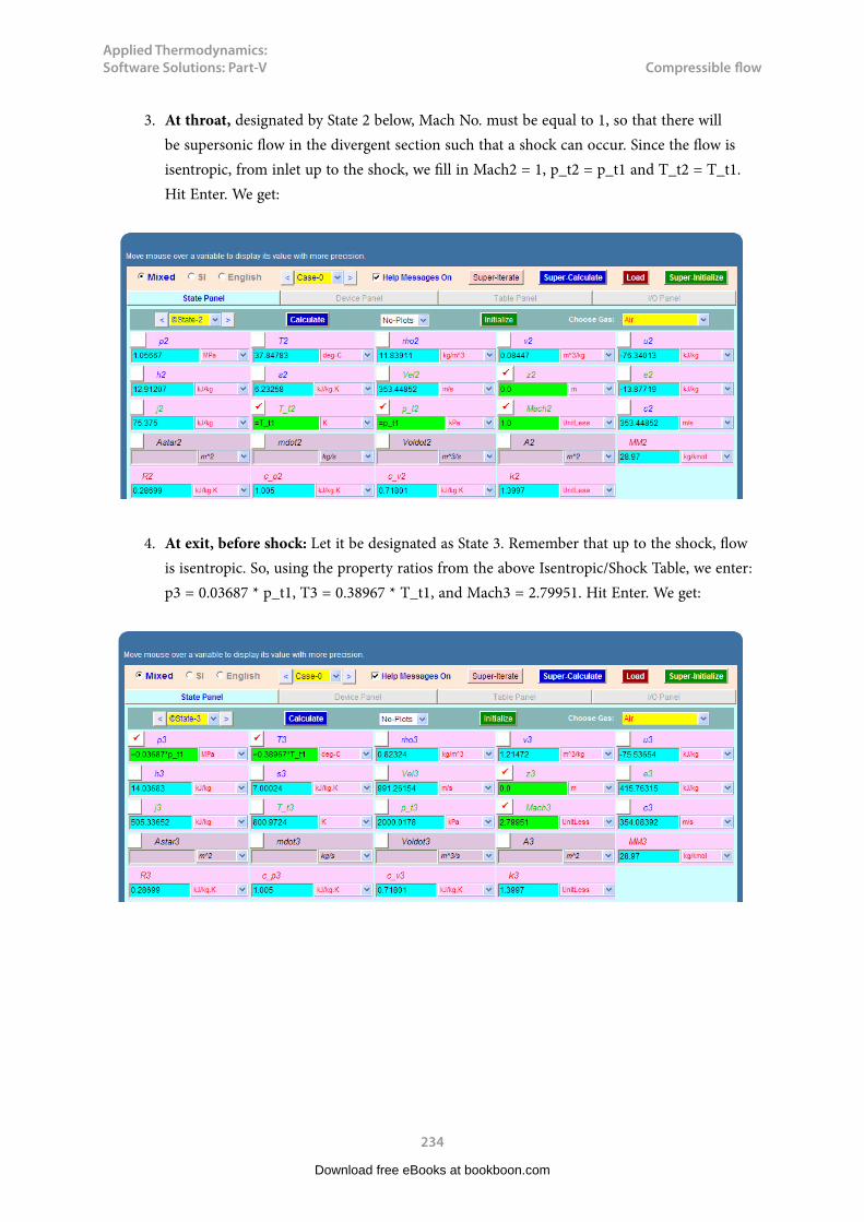
Applied Thermodynamics: Software Solutions: Part-V
234
Compressible flow
3. At throat, designated by State 2 below, Mach No. must be equal to 1, so that there will be supersonic flow in the divergent section such that a shock can occur. Since the flow is isentropic, from inlet up to the shock, we fill in Mach2 = 1, p_t2 = p_t1 and T_t2 = T_t1. Hit Enter. We get:
4. At exit, before shock: Let it be designated as State 3. Remember that up to the shock, flow is isentropic. So, using the property ratios from the above Isentropic/Shock Table, we enter: p3 = 0.03687 * p_t1, T3 = 0.38967 * T_t1, and Mach3 = 2.79951. Hit Enter. We get:
Download free eBooks at bookboon.com

Applied Thermodynamics: Software Solutions: Part-V
235
Compressible flow
5. At exit, after shock: Let it be designated as State 4. Using the property ratios from the above Isentropic/Shock Table, we enter: p_t4 = 0.3895 * p_t3, Vel4 = 0.0.2729 * Vel3, and Mach4 = M_e = 0.48814. Hit Enter. We get:
Note from the above that p4 = 0.6619 MPa.
i.e. back pressure required to produce a normal shock at exit = p4 = 0.6619 MPa…Ans.
6. Click on SuperCalculate and get TEST code etc from the I/O Panel:
#~~~~~~~~~~~~~~~~~~~~~OUTPUT OF SUPER-CALCULATE
# Daemon Path: Systems>Open>SteadyState>Specific>GasDynamics; v-10.ce02
#––––––––––Start of TEST-code –––––––––––––––––––––––––––––––––––-
States {
State-1: Air;
Given: { p1= 2.0 MPa; T1= 100.0 deg-C; Vel1= 0.0 m/s; z1= 0.0 m; }
State-2: Air;
Given: { z2= 0.0 m; T_t2= “T_t1” K; p_t2= “p_t1” kPa; Mach2= 1.0 UnitLess; }
State-3: Air;
Download free eBooks at bookboon.com

Applied Thermodynamics: Software Solutions: Part-V
236
Compressible flow
Given: { p3= “0.03687*p_t1” MPa; T3= “0.38967*T_t1” deg-C; z3= 0.0 m; Mach3= 2.79951 UnitLess; }
State-4: Air;
Given: { Vel4= “0.2729*Vel3” m/s; z4= 0.0 m; p_t4= “0.3895*p_t3” kPa; Mach4= 0.48814 UnitLess; }
}
#–––––––––––End of TEST-code –––––––––––––––––––––––––––––––––––
=======================================================================
Download free eBooks at bookboon.com
Click on the ad to read moreClick on the ad to read moreClick on the ad to read moreClick on the ad to read moreClick on the ad to read moreClick on the ad to read moreClick on the ad to read moreClick on the ad to read moreClick on the ad to read moreClick on the ad to read moreClick on the ad to read moreClick on the ad to read moreClick on the ad to read moreClick on the ad to read moreClick on the ad to read moreClick on the ad to read moreClick on the ad to read moreClick on the ad to read moreClick on the ad to read moreClick on the ad to read moreClick on the ad to read moreClick on the ad to read moreClick on the ad to read moreClick on the ad to read moreClick on the ad to read moreClick on the ad to read moreClick on the ad to read moreClick on the ad to read moreClick on the ad to read moreClick on the ad to read moreClick on the ad to read moreClick on the ad to read moreClick on the ad to read moreClick on the ad to read moreClick on the ad to read moreClick on the ad to read moreClick on the ad to read moreClick on the ad to read moreClick on the ad to read moreClick on the ad to read moreClick on the ad to read moreClick on the ad to read moreClick on the ad to read moreClick on the ad to read moreClick on the ad to read moreClick on the ad to read moreClick on the ad to read moreClick on the ad to read moreClick on the ad to read moreClick on the ad to read moreClick on the ad to read moreClick on the ad to read moreClick on the ad to read moreClick on the ad to read moreClick on the ad to read moreClick on the ad to read moreClick on the ad to read moreClick on the ad to read moreClick on the ad to read moreClick on the ad to read moreClick on the ad to read moreClick on the ad to read moreClick on the ad to read moreClick on the ad to read moreClick on the ad to read moreClick on the ad to read moreClick on the ad to read moreClick on the ad to read moreClick on the ad to read moreClick on the ad to read moreClick on the ad to read moreClick on the ad to read moreClick on the ad to read moreClick on the ad to read moreClick on the ad to read moreClick on the ad to read more
STEP INTO A WORLD OF OPPORTUNITYwww.ecco.com/[email protected]
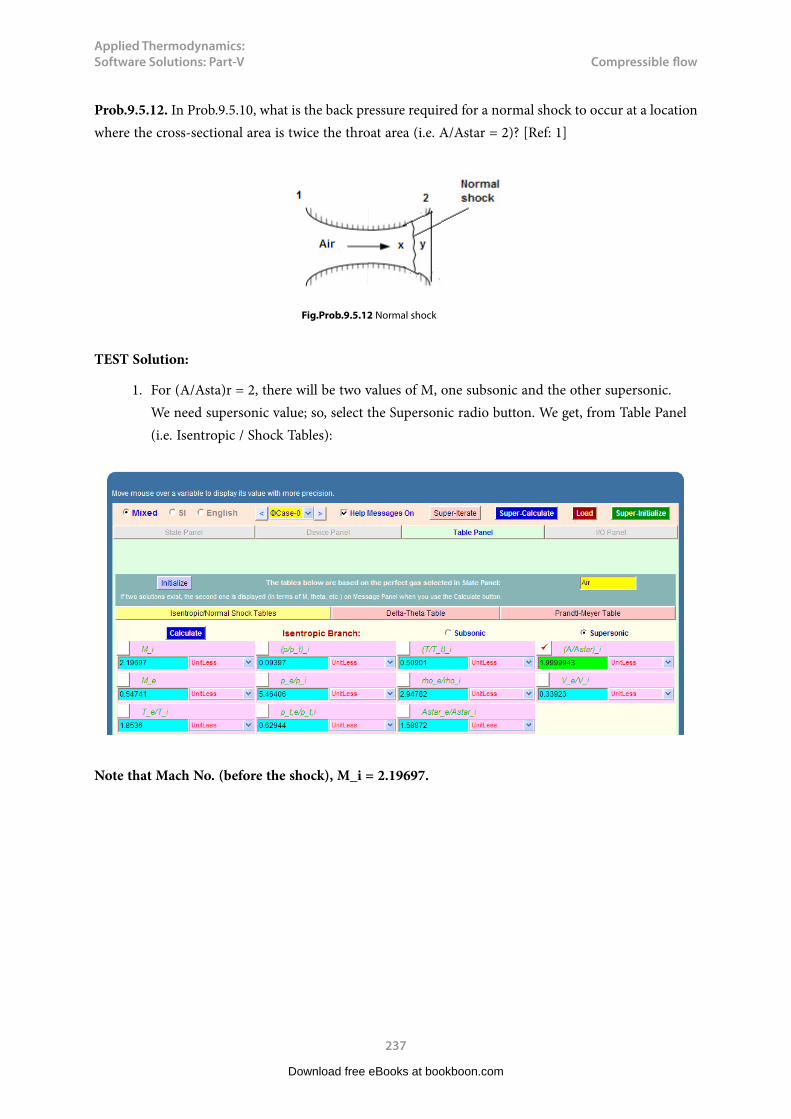
Applied Thermodynamics: Software Solutions: Part-V
237
Compressible flow
Prob.9.5.12. In Prob.9.5.10, what is the back pressure required for a normal shock to occur at a location where the cross-sectional area is twice the throat area (i.e. A/Astar = 2)? [Ref: 1]
Fig.Prob.9.5.12 Normal shock
TEST Solution:
1. For (A/Asta)r = 2, there will be two values of M, one subsonic and the other supersonic. We need supersonic value; so, select the Supersonic radio button. We get, from Table Panel (i.e. Isentropic / Shock Tables):
Note that Mach No. (before the shock), M_i = 2.19697.
Download free eBooks at bookboon.com

Applied Thermodynamics: Software Solutions: Part-V
238
Compressible flow
2. Now, go to State 3, before the shock, and change Mach3 = 2.19697. Also, using the Isentropic flow functions in the above Table, enter p3 = 0.09397 * p_t1 and T3 = 0.50901 * T_t3, and hit Enter. We get:
Above screen shot gives properties before shock.
3. And, after the shock: Let the state be designated as State 4. Enter p_t4, Vel4 and Mach4 (= M_e) from the Isentropic/Shock Table. Hit Enter. We get:
We see that p4 = 1.02692 MPa.
i.e. back pressure for this condition = p4 = 1.0269 MPa.
=======================================================================
Download free eBooks at bookboon.com

Applied Thermodynamics: Software Solutions: Part-V
239
Compressible flow
Prob.9.5.13. Air flowing steadily in a nozzle experiences a normal shock at a Mach No. M = 3.2. If the pressure and temp of air are 58 kPa and 270 K respectively upstream of the shock, calculate the P, T, Vel, Mach No. and stagnation pressure downstream of the shock. Also, find the entropy change across the normal shock. Compare these results with those for helium undergoing a normal shock under the same conditions. [Ref: 1]
Fig.Prob.9.5.13 Normal shock
Download free eBooks at bookboon.com
Click on the ad to read moreClick on the ad to read moreClick on the ad to read moreClick on the ad to read moreClick on the ad to read moreClick on the ad to read moreClick on the ad to read moreClick on the ad to read moreClick on the ad to read moreClick on the ad to read moreClick on the ad to read moreClick on the ad to read moreClick on the ad to read moreClick on the ad to read moreClick on the ad to read moreClick on the ad to read moreClick on the ad to read moreClick on the ad to read moreClick on the ad to read moreClick on the ad to read moreClick on the ad to read moreClick on the ad to read moreClick on the ad to read moreClick on the ad to read moreClick on the ad to read moreClick on the ad to read moreClick on the ad to read moreClick on the ad to read moreClick on the ad to read moreClick on the ad to read moreClick on the ad to read moreClick on the ad to read moreClick on the ad to read moreClick on the ad to read moreClick on the ad to read moreClick on the ad to read moreClick on the ad to read moreClick on the ad to read moreClick on the ad to read moreClick on the ad to read moreClick on the ad to read moreClick on the ad to read moreClick on the ad to read moreClick on the ad to read moreClick on the ad to read moreClick on the ad to read moreClick on the ad to read moreClick on the ad to read moreClick on the ad to read moreClick on the ad to read moreClick on the ad to read moreClick on the ad to read moreClick on the ad to read moreClick on the ad to read moreClick on the ad to read moreClick on the ad to read moreClick on the ad to read moreClick on the ad to read moreClick on the ad to read moreClick on the ad to read moreClick on the ad to read moreClick on the ad to read moreClick on the ad to read moreClick on the ad to read moreClick on the ad to read moreClick on the ad to read moreClick on the ad to read moreClick on the ad to read moreClick on the ad to read moreClick on the ad to read moreClick on the ad to read moreClick on the ad to read moreClick on the ad to read moreClick on the ad to read moreClick on the ad to read moreClick on the ad to read moreClick on the ad to read more

Applied Thermodynamics: Software Solutions: Part-V
240
Compressible flow
TEST Solution:
Following are the steps:
1. Go to Gas Dynamics calculator. In the State Panel, select Air as working substance. Enter the parameters of flow, viz. p1, T1 and Mach1= 3.2, as shown. Hit Enter. We get:
2. Go to Table Panel to get Isentropic/Normal shock functions. Enter M_i = 3.2 and hit Return. We get:
Download free eBooks at bookboon.com

Applied Thermodynamics: Software Solutions: Part-V
241
Compressible flow
3. After the shock: This state is designated as State 2. Use the property ratios in the above Table to get properties after the shock. Enter Vel2, p_t2 and Mach2 as shown below, and hit Enter. We get:
Thus:
After the shock: p2 = 683.17 kPa, T2 = 788.56 K, Vel2 = 261.3 m/s, Mach2 = 0.46428, and stagn. pressure p_t2 = 791.91 kPa …. Ans.
Entropy change across the shock = (s2 – s1) = (7.29281 – 6.92347) = 0.36934 kJ/kg.K = 369.34 J/kg.K …. Ans.
(b) For Helium: Go to State 1, change the substance to helium, click on SuperCalculate. All calculations get updated. We get:
1. Before shock:
Download free eBooks at bookboon.com
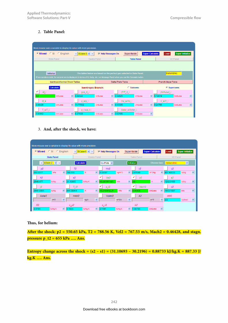
Applied Thermodynamics: Software Solutions: Part-V
242
Compressible flow
2. Table Panel:
3. And, after the shock, we have:
Thus, for helium:
After the shock: p2 = 550.65 kPa, T2 = 788.56 K, Vel2 = 767.53 m/s, Mach2 = 0.46428, and stagn. pressure p_t2 = 655 kPa …. Ans.
Entropy change across the shock = (s2 – s1) = (31.10693 – 30.2196) = 0.88733 kJ/kg.K = 887.33 J/kg.K …. Ans.
Download free eBooks at bookboon.com

Applied Thermodynamics: Software Solutions: Part-V
243
Compressible flow
4. Click on SuperCalculate and get TEST code etc from the I/O Panel:
#~~~~~~~~~~~~~~~~~~~~~OUTPUT OF SUPER-CALCULATE
# Daemon Path: Systems>Open>SteadyState>Specific>GasDynamics; v-10.ce02
#––––––––––Start of TEST-code –––––––––––––––––––––––––––––––––––-
States {
State-1: Helium(He);
Given: { p1= 58.0 kPa; T1= 270.0 K; z1= 0.0 m; Mach1= 3.2 UnitLess; }
State-2: Helium(He);
Given: { Vel2= “0.24795*Vel1” m/s; z2= 0.0 m; p_t2= “0.27609*p_t1” kPa; Mach2= 0.46428 UnitLess; }
}
#–––––––––––End of TEST-code –––––––––––––––––––––––––––––––––––
Download free eBooks at bookboon.com
Click on the ad to read moreClick on the ad to read moreClick on the ad to read moreClick on the ad to read moreClick on the ad to read moreClick on the ad to read moreClick on the ad to read moreClick on the ad to read moreClick on the ad to read moreClick on the ad to read moreClick on the ad to read moreClick on the ad to read moreClick on the ad to read moreClick on the ad to read moreClick on the ad to read moreClick on the ad to read moreClick on the ad to read moreClick on the ad to read moreClick on the ad to read moreClick on the ad to read moreClick on the ad to read moreClick on the ad to read moreClick on the ad to read moreClick on the ad to read moreClick on the ad to read moreClick on the ad to read moreClick on the ad to read moreClick on the ad to read moreClick on the ad to read moreClick on the ad to read moreClick on the ad to read moreClick on the ad to read moreClick on the ad to read moreClick on the ad to read moreClick on the ad to read moreClick on the ad to read moreClick on the ad to read moreClick on the ad to read moreClick on the ad to read moreClick on the ad to read moreClick on the ad to read moreClick on the ad to read moreClick on the ad to read moreClick on the ad to read moreClick on the ad to read moreClick on the ad to read moreClick on the ad to read moreClick on the ad to read moreClick on the ad to read moreClick on the ad to read moreClick on the ad to read moreClick on the ad to read moreClick on the ad to read moreClick on the ad to read moreClick on the ad to read moreClick on the ad to read moreClick on the ad to read moreClick on the ad to read moreClick on the ad to read moreClick on the ad to read moreClick on the ad to read moreClick on the ad to read moreClick on the ad to read moreClick on the ad to read moreClick on the ad to read moreClick on the ad to read moreClick on the ad to read moreClick on the ad to read moreClick on the ad to read moreClick on the ad to read moreClick on the ad to read moreClick on the ad to read moreClick on the ad to read moreClick on the ad to read moreClick on the ad to read moreClick on the ad to read moreClick on the ad to read moreClick on the ad to read more
STUDY. PLAY.The stuff you'll need to make a good living The stuff that makes life worth living
NORWAY. YOUR IDEAL STUDY DESTINATION.
WWW.STUDYINNORWAY.NOFACEBOOK.COM/STUDYINNORWAY
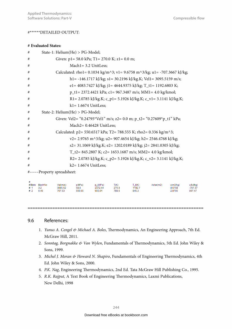
Applied Thermodynamics: Software Solutions: Part-V
244
Compressible flow
#******DETAILED OUTPUT:
# Evaluated States:# State-1: Helium(He) > PG-Model;# Given: p1= 58.0 kPa; T1= 270.0 K; z1= 0.0 m;# Mach1= 3.2 UnitLess; # Calculated: rho1= 0.1034 kg/m^3; v1= 9.6758 m^3/kg; u1= -707.3667 kJ/kg;# h1= -146.1717 kJ/kg; s1= 30.2196 kJ/kg.K; Vel1= 3095.5159 m/s;# e1= 4083.7427 kJ/kg; j1= 4644.9375 kJ/kg; T_t1= 1192.6803 K;# p_t1= 2372.4421 kPa; c1= 967.3487 m/s; MM1= 4.0 kg/kmol;# R1= 2.0785 kJ/kg.K; c_p1= 5.1926 kJ/kg.K; c_v1= 3.1141 kJ/kg.K;# k1= 1.6674 UnitLess;# State-2: Helium(He) > PG-Model;# Given: Vel2= “0.24795*Vel1” m/s; z2= 0.0 m; p_t2= “0.27609*p_t1” kPa;# Mach2= 0.46428 UnitLess;# Calculated: p2= 550.6517 kPa; T2= 788.555 K; rho2= 0.336 kg/m^3;# v2= 2.9765 m^3/kg; u2= 907.4654 kJ/kg; h2= 2546.4768 kJ/kg;# s2= 31.1069 kJ/kg.K; e2= 1202.0189 kJ/kg; j2= 2841.0305 kJ/kg;# T_t2= 845.2807 K; c2= 1653.1687 m/s; MM2= 4.0 kg/kmol;# R2= 2.0785 kJ/kg.K; c_p2= 5.1926 kJ/kg.K; c_v2= 3.1141 kJ/kg.K;# k2= 1.6674 UnitLess;#––––Property spreadsheet:
=======================================================================
9.6 References:
1. Yunus A. Cengel & Michael A. Boles, Thermodynamics, An Engineering Approach, 7th Ed. McGraw Hill, 2011.
2. Sonntag, Borgnakke & Van Wylen, Fundamentals of Thermodynamics, 5th Ed. John Wiley & Sons, 1999.
3. Michel J. Moran & Howard N. Shapiro, Fundamentals of Engineering Thermodynamics, 4th Ed. John Wiley & Sons, 2000.
4. P.K. Nag, Engineering Thermodynamics, 2nd Ed. Tata McGraw Hill Publishing Co., 1995.5. R.K. Rajput, A Text Book of Engineering Thermodynamics, Laxmi Publications,
New Delhi, 1998
Download free eBooks at bookboon.com

Applied Thermodynamics: Software Solutions: Part-V
245
Compressible flow
6. Domkunndwar et al, A course in Thermal Engineering, Dhanpat Rai & Co., New Delhi, 20007. www.thermofluids.net … TEST Software8. http://www.pdas.com/vucalc.html ....vucalc … window based compressible flow calculator
based on a program of the same name written by Tom Benson of NASA Glenn as an aid to making calculations in compressible fluid dynamics.
9. http://www.dept.aoe.vt.edu/~devenpor/aoe3114/calc.html … compressible Aerodynamic calculator …by Devenport
10. S.M.Yahya, Fundamentals of Compressible flow, 2nd Ed. New Age Intl. Ltd. N. Delhi, 1997.11. http://www.potto.org/gasDynamics/gasDynamics.php: Free Text Book on ‘Fundamentals of
compressible flow Mechanics’ by Genick Bar- Meir
=======================================================================
Download free eBooks at bookboon.com
Click on the ad to read moreClick on the ad to read moreClick on the ad to read moreClick on the ad to read moreClick on the ad to read moreClick on the ad to read moreClick on the ad to read moreClick on the ad to read moreClick on the ad to read moreClick on the ad to read moreClick on the ad to read moreClick on the ad to read moreClick on the ad to read moreClick on the ad to read moreClick on the ad to read moreClick on the ad to read moreClick on the ad to read moreClick on the ad to read moreClick on the ad to read moreClick on the ad to read moreClick on the ad to read moreClick on the ad to read moreClick on the ad to read moreClick on the ad to read moreClick on the ad to read moreClick on the ad to read moreClick on the ad to read moreClick on the ad to read moreClick on the ad to read moreClick on the ad to read moreClick on the ad to read moreClick on the ad to read moreClick on the ad to read moreClick on the ad to read moreClick on the ad to read moreClick on the ad to read moreClick on the ad to read moreClick on the ad to read moreClick on the ad to read moreClick on the ad to read moreClick on the ad to read moreClick on the ad to read moreClick on the ad to read moreClick on the ad to read moreClick on the ad to read moreClick on the ad to read moreClick on the ad to read moreClick on the ad to read moreClick on the ad to read moreClick on the ad to read moreClick on the ad to read moreClick on the ad to read moreClick on the ad to read moreClick on the ad to read moreClick on the ad to read moreClick on the ad to read moreClick on the ad to read moreClick on the ad to read moreClick on the ad to read moreClick on the ad to read moreClick on the ad to read moreClick on the ad to read moreClick on the ad to read moreClick on the ad to read moreClick on the ad to read moreClick on the ad to read moreClick on the ad to read moreClick on the ad to read moreClick on the ad to read moreClick on the ad to read moreClick on the ad to read moreClick on the ad to read moreClick on the ad to read moreClick on the ad to read moreClick on the ad to read moreClick on the ad to read moreClick on the ad to read moreClick on the ad to read moreClick on the ad to read more
Technical training on WHAT you need, WHEN you need it
At IDC Technologies we can tailor our technical and engineering training workshops to suit your needs. We have extensive
experience in training technical and engineering staff and have trained people in organisations such as General Motors, Shell, Siemens, BHP and Honeywell to name a few.Our onsite training is cost effective, convenient and completely customisable to the technical and engineering areas you want covered. Our workshops are all comprehensive hands-on learning experiences with ample time given to practical sessions and demonstrations. We communicate well to ensure that workshop content and timing match the knowledge, skills, and abilities of the participants.
We run onsite training all year round and hold the workshops on your premises or a venue of your choice for your convenience.
Phone: +61 8 9321 1702Email: [email protected] Website: www.idc-online.com
INDUSTRIALDATA COMMS
AUTOMATION & PROCESS CONTROL
ELECTRONICS
ELECTRICAL POWER
MECHANICAL ENGINEERING
OIL & GASENGINEERING
For a no obligation proposal, contact us today at [email protected] or visit our website for more information: www.idc-online.com/onsite/
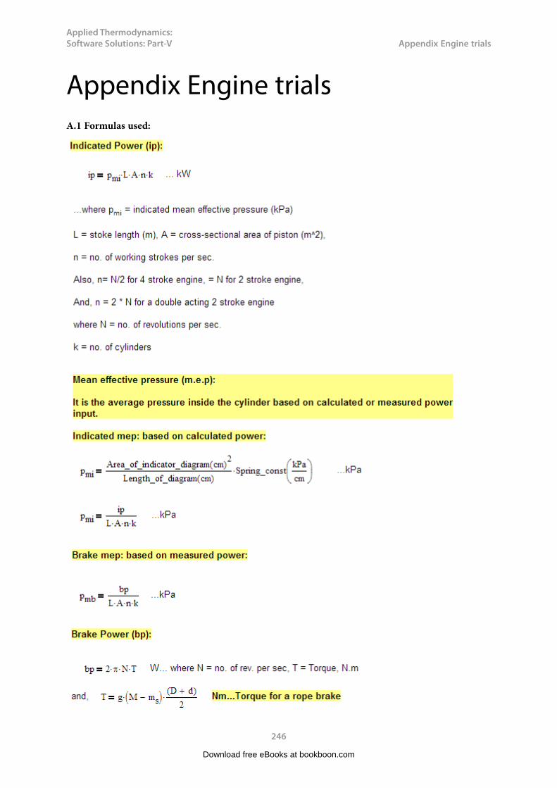
Applied Thermodynamics: Software Solutions: Part-V
246
Appendix Engine trials
Appendix Engine trialsA.1 Formulas used:
Download free eBooks at bookboon.com

Applied Thermodynamics: Software Solutions: Part-V
247
Appendix Engine trials
Download free eBooks at bookboon.com
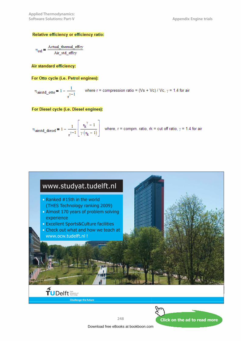
Applied Thermodynamics: Software Solutions: Part-V
248
Appendix Engine trials
Download free eBooks at bookboon.com
Click on the ad to read moreClick on the ad to read moreClick on the ad to read moreClick on the ad to read moreClick on the ad to read moreClick on the ad to read moreClick on the ad to read moreClick on the ad to read moreClick on the ad to read moreClick on the ad to read moreClick on the ad to read moreClick on the ad to read moreClick on the ad to read moreClick on the ad to read moreClick on the ad to read moreClick on the ad to read moreClick on the ad to read moreClick on the ad to read moreClick on the ad to read moreClick on the ad to read moreClick on the ad to read moreClick on the ad to read moreClick on the ad to read moreClick on the ad to read moreClick on the ad to read moreClick on the ad to read moreClick on the ad to read moreClick on the ad to read moreClick on the ad to read moreClick on the ad to read moreClick on the ad to read moreClick on the ad to read moreClick on the ad to read moreClick on the ad to read moreClick on the ad to read moreClick on the ad to read moreClick on the ad to read moreClick on the ad to read moreClick on the ad to read moreClick on the ad to read moreClick on the ad to read moreClick on the ad to read moreClick on the ad to read moreClick on the ad to read moreClick on the ad to read moreClick on the ad to read moreClick on the ad to read moreClick on the ad to read moreClick on the ad to read moreClick on the ad to read moreClick on the ad to read moreClick on the ad to read moreClick on the ad to read moreClick on the ad to read moreClick on the ad to read moreClick on the ad to read moreClick on the ad to read moreClick on the ad to read moreClick on the ad to read moreClick on the ad to read moreClick on the ad to read moreClick on the ad to read moreClick on the ad to read moreClick on the ad to read moreClick on the ad to read moreClick on the ad to read moreClick on the ad to read moreClick on the ad to read moreClick on the ad to read moreClick on the ad to read moreClick on the ad to read moreClick on the ad to read moreClick on the ad to read moreClick on the ad to read moreClick on the ad to read moreClick on the ad to read moreClick on the ad to read moreClick on the ad to read moreClick on the ad to read moreClick on the ad to read more
���������� ����� ��������� �������������������������������� �!�" ��#������"��$�%��&��!�"��'����� �(%����������(������ ��%�� ")*+� +���$����� ��"��*������+ ���� ����������� ������ �� ���,���, +��$ ,���-
���," +�� , +��$ ,��

Applied Thermodynamics: Software Solutions: Part-V
249
Appendix Engine trials
Download free eBooks at bookboon.com
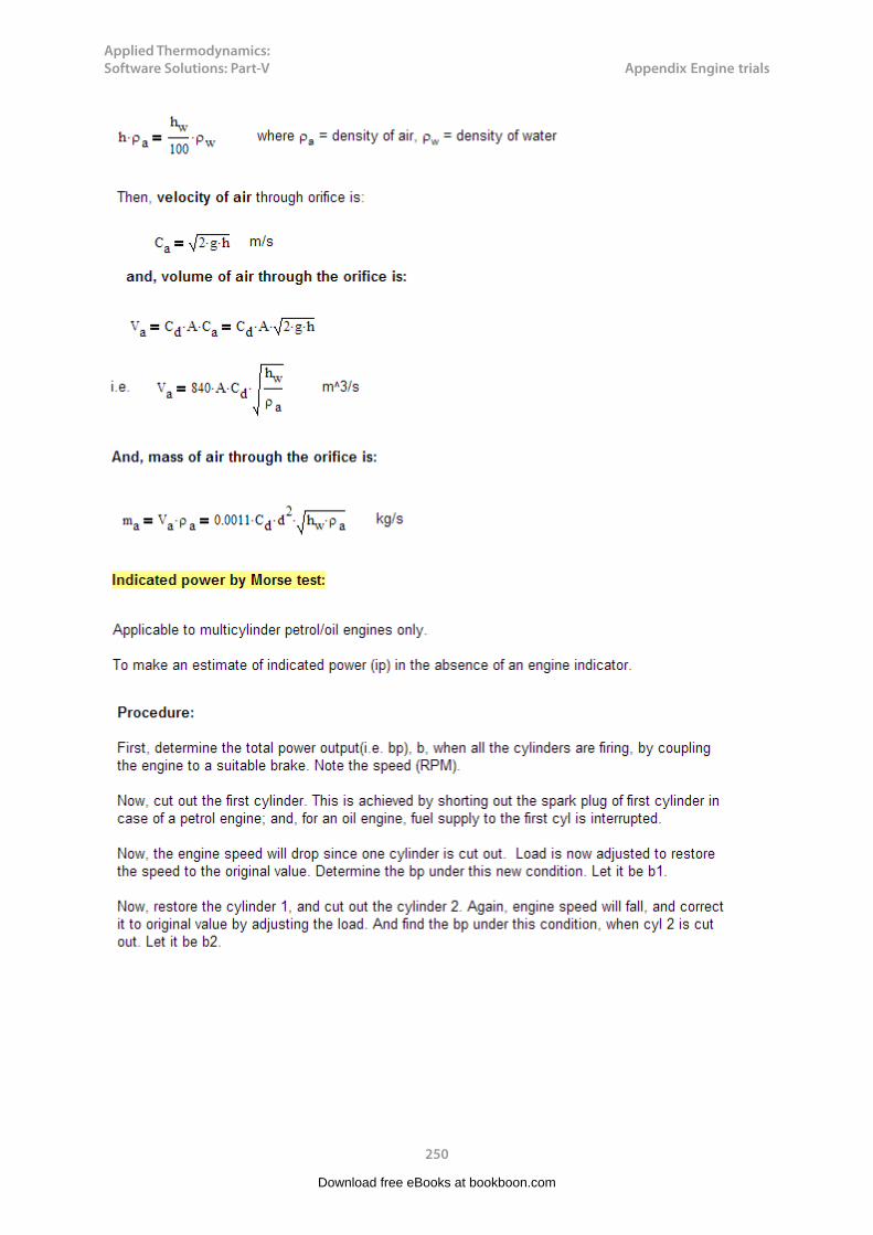
Applied Thermodynamics: Software Solutions: Part-V
250
Appendix Engine trials
Download free eBooks at bookboon.com

Applied Thermodynamics: Software Solutions: Part-V
251
Appendix Engine trials
=======================================================================
A.2 Problems solved with Mathcad:
Prob.A.2.1 For a 4 cyl, 4 stroke petrol engine, air flow was measured by a 75 mm dia sharp edged orifice, Cd = 0.65. Following data obtained during a test: bore = 110 mm, stroke = 130 mm, speed = 2500 rpm, b.p. = 40 kW, fuel consumption = 11 kg/h, CV of fuel = 42000 kJ/kg, pressure drop across orifice = 4.1 cm of water, atm. temp and pressure are 15 C and 1.013 bar. Calculate: brake thermal effcy., bmep and vol. effcy. based on free air conditions.
Mathcad Soution:
Download free eBooks at bookboon.com

Applied Thermodynamics: Software Solutions: Part-V
252
Appendix Engine trials
Download free eBooks at bookboon.com
Click on the ad to read moreClick on the ad to read moreClick on the ad to read moreClick on the ad to read moreClick on the ad to read moreClick on the ad to read moreClick on the ad to read moreClick on the ad to read moreClick on the ad to read moreClick on the ad to read moreClick on the ad to read moreClick on the ad to read moreClick on the ad to read moreClick on the ad to read moreClick on the ad to read moreClick on the ad to read moreClick on the ad to read moreClick on the ad to read moreClick on the ad to read moreClick on the ad to read moreClick on the ad to read moreClick on the ad to read moreClick on the ad to read moreClick on the ad to read moreClick on the ad to read moreClick on the ad to read moreClick on the ad to read moreClick on the ad to read moreClick on the ad to read moreClick on the ad to read moreClick on the ad to read moreClick on the ad to read moreClick on the ad to read moreClick on the ad to read moreClick on the ad to read moreClick on the ad to read moreClick on the ad to read moreClick on the ad to read moreClick on the ad to read moreClick on the ad to read moreClick on the ad to read moreClick on the ad to read moreClick on the ad to read moreClick on the ad to read moreClick on the ad to read moreClick on the ad to read moreClick on the ad to read moreClick on the ad to read moreClick on the ad to read moreClick on the ad to read moreClick on the ad to read moreClick on the ad to read moreClick on the ad to read moreClick on the ad to read moreClick on the ad to read moreClick on the ad to read moreClick on the ad to read moreClick on the ad to read moreClick on the ad to read moreClick on the ad to read moreClick on the ad to read moreClick on the ad to read moreClick on the ad to read moreClick on the ad to read moreClick on the ad to read moreClick on the ad to read moreClick on the ad to read moreClick on the ad to read moreClick on the ad to read moreClick on the ad to read moreClick on the ad to read moreClick on the ad to read moreClick on the ad to read moreClick on the ad to read moreClick on the ad to read moreClick on the ad to read moreClick on the ad to read moreClick on the ad to read moreClick on the ad to read moreClick on the ad to read moreClick on the ad to read more
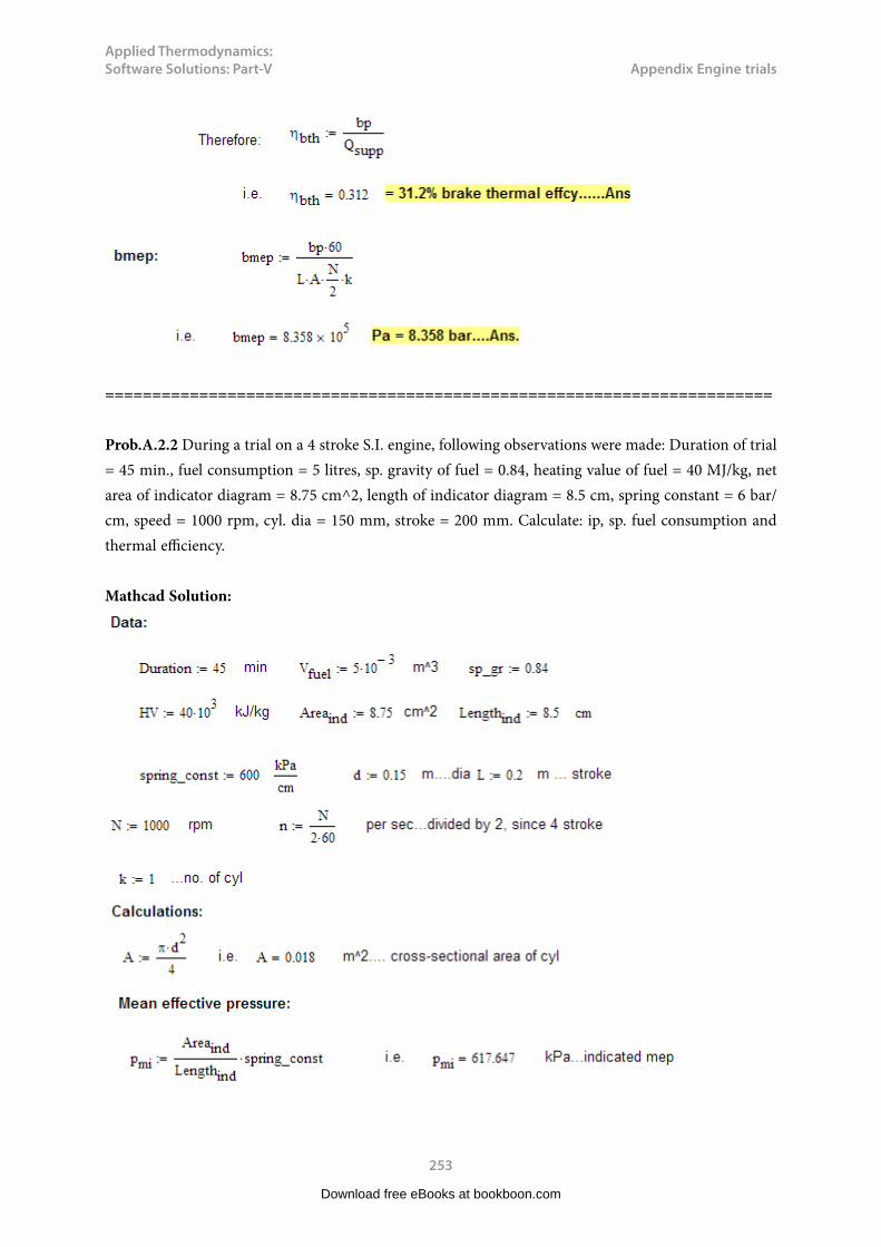
Applied Thermodynamics: Software Solutions: Part-V
253
Appendix Engine trials
=======================================================================
Prob.A.2.2 During a trial on a 4 stroke S.I. engine, following observations were made: Duration of trial = 45 min., fuel consumption = 5 litres, sp. gravity of fuel = 0.84, heating value of fuel = 40 MJ/kg, net area of indicator diagram = 8.75 cm^2, length of indicator diagram = 8.5 cm, spring constant = 6 bar/cm, speed = 1000 rpm, cyl. dia = 150 mm, stroke = 200 mm. Calculate: ip, sp. fuel consumption and thermal efficiency.
Mathcad Solution:
Download free eBooks at bookboon.com
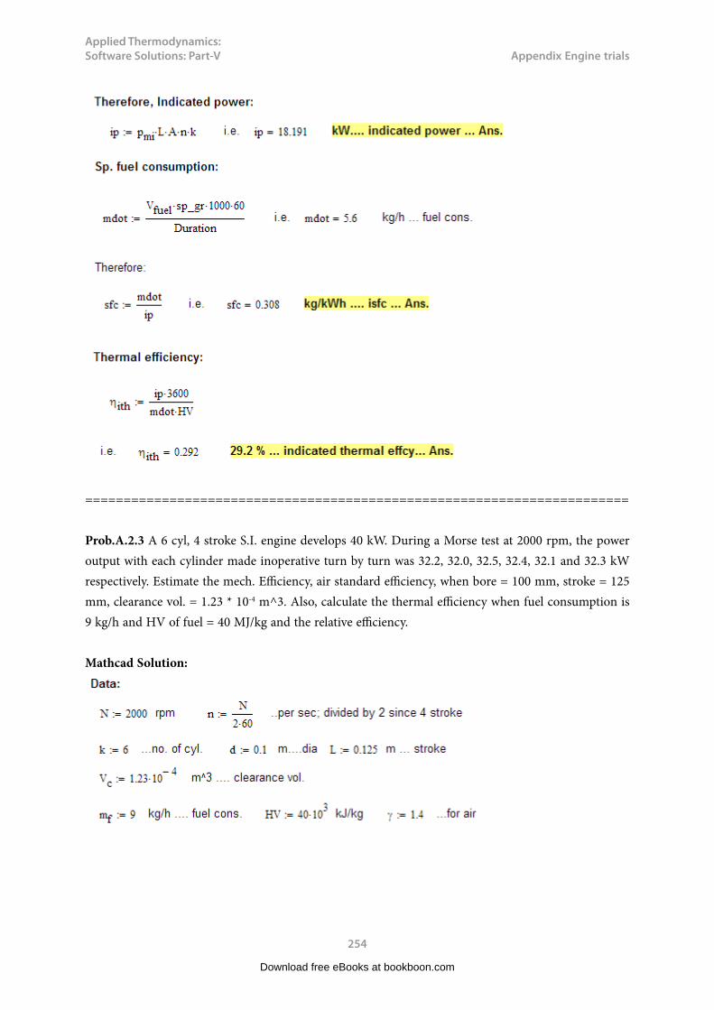
Applied Thermodynamics: Software Solutions: Part-V
254
Appendix Engine trials
=======================================================================
Prob.A.2.3 A 6 cyl, 4 stroke S.I. engine develops 40 kW. During a Morse test at 2000 rpm, the power output with each cylinder made inoperative turn by turn was 32.2, 32.0, 32.5, 32.4, 32.1 and 32.3 kW respectively. Estimate the mech. Efficiency, air standard efficiency, when bore = 100 mm, stroke = 125 mm, clearance vol. = 1.23 * 10-4 m^3. Also, calculate the thermal efficiency when fuel consumption is 9 kg/h and HV of fuel = 40 MJ/kg and the relative efficiency.
Mathcad Solution:
Download free eBooks at bookboon.com

Applied Thermodynamics: Software Solutions: Part-V
255
Appendix Engine trials
Download free eBooks at bookboon.com
Click on the ad to read moreClick on the ad to read moreClick on the ad to read moreClick on the ad to read moreClick on the ad to read moreClick on the ad to read moreClick on the ad to read moreClick on the ad to read moreClick on the ad to read moreClick on the ad to read moreClick on the ad to read moreClick on the ad to read moreClick on the ad to read moreClick on the ad to read moreClick on the ad to read moreClick on the ad to read moreClick on the ad to read moreClick on the ad to read moreClick on the ad to read moreClick on the ad to read moreClick on the ad to read moreClick on the ad to read moreClick on the ad to read moreClick on the ad to read moreClick on the ad to read moreClick on the ad to read moreClick on the ad to read moreClick on the ad to read moreClick on the ad to read moreClick on the ad to read moreClick on the ad to read moreClick on the ad to read moreClick on the ad to read moreClick on the ad to read moreClick on the ad to read moreClick on the ad to read moreClick on the ad to read moreClick on the ad to read moreClick on the ad to read moreClick on the ad to read moreClick on the ad to read moreClick on the ad to read moreClick on the ad to read moreClick on the ad to read moreClick on the ad to read moreClick on the ad to read moreClick on the ad to read moreClick on the ad to read moreClick on the ad to read moreClick on the ad to read moreClick on the ad to read moreClick on the ad to read moreClick on the ad to read moreClick on the ad to read moreClick on the ad to read moreClick on the ad to read moreClick on the ad to read moreClick on the ad to read moreClick on the ad to read moreClick on the ad to read moreClick on the ad to read moreClick on the ad to read moreClick on the ad to read moreClick on the ad to read moreClick on the ad to read moreClick on the ad to read moreClick on the ad to read moreClick on the ad to read moreClick on the ad to read moreClick on the ad to read moreClick on the ad to read moreClick on the ad to read moreClick on the ad to read moreClick on the ad to read moreClick on the ad to read moreClick on the ad to read moreClick on the ad to read moreClick on the ad to read moreClick on the ad to read moreClick on the ad to read moreClick on the ad to read moreClick on the ad to read more
DTU, Technical University of Denmark, is ranked as one of the best technical universities in Europe, and offers internationally recognised Master of Science degrees in 39 English-taught programmes.
DTU offers a unique environment where students have hands-on access to cutting edge facilities and work
closely under the expert supervision of top international researchers.
DTU’s central campus is located just north of Copenhagen and life at the University is engaging and vibrant. At DTU, we ensure that your goals and ambitions are met. Tuition is free for EU/EEA citizens.
Visit us at www.dtu.dk
Study at one of Europe’s leading universities

Applied Thermodynamics: Software Solutions: Part-V
256
Appendix Engine trials
=======================================================================
Download free eBooks at bookboon.com

Applied Thermodynamics: Software Solutions: Part-V
257
Appendix Engine trials
Prob.A.2.4 Following observations were recorded in a test of 1 hour duration on a single cylinder, 4 stroke oil engine: Bore = 220 mm, stroke = 300 mm, fuel used = 4 kg, CV of fuel = 42000 kJ/kg, shaft speed = 300 rpm, no. of explosions/min = 148, mep = 5 bar, load on brake drum = 60 kg, spring balance reading = 30 N, dia of brake drum = 1.4 m, quantity of cooling water circulated = 500 kg, increase in temp of cooling water = 20 C, AF ratio = 16, exhaust gas temp = 410 C, sp. heat of exh. gases = 1.1 kJ/kg.K, ambient temp = 30 C. Determine: ip, bp, mech. efficiency, brake thermal effcy., sfc. Draw the heat balance in kJ/min. [VTU]
Mathcad Solution:
Download free eBooks at bookboon.com

Applied Thermodynamics: Software Solutions: Part-V
258
Appendix Engine trials
Download free eBooks at bookboon.com
Click on the ad to read moreClick on the ad to read moreClick on the ad to read moreClick on the ad to read moreClick on the ad to read moreClick on the ad to read moreClick on the ad to read moreClick on the ad to read moreClick on the ad to read moreClick on the ad to read moreClick on the ad to read moreClick on the ad to read moreClick on the ad to read moreClick on the ad to read moreClick on the ad to read moreClick on the ad to read moreClick on the ad to read moreClick on the ad to read moreClick on the ad to read moreClick on the ad to read moreClick on the ad to read moreClick on the ad to read moreClick on the ad to read moreClick on the ad to read moreClick on the ad to read moreClick on the ad to read moreClick on the ad to read moreClick on the ad to read moreClick on the ad to read moreClick on the ad to read moreClick on the ad to read moreClick on the ad to read moreClick on the ad to read moreClick on the ad to read moreClick on the ad to read moreClick on the ad to read moreClick on the ad to read moreClick on the ad to read moreClick on the ad to read moreClick on the ad to read moreClick on the ad to read moreClick on the ad to read moreClick on the ad to read moreClick on the ad to read moreClick on the ad to read moreClick on the ad to read moreClick on the ad to read moreClick on the ad to read moreClick on the ad to read moreClick on the ad to read moreClick on the ad to read moreClick on the ad to read moreClick on the ad to read moreClick on the ad to read moreClick on the ad to read moreClick on the ad to read moreClick on the ad to read moreClick on the ad to read moreClick on the ad to read moreClick on the ad to read moreClick on the ad to read moreClick on the ad to read moreClick on the ad to read moreClick on the ad to read moreClick on the ad to read moreClick on the ad to read moreClick on the ad to read moreClick on the ad to read moreClick on the ad to read moreClick on the ad to read moreClick on the ad to read moreClick on the ad to read moreClick on the ad to read moreClick on the ad to read moreClick on the ad to read moreClick on the ad to read moreClick on the ad to read moreClick on the ad to read moreClick on the ad to read moreClick on the ad to read moreClick on the ad to read moreClick on the ad to read moreClick on the ad to read more
Increase your impact with MSM Executive Education
For more information, visit www.msm.nl or contact us at +31 43 38 70 808
or via [email protected] the globally networked management school
For more information, visit www.msm.nl or contact us at +31 43 38 70 808 or via [email protected]
For almost 60 years Maastricht School of Management has been enhancing the management capacity
of professionals and organizations around the world through state-of-the-art management education.
Our broad range of Open Enrollment Executive Programs offers you a unique interactive, stimulating and
multicultural learning experience.
Be prepared for tomorrow’s management challenges and apply today.
Executive Education-170x115-B2.indd 1 18-08-11 15:13
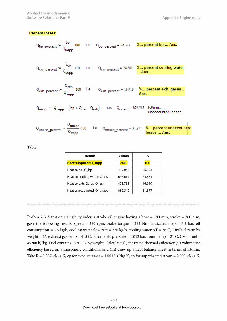
Applied Thermodynamics: Software Solutions: Part-V
259
Appendix Engine trials
Table:
Details kJ/min %
Heat supplied: Q_supp 2800 100
Heat to bp: Q_bp 737.055 26.323
Heat to cooling water: Q_cw 696.667 24.881
Heat to exh. Gases: Q_exh 473.733 16.919
Heat unaccounted: Q_unacc 892.545 31.877
=======================================================================
Prob.A.2.5 A test on a single cylinder, 4 stroke oil engine having a bore = 180 mm, stroke = 360 mm, gave the following results: speed = 290 rpm, brake torque = 392 Nm, indicated mep = 7.2 bar, oil consumption = 3.5 kg/h, cooling water flow rate = 270 kg/h, cooling water ΔT = 36 C, Air/Fuel ratio by weight = 25, exhaust gas temp = 415 C, barometric pressure = 1.013 bar, room temp = 21 C, CV of fuel = 45200 kJ/kg. Fuel contains 15 % H2 by weight. Calculate: (i) indicated thermal efficiency (ii) volumetric efficiency based on atmospheric conditions, and (iii) draw up a heat balance sheet in terms of kJ/min. Take R = 0.287 kJ/kg.K, cp for exhaust gases = 1.0035 kJ/kg.K, cp for superheated steam = 2.093 kJ/kg.K.
Download free eBooks at bookboon.com

Applied Thermodynamics: Software Solutions: Part-V
260
Appendix Engine trials
Mathcad Solution:
Download free eBooks at bookboon.com

Applied Thermodynamics: Software Solutions: Part-V
261
Appendix Engine trials
Download free eBooks at bookboon.com
Click on the ad to read moreClick on the ad to read moreClick on the ad to read moreClick on the ad to read moreClick on the ad to read moreClick on the ad to read moreClick on the ad to read moreClick on the ad to read moreClick on the ad to read moreClick on the ad to read moreClick on the ad to read moreClick on the ad to read moreClick on the ad to read moreClick on the ad to read moreClick on the ad to read moreClick on the ad to read moreClick on the ad to read moreClick on the ad to read moreClick on the ad to read moreClick on the ad to read moreClick on the ad to read moreClick on the ad to read moreClick on the ad to read moreClick on the ad to read moreClick on the ad to read moreClick on the ad to read moreClick on the ad to read moreClick on the ad to read moreClick on the ad to read moreClick on the ad to read moreClick on the ad to read moreClick on the ad to read moreClick on the ad to read moreClick on the ad to read moreClick on the ad to read moreClick on the ad to read moreClick on the ad to read moreClick on the ad to read moreClick on the ad to read moreClick on the ad to read moreClick on the ad to read moreClick on the ad to read moreClick on the ad to read moreClick on the ad to read moreClick on the ad to read moreClick on the ad to read moreClick on the ad to read moreClick on the ad to read moreClick on the ad to read moreClick on the ad to read moreClick on the ad to read moreClick on the ad to read moreClick on the ad to read moreClick on the ad to read moreClick on the ad to read moreClick on the ad to read moreClick on the ad to read moreClick on the ad to read moreClick on the ad to read moreClick on the ad to read moreClick on the ad to read moreClick on the ad to read moreClick on the ad to read moreClick on the ad to read moreClick on the ad to read moreClick on the ad to read moreClick on the ad to read moreClick on the ad to read moreClick on the ad to read moreClick on the ad to read moreClick on the ad to read moreClick on the ad to read moreClick on the ad to read moreClick on the ad to read moreClick on the ad to read moreClick on the ad to read moreClick on the ad to read moreClick on the ad to read moreClick on the ad to read moreClick on the ad to read moreClick on the ad to read moreClick on the ad to read moreClick on the ad to read moreClick on the ad to read more
EXPERIENCE THE POWER OF FULL ENGAGEMENT…
RUN FASTER. RUN LONGER.. RUN EASIER…
READ MORE & PRE-ORDER TODAY WWW.GAITEYE.COM
Challenge the way we run
1349906_A6_4+0.indd 1 22-08-2014 12:56:57
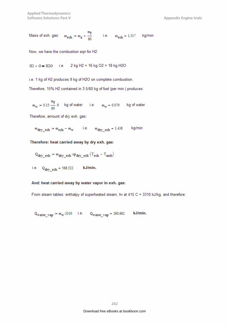
Applied Thermodynamics: Software Solutions: Part-V
262
Appendix Engine trials
Download free eBooks at bookboon.com
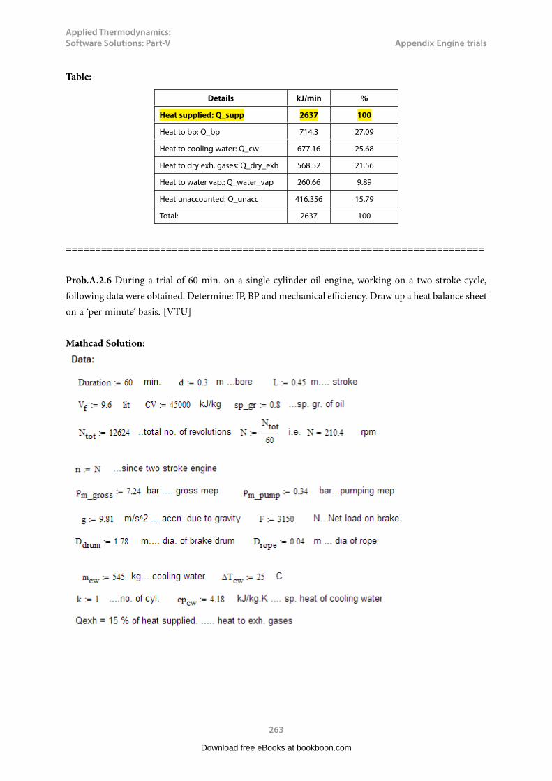
Applied Thermodynamics: Software Solutions: Part-V
263
Appendix Engine trials
Table:
Details kJ/min %
Heat supplied: Q_supp 2637 100
Heat to bp: Q_bp 714.3 27.09
Heat to cooling water: Q_cw 677.16 25.68
Heat to dry exh. gases: Q_dry_exh 568.52 21.56
Heat to water vap.: Q_water_vap 260.66 9.89
Heat unaccounted: Q_unacc 416.356 15.79
Total: 2637 100
=======================================================================
Prob.A.2.6 During a trial of 60 min. on a single cylinder oil engine, working on a two stroke cycle, following data were obtained. Determine: IP, BP and mechanical efficiency. Draw up a heat balance sheet on a ‘per minute’ basis. [VTU]
Mathcad Solution:
Download free eBooks at bookboon.com

Applied Thermodynamics: Software Solutions: Part-V
264
Appendix Engine trials
Download free eBooks at bookboon.com
Click on the ad to read moreClick on the ad to read moreClick on the ad to read moreClick on the ad to read moreClick on the ad to read moreClick on the ad to read moreClick on the ad to read moreClick on the ad to read moreClick on the ad to read moreClick on the ad to read moreClick on the ad to read moreClick on the ad to read moreClick on the ad to read moreClick on the ad to read moreClick on the ad to read moreClick on the ad to read moreClick on the ad to read moreClick on the ad to read moreClick on the ad to read moreClick on the ad to read moreClick on the ad to read moreClick on the ad to read moreClick on the ad to read moreClick on the ad to read moreClick on the ad to read moreClick on the ad to read moreClick on the ad to read moreClick on the ad to read moreClick on the ad to read moreClick on the ad to read moreClick on the ad to read moreClick on the ad to read moreClick on the ad to read moreClick on the ad to read moreClick on the ad to read moreClick on the ad to read moreClick on the ad to read moreClick on the ad to read moreClick on the ad to read moreClick on the ad to read moreClick on the ad to read moreClick on the ad to read moreClick on the ad to read moreClick on the ad to read moreClick on the ad to read moreClick on the ad to read moreClick on the ad to read moreClick on the ad to read moreClick on the ad to read moreClick on the ad to read moreClick on the ad to read moreClick on the ad to read moreClick on the ad to read moreClick on the ad to read moreClick on the ad to read moreClick on the ad to read moreClick on the ad to read moreClick on the ad to read moreClick on the ad to read moreClick on the ad to read moreClick on the ad to read moreClick on the ad to read moreClick on the ad to read moreClick on the ad to read moreClick on the ad to read moreClick on the ad to read moreClick on the ad to read moreClick on the ad to read moreClick on the ad to read moreClick on the ad to read moreClick on the ad to read moreClick on the ad to read moreClick on the ad to read moreClick on the ad to read moreClick on the ad to read moreClick on the ad to read moreClick on the ad to read moreClick on the ad to read moreClick on the ad to read moreClick on the ad to read moreClick on the ad to read moreClick on the ad to read moreClick on the ad to read moreClick on the ad to read moreClick on the ad to read more
GET THERE FASTER
Oliver Wyman is a leading global management consulting firm that combines
deep industry knowledge with specialized expertise in strategy, operations, risk
management, organizational transformation, and leadership development. With
offices in 50+ cities across 25 countries, Oliver Wyman works with the CEOs and
executive teams of Global 1000 companies.
An equal opportunity employer.
Some people know precisely where they want to go. Others seek the adventure of discovering uncharted territory. Whatever you want your professional journey to be, you’ll find what you’re looking for at Oliver Wyman.
Discover the world of Oliver Wyman at oliverwyman.com/careers
DISCOVEROUR WORLD
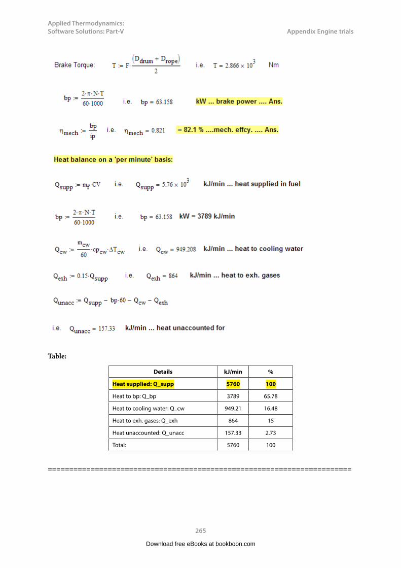
Applied Thermodynamics: Software Solutions: Part-V
265
Appendix Engine trials
Table:
Details kJ/min %
Heat supplied: Q_supp 5760 100
Heat to bp: Q_bp 3789 65.78
Heat to cooling water: Q_cw 949.21 16.48
Heat to exh. gases: Q_exh 864 15
Heat unaccounted: Q_unacc 157.33 2.73
Total: 5760 100
=======================================================================
Download free eBooks at bookboon.com

Applied Thermodynamics: Software Solutions: Part-V
266
Appendix Engine trials
A.3 References:
1. Rayner Joel, Basic Engineering Thermodynamics, 5th Ed. Addison Wesley Longman Inc. 1996.2. R.K. Rajput, Thermal Engineering, Laxmi Publications, New Delhi, 20013. Domkunndwar et al, A course in Thermal Engineering, Dhanpat Rai & Co., New Delhi, 2000
Download free eBooks at bookboon.com
Click on the ad to read moreClick on the ad to read moreClick on the ad to read moreClick on the ad to read moreClick on the ad to read moreClick on the ad to read moreClick on the ad to read moreClick on the ad to read moreClick on the ad to read moreClick on the ad to read moreClick on the ad to read moreClick on the ad to read moreClick on the ad to read moreClick on the ad to read moreClick on the ad to read moreClick on the ad to read moreClick on the ad to read moreClick on the ad to read moreClick on the ad to read moreClick on the ad to read moreClick on the ad to read moreClick on the ad to read moreClick on the ad to read moreClick on the ad to read moreClick on the ad to read moreClick on the ad to read moreClick on the ad to read moreClick on the ad to read moreClick on the ad to read moreClick on the ad to read moreClick on the ad to read moreClick on the ad to read moreClick on the ad to read moreClick on the ad to read moreClick on the ad to read moreClick on the ad to read moreClick on the ad to read moreClick on the ad to read moreClick on the ad to read moreClick on the ad to read moreClick on the ad to read moreClick on the ad to read moreClick on the ad to read moreClick on the ad to read moreClick on the ad to read moreClick on the ad to read moreClick on the ad to read moreClick on the ad to read moreClick on the ad to read moreClick on the ad to read moreClick on the ad to read moreClick on the ad to read moreClick on the ad to read moreClick on the ad to read moreClick on the ad to read moreClick on the ad to read moreClick on the ad to read moreClick on the ad to read moreClick on the ad to read moreClick on the ad to read moreClick on the ad to read moreClick on the ad to read moreClick on the ad to read moreClick on the ad to read moreClick on the ad to read moreClick on the ad to read moreClick on the ad to read moreClick on the ad to read moreClick on the ad to read moreClick on the ad to read moreClick on the ad to read moreClick on the ad to read moreClick on the ad to read moreClick on the ad to read moreClick on the ad to read moreClick on the ad to read moreClick on the ad to read moreClick on the ad to read moreClick on the ad to read moreClick on the ad to read moreClick on the ad to read moreClick on the ad to read moreClick on the ad to read moreClick on the ad to read moreClick on the ad to read moreClick on the ad to read more

Applied Thermodynamics: Software Solutions: Part-V
267
Postscript
PostscriptDear Student,
Thank you for walking with me up to this point.
I hope that we had an interesting exploration of the subject of ‘Thermodynamics’, together.
In this series of 10 books, (i.e. 5 on Basic Thermodynamics and 5 on Applied Thermodynamics), we solved problems using 3 softwares: Mathcad, Engineering Equation Solver (EES) and The Expert System for Thermodynamics (TEST). In the beginning of each chapter, for quick reference, we gave a summary of Definitions, Statements and Formulas used. But, our emphasis was on problem solving.
In addition to solving problems on Basic and Applied Thermodynamics, these books will also help you learn the use of these softwares.
I would like to state again: simply reading these books will not be enough. To derive full benefit from these books, using the solutions given here as a guide, you should solve the problems yourself. I am sure that the large number of examples showing parametric analysis and graphical presentations, given in these books, will enthuse you to work further.
Finally, I would like to say that I greatly enjoyed solving these problems with these three softwares. And I hope that you will also appreciate their utility in problem solving, parametric analysis and graphical presentation of results.
Good luck!
M. ThirumaleshwarAuthorOctober, 2014
Download free eBooks at bookboon.com