
Contents Chemical Thermodynamics Contents
90
-
Upload
independent -
Category
Documents
-
view
2 -
download
0
Transcript of Contents Chemical Thermodynamics Contents

Download free ebooks at bookboon.com
3
Chemical Thermodynamics© 2009 Leo Lue & Ventus Publishing ApSISBN 978-87-7681-497-7
Download free ebooks at bookboon.com
Ple
ase
clic
k th
e ad
vert
Chemical Thermodynamics
4
Contents
Contents
1 Introduction 1.1 Basic concepts 1.1.1 State function versus path function 1.1.2 Intensive property versus extensive property 1.2 Brief review of thermodynamics 1.2.1 The fi rst law of thermodynamics 1.2.2 The second law of thermodynamics 1.3 The fundamental equation of thermodynamics 1.4 The calculus of thermodynamics 1.5 Open systems 1.6 Legendre transforms and free energies
2 Single component systems 2.1 General phase behavior 2.2 Conditions for phase equilibrium 2.3 The Clapeyron equation
88888899111314
17171820
Designed for high-achieving graduates across all disciplines, London Business School’s Masters in Management provides specific and tangible foundations for a successful career in business.
This 12-month, full-time programme is a business qualification with impact. In 2010, our MiM employment rate was 95% within 3 months of graduation*; the majority of graduates choosing to work in consulting or financial services.
As well as a renowned qualification from a world-class business school, you also gain access to the School’s network of more than 34,000 global alumni – a community that offers support and opportunities throughout your career.
For more information visit www.london.edu/mm, email [email protected] or give us a call on +44 (0)20 7000 7573.
Masters in Management
The next step for top-performing graduates
* Figures taken from London Business School’s Masters in Management 2010 employment report
Download free ebooks at bookboon.com
Ple
ase
clic
k th
e ad
vert
Chemical Thermodynamics
5
Contents
3 Multicomponent systems 3.1 Thermodynamics of multicomponent systems 3.1.1 The fundamental equation of thermodynamics 3.1.2 Phase equilibria 3.1.3 Gibbs phase rule 3.2 Binary mixtures 3.2.1 Vapor-liquid equilibrium 3.2.2 Liquid-liquid equilibria 3.2.3 Vapor-liquid-liquid equilibria 3.3 Ternary mixtures
4 The ideal solution model 4.1 Defi nition of the ideal solution model 4.2 Derivation of Raoult’s law
5 Partial molar properties 5.1 Defi nition 5.2 Relationship between total properties and partial molar properties 5.3 Properties changes on mixing 5.4 Graphical representation for binary systems
22222222232525303134
363637
4040414343
© Agilent Technologies, Inc. 2012 u.s. 1-800-829-4444 canada: 1-877-894-4414
Teach with the Best. Learn with the Best.Agilent offers a wide variety of affordable, industry-leading electronic test equipment as well as knowledge-rich, on-line resources —for professors and students.We have 100’s of comprehensive web-based teaching tools, lab experiments, application notes, brochures, DVDs/ CDs, posters, and more. See what Agilent can do for you.
www.agilent.com/find/EDUstudentswww.agilent.com/find/EDUeducators

Download free ebooks at bookboon.com
Ple
ase
clic
k th
e ad
vert
Chemical Thermodynamics
6
Contents
6 Nonideal solutions 6.1 Deviations from Raoult’s law and the activity coeffi cient 6.2 Modifi ed Raoult’s law 6.3 Empirical activity coeffi cient models 6.4 The Gibbs-Duhem equation 6.5 Azeotropic systems
7 Stability 7.1 Introduction 7.2 Liquid-liquid equilibrium
8 Solid-liquid equilibrium 8.1 Introduction 8.2 Phase behavior 8.3 Conditions for equilibrium
9 Gas solubility and Henry’s law 9.1 Henry’s law 9.2 Activity coeffi cients
474748515253
565660
6262 6262
666667
© U
BS
2010
. All
rig
hts
res
erve
d.
www.ubs.com/graduates
Looking for a career where your ideas could really make a difference? UBS’s
Graduate Programme and internships are a chance for you to experience
for yourself what it’s like to be part of a global team that rewards your input
and believes in succeeding together.
Wherever you are in your academic career, make your future a part of ours
by visiting www.ubs.com/graduates.
You’re full of energyand ideas. And that’s just what we are looking for.

Download free ebooks at bookboon.com
Ple
ase
clic
k th
e ad
vert
Chemical Thermodynamics
7
Contents
10 Equations of state 10.1 The principle of corresponding states 10.2 The van der Waals equation and cubic equations of state 10.3 Equations of state for mixtures
11 Thermodynamics from equations of state 11.1 The residual Helmholtz free energy 11.2 Fugacity 11.3 Vapor-liquid equilibrium with a non-ideal vapor phase
12 Chemical reaction equilibria 12.1 Conditions for equilibrium 12.2 The phase rule for chemically reacting systems 12.3 Gas phase reactions 12.4 The standard Gibbs free energy of formation 12.5 The infl uence of temperature 12.6 Liquid phase reactions
70707276
77778182
84848686878890
© Deloitte & Touche LLP and affiliated entities.
360°thinking.
Discover the truth at www.deloitte.ca/careers
© Deloitte & Touche LLP and affiliated entities.
360°thinking.
Discover the truth at www.deloitte.ca/careers
© Deloitte & Touche LLP and affiliated entities.
360°thinking.
Discover the truth at www.deloitte.ca/careers © Deloitte & Touche LLP and affiliated entities.
360°thinking.
Discover the truth at www.deloitte.ca/careers
Download free ebooks at bookboon.com
Chemical Thermodynamics
8
Introduction
1 Introduction
In this Chapter, we quickly review some basic definitions and concepts from thermodynamics. Wethen provide a brief description of the first and second laws of thermodynamics. Next, we discuss themathematical consequences of these laws and cover some relevant theorems in multivariate calculus.Finally, free energies and their importance are introduced.
1.1 Basic concepts
1.1.1 State function versus path function
A state function is a function that depends only on the current properties of the system and not on thehistory of the system. Examples of state functions include density, temperature, and pressure.
A path function is a function that depends on the history of the system. Examples of path functionsinclude work and heat.
1.1.2 Intensive property versus extensive property
An extensive property is a characteristic of a system that is proportional to the size of the system.That is, if we double the size of the system, then the value of an extensive property would alsodouble. Examples of extensive properties include total volume, total mass, total internal energy, etc.Extensive properties will be underlined. For example, the total entropy of the system, which is anextensive property, will be denoted as
¯S.
An intensive property is a characteristic of a system that does not depend on the size of the system.That is, doubling the size of the system leave the value of an intensive property unchanged. Examplesof intensive properties are pressure, temperature, density, molar volume, etc. By definition, an inten-sive property can only be a function of other intensive properties. It cannot be a function of propertiesthat are extensive because it would then depend on the size of the system.
1.2 Brief review of thermodynamics
1.2.1 The first law of thermodynamics
The first law of thermodynamics is simply a statement of the conservation of energy. Energy can takeon a variety of forms, for example kinetic energy, chemical energy, or thermal energy. These differentforms of energy can transform from one to another; however, the sum total of all the types of energymust remain constant.
Download free ebooks at bookboon.com
Chemical Thermodynamics
9
Introduction
Let’s apply the first law of thermodynamics to a closed system (i.e. a system that can exchange heatand work with its surroundings, but not matter). The first law for a closed system can be written as
d¯U = δQ− δW + · · · (1.1)
where¯U is the internal energy of the system, δQ is the heat (thermal energy) transferred to the system,
and δW is the work performed by the system. Other forms of energy may contribute to the energybalance, such as kinetic energy or potential energy (e.g., from a gravitational or electrostatic field).
1.2.2 The second law of thermodynamics
The second law of thermodynamics formalizes the observation that heat is spontaneously transferredonly from higher temperatures to lower temperatures. From this observation, one can deduce theexistence of a state function of a system: the entropy
¯S. The second law of thermodynamics states
that the entropy change d¯S of a closed, constant-volume system obeys the following inequality
d¯S ≥
δQ
T(1.2)
where T is the absolute temperature of the system, and δQ is the amount of heat transfered to thesystem. A process will occur spontaneously in a closed, constant-volume system only if Eq. (1.2)is satisfied. For a reversible process, the equality is satisfied; for an irreversible process, the entropychange is greater than the right-hand side of the relation.
Note that the second law of thermodynamics is unique among the various laws of nature in that itis not symmetric in time. It sets a direction in time, and consequently there is a distinction betweenrunning forward in time and running backwards in time. We can notice that a film is being played inreverse because we observe events that seem to violate the second law.
1.3 The fundamental equation of thermodynamics
Now consider a closed system that can alter its volume¯V . In this case, the work performed by the
system is δW = pd¯V . Combining the first and the second laws of thermodynamics for a closed
system (i.e. inserting the inequality in Eq. (1.2) into Eq. (1.1)), we obtain
d¯U ≤ Td
¯S − pd
¯V for constant N (1.3)
For any spontaneous change (process) in the system, the inequality given in Eq. (1.3) will be satisfied.The equality will be satisfied only in a reversible process.
An isolated system is a system that does not exchange work δW = 0, heat δQ = 0, or matterdN = 0 with its surroundings. Consequently, the total internal energy and volume remain constant;

Download free ebooks at bookboon.com
Ple
ase
clic
k th
e ad
vert
Chemical Thermodynamics
10
Introduction
that implies that d¯U = 0 and d
¯V = 0. Substituting these relations into Eq. (1.3), we find that
processes occur spontaneously in an isolated system only if the entropy does not decrease. In thiscase,
d¯S ≥ 0 (1.4)
Note that in an isolated system, every spontaneous event that occurs always increases the total entropy.Therefore, at equilibrium, where the properties of a system no longer change, the entropy of thesystem will be maximized.
For a system where entropy and volume are held fixed (i.e. d¯S = 0 and
¯V = 0), a process will occur
spontaneously ifd¯U ≤ 0 at constant
¯S,
¯V , and N (1.5)
For a reversible process, where the system is always infinitesmally close to equilibrium, the equality inEq. (1.3) is satisfied. The resulting equation is known as the fundamental equation of thermodynamics
d¯U = Td
¯S − pd
¯V at constant N (1.6)
Download free ebooks at bookboon.com
Chemical Thermodynamics
11
Introduction
1.4 The calculus of thermodynamics
From the fundamental equation of thermodynamics, we can deduce relations between the variousproperties of the system. To see this, let’s consider a function f with independent variables x and y.The differential of f (i.e. the total change in f ) can be written as:
df =
(∂f
∂x
)y
dx +
(∂f
∂y
)x
dy (1.7)
The first term represents the change in f due to changes in the independent variable x, and the secondterm representce changes due to the independent variable y. Note that Eq. (1.7) is just a generalizationof a first order Taylor series expansion to a function of two variables.
If we consider the internal energy of the system¯U to be a function of the variables
¯S and
¯V , then
taking f →¯U , x→
¯S, and y →
¯V , we find
d¯U =
(∂¯U
∂¯S
)¯V
d¯S +
(∂¯U
∂¯V
)¯S
d¯V (1.8)
Comparing Eq. (1.8) with the fundamental equation of thermodynamics Eq. (1.6), we can make theidentifications (
∂¯U
∂¯S
)¯V
= T (1.9)(
∂¯U
∂¯V
)¯S
= −p (1.10)
Therefore, we see that the temperature and pressure of the system can be related to derivatives of itsinternal energy.
For most functions, the order of differentiation does not matter. That is
[∂
∂x
(∂f
∂y
)x
]y
=
[∂
∂y
(∂f
∂x
)y
]x
(1.11)
If we apply Eq. (1.11) to the internal energy, we find[
∂
∂¯V
(∂¯U
∂¯S
)¯V
]¯S
=
[∂
∂¯S
(∂¯U
∂¯V
)¯S
]¯V(
∂T
∂¯V
)¯S
= −
(∂p
∂¯S
)¯V
(1.12)
where we have used Eqs. (1.9) and (1.10). These types of relations are known as Maxwell relations.We will encounter more of these kind of relations later on.
There are three additional relations that need to be mentioned. These relations are useful in converting
Download free ebooks at bookboon.com
Chemical Thermodynamics
12
Introduction
properties that depend on “unmeasureable” quantities, such as entropy, to properties that are measure-able, such as temperature or pressure. The first is a generalization of the chain rule to functions ofmultiple variables
(∂f
∂y
)x
=
(∂f
∂z
)x
(∂z
∂y
)x
(1.13)
To determine the other two relations, let’s consider a function of three variables that is constrained tobe equal to zero. That is
f(x, y, z) = 0.
This defines a two-dimensional surface embedded in a three-dimensional space. The above equationcan be interpreted as defining the functions:
x = x(y, z) y = y(x, z) z = z(x, y).
Each of these functions can be expanded in terms of its respective independent variables
dx =
(∂x
∂y
)z
dy +
(∂x
∂z
)y
dz (1.14)
dy =
(∂y
∂x
)z
dx +
(∂y
∂z
)x
dz (1.15)
dz =
(∂z
∂x
)y
dx +
(∂z
∂y
)x
dy (1.16)
By substituting Eq. (1.15) in to Eq. (1.14) to eliminate the dy term, we find
dx =
(∂x
∂y
)z
[(∂y
∂x
)z
dx +
(∂y
∂z
)x
dz
]+
(∂x
∂z
)y
dz (1.17)
0 =
[(∂x
∂y
)z
(∂y
∂x
)z
− 1
]dx +
[(∂x
∂y
)z
(∂y
∂z
)x
+
(∂x
∂z
)y
]dz (1.18)
This equation should hold for any value of dx and dz. In order for this to be true, the coefficients ofthe dx and dz must vanish. For the dx coefficient, we find
(∂x
∂y
)z
=
(∂y
∂x
)−1
z
(1.19)
The coefficient of the dz term leads to(∂x
∂z
)y
= −
(∂x
∂y
)z
(∂y
∂z
)x
(1.20)
This relation is known as the triple product rule.

Download free ebooks at bookboon.com
Ple
ase
clic
k th
e ad
vert
Chemical Thermodynamics
13
Introduction
1.5 Open systems
We can extend Eq. (1.6) to open systems (i.e. systems in which the number of moles N can vary) byincluding a term called the chemical potential μ. Mathematically, this quantity represents the increasein the internal energy when a small amount of material is introduced to the system at constant totalentropy and volume:
μ =
(∂¯U
∂N
)¯S,
¯V
(1.21)
The fundamental equation of thermodynamics can then be written as
d¯U = Td
¯S − pd
¯V + μdN (1.22)
Let’s determine what the chemical potential is. To do this, we rewrite all total quantities in terms ofmolar properties. For example, the total internal energy can be written as
¯U = NU , where U is the
molar internal energy of the system, and N is the total number of moles in the system. Substituting
your chance to change the worldHere at Ericsson we have a deep rooted belief that the innovations we make on a daily basis can have a profound effect on making the world a better place for people, business and society. Join us.
In Germany we are especially looking for graduates as Integration Engineers for • Radio Access and IP Networks• IMS and IPTV
We are looking forward to getting your application!To apply and for all current job openings please visit our web page: www.ericsson.com/careers
Download free ebooks at bookboon.com
Chemical Thermodynamics
14
Introduction
these relations into the fundamental equation, we find
d(NU) = Td(NS)− pd(NV ) + μdN
NdU + UdN = NTdS + TSdN −NpdV − pV dN + μdN
NdU = N(TdS − pdV )− (U + pV − TS − μ)dN
dU = TdS − pdV −1
N(G− μ)dN (1.23)
where in the last line, we have introduced the definition of the molar Gibbs free energy G ≡ U +
pV − TS.
The molar internal energy U is an intensive property of the system; therefore, it should be independentof extensive properties of the system, in particular, the total number of moles in the system N . Inorder for this to be true, the chemical potential μ must be equal to the molar Gibbs free energy G. Inotherwords:
μ ≡ G (1.24)
Note that this derivation is restricted to pure substances. For multicomponent systems, we need togeneralize this relation. This will be done later.
1.6 Legendre transforms and free energies
The natural variables of the internal energy¯U are the entropy
¯S, volume
¯V , and total number of moles
N of the system. In many situations, however, these variables are not convenient.
We can easily arrive at a new function that has different natural variables by performing a Legendretransform. For example, to arrive at a new state property that posesses the independent variables T
and V , we define the Helmholtz free energy¯A as:
¯A ≡
¯U − T
¯S (1.25)
Inserting this relation into Eq. (1.3), generalized to open systems, we find
d¯U ≤ Td
¯S − pd
¯V + μdN
d(¯A + T
¯S) ≤ Td
¯S − pd
¯V + μdN
d¯A ≤ −
¯SdT − pd
¯V + μdN (1.26)
From this equation, we see that for a system with the temperature, volume, and total number of molesheld fixed (i.e., dT = 0, d
¯V = 0, and dN = 0), a process is spontaneous if it decreases the Helmholtz
free energy.
Download free ebooks at bookboon.com
Chemical Thermodynamics
15
Introduction
In addition, at equilibrium where the equality holds, we find
d¯A = −
¯SdT − pd
¯V + μdN (1.27)
From this expression, we see that the natural variables of the Helmholtz free energy¯A are the tem-
perature, volume, and total number of moles of the system.
Similarly, if we define the Gibbs free energy¯G ≡
¯U − T
¯S + p
¯V , then the fundamental equation of
thermodynamics becomes
d¯G = −
¯SdT +
¯V dp + μdN (1.28)
The Gibbs free energy is minimized for a system at constant temperature, pressure, and total numberof moles. The Gibbs free energy is important because in most experiments the temperature andpressure are variables that we control. This will become useful to us later when we consider phaseequilibria.
The corresponding equation for the enthalpy¯H ≡
¯U + p
¯V is
d¯H = Td
¯S +
¯V dp + μdN (1.29)
As we have seen, free energies such as the internal energy and Gibbs free energy are useful in thatthey tell us whether a process will occur spontaneously or not. A process in which the requisite freeenergy decreases will occur spontaneously. A process in which the free energy increases will notoccur spontaneously. This does not mean that the process cannot happen; we can force the processto occur by performing work on the system. Therefore, we see that free energies are useful to us,qualitatively, in that they tell us the direction in which things will naturally happen.
Free energies also provide us with quantitative information about processes. The change in the freeenergy is equal to the maximum work that can be extracted from a spontaneous process, or in the caseof a non-spontaneous processes, the minimum amount of work that is required to cause the processto occur.

Download free ebooks at bookboon.com
Ple
ase
clic
k th
e ad
vert
Chemical Thermodynamics
16
Introduction
Free energies also have an additional, fundamental importance. Once the mathematical form of thefree energy of a system is known in terms of its natural independent variables (e.g., the Gibbs freeenergy as a function of T , p, and N ), then all the thermodynamic properties of the system can bedetermined. In the remainder of the course, we will be learning how to both develop approximatemodels for the free energy and how to use these models to estimate the thermodynamic behavior ofvarious systems.
Maersk.com/Mitas
�e Graduate Programme for Engineers and Geoscientists
Month 16I was a construction
supervisor in the North Sea
advising and helping foremen
solve problems
I was a
hes
Real work International opportunities
�ree work placementsal Internationaor�ree wo
I wanted real responsibili� I joined MITAS because
Download free ebooks at bookboon.com
Chemical Thermodynamics
17
Single component systems
2 Single component systems
In this Chapter, we describe the basic thermodynamic properties of single component systems. Webegin with a qualitative description of their general phase behavior. Then, we discuss the mathemati-cal relations that govern this behavior.
2.1 General phase behavior
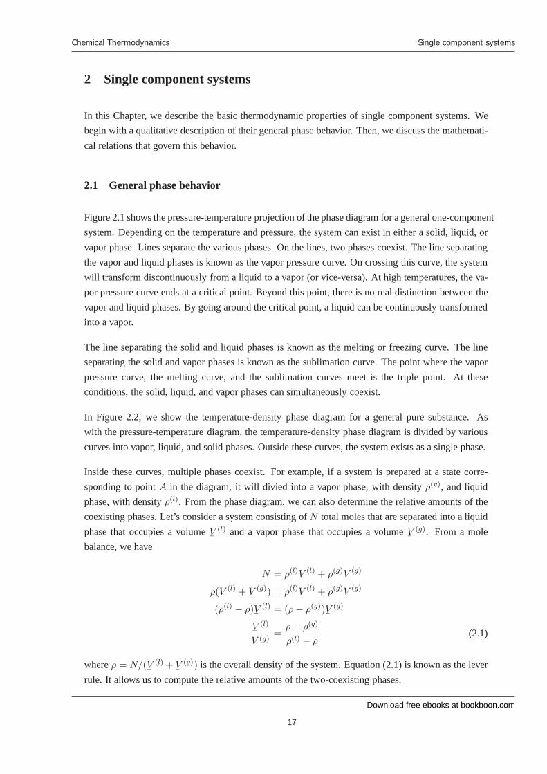
Figure 2.1 shows the pressure-temperature projection of the phase diagram for a general one-componentsystem. Depending on the temperature and pressure, the system can exist in either a solid, liquid, orvapor phase. Lines separate the various phases. On the lines, two phases coexist. The line separatingthe vapor and liquid phases is known as the vapor pressure curve. On crossing this curve, the systemwill transform discontinuously from a liquid to a vapor (or vice-versa). At high temperatures, the va-por pressure curve ends at a critical point. Beyond this point, there is no real distinction between thevapor and liquid phases. By going around the critical point, a liquid can be continuously transformedinto a vapor.
The line separating the solid and liquid phases is known as the melting or freezing curve. The lineseparating the solid and vapor phases is known as the sublimation curve. The point where the vaporpressure curve, the melting curve, and the sublimation curves meet is the triple point. At theseconditions, the solid, liquid, and vapor phases can simultaneously coexist.
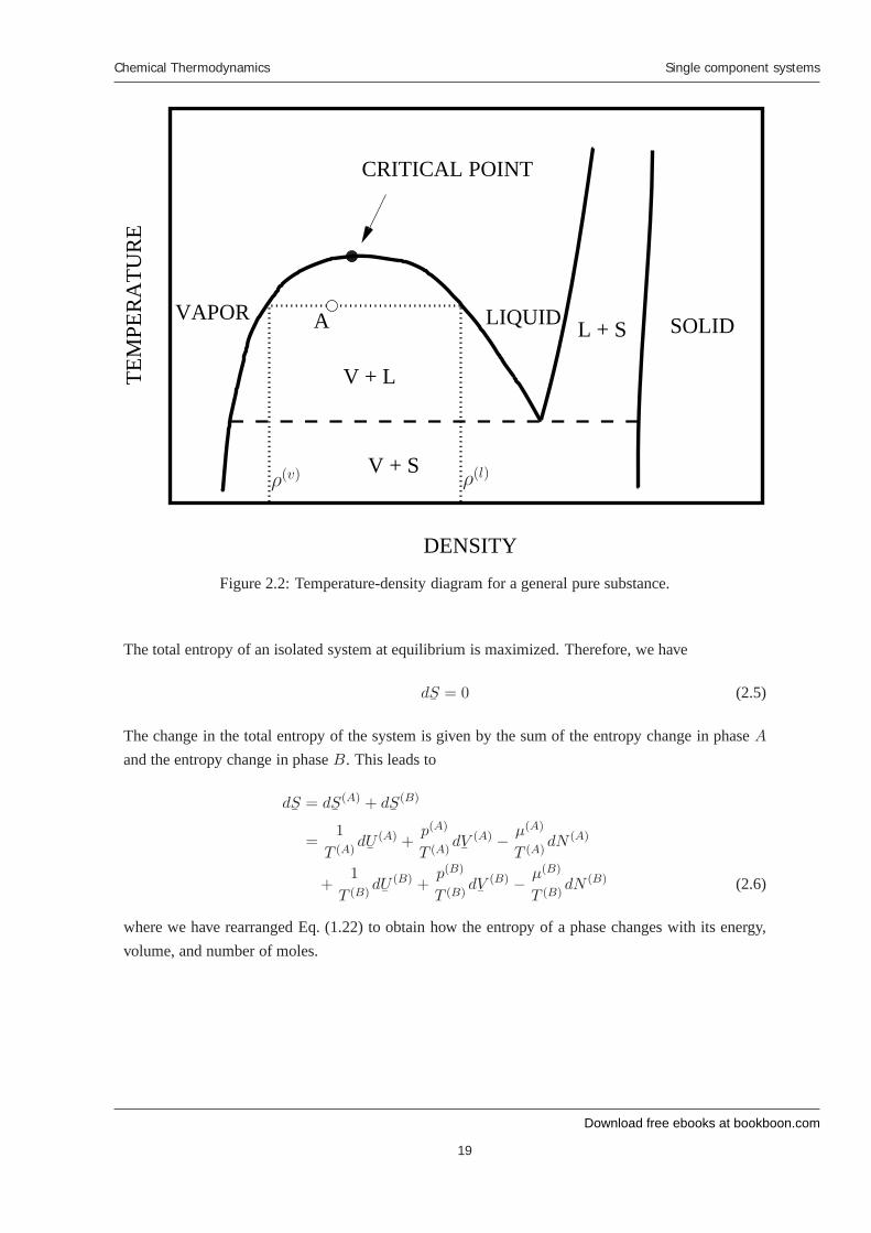
In Figure 2.2, we show the temperature-density phase diagram for a general pure substance. Aswith the pressure-temperature diagram, the temperature-density phase diagram is divided by variouscurves into vapor, liquid, and solid phases. Outside these curves, the system exists as a single phase.
Inside these curves, multiple phases coexist. For example, if a system is prepared at a state corre-sponding to point A in the diagram, it will divied into a vapor phase, with density ρ(v), and liquidphase, with density ρ(l). From the phase diagram, we can also determine the relative amounts of thecoexisting phases. Let’s consider a system consisting of N total moles that are separated into a liquidphase that occupies a volume
¯V (l) and a vapor phase that occupies a volume
¯V (g). From a mole
balance, we have
N = ρ(l)
¯V (l) + ρ(g)
¯V (g)
ρ(¯V (l) +
¯V (g)) = ρ(l)
¯V (l) + ρ(g)
¯V (g)
(ρ(l)− ρ)
¯V (l) = (ρ− ρ(g))
¯V (g)
¯V (l)
¯V (g)
=ρ− ρ(g)
ρ(l) − ρ(2.1)
where ρ = N/(¯V (l) +
¯V (g)) is the overall density of the system. Equation (2.1) is known as the lever
rule. It allows us to compute the relative amounts of the two-coexisting phases.
Download free ebooks at bookboon.com
Chemical Thermodynamics
18
Single component systems
Figure 2.1: Pressure-temperature diagram for a general one-component system.
The dashed-line represents the triple point. Anywhere along the dashed-line, the vapor, liquid, andsolid phases can simultaneously exist.
2.2 Conditions for phase equilibrium
Now let’s derive the mathematical conditions for equilibrium between two coexisting phases. Weconsider an isolated system that is separated into two phases, which we label A and B. The volumeoccupied by each phase can change; in addition, the both phases can freely exchange energy andmaterial with each other. Because the system is isolated, the total energy
¯U , the total volume
¯V ,
and the total number of moles N in the system must remain constant. This leads to the followingrelations:
¯U (A) +
¯U (B) =
¯U =⇒ d
¯U (A) = −d
¯U (B) (2.2)
¯V (A) +
¯V (B) =
¯V =⇒ d
¯V (A) = −d
¯V (B) (2.3)
N (A) + N (B) = N =⇒ dN (A)= −dN (B) (2.4)
where¯U (i) is the total energy of phase i,
¯V (i) is the total volume of phase i, and N (i) is the total
number of moles in phase i.
Download free ebooks at bookboon.com
Chemical Thermodynamics
19
Single component systems
TEM
PER
ATU
RE
DENSITY
L + S
V + S
CRITICAL POINT
V + L
AVAPOR LIQUID SOLID
ρ(v) ρ(l)
Figure 2.2: Temperature-density diagram for a general pure substance.
The total entropy of an isolated system at equilibrium is maximized. Therefore, we have
d¯S = 0 (2.5)
The change in the total entropy of the system is given by the sum of the entropy change in phase A
and the entropy change in phase B. This leads to
d¯S = d
¯S(A) + d
¯S(B)
=1
T (A)d¯U (A) +
p(A)
T (A)d¯V (A)
−μ(A)
T (A)dN (A)
+1
T (B)d¯U (B) +
p(B)
T (B)d¯V (B)
−μ(B)
T (B)dN (B) (2.6)
where we have rearranged Eq. (1.22) to obtain how the entropy of a phase changes with its energy,volume, and number of moles.
Download free ebooks at bookboon.com
Chemical Thermodynamics
20
Single component systems
Substituting the relations given in Eq. (2.4) into Eq. (2.6), we find
d¯S =
1
T (A)d¯U (A) +
p(A)
T (A)d¯V (A)
−μ(A)
T (A)dN (A)
−1
T (B)d¯U (A)
−p(B)
T (B)d¯V (A) +
μ(B)
T (B)dN (A)
0 =
(1
T (A)−
1
T (B)
)d¯U (A) +
(p(A)
T (A)−
p(B)
T (B)
)d¯V (A)
−
(μ(A)
T (A)−
μ(B)
T (B)
)dN (A) (2.7)
The quantities d¯U (A), d
¯V (A), and dN (A) on the right-hand side of Eq. (2.7) can be chosen arbitrarily.
From Eq. (2.6), we know that the left-hand side of Eq. (2.7) must equal zero. The only manner inwhich to guarantee the equality between the two sides of Eq. (2.7) is if coefficients of the d
¯U (A),
d¯V (A), and dN (A) terms are each equal to zero. As a result, this implies the relations:
T (A) = T (B)
p(A) = p(B)
μ(A) = μ(B)
(2.8)
Therefore, we find that the temperatures, pressures, and chemical potentials are equal for coexistingphases in equilibrium. We will later extend this derivation to multicomponent system.
One interesting point to note is that the labels A and B which we used to derive Eqs. (2.8) do nothave to refer to different phases. For example, A and B can refer to different parts of a one phasesystem. Therefore, Eqs. (2.8) can be interpreted as stating the the temperature, pressure, and chemicalpotential of a system at equilibrium are uniform (N.B., we did not include the influence of externalfields, such as gravitional or electrostatic fields).
2.3 The Clapeyron equation
In this section, we derive the Clapeyron equation. This equation relates changes in the pressure tochanges in the temperature along a two-phase coexistence curve (e.g., the vapor pressure curve or themelting curve). Note that the condition for equilibrium between two phases is given by
μ(A) = μ(B)
G(A) = G(B)
dG(A) = dG(B)
−S(A)dT + V (A)dp = −S(B)dT + V (B)dp
dp
dT=
S(A) − S(B)
V (A) − V (B)(2.9)
This is one form of the Clapeyron equation. It relates the slope of the coexistence curve to the entropychange and volume change of the phase transition.

Download free ebooks at bookboon.com
Ple
ase
clic
k th
e ad
vert
Chemical Thermodynamics
21
Single component systems
Entropy is not directly measureable, and, therefore, the Clapeyron equation as written above is notin a convenient form. However, we can relate entropy changes to enthalpy changes, which can bedirectly measured. At equilibrium, we have
μ(A) = μ(B)
G(A) = G(B)
H(A)− TS(A) = H(B)
− TS(B)
S(A)− S(B) =
1
T(H(A)
−H(B)) (2.10)
Thus, the entropy change of a phase transition, which is not directly measureable, can be determinedfrom the enthalpy change of the phase transition, which is directly measureable.
Substituting this relation into Eq. (2.9), we find
dp
dT=
H(A) −H(B)
T (V (A) − V (B))(2.11)
This is the more commonly used form of the Clapeyron equation.
We will turn your CV into an opportunity of a lifetime
Do you like cars? Would you like to be a part of a successful brand?We will appreciate and reward both your enthusiasm and talent.Send us your CV. You will be surprised where it can take you.
Send us your CV onwww.employerforlife.com
Download free ebooks at bookboon.com
Chemical Thermodynamics
22
Multicomponent systems
3 Multicomponent systems
In this section, we examine the thermodynamics of systems which contain a mixture of species.First, we generalize the thermodynamic analysis of the previous section to multicomponent systems,deriving the Gibbs phase rule. Then we describe the general phase behavior of binary and ternarymixtures.
3.1 Thermodynamics of multicomponent systems
3.1.1 The fundamental equation of thermodynamics
In this section, we extend the results of the previous lectures to multicomponent systems. All thatneeds to be done is to define a chemical potential for each species α in the system
d¯U = Td
¯S − pd
¯V +
∑α
μαdNα (3.1)
where μα is the chemical potential of component α. From this, we see that
μα ≡
(∂¯U
∂Nα
)¯S,
¯V,N
α′ �=α
(3.2)
Physically, μα is the change in the internal energy of the system with respect to an increase in thenumber of moles of species α, while holding all number of moles of all other species constant.The other forms of the fundamental equation of thermodynamics can be similarly generalized byperforming the Legendre transform:
d¯A = −
¯SdT − pd
¯V +
∑α
μαdNα
d¯G = −
¯SdT +
¯V dp +
∑α
μαdNα
d¯H = Td
¯S +
¯V dp +
∑α
μαdNα (3.3)
From these relations, we see that there are the following alternate interpretations of the chemicalpotential:
μα ≡
(∂¯A
∂Nα
)T,
¯V,N
α′ �=α
≡
(∂
¯G
∂Nα
)T,p,N
α′ �=α
≡
(∂
¯H
∂Nα
)¯S,p,N
α′ �=α
(3.4)
3.1.2 Phase equilibria
The conditions for phase equilibria can also be extended to multicomponent systems. Consider anisolated system consisting of ω components and two phases, which we refer to as A and B. The
Download free ebooks at bookboon.com
Chemical Thermodynamics
23
Multicomponent systems
system is isolated, with a total internal energy of¯U , a total volume of
¯V , and Nα moles of species α.
Because the system is isolated, we have the following
¯U (A)+
¯U (B)=
¯U =⇒ d
¯U (A)=−d
¯U (B)
¯V (A)+
¯V (B)=
¯V =⇒ d
¯V (A)=−d
¯V (B)
N(A)α +N
(B)α =Nα =⇒ dN
(A)α =−dN
(B)α
(3.5)
where¯U (i) is the internal energy of phase i,
¯V (i) is the volume of phase i, and N
(i)α is the number of
moles of species α in phase i.
For an isolated system at equilibrium, the total entropy is maximized. Stated mathematically, we have
d¯S = d
¯S(A) + d
¯S(B) = 0
=1
T (A)d¯U (A) +
p(A)
T (A)d¯V (A)
−∑α
μ(A)α
T (A)dN (A)
α
+1
T (B)d¯U (B) +
p(B)
T (B)d¯V (B)
−∑α
μ(B)α
T (B)dN (B)
α (3.6)
Inserting the constraint relations given in Eq. (3.5) into Eq. (3.6), we find
d¯S =
(1
T (A)−
1
T (B)
)d¯U (A) +
(p(A)
T (A)−
p(B)
T (B)
)d¯V (A)
−∑α
(μ
(A)α
T (A)−
μ(B)α
T (B)
)dN (A)
α (3.7)
This is equal to zero only if all the coefficients of the change terms are zero. As a consequence, wefind
T (A) = T (B)
p(A) = p(B)
μ(A)α = μ(B)
α for all components α
This argument can be generalized to a system containing π phases and ω components. In this case,we have the temperature, pressure, and chemical potentials of each species are equal in each phase.
T (A) = T (B) = · · · = T (π)
p(A) = p(B) = · · · = p(π)
μ(A)α = μ(B)
α = · · · = μ(π)α for all components α (3.8)
3.1.3 Gibbs phase rule
How many variables need to be specified in order to fix the state of a system? In order to fix thestate of a one-phase system, the composition of the phase must be specified as well as two additional
Download free ebooks at bookboon.com
Ple
ase
clic
k th
e ad
vert
Chemical Thermodynamics
24
Multicomponent systems
intensive variables (e.g., temperature and pressure). For a phase with ω components, ω − 1 molefractions are required to specify the composition. Therefore, a total of ω + 1 intensive variables arerequired to specify the state of a single phase.
For a system with π phases, there are a total of (ω + 1)π unknowns. However, not all of these areindependent. The conditions for phase equilibrium (see Eqs. (3.8)) give us (ω + 2)(π − 1) equationsthat must be satisfied between each of the phases. The difference between the number of unknowns inthe system and the number of constraints (or equations) is equal to the number of degrees of freedomf in the system.
f = (ω + 1)π − (ω + 2)(π − 1)
= 2 + ω − π (3.9)
This is known as the Gibbs phase rule. It tells us the number of variables f that must be specified inorder to fix the (intensive) state of the system.
Win one of the six full tuition scholarships for International MBA or MSc in Management
Are you remarkable?
register now
www.Nyenrode
MasterChallenge.com
Download free ebooks at bookboon.com
Chemical Thermodynamics
25
Multicomponent systems
0.00.2
0.40.6
0.81.0 100
150 200
250 300
350
0 1 2 3 4 5 6 7
pres
sure
(MP
a)
mole fraction of ethane
temperature (K)
pres
sure
(MP
a)
AB
C1 C2
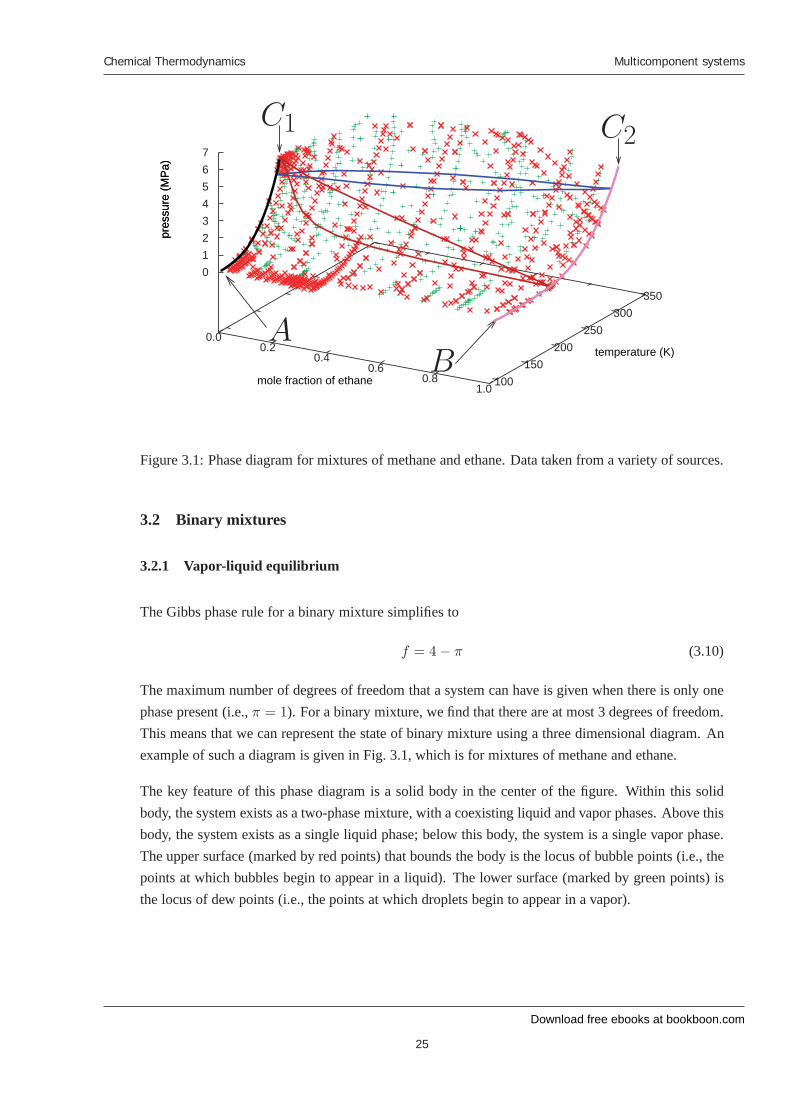
Figure 3.1: Phase diagram for mixtures of methane and ethane. Data taken from a variety of sources.
3.2 Binary mixtures
3.2.1 Vapor-liquid equilibrium
The Gibbs phase rule for a binary mixture simplifies to
f = 4− π (3.10)
The maximum number of degrees of freedom that a system can have is given when there is only onephase present (i.e., π = 1). For a binary mixture, we find that there are at most 3 degrees of freedom.This means that we can represent the state of binary mixture using a three dimensional diagram. Anexample of such a diagram is given in Fig. 3.1, which is for mixtures of methane and ethane.
The key feature of this phase diagram is a solid body in the center of the figure. Within this solidbody, the system exists as a two-phase mixture, with a coexisting liquid and vapor phases. Above thisbody, the system exists as a single liquid phase; below this body, the system is a single vapor phase.The upper surface (marked by red points) that bounds the body is the locus of bubble points (i.e., thepoints at which bubbles begin to appear in a liquid). The lower surface (marked by green points) isthe locus of dew points (i.e., the points at which droplets begin to appear in a vapor).
Download free ebooks at bookboon.com
Chemical Thermodynamics
26
Multicomponent systems
100 150 200 250 300 350temperature (K)
0
2
4
6
8
10
pres
sure
(MPa
)liquid
vapor
C1 C2
A B
critical locus
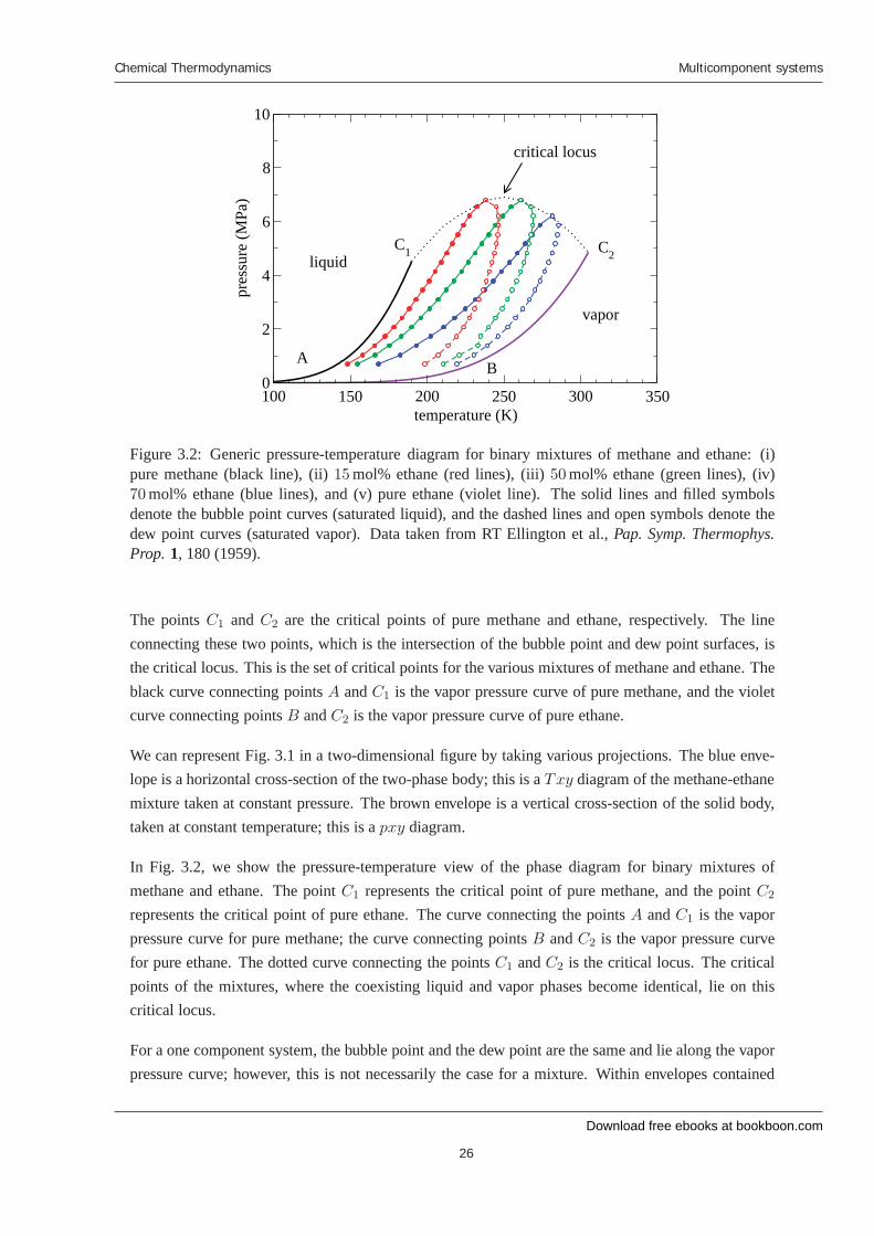
Figure 3.2: Generic pressure-temperature diagram for binary mixtures of methane and ethane: (i)pure methane (black line), (ii) 15 mol% ethane (red lines), (iii) 50 mol% ethane (green lines), (iv)70 mol% ethane (blue lines), and (v) pure ethane (violet line). The solid lines and filled symbolsdenote the bubble point curves (saturated liquid), and the dashed lines and open symbols denote thedew point curves (saturated vapor). Data taken from RT Ellington et al., Pap. Symp. Thermophys.Prop. 1, 180 (1959).
The points C1 and C2 are the critical points of pure methane and ethane, respectively. The lineconnecting these two points, which is the intersection of the bubble point and dew point surfaces, isthe critical locus. This is the set of critical points for the various mixtures of methane and ethane. Theblack curve connecting points A and C1 is the vapor pressure curve of pure methane, and the violetcurve connecting points B and C2 is the vapor pressure curve of pure ethane.
We can represent Fig. 3.1 in a two-dimensional figure by taking various projections. The blue enve-lope is a horizontal cross-section of the two-phase body; this is a Txy diagram of the methane-ethanemixture taken at constant pressure. The brown envelope is a vertical cross-section of the solid body,taken at constant temperature; this is a pxy diagram.
In Fig. 3.2, we show the pressure-temperature view of the phase diagram for binary mixtures ofmethane and ethane. The point C1 represents the critical point of pure methane, and the point C2
represents the critical point of pure ethane. The curve connecting the points A and C1 is the vaporpressure curve for pure methane; the curve connecting points B and C2 is the vapor pressure curvefor pure ethane. The dotted curve connecting the points C1 and C2 is the critical locus. The criticalpoints of the mixtures, where the coexisting liquid and vapor phases become identical, lie on thiscritical locus.
For a one component system, the bubble point and the dew point are the same and lie along the vaporpressure curve; however, this is not necessarily the case for a mixture. Within envelopes contained
Download free ebooks at bookboon.com
Chemical Thermodynamics
27
Multicomponent systems
0.0 0.2 0.4 0.6 0.8 1.0mole fraction of toluene
350
360
370
380
390te
mpe
ratu
re (K
)
0.0 0.2 0.4 0.6 0.8 1.0mole fraction of toluene
10
15
20
25
30
35
40
pres
sure
(kPa
)
liquid
vapor liquid
vapor
(a) (b)
dew point curve
dew point curvebubble point curve
bubble point curve
C
A
A
C
D E B
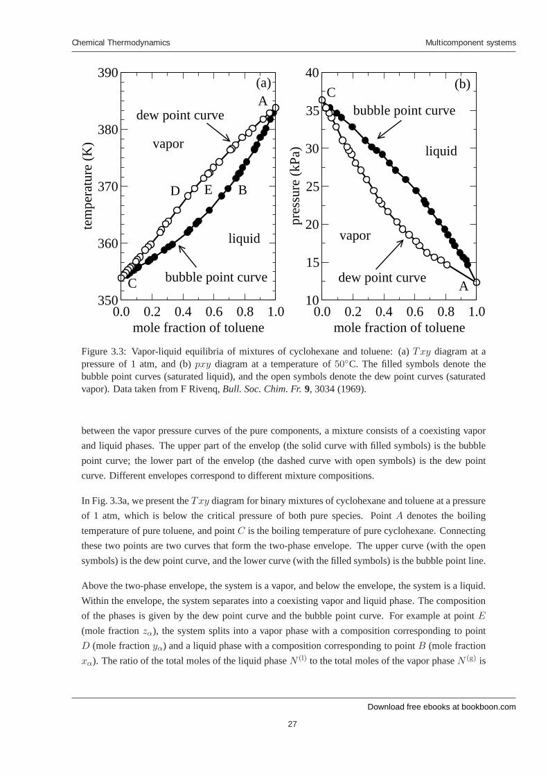
Figure 3.3: Vapor-liquid equilibria of mixtures of cyclohexane and toluene: (a) Txy diagram at apressure of 1 atm, and (b) pxy diagram at a temperature of 50◦C. The filled symbols denote thebubble point curves (saturated liquid), and the open symbols denote the dew point curves (saturatedvapor). Data taken from F Rivenq, Bull. Soc. Chim. Fr. 9, 3034 (1969).
between the vapor pressure curves of the pure components, a mixture consists of a coexisting vaporand liquid phases. The upper part of the envelop (the solid curve with filled symbols) is the bubblepoint curve; the lower part of the envelop (the dashed curve with open symbols) is the dew pointcurve. Different envelopes correspond to different mixture compositions.
In Fig. 3.3a, we present the Txy diagram for binary mixtures of cyclohexane and toluene at a pressureof 1 atm, which is below the critical pressure of both pure species. Point A denotes the boilingtemperature of pure toluene, and point C is the boiling temperature of pure cyclohexane. Connectingthese two points are two curves that form the two-phase envelope. The upper curve (with the opensymbols) is the dew point curve, and the lower curve (with the filled symbols) is the bubble point line.
Above the two-phase envelope, the system is a vapor, and below the envelope, the system is a liquid.Within the envelope, the system separates into a coexisting vapor and liquid phase. The compositionof the phases is given by the dew point curve and the bubble point curve. For example at point E
(mole fraction zα), the system splits into a vapor phase with a composition corresponding to pointD (mole fraction yα) and a liquid phase with a composition corresponding to point B (mole fractionxα). The ratio of the total moles of the liquid phase N (l) to the total moles of the vapor phase N (g) is
Download free ebooks at bookboon.com
Ple
ase
clic
k th
e ad
vert
Chemical Thermodynamics
28
Multicomponent systems
given by the lever rule:
zαN = xαN (l) + yαN (g)
zα(N (l) + N (g)) = xαN (l) + yαN (g)
N (l)
N (g)=
zα − yα
xα − zα(3.11)
where N = N (l) + N (g) is the total number of moles in the system.
In Figure 3.3b, we show the pxy diagram for binary mixtures of cyclohexane and toluene at 50◦C,which is below the critical temperature of both species. Point A is the boiling pressure of pure toluene,and point C is the boiling pressure of pure cyclohexane. Connecting these two points are the bubblepoint (upper) and dew point (lower) curves. Above the bubble point curve, the system is entirely inthe liquid phase, while below the dew point curve, the system is in the vapor phase. Between thesetwo curves, the system separates into a coexisting liquid and vapor phase. The lever rule, describedpreviously for the Txy diagram, also applies to the pxy diagram and can be used to determine therelative proportions of these phases.
© Agilent Technologies, Inc. 2012 u.s. 1-800-829-4444 canada: 1-877-894-4414
Budget-Friendly. Knowledge-Rich.The Agilent InfiniiVision X-Series and 1000 Series offer affordable oscilloscopes for your labs. Plus resources such as lab guides, experiments, and more, to help enrich your curriculum and make your job easier.
See what Agilent can do for you.www.agilent.com/find/EducationKit
Scan for free Agilent iPhone Apps or visit qrs.ly/po2Opli
Download free ebooks at bookboon.com
Chemical Thermodynamics
29
Multicomponent systems
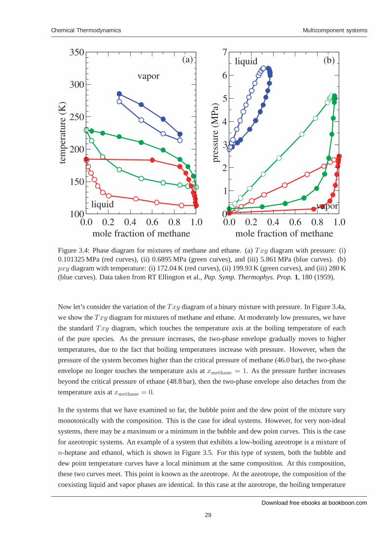
Figure 3.4: Phase diagram for mixtures of methane and ethane. (a) Txy diagram with pressure: (i)0.101325 MPa (red curves), (ii) 0.6895 MPa (green curves), and (iii) 5.861 MPa (blue curves). (b)pxy diagram with temperature: (i) 172.04 K (red curves), (ii) 199.93 K (green curves), and (iii) 280 K(blue curves). Data taken from RT Ellington et al., Pap. Symp. Thermophys. Prop. 1, 180 (1959).
Now let’s consider the variation of the Txy diagram of a binary mixture with pressure. In Figure 3.4a,we show the Txy diagram for mixtures of methane and ethane. At moderately low pressures, we havethe standard Txy diagram, which touches the temperature axis at the boiling temperature of eachof the pure species. As the pressure increases, the two-phase envelope gradually moves to highertemperatures, due to the fact that boiling temperatures increase with pressure. However, when thepressure of the system becomes higher than the critical pressure of methane (46.0 bar), the two-phaseenvelope no longer touches the temperature axis at xmethane = 1. As the pressure further increasesbeyond the critical pressure of ethane (48.8 bar), then the two-phase envelope also detaches from thetemperature axis at xmethane = 0.
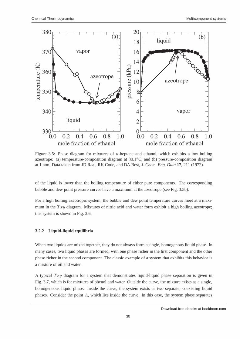
In the systems that we have examined so far, the bubble point and the dew point of the mixture varymonotonically with the composition. This is the case for ideal systems. However, for very non-idealsystems, there may be a maximum or a minimum in the bubble and dew point curves. This is the casefor azeotropic systems. An example of a system that exhibits a low-boiling azeotrope is a mixture ofn-heptane and ethanol, which is shown in Figure 3.5. For this type of system, both the bubble anddew point temperature curves have a local minimum at the same composition. At this composition,these two curves meet. This point is known as the azeotrope. At the azeotrope, the composition of thecoexisting liquid and vapor phases are identical. In this case at the azeotrope, the boiling temperature
Download free ebooks at bookboon.com
Chemical Thermodynamics
30
Multicomponent systems
Figure 3.5: Phase diagram for mixtures of n-heptane and ethanol, which exhibits a low boilingazeotrope: (a) temperature-composition diagram at 30.1◦C, and (b) pressure-composition diagramat 1 atm. Data taken from JD Raal, RK Code, and DA Best, J. Chem. Eng. Data 17, 211 (1972).
of the liquid is lower than the boiling temperature of either pure components. The correspondingbubble and dew point pressure curves have a maximum at the azeotrope (see Fig. 3.5b).
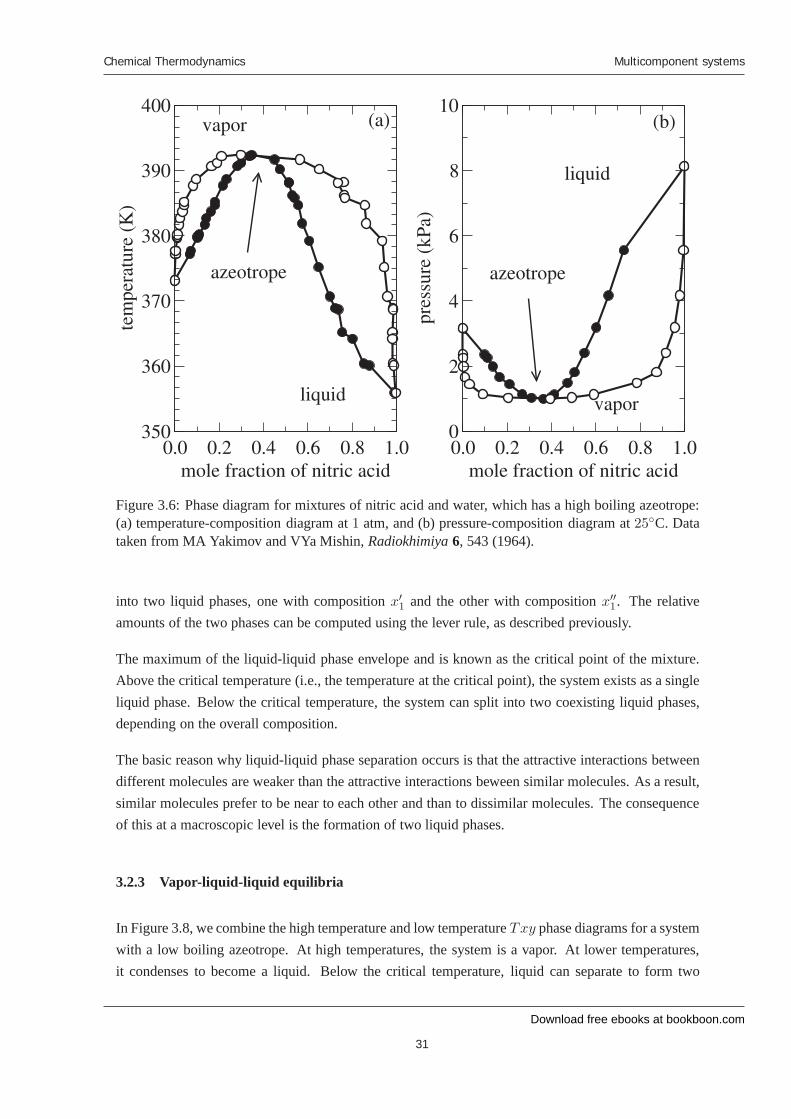
For a high boiling azeotropic system, the bubble and dew point temperature curves meet at a maxi-mum in the Txy diagram. Mixtures of nitric acid and water form exhibit a high boiling azeotrope;this system is shown in Fig. 3.6.
3.2.2 Liquid-liquid equilibria
When two liquids are mixed together, they do not always form a single, homogenous liquid phase. Inmany cases, two liquid phases are formed, with one phase richer in the first component and the otherphase richer in the second component. The classic example of a system that exhibits this behavior isa mixture of oil and water.
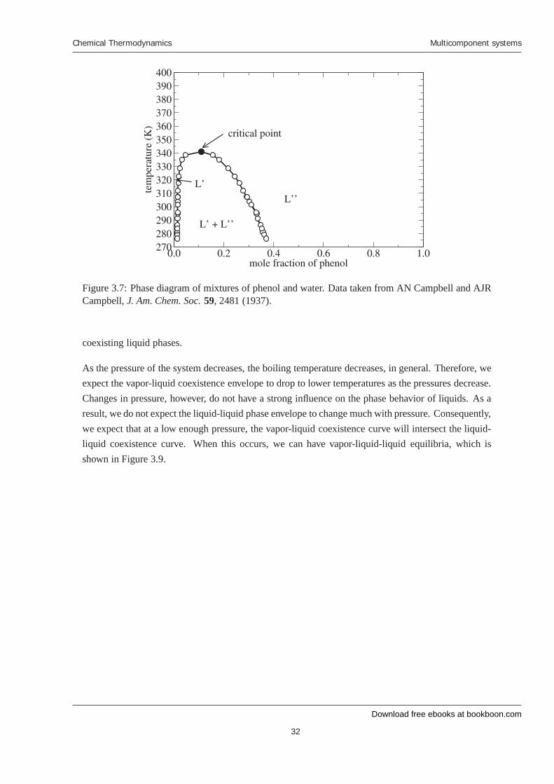
A typical Txy diagram for a system that demonstrates liquid-liquid phase separation is given inFig. 3.7, which is for mixtures of phenol and water. Outside the curve, the mixture exists as a single,homogeneous liquid phase. Inside the curve, the system exists as two separate, coexisting liquidphases. Consider the point A, which lies inside the curve. In this case, the system phase separates
Download free ebooks at bookboon.com
Chemical Thermodynamics
31
Multicomponent systems
Figure 3.6: Phase diagram for mixtures of nitric acid and water, which has a high boiling azeotrope:(a) temperature-composition diagram at 1 atm, and (b) pressure-composition diagram at 25◦C. Datataken from MA Yakimov and VYa Mishin, Radiokhimiya 6, 543 (1964).
into two liquid phases, one with composition x′1 and the other with composition x′′1. The relativeamounts of the two phases can be computed using the lever rule, as described previously.
The maximum of the liquid-liquid phase envelope and is known as the critical point of the mixture.Above the critical temperature (i.e., the temperature at the critical point), the system exists as a singleliquid phase. Below the critical temperature, the system can split into two coexisting liquid phases,depending on the overall composition.
The basic reason why liquid-liquid phase separation occurs is that the attractive interactions betweendifferent molecules are weaker than the attractive interactions beween similar molecules. As a result,similar molecules prefer to be near to each other and than to dissimilar molecules. The consequenceof this at a macroscopic level is the formation of two liquid phases.
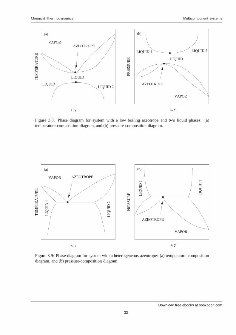
3.2.3 Vapor-liquid-liquid equilibria
In Figure 3.8, we combine the high temperature and low temperature Txy phase diagrams for a systemwith a low boiling azeotrope. At high temperatures, the system is a vapor. At lower temperatures,it condenses to become a liquid. Below the critical temperature, liquid can separate to form two
Download free ebooks at bookboon.com
Chemical Thermodynamics
32
Multicomponent systems
Figure 3.7: Phase diagram of mixtures of phenol and water. Data taken from AN Campbell and AJRCampbell, J. Am. Chem. Soc. 59, 2481 (1937).
coexisting liquid phases.
As the pressure of the system decreases, the boiling temperature decreases, in general. Therefore, weexpect the vapor-liquid coexistence envelope to drop to lower temperatures as the pressures decrease.Changes in pressure, however, do not have a strong influence on the phase behavior of liquids. As aresult, we do not expect the liquid-liquid phase envelope to change much with pressure. Consequently,we expect that at a low enough pressure, the vapor-liquid coexistence curve will intersect the liquid-liquid coexistence curve. When this occurs, we can have vapor-liquid-liquid equilibria, which isshown in Figure 3.9.
Download free ebooks at bookboon.com
Chemical Thermodynamics
33
Multicomponent systems
Figure 3.8: Phase diagram for system with a low boiling azeotrope and two liquid phases: (a)temperature-composition diagram, and (b) pressure-composition diagram.
Figure 3.9: Phase diagram for system with a heterogeneous azeotrope: (a) temperature-compositiondiagram, and (b) pressure-composition diagram.
Download free ebooks at bookboon.com
Chemical Thermodynamics
34
Multicomponent systems
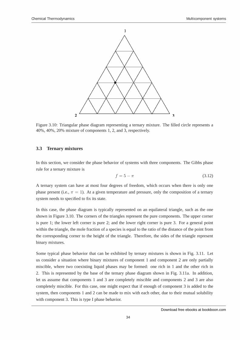
Figure 3.10: Triangular phase diagram representing a ternary mixture. The filled circle represents a40%, 40%, 20% mixture of components 1, 2, and 3, respectively.
3.3 Ternary mixtures
In this section, we consider the phase behavior of systems with three components. The Gibbs phaserule for a ternary mixture is
f = 5− π (3.12)
A ternary system can have at most four degrees of freedom, which occurs when there is only onephase present (i.e., π = 1). At a given temperature and pressure, only the composition of a ternarysystem needs to specified to fix its state.
In this case, the phase diagram is typically represented on an equilateral triangle, such as the oneshown in Figure 3.10. The corners of the triangles represent the pure components. The upper corneris pure 1; the lower left corner is pure 2; and the lower right corner is pure 3. For a general pointwithin the triangle, the mole fraction of a species is equal to the ratio of the distance of the point fromthe corresponding corner to the height of the triangle. Therefore, the sides of the triangle representbinary mixtures.
Some typical phase behavior that can be exhibited by ternary mixtures is shown in Fig. 3.11. Letus consider a situation where binary mixtures of component 1 and component 2 are only partiallymiscible, where two coexisting liquid phases may be formed: one rich in 1 and the other rich in2. This is represented by the base of the ternary phase diagram shown in Fig. 3.11a. In addition,let us assume that components 1 and 3 are completely miscible and components 2 and 3 are alsocompletely miscible. For this case, one might expect that if enough of component 3 is added to thesystem, then components 1 and 2 can be made to mix with each other, due to their mutual solubilitywith component 3. This is type I phase behavior.

Download free ebooks at bookboon.com
Ple
ase
clic
k th
e ad
vert
Chemical Thermodynamics
35
Multicomponent systems
Figure 3.11: Generic phase behavior of ternary mixtures: (a) type I, (b) type II, and (c) type III.
A type II phase diagram, shown in Fig. 3.11b, corresponds to a situation where components 1 and3 are completely miscible, but both components 1 and 2 and components 2 and 3 are only partiallymiscible.
Finally, type III phase behavior is shown in Fig. 3.11c. In this case, the various binary mixtures ofthe three components are each only partially miscible. The shaded triangle in the center of the phasediagram is a region where three phases are in coexistence with each other. Systems with a compositionwhich lies within this shaded triangle will split into three separate phases; the composition of eachof these phases corresponds to one of the corners of the triangle. The composition of the individualphases will not vary with the system’s location within the triangle (i.e., its overall composition);however, the relative amounts of each of the phases will.
Download free ebooks at bookboon.com
Chemical Thermodynamics
36
The ideal solution model
4 The ideal solution model
In many situations, we need to predict the properties of a mixture, given that we already know theproperties of the pure species. To do this requires a model that can describe how various componentsmix. In mathematical terms, this means that we need to relate the Gibbs free energy of a mixture tothe Gibbs free energy of the various pure components. One of the simplest models that achieves thisis the ideal solution model. In this lecture, we present the ideal solution model. Then we apply thismodel to describe vapor-liquid equilibria, and as a result, derive Raoult’s law.
4.1 Definition of the ideal solution model
For an ideal solution, the Gibbs free energy¯G defined as:
¯G(T, p,N1, N2, . . . ) =
∑α
Nαμ◦α(T, p) + RT∑α
Nα ln xα (4.1)
where T is the absolute temperature of the system, p is the pressure of the system, R is the idealgas constant, Nα is the number of moles of component α, xα is the mole fraction of component α,and μ◦α(T, p) is the molar Gibbs free energy of pure component α (recall that for pure systems, themolar Gibbs free energy is equal to the chemical potential). The first term on the right-hand side ofEq. (4.1) represents the Gibbs free energy of the system if its components were unmixed. The secondterm represents the contribution due to the entropy of mixing.
In all calculations involving the ideal solution model, we assume that we know the molar Gibbs freeenergy of each of the pure species as a function of temperature and pressure. Mathematically, thismeans that know the form of the functions μ◦α(T, p). Physically, this means that we know everythingabout the thermodynamics of the pure species.
Once we know the Gibbs free energy of a system as a function of temperature, pressure, and compo-sition, we know everything about its thermodynamics. For example, the total volume of the system
¯V can be derived from the Gibbs free energy:
¯V =
(∂
¯G
∂p
)T,Nα
=∑α
Nα
(∂μ◦α∂p
)T,Nα
=∑α
NαV ◦α (4.2)
where V ◦α is the molar volume of pure species α, and we have used the relation V ◦α = (∂μ◦α/∂p).The total volume is equal to the sum of the volumes of the pure components. Therefore, there is nochange of volume on mixing for an ideal solution.
Download free ebooks at bookboon.com
Chemical Thermodynamics
37
The ideal solution model
The total entropy¯S of the system is given by
¯S = −
(∂
¯G
∂T
)p,Nα
=∑α
NαS◦α(T, p)−R∑α
Nα ln xα (4.3)
where S◦α is the molar entropy of pure component α, and we have used the relation S◦α = −(∂μ◦α/∂T ).Unlike the case for volume, the total entropy of the mixture is not the same as the sum of the entropiesof the unmixed systems. In fact, due to the second term in Eq. (4.3), the entropy increases upon mix-ing.
The total enthalpy¯H of the system is given by
¯H =
¯G + T
¯S
=∑α
Nαμ◦α(T, p) + RT∑α
Nα ln xα + T
(∑α
NαS◦α(T, p)−R∑α
Nα ln xα
)
=∑α
NαH◦α(T, p) (4.4)
where H◦α is the molar enthalpy of pure α, and we have used the relation H◦
α = μ◦α + TS◦α. In thiscase, we see that the total enthalpy of the system is the same as the sum of the enthalpies of the purecomponents. No heat is absorbed or released upon mixing an ideal solution.
The chemical potential of species α is given by
μα(T, p, x2, x3, . . . ) =
(∂
¯G
∂Nα
)T,p,N
α′ �=α
= μ◦α(T, p) + RT ln xα (4.5)
In an ideal solution, we see that the chemical potential of a species depends on its mole fraction andnot directly on the composition of the other components in the system. Also, we see that mixingcauses the chemical potential of each component to decrease.
4.2 Derivation of Raoult’s law
Now we will use the ideal solution model to develop a mathematical description of vapor-liquidequilibrium in a multicomponent solution. We will make the assumption that we have a system thatis separated into a coexisting vapor and liquid phase. The vapor phase will be assumed to behave likean ideal gas, while the liquid phase will be assumed to behave as an ideal solution.
Download free ebooks at bookboon.com
Chemical Thermodynamics
38
The ideal solution model
The basic condition for equilibrium between phases is
μvα(T, p, y2, y3, . . . ) = μl
α(T, p, x2, x3, . . . ) (4.6)
where μvα is the chemical potential of component α in the vapor phase, μl
α is the chemical potentialof component α in the liquid phase, yα is the mole fraction of component α in the vapor phase, andxα is the mole fraction of component α in the liquid phase.
Since the liquid phase behaves as an ideal mixture, we have
μlα(T, p, x2, x3, . . . ) = μ◦,lα (T, p) + RT ln xα
= μ◦,lα (T, pvapα ) +
∫ p
pvapα
dp′∂μ◦,lα (T, p′)
∂p+ RT ln xα
= μ◦,lα (T, pvapα ) +
∫ p
pvapα
dp′V ◦,lα (T, p′) + RT lnxα (4.7)
where we have used the relation (∂μ◦,lα /∂p) = V ◦,lα , and V ◦,lα is the molar volume of pure α in theliquid phase. If we assume that the volume of the liquid is nearly independent of pressure, thenEq. (4.7) becomes:
μlα(T, p, x2, x3, . . . ) = μ◦,lα (T, pvap
α ) + V ◦,lα (T, p)(p − pvapα ) + RT ln xα (4.8)
Since the vapor phase can be considered an ideal gas, we have
μvα(T, p, y2, y3, . . . ) = μ◦,vα (T, p) + RT ln yα
= μ◦,vα (T, pvapα ) +
∫ p
pvapα
dp′∂μ◦,vα (T, p′)
∂p+ RT ln yα
= μ◦,vα (T, pvapα ) +
∫ p
pvapα
dp′V ◦,vα (T, p′) + RT ln yα (4.9)
where V ◦,vα is the molar volume of pure α in the vapor phase. For an ideal gas, we have V ◦,vα (T, p) =
RT/p, and, therefore,
μvα(T, p, y2, y3, . . . ) = μ◦,vα (T, pvap
α ) +
∫ p
pvapα
dp′RT
p′+ RT ln yα
= μ◦,vα (T, pvapα ) + RT ln
p
pvapα
+ RT ln yα (4.10)
Inserting Eqs. (4.8) and (4.10) into Eq. (4.6) yields
μ◦,vα (T, pvapα ) + RT ln
p
pvapα
+ RT ln yα = μ◦,lα (T, pvapα ) + V ◦,lα (T, p)(p − pvap
α ) + RT ln xα
(4.11)
We note that at the vapor pressure of a pure system, the chemical potentials of the liquid and vapor

Download free ebooks at bookboon.com
Ple
ase
clic
k th
e ad
vert
Chemical Thermodynamics
39
The ideal solution model
phases are equal. That is, μ◦,vα (T, pvapα ) = μ◦,lα (T, pvap
α ). Substituting this relation into Eq. (4.11)gives
RT lnp
pvapα
+ RT ln yα = V ◦,lα (T, p)(p − pvapα ) + RT ln xα
yαp = xαpvapα exp
[V ◦α (p − pvap
α )
RT
](4.12)
The exponential term on the right-hand side of Eq. (4.12) is known as the Poynting factor. For mostsystems at low to moderate pressures, the Poynting factor is almost equal to one. In the case of waterat 25◦C:
V ◦α (p− pvapα )
RT≈
(10−6 m3/g)(18.02 g/mol)(101325 − 3170) Pa
(8.314 J mol−1K−1)(298.15 K)
≈ 7.14 × 10⁻⁴ (4.13)
This leads to a Poynting factor of 1.000714, which is essentially equal to one. If we assume that thePoynting factor is close to one, we have Raoult’s law:
yαp = xαpvapα (T ) (4.14)
With us you can shape the future. Every single day. For more information go to:www.eon-career.com
Your energy shapes the future.
Download free ebooks at bookboon.com
Chemical Thermodynamics
40
Partial molar properties
5 Partial molar properties
In Chapter 4, we examined the properties of ideal solutions. Many properties of an ideal solution donot change on mixing. For example, the volume of a mixture is equal to the sum of the volume ofthe original unmixed solutions. In this situation, it is straightforward to assign how much volume isoccupied by each component in the system — it is simply the volume occupied by components intheir unmixed state.
For a general system, however, the volume, as well as other properties, is not additive. That is, thevolume of a mixture is not equal to the sum of the volumes of the individual pure components. Inthis situation, it is not clear how to assign how much volume is occupied of each species. One logicalmanner to do this is through the use of partial molar properties.
In this Chapter, we define partial molar properties and describe their application. We then discusstheir relationship with the change of properties of a system on mixing. Finally, we examine thegraphical representation of partial molar properties for binary mixtures.
5.1 Definition
In general for any extensive property¯X of a system, we define a partial molar property of component
α asX̄α ≡
(∂
¯X
∂Nα
)T,p,N
α′ �=α
, (5.1)
where Nα is the number of moles of species α, T is the temperature, and p is the pressure of thesystem. Physically, the partial molar quantity X̄α corresponds to the change of the property
¯X with
the addition of a small amount of component α, while holding constant the temperature, pressure, andnumber of moles of all other species. Note that partial molar properties are intensive and, therefore,do not depend on the system size.
Examples of partial molar properties include the partial molar enthalpy H̄α, which is defined as
H̄α ≡
(∂
¯H
∂Nα
)T,p,N
α′ �=α
, (5.2)
and the partial molar volume V̄α, which is defined as
V̄α ≡
(∂¯V
∂Nα
)T,p,N
α′ �=α
. (5.3)
Note also that from the relation (see Eq. (3.4))
μα ≡
(∂
¯G
∂Nα
)T,p,N
α′ �=α
, (5.4)
Download free ebooks at bookboon.com
Chemical Thermodynamics
41
Partial molar properties
we see that the chemical potential is equal to the partial molar Gibbs free energy.
5.2 Relationship between total properties and partial molar properties
Any extensive property of a system can be written in terms of its partial molar quantities. Recall thatan extensive property is a property that scales proportionally with the size of the system. If the systemdoubles in size, then value of the extensive property should double. If the size of the system increasesby a factor t, then the value of the extensive property should increase by a factor t. For example,taking X to be the volume V , then we expect the total volume of the system
¯V to increase by a factor
t if the number of total moles in the system are increased by a factor t, holding the composition of thesystem fixed. This feature can be expressed mathematically as
t¯X(T, p,N1, N2, . . . ) =
¯X(T, p, tN1, tN2, . . . ) (5.5)
Taking the derivative of both sides of the Eq. (5.5) with respect to t, while keeping all other variablesconstant, yields
¯X(T, p,N1, N2, . . . ) =
∑α
(∂
¯X
∂tNα
)T,p,tN
α′ �=α
(∂tNα
∂t
)Nα
=∑α
X̄αNα
¯X(T, p,N1, N2, . . . ) =
∑α
NαX̄α (5.6)
The value of any extensive property of a system is equal to the sum of the partial molar propertiesof each component multiplied by the amount of each component in the system. Therefore, we can“divide” the property of a mixture , such as the volume or enthalpy, between its individual componentsaccording to their partial molar properties.
One important example of this, which we will utilize later, is the Gibbs free energy G. In this case, thetotal Gibbs free energy
¯G can be expressed in terms of the chemical potentials μα of each component
(partial molar Gibbs free energy)
¯G(T, p,N1, N2, . . . ) =
∑α
Nαμα (5.7)
By dividing both sides of Eq. (5.6) by N , the total number of moles in the system, we find that molarproperties are similarly related to partial molar properties
X =∑α
xαX̄α (5.8)
where xα is the mole fraction of component α.
Download free ebooks at bookboon.com
Ple
ase
clic
k th
e ad
vert
Chemical Thermodynamics
42
Partial molar properties
The derivative of a molar property with respect to xα can also be written in terms of partial molarproperties. To demonstrate this, let us consider that an extensive property
¯X is a function of T , p,
mole numbers Nα. We can express its differential as
d¯X =
(∂
¯X
∂T
)p,Nα
dT +
(∂
¯X
∂p
)T,Nα
dp +∑α
(∂
¯X
∂Nα
)T,p,N
α′ �=α
dNα
=
(∂
¯X
∂T
)p,Nα
dT +
(∂
¯X
∂p
)T,Nα
dp +∑α
X̄αdNα (5.9)
Now, we take the derivative of¯X with respect to xα, holding T , p, all other mole fractions (with the
exception of x1), and total number of moles N constant:(
∂¯X
∂xα
)T,p,x
α′ �=α,1,N
=∑α′
X̄α′
(∂Nα′
∂xα
)T,p,x
α′ �=α,1,N
N
(∂X
∂xα
)T,p,x
α′ �=α,1
= N(X̄α − X̄1)
(∂X
∂xα
)T,p,x
α′ �=α,1
= X̄α − X̄1 (5.10)
where we have used the relations Nα = Nxα and x1 = 1−∑
α�=1 xα.
Download free ebooks at bookboon.com
Chemical Thermodynamics
43
Partial molar properties
5.3 Properties changes on mixing
Often when pure components are mixed together to form a solution, the properties of the overallsystem change. For example, if we mix a quantity of pure liquid ethanol with pure liquid water, thevolume of the final mixture has a slightly smaller volume than the sum of the volumes of the originalpure liquid. This system has a negative volume change on mixing. If a solution of concentratedsulfuric acid is mixed with pure water, then a large amount of heat is released because the enthalpy ofthe mixture (at equilibrium) is lower than the sum of the enthalpy of the unmixed components. Thissystem has a negative enthalpy of mixing.
To characterize this change, the property change on mixing Δ¯Xmix is defined as the difference be-
tween the property of the mixture and the properties of the pure components:
Δ¯Xmix =
¯X −
∑α
NαX◦α
=∑α
Nα(X̄α −X◦α) (5.11)
where X◦α is the molar property of pure α. If the property increases on mixing, then Δ
¯Xmix is
positive; if the property decreases on mixing, then Δ¯Xmix is negative.
Similarly, the molar change of a property on mixing ΔXmix is given by:
ΔXmix =∑α
xα(X̄α −X◦α) (5.12)
5.4 Graphical representation for binary systems
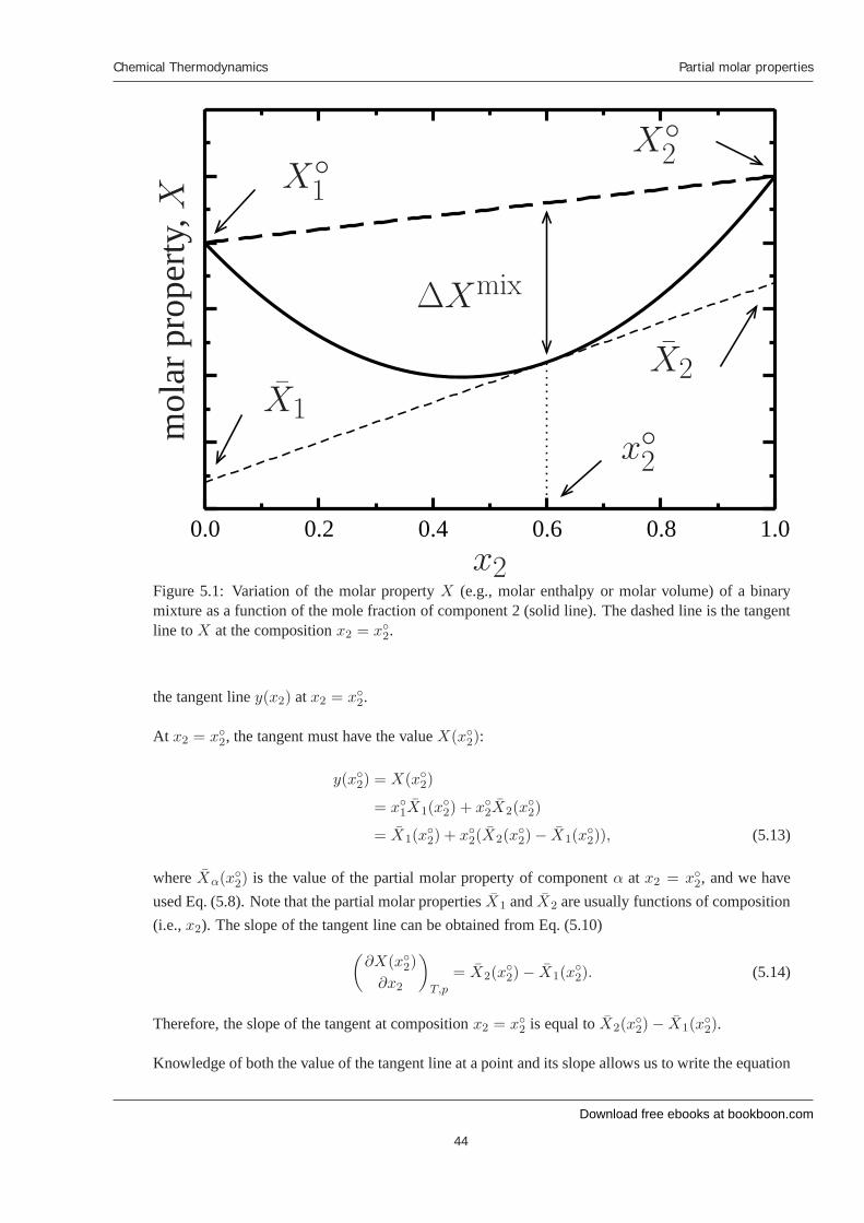
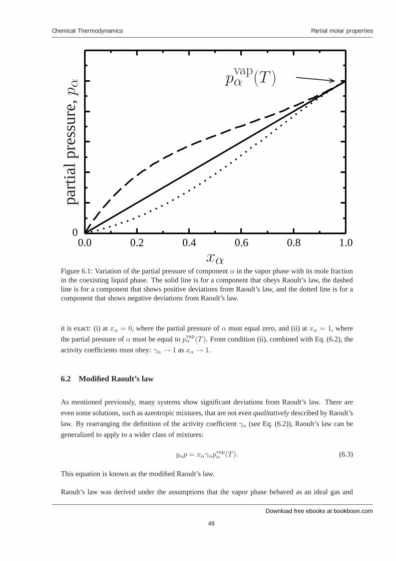
The relations derived in this section provide us a means to easily extract the partial molar propertiesof a system from a graph of the corresponding molar property with repect to composition. A genericplot of the variation of a molar property of a binary mixture with composition is given by the solidline in Fig. 5.1. When x2 = 0, the system consists only of component 1, and the value of the molarproperty should be equal to the molar property of pure component 1 X◦
1 . Likewise, when x2 = 1,the system consists only of component 2, and the value of X should be equal to X◦
2 . The variation ofa molar property of an unmixed system composed of pure 1 and pure 2 is given by the thick dashedline in Fig. 5.1.
The distance between the thick dashed line and the solid line represents the difference between amolar property of the mixture and that of the unmixed system. This difference is equal to ΔXmix.
Now consider a line that is tangent to X (i.e., the solid line) at the composition x2 = x◦2. This isdenoted by the thin dashed line in Fig. 5.1. The intercept of the tangent line at x2 = 0 and x2 = 1 areequal to X̄1 and X̄2, respectively; that is, the intercepts of the tangent line are equal to the partial molarproperties of the system at a given composition. To demonstrate this, let’s determine the equation for
Download free ebooks at bookboon.com
Chemical Thermodynamics
44
Partial molar properties
0.0 0.2 0.4 0.6 0.8 1.0x2
x◦2
mol
arpr
oper
ty,X
ΔXmix
X̄1
X̄2
X◦1
X◦2
Figure 5.1: Variation of the molar property X (e.g., molar enthalpy or molar volume) of a binarymixture as a function of the mole fraction of component 2 (solid line). The dashed line is the tangentline to X at the composition x2 = x◦2.
the tangent line y(x2) at x2 = x◦2.
At x2 = x◦2, the tangent must have the value X(x◦2):
y(x◦2) = X(x◦2)
= x◦1X̄1(x◦2) + x◦2X̄2(x
◦2)
= X̄1(x◦2) + x◦2(X̄2(x
◦2)− X̄1(x
◦2)), (5.13)
where X̄α(x◦2) is the value of the partial molar property of component α at x2 = x◦2, and we haveused Eq. (5.8). Note that the partial molar properties X̄1 and X̄2 are usually functions of composition(i.e., x2). The slope of the tangent line can be obtained from Eq. (5.10)
(∂X(x◦2)
∂x2
)T,p
= X̄2(x◦2)− X̄1(x
◦2). (5.14)
Therefore, the slope of the tangent at composition x2 = x◦2 is equal to X̄2(x◦2)− X̄1(x
◦2).
Knowledge of both the value of the tangent line at a point and its slope allows us to write the equation

Download free ebooks at bookboon.com
Ple
ase
clic
k th
e ad
vert
Chemical Thermodynamics
45
Partial molar properties
for the tangent line:
y(x2) = y(x◦2) + [X̄2(x◦2)− X̄1(x
◦2)](x2 − x◦2)
= X̄1(x◦2) + x◦2(X̄2(x
◦2)− X̄1(x
◦2)) + [X̄2(x
◦2)− X̄1(x
◦2)](x2 − x◦2)
= X̄1(x◦2) + [X̄2(x
◦2)− X̄1(x
◦2)]x2 (5.15)
From Eq. (5.15), we see that when x2 = 0, the tangent line has a value equal to X̄1(x◦2), and when
x2 = 1, it has a value equal to X̄2(x◦2). This is shown graphically by the thin dashed line in Fig. 5.1.
For an ideal solution, the molar volume V of a mixture satisfies
V = x1V◦1 + x2V
◦2 (5.16)
where V ◦1 and V ◦2 is the molar volume of pure species 1 and 2, respectively. Therefore, ΔV mix = 0
for an ideal solution. Similarly, the molar enthalpy H is given by
H = x1H◦1 + x2H
◦2 (5.17)
where H◦1 and H◦
2 is the molar volume of pure species 1 and 2, respectively. Therefore, ΔHmix = 0
for an ideal solution.
By 2020, wind could provide one-tenth of our planet’s electricity needs. Already today, SKF’s innovative know-how is crucial to running a large proportion of the world’s wind turbines.
Up to 25 % of the generating costs relate to mainte-nance. These can be reduced dramatically thanks to our systems for on-line condition monitoring and automatic lubrication. We help make it more economical to create cleaner, cheaper energy out of thin air.
By sharing our experience, expertise, and creativity, industries can boost performance beyond expectations.
Therefore we need the best employees who can meet this challenge!
The Power of Knowledge Engineering
Brain power
Plug into The Power of Knowledge Engineering.
Visit us at www.skf.com/knowledge
Download free ebooks at bookboon.com
Chemical Thermodynamics
46
Partial molar properties
Equations (5.16) and (5.17) correspond to a straight line connecting the molar properties of the purecomponents (e.g., the thick dashed line in Fig. 5.1). In this case, we see that the partial molar volumesand partial molar enthalpies of each species are equal to the respective molar quantities in the purestate. We expect ideal behavior when the fluids that are mixed consist of similar molecules.
Most solutions do not exhibit ideal behavior, and the actual curve corresponding to the variation of themolar volume or enthalpy of the mixture deviates from a straight line (e.g., the solid line in Fig. 5.1).When the curve for the molar volume lies above the ideal mixture line, the system expands uponmixing; when the curve lies below the line, the system contracts. In the case of the molar enthalpy, acurve that lies above the ideal mixture line corresponds to the system that absorbs heat (e.g., mixinglead bromide and water); a curve that lies below the line corresponds to the system releasing heat(e.g., mixing sulfuric acid and water). This non-ideal mixing in the case of the molar enthalpy isthe principle used in cold packs and heat packs. We will develop mathematical models to describenon-ideal mixtures. We use partial molar properties in more detail later.
Download free ebooks at bookboon.com
Chemical Thermodynamics
47
Partial molar properties
6 Nonideal solutions
In Chapter 4, we developed the ideal solution model, which enables the estimation of the propertiesof mixtures from knowledge of the thermodynamic behavior of the pure species. While the idealsolution model does provide accurate predictions for mixtures of relatively similar substances, manysystems do exhibit substantial deviations from the ideal solution model.
In this chapter, we present methods for mathematically describing the properties of non-ideal solu-tions — mixtures that deviate from the ideal solution model.
6.1 Deviations from Raoult’s law and the activity coefficient
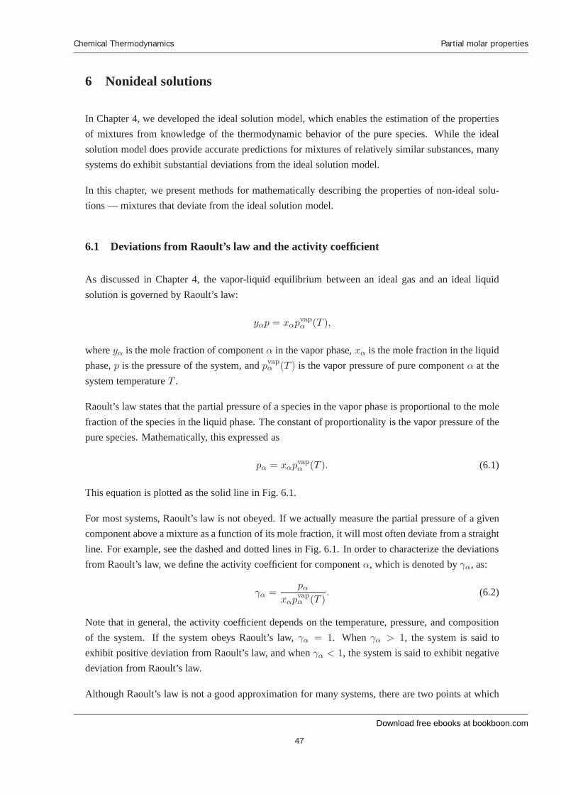
As discussed in Chapter 4, the vapor-liquid equilibrium between an ideal gas and an ideal liquidsolution is governed by Raoult’s law:
yαp = xαpvapα (T ),
where yα is the mole fraction of component α in the vapor phase, xα is the mole fraction in the liquidphase, p is the pressure of the system, and pvap
α (T ) is the vapor pressure of pure component α at thesystem temperature T .
Raoult’s law states that the partial pressure of a species in the vapor phase is proportional to the molefraction of the species in the liquid phase. The constant of proportionality is the vapor pressure of thepure species. Mathematically, this expressed as
pα = xαpvapα (T ). (6.1)
This equation is plotted as the solid line in Fig. 6.1.
For most systems, Raoult’s law is not obeyed. If we actually measure the partial pressure of a givencomponent above a mixture as a function of its mole fraction, it will most often deviate from a straightline. For example, see the dashed and dotted lines in Fig. 6.1. In order to characterize the deviationsfrom Raoult’s law, we define the activity coefficient for component α, which is denoted by γα, as:
γα =pα
xαpvapα (T )
. (6.2)
Note that in general, the activity coefficient depends on the temperature, pressure, and compositionof the system. If the system obeys Raoult’s law, γα = 1. When γα > 1, the system is said toexhibit positive deviation from Raoult’s law, and when γα < 1, the system is said to exhibit negativedeviation from Raoult’s law.
Although Raoult’s law is not a good approximation for many systems, there are two points at which
Download free ebooks at bookboon.com
Chemical Thermodynamics
48
Partial molar properties
0.0 0.2 0.4 0.6 0.8 1.00
pvapα (T )
xα
parti
alpr
essu
re,p
α
Figure 6.1: Variation of the partial pressure of component α in the vapor phase with its mole fractionin the coexisting liquid phase. The solid line is for a component that obeys Raoult’s law, the dashedline is for a component that shows positive deviations from Raoult’s law, and the dotted line is for acomponent that shows negative deviations from Raoult’s law.
it is exact: (i) at xα = 0, where the partial pressure of α must equal zero, and (ii) at xα = 1, wherethe partial pressure of α must be equal to pvap
α (T ). From condition (ii), combined with Eq. (6.2), theactivity coefficients must obey: γα → 1 as xα → 1.
6.2 Modified Raoult’s law
As mentioned previously, many systems show significant deviations from Raoult’s law. There areeven some solutions, such as azeotropic mixtures, that are not even qualitatively described by Raoult’slaw. By rearranging the definition of the activity coefficient γα (see Eq. (6.2)), Raoult’s law can begeneralized to apply to a wider class of mixtures:
yαp = xαγαpvapα (T ). (6.3)
This equation is known as the modified Raoult’s law.
Raoult’s law was derived under the assumptions that the vapor phase behaved as an ideal gas and
Download free ebooks at bookboon.com
Chemical Thermodynamics
49
Partial molar properties
that the liquid phase behaved as an ideal solution. In this section, we will relax the assumption thatthe liquid behaves as an ideal solution to derive the modified Raoult’s law, given in Eq. (6.3). If were-examine the derivation of Raoult’s law, we find that we can arrive at the modified Raoult’s law ifthe chemical potential of the liquid phase can be written as:
μlα(T, p, x2, x3, . . . ) = μ◦,lα (T, p) + RT ln xαγα (6.4)
where μ◦,lα (T, p) is the chemical potential of pure component α. Note that we can divide the chemicalpotential into an ideal contribution μid
α , given by the ideal solution model, and a non-ideal contribution(or excess) μex
α , which is directly related to the activity coefficient:
μα(T, p, x2, x3, . . . ) = μidα (T, p, x2, x3, . . . ) + μex
α (T, p, x2, x3, . . . ), (6.5)
where
μidα (T, p, x2, x3, . . . ) = μ◦,lα (T, p) + RT ln xα, (6.6)
andμex
α (T, p, x2, x3, . . . ) = RT ln γα(T, p, x2, x3, . . . ). (6.7)
In general, an excess property Xex is defined as the deviation of a property from its ideal solutionvalue:
Xex(T, p, x2, x3, . . . ) = X(T, p, x2, x3, . . . )−X id(T, p, x2, x3, . . . ) (6.8)
Substituting the expression for the chemical potential given in Eq. (6.4) into Eq. (5.7), we find thatthe Gibbs free energy of a non-ideal solution can be written as:
¯G =
∑α
Nαμα
=∑α
Nα(μ◦α + RT ln xαγα)
=∑α
Nα(μ◦α + RT ln xα) + RT∑α
Nα ln γα
¯G =
¯Gid +
¯Gex (6.9)
where¯Gid is the Gibbs free energy of an ideal solution, defined as
¯Gid =
∑α
Nαμ◦α + RT∑α
Nα lnxα (6.10)
and¯Gex is the excess Gibbs free energy, which is given by
¯Gex = RT
∑α
Nα ln γα (6.11)

Download free ebooks at bookboon.com
Ple
ase
clic
k th
e ad
vert
Chemical Thermodynamics
50
Partial molar properties
While the theoretical treatment we have presented for non-ideal solutions are all formally exact, theyare of no practical use until we have some kind of model for the variation of the activity coefficientswith the system composition, temperature, and pressure. In the next section, we present variousmodels that can be employed to describe the activity coefficients.
Are you considering aEuropean business degree?LEARN BUSINESS at university level. We mix cases with cutting edge research working individually or in teams and everyone speaks English. Bring back valuable knowledge and experience to boost your career.
MEET a culture of new foods, music and traditions and a new way of studying business in a safe, clean environment – in the middle of Copenhagen, Denmark.
ENGAGE in extra-curricular activities such as case competitions, sports, etc. – make new friends among cbs’ 18,000 students from more than 80 countries.
See what we look likeand how we work on cbs.dk
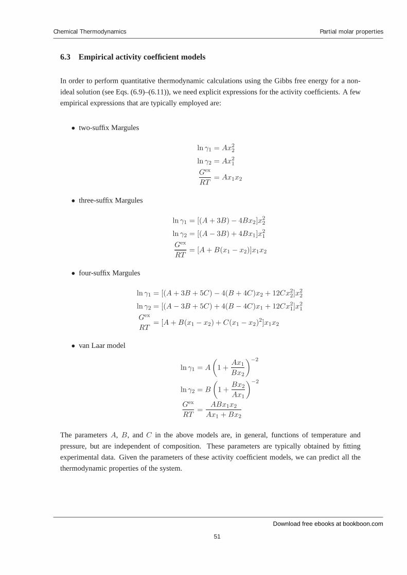
Download free ebooks at bookboon.com
Chemical Thermodynamics
51
Partial molar properties
6.3 Empirical activity coefficient models
In order to perform quantitative thermodynamic calculations using the Gibbs free energy for a non-ideal solution (see Eqs. (6.9)–(6.11)), we need explicit expressions for the activity coefficients. A fewempirical expressions that are typically employed are:
• two-suffix Margules
ln γ1 = Ax22
ln γ2 = Ax21
Gex
RT= Ax1x2
• three-suffix Margules
ln γ1 = [(A + 3B)− 4Bx2]x22
ln γ2 = [(A− 3B) + 4Bx1]x21
Gex
RT= [A + B(x1 − x2)]x1x2
• four-suffix Margules
ln γ1 = [(A + 3B + 5C)− 4(B + 4C)x2 + 12Cx22]x
22
ln γ2 = [(A− 3B + 5C) + 4(B − 4C)x1 + 12Cx21]x
21
Gex
RT= [A + B(x1 − x2) + C(x1 − x2)
2]x1x2
• van Laar model
ln γ1 = A
(1 +
Ax1
Bx2
)−2
ln γ2 = B
(1 +
Bx2
Ax1
)−2
Gex
RT=
ABx1x2
Ax1 + Bx2
The parameters A, B, and C in the above models are, in general, functions of temperature andpressure, but are independent of composition. These parameters are typically obtained by fittingexperimental data. Given the parameters of these activity coefficient models, we can predict all thethermodynamic properties of the system.
Download free ebooks at bookboon.com
Chemical Thermodynamics
52
Partial molar properties
6.4 The Gibbs-Duhem equation
Not all the chemical potentials (and therefore, the activity coefficients) in a mixture are independentof each other. They are all related to one another through the Gibbs-Duhem equation. To derive thisequation, we start with the fundamental equation of thermodynamics for the Gibbs free energy, whichcan be written as
d¯G = −
¯SdT +
¯V dp +
∑α
μαdNα (6.12)
By substituting Eq. (5.7) into Eq. (6.12), we find
d
(∑α
Nαμα
)= −
¯SdT +
¯V dp +
∑α
μαdNα
∑α
Nαdμα +∑α
μαdNα = −¯SdT +
¯V dp +
∑α
μαdNα
∑α
Nαdμα = −¯SdT +
¯V dp (6.13)
This relation is known as the Gibbs-Duhem equation. Dividing both sides of the equation by the totalnumber of moles in the system, we find that the Gibbs-Duhem equation can also be written as
∑α
xαdμα = −SdT + V dp (6.14)
The Gibbs-Duhem equation provides a relation between the chemical potentials of each of the chem-ical species in a given phase. At constant temperature and pressure, this relation simplifies to
∑α
xαdμα = 0 (6.15)
The chemical potential can be written in terms of the activity coefficient (see Eq (6.4)). Subsitutingthis expression into the Gibbs-Duhem equation, at constant temperature and pressure, we find
∑α
xαd(μ◦α + RT ln xαγα) = 0
RT∑α
xαd ln xαγα = 0
RT∑α
xα(d ln xα + d ln γα) = 0
∑α
xα
(dxα
xα+ d ln γα
)= 0
∑α
(dxα + xαd ln γα) = 0
∑α
xαd ln γα = 0 (6.16)
Download free ebooks at bookboon.com
Chemical Thermodynamics
53
Partial molar properties
where in the last line we have used the relationship∑
α dxα = 0. This equation provides a rela-tionship between the activity coefficients of all of the components in a system. Therefore, not allthe activity coefficients in a system are independent. If we know the activity coefficients for all butone of the components in a mixture, we can determine the unknown activity coefficient by using theGibbs-Duhem equation. We demonstrate this for a binary system.
Suppose we know the activity coefficient of component 1 γ1 as a function of composition. Then, wecan determine the activity coefficient of component 2 γ2:
x1d ln γ1 + x2d ln γ2 = 0
x1d ln γ1
dx2+ x2
d ln γ2
dx2= 0
d ln γ2
dx2= −
x1
x2
d ln γ1
dx2∫ x2
1dx2
d ln γ2
dx2= −
∫ x2
1dx2
x1
x2
d ln γ1
dx2
ln γ2(x2)− ln γ2(x2 = 1) = −
∫ x2
1dx2
1− x2
x2
d ln γ1
dx2
ln γ2(x2) = −
∫ x2
1dx2
1− x2
x2
d ln γ1
dx2(6.17)
where we have used the fact that γ2 → 1 as x2 → 1. Given the γ1(x2), Eq. (6.17) can be used todetermine γ2(x2).
For example, if we are given ln γ1(x2) = Ax22 (the two-suffix Margules model), then
ln γ2(x2) = −
∫ x2
1dx2
1− x2
x2
d
dx2(Ax2
2)
= −
∫ x2
1dx2
1− x2
x2(2Ax2)
= −2A
∫ x2
1dx2(1− x2)
= −2A
[x2 −
x22
2
]x2
1
= −2A
[(x2 − 1)−
(x22 − 1)
2
]
= A(1− x2)2 (6.18)
6.5 Azeotropic systems
One of the shortcomings of Raoult’s law is that it cannot describe the behavior of azeotropic systems.The modified Raoult’s law, however, can describe azeotropic systems as we will demonstrate below.
Download free ebooks at bookboon.com
Ple
ase
clic
k th
e ad
vert
Chemical Thermodynamics
54
Partial molar properties
For a binary mixture, the modified Raoult’s law can be written as
y1p = γ1x1pvap1
y2p = γ2x2pvap2 (6.19)
At the azeotrope, the vapor composition is the same as the liquid composition:
yazeoα = xazeo
α (6.20)
At this point, we can cancel the compositions from both sides of Eq. (6.19), which gives
p = γ1pvap1 (T )
p = γ2pvap2 (T ) (6.21)
These two equations can be combined into a single equation that can be used to solve for the azeotropiccomposition xazeo
2 :
γ1pvap1 (T ) = γ2p
vap2 (T )
γ1
γ2=
pvap2 (T )
pvap1 (T )
lnγ1
γ2= ln
pvap2 (T )
pvap1 (T )
(6.22)
Note that Eqs. (6.21) and (6.22) are only valid at the azeotropic composition.
The financial industry needs a strong software platformThat’s why we need you
Meet Lars and other employees at simcorp.com/meetouremployees
Mitigate risk Reduce cost Enable growthsimcorp.com
Working at SimCorp means making a difference. At SimCorp, you help create the tools
that shape the global financial industry of tomorrow. SimCorp provides integrated
software solutions that can turn investment management companies into winners.
With SimCorp, you make the most of your ambitions, realising your full potential in
a challenging, empowering and stimulating work environment.
Are you among the best qualified in finance, economics, computer science or mathematics?
Find your next challenge at www.simcorp.com/careers
“When I joined SimCorp, I was very impressed with the introduc-tion programme offered to me.”
Download free ebooks at bookboon.com
Chemical Thermodynamics
55
Partial molar properties
Given an activity coefficient model, we can use Eq. (6.22) to determine the azeotropic composition.For example, if we use a two-suffix Margules model, where
ln γ1 = Ax22
ln γ2 = Ax21
we have
lnγ1
γ2= Ax2
2 −Ax21
= A(x2 + x1)(x2 − x1)
= A(x2 − x1)
= A(2x2 − 1) (6.23)
By substituting Eq. (6.23) into Eq. (6.22), we find
A(2xazeo2 − 1) = ln
pvap2 (T )
pvap1 (T )
xazeo2 =
1
2
[1 +
1
Aln
pvap2 (T )
pvap1 (T )
](6.24)
Therefore, if we are given the parameter A, we can determine the azeotropic composition.
On the other hand, if we are given the azeotropic composition, then we can fit the parameter A.Rearranging Eq. (6.24) yields
A =1
2xazeo2 − 1
lnpvap2 (T )
pvap1 (T )
(6.25)
We can also determine what values of the parameter A will lead to an azeotropic system. By notingthe restriction 0 ≤ xazeo
2 ≤ 1, a system will have an azeotrope if the A parameter satisfies:
− lnpvap2 (T )
pvap1 (T )
< A < lnpvap2 (T )
pvap1 (T )
(6.26)
where we have made the assumption that pvap2 (T ) > pvap
1 (T ).
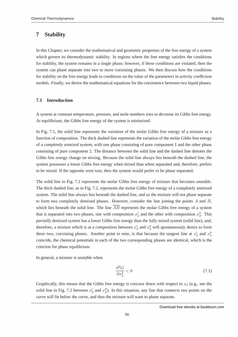
Download free ebooks at bookboon.com
Chemical Thermodynamics
56
Stability
7 Stability
In this Chapter, we consider the mathematical and geometric properties of the free energy of a systemwhich govern its thermodynamic stability. In regions where the free energy satisfies the conditionsfor stability, the system remains in a single phase; however, if these conditions are violated, then thesystem can phase separate into two or more coexisting phases. We then discuss how the conditionsfor stability on the free energy leads to conditions on the value of the parameters in activity coefficientmodels. Finally, we derive the mathematical equations for the coexistence between two liquid phases.
7.1 Introduction
A system at constant temperature, pressure, and mole numbers tries to decrease its Gibbs free energy.At equilibrium, the Gibbs free energy of the system is minimized.
In Fig. 7.1, the solid line represents the variation of the molar Gibbs free energy of a mixture as afunction of composition. The thick dashed line represents the variation of the molar Gibbs free energyof a completely unmixed system, with one phase consisting of pure component 1 and the other phaseconsisting of pure component 2. The distance between the solid line and the dashed line denotes theGibbs free energy change on mixing. Because the solid line always lies beneath the dashed line, thesystem possesses a lower Gibbs free energy when mixed than when separated and, therefore, prefersto be mixed. If the opposite were true, then the system would prefer to be phase separated.
The solid line in Fig. 7.2 represents the molar Gibbs free energy of mixture that becomes unstable.The thick dashed line, as in Fig. 7.2, represents the molar Gibbs free energy of a completely unmixedsystem. The solid line always lies beneath the dashed line, and so the mixture will not phase separateto form two completely demixed phases. However, consider the line joining the points A and B,which lies beneath the solid line. The line AB represents the molar Gibbs free energy of a systemthat is separated into two phases, one with composition x′2 and the other with composition x′′2. Thispartially demixed system has a lower Gibbs free energy than the fully mixed system (solid line), and,therefore, a mixture which is at a composition between x′2 and x′′2 will spontaneously demix to formthese two, coexisting phases. Another point to note, is that because the tangent line at x′2 and x′′2coincide, the chemical potentials in each of the two corresponding phases are identical, which is thecriterion for phase equilibrium.
In general, a mixture is unstable when
∂2G
∂x22
< 0 (7.1)
Graphically, this means that the Gibbs free energy is concave down with respect to x2 (e.g., see thesolid line in Fig. 7.2 between x′2 and x′′2). In this situation, any line that connects two points on thecurve will lie below the curve, and thus the mixture will want to phase separate.
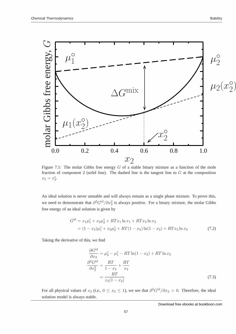
Download free ebooks at bookboon.com
Chemical Thermodynamics
57
Stability
0.0 0.2 0.4 0.6 0.8 1.0x2
x◦2
mol
arG
ibbs
free
ener
gy,G
μ1(x◦2)
μ2(x◦2)
μ◦1 μ◦2
ΔGmix
Figure 7.1: The molar Gibbs free energy G of a stable binary mixture as a function of the molefraction of component 2 (solid line). The dashed line is the tangent line to G at the compositionx2 = x◦2.
An ideal solution is never unstable and will always remain as a single phase mixture. To prove this,we need to demonstrate that ∂2Gid/∂x2
2 is always positive. For a binary mixture, the molar Gibbsfree energy of an ideal solution is given by
Gid = x1μ◦1 + x2μ
◦2 + RTx1 ln x1 + RTx2 ln x2
= (1− x2)μ◦1 + x2μ
◦2 + RT (1− x2) ln(1− x2) + RTx2 ln x2 (7.2)
Taking the derivative of this, we find
∂Gid
∂x2= μ◦2 − μ◦1 −RT ln(1− x2) + RT ln x2
∂2Gid
∂x22
=RT
1− x2+
RT
x2
=RT
x2(1− x2)(7.3)
For all physical values of x2 (i.e., 0 ≤ x2 ≤ 1), we see that ∂2Gid/∂x2 > 0. Therefore, the idealsolution model is always stable.
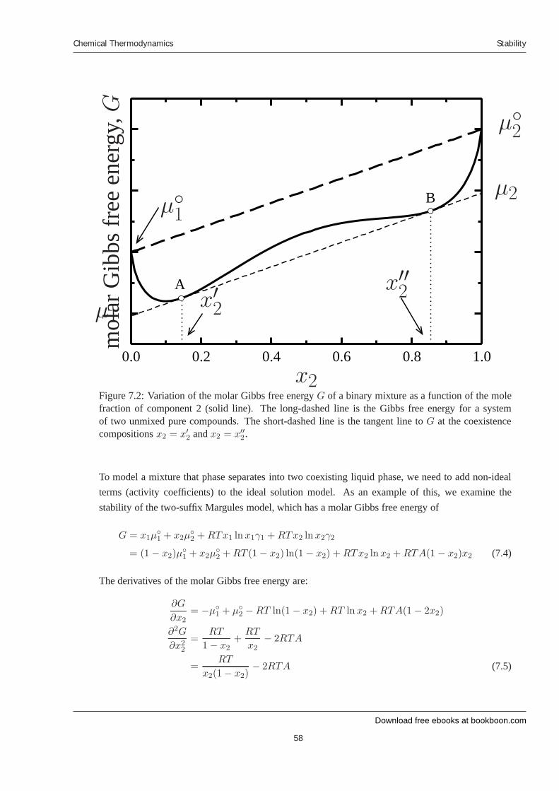
Download free ebooks at bookboon.com
Chemical Thermodynamics
58
Stability
0.0 0.2 0.4 0.6 0.8 1.0
A
B
x2
x′2x′′2
mol
arG
ibbs
free
ener
gy,G
μ1
μ2μ◦1
μ◦2
Figure 7.2: Variation of the molar Gibbs free energy G of a binary mixture as a function of the molefraction of component 2 (solid line). The long-dashed line is the Gibbs free energy for a systemof two unmixed pure compounds. The short-dashed line is the tangent line to G at the coexistencecompositions x2 = x′2 and x2 = x′′2.
To model a mixture that phase separates into two coexisting liquid phase, we need to add non-idealterms (activity coefficients) to the ideal solution model. As an example of this, we examine thestability of the two-suffix Margules model, which has a molar Gibbs free energy of
G = x1μ◦1 + x2μ
◦2 + RTx1 ln x1γ1 + RTx2 ln x2γ2
= (1− x2)μ◦1 + x2μ
◦2 + RT (1− x2) ln(1− x2) + RTx2 ln x2 + RTA(1− x2)x2 (7.4)
The derivatives of the molar Gibbs free energy are:
∂G
∂x2= −μ◦1 + μ◦2 −RT ln(1− x2) + RT ln x2 + RTA(1− 2x2)
∂2G
∂x22
=RT
1− x2+
RT
x2− 2RTA
=RT
x2(1− x2)− 2RTA (7.5)

Download free ebooks at bookboon.com
Ple
ase
clic
k th
e ad
vert
Chemical Thermodynamics
59
Stability
The system is unstable when
A >1
2x2(1− x2)(7.6)
The right-hand side of Eq. (7.6) is plotted in Fig. 7.3. In Fig. 7.3, the x-axis represents the molefraction of component 2, and the y-axis represents the value of the parameter A in the Margules model.The shaded region denotes the area where the inequality given in Eq. (7.6) is true, and therefore, thesystem will undergo liquid-liquid phase separation. Outside this region, the mixture is stable.
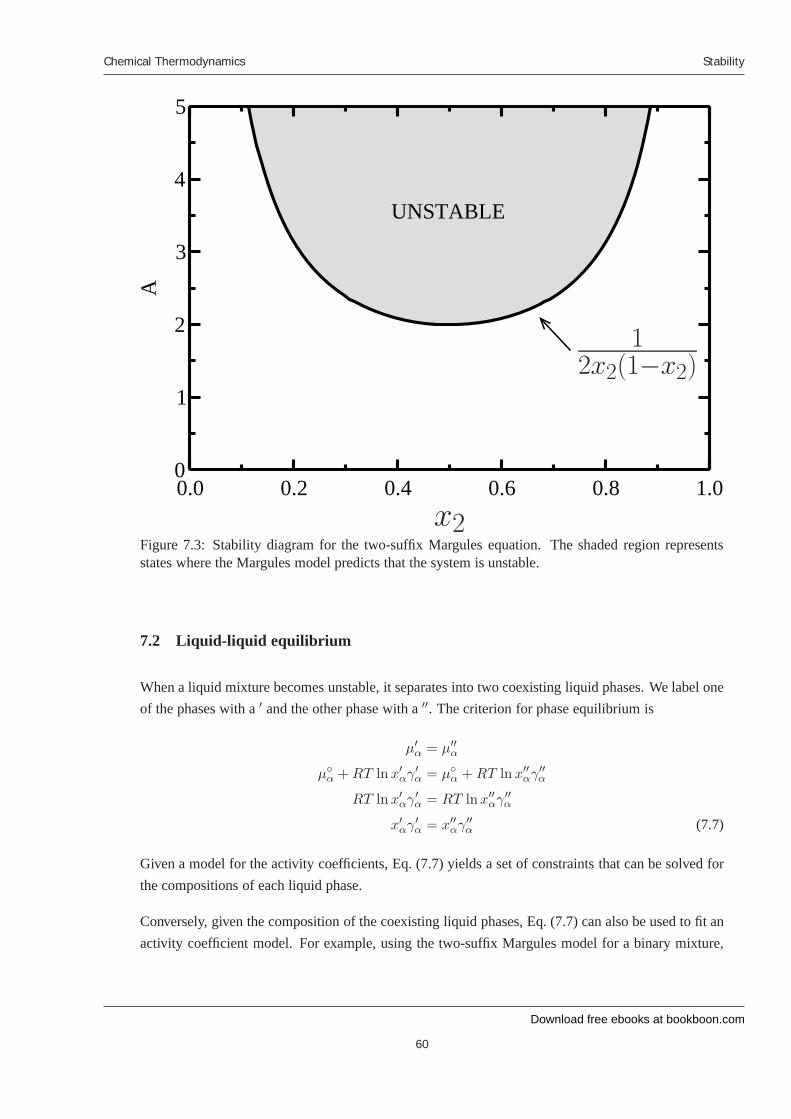
Download free ebooks at bookboon.com
Chemical Thermodynamics
60
Stability
0.0 0.2 0.4 0.6 0.8 1.00
1
2
3
4
5
A
UNSTABLE
x2
12x2(1−x2)
Figure 7.3: Stability diagram for the two-suffix Margules equation. The shaded region representsstates where the Margules model predicts that the system is unstable.
7.2 Liquid-liquid equilibrium
When a liquid mixture becomes unstable, it separates into two coexisting liquid phases. We label oneof the phases with a ′ and the other phase with a ′′. The criterion for phase equilibrium is
μ′α = μ′′α
μ◦α + RT ln x′αγ′α = μ◦α + RT ln x′′αγ′′α
RT ln x′αγ′α = RT lnx′′αγ′′α
x′αγ′α = x′′αγ′′α (7.7)
Given a model for the activity coefficients, Eq. (7.7) yields a set of constraints that can be solved forthe compositions of each liquid phase.
Conversely, given the composition of the coexisting liquid phases, Eq. (7.7) can also be used to fit anactivity coefficient model. For example, using the two-suffix Margules model for a binary mixture,

Download free ebooks at bookboon.com
Ple
ase
clic
k th
e ad
vert
Chemical Thermodynamics
61
Stability
we can determine the parameter A
lnγ′1γ′′1
= lnx′′1x′1
Ax′22 −Ax′′22 = lnx′′1x′1
A =1
x′22 − x′′22
lnx′′1x′1
(7.8)
Do you want your Dream Job?
More customers get their dream job by using RedStarResume than any other resume service.
RedStarResume can help you with your job application and CV.
Go to: Redstarresume.com
Use code “BOOKBOON” and save up to $15
(enter the discount code in the “Discount Code Box”)
Download free ebooks at bookboon.com
Chemical Thermodynamics
62
Solid-liquid equilibrium
8 Solid-liquid equilibrium
8.1 Introduction
At atmospheric pressure, water will freeze at 0◦C. If a solute is added to water, then the mixture willfreeze at a lower temperature. This is known as freezing point depression and occurs with any generalmixture. Using a model for the activity coefficients, we can quantitatively predict the magnitude ofthis effect.
8.2 Phase behavior
To demonstrate the general freezing behavior of a binary mixture, we present the solid-liquid phasediagram for systems of ethanol and water at 1 atm in Fig. 8.1. The solid line with the filled symbolsis the freezing curve of water in the mixture. Above the curve the solution is completely liquid;below the curve, it is a liquid mixture coexists with solid water (i.e., ice). At this pressure, pure waterfreezes at 273.15 K. As ethanol is added to the solution, the temperature at which ice begins to formin gradually decreases.
The dotted line with the open symbols on the right side of the diagram is the freezing curve ofethanol in the mixture. As one passes downward through this curve, solid ethanol precipitates fromthe solution. Note that the temperature at which ethanol begins to freeze decreases as the amountof water in the solution increases. Therefore, we see that the addition of impurities decreases thefreezing temperature of a substance. This phenomena is known as freezing point depression.
The point where the two freezing curves intersect with each other is called the eutectic point. This isthe lowest temperature at which a binary mixture can remain in liquid without either of its componentsprecipitating.
Finally, we note that below the dotted line in Fig. 8.1 the system exists as two coexisting solid phases:one consisting of pure ice, and the other composed of pure solid ethanol. The relative amounts ofthese two phases is given by the lever rule.
8.3 Conditions for equilibrium
In this section, we derive the equation that governs the shape of the freezing curve. Let’s consider thefreezing of a species in a general multicomponent mixture. We make the assumption that the solidphase consists of pure component α. At equilibrium, the chemical potential of the solid phase is the
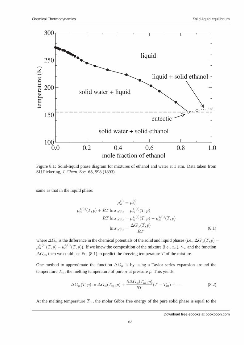
Download free ebooks at bookboon.com
Chemical Thermodynamics
63
Solid-liquid equilibrium
Figure 8.1: Solid-liquid phase diagram for mixtures of ethanol and water at 1 atm. Data taken fromSU Pickering, J. Chem. Soc. 63, 998 (1893).
same as that in the liquid phase:
μ(l)α = μ(s)
α
μ◦,(l)α (T, p) + RT lnxαγα = μ◦,(s)α (T, p)
RT lnxαγα = μ◦,(s)α (T, p)− μ◦,(l)α (T, p)
lnxαγα =ΔGα(T, p)
RT(8.1)
where ΔGα is the difference in the chemical potentials of the solid and liquid phases (i.e., ΔGα(T, p) =
μ◦,(s)α (T, p)−μ
◦,(l)α (T, p)). If we knew the composition of the mixture (i.e., xα), γα, and the function
ΔGα, then we could use Eq. (8.1) to predict the freezing temperature T of the mixture.
One method to approximate the function ΔGα is by using a Taylor series expansion around thetemperature Tm, the melting temperature of pure α at pressure p. This yields
ΔGα(T, p) ≈ ΔGα(Tm, p) +∂ΔGα(Tm, p)
∂T(T − Tm) + · · · (8.2)
At the melting temperature Tm, the molar Gibbs free energy of the pure solid phase is equal to the
Download free ebooks at bookboon.com
Ple
ase
clic
k th
e ad
vert
Chemical Thermodynamics
64
Solid-liquid equilibrium
molar Gibbs free energy of the pure liquid phase. That is
ΔGα(Tm, p) = 0 (8.3)
Therefore, the first term of the Taylor series expansion in Eq. (8.2) vanishes.
From the fundamental equation of thermodynamics, we arrive at
∂ΔGα
∂T= −ΔSα (8.4)
where ΔSα is the molar entropy change of freezing. From the relation G = H − TS, we can relatethe entropy change of freezing to the enthalpy of freezing ΔHα, which is the heat released by thesystem when it transforms from a liquid to a solid:
ΔGα(Tm, p) = ΔHα(Tm, p)− TmΔSα(Tm, p)
0 = ΔHα(Tm, p)− TmΔSα(Tm, p)
ΔSα(Tm, p) =1
TmΔHα(Tm, p). (8.5)
Combining this with Eq. (8.2) yields
ΔGα(T, p) ≈ −ΔHα(Tm, p)
Tm(T − Tm) + · · · (8.6)
Challenging? Not challenging? Try more
Try this...
www.alloptions.nl/life
Download free ebooks at bookboon.com
Chemical Thermodynamics
65
Solid-liquid equilibrium
Finally, we find:
ln xαγα = −ΔHα(Tm, p)
RTTm(T − Tm)
ln xαγα = −ΔHα(Tm, p)
RTm
(1−
Tm
T
)(8.7)
This equation allows the prediction of the freezing curve of a mixture. It requires from knowledge ofthe freezing temperature and enthalpy of melting of the pure component α, as well as a model of theactivity coefficients of the liquid mixture. In the absence of information for the activity coefficients,the ideal solution model can be used (i.e., γα = 1); Eq. (8.7) then reduces to the van’t Hoff equation.
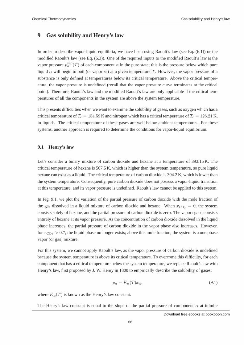
Download free ebooks at bookboon.com
Chemical Thermodynamics
66
Gas solubility and Henry’s law
9 Gas solubility and Henry’s law
In order to describe vapor-liquid equilibria, we have been using Raoult’s law (see Eq. (6.1)) or themodified Raoult’s law (see Eq. (6.3)). One of the required inputs to the modified Raoult’s law is thevapor pressure pvap
α (T ) of each component α in the pure state; this is the pressure below which pureliquid α will begin to boil (or vaporize) at a given temperature T . However, the vapor pressure of asubstance is only defined at temperatures below its critical temperature. Above the critical temper-ature, the vapor pressure is undefined (recall that the vapor pressure curve terminates at the criticalpoint). Therefore, Raoult’s law and the modified Raoult’s law are only applicable if the critical tem-peratures of all the components in the system are above the system temperature.
This presents difficulties when we want to examine the solubility of gases, such as oxygen which has acritical temperature of Tc = 154.59 K and nitrogen which has a critical temperature of Tc = 126.21 K,in liquids. The critical temperature of these gases are well below ambient temperatures. For thesesystems, another approach is required to determine the conditions for vapor-liquid equilibrium.
9.1 Henry’s law
Let’s consider a binary mixture of carbon dioxide and hexane at a temperature of 393.15 K. Thecritical temperature of hexane is 507.5 K, which is higher than the system temperature, so pure liquidhexane can exist as a liquid. The critical temperature of carbon dioxide is 304.2 K, which is lower thanthe system temperature. Consequently, pure carbon dioxide does not possess a vapor-liquid transitionat this temperature, and its vapor pressure is undefined. Raoult’s law cannot be applied to this system.
In Fig. 9.1, we plot the variation of the partial pressure of carbon dioxide with the mole fraction ofthe gas dissolved in a liquid mixture of carbon dioxide and hexane. When xCO2
= 0, the systemconsists solely of hexane, and the partial pressure of carbon dioxide is zero. The vapor space consistsentirely of hexane at its vapor pressure. As the concentration of carbon dioxide dissolved in the liquidphase increases, the partial pressure of carbon dioxide in the vapor phase also increases. However,for xCO2
> 0.7, the liquid phase no longer exists; above this mole fraction, the system is a one phasevapor (or gas) mixture.
For this system, we cannot apply Raoult’s law, as the vapor pressure of carbon dioxide is undefinedbecause the system temperature is above its critical temperature. To overcome this difficulty, for eachcomponent that has a critical temperature below the system temperature, we replace Raoult’s law withHenry’s law, first proposed by J. W. Henry in 1800 to empirically describe the solubility of gases:
pα = Kα(T )xα, (9.1)
where Kα(T ) is known as the Henry’s law constant.
The Henry’s law constant is equal to the slope of the partial pressure of component α at infinite
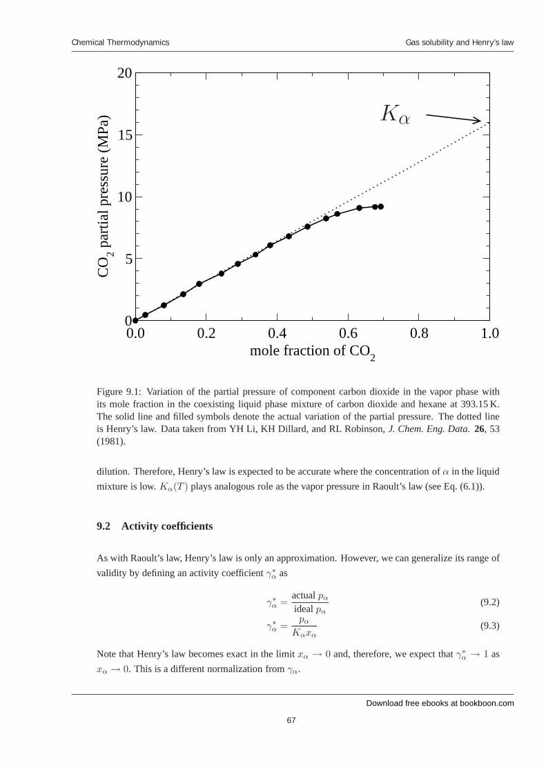
Download free ebooks at bookboon.com
Chemical Thermodynamics
67
Gas solubility and Henry’s law
0.0 0.2 0.4 0.6 0.8 1.0mole fraction of CO2
0
5
10
15
20
CO
2 par
tial p
ress
ure
(MPa
) Kα
Figure 9.1: Variation of the partial pressure of component carbon dioxide in the vapor phase withits mole fraction in the coexisting liquid phase mixture of carbon dioxide and hexane at 393.15 K.The solid line and filled symbols denote the actual variation of the partial pressure. The dotted lineis Henry’s law. Data taken from YH Li, KH Dillard, and RL Robinson, J. Chem. Eng. Data. 26, 53(1981).
dilution. Therefore, Henry’s law is expected to be accurate where the concentration of α in the liquidmixture is low. Kα(T ) plays analogous role as the vapor pressure in Raoult’s law (see Eq. (6.1)).
9.2 Activity coefficients
As with Raoult’s law, Henry’s law is only an approximation. However, we can generalize its range ofvalidity by defining an activity coefficient γ∗α as
γ∗α =actual pα
ideal pα(9.2)
γ∗α =pα
Kαxα(9.3)
Note that Henry’s law becomes exact in the limit xα → 0 and, therefore, we expect that γ∗α → 1 asxα → 0. This is a different normalization from γα.
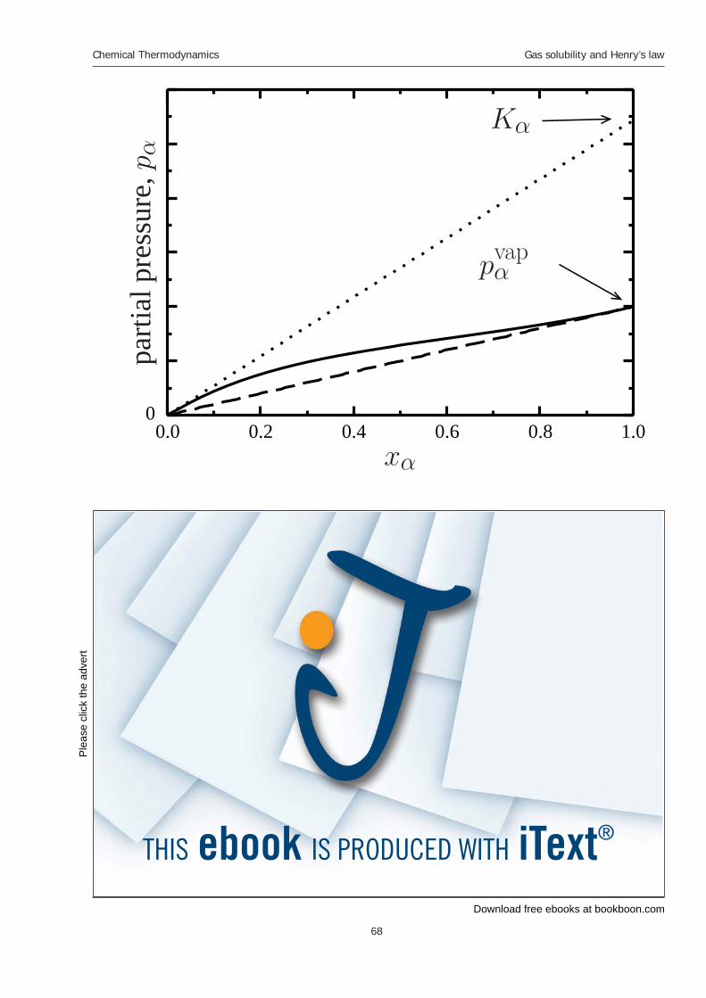
Download free ebooks at bookboon.com
Ple
ase
clic
k th
e ad
vert
Chemical Thermodynamics
68
Gas solubility and Henry’s law
0.0 0.2 0.4 0.6 0.8 1.00
pvapα
Kα
xα
parti
alpr
essu
re,p
α
Download free ebooks at bookboon.com
Chemical Thermodynamics
69
Gas solubility and Henry’s law
Figure 9.2: Variation of the partial pressure of component α in the vapor phase with its mole fractionin the coexisting liquid phase. The solid line is the actual variation of the partial pressure. The dashedline is the prediction of Raoult’s law, and the dotted line is the prediction of Henry’s law.
In Fig. 9.2, we plot a schematic drawing of the variation of the partial pressure of a component withits mole fraction in the liquid phase. The solid line represent the experimental variation of the partialpressure, the dashed line is the prediction of Raoult’s law, and the dotted line is the prediction ofHenry’s law.
Even if a component has a vapor pressure at the system temperature (i.e., its critical temperature isgreater than the system temperature), we still may prefer to use Henry’s law instead of Raoult’s law.This is usually done for components that are very dilute, where Henry’s law becomes more and moreaccurate.
If we compare Henry’s law and the modified Raoult’s law, then we find that Henry’s law can beconsidered as the modified Raoult’s law with γα = Kα/pvap
α .
Download free ebooks at bookboon.com
Chemical Thermodynamics
70
Equations of state
10 Equations of state
An equation of state (EOS) provides a relation between the pressure, temperature, volume, and com-position of a system. Typically, this is given as an explicit function of temperature, molar volume,and composition p = p(T, V, x2, x3, · · · ). One example is the ideal gas law, where the pressure isgiven by
p =RT
V(10.1)
where R is the universal gas constant.
Real materials have much more complicated equations of state. In this chapter, we present otherequations of state that are used to model real systems and demonstrate how to use them to determinevarious thermodynamics properties from them.
10.1 The principle of corresponding states
The properties of different fluids are in general quite different from each other. In Fig. 10.1, we plotthe liquid-vapor coexistence curves for a variety of fluids. However, Guggenheim observed that ifthe properties of a certain class fluids are plotted in terms of reduced variables, variables divided bytheir critical values, the data can be collapsed onto a single curve, independent of the identity of thefluid. This can be seen on the right plots in Fig. 10.1. This collapse of the properties is known as theprinciple of corresponding states.
This observation implies that the thermodynamic properties of all materials are given by a single,“universal” function, independent of the identity of the material. For example, defining the compress-ibility factor Z as
Z =pV
RT, (10.2)
the principle of corresponding states implies that
Z = Z(Tr, pr) (10.3)
where Tr = T/Tc is the reduced temperature, pr = p/pc is the reduced pressure, Tc is the criticaltemperature of the material, and pc is its critical pressure.
Guggenheim observed that this principle actually holds very well for many simple fluids, fluids com-posed of molecules that are roughly spherical. However, in general, this principle does not hold foran arbitrary fluid, in particular, for polar fluids, such as water, and for fluids composed of highlynon-spherical molecules, such has n-hexane.
Pitzer noticed that as the molecules in a fluid begin to elongate and deviate from a spherical shape,
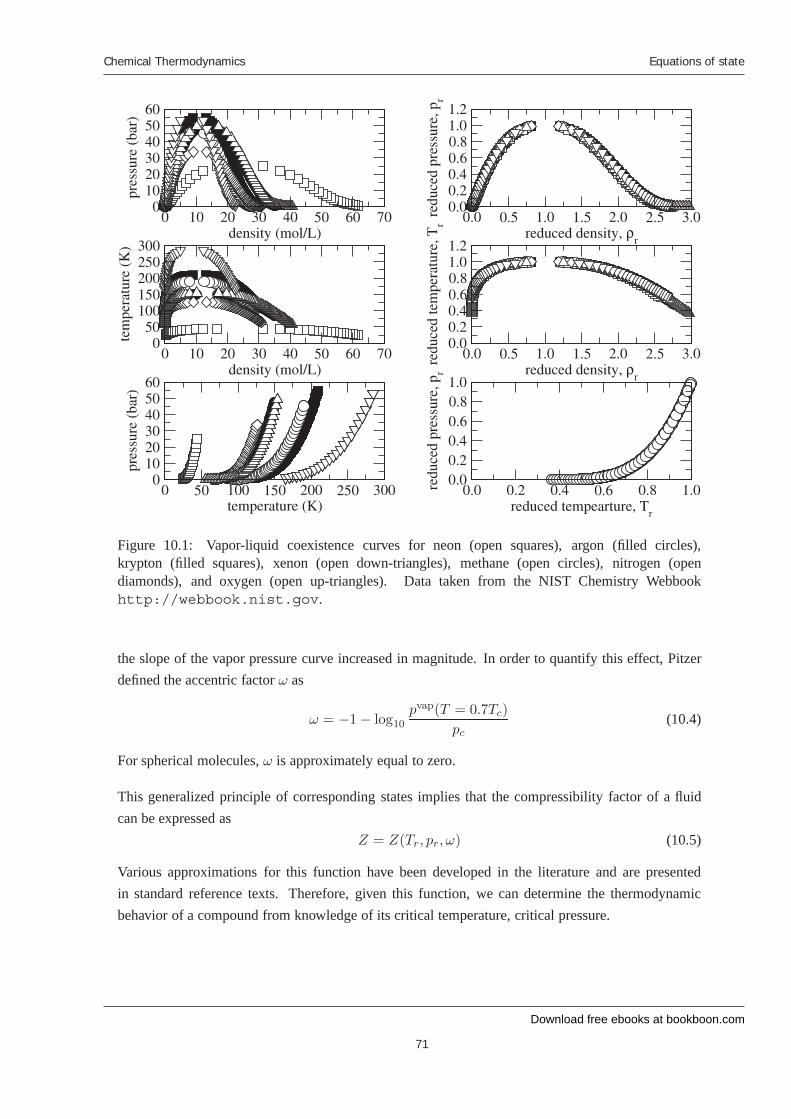
Download free ebooks at bookboon.com
Chemical Thermodynamics
71
Equations of state
Figure 10.1: Vapor-liquid coexistence curves for neon (open squares), argon (filled circles),krypton (filled squares), xenon (open down-triangles), methane (open circles), nitrogen (opendiamonds), and oxygen (open up-triangles). Data taken from the NIST Chemistry Webbookhttp://webbook.nist.gov.
the slope of the vapor pressure curve increased in magnitude. In order to quantify this effect, Pitzerdefined the accentric factor ω as
ω = −1− log10pvap(T = 0.7Tc)
pc(10.4)
For spherical molecules, ω is approximately equal to zero.
This generalized principle of corresponding states implies that the compressibility factor of a fluidcan be expressed as
Z = Z(Tr, pr, ω) (10.5)
Various approximations for this function have been developed in the literature and are presentedin standard reference texts. Therefore, given this function, we can determine the thermodynamicbehavior of a compound from knowledge of its critical temperature, critical pressure.
Download free ebooks at bookboon.com
Chemical Thermodynamics
72
Equations of state
10.2 The van der Waals equation and cubic equations of state
The basic assumption in deriving the ideal gas equation of state is that the interactions between themolecules that compose the gas are negligible. At very low densities, where the average distancebetween molecules is extremely large compared to the range of the intermolecular interactions (orsize of a molecule) and collisions between molecules occur only rarely, this assumption is fairly good.However, for moderately dense gases, this assumption begins to breakdown, as collisions betweenmolecules become more and more frequent. In the case of liquids, this assumption is completelyerroneous, as intermolecular interactions dominate the properties of the liquid.
To account for the finite size of molecules in the system. If we consider molecules to be of volume b,then the actual volume available to the system is approximately V − b. Therefore, we replace V inthe ideal gas equation of state with V − b. In addition, at large distances, the molecules in a gas exertan attractive interaction between each other due to dispersion forces. The van der Waals equationof state, which accounts for both the short-ranged repulsions and long-ranged attractions betweenmolecules, is given by
p =RT
V − b−
a
V 2(10.6)
A schematic plot of the variation of the pressure with volume, as predicted by the van der Waalsequation of state, at various temperatures is given in Fig. 10.2. At temperatures above the criticaltemperature, the pressure-volume variation is monotonic and qualitatively similar to that of an idealgas (see dotted-line). At temperatures below the critical temperature, the pressure-volume curve be-gins to oscillate, exhibiting a “van der Waals” loop (see dashed-line). This behavior is unphysical, butrepresents the vapor-liquid transition, and should be replaced by the solid line. The precise locationof the solid line is given by the Maxwell construction.
When the temperature is equal to the critical temperature, the pressure-volume curve exhibits a pointwith the inflection (concavity) of the curve changes sign. This occurs at the critical point, where wehave:
∂p
∂V= 0 (10.7)
∂2p
∂V 2= 0 (10.8)
Applying Eqs. (10.7) and (10.8) to the van der Waals equation of state, we find
∂p
∂V= −
RTc
(Vc − b)2+
2a
V 3c
= 0 (10.9)
∂2p
∂V 2=
2RT
(Vc − b)3−
6a
V 4c
= 0 (10.10)
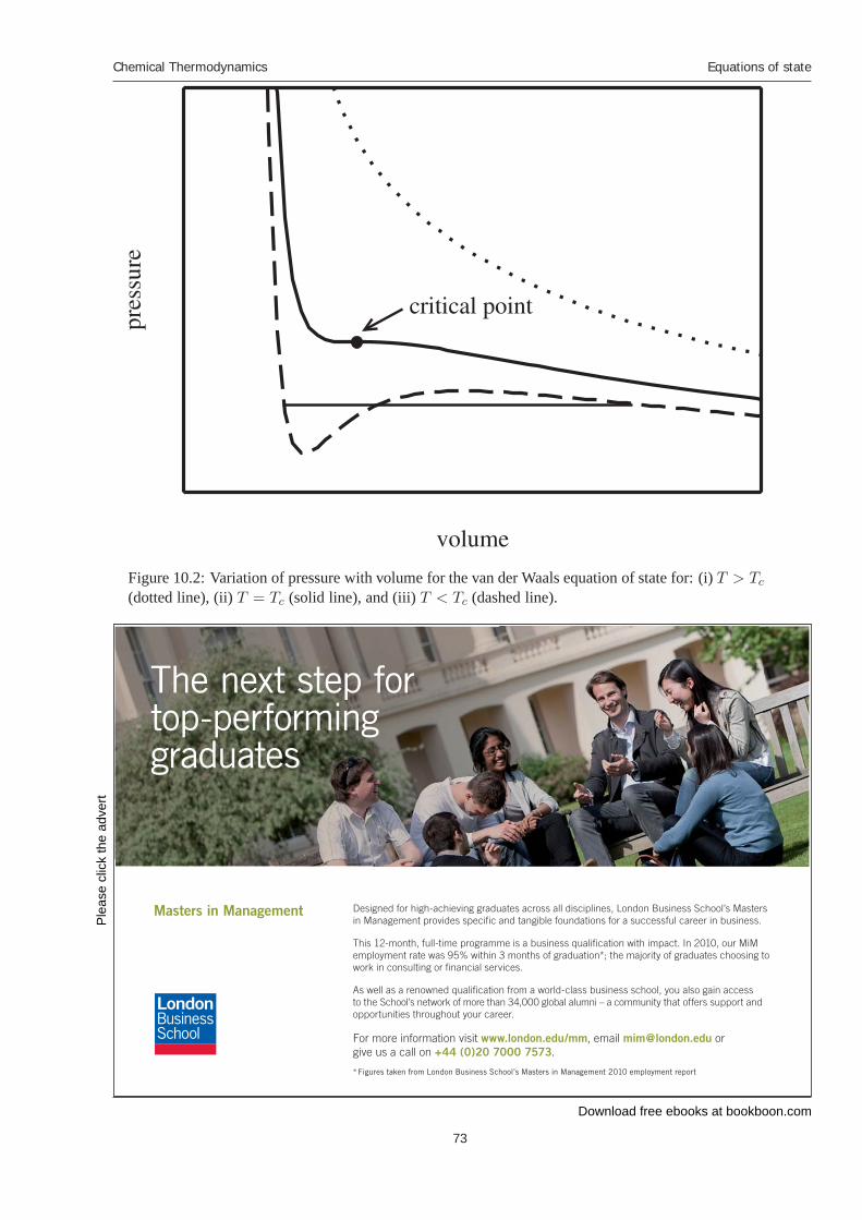
Download free ebooks at bookboon.com
Ple
ase
clic
k th
e ad
vert
Chemical Thermodynamics
73
Equations of state
Figure 10.2: Variation of pressure with volume for the van der Waals equation of state for: (i) T > Tc
(dotted line), (ii) T = Tc (solid line), and (iii) T < Tc (dashed line).
Designed for high-achieving graduates across all disciplines, London Business School’s Masters in Management provides specific and tangible foundations for a successful career in business.
This 12-month, full-time programme is a business qualification with impact. In 2010, our MiM employment rate was 95% within 3 months of graduation*; the majority of graduates choosing to work in consulting or financial services.
As well as a renowned qualification from a world-class business school, you also gain access to the School’s network of more than 34,000 global alumni – a community that offers support and opportunities throughout your career.
For more information visit www.london.edu/mm, email [email protected] or give us a call on +44 (0)20 7000 7573.
Masters in Management
The next step for top-performing graduates
* Figures taken from London Business School’s Masters in Management 2010 employment report
Download free ebooks at bookboon.com
Chemical Thermodynamics
74
Equations of state
Multiplying the Eq. (10.9) by 2/(Vc − b) and adding it Eq. (10.10) yields
−2RT
(Vc − b)3+
4a
V 3c (Vc − b)
+2RT
(Vc − b)3−
6a
V 4c
= 0 = 0
4a
V 3c (Vc − b)
−6a
V 4c
= 0
2Vc = 3(Vc − b)
Vc = 3b
Substituting Vc = 3b into Eq. (10.9) yields
−RTc
(Vc − b)2+
2a
V 3c
= 0
RTc =2a(Vc − b)2
V 3c
=2a(3b − b)2
(3b)3
=8
27
a
b(10.11)
We can compute the critical pressure by substituting Tc and Vc into the equation of state,
pc =RT
Vc − b−
a
V 2c
=8a/(27b)
3b− b−
a
(3b)2
=a
27b2(10.12)
We have shown that, given the parameters a and b of the van der Waals equation of state, one candetermine the critical properties of a fluid. However, we can perform the inverse task. That is, giventhe critical temperature and pressure for a fluid, one can determine the a and b parameters of the vander Waals equation of state. Dividing Eq. (10.11) by Eq. (10.12)
RTc
pc=
8a/(27b)
a/(27b2)
b =RTc
8pc(10.13)
Inserting the expression for b into Eq. (10.11), we find
RTc =8
27
a
RTc/(8pc)(10.14)
a =27
64
(RTc)2
pc(10.15)
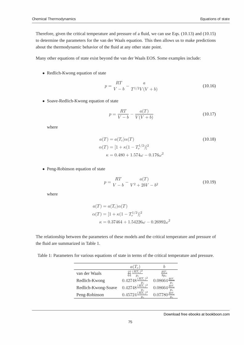
Download free ebooks at bookboon.com
Chemical Thermodynamics
75
Equations of state
Therefore, given the critical temperature and pressure of a fluid, we can use Eqs. (10.13) and (10.15)to determine the parameters for the van der Waals equation. This then allows us to make predictionsabout the thermodynamic behavior of the fluid at any other state point.
Many other equations of state exist beyond the van der Waals EOS. Some examples include:
• Redlich-Kwong equation of state
p =RT
V − b−
a
T 1/2V (V + b)(10.16)
• Soave-Redlich-Kwong equation of state
p =RT
V − b−
a(T )
V (V + b)(10.17)
where
a(T ) = a(Tc)α(T ) (10.18)
α(T ) = [1 + κ(1− T 1/2r )]2
κ = 0.480 + 1.574ω − 0.176ω2
• Peng-Robinson equation of state
p =RT
V − b−
a(T )
V 2 + 2bV − b2(10.19)
where
a(T ) = a(Tc)α(T )
α(T ) = [1 + κ(1 − T 1/2r )]2
κ = 0.37464 + 1.54226ω − 0.26992ω2
The relationship between the parameters of these models and the critical temperature and pressure ofthe fluid are summarized in Table 1.
Table 1: Parameters for various equations of state in terms of the critical temperature and pressure.
a(Tc) b
van der Waals 2764
(RTc)2
pc
RTc
8pc
Redlich-Kwong 0.42748 (RTc)2
pc0.08664RTc
pc
Redlich-Kwong-Soave 0.42748 (RTc)2
pc0.08664RTc
pc
Peng-Robinson 0.45724 (RTc)2
pc0.07780RTc
pc
Download free ebooks at bookboon.com
Chemical Thermodynamics
76
Equations of state
10.3 Equations of state for mixtures
Thus far, we have only been considering single component systems. One method of extending anequation of state to mixtures is by making the parameters a and b a function of composition. Thisis done through the application of mixing rules. For example, we can define the parameter b of themixture as
b =∑α
yαbα (10.20)
where bα is the b parameter for pure α, and yα is the mole fraction of α in the system.
Similarly, we can define the parameter a of the mixture as
a =∑α,α′
yαyα′aαα′ (10.21)
where aαα′ = (1−kαα′)(aαaα′)1/2, aα is the a parameter of pure α, and kαα′ is the binary interactionparameter between species α and α′. The binary interaction parameter kαα′ is a purely empiricalparameter that is used to obtain better agreement between the predictions of the equation of state andexperimental data. Typical values of the parameter are given in Table 2.
Table 2: Typical values of the binary interaction parameters for various mixtures.
mixture kαα′
hydrocarbon/hydrocarbon ∼ 0CO2/hydrocarbon ∼ 0.15water/hydrocarbon ∼ 0.5
Download free ebooks at bookboon.com
Chemical Thermodynamics
77
Thermodynamics from equations of state
11 Thermodynamics from equations of state
Equations of state relate the pressure, temperature, volume, and composition of a system to eachother. In this Chapter, we show how to determine other thermodynamic properties of the systemfrom an equation of state. In a typical equation of state, the pressure is given as an explicit functionof temperature, volume, and composition. Therefore, the “natural” variables are the temperature,volume, and composition of the system. That is, once given the volume, temperature, and compositionof the system, the pressure is readily calculated from the equation of state.
Once one of the free energies of a system is known as a function of its natural variables, then allthe other thermodynamic properties of the system can be derived. For these equations of states, theHelmholtz free energy is the relevant quantity. In the following, we demonstrate how to determinethe Helmholtz free energy from an equation and then proceed to show how to derive other propertiesfrom it.
11.1 The residual Helmholtz free energy
The free energy that has temperature, volume, and mole numbers as its natural variables is theHelmholtz free energy. Before we stated that once the Gibb’s free energy of a system is known as afunction of temperature, pressure, and mole numbers
¯G(T, p,N1, N2, . . . ), all the thermodynamics
of the system are known. This is equivalent to the statement that once the Helmholtz free energy isknown as a function of temperature, volume, and mole numbers of the system
¯A(T, V,N1, N2, . . . ),
all the thermodynamics of the system are known. The fundamental equation of thermodynamics canbe written in terms of the Helmholtz free energy as
d¯A = −
¯SdT − pd
¯V +
∑α
μαdNα (11.1)
Given and equation of state, we can determine an explicit expression for the Helmholtz free energyfrom the fundamental equation of thermodynamics. At constant temperature and mole numbers, wehave
d¯A = −pd
¯V (11.2)
By integrating both sides of this equation from a total volume¯V1 to a total volume
¯V2
¯A(T,
¯V2, N1, N2, . . . )−
¯A(T,
¯V1, N1, N2, . . . ) = −
∫¯V2
¯V1
d¯V ′p (11.3)
Download free ebooks at bookboon.com
Chemical Thermodynamics
78
Thermodynamics from equations of state
For an ideal gas, we have p = NRT/¯V , so
¯Aig(T,
¯V2, N1, N2, . . . )−
¯Aig(T,
¯V1, N1, N2, . . . ) = −
∫¯V2
¯V1
d¯V ′
NRT
¯V ′
(11.4)
Subtracting Eq. (11.4) from Eq. (11.3), we find
[¯A(T,
¯V2, N1, N2, . . . )−
¯A(T,
¯V1, N1, N2, . . . )]
−[¯Aig(T,
¯V2, N1, N2, . . . )−
¯Aig(T,
¯V1, N1, N2, . . . )] = −
∫¯V2
¯V1
d¯V ′
(p−
NRT
¯V ′
)
[¯A(T,
¯V2, N1, N2, . . . )−
¯Aig(T,
¯V2, N1, N2, . . . )]
−[¯A(T,
¯V1, N1, N2, . . . )−
¯Aig(T,
¯V1, N1, N2, . . . )] = −NRT
∫¯V2
¯V1
d¯V ′
¯V ′
(Z − 1) (11.5)
¯Ares(T,
¯V2, N1, N2, . . . )−
¯Ares(T,
¯V1, N1, N2, . . . ) = −NRT
∫¯V2
¯V1
d¯V ′
¯V ′
(Z − 1)
where we have defined a residual property¯Xres as the difference of the value of the property of the
system and that of an ideal gas at the same temperature, volume, and species mole numbers
¯Xres(T, V,N1, N2, . . . ) =
¯X(T, V,N1, N2, . . . )−
¯Xig(T, V,N1, N2, . . . ) (11.6)
As the density of the system approaches zero, or the molar volume of the system approaches infinity,the properties of a system approach those of an ideal gas. In particular,
¯A(T, V,N1, N2, . . . ) →
¯Aig(T, V,N1, N2, . . . ) as V →∞. (11.7)
If we let¯V2 =
¯V and
¯V1 →∞ in Eq. (11.6), then we find
¯Ares(T,
¯V,N1, N2, . . . ) = −NRT
∫¯V
∞
d¯V ′
¯V ′
(Z − 1)
= NRT
∫ ∞
¯V
d¯V ′
¯V ′
(Z − 1) (11.8)
Given an expression for the compressibility factor Z as a function of temperature and volume for afluid (an equation of state), we can determine the residual Helmholtz free energy of the system.
Download free ebooks at bookboon.com
Chemical Thermodynamics
79
Thermodynamics from equations of state
For the van der Waals equation of state, the compressibility factor is given by
Z =pV
RT
=V
RT
(RT
V − b−
a
V 2
)
=V
V − b−
a
RTV
Z − 1 =b
V − b−
a
RTV(11.9)
Substituting this expression into Eq. (11.8), we can obtain the residual Helmholtz free energy for thevan der Waals equation of state:
¯Ares(T, V,N1, N2, . . . )
NRT=
∫ ∞
V
dV
V
(b
V − b−
a
RTV
)
=
∫ ∞
VdV
(1
V − b−
1
V−
a
RTV 2
)(11.10)
=
[ln
V − b
V+
a
RTV
]∞V
= ln
(V
V − b
)−
a
RTV
The residual chemical potential of species α can be obtained from the residual Helmholtz free energyby differentiating by the number of moles of α (see Eq. (11.1)):
μresα =
∂¯Ares
∂Nα(11.11)
For the van der Waals equation of state, this becomes
μresα =
∂
∂Nα
{NRT
[ln
(¯V
¯V −Nb
)−
Na
RT¯V
]}
= RT ln
(¯V
¯V −Nb
)+
(NRT
¯V −Nb
)∂Nb
∂Nα−
1
¯V
∂N2a
∂Nα(11.12)
To obtain the derivative of the a and b parameters with respect to Nα, we need to use the mixing rulesgiven in Eqs. (10.20) and (10.21). This yields
∂Nb
∂Nα=
∂
∂NαN
∑α′
yα′bα′
=∂
∂Nα
∑α′
Nα′bα′
= bα (11.13)
Download free ebooks at bookboon.com
Ple
ase
clic
k th
e ad
vert
Chemical Thermodynamics
80
Thermodynamics from equations of state
and
∂N2a
∂Nα=
∂
∂NαN2
∑α′,α′′
yα′yα′′aα′α′′
=∂
∂Nα
∑α′,α′′
Nα′Nα′′aα′α′′
= 2∑α′
Nα′aαα′
= 2N∑α′
yα′aαα′ (11.14)
Using these expressions, we find that the residual chemical potnetial for the van der Waals equationof state is given by
μresα = RT ln
(V
V − b
)+
RTbα
V − b−
2
V
∑α′
yα′aαα′ (11.15)
© Agilent Technologies, Inc. 2012 u.s. 1-800-829-4444 canada: 1-877-894-4414
Teach with the Best. Learn with the Best.Agilent offers a wide variety of affordable, industry-leading electronic test equipment as well as knowledge-rich, on-line resources —for professors and students.We have 100’s of comprehensive web-based teaching tools, lab experiments, application notes, brochures, DVDs/ CDs, posters, and more. See what Agilent can do for you.
www.agilent.com/find/EDUstudentswww.agilent.com/find/EDUeducators
Download free ebooks at bookboon.com
Chemical Thermodynamics
81
Thermodynamics from equations of state
11.2 Fugacity
An ideal gas is an ideal solution. Thus, the chemical potential of species α in an ideal gas mixture attemperature T , pressure p, and species mole fractions y1, y2,. . . is given by
μigα (T, p, y1, y2, . . . ) = μ◦,igα (T, p) + RT ln yα (11.16)
where μ◦,igα (T, p) is the chemical potential of pure α.
The difference in the chemical potential of an ideal gas at pressure p and mole fractions y1, y2, . . . andan ideal gas at pressure p′ and mole fractions y′1, y′2,. . . is given by
μigα (T, p, y1, y2, . . . ) = μig
α (T, p′, y′1, y′2, . . . ) + RT ln
yαp
y′αp′
= μigα (T, p′, y′1, y
′2, . . . ) + RT ln
pα
p′α(11.17)
Note that we have made use of the relation In analogy with ideal gases, we define the fugacity of areal gas as
μα(T, p, y1, y2, . . . ) = μα(T, p′, y′1, y′2, . . . ) + RT ln
fα(T, p, y1, y2, . . . )
fα(T, p′, y′1, y′2, . . . )
(11.18)
where fα is a function of temperature, pressure, and the system composition.
The fugacity coefficient φα is defined as
φα =fα
pα=
fα
yαp(11.19)
This gives us the difference between the chemical potential of the system and the chemical potentialof an ideal gas at the same temperature, pressure, and composition. That is:
μα(T, p, y2, y3, . . . )− μigα (T, p, y2, y3, . . . ) = RT ln φα (11.20)
The residual chemical potential is equal to the difference between the chemical potential of the systemand the chemical potential of an ideal gas at the same temperature, molar volume, and composition.The difference given in Eq. (11.20) is between the system and an ideal gas at the same temperature,pressure, and composition. This is not the same as the residual chemical potential. However, thetwo quantities are related. If we consider an ideal gas with the same molar volume as the system, itspressure will be equal to p′ = RT/V , which will, in general, not be equal to the actual pressure p of
Download free ebooks at bookboon.com
Chemical Thermodynamics
82
Thermodynamics from equations of state
the system.
μigα (T, p, y2, y3, . . . ) = μig
α (T, p′ = RT/V, y2, y3, . . . ) + RT lnp
p′
= μigα (T, p′ = RT/V, y2, y3, . . . ) + RT ln
pV
RT(11.21)
= μigα (T, p′ = RT/V, y2, y3, . . . ) + RT ln Z (11.22)
where Z is the compressibility factor of the system. Substituting this expression in to Eq. (11.20), wefind:
RT ln φα = μα(T, p, y2, y3, . . . )− μigα (T, p, y2, y3, . . . )
= μα(T, p, y2, y3, . . . )− μigα (T, p′, y2, y3, . . . )−RT ln Z
= μresα (T, p, y2, y3, . . . )−RT lnZ (11.23)
Therefore, given an equation of state, we can use Eq. (11.23) to obtain an expression for the fugacitycoefficient of a system.
11.3 Vapor-liquid equilibrium with a non-ideal vapor phase
Raoult’s law assumes that the liquid phase is an ideal solution and the vapor phase is an ideal gas.With an equation of state, such as the van der Waals equation of state, the vapor phase can nowdescribed more realistically, and we do not need to make the ideal gas assumption. In this situation,the chemical potential of the vapor phase
μα(T, p, y2, . . . ) = μ◦α(T, pvapα ) + μα(T, p, y2, . . . )− μ◦α(T, pvap
α )
= μ◦α(T, pvapα ) + RT ln
fα(T, p, y2, . . . )
f◦α(T, pvapα )
(11.24)
where f◦α is the fugacity of pure component α.
Now if we equate the chemical potentials of the liquid and vapor phases, we find
μgα(T, p, y2, . . . ) = μl
α(T, p, x2, . . . )
μ◦,gα (T, pvapα ) + RT ln
fα
f◦α= μ◦,lα (T, p) + RT ln γαxα
μ◦,gα (T, pvapα ) + RT ln
fα
f◦α= μ◦,lα (T, pvap
α ) +
∫ pvapα
pdp′
∂μ◦,lα (T, p)
∂p+ RT ln γαxα
RT lnfα
f◦α=
∫ pvapα
pdp′V ◦,lα (T, p) + RT ln γαxα
RT lnyαpφα(T, p, y2, . . . )
pvapα φ◦α(T, pvap
α )=
∫ pvapα
pdp′V ◦,lα (T, p) + RT ln γαxα
Download free ebooks at bookboon.com
Ple
ase
clic
k th
e ad
vert
Chemical Thermodynamics
83
Thermodynamics from equations of state
Neglecting the first term on the right side of the above equation is equivalent to assuming that thePoynting factor is equal to one. Making this assumption leads to
yαpφα(T, p, y2, . . . )
pvapα φ◦α(T, pvap
α )= γαxα
yαpφα(T, p, y2, . . . )
φ◦α(T, pvapα )
= γαxαpvapα (11.25)
If the vapor phase is ideal, then the fugacity coefficients are equal to one, and we see that Eq. (11.25)becomes the modified Raoult’s law that we have derived previously.
We do not need to apply an activity coefficient for the liquid phase. In fact, we can, in principle, applythe equation of state to determine the thermodynamics of both phases. In this case, we have
μgα = μl
α
μigα (T, p, y1, . . . ) + RT ln φg
α = μigα (T, p, x1, . . . ) + RT ln φl
α
yαpφgα = xαpφl
α (11.26)
where we have used Eq. (11.17). Finally, we note that the ratio of the vapor mole fraction to the liquidmole fraction is related to the ratio of the fugacity coefficients:
yα
xα=
φlα
φgα
(11.27)
© U
BS
2010
. All
rig
hts
res
erve
d.
www.ubs.com/graduates
Looking for a career where your ideas could really make a difference? UBS’s
Graduate Programme and internships are a chance for you to experience
for yourself what it’s like to be part of a global team that rewards your input
and believes in succeeding together.
Wherever you are in your academic career, make your future a part of ours
by visiting www.ubs.com/graduates.
You’re full of energyand ideas. And that’s just what we are looking for.
Download free ebooks at bookboon.com
Chemical Thermodynamics
84
Chemical reaction equilibria
12 Chemical reaction equilibria
In this section, we discuss the thermodynamics of systems undergoing chemical reactions. First wederive the conditions for equilibrium. Then, we generalize the Gibbs phase rule for reacting systems.Afterwards, we examine the calculation of the and introduce the equilibrium constant. Finally, weexamine the influence of pressure and temperature on chemical reaction equilibria.
12.1 Conditions for equilibrium
Let’s consider a system that initially contains N(0)N2
moles of nitrogen, N(0)H2
moles of hydrogen, andN
(0)NH3
moles of ammonia. This system can undergo the following reversible chemical reaction:
N2 + 3H2 � 2NH3 (12.1)
where nitrogen and hydrogen react to form ammonia, or ammonia can decompose to form nitrogenand hydrogen.
If the reaction proceeds forward by ξ moles (i.e., ξ moles of nitrogen combine with 3ξ moles ofhydrogen combine to form 2ξ moles of ammonia), then, from a mole balance, the number of molesof each species in the system is given by
NN2= N
(0)N2− ξ
NH2= N
(0)H2− 3ξ
NNH3= N
(0)NH3
+ 2ξ
(12.2)
The quantity ξ is known as the extent of reaction. If the system does not react, then the extentof reaction equals zero (i.e., ξ = 0), and the mole numbers are equal to their initial value (i.e.,Nα = N
(0)α ). If the reaction proceeds backwards (i.e., ammonia decomposes into nitrogen and
hydrogen), then ξ has a negative value.
Note that the coefficient in front of the extent of reaction in the second term on the right side ofEqs. (12.2) is known as the stoichiometric coefficient for the component in the reaction. For a generalreaction, we have
Nα = N (0)α + ναξ (12.3)
where να is the stoichiometric coefficient for component α in the reaction. The stoichiometric coef-ficient is positive for products of the reaction, and it is negative for the reactants of the reaction. Theabsolute value of the stoichiometric coefficient of a component is equal to the numerical value of itscoefficient in the reaction. For example, in the reaction given in Eq. (12.1), we have
νN2= −1, νH2
= −3, νNH3= 2 (12.4)
Download free ebooks at bookboon.com
Ple
ase
clic
k th
e ad
vert
Chemical Thermodynamics
85
Chemical reaction equilibria
From Eq. (12.3), we directly relate the changes of the number of moles of species α with the changein the extent of reaction:
dNα = ναdξ (12.5)
For an isolated system where the total energy and volume are constant (i.e., d¯U = 0 and
¯V = 0), the
total entropy is maximized at equilibrium; therefore, we must have d¯S = 0. The change in entropy
of a system with respect to changes in the energy, volume, and number of moles of each species isgiven by (see Eq. (3.1))
d¯S =
1
Td¯U +
p
Td¯V −
∑α
μα
TdNα
=1
T
∑α
ναμαdξ (12.6)
where we have used Eq. (12.5) to relate changes in the mole numbers to the extent of reaction.
In order to ensure that d¯S = 0, the coefficient of the dξ term must equal zero. Consequently, the
criterion for chemical reaction equilibrium is
∑α
ναμα = 0 (12.7)
for each chemical reaction that takes place in the system.
© Deloitte & Touche LLP and affiliated entities.
360°thinking.
Discover the truth at www.deloitte.ca/careers
© Deloitte & Touche LLP and affiliated entities.
360°thinking.
Discover the truth at www.deloitte.ca/careers
© Deloitte & Touche LLP and affiliated entities.
360°thinking.
Discover the truth at www.deloitte.ca/careers © Deloitte & Touche LLP and affiliated entities.
360°thinking.
Discover the truth at www.deloitte.ca/careers
Download free ebooks at bookboon.com
Chemical Thermodynamics
86
Chemical reaction equilibria
12.2 The phase rule for chemically reacting systems
Because the presence of chemical reactions introduces additional constraints on a system, we needto reconsider the Gibbs phase rule. In the absence of chemical reactions, the number of degrees offreedom f in a system is given by
f = 2 + ω − π
where ω is the number of components, and π is the number of phases.
For a system with chemical reactions, there is one addition equation (see Eq. (12.7)) for every in-dependent chemical reaction in the system. The presence of chemical reactions, therefore, imposesconstraints on a system, which decrease its degrees of freedom. The phase rule now becomes:
f = 2 + ω − π − r (12.8)
where r is the number of independent reactions.
12.3 Gas phase reactions
Now we discuss how to calculate the equilibrium composition of a reacting non-ideal gas mixture. Inorder to use Eq. (12.7), we need an expression for the dependence of the chemical potential of eachspecies in the system with its composition. In general, this can be expressed as (see Sec. 11):
μα(T, p, y2, y3, . . . ) = μig,◦α (T, p0) + RT ln
yαφαp
p0(12.9)
where μig,◦α (T, p) is the chemical potential of pure α in an ideal gas state at temperature T and
pressure p, and p0 is a reference pressure (typically taken to be either 1 atm or 1 bar). Inserting thisexpression for the chemical potentials into the condition for chemical reaction equilibrium Eq. (12.7),we find
∑α
ναμα = 0
∑α
να[μig,◦α (T, p) + RT ln yαφαp] = 0
RT ln∏α
(yαφαp)να = −∑α
ναμig,◦α (T, p)
∏α
(yαφαp)να = Keq(T, p0) (12.10)
Download free ebooks at bookboon.com
Chemical Thermodynamics
87
Chemical reaction equilibria
where Keq is the equilibrium constant, defined as:
Keq(T, p0) ≡ exp
[−
ΔGrxn(T, p0)
RT
](12.11)
and ΔGrxn(T, p0) ≡∑
α ναμig,◦α (T, p0) is the Gibbs free energy of reaction.
The equilibrium constant and the Gibbs free energy of reaction are independent of the compositionand pressure of the system but are dependent on the temperature of the system and the choice of thereference pressure. The greater the value of the equilibrium constant (which corresponds to morenegative values of the Gibbs free energy of reaction), the further the reaction proceeds to completion.Given a value for the equilibrium constant and the pressure of the system, Eq. (12.10) can be solvedto determine the equilibrium composition of the system. In the next section, we discuss how todetermine the value of the equilibrium constant.
12.4 The standard Gibbs free energy of formation
In order to determine the equilibrium constant, we need to be able to compute the Gibbs free energyof reaction ΔGrxn. This is dependent on the quantities μig,◦
α (T, p0) — the chemical potential of purespecies α in an ideal gas state at temperature T and pressure p0. These can be directly related to thestandard Gibbs free energy of formation.
The standard Gibbs free energy of formation of a compound is defined as the Gibbs free energychange for the reaction of forming one mole of the compound from its constituent elements in theirstandard state at a temperature of 25◦C and a pressure of 1 bar (or 1 atm). The standard state of anelement is its stable form at 25◦C and 1 bar. For example, the standard state for oxygen is the formO2 in the (ideal) gas state, the standard state for bromine is in the liquid state, and the standard statefor carbon is in the form of graphite. The standard Gibbs free energy of formation of elements in theirstandard state at 25◦C and 1 bar is defined to be zero. Tabulations of values for the standard Gibbsfree energy of formation for a broad range of compounds can be found in standard references, suchas the CRC Handbook of Chemistry and Physics or Perry’s Handbook of Chemical Engineering, oron online resource, such as the NIST Chemistry webbook (http://webbook.nist.gov). Thestandard enthalpy and Gibbs free energy of formation are listed in Table 3.
Table 3: Standard formation enthalpy and Gibbs free energies of various compounds at T = 25◦Cand p = 1 bar.
Hf Gf
(kJ mol−1) (kJ mol−1)H2(g) 0.00 0.00N2(g) 0.00 0.00NH3(g) −46.11 −16.45
Download free ebooks at bookboon.com
Chemical Thermodynamics
88
Chemical reaction equilibria
The Gibbs free energy of the reaction in Eq. (12.1) can be obtained from Table 3
ΔGrxn(25◦C, 1 bar) = 2(−16.45) − 1(0.00) − 3(0.00) = −32.9 kJ mol−1,
From this, we can compute the corresponding value of the equilibrium constant.
Tables of the standard Gibbs free energy of formation allow the calculation of the equilibrium constantat standard conditions (i.e., T = 25◦C and p = 1 bar). However, in most situations, we requirethe equilibrium constant at other conditions. In the next section, we discuss how to estimate theequilibrium constant at other temperatures.
12.5 The influence of temperature
Often, we want to know how the equilibrium constant depends on temperature to determine the opti-mal conditions to perform a reaction. To determine this, we need to know how ΔGrxn/(RT ) changeswith temperature. The variation of the Gibbs free energy with temperature is given by
d
(G
T
)=
dG
T−
GdT
T 2
=−SdT + V dp
T−
(H − TS)dT
T 2
= −H
T 2dT +
V
Tdp
= Hd
(1
T
)+
V
Tdp (12.12)
which leads to
∂(G/T )
∂(1/T )= H (12.13)
Therefore, we find that the Gibbs free energy of reaction can be obtained directly from the enthalpyof reaction:
ΔGrxn(T, p)
RT=
ΔGrxn(T0, p)
RT0−
∫ T
T0
dT ′ΔHrxn(T
′, p)
RT ′2(12.14)
In order to utilize this equation, we need to know how the enthalpy of reaction varies with temperature.
One approximation is to assume that the enthalpy of reaction is approximately independent of tem-perature. We can now perform the above integration with respect to T ′ to obtain:
ΔGrxn(T, p)
RT≈
ΔGrxn(T0, p)
RT−
ΔHrxn(T0, p)
RT0
(1−
T0
T
)+ · · · (12.15)
where ΔHrxn(T0, p) is the enthalpy of reaction at a temperature T0. Note that this relation relieson the enthalpy of reaction being approximately constant in the range of temperatures from T0 to

Download free ebooks at bookboon.com
Ple
ase
clic
k th
e ad
vert
Chemical Thermodynamics
89
Chemical reaction equilibria
T . This condition, however, can be relaxed by incorporating knowledge of the heat capacities of thecomponents involved in the reaction.
With this expression for ΔGrxn, the corresponding expression for the temperature dependence of theequilibrium constant is:
Keq(T ) = Keq(T0) exp
[ΔHrxn(T0, p)
RT0
(1−
T0
T
)](12.16)
For an exothermic reaction, where ΔHrxn(T0, p) < 0, an increase in temperature will lead to adecrease in the equilibrium constant, thereby shifting the reaction to the reactants side. For an en-dothermic reaction, where ΔHrxn(T0, p) > 0, an increase in temperature will lead to an increase inthe equilibrium constant, thereby shifting the reaction to the products side.
Chemical Thermodynamics
90
Chemical reaction equilibria
12.6 Liquid phase reactions
For reactions in the liquid phase, the calculations proceed in a manner similar to those for the gasphase. Often for liquids, it is more convenient to express the chemical potential in terms of activitycoefficients
μα = μ◦α(T, p) + RT ln xαγα (12.17)
where μ◦α(T, p) is the chemical potential of pure species α in the liquid state at temperature T andpressure p. If we substitute this expression for the chemical potential into Eq. (12.7), we find
∑α
ναμα = 0
∑α
να(μ◦α + RT ln xαγα) = 0
RT∑α
να ln xαγα = −∑α
ναμ◦α
ln∏α
(xαγα)να = −1
RT
∑α
ναμ◦α
∏α
(xαγα)να = exp
[−
ΔGrxn(T, p)
RT
](12.18)
where ΔGrxn =∑
α ναμ◦α(T, p) is the Gibbs free energy of reaction.
Defining the equilibrium constant Keq as ln Keq = −ΔGrxn/(RT ), we find
∏α
(xαγα)να = Keq(T, p) (12.19)
This equation is also known as the law of mass action.