materials thermodynamics
318
-
Upload
khangminh22 -
Category
Documents
-
view
1 -
download
0
Transcript of materials thermodynamics


MATERIALSTHERMODYNAMICS
Y. Austin ChangDepartment of Materials Science and EngineeringUniversity of WisconsinMadison, Wisconsin
W. Alan OatesInstitute for Materials ResearchUniversity of SalfordSalford, United Kingdom
A JOHN WILEY & SONS, INC., PUBLICATION


MATERIALSTHERMODYNAMICS


MATERIALSTHERMODYNAMICS
Y. Austin ChangDepartment of Materials Science and EngineeringUniversity of WisconsinMadison, Wisconsin
W. Alan OatesInstitute for Materials ResearchUniversity of SalfordSalford, United Kingdom
A JOHN WILEY & SONS, INC., PUBLICATION

Copyright © 2010 by John Wiley & Sons, Inc. All rights reserved
Published by John Wiley & Sons, Inc., Hoboken, New JerseyPublished simultaneously in Canada
No part of this publication may be reproduced, stored in a retrieval system, or transmitted in anyform or by any means, electronic, mechanical, photocopying, recording, scanning, or otherwise,except as permitted under Section 107 or 108 of the 1976 United States Copyright Act, withouteither the prior written permission of the Publisher, or authorization through payment of theappropriate per-copy fee to the Copyright Clearance Center, Inc., 222 Rosewood Drive, Danvers,MA 01923, (978) 750-8400, fax (978) 750-4470, or on the web at www.copyright.com. Requeststo the Publisher for permission should be addressed to the Permissions Department, John Wiley &Sons, Inc., 111 River Street, Hoboken, NJ 07030, (201) 748-6011, fax (201) 748-6008, or online athttp://www.wiley.com/go/permission.
Limit of Liability/Disclaimer of Warranty: While the publisher and author have used their bestefforts in preparing this book, they make no representations or warranties with respect to theaccuracy or completeness of the contents of this book and specifically disclaim any impliedwarranties of merchantability or fitness for a particular purpose. No warranty may be created orextended by sales representatives or written sales materials. The advice and strategies containedherin may not be suitable for your situation. You should consult with a professional whereappropriate. Neither the publisher nor author shall be liable for any loss of profit or any othercommercial damages, including but not limited to special, incidental, consequential, or otherdamages.
For general information on our other products and services or for technical support, please contactour Customer Care Department with the United States at (800) 762-2974, outside the United Statesat (317) 572-3993 or fax (317) 572-4002.
Wiley also publishes its books in a variety of electronic formats. Some content that appears in printmay not be available in electronic formats. For more information about Wiley products, visit ourweb site at www.wiley.com.
Library of Congress Cataloging-in-Publication Data:
Chang, Y. Austin.Materials thermodynamics / Y. Austin Chang, W. Alan Oates.
p. cm. – (Wiley series on processing engineering materials)ISBN 978-0-470-48414-2 (cloth)
1. Materials–Thermal properties. 2. Thermodynamics. I. Oates, W. Alan, 1931-II. Title.TA418.52.C43 2010620.1′1296–dc22
2009018590
Printed in the United States of America
10 9 8 7 6 5 4 3 2 1

Thanks to my spouse, Jean Chang, for constant support, and a special tribute tomy mother, Shu-Ying Chang, for teaching and guiding me during my youthful
days in a remote village in Henan, China
Y. A. C.


Contents
Preface xiii
Quantities, Units, and Nomenclature xix
1 Review of Fundamentals 1
1.1 Systems, Surroundings, and Work 21.2 Thermodynamic Properties 41.3 The Laws of Thermodynamics 51.4 The Fundamental Equation 81.5 Other Thermodynamic Functions 9
1.5.1 Maxwell’s Equations 111.5.2 Defining Other Forms of Work 11
1.6 Equilibrium State 14Exercises 15
2 Thermodynamics of Unary Systems 19
2.1 Standard State Properties 192.2 The Effect of Pressure 27
2.2.1 Gases 282.2.2 Condensed Phases 29
2.3 The Gibbs–Duhem Equation 302.4 Experimental Methods 31
Exercises 32
3 Calculation of Thermodynamic Properties of Unary Systems 35
3.1 Constant-Pressure/Constant-Volume Conversions 363.2 Excitations in Gases 37
3.2.1 Perfect Monatomic Gas 373.2.2 Molecular Gases 39
3.3 Excitations in Pure Solids 393.4 The Thermodynamic Properties of a Pure Solid 43
3.4.1 Inadequacies of the Model 46Exercises 46
vii

viii CONTENTS
4 Phase Equilibria in Unary Systems 49
4.1 The Thermodynamic Condition for Phase Equilibrium 524.2 Phase Changes 54
4.2.1 The Slopes of Boundaries in Phase Diagrams 544.2.2 Gibbs Energy Changes for Phase Transformations 57
4.3 Stability and Critical Phenomena 594.4 Gibbs’s Phase Rule 61
Exercises 63
5 Thermodynamics of Binary Solutions I: Basic Theoryand Application to Gas Mixtures 67
5.1 Expressing Composition 675.2 Total (Integral) and Partial Molar Quantities 68
5.2.1 Relations between Partial and Integral Quantities 705.2.2 Relation between Partial Quantities: the Gibbs–Duhem
Equation 725.3 Application to Gas Mixtures 73
5.3.1 Partial Pressures 735.3.2 Chemical Potentials in Perfect Gas Mixtures 745.3.3 Real Gas Mixtures: Component Fugacities and
Activities 75Exercises 75
6 Thermodynamics of Binary Solutions II: Theoryand Experimental Methods 79
6.1 Ideal Solutions 796.1.1 Real Solutions 826.1.2 Dilute Solution Reference States 83
6.2 Experimental Methods 856.2.1 Chemical Potential Measurements 86Exercises 89
7 Thermodynamics of Binary Solutions III: Experimental Resultsand Their Analytical Representation 93
7.1 Some Experimental Results 937.1.1 Liquid Alloys 937.1.2 Solid Alloys 95
7.2 Analytical Representation of Results for Liquid or SolidSolutions 97Exercises 102
8 Two-Phase Equilibrium I: Theory 103
8.1 Introduction 103

CONTENTS ix
8.2 Criterion for Phase Equilibrium Between Two SpecifiedPhases 1048.2.1 Equilibrium between Two Solution Phases 1048.2.2 Equilibrium between a Solution Phase and a Stoichiometric
Compound Phase 1078.3 Gibbs’s Phase Rule 108
Exercises 110
9 Two-Phase Equilibrium II: Example Calculations 113
Exercises 121
10 Binary Phase Diagrams: Temperature–Composition Diagrams 125
10.1 True Phase Diagrams 12610.2 T –xi Phase Diagrams for Strictly Regular Solutions 128
10.2.1 Some General Observations 13110.2.2 More on Miscibility Gaps 13310.2.3 The Chemical Spinodal 134
10.3 Polymorphism 135Exercises 136
11 Binary Phase Diagrams: Temperature–Chemical PotentialDiagrams 139
11.1 Some General Points 140Exercises 146
12 Phase Diagram Topology 149
12.1 Gibbs’s Phase Rule 15112.2 Combinatorial Analysis 15112.3 Schreinemaker’s Rules 15312.4 The Gibbs–Konovalov Equations 154
12.4.1 Slopes of T –μi Phase Boundaries 15512.4.2 Slopes of T –xi Phase Boundaries 15712.4.3 Some Applications of Gibbs–Konovalov Equations 159Exercises 162
13 Solution Phase Models I: Configurational Entropies 165
13.1 Substitutional Solutions 16813.2 Intermediate Phases 16913.3 Interstitial Solutions 172
Exercises 174
14 Solution Phase Models II: Configurational Energy 177
14.1 Pair Interaction Model 178
x CONTENTS
14.1.1 Ground-State Structures 17914.1.2 Nearest Neighbor Model 180
14.2 Cluster Model 183Exercises 188
15 Solution Models III: The Configurational Free Energy 189
15.1 Helmholtz Energy Minimization 19015.2 Critical Temperature for Order/Disorder 193
Exercises 196
16 Solution Models IV: Total Gibbs Energy 197
16.1 Atomic Size Mismatch Contributions 19916.2 Contributions from Thermal Excitations 202
16.2.1 Coupling between Configurational and ThermalExcitations 203
16.3 The Total Gibbs Energy in Empirical Model Calculations 204Exercises 205
17 Chemical Equilibria I: Single Chemical Reaction Equations 207
17.1 Introduction 20717.2 The Empirical Equilibrium Constant 20717.3 The Standard Equilibrium Constant 208
17.3.1 Relation to �rG◦ 208
17.3.2 Measurement of �rG◦ 211
17.4 Calculating the Equilibrium Position 21317.5 Application of the Phase Rule 217
Exercises 218
18 Chemical Equilibria II: Complex Gas Equilibria 221
18.1 The Importance of System Definition 22118.2 Calculation of Chemical Equilibrium 224
18.2.1 Using the Extent of Reaction 22518.2.2 Using Lagrangian Multipliers 227
18.3 Evaluation of Elemental Chemical Potentials in Complex GasMixtures 229
18.4 Application of the Phase Rule 231Exercises 232
19 Chemical Equilibria Between Gaseous and Condensed Phases I 233
19.1 Graphical Presentation of Standard Thermochemical Data 23319.2 Ellingham Diagrams 234
19.2.1 Chemical Potentials 238Exercises 240

CONTENTS xi
20 Chemical Equilibria Between Gaseous and Condensed Phases II 243
20.1 Subsidiary Scales on Ellingham Diagrams 24420.2 System Definition 247
Exercises 252
21 Thermodynamics of Ternary Systems 255
21.1 Analytical Representation of Thermodynamic Properties 25621.1.1 Substitutional Solution Phases 25621.1.2 Sublattice Phases 259
21.2 Phase Equilibria 260Exercises 264
22 Generalized Phase Diagrams for Ternary Systems 267
22.1 System Definition 276Exercises 278
Appendix A Some Linearized Standard Gibbs Energies ofFormation 279
Appendix B Some Useful Calculus 281
Index 289


Preface
Much of this book has been used for a course in thermodynamics for beginninggraduate students in materials science and engineering (MS&E) and is consideredas core material. Those who enroll in the course come with a variety of back-grounds, although all have encountered thermodynamics at least once in theirprevious studies so that a minimum amount of time is spent on the fundamentalsof the subject.
As compared with the available texts on MS&E thermodynamics, we thinkthat the material covered in this book can claim to adopt a more modern approachin that we:
(A) Recognize the impact of the computer on the teaching of MS&E thermo-dynamics. While the impact of computers on the application of thermo-dynamics in industry is widely known, their influence on the teaching ofthermodynamics to MS&E students has not been sufficiently recognizedin texts to date. Our philosophy on how computers can best be utilized inthe teaching environment is given in more detail below.
(B) Make the students aware of the practical problems in using thermodynam-ics. It has been our experience that it is easy for students to be seduced bythe charming idea of the ability of thermodynamics to predict somethingfrom nothing. Many seem to believe that one has only to sit down with apiece of commercial software and request the prediction of equilibrium inthe X–Y–Z system. In an effort to enable students to have a more realisticoutlook, we have placed a lot of emphasis on system definition. Propersystem definition can be particularly difficult when considering chemicalequilibria in high-temperature systems. The ability to arrive at incorrectresults from thermodynamic calculations on a poorly defined system issomething of which all students should be made aware.
(C) Emphasize that the calculation of the position of phase and chemical equi-librium in complex systems, even when properly defined, is not easy. Itusually involves finding a constrained minimum in the Gibbs energy. Itis nevertheless possible to illustrate the principles involved to studentsand this we have set out to try and do. With this aim in mind, the useof Lagrangian multipliers is introduced early on for the simplest case ofphase equilibrium in unary systems. The same procedure is then followedin its application to phase equilibria in binary systems and the calculationof chemical equilibria in complex systems.
xiii
xiv PREFACE
(D) Relegate concepts like equilibrium constants, activities, activity coeffi-cients, free-energy functions, Gibbs–Duhem integrations, all of whichseemed so important in the teaching of thermodynamics 50 years ago,to a relatively minor role. This change in emphasis is again a result of theimpact of computer-based calculations.
(E) Consider the use of approximations of higher order than the usualBragg–Williams in solution-phase modeling.
THE ROLE OF COMPUTERS IN THE TEACHINGOF THERMODYNAMICS
New tools can lead us to new, better ways of teaching, if only we apply amodicum of creativity and common sense. In the process some of our cherishedtraditions will need to go, as will some of what we teach now.
There is no denying the impact of computers on the application of thermo-dynamics to practical problems in MS&E. There is an equal expectation thatcomputers should also have a major influence on the way that thermodynamicsis taught to students in this discipline. One might ask whether ground-breakerslike Lewis and Randall, who did so much to influence the way that chemicalthermodynamics was taught some 80 or so years ago, would have done thingsas they did if they had had access to a modern computer.
Some consideration is needed, however, to achieve the optimum use of com-puters in a course such as the one covered by these chapters. There can be noargument about the tremendous graphics capabilities of computers, a tool capableof providing a vast improvement in the presentation of results from thermody-namic calculations. This aspect alone would have delighted Gibbs, who was keenon using plaster models for property visualization.
We firmly believe that the use of commercial blackbox thermodynamic soft-ware, widely used in research and industry, has no place in the teaching ofthermodynamics. It is much more important that students understand the fun-damentals of the problem they are trying to solve. As an intermediate way,between the use of blackbox thermodynamic software and students having towrite their own programs, we believe that the use of nonlinear equation solversis to be preferred. Their use demands that students understand the fundamentalsand yet still offers the advantages afforded only by the use of computers withoutrequiring the student to be either a skilled programmer or an expert in numer-ical methods. There are many appropriate packages around which are suitablefor this task—Matlab©, MathCad©, EES©, and Solver in Microsoft Excel© areexamples. Many of the problems in these chapters are written around the use ofsuch programs. While there remain some of the older style of problem, with sim-ple models, used for hand calculation, their use permits the student to encounterproblems based on real systems.
The solution of thermodynamic problems invariably involves the minimizationof a function or the solution of a set of nonlinear equations. Before computers,

PREFACE xv
this led to the simplification of problems so that they were made amenable forhand calculation. With computer assistance, however, it is no longer necessarythat student exercises involve only perfect gases or ideal or regular solutionsor that the calculation of phase diagrams should be confined to the simplesttwo-phase equilibrium problems. With a computer, solving real system problemsbecomes just as straightforward. There is the added advantage that computationalerrors, so common in hand calculations, are more easily avoided.
There is another important aspect to the impact of computers in thermody-namics: They have changed the way in which calculations are carried out andwe believe that this should also be reflected in the material presented in a courseon MS&E Thermodynamics. For example:
1. In the teaching of phase equilibria, it has been usual to consider the equal-ity of chemical potentials of all components in all phases, μ
(i)i = μ
(j)
i , asthe cornerstone of such calculations. Although not denying the importanceof students learning the derivation and application of these criteria, theyshould also appreciate that its application is restricted to calculating theequilibrium between two prespecified phases. When more complex situa-tions have to be considered, a whole new philosophy for carrying out phaseequilibria calculations is needed. Modern students should be aware of thesedevelopments.
2. The equation �G◦ = −RT loge K
◦ has played a key role in the teach-ing of chemical thermodynamics, but it should be remembered that thisequation is applicable to a single-chemical-reaction equation. Real-worldapplications, however, often involve systems containing many species and,therefore, many independent reaction equations. The solution of the chem-ical equilibrium problem for such complex systems requires a differentapproach. Again, while not denying that students should derive and use theequilibrium constant equation, we believe that they should also be madeaware of how more complex systems can be handled through the use ofcomputers.
3. Analytical representation of thermodynamic properties, no matter how com-plex the function required, is also of little concern when fed into a computer.But it has changed the way that students spend their time in learning thefundamentals. Things like the counting of squares or the weighing of papercut-outs for the graphical solution of Gibbs–Duhem integrations, so mucha part of the learning experience in the precomputer era, are a thing of thepast.
In considering both unary and binary systems, the approach has been to presentthe material in the following order:
(i) Macroscopic thermodynamics(ii) Microscopic models
(iii) Phase equilibria

xvi PREFACE
We are aware of some of the shortcomings of the material presented. Specifi-cally:
1. The book is restricted almost completely to a consideration of unary andbinary systems, although there are two chapters specifically on ternaryalloys and, in the case of homogeneous chemical equilibria, emphasis isplaced on treating multispecies systems.
2. We have avoided using any statistical mechanics in the chapters: There isno mention of Hamiltonians or partition functions. We have also avoidedany mention of correlation functions by using the equivalent cluster proba-bilities. Students who have completed the course should be in good shape tofollow up with a more formal study of statistical mechanics. Similarly, thetext is restricted to a consideration of alloys only but, again, students whounderstand this material would have no difficulty in applying the conceptsto other types of materials.
3. There is almost nothing on stress as a variable since this requires aspecialized background of its own. For an excellent tutorial on this topicsee W. C. Johnson, “Influence of Stress on Phase Transformations,”in Lectures on the Theory of Phase Transformations , Second Edition,H. Aaronson, Editor, The Minerals, Metals and Materials Society,Warrendale, PA, 1999, p. 35.
4. There is almost nothing on the influence of pressure on phase equilibria.
FURTHER READING
The following classic texts are especially valuable in giving an insight into themeaning of thermodynamics and should be consulted by all students wishing tospecialize in the subject.
H. B. Callen, Thermodynamics and an Introduction to Thermostatics , 2nd ed., Wiley,New York, 1985.
K. G. Denbigh, Principles of Chemical Equilibrium: With Applications to Chemistryand Chemical Engineering , 4th ed., Cambridge University Press, 1981.
E. A. Guggenheim, Thermodynamics , 5th ed., North-Holland, 1967.
A. P. Pippard, Classical Thermodynamics , Cambridge University Press, 1960.
I. Prigogine and R. Defay, Chemical Thermodynamics , translated by D. H. Everett,Longmans Green and Co., 1954.
H. Reiss, Methods of Thermodynamics , Dover Publications, 1996.
J. W. Tester and M. Modell, Thermodynamics and its Applications , Prentice-Hall, 3rded., 1996

PREFACE xvii
Some books which are oriented to the application of thermodynamics to MS&Eand hence to the material covered in the present text are, in order of year ofpublication:
C. Wagner, Thermodynamics of Alloys , Addison-Wesley, 1952.
L. S. Darken and R. W. Gurry, Physical Chemistry of Metals , McGraw-Hill, 1953.
A. Prince, Alloy Phase Equilibria , Elsevier, Amsterdam, 1966.
T. B. Reed, Free Energy of Formation of Binary Compounds , MIT Press, Boston,1971.
R. A. Swalin, Thermodynamics of Solids , 2nd ed., Wiley, New York, 1972.
E. T. Turkdogan, Physical Chemistry of High Temperature Technology , Academic, NewYork, 1980.
C. H. P. Lupis, Chemical Thermodynamics of Materials , North-Holland, 1983.
O. F. Devereux, Topics in Metallurgical Thermodynamics , Wiley, New York, 1983.
O. Kubaschewski, C. B. Alcock, and P. J. Spencer, Materials Thermochemistry , 6thed., Pergamon, 1993.
D. R. Gaskell, Introduction to the Thermodynamics of Materials , 3rd ed., Taylor &Francis, 1995.
D. V. Ragone, Thermodynamics of Materials , Vols. I and II, Wiley, New York, 1995.
D. L. Johnson and G. B. Stracher, Thermodynamic Loop Applications in MaterialsSystems , Minerals, Metals and Materials Society, Warrendale, PA, 1995.
J. B. Hudson, Thermodynamics of Materials: A Classical and Statistical Synthesis ,Wiley, New York, 1996.
N. G. Saunders and A. P. Miodownik, CALPHAD: A Comprehensive Guide, PergamonMaterials Series, Elsevier, Amsterdam, 1996.
M. Hillert, Phase Equilibria, Phase Diagrams and Phase Transformations: Their Ther-modynamic Basis , Cambridge University Press, 1998.
H. Aaronson, Ed., Lectures on the Theory of Phase Transformations , 2nd ed., Minerals,Metals and Materials Society, Warrendale, PA, 1999.
D. R. F. West and N. Saunders, Ternary Phase Diagrams in Materials Science, 3rded., Institute of Materials, London, 1992.
B. Predel, M. Hoch, and M. Pool, Phase Diagrams and Heterogeneous Equilibria: APractical Introduction , Springer-Verlag, Berlin, 2004.
S. Stolen and T. Grande, Chemical Thermodynamics of Materials: Macroscopic andMicroscopic Aspects , Wiley, Hoboken, NJ, 2005.
R. T. DeHoff, Thermodynamics in Materials Science, 2nd ed., CRC Press, Boca Raton,FL, 2006.
H. L. Lukas, S. G. Fries, and B. Sundman, Computational Thermodynamics: TheCalphad Method , Cambdidge University Press, 2007.

xviii PREFACE
ACKNOWLEDGMENTS
We both have taught thermodynamics to metallurgy and materials science andengineering students for several decades. Much of the material presented has, ofcourse, drawn heavily on previously published books and articles. The origin ofthis material has, in many cases, long since been forgotten. To those who mightrecognize their work and see it unacknowledged, we can only apologize.
To Andy Watson and Helmut Wenzl, who have helped by reading much of themanuscript and have picked up countless errors, we say thank you. Undoubtedly,through no fault of theirs, many, both serious and not so serious, remain.
Y. AUSTIN CHANG
W. ALAN OATES
Madison, Wisconsin
Salford, United Kingdom
October 2009

Quantities, Units, and Nomenclature
QUANTITIES AND UNITS
We have tried, throughout, to stick with the recommendations of the IUPAC(International Union of Pure and Applied Chemistry) and IUPAP (InternationalUnion of Pure and Applied Physics) on quantities, units, and symbols and alsofor the labeling of graph axes and table headings. See the following references:
1. Mills et al., Quantities, Units and Symbols in Physical Chemistry , 2nd ed.,Blackwell, Oxford, 1993
2. IUPAC Report, Notation for states and processes, significance of the word“standard” in chemical thermodynamics, and commonly tabulated forms ofthermodynamic functions, J. Chem. Thermo., 14 (1982), 805–815.
Physical quantity = numerical value × unit
SI Units (SI = Systeme International) are used.
Primary Quantity Name Symbol Unit Symbol
Length l Meter mMass M Kilogram kgTime t Second sElectric current I Ampere AThermodynamic temperature T Kelvin KAmount of substance n Mole molLuminous intensity Iv Candela cd
The amount of substance is of special importance to us. Previously referredto as the number of moles , this practice should be abandoned since it is wrongto confuse the name of a physical quantity with the name of a unit. The amountof substance is proportional to the number of specified elementary entities ofthat substance, the proportionality factor being the same for all substances: Thereciprocal of this proportionality constant is the Avogadro constant . An acceptableabbreviation for amount of substance is the single word amount .
xix

xx QUANTITIES, UNITS, AND NOMENCLATURE
The elementary entities may be chosen as convenient. The concept of formulaunit is important. One mole of Fe2O3 contains 5 mol of atoms, 1 mol of AlNicontains 2 mol of atoms, and 1 mol of Al0.5Ni0.5 contains 1 mol of atoms.
Derived Quantity Name Unit Symbola
Force Newton N (m kg−2)Pressure (or stress) Pascal Pa (N m−2)Energy (or work or quantity of heat) Joule J (N·m)Surface tension Newton per meter N m−1
Heat capacity (or entropy) Joule per kelvin J K−1
Specific heat capacity, specific entropy Joule per kilogram kelvin J kg−1 K−1
Specific energy Joule per kilogram J kg−1
Molar energy Joule per mole J mol−1
Molar heat capacity (or entropy) Joule per mole kelvin J mol−1 K−1
aSymbols in parentheses refer to primary units.
NOMENCLATURE
Some IUPAC recommendations which are particularly relevant to these notes areas follows:
1. Number of entities (atoms, molecules, formula units) N
2. Amount n
3. Mass M
4. A specific quantity refers to per-unit mass, a molar quantity to per-unitamount of substance. We use lowercase for specific and subscripted withm for molar. In the case of volume, for example,
v = V
MVm = V
n
5. Avogadro’s constant L or NA
6. Relative atomic mass (atomic weight) Ar ; relative molecular mass (molec-ular weight) Mr . The terms atomic and molecular weights are obsolete.
7. Mass fraction w; mole fraction x; sublattice mole fraction y(j)
i for speciesi on sublattice j
8. Total pressure p; partial pressure pi
9. Partial molar quantities are written as �GFe and not as �GFe. The subscriptis sufficient to denote that it is a partial quantity without any additional barover the symbol.
10. Accepted notations for state of aggregation are g for gas, l for liquid, s forsolid. Further distinctions like cr for crystalline, vit for vitreous, and so on,are acceptable.

NOMENCLATURE xxi
11. Methods for denoting processes: Any of the following may be used:
�gl H
◦ = �vapH◦ = H
◦(g) − H
◦(l)
Accepted abbreviations for vaporization, sublimation, melting are vap, sub,and fus, respectively.
The symbol for mixing (formation from pure components of the samestructure as the solution) is mix as a subscript, for example, the molarenthalpy of mixing is written as
�mixHm(500 K)
The symbol for formation (formation from pure components in theirstable state at the temperature of interest) is f and so the standard molarenthalpy of formation is written as
�f H◦m(298.15 K)
The symbol for reaction is r and so the standard molar Gibbs energy ofreaction is written as
�rG◦m(1000 K)
A process under fixed conditions is written with the function followedby | with the conditions as a subscript, for example, dG|T ,P
12. The notation for pure substance when not in its standard state is ∗, forexample H ∗.
13. The ideal state should be superscripted, for example, �mixHidm .
14. Note that unit names are always in lowercase, even if the symbols are inuppercase. This is the case even where the quantity has been named afteran eminent scientist. Thus we write zero kelvin or 0 K but not zero Kelvin.
15. There are no dots in unit abbreviations, for example, r = 10 cm (not r = 10cm.).
16. There are no dots between unit symbols, for example, J mol−1 K−1
17. It is often advantageous to express many molar thermodynamic quantitiesin dimensionless form, for example, G/RT or S/R.
18. It is occasionally advantageous to use more than one subscript separatedby commas. Subscripts to subscripts should be avoided.
19. Graph and table labeling should be like T /K and not T (K). This removesconfusion with some of the more complicated quantities.


1 Review of Fundamentals
The following brief notes cover some of the more important points which studentshave met in previous courses on thermodynamics.
A principal objective of thermodynamics is to provide relations between cer-tain equilibrium properties of matter. These relations lead to predictions aboutunmeasured properties. Thus, redundant measurements can be avoided, as thefollowing sketch illustrates.
PropertiesD, E, F
PropertiesA, B, C
Thermodynamicrelations
Prediction
Measure separately
or, gothis way
These thermodynamic relations sometimes connect quantities which might notappear to be related at first glance. An important example in regard to the subjectof this book is illustrated in the following sketch:
PropertiesΔH, cp, m
Phasediagram
Thermodynamicrelations
Prediction
Measure separately
or, gothis way
It is not immediately obvious that the phase diagram shown in the sec-ond sketch, traditionally obtained from thermal analysis measurements, can becalculated, in principle, from appropriate thermochemical measurements: Ther-modynamics is concerned with the macroscopic properties of substances andsystems at equilibrium (the definition of equilibrium is given later). Statisticalmechanics is concerned with interpreting the equilibrium macroscopic propertiesin terms of microscopic properties, that is, in terms of atoms, electrons, bonds
Materials Thermodynamics. By Y. Austin Chang and W. Alan OatesCopyright 2010 John Wiley & Sons, Inc.
1

2 REVIEW OF FUNDAMENTALS
between atoms, and so on. Specification of a microscopic state requires ≈1023
independent variables, usually called degrees of freedom in thermodynamics,whereas specification of a macroscopic state requires only a few independentvariables (two in the case of a pure substance undergoing p–V work only). Thereason for this enormous reduction in the number of independent variables isthat the macroscopic properties are determined by the time average of the manypossible microscopic states.
Most of this course is concerned with macroscopic thermodynamics, but wewill also cover some elementary aspects of statistical mechanics.
Historical Perspective Newton (1687) quantified the concepts of force andphysical work (= force × distance) but never mentioned energy. This conceptcame much later from Thomas Young (1807) and Lord Kelvin (1851), the latterappreciating that energy was the primary principle of physics. The science ofmechanics is concerned with applying the conservation of energy to physicalwork problems.
Energy is the capacity to do work, potential energy being the form by virtueof position and kinetic energy being the form by virtue of motion.
There is no mention of heat in mechanics. The early calorific theory of heat hadto be discarded following the experiments of Count Rumford (1798) and Joule(ca. 1850), who showed the equivalence of work transfer and heat transfer; thatis, they are simply different forms of energy transfer. Work is energy transferredsuch that it can, in principle, be used to raise a weight, while heat is energytransferred as a result of a temperature difference. Atomistically, in work transfer,the atoms move in a uniform fashion while in heat transfer the atoms are movingin a disorganized fashion.
The equivalence of work transfer and heat transfer led to a broadening of themeaning of the conservation of energy and this became the first law in the newscience of thermodynamics.
Later developments came from Carnot, Lord Kelvin, Clausius, and Boltzmannwith the realization that there are some limitations in the heat transfer–worktransfer process. This led to the idea of the quality of energy and the introductionof a new quantity, entropy. The limitations on different processes could beunderstood in terms of whether there is an overall increase in the thermal and/orpositional disorder.
1.1 SYSTEMS, SURROUNDINGS, AND WORK
In thermodynamics we consider the system and its surroundings. It is up to thethermodynamicist to define the system and the surroundings. The two might be
(i) isolated from one another, an isolated system;(ii) in mechanical contact only, an adiabatic system;
(iii) in mechanical and thermal contact, a closed system; or(iv) also able to exchange matter, an open system.
SYSTEMS, SURROUNDINGS, AND WORK 3
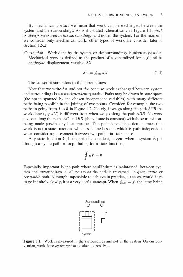
By mechanical contact we mean that work can be exchanged between thesystem and the surroundings. As is illustrated schematically in Figure 1.1, workis always measured in the surroundings and not in the system. For the moment,we consider only mechanical work; other types of work are consider later inSection 1.5.2.
Convention Work done by the system on the surroundings is taken as positive.Mechanical work is defined as the product of a generalized force f and itsconjugate displacement variable dX:
δw = fsurr dX (1.1)
The subscript surr refers to the surroundings.
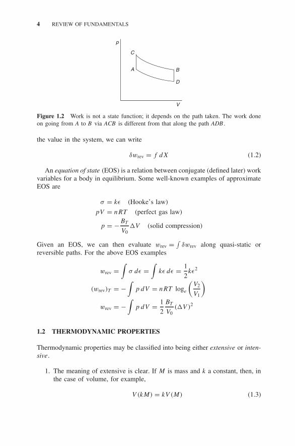
Note that we write δw and not dw because work exchanged between systemand surroundings is a path-dependent quantity. Paths may be drawn in state space(the space spanned by the chosen independent variables) with many differentpaths being possible in the joining of two points. Consider, for example, the twopaths in going from A to B in Figure 1.2. Clearly, if we go along the path ACB thework done (
∫p dV ) is different from when we go along the path ADB . No work
is done along the paths AC and BD (the volume is constant) with these transitionsbeing made possible by heat transfer. This path dependence demonstrates thatwork is not a state function. which is defined as one which is path independentwhen considering movement between two points in state space.
Any state function Y , being path independent, is zero when a system is putthrough a cyclic path or loop, that is, for a state function,∮
dY = 0
Especially important is the path where equilibrium is maintained, between sys-tem and surroundings, at all points as the path is traversed—a quasi-static orreversible path. Although impossible to achieve in practice, since we would haveto go infinitely slowly, it is a very useful concept. When fsurr = f , the latter being
System
w
Surroundings
Figure 1.1 Work is measured in the surroundings and not in the system. On our con-vention, work done by the system is taken as positive.
4 REVIEW OF FUNDAMENTALS
A
C
B
D
p
V
Figure 1.2 Work is not a state function; it depends on the path taken. The work doneon going from A to B via ACB is different from that along the path ADB .
the value in the system, we can write
δwrev = f dX (1.2)
An equation of state (EOS) is a relation between conjugate (defined later) workvariables for a body in equilibrium. Some well-known examples of approximateEOS are
σ = kε (Hooke’s law)
pV = nRT (perfect gas law)
p = −BT
V0�V (solid compression)
Given an EOS, we can then evaluate wrev = ∫δwrev along quasi-static or
reversible paths. For the above EOS examples
wrev =∫
σ dε =∫
kε dε = 1
2kε2
(wrev)T = −∫
p dV = nRT loge
(V2
V1
)
wrev = −∫
p dV = 1
2
BT
V0(�V )2
1.2 THERMODYNAMIC PROPERTIES
Thermodynamic properties may be classified into being either extensive or inten-sive.
1. The meaning of extensive is clear. If M is mass and k a constant, then, inthe case of volume, for example,
V (kM) = kV (M) (1.3)

THE LAWS OF THERMODYNAMICS 5
Mathematically, extensive properties like V are said to be homogenousfunctions of the first degree.
2. Intensive properties can be divided into two types and it is important todistinguish between the two:(a) Field : T , p, μ (much more later about this function)(b) Density : Vm = V/Ntotal, Hm = H/Ntotal, and mole fraction xi =
Ni/Ntotal
There is an important distinction between these two kinds of intensive variablesin that a field variable takes on identical values in any coexisting phases atequilibrium, a density variable does not.
1.3 THE LAWS OF THERMODYNAMICS
The laws of thermodynamics can be introduced historically via experimentalobservations and many equivalent statements are possible. Alternatively, theymay be stated as postulates, axiomatic statements, or assumptions based onexperience. In this approach, the existence of some new state functions (bulkproperties) is postulated with a recipe given for how to measure each of them.This latter approach is adopted here.
(a) Zeroth Law Thermodynamic temperature T is a state function.Recipe The thermodynamic temperature is equal to the ideal gas tempera-
ture, pVm/R. It is possible, therefore, to define T in terms of mechanicalideas only, with no mention of heat. Note, however, that the thermody-namic temperature is selected as a primary quantity in the SI system.
(b) First Law The internal energy U is a state function.Recipe If we proceed along an adiabatic path in state space, then
dU = −δwadiabatic (1.4)
The negative sign here arises since, if work is done by the system, itsenergy is lowered. Note that only changes in U can be measured. Thisapplies to all energy-based extensive thermodynamic quantities.
The first law leads to the definition of heat. Heat should only bereferred to as an energy transfer and not as an energy or heat content ;that is, heat is not a noun, heat flow is a process.
For a nonadiabatic process, the change in U is no longer given bythe work done on the system. The missing contribution defines the heattransferred:
dU = δq − δw (first law) (1.5)

6 REVIEW OF FUNDAMENTALS
Just as δw is path dependent, δq is also path dependent; that is, q is nota state function, whereas U is.
Equation (1.5) is the differential form of the conservation of energyor first law for any system. Note that there is no specific mention ofp–V work in this statement. It is generally valid.
Convention Heat flow into the system is taken to be positive (Fig. 1.3).Since both work and heat flow are measured in the surroundings, wherethe field variables are taken to be constant, any changes in state in thesurroundings are always considered to be made quasi-statically.
(c) Second Law while the first law is concerned with the conservation ofenergy, the second law is concerned with how energy is spread. Any spon-taneous process occurs in a way so as to maximize the spread of energybetween accessible states of the system and its surroundings . Entropy is theproperty which is the measure of this spread.
The second law is usually stated in two parts:
1. Entropy S of the system is a state function.Recipe If the state of a system is changed reversibly by heat flow,then the entropy change is given by
dS = δqrev
T(second law, part 1) (1.6)
2. In a spontaneous process, entropy in the system plus surroundings, some-times called the universe, is created (energy is spread).
The total entropy change of the system plus surroundings is thengiven by
dSuniv = dS + dSsurr ≥ 0 (1.7)
In an isolated system there is no external creation of entropy so that
dSsurr = 0 and dS ≥ 0
q
System
Surroundings
Figure 1.3 Heat flow is measured in the surroundings. In our convention, heat flow intothe system is taken as positive.
THE LAWS OF THERMODYNAMICS 7
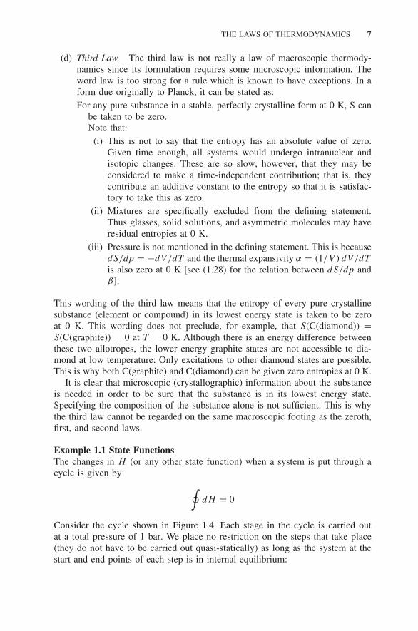
(d) Third Law The third law is not really a law of macroscopic thermody-namics since its formulation requires some microscopic information. Theword law is too strong for a rule which is known to have exceptions. In aform due originally to Planck, it can be stated as:For any pure substance in a stable, perfectly crystalline form at 0 K, S can
be taken to be zero.Note that:
(i) This is not to say that the entropy has an absolute value of zero.Given time enough, all systems would undergo intranuclear andisotopic changes. These are so slow, however, that they may beconsidered to make a time-independent contribution; that is, theycontribute an additive constant to the entropy so that it is satisfac-tory to take this as zero.
(ii) Mixtures are specifically excluded from the defining statement.Thus glasses, solid solutions, and asymmetric molecules may haveresidual entropies at 0 K.
(iii) Pressure is not mentioned in the defining statement. This is becausedS/dp = −dV/dT and the thermal expansivity α = (1/V ) dV/dT
is also zero at 0 K [see (1.28) for the relation between dS/dp andβ].
This wording of the third law means that the entropy of every pure crystallinesubstance (element or compound) in its lowest energy state is taken to be zeroat 0 K. This wording does not preclude, for example, that S(C(diamond)) =S(C(graphite)) = 0 at T = 0 K. Although there is an energy difference betweenthese two allotropes, the lower energy graphite states are not accessible to dia-mond at low temperature: Only excitations to other diamond states are possible.This is why both C(graphite) and C(diamond) can be given zero entropies at 0 K.
It is clear that microscopic (crystallographic) information about the substanceis needed in order to be sure that the substance is in its lowest energy state.Specifying the composition of the substance alone is not sufficient. This is whythe third law cannot be regarded on the same macroscopic footing as the zeroth,first, and second laws.
Example 1.1 State FunctionsThe changes in H (or any other state function) when a system is put through acycle is given by ∮
dH = 0
Consider the cycle shown in Figure 1.4. Each stage in the cycle is carried outat a total pressure of 1 bar. We place no restriction on the steps that take place(they do not have to be carried out quasi-statically) as long as the system at thestart and end points of each step is in internal equilibrium:

8 REVIEW OF FUNDAMENTALS
Si(s) + O2(g) B SiO2(s)
1000 K
C
D
A
SiO2(s)
298 K
Si(s) + O2(g)
Figure 1.4 Enthalpy is a state function.
(A)[H
◦(1000) − H
◦(298)
]Si(s) + [
H◦(1000) − H
◦(298)
]O2(g)
=∫ 1000
298[Cp(Si) + Cp(O2)] dT = 17,075 + 22,694 J
(B) −�f H◦(SiO2(s), 1000) = −857,493 J
(C)[H
◦(298) − H
◦(1000)
]SiO2
=∫ 298
1000Cp(SiO2) dT = −43,611 J
(D) �f H◦(SiO2(s), 298.15) = +861,335 J
from which, for the cycle∮(A − B − C − D) = 17,075 + 22,694 − 857,493 − 43,611 + 861,335 = 0
The same procedure may be followed for the state properties U, S, A, and G.For all of these state functions,
∮dY = 0.
1.4 THE FUNDAMENTAL EQUATION
The combined statement of the first and second laws comes by first expressingthe first law for any process,
δq = dU + δw (1.8)
and then introducing the second law for a reversible process, δqrev = T dS, toobtain
T dS = dU + δwrev (1.9)
For a closed system of fixed amounts of substances doing p–V work only we canwrite δwrev = p dV so that
dU = T dS − p dV (p–V work only, fixed amounts) (1.10)

OTHER THERMODYNAMIC FUNCTIONS 9
Although we have derived this equation by considering reversible processes, itis applicable to any process as long as the initial and final states are in internalequilibrium, since it involves state functions only. It is called the fundamentalequation or Gibbs’s first equation and we consider its application later.
It can be seen from (1) that the natural independent variables of the statefunction U are S and V .
1.5 OTHER THERMODYNAMIC FUNCTIONS
For systems undergoing p–V work only, we have seen that the primary func-tions of thermodynamics are the mechanical variables p and V together withthe variables T , U , and S. For convenience, however, many other state func-tions are defined since it is usually not convenient for the natural variables of asystem to be S and V ; that is, we do not usually hold these variables constantwhen carrying out experiments. The introduction of new state functions enableus to change the natural variables to anything desired (in mathematical terms, weperform Legendre transformations).
The most important of these new derived functions are as follows:
1. Enthalpy H is defined as
H = U + pV (1.11)
Its usefulness comes from the fact that, at constant p,
dH |p = dU + p dV (1.12)
and, if this equation is compared with
dU = δq − p dV (1.13)
then we see that
dH |p = δq (1.14)
Note that there is nothing in this last equation about maintaining constant T
or carrying out the process reversibly. An enthalpy change can be obtainedfrom the measured heat flow required to bring about the change at constantp. This is the basis of calorimetry .
2. Heat capacities Cp and CV are two response functions (partial derivativesof other functions):
CV =(
∂U
∂T
)V
Cp =(
∂H
∂T
)p
3. Helmholtz energy A is defined as A = U − T S. For an isothermal processdA = dU − T dS, but for a reversible process δwrev = −dU + T dS, so

10 REVIEW OF FUNDAMENTALS
that, for a reversible, isothermal process,
−dA|T = δwrev (1.15)
that is, in an isothermal process, the decrease in A measures the maximumwork performed by the system.
4. Entropy change has already been defined: δqrev = T dS, where δqrev canbe expressed in terms of the heat capacity at constant pressure. This thengives
dS|p = δqrev|pT
= Cp
TdT (1.16)
and, when this is integrated, advantage is taken of the third law to obtainabsolute entropies:
S|p(T ) =∫ T
0
Cp
TdT (1.17)
In practice, it is more useful to do the integration in two stages:
S|p(T ) − S|p(298 K) =∫ T
298K
Cp
TdT (1.18)
5. Gibbs energy G is defined as G = U + pV − T S. For an isothermal, iso-baric process
dG = dU + p dV − T dS (1.19)
For a reversible isothermal, isobaric process (combine with δwrev =−dU + T dS),
−dG|p,T = δwrev − p dV (1.20)
This is the total reversible work less the p–V work so that, in an isothermal,isobaric process, the decrease in G measures the maximum non–p–V workperformed . It is the most widely used derived function in materials ther-modynamics. The non–p–V work of most interest to us is chemical work.
By using the definitions of the derived functions H , A, G, we can derive theother three Gibbs equations for p–V work only, fixed amounts:
dH = T dS + V dp (1.21)
dA = −S dT − p dV (1.22)
G = −S dT + V dp (1.23)
The natural variables of G are p, T , which are the ones usually controlled inexperiments and this accounts for the importance of this particular state function.

OTHER THERMODYNAMIC FUNCTIONS 11
1.5.1 Maxwell’s Equations
Return to (1.10), which is the total differential of U = U(S, V ). We can rewritethis equation in terms of partial derivatives as follows:
dU =(
∂U
∂S
)V
dS +(
∂U
∂V
)S
dV (1.24)
If we compare (1.10) with (1.24), we see that
(∂U
∂S
)V
= T (1.25)
(∂U
∂V
)S
= −p (1.26)
Application of standard partial differentiation theory like this to the otherGibbs equations leads to similar relations and further relations can be obtainedfrom the cross-derivatives, for example,
(∂2U
∂S ∂V
)V
=(
∂2U
∂V ∂S
)S
(1.27)
which, using (1.25), gives
−(
∂p
∂S
)V
=(
∂T
∂V
)S
(1.28)
Such relations are called Maxwell’s equations. Their importance lies in the factthat they can point to the recognition of redundant measurements and offer thepossibility of obtaining difficult-to-measure property variations from variationsin properties which are easier to measure.
All the equations in this section apply to systems performing p–V work onlyand are of fixed composition. We must now consider the modifications broughtabout by the inclusion of other types of work and the effect of changes in theamounts of substances which comprise the system.
1.5.2 Defining Other Forms of Work
With the conservation of energy as the fundamental principle, it is possible toinvent other forms of thermodynamic work which can then be incorporated intothe conservation-of-energy equation. By doing this, force and displacement areused in a much broader sense than they are in mechanical work. Any form ofwork which brings about a change in internal energy is to be considered. It maybe a potential times a capacity factor or a field times a polarization.

12 REVIEW OF FUNDAMENTALS
Most notably in the present context is the invention, made by Gibbs, ofchemical work. Chemical work can, of course, be considered as originating inthe potential and kinetic energies of the atoms and electrons, but Gibbs realizedthat it is more useful to regard it as a separate form of work. In doing so, heintroduced a most important new state function, the chemical potential , and alsoextended the fundamental equations to incorporate this new form of work.
The fundamental equations previously given apply to closed systems, that is,of fixed amounts of substance. They can be extended to include varying amounts,either for the case of a closed system, in which the amounts of substances arevarying due to chemical reactions occurring within the system, or to open sys-tems, where substances are being exchanged with the surroundings and in whichreactions may or may not be occurring. In both cases chemical work is involved;that is, changes in internal energy are occurring.
If the amounts of substances can vary in a system, then, clearly, the statefunctions will depend on the ni . In the case of U , for example, we now haveU = U(S, V, n1, n2 . . .). Equation (1.24) will be modified to
dU =(
∂U
∂S
)V,nj
dS +(
∂U
∂V
)S,nj
dV +∑
i
(∂U
∂ni
)S,V,nj
dni (1.29)
where nj means all the others except i.In order to be able to write this in a manner similar to (1.10), we need a
symbol for the partial derivative of U with respect to ni . The usual symbol is μi
and its name is the chemical potential (p–V and chemical work only):
dU = T dS − p dV +∑
i
μi dni (1.30)
The other Gibbs equations may be modified in a similar fashion (p–V andchemical work only):
dH = T dS + V dp +∑
i
μi dni (1.31)
dA = −S dT − p dV +∑
i
μi dni (1.32)
dG = −S dT + V dp +∑
i
μi dni (1.33)
Note that the definition of μi varies depending on which function is being used:
μi =(
∂U
∂ni
)S,V,nj
=(
∂H
∂ni
)S,p,nj
=(
∂A
∂ni
)T ,V,nj
=(
∂G
∂ni
)T ,p,nj
(1.34)
OTHER THERMODYNAMIC FUNCTIONS 13
This extension of thermodynamics from a study of heat engines to its applica-tion to phase and chemical equilibrium by Gibbs represents one of the greatestachievements in nineteenth-century science. Recall that, in the application ofthermodynamics to heat engines, the nature of the fluid of the engine is unim-portant, but in introducing chemical work, the nature of the material constitutingthe system becomes all important.
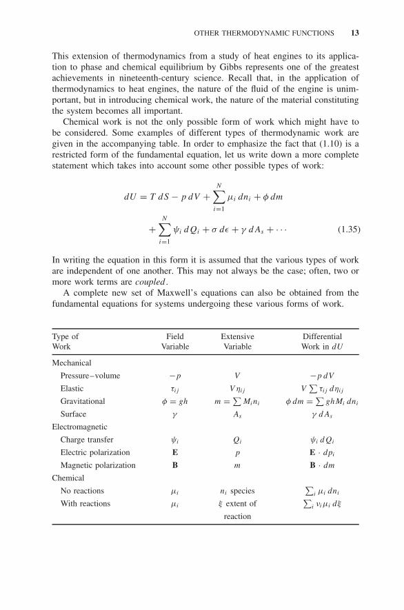
Chemical work is not the only possible form of work which might have tobe considered. Some examples of different types of thermodynamic work aregiven in the accompanying table. In order to emphasize the fact that (1.10) is arestricted form of the fundamental equation, let us write down a more completestatement which takes into account some other possible types of work:
dU = T dS − p dV +N∑
i=1
μi dni + φ dm
+N∑
i=1
ψi dQi + σ dε + γ dAs + · · · (1.35)
In writing the equation in this form it is assumed that the various types of workare independent of one another. This may not always be the case; often, two ormore work terms are coupled .
A complete new set of Maxwell’s equations can also be obtained from thefundamental equations for systems undergoing these various forms of work.
Type of Field Extensive DifferentialWork Variable Variable Work in dU
Mechanical
Pressure–volume −p V −p dV
Elastic τij V ηij V∑
τij dηij
Gravitational φ = gh m = ∑Mini φ dm = ∑
ghMi dni
Surface γ As γ dAs
Electromagnetic
Charge transfer ψi Qi ψi dQi
Electric polarization E p E · dpi
Magnetic polarization B m B · dm
Chemical
No reactions μi ni species∑
i μi dni
With reactions μi ξ extent of∑
i νiμi dξ
reaction

14 REVIEW OF FUNDAMENTALS
1.6 EQUILIBRIUM STATE
A precise definition of a system in equilibrium is not straightforward. To define asystem as being in equilibrium when its properties are not changing with time isunacceptable—the state which involves a steady flow of heat or matter througha system is a time-independent state but systems in which these processes areoccurring are not in equilibrium; there are field gradients. We need a betterdefinition and one is discussed below.
The second law, part 2, states that dSuniv ≥ 0, with the inequality referring tospontaneous processes and the equality to reversible processes, the latter corre-sponding with the system being in equilibrium.
If we consider an isolated system (no work or heat flow and, therefore, constantU and V ), then dSsurr = 0 so that
dS|U,V = dSuniv ≥ 0 (1.36)
In other words, for an isolated system, S reaches a maximum at the equilibriumstate, making this state function the appropriate thermodynamic potential forisolated systems. The important point here is that, under certain constraints, wehave replaced a property of the universe (system + surroundings) by a propertyof the system alone.
Of more practical interest is to obtain the appropriate thermodynamic potentialfor constant p and T conditions and the nature of the extrema conditions. Wecan do this as follows:
G = U + pV − T S (1.37)
dG = dU + p dV + V dp − T dS − S dT (1.38)
= δq − psurr dV + p dV + V dp − T dS − S dT (1.39)
and at constant p and T where psurr = p we have
dG|p,T = −T dSsurr − T dS
= −T dSuniv ≤ 0 (1.40)
From the general statement of the second law, dSuniv is a maximum atequilibrium, it follows from (1.40) that the appropriate thermodynamic potentialfor conditions of constant p and T is the Gibbs energy and G evolves to aminimum at equilibrium . Since these conditions are the most frequently met, theGibbs energy is usually the most important thermodynamic potential of interest.Note that, again, a property of the universe has been replaced by a property ofthe system alone.
For small excursions from an equilibrium state, we can expand any functionfor G as a Taylor series in the state space variables. As illustrated in Figure 1.5,which shows G as a function of only two state space variables, the extrema in

EXERCISES 15
Local minimum
Maximum
Saddle point
Global minimum
Figure 1.5 Local and global equilibrium, drawn using Matlab®.
multidimensional space can be maxima, minima, or saddle points (a maximum insome directions, a minimum in others). The required conditions for the extremumto be a minimum when there are two such variables, x and y, can be written as
∂2G
∂x2and
∂2G
∂y2> 0 (1.41)
∂2G
∂x2
∂2G
∂y2>
(∂2G
∂x ∂y
)2
(1.42)
Failure of the condition given in (1.40) implies a saddle point.These conditions only apply, however, for small excursions from the equilib-
rium point. As shown in Figure 1.5, it is possible to have a local minimum whichfulfils the above conditions, but it is not the global minimum which we seek inour thermodynamic calculation.
For both the local and global minima, a small fluctuation from the equilibriumpoint will result in dG|p,T > 0 and the system will wish to return to its equilibriumpoint. In both cases also the field variables (T , p, μA) are constant throughoutthe system. This means that we can apply the equations of thermodynamicsequally well to the metastable local equilibrium and the stable global equilibriumsituations if we ensure that there are no large-scale fluctuations which will takeus from the local to the global equilibrium.
The global equilibrium, that is, the true equilibrium state, is when �G|p,T > 0for any excursions from that state, providing the start and end states are main-tained in internal equilibrium by the imposition of extra constraints. It is thisdefinition of the equilibrium state which is mainly used throughout these chapters,but, as has been indicated previously, other thermodynamic potentials fulfil thesame role as G for other conditions.
EXERCISES
1.1 Starting from Al(s) and O2(g) at 298 K and 1 bar, use the data given belowand the cycle illustrated in Figure 1.6 to confirm that
∮dS = 0:

16 REVIEW OF FUNDAMENTALS
2Al(l) + 1.5O2(g) B Al2O3(s)
1000 K
C
D
A
298 K
2Al(s) + 1.5O2(g) Al2O3(s)
Figure 1.6 Cycle to be considered.
Tfus(Al) = 933 K �fusHm = 10460 J mol−1
Cp = a + bT + cT 2 + dT −2
a b/103 c/106 d/10−5 S◦(298)/J K−1 mol−1
Al(s) 20.7 12.4 0 0 28.3Al(l) 31.8 0 0 0 0O2(g) 30 4.184 0 −1.67 205.0Al2O3(s) 106.6 17.78 0 −28.53 51.0
1.2 Starting with CaCO3(s) at 298 K and 1 bar: .
(a) Calculate the heat transferred in producing 1 mol of CaO(s) at 1200 Kand 1 mol of CO2(g) at 500 K.
(b) Calculate the standard entropy change for this process.
1.3 .(a) Write down the full equations required for evaluation of the standardenthalpy and Gibbs energy for the reaction equation
CaCO3(s) = CaO(s) + CO2(g)
(b) Determine the temperature at which �G◦ = 0 for this reaction equation.
(c) Calculate the enthalpy of reaction at the temperature for which theequilibrium pressure of CO2 is 1 bar.
Cp = a + bT + cT 2 + dT −2/J K−1 mol−1
�f H◦(298K)/ S◦
(1000K)/
Substance kJ mol−1 J K−1 mol−1 a b × 103 c × 105 d × 10−5
CaO(s) −634.92 96.96 57.75 −107.79 0.53 −11.51CO2(g) −393.51 269.19 44.14 9.04 0 −8.54CaCO3(s) −1206.60 220.21 99.55 27.14 0 −21.48

EXERCISES 17
1.4 Given the following data:Note that 〈C◦
p〉 refers to the average values of C◦p over the range 298–
1000 K. Calculate: .
(a) The standard entropy of oxidation of Si(s) to SiO2(s) at 1000 K.(b) The same using the values of 〈C◦
p〉. Compare with the result from (a).
S◦(s, 298 K)/ S
◦1000 − S
◦298)/ 〈C◦
p〉/Substance J K−1 mol−1 J K−1 mol−1 J K−1 mol−1
Si(s) 18.81 28.69 23.23O2(g) 209.15 38.43 32.10SiO2(s) 27.78 72.15 56.02
(c) �f H◦(SiO2, 1000 K) using the value of �f H
◦(SiO2, 298 K) in the
text.
1.5 Derive (1.21), (1.22), and (1.23) from (1.10) and the definitions of thefunctions H , A and G.
1.6 .(a) If the entropy of transition of a pure substance A, �βαS
◦(A), at constant
p is constant, show that the corresponding enthalpy change, �βαH
◦(A),
is also constant.(b) If the phase transition of a pure substance is a function of T and p and
the value of �βαS
◦(A) is independent of the change in conditions, show
that the value of �βαH
◦(A) is no longer constant, as was the case for
the constraint of constant p. (Hint : Use the Maxwell relationships.)


2 Thermodynamics of UnarySystems
A unary, or one-component, system refers to a pure substance of fixed compo-sition. Importantly, this includes molecules and compounds as well as the pureelements. For molecules and compounds, their formation properties are often themost important. Formation properties are defined as the properties of the com-pound relative to those of the elements in their most stable form at the temperatureand pressure of interest.
In this chapter, only p–V work is considered. Chemical work, surface work,and so on, are ignored.
2.1 STANDARD STATE PROPERTIES
Standard states, by definition, always refer to a pressure of 1 bar. Reference states,which are also used in thermodynamics, are not necessarily so constrained. Wecan also speak of reference states for standard state properties, for example, areference state at 298.15 K for a standard state property at 1 bar.
For the moment we concentrate on properties at 1 bar, that is, on standardstate properties.
Collating all the available experimental data for pure substances and arriving atrecommended values for thermochemical properties comprise a highly skilled andmajor exercise. It has been done by large organizations, for example, the NationalInstitute of Standards and Technology (NIST), the National Aeronautics andSpace Administration (NASA), and the U.S. Bureau of Mines. Before computers,thermochemical data were usually presented in the form of tables; occasionallythey were presented as analytical approximations. With the advent of computers,however, analytical representations have almost totally supplanted the use oftables. The storage of the coefficients in analytical expressions is much moreconvenient for computer usage than their presentation in tabular form.
A quantity of primary interest is the standard Gibbs energy of formation ofa compound, which is related to the standard enthalpy and entropy of formationby
�f G◦(T ) = �f H
◦(T ) − T �f S
◦(T ) (2.1)
Materials Thermodynamics. By Y. Austin Chang and W. Alan OatesCopyright 2010 John Wiley & Sons, Inc.
19
20 THERMODYNAMICS OF UNARY SYSTEMS
From values of �f G◦(T ) for the participating substances, we can obtain standard
Gibbs reaction energies, �rG◦(T ), for any reaction:
�rG◦(T ) =
∑i
νi�f G◦(i, T ) (2.2)
Here νi is the stoichiometric coefficient, which is positive for products and nega-tive for reactants in a chemical reaction, that is, for a formation reaction such as
Pb + 12 O2(g) = PbO
νPbO = 1 νPb = −1 νO2 = − 12
Standard Heat Capacities As will be discussed in Chapter 3, the standard heatcapacity of a substance varies with temperature in a rather complex manner atlow temperatures. Above room temperature, however, and in the absence of anyphase transformations, its variation with T can be represented to a sufficientlyhigh accuracy by a polynomial. The approximation usually used is of the form
C◦p(T ) = a + bT + cT 2 + dT −2 (2.3)
Note, however, that some data compilations use slightly different analyticalexpressions.
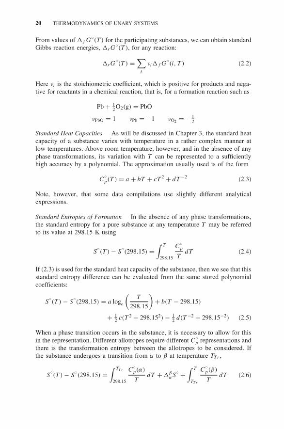
Standard Entropies of Formation In the absence of any phase transformations,the standard entropy for a pure substance at any temperature T may be referredto its value at 298.15 K using
S◦(T ) − S
◦(298.15) =
∫ T
298.15
C◦p
TdT (2.4)
If (2.3) is used for the standard heat capacity of the substance, then we see that thisstandard entropy difference can be evaluated from the same stored polynomialcoefficients:
S◦(T ) − S
◦(298.15) = a loge
(T
298.15
)+ b(T − 298.15)
+ 12 c(T 2 − 298.152) − 1
2 d(T −2 − 298.15−2) (2.5)
When a phase transition occurs in the substance, it is necessary to allow for thisin the representation. Different allotropes require different C
◦p representations and
there is the transformation entropy between the allotropes to be considered. Ifthe substance undergoes a transition from α to β at temperature TT r ,
S◦(T ) − S
◦(298.15) =
∫ TT r
298.15
C◦p(α)
TdT + �β
αS◦ +
∫ T
TT r
C◦p(β)
TdT (2.6)

STANDARD STATE PROPERTIES 21
If the substance undergoes a magnetic transition, say from ferromagnetic to para-magnetic, the heat capacity variation is more complex and the simple polynomialrepresentation has to be augmented with another representation for the magneticcontribution.
The Planck postulate (S for any pure substance in a stable perfect crystallineform at 0 K is taken to be zero) is taken advantage of in obtaining S
◦(298.15).
Although C◦p below room temperature is a complex function of temperature
which cannot be represented by a simple polynomial like (2.3), once it has beenmeasured, the standard entropy of a crystalline substance at 298.15 K can beobtained from
S◦(298.15) =
∫ 298.15
0
C◦p(T )
TdT (2.7)
This means that the computer storage of S◦(298.15 K) plus the coefficients in
the standard heat capacity equation (2.3) is sufficient for evaluating the standardentropies of pure substances in a particular structural form at any temperatureabove room temperature.
For a pure compound substance it is the formation property which is of majorinterest. In view of the Planck postulate we can write
�f S◦(298.15) =
∑i
νiS◦(i, 298.15) (2.8)
where the summation is over all participating substances in the formation reac-tion equation. Equation (2.8) can then be used in the calculation of the high-temperature standard entropy of formation of the compound:
�f S◦(T ) = �f S
◦(298.15) +
∑i
νi
[S
◦(i, T ) − S
◦(i, 298.15)
](2.9)
where (2.5) is used for S◦(i, T ) − S
◦(i, 298.15).
If phase transformations occur in either products or reactants, (2.9) has to bemodified in a manner similar to that given in (2.6).
Standard Enthalpies of Formation The difference in standard enthalpy for asubstance between two temperatures is given by
H◦(T2) − H
◦(T1) =
∫ T2
T1
Cp dT (2.10)
Whereas standard entropies have a natural reference point by taking advantageof the Planck postulate, there is no similar natural reference point for enthalpies.
In the following we concentrate on the two most commonly used choicesof reference state. The first one is used in most tabular presentations while thesecond one is favored in computer databases:

22 THERMODYNAMICS OF UNARY SYSTEMS
1. Standard Substance Reference (SSR) State The enthalpies of all subs-tances in their most stable form at 1 bar and 298.15 K are selected to be zero.
Table 2.1 for copper, taken from the NIST-JANAF tables, illustrates this selec-tion. It can be seen that H
◦(298.15 K) = 0. It also has this value for compound
substances.Using the SSR state, the enthalpy of formation of a pure compound can be
obtained from
�f H◦(T ) = �f H
◦(298.15) +
∑i
νi
[H
◦(i, T ) − H
◦(i, 298.15)
](2.11)
There is no equation analogous to (2.8) for formation enthalpies at 298.15 K.These have to be determined by experiment or calculation.
If (2.3) is used for the heat capacity, the bracketed terms on the right-handside of (2.11) are given by
H◦(i, T ) − H
◦(i, 298.15 K) = a(T − 298.15) + 1
2b(T 2 − 298.152)
+ 13c(T 3 − 298.153) − d(T −1 − 298.15−1)
(2.12)
In tabular form as shown in Table 2.1 for Cu, data are usually presented at 100 Kintervals. If data at temperatures intermediate to these are required, it is necessaryto interpolate. In order to assist in doing this with some accuracy, some functionwhich is a slowly varying function of temperature is desired. Such a function isthe so-called Gibbs energy function gef (a confusing term) defined as
gef(T ) = −G◦(T ) − H
◦(298.15)
T(2.13)
As can be seen in Table 2.1 for Cu, this function has the desired property ofbeing slowly varying with temperature and is therefore easily and accuratelyinterpolated. Given the values of gef for all the species involved in the formationreaction, the calculation of �f G
◦(T ) is then straightforward. From (2.13),
T × gef(T ) = −G◦(T ) + H
◦(298.15)
and we see that �f G◦(T ) can be obtained from
�f G◦(T ) = �f H
◦(298.15) − T
∑i
νi gef(i, T ) (2.14)
In order to evaluate �f G◦(T ), all that is required is the room temperature
standard enthalpy of formation and the tables can then be used to obtain∑i νi gef(i, T ) for the formation of the substance. It should be noted that the
difference,∑
i νi gef(i, T )), usually varies even more slowly with T than thegef values for the individual substances.

STANDARD STATE PROPERTIES 23
TABLE 2-1 Tabular Presentation of Thermodynamic Properties of Copper fromNIST-JANAF Tables
Enthalpy Reference Temperature Ts = 298.15 K Standard State Pressure = 0.1 MPa
J K−1 mol−1 kJ mol−1
T/K C◦p S
◦ −[G◦ − H◦(Ts)]
TH
◦ − H◦(Ts) �f H
◦�f G
◦ log Kt
0 0 0 0 −5.007 0 0 0100 16.010 10.034 53.414 −4.338 0 0 0200 22.631 23.73 35.354 −2.325 0 0 0250 23.782 28.915 33.563 −1.162 0 0 0298.15 24.442 33.164 33.164 0.000 0 0 0300 24.462 33.315 33.164 0.045 0 0 0350 24.975 37.127 33.464 1.282 0 0 0400 25.318 40.484 34.136 2.539 0 0 0450 25.686 43.489 35.011 3.815 0 0 0500 25.912 46.206 35.997 5.105 0 0 0600 26.481 50.982 38.107 7.725 0 0 0700 26.996 55.030 40.247 10.399 0 0 0800 27.494 58.739 42.336 13.123 0 0 0900 28.049 62.009 44.343 15.899 0 0 0
1000 28.662 64.994 46.261 18.733 0 0 01100 29.479 67.763 48.091 21.638 0 0 01200 30.519 70.368 49.840 24.633 0 0 01300 32.143 72.871 51.516 27.762 0 0 01358 33.353 74.300 52.459 29.660 Crystal ←→ Liquid1358 32.844 83.974 52.459 42.798 Transition1400 32.844 84.974 53.419 44.177 0 0 01500 32.844 87.240 55.599 47.462 0 0 01600 32.844 89.360 57.644 50.746 0 0 01700 32.844 91.351 59.569 54.031 0 0 01800 32.844 93.229 61.387 57.315 0 0 02000 32.844 96.689 64.747 63.884 0 0 02200 32.844 99.819 67.795 70.453 0 0 02400 32.844 102.677 70.585 77.022 0 0 02600 32.844 105.306 73.156 83.591 0 0 02800 32.844 107.740 75.540 90.159 0 0 02843.3 32.844 108.244 76.034 91.580 FUGACITY = 1 bar2900 32.844 108.893 76.671 93.444 −300.204 5.996 −0.1083000 32.844 110.006 77.764 96.728 −299.409 16.541 −0.2883200 32.844 112.126 79.846 103.297 −297.971 37.556 −0.6133400 32.844 114.117 81.804 109.866 −296.737 58.488 −0.8993600 32.844 115.995 83.652 116.435 −295.703 79.352 −1.1513800 32.844 117.770 85.401 123.004 −294.962 100.165 −1.3774000 32.844 119.455 87.062 129.573 −294.199 120.938 −1.579
Note: The data for some temperatures have been removed to decrease the size of the table.

24 THERMODYNAMICS OF UNARY SYSTEMS
The NIST-JANAF compilation also presents tables for other choices ofreference state. In one set of tables, as discussed above, the most stable format 1 bar and 298.15 K is selected while, in another set, the enthalpies of allsubstances in the designated form, regardless of whether that form is the moststable or not, are selected to be zero at 1 bar and 298.15 K. For example,the properties for a liquid substance are referred to the liquid at 298.15 Kin this other form of presentation. Other compilations select the enthalpy ofthe substance in its most stable form at 0 K to be zero and it is clear thatsome care is required if these different presentations of data are to be usedcorrectly.
With the advent of the computer storage of data, tabular presentations are atthe obsolescent stage.
2. Standard Element Reference (SER) State The enthalpies of the elementsin their most stable form at 1 bar and 298.15 K are selected to be zero.
In order to distinguish between the SSR and SER states for the standardenthalpy, we will use H SER to refer to H
◦(298.15) when the element referencestate is being used. Here, H SER is set to zero for the elements in their moststable state at 298.15 K while H SER(298.15) for a compound (abbreviation cpd)is equal to its enthalpy of formation at that temperature:
H SER(cpd, 298.15) = �f H◦(cpd, 298.15) (2.15)
The standard formation enthalpy for a compound at any temperature on thisreference state is then given by
�f H◦(T ) =
∑νiH
◦(i, T ) (2.16)
an equation which can be compared with (2.11) based on using the substancereference state.
When phase transformations are present, the enthalpies of transition must beincorporated into (2.16).
Table 2.2 shows the way that the necessary coefficients, used in the SER, arestored in computer databases for PbO.
(i) Line 1 in Table 2.2 gives the values for H SER and S◦(298.15).
(ii) Line 2 gives the heat capacity coefficients between 298.15 and 762K. At this temperature there is a phase transformation in PbO(s).
(iii) Line 3 gives the enthalpy change at this transition. The standardentropy change can be obtained from �T rH
◦/T
◦T r since �T rG
◦ = 0at this temperature.
(iv) Line 4 gives the heat capacity coefficients for the temperature range720–1162 K. PbO melts at this temperature.
(v) Line 5 gives the standard enthalpy of fusion. Again the standardentropy of fusion can be obtained from �fusH
◦/T
◦fus.
(vi) Line 6 gives the heat capacity coefficients for liquid PbO.
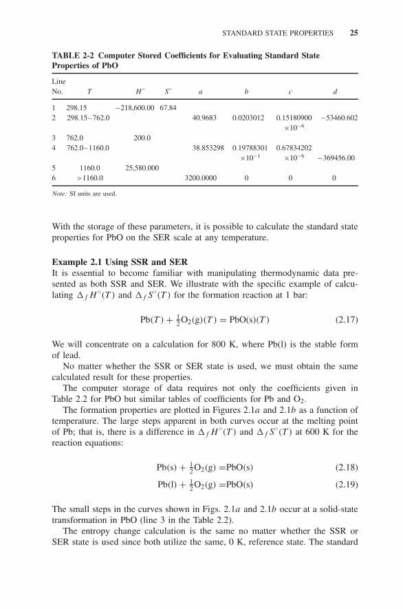
STANDARD STATE PROPERTIES 25
TABLE 2-2 Computer Stored Coefficients for Evaluating Standard StateProperties of PbO
LineNo. T H
◦S
◦a b c d
1 298.15 −218,600.00 67.842 298.15–762.0 40.9683 0.0203012 0.15180900 −53460.602
×10−6
3 762.0 200.04 762.0–1160.0 38.853298 0.19788301 0.67834202
×10−1 ×10−6 −369456.005 1160.0 25,580.0006 >1160.0 3200.0000 0 0 0
Note: SI units are used.
With the storage of these parameters, it is possible to calculate the standard stateproperties for PbO on the SER scale at any temperature.
Example 2.1 Using SSR and SERIt is essential to become familiar with manipulating thermodynamic data pre-sented as both SSR and SER. We illustrate with the specific example of calcu-lating �f H
◦(T ) and �f S
◦(T ) for the formation reaction at 1 bar:
Pb(T ) + 12 O2(g)(T ) = PbO(s)(T ) (2.17)
We will concentrate on a calculation for 800 K, where Pb(l) is the stable formof lead.
No matter whether the SSR or SER state is used, we must obtain the samecalculated result for these properties.
The computer storage of data requires not only the coefficients given inTable 2.2 for PbO but similar tables of coefficients for Pb and O2.
The formation properties are plotted in Figures 2.1a and 2.1b as a function oftemperature. The large steps apparent in both curves occur at the melting pointof Pb; that is, there is a difference in �f H
◦(T ) and �f S
◦(T ) at 600 K for the
reaction equations:
Pb(s) + 12 O2(g) =PbO(s) (2.18)
Pb(l) + 12 O2(g) =PbO(s) (2.19)
The small steps in the curves shown in Figs. 2.1a and 2.1b occur at a solid-statetransformation in PbO (line 3 in the Table 2.2).
The entropy change calculation is the same no matter whether the SSR orSER state is used since both utilize the same, 0 K, reference state. The standard

26 THERMODYNAMICS OF UNARY SYSTEMS
1000 1000800600400800600
T (K)
(a) ΔfH°m (b) ΔfS°m
T (K)
400
−216
−217
−218
−219
−220
−221
−222
−94
−96
−98
−100
−102
−104Δ fH
°(P
bo)(
kJ m
ol−1
)
Δ fS
°(J
K−1
mol
−1)
Figure 2.1 Formation properties of PbO(s) as a function of T .
150
125
100
75
50400 1000800600
Pb(s)
Pb(l)
0.5O2(g)
PbO(s)
T (K)
S°(
J K
−1 m
ol−1
)
Figure 2.2 Standard molar entropies for PbO(s), Pb(l), and 0.5O2(g).
entropies for the participating substances are shown in Figure 2.2. At 800 K
�f S◦(800) = S
◦(PbO(s), 800) − S
◦(Pb(l), 800) − 0.5S
◦(O2(g), 800)
= 118.329 − 101.172 − 0.5 × 235.819
= −100.75 JK−1 mol−1
The value of 118.329 J K−1 mol−1 for PbO(s) has been obtained from (2.5)using the coefficients given in Table 2.2 and is also shown in Figure 2.1b.
The calculation of the standard formation enthalpy, on the other hand, differs,depending on whether the SSR or SER state is used. The standard enthalpies with

THE EFFECT OF PRESSURE 27
400 600 800 10000
10
20
30
40H
°(T
)-H
°(S
SR
, 298
)(kJ
mol
−1)
H°(
T)-
HS
ER (
kJ m
ol−1
)
T (K)
(a) SSR (b) SER
400 600 800 1000−250
−200
−150
−100
−50
0
50
T (K)
PbO(s)
PbO(s)
Pb(l)
Pb(l)
0.5O2(g)
0.5O2(g)
Figure 2.3 Standard molar enthalpies for PbO(s), Pb(l), and 0.5O2(g).
respect to the two reference states under consideration are shown in Figures 2.3aand 2.3b.
Using the SSR,
�f H◦(800) = �f H
◦(298.15) + [H ◦
(PbO(s), 800) − H◦(PbO(s), 298.15)]
− [H ◦(Pb(l), 800) − H
◦(Pb(l), 298.15)]
− 0.5[H ◦(O2(g), 800)) − H
◦(O2(g), 298.15)]
= −218.6 + 26.143 − 19.403 − 0.5 × 15.837
= −219.78 kJ mol−1
Using the H SER,
�f H◦(800) = H
◦(PbO(s), 800) − H
◦(Pb(l), 800) − 0.5H
◦(O2(g), 800)
= −192.457 − 19.403 − 0.5 × 15.837
= −219.78 kJ mol−1
When the SER is used, we will usually denote the standard Gibbs energy G◦(T )
as G(SER, T ), where
G(SER, T ) = [H ◦(T ) − H SER] − T S
◦(T ) (2.20)
2.2 THE EFFECT OF PRESSURE
The EOS for a pure substance is a relationship between any four thermodynamicproperties of the substance, three of which are independent. Usually the EOSinvolves pressure p, volume V , temperature T , and amount of substance in thesystem, n:
π(p, V, T , n) = 0 (2.21)

28 THERMODYNAMICS OF UNARY SYSTEMS
which indicates that, if any three of the four properties are fixed, the fourth isdetermined. More usually, the EOS is written in a form which depends only onthe nature of the system and not on how much of the substance is present; henceall extensive properties are replaced by their corresponding specific values. Themolar form of the above EOS is
π(p, Vm, T ) = 0 (2.22)
If any two of these thermodynamic properties are fixed, the third is determined.Some simple EOS for gases and condensed phases which have been proposedare given below.
2.2.1 Gases
2.2.1.1 The Perfect Gas. The EOS for a perfect gas is familiar:
pVm = RT (2.23)
We can now illustrate how knowledge of an EOS gives us the pressure variation ofthe thermodynamic properties at constant temperature. The fourth Gibbs equationfor a pure substance is
dG = −S dT + V dp (p–V work only) (2.24)
Substituting the ideal gas EOS into the above equation, we have
dG = −S dT + nRT
pdp (2.25)
= −S dT + nRT d loge p (2.26)
At constant T , for a perfect gas only, and for 1 mol, this reduces to
dGm|T = RT d loge p (2.27)
or, in integral form,
G∗m(T , p) − G
◦m(T ) = RT loge
(p∗
p◦
)(2.28)
Here we have introduced the superscript asterisk to indicate the quantity for apure substance at any pressure other than the standard.
2.2.1.2 Real Gases. In chemical engineering, where there is much interest inthe behavior of substances in those parts of state space where the distinctionbetween gas and liquid becomes blurred, it is necessary to have an EOS which
THE EFFECT OF PRESSURE 29
permits the calculation of the thermodynamic properties at all temperatures andpressures. A large number of such equations has been proposed and we will meetone of these later in Chapter 4.
In the regime where the properties of a real gas do not deviate substantiallyfrom those of a perfect gas, it is common to use the concept of fugacity . Thefunctional form of (2.27) is retained but the fugacity f is used to replace pressure.Fugacity has the same units as for pressure. In differential form
dGm(T ) = RT d loge f (real gas, constant T ) (2.29)
which, in integrated form, becomes
G∗m(T , p) − G
◦m(T ) = RT loge
(f ∗
f ◦
)(2.30)
Tabulations as well as graphical and analytical presentations of the fugacities ofthe common gases are readily available.
2.2.2 Condensed Phases
Condensed phases are much less compressible than gases and it is rare that theeffect of pressure on thermodynamic properties has to be taken into accountin calculations in material science and engineering (MS&E), in contrast, forexample, to such calculations in applications to geochemistry and astrophysics.
The difference in the effect of pressure on solids and liquids as comparedwith its effect on gases is readily illustrated. At constant T for a pure substanceundergoing p–V work only,
dGm|T = Vm dp (2.31)
For a perfect gas at standard temperature and pressure (STP), Vm = 22,400 cm3
mol−1, but for a solid or liquid Vm is much smaller, on the order of 10 cm3
mol−1. The large difference in the effect of pressure on G is due to these largedifferences in molar volume.
The simplest EOS which may be used to describe a solid under pressurechanges at constant temperature comes from the definition of isothermal com-pressibility:
κT = − 1
V
(∂V
∂p
)T
(2.32)
If κT is assumed independent of pressure, then integration gives
V − V◦
V ◦ ≈ −κT (p − p◦) (2.33)
30 THERMODYNAMICS OF UNARY SYSTEMS
and hence, using (2.31), the Gibbs energy is
G∗m(T , p) − G
◦m(T ) ≈ −V ∗ − V
◦
V ◦κT
(2.34)
More sophisticated expressions for the EOS for solids take into account the effectof p and T on Vm and κT .
Summarizing : To a good approximation , it is usually safe in MS&E to use
G∗m(T , p) ≈ G◦
m(T ) + RT loge
(p∗
p◦
)(pure gases) (2.35)
G∗m(T , p) ≈ G◦
m(T ) (pure solids, liquids) (2.36)
2.3 THE GIBBS–DUHEM EQUATION
Although there are the three field variables T , p, and μ to consider for a puresubstance, we have previously stated that the state of a one-component, single-phase system is fully specified by only two independent variables. Thus theremust be a relationship between the three field variables in a single-phase unarysystem. This relation is the important Gibbs–Duhem equation (we will meet itagain when discussing solution phases). One way by which it may be derived isgiven below.
The fundamental equation for a pure substance A is
dU = T dS − p dV + μA dnA (2.37)
Since all three independent variables in this equation are extensive, its integrationgives the integral extensive quantity as follows:
U = T S − pV + nAμA (2.38)
This equation can also be obtained from (2.37) by applying Euler’s theorem forhomogeneous functions of degree 1 (see Appendix B).
When we define H = U + pV and A = U − T S, however, the fundamentalequations are
dH = T dS + V dp + μA dnA (2.39)
dA = −S dT − p dV + μA dnA (2.40)
These equations now have only two extensive independent variables, the otherbeing a field variable. The extensive integral quantities are obtained in this case

EXPERIMENTAL METHODS 31
by considering only the extensive variables to give
H = T S + nAμA (2.41)
A = −pV + nAμA (2.42)
On defining the Gibbs energy, G = H − T S, the resulting fundamental equationis now a function of only one extensive independent variable:
dG = −S dT + V dp + μA dnA (2.43)
and the integral quantity is obtained by considering only this independent variableto give
G = nAμA (2.44)
It is possible to go one step further by defining the new function, called the grandpotential and defined as � = G − nAμA. Using (2.44) we see that both � andd� equal 0 and there is now a new fundamental equation:
0 = −S dT + V dp + nA dμA (2.45)
This is the Gibbs–Duhem equation , which gives the relation between the threefield variables for a single-phase unary system. The Gibbs–Duhem equationconfirms that the state of a single-phase unary system is fully specified by onlytwo field variables.
2.4 EXPERIMENTAL METHODS
It is clear from the material presented earlier in this chapter that, in order tobe able to calculate all the high-temperature thermodynamic properties of puresubstances at 1 bar, certain experimental information is required. The measure-ments which are made in order to provide the necessary data rely heavily on theuse of calorimeters which are of two types: substance calorimeters and reactioncalorimeters.
Substance calorimeters comprise:
1. High-temperature heat capacity calorimeters (from room temperatureupward) are used to obtain C
◦p, from which both H
◦(T ) − H
◦(298.15) and
S◦(T ) − S
◦(298.15) can be obtained. Differential scanning calorimetery
(DSC) is a relatively modern, easy-to-use technique which can be usedfor measuring C
◦p on a few milligrams of material, although not with the
accuracy achievable from using a calorimeter designed specifically for thepurpose.

32 THERMODYNAMICS OF UNARY SYSTEMS
In addition, H◦(T ) − H
◦(298.15) can be measured directly in a drop
calorimeter, where the specimen at temperature T is dropped into acalorimeter maintained at room temperature. Many high-temperature C
◦p
values have been obtained from the temperature derivative of the resultsobtained from using a drop calorimeter.
2. Low-temperature heat capacity calorimeters (from close to 0 K to roomtemperature) are used to obtain C
◦p and hence S
◦(298.15 K) for all sub-stances.
Reaction calorimeters, which are used to measure �rH◦ at either 298.15 K or at
elevated temperatures, can be further subdivided into synthesis calorimeters, inwhich the reactants combine to form the pure substance of interest, and solutioncalorimeters, in which �f H
◦ is obtained from dissolving both reactants andproducts in a suitable solvent and then using
∮H
◦ = 0 to obtain the formationenthalpies from the solution enthalpies.
Although calorimetry is an important tool in obtaining the thermodynamicproperties of pure condensed-phase substances, we will see later that it is alsopossible to obtain thermodynamic data for pure substances from phase and chem-ical equilibrium measurements.
We have also seen that it is important to have information for solids in theirdifferent structural forms. Many of these will be metastable or even unstablein certain temperature ranges and not amenable to direct measurement. In thiscase, the desired thermodynamic properties may have to be obtained by indirectmethods.
In the last decade or so, the first-principles calculations of 0 Kelvin totalenergies have become commonplace. The best of the results from these densityfunctional calculations are capable of giving results of comparable accuracy tothose obtainable at 298.15 K by experimental measurement. Calculations havethe big advantage over experimental measurement that they can be carried out onunstable structures just as readily as they can on the most stable. This is rarelypossible experimentally.
The thermodynamic properties of perfect gases are usually not measured byany of the techniques outlined above but are obtained from a combination ofspectroscopic measurements and statistical mechanics. This will be discussedbriefly in Chapter 3.
EXERCISES
2.1 Show that the storage of data as the six coefficients mentioned in Table 2.1for PbO leads to the following expression for the Gibbs energy:
G = A + BT + CT ln(T ) + DT 2 + ET 3 + F
T(2.46)

EXERCISES 33
Relate the parameters in this equation to the heat capacity equationparameters given in (2.3).
2.2 .(a) Calculate the enthalpy of oxidation of Si(l) to SiO2(β) at 1700 Kusing the data given below using both the standard substance and H SER
approaches. The result obtained from both methods should be identical.(b) Calculate �f G
◦(SiO2, 1700 K) using either of the reference statesin (a) and compare your calculated result with that obtained using�f H
◦(SiO2, 298.15K) = −910.7 kJ mol−1 and the values of the gef
at 1700 K.(c) By assuming that �f (gef) is temperature independent, obtain the lin-
ear equation for �f G◦ as a function of temperature in the region of
1700 K.The element Si melts at 1685 K and α-SiO2 (alpha quartz) transformsto β-SiO2 (beta quartz) at 844 K. Also β-SiO2 is actually metastableabove 1400 K, but this fact is to be ignored in the problem.
(H◦T − H
◦298.15)/T S
◦T −gef 〈C◦
p〉T /K Substance /J K−1 mol−1 /J K−1 mol−1 /J K−1 mol−1 /J K−1 mol−1
298.15 Si(s) 0 18.81 18.81 19.94298.15 O2(g) 0 205.15 205.15 29.37298.15 SiO2(α) 0 41.46 41.46 44.59
1700 Si(l) 51.085 92.03 40.95 25.521700 O2(g) 28.226 262.69 234.46 37.111700 SiO2(β) 56.291 153.85 97.56 75.98
2.3 The element Fe, exhibiting body-centered-cubic (bcc) structure (α-Fe) atlow temperatures, transforms first to face-centered-cubic (fcc) structure (γ -Fe) at 1042 K, next to the bcc structure (δ-Fe) at 1184 K, and to the liquidstate (or melts) at 1665 K, with the pressure maintained at 1 bar.
The enthalpies of the transitions of Fe at these temperatures are 958.6,899.8, and 1015.7 J mol−1 respectively.
The enthalpy of α-Fe at 1042 K relative to its enthalpy at 298.15 K is26,410 J mol−1.
The corresponding entropy changes are 0.92, 0.76, and 0.61 J K−1 mol−1,respectively. The entropy of α-Fe at 1042 K is 68.84 J K−1 mol−1.
The average specific heats (Cp) for γ -Fe (1042–1184 K), δ-Fe(1184–1665 K), and the liquid Fe, L-Fe (>1665 K) are 43.87, 35.71, and41.69 J K−1 mol−1, respectively. .
(a) Calculate and plot the enthalpies of Fe as a function of temperaturefrom 298.15 to 1800 K.
(b) Calculate and plot the entropies of Fe as a function of temperature from298.15 to 1800 K.

34 THERMODYNAMICS OF UNARY SYSTEMS
(c) Calculate and plot the Gibbs energies of Fe as a function of temperaturefrom 298.15 to 1800 K.
(d) We nearly always use 298.15 K as the reference state. However, it maybecome more convenient to use γ -Fe (1042 K) as the reference state.Calculate the Gibbs energies of Fe using this reference state and plotthe Gibbs energies as a function of temperature from 298.15 to 1800 K.Convince yourself that the Gibbs energy difference between any chosentemperatures is the same regardless of the references state you use, thatis, α-Fe at 298.15 K or γ -Fe at 1042 K.
2.4 Use some, if not all, of the following thermodynamic data to carry out therequired calculations. The tabulated values refer to 1 mol of substance.
Substance 〈C〉◦p/(J K−1) �fusH◦/J �f H
◦(298 K)/J S
◦(1000 K)/(J K−1)
Zn(s) 27.5 7,320 0 74.55Zn(l) 31.38 — — 86.54O2(g) 32.10 — 0 243.58ZnO(s) 46.77 — −350,460 101.76
Zinc melts at 693 K.The oxidation of Zn(l) to ZnO(s) at 1000 K may be represented by thefollowing chemical reaction: Zn(l) + 0.5 O2(g) = ZnO(s). .
(a) Based on the standard reference state, what are the enthalpies of Zn(l),O2(g), and ZnO(s) at 1000 K?
(b) Based on the SER state, what are the enthalpies of Zn(l), O2(g), andZnO(s) at 1000 K?
(c) Using the SER state, calculate the enthalpy of oxidation of Zn(l) toZnO(s) at 1000 K.
(d) Calculate the entropy of oxidation of Zn(l) at 1000 K.(e) Calculate the Gibbs energy of oxidation of Zn(l) at 1000 K.

3 Calculation of ThermodynamicProperties of Unary Systems
The aim of microscopic thermodynamics or statistical mechanics is to provide anunderstanding, at the atomic level, of the observed macroscopic thermodynamicproperties.
The calculation of ground-state energies and the energy levels of the variousexcited states for a substance is the business of quantum mechanics. The calcu-lation of the occupation of these energy levels, and hence the mean energy andthe spread in the energy, resulting in the calculation of the bulk properties of thesubstance, is the business of statistical mechanics.
In this Chapter we will attempt to illustrate the kind of things which resultfrom the application of statistical mechanics without becoming too involved inthe details. This will give rise to a few “it can be shown that. . .” statements.
Maxwell gave a thorough treatment of the kinetic theory of gases and showedhow the bulk thermodynamic (and dynamic) properties of a gas could be cal-culated from its atomic properties. Boltzmann extended Maxwell’s work andshowed how probabilistic system averages could be obtained from kinetic (timeaverages)—an equivalence which is known as the ergodic hypothesis. He pos-tulated that each microstate for a system has an equal probability of occurringand that the measured bulk properties are those obtained from the calculation ofmicrostate probabilities. In particular, he related the bulk property S for a systemof fixed energy to the number of accessible microstates (often called the thermo-dynamic probability W ). Note that it is the number of accessible states and notthe number of states actually accessed during the making of an observation. Thenumber of accessed states is, generally, only a very small fraction of the numberof possible accessible states.
The form of the Boltzmann relation can be understood by considering a systemcomprised of two subsystems. The entropy property is additive but the numberof microstates is multiplicative:
S = S1 + S2 W = W1W2 (3.1)
From these differences in behavior, it follows that
S α loge W (3.2)
Materials Thermodynamics. By Y. Austin Chang and W. Alan OatesCopyright 2010 John Wiley & Sons, Inc.
35

36 CALCULATION OF THERMODYNAMIC PROPERTIES OF UNARY SYSTEMS
The proportionality constant is now known as the Boltzmann constant kB andthe final Boltzmann equation is then
S = kB loge W (3.3)
This expression is often used, but it should be remembered that it applies tosystems of fixed energy.
3.1 CONSTANT-PRESSURE/CONSTANT-VOLUME CONVERSIONS
Experimental measurements are usually carried out at constant pressure whereastheoretical calculations often refer to constant volume. It follows that we oftenneed to be able to convert constant-volume properties to those at constantpressure. We illustrate this property transformation by considering the relationbetween the two heat capacities CV and Cp. Macroscopic thermodynamics pro-vides the necessary relationships for carrying out this and similar transformations.
If we select T and V as independent variables, then, from the differential formof the first law for p –V work only,
δq = dU + p dV
δq
δT=(
∂U
∂T
)V
+[(
∂U
∂V
)T
+ p
]dV
= CV +[(
∂U
∂V
)T
+ p
]dV (3.4)
If T and V are varied so that p remains constant, then, when T changes by dT ,V will change by (∂V/∂T )p dT and the amount of heat transferred is
δq|p = Cp dT = CV dT +[(
∂U
∂V
)T
+ p
](∂V
∂T
)p
dT (3.5)
We now have the desired relation between the constant-pressure and constant-volume properties:
Cp = CV +(
∂V
∂T
)p
[(∂U
∂V
)T
+ p
](3.6)
The experimental values for C◦p for Ti metal over a wide temperature range are
shown in Figure 3.1. Not shown in the figure is the fact that C◦p → 0 as T → 0
(the way it does this is discussed in Section 3.4). Titanium has been selected forillustration since it has an allotropic transformation and the figure shows how C
◦p
changes for the two solid phases, the liquid phase, and the gas phase [monatomic

EXCITATIONS IN GASES 37
T (K)
0 1000 2000 3000 4000 5000
C° p(
JK−1
mol
−1)
15
20
25
30
35
40
45
50a b Liquid Gas
R52
Figure 3.1 Standard heat capacity of Ti over wide temperature range.
Ti(g)]. From the Maxwell relation(∂Cp
∂p
)T
= −T
(∂2V
∂T 2
)p
(3.7)
we see that, for perfect gases, Cp is pressure independent. For condensed phases,in the absence of any phase changes, (3.7) can be used to show that the effect ofpressure on Cp is very small. It can also be seen in Figure 3.1 that, at each phasechange, there is a discontinuity in C
◦p resulting from the different ways in which
the different energy levels are occupied in the various phases. The meaning ofthe dashed and dotted curves is discussed in Section 3.3.
The standard entropies of the various Ti phases are shown by the solid curvesin Figure 3.2. Also shown are the nonstandard entropies at 0.01 bar. The prop-erties of the condensed phases are unchanged by this pressure variation, but itcan be seen that, contrary to the situation for Cp , S for the gas phase is pressuredependent, even when the gas is perfect. The entropy of a perfect gas increasesas the pressure decreases. The transformation temperature between liquid and gasphases is also pressure dependent (the temperatures where the vapor pressure is1 bar or 0.01 bar can be read from the graph). The large value for �vapS
◦ ascompared with �
βαS
◦ and �fusS◦ is also clearly apparent in this figure.
3.2 EXCITATIONS IN GASES
3.2.1 Perfect Monatomic Gas
(a) Translational Contributions The following is based on the use of clas-sical mechanics, not quantum mechanics, this being satisfactory for gases exceptat the lowest temperatures (�10 K).

38 CALCULATION OF THERMODYNAMIC PROPERTIES OF UNARY SYSTEMS
T (K)
0 1000 2000 3000 4000 5000
S°(
JK−1
mol
−1)
0
50
100
150
200
250
300
350
a b Liquid Gas
p =1 barp = 0.01 bar
Figure 3.2 Solid curve: standard entropy of Ti; dashed curve: entropy at 0.01 bar.
For a system of N noninteracting particles of mass m confined in a box ofvolume V and traveling with root-mean-square velocity u, it can be shown thatthe pressure p is given by
p = 1
3
Nmu2
V(3.8)
and since the kinetic energy (KE) of the particles = 1/2 Nmu2, we see that
pV = 23 KE (3.9)
Since there is no other contribution to the energy of the noninteracting particles,KE is the same as the total energy U , and since the EOS is that for a perfectgas, pV = NkBT , we obtain
Um = 32RT (noninteracting particles) (3.10)
The three degrees of freedom for a three-dimensional translator mean that thereis an energy contribution of 1/2RT per degree of freedom. This theorem ofthe equipartition of energy (Boltzmann) applies to all other possible degrees offreedom where classical mechanics is valid.
From (3.10) we obtain the following equation for the constant-volume heatcapacity:
CV =(
∂Um
∂T
)V
= 3
2R (noninteracting particles) (3.11)

EXCITATIONS IN PURE SOLIDS 39
We can now use (3.3) to obtain Cp . For a perfect gas of noninteracting particles(∂U/∂V )T = 0 and, using the perfect gas law, we obtain
Cp = CV +(
R
V
)V = CV + R = 5
2R (3.12)
Note that this value is pressure independent, in agreement with the results forTi(g) shown in Figure 3.1. It can also be seen in this figure that this value isfound for Ti(g) at low temperatures but not at high temperatures (the explanationfor this is given below).
We cannot obtain S from Cp just by using S = ∫Cp/T dT since the allowed
energies for particles in a box depend not just on temperature but also on the vol-ume of the box. Without going into the derivation, the Sackur–Tetrode equationgives the translational entropy for a gas of noninteracting particles as a functionof p and T :
Sm
R= 5
2ln T − ln p + ln
(2πm
h2
)3/2
k5/2B + 5
2(3.13)
The first term in this expression leads to Cp = 5/2R and it can be seen that, asshown in Figure 3.2, the translational entropy increases as the pressure decreases.
(b) Electronic Contributions The reason that, at high temperatures formonatomic gases, Cp �= 5/2R (see Fig. 3.1) is where electronic excitations arebeing superimposed on the translational component of the monatomic gas: Thereare many electronic energy levels and these become increasingly occupied withincreasing temperature, that is, the energy spread increases.
3.2.2 Molecular Gases
Molecular gases have extra modes for absorbing energy so that, as well as trans-lation and electronic, other contributions to Cp have to be considered, namely,rotation and harmonic and anharmonic vibration. The energy levels associatedwith these excitations can be obtained from spectroscopic measurements and thelevels used in the appropriate equations derived from statistical mechanics forcalculating C
◦p and S
◦. This combination of spectroscopic-level measurementswith theory is now the accepted method for obtaining the best values of standardthermodynamic functions for perfect gases.
3.3 EXCITATIONS IN PURE SOLIDS
The thermal excitations in the energy for elemental or pure compound solids arenot translational, as in gases, but involve vibrational, electronic, and magneticcontributions:
(a) Vibrational Application of the Boltzmann energy equipartition theoremto a solid, which possesses six vibrational degrees of freedom, leads to Dulong

40 CALCULATION OF THERMODYNAMIC PROPERTIES OF UNARY SYSTEMS
and Petit’s equation for the constant-volume heat capacity, namely, CV = 6 ×1/2R = 3R = 24.95 J K−1 mol−1. It is apparent, however, from experimentalresults, that this equation does not hold at low temperatures, as can be seen inFigure 3.3, which shows the standard constant-pressure heat capacity of silver(the constant-pressure/volume correction is quite small in this region so thatCV ∼ Cp).
An explanation for the principal features of the low-temperature heat capacityof solids was one of the early triumphs in the application of quantum theory.
Einstein considered a system of N atoms as a set of 3N independent simpleharmonic oscillators with angular frequency ω. From quantum mechanics, theenergy levels of such an oscillator are given by
En = (n + 12 )�ω (3.14)
where n is the principal quantum number and the mean or expectation value (thebulk observed value) of the energy is related to the probabilities of the occupationof the different energy levels:
〈E〉 =∑
n
pnEn (3.15)
The calculation of the probabilities is carried out using statistical mechanics andthis mean energy is found to be
〈E〉 = 1
2�ω + �ω
exp[hω/(kT )] − 1(3.16)
Since the oscillators are assumed independent, the molar internal energy is givenby 3N times this and the constant-volume heat capacity is then found, by differ-entiation, to be
CV = 3R
(θE
T
)2 exp (θE/T )[exp (θE/T ) − 1
]2 (3.17)
where the Einstein temperature θE = �ω/kB .This equation produces a curve of similar form to that shown for Ag in
Figure 3.3. It also gives the desired classical high-temperature limit of 3R. Theweakness of the Einstein model lies in the assumption of independent oscillatorsvibrating with a single frequency. The atoms in real solids are strongly coupledwith a continuous spectrum of vibration frequencies. Debye removed the Einsteinassumption and made the simplest possible assumption for the vibrational fre-quency spectrum (a continuous distribution with maximum frequency ω), fromwhich he was able to derive the following equation for CV in terms of a singleparameter, the Debye temperature θD = �ω/kB :
CV = 3R
[4D
(θD
T
)− (3θD/T )
exp(θD/T ) − 1
](3.18)

EXCITATIONS IN PURE SOLIDS 41
0 50 100
T (K)
150 200 2500
0
.2
.4
.6
.8
1.0
0 5 10 15 20
5
10
15
20
25
C° p
(JK
−1 m
ol−1
)
Figure 3.3 Constant-pressure heat capacity of Ag(s) below room temperature.
where D is known as the Debye function defined by
D(x) = 3
x3
∫ x
0
z3 dz
exp(z) − 1(3.19)
The Debye equation for CV indicates that, if we plot CV versus θD/T , the resultsfor all solid substances lie on the same curve. This curve is shown in Figure 3.4.
The vibrational contributions to the internal energy, entropy, and Helmholtzenergy according to the Debye model are given by
Um (Debye) = 98RθD + 3RTD
(θD
T
)(3.20)
Sm (Debye) = R
[−3 loge(1 − exp(−θD
T+ 4D
(θD
T
)](3.21)
Am (Debye) = 98RθD + RT
[3 loge(1 − exp(−θD
T− D
(θD
T
)](3.22)
Here, the first, temperature-independent, term in Um and Am represents thezero-point energy (ZPE), which originates from the atoms being in their lowestvibrational state at 0 K.
The Debye model turns out to be fairly satisfactory for metals and alloys, andwe will use it again in Section 3.4 when discussing the temperature and volumevariation of the thermodynamic properties of a solid.
(b) Electronic Drude (1900) realized that the high electrical conductivity ofmetals was due to free electrons. But if classical Maxwell–Boltzmann statistics
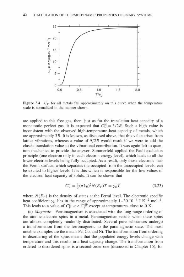
42 CALCULATION OF THERMODYNAMIC PROPERTIES OF UNARY SYSTEMS
0.0 0.5 1.0 1.5 2.0
25
20
15
10
5
0
T /qD
CV
(Deb
ye)(
JK−1
mol
−1)
Figure 3.4 CV for all metals fall approximately on this curve when the temperaturescale is normalized in the manner shown.
are applied to this free gas, then, just as for the translation heat capacity of amonatomic perfect gas, it is expected that Cel
V = 3/2R. Such a high value isinconsistent with the observed high-temperature heat capacity of metals, whichare approximately 3R. It is known, as discussed above, that this value arises fromlattice vibrations, whereas a value of 9/2R would result if we were to add theclassic translation value to the vibrational contribution. It was again left to quan-tum mechanics to provide the answer. Sommerfeld applied the Pauli exclusionprinciple (one electron only in each electron energy level), which leads to all thelower electron levels being fully occupied. As a result, only those electrons nearthe Fermi surface, which separates the occupied from the unoccupied levels, canbe excited to higher levels. It is this which is responsible for the low values ofthe electron heat capacity of solids. It can be shown that
CelV = 1
3 (πkB)2N(EF )T = γelT (3.23)
where N(EF ) is the density of states at the Fermi level. The electronic specificheat coefficient γel lies in the range of approximately 1–30.10−4 J K−2 mol−1.This leads to a value of Cel
V << CvibV except at temperatures close to 0 K.
(c) Magnetic Ferromagnetism is associated with the long-range ordering ofthe atomic electron spins in a metal. Paramagnetism results when these spinsare almost completely randomly distributed. Several pure substances undergoa transformation from the ferromagnetic to the paramagnetic state. The mostnotable examples are the metals Fe, Co, and Ni. The transformation from orderingto disordering of the spins means that the populated energy levels change withtemperature and this results in a heat capacity change. The transformation fromordered to disordered spins is a second-order one (discussed in Chapter 15), for

THE THERMODYNAMIC PROPERTIES OF A PURE SOLID 43
00
10
20
30
40
200 400 600 800 1000
T (K)
C° p
(JK
−1 m
ol−1
)
Figure 3.5 Heat capacity for Ni, showing a cusp associated with magnetic contribution.
which the heat capacity–temperature curve shows a characteristic cusp like thatshown for Ni in Figure 3.5. The temperature where there is a sudden drop in Cp
is known as the Curie temperature.Note that some substances are anti-ferromagnetic, where the low-temperature
ordered state consists of the spins being antiparallel, so that there is no netmagnetic moment in the fully ordered state (the spin alignment can be observedin neutron-scattering experiments). The transition to the disordered paramagneticstate occurs at the Neel temperature.
3.4 THE THERMODYNAMIC PROPERTIES OF A PURE SOLID
In the above discussion we have concentrated principally on the heat capacities ofa pure solid. We now wish to concentrate on the other thermodynamic propertiesof a simple pure solid. In order to do so, we will consider the simplest possiblemodel in some detail in order to illustrate the approach. The model has beenchosen to simplify the mathematics without making the physics unrealistic:
(i) Only vibrational excitations are considered and we assume that these canbe represented by the Debye model. The Debye temperature is assumedto be independent of both temperature and volume.
(ii) The thermal expansivity and compressibility are assumed to be indepen-dent of temperature and volume.
The volume coefficient of expansion, α, and the isothermal compressibility,κT , are defined as
α = 1
Vm
(∂Vm
∂T
)p
κT = − 1
Vm
(∂Vm
∂p
)T
(3.24)

44 CALCULATION OF THERMODYNAMIC PROPERTIES OF UNARY SYSTEMS
If we consider a differential volume change as a function of pressure and tem-perature,
dV =(
∂V
∂T
)p
dT +(
∂V
∂p
)T
dp
By introducing our model approximations into this equation, we obtain
dV = V 00 (α dT − κT dp) (3.25)
which, on integration, gives the following simple EOS for our solid:
V = V 00 (1 + αT + κT p) (3.26)
= V 0T κT p (3.27)
where V 00 is the volume at zero temperature and zero pressure and V 0
T is thevolume at temperature T and zero pressure.
We may use Maxwell relations in order to obtain the volume derivatives of thethermodynamic properties from the EOS. The following table shows the generalMaxwell relations, applicable to any EOS, and also the specific values for theEOS being used:
Derivative General Specific(∂U
∂V
)T
T
(∂p
∂T
)V
− pαT
κT
− p(∂S
∂V
)T
(∂p
∂T
)V
α
κT(∂A
∂V
)T
−p V 0T
We may now use these relations to obtain the static (abbreviation stat) con-tributions to the thermodynamic properties:
Ustat(V, T ) − U◦(V 0
T ) = αT
κT
∫ V
V 0dV −
∫ V
V 0p dV (3.28)
= αT
κT
(V − V 0T ) +
∫ V
V 0
V − V 0T
κT V 00
dV (3.29)
= αT
κT
(V − V 0T ) +
12 (V − V 0
T )2
κT V 00
(3.30)
Sstat(V, T ) − S◦(V 0
T ) = α
κT
∫ V
V 0T
dV (3.31)
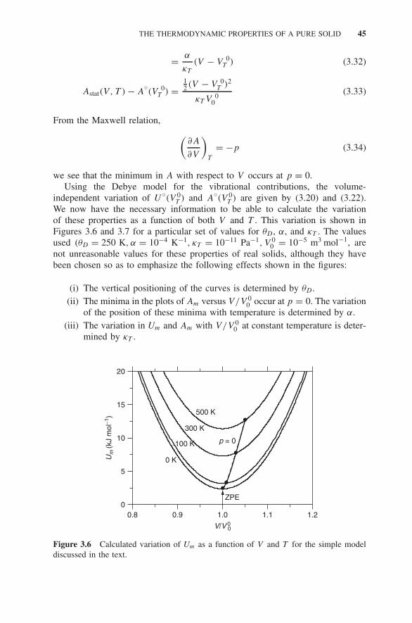
THE THERMODYNAMIC PROPERTIES OF A PURE SOLID 45
= α
κT
(V − V 0T ) (3.32)
Astat(V, T ) − A◦(V 0
T ) =12 (V − V 0
T )2
κT V 00
(3.33)
From the Maxwell relation, (∂A
∂V
)T
= −p (3.34)
we see that the minimum in A with respect to V occurs at p = 0.Using the Debye model for the vibrational contributions, the volume-
independent variation of U◦(V 0
T ) and A◦(V 0
T ) are given by (3.20) and (3.22).We now have the necessary information to be able to calculate the variationof these properties as a function of both V and T . This variation is shown inFigures 3.6 and 3.7 for a particular set of values for θD , α, and κT . The valuesused (θD = 250 K, α = 10−4 K−1, κT = 10−11 Pa−1, V 0
0 = 10−5 m3 mol−1, arenot unreasonable values for these properties of real solids, although they havebeen chosen so as to emphasize the following effects shown in the figures:
(i) The vertical positioning of the curves is determined by θD .(ii) The minima in the plots of Am versus V/V 0
0 occur at p = 0. The variationof the position of these minima with temperature is determined by α.
(iii) The variation in Um and Am with V/V 00 at constant temperature is deter-
mined by κT .
500 K
300 K
100 K
0 K
ZPE
p = 0
0.80
5
Um
(kJ
mol
−1)
10
15
20
0.9 1.0
V/V 00
1.1 1.2
Figure 3.6 Calculated variation of Um as a function of V and T for the simple modeldiscussed in the text.
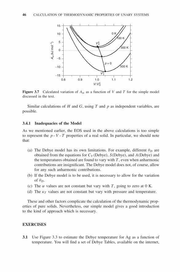
46 CALCULATION OF THERMODYNAMIC PROPERTIES OF UNARY SYSTEMS
500 K
300 K
100 K
0 K
p = 0
0.8
0
5
−5Am
(kJ
mol
−1)
10
−10
15
−150.9 1.0
V /V 00
V 0T
V 00
1.1 1.2
Figure 3.7 Calculated variation of Am as a function of V and T for the simple modeldiscussed in the text.
Similar calculations of H and G, using T and p as independent variables, arepossible.
3.4.1 Inadequacies of the Model
As we mentioned earlier, the EOS used in the above calculations is too simpleto represent the p–V –T properties of a real solid. In particular, we should notethat:
(a) The Debye model has its own limitations. For example, different θD areobtained from the equations for CV (Debye), S(Debye), and A(Debye) andthe temperatures obtained are found to vary with T , even when anharmoniccontributions are insignificant. The Debye model does not, of course, allowfor any such anharmonic contributions.
(b) If the Debye model is to be used, it is necessary to allow for the variationof θD .
(c) The α values are not constant but vary with T , going to zero at 0 K.(d) The κT values are not constant but vary with pressure and temperature.
These and other factors complicate the calculation of the thermodynamic prop-erties of pure solids. Nevertheless, our simple model gives a good introductionto the kind of approach which is necessary.
EXERCISES
3.1 Use Figure 3.3 to estimate the Debye temperature for Ag as a function oftemperature. You will find a set of Debye Tables, available on the internet,
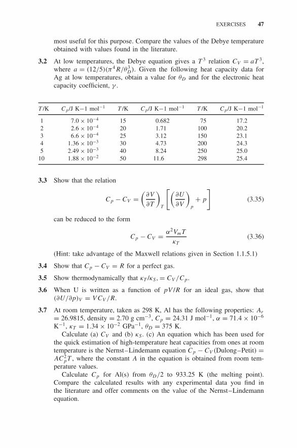
EXERCISES 47
most useful for this purpose. Compare the values of the Debye temperatureobtained with values found in the literature.
3.2 At low temperatures, the Debye equation gives a T 3 relation CV = aT 3,where a = (12/5)(π4R/θ3
D). Given the following heat capacity data forAg at low temperatures, obtain a value for θD and for the electronic heatcapacity coefficient, γ .
T /K Cp/J K−1 mol−1 T /K Cp/J K−1 mol−1 T /K Cp/J K−1 mol−1
1 7.0 × 10⁻⁴ 15 0.682 75 17.22 2.6 × 10⁻⁴ 20 1.71 100 20.23 6.6 × 10⁻⁴ 25 3.12 150 23.14 1.36 × 10⁻³ 30 4.73 200 24.35 2.49 × 10⁻³ 40 8.24 250 25.0
10 1.88 × 10⁻² 50 11.6 298 25.4
3.3 Show that the relation
Cp − CV =(
∂V
∂T
)T
[(∂U
∂V
)p
+ p
](3.35)
can be reduced to the form
Cp − CV = α2VmT
κT
(3.36)
(Hint: take advantage of the Maxwell relations given in Section 1.1.5.1)
3.4 Show that Cp − CV = R for a perfect gas.
3.5 Show thermodynamically that κT /κS,= CV /Cp .
3.6 When U is written as a function of pV /R for an ideal gas, show that(∂U/∂p)V = V CV /R.
3.7 At room temperature, taken as 298 K, Al has the following properties: Ar
= 26.9815, density = 2.70 g cm−3, Cp = 24.31 J mol−1, α = 71.4 × 10⁻⁶
K−1, κT = 1.34 × 10⁻² GPa−1, θD = 375 K.Calculate (a) CV and (b) κS . (c) An equation which has been used for
the quick estimation of high-temperature heat capacities from ones at roomtemperature is the Nernst–Lindemann equation Cp − CV (Dulong–Petit) =AC2
pT , where the constant A in the equation is obtained from room tem-perature values.
Calculate Cp for Al(s) from θD/2 to 933.25 K (the melting point).Compare the calculated results with any experimental data you find inthe literature and offer comments on the value of the Nernst–Lindemannequation.


4 Phase Equilibria in UnarySystems
The calculation of phase diagrams provides an excellent illustration of the wayin which thermodynamics permits one set of properties to be calculated from anapparently completely different set of properties.
For the moment we are concentrating on unary (one-component, pure sub-stance) systems. As we will see, however, many of the features which areencountered in binary phase diagrams have their counterpart in unary phasediagrams.
In the absence of external fields (e.g., magnetic), the state of a one-componentsystem is uniquely specified by two variables (see Section 2.3). Differentchoices of these variables are possible and give different possibilities for atwo-dimensional representation of the system’s phase behavior (phase diagrams).We have mentioned previously that the intensive thermodynamic variables canbe divided into two categories: field variables and density variables. A fieldvariable, for example, T , takes on identical values in any coexisting phases atequilibrium, while a density variable, for example, Vm, does not.
Figure 4.1 shows examples of the only possible different types of two–dimensional phase diagrams for a unary system:
(A) Field–Field Type The p−T (field–field) phase diagram (Fig. 4.1a)shows single-phase areas, two-phase coexistence lines, a triple point, anda critical point . A two-phase line indicates where two coexisting phaseshave the same temperature and pressure. Similarly, at the triple point , thecoexisting gas, liquid, and solid phases have exactly the same tempera-ture and pressure. At the critical point the liquid and gas phases becomeindistinguishable.
(B) Field–Density Type In the p−Sm (field–density) representation(Fig. 4.1b) there are single-phase areas as in a field–field diagram. Buttwo-phase coexistence is now indicated by areas, and the triple pointhas become a horizontal triple line. The horizontal tie-lines in, say,the gas–liquid coexistence region indicate that any coexisting gas andliquid must have the same pressure (the field variable), but they havedifferent Sm (the density variable). A similar interpretation holds for the
Materials Thermodynamics. By Y. Austin Chang and W. Alan OatesCopyright 2010 John Wiley & Sons, Inc.
49

50 PHASE EQUILIBRIA IN UNARY SYSTEMS
p p
s s
s
l + g
s + g
s + g
s + l + g
l + g
s+ l
g
T Sm
Sm
Vm
s+gl
l
l
(a) (b)
(c)
g
g
Figure 4.1 Different types of phase diagram for one-component system: (a) field–field;(b) field–density; (c) density–density.
gas, liquid, and solid coexisting along the triple line—equality of p butdifferent Sm.
(C) Density–Density Type In the Vm –Sm representation shown inFigure 4.1c, we have two-phase regions with oblique tie-lines anda triple triangle. The sloping tie-lines in the gas–liquid region, forexample, tell us that any coexisting gas and liquid have different Vm aswell as different Sm (although they still have the same p and T ). Theusual lever rule applies to the determination of the relative amounts ofany coexisting phases along one of these sloping tie-lines. Any point inthe triple triangle represents a system with coexisting gas, liquid, andsolid phases, which differ from each other in both Vm and Sm. The leverrule can also be applied in this three-phase region for the determinationof the relative volume amounts of the three phases.
When the solid phase has more than one crystal structure (polymorphism orallotropy), then unary phase diagrams can become more complex. A p−T phasediagram for pure Fe is shown in Figure 4.2. At p → 0 we see the usual trans-formations bcc → fcc → bcc → liquid as the temperature is increased, but athigh p it can be seen that the pattern of transformations is quite different.
A plot of one thermodynamic function against another does not always giverise to a true phase diagram, defined as one where any point on the diagram gives

PHASE EQUILIBRIA IN UNARY SYSTEMS 51
00
50 bcc
bcc
liq
hcp
fcc
100
150
200
250
500 1000 1500
T (K)
p (k
bars
)
2000 2500
Figure 4.2 p−T phase diagram for Fe.
a unique answer concerning the existence of individual phases and combinationsof phases. The ones shown in Figure 4.1 are true phase diagrams, but somediagrams which show the range of existence of phases and their combinationsare not. This is illustrated in Figures 4.3a and 4.3b. Although these diagrams arefield–density diagrams and the topography of Figure 4.3a is similar to that forthe plot of p versus Sm shown in Figure 4.3b, it is not a true phase diagram. Thisis apparent from Figure 4.3b, which shows a similar p-versus-Vm diagram butwhere the molar volume of the solid is greater than that of the liquid. Water andbismuth are common examples of materials which fall into this latter category.It is clear that in the neighborhood of the black dot the system’s properties arenot uniquely defined.
Plotting conjugate variables , for example, p versus Vm, is the source of theproblem. Any plot of a property versus its conjugate property does not give atrue phase diagram. We will meet this again when discussing binary systems (see
p
Vm
g
s + g
l + g
l s
l+s
p
High T
Vm
g
s + g
l + gs
ls+l
Figure 4.3 Plots of conjugate variables are not true phase diagrams: (a) appears to be atrue phase diagram when Vm(l) >Vm(s); (b) clearly not a true phase when Vm(s) >Vm(l).

52 PHASE EQUILIBRIA IN UNARY SYSTEMS
Chapter 8). Suffice to mention here that the definition of conjugate variables issomewhat broader than encountered previously. For example, it is possible torewrite the fundamental equation as
dSm = 1
TdUm + p
TdVm (4.1)
In this case, p/T and Vm are seen to be conjugate variables so that a plot ofthese quantities will not give a true phase diagram.
An interesting feature arises for properties in the liquid–gas region. It is foundthat, if the p−V −T variables are expressed relative to the values at the criticalpoint for that particular substance, that is, as reduced variables
pr = p
pc
Vr = V
Vc
Tr = T
Tc
ρr = ρ
ρc
(4.2)
then the liquid–vapor coexistence curves plotted in terms of these reduced vari-ables approximately coincide for simple molecules. These are examples of theapplication of the law of corresponding states , which can be useful in the estima-tion of the properties for substances where only limited information is available.
4.1 THE THERMODYNAMIC CONDITION FOR PHASEEQUILIBRIUM
Since we are usually interested in phase equilibrium at constant total pressureptotal and T , the following derivation is based on using the Gibbs energy, whosenatural variables are p and T .
Consider two phases, liquid and gas, to be in open contact as illustrated inFigure 4.4. Matter can be transferred between the phases at constant ptotal andT , although the two-phase system is considered closed.
The Gibbs energy of the whole system, comprising the two phases, is then
Gtotal = Gliq + Ggas (4.3)
and we wish to find the minimum in this total Gibbs energy, which we canwrite as
Gtotal = nlAμl
A + ngAμ
gA (4.4)
There is, however, a constraint on this minimization, since the complete liquid/gassystem is closed and the total amount of a is fixed, ntotal
A = nlA + n
gA.
Constrained minimization problems like this are conveniently handled usingLagrangian multipliers (see Appendix B for an introduction). In this case, onlyone λ is required:
λ : nA(total) − nlA − n
gA = 0 (4.5)

THE THERMODYNAMIC CONDITION FOR PHASE EQUILIBRIUM 53
Gas
Liquid
A
pA
pinert
ptotal
Figure 4.4 Phase equilibrium between pure liquid A and a gas phase comprising A andan inert gas. Both gas and liquid are maintained at the same total pressure ptotal.
and the Lagrangian function L to be minimized becomes
L = G + λ(nA − nlA − n
gA) (4.6)
= nlAμl
A + ngAμ
gA + λ(nA − nl
A − ngA) (4.7)
Partial differentiation with respect to nlA and n
gA gives the minimum in L:
∂L∂nl
A
= μlA − λ = 0 (4.8)
∂L∂n
gA
= μgA − λ = 0 (4.9)
Elimination of the Lagrangian multiplier leads to the condition for the constrainedminimum in G, that is, the condition of equilibrium:
μlA = μ
gA (4.10)
As is apparent from (4.8) and (4.9), the physical meaning of the Lagrangianmultiplier used for the mass balance constraint, λ, is seen to be that of thechemical potential.
For either of the single phases we can write
G(A) = nAμA (4.11)
or
μA = G(A)
nA
= Gm(A) (4.12)
54 PHASE EQUILIBRIA IN UNARY SYSTEMS
that is, for a unary system, we may also write the phase equilibrium condition as
Gm
(Al, p, T
) = Gm
(Ag, p, T
)(4.13)
Equations (4.10) and (4.13) appear to be equivalent ways of expressing thecondition of phase equilibrium. There is, however, an important differencebetween these two equations. Equation (4.10) is still obtained if we start withdifferent fixed external conditions; for example, at constant S and V and weused the fundamental equation for U , whereas (4.13) applies only at constantp and T .
The conditions for two bulk phases of a pure substance to be in equilibriumthen are:
(i) Their temperatures must be equal so that there is no heat flow between thetwo phases.
(ii) Their total pressures must be equal so that there is no bulk material flowbetween the two phases.
(iii) The chemical potentials of the substance must be equal in the two phasesso that there is no mass (diffusive) flow between the two phases.
As will become apparent later, this last criterion, as well as the usual equalityof p and T , holds in much more complex situations than those being discussedhere.
It is very important to appreciate that this equilibrium condition for masstransfer, (4.10), is a necessary but not sufficient condition for evaluating the globalequilibrium in a system. The condition (4.10) alone can only be used when thetwo phases are actually specified beforehand, for example, Al and Ag. These,however, may not be the global equilibrium ones for the specified conditions.For example, in Figure 4.4, the equilibrium condensed phase might be solid arather than liquid a under the specified p and T . At this total p and T , we canuse (4.10) to evaluate pA in the gas phase for equilibrium with either liquid orsolid a . Under the particular conditions chosen, only one of them would representthe global equilibrium. The other would represent a metastable equilibrium. It isnecessary to check, using (4.4), which of the two equilibria has the lower Gibbsenergy in order to decide which is the global equilibrium and which is a local,metastable, equilibrium.
4.2 PHASE CHANGES
4.2.1 The Slopes of Boundaries in Phase Diagrams
Consider a p−T plot for a pure substance like that shown in Figure 4.1a . Animportant relation for the slopes of the two-phase equilibrium lines on such adiagram can be derived in the following way.

PHASE CHANGES 55
At any point along the line for solid–liquid equilibrium
G(s) = Gl (4.14)
Since this applies for all points along the two-phase equilibrium curve, then forany displacement from a particular point along the curve for two-phase equilib-rium
� [G(l) − G(s)] = 0 (4.15)
For one of the phases, the total differential for G as a function of p and T is
dG =(
∂G
∂p
)T
dp +(
∂G
∂T
)p
dT (4.16)
Repeating for the other phase and substituting into (4.15) and rearranging givethe slope of the pressure–temperature phase equilibrium curve:
dp
dT= −�
[(∂G/∂T )p
]�[(∂G/∂p)T
]= �S
�V(4.17)
and since �G = 0 along the two-phase equilibrium, �H = T �S. Hence, wemay rewrite (4.17) as
dp
dT= �H
T �V(4.18)
This last equation is known as the Clausius–Clapeyron equation. From it,we can predict the slope of a p−T phase boundary from the enthalpy andvolume change associated with the phase transformation. Alternatively, theinverse of (4.18) can be used to obtain the variation of �fusH
∗m as a function of
pressure from measurements of the pressure change of the melting point andvolume. These represent good examples of using thermodynamic relations forpredicting one property of a substance from properties which might be easierto measure.
It is found experimentally that, while �fusV∗m and Tfus change markedly with
pressure, the change in �fusH∗m is small, that is,
�fusH∗m ≈ �fusH
◦m (4.19)
A special case of the Clausius–Clapeyron equation, which involves usingapproximations , arises in its application to gas/condensed-phase equilibriumat low pressures. Assuming the gas is perfect (first approximation) and that

56 PHASE EQUILIBRIA IN UNARY SYSTEMS
Vm(l) � Vgm (second approximation), then almost all the volume change occurs
in the gas phase and is given by
�vapV ≈ RT
p(4.20)
giving
d loge p
dT≈ �vapH
RT 2(liquid (or solid), perfect gas only) (4.21)
which is known as the Clapeyron equation.Another aspect of the slopes of phase boundaries which is apparent in
field–field phase diagrams is concerned with how two-phase equilibrium curvesextend through three-phase equilibrium points (see Fig. 4.5a).
Consider the solid–liquid–gas equilibrium shown in the sketch. Using theClausius–Clapeyron equation, with superscripts to indicate which two-phaseequilibrium is being considered, we see that
(dp
dT
)s−g
= �gs H
T �gs V
= �gl H + �l
sH
T �gs V
(4.22)
= �gl V
�gsV
(dp
dT
)l−g
+ �lsV
�gs V
(dp
dT
)s−l
(4.23)
= (1 − vf )
(dp
dT
)l−g
+ vf
(dp
dT
)s−l
(4.24)
where vf is the volume fraction of the total s–g volume change which is due tothe s–l volume change.
It follows from (4.24) that the slope of the s–g curve must lie between thatof the s–l and l–g curves; that is, the extension of all three curves through
p
T
s l
g
(b)(a)
p
T
s l
g
Figure 4.5 Extensions of phase boundaries in field–field phase diagrams: (a) correct;(b) impossible.

PHASE CHANGES 57
the triple point is into the opposite single-phase region. This phase boundaryextension requirement is known as Schreinemaker’s rule.
An impossible extension is shown in Figure 4.5b.The equivalent requirement of Schreinemaker’s rule in field–density and
density–density phase diagrams such as those shown in Figures 4.1b and 4.1cis that the phase boundaries must always extend into the two-phase regions onthe opposite side of the invariant point. Some published phase diagrams indicatethat this thermodynamic requirement has not always been complied with byexperimentalists.
4.2.2 Gibbs Energy Changes for Phase Transformations
The magnitudes of the Gibbs energies for any phase change in pure substancesis of paramount importance. We will meet these quantities frequently in theapplication of thermodynamics to the calculation of binary phase diagrams (seeChapters 8 to 12).
At the equilibrium transition temperature for a pure substance at constantpressure
�trG∗m(T ∗
tr ) = 0 (4.25)
and so
�trS∗m(T ∗
tr ) = �trH∗m(T ∗
tr )
T ∗tr
(4.26)
It can be seen from the sketches in Figure 4.6, which apply for standardconditions, that �trG
∗m �= 0 at temperatures away from the equilibrium transition
temperature.
H°
S°
G°
T
T
T
ΔtrH°
ΔtrS°
ΔtrG°= 0
Figure 4.6 Variation of enthalpy, entropy, and Gibbs energy differences in neighborhoodof first-order phase transformation.

58 PHASE EQUILIBRIA IN UNARY SYSTEMS
A linear approximation for �trG◦, which is equivalent to assuming that �H
◦
and �S◦ are temperature independent, is also very useful and much used:
�trG◦(T ) = �trH
◦(T ) − T �trS
◦(T ) (4.27)
0 = �trH◦(T
◦tr ) − T
◦tr �trS
◦(T
◦tr ) (4.28)
These two equations always hold, but if we now assume that �trH◦(T ) ≈
�trH◦(T
◦tr ) and �trS
◦(T ) ≈ �trS
◦(T
◦tr ), then a useful approximation is obtained:
�trG◦(T ) ≈ (T
◦tr ) − T )�trS
◦ ≈ (T◦
tr ) − T
T◦
tr�trH
◦(T
◦tr ) (4.29)
Some useful approximations for the magnitudes of �trS◦(Ttr) and �trH
◦(Ttr)
for various types of phase transformation in pure substances are summarizedbelow. Approximations like these are useful when it is necessary, due to theabsence of experimental data, to estimate properties.
(A) Evaporation Since S◦,g � S
◦,l, then it follows that �vapS◦ ≈ S
◦,g andsince all monatomic gases have approximately the same entropy (seeChapter 3), it comes as no surprise that �vapS
◦m is approximately constant
for all metals (very few metals have significant amounts of molecularspecies in their vapors). This is the basis of Trouton’s rule:
�vapS◦m ≈ 84 J mol−1 K−1 (4.30)
If the transformation temperature is 1000 K, we see that �vapH◦m is esti-
mated to be ≈ 84 kJ mol−1, which is quite a large value.(B) Fusion Since S
◦,l ≈ S◦,s, then it is not to be expected that there is
a similar constancy in �fusS◦m. Nevertheless, for metals, Richard’s rule
works quite well:
�fusS◦m ≈ 9 J mol−1 K−1 (4.31)
which, if the transition temperature is 1000 K, gives �fusH◦m ≈ 9 kJ
mol−1, much smaller than for vaporization.Semiconductors and inorganic compounds can have much larger valuesfor �fusS
◦m than for metals, so that Richard’s rule should not be used in
estimating this quantity for these materials.(C) Allotropic Transformations The enthalpies for the transformation
between different polymorphic forms of both elements and compoundsare important in the calculation of phase diagrams. These enthalpiesare often referred to as the relative lattice stabilities . Some examplesare shown in Figure 4.7. It can be seen that, at the beginning of a

STABILITY AND CRITICAL PHENOMENA 59
Group number
−8
−6
−4
−2
0
2
4
6
8
10
4B 5B 6B 7B 8 8 8 1B 2B
Δhcp H
° m(k
J m
ol−1
)bc
c
Figure 4.7 Relative lattice stability for some transition metals shown as the differencein the standard enthalpies between the bcc and hcp structures.
transition period, the hexagonal close-packed (hcp) structure is morestable than the bcc structure, but this trend is first reversed and thenrecovered towards the end of the period. Note that the values of �trH
◦m
for solid/solid transformations are generally smaller than for fusion.
4.3 STABILITY AND CRITICAL PHENOMENA
In Chapter 2 we considered some basic EOS for gases and condensed phases.It is apparent from Figure 4.1, however, that the gas and liquid phases becomeindistinguishable at the critical point. As a result, there has been a desire todevelop EOS which apply throughout the whole p−V −T gas/liquid region,so that even isotherms both above and below the critical temperature can berepresented analytically.
Figure 4.8 shows a p−V diagram which includes two isotherms, one aboveand one below the critical temperature. Van der Waals first proposed an EOSwhich, although it has several shortcomings from a theoretical and practicalstandpoint, illustrates how both these super- and subcritical isotherms can berepresented by one equation. The van der Waals equation is
p = RT
Vm − b− a
V 2m
(4.32)
where a and b are parameters. The first term on the right-hand side is due tothe attraction between the molecules and the second term accounts for repulsionforces between them. Being an analytical equation, it can be plotted for any

60 PHASE EQUILIBRIA IN UNARY SYSTEMS
VB
B ′
C
ND
L
MA
V
p
Figure 4.8 A loop in a subcritical isotherm when the van der Waals EOS is used.Source: I. Prigogine and R. Defay, Chemical Thermodynamics , Longman, 1954.
values of the parameters and variables. At a temperature below the critical, then,as can be seen in Figure 4.8, the shape of the isotherm is quite different fromthose found above the critical temperature. At very high temperatures, the vander Waals EOS gives isotherms which approach those for the perfect gas, whilebelow Tc they show the so-called van der Waals loop.
The various parts of the continuous curve AVNMLD on the subcritical isothermhave distinct physical significances. It can be seen that for the part between N
and M
(∂p
∂V
)T
> 0 (4.33)
which means that such states are mechanically unstable (the volume mustdecrease with increase of pressure) and therefore not realizable in practice; thatis, any point between N and M is unstable. The calculated isotherms have nophysical meaning here and are just the result of an analytical representationwhich gives a continuous curve at all p and Vm. The loci of the points M and N ,where
(∂p
∂V
)T
= 0
at different temperatures gives the region marked unstable in Figure 4.9. Thecurve which separates the unstable region from the metastable region is calledthe spinodal curve. The portion of the curve marked V N in Figure 4.8 represents
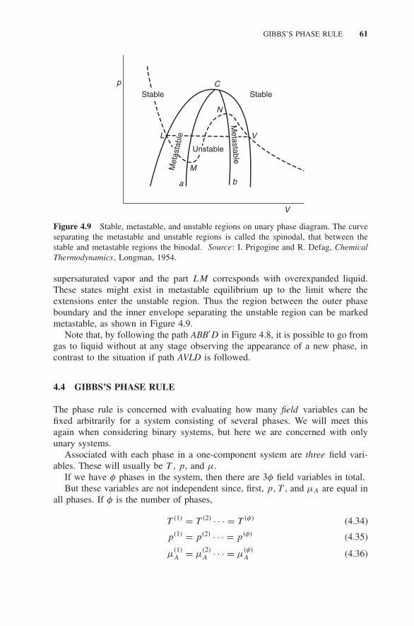
GIBBS’S PHASE RULE 61
Unstable
Stable
V
M
a b
N
C
L
p
V
Stable
Metastable
Met
asta
ble
Figure 4.9 Stable, metastable, and unstable regions on unary phase diagram. The curveseparating the metastable and unstable regions is called the spinodal, that between thestable and metastable regions the binodal. Source: I. Prigogine and R. Defag, ChemicalThermodynamics , Longman, 1954.
supersaturated vapor and the part LM corresponds with overexpanded liquid.These states might exist in metastable equilibrium up to the limit where theextensions enter the unstable region. Thus the region between the outer phaseboundary and the inner envelope separating the unstable region can be markedmetastable, as shown in Figure 4.9.
Note that, by following the path ABB′D in Figure 4.8, it is possible to go fromgas to liquid without at any stage observing the appearance of a new phase, incontrast to the situation if path AVLD is followed.
4.4 GIBBS’S PHASE RULE
The phase rule is concerned with evaluating how many field variables can befixed arbitrarily for a system consisting of several phases. We will meet thisagain when considering binary systems, but here we are concerned with onlyunary systems.
Associated with each phase in a one-component system are three field vari-ables. These will usually be T , p, and μ.
If we have φ phases in the system, then there are 3φ field variables in total.But these variables are not independent since, first, p, T , and μA are equal in
all phases. If φ is the number of phases,
T (1) = T (2) · · · = T (φ) (4.34)
p(1) = p(2) · · · = p(φ) (4.35)
μ(1)A = μ
(2)A · · · = μ
(φ)
A (4.36)

62 PHASE EQUILIBRIA IN UNARY SYSTEMS
Second, we have a Gibbs–Duhem relation between the three field variables foreach phase:
0 = −S dT + V dp + nA dμA
so that there are 3(φ − 1) − φ constraints placed on the total number of fieldvariables.
The number of independent variables or, as it is more usually called in ther-modynamics, the number of degrees of freedom F is, therefore
F = 3φ − 3(φ − 1) − φ = 3 − φ (4.37)
which is the usual way of writing Gibbs’s phase rule for one-component systems.Figure 4.10 Illustrates the number of degrees of freedom for one-, two-, andthree-phase equilibrium in a unary system.
In words, the rule states that the existence of a single phase requires thespecification of two field variables (it has two degrees of freedom; the system isbivariant), the third field variable being fixed through the Gibbs–Duhem equation;when two phases coexist, specification of one field variable automatically fixesthe other (there is one degree of freedom; the system is univariant); if threephases coexist in equilibrium the values of all the field variables are fixed (zerodegrees of freedom; the system is invariant). Under no circumstances can fourphases of a one-component system coexist in equilibrium.
It is interesting to note that the phase rule may not appear to apply at thecritical point where there is also only a single phase present but where F =0 rather than 2, as suggested by (4.37). The reason for this apparent break-down is that the constraints given in (4.37) are no longer applicable since thereis only one phase. Instead, some extra constraints are introduced. The samething arises in binary systems and will be discussed in detail when encounteredthere.
p
T
F = 2
F = 1
F = 0
I II
III
Figure 4.10 Number of degrees of freedom for one-, two-, and three-phase equilibriumin unary system.

EXERCISES 63
EXERCISES
4.1 The following linearized equations give the approximate standard Gibbsenergies of Zn in solid, liquid, and gaseous forms:
G◦g(Zn,SER, T ) = 137,000 − 182.2T J/mol
G◦s(Zn,SER, T ) = 4175 − 53.95T J/mol
G◦l(Zn,SER, T ) = 11,200 − 64.1T J/mol
Assume that the condensed-phase properties are independent of pressureand that the gas phase is perfect.
(a) Calculate the equilibrium vapor pressure in contact with both liquidand solid Zn at (i) 685 K and (ii) 700 K.
(b) Calculate which equilibrium has the lower G at these two tempera-tures.
(c) Does the stable state have a higher or lower vapor pressure than themetastable state?
(d) plot a T −μZn diagram which shows these results by plotting thecondensed-phase lines and vapor lines for fixed values of pZn.
(e) Is this field–field diagram a true phase diagram?
4.2 The following results were obtained for the melting point (mp) andthe volume change accompanying the melting of a solid at differentpressures:
p/MPa mp/◦C �fusV∗m/cm3 mol−1
0.1 97.6 2.787200.0 114.2 2.362400.0 129.8 2.072600.0 142.5 1.873800.0 154.8 1.711
1000.0 166.7 1.5561200.0 177.2 1.398
Evaluate �fusH∗ as a function of pressure and plot the ratios of
�fusV∗m/�fusV
◦m and �fusH
∗m/�fusH
◦m as a function of pressure. Do these
results support our MS&E assumption that �fusH∗m ≈ �fusH
◦m?
4.3 Derive (4.19) from (4.16).

64 PHASE EQUILIBRIA IN UNARY SYSTEMS
4.4 Sketch a complete schematic p−T phase diagram for Fe in the solid,liquid, and gaseous states. Use the information in Figures 4.1 and 4.2.
4.5 The vapor pressure of Sil is represented by the equation
log10 p (torr) = 10.78–20,900T −1 − 0.565 log T
Calculate its enthalpies of vaporization at 1700 and 1500 K (undercooledliquid).
4.6 The vapor pressure of a pure element such as Cu, Si, and Ni is oftenexpressed in either of the following equations:
loge p = A + B
Tor loge p = A′ + B ′
T+ C′ ln T
(a) Starting from the Clausius–Clapeyron equation, show under what ther-modynamic condition do these two equations given above apply?
(b) Take the vapor pressures of Si tabulated as a function of temperaturefrom a reference book such as the NIST-JANAF thermochemicaltables and obtain values of A and B as well as A′, B ′, and C′ in theabove two equations from 298.15 to their melting point. Compare thevalues calculated from either of these equations with the tabulatedvalues.
4.7 The densities of α-Fe(bcc) and γ -Fe(fcc) are 7.57 and 7.63 g cm−3, respec-tively, at 1184 K, 1 bar, when they are in equilibrium with each other.The enthalpies of transformation from α-Fe to γ -Fe are 900 J mol−1 atthe transition temperature 1184 K and 1660 J mol−1 at 1100 K. Calculatethe pressure under which both forms of Fe can coexist at 950 K. State theassumptions you make in order to carry out the calculation.
4.8 Starting from the equation dG = V dp − S dT, do a back-of-the-envelopecalculation to estimate the pressure needed to transform α-Fe(bcc) to acloser packed γ -Fe(fcc) at room temperature given the entropy of α-Fe(bcc) to be about 55 J K−1 mol−1 and density to be about 7.5 g cm−3.
4.9 The vapor pressure of liquid silver is given by
log10[p (bar)] = 8.83 − 14,400
T− 0.85 log10 T
How much heat is required to evaporate 0.11 mol of Ag at 2300 K? Thenormal boiling point of silver is 2436 K.
4.10 Calculate the partial pressure of zinc over liquid zinc at 600◦C using thethermodynamic data of Zn(l) and Zn(g) given below:

EXERCISES 65
800 K 900 K
gef(g)/J mol−1 K−1 168.35 169.94gef(l)/J mol−1 K−1 52.672 55.865
�subH◦(298 K) (kJ mol−1) = 130.42
where gef = −[G◦(T ) − H
◦(298 K)]/T .
4.11 Calculated �rG◦ for the reduction of SiO2(s) by Al(l) at 1200 K. Do you
think that pure Al will reduce SiO2 at this temperature?


5 Thermodynamics of BinarySolutions I: Basic Theory andApplication to Gas Mixtures
Gas mixtures are a familiar type of solution phase. While gas-phase solutionsare usually referred to as gas mixtures, this is not the case for condensed phases.There, the term mixture is usually used to refer to a mechanical mixture of thecomponents and the term solution when one component actually dissolves in theother.
Water and alcohol form a continuous series of liquid solutions; we say theyare completely miscible. Water and oil do not; they have no appreciable mutualsolubility ; they are nearly immiscible. Water and salt form a limited liquid solu-tion. On continuing the addition of the salt, the solution becomes saturated withthe solid phase.
Metals in the liquid and solid states also form solutions. In the latter casewe speak of solid solutions . Solid solutions are further distinguished as beingeither substitutional or interstitial . In substitutional solid solutions all the atomsare on the one lattice. Familiar examples are (Cu,Zn), (Cu,Sn), (Cu,Ni), (Si,Ge)alloys. In interstitial solid solutions the smaller atoms reside in the intersticesof the sublattice formed by the larger atoms. It is convenient to adopt the nota-tion (M):(I) to represent the occupation of the metal and interstitial sublattices.Familiar examples using this notation are (Fe):(C) and (Pd):(H).
5.1 EXPRESSING COMPOSITION
Three methods are commonly used:
(i) Mole fraction or percent(ii) Mass fraction or percent
(iii) Volume fraction or percent
Volume percent is the usual way of expressing the composition of gas mixtures.Because gas volumes change markedly with p and T , it is necessary to specify
Materials Thermodynamics. By Y. Austin Chang and W. Alan OatesCopyright 2010 John Wiley & Sons, Inc.
67
68 THERMODYNAMICS OF BINARY SOLUTIONS I
both. The most common way is to refer the volumes to STP (standard temperatureand pressure), that is, T = 273.15 K and p = 1 bar.
Mole and mass fractions or percents are the most commonly used ways ofexpressing the composition of condensed phases. The definitions of mole fractionand weight percent require that
∑i
xi = 1∑
i
wt % i = 100 (5.1)
Consider a liquid or substitutional solid solution such as (Cu,Zn). The term molefraction refers to 1 mol of alloy atoms, that is, to Cu1−xZnx , where the subscriptx refers to the mole fraction of Zn and 1 − x to the mole fraction of Cu:
xZn = nZn
nZn + nCu(5.2)
wt % Zn = mZn
mZn + mCu× 100 (5.3)
Conversion from one composition variable to the other is straightforward since
nZn = mZn
Ar,Zn(5.4)
For a solution of binary compounds such as FeO–MnO the mole fraction is
xMnO = nMnO
nMnO + nFeO(5.5)
and equivalently for the weight percent. Conversion between composition vari-ables in this case is obtained by using
nMnO = mMnO
Mr,MnO(5.6)
5.2 TOTAL (INTEGRAL) AND PARTIAL MOLAR QUANTITIES
The magnitudes of the extensive thermodynamic properties of a solution phaseare rarely found to be the composition-weighted average of the properties of thepure components, that is, that of the mechanical mixture. For example, for thevolume of a solution of water and alcohol:
100 ml water + 100 ml alcohol �= 200 ml of solution but ≈ 190 ml of solution
In this instance, there is a volume contraction (at the microscopic level, thereis strong attraction between the molecules of water and alcohol, resulting in areduction of the solution volume).

TOTAL (INTEGRAL) AND PARTIAL MOLAR QUANTITIES 69
Similar nonlinear behavior is found in all types of solutions for the otherextensive thermodynamic quantities, U , H , G, A, S, . . ..
Any extensive thermodynamic quantity Y , at constant p and T , is a functionof the amounts of substance of the components, A and B, that is,
Y |p,T = Y (nA, nB) (5.7)
and the differential quantity is given by
dY |p,T =∑
i
Yi dni (5.8)
where Yi is the partial derivative at constant p and T and nj is the amount ofsubstance of the other component(s):
Yi =(
∂Y
∂ni
)p,T ,nj
(5.9)
This last equation defines a partial molar quantity . Note that these partial deriva-tives are only referred to as partial molar quantities when the derivatives refer toconstant p and T .
Extensive thermodynamic functions are homogeneous functions of the firstdegree, that is,
kY (ni) = Y (kni) (5.10)
where k is a constant, and by Euler’s theorem for such functions, the integralquantity is related to the partial molar quantities by
Y =∑
i
niYi (5.11)
The difference between a total (or integral) property and a partial molar prop-erty is clear from the two experiments sketched in Figure 5.1. The sketch on theleft shows how the total or integral enthalpy of mixing �mixH for a liquid (A,B)alloy at a particular composition, A0.7B0.3(l), at constant temperature and pres-sure. The relative amounts of the pure components required to give the desiredcomposition are simply mixed. The sketch on the right shows how the partialmolar enthalpy of mixing of A, �HA, in a liquid alloy of the same composition,A0.7B0.3(l), and at the same temperature and pressure is measured. A very smallamount of component A is added to a relatively large amount of the alloy. Theresult from this experiment is independent of the size of the alloy bath as longas it is very large compared with the amount of A added.
Because of the relation between total (extensive) and partial molar quantities,Y = ∑
i niYi , we can see that all the relations previously met for the extensive

70 THERMODYNAMICS OF BINARY SOLUTIONS I
nA = 0.7 nB = 0.3
A0.7B0.3 A0.7B0.3
Totalor
integralΔmixH
oO
Pure A
Partialmolar
dnA
( )dHdnA nB
A B
Figure 5.1 Difference between total or integral thermodynamic property and partialmolar property. Both mixing processes are carried out at constant p and T .
properties of unary systems apply equally well to the partial molar quantities insolutions (remember that the partial molar quantities are only defined at constantp and T ). Some examples are
Gi = Hi − T Si (5.12)
Hi = Ui + pVi (5.13)
�mixGi = �mixHi − T �mixSi (5.14)(∂Gi
∂T
)p
= −Si (5.15)
(∂Gi
∂p
)T
= −Vi (5.16)
5.2.1 Relations between Partial and Integral Quantities
We will show how (5.9) and (5.11) can be used to derive some important relationsbetween partial and integral quantities.
The molar form of (5.8) can be obtained for a binary solution by dividing bynA + nB :
dYm = YA dxA + YB dxB (5.17)
and since xA + xB = 1, then dxA = −dxB , giving
dYm = (YB − YA) dxB (5.18)
or
dYm
dxB
= YB − YA (5.19)

TOTAL (INTEGRAL) AND PARTIAL MOLAR QUANTITIES 71
.
XB
Ym
Ym(x)
x
YA(x)
YB(x)
(1 − x) dYm(x)
dxB
0 1A B
Figure 5.2 Tangent–intercept relation between partial and integral molar quantities atconstant p and T .
Graphically, this means that, for a binary solution, the tangent slope at a pointon a plot of an integral molar quantity is equal to the difference in the partialmolar properties at that point.
Similarly, the molar form of (5.7) for a binary solution is given by
Ym = xAYA + xBYB = (1 − xB)YA + xBYB (5.20)
Combination of (5.19) and (5.20) yields equations from which the individualpartial molar quantities can be obtained from the integral molar quantity:
YA = Ym − xB
dYm
dxB
(5.21)
YB = Ym + (1 − xB)dYm
dxB
(5.22)
These equations also have a very simple graphical interpretation which is shownin Figure 5.2. The partial molar quantities are given by the intercepts on theordinate (property) axes of the tangent to the integral property curve at the com-position of interest.
Example 5.1 Calculation of Partial Molar from Integral Enthalpies of MixingThe enthalpy of mixing of Cu(l) with Sn(l) to form 1 mol of liquid Cu1−xSnx alloyas a function of composition at 1400 K (and p = 1 bar) is shown in Figure 5.3.The tangent shown refers to a composition xSn = 0.2. The two tangent interceptsat this composition are shown on the two ordinate axes. These two values for thepartial molar properties are then shown by dots in Figure 5.4 for this particularcomposition. The curves in the latter figure are obtained by repeating this pro-cedure at all compositions. The advantage of having an analytical representationof the integral property and then being able to do the necessary differentiationsanalytically is obvious. We will return to this point later.

72 THERMODYNAMICS OF BINARY SOLUTIONS I
−6
−4
−2
0
0 0.2 0.4 0.6 0.8 1Cu SnxSn
−8Δ m
ixH
/ kJ
mol
−1
ΔHCu ΔmixH
ΔHSn
Figure 5.3 �mixHm for liquid Cu1−xSnx alloys at 1400 K and 1 bar. The referencestates are Cu(l) and Sn(l).
−50
−40
−30
−20
−10
0
10
0 0.2 0.4 0.6 10.8Cu
Δ mixH
i / k
J m
ol−1
SnxSn
Cu
Sn
Figure 5.4 Partial molar enthalpies of mixing for liquid Cu1−xSnx alloys at 1400 K and1 bar. The reference states are Cu(l) and Sn(l).
5.2.2 Relation between Partial Quantities: the Gibbs–Duhem Equation
The fourth Gibbs equation for a solution phase is
dG = −S dT + V dp +∑
i
μi dni (5.23)
Since one of the independent variables, ni , is extensive, while the other two, p
and T , are independent of the size of the system, integration of this equationgives the equation
G =∑
i
niμi (5.24)
where the μi are functions of p and T .The result from this integration also follows from Euler’s equation for homo-
geneous functions of degree 1 (see Appendix B):

APPLICATION TO GAS MIXTURES 73
The total differential of (5.24) is
dG =∑
i
ni dμi +∑
i
μi dni (5.25)
Subtracting (5.23) from (5.24) gives
0 = −S dT + V dp +∑
i
ni dμi (5.26)
which is the Gibbs–Duhem equation for a solution phase.At constant p and T it becomes
0 =∑
i
ni dμi (5.27)
from which we see that the chemical potentials in a solution phase are not inde-pendent.
The molar form of (5.27) for a binary system is obtained by dividing bynA + nB and taking the derivative with respect to xB :
xA
(∂μA
∂xB
)p,T
+ xB
(∂μB
∂xB
)p,T
= 0 (5.28)
which, on integrating, gives∫dμB = −
∫1 − xB
xB
(∂μA
∂xB
)p,T
dxB (5.29)
We can see from this equation that, if the composition variation of one chemicalpotential is known in a binary solution for a given p and T , then the other chem-ical potential can be evaluated. This represents another example of using thermo-dynamics to avoid, in principle, having to carry out extraneous measurements.
The constant p and T version of the Gibbs–Duhem equation can be equallyapplied to the other partial molar properties of a solution:
0 =∑
i
ni dHi (5.30)
5.3 APPLICATION TO GAS MIXTURES
5.3.1 Partial Pressures
Pressure is a field quantity (see Chapter 4). In a gas mixture we wish to assign theseparate contributions of the components to the total pressure. Partial pressures

74 THERMODYNAMICS OF BINARY SOLUTIONS I
are defined to do just this; that is, their sum is equal to the total pressure:
pi = xip (5.31)
from which we see that the definition ensures that the sum of the partial pressuresequals the total pressure:∑
i
pi =∑
i
xip = p∑
i
xi = p (5.32)
Because it is a definition, this equation applies independently of whether thegas is perfect or not. Note that (5.31) is not , as is sometimes claimed, Dalton’sso-called law of partial pressures. Dalton found experimentally that the totalpressure of a gas mixture, in a constant-volume enclosure at constant T , wasapproximately equal to the sum of the pure component pressures in the sameenclosure: p ≈ ∑
i p∗i
5.3.2 Chemical Potentials in Perfect Gas Mixtures
We have already seen in (2.28) in Chapter 2 that, for a unary gas,
G∗m(T , p) − G
◦m(T , p
◦) = RT loge
(p∗
p◦
)perfect gas (5.33)
We can go through a derivation similar to that used for obtaining (5.33) for acomponent of a perfect gas mixture at constant T :
dGi |T = Vi dpi (5.34)
and for a perfect gas
dGi |T = RT
pi
dpi (5.35)
On integration this gives, with respect to the standard conditions,
Gi(T , p∗) − G◦i (T , p
◦i ) = RT loge
(pi
p◦i
)(5.36)
or, for any conditions,
μi(T , pi) − μ◦i (T ) = RT loge
(pi
p◦i
)componentperfect gas mixture
(5.37)
This equation is used very often in MS&E calculations, where it is usually safeto assume that gases are perfect. It gives us a recipe for calculating μi for acomponent of a gas mixture from observable quantities (gas analysis).

EXERCISES 75
5.3.3 Real Gas Mixtures: Component Fugacities and Activities
Defining the fugacity of a component in a mixture is similar to that already metwith in Chapter 2 for a pure gas—for a real gas we keep the same form as (5.37)in order to define the fugacity of a component:
μi(T , pi) − μ◦i (T ) = RT loge
(fi
f◦i
)real gas mixture (5.38)
where f◦i is the standard state fugacity of component i at p
◦i , T .
The activity of a component is defined as the ratio of its fugacity in the stateit happens to be in to its fugacity in the standard state:
ai = fi
f◦i
(5.39)
When the gas phase can be assumed perfect, then the activity of a componentcan be obtained from
ai = pi
p◦i
(5.40)
The relation between chemical potential and activity is given by
μi(T , pi) − μ◦i (T ) = RT loge ai (5.41)
and we see that the functions fugacity and activity are just alternative ways ofexpressing the chemical potential of a component in a gas mixture. The samefunctions are used for components of solid and liquid solutions.
EXERCISES
5.1 The integral enthalpy of mixing of liquid (Cu,Zn) solution can be approx-imated by the following equation using Cu(l) and Zn(l) as the referencestates: �mixHm = −19, 250xCuxZn J mol−1 at 1400 K.
(a) Derive the corresponding partial quantities of Cu and Zn, respectively.(b) Show the two partial equations are internally consistent with the
Gibbs–Duhem equation.(c) Plot the integral enthalpy values at 1400 K as a function of composition.
Draw a tangent at 50 mol% Zn and obtain the two partial quantitiesgraphically as shown in Figure 5.3.

76 THERMODYNAMICS OF BINARY SOLUTIONS I
(d) Plot the variation of the integral and partial quantities graphically andmake a comparison with the data shown in Figures 5.3 and 5.4. Pleasemake any comment you may have on the different behaviors betweenthe two alloy systems.
5.2 .(a) Calculate the enthalpy effect �H for dissolving 1 mol of solid nickelin 9 mol of liquid copper at 1473 K, assuming an ideal solution isformed. In other words, the enthalpy of mixing liquid (Cu,Ni) alloys isnegligibly small and can be taken to be zero. The enthalpies of meltingfor Ni and Cu are 17,470 J mol−1 at Tfus = 1726 K and 13,055 J mol−1
at Tfus = 1356.6 K.(b) Calculate the entropy change of the system and of the surroundings for
this process.
5.3 .(a) A stream of argon gas is passed in a closed system over a boat con-taining mercury at 273 K. The flow rate of the argon is slow enoughto allow this gas to become saturated with mercury vapor. The totalvolume of nitrogen used is 22 liters measured at 293.15 K and 1 bar.The argon was found to contain 0.0674 g of mercury. Calculate thevapor pressure of mercury at 273.15 K.
(b) The same experiment is carried out with a sodium amalgam (Na + Hg)in which the atomic fraction of sodium is 0.122; 22 liters of argon gassaturated with mercury is found to contain 0.0471 g of mercury. Takepure mercury as the reference state and calculate the chemical potentialof Hg relative to that of Hg(l), that is, μHg − μ
◦Hg.
5.4 Copper (Cu) and nickel (Ni) form a continuous series of solutions in boththe liquid- and solid state. The crystal structure of both solid elements isface-centered cubic.
The following experiments have been carried out to measure the enthalpyof solution of Cu(l, 1823 K, 1 bar) and that of Ni(l, 1823 K, 1 bar) in aliquid Cu0.6Ni0.4 alloy, also held at 1823 K, 1 bar.
Specifically a sample of 0.2 g of liquid Cu held at 1823 K, 1 bar, isdropped into a large bath of liquid Cu0.6Ni0.4 alloy (say, 1000 g) also heldat 1823 K and 1 bar. The enthalpy change measured is 6.14 J (endothermicor heat flow into system).
A similar experiment is also carried out by dropping 0.2 g of Ni heldat 1823 K and 1 bar into the same bath under identical conditions. Theenthalpy change measured is 14.96 J (also endothermic).
S◦,sm (298 K) 〈C◦,s
p 〉 〈C◦,lp 〉 T
◦fus �fusH
◦m(T
◦fus) Vapor
Element Ar /J K−1 mol−1 /J K−1 mol−1 /J K−1 mol−1 / K /J Pressure/bar
Cu 63.54 28.5 27.2 32.6 1356.6 13055.0 6.80 × 10⁻⁴
Ni 58.71 33.5 32.5 43.1 1726 17470.0 2.76 × 10⁻⁵

EXERCISES 77
Use these experimental data as well as any other thermodynamic data givenin the above table (note that you may not need all the data in the table) tocalculate the following (stating any assumptions you may have to make incarrying out some of the calculations):
(a) Relative partial molar enthalpy of Cu, �mixHCu(1823 K, 1 bar), inCu0.6Ni0.4
(b) Relative partial molar enthalpy of Ni, �mixHNi(1823 K, 1 bar), inCu0.6Ni0.4
(c) Integral molar enthalpy of mixing, �mixHm, for Cu0.6Ni0.4 (l, 1823 K,1 bar)
(d) Relative partial molar enthalpy of Cu at 1823 K and 1 bar but withrespect to Cu(s)
(e) Relative partial molar enthalpy of Cu at 1823 K and 1 bar but withrespect to the SER reference state
(f) Equilibrium partial pressures of Cu and Ni over the alloy Cu0.6Ni0.4 at1823 K. You may assume that �mixSm is the same as that for an idealsolution.


6 Thermodynamics of BinarySolutions II: Theory andExperimental Methods
6.1 IDEAL SOLUTIONS
Just as the perfect gas mixture provides a useful concept when discussing theproperties of a real gas mixture, it is similarly useful to define ideal solutionsfor condensed phases and then discuss the behavior of real solutions in terms oftheir deviation from the defined ideal behavior.
With gases, it was clear how to define a perfect gas—one whose EOS is givenby pV = nRT , which results when intermolecular interactions are negligible.Real gases at moderate pressures, and particularly at high temperatures, approachthis defined ideal behavior. In the case of liquid and solid solutions, however,we have the situation where the balance between attractive and repulsive forcesbetween the atoms or molecules is actually responsible for the stability of thecondensed phase, so that we cannot define a condensed-phase ideal solutionon the basis of zero atomic or molecular interactions. Such a definition is notnecessary, however, since we are only interested in property changes on mixingto form a solution and we might, therefore, define an ideal solution as one wherethere are negligible effects brought about by changes in the atomic or molecularinteractions on forming the solution. On the basis of this definition, we onlyexpect a real solution to approach this ideal behavior when the components arechemically identical. Mixtures or solutions of isotopes are, therefore, the mostlikely candidates for forming an ideal solution. An alloy of the chemically similarelements Ag and Au might be expected to approach ideal solution behavior whilechemically dissimilar elements like Al and Ti would not.
For a component i of a perfect gas mixture the chemical potential relative tothat for the pure component at pressure p∗
i is given by
μi(pi, T ) − μ∗i (p
∗i , T ) = RT loge
(pi
p∗i
)(6.1)
Materials Thermodynamics. By Y. Austin Chang and W. Alan OatesCopyright 2010 John Wiley & Sons, Inc.
79

80 THERMODYNAMICS OF BINARY SOLUTIONS II
and from the definition of partial pressure:
pi = xip∗i (6.2)
In such a perfect gas mixture we may write the chemical potential of the com-ponent i in terms of molar concentration as
μi(pi, T ) − μ∗i (p
∗i , T ) = RT loge
(xip
∗i
p∗i
)(6.3)
μi(pi, T ) − μ∗i (p
∗i (xi = 1), T ) = RT loge xi (6.4)
In liquid or solid solutions we are interested in solutions at, effectively, p = 1bar (in MS&E, the effect of pressure on condensed-phase properties is generallynegligible). Comparison with (6.3) leads to a plausible definition of an idealsolution for condensed phases:
μi(xi, T ) − μ∗i (xi = 1, T ) ≈ μi(xi, T ) − μ
◦i (xi = 1, T )
= RT loge xi (6.5)
which we will usually write as
�mixμidi = RT loge xi (6.6)
Recall that the subscript mix is used whenever the reference states for the purecomponents have the same structure as that of the phase of interest.
It should be made clear that an ideal solution could be defined differentlyfrom (6.6); the definition is in the hands of the thermodynamicist and is not anabsolute. The aim is to use a definition such that the properties of the definedideal solution are approached by real solutions.
Solutions conforming to the definition given in (6.6) are said to be Raoultianideal. But other definitions of ideal solutions, more appropriate for other typesof solution, are used. For the moment, it should be emphasized that we havedefined an ideal solution and not the ideal solution. This particular definition isuseful when discussing liquid metal alloys and solid substitutional alloys. For theremainder of this chapter, we will usually drop the prefix Raoultian and simplyuse the term ideal solution.
The following equations for �H idi , �Sid
i , and �V idi , at constant xi , for our
defined ideal solution are readily obtained:
�mixHidi = ∂(�μid
i /T )
∂(1/T )= ∂(R ln xi)
∂(1/T )= 0 (6.7)
�mixSidi = −∂ �μid
i
∂T= −∂(RT ln xi)
∂T= −R loge xi (6.8)

IDEAL SOLUTIONS 81
�mixVidi = ∂ �μid
i
∂p= ∂(RT loge xi)
∂p= 0 (6.9)
The integral molar quantities may be obtained from these partial molar quantitiesby using, for any property Y , Ym = ∑
i xiYi . For a binary solution (A,B)
�mixGidm = RT [xA loge xA + xB loge xB ] (6.10)
�mixHidm = 0 (6.11)
�mixSidm = −R[xA loge xA + xB loge xB ] (6.12)
�mixVidm = 0 (6.13)
The compositional variations of the partial and integral entropies and Gibbs ener-gies (in dimensionless units) are shown in Figures 6.1 and 6.2 for a Raoultianideal solution in a binary system. The integral and partial enthalpies and volumesof mixing are zero.
As shown in Figure 6.2, the Gibbs energy of mixing for this ideal solu-tion is symmetrical with respect to composition; it attains a minimum valueof −0.69315R at the equi-atomic composition and approaches zero at the purecomponent elements. On the other hand, the partial quantities change much moremarkedly with composition due to the logarithmic term involved:
xi → 1 �Si, �Gi → 0
xi → 0 �Si → +∞ �Gi → −∞At the midcomposition, the integral and partial Gibbs energies attain the same
value in the defined ideal solution since the horizontal tangent to the integralGibbs energy curve �G/RT at this point intercepts the ordinate axes at the samevalue as that of the integral quantity. These intercepts are the chemical potentials(or partial molar Gibbs energies in this case) of the component elements for thealloy at the equi-atomic composition.
ΔmixS
RΔmixSB
R
ΔmixSA
R
ΔmixSm0.69315
00.0 0.2 0.4 0.6 0.8 1.0
A xB B
1
2
3
R
Figure 6.1 Integral and partial molar entropies for Raoultian ideal solution as definedin (6.6).

82 THERMODYNAMICS OF BINARY SOLUTIONS II
ΔmixG
RT
−30.0 0.2 0.4 0.6 0.8 1.0
A xB B
−2
−1
0
ΔmixGm
RT
ΔmixGB
−0.69315
RT
ΔmixGA
RT
Figure 6.2 Integral and partial molar Gibbs energies for Raoultian ideal solution asdefined in (6.6).
6.1.1 Real Solutions
The experimental results for many real systems indicate deviations from idealsolution behavior and it is useful to define quantities which are suited to describ-ing their behavior. There are several commonly used ways of doing this. One ofthese, already met in Chapter 5, is to retain the form of (6.5) but to replace themole fraction with another dimensionless quantity called the activity :
μi(xi, T ) − μ◦i (xi = 1, T ) = RT loge ai (6.14)
Comparison of (6.14) with (6.6) shows that, for an ideal solution,
ai (xi ) = xi Raoultian ideal, p◦ = 1 bar (6.15)
The variation of component activities with composition for a Raoultian idealsolution is shown in Figure 6.3. Equation (6.14) can be rewritten as
μi(xi, T ) − μ◦i (xi = 1, T ) = RT loge xi + RT loge γi (6.16)
where γi is known as the activity coefficient or, more precisely, as the Raoultianactivity coefficient.
Note that, because of the way that activity is defined, a solution at a pressureother than 1 bar in which the compositional variation of the chemical potentialis given by
dμi |p,T = RT d loge xi (6.17)
does not obey (6.15).

IDEAL SOLUTIONS 83
A0
0
1
B1
xB
aA
aB
aA aB
Figure 6.3 Variation of component activities with composition for a Raoultian idealsolution.
Another way for describing the properties of the real solutions is to use depar-ture or excess functions. These also describe the deviation from the defined idealsolution behavior. The excess integral and partial molar properties are defined by
Y E = �mixY − �mixYid (6.18)
Y Ei = �mixYi − �mixY
idi (6.19)
As will become apparent later, there are definite advantages in defining such newfunctions. The most important excess properties are
GEm = �mixGm − �mixG
idm (6.20)
HEm = �mixHm − �mixH
idm = �mixHm (6.21)
μEi = �mixμi − �mixμ
idi (6.22)
It can be seen that the excess chemical potential is related to the activity coeffi-cient by
μEi = RT loge
(ai
xi
)= RT loge γi (6.23)
Note that, while �mixμi = �mixGi → −∞ as xi → 0, μEi and �mixHi remain
finite in this limit, since they do not contain the logarithmic term associated withthe mixing entropy.
6.1.2 Dilute Solution Reference States
So far we have concentrated on using the pure substance reference state. Some-times the required pure substance may not exist, as, for example, when onlydilute solutions can be investigated experimentally. In such cases, it is more con-venient and perhaps necessary to select a more appropriate reference state for the

84 THERMODYNAMICS OF BINARY SOLUTIONS II
solute (the pure substance reference state can be used for the solvent). Several arepossible and we illustrate with just the one—the mole fraction infinitely dilutesolution reference state.
In the pure substance reference state γi → 1 as xi → 1. When the mole frac-tion infinitely dilute reference state is chosen, a new activity coefficient,fi , isdefined so that fi → xi as xi → 0. The differences between the pure substanceand mole fraction infinitely dilute solution reference states, assuming results areavailable over the whole concentration range, are shown in Figure 6.4. The dif-ferences are also apparent in the definitions:
μi = μ◦i + RT loge xi + RT loge γi (6.24)
= μ�i + RT loge xi + RT loge fi (6.25)
where we have used μ�i for the standard reference state for the mole fraction
infinitely dilute solution to distinguish it from the pure substance standardstate. As can be seen from (6.25), the value of μ�
i can be obtained from dilutesolution results by plotting μi − RT loge xi versus xi . The intercept at xi = 0 isthen the value of μ�
i , since this is where fi = 1. If results are available over thewhole concentration range, comparison of (6.24) with (6.25) gives the relationbetween fi and γi :
fi = γi exp
(μ
◦i − μ�
i
RT
)(6.26)
It is sometimes found experimentally that fi appears to remain approximatelyconstant at fi = 1 (or, alternatively, γi is constant, at a value usually representedas γ
◦i ) in very dilute solution of the solute i. Under these circumstances, the
linear relation ai(pure substance scale) = γ◦i xi is known as Henry’s law . It is
more often used in dilute aqueous solutions than in alloy solutions.
0.0 m°B
mB
−0.5RT
GEm
−1.0
−1.5
−2.0
0.0 0.2 0.4 0.6 0.8 1.0A xB B
Figure 6.4 Difference between pure substance and infinitely dilute solution referencestates.
EXPERIMENTAL METHODS 85
In the dilute solution region, it is possible to use an interpolation formulaas an approximation for calculating the activity coefficient of a solute in diluteconcentration in a multicomponent solution. The values for the individual solutesare stored as interaction coefficients in binary and ternary systems:
εii =
(∂ loge fi
∂xi
)ε
j
i =(
∂ loge fi
∂xj
)
Then, in the multicomponent solution,
loge fi = 1 + xiεii +
∑j
xj εj
i (6.27)
It is emphasized that such a linear interpolation should only be used for solutesin very dilute solutions.
6.2 EXPERIMENTAL METHODS
As we saw in Chapter 5, it is possible, in principle, to obtain all the mixingthermodynamic quantities, that is, both the integral and the partial Gibbs ener-gies, enthalpies, and entropies of mixing for a binary solution phase when thechemical potential of one component is measured as a function of compositionand temperature. The Gibbs–Duhem equation provides the means for doing this.
In practice, however, the values for the derived mixing entropies and enthalpiesobtained by this procedure may not always be reliable, even though the Gibbsenergy values themselves may be satisfactory (there are practical difficulties inobtaining accurate slopes and intercepts from a plot of loge ai versus reciprocaltemperature).
Improved approaches to obtaining accurate thermodynamic properties of solu-tions are to:
(a) Determine simultaneously the chemical potentials of both components. Thiscan often be done by mass spectrometry measurements of the componentvapor pressures.
(b) Determine the chemical potential of one component, for example, by vaporpressure measurements, together with either the integral or partial enthalpyof mixing using calorimetry.
The methods which are used in obtaining the high-temperature thermodynamicproperties of alloys can be summarized as follows:
1. First-principles calculations of the 0 K total energies plus model calcula-tions of excitational energies
2. Substance calorimetry

86 THERMODYNAMICS OF BINARY SOLUTIONS II
(a) Heat capacity, Cp
(b) Enthalpy difference, H(T2) − H(T1)
3. Reaction calorimetry(a) Integral enthalpies of mixing, �mixHm
(b) Direct(c) Solution(d) Partial molar enthalpies of mixing, �mixHi
4. Chemical potential measurements, μi , via one of the following:(a) Phase equilibria(b) Chemical equilibria(c) Electrochemical equilibria
Substance and reaction calorimetry for unary systems was discussed in Chapter 2.There are no differences in the methods used for obtaining alloy formation prop-erties from those used for compound formation properties and so it is unnecessaryto consider them again here.
The principle behind the measurement of a component chemical potentialin a phase is, most commonly, to equilibrate that phase with another phase inwhich its chemical potential is already known (phase equilibria). We anticipatethe important relation, to be discussed in Chapter 8, that, for equilibrium betweentwo phases, the chemical potentials of any given mobile component are equal inthe two phases. If chemical reactions are involved between the phases involved,then a modified equilibrium criterion, to be discussed in detail in Chapter 18, isused. Similarly, when electrochemical reactions are involved between the phases(electrochemical equilibria), another equilibrium relation is necessary.
6.2.1 Chemical Potential Measurements
6.2.1.1 Phase Equilibria. The relation used is μ′i = μ′′
i , where the value in onephase is known. The latter is usually the gas phase at low pressures, whereμi = μ
◦i + RT loge(pi/p
∗i ) can be used with high accuracy.
Most of the older vapor pressure methods measure the total pressure rather thanthe individual component vapor pressures. As a result, these methods are suitableonly for alloys where the vapor pressures of the two component elements differfrom each other by at least three orders of magnitude. The measurement of vaporpressures at high temperature is not straightforward. Either the whole apparatusmust be at a high temperature to prevent any undesirable condensation or somepressure-balancing device must be introduced to isolate the high-temperaturereactive system from a room temperature inert gas pressure-measuringsystem.
An example is provided by liquid (Pb,Sn) alloys. For this binary system, thevapor pressure of Pb(l) is many orders of magnitude higher than that of Sn(l).Accordingly, the measured total pressures over (Pb,Sn) alloys are essentially thepartial pressures of Pb, with the partial pressure of Sn being negligibly small
EXPERIMENTAL METHODS 87
if the concentration of Pb is at all significant. When the partial pressure of Pbis measured at a constant temperature as a function of composition from purePb to nearly pure Sn, the chemical potential or activity of Pb can be calculatedfrom
aPb = pPb
p∗Pb
≈ ptot
p∗Pb
(6.28)
The activity of Sn can then be obtained from those for Pb via theGibbs–Duhem relationship and the integral Gibbs energy from the two partialquantities.
A relatively new method by which it is possible to simultaneously determinethe vapor pressures and therefore the activities of both components is known asKEMS (Knudsen effusion mass spectrometry). The simultaneous mass spectro-metric measurements can, however, only be carried out when the temperaturesand alloy components and compositions are such that the component vapor pres-sures do not differ by too many orders of magnitude.
6.2.1.2 Chemical Equilibria. To illustrate, we present the example of using amixture of CO(g) and CO2(g) gases to obtain the activity of C in ferrous alloys.Graphite, C(gr), is used as the reference state for C. The following chemicalreaction represents the chemical equilibrium between a mixture of CO and CO2
and C in an Fe alloy:
CO2(g) + C(gr) = 2CO(g)
The equilibrium constant Kp for this reaction is
Kp = p2CO
pCO2aC(gr)(6.29)
The value of Kp is obtained from the value of the p2CO/pCO2 ratio in equilibrium
with pure C(gr) so that the activity of C(gr) in the alloy can be obtained from
aC(gr) =(p2
CO/pCO2
)alloy(
p2CO/pCO2
)gr
(6.30)
In practice, a gas mixture with a known ratio of p2CO/pCO2 is passed over the
ferrous alloy until equilibrium is attained and the concentration of C in the alloythen determined by chemical analysis.

88 THERMODYNAMICS OF BINARY SOLUTIONS II
6.2.1.3 Electrochemical Equilibria. An extension of the fundamental equationfor Gibbs energy changes is necessary in order to allow for the fact that anelectrochemical cell also does electrical work (in the surroundings). Just as withp–V work (δw = −p dV ), electrical work can be expressed as an intensivequantity and its conjugate extensive property, namely, δw = E dq, where E isthe electric potential and q the charge moved. The Gibbs energy form of thecombined statement of the first and second laws for a system carrying out p–V ,chemical, and electrical work is then
dG = S dT + V dp +∑
i
μi dni + E dq (6.31)
An electrochemical cell is in equilibrium when no actual charge is flowing; whenit is an open circuit cell, the electromotive force (emf) of which can be measuredby using a very high impedance voltmeter.
At constant p and T and for an electrochemical cell in equilibrium, dG|p,T =0 and therefore
∑i
μi dni + E dq = 0 (6.32)
Since we wish to express E in volts and q in coulombs, a conversion factor isinvolved:
∑i
μi dni = −∑
i
ziFE dni (6.33)
where zi is the charge on the ion being transported through the cell and F is theFaraday constant, being 96,494 when the μi are in joules and E, the emf of thecell, is in volts.
If only one species is being transported (at an infinitely slow rate), then forthe difference in chemical potential between the two electrodes we can write:
�μi = μ′i − μ′′
i = −ziFE (6.34)
In order to be able to use this equation, the electrochemical cell must have anelectrolyte which transports only the ion of the alloy component under consider-ation and there must be no electron conduction in the electrolyte. Certain liquids,for example, some molten salts, and a few solids have this property.
As an example, an alkali metal chloride has been used as the electrolyte inthe determination of the activity of Cd in liquid (Cd,Pb) alloys. Such a cell maybe represented schematically as
Cd(l, T ) ‖ CdCl2 (in alkali chloride) ‖ Cd (Cd1−xPbx, l, T )

EXERCISES 89
From (6.34) we see that the activity of Cd in the alloy can be determined from
aCd(l, T ) = exp
[−(
2FE
RT
)](6.35)
since E = 0 when x = 0.As was briefly mentioned in Chapter 2 for unary systems, another important
source of experimental data, which has become important in the last decade, isthe quantum mechanical calculation of the energies of formation of ordered com-pounds. The results from the best calculations are now of comparable accuracyto those which can be determined experimentally. Although the calculations referto 0 K, it is possible, albeit with less precision at present, to also gain some infor-mation of the high-temperature properties by using appropriate models for theexcitation processes. These first-principles calculations have the great advantageover experimental measurements in that it is just as easy to do calculations onunstable compounds as it is on the stable forms, whereas the experimentalist isusually constrained to carry out measurements on only the stable forms. Calcula-tions on disordered alloy phases are more difficult at present, although by usingsupercells of certain ordered structures, approximations to the disordered statecan be achieved.
EXERCISES
6.1 The following values for pPb over liquid (Pb,Sn) alloys at 1050 K havebeen reported:
Pb : Tfus = 600.6 K �fusH◦ = 4799 J mol−1
xPb 0.879 0.737 0.657 0.514 0.397 0.282 0.176 0.091
105p /bar 4.253 4.101 3.889 3.621 2.929 2.311 1.555 1.015
Sn : Tfus = 505.1 K �fusH◦ = 7029 J mol−1
.(a) Calculate the activity, activity coefficient, partial molar Gibbs energy,and excess partial molar Gibbs energy of Pb relative to the Pb(l) refer-ence state at 1050 K.
(b) Calculate the activity, activity coefficient, partial molar Gibbs energy,and excess partial molar Gibbs energy of Pb relative to a reference stateof Pb(S) at 1050 K.
(c) Attempt to describe the data by a regular solution model and find thedeviations of the data from this model.
(d) Plot GEPb/(1 − xPb)
2 versus xPb and carry out a regression analysis. Arethe experimental data well described by a subregular solution model?

90 THERMODYNAMICS OF BINARY SOLUTIONS II
6.2 Assume that 1 mol of liquid nickel and 2 mol of liquid copper mix withoutan appreciable enthalpy and volume change. Is there a change in internalenergy, U? In entropy, S? In Gibbs energy, G? Is any work done in thisprocess if the mixing is carried out in a vacuum under an atmosphere ofargon?
6.3 One mole of Cr(s) at 1600◦C is added to a large quantity of (Fe,Cr) liquidsolution (in which xFe = 0.8) which is also at 1600◦C. If Fe and Cr formRaoultian ideal solutions, calculate the enthalpy and entropy changes in thesolution resulting from the addition, assume the heat capacity differencebetween solid and liquid Cr is negligible.
Element T◦
fus/ K �fusH◦m/ kJ mol−1
Cr 2130 16.93Fe 1809 13.81
6.4 The activity coefficients of Ni [reference state Ni(l)] in liquid (Ni,Ti) alloysat 1700◦C are:
xTi 1 0.9 0.8 0.7 0.6 0.5 0.4 0.3 0.2 0.1 0
γNi 0.021 0.023 0.052 0.104 0.189 0.313 0.474 0.659 0.834 0.956 1
(a) Calculate aTi over the entire composition at intervals of 0.1 in xTi.(b) Plot aTi and aNi as a function of composition.(c) What are the Henry’s law constants for Ni and Ti?
6.5 The excess Gibbs energies of bcc solid solutions of (Fe, Cr) and fcc solidsolutions of (Fe, Cr) may be represented by the following expressions:
GE(bcc)/J = xCrxFe (25,104 − 11.7152T )
GE(fcc)/J = xCrxFe (13,108 − 31.823T + 2.748T loge T )
For the bcc phase: .
(a) Calculate the partial Gibbs energy expressions for Fe and Cr.(b) Plot the integral and partial Gibbs energies as a function of composition
at 873 K.(c) Plot aCr and aFe as a function of composition at 873 K.
6.6 The enthalpy of an alloy is often obtained by solution calorimetry sincedirect reaction of two elemental components may not always go to com-pletion. One of the solvents used for metallic alloys is Sn since it has a

EXERCISES 91
low melting point but a high boiling point, making its vapor pressure lowto quite high temperatures.
Two grams of Au, Cu, and Au0.5Cu0.5 at 298 K was individually droppedinto a large bath of molten Sn maintained at 623 K. The chemical reactionequation is given by
M(s, 298 K) = M(in Sn(l), 623 K, xM → 0)
where M refers to Au, Cu, or Au0.5Cu0.5. The enthalpies for the dissolutionof M in the tin bath at 623 K were -142.1 J for Au, +614.6 J for Cu, and−176.3 J for Au0.5Cu0.5.
(a) Calculate the enthalpy of formation of Au0.5Cu0.5 at 298.15 K.(b) Calculate the enthalpy of formation of Au0.5Cu0.5 at 623 K.
The values in the following table are required and refer to 1 mol ofsubstance.
Tfus/K �fusH◦/J 〈C◦〉p/J K−1 Ar
Au 1336 12,550 26.0 197.2Cu 1357 13,055 25.7 63.54Au 0.5Cu 0.5 — — 26.0
6.7 .(a) A stream of nitrogen gas is passed in a closed system over a boatcontaining mercury at 100◦C. The flow rate of the nitrogen is slowenough to allow this gas to become saturated with mercury vapor. Thetotal volume of nitrogen used is 22 liters measured at 20◦C and 1 bar.The nitrogen was found to contain 0.0674 g of mercury. Calculate thevapor pressure of mercury at 100◦C.
(b) When the same experiment is carried out with a sodium amalgam(Na+Hg) in which xNa = 0.122, 22 liters of nitrogen gas saturatedwith mercury was found to contain 0.0471 g of mercury. Take puremercury as the reference state and calculate the activity a, the activitycoefficient γHg, and the difference μHg − μ
◦Hg in this amalgam.
6.8 .(a) Will a gas mixture containing 97% H2O and 3% H2 oxidize nickel at1000 K?
(b) An alloy containing 10 at % Ni and 90 at % Au is a solid solutionto 1000 K. It is found that this solution reacts with water vapor toform NiO. Assume that approximate measurements indicate that thereaction reaches equilibrium when the water vapor–hydrogen mixturecontains 0.35% hydrogen by volume. Find the corresponding value ofthe activity coefficient γ of Ni in the alloy.

92 THERMODYNAMICS OF BINARY SOLUTIONS II
6.9 A pure iron wire is exposed to an atmosphere composed of 95% CO and5% CO2 at a total pressure of 1 bar and 1200 K. When equilibrium isestablished, the carbon content of the wire is found to be 0.4 wt %, Ar (C)= 12.01, and Ar (Fe) = 55.84. .
(a) Calculate aC with reference to graphite as the reference state.(b) If the experiment is reported at the same temperature and same gas
composition but with the total gas pressure of 2 bars, estimate theequilibrium carbon concentration in the wire. State any assumptionsmade.
(c) Solutions of carbon in solid iron exhibit positive deviations fromHenry’s law. Given the information, is your answer to part (b) toohigh or too low?
7 Thermodynamics of BinarySolutions III: ExperimentalResults and Their AnalyticalRepresentation
7.1 SOME EXPERIMENTAL RESULTS
For an alloy to be stable, at a given p and T , with respect to the componentelements in the same structural form at a particular composition, �mixGm <
0. If this were not the case, a mechanical mixture of the perfectly pure metalcomponents would be stable at that composition.
It is possible, however, to obtain negative �mixGm values from different com-binations of the contributory �mixHm and �mixSm values:
(i) If �mixHm > 0, then �mixGm < 0 only if �mixSm >�mixHm/T .(ii) If �mixHm � 0, then �mixGm can be < 0 not only for �mixSm > 0 but
perhaps also when �mixSm < 0.
Experimental results for the thermodynamic properties of real binary alloys showthese different ways in which �mixGm can be < 0.
7.1.1 Liquid Alloys
A cursory glance at any compilation of phase diagrams reveals that liquid metalsare much more likely to form a complete series of liquid alloy solutions than isthe case for solid alloys. Immiscibility and compound formation are much morelikely to be found in solid alloys.
Some results for �mixHm and �mixSm for liquid alloys are presented typicalin Figures 7.1 and 7.2.
Figure 7.1 shows an example for liquid (Al,Ti) alloys, where �mixHm < 0,and one for liquid (Pb,Zn) alloys, where �mixHm > 0. Note that the magnitude
Materials Thermodynamics. By Y. Austin Chang and W. Alan OatesCopyright 2010 John Wiley & Sons, Inc.
93

94 THERMODYNAMICS OF BINARY SOLUTIONS III
0Δ m
ixH
m/k
J m
ol−1
0.0 0.2xAI
0.4Ti Al
0.6
(a) (b)
0.8 1.0
−10
−20
−30
8000
6000
4000
2000
0
Δ mixH
m/k
J m
ol−1
0.0 0.2xZn
0.4Pb Zn
0.6 0.8 1.0
Figure 7.1 �mixHm > 0 for two liquid alloys: (a) (Ti,Al) alloys at 2000 K; (b) (Pb,Zn)alloys at 926 K.
0.0 0.2 0.4 0.6 0.8 1.00
2
4
6
8
Δ mixS
m/J
K−1
mol
−1
xZnSn
Ideal
Zn
0.0 0.2 0.4 0.6 0.8 1.0
−5
−1
−2
−3
−4
0
Δ mixS
m/J
K−1
mol
−1
xsiFe Si
(a) (b)
Figure 7.2 �mixSm > 0 for two liquid alloys: (a) (Sn,Zn) alloys at 800 K; (b) (Fe,Si)alloys at 1853 K.
of �mixHm for (Al,Ti) is considered to be fairly large for alloy mixing, althoughthe magnitudes are much lower than can be found for ionic compound formation,for example.
Figure 7.2 shows an example for liquid (Sn,Zn) alloys, where �mixSm > 0, andone for liquid (Fe,Si) alloys, where �mixSm < 0. The values of �mixS
idm for an
ideal solution are also shown in Figure 7.2a . It can be seen that the results shownfor (Fe,Si) represent a large negative deviation from that for an ideal solution,that is, SE
m(= �mixSm − �mixSidm) is large and negative.
The results for SEm from a compilation for 107 liquid binary alloys are shown
as a histogram in Figure 7.3. It is apparent that SEm often departs significantly
from zero, that is, many binary liquid alloys have entropies of mixing whichdeviate significantly from that of an ideal solution. It can also be seen that SE
m ismore often negative than positive and that, in many cases, SE
m is sufficiently large

SOME EXPERIMENTAL RESULTS 95
−15 −10 −5 0 5 100
10
20
30
SEm /JK−1 mol−1
ΔmixSm < 0
Num
ber
Figure 7.3 Histogram of SEm for some liquid binary alloys. (Results from Journal of
Alloys and Compounds , 325 (2001) 118).
and negative that �mixSm is itself negative (the dashed vertical line correspondswith SE
m = −�mixSm at the midcomposition for an ideal solution).
7.1.2 Solid Alloys
Alloy solution phases which exist over the whole composition range are not verycommon in the case of solid alloys. These continuous series of solid solutionsoccur when the magnitudes of the values for �mixHm are relatively small. Twoexamples, one for (Ag,Pd) where �mixHm < 0 and another for (Au,Ni) where�mixHm > 0, are shown in Figure 7.4a . In those solid alloys which do forma continuous series of solid solutions it is also found that, because �mixHm isnecessarily small, SE
m is close to zero. On this point, as shown in Figure 7.5, thereappears to be a correlation between �mixHm and SE
m for liquid and solid solutions.A more common occurrence with solid alloys is for them either to be immis-
cible or to form intermediate phases.Phase separation will occur below some temperature whenever �mixHm > 0
because of the decreasing influence of temperature on the T �mixSm term, that is,�mixGm will eventually become > 0 if �mixHm > 0. In the case of the (Au,Ni)system shown in Figure 7.4b, phase separation occurs at temperatures belowabout 1083 K.
Intermediate-phase formation occurs whenever �mixHm is large and negative,indicative of a strong chemical affinity between the two metals involved. In suchcases, several different intermediate phases are often found to occur and thesewill most likely be based on different parent phase structures; that is, some willbe based on an fcc parent structure, others on a bcc parent. This means that it

96 THERMODYNAMICS OF BINARY SOLUTIONS III
−6
−5
−4
−3
−2
−1
0Δ m
ixH
m/k
J m
ol−1
8
6
4
2
0
Δ mixH
m/k
J m
ol−1
0.0 0.2 0.4 0.6 0.8 1.0xPdAg Pd
0.0 0.2 0.4 0.6 0.8 1.0xNiAu Ni
(a) (b)
Figure 7.4 Differing signs of �mixHm for two solid solution alloys: (a) fcc (Ag,Pd)alloys at 1000 K, have small exothermic �mixHm; (b) fcc (Au,Ni) alloys at 1153 K, havesmall endothermic �mixHm.
Liquid alloysSolid alloys
0.5
0.0
SE (
max
)/R
−0.5
−1.0
−20 −10 100−1.5
ΔmixH (max) / kJ mol−1
ΔmixS < 0
Figure 7.5 Kubaschewski correlation between excess entropies and enthalpies of mixingfor some liquid and solid solution phases.
is no longer possible to plot �mixHm or �mixSm as a function of compositionas we did for the case when a continuous series of solid solutions are formed.Nevertheless, it is possible to observe the general trend by plotting �f Hm or�f Sm with respect to the stable element reference states at that temperature. Anexample is given in Figure 7.6 for solid (Al,Ni) alloys. The reference states hereare Al(l) and Ni(fcc). The solid lines where there are no points represent thetwo phase regions (at 1000 K). Very large negative �f Sm values are indicatedin this system and this conclusion would not change markedly were referencestates selected for each intermediate phase which are appropriate for calculating�mixSm for that particular phase.

ANALYTICAL REPRESENTATION OF RESULTS FOR LIQUID OR SOLID SOLUTIONS 97
0.0 0.2 0.4
(a) (b)
0.6 0.8 1.0−80
−60
−40
−20
0
xAlNi Al0.0 0.2 0.4 0.6 0.8 1.0
−15
−10
−5
0
Δ fS
m/J
K−1
mol
−1
xAlNi Al
Δ fH
m/k
J m
ol−1
Figure 7.6 Properties at 1000 K for solid (Al,Ni) alloys. Reference states Al(l) andNi(fcc): (a) �f Hm; (b) �f Sm.
Just as is apparent from the histogram shown in Figure 7.3 for liquid alloys,a similar plot for solid alloys also indicates that negative �f Sm values are oftenfound in solid alloys.
Summary The experimental results for the thermodynamic properties of realbinary alloys indicate that:
(i) Both positive (endothermic) and negative (exothermic) values for �mixHm
or �f Hm are found in both liquid and solid alloys.(ii) Deviations of the entropies of mixing from �mixS
idm are commonplace.
(iii) Both positive and negative values for SEm are found, although negative SE
m
values are more common. Frequently, negative deviations from ideal mixingcan be so large that �mixSm and �f Sm are negative.
(iv) Asymmetry of the properties as a function of composition is frequentlyfound.
These observations concerning the thermodynamic properties of liquid and solidbinary alloys must be taken into account when attempting to atomistically modelthese properties.
7.2 ANALYTICAL REPRESENTATION OF RESULTS FOR LIQUIDOR SOLID SOLUTIONS
Principal reasons for having analytical representations are:
1. It provides the means for obtaining efficient storage solution-phase prop-erties in computer databases.

98 THERMODYNAMICS OF BINARY SOLUTIONS III
2. The equations for the integral and partial molar properties are thermody-namically self-consistent. Thus it is unnecessary, for example, to carry outany Gibbs–Duhem integrations.
The principal reason for defining and having analytical representations of theexcess thermodynamic functions comes from the fact that, in calculating them,the logarithmic terms are removed from the integral and partial molar expressionsfor �mixSm and �mixGm. With these removed, there is the possibility of obtainingsimple polynomial expressions for the excess functions.
Margules first suggested a polynomial representation of HEm(= �mixHm since
�mixHidm = 0):
HEm = xAxB
[λ0 + λ1xB + λ2x
2B + λ3x
3B + · · ·]
= xAxB
n∑i=0
λixiB (7.1)
It can be seen that this form of representation has the required limiting valueof zero at both end compositions. A polynomial of any required order in xB
can be used in the summation term and the λ’s may or may not be temperaturedependent.
More recently, (7.2) has been assumed to apply to GEm rather than to just HE
m:
GEm = xAxB
n∑i=0
λixiB (7.2)
Polynomials for GEm which differ slightly from the one given in (7.2) are possible.
One which is frequently used in computer databases, because it is more readilyextended for use with multicomponent solutions than (7.1), is known as theRedlich–Kister equation:
GEm = xAxB
n∑j=0
Lj (xA − xB)j (7.3)
In this equation the Lj parameters may or may not have to be assumed to betemperature dependent in describing a set of experimental results.
The expressions for the partial molar quantities corresponding with (7.2) are
μEA = x2
B
n∑j=0
Lj(xA − xB)j−1[(2j + 2)xA − 1] (7.4)
μEB = x2
A
n∑j=0
Lj (xA − xB)j−1[1 − xB(2j + 2)] (7.5)

ANALYTICAL REPRESENTATION OF RESULTS FOR LIQUID OR SOLID SOLUTIONS 99
A Raoultian ideal solution is one where all the Lj parameters are zero. Whenonly the term with n = 0 is required to describe the experimental results, thenthe integral and partial molar quantities are given by
GEm = L0xAxB (7.6)
�mixGm = L0xAxB + RT (xA loge xA + xB loge xB) (7.7)
μEA = L0x
2B (7.8)
�mixμA = L0x2B + RT loge xA (7.9)
μEB = L0x
2A (7.10)
�mixμB = L0x2A + RT loge xB (7.11)
A solution whose thermodynamic properties can be adequately described by theseequations is called a regular solution . If the experimental results can be describedwithout L0 being temperature dependent, then the solution is said to be strictlyregular . In this case, the first terms in (7.7), (7.9), and (7.11) are enthalpiesand second terms are entropies. Because the strictly regular solution is simpleto handle and because it is occasionally not all that far away from providing areasonable representation of the properties of some real alloys, it is often used inillustrative phase diagram calculations. Note that while a regular solution has aconstant value of GE
m/xAxB , the converse is not true. It is possible for GEm/xAxB
to be a composition-independent constant even when �mixSm �= �mixSidm .
When the properties of a solution are not well represented by using just theL0 terms, additional terms are added in (7.3). Those solutions which can berepresented by using only the L0 and L1 terms have often been called subregularand those requiring L0, L1, and L2 sub-subregular. The sketch in Figure 7.7
0Ideal
Regular
Subregular
Sub-subregular
GE
xAxB
A xBB
Figure 7.7 Behavior of GEm/xAxB for different numbers of coefficients used in
Redlich–Kister equation. No coefficients—ideal solution; L0 only—regular solution;L0, L1 only—subregular solution; L0, L1, L3 only—sub-subregular solution.

100 THERMODYNAMICS OF BINARY SOLUTIONS III
shows how GEm/xAxB varies as a function of composition with an increasing
number of Lj parameters together with the names usually given.The use of high-order polynomials is not recommended in the fitting of exper-
imental results. It would be rare to go beyond the use of L3, since the use offurther terms increases the likelihood of finding waves in the polynomial repre-sentation of sparse data. If a solution’s properties cannot be fitted by a low-orderpolynomial, then it is time to look for another type of representation which isbased more on the physicochemical nature of the solution. This is the situation,to be discussed in later chapters, when wishing to describe the thermodynamicproperties of intermediate phases.
0 0.2 0.4
(a)
0.6 0.8 1
500
−500
−1500
−2500
−3500
xB
GE/J
mol
−1
A B
R2 = 0.3818MSE = 937,500
L0 = 10,890L1 = 0L2 = 0L3 = 0
R2 = 0.986MSE = 21,283
L0 = −9630L1 = 12,961L2 = −8822L3 = 0
R2 = 0.937MSE = 95,523
L0 = 10,890L1 = 12,961L2 = 0L3 = 0
R2 = 0.9979MSE = 3126
L0 = −9630L1 = 9800L2 = −8822L3 = 9488
0 0.2 0.4
(c)
0.6 0.8 1
500
−500
−1500
−2500
−3500
xB
GE/J
mol
−1
A B
0 0.2 0.4
(d )
0.6 0.8 1
500
−500
−1500
−2500
−3500
xB
GE/J
mol
−1
A B
0 0.2 0.4
(b)
0.6 0.8 1
500
−500
−1500
−2500
−3500
xB
GE/J
mol
−1
A B
Figure 7.8 Illustration of improved fitting with increasing number of terms inRedlich–Kister equation: (a) L0 parameter only used in fitting; (b) L0 and L1 parametersused in fitting; (c) L0, L1, and L2 parameters used in fitting; (d ) L0, L1, L2, and L3
parameters used in fitting.

ANALYTICAL REPRESENTATION OF RESULTS FOR LIQUID OR SOLID SOLUTIONS 101
Example 7.1 Using Redlich–Kister Equation to Describe ExperimentalResultsA satisfactory analytical description of the excess thermodynamic propertiesrequires the least-squares fitting of the Redlich–Kister equation to the experi-mental results. A decision has to be made as to how many parameters in thisequation should be used in the description. This is a standard statistical problemand, without going into any detail, we may illustrate what is involved by con-sidering the experimental results shown in Figure 7.8. The results available inthis example are more plentiful than is normally the case for real experimentalresults: this having been done purposely in order to illustrate the procedure.
One can start off by using only the L0 term in (7.3). It is immediately obviousin Figure 7.8a that the description using this single parameter is very poor. This isalso apparent from the low value of the coefficient of determination, R2 statistic(gives the probability of variability in a data set accounted for by the model), andthe high value of the mean-square error (MSE) (a measure of accuracy which iscomputed by squaring the individual errors for each item in the data, then findingthe average of the sum of those squares).
The remaining figures in Figure 7.8 show the effect of increasing the numberof L parameters in the description. In this case, the values of R2 and the MSEhave reached acceptable values only when the L0, L1, L2, and L3 parameters areused, a fact which is also obvious by visual inspection.
Experimental results for the thermodynamic properties of a solution phase arerarely as plentiful as the ones shown in Figure 7.8. When the data are sparse,it is dangerous to use a third-order Redlich–Kister polynomial to describe theresults. This is illustrated in Figure 7.9. The fitted curve shown has includedthe L0, L1, L2, and L3 parameters and it can be seen that waves have alreadystarted to appear in the least-squares curve. When it is recalled that it is thederivative of this fitted curve which is required in the calculation of the partialmolar quantities, the dangers are obvious.
0
−1000
GE/J
mol
−1
−2000
−30000.0 0.2
A BxB
0.4 0.6 0.8 1.0
Figure 7.9 When the data are sparse, it is dangerous to use a high-order Redlich–Kisterpolynomial to describe the solution properties.

102 THERMODYNAMICS OF BINARY SOLUTIONS III
EXERCISES
7.1 When μEB = L0(1 − xB)2, show by the Gibbs–Duhem relationship that
μEA = L0(1 − xA)2.
7.2 Liquid solutions of (Mg,Al) exist from pure Mg(l) to Al(l) at 700◦C. Esti-mate the partial pressure of Mg over an alloy containing 90 at % Al, 700◦C,making any assumption necessary. Use the following equations for the vaporpressures of Al(l) and Mg(l):
Al(l933–2793 K): log10
( p
Pa
)= −16, 380
T− 1.0 log10 T + 14.445
Mg(l922–1363 K): log10
( p
Pa
)= −7550
T− 1.41 log10 T + 14.915
7.3 The results for liquid (Cu,Sn) alloys shown in Figure 5.3 are described bythe following equation:
�mixHm = xCuxSn[−90028.0 − 5, 8381T
− (20100.4 − 3.6366T )(xCu − xSn)
− 10528.4(xCu − xSn)2] J/mol
Derive the equation for �mixHSn and compare the results with those shownin Figure 5.4.
7.4 Show that the coefficients used in (7.1) and (7.3) are related to one another.The enthalpy of mixing of (Cu,Ni) alloys exhibiting the fcc structure canbe described approximately by the equation
�mixHm = 8400xNi(1 − xNi) J/mol (7.12)
.(a) Calculate the integral enthalpy of mixing with 30 mol % of Ni.(b) Calculate the partial enthalpy of mixing of Cu and Ni in an alloy with
30 mol % of Ni.
7.5 The partial molar enthalpy of mixing of Ge in (Si,Ge) alloys can be repre-sented by the equation
�mixHGe = 5820(1 − xGe)2 J/mol (7.13)
.(a) Calculate the partial enthalpy of mixing of Ge in a (Si,Ge) alloy with40 mol % Ge.
(b) Calculate the partial enthalpy of mixing of Si in the same alloy.(c) Calculate the integral enthalpy of mixing of (Si,Ge) for the same alloy.

8 Two-Phase Equilibrium I: Theory
8.1 INTRODUCTION
We have seen that the most stable equilibrium state in a closed system at constantp and T coincides with where the Gibbs energy is at its global minimum value.But we have also seen that it is possible to have local equilibrium points whichexist in a metastable state. Liquid water existing below 0◦C is an example of ametastable phase in a one-component system.
Metastable states are often encountered in alloys and it is important to appre-ciate that these local equilibria are just as amenable to the application of thermo-dynamics as is the stable state; that is, thermodynamics is applicable to situationswhere any change of the system with time is imperceptible in the time window ofour observations. For example, in a plain carbon steel, we may have metastablemartensite at room temperature; its decomposition rate is imperceptible. The usualthermodynamic relations can be applied and thermodynamic properties assignedto martensite in this state. On tempering the steel at a higher temperature, itstarts to decompose (the system is changing with time) and thermodynamics isnot applicable to this state. When the martensite is completely decomposed toferrite and carbide and the system is once more effectively time independent,thermodynamics is again applicable. However, another transition state can thenbe obtained if the alloy is annealed at a higher temperature to give the final globalequilibrium of ferrite plus graphite. Thermodynamic relations are not applicableduring the transition stage, except in providing hints for the direction of change.Thermodynamics is again applicable, in a quantitative way, to the final globalequilibrium.
In the following, we are concerned with finding solutions to a more restrictedproblem, namely, locating the equilibrium position, metastable or stable,between two prespecified phases. The equilibrium conditions for this situationcan be derived in a straightforward way. Just as we did for unary systems,we seek a constrained minimization of the Gibbs energy by using Lagrangianmultipliers.
Materials Thermodynamics. By Y. Austin Chang and W. Alan OatesCopyright 2010 John Wiley & Sons, Inc.
103

104 TWO-PHASE EQUILIBRIUM I: THEORY
8.2 CRITERION FOR PHASE EQUILIBRIUM BETWEEN TWOSPECIFIED PHASES
8.2.1 Equilibrium between Two Solution Phases
Consider two binary solution phases, α and β, in contact with one another asshown in Figure 8.1. The total system comprising the two phases is closed, buteach subsystem, namely, each individual phase, is open to the other.
The Gibbs energy in each phase is given by the weighted sum of the chemicalpotentials, that is, G = ∑
i niμi , and the total Gibbs energy of the two-phasesystem by G = ∑
j
∑i n
j
i μj
i .We can write the constraints on the Gibbs energy minimization and give an
associated Lagrangian multiplier as follows:
λ1 for nA(total) − nαA − n
β
A = 0 (8.1)
λ2 for nB(total) − nαB − n
β
B = 0 (8.2)
and the Lagrangian function L to be minimized becomes
L = G + λ1(nA − nαA − n
β
A) + λ2(nB − nαB − n
β
B) (8.3)
= nαAμα
A + nβ
Aμβ
A + nαBμα
B + nβ
Bμβ
B (8.4)
+ λ1(nA − nαA − n
β
A) + λ2(nB − nαB − n
β
B) (8.5)
Partial differentiation with respect to, for example, nαA gives the minimum in L:
∂L∂nα
A
= μαA − λ1 = 0 (8.6)
∂L∂n
β
A
= μβ
A − λ1 = 0 (8.7)
∂L∂nα
B
= μαB − λ2 = 0 (8.8)
∂L∂n
β
B
= μβ
B − λ2 = 0 (8.9)
a(A,B )
(A,B )b
Figure 8.1 The two solution phases α and β are in open contact with one another butthe α + β system is closed.

CRITERION FOR PHASE EQUILIBRIUM BETWEEN TWO SPECIFIED PHASES 105
Elimination of the Lagrangian multipliers leads to the condition for the con-strained minimum in G, that is, the condition of equilibrium:
μαA = μ
β
A (8.10)
μαB = μ
β
B (8.11)
In general, the condition of equilibrium between any two prespecified phases α
and β is
μαi = μ
β
i for all components i in phases α and β (8.12)
The physical meaning of the Lagrangian multipliers used for the mass balanceconstraints λ1 and λ2 is apparent from (8.6)–(8.9). They are seen to be chemicalpotentials.
Since μii = f
(p, T , xi
i
), then solution of the set of equations (8.12) yields
the compositions of the phases in equilibrium at a given p and T . The meaningof (8.12) is shown graphically in Figure 8.2. At the constant p and T chosen,Figure 8.2a shows the Gibbs energies for the two phases. Starting from the A-rich side, it can be seen that the α-phase has the lower Gibbs energy until thecomposition xα
B is reached. From there until the composition xβ
B , the two-phasemixture of α + β has a lower Gibbs energy than either of the single phases. Afterx
β
B the β-phase becomes the stable state. Figure 8.2b summarizes this informationin a tie-line of the T − xi phase diagram. There is another important result from
Gm
mA
a
b
b
a
a+b
T
A B
mB
xB
(a)
(b)
0 1
xBbxB
a
Figure 8.2 Equilibrium between two phases in Figure 8.1.

106 TWO-PHASE EQUILIBRIUM I: THEORY
the calculation. The constraint nA = nαA + n
β
A can be rewritten as
nA
N= nα
A
N+ n
β
A
N= Nα
N· nα
A
Nα
+ Nβ
N· n
β
A
Nβ
(8.13)
which is equivalent to
xA = f αxαA + f βx
β
A (8.14)
which is a statement of the Lever rule. Not only are the compositions of thephases in equilibrium obtained but also their relative amounts.
We see, then, that the constrained Gibbs energy minimization for two prespec-ified phases in equilibrium in a closed system of given overall composition atconstant p and T gives us two important results:
(i) The phase compositions from μii = μ
j
i
(ii) The phase fractions from xi = f ixii + f jx
j
i
It is emphasized again that (8.12) is a necessary but not a sufficient conditionfor calculating the stable or global equilibrium in a system. This is illustratedgraphically in Figure 8.3. There, the tangent intercepts to both pairs of points ab
and cd fulfill the condition given in (8.12), but it is clear that, for an alloy withcomposition between points b and c, only one of them, the tangent to the pointsab refers to the global equilibrium. Remember also that the equilibrium betweentwo bulk phases at constant p and T is being discussed. We have not consideredany effects due to stresses, external magnetic fields, and so on.
In this case of simple binary systems we can look at the phases singly andtwo at a time, using (8.12) to obtain the compositions of phases in equilibrium.It is then possible to determine the location of the global equilibrium by findingwhich phase or combination of phases has the lowest G. The calculation of
I II
a
bc d
A B
G
xB
0 1
Figure 8.3 Illustration of difference between global and local minimum in G for two-phase mixtures.

CRITERION FOR PHASE EQUILIBRIUM BETWEEN TWO SPECIFIED PHASES 107
multicomponent, multiphase phase diagrams requires a more sophisticatedalgorithm.
8.2.2 Equilibrium between a Solution Phase and a StoichiometricCompound Phase
To some extent this calculation is simpler than the one discussed above in thatthere is only one unknown, the solution-phase composition, since the compositionof the stoichiometric phase is given. The Gibbs energies involved are sketchedin Figure 8.4. The Gibbs energy of the stoichiometric compound is a point onthis G − xB diagram. Although a tangent cannot be drawn to a point, it is clearfrom the figure that there is a unique solution to the problem.
Suppose that the β-phase is a stoichiometric compound, AmBn. The need tomaintain stoichiometry introduces another constraint into the Gibbs energy min-imization over those used for the two-solution-phase case. The extra Lagrangianmultiplier is
λ3 for mnβ
B − nnβ
A = 0 (8.15)
Minimization of the Lagrangian function using (8.1), (8.2), and (8.15) gives
∂L∂nα
A
= μαA − λ1 = 0 (8.16)
∂L∂n
β
A
= μβ
A − λ1 − nλ3 = 0 (8.17)
∂L∂nα
B
= μαB − λ2 = 0 (8.18)
∂L∂n
β
B
= μβ
B − λ2 + mλ3 = 0 (8.19)
AmBnxB(a)A B
n m
Gm
Gm (B)
Gm(A)Gm(AmBn)mA
mB
0 1
a
Figure 8.4 Equilibrium between solution phase, α, and stoichiometric compound phase,AmBn.

108 TWO-PHASE EQUILIBRIUM I: THEORY
Elimination of the Lagrangain multipliers from these equations yields the condi-tion of equilibrium:
mμβ
A + nμβ
B = Gm(AmBn) = mμαA + nμα
B (8.20)
The graphical interpretation of this equation is clear from Figure 8.4. It can beseen that Gm(AmBn) is given by the composition-weighted sum of the chemicalpotentials in the α-phase when the same reference states are used for both solutionand compound phases.
In discussing stoichiometric phases, it should be appreciated that all interme-diate phases are nonstoichiometric to some extent above 0 K since, as well asvibrational excitations, atomic disorder excitations (defects) are always present.With a compound like GaAs, for example, the deviation from stoichiometry isless than one part in 10,000 even close to its melting point. But its importanttechnological properties, that is, its electrical properties, are extremely sensitiveto these very small deviations. With such small deviations from stoichiometry,we are usually justified in using the approach discussed above.
In the case of some alloy intermediate phases, however, the deviation fromstoichiometry can be quite large (on the order of �x = 0.1). For such phases, theabove treatment is inadequate. But it is also found that a low-order polynomialrepresentation for GE, as we have used for solution phases, is also unsatisfactoryfor nonstoichiometric intermediate phases. It is necessary to look at the phys-ical modeling of these intermediate phases in order to obtain a more reliablerepresentation for their Gibbs energy. This is left for later chapters.
8.3 GIBBS’S PHASE RULE
The phase rule is concerned with evaluating the number of independent fieldvariables required to specify a state. In the following we evaluate the number ofdegrees of freedom (independent variables) for p − V work systems. If we havemore than just p − V work, then the number of independent variables increasesand the following derivation is no longer correct. The following derivation isvery similar to that already given for unary systems.
(A) Total Number of Field Variables For C components the field variablesare p, T , μ1, μ2, . . . , μC . The total number of variables for each phase isC + 2 and the total number of variables for φ-phases is φ(C + 2).
(B) Number of Constraints on Field Variables The field variables are not allindependent:(a) T (1) = T (2) = · · · = T (φ) φ − 1 relations(b) p(1) = p(2) = · · · = p(φ) φ − 1 relations
(c) μ(j)
i constraints Rμ relationsHere, Rμ is the number of chemical potential constraints. The total numberof constraints equals 2(φ − 1) + Rμ.

GIBBS’S PHASE RULE 109
(C) Number of Independent Variables, F This is given by the total numberof variables minus the number of constraints, φ(C + 2) − 2(φ − 1) − Rμ,which gives
F = φC + 2 − Rμ p − V work only (8.21)
which is the general form of Gibbs’s phase rule for systems undergoingp − V work only. At constant total pressure we lose one degree of freedomand the phase rule for p − V work only becomes
F = φC + 1 − Rμ fixed pressure (8.22)
Let us now consider the number of chemical potential constraints, Rμ. If weassume that all species are mobile between all the φ-phases, then
μ(1)i = μ
(2)i = · · · = μ
φi (8.23)
Thus there are C(φ − 1) constraints on the chemical potentials for C components.But we must also remember that the constant p, T Gibbs–Duhem equation,∑
i ni dμi = 0, places an extra constraint on the various μi in each phase; thatis, there are φ more constraints to include. Thus
Rμ = C(φ − 1) + φ (8.24)
Substituting (8.24) into (8.21), the phase rule becomes
phase equilibrium,
F = C − φ + 2 p − V work only, (8.25)
all species mobile in all phases
If the total pressure is held constant, then one independent variable is lostand we obtain the most frequently encountered form of the phase rule for use inphase diagram work:
phase equilibrium, fixed pressure,
F = C − φ + 1 p − V work only, (8.26)
all species mobile in all phases
Using (8.26), we see that, for a single phase (φ = 1) in a binary system(C = 2), F = 2. This means that, as we have already seen, all the informationfor this system can be plotted on a two-dimensional phase diagram. When twophases are present, F = 1, which means that, if the temperature is specified

110 TWO-PHASE EQUILIBRIUM I: THEORY
(at constant total pressure), everything else is fixed, that is, the compositions ofthe coexisting phases.
It is important to appreciate the assumptions used in arriving at this mostcommonly used form of the phase rule, (8.26). As well as assuming that weare dealing with p − V work only systems, we assume that all the species aremobile between all phases and that no chemical reactions are occurring within thesystem. When any such constraint comes into play, (8.26) is no longer applicable.
Note that the number of degrees of freedom specifies the number of indepen-dent variables which are required to fix all the field properties of the system.If we wish to fix the extensive properties, then it is necessary to also fix anextensive property so that the size of each phase in the system is fixed.
EXERCISES
8.1 Use the Lagrangian function approach to derive the equilibrium conditionbetween a solution phase, (A,B), and the pure metal B.
8.2 Given the experimental data below for GEm/J mol−1 for some binary liquid
alloys, decide, for each alloy, the number of terms which should be usedin a Redlich–Kister representation.
Ag–Au Fe–Ti Cu–Zn Al–CaxB 1500 K 2000 K 1500 K 1000 K
0 0 0 0 00.05 −697.87 −2480.87 −1150.61 −2517.210.1 −1322.28 −4658.02 −2176.18 −4987.050.15 −1873.23 −6538.54 −3069.88 −7332.120.2 −2350.72 −8129.54 −3826.62 −9486.690.25 −2754.75 −9438.09 −4443.11 −11396.10.3 −3085.32 −10471.3 −4917.78 −13016.20.35 −3342.43 −11236.3 −5250.87 −14312.60.4 −3526.08 −11740.1 −5444.33 −152600.45 −3636.27 −11989.9 −5501.91 −15841.80.5 −3673 −11992.8 −5429.11 −16049.20.55 −3636.27 −11755.7 −5233.19 −15880.80.6 −3526.08 −11286 −4923.18 −15341.80.65 −3342.43 −10590.5 −4509.85 −14443.20.7 −3085.32 −9676.51 −4005.77 −13201.80.75 −2754.75 −8551.03 −3425.23 −11638.80.8 −2350.72 −7221.18 −2784.32 −9779.660.85 −1873.23 −5694.06 −2100.86 −7653.370.9 −1322.28 −3976.76 −1394.45 −5291.720.95 −697.87 −2076.37 −686.46 −2728.731 0 0 0 0

EXERCISES 111
8.3 The following sparse experimental values for GE for a liquid alloy (A,B)have been obtained. Fit them to a Redlich–Kister equation using L0, . . . , L4
parameters and plot your results. Now use the fitted equation to obtain μB
as a function of xB . What do you conclude?
xB 0 0.1 0.2 0.3 0.4 0.5 0.6 0.7 0.8 0.9 1
GE/kJ mol−1 0 −4.55 −8.95 −11.82 −12.63 −14.4 −15.34 −12.19 −7.76 −2.79 0
8.4 Equation (8.26), for the constant-total-pressure form of the phase rule, wasderived on the basis of assuming that all species are mobile between allphases. Consider the case of the two-phase equilibrium (A, B,C)/(A, B),that is, where species C is not mobile between the two phases and examinewhether any modifications to the previous phase rule are necessary.


9 Two-Phase Equilibrium II:Example Calculations
In this chapter we will be concerned with some specific examples which havebeen chosen to illustrate the calculation of the equilibrium between two prespeci-fied phases in a binary system. Such calculations may be carried out by followingthese steps:
(A) Introduce Thermodynamic Relations The condition of equilibriumbetween two prespecified phases, α and β, assuming that all species aremobile between both phases, is given by
μαi = μ
β
i ∀i (9.1)
We will always use the MS&E approximation where the thermodynamicproperties of condensed phases are assumed to be independent of the totalpressure.
(B) Select Reference States In order to be able to use (9.1) we must choosethe same reference state for a particular component in both phases. Com-puter databases use the SER state for all substances in all phases, so thatthis requirement is fulfilled. Consider, for example, pure Fe(fcc) at tem-perature T . Its standard molar enthalpy at a temperature T , using SER,is given as
H◦m(Fe(fcc),SER, T )
= H◦m(Fe(fcc), T ) − H
◦m(Fe(bcc), 298.15 K) (9.2)
since Fe(bcc) is the stable form of Fe at 298.15 K. It can be seen inFigure 9.1a that H
◦m(T ) goes through zero at 298.15 K for the bcc form
but not for Fe(fcc) or Fe(l).In the case of S
◦m(T ) the Planck postulate is used for all crystalline sub-
stances so that we may write
S◦m(Fe(fcc), T ) = S
◦m(Fe(fcc), 298.15 K)
+ [S◦m(Fe(fcc), T ) − S
◦m(Fe(fcc), 298.15 K)] (9.3)
Materials Thermodynamics. By Y. Austin Chang and W. Alan OatesCopyright 2010 John Wiley & Sons, Inc.
113

114 TWO-PHASE EQUILIBRIUM II: EXAMPLE CALCULATIONS
H° m
(SE
R)/
kJ m
ol−1
80
60
40
20
0400 800 1200
(a)
(c)
(b)
T / K
1600 2000
S° m
/Jk−1
mol
−1
100
80
60
40
20400 800 1200
T / K
1600 2000
Liquid
Liquid
fcc
bccfcc
bcc
G° m
(SE
R)
/ kJ
mol
−1
0
−40
−80
−120
400 800 1200
T / K
1600 2000
Liquidfcc
bcc
Figure 9.1 Values of standard state properties (using SER) for pure Fe in bcc, fcc, andliquid forms: (a) H
◦m(SER, T ); (b) S
◦m(T ); (c) G
◦m(SER, T ).
The values at 298.15 K are the standard entropies, none of which arezero. This can be seen in Figure 9.1b for the three structural forms of Fe.The standard Gibbs energy G
◦m for Fe(fcc) is, as usual,
G◦m(Fe(fcc),SER, T )
= H◦m(Fe(fcc),SER, T ) − T S
◦m(Fe(fcc), T ) (9.4)
and, as can be seen in Figure 9.1c, it does not go through zero at 298.15K for any of the structural forms. It can also be seen that a definitecurvature exists in the G
◦m-versus-T curves, particularly at lower temper-
atures. This is handled by a polynomial representation, as was discussed inChapter 2.By using the SER, standard Gibbs energies and standard chemical poten-tials may be used as though they are absolute values.

TWO-PHASE EQUILIBRIUM II: EXAMPLE CALCULATIONS 115
(C) Introduce Appropriate Solution-Phase Model For a component i in theα-phase at constant T , we can write
μαi = μ
◦αi (SER) + �mixμ
id,αi + μ
E,αi (9.5)
and since μ◦αi (SER) = G
◦,αm (i, SER), we obtain the following equation
for the chemical potential of a component in a solution phase:
μαi = G
◦,αm (i, SER) + �mixμ
id,αi + μ
E,αi (9.6)
Combination of the equilibrium conditions given in (9.1) with (9.6) forthe two-phase equilibrium between α- and β-phases in a binary alloy(A,B) at constant T can now be written as
μ◦,αA (SER) + �mixμ
id,αA + μ
E,αA = μ
◦,β
A (SER) + �mixμid,β
A + μE,β
A (9.7)
μ◦,αB (SER) + �mixμ
id,αB + μ
E,αB = μ
◦,β
B (SER) + �mixμid,β
B + μE,β
B (9.8)
In order to proceed further, an appropriate modeling equation is requiredfor the excess chemical potentials in the different solution phases. Themost common way of representing the experimental results for liquid andsubstitutional solid phases is with a Redlich–Kister polynomial. For abinary system (A,B):
μEA = x2
B
n∑j=0
Lj (xA − xB)j−1[(2j + 2)xA − 1] (9.9)
μEB = x2
A
n∑j=0
Lj(xA − xB)j−1[1 − xB(2j + 2)] (9.10)
Example 9.1 Miscibility Gap Formation in Al–Zn SystemWe wish to calculate the equilibrium phase compositions and phase fractions foran alloy of overall composition Al0.7Zn0.3 at 500 K assuming that only the fccphase has to be considered.
The following parameters are given. Note that the G◦m values for both elements
have been linearized as a function of temperature to assist in simplifying thecalculation:
G◦m(Al(fcc), SER) ≈ 4627.33 − 41.18T J mol−1
G◦m(Zn(fcc), SER) ≈ 7700.09 − 56.37T J mol−1
GEm(fcc) = xZn(1 − xZn)[L0 + L1(1 − 2xZn) + L2(1 − 2xZn)
2]
L0 = 6656.0 + 1.615T J mol−1

116 TWO-PHASE EQUILIBRIUM II: EXAMPLE CALCULATIONS
L1 = 6793.0 − 4.982T J mol−1
L2 = −5352.0 + 7.261T J mol−1
While Al(fcc) is the stable form of Al at 500 K, the stable form of Zn at thistemperature is hcp. The above equation for G
◦m(Zn) thus refers to metastable
Zn(fcc).Miscibility gap formation represents one of the simplest type of phase dia-
grams since there is only one phase description to consider—at high temperaturesa single phase exists over the whole composition range but at lower temperaturesthe single phase splits into two coexisting phases. This requires that �mixHm > 0,but it should be remembered that the logarithmic nature of the mixing entropyterm (and hence of −T �mixSm) gives an infinite slope in the infinitely dilutesolution, whereas �mixHm has a finite slope. This difference in asymptotic behav-ior ensures that there is always a minimum in �mixGm in dilute solution all theway down to 0 K.
A good example of a miscibility gap is found in fcc (Al,Zn) alloys. The stablephase diagram for the system is shown in Figure 9.2. Also shown (dashed) isthe phase diagram which results when the liquid and hcp phases are suppressedto leave only the fcc phase to consider. Part of this fcc phase diagram is seen torepresent a local and not a global equilibrium; that is, part is a metastable phasediagram. At 500 K, for example, the fcc phase equilibrium is metastable withrespect to the fcc–hcp phase equilibrium.
Figure 9.3 shows �mixGm for the fcc alloys at various temperatures, bothabove and below the critical temperature of 622.3 K. It can be seen that the�mixGm versus xZn curve at the highest temperature is convex everywhere, indi-cating that the single phase is stable over the entire composition range. At the
300
500
700
900
1100
0 0.2 0.4 0.6 0.8 1xZn
T/K
Al Zn
Liquid
fcc
fcc + fcc
fcc+
hcp
Figure 9.2 Stable Al–Zn phase diagram with metastable fcc phase diagram superim-posed.

TWO-PHASE EQUILIBRIUM II: EXAMPLE CALCULATIONS 117
0.0 0.2 0.4 0.6 0.8 1.0−2.5
−2.0
−1.5
−1.0
−0.5
0.0
0.5
700 K
622.3 K
Δ mixG
m/k
J m
ol−1
500 K
400 K
300 K
Al ZnxZn
Figure 9.3 �mixGm for fcc (Al,Zn) alloys at several temperatures.
three lowest temperatures, however, the �mixGm-versus-xB curve exhibits twominima and one maximum, due to the fact that the −T �mixSm term becomes oflesser importance with decreasing temperature.
The relevant properties for Al required in the calculation can be written as
μ◦,αAl (SER, 500 K) = G
◦m(Al(fcc), SER, 500 K) = −15962.6 J mol−1
μE,αAl = (xα
Zn)2[L0 + L1(3 − 4xα
Zn) + L2(1 − 2xαZn)(5 − 6xα
Zn)]
There are analogous equations for Zn.When these equations for both components in both phases are inserted into
(9.7) and (9.8), the following solution is obtained:
xαZn = 0.101 xα′
Zn = 0.661 f α′ = 0.356
Example 9.2 Solution/Solution-Phase Equilibrium in Fe–Mo SystemWe wish to calculate the equilibrium phase compositions of the liquid and bccphases and their phase fractions for an Fe0.4Mo0.6 alloy at 2000 K and are requiredto provide a Gm−x plot which illustrates the results from the calculation.
The following parameters are given:
G◦m(Fe(l), SER) ≈ 69714 − 98.38T J mol−1
G◦m(Mo(l), SER) ≈ 83383 − 91.98T J mol−1
G◦m(Fe(bcc), SER) ≈ 56097 − 90.85T J mol−1
G◦m(Mo(bcc), SER) ≈ 41690 − 77.38T J mol−1

118 TWO-PHASE EQUILIBRIUM II: EXAMPLE CALCULATIONS
GEm(l) = xMo(1 − xMo)[L0 + L1(1 − 2xMo)]
L0(l) = −6973 − 0.37T J mol−1
L1(l) = −9424 + 4.502T J mol−1
L0(bcc) = 36818 − 9.141T J mol−1
L1(bcc) = −362 − 5.724T J mol−1
The phase diagram for the Fe–Mo system is shown in Figure 9.4 with the tie-linerelevant to the calculation shown dashed. The Gbbs energy curver for the twophases at the same temperature are shown in figure 9.5.
When the equations for both components in both phases are inserted into (9.7)and (9.8), the following solution is obtained.
xbccMo = 0.8315 xl
Mo = 0.4784 f l = 0.6566
Example 9.3 Solution/Stoichiometric Compound Phase Equilibrium inMg–Si SystemWe wish to calculate:
(i) The liquid-phase composition and fraction at 1273 K for the alloy Mg0.6Si0.4
in equilibrium with the stoichiometric compound Mg2Si(ii) The activity of Mg relative to Mg(l) in these two phases
(iii) A Gm−x plot which illustrates the results from the calculation
The following parameters are given:
G◦m(Mg(l), SER) ≈ 35004 − 82.01T J mol−1
3000
2500
2000
1500
1000
T/K
500
0.0Fe xMo Mo
0.2 0.4 0.6 0.8 1.0
Liquid
bcc
bcc
Figure 9.4 Phase diagram for Fe–Mo system. The tie-line at 2000 K for the equilibriumbetween the liquid and bcc phases is shown dashed.

TWO-PHASE EQUILIBRIUM II: EXAMPLE CALCULATIONS 119
0.0 0.2 0.4 0.6 0.8 1.0
−140
−130
−120
−110
−100
bcc
Liquid
Liquid+
bcc
.
xMo
.
Liquid bcc
Fe Mo
Gm
SE
R/ k
J m
ol−1
Figure 9.5 G◦m for liquid and bcc phases in Fe–Mo system at 2000 K.
G◦m(Si(l), SER) ≈ 72406 − 82.103T J mol−1
G◦m(Mg0.667Si0.333(s), SER) = −2556.4 − 58.017T J mol−1
GEm = xSi(1 − xSi)[L0 + L1(1 − 2xSi)]
L0 = −47052.64 J mol−1
L1 = −2385.71 J mol−1
The Mg–Si phase diagram shown in Figure 9.6, calculated from the aboveapproximated data, is an example of where a nearly stoichiometric compound isformed as a result of the strong chemical interaction between the components.
The maximum in the liquid at the Mg2Si composition is known as a congruentpoint .
A rapid change in the component activities takes place in these “stoichio-metric” compounds. This can be appreciated in Figure 9.7, which shows thevariation of aMg [reference state Mg(l)] with composition over the whole com-position range at 1273 K and can be understood while referring to the phasediagram in Figure 9.6 and the Gbbs energy curves shown in Figure 9.8.
The activity of Mg in the liquid phase first decreases gradually with increasingxSi up to the solubility limit and then remains constant within the two-phase fielduntil the stoichiometric composition is reached. It then decreases abruptly to amuch lower value. The activity then remains constant within the two-phase field,decreases again as we pass through the liquid phase until it reaches (almost)zero, when it becomes saturated with almost pure Si(s) at higher concentrationsof Si.

120 TWO-PHASE EQUILIBRIUM II: EXAMPLE CALCULATIONS
1750
1500
1250
1000
750
500
T/K
LiquidLiquid
Mg2Si
0.0Mg xSi Si
0.2 0.4 0.6 0.8 1.0
Figure 9.6 The Mg–Si phase diagram together with tie-line for equilibrium betweenMg2Si and liquid phase at 1273 K.
0.0 0.2 0.4 0.6 0.8 1.0
aM
gre
l. to
Mg(
l)
0.0
0.2
0.4
0.6
0.8
1.0
1.2
Liquid
Liquid+Mg2Si
Liquid+Mg2Si
Liquid Liquid + Si
SixSiMg
Figure 9.7 The aMg relative to Mg(l) at 1273 K in Mg–Si system.
There is only one unknown, the liquid-phase composition, and we can use(8.20), which, for this particular case, reads
0.667μlMg + 0.333μl
Si = Gm(Mg2Si) (9.11)
As is apparent from the phase diagram there are two solutions for the liquid-phase composition, one on each side of the stoichiometric compound. The twosolutions can be obtained by appropriate selection of the starting values used inthe equation solver. In the question, we are only required to find the solution onthe Si-rich side of the compound.

EXERCISES 121
0
−20
−40
−60
−80
0.0 0.2Mg SixSi
0.4 0.6 0.8 1.0−100
Gm°
(SE
R)/
kJ m
ol−1
Liquid
Figure 9.8 The G◦m(SER) for liquid and Mg2Si phases at 1273 K.
When (9.11) is used in conjunction with (9.7) and (9.8), the following solutionis obtained:
xlSi = 0.5063 f Mg2Si = 0.615
EXERCISES
9.1 Confirm the solutions for Examples 9.1–9.3 discussed in the text.
9.2 Components A and B form a regular solution in the solid state with a fccstructure designated by α for which �mixH(α) = 20,000xAxB J mol−1.Calculate the composition of α′ and α′′ in equilibrium and the chemicalspinodal compositions at 1000 K.
9.3 Derive an expression which indicates the factors determining the maxi-mum width of the liquid/solid two-phase region when both liquid and solidsolutions are ideal.
9.4 Using the following data, calculate the Ag–Au phase diagram assumingthat both the liquid and solid solutions are ideal. Compare the calculateddiagram with the real one (see a reference book i.e., Metals Handbook ).
Ag Au
T◦
fus/K 1234 1336.15�fusS
◦/ J mol−1 K−1 9.16 9.39
For semiconductors such as Si and Ge, the entropy of fusion is about 30.1 JK−1 mol−1. Assume the entropy of fusion for Ag and Au to be 30.1 J K−1
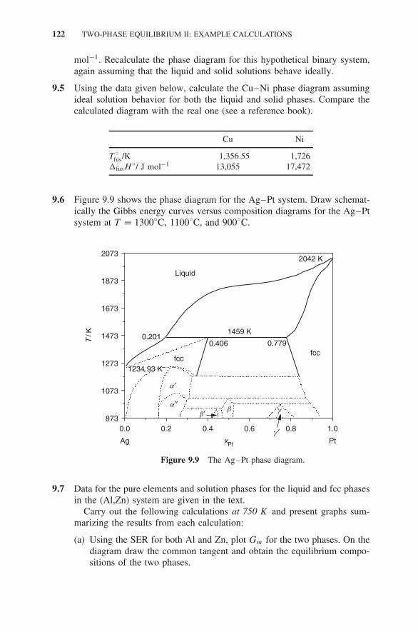
122 TWO-PHASE EQUILIBRIUM II: EXAMPLE CALCULATIONS
mol−1. Recalculate the phase diagram for this hypothetical binary system,again assuming that the liquid and solid solutions behave ideally.
9.5 Using the data given below, calculate the Cu–Ni phase diagram assumingideal solution behavior for both the liquid and solid phases. Compare thecalculated diagram with the real one (see a reference book).
Cu Ni
T◦
fus/K 1,356.55 1,726�fusH
◦/ J mol−1 13,055 17,472
9.6 Figure 9.9 shows the phase diagram for the Ag–Pt system. Draw schemat-ically the Gibbs energy curves versus composition diagrams for the Ag–Ptsystem at T = 1300◦C, 1100◦C, and 900◦C.
2073
1873
1673
1473
1273
1073
0.0
Ag PtxPt
0.2 0.4 0.6 0.8 1.0873
T/K
Liquid
2042 K
0.2011459 K
0.406
fcc
0.779fcc
1234.93 K
a″
a′
b′b g
g ′
Figure 9.9 The Ag–Pt phase diagram.
9.7 Data for the pure elements and solution phases for the liquid and fcc phasesin the (Al,Zn) system are given in the text.
Carry out the following calculations at 750 K and present graphs sum-marizing the results from each calculation: .
(a) Using the SER for both Al and Zn, plot Gm for the two phases. On thediagram draw the common tangent and obtain the equilibrium compo-sitions of the two phases.

EXERCISES 123
(b) Calculate xαB, x
β
B, f β at xB = 0.3, T = 400 K.(c) Generate plots of another function which enables you to obtain these
compositions more accurately than can be obtained from the commontangent to G.
(d) Repeat (a) and (b) using Al(l) and Zn(l) as the reference states andconfirm that you get the same answer for the equilibrium compositions.
(e) Repeat (a) and (b) using Al(fcc) and Zn(fcc) as reference states for thefcc phase and Al(l) and Zn(l) as reference states for the liquid phase.Why do you now get a different answer for the two-phase equilibrium?
(f) Repeat (a)–(d) but obtain plots of μZn for both phases. Label the mean-ing of the value of each intercept on the pure Zn axis, for example,μ
◦Zn(fcc, 750 K)–μ
◦Zn(l, 750 K).
9.8 For the temperature range 1000–1500 K, the activity coefficient of zinc inliquid brass can be expressed by the equation
RT loge γZn = −19,245x2Cu J mol−1
Calculate the partial pressure of zinc, pZn, over a solution of 60 at %copper and 40 at % zinc at 1500 K.


10 Binary Phase Diagrams:Temperature–CompositionDiagrams
We have indicated previously that, for unary systems, two-dimensional phasediagrams may be classified as follows:
Field–field phase diagramsField–density phase diagramsDensity–density phase diagrams
Field variables are intrinsically intensive quantities like p, T , μi . Density vari-ables are intensive quantities formed from extensive quantities by division byeither mass or amount and are referred to as specific quantities.
This same classification applies to phase diagrams for binary systems but,because of the additional component, there is an additional independent variable.It now requires three independent variables to specify the properties of a binarysingle phase. This means that, in order to be able to plot properties or phase dia-grams in two dimensions, it is necessary to fix one of the independent variables.In MS&E, phase diagrams are invariably displayed at a fixed total pressure of 1bar.
For binary systems, commonly met examples of the three types of plots areT − μi , T − xi , and Hm − xi diagrams, respectively. Schematic examples ofthese three are shown in Figure 10.1.
Just as in the case of unary systems, the topology of the three types ofphase diagram differs. The three-phase invariant equilibrium is a point infield–field phase diagrams, a line in field–density phase diagrams, and an areain density–density phase diagrams.
As will be discussed in the next section, arbitrary plots of two propertiesdo not necessarily result in a true phase diagram. There are constraints on theselection of the variables which can be plotted if a true phase diagram is to beobtained.
Materials Thermodynamics. By Y. Austin Chang and W. Alan OatesCopyright 2010 John Wiley & Sons, Inc.
125

126 BINARY PHASE DIAGRAMS: TEMPERATURE–COMPOSITION DIAGRAMS
1
1 12
22
3
32
2
2
1
1 1
T T
Hm
mB
1
1
12
2
2
3
A
A
< 0B
B
0
a
aa
b
bb
Liquid
LiquidLiquid
xB
xB
Figure 10.1 Examples of field–density, field–field, and density–density binary phasediagrams. The numerals indicate the number of phases present in that region of thediagram.
10.1 TRUE PHASE DIAGRAMS
Each thermodynamic potential has its natural variables , which are apparent fromthe appropriate Gibbs equation. For example, from dU = T dS − p dV , the nat-ural variables of U are S and V . If the potential is known as a function of itsnatural variables, then all the thermodynamic properties of the system are fixed.Thus, for a multicomponent system, knowledge of G = G(p, T , ni) fixes allthe other thermodynamic properties but, for example, knowing G = G(V, T , ni)
does not.Every extensive thermodynamic function has an intensive thermodynamic
potential which is its conjugate variable. These pairs come from the definition ofwork in its widest, thermodynamic, sense. As can be seen from the fundamentalequation
dU = T dS − p dV +∑
i
μi dni (10.1)
T and S are conjugate variables, as are −p and V , and as are μi and ni .A plot of any pair of conjugate variables does not result in a true phase
diagram, by which we mean one where all points on the diagram give a uniqueanswer to the phase constitution at that point. Plots of conjugate variables simplylead to a property diagram, not a phase diagram.
A multitude of thermodynamically valid equations similar to (10.1) are pos-sible. As an example, consider the constant-pressure Gibbs–Duhem equation for
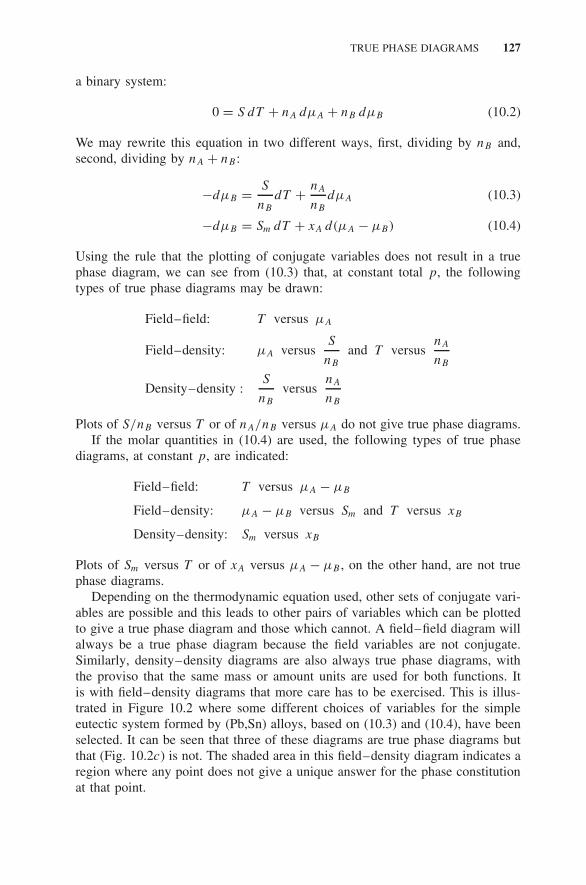
TRUE PHASE DIAGRAMS 127
a binary system:
0 = S dT + nA dμA + nB dμB (10.2)
We may rewrite this equation in two different ways, first, dividing by nB and,second, dividing by nA + nB :
−dμB = S
nB
dT + nA
nB
dμA (10.3)
−dμB = Sm dT + xA d(μA − μB) (10.4)
Using the rule that the plotting of conjugate variables does not result in a truephase diagram, we can see from (10.3) that, at constant total p, the followingtypes of true phase diagrams may be drawn:
Field–field: T versus μA
Field–density: μA versusS
nB
and T versusnA
nB
Density–density :S
nB
versusnA
nB
Plots of S/nB versus T or of nA/nB versus μA do not give true phase diagrams.If the molar quantities in (10.4) are used, the following types of true phase
diagrams, at constant p, are indicated:
Field–field: T versus μA − μB
Field–density: μA − μB versus Sm and T versus xB
Density–density: Sm versus xB
Plots of Sm versus T or of xA versus μA − μB , on the other hand, are not truephase diagrams.
Depending on the thermodynamic equation used, other sets of conjugate vari-ables are possible and this leads to other pairs of variables which can be plottedto give a true phase diagram and those which cannot. A field–field diagram willalways be a true phase diagram because the field variables are not conjugate.Similarly, density–density diagrams are also always true phase diagrams, withthe proviso that the same mass or amount units are used for both functions. Itis with field–density diagrams that more care has to be exercised. This is illus-trated in Figure 10.2 where some different choices of variables for the simpleeutectic system formed by (Pb,Sn) alloys, based on (10.3) and (10.4), have beenselected. It can be seen that three of these diagrams are true phase diagrams butthat (Fig. 10.2c) is not. The shaded area in this field–density diagram indicates aregion where any point does not give a unique answer for the phase constitutionat that point.

128 BINARY PHASE DIAGRAMS: TEMPERATURE–COMPOSITION DIAGRAMS
600
550
500
450
400
T/K
350
300
500
400
300
200
(S/n
Sn)
/J K
−1 m
ol−1
100
0−60 −50
bct
fcc
fcc
bct
Liquid
Liquid+
fcc
fcc+
bct
Liquid + bct
Liquid
−40
(a) (b)
(c) (d )
−30 −20
mpb / kJ mol−1
−50 −45 −40 −35 −30 −25 −20
mpb / kJ mol−1
Sm°
/ J K
−1 m
ol−1
Liquid
fcc
bct
Liquid+
bctfcc+
bct
Liquid+ bct
90
80
70
60
400 420 440 460 480 500
T / K
Liquid
fcc
bct
bct+
fcc
bct+
Liquid
fcc + LiquidS
m°/J
K−1
mol
−1
100
90
70
80
60
50−10 −9 −8 −7 −6 −5 −4
(mpb – mSn) / kJ mol−1
Figure 10.2 Plots of different thermodynamic functions for Pb–Sn system illustratingwhat are and what are not true phase diagrams: (a) field–field and (b) density–field truephase diagrams; (c) density–field diagram of conjugate variables; (d) density–field truephase diagram. The SER reference states have been used.
Many different types of phase diagram have a practical value. Plots ofHm − xi , for example, are useful in heat balance calculations. The type of mostsignificance in MS&E is the T –xi diagram and we now discuss some aspectsof these in more detail.
10.2 T –xi PHASE DIAGRAMS FOR STRICTLY REGULARSOLUTIONS
Application of (9.7) and (9.8) to a liquid and solid (α) phases with the assumptionthat both solution phases are strictly regular gives, at constant p, T ,
μlA = μα
A (10.5)
μ◦,αA + �μ
id,αA + μ
E,αA = μ
◦,lA + �μ
id,lA + μ
E,lA
− (μ◦,lA − μ
◦,αA ) (10.6)

T –xi PHASE DIAGRAMS FOR STRICTLY REGULAR SOLUTIONS 129
The last term in (10.6) can be expressed as
(μ◦,lA − μ
◦,αA ) = �fusH
◦m(A) − T �fusS
◦m(A) (10.7)
≈ [T ◦fus(A) − T ]�fusS
◦m(A) (10.8)
so that we obtain the working equation for component A:
RT loge(1 − xlB) + Ll
0(xlB)2 = RT loge(1 − xα
B) + Lα0 (xα
B)2
− [(T ◦fus(A) − T ) �fusS
◦m(A)] (10.9)
RT loge
(xl
A
xαA
)= [Lα
0 (xαB)2 − Ll
0(xlB)2]
− [(T ◦fus(A) − T ) �fusS
◦(A)] (10.10)
with a similar equation for the other component, B. The two equations can besolved to calculate binary phase diagrams for strictly regular solutions.
From (10.10) and the analogous equation for B, we see that the location ofphase boundaries depends on:
(i) T◦
fus(A) and T◦
fus(B)
(ii) �fusS◦m(A) and �fusS
◦(B)
(iii) Ll0 and Lα
0
As is illustrated below, variation of these factors can have a profound effecton the phase diagram topology for these strictly regular solutions. For mostmetals, �fusS
◦m ≈ 10 J K−1 mol−1 while it may be much higher than this for
semiconductors. For the other pure component properties we have selected twosets of parameters, one set where there is a small difference in T
◦fus of the two
components and the other set with a large difference:
T◦
fus(A) = 1000 K T◦
fus(A) = 500 K
T◦
fus(B) = 1200 K T◦
fus(B) = 3000 K
�fusS◦m(A) = 10 J mol−1 K−1 �fusS
◦m(A) = 10 J mol−1
�fusS◦m(B) = 10 J mol−1 K−1 �fusS
◦m(B) = 10 J mol−1K−1
In Figure 10.3, the phase diagrams on the left have been calculated using the firstset of parameters, with a small difference in fusion points of the components;those on the right are obtained when large differences in the fusion points areselected.
The effect of varying the solution parameters of the two phases are apparentin the figure.

130 BINARY PHASE DIAGRAMS: TEMPERATURE–COMPOSITION DIAGRAMS
1200
1000
800
T /
K
600
400
0.0A x
Bx
B
xB
xB
xB
xB
B0.2 0.4 0.6
(a) (b)
(c) (d )
(e) (f )
0.8 1.0
3000
2000
T /
KT
/ K
1000
3000
2000
1000
0.0A B
0.2 0.4 0.6 0.8 1.0
0.0A B
0.2 0.4 0.6 0.8 1.0
Liquid
Liquid
Liquid + a
Liquid + a
Liquid
a
1200
900
600
T /
KT
/ K
300
1200
1000
800
600
400
0.0A B
0.2 0.4 0.6 0.8 1.0
0.0A B
0.2 0.4 0.6 0.8 1.0
Liquid
Liquid + aLiquid + a
aa
a
a
T /
K
3000
2000
1000
0.0A B
0.2 0.4 0.6 0.8 1.0
Liquid + a
Liquid
a
a + a
a + a
a + a
a + a
Liquid + aLiquid + Liquid
Liquid
aa
Figure 10.3 Phase diagrams involving two phases, both of which are strictly regularsolutions. There is a 200-K difference in melting points for those in the left column,a 2500-K difference for those in the right column: (a, b) Ll
0 = 0, Lα0 = 0; (c, d) Ll
0 =0;Lα
0 = +15 kJ mol−1; (e, f ) Ll0 = +20 kJ mol−1, Lα
0 = +20 kJ mol−1.

T –xi PHASE DIAGRAMS FOR STRICTLY REGULAR SOLUTIONS 131
10.2.1 Some General Observations
It is clear from these phase diagrams for strictly regular solutions that a con-siderable variety can be found by changing just a few model parameters. Anexamination of diagrams in Figures 10.3 and 10.4 enables us to reach somegeneral observations as to when we might expect to see different types of simplephase diagrams.
1300
1200
1100
1000
900
T/K
Liquid
a
0.0 0.2 0.4 0.6 0.8 1.0A BxB
(a)
1300
1200
1100
1000
900
T/K
Liquid
a
0.0 0.2 0.4 0.6 0.8 1.0A BxB
(b)
1200
1100
1000
T/K
Liquid
a
0.0 0.2 0.4 0.6 0.8 1.0A BxB
(c)
2000
1600
1200
800
400
T/K
Liquid
a
Liquid + aLiquid + a
Liquid + Liquid
a + a
0.0 0.2 0.4 0.6 0.8 1.0A BxB
(e)
1200
1000
800
600
400
T/K
Liquid
a
a + a
0.0 0.2 0.4 0.6 0.8 1.0A BxB
(d )
2000
1600
1200
800
400
T/K
Liquid
a
a
Liquid + aLiquid + Liquid
a + a
0.0 0.2 0.4 0.6 0.8 1.0A BxB
(f )
Figure 10.4 Phase diagrams involving two phases, both of which are strictly reg-ular solutions. All refer to systems with a 200-K difference in melting points:(a) Ll
0 = −5 kJ mol−1, Lα0 = 0; (b) Ll
0 = 0, Lα0 = −5 kJ mol−1; (c) Ll
0 = −10 kJmol−1, Lα
0 = −10 kJ mol−1; (d) Ll0 = +10 kJ mol−1, Lα
0 = +10 kJ mol−1; (e) Ll0 =
+30 kJ mol−1, Lα0 = +10 kJ mol−1; (f ) Ll
0 = +30 kJ mol−1, Lα0 = +20 kJ mol−1.

132 BINARY PHASE DIAGRAMS: TEMPERATURE–COMPOSITION DIAGRAMS
(i) Complete Solubility Phase Diagrams Complete solubility results whenboth phases are ideal, that is, Ll
0 = Lα0 = 0. But we can have a complete solubility
phase diagram even when the solutions are not ideal. Such diagrams result whenLl
0 ≈ Lα0 . Real alloy examples include the Ag–Au, Ag–Pd, Cd–Mg, and Co–Ni
systems.When both Ll
0 and Lα0 are negative, the phase diagram is similar to that for
the case Ll0 = Lα
0 = 0, but when Ll0 ≈ Lα
0 � 0, miscibility gaps are formed atlower temperatures. A real alloy example of this is found in the Au–Ni system,where Lα
0 � 0.Other features to note are:
(i) When Ll0 ≈ Lα
0 � 0, the width of the melting region becomes largerthan for the ideal solution case. Conversely, when Ll
0 ≈ Lα0 < 0, the
width of the melting region is narrower than for the ideal solutioncase.
(ii) The width of the two-phase region also depends on the relative melt-ing points and entropies of fusion of the components. The freezingranges for semiconductor alloys (e.g., Ge–Si) are particularly large,due primarily to the large entropies of fusion for the two elementalsemiconductors.
(ii) Peritectic Phase Diagrams Peritectic phase diagrams are more likely tooccur when:
(a) There is a large difference between T◦
fus(A) and T◦
fus(B).(b) Ll
0 ≈ Lα0 > 0.
(c) The critical temperature Tc for the (metastable) miscibility gap of thesolid phase intercepts the (metastable) solidus curve.
Real alloy examples include the Ag–Pt and Co–Cu systems.(iii) Phase Diagrams with Maximum and Minimum Congruent Melting
Points A maximum occurs when the solid phase is more stable than the liquidphase and vice versa but when Ll
0 ≈ Lα0 and both are small. If they are too high
and positive, miscibility gaps will occur.When Ll
0 < Lα0 and Ll
0 is not too large, a maximum occurs in the liquid/solid.An example of a congruent maximum in a real alloy system occurs in the Pb–Tlsystem. When Ll
0 >Lα0 and Lα
0 is not too large, a minimum occurs in the liq-uid/solid. Examples of real alloy systems showing congruent minima are Co–Pdand Cr–Mo.
(iv) Eutectic Phase Diagrams When Lα0 >> 0 and Ll
0 ≤ 0 and thedifference in melting points of the two components is not too large, a eutecticphase diagram is found. Cu–Ag is a real alloy system with this type of phasediagram.
(v) Monotectic, Syntectic, and Monotectic + Syntectic Phase DiagramsMiscibility gaps form in the liquid phase when Ll
0 � 0. Pb–Zn is a real alloysystem which shows a liquid-phase miscibility gap.

T –xi PHASE DIAGRAMS FOR STRICTLY REGULAR SOLUTIONS 133
10.2.2 More on Miscibility Gaps
By examining the compositional dependencies of G and its derivatives, we canobtain the conditions which pertain at the critical temperature. We illustrate byreference to the Al–Zn system, which was discussed as Example 9.1, the sta-ble phase diagram for the system having been given in Figure 9.2. The stablemiscibility gap exists over a fairly small temperature range. Its metastable exten-sion to lower temperatures is shown in Figure 10.5a. The critical point occurs atapproximately 622.3 K. The first three derivatives of the Gibbs energy of mixingwith respect to xZn for the fcc (Al,Zn) phase at this temperature are shown inFigures 10.5b –10.5d .
It can be seen that, at the critical point, d2G/dx2B = d3G/dx3
B = 0 but thatdG/dxB �= 0 (we have abbreviated �mixG to G). We have selected the fcc(Al,Zn) example since it is not a regular solution. For the latter, the criticalpoint occurs at x = 0.5, and this gives rise to a special case where the firstderivative is also zero at that point. This is not a general condition.
The zero values of the second and third derivatives at the critical point arerelevant to an apparent breakdown of the phase rule when applied to misci-bility gap systems at the critical point. Clearly, F = 0 at this point since the
700
600
500
400
300
T/K
20,000
15,000
10,000
5,000
0
0.0 0.2 0.4 0.6 0.8 1.0Al ZnxZn
(a)
0.0 0.2 0.4 0.6 0.8 1.0Al ZnxZn
(c)
0.0 0.2 0.4 0.6 0.8 1.0Al ZnxZn
(b)
0.0 0.2 0.4 0.6 0.8 1.0Al ZnxZn
(d )
20,000
10,000
0
−10,000
−20,000
dG dxzn
200,000
100,000
0
−100,000
d3G
dx3 Z
n
d2G
dx2 zn
Figure 10.5 First, second, and third derivatives of G with respect to xZn for fcc Al–Znat critical temperature of 622.29 K: (a) miscibilty gap in fcc phase; (b) first derivative ofG; (c) second derivative of G; (d) third derivative of G. The critical composition occursat xZn = 0.347.

134 BINARY PHASE DIAGRAMS: TEMPERATURE–COMPOSITION DIAGRAMS
temperature and composition are fixed (at constant total pressure). But, if weapply (8.26), we find that F = 2 − 1 + 1 = 2, which is incorrect. The reason isthat there are other constraints on the μi at this point and we must apply (8.21).The extra constraints are those already discussed, namely, at the critical point,d2Gm/dx2
B = d3Gm/dx3B = 0, so that, with the Gibbs–Duhem relation, Rμ = 3.
Applying (8.21), we see that F = 1 × 2 + 1 − 3 = 0, as it should be.
10.2.3 The Chemical Spinodal
The dashed curve shown in Figure 10.5a is the locus of compositions whered2G/dx2
B = 0 and is called the chemical spinodal curve. The phase boundaryfor the two-phase stable equilibrium is referred to as the binodal curve.
The significance of the spinodal can be understood by referring to Figure 10.6.The points s1 and s2 are the spinodal points.
When a single-phase alloy with a composition between the spinodals is broughtfrom a high temperature (T >Tc) to a lower temperature within the miscibilitygap, this alloy becomes thermodynamically unstable. The equilibrium system willconsist of a two-phase mixture. There are, however, two quite different ways inwhich the phase decomposition can occur:
(a) Between the spinodal compositions, the G − xB curve is concave. In thiscase, the Gibbs energy of the homogenous single-phase alloy is alwayshigher than that of any mixture of compositions (c and d , for example)which can form from a decomposition of this phase.
0.0 0.2 0.4 0.6 0.8 1.0
−0.8
−0.6
−0.4
−0.2
0.0
0.2
0.4
Al Zn
s1
s2
a
b
cd
Δ mixG
m/ k
J m
ol−1
xZn
Figure 10.6 The �mixG◦m for fcc (Al,Zn) at 300 K. At compositions inside the spinodal,
any fluctuations in composition are unstable, whereas in the metastable region, betweenthe binodal and the spinodal, fluctuations are stable.

POLYMORPHISM 135
(b) When a single-phase alloy with a composition between the miscibility gapand the nearby spinodal composition is brought to a T < Tc, the situationis quite different. Due to the convex nature of the G − xB curve in thiscomposition range, there would be an increase of the Gibbs energy if asingle-phase alloy decomposed locally to form any mixture of compositions(a and b, for example); that is, there is no thermodynamic driving forcefor decomposition by fluctuations when the composition falls between thespinodal and binodal. Decomposition in this case can only take place bynucleation of a phase in the other.
These two different mechanisms, spinodal decomposition and nucleation, arevery important in the theory of phase transformations.
10.3 POLYMORPHISM
The Hf–Ta phase diagram shown in Figure 10.7 indicates that there is anallotropic transformation in Hf. The hcp form is stable at low temperatures witha transformation to bcc occurring at 1743◦C. Tantalum is bcc at all temperaturesin the solid state. It can be seen that the two bcc forms are completely miscible.But the difference in the two structures at low temperatures brings about acompletely different topology to the phase diagram than would have been thecase if only the high-T form of Hf existed. The method of calculation of thephase equilibrium boundaries between the Hf-rich hcp phase and the bcc phaseis identical with that discussed above for the liquid/α equilibrium.
3473
3073
2673
2273
1873
1473
1073
2504 K
2016 K
3293 K
2403 K
T/K
0.0 0.2 0.4 0.6 0.8 1.0TaxTaHf
0.087 0.8110.40
0.20
Liquid
1356 K1413 K
( bHf,Ta)
(aHf)
Figure 10.7 The Hf–Ta phase diagram.

136 BINARY PHASE DIAGRAMS: TEMPERATURE–COMPOSITION DIAGRAMS
EXERCISES
10.1 In the Mo–Ru phase diagram given in Figure 10.8, there exists a bcc (Mo,Ru) solid solution, a hcp (Ru, Mo) solid solution, an intermetallic phasedenoted by σ , and a liquid phase. Suppose the σ -phase does not exist inthis system. Estimate �G
hcpbcc(Mo) and �Gbcc
hcp(Ru) at 1800◦C on the basisof the solubility of Ru in bcc (Mo, Ru) and that of Mo in hcp (Ru, Mo),making any needed assumption to carry out this calculation.
The solubility curves in Figure 10.8 were determined for the bcc + σ
and σ + hcp two-phase fields. If σ does not form due to kinetic difficulties,we would then have a metastable equilibrium between bcc and hcp. Wouldthe solubilities of Ru in bcc (Mo, Ru) and of Mo in hcp (Ru, Mo) decreaseor increase for the metastable equilibrium?
3073
2673
2273
1873
1473
1073
T/K
0.0 0.2 0.4 0.6 0.8 1.0Mo RuxRu
2896 K
2607 K
2188 K
1416 K
Liquid
hcpbcc
s
Figure 10.8 The Mo–Ru phase diagram.
10.2 Derive the critical point conditions for a subregular solution with the fol-lowing expression for GE:
GE = xAxB [L0 + L1(xa − xB)] (10.11)
10.3 GEm for fcc (Al,Zn) alloys may be represented by
GEm/J mol−1 = xAlxZn[6656.0 + 1.615T ) + (6793.0 − 4.982T )(xAl − xZn)
+ (−5352.0 + 7.261T )(xAl − xZn)2]
Calculate the miscibility gap and evaluate the critical point (approxi-mately). At the critical temperature, plot �mixGm and the first, second,

EXERCISES 137
and third derivatives of �mixGm as a function of xZn and note which onesare zero at the critical composition.
10.4 If it is assumed that both the liquid and solid solution phases are ideal,a very simple phase diagram results in which the solid solution is stabledown to 0 K. How does this tie in with your understanding of the Planckpostulate?


11 Binary Phase Diagrams:Temperature–ChemicalPotential Diagrams
To date, we have considered only temperature–composition phase diagrams,which, as we have seen, are actually a constant total pressure slice through athree-dimensional diagram in pressure–temperature–composition space. Thesephase diagrams are the most widely used two-dimensional phase diagrams forbinary systems. There are good reasons for this:
(i) Examination of temperature–composition space is the normal way ofexperimentally obtaining phase equilibrium information.
(ii) Alloys are usually used in temperature–composition space in their pro-duction and applications.
In thermodynamic language, these two points mean that we usually carry outmeasurements on and use binary systems, especially alloys, in a closed-systemsense.
This T –xi representation, however, is not always the most useful and it iscertainly not the only way of graphically presenting information about phaseequilibrium.
In chapter 10, we noted that, in a true phase diagram, any point on that diagramgives a unique answer as to the phase constitution represented at that point.We also noted that a field–field phase diagram is always a true phase diagramsince two field variables can never be conjugate variables. The most useful ofthe field–field diagrams, whenever an open system is being considered (wherecomposition is not fixed), is a plot of T versus μi at constant total pressure. Whenone or more of the components (or compounds of the components) are volatile atthe temperatures of interest, composition may then become a dependent variablewith an external chemical potential being the independent variable.
We first discuss some general points about these T –μi phase diagrams andwill then discuss some examples. This same type of representation will be dis-cussed again in Chapters 19–22, when we will refer to heterogeneous chemicalequilibrium. For the moment, we concentrate on phase equilibrium.
Materials Thermodynamics. By Y. Austin Chang and W. Alan OatesCopyright 2010 John Wiley & Sons, Inc.
139

140 BINARY PHASE DIAGRAMS: TEMPERATURE–CHEMICAL POTENTIAL DIAGRAMS
11.1 SOME GENERAL POINTS
In earlier chapters we placed emphasis on the value of the SER in carrying outequilibrium calculations. This reference state is not, of course, the only possibleselection. It is not usually the reference state of choice in the presentation ofT –μi phase diagrams. A more useful choice (but not a mandatory one) is totake the pure component at T , p = 1 bar as the reference state. By making thisselection, the T –μi phase diagram is made to resemble the equivalent T –xi
phase diagram (remember that there is a monotonic relation between chemicalpotential and composition in single-phase regions).
This selection of the reference state selection presents no ambiguity in the caseof gases but, for condensed phases, it is necessary to decide whether to selectthe pure solid or the pure liquid component at all temperatures (and standardpressure) as the reference state. In the remainder of this chapter we will use thepure solid reference state so that, when we write μi , we mean μi(T , 1 bar, xi) −μ
◦,si (T , 1 bar, xi = 1). Since we will concentrate on T –μB phase diagrams for
an A–B system, we are selecting B(s) at the T of interest as the reference state.
Example 11.1 System with Two Ideal Solution PhasesAs an introduction to T –μi diagrams, we will consider the simplest possiblecase where both the liquid and solid phases form ideal solutions. The T –xB
phase diagram is shown in Figure 11.1. This phase diagram has been calculatedon the assumption that �fusS
◦m = 10 J K−1 mol−1 for both components. The
chosen melting points are apparent on the phase diagram. It can be seen fromFigure 11.1 that a liquid alloy with xB = 0.1 is in equilibrium with an α phasealloy with xB = 0.374 at 1432 K.
Having selected the B(s) as the reference state, it is necessary to calculate aline on the T –μB diagram representing the properties of pure B(l). This can be
T/K
3000
2000
1000
0
A B
0.0 0.2 0.4 0.6 0.8 1.0xB
0.374
1432 K
0.1
a
Figure 11.1 The T –xB phase diagram where both solid and liquid form ideal solutions.

SOME GENERAL POINTS 141
obtained as follows:
�fusμ◦B = μ
◦,lB (T ) − μ
◦,sB (T ) = �fusG
◦m(B, T )
� 〈�fusH◦m(B)〉 − T 〈�fusS
◦m(B)〉 (11.1)
where, in the last equation, we have used the linear approximation for �fusG◦m.
The bracketed terms are average values for the quantities. This linear approxi-mation is quite satisfactory when used in high-temperature calculations (aboveroom temperature). The average values in (11.1) refer to values obtained fromhigh-temperature results, even though they are used, but only for constructionpurposes, at lower temperatures, including 0 K. In this linear approximation,these construction lines are given by:
(i) At T = 0 K : �fusμ◦B(0 K) = 〈�fusH
◦m(B)〉
(ii) At T = T◦
fus : �fusμB = 0
so that it is possible to draw the line going through these two points on a T –μB
diagram. This is illustrated in Figure 11.2. We can extend the calculations to alloysby putting lines on the T –μB phase diagram for different alloy compositions inboth the solid and liquid phases. Since both the solid and liquid alloys have beenassumed to form ideal solutions, the chemical potentials in the solid and liquidphases, relative to pure solid B as the reference state, are given by
μsB(xB) − μ
◦,sB = RT loge xs
B (11.2)
μlB(xB) − μ
◦,sB = RT loge xl
B + �fusG◦m(B) (11.3)
These two equations give rise to composition fans on the T –μB diagram.These fans for the solid solution phase originate, at T = 0 K, according to (11.2)
Liquid
3000
2000
1000
0
T/K
Tfus
T = 1432 K
xB = 0.1
XB = 0.374
Solid B
40200–20–40–60
ΔfusHm° mB /kJ mol–1
a
mB ° − m
B ° (s)
Figure 11.2 The T –μB phase diagram where both solid and liquid form ideal solutions.

142 BINARY PHASE DIAGRAMS: TEMPERATURE–CHEMICAL POTENTIAL DIAGRAMS
at the origin, while those for the liquid phase originate, according to (11.3), atT = 0 K at the point �fusH
◦m(B).
The T –μB phase diagram shown in Figure 11.2 is seen to be similar to theT –xB diagram given in Figure 11.1 but with the difference that the two-phaseregion in the T –xB diagram has contracted to a single curve in the T –μB
diagram. The line for xB = 0.1 for the liquid phase emanates from the point onthe 0 K axis marked as �fusH
◦m. It can be seen to intersect with the composition
line for xB = 0.374 for the solid solution phase, which emanates from the originof the figure, at the temperature of 1432 K.
It is clear that there is exactly the same information on the T –μB diagram ason the T –xB phase diagram. Note that we could show μB on the T –xB diagramso that then both diagrams would contain exactly the same information. Becausethe introduction of the μB lines on the T –xB phase diagram would lead to clutter,it is much more convenient to use the T –μB plot in those circumstances whereμB is under external control.
It is also possible to include the gas-phase properties on both the T –xB
and T –μB diagrams. Taking the same example as above and assuming that�vapG
◦m = 340,000 + 85T J mol−1, which gives a normal boiling point of 4000
K, we can insert curves for selected pB on the T –xB phase diagram, as shown inFigure 11.3. The inclusion of gas-phase partial pressure fans on a T –μB diagramrequires a very similar procedure to that used for composition fans for the liquidand solid phases in Figure 11.2. Phase equilibrium is governed by the relationμ
gB = μs
B . In order to incorporate the gas-phase properties on the T –μB diagram,they must be referred to the pure solid B reference state.
00.2 0.4 0.6 0.8 1
fcc
Liquid
Liquid + GAS
0.1 bar
0.01 bar
0.001 bar
PB = 1 bar
00
1000
2000
3000
4000
5000
xB
T/K
A B
Figure 11.3 Inclusion of lines of constant pB on temperature–composition diagram.

SOME GENERAL POINTS 143
For the standard property difference between gas and solid, we may write(using the abbreviation sub for sublimation)
μ◦,gB (xB) − μ
◦,sB = �subG
◦m(B, T ) (11.4a)
� 〈�subH◦m(B)〉 − T 〈�subS
◦m(B)〉 (11.4b)
where we have again used the linear approximation. From (11.4) we see that, inthe linear approximation, the construction lines are given by:
(i) At T = 0 K: μ◦,gB (0 K) − μ
◦,gB (0 K) = 〈�subH
◦m(B)〉
(ii) At T = T◦
sub: μ◦,gB (T
◦sub) − μ
◦,sB (T
◦sub) = 0
If the gases are assumed perfect, we may use
μgB(pB) − μ
◦,gB = RT loge
(pB
p◦B
)(11.5)
The chemical potential relative to pure solid B is then obtained by adding (11.4a)and (11.5):
μgB(pB) − μ
◦,sB = RT loge
(pB
p◦B
)+ �subG
◦m(B, T ) (11.6)
We can now superimpose the gas-phase information onto Figure 11.2 to yield aphase diagram from which we are able to read the liquid or solid compositionsin equilibrium with a gas phase of fixed pB at any temperature T . The resultingT –μB phase diagram is shown in Figure 11.4.
4000
3000
5000
2000
1000
0
T/K
Liquid
0.1 bar
Tfus (B)
Tbpt (B)
Tfus (A)
–200 –100 1000 200 300 400
a
mB /kJ mol–1
ΔfusHm° ΔsubHm
°
mB° (g) − m
B° (s)
Figure 11.4 Inclusion of lines of constant pB on T –μB phase diagram.
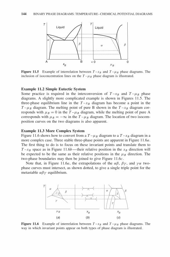
144 BINARY PHASE DIAGRAMS: TEMPERATURE–CHEMICAL POTENTIAL DIAGRAMS
T T
xB mB
A
a
ab b
LiquidLiquid
B < 0 0
Figure 11.5 Example of interrelation between T –xB and T –μB phase diagrams. Theinclusion of isoconcentration lines on the T –μB phase diagram is illustrated.
Example 11.2 Simple Eutectic SystemSome practice is required in the interconversion of T –xB and T –μB phasediagrams. A slightly more complicated example is shown in Figures 11.5. Thethree-phase equilibrium line in the T –xB diagram has become a point in theT –μB diagram. The melting point of pure B shown in the T –xB diagram cor-responds with μB = 0 in the T –μB diagram, while the melting point of pure Acorresponds with μB = −∞ in the T –μB diagram. The location of two isocom-position curves on the two diagrams is also apparent.
Example 11.3 More Complex SystemFigure 11.6 shows how to convert from a T –μB diagram to a T –xB diagram in amore complex case. Three stable three-phase points are apparent in Figure 11.6a .The first thing to do is to focus on these invariant points and translate them toT –xB space as in Figure 11.6b —their relative position in the xB direction willbe expected to be the same as their relative positions in the μB direction. Thetwo-phase boundaries may then be joined to give Figure 11.6c.
Note that, in Figure 11.6a , the extrapolations of the αβ, βγ , and γα two-phase curves must intersect, as shown dotted, to give a single triple point for themetastable αβγ equilibrium.
xB
Ta
b
g
d
mB
a
g
db
xB
(a) (b) (c)
Figure 11.6 Example of interrelation between T –xB and T –μB phase diagrams. Theway in which invariant points appear on both types of phase diagram is illustrated.

SOME GENERAL POINTS 145
Example 11.4 Preparation of GaAsIn the making of a (Pb,Sn) solder, Pb and Sn can be weighed out in a molar ratioof about 1 : 3. The resulting alloy will act as a low-melting-point solder withlittle mushy freezing. If we are a little out in the weighing of the constituents, itwill not make all that much difference to the engineering utility of the alloy.
This preparation of a solder may be contrasted with the very different situationfor the preparation of GaAs, whose engineering applications depend on its electri-cal properties. According to the normal temperature–composition phase diagramshown in Figure 11.7a , GaAs is essentially stoichiometric. But, if we make onealloy with (0.4999 Ga, 0.5001 As) and one with (0.5001 Ga, 0.4999 As), thenit is found that these two alloys have completely different engineering proper-ties. This is because GaAs is marginally nonstoichiometric, as is apparent in agross expansion of the composition scale of the temperature–composition phasediagram in the neighborhood of the stoichiometric composition (see Fig. 11.7b).An alloy composition cannot be guaranteed to this degree of precision if it ismade up by weighing. Fortunately, however, it is possible to take advantage of
1673
1473
1273
1073
873
673
473
273
T/K
0.0 0.2 0.4 0.6 0.8 1.0
xAsAsGa
Liquid 1511 K
1090 K1083 K
(As)
GaA
s
(Ga)302.7741 K
(a)
T/K
xAs
nonstoichimetricGaAs
Liquid + GaAs
Liqu
id+
GaA
s
Liquid
GaAs + As(s)
0.50000 0.50005 0.50010
1600
1400
1200
1000
(b)
T/K
(c)
As(c)
As(c)
Ga(c)
As(l)
As(l)
As4(g) As2(g)
Ga1−xAsx(c)
Ga1−yAsy(l)
−100−80 −60 −40 −20 200 40 60 80 100
1600
1400
1200
1000
800
600
400
200
0
0.01
0.1 1.0
y = 0.001
ΔmAs/kJ mol−1
−2
2
1−3 −1
0
0
−2−4−6 log(pAs4/atm)
log(pAs2/atm)
Figure 11.7 Phase diagrams for Ga–As system: (a) normal T –xAs and (b) expandedT –xAs phase diagrams; (c) T –μAs phase diagram.

146 BINARY PHASE DIAGRAMS: TEMPERATURE–CHEMICAL POTENTIAL DIAGRAMS
the fact that μAs changes considerably over this very narrow composition range.In practical terms, orders-of-magnitude changes in the arsenic pressure can bringabout minuscule, but extremely significant, changes in composition. This is clearin the T –μAs phase diagram shown in Figure 11.7c.
It is quite clear that, to those interested in the production of single crystals ofGaAs, a T –xi phase diagram is not as useful as a T –μi phase diagram.
As we will see in later chapters, open systems are frequently encounteredwhen examining heterogeneous equilibria in chemically reacting systems. In thesesituations, T –μi diagrams are the more useful way for graphically presenting theresults.
EXERCISES
11.1 Calculate T –μA phase diagrams from the T –xB phase diagrams shownin Figures 11.1 and 11.5.
11.2 Figure 11.8 shows a “double” Fe–C temperature–composition phase dia-gram. The heavy lines refer to the iron–graphite system and the dashedlines to the metastable iron–carbide system. To those interested in car-burizing or decarburizing of Fe, a T –μC phase diagram is a more usefultype of presentation. Use the T –xC double diagram to sketch the T –μC
phase diagram using graphite as the reference state at all temperatures.
2000
1800
1600
1400
1200
1000
800
T/K
0.0 0.1 0.2 0.3 0.4Fe xc
Fe3C
Figure 11.8 The T –xC stable and metastable phase diagrams for Fe–C system.

EXERCISES 147
11.3 Sketch the T –xB phase diagram corresponding to the T –μB phase dia-gram shown in Figure 11.9. Include, with dashed lines, the location ofthe metastable αβγ invariant equilibrium and the associated univariantequilibria.
a b
g
d
mB
T
< 0 0
Figure 11.9 A T –μB phase diagram.


12 Phase Diagram Topology
As we have seen in the previous chapters, some of the constant-pressure T –xi
phase diagrams for real binary alloys are fairly simple. Many others, on theother hand, seem quite complex but all are comprised of one-phase regions, two-phase regions, and horizontal lines connecting three phases in equilibrium. Thesecorrespond with bivariant, univariant, and invariant equilibria, respectively.
When the invariant three-phase equilibria , or as they are sometimes calledreaction types, are examined, it is found that they are one of only two basictypes, as shown in Figure 12.1. In the first type, (a), a high-temperature phaseis no longer stable below the invariant temperature or, in reaction terms, thephase stable at high temperature dissociates into two other phases at the invarianttemperature. In the other type, (b), a phase which is unstable at high temperaturebecomes stable below the invariant temperature. In reaction terms, two phasesstable at high temperature react at the invariant temperature to form a new phase.
It is usual to go further and subdivide these two types of invariant equilibriainto subcategories which depend on what kind of phases are involved at theinvariant temperature. A complex, albeit hypothetical, phase diagram is shown inFigure 12.2. The names given to the different types of the subcategories of the twobasic types are indicated on this diagram. The two other types of invariant pointwhich have been met with previously, namely, a critical point and a congruentpoint, but which are not three-phase equilibria are also shown in this figure.
In this Chapter we will examine, more closely, the factors which determine theshape or topology of phase diagrams. There are constraints on what is and what isnot acceptable and many published phase diagrams, determined by conventionalmeans, have not complied with these constraints. With the increasing awarenessof thermodynamic constraints, this is a less frequent occurrence nowadays.
A complete understanding of the observed topology of a given phase diagramrequires consideration of:
1. The phase rule, which tells us the number of phases which can be presentat each topographical feature.
2. A combinatorial analysis, which will tells us the maximum possible numberof topographical features present in a given system.
3. Schreinemaker’s rules, which tell us what are some of the topographicalpossibilities and impossibilities .
Materials Thermodynamics. By Y. Austin Chang and W. Alan OatesCopyright 2010 John Wiley & Sons, Inc.
149

150 PHASE DIAGRAM TOPOLOGY
4. The Gibbs–Konovalov equation, which reveals the factors responsible fordetermining the slopes of phase boundaries
The application of all these concepts together is particularly useful for gainingan understanding of multicomponent phase diagrams, but we can illustrate theprinciples by confining ourselves to a consideration of binary systems only.
a
a
b
b
g
g
b −−> a + g
a + g −−> b
(a)
(b)
a gb
a
b
g
T
Figure 12.1 Two types of invariant equilibria in both T –xi and T –μi planes.
A BComposition
Polymorphic
h h
h
s
h
s+
h
s+
a + h
a + L
a + b
a + g
L1 + g
g + L3
L1 + L2
L2 + L3
h + d
d′ + t
d ÷ t
h + d′
g1 + d′
g + d′
g1 + g2
h + g1
g1
g2Critical
Critical
Critical
a
g
g
EutecticEutectic
Peritectold
Peritectic
b
b+
+
+ +
+
LL2
L2
L1
L3
L
L L
L
d′
d′
d
d′
t
t
EutectoidCongruent
Congruent
Monotectoid
Monotectic
SyntecticAllotropic
Tci
npcr
alur
c
Latectic
Figure 12.2 Hypothetical phase diagram which illustrates different types of invariantequilibria. Source: ASM Handbook Vol. 3 , 10th Edition.

COMBINATORIAL ANALYSIS 151
12.1 GIBBS’S PHASE RULE
A principal use of the phase rule is to tell us how many phases are presentat each topographical feature, each of which corresponds to a different valueof F , the number of degrees of freedom, where F is the number of intensivevariables which may be independently varied without changing the number ofphases present at a selected point on the phase diagram.
At constant total pressure, where all species are mobile and in the absenceof external fields and chemical reactions, F = C − φ + 1. In a binary system,under these conditions, F = 3 − φ. It follows that we may have only bivariant,univariant, and invariant equilibria corresponding to the presence of single-phase,two-phase, and three-phase regions on a phase diagram.
Two examples of topographical features which are obvious violations of thephase rule are shown in Figure 12.3. The first, illustrating a four-phase equilib-rium, leads to F = −1 and the second suggests a three-phase equilibrium (F = 0)with the coexisting phases at different temperatures.
12.2 COMBINATORIAL ANALYSIS
The phase rule does not give any indication of how many of the different typesof topographical features are present in a given system. A combinatorial analysis,on the other hand, permits the calculation of the upper limit to the number ofdifferent topographical features. Not all of the features included in this maxi-mum total number are necessarily present in the phase diagram for a particularsystem.
In a system with C components and N total number of phases, the upper limitof invariant features, that is, where F = 0 and φ = C + 1, may be calculated fromthe combinatorial rule,
(N
C+1
). Similar evaluations can be made for univariant
and bivariant features. In the case of phases which show a miscibility gap, it isnecessary to include both segregated phases in the counting procedure. Also, thecombinatorial calculation for the maximum possible number of the topographicalfeatures does not take the single-phase invariant congruent points and criticalpoints into consideration.
Let us use the combinatorial formula for evaluating the maximum possiblenumber of each feature in a binary system in which there are four different phasesin total. From the phase rule, the maximum number of phases in equilibrium at
Figure 12.3 Phase rule violations in T –xi phase diagrams. Source: H. Okamoto andT. B. Massalski, J. Phase Equilib. 12 148–168, 1991.

152 PHASE DIAGRAM TOPOLOGY
constant p (where F = 0) is 3. Therefore, the maximum possible total number ofinvariant features is
(43
) = 4, the maximum possible total number of univariantfeatures is
(42
) = 6, and the maximum possible total number of bivariant featuresis(4
1
) = 4. In more detail, for a system where the four phases are designatedα, β, γ, δ, we can summarize all the possible topographical features as follows:
F φ Total Combinations
0 3 4 αβγ , αβδ, αγ δ, βγ δ
1 2 6 αβ, αγ , αδ, βγ , βδ, γ δ
2 1 4 α, β, γ , δ
It is obvious from this table that, for a given invariant feature, all possibleunivariant features may be calculated by combination of any two of the phasesinvolved in the invariant equilibrium, for example, αβγ → αβ, αγ, βγ (seethe sketches on the right-hand side of Figures 12.1a and 12.1b for a three-phaseinvariant point on a T –μi diagram).
The combinatorial calculation does not give information on which of the totalnumber of possible features are likely to be stable and which features are likely tobe metastable and therefore absent. The concept of the missing invariant pointscan be appreciated by considering a binary system in which there is a singlestoichiometric compound and two eutectics on either side of the compound (seeFig. 12.4a).
Since there are four phases, the combinatorial result is that there is a total offour invariant equilibria (at constant p). But the actual phase diagram shows onlytwo (plus the congruent point). In this case there must be two other metastableinvariant points. The location of these metastable invariant equilibria are shownschematically on the T –xi and T –μi phase diagrams in Figure 12.4.
a
bg
a g
b
mB
L
abg
Lab
T
xB
LL
(a) (b)
T
A B 0< 0
Figure 12.4 The T –xi and T –μi phase diagrams for system with stoichiomet-ric compound. Locations of the metastable invariant equilibria are indicated on bothdiagrams.

SCHREINEMAKER’S RULES 153
12.3 SCHREINEMAKER’S RULES
Schreinemaker’s rules are based on the concept that an equilibrium phase orphase assemblage must only have its stability field constricted by considerationof another yet more stable assemblage.
The rules are clearer in a field–field phase diagram than in a field–densityphase diagram. In the former type:
1. Adjacent univariant curves around an invariant point are constrained to be<180◦.
2. The metastable extension of a stable univariant curve to the opposite sideof an invariant point must be into a different single-phase region.
Acceptable and unacceptable topologies are shown in Figure 12.5. It can be seenthat application of the rules to extrapolations is clearer in the field–field phasediagram than they are in the field–density diagram. The correctness of theirapplication to T –xB phase diagrams can be appreciated from G − xB curves,such as those shown in Figure 12.6. It can be seen there that the phase boundariesfor the metastable α/β equilibrium lie inside those for the stable liq/α and liq/β
equilibria.
a a
(a) (b)
b b
LL L L
a ab b
Figure 12.5 Stable phase boundaries and their extrapolations into metastable regions inboth T –μi and T –xi phase diagrams: (a) acceptable; (b) unacceptable.
a b
.
. ..
.
.
G
xBA B
Liquid
Figure 12.6 Application of Schreinemaker’s rules can be appreciated from G–xB
curves.

154 PHASE DIAGRAM TOPOLOGY
12.4 THE GIBBS–KONOVALOV EQUATIONS
The phase rule, combinatorics, or the application of Schreinemaker’s rules willnot tell us if there actually is a miscibility gap, a congruently melting compound,or anything about the actual juxtaposition of the different phases and locationof the invariant equilibria in a particular system. Only knowledge of the ther-modynamic properties of the phases involved can do this. The thermodynamicproperties also determine the slopes of the phase boundaries in both T –xi andT –μi phase diagrams and it is on this aspect that we will concentrate here.
The phase diagrams shown in Figures 12.7 and 12.8 are examples whichexhibit some rather unusual features.
The diagram in Figure 12.7a shows an increase in solid solubility with fallingtemperature which is then followed by a decrease in the solubility. The solutewhose solubility increases with decreasing temperature is said to have retro-grade solubility. The phase diagram shown in Figure 12.7b is unusual in that it
1873
1673
1473
1273
1073
873
T/K
0.0 0.2 0.4 0.6 0.8 1.0Fe Cux
Cu
1119 K
1369 K
1761 K(dFe)
0.067
0.025
0.963
0.952
0.9880.016
0.116
0.074
fcc
bcc
(Cu)
Liquid
(a)
1873
1473
1073
673
T/K
0.0 0.2 0.4 0.6 0.8 1.0Au Ptx
Pt
fcc
Liquid
a + a′
a a′
0.61,1533 K1337.43 K
2042 K
(b)
Figure 12.7 Some unusual topological features found in phase diagrams: (a) Cu–Fe;(b) Au–Pt.
1600
1400
1200
1000
T/K
0.0 0.40.2 0.6 0.8 1.0Ca xF F
Liquid
Liquid
Liquid + CaF2
CaF
2+
Liqu
id
Ca + CaF2
Figure 12.8 Apparent sharp congruent point in Ca–F system.

THE GIBBS–KONOVALOV EQUATIONS 155
shows an almost completely flat solidus. That in Figure 12.8 shows a congru-ent point which is apparently quite sharp. These and other topological featurescan be understood from a thermodynamic analysis of the factors which controlthe slopes of phase boundaries. Such an analysis can prevent an experimentalistfrom interpolating/extrapolating his or her results in an erroneous manner in theconstruction of the final phase diagram. This kind of analysis is unimportant incalculated phase diagrams since thermodynamic consistency is automatic.
The object is to determine the factors which are responsible for the slopes ofphase boundaries on isobaric phase diagrams of both the T –μi and T –xi type,that is, we wish to calculate
(∂T
∂μi
)p
and
(∂T
∂xαi
)p
Note that, in the second case, it is necessary to specify both the component andthe phase since there are two phases of different composition, that is, two phaseboundaries, to consider.
Both of the above partial derivatives refer to univariant equilibria and, alongthe univariant phase boundaries, the component chemical potentials are equal inboth phases. The total differentials of μi for each component in each phase arealso equal:
dμαA = dμ
β
A = dμA (12.1)
dμαB = dμ
β
B = dμB (12.2)
We will use these relations in the derivations given below.
12.4.1 Slopes of T –μi Phase Boundaries
The Gibbs–Duhem equations for both phases along the phase boundary are
xαA dμA + xα
B dμB + Sα dT + V α dp = 0 (12.3)
xβ
A dμA + xβ
B dμB + Sβ dT + V β dp = 0 (12.4)
At constant p, we can eliminate dμA from these equations by multiplying withthe appropriate factors and then subtracting:
xαAx
β
A dμA + xαBx
β
A dμB + xβ
ASα dT = 0 (12.5)
xαAx
β
A dμA + xαAx
β
B dμB + xαASβ dT = 0 (12.6)
(xαAx
β
B − xαBx
β
A) dμB + (xαASβ − x
β
ASα) dT = 0 (12.7)

156 PHASE DIAGRAM TOPOLOGY
and, since xαAx
β
B − xαBx
β
A = xαA − x
β
A, we have
(∂T
∂μB
)p
= xαA − x
β
A
xβ
ASα − xαASβ
(12.8)
There is, of course, an analogous equation for dT /dμA.
Example 12.1 Phase Boundary SlopesConfirm (12.8) for the following system at 600 K. The calculated phase diagramis shown in Figure 12.9. This phase diagram was obtained by taking the liquidphase to be strictly regular and the solid phase to be strictly subregular. The pureliquids are chosen as reference states:
μ◦,lA = μ
◦,lB = 0
μ◦,sA − μ
◦,lA = −9000 + 10T J mol−1
μ◦,sB − μ
◦,lB = −12,000 + 10T J mol−1
GE(l) = 5000xAxB J mol−1
GE(s) = xAxB(10,000 + 10,000(xA − xB)) J mol−1
Using the phase boundary values given in Figure 12.9 for T = 600 K, we have
dT
dμA
= 0.9866 − 0.3033
0.3033(−9.409) − 0.9866(−4.898)= 0.345
dT
dμB
= 0.0134 − 0.697
0.6967(−9.409) − 0.0134(−4.898)= 0.105
which agree well with the slopes given in Figure 12.10a .
0.0 0.2 0.4 0.6 0.8 1.0200
400
600
800
1000
1200
1400
A BxB
T/K
Figure 12.9 Calculated phase diagram used in the example.

THE GIBBS–KONOVALOV EQUATIONS 157
−30000 −20000 −10000 0200
400
600
800
1000
1200
1400
dT/d
mA
= 0.
34
dT/d
mB =
0.1
0 ..
A
B
T/K
mP /J mol−1
(a)
0.0 0.2 0.4 0.6 0.8 1.0−11
−10
−9
−8
−7
−6
−5
−4
xB = 0.0134
S = −9.409
xB = 0.6967
S = −4.898
A BxB
Sm
/J K
−1 m
ol−1
(b)
Figure 12.10 (a) dμ/dT and (b) Sm(600 K) − xB diagrams for system shown inFigure 12.9.
12.4.2 Slopes of T –xi Phase Boundaries
The derivation of the equations for the phase boundary slopes is again basedon using procedures very similar to those used in the derivation of theClausius–Clapeyron. Along the equilibrium phase boundary between the twophases we have
μαi − μ
β
i = 0 dμαi − dμ
β
i = 0
At constant total p, the total differential for μi is
dμi =(
∂μi
∂xi
)T
dxi +(
∂μi
∂T
)xi
dT (12.9)
The two partial derivatives may now be obtained:
(a) From the tangent intercept relation at constant p:
μi = Gm + (1 − xi)
(∂Gm
∂xi
)
so that
(∂μi
∂xi
)T
=(
∂Gm
∂xi
)T
+ (1 − xi)Gxixi(T ) −
(∂Gm
∂xi
)T
= (1 − xi)Gxixi(T )
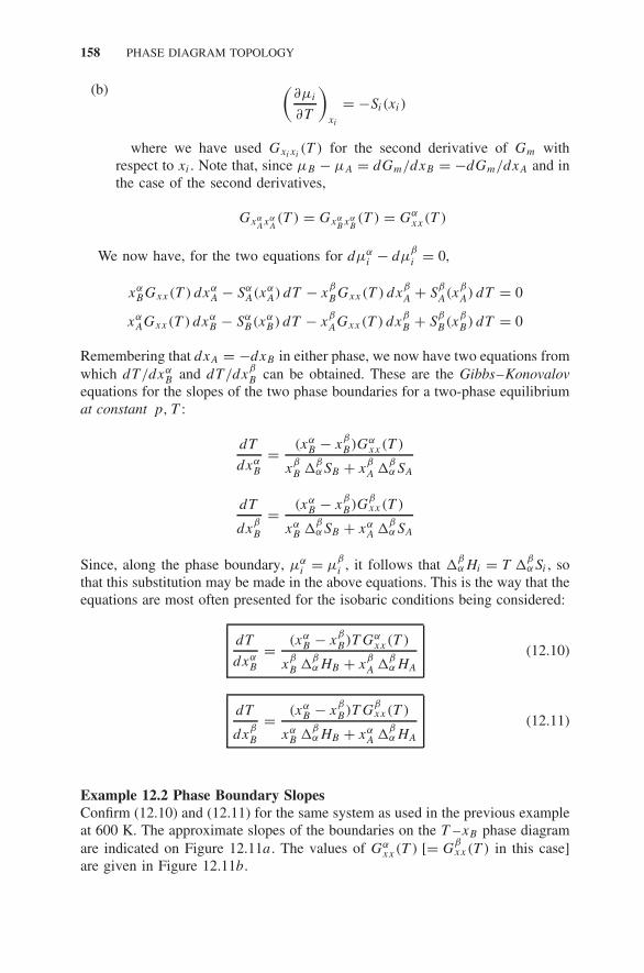
158 PHASE DIAGRAM TOPOLOGY
(b) (∂μi
∂T
)xi
= −Si(xi)
where we have used Gxixi(T ) for the second derivative of Gm with
respect to xi . Note that, since μB − μA = dGm/dxB = −dGm/dxA and inthe case of the second derivatives,
GxαAxα
A(T ) = Gxα
BxαB(T ) = Gα
xx(T )
We now have, for the two equations for dμαi − dμ
β
i = 0,
xαBGxx(T ) dxα
A − SαA(xα
A) dT − xβ
BGxx(T ) dxβ
A + Sβ
A(xβ
A) dT = 0
xαAGxx(T ) dxα
B − SαB(xα
B) dT − xβ
AGxx(T ) dxβ
B + Sβ
B(xβ
B) dT = 0
Remembering that dxA = −dxB in either phase, we now have two equations fromwhich dT /dxα
B and dT /dxβ
B can be obtained. These are the Gibbs–Konovalovequations for the slopes of the two phase boundaries for a two-phase equilibriumat constant p, T :
dT
dxαB
= (xαB − x
β
B)Gαxx(T )
xβ
B �βαSB + x
β
A �βαSA
dT
dxβ
B
= (xαB − x
β
B)Gβxx(T )
xαB �
βαSB + xα
A �βαSA
Since, along the phase boundary, μαi = μ
β
i , it follows that �βαHi = T �
βαSi , so
that this substitution may be made in the above equations. This is the way that theequations are most often presented for the isobaric conditions being considered:
dT
dxαB
= (xαB − x
β
B)T Gαxx(T )
xβ
B �βαHB + x
β
A �βαHA
(12.10)
dT
dxβ
B
= (xαB − x
β
B)T Gβxx(T )
xαB �
βαHB + xα
A �βαHA
(12.11)
Example 12.2 Phase Boundary SlopesConfirm (12.10) and (12.11) for the same system as used in the previous exampleat 600 K. The approximate slopes of the boundaries on the T –xB phase diagramare indicated on Figure 12.11a . The values of Gα
xx(T ) [= Gβxx(T ) in this case]
are given in Figure 12.11b.

THE GIBBS–KONOVALOV EQUATIONS 159
The slopes given in the figure are only approximate:
dT
dxαB
= (0.0134 − 0.6967)2.989 × 10⁵
0.6967(−32.85) − 0.3033(−9.807)= +10,252
dT
dxβ
B
= (0.0134 − 0.6967)0.272 × 10⁵
0.0134(−32.85) − 0.9866(−9.807)= −2011
12.4.3 Some Applications of Gibbs–Konovalov Equations
We may now consider the application of (12.8) and the Gibbs–Konovalovequations, (12.10) and (12.11), in order to explain the slopes of phase boundarieson both T –μi and T –xi phase diagrams. We concentrate on the featuresillustrated in the hypothetical phase diagram shown in Figure 12.12.
We use, as is apparent from Figure 12.11b, that, in the infinitely dilute solu-tions, Gxx → ∞. At other compositions, it may be either positive or negative.We have previously noted that this second derivative is zero at a critical point.
1. Congruent and Critical Points At both congruent and critical points (thepoints indicated by 1 in Fig. 12.12), xα
B = xβ
B , so it follows, from (12.8), (12.10),and (12.11), that
dT
dμB
= dT
dxαB
= dT
dxβ
B
= 0
At a liquid/solid intermediate-phase transformation, both the liquidus and solidushave zero slope at the actual congruent point. Although it may appear that thecongruent point in Figure 12.8 is quite sharp, it must actually be rounded. Thiscan be demonstrated through the use of appropriate modeling equations for the
. .
0.0 0.2 0.4 0.6 0.8 1.0400
800
1200
dT/dx ~ −2000dT/dx ~ +10,000
A BxB
T/K
(a)
xB
0
10,0000
20,0000
30,0000
40,0000
50,0000
Gxx
xB
= .0134
Gxx = 2.989 × 10⁻⁵
xB
= .6967
Gxx = 0.272 × 10⁻⁵
A B0 10.2 0.4 0.6 0.8
(b)
Figure 12.11 Phase boundary slopes and values of Gxx at 600 K for system considered:(a) slopes of T –xi phase diagram; (b) Gxx at phase boundaries.
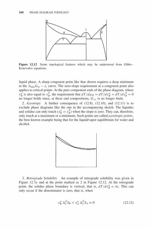
160 PHASE DIAGRAM TOPOLOGY
Figure 12.12 Some topological features which may be understood from Gibbs–Konovalov equations.
liquid phase. A sharp congruent point like that shown requires a deep minimumin the �mixGm − xi curve. The zero-slope requirement at a congruent point alsoapplies to critical points. At the pure component ends of the phase diagram, wherexα
B is also equal to xβ
B , the requirement that dT /dμB = dT /dxαB = dT /dx
β
B = 0no longer holds since, at these end compositions, Gxx is no longer finite.
2. Azeotropy A further consequence of (12.8), (12.10), and (12.11) is toexclude phase diagrams like the one in the accompanying sketch. The liquidusand solidus can only touch (xα
B = xβ
B ) when the slope is zero. They can, therefore,only touch at a maximum or a minimum. Such points are called azeotropic points ,the best known example being that for the liquid/vapor equilibrium for water andalcohol.
3. Retrograde Solubility An example of retrograde solubility was given inFigure 12.7a and at the point marked as 2 in Figure 12.12. At the retrogradepoint, the solidus phase boundary is vertical, that is, dT /dxα
B = ∞. This canonly occur if the denominator is zero, that is, when
xαB �
β
I SB + xαA �
β
I SA = 0 (12.12)

THE GIBBS–KONOVALOV EQUATIONS 161
4. Inflection Points At the critical point Gαxx = 0 so that, in the neighborhood
of this critical point, Gαxx ≈ 0, and since, from (12.10) and (12.11)
dT
dxB(s)∝ Gxx(s)
it follows that if the solidus is fairly close to the critical point for the solid-statemiscibility gap as in the case of the points marked 1 and 4 in Figure 12.12 andin Figure 12.7b for the (Au,Pt) system, then
dT
dxαB
≈ 0
that is, under these conditions, an inflection point will occur in the solidus (thesolidus can never be horizontal except at an azeotropic point). An accompanyinginflection point in the liquidus is not necessary—this would require Gxx(l) ≈ 0,which would only occur if the liquid phase was itself close to giving rise to phaseseparation.
5. Dilute Solutions For xB → 0, xA → 1, we can take the ideal entropy sothat Gα
xx → RT/xαB . Under these conditions, the Gibbs–Konovalov equations
simplify to
dT
dxαB
= (xαB − x
β
B)RT
xαB �
βαSA
(12.13)
dT
dxβ
B
= (xαB − x
β
B)RT
xβ
B �βαSA
(12.14)
If we invert these and subtract,
dxαB
dT− dx
β
B
dT= �
βαSA
RT(12.15)
T
xB

162 PHASE DIAGRAM TOPOLOGY
If the α phase is the low-temperature phase, then �β
I SA will be positive, whichmeans that the difference in the reciprocal slopes of the coexistence in verydilute solution, (12.15), must be positive. If both are positive, say, dT /dxα
B = 2and dT /dx
β
B = 4, then the difference of the reciprocals is 12 − 1
4 = 14 . If both
are negative, say, dT /dxαB = −4 and dT /dx
β
B = −2, then the difference of thereciprocals is − 1
4 + 12 = 1
4 . But if one is positive and the other negative, saydT /dxα
B = −2 and dT /dxβ
B = 4, then the difference of the reciprocals is − 12 −
14 = − 3
4 , which is negative. This means that a phase diagram like the one in thesketch on page 161, where the liquidus on the A-rich end has a positive slopewhile the solidus has a negative slope, is impossible.
Summary The computer calculation of phase diagrams ensures that all thermo-dynamic requirements are met, that is, there are no errors in calculated phase dia-grams due to any failure in meeting the requirements of the phase rule, Schreine-maker’s rules, or the Gibbs–Konovalov equation. Nevertheless, many publishedphase diagrams have not been computed but are based on experimental results.They are thus prone to contain mistakes which are thermodynamically incorrect.
EXERCISES
12.1 The hypothetical phase diagram in Figure 12.13 contains many mistakeswhich are indicated by a letter. For each of these mistakes, list the typeof error in terms of its failure to be in line with the requirements of:
A
A
Bmole fraction B
Tem
pera
ture
b + ga + b
a + g
b
g
g
b+
a
a
e
d
m
x1
x2
XM
N
KL
B
D
L
Q
Y
G F
E
PR
JZ
o
I
C
H l
ST
Figure 12.13 Hypothetical phase diagram containing many topological errors.

EXERCISES 163
(i) The phase rule(ii) Schreinemakers’s rules
(iii) The Gibbs–Konovalov’s equation
12.2 Using the data below, calculate the phase diagram, evaluate the retrogradepoint, and confirm (12.12).
Be sure to use the same reference state for both phases when evaluatingthe entropy difference terms in (12.12).
μ◦,lA = μ
◦,lB = 0
μ◦,sA − μ
◦,lA = −22,500 + 15T J mol−1
μ◦,sB − μ
◦,lB = −7500 + 15T J mol−1
GE(l) = 10,000xAxB J mol−1
GE(s) = 15,000xAxB J mol−1


13 Solution Phase Models I:Configurational Entropies
Up until this point we have discussed the representation of the thermodynamicproperties of solution phases by using polynomials such as the Redlich–Kisterequation:
GE = xAxB [L0 + L1(xA − xB) + L2(xA − xB)2 . . .]
where the parameters Li may be temperature dependent. Such representationsdo, however, have some limitations:
(a) Fitting sparse experimental results to polynomials, particularly high-orderpolynomials, can be dangerous, particularly when it is necessary to extrap-olate the equations outside the region (of composition and/or temperature)where the fitting was carried out.
(b) The experimental results for some phases are unsuited to polynomial rep-resentation. This is particularly true of some intermediate phases, whichare formed when there is a strong chemical affinity between the alloy-ing elements involved. These phases progress from being fully ordered atlow temperatures, as illustrated schematically in Figure 13.1b, to beingdisordered at high temperatures (as in Fig. 13.1a). As we will see later,�mixHm changes quite markedly with composition and temperature dueto the ordering process, and not in the simple way that can be representedreliably by a Redlich–Kister type of equation.
(c) To date, we have been concerned only with substitutional alloys, assketched in Figures 13.1a and b. Sometimes, however, we encounterinterstitial solid solution phases, as represented in Figure 13.1c. In thelatter, the metal host atoms form one sublattice while the interstitial sites,formed within the metal atom sublattice, are occupied by the interstitialatoms. Since the metal atom cage must always be present to provide theinterstitial sites, it is clear that this type of solution cannot exist acrossthe whole composition range from one pure element to the other, as itdoes in the case of a substitutional solution. A (mathematical) modelingequation like the Redlich–Kister equation can be modified from that
Materials Thermodynamics. By Y. Austin Chang and W. Alan OatesCopyright 2010 John Wiley & Sons, Inc.
165

166 SOLUTION PHASE MODELS I: CONFIGURATIONAL ENTROPIES
(a) (b)
(c)
Figure 13.1 Some different types of lattice models: (a) disordered substitutional phase,all sites available for all types of atoms; (b) fully ordered intermediate phase, separatesublattices for each type of atom; (c) interstitial solution phase, interstitial atoms occupytheir own sublattice.
used for substitutional solution phases as long as the interstitial solidsolution is disordered. But interstitial solid solutions can also undergoordering transitions and, again, a polynomial representation of theirthermodynamic properties is unsatisfactory.
It is for these reasons that we need to supplement a wholly mathematicalapproach to modeling equations, by introducing a little more physics into themodeling process with the hope of obtaining a better representation of the exper-imental (or theoretically calculated) results. In particular, we wish to be able tohandle sublattice phases of either the interstitial solution- or intermediate-phasetype and we particularly wish to be able to have a model which will lead to arepresentation which is suitable for those phases which undergo order/disordertransitions.
The physicochemical factors which contribute to solid solution and compoundformation between metals were summarized by Hume-Rothery in the 1930s, whofound the following atomic properties to be important:

SOLUTION PHASE MODELS I: CONFIGURATIONAL ENTROPIES 167
(i) Atomic Size Factor If the atomic radii of the elements differ by morethan ≈15%, solid solution formation is not favored.
(ii) Crystal Structure Factor For appreciable solid solubility, the crystalstructure of the component metals must be the same.
(iii) Electrochemical Factor The greater the electronegativity differencebetween the components, the greater the tendency to form intermetalliccompounds.
(iv) Valence Factor For extensive solid solubility, the components shouldhave the same valences. A metal will dissolve another metal of highervalency more than it will one of lower valency.
Hume-Rothery discovered these rules from the relatively small amount of infor-mation available to him some 80 years ago. Very large databases are now availablefor metal properties, and when these are linked with a machine learning system(data mining), predictions can be made about the structural and stability propertiesof alloys. It is interesting to note that the atomic properties used in correlating theinformation on alloy phase stability in one such large database are very similarto the ones used by Hume-Rothery: size, atomic (Mendeleev) number, valenceelectron, electrochemical, angular-valence orbital, and cohesive energy factors.
In obtaining such correlations, it is being assumed that alloy properties can beunderstood wholly in terms of the component atomic properties, which would seemto be a little optimistic. Although the elemental properties clearly give some clues asto the important factors which contribute to alloy thermodynamic mixing properties,they cannot lead to what is required in the present instance, namely, an analyticalexpression for these properties as a function of temperature and compositions.Recent first-principles calculations have been quite successful in calculating totalenergies for binary compounds at 0 K. Some improvements are still required,however, in the calculation of high-temperature Gibbs energies and in extending thecalculations to disordered phases. As a result, a less ambitious phenomenologicalor empirical approach to solution-phase modeling is still necessary. Some physicsis introduced but the model parameters are obtained, not by calculation, but bytheir optimization with respect to the available experimental or calculated resultsto give the best description of the experimental Gibbs energies. This empiricalapproach will probably be necessary for some years to come, particularly sinceit is multicomponent alloys which are of primary technological significance.First-principles calculations for these would seem some considerable way off.
In order to obtain the desired analytical representation, we simplify things byassuming that the Gibbs energy of mixing can be separated additively into:
(i) Configuration independent (abbreviation conf indep) contributions. Thesedepend only on the alloy composition and not on how the componentatoms are distributed in the alloy; that is, these contributions are iden-tical for the fully ordered and for the random solution. A large part ofany atomic size mismatch contributions and some part of electronic bandcontributions may fall into this category.

168 SOLUTION PHASE MODELS I: CONFIGURATIONAL ENTROPIES
(ii) Configuration dependent (abbreviation conf) contributions. These dodepend on how the component atoms are distributed in the alloy. Anordered alloy has different properties from a disordered alloy from thesecontributions. In other words, these are local environment effects . Apartfrom the mixing properties themselves, we might expect that at least partof the vibrational properties of an atom will be sensitive to the localenvironment.
With this assumption of the two contributions being independent of oneanother, we can write the solution-phase Gibbs energy as follows:
Gm = Gconfm + Gconfindep
m (13.1)
It should be emphasized that this factorization of Gm can be an oversimplificationin that the the two contributions may be coupled .
Now Gconfm = H conf
m − T Sconfm and here we will make another big assumption,
namely, that these two contributions to Gconfm can be treated independently, so
that we may now write
Gm = [H conf
m − T Sconfm
]+ Gconfindepm
In the remainder of this chapter we concentrate on the calculation of Sconfm for
the three types of solution phase shown in Figure 13.1.
13.1 SUBSTITUTIONAL SOLUTIONS
We have previously met the Boltzmann equation, applicable to systems of fixedenergy:
S = kB loge W (13.2)
This equation indicates that we can evaluate the entropy from a calculation of thenumber of microstates available to a system. For any solid substance the availablestates will include nuclear, electronic (including nuclear and electronic spin), andvibration energy levels— thermal disorder. For the moment, however, we areconcerned only with configurational disorder—the more numerous the possibleways of arranging the atoms on a lattice, the higher the configurational entropy.
In a substitutional solid solution, all the lattice sites are considered to beavailable for occupation by every atom. If the energy of mixing is taken to havethe constant value of zero, it is then straightforward to calculate the number ofmicrostates for a random binary solution. This random approximation is referredto as the point, zeroth, or regular solution approximation. When NA and NB
particles are distributed randomly on Ns = NA + NB sites, then
W = Ns!
NA! NB !(13.3)

INTERMEDIATE PHASES 169
Use Stirling’s approximation for the factorial of a large number,
loge x! ≈ x loge x − x
we obtain from (13.2) and (13.3)
Sconf
kB
= Ns loge Ns − NA loge NA − NB loge NB (13.4)
Since W = 1 for the pure components, the entropy for the random solution isthe same as integral mixing entropy per mole of sites for the alloy, �mixS
confm :
−�mixSconfm
NskB
= xA loge xA + xB loge xB random subst. soln. (13.5)
The partial molar entropies can be obtained by differentiating (13.4):
SconfA
kB
=(
∂S/kB
∂NA
)NB
= loge Ns − loge NA = − loge xA
Using i to represent any component, the partial molar entropy of mixing isgiven by
−�mixSconfi
R= loge xi random subst. soln. (13.6)
As we have seen previously, such a random substitutional alloy with a zeroenergy of mixing will obey Raoult’s law.
13.2 INTERMEDIATE PHASES
Consider the simple case where the intermediate phase can be described as beingcomprised of only two sublattices, similar to that shown schematically in Figure13.1b. The usual notation for representing such an intermediate phase is
(A,B)f α : (B,A)f β
where A is the predominant species on the first sublattice and B on the secondsublattice.
We will use i to refer to any sublattice constituent and (j) to refer to anysublattice. Thus f (j), which is the fraction of the total sites which are on sublattice(j), is given by
f (j) = N(j)s
Ns
where∑(j)
f (j) = 1

170 SOLUTION PHASE MODELS I: CONFIGURATIONAL ENTROPIES
with N(j)s being the number of sites on sublattice (j) and Ns the total number
of sites.It is also useful to define the sublattice mole fraction as
y(j)
i = N(j)
i
N(j)s
The relation between the sublattice mole fractions and the mole fraction can beobtained as follows:
xi = Ni
Ns
= Nαi + N
β
i
Ns
= f αNαi
Nαs
+ f βNβ
i
Nβs
or, in general,
xi =∑(j)
∑i
f (j)y(j)
i (13.7)
Let us now obtain the expression for the mixing entropy for this case. Analogousto the disordered alloy, we will assume that there is random mixing on eachindividual sublattice. This is known as the Bragg–Williams (BW) approximation.Under these circumstances, the energy of mixing is fixed at constant composition,so that the Boltzmann equation can be applied.
The equation for the thermodynamic probability is now given by
W =[
Nαs !
NαA! Nα
B !× N
βs !
Nβ
A! Nβ
B !
](13.8)
From the Boltzmann equation and using the Stirling approximation and general-izing,
Sconf
kB
=∑(j)
[N(j)
s loge N(j)s −
∑i
N(j)
i loge N(j)
i
](13.9)
=∑(j)
∑i
N(j)
i loge y(j)
i (13.10)
Dividing by Ns to obtain the entropy per lattice site,
− Sconf
kBNs
=∑(j)
f (j)∑
i
y(j)
i loge y(j)
i (13.11)

INTERMEDIATE PHASES 171
Since W = 1 for the pure elements, this is also the molar mixing entropy:
−�mixSconfm
R=∑(j)
f (j)∑
i
y(j)
i loge y(j)
i BW approx. (13.12)
The partial molar entropies are given by
−�mixSconfi
R=∑(j)
f (j)∑
i
loge y(j)
i BW approx. (13.13)
These expressions have the correct high-temperature limit of giving the sameanswer as for the random substitutional solid solution. When there is only onesublattice,f (j) = 1, and then, from (13.7), y
(j)
i = xi , and we recover (13.5) from(13.9).
We can also readily evaluate (13.12) and (13.13) for the BW most orderedstate.
At the stoichiometric composition, AB, and in the fully ordered condition,the first sublattice is occupied by A atoms only and the second sublattice byB atoms only, that is, yα
B = 0, yβ
B = 1. On moving to the B-rich side, we canonly increase yα
B since the second sublattice is already filled. The variation ofyα
B and yβ
B as a function of xB , over the whole composition range, is shown inFigure 13.2. It can be seen that, for this most ordered state,
yαB = 0 y
β
B = 2xB for xB ≤ 12
yαB = 2xB − 1 y
β
B = 1 for xB > 12
Similar equations exist for yA and we can then substitute these values for thesublattice mole fractions into (13.12) and (13.13) in order to calculate the integraland partial molar mixing entropies for this most ordered state. The followingrelations are obtained for the integral and partial quantities (for component B):
−�mixSconfm
R=
12 [2xB loge(2xB) + (1 − 2xB) loge(1 − 2xB)] xB < 1
2 (13.14)
12 [2xA loge(2xA) + (1 − 2xA) loge(1 − 2xA)] xB > 1
2 (13.15)
−�mixSB
R= loge 2xB − 1
2 loge(1 − 2xB) xB < 12 (13.16)
12 loge(2xB − 1) xB > 1
2 (13.17)
The results for the integral and partial quantities for both the random and mostordered states are shown in Figures 13.3a and 13.3b, respectively. These representthe low- and high-temperature limits for these quantities.

172 SOLUTION PHASE MODELS I: CONFIGURATIONAL ENTROPIES
0.0 0.2 0.4 0.6 0.8 1.0
Sub
latti
ce m
ole
frac
tions
0.0
0.2
0.4
0.6
0.8
1.0
A
yb
B ya
B
xB B
Figure 13.2 Variation of sublattice mole fraction with composition for BW most orderedstate in two-sublattice intermediate phase.
0.0 0.2 0.4 0.6 0.8 1.0−20
−10
0
10
20
Random
Mostordered
Mostordered
Δ mixS
B/J
K−1
mol
−1
A BxB
0.0 0.2 0.4 0.6 0.8 1.0
Δ mixS
m/J
K−1
mol
−1
0
1
2
3
4
5
6
7
Random
Mostordered
A BxB
(a) (b)
Figure 13.3 Integral and partial molar configurational mixing entropies for two-sublattice intermediate phase in BW most ordered state: (a) integral �mixSm; (b) partial�mixSB .
13.3 INTERSTITIAL SOLUTIONS
Now consider a binary interstitial solid solution with two sublattices: one, α,occupied by the metal atoms, M, and another, β, formed by the spaces lyingbetween the metal atoms and in which an element, I, occupies some fraction ofthese interstitial sites. This model can be represented by the following notation:
(M)f α : (I, Va)f β
where Va represents a vacancy on the interstitial sublattice.
INTERSTITIAL SOLUTIONS 173
We may go straight to using (13.9) and consider the random mixing of atomsand vacancies on the interstitial sublattice:
Sconf
kB
= Nβs loge Nβ
s − [Nβ
I loge Nβ
I + NβVa loge N
βVa] (13.18)
We may eliminate NVa and express S in terms of only the chemical componentsby using N
βVa = N
βs − N
β
I :
Sconf
kB
= Nβs loge Nβ
s −[N
β
I loge Nβ
I + (Nβs − N
β
I ) loge(Nβs − N
β
I )]
(13.19)
and can express this, per mole of interstitial sites, by dividing by Nβs :
− Sconf
kBNβs
=[y
β
I loge yβ
I + (1 − yβ
I ) loge(1 − yβ
I )]
(13.20)
which has the same analytical form as the equation for a random substitutionalsolid solution.
Equation (13.9) can be differentiated to obtain the partial quantity for theinterstitial element I. Per atom,
SconfI
kB
=(
∂Sconf/kB
∂NI
)NM
= − loge Nβ
I + loge(Nβs − N
β
I )
= − loge
(y
βI
1 − yβI
)(13.21)
and for the partial molar quantity,
SconfI
R= − loge
(y
β
I
1 − yβ
I
)(13.22)
In order to obtain the partial quantity for M we must express Nβs in terms of
NM . Let Nβs = ζNM , where ζ is the number of interstitial sites per metal atom
[this means that f α = 1/(1 + ζ ) and f β = ζ/(1 + ζ )]. Using this in (13.18) anddifferentiating, per atom,
SconfM
kB
=(
∂Sconf/kB
∂NM
)NI
= loge ζNM − loge(ζNM − Nβ
I )
= −ζ loge(1 − yβI ) (13.23)

174 SOLUTION PHASE MODELS I: CONFIGURATIONAL ENTROPIES
0.0 0.2 0.4 0.6 0.8 1.0−20
−10
0
10
20
SMSI
S/J
K−1
mol
−1
M xI I
Figure 13.4 Partial molar entropies of mixing for random interstitial solid solution withζ = 1.
and for the partial molar quantity,
SconfM
R= −ζ loge(1 − y
β
I ) (13.24)
Note that, even though the metal sublattice remains totally unaffected by themixing process, which occurs only on the interstitial sublattice, there is a changein its partial molar property with composition.
The partial molar entropies for this random interstitial solid solution are shownin Figure 13.4a for the case where ζ = 1 (which corresponds with the octahedralinterstitial sites in the fcc lattice). The partial molar quantity for the interstitialcomponent goes to plus and minus infinity, which is quite different behavior fromthat for the substitutional alloy. It is clear that a random interstitial solution willnot be expected to obey Raoult’s law; that is, obeying Raoult’s law is not anappropriate definition of an ideal solution for an interstitial solid solution.
A random interstitial solid solution whose partial molar configurational ent-ropies are given by the above equations is said to form a Langmuir ideal solution.
We should note again that a thermodynamicist may define an ideal solu-tion in any way that he or she wants. We have now met two different typesand definitions: Raoultian and Langmuir ideal solutions. The major point is thateach is defined to be a limit to which real solutions of that type may approach.A Raoultian ideal solution is appropriate for substitutional phases and a Langmuirideal solution for interstitial phases.
EXERCISES
13.1 Starting from the Boltzmann equation, (13.2), derive �mixSconfm for a ran-
dom solution mixture of (Fe, Ni)0.75 : (C, Va)0.25.

EXERCISES 175
13.2 Derive the analogous equations to (13.16) and (13.17) for component A.
13.3 Derive integral and partial expressions for the mixing entropy in a four-sublattice model for the most ordered and random solutions. Provide plotsof the results.
13.4 Titanium monocarbide possesses the NaCl structure but, unlike NaCl, TiCexists over a wide range of homogeneity, varying from 32 mol % C toa maximum of 48.8 mol % C. using the sublattice notation, write downthe appropriate model for this phase and calculate the Bragg–Williamsentropy of mixing of this carbide having 46 mol % C. Give your resultsin both joules per mole of atoms and per mole of Ti.


14 Solution Phase Models II:Configurational Energy
In the previous chapter we introduced a factorization of the Gibbs energy inorder to consider a basic thermodynamic model for a substitutional alloy phase.In this model, the experimental (or calculated) results for the Gibbs energy offormation of an alloy are assumed to contain separable configuration-dependentand configuration-independent contributions (the rationale behind this assumptionis discussed in chapter 16):
�mixGm = �mixHconfm − T �mixS
confm + �mixG
conf indepm
We then calculated the configurational mixing entropy for this model for twoextremes of a sublattice phase alloy—the most ordered state and the randomstate. Under these circumstances we could use the Boltzmann equation.
In this chapter, we turn our attention to the enthalpy of mixing, �mixHconfm .
We will also make the additional assumption that the configurational part of theenergy is volume independent so that �mixH
confm is equal to the energy of mixing,
�mixUconfm .
The aim is to express �mixUconfm in a form which depends on the atomic
distribution, that is, in terms of local environment effects. In the simplest typeof ordered alloy, comprised of two sublattices, the nearest neighbors of A atomsare the maximum number possible of B atoms. In some lattices, however, thenearest neighbors in the fully ordered state cannot all be B atoms. In an fcc alloy,for example, it is not possible to arrange for all nearest neighbors to be unlikeatoms and obtain an ordered structure. This is called frustration . In a disorderedalloy there will be a significant proportion of like-atom neighbors with the actualratio of like and unlike depending on the temperature and composition and thedegree of short-range order (SRO).
In almost all thermodynamic models of solid solution phases, the experimentalvalues for �mixH
confm are mapped onto the energy parameters of what is called an
Ising-like model . The original Ising model was for a lattice model of a ferromag-net in which the atomic magnetic moments (designated as up-spin or down-spin)were located on the lattice sites and interacted via constant pairwise exchangeenergies. There is a one-to-one correspondence between this model of a magnet
Materials Thermodynamics. By Y. Austin Chang and W. Alan OatesCopyright 2010 John Wiley & Sons, Inc.
177

178 SOLUTION PHASE MODELS II: CONFIGURATIONAL ENERGY
and that for a binary alloy, with the up-spin being equivalent to an A atom and adown-spin to a B atom. In order to extend the model by including the possibilityof energy representations other than only pair representations, the term Ising-likemodel is used.
In using an Ising-like model, it is usually assumed that the model energyparameters are configuration independent ; that is, we can apply the energyparameters derived from one configuration to other configurations in that alloy.We may, for example, use the information on �mixU
confm for the fully ordered sto-
ichiometric compound to calculate the Ising-like energy parameters and then usethese same parameters in order to calculate �mixU
confm for the partially ordered
nonstoichiometric phase or for the disordered phase.As will become apparent later, it should be emphasized that there is no unique
way of carrying out the energy mapping . This should make it clear that the derivedmodel energy parameters should not be confused with believing that they areactual chemical bonding energies. We are wanting to map the total energy insuch a way that it embraces only the near neighbors; that is, we are assumingthat the interactions outside a small circle of influence are substantially weakerthan those inside the circle.
14.1 PAIR INTERACTION MODEL
In order to illustrate, we will consider two examples. In the first, only one orderedphase is formed, at the composition AB. The configurational energy in the BWmost ordered state will vary with composition as shown in Figure 14.1.
mol fraction B
0.0 0.2 0.4 0.6 0.8 1.0
Con
figur
atio
nal e
nerg
y
−30
−25
−20
−15
−10
−5
0
A B
Figure 14.1 Configurational mixing energy for BW most ordered alloys in two-sublatticemodel.

PAIR INTERACTION MODEL 179
We consider a model comprising two sublattices only and assume that theseare of equal size. This is the same model considered in the previous chapters forthe calculation of the configurational mixing entropies and can be represented bythe notation
(A,B)0.5 : (B,A)0.5
With two sublattices of equal size there can only be one fully ordered stoichio-metric compound, AB. At 0 K for this stoichiometric alloy, all the A atoms areon one sublattice (1) and all the B atoms on the other (2). At higher temperatures,or with deviations from stoichiometry, antisite disorder excitation of the atomsoccurs (some of the atoms occupy the wrong sublattice). Eventually, at a suf-ficiently high temperature or deviation from stoichiometry, the A and B atomsbecome evenly distributed on both sublattices. At this stage there is only onelattice; that is, we have a substitutional solid solution. The phase has undergonean order/disorder transformation.
14.1.1 Ground-State Structures
The term ground-state structure is used to refer to the most stable structure at0 K. Even with just the two sublattices of equal size, it is possible to obtaindifferent structures at the stoichiometric composition AB. In the structures basedon the bcc lattice, two possibilities are shown in Figure 14.2—the occupationof the two sublattices is different in the two cases. It is clear, therefore, thatin our thermodynamic modeling, it is not sufficient to know only the stoichio-metric composition of the phase in order to be able to map the configurationalenergy onto an Ising-like model. We must also know the ground-state struc-ture of the alloy. It is obvious that, in Figure 14.2a , the B2 structure will bestable when the nearest neighbor pair interaction energy between unlike atoms,ε(1)AB < 0 dominates, while the B32 structure shown in Figure 14.2b will not
be stable under these conditions. Rather, it will be necessary to have ε(2)AB < 0
and with this second nearest neighbor interaction dominating in order for this
(a) (b)
Figure 14.2 (a) the B2 and (b) B32 ground-state structures in a bcc lattice. The dotsrepresent the A atoms and the crosses the B atoms.

180 SOLUTION PHASE MODELS II: CONFIGURATIONAL ENERGY
structure to become stable. But over what range of ε(2)AB/ε
(1)AB will the B2 struc-
ture be stable? To answer this question, we must evaluate which structure hasthe lower formation energy over all possible values of the ratio. The resultsfrom this kind of study can then be summarized in a phase stability map.Such maps, showing the various possible ground-state structures for differentratios of the pair interaction energies, are available for the fcc, hcp, and bcclattices.
We will simplify our two-sublattice model by considering nearest neighborinteraction mappings only. In the case of a bcc-based intermediate phase, thismeans that the compound AB has the B2 structure. As we have indicated, thisphase would remain stable if we took ε
(2)AB/ε
(1)AB to be other than zero. Different
values of ε(1)AB and ε
(2)AB could be selected to agree with the same �mixU
confm values,
a result which emphasizes that there is no unique mapping of the configurationalenergy onto an Ising-like model’s energy parameters.
14.1.2 Nearest Neighbor Model
As shown in Figure 14.3 for the two-dimensional equivalent lattice for the sub-lattice model being discussed, nearest neighbors reside on different sublattices.Examples of the four different types of inter-sublattice pairs in a binary alloy areshown. In our model we assume that the alloy’s configurational energy is beingmapped onto these nearest neighbor pair interactions only.
The molar configurational energy of the alloy, in any given atomic arrange-ment, can be expressed in terms of the average probabilities of the different typesof pairs and the pair energies, εPQ, whose values are to be determined. For abinary AB system, the alloy energy is
U alloym = 〈pAA〉εAA + 〈pAB〉εAB + 〈pBA〉εBA + 〈pBB〉εBB (14.1)
A
A
A
A
A
A
A
AB
B
B
B
B
BBBB
BB
B B
B B
B
BB A
B
A
AA
Figure 14.3 Two-dimensional two-sublattice model in which it is assumed that onlynearest neighbor interactions are present.

PAIR INTERACTION MODEL 181
where the angular bracketed terms refer to the mean probability of occurrence ofa particular type of pair.
Note that, since the dimensions of Um are per mole of sites, then the dimen-sions of the pair interaction energies used in (14.1) also refer to an energy permole of sites and not, for the moment, to an energy per mole of pairs.
For the mechanical mixture (or the fully segregated alloy or the composi-tion weighted sum) of the pure components in the same structure as that of theintermediate phase,
Umixtm = xAεAA + xBεBB (14.2)
The equations which relate the mole fractions to the average pair probabilitiesare
xA = 〈pAA〉 + 12 (〈pAB〉 + 〈pBA〉)
xB = 〈pBB〉 + 12 (〈pAB〉 + 〈pBA〉)
Note that, when these two equations are added, the sum of both the left-handand right-hand sides equals 1, as they should.
We can now rewrite the equation for the mechanical mixture as
Umixtm = [〈pAA〉 + 1
2 (〈pAB〉 + 〈pBA〉)] εAA
+ [〈pBB〉 + 12 (〈pAB〉 + 〈pBA〉)] εBB (14.3)
Subtracting (14.3) from (14.1) gives the mixing energy:
�mixUconfm = 〈pAB〉 [εAB − 1
2 (εAA + εBB)]
+ 〈pBA〉 [εBA − 12 (εAA + εBB)
]or
�mixUconfm = 1
2z (〈pAB〉 + 〈pBA〉) WAB (14.4)
where WAB = εAB − 1/2(εAA + εBB) is called the pair exchange energy and wehave taken WAB = WBA; that is, the pair exchange energy is assumed independentof the actual location of the A and B atoms.
Note that WAB is now expressed as the energy per mole of pairs by multiplyingthe previous energies per mole of sites by the number of pairs per site (= z/2,where z is the coordination number of the lattice; z = 4 in Fig. 14.3).
As we did with the mixing entropy, we can evaluate (14.4) for the two limitingcases considered in Chapter 13, namely, the BW most ordered and the randomsolution.

182 SOLUTION PHASE MODELS II: CONFIGURATIONAL ENERGY
The pair probability distributions for the BW most ordered state are shown inFigure 14.4a, where it can be seen that
〈pBA〉 = 0 all compositions
〈pAB〉 ={
2xB
2(1 − xB)
for xB ≤ 12
for xB > 12
〈pAA〉 ={
1 − 2xB
0
for xB ≤ 12
for xB > 12
〈pBB〉 ={
0
2xB − 1
for xB ≤ 12
for xB > 12
For the random solution case, we can use the binomial expansion to calculatethe probabilities:
〈pAB〉 = 〈pBA〉 = 〈pA〉〈pB〉 = xAxB
〈pAA〉 = x2A 〈pBB〉 = x2
B
AA AB
BA
1.0
1.0
0.8
0.8
0.6
0.6
0.4
0.4
0.2
0.0
0.20.0
A
(a) (b)
(c) (d)
xB B
Pro
babi
lity
BB
Random
BWmost ordered
−5
1.0
−10
0
0.8
−15
0.6
−20
0.4
−25
−300.20.0
A xB B
Δ mixU
m (
conf
)/kJ
mol
−1
Random
BWmost ordered
1.0
−10
0
0.8
−20
0.6
−30
0.4
−40
−50
0.20.0
A xB B
Δ mixU
B (
conf
)/kJ
mol
−1
AA
AB + BA
1.0
1.0
0.8
0.8
0.6
0.6
0.4
0.4
0.2
0.00.20.0
A xB B
Pro
babi
lity
BB
Figure 14.4 Pair probabilities and integral and partial molar configurational mixing ener-gies for BW most ordered and random states in two-sublattice model: (a) pair probabilitiesfor BW most ordered state; (b) pair probabilities for random state; (c) �mixUm for BWmost ordered and random states; (d) �mixUB for BW \newline most ordered and randomstates.

CLUSTER MODEL 183
The pair probability distributions for the random state are shown in Fig-ure 14.4b.
Substitution of these equations for the two limiting cases into (14.4) gives thefollowing mixing energies:
�mixUconfm =
⎧⎪⎨⎪⎩
zWABxB BW most ordered, xB ≤ 12
zWABxA BW most ordered, xB > 12
zWABxAxB random solution, all compositions
The partial molar properties for the most ordered and random mixing limits maynow be obtained from these integral quantities. For the component B,
�mixUconfB =
⎧⎪⎪⎨⎪⎪⎩
zWAB BW most ordered, xB ≤ 12
0 BW most ordered, xB > 12
zWABx2A random solution, all compositions
It can be seen that the mixing energy for the disordered (random) state is ofexactly the same form as that already met when using the Redlich–Kister repre-sentation with L0 = zWAB . Thus we have one possible model which physicallymodels the behavior of this empirical modeling equation. It would be wrong, how-ever, to believe that the only model to yield this result is this nearest neighborpair interaction model.
Both �mixUconfm and �mixU
confB for these two limiting cases are shown in
Figures 14.4c and 14.4d . It can be clearly seen that, as the temperature isincreased in going from the most ordered state to the random disordered state,there is a decrease in the magnitude of �mixU
confm , even though we have used
the same temperature- (and composition-) independent energy parameter in thisIsing-like model.
Note the physical inconsistency in our having used a model which possessesa finite mixing energy when we have assumed a random mixing entropy. Finitepair interaction energies will give rise to SRO, which will in turn lead to both amodified mixing energy and entropy. The BW model for sublattice phases and thepoint, zeroth, or regular solution approximation for substitutional solid solutionsignores this fact.
14.2 CLUSTER MODEL
The two-sublattice model discussed above can be applied to ordered phases whosestoichiometry is different from f α = f β = 1
2 . Similar arguments and derivationsto those used above could be equally well applied to, for example, A3B, but,in every case, �mixU
confm for the most ordered state will look similar to that

184 SOLUTION PHASE MODELS II: CONFIGURATIONAL ENERGY
shown in Figure 14.1, that is, with a single sharp minimum at the stoichiometriccomposition.
Two types of complication can arise, however, which suggest that improve-ments to our two-sublattice model may sometimes be necessary:
(a) If structure is to be taken into consideration, it may be necessary to intro-duce interactions between more distant neighbors than just the nearest. Thecase of bcc alloys was mentioned earlier—the B2 structure is expectedwhen ε
(2)AB/ε
(1)AB is small but the B32 structure is expected to be stable when
it is large.(b) Ordered phases can form at more than one composition from the same
parent disordered phase. In this case �mixUconfm for the most ordered state
will look like that shown in Figure 14.5. Here, there are three orderedphases to consider, A3B, AB, and AB3. It can be seen that there is only oneminimum in this curve, with inflexions in the curve occurring at the otherordered phase compositions. The classic example of this kind of behavioris found in the Au–Cu system where the disordered fcc parent phase givesrise to ordered phases at the Au3Cu, CuAu, and Cu3Au compositions.
In order to take these points into consideration we will use a four-sublattice modelinstead of our previous two-sublattice model. The notation for this sublatticemodel is
(A, B)0.25 : (A, B)0.25 : (A, B)0.25 : (A, B)0.25
0.0 0.2 0.4 0.6 0.8 1.0
Con
figur
atio
nal e
nerg
y
−30
−25
−20
−15
−10
−5
0
A BxB
Figure 14.5 Configurational mixing energy for fully ordered alloys in four-sublatticemodel.

CLUSTER MODEL 185
Figure 14.6 Nearest neighbor tetrahedron cluster in fcc lattice.
The four near neighbor sites form a tetrahedron cluster in both the fcc and bccstructures. In the fcc lattice the six tetrahedron edges are the nearest neighbors,as illustrated in Figure 14.6. In the bcc lattice, on the other hand, the nearestand next nearest neighbors form an irregular tetrahedron, as is apparent fromFigure 14.2.
In the cluster model, the alloy’s configurational energy is given by
U alloym =
5∑i=1
piεi (14.5)
where the εi are the cluster energies per site.Just as in the case of the pair approximation, where we used WAB = WBA,
we will assume that the energy of a cluster depends only on the number of thevarious participating atoms and not on their arrangement , for example, εABBA =εBAAB = · · · = εA2B2 . This means that, in a binary system with a 4-point cluster,there are only 5 independent alloy cluster energies to consider instead of the 16,were we to consider the influence of atom arrangements on the cluster energiesas well.
As we did for the pair approximation model, we can write the equation forthe mechanical mixture:
Umixtm = xAεA4 + xBεB4 (14.6)
and use the relation between the mole fractions and the cluster probabilities (notethat both sides sum to unity):
xA = 〈pA4〉 + 34 〈pA3B〉 + 1
2 〈pA2B2〉 + 14 〈pAB3〉 (14.7)
xB = 14 〈pA3B〉 + 1
2 〈pA2B2〉 + 34 〈pAB3〉 + 〈pB4〉 (14.8)
The cluster probabilities for the most ordered and the random states are shownin Figures 14.7a and 14.7b, respectively.

186 SOLUTION PHASE MODELS II: CONFIGURATIONAL ENERGY
In the case of the pair cluster in the two-sublattice model, there was no pos-sibility of the energy being shared between the clusters. This is not the case,however, in the case of tetrahedron clusters in the fcc lattice. It is possible toclosely pack the tetrahedra so that they share edges or to loosely pack them ina different way so that there is no sharing of edges, but only of corners. In thetwo cases, the number of clusters per site, γ , and the energy assigned to a sin-gle cluster must differ but the resulting total energy must be the same in bothcases.
The mixing energy is given by the difference of (14.5) and (14.3) while using(14.7):
�mixUconfm = γ [〈pA3B〉VA3B + 〈pA2B2〉VA2B2 + 〈pAB3〉VAB3 ] (14.9)
0.00 0.25 0.50 0.75 1.00
Pro
babi
lity
0.0
0.2
0.4
0.6
0.8
1.0
A3B A2B2 AB3
A4 B4
A BxB
0.0 0.2 0.4 0.6 0.8 1.0
Pro
babi
lity
Sm
/R
0.0
0.2
0.4
0.6
0.8
0.0
0.2
0.4
0.6
0.8
1.0
A4 B4
A3B AB3A2B2
A BxB
0.0 0.2 0.4 0.6 0.8 1.0A BxB
0.0 0.2 0.4 0.6 0.8 1.0A BxB
Random
BWmost ordered
−10
0
−20
−30
Δ mixU
mconf
/kJ
mol
−1 Random
Most ordered
(a) (b)
(c) (d)
Figure 14.7 Cluster probabilities and configurational mixing energies and entropies forBW most ordered and random states in four-sublattice model: (a) cluster fractions in BWmost ordered state; (b) cluster fractions in random state; (c) �mixUm for BW most orderedand random states; (d) �mixSm for BW most ordered and random states.

CLUSTER MODEL 187
where VAB3 = εAB3 − (1/4εA4 + 3/4εB4), and so on. These cluster exchangeenergies are analogous to the pair exchange energies in the pair approxima-tion used previously. Because of the introduction of the γ conversion factor (thenumber of clusters per site), the cluster energies are now in units of energy percluster.
We can use the results for the most ordered and for the random states shown inFigures 14.7a and 14.7b together with (14.9) to obtain �mixU
confm for these two
limiting cases. For the most ordered case, the values between the stoichiometriccompounds are simply the linear joins, while, for the random solution case,�mixU
confm is obtained from a binomial expansion and is given by
�mixUconfm = γ (4x3
AxBVA3B + 6x2Ax2
BVA2B2 + 4xAx3BVAB3) (14.10)
The calculated integral energies and entropies of mixing for the most orderedand random alloys are shown in Figures 14.7c and 14.7d , respectively.
If desired, it is possible to continue to express the cluster energies in terms ofthe near neighbor pair interaction energies. For the fcc-based lattice and assumingthat WAB is constant, it is easy to see that, at the AB composition, �mixU
confm =
4WAB , whereas at the A3B and AB3 compositions, �mixUconfm = 3WAB .
However, if we use the values for �mixUconfm given in Figure 14.5, we would
find that there are three different values for WAB :
A3B: WAB = −22
3= −7.33 kJ
AB: WAB = −25
4= −6.25 kJ
AB3: WAB = −19
3= −6.33 kJ
In this situation, we might accept the volume (or composition) dependence ofWAB or, alternatively, use the cluster energies.
Summarizing, any energy representation adopted should give rise to theobserved ground-state structures for that system.
The models discussed have used the following important assumptions:
• Additive separation of the Gibbs energy into configuration-dependent andconfiguration independent contributions.
• The configuration-dependent energy is volume independent. This may bethe weakest of the assumptions used.
• The cluster energy parameters are temperature and composition independent.• The parameters of the Ising-like model can be used for all configurations.• The energies of clusters, including pairs, depend only on the number and not
on the arrangement of the different types of atoms, for example, VABBA =VBAAB = VA2B2 , WAB = WBA.

188 SOLUTION PHASE MODELS II: CONFIGURATIONAL ENERGY
EXERCISES
14.1 Derive the expressions for the partial molar energy of B in the tetrahedroncluster model for the most ordered and random mixing cases. Using theintegral mixing energy and entropy values given in Figures 14.7c and14.7d , calculate the partial molar values for both properties in the mostordered and random states.

15 Solution Models III: TheConfigurational Free Energy
In the last two chapters, we have seen how:
1. The configurational entropy for a sublattice phase can readily be calculatedin the point, zeroth, or BW approximation (hereafter referred to as theBW approximation) for any set of sublattice mole fractions, y
(j)
i . In thisapproximation, the atoms on the individual sublattices are assumed to berandomly distributed and the configurational mixing entropy �mixS
confm is
given by
�mixSconfm = −R
∑(j)
f (j)∑
i
y(j)
i loge y(j)
i (15.1)
2. The total configurational energy of the phase can be mapped onto the energyparameters of an Ising-like model. In terms of a four-point cluster model,the energy is related to the cluster probabilities and the cluster energies by
�mixUconfm = γ
∑αβγ δ
∑ijkl
〈pαβγ δ
ijkl 〉Vijkl (15.2)
where the superscripts on the V ’s have been dropped because of our assumptionthat the cluster energy depends only on the number or the different types of atomsin the cluster and not on their arrangement.
In the previous chapter we used (15.1) and (15.2) to calculate the propertiesfor two extreme cases—the BW most ordered state and the the random mixingstate, corresponding with 0 K and infinite temperature, respectively. We nowwish to calculate the configurational Helmholtz energy of mixing, �mixA
confm , for
any given temperature and composition. Since our configurational model is aconstant-volume model, the appropriate free energy is the Helmholtz energy andnot the Gibbs energy.
The calculation is simplified by using the BW approximation where, nomatter how large the magnitude of the pair or cluster energies, the atoms areassumed to be distributed randomly on the individual sublattices. Similarly, in
Materials Thermodynamics. By Y. Austin Chang and W. Alan OatesCopyright 2010 John Wiley & Sons, Inc.
189

190 SOLUTION MODELS III: THE CONFIGURATIONAL FREE ENERGY
the single-lattice disordered phase, we assume that the distribution of atomson that lattice is also independent of the magnitude of the pair or clusterformation energies. This BW approximation is clearly not a self-consistentone since a set of large negative pair or cluster formation energies means astrong tendency for nonrandom mixing. The approach is very useful, however,for illustrating solution-phase modeling. It has the big advantage that theenergy and entropy may be treated separately. When we allow for the couplingbetween the energy and entropy, it is necessary to use more sophisticatedmodels.
The assumed random mixing on the sublattices means that the cluster prob-abilities are given by the product of the average site occupation probabilitieson the individual sublattices which, in turn, are the same as the sublattice molefractions. For a four-point cluster
〈pαβγ δ
ijkl 〉 = 〈pαi 〉〈pβ
j 〉〈pγ
k 〉〈pδl 〉 = yα
i yβ
j yγ
k yδl
In this approximation, �mixUconfm is given by
�mixUconfm = γ
∑αβγ δ
∑ijkl
yαi y
β
j yγ
k yδl Vijkl (15.3)
and the equation for the configurational Helmholtz energy of mixing in thiscluster model in the BW approximation becomes
�mixAconfm = γ
∑ijkl
∑ijkl
yαi y
β
j yγ
k yδl Vijkl
+ RT∑(j)
f (j)∑
i
y(j)
i loge y(j)
i (15.4)
It should be noted that, by using the BW approximation, the 16 tetrahedronprobabilities, p
αβγ δ
ijkl , have been reduced to only 4 point probabilities, yαi . This
reduction is extremely important from a computational viewpoint.Equation (15.4) does not contain the mole fractions as a variable so that we
cannot simply substitute values for T and xB and obtain a value of �mixAconfm , as
we are able to do when using a polynomial representations of �mixAconfm values.
15.1 HELMHOLTZ ENERGY MINIMIZATION
The y(j)
i ’s are internal variables in the minimization of �mixAconfm ; that is, it is
a functional rather than a function. Equilibrium at any composition depends onminimizing �mixA
confm with the yα
i as the independent variables but subject to theconstraint of constant composition (recall that xi = ∑
(j)
∑i f (j)yα
i ).In order to discuss the procedure and the kind of results obtained, we will
consider the nearest neighbor two-sublattice model and assume that the single

HELMHOLTZ ENERGY MINIMIZATION 191
energy parameter WAB has been obtained from a knowledge of the configura-tional energy for a known atom distribution. Usually, this is from informationon the most ordered state. In the following we assume that WAB is temperatureand composition independent.
For two equally sized sublattices in the pair approximation, (15.4) can bewritten out in full as
�mixAconfm = 1
2z[yαAy
β
B + yαBy
β
A]WAB
+ 12RT [yα
A loge yαA + yα
B loge yαB + y
β
A loge yβ
A + yβ
B loge yβ
B ](15.5)
The low- and high-temperature limits of (15.5) can be obtained from equationsgiven in the two previous chapters. In the high-temperature limit (the randomstate)
�mixAconfm = zxAxBWAB + RT (xA loge xA + xA loge xB)
and in the low-temperature limit (the most ordered state) and for xB < 12
�mixAconfm = zxBWAB + RT [(1 − 2xB) loge(1 − 2xB) + 2xB loge(2xB)]
We can also minimize the Helmholtz energy functional, (15.5), for intermediatestages of ordering and obtain results for the various properties which lie betweenthose for the the low- and high-temperature limits.
The Lagrangian multiplier method could be used to solve the constrainedminimization problem, but a simpler way, in this particular case, is to change thevariables so that the constraining conditions are built into the functional. To dothis, we define a long-range order (LRO) parameter as follows:
η = yαA − y
β
A = yβ
B − yαB
In the disordered state, where yαB = y
β
B , η = 0. In the ordered state, where yαB �=
yβ
B (yβ
B>yα
B ), η > 0.To change variables, we use the constraining condition on the sublattice mole
fractions:
xA = 12 (yα
A + yβ
A) xB = 12 (yα
B + yβ
B)
and then express the yαi ’s in terms of the xi’s and η:
yαA = xA + 1
2η yβ
A = xA − 12η
yαB = xB − 1
2η yβ
B = xB + 12η
(15.6)

192 SOLUTION MODELS III: THE CONFIGURATIONAL FREE ENERGY
0 0.2 0.4h
0.6 0.8 1
−1.50
−1.55
−1.60
−1.65
−1.70
−1.45
Am
Figure 15.1 Variation of Helmholtz energy with long-range parameter η forzWAB/RT = −3.2 at xB = 0.5.
If we now insert (15.6) into (15.3) and (15.1), we can remove the sublattice molefractions from the equations for the mixing quantities:
�mixUconfm = 1
2zWAB
(2xAxB + 1
2η2) (15.7)
�mixSconfm = − 1
2R[(xA + 12η) loge(xA + 1
2η) + (xB − 12η) loge(xB − 1
2η)
+ (xA − 12η) loge(xA − 1
2η) + (xB + 12η) loge(xB + 1
2η)] (15.8)
so that we now have �mixAconfm as a function of the single internal variable, η,
with the constraints for the relation between lattice and sublattice mole fractionsalready incorporated. An example showing how Am varies with η is given inFigure 15.1. It can be seen that, at the particular value of WAB/RT chosen, thereis a Helmholtz minimum close to η = 0.9. Once solved for the equilibrium valueof η, (15.6) can be used to obtain the sublattice mole fractions.
In Chapter 13, we showed how the sublattice mole fractions varied with themole fraction for the most ordered case. Figure 15.2 shows this variation atintermediate levels of the disordering.
Minimization of �mixAconfm (= �mixU
confm − T �mixS
confm ) with respect to η
yields(∂�mixAm
∂η
)xB
= ηz
2WAB + RT
4loge
[(xA + η/2)(xB + η/2)
(xA − η/2)(xB − η/2)
]= 0 (15.9)
The sudden changes in the slopes of the integral quantity curves at composi-tions which depend on temperature is due to the change from the disorderedphase (single lattice) to the ordered phase (two sublattices). In this particularcase of a second-order order/disorder transformation, there is no discontinuity

CRITICAL TEMPERATURE FOR ORDER/DISORDER 193
0.00.0 0.2 0.4 0.6 0.8 1.0
0.2
0.4
0.6
0.8
1.0
y B
xBA B
−3−1.50
y (2)B
y (1)B
Figure 15.2 Sublattice mole fractions of B for different values of WAB/RT (numberson the curves) in the two-sublattice model.
(only a singularity) in the first derivatives of �mixAm(conf) (both �mixSconfm =
−∂ �mixAm/∂T and �mixμconfi = −∂ �mixA/∂Ni at the transition). There are,
however, discontinuities in the second derivatives at the phase boundary andthese can be seen in Figure 15.3 for �mixS
confB and �mixH
confB .
It is clear from these plots why a polynomial representation of the thermo-dynamic properties as a function of composition and temperature is out of thequestion for this type of intermediate phase.
15.2 CRITICAL TEMPERATURE FOR ORDER/DISORDER
The temperature at which the distinction between the sublattices, or LRO, dis-appears is the order/disorder critical temperature. In the case of the pair cluster,two-sublattice model in the BW approximation, the limiting value of WAB whereη → 0 can be obtained from (15.9) by concentrating on the critical composition,xA = 1
2 :
ηz
2WAB + RTcη
4xAxB
= 0 (15.10)
where we have used the general relation
lim δ → 0 loge
[x + δ
x − δ
]= 2δ
x
At the critical composition, (15.10) becomes
z
2WAB = −RTc
BW approx.
order/disorder(15.11)

194 SOLUTION MODELS III: THE CONFIGURATIONAL FREE ENERGY
0.0
Δ mixH
m/ K
J m
ol−1
Δ mixU
B/ K
J m
ol−1
0
−10
−20
−30
−40
−60
−40
−20Δ m
ixS
B/ K
J−1 m
ol−1
−20
0
20
400
Δ mixS
m/ J
K−1
mol
−1
6
5
4
3
0
1
2
0.2 0.4 0.6 0.8 1.0
xB
A B
0.0 0.2 0.4 0.6 0.8 1.0
xB
(a)
0.0 0.2 0.4 0.6 0.8 1.0
xB
A B
(c)
0.0 0.2 0.4 0.6 0.8 1.0
xB
A B
(d)
(b)
A B
Figure 15.3 Integral and partial molar configurational thermodynamic properties fortwo-sublattice model for different values of WAB/RT (0,−1.5,−3): (a) �mixU
confm ;
(b) �mixSconfm ; (c) �mixU
confB ; (d) �mixS
confB . The values for the BW most ordered structures
are also shown for the integral quantities.
Note that this relation for the order/disorder critical point is different fromthat for the segregation critical point. The latter can be obtained from putting∂2Am/∂x2
B = ∂3Am/∂x3B = 0 with η = 0 in (15.7) and (15.8). The result is
z
4WAB = RTc
BW approx.
phase separation(15.12)
Figure 15.4a shows the resulting phase diagram for this two-sublattice, nearestneighbor pair interaction model in the BW approximation. Figure 15.4b showshow the sublattice mole fractions change with temperature for an alloy withcomposition xB = 0.5. The loss of LRO with increasing temperature can beseen. Unlike the case for most phase diagrams, where the different phases areseparated by a two-phase region, there is only a single phase boundary on thisparticular phase diagram, which separates the ordered from the disordered region.This indicates that the order/disorder transformation is of the second-order type.

CRITICAL TEMPERATURE FOR ORDER/DISORDER 195
0
1
2
3
4
5
Ordered
Fully ordered
Antisites
Disordered
Disordered
0.0 0.0
0.2
0.4
Sub
latti
ce m
ole
frac
tions
0.6
0.8
1.0
0.2 0.4 0.6 0.8 1.00 1 2 3 4 5
xBA B
(a)(b)
−2RT
WAB
−2RT /WAB
Figure 15.4 Two-sublattice, nearest neighbor pair interaction model in BW approxima-tion: (a) phase diagram; (b) sublattice mole fractions for xB = 1
2 .
0.00
1A1 L12 L10
2
3
4
0.1 0.2 0.3 0.4 1.5
xBA
−2RTWAB
Figure 15.5 Comparison of phase diagram calculated using BW approximation with“exact” one obtained from Monte Carlo simulations for nearest neighbor pair interactionmodel in fcc alloys.
This is also apparent from Figure 15.4 and from a consideration of the integraland partial molar thermodynamic properties shown in Figures 15.3c and 15.3d .
Some other order/disorder transitions are found to be of first order (disconti-nuities are present in the first derivatives of A). There are then two-phase regionson the order/disorder phase diagram, as is illustrated in Figure 15.5. Both phasediagrams shown result from using nearest neighbor pair interaction energies inthe four-sublattice model for the fcc lattice. The solid-line diagram is obtainedby using the BW approximation (the dashed line is for a second-order transitionbetween two ordered phases). The exact phase diagram obtained by using Monte

196 SOLUTION MODELS III: THE CONFIGURATIONAL FREE ENERGY
Carlo simulations is shown as individual points. It can be seen that the topologyof the two diagrams are quite different as are the magnitudes of the RT/WAB atthe critical points and the absence of the second-order transition. This confirms,as we expect, that there is an inconsistency in using a model in which randomsublattice mixing is assumed when there are finite interaction energies.
EXERCISES
15.1 Use (15.5) to derive expressions for the partial molar properties of thetwo-sublattice phase.
15.2 Derive (15.9).
15.3 Derive (15.10).
16 Solution Models IV: TotalGibbs Energy
It has been assumed earlier that �mixGm can be separated additively as follows:
�mixGm = [�mixHconfm − T �mixS
confm ] + �mixG
confindepm
The configurational energy model used in Chapters 14 and 15 is a constant-volume model. The assumption of volume-independent pair or cluster energies isnot a good one since a change of volume means a change in interatomic distances,which, in turn, will be expected to give rise to a change in interaction energies.
In a constant-volume model, �mixHconfm can be replaced by �mixU
confm so that
�mixGm = [�mixUconfm − T �mixS
confm ] + �mixG
confindepm
= �mixAconfm + �mixG
confindepm
In this chapter we will concentrate on the term �mixGconfindepm . We can demon-
strate its importance by considering two examples:
1. The phase diagram for the Au–Ni system is shown in Figure 16.1, where itcan be seen that a miscibility gap exists in the fcc solid solution. Accord-ing to our simple configurational model, this would indicate a repulsionbetween Au and Ni atoms, (WAuNi > 0). But in the solid solution region,near to that marked by a cross on the diagram, it is known experimentally(from diffraction studies) that substantial short-range ordering exists, thatis, that there is an attraction between Au and Ni atoms, (WAuNi < 0). Thisapparent discrepancy is due to our failure to take into account the largeatomic size difference which exists between Au and Ni. All the modelsdiscussed to date have been constant-volume models.
2. We have seen that �mixSconfm is always ≥ 0, as is illustrated in the upper part
of Figure 16.2. In the lower part of this figure it is shown how �f Sm varieswith composition for the Al–Ni system. Although there are many differentordered phases with many different structures in this system, it is clear thatthere are other very important contributions to the total �mixGm (changes of
Materials Thermodynamics. By Y. Austin Chang and W. Alan OatesCopyright 2010 John Wiley & Sons, Inc.
197

198 SOLUTION MODELS IV: TOTAL GIBBS ENERGY
Au NixNi
Tem
pera
ture
X
0 1
Figure 16.1 Phase diagram for Au–Ni system. Short-range order is known to exist inthe region marked.
−10
−8
−6
−4
−2
0
0.0 0.2 0.4 0.6 0.8 1.0
2
Δ fS
m /
J K
−1 m
ol−1
4
6
Al NixNi
Figure 16.2 Negative values of �f Sm in Al–Ni system.
reference states do not have a major effect). This same conclusion appliesto many other alloy systems.
From these two examples it is clear that we should consider at least twocontributions to �mixG
confindepm :
�mixGconfindepm = �mixG
asmm + �mixG
excitm (16.1)
where the superscripts asm and excit refer to atomic size mismatch and thermalexcitations, respectively.

ATOMIC SIZE MISMATCH CONTRIBUTIONS 199
Equation (16.1) implies the independence and separation of these contributingterms to �mixG
confindepm and remember that we have already assumed the inde-
pendence of the configurational and nonconfigurational contributions. We willexamine these assumptions later and discuss some important coupling effectswhich are being ignored when the terms are separated in this way.
16.1 ATOMIC SIZE MISMATCH CONTRIBUTIONS
The molar volumes of the pure components in a binary system are rarely thesame and the alloys formed from these components will usually have interme-diate molar volumes. This means that it is necessary to perform some work inbringing pure component A and pure component B to the volume of the alloy—inFigure 16.3 a dilation of A and the compression of B is necessary in the forma-tion of the alloy. We are again simplifying by assuming that the metals and alloyare elastically isotropic.
The process being considered is sketched in Figure 16.3 and shown as a p–V
diagram in Figure 16.4. The p–Vm relations for pure A, pure B and for 1 mol ofan alloy A1−xBx are shown. The energies involved for the individual componentsare shown shaded in Figure 16.4. The equilibrium volume V of the alloy is givenby ∂A/∂V = 0 and this corresponds with the p = 0 point on the curve for thealloy. Before the pure components are mixed and acquire the volume of the alloy,they are under compressive or dilatational stress. When they are now mixed toform the alloy, the pressure is again reduced to zero. Since there is no volumechange in this stage of the process, there is no work done and no change in theHelmholtz energy.
The total deformation energy (Helmholtz energy) involved in the formationof 1 mol total of pure components in the amounts present in the alloy and at the
AB
A1−xBx
p = 0
p = 0
p = 0
p > 0p < 0 A B
Figure 16.3 Molar volume changes on alloying.

200 SOLUTION MODELS IV: TOTAL GIBBS ENERGY
p
V
A B
p dV
p dVAB
VA VBVAB
p = 0
Figure 16.4 The p − V work involved in alloying.
final volume of the alloy is
�mixAasmm (A1−xBx, VAB) = (1 − x) �Am(A, VA) + x �Am(B, VB) (16.2)
The volume changes involved in this dilation/compression from the pure metal tothe alloy are generally much larger than those found for the volume differencesbetween the ordered and disordered forms of a given phase; that is, the assumptionthat the volume changes are composition independent is a fairly good one.
Consider first the dilation or compression of a pure solid. The work done bythe system, δw = p dV , is negative in both cases (if p > 0, dV < 0 and δW < 0;if p < 0, dV > 0 and δW < 0).
The isothermal compressibility κT is defined by
κT = − 1
V ◦
(∂V
∂p
)T
If it is assumed that κT is independent of p, as we did for a unary substance inChapter 3, then integration of this equation gives
p = −V − V◦
κT V ◦
so that the work done on the system increases the Helmholtz energy of thecomponent by an amount
�A =∫
V − V◦
κT V ◦ dV (16.3)
so that we can write
�Am = 1
2V
◦m
(�Vm
κT V ◦m
)2
(16.4)

ATOMIC SIZE MISMATCH CONTRIBUTIONS 201
As expected, this equation demonstrates that there is a Helmholtz energy increaseno matter whether the work done on the solid has been to compress it or dilate it.
We actually want the change in the Gibbs, as distinct from the Helmholtz,energy for this compress/dilate/mix process. Since
G = A + pV �G = �A + �(pV )
then for the compress/dilate part of the process from the initial p = 0 state,
�G = �A + pV
and for the mix part of the process to the final p = 0 state,
�G = 0 − pV
and we see that, for the compress/dilate/mix process, �mixGm = �mixAm.
Example 16.1 Calculation of Atomic Size Mismatch ContributionCalculate �mixG
asmm for the Cr–Ta system.
The following table gives the property values at room temperature. We willsimplify the calculation by making the (rather drastic) assumption that the molardensity and elastic properties of Cr and Ta are the same in the alloy as in thepure components.
Vm/cm3 mol−1 BT /GPa
Cr 7.26 167Ta 10.86 196
If we consider the alloy with x = xT a = 12 and substitute the given property
values into (16.4),
�mixGm(Cr0.5Ta0.5, V ) = (1/8) × (10.86 − 7.26)2 × 10⁻¹²
(1/2)[7.26/167 + 16.86/196
]× 1015
= +32.77 kJ (mol alloy)−1
If this calculation is repeated at different compositions, then the curve shown inFigure 16.5 is obtained.
In this particular system, the atomic size mismatch is quite large and, as aconsequence, the effect is seen to give a very substantial contribution �mixGm.As can be seen in Figure 16.5, the equation is approximately parabolic and equiv-alent to a value of �mixGm ≈ 131xCrxTa kJ mol−1 (much larger than the valuesconsidered when we examined some strictly regular solution-phase diagrams).

202 SOLUTION MODELS IV: TOTAL GIBBS ENERGY
0.0 0.2 0.4 0.6 0.8 1.00
10
20
30
40
TaCr
Δ mixG
m(c
onf i
nd)/
KJ
mol
−1
xTa
Figure 16.5 Calculated atomic size mismatch contribution, �mixGasmm , for (Cr,Ta) alloys.
The dashed curve is a parabolic approximation to the curve calculated from (16.4).
It is clear from this example that, even though the model adopted is verycrude, the atomic size mismatch contribution to the mixing properties, which isalways positive, cannot be neglected. This configuration-independent contributionapplies equally to ordered phases as well as to disordered phases; that is, thiseffect is due not to local elastic distortions of the atoms from their lattice sitesbut to the different molar volumes of the alloy as compared with those of thepure components. The effect of local lattice distortions is relatively small incomparison.
16.2 CONTRIBUTIONS FROM THERMAL EXCITATIONS
In the absence of any significant magnetic contributions to �mixGexcitm , the most
important are the vibrational contributions.We will use the Debye model, previously discussed in Chapter 3 for pure sub-
stances, in the high-temperature approximation. In this approximation, �mixCV =0 (CV = 3R for both alloy and elements) and Svib
m = −3R loge θD . Using thisapproximation, the following values for the vibrational contributions to the energyand entropy of mixing can be obtained:
�mixUvibm =
∫�mixCV dT = 0 (16.5)
�mixSvibm = −3R loge
(θD(A1−xBx)
θ1−xD (A)θx
D(B)
)= const (16.6)

CONTRIBUTIONS FROM THERMAL EXCITATIONS 203
00 500 15001000
T /K
2000
5
ΔAm
(D
ebye
)10
15
20
Figure 16.6 The �mixAvibm for Debye model where θD = 200 K for the pure metals and
θD = 300 K for alloy.
As an example, consider two metals, A and B, each with θD = 200 K which forman alloy, A1−xBx , with θD = 300 K. The magnitudes and differences of theseDebye temperature values do not affect the conclusions. Figure 16.6 shows how�mixA
vibm varies with temperature. It can be seen that, in agreement with (16.5)
and (16.6), there is a linear variation with temperature in the high-temperatureregion:
�mixGexcitm ≈ �mixA
vibm = const × T (16.7)
16.2.1 Coupling between Configurational and Thermal Excitations
Because of the vastly different time scales of the thermal excitational processes ascompared with lattice configuration changes by atomic interchange, it is possibleto coarse grain the alloy free energy by integrating over all the possible excitationstates for just one configurational state. As a result, the configurational energycan be expressed as temperature-dependent effective cluster interactions; that is,for �mixGm we can write
�mixGm = [�mixAconfm + �mixG
excitm ] + �mixG
asmm
= [�mixUconfm + �mixA
vibm ] − T �mixS
confm + �mixG
asmm (16.8)
where, from the Debye model in the high-temperature approximation at least, thesquare bracketed term is a linear function of temperature and is the one used inthe configurational energy calculation.
Note, particularly, an unusual feature of (16.8). The square bracketed termfor the temperature-dependent configurational energy includes an excitationalfree energy.
204 SOLUTION MODELS IV: TOTAL GIBBS ENERGY
16.3 THE TOTAL GIBBS ENERGY IN EMPIRICAL MODELCALCULATIONS
If it is assumed that the term from the atomic size mismatch contribution isparabolic and the configuration-dependent contribution is for a four-point clusterin the BW approximation, we can write the following expression for the totalGibbs energy of mixing:
�mixGm = �xAxB +∑αβγ δ
∑ijkl
yαi y
β
j yγ
k yδl Vijkl(T )
+ RT∑(j)
∑i
f (j)y(j)
i loge y(j)
i (16.9)
Although (16.9) has been derived by considering ordered phases, it should alsoapply to the case where there is no long-range ordering and even when the clusterformation energies are positive. In this case, the mixing entropy term becomesthat for a Raoultian ideal substitutional solution.
If we now compare the first two terms of this modeling equation with theRedlich–Kister polynomial expression previously used for these solutions,
GE = xAxB [L0 + L1(xA − xB) + L2(xA − xB)2 · · ·]
we can see that the regular solution parameter L0 could arise from either thelong-range configuration-independent term, �xAxB , or the cluster energies, thatis, from configuration-dependent terms. Given only the experimental thermo-dynamic properties of a phase, it is not possible to evaluate the individualcontributions from these effects. In a more sophisticated treatment, both wouldbe considered in a self-consistent way. The only reason for the separation intovolume-independent, short-range chemical interactions and volume-dependent,atomic size mismatch effect has been to keep the model simple.
An example of the effect of introducing atomic size mismatch on the phasediagram is illustrated in Figure 16.7. In this example, for the A2/B2 order-ing transformation in bcc alloys, both terms have been taken to be of similarmagnitude. In the absence of the configuration-independent contribution, theorder/disorder phase diagram appears as in Figure 16.7a . There is a second-order phase transition in this case. When a positive configuration-independentcontribution is included, the phase diagram changes dramatically, as shown inFigure 16.7b. The second-order transition becomes a first-order transition at lowtemperatures. The junction point where the second order changes into a first orderis called a tricritical point .
A real alloy which seems to exhibit this kind of behavior is found in theFe–Ti system, the phase diagram for which is shown in Figure 16.8. Althoughthe whole of the order/disorder phase diagram is not actually visible in this casebecause of the intrusion of other phases, it is possible to see similarities of theA2/B2 transition with that shown in Figure 16.7b.

EXERCISES 205
0.0 0.2 0.4 0.6 0.8 1.00
xBA B
0.0 0.2 0.4 0.6 0.8 1.00.0
0.2
0.4
0.6
0.8
1.2
1.0
A Mole Fraction B B
1
0.5
Red
uced
tem
pera
ture
Red
uced
tem
pera
ture
B2
A2
A2 + B2 A2 + B2
B2
A2
Figure 16.7 Calculated order/disorder phase diagrams, two-sublattice model, BWapproximation: (a) without atomic size mismatch; (b) with atomic size mismatch.
xFe
2473
2273
2073
1873
1673
1473
1273
1073
873
6730.0 0.2 0.4 0.6 0.8 1.0
Ti Fe
(gFe)
TiFe
TiF
e 2
(aFe)(bTi)
Liquid
(aTi)
Magnetictransition
T/K
Figure 16.8 The Fe–Ti phase diagram. The dashed line is a schematic extension for theA2/B2 phase equilibrium.
EXERCISES
16.1 Given the following properties for Cr and Ni at room temperature, calculatean approximate parabolic relation of the form �mixG
asmm = �xAxB for the
effect of atomic size mismatch.
Vm/cm3 mol−1 BT /GPa
Cr 7.26 167Ni 6.592 186.5

206 SOLUTION MODELS IV: TOTAL GIBBS ENERGY
16.2 The following experimental results were obtained for the system (A,B) inwhich only one ordered phase is formed at midcomposition:
(a) �mixHm(random) = −2.5 kJ/mol alloy(b) �mixHm(fully ordered) = −7.5 kJ/mol alloy(c) Tc = 1203 K
If a configuration-independent Gibbs energy is represented by �mixGm
(conf ind) = �x(1 − x), what values of WAB and � can reconcile thethree sets of results?

17 Chemical Equilibria I: SingleChemical Reaction Equations
17.1 INTRODUCTION
In the next four chapters we will consider the thermodynamics of chemical equi-libria. We begin by considering a single-chemical-reaction equation involvinggaseous species only and introduce some different methods for solving the gen-eral problem of calculating the equilibrium state given the input amounts and theconditions (usually constant p and T ).
It is important to note that this chapter is entitled single-chemical-reactionequations and not single chemical reactions. The distinction is very important inthermodynamics. In thermodynamics, when we write an equation like CO(g) +0.5O2(g) = CO2, we are not suggesting that this chemical reaction is actuallyoccurring in the system. This may or may not be true and, in any case, a concernfor an actual reaction mechanisms is irrelevant in thermodynamics. The writingof this particular equation tells us that we have defined the system as consistingof three molecular species made from two types of elements and that we canhope to experimentally measure or calculate the amounts of these species atequilibrium under the imposed conditions. The chemical reaction equation issimply a statement of the stoichiometric relations between the molecular speciesdefined as constituting the system. This distinction between a chemical reactionand a chemical reaction equation will become clearer when we consider a systemcomprised of several species, which requires the writing of more than one reactionequation.
17.2 THE EMPIRICAL EQUILIBRIUM CONSTANT
Consider the reaction equation
CH4(g) + H2O(g) = CO(g) + 3H2(g) (17.1)
Materials Thermodynamics. By Y. Austin Chang and W. Alan OatesCopyright 2010 John Wiley & Sons, Inc.
207

208 CHEMICAL EQUILIBRIA I: SINGLE CHEMICAL REACTION EQUATIONS
The empirical equilibrium constant Kp for this reaction equation is an experi-mental quantity and is evaluated from
Kp =(
peqCO(p
eqH2
)3
peqCH4
peqH2O
)(17.2)
where the superscripts refer to the fact that we are talking about equilibriumconditions. Note that, when it is written in this way, Kp may or may not bedimensionless. It is not, for example, in the case of the particular example givenin (17.2). We will have more to say on this point later.
Equation (17.2) can be generalized and written compactly as
Kp =∏j
pνj ,eqj gaseous reaction equations (17.3)
where the stoichiometric coefficient νi is positive for product species and negativefor reactant species.
It is also useful to define an empirical reaction equation quotient, Qp , whichapplies to the reaction equation for any values of the partial pressures:
Qp =∏j
pνj
j gaseous reaction equations (17.4)
where Qp is useful when discussing driving forces for reaction equations.
17.3 THE STANDARD EQUILIBRIUM CONSTANT
17.3.1 Relation to �rG◦
In the case of phase equilibrium, the condition of equilibrium between two phasesα and β is given by
μαi = μ
β
i ∀ i (17.5)
This equilibrium condition has to be modified when stoichiometry within thesystem is constrained by a chemical reaction equation. The general condition isreadily appreciated by considering a specific example. If the system is defined tocontain the species SO2(g), O2(g), and SO3(g), the reaction equation constrainingthese species is SO2(g) + 0.5O2(g) = SO3(g). As is shown later in this chapter[see (17.43)], the condition of equilibrium is now given by
μSO3 − μSO2 − 12μO2 = 0

THE STANDARD EQUILIBRIUM CONSTANT 209
The general condition for equilibrium when a chemical reaction equation con-straint is present has to be modified to read
∑i
νiμi = 0 single-chemical-reaction equation (17.6)
Although we have considered a single reaction equation in a single (gas) phase,the effect of reaction equation constraints is similar when the reaction equationinvolves more than one phase. The condition for phase equilibrium, (17.5), isseen to correspond with all the νi being ±1.
In order to be able to express (17.6) in a more useful form, we can make useof the relation previously introduced for a component of a perfect gas mixture:
μj = μ◦j + RT loge
(pj
p◦j
)(17.7)
Substituting this into (17.6), the equilibrium condition for the reaction can beexpressed as:
∑j
νj
[μ
◦j + RT loge
(pj
p◦j
)]= 0 perfect gas mixtures only (17.8)
or, equivalently,
∑j
νjμ◦j + RT loge
⎡⎣∏
j
(pj
p◦j
)νj
⎤⎦ = 0 (17.9)
Now the first term on the left-hand side is just the standard Gibbs energy ofreaction, which refers to the complete conversion of reactants to products at 1bar: ∑
j
νjμ◦j = �rG
◦ (17.10)
so that (17.9) can be written as
�rG◦ + RT loge
[∏(pj
p◦j
)νj]
= 0 (17.11)
If we now define a new quantity, the standard equilibrium constant K◦, using
�rG◦ = −RT loge K
◦ (17.12)
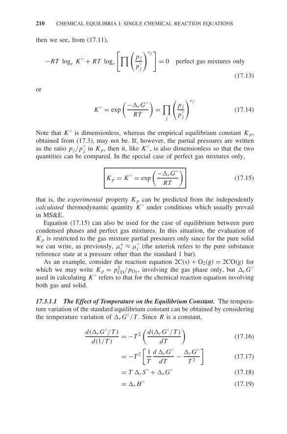
210 CHEMICAL EQUILIBRIA I: SINGLE CHEMICAL REACTION EQUATIONS
then we see, from (17.11),
−RT loge K◦ + RT loge
[∏(pj
p◦j
)νj]
= 0 perfect gas mixtures only
(17.13)
or
K◦ = exp
(−�rG◦
RT
)=∏j
(pj
p◦j
)νj
(17.14)
Note that K◦ is dimensionless, whereas the empirical equilibrium constant Kp,
obtained from (17.3), may not be. If, however, the partial pressures are writtenas the ratio pj/p
◦j in Kp, then it, like K
◦, is also dimensionless so that the twoquantities can be compared. In the special case of perfect gas mixtures only,
Kp = K◦ = exp
(−�rG◦
RT
)(17.15)
that is, the experimental property Kp can be predicted from the independentlycalculated thermodynamic quantity K
◦ under conditions which usually prevailin MS&E.
Equation (17.15) can also be used for the case of equilibrium between purecondensed phases and perfect gas mixtures. In this situation, the evaluation ofKp is restricted to the gas mixture partial pressures only since for the pure solidwe can write, as previously, μ∗
i ≈ μ◦i (the asterisk refers to the pure substance
reference state at a pressure other than the standard 1 bar).As an example, consider the reaction equation 2C(s) + O2(g) = 2CO(g) for
which we may write Kp = p2CO/pO2, involving the gas phase only, but �rG
◦
used in calculating K◦ refers to that for the chemical reaction equation involving
both gas and solid.
17.3.1.1 The Effect of Temperature on the Equilibrium Constant. The tempera-ture variation of the standard equilibrium constant can be obtained by consideringthe temperature variation of �rG
◦/T . Since R is a constant,
d(�rG◦/T )
d(1/T )= −T 2
(d(�rG
◦/T )
dT
)(17.16)
= −T 2[
1
T
d �rG◦
dT− �rG
◦
T 2
](17.17)
= T �rS◦ + �rG
◦ (17.18)
= �rH◦ (17.19)

THE STANDARD EQUILIBRIUM CONSTANT 211
log e
Kp
1/T
R−ΔrH°
Figure 17.1 Standard enthalpy of reaction can be obtained from the slope of a plotof loge Kp versus reciprocal temperature for reaction equations involving perfect gasmixtures and pure solids.
where we have used �rG◦ = �rH
◦ − T �rS◦ and(
∂ �rG◦
∂T
)p
= −�rS◦
Then, from the relation between �rG◦ and K
◦, the above equation can bere-written as
d loge K◦
d (1/T )= −�rH
◦
Rgeneral relation (17.20)
and, when it is safe to assume that Kp = K◦,
d loge Kp
d (1/T )= −�rH
◦
Rperfect gas mixtures only (17.21)
Equation (17.21) is known as the Gibbs–Helmholtz equation. As shown inFigure 17.1, loge Kp for a chemical reaction equation is plotted as a functionof 1/T over a small range of temperature, we expect to obtain a straight linein circumstances where the perfect gas assumption holds. In this case, the slopeyields the negative of the standard enthalpy of reaction, valid for the temperatureinterval investigated. In practice, it is unlikely that �rC
◦p will be exactly zero so
that we should not expect to obtain a perfectly straight line over a large rangeof temperature, although, because of uncertainty in the data, we may go aheadand fit the results to a linear equation from which we can obtain an approximatevalue for �rH
◦(T ).
17.3.2 Measurement of �rG◦
Previously, we have seen how �rG◦ can be obtained from a combination ofsubstance and reaction calorimetric measurements alone.

212 CHEMICAL EQUILIBRIA I: SINGLE CHEMICAL REACTION EQUATIONS
But we can also make use of �rG◦ = −RT loge K
◦ if we work in a regimewhere it is safe to assume that Kp = K
◦, that is, high temperatures and lowpressures. This has been discussed briefly in Chapter 6. Here, we will give alittle more detail.
We will illustrate with two examples, one involving phase equilibrium and theother chemical equilibrium:
1. Suppose we set out to measure the vapor pressure of Ag(l). Note that thisis not straightforward experimentally. We cannot just connect the Ag athigh temperature to a manometer at room temperature since this wouldresult in the distillation of the Ag from the hot region to the cold region.Nevertheless, there are practical ways of overcoming this kind of problem.Knudsen effusion mass spectroscopy (KEMS) is another useful techniquefor measuring very low vapor pressures and can, in certain circumstances,lead to the simultaneous measurement of both of the component vaporpressures in a binary alloy, thereby giving a check with Gibbs–Duhemcalculations.
For the phase equilibrium represented by Ag(l) = Ag(g), we have�vapG
◦(Ag, T ) = −RT loge(pAg/bar) so that the vapor pressure
measurement gives us the thermodynamic quantity �vapG◦(Ag, T ) and,
if the equilibrium is measured as a function of T ,�vapH◦(Ag,T )and
�vapS◦(Ag,T ) can be obtained.
2. The Kp for the reaction equation
Fe(s) + H2O(g) = FeO(s) + H2(g)
can be measured in an apparatus similar to that in Figure 17.2. After evac-uation, the Fe(s) sample is exposed to the water vapor from the H2O(l)reservoir. The formation of FeO(s) from Fe(s) takes place with the for-mation of H2(g). The controlled temperature of the H2O(l) fixes pH2O
throughout the apparatus. It is also the coldest part of the apparatus sothat there is no chance of condensation elsewhere. The manometer read-ing gives pH2 + pH2O so that the individual pH2 and pH2O values can beobtained. Hence Kp = pH2/pH2O is known. With the justified assumptionthat K
◦ = Kp, �rG◦ for the above reaction equation can be evaluated. If
�rG◦ for the reaction equation
Fe(s) + H2O(g) = FeO(s) + H2(g)
is combined with that for the reaction equation
H2(g) + 12 O2(g) = H2O(g)
for which �rG◦ is known with great accuracy, it then becomes possible to
obtain �f G◦(FeO(s),T ) from the equilibrium measurements. When �rG
◦

CALCULATING THE EQUILIBRIUM POSITION 213
X
Vacuum
pt
H2O
Fe
Furnace
Figure 17.2 Simple apparatus for measurement of equilibrium for chemical reactionequation Fe(s) + H2O(g) = FeO(s) + H2(g).
is measured as a function of T , both �f H◦(FeO(s),T ) and �f S
◦(FeO(s),T )can be obtained.
In most of the databases available for pure substances, approximately one-halfof the data for �f G
◦ have come from calorimetric measurements and the otherhalf from equilibrium measurements similar to those described above.
17.4 CALCULATING THE EQUILIBRIUM POSITION
Calculating the final chemical equilibrium from a set of chosen initial amountsof substances and system conditions can be approached in exactly the same man-ner as has been described previously for phase equilibrium. The whole system,comprising either one or several phases and which is assumed to be closed andat constant total p and T , leads toward a minimization of the Gibbs energy in itsapproach to equilibrium. When chemical reaction equations are involved, how-ever, the constraints on the minimization are different from those found for thecase of phase equilibrium since the element mass balance for each element mayinvolve more than one species containing that element and these may be in morethan one phase.
A straightforward minimization of G subject to the constraints is not the onlyway of calculating the position of chemical equilibrium and, in the following, wewill describe three different methods for calculating the equilibrium in a systemwhich contains species related by a single reaction equation.
For illustration purposes, we will refer to the reaction equation
SO2(g) + 12 O2(g) = SO3(g) (17.22)
Note that, since there is a change in the total amounts of substance in goingfrom reactants to products in this particular reaction equation, the position ofequilibrium depends on the total pressure.
(A) Using the Mass Action Law For this example, the element mass balancesfor S and O and for the total number of species moles, ntot, can be written

214 CHEMICAL EQUILIBRIA I: SINGLE CHEMICAL REACTION EQUATIONS
as follows:
nS = n0SO2
+ n0SO3
= nSO2 + nSO3 (17.23)
nO = 2n0SO2
+ 2n0O2
+ 3n0SO3
= 2nSO2 + 2nO2 + 3nSO3 (17.24)
ntot = nSO2 + nO2 + nSO3 (17.25)
where n0j represents the initial amount of species j and ntot the total amounts of
substances in the gas phase. The gaseous species partial pressures are related tothe amounts and total pressure by
pj = xjptot =(
nj
ntot
)ptot (17.26)
The equilibrium condition (17.6) for this reaction is
μSO3 − μSO2 − 12μO2 = 0 (17.27)
which, for perfect gas mixtures, can be rewritten as
[μ
◦SO3
− μ◦SO2
− 12μ
◦O2
]+ RT loge
(pSO3
pSO2 × p1/2O2
)= 0 (17.28)
or
�rG◦ + RT loge
(pSO3
pSO2 × p1/2O2
)= 0 (17.29)
or
K◦ =
(pSO3
pSO2 × p1/2O2
)(17.30)
This last equation is usually known as the mass action law when K◦ is replaced
wth Kp.The mass balance requirements (17.23)–(17.25), the partial pressure conver-
sion (17.26), and the equilibrium condition (17.30) may be used to calculatethe individual equilibrium partial pressures. The solution requires solving severalnonlinear simultaneous equations.
In this simple case of a single reaction, a hand calculation may be carried outby using the mass balance equations to eliminate two of the species, for example,
nSO2 = nS − nSO3
nO2 = 12 (nO − 2nS − nSO3)

CALCULATING THE EQUILIBRIUM POSITION 215
and substitute the resulting partial pressures from (17.26) into (17.30) to solve forpSO3. The other equilibrium partial pressures can then be obtained subsequently.
(B) Using the Extent of Reaction, ξ In this method the element mass balanceequations are circumvented by taking advantage of the fact that the changes inthe species amounts, dnj , during a reaction are not independent but are relatedthrough the stoichiometry of the reaction equation. As a result, only one parameterper reaction equation is required to specify the changes in the amounts of thespecies. The differential changes in the species amounts for the reaction equationunder consideration are seen to be
dnSO2
−1= dnO2
−1/2= dnSO3
+1= dξ (17.31)
The variable ξ is called the extent of reaction (units are moles), and it can beseen that this one variable expresses the changes in the amount of any species,j , in the chemical reaction equation, that is, dnj = νj dξ , which on integrationgives
nj = n0j + νj ξ (17.32)
where ξ is taken to be zero in the initial state. For the reaction equation (17.22)the input amounts are given by:
nSO2 = n0SO2
− ξ (17.33)
nO2 = n0O2
− 12ξ (17.34)
nSO3 = n0SO3
+ ξ (17.35)
ntot = n0SO2
+ n0O2
+ n0SO3
− 12ξ (17.36)
Equations (17.33)–(17.36) together with (17.26) and (17.30) may be solvedsimultaneously to obtain the individual partial pressures. Alternatively, the equi-librium constant can be expressed solely in terms of ξ and the starting amountsof species.
(C) Using Lagrangian Multipliers With both of the previous methods it isnecessary to know the chemical reaction equation. While this causes no prob-lem in a simple system, the advantage of the method based on Lagrangianmultipliers is that a reaction equation is not required. It is only necessary tospecify the species designated as comprising the system. The element mass bal-ance equations, for example, (17.23)–(17.25), are also used once the system isspecified.
The introduction of the Lagrangian multipliers λi transforms the constrainedminimization of the G = ∑
j niμj problem into an unconstrained minimizationof a Lagrangian function L with Lagrangian multipliers assigned to the elementmass balances.
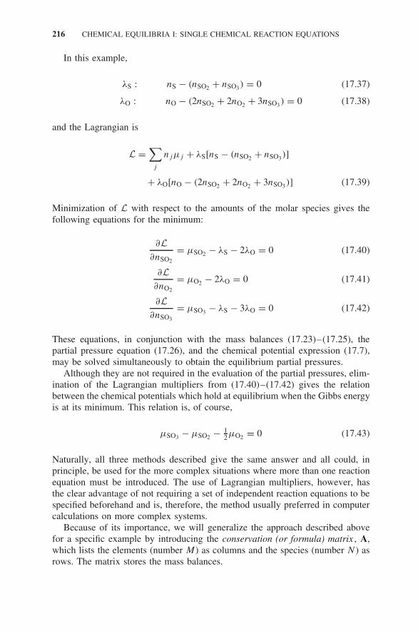
216 CHEMICAL EQUILIBRIA I: SINGLE CHEMICAL REACTION EQUATIONS
In this example,
λS : nS − (nSO2 + nSO3) = 0 (17.37)
λO : nO − (2nSO2 + 2nO2 + 3nSO3) = 0 (17.38)
and the Lagrangian is
L =∑
j
njμj + λS[nS − (nSO2 + nSO3)]
+ λO[nO − (2nSO2 + 2nO2 + 3nSO3)] (17.39)
Minimization of L with respect to the amounts of the molar species gives thefollowing equations for the minimum:
∂L∂nSO2
= μSO2 − λS − 2λO = 0 (17.40)
∂L∂nO2
= μO2 − 2λO = 0 (17.41)
∂L∂nSO3
= μSO3 − λS − 3λO = 0 (17.42)
These equations, in conjunction with the mass balances (17.23)–(17.25), thepartial pressure equation (17.26), and the chemical potential expression (17.7),may be solved simultaneously to obtain the equilibrium partial pressures.
Although they are not required in the evaluation of the partial pressures, elim-ination of the Lagrangian multipliers from (17.40)–(17.42) gives the relationbetween the chemical potentials which hold at equilibrium when the Gibbs energyis at its minimum. This relation is, of course,
μSO3 − μSO2 − 12μO2 = 0 (17.43)
Naturally, all three methods described give the same answer and all could, inprinciple, be used for the more complex situations where more than one reactionequation must be introduced. The use of Lagrangian multipliers, however, hasthe clear advantage of not requiring a set of independent reaction equations to bespecified beforehand and is, therefore, the method usually preferred in computercalculations on more complex systems.
Because of its importance, we will generalize the approach described abovefor a specific example by introducing the conservation (or formula) matrix , A,which lists the elements (number M) as columns and the species (number N ) asrows. The matrix stores the mass balances.

APPLICATION OF THE PHASE RULE 217
For the above example system the conservation matrix is written as
A =⎛⎝ SO2 O2 SO3
S 1 0 1O 2 2 3
⎞⎠
where the member Aij gives the number of i elements in the j th species.In general, the mass balance relations can be written in terms of the members
of A as
ni −N∑
j=1
Aijnj = 0 ∀ elements i (17.44)
and the Lagrangian function as
L =N∑
j=1
njμj +M∑i=1
λi
⎛⎝ni −
N∑j=1
Aijnj
⎞⎠ (17.45)
where M is the number of elements and N the number of species. This equationis a generalization of (17.39).
Differentiation of the Lagrangian with respect to the amount of each speciesand setting the derivatives to zero gives the equilibrium conditions
∂L∂nj
= μj +M∑i
λiAij = 0 ∀ elements i (17.46)
which is a generalization of (17.40)–(17.42).
17.5 APPLICATION OF THE PHASE RULE
We have seen that, when chemical reaction equations have to be considered, theconstraints on the chemical potentials are different from those met when consid-ering phase equilibria. This influences the number of independent components ,C, to be used in the phase rule, F = C − φ + 2. In the case of alloy-phaseequilibria, we simply equated C with the number of elements. The number ofconstraints on the μα
i = μβ
i relations is C(φ − 1) (see Chapter 8). There is alsoa Gibbs–Duhem constraint for each phase.
In the case of a single-chemical-reaction equation involving N species thereis just the one constraint given in (17.6), namely,
∑Nj νjμj = 0, so that the
number of independent components C = N − 1. The phase rule for this case isthen modified to read
F = (N − 1) − φ + 2 = N − φ + 1 (17.47)

218 CHEMICAL EQUILIBRIA I: SINGLE CHEMICAL REACTION EQUATIONS
If we apply this to the example of the homogeneous gas reaction equation
SO2(g) + 12 O2(g) = SO3(g)
then
F = 3 − 1 + 1 = 3 (17.48)
and we see that, if we fix ptot, T , and the initial amount of one substance, thesystem is fully specified.
In the case of the reaction equation CaCO3(s) = CaO(s) + CO2(g), we haveto consider a three-phase system so that
F = 3 − 3 + 1 = 1 (17.49)
and fixing T is sufficient to specify the equilibrium state.We will return to the application of the phase rule to more complex chemical
reaction equation situations in the next chapter.
EXERCISES
17.1 A gas mixture of 50% CO, 25% CO2, and 25% H2 (percentages byvolume) is fed into a furnace at 900◦C. Find the composition of the equi-librium CO–CO2 –H2O–H2 gas if the total pressure in the furnace is 1 bar.
17.2 How much heat is evolved when 1 mol of SO2 and 12 mol of O2 react
to form the equilibrium SO3 –SO2 –O2 mixture at 1000 K and at a totalpressure of 1 bar?
17.3 What is the oxygen partial pressure exerted by an equilibrium gas mixtureof CO2 –CO–H2 –H2O produced at 1600◦C by mixing CO2 and H2 in theratio of 3 : 1?
17.4 If you wish to make a mixture of CO2 –CO–H2 –H2O at 1600◦C with anoxygen partial pressure of 10−7 bar at a total pressure of 1 bar, what is theinitial ratio of CO2 and H2 needed to produce this equilibrium mixture?
17.5 .(a) Calculate �rG◦(1000 K) for the reaction
CH4(g) + CO2(g) = 2CO(g) + 2H2(g)
(b) Assuming that K◦ = Kp, at what temperature does Kp = 1?
(c) In which direction does the equilibrium shift when:(i) The temperature of an equilibrated CH4 –CO2 –CO–H2 gas mix-
ture is increased?(ii) The total pressure is decreased?

EXERCISES 219
17.6 By establishing the equilibrium PCl5 = PCl3 + Cl2 in a mixture of PCl5and PCl3, it is required to obtain a partial pressure of Cl2 of 0.1 bar at500 K when the total pressure is 1 bar. In what ratio must PCl5 and PCl3be mixed?
17.7 A producer of copper parts uses the powder metallurgy technique to makethese parts. To increase the strength of these parts, they are dispersionhardened with fine Al2O3 powders.
The producer can buy Cu powder containing 2% Fe much cheaper thanthe pure Cu powder he has been using. (The less pure Cu powder is aby-product of the cement copper process.) Also, he finds that magnetite(Fe3O4) is almost as effective in dispersion hardening of copper as Al2O3.
If he sinters the less pure powder in the normal H2 atmosphere (orvacuum), the result is a (Cu, Fe) alloy containing 2% Fe. Such an alloyis unsuitable for the requirements of his parts, however. Describe an oxi-dizing/sintering step that he can use in order to internally oxidize the Feto produce a relatively pure Cu part in which are well dispersed fine ironoxide particles. What is the lowest aFe obtainable in the Cu solid solution?Just how, in practice, would be a reasonable way to conduct the internaloxidation step?
Assume (Cu, Fe) solid solution behaves like a strictly regular solutionwith L0 ≈ 30,750 J mol−1.


18 Chemical Equilibria II:Complex Gas Equilibria
Most chemically reacting systems of interest in MS&E are complex so that itis rare that such systems can be expressed in terms of just the one chemicalreaction equation, as was discussed in Chapter 17. Atmospheres generated fromfossil fuel combustion, for example, contain, principally, molecules, atoms, andions containing the elements C, H, O, S, and N and the number of possiblemolecular species based on these five elements can be extremely large. The mostfamiliar are H2, O2, S2, N2, H2O, H2S, NH3, CH4, CO, CO2, SO2, and SO3 butthere are countless others, often including undesirable dioxins as well as elementslike U, Th, and As.
Figure 18.1 shows the gas phase composition resulting from the combustionof methane in oxygen as function of temperature. Considerably more complexgas phase compositions can result, for example, in Chemical Vapor Depositionprocesses.’’
System complexity is also the norm in the metal-processing industries. There,it is common to find more than two phases in contact, for example, in the copperextraction industry the system may comprise gas, slag, matte, and metal phases,each of which is chemically complex, with material passing between the phasesby chemical interaction in the attempt to reach thermodynamic equilibrium.
The keyword to be borne in mind here is complexity. We need to learn howthermodynamics can be gainfully applied to such complex, chemically react-ing systems. As a preliminary, in this chapter, we consider the calculation ofequilibrium in complex gas mixtures. Chemical equilibria involving gases andcondensed phases will be discussed in Chapters 19 and 20.
18.1 THE IMPORTANCE OF SYSTEM DEFINITION
Any discussion of equilibrium in chemically reacting systems leads to an appre-ciation of what thermodynamics can and cannot do:
Although thermodynamics is used to accurately predict properties or data fromother properties or data, it can only make these predictions for the system definedby the thermodynamicist.
Materials Thermodynamics. By Y. Austin Chang and W. Alan OatesCopyright 2010 John Wiley & Sons, Inc.
221

222 CHEMICAL EQUILIBRIA II: COMPLEX GAS EQUILIBRIA
−0.2400 600 800
graphite
CO2
CO
CH4
CH4 + 0.750 O2
H2O
H2
1000 1200
0.0
0.2
0.4
prod
ucts
,n/m
ol
T /K
0.6
0.8
1.0
1.2
1.4
1.6
1.8
Figure 18.1 Calculated gas phase composition in the combustion of 1 mole of methanewith 0.75 mole oxygen. Reproduced with permission from H. Yokokawa, J. Phase Equilib.26, p. 155, 2002.
A poorly defined system will lead to an incorrect prediction of properties. Themost common way in which this is encountered is the failure to include somespecies in the system specification. This neglect, which may be due to ignoranceor oversight, cannot be attributed to a failure of thermodynamics.
Problems associated with system definition are much less frequently encoun-tered in the case of phase equilibrium calculations. Thus, if a calculated stableAl–Zn phase diagram were to be presented as shown in Figure 18.2a , one wouldquickly be alerted to the fact that the hcp phase had been overlooked in the cal-culation. When this oversight is rectified, the more familiar phase diagram shownin Figure 18.2b can then be calculated.
This type of neglect, however, with the user often being unaware of it, happensfrequently in calculations of chemically reacting systems, particularly for thoseinvolving high-temperature calculations of heterogeneous equilibria.
Example 18.1 Combustion of H2(g) with O2(g)A very simple illustration of the importance of the role of the thermodynamicistin performing meaningful thermodynamic calculations arises in the calculationof the adiabatic flame temperature for the stoichiometric combustion of H2(g)with O2(g) at a total pressure of 1 bar. This calculation entails assuming that thereaction between H2(g) and O2(g) takes place in a closed system whose volumecan vary in order to maintain a constant pressure of 1 bar. The combustion takesplace without any heat flow to or from the surroundings. This results in the

THE IMPORTANCE OF SYSTEM DEFINITION 223
1000
800
600
400
0.0 0.2 0.4 0.6 0.8 1.0ZnAl xZn
(a ) (b )
0.0 0.2 0.4 0.6 0.8 1.0ZnAl xZn
T/K
1000
800
600
400
T/K
Figure 18.2 Calculated Al–Zn phase diagrams: (a) Without hcp phase taken intoaccount; (b) with all phases taken into account.
enthalpy of the input gases being equal to the enthalpy of the product gases, thatis, �rH
◦ for the following reaction equation is zero:
H2(g)(298.15 K) + 12 O2(g)(298.15 K) = H2O(g)(T ) (18.1)
Consider the different outcomes from three different decisions by the thermody-namicist concerning the calculation:
(i) Thermodynamicist A assumes that the reaction goes to completion, that is,T is calculated from the enthalpy changes for the two following reactionequations:
H2(g)(298.15 K) + 12 O2(g)(298.15 K) = H2O(g)(298.15 K)
�H = �f H◦(298.15 K)
H2O(g)(298.15 K) = H2O(g)(T ) �H =∫ T
298.15 KC
◦p(H2O) dT
(ii) Thermodynamicist B defines the system as comprising H2(g), O2(g), andH2O(g) but considers the possibility that the chemical reaction equationgiven in (18.1) does not go to completion, that is, all three species maybe present at the final temperature. The relative amounts of the three gasesare governed by �rG
◦ at the final temperature as well as by mass balanceconstraints.
(iii) Thermodynamicist C defines the system as comprising all the gaseousspecies contained in a comprehensive database containing the elements Hand O in addition to the species H2(g), O2(g), and H2O(g). All these extraspecies may be present at the final temperature.

224 CHEMICAL EQUILIBRIA II: COMPLEX GAS EQUILIBRIA
The calculated flame temperature and partial pressure results obtained fromthese three different assumptions are as follows:
Species p (bars) Species p (bars)Flame Temperature: 4894 K Flame Temperature: 3146.31 KH2O 1.0 H2O 0.618H2 0.0 H2 0.157O2 0.0 H 0.0964
O2 0.0774Flame Temperature: 3508.91 K O 0.0508H2O 0.569 H2O2 3.57 × 10⁻⁶
H2 0.287 O3 4.19 × 10⁻⁸
O2 0.144
It can be seen that the results obtained for the calculated adiabatic flame tem-perature differ markedly (the result obtained by thermodynamicist C will be closeto the experimental value). The important point to appreciate is that the differ-ences in the calculated results stem from the different decisions made by thethermodynamicists. They do not represent any failure on the part of thermody-namics.
This problem of system definition is exacerbated when more complex situa-tions than this simple example are considered. We will encounter it again whenwe come to discuss equilibrium involving both gaseous and condensed phases.For the present, we emphasize that the failure to properly define the system inthermodynamic calculations of chemical equilibria is a common occurrence.
18.2 CALCULATION OF CHEMICAL EQUILIBRIUM
In Chapter 17 we examined some different approaches to the calculation of theposition of chemical equilibrium for single-reaction equations involving perfectgas mixtures and pure solids. All these methods can be applied to more complexsituations, but when the gases are not perfect and the condensed phases arenonideal solutions, then, just as in the case of phase equilibria, local minima inthe Gibbs energy can arise. These local minima make the equilibrium calculationsconsiderably more difficult. In this chapter we will restrict ourselves to somefairly straightforward examples which avoid these complications by consideringthe case of several species present in a perfect gas mixture. Even here, somecalculation methods are preferable to others.
Specifically, we will illustrate with a system defined as containing the gaseousmolecular species CH4(g), O2(g), CO2(g), H2O(g), CO(g), and H2(g). Note that,although there are many other molecular species which contain the elements C,H, and O, we have elected to define the system as containing just these sixspecies. We might elect to do this, for example, if we know that under the

CALCULATION OF CHEMICAL EQUILIBRIUM 225
conditions where the results from the calculations are to be used it is known thatthe concentration of, say, C2H2(g), is unimportant.
18.2.1 Using the Extent of Reaction
A principal objective of chemical reaction stoichiometry is to determine the num-ber of independent chemical reaction equations, R, required to determine theequilibrium in the defined system. In this relatively simple case, it is possible tosee, by inspection, that one set of independent chemical reaction equations is thefollowing:
CH4(g) + 2O2(g) = CO2(g) + 2H2O(g) (18.2)
2CO2(g) = 2CO(g) + O2(g) (18.3)
CH4(g) + O2(g) = CO2(g) + 2H2(g) (18.4)
so that, in this case, R = 3. This selection is, of course, not the only set ofindependent reaction equations which can be written involving these six species.The number of independent equations will, however, always be three.
When the number of species is much larger than that in our example, it isnecessary to have a more general method for determining R. In order to do this,we first set up the formula or conservation matrix A. For our example, this is anM × N matrix:
A =
⎛⎜⎜⎝
CH4 O2 CO2 H2O CO H2
C 1 0 1 0 1 0H 4 0 0 2 0 2O 0 2 2 1 1 0
⎞⎟⎟⎠
The number of independent components, C, is given by rank(A). In this example,C = 3. The value of R can then be obtained from R = N − C. In this example,R = 6 − 3 = 3.
Having obtained the number of independent reaction equations, it is necessaryto assign an extent of reaction, ξ , to each of the chosen reaction equations. Inour example, ξ1, ξ2, and ξ3 are assigned to (18.2)–(18.4), respectively. Then wemay proceed exactly as we did for a single reaction in Chapter 17. For example,for (18.2), we may write
dnCH4
−1= dnO2
−2= dnCO2
+1= dnH2O
+2= dξ1 (18.5)
From this and similar equations for the reaction equations (18.3) and (18.4), wemay integrate and obtain the values of the species amounts in terms of the three

226 CHEMICAL EQUILIBRIA II: COMPLEX GAS EQUILIBRIA
reaction variables:
nCH4 = noCH4
− ξ1 − ξ3 (18.6)
nO2 = noO2
− 2ξ1 + ξ2 − ξ3 (18.7)
nCO2 = noCO2
+ ξ1 − 2ξ2 + ξ3 (18.8)
nH2O = noH2O + 2ξ1 (18.9)
nCO = noCO + 2ξ2 (18.10)
nH2 = noH2
+ 2ξ3 (18.11)
ntot = noCH4
+ noO2
+ noCO2
+ noH2O + no
CO + noH2
+ ξ2 + ξ3 (18.12)
The partial pressures are related to the amounts and total pressure by
pj =(
nj
ntot
)ptot (18.13)
and the equilibrium conditions for these reactions are
�rG◦1 + RT loge
(pCO2 × p2
H2O
pCH4 × p2O2
)= 0 (18.14)
�rG◦2 + RT loge
(p2
CO × pO2
p2CO2
)= 0 (18.15)
�rG◦3 + RT loge
(pCO2 × p2
H2
pCH4 × pO2
)= 0 (18.16)
The set of mass balance equations 18.6–18.12 plus the relation between molaramounts and the partial and total pressures, (18.13), together with the equilibriumrelations (18.14)–(18.16) can be used to solve for the final chemical equilibrium.
Figure 18.3 shows, qualitatively, how the Gibbs energy varies as a functionof ξ1 and ξ2 for a system defined by two independent reaction equations. Theequilibrium position is given by the minimum in the Gibbs energy, which canbe obtained by satisfying
(∂G
∂ξ1
)=(
∂G
∂ξ2
)= 0 (18.17)

CALCULATION OF CHEMICAL EQUILIBRIUM 227
10.8
0.6
0.5
−360.4
0.4
−34
0.3
−32
−30
0.20.2
−28
0.1
−26
00
G/k
J m
ol−1
x1
x2
Figure 18.3 Variation of G as function of ξ1 and ξ2, drawn using Maple®.
18.2.2 Using Lagrangian Multipliers
In the example which involves only six species and three independent reactions,application of the extent of the reaction method is straightforward. When thesystem comprises on the order of 100 molecular species derived from just a fewelements, it is more difficult and the method based on Lagrangian multipliers isto be preferred.
A Lagrangian multiplier, λi , is assigned to the mass balance for each element:
λC : nC − (nCO + nCO2 + nCH4) (18.18)
λH : nH − (2nH2 + 2nH2O + 4nCH4) (18.19)
λO : nO − (nCO + 2nO2 + 2nCO2 + nH2O) (18.20)
and the Lagrangian function is written as
L =N∑
j=1
njμj +M∑i=1
λi
⎛⎝ni −
N∑j=1
Aijnj
⎞⎠ (18.21)
Differentiation of this function with respect to the amount of each species andsetting the derivatives to zero gives the equilibrium conditions. For our example,
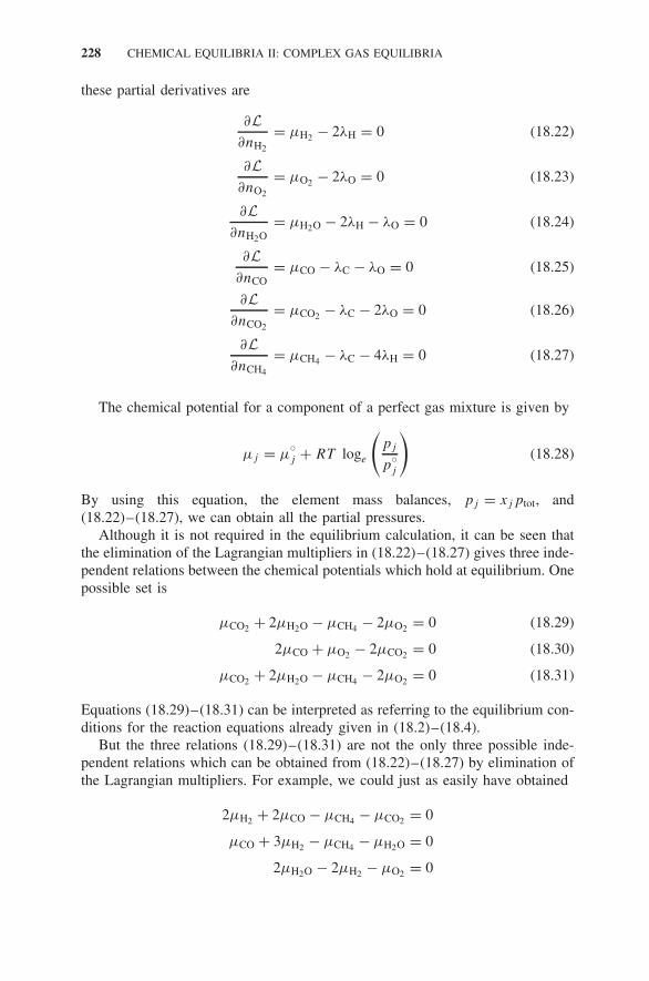
228 CHEMICAL EQUILIBRIA II: COMPLEX GAS EQUILIBRIA
these partial derivatives are
∂L∂nH2
= μH2 − 2λH = 0 (18.22)
∂L∂nO2
= μO2 − 2λO = 0 (18.23)
∂L∂nH2O
= μH2O − 2λH − λO = 0 (18.24)
∂L∂nCO
= μCO − λC − λO = 0 (18.25)
∂L∂nCO2
= μCO2 − λC − 2λO = 0 (18.26)
∂L∂nCH4
= μCH4 − λC − 4λH = 0 (18.27)
The chemical potential for a component of a perfect gas mixture is given by
μj = μ◦j + RT loge
(pj
p◦j
)(18.28)
By using this equation, the element mass balances, pj = xjptot, and(18.22)–(18.27), we can obtain all the partial pressures.
Although it is not required in the equilibrium calculation, it can be seen thatthe elimination of the Lagrangian multipliers in (18.22)–(18.27) gives three inde-pendent relations between the chemical potentials which hold at equilibrium. Onepossible set is
μCO2 + 2μH2O − μCH4 − 2μO2 = 0 (18.29)
2μCO + μO2 − 2μCO2 = 0 (18.30)
μCO2 + 2μH2O − μCH4 − 2μO2 = 0 (18.31)
Equations (18.29)–(18.31) can be interpreted as referring to the equilibrium con-ditions for the reaction equations already given in (18.2)–(18.4).
But the three relations (18.29)–(18.31) are not the only three possible inde-pendent relations which can be obtained from (18.22)–(18.27) by elimination ofthe Lagrangian multipliers. For example, we could just as easily have obtained
2μH2 + 2μCO − μCH4 − μCO2 = 0
μCO + 3μH2 − μCH4 − μH2O = 0
2μH2O − 2μH2 − μO2 = 0

EVALUATION OF ELEMENTAL CHEMICAL POTENTIALS 229
This emphasizes the point that, although there are only three independent relationsbetween the chemical potentials of the species, the relations can be selected indifferent ways. It also follows that there is nothing in a balanced chemical reactionequation which relates to any actual mechanisms of chemical reactions occurringwithin the system.
18.3 EVALUATION OF ELEMENTAL CHEMICAL POTENTIALSIN COMPLEX GAS MIXTURES
Usually, it is the behavior of one or, occasionally, two particular elements in acomplex gas atmosphere which is of primary interest. We may wish to know,for example, whether a gas at a given p, T and initial composition is oxidizing,reducing, sulfurizing, carburizing, nitriding, and so on, to the particular condensedphase the gas phase is contacting. Complete knowledge of the chemical analysisof the gas becomes of secondary importance in these situations.
If we concentrate on the oxidizing/reducing power of a gas mixture for themoment, then it is the chemical potential of oxygen which is of interest. Athigh oxygen potentials the gas is likely to be oxidizing, at low oxygen potentialsreducing. The oxygen potential is defined (in a perfect gas mixture) by
�μO2 = μO2 − μ◦O2
= RT loge
(pO2
p◦O2
)(18.32)
It is often the case that the partial pressure of O2(g) is much too small to beobtained from chemical analysis. In such cases it is useful to be able to get ahandle on its magnitude by other means.
No physical meaning was given to the Lagrangian parameters in(18.22)–(18.27) since this was unnecessary in the solution of the chemicalequilibrium problem. But it is clear from these equations that the Lagrangianparameters are in fact chemical potentials of the elements. For example, we mayappreciate their meaning by considering (18.25):
μCO − λC − λO = 0
which is equivalent to writing
μCO − μC − μO = 0 (18.33)
or
μCO − μC − 12μO2 = 0 (18.34)
so that we already know the element chemical potentials when the Lagrangianmethod is used for calculating chemical equilibrium. They are just the Lagrangianparameters associated with the mass balances.

230 CHEMICAL EQUILIBRIA II: COMPLEX GAS EQUILIBRIA
The relation of element chemical potentials to molecular species chemicalpotentials can also be seen directly by considering particular reaction equations.By doing this we can see how to obtain an element chemical potential from themolecular gas analysis. Consider, for example, the reaction equation
2CO(g) + O2(g) = 2CO2(g)
By using the relation between the standard Gibbs energy of reaction and thestandard equilibrium constant and assuming that the latter is the same as theempirical equilibrium constant (perfect gas mixtures), we can write
�rG◦(T ) = −2RT loge
(pCO2
pCO
)+ RT loge pO2 (18.35)
Rearranging gives
�μO2(T ) = 2[�f G
◦(CO2(g), T ) − �f G
◦(CO(g), T )
]+ 2RT loge
(pCO2
pCO
)(18.36)
Similarly, by considering the reaction equation,
2H2(g) + O2(g) = 2H2O(g)
we have
�rG◦(T ) = −2RT loge
(pH2O
pH2
)+ RT loge pO2 (18.37)
�μO2(T ) = 2 �f G◦(H2O(g), T ) + 2RT loge
(pH2O
pH2
)(18.38)
This type of procedure can be used for other elements to specify the elementalchemical potentials in terms of the ratios of different constituents of a complexmixture.
For example, carbon potentials can be obtained from consideration of one ofthe following reaction equations:
C(s) + 2H2(g) = CH4(g) (18.39)
C(s) + CO2(g) = 2CO(g) (18.40)
sulfur potentials from
S2(g) + 2H2(g) = 2H2S(g) (18.41)
S2(g) + 4SO3(g) = 6SO2(g) (18.42)

APPLICATION OF THE PHASE RULE 231
and nitrogen potentials from
N2(g) + 3H2(g) = 2NH3(g) (18.43)
18.4 APPLICATION OF THE PHASE RULE
If we apply the most frequently used form of the phase rule, (8.26), namely,F = C − φ + 2, to the single-reaction equation CO(g) + 1
2 O2(g) = CO2(g) andtake the number of components to be the same as the number of molecularspecies, that is, three, then application of this equation gives F = 3 − 1 + 2 = 4,which is incorrect. If, on the other hand, we take C = N − R = 3 − 1 = 2, thenF = 2 − 1 + 2 = 3, which is correct. If, for example, we fix p, T , and pCO2 ,then the two remaining partial pressures can be obtained from the equilibriumconstant and the fact that the sum of the partial pressures is equal to the fixedtotal pressure.
Similar reasoning applies to more complex situations. In our example of asystem comprising six molecular species, if we use F = 6 − 1 + 2 = 7, we obtainan incorrect answer. If, however, we use C = N − R = 6 − 3 = 3, then F =3 − 1 + 2 = 4, which is correct. Fixing p, T , pO2, and pCO2 leaves us with fourunknowns. These can be obtained from the three equilibrium constants and thepartial pressure sum.
The selection of constituents (the independent species) required to describe asystem is not unique but their number is. The number of components is the sameas the number of constituents , but the components may or may not involve theconstituents.
The selected components may be these constituents but other selections maybe made. The only requirement of a component is that it can be used to expresscomposition over the range of interest for the system under consideration.
With some selections of components, it is possible for some compositions tohave negative amounts of the selected components. As an illustration, considerthe following selections of components for the Fe–O system. In the first wechoose Fe and O as the components and in the second we choose FeO andFe2O3.
The conservation matrices for these two choices are as follows:
A =
⎛⎜⎜⎝
phase
componentFe(s) FeO(s) Fe3O4(s) Fe2O3(s) O2(g)
Fe 1 1 3 2 0O 0 1 4 3 2
⎞⎟⎟⎠
A =
⎛⎜⎜⎝
phase
componentFe(s) FeO(s) Fe3O4(s) Fe2O3(s) O2(g)
FeO 3 1 1 0 −4Fe2O3 −1 0 1 1 2
⎞⎟⎟⎠

232 CHEMICAL EQUILIBRIA II: COMPLEX GAS EQUILIBRIA
Although the selection of components is different in these two formula matri-ces, their rank, and hence the number of independent components, remains thesame.
EXERCISES
18.1 Acetylene, C2H2(g), is burnt at room temperature with O2(g).Assume the system comprises C(s), C2H2(g), CH4(g), CO(g), CO2(g),H2(g), and H2O(g).
(a) Using the Lagrangian multiplier method, evaluate the equilibrium com-position, the oxygen potential, and the carbon potential as a functionof temperature and C2H2(g)/O2(g) ratio.
(b) Evaluate the adiabatic flame temperature as a function of theC2H2(g)/O2(g) ratio.
(c) What molar ratio of C2H2(g)/O2(g) is required in order to avoid Cdeposition at all temperatures?
18.2 A system is assumed to comprise the species C(s), CO2(g), CO(g), andO2(g) at 1000 K.
(i) Construct the formula matrix.(ii) Use the Lagrangian multiplier method to derive a set of independent
chemical reactions for this system.(iii) Write down the equations for the empirical equilibrium constants
assuming perfect gas mixtures.(iv) Derive the relation between G and the extents of reaction if the system
initially contains 1 mol C(s) and 1 mol CO2(g) at 2 bars.(v) Obtain expressions for the derivatives of G with respect to the extents
of reaction.
18.3 Solve this same problem using the Lagrangian multiplier method.
18.4 Derive the expressions for carbon, sulfur, and nitrogen potentials in termsof molecular gas species using the reaction equations discussed in thischapter.

19 Chemical EquilibriaBetween Gaseousand Condensed Phases I
Chemical reactors in which a complex gas mixture is in contact with a condensedphase are often used in materials production and processing. The thermodynamicproblem of interest here is in deciding whether or not the condensed-phase mate-rial is carburized, hydrided, oxidized, sulfurized, nitrided, silicided, phosphorized,and so on, by the surrounding complex gas mixture.
We have seen earlier how the thermodynamic data for many pure substancesin their standard states are presented in different forms in computer databases ascompared with their presentation in tables:
(i) In computer databases the SER state is usually preferred. This involves thestoring of several coefficients from which all the thermodynamic propertiescan be derived.
(ii) In many tabular presentations the SSR state is used. All the necessarydifferentiations/integrations have already been carried out and the variousthermodynamic properties can be read at regular temperature intervals.
19.1 GRAPHICAL PRESENTATION OF STANDARDTHERMOCHEMICAL DATA
Computer calculations of complex heterogeneous chemical equilibria can lead tovoluminous data outputs so that there is much to be said in favor of a simplergraphical presentation of the results, just as phase diagrams are so useful inthe case of phase equilibria. While there is a loss of accuracy in presenting thedata this way and hence in any calculations performed in using them, graphicalsolutions can be very useful for carrying out back-of-the-envelope calculationsand obtaining a bird’s eye view of the behavior for a class of systems. It is onthis aspect of the graphical representation of heterogeneous chemical equilibriawhich this and the following chapters are concerned.
The graphical representation is made particularly useful from the realizationthat, for almost all compounds, �f G
◦ is, to a very good approximation, usually
Materials Thermodynamics. By Y. Austin Chang and W. Alan OatesCopyright 2010 John Wiley & Sons, Inc.
233
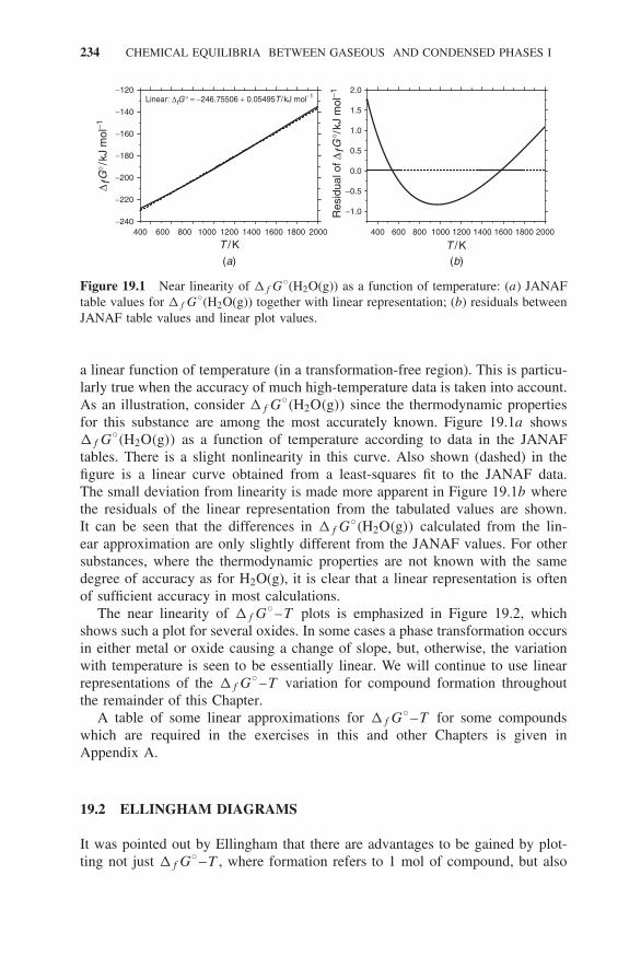
234 CHEMICAL EQUILIBRIA BETWEEN GASEOUS AND CONDENSED PHASES I
−120
−140
−160
−180
−200
−220
−240−1.0
−0.5
0.0
0.5
1.0
1.5
2.0
400 600 800 1000 1200 1400 1600 1800 2000
Linear: ΔfG° = −246.75506 + 0.05495T /kJ mol−1Δ
fG°/
kJ m
ol−1
Res
idua
l of Δ
fG°/
kJ m
ol−1
T /K
(a) (b)
400 600 800 1000 1200 1400 1600 1800 2000
T /K
Figure 19.1 Near linearity of �f G◦(H2O(g)) as a function of temperature: (a) JANAF
table values for �f G◦(H2O(g)) together with linear representation; (b) residuals between
JANAF table values and linear plot values.
a linear function of temperature (in a transformation-free region). This is particu-larly true when the accuracy of much high-temperature data is taken into account.As an illustration, consider �f G
◦(H2O(g)) since the thermodynamic properties
for this substance are among the most accurately known. Figure 19.1a shows�f G
◦(H2O(g)) as a function of temperature according to data in the JANAF
tables. There is a slight nonlinearity in this curve. Also shown (dashed) in thefigure is a linear curve obtained from a least-squares fit to the JANAF data.The small deviation from linearity is made more apparent in Figure 19.1b wherethe residuals of the linear representation from the tabulated values are shown.It can be seen that the differences in �f G
◦(H2O(g)) calculated from the lin-
ear approximation are only slightly different from the JANAF values. For othersubstances, where the thermodynamic properties are not known with the samedegree of accuracy as for H2O(g), it is clear that a linear representation is oftenof sufficient accuracy in most calculations.
The near linearity of �f G◦ –T plots is emphasized in Figure 19.2, which
shows such a plot for several oxides. In some cases a phase transformation occursin either metal or oxide causing a change of slope, but, otherwise, the variationwith temperature is seen to be essentially linear. We will continue to use linearrepresentations of the �f G
◦ –T variation for compound formation throughoutthe remainder of this Chapter.
A table of some linear approximations for �f G◦ –T for some compounds
which are required in the exercises in this and other Chapters is given inAppendix A.
19.2 ELLINGHAM DIAGRAMS
It was pointed out by Ellingham that there are advantages to be gained by plot-ting not just �f G
◦ –T , where formation refers to 1 mol of compound, but also

ELLINGHAM DIAGRAMS 235
400
−1600
−1200
−800Δ f
G°/
kJ m
ol−1
−400
0
800
Cu + 1/2O2(g) = CuO
Zn + 1/2O2(g) = ZnO
2Fe + 3/2O2(g) = Fe2O3
2Al + 3/2O2(g) = Al2O3
Ti + O2(g) = TiO2
1200T /K
1600 2000
Figure 19.2 The �f G◦ as function of temperature for several oxides.
�rG◦ –T , where the reaction refers to 1 mol of O2(g). Figure 19.3 shows the
same data as plotted previously in Figure 19.2 but now on a per mole of O2(g)basis rather than per mole of compound.
As we discuss below, the reason for plotting per mole of O2(g) lies in the abil-ity of being able to use plots in this form for carrying out equilibrium calculationsrather than as just a means of presenting thermodynamic data.
Most of the lines shown in Figure 19.4 are for the formation of an oxidefrom the elements but some are not. What they have in common is that all thereactions refer to 1 mol of O2(g), for example,
2Fe(s) + O2(g) = 2FeO(s)
6FeO(s) + O2(g) = 2Fe3O4(s)
400−1200
−1000
−800
−600
Δ rG
°/kJ
(m
ol O
2)−1
−400
−200
0
800 1200T/K
1600 2000
2Cu + O2(g) = 2CuO
2Zn + O2(g) = 2ZnO4/3Fe + O2(g) = 2/3Fe2O3
4/3Al + O2(g) = 2/3Al2O3
Ti + O2(g) = TiO2
Figure 19.3 Same thermochemical data as used in Figure 19.2 but plotted per moleO2(g).

236 CHEMICAL EQUILIBRIA BETWEEN GASEOUS AND CONDENSED PHASES I
A more complete set of �rG◦ –T curves for the formation of oxides is
shown in Figure 19.4. Similar collections of curves for different groups ofcompounds—sulfides, carbides, nitrides, chlorides, and so on—have been pub-lished. We will continue to concentrate on metal/metal oxide Ellingham diagrams,but the following remarks pertaining to the �rG
◦ –T curves in Figure 19.4 areequally valid to diagrams for other kinds of compounds:
4Ag + O2 = 2Ag2
O
4Cu + O2 = 2Cu2
O
2Ca + O 2 = 2CaO
2Mg + O 2 = 2MgO
3/2Fe + O 2 = 1/3Fe 3
O 4
4/3Cr + O 2 = 2/3Cr 2
O 3
4/3Al+ O 2 = 2/3Al 2
O 3
2Co + O 2 = 2CoO
2Co + O 2 = 2CO 2
2H2+ O2
= 2H2O
2C + O2 = 2CO
2Ni + O 2 = 2NiO
2Fe + O2 = 2FeO
2MnO + O 2 = 2MnO
Si + O 2 = SiO 2
Ti + O 2 = TiO 2
0−1200
Δ rG
°/kJ
(mol
O2)
−1
−1100
−1000
−900
−800
−700
−500
−400
−300
−200
−100
0
200 400 600 800 1000 1200 1400 1600
C + O2 = 2CO2
−600
M
M
M
M
M
MM
M
M
MM
M
B
B
B
M
M
M
M
Melting point of metalBoiling point of metalMelting point of oxide
temperature, °C
6Fe + O 2 = 2Fe 3
O 4
Figure 19.4 Meta/metal oxide Ellingham diagram. Adapted from D.R. Gaskell, Ther-modynamics of Materials , 3rd Edition, Taylor and Francis, Washington, DC, 2002.

ELLINGHAM DIAGRAMS 237
1. The slope of the tangent to a curve at any chosen temperature gives thenegative of the standard entropy of reaction at that temperature:
�rS◦(T ) = −d�rG
◦(T )
dT
2. The intercept at T = 0 K of the tangent to the curve at T gives �rH◦(T ).
3. The curves of �rG◦(T ) versus T are almost straight lines between tran-
sition points so that a good approximation for �rG◦(T ), over a specified
temperature range, is
�rG◦(T ) ≈ 〈�rH
◦〉 − T 〈�rS◦〉
4. Although good estimates of �rG◦(T ) can be obtained from the straight-line
approximation, it is less accurate to try and obtain �rH◦(T ) and �rS
◦(T )
from 〈�rH◦〉 and 〈�rS
◦〉; that is, there is some canceling of errors in thesum, �rG
◦.5. A majority of the curves in Figure 19.4 are approximately parallel, the
occasional one is approximately horizontal and, rarely, a curve may have anegative slope. These patterns in the slopes of the curves can be understoodfrom the equation
�rS◦(T ) =
∑i
νiS◦i (T ) (19.1)
and the fact that S◦(gases) � S
◦(solids or liquids).If we now look at the different types of reaction equations whose valuesare plotted in Figure 19.4, we can then see, using (19.1), that
M(s) + O2(g) = MO2(s) �rS◦ ≈ −S
◦(g)
2H2(g) + O2(g) = 2H2O(g) �rS◦ ≈ −S
◦(g)
C(s) + O2(g) = CO2(g) �rS◦ ≈ 0
2C(s) + O2(g) = 2CO2(g) �rS◦ ≈ +S
◦(g)
6. Changes in the slope are found when phase transformations occur in eitherthe reactant or product phases. These can be understood by considering themelting of either the reactant or product:
M(s) + O2(g) = MO2(s) �rG◦(T ) = −A + BT
M(s) = M(l) �fusG◦(T ) = C − DT
MO2(s) = MO2(l) �fusG◦(T ) = E − FT
M(l) + O2(g) = MO2(s) �rG◦(T ) = −(A + C) + (B + D)T
M(s) + O2 = MO2(l) �rG◦(T ) = −(A − E) + (B − F)T

238 CHEMICAL EQUILIBRIA BETWEEN GASEOUS AND CONDENSED PHASES I
ΔG°
T
M(s) + O2(g) = MO2(s)
M(s) + O2(g) = MO2(l)
−(A − E )
−A
0
(a) (b)
ΔG°
T
M(s) + O2(g) = MO2(s)
M(l) + O2(g) = MO2(s)
−A
−(A + C)
0
Figure 19.5 Variations in slope caused by phase transformations in reactant and productphases: (a) increase in slope occurring at phase transformation occurring in reactant phase;(b) decrease in slope occurring at phase transformation occurring in product phase.
As is apparent from these equations and from Figure 19.5a , there is anincrease in slope with T when a reactant condensed phase undergoes aphase transition and, in Figure 19.5b, a decrease in slope with T whena product condensed phase undergoes a phase transition.
Since �vapS◦ � �fusS
◦ >�βαS
◦, these changes in slope are much greaterat vaporization transitions than at fusion.
Although the above discussion relates to a discussion of metal/metal oxide sys-tems, the same principles apply to the other types of Ellingham diagrams.
19.2.1 Chemical Potentials
We now discuss why Ellingham diagrams are of value when examining het-erogeneous chemical equilibria. In the next chapter we will emphasize that thisstatement comes with an extremely important proviso when they are used cor-rectly . It is very easy to use them incorrectly.
Concentrating on the metal/metal oxide Ellingham diagram, the equivalenceof �rG
◦(T ) with the oxygen chemical potential is easily demonstrated by con-
sidering the reaction
M(s) + O2(g) = MO2(s) (19.2)
for which we may write
�rG = �rG◦ + RT loge Qp
where Qp is the reaction equation quotient previously defined in (17.4). Sincethe metal and metal oxide being considered are pure, this last equation can berewritten as
�rG = �rG◦ − RT loge pO2 perfect gas, pure condensed (19.3)
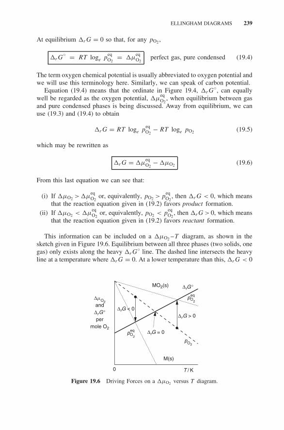
ELLINGHAM DIAGRAMS 239
At equilibrium �rG = 0 so that, for any pO2,
�rG◦ = RT loge p
eqO2
= �μeqO2
perfect gas, pure condensed (19.4)
The term oxygen chemical potential is usually abbreviated to oxygen potential andwe will use this terminology here. Similarly, we can speak of carbon potential.
Equation (19.4) means that the ordinate in Figure 19.4, �rG◦, can equally
well be regarded as the oxygen potential, �μeqO2
, when equilibrium between gasand pure condensed phases is being discussed. Away from equilibrium, we canuse (19.3) and (19.4) to obtain
�rG = RT loge peqO2
− RT loge pO2 (19.5)
which may be rewritten as
�rG = �μeqO2
− �μO2 (19.6)
From this last equation we can see that:
(i) If �μO2 >�μeqO2
or, equivalently, pO2 > peqO2
, then �rG < 0, which meansthat the reaction equation given in (19.2) favors product formation.
(ii) If �μO2 < �μeqO2
or, equivalently, pO2 < peqO2
, then �rG> 0, which meansthat the reaction equation given in (19.2) favors reactant formation.
This information can be included on a �μO2 –T diagram, as shown in thesketch given in Figure 19.6. Equilibrium between all three phases (two solids, onegas) only exists along the heavy �rG
◦ line. The dashed line intersects the heavyline at a temperature where �rG = 0. At a lower temperature than this, �rG < 0
T / K
ΔmO2and
ΔrG°per
mole O2
ΔrG < 0ΔrG > 0
ΔrG = 0
ΔrG°
M(s)
MO2(s)
pO2
0
pO2
eq
pO2
eq
Figure 19.6 Driving Forces on a �μO2 versus T diagram.

240 CHEMICAL EQUILIBRIA BETWEEN GASEOUS AND CONDENSED PHASES I
ΔmO2
ΔG°
M(s)
M(l)
M(g)
MO2(s)
MO2(l)
MO2(g)
T
Figure 19.7 Domains of stability for various phases.
(product phase stable), the equilibrium pO2 at this temperature being given bythe intersection of the dotted line with the heavy line. Similar reasoning followsfor temperatures higher than those corresponding with the original intersection,where the reactant phase is now stable.
Summarizing: at oxygen potentials higher than those corresponding to theheavy line, the product phase is stable, the reactant phase unstable. The reverseis true for lower oxygen potentials than those corresponding to the heavy line.
This recognition of the importance of driving force leads to the concept ofdomains of stability for the different phases. These can be indicated on an Elling-ham diagram. One is shown schematically in Figure 19.7. Note that, if M(g)or MO2(g) are involved, the lines on the diagram refer to these phases at thestandard pressure so that the marked domains of stability also refer to theseconditions.
EXERCISES
19.1 One step in the manufacture of specially purified nitrogen is the removalof small amounts of residual oxygen by passing the gas over copper gauzeat approximately 500◦C. The following reaction takes place:
Cu(s) + 12 O2(g) = Cu2O(s)
.(a) Assuming that equilibrium is reached in this process, calculate theoxygen pressure in the purified nitrogen.
(b) What would be the effect of raising the temperature to 800◦C? Whatif the temperature is lowered to 300◦C? What is the probable reasonfor using 500◦C?
(c) What would be the effect of increasing the pressure?

EXERCISES 241
19.2 In a gas analysis train which is part of a vacuum fusion apparatus, car-bon monoxide is oxidized to carbon dioxide by cupric oxide (which issubsequently reduced to cuprous oxide) at about 300◦C. .
(a) Calculate the concentration of residual carbon monoxide in equilibriumwith carbon dioxide, assuming the latter to be at 0.5 bar pressure.
(b) In the operation of this equipment, the gases are passed through an effi-cient adsorber of carbon dioxide and recirculated over the cupric oxide.How does this affect the residual carbon monoxide concentration?
19.3 The partial pressure of oxygen in equilibrium with Cu2O(s) and CuO hasbeen found to be 0.028 bar at 900◦C and 0.1303 bar at 1000◦C. Calculate�rH
◦ for the reaction
2Cu2O(s) + O2(g) = 4CuO(s)
at 298, 1173, and 1273 K.
19.4 Hydrogen is often used to protect Cr from oxidation at high temperatures.However, H2(g) always contains trace amounts of H2O(g). .
(a) How much moisture content in H2(g) can be tolerated at 1300 K beforechromium becomes oxidized?
(b) Is the oxidation of Cr by H2O endothermic or exothermic at 1300 K?What, if anything, can be said from this reaction about the heat effectat 1300 K by the oxidation of Cr by pure O2?
(c) Would the equilibrium in the above reaction be affected by a changein the pressure of the H2 –H2O mixture from 1 bar to 2 bars? What ifit were changed to 200 bars?
�f H◦(298 K)/kJ mol−1 gef/J mol−1 K−1
H2(g) 0 130.68H2O(g) −241.8 188.83Cr(s) 0 23.64Cr2O3(s) −1134.7 81.17
19.5 A mixture of argon gas and hydrogen gas at 1 bar total pressure is passedthrough a reaction chamber containing a mixture of liquid Sn and liquidSnCl2 at 900 K. The composition of the gas leaving the reaction chamberis 50% H2, 0.01% HCl, and 49.99% Ar. Has equilibrium been attainedbetween the gas phase and the liquid phase in the reaction chamber?
19.6 A solid metal M can form two oxides, MO and M3O4. The metal canexist in equilibrium with one of these oxides at low temperatures and can

242 CHEMICAL EQUILIBRIA BETWEEN GASEOUS AND CONDENSED PHASES I
exist in equilibrium with the other oxide at high temperatures. The Gibbsenergies of formation of these oxides are
�f G◦(MO(s), T )/kJ mol−1 = −259.6 + 0.06255T
�f G◦(M3O4(s), T )/kJ mol−1 = −1090.8 + 0.3128T
Determine which of the two oxides is in equilibrium with the metal atroom temperature and the maximum temperature at which this oxide is inequilibrium with M.
19.7 Plot %CO2 as a function of temperature from 400 to 1200◦C for theoxidation of: .
(a) Fe to magnetite (Fe3O4) at low temperatures and to wustite (FeO) athigh temperatures
(b) wustite (FeO) to magnetite (Fe3O4)
(c) magnetite (Fe3O4) to hematite (Fe2O3)
Would you use CO2 to oxidize magnetite to hematite (Fe2O3) at thesetemperatures?
19.8 Calculate the equilibrium oxygen pressure between Al2O3 and Al(l) at1000 K. Could a vacuum of 10−10 torr prevent the oxidation of Al?

20 Chemical EquilibriaBetween Gaseousand Condensed Phases II
In the previous chapter, we introduced the graphical presentation of �f G◦ and
�rG◦ for a selected group of compounds, for example, oxides and sulfides. It
was noted that, when phase transitions do not interfere, these two thermodynamicquantities are, usually, nearly linear functions of temperature. In practice, a linearrepresentation of �f G
◦ versus T is often within the accuracy of the experimentalresults. Some examples of such representations are given in Appendix A, andthese can be used in many of the exercises in this chapter and Chapter 21.
We also noted that a graphical presentation of standard Gibbs energies which isof particular value is the one introduced by Ellingham where, instead of plotting�f G
◦ versus T , a graph of �rG◦ versus T is plotted, where all the members of
a group of reaction equations refer to 1 mol of O2(g) (or, e.g., S2). The advantageof this method of plotting comes from the fact that, when the condensed phasesare in their pure state, then, from the relation between the empirical equilibriumconstant (for the metal/metal oxide case),
�rG◦ per mole O2(g) = RT loge pO2 = �μO2 (20.1)
In this case, all the domains of stability for the condensed-phase substancespresented on the Ellingham diagram are categorized in terms of the oxygenpotential. By plotting all reaction equations on the basis of 1 mol of O2(g),the graph has been transformed from one of just being the graphical presen-tation of thermochemical data to one of value in carrying out equilibriumcalculations.
Ellingham diagrams are particularly useful for back-of-the-envelope calcula-tions and for visualizing heterogeneous chemical equilibria. They can, however,be used badly and we will pay particular attention to this aspect.
For illustration purposes, we will mainly concentrate on metal/metal oxidediagrams, but the same principles apply to Ellingham diagrams for all the othergroups of compounds.
Materials Thermodynamics. By Y. Austin Chang and W. Alan OatesCopyright 2010 John Wiley & Sons, Inc.
243

244 CHEMICAL EQUILIBRIA BETWEEN GASEOUS AND CONDENSED PHASES II
20.1 SUBSIDIARY SCALES ON ELLINGHAM DIAGRAMS
The value of Ellingham diagrams can be enhanced by the inclusion of varioussubsidiary scales placed around the perimeter of a diagram. We can illustrate thisby first considering how �μO2 varies for a fixed value of pO2.
Using (20.1), this variation is illustrated in Figure 20.1 for pO2 = 10−10 bar.At 2000 K, the point on the figure indicates a value of �μO2 = −382.9 kJ (molO2)−1 for this oxygen pressure.
It can be seen that the whole diagram can be covered by an oxygen pressurefan, with origin at zero oxygen potential and 0 K. In order to be able to have afairly accurate idea of pO2 at any point on the diagram, it is convenient to adda nomogram around the perimeter of the diagram. This enables the connectionbetween pO2, �μO2, and T to be read immediately at any point on the diagram.The construction of the nomogram is illustrated in Figure 20.1b. Note that theanchor point at 0 K is at �μO2 = 0 for all values of pO2 .
It is also possible to include information about the oxygen potentials ofcomplex gas mixtures on the �μO2 –T diagram. In Chapter 18 we saw howknowledge of �rG
◦ for the reaction equations
2CO(g) + O2(g) = 2CO2(g)
2H2(g) + O2(g) = 2H2O(g)
could be used to define �μO2 in terms of the (pCO2/pCO) or (pH2O/pH2) ratios:
�μO2 = 2[�f G
◦(CO2(g), T ) − �f G
◦(CO(g), T )
]+ 2RT loge
(pCO2
pCO
)(20.2)
T/K
0
0 2000
−200
−400
−600
−800
1
10−5
10−10
10−15
10−20
0
0
2000−600
T /K
−382.9 kJ (mol O2)−1
pO
2 = 10 −10bar
pO2/bar
ΔmO
2 = R
T In
(pO
2)/kJ
(mol
O2)
−1
ΔmO
2 = R
T In
(pO
2)/kJ
(mol
O2)
−1
(a) (b)
Figure 20.1 Construction of pO2 nomogram on metal/metal oxide Ellingham diagram:(a) oxygen potential as function of T for pO2 = 10−10; (b) fan of lines for various pO2 .

SUBSIDIARY SCALES ON ELLINGHAM DIAGRAMS 245
�μO2 = 2 �f G◦(H2O(g), T ) + 2RT loge
(pH2O
pH2
)(20.3)
It can be seen that there are fans of lines for the oxygen potentials obtainablefrom gas mixtures containing different ratios of these molecular species. Showingthe dependence of oxygen potential on these ratios is again most convenientlydone with the aid of nomograms, comprising an anchor point for the fan at 0 Ktogether with a perimeter scale. Figure 20.2 shows how the oxygen potential canbe specified at any T through pO2 , pCO2/pCO, or pH2O/pH2 .
0−1200
0 K
ΔmO
2=
RT
In(p
O2)/
kJ (
mol
O2)
−1
−1100
−1000
−900
−800
−700
−500
−400
−300
−200
−100
0
200 400 600 800 1000 1200 1400 1600
−600
pO2. (atm) 10−100 10−80 10−60 10−50 10−42 10−38 10−34
10−30
10−28
10−26
10−24
10−22
10−20
10−18
10−16
10−14
10−12
10−10
10−8
10−6
10−4
10−3
10−2
10−1
10−3
10−2
10−1
102
103
104
105
106
107
108
109
1010
1011
1012
1013
1014
10
1
10−410−510−610−710−810−910−1010−1210−14
1
pCO/pCO2
pH2/pH2O
pCO/pCO2
pH2/pH2O 10−3
10−2
10−1
102
103
104
105
106
107
108
109
1010
1011
1012
1013
10
1
10−410−510−610−710−8
H
C
A
O
temperature °C
Figure 20.2 �μO2 versus T , showing how oxygen potential can be specified in termsof gas mixture composition. Adapted from D. R. Gaskell, Thermodynamics of Materials ,Taylor and Francis, Washington, DC, 2002.

246 CHEMICAL EQUILIBRIA BETWEEN GASEOUS AND CONDENSED PHASES II
With the aid of the subsidiary scales, it is now possible to assign values toT , pO2, �μO2, as well as pCO2/pCO or pH2O/pH2 ratios. The dashed lines inFigure 20.2 are for pH2O/pH2 = pCO2/pCO = 1. They correspond with �rG
◦
for both reactions. The point marked A in the figure is where a gas mixturecontaining equal amounts of all four gases can exist and is known as the watergas equilibrium. The temperature is ≈1095 K and the oxygen pressure there is≈5 × 10⁻¹⁸ bar, a quite low oxygen potential but one easily controlled using gasmixtures containing the four molecular species under consideration.
Figure 20.3 shows how the database for �rG◦ /kJ mol O−1
2 shown in Figure19.4 can be combined with the plot given in Figure 20.2 for �μO2 /kJ mol O−1
2 ,
4Ag + O2 = 2Ag2
O
4Cu + O2 = 2Cu2
O
2Ca + O 2 = 2CaO
2Mg + O 2 = 2MgO
3/2Fe + O 2 = 1/3Fe 3
O 4
4/3Cr + O 2 = 2/3Cr 2
O 3
4/3Al+ O 2 = 2/3Al 2
O 3
2Co + O 2 = 2CoO
2Co + O 2 = 2CO 2
2H2+ O2
= 2H2O
2C + O2 = 2CO
2Ni + O 2 = 2NiO
2Fe + O2 = 2FeO
2MnO + O 2 = 2MnO
Si + O 2 = SiO 2
Ti + O 2 = TiO 2
0−1200
0 K
ΔmO
2=
Δ rG
° =
RT
In (
p O2)/
kJ (
mol
O2)
−1
−1100
−1000
−900
−800
−700
−500
−400
−300
−200
−100
0
200 400 600 800 1000 1200 1400 1600
C + O2 = 2CO2
−600
M
M
M
M
M
MM
M
M
MM
M
B
B
B
M
M
M
M
Melting point of metal
Boiling point of metalMelting point of oxide
temperature, °C
pO2. (atm)
10−100 10−80 10−60 10−50 10−42 10−38 10−34
10−30
10−28
10−26
10−24
10−22
10−20
10−18
10−16
10−14
10−12
10−10
10−8
10−6
10−4
10−3
10−2
10−1
10−3
10−2
10−1
102
103
104
105
106
107
108
109
1010
1011
1012
1013
1014
10
1
10−410−510−610−710−810−910−1010−1210−14
1
10−3
10−2
10−1
102
103
104
105
106
107
108
109
1010
1011
1012
1013
10
1
10−410−510−610−710−8
H
C
6Fe + O 2 = 2Fe 3
O 4
pCO/pCO2
pH2/pH2O
pCO/pCO2
pH2/pH2O
Figure 20.3 Metal/metal Oxide Ellingham diagram. Adapted from D. R. Gaskell, Ther-modynamics of Materials , 3rd Edition, Taylor and Francis, Washington, DC, 2002.

SYSTEM DEFINITION 247
to yield a very useful way of carrying out calculations of heterogenous chemicalequilibria. Although we have concentrated our discussion on oxide equilibria,analogous diagrams can be constructed for sulfides, nitrides, carbides, halides,etc. Provided that these diagrams are used correctly (we illustrate later how itis very easy to reach wrong conclusions when Ellingham Diagrams are usedincorrectly), they provide a very useful means for quickly obtaining approximateanswers for equilibrium calculations.
It is worth noting that, if the oxygen potential is being controlled by usingCO2/CO mixtures (or by any other gas mixture), it is unnecessary for O2(g) to beactually present in the gas phase to obtain the desired oxygen potential. It mayor may not be actually present (usually in immeasurably small concentrationswhen it is), this being a function of the kinetics of the reactions involved. From athermodynamic point of view, this is of no consequence; only the CO2/CO ratioat the selected temperature is important.
This example of using a gas mixture to control an elemental chemical potentialwhen the actual element itself is not present (a metastable equilibrium) can beparticularly well illustrated by another example. A mixture of H2(g) and NH3(g)can be used to control the nitrogen potential of the gas phase. The appropriatereaction equation is
3H2(g) + N2(g) = 2NH3(g)
from which we can see that
�μN2 = �rG◦ + RT loge
((pNH3)
2
(pH2)3
)(20.4)
At high temperatures, however, �rG◦ for this reaction is positive and, as a
result, NH3(g) should start to decompose to N2(g) and H2(g). This would meanthat the gas ratio and hence the nitrogen potential would be quite different fromthat intended. But the decomposition of NH3(g) requires a catalyst and may notoccur. If the decomposition can be avoided, a gas mixture of H2(g) and NH3(g)can actually be used to obtain high nitrogen potentials; this is taken advantageof in the nitriding of steel, summarized in the reaction equation
3H2(g) + 2N(in Fe) = 2NH3(g)
20.2 SYSTEM DEFINITION
Having said that a primary concern of thermodynamics is in predicting propertiesof systems in equilibrium, we emphasize again that the application of thermody-namics will provide the wrong output if it is fed the wrong input . It is absolutelyessential that the system should be defined appropriately .
We introduced the important point in Chapter 18 that the responsibilityfor defining the system lies in the hands of the thermodynamicist. A simple

248 CHEMICAL EQUILIBRIA BETWEEN GASEOUS AND CONDENSED PHASES II
adiabatic flame temperature calculation in the combustion of hydrogen with oxy-gen was used as an example. In systems comprising only a gas phase, poor systemdefinition is rare these days since all relevant species will normally be containedin the computer database used. This may not be the case, however, when thesystem involves condensed phases since the thermodynamicist may, sometimes,be unaware of all the phases which should be taken into account. In such cases,it is very easy to carry out calculations for a metastable equilibrium in a poorlydefined system instead of on the true equilibrium for a properlydefined system.
Relying on the information presented in Ellingham diagrams can be par-ticularly dangerous in this regard because many of the lines presented referto metastable equilibria and not all known species occurring in a particularmetal/metal oxide (e.g., sulfide) system are taken into account. We will illustratethese important points by considering two examples.
Example 20.1 The Fe–O SystemFigure 20.4 shows �rG
◦ per mole O2 as a function of temperature for the sixpossible reaction equations which involve Fe(s), FeO(s), Fe3O4(s), and Fe2O3(s);that is, these lines are a mini–Ellingham diagram. The kinks in the curves arewhere phase transformations occur. The temperature–composition phase diagramfor this system is shown in Figure 20.5. From this we can immediately see whichof the six curves in Figure 20.4 represent metastable equilibria and which are forthe stable equilibria. It follows that the oxygen potential–temperature relation forthis system is not that presented in our mini–Ellingham diagram, Figure 20.4. Werequire a phase diagram in oxygen potential–temperature space analogous to theT –xO phase diagram given in Figure 20.5. In order to distinguish the Ellinghamdiagram from the equilibrium phase diagram, we plot T versus μO2 rather than
500 750 1000 1250 1500 1750 2000
T /K
−600
−400
−200
0
(6)
(5)(4)
(3)(2)(1)
(2) 3/2Fe + O2 = 1/2Fe3O4
(3) 4/3Fe + O2 = 2/3Fe2O3
(4) 6FeO + O2 = 2Fe3O4
(5) 4FeO + O2 = 2Fe2O3
(6) 4Fe3O4 + O2 = 6Fe2O3
(1) 2Fe + O2 = 2FeO
Δ rG
°/kJ
(m
ol O
2)−1
Figure 20.4 Standard Gibbs energies of reaction per mole of O2 for various reactionsin Fe–O system.

SYSTEM DEFINITION 249
0.20.0 0.4 0.6 0.8 1.0Fe xO OH
2000
1500
1000
500
T/K
Fe3O4
Fe2O3Fe1−xO
Fe−Ο(l)
Figure 20.5 T –xO phase diagram for Fe–O system.
the reverse. This mode of plotting, shown in Figure 20.6, also has the advantagethat its appearance is more like the more familiar T –xO phase diagram. It is alsothe method of presentation introduced earlier in Chapter 11.
The phase diagram given in Figure 20.6 may safely be used in true equilibriumcalculations in the Fe–O system. It could, of course, incorporate subsidiary scalesfor pO2 , pCO2/pCO, or pH2O/pH2 just as on the Ellingham diagram.
Example 20.2 Melting of Ti in Al2O3 CruciblesA good example illustrating poor system definition by the thermodynamicistconcerns the feasibility of melting Ti metal in an alumina (Al2O3) crucible with
−500 −400 −300 −200 −100 0
ΔmO2/kJ (mol O2)−1
2000
1500
1000
500
T/K
Fe−O(l)Fe(l)
gFe
dFe
aFe
Fe2O3
Fe3O4
Fe 1−xO
Figure 20.6 T –μO2 phase diagram for Fe–O system.

250 CHEMICAL EQUILIBRIA BETWEEN GASEOUS AND CONDENSED PHASES II
the aim of producing ductile Ti, a property which depends on the metal havinga very low O content.
We will proceed as we did in calculating the adiabatic flame temperature inChapter 18; namely, we make three different assumptions, of increasing sophis-tication concerning the definition of the system. The standard melting point of Tiis 1943 K. We will concentrate on calculations at 2200 K (chosen so that Ti–Oalloys are liquid at all concentrations of O):
(i) Thermodynamicist A defines the system as comprising Ti(l), Al2O3(s),Al(l), and TiO2(s), all pure. Consequently, the following chemical reactionequation is relevant:
32 Ti(l) + Al2O3(s) = 2Al(l) + 3
2 TiO2(s) (20.5)
Thermodynamicist A uses the Ellingham diagram in Figure 20.3 for his or hersource of data.
Consider any pair of reactions on that diagram that evaluate the Gibbs reactionenergy for a condensed-phase reaction equation such as
A(s) + BO2(s) = B(s) + AO2(s)
Then �rG◦ (T ) for this reaction is given by
�rG◦(T ) = �f G
◦(AO2(s), T ) − �f G
◦(BO2(s), T )
= �μeqO2
(A/AO2) − �μeqO2
(B/BO2)
and we see that �rG◦
< 0 when �f G◦(AO2(s), T ) < �f G
◦(BO2(s), T ). Put
another way: If the A/AO2 line is lower down on the Ellingham diagram thanthe B/BO2 line, then A(s) will reduce BO2(s) and vice versa.
Using Figure 20.3, thermodynamicist A concludes that, since the Al/Al2O3
line lies below that for Ti/TiO2 on the Ellingham diagram, it is safe to melt Tiin an Al2O3 crucible.
(ii) Thermodynamicist B is aware that, in order for Ti to be technologicallyuseful, it must possess a very low oxygen concentration and is also aware, asis apparent in Figure 20.7, that both solid and liquid Ti can absorb considerableamounts of oxygen. It is also clear from this phase diagram that the coexistenceof Ti with TiO2, as might be implied from using Figure 20.3, is very much ametastable equilibrium. The important thing to ask is what oxygen potential isrequired to melt Ti with a low oxygen content? He or she calculates the T –μO2
phase diagram shown in Figure 20.8. This reveals that extremely low oxygenpotentials are required in order to obtain the necessary low O concentrationsin liquid Ti at 2200 K. These low oxygen potentials are compared with theoxygen potentials associated with Al/Al2O3 in Figure 20.9. According to theEllingham diagram calculation by thermodynamicist A, the fact that the Ti/TiO2
curve lies above (at higher oxygen potentials) than the Al/Al2O3 curve, leads

SYSTEM DEFINITION 251
0.0 0.1 0.2 0.3 0.4 0.5 0.6 0.7
xOTi O
2500
2000
1500
1000
500
T/K
Liquid
hcp
TiO
2−x
+ ga
s
TiOxbcc
Figure 20.7 Temperature–composition diagram for Ti–O system. The black area com-prises several closely spaced intermediate phases.
−1200 −1000 −800 −600 −400 −200 0
ΔmO2/kJ mol−1
2500
2000
1500
1000
500
T/K
Ti 2
O3
TiO2−x
TiO
x
bcc
Liquid
hcp
O2 (g) 1 bar
0.00010.001
0.01
0.1
0.05
Figure 20.8 Temperature–oxygen potential diagram for Ti–O system.
thermodynamicist A to conclude that it is safe to melt Ti in an Al2O3 crucible.It can be seen from Figure 20.9 that the oxygen potential required to obtainO-free Ti is approximately −1100 kJ (mol O2)
−1, which is much lower thanthat required for the stability of Al2 O3, as can be seen from the location of theAl/Al2O3 curve. Thermodynamicist B concludes, correctly, that it is not possibleto obtain O-free Ti by melting in Al2O3 crucibles.

252 CHEMICAL EQUILIBRIA BETWEEN GASEOUS AND CONDENSED PHASES II
500 1000 1500 2000 2500
T /K
−1200
−1000
−600
−800
mO
2/k
J m
ol−1
O2 potentialsfor "O-free" Ti(l)
4/3Al + O2(g) = 2/3Al2 O3(s
)Ti + O2(g) = TiO2
Figure 20.9 Oxygen potentials required for obtaining oxygen-free Ti(l) are shown cir-cled.
(iii) Thermodynamicist C realizes that thermodynamicist B’s system def-inition is much better that thermodynamicist A’s, who reached an incorrectconclusion resulting from a very poor system definition. Although thermodynam-icist B reached the correct conclusion, thermodynamicist C realizes that it hasbeen reached via a system definition which is still not complete: It is necessaryto consider all possible phases occurring in the ternary Ti–Al–O system.
Since we are only considering binary systems in this chapter, discussion ofthermodynamicist C’s deliberations is postponed until Chapter 22.
EXERCISES
20.1 The following reactions are sufficient to evaluate the equilibrium in a C(s),O2(g), CO(g), CO2(g) system:
CO(g) + 12 O2(g) = CO2(g) (20.6)
C(s) + O2(g) = CO2(g) (20.7)
Obtain �rG◦ for reactions (1) and (2) from the oxide Ellingham diagram
shown in Figure 20.3. .
(a) If we start with 1 mol CO(g) and feed it into a closed quartz boxmaintained at a total external pressure of 1 bar and 1000 K, evaluatethe final partial pressures of the gases.

EXERCISES 253
(b) Repeat the calculation for the case where the box is made of Fe andalso calculate how much C is formed. Note: You will simplify thecalculation in this part considerably if you use the metal oxide Elling-ham diagram to help you make a good approximation.
Important Note: Carbon deposition from CO(g) requires a catalystbefore it can occur. Iron is one such catalyst, quartz is not.
20.2 .(a) Draw a carbon potential �μC(T )–T diagram. Make the T axis0–2000 K and the ordinate axis run from +200 to −200 kJ (molC)−1.
(b) Put on a fan (anchor point and perimeter scale) which enables speci-fication of �μC(T ) in terms of a combination of CH4 and H2 partialpressures.
(c) Put on a fan (anchor point and perimeter scale) which enables speci-fication of �μC(T ) in terms of a combination of CO and CO2 partialpressures.
(d) Assume a gas containing equimolar amounts of CO and CO2 at 1 bartotal pressure is passed into a furnace at 1300 K:
(i) Will the C(s) either deposit (assuming the furnace structure con-tains lots of Fe) in the furnace or exit from the furnace?
(ii) Will pure Si(s) in the furnace be converted and, if so, to what?
20.3 Calculate the equilibrium oxygen pressure between Al2O3 and Al(l) at1000 K. Would a vacuum of 10−8 Pa prevent the oxidation of Al at thistemperature?


21 Thermodynamics of TernarySystems
In the earlier chapters the focus has been on the thermodynamics of unaryand binary systems. However, multicomponent systems are often encounteredin MS&E. Engineering alloys, for example, usually consist of more than 2 ele-ments, sometimes more than 10. In this and the following chapter, we extendour discussion of the thermodynamics of binaries to that of ternaries. Once thethermodynamic properties of ternaries are understood, it is usually straightfor-ward to extend the concepts to higher order alloys. Experience shows that onceall the binary and ternary thermodynamic properties are known, extrapolation tohigher order systems can usually be carried out with confidence. This is becausethe number of near neighbor contacts which involve more than three differenttypes of atoms will usually be very small in multicomponent alloys. Rarely, whenstrong chemical interactions are present, this can break down due to the formationof multicomponent compound phases.
In line with our earlier discussions of binary alloys, we will first discuss thethermodynamics of ternary solution phases and then discuss phase equilibria.More general aspects of the geometric presentation of phase equilibria in ternaryalloys, including heterogeneous chemical equilibria, are discussed in the nextchapter.
We have seen that, for two preselected phases α and β, the conditions ofequilibrium, assuming all species are mobile between both phases, are given by
μαi = μ
β
i ∀ i (21.1)
In order to be able to apply (21.1) to ternary phase equilibria we need to know theμi in the participating ternary phases. Because of the relatively poor availabilityof experimental results for ternary systems, the estimation of the thermodynamicproperties of ternaries from those of the constituent binaries takes on a cardinalrole and we first discuss some ways by which this is done.
Materials Thermodynamics. By Y. Austin Chang and W. Alan OatesCopyright 2010 John Wiley & Sons, Inc.
255

256 THERMODYNAMICS OF TERNARY SYSTEMS
21.1 ANALYTICAL REPRESENTATION OF THERMODYNAMICPROPERTIES
21.1.1 Substitutional Solution Phases
It is necessary to decide which composition of a binary alloy should be used inestimating the contribution of the properties from that binary to the propertiesof a selected ternary alloy. Figure 21.1 shows just four of an infinite number ofpossible ways which could be used in deciding which composition of the binaryBC would be the most appropriate for estimating the contribution of this binary’sproperty to the ternary alloy’s property (at the circled point). Two widely usedsymmetric geometric methods for adding the binary contributions to the ternary,due to Kohler and Muggianu, respectively, are shown in Figure 21.2. An asym-metric addition may be more appropriate in other circumstances, for example,if one of the components is an interstitial element. Here we will concentrate onsymmetric extrapolations for substitutional solutions.
If both the binaries and the ternary are assumed to be regular solutions and alsothat the various binary interaction energies are the same in the ternary as they arein the relevant binary system, then it is straightforward to calculate the ternaryalloy’s properties. In this case, the numbers of A–B, B–C, and C–A contacts inthe A–B–C ternary are known because of the random mixing assumption. Theternary properties are given by
GEm(xA, xB, xC) = xAxBLAB
0 + xBxCLBC0 + xCxALCA
0 (21.2)
This estimation is just that expected from the Muggianu extrapolation shownin Figure 21.2b. This then suggests an obvious way to extend (21.2), namely,
OO
O O
A A
AA
BB
B B
C
C C
C
(a) (b)
(d)(c)
Figure 21.1 Some of the infinite number of possible ways of estimating the B–C con-tribution to the properties of a ternary A–B–C alloy.

ANALYTICAL REPRESENTATION OF THERMODYNAMIC PROPERTIES 257
O
A
B C
O
A
B C
(a) (b)
Figure 21.2 Example of two different ways for estimating ternary system properties fromconstituent binary system properties: (a) Kohler extrapolation; (b) Muggianu extrapola-tion.
use the Redlich–Kister polynomial to allow for any deviations from the regularsolution model in the binary systems and add them as in (21.2). This assumptionleads to the so-called Redlich–Kister–Muggianu (RKM) equation, which is themost widely used extrapolation equation for substitutional and liquid alloys:
GEm(xA, xB, xC) = xAxB
n∑i=0
LABi (xA − xB)i
+ xBxC
n∑i=0
LBCi (xB − xC)i
+ xCxA
n∑i=0
LCAi (xC − xA)i (21.3)
Equations for μEA can be obtained from this equation by using the framed equation
given below, which is a general equation for obtaining partial molar quantitiesfrom integral quantities for multicomponent systems. Its derivation (we use i forthe component of interest and j for any component) is as follows:
μEi =
(∂GE
∂Ni
)p,T ,{Nj }
=(
∂NGEm
∂Ni
)p,T ,{Nj }
(21.4)
where N = ∑i Ni and j �= i.
∂NGEm
∂Ni
= GEm + N
(∂GE
m
∂Ni
)
= GEm + N
⎡⎣∂GE
m
∂xi
· ∂xi
∂Ni
+∑j �=i
∂GEm
∂xj
· ∂xj
∂Ni
⎤⎦
258 THERMODYNAMICS OF TERNARY SYSTEMS
The relations between the mole fractions and the amounts can be obtained fromthe differentiation of
xi = 1 −∑
j
Nj
N(21.5)
and they are given by
∂xi
∂Ni
= 1 − xi
N
∂xi
∂Nj
= −xi
Nj �= i
Finally we can obtain the relation between the partial molar quantity and theintegral quantity:
μEi = GE
m + (1 − xi)
(∂GE
m
∂xi
)−∑j �=i
xj
(∂GE
m
∂xj
)
μEi = GE
m +(
∂GEm
∂xi
)−∑
j
xj
(∂GE
m
∂xj
)(21.6)
This equation represents a generalization of the equation corresponding with thetangent–intercept method discussed earlier for binary solutions. The equation forbinaries can be obtained directly from this general equation, (21.6).
The excess chemical potentials may be obtained from (21.3) for GEm by using
(21.6). For component A:
μEA = LAB
0 xB(1 − xA) + LCA0 xC(1 − xA)
+n∑
i=1
LABi xB(xA − xB)(i−1)[(1 − xA)(xA − xB)(i + 1) + ixB ]
+n∑
i=1
LCAi xC(xC − xA)(i−1)[(1 − xA)(xC − xA)(i + 1) + ixC]
− xBxC
[LBC
0 +n∑
i=1
LBCi (xB − xC)i(i + 1)
](21.7)
Similar relations can be written for μEB and μE
C .If extra parameters are required in the fitting to experimental results, the RKM
equation can be extended by adding ternary interaction terms to (21.3). Theseextra terms must be selected so that they reduce to the correct binary solution
ANALYTICAL REPRESENTATION OF THERMODYNAMIC PROPERTIES 259
equation when there are only two components. If we consider just the first twoternary interaction terms, the additional contribution to GE
m is given by
GEm(xA, xB, xC) = xAxBxCLABC
0 + 13 (1 + 2xA − xB − xC)LABC
1
+ 13 (1 + 2xB − xC − xA)LBCA
1
+ 13 (1 + 2xC − xA − xB)LCAB
1 (21.8)
and the extra contribution to μEA is given by
μEA = xBxC(1 − 2xA)LABC
0 + LABC1 (21.9)
with analogous equations for the extra contributions to μEB and μE
C .
21.1.2 Sublattice Phases
We have already met, in Chapter 14, the following modeling equation for abinary sublattice phase with two equally sized sublattices and whose configura-tional energy is determined by nearest neighbor interaction energies. In the BWapproximation,
�mixAconfm = z
2WAB
(yα
Ayβ
B + yαBy
β
A
)+∑
α
f α∑
i
yαi loge yα
i (21.10)
Assuming there are no additional ternary terms, this can be extended for use withternary alloys in a manner similar to that used for substitutional phases:
�mixAconfm = z
2WAB
(yα
Ayβ
B + yαBy
β
A
)+ z
2WBC
(yα
Byβ
C + yαCy
β
B
)+ z
2WCA
(yα
Cyβ
A + yαAy
β
C
)+∑α
f α∑
i
yαi loge yα
i (21.11)
from which it can be shown that the chemical potential of A is given by
μA = zWAByαBy
β
B + zWCAyαCy
β
C + 12 loge(y
αAy
β
A) (21.12)
with analogous relations for μB and μC .Equation (21.11) is a free-energy functional with internal variables, the y
(j)
i ,and has to be minimized subject to the mass balance constraints, for example,

260 THERMODYNAMICS OF TERNARY SYSTEMS
xC = 0.5(yαC + y
β
C), in order to obtain the equilibrium values of the sublatticemole fractions and the thermodynamic properties.
Similar equations can be used for the four-point cluster model discussed pre-viously for binary alloys.
For both the two- and four-sublattice modeling equations, extra terms, involv-ing ternary and/or quaternary parameters, could be added if required in the fittingto experimental results.
21.2 PHASE EQUILIBRIA
The most common type of binary phase diagram encountered in MS&E showstemperature as a function of composition at constant p, normally at 1 bar. Withan additional component, one further variable must be fixed if a two-dimensionalphase diagram is required for the ternary system. The phase diagrams are mostfrequently presented as isothermal sections at constant p (1 bar). Many suchisothermal sections are required in order to gain a complete understanding of thetemperature–composition relationships for a ternary system.
Equation (21.1) together with the use of either (21.7) (substitutional phases)or (21.12) (sublattice phases) may be solved to calculate the position of phaseequilibrium between two preselected phases. We will illustrate the procedure byconsidering three examples.
Example 21.1 Miscibility Gap SystemAssume as given the following RK parameters for the constituent binary systems:
LAB0 = +20 kJ mol−1
LAB1 = −5 kJ mol−1
LCA0 = LBC
0 = +10 kJ mol−1
Calculate an isothermal section at 1000 K for the A–B–C system by using theRKM equation.
There is only a single phase to consider in this simple example. It is clearfrom Figure 21.3a that, at 1000 K, the A–B binary exhibits a miscibility gapwhile the other two binaries do not.
For a ternary alloy with an overall composition inside the miscibility gap, thereare five unknowns, namely, xα
A, xα′A , xα
B, xα′B , and f , the fraction of the α-phase.
The equilibrium values of the independent variables can be obtained from thesolution of the following five equations:
μαA(xα
A) = μα′A (xα′
A ) (21.13)
μαB(xα
B) = μα′B (xα′
B ) (21.14)
μαC(xα
C) = μα′C (xα′
C ) (21.15)

PHASE EQUILIBRIA 261
A
0.0 0.2 0.4 0.6 0.8 1.0−3.5
−3.0
−2.5
−2.0
−1.5
−1.0
−0.5
0.0
Mole fraction Mole fraction C
Mol
e fra
ctio
n A(A,B)
(B,C) and (C,A)
Δ mixG
m/k
J m
ol−1
0.200
0.2
0.4
0.6
0.8
1
0.4 0.6 0.8 1B C
(a) (b)
Figure 21.3 Binary �mixGm and calculated ternary isothermal section at 1000 K:(a) �mixGm for binaries; (b) isothermal section for ternary system.
xA = f xαA + (1 − f )xα′
A (21.16)
xB = f xαB + (1 − f )xα′
B (21.17)
where the chemical potentials are given by
μαi = μ
◦,αi + RT loge xα
i + μE,αi (21.18)
and μE,αi is given by (21.7).
These equations may be solved at a fixed value of xC and a fixed ratio ofxB/xA, which guarantees a composition lying within the two-phase region. UsingxC = 0.05 and xB/xA = 1.111, the solution of these equations at 1000 K givesthe solution for the independent variables:
xαA = 0.09749 xα
B = 0.8412
xα′A = 0.7119 xα′
B = 0.244 (21.19)
f = 0.3449
The phase diagram shown in Figure 21.3b shows the complete isothermal sectionat 1000 K plotted on triangular coordinates (Gibbs triangle). An example of areal system which shows a phase diagram similar to this is the fcc (Au,Cu,Ni)phase in the Au–Cu–Ni system, with the miscibility gap extending from thebinary Au–Ni.
Example 21.2 Liquid-Phase/Sublattice-Phase equilibriumAn isothermal section of a calculated phase diagram for the equilibrium betweenliquid and B2 phases is shown in Figure 21.4. We wish to confirm this phasediagram by calculating the tie-line marked as l–b on the diagram.

262 THERMODYNAMICS OF TERNARY SYSTEMS
0.20.00.0
0.2
0.4
0.6
0.8
1.0
0.4 0.6 0.8 1.0C A
B
xA
xBx C
1.0
0.8
0.6
0.4
0.2
0.0
Liquid
Liquid
l
b
B2
Liqu
id+ B
2
Liqu
id+
B2
Figure 21.4 Isothermal phase diagram for system showing equilibrium between liquidphase and sublattice phase. One tie-line in the two-phase region is shown.
The isothermal section is for a temperature of 1050 K and the endpoints ofthe tie-line are given in Table 21.1.
The parameters used in the calculation of Figure 21.4, are as follows: Thestabilities of the pure bcc components relative to the pure liquid components aregiven by
G(A, bcc) = G(B, bcc) = G(C, bcc) = −10 + 0.01T kJ mol−1
For the liquid solution phase, the binary RK parameters are
LAB0 = −5 kJ mol−1 LAC
0 = −4 kJ mol−1 LBC0 = 0
These may be used to calculate the ternary properties by using simplified formsof the RKM equation given in (21.7)—only the L0 terms have to be considered.
For the two-sublattice B2 (bcc) phase, the pair exchange energies are
WAB = WBA = −5 kJ mol−1
WAC = WCA = −4 kJ mol−1
WBC = WCB = +1.25 kJ mol−1
TABLE 21-1 Compositions of the Tie-Line 1-B in Figure 21.4
xA xB xC
Liquid 0.460173 0.403839 0.135988B2 0.331947 0.533263 0.134789
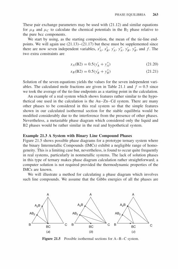
PHASE EQUILIBRIA 263
These pair exchange parameters may be used with (21.12) and similar equationsfor μB and μC to calculate the chemical potentials in the B2 phase relative tothe pure bcc components.
We start by using, as the starting composition, the mean of the tie-line end-points. We will again use (21.13)–(21.17) but these must be supplemented sincethere are now seven independent variables, xl
A, xlB , y′
A, y′′A, y′
B , y′′B , and f . The
two extra constraints are
xA(B2) = 0.5(y ′A + y′′
A) (21.20)
xB(B2) = 0.5(y ′B + y′′
B) (21.21)
Solution of the seven equations yields the values for the seven independent vari-ables. The calculated mole fractions are given in Table 21.1 and f = 0.5 sincewe took the average of the tie-line endpoints as a starting point in the calculation.
An example of a real system which shows features rather similar to the hypo-thetical one used in the calculation is the Au–Zn–Cd system. There are manyother phases to be considered in this real system so that the simple featuresshown in our calculated isothermal section for the stable equilibria would bemodified considerably due to the interference from the presence of other phases.Nevertheless, a metastable phase diagram which considered only the liquid andB2 phases would be rather similar in the real and hypothetical system.
Example 21.3 A System with Binary Line Compound PhasesFigure 21.5 shows possible phase diagrams for a prototype ternary system wherethe binary Intermetallic Compounds (IMCs) exhibit a negligible range of homo-geneity. This is a limiting case but, nevertheless, is found to occur quite frequentlyin real systems, particularly in nonmetallic systems. The lack of solution phasesin this type of ternary makes phase diagram calculation rather straightforward; acomputer solution is not required provided the thermodynamic properties of theIMCs are known.
We will illustrate a method for calculating a phase diagram which involvessuch line compounds. We assume that the Gibbs energies of all the phases are
A
B CBC.
..
A
B CBC.
..
A
B CBC.
..
(a) (b) (c)
A2B A2B A2B
AB2 AB2 AB2
Figure 21.5 Possible isothermal sections for A–B–C system.

264 THERMODYNAMICS OF TERNARY SYSTEMS
known with the following values of �f G◦m at 1000 K:
A2B = −10.00 kJ mol−1
AB2 = −9.67 kJ mol−1
BC = −9.00 kJ mol−1
The three possibilities for this phase diagram are shown in Figure 21.5. Thereit can be seen that the AB2 –BC join is common to all three possible phasediagrams. The other two joins are seen to vary between where both involveBC (Fig. 21.5a), both involve C (Fig. 21.5b), and one involves BC and one C(Fig.21.5c). We may determine which is the correct phase diagram by consideringthe reaction equations
3BC + A2B = C + 2AB2 (21.22)
3C + 2A = C + A2B (21.23)
The values for �rG◦ for these two reactions are
2(−9.67) − [3(−9) + (−10)] = +27.66
(−10) − [(−9)] = −1
from which we conclude that Figure 21.5c represents the stable phase diagramin this case.
EXERCISES
21.1 Derive (21.12).
21.2 Confirm the results given in (21.19).
21.3 Confirm the results given in Table 21.1.
21.4 Derive the equation for the Kohler interpolation for the case where allthree binaries are strictly regular. (Hint: The ratio of two components isthe same in the ternary and binary alloys.) Compare the estimated valuesfor GE in ternary solutions of composition (xA = 0.333, xB = 0.333) and(xA = 0.8, xB = 0.1) when the RKM and Kohler methods are used forstrictly regular solutions. Which extrapolation method do you think is thebetter?
21.5 .(a) There is one intermediate phase in the In–P system, InP, two IMCsin the In–Co system, CoIn3 and CoIn2, and three IMCs in the Co–Psystem, PCo2, PCo, and P3Co.

EXERCISES 265
The enthalpies of formation of these IMCs at 298.15 K are InP(−18.85); CoIn3 (−0.975), CoIn2 (−2.17); PCo2 (−21.77), PCo(−39.55), and P3Co (−18.1), all expressed in term of kilojoules permole of atoms.
On the basis of these data, calculate the composition isotherm forthe In–Co–P system at 298.15 K. What assumption do you have tomake in order to calculate this diagram?
(b) Suppose that you need to make an electrical contact to an InP alloy.Would you recommend the use of Co at room temperature? Whatabout at 373 K? Why?
21.6 Ni and Si form three IMCs, Ni3Si, Ni5Si2, and Ni2Si. Si and C form onlyone, SiC. Calculate the ternary phase diagram of Ni–Si–C at 600◦C.
The standard Gibbs energies of formation of these phases are Ni2Si(−142.7), Ni5Si2 (−315.0), Ni3Si (−160.0), and SiC (−66.9), allexpressed in term of kilojoules per mole of formula.
21.7 For a ternary A–B–C system, there exist three binary intermetallic phases,AB, BC, and AC.
The standard Gibbs energies of formation of these three compoundsat 1000 K are A0.5B0.5 (−10), A0.5C0.5 (−20), and B0.5C0.5 (−5), allexpressed in terms of kilojoules per mole of atoms. .
(a) Calculate the 1000-K isotherm assuming there are mutual solubilitiesin pure A, B, and C and the three binary compounds are negligible.
(b) Calculate and plot an isothermal field–density phase diagram usingμC/RT as a function of xB /(xB + xA) at 1000 K. Assume that thereare no mutual solubilities between any of the phases. Draw another(schematic) diagram where finite solubilities between these phases isassumed.


22 Generalized Phase Diagrams forTernary Systems
In discussing unary and binary systems, we have already met some different waysof graphically presenting the results from equilibrium calculations in the form oftwo-dimensional phase diagrams.
(A) Unary For unary systems, phase diagrams can be plotted in two dimen-sions without any constraints. This can be understood from the Gibbs–Duhemequation for a unary system:
S dT − V dp + n dμ = 0
or, in molar form,
Sm dT − Vm dp + dμ = 0 (22.1)
from which it can be seen that, for given values of any two of the field variables,the third is automatically adjusted.
This leads to the following classification for unary, two-dimensional phasediagrams:
(i) field–field phase diagrams, for example, p versus T
(ii) field–density phase diagrams, for example, p versus Sm but notinvolving conjugate variables such as T versus Sm
(iii) density–density phase diagrams, for example, Sm versus Vm
(B) Binary For binary systems, it is necessary to fix one independent vari-able in order to be able to plot a two-dimensional phase diagram. Most binaryphase diagrams used in MS&E refer to a constant total pressure of 1 bar and,under these constant-pressure conditions, the Gibbs–Duhem equation is
S dT + nA dμA + nB dμB = 0
or, in molar form,
Sm dT + (1 − xB) dμA + xB dμB = 0 (22.2)
Materials Thermodynamics. By Y. Austin Chang and W. Alan OatesCopyright 2010 John Wiley & Sons, Inc.
267

268 GENERALIZED PHASE DIAGRAMS FOR TERNARY SYSTEMS
from which it can be seen that, if two field variables are fixed, the third isautomatically adjusted. As a result, constant-total-pressure two-dimensional phasediagrams can be classified in the same way as for unary systems:
(i) field–field phase diagrams, for example, T versus μB
(ii) field–density phase diagrams, for example, T versus xB and μB
versus Sm but not involving conjugate variables such as T versus Sm
(iii) density–density phase diagrams, for example, Sm versus xB
(C) Ternary The situation for ternary systems may be understood by againconsidering the constant-total-pressure Gibbs–Duhem equation:
S dT + nA dμA + nB dμB + nC dμC = 0
This equation can be manipulated in different ways to convert the extensivequantity to a density:
S
nC
dT + nA
nC
dμA + nB
nC
dμB + dμC = 0
S
nA + nB
dT + nA
nA + nB
dμA + nB
nA + nB
dμB + nC
nA + nB
dμC = 0
This last equation can be written more compactly as
Sn dT + (1 − ξ) dμA + ξ dμB + r dμC = 0 (22.3)
where
Sn = S
nA + nB
ξ = nB
nA + nB
r = nC
nA + nB
The use of ξ and r takes advantage of the fact that there are only two independentcomposition variables (xA + xB + xC = 1).
It is clear that, for ternaries, it is now necessary to fix two properties beforea two-dimensional phase diagram can be drawn. Constant total pressure is oneobvious choice with a constant field or density being the other obvious choice.However, another possibility exists and we first discuss this before returning toa classification of the different possible phase diagrams for ternary systems.
Special Constraints in Ternary Systems. A situation with no counterpartin binary alloys may occur when one of the three alloying elements diffusesmuch more rapidly than the other two, for example, when one of the elementsdissolves interstitially (e.g., H, C, N). The best known example of this, which wewill consider, occurs during the transformation of austenite (γ ) to ferrite (α) inFe–C–X alloys, where X is a substitutional alloying element. The interface willbe mobile during an actual transformation but, since we are concerned only withthermodynamics, we will consider the situation where the interface is immobilebut where the Fe/X ratio remains constant.

GENERALIZED PHASE DIAGRAMS FOR TERNARY SYSTEMS 269
In the case of complete equilibrium (all species are considered mobile), we canuse μα
i = μγ
i for all three elements as the condition of equilibrium. At constanttotal p, a single phase in the ternary alloy has three degrees of freedom and it istherefore necessary to fix another variable if we wish to plot a two-dimensionalphase diagram. The most obvious one to fix is T . Figure 22.1 shows a schematiccomplete equilibrium field–density phase diagram at high Fe concentrations (thedashed curves). If we start with the α-phase and increase the carbon potential,the α will first transform into the γ -phase of a different Fe/X ratio. Eventually,at the completion of the transformation, the γ -phase will have the same Fe/Xratio as the original.
The constrained equilibrium situation is quite different. First, because(Fe/X)α = (Fe/X)γ at all times, the system acts like a pseudobinary and,second, we can no longer use μα
i = μγ
i for all three components but only forC, μα
C = μγ
C. We may obtain another constraining condition for the chemicalpotentials via the use of a Lagrangian multiplier, λ, for the mass balanceconstraint Nα
FeNγX − N
γFeN
αX = 0. The Lagrangian for the α/γ is given by
L = Gα + Gγ + λ(NαFeN
γX − N
γFeN
αX)
and its minimization gives
∂L∂Nα
Fe= μα
Fe + NγXλ = 0
∂L∂Nα
Fe= μα
X − NγFeλ = 0
∂L∂Nα
Fe= μ
γFe − Nα
Xλ = 0
∂L∂Nα
Fe= μ
γX + Nα
Feλ = 0
Fe X
Complete
mc
a
g
x
Constrained
const. T
Figure 22.1 Schematic μC –ξ isotherm for Fe–C–X system. Both complete (dashedcurves) and constrained (solid curve) equilibrium phase diagrams are shown.

270 GENERALIZED PHASE DIAGRAMS FOR TERNARY SYSTEMS
The λ may be eliminated from these equations to give the equilibrium relationbetween the chemical potentials for this constrained equilibrium:
(1 − ξ)μαFe + ξμα
X = (1 − ξ)μγFe + ξμ
γX (22.4)
This last equation can be written as
Gαn = Gβ
n (22.5)
where the subscript refers to the unit amount of the immobile (Fe and X) com-ponents.
Another, rather similar, constraint may also occur in a ternary system. Thiscan be seen by referring to Figure 22.2, which shows an isothermal section at1600 K for the FeO–Fe2O3 –SiO2 system. It can be seen that the liquid phasecan be saturated with either metallic or oxide phases. The metallic phase isnot pure Fe but is an Fe–Si alloy. Following a similar argument to that givenabove for the constrained equilibrium in the Fe–X–C system, we can see thatthe equilibrium condition along this metal-saturated boundary, with pure Fe andpure Si as reference states, is
(1 − ξ)μFe + ξμSi = 0 (22.6)
0.2
0.2
0.40.6
liquid +(Fe,Si)
liquid +'FeO'
0.80.2
FeO
liqui
d
Fe2O3
liquid +Fe3O4
liqui
d+
SiO
2
XFe2O3
X FeO X
SiO2
Fe 3
O4
+ S
iO2
SiO2
0.4 0.6 0.8
Figure 22.2 Isothermal section for FeO–Fe2O3 –SiO2 system at 1600 K.
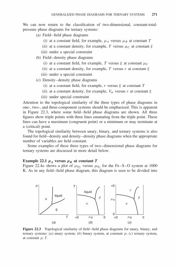
GENERALIZED PHASE DIAGRAMS FOR TERNARY SYSTEMS 271
We can now return to the classification of two-dimensional, constant-total-pressure phase diagrams for ternary systems:
(a) Field–field phase diagrams(i) at a constant field, for example, μA versus μB at constant T
(ii) at a constant density, for example, T versus μC at constant ξ
(iii) under a special constraint(b) Field–density phase diagrams
(i) at a constant field, for example, T versus ξ at constant μC
(ii) at a constant density, for example, T versus r at constant ξ
(iii) under a special constraint(c) Density–density phase diagrams
(i) at a constant field, for example, r versus ξ at constant T
(ii) at a constant density, for example, Vm versus r at constant ξ
(iii) under special constraintAttention to the topological similarity of the three types of phase diagrams inone-, two-, and three-component systems should be emphasized. This is apparentin Figure 22.3, where some field–field phase diagrams are shown. All threefigures show triple points with three lines emanating from the triple point. Theselines can have a maximum (congruent point) or a minimum or may terminate ata (critical) point.
The topological similarity between unary, binary, and ternary systems is alsofound for field–density and density–density phase diagrams when the appropriatenumber of variables are held constant.
Some examples of these three types of two–dimensional phase diagrams forternary systems are discussed in more detail below.
Example 22.1 μA versus μB at constant TFigure 22.4a shows a plot of μO2 versus μS2 for the Fe–S–O system at 1000K. As in any field–field phase diagram, this diagram is seen to be divided into
sliquid
liquid
g
(a) (b) (c)
0
T
T mB
mA
a a
g
b b
0<0 mB 0<0
<0p
Figure 22.3 Topological similarity of field–field phase diagrams for unary, binary, andternary systems: (a) unary system; (b) binary system, at constant p; (c) ternary system,at constant p, T .

272 GENERALIZED PHASE DIAGRAMS FOR TERNARY SYSTEMS
0
0
Fe2(SO4)3
Fe2(SO4)3
Fe2O3
Fe2O3
Fe3O4
Fe2O3
FeO
FeO
Fe
Fe FeS
FeSFeS2
FeS2
p = 1 bar
FeSO4
FeSO4
−100
−200
−300
ΔmO
2/K
J (m
ol O
2)−1
log 1
0 (p
O2/b
ar)
log10 (pSO2/bar)
ΔmS2/KJ (mol S2)−1
−400
−400 −300 −200 −100 0
(b)
(a)
−5−10−20 −15−25 0
−500
−10
−20
−30
Figure 22.4 Isothermal sections at 1000 K for Fe–S–O system: (a) μO2 versus μS2 ;(b) log10 pO2 versus log10 pSO2 .
the various domains of stability for the various condensed phases and hence thename often given to this type of phase diagram is predominance area diagram.
In the diagram shown in Figure 22.4a the horizontal lines refer to simpleoxidation reactions, for example,
2Fe(s) + O2(g) = 2FeO(s)
while the vertical line refers to a simple sulfidation reactions, for example,
2Fe(s) + S2(g) = 2FeS(s)

GENERALIZED PHASE DIAGRAMS FOR TERNARY SYSTEMS 273
The sloping lines refer to reactions which involve both O2 and S2, for example,
FeO(s) + S2(g) = FeS(s) + O2(g)
The diagram axes selected for Figure 22.4a are not necessarily the most con-venient ones to use in a practical application. It is straightforward to changeto a more suitable pair of variables. These will be related to the two used inFigure 22.4a. Consider, for example, the chemical reaction equations
2SO2 + O2 = 2SO3 (22.7)
4SO3 + S2 = 6SO2 (22.8)
S2 + 2O2 = 2SO2 (22.9)
It can seen that the sulfur potential can be specified through (pSO2)6/(pSO3)4
or through (pSO2)/pO2)2 and the oxygen potential through (pSO3/pSO2)2. If we
were to select log10 pSO2 as one axis, then we have several possible choices forthe other axis (e.g., log10 pO2). A phase diagram equivalent to Figure 22.4a isshown in Figure 22.4b.
Example 22.2 T –μi under Special ConstraintIn the FeO–Fe2O3 –SiO2 system, an isothermal section for which was shown inFigure 22.2, oxygen potentials will vary as a function of composition across theliquid phase region. If we wish to introduce temperature as a variable, then itwill be necessary to fix a different variable if a two-dimensional phase diagramis still required. One possibility is to fix the oxygen potential or partial pressureand show the phase diagram, for example, at 1 bar of air. Another is to show thetemperature variation of the oxygen potentials along the alloy-saturated boundarywhich, thermodynamically, corresponds with the chemical potential conditiongiven previously in (22.6). Under this constraint, the T –μO2 phase diagramshown in Figure 22.5 is obtained.
A brief explanation of this phase diagram is warranted. The curve shownat the highest oxygen potentials in Figure 22.5 corresponds with the Fe/FeOequilibrium. At oxygen potentials higher than those given by this curve, we willno longer have metal saturation with the higher oxides of Fe becoming stable. Thecurve shown at the lowest oxygen potentials in the diagram corresponds with theSi/SiO2 equilibrium. At oxygen potentials lower than those given by this curve,only Si can exist. In the region between the upper and lower bounds set bythe Fe/FeO and Si/SiO2 curves metal saturation must correspond with alloys ofintermediate compositions: Si-rich alloys at low oxygen potentials and Fe-richalloys as the Fe/FeO curve is approached. In other words, the domains of stabilityfor the different phases in the intermediate region must resemble those found ina T –μSi phase diagram for the Fe–Si system. These domains of stability for thedifferent phases are indicated on the areas in Figure 22.5. It is also possible toinsert lines for different compositions of both the metallic and oxide phases on

274 GENERALIZED PHASE DIAGRAMS FOR TERNARY SYSTEMS
2200
(Fe,Si)(l) + SiO2(l)
2Fe
+ O
2=
2FeO
a +
Fe 2S
iO4
(Fe,Si)(l) + SiO2(s)
(Fe,
Si)
+ si
licat
e m
elts
(Fe,Si)(g) + SiO2(s
)
Si+
O 2=
SiO 2
1800
−600 −500
ΔmO2/KJ mol−1
−400 −300
T/K
1400
1000(Fe,Si)(a) + SiO2(s)
g+
Fe,S
iO4
e+ S
iO2(
s)
Figure 22.5 Alloy-saturated T –�μO2 phase diagram for Fe–Si–O system.
this phase diagram. In the liquid-phase region for the liquid alloys, lines for theconcentration of O as well as those for Si could also be inserted. Such lines areuseful for indicating the deoxidation behavior of molten steel by Si.
Example 22.3 Field–Density at a Constant FieldA 773-K isotherm for the Fe–Cr–O ternary system is shown in Figure 22.6a .Several line compounds are present in this system, that is, Fe3O4 and Fe2O3
in the binary Fe–O and Cr2O3 in the binary Cr–O. Solution phases of (Fe,Cr)are present in the binary Fe–Cr system and in (Fe,Cr)2O3 in the pseudobinaryFe2O3 –Cr2O3 system. A ternary spinel phase (Fe,Cr)3O4 is found along the 57.1at % O join, but this phase is stable only in the ternary composition region, notin the binary Fe–O and Cr–O systems.
The type of phase diagram presentation given in Figure 22.6a can be supple-mented by a field–density isotherm like that presented in Figure 22.6b.
The relative utility of these different forms of presentation will vary: Forthose interested in open systems, Figure 22.6b is the more useful method ofpresentation, while the reverse is true for those interested in closed systems.
Example 22.4 Three-Dimensional Phase DiagramsThree-dimensional phase diagrams overcome the constraints imposed by plottingtwo-dimensional diagrams. A μA − μB − μC isotherm for the Fe–S–O system isshown in Figure 22.7. While such phase diagrams have a role, it is apparent fromthis figure that it is difficult to obtain quantitative information about equilibriaoccurring in the center of the figure.

GENERALIZED PHASE DIAGRAMS FOR TERNARY SYSTEMS 275
log 1
0(p O
2)
bcc
Spinel
fcc
Hal
ite
Corundum
−15
−5
0
−10
−200 0.2 0.4
Fe Crx
0.6 0.8 1
(b)
I
IV
III
II
(Cr)(Fe)
0.8
0.6
0.4
0.2
0.0 0.2 0.4 0.6 0.8 1.0
1.0 O
Mol
e fra
ctio
n of
O
Mole fraction of Cr
(a)
CrFe
Cr2O3(Fe,Cr)2O3
(Fe3O4
(Fe2O3
(Fe,C
r) 3O 4
Figure 22.6 Phase diagrams for Fe–Cr–O system: (a) density–density isothermalsection at 773 K; (b) field–density isothermal section at 1573 K.

276 GENERALIZED PHASE DIAGRAMS FOR TERNARY SYSTEMS
0m(Fe)/RT
m(S)/RT
m(O
)/R
T
FeS1
Fe3O4
Fe3.877S
FeSO4
Fe2(SO4)
Fe2O3
Fe S
0
−10
−10
−20
−30
−30
−20
−40
−20−30
Figure 22.7 Isothermal section of Fe–S–O system at 1973 K. Source: H. Yokokawa,J. Phase Equilib., 20, pp. 258–287, 1999.
22.1 SYSTEM DEFINITION
Here we will further develop the discussion begun in Chapter 20 concerning theimportance of using a good system definition before performing thermodynamiccalculations.
Example 22.5 Melting of Ti in Al2O3 Crucibles
(i) Thermodynamicist A simply used the data presented on an Ellingham dia-gram. The system definition is poor and, as a result, an incorrect answerwas obtained.
(ii) Thermodynamicist B defined the system better and obtained the correctanswer by appreciating that a low O concentration in Ti(l) requires anextremely low oxygen potential.
(iii) Thermodynamicist C realized that it is necessary to consider all possiblephases occurring in the ternary Ti–Al–O system.
If the system is assumed to be completely closed at 2200 K (no loss of Ti,Al, or O from the system), then any contact between Ti and Al2O3 must resultin some final composition along the heavy dashed curve in Figure 22.8. Theheavy solid curve in that figure represents a crude guess of the location of theliquid compositions at this temperature. It can be seen that the intersection ofthis phase boundary curve with the dashed mass balance constraint curve willresult in a liquid phase which is high in both O and Al. The oxygen potential ofthis (Ti,Al,O)(l)–Al2O3 system will be considerably higher than that required for

SYSTEM DEFINITION 277
Ti Al
O
Al2O3
(Ti,Al,O)(l)
Figure 22.8 Isothermal section for Ti–Al–O system at 2200 K.
the preparation of O–free Ti (a guess of around −600 instead of approximately−1100 kJ (mol O2)−1)
Thermodynamicist C is also aware that this conclusion may be faulty becauseof the closed-system assumption. He or she is aware of the possibility of volatilespecies being present and carries out a back-of-the-envelope calculation for theAl–O system by constructing an Ellingham diagram as shown in Figure 22.9. Itcan be seen that, at 2200 K and an oxygen potential of around −600 kJ (molO2)−1, the partial pressure of Al2O(g) could be significant so that volatile speciesshould be considered in a full thermodynamic analysis.
These considerations by thermodynamicist C emphasize not only the impor-tance of having a good system definition but also the difficulties associated withtrying to arrive at this aim. In high-temperature systems like the one discussed,
AI2O3
0
AlAl 2O(g) + O2(
g ) = Al 2O
3(s)
1000 2000
T /K
3000
mO
2/K
J m
ol−1
−1750
−1500
−1250
−1000
−750
−500
−250
0
4/3Al + O2(g) = 2/3Al2O3(s)
4Al(l) + O2(g) = 2Al2O(g) Al2O(g) 1 bar
Al2O(g) 1 bar
AI(
g) 1
bar
10−10 bar
10 −10 bar
Figure 22.9 Ellingham diagram which takes into account some vapor species for Al–Osystem.

278 GENERALIZED PHASE DIAGRAMS FOR TERNARY SYSTEMS
the calculation may be very difficult qualitatively and often impossible quan-titatively because of the lack of the necessary thermochemical data for all thespecies in the defined system.
EXERCISES
22.1 .(a) Calculate the 1300-K isotherm for the section Cu–Co–CoO–CuO.Ignore any equilibria on the oxygen-rich side of the CuO–CoO sectionand assume that there is negligible solubility between the followingphases: Cu and Co, Co and CoO, Cu and Cu2O, Cu2O and CuO, CuOand CoO.
(b) Calculate the values of log pO2 at the phase equilibria.
22.2 For the unary, binary, and ternary field–field phase diagrams given inFigure 22.3, sketch the corresponding field–density and density–densityphase diagrams.

APPENDIX ASome Linearized Standard GibbsEnergies of Formation
Substance Temperature Range/K �f G◦m/J mol−1
CO2(g) 298.15–2500 −394,886−0.77TCO(g) 298.15–2500 −113,262−86.37TCH4(g) 298.15–2500 −86,846 + 107.77TH2O(g) 298.15–1500 −246,490 + 54.8TSO2(g) 298.15–2500 362,420 + 72.4TSO3(g) 298.15–2500 −456,980 + 161.8TSiO2(quartz) 298.15–1687 −906.71 + 0.176TSiO2(quartz) 1687–1983 −947.29 + 0.199TFe0.95O(s) 298.15–1184 −263,376 + 64.9TFe0.95O(s) 1184–1600 −263,332 + 64.8TCu2O(s) 298.15–1357 −169,337 + 73.4TCuO(s) 298.15–1357 −152,728 + 86.0TCoO(s) 298.15–2000 −234,689.5 + 71.1TAl2O3(s) 298–933.47 −167,5430 + 313TAl2O3(s) 933.47–2323 −1,682,880 + 324T
Materials Thermodynamics. By Y. Austin Chang and W. Alan OatesCopyright 2010 John Wiley & Sons, Inc.
279


APPENDIX BSome Useful Calculus
RELATIONS BETWEEN PARTIAL DERIVATIVES
For simple unary systems (those which undergo only p−V work), the principalthermodynamic functions are p, V, T , U, S, A,H , and G. More than 300 partialderivatives can be formed from these 8 variables and more than 5 × 10⁸ formulascan be formed from the derivatives.
Some rationalization of the most important formulas can be obtained byexpressing all other derivatives in terms of the standard observable quantities,(∂V/∂T )p , (∂V/∂p)T , and (∂H/∂T )p.
The following four methods can be used for this purpose:
1. The standard relation between a total differential and the partial derivativesfor a function z = z(x, y) is
dz =(
∂z
∂x
)y
dx +(
∂z
∂y
)x
dy (B-1)
This relation allows us to use a Gibbs equation like dG = V dp − S dT toobtain the relations (
∂G
∂p
)T
= V (B-2)
(∂G
∂T
)p
= −S (B-3)
2. The relation between ordinary derivatives,
dy
dx= dy/du
dx/du(B-4)
Materials Thermodynamics. By Y. Austin Chang and W. Alan OatesCopyright 2010 John Wiley & Sons, Inc.
281

282 SOME USEFUL CALCULUS
also applies to partial derivatives, for example,(∂y
∂x
)z
= (∂y/∂u)z
(∂x/∂u)z(B-5)
We can use this equation to see, for example, that(∂A
∂p
)T
= (∂A/∂V )T
(∂p/∂V )T(B-6)
When this is used in conjunction with a Gibbs equation, for example,dA = −p dV − S dT , from which(
∂A
∂V
)T
= −p (B-7)
then we obtain (∂A
∂p
)T
= −p
(∂V
∂p
)T
(B-8)
3. Equation (B.1) can also be used to obtain another relation which is oftenused for changing variables. If z is maintained constant in (B.1), then
0 =(
∂z
∂x
)y
+(
∂z
∂y
)x
(∂y
∂x
)z
(B-9)
or (∂z
∂y
)x
(∂y
∂x
)z
(∂x
∂z
)y
= −1 (B-10)
As a thermodynamic example, we can use this equation to see that(∂p
∂T
)V
(∂T
∂V
)p
(∂V
∂p
)T
= −1 (B-11)
4. There is an important theorem for reciprocal relations between the secondpartial derivatives. Using (B.1), this theorem is given by(
∂
∂y
(∂z
∂x
)y
)x
=(
∂
∂x
(∂z
∂y
)x
)y
(B-12)
The so-called Maxwell relations are obtained by applying this theorem tothe Gibbs equations. For example, for the Gibbs equation dG = V dp −S dT , its application leads to(
∂V
∂T
)p
= −(
∂S
∂p
)T
(B-13)

SOME USEFUL CALCULUS 283
Example B.1 As an illustration of the use of these four methods, we will obtainan expression for (∂G/∂T )V in terms of the standard measurable partial deriva-tives.From dG = V dp − S dT , we see that(
∂G
∂T
)p
= −S
(∂G
∂p
)T
= V (B-14)
and then, using (B.1) for G = G(p, T ),
dG =(
∂G
∂T
)p
dT +(
∂G
∂p
)T
dp (B-15)
we can now obtain the desired partial derivative:(∂G
∂T
)V
=(
∂G
∂T
)p
(∂T
∂T
)V
+(
∂G
∂p
)T
(∂p
∂T
)V
(B-16)
= −S + V
(∂p
∂T
)V
(B-17)
= −S − V(∂V/∂T )p
(∂V/∂p)T(B-18)
EULER’S THEOREM FOR HOMOGENEOUS FUNCTIONS
If we can write
f (αx1, . . . , αxN) = αnf (x1, . . . , xN) (B-19)
then f (x1, . . . , xN) is said to be a homogeneous function of degree n.As an example, consider the function
f (x, y) = x
x2 + y2(B-20)
Then
f (αx, αy) = αx
α2x2 + α2y2= α−1f (x, y) (B-21)
so that this function is homogeneous of degree −1.In thermodynamics we deal with homogeneous functions of degree 1. For
these functions, Euler’s theorem states that
N∑i
xi
∂f
∂xi
= f (x1, . . . , xN) (B-22)

284 SOME USEFUL CALCULUS
Its proof is given in standard texts on advanced calculus. We will illustrate theapplication of the theorem to some thermodynamic situations.
(i) For volume, V (p, T , n1, . . . , nN), only the amounts enter into the theorem:
V (p, T , αna, . . . , αnN) = αV (p, T , n1, . . . , nN) (B-23)
and so
V (p, T , n1, . . . , nN) =N∑i
ni
(∂V
∂ni
)p,T {nj }
(B-24)
=N∑i
niVi (B-25)
(ii) The Helmholtz energy for a unary system is homogeneous of degree 1 inthe volume and the amount of substance. Application of Euler’s theorem inthis case gives
A(T , V, N) = V
(∂A
∂V
)T ,N
+ N
(∂A
∂N
)T ,V
(B-26)
= −pV + μN (B-27)
(iii) The Gibbs energy for a multicomponent system is homogeneous of degree1 in the amounts of substances. Application of Euler’s theorem gives
G(T , p, n1, . . . , nN) =N∑i
ni
(∂G
∂ni
)T ,p
(B-28)
=N∑i
niμi (B-29)
STATIONARY VALUES UNDER CONSTRAINTS
A situation which is often encountered in thermodynamics is the need to minimizea function subject to certain other constraints which arise from the fact that someor all of the other variables are not truly independent. We can illustrate this byconsidering a simple example.
Example B.2 Find the minimum of
z = (x − 2)2 + (y − 3)2

SOME USEFUL CALCULUS 285
subject to the constraint
4x + y = 3
The unconstrained minimum of the function, when x and y are independent,can be found from dz = 0:
dz =(
∂z
∂x
)y
dx +(
∂z
∂y
)x
dy (B-30)
0 =(
∂z
∂x
)y
(B-31)
0 =(
∂z
∂y
)x
(B-32)
In our example,
Min z = (x − 2)2 + (y − 3)2 (B-33)
0 =(
∂z
∂y
)x
= 2x − 4 (B-34)
0 =(
∂z
∂x
)y
= 2y − 6 (B-35)
that is, the minimum for this function, which is shown in Figure B.1a , occurs atx = 2, y = 3.
The effect of the constraint is to shift the attainable minimum in the function,as can be seen from the intersection of the function and the constraining relationin Figure B.1b.
12
5
0
4
2
3
4
y3
x
6
8
24
1 05
y5
0
3
12
4
2
4
3
6
8
2 41
(b)(a)
0 5x
Figure B.1 Minimum in function z = (x − 2)2 + (y − 3)2: (a) no constraints; (b) underconstraint 4x + y = 3.

286 SOME USEFUL CALCULUS
It is possible to solve this constrained minimization problem by incorporatingthe constraint equation into the function equation (B.33). If we substitute for y,we obtain
z = (x − 2)2 + (−4x)2 (B-36)
and we may now obtain the stationary point from (dz/dx) = 0:
dz
dx= 34x − 4 = 0 (B-37)
x = 434 = 0.118 (B-38)
The value of y = 2.529 at the stationary point can be obtained by substitutingfor x in the constraint equation.
An alternative method for solving this problem is to use Lagrange’s methodof undetermined multipliers . This method, which is superior to the substitutionmethod when there are several constraints or when some constraints are nonlinear,is the one which has been used throughout this text.
The total differentials for both the original function z = z(x, y) and the con-straining function, which we can write as g(x, y) = 0, are zero at the constrainedminimum, that is, dz = 0 and dg = 0. But neither (∂z/∂x)y nor (∂z/∂y)x arezero at this minimum because we now have only one independent variable. Butif we define a new Lagrangian function L as
L = z + λg (B-39)
then
dL = dz + λ dg (B-40)
=(
∂z
∂x+ λ
∂g
∂x
)+(
∂z
∂y+ λ
∂g
∂y
)(B-41)
The unconstrained Lagrangian is now zero at the stationary point so that the twobracketed terms are individually also zero. Applying this to our example,
L = (x − 2)2 + (y − 3)2 + λ(4x + y − 3) (B-42)
∂L∂x
= 2x − 4 + 4λ = 0 (B-43)
∂L∂y
= 2y − 6 + λ = 0 (B-44)

SOME USEFUL CALCULUS 287
Elimination of the λ gives
x − 4y + 10 = 0 (B-45)
which can be combined with the constraining equation 4x + y − 3 = 0 to givethe same values for x and y at the constrained minimum as obtained previouslyby the substitution method.


Index
Activity, 75Adiabatic system, 2Allotropic transformations, 58Alloying
molar volume changes on, 199p − V work involved in, 200
Atomic size factor, 167Atomic size mismatch, 199–202
calculation of, 201–202Au–Ni system
phase diagram, 198Azeotropic points, 160
Binary phase diagrams, 125–135, 139–146, Seealso Temperature–composition diagrams;T − xi phase diagrams
chemical spinodal curve, 134–135miscibility gaps, 133–134polymorphism, 135
Binary solutions I, thermodynamics, 67–75application to gas mixtures, 73–75
chemical potentials in perfect gas mixtures,74
partial pressures, 73–74basic theory and application to gas mixtures,
67–75expressing composition, 67–68partial and integral quantities, relations
between, 70–72partial quantities, relation between, 72–73total (integral) and partial molar quantities,
68–73real gas mixtures, 75
Binary solutions II, thermodynamics, 79–89, Seealso Ideal solutions
chemical potential measurements, 86–89chemical equilibria, 87electrochemical equilibria, 88–89phase equilibria, 86–87
dilute solution reference states, 83–85experimental methods, 85–89
Materials Thermodynamics. By Y. Austin Chang and W. Alan OatesCopyright 2010 John Wiley & Sons, Inc.
first-principles calculations, 85reaction calorimetry, 86substance calorimetry, 85
real solutions, 82–83theory, 79–89
Binary solutions III, thermodynamics, 93–101analytical representation, 97–101experimental results, 93–101liquid alloys, 93–95solid alloys, 95–97
Boltzmann relation, 35–36BW approximation, 189
Calculus, 281–287Calorimeters, 31
high-temperature heat capacity calorimeters,31
low-temperature heat capacity calorimeters,32
reaction calorimeters, 32substance calorimeters, 31
Calorimetry, 9Chemical equilibria
binary solutions II, 87chemical equilibria I, 207–218chemical equilibria II, 221
Chemical potential, 12measurements, binary solutions II, 86–89in perfect gas mixtures, 74
Chemical spinodal curve, 134–135Clausius–Clapeyron equation, 55–56Closed system, 2, 12Cluster model, 183–187Combinatorial analysis, 149, 151–152Complete solubility phase diagrams,
132Complex gas equilibria, 221–231
chemical equilibrium, calculation of, 224–229using Lagrangian multipliers, 227–229using the extent of reaction, 225–227
combustion of H2(g) with O2(g), 222–224
289

290 INDEX
Complex gas equilibria (contd.)evaluation of elemental chemical potentials,
229–230phase rule, application of, 231system definition, importance of, 221
Composition, expressing, 67–68mass fraction, 67mole fraction, 67volume fraction, 67
Condensed phases Ichemical equilibria between gaseous and,
233–240Ellingham diagrams, 234–240graphical presentation of standard
thermochemical data, 233–234Condensed phases II
chemical equilibria between gaseous and,243–252
Ellingham diagrams, subsidiary scales on,244–247
Fe–O system, 248–249melting of Ti in Al2O3 crucibles, 249–252system definition, 247–252
Configurational disorder, 168Configurational energy, 177–187
cluster model, 183–187pair interaction model, 178–183
Configurational entropies, 165–174intermediate phase, 169–172interstitial solutions, 172–174substitutional solutions, 168–169
Configurational free energy, 189–196critical temperature for order/disorder,
193–196Helmholtz energy minimization, 190–193
Congruent point, 119, 159–160Conjugate variables, 51, 126Conservation matrix, 225Constant-pressure/constant-volume conversions,
36–37Constrained equilibrium situation, 269Conventions, thermodynamics, 3Critical point, 49, 159–160Crystal structure factor, 167Curie temperature, 43
Debye function/model, 39–45, 202–203Density–density phase diagrams, 125–127Density–density type phase equilibria in unary
systems, 50Dilute solutions, 161–162
reference states, 83–85Dulong and Petit’s equation, 40
Electrochemical equilibria, binary solutions II,88–89
Electrochemical factor, 167Electronic excitations in pure solids, 41–42Ellingham diagrams, 234–240
advantage, 243chemical potentials, 238–240subsidiary scales on, 244
Empirical equilibrium constant, 207–208Energy, concept, 2Enthalpy (H) concept, 9Entropy (S), concept, 6Equation of state (EOS), 4Equations, thermodynamic, 8–9Equilibrium state, 14–15
global equilibrium, 15local equilibrium, 15
Equilibrium, systems at, 1Equipartition of energy, 38Euler’s equation/theorem, 72, 283–284Eutectic phase diagrams, 132Eutectic system, 144Evaporation, in unary systems, 58Excitations in gases, unary systems, 37–39Extensive property, 4–5Extent of reaction, 215, 225–227
Fe–O system, 248–2249standard Gibbs energies of reaction, 248T –xO phase diagram, 249T–μO2 phase diagram, 249
Field–density phase diagrams, 125–127Field–density type phase equilibria in unary
systems, 49–50Field–field phase diagrams, 125–127Field–field type phase equilibria in unary
systems, 49–50First Law of thermodynamics, 5–6Force, concept, 2Formula matrix, 225Frustration, 177Fugacity, 29, 75Fusion, in unary systems, 58
GaAs, preparation of, 145–146phase diagrams, 145–146
Gases, 28–30condensed phases, 29–30perfect gases, 28real gases, 28–29
Gibbs energy (G), 10, 168changes in phase transformations, 57–59
Gibbs energy, total, 197–205atomic size mismatch contributions, 199–202

INDEX 291
contributions from thermal excitations,202–203
in empirical model calculations, 204–205Gibbs’s phase rule, 61–62, 108–109, 151Gibbs–Duhem equation, 30–31, 62, 72–73, 155Gibbs–Konovalov equation, 150, 154–162
applications, 159–162phase boundary slopes, 156, 158–159slopes of T –xi phase boundaries, 156–159slopes of T –μi phase boundaries, 155
Global equilibrium, 15Ground-state structures, 179–180
Heat capacities (Cp and CV ), concept, 9Heat, concept, 2Helmholtz energy (A), 190–193
concept, 9–10variation of, 192
High-temperature heat capacity calorimeters, 31Historical perspective, thermodynamics, 2Homogeneous functions, Euler’s theorem for,
283–284
Ideal solutions, 79–85Raoultian, 80–81
Inflection points, 161Intensive property, 4–5Interaction coefficients, 85Interstitial solid solution phases, 165–166Interstitial solutions, 172–174Invariant equilibria, 150Ising model, 177Ising-like model, 178Isolated system, 2
Knudsen effusion mass spectroscopy (KEMS),87, 212
Kohler extrapolation, 257Kubaschewski correlation, 96
Lagrange’s method, 52, 104, 191, 215, 227–229,286
Laws of thermodynamics, 5–8First Law, 5–6Second Law, 6Third Law, 7Zeroth Law, 5
Liquid alloys, 93–95Liquid-phase/sublattice-phase equilibrium, 261Local environment effects, 168Local equilibrium, 15Low-temperature heat capacity calorimeters,
32
Macroscopic properties, substances, 1Magnetic excitations in pure solids, 42–43Mass action law, 213–214Mass fraction, 67Maxwell’s equations, 11, 282Microscopic properties, substances, 1–2Miscibility gaps, 133–134, 260–261Miscible solutions, 67Mixture, 67Molar quantities, 68–73
partial, 68–73total, 68–73
Mole fraction, 67Molecular gases, 39Muggianu extrapolation, 257
Natural variable, 126Nearest neighbor model, 180–183
Open systems, 2, 12
Pair exchange energy, 181Pair interaction model, 178–183
ground-state structures, 179–180nearest neighbor model, 180–183
Partial derivatives, relations between, 281–283between ordinary derivatives, 281between total differential and partial
derivatives, 281Partial molar entropy, 174Partial molar quantity, 68–73Partial pressures, 73–74Perfect gases, 28
chemical potentials in, 74Perfect monatomic gas, 37–39
electronic contributions, 39molecular gases, 39translational contributions, 37
Peritectic phase diagrams, 132Phase diagram topology, 149–162
combinatorial analysis, 151–152Gibbs’s phase rule, 151Gibbs–Konovalov equation, 154–162Schreinemaker’s rules, 153
Phase diagrams with maximum and minimumcongruent melting points, 132
Phase equilibria in unary systems, 49–62conjugate variables, 51density variables, 49density–density type, 50field variables, 49field–density type, 49–50field–field type, 49–50phase changes, 54–59
292 INDEX
Phase equilibria in unary systems (contd.)allotropic transformations, 58evaporation, 58fusion, 58Gibbs energy changes, 57–59slopes of boundaries in phase diagrams,
54–57stability and critical phenomena, 59–61
spinodal curve, 60thermodynamic condition for, 52–54
Phase equilibriabinary solutions II, 86–87ternary systems, 260–264
miscibility gap system, 260–261Phase rules, 149application of, 217–218, 231–232
Phase stability map, 180Planck postulate, 21Polymorphism, 135Pure solids, excitations in, 39–43
electronic, 41–42magnetic, 42–43thermodynamic properties, 43–46vibrational, 39
Raoultian ideal solution, 80–81Reaction calorimeters, 32Reaction types, 149Real gas mixtures, 75Real gases, 28–29Real solutions, 82–83Redlich–Kister equation/polynomial, 98, 101,
115, 165, 257Redlich–Kister–Muggianu (RKM) equation, 257Regular solution, 99Relative lattice stabilities, 58Retrograde solubility, 154, 160Richard’s rule, 58
Sackur–Tetrode equation, 39Schreinemaker’s rules, 57, 149, 153Second Law of thermodynamics, 6Single chemical reaction equations, 207–218
empirical equilibrium constant, 207–208equilibrium position calculation, 213–217phase rule, application of, 217–218standard equilibrium constant, 208–213
Solid alloys, 95–97Solution models
I, 165–174II, 177–187III, 189–196IV, 197–205
Solution phases, equilibrium between twosolution phases, 104–107
Solutions, 67miscible solutions, 67mutual solubility, 67saturated solution, 67
Standard equilibrium constant, 208–213effect of temperature, 210measurement of �r G◦, 211–213relation to �rG
◦, 208–211Standard state properties, 19–27
standard element reference (SER) state, 24standard enthalpies of formation, 21standard entropies of formation, 20standard heat capacities, 20standard substance reference (SSR) state, 22
Stationary values under constraints, 284–287Stirling’s approximation, 169Strictly regular solution, 99
T − xi phase diagrams for, 128–135Sublattice phases, 259–260Substance calorimeters, 31Substitutional solution phases, 165–169
analytical representation, 256–259Kohler extrapolation, 257Muggianu extrapolation, 257Redlich–Kister polynomial, 257Redlich–Kister–Muggianu (RKM)
equation, 257Surroundings, concept, 2–4Systems, concept, 2–4
adiabatic system, 2closed system, 2isolated system, 2open system, 2ternary systems, definition, 276–278
Temperature–composition diagrams, 125–135,139–146
complex system, 144density–density phase diagrams, 125–127field–density phase diagrams, 125–127field–field phase diagrams, 125–127GaAs, preparation of, 145–146simple eutectic system, 144true phase diagrams, 126–128two ideal solution phases, system with,
140–144Ternary systems, generalized phase diagrams for,
267–278binary, 267–268field–density at a constant field, 274μA versus μB at constant T, 271–272special constraints in, 268

INDEX 293
system definition, 276–278ternary, 268three-dimensional phase diagrams, 274T –μi under special constraint, 273unary, 267
Ternary systems, thermodynamics of, 255–264,See also Phase equilibria
analytical representation, 256–260, See alsoSubstitutional solution phases
liquid-phase/sublattice-phase equilibrium, 261sublattice phases, 259–260system with binary line compound phases, 263
Thermal disorder, 168Thermal excitations, 202–203
coupling between configurational and, 203Thermodynamic properties, 4–5
extensive, 4–5intensive, 4–5
Third Law of thermodynamics, 7Three-phase equilibria, 149Ti–O system
temperature–composition diagram, 251temperature–oxygen potential diagram, 251
Total molar quantity, 68–73Tricritical point, 204Triple point, 49Trouton’s rule, 58True phase diagrams, 126–128Two-phase equilibrium I, theory, 103–110
Gibbs’s phase rule, 108–109number of constraints on field variables, 108number of independent variables, 109total number of field variables, 108
solution phase and stoichiometric compoundphase, equilibrium between, 107–108
two specified phases, equilibrium between,criterion for, 104–108
phase compositions, 106phase fractions, 106two solution phases, 104–107
Two-phase equilibrium II, calculations, 113–121Al–Zn system, miscibility gap formation in,
115–116appropriate solution-phase model, introducing,
115
Fe–Mo system, solution/solution-phaseequilibrium in, 117
Mg–Si system, solution/stoichiometriccompound phase equilibrium in,118
reference states, selecting, 113–114thermodynamic relations, introducing,
113T − xi phase diagrams for strictly regular
solutions, 128–135complete solubility phase diagrams, 132eutectic phase diagrams, 132monotectic, syntectic, and monotectic +
syntectic phase diagrams, 132peritectic phase diagrams, 132phase diagrams with maximum and minimum
congruent melting points, 132
Unary systems, thermodynamic propertiescalculation, 35–46
constant-pressure/constant-volumeconversions, 36–37
excitations in gases, 37–39, See also Perfectmonatomic gas
inadequacies of the model, 46Unary systems, thermodynamics, 19–32, See
also Standard state properties; Phaseequilibria
condensed phases, 29–30experimental methods, 31–32pressure, effect of, 27–30
Valence factor, 167van der Waals equation, 59–60Vibrational excitations in pure solids, 39Volume fraction, 67
Water gas equilibrium, 246Work, concept, 2–4
conventions, 3related definitions, 11–13
Zero-point energy (ZPE), 41Zeroth Law of thermodynamics, 5