Improving uncertainty estimation in urban hydrological modeling by statistically describing bias

Hydrol. Earth Syst. Sci., 17, 4209–4225, 2013www.hydrol-earth-syst-sci.net/17/4209/2013/doi:10.5194/hess-17-4209-2013© Author(s) 2013. CC Attribution 3.0 License.

Hydrology and

Earth System

Sciences

Open A

ccess

Improving uncertainty estimation in urban hydrological modelingby statistically describing bias

D. Del Giudice1,2, M. Honti 1, A. Scheidegger1, C. Albert1, P. Reichert1,2, and J. Rieckermann1

1Eawag: Swiss Federal Institute of Aquatic Science and Technology, 8600 Dübendorf, Switzerland2ETHZ: Swiss Federal Institute of Technology Zürich, 8093 Zürich, Switzerland

Correspondence to: D. Del Giudice ([email protected])

Received: 16 April 2013 – Published in Hydrol. Earth Syst. Sci. Discuss.: 23 April 2013Revised: 29 August 2013 – Accepted: 13 September 2013 – Published: 28 October 2013

Abstract. Hydrodynamic models are useful tools for urbanwater management. Unfortunately, it is still challenging toobtain accurate results and plausible uncertainty estimateswhen using these models. In particular, with the currently ap-plied statistical techniques, flow predictions are usually over-confident and biased. In this study, we present a flexible andrelatively efficient methodology (i) to obtain more reliablehydrological simulations in terms of coverage of validationdata by the uncertainty bands and (ii) to separate predictionuncertainty into its components. Our approach acknowledgesthat urban drainage predictions are biased. This is mostlydue to input errors and structural deficits of the model. Weaddress this issue by describing model bias in a Bayesianframework. The bias becomes an autoregressive term addi-tional to white measurement noise, the only error type ac-counted for in traditional uncertainty analysis. To allow forbigger discrepancies during wet weather, we make the vari-ance of bias dependent on the input (rainfall) or/and output(runoff) of the system. Specifically, we present a structuredapproach to select, among five variants, the optimal bias de-scription for a given urban or natural case study. We testedthe methodology in a small monitored stormwater systemdescribed with a parsimonious model. Our results clearlyshow that flow simulations are much more reliable whenbias is accounted for than when it is neglected. Furthermore,our probabilistic predictions can discriminate between threeuncertainty contributions: parametric uncertainty, bias, andmeasurement errors. In our case study, the best performingbias description is the output-dependent bias using a log-sinh transformation of data and model results. The limita-tions of the framework presented are some ambiguity dueto the subjective choice of priors for bias parameters and its

inability to address the causes of model discrepancies. Fur-ther research should focus on quantifying and reducing thecauses of bias by improving the model structure and propa-gating input uncertainty.

1 Introduction

Mathematical simulation models play an important role inthe design and assessment of urban drainage systems. Onthe one hand, they are used to investigate the current sys-tem, for example regarding the capacity for and likelihood offlooding. On the other hand, engineers use them to predictthe consequences of future changes of boundary conditionsor control strategies (Gujer, 2008; Kleidorfer, 2009; Korvinand Clemens, 2005). Traditionally, according to standards ofgood engineering practice, such models were calibrated byadjusting parameters to allow predicted flows to closely re-flect field data. In recent years, it has been suggested thatpredictions of urban drainage models are not of much practi-cal use without an estimate of their uncertainty (Dotto et al.,2011; Kleidorfer, 2009; Korvin and Clemens, 2005; Reichertand Borsuk, 2005). Unfortunately, there are so far no es-tablished methods available to assess prediction uncertaintyin sewer hydrology in a statistically satisfactory way (Freniet al., 2009b; Breinholt et al., 2012).

In the context of design, operation and assessment of ur-ban hydrosystems, it is important to obtain reliable predic-tions from a calibrated model (Sikorska et al., 2012). Thismeans that random draws from the model should have similarstatistical properties (such as variance or autocorrelation) asthe data. Additionally, for reliable predictions, the observed

Published by Copernicus Publications on behalf of the European Geosciences Union.

4210 D. Del Giudice et al.: Improving uncertainty estimation in urban hydrology

coverage of the simulated uncertainty bounds should match,or exceed, the nominal coverage. Ideally, this can be achievedby representing the dominant sources of uncertainty explic-itly in the model. This could be done by considering uncer-tainty in (i) model parameters, (ii) measured outputs, (iii)measured inputs and (iv) the model structure and by prop-agating these uncertainties to the model output.

While there have been some attempts to formulate asound “total error analysis framework” in natural hydrol-ogy (Kavetski et al., 2006; Vrugt et al., 2008; Reichert andMieleitner, 2009; Montanari and Koutsoyiannis, 2012), ap-plications in urban hydrology are lacking, probably due tothe complexity of these approaches. Instead, it is usually (of-ten implicitly) assumed, first, that the model is correct and,second, that residuals, i.e., the differences between modeloutput and data, are only due to white measurement noise(Breinholt et al., 2012; Dotto et al., 2011). Furthermore, theseobservation errors are considered to be identically (usuallynormally) and independently distributed (iid) around zero(Willems, 2012). Unfortunately, these are very strong as-sumptions in urban hydrology, where processes are fasterthan in natural watersheds, the spatial heterogeneity of pre-cipitation may have a bigger effect (Willems et al., 2012), andrainfall runoff can increase by several orders of magnitudewithin a few minutes. This “flashy” reaction can be challeng-ing to reproduce correctly in time and magnitude with currentcomputer models and precipitation measurements (Schellartet al., 2012). In addition, sewer flow data have a high res-olution of a few minutes and are usually more precise thanthose of natural channels. Having temporally dense and pre-cise measurements exacerbate the effects of systematic dis-crepancies between model outputs and data (Reichert andMieleitner, 2009). If such model bias, mainly induced by in-put and structural errors, is not properly accounted for, au-tocorrelated and heteroskedastic residual errors and overcon-fident (i.e., too narrow) uncertainty intervals are generated(Neumann and Gujer, 2008).

To better fulfill the statistical assumptions of homoskedas-ticity and normality of calibration residuals, and so obtainmore reliable predictions, a commonly applied technique inhydrology is to transform simulation results and output data.The Box–Cox transformation (Box and Cox, 1964) has in-deed been successfully used in several case studies, both ru-ral (e.g., Kuczera, 1983; Bates and Campbell, 2001; Yanget al., 2007b, a; Frey et al., 2011; Sikorska et al., 2012) andurban (e.g., Freni et al., 2009b; Dotto et al., 2011; Breinholtet al., 2012). Admittedly, transformation stabilizes the vari-ance of the residual errors in the transformed space. Unfor-tunately, it has almost no effect on the serial autocorrelationof residuals and thus cannot capture model bias.

To account for systematic deviations of model results fromfield data, it seems promising to apply autoregressive errormodels that lump all uncertainty components into a singleprocess (Kuczera, 1983; Bates and Campbell, 2001; Yanget al., 2007b; Evin et al., 2013). Such models are not only

relatively straightforward to apply, but also often help tomeet the underlying statistical assumptions. However, a dis-advantage of such lumped error models is that only pa-rameter uncertainty can be separated from the total predic-tive uncertainty. By not distinguishing among error com-ponents, they do not help to reduce predictive uncertainty.To additionally separate bias from random measurement er-rors, Kennedy and O’Hagan (2001), Higdon et al. (2005),Bayarri et al. (2007) and others suggested using a Gaus-sian stochastic process to describe the knowledge about thebias, plus an independent error term for observation error.This approach has been applied to environmental modelingand linked to multi-objective model calibration by Reichertand Schuwirth (2012). Recently, a more complex input-dependent description of bias has been applied successfullyby Honti et al. (2013). In their study, this solved the problemthat model bias was greater during rainy periods than dur-ing dry weather, a common situation in hydrology (Breinholtet al., 2012). Going into a different direction of error sepa-ration, Sikorska et al. (2012) combined the lumped autore-gressive error model with rainfall multipliers to separate theeffect of input uncertainty from (lumped, remaining) bias andflow measurement errors.

In summary, there are three major interrelated needs in (ur-ban) hydrological modeling: (i) to obtain reliable predictions,(ii) to disentangle prediction uncertainty into its components,and (iii) to fulfill the statistical assumptions behind modelcalibration. In particular, need (iii) is necessary to fulfill re-quirements (i) and (ii) in a satisfying way.

To address these issues, here we adapt the framework ofKennedy and O’Hagan (2001), as formulated by Reichertand Schuwirth (2012), to assess model bias along with otheruncertainty components. This makes it possible to providereliable predictions of (urban) hydrological models whileimproving the fulfillment of the underlying statistical as-sumptions. At the same time, this approach considers threedifferent uncertainty components, namely output measure-ment errors, parametric uncertainty and the effect of struc-tural deficits and input measurement errors on model output.With this approach all uncertainties are described in the out-put. This does not allow separating input errors from struc-tural deficits. However, a statistical bias description is sim-pler and less computationally intensive than addressing thecauses of bias via mechanistic propagation of rainfall uncer-tainty (Renard et al., 2011), stochastic time-dependent pa-rameters (Reichert and Mieleitner, 2009), or by combiningfiltering and data augmentation (Bulygina and Gupta, 2011).

Although focused on urban settings, our methodology isalso suitable in other contexts like natural watersheds, wheregenerally processes occur on longer timescales and outputmeasurements are more uncertain. In this paper, we do notadvocate an ideal error model that fits every situation. In ourview, although very desirable, such a model might be unre-alistic because watershed behaviors, measurement strategiesand hydrodynamic models differ from case to case. Instead,

Hydrol. Earth Syst. Sci., 17, 4209–4225, 2013 www.hydrol-earth-syst-sci.net/17/4209/2013/

D. Del Giudice et al.: Improving uncertainty estimation in urban hydrology 4211

we suggest a structured approach to find the most suitabledescription of model bias for a given hydrosystem and agiven deterministic model.

Specifically, we investigate different strategies to parame-terize the bias description, making it (i) input-dependent and(ii) output-dependent by applying two different transforma-tions. The innovations of our study are the following.

i. A formal investigation of model bias in urban hydrol-ogy. This makes it possible to obtain reliable uncer-tainty intervals of sewer flows, also because the under-lying statistical assumptions are better fulfilled.

ii. An assessment of the importance of model bias by sep-arating prediction uncertainty into the individual con-tributions of bias, effect of model parameter uncer-tainty and measurement errors.

iii. A systematic comparison of different bias formula-tions and transformations. This is highly relevant forboth natural and urban hydrology because we can ac-quire knowledge for potential future studies.

iv. An assessment of predictive uncertainties of flows forpast (calibration) and future (extrapolation) systemstates. We find that considering bias not only producesreliable prediction intervals. It also accounts for in-creasing uncertainty when flow predictions move fromobserved past into unknown future conditions. Further-more, we discuss how the exploratory analysis of biasand monitoring data can be used to improve the hydro-dynamic model.

The remainder of this article is structured as follows: first,we present the statistical description of model bias and com-pare it to the classical approach. Second, we introduce twodifferent bias formulations and two transformations, and de-scribe how we evaluate the performance of the resultingrunoff predictions. Third, we test our approach on a high-quality data set from a real-world stormwater system inPrague, Czech Republic, and present the results obtainedwith the different error models. Fourth, we discuss these re-sults as well as advantages and limitations of our approachbased on theoretical reflections and our practical experience.In addition, we suggest how to select the most appropriateerror formulations for urban and also natural hydrologicalstudies and outline future research needs.

2 Methods

2.1 Likelihood function

To statistically estimate the predictive uncertainty of urbandrainage models, we need a likelihood function (a.k.a. sam-pling model),f

(

yo|θ ,ψ,x)

, which combines (in this partic-ular case) a deterministic model (a.k.a. simulator),M, with

a probabilistic error term.f(

yo|θ ,ψ,x)

describes the jointprobability density of observed system outcomes,yo, giventhe simulator and error model parameters (θ ,ψ), and externaldriving forces,x, such as precipitation. The probability den-sity, f

(

yo|θ ,ψ,x)

, may have a frequentist or a Bayesian in-terpretation. While the former considers probabilities as thelimiting distribution of a large number of observations, thelatter uses probabilities to describe knowledge or belief abouta quantity, e.g., output variable. Only frequentist elements ina likelihood function can be empirically tested. To formu-late such a likelihood function, we need (i) a simulator of thesystem with parametersθ , and (ii) a stochastic model of theerrors with parametersψ . A generic likelihood function as-suming a multivariate Gaussian distribution with covariancematrix 6(θ ,ψ,x) of output transformed by a functiong()can be written as

f (yo | θ ,ψ,x)=(2π)−

n2

√

det(6(ψ,x))

·exp

(

−1

2

[

yo − yM(θ ,x)]T6(ψ,x)−1 [

yo − yM(θ ,x)]

) n∏

i=1

dg

dy

(

yo,i,ψ)

, (1)

wheren is the number of observations, i.e., the dimension ofyo, which could be, for instance, a sewer flow time series.yM are the corresponding model predictions. The tilde de-notes transformed quantities, i.e.,y = g(y). Note that Eq. (1)assumes the residual errors to have 0 as expected value.

Uncertainty analysis for predictions is usually precededby model calibration, which requires that the statistical as-sumptions underlying the likelihood function are approxi-mately fulfilled. This means that the Bayesian part of thelikelihood function should correctly represent (conditional)knowledge/belief of the analyst about the error distribution(given the model parameters). This assumption is not testableby frequentist techniques. Instead, the appropriateness of thepriors can be checked by carefully eliciting the knowledgeof the experts (O’Hagan et al., 2006). Additionally, frequen-tist assumptions can be tested by comparing empirical dis-tributions with model assumptions. In our error models, wewill have a frequentist interpretation of the observation er-ror that can be tested, whereas the distributional assumptionof the bias cannot be tested. If frequentist assumptions areviolated, options are (i) to improve the structure of the deter-ministic model, (ii) to modify the distributional assumptions,or (iii) to improve the error model, e.g., by using a statistical(Bayesian) bias description.

i. Regarding improving the model structure, e.g., by amore detailed description of relevant processes or byincreasing the spatial resolution, bias can be reduced,but not completely eliminated for environmental mod-els. Natural systems are so complex that models willalways be a simplified abstraction of the physical real-ity, unable to describe natural phenomena without bias.In addition, increasing model complexity will increaseparametric uncertainty and computation time. Thus,adequate model complexity must balance between bias

www.hydrol-earth-syst-sci.net/17/4209/2013/ Hydrol. Earth Syst. Sci., 17, 4209–4225, 2013


and parametric uncertainty. Input errors are relevantwhen dealing with highly variable forcing fields, asit is the case for precipitation. Having a denser pointmeasurement network or combining different types ofinput observations (e.g., from pluviometers, radar andmicrowave links) can reduce this uncertainty. How-ever, for practical reasons, input errors cannot be com-pletely eliminated (Berne et al., 2004).

ii. Regarding improving the distributional assumptions, asimple way is to transform data and model results andapplying the convenient distributional assumptions tothe transformed values. This technique is commonlyapplied in hydrology to reduce heteroscedasticity andskewness of (random observation) errors, while simul-taneously accounting for increasing uncertainty dur-ing high flow periods (Wang et al., 2012; Breinholtet al., 2012). Alternatively, a similar effect can beachieved through heteroscedastic error models witherror variance dependent on external forcings (Hontiet al., 2013) or simulated outputs (Schoups and Vrugt,2010).

iii. Regarding accounting for difficult-to-reduce input andstructural errors responsible for autocorrelated residu-als, it has been suggested to describe prior knowledgeof model bias by means of a stochastic process and toupdate this knowledge through conditioning with thedata (Craig et al., 2001; Kennedy and O’Hagan, 2001;Higdon et al., 2005; Bayarri et al., 2007).

To increase the reliability of our probabilistic predictionsand the fulfillment of the underlying assumptions for a givenmodel, we suggest to combine strategies (ii) and (iii).

In the following paragraphs, we consider nine differ-ent likelihood functions by systematically modifying (i) thevariance–covariance matrix of the residuals6 (Sects. 2.1.1,2.1.2) and (ii) the transformation functiong (Sect. 2.1.3).Specifically, we take into account three forms of parame-terization of the bias process: neglection of bias (traditionalerror model with independent observation errors only), astationary bias process, and an input-dependent bias pro-cess. Regarding output transformation, we compare the iden-tity (no transformation), the Box–Cox transformation, anda recently suggested log-sinh transformation (references aregiven below).

2.1.1 Independent error model

In urban hydrology, the most commonly used statistical tech-nique to estimate predictive uncertainty assumes an indepen-dent error model (Dotto et al., 2011; Freni et al., 2009a;Breinholt et al., 2012). Besides the absence of serial cor-relation, this requires residual errors identically distributedaround zero.

The transformed observed system output,Y o, is modeledas the sum of a deterministic model outputyM(x,θ) and an

error term representing the measurement noise of the systemresponseE:

Y o(x,θ ,ψ)= yM(x,θ)+E(ψ), (2)

where variables in capitals represent random variables,whereas those in lowercase are deterministic functions.

Assuming independent identically distributed normal er-rors in the transformed space,E follows a multivariate nor-mal distribution with mean 0 and a diagonal covariancematrix,

6E = σ 2E

❉✐s❝✉

ss✐♦♥P❛♣❡r

⑤❉✐s❝✉


⑤❉✐s❝✉

ss✐♦♥P❛♣

❡r⑤

❉✐s❝✉

ss✐♦♥P❛♣

❡r⑤

2

E1. (3)

We then haveψ = σE , and the covariance matrix of Eq. (1)is given by6 =6E . As E(ψ) is interpreted to representobservation error, the distributional assumptions are testablethrough residual analysis. Note that while in hydrology theobservation and measurement errors are used as synonyms,in other environmental contexts observation errors can con-tain additional sampling errors.

2.1.2 Autoregressive bias error model

In contrast to the independent error model, the autoregres-sive bias error model explicitly acknowledges the fact thatsimulators cannot describe the “true” behavior of a system.This has been originally suggested in the statistical literature(Craig et al., 2001; Kennedy and O’Hagan, 2001; Higdonet al., 2005; Bayarri et al., 2007) and later adapted to envi-ronmental modeling (Reichert and Schuwirth, 2012).

Technically, model inadequacy (also called bias or dis-crepancy) is considered by augmenting the independent errormodel with a bias term:

Y o(x,θ ,ψ)= yM(x,θ)+BM(x,ψ)+E(ψ). (4)

On the one hand, this model biasBM can capture the ef-fect of errors in input measurements and structural limita-tions. On the other hand, it can also describe systematic out-put measurement errors, e.g., from sensor failure, incorrectlycalibrated devices or erroneously estimated rating curves. Inits simplest form, the bias is modeled as an autocorrelatedstationary random process (Reichert and Schuwirth, 2012).However, it can also have a more complex structure and,for instance, be input-dependent (Honti et al., 2013). Strictlyspeaking,BM represents a bias-correction whereas the biasitself is its negative.

Conceptually, one difficulty is the identifiability problembetween model and bias, which is apparent in Eq. (4). Asboth cannot be observed separately, this issue can only besolved by considering prior knowledge on the bias in param-eter estimation. This requires a Bayesian framework for in-ference and prior distributions that favor the smallest possi-ble bias. Indeed, we want output dynamics to be describedas accurately as possible by the simulator and only the re-maining deviations by the bias. The distribution of the resid-uals,BM(x,ψ)+E(ψ), is not testable due to the Bayesian



interpretation ofBM(x,ψ). However, when estimating bothBM(x,ψ) andE(ψ), the assumptions regarding the obser-vation error,E(ψ), can be tested by frequentist tests.

Practically, the choice of an adequate bias formulationis challenging. On the one hand, examples from urban hy-drological applications are currently lacking. On the otherhand, the bias results from the complex interplay between thedrainage system, the simulator and the monitoring data. Thisis not straightforward to assess a priori. In contrast, the auto-correlated bias and the random observation errors are usuallywell distinguishable due to their distinct statistical properties.

In the following, we investigate four different bias for-mulations: (i) constant (i.e., input- and output-independent),(ii) output-dependent, (iii) input-dependent, (iv) input- andoutput-dependent. The constant bias is modeled via astandard Ornstein–Uhlenbeck (OU) process. The input-dependence uses a modified OU process, which is perturbedby rainfall. The output-dependence is considered throughtransformation of measured and simulated data.

Constant bias

The simplest bias formulation is a mean-reverting OU pro-cess (Uhlenbeck and Ornstein, 1930), the discretization ofwhich would be a first-order autoregressive process (AR(1))with Gaussian iid noise. The OU process is a stationaryGauss–Markov process with a long-term equilibrium valueof zero (in our application) and a constant variance, eitherin the original or transformed space. The one-dimensionalOU processBM is described by the stochastic differentialequation

dBM(t)= −BM(t)

τdt +

√

2

τσBctdW(t), (5)

whereτ is the correlation time andσBct is the asymptoticstandard deviation of the random fluctuations around theequilibrium. dW(t) is a Wiener process, which is the sameas standard Brownian motion (random walk with indepen-dent Gaussian increments). For an introduction to stochasticprocesses see, e.g.,Henderson and Plaschko (2006); Iacus(2008); Kessler et al. (2012).

This stationary bias results in the likelihood function ofEq. (1) with covariance matrix6 =6E +6BM with

6BM ,i,j (ψ)= σ 2Bct

exp

(

−1

τ|ti − tj |

)

. (6)

In contrast to the formulation given by Eq. (6), the covari-ance in the original formulation by Kennedy and O’Hagan(2001) had an exponentα for the term|ti − tj |. To guaran-tee differentiability, this exponent is often chosen to be equalto two. For hydrological applications we prefer an exponentof unity to be compatible with the OU process, which canbe assumed to be a simple description of underlying mecha-nisms leading to a decay of correlation (Yang et al., 2007a;

Sikorska et al., 2012). Indeed, such a covariance structuremakes it possible to transfer the autoregressive error mod-els (Kuczera, 1983; Bates and Campbell, 2001; Yang et al.,2007b) to the bias description framework (Honti et al., 2013).

Input-dependent bias

A more complex bias description considers input-dependency to mechanistically increase the uncertaintyof flow predictions during rainy periods. Following Hontiet al. (2013), we suggest an OU process whose variancegrows quadratically with the precipitation intensity,x,shifted in time by a lagd. The equation for the rate of changeof the input-dependent bias is then given by

dBM(t)= −BM(t)

τdt +

√

2

τ

(

σ 2Bct

+ (κx(t − d))2)

dW(t), (7)

whereκ is a scaling factor andd denotes the response timeof the system to rainfall. For an equidistant time discretiza-tion, with ti+1 − ti =1t , assuming that the lag is a constantmultiple of1t , d = δ1t , and the input is constant betweentime points, we derive from Eq. (7) the recursion formula forthe variance:

E[

B2M(ti)

]

= E[

B2M(ti−1)

]

exp

(

−2

τ1t

)

+[

σ 2Bct

+ (κxi−δ)2]

(

1− exp

(

−2

τ1t

))

. (8)

The parametersψ of this bias are given by

ψ = (σBct,τ,κ,δ)T . (9)

The resulting bias covariance matrix,6BM , is given by

6BM ,i,j (ψ,x)= E[

B2M

(

min(ti, tj ))

]

exp

(

−1

τ|tj − ti |

)

. (10)

In comparison to the original bias formulation by Honti et al.(2013), we modified two aspects. First, we consider the re-sponse time of the system by introducing a time lag of theinput, which was necessary due to the high-frequent mon-itoring data with a temporal resolution of 2 min. Indeed, in-stead of working with daily discharge data used in Honti et al.(2013), here we had output observations every two minutes.Second, we omitted the fast bias component, which accountsfor additional noise coming into action during the rainy timesteps. In our experience, this component did not have a sig-nificant effect at this short timescale and its elimination ledto a greater simplicity and robustness of the error model.

2.1.3 Output transformation

In hydrological modeling, it is common practice to apply atransformation to account for increasing variance with in-creasing discharge. The two variance stabilization techniqueswhich are, in our view, most promising for urban drainageapplications are: the Box–Cox transformation (Box and Cox,1964) and the log-sinh transformation (Wang et al., 2012).



Box–Cox

The Box–Cox transformation has been successfully used inmany hydrological studies to reduce the output-dependenceof the residual variance in the transformed space (e.g.,Kuczera, 1983; Bates and Campbell, 2001; Yang et al.,2007a; Reichert and Mieleitner, 2009; Dotto et al., 2011;Sikorska et al., 2013).

The one-parameter Box–Cox transformation can be writ-ten as

g(y)=

{

yλ−1λ

if λ 6= 0log(y) if λ= 0,

(11)

g−1(z)=

{

(λz+ 1)1/λ if λ 6= 0exp(z) if λ= 0,

(12)

dg

dy= yλ−1, (13)

whereg indicates the forward andg−1 the backward trans-formation, whereasdgdy is the transformation derivative.y,g(y), andz represent the transformed output.λ is a param-eter that determines how strong the transformation is. It ischosen from the interval (0,1), with the extreme cases of 1leading to the (shifted) identity transformation, and 0 to alog transformation. We choose aλ= 0.35, which has lead tosatisfactory results in many similar investigations (Willems,2012; Honti et al., 2013; Yang et al., 2007b, a; Wang et al.,2012; Frey et al., 2011). Assuming a constant variance in thetransformed space, this value yields a moderate increase ofvariance in non-transformed output. This accounts for an ob-served increase in residual variance while keeping the weightof high discharge observations sufficiently high for calibra-tion. In other words, this moderateλ assures a good compro-mise between the performances of the error model and the fitof the simulator. The behavior of the Box–Cox transforma-tion and its derivative for the stormwater runoff in our studyare shown in Figs. 1 and S1.

Log-sinh

The log-sinh transformation has recently shown very promis-ing results for hydrological applications (Wang et al., 2012).In contrast to the original notation, we prefer a reparam-eterized form with parameters that have a more intuitivemeaning:

g(y)= β log(

sinh(α+ y

β

)

)

, (14)

g−1(z)=(

arcsinh(

exp(z

β))

−α

β

)

β, (15)

dg

dy= coth

(α+ y

β

)

, (16)

whereα (originallya/b) andβ (originally 1/b) are lower andupper reference outputs, respectively.α controls how the rel-ative error increases for low flows. For outputs larger thanβ,

❉✐s❝✉

ss✐♦♥P❛♣

❡r⑤

❉✐s❝✉

ss✐♦♥P❛♣

❡r⑤

❉✐s❝✉

ss✐♦♥P❛♣

❡r⑤

❉✐s❝✉

ss✐♦♥P❛♣

❡r⑤

0 100 200 300 400 500 600

05

1015

2025

y

g BC(y

) Box−Cox

λ = 0.35

log−sinh

α = 5β = 100

−20

00

200

400

g ls(y

)

Fig. 1. Behavior of the Box–Cox (solid line) and log-sinh (dashedline) transformation as a function of the output variable (e.g., dis-charge in L s−1) with parameters used in this study.

instead, the absolute error gradually stops increasing and thescaling of the error (derivative ofg) becomes approximatelyequal to unity. In our study, we choseα to be a runoff in therange of the smallest measured flow andβ to be an interme-diately high discharge above which uncertainty was assumednot to significantly increase. These considerations are also inagreement with the transformation parameter values deter-mined by Wang et al. (2012). Given the characteristics of ourcatchment and model we setα = 5 L s−1 andβ = 100 L s−1.The graphs of the transformation function and its derivativewith these parameter values are provided in Figs. 1 and S1.

Both transformations are able to reduce the heteroscedas-ticity of residuals, which represents the fact that flowmetersand rating curves are more inaccurate during high flows andsystematic errors lead to a higher uncertainty during highflows. Another positive characteristic is that these transfor-mations make error distributions asymmetric, substantiallyreducing the proportion of negative flow predictions, whichcan otherwise occur during error propagation.

2.2 Inference and predictions

The following steps are needed to calibrate a deterministicmodelM with a statistical bias description and observationerror and to analyze the resulting prediction uncertainties:(i) definition of the prior distribution of the parameters, (ii)obtaining the posterior distribution with Bayesian inference,(iii) probabilistic predictions for the temporal points (in thefollowing called layout) used in calibration, and (iv) proba-bilistic predictions for the extrapolation period. In these lasttwo phases credible intervals are estimated by uncertaintypropagation via Monte Carlo simulations. Finally, one hasto assess the quality of the predictions and verify the statis-tical assumptions. We highly recommended an exploratoryanalysis of the bias, which can help to improve the structureof the simulator.



2.2.1 Prior definition

First, one has to define the joint prior distribution of theparameters of the hydrological model,θ , and of the errormodel,ψ . In particular, this requires an informative prior ofthe covariance matrix of the flow measurements. Althougha first guess can be obtained from manufacturer’s specifica-tions, it is recommended to assess it separately with redun-dant measurements (see Dürrenmatt et al., 2013). As stated inSect. 2.1.2, it is important that the prior of the bias reflects thedesire to avoid model inadequacy as much as possible. This isobtained by a probability density decreasing with increasingvalues ofσBct andκ (e.g., an exponential distribution). Thishelps to reduce the identifiability problem between the deter-ministic model and the bias. For the prior forσBct, one couldtake into account that the maximum bias scatter is unlikelyto be higher than the observed discharge variability. On theother hand, the maximum value ofκ is in the same order ofmagnitude as the maximum discharge divided by the corre-sponding maximum precipitation of a previously monitoredstorm event. Additionally,τ should represent the character-istic correlation length of the residuals and could be approx-imately set to 1/3 of the hydrograph recession time. Moreprior information may be available from previous model ap-plications to the same or a similar hydrological system. Fi-nally, the parameters of the chosen transformation have to bespecified. These parameters influence the priors ofσE , σBct,andκ, which are defined in the transformed space.

We recognize that assigning priors for bias parametersmight be challenging. Therefore we suggest testing a pos-teriori the sensitivity of the updated parameter distributionsto the priors. We advise against using uninformative uniformpriors for two reasons. First, as discussed above, our igno-rance about bias parameters is not total. Second, if one lacksknowledge aboutψ one should also lack knowledge aboutψ2, but no distribution exists that is uniform on bothψ andψ2 (Christensen et al., 2010).

2.2.2 Bayesian inference

Second, the posterior distribution of the simulator and the er-ror model parametersf (θ ,ψ | yo,x) is calculated using theprior distribution,f (θ ,ψ), the likelihood function,f (yo |

θ ,ψ,x), and the observed data,yo, according to Bayes’theorem:

f (θ ,ψ | yo,x)=f (θ ,ψ)f (yo | θ ,ψ,x)

∫∫

f (θ ′,ψ ′)f (yo | θ ′,ψ ′,x)dθ ′dψ ′. (17)

In other words, during a Bayesian calibration, the jointprobability density of parameter and model results, the prod-uct of the prior of the parameters and the likelihood, is con-ditioned on the data.

In order to cope with analytically intractable multi-dimensional integrals, such as the ones in the denominatorof Eq. (17) or those raising when marginalizing the joint

posterior, numerical techniques have to be applied. In thiscontext, Markov Chain Monte Carlo (MCMC) simulationsare useful for approximating properties of the posterior dis-tribution based on a sample, even if the normalization con-stant in Eq. (17) is unknown. Details are given in Sect. 3.2.

2.2.3 Predictions for the calibration layoutL1

Third, one has to compute posterior predictive distributionsfor the observations that have been used for parameter esti-mation. The experimental layout of this data set (here: cali-bration layout),L1, specifies which output variables are ob-served, where and when. Here, the model output at calibra-tion layoutL1 is given by the vectoryL1 = (yst1, . . .,y

stn1),

whereys denotes the discharge at the location,s, of the mea-surements andti , for i = 1, . . . ,n1, the time points of themeasurements.

In order to separate different uncertainty components, wecompute predictions from (i) the simulatoryL1

M , which onlycontains uncertainty from hydrological model parameters;(ii) our best knowledge about the system responseg−1(y

L1M +

BL1M ), which comprehends additional uncertainty from input

errors and structural deficits; and (iii) observations of the sys-tem response,g−1(y

L1M +B

L1M +EL1), which, in addition, in-

cludes random flow measurement errors (note that we meanhere the application of the scalar functiong−1 to all compo-nents of the vector specified as its argument). Usually, hy-drological “predictions” describe simulation results for timepoints or locations where we do not have measurements.Here, consistent with Higdon et al. (2005) and Reichert andSchuwirth (2012), “predictions” designate the generation ofmodel outputs (with uncertainty bounds) in general.

To obtain probabilistic predictions for multivariate nor-mal distributions involved in the evaluation of these randomvariables, the reader is referred to Kendall et al. (1994) andKollo and von Rosen (2005). Taking as an example the pos-terior knowledge of the true system output without obser-vation error conditional on model parameters, the expectedtransformed values are given by

E[

yL1M +B

L1M | YL1

o ,θ ,ψ]

=

yL1M +6

BL1M

(

6EL1 +6BL1M

)−1

·(

yL1o − y

L1M

)

(18)

and their covariance matrix by

Var[

yL1M +B

L1M | YL1

o ,θ ,ψ]

=6BL1M

(

6EL1 +6BL1M

)−16EL1 . (19)

To obtain the posterior predictive distribution of the bias-corrected output,yL1

M +BL1M , first, we have to propagate a

large sample from the posterior distribution through the sim-ulator, yL1

M , and draw realizations ofyL1M +B

L1M by using

Eqs. (18) and (19). Then, we transform these results back tothe original observation scale by applying the inverse trans-formationg−1. Finally, to visualize the best knowledge and



uncertainty intervals of this distribution, we compute thesample quantile intervals (e.g., 0.025, 0.5, and 0.975 quan-tiles). A similar procedure has to be applied to derive thepredictive distributions ofyL1

M andyL1M +B

L1M +EL1.

Besides calculating the posterior predictive distribution, itis important to check the assumptions of the likelihood func-tion. As our posterior represents our knowledge of systemoutcomes, bias and observation errors, of which not all havea frequentist interpretation, we cannot apply a frequentist testto the residuals of the deterministic model at the best guess ofthe model parameters. However, we can perform a frequen-tist test based on our knowledge of the observation errors.This makes it necessary to split the residuals into bias andobservation errors and to derive the posterior of the observa-tion errors alone. A numerical sample of this posterior canbe gained by substituting the sample for the random variableyL1M +B

L1M in

EL1 = yL1o −

(

yL1M (x,θ)+B

L1)

. (20)

In this equationyL1o refers to the field data. The medians of

the components of this sample represent our best point esti-mates of the observation errors that we will use to test thestatistical assumptions as described in Sect. 2.2.5.

2.2.4 Predictions for the validation layoutL2

Fourth, one computes posterior predictive distributions forthe extrapolation layout,L2, where data are not available ornot used for calibration. If data are available, they can beused for validation. In our study,L2 denotes the location andthe time points of the extrapolation range, and the associatedmodel output is given byyL2 = (ystn1+1

, . . .,ystn2). This lay-

out, however, could also contain interpolation points betweencalibration data.

A sample for layoutL2 could be calculated similarly tothe one forL1 by using Eqs. (35) and (36) of Reichert andSchuwirth (2012) instead of Eqs. (18) and (19). However,the specific form of our bias formulation as an Ornstein–Uhlenbeck process (Eqs. 5, 7) offers a potentially more ef-ficient alternative. As the OU process is a Gauss–Markovprocess, we can draw a realization for the entire period byiteratively drawing the realization for the next time step attime tj from that of the previous time step at timetj−1 froma normal distribution. The expected value and variance of thenormal distribution of the bias given the model parameters isgiven by

E[

BL2M,j | B

L2M,j−1 = bj−1,θ ,ψ

]

= bj−1·exp

(

−1t

τ

)

, (21)

Var[

BL2M,j | B

L2M,j−1,θ ,ψ

]

=

(

σ 2Bct

+(

κxj−d)2

)

·

(

1− exp(

− 21t

τ

)

)

. (22)

The sample of the bias forL2 can be generated by drawingiteratively from these distributions for all required values ofj starting from the last result of each sample point from lay-outL1. By calculating the results of the deterministic modeland drawing from the observation error distribution, samplesfor yL2

M , g−1(yL2M +B

L2M ), andg−1(y

L2M +B

L2M +EL2) can be

constructed similarly as for layoutL1.

2.2.5 Performance analysis

Fifth, the quality of the predictions is evaluated by assessing(i) the coverage of prediction for the validation layout and(ii) whether the statistical assumptions underlying the errormodel are met for the calibration layout.

Checking the predictive capabilities

The predictive capability of the model can be assessed bytwo metrics, the “reliability” and the “average bandwidth”(Breinholt et al., 2012). The reliability measures what per-centage of the validation data are included in the 95 % credi-bility intervals ofg−1(yM +BM +E). When this percentageis larger than or equal to 95 %, the predictions are reliable.In general we expect this percentage to be larger than 95 %as our uncertainty bands describe our (lack of) knowledgeabout future predictions. This combines Bayesian paramet-ric and bias uncertainty with the uncertainty due to the ob-servation error. These three components of predictive inter-vals are thus systematically more uncertain than the obser-vation error alone. The limiting case of an exact coverage isonly expected to occur if parameter uncertainty and bias issmall compared to the observation error. In contrast, the av-erage bandwidth (ABW) measures the average span of the95 % credibility intervals. Ideally, we seek the narrowest re-liable bands. Besides these two criteria, the Nash–Sutcliffeefficiency index (Nash and Sutcliffe, 1970), a metric oftenused in hydrology, is applied to evaluate goodness of fit ofthe deterministic model to the data.

As a side note, it has been suggested to check the pre-diction performance of a model by examining the number ofdata points included in the prediction uncertainty intervals re-sulting only from parameter uncertainty (Dotto et al., 2011).Unfortunately, this is not conclusive because the field obser-vations are not realizations of the deterministic model but ofthe model plus the errors.

Checking the underlying statistical assumptions

The underlying statistical assumptions of the error model areusually verified by residual analysis (Reichert, 2012). This,however, is only meaningful for frequentist quantities. In aBayesian framework probabilities express beliefs, which candiffer from one data analyst to another and thus cannot betested in a frequentist way. In our error model (Eq. 4), the ob-servation error is the frequentist part of the likelihood func-tion and frequentist tests can thus only be applied to this



term. As outlined in Sect. 2.2.3, we can use the median ofthe posterior of the observation error at layoutL1 to do sucha frequentist test. One should test whether these observationerrors are (i) normally distributed, (ii) have constant varianceand (iii) are not autocorrelated. As the observation errors mayonly represent a small share of the residuals of the determin-istic model, posterior predictive analysis based on indepen-dent data, as outlined in the previous paragraph, remains animportant performance measure.

As a side note, it is conceptually incorrect to check fre-quentist assumptions by using the full (Bayesian) posteriordistribution (e.g., Renard et al., 2010). Using the full pos-terior instead of the best point estimate of the observationerrors adds additional uncertainty from the imprecise priorknowledge of parameter values. In our view, this distorts theinterpretation of frequentist tests.

2.2.6 Improving the simulator

Finally, after performance checking, one should evaluate theopportunity to improve the simulator and/or the measure-ment design for the model’s input. Hints for improvementcan be obtained by exploratory analysis of the bias, for exam-ple by investigating the relation between its median and out-put variables or input. On the one hand, systematic patternsin the relation of the bias to model input or output wouldsuggest the presence of model structural deficits that couldbe corrected. On the other hand, increasing variance of thebias with increasing discharge could be a sign of excessiveuncertainty in rainfall data. This could be improved by morereliable rainfall information.

3 Material

To demonstrate the applicability and usefulness of our ap-proach, we evaluate the performance of nine different errormodels in a real-world urban drainage modeling study. In thefollowing we will briefly describe the case study and detailson the numerical implementation of the bias framework.

3.1 Case study

We tested the uncertainty analysis techniques on a small ur-ban catchment in Sadová, Hostivice, in the vicinity of Prague(CZ). The system has an area of 11.2 ha and is drained by aseparate sewer system. It is a green residential area with anaverage slope of circa 2 %.

The monitoring data of rainfall and runoff were collectedin summer 2010 (Bareš et al., 2010). Flow was measuredat the outlet of the stormwater system in a circular PVCpipe with a diameter of 0.6 m. A PCM Nivus area-velocityflowmeter was used to record water level and mean velocityevery 2 min. These output data show that the hydrosystem isextremely dynamic, with a response ranging approximately

Fig. 2. Aerial photo of our Sadová case study catchment. The mapshows the layout of the main stormwater conduits and the locationof the rain gauges and the flowmeter.

from 2 L s−1 during dry weather to 600 L s−1 during strongrainfall.

Rainfall intensities were measured with two tipping bucketrain gauges that were installed only a few hundred metersfrom the catchment (Fig. 2). These two input temporal datasets have been aggregated to 2 min time steps using inversedistance weighting.

For model calibration, we selected two periods with 6 ma-jor rainfall events. One on 27 August between 01:52 LT and12:58, and the second in July between 22 July at 23:32 and23 July at 19:00. For validation, a single period from 23 Julyat 19:02 to the next day at 07:00 was selected. Calibrationand validation storms had a maximum rain rate ranging from13 to 65 mm h−1 and from 8 to 34 mm h−1, respectively. Themonitored rainstorms had a duration of 0.5–4 h with a cumu-lative height varying from 2.3 to 33 mm. The calibration andvalidation data of July 2010 are illustrated in Fig. 4.

3.2 Model implementation

We modeled runoff in the stormwater system using theSWMM software (Rossman and Supply, 2010). The modelwas set to a simple configuration, namely a nonlinear reser-voir representing the catchment connected to a pipe with aconstant groundwater inflow. Lumped modeling is particu-larly appropriate when a study focuses on outlet dischargeand computation can be a limiting factor (Coutu et al., 2012).The parameters that we inferred during calibration were theimperviousness, the width, the dry weather inflow, the lengthof the conduit and the slope of the catchment.

The procedure outlined in Sect.2.2 to compute the poste-rior predictive distributions was implemented inR (R CoreTeam, 2013). For a simulation, an input file with parame-ters and rainfall series was read. The input file was iterativelymodified to update the parameters by usingawk (Aho et al.,


4218 D. Del Giudice et al.: Improving uncertainty estimation in urban hydrology❉✐s❝✉


⑤❉✐s❝✉


⑤❉✐s❝✉

ss✐♦♥P❛♣

❡r⑤

❉✐s❝✉

ss✐♦♥P❛♣

❡r⑤

Q [l

/s]

Transformationlog−sinhBox−Coxnone

Bia

s de

scrip

tion

Inpu

t−de

p.C

onst

ant

none

time

020

040

060

0●●●●●●●●●●●●●●●●●●

●

●●●●●●●●●●●●●●●●●●●●●●

●

●

●

●

●

●

●

●

●

●

●●●●●●●●●●●●●●●●●●

●

●●●●●●●●●●●●●●●●●●●●●●

●

●

●

●

●

●

●

●

●

●

●●●●●●●●●●●●●●●●●●

●

●●●●●●●●●●●●●●●●●●●●●●

●

●

●

●

●

●

●

●

●

●

Q [l

/s]

020

040

060

0

●●●●●●●●●●●●●●●●●●

●

●●●●●●●●●●●●●●●●●●●●●●

●

●

●

●

●

●

●

●

●

●

●●●●●●●●●●●●●●●●●●

●

●●●●●●●●●●●●●●●●●●●●●●

●

●

●

●

●

●

●

●

●

●

●●●●●●●●●●●●●●●●●●

●

●●●●●●●●●●●●●●●●●●●●●●

●

●

●

●

●

●

●

●

●

●

18:00 19:00 20:00

020

040

060

0

Q [l

/s]

●●●●●●●●●●●●●●●●●●

●

●●●●●●●●●●●●●●●●●●●●●●

●

●

●

●

●

●

●

●

●

●

18:00 19:00 20:00

●●●●●●●●●●●●●●●●●●

●

●●●●●●●●●●●●●●●●●●●●●●

●

●

●

●

●

●

●

●

●

●

18:00 19:00 20:00

●●●●●●●●●●●●●●●●●●

●

●●●●●●●●●●●●●●●●●●●●●●

●

●

●

●

●

●

●

●

●

●

Fig. 3.The 95 % credible intervals for flow predictions for the transition phase obtained with different assumptions on error distribution. Thevertical dotted line divides the calibration layout (past) from the validation layout (future). The solid line is the deterministic model outputwith the optimized parameter set, whereas the dashed line is the bias-corrected output representing our best estimation of the true systemresponse. Observed output of the system is represented by circles and triangles. Triangles were only used to validate the model. Colors ofthe credibility intervals: deterministic model predictions (light gray), predictions of the real system output (intermediate gray), predictionsof new observations (dark gray). When considering bias, the contribution of uncorrelated observation errorsE to total uncertainty becomesvery small (. 1 L s−1) and therefore is not visible at this scale. Consequently, the credibility intervals for the system output (g−1(yM +BM))and the observations (g−1(yM +BM +E)) are almost identical and overlap.

1987).awk was also used to extract the runoff time seriesfrom the output file.

From a numerical viewpoint, we solved the “inverse prob-lem” described in Sect. 2.2.2 by using a Metropolis–HastingsMCMC algorithm (Hastings, 1970). Before sampling fromf (θ ,ψ | yo,x), we obtained a suitable jump distribution(a.k.a. transition function or proposal density) by using astochastic adaptive technique to draw from the posterior(Haario et al., 2001). For better performance we added a size-scaling step, which depends on the target acceptance rate. Forour inference problem, this algorithm proved to be more ro-bust than others, such as Vihola (2012). However, researchon efficient techniques for posterior sampling is evolvingrapidly and other approaches could also be used. See Lianget al. (2011) and Laloy and Vrugt (2012) for recent develop-ments in Bayesian computation.

4 Results

In general, accounting for model bias produced substantiallywider prediction uncertainty bands in the extrapolation do-main and separated them in three components. The bias

error models also substantially reduced the magnitude of theidentified independent observation errors and decreased theirautocorrelation. The different formulations of model inade-quacy, however, show a considerable variability in terms ofpredictive distributions and behavior of the identified obser-vation errors.

4.1 Evaluating the performance of probabilistic sewerflow predictions

As expected, the different assumptions underlying the nineerror models lead to different credibility intervals forstormwater runoff at the monitoring point (Fig. 3, Table 1).Predictions did not exhibit considerable sensitivity to theprior for the bias (results not shown).

For our case study, the best error model clearly was theconstant bias model with log-sinh transformation (Fig. 4).It leads to a high reliability, Nash–Sutcliffe index and sharptotal uncertainty intervals.

Although the deterministic model reproduced the mea-sured discharge dynamics well, the total uncertainty duringstrong rain events in the validation period is still rather large.Indeed, as illustrated in Fig. 4, even the best performing



error model has a 95 % interquantile range up to∼ 140 L s−1,which is about 32 % of the maximum runoff modeled in theextrapolation phase.

In general, we found that most of the error formulationswith model bias produced reliable predictions and around95 % or more of validation data fell within the 95 % predic-tion interval range for new observations (Table 1). In addi-tion, the bias framework separated the total uncertainty intoparametric uncertainty, effect of input plus structural deficits,and observation errors (Figs. 3, 4). All the autoregressive er-ror models indicated that most of the predictive uncertaintyis due to model bias. Interestingly, uncertainty due to randommeasurement noise is generally so small that it is not visiblein the plots.

In contrast, all error models that ignore model bias, with orwithout transformation, generated overconfident predictionswith too narrow uncertainty bands. As previously stated, theyalso could not separate the total uncertainty into the individ-ual error contributions.

Besides providing reliable estimates of the total predic-tive uncertainty, a second advantage of the bias frameworkis that it takes into account the different knowledge withinthe calibration and validation layouts. As shown in Fig. 3,the predictions obtained with bias description for the calibra-tion layout, to the left of the dotted line, included most ofthe observations while being, at the same time, very narrow.This takes into account that in the calibration range, wheredata are available, our knowledge on stormwater runoff israther accurate and precise. In contrast, for the extrapolationdomain where no observations are available, the uncertaintyintervals are much larger.

In addition, we found that the conditioning on the monitor-ing data became increasingly weak the further the model pre-dicts into the future. This gradually increases the uncertaintyin the transition phase as the prediction horizon moves fromthe past into the future. Again, this is not possible with thetraditional error models. Indeed, models with uncorrelatederror terms cannot describe the propagation of informationobtained from calibration data to nearby time points. There-fore, their prediction intervals are equally wide for both thecalibration and validation layouts.

A third advantage of bias description is that it providesan estimate of the most probable system responseg−1(yM +

BM), which is depicted by the dashed line in Fig. 3. In thecalibration layout it closely follows the observations, whichare comparably precise and therefore contain the best infor-mation on the state of the system. For the extrapolation lay-out, this information is lacking. However, instead of abruptlyreverting to the simulator, the transition is gradual becausethe autocorrelated bias carries the information from the lastmonitoring data into the future. This “de-correlation” typi-cally takes a few correlation lengths (here circa 30–50 min).

As can be seen in Table 1 and Fig. 3, even though theuncertainty intervals are more reliable when bias is consid-ered, the deterministic model performs best when residual

❉✐s❝✉

ss✐♦♥P❛♣

❡r⑤

❉✐s❝✉

ss✐♦♥P❛♣

❡r⑤

❉✐s❝✉

ss✐♦♥P❛♣

❡r⑤

❉✐s❝✉

ss✐♦♥P❛♣

❡r⑤

Fr 00:00 Fr 05:00 Fr 10:00 Fr 15:00 Fr 20:00 Sa 01:00 Sa 06:00

0.0

20

0.0

05

I [m

m/s

]

Fr 00:00 Fr 05:00 Fr 10:00 Fr 15:00 Fr 20:00 Sa 01:00 Sa 06:00

0100

200

300

400

500

600

Q [l/s]

Uncertainty Bands

cred. int. of predicted observations

cred. int. of predicted system output

cred. int. of model predictions

model at posterior's median

Extrapolation layout (L2)Calibration layout (L

1)

Fig. 4. Probabilistic runoff predictions for part of the calibration(left) and the validation period (right) with the constant bias modeland log-sinh transformation. The input time series (hyetograph) isshown on the top. The observed hydrograph is represented by dots,with the triangular data points being used only for validation. The95 % credible intervals are interpreted as follows: parametric uncer-tainty due toyM (light gray), parametric plus input and structuraluncertainty due tog−1(yM +BM) (intermediate), total uncertaintydue tog−1(yM +BM +E) (dark gray). Validation data not includedin this dark gray region are marked in red. The prediction intervalsfor the system output and the observations are almost indistinguish-able and therefore only the intermediate gray band is visible at thisscale.

autocorrelation and heteroscedasticity are not taken into ac-count. This is not surprising since maximizing the posteriorwith the simple iid error model with no transformation cor-responds to minimizing the sum of the squares of the errorsand therefore produces the best fit.

Comparing the input-independent and dependent bias for-mulations, two important points are observed. First, the con-stant bias description produced on average narrower uncer-tainty bands than the input-dependent version. The latter,in particular, produced huge uncertainties during rain eventsand very narrow intervals during dry weather. Second, as ex-pressed in Table 1, the constant bias almost produced thesame simulator fit as the simple error model, whereas theinput-dependent bias formulation performed on average lesssatisfactorily.

The transformation created skewed predictive distributionsand, as expected, increased the wet weather uncertainty inthe “real” space. This substantially reduced occurrence ofnegative predicted flows with the Box–Cox transformation,and avoided them altogether with log-sinh. The most notice-able observation about transformation is that combining theinput-dependent bias with the Box–Cox transformation weobtained the largest uncertainty bands and among the poor-est deterministic model performances.



Table 1. Prediction performance metrics for the different error models: iid untransformed error model (iidE), Box–Cox transformed(iidE.BC), and log-sinh transformed (iidE.ls), constant untransformed bias (CtB), Box–Cox transformed (CtB.BC), and log-sinh transformed(CtB.ls), input-dependent untransformed bias (IDB), Box–Cox transformed (IDB.BC), and log-sinh transformed (IDB.ls). The criteria on theleft represent the Nash–Sutcliffe index in calibration (NS.cal) and validation (NS.val) phases in the non-transformed space, the percentageof validation data points falling into 95 % prediction interval (Cover.val), and the average bound width [L s−1] in the extrapolation domain(ABW.val).

iidE iidE.BC iidE.ls CtB CtB.BC CtB.ls IDB IDB.BC IDB.ls

NS.cal 0.948 0.924 0.936 0.885 0.921 0.876 0.847 0.839 0.904NS.val 0.839 0.782 0.806 0.821 0.796 0.817 0.729 0.731 0.827Cover.val 89.2 58.1 66.1 95.3 74.7 97.5 95 88.3 90ABW.val 44.4 21.2 22.9 85 25.8 53.2 81.5 134 55.6

❉✐s❝✉


⑤❉✐s❝✉

ss✐♦♥P❛♣

❡r⑤

❉✐s❝✉

ss✐♦♥P❛♣

❡r⑤

❉✐s❝✉

ss✐♦♥P❛♣

❡r⑤

●●●●●●●●●●●●●●●●●●●●●●●●●●●●●●●●●●●●●●●●●●●●●●●●●●●●●●●●●●●●●●●●●●●●●●●●●●●●●●●

●

●

●

●

●

●

●

●●

●

●

●

●

●

●

●●●●●●●

●●●●●

●

●●●●●●●●

●

●●●●●●●●●●●●●

●●●●●●●●●●●●●●●●●●

●●●●●●●●●●●●●●●●●●●●●●●●●●●●●●●●●●●●●●●●●●●●●●●●●●●●●●●●●●●●●●●●●●●●●●●●●●●●●●●●●●●●●●●●●●●●●●●●●●●●●

●

●

●●

●●●●●●●●●●●

●●●●●●●●●●●●●●●●●●●●●●●●●●●●●●●●●●●●●●●●●●●●●●●●

●●●●●●●●●

●

●●●

●

●

●

●

●

●

●

●

●

●●●

●●●●●●●●●●●●●●●●●●●●●●●●●●●●●●●●●●●●●●●●●●●●●●●●●●●●●●●●●●●●●●●●●●●●●●●●●●●●●●●●●●●●●●●●●●●●●●●●●●●●●●●●●●●●●●●●●●●●●●●●●●●●●●●●●●●●●●●●●●●●●●●●●●●●●●●●●●●●●

●●●●●●●●●●●●●●●●●●●●●●●●●●●●●●●●●●●●●●●●●●●●●●●●●●●●●●●●●

●

●

●

●

●●●●●●●●●●●

●●●●●●●●●

●

●●

●●

●

●

●

●

●

E

Transformationlog−sinhBox−Coxnone

Bia

s de

scrip

tion

Inpu

t−de

p.C

onst

ant

none

time

−10

00

5015

0

●●●●●●●●●●●●●●●●●●●●●●●●●●●●●●●●●●●●●●●●●●●●●

●●●●●●●●●●●●●●●●●●●●●●●●●

●●●●

●●●●

●

●

●

●

●

●

●

●

●●

●

●

●

●

●

●

●●●●●●●

●●●●

●

●

●

●●●

●●

●

●

●

●●●●●

●●

●

●●●●

●

●●

●

●●●●●●●●●●●●●●

●

●●●●

●●●●●●●●●●●●●●●●●●●●●●●●●●●●●●●●●●●●●●●●●●●●●●●●●●●●●●●●●●●●●●●●●●●●●●●●●●●●●●●●●●●●●●●●●●●●●●

●●

●

●

●

●

●

●

●●

●

●●●

●

●●●

●

●●●●●●●●●●●●●●●●●●●●●●●●●●●●●●●●●●●

●●●●●●●●●●●

●

●

●

●●●●

●

●●

●

●

●

●

●

●

●

●

●

●

●

●

●

●●

●

●

●

●●

●●●●●●●

●

●●●●●●●●●●●●●●

●●●●●●●●●●●●●●●●●●●●●●●●●●●●●●●●●●●●●●●●●●●●●●●●●●●●●●●●●●●●●●●●●●●●●●●●●●●●●●●●●●●●●●●●●●●●●●●●●●●●●●●●●●●●●●●●●●●●●●●●●●●●●●●●

●●●

●●●●●●●●●●●●●

●●●●●●●●●●●●●●●●●●●●●●●●●●●●●●●●●●●●●●●●●●●

●

●

●

●

●

●●●●

●

●●●

●●

●

●

●●

●

●●

●●●

●

●●

●●

●

●

●

●

●

−4

−2

02

4

●●●●●●●●●●●●●●●●●●●●●●●●●●●●●●●●●●●●●●●●●●●●●

●●●●●●●●●●●●●●●●●●●●●●●●●

●●●●

●●●●

●

●

●

●

●

●

●

●

●●

●

●

●

●

●

●

●●●●●●●

●●●●●

●

●

●●●●●●

●

●

●●●●●

●●

●●●●●

●

●●

●

●●●●●●●●●●●●●●

●

●●●●●●●●●●●●●●●●●●●●●●●●●●●●●●●●●●●●●●●●●●●●●●●●●●●●●●●●●●●●●●●●●●●●●●●●●●●●●●●●●●●●●●●●●●●●●●●●●●

●●

●

●

●

●

●

●●●

●

●●●

●

●●●

●

●●●●●●●●●●●●●●●●●●●●●●●●●●●●●●●●●●●

●●●●●●●●●●

●

●

●

●

●●●●●

●●

●

●

●●

●

●

●

●

●

●

●

●

●

●●

●

●

●

●●

●●●●●●●

●

●●●●●●●●●●●●●●

●●●●●●●●●●●●●●●●●●●●●●●●●●●●●●●●●●●●●●●●●●●●●●●●●●●●●●●●●●●●●●●●●●●●●●●●●●●●●●●●●●●●●●●●●●●●●●●●●●●●●●●●●●●●●●●●●●●●●●●●●●●●●●●●●●●

●●●●●●●●●●●●●●●●●●●

●●●●●●●●●●●●●●●●●●●●●●●●●●●●●●●●●●●●●

●

●

●

●

●

●●●●

●

●●●

●●●

●

●●

●

●●

●●●

●

●●

●

●

●

●

●

●

●

−15

0−

5050

150

●●●●●●●●●●●●●●●●●●●●●●●●●●●●●●●●●●●●●●●●●●●●●●●●●●●●●●●●●●●●●●●●●●●●●●●●●●●●●●●●

●

●

●

●

●

●

●

●

●

●

●

●●

●●

●●●●●●

●●●

●

●

●

●

●●●●●●

●

●

●●●●●●●●●●●●

●

●●

●

●●●●●●●●●●●●●●

●

●●●●●●●●●●●●●●●●●●●●●●●●●●●●●●●●●●●●●●●●●●●●●●●●●●●●●●●●●●●●●●●●●●●●●●●●●●●●●●●●●●●●●●●●●●●●●●●●●●●●

●

●

●

●

●

●

●●●●●●●●●●●●●●●●●●●●●●●●●●●●●●●●●●●●●●●●●●●●●●●●●●●●●●●●●●●●

●●●●●●●

●

●

●●

●

●

●

●

●

●

●●

●

●

●

●

●●●●●●●●●●●●

●●●●●●●●●●●●●●●●●●●●●●●●●●●●●●●●●●●●●●●●●●●●●●●●●●●●●●●●●●●●●●●●●●●●●●●●●●●●●●●●●●●●●●●●●●●●●●●●●●●●●●●●●●●●●●●●●●●●●●●●●●●●●●●●●●●●●●●●●●●●●●●●●●●●●●●●●●●●●●●●●●●●●●●●●●●●●●●●●●●●●●●●●●●●●●●●●●●●●●●●●●

●

●

●

●

●●●●

●

●●●●●●●●●

●

●●●●

●●

●●●

●

●●

●

●

●

E

−3

−1

12

3

●●●●●●●●●●●●●●●●●

●●●●●●●●●●●●●●●●●●●●●●●●●●●●●

●●●●●●●●●●●●●●●●

●●●●●●●●●●●

●

●

●●

●

●

●

●

●

●

●

●

●

●

●

●

●

●

●

●

●

●

●

●

●

●●

●

●●

●

●

●

●

●

●

●●

●●

●

●

●

●

●●

●●

●

●

●

●

●

●

●

●

●

●

●

●

●●●●●●●●●●●●

●

●

●

●●●

●●●●●●●●●●●●●●●●●●●●●●●●●●●●●●●●●

●●●●●●●●●●●●●●●●●●●●●●●●●●●●

●●●●●●●●●●●●

●●●●●●●●●●●●●●●●●●●●

●

●

●

●

●

●

●

●

●

●

●●

●

●●

●

●●

●●

●●●●●●●●●●●●●●

●●●●●●●●●●●●●●●●●●●●●●●●●●●●●●●●●●

●

●

●

●●●

●●

●

●

●

●

●

●

●

●

●

●

●

●

●

●

●

●

●

●

●●

●

●●

●●●●

●

●

●

●

●●●●●●●●●●●

●●●●●●●●●●●●●●●●●●●●●●

●●●●●●●●●●●●●●●●●●●●●●●●●●●●●

●●●●●●●●●●●●●●●●●●●●●●●●●●●●●●●●●●●●●●●●●●●●●●●●●●●●●●●●●●●●●●●

●●●●●●●●●●●●●●

●●●●●●●●●●●●●●●●●●●●●●●●●●

●●●●●●●●●●●

●●●●●●●●●●●●●●●●●●●

●●

●●

●

●●

●

●

●●●

●

●

●●

●●●

●●

●

●

●

●

●

●

●

●

●

●

●

●

●

●

●

●

●

−0.

150.

000.

10

●●●●●●

●

●●●●●●●●●●●●●●●●●●●●●●●●●●●●●●●●●●●●●●●

●●●●●●●●●●●●●●●●●●●●●●●●●●●

●

●

●●

●

●

●

●

●

●

●

●

●

●

●

●

●

●

●●

●●

●●

●

●●

●

●

●

●

●

●

●

●

●

●●

●

●

●

●

●

●

●●

●●

●

●

●

●

●

●

●

●

●

●

●

●

●●●●●●●●●●●

●

●

●

●

●●●

●●●●●●●●●●●●●●●●●●●●●●●

●●●●●●●●●●●●●●●●●●●●●●●●●●●●●●●●●●●●●●

●●●●●●●●●●●●●●

●●●●●●●●●●●●●●●●●●

●

●

●

●

●

●

●

●

●

●

●●

●

●

●

●

●●

●●

●●●

●

●●●●●●●●●●●●●●●●●●●

●●●●●●●●●●●●

●●●●●●●●●●●●●

●

●

●

●●

●

●●

●●

●

●

●

●

●

●

●

●

●

●

●

●

●

●

●

●

●●

●

●

●

●●●●

●

●

●

●

●●●●●●●●●●●●●●●●●●●●●●●●●●●●●●●●●

●●●●●●●●●●●●●●●●●●●●●●●●●●

●●●●●●●●●●●●●●●●●●●●●●●●●●●●●●●●●●●●●●

●●●●●●●●●●●●●●●●●●●●●●●●●●●●●●●●●●●●

●●●●●●

●

●●

●●●●●●●●●●●●●●●●●●●●●●●

●●●●●●●●●●●●●●●●

●●●●●●●●●●●●●●●●

●●

●

●●

●

●

●●●

●

●

●●

●●●

●●

●

●

●

●

●

●

●

●

●

●●

●

●●

●

●

●

−3

−1

12

3

●

●●●●●●

●●●●●●●●●●●●●●●●

●●●●●●●●●●●●●●●●●

●●●●●●●●●●●●●●●●●●●●●●●●●●●●●●●●●●●●●●●●●●●●●●●●●●●●●●●●●●●●●●●●●●●●●●●●●●

●

●●●●●●●●●●●

●

●

●

●

●

●

●

●●

●

●●●

●

●●●●●●

●

●

●●

●●

●

●●

●●●●●●●●●●●●●●●●●●●●●●●●●●●●●●●●●●●●●●●●●●●●●●●●●●●●●●●●●

●●●●●●●●●●●●

●●●●●●●●●●●●●●●●●●●●●●●●●●●●●●●●

●

●

●

●

●●

●

●

●●●

●

●●●●●●●●●●●●●●●●●●●●●●●●●●

●●●●●

●

●

●●●●●●●●●●●●●●●●●●●●●●●●●●●●

●●●●●●

●

●

●

●

●

●

●

●

●●

●

●

●

●

●

●

●

●

●●●●●●●●●●●●●●●●●●●●●●●●●●●●●●●

●●●●●●●●●●●●●●●●●●●●●●●●●●

●●●●●●●●●●●●●●●●●

●●●●●●●●●●●●●●●●●●●●●

●●●●●●●●●●●●●●●●

●●●●●●●●●●●●●●●●●●●●●●●●●●●●●●

●

●●

●●●●

●●●●●●●●●●●●●●●●●●●●●●●●●●●●●●●●●●●●●●●●●●●●●●●●

●

●●●●●●●●●

●

●●●●●

●●●●●

●

●

●●●●●●●●●●●●

00:00 05:00 10:00 15:00

−6

−4

−2

02

4

E

●

●●

●●●

●

●●●●●●●●●●●●●●●●

●●●●●●●●●●●●●●●●●●●●

●●●●

●●●●

●

●●●●●●●●●●●●●●●●●●●

●●●

●●●●●

●●●●●●●●●●●●●●●●●●●●●●●●●●●●●

●●●●●●

●

●

●●●●●●●

●

●●●

●

●

●

●

●

●

●●

●●●●●

●●●●●●

●

●●●

●●●

●●●●

●●●●●●●●●●●●●●●●●●●●●●●●●●●●●●●●●●●●●●●●●●●●●●●●●●

●●●●●●●●●●●●●●●●●

●●●●●●●●●●●●●●●●●●●●●

●

●●●●●●●●●●

●

●●

●

●●

●

●

●●●

●

●●●●●●●●●●●●●●●●●●●●●

●●●●●●●●●●●●

●

●●●●●●●●●●●●

●

●●●●●●●●●●●●●●

●●●●●●

●●

●

●●

●

●

●

●●

●●

●

●

●

●

●

●●

●●●●●●●●●●●●●●●●●●●

●●●●●●●●●●●●●●●●●●●●●●●●●●●●●●●●●●●

●●●●●●●●●●●●●●●

●●●●●●●●●●●●●●●●●●●●●●●

●●●●●●●●●●●●●●●●

●●●●●●●●●●●●●

●●●●●●●●●●●●●●

●

●

●●

●●

●●

●●●●●●●●●●●●●●●●●●●●●●●●●

●●●●●●●●●●●●●●●●●●●

●●●●●●●

●

●●

●●●●●●●

●

●

●●●●●

●●●

●

●

●

●

●●●●●●●●●●●●

00:00 05:00 10:00 15:00

−1.

00.

00.

5

●

●●●●●

●

●●●●●●●●●●●●●●●●●●●●●●●●●●●●●●●●●●●●●●●

●●●●●●●●●●●●●●●●

●●●●●●●

●●●●

●

●

●●

●●

●

●●●●

●●

●●●●●●●●●●●

●●●●●●●●●

●

●

●●●●●●

●

●

●●●

●●

●

●

●

●

●

●

●

●

●

●

●

●

●

●●●●●●

●

●

●●

●

●

●

●

●●●

●

●

●●●●

●●●●●●●●●●●●●●●●●●●●●●●●●●●●●●●●●●●●●●●●●●●●●●●●●●●

●●●●●

●●●●●●●●●●●●●●●●●●●●●

●●●●●●●●●●●

●●●

●●

●

●

●

●

●

●

●

●●

●

●●

●

●

●

●●

●

●●●●●●●●●●●●●●●●●●●●●●●●●●●●●●

●

●

●

●

●●●●●●

●●●●●

●

●

●●●

●●●●●●●●●

●●

●

●●●

●

●

●

●

●

●

●

●

●

●●●

●●

●

●

●

●

●

●●

●●●●●●●●●●●●●●●●●●●

●●●●●●●●●●●●●●●●●●●●

●●●●●●●●●●●●●●●●●

●●●●●●●●●●●●●

●●●●●●●●●●●●●●●●●●●●●●●

●●●●●●●●●●●●●●●●

●●●●●●●●●●●●●

●●●●●●●●●●●●●●●●

●●

●

●●

●

●●●●●●●●●●●●●●●●●●●●

●●●●●

●●●●●●●●●●●●●●●●●●●●

●●●●●●

●

●●●

●

●

●

●●●

●

●

●

●

●●

●●●●

●

●

●

●

●●

●●●●●●●●●●

00:00 05:00 10:00 15:00

−10

−5

05

Fig. 5. Time series of median ofE, the part of residuals assumed to come from random observation errors. The range illustrated is the samepart of the calibration period as shown in Fig. 4. The ordinate axis is in transformed flow units.

4.2 Analysis of estimated observation errors

In general, the analysis of the measurement errors is con-sistent with the predictive performance analysis. Again, theerror model with a constant bias and the log-sinh transfor-mation is among the ones that best fulfills the statistical as-sumptions (Fig. 5). The estimate of the observation errors hasalmost no autocorrelation and relatively low heteroskedastic-ity. Diagnostic plots onE are only shown as “Supplement”since the usefulness of formal statistical tests can be ques-tioned when the testable errors are much smaller than thebias.

In contrast, the residuals of the iid error models are het-eroskedastic and heavily autocorrelated and thus strongly vi-olate the statistical assumptions. They are also several orders

of magnitude larger than observation errors estimated with abias description. Such huge residuals clearly lose their mean-ing as random measurement errors of the flow.

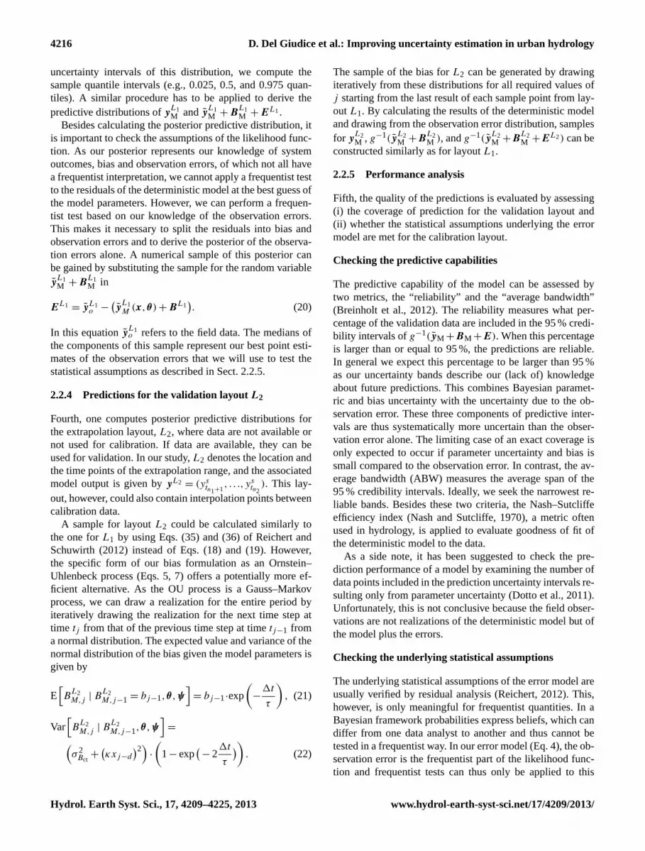
Finally, besides frequentist analyses of the white measure-ment noise, one should check what can be learned from anexploratory analysis of the model bias. Plotting the modelbias against flow data (Fig. 6) shows an almost constant scat-ter with only weak trends. In general, we observed a negativebias in the intermediate flow range and a positive bias duringsevere storms. While the first systematic deviation is causedby slightly overestimating the runoff in the decreasing limbof the hydrograph, the second reveals that the model sys-tematically underestimates the highest peak discharges (seeFig. 4).



❉✐s❝✉

ss✐♦♥P❛♣

❡r⑤

❉✐s❝✉

ss✐♦♥P❛♣

❡r⑤

❉✐s❝✉

ss✐♦♥P❛♣

❡r⑤

❉✐s❝✉

ss✐♦♥P❛♣

❡r⑤

●●●●●●●●●●●●●●●●●●●●●●●●●●●●●●●●●●●●●●●●●●●●●

●●●●●●●●●●●●●●●●●●●●●●●●●

●●

●●

●●●●

●

●

●

●

●

●

●

●

●●

●

●

●

●●

●

●●●●●●●

●●●

●●

●

●

●●●●●

●●

●

●●●●●

●●

●●

●●●

●

●●

●

●●●●●●●●●●●●●●

●

●●●●●●●●●●●●●

●●●●●●●●●●●●●●●●●●●●●●●●●●●●●●

●●●●●●●●●●●●●●●●●●●●●●●●●●●●●●●●●●●●●●●●●●●●●●●●●●●●●●●

●

●●

●

●

●

●

●●●●●

●●●●●

●

●

●●●●

●●●●●●●

●●●●●●●●●●●

●●●●●●●●●●●●●

●●●●●●●●●●●●

●

●●●

● ●●

●●

●●

●●

●●

●

●

●

●

●

●

●

●●

●

●●

●●●●

●●●●●

●

●●●●

●●●●●●

●●●●●●●

●●●●●●●●●●●●●●●●●●●●●●●●●●●●●●●●●●●●●●●●●●●●●●●●●●●●●●●●●●●●●●●●●●●●●●●●●●●●●●●●●●●●●●●●●●●●●●●●●●●●●●●●●●●●●●●●●●●●●●●●●●●●

●●●

●●●●

●●●●●●●●●●●●●●●●●●●●●●●●●●●●●●●●●●●●●●●●●●●●●●●●●●●●●

●

●

●

●

●

●

●●

●

●

●●●

●●●

●

●●

●●●

●● ●

●

●●

●

●

●

●

●

●

●

−200 0 200 400

−15

0−

500

5010

0

Y~

o

µ 12(B

M)

Fig. 6. Median of model inadequacy versus transformed observedrunoff for the calibration period shown in Fig. 4. Results are shownfor the best solution: the constant bias log-sinh transformed errormodel.

5 Discussion

The outcomes of this study, in agreement with theoreticalconsiderations, confirmed that describing bias by means ofa stochastic process produces much more reliable and inter-pretable hydrological predictions than the overly simplistictraditional error model. Additionally, the bias error modelnaturally describes the increase in uncertainty about the sys-tem response when passing from the calibration to the ex-trapolation range. In the following, we will interpret the re-sults obtained for our system, assess the differences amongthe proposed bias description formulations, analyze the dis-similarities between natural and urban hydrology, and finallyprovide guidelines on how to describe model discrepanciesin future studies.

5.1 Bias analysis in the case study

The analysis of the uncertainties in our stormwater sys-tem demonstrated that our parsimonious deterministic modelcaptures most of the hydrograph dynamics. Nevertheless,it produced partially biased simulations. By accounting forthese systematic deviations with the most plausible errormodel, we observed almost a constant variance of the esti-mated observation errors in the transformed space. Further-more, the bias tended to be negative during intermediate rainevents and positive at very high discharges. These findingsindicate that a part of the predictive uncertainty stems fromstructural deficits due to oversimplification of the simulator,which produce systematic trends in the residuals (Frey et al.,2011). Another part of prediction uncertainty, instead, stemsfrom imprecise precipitation measurements, which increasethe scatter of the residuals.

If the study’s goal is to reduce prediction uncertainty, oneshould, after detecting structural deficiencies, improve themodel. This can be done by modifying process formulationsor increasing the model complexity. In our case, analyzing

how model discrepancies depend on the measured dischargegave us the necessary information to improve the simulator.Increasing the number of calibration parameters from prelim-inary simulations reduced a strong positive bias (results notshown) to some mild remaining systematic trends (Fig. 6).

5.2 Comparison of different bias descriptions

In this paper we proposed 5 different descriptions of modelinadequacy. The bias description where the variance quadrat-ically increases with precipitation is the conceptually mostappealing form since it mechanistically accounts for higheruncertainty during rainy periods. Furthermore, in contrastto the empirical output-dependence via data transformation,input-dependence acknowledges that the rising limb of thehydrograph is more uncertain than the recessive limb.

Notwithstanding its theoretical appeal, the input-dependent bias has several drawbacks. First, it has twoparameters more than the constant bias, which potentiallyreduces the robustness of this approach. In particular, duringestimation, the proportionality constantκ tends to reachvery high posterior values (see Supplement for priors andposteriors) and, in this way, leads to inflated variancesduring rainfall and too small variances during dry weather.Second, since we always assume a normal distributionof the bias, the input-dependent description frequentlyrequires a transformation anyway in order to avoid negativepredictions that are physically meaningless. Third, linkedto the two previous considerations, the input and outputdependent error model has the tendency to include too manymechanisms to describe model inadequacy. This complexrepresentation reproduces data dynamics “excessively well”and therefore motivates the deterministic model less to fitthe observations.

It is interesting to notice that the input-dependent errormodel never reverted back to a constant bias (i.e.,κ never cal-ibrated to 0), even in cases where all performance indicatorsfavored the simpler error description. This can be explainedconsidering that the input-dependent bias has a basic vari-ance plus a variance induced by precipitation. In our case, theposterior basic variance for the input-dependent bias was, ir-respective of the transformation, smaller than for the constantbias. This is caused by three combined phenomena: first, anerror distribution with smaller variance has generally higherlikelihood, second, our simulator could match the baseflowalmost exactly, and third, a large part of the calibration pe-riod had an output equal to the baseflow. Since the input-dependent error model still had to account for big errors dur-ing wet weather, it did so by increasing the precipitation-induced error variance, producing sometimes too wide un-certainty intervals for the future storm events.



5.3 Bias assessment in urban and natural hydrology

Interestingly, for Honti et al. (2013) the input-dependentBox–Cox transformed error model produced the best pre-dictions. This different outcome, however, is not necessarilyin contrast with our findings. First, as mentioned in the in-troduction, different case studies can display extremely dis-similar error properties. Our urban catchment had a muchstronger difference in the hydrologic response between dryand wet periods than Honti et al.’s natural watershed, whichadditionally presented fewer points of constant minimal dis-charge. Second, their formulation presented an additionalprecipitation-dependent bias component, while neglectingthe delay between precipitation occurrence and uncertaintyincrease. Third, in Honti et al. (2013) the log-sinh transfor-mation was not implemented.

Comparing urban to natural catchments, an important as-pect is, first, that urban hydrosystems react much morerapidly and strongly and therefore require much more fre-quent measurements of the hydrologic response (typically atminute scale instead of daily scale). Furthermore, the dis-charge in sewers can be ascertained with much higher pre-cision and accuracy than in the case of rivers. Indeed, indrainage conduits the area-velocity sensors can measure thevelocity directly, without requiring a rating curve, which is anadditional source of uncertainty in streamflow observations(Sikorska et al., 2013; Montanari and Di Baldassarre, 2013).The elevated temporal density and precision of the mea-surements, as discussed byReichert and Mieleitner (2009),leads to an even higher need to address model discrepanciesexplicitly.

Second, in natural watersheds the high flow can be asso-ciated with floodplain inundations, which dramatically in-crease the uncertainty of flow measurements. In sewer sys-tems, by contrast, the well-defined geometry of the pipesand the reliable flow measurement devices lead to a muchsmaller increase in observation uncertainty with increasingdischarge. This situation underlines the advantage of a log-sinh transformation in urban hydrology instead of the tra-ditional Box–Cox. Indeed, the former assumes that residualscatter in high streamflow ranges is limited.

Regarding uncertainty estimation, it seems that a formu-lation where the standard deviation of the input-dependentbias component linearly increases with precipitation is sub-optimal for urban systems. Indeed, most urban water basins,especially those only draining stormwater and having lowgroundwater infiltration, exhibit extremely high contrasts be-tween low and high flows. Such strong dynamics and lin-ear input dependence can result in unnecessarily wide uncer-tainty intervals.

5.4 Recommendations

As our results demonstrate, hydrological predictions aremore reliable when model deficiencies are considered

explicitly, especially for urbanized areas. This is in agree-ment with many other studies (Breinholt et al., 2012; Yanget al., 2007b; Schoups and Vrugt, 2010; Reichert andMieleitner, 2009). If the modeler is not interested in sepa-rating predictive uncertainty into its contributing sources be-cause data collection or model building processes are fixed,we suggest using a lumped autoregressive error model (Batesand Campbell, 2001; Yang et al., 2007b; Evin et al., 2013).Such formulations are usually sufficient to reliably estimatetotal output uncertainty. However, it is often useful to assesshow far the prediction uncertainty can be reduced by min-imizing a particular error source (Sikorska et al., 2012). Inthese cases, we recommend applying our five-variant biasdescription in order to disentangle the effects of model dis-crepancies and random measurement errors. In particular, wesuggest starting with a constant log-sinh transformed biasand setting priors of the error model parameters using the rec-ommendations given in Sect. 2.2.1. This likelihood formula-tion is simple and robust and proved to perform extremelywell in our case study. Then, if the efficiency of this error de-scription is unsatisfactory, the Box–Cox transformation andeventually the input-dependent bias description in its threevariants can be applied. Finally, we propose selecting amongthe error description providing the best validation coveragewith the narrowest bands and the most iid transformed ob-servation errors, and applying this likelihood formulation tosubsequent predictions.

If the input-dependence is of particular interest thoughproviding dubious predictions, considering what we dis-cussed above, we suggest adapting this dependence on pre-cipitation as a function of the system’s dynamics. One pos-sibility could be to modify Eq. (7) and, instead of a lin-ear increase of uncertainty with the precipitation, one couldadopt a power relationship with the exponent as calibrationparameter.

6 Conclusions

In this study, we proposed different strategies for obtainingreliable flow predictions and quantifying different error con-tributions. We adapted a Bayesian description of model dis-crepancy to urban hydrology, making the bias variance in-crease during wet weather in five different ways. From theexperience gained in this modeling study and theoretical con-siderations, we conclude the following.

i. Due to input uncertainty, structural deficits, and (pos-sibly) systematic errors in flow measurements, urbanhydrological simulations are biased. When using pre-cise and high-frequency output measurements to cali-brate and analyze the uncertainties of these simulatorsby means of traditional iid error models, we obtain im-plausible predictions.



ii. We can obtain much sounder predictions and signifi-cantly improve the fulfillment of the assumptions byadding a model discrepancy function to the classicalerror model. Such a bias term should have a variancethat increases during storm events as a function of rain-fall and/or runoff. Finally, the results demonstrate thatrandom output observation errors are much smallerthan uncertainty due to bias.

iii. In our study, a rather simple constant autoregressivebias with a log-sinh transformation outperformed aninput-dependent bias description. Although the latteris conceptually superior, the simpler formulation ap-peared more suitable for systems with alternating longlow flow periods and short high discharge pulses, suchas urban watersheds. Indeed, it is apparently less sus-ceptible to producing excessively wide error bands andsuboptimal fit. Therefore, we suggest to test this firstand then try the other bias descriptions, if necessary.

iv. Although it generally outperforms the traditional er-ror assumptions, we are aware of the limitations of ourapproach. The presence of bias, to which we have toassign a weight in the form of priors, inevitably intro-duces subjectivity in the uncertainty analysis. More-over, this statistical method can “only” describe thedifferent types of output uncertainties, but cannot ad-dress directly the causes of bias nor can it straightfor-wardly lead to an uncertainty reduction.

v. Despite remaining challenges, our approach has fur-ther advantages besides providing separated and plau-sible prediction intervals. First, a bias description canbe associated with a fully fledged framework that prop-agates the uncertainty sources and supports bias re-duction, to describe “remnant” errors. So far, this re-maining bias due to imperfect description of the uncer-tainty sources has been modeled as white noise (e.g.,Renard et al., 2010). Second, the exploratory analy-sis of model bias, for example investigating its de-pendence on the output, can provide valuable insightinto whether model discrepancy is dominated by inputuncertainty or inadequate model formulation. Third,this statistically sound approach is computationallynot more intensive than the classical methods. Indeed,it is cheaper than the mechanistic error propagationframeworks.

vi. Open questions that require further research includehow the bias description can be applied to quantifythe structural errors of complex hydrodynamic mod-els with multiple outputs. Moreover, it is unclear howinput errors can be separated from structural deficitsas this requires a probabilistic formulation and prop-agation through the simulator. A further challenge isthat complex sewer models are prohibitively slow for

many iterative simulations. This can be possibly over-come by statistical approximations, such as emulators(Reichert et al., 2011).

Supplementary material related to this article isavailable online at http://www.hydrol-earth-syst-sci.net/17/4209/2013/hess-17-4209-2013-supplement.pdf.

Acknowledgements. We would like to thank Vojtech Bareš andMartin Fencl for providing the monitoring data and informationabout the case study. We are also grateful to David Machac forthe computational support and Anna Sikorska, Dmitri Kavetski,Saket Pande, Eberhard Morgenroth, and two anonymous refereesfor helpful comments. The Swiss National Science Foundation isacknowledged for financing this research within the scope of theCOMCORDE project (grant No. CR2212_135551).

Edited by: G. Di Baldassarre

References

Aho, A., Kernighan, B., and Weinberger, P.: The AWK program-ming language, Addison-Wesley Longman Publishing Co., Inc.,1987.

Bareš, V., Stránský, D., Kopecká, J., and Fridrich, J.: Monitoringpovodi a stokove sito Mesta Hostivice – lokalita Sadová [Moni-toring a sewer watershed in Hostivice municipality – Sadová dis-trict], Tech. rep., Czech Technical University in Prague, 2010 (inCzech).

Bates, B. and Campbell, E.: A Markov chain Monte Carlo schemefor parameter estimation and inference in conceptual rainfall-runoff modeling, Water Resour. Res., 37, 937–947, 2001.

Bayarri, M., Berger, J., Paulo, R., Sacks, J., Cafeo, J., Cavendish,J., Lin, C., and Tu, J.: A framework for validation of computermodels, Technometrics, 49, 138–154, 2007.

Berne, A., Delrieu, G., Creutin, J.-D., and Obled, C.: Tem-poral and spatial resolution of rainfall measurements re-quired for urban hydrology, J. Hydrol., 299, 166–179,doi:10.1016/j.jhydrol.2004.08.002, 2004.

Box, G. and Cox, D.: An analysis of transformations, J. Roy. Stat.Soc. B, 26, 211–252, 1964.

Breinholt, A., Møller, J., Madsen, H., and Mikkelsen, P.: A formalstatistical approach to representing uncertainty in rainfall-runoffmodelling with focus on residual analysis and probabilistic out-put evaluation-distinguishing simulation and prediction, J. Hy-drol., 472–473, 36–52, doi:10.1016/j.jhydrol.2012.09.014, 2012.

Bulygina, N. and Gupta, H.: Correcting the mathematical structureof a hydrological model via Bayesian data assimilation, WaterResour. Res., 47, W05514, doi:10.1029/2010WR009614, 2011.

Christensen, R., Johnson, W., Branscum, A., and Hanson, T.:Bayesian ideas and data analysis: An introduction for scientistsand statisticians, CRC, 2010.

Coutu, S., Del Giudice, D., Rossi, L., and Barry, D.: Parsimonioushydrological modeling of urban sewer and river catchments, J.Hydrol., 464–465, 477–484, doi:10.1016/j.jhydrol.2012.07.039,2012.


http://www.hydrol-earth-syst-sci.net/17/4209/2013/hess-17-4209-2013-supplement.pdf

http://www.hydrol-earth-syst-sci.net/17/4209/2013/hess-17-4209-2013-supplement.pdf

http://dx.doi.org/10.1016/j.jhydrol.2004.08.002


http://dx.doi.org/10.1029/2010WR009614



Craig, P., Goldstein, M., Rougier, J., and Seheult, A.: Bayesian fore-casting for complex systems using computer simulators, J. Am.Stat. Assoc., 96, 717–729, 2001.

Dotto, C. B. S., Kleidorfer, M., Deletic, A., Rauch, W., McCarthy,D. T., and Fletcher, T. D.: Performance and sensitivity analysisof stormwater models using a Bayesian approach and long-termhigh resolution data, Environ. Model. Softw., 26, 1225–1239,2011.

Dürrenmatt, D., Del Giudice, D., and Rieckermann, J.: Dynamictime warping improves sewer flow monitoring, Water Res., 47,3803–3816, doi:10.1016/j.watres.2013.03.051, 2013.

Evin, G., Kavetski, D., Thyer, M., and Kuczera, G.: Pitfalls and im-provements in the joint inference of heteroscedasticity and au-tocorrelation in hydrological model calibration, Water Resour.Res., 49, 4518–4524, doi:10.1002/wrcr.20284, 2013.

Freni, G., Mannina, G., and Viviani, G.: Uncertainty assessment ofan integrated urban drainage model, J. Hydrol., 373, 392–404,doi:10.1016/j.jhydrol.2009.04.037, 2009a.

Freni, G., Mannina, G., and Viviani, G.: Urban runoff mod-elling uncertainty: Comparison among Bayesian and pseudo-Bayesian methods, Environ. Modell. Softw., 24, 1100–1111,doi:10.1016/j.envsoft.2011.03.013, 2009b.

Frey, M. P., Stamm, C., Schneider, M. K., and Reichert, P.: Us-ing discharge data to reduce structural deficits in a hydrologicalmodel with a Bayesian inference approach and the implicationsfor the prediction of critical source areas, Water Resour. Res., 47,W12529, doi:10.1029/2010WR009993, 2011.

Gujer, W.: Systems analysis for water technology, Springer, 2008.Haario, H., Saksman, E., and Tamminen, J.: An Adaptive Metropo-

lis Algorithm, Bernoulli, 7, 223–242, available at: http://www.jstor.org/stable/3318737, 2001.

Hastings, W.: Monte Carlo sampling methods using Markov chainsand their applications, Biometrika, 57, 97–109, 1970.

Henderson, D. and Plaschko, P.: Stochastic Differential Equationsin Science and Engineering, World Scientific, Singapore, 2006.

Higdon, D., Kennedy, M., Cavendish, J. C., Cafeo, J. A., and Ryne,R. D.: Combining Field Data and Computer Simulations for Cal-ibration and Prediction, SIAM J. Sci. Comput., 26, 448–466,doi:10.1137/S1064827503426693, 2005.

Honti, M., Stamm, C., and Reichert, P.: Integrated uncertainty as-sessment of discharge predictions with a statistical error model,Water Resour. Res., 49, 4866–4884, doi:10.1002/wrcr.20374,2013.

Iacus, S. M.: Simulation and inference for stochastic differentialequations: with R examples, Springer, 2008.

Kavetski, D., Kuczera, G., and Franks, S. W.: Bayesian analysisof input uncertainty in hydrological modeling: 1. Theory, WaterResour. Res., 42, W03407, doi:10.1029/2005WR004368, 2006.

Kendall, M., Stuart, A., and Ord, J.: Advanced Theory of Statistics,Distribution Theory (Vol. 1), London, Arnold, 1994.

Kennedy, M. and O’Hagan, A.: Bayesian calibration of computermodels, J. Roy. Stat. Soc. B, 63, 425–464, 2001.

Kessler, M., Lindner, A., and Sorensen, M.: Statistical methods forstochastic differential equations, Vol. 124, CRC Press, 2012.

Kleidorfer, M.: Uncertain Calibration of Urban Drainage Models:A Scientific Approach to Solve Practical Problems, Ph.D. thesis,2009.

Kollo, T. and von Rosen, D.: Advanced multivariate statistics withmatrices, Vol. 579, Springer, 2005.

Korving, H. and Clemens, F.: Impact of dimension uncertainty andmodel calibration on sewer system assessment, Water Sci. Tech-nol., 52, 35–42, 2005.

Kuczera, G.: Improved parameter inference in catchment models: 1.Evaluating parameter uncertainty, Water Resour. Res., 19, 1151–1162, doi:10.1029/WR019i005p01151, 1983.

Laloy, E. and Vrugt, J.: High-dimensional posterior explorationof hydrologic models using multiple-try DREAM (ZS) andhigh-performance computing, Water Resour. Res., 48, W01526,doi:10.1029/2011WR010608, 2012.

Liang, F., Liu, C., and Carroll, R.: Advanced Markov chain MonteCarlo methods: learning from past samples, Vol. 714, Wiley,2011.

Montanari, A. and Di Baldassarre, G.: Data errors and hydro-logical modelling: The role of model structure to propagateobservation uncertainty, Adv. Water Resour., 51, 498–504,doi:10.1016/j.advwatres.2012.09.007, 2013.

Montanari, A. and Koutsoyiannis, D.: A blueprint for process-basedmodeling of uncertain hydrological systems, Water Resour. Res.,48, W09555, doi:10.1029/2011WR011412, 2012.

Nash, J. and Sutcliffe, J.: River flow forecasting through conceptualmodels part I : A discussion of principles, J. Hydrol., 10, 282–290, doi:10.1016/0022-1694(70)90255-6, 1970.

Neumann, M. B. and Gujer, W.: Underestimation of uncertaintyin statistical regression of environmental models: influence ofmodel structure uncertainty, Environ. Sci. Technol., 42, 4037–4043, 2008.

O’Hagan, A., Buck, C. E., Daneshkhah, A., Eiser, J. R., Garthwaite,P. H., Jenkinson, D. J., Oakley, J. E., and Rakow, T.: Uncertainjudgments: eliciting experts’ probabilities, Wiley. com, 2006.

R Core Team: R: A Language and Environment for Statistical Com-puting, R Foundation for Statistical Computing, Vienna, Austria,available at: http://www.R-project.org/, last access: 1 April 2013.

Reichert, P.: Conceptual and practical aspects of quantifying un-certainty in environmental modelling and decision support, 2012International Congress on Environmental Modelling and Soft-ware, International Environmental Modelling and Software So-ciety (iEMSs), 2012.

Reichert, P. and Borsuk, M.: Does high forecast uncertainty pre-clude effective decision support?, Environ. Modell. Softw., 20,991–1001, 2005.

Reichert, P. and Mieleitner, J.: Analyzing input and structuraluncertainty of nonlinear dynamic models with stochastic,time-dependent parameters, Water Resour. Res., 45, W10402,doi:10.1029/2009WR007814, 2009.

Reichert, P. and Schuwirth, N.: Linking statistical bias descrip-tion to multiobjective model calibration, Water Resour. Res., 48,W09543, doi:10.1029/2011WR011391, 2012.

Reichert, P., White, G., Bayarri, M. J., and Pitman, E. B.:Mechanism-based emulation of dynamic simulation models:Concept and application in hydrology, Comput. Stat. Data Anal.,55, 1638–1655, doi:10.1016/j.csda.2010.10.011, 2011.

Renard, B., Kavetski, D., Kuczera, G., Thyer, M., and Franks, S. W.:Understanding predictive uncertainty in hydrologic modeling:The challenge of identifying input and structural errors, WaterResour. Res., 46, W05521, doi:10.1029/2009WR008328, 2010.


http://dx.doi.org/10.1016/j.watres.2013.03.051

http://dx.doi.org/10.1002/wrcr.20284


http://dx.doi.org/10.1016/j.envsoft.2011.03.013

http://dx.doi.org/10.1029/2010WR009993

http://www.jstor.org/stable/3318737

http://www.jstor.org/stable/3318737

http://dx.doi.org/10.1137/S1064827503426693

http://dx.doi.org/10.1002/wrcr.20374

http://dx.doi.org/10.1029/2005WR004368

http://dx.doi.org/10.1029/WR019i005p01151

http://dx.doi.org/10.1029/2011WR010608

http://dx.doi.org/10.1016/j.advwatres.2012.09.007

http://dx.doi.org/10.1029/2011WR011412

http://dx.doi.org/10.1016/0022-1694(70)90255-6

http://www.R-project.org/

http://dx.doi.org/10.1029/2009WR007814

http://dx.doi.org/10.1029/2011WR011391

http://dx.doi.org/10.1016/j.csda.2010.10.011

http://dx.doi.org/10.1029/2009WR008328


Renard, B., Kavetski, D., Leblois, E., Thyer, M., Kuczera, G., andFranks, S. W.: Toward a reliable decomposition of predictive un-certainty in hydrological modeling: Characterizing rainfall errorsusing conditional simulation, Water Resour. Res., 47, W11516,doi:10.1029/2011WR010643, 2011.

Rossman, L. and Supply, W.: Storm water management modeluser’s manual, version 5.0, National Risk Management ResearchLaboratory, Office of Research and Development, US Environ-mental Protection Agency, 2010.

Schellart, A., Shepherd, W., and Saul, A.: Influence of rainfallestimation error and spatial variability on sewer flow predic-tion at a small urban scale, Adv. Water Resour., 45, 65–75,doi:10.1016/j.advwatres.2011.10.012, 2012.

Schoups, G. and Vrugt, J. A.: A formal likelihood function for pa-rameter and predictive inference of hydrologic models with cor-related, heteroscedastic, and non-Gaussian errors, Water Resour.Res., 46, W10531, doi:10.1029/2007WR006720, 2010.

Sikorska, A. E., Scheidegger, A., Banasik, K., and Rieckermann,J.: Bayesian uncertainty assessment of flood predictions in un-gauged urban basins for conceptual rainfall-runoff models, Hy-drol. Earth Syst. Sci., 16, 1221–1236, doi:10.5194/hess-16-1221-2012, 2012.

Sikorska, A. E., Scheidegger, A., Banasik, K., and Rieckermann,J.: Considering rating curve uncertainty in water level pre-dictions, Hydrol. Earth Syst. Sci. Discuss., 10, 2955–2986,doi:10.5194/hessd-10-2955-2013, 2013.

Uhlenbeck, G. and Ornstein, L.: On the theory of the Brownian mo-tion, Phys. Rev., 36, 823–841, 1930.

Vihola, M.: Robust adaptive Metropolis algorithm with coerced ac-ceptance rate, Stat. Comput., 22, 997–1008, 2012.

Vrugt, J. A., ter Braak, C. J. F., Clark, M. P., Hyman, J. M.,and Robinson, B. A.: Treatment of input uncertainty in hy-drologic modeling: Doing hydrology backward with Markovchain Monte Carlo simulation, Water Resour. Res., 44, W00B09,doi:10.1029/2007WR006720, 2008.

Wang, Q., Shrestha, D., Robertson, D., and Pokhrel, P.: A log-sinhtransformation for data normalization and variance stabilization,Water Resour. Res., 48, W05514, doi:10.1029/2011WR010973,2012.

Willems, P.: Model uncertainty analysis by variance decomposition,Phys. Chem. Earth, 42, 21–30, doi:10.1016/j.pce.2011.07.003,2012.

Willems, P., Molnar, P., Einfalt, T., Arnbjerg-Nielsen, K., Onof, C.,Nguyen, V.-T.-V., and Burlando, P.: Rainfall in the urban con-text: Forecasting, risk and climate change, Atmos. Res., 103, 1–3, doi:10.1016/j.atmosres.2011.11.004, 2012.

Yang, J., Reichert, P., and Abbaspour, K.: Bayesian uncertaintyanalysis in distributed hydrologic modeling: A case study inthe Thur River basin (Switzerland), Water Resour. Res., 43,W10401, doi:10.1029/2006WR005497, 2007a.

Yang, J., Reichert, P., Abbaspour, K. C., and Yang, H.: Hydrolog-ical modelling of the Chaohe Basin in China: Statistical modelformulation and Bayesian inference, J. Hydrol., 340, 167–182,doi:10.1016/j.jhydrol.2007.04.006, 2007b.


http://dx.doi.org/10.1029/2011WR010643

http://dx.doi.org/10.1016/j.advwatres.2011.10.012

http://dx.doi.org/10.1029/2007WR006720

http://dx.doi.org/10.5194/hess-16-1221-2012

http://dx.doi.org/10.5194/hess-16-1221-2012

http://dx.doi.org/10.5194/hessd-10-2955-2013

http://dx.doi.org/10.1029/2007WR006720

http://dx.doi.org/10.1029/2011WR010973

http://dx.doi.org/10.1016/j.pce.2011.07.003

http://dx.doi.org/10.1016/j.atmosres.2011.11.004

http://dx.doi.org/10.1029/2006WR005497


Improving uncertainty estimation in urban hydrological modeling by statistically describing bias

Documents

Transcript of Improving uncertainty estimation in urban hydrological modeling by statistically describing bias