Describing corpora, comparing corpora - Roland Schäfer
205
Describing corpora, comparing corpora Felix Bildhauer* and Roland Schäfer** * IDS Mannheim, **Freie Universität Berlin CL tutorial @ DGfS 41st annual meeting 5 March 2019, Bremen Felix Bildhauer & Roland Schäfer Describing corpora, comparing corpora DGfS-CL 1 / 133
-
Upload
khangminh22 -
Category
Documents
-
view
1 -
download
0
Transcript of Describing corpora, comparing corpora - Roland Schäfer

Describing corpora, comparing corpora
Felix Bildhauer* and Roland Schäfer**
* IDS Mannheim, **Freie Universität Berlin
CL tutorial @ DGfS 41st annual meeting5 March 2019, Bremen
Felix Bildhauer & Roland Schäfer Describing corpora, comparing corpora DGfS-CL 1 / 133

Schedule
11:00 – 12:30 Session 1: Describing corpora14:00 – 15:30 Session 2: Comparing corpora16:00 – 17:30 Session 3: Modelling
Data packages: https://www.webcorpora.org/dgfs19/
R-Studio: https://www.rstudio.com
Felix Bildhauer & Roland Schäfer Describing corpora, comparing corpora DGfS-CL 1 / 133

Why describe / compare corpora?
Choose an appropriate resource for a particular purpose
Is corpus A suitable from a technical viewpoint(quality of post-processing and annotations)
Using a different corpus, would linguistics findings differ significantly?
Does the performance of tool X vary with different corpora?
How does a tool trained on corpus A perform on data from corpus B?
How broad a claim can be made based on my findings?
Can corpus A be used as a substitue for corpus B(especially if corpus B is unavailable / unaffordable and corpus A is free)
…
Felix Bildhauer & Roland Schäfer Describing corpora, comparing corpora DGfS-CL 2 / 133

Different corpora, different findings
Proportion of genitive complements after selected prepositions, by corpus(Bildhauer & Schäfer, in prep.)
auß
erge
genü
ber
nebs
tsa
mt
gem
äßen
tgeg
enm
itsam
tm
ange
lsw
egen
dank
zuzü
glic
htr
otz
eins
chlie
ßlic
hm
ittel
sbe
zügl
ich
abzü
glic
hw
ähre
ndvo
rbeh
altli
chhi
nsic
htlic
han
gesi
chts
seite
nsan
läss
lich
betr
effs
0.0
0.2
0.4
0.6
0.8
1.0decowdereko
Felix Bildhauer & Roland Schäfer Describing corpora, comparing corpora DGfS-CL 3 / 133

Domain adaptation
CMC WEBTagger STTS_IBK STTS 1.0 STTS_IBK STTS 1.0
Prange et al. (2016) 87.33 90.28 93.55 94.62COW 77.89 81.51 91.82 92.96TreeTagger 73.21 76.81 91.75 92.89Stanford 70.60 75.83 89.42 92.52
Figure: EmpiriST shared task results (Beißwenger et al., 2016)
Felix Bildhauer & Roland Schäfer Describing corpora, comparing corpora DGfS-CL 4 / 133

Corpora used in this tutorial
DeReKo / KoGra
≈ 7bn tokens
subset of Deutsches Referenzkorpus (DeReKo), Kupietz et al., 2010
defined and used in IDS project ”‘Korpusgrammatik”’
stratification: Bubenhofer, Konopka & Schneider, 2014
mostly newspaper texts
rich linguistic annotation
not (yet) available to the public
This tutorial’s color code: red
Felix Bildhauer & Roland Schäfer Describing corpora, comparing corpora DGfS-CL 5 / 133

Corpora used in this tutorial (II)
DECOW16B (COW initiative, Schäfer & Bildhauer, 2012)
≈ 20.5bn tokens
web corpus
created with 2016 technology of the COW initiative
breadth-first web crawl
rich linguistic annotation
publicly available at https://www.webcorpora.org/
This tutorial’s color code: green
Felix Bildhauer & Roland Schäfer Describing corpora, comparing corpora DGfS-CL 6 / 133

Corpora used in this tutorial (III)
RanDECOW-1m (COW initiative, Schäfer, 2016)
≈ 1m tokens
web corpus
data collected through random walks
corrected for host biasrich linguistic annotation
publicly available at https://www.webcorpora.org/
This tutorial’s color code: blue
Felix Bildhauer & Roland Schäfer Describing corpora, comparing corpora DGfS-CL 7 / 133

The structure of the web
SCCIN OUT
TUBE
TENDRIL
Manning, Raghavan & Schütze, 2009, p. 427
Broder et al. (2000): IN, OUT, SCC, and TENDRIL components are notextremely different in size.
A more detailed report on the sizes: Ángeles Serrano et al. (2007).
Felix Bildhauer & Roland Schäfer Describing corpora, comparing corpora DGfS-CL 8 / 133
Part I: Describing corpora
Felix Bildhauer & Roland Schäfer Describing corpora, comparing corpora DGfS-CL 9 / 133

Kinds of meta data
Felix Bildhauer & Roland Schäfer Describing corpora, comparing corpora DGfS-CL 10 / 133
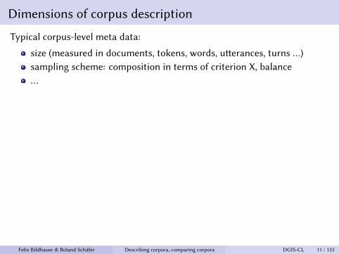
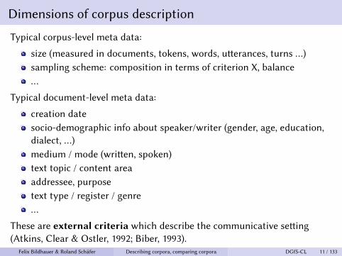
Dimensions of corpus description
Typical corpus-level meta data:
size (measured in documents, tokens, words, utterances, turns …)sampling scheme: composition in terms of criterion X, balance…
Typical document-level meta data:
creation datesocio-demographic info about speaker/writer (gender, age, education,dialect, …)medium / mode (written, spoken)text topic / content areaaddressee, purposetext type / register / genre…
These are external criteria which describe the communicative setting(Atkins, Clear & Ostler, 1992; Biber, 1993).
Felix Bildhauer & Roland Schäfer Describing corpora, comparing corpora DGfS-CL 11 / 133

Text type / register / genre
intuitively, register/ text is an important dimension of variation, but …
long tradition of investigation into registers, text types, genres
large body of research in within different research traditions
no coherent use / widely accepted definitions of these terms(could be used interchangeably or encode important theoreticaldistinctions)
with any given taxonomy: operationalization often problematic(more or less prototypical cases)
different taxonomies often not campatible with each other(or mapping of cetegories is unclear)
Felix Bildhauer & Roland Schäfer Describing corpora, comparing corpora DGfS-CL 12 / 133

Common kinds of mata data in popular corpora (I)
DWDS Kernkorpus (Geyken, 2007), ≈ 100m words, balanced
Stratified by decade and text type:
Novels Newspaper Scientific Other(“Belletristik”) (“Zeitung”) (“Wissenschaft”) (“Gebrauchsliteratur”)
28.42% 27.36% 23.15% 21.05%
1990s “Wissenschaft”: mostly encyclopediae (Islam, Buddhism, idioms,nazi, opera, pedagogy)
1990s “Gebrauchsliteratur”: 1953 of 2319 texts from aktuelles Lexikon(Süddeutsche Zeitung), some political communication
Felix Bildhauer & Roland Schäfer Describing corpora, comparing corpora DGfS-CL 13 / 133

Common kinds of mata data in popular corpora (II)
Deutsches Referenzkorpus (DeReKo, Kupietz et al., 2010), ≈ 42bn words
Selection of attributes; not all documents are annotated:
Category example valueauthor eigene Bearbeitung; Antonia LangsdorfdocTitle Hamburger Morgenpost, Januar 2006pubDate 2006-01-04pubPlace Hamburgpublisher Morgenpost Verlagreference MOPO, 04.01.2006, S. 19; Jahreshoroskop 2006textClass staat-gesellschaft familie-geschlechttextColumn SerietextType Zeitung: Tageszeitung, BoulevardzeitungtextTypeArt Serie
Felix Bildhauer & Roland Schäfer Describing corpora, comparing corpora DGfS-CL 14 / 133

Common kinds of mata data in popular corpora (III)
DeReKo, some text types:
Aphorismus, Autobiografie, Bericht, Biografie, Brief, Denkschrift,Erlass, Erzählung Essay, Fußnote, Forschungsbericht, Gebet,Gebrauchsanweisung, Gedicht, Hörspiel, Interview, Klappentext,Kommentar, Leserbrief, Leitartikel, Märchen, Nachruf, Nachwort,Parteiprogramm, Petition, Presseerklärung, Produktbeschreibung,Protokoll, Ratgeber, Rede, Reportage, Rezension, Roman, Schauspiel,Tagebuch, Werbung
But also:Nachrichten, Abhandlung, Aufsatz, Flugblatt, Handzettel, Vorspann,Bericht, Feuilleton, Tipps Service, Lokales, Essen und Trinken,Beilage, Serie, Bericht/Reportage, Porträt:Stadtporträt,Porträt:Länderporträt, Bericht:Wetterbericht, Bericht:Sportbericht,Bericht:Schicksalsbericht, Bericht:Erfahrungsbericht, Fall:KurioserFall, Fall:Spektakulärer Fall
Felix Bildhauer & Roland Schäfer Describing corpora, comparing corpora DGfS-CL 15 / 133

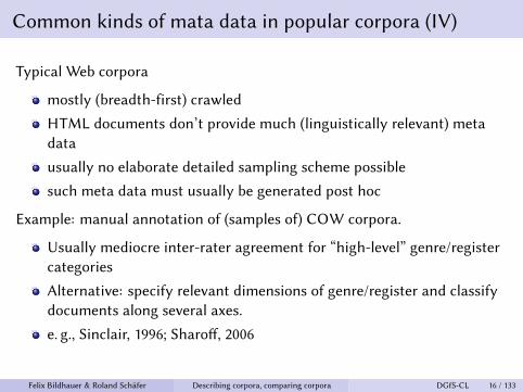
Common kinds of mata data in popular corpora (IV)
Typical Web corpora
mostly (breadth-first) crawled
HTML documents don’t provide much (linguistically relevant) metadata
usually no elaborate detailed sampling scheme possible
such meta data must usually be generated post hoc
Example: manual annotation of (samples of) COW corpora.
Usually mediocre inter-rater agreement for “high-level” genre/registercategories
Alternative: specify relevant dimensions of genre/register and classifydocuments along several axes.
e. g., Sinclair, 1996; Sharoff, 2006
Felix Bildhauer & Roland Schäfer Describing corpora, comparing corpora DGfS-CL 16 / 133

The COWCat taxonomy
based on Sinclair, 1996; Sharoff, 2006
multiple dimensions, no genres
only categories with a potential influenceon grammatical features
Aim, Audience, Authorship, Domain, Mode
Felix Bildhauer & Roland Schäfer Describing corpora, comparing corpora DGfS-CL 17 / 133

COWCat Aim and Audience
Aim has 5 distinct categories:
1 Recommendation (Re)2 Instruction (Is)3 Information (If)4 Discussion (Di)5 Fiction (Fi)
Audience has 3 distinct categories:
1 General (Ge)2 Informed or Restricted (In)3 Professional (Pr)
Felix Bildhauer & Roland Schäfer Describing corpora, comparing corpora DGfS-CL 18 / 133

Experiment for German
4 raters
800 documents
training phase: 100 documents, 2 meetings
Felix Bildhauer & Roland Schäfer Describing corpora, comparing corpora DGfS-CL 19 / 133

Results
Agreement and 𝜅 (Fleiss) for 4 raters:
Aim (5) Aud (3) Auth (5) Mode (4)
Agree 0.67 0.59 0.53 0.82𝜅 0.50 0.42 0.63 0.78
Agreement and 𝜅 (Cohen) for for best pairwise raters:
Aim (5) Aud (3) Auth (5) Mode (4)
Agree 0.84 0.86 0.78 0.91𝜅 0.49 0.53 0.71 0.82
Felix Bildhauer & Roland Schäfer Describing corpora, comparing corpora DGfS-CL 20 / 133

Aim by top-level domain
Felix Bildhauer & Roland Schäfer Describing corpora, comparing corpora DGfS-CL 21 / 133

Audience by top-level domain
Ge If Pr
DeEsUk
Comparison of corpus composition: Audience0
2040
6080
100
Felix Bildhauer & Roland Schäfer Describing corpora, comparing corpora DGfS-CL 22 / 133

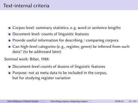
Text-internal criteria
Corpus level: summary statistics, e. g. word or sentence lengths
Document level: counts of linguistic features
Provide useful information for describing / comparing corpora
Can high-level categories (e. g., register, genre) be inferred from suchdata? (to be addressed later)
Seminal work: Biber, 1988:
Document-level counts of dozens of linguistic features
Purpose: not as meta data to be included in the corpus,but for studying register variation
Felix Bildhauer & Roland Schäfer Describing corpora, comparing corpora DGfS-CL 23 / 133

COReX
Feature extractorOver 60 normalised feature counts at the document level
morphologicallexicalsyntacticstylistic markerssome non-linguistic features TTR, number of sentences etc.
Requires pre-processed text, uses information from POS tags,morphological analyses, NE recognition, topological parse, customword lists
Implemented in Python, open source, extendible to cover more features
Felix Bildhauer & Roland Schäfer Describing corpora, comparing corpora DGfS-CL 24 / 133

COReX features (selection)
Feature Explanationcn common nouns per 1,000 wordsadj adjectives per 1,000 wordscmpnd compounds per 1,000 common nounspper_2nd 2nd person pronouns per 1,000 wordsgen genitives per 1,000 nounsclitindef clitic indefinite articles per 1,000 indef. articlesimp imperatives per 1,000 wordsneper person names per 1,000 wordsclausevf clausal Vf per 1,000 Vfpass passive constructions per clauseperf perfect constructions per clausevpast number of past verbs per 1,000 wordscnloan loan nouns with recognizable suffix (‘-ik’, ‘-um’) per 1,000 nounsqsvoc short/contracted forms (’nich’, ’schomma’) per 1,000 wordsshort non-standard contracted forms (’gehts’, ’aufm’) per 1,000 words
Felix Bildhauer & Roland Schäfer Describing corpora, comparing corpora DGfS-CL 25 / 133

Exercise: read COReX meta data into an R data frame
1 Download the archive XYZ fromhttps://www.webcorpora.org/dfgs19/data.tar.gz and unpack it.
2 It contains 3 .tsv files with meta data froma sample from DECOW16B (70,000 docs)a sample from DeReKo/KoGra (70,000 docs)a sample from RanDECOW (70,000 docs)
3 Read the .tsv files into separate data frames, e. g.:
decow.corex <- read.table("/path/to/random_decow_70k.tsv", sep="t", header = TRUE)
Felix Bildhauer & Roland Schäfer Describing corpora, comparing corpora DGfS-CL 26 / 133

Aggregated data
Felix Bildhauer & Roland Schäfer Describing corpora, comparing corpora DGfS-CL 27 / 133

Data aggregation
Two examples:
1 Factor analysis2 Register classification
Felix Bildhauer & Roland Schäfer Describing corpora, comparing corpora DGfS-CL 28 / 133
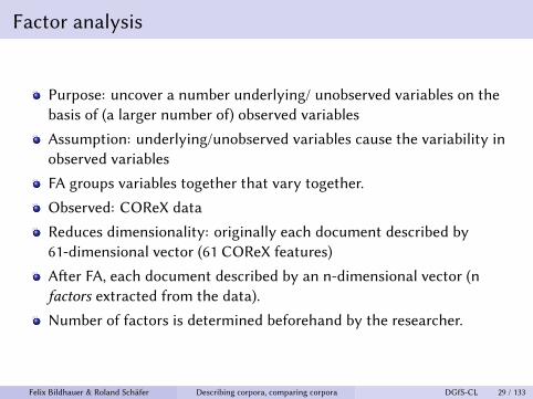
Factor analysis
Purpose: uncover a number underlying/ unobserved variables on thebasis of (a larger number of) observed variables
Assumption: underlying/unobserved variables cause the variability inobserved variables
FA groups variables together that vary together.
Observed: COReX data
Reduces dimensionality: originally each document described by61-dimensional vector (61 COReX features)
After FA, each document described by an n-dimensional vector (nfactors extracted from the data).
Number of factors is determined beforehand by the researcher.
Felix Bildhauer & Roland Schäfer Describing corpora, comparing corpora DGfS-CL 29 / 133

Biber, 1988
In linguistics, pioneering work by Biber (1988 and subsequent).
7 factors / dimensions of variation in a varied corpus of English.Factors interpreted linguistically / functionally,
1 by examining feature loadings in factors2 by examining documents with particularly high or low scores on a factor
Felix Bildhauer & Roland Schäfer Describing corpora, comparing corpora DGfS-CL 30 / 133
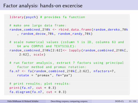
Factor analysis: hands-on excercise
library{psych} # provides fa function
# make one large data frame:random_combined_210k <- rbind.data.frame(random_dereko_70k
, random_decow_70k, random_randy_70k)
# scale numerical values (column 1 is ID , columns 63 and64 are CORPUS and TEXTSIGLE):
random_combined_210k[2:62] <- lapply(random_combined_210k[,2:62], scale)
# run factor analysis , extract 7 factors using principalfactor method and promax rotation:
fa.n7 <- fa(random_combined_210k[,2:62], nfactors=7,rotate = "promax", fm="pa")
# print results; plot results:print(fa.n7 , cut = 0.3)fa.diagram(fa.n7 , cut = 0.3)
Felix Bildhauer & Roland Schäfer Describing corpora, comparing corpora DGfS-CL 31 / 133

Factor analysis: results
vfin vv
card
vaux
v2 neorg
indef cn
neloc subjs neg
dem
esvf
short
clitindef itj
imp
unkn qsvoc
emo
adv pper_2nd
cmpnd
prep
ttrat
answ
nonwrd sapos
parta
slen
vlast rsimpx
simpx
vflen psimpx
wlen conj
adj
dq
neper
vpressubj
perf
clausevf
cnloan
vvieren poss
pper_3rd
def pass
gen
pper_1st
vpast
vpres
plu
wh
inf
zuinf
mod subji
vvpastsubj
wpastsubj
F2
0.90.7−0.60.6
0.6−0.50.3
−0.3
F1
0.70.7
0.60.50.50.50.50.4
0.4
F5
0.90.70.60.50.4 F4
−0.6−0.6−0.60.3
0.30.3 F7
−0.6−0.6
0.60.50.4
−0.4
F6
1−0.90.5
F3
0.90.60.50.4
Felix Bildhauer & Roland Schäfer Describing corpora, comparing corpora DGfS-CL 32 / 133

Factor scores
For each document, calculate a “score” on each of the 7 factors.
Biber’s method:
For a given factor, add up a document’s value of each variable that isprominently “loaded” for that factor.
Example:
Features w/ high loadings on factor 5: slen, vlast, rsimpx, simpx, vflen
Document XY:slen= 1.48, vlast= −0.16, rsimpx= 1.24, simpx= 0.27, vflen= −0.23Then document XY’s factor score on factor 5 is:1.48 − 0.16 + 1.24 + 0.27 − 0.23 = 2.6
Felix Bildhauer & Roland Schäfer Describing corpora, comparing corpora DGfS-CL 33 / 133
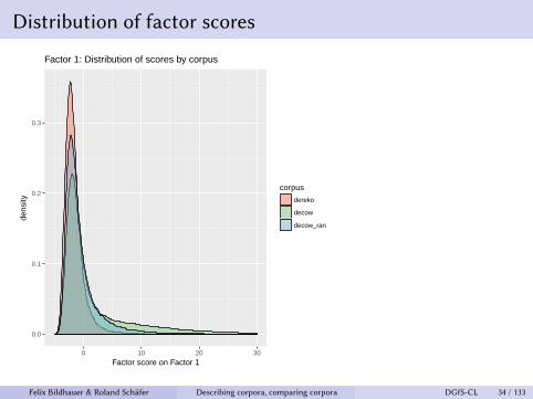
Distribution of factor scores
0.0
0.1
0.2
0.3
0 10 20 30
Factor score on Factor 1
dens
ity
corpus
dereko
decow
decow_ran
Factor 1: Distribution of scores by corpus
Felix Bildhauer & Roland Schäfer Describing corpora, comparing corpora DGfS-CL 34 / 133

Distribution of factor scores (II)
0.0
0.1
0.2
0.3
0 10 20 30 40 50
Score on Factor 1 (short, clitindef, itj, emo, qsvoc, pper2nd, ...)
dens
ity
forum
0
1
Factor 1: Distribution of scores by document type
Felix Bildhauer & Roland Schäfer Describing corpora, comparing corpora DGfS-CL 35 / 133
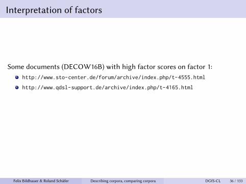
Interpretation of factors
Some documents (DECOW16B) with high factor scores on factor 1:http://www.sto-center.de/forum/archive/index.php/t-4555.html
http://www.qdsl-support.de/archive/index.php/t-4165.html
Some dimensions are readily interpretable, others unclear.
Felix Bildhauer & Roland Schäfer Describing corpora, comparing corpora DGfS-CL 36 / 133

Linguistic features for register / text type / genreclassification
Factor analysis describes each document along along a number ofdimensions.
These are not register / text type categories.
What about automatic document classication for high-level categories(e. g., register / text type)?
Felix Bildhauer & Roland Schäfer Describing corpora, comparing corpora DGfS-CL 37 / 133
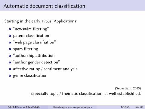
Automatic document classification
Starting in the early 1960s. Applications:
“newswire filtering”
patent classification
“web page classifiation”
spam filtering
“authorship attribution”
“author gender detection”
affective rating / sentiment analysis
genre classification
(Sebastiani, 2005)
Especially topic / thematic classification ist well establishhed.
Felix Bildhauer & Roland Schäfer Describing corpora, comparing corpora DGfS-CL 38 / 133

Automatic Classification
The document classification problem:
Given a set of classes: determine which class(es) a given objectbelongs to.
one-of problems (single-label task) vs. any-of problem (multi-label task)
Supervised classification: requires manually annotated training set.
Fixed set of classes: C = {𝑐1, 𝑐2, 𝑐2, … , 𝑐𝑗}Document space: XDescription 𝑑 ∈ X of a documentTraining set D of labeled documents ⟨𝑑, 𝑐⟩, where ⟨𝑑, 𝑐⟩ ∈ X × C
Classification function 𝛾 maps documents to classes: 𝛾 ∶ X ↦ C
Learning method: Γ(D) = 𝛾(i. e., Γ takes training set as input, returns classification function 𝛾)
(Manning, Raghavan & Schütze, 2009, ch. 13)
Felix Bildhauer & Roland Schäfer Describing corpora, comparing corpora DGfS-CL 39 / 133

Automatic Classification
The document classification problem:
Given a set of classes: determine which class(es) a given objectbelongs to.
one-of problems (single-label task) vs. any-of problem (multi-label task)
Supervised classification: requires manually annotated training set.
Fixed set of classes: C = {𝑐1, 𝑐2, 𝑐2, … , 𝑐𝑗}
Document space: XDescription 𝑑 ∈ X of a documentTraining set D of labeled documents ⟨𝑑, 𝑐⟩, where ⟨𝑑, 𝑐⟩ ∈ X × C
Classification function 𝛾 maps documents to classes: 𝛾 ∶ X ↦ C
Learning method: Γ(D) = 𝛾(i. e., Γ takes training set as input, returns classification function 𝛾)
(Manning, Raghavan & Schütze, 2009, ch. 13)Felix Bildhauer & Roland Schäfer Describing corpora, comparing corpora DGfS-CL 39 / 133

Automatic Classification
The document classification problem:
Given a set of classes: determine which class(es) a given objectbelongs to.
one-of problems (single-label task) vs. any-of problem (multi-label task)
Supervised classification: requires manually annotated training set.
Fixed set of classes: C = {𝑐1, 𝑐2, 𝑐2, … , 𝑐𝑗}Document space: X
Description 𝑑 ∈ X of a documentTraining set D of labeled documents ⟨𝑑, 𝑐⟩, where ⟨𝑑, 𝑐⟩ ∈ X × C
Classification function 𝛾 maps documents to classes: 𝛾 ∶ X ↦ C
Learning method: Γ(D) = 𝛾(i. e., Γ takes training set as input, returns classification function 𝛾)
(Manning, Raghavan & Schütze, 2009, ch. 13)Felix Bildhauer & Roland Schäfer Describing corpora, comparing corpora DGfS-CL 39 / 133

Automatic Classification
The document classification problem:
Given a set of classes: determine which class(es) a given objectbelongs to.
one-of problems (single-label task) vs. any-of problem (multi-label task)
Supervised classification: requires manually annotated training set.
Fixed set of classes: C = {𝑐1, 𝑐2, 𝑐2, … , 𝑐𝑗}Document space: XDescription 𝑑 ∈ X of a document
Training set D of labeled documents ⟨𝑑, 𝑐⟩, where ⟨𝑑, 𝑐⟩ ∈ X × C
Classification function 𝛾 maps documents to classes: 𝛾 ∶ X ↦ C
Learning method: Γ(D) = 𝛾(i. e., Γ takes training set as input, returns classification function 𝛾)
(Manning, Raghavan & Schütze, 2009, ch. 13)Felix Bildhauer & Roland Schäfer Describing corpora, comparing corpora DGfS-CL 39 / 133

Automatic Classification
The document classification problem:
Given a set of classes: determine which class(es) a given objectbelongs to.
one-of problems (single-label task) vs. any-of problem (multi-label task)
Supervised classification: requires manually annotated training set.
Fixed set of classes: C = {𝑐1, 𝑐2, 𝑐2, … , 𝑐𝑗}Document space: XDescription 𝑑 ∈ X of a documentTraining set D of labeled documents ⟨𝑑, 𝑐⟩, where ⟨𝑑, 𝑐⟩ ∈ X × C
Classification function 𝛾 maps documents to classes: 𝛾 ∶ X ↦ C
Learning method: Γ(D) = 𝛾(i. e., Γ takes training set as input, returns classification function 𝛾)
(Manning, Raghavan & Schütze, 2009, ch. 13)Felix Bildhauer & Roland Schäfer Describing corpora, comparing corpora DGfS-CL 39 / 133

Figure: Supervised classification: Training and prediction (from Bird, Klein & Loper,2009)
Felix Bildhauer & Roland Schäfer Describing corpora, comparing corpora DGfS-CL 40 / 133

Features
Numerous attempts at automatic genre indentification:Karlgren & Cutting, 1994; Kessler, Nunberg & Schütze, 1997; Lee &Myaeng, 2002; Freund, Clarke & Toms, 2006; Kanaris & Stamatatos,2009; Mehler, Sharoff & Santini, 2010; Biber & Egbert, 2015
Using linguistic and / or non-linguistic information (markup etc.)
Felix Bildhauer & Roland Schäfer Describing corpora, comparing corpora DGfS-CL 41 / 133

Automatic register identification using grammaticalfeatures
State-of-the-art classification results (Biber & Egbert, 2015):
web documents
32 register categories
42.1% accuracy
.27 precision, .29 recall
Felix Bildhauer & Roland Schäfer Describing corpora, comparing corpora DGfS-CL 42 / 133

Automatic register identification using grammaticalfeatures
State-of-the-art classification results (Biber & Egbert, 2015):
web documents
32 register categories
42.1% accuracy
.27 precision, .29 recall
Felix Bildhauer & Roland Schäfer Describing corpora, comparing corpora DGfS-CL 42 / 133
More problems
Problems with automatic annotation for large “general purpose” corpora:
1 Conceptual: Typically use many grammatical features: risk ofcircularity if the resulting categories are used for controlling registervariation
2 Technical: clustering / classification reduces the dimensions of theoriginal input features: loss of information.
We will explore the consequences of such data aggregation later in amodelling excercise.
Felix Bildhauer & Roland Schäfer Describing corpora, comparing corpora DGfS-CL 43 / 133

Thematic description
Felix Bildhauer & Roland Schäfer Describing corpora, comparing corpora DGfS-CL 44 / 133

The purpose(s) of thematic description / classification
large, unstructured document collections(any kind of data base, also web corpora)
knowing what the documents are about
highly relevant in IR: find documents about something(genes, diseases, companies, products, …)
(corpus) linguistics: themes of documents can becorrelated with other categories (genres, etc.)
distribution of linguistic features varyingwith topical structure
Felix Bildhauer & Roland Schäfer Describing corpora, comparing corpora DGfS-CL 45 / 133
What a document is about I
often: things denoted by words contained in the document
primary subject referenced in title/headline (if any)
but direct mentioning of subjects not necessary
depends on granularity of “subject” or “topic”
“broad” topics, e. g.:
foreign policy national affairs sports
more fine-grained topics, e. g.:
Chinese foreign policy Middle East conflict
the U.S.’s relationship with Russia
Felix Bildhauer & Roland Schäfer Describing corpora, comparing corpora DGfS-CL 46 / 133

Approaches to thematic description of documents /corpora
Keyword analysis
Supervised approaches (document classification)
Unsupervised approaches (e. g. topic modelling)
Felix Bildhauer & Roland Schäfer Describing corpora, comparing corpora DGfS-CL 47 / 133

Keyword analysis with tf.idf
Term frequency by inverse document frequency
Goal: Find terms that are characteristic of a document.
A term is characteristic if it is frequent in that document(“term frequency”, 𝑡𝑓)
A term is characteristic if it does not occur in many other documents(“document frequency”, 𝑑𝑓 )
Several normalisations/weightings improve results(see Manning, Raghavan & Schütze, 2009, Ch. 6.2)
Felix Bildhauer & Roland Schäfer Describing corpora, comparing corpora DGfS-CL 48 / 133

Keyword analysis with tf.idf (II)
tf(t,d)frequency of term 𝑡 in document 𝑑
df(t)document frequency of term 𝑡(number of documents that contain term 𝑡)
idf(t) = Ndf(t)
inverse document frequency: total number of documents divided bynumber of documents that contain 𝑡
tf.idf(t,d) = tf(t,d) ⋅ log Ndf(t)
Felix Bildhauer & Roland Schäfer Describing corpora, comparing corpora DGfS-CL 49 / 133

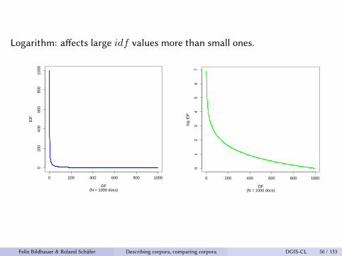
Logarithm: affects large 𝑖𝑑𝑓 values more than small ones.
0 200 400 600 800 1000
020
040
060
080
010
00
(N = 1000 docs)DF
IDF
0 200 400 600 800 1000
01
23
45
67
(N = 1000 docs)DF
log
IDF
Felix Bildhauer & Roland Schäfer Describing corpora, comparing corpora DGfS-CL 50 / 133
Logarithm: affects large 𝑖𝑑𝑓 values more than small ones.
0 200 400 600 800 1000
020
040
060
080
010
00
(N = 1000 docs)DF
IDF
0 200 400 600 800 1000
01
23
45
67
(N = 1000 docs)DF
log
IDF
Felix Bildhauer & Roland Schäfer Describing corpora, comparing corpora DGfS-CL 50 / 133

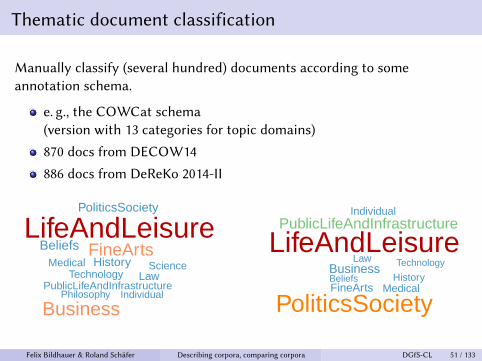
Thematic document classification
Manually classify (several hundred) documents according to someannotation schema.
e. g., the COWCat schema(version with 13 categories for topic domains)
870 docs from DECOW14
886 docs from DeReKo 2014-II
HistoryFineArts
TechnologyPublicLifeAndInfrastructure
LifeAndLeisure
Philosophy
BusinessIndividual
LawMedical Science
PoliticsSociety
BeliefsLaw
Business
LifeAndLeisureBeliefsFineArts
PublicLifeAndInfrastructure
PoliticsSocietyMedical
History
Individual
Technology
Felix Bildhauer & Roland Schäfer Describing corpora, comparing corpora DGfS-CL 51 / 133

Thematic document classification
Manually classify (several hundred) documents according to someannotation schema.
e. g., the COWCat schema(version with 13 categories for topic domains)
870 docs from DECOW14
886 docs from DeReKo 2014-II
HistoryFineArts
TechnologyPublicLifeAndInfrastructure
LifeAndLeisure
Philosophy
BusinessIndividual
LawMedical Science
PoliticsSociety
Beliefs
LawBusiness
LifeAndLeisureBeliefsFineArts
PublicLifeAndInfrastructure
PoliticsSocietyMedical
History
Individual
Technology
Felix Bildhauer & Roland Schäfer Describing corpora, comparing corpora DGfS-CL 51 / 133
Thematic document classification
Manually classify (several hundred) documents according to someannotation schema.
e. g., the COWCat schema(version with 13 categories for topic domains)
870 docs from DECOW14
886 docs from DeReKo 2014-II
HistoryFineArts
TechnologyPublicLifeAndInfrastructure
LifeAndLeisure
Philosophy
BusinessIndividual
LawMedical Science
PoliticsSociety
BeliefsLaw
Business
LifeAndLeisureBeliefsFineArts
PublicLifeAndInfrastructure
PoliticsSocietyMedical
History
Individual
Technology
Felix Bildhauer & Roland Schäfer Describing corpora, comparing corpora DGfS-CL 51 / 133

Use as training data for classifier
Figure: Supervised classification: Training and prediction (Bird, Klein & Loper, 2009)
Classifiers: Naive Bayes, Support Vector Machines, Artficial NeuralNetworks and many, many moreGood starting point: WEKA (Frank, Hall & Witten, 2016),https://www.cs.waikato.ac.nz/ml/weka/
Felix Bildhauer & Roland Schäfer Describing corpora, comparing corpora DGfS-CL 52 / 133

Topic modeling
What is probabilistic topic modeling?
Statistical methods for discovering and annotating large archives ofdocuments with thematic informationAnalyze the words of the original texts to discover:
the themes that run through the textshow those themes are connected to each otherhow they change over time
Can be applied to massive amounts of data.
Can be adapted to many kinds of data(text documents, genetic data, images, social networks, …)
Does not require any prior annotations or labeling of the documents.
(from Blei, 2012)
Felix Bildhauer & Roland Schäfer Describing corpora, comparing corpora DGfS-CL 53 / 133

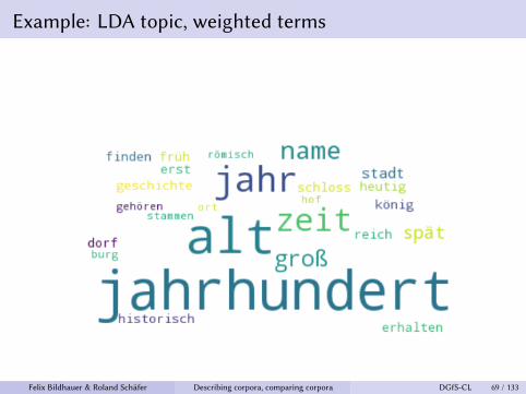
Latent Dirichlet Allocation (LDA; Blei, Ng & Jordan, 2003)
Intuition: Documents exhibit multiple topics.
Documents may blend topics in different proportions.
e. g., a document may be primarily about sports, plus business pluswhite-collar crime
knowing how a documens blends various topics helps situate it in acollection of documents
LDA: statistical model of document collections designed to capture thisintuition
LDA: all the documents in the collection share the same set of topics,but each document exhibits those topics in different proportion
Felix Bildhauer & Roland Schäfer Describing corpora, comparing corpora DGfS-CL 54 / 133

LDA: History
LSA / LSI Latent Semantic Analysis / Indexing (Deerwester et al., 1990)
↓pLSI probabilistic LSI (Hofmann, 1999)
↓LDA Latent Dirichlet Allocation (Blei, Ng & Jordan, 2003)
Felix Bildhauer & Roland Schäfer Describing corpora, comparing corpora DGfS-CL 55 / 133

LDA (II)
LDA assumes that documents arise from a generative process.
Topic: a distribution over a fixed vocabulary
e. g., a sports topic has words about sports with high probability
e. g., a business topic has words about business with high probability
Generating a document is two-stage process:
1 Randomly choose a distribution T over topics.2 For each word in the document:
1 Randomly choose a topic from T.2 Randomly choose a word from the corresponding distribution over the
vocabulary.
Felix Bildhauer & Roland Schäfer Describing corpora, comparing corpora DGfS-CL 56 / 133

LDA (III)
1 Randomly choose a distribution T over topics.2 For each word in the document:
1 Randomly choose a topic from T.2 Randomly choose a word from the corresponding distribution over the
vocabulary.
Each document exhibits the topics in different proportion (1).
Each word in each document is drawn from one of the topics (2b),
the selected topic is chosen from the per-document distribution overtopics (2a)
Felix Bildhauer & Roland Schäfer Describing corpora, comparing corpora DGfS-CL 57 / 133

LDA IV
Topic structure: the topics, per-document topic distributions, and theper-document per-word topic assignments
documents themselves are observed
topic structure is hidden structure
computational problem:use the observed documents to infer the hidden topic structure
or: What is the hidden structure that likely generated the observedcollection?
Felix Bildhauer & Roland Schäfer Describing corpora, comparing corpora DGfS-CL 58 / 133

Generative probabilistic modeling
Generative probabilistic modeling in general:
Assumption: data arises from a generative process that includeshidden variablesGenerative process: defines joint probability distribution over observedand hidden random variables
Data analysis: use joint distribution to compute conditionaldistribution of the hidden variables given the observed variables
Conditional distribution: posterior distribution
LDA:
observed variables: the words of the documents
the hidden variables: topic structure
computational problem: computing the posterior dsitribution(the conditional distribution of the hidden variables given thedocuments)
Felix Bildhauer & Roland Schäfer Describing corpora, comparing corpora DGfS-CL 59 / 133

The posterior distribution
The true posterior distribution is intractable to compute.
involves exponentially large number of every possible instantiation ofthe hidden topic structureinstead, topic modeling algorithms approximate the true posteriordistribution
1 sampling-based algorithms (usually Gibbs sampling)2 variational algorithms (deterministic alternative)
Which approach is better is a matter of debate.
Felix Bildhauer & Roland Schäfer Describing corpora, comparing corpora DGfS-CL 60 / 133

Example: LDA topic, weighted terms
Felix Bildhauer & Roland Schäfer Describing corpora, comparing corpora DGfS-CL 61 / 133

Example: LDA topic, weighted terms
Felix Bildhauer & Roland Schäfer Describing corpora, comparing corpora DGfS-CL 62 / 133

Example: LDA topic, weighted terms
Felix Bildhauer & Roland Schäfer Describing corpora, comparing corpora DGfS-CL 63 / 133

Example: LDA topic, weighted terms
Felix Bildhauer & Roland Schäfer Describing corpora, comparing corpora DGfS-CL 64 / 133

Example: LDA topic, weighted terms
Felix Bildhauer & Roland Schäfer Describing corpora, comparing corpora DGfS-CL 65 / 133

Example: LDA topic, weighted terms
Felix Bildhauer & Roland Schäfer Describing corpora, comparing corpora DGfS-CL 66 / 133

Example: LDA topic, weighted terms
Felix Bildhauer & Roland Schäfer Describing corpora, comparing corpora DGfS-CL 67 / 133

Example: LDA topic, weighted terms
Felix Bildhauer & Roland Schäfer Describing corpora, comparing corpora DGfS-CL 68 / 133
Example: LDA topic, weighted terms
Felix Bildhauer & Roland Schäfer Describing corpora, comparing corpora DGfS-CL 69 / 133

Example: LDA topic, weighted terms
Felix Bildhauer & Roland Schäfer Describing corpora, comparing corpora DGfS-CL 70 / 133

Example: LDA topic, weighted terms
Felix Bildhauer & Roland Schäfer Describing corpora, comparing corpora DGfS-CL 71 / 133

Example: LDA topic, weighted terms
Felix Bildhauer & Roland Schäfer Describing corpora, comparing corpora DGfS-CL 72 / 133

Example: LDA topic, weighted terms
Felix Bildhauer & Roland Schäfer Describing corpora, comparing corpora DGfS-CL 73 / 133

Example: LDA topic, weighted terms
Felix Bildhauer & Roland Schäfer Describing corpora, comparing corpora DGfS-CL 74 / 133

Example: LDA topic, weighted terms
Felix Bildhauer & Roland Schäfer Describing corpora, comparing corpora DGfS-CL 75 / 133

Example: LDA topic, weighted terms
Felix Bildhauer & Roland Schäfer Describing corpora, comparing corpora DGfS-CL 76 / 133

Example: LDA topic, weighted terms
Felix Bildhauer & Roland Schäfer Describing corpora, comparing corpora DGfS-CL 77 / 133

Example: LDA topic, weighted terms
Felix Bildhauer & Roland Schäfer Describing corpora, comparing corpora DGfS-CL 78 / 133

Example: LDA topic, weighted terms
Felix Bildhauer & Roland Schäfer Describing corpora, comparing corpora DGfS-CL 79 / 133

Example: LDA topic, weighted terms
Felix Bildhauer & Roland Schäfer Describing corpora, comparing corpora DGfS-CL 80 / 133

Part II: Comparing corpora
Felix Bildhauer & Roland Schäfer Describing corpora, comparing corpora DGfS-CL 81 / 133

Corpus comparison
Questions researchers might ask:
Are corpus X and corpus Y similar to each other?
How similar are they to each other?
Are they significantly different from each other?
Given corpus X and corpus Y, where is corpus Z located between these?
…
Big question: Similarity with respect to which criterion?
Felix Bildhauer & Roland Schäfer Describing corpora, comparing corpora DGfS-CL 82 / 133

Corpus similarity
What does it mean for two corpora to be “similar” to each other?
no such thing as a single measure of corpus similarity
no simple, single answer to this question
Corpora can be similar by one criterion and different by another, e. g.:
corpus A: docs about sports and politics, from forum discussions
corpus B: docs about sports and politics, from newspaper articles
Many different approaches, e. g.:
compare corpus composition (text types, topics, authorship etc.)
compare distribution of linguistic entities(words, other linguistic features)
compare corpora with respect to a specific task(collocation extraction, word similarity tasks)
(See Kilgarriff, 2001 for discussion.)
Felix Bildhauer & Roland Schäfer Describing corpora, comparing corpora DGfS-CL 83 / 133

Corpus similarity
What does it mean for two corpora to be “similar” to each other?
no such thing as a single measure of corpus similarity
no simple, single answer to this question
Corpora can be similar by one criterion and different by another, e. g.:
corpus A: docs about sports and politics, from forum discussions
corpus B: docs about sports and politics, from newspaper articles
Many different approaches, e. g.:
compare corpus composition (text types, topics, authorship etc.)
compare distribution of linguistic entities(words, other linguistic features)
compare corpora with respect to a specific task(collocation extraction, word similarity tasks)
(See Kilgarriff, 2001 for discussion.)Felix Bildhauer & Roland Schäfer Describing corpora, comparing corpora DGfS-CL 83 / 133

Overview slide here?
Felix Bildhauer & Roland Schäfer Describing corpora, comparing corpora DGfS-CL 84 / 133

Comparing keywords
Idea: compare lists of keywords extracted from two corpora
Keywords: words that are characteristic of a corpus
Key-ness: relative notion
Compute a statistic from the frequency of each in corpus A, and thefrequency of the same word in corpus B
Sometimes, calculate p-values and dispersion
Felix Bildhauer & Roland Schäfer Describing corpora, comparing corpora DGfS-CL 85 / 133

Keyword extraction statistics
Ratio of relative frequencies (e. g., Edmundson & Wyllys, 1961;Damerau, 1993; Kilgarriff, 2012)Yule, 1944 difference coefficient (e. g., Hofland & Johansson, 1982)𝜒2 (e. g., Scott, 1997)-2 Log-Likelihood (e. g., Scott, 2001)Mann-Whitney U (Kilgarriff, 2001)tf.idf (Spärck Jones, 1972)
Different statistics may result in quite different keyword lists.
Felix Bildhauer & Roland Schäfer Describing corpora, comparing corpora DGfS-CL 86 / 133

Keyword extraction with 𝜒2
Compute a 𝜒2 value from a 2×2 table for each word type in the joinedcorpus (Corpus A ∪ Corpus B)
Multipy value by the sign of the first table cell(positive if a word is over-represented in Corpus A, negative otherwise)
𝜒2 × 𝑠𝑔𝑛(𝑂1,1 − 𝐸1,1)Sort the list on the signed 𝜒2 value
Illustration:
Keyword extraction with 𝜒2 from two samples of DECOW12(1.2 G tokens each).
Felix Bildhauer & Roland Schäfer Describing corpora, comparing corpora DGfS-CL 87 / 133

Example: keyword extraction with 𝜒2
Score Word Translation f Corpus A f Corpus A213857 Selbstbewusstsein ‘self-consciousness’ 230086 7103180761 der ‘the’ 25823958 23332624112942 Stärken ‘strengths’ 147041 13782110867 des ‘of.the’ 5467541 4511218109470 stärken ‘strengthen’ 150609 1680781735 in ‘in’ 14531108 1329186180314 Niederösterreich ‘Lower Austria 81732 99769230 und ‘and’ 27615823 2620999967723 Steiermark ‘Styria’ 69845 116561955 Schwächen ‘weaknesses’ 101680 1703458046 Sie ‘you’ 2389178 192935448998 Selbstbewusstseinstraining ‘self-consciousness training’ 48100 345075 Die ‘the’ 4725965 417691741216 Oberösterreich ‘Upper Austria’ 43930 121738921 werden ‘become’ 3889092 342477233635 , , 61275629 6044099833447 die ‘the’ 26896810 2607551333069 wir ‘we’ 2751969 238820332967 Gott ‘God’ 277819 16158727182 » » 499957 35550026135 durch ‘through’ 2028104 174948025822 uns ‘us’ 1432263 119646125367 von ‘from’ 8958078 845865524745 Beispiele ‘examples’ 95118 3880724657 « « 437106 30851523838 Menschen ‘people’ 804843 63320523655 zur ‘to.the’ 1887285 163189223466 In ‘in 1267897 105621823359 sich ‘oneself’ 7073007 663692423056 Coaching ‘coaching’ 32678 3958
Felix Bildhauer & Roland Schäfer Describing corpora, comparing corpora DGfS-CL 88 / 133

Example: keyword extraction with 𝜒2
Score Word Translation f Corpus A f Corpus B-49228 es ‘it’ 7191558 8203365-52339 ! ! 3539669 4250013-55500 jetzt ‘now’ 1093904 1497137-58057 so ‘so’ 4078118 4881829-58090 meine ‘my’ 743321 1086311-61785 was ‘what’ 2368986 2994141-62641 wenn ‘if’ 2525537 3175758-62847 :zustimm: ‘agree 4 64046-65120 bin ‘am’ 898077 1296452-68224 das ‘the’ 11114277 12601969-68699 : : 7361865 8552945-69360 Du ‘you’ 856126 1258723-70448 dann ‘then’ 2705021 3418243-73501 :-D :-D 4080 86533-74531 schon ‘already’ 2299966 2975671-79816 mich ‘me’ 1776035 2391232-80099 auch ‘too’ 7618001 8919734-99309 da ‘there’ 2125894 2876793
-102364 aber ‘but’ 3900764 4932552-115949 du ‘you’ 1501636 2189889-117379 hab ‘have’ 606783 1065271-138531 nicht ‘not’ 9679787 11587724-144946 habe ‘have’ 1725867 2552673-166247 ja ‘yes’ 1806276 2714682-176159 mir ‘me’ 2190317 3215638-176735 Ich ‘I’ 2664716 3791898-186177 ? ? 3889053 5278796-186838 mal ‘once’ 2000220 3014011-333374 … … 3418151 5189644-709423 ich ‘I’ 8606043 12673625
Felix Bildhauer & Roland Schäfer Describing corpora, comparing corpora DGfS-CL 89 / 133

Keyword extraction with the ratio of relative frequencies
Ratio of relative frequencies (RRF): early research on automaticdocument summarization and indexing (Edmundson & Wyllys, 1961)
For every word ocurring in Corpus A or Corpus B:divide the word’s relative frequency in Corpus A by its relativeferquency in Corpus B(after adding a smoothing constant)
Sort on the resulting score (between 0 and ∞).
Kilgarriff, 2012: obtain keywords from different frequency bands byvarying the smoothing constant.
Illustration:
Keyword extraction with RRF from the same two samples of DECOW12(1.2 G tokens each).
Felix Bildhauer & Roland Schäfer Describing corpora, comparing corpora DGfS-CL 90 / 133

Example: keyword extraction with RRF
Ratio Word Translation f Corpus A f Corpus B14193 IntSel®-Selbstbewusstseinstraining ‘IntSel® self-consciousness training’ 13929 012252 Selbstbewusstseinstraining ‘self-consciousness training’ 48100 311414 IntSel®-Selbstbewusstseinstrainings ‘IntSel® self-consciousness trainings’ 11201 07253 moviac moviac (NE) 7118 05022 Kinder-Selbstbewusstseins-Coach ‘children’s self-consciousness coach’ 4928 03876 www.theaterstuebchen.de www.theaterstuebchen.de 3803 02876 Selbstbewusstseinstrainer ‘self-consciousness coach’ 2822 02854 ’schmökern ‘to browse’ 2800 02853 IntSel®-Wertekonzept ‘IntSel® scheme of values’ 2799 02853 IntSel®-Stärkenleiter ‘IntSel® scale of strengths’ 2799 02853 Angst-Vermeidungsstrategien ‘fear avoidance strategies’ 2799 02853 ’Austherapierte ‘healed persons’ 2799 02693 HR-Lieblingsschiff ‘HR favorite ship’ 2642 02613 Schwehm Schwehm (NE) 17949 62158 www.bauemotion.de www.bauemotion.de 2117 02068 :futsch: emoticon 2029 01961 Litaraturmarkt ‘literature market’ 1924 01721 Thor’al Thor’al (NE) 1688 01631 Grujicic Grujicic (NE) 1600 01591 :fletch: emoticon 1561 01554 Terror-Die terror-the 1524 01550 Architektur-Meldungen ‘architecture news’ 1520 01496 Beamt-er/ ‘state employee’ 1467 01469 91785 91785 2883 11464 Systemcoach ‘system coach’ 2872 11438 Party-Highlight ‘party highlight’ 1410 01435 Tiergefahren ‘danger from animals’ 1407 01434 Tybrang Tybrang (NE) 1406 01433 Titelvertei-digung ‘title defense’ 1405 01433 Riesen-Herausforderer ‘big contender’ 1405 0
Felix Bildhauer & Roland Schäfer Describing corpora, comparing corpora DGfS-CL 91 / 133

Example: keyword extraction with RRF
Ratio Word Translation f Corpus 1 f Corpus 24.268E-04 :five: emoticon 1 47744.265E-04 @vandeStonehill @vandeStonehill 0 23884.265E-04 #WeLove #WeLove 0 23884.265E-04 #HighSchoolMusical3 #HighSchoolMusical3 0 23884.208E-04 :aargh: emoticon 0 24204.195E-04 :meinemeinung emoticon 0 24284.189E-04 |supergri emoticon 0 24314.125E-04 :zickig: emoticon 0 24694.107E-04 *seh *seh 0 24804.098E-04 |kopfkrat emoticon 0 24854.096E-04 kostenlose-urteile.de kostenlose-urteile.de 0 24864.072E-04 Migrantenrat ‘immigrants’ board’ 1 50034.072E-04 MV-Politiker ‘MV-politician’ 0 25013.971E-04 berlin.business-on.de berlin.business-on.de 0 25653.731E-04 :fürcht: emoticon 0 27303.655E-04 :leiderja: emoticon 0 27873.473E-04 Bollywoodsbest Bollywoodsbest 0 29333.329E-04 Fotoserver ‘photo server’ 0 30603.192E-04 :urgs: emoticon 0 31913.174E-04 :habenmuss: emoticon 0 32093.168E-04 Stachelhausen Stachelhausen (NE) 1 64312.906E-04 :rothlol: emoticon 0 35052.637E-04 Juusuf Juusuf (NE) 0 38632.489E-04 :zumgluecknein: emoticon 0 40922.136E-04 :zufrieden: emoticon 0 47701.953E-04 :menno: emoticon 0 52171.818E-04 @ProSieben @ProSieben 0 56021.682E-04 :dollschaem: emoticon 0 60561.331E-04 :traeum: emoticon 0 76561.281E-04 :dollfreu: emoticon 0 7955
Felix Bildhauer & Roland Schäfer Describing corpora, comparing corpora DGfS-CL 92 / 133

Keyword extraction: properties of 𝜒2 versus RRF
Corpus 1 Corpus 2f absolute f relative f absolute f relative Ratio of rel. freqs. 𝜒2
50 .05 100 .1 0.5 17.3100 .1 200 .2 0.5 38.4200 .2 400 .4 0.5 94.3
Figure: 𝜒2 vs. ratio of relative frequencies in keyword extraction, illustrated by twocorpora of 1,000 tokens each.
Felix Bildhauer & Roland Schäfer Describing corpora, comparing corpora DGfS-CL 93 / 133

Compare association of documents with induced topics
−1.0 −0.5 0.0 0.5
DeReKo DECOW
Figure: Log ratio of relative frequencies: proportion of documents with topic Xamong their 3 most strongly associated topics
Felix Bildhauer & Roland Schäfer Describing corpora, comparing corpora DGfS-CL 94 / 133

Measuring thematic corpus balance
Ciamarita & Baroni (2006): ensure that no topic is heavily over-representedin a corpus.Method:
Create a number of corpora that are deliberately biased towards sometopic.
Calculate mean distance of each one of these corpora to all othercorpora.
Distance: based on word frequencies, measured as relative entropy(or Kullback-Leibler distance, KullbackLeibler1951).Measure distance of a target corpus to all other corpora.
Expectation: if the target corpus is unbiased, it is “in between” all thebiased corporamean distance of target corpus should be smaller than mean distanceof biased corpora.
Felix Bildhauer & Roland Schäfer Describing corpora, comparing corpora DGfS-CL 95 / 133

Comparing word frequency lists
Top 20 common nouns in FRCOW2011 and frWaC (Baroni et al., 2009):
Rank FRCOW 2011 (few seed URLs) FRWAC (many seed URLs)1 année ‘year’ site2 travail ‘work’ an3 temps ‘time’ travail4 an ‘year’ jour5 jour ‘day’ année6 pays ‘country’ service7 monde ‘world’ temps8 vie ‘life’ article9 personne ‘person’ personne
10 homme ‘man’ projet11 service information12 cas ‘case’ entreprise ‘company’13 droit ‘right’ recherche ‘(re-)search’14 effet ‘effect’ vie15 projet ‘project’ droit16 question page17 enfant ‘child’ formation (‘education’)18 fois ‘time (occasion)’ commentaire ‘comment’19 place cas20 site fois
Fairly good overlapBut method is impressionistic, no “measure” of the differenceAre these corpora “significantly” (dis-)similar to each other?
Felix Bildhauer & Roland Schäfer Describing corpora, comparing corpora DGfS-CL 96 / 133

Testing for differences: 𝜒2-test
𝐻0: The corpora are samples from the same population(the frequency of a word is not correlated with variable corpus are notcorrelated)
𝜒2-test test compares frequencies of a word type in the two corpora
Corpus 1 Corpus 2word X freq(X) freq(X)
¬ word X freq(¬X) freq(¬X)
Felix Bildhauer & Roland Schäfer Describing corpora, comparing corpora DGfS-CL 97 / 133

Corpus comparison using the 𝜒2-test
Frequency 𝜒2 pWord Corpus 1 Corpus 2de 6781719 6802262 32.99 <.001, 5627749 5633555 3.12 .077la 3613946 3614049 0.001 .975. 3574395 3579032 3.08 .079que 2963992 2956662 9.36 <.010y 2642241 2653365 23.88 <.001en 2562028 2564809 1.53 .217el 2450353 2446328 3.40 .065a 1885112 1882813 1.44 .230los 1597103 1603537 13.09 <.001del 1173860 1172623 0.67 .415se 1139311 1143202 6.68 <.010las 1054729 1054924 0.02 .896un 1001556 1000106 1.07 .302
Figure: 𝜒2 14 most frequent word types in two Spanish Web corpora (110m tokens)
Overall score?𝜒2 statistic for the 14 × 2 table (13 df): 𝜒2 = 76.87, 𝑝 < .001But: these are in fact random subcorpora from ESCOW2012.
Felix Bildhauer & Roland Schäfer Describing corpora, comparing corpora DGfS-CL 98 / 133

Corpus comparison using the 𝜒2-test
Frequency 𝜒2 pWord Corpus 1 Corpus 2de 6781719 6802262 32.99 <.001, 5627749 5633555 3.12 .077la 3613946 3614049 0.001 .975. 3574395 3579032 3.08 .079que 2963992 2956662 9.36 <.010y 2642241 2653365 23.88 <.001en 2562028 2564809 1.53 .217el 2450353 2446328 3.40 .065a 1885112 1882813 1.44 .230los 1597103 1603537 13.09 <.001del 1173860 1172623 0.67 .415se 1139311 1143202 6.68 <.010las 1054729 1054924 0.02 .896un 1001556 1000106 1.07 .302
Figure: 𝜒2 14 most frequent word types in two Spanish Web corpora (110m tokens)
Overall score?
𝜒2 statistic for the 14 × 2 table (13 df): 𝜒2 = 76.87, 𝑝 < .001But: these are in fact random subcorpora from ESCOW2012.
Felix Bildhauer & Roland Schäfer Describing corpora, comparing corpora DGfS-CL 98 / 133

Corpus comparison using the 𝜒2-test
Frequency 𝜒2 pWord Corpus 1 Corpus 2de 6781719 6802262 32.99 <.001, 5627749 5633555 3.12 .077la 3613946 3614049 0.001 .975. 3574395 3579032 3.08 .079que 2963992 2956662 9.36 <.010y 2642241 2653365 23.88 <.001en 2562028 2564809 1.53 .217el 2450353 2446328 3.40 .065a 1885112 1882813 1.44 .230los 1597103 1603537 13.09 <.001del 1173860 1172623 0.67 .415se 1139311 1143202 6.68 <.010las 1054729 1054924 0.02 .896un 1001556 1000106 1.07 .302
Figure: 𝜒2 14 most frequent word types in two Spanish Web corpora (110m tokens)
Overall score?𝜒2 statistic for the 14 × 2 table (13 df): 𝜒2 = 76.87, 𝑝 < .001
But: these are in fact random subcorpora from ESCOW2012.
Felix Bildhauer & Roland Schäfer Describing corpora, comparing corpora DGfS-CL 98 / 133

Corpus comparison using the 𝜒2-test
Frequency 𝜒2 pWord Corpus 1 Corpus 2de 6781719 6802262 32.99 <.001, 5627749 5633555 3.12 .077la 3613946 3614049 0.001 .975. 3574395 3579032 3.08 .079que 2963992 2956662 9.36 <.010y 2642241 2653365 23.88 <.001en 2562028 2564809 1.53 .217el 2450353 2446328 3.40 .065a 1885112 1882813 1.44 .230los 1597103 1603537 13.09 <.001del 1173860 1172623 0.67 .415se 1139311 1143202 6.68 <.010las 1054729 1054924 0.02 .896un 1001556 1000106 1.07 .302
Figure: 𝜒2 14 most frequent word types in two Spanish Web corpora (110m tokens)
Overall score?𝜒2 statistic for the 14 × 2 table (13 df): 𝜒2 = 76.87, 𝑝 < .001But: these are in fact random subcorpora from ESCOW2012.
Felix Bildhauer & Roland Schäfer Describing corpora, comparing corpora DGfS-CL 98 / 133

Why the 𝜒2-test is not suitable
𝜒2 statistic grows as a function of sample sizeHuge sample size: minor differences lead to large 𝜒2 values
Form Corpus 3 Corpus 4 𝜒2 pde 13579307 13563617 9.65 <.010, 11264561 11274225 4.38 .036la 7227386 7236002 5.31 .021. 7157262 7150075 3.72 .054que 5924861 5932089 4.53 .033y 5303604 5292011 12.98 <.001en 5117964 5123526 3.10 .078el 4885947 4900224 21.31 <.001a 3766747 3773854 6.82 <.010los 3203514 3193313 16.49 <.001del 2340110 2338707 0.42 .515se 2277149 2284887 13.27 <.001las 2105694 2109117 2.81 .094un 1998736 2002337 3.27 .070
Figure: Two random subcorpora from ESCOW2012, 220m tokens each
Felix Bildhauer & Roland Schäfer Describing corpora, comparing corpora DGfS-CL 99 / 133
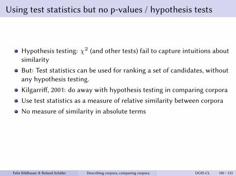
Using test statistics but no p-values / hypothesis tests
Hypothesis testing: 𝜒2 (and other tests) fail to capture intuitions aboutsimilarity
But: Test statistics can be used for ranking a set of candidates, withoutany hypothesis testing.
Kilgarriff, 2001: do away with hypothesis testing in comparing corpora
Use test statistics as a measure of relative similarity between corpora
No measure of similarity in absolute terms
Which test statistic should be used?
Felix Bildhauer & Roland Schäfer Describing corpora, comparing corpora DGfS-CL 100 / 133

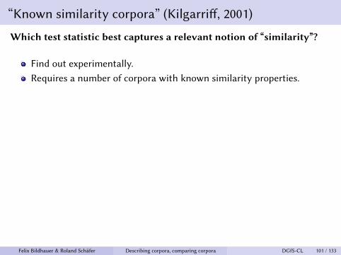
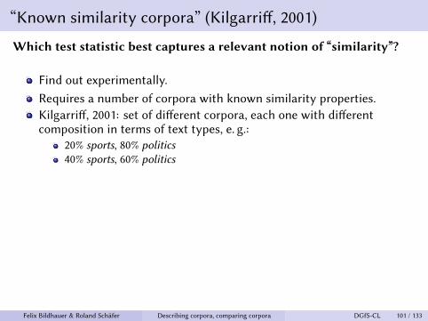
“Known similarity corpora” (Kilgarriff, 2001)
Which test statistic best captures a relevant notion of “similarity”?
Find out experimentally.Requires a number of corpora with known similarity properties.Kilgarriff, 2001: set of different corpora, each one with differentcomposition in terms of text types, e. g.:
20% sports, 80% politics40% sports, 60% politics
Gold standard for similarity ranking”40_sports_60_politics is more similar to 100_sports than20_sports_80_politics” etc.
Compute test statistic for 𝑛 most frequent tokens, sum up, evaluatehow many gold standard rankings are predicted correctlyResult: 𝜒2 outperforms all others(including Spearman rank correlation coefficient & variants ofcross-entropy measures)
Felix Bildhauer & Roland Schäfer Describing corpora, comparing corpora DGfS-CL 101 / 133

“Known similarity corpora” (Kilgarriff, 2001)
Which test statistic best captures a relevant notion of “similarity”?
Find out experimentally.
Requires a number of corpora with known similarity properties.Kilgarriff, 2001: set of different corpora, each one with differentcomposition in terms of text types, e. g.:
20% sports, 80% politics40% sports, 60% politics
Gold standard for similarity ranking”40_sports_60_politics is more similar to 100_sports than20_sports_80_politics” etc.
Compute test statistic for 𝑛 most frequent tokens, sum up, evaluatehow many gold standard rankings are predicted correctlyResult: 𝜒2 outperforms all others(including Spearman rank correlation coefficient & variants ofcross-entropy measures)
Felix Bildhauer & Roland Schäfer Describing corpora, comparing corpora DGfS-CL 101 / 133
“Known similarity corpora” (Kilgarriff, 2001)
Which test statistic best captures a relevant notion of “similarity”?
Find out experimentally.Requires a number of corpora with known similarity properties.
Kilgarriff, 2001: set of different corpora, each one with differentcomposition in terms of text types, e. g.:
20% sports, 80% politics40% sports, 60% politics
Gold standard for similarity ranking”40_sports_60_politics is more similar to 100_sports than20_sports_80_politics” etc.
Compute test statistic for 𝑛 most frequent tokens, sum up, evaluatehow many gold standard rankings are predicted correctlyResult: 𝜒2 outperforms all others(including Spearman rank correlation coefficient & variants ofcross-entropy measures)
Felix Bildhauer & Roland Schäfer Describing corpora, comparing corpora DGfS-CL 101 / 133
“Known similarity corpora” (Kilgarriff, 2001)
Which test statistic best captures a relevant notion of “similarity”?
Find out experimentally.Requires a number of corpora with known similarity properties.Kilgarriff, 2001: set of different corpora, each one with differentcomposition in terms of text types, e. g.:
20% sports, 80% politics40% sports, 60% politics
Gold standard for similarity ranking”40_sports_60_politics is more similar to 100_sports than20_sports_80_politics” etc.
Compute test statistic for 𝑛 most frequent tokens, sum up, evaluatehow many gold standard rankings are predicted correctlyResult: 𝜒2 outperforms all others(including Spearman rank correlation coefficient & variants ofcross-entropy measures)
Felix Bildhauer & Roland Schäfer Describing corpora, comparing corpora DGfS-CL 101 / 133

“Known similarity corpora” (Kilgarriff, 2001)
Which test statistic best captures a relevant notion of “similarity”?
Find out experimentally.Requires a number of corpora with known similarity properties.Kilgarriff, 2001: set of different corpora, each one with differentcomposition in terms of text types, e. g.:
20% sports, 80% politics40% sports, 60% politics
Gold standard for similarity ranking”40_sports_60_politics is more similar to 100_sports than20_sports_80_politics” etc.
Compute test statistic for 𝑛 most frequent tokens, sum up, evaluatehow many gold standard rankings are predicted correctly
Result: 𝜒2 outperforms all others(including Spearman rank correlation coefficient & variants ofcross-entropy measures)
Felix Bildhauer & Roland Schäfer Describing corpora, comparing corpora DGfS-CL 101 / 133

“Known similarity corpora” (Kilgarriff, 2001)
Which test statistic best captures a relevant notion of “similarity”?
Find out experimentally.Requires a number of corpora with known similarity properties.Kilgarriff, 2001: set of different corpora, each one with differentcomposition in terms of text types, e. g.:
20% sports, 80% politics40% sports, 60% politics
Gold standard for similarity ranking”40_sports_60_politics is more similar to 100_sports than20_sports_80_politics” etc.
Compute test statistic for 𝑛 most frequent tokens, sum up, evaluatehow many gold standard rankings are predicted correctlyResult: 𝜒2 outperforms all others(including Spearman rank correlation coefficient & variants ofcross-entropy measures)
Felix Bildhauer & Roland Schäfer Describing corpora, comparing corpora DGfS-CL 101 / 133

Other features, other statistics
Teich & Fankhauser, 2009: comparing F-LOB (Freiburg–LOB Corpus ofBritish English) with corpus of scientific writing (≈ 1M tokens each)
Features:
Standardized type-token ratio (STTR) as a potential indicator oftechnical language
Relative number of nouns, lexical verbs, and adverbs potentialindicators of abstract language
Lexical density (avg. number of lexical words per clause) as a measurefor the informational density
Statistic: information gain (measures how well a feature distinguishesbetween classes)
STTR as best performing feature
“Shallow features such as a low type-token ratio clearly characterize themeta-register of scientific writing.”
Felix Bildhauer & Roland Schäfer Describing corpora, comparing corpora DGfS-CL 102 / 133

Other features, other statistics (II)
Denoual (2006): Locate target corpus X between two reference corpora Yand Z.Features:
Character 𝑁 -grams (1 < 𝑛 < 17)Does not require tokenization or lemmatization.
Statistic: cross-entropy
Construct several N-gram character models from reference corpora
Use these language models to estimate the cross-entropy,in terms of bits per character needed to encode a test corpus
Two corpora are similar when one of them can be completely predictedgiven the knowledge of the other one
Evaluation: on Japanese, with known similarity copora
cross entropy & N-grams performs equally well as words & 𝜒2
Felix Bildhauer & Roland Schäfer Describing corpora, comparing corpora DGfS-CL 103 / 133

Extrinsic evaluation: collocation extraction Biemann et al.,2013
Stefan Evert’s work reported in (Biemann et al., 2013)
compares different corpora with a gold standard
size POS basicname (tokens) corpus type tagged lemmatized unitBNC 0.1 G reference corpus + + textWP500 0.2 G Wikipedia + + fragmentWackypedia 1.0 G Wikipedia + + articleukWaC 2.1 G web corpus + + web pageWebBase 3.3 G web corpus + + paragraphUKCOW 4.0 G web corpus + + sentenceLCC 0.9 G web corpus + − sentenceLCC (𝑓 ≥ 𝑘) 0.9 G web n-grams + − n-gramWeb1T5 (𝑓 ≥ 40) 1000.0 G web n-grams − − n-gram
Felix Bildhauer & Roland Schäfer Describing corpora, comparing corpora DGfS-CL 104 / 133

English verb-particle combinations (I)
gold standard: 3,078 verb-partikel combinations, non-compositional(carry on, knock out) oder kompositional bring together, peer out)
extracted: co-occurrences of word pairs(3-words window left / right right to the verb)
Felix Bildhauer & Roland Schäfer Describing corpora, comparing corpora DGfS-CL 105 / 133

English verb-particle combinations (II)
POS size average precisioncorpus filter (tokens) 𝐺2 𝑡 MI Dice MI2 𝑋2
BNC + 0.1 G 31.06 29.15 22.58 30.13 30.97 32.12WP500 + 0.2 G 28.01 25.73 27.81 30.29 29.98 31.56Wackypedia + 1.0 G 28.03 25.70 27.39 30.35 30.10 31.58ukWaC + 2.2 G 30.01 27.82 25.76 30.54 30.98 32.66WebBase + 3.3 G 30.34 27.80 27.95 31.74 32.02 33.95UKCOW + 4.0 G 32.31 30.00 26.43 32.00 32.96 34.71LCC + 0.9 G 25.61 24.83 22.14 26.82 25.09 26.38LCC (𝑓 ≥ 5) + 0.9 G 26.95 26.45 25.54 27.78 25.96 27.66LCC (𝑓 ≥ 10) + 0.9 G 27.34 26.81 27.13 27.85 25.95 28.09LCC − 0.9 G 24.67 23.63 21.41 25.36 23.88 25.63LCC (𝑓 ≥ 5) − 0.9 G 25.45 24.79 23.54 26.30 24.55 26.21LCC (𝑓 ≥ 10) − 0.9 G 25.84 25.16 25.28 26.49 24.71 26.63Web1T5 (𝑓 ≥ 40) − 1000.0 G 26.61 26.12 21.67 27.82 25.72 27.14
Felix Bildhauer & Roland Schäfer Describing corpora, comparing corpora DGfS-CL 106 / 133

English verb-particle combinations (III)
Clean, annotated web corpora can replace more traditional corpora likethe BNC.
Diversity might play a role: web corpora need to be 1 GT in size to rivalthe BNC.
Web1T5: size alone is not sufficient, good filtering and linguisticannotation are necessary.
Felix Bildhauer & Roland Schäfer Describing corpora, comparing corpora DGfS-CL 107 / 133

Homogeneity
How similar to each other are subparts of a corpus?
Subparts are usually sets of texts / documents
Common method:
Choose a feature(in a broad sense: could also be a lexical item syntactic constructionconstruction; see also Stefan Gries, 2006)
Assess occurrence in subparts
Compute summary statistic
Homogeneity is an intra-corpus measure, but it makes sense to interpret itwith respect to other corpora.
Felix Bildhauer & Roland Schäfer Describing corpora, comparing corpora DGfS-CL 108 / 133

Homogeneity: Illustration
Assess sampling distribution of the mean of some feature X.
Draw 𝑚 samples of 𝑛 documents from the corpus.
For each sample, get the mean value of feature X.
Calculate the standard error of the mean.
Plot density of distribution of sample means.
Repeat this 𝑡 times.
Felix Bildhauer & Roland Schäfer Describing corpora, comparing corpora DGfS-CL 109 / 133

Plotting exercise
Run the R-Script tutorial-resampling.R and reproduce the plot forpaste tense verbs.
source(tutorial -resampling.R)
Open the script file and modify it: select one or two other COReXfeatures and plot the sampling distribution of their mean.
# which other COReX features are there?colnames(random_dereko_70k)
# edit this line (select new feature):feature <-"vpast"
# edit this line (remove ylim and xlim):plot(density(m), ylim=c(0,1), xlim=(c(5,35)), ... )
# edit this line (adapt position of the legend):legend (15,1, ... )
Felix Bildhauer & Roland Schäfer Describing corpora, comparing corpora DGfS-CL 110 / 133

Part III: Modelling
Felix Bildhauer & Roland Schäfer Describing corpora, comparing corpora DGfS-CL 111 / 133

Example GLM… or rather logistic regression
Alternation of genitive and case identityin German measure NPs; much more complex real model cf.Schäfer (accept with revisions September 2017)http://rolandschaefer.net/?p=1290
Wir trinken eine Flasche guten Wein. (Agree=1)
Wir trinken eine Flasche guten Weines. (Agree=0)
which factors incluence Agreesome of the possible regressors
casedefinitenesscardinal determiner
Felix Bildhauer & Roland Schäfer Describing corpora, comparing corpora DGfS-CL 112 / 133

Why not a Linear Model?
●● ●●
● ●● ●● ●
0 5 10 15 20
−0.
50.
00.
51.
01.
5
x
y
LM predicts continuous variable
not plausible for dichotomous outcome
also not usable as probability (outside [0, 1])normality assumption for errors violated
Felix Bildhauer & Roland Schäfer Describing corpora, comparing corpora DGfS-CL 113 / 133
GLM: Logits
For a GLM, we pretend a linear combination is possible:
predicting probabilities of Agree=1
…from a linear combination of regressors
the linear term gives us logits:
𝑧 = 𝛽1𝑥1 + 𝛽2𝑥2 + ⋯ + 𝛽𝑛𝑥𝑛 + 𝛽0
Felix Bildhauer & Roland Schäfer Describing corpora, comparing corpora DGfS-CL 114 / 133

GLM: Logits
For a GLM, we pretend a linear combination is possible:
predicting probabilities of Agree=1
…from a linear combination of regressors
the linear term gives us logits:
𝑧 = 𝛽1𝑥1 + 𝛽2𝑥2 + ⋯ + 𝛽𝑛𝑥𝑛 + 𝛽0
Felix Bildhauer & Roland Schäfer Describing corpora, comparing corpora DGfS-CL 114 / 133

GLM: Link functions
Logits transformed into probabilities via some exponential CDF(cumulative density function) like the logistic or normal (probit) CDF
𝑝(𝑦 = 1) = 11+𝑒−𝑧
For binary predictions:
𝑦 = {0 if 𝑝(𝑦 = 1) ≤ 0.51 if 𝑝(𝑦 = 1) > 0.5
Felix Bildhauer & Roland Schäfer Describing corpora, comparing corpora DGfS-CL 115 / 133
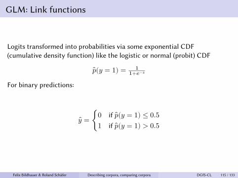

Logit transform
Transformed logits as 𝑝(𝑦 = 1):
−10 −5 0 5 10
0.0
0.2
0.4
0.6
0.8
1.0
Logits
p(y=
1)
Felix Bildhauer & Roland Schäfer Describing corpora, comparing corpora DGfS-CL 116 / 133

Interpretation of the coefficients
only indirect interpretation of coefficients
𝛽𝑖 positive ⇒ positive influence on 𝑝(𝑦 = 1)𝛽𝑖 negative ⇒ negative influence on 𝑝(𝑦 = 1)
non-linear influence on probabilities!
linear influence on logits only
divide-by-4 (Gelman & Hill, 2006, p. 82):coefficients around 0.5 can be divided by 4to give an upper bound for effect on the probability scale
Felix Bildhauer & Roland Schäfer Describing corpora, comparing corpora DGfS-CL 117 / 133
Interpretation of the coefficients
only indirect interpretation of coefficients
𝛽𝑖 positive ⇒ positive influence on 𝑝(𝑦 = 1)
𝛽𝑖 negative ⇒ negative influence on 𝑝(𝑦 = 1)
non-linear influence on probabilities!
linear influence on logits only
divide-by-4 (Gelman & Hill, 2006, p. 82):coefficients around 0.5 can be divided by 4to give an upper bound for effect on the probability scale
Felix Bildhauer & Roland Schäfer Describing corpora, comparing corpora DGfS-CL 117 / 133

Interpretation of the coefficients
only indirect interpretation of coefficients
𝛽𝑖 positive ⇒ positive influence on 𝑝(𝑦 = 1)𝛽𝑖 negative ⇒ negative influence on 𝑝(𝑦 = 1)
non-linear influence on probabilities!
linear influence on logits only
divide-by-4 (Gelman & Hill, 2006, p. 82):coefficients around 0.5 can be divided by 4to give an upper bound for effect on the probability scale
Felix Bildhauer & Roland Schäfer Describing corpora, comparing corpora DGfS-CL 117 / 133
Interpretation of the coefficients
only indirect interpretation of coefficients
𝛽𝑖 positive ⇒ positive influence on 𝑝(𝑦 = 1)𝛽𝑖 negative ⇒ negative influence on 𝑝(𝑦 = 1)
non-linear influence on probabilities!
linear influence on logits only
divide-by-4 (Gelman & Hill, 2006, p. 82):coefficients around 0.5 can be divided by 4to give an upper bound for effect on the probability scale
Felix Bildhauer & Roland Schäfer Describing corpora, comparing corpora DGfS-CL 117 / 133
Skipping
Maximum Likelihood Estimation
model selection (LLR test, bootstrap)
AIC (also model selection)
prediction accuracy and PRE, cross-validation
overidspersion in count GLMs
collinearity diagnostics
homogeneity of variance/graphical model validation
other links and error distributions
variance structures (gls)
power calculations for GLM(M)shighly important depending on your statistical philosophy
Felix Bildhauer & Roland Schäfer Describing corpora, comparing corpora DGfS-CL 118 / 133

Contrast coding
Categorical regressors (factors) have to be coded(automatically by R) as a series of dichotomous variables.
Example of three-level variable A and dummy regressors 𝑥1..3
A = 1 A = 2 A = 3x1 = 1 0 0x2 = 0 1 0x3 = 0 0 1
But! De facto there are only 𝑘 − 1 dummies for a factor with 𝑘 levels.The other one is used as a reference for the others and is encodedby the intercept.
Felix Bildhauer & Roland Schäfer Describing corpora, comparing corpora DGfS-CL 119 / 133

Dummy-coded factors in model equations
Example of a dummy-coded regressor 𝐴 as dummies 𝑥1..3plus one numerical regressor 𝑥4:
𝑝(𝑦 = 1) = 11+𝑒−𝑧
with 𝑧 = 𝛽1𝑥1 + 𝛽2𝑥2 + 𝛽3𝑥3 + 𝛽4𝑥4 + 𝛽0
With the specific values:
𝑥1..3: 0 oder 1If 𝑥1 = 1 then 𝑥2 = 0 und 𝑥3 = 0 etc.
𝑥4 ∈ IR
Felix Bildhauer & Roland Schäfer Describing corpora, comparing corpora DGfS-CL 120 / 133
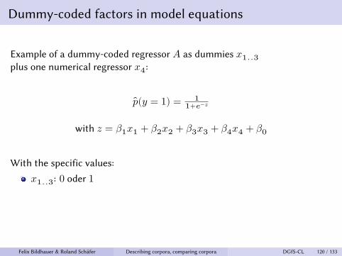
Dummy-coded factors in model equations
Example of a dummy-coded regressor 𝐴 as dummies 𝑥1..3plus one numerical regressor 𝑥4:
𝑝(𝑦 = 1) = 11+𝑒−𝑧
with 𝑧 = 𝛽1𝑥1 + 𝛽2𝑥2 + 𝛽3𝑥3 + 𝛽4𝑥4 + 𝛽0
With the specific values:
𝑥1..3: 0 oder 1
If 𝑥1 = 1 then 𝑥2 = 0 und 𝑥3 = 0 etc.
𝑥4 ∈ IR
Felix Bildhauer & Roland Schäfer Describing corpora, comparing corpora DGfS-CL 120 / 133
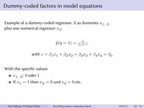
Dummy-coded factors in model equations
Example of a dummy-coded regressor 𝐴 as dummies 𝑥1..3plus one numerical regressor 𝑥4:
𝑝(𝑦 = 1) = 11+𝑒−𝑧
with 𝑧 = 𝛽1𝑥1 + 𝛽2𝑥2 + 𝛽3𝑥3 + 𝛽4𝑥4 + 𝛽0
With the specific values:
𝑥1..3: 0 oder 1If 𝑥1 = 1 then 𝑥2 = 0 und 𝑥3 = 0 etc.
𝑥4 ∈ IR
Felix Bildhauer & Roland Schäfer Describing corpora, comparing corpora DGfS-CL 120 / 133

Dummy-coded factors in model equations
Example of a dummy-coded regressor 𝐴 as dummies 𝑥1..3plus one numerical regressor 𝑥4:
𝑝(𝑦 = 1) = 11+𝑒−𝑧
with 𝑧 = 𝛽1𝑥1 + 𝛽2𝑥2 + 𝛽3𝑥3 + 𝛽4𝑥4 + 𝛽0
With the specific values:
𝑥1..3: 0 oder 1If 𝑥1 = 1 then 𝑥2 = 0 und 𝑥3 = 0 etc.
𝑥4 ∈ IR
Felix Bildhauer & Roland Schäfer Describing corpora, comparing corpora DGfS-CL 120 / 133
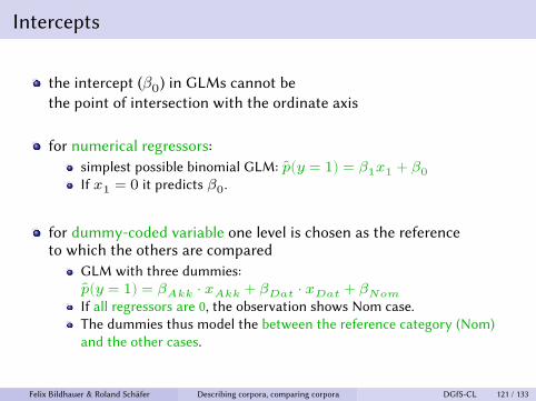
Intercepts
the intercept (𝛽0) in GLMs cannot bethe point of intersection with the ordinate axis
for numerical regressors:simplest possible binomial GLM: ��(𝑦 = 1) = 𝛽1𝑥1 + 𝛽0If 𝑥1 = 0 it predicts 𝛽0.
for dummy-coded variable one level is chosen as the referenceto which the others are compared
GLM with three dummies:��(𝑦 = 1) = 𝛽𝐴𝑘𝑘 ⋅ 𝑥𝐴𝑘𝑘 + 𝛽𝐷𝑎𝑡 ⋅ 𝑥𝐷𝑎𝑡 + 𝛽𝑁𝑜𝑚If all regressors are 0, the observation shows Nom case.The dummies thus model the between the reference category (Nom)and the other cases.
Felix Bildhauer & Roland Schäfer Describing corpora, comparing corpora DGfS-CL 121 / 133

𝜆 and pseudo-𝑅2
𝜆: proportional reduction of the prediction error𝜆 = prediction error without model−prediction error with model
prediction error without model
𝑅2: proportion of variance explained by the regressorsa measure that can (with limitations) be used to compare models
Cox & Snell: 𝑅2𝐶 = 1 − ( 𝐿0
𝐿𝑓) 2
𝑛
Problem: Never reaches 1!
Nagelkerke: 𝑅2𝑁 = 𝑅2
𝐶𝑅2𝑚𝑎𝑥
mit 𝑅2𝑚𝑎𝑥 = 1 − (𝐿0) 2
𝑛
Felix Bildhauer & Roland Schäfer Describing corpora, comparing corpora DGfS-CL 122 / 133
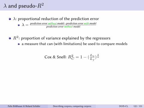
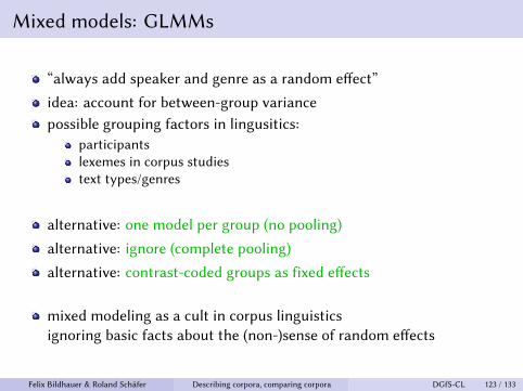
Mixed models: GLMMs
“always add speaker and genre as a random effect”
idea: account for between-group variancepossible grouping factors in lingusitics:
participantslexemes in corpus studiestext types/genres
alternative: one model per group (no pooling)
alternative: ignore (complete pooling)
alternative: contrast-coded groups as fixed effects
mixed modeling as a cult in corpus linguisticsignoring basic facts about the (non-)sense of random effects
Felix Bildhauer & Roland Schäfer Describing corpora, comparing corpora DGfS-CL 123 / 133

Situation for nested random effect
Exemplar Speaker Region
1 Daryl Tyneside2 Daryl Tyneside3 Riley Tyneside4 Riley Tyneside5 Dale Greater London6 Dale Greater London7 Reed Greater London8 Reed Greater London
Table: Illustration of nested factors
Felix Bildhauer & Roland Schäfer Describing corpora, comparing corpora DGfS-CL 124 / 133

Situation for crossed random effects
Exemplar Speaker Mode
1 Daryl Spoken2 Daryl Written3 Riley Spoken4 Riley Spoken5 Dale Written6 Dale Written7 Reed Spoken8 Reed Written
Table: Illustration of crossed factors
Felix Bildhauer & Roland Schäfer Describing corpora, comparing corpora DGfS-CL 125 / 133

Model specification: fixed vs. random
Adding a grouping factor as a fixed effect = dummy coding:
𝑃 𝑟(𝑦𝑖 = 1) = 𝑙𝑜𝑔𝑖𝑡−1(𝛼0 +𝛽𝑑 ⋅𝑥𝑖𝑑 +𝛽𝑙1
⋅𝑥𝑖𝑙1
+𝛽𝑙2⋅𝑥𝑖
𝑙2+⋯+𝛽𝑙𝑚−1
⋅𝑥𝑖𝑙𝑚−1
)(1)
Adding a modeled random effect:
𝑃 (𝑦𝑖 = 1) = 𝑙𝑜𝑔𝑖𝑡−1(𝛼𝑗[𝑖]𝑙 + 𝛽𝑑 ⋅ 𝑥𝑖
𝑑) (2)
𝛼𝑗𝑙 ∼ 𝑁(𝜇𝑙, 𝜎2
𝑙 ) (3)
Felix Bildhauer & Roland Schäfer Describing corpora, comparing corpora DGfS-CL 126 / 133

What are modeled effects, conceptually
nothing very specific
see Gelman & Hill (2006, pp. 245–247)rather a technical question
many levels: modeled effect, few levels: non-modeledfew data points in some levels: modeled effect(shrinkage = partial pooling)testing needed (really?): non-modeled fixed parameter estimatemodeled: conditional means/modes (BLUPs) are predictionstests on predictions: never
An illustrative simulation of:
𝑃(𝑦𝑖 = 1) = 𝑙𝑜𝑔𝑖𝑡−1(𝛼𝑗[𝑖] + 𝛽1 ⋅ 𝑥𝑖1 + 𝛽𝑖
2 ⋅ 𝑥𝑖2) (4)
𝛼𝑗 ∼ 𝑁(𝜇, 𝜎) (5)
Felix Bildhauer & Roland Schäfer Describing corpora, comparing corpora DGfS-CL 127 / 133

Fixed parameter estimates vs. conditional modes I
−5 −4 −3 −2 −1 0
0.0
0.1
0.2
0.3
0.4
0.5
0.6
group0002
mean = −1.69
median = −1.632.5% = −3.2997.25% = −0.4
true = −1.88
−1 0 1 2 3 40.
00.
10.
20.
30.
40.
50.
6
group0003
mean = 1.18
median = 1.132.5% = −0.0297.25% = 2.73
true = 1.27
−4 −3 −2 −1 0 1
0.0
0.1
0.2
0.3
0.4
0.5
0.6
group0004
mean = −1.15
median = −1.092.5% = −2.6197.25% = −0.01
true = −1.25
−1 0 1 2 3 4 5
0.0
0.1
0.2
0.3
0.4
0.5
0.6
group0005
mean = 1.51
median = 1.452.5% = 0.2597.25% = 3.11
true = 1.69
−10 −8 −6 −4 −2 0
0.0
0.1
0.2
0.3
0.4
0.5
group0002
mean = −2.16
median = −2.022.5% = −3.9797.25% = −0.69
true = −1.88
0 5 10 15 20
0.0
0.1
0.2
0.3
0.4
0.5
group0003
mean = 1.54
median = 1.362.5% = 0.0597.25% = 3.43
true = 1.27
−1.5 −0.5 0.0 0.5 1.0 1.5
0.0
0.1
0.2
0.3
0.4
0.5
group0004
mean = −1.4
median = −1.322.5% = −3.0597.25% = −0.09
true = −1.25
0 5 10 15 20
0.0
0.1
0.2
0.3
0.4
0.5
group0005
mean = 2.28
median = 1.82.5% = 0.4497.25% = 5.81
true = 1.69
Figure: LEFT: Group levels in sample GLMM based on predicted random effect (conditionalmode); 5 groups; 20 observations per group; 1,000 simulations; the horizontal line marks thetrue value; RIGHT: Estimated fixed effects for the grouping factor in sample GLM; 5 groups;20 observations per level of the grouping factor; 1,000 simulations; the horizontal line marksthe true value
Felix Bildhauer & Roland Schäfer Describing corpora, comparing corpora DGfS-CL 128 / 133

Pseudo-𝑅2 for these simulations I
0.0 0.2 0.4 0.6 0.8
01
23
45
Nakagawa & Schielzeth's R−squared (GLMM)
Estimates
Den
sity
marginal R−squaredconditional R−squared
0.0 0.2 0.4 0.6 0.8
01
23
4
Nagelkerke's R−squared (GLM)
Estimates
Den
sity
ignore randomrandom as fixed
Figure: LEFT: Distribution of Nakagawa & Schielzeth’s 𝑅2 in the simulations;RIGHT: Nagelkerke’s 𝑅2 in the simulations for a GLM that ignores the groupingfactor and a model that includes it as a fixed effect
Felix Bildhauer & Roland Schäfer Describing corpora, comparing corpora DGfS-CL 129 / 133

Gries
What I call Gries’ Modelling Everything Approach (MEA)is an extremists’ version of multifactorial modelling
Stefan Th. Gries (2015): by default, thou shalt add random effects for:text types,speakers,lemmas,etc.
Stefan Th. Gries (2017): by default, thou shalt model:lengths of words and constituents,information-structural predictors,NP types,animacy,priming/persistency predictors (encoding numerous effectsof words and constructions which occurred before the target item),etc.
Felix Bildhauer & Roland Schäfer Describing corpora, comparing corpora DGfS-CL 130 / 133

Schäfer (2018)
MEA leads to highly complex models
huge amounts of data required
massive annotation work (Stefan Th. Gries, 2017, p. 24)
overparametrisation (Schäfer, 2018)
…means the data don’t support the complex model structure
not a problem of a suboptimal optimiser but a problemof the data and the demands of the model(Bates et al., 2015; Matuschek et al., 2017)
Data dredging leads to spurious “significances”!
Felix Bildhauer & Roland Schäfer Describing corpora, comparing corpora DGfS-CL 131 / 133

Why, oh why?
An exmple (p. c.) from cancer drug development…
target: extend the life expectancy or quality of life
hundreds of factors are known to influence those targets
individual studies look at the effect of one drug
…for which the working mechanism is (ideally) known
other factors?potentially control for age, sex, preconditions…if they have a known effect on the working mechanism of the drug
all other effects: randomisation (Fisher, 1935)
Felix Bildhauer & Roland Schäfer Describing corpora, comparing corpora DGfS-CL 132 / 133

Informed minimal models
Severe modelling (Schäfer, n.d., based on Mayo, 2018)
model only effects relevant to your proposed causal mechanism
use statistical tests with care(Fisherian interpretation or Severe Testing)
don’t do model selection(= tweaking of potentially spurious “significances”)
model or control known relevant nuisance factors
apart from that: randomisation
better: find a significant influential causal factorcontrolling speakers’ bevaiour
worse: try to model everything and work with overparametrisedmodels and muddy inferences (many of them will just be wrong)
Felix Bildhauer & Roland Schäfer Describing corpora, comparing corpora DGfS-CL 133 / 133

References
Ángeles Serrano, M., Ana Maguitman, Marián Boguñá, Santo Fortunato & Alessandro Vespignani. 2007.Decoding the structure of the WWW: a comparative analysis of web crawls. ACM Transactions onthe Web 1(2). Article 10.
Atkins, Sue, Jeremy Clear & Nicholas Ostler. 1992. Corpus design criteria. Literary and LinguisticComputing 7(1). 1–16.
Baroni, Marco, Silvia Bernardini, Adriano Ferraresi & Eros Zanchetta. 2009. The WaCky Wide Web: Acollection of very large linguistically processed web-crawled corpora. Language Resources andEvaluation 43(3). 209–226.
Bates, Douglas, Martin Mächler, Ben Bolker & Steve Walker. 2015. Fitting linear mixed-effects modelsusing lme4. Journal of Statistical Software 67(1). 1–48.
Beißwenger, Michael, Sabine Bartsch, Stefan Evert & Kay-Michael Würzner. 2016. EmpiriST 2015: AShared Task on the Automatic Linguistic Annotation of Computer-Mediated Communication and WebCorpora. Berlin. http://aclanthology.coli.uni-saarland.de/pdf/W/W16/W16-2606.pdf.
Biber, Douglas. 1988. Variation across speech and writing. Cambridge: Cambridge University Press.http://www.loc.gov/catdir/toc/cam023/87038213.html.
Biber, Douglas. 1993. Representativeness in corpus design. Literary and Linguistic Computing 8(4).243–257.
Biber, Douglas & Jesse Egbert. 2015. Using grammatical features for automatic register identification inan unrestricted corpus of documents from the open web. Journal of Research Design and Statistics inLinguistics and Communication Science 2(1). 3–36.
Felix Bildhauer & Roland Schäfer Describing corpora, comparing corpora DGfS-CL 134 / 133

Biemann, Chris, Felix Bildhauer, Stefan Evert, Dirk Goldhahn, Uwe Quasthoff, Roland Schäfer,Johannes Simon, Leonard Swiezinski & Torsten Zesch. 2013. Scalable construction of high-qualityweb corpora. Journal for Language Technology and Computational Linguistics 28(2). 23–60.
Bird, Steven, Ewan Klein & Edward Loper. 2009. Natural language processing with Python. Analyzing textwith the Natural Language Toolkit. O’Reilly.
Blei, David M. 2012. Probabilistic topic models. Communications of the ACM 55(4). 77–84.http://doi.acm.org/10.1145/2133806.2133826.
Blei, David M., Andrew Y. Ng & Michael I. Jordan. 2003. Latent dirichlet allocation. Journal of MachineLearning Research 3. 993–1022.
Broder, Andrei, Ravi Kumar, Farzin Maghoul, Prabhakar Raghavan, Sridhar Rajagopalan, Raymie Stata,Andrew Tomkins & Janet Wiener. 2000. Graph structure in the web. Computer Networks 33. 309–320.
Bubenhofer, Noah, Marek Konopka & Roman Schneider. 2014. Präliminarien einer korpusgrammatik.Vol. 4 (Korpuslinguistik und interdisziplinäre Perspektiven auf Sprache). Unter Mitwirkung vonCaren Brinckmann. Tübingen: Narr.
Ciamarita, Massimiliano & Marco Baroni. 2006. Measuring web-corpus randomness: A progress report.In Marco Baroni & Silvia Bernardini (eds.), Wacky! Working papers on the web as corpus. Bologna:GEDIT.
Damerau, Fred J. 1993. Generating and evaluating domain-oriented multi-word terms from texts.Information Processing & Management 29(4). 433–447.
Felix Bildhauer & Roland Schäfer Describing corpora, comparing corpora DGfS-CL 135 / 133

Deerwester, Scott, Susan T. Dumais, George W. Furnas, Thomas K. Landauer & Richard Harshman. 1990.Indexing by latent semantic analysis. Journal of the American Society of Information Science 41(6).391–407.http://www.cob.unt.edu/itds/faculty/evangelopoulos/dsci5910/LSA_Deerwester1990.pdf.
Denoual, Etienne. 2006. A method to quantify corpus similarity and its application to quantifying thedegree of literality in a document. International Journal of Technology and Human Interaction 2(1).51–66.
Edmundson, H. P. & R. E. Wyllys. 1961. Automatic abstracting and indexing. survey andrecommendations. Communications of the ACM 4(5). 226–234.
Fisher, Ronald A. 1935. The design of experiments. London: Macmillan.
Frank, Eibe, Mark A. Hall & Ian H. Witten. 2016. The WEKA Workbench. Online Appendix for ”DataMining: Practical Machine Learning Tools and Techniques”, Morgan Kaufmann, Fourth Edition.
Freund, Luanne, Charles L. A. Clarke & Elaine G. Toms. 2006. Towards genre classification for ir in theworkplace. In Proceedings of the 1st international conference on information interaction in context(IIiX), 30–36. Copenhagen, Denmark: ACM. http://doi.acm.org/10.1145/1164820.1164829.
Gelman, Andrew & Jennifer Hill. 2006. Data analysis using regression and multilevel/hierarchical models.Cambridge: Cambridge University Press.
Geyken, Alexander. 2007. The DWDS corpus: a reference corpus for the German language of the 20thcentury. In Christiane Fellbaum (ed.), Collocations and idioms: Linguistic, lexicographic, andcomputational aspects, 23–41. London: Continuum Press.
Gries, Stefan. 2006. Exploring variability within and between corpora: some methodologicalconsiderations. Corpora 1. 109–151.
Felix Bildhauer & Roland Schäfer Describing corpora, comparing corpora DGfS-CL 136 / 133

Gries, Stefan Th. 2015. The most underused statistical method in corpus linguistics: multi-level (andmixed-effects) models. Corpora 10(1). 95–126.
Gries, Stefan Th. 2017. Syntactic alternation research. taking stock and some suggestions for the future.In Ludovic De Cuypere, Clara Vanderschueren & Gert De Sutter (eds.), Current trends in analyzingsyntactic variation, vol. 31 (Belgian Journal of Lingustics), 7–27. Amsterdam: Benjamins.
Hofland, Knut & Stig Johansson. 1982. Word frequencies in British and American English. Bergen: TheNorwegian Computiing Cente for the Humanities.
Hofmann, Thomas. 1999. Probabilistic latent semantic analysis. In Proceedings of the fifteenth conferenceon uncertainty in artificial intelligence (UAI’99), 289–296. Stockholm, Sweden: Morgan KaufmannPublishers Inc. http://dl.acm.org/citation.cfm?id=2073796.2073829.
Kanaris, Ioannis & Efstathios Stamatatos. 2009. Learning to recognize webpage genres. InformationProcessing and Management 45(5). 499–512.
Karlgren, Jussi & Douglass Cutting. 1994. Recognizing text genres with simple metrics usingdiscriminant analysis. In Proceedings of coling 94, 1071–1075.
Kessler, Brett, Geoffrey Nunberg & Hinrich Schütze. 1997. Automatic detection of text genre. InProceedings of the 35th annual meeting of the association for computational linguistics and eighthconference of the european chapter of the association for computational linguistics (ACL ’98), 32–38.Madrid, Spain: Association for Computational Linguistics.http://dx.doi.org/10.3115/976909.979622.
Kilgarriff, Adam. 2001. Comparing corpora. International Journal of Corpus Linguistics 6(1). 97–133.
Felix Bildhauer & Roland Schäfer Describing corpora, comparing corpora DGfS-CL 137 / 133

Kilgarriff, Adam. 2012. Getting to know your corpus. In Petr Sojka, Aleŝ Horák, Ivan Kopeĉek &Karel Pala (eds.), Text, speech and dialogue - 15th international conference, tsd 2012, brno, czechrepublic, september 3-7, 2012. proceedings, 3–15. Heidelberg: Springer.
Kupietz, Marc, Cyril Belica, Holger Keibel & Andreas Witt. 2010. The German reference corpus DeReKo:a primordial sample for linguistic research. In Nicoletta Calzolari, Khalid Choukri, Bente Maegaard,Joseph Mariani, Jan Odijk, Stelios Piperidis, Mike Rosner & Daniel Tapias (eds.), Proceedings of theseventh international conference on language resources and evaluation (LREC ’10), 1848–1854. Valletta,Malta: European Language Resources Association (ELRA).
Lee, Yong-Bae & Sung Hyon Myaeng. 2002. Text genre classification with genre-revealing andsubject-revealing features. In Proceedings of the 25th annual international acm sigir conference onresearch and development in information retrieval (SIGIR ’02), 145–150. Tampere, Finland: ACM.http://doi.acm.org/10.1145/564376.564403.
Manning, Christopher D., Prabhakar Raghavan & Hinrich Schütze. 2009. An introduction to informationretrieval. Cambridge: cup.
Matuschek, Hannes, Reinhold Kliegl, Shravan Vasishth, Harald Baayen & Douglas M. Bates. 2017.Balancing type I error and power in linear mixed models. Journal of Memory and Language 94.305–315.
Mayo, Deborah G. 2018. Statistical inference as severe testing: how to get beyond the statistics wars.Cambridge: Cambridge University Press.
Mehler, Alexander, Serge Sharoff & Marina Santini (eds.). 2010. Genres on the web: computational modelsand empirical studies. Vol. 42 (Text, speech and language technology). New York: Springer.
Felix Bildhauer & Roland Schäfer Describing corpora, comparing corpora DGfS-CL 138 / 133

Schäfer, Roland. 2016. On bias-free crawling and representative web corpora. In Proceedings of the 10thweb as corpus workshop, 99–105. Berlin: Association for Computational Linguistics.http://aclweb.org/anthology/W16-2612.
Schäfer, Roland. 2018. Probabilistic German morphosyntax. Humboldt Universität zu Berlin Habilitationthesis. http://rolandschaefer.net/?p=1410.
Schäfer, Roland. accept with revisions September 2017. Competing constructions for German measurenoun phrases: from usage data to experiment. Cognitive Linguistics.
Schäfer, Roland. N.d. Statistische Inferenz in der Linguistik. in preparation.
Schäfer, Roland & Felix Bildhauer. 2012. Building large corpora from the web using a new efficient toolchain. In Nicoletta Calzolari, Khalid Choukri, Thierry Declerck, Mehmet Ugur Dogan,Bente Maegaard, Joseph Mariani, Jan Odijk & Stelios Piperidis (eds.), Proceedings of the EighthInternational Conference on Language Resources and Evaluation (LREC’12), 486–493. Istanbul: ELRA.
Scott, Mike. 1997. PC analysis of key words - and key key words. System 25(2). 233–245.
Scott, Mike. 2001. Comparing corpora and identifying keywords, collocations, frequency distributionsthrough the WordSmith Tools suite of computer programs. In Mohsen Ghadessy, Alex Henry &Robert L. Roseberry (eds.), Small corpus studies and ELT, 47–67. Amsterdam & Philadelphia:Benjamins.
Sebastiani, Fabrizio. 2005. Text categorization. In Jorge H. Doorn Laura C. Rivero & VivianaE. Ferraggine (eds.), The encyclopedia of database technologies and applications, 683–687. Hershey, US:dea Group Publishing.
Sharoff, Serge. 2006. Creating general-purpose corpora using automated search engine queries. InMarco Baroni & Silvia Bernardini (eds.), Wacky! working papers on the web as corpus. Bologna: GEDIT.
Felix Bildhauer & Roland Schäfer Describing corpora, comparing corpora DGfS-CL 139 / 133

Sinclair, John. 1996. Preliminary recommendations on corpus typology. Tech. rep. EAG–TCWG–CTYP/P.Expert Advisory Group on Language Engineering Standards document.
Spärck Jones, Karen. 1972. A statistical interpretation of term specificity and its application in retrieval.Journal of Documentatio 28(1). 11–21.
Teich, Elke & Peter Fankhauser. 2009. Exploring a corpus of scientific texts using data mining. Languageand Computers 71. 233–247.
Yule, G. Udny. 1944. The statistical study of literary vocabulary. Cambridge: Cambridge University Press.
Felix Bildhauer & Roland Schäfer Describing corpora, comparing corpora DGfS-CL 140 / 133