Common Crawled web corpora - DUO (uio.no)
103
Common Crawled web corpora Constructing corpora from large amounts of web data Kjetil Bugge Kristoffersen Thesis submitted for the degree of Master in Informatics: Programming and Networks (Language Technology group) 60 credits Department of Informatics Faculty of mathematics and natural sciences UNIVERSITY OF OSLO Spring 2017
-
Upload
khangminh22 -
Category
Documents
-
view
0 -
download
0
Transcript of Common Crawled web corpora - DUO (uio.no)

Common Crawled web corpora
Constructing corpora from large amounts ofweb data
Kjetil Bugge Kristoffersen
Thesis submitted for the degree ofMaster in Informatics: Programming and Networks
(Language Technology group)60 credits
Department of InformaticsFaculty of mathematics and natural sciences
UNIVERSITY OF OSLO
Spring 2017

Common Crawled web corpora
Constructing corpora from large amounts of webdata
Kjetil Bugge Kristoffersen

© 2017 Kjetil Bugge Kristoffersen
Common Crawled web corpora
http://www.duo.uio.no/
Printed: Reprosentralen UiO
Abstract
Efforts to use web data as corpora seek to provide solutions to problems traditionalcorpora suffer from, by taking advantage of the web’s huge size and diversetype of content. This thesis will discuss the several sub-tasks that make upthe web corpus construction process – like HTML markup removal, languageidentification, boilerplate removal, duplication detection, etc. Additionally, byusing data provided by the Common Crawl Foundation, I develop a new very largeEnglish corpus with more than 135 billion tokens. Finally, I evaluate the corpusby training word embeddings and show that the trained model largely outperformsmodels trained on other corpora in a word analogy and word similarity task.


Acknowledgements
I would like to thank my supervisors Stephan Oepen and Erik Velldal. From thefeedback and editing, to taking hours from a busy afternoon to assist me when Iwas stuck – this thesis would not have been without their guidance.
Thanks to Helene Holter and Henrik Hillestad Løvold, who have made the lastyear a year of more breaks and coffee than I originally thought was either cleveror healthy, respectively. Every day was a bit brighter because of you.
Additionally, I would like to extend my gratitude to the developers and creators ofthe tools and datasets that were used in this thesis, and for making them availableopen source.
To the largest sponsor of this work and the work leading up to it, without whommy education would not be possible, a large thank you to the Norwegian welfarestate and its policy of free education for all.
Finally, to my girlfriend Ane Granli Kallset: Thank you for your support andunderstanding, for your love and cups of tea, and for urging me to join late nightsout and birthday parties on days when I thought there was no time for such. I loveyou.


Contents
Contents iv
List of Tables vii
List of Figures ix
1 Introduction 1
2 Background 52.1 Text corpora . . . . . . . . . . . . . . . . . . . . . . . . . . . . . . . . 5
2.1.1 Usage of corpora . . . . . . . . . . . . . . . . . . . . . . . . 52.1.2 Towards larger corpora . . . . . . . . . . . . . . . . . . . . . 6
2.2 Web corpora . . . . . . . . . . . . . . . . . . . . . . . . . . . . . . . 72.2.1 The beginning of the web as corpus . . . . . . . . . . . . . 72.2.2 Hit counts are not a traditional corpus . . . . . . . . . . . . 72.2.3 Constructing large corpora from the web . . . . . . . . . . . 8
2.3 Techniques and tasks . . . . . . . . . . . . . . . . . . . . . . . . . . . 102.3.1 Data collection . . . . . . . . . . . . . . . . . . . . . . . . . 112.3.2 Cleaning the data . . . . . . . . . . . . . . . . . . . . . . . . 142.3.3 Metadata and annotation . . . . . . . . . . . . . . . . . . . . 21
2.4 Evaluating web corpora . . . . . . . . . . . . . . . . . . . . . . . . . 212.4.1 Statistical quality metrics . . . . . . . . . . . . . . . . . . . 222.4.2 Do web corpora represent languages as well as traditional
corpora? . . . . . . . . . . . . . . . . . . . . . . . . . . . . . 222.5 The goal of this project . . . . . . . . . . . . . . . . . . . . . . . . . 25
2.5.1 High-quality connected text extraction from the CommonCrawl . . . . . . . . . . . . . . . . . . . . . . . . . . . . . . . 25
2.5.2 Concurrent work . . . . . . . . . . . . . . . . . . . . . . . . 25
3 Exploring the Common Crawl 273.1 The data . . . . . . . . . . . . . . . . . . . . . . . . . . . . . . . . . . 27
3.1.1 A note on scale . . . . . . . . . . . . . . . . . . . . . . . . . 293.1.2 Retrieving the data . . . . . . . . . . . . . . . . . . . . . . . 30
3.2 Getting my feet WET . . . . . . . . . . . . . . . . . . . . . . . . . . 313.2.1 A preliminary inspection . . . . . . . . . . . . . . . . . . . . 32
v
CONTENTS
3.2.2 WET vs. cleaned WARC . . . . . . . . . . . . . . . . . . . . 323.2.3 Where do the documents go? . . . . . . . . . . . . . . . . . 353.2.4 Language distribution . . . . . . . . . . . . . . . . . . . . . 363.2.5 What now? . . . . . . . . . . . . . . . . . . . . . . . . . . . . 36
4 Text extraction from the Common Crawl 394.1 Choosing a tool for the job . . . . . . . . . . . . . . . . . . . . . . . 39
4.1.1 Desiderata . . . . . . . . . . . . . . . . . . . . . . . . . . . . 394.1.2 texrex: An overview . . . . . . . . . . . . . . . . . . . . . . 41
4.2 texrex with the Common Crawl on a SLURM cluster . . . . . . . . 464.2.1 Running the texrex tool . . . . . . . . . . . . . . . . . . . . 464.2.2 A tender deduplication . . . . . . . . . . . . . . . . . . . . . 504.2.3 tecl-ing the near-duplicated documents . . . . . . . . . . . . 534.2.4 HyDRA and rofl . . . . . . . . . . . . . . . . . . . . . . . . . 534.2.5 xml2txt . . . . . . . . . . . . . . . . . . . . . . . . . . . . . . 544.2.6 Tokenisation and conversion to CoNLL . . . . . . . . . . . 55
4.3 Presenting enC3: the English CommonCrawl Corpus . . . . . . . . 564.3.1 XML . . . . . . . . . . . . . . . . . . . . . . . . . . . . . . . 564.3.2 Text . . . . . . . . . . . . . . . . . . . . . . . . . . . . . . . . 574.3.3 CoNLL . . . . . . . . . . . . . . . . . . . . . . . . . . . . . . 574.3.4 enC³ . . . . . . . . . . . . . . . . . . . . . . . . . . . . . . . 57
5 Evaluating the English Common Crawl Corpus 595.1 Inspection vs. downstream task experiments . . . . . . . . . . . . . 60
5.1.1 Intrinsic evaluation . . . . . . . . . . . . . . . . . . . . . . . 605.1.2 Extrinsic evaluation . . . . . . . . . . . . . . . . . . . . . . . 615.1.3 How to evaluate the English Common Crawl Corpus . . . . 61
5.2 Embedded word vectors in low-dimensional spaces . . . . . . . . . 625.2.1 Explicit word representations . . . . . . . . . . . . . . . . . 625.2.2 Word embeddings . . . . . . . . . . . . . . . . . . . . . . . . 635.2.3 Evaluation of word vectors . . . . . . . . . . . . . . . . . . . 66
5.3 Training and evaluating word embeddings with enC³ data . . . . . 685.3.1 Training word vectors using GloVe . . . . . . . . . . . . . . 685.3.2 Evaluation of the word embeddings . . . . . . . . . . . . . 705.3.3 Better intrinsic results: A better corpus? . . . . . . . . . . . 76
6 Conclusion and future work 796.1 Future work . . . . . . . . . . . . . . . . . . . . . . . . . . . . . . . . 81
6.1.1 Replicating the process . . . . . . . . . . . . . . . . . . . . . 816.1.2 Researching the impact of boilerplate . . . . . . . . . . . . 816.1.3 Investigating overlap between monthly crawls . . . . . . . 826.1.4 noC³? . . . . . . . . . . . . . . . . . . . . . . . . . . . . . . . 826.1.5 Evaluation with more tasks . . . . . . . . . . . . . . . . . . 82
Bibliography 85
vi
List of Tables
2.1 Boilerplate classification techniques evaluated using CleanEval . . 18
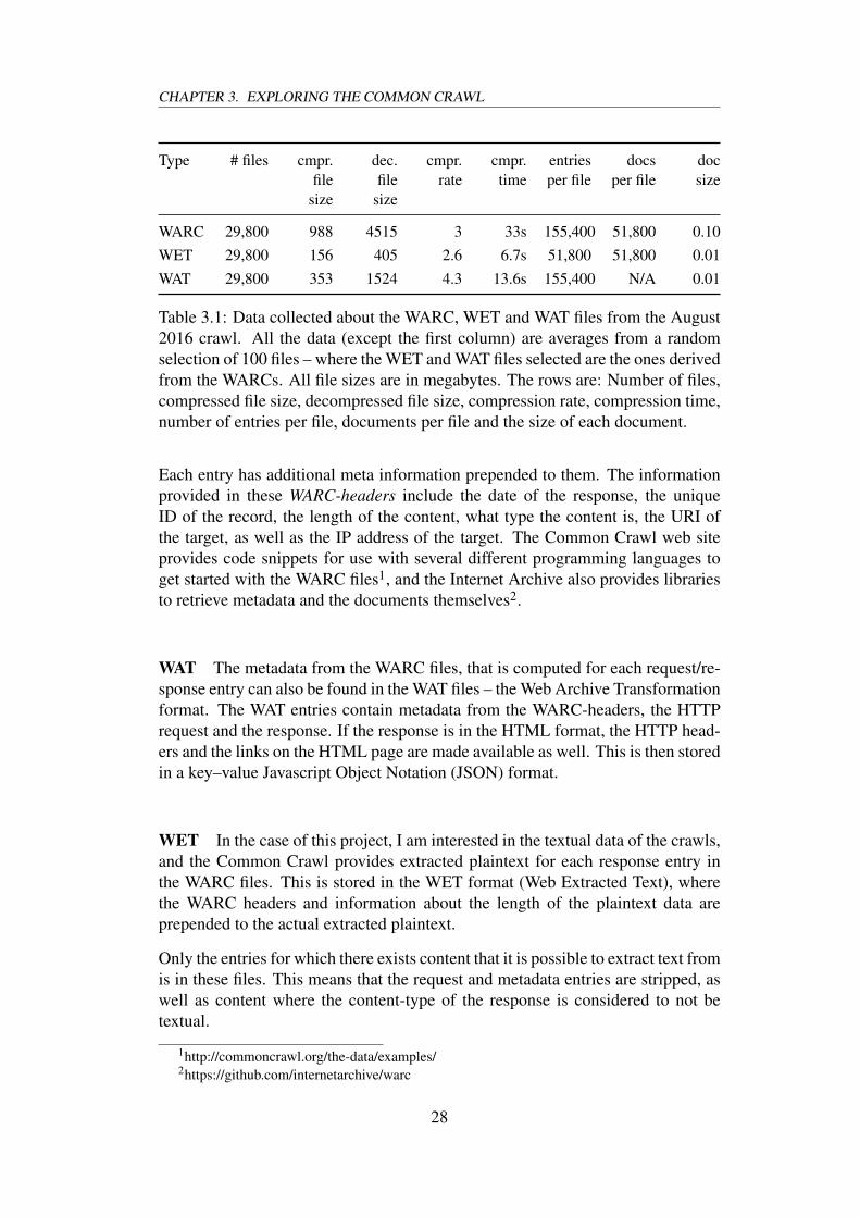
3.1 Data collected about the WARC, WET and WAT files from theAugust 2016 crawl. All the data (except the first column) areaverages from a random selection of 100 files – where the WETand WAT files selected are the ones derived from the WARCs.All file sizes are in megabytes. The rows are: Number of files,compressed file size, decompressed file size, compression rate,compression time, number of entries per file, documents per fileand the size of each document. . . . . . . . . . . . . . . . . . . . . . 28
3.2 The time required for performing different operations on theAugust 2016 Common Crawl . . . . . . . . . . . . . . . . . . . . . . 29
3.3 The speedup and efficiency of the download using a differentnumber of processors . . . . . . . . . . . . . . . . . . . . . . . . . . 31
3.4 The remaining HTML tags of the different corpora. From the left:The number of tags remaining, the number of documents that hadremaining tags, the percentage of documents that had remainingtags and how many tags there were per document . . . . . . . . . . 33
3.5 The remaining HTML entities of the different corpora. From theleft: The number of entities remaining, the number of documentsthat had remaining entities, the percentage of documents that hadremaining entities and how many entities there were per document 33
3.6 Top five frequent entities in the texrex corpus . . . . . . . . . . . . . 343.7 Number of documents with encoding errors . . . . . . . . . . . . . 343.8 Number of tokens in the corpora . . . . . . . . . . . . . . . . . . . . 343.9 The percentage of documents removed per processing step from
the total number of initial documents. Language detection was notperformed for the experiment, but is left in the table for illustration. 35
3.10 Distribution of language in the different corpora, as percentage oftotal number of characters . . . . . . . . . . . . . . . . . . . . . . . . 36
4.1 A breakdown of how I ended up setting up the jobs for thedifferent processes . . . . . . . . . . . . . . . . . . . . . . . . . . . . 50
4.2 Randomly selected rofl changes manually assessed to either beuser-generated, correctly changed or incorrectly changed . . . . . . 54
vii

LIST OF TABLES
4.3 Structure of the corpus files. The raw text also come with as manymeta files using about 5GB of space. . . . . . . . . . . . . . . . . . . 56
4.4 Some corpus statistics from selected large corpora. t: tokens, d:documents, s: sentences. All absolute numbers are in millions.Relative numbers (e.g. tokens per document) are as they are. . . . . 58
5.1 Co-occurrence probabilities for target words ice and steam. Largeprobability ratios correlate well with properties specific to ice,while very small ratios correlate well with properties specific tosteam (ice is solid, steam is a gas). Words that both target wordsrelate to equally is about 1. . . . . . . . . . . . . . . . . . . . . . . . 65
5.2 The parameters chosen for the co-occurrence counting and thetraining of the word vectors. The window size represents thenumber of context words to the left and to the right. η is the initiallearning rate, α represents the exponent in the weighting functionused in the cost function of the least squares problem and xmaxrepresents the cutoff in the same weighting function. . . . . . . . . 69
5.3 How the different processes were set up. . . . . . . . . . . . . . . . 705.4 The results of the analogy task, broken down to semantic and
syntactic parts . . . . . . . . . . . . . . . . . . . . . . . . . . . . . . . 725.5 The results of the word similarity task with vector normalisation
so that each vector has length 1 . . . . . . . . . . . . . . . . . . . . . 735.6 The results of the word similarity task where each feature is
normalised across the vocabulary. . . . . . . . . . . . . . . . . . . . 73
viii

List of Figures
2.1 An excerpt of the Wikipedia page “List of lists of lists”, which isan example of an unwanted document for corpus purposes . . . . . 15
2.2 Example of how assessing corpus statistics enables comparingcorpora and disovering signs of flaws . . . . . . . . . . . . . . . . . 23
3.1 The execution time of downloading the same 150 gzipped WARCfiles per number of processes. (Note that this was done on a CPUwith 16 cores) . . . . . . . . . . . . . . . . . . . . . . . . . . . . . . . 31
3.2 An example extract from what should have been extracted textwithout HTML remaining from a WET file of the Common Crawl 37
4.1 The flow of texrex, showing the output of texrex entered as inputto later tools . . . . . . . . . . . . . . . . . . . . . . . . . . . . . . . . 42
4.2 An example extract of a document produced by texrex . . . . . . . 444.3 How texrex was run – each texrex process got 3–4 WARC files as
input . . . . . . . . . . . . . . . . . . . . . . . . . . . . . . . . . . . . 494.4 The abandoned idea of merging tender processes until ending up
with one . . . . . . . . . . . . . . . . . . . . . . . . . . . . . . . . . . 514.5 The tender setup: tender jobs produce blacklists, which goes into
a final tender together with the shingles . . . . . . . . . . . . . . . . 524.6 The tecl setup – corpus files and blacklists go into tecl and result
in merged corpus files . . . . . . . . . . . . . . . . . . . . . . . . . . 53
5.1 The vector representation of selected words from s1 to s4 with‘band’ and ‘play’ as axes . . . . . . . . . . . . . . . . . . . . . . . . 63
5.2 The difference between the skip-gram and the CBOW models.The CBOW model takes surrounding words as input, and tries topredict the word in the middle, while the skip-gram model takes asingle word as input to predict the surrounding words. . . . . . . . 65
5.3 The vector differences encode the syntactic relationship betweenconjugated verbs . . . . . . . . . . . . . . . . . . . . . . . . . . . . . 67
ix


Chapter 1
Introduction
A corpus is a collection of texts, and is used for a multitude of tasks in NaturalLanguage Processing, and also by other users such as lexicographers. Corpora areoften used statistically to be able to say something about the corpus, or even thelanguage, by for instance using them for creating language models or by providingthem as data for unsupervised machine learning tasks to represent words as low-dimensional vectors. The construction of corpora that strike a balance of sizeand ‘quality’ (see below) is a methodological and engineering challenge that hasreceived much attention for the past several decades and still today.
The World Wide Web contains vast amounts of text, and therefore offers thepossibility to create large and possibly high-quality text collections. The dataretrieved from the web are different types of documents – often HTML documents– that need to be refined or cleaned before they can be used. There are severalsub-tasks with varying degrees of complexity and scalability that are part of thisdata refinement, like for instance removing markup and extracting text, removingduplication, and removing so-called boilerplate (see below).
The latter task is an example of the complexity that is in large part idiosyncraticto the construction of corpora based on web data. In addition to a web page’smain text content, there will often exist elements that are to varying degreesdifficult to assess the relevancy of. Elements like navigational menus, timestamps,advertisements, button labels, etc. will intuitively introduce more noise (thanlinguistically relevant content) if added to a corpus. Too much of this noisy datacould affect the models created from such a corpus negatively. Identifying what isrelevant content and what is not is challenging enough for humans, and even moredifficult for computers.
Another challenging aspect of constructing large corpora from the web is the scaleof the data. For example, my project takes as its point of departure snapshots ofweb content distributed by the Common Crawl Foundation (see below), and justreading through all files of one such snapshot sequentially, without any actualprocessing of the data, takes about 18 hours, which is not a time-consuming
1
CHAPTER 1. INTRODUCTION
task relative to the ones required to refine the data. Therefore, to construct largecorpora on such a scale, parallel computing is required.
The Common Crawl Foundation is a non-profit organisation that provide monthlycrawls of the web for free. This thesis use one of these monthly crawls toconstruct a very large web corpus – enC³, or the English Common Crawl Corpus– consisting of over 135 billion tokens. To my knowledge, the constructed corpusis the largest web corpus described or available, with the next largest, enClueWeb(Pomikálek, Jakubícek, and Rychlý, 2012), consisting of 82 billion tokens. Thecorpus is then evaluated by training low-dimensional word vectors, evaluatingthose, and comparing the results to word vectors trained on other corpora.
The results of the thesis are concrete contributions to the NLP community: Alarge corpus constructed from web data, as well as the word vectors trained on thecorpus using the GloVe model (Pennington, Socher, and Manning, 2014). Bothof these resources are made available through the community repository launchedby Fares, Kutuzov, Oepen, and Velldal (2017). Additionally, I provide an in-depthassessment of the Common Crawl, including a critical assessment of its text-onlyversions. Also, the corpus construction process is documented thoroughly, toencourage and lower the bar for replication. Finally, the tools made to analyseand process the data are made publicly available1.
The structure of the thesis is as follows:
In chapter 2, desiderata for corpus construction are reviewed from various anglesand ‘traditional’ approaches are contrasted with web-based ones. Additionally,the development of the web corpus construction task and its subtasks is described.Finally, the chapter presents an overview of previous work in the field, and howweb corpora have been evaluated.
Chapter 3 provides a systematic review of what the Common Crawl contains,and especially of the extracted text-only files that are already provided by theCommon Crawl. It further compares a selection of these extracted text files to thecorresponding raw web data, refined by the process described in chapter 4.
Chapter 4 discusses the requirements for the process of corpus construction,and I review a selection of candidate tools and pick one. The chosen pipelineis described, together with the process of configuring and scaling up the toolsto be able to process large quantities of data in an acceptable amount of time.Additionally, the post-processing steps of extracting raw non-boilerplate text fromthe final corpus and tokenising and sentence segmenting said text is discussed.Finally, the constructed corpus is presented in its three representations: XML,text and a popular, de-facto standard corpus format for NLP – CoNLL.
Chapter 5 discusses how the constructed corpus can be evaluated, and evaluatesthe corpus by training dense low-dimensional word vectors – so-called word
1https://github.com/kjetilbk/enc3tools
2

embeddings – using the corpus as input. These word embeddings are thenevaluated using a word analogy task and word similarity tasks. The results arecompared to the results of word vectors trained on two other corpora, one based onWikipedia and news text and the other on web data. Finally, the corpus constructedin this thesis is shown to outperform the two others in the analogy task, and in amajority of the word similarity tasks.
Chapter 6 concludes and sums up the thesis, and discusses future work related tothe thesis.
3

Chapter 2
Background
To understand the motivation behind the project, one has to understand whyand how text corpora are used, especially within the fields of natural languageprocessing (NLP) and corpus linguistics.
2.1 Text corpora
There are differences in opinion as to what constitutes a corpus. Kilgarriff andGrefenstette (2003) describe two of these opinions. One is presented by McEneryand Wilson (2001), and states that while a corpus in principle can be as simple as“any body of text”, they believe there to be more inherent meaning to the wordthan that, and that qualities such as representativeness and machine-readabilityplay a part in whether the collection of texts is a corpus or not.
Kilgarriff and Grefenstette (2003, p. 2) state:
McEnery and Wilson (2001) mix the question “what is a corpus?”with “what is a good corpus (for certain kinds of linguistic study)”,muddying the simple question “is corpus x good for task y?” with thesemantic question, “is x a corpus at all?”
While I will discuss representativeness and other qualities of corpora whenexamining how one evaluates constructed corpora in section 2.4, I will, likeKilgarriff and Grefenstette (2003) simply consider a corpus “a collection oftexts”.
2.1.1 Usage of corpora
Generally, corpora are often analysed using computers to obtain knowledge aboutlanguage. Specifically, one often uses statistical measures counted from the
5

CHAPTER 2. BACKGROUND
corpus, like for instance how often tokens (words) occur and which tokens theyoccur next to. From these measures, you can for instance create language models,where you can tell the probability of a phrase based on the corpus, you cando statistical machine translation (where computers read corpora with the sametexts, but in different languages (parallel corpora)) to learn how to translate textsautomatically, etc.
In the past few years, neural networks have become increasingly popular asmachine-learning models to solve a multitude of NLP tasks (Goldberg, 2015;Collobert et al., 2011). These networks often require dense vectors as input.Hence, the use of corpora as unlabeled data in unsupervised learning to representwords as dense vectors has been increasing (Collobert and Weston, 2008;Mikolov, Chen, Corrado, and Dean, 2013; Pennington et al., 2014, and section5.2).
Other users of corpora include lexicographers, the people who write dictionaries.To be able to provide explanations for what words mean and how they worktogether to form sentences, lexicographers use corpora to extract said information.This can be so-called concordances – extracts of a specific word being used in acorpus, together with its immediate context – or collocations, words that have atendency to go together based on the corpus.
Often, the goal of these tasks is to be able to say something about thecorpus, or even try to say something about the language in general. This is achallenge, as corpora are collections of real-world text – a subset of the language.Consequently, they do not contain every single word or word sequence of alanguage, nor do they have the same relative token frequency as the languageas a whole. Because of this, rare word sequences in the language might not showup even once in the corpus. A word sequence that does not show up once in thecorpus is impossible to separate from word sequences that are not actual words inthe language.
2.1.2 Towards larger corpora
Due to the inherent productivity of language, it is impossible to see every‘language event’, no matter the size of the corpus. However, a larger amount oftokens would increase the likelihood of rarer words showing up in the corpus, thusincreasing the amount of non-zero counts, and counteracting the problem of datasparsity. Furthermore, a larger amount of tokens means having a larger sampleof the population, which will possibly bring more precise statistics. Banko andBrill (2001) explore the performance of a number of machine learning algorithmswhen increasing the data size, and make the argument that getting more data forthe machine-learning algorithms will make more of a difference than fine-tuningthe algorithms.
While having more data might not bring better results in all cases, it is a clear
6

2.2. WEB CORPORA
motivation for having larger corpora. Unsupervised machine learning tasks thatdoes not require labeled data will especially be able to benefit directly fromincreased corpus sizes.
Over the years, manually constructed corpora have been increasing in size. Fromthe one million word Brown corpus in the 1960s, the COBUILD project had eightmillion words in the 1980s, and in 1995 the British National Corpus was releasedwith 100 million words.
A seemingly obvious candidate for a very large collection of textual content is theworld wide web, due to its vast size.
2.2 Web corpora
2.2.1 The beginning of the web as corpus
Because the web has so much data, and because so much of it is textual, therehave been increasing efforts to use web data as a corpus. Early efforts retrievedboth token and phrase frequencies from querying commercial search engines,while others gathered and grouped a lot of ‘relevant’ documents. Early worksof using search engine hit counts are, for example, the usage for word sensedisambiguation (Mihalcea and Moldovan, 1999), or (probably most cited) forobtaining frequencies of bigrams that were unseen in a given corpus (Kellerand Lapata, 2003). Using one document as a search query, Jones and Ghani(2000) grouped the resulting documents together to create a corpus in the inputdocument’s language. Parallel corpora have been created by grouping documentson the web that were equal, but in different languages – like the same manualtranslated to both the target languages, or a web site offering two identicalversions but with different languages depending on the top-level domain (Resnik,1999).
2.2.2 Hit counts are not a traditional corpus
While using the web in this way to solve NLP problems is a way of using the webas a corpus, these uses are different from using a traditional corpus. Hit countsfor words and phrases from commercial search engines, like mentioned above,have been shown to give desired results for some tasks, but this technique is alot more difficult and time-consuming to use than a regular corpus (Bernardini,Baroni, and Evert, 2006). Additionally, search engine hit counts do not give youas much information as using a traditional corpus does, as the search engines donot part-of-speech-tag or give you the context of the hits. Also, the frequenciesyou receive are (approximations of) the number of documents the words are in,and not the number of word occurences (Kilgarriff, 2007). The Google N-gram
7

CHAPTER 2. BACKGROUND
corpus makes searchable N-grams (albeit only up to n = 5) frequencies available,and began providing part-of-speech tags from January 2016. However, the corpusstill has the same drawbacks with respect to lack of context that other hit countbased methods suffer from.
2.2.3 Constructing large corpora from the web
Work in the field of constructing very large collections of texts from the web,formatted and used like traditional corpora, cannot be attributed to one group orperson, but was described as early as by Kilgarriff and Grefenstette (2003). Theearly descriptions were concretised when Baroni and Bernardini (2004) createdthe BootCaT toolkit, a software collection constructing a specialised web corpusbased on user-input search terms.
WaCky (Web as Corpus kool ynitiative) continued this work in 2005, andtried to identify and discuss the subtasks that went into the task of webcorpus construction. This coincided with the beginning of the yearly Webas Corpus workshops, organised by The Special Interest Group on Web asCorpus (SIGWAC) of the Association for Computational Linguistics (ACL).These workshops, among a few others, have since been progressing the researchon constructing a traditional-like corpus from the web.
Below I will give a summary of some efforts and tools that have tried to solvethis task. The detailed differences in their approaches to the sub-tasks will bediscussed in section 2.3.
BootCaT
The BootCaT toolkit is made up of multiple Perl programs, where the output ofone can be fed into the next, making up a suite that can create a corpus from a setof search terms. Baroni and Bernardini (2004, p. 1) wrote:
The basic idea is very simple: Build a corpus by automaticallysearching Google for a small set of seed terms; extract new (single-word) terms from this corpus; use the latter to build a new corpus viaa new set of automated Google queries; extract new terms/seeds fromthis corpus and so forth. The final corpus and unigram term list arethen used to build a list of multi-word terms. These are sequencesof words that must satisfy a set of constraints on their structure,frequency and distribution.
8

2.2. WEB CORPORA
WaCky
From the article where WaCky is introduced, they introduce several subtasks thatthey describe as the basic steps to construct a web corpus (Bernardini et al.,2006):
1. Selecting seed URLs
2. Crawling
3. Cleaning the data
4. Annotating the data
These subtasks are still essential parts of constructing web corpora today, withsome additional subtasks being introduced. The tools and techniques used tosolve them, however, have been where most of the discussion, innovation anddevelopment has occurred. In-depth discussion of all subtasks, both original andnew, will be done in section 2.3.
WaCky was a continuation of the BootCaT effort, and a number of the corporabuilt within the early WaCky paradigm used BootCaT for several of the subtasks.As WaCky has been a continuous project with a goal of advancing the field ofweb corpora for several years, there are differences between corpora constructedwithin the paradigm, especially between the earliest and the latest.
WaCky and its toolset(s) have been used to create several web corpora, like the2 billion word ukWaC, itWaC (2.6 billion words), frWaC (1.6 billion words),deWaC (1.7 billion words) and noWaC (700 million words). Compared totraditional corpora, like the British National Corpus, with 100 million words, theseare quite large corpora.
SpiderLing
Where WaCky introduced and discussed individual subtasks to achieve theconstruction of web corpora, Suchomel and Pomikálek (2012) created theSpiderLing toolset which does several of the tasks at the same time (likedoing language identification while crawling), all pipelined within the sametoolset.
The methods of SpiderLing diverge from WaCky’s school of thought pertainingto some of the subtasks. Specifically, the crawling is done differently and with adifferent focus, where a larger effort to make the crawling efficient (not needing todownload as much data, while still not losing much of the final corpus data – seesection 2.3.1) is made. The data cleaning sub-tasks – boilerplate and duplicationremoval – are different as well.
9
CHAPTER 2. BACKGROUND
COW
Schäfer and Bildhauer (2012)’s Corpora from the Web (COW) follows the WaCkyinitiative’s subtasks, but aims to make “incremental improvements” on WaCky’smethods and solutions. The result is the texrex tool chain, which has been used toconstruct several COW corpora (including a 16 billion word English corpus and 20billion word German corpus). The paper fleshes out some of WaCky’s descriptionsof subtasks to be more in-depth, and introduces their own philosophies andpriorities as well.
This can be seen in the crawling, that, while done similarly, has more focus onmitigating host bias (see section 2.3.1), as well as almost every step of the datacleaning, which use WaCky’s methods as a basis, and then either goes anotherway for some tasks or expands on the method for others.
Like Wacky, the texrex toolchain has also seen continous development sinceits inception, with improvements made to crawling (Schäfer, 2016c), textquality assessment (Schäfer, Barbaresi, and Bildhauer, 2013) and boilerplateclassification (Schäfer, 2016a).
WebCorpus
Biemann et al. (2013) introduce WebCorpus, a tool chain written in Java and basedon the MapReduce framework Hadoop. It also follows many of the same subtasksas COW and WaCky, but implements them in a MapReduce context, due to thenature of the problem being “embarrasingly parallell”.
2.3 Techniques and tasks
The problem of constructing web corpora can be split into a number of subtasks.There are variations from web corpus to web corpus and between methods whenit comes to how much of a focus they have on a given subtask – some subtasksare almost not mentioned for some corpora at all. As there are no establishedstandards or agreements on which subtasks that make up the task, nor whatconstitutes those subtasks, this is not that surprising. Common for all web corporaapproaches, however, is that they gather data – which I describe in section 2.3.1below – as well as manage, mold or clean the data, which I discuss in section2.3.2.
10
2.3. TECHNIQUES AND TASKS
2.3.1 Data collection
To construct a web corpus, one needs data. A common way of collecting this datais by crawling. A crawler is programmed to visit web pages and follow links fromthose web pages to other web pages, and then repeat the procedure recursively.What the crawler does at each web page varies for each use case, but for webcorpus construction we want to download the page to later extract the relevantinformation for use in our corpus.
Data collection by search engine
The BootCaT toolset (Baroni and Bernardini, 2004) does not use its own crawler,but relies on commercial search engine’s crawls. This is done by querying thesecommercial search engines with relevant search terms, extracting text from thetop k hits, retrieve relevant terms from those texts and repeating the process withthese new terms as input. This way of collecting data can give usable results, asseen from (Baroni and Bernardini, 2004), but is impractical when the goal is toconstruct very large corpora, according to Schäfer and Bildhauer (2012).
DIY crawl
Custom crawls are used by for instance Schäfer and Bildhauer (2012), Baroni,Bernardini, Ferraresi, and Zanchetta (2009), Suchomel and Pomikálek (2012),and Biemann et al. (2013) and crawling seems to be the de-facto norm in modernweb corpus construction. Many use the Heritrix crawler1, and customise it toachieve the goals they deem important. The first common step to crawling is theselection of seed URLs.
Seed URLs The seed URLs are the URLs given to the crawler as input. Theyare the starting point of the crawler, and greatly influence the results of the crawl(Ueyama, 2006).
Baroni et al. (2009) choose seed URLs from search engines with a focus onensuring variety in content and genre. They do this by querying search engineswith words from three groups, that give them three lists:
1. Mid-frequency content words from the British National Corpus (notfunction words).
2. Randomly combining words from the spoken word section of the BNC.
3. Words generated from a word list for foreign learners of English.
1http://crawler.archive.org/index.html
11
CHAPTER 2. BACKGROUND
They then concatenate these lists. The wish is that they with this will getcontent from respectively ‘public sphere’ documents, ‘personal interest’ pages,and ‘academic texts’.
Schäfer and Bildhauer (2012) use a similar technique to Wacky’s first mid-frequency content words, and query search engines using 3-tuples of randomlyselected content words ranked 1001st through 6000nd in frequency lists. Theyuse a maximum of 10 URLs per 3-tuple.
Host bias An objective for Schäfer and Bildhauer (2012)’s crawling is thenotion of reducing host bias. While Baroni et al. (2009) have a goal for “thecorpus to be representative of the language of interest”, Schäfer and Bildhauer(2012, p. 2) state that
Even though a web corpus (or a set of search engine results) mightnever be called balanced, it should count as biased if it proportionallycontains a huge number of documents from only a few hosts.
The host bias is defined as the proportion of the total URLs that come from the nmost popular hosts in the whole sample.
By using what they describe as “an extremely large seed set of unique seed URLs”,as well as crawling for an extended period of time, they end up with web pages intheir corpus not even indexed by a commercial search engine, and the host bias isshown to go down considerably.
One might wonder if the extension of crawl time helps with decreasing host biasin the general case, as a prolonged crawl does not necessarily mean an increasedamount of time not spent crawling the already over-represented host(s). WhileSchäfer and Bildhauer (2012)’s experimental approach shows a relation betweencrawl time and host bias, they also point out that this alone is not enough, and thatthe breadth-first search algorithm itself might need to be revised.
As the Heritrix crawler uses a breadth-first search algorithm, there have beenseveral calls for creating new crawling tools based on random walks. One suchcrawling tool made by Schäfer (2016c) is ClaraX.
A limit on the number of documents from one host might also be considered, butis not recommended by Schäfer and Bildhauer (2012).
Yield rate While using the Heritrix crawler, Suchomel and Pomikálek (2012)observe that some domains give them almost no resulting corpus data, even thoughthey have downloaded a lot of data from the domain. This is because of thecleaning and filtering of the data – for instance will a Swedish site not be relevantfor an English corpus, and be discarded. Because of this, they came up with the
12

2.3. TECHNIQUES AND TASKS
notion of the yield rate:
y =final data
downloaded data(2.1)
This observation made them move away from the Heritrix crawler, and make theirown crawler that samples each domain, decides the yield rate and does not crawldomains with a sample yield rate below a set cutoff.
Schäfer, Barbaresi, and Bildhauer (2014) are able to use something similar inspirit to the yield rate with the Heritrix crawler by crawling for a while, doingtheir cleaning, and using the ‘cleanest’ URLs as seeds for the next crawl. Thisprocess is then repeated.
Common Crawl
The Common Crawl Foundation is a non-profit organisation that aims to providecrawls of the web free of charge, with the stated goal of “democratizing the web byproducing and maintaining an open repository of web crawl data that is universallyaccessible and analyzable”.
The foundation releases (with some exceptions) monthly crawls, made availablefrom Amazon Web Services (AWS)’ servers as part of the Public Dataset program.By enabling access to public data for free, AWS states that they hope to “enablemore innovation, more quickly”. As these data sets are very large, they are anatural point of interest for web corpus construction workers. How to retrievethe data, and how the data is structured is described in more detail in chapter3.1.
Only Luotolahti, Kanerva, Laippala, Pyysalo, and Ginter (2015) and Schäfer(2016b) have started experimentation on using the Common Crawl to constructcorpora, as far as I know.
The potential is certainly there, as a quick comparison of the number of documentsbetween one Common Crawl snapshot, and for instance DECOW (before anyfiltering is done) is telling: The June 2015 Common Crawl snapshot contained112,700 million documents (Schäfer, 2016b), while DECOW 2012 contained 130million documents.
While both COW and WaCky select seed URLs for their crawler based on the taskof corpus construction and the Common Crawl does not have corpus constructionin mind, the sheer size of the Common Crawl makes it an interesting avenue forfurther corpus construction research.
No matter how the web data is obtained, textual and linguistic content must beextracted and cleaned.
13
CHAPTER 2. BACKGROUND
2.3.2 Cleaning the data
The web is noisy, and has a lot of non-relevant data. A website can contain a lotof other things than text, like scripts and markup, and the text that actually is theremight not be interesting for corpus use. Menus, buttons, advertisements and tablescan contain text, but will often be in keyword form (“Click here”, “Home”, etc.).There is an evident need for cleaning crawled data, and this is one of the sub-taskswhere a lot of work has been done.
There are differences between corpus construction solutions in how these cleaningsubtasks are solved – some solve several subtasks in one process, while othersseparate them fully.
HTML stripping
Removing HTML tags and scripts is a trivial task (Schäfer and Bildhauer,2012), where the HTML is parsed, tags are removed, and paragraph breaks areinserted where appropriate. HTML entities, like & and < (‘&’ and ‘<’respectively) are normalised to their unicode glyphs, and a second pass of HTMLtag stripping is performed. The second pass is neccessary because the HTMLentity normalisation can reveal more HTML tags – for instance can < br >become <br>, which must be removed.
Connected text identification
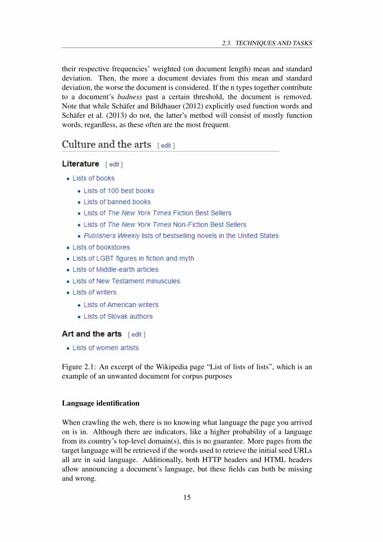
As we are not interested in documents only containing word clouds, tables, listsor other non-sentences (see figure 2.1) when building web corpora, we have toidentify text that is connected. ‘Connected text’ means text that is not a list-likestructure of words, but full sentences. Detecting connected text is done whileidentifying language by both Baroni et al. (2009) and Schäfer and Bildhauer(2012). The latter’s methods has since been developed further, and rebrandedas “text quality assessment”, but still stays true to the main principle (Schäfer etal., 2013).
Baroni et al. (2009) accepts a document if it contains at least ten types, thirtytokens and at least a quarter of all words are function words – closed-class high-frequency words like ‘the’, ‘or’, ‘and’, ‘of’, ‘for’. The accepted document willthen be deemed to have enough connected text to be relevant.
Schäfer and Bildhauer (2012) claims this method relies too much on overalldocument size, and introduces a similar method, but weighted with respect todocument size.
This method is again improved upon by Schäfer et al. (2013). Here, the tenmost frequent types of a sample of the corpus will be calculated, together with
14
2.3. TECHNIQUES AND TASKS
their respective frequencies’ weighted (on document length) mean and standarddeviation. Then, the more a document deviates from this mean and standarddeviation, the worse the document is considered. If the n types together contributeto a document’s badness past a certain threshold, the document is removed.Note that while Schäfer and Bildhauer (2012) explicitly used function words andSchäfer et al. (2013) do not, the latter’s method will consist of mostly functionwords, regardless, as these often are the most frequent.
Figure 2.1: An excerpt of the Wikipedia page “List of lists of lists”, which is anexample of an unwanted document for corpus purposes
Language identification
When crawling the web, there is no knowing what language the page you arrivedon is in. Although there are indicators, like a higher probability of a languagefrom its country’s top-level domain(s), this is no guarantee. More pages from thetarget language will be retrieved if the words used to retrieve the initial seed URLsall are in said language. Additionally, both HTTP headers and HTML headersallow announcing a document’s language, but these fields can both be missingand wrong.
15
CHAPTER 2. BACKGROUND
As the types, tokens and function words used as metrics in the connected textevaluation belong to one given language, the language will also be identifiedduring this process. The reason is that the connected text identification will notfind the function words it has been given, because the languages differ, and willremove the document.
For instance, searching a Norwegian text for the English words “the” or “and”will not provide the correct frequency counts.
This method can struggle with documents where there are more languages in onesite, or where two closely related languages share function words (like Danish andNorwegian). In those cases, another state-of-the-art language identifier might beneeded.
Schäfer et al. (2014) use an off-the-shelf naive-bayes classifier to identifylanguages (Lui and Baldwin, 2012).
Boilerplate removal
Boilerplate typically refers to menus, buttons, labels of input fields, copyrightdisclaimers, advertisements, navigational elements, etc. Schäfer (2016a, p. 2),provide a more formal definition of boilerplate:
I define boilerplate as all material that remains after markup stripping,and which does not belong to one of those blocks of content on theweb page that contain coherent text.
Using this definition, everything is boilerplate, except if it is related directly toconnected text.
Boilerplate removal is one of the areas that are deemed most difficult, and one ofthe most important to ensure the quality of web corpora. Therefore, a lot of workhas been devoted to this task, and I will grant the discussion of this sub-task andits development more space than the others.
In 2007, the CleanEval shared task was initiated, which is a competitive evaluationof cleaning web pages. From this competition, Baroni, Chantree, Kilgarriff, andSharoff (2008, p. 1), stated:
It is a low-level, unglamorous task and yet it is increasingly crucial:the better it is done, the better the outcomes. All further layers oflinguistic processing depend on the cleanliness of the data.
To solve this, Baroni et al. (2009) lean on the observation that boilerplate is oftenaccompanied by a lot of HTML tags. Of all possible spans of text in the document,they pick the text that has the highest N(tokens) − N(tags).
Schäfer and Bildhauer (2012, p. 4), states the following about this method:
16
2.3. TECHNIQUES AND TASKS
This has the advantage of selecting a coherent block of text fromthe web page, but also has the disadvantage of allowing interveningboilerplate to end up in the corpus. Also, many web pages fromblog and forum sites contain several blocks of text with interveningboilerplate, of which many can be lost if this method is applied.
CleanEval provided data sets and tools to evaluate boilerplate removal algorithmswith. Several general-purpose HTML web page boilerplate detectors usingdifferent types of standard machine learning algorithms have been suggested. Forinstance:
Bauer et al. (2007) utilised Support Vector Machines implemented with “linguisticfeatures” (such as text, token, type or sentence lengths, the frequency of certainkeywords that are indicative of clean or dirty text, etc.), “structural features”(density of tags and attributes and whether the tags are indicative of text), and“visual features” (where they render the page and analyse the image). Theyachieve an F-score2 of 0.652.
Spousta, Marek, and Pecina (2008) achieved an F-score of 0.8 using ConditionalRandom Fields with features divided into markup-based features (what kind oftag surrounds or is contained within a paragraph), content-based features (lengthsand counts of sentences, tokens, etc. in a paragraph) and document-relatedfeatures (token and sentence count of the whole document, and the position ofthe considered block within the document).
A semi-supervised approach using a Naive Bayes Classifier on each token toconsider it “out-of-article” (boilerplate) or “in-article” (non-boilerplate), and thenfinding the highest-scoring sequences of tokens was used by Pasternack and Roth(2009) to achieve a CleanEval F-score of 0.92. The two features used for theNaive Bayes classifier on the CleanEval data was unigrams and the most recentunclosed HTML tag.
Kohlschütter, Fankhauser, and Nejdl (2010) combine techniques – decision treesand linear support vector machines – using 67 features. They identify that usingonly 2 of them, link density and “text density” (based on number of words andnumber of lines per ‘block’ (paragraph)), give almost the same performance asusing all features. They achieve an F-score of 0.95.
Suchomel and Pomikálek (2012) used the tools developed by Pomikálek (2011)3.Unlike the other methods, jusText does not use machine learning, but rather analgorithm using stop word density, link density and block length as inputs, as wellas the context of the block as a cue. The F-score, depending on dataset, is between0.92 to 0.98.
2Unless stated otherwise, I mean F1-score when I say “F-score”.3I was not able to find and read this thesis, so my knowledge of jusText is based on Schäfer
(2016a).
17

CHAPTER 2. BACKGROUND
Technique F-score
SVMs 0.65CRFs 0.8Naive Bayes 0.9Combo 0.95jusText 0.95
Table 2.1: Boilerplate classification techniques evaluated using CleanEval
For texrex, Schäfer and Bildhauer (2012) decided to train a multilayer perceptronwith nine different input values, and use it on every paragraph. They end up withan F-score of 0.75 (however, this is not evaluated using the CleanEval evaluation– see below).
Although this was far from state-of-the-art, multilayer perceptrons are veryefficient. Therefore, Schäfer (2016a) takes the MLPs in texrex further. By using37 input features, the F-score is increased to between 0.977 (for English) and0.994 (for French).
Below is an excerpt of some of the features that were used for training the MLP.While they might not seem to be language dependent, they prove to be, probablydue to innate differences between the languages.
• Paragraph length
• Proportion of HTML markup to all text in the non-stripped document
• Number of sentences in paragraph
• Does the paragraph end with punctuation?
• Average sentence length
• Number of sentences ended in punctuation
• The proportion of HTML markup to text in the neighbouring paragraphs
• The proportion of the number of paragraph characters to the whole page
• Is the tag surrounding the paragraph a <p> tag?
It should be noted that the evaluation scores for the texrex boilerplate detectionare not evaluated using the CleanEval data set, and is difficult to compare directlywith other solutions because of this. The reasons are manifold (Schäfer et al.,2014):
• The CleanEval shared task requires the detection of text structure, likeheadlines, lists, etc. on top of the detection of whether text is boilerplateor not. This detection is not needed or supported in texrex.
18

2.3. TECHNIQUES AND TASKS
• The data used for evaluation in CleanEval has been stripped of some keydata, like HTML and crawl headers, which is used directly as features inthe texrex boilerplate classifier.
• The encodings of CleanEval’s gold standard data is not normalised to UTF-8 like texrex’s data is, and cannot be directly matched by the CleanEvalevaluation script.
• CleanEval’s annotation guidelines are designed for destructive removal,while texrex is designed for non-destructive classification. This differencein philosophy makes for some incompatible differences: Some content thatis boilerplate, but is relevant or important at the same time must be classifiedas non-boilerplate by CleanEval, so it does not get deleted. texrex can keepit and deem it to be boilerplate. An example of such content is non-humangenerated timestamps for forum posts. They give important information,but is definitely boilerplate.
• CleanEval broke new ground in 2008, but technology moves fast, and 9years is a long time. The web looked different then and HTML5, forinstance, didn’t even exist. Even though CleanEval evaluation is stillused by some developers of corpus creation tools (Habernal, Zayed, andGurevych, 2016), it can be argued that it is outdated at this point.
See section 2.5.2 for developments that have happened during the writing of thisthesis.
Duplicate and near-duplicate removal
Duplicates occur quite frequently on the web. Whether it is the same quote,book or article that is quoted on different pages, or actual true copies, theyneed to be dealt with to avoid a doubling of a document’s effect on the tokenfrequencies.
True duplicate removal True duplicates are the documents that are identi-cal.
To remove these, Schäfer and Bildhauer (2012) create an array for each document,and fills it with evenly distributed characters in the document. If two sucharrays match, the copy is discarded. Suchomel and Pomikálek (2012) hash thedocuments in two steps, both before they were cleaned and afterwards, thenremove all matching copies.
Near-duplicate removal Documents can also be near-duplicates, where a lot ofthe content is found in other documents.
19

CHAPTER 2. BACKGROUND
Doing this step after the boilerplate removal can be beneficial, as boilerplate cancreate false positives (by different content sharing so much boilerplate that theduplication removal algorithm thinks they are identical), and false negatives (thesame content having different boilerplate, making the classifier think they aredifferent documents) (Baroni et al., 2009).
Both Baroni et al. (2009) and Schäfer and Bildhauer (2012) use variations of aw-shingling algorithm as described by Broder (1997). In essence, the algorithmmakes n-grams – called shingles – out of the document’s tokens and sees howmany of these are shared between other documents to find how similar theyare.
With n = 4, the document “a shingle is a shingle is a shingle” can be made intoshingles like this:
Document: “a shingle is a shingle is a shingle”shingles: { (a,shingle,is,a), (shingle,is,a,shingle), (is,a,shingle,is) }
The first two shingles will show up twice. For efficiency, these shingles can behashed. If the shingles that were shared between two documents exceed a tresholdof resemblance (using a Jaccard coefficient, for instance), the longest is kept.Baroni et al. (2009) use a simplified version of the algorithm, where the shinglesare not hashed like described by Broder (1997). Additionally, they only performnear-duplicate removal, and does not perform perfect duplicate removal.
Suchomel and Pomikálek (2012) use a tool called onion4, that performsdeduplication on a paragraph level. Paragraphs containing more than 50% 7-tuples previously encountered are discarded.
Encoding
The web contains a lot of pages, with many of them using different encodings.With the limitations from the ASCII standard of early computers making peoplefrom different regions and countries come up with their own encoding to be ableto use their own characters, a corpus must accomodate for this encoding diversity.Additionally, a corpus should unify the encodings so all the documents have thesame encoding throughout the corpus.
The HTTP protocol has ways of announcing the encoding a page is using, butthere are several ways this can be misleading. There might be text from differentencodings in the same page, the text might be corrupted and not follow anyencoding (or the wrong one), or the encoding announced might be different fromthe actual encoding on the page.
4http://corpus.tools/wiki/Onion
20

2.4. EVALUATING WEB CORPORA
Web browsers are robust when it comes to encoding, being able to handle most ofthese cases, and the corpus must be able to as well.
The obvious encoding for a modern corpus to use as its standard is unicode(UTF-8), the encoding trying to unify characters from as many other encodings aspossible.
2.3.3 Metadata and annotation
Metadata about each document can be important information depending on whatthe corpus is to be used for. Document metadata can often be found in theHTML headers of a document in “<meta>”-tags or in the HTTP headers, whereinformation such as what type of content the page contains, keywords to describethe content, what language it is in, etc. can be saved. Whether to either use thisdata while constructing the corpus or making the metadata available to the corpususer in some fashion are decisions corpus constructors must make.
While all kinds of metadata can be saved in the HTML headers, normalisingthese can be difficult, as some documents may have little to no metadata and themetadata that exists may be saved differently, or have different notation. Somelinguists might be interested in for instance the gender, age or nationality of theauthor of the text, and those kinds of data will often be approximations, oftenthrough automatic classification (Biemann et al., 2013).
Annotating the corpus means performing tasks such as tokenisation, lemmatisa-tion and part-of-speech tagging. Some libraries and software seem to be quitecommonly used for these tasks – often off-the-shelf software. One can questionwhether this software is state of the art, and how precise the results of the off-the-shelf software are.
2.4 Evaluating web corpora
Like mentioned earlier, Banko and Brill (2001) make the case that larger corporaimprove the performance of machine learning algorithms more than manuallytuning the algorithms themselves. Intuitively, however, size is not everything:For instance, having the same word or sentence repeated over and over will notget you desired results. Additionally, Versley and Panchenko (2012) give severalexamples where using the manually annotated 100 million token British NationalCorpus give superior results to using the 2.25 billion token ukWaC.
Therefore some notion of corpus quality must be assessed. There currently seemsto be two quite different approaches to this challenge.
21

CHAPTER 2. BACKGROUND
One approach is to assess the given corpus’ quality by finding ways to compare itto other corpora. By comparing corpus statistics, on top of corpus size, one cansay something about the corpus quality – and get hints to what one might need toimprove: Did we identify any languages other than our target language? Did wemanage to remove duplicates? Did the boilerplate removal remove “sufficient”boilerplate? etc.
Another approach is the linguistic evaluation of the web corpus as a representativesample of the language in general.
2.4.1 Statistical quality metrics
Statistical parameters can be used to characterize a corpus – and thus enablecomparing corpora.
According to Biemann et al. (2013), typical assessment statistics for corpusquality are for instance the distribution of word, sentence or document length,the distributions of characters or n-grams, or the corpus’ agreement with certainempirical laws of language such as Zipf’s law.
These statistical measures can be used to identify anomalies, or signs that adocument should have been caught by the filtering procedures. For instance,Biemann et al. (2013) introduce several statistics that they use to identify differentkinds of preprocessing problems:
• The relative size of the largest domains represented in the corpus canindicate problems with the crawling, as it can be an indicator of host bias.
• The length distribution of sentences can be used to identify problems withnear-duplicate removal: If the length of the sentences doesn’t follow thesame distribution as expected (for a given language, genre, etc.), theremight be sentence duplication affecting it. An example is in figure 2.2,where you can see heavy spikes for Hindi news. Biemann et al. (2013)say these showed signs of being, and proved to be, boilerplate material andduplication that should have been removed.
2.4.2 Do web corpora represent languages as well astraditional corpora?
In their WaCky-article, Baroni et al. (2009, p. 5) state:
Notice that the rationale here is for the corpus to include a sample ofpages that are representative of the language of interest, rather thangetting a random sample of web pages representative of the languageof the web.
22

2.4. EVALUATING WEB CORPORA
Figure 2.2: Example of how assessing corpus statistics enables comparing corporaand disovering signs of flaws
Herein lies the notion of representativeness – the notion that the documents youretrieve represent some bigger whole. The quote from WaCky even makes clearthat they take steps to make sure their result is representative of something, andalso that it is not representative of something else. They do this by detectingtext types and topics while crawling, and making sure that their corpus includesdocuments from newspapers, spoken word, technical manuals as well as blogs andforum posts. By making sure it does, Baroni et al. (2009) seem to believe theircorpus to be sufficiently representative.
“As representative as reference corpora”
Biemann et al. (2013, p. 15) emphasize the syntactic and lexical core of thelanguage as what to base the evaluation of the corpus’ representativeness on:
The linguistic usefulness of web corpora as representative samples ofgeneral language (rather than web-specific genres) can be evaluatedby comparison with a traditional reference corpus, using frequentgeneral-language words and constructions as test items. Theunderlying assumption is that an ideal web corpus should agree withthe reference corpus on the syntactic and lexical core of the language,while offering better coverage of less frequent words and construction[sic], highly specialized expressions, and recently coined words.
That is: If a web corpus and a manually constructed reference corpus agree on coreparts of the language, the web corpus is as representative of the language as thereference corpus – which is commonly believed to be sufficiently representative.Thus, the web corpus can also be said to be sufficiently representative.
23
CHAPTER 2. BACKGROUND
Biemann et al. (2013) also offer examples of how to test this agreement onlanguage core, by using the corpora for two tasks, and comparing the corpusperformance on those tasks: the first task were verb–particle combinations forEnglish, and the second creating word collocation lists based on the corpora.
The results from the first task show that the manually constructed BritishNational Corpus does well, but that the web corpora do better as their sizeincrease. However, the good performance of the web corpora requires morethan a magnitude more data than the BNC. Interestingly, the very large Web1T5(Google’s 1TB large 5-gram database) performs very poorly, in spite of beingmuch larger. This can be a sign of poor quality or its limited context, and furtheremphasizes the need for both high quality, and large corpora.
The same linear performance increase with size is seen for the second task, buthere the BNC outperforms the web corpora, although not by much. This showsthat web corpora for some tasks can do as well as reference corpora, and as theirsize increase, perhaps surpass them.
Representative of the general language
A wish for some corpus users is to be able to say something general about thelanguage as a whole by being able to say something about the corpus. For thisto be true, the corpus must be representative of that language. This is a fieldof some controversy – for instance, Kilgarriff and Grefenstette (2003) say thatit is impossible to create a corpus representative of English, as the population of“English language events” are so difficult to define, and to know sufficiently aboutto create something that is representative of it.
For the corpus to be representative, or balanced, two things should be evaluated,according to Biemann et al. (2013):
1. Is the corpus a “random selection” of the population – i.e. the language?If so, it should reflect the distribution of topics, genres, text types, etc.However, if one managed to gather a truly random sample of the web ina given language, is that the same as getting a truly random sample of agiven language?
2. No genre or topic should be heavily over-represented – it should be“balanced”. If one imagines that the web does not have the same distributionof genres or topics as what the distribution would be in a reference corpus,is a random selection of the web desirable if wanting balance?
While Biemann et al. (2013) avoid giving a recommendation on whetherto prioritise randomness or balance while constructing corpora, Schäfer andBildhauer (2012) seem to favour the random selection approach, stating that theydo not believe a corpus could ever be balanced.
24

2.5. THE GOAL OF THIS PROJECT
2.5 The goal of this project
This project will investigate how one can use the Common Crawl’s data toconstruct a large web corpus. There are several diverging paths depending onwhat is found from these investigations and what decisions are taken based onthose.
2.5.1 High-quality connected text extraction from theCommon Crawl
In addition to the raw archive files (WARC), Common Crawl offers extracted textversions of their crawls, so-called WET-files. An initial task will be to investigatehow viable these text extractions are for corpus construction with regards toquality.
The results of that investigation will determine what files to proceed with, whichwill in turn affect the corpus creation process.
Finally, when a corpus has been constructed, its usefulness needs to be evaluated– how that will happen will be discussed in chapter 5.
2.5.2 Concurrent work
C4Corpus
While this thesis was being written, other relevant work on the topic has beenoccuring at the same time. Some of it I might have been able to integrate withthis thesis, while other papers or toolkits might have been released too late in theprocess to be accomodated for.
One such toolkit is the C4Corpus5 (Habernal et al., 2016).
Like this thesis, they use Common Crawl data as the basis for their constructedcorpus, but diverge from the choices made in coming chapters in other areas. Theirsoftware is written in Java, using the Hadoop framework, and they focus heavilyon licensing – making their corpus available to the public for free, by restrictingtheir corpus to documents with a CreativeCommons license.
Their boilerplate removal method is a Java reimplementation of jusText, thesame library used in the earlier mentioned paper by Suchomel and Pomikálek(2012).
5https://github.com/dkpro/dkpro-c4corpus
25

CHAPTER 2. BACKGROUND
The deduplication is similar to the one popularly used as perfect-duplicateremoval, the hashing of 64-bit shingles then used as fingerprints for docu-ments.
CleanerEval
As a follow-up to 2008’s CleanEval, the 2017 Web as Corpus Workshop, hostedby the SIGWAC will feature the first meeting of a new shared task: CleanerEval.In the same spirit as Schäfer (2016a) and Schäfer et al. (2013), the sharedtask will focus on boilerplate removal and assessing the linguistic quality of adocument.
The WAC-XI conference will be hosted July 27, 2017.
26
Chapter 3
Exploring the Common Crawl
Recall the description of the Common Crawl in section 2.3.1. The data is availableboth for download, or to be used directly by running software on Amazon’s servers– either with their EC2 instances or their Hosted Hadoop clusters. In this project, Iwill be downloading the data to NorStore – the Norwegian national infrastructurestorage resource, and use it with the University of Oslo’s cluster Abel (see section4.2).
3.1 The data
Common Crawl data is stored in three different ways, as:
• Raw crawl data
• Metadata
• Extracted text data
WARC The raw web data (with the HTTP header information included) isprovided in the Web ARChive format – or the WARC format. This format is anISO standard format building on the ARC format orginally used by The InternetArchive to archive web pages (International Organization for Standardization,2009). The WARC files contain four types of entries:
• The WARC info-entry: There is one of these per WARC file describing theWARC format, the date of its saving, etc.
• Requests: The HTTP requests that were sent.
• Responses: The HTTP responses, including headers.
• Metadata: Computed metadata entries – for the August 2016 crawl, thisonly contained the fetch time of the crawl.
27
CHAPTER 3. EXPLORING THE COMMON CRAWL
Type # files cmpr.file
size
dec.file
size
cmpr.rate
cmpr.time
entriesper file
docsper file
docsize
WARC 29,800 988 4515 3 33s 155,400 51,800 0.10WET 29,800 156 405 2.6 6.7s 51,800 51,800 0.01WAT 29,800 353 1524 4.3 13.6s 155,400 N/A 0.01
Table 3.1: Data collected about the WARC, WET and WAT files from the August2016 crawl. All the data (except the first column) are averages from a randomselection of 100 files – where the WET and WAT files selected are the ones derivedfrom the WARCs. All file sizes are in megabytes. The rows are: Number of files,compressed file size, decompressed file size, compression rate, compression time,number of entries per file, documents per file and the size of each document.
Each entry has additional meta information prepended to them. The informationprovided in these WARC-headers include the date of the response, the uniqueID of the record, the length of the content, what type the content is, the URI ofthe target, as well as the IP address of the target. The Common Crawl web siteprovides code snippets for use with several different programming languages toget started with the WARC files1, and the Internet Archive also provides librariesto retrieve metadata and the documents themselves2.
WAT The metadata from the WARC files, that is computed for each request/re-sponse entry can also be found in the WAT files – the Web Archive Transformationformat. The WAT entries contain metadata from the WARC-headers, the HTTPrequest and the response. If the response is in the HTML format, the HTTP head-ers and the links on the HTML page are made available as well. This is then storedin a key–value Javascript Object Notation (JSON) format.
WET In the case of this project, I am interested in the textual data of the crawls,and the Common Crawl provides extracted plaintext for each response entry inthe WARC files. This is stored in the WET format (Web Extracted Text), wherethe WARC headers and information about the length of the plaintext data areprepended to the actual extracted plaintext.
Only the entries for which there exists content that it is possible to extract text fromis in these files. This means that the request and metadata entries are stripped, aswell as content where the content-type of the response is considered to not betextual.
1http://commoncrawl.org/the-data/examples/2https://github.com/internetarchive/warc
28

3.1. THE DATA
Operation Time required
Reading 17.5 hoursDecompressing 11 daysDownloading 14.5 days
Table 3.2: The time required for performing different operations on the August2016 Common Crawl
As the size of each crawl is quite large, the data is split in a large number ofgzipped files containing thousands of WARC entries. For the August crawl of2016, the file count for the WARC files was 29 800, where each file was about1GB (see table 3.1). As the WAT and WET files are generated based on the WARCfiles, the file count is similar for those, but while the compressed WARC files aresized around 1GB, the WET and WAT files are a lot smaller, with WARC >> WAT> WET.
While it seems obvious that the original documents in the WARC files take upthe most space, it might not be as intuitive as to why the files only containingmetadata, the WAT files, are much larger than the extracted text files, the WETfiles. The reason for this is that the WET files only contain records where thereare textual content to be extracted, and where no HTTP header information isincluded. Subsequently, the WAT files contain information about both the requestand the response, while WET only contains responses.
A master paths file for each of WARC, WET and WAT is published on theCommon Crawl’s Amazon bucket, as well as with a link from the Common Crawlblog3. These paths files contain a relative link to a file per line. Concatenatingthe relevant prefix with the line results in the absolute link needed to access thefile. The prefix can either be in http form or in S3 form, depending on whetheryou want to access the data through HTTP or through Amazon’s Simple StorageService protocol.
3.1.1 A note on scale
30 terabytes of web archive data is a lot of data. Both handling and processingdata of this scale takes a lot of time. As an example, the time required to justopen the decompressed archive files, and reading through them without any actualprocessing took about 17.5 hours. Any additional operation performed whileprocessing the data will only increase this amount of time. See table 3.2.
To be able to analyse and process the data in a more reasonable amount of time,parallel computing is an absolute neccessity. Parallelising the processes is not
3http://commoncrawl.org/connect/blog/
29

CHAPTER 3. EXPLORING THE COMMON CRAWL
always trivial, and adds additional development time on top of the time alreadyrequired.
In addition to the amount of time required to process the complete crawl, eachfile is also of significant size. A compressed WARC file at 1 GB can require fromseconds to a couple of minutes to process, and makes the process of creating andtesting analysis tools even longer.
The scale of the data affects the whole process, from data analysis to the actualprocessing of it for corpus creation, and should be taken into account whenplanning these types of projects.
3.1.2 Retrieving the data
As retrieving about 30 000 1GB sized WARC files can take some time,parallelisation of the download process can seem like a time-saving prospect.However, this requires that both the client and the server can handle large paralleldata transfers. In my case, this means that NorStore needs to handle paralleltransfers well. Consequenctly, NorStore needs to have a good bandwith, that thefile system can be saved to in parallel, and that the processing power is greatenough to handle saving to the file system. Additionally, parallelisation is alsodependant on Amazon’s routing: If two separate download requests from thesame client go to two different Amazon end points, the efficiency of the transferis maximimised.
In a preliminary study, downloading 150 files, using 1, 2, 4, 8, 16 and 32 processesat the same time (but on a CPU with only 16 cores), gave the results shown infigure 3.1.
The results show that parallelising using 32 processes cuts the download time to13.3% of the non-parallel download time, from an average download speed of23.9 MB/s with one process, to an average download speed of 200.5 MB/s with32 processes. That makes the total download time of the complete 30 terabytesabout 41 hours. Compared to the sequential download speed of 14.5 days, this isa big improvement.
As seen from the graph, the relative speedup gain is the largest up to 8 processors,but the gain with 16 processors is still good, although not as efficient as 8 – seethe efficiency comparison below. I also tried using 32 processes, and did receive asmall speedup, although arguably negligible. As the CPU did not have more than16 cores, this is not that surprising.
30

3.2. GETTING MY FEET WET
32168421
20
40
60
80
100
Number of processes
Exe
cutio
ntim
ein
min
utes
Figure 3.1: The execution time of downloading the same 150 gzipped WARC filesper number of processes. (Note that this was done on a CPU with 16 cores)
Processors Speedup Efficiency
2 1.1 0.64 2.5 0.68 5.3 0.6
16 7.9 0.532 8.4 0.3
Table 3.3: The speedup and efficiency of the download using a different numberof processors
Above one can see that going from 8 processes to 16 does give a speedup (5.3 to7.9), while the efficiency goes down (0.66 to 0.49) – each process isn’t used asefficiently as possible.
3.2 Getting my feet WET
As the crawls already offer extracted plaintext as WET files, these files are anatural place to start: If the text extraction is of sufficient quality, there is noneed to do such an extraction step myself.
While remaining HTML in the WET files can be fixed in an additional HTMLstripping step, there is little point in using the WET files as the basis if the reasonwe wish to use them is to forego this step entirely.
31

CHAPTER 3. EXPLORING THE COMMON CRAWL
3.2.1 A preliminary inspection
An initial rough inspection of one WET file reveal that quite a lot of HTML remainin the documents. By picking one WET file at random, splitting it up to one fileper crawled document, and then doing a simple search for remaining HTML bysearching for occurences of “<div>”, “<article>”, “<span>”, “<p>” , “<body>”,“<a>” and “<html>”, I found the following:
The file contained 50300 documents, where 1300 of them still had HTMLremaining. The average number of HTML tags per file that still contained HTMLwere about 5, and this was with a very naive approach: There are more HTMLtags than the ones I searched for, as well as Javascript and CSS that this approachwon’t find. However, it is enough to see that the HTML is not sufficiently stripped,and that a separate step of text extraction is required. See figure 3.2 for an exampleof a document where there are still remnants of HTML.
3.2.2 WET vs. cleaned WARC
In chapter 4, I describe my chosen method for text extraction – texrex. Extendingthe inspection above by comparing the corpus made from texrex with the WETfiles further cements the need for using the WARC files, and giving up the WETfiles. Comparing both a corpus made from four WARC files and the correspondingfour WET files for remaining HTML tags, remaining HTML entities, encodingerrors, token count and language distribution, the corpus outperforms the WETfiles in every regard.
It is important to note that this test corpus was made with parts like boilerplatedetection and language detection turned off, as both are language dependent, andmust be switched off to be able to assess the corpus without committing to onelanguage. The size filtering option – where documents with a size above or belowcertain thresholds are removed both before and after cleaning (see section 4.2.1) –was turned on, however, together with the de-duplication. Because of these filters,there are fewer documents in the corpus than in the WET files.
For the files picked, this ended up being 90 500 documents in the constructedcorpus and 244 000 documents in the WET files. Note that this means that about160 000 documents that were included in the WET files are not included in thecorpus. This stood out as a large amount, and is addressed in section 3.2.3.
Below, I retrieve data from the WET files, the corpus made with texrex, as wellas the documents from WET that can also be found in the corpus, the intersection(noted as ‘WET ∩ corpus’ below).
4WET ∩ corpus are the documents from the WET files, but where the documents that is notincluded in the constructed corpus is removed. This makes for a more direct comparison.
32

3.2. GETTING MY FEET WET
Data tags # docs w/tags (σ)
% docsw/ tags
tags/doc
WET 37,173 3055 (5.50) 1.20% 0.2WARC-corpus 28 28 (0.02) 0.03% 0.0003WET ∩ corpus4 15,114 1139 (5.40) 1.26% 0.17
Table 3.4: The remaining HTML tags of the different corpora. From the left: Thenumber of tags remaining, the number of documents that had remaining tags, thepercentage of documents that had remaining tags and how many tags there wereper document
Data entities # docs w/entities (σ)
% docs w/entities
entitiesper doc
WET 166,307 5311 (55.3) 3.2% 0.7WARC-corpus 8,772 2284 (1.7) 2.5% 0.1WET ∩ corpus 136,770 2897 (77.7) 3.2% 1.5
Table 3.5: The remaining HTML entities of the different corpora. From the left:The number of entities remaining, the number of documents that had remainingentities, the percentage of documents that had remaining entities and how manyentities there were per document
From table 3.4, it is clear that the WET files are far inferior to the corpus madewith texrex in terms of removal of HTML tags. The HTML stripping done on theWET files is lacking severely, while the HTML stripping from the texrex corpushas managed to remove almost every tag.
There are a lot of remaining HTML entities in both the WET files and the corpus.However, compared to the WET files, the corpus has far fewer entities remaining,with the intersection having about 16 times as many entities remaining (see table3.5). While the corpus is in the XML format, and therefore needs to escape somecharacters with XML entities itself (namely & (&), " (”), ' (’),< (<) and > (>)), these are not the entities making this number so large, asthe top entities in the texrex corpus were dominated by entities not in the XMLspecification (see table 3.6). All of these entities have corresponding unicodeglyphs, so this suggests that the entity normalisation is incomplete.
33

CHAPTER 3. EXPLORING THE COMMON CRAWL
Entity Frequency
4594▄ 1170& 510© 345♦ 288
Table 3.6: Top five frequent entities in the texrex corpus
As the WET files do not include the HTTP headers like the WARC files do,one must assume that the encoding is supposed to be unified. However, tryingto interpret the documents as unicode showed that this work has not beencompleted.
Corpus # docs % docs
WET 5019 2.1WARC corpus 0 0WET ∩ corpus 1990 2.2
Table 3.7: Number of documents with encoding errors
Table 3.7 shows the amount of documents with encoding errors, i.e. documentscontaining bytes not possible to interpret and convert to unicode.
Corpus # tokens #tokens/doc σ (SD)
WET 226,261,200 927.3 2140.6WARC-corpus 93,685,600 1035.2 1508.6WET ∩ corpus 101,109,315 1117.23 2842.3
Table 3.8: Number of tokens in the corpora
The number of tokens per document in the different corpora are quite similaracross WET and the constructed corpus (table 3.8), but the differences areinteresting: The difference between WET and the WET ∩ corpus makes itprobable that the constructed corpus indeed selected the documents where moretext remained after cleaning. The difference between the constructed corpus andthe intersection might be because of the remaining HTML in the intersectiondocuments. The standard deviation is larger for the WET files, maybe because
34
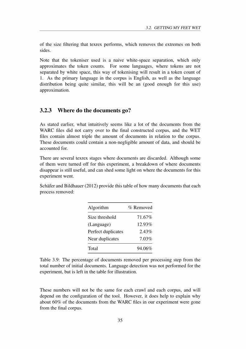
3.2. GETTING MY FEET WET
of the size filtering that texrex performs, which removes the extremes on bothsides.
Note that the tokeniser used is a naive white-space separation, which onlyapproximates the token counts. For some languages, where tokens are notseparated by white space, this way of tokenising will result in a token count of1. As the primary language in the corpus is English, as well as the languagedistribution being quite similar, this will be an (good enough for this use)approximation.
3.2.3 Where do the documents go?
As stated earlier, what intuitively seems like a lot of the documents from theWARC files did not carry over to the final constructed corpus, and the WETfiles contain almost triple the amount of documents in relation to the corpus.These documents could contain a non-negligible amount of data, and should beaccounted for.
There are several texrex stages where documents are discarded. Although someof them were turned off for this experiment, a breakdown of where documentsdisappear is still useful, and can shed some light on where the documents for thisexperiment went.
Schäfer and Bildhauer (2012) provide this table of how many documents that eachprocess removed:
Algorithm % Removed
Size threshold 71.67%(Language) 12.93%Perfect duplicates 2.43%Near duplicates 7.03%
Total 94.06%
Table 3.9: The percentage of documents removed per processing step from thetotal number of initial documents. Language detection was not performed for theexperiment, but is left in the table for illustration.
These numbers will not be the same for each crawl and each corpus, and willdepend on the configuration of the tool. However, it does help to explain whyabout 60% of the documents from the WARC files in our experiment were gonefrom the final corpus.
35

CHAPTER 3. EXPLORING THE COMMON CRAWL
The largest culprit, the size filters, are explained more thoroughly in section4.2.1.
3.2.4 Language distribution
I also ran language identification on the same files as the above inspection wasperformed on, to see if there were differences. The language identifier that wasused5 output the top three languages being present in one document, and a number,the percentage of the document that was in said language. The tables below arehow many of the characters in the whole corpus that was deemed to be in a givenlanguage.
Language WET WARC-corpus WET ∩ Corpus
English 81.4% 75.3% 78.6%German 2.0% 2.5% 2.0%Spanish 1.9% 2.5% 2.1%Chinese 1.5% 3.3% 2.0%French 1.3% 1.7% 1.2%...Norwegian 0.12% 0.08% 0.08%
Table 3.10: Distribution of language in the different corpora, as percentage of totalnumber of characters
Table 3.10 says that the language distribution is quite similar between the corpusand the intersected WET documents. The differences can both be because of theremaining HTML confusing the classifier, or because some documents couldn’tget their language classified because of encoding errors in the WET files.
3.2.5 What now?
The WET files are clearly not cleaned sufficiently to be usable without doing a lotof the steps that I would be doing with the WARC files anyway. Therefore, I willbe continuing with the WARC files and leaving the WET files behind.
As the Common Crawl seem dominated by English content and does not containenough data from under-resourced languages, like Norwegian, to construct acorpus of sufficient quantity, I will proceed with the goal of constructing anEnglish corpus.
5https://github.com/CLD2Owners/cld2
36

3.2. GETTING MY FEET WET
WARC/ 1 . 0WARC−Type : c o n v e r s i o nWARC−Targe t −URI : h t t p : / / 1 0 0 3 t h e p e a k . i h e a r t . com / p h o t o s /
snap − s h o t s / c e l e b r i t y −dogs −366430/WARC−Date : 2016−08−24T04 : 5 6 : 3 5 ZWARC−Record −ID : < urn : uu id : bbe19425 −884e−48 f2 −92be −980
a4270c089>WARC−Refe r s −To : < urn : uu id :61370 b1a −8107−4084−83 e4−
d483e9045c2d>WARC−Block −D i g e s t : sha1 :
IUC52ZDJFWFA72ZJMCAEXNC2DA7VNNYLConten t −Type : t e x t / p l a i nConten t −Length : 4492
<p><span s t y l e =" f o n t − s i z e : 9px ; ">Photo : S p l a s h news < /span> I f J e s s i c a Har t was a dog she would be t h i st h i n g .
<p><span s t y l e =" f o n t − s i z e : 9px ; ">Photo : S p l a s h news < /span> Snooki and JWoww d r e s s t o match t h e i r dogs .
<p><span s t y l e =" f o n t − s i z e : 9px ; ">Photo : S p l a s h news < /span> We can ’ t r e a l l y t e l l which i s Ozzy !I n c r e d i b l e !
<p><span s t y l e =" f o n t − s i z e : 9px ; ">Photo : S p l a s h news < /span> Coco and h e r p i t b u l l . I d e n t i c a l !
<p><span s t y l e =" f o n t − s i z e : 9px ; ">Photo : S p l a s h news < /span> Luke Wilson l o o k s a l o t l i k e h i s s t o c k y pup .
<p><span s t y l e =" f o n t − s i z e : 9px ; ">Photo : S p l a s h news < /span> Th i s i s amanda Byne ’ s dog . . . <p><span s t y l e ="f o n t − s i z e : 9px ; ">Photo : S p l a s h news < / span> Blondes! Seann Wil l i am S c o t t would most d e f i n i t e l y have aye l l ow l a b .
<p><span s t y l e =" f o n t − s i z e : 9px ; ">Photo : S p l a s h news < /span> B r u n e t t e s ! Anne Hathaway wi th h e r c h o c o l a t eLabrador , Esmera lda . <p><span s t y l e =" f o n t − s i z e : 9px; ">Photo : S p l a s h news < / span> Jon Hamm and h i s mut t
o f t e n make s i m i l a r f a c i a l e x p r e s s i o n s .
Figure 3.2: An example extract from what should have been extracted text withoutHTML remaining from a WET file of the Common Crawl
37

Chapter 4
Text extraction from the CommonCrawl
Given the limitations of the extracted text files offered by the Common Crawl thatwere established in section 3.2, other ways of producing high-quality linguisticcontent are needed.
Such a process will need to process WARC files, and by performing tasks asdescribed in chapter 2 – such as for instance HTML stripping, boilerplate removal,duplicate and near-duplicate removal – produce files containing extractedtext.
4.1 Choosing a tool for the job
In chapter 2, I investigated solutions to the aforementioned challenges. Whileearlier efforts such as WaCky (Bernardini et al., 2006) broke new groundwhen it was released, newer solutions have shown that they give better results.In particular, Schäfer and Bildhauer (2012)’s texrex, Biemann et al. (2013)’sWebCorpus1 and the individual software in Suchomel and Pomikálek (2012)’sSpiderLing stuck out in my preliminary research as the ones that appeared tobe the most modern and state-of-the-art of the alternatives. For our purposes,there are several desiderata that the result should satisfy, as well as others that theprocess itself should satisfy.
4.1.1 Desiderata
The most important goals for the resulting extracted text to fulfill are:
1https://sourceforge.net/projects/webcorpus/
39
CHAPTER 4. TEXT EXTRACTION FROM THE COMMON CRAWL
• High quality (relatively “clean”) data
• High quantity data
• Delivered in a format that is easy to use further, easy to extract relevantmetadata from, etc.
• Preserving as much information as possible, such as original paragraphbreaks, as well as metadata
• Should be in one language
• Should represent that language to a certain degree (i.e. removing non-relevant text (boilerplate) successfully)
• Generation of additional data and annotations is a plus (POS-tagging,tokenising, etc.)
Additionally, the process itself has some desired properties. It should be:
• Relatively easy to setup and use
• Possible/practical to run on the University of Oslo’s architecture
• Should scale well with parallel processing units
• Have a good degree of configurability
• If a process is unsuccessful and terminates prematurely, ease of continuingwhere it left off
• Ideally cover the whole process, from reading WARC files, to outputtingthe desired result
texrex and WebCorpus are two different pieces of software trying to solve asimilar problem, both fulfilling many of my desiderata. They both read both ARCand WARC files and produce clean, high-quality text from them. WebCorpuscomputes and generates more useful data as well, like generation of an n-gramcorpus and a cooccurence corpus.
SpiderLing, meanwhile, pipeline its crawler with the boilerplate removal ofPomikálek (2011), and the onion deduplication, among others. While using theseparate sub-task solutions indivudually is possible, the amount of work requiredto do so seems substantially higher than the others.
Comparing the subtask solutions of the different tools directly is difficult. Someof the WebCorpus techniques, like the boilerplate detection, I can not seem to findevaluations for at all, and as stated in section 2.3.2, there are differences in how theboilerplate removal is evaluated. The quality of the corpus depends heavily uponthe boilerplate detection, and the solution used in texrex probably is the currentstate of the art (agin, see section 2.3.2), which contributes further to the choice oftexrex over the others. It must be said, however, that the jusText algorithm usedin SpiderLing also performs very well in evaluations.
40
4.1. CHOOSING A TOOL FOR THE JOB
In the end, I will use texrex because it is maintained, highly configurable and not,unlike WebCorpus, using the Hadoop framework (which there is no immediatesupport for at the University of Oslo’s Abel cluster). As texrex requires less workthan the tools in SpiderLing to set up because of the way it performs almost allthe desired tasks while processing the WARC files, this further demonstrates theadvantages of texrex.
4.1.2 texrex: An overview
All the COW corpora are output of the tool chain texrex, made by Roland Schäferand offered as free software on github2. It is written in FreePascal, and fulfillsmost of the desiderata mentioned in section 4.1.1: it produces high-quality textfrom the WARC files that the Common Crawl use, delivered in an easy-to-understand XML format. However, it does not perform additional annotation,such as tokenisation or PoS-tagging, and does not support continuing a task whereit dropped off.
2https://github.com/rsling/texrex
41

CHAPTER 4. TEXT EXTRACTION FROM THE COMMON CRAWL
WARC WARC WARC WARC WARC
texrex
TARC
Shingles
Tokens
XML docs
Links
tender
Blacklist
tecl
Finished corpus
Figure 4.1: The flow of texrex, showing the output of texrex entered as input tolater tools
The toolchain is made up of several programs – see below, as well as figure 4.1.2.One typical run will use three of these programs, feeding the output of one intothe next: texrex → tender → tecl.
texrex Named like the toolchain, this program is where most of the corpusconstruction takes place. The input is a configuration file, where the user canconfigure many of the subtasks of the process, in addition to the WARC files.The user can also specify what types of output are desired, where it is possible toproduce the following:
• Shingles – the document fingerprints used to detect duplication in tender
42
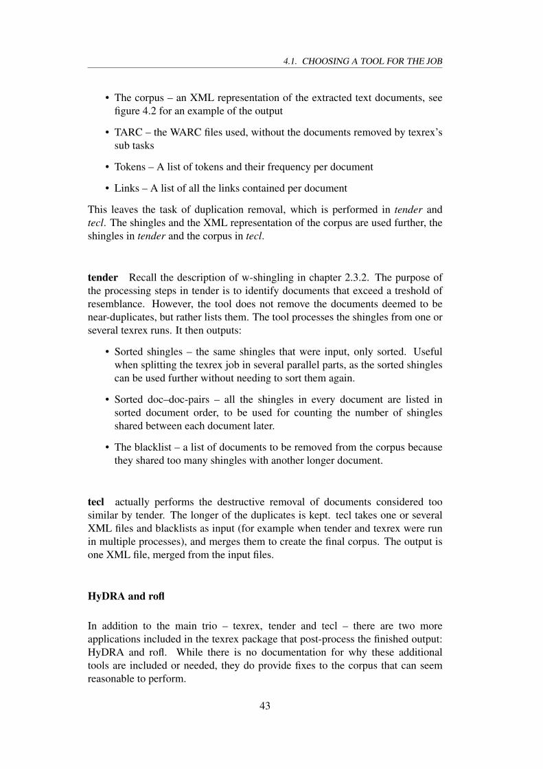
4.1. CHOOSING A TOOL FOR THE JOB
• The corpus – an XML representation of the extracted text documents, seefigure 4.2 for an example of the output
• TARC – the WARC files used, without the documents removed by texrex’ssub tasks
• Tokens – A list of tokens and their frequency per document
• Links – A list of all the links contained per document
This leaves the task of duplication removal, which is performed in tender andtecl. The shingles and the XML representation of the corpus are used further, theshingles in tender and the corpus in tecl.
tender Recall the description of w-shingling in chapter 2.3.2. The purpose ofthe processing steps in tender is to identify documents that exceed a treshold ofresemblance. However, the tool does not remove the documents deemed to benear-duplicates, but rather lists them. The tool processes the shingles from one orseveral texrex runs. It then outputs:
• Sorted shingles – the same shingles that were input, only sorted. Usefulwhen splitting the texrex job in several parallel parts, as the sorted shinglescan be used further without needing to sort them again.
• Sorted doc–doc-pairs – all the shingles in every document are listed insorted document order, to be used for counting the number of shinglesshared between each document later.
• The blacklist – a list of documents to be removed from the corpus becausethey shared too many shingles with another longer document.
tecl actually performs the destructive removal of documents considered toosimilar by tender. The longer of the duplicates is kept. tecl takes one or severalXML files and blacklists as input (for example when tender and texrex were runin multiple processes), and merges them to create the final corpus. The output isone XML file, merged from the input files.
HyDRA and rofl
In addition to the main trio – texrex, tender and tecl – there are two moreapplications included in the texrex package that post-process the finished output:HyDRA and rofl. While there is no documentation for why these additionaltools are included or needed, they do provide fixes to the corpus that can seemreasonable to perform.
43
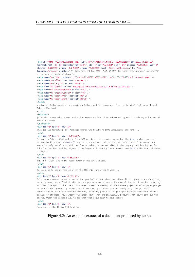
CHAPTER 4. TEXT EXTRACTION FROM THE COMMON CRAWL
Figure 4.2: An example extract of a document produced by texrex
44

4.1. CHOOSING A TOOL FOR THE JOB
HyDRA or Hyphenation Detection and Removal Application, does what thename entails: it removes hard hyphenation, which is hyphenation inserted inwords to signal a line break, often used in print where there is no room in aline for a word. The corpus has removed the context for which the line breakwas necessary and will therefore need to detect the occurrences of line breakhyphenation that is no longer necessary.
hyphe– nation → hyphenation
An example of hard hyphenation being removed
Why these hard hyphenations occur in web sites is not immediately intuitive, as itdoes not seem usual for text to be edited to fit in a set size on the web. Rather theopposite, the web site dynamically adjusting the size of its containers for the textseems to be the norm. Transcripts from printed text may be one source of hardhyphenation on the web, but in these cases it can be discussed whether one wouldwant to fix the occurences, or let it stay true to the original content.
The program takes a list of unigrams with frequencies that are to be deemed validwords as input, and removes hyphenation if the removal of it produces a wordfrom the unigram list. In addition to the unigram list, the corpus is also neededas input. The output is the corpus, but with the hyphenation removed. The inputcorpus does not need to be in the output format of texrex, as long as it is text.
rofl In addition to HyDRA, there is one more post-processing tool, rofl – orrun-on fixer lab. This is “a tool to fix run-together sentences based on word lists”(Schäfer, 2014, p. 2). Sentences like “This sentence ends in punctuation.Andthis sentence has no white-space after said punctuation” will be split up in twosentences.
Unlike HyDRA, rofl does not take unigrams with frequencies as input, but rather alist of valid words, in addition to the corpus. As there are several examples whereno whitespace around punctuation is intended, rofl also supports specifying lists ofprefixes and suffixes to ignore if found right before or right after punctuation. Thisis needed to avoid splitting urls (“nrk.no” would become “nrk. no” without ‘no’listed in the suffix list). Additionally, one can make rofl ignore a line completelyif it matches a user-specified regex string. This is useful to skip lines of metadata.
Like HyDRA, it is not obvious why such a tool is considered to be needed. Theremight be lacking white-space between sentences where non-text markup workedas a sentence splitter before said markup was removed. If this is the case, thenwhite-space will need to be inserted, and a tool like rofl makes sense. But in othercases, it is not obvious whether editing the original content is wanted, even thoughwe might disagree with the way the content was written. See the discussion insection 4.2.4.
45
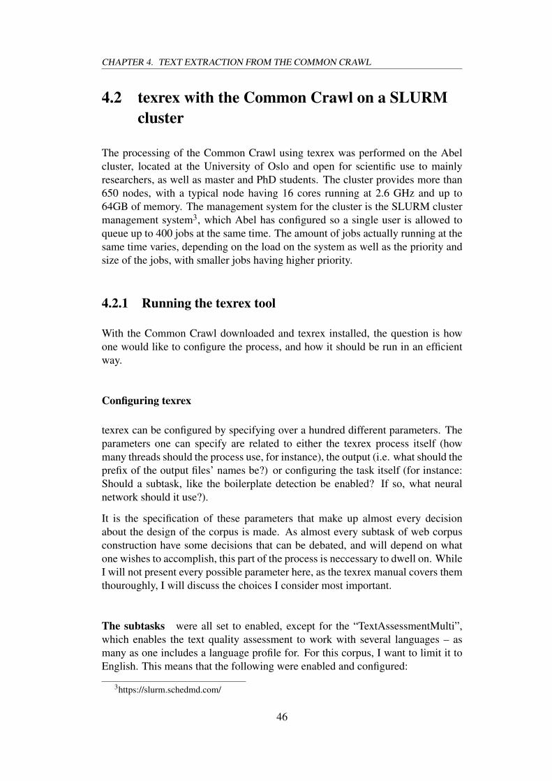
CHAPTER 4. TEXT EXTRACTION FROM THE COMMON CRAWL
4.2 texrex with the Common Crawl on a SLURMcluster
The processing of the Common Crawl using texrex was performed on the Abelcluster, located at the University of Oslo and open for scientific use to mainlyresearchers, as well as master and PhD students. The cluster provides more than650 nodes, with a typical node having 16 cores running at 2.6 GHz and up to64GB of memory. The management system for the cluster is the SLURM clustermanagement system3, which Abel has configured so a single user is allowed toqueue up to 400 jobs at the same time. The amount of jobs actually running at thesame time varies, depending on the load on the system as well as the priority andsize of the jobs, with smaller jobs having higher priority.
4.2.1 Running the texrex tool
With the Common Crawl downloaded and texrex installed, the question is howone would like to configure the process, and how it should be run in an efficientway.
Configuring texrex
texrex can be configured by specifying over a hundred different parameters. Theparameters one can specify are related to either the texrex process itself (howmany threads should the process use, for instance), the output (i.e. what should theprefix of the output files’ names be?) or configuring the task itself (for instance:Should a subtask, like the boilerplate detection be enabled? If so, what neuralnetwork should it use?).
It is the specification of these parameters that make up almost every decisionabout the design of the corpus is made. As almost every subtask of web corpusconstruction have some decisions that can be debated, and will depend on whatone wishes to accomplish, this part of the process is neccessary to dwell on. WhileI will not present every possible parameter here, as the texrex manual covers themthouroughly, I will discuss the choices I consider most important.
The subtasks were all set to enabled, except for the “TextAssessmentMulti”,which enables the text quality assessment to work with several languages – asmany as one includes a language profile for. For this corpus, I want to limit it toEnglish. This means that the following were enabled and configured:
3https://slurm.schedmd.com/
46

4.2. TEXREX WITH THE COMMON CRAWL ON A SLURM CLUSTER
• Duplication detection
The duplication detection includes removing true duplicates and producingshingles for the near-duplication removal in the next tool in the tool chain –tender. There are a couple of key decisions to make for this step:
○ The size of each document’s fingerprint: Set to 64 bytes.
○ Shingles are n-grams, but what should n be? Broder (1997) use 10,while the manual and Schäfer and Bildhauer (2012) use 5. I went with5, as well, as the paper’s results using 5 were good.
• Size filtering, the removal of too large or too small documents, is donetwice, once while reading files (before any HTML stripping) and onceafter the HTML is stripped. This is the first step that performs removal ofdocuments, before the boilerplate detector and duplicate remover performsadditional filtering later.
Recall the amount of documents removed per step from table 3.9, where thesize thresholds ended up removing a lot of the crawled documents. Becauseof this relatively high amount of removed documents due to size, it is naturalto question if the thresholds here and after boilerplate classification are settoo aggressively.
The purpose of the lower size thresholds are to remove documents thatis assumed to end up with little to no text after cleaning. The upperthresholds are set for the documents that are very large, and that will beexpensive for the more costly algorithms to process, like the boilerplateand duplication detection. The texrex manual (Schäfer, 2014) recommendsdiscarding documents above 256 or 512 kilobytes.
I followed the recommendations of the manual and from Schäfer andBildhauer (2012), and set:
○ Min. size of non-cleaned document: 2kb
○ Max. size of non-cleaned document: 512kb
○ Min. number of texrex-separated paragraphs (after HTML stripping):2
○ Minimum character count per document (after HTML stripping): 1000
• UTF-8 validation is done with IBM’s ICU, where the documents’ encodingis identified and converted to UTF-8. If the encoding is invalid, thedocument is removed.
• Boilerplate detection has many configurable parameters, from whichneural network to use (recall section 2.3.2) to where the boundary betweenboilerplate and non-boilerplate should go. My settings were:
47

CHAPTER 4. TEXT EXTRACTION FROM THE COMMON CRAWL
○ The neural net to use for classification: texrex comes with someneural nets that are already trained. The one chosen was the onetrained for English-, as per the results of Schäfer (2016a), which gavehigher precision/recall/F1-scores for a neural net trained specificallyfor English.
○ The threshold for when to count a paragraph as boilerplate: 0.5.Thresholds between 0.3 and 0.7 all provide decent accuracy andprecision/recall. The ‘optimal’ cut-off point (where precision =recall = F1) varied for different data sets (a data set per language),between 0.49 and 0.62. But as he concludes:
“The accuracy is virtually unchanged when moving from thebalanced thresholds to the default threshold of 0.5” (Schäfer,2016a, p. 8)
○ Minimum amount of non-boilerplate paragraphs in a document to keepit: 1
○ Minimum relative amount of non-boilerplate paragraphs to keepdocument: 0.1
○ Minimum amount of non-boilerplate characters to keep document4:500
○ Minimum relative amount non-boilerplate characters to keep docu-ment: 0.25
○ For the four thresholds above, I went with the default metrics, asthey seem like a good compromise between keeping as much dataas possible at the same time as removing documents that are almostcompletely composed of boilerplate.
• Text quality assessment and language detection, also called “TextAssessment” or “Connected text identification” requires tokenisation for thetoken counts, so I include the parameters for tokenisation as well.
The tokeniser of 2012’s texrex (Schäfer and Bildhauer, 2012) worked byconsidering anything between two non-letters in the ISO-8859 encoding astokens. As texrex is now using UTF-8 as its encoding, a similar but slightlydifferent tokenisation method is surely used. However, I have not found anyupdated information about this.
○ The threshold for when to count a paragraph as boilerplate whencounting tokens for the unigram list: 55
○ Minimum char length of div to count the tokens: 100
4Note that the size filter right after HTML stripping removed documents smaller than 1000characters. This setting also takes the amount of non-boilerplate characters into account.
48
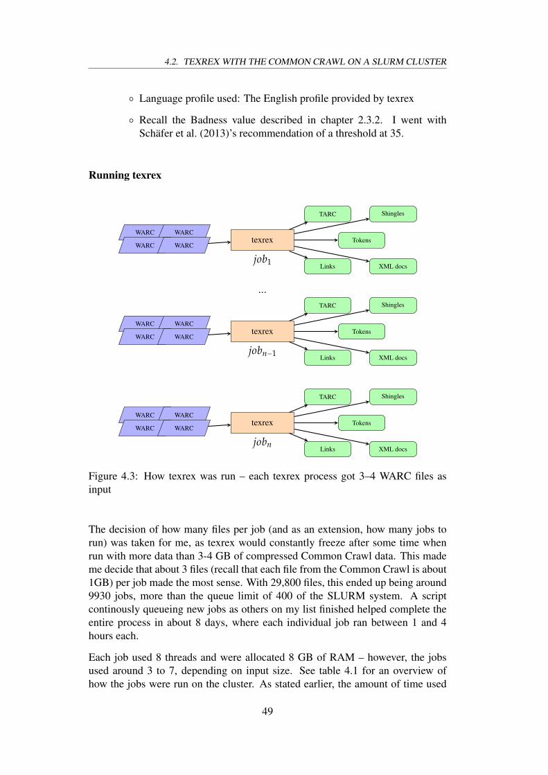
4.2. TEXREX WITH THE COMMON CRAWL ON A SLURM CLUSTER
○ Language profile used: The English profile provided by texrex
○ Recall the Badness value described in chapter 2.3.2. I went withSchäfer et al. (2013)’s recommendation of a threshold at 35.
Running texrex
WARC WARC
WARC WARCtexrex
job1 Links
TARC
Tokens
Shingles
XML docs
...
WARC WARC
WARC WARCtexrex
jobn−1 Links
TARC
Tokens
Shingles
XML docs
WARC WARC
WARC WARCtexrex
jobnLinks
TARC
Tokens
Shingles
XML docs
Figure 4.3: How texrex was run – each texrex process got 3–4 WARC files asinput
The decision of how many files per job (and as an extension, how many jobs torun) was taken for me, as texrex would constantly freeze after some time whenrun with more data than 3-4 GB of compressed Common Crawl data. This mademe decide that about 3 files (recall that each file from the Common Crawl is about1GB) per job made the most sense. With 29,800 files, this ended up being around9930 jobs, more than the queue limit of 400 of the SLURM system. A scriptcontinously queueing new jobs as others on my list finished helped complete theentire process in about 8 days, where each individual job ran between 1 and 4hours each.
Each job used 8 threads and were allocated 8 GB of RAM – however, the jobsused around 3 to 7, depending on input size. See table 4.1 for an overview ofhow the jobs were run on the cluster. As stated earlier, the amount of time used
49

CHAPTER 4. TEXT EXTRACTION FROM THE COMMON CRAWL
process # jobs thr./job alloc. mem. (GB) hours/job hours total
texrex 10k 8 8 1 – 4 200tender 995 1 16 0.5 - 1 (72) 100tecl 498 1 12 3 48HyDRA 71 1 2 10 12rofl 71 1 2 16 20
Table 4.1: A breakdown of how I ended up setting up the jobs for the differentprocesses
to complete the jobs depends heavily on the cluster’s load, so one’s mileage mayvary, even on similar systems.
About 150 jobs had either timed out or crashed, with no output as the result. Re-running these jobs saw that number decline to about 30 jobs that would not finishsuccessfully. Inspection revealed a similar problem to the one seen when tryingto run texrex with too much data, and so I set up new jobs with this data, leavingone file per job. Every job proceeded to complete successfully.
4.2.2 A tender deduplication
The next tool in the chain, tender, can take in several shingle files output by eachtexrex job, sort them and produce a blacklist of duplicate documents that shouldbe removed.
It is possible to configure the tool, but unlike the extensive configuration optionsof texrex, tender is configured using simple command line options. The mostimportant one is likely the --limit option, the threshold for how many shingles thatneed to overlap between documents to consider them near-duplicates. The defaultis 5, which is also used in the paper, and is what I used as well.
As tender needs to compare each document’s shingles with each other, there needsto be one single superprocess that in the end takes all the shingles as its input.Luckily, tender also supports taking blacklists that have already been produced byother tender processes as input, skipping the documents that already occur on theblacklist.
The first try Initially, I tried running tender concurrently by splitting the task inseveral ‘layers’ of jobs, where the first layer would consist of 995 jobs havingshingle files from 10 texrex processes per tender job, going from about 9950shingle files to 995 blacklists. I then planned to continue to merge groups of outputfrom processes from the previous layer to keep running processes concurrently
50
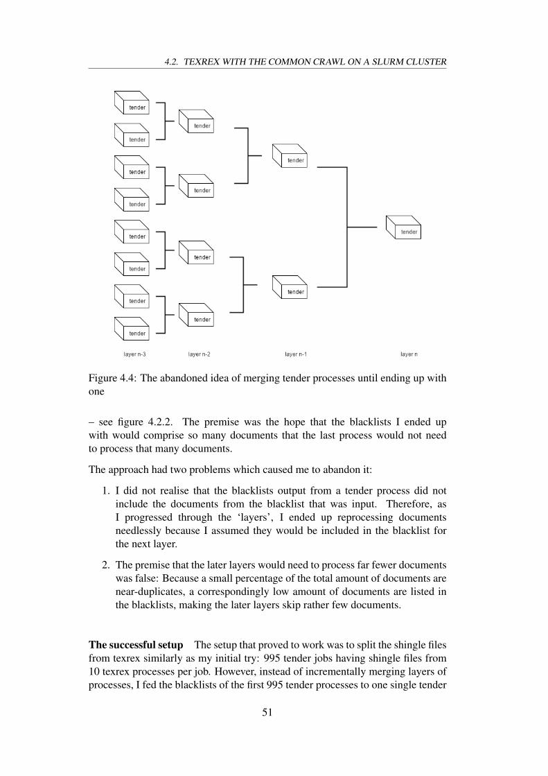
4.2. TEXREX WITH THE COMMON CRAWL ON A SLURM CLUSTER
Figure 4.4: The abandoned idea of merging tender processes until ending up withone
– see figure 4.2.2. The premise was the hope that the blacklists I ended upwith would comprise so many documents that the last process would not needto process that many documents.
The approach had two problems which caused me to abandon it:
1. I did not realise that the blacklists output from a tender process did notinclude the documents from the blacklist that was input. Therefore, asI progressed through the ‘layers’, I ended up reprocessing documentsneedlessly because I assumed they would be included in the blacklist forthe next layer.
2. The premise that the later layers would need to process far fewer documentswas false: Because a small percentage of the total amount of documents arenear-duplicates, a correspondingly low amount of documents are listed inthe blacklists, making the later layers skip rather few documents.
The successful setup The setup that proved to work was to split the shingle filesfrom texrex similarly as my initial try: 995 tender jobs having shingle files from10 texrex processes per job. However, instead of incrementally merging layers ofprocesses, I fed the blacklists of the first 995 tender processes to one single tender
51
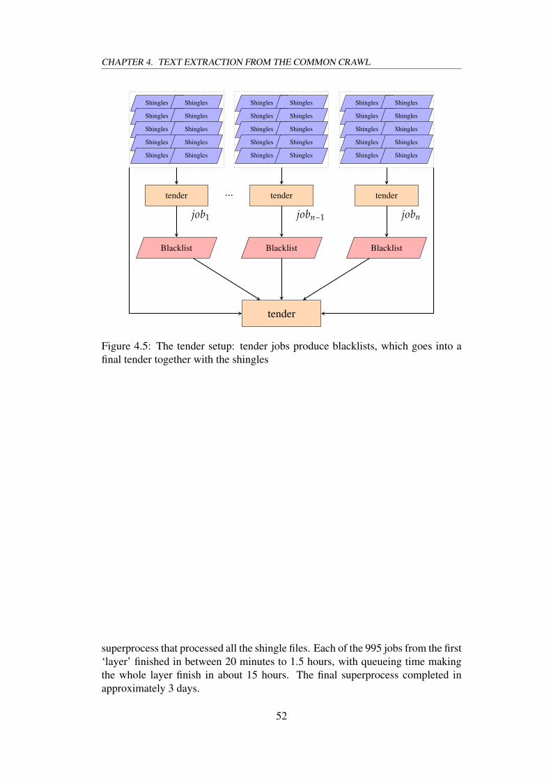
CHAPTER 4. TEXT EXTRACTION FROM THE COMMON CRAWL
Shingles Shingles
Shingles Shingles
Shingles Shingles
Shingles Shingles
Shingles Shingles
Shingles Shingles
Shingles Shingles
Shingles Shingles
Shingles Shingles
Shingles Shingles
Shingles Shingles
Shingles Shingles
Shingles Shingles
Shingles Shingles
Shingles Shingles
tender
job1
... tender
jobn−1
tender
jobn
Blacklist Blacklist Blacklist
tender
Figure 4.5: The tender setup: tender jobs produce blacklists, which goes into afinal tender together with the shingles
superprocess that processed all the shingle files. Each of the 995 jobs from the first‘layer’ finished in between 20 minutes to 1.5 hours, with queueing time makingthe whole layer finish in about 15 hours. The final superprocess completed inapproximately 3 days.
52
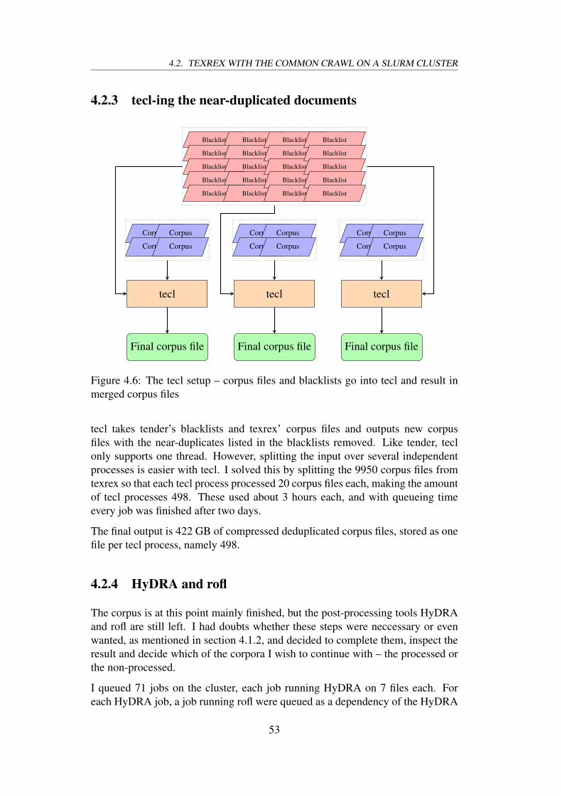
4.2. TEXREX WITH THE COMMON CRAWL ON A SLURM CLUSTER
4.2.3 tecl-ing the near-duplicated documents
Blacklist Blacklist
Blacklist Blacklist
Blacklist Blacklist
Blacklist Blacklist
Blacklist Blacklist
Blacklist
Blacklist
Blacklist
Blacklist
Blacklist
Blacklist
Blacklist
Blacklist
Blacklist
Blacklist
Corpus Corpus
Corpus Corpus
Corpus Corpus
Corpus Corpus
Corpus Corpus
Corpus Corpus
tecl tecltecl
Final corpus file Final corpus fileFinal corpus file
Figure 4.6: The tecl setup – corpus files and blacklists go into tecl and result inmerged corpus files
tecl takes tender’s blacklists and texrex’ corpus files and outputs new corpusfiles with the near-duplicates listed in the blacklists removed. Like tender, teclonly supports one thread. However, splitting the input over several independentprocesses is easier with tecl. I solved this by splitting the 9950 corpus files fromtexrex so that each tecl process processed 20 corpus files each, making the amountof tecl processes 498. These used about 3 hours each, and with queueing timeevery job was finished after two days.
The final output is 422 GB of compressed deduplicated corpus files, stored as onefile per tecl process, namely 498.
4.2.4 HyDRA and rofl
The corpus is at this point mainly finished, but the post-processing tools HyDRAand rofl are still left. I had doubts whether these steps were neccessary or evenwanted, as mentioned in section 4.1.2, and decided to complete them, inspect theresult and decide which of the corpora I wish to continue with – the processed orthe non-processed.
I queued 71 jobs on the cluster, each job running HyDRA on 7 files each. Foreach HyDRA job, a job running rofl were queued as a dependency of the HyDRA
53
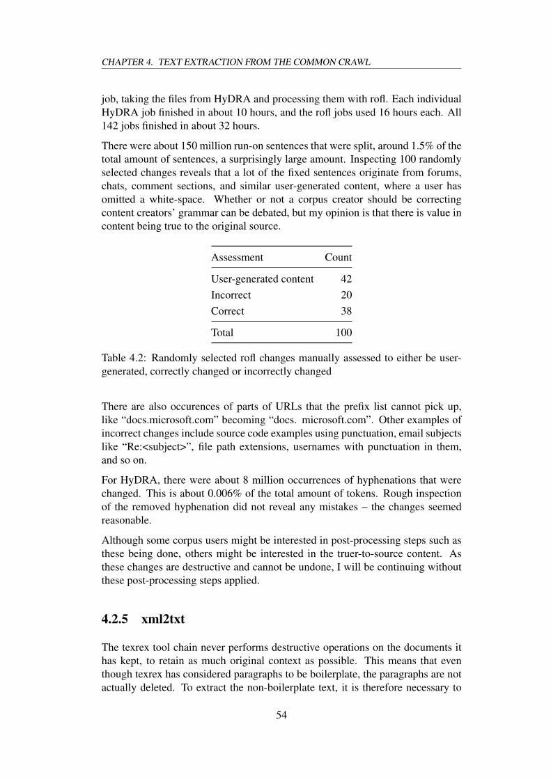
CHAPTER 4. TEXT EXTRACTION FROM THE COMMON CRAWL
job, taking the files from HyDRA and processing them with rofl. Each individualHyDRA job finished in about 10 hours, and the rofl jobs used 16 hours each. All142 jobs finished in about 32 hours.
There were about 150 million run-on sentences that were split, around 1.5% of thetotal amount of sentences, a surprisingly large amount. Inspecting 100 randomlyselected changes reveals that a lot of the fixed sentences originate from forums,chats, comment sections, and similar user-generated content, where a user hasomitted a white-space. Whether or not a corpus creator should be correctingcontent creators’ grammar can be debated, but my opinion is that there is value incontent being true to the original source.
Assessment Count
User-generated content 42Incorrect 20Correct 38
Total 100
Table 4.2: Randomly selected rofl changes manually assessed to either be user-generated, correctly changed or incorrectly changed
There are also occurences of parts of URLs that the prefix list cannot pick up,like “docs.microsoft.com” becoming “docs. microsoft.com”. Other examples ofincorrect changes include source code examples using punctuation, email subjectslike “Re:<subject>”, file path extensions, usernames with punctuation in them,and so on.
For HyDRA, there were about 8 million occurrences of hyphenations that werechanged. This is about 0.006% of the total amount of tokens. Rough inspectionof the removed hyphenation did not reveal any mistakes – the changes seemedreasonable.
Although some corpus users might be interested in post-processing steps such asthese being done, others might be interested in the truer-to-source content. Asthese changes are destructive and cannot be undone, I will be continuing withoutthese post-processing steps applied.
4.2.5 xml2txt
The texrex tool chain never performs destructive operations on the documents ithas kept, to retain as much original context as possible. This means that eventhough texrex has considered paragraphs to be boilerplate, the paragraphs are notactually deleted. To extract the non-boilerplate text, it is therefore necessary to
54

4.2. TEXREX WITH THE COMMON CRAWL ON A SLURM CLUSTER
process the XML files and retrieve the text where the boilerplate classificationscore for a div is below the threshold.
This was solved by developing a script extracting the relevant information fromthe different XML elements, before collecting the raw text from the paragraphsbelow the threshold. Only the paragraphs with a boilerplate score below a valueinput by the user of the script (0.5 here) is kept in the text version.
Parsing the XML is also possible, but a robust parser is required, as there are afew (around 100 in total for this corpus) mistakes, where it seems like texrex hasoverlapped two documents, even sometimes beginning a new document inside anXML tag of the previous document.
The result of the text extraction is about 115 billion white-space separated tokens,split in files containing 10,000 documents per file – bringing the total amount to8688 files at an average size of 74 MB. Each document is separated by a form-feed character (an ASCII control character, represented as ‘\f’ in C and otherprogramming languages), and each sentence is separated by a new-line character(‘\n’). To keep the link between the extracted non-boilerplate text and the originaldocument, the script generates .meta-files where each line represents a document,with the file name of the origin XML file and the byte offset to find said documentlisted.
To see how much boilerplate that is still kept, I ran xml2txt once more, onlyextracting boilerplate instead of extracting non-boilerplate. This was done bykeeping the paragraphs above a boilerplate score of 0.5. The result was 45 billionwhite-space separated tokens of boilerplate text – a noticeably large amount.
4.2.6 Tokenisation and conversion to CoNLL
While the corpus now exists in both an XML and raw text-format, tokenising itusing a more advanced tokeniser than a white-space tokeniser is a logical nextstep. I used Stanford’s CoreNLP (Manning et al., 2014) for tokenising. The 8688text files were split to 49 jobs of CoreNLP tasks, configured to only tokeniseand sentence split. CoreNLP can do other tasks as well, like part-of-speech–tagging, lemmatisation, Named-Entity Recognition, etc. However, these tasks areexpensive to perform, and was not prioritised.
The output is in the CoNLL format, originally created for the yearly shared task atthe Computational Natural Language Learning conference. Slight changes on thestructure of the format occur from year to year, but the CoreNLP website writesthat their CoNLL format does not correspond to any specific existing formats5.Each line represents a token, and each line has tab-separated information aboutsaid token. Normally, this is information like the lemma of the token, the Part-of-
5https://stanfordnlp.github.io/CoreNLP/cmdline.html
55

CHAPTER 4. TEXT EXTRACTION FROM THE COMMON CRAWL
Representation # Files Total size (GB) Avg. file size
XML 498 1376 847 MBRaw text 8688 645 74 MBCoNLL 8688 2300 264 MB
Table 4.3: Structure of the corpus files. The raw text also come with as many metafiles using about 5GB of space.
Speech tag or similar annotation. As this corpus is only tokenised and sentencesplit, the index and token is the only information per line.
Many NLP tools can read the CoNLL format directly – which makes it apopular format, and the latest CoNLL-U format is a de-facto standard within thefield.
The 49 jobs each ran between 1 and 3 hours. Although each job got the sameamount of files, and each file contains the same amount of documents, eachdocument is not the same size. Therefore, some files are a lot larger than others,and this was evident when running CoreNLP. The memory requirements werelarge, and several of the jobs had to be re-queued because they ran out of memory.For the jobs requiring the most, I had to allocate 24 GB of memory.
4.3 Presenting enC3: the English CommonCrawlCorpus
As the size of the corpus is large, seemingly trivial steps such as extracting textfrom XML, tokenisation or sentence segmentation can take a long time. There aredifferences in the needs of corpus users, as well as differences between what kindsof resources users have access to – everyone does not have access to a cluster, forinstance. Because of this, the corpus is made available in three ways:
• XML
• Raw text + linker files to the XML
• CoNLL
4.3.1 XML
The XML representation is the primary format of the corpus, where all originalmeta data is available and where no text has been removed from the documents,even though the classifier has deemed it boilerplate. This representation is for the
56
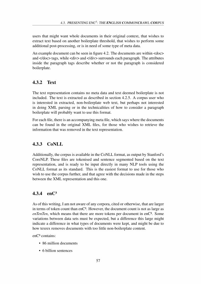
4.3. PRESENTING ENC3: THE ENGLISH COMMONCRAWL CORPUS
users that might want whole documents in their original context, that wishes toextract text based on another boilerplate threshold, that wishes to perform someadditional post-processing, or is in need of some type of meta data.
An example document can be seen in figure 4.2. The documents are within <doc>and </doc> tags, while <div> and </div> surrounds each paragraph. The attributesinside the paragraph tags describe whether or not the paragraph is consideredboilerplate.
4.3.2 Text
The text representation contains no meta data and text deemed boilerplate is notincluded. The text is extracted as described in section 4.2.5. A corpus user whois interested in extracted, non-boilerplate web text, but perhaps not interestedin doing XML parsing or in the technicalities of how to consider a paragraphboilerplate will probably want to use this format.
For each file, there is an accompanying meta file, which says where the documentscan be found in the original XML files, for those who wishes to retrieve theinformation that was removed in the text representation.
4.3.3 CoNLL
Additionally, the corpus is available in the CoNLL format, as output by Stanford’sCoreNLP. These files are tokenised and sentence segmented based on the textrepresentation, and is ready to be input directly in many NLP tools using theCoNLL format as its standard. This is the easiest format to use for those whowish to use the corpus further, and that agree with the decisions made in the stepsbetween the XML representation and this one.
4.3.4 enC³
As of this writing, I am not aware of any corpora, cited or otherwise, that are largerin terms of token count than enC³. However, the document count is not as large asenTenTen, which means that there are more tokens per document in enC³. Somevariations between data sets must be expected, but a difference this large mightindicate a difference in what types of documents were kept, and might be due tohow texrex removes documents with too little non-boilerplate content.
enC³ contains:
• 86 million documents
• 6 billion sentences
57
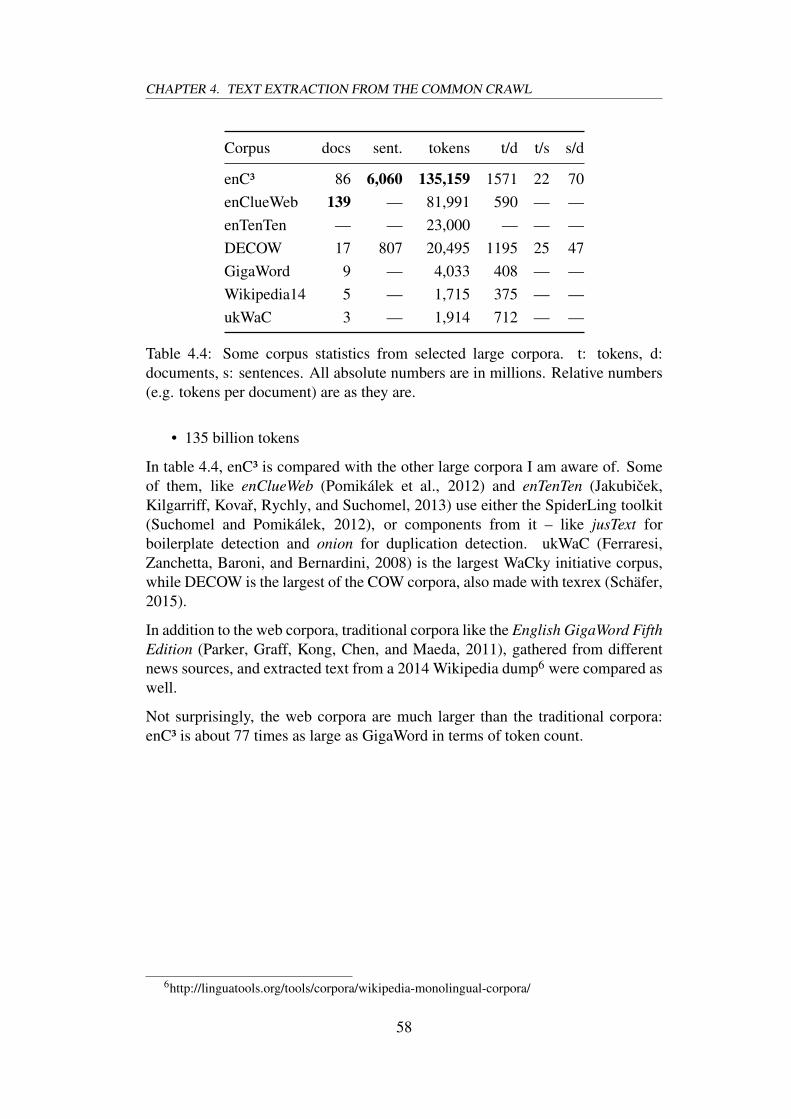
CHAPTER 4. TEXT EXTRACTION FROM THE COMMON CRAWL
Corpus docs sent. tokens t/d t/s s/d
enC³ 86 6,060 135,159 1571 22 70enClueWeb 139 — 81,991 590 — —enTenTen — — 23,000 — — —DECOW 17 807 20,495 1195 25 47GigaWord 9 — 4,033 408 — —Wikipedia14 5 — 1,715 375 — —ukWaC 3 — 1,914 712 — —
Table 4.4: Some corpus statistics from selected large corpora. t: tokens, d:documents, s: sentences. All absolute numbers are in millions. Relative numbers(e.g. tokens per document) are as they are.
• 135 billion tokens
In table 4.4, enC³ is compared with the other large corpora I am aware of. Someof them, like enClueWeb (Pomikálek et al., 2012) and enTenTen (Jakubicek,Kilgarriff, Kovar, Rychly, and Suchomel, 2013) use either the SpiderLing toolkit(Suchomel and Pomikálek, 2012), or components from it – like jusText forboilerplate detection and onion for duplication detection. ukWaC (Ferraresi,Zanchetta, Baroni, and Bernardini, 2008) is the largest WaCky initiative corpus,while DECOW is the largest of the COW corpora, also made with texrex (Schäfer,2015).
In addition to the web corpora, traditional corpora like the English GigaWord FifthEdition (Parker, Graff, Kong, Chen, and Maeda, 2011), gathered from differentnews sources, and extracted text from a 2014 Wikipedia dump6 were compared aswell.
Not surprisingly, the web corpora are much larger than the traditional corpora:enC³ is about 77 times as large as GigaWord in terms of token count.
6http://linguatools.org/tools/corpora/wikipedia-monolingual-corpora/
58

Chapter 5
Evaluating the English CommonCrawl Corpus
Kilgarriff et al. (2014, p. 1) describe how cooks preparing food depend as much onthe quality of their ingredients as their own skill, and draw a parallel to languagetechnology:
Be aware of your sources, you want your produce to be from a farmerwho cares about quality. So it is with language technology. Thosewriting the applications are the cooks, those preparing corpora, thefarmers. The applications are crucial to the success of the enterprise.But – and this becomes inescapable as more and more methods arebased on learning from data – so too is the quality of the data they arebased on.
The paper goes on to describe how there has been a tradition for at least 20 yearsfor evaluating language technology systems. For these evaluations, the samedata has typically been used, with the purpose of leveling the playing field andattributing the prospective better results to the improved system. Specifically, the“same data” that is used are often corpora, and for the purpose of comparabilityto other systems’ results, the same corpora are used for all evaluations.
As was argued with the “chefs and ingredients” example above, making sure thesystem is performing well without regard for the quality of the input data is notsufficient to maximise the quality of the output. An example of this, as mentionedin chapter 2, is Banko and Brill (2001)’s experiments. They showed that for someselected tasks, the performance boost of increasing the size of the input was largerthan fine-tuning the machine-learning algorithms.
Conversely, Versley and Panchenko (2012) quote several experiments where largeweb corpora perform worse than much smaller manually constructed corpora.Similarly, the experiments of Biemann et al. (2013) show that the performance oftheir chosen task, matching corpus collocations with a combinatorial dictionary,
59

CHAPTER 5. EVALUATING THE ENGLISH COMMON CRAWL CORPUS
increase with the size of the web corpus, but gives better results with the smaller,manually constructed British National Corpus regardless.
The differing results might be due to corpus quality, but some task results canperhaps be attributed to the tasks being biased to some text type or domain. Taskstesting for words typically present in news might do better on collections of newstext, while other tasks requiring high coverage of proper nouns might performwell with encyclopedic text. While many desire web corpora that do well witha multitude of tasks, including tasks like the previous examples, it is importantto note this difference in types and domain, and that some tasks might see theirresults affected.
As more corpora become available, corpus users might wonder which corpus tochoose for their task, and corpus creators need to know whether or not they havedone a good job.
Hence, there is a need for some way of evaluating corpora, which could eitherbe done by inspection of the corpus or by using it for downstream tasks, andcomparing the results to other corpora used in the same task.
5.1 Inspection vs. downstream taskexperiments
Language technology systems are often evaluated in an intrinsic or an extrinsicperspective.
5.1.1 Intrinsic evaluation
Intrinsic evaluation is when the quality of a system is assessed by direct analysis ofthe system’s characteristics, and how they relate to some given criteria. Often, thehope is that good results in an intrinsic evaluation will be telling of a system’squality and of its aptness for further use in downstream tasks (however, thisassumption might not always be true – see discussion in section 5.3.3).
Similarly, inspection of corpora and collection of corpus statistics can make surethat some criteria hold true – like the absence of duplicated content, or avoidinghost bias. To illustrate, Biemann et al. (2013) use several corpus statistics –such as the most frequent words, the length distribution of sentences, etc. – toidentify problems, or the lack of them, such as for instance many malformedsentences.
60

5.1. INSPECTION VS. DOWNSTREAM TASK EXPERIMENTS
5.1.2 Extrinsic evaluation
Unlike with intrinsic evaluation, one who performs extrinsic evaluation does notassess or inspect the system directly. Rather, the system is assessed by the useof its output as input in another downstream task. The results of this downstreamtask is then indicative of the quality of the original system, often by comparing thetask results with the results of the same task using other input. However, extrinsicevaluation using one given task may not represent the quality of the system foruse with a different task. Thus, good results in one task do not necessarily implygood results in another.
As stated earlier, corpora are used as data for many machine learning basedlanguage technology tasks. These tasks are candidates for evaluating corporaextrinsically, and some of them have been used for that purpose: Kilgarriff et al.(2014) describe a method for extrinsic evaluation of corpora using a collocationdictionary task, while Biemann et al. (2013) use a combinatorial dictionarycollocation task and a verb-particle combination task.
5.1.3 How to evaluate the English Common CrawlCorpus
Evaluating how well the sub-tasks solved during corpus construction performedcan be useful information. Did the boilerplate removal remove sufficientboilerplate? How much duplication is left? Additionally, corpus statistics toidentify other problems with the content can also be helpful.
However, obtaining every convenient metric to get a fuller understanding of thecorpus is, sadly, too time-consuming. The scale of this project requires choosingone evaluation method. The primary goal of that evaluation is to be able to geta sense of how enC³ fares compared to other corpora in a real-world application,and to get an indication of whether constructing corpora from the web is worththe effort. Hence, choosing a downstream task and comparing the results usingdifferent corpora will be the chosen method of evaluation.
While there probably never will exist a task where good results for that taskcorrespond with good results for all tasks, some probably lend themselves betterto evaluation purposes than others. Tasks where the result greatly depend on theinput data and where a good result can be easily discerned from a poor one arepreferred.
Presently, there is no standard downstream task for corpus evaluation – differentconstructed corpora are evaluated using different methods, and no one methodseems more usual than others. For that reason, the chosen task will not beselected based on what others have done before. Instead, in addition to the pointsmade in the previous paragraph, the task will be selected based on how useful
61

CHAPTER 5. EVALUATING THE ENGLISH COMMON CRAWL CORPUS
the results will be and to keep the complexity of the task as simple as possible.Low complexity tasks are often less time-consuming, and have fewer factors thatcontribute to the result, making it easier to attribute it to the corpus.
One such task that shows disparities between the results of using ‘poor’corpora and ‘good’ corpora, as well as being of large interest to the NaturalLanguage Processing community is the training and evaluation of so-called wordembeddings, or dense word vectors. This will be the chosen task for the evaluationof enC³. Before presenting and discussing the different word embedding modelsand the chosen benchmark tests, I will provide some background on distributionalsemantic representations.
5.2 Embedded word vectors in low-dimensionalspaces
Distributional semantic representations in the form of word vectors have seen anincrease in popularity in the last couple of years. This new-found interest has beenparticularly apparent when it comes to representing words as word embeddings –or dense vectors embedded in low-dimensional spaces.
Representing words as vectors has a long tradition in NLP, and these traditionalrepresentations are often referred to as ‘count-based’ models, contrasted withthe new generation of ‘predict-based’ models. This distinction is not clear-cut, however, and Fares et al. (2017) instead suggest separating explicitrepresentations, “where each dimension of a high-dimensional and sparse vectordirectly corresponds to a contextual feature” and the continuous low-dimensionalword-embeddings.
5.2.1 Explicit word representations
The purpose of constructing vectors representing words is to create a spatialrepresentation of word meaning. In this geometric representation, words that areclose together in the vector space will often be semantically similar as well. Theidea is that words that are used in a similar way often have similar meaning aswell, and thus will co-occur with many of the same words (Harris, 1954; Firth,1957).
Traditionally, word vector representations have as many dimensions as thereare words in the vocabulary, where each word represents one dimension. Theconstruction of the word vector is done by counting how many times the givenword co-occurs with the other words in a specific context (within the samesentence, document, etc). To illustrate, one can imagine the following constructedexample:
62
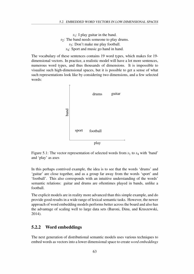
5.2. EMBEDDED WORD VECTORS IN LOW-DIMENSIONAL SPACES
s1: I play guitar in the band.s2: The band needs someone to play drums.
s3: Don’t make me play football.s4: Sport and music go hand in hand.
The vocabulary of these sentences contains 19 word types, which makes for 19-dimensional vectors. In practice, a realistic model will have a lot more sentences,numerous word types, and thus thousands of dimensions. It is impossible tovisualise such high-dimensional spaces, but it is possible to get a sense of whatsuch representations look like by considering two dimensions, and a few selectedwords:
play
band
guitardrums
footballsport
Figure 5.1: The vector representation of selected words from s1 to s4 with ‘band’and ‘play’ as axes
In this perhaps contrived example, the idea is to see that the words ‘drums’ and‘guitar’ are close together, and as a group far away from the words ‘sport’ and‘football’. This also corresponds with an intuitive understanding of the words’semantic relations: guitar and drums are oftentimes played in bands, unlike afootball.
The explicit models are in reality more advanced than this simple example, and doprovide good results in a wide range of lexical semantic tasks. However, the newerapproach of word embedding models performs better across the board and also hasthe advantage of scaling well to large data sets (Baroni, Dinu, and Kruszewski,2014).
5.2.2 Word embeddings
The next generation of distributional semantic models uses various techniques toembed words as vectors into a lower dimensional space to create word embeddings
63

CHAPTER 5. EVALUATING THE ENGLISH COMMON CRAWL CORPUS
(Bengio, Ducharme, Vincent, and Jauvin, 2003; Collobert and Weston, 2008;Mikolov et al., 2013; Pennington et al., 2014; Bojanowski, Grave, Joulin, andMikolov, 2016).
There are several models for training word embeddings, and for the purposes ofevaluating enC³, one of the three most recent will be chosen: Word2Vec (Mikolovet al., 2013), GloVe (Pennington et al., 2014) or fastText (Bojanowski et al., 2016).They are similar in that they all provide word vectors from an input corpus andperform well in the oft-used evaluation tasks (discussed in section 5.2.3).
Word2Vec
Mikolov et al. (2013) took earlier efforts further and can be said to have kickedoff the current popularity of word embeddings with Word2Vec. Unlike the explicitrepresentations and counting co-occurrences, Word2Vec is a prediction basedneural network model that estimate the vectors by predicting words, and tweakingthe weights of the input vector using back propagation based on the success of theprediction.
They provided two different architectures for the creation of the vectors – the skip-gram and continuous bag-of-words models. Both are shallow two-layer neuralnetworks that use a continuous window of n words for their prediction. They aredifferent in what they try to predict: the skip-gram model uses a single word totry to predict the n surrounding words. The CBOW model uses the n surroundingwords to predict a single word. See figure 5.2.
GloVe
Interestingly, Pennington et al. (2014)’s Global Vectors goes back to counting co-occurrences, criticising Word2Vec for using local context windows and not takingadvantage of global corpus statistics. The paper identifies how ‘certain aspectsof meaning’ can be extracted by using ratios of co-occurrence probabilities ratherthan the probabilities themselves (see table 5.1). They go on to train word vectorsby minimising the difference between the dot product of the word vector and thelogarithm of the words’ probability of co-occurrence.
fastText
fastText (Bojanowski et al., 2016) is an extension on Word2Vec’s Skip-grammodel that also incorporates character n-grams in their model. That is, a wordvector in the fastText model is the sum of the vectors of the character n-grams thatmake up the word. The advantage, according to the paper, is that rare words canbe represented more accurately, as the character n-grams that make up the word
64
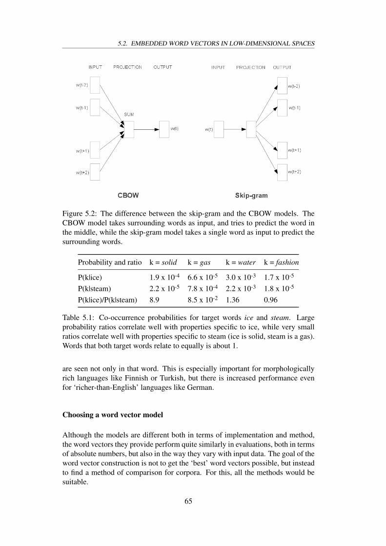
5.2. EMBEDDED WORD VECTORS IN LOW-DIMENSIONAL SPACES
Figure 5.2: The difference between the skip-gram and the CBOW models. TheCBOW model takes surrounding words as input, and tries to predict the word inthe middle, while the skip-gram model takes a single word as input to predict thesurrounding words.
Probability and ratio k = solid k = gas k = water k = fashion
P(k|ice) 1.9 x 10⁻⁴ 6.6 x 10⁻⁵ 3.0 x 10⁻³ 1.7 x 10⁻⁵
P(k|steam) 2.2 x 10⁻⁵ 7.8 x 10⁻⁴ 2.2 x 10⁻³ 1.8 x 10⁻⁵
P(k|ice)/P(k|steam) 8.9 8.5 x 10⁻² 1.36 0.96
Table 5.1: Co-occurrence probabilities for target words ice and steam. Largeprobability ratios correlate well with properties specific to ice, while very smallratios correlate well with properties specific to steam (ice is solid, steam is a gas).Words that both target words relate to equally is about 1.
are seen not only in that word. This is especially important for morphologicallyrich languages like Finnish or Turkish, but there is increased performance evenfor ‘richer-than-English’ languages like German.
Choosing a word vector model
Although the models are different both in terms of implementation and method,the word vectors they provide perform quite similarly in evaluations, both in termsof absolute numbers, but also in the way they vary with input data. The goal of theword vector construction is not to get the ‘best’ word vectors possible, but insteadto find a method of comparison for corpora. For this, all the methods would besuitable.
65

CHAPTER 5. EVALUATING THE ENGLISH COMMON CRAWL CORPUS
There are few points of reference in terms of how much time each method requiresto train, and also how they scale to larger data sets. The few informal sources thatdo exist12 made me lean towards GloVe, as it seems to require a lot of RAM, butthe payoff is that it runs quicker. This fits with my situation, where I have accessto a system with a lot of RAM, and where time is the largest constraint.
Additionally, the then–state-of-the-art evaluation results Pennington et al. (2014)reported were evaluated on word vectors trained on Common Crawl data, whichis provided on the GloVe website3 together with several other pre-trained vectors.This is an interesting point of comparison for evaluating enC³, and made me selectGloVe as my word vector model.
5.2.3 Evaluation of word vectors
Unlike with the evaluation of corpora, there do exist oft-used, standard waysof evaluating word vectors. All the word embedding training architectures usethese methods to compare themselves with each other. The methods are wordanalogy tasks and comparisons with human word similarity judgments. Bothtasks are based on the word vectors’ capability of encoding different kinds ofsimilarity.
Word analogy tasks
Mikolov et al. (2013) presented the observation that word vectors encode morecomplex kinds of similarities than semantically similar words also being close invector space (in terms of cosine similarity or euclidean distance) – like ‘France’and ‘Italy’. They designed a task that tests for other kinds of similarities,similarities that show relations and analogies between words.
The task is to solve the question “A is to B as C is to D”, where D will be filled inusing the word vectors, and A, B and C is given as input. For instance, the question“Oslo is to Norway as Athens is to ___” can be solved by vector algebra:
X = vector(“Norway”) − vector(“Oslo”) + vector(“Athens”) (5.1)
Then the vector space is searched for the word closest to the vector X measuredby cosine distance (disregarding the input question words in the search), andthis word is used as the answer. The idea is that if the word embeddings areof sufficient quality, the intuitive semantic relationship matches the output. Forthe example above, “Greece” is expected as output.
1http://dsnotes.com/post/glove-enwiki/2https://rare-technologies.com/fasttext-and-gensim-word-embeddings/3https://nlp.stanford.edu/projects/glove/
66

5.2. EMBEDDED WORD VECTORS IN LOW-DIMENSIONAL SPACES
Figure 5.3: The vector differences encode the syntactic relationship betweenconjugated verbs
This method reveals that general relationships between words are encoded in thevector differences (see figure 5.3), and that this analogical similarity-task canfind different types of relationships. Mikolov et al. (2013) created a dataset of8869 semantic and 10675 syntactic questions. The semantic relationships thatare tested include currency (Norway → kroner, USA → dollar) and female–male(brother → sister, grandson → granddaughter), while the syntactic word pairs testfor relationships such as present participle (think→ thinking, read→ reading) andnationality adjectives (Denmark → Danish, Germany → German).
Word similarity
The analogy task tests for more complex vector space substructures, but the moretraditional test for semantic similarity by looking for a word’s nearest neighbourin vector space is also useful.
This is done by using lists of word pairs that have had their similarity assessedby human judges. There are differences in how these lists are compiled, how thesimilarity scores for a word pair are determined and what types of words that areincluded in the list. I will discuss the differences between some popular wordsimilarity lists in section 5.3.2.
67

CHAPTER 5. EVALUATING THE ENGLISH COMMON CRAWL CORPUS
These word pair lists are then assessed using the word vectors, where a similarityscore is found by calculating the cosine similarity between the words. In theend, there will be two lists sorted by the similarity score: One using the humanjudgments and one using the scores from the word vectors.
The word vectors are considered to perform well if the two lists have rankedthe word pairs similarly. Specifically, Spearman’s rank correlation coefficient(Spearman, 1904) is often used to find a number ranging between -1 (the lists’rankings are opposite of each other) and 1 (the lists’ rankings are identical), and asclose to 1 the score is, the better the word vectors are considered to perform.
5.3 Training and evaluating word embeddings withenC³ data
Training word vectors on 135 billion tokens will be an expensive operation.Just like with the corpus construction, the Abel cluster will be used for thetraining.
5.3.1 Training word vectors using GloVe
Several parameters need to be configured for the model, and because the intentionis to be able to compare the resulting word vectors to the word vectors ofPennington et al. (2014), the parameters are set equal to the ones the paperdescribes when training their example vectors (see table 5.2), except for the initiallearning rate and the vocabulary size – see discussion below. In addition to theparameters, enC³ is pre-processed in the same way the paper pre-processed theircorpora: Tokenised using the Stanford tokeniser, lowercased and merged to onefile.
GloVe training is split up in four processes:
• Creating the vocabulary
• Counting co-occurrences
• Shuffling the co-occurrences
• Training the word vectors
Building the vocabulary
Creating the vocabulary was a relatively inexpensive operation, and completedin about 15 hours, using one thread. Pennington et al. (2014) stated that forthe smaller corpora, a vocabulary size of 400,000 was used, but for the larger
68

5.3. TRAINING AND EVALUATING WORD EMBEDDINGS WITH ENC³ DATA
Param. Value
Vocabulary size 2,000,000Window size 10Vector dimension 300η 0.03α 0.75xmax 100Iterations 100
Table 5.2: The parameters chosen for the co-occurrence counting and the trainingof the word vectors. The window size represents the number of context words tothe left and to the right. η is the initial learning rate, α represents the exponent inthe weighting function used in the cost function of the least squares problem andxmax represents the cutoff in the same weighting function.
Common Crawl based corpora, a vocabulary of “about 2,000,000 words” wasused. The specific vocabulary sizes of their two large corpora did not match,however, and I speculate they really used a frequency threshold instead of amax vocabulary size (the real vocabulary sizes used for their two large corporawere 1.9 million and 2.1 million). I did not come to this realisation until afterthe vocabulary was built, however, and used a vocabulary size of 2,000,000words.
Counting and shuffling co-occurrences
The co-occurrence counting program did not support multi-threading, and tookabout 35 hours. There is a customisable upper memory limit that, if reached,dumps the counted co-occurrences in memory to an overflow file and thencontinues. However, the program must merge these co-occurrence files later, anddid not succeed with low memory requirements. The problem was solved whenusing 200 GB of memory. The resulting co-occurrence matrix file was 147 GB insize. The shuffling of the matrix then took a couple of hours.
Fitting the GloVe
Training the model was the most expensive step, requiring about 30 GB ofmemory and almost 8 days of run time with my setup of 32 threads, 100 iterationsand a vector dimension of 300. A single iteration took around 1.9 hours. Theresulting word vectors were 5.4 GB in size.
The paper originally used an η of 0.05, but this caused the process to output “-nan”
69

CHAPTER 5. EVALUATING THE ENGLISH COMMON CRAWL CORPUS
Process Memory Run-time Threads
Vocab. building 5G 15h 1Counting/Shuffling Co-occurrences 200G 40h 1Training the model 30G 190h 32
Total — 245h —
Table 5.3: How the different processes were set up.
instead of the result of the cost function. There was advise on the GloVe forumsto lower the initial training rate, and an η of 0.03 solved the problem4.
The model generates two sets of word vectors, the vectors themselves (W) andthe context word vectors (W). Pennington et al. (2014) write that when the co-occurrence matrix is symmetric (which it is when choosing a context both to theleft and the right of the word), W and W are equivalent, differing only from theirrandom initialisations. They choose to combine the two vectors, as that gives asmall performance boost, and this is also the default output of the training tool.Like the paper, I configured GloVe to output W+W.
5.3.2 Evaluation of the word embeddings
As was stated earlier, the intention of the enC³ word vectors is to be as comparableto the example GloVe word vectors as possible, as it is not feasible for this projectto train more word vectors based on other corpora for comparison. This alsomeans that the evaluation scores of the enC³ word vectors cannot be compareddirectly with word vectors created with other frameworks like Word2Vec orfastText, or even with GloVe vectors created with different parameters than these.The ‘most optimal’ word vectors for enC³ are in other words yet to be created, andwill also depend on the task.
The evaluation scores of the GloVe example vectors are listed in the paper, butthey are also available for download from the GloVe website. For the evaluationand comparison, I have run my own evaluations using two of the available sets ofpre-trained word vectors, in addition to my own:
The first word vectors are trained on a Wikipedia 2014 dump (1.6B tokens)concatenated with the Gigaword Fifth Edition (4.3B tokens). Wikipedia datais also used by Bojanowski et al. (2016), and the Wikipedia + GigaWordcombination is used by Fares et al. (2017). The latter find vectors trained onWikipedia data to be especially good at the semantic analogy task. As the semanticanalogy task tests for a lot of proper nouns like city and country names, the high
4https://groups.google.com/forum/#!msg/globalvectors/LHxRIWJnR6g/-IvY78hPNEAJ
70

5.3. TRAINING AND EVALUATING WORD EMBEDDINGS WITH ENC³ DATA
performance of Wikipedia data on this task is expected, as it has particularly highcoverage of those.
The second set of GloVe vectors are trained on Common Crawl data. From theGloVe paper and available documentation, it is unknown whether this data wastaken from the WET files or extracted from HTML, the version(s) of the CommonCrawl snapshot(s) used, and whether several months of data or only one monthlycrawl was used. It seems unlikely that Pennington et al. (2014) have used a lot oftime and resources on cleaning the data as extensively as described in this thesis,but it cannot be ruled out.
As of this writing, there is no information about the Common Crawl data set thatwas used at all, except for its size: 42 billion tokens. Information about how thedata was obtained seems to be lost5. Since the best results of the evaluations ofthe GloVe model all came from the vectors trained on this data, this is unfortunatein terms of replicability.
The evaluation process
The same evaluation tasks that were described in section 5.2.3 will be used forthis evaluation.
For the analogical similarity task, the same data set used by Mikolov et al. (2013)is used, similarly divided into semantic and syntactic parts. The evaluationsare done using the Python evaluation code included in the GloVe-project, wherevectors are normalised so that each vector has a length of 1 before the vectorarithmetic is performed.
Evaluation of the different word similarity lists were done using the commandline tools of Faruqui and Dyer (2014)6. The tools compute the Spearman’s rankcorrelation coefficient between the human-rated lists taken as input and the rankedlists the tools produced by using the word vectors and cosine similarities.
However, for the word similarity task only, the above tools and Pennington etal. (2014) normalise their vectors in different ways, leading to different results.Both approaches use the cosine similarity, and thus inherently normalise so thateach vector has a length of 1. However, Pennington et al. (2014, p. 8) state that“A similarity score is obtained from the word vectors by first normalising eachfeature across the vocabulary...”, in addition to the normalisation done in cosinesimilarity calculation. I interpreted this as column-wise normalisation (if thinkingof the set of word vectors as a matrix), where each feature is divided by thesquare root of the sum of its column’s squared features – a sort of vector lengthnormalisation, but using the column to calculate the norm instead of the row (thevector). Interestingly, the latter approach makes the similarity scores higher for
5https://github.com/stanfordnlp/GloVe/issues/746https://github.com/mfaruqui/eval-word-vectors
71

CHAPTER 5. EVALUATING THE ENGLISH COMMON CRAWL CORPUS
Model Results
Corpus Dim. Size Semantic Syntactic Total
WikiGiga 300 6B 77.44 67.00 71.74GloveCC 300 42B 81.85 69.25 74.96enC³ 300 135B 77.89 73.14 75.30
Table 5.4: The results of the analogy task, broken down to semantic and syntacticparts
all corpora and all tests, but does also introduce different relative results betweenthe different corpora.
The performance boost with column-wise normalisation is noteworthy, and is asfar as I know not widespread – I could not find any reports of it other than theshort notice by Pennington et al. (2014). Both approaches were used for theseevaluations, and as the former approach is the prevalent approach and the latterprovides the best results, both results are reported below.
The analogy similarity results
The results of the analogy task can be seen in table 5.4. The most obvious resultto note is that both models based on web corpora perform better than the modeltrained on the Wikipedia/Gigaword corpus. This can perhaps be an indicationthat size does matter. However, the data set the WikiGiga model is based on ishighly dissimilar from the Common Crawl-based data sets of the two others, andattributing any performance difference to any specific reason is at this point notpossible.
What is interesting is the break-down of the scores in their semantic and syntacticparts. The GloVe vectors based on Common Crawl data, or GloveCC, performreally well on the semantic task – a task Wikipedia based vectors normallyperform well at. The enC³ model also outperforms the WikiGiga model in thesemantic task, although not by much, and is beaten by around 4 percentage pointsby GloveCC. This is noteworthy, as the two corpora are based on the same type ofdata, and enC³ is over three times the size of GloveCC. With GloveCC’s largeperformance increase over WikiGiga, one could have expected enC³ to eithermatch or outperform GloveCC in this area.
Similarly interesting, enC³ outperforms the other two models in the syntactic partof the results. While GloveCC has a syntactic performance increase over theWikiGiga model, its largest increase was in the semantic results. It is not easy toattribute the performance gain of the enC³ model to some inherent characteristicof the corpus. The size difference can be the whole reason the results are better,
72

5.3. TRAINING AND EVALUATING WORD EMBEDDINGS WITH ENC³ DATA
Model WS353 MC RG SCWS RW SL999 YP V144
WikiGiga 60.5 70.3 76.6 56.3 41.27 37.1 56.1 30.5GloveCC 62.9 77.7 81.2 54.1 38.5 37.4 53.2 32.8enC³ 65.1 76.7 78.6 56.8 39.4 37.1 56.4 35.5
Table 5.5: The results of the word similarity task with vector normalisation so thateach vector has length 1
Model WS353 MC RG SCWS RW SL999 YP V144
WikiGiga 65.6 72.4 76.9 61.4 45.9 40.8 58.0 36.1GloveCC 75.7 83.6 82.3 65.3 48.7 45.3 59.6 37.2enC³ 75.7 79.7 78.0 66.1 50.1 42.3 59.8 37.8
Table 5.6: The results of the word similarity task where each feature is normalisedacross the vocabulary.
or the performance increase may come from the corpus cleaning.
In total, the enC³ model performs slightly better than the GloveCC model, and alot better than the WikiGiga model.
The word similarity results
The word pair lists that were chosen are listed and described below. They haveeither been created using different methods, or are trying to test for differentcharacteristics. Some tests are included because they are popular, and typicallyused for the word similarity task. All of the lists have had their word pairs scoredby a number of human judges, and the score used to rank the word pairs is theaverage of the human scores. The scales used are different for the different wordpair lists, but all of the lists have asked their raters to rate word pairs on a scalefrom non-similar to similar, with some lists like SimLex-999 giving additionalinstructions.
WS353 was prepared by Finkelstein et al. (2001), and contains 353 noun pairsthat have had their similarities judged by humans, 153 of them by 13 judges andthe other 200 by 16 judges.
MC contains 30 human annotated noun pairs that were originally prepared toshow the relationship between semantic similarities and similar contexts (Miller
7The out of vocabulary rate is very high, at 12.4%, so the score of 41.2 is not comparable tothe others. The oov rate was 0.9% for enC³ and 1.0% for GloveCC.
73

CHAPTER 5. EVALUATING THE ENGLISH COMMON CRAWL CORPUS
and Charles, 1991).
RG is similar in intention to the MC data set, and contains 65 noun word pairs(Rubenstein and Goodenough, 1965). Both MC and RG are small and olderdatasets, and it is questionable whether they are large enough to give an accurateaccount of performance in the word similarity task. Small rank differences usinglists of such a small size can give large score differences, and it can be argued thathigh correlations with the larger lists should count for more. However, as theselists are prevalent when the word similarity task is performed, I’m including themfor relatability and comparability.
SCWS – or Stanford’s Contextual Word Similarities – was an answer to theword pair lists above. They state that it is unclear how assigning similarities towords in isolation, without the context, affects the scores human judges set onword pairs. In SCWS, they provide the context and POS-tag together with thewords, and let 10 human raters score the similarity of the word pair. It is importantto note that there are 10 human raters per word pair, and not 10 individualsjudging all the word pairs. They did this by using Amazon Mechanical Turk, andletting highly rated non-experts rate the similarity, citing the experiments of Snow,O’Connor, Jurafsky, and Ng (2008), who showed that non-expert annotators canachieve very close inter-annotator agreement with expert raters. The dataset has1328 noun–noun-pairs, 399 verb–verb, 140 verb–noun, 97 adjective–adjective, 30noun–adjective and 9 verb–adjective pairs, for a total of 2003 word pairs (Huang,Socher, Manning, and Ng, 2012).
RW (Rare Word) specifically tests for the embeddings’ ability to model rarewords, by preparing 2034 word pairs collected from different frequency ranges,thus making sure rare words are present (Luong, Socher, and Manning, 2013).These word pairs are rated in the same way as the SCWS data set, using AmazonMechanical Turk and collecting 10 ratings per word pair. Because of the natureof rare words, many of these words are out of the vocabulary of popular wordvectors, and this is one of the tests where corpus size probably affects the out-of-vocabulary rate directly.
SimLex-999 is different from several of the other word pair lists, because itexplicitly differentiates words that are similar (coast–shore) with words that areassociated, but not similar (clothes–closet), giving high scores to the former, andlow to the latter (Hill, Reichart, and Korhonen, 2016). The popular WS353 listdescribed above gives high scores to both of these examples. SimLex-999 is ratedby 500 human raters, also using Amazon Mechanical Turk, where each word pairwas on average rated by 50 raters. The data set contains 666 noun–noun pairs,222 verb–verb and 111 adjective–adjective, for a total of 999 word pairs.
74
5.3. TRAINING AND EVALUATING WORD EMBEDDINGS WITH ENC³ DATA
YP was made by Yang and Powers (2006), who made their own verb–verb wordpair list, containing 130 verb pairs, because most datasets at the time mostly hadnoun pairs. The word pairs were rated by 2 academic staff and 4 postgraduatestudents.
V144 – or the Verb-144 dataset – is in the same spirit as the YP dataset. Likethe name implies, the dataset contains 144 verb pairs scored by 10 native Englishspeaking people (Baker, Reichart, and Korhonen, 2014).
The two sets of results show non-trivial differences between which model thatperforms the best, and as with other areas of NLP, performance is task-specific:Good relative performance of a model on one word pair list does not necessarilyequate to good performance on another list.
The results are presented in both table 5.5 and in table 5.6. As mentionedearlier, there are two sets of results of the word similarity task, because of thedifferent way Pennington et al. (2014) normalise the vectors. In table 5.5, theresults of the task with ‘regular’ length normalisation are presented, while table5.6 has the results of the feature normalisation – where each feature is normalisedacross the vocabulary, column for column, in addition to the length normalisation.Interestingly, this additional layer of normalisation makes a larger difference inthe results of this task than the choice of corpus for most of the datasets.
There are large differences between the two ways of normalising, where everysingle score improves from doing length normalisation to feature normalisation.The differences between the models are also affected by the different normalisa-tion, and in some cases this change in difference affects which model performsbetter than the others: From enC³ scoring the highest with the WS353 list whenlength normalised, GloveCC matches the score when feature normalising. TheRare Word list favor the WikiGiga model (although the out of vocabulary-rate isa lot higher than the two other models) with length normalisation, but favor enC³with feature normalisation. Some differences become larger, like the MC, RGand SimLex-999 scores being even more in favor of GloveCC, and some becomesmaller, like YP and Verb-144.
Even when performing the feature normalisation and obtaining the higher results,some of the results do not match the results of Pennington et al. (2014), whileothers do. In particular, the scores using the RG, SCWS and RW lists deviate fromthe results listed by the paper, while the scores from using WS353 and MC arealmost the same (a variation of 0.2 and 0 percentage points, respectively). This isan issue of replicability, and while regrettable, does not affect these comparisons,as all the corpora were tested using the same code and datasets. The code, createdby Faruqui and Dyer (2014) and modified by me to achieve the extra feature
75

CHAPTER 5. EVALUATING THE ENGLISH COMMON CRAWL CORPUS
normalisation, is available online8.
The scores do not give a clear picture for which model that performs best, but doclearly show that the WikiGiga model is outperformed in all cases. Like in theanalogy task, it is difficult to point to why this is, but it seems unlikely that webdata would be inherently better suited for this task, and an argument can perhapsbe made that the size difference matters. The larger word pair lists all favor enC³,except for SimLex-999, that have more advanced notions of similarities. Bysimply counting how many word pair lists favor the different models, however,enC³ achieves the best score for most lists.
5.3.3 Better intrinsic results: A better corpus?
The enC³ model can be said to have performed marginally better than theCommon Crawl model used in the GloVe paper and clearly better than theWikipedia/GigaWord-model that is typically used in intrinsic evaluations of wordembeddings. This is exciting, and might be an indicator that larger corpora (andperhaps cleaned corpora) are good sources of data for these tasks.
The comparison done in this chapter was done by training the enC³ wordembeddings using as similar parameters to the GloVe embeddings as possible.This was done to make sure that the prospective performance differences cameas a result of the differences in corpus quality, and not from choosing parametersmore suited to the chosen tasks. However, the disadvantage of this approach isthat the potential of the enC³ corpus might have been impeded by not choosingthe parameters most suited for the corpus. For instance, Pennington et al. (2014)increase vocabulary size as corpus size increases. Other parameters might alsoaffect the performance of the word vectors because of corpus size. As an example,it seems likely that higher vector dimensions are more suited to exploit largecorpus sizes. As a result, the best comparison of corpora using word embeddingswould probably be to tweak the parameters individually for the different corporaso that each corpus performs the best for the chosen task, and then compare theresults. This is a time-consuming endeavour, however, seeing as the training ofone set of word vectors from enC³ took over a week.
Another question is whether or not the results of these intrinsic word vectorevaluations actually give an indication of corpus quality outside of the tasks thatwere performed. For instance, Chiu, Korhonen, and Pyysalo (2016) show in theirpaper that there is no correlation between the performance of the word similaritytask and the performance of their three chosen downstream tasks (Named EntityRecognition, PoS-tagging and chunking), except for one of the word pair lists:SimLex-999.
This might only mean that word vectors specifically tuned to perform well
8https://github.com/kjetilbk/enc3tools
76

5.3. TRAINING AND EVALUATING WORD EMBEDDINGS WITH ENC³ DATA
in different word similarity tasks do not necessarily perform well in otherdownstream tasks, and does not necessarily say much about the corpus used totrain the embeddings. It would be interesting to do similar extensive researchusing different corpora with different word vector training parameters on severaldownstream tasks, to see which corpora perform the best, and whether or not theirperformance is task-specific.
77

Chapter 6
Conclusion and future work
In this project, I have constructed a large collection of texts from web dataprovided by the Common Crawl Foundation. The 135 billion word corpus wasconstructed using texrex, an open-source toolchain that combines several cleaningtasks to produce a high-quality corpus from noisy web documents. While severalweb corpora exist, there are none at the scale of this thesis’ English CommonCrawl Corpus – or enC³. The results of the corpus evaluation showed largeimprovements over the much smaller, more typically used Wikipedia+Gigawordcorpus, and incremental improvements over a web corpus at a third the size usedas comparison. This indicates that size does matter, although it is not the soleimportant factor of corpus quality.
The corpus was constructed using data from the August 2016 Common Crawl,and chapter 3 provided the first systematic review of said data, where the qualityof the provided extracted text files was also assessed and deemed insufficient.Specifically, the text extraction itself – the removal of HTML tags and entities,as well as fixing broken encoding – was incomplete, and would have needed tobe redone. The low quality of the text extraction left the files containing archivedweb data as the best source of data for the corpus construction. The extracted textfiles were compared to the text extraction performed by texrex, which showed thattexrex cleaned the data much better than what has been done with the extractedtext files. All the steps required for high-quality text extraction thus had to beperformed from scratch. Additionally, language identification was performed onthe Common Crawl data, identifying the low amount of data from languages otherthan English, making it difficult to construct large corpora for them.
Discussion about the desiderata of a corpus construction pipeline, beforeconcluding with and presenting the texrex pipeline was done in chapter 4. Then,the particular configuration of the tools that I chose for the current work werediscussed. The corpus construction was configured to achieve high quality,but also to run efficiently, possibly removing non-negligible amounts of data toachieve acceptable run times. A large challenge of the process was handling
79

CHAPTER 6. CONCLUSION AND FUTURE WORK
the extensive amounts of data, which elicited these kinds of choices in theconfiguration. Next, the chapter gave a detailed account of how the jobs wereset up to run on a cluster, focusing on replicability, due to the desire to possiblyrepeat the process in the future (see future work below). The result was the firstrepresentation of the enC³ corpus: the XML representation. The post-processingof these resulting corpus files was done in two steps. As texrex performs non-destructive boilerplate detection, the first step was to provide a boilerplate-freetext representation of the corpus by developing a tool called xml2txt. The secondstep provided the third and final corpus representation, where Stanford CoreNLPwas used to produce tokenised and sentence-segmented CoNLL files. Given thecorpus size, such post-processing steps are not trivial to perform. By making enC³available in all of these representations, the corpus is easy to use immediately fordownstream tasks, while still preserving as much data as possible, should a userwish to perform post-processing using different parameters than I used.
The evaluation of the corpus was performed by training word vectors using GloVewith the corpus as input, and was described in chapter 5. The parameters used forthis training were as close to the ones used by Pennington et al. (2014) as possible,seeing as the intention was not to train the best possible word embeddings for thechosen tasks, but to give as much of an apples-to-apples comparison as possible.The word vectors were compared with two of the pre-trained word vectorsavailable from GloVe, the first trained on a 6 billion token Wikipedia+GigaWordcorpus and the second trained on a 42 billion token web corpus also based onCommon Crawl data.
Two tasks were performed to evaluate the word vectors: A word analogy taskusing the standard dataset provided by Mikolov et al. (2013) and a word similaritytask, where the latter was performed with respect to a large suite of standardbenchmark datasets for word similarity. The findings were interesting in severalregards. For one, a significant performance boost was achieved by column-wisenormalisation of the vectors. Furthermore, both the web corpora considerablyoutperformed the smaller Wikipedia/News corpus, and while the enC³ model didlargely outperform the smaller web corpus, the manner in which it did so wasunexpected. The smaller web corpus outperformed the enC³ model in the semanticpart of the analogy task by a substantial margin, as well as in the word similaritytask using the more complex SimLex-999 word pair list. It is clear that whilecorpus size is an important factor for word vector performance, it is not the onlyone at play.
This work has investigated how to construct a corpus from web data at a largescale, and has evaluated the resulting corpus using the popular task of trainingword vectors, which result is used for a large number of tasks in NLP. As such,it should be noted that the word vectors themselves provide a valuable asset tothe NLP community, and I will make the pre-trained enC³ embeddings availablethrough the community repository launched by Fares et al. (2017), open for non-commercial researchers in the Nordic region. The results of the thesis are concrete
80

6.1. FUTURE WORK
contributions to the NLP community:
• enC³ – a very large web corpus, available through the mentioned communityrepository.
• The word vectors trained on enC³ – also available through said repository.
• A detailed account of how to perform web corpus construction using texrex,if one wants to replicate the process.
• A systematic review of the WET files provided by the Common Crawl, andtheir shortcomings.
• The tools developed for analysing Common Crawl files, and for extractingnon-boilerplate text from the corpus files, made publicly available1.
6.1 Future work
Several parts of this thesis can be fleshed out and explored further in futurework. This relates to issues that either manifested themselves as a consequenceof questions that were revealed after observing the results, or would have requiredtoo much time to perform within the constraints of this thesis. Some suchdirections for future work are summarised below.
6.1.1 Replicating the process
Using the work of this thesis and the tools provided with it, a goal for theLanguage Technology Group at the University of Oslo is to replicate the processand construct an updated web corpus from Common Crawl data once a year.Seeing how Common Crawl data has developed and increased in size from whenthis thesis was begun – with the compressed WARC files in August 2016 takingup 30TB, and 60TB in the March 2017 crawl – there is absolutely potential forlarge, clean web corpora to be produced each year.
6.1.2 Researching the impact of boilerplate
Much of the text that was removed in the cleaning process was boilerplate, becauseof the assumption of boilerplate impeding the quality of the corpus. There areseveral reasons why it would be interesting to test that assumption, however. Theresults of the word vector evaluation showed that in a few areas, the smallerweb corpus performed better than enC³. There is no knowing how that corpuswas constructed, but I assume thorough cleaning like it was done with enC³ was
1https://github.com/kjetilbk/enc3tools
81

CHAPTER 6. CONCLUSION AND FUTURE WORK
not performed. It is hard to know exactly what the practical implications are forvarious use cases, but being able to account for the impact of boilerplate on taskresults could help explain some of the results.
Additionally, even though the boilerplate removal performs well, it will never beperfect and will sometimes remove paragraphs that are non-boilerplate content.If it appears that boilerplate has little impact on corpus quality, these removedparagraphs of text could have increased corpus size, and as an extension, impactedresults of tasks using the corpus.
The XML representation of the enC³ corpus – where boilerplate detection wasperformed in a non-destructive manner, making boilerplate still possible to extract– suits this task well. Extracting two text sub-corpora from this representation –one with a lot of boilerplate and one with very little – is trivial, and would providea good basis for measuring the impact of boilerplate.
6.1.3 Investigating overlap between monthly crawls
The Common Crawl Foundation provides monthly crawls, but it is not clearto what degree the different crawls overlap. There probably is a lot ofduplication between the August and the September crawls, but what about crawlsseveral months, or even a year apart? This investigation can lead to knowingwhether or not it is worth downloading several crawls and create a multi-monthcorpus, possibly increasing the size of enC³, or making C³ of other languagespossible.
6.1.4 noC³?
Including the possibilities that open up if the overlap question is clarified, theCommon Crawl Foundation announced with the release of their December 2016crawl2 that future crawls would have greater coverage of multi-lingual content.Even if processing multiple monthly crawls is deemed too costly, the increasednon-English support could prove to be enough to construct corpora for under-resourced languages like Norwegian.
6.1.5 Evaluation with more tasks
As corpora are used for so many tasks – including training word vectors thatare also used for a large number of tasks – it would be preferable with a fullerunderstanding of what a good corpus for different types of tasks is. Evaluation ofconstructed corpora using more downstream tasks can possibly give some of that
2http://commoncrawl.org/2016/12/december-2016-crawl-archive-now-available/
82

6.1. FUTURE WORK
understanding, as the results for each task are interesting in and of themselves,and perhaps they together will provide an indication of some common factors thatcontribute to good performance in several downstream tasks.
Text types, domain and genre also play a part in how well a corpus performs fordifferent tasks, and for processing of general web text a large web corpus mightbe exactly what is desired.
83

Bibliography
Baker, S., Reichart, R., & Korhonen, A. (2014). An Unsupervised Modelfor Instance Level Subcategorization Acquisition. In Proceedings of the2014 Conference on Empirical Methods in Natural Language Processing(pp. 278–289). Doha, Qatar.
Banko, M. & Brill, E. (2001). Scaling to very very large corpora for naturallanguage disambiguation. In Proceedings of the 39th Annual Meeting onAssociation for Computational Linguistics (pp. 26–33). Toulouse, France.
Baroni, M. & Bernardini, S. (2004). BootCaT: Bootstrapping Corpora and Termsfrom the Web. In Proceedings of the ninth international conference onLanguage Resources and Evaluation. Lisbon, Portugal.
Baroni, M., Bernardini, S., Ferraresi, A., & Zanchetta, E. (2009). The WaCkyWide Web: A collection of very large linguistically processed web-crawledcorpora. Language Resources and Evaluation, 43(3), 209–226.
Baroni, M., Chantree, F., Kilgarriff, A., & Sharoff, S. (2008). Cleaneval: A com-petition for cleaning web pages. In Proceedings of the sixth internationalconference on Language Resources and Evaluation. Marrakech, Morroco.
Baroni, M., Dinu, G., & Kruszewski, G. (2014). Don’t count, predict! Asystematic comparison of context-counting vs. context-predicting semanticvectors. In Proceedings of the 52nd Annual Meeting of the Associationfor Computational Linguistics (Volume 1: Long Papers) (pp. 238–247).Baltimore, Maryland, USA.
Bauer, D., Degen, J., Deng, X., Herger, P., Gasthaus, J., Giesbrecht, E., . . .Evert, S. (2007). FIASCO: Filtering the Internet by Automatic SubtreeClassification, Osnabruck. In Proceedings of the 3rd Web as CorpusWorkshop (Vol. 4, pp. 111–121). Louvain-la-Neuve, Belgium.
Bengio, Y., Ducharme, R., Vincent, P., & Jauvin, C. (2003). A neural probabilisticlanguage model. Journal of Machine Learning Research, 3, 1137–1155.
Bernardini, S., Baroni, M., & Evert, S. (2006). A WaCky introduction.Biemann, C., Bildhauer, F., Evert, S., Goldhahn, D., Quasthoff, U., Schäfer, R.,
. . . Zesch, T. (2013). Scalable Construction of High-Quality Web Corpora.Journal for Language Technology and Computational Linguistics, 28(2),23–59.
Bojanowski, P., Grave, E., Joulin, A., & Mikolov, T. (2016). Enriching WordVectors with Subword Information. arXiv preprint arXiv:1607.04606.
85

BIBLIOGRAPHY
Broder, A. Z. (1997). On the resemblance and containment of documents. InProceedings of the Compression and Complexity of Sequences (pp. 21–29).Washington DC, USA.
Chiu, B., Korhonen, A., & Pyysalo, S. (2016). Intrinsic Evaluation of WordVectors Fails to Predict Extrinsic Performance. (pp. 1–6). Berlin, Germany.
Collobert, R. & Weston, J. (2008). A Unified Architecture for Natural LanguageProcessing: Deep Neural Networks with Multitask Learning. In Proceed-ings of the 25th international conference on Machine learning (pp. 160–167). Helsinki, Finland.
Collobert, R., Weston, J., Bottou, L., Karlen, M., Kavukcuoglu, K., & Kuksa,P. (2011). Natural Language Processing (almost) from Scratch. Journal ofMachine Learning Research, 12, 2493–2537.
Fares, M., Kutuzov, A., Oepen, S., & Velldal, E. (2017). Word vectors, reuse, andreplicability: Towards a community repository of large-text resources. InProceedings of the 21st Nordic Conference on Computational Linguistics.Gothenburg, Sweden.
Faruqui, M. & Dyer, C. (2014). Community evaluation and exchange ofword vectors at wordvectors.org. In Proceedings of the Association forComputational Linguistics: System Demonstrations. Baltimore, Maryland,USA.
Ferraresi, A., Zanchetta, E., Baroni, M., & Bernardini, S. (2008). Introducingand evaluating ukWaC, a very large web-derived corpus of English. InProceedings of the 4th Web as Corpus Workshop (pp. 47–54). Marrakech,Morocco.
Finkelstein, L., Gabrilovich, E., Matias, Y., Rivlin, E., Solan, Z., Wolfman, G.,& Ruppin, E. (2001). Placing search in context: The concept revisited.In Proceedings of the 10th international conference on World Wide Web(pp. 406–414). Hong Kong, China.
Firth, J. R. (1957). A synopsis of linguistic theory, 1930-1955. Studies in linguisticanalysis.
Goldberg, Y. (2015). A Primer on Neural Network Models for Natural LanguageProcessing. Journal of Artificial Intelligence Research, 57, 345–420.
Habernal, I., Zayed, O., & Gurevych, I. (2016). C4Corpus: Multilingual Web-sizeCorpus with Free License. In Proceedings of the Tenth International Con-ference on Language Resources and Evaluation (pp. 914–922). Portorož,Slovenia.
Harris, Z. S. (1954). Distributional structure. Word, 10(2-3), 146–162.Hill, F., Reichart, R., & Korhonen, A. (2016). SimLex-999: Evaluating Semantic
Models with (Genuine) Similarity Estimation. Computational Linguistics.Huang, E. H., Socher, R., Manning, C. D., & Ng, A. Y. (2012). Improving
Word Representations via Global Context and Multiple Word Prototypes.In Proceedings of the 50th Annual Meeting of the Association forComputational Linguistics: Long Papers (Vol. 1, pp. 873–882). Jeju Island,South Korea.
86
BIBLIOGRAPHY
International Organization for Standardization. (2009). ISO 28500-2009, Infor-mation and documentation – WARC file format.
Jakubicek, M., Kilgarriff, A., Kovar, V., Rychly, P., & Suchomel, V. (2013).The TenTen corpus family. In Proceedings of the 7th International CorpusLinguistics Conference (pp. 125–127). Valladolid, Spain.
Jones, R. & Ghani, R. (2000). Automatically building a corpus for a minoritylanguage from the web. In Proceedings of the 38th Annual Meeting onAssociation for Computational Linguistics (Vol. 38, pp. 29–36). HongKong, China.
Keller, F. & Lapata, M. (2003). Using the Web to Obtain Frequencies for UnseenBigrams. Computational Linguistics, 29(3), 459–484.
Kilgarriff, A. (2007). Googleology is bad science. Computational Linguistics,33(1), 147–151.
Kilgarriff, A. & Grefenstette, G. (2003). Introduction to the special issue on theweb as corpus. Computational Linguistics, 29(3), 333–347.
Kilgarriff, A., Rychlý, P., Jakubicek, M., Kovár, V., Baisa, V., & Kocincová, L.(2014). Extrinsic Corpus Evaluation with a Collocation Dictionary Task. InProceedings of the Ninth International Conference on Language Resourcesand Evaluation. Reykjavik, Iceland.
Kohlschütter, C., Fankhauser, P., & Nejdl, W. (2010). Boilerplate detection usingshallow text features. In Proceedings of the third international conferenceon Web search and data mining (pp. 441–450). New York City, USA.
Lui, M. & Baldwin, T. (2012). Langid.Py: An Off-the-shelf Language Identifica-tion Tool. In Proceedings of the Association for Computational Linguistics:System Demonstrations (pp. 25–30). Jeju Island, South Korea.
Luong, M.-T., Socher, R., & Manning, C. D. (2013). Better Word Representationswith Recursive Neural Networks for Morphology. In Proceedings of theSeventeenth Conference on Computational Natural Language Learning(pp. 104–113). Sofia, Bulgaria.
Luotolahti, J., Kanerva, J., Laippala, V., Pyysalo, S., & Ginter, F. (2015).Towards Universal Web Parsebanks. Proceedings of the Third InternationalConference on Dependency Linguistics, 211–220.
Manning, C. D., Surdeanu, M., Bauer, J., Finkel, J., Bethard, S. J., & McClosky,D. (2014). The Stanford CoreNLP Natural Language Processing Toolkit.In Proceedings of the Association for Computational Linguistics: SystemDemonstrations (pp. 55–60). Baltimore, Maryland, USA.
McEnery, T. & Wilson, A. (2001). Corpus Linguistics: An Introduction. Edin-burgh University Press.
Mihalcea, R. & Moldovan, D. I. (1999). A method for word sense disambiguationof unrestricted text. In Proceedings of the 37th annual meeting of theAssociation for Computational Linguistics (pp. 152–158). College Park,Maryland, USA.
Mikolov, T., Chen, K., Corrado, G., & Dean, J. (2013). Efficient estimation ofword representations in vector space. arXiv preprint arXiv:1301.3781.
87
BIBLIOGRAPHY
Miller, G. A. & Charles, W. G. (1991). Contextual correlates of semanticsimilarity. Language and cognitive processes, 6(1), 1–28.
Parker, R., Graff, D., Kong, J., Chen, K., & Maeda, K. (2011). English GigawordFifth Edition. Technical Report. Linguistic Data Consortium, Philadelphia.
Pasternack, J. & Roth, D. (2009). Extracting article text from the web with max-imum subsequence segmentation. In Proceedings of the 18th internationalconference on World wide web (pp. 971–980). New York, USA.
Pennington, J., Socher, R., & Manning, C. D. (2014). Glove: Global Vectors forWord Representation. In Proceedings of the 2014 Conference on EmpiricalMethods in Natural Language Processing (Vol. 14, pp. 1532–1543). Doha,Qatar.
Pomikálek, J. (2011). Removing boilerplate and duplicate content from webcorpora (Doctoral thesis, Masaryk University, Faculty of Informatics,Brno).
Pomikálek, J., Jakubícek, M., & Rychlý, P. (2012). Building a 70 billion wordcorpus of English from ClueWeb. In Proceedings of the eighth internationalconference on Language Resources and Evaluation (pp. 502–506). Istanbul,Turkey.
Resnik, P. (1999). Mining the web for bilingual text. In Proceedings of the37th annual meeting of the Association for Computational Linguistics onComputational Linguistics (pp. 527–534). College Park, Maryland, USA.
Rubenstein, H. & Goodenough, J. B. (1965). Contextual Correlates of Synonymy.Communications of the ACM, 8(10), 627–633.
Schäfer, R. (2014). texrex. The manual for the texrex toolchain.Schäfer, R. (2015). Processing and querying large web corpora with the COW14
architecture. In Proceedings of the 3rd Workshop on Challenges in theManagement of Large Corpora (pp. 28–34). Lancaster, United Kingdom.
Schäfer, R. (2016a). Accurate and efficient general-purpose boilerplate detectionfor crawled web corpora. Language Resources and Evaluation. online first.
Schäfer, R. (2016b). CommonCOW: Massively Huge Web Corpora from Com-monCrawl Data and a Method to Distribute them Freely under RestrictiveEU Copyright Laws. In Proceedings of the Tenth International Conferenceon Language Resources and Evaluation. Portorož, Slovenia.
Schäfer, R. (2016c). On Bias-free Crawling and Representative Web Corpora. InProceedings of the 10th Web as Corpus Workshop (pp. 99–105). Berlin,Germany.
Schäfer, R., Barbaresi, A., & Bildhauer, F. (2013). The Good, the Bad, and theHazy: Design Decisions in Web Corpus Construction. In Proceedings of the8th Web as Corpus Workshop (pp. 7–15). Lancaster, United Kingdom.
Schäfer, R., Barbaresi, A., & Bildhauer, F. (2014). Focused Web Corpus Crawling.In Proceedings of the 9th Web as Corpus workshop (pp. 9–15). Gothenburg,Sweden.
Schäfer, R. & Bildhauer, F. (2012). Building Large Corpora from the Web Usinga New Efficient Tool Chain. In Proceedings of the Eight International Con-
88
BIBLIOGRAPHY
ference on Language Resources and Evaluation (pp. 486–493). Istanbul,Turkey.
Snow, R., O’Connor, B., Jurafsky, D., & Ng, A. Y. (2008). Cheap and fast—but isit good?: Evaluating non-expert annotations for natural language tasks. InProceedings of the conference on Empirical Methods in Natural LanguageProcessing (pp. 254–263). Honolulu, Hawaii.
Spearman, C. (1904). The proof and measurement of association between twothings. The American Journal of Psychology, 15(1), 72–101.
Spousta, M., Marek, M., & Pecina, P. (2008). Victor: The web-page cleaning tool.In Proceedings of the 4th Web as Corpus Workshop (pp. 12–17). Marrakech,Morroco.
Suchomel, V. & Pomikálek, J. (2012). Efficient web crawling for large textcorpora. In Proceedings of the seventh Web as Corpus Workshop (pp. 39–43). Lyon, France.
Ueyama, M. (2006). Evaluation of Japanese web-based reference corpora: Effectsof seed selection and time interval. WaCky! Working papers on the Web asCorpus, 99–126.
Versley, Y. & Panchenko, Y. (2012). Not Just Bigger: Towards Better-Quality WebCorpora. In Proceedings of the 7th Web as Corpus workshop. Lyon, France.
Yang, D. & Powers, D. M. W. (2006). Verb similarity on the taxonomy of wordnet.In In the 3rd International WordNet Conference. Jeju Island, Korea.
89