UNIVERSITY OF OSLO Department of informatics Capacity and performance study of IEEE 802.11e in WLANs and ad hoc networks

Master thesis 60 credits Frank Roar Mjøberg 2. May 2007

2

Abstract Today, WLANs allow users a limited freedom of mobility. This follows from the observation that these networks rely on access points to extend the network. The new mobile phones with integrated WLAN access are a step in the right direction to extend the mobility. To overcome this low mobility approach, a new type of wireless networks is on our front step - the Mobile Ad Hoc Network (MANET). MANETs are infrastructure-less, self-configuring networks that consist of STAs with diverse mobility pattern. This master thesis focuses on the IEEE 802.11e Enhanced Distribution Channel Access (EDCA). The IEEE 802.11e protocol became an IEEE standard in November 2005 and is a very popular research topic. Even though the protocol has been tested for faults and errors a long time there are still research topics to explore. This thesis will try to answer some of those topics. The main topic in this thesis is how the IEEE 802.11e MAC operates in a multihop ad hoc network. We discuss and evaluated the findings along with simulation results, and compare our work with earlier work on the same topic that used the legacy IEEE 802.11 standard. The results we present are interesting throughput results that seem to tell us that the new IEEE 802.11e is better then the original WLAN standard when it comes to multihop ad hoc network forwarding.

3

Acknowledgments This thesis concludes my Master Degree in Computer Science, and is submitted to the Department of Informatics at the University of Oslo. I would like to thank my advisors Paal Engelstad at Telenor R&I and Frank Young Li at UNIK for their excellent guidance, thoughts, good comments and helpful advice during my work. Thanks to my family and friends for their patience and encouragement. Finally, I want to thank Telenor R&I and UNIK for making laboratory and office space available.

4

Chapter 1.............................................................................................................. 6 Introduction ......................................................................................................... 6

1.1 Problem statement.......................................................................................................... 6 1.2 Chapter overview ........................................................................................................... 7

Chapter 2.............................................................................................................. 8 The IEEE 802.11 Wireless Local Area Network (WLAN) and MANET ...... 8

2.1 Introduction .................................................................................................................... 8 2.2 IEEE 802.11 Legacy ....................................................................................................... 9 2.3 IEEE 802.11 Architecture............................................................................................ 10

2.3.1 Basic Service Set .................................................................................................... 11 2.3.2 Distribution system (DS)....................................................................................... 13

2.4 Network services........................................................................................................... 14 2.4.1 STA services ........................................................................................................... 14

2.4.2 Distribution services.................................................................................................. 14 2.5 The MAC layer ............................................................................................................. 15

2.5.1 MAC frame exchange protocol ............................................................................ 15 2.5.2 Hidden node problem............................................................................................ 16 2.5.3 The RTS/CTS mechanism .................................................................................... 16 2.5.4 Shortcomings of the RTS/CTS solution .............................................................. 17 2.5.5 Exposed node problem.......................................................................................... 17 2.5.6 MAC Access modes ............................................................................................... 18

2.6 The PHY layer .............................................................................................................. 26 2.6.1 The radio link ........................................................................................................ 26 2.6.2 Spread spectrum.................................................................................................... 27

2.7 MANET ......................................................................................................................... 29 2.7.1 Introduction ........................................................................................................... 29 2.7.2 Routing protocols in MANET .............................................................................. 31 2.7.3 Overview of routing methods ............................................................................... 32 2.7.4 Destination-sequence distance vector protocol (DSDV) .................................... 33 2.7.5 Optimized Link State Routing (OLSR)............................................................... 34 2.7.6 The Dynamic Source Routing Protocol for Multihop Wireless Ad Hoc Networks (DSR).............................................................................................................. 35 2.7.8 The Ad Hoc On-Demand Distance-Vector Protocol .......................................... 36

Chapter 3............................................................................................................ 40 IEEE 802.11e: standard overview, simulation study and comparison with legacy IEEE 802.11............................................................................................ 40

3.1 Introduction .................................................................................................................. 40 3.2 Hybrid coordination function (HCF) ......................................................................... 41

3.2.1 Coordination function........................................................................................... 41 3.2.2 The frame format .................................................................................................. 42

3.3 Enhanced distributed channel access (EDCA) .......................................................... 44 3.4 HCF controlled channel access (HCCA) .................................................................... 46 3.5 Contention free burst and Direct link protocol ......................................................... 46

3.5.1 Contention free burst ............................................................................................ 46 3.5.2 Block acknowledgments........................................................................................ 47 3.5.3 Direct link setup .................................................................................................... 47

5

3.6 IEEE 802.11 DCF versus IEEE 802.11e EDCA......................................................... 47 3.6.1 Parameters ............................................................................................................. 47 3.6.2 Simulation .............................................................................................................. 48 3.6.3 Analysis .................................................................................................................. 50 3.6.4 Conclusion.............................................................................................................. 50

3.7 QoS in WLAN............................................................................................................... 51 3.7.1 Introduction ........................................................................................................... 51 3.7.2 QoS limitations of IEEE 802.11 ........................................................................... 51

Chapter 4............................................................................................................ 52 IEEE 802.11e: performance study in ad hoc networks ................................. 52

4.1 The simulation model................................................................................................... 52 4.1.1 Standard parameter setting.................................................................................. 53

4.2 Verifying the simulation model ................................................................................... 53 4.2.1 No Ad Hoc routing agent ...................................................................................... 54

4.3 Throughput from 1 STA to 1 base station using No Ad Hoc (NOAH).................... 54 4.4 Throughput of 1 STA to 1 base station using the AODV routing protocol. ........... 56 4.5 Throughput of 2 STA using AODV in adhoc mode. ................................................. 57 4.6 Comparing AODV and DSDV .................................................................................... 59

4.6.1 Overview ................................................................................................................ 59 4.6.2 Resource utilization............................................................................................... 59 4.6.3 Response to mobility ............................................................................................. 60 4.6.4 Throughput simulation of AODV and DSDV..................................................... 60 4.6.5 Throughput table DSDV....................................................................................... 62 4.6.6 Throughput table of AODV in ad hoc mode....................................................... 63 4.6.7 Other comparisons of the AODV protocol ......................................................... 64

4.7 Throughput results....................................................................................................... 64 4.8 Study of the RTS/CTS 4-way handshake in WLAN ................................................. 68

4.8.1 Simulation without RTS/CTS .............................................................................. 68 4.8.2 Scenarios with the RTS/CTS ................................................................................ 70

4.9 Capacity of a chain of STAs ........................................................................................ 72 4.9.1 Optimum offered load for ad hoc forwarding .................................................... 72

6

Chapter 1 Introduction

1.1 Problem statement The increasing demand for wireless communication whenever and wherever is reaching new limits every year. The demand for a robust protocol to serve this trend is an absolute necessity since WLAN has become ubiquitous. The trend is seen in the exponential growth with handheld devices such as cellular phones, laptops and personal digital assistants (PDA). The cellular phones are more and more capable of running application only seen in laptops before. Examples are video calls, web-surfing and streaming television programs using either 3G or WLAN. The new mobile phones have now the ability to search and use WLAN access points in the same way as laptops, and laptops have taken over as the main computer equipment the computer users are buying on behalf of stationary computers [5]. The trend is clear: more people online everywhere. A consideration pro wireless communication is for companies that is about to deploy a new network. These companies can get several benefits by making the network wireless [5]. Examples supporting the wireless solution are where physical and environmental factors make wiring difficult or simply not possible. The structures in existing buildings may be infeasible to retrofit for wired network access. Existing structures that are very difficult to wire include concrete- and historical buildings. WLAN are also an alternative because of lower installation and maintenance cost then experienced when changes needs to be done in traditional wired LAN infrastructures. No cable means no re-cabling. Lastly, the operational environment may not accommodate a wired network, or the network may be temporary and operational for a short time, making the installation of a wired network impractical. Examples where this is true include scenarios as emergency relief centres, and tactical military environment (e.g. sensor networks) [1]. These last scenarios are dependent on a functional protocol that is able to accommodate multihop in ad hoc networks. This is something we investigate in this thesis. High mobility hotspots as airports, hotels, train stations (even trains themselves) and offices are deemed to have a wireless network. Taking the rising quality of service demand in data transmission for people on the move into consideration, the protocol for wireless communication becomes more and more complex. So with the need for mobility, the ease of speed and deployment, the flexibility and low costs, it all directs to a total wireless network environment. On the other hand, with the increasing popularity of diverse user applications, including both best-effort traffic and delay- or loss constrained applications; quality of service (QoS) support in wireless networks has become more and more important in order to fulfil what the users demands. QoS is also important to provide so the network can function as optimally as possible. QoS can be interpreted as the ability of a network to provide some consistent service for diverse traffic delivery. Compared to wired networks, to provide QoS in wireless networks is even more difficult since wireless networks have many changing parameters such as: limited

7

bandwidth, and error prone radio channels, affected by multipath, shadowing, interference weather, etc. This is making the task of implementing QoS in WLAN to be very difficult. Since wireless communications and WLAN are such hot topics in the internet today it is interesting to study how QoS mechanisms perform in WLANs. We will try to investigate some of these issues here in this thesis along with how the QoS performs in ad hoc scenarios, since MANETs are emerging. Our problem statement is how the IEEE 802.11e operates in ad hoc forwarding networks. Although this thesis is using the IEEE 802.11e EDCA protocol, the focus is not on the protocol itself, but how good the throughput is at the last hop in a chain of STAs. We want to investigate this subject because of earlier studies that conclude that the original IEEE 802.11 standard has a very low throughput when it comes to ad hoc forwarding. The IEEE 802.11e was submitted to enhance the WLAN with QoS so let us see if it can hold water in our study. 1.2 Chapter overview Chapter 2 The IEEE 802.11 WLAN and MANET An overview of the IEEE 802.11 protocol and outline of MANET technology. Chapter 3 IEEE 802.11e: standard overview, simulation study and comparison with legacy IEEE 802.11 Overview of the IEEE 802.11e protocol, comparison IEEE 802.11 versus IEEE 802.11e through simulation scenarios. Chapter 4 IEEE 802.11e: performance study in ad hoc networks Simulation of several scenarios to find out how the IEEE 802.11e operates in ad hoc WLANs. Chapter 5 Conclusion

8

Chapter 2 The IEEE 802.11 Wireless Local Area Network (WLAN) and MANET The IEEE was developing an international WLAN standard identified as IEEE 802.11 [1]. This project was standardised in 1997 and revised in 1999. The scope of the standard is “to develop a Medium Access Control (MAC) and Physical Layer (PHY) specification for wireless connectivity for fixed, portable and moving stations within a local area” [1]. 2.1 Introduction The purpose of the standard is twofold [1]:

– “To provide wireless connectivity to automatic machinery, equipment, or stations that requires rapid deployment, which may be portable, or handheld or which may be mounted on moving vehicles within a local area” – “To offer a standard for use by regulatory bodies to standardize access to one or more frequency bands for the purpose of local area communication”

The standard not only defines the specifications, but also includes a wide range of services including [3]: • support of asynchronous and time-bounded (time-critical) delivery services; • continuity of service within extended areas via a Distributed System, such as Ethernet; • accommodation of transmission rates; • support of most market applications; • multicast (including broadcast) services; • network management services; and, • registration and authentication services. The goal of the IEEE 802.11 standard is to describe a WLAN that delivers the same service only found earlier in LANs, e.g. high throughput, highly reliable data delivery, and continuous network connections.

9

2.2 IEEE 802.11 Legacy The original version of the standard released in 1997 specifies two raw data rates of 1 and 2 megabits per second (Mbps) to be transmitted via infrared (IR) signals, or in the Industrial Scientific Medical frequency band at 2.4 GHz by two implementation in the physical layer. The physical layer implementations are Frequency Hopping Spread Spectrum (FHSS) and Direct Sequence Spread Spectrum (DSSS). IR remains a part of the standard but has no actual implementations. The figure 2.1 below illustrates the IEEE 802.11 protocol architecture.

Figure 2.1: IEEE 802.11 protocol architecture

In 1999, the IEEE 802.11 Working Group standardized two new modulation techniques for the physical layer. The first using Orthogonal Frequency Division Multiplexing (OFDM) in the 5 GHz band IEEE 802.11a, and the second using High- Speed DSSS (HS-DSSS) IEEE 802.11b in the 2.4 GHz band. These implementations have made higher maximum throughput in wireless environment achievable by up to 54 Mbps and 11 Mbps respectively. Although IEEE 802.11b is slower than IEEE 802.11a, its range is about 7 times greater, which can be more important in many situations [10]. In 2002, the working group completed the standardization of an extension to IEEE 802.11b, named IEEE 802.11g, which adds all of the OFDM capabilities to radios operating in the 2.4 GHz band. IEEE 802.11g is backward compatibly with IEEE 802.11b. This has the expense of additional overhead when IEEE 802.11b and IEEE 802.11g users coexists on the same access point (AP), reducing the maximum throughput for IEEE 802.11g users. Like all IEEE 802 standards, the IEEE 802.11 standards focus on the bottom two levels of the ISO model, the physical layer (PHY) and link layer (see figure 2.2 below). The MAC is a set

10

of rules to determine how to access the medium/channel and send data. The details of transmission and reception are left to the PHY. IEEE 802.11 uses the same IEEE 802.2 Logical Link control (LLC) [8] and 48-bit addressing as other IEEE 802 LANs, allowing for very simple bridging from wireless to wired networks, but the MAC is unique to WLANs. The IEEE 802.11 MAC is very similar in concept to IEEE 802.3 [9], in that it is designed to support multiple users on a shared medium by having the sender sense the medium before accessing it.

Figure 2.2: Protocol stack

2.3 IEEE 802.11 Architecture The IEEE 802.11 architecture appears complex. However, this complexity is what provides WLAN with its robustness and flexibility. It is the level of indirection handled entirely with the IEEE 802.11 architecture and transparent to protocol users of the WLAN, that provides the ability of a mobile stations (STA) to roam throughout a WLAN and appear to be stationary to the protocols above the MAC that have no concept of mobility. [4] Architecturally, WLANs usually act as a final link between end-users equipment and the wired structure of corporate computers, servers and routers. The components of IEEE 802.11 LANs are [5]: STA

STA are devices with wireless network interfaces and may be mobile, portable, or stationary. A typical STA are a battery-operated laptop. There is no reason why STA must be portable. In some environments, wireless networking is used to avoid pulling new cable, and desktops are connected using wireless LANs.

11

Access points

A WLAN is usually a link to a wired LAN. Frames on an IEEE 802.11 network must be converted to another type of frame for delivery to the wired LAN. Devices called access points (AP) perform this function. An AP is a STA that also provides distribution services which will be discussed later in this chapter. Initially, AP functions were put into standalone devices. Newer products are dividing the IEEE 802.11 protocol between “thin” AP and AP controllers.

Wireless Medium

The standard uses radio propagation to move frames from STA to STA. The architecture allows multiple physical layers to be developed to support the IEEE 802.11 MAC.

Distribution system

When several APs are connected to form a large coverage area, they must communicate with each other to exchange frames for STAs, forward frames to track mobile STAs, and exchange frames with wired networks. The distribution system (DS) is the mechanism to forward frames to their destination. The standard does not specify any particular technology for the DS, nor does it say it has to be a network. Only the services it must provide are specified. In most commercial products, the DS is implemented as a combination of a bridging engine and a DS medium, which is the backbone network used to relay frames. It is often called the backbone network.

2.3.1 Basic Service Set The basic building block of an IEEE 802.11 network is the basic service set (BSS). The BSS forms a group of STAs that communicates with each other inside the coverage area which is called the basic service area. There are two variations of BSSs as the pictures below shows us.

Figure 2.3: Illustration of a BSS Figure 2.4: Illustration of an IBSS

12

2.3.1.1 Independent BSS When all of the STAs in the BSS are mobile STAs and there is no relay connection to a wired network, the BSS is called an independent BSS (IBSS). STAs in an IBSS communicate directly with each other and must therefore be within each others radio range. IBSSs are sometimes referred to as ad hoc BSSs, or ad hoc networks, because they often tend to be short-lived networks. Examples of such ad hoc networks may be tactical military sensor networks, networks for emergency relief centres, or simply in an office meeting sharing data between the STAs. 2.3.1.2 Infrastructure BSS Infrastructure networks are distinguished by the use of an AP. It is called infrastructure BSS, but simply referred to as BSS. APs are used for all communication in infrastructure networks. Frames sent between two STAs in the same basic service area and frames to other networks must be sent to the AP which provides the relay function. Thus, the communication originating and ending in the same BSS must take two hops. When all communication is relayed through an AP, this process causes consume of twice the bandwidth as directed links. Although the multihop transmission takes more transmission capacity then a directed frame from sender to receiver, the benefits provided by the AP far outweigh this cost. Two major advantages are:

• The AP can buffer traffic for a STA while that STA is operating in a very low power state.

• There is no restrictions placed on the distance between STAs, but all STAs

must be inside the range of the AP. Direct communication between STAs would save transmission capacity but at the cost of complexity in the PHY layer because of neighbour discovery inside the basic service area.

A STA must associate with an access point to obtain network services in an infrastructure network. The process of association is where the STA joins the IEEE 802.11 network, which is similar to plugging in the network cable on an Ethernet. The STA initiate the association process and the AP may choose to grant or decline access based on the content of the request. A STA can only be associated with one AP. There is only practical consideration of how many STAs an AP can serve, due to relatively low throughput in wireless networks. 2.3.1.3 Extended service set (ESS) One BSS can create coverage in small offices and homes, but one single BSS can not provide the desirable benefit of total mobility through a bigger building structure of a large company. To provide this feature we need to link several BSSs into an extended service set (ESS). The ESS has the appearance of one large BSS to the logical link control (LLC) sublayer of each STA [1]. An ESS is created by chaining infrastructure BSSs together with a backbone network. All the APs in an ESS is given the same service set identifier (SSID), which serves as a network identifier for the users/nodes. The APs communicate with each other to forward traffic from on BSS to another and to facilitate the movement of the STAs from one BSS to another. All external networks see the ESS as one single MAC sublayer networks where all STAs appear physically stationary.

13

2.3.2 Distribution system (DS) The distribution system provides mobility by connecting several access points together. This is the platform where the APs perform their communication. IEEE 802.11 specifies the DS as implementation independent and can therefore be either a wired or wireless network. The DS can be thought of as a backbone network that is responsible for MAC-level transmission of MAC service data units (MSDU) between APs in an ESS [1]. The DS is a thin layer in each AP that determines if communications received from the BSS are to be relayed back to a destination in the BSS, forwarded on the DS to another AP, or sent to an external network [5]. Communications received from the DS to an AP is transmitted to the destination STA in the APs basic service area. The DS consists not only of the backbone network, because it has no way of choosing between different APs. The rest of the DS is the APs themselves which operate as bridges. They have at least one network interface for a wireless and at least one interface for Ethernet network. A bridging engine controls the relaying of frames between the networks. Since STAs in a BSS depend on the DS to communicate with each other, every frame sent by a STA in a BSS must use the DS. The DS becomes complete as the APs inform one another of associated STAs for delivering of frames relayed by the bridging engine in the APs.

Figure 2.5: Illustration of a distribution system with one Extended BSS and to connected BSS Figure 2.5 shows us an illustration of a DS. Several STAs in two different BSS is connected to their APs. The two BSS in the figure is forming an ESS, connected with each other through the APs. For one STA, in either of the BSS, to transmit a packet to another STA in either its own BSS or the other BSS, it needs to transmit this through its AP and therefore through the DS.

14

2.4 Network services There are nine services defined by the IEEE 802.11 architecture. These services are divided into STA services and distribution services. 2.4.1 STA services Authentication This service is similar to physically connecting to a network cable in a wired network. The service is used to prove the identity of a STA. STAs is not allowed to use the network without proper authentication. The STA will use its MAC address in the identity exchange with an AP. This happens prior to association. Deauthentication The deauthentication is used to terminate an authenticated relationship. The STA can no longer access the WLAN after being deauthenticated. Confidentiality The design goal of this service is to provide a level of protection for data traversing the WLAN. This service was in the initial version of the IEEE 802.11 called privacy, and provided by the WEP (wired equivalent privacy) protocol. New encryption schemes now exist along with IEEE 802.11i. MSDU delivery This data delivery service provides reliable delivery of MAC service data units (MSDU) from the MAC in one STA to the MAC in one or more other STAs. 2.4.2 Distribution services The below mentioned services allows STAs to roam freely within an ESS, and a WLAN to connect to a wired network. Association Delivery of data frames to STAs is possible because STAs associate with APs. The association process makes a logical connection between a STA and an AP. The DS use this registration information to determine where and how to deliver data to the STA. The AP needs the logical connection to accept data frames from the STA and to allocate resources to support the STA. Reassociation Similar to the association service, described above. When a STA moves between basic service areas within a single ESS, it must evaluate signal strength and perhaps switch the AP with which it is associated [5]. The service is initiated by the STA and it includes information about the AP with which the STA has been previously associated. By using the reassociation service, a STA provides information to the AP to which it will be associated that allows that AP to contact the AP with which the STA was previously associated, to obtain frames that may be waiting there for delivery to the STA [4].

15

Disassociation This service can be used by either an AP or a STA to terminate an existing association. An AP can force a STA to associate elsewhere and inform one or more STAs that it no longer can give them a network attachment point. A STA can use this service to inform an AP that it no longer requires the services of the WLAN. Distribution Every time a frame is sent in a BSS this service is invoked. An AP uses this service to deliver the frame to its destination. The distribution service determines if the frame should be sent to another AP or to a portal. Integration The integration service is used for WLAN connecting to other WLANs or LANs. A portal performs this service and is provided by the DS. 2.5 The MAC layer The medium access mechanism defined in the standard is Carrier Sense Multiple Access with Collision Avoidance (CSMA/CA). CSMA/CA is a “listen before talk” (LBT) access scheme. Unlike nodes in wired LANs, the STA in a wireless network can not detect collision while transmitting and can therefore not use the CSMA protocol with collision detection (CSMA/CD). This has to do with radio wave propagation where the transmission of a signal drowns out the ability of the STA to “hear” a collision while transmitting a frame itself. This is known as the “near/far” problem [1]. If the medium is busy, the STA that is listening will not begin its own transmission. This feature is the CSMA portion of the access mechanism and is implemented, in part, using a physical carrier sensing mechanism provided by the physical layer [4]. The STA will after detecting another ongoing transmission enter a deferral period determined by the binary exponential backoff algorithm. The algorithm chooses a random number, called the contention window (CW), which indicates the amount of time that must elapse before the listening STA may attempt to begin its transmission again. The CW value doubles, until a max value is reached, every time a STA must enter a deferral period, i.e. the medium is busy. The value or range of the CW is reduced to its minimum value once a frame is successfully transmitted [4]. 2.5.1 MAC frame exchange protocol IEEE 802.11 incorporates positive acknowledgments (ACK) on all transmitted frames due to the fact that if any part of the transfer fails the frame is considered lost. This function is used because the media used by the IEEE 802.11 WLAN is noisy and unreliable [4]. The sequence when sending a frame and receiving an acknowledgment is an atomic operation. This means that it is a single transactional unit although there are multiple steps in the transaction. This transaction will not be interrupted by other STAs in the BSS since IEEE 802.11 allows STAs to lock out contention during atomic operations [5]. The frame exchange protocol adds some overhead beyond that of other MAC protocols because it is not sufficient on a wireless media to expect that the destination STA has received the frame correctly. The retransmission of data frames are a trade off between error rate and bandwidth consumption. This mechanism is best to deal with at the MAC sublayer since higher layer protocols measures retransmissions timeouts in seconds [4]. In a WLAN we can also not expect all STAs to be in radio range of

16

each other. This leads to a situation which is called the hidden node problem. The frame exchange protocol requires the participation of all STAs in the WLAN. For this reason, every STA decodes and react to information in the MAC header of every frame it receives [4]. 2.5.2 Hidden node problem

Figure 2.6: Illustration of the hidden node problem

Due to the wireless and mobility features in IEEE 802.11 we can not expect every STA in the WLAN to communicate directly with every other STA or to know the whereabouts of every other STA. This is the reason why there exists a hidden node problem. An example explains this best (see figure above): We have two STAs in a basic service area. STA A and STA B only can communicate with the AP which is located in the middle of these two “edge” STAs. If STA A and STA B start transmission simultaneously or before each others transmissions is completely received at the AP, a collision will occur at the AP and both frames will be unrecognizable. The AP will be the only one knowing a collision has occurred because it is a local collision. The result is that both transmissions are lost and the frames need to be retransmitted. To deal with this problem in the wireless media IEEE 802.11 has introduced two additional frames in the MAC frame exchange protocol, called RTS and CTS. These two frames are further discussed in the next section. 2.5.3 The RTS/CTS mechanism To prevent collisions STAs sends out a Request to send (RTS) and Clear to send (CTS) frames to signal that a transmission is about to happen and find out if the media is busy or not. The source STA sends the RTS frame to its destination which returns a CTS frame back to the source. The RTS and CTS frames serve to announce to all STAs in the neighbourhood of both source and receiver the upcoming frame transmission. The information received via these two frames tells the STAs receiving them how long the transmission will occur and to delay any transmissions of their own.

Figure 2.7: Illustration of the RTS/CTS mechanism

17

The figure 2.7 above shows us that two contending STAs wants to get hold of the channel at the same time. A RTS frame is sent from both STA A and STA B to the AP. The AP receives the RTS from STA A first and issues a CTS frame which tells all hearing STA that STA A is the STA that is allowed to use the channel first. This information is contained in the CTS and STA A starts transmitting with a data frame. The AP acknowledges the data frame with an ACK. The RTS frame, CTS frame, the data frame, and the ACK are all part of the same atomic operation and solve the hidden node problem. If this frame exchange fails at any point, the state of the exchange and the information carried in each of the frames allow the STAs that have received these frames to recover and regain control of the medium in a minimal amount of time. The source will retransmit a frame that has not been acknowledged after rules for scheduling retransmissions. To prevent the MAC from being monopolized by attempts to deliver a single frame, there are retry counters and timers to limit the lifetime of a frame [4]. The RTS/CTS procedure is a required function of the MAC, but it may be adjusted by setting the RTS threshold in the device driver or disabled. This four-way frame exchange is performed for frames larger then the threshold. Frames shorter then the threshold are simply sent [5]. 2.5.4 Shortcomings of the RTS/CTS solution Toh in [7] and Xu, et al in [14] describes why the RTS/CTS mechanism is not a perfect solution to the hidden node problem. Consider four STAs where STA B is granting a CTS frame to the RTS frame sent by STA A. This frame can collide with the RTS frame sent by STA D at STA C. STA D is a hidden node from STA B. Because STA D does not receive the expected CTS frame from STA C, it retransmits the RTS frame. When STA A receives the CTS frame, it is not aware of the collision at STA C and proceeds with a data frame to STA B. This data frame will collide with the CTS frame sent by STA C in response to STA D’s RTS frame since STA B hears and receives both STA A and STA C’s transmissions. Toh brings up another problem scenario that can occur when multiple CTS frames are granted to different neighbouring STAs. STA A transmits a RTS frame to STA B. When STA B is returning a CTS frame back to STA A, STA C transmits a RTS frame to STA D. Because STA C cannot hear the CTS frame sent by STA B while it is transmitting a RTS frame to STA D, STA C is not aware of the communications between STA A and B. STA D sends a CTS to STA C and since both STA A and C are granted transmission a collision will occur when both start sending data. 2.5.5 Exposed node problem The exposed node problem occurs when one STA overhears a transmission from neighbouring STAs. An exposed STA is a STA in radio range of the transmitter, but out of radio range of the receiver. In IEEE 802.11 the sensing range can be up to 550 meters, will the transmission range is up to 250 meters. A STA overhearing a transmission becomes silent, but could in fact be transmitting it self in the opposite direction without interfering with the already ongoing transmission, and thereby wasting bandwidth in the WLAN. Toh describes two different solutions to the exposed node problem with the use of separate control and data channels or the use of directional antennas.

18

In the figure 2.8 we see four STAs where the transmission from STA C to STA D is interfered because STA C hears STA B transmission to STA A. Both transmission could be sent and received without interference but the sensing range in the radios to the STAs picks up, in this example, to much information.

Figure 2.8: Illustration of the exposed node problem

2.5.6 MAC Access modes The IEEE 802.11 standard describes a mandatory support for asynchronous data transfer as well as optional support for distributed time-bounded services. Asynchronous data transfer refers to traffic that is not dependent of having stringent quality of service (QoS) needs. An example of this kind of data traffic is electronic mail and file transfers. Time-bounded traffic, on the other hand, has certain criteria for QoS, such as delay and jitter, to be able to achieve acceptable throughput. To support both asynchronous and time-bounded services the standard holds two different MAC schemes. The first scheme, distributed coordination function (DCF), is equal to plain IP network with best effort service. The DCF is designed for asynchronous data traffic, where the nodes with traffic to send compete on a fairly manner for channel access. The second scheme, point coordination function (PCF), is based on controlled polling by an AP. This scheme is primarily designed for delay sensitive data traffic. 2.5.6.1 Carrier-sensing functions and the Network Allocation Vector There are two carrier-sensing functions described by the IEEE 802.11: the physical and the virtual. Both are used to detect if the medium is busy or not. The MAC reports to higher layers if the medium is busy. Physical carrier-sensing functions are provided by the physical layer and depend on the medium and modulation used [5]. Since hidden nodes can be a potential treat this function cannot provide all the necessary information. Virtual carrier-sensing is provided by the network allocation vector (NAV). The NAV is a timer that indicates the amount of time the medium will be reserved in microseconds [5]. STAs set the NAV to the time they expect to use for the upcoming transmission, including any frames necessary to complete the operation. When the NAV is non-zero, the medium is busy, otherwise the medium is idle. By using the NAV, STAs can ensure that atomic operations, like the four-way frame exchange, are not interrupted. All STAs detecting the transmission will defer access to the medium and count down from NAV to 0 before attempting to access the medium again. 2.5.6.2 Timing intervals A STA decides if the medium is idle before beginning its own transmission based on timing intervals [4]. Two basic intervals are determined by the PHY: the short interframe space (SIFS) and the slot time. Three other intervals are built from the two basic intervals: PCF

19

interframe space (PIFS), DCF interframe space (DIFS), and the extended interframe space (EIFS). Using different interframe spaces create the possibility to differentiated types of traffic [5]. High-priority traffic has a chance of accessing the network before lower priority traffic because high-priority traffic doesn’t have to wait as long after the medium has become idle. Short interframe space (SIFS) This is the shortest interval and used for high-priority transmissions such as RTS/CTS frames and positive acknowledgment. High-priority traffic can begin once the SIFS has elapsed and the medium becomes busy. PCF interframe space (PIFS) This interval is used by the PCF during contention-free operation. STAs with data to transmit in the contention-free period can transmit after the PIFS has elapsed. DCF interframe space (DIFS) The DIFS is the minimum medium idle time for contention-based services. STAs may transmit if it has been free for a period longer then DIFS. Extended interframe space (EIFS) This interval is only used when an error has occurred in the frame transmission. The figure 2.9 illustrates the relationship between the different interframe spaces.

Figure 2.9: Interframe spacing relationship

2.5.6.3 Distributed coordination function (DCF) DCF works as a “listen-before-talk” scheme based on CSMA/CA where stations listen to the wireless channel to determine if it is free. DCF is a contention-based access control scheme targeted at delivering classic data services, and allows multiple STAs to interact without central control. This MAC scheme can be used in either IBSS networks or BSS networks, i.e., both in independent and infrastructure networks. In practice, most 802.11 products in the market only support DCF. When a STA has data to send, it requests its MAC to transmit a frame. Before attempting to transmit, each STA checks whether the medium is idle with the physical and virtual carrier sensing functions and initiate a backoff counter. The backoff counter is a uniformly distributed random number between 0 and contention window (CW). If both sensing functions indicate that the medium is not in use for an interval of DIFS, or EIFS, the MAC may begin transmission of the frame. If the medium is busy the STA must defer access. The MAC will select a backoff interval using the binary exponential algorithm and increment a retry counter.

20

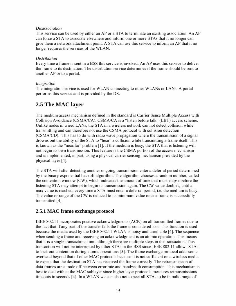
Each time the medium is sensed idle by both carrier-sensing functions, the backoff counter is decremented by one slot time. Once the backoff counter has reached zero and the medium is still free, the MAC begins transmission. After a data frame has been successfully transmitted and received at the destination, an ACK frame will be transmitted in return to the source. Between a data frame and its ACK frame, a SIFS is used to prevent other stations from accessing the channel. If the medium becomes busy in the middle of the decrement of the backoff counter, the station freezes this counter, and resumes the countdown after deferring for a period of time, which is indicated by the NAV stored in the winning station’s packet header and a DIFS period. In case of a collision, where two or more stations begin to transmit at the same time, the CW is doubled, a new backoff interval selected, and the backoff countdown begins again. This process will continue until the transmission is sent successfully or it is cancelled [4]. Collisions are inferred by no ACK from the receiver. After a collision, all the involved stations double their CWs (up to a maximum value, CWmax) and compete to gain control of the medium the next time. When a station succeeds in channel access, thus receives an ACK, the station resets its CW to CWmin.

Figure 2.10: DCF operation with NAV and 4-way handshake Figure 2.10 shows how the DCF operation works. After the source STA has deferred access to the channel for DIFS time and the channel is idle, the source sends a RTS frame to its destination. With this RTS frame the NAV is set, such that other listening STAs can set their NAV accordingly, and indicates that the medium will be occupied for the time of the return of the ACK to the transmitted RTS. The destination STA waits for a SIFS time before sending a CTS frame back to the source of the RTS frame, and the NAV set accordingly like the RTS did. After a SIFS period of time the source starts its data transmission. Again the NAV is set to as long the data frame and its belonging ACK is going to occupy the channel. Upon receiving the data frame the destination STA sends back to the source an ACK. After DIFS time the channel can be accessed again by any STA in the BSS.

21

DCF does not provide QoS support since all stations operate with the same channel access parameters and have the same probability to gain control over the medium. There is no mechanism to differentiate different stations and different traffic [2]. 2.5.6.4 Point coordination function (PCF) To support applications that require near real-time service, the IEEE 802.11 standard includes the point coordination function. The PCF has not been widely implemented and is an optional part of the standard, though STAs that implement only the DCF will interoperate with point coordinators [5]. The PCF is built over the DCF, and both operate simultaneously. This centrally controlled access mechanism uses a poll and response protocol to eliminate the possibility of contention for the medium. A point coordinator (PC) controls the PCF and is always located in the AP, thus access to the medium is restricted by the PC. STAs associated with this AP can only transmit data when they are polled by the PC. Although access is under control of the PC, all frames must be acknowledged. In PCF time is divided into super frames. A super frame includes a contention period (CP), where DCF is used, and a contention-free period (CFP), where PCF is used. A super frame starts with a beacon management frame transmitted by the PC. The PCF may be used if contention-free delivery is required, but contention-free service is not provided full-time. Periods of contention-free service alternate with the standard DCF-based service. The relative size of the contention-free period can be configured, but the standard requires that the contention period be long enough to contain at least one maximum length frame and its acknowledgment. 2.5.6.4.1 PCF operation STAs that have data to send, request that the PC register them on the polling list. The PC then regularly polls the STAs (usually in a round-robin manner) according to a predetermined order for traffic while also delivering traffic to the STAs. The PCF uses the PIFS, which is a shorter time interval then DIFS, to take control over the medium. After gaining access to the medium the PC begins a period of operation in the CFP, and transmits a beacon frame. The beacon announcement tells all STAs receiving the beacon to adjust their NAV according to the maximum duration of the CFP to lock out DCF-based access to the medium. The CFP is called contention free because access to the medium is completely controlled by the PC and the DCF is prevented from gaining access to the medium. Once the PC is in control, it begins to deliver traffic to STAs in its BSS and may poll STAs that have requested to be on the polling list. The PC sends a contention-free poll (CF-poll) frame to STAs that have requested for contention-free service. The STAs receiving the CF-poll can transmit one frame for each CF-poll received. Since all contention-free transmissions are separated by the SIFS and the PIFS, no DCF-based STAs can gain access to the medium because both these intervals are shorter then the DIFS.

22

Figure 2.11: PCF operation with NAV

As for QoS support, PCF has some problems. For example, it is very difficult to predict transmission time of a polled station because the polled station can transmit a frame of any length between 0 and the size of the maximum MSDU (1500 bytes). 2.5.6.5 Fragmentation Some large management frames may need to be broken into smaller pieces to fit through the wireless channel. Fragmentation may also help to improve the reliability in the presence of interference. Wireless STAs can fragment transmissions so that interference affects only small fragments, not large frames. The fragmentation feature can result in higher effective throughput when the amount of data that can be corrupted is reduced [5]. To reassembly the fragmented frames each frame have the same sequence number and also an ascending fragment number. Frame control in the packet header gives information if there is coming more fragmented frames. When a packet is being fragmented, all of the fragments that comprise the packet are normally sent in one fragmentation burst, which is shown in figure 2.12 below.

Figure 2.12: Fragmentation burst with NAV

23

There exists a fragmentation threshold set in bytes. This is commonly sat to the same value as the RTS threshold is. In this master thesis these to thresholds has the same value. The figure 2.12 above illustrates how the NAV and SIFS are used in combination to control access to the shared channel. Fragments and their ACKs are separated by the SIFS, so a STA remains in control of the channel during a fragmentation burst. The NAV is also used to ensure that other STAs do not use the channel during the burst. The NAV is set, as usual, from the expected time to the end of the first fragments in the air. The next fragments form a chain of fragments. Each fragment set the NAV to hold the medium until the end of the ACK of the next frame. Fragment 0 sets the NAV to hold the channel until ACK1 is finished, fragment 1 sets the NAV to hold the channel until ACK 2 is finished, and so on. After the last fragment and its ACK have been sent, the NAV is set to 0, indicating that the channel will be released after the fragmentation burst completes. 2.5.6.6 Frame format The IEEE 802.11 protocol defines three different classes of frames: data, control and management frames. Data frames are used for sending data between STAs, to deal with handshaking before sending data and acknowledgments the MAC uses the control frames. Management is used for beacon frames, association, disassociation, authentication, deauthentication, and for distribution of different kinds of parameters. Each of these frames has a header with a variety of fields used within the MAC sub layer. There are also some headers that are used by the physical layer that mostly deal with the modulation techniques used. These till not be further discussed in this master thesis. The MAC of the IEEE 802.11 names the data frames as MAC service data units (MSDUs). The MAC accepts these MSDUs from layers higher up in the protocol stack (see figure 1.2), e.g. the network layer, for the meaning of reliable sending of those MSDUs to the network layer in another STA. The MAC adds headers and trailer to create a MAC protocol data unit (MPDU). With these headers and trailer the MAC can pass the MPDU to the physical layer for sending over the wireless medium to the other STA. The header and trailer information, in combination with the information received as the MSDU, is referred to as the MAC frame. We will discuss in more details the contents of the frame in the next sections. 2.5.6.6.1 The data frame The format of the data frame is shown in figure 2.13 below. It is more complex than the format of other LAN protocols. The frame starts with a MAC header. The first two bytes of the header is the frame control field. The frame control field will be described in details later. The field contains the information the MAC requires to interpret all of the subsequent fields of the header. The second field of the frame is the duration field which tells how long this frame will occupy the channel along with its ACK. This field is responsible to how other STAs manage the NAV mechanism. The frame header also contains four address fields. The first two is the source address and the destination address. The nest two address fields are used for the source base station and destination base station if the frame enters intercell traffic. The sequence field numbers the fragments if any. The data field contains the data and the header is ended with a checksum. All these fields are not used in all frames.

24

Figure 2.13: Illustration of the IEEE 802.11 frame format

2.5.6.6.2 Frame control The frame control field contains the information the MAC needs to interpret all of the subsequent fields of the MAC header. The next subsections will provide some details about the different fields that are contained in the frame control field. Protocol version In the frame control field, the protocol version is the first field. This field allows two versions of the protocol to operate at the same time, since there is only one MAC version of the IEEE 802.11 currently this field is set to zero. If the protocol version indicates that the frame received was not constructed by a MAC version the STA understand, the STA must discard the frame and not transmit any response on the channel. Type and subtype The next field called type specifies if the frame is either a data, control or management frame. These three frames can have several subtypes. See table 3-1 in [4 and 5] for full listing of all frame type and subtype combinations. To DS and From DS The To DS field is only used in data frames. Like the name indicates this field tells if the frame is destined for the DS. Every data frame sent from a STA to the AP will have this bit set. The bit is set to zero in control and management frames. There are four combinations for these two subfields. They indicate direct transmission between two STAs, transmission to or from the DS, or that the WLAN is being used as the DS. This last combination is to allow the DS to occupy the same medium as the BSS. This last case is when two AP transmits frames to each other. More fragment Like the name indicates this field distributes information if the frame is a fragmented frame or not. It’s set to zero whenever the last fragment of a data or management frame is transmitted, in all control frames, and in any non fragmented frames.

25

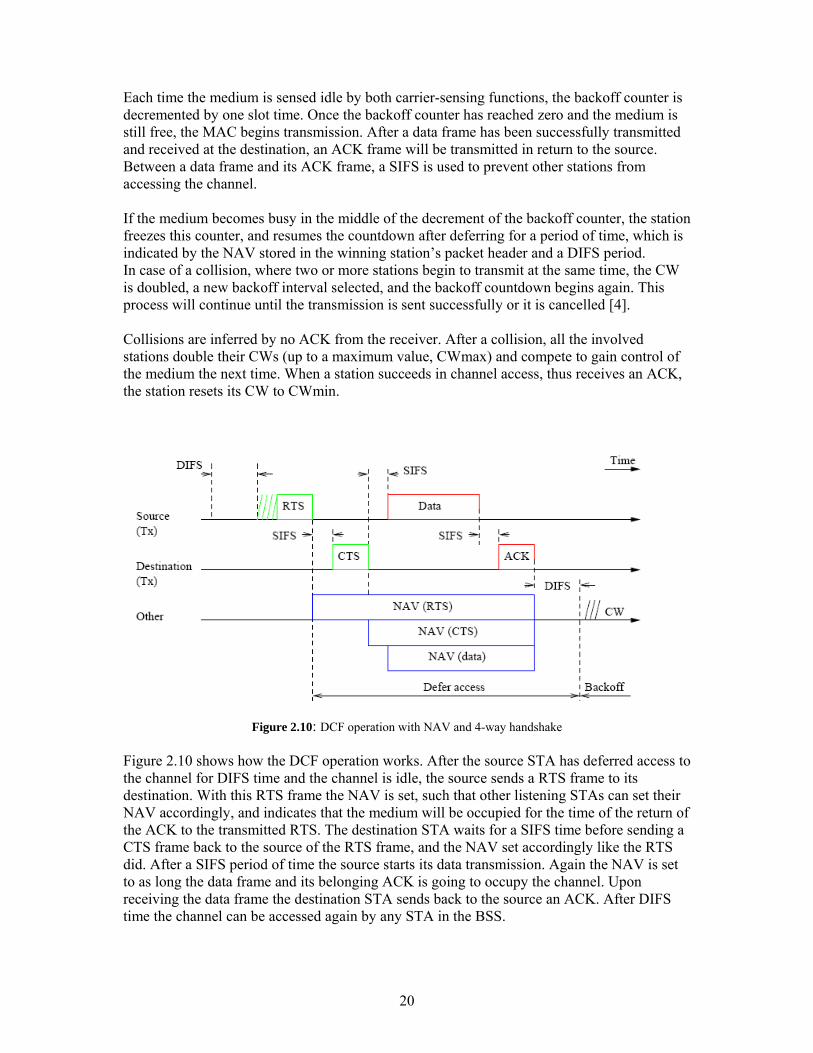
Retry Whenever there happens that a frame need to be retransmitted, this field indicates this with the bit set to one to aid the receiving STA in knowing that it is a duplicate frame. Power management A STA uses this field to announce its power management state. After completion of an atomic frame exchange this bit is set to one to indicate that the STA will be in power saving mode, and set to zero if it is still available to communication. More data This bit in the frame control fields is used by the AP to indicate to a STA that there is at least one data frame buffered in the AP to that STA. One indicates there exist a frame and zero indicates that there are no frames buffered. WEP/Protected frame This field indicates with the bit set to one that the frame has been encrypted by link layer security protocols. This bit may only be set to one in data frames and management frames of subtype authentication. In all other frame types or subtypes it is set to zero. Order The last bit in the frame control field is order. This tells the MAC when the bit is set to one that the content of the data frame was provided to the MAC with a request for strictly ordered service. This additional processing information is given to the AP and DS to allow this sort of service.

26

2.6 The PHY layer The second major component of the IEEE 802.11 architecture is the physical layer, from now on called PHY. We find the PHY at the bottom of the Open System Interconnection (OSI) stack. The PHY is the interface between the MAC and the radio link. It is responsible for transmission and receiving of data frames over a shared wireless medium. The PHY is divided into two sub layers: the physical layer convergence procedure (PLCP) sub layer and the physical medium dependent sub layer (PMD). Figure 2.14 illustrates the PHY and the binding to the MAC. The PLCP receives frames from the MAC and adds its own header to help synchronize transmissions. The PMD is responsible for transmitting any bits it receives from the PLCP into the air using the antenna. It uses signal carrier and spread spectrum modulation to transmit data frames over the media. The PHY also incorporates a carries sense indication function to indicate back to the MAC when a signal is detected [4, 5].

Figure 2.14: The PHY layer with bindings to the MAC 2.6.1 The radio link Three physical layers were standardized in the initial revision of the IEEE 802.11 [5]:

• Frequency-hopping spread-spectrum (FHSS) radio PHY • Direct-sequence spread-spectrum (DSSS) radio PHY • Infrared light (IR) PHY

Later, three further PHY based radio technology were developed [5]:

• 802.11a: Orthogonal frequency division multiplexing (OFDM) • 802.11b: High-rate direct sequence (HR/DS or HR/DSSS) • 802.11g: Extended rate PHY (ERP) • 802.11n: Multiple input multiple output (MIMO) or the high-throughput PHY

The infrared physical layer will not be further discussed because of the lack of implementations in commercial products.

27

2.6.2 Spread spectrum Traditional radio communications focus on getting as much signal as possible into as narrow a band as possible. Spread spectrum works by using mathematical functions to diffuse signal power over a large range of frequencies. The receiver performs the inverse operation, and the signals are reconstituted as a narrow-band signal. Any narrow-band noise is also smeared out so the signal is easy to detect [5]. 2.6.2.1 Frequency hopping spread spectrum (FHSS) There are two good reasons to use FHSS. First, the electronics used to support FH modulation are relatively cheap and have low power requirements. Second, a great number of networks can coexist with reasonable high throughput. Today FH networks have become only a footnote in the history of IEEE 802.11 largely because of higher-throughput specifications [5]. 2.6.2.1.1 Frequency-hopping transmissions FH uses a predetermined, pseudorandom pattern to rapidly change the transmission frequency.

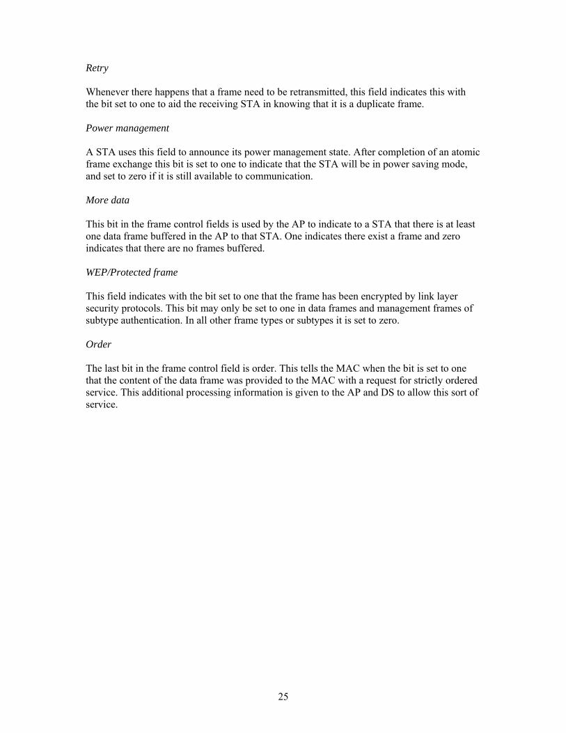
Figure 2.15: Illustration of Frequency Hopping The vertical axis of the graph in figure 2.15 divides the available frequency into a number of slots. Time is also divided into a series of slots. The success of FH transmissions is based on timing the hops accurately, and that both transmitter and receiver must be synchronized so the receiver is always listening on the correct frequency. 2.6.2.1.2 FHSS modulation and channel hopping The modulation used by the FHSS PMD to transmit is two-level Gaussian frequency shift key (2GFSK) at the basic rate of 1 Mbit/s. This modulation technique encodes data bits as shifts in the transmission frequency from the channel center. Channels are defined by their center frequencies, which begin at 2.402 GHz in North America and in Europe (excluding Spain and France). The number of hopping channels is 79 and spaced uniformly across the 2.4 GHz band occupying a bandwidth of 1 MHz (2.402 – 2.479 GHz). Channel hopping is controlled by the FHSS PMD. The hop rate in the U.S. is at least 2.5 hops per second with a minimum hop distance of 6 MHz [4, 5].

28

2.6.3.1 Direct sequence spread spectrum (DSSS) The DSSS had data rates of 1 Mbps and 2 Mbps, the same as frequency hopping. Although, it quickly became clear that direct sequence technologies had the potential for higher speeds then FH technologies. In 1999, the IEEE 802.11b was standardized and provided rates of 5.5 Mbps and 11 Mbps. The older 1 and 2 Mbps PHYs and the newer higher data rates PHYs are often combined into a single interface, even though they are described by different specifications [5]. 2.6.3.1.1 Direct sequence transmission The basic approach of direct-sequence techniques is to spread a signal over a wider bandwidth at a reduced radio frequency (RF) power level. Changes in the radio carrier are present over a wide band, and receivers can perform correlation processes to look for changes. The basic approach is shown in the figure 2.16 below.

Figure 2.16: Illustration of direct spread spectrum The initial signal is a traditional narrowband radio signal. It is processed by a spreader, which take the narrowband input and flatten the amplitude across a relatively wide frequency band. The transmitted signal looks like low-level noise because its RF energy is spread across a very wide band. Receivers can by monitoring a wide frequency band, pick up the signal by looking for changes in the entire band. A correlator recovers the initial signal by inverting the spreading process. Correlation gives DS transmission also protection against interference since noise is usually relatively narrow pulses. The correlation function spreads out noise across the band, and the correlated signal is easily picked up since its amplitude now are of much greater power then the noise [5]. DS modulation works by applying a chipping sequence to the data stream. The modulation type used by the DSSS PMD is differential phase shift keying (DPSK), which uses a balance in-phase/quadrature (I/Q) modulator to generate an RF carrier. The RF carrier is phase modulated and carries symbols. The chip in the chipping sequence is a binary digit used by the spreading process. Bits are higher-level data, while chips are binary numbers used in the encoding process. Chipping streams, which are also called pseudorandom noise codes (PN codes), must run at a much higher rate then the underlying data. An 11-bit code is combined with the single data bit, which produce 11 chips that carry the single data bit. This process spreads the signal power over a much wider bandwidth. The number of chips used to transmit a single bit is called spreading ratio. Doubling the spreading ratio means doubling the required bandwidth, but higher spreading ratio improves the ability to recover the transmitted signal [4, 5].

29

2.7 MANET 2.7.1 Introduction MANET (mobile ad hoc networking) [26] are describes as a distributed, mobile, wireless, multihop network that operate without the benefit of any pre-existing infrastructure, except for the nodes themselves using radio as the communication medium. A MANET is composed of autonomous, potentially mobile, wireless nodes that may be connected at the edges to the fixed, wired Internet, communicating without the intervention of a system administrator or centralized access point. DARPA discovered the merits of having an infrastructure less network in the 1970s [29]. DARPA had a packet radio project (ALOHA) with a technology that extended the concept of packet switching to the domain of broadcast radio networks. The ALOHA project first demonstrated the possibility of using the broadcasting property of radios to send and receive data packets in a single radio hop system. Later the ALOHA project evolved to a multihop multiple-access packet radio network (PRNET) with sponsorship from the Advanced Research Project Agency (ARPA). The difference from ALOHA to PRNET is that PRNET permits multihop communications over a wide geographical area [29]. 2.7.1.1 Motivation The concept of mobile packet radio networks, where every node in the network is mobile and where wireless multihop (store-and-forward) routing is utilized comes from the U.S. Department of Defence (DoD) DARPA PRNet program [27]. Their original motivations for MANET were for military operations and battlefield survivability. With the freedom of movement and mobile wireless communications system for coordination, single point of failures such as centralized control stations was avoided. Another motivation for the military to use MANET is that military operations often are battled in environments where there is no terrestrial communications infrastructure, or the infrastructure is destroyed before entering. A third motivating factor for using MANET is the store-and-forward behaviour that makes MANET possible to use beyond line of sight (LOS), i.e. using multihop to transfer information, see figure 2.17 below which shows the principle.

Figure 2.17: The figure shows that node A needs node B as router to reach node C and E in an ad hoc network.

30

2.7.1.2 Design issues “A rapidly deployable, self-organizing mobile infrastructure is the primary factor that differentiates MANET design issues from those associated with commercial cellular systems [27]”. As a result of not relying on any existing infrastructure and the use of radio communication, multihop ad hoc networks have several salient and unique features: Network topology The network topologies are dynamic and changes often rapidly because of unpredictable and arbitrary node movement, repeater failures or recovery, and network congestion state. It is possible to have cases of very high node mobility without changes in link connectivity, typically when military units move in same direction, and cases with rapid changes in link connectivity with no node mobility because of inoperative nodes due to dead batteries. The density of a network is defined by the number of nodes within a given geographic area. Shared medium This feature makes the availability of resources at one node being affected by its contending neighbours – local interference conditions. Thus, node interconnectivity and link properties such as capacity and bit error rate cannot be pre-determined. This is one of the major difficulties when operating with MANETs. Environment MANETs can operate in terrain that may prevent LOS operation (urban, rural, maritime, etc). Distance between the two end links, obstacles, externally generated noise and interference cause by other transmissions will make the capacity of a wireless link reduced and to be highly variable. Therefore, the wireless link has a bandwidth-constrained and variable capacity [28]. Energy Because of the power-constrained lightweight batteries in MANET nodes, the limited power supply limits the transmission range, data rate, communication activity and processing speed. Since there are no fixed base stations in a MANET, the energy burden cannot be transferred to such and entity in the network. Upon designing a MANET one must take in consideration the energy consumption of the layers above the physical layer. An inefficient data link, MAC, or network layer design can result in additional packets being transmitted (and/or re-transmitted) and more energy being used [27]. There exist several energy-saving techniques such as shutting down one node. But then the question on how and when to wake up a sleeping node must be answered. Distributed operation Only local information is known to any node in the network since there may not be any centralized administration to send out global information to the nodes. This implies that distributed operation is required on every node. Medium access TDMA or FDMA schemes are not suitable for medium access because of no centralized control and global synchronization. Scheduling of frames for timely transmission to support QoS is difficult because many MAC protocols do not deal with host mobility. Since the

31

medium is shared the MAC protocol must contend for access to the channel while at the same time avoiding possible collisions with neighbouring STAs. Access to the shared channel must be made in a distributed manner, through the presence of a MAC protocol in ad hoc networks [29]. There are also other MANET design issues that need to be considered. First, distinguish network nodes from endpoints. Second, user traffic, does the traffic that is supposed to take advantaged of the network have QoS demands or not? Third, regulatory power spectral density requirements must be met. Forth, performance metrics must be acknowledged and implemented and lastly cost-versus-performance tradeoffs must be made if the MANET design is to be implemented. 2.7.2 Routing protocols in MANET Since ad hoc networks has several different features then existing networks, the routing protocols supporting ad hoc networks must be designed specifically to their kind. First, the routing protocols must provide a self-starting behaviour [27]. Second, the limitations of the wireless links and devices such as limited bandwidth, finite battery power and limited computing power added with the dynamic nature of MANETs makes the design of routing protocols a very challenging task [30]. Lastly, since MANETs operating in wireless medium it requires that whichever routing protocol chosen must be modified. The MANET working group in IETF is responsible for developing and evaluating MANET routing protocols. Many routing protocols have been developed and many are still under development, configuring and evaluation. We can classify ad hoc routing protocols in three main groups:

1. Unicast routing protocols a. Topology based routing

i. Proactive protocols ii. Reactive protocols

iii. Hybrid protocols b. Geographical assisted routing protocols

2. Multicast routing protocols 3. Broadcast routing protocols

Figure 2.18 Overview of ad hoc routing protocols

32

2.7.3 Overview of routing methods A data packet sent from a source contains always a destination STA identifier in its header [27]. When this data packet arrives at a STA it checks the header information and forwards it to its next hop. This forwarding procedure continues until the packet reaches its destination. How routing tables are maintained is different from one routing method to another. The common objective is to attempt to route the packet along the optimal path. The next-hop routing methods can be categorized into two main classes: link-state and distance-vector. 2.7.3.1 Link-state algorithm In the link-state approach each STA maintains a view of the network topology with a cost for each link. The STAs maintains this view via periodically broadcasting the link costs of its outgoing links to all other STAs using a flooding protocol. Wrong information about link cost can occur because of long propagation delays. An example of a link-state routing protocol is Open Shortest Path First (OSPF). The link-state approach has large overhead because of the periodically broadcasting, and will also experience scalability problems in large MANETs. 2.7.3.2 Distance-vector algorithm In distance-vector routing each router sends routing information to its neighbours. The information sent is an estimation of the routers path costs to all its neighbouring STAs. Distance estimate information is kept up to date via monitoring the cost of its outgoing links and periodically broadcasts, to all its neighbours, its current estimate of the shortest distance to every other STA in the network. The routers determine the next-hop information using the distributed Bellman-Ford algorithm on the received estimated path costs. One example of a distance-vector routing protocol is the Routing Information Protocol (RIP). RIP has the counting-to-infinity problem, and has limited usefulness regarding ad hoc networks because it was not designed to handle rapid topology changes [27]. Like link-state, distance-vector routing has scalability problems in large MANETs. 2.7.3.3 Proactive routing The link-state and distance-vector routing protocols are proactive meaning that every STA maintains routing information to every other STA in the network. This is done by regularly updating routing tables in every STA via periodically update messages. When the topology changes the STAs must send information to the other STAs, causing overhead in the network. The positive is that routes are always known and available on request. Two examples of proactive routing protocols are Destination-sequence distance vector (DSDV) and Optimized Link State Routing (OLSR) both will be further discussed later in this chapter.

33

2.7.3.4 Reactive routing Reactive routing protocols make route paths on-demand. A STA initiate a route request to its packets destination STA and a route reply will be returned if the destination STA is accessible. No route table or routing information exists in the STAs before a request for a route is made. Reactive routing protocols wastes less bandwidth then proactive protocols because there is no routing table information to maintain. AODV and DSR are two reactive routing protocols that will be further discussed later in this chapter. 2.7.3.5 Hybrid routing The hybrid routing protocols combines the advantages to both the proactive and reactive approach. This master thesis will not further discuss any hybrid routing protocols, only mention an example in Zone Routing Protocol (ZRP) [33, 34]. 2.7.4 Destination-sequence distance vector protocol (DSDV) The DSDV protocol [11] uses destination sequence numbers in the routing table at every STA to provide loop-free routes. The consistency of the tables is maintained by triggered updates to propagate topology changes when these are discovered, but the routing tables are also periodically updated. These packets are sent using broadcast or multicast and will indicate to each STA which STA are accessible and the number of hops necessary to reach them. 2.7.4.1 Route advertisements The DSDV protocol requires that every STA broadcasts its own route table. Since the entries in the routing tables can change very rapidly, the advertisements must be made often enough to ensure that every STA can almost always locate every other STA in the entry list [27]. With DSDV every STA must agree to relay data packets to other STA upon request. 2.7.4.2 Route table The data broadcasted or multicasted by the STAs will contain its new sequence number and the following information for each new route [27]:

• The destination address • The number of hops required to reach the destination • The sequence number of the information received regarding that destination

When transmitting the route tables, the header also contains the hardware address, and the network address of the STA transmitting if appropriate. The transmitting STA will also create a sequence number. Upon deciding the forwarding routes, routes with recent sequence numbers are always preferred. When two routes have the same sequence number, the route with the smallest metric will be used. Routing information is distributed between STAs by sending full dumps infrequently and smaller incremental updates more frequently. The time between sending the routing information packets, is one of the most important parameters to be chosen. A STA will retransmit any new or substantially modified route

34

information as soon as possible. This quick rebroadcast can introduce a problem called the broadcast storm problem [38]. This problem will degrade the shared channel upon STA movement. DSDV was one of the early algorithms available to MANETs [37]. It is better for creation of ad hoc networks with a small amount of STAs. The algorithm presented has no commercial implementation. But there has been done some modification on the algorithm such as the AODV protocol, which may be viewed as an on-demand modification of DSDV [Perkins 2001]. 2.7.5 Optimized Link State Routing (OLSR) OLSR [31] is a proactive, table driven routing protocol for MANETs. The protocol utilizes a technique called multipoint relaying for message flooding and collects data about available networks and calculates an optimized routing table [32]. OLSR is a hop-by-hop routing protocol, distributed, and based on the traditional link-state algorithm. The protocol is best suited for large and dense MANETs, because of the MPRs optimizing of the link-state routing. The RFC 3626 [35] divides OLSR into two functioning groups. The first is core functioning, which is always required for the protocol to operate. The second group is called auxiliary functioning and provides not-mandatory functionality. 2.7.5.1 Multipoint Relays (MPR) A STA needs to find its neighbours in the network before selecting its MPR. MPR is the key advantage in OLSR. Via the HELLO message a STA finds its one-hop neighbours and two-hop neighbours through their response, called neighbour discovery. MPRs are selected one-hop STAs that’s has the best routes to the two-hop STAs (see figure 2.19). MPRs reduce the control traffic overhead in the network by forwarding the packets instead of using flooding as the mechanism to reach other STAs.

Figure 2.19: MPR selection routine The HELLO messages are exchanged between neighbours only and each STA broadcast is periodically via its MPRs. The HELLO message contains the STAs address, a list of known neighbours, and link status (symmetric or asymmetric). OLSR achieve optimization when it

35

uses the MPRs as the only STAs to forward the broadcasts messages into the network, thus reducing message overhead. 2.7.6 The Dynamic Source Routing Protocol for Multihop Wireless Ad Hoc Networks (DSR) 2.7.6.1 Introduction The dynamic source routing protocol (DSR) [39] is specifically designed for use in multihop wireless ad hoc networks with mobile STAs. The two main mechanisms of the protocol named “Route Discovery” and “Route Maintenance” works together to allow the STAs to discover and maintain routes to all other destination in the network. The protocol is entirely an on-demand routing protocol, which give little routing packet overhead, and makes DSR scale automatically to only that needed to react to changes in the routes currently in use. With source routing, i.e. the STAs knows the complete hop-by-hop route to the destination, the protocol allows packet routing to be loop free. The routing is “soft-state”, which avoids the need for up-to-date routing information in the intermediate STAs through which packets are forwarded, and allows STAs that are forwarding or overhearing packets to cache the routing information in them to their own use. These source routes are carried in the data packet header and stored in a route cache in the STAs. Other advantages in the protocol are rapid recovery when the routes change. The draft tells us that the protocol is designed mainly for mobile ad hoc networks of up to about two hundred STAs, even with high mobility among the STAs. 2.7.6.2 Route Discovery and Route Maintenance The two main components of the DSR protocol work together to allow the discovery and maintenance of source routes in the ad hoc network. Route Discovery is used when a STAs wants to send a packet to a destination and does not already know the route to it. Route discovery works by flooding the network with route request packets (RREQ). The RREQ is piggybacked with a route reply packet (RREP) and can contain other small data packets [27]. With Route Maintenance a STA is able to detect if the network topology has changed such that it can no longer use its route to a specific destination, i.e. a link along the route has broken down. When Route Maintenance indicates that a source route is no longer working, the STA can attempt to use any other route to the destination it happens to know, or it can use Route Discovery again to find a new route, if any. The Route Maintenance mechanism is only used upon a STA is actually sending packets to a known destination [27]. When a STA in the ad hoc network wants to send a data packet to a destination for which it does not already know the route, it uses the route discovery process to dynamically determine such a route. Each STA receiving an RREQ rebroadcasts it, unless it is the destination or it has a route to the destination in its route cache. Upon receiving a RREQ a STA replies with a RREP that is routed back to the original source STA. RREQ and RREP packets are also source routed. The RREQ builds up the path traversed across the network. The RREP packet route itself back to the source by traversing this path backwards. The route carried back by the RREP packet is cached at the source STA for future use. The caching of multiple routes at each STA avoids the overhead incurred by performing a new route discovery every time a route in use breaks.

36

A route error packet (RERR) is sent to the source STA if any link in a source route is broken. The STAs using this link removes this from its cache. A new route discovery process must be progressed if the source STA still needs this particularly route. The DSR protocol has another feature called Send Buffer [27]. The send buffer keeps a copy of the packets that the sending STAs has no source route established to yet. Each packet is time stamped and is discarded after residing in the send buffer for some time-out period. FIFO or other empty-queue mechanism can be used to prevent overflow the buffer. A STA should occasionally initiate a new route discovery process for the packets destination address in a limited rate fashion. To reduce new route discovery DSR uses exponential backoff to limit the rate at which new route discoveries may be initiated by any node for the same target. Several additional optimizations have been proposed and have been evaluated to be very effective by the authors of the protocol [40]: Packet Salvaging: If a source route is broken, an intermediate STA can use an alternate route from its own cache to salvage the data packet. The salvaging STA sends a RERR to the source STA, and replaces its own source route into the original source route on the packet before forwarding it. Gratuitous route repair: A source node receiving an RERR packet piggybacks the RERR in the following RREQ. This helps clean up the caches of other nodes in the network that may have the failed link in one of the cached source routes. Promiscuous listening: When a node overhears a packet not addressed to it self, it checks whether the packet could be routed via itself to gain a shorter route. If so, the node sends a gratuitous RREP to the source of the route with this new, better route. Aside from this, promiscuous listening helps a node to learn different routes without directly participating in the routing process. 2.7.8 The Ad Hoc On-Demand Distance-Vector Protocol 2.7.8.1 Introduction The RFC 3561 [41] tells us that the Ad Hoc On-Demand Distance Vector (AODV) routing protocol was designed for use by mobile STAs in an ad hoc network. The protocol offers several features:

• Quick adaptation to dynamic link conditions • Low Processing and memory overhead • Low network utilization • Determines unicast routes • Loop free with sequence numbers

Perkins and Royer made the initial design of AODV after experiencing with the DSDV routing algorithm. The goal of AODV is to reduce the need for system-wide broadcast to the furthest extent possible [27]. This means that when two STAs enter communication range of each other or when two STAs drift out of communication range there will be no system-wide broadcast in AODV. Broadcast only occurs in such setting when the link status has affect on ongoing communication or multicast tree maintenance. In AODV, the only global effect is

37

when a distant STA tries to use a broken link. In DSDV, local movements have global effects. With AODV only the STAs using this broken link is informed of the link’s changed status. Another feature to reduce the number of broadcasts when a link break is when a route between source and destination are available AODV does not add any overhead to the packets carrying the data. And whenever routes are not used, they are expired and discarded to reduce the effects of stale routes as well as the need for route maintenance for unused routes. This aging of routes is difficult to manage when there is no other timing information. 2.7.8.2 Properties AODV is on-demand driven. Routes are discovered as needed and are maintained only as long as they are necessary. The protocol offers loop-freedom by the use of sequence numbers. Every node increases its sequence number each time a change in the topology requires it. In this way the most recent routes are used whenever route discovery is processed. AODV supports unicast, multicast and broadcast. With the support of multicast it is possible that unicast and multicast can share a common knowledge of the routing information. In contrast to DSR, AODV has only one entry per destination in its routing table. The route table where each route table entry is composed of the destination address, next-hop to reach the destination, destination sequence number, hop-count to the destination, and a lifetime (the time an entry is valid). The route table is used to store pertinent routing information and for each destination it also maintains a list of precursor STAs. These precursors may be forwarding STAs on the route and will be notified if there is detected a loss of the next hop link. 2.7.8.3 Route establishment The route discovery process is on-demand and uses a cycle of route request and route reply messages. See figure 4.1 below, which outline the cycle with picture a representing the propagation of the RREQ to the destination, and picture b representing the propagation of the RREP back to the source.

Figure 2.20: AODV route establishment

38

2.7.8.4 Route Discovery When a STA wants to send a packet to a destination is does not have a valid entry for in its routing table, the STA must start the route discovery process by broadcasting a RREQ packet to its neighbours. See figure 4.1 where source STA A wants to reach destination STA F. The RREQ packet contains the source IP address and current sequence number, the destination IP address and last known sequence number. Intermediate STAs can only reply to the RREQ if they have a route to the destination whose corresponding destination sequence number is greater than or equal to that contained in the RREQ [29]. The RREQ also contains a broadcast ID. With this ID the receiving STAs can distinguish several RREQ broadcasted from the same source from each other. Meaning that, if they receive this packet twice they silently discards it, or otherwise if it is the first time seeing this packet records the information and processes it. See figure 2.21 below for overview of the RREQ message format.

0 1 2 3 0 1 2 3 4 5 6 7 8 9 0 1 2 3 4 5 6 7 8 9 0 1 2 3 4 5 6 7 8 9 0 1 +-+-+-+-+-+-+-+-+-+-+-+-+-+-+-+-+-+-+-+-+-+-+-+-+-+-+-+-+-+-+-+-+ | Type |J|R|G|D|U| Reserved | Hop Count | +-+-+-+-+-+-+-+-+-+-+-+-+-+-+-+-+-+-+-+-+-+-+-+-+-+-+-+-+-+-+-+-+ | RREQ ID | +-+-+-+-+-+-+-+-+-+-+-+-+-+-+-+-+-+-+-+-+-+-+-+-+-+-+-+-+-+-+-+-+ | Destination IP Address | +-+-+-+-+-+-+-+-+-+-+-+-+-+-+-+-+-+-+-+-+-+-+-+-+-+-+-+-+-+-+-+-+ | Destination Sequence Number | +-+-+-+-+-+-+-+-+-+-+-+-+-+-+-+-+-+-+-+-+-+-+-+-+-+-+-+-+-+-+-+-+ | Originator IP Address | +-+-+-+-+-+-+-+-+-+-+-+-+-+-+-+-+-+-+-+-+-+-+-+-+-+-+-+-+-+-+-+-+ | Originator Sequence Number | +-+-+-+-+-+-+-+-+-+-+-+-+-+-+-+-+-+-+-+-+-+-+-+-+-+-+-+-+-+-+-+-+

Figure 2.21 RREQ message format To process the RREQ packet, the intermediate STAs sets up a reverse route entry for the source in its route table. This entry contains the source IP address and sequence number, as well as the number of hops to the source and the IP address from which it received the RREQ. The intermediate STAs can than use this information for further use when forwarding to the source another time. Figure 4.1 shows an example where the route to the destination STA is not known. In such scenarios, the RREQ is only replayed by the destination STA (STA F in this example), which unicasts back to the source an RREP packet. 2.7.8.5 Expanding ring search When a RREQ is flooded to a large network, this packet becomes a network-wide broadcast which can make impact on the network. To reduce network-wide broadcasts the source can use an expanding ring search technique [27]. To use this technique the source STA defines the time to live (TTL) parameter of the RREQ. If no luck on the first try, the source increases the TTL value incrementally. This process continues to the destination is reached. The TTL increment is recorded for later use to reach the destination.

39

2.7.8.6 Route Maintenance The route between a source and a destination is only maintained as long as it is needed by the source. In AODV we have something called an active path. Only movement along an active path will trigger action from the protocol. A new route discovery will be initiated if the source moves during a session. When the destination or some intermediate forwarding STA moves during a session a route error message is sent to the affected source STAs. This RERR is sent from the STA upstream of the break, closer to the source. The RERR lists all broken links. If the broken link was used by more than one STA the RERR is broadcasted by the STA upstream of the break. The neighbours receiving this RERR must mark their route to the destination as invalid by setting the destination equal to infinity (∞). When a source receives a RERR it can reinitiate the route discovery process if the route is sill needed. Figure 4.3 illustrates the route maintenance routine. The original path from the source A to the destination E is through B, C, and D. STA D moves or is not reachable for some other reason, causing a break in connectivity with STA C. STA B notices this break and send a RERR to the source. Once receiving the RERR, the source determines that it still needs the route, so it initiates route discovery again. The new route to E is now forwarded through F as we can see by the new route marked in red in figure 4.3 below.

Figure 2.22: RERR propagation in AODV

2.7.8.7 The hello_interval An additional aspect to the AODV protocol is the hello_interval. If one STA receives a broadcast and there is no entry to that destination in the route table, the STA creates one. If a STA has not broadcasted anything within the last hello_interval, it can broadcast a HELLO packet to inform its neighbours that it still is alive and reachable. This HELLO message is a special RREP that contains the STAs IP address and current sequence number. It will not be rebroadcasted outside its neighbourhood because of the TTL value that is set to 1 [27]. AODV has this feature so the protocol can work with IEEE 802.11 without relying on any other underlying protocol when in comes to connectivity information.

40

Chapter 3 IEEE 802.11e: standard overview, simulation study and comparison with legacy IEEE 802.11 The new MAC of IEEE 802.11e [11] enables the values of the new interframe space AIFS (arbitration interframe space), CWmin (contention windows minimum value), CWmax (contention window maximum value) and TXOP (transmission opportunities) to be set on a per-class basis for each STA. At each STA traffic is directed to up to four different queues, with each queue assigned different MAC parameter values. This is intended to greatly benefit the challenging QoS management in wireless networks. 3.1 Introduction The wireless medium has relatively limited bandwidth and much higher packet-error rates with high packet overhead, contrary to wired networks. Real-time applications such as Voice over IP (VoIP) telephony and other multimedia applications are causing challenging QoS requirements in wireless networks. Together with the demand for more and more bandwidth in the wireless environment, network administrators need a mechanism to control these QoS requirements. End-users expect not only the mobility provided by the IEEE 802.11, but also QoS support when they are on the move. This is the reasons why IEEE developed the 802.11e standard, which brings QoS enhancement to the IEEE 802.11 standard. The IEEE 802.11e standard is limited to specifying the PHY layer and to enable the MAC layer to do prioritization and classifying services over a WLAN. But since QoS is a system-level concept it may involve higher layers to provide end-to-end QoS services. While IEEE 802.11e provides some mechanisms to control the use of available wireless bandwidth, there is no such thing as guaranteed QoS over a WLAN connection [5]. The key benefits of the IEEE 802.11e standard are [6]:

• Reduces latency by prioritizing wireless packets based on traffic type • Enables AP to schedule resources based on client/STA data rate and latency needs • Improves wireless bandwidth efficiency and packet overheads

When networks become overloaded with the basic access scheme used in IEEE 802.11, the performance becomes equally poor for all users and all type of data. QoS modifies the access rules to provide a useful form of “controlled unfairness”. The IEEE 802.11e MAC provides techniques to classify different data traffic types into different classes and give higher priority traffic/classes preferential access to the medium.

41

The IEEE 802.11 has a coordination function in PCF as an option to deliver QoS. Although the PCF has potential, it has too many limitations to support QoS in WLAN [6]:

• Lack of mechanisms to differentiate different traffic types • No mechanism for the STAs to communicate their QoS requirements to the AP • No management interface to control an setup CFP • The polling schedule is not tightly controlled

The hybrid coordination function described in IEEE 802.11e is supposed to provide the functions that the PCF does not have, for the support of QoS in a wireless environment, along other functions and capabilities. The hybrid coordination function will be further discussed in the next section. The IEEE 802.11e standard also brings new names for a STA and an AP. A STA that supports QoS is referred to as a QoS enhanced STA (QSTA) and it is mandatory to implement the HCF. A QoS supported AP is referred to as a QAP. A QoS supported BSS is called a QoS BSS, abbreviated QBSS, and the simplest type of an IEEE 802.11e WLAN is the QoS independent basic service set (QIBSS), i.e. an ad hoc QBSS. 3.2 Hybrid coordination function (HCF) The IEEE 802.11e QoS framework defines a new coordination function called the hybrid coordination function (HCF). This coordination function multiplexes between two medium access modes: a distributed scheme called enhanced distributed channel access (EDCA), and a centralized scheme called HCF controlled channel access (HCCA). See figure 3.1 which illustrates the relationship between IEEE 802.11e HCF and the legacy DCF and PCF of the IEEE 802.11 standard. The HCF replaces the DCF and PCF in a STA that has implemented IEEE.802.11e.

Figure 3.1 The IEEE 802.11e architecture

3.2.1 Coordination function The coordination function is the logical function that determines when a STA within a BSS is allowed to transmit frames and may be able to receive protocol data units (PDUs) via the wireless medium. The coordination function within a BSS may have one hybrid coordination function (HCF), or it may have one HCF and one PCF and will have one distributed coordination function (DCF). A QBSS will have one DCF and one HCF [11].

42

The legacy PCF has different access rules based on polling by a point coordinator in an AP. To separate between a contention-free period and a contention period the PC uses special control frames called Beacon frames to divide the time. During a CFP there is a continuing exchange of frames between the STA and the AP with no collisions. Unlike the PCF, the HCF defines a uniform set of frame exchange sequences that are usable at any time. Both access schemes, EDCA and HCCA, enhance or extend functionality of the original MAC coordination function methods, DCF and PCF, specified in IEEE 802.11a/b/g. See figure 3.2 which illustrates the relationship and differences between DCF, PCF and HCF. During the contention period, EDCA is used for channel access, whereas during the contention free period, HCCA is mostly used.

Figure 3.2: MAC coordination functions

While PCF use polling technique and DCF has an equally fair access probability to the wireless medium, the HCF allocates a QSTAs the right to transmit data through transmit opportunities (TXOP). A TXOP grants a QSTA the right to use the medium at a defined start time and with a maximum duration time. During this time the QSTA can transmit a series of frames if it wants to. This TXOP is a new option whereas the legacy 802.11 technology only provides the opportunity to send one frame at a time. The duration of the TXOP is globally communicated in the Beacon frame from the QAP for STAs using EDCA. 3.2.2 The frame format The HCF introduces two new acknowledgment options: no acknowledgment and block acknowledgment. These options are specified in the QoS control field of the data frames. See figure 3.3 for the frame format in IEEE 802.11e. The no acknowledgment option is useful for applications where the data would not be useful after the delay of a frame that had to be retransmitted, such as streaming using multimedia applications. The block acknowledgment option is optional to implement but can increase efficiency by collecting the ACK frames for multiple received data frames into a single response, thus reducing overhead in the channel.

43

Figure 3.3: Frame format in QoS

The only new field in the MAC header from the original IEEE 802.11 frame format is the QoS control field. The QoS control field will be further discussed later. The two new subtype bits in the frame control field indicate whether this is a QoS packet or not. The new control frame subtypes are block acknowledgment (BlockAck) and block acknowledgment request (BlockAckReq). The IEEE 802.11e expands the IEEE 802.11 standard with eight new data subtypes. These subtypes were reserved before and correspond to the non-QoS data subtypes in the IEEE 802.11 standard. 3.2.2.1 QoS control field The TID (traffic identifier) subfield in the QoS control field describes the traffic category of traffic stream of the data in the frame. The first bit of this field decides if the next one is in use. The next three bits indicate if the QoS is a user priority (UP) for a prioritized traffic class (TC), or a traffic stream identifier (TSID) for traffic parameterized stream. We can see the QoS control field in figure 3.4. More details about this field can be found in table 5-3 in [4] or in [11].

Figure 3.4 Outline of the QoS control field

The EOSP (end of service period) bits tells the QSTA that the current frame is just what the name says, the end of the service period. The ACK policy indicates normal ACK, no ACK, no explicit ACK or block ACK. All the details to ACK policy can be found in table 5-4 in [4]. The last subfield called TXOP has several roles and depends if the frame is transmitted by a HC or a QSTA that is not an AP.

44

3.3 Enhanced distributed channel access (EDCA) This is the prioritized carrier sense multiple access with collision avoidance (CSMA/CA) access mechanism used by QSTAs in a QoS basic service set (QBSS). This access mechanism is also used by the QAP and operates concurrently with the hybrid coordination function (HCF) controlled channel access (HCCA), which will be discussed in the next section. EDCA contention access is an extension to the DCF and includes prioritized access to the wireless medium [4]. QoS support in EDCA is realized by introducing four different access categories (AC) based on the IEEE 802.1D standard [12], defined to provide priorities. The mapping from UP to AC is shown in table 3.1 below.

Table 3.1 User Priority to Access Category mapping

AC_VO is the highest priority and is intended for voice traffic that has stringent demands regarding jitter, latency and bandwidth. AC_VI is the next highest priority and used by video traffic and have high bandwidth demands, but lesser demands regarding jitter and latency as AC_VO. AC_BK is meant for background traffic and has higher priority then AC_BE which is similar to the legacy best effort standard in IEEE 802.11. As shown eight user priority levels are available, which is mapped to an AC and corresponds to one of four transmit queues. The priority between the ACs is defined by the EDCA parameter set maintained and advertised by the QAP.

Table 3.2 EDCA parameters

Access Category AIFS CW_min CW_max

AC_VO 2 ((AC_min + 1)/4) -1

((AC_min + 1)/2) -1

AC_VI 2 ((AC_min + 1)/2) -1 AC_min

AC_BK 3 AC_min AC_max AC_BE 7 AC_min AC_max

45

Table 3.2 shows the recommended EDCA parameters to be used with IEEE 802.11e. The differentiation between the four ACs is AIFS and the minimum and maximum values of the contention window. These three parameters can be used together or alone to obtain differentiation. All the parameters will by decreasing them give better chance to win the contention of the wireless medium, since the lower the values are the higher priority you get. The parameters are announced in the beacon frames sent by the HC. This will have the effect that all STA uses the same parameter setting for each AC and thereby produce fairness. Figure 3.5 displays the internal contention for the medium in EDCA. Each AC contends independently for TXOPs using a set of EDCA parameters received from the QAP in Beacon frames and in all Probe Response and (Re) Association Response frames. The CW and backoff times are adjusted to change the probability of gaining access to favour higher priority classes. The parameter set can be adjusted dynamically and are stored locally at the QSTA. The parameters will be different for each AC. STAs and APs use the same access mechanism and contend on an equal basis at a given priority. When a collision occurs within a QSTA, the collision is resolved in the QSTA by granting the TXOP to the AC with the highest priority. The data frame of the lower priority AC behaves like there has been an external collision, thus it doubles its CW. Contention-based medium access can experience very low channel throughput when overloaded. In overloaded conditions the CWs become large because of many external or internal collisions and the STAs spend more time in backoff delays than sending data. By using admission control it is possible to regulate the amount of data contending for the medium. EDCA admission control is mandatory at the AP, but optional at the STA. In this master thesis the STAs does not support admission control. The reason for this is that this feature is not relevant for our problem definition. See [15] for detailed discussion on DiffServ [23] with admission control in 802.11e EDCA, and [24] for a measurement- and model-based approach of admission control in EDCA.

Figure 3.5: Internal contention in EDCA

46

3.4 HCF controlled channel access (HCCA) HCCA uses a hybrid coordinator (HC) to centrally manage the medium access to provide parameterized QoS. The intent of this coordination function is to increase efficiency by reducing the contention on the medium, with a polled-based mechanism. Parameterized QoS refers to the capability of providing QoS flows from applications with specific QoS parameters for the benefit of having tighter control of latency and scheduling. The HC has a highest medium access priority over all QSTAs because it has the shortest waiting time of all contending QSTAs. The HC assigns TXOP under consideration of the current QoS requirements in the BSS. The difference between a HC and the legacy PC is that the HC can control the medium in both the CFP and the CP. A nearly continuous sequence of frame exchange can be maintained with short, fixed delays between frames, under the control of the HC. The interframe delay does not increase with increasing traffic, unlike the CW parameter used in EDCA mode. The HC is responsible for controlling the allocation of time on the medium through the use of polled TXOPs. The traffic-flow requirements of the QSTAs are specified using traffic specifications (TSPEC), and describe requirements such as data rate, delay, packet size and service interval. TSPECs are requested by the QSTA, and the QAP may grant or deny a TSPEC. The IEEE 802.11e specifies the use of TSPECs for negotiating admission control for both EDCA and HCCA [4, 6]. Different priority classes in HCCA are implemented by the so-called Traffic Stream (TS) operation. TSs are a set of MSDUs transmitted with the same traffic characteristics and QoS requirements as defined in the Traffic Specification (TSPEC) element during the creation of a traffic stream performed by QSTAs. The TSPEC describes the TS characteristics such as the data rate, MSDU size, service interval, delay bound and the service start time. QSTAs requesting TXOPs indicate to which TS the TXOP shall belong to. If there are no TS fulfilling the traffic flow’s QoS requirements available, new TS can be created by the requesting QSTA. Every QSTA can support up to eight TSs from the HC to itself and eight in the opposite direction. After the HC has received all the TXOP requests, it schedules their assignment according to a scheduling algorithm. The IEEE 802.11e standard does not specify a mandatory scheduling algorithm but proposes a simple scheduler based on the mean data rate, nominal MSDU size and maximum service interval or delay bound information provided in the TSPEC. 3.5 Contention free burst and Direct link protocol Together with block acknowledgments the contention free burst (CFB) and direct link setup (DLS) are the optional features in the IEEE 802.11e standard. 3.5.1 Contention free burst If a STA or an AP has time left in an already granted TXOP, a CFB can be used to send additional data frames. Without contending for the medium the STA or AP can resume transmitting after a SIFS time delay. The CFB must fit within the TXOP that was given in first place under EDCA or HCCA. As we tell, CFB is able to improve efficiency in the

47

channel by eliminating some contention, and by that a little less delay and bandwidth lost in idle time. 3.5.2 Block acknowledgments We mentioned the control frame subtypes, block acknowledgment and block acknowledgment request before. This feature is new to IEEE WLAN [4]. With the legacy IEEE 802.11 all frames sent was acknowledged by an ACK from the MAC. With block ACK several data frames can be transmitted without the hassle of being ACKed every time a frame is successfully received. This efficiencies the wireless channel for the better to all user since every frames sent has a significant overhead for radio transmissions. This feature is initiated through a setup and negotiation process between STA and AP. After the setup, multiple frames can be transmitted in a CFB with SIFS delay in between. 3.5.3 Direct link setup With the direct link setup (DLS), two STAs in a QBSS can send directly to each other without the hassle of going through the AP. The legacy IEEE 802.11 MAC demands that every packet must traverse the AP to be sent, even to the nearest neighbor in the BSS. The DLS is setup via the AP, since it is not allowed in the ordinary cases to transmit directly between each other, through request and response frames. After the handshake setup, every AC in each STA can communicate with another AC in another STA. In the ad hoc mode this feature can not be pulled, with the lack of AP. 3.6 IEEE 802.11 DCF versus IEEE 802.11e EDCA Since we now have talked about both the IEEE 802.11 standard and the IEEE 802.11e standard. Let us see in a simulation environment how they behave and what the differences are. 3.6.1 Parameters The experiment IEEE 802.11 versus IEEE 802.11e is with the original parameters that both standards recommend. The legacy DCF has MAC settings as this: DIFS 2, minimum contention window 31 and maximum contention window 1023. DIFS are set in microseconds and the contention windows in slots. The EDCA parameters are different for each AC:

Flow AIFS CW_min CW_max AC_VO 2 7 15AC_VI 2 15 31AC_BK 3 31 1023AC_BE 7 31 1023

The TXOP parameter for every AC is set to zero, meaning that this parameter will not matter in this simulation. The packet length is 1500 byte and the 7 STA are spread on a chain with 200 meters apart. In the simulation of IEEE 802.11 the increment increase the offered load with 100 kbps each time. The experiment has 30 increments meaning that the maximum offered load is 3000 kbps. The IEEE 802.11e simulation has 4 ACs with each AC starting and increasing with 25 kbps, which equals the IEEE 802.11 simulation run. The data rate is 2 Mb and the PHY

48

equals IEEE 802.11b standard for both. It is important to notice that this simulation is without the RTS/CTS mechanism. The RTS/CTS mechanism will be analyzed later in this thesis. 3.6.2 Simulation First we simulate with IEEE 802.11e and its 4 access categories.

Throughput IEEE 802.11e

0

20

40

60

80

100

120

140

160

180

200

0 500 1000 1500 2000 2500 3000 3500

Offered load (Kbps)

Chai

n th

roug

hput

(Kbp

s) Throughput AC_VO (Kbps)

Throughput AC_VI (Kbps)

Throughput AC_BK (Kbps)

Throughput AC_BE (Kbps)

Figure 3.6: Throughput of IEEE 802.11e with 4 ACs.

The figure 3.6 shows that the differentiation the standard was developed for is functioning. The AC_VO gets the highest throughput and remains in control of the channel from the start and throughout the simulation. We can see that the lowest priority is given almost nothing in bandwidth. The AC_VI is given a fairly good throughput, but still well below the upper priority. We have to see the total throughput of the figure above to compare with the throughput of IEEE 802.11 standard.

49

Total Throughput 802.11e all ACs (Kbps)

0

50

100

150

200

250

300

350

0 500 1000 1500 2000 2500 3000 3500

Offered load (Kbps)

Cha

in th

roug

hput

tota

l (Kb

ps)

Total Throughput all AC(Kb )

Figure 3.7: Throughput of IEEE 802.11e all ACs

As we can see from figure 3.7 the total throughput of all four ACs together is on average between 300 kbps and 250 kbps. This gives us a throughput on average for all ACs of 275 kbps. In the throughput table, which is the basis of these figures, I can see that the average throughput is fairly close to 275 kbps. Now that we have the comparable throughput graph of IEEE 802.11e let’s see how the IEEE 802.11 will perform in the same simulation environment.

Total throughput 802.11

0

50

100

150

200

250

300

350

0 500 1000 1500 2000 2500 3000 3500

Offered load (Kbps)

Cha

in th

roug

hput

tota

l (Kb

ps)

Total throughput(Kb )

Figure 3.8: Throughput graph of IEEE 802.11

50

The figure 3.8 shows that the IEEE 802.11 has a crack in the throughput early in the simulation run, but is stable from the drop point on throughout the simulation. The other interesting thing to notice in this figure is that the average throughput seems to outperform the throughput of IEEE 802.11e displayed by figure 3.7. When I look at the throughput table of figure 3.8 it’s clearly that the total throughput is greater then the table of figure 3.7. On average the IEEE 802.11 is 10 kbps better then IEEE 802.11e when we look at the total throughput. 3.6.3 Analysis If we look at the differentiation the IEEE 802.11e provides in figure 3.6, it is clear that this is working on behalf of the higher priority class(es). Higher priority is given higher throughput. The problem with this “hard” differentiation is that in heavy load cases, a low priority transfer is given a very small chance to get data through the channel. The higher priority classes starve the lower priority classes. It is important to analyse the throughput graphs a little further. A multimedia application will be better off using IEEE 802.11e even though the IEEE 802.11 graph show greater total throughput. The reason for this assumption is that if we had been using the IEEE 802.11 best effort case with four applications, they would have seen there throughput been divided by four, since the channel access is given on an equally fair basis. This means that the average throughput would have been 285 kbps divided by four, approximately. This equals 71.25 kbps per application. This is not good enough for a multimedia application running in a wireless environment. The bandwidth demand is far more greater then this for several multimedia applications. If we had being using IEEE 802.11e the application with the stringent demands for QoS, like a multimedia application, would have been granted the AC_VO parameters and obtained a throughput on average well above the 71.2 kbps that the best effort service which IEEE 802.11 grants. If we take a look at the figure 4.6 again, we can see that the AC_VO is actually having a “throughput run” of around 190 kbps throughout the simulation. This is closer to what a multimedia application demands, but this application would presumably not be resident as the last hop in an adhoc chain though. 3.6.4 Conclusion The conclusion of this simulation is that IEEE 802.11 gives the best total throughput. But the standard to use if you have QoS demanding applications is IEEE 802.11e. To be sure of the delivery of QoS to real time traffic with IEEE 802.11e one must have some kind of admission control and scheduling regime. This will also help the fairness of the channel access to the lower priority classes.

51

3.7 QoS in WLAN With the increasing popularity of multimedia applications, QoS support in communication networks, both wired and wireless, has become more and more important. QoS can be interpreted as the ability of a network to provide consistent parameters as bandwidth, delay, jitter and latency. This is a more challenging task to handle in wireless networks because of the nature of the network meaning, limited bandwidth, error-prone radio channels, multipath, shadowing, interference, and so on. 3.7.1 Introduction Different applications have different QoS demands. File transfer applications like e-mail and video are not delay sensitive. Web-surfing are more delay sensitive, while real-time applications such as IP-telephony and video-streaming have strict delay demands. Audio is more sensitive to jitter than video. If you are streaming a video no harm to the view is done if all frames are delayed by exactly the same time. By this way the viewer does not see any shimmering in the video he or she is watching. But if the transmission time varies randomly, the result on the screen will be in many cases not watch able. A jitter of even only a few milliseconds will clearly ravage an IP-phone conversation. 3.7.2 QoS limitations of IEEE 802.11 To begin with I will summarize the QoS limitations of IEEE 802.11. The DCF lacks support beyond best-effort service. This is a major factor to be to provide QoS to multimedia applications in WLAN. Further, the DCF has no guarantee in bandwidth, packet delay or jitter and the throughput decreases by many factors in heavy load environment. The PCF has firstly an inefficient central polling scheme. Further, it has unpredictably beaconing delay due to incompatible cooperation between CP and CFP. A third driving factor to why PCF is not scheduled to run QoS in WLAN is that the transmission time of the polled STA is not known. Therefore it can be quite difficult to calculate when the next STA can transmit its packets.

52

Chapter 4

IEEE 802.11e: performance study in ad hoc networks The Ns2 [15] discrete event simulator version 2.28 is used for the simulations in this thesis. The Ns2 version is patched with the IEEE 802.11e EDCA extension model implemented by the Telecommunication Networks Group (TKN) at the Technical University of Berlin, Germany [16]. This EDCA extension model is an upgrade from the EDCF patch used together with Ns2 version 2.26. Our simulation model can choose between using ns2 version 2.26 or 2.28. The simulations in this thesis could also have been tested with the J-Sim [17] or OPNET [18]. The Ns2 was chosen because of the already implemented IEEE 802.11e functionality. With either J-Sim or OPNET the whole functionality of the IEEE 802.11e would had to be implemented. This would have caused a lot of unnecessary work contrary to use and extend the already implemented 802.11e functionality in the Ns2 event simulator. In the early stage of this master thesis we taught that comparing Ns2 with OPNET would be a good idea. But this was put on hold because of the trouble of the expensive license to this simulator both at UNIK [19], IFI [20] and Telenor R&I [21]. Only Telenor had one license to this product (at that time being), but the licence was in use by an employee at Telenor. Throughput is measured per hop, and the traffic is aggregated at the first STA in the chain with linearly increasing offered load. The last hop in the chain is the only throughput results shown in this thesis. The other hops are not included, but can be displayed if desired. The total offered load in the chain is shared between the four different ACs the IEEE 802.11e provides. There is no other weighting then the underlying differentiation in the EDCA MAC between the four ACs. Since the IEEE 802.11e MAC implements a scheduling system between the four different ACs, it is interesting to find out how this scheduling system differentiates between the classes, and how this affect the throughput compared to the legacy IEEE 802.11 MAC. The simulation model used for this thesis also measures minimum, average and maximum latency between the STAs in the chain. These results are not presented, but are available if desired. 4.1 The simulation model Many different scenarios have been tested in order to develop as realistic simulation as possible and to discover the same results that [22] did in their work. It is important that we find scenarios that are as realistic as possible to make reasonable assumptions, and find scenarios that we can compare the simulations in [22] with IEEE 802.11e scenarios.

53

The scenarios explored use a chain topology with no AP and varying number of STAs. The traffic is always aggregated from the first STA in the chain and is destined to the last STA in the chain. In this master thesis we have during the simulation runs used for the most the same set of parameters. These parameters are set as like as [22]. If some of the test runs or other simulation scenarios does not used the same parameter set, it will be noted in detail which parameter(s) that differ. 4.1.1 Standard parameter setting Packet length 1500 bytes Traffic type EXP Transport protocol UDP Start time 2 seconds Stabilize time 28 seconds Stop time 330 seconds Queue length 50 Node distance 200 meters MAC data rate (data frames) 2 Mbps MAC basic rate (control frames) 1 Mbps Contention Free Burst disabled Admission control disabled Beacon handler disabled Admitted rate disabled Ad Hoc mode enabled Physical layer settings IEEE 802.11b EDCA parameters:

AC_VO: [2, 7, 15, 0] [AIFS, CWmin, AC_VI: [2, 15, 31, 0] CWmax, TXOP limit] AC_BK: [3, 31, 1023, 0] AC_BE: [7, 31, 1023, 0] The antenna height of transmitter and receiver is 1.5 meters. The propagation model is Two Ray Ground model. The Two Ray Ground model is used because we have line-of-sight between the STAs (chain topology) and reflection of ground is considered. 4.2 Verifying the simulation model The first thing we had to do was to verify our simulation model. We run several simulation runs to verify that or simulation model was correct. The first test run was about to show us that the scripts gave almost the same result running NOAH with 1 base station and 1 STA, and running AODV in the same matter. AODV is specifically designed for MANETs, as mentioned earlier, but can also be used in wired networks as well. Here we use the protocol with a link to a base station. The test run showed us that our simulation model was up and running, tested, and now also verified.

54

The parameters differs some from the rest at this master thesis. The parameters that are not the same as the rest of the simulation runs in this master thesis are the simulation run time, this test run is run in 130 seconds of simulation time. The fact that we used base station in this test run is only because the tcl script was written this way at the time we did the test. This test is also different because of the use of base station and therefore not in ad hoc mode, unlike the rest of this thesis. The node distance here in this test is only 0.5 meters, and the packet length is 1024 byte. Also, the data rate at the MAC layer is 16 Mbps. This is different from other simulations done is this thesis. The main simulations done her are ran with a data rate of 2 Mbps. 4.2.1 No Ad Hoc routing agent AODV is described very well another place in this thesis, but NOAH has not been introduced yet. NOAH was, together with AODV, chosen to be used in the verification of our simulation model. They both can be used link to a base station, thus without the use of the ad hoc mode. This will create a stable simulation where the result is meant to equal each other as much as possible. NOAH is a wireless routing agent and can be used in Ns2 as the routing protocol although it does not send any routing related packets. This routing agent is typically used as the name says, in no ad hoc mode, where direct communication between two STAs or between a STA and an AP. It also supports mobile nodes in cases where Mobil IP [25] is used. 4.3 Throughput from 1 STA to 1 base station using No Ad Hoc (NOAH) The result from the first scenario with 1 STA and 1 BS using NOAH was as expected. We can clearly see the differentiation upon using IEEE 802.11e with four access categories classes in the figure 4.1. This differentiation is expected and shows that the highest access category AC_VO is given the highest throughput over time. Likewise the lower ACs is treated with expected manner. The AC_VI is given the second most throughput, and so on.

55

Throughput 802.11e NOAH 1STA 1 BS

0

500

1000

1500

2000

2500

3000

0 500 1000 1500 2000 2500 3000

Total offered load (Kbps)

Chai

n th

roug

hput

(Kbp

s)

Throughput AC_VO (Kbps)

Throughput AC_VI (Kbps)

Throughput AC_BE (Kbps)

Throughput AC_BK (Kbps)

Figure 4.1: Diagram of throughput test run with NOAH

The throughput table can in detail show how the throughput is for each AC and also the total of them all.

Total Recv kbps AC_VO

Total Recv kbps AC_VI

Total Recv kbps AC_BE

Total Recv kbps AC_BK

Total BW kbps

103,3829 103,5882 94,9644 107,5921 409,5277 193,4195 201,8379 203,0699 199,374 797,7013 303,2702 292,2852 300,7036 297,6237 1193,8827 399,1587 404,9079 401,5199 400,596 1606,1824 505,0055 500,6936 504,6975 502,6442 2013,0409 614,9589 580,8744 610,031 584,7756 2390,64 692,8811 702,4289 710,2314 690,4172 2795,9585 791,5415 784,663 793,8001 803,9638 3173,9683 894,5137 891,2285 909,708 903,5482 3598,9984 979,7251 1005,2885 999,6419 1001,1819 3985,8373 1076,1268 1076,9481 1094,6064 1102,7168 4350,3981 1170,9886 1174,5818 1203,8411 1191,6241 4741,0357 1279,1967 1305,2734 1276,7328 1283,098 5144,3009 1374,2638 1383,5036 1388,1235 1333,0955 5478,9864 1476,6201 1473,5402 1470,5629 1143,9879 5564,711 1575,3831 1598,6879 1580,003 872,0302 5626,1043 1663,4691 1674,1461 1533,2908 787,5376 5658,4435 1756,5855 1766,6466 1452,802 711,1553 5687,1895 1856,8885 1868,3869 1321,3917 661,6712 5708,3383 1958,8341 1964,378 1210,5143 597,506 5731,2325 2051,7453 2067,2476 1132,4895 500,0776 5751,56 2177,7143 2146,9151 1006,1098 446,0762 5776,8154

56

2264,7736 2253,8912 921,5144 364,0475 5804,2268 2346,3917 2339,7185 815,7702 318,1566 5820,0371 2435,915 2340,7452 761,3582 290,9505 5828,9689 2526,4648 2302,4514 725,323 283,456 5837,6953 2634,4676 2219,4987 734,0495 256,866 5844,8818 2753,4555 2163,0334 687,0292 248,9608 5852,479 2820,598 2124,0209 667,831 243,725 5856,1749 2903,448 2075,7687 653,5607 225,656 5858,4335 3001,2871 2013,6569 640,625 210,2564 5865,8253

Table 4.1 Listing of throughput with 1 base station and 1 STA using NOAH The total throughput of 5865,8253 kbps is a very high number. Remember that we are simulating with a possible data rate of 16 mbps in these scenarios. 4.4 Throughput of 1 STA to 1 base station using the AODV routing protocol. It is not easy to see any difference in the throughput diagram below (figure 4.2) for the AODV protocol in contrast from the diagram with the NOAH protocol above. This tells us that our simulation test run is very similar, and that was the thing we wanted to discover. If these two simulation runs have had big differences in throughput our simulation model would have been wrong.

Throughput AODV 1STA 1BS 802.11e

0

500

1000

1500

2000

2500

3000

0 500 1000 1500 2000 2500 3000

Total offered load (Kbps)

Cha

in th

roug

hput

(Kbp

s)

Throughput AC_VO (Kbps)

Throughput AC_VI (Kbps)

Throughput AC_BE (Kbps)

Throughput AC_BK (Kbps)

Figure 4.2: Throughput graph of 1 BS and 1 STA using AODV

To see the difference we must look at the throughput table for the AODV simulation run as well. The graphs are not able to tell us exactly how similar these two simulation runs are.

57

Total Recv kbps AC_VO

Total Recv kbps AC_VI

Total Recv kbps AC_BE

Total Recv kbps AC_BK

Total kbps all AC

102,9723 97,6337 106,4628 97,0177 404,0865 201,9406 206,8685 200,4006 198,5527 807,7624 301,2169 297,4184 303,0649 290,0265 1191,7268 407,3718 397,6187 403,8812 400,9039 1609,7756 504,1842 508,7014 498,127 488,5792 1999,5918 600,5859 619,1682 592,4755 604,8978 2417,1274 694,0104 694,2157 698,3223 689,4932 2776,0417 793,5948 797,496 790,6175 793,4921 3175,2003 877,9848 898,2096 899,4416 898,8256 3574,4616

1015,0416 1003,0298 998,5126 984,8583 4001,4423 1084,2373 1108,5687 1072,0202 1114,1126 4378,9388 1199,7346 1186,3882 1208,6664 1183,8216 4778,6108 1261,6411 1288,2312 1295,8283 1277,4514 5123,152 1383,0929 1385,5569 1388,8421 1322,0077 5479,4997 1462,1444 1485,5519 1472,1029 1143,2692 5563,0684 1597,1479 1583,9042 1575,8964 877,6768 5634,6254 1668,9103 1687,8005 1527,3362 779,1191 5663,1661 1757,7148 1779,8903 1432,2691 712,6953 5682,5696 1846,5194 1859,4551 1354,2443 647,4008 5707,6197 1956,1649 1963,2487 1236,3857 579,1291 5734,9284 2027,6192 2053,1826 1142,2426 527,8996 5750,944 2123,9183 2141,9872 1036,6011 473,2823 5775,7888 2231,2024 2249,2713 925,8263 391,5615 5797,8616

2349,369 2334,688 822,1354 315,7953 5821,9877 2446,0787 2342,2852 766,2861 278,5281 5833,1781 2539,9139 2292,6983 736,3081 272,471 5841,3912 2622,9693 2254,6099 699,657 265,4898 5842,7259 2736,6186 2164,2653 705,4061 245,1623 5851,4523 2824,3965 2144,3485 652,0207 233,0479 5853,8136 2908,6839 2066,3236 664,4431 222,4735 5861,9241 3021,9226 2001,2345 638,1611 205,5339 5866,852

Table 4.2 Listing of throughput with 1 base station and 1 STA using AODV With a total throughput of 5866,852 kbps the AODV protocol is the “winning” protocol by 1 kbps. Obviously, the two protocols are very similar in use for this simple scenario. Comparing the AODV protocol with the NOAH protocol shows that the two protocols are very similar with the same scenario. The difference in throughput does almost not exist. This result is great for us and for our further work. Since our research work in this master thesis is done in ad hoc mode, is it important to also verify that the simulation model is running as it should in ad hoc mode. The phyton and tcl scripts we have created and that makes the simulation running is able to switch between ad hoc mode and infrastructure mode. 4.5 Throughput of 2 STA using AODV in adhoc mode. We will do the same scenario check here like we have done above. First we run the simulation to get a graph of the throughput.

58

Throughput AODV 2 STA in adhoc mode

0

500

1000

1500

2000

2500

3000

0 500 1000 1500 2000 2500 3000

Offered load (Kbps)

Cha

in th

roug

hput

(Kbp

s)

Throughput AC_VO (Kbps)

Throughput AC_VI (Kbps)

Throughput AC_BK (Kbps)

Throughput AC_BE (Kbps)

Figure 4.3: Diagram of the throughput of 2 STA using AODV I adhoc mode

The figure 4.3 shows that the throughput result running in adhoc mode is quite similar the other two simulation run using the infrastructure mode. Once again we have to see the throughput table to tell if there are any differences. All parameters are still the same, only the switch from infrastructure to adhoc mode has changed.

Offered Load

Throughput AC_VO (Kbps)

Throughput AC_VI (Kbps)

Throughput AC_BK (Kbps)

Throughput AC_BE (Kbps)

Total Throughput all AC (Kbps)

100 99,8923 100,8163 99,379 101,227 401,3146 200 200,298 202,3513 206,0472 192,0848 800,7812 300 298,8557 301,0116 300,293 297,829 1197,9893 400 398,5427 406,2425 410,5544 402,9572 1618,2968 500 501,1043 501,8229 502,0282 504,1842 2009,1396 600 590,6275 592,9888 596,89 599,5593 2380,0656 700 695,1397 693,5998 690,3145 701,9156 2780,9696 800 795,5454 803,8612 789,5908 776,8605 3165,8579 900 893,1791 899,1336 893,8977 893,3844 3579,5949

1000 991,7368 997,6913 957,0363 984,7556 3931,22 1100 1080,2334 1074,5868 1089,8838 1085,5719 4330,2759 1200 1191,4188 1190,0841 1198,1946 1175,3005 4754,998 1300 1273,1395 1311,844 1264,3104 1276,3221 5125,616 1400 1382,169 1384,7356 1379,9104 1343,8752 5490,6901 1500 1480,008 1477,1334 1472,2055 1133,7215 5563,0684 1600 1556,5956 1590,8854 1566,862 906,1148 5620,4577 1700 1684,3099 1676,1994 1539,2453 762,8981 5662,6527 1800 1752,9923 1759,4601 1456,2926 714,6459 5683,3909 1900 1870,1322 1846,9301 1325,1903 664,5458 5706,7984

59

2000 1950,2103 1968,1766 1215,0316 598,2247 5731,6431 2100 2055,0305 2095,2749 1120,9911 485,294 5756,5905 2200 2171,4518 2193,9353 991,2235 429,4446 5786,0552 2300 2279,7626 2224,7346 925,1077 374,8272 5804,4321 2400 2348,8557 2324,1136 832,2992 314,974 5820,2424 2500 2434,683 2339,6159 764,2328 296,1864 5834,718 2600 2518,2517 2311,5885 739,2854 267,5431 5836,6687 2700 2625,7412 2238,2863 730,6616 250,8088 5845,4978 2800 2703,9714 2213,6468 681,896 249,2688 5848,7831 2900 2816,0807 2133,1581 676,7628 229,5573 5855,5589 3000 2923,2622 2073,0995 656,9486 207,4845 5860,7948 3100 3004,367 2022,8966 619,9895 217,1349 5864,388

Table 4.3: Throughput table of 2 STA using AODV in adhoc mode. The results in table 4.3 show that the simulation model is correct. The adhoc simulation run is only 1 and 2 kbps less, at the maximum offered load in total throughput, then the other two simulation runs. This verifies that our simulation model works in both infrastructure and adhoc mode. 4.6 Comparing AODV and DSDV Both AODV and DSDV use the distance vector routing algorithm. The distance vector routing algorithm operate by having each router (i.e. STAs in MANETs) to maintain a route table giving the best known distance to every destination and which link to use to get there. 4.6.1 Overview The AODV is a strictly on-demand reactive routing protocol. This means that the route a STA needs to use to reach a destination is discovered upon request only when needed, by route discovery, and only maintained as long as this path is still necessary. The DSDV is a proactive table driven routing protocol. Using DSDV every STA has route tables that list all available destinations and the number of hops to each one of them. Each STA is required to broadcast to each of its current neighbours its own routing table. 4.6.2 Resource utilization In the way AODV is reactive and on-demand driven, this protocol is sensitive to resource usage. Most of the control traffic is emitted during route discovery and this protocol consumes most of the resource and bandwidth of the channel under actual packet transmission. Because information about all neighbours to a STA needs to be maintained at all times using DSDV, the protocol requires a large amount of storage complexity and channel usage. Hence, there is a greater demand for storage capacity for STAs in MANETs then when using AODV. The control overhead adds to the necessary processing in each STA is also increasing the battery depletion time and channel utilization. Another downside to DSDV compared to AODV is that every STA must maintain information about routes to destination that may never be used. This wastes possibly scarce resources in the MANET.

60

AODV greatly simplifies the storage complexity and reduces energy consumption by keeping only the information needed about active routes stored at a STA. The processing overhead is less than with DSDV, as little or near no useless routing information is maintained. 4.6.3 Response to mobility AODV and DSDV have different strengths and weaknesses when it comes to node mobility in MANETs. Unlike wired networks, the topology in wireless ad-hoc networks may be highly dynamic, causing frequent link breaks to on-going packet transmission. When a link break occurs, new routes to a destination need to be found. As DSDV always has one or more route entry to one destination in its route table information, routes can be immediately re-routed to a new link reaching the same destination. Because AODV is a reactive protocol, this immediate re-routing is not possible like DSDV is capable of, so a route discovery process must be initiated by the source STA to find a path to the same destination STA. In situations where the network traffic is sparse, DSDV offers less routing overhead due to having found the routes pro-actively up front. AODV, on the other hand, will have to first discover a route before the actual data packet can be transmitted. This calls for more control overhead per packet. In cases where the network traffic is more or less static, however, AODV may perform better, as the amount of control overhead per packet decreases. 4.6.4 Throughput simulation of AODV and DSDV It is easier to show the differences regarding AODV and DSDV when used in the same simulation environment by diagram examples and tables. The diagram for both AODV and DSDV are displaying only the result of throughput at the last hop in a chain topology with 7 STAs, thus the hop between STA 6 and STA 7. The bandwidth starts for each AC at 100 kbps. For each increment all four access categories of the IEEE 802.11e standard is raised by 100 kbps in offered bandwidth. The simulation run is without the RTS/CTS mechanism. The packets sent are all 1500 byte big and the traffic type is EXP (exponential poison). As we can se in diagram 4.4 the DSDV throughput is somewhat not consistent. The AC_VO gets the most of the channel throughput, which is expected, but the swing in throughput when the offered load in the chain is at 1400 kbps is strange. As we can see from figure x.1 the AC_VO and AC_VI gets a deep fall in throughput. This behaviour is seen in all my simulation runs with DSDV, but I cannot explain it that much. It may be the DSDV protocol that behaves this way, or it may be a fault in my Ns2 simulator model. But the highest ACs gets the best throughput, in the same way as the standard says it should. And the differentiation in AC’s is also as it shall be.

61

Throughput 802.11e using DSDV Adhoc mode

0

20

40

60

80

100

120

140

160

180

200

0 500 1000 1500 2000 2500 3000

Total offered load (Kbps)

Chai

n th

roug

hput

(Kbp

s)

Throughput AC_VO (Kbps)

Throughput AC_VI (Kbps)

Throughput AC_BK (Kbps)

Throughput AC_BE (Kbps)

Figure 4.4: Throughput of using DSDV in ad hoc mode

The figure 4.5 of AODV in the same simulation environment shows no sign to drop in throughput at any specific offered load instance. With AODV the AC_VO gains quickly control of the channel. The diagram also shows that the channel throughput for all four ACs is steady and that is expected. It is not easy to see the difference in the overall throughput of the channel comparing AODV and DSDV in the diagrams, so we will look at the throughput tables that made the diagrams. But we can see that AC_VO is given a far better throughput with AODV then with DSDV. The same goes to AC_VI, AODV is better then DSDV. The third thing we can see is that with AODV the best effort class AC_BE is given nearly nothing as throughput.

62

Throughput 802.11e using AODV AdHoc mode

0

20

40

60

80

100

120

140

160

180

200

0 500 1000 1500 2000 2500 3000

Total offered load (Kbps)

Chai

n th

roug

hput

(Kbp

s)

Throughput AC_VO (Kbps)

Throughput AC_VI (Kbps)

Throughput AC_BE (Kbps)

Throughput AC_BK (Kbps)

Figure 4.5: Throughput using AODV in ad hoc mode

The figure 4.5 also shows that AODV has very stable throughput and that the four access categories classes of IEEE 802.11e is given a differentiated throughput of the channel as expected. The AC_BE and AC_BK have been mixed up in this figure. The simulation run is showing the right result, but the text box to the right of the diagram has named the two AC wrong. The yellow throughput is the AC_BK and the cyan throughput is AC_BE. 4.6.5 Throughput table DSDV We can see in table 4.4 that the routine of getting the STAs in the network to get route information in their routing table to its neighbours is taken up considerably amount of the channels throughput. This control packet overhead is mainly at the first increment and then the channel utilization evens out.

Nr of Nodes

Measured Hop

Offered Load

Total Recv kbps AC_VO

Total Recv kbps AC_VI

Total Recv kbps AC_BK

Total Recv kbps AC_BE

Total Recv kbps

7 6 100 87,1875 91,6406 69,1406 28,1641 276,13287 6 200 165,3125 67,5391 10,625 4,2188 247,69537 6 300 168,2031 60,9375 9,5312 3,7109 242,38287 6 400 145,3516 57,7344 12,7344 1,4844 217,30477 6 500 164,5312 63,125 10,4297 1,3672 239,45317 6 600 150,7422 54,5312 10,5859 2,2266 218,08597 6 700 166,1719 65,5469 12,0703 4,4141 248,20317 6 800 165,7812 65,4297 11,7969 3,5156 246,52347 6 900 161,6016 63,0469 9,6484 1,7578 236,05477 6 1000 168,8281 66,4062 11,0547 0,8594 247,14847 6 1100 169,9219 64,8438 9,4531 1,1719 245,3906

63

7 6 1200 163,0078 63,3203 11,4453 1,3281 239,10167 6 1300 149,2188 57,5781 9,4922 3,0078 219,29697 6 1400 93,3594 39,4531 6,9531 1,4453 141,21097 6 1500 173,5156 63,8672 9,6094 0,9375 247,92977 6 1600 155,2734 63,8281 12,3828 3,3203 234,80477 6 1700 149,4141 53,5156 7,9297 1,1719 212,03127 6 1800 125,1562 53,75 12,5 6,1328 197,53917 6 1900 172,3438 63,8672 8,0469 0,8984 245,15627 6 2000 143,4766 55,0781 8,5156 2,3047 209,3757 6 2100 168,75 64,4922 10,4688 1,875 245,58597 6 2200 168,4766 66,6406 10,7031 3,3984 249,21887 6 2300 167,8125 66,7578 11,8359 0,5859 246,99227 6 2400 161,4453 66,9141 10,5859 2,3828 241,32817 6 2500 169,6094 65,2344 9,2969 0,6641 244,80477 6 2600 149,375 56,2891 9,7656 2,2266 217,65627 6 2700 151,9531 59,6875 11,875 4,1797 227,69537 6 2800 148,9844 59,1016 8,9844 1,3281 218,39847 6 2900 161,9531 59,9219 11,0156 0,7812 233,67197 6 3000 144,2578 53,3203 12,6562 3,3594 213,5938

Table 4.4: Throughput of DSDV with 7 STAs in ad hoc mode measured at the last hop Why the DSDV simulation run experience a significant drop at increment 14, i.e. at 1400 kbps offered load in the channel, is not known. We run the same simulation several times but this crack in throughput delivery happened every time at the 14.increment. 4.6.6 Throughput table of AODV in ad hoc mode Nr of Nodes

Measured Hop

Offered Load

Total kbps AC_VO

Total kbps AC_VI

Total kbps AC_BK

Total kbps AC_BE

Total kbps all ACs

7 6 100 98,9844 101,2109 74,2969 31,9922 306,48447 6 200 192,5 78,8672 10,8984 2,2656 284,53127 6 300 190,3125 73,2031 9,8828 0,7812 274,17977 6 400 187,4219 73,5938 13,7891 0,7031 275,50787 6 500 188,5156 73,1641 11,8359 1,0156 274,53127 6 600 191,8359 69,4922 12,4219 0,625 274,3757 6 700 192,9688 71,4062 8,7891 0,9766 274,14067 6 800 192,4219 69,6094 12,7734 0,7812 275,58597 6 1000 187,5391 74,8438 11,9531 0,7812 275,11727 6 1100 189,1797 75,6641 9,375 0,9375 275,15627 6 1200 187,1875 72,3047 11,2109 1,25 271,95317 6 1300 190,8594 69,9219 12,3828 1,0156 274,17977 6 1400 191,7969 70,7422 11,0938 0,5469 274,17977 6 1500 194,5703 67,9688 10,5469 0,5078 273,59387 6 1600 192,7344 71,1328 10,5078 0,7031 275,07817 6 1700 192,1094 74,4922 8,0469 0,7422 275,39067 6 1800 188,4766 74,1797 12,9688 0,8594 276,48447 6 1900 191,25 71,6406 11,6797 1,1719 275,74227 6 2000 191,3281 73,5938 10,7812 0,8203 276,52347 6 2100 190,9375 72,0703 11,3281 1,0547 275,39067 6 2200 189,8828 71,7578 11,6406 0,9375 274,21887 6 2300 188,0078 73,9844 10,1562 0,7812 272,92977 6 2400 188,3594 74,5703 9,4531 1,4062 273,7891

64

7 6 2500 191,9531 73,3203 9,9609 0,7031 275,93757 6 2600 191,7188 72,8125 10,8594 0,8594 276,257 6 2700 194,4141 70,3125 10,4688 0,8594 276,05477 6 2800 190,1172 73,4766 9,2969 0,8984 273,78917 6 2900 191,0547 73,6328 8,8672 0,8203 274,3757 6 3000 189,8828 69,9219 12,8516 1,0547 273,7109

Table 4.6: Throughput of AODV with 7 STAs in ad hoc mode measured at the last hop By comparing the two tables 4.5 and 4.6 we can see that overall AODV gets a better throughput then what DSDV does. AODV does not have the starting downfall in throughput because of the nature of the simulation. In the simulation for both AODV and DSDV it is only the first STA in the chain that generates packets. All this packets are to be sent to the last node in the topology, thus STA 7. The Overall AODV only manage to utilize to channel with an average total throughput of 267 kbps. DSDV on the other hand makes on average of 231 kbps on the total throughput. The DSDV simulation also show much less stability in its total throughput than AODV does. AODV is steady, at most around 275 kbps, while the DSDV fluctuates from 141 of total kbps to 276. The throughput for DSDV stays in the area of around 217 kbps to 245 kbps at most of the time though. If we sum the total kbps all ACs in the two tables, the channel is able to give over a 1000 kbps of throughput in this scenario. This shows that over time AODV is much better than DSDV. So the conclusion is that AODV is the routing protocol to use running IEEE 802.11e in adhoc mode. Further in this master thesis we will use the AODV protocol as it seams to be the best routing protocol for our simulation. 4.6.7 Other comparisons of the AODV protocol AODV is a well established routing protocol in MANET. It has been compared against several other routing protocols, see [40] for AODV compared to DSR and [42] for AODV compared with OLSR. 4.7 Throughput results In this section we investigate how the throughput develops through scenarios with 2, 3, 5 and 8 STAs. Since the STAs are separated by 200 meters, the number 2 STA in the chain need to forward packets from STA 1 to STA 3 and so on. In the figure 4.6 we see the throughput results from a scenario with 2 STAs. This scenario measures the throughput at the first hop, i.e. from STA number 1 to STA number 2. STA 1 in this scenario will not experience any interference from other STAs trying to forward packets at the same time, so the throughput is as good as it gets for simulation in a wireless ad hoc environment.

65

Throughput 2 STA 802.11e

0

50

100

150

200

250

300

0 500 1000 1500 2000

Offered load (kbps)

Cha

in th

roug

hput

(kbp

s)

Throughput AC_VO (kbps)

Throughput AC_VI (kbps)

Throughput AC_BK (kbps)

Throughput AC_BE (kbps)

Figure 4.6: Throughput of 2 STAs.

The differentiation in throughput between the four ACs is as expected in this simulation. All four classes increase linearly initially, bur as the offered load gets higher the greedy AC_VO is granted more and more of the available bandwidth. The highest class makes the throughput of the two lower classes to reach almost zero by the end of this scenario. The AC_VI class gets a throughput higher then the average between the lower classes and the AC_VO class.

66

Throughput 3 STA 802.11e

0

20

40

60

80

100

120

140

160

180

0 500 1000 1500 2000

Offered load (Kbps)

Chai

n th

roug

hput

(Kbp

s)

Throughput AC_VO (Kbps)

Throughput AC_VI (Kbps)

Throughput AC_BK (Kbps)

Throughput AC_BE (Kbps)

Figure 4.7: Throughput of 3 STAs.

The result for this scenario was as expected. As the graph shows in the figure 4.7, the throughput of the four ACs initially increase linearly up to the point where AC_VO becomes greedy and the throughput of the two lower classes decrease dramatically. The AC_VI class still gets a fair share of the offered load, but as we can see experience a downfall too in throughput near the end of the simulation. The AC_BK and AC_BE get close to zero throughput in the end. The throughput of AC_VO in this scenario is over 100kbps lower then in the scenario of only 2 STAs. This has to do with the interference the channel experience when the second STA in the chain most forward packets to the destination STA for the aggregating STA. The downfall from the first scenario were the AC_VO had a peak throughput in the end by around 280 kbps to around 165 kbps in the scenario with 3 STAs is 60 percent. This is a huge downfall in throughput, and clearly demonstrates the difficulties of providing QoS in WLAN.

67

Throughput 5 STAa 802.11e

0

20

40

60

80

100

120

140

160

180

0 500 1000 1500 2000

Offered load (Kbps)

Cha

in th

roug

hput

(Kbp

s)

Throughput AC_VO (Kbps)

Throughput AC_VO (Kbps)

Throughput AC_VO (Kbps)

Throughput AC_VO (Kbps)

Figure 4.8: Throughput of 5 STAs.

The throughput results for 3, 5 and 8 STAs scenario are very similar. The difference in throughput is only minimal as shown in figure 4.8 and 4.9. The same conclusion for 5 and 8 STA scenario can be drawn from these figures as from figure 4.7 and will not be repeated.

Throughput 8 STA 802.11e

0

20

40

60

80

100

120

140

160

180

0 500 1000 1500 2000

Offeread load (kbps)

Chai

n th

roug

hput

(kbp

s)

Throughput AC_VO (Kbps)

Throughput AC_VI (Kbps)

Throughput AC_BK (Kbps)

Throughput AC_BE (Kbps)

Figure 4.9: Throughput of 8 STAs.

68

Scenarios with 10 and 12 STAs is similar to the figure 4.9, so there is no point in displaying them in addition to the already displayed scenarios. . 4.8 Study of the RTS/CTS 4-way handshake in WLAN We outlined the RTS/CTS mechanism in 2.5.3 earlier in this thesis so we will not go into detail how the RTS/CTS functionality works here. The 4-way handshake is meant to refrain a STA that has enabled this function from sending a data frame until the STA completes a handshake with the receiving node. This can either be another STA or an AP. In our scenarios it is always another STA since we are running throughput results in ad hoc mode. The RTS/CTS mechanism was not implemented in the Ns2 version 2.28, with TKN Berlin 802.11e EDCA patch, we where using. This issue had to be solved since the paper we are where about to analyze used this method in there simulation study capacity of ad hoc wireless networks. Geir Egeland , a PhD candidate at University of Stavanger and research scientist at Telenor R&I, was already trying to solve this matter for his PhD study. We was both situated at Telenor and made contact. I gave him with my error messages after numerous scenarios and the code I was using, and he managed to debug the code and locate the problem in the code. TKN Berlin meant they had implemented the mechanism, but writes on their home page that the RTS/CTS solution was not verified and could not be trusted. The RTS/CTS did not function at all when we tried our test scenarios. So the debugging work was absolutely needed for this RTS/CTS mechanism to work. In IEEE 802.11 the RTS/CTS mechanism is not able to work unless the three radio ranges transmission range, carrier sensing range and interference range work properly. To deal with interference problems in the wireless channel IEEE 802.11 needs both the RTS/CTS handshake and the physical carrier sensing. The transmission range is for the most determined by transmission power and radio propagation properties and is the range within which a packet is successfully received. The packet is received successfully when there is no interference from other radios. The second radio range to be aware of in the wireless environment is the carrier sensing range which is the range within which a transmitter triggers carrier sense detection. The transmitter does not start a transmission unless the media it senses are free. This range is determined by the antenna sensitivity. The interference range which is the range where a STA can be interfered by an unrelated transmitter is the last radio range to take into consideration. 4.8.1 Simulation without RTS/CTS We start this section with scenarios without the RTS/CTS mechanism. We will display scenarios running both standards, i.e. IEEE 802.11 and IEEE 802.11e, and than make some conclusion of the results. The throughput in the scenarios is still measured at the last hop in the chain of 7 STAs. The figure 4.10 shows the throughput result of IEEE 802.11e. This is the same figure as 3.7 shown earlier in this thesis, but the focus here is comparison with and without RTS/CTS between legacy IEEE 802.11 and IEEE 802.11e.

69

Throughput all AC (Kbps)

0

50

100

150

200

250

300

350

0 500 1000 1500 2000 2500 3000 3500

Offeredload (Kbps)

Chai

n th

roug

hput

(Kbp

s)

Throughput all AC (Kbps)

Figure 4.10: Throughput graph of IEEE 802.11e without the RTS/CTS functionality.

As we can see the total throughput for the scenarios displayed in figure 4.10 and 4.11 is a little better in the scenario running the original WLAN standard.

Total throughput 802.11

0

50

100

150

200

250

300

350

0 500 1000 1500 2000 2500 3000 3500

Offered load (Kbps)

Chai

n th

roug

hput

tota

l (K

bps)

Total throughput(Kb )

Figure 4.11: Throughput graph of IEEE 802.11 without the RTS/CTS functionality.

70

The difference is not significant and one must put to mind that since the IEEE 802.11e differentiates the channel throughput to four different ACs that standard is better to than the best effort standard in IEEE 802.11. 4.8.2 Scenarios with the RTS/CTS The next thing to do then is to simulate scenarios with the RTS/CTS function enabled. This is done by setting the RTSThreshold_ value to 0. By doing this we tell the scripts running the network simulator that every data frame that is about to be sent must use the RTS/CTS 4-way handshake before transmission. The figure 4.12 shows the result of the total throughput of all ACs when running IEEE 802.11e. The throughput compared with figure 4.10 which is without RTS/CTS are as we can see a little bit lower. This result is as expected. The throughput could not have been higher with the RTS/CTS function since this function brings overhead to the channel.

Throughput all ACs (Kbps)

0

50

100

150

200

250

300

0 500 1000 1500 2000 2500 3000 3500

Offered load (Kbps)

Chai

n th

roug

hput

(Kbp

s)

Throughput all ACs (Kbps)

Figure 4.12: Throughput IEEE 802.11e with RTS/CTS turned on.

This scenario faulted in the 10. increment and in the 29. increment, i.e. when the offered load in the channel was at 1000 kbps and at 2900 kbps. This is because the RTS/CTS function is not perfectly implemented in the Ns2 code yet. This should not infect the result in any statically way.

71

The next scenario is throughput of the legacy WLAN standard with the RTS/CTS function turned on. The figure 4.13 displays the result from this scenario. The graph below has a clear downfall in throughput in the beginning of the scenario. After the decrease the graph is stable around 225 kbps even the offered load increase throughout the scenario. If we compare the figure 4.13 with figure 4.12 the throughput of the scenario with IEEE 802.11e is now greater then IEEE 802.11 contrary to the scenarios without the RTS/CTS 4-way handshake.

Total throughput (Kbps)

0

50

100

150

200

250

300

0 500 1000 1500 2000 2500 3000 3500

Offered load (Kbps)

Cha

in th

roug

hput

(Kbp

s)

Total throughput (Kbps)

Figure 4.13: Throughput of IEEE 802.11 with RTS/CTS

The crack in throughput in the beginning of the scenario happens because of the lack in the IEEE 802.11 MAC to schedule greedy senders the optimally for ad hoc forwarding [22]. This statement will we investigate further in the next section, and try to see if the IEEE 802.11e behaves in the same way as the legacy MAC does. The conclusion to the scenarios studying the RTS/CTS 4-way handshake is that the RTS/CTS function brings overhead to the channel which leads to a decrease in throughput contrary to scenarios without this function. A wireless Ad hoc network does not need more packets to send. But the reason for using the RTS/CTS is to clear out the possibility of hidden nodes in the network. This has to be taken under consideration. If the topology and the mobility of the nodes are known for the ad hoc network it is much easier to see if the effect of the 4-way handshake is to a benefit of the throughput or not. In [13] the authors make a good point in that the carrier sensing range can be manipulated so the RTS/CTS function does not need to be used. The focus in this thesis is how the IEEE 802.11e operates in a multihop ad hoc network, and from that point of view it seems from the scenarios that the IEEE 802.11e functions better then the legacy standard. It is also shown in the graphs that the throughput in the last hop of the chain is better running scenarios without the 4-way handshake.

72

4.9 Capacity of a chain of STAs In this section we are ready to investigate how the IEEE 802.11e operates in a wireless ad hoc network with forwarding of packets from the first to the last STA in a chain of STAs. We start this study by trying to find the same result as the authors in [22] did. The next scenario we will do is to see if the IEEE 802.11e protocol makes a better display then what the IEEE 802.11 does. In [22] the study is based upon how the IEEE 802.11 MAC interactions with ad hoc forwarding, their effect on the network capacity, and the scaling behavior of per node capacity as networks grow bigger. 4.9.1 Optimum offered load for ad hoc forwarding The authors in [22] have found a peak rate which is not maintained by the IEEE 802.11 MAC. By that fact they mean that the original MAC in IEEE 802.11 is not able to schedule greedy senders optimally for ad hoc forwarding. The figure 4.14 displays this scenario.

Total throughput IEEE 802.11

0

50

100

150

200

250

300

0 500 1000 1500 2000 2500

Offered load (kbps)

Chai

n th

roug

hput

(kbp

s)

Total throughput

Figure 4.14: Throughput graph of peak rate in IEEE 802.11

Figure above shows the same result as figure 4 does in [22]. This graph shows throughput delivery of 8 STA in a chain using 1500 bytes packets. The graph displays the fact that IEEE 802.11 MAC is not able to maintain the optimum peak rate and does not schedule greedy senders optimally for ad hoc forwarding.

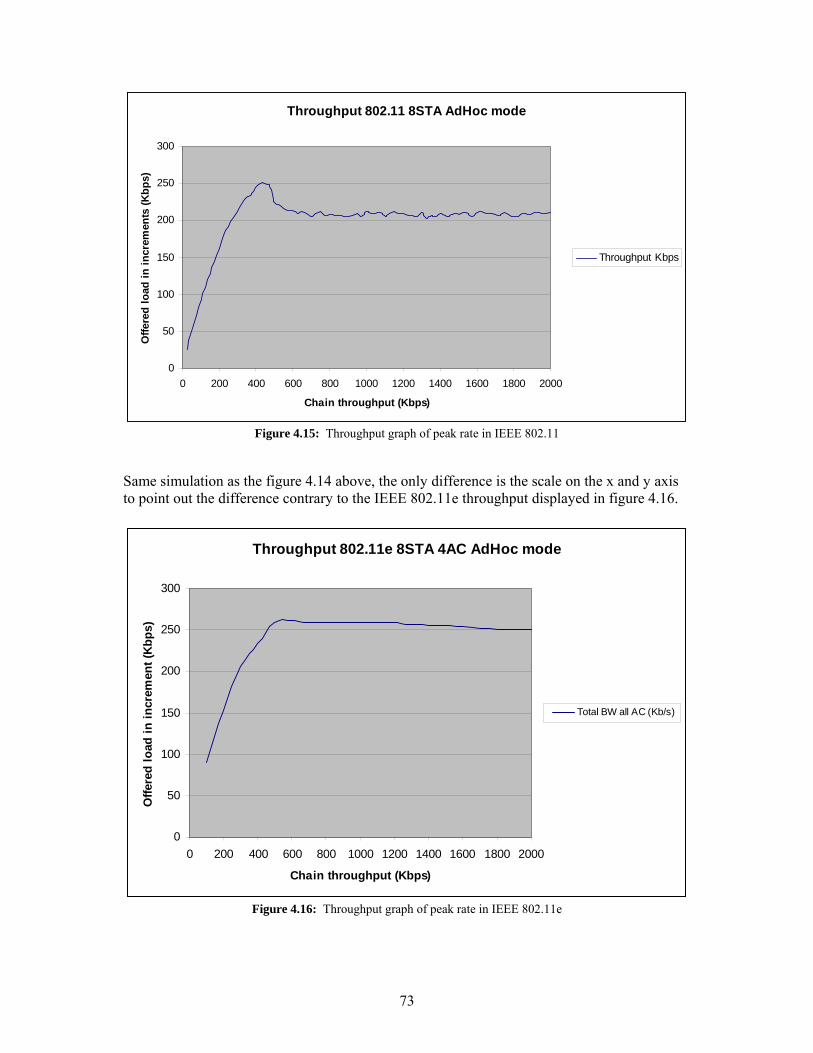
73

Throughput 802.11 8STA AdHoc mode

0

50

100

150

200

250

300

0 200 400 600 800 1000 1200 1400 1600 1800 2000

Chain throughput (Kbps)

Offe

red

load

in in

crem

ents

(Kbp

s)

Throughput Kbps

Figure 4.15: Throughput graph of peak rate in IEEE 802.11

Same simulation as the figure 4.14 above, the only difference is the scale on the x and y axis to point out the difference contrary to the IEEE 802.11e throughput displayed in figure 4.16.

Throughput 802.11e 8STA 4AC AdHoc mode

0

50

100

150

200

250

300

0 200 400 600 800 1000 1200 1400 1600 1800 2000

Chain throughput (Kbps)

Offe

red

load

in in

crem

ent (

Kbp

s)

Total BW all AC (Kb/s)

Figure 4.16: Throughput graph of peak rate in IEEE 802.11e

74

We can clearly see the difference between IEEE 802.11 throughput graph in figure 4.15 and the IEEE 802.11e throughput graph in figure 4.16. The figure displaying IEEE 802.11e does not have any crack in its graph. The graph shows us that the IEEE 802.11e experiences a tiny decrease in throughput in the beginning of the scenario, but as the offered load increase the throughput does not fall significantly. This shows us that the IEEE 802.11.e MAC is more stable than what was found in [22]. To draw a conclusion the IEEE 802.11e MAC is shown better then it is predecessor in IEEE 802.11. The throughput measured at the last hop in a multihop ad hoc network is experienced better with IEEE 802.11e when it comes to forwarding packets in a chain of STAs.

75

Chapter 5 Conclusion In this thesis we have studied the performance of the IEEE 802.11e in WLANs and in ad hoc networks. We have compared the protocol against the legacy WLAN standard, i.e. the IEEE 802.11 protocol. The goal of this thesis was to see how the throughput in the last hop of a chain of STAs was and if IEEE 802.11e was better then IEEE 802.11 to provide QoS in this environment. Our research showed that IEEE 802.11e is better then IEEE 802.11 upon forwarding packets in ad hoc networks. The study also made the observation that IEEE 802.11e is more stable in throughput then IEEE 80.11. This study can prove to some point that IEEE 802.11e can provide QoS in ad hoc networks. Our scenarios show that the protocol has better throughput then its predecessor.

76

References [1] Crow, B.P; Widjaja, I; Kim, L.G; Sakai, P.T , ‘IEEE 802.11 wireless local area networks’. [2] IEEE 802.11. 1999 standard [3] http://www.cisco.com/warp/public/ 784/packet/jul01/pdfs/whitepaper [4] Bob O’Hara and Al Petrick, ‘IEEE 802.11 Handbook, A designer’s companion’. [5] Matthew S. Gast, 802.11 wireless networks, the definitive guide’. [6] Intel: Providing QoS in WLANs, how the IEEE 802.11e standard QoS enhancements will affect the performance of WLANs. [7] Ad Hoc mobile Wireless Networks – C – K Toh [8] http://standards.ieee.org/getieee802/download/802.2-1998.pdf [9] http://www.ieee802.org/3/ [10] Computer networks – Tanenbaum [11] IEEE Std 802.11.e – 2005 [12] http://www.ieee802.org/1/files/private/d-rev-drafts/d4/802-1d-D4.pdf [13] Xu, Gerla, Bae, How Effective is the IEEE 802.11 RTS/CTS Handshake in Ad Hoc Networks? [14] Aleksander Bai, Interoperation between 802.11e EDCA and differentiated services with admission control, Master thesis, University of Oslo, 2006. [15] http://nsnam.isi.edu/nsnam/index.php/Main_Page [16] http://www.tkn.tu-berlin.de [17] http://www.j-sim.org [18] http://www.opnet.com [19] http://www.unik.no [20] http://www.ifi.uio.no/ [21] http://www.telenor.com/rd [22] Li, Blake, Couto, Lee and Morris, Capacity of Ad Hoc wireless networks, MIT Laboratory for Computer Science

77

[23] RFC 2475 - An Architecture for Differentiated Services [24] Gao, Cai and Ngan, Admission control in IEEE 802.11e wireless LANs [25] Charles Perkins, D. Cong & M. Hamlen, RFC 2006 - Mobile IP MIB Definition using SMIv2 [26] Corson and Macker, RFC 2501 -Mobile Ad hoc Networking (MANET), [27] Charles E. Perkins, Ad hoc networking [28] Dan Li and Peng-Yong Kong, A scheme to provide proportionally differentiated end-to-end packet delay in wireless multi-hop ad hoc networks [29] C – K Toh, Ad Hoc mobile Wireless Networks [30] IETF MANET working group - http://www.ietf.org/html.charters/manet-charter.html [31] http://www.olsr.org/ [32] http://en.wikipedia.org/wiki/OLSR [33] http://en.wikipedia.org/wiki/Zone_Routing_Protocol [34] http://people.ece.cornell.edu/%7Ehaas/wnl/Publications/draft-ietf-manet-zone-zrp-04.txt [35] http://www.ietf.org/rfc/rfc3626.txt [36] http://www.cs.virginia.edu/~cl7v/cs851-papers/dsdv-sigcomm94.pdf [37] http://en.wikipedia.org/wiki/Destination-Sequenced_Distance_Vector_routing [38] Sze-Yao Ni, Yu-Chee Tseng, Yuh-Shyan Chen, and Jang-Ping Sheu, The Broadcast Storm Problem in a Mobile Ad Hoc Network [39] Johnson, Maltz, Hu, The Dynamic Source Routing Protocol for Mobile Ad Hoc Networks (DSR), draft-ietf-manet-dsr-10.txt, (Work in progress) [40] Perkins, Royer, Das and Marina, Performance Comparison of Two On-Demand Routing Protocols for Ad Hoc Network . [41] Perkins, Royer, Das, Ad Hoc On-Demand Distance Vector (AODV) routing protocol, RFC 3561 [42] Kenneth Holter, Wireless Extensions to OSPF: Implementation of the Overlapping Relays Proposal, Master thesis, University of Oslo, 2006

78

Appendix

79

# adhoc.tcl by Frank Roar Mjøberg # A X-node example for ad-hoc simulation with AODV # # Globals and flags # set ns [new Simulator] # Define options set opt(chan) Channel/WirelessChannel ;# channel type #set opt(prop) Propagation/FreeSpace ;# radio-propagation model LOS u/refl set opt(prop) Propagation/TwoRayGround ;# LOS med refleksjoner set opt(netif) Phy/WirelessPhy ;# network interface type set opt(mac) Mac/802_11e ;# MAC type #set opt(ifq) Queue/DropTail/PriQueue ;# interface queue type for 802.11 set opt(ifq) Queue/DTail/PriQ ;# interface queue type for 802.11e #set opt(ifq) CMUPriQueue ;# interface queue type for DSR set opt(ll) LL ;# link layer type set opt(ant) Antenna/OmniAntenna ;# antenna model #set opt(ifqlen) 50 ;# max packet in ifq #set val(nn) 7 ;# number of mobilenodes #set opt(adhocRouting) AODV ;# routing protocol set opt(x) 670 ;# X dimension of topography set opt(y) 670 ;# Y dimension of topography #set val(stop) 130 ;# time of simulation end #set opt(packet_size) 1024 ;# bytes per packet #Phy/WirelessPhy set bandwidth_ 0Mb ;# PHY data rate ## Changing this parameter caused no effect in sim runs #Phy/WirelessPhy set freq_ 2.464e9 ;# channel-13. 2.472GHz #set val(seed) 2222222 ;# random seed value #set randGen [new RNG] ;# random seed values #set rng [new RNG] #$randGen seed 214748364 #$randGen seed 2147483646 #$randGen next-substream #$rng exponential #$rng seed 1123456 #for generating random integer b/n min and max # set nextseed 0.0 # puts "utenfor RNG lokken" # proc randomNumber {0 2147483646} {

80

# puts "inni RNG lokken" # global nextseed # global defaultRNG # $defaultRNG seed $nextseed # set nRNG [new RNG] # $nRNG next-substream # set num_ [new RandomVariable/Uniform] # $num_ set min_ 0 # $num_ set max_ 2147483646 # $num_ use-rng $nRNG # set nextseed [expr round([$num_ value])] # return $nextseed # } # Load the parameter file set opt(param) "/home/ns2/simulation/tmp/parameters" source $opt(param) # Needed because of fragmentation, can be set to the same as RTS_Threshold Agent/UDP set packetSize_ $opt(packetSize) # set MAC dataRate_ in Mb if { $opt(mac) == "Mac/802_11e" } { if { $opt(MACdataRate) != 0 } { Mac/802_11e set dataRate_ $opt(MACdataRate)Mb #puts "Using Mac_dataRate_" $MACdataRate "Mb" } } if { $opt(mac) == "Mac/802_11" } { if { $opt(MACdataRate) != 0 } { Mac/802_11 set dataRate_ $opt(MACdataRate)Mb #puts "Using Mac_dataRate_" $MACdataRate "Mb" } } # set MAC control frames rate in Mb Mac/802_11e set basicRate_ 1Mb # set opt(rep) 5 # if {$opt(rep) > 1} { # puts "Usage: ns rng-test.tcl \[replication number\]" # exit # } # set run 1 # if {$opt(rep) == 1} { # set run [lindex $argv 0] # } # if {$run < 1} { # set run 1 # } # if {$argc > 1} { # puts "Usage: ns rng-test.tcl \[replication number\]" # exit # } set run 1 if {$argc == 1} { set run [lindex $argv 0]

81

} if {$run < 1} { set run 1 } # seed the default RNG global defaultRNG $defaultRNG seed $opt(seed) # create the RNGs and set them to the correct substream set arrivalRNG [new RNG] set sizeRNG [new RNG] for {set j 1} {$j < $run} {incr j} { $arrivalRNG next-substream $sizeRNG next-substream } # arrival_ is a exponential random variable describing the time # between consecutive packet arrivals set arrival_ [new RandomVariable/Exponential] $arrival_ set avg_ 5 $arrival_ use-rng $arrivalRNG # size_ is a uniform random variable describing packet sizes set size_ [new RandomVariable/Uniform] $size_ set min_ 100 $size_ set max_ 210000 $size_ use-rng $sizeRNG # print the first 5 arrival times and sizes for {set j 0} {$j < 5} {incr j} { puts [format "%-8.3f %-4d" [$arrival_ value] \ [expr round([$size_ value])]] } #Phy/WirelessPhy set CPThresh_ 10.0 ;# capture threshold 10dB #Phy/WirelessPhy set CSThresh_ 5.011872e-12 ;# carrier sense threshold in W # receiver sensitivity -83dBm #Phy/WirelessPhy set RXThresh_ 1.02054e-10 ;# receive threshold in dB # Use of RTS/CTS or not. if { $opt(mac) == "Mac/802_11e" } { if { $opt(rts_cts) == 1 } { Mac/802_11e set RTSThreshold_ 0 puts "Using RTS/CTS mechanism" } else { Mac/802_11e set RTSThreshold_ 3000 puts "No RTS/CTS mechanism" } } if { $opt(mac) == "Mac/802_11" } { if { $opt(rts_cts) == 1 } { Mac/802_11 set RTSThreshold_ 0 puts "Using RTS/CTS mechanism" } else { Mac/802_11 set RTSThreshold_ 3000 puts "No RTS/CTS mechanism" }

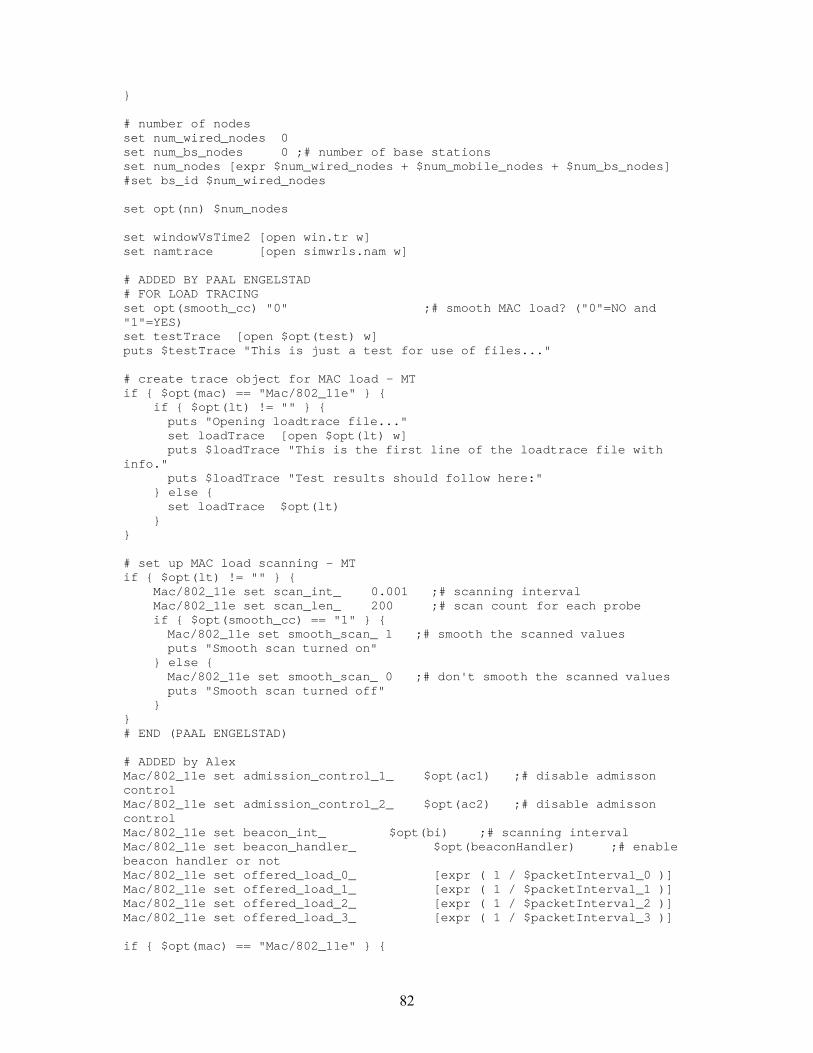
82

} # number of nodes set num_wired_nodes 0 set num_bs_nodes 0 ;# number of base stations set num_nodes [expr $num_wired_nodes + $num_mobile_nodes + $num_bs_nodes] #set bs_id $num_wired_nodes set opt(nn) $num_nodes set windowVsTime2 [open win.tr w] set namtrace [open simwrls.nam w] # ADDED BY PAAL ENGELSTAD # FOR LOAD TRACING set opt(smooth_cc) "0" ;# smooth MAC load? ("0"=NO and "1"=YES) set testTrace [open $opt(test) w] puts $testTrace "This is just a test for use of files..." # create trace object for MAC load - MT if { $opt(mac) == "Mac/802_11e" } { if { $opt(lt) != "" } { puts "Opening loadtrace file..." set loadTrace [open $opt(lt) w] puts $loadTrace "This is the first line of the loadtrace file with info." puts $loadTrace "Test results should follow here:" } else { set loadTrace $opt(lt) } } # set up MAC load scanning - MT if { $opt(lt) != "" } { Mac/802_11e set scan_int_ 0.001 ;# scanning interval Mac/802_11e set scan_len_ 200 ;# scan count for each probe if { $opt(smooth_cc) == "1" } { Mac/802_11e set smooth_scan_ 1 ;# smooth the scanned values puts "Smooth scan turned on" } else { Mac/802_11e set smooth_scan_ 0 ;# don't smooth the scanned values puts "Smooth scan turned off" } } # END (PAAL ENGELSTAD) # ADDED by Alex Mac/802_11e set admission_control_1_ $opt(ac1) ;# disable admisson control Mac/802_11e set admission_control_2_ $opt(ac2) ;# disable admisson control Mac/802_11e set beacon_int_ $opt(bi) ;# scanning interval Mac/802_11e set beacon_handler_ $opt(beaconHandler) ;# enable beacon handler or not Mac/802_11e set offered_load_0_ [expr ( 1 / $packetInterval_0 )] Mac/802_11e set offered_load_1_ [expr ( 1 / $packetInterval_1 )] Mac/802_11e set offered_load_2_ [expr ( 1 / $packetInterval_2 )] Mac/802_11e set offered_load_3_ [expr ( 1 / $packetInterval_3 )] if { $opt(mac) == "Mac/802_11e" } {

83

if { $opt(beaconHandler) != 0 } { puts "Opening beacontrace file..." set beaconTrace [open $opt(beacontrace) w] } } # End Alex #set up for hierarchical routing when you have both wired and wireless network together #(needed for routing over a basestation) #This is not likely to cause any effect running this script #$ns node-config -addressType hierarchical AddrParams set domain_num_ 1 ;# number of domains lappend cluster_num 1 ;# number of clusters in each domain AddrParams set cluster_num_ $cluster_num lappend eilastlevel $num_mobile_nodes ;# number of nodes for each cluster AddrParams set nodes_num_ $eilastlevel $ns trace-all $ntr $ns namtrace-all-wireless $namtrace $opt(x) $opt(y) set chan [new $opt(chan)] set topo [new Topography] $topo load_flatgrid $opt(x) $opt(y) # Create God set god [create-god $num_mobile_nodes] #create-god $val(nn) #$god set-dist 1 $num_mobile_nodes $num_mobile_nodes #$god set-dist 1 2 2 # Create nn mobilenodes [$num_mobile_nodes] and attach them to the channel. # if { $layer == "MAC" } { $ns node-config -adhocRouting $opt(adhocRouting) \ -llType $opt(ll) \ -macType $opt(mac) \ -ifqType $opt(ifq) \ -ifqLen $opt(ifqlen) \ -antType $opt(ant) \ -propType $opt(prop) \ -phyType $opt(netif) \ -channel $chan \ -topoInstance $topo \ -wiredRouting OFF \ -agentTrace ON \ -routerTrace ON \ -macTrace ON \ -movementTrace OFF } if { $layer == "AGT" } { $ns node-config -adhocRouting $opt(adhocRouting) \ -llType $opt(ll) \ -macType $opt(mac) \ -ifqType $opt(ifq) \ -ifqLen $opt(ifqlen) \ -antType $opt(ant) \ -propType $opt(prop) \

84

-phyType $opt(netif) \ -channel $chan \ -topoInstance $topo \ -wiredRouting OFF \ -agentTrace ON \ -routerTrace ON \ -macTrace OFF \ -movementTrace OFF } # for {set i 0} {$i < $num_mobile_nodes} {incr i} { # set wl_node_($i) [$ns node] ;# 1.0.[expr $i +1]] # $wl_node_($i) random-motion 0 # puts "wireless node $i created ..." # # BS not used here -> adhoc # #$wl_node_($i) base-station [AddrParams addr2id [$BS(0) node-addr]] # $wl_node_($i) set X_ [expr $i*$nodeDistance + (300-(($num_mobile_nodes-1)/2*$nodeDistance))] # $wl_node_($i) set Y_ [expr 300 + $nodeDistance] # $wl_node_($i) set Z_ 0.0 # #puts [expr $i*$nodeDistance + (300-(($num_mobile_nodes-1)/2*$nodeDistance))] # #puts [expr 300 + $nodeDistance] # } # nodene skal stå på rekke som i en kjede derfor Y = 100 på alle noder # ingen adresser da noden er i adhoc modus for {set i 0} {$i < $num_mobile_nodes} {incr i} { set wl_node_($i) [$ns node] ;# 1.0.[expr $i +1]] $wl_node_($i) random-motion 0 puts "wireless node $i created ..." # BS not used here because of ad hoc mode #$wl_node_($i) base-station [AddrParams addr2id [$BS(0) node-addr]] $wl_node_($i) set X_ [expr $i*$nodeDistance + (300-(($num_mobile_nodes-1)/2*$nodeDistance))] $wl_node_($i) set Y_ 100 $wl_node_($i) set Z_ 0.0 #puts [expr $i*$nodeDistance + (300-(($num_mobile_nodes-1)/2*$nodeDistance))] } # ADDED BY PAAL ENGELSTAD # Binding load trace to trace file for mobile nodes... # NOTE: Binding load trace to wired nodes is not indended here... if { $opt(mac) == "Mac/802_11e" } { for {set i 0} {$i < $num_mobile_nodes } {incr i} { # bind MAC load trace file - MT # puts "DEBUG: Using load-trace command..." [$wl_node_($i) set mac_(0)] load-trace $loadTrace # Evt: $wl_node_($i) load-trace $loadTrace ...??? Check... } } # END (PAAL ENGELSTAD) # # MODIFIED BJØRN SELVIG # source "/home/ns2/simulation/scripts/common/generateFlow.tcl"

85

# # for each station put up the same flows # for {set j 0} {$j < $num_mobile_nodes} {incr j} { # if {$packetInterval_0 != "-1.0" } { # generate_flow 0 $packetLength_0 $packetInterval_0 $trafficType_0 $startTime $wl_node_($j) $BS(0) [expr $j*4 + 0] # } # if {$packetInterval_1 != "-1.0"} { # generate_flow 1 $packetLength_1 $packetInterval_1 $trafficType_1 $startTime $wl_node_($j) $BS(0) [expr $j*4 + 1] # } # if {$packetInterval_2 != "-1.0"} { # generate_flow 2 $packetLength_2 $packetInterval_2 $trafficType_2 $startTime $wl_node_($j) $BS(0) [expr $j*4 + 2] # } # if {$packetInterval_3 != "-1.0"} { # generate_flow 3 $packetLength_3 $packetInterval_3 $trafficType_3 $startTime $wl_node_($j) $BS(0) [expr $j*4 + 3] # } # } ## END BJØRN SELVIG ##Edited by Frank Roar Mjøberg # BS is no longer the destination node as before. The dest_node is now the last node since we are # about to measure the capacity in a chain of nodes where throughput to the last node in the # chain is of interest. # # Tatt bort BS(0) og satt [expr $num_mobile_nodes - 1] som dest_ node source "/home/ns2/simulation/scripts/common/generateFlow.tcl" # for each station put up the same flows #for {set j 0} {$j < $num_mobile_nodes} {incr j} { if {$packetInterval_0 != "-1.0" } { generate_flow 0 $packetLength_0 $packetInterval_0 $trafficType_0 $startTime $wl_node_(0) $wl_node_([expr $num_mobile_nodes - 1]) 0 } if {$packetInterval_1 != "-1.0"} { generate_flow 1 $packetLength_1 $packetInterval_1 $trafficType_1 $startTime $wl_node_(0) $wl_node_([expr $num_mobile_nodes - 1]) 1 } if {$packetInterval_2 != "-1.0"} { generate_flow 2 $packetLength_2 $packetInterval_2 $trafficType_2 $startTime $wl_node_(0) $wl_node_([expr $num_mobile_nodes - 1]) 2 } if {$packetInterval_3 != "-1.0"} { generate_flow 3 $packetLength_3 $packetInterval_3 $trafficType_3 $startTime $wl_node_(0) $wl_node_([expr $num_mobile_nodes - 1]) 3 } #} # source "/home/ns2/simulation/scripts/common/generateFlow.tcl" # # for each station put up the same flows # for {set j 0} {$j < $num_mobile_nodes} {incr j} {

86

# if {$packetInterval_0 != "-1.0" } { # generate_flow 0 $packetLength_0 $packetInterval_0 $trafficType_0 $startTime $wl_node_(0) $wl_node_(2) [expr $j*4 + 0] # } # if {$packetInterval_1 != "-1.0"} { # generate_flow 1 $packetLength_1 $packetInterval_1 $trafficType_1 $startTime $wl_node_(0) $wl_node_(2) [expr $j*4 + 1] # } # if {$packetInterval_2 != "-1.0"} { # generate_flow 2 $packetLength_2 $packetInterval_2 $trafficType_2 $startTime $wl_node_(0) $wl_node_(2) [expr $j*4 + 2] # } # if {$packetInterval_3 != "-1.0"} { # generate_flow 3 $packetLength_3 $packetInterval_3 $trafficType_3 $startTime $wl_node_(0) $wl_node_(2) [expr $j*4 + 3] # } # } # source "/home/ns2/simulation/scripts/common/generateFlow.tcl" # # for each station put up the same flows # for {set j 0} {$j < $num_mobile_nodes} {incr j} { # if {$packetInterval_0 != "-1.0" } { # generate_flow 0 $packetLength_0 $packetInterval_0 $trafficType_0 $startTime $wl_node_([expr $num_mobile_nodes - $num_mobile_nodes]) $wl_node_([expr $num_mobile_nodes - 1]) [expr $j*4 + 0] # } # if {$packetInterval_1 != "-1.0"} { # generate_flow 1 $packetLength_1 $packetInterval_1 $trafficType_1 $startTime $wl_node_([expr $num_mobile_nodes - $num_mobile_nodes]) $wl_node_([expr $num_mobile_nodes - 1]) [expr $j*4 + 1] # } # if {$packetInterval_2 != "-1.0"} { # generate_flow 2 $packetLength_2 $packetInterval_2 $trafficType_2 $startTime $wl_node_([expr $num_mobile_nodes - $num_mobile_nodes]) $wl_node_([expr $num_mobile_nodes - 1]) [expr $j*4 + 2] # } # if {$packetInterval_3 != "-1.0"} { # generate_flow 3 $packetLength_3 $packetInterval_3 $trafficType_3 $startTime $wl_node_([expr $num_mobile_nodes - $num_mobile_nodes]) $wl_node_([expr $num_mobile_nodes - 1]) [expr $j*4 + 3] # } # } ## END FRM # Define node initial position in nam for {set i 0} {$i < $num_mobile_nodes} {incr i} { $ns initial_node_pos $wl_node_($i) 20 } ##Edited by Frank Roar Mjøberg # Kommentert ut fordi det ikke brukes beaconHandler i adhoc mode (foreløpig..) #if { $opt(beaconHandler) != 0} { # $ns at [expr $stopTime - 1] "[$BS(0) set mac_(0)] beacon-print test]" #} ##End FRM # # Tell nodes when the simulation ends

87

# for {set i 0} {$i < $num_mobile_nodes } {incr i} { $ns at $stopTime "$wl_node_($i) reset"; } proc stop {} { global ns ntr close $ntr #close $nf } #$ns at $stopTime "puts \"NS EXITING...\" ; $ns halt" #$ns at $stopTime "stop" # ADDED BY PAAL ENGELSTAD proc finish {} { global ns loadTrace testTrace ntr namtrace puts "DEBUG fra proc finish: Lukker filene..." close $loadTrace close $testTrace close $ntr close $namtrace puts "NS EXITING...(from proc finish)" $ns halt #exit 0 } # TRIED TO REPLACE: # $ns at $stopTime "puts \"NS EXITING...\" ; $ns halt" # $ns at $stopTime "stop" # WITH: $ns at $stopTime "finish" # END (PAAL ENGELSTAD) # run the simulation $ns run

88

The python script: #!/bin/sh """:" exec python $0 ${1+"$@"} """ import shutil, os, re, sys, time, string from time import gmtime, strftime print "=================================================" print "Simulation started" ##################################################################################### ################## PARAMETER SETTINGS ######################################### ##################################################################################### ## Added by Frank Roar Mjøberg autum 2006 ########################################## ## Ad hoc parameter - used for simulation of ad hoc mode # 1 = on (ad hoc mode), 0 = off (infrastruture mode) # Ved adhoc mode endres adhoc/AdHocRegular.tcl, ved infrastructure mode endres regular.tcl adhoc = 1 ## RTSThreshold parameter: do you want to use RTS/CTS mechanism or not? # 1 = Use RTS/CTS and 0 = No RTS/CTS rts_cts = 1 # Which (AdHoc) routing protocol to use:"AODV", "DSR", "DSDV" or "NOAH" adhocRouting = "AODV" # nodeDistance should be 200 meters in according to paper if adhoc == 0: nodeDistance = 0.5 else: nodeDistance = 200 ## Endre resultat fil for å kunne ta ut throughput på siste node og mellomliggende. # 1 = true, 0 = false resultsOnlyLastHop = 0 # Set UDP packet size (Agent/UDP set packetSize_) to prevent fragmentation packetSize = 1500 # Set seed value - 3333 is recommended after several runs to find the one who let AC_VO send first # Default RNG value is 1234 seed = 3333 # Set MAC dataRate_ in Mb MACdataRate = 2 ############################################################################################ ############## PARAMETERS ONLY USED IN AD HOC MODE #####################################

89

############################################################################################ # 0 = chain topology, 1 =.. osv. # ikke i bruk enda #topology = 0 # evt bruke default verdier. Må evt regne om til Txpower eller threshold eller noe liknende... # CSThresh_ verdien bestemmer om en ramme blir detektert av mottaker eller ikke. #transmissionRange = 250 # evt bruke default verdier. Må evt regne om til Txpower eller threshold eller noe liknende.. # RxThresh_ en ramme må ha større styrke (høyere verdi) enn denne verdien for å bli korrekt mottatt etter mottagelse. #interferenceRange = 550 ############################################################################################# ########################### ARBEIDSPLAN: ################################################ ############################################################################################# # # 1) Kjøre med AODV i steden for NOAH (bruke infrastruktur mode som allerede er laget) # Teste ut at adhoc = 0 og adhoc = 1 gir omtrent samme resultater # # 2) Lage en chain topologi med 2 noder (alt ellers likt), det betyr droppe BS, # Node distance = 0.5 fremdeles osv. - gjøre målingene på den siste noden # # 3) Lage en 3 node topologi # 4) Lage en n-node topologi # 5) Kunne forandre på nodeDistance # 6) Kunne forandre på transmission Range (bør kunne settes i meter - krever trolig omregning) # #set opt(txPower) 1.4 ;# transmitting power in mW = 1.4 # # 7) Kunne forandre på interference range (bør kunne settes i meter) # #set opt(sensePower) 0.00000175 ;# sensing power in mW # # 8) Ta ut resultater på ulike noder i en rekke... Finne et bra format for resultatfilen. # Bør kunne ta ut throughput på alle 4 klassene for node 1,2,3,4,5,6 + siste node i rekken. # (Siste node i rekken bør komme først). # # 9) Implementere funksjonalitet som gir større innsikt i paperet, enn det som er skrevet der... ##################################################################################### # Edited by Frank Roar Mjøberg # Modified and ported version of the old python file from Bjørn Selvig and Alex Bai # END FRM # Debug - provides more output during simulation # 1 = on, 0 = off

90

debug = 1 # Result file resultFile = "results-frank-AODV-8STA-21april-250kbps-4ac" # which ns version to use # 1 = ns2-2.28, 0 = ns2-2.26 nsVer = 1 # Number of nodes (Infrastructure: Excluding the BS, Ad hoc: Number of nodes) #num_wireless_nodes = [2,3,4,5,6,7,8,9,10] num_wireless_nodes = [8] # Specify bandwidths in Kb/s # Bandwidth is specified at the IP layer # parameters for flow with priority 0 bandwidth_0 = 250.0 bandwidthInc_0 = 250.0 trafficType_0 = "EXP" txop_budget_0 = 0.10 admittedRate_0 = 100.0 # parameters for flow with priority 1 bandwidth_1 = 250.0 bandwidthInc_1 = 250.0 trafficType_1 = "EXP" txop_budget_1 = 0.10 admittedRate_1 = 100.0 # parameters for flow with priority 2 bandwidth_2 = 250.0 bandwidthInc_2 = 250.0 trafficType_2 = "EXP" txop_budget_2 = 0.10 admittedRate_2 = 100.0 # parameters for flow with priority 3 bandwidth_3 = 250.0 bandwidthInc_3 = 250.0 trafficType_3 = "EXP" txop_budget_3 = 0.10 admittedRate_3 = 100.0 # Packet Lengths for the simulation, specify in Bytes at the IP layer packetLengthSets = [[1500,1500,1500,1500]] #packetLengthSets = [[1024,1024,1024,1024]] #packetLengthSets = [[512,512,512,512]] #packetLengthSets = [[64,64,64,64]] # BJORN SELVIG, 08.06.2005, added for stabtime testing # Specify startime, stoptime and stabilizetime for the simulation timeSets = [[2,300,28]] # Number of bandwidth increments for each timeset bandwidthIncrements = 4 # Enable Admitted Rate or not # 0 = disabled, 1 = enabled admittedRate = 0

91

# enable Admisson Control 1 (measurement based) # 0 = disabled, 1 = enabled admissionControl_1 = 0 # enable Admisson Control 2 (model based) # 0 = disabled, 1 = enabled admissionControl_2 = 0 # Enabled beacon handler beaconHandler = 0 # Specify beacon interval time in seconds beaconInterval = 0.1 # set CFB, 0 disables CFB, 1 enables CFB cfb = 0 # loadtrace #loadtraceScanLength = 200 #loadtraceScanInterval = 0.001 loadtraceScanLength = 0 loadtraceScanInterval = 0 # Queue length ifqLength = 50 # set whether latency distribution file for finding percentile results should be created or not # 0 = disabled, 1 = enabled createDelayDistributionFile = 0 # set granularity for latency distribution,number of intervals between minimum and maximum latency DistributionFileGranularity = 1000 # Percentile for results percentile = 95 # Which IEEE 802.11 version to use: # set to 'a' or 'b' specVersion = 'b' ##EDCF parameters for the simulation.802.11e parameterfile will be updated with these parameters. #EDCFparametersets = [[2,3,7,1.5, # 2,7,15,3.0, # 3,15,1023,1.5, # 7,15,1023,0]] ## EDCA parameter set if you run one class only. Use only AC_BK with 2,31,1023,0- like 802.11 #EDCFparametersets = [[99,1023,2047,0, # 99,1023,2047,0, # 2,31,1023,0, # 99,1023,2047,0]] ## EDCA parameter set used in the thesis EDCFparametersets = [[2,7,15,0, 2,15,31,0, 3,31,1023,0,

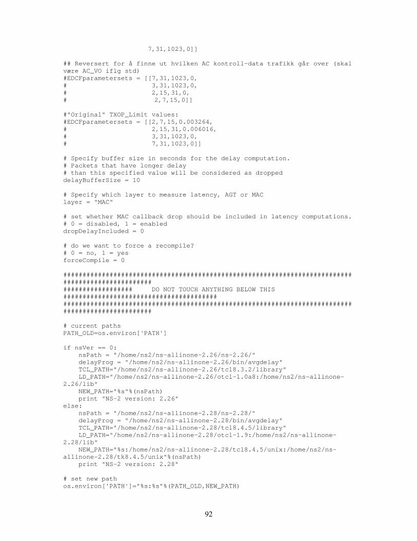
92

7,31,1023,0]] ## Reversert for å finne ut hvilken AC kontroll-data trafikk går over (skal være AC_VO iflg std) #EDCFparametersets = [[7,31,1023,0, # 3,31,1023,0, # 2,15,31,0, # 2,7,15,0]] #"Original" TXOP_Limit values: #EDCFparametersets = [[2,7,15,0.003264, # 2,15,31,0.006016, # 3,31,1023,0, # 7,31,1023,0]] # Specify buffer size in seconds for the delay computation. # Packets that have longer delay # than this specified value will be considered as dropped delayBufferSize = 10 # Specify which layer to measure latency, AGT or MAC layer = "MAC" # set whether MAC callback drop should be included in latency computations. # 0 = disabled, 1 = enabled dropDelayIncluded = 0 # do we want to force a recompile? # 0 = no, 1 = yes forceCompile = 0 ################################################################################################## ################## DO NOT TOUCH ANYTHING BELOW THIS ######################################## ################################################################################################## # current paths PATH_OLD=os.environ['PATH'] if nsVer == 0: nsPath = "/home/ns2/ns-allinone-2.26/ns-2.26/" delayProg = "/home/ns2/ns-allinone-2.26/bin/avgdelay" TCL_PATH="/home/ns2/ns-allinone-2.26/tcl8.3.2/library" LD_PATH="/home/ns2/ns-allinone-2.26/otcl-1.0a8:/home/ns2/ns-allinone-2.26/lib" NEW_PATH="%s"%(nsPath) print "NS-2 version: 2.26" else: nsPath = "/home/ns2/ns-allinone-2.28/ns-2.28/" delayProg = "/home/ns2/ns-allinone-2.28/bin/avgdelay" TCL_PATH="/home/ns2/ns-allinone-2.28/tcl8.4.5/library" LD_PATH="/home/ns2/ns-allinone-2.28/otcl-1.9:/home/ns2/ns-allinone-2.28/lib" NEW_PATH="%s:/home/ns2/ns-allinone-2.28/tcl8.4.5/unix:/home/ns2/ns-allinone-2.28/tk8.4.5/unix"%(nsPath) print "NS-2 version: 2.28" # set new path os.environ['PATH']="%s:%s"%(PATH_OLD,NEW_PATH)

93

os.environ['LD_LIBRARY_PATH']="%s"%(LD_PATH) os.environ['TCL_LIBRARY']="%s"%(TCL_PATH) tmpPath = "/home/ns2/simulation/tmp/" commonPath = "/home/ns2/simulation/scripts/common/" if adhoc == 0: resultPath = "/home/ns2/simulation/results/%s"%(resultFile) logPath = "/home/ns2/simulation/results/%s-ac2.log"%(resultFile) else: resultPath = "/home/ns2/simulation/AdHocResults/%s"%(resultFile) logPath = "/home/ns2/simulation/AdHocResults/%s-ac2.log"%(resultFile) errorFile = "%s-error"%(resultPath) if admissionControl_1 and admissionControl_2: print "WARNING!\nYou CAN NOT use both admission controls at once!" sys.exit(0) if admissionControl_1 == 1: nsFile = "%sac1.tcl"%(commonPath) print "NOTICE! The actual scenario is specified in %s"%(nsFile) elif admissionControl_2 == 1: nsFile = "%sac2.tcl"%(commonPath) print "NOTICE! The actual scenario is specified in %s"%(nsFile) elif adhoc == 1: #nsFile = "%sAdHocRegular.tcl"%(commonPath) nsFile = "%sadhoc.tcl"%(commonPath) print "Running in AdHoc Mode\n" else: nsFile = "%sregular.tcl"%(commonPath) print "Infrastructure Mode\n" EDCFParamFile_ = "%smac/802_11e/priority.tcl"%(nsPath) MACTclFile_ = "%stcl/lan/ns-mac.tcl"%(nsPath) MACTclFile_a_ = "%stcl/lan/ns-mac_11a.tcl"%(nsPath) MACTclFile_b_ = "%stcl/lan/ns-mac_11b.tcl"%(nsPath) MACTclFile_a_CFB = "%stcl/lan/ns-mac_11a-CFB.tcl"%(nsPath) MACTclFile_b_CFB = "%stcl/lan/ns-mac_11b-CFB.tcl"%(nsPath) MACHeaderFile_ = "%smac/802_11e/mac-802_11e.h"%(nsPath) MACHeaderFile_a_ = "%smac/802_11e/mac-802_11e-a.h"%(nsPath) MACHeaderFile_b_ = "%smac/802_11e/mac-802_11e-b.h"%(nsPath) # make sure we are not running as root cmd = "whoami > %swho"%(tmpPath) os.system(cmd) infile = open("%swho"%(tmpPath), 'r') line = infile.readline() if string.find(line, "ns2") == -1: print "WARNING!!\nYou MUST run as user ns2" sys.exit(0) ################################################################################################## ######################## Definitions ############################################################# ################################################################################################## #IP_HEADER_LENGTH = 120 #UDP_HEADER_LENGTH = 8

94

#RTP_HEADER_LENGTH = 12 #LLSnap_HEADER_LENGTH = 8 pattern1 = r"802.11a" pattern2 = r"802.11b" pattern3 = r"CFB-enabled" version = 0 file_CFB = 0 compile = False linkCapasity = 0 if specVersion == 'b': linkCapasity = 0 elif specVersion == 'a': linkCapasity = 24000 ################################################################################################## ##### Compile with correct 802.11 version and EDCA parameters #################################### ################################################################################################## MACTclFile = open(MACTclFile_, 'r') MACHeaderFile = open(MACHeaderFile_, 'r') line = MACTclFile.readline() line1 = MACTclFile.readline() line2 = MACHeaderFile.readline() match1 = re.search(pattern1,line) match2 = re.search(pattern2,line) match3 = re.search(pattern1, line2) match4 = re.search(pattern2, line2) match5 = re.search(pattern3, line1) if match1 and match3: version = 'a' elif match2 and match4: version = 'b' if match5: file_CFB = 1 MACTclFile.close() MACHeaderFile.close() print "802.11 Version: %s\n"%(version) # Replace header files with correct version if (version != specVersion) or (file_CFB != cfb): compile = True if specVersion == 'a': if cfb == 1: copy_cmd = ("cp %s %s"%(MACTclFile_a_CFB, MACTclFile_)) else: copy_cmd = ("cp %s %s"%(MACTclFile_a_, MACTclFile_)) copy_cmd2 = ("cp %s %s"%(MACHeaderFile_a_, MACHeaderFile_)) os.system(copy_cmd) os.system(copy_cmd2) elif specVersion == 'b': if cfb == 1: copy_cmd = ("cp %s %s"%(MACTclFile_b_CFB, MACTclFile_)) else:

95

copy_cmd = ("cp %s %s"%(MACTclFile_b_, MACTclFile_)) copy_cmd2 = ("cp %s %s"%(MACHeaderFile_b_, MACHeaderFile_)) os.system(copy_cmd) os.system(copy_cmd2) # Replace with correct EDCA parameters for EDCFparameterset in EDCFparametersets: copy_cmd = ("cp %s %s_copy"%(EDCFParamFile_,EDCFParamFile_)) os.system(copy_cmd) EDCFParamFile = open(EDCFParamFile_, 'w') EDCFParamFile_copy = open(("%s_copy"%(EDCFParamFile_)), 'r') while 1: line = EDCFParamFile_copy.readline() if not line: break newLine = re.sub("Prio 0 AIFS .*","Prio 0 AIFS %d"%(EDCFparameterset[0]), line) newLine = re.sub("Prio 0 CW_MIN .*","Prio 0 CW_MIN %d"%(EDCFparameterset[1]), newLine) newLine = re.sub("Prio 0 CW_MAX .*","Prio 0 CW_MAX %d"%(EDCFparameterset[2]), newLine) newLine = re.sub("Prio 0 TXOPLimit .*","Prio 0 TXOPLimit %f"%(EDCFparameterset[3]), newLine) newLine = re.sub("Prio 1 AIFS .*","Prio 1 AIFS %d"%(EDCFparameterset[4]), newLine) newLine = re.sub("Prio 1 CW_MIN .*","Prio 1 CW_MIN %d"%(EDCFparameterset[5]), newLine) newLine = re.sub("Prio 1 CW_MAX .*","Prio 1 CW_MAX %d"%(EDCFparameterset[6]), newLine) newLine = re.sub("Prio 1 TXOPLimit .*","Prio 1 TXOPLimit %f"%(EDCFparameterset[7]), newLine) newLine = re.sub("Prio 2 AIFS .*","Prio 2 AIFS %d"%(EDCFparameterset[8]), newLine) newLine = re.sub("Prio 2 CW_MIN .*","Prio 2 CW_MIN %d"%(EDCFparameterset[9]), newLine) newLine = re.sub("Prio 2 CW_MAX .*","Prio 2 CW_MAX %d"%(EDCFparameterset[10]), newLine) newLine = re.sub("Prio 2 TXOPLimit .*","Prio 2 TXOPLimit %f"%(EDCFparameterset[11]), newLine) newLine = re.sub("Prio 3 AIFS .*","Prio 3 AIFS %d"%(EDCFparameterset[12]), newLine) newLine = re.sub("Prio 3 CW_MIN .*","Prio 3 CW_MIN %d"%(EDCFparameterset[13]), newLine) newLine = re.sub("Prio 3 CW_MAX .*'","Prio 3 CW_MAX %d"%(EDCFparameterset[14]), newLine) newLine = re.sub("Prio 3 TXOPLimit .*","Prio 3 TXOPLimit %f"%(EDCFparameterset[15]), newLine) if cmp(line, newLine) != 0: compile = True EDCFParamFile.writelines(newLine) EDCFParamFile.close() EDCFParamFile_copy.close() # Make the ns project with the new EDCF parameter values if (compile | forceCompile): cmd = ("cd %s; ./configure 1>/dev/null 2>%s; make clean 1>/dev/null 2>%s; make depend 1>/dev/null 2>%s; make 1>/dev/null 2>%s;"%(nsPath,errorFile,errorFile,errorFile,errorFile))

96

print "Compiling..." os.system(cmd) print "Compiling done!" compile = False ################################################################################################## ###### Write EDCF parameter values to the results file ########################################### ################################################################################################## # Modified by Alex 02.03.06 - Print all the information needed to run this simulation #outfile = open(resultPath, 'a') outfile = open(resultPath, 'w') outfile.write("\n\n\n########################### New Simulation #############################\n") if nsVer == 0: outfile.write("%s\nNs-2 Version: 2.26\nSpec Version: %s\n\n"%(strftime("%a, %d %b %Y %H:%M:%S +0000", gmtime()), specVersion)) else: outfile.write("%s\nNs-2 Version: 2.28\nSpec Version: %s\n\n"%(strftime("%a, %d %b %Y %H:%M:%S +0000", gmtime()), specVersion)) outfile.write("Flow\tStart Kbs\tInc Kbs\tTraffic type\tTXOP Budget\tAdmitted Rate (%)\n") outfile.write("Prio0\t%f\t%f\t%s\t%f\t%f\n"%(bandwidth_0,bandwidthInc_0,trafficType_0,txop_budget_0,admittedRate_0)) outfile.write("Prio1\t%f\t%f\t%s\t%f\t%f\n"%(bandwidth_1,bandwidthInc_1,trafficType_1,txop_budget_1,admittedRate_1)) outfile.write("Prio2\t%f\t%f\t%s\t%f\t%f\n"%(bandwidth_2,bandwidthInc_2,trafficType_2,txop_budget_2,admittedRate_2)) outfile.write("Prio3\t%f\t%f\t%s\t%f\t%f\n\n"%(bandwidth_3,bandwidthInc_3,trafficType_3,txop_budget_3,admittedRate_3)) outfile.write("Flow\tAIFS\tCW_min\tCW_max\tTXOP_limit\tTraffic Type\n") outfile.write("Prio0\t%d\t%d\t%d\t%6f\t%s\n"%(EDCFparameterset[0],EDCFparameterset[1],EDCFparameterset[2],EDCFparameterset[3], trafficType_0)) outfile.write("Prio1\t%d\t%d\t%d\t%6f\t%s\n"%(EDCFparameterset[4],EDCFparameterset[5],EDCFparameterset[6], EDCFparameterset[7], trafficType_1)) outfile.write("Prio2\t%d\t%d\t%d\t%6f\t%s\n"%(EDCFparameterset[8],EDCFparameterset[9],EDCFparameterset[10], EDCFparameterset[11], trafficType_2)) outfile.write("Prio3\t%d\t%d\t%d\t%6f\t%s\n\n"%(EDCFparameterset[12],EDCFparameterset[13],EDCFparameterset[14], EDCFparameterset[15],trafficType_3)) outfile.write("Packet lengths\nPrio0\tPrio1\tPrio2\tPrio3\n") outfile.write("%d\t%d\t%d\t%d\n"%(packetLengthSets[0][0], packetLengthSets[0][1], packetLengthSets[0][2], packetLengthSets[0][3])) outfile.write("Number of increments: %d\n"%(bandwidthIncrements)) outfile.write("Queue Length: %d\n"%(ifqLength)) outfile.write("Node Distance: %f\n\n"%(nodeDistance))

97

if cfb == 1: outfile.write("CFB enabled\n") else: outfile.write("CFB disabled\n") if admittedRate == 1: outfile.write("Rate Configuration enabled\n") else: outfile.write("Rate Configuration disabled\n") if admissionControl_1 == 1: outfile.write("Admission control 1 enabled\n") beaconHandler = 1 elif admissionControl_2 == 1: outfile.write("Admission control 2 enabled\n") beaconHandler = 1 else: outfile.write("Admission control disabled\n") if beaconHandler == 1: outfile.write("Beacon Handler enabled\n") outfile.write("Beacon interval: %d\n"%(beaconInterval)) else: outfile.write("Beacon handler disabled\n") outfile.write("Latency measured at layer: %s\n"%(layer)) outfile.write("Delay buffer size: %d\n"%(delayBufferSize)) if dropDelayIncluded == 1: outfile.write("MAC callback drop for latency computations: included\n\n") else: outfile.write("MAC callback drop for latency computations: NOT included\n\n") if createDelayDistributionFile == 1: outfile.write("createDelayDistributionFile enabled\n") outfile.write("DistributionFileGranularity: %d\npercentile: %d\n\n"%(DistributionFileGranularity, percentile)) else: outfile.write("createDelayDistributionFile disabled\n\n") outfile.write("Loadtrace scanlength: %d\nLoadtrace scanInterval: %d\n\n\n"%(loadtraceScanLength, loadtraceScanInterval)) outfile.write("StartTime\tStopTime\tStabilizeTime\t") outfile.write("Status\tNodes\tMeasured Hop\tOffered Load\tTotal Recv BW 0 (Kb/s)\tTotal Recv BW 1 (Kb/s)\tTotal Recv BW 2 (Kb/s)\tTotal Recv BW 3 (Kb/s)\tTotal BW all (Kb/s)\tGrepped BW 0 (Kb/s)\tGrepped BW 1 (Kb/s)\tGrepped BW 2 (Kb/s)\tGrepped BW 3 (Kb/s)\tTotal Grepped BW(Kb/s)\tAverage Channel load\tAvg Latency 0\tAvg Latency 1\tAvg Latency 2\tAvg Latency 3\tAvg Lat Square 0\tAvg Lat Square 1\tAvg Lat Square 2\tAvg Lat Square 3\tMax Lat 0\tMax Lat 1\tMax Lat 2\tMax Lat 3\tMin Lat 0\tMin Lat 1\tMin Lat 2\tMin Lat 3\tIFQ drop 0 (%)\tIFQ drop 1 (%)\tIFQ drop 2 (%)\tIFQ drop 3 (%)\tRTR CBK drop 0 (%)\tRTR CBK drop 1 (%)\tRTR CBK drop 2 (%)\tRTR CBK drop 3 (%)\tTotal Offered BW 0 (Kb/s)\tTotal Offered BW 1 (Kb/s)\tTotal Offered BW 2 (Kb/s)\tTotal Offered BW 3 (Kb/s)\tPacket Length 0 (B)\tPacket Length 1 (B)\tPacket Length 2 (B)\tPacket Length 3 (B)\tAvg Lat RTR CBK 0\tAvg Lat RTR CBK 1\tAvg Lat RTR CBK 2\tAvg Lat RTR CBK 3\tpercentile lat 0\tTau 0\tTau 1\tTau 2\tTau 3\tSat 0\tSat 1\tSat 2\tSat 3\tRo 0\tRo 1\tRo 2\tRo 3\tColl 0\tColl 1\tColl 2\tColl 3\n")

98

outfile.close() ################################################################################################## ######### Simulate ############################################################################### ################################################################################################## j = 0 for timeSet in timeSets: j = j + 1 print "Getting ready to simulate with timeset %d: [%d, %d, %d]"%(j,timeSet[0],timeSet[1],timeSet[2]) for num_wireless_node in num_wireless_nodes: for packetLengthSet in packetLengthSets: bw_0 = bandwidth_0 bw_1 = bandwidth_1 bw_2 = bandwidth_2 bw_3 = bandwidth_3 # Alex - 06.02.06 for i in range(0, bandwidthIncrements + 1, 1): if admittedRate == 1: if bw_0 > (admittedRate_0*linkCapasity)/(100*num_wireless_node): bw_0 = (admittedRate_0*linkCapasity)/(100*num_wireless_node) if bw_1 > (admittedRate_1*linkCapasity)/(100*num_wireless_node): bw_1 = (admittedRate_1*linkCapasity)/(100*num_wireless_node) if bw_2 > (admittedRate_2*linkCapasity)/(100*num_wireless_node): bw_2 = (admittedRate_2*linkCapasity)/(100*num_wireless_node) if bw_3 > (admittedRate_3*linkCapasity)/(100*num_wireless_node): bw_3 = (admittedRate_3*linkCapasity)/(100*num_wireless_node) outfile = open(resultPath, 'a') if adhoc != 1: outfile.write("%2f\t%2f\t%2f\t"%(timeSet[0], timeSet[1], timeSet[2])) outfile.close() print "\tIncrement run %d:"%(i) if adhoc == 1: cmd = "python %sAdHocNs_run_inner.py %f %f %f %d %f %f %f %f %s %s %s %s %d %d %d %d %d %f %s %s %f %s %s %d %d %f %d %d %d %f %f %f %f %f %d %s %s %d %d %s %d %d %s %d %d %d %d"%( \ commonPath, timeSet[0], timeSet[1], timeSet[2], num_wireless_node, bw_0, bw_1, bw_2, bw_3, trafficType_0, trafficType_1, trafficType_2, trafficType_3, \ packetLengthSet[0], packetLengthSet[1], packetLengthSet[2], packetLengthSet[3], loadtraceScanLength, loadtraceScanInterval, nsFile, resultPath, \

99

delayBufferSize, delayProg,layer, dropDelayIncluded, ifqLength, nodeDistance, createDelayDistributionFile, \ DistributionFileGranularity,percentile,txop_budget_0,txop_budget_1,txop_budget_2,txop_budget_3,beaconInterval,admissionControl_1,tmpPath,errorFile,beaconHandler,debug,logPath,admissionControl_2,rts_cts,adhocRouting,resultsOnlyLastHop,packetSize,seed,MACdataRate) else: cmd = "python %sns_run_inner.py %f %f %f %d %f %f %f %f %s %s %s %s %d %d %d %d %d %f %s %s %f %s %s %d %d %f %d %d %d %f %f %f %f %f %d %s %s %d %d %s %d %d %s"%( \ commonPath, timeSet[0], timeSet[1], timeSet[2], num_wireless_node, bw_0, bw_1, bw_2, bw_3, trafficType_0, trafficType_1, trafficType_2, trafficType_3, \ packetLengthSet[0], packetLengthSet[1], packetLengthSet[2], packetLengthSet[3], loadtraceScanLength, loadtraceScanInterval, nsFile, resultPath, \ delayBufferSize, delayProg,layer, dropDelayIncluded, ifqLength, nodeDistance, createDelayDistributionFile, \ DistributionFileGranularity,percentile,txop_budget_0,txop_budget_1,txop_budget_2,txop_budget_3,beaconInterval,admissionControl_1,tmpPath,errorFile,beaconHandler,debug,logPath,admissionControl_2,rts_cts,adhocRouting) os.system(cmd) bw_0 += bandwidthInc_0 bw_1 += bandwidthInc_1 bw_2 += bandwidthInc_2 bw_3 += bandwidthInc_3 ################################################################################################ ################################################################################################# ################################## Finish ######################################################################################################################################################################################################################################################## # Replace '.' with ',' in the resultfile outfile = open(resultPath, 'r') outfile2 = open("%s_"%(resultPath), 'w') while 1: line = outfile.readline() if not line: break newLine = re.sub(r'\.', ',', line) outfile2.writelines(newLine) outfile.close() outfile2.close() cmd = "rm %s; mv %s_ %s"%(resultPath, resultPath, resultPath) os.system(cmd) print "=================================================" print "Simulation done!" print "Results are left in %s"%(resultPath) if admissionControl_2 == 1: print "Logging results for the admission control are left in %s\n"%(logPath)

100

print "Remember that the actually scenario and settings are left in %s"%(nsFile) elif admissionControl_1 == 1: print "Logging results for the admission control are left in /home/ns2/simulation/results/dynamic-ATL.tr" print "Logging results for the atl values are left in home/ns2/simulation/results/atl-values\n" print "Remember that the actually scenario and settings are left in %s"%(nsFile) print "Errors (if any) are left in %s"%(errorFile)