The effect of retirement on mortality

Event history analyses and quasi-experimental

evidence from Norway

Adrian Farner Rogne

Master’s thesis in Sociology

Department of Sociology and Human Geography

Faculty of Social Sciences

UNIVERSITY OF OSLO

November 2016

2

3

The effect of retirement on mortality

Event history analyses and quasi-experimental

evidence from Norway

Adrian Farner Rogne

4

© Adrian Farner Rogne

2016

The effect of retirement on mortality: Event history analyses and quasi-experimental evidence

from Norway

Adrian Farner Rogne

http://www.duo.uio.no/

Print: Statistics Norway

5

Summary

On average, people who retire earlier tend to die sooner. This is partly because poor health is

an important reason for early retirement. But does retirement affect mortality? A number of

studies have investigated the relationship between retirement and mortality. While the

majority of studies find earlier retirement to be associated with higher mortality, there is no

consensus about the causal relationship between retirement and mortality.

In this thesis, I first investigate the association between retirement and mortality in two full

Norwegian birth cohorts (1906 and 1907). Event history analyses show that those who have

retired have a higher mortality risk than those who are the same age but have not retired. This

difference increases with time since retirement, even when disability pensioners are excluded.

I then turn to a pension reform that came into effect in 1973. This reform lowered the

eligibility age for old age pensions in the national insurance scheme from 70 to 67 years. I

treat this reform as a natural experiment whereby some birth cohorts were allowed to retire up

to three years earlier than other cohorts. This allows me to estimate the effect of being eligible

for retirement and the effect of actually retiring earlier. For these analyses, I sample five full

Norwegian birth cohorts born between 1902 and 1906. I then exploit the exogenous variation

in retirement eligibility age that stems from this reform by employing difference-in-

differences, individual fixed effects and instrumental variables methods. The main advantage

of these approaches is that the estimates can be given a causal interpretation.

There are several other advantages to studying the 1973 reform. More or less the entire

mortality history of the affected cohorts can be studied, and the reform affected most of the

working population. Additionally, mortality was higher in the 1970s among people in their

late sixties than among younger groups affected by later reforms.

The results show that retirement increased mortality in 1970s Norway. Retiring one year

earlier increased the probability of dying before age 80 by 1.5 percentage points among men

and 0.5 percentage points among women. Among men, the effect was larger among those

with low education, while the opposite was true for women. These effects appear to be driven

by a relatively short-term increase in mortality following retirement. In sum, these results are

in line with the view of retirement as a stressful life event and with theories predicting

retirement to have short-term negative health consequences. The results can thus be taken to

support the notion that postponing retirement may entail some health benefits.

6

This thesis was written as a part of the project “Age of retirement and mortality in Norway”

at Statistics Norway.

7

Acknowledgements

A lot of people deserve many thanks for helping me with this thesis. First and foremost I want

to thank my main supervisor Astri Syse. She has provided more enthusiasm, effort, practical

help, expertize and moral support than I could ever have hoped for. She has always reminded

me to be meticulous and thorough, and she has put in a great effort providing data, discussing

theory and methods, giving feedback on text, listening to my frustrations, helping me code in

SAS and much more.

I also owe great thanks to my co-supervisor Torkild Hovde Lyngstad, who has given very

useful feedback and comments along the way. Several others have also given me invaluable

help. I particularly want to thank Kjetil Telle and Nicolai Topstad Borgen for very useful

discussions and input on methods. I also want to thank Synøve Nygaard Andersen, Rannveig

Kaldager Hart, Janna Bergsvik, Stefan Leknes, Andreas Fagereng, Sturla Løkken, Lars

Kirkebøen, Bjørn Dapi, Trude Lappegård and Victoria Sparrman for their answers, comments

and advice. Also thanks to Axel West Pedersen and Nils Martin Stølen for answering

questions regarding pensions and to Ragnhild Lunner and Eivind Marienborg for trying their

best to help me understand the intricacies of the pension legislation. Marianne Nordli Hansen

and the participants in her seminars in SOS4090 have also given very useful feedback along

the way. A lot of nice people have also made my stay at Statistics Norway very enjoyable;

Caroline W. S. Yakubu, Kenneth Aarskaug Wiik, Lars Dommermuth, Marianne Tønnessen,

Sofie Vanassche and Svein Blom should be mentioned along with several of those above. But

the list is far from exhaustive. Also thanks to Statistics Norway for providing me with an

office, colleagues, free coffee, data, a very good working environment and much more.

Finally, my dear Amanda has been extremely supportive and patient. She has listened to my

frustrated rants and my enthusiastic monologues, tolerated my late working nights and even

spent a lot of time trying to help me by typing long lists of occupational codes and industry

sectors that I ended up not using. She and Julian have kept me motivated to work harder so

that I could go home sooner every day.

None of the people mentioned here bear any responsibility for errors in this thesis. That

responsibility is mine.

Adrian Farner Rogne

Oslo, October 27th

2016

8

9

Contents 1 Introduction ...................................................................................................................... 12

1.1 Earlier retirement and longer lives ............................................................................ 12

1.2 Does retirement kill you? And if so, why does it matter? ......................................... 13

1.3 The Norwegian setting ............................................................................................... 14

1.4 Defining retirement, health and health behavior ....................................................... 16

1.5 The structure of this thesis ......................................................................................... 17

2 Theory .............................................................................................................................. 19

2.1 Action theory and health behavior ............................................................................. 19

2.2 Health behavior and work related risks as determinants for health and mortality .... 20

2.2.1 Socioeconomic differentials in health behavior and work related risks ............. 22

2.3 Grossman’s microeconomic health capital framework ............................................. 23

2.3.1 Health capital and the health investment model ................................................. 23

2.3.2 Strengths and weaknesses of the Grossman model ............................................ 24

2.3.3 Predictions from the Grossman model ............................................................... 25

2.4 Gerontological theories about aging .......................................................................... 29

2.4.1 Activity theory and continuity theory ................................................................ 29

2.4.2 Disengagement theory ........................................................................................ 30

2.4.3 Retirement as a stressful life event ..................................................................... 31

2.4.4 The no effect assumption ................................................................................... 32

2.5 Atchley’s process approach ....................................................................................... 33

2.5.1 The phases of retirement .................................................................................... 33

2.5.2 Strenghts, weaknesses and interpretations of Atchley’s theory ......................... 35

2.6 Comparing the predictions of the theories ................................................................. 37

3 Empirical background ...................................................................................................... 40

3.1 Descriptive studies ..................................................................................................... 40

3.1.1 Association between retirement and health ........................................................ 40

3.1.2 Association between retirement and mortality ................................................... 42

3.2 Studies designed for making causal claims ............................................................... 43

3.2.1 Effect of retirement on health ............................................................................. 43

3.2.2 Effect of retirement on mortality ........................................................................ 45

3.3 Is there evidence for the process theory? ................................................................... 46

4 Deduction of hypotheses .................................................................................................. 48

10

4.1 The association between retirement and mortality .................................................... 49

4.2 The effect of retirement on mortality ........................................................................ 51

5 Choice of empirical strategy............................................................................................. 56

5.1 The association between retirement and mortality .................................................... 56

5.2 The effect of retirement on mortality ........................................................................ 57

5.2.1 The national insurance pension reform of 2011 ................................................. 57

5.2.2 Lowering of the contractual early retirement age in the 1990s .......................... 59

5.2.3 Lowering of the retirement age in the national insurance scheme in 1973 ........ 60

6 Data .................................................................................................................................. 64

6.1 Data sources ............................................................................................................... 64

6.2 Merging, recoding and sample restrictions ................................................................ 65

7 Methods ............................................................................................................................ 68

7.1 Event history analysis ................................................................................................ 68

7.2 The policy reform experiment ................................................................................... 70

7.2.1 The effect of the reform on actual retirement .................................................... 71

7.3 Difference-in-differences ........................................................................................... 73

7.4 Instrumental variables ................................................................................................ 77

8 Descriptive statistics and checks for balance ................................................................... 81

8.1 Descriptive statistics .................................................................................................. 81

8.2 Between-cohort variation in some potential confounders ......................................... 84

8.3 Parallel trends in the probability of being dead? ....................................................... 88

9 Results .............................................................................................................................. 90

9.1 The association between retirement and mortality .................................................... 90

9.1.1 The association between retirement duration and mortality .............................. 90

9.1.2 Distinguishing between pension types ............................................................... 91

9.2 The effect of retirement eligibility on mortality ........................................................ 93

9.2.1 The effect of retirement eligibility duration – is there a honeymoon? ............... 94

9.3 The effect of retirement age on mortality .................................................................. 95

9.3.1 IV estimates of the effect of retirement age on the probability of dying before

different ages .................................................................................................................... 97

9.3.2 IV estimates of age-specific mortality ............................................................... 98

9.4 Does the effect of retirement on mortality follow an educational gradient? ............. 99

9.5 Robustness checks ................................................................................................... 101

9.5.1 Are the DiD results driven by the unconventional censoring? ......................... 101

11

9.5.2 Are the IV results driven by cohort trends? ..................................................... 102

10 Discussion ...................................................................................................................... 103

10.1 How is retirement associated with higher mortality? ........................................... 103

10.2 The effect of retirement on mortality – drawing a detailed picture ..................... 104

10.3 The research literature and the importance of context ......................................... 107

10.4 Recommendations for future research ................................................................. 110

11 Conclusions .................................................................................................................... 112

12 References ...................................................................................................................... 114

12

1 Introduction

1.1 Earlier retirement and longer lives

Between the 1970s and early 2000s, there has been a trend towards earlier retirement in the

OECD countries. This development has occurred despite general improvements in life

expectancy, living conditions, health behavior and access to health care. Life expectancy has

risen steadily in industrialized countries for decades, contributing to aging populations and

prospects for increasing public pension expenditures (OECD, 2013; OECD/EU, 2014). Both

rising life expectancies and earlier retirement mean that people spend an ever greater portion

of their lives as retirees and that retirees constitute an increasing proportion of the population.

Faced with aging populations and issues related to the fiscal sustainability of their pension

systems, many countries have introduced pension reforms aimed at reducing the

consequences of an increasing old age dependency ratio. These reforms have commonly

included measures such as higher retirement ages, adjustment of benefits in relation to

increasing life expectancies and the modification of indexation rules for pension benefits.

Recent figures indicate that this has contributed to a slight increase in effective labor market

exit ages over the last decade (OECD, 2013).

In light of these interrelated social, demographic and political trends, it should be no surprise

that questions relating to retirees, retirement decisions, pension systems and the health and

mortality of old people are becoming increasingly important research topics in several

disciplines. Among the questions that have been raised in the scientific literature, are those

concerning the relationship between retirement, health and mortality. Do people who retire

earlier die sooner? Does poor health predict retirement and vice versa? Does retirement affect

health and mortality? Answers to these questions should be of interest to both policymakers

and individuals making retirement decisions.

In this thesis, I look at the relationship between retirement and all-cause mortality, and

attempt to answer whether people who retire early die sooner and whether retirement affects

mortality. I also investigate whether the effect varies between people of different educational

levels and between the sexes. In doing this, I draw on research from several scientific

disciplines, including geriatric medicine, psychology, economics and demography. However,

I hope this thesis demonstrates that the subject can be analyzed and understood using

sociological concepts and perspectives. After all, the questions relate to some of the core

13

topics in sociology; how institutions such as welfare schemes (public pensions) enable and

shape individual behavior (retirement), and how such behavior affects health and longevity.

1.2 Does retirement kill you? And if so, why does it matter?

A substantial body of research has investigated the relationship between retirement and

health, and between retirement and mortality. Many of these studies have investigated

whether and how retirement is associated with longer or shorter lives or relative changes in

health. Others have studied whether there is a causal relationship between retirement on the

one hand and either health or mortality on the other. Questions about association and

questions about causality are both highly interesting and merit thorough investigation. But

they have different implications for both policy and individual behavior.

One imaginable scenario could be that earlier retirement is associated with relative health

deterioration and/or increased mortality risk, but that this relationship is due to selection

processes rather than causation. In this case, the individual should not be too concerned about

potential health and mortality consequences of retirement decisions. For policymakers,

however, this information could be very useful as it identifies early retirees as a potential risk

group and it would point towards health improvements among older workers as a potentially

important means to prolong people’s working lives. If the relationship is chiefly a causal one,

however, individuals should perhaps be advised to take health and mortality concerns into

account when making retirement decisions. Also, policymakers may be interested to know if

the fiscal gains from raising the minimum age of retirement in order to reduce pension

expenditures may be offset by greater health expenditures. The opposite case, that retirement

benefits health and longevity, would perhaps be an argument in favor of preserving the

opportunities to retire early for health reasons and the flexibility of the Norwegian pension

system. But the combination of earlier retirement and resulting longer life expectancies may

in itself pose a challenge for pension systems. Finally, it is plausible that both causal

processes and selection processes are at work. In such a case, it would be interesting to know

about the relative strengths of such processes. In sum, the policy implications of research on

this topic are intricate but interesting.

This thesis addresses both the question of association and the question of causality, and it

adds to the research literature in several ways. First, it uses longitudinal data on two full

Norwegian birth cohorts (1906 and 1907) to explore the relationship between retirement and

14

all-cause mortality in event history analyses. Second, it samples the cohorts born between

1902 and 1906 and exploits a pension reform that lowered the eligible retirement age by three

years. These analyses provide estimates of the causal effect of retirement on subsequent

mortality, using both difference-in-differences (DiD), individual fixed effects (FE) and

instrumental variable (IV) methods. The use of this reform allows for an analysis with a long

observation window where I can observe (virtually) the entire mortality history of the birth

cohorts under study. The reform took place in 1973, and affected people in an age group and a

period with higher mortality than those affected by later reforms. These “favorable”

conditions mean that the reform can be seen as constituting a critical case (Flyvbjerg, 2006);

it is a scenario where one should expect to be able to identify an effect if there is one. Third,

the thesis provides a test of a common interpretation of Robert C. Atchley’s (1976) theory

about different phases of retirement, namely that retirement causes short-term fluctuations in

age-specific mortality (Ekerdt, 1987; Minkler, 1981; Solem, 1987).

The identification strategy used in this thesis is a strength with regard to the internal validity

of the causal claims I make. However, the use of the 1973 reform clearly make the results

somewhat dated, and this should inform the generalization of the results. Although the reform

affected more or less the entire elderly working population, the Norwegian society has

changed a great deal since 1973. Therefore, the effects estimated here will be local (meaning

that they relate to a specific time period, group and context), and may not be generalizable to

other time periods or contexts. On the other hand, the causal mechanisms producing an effect

in the 1970s may very well still be at work today. In the end, the generalization of the findings

is a theoretical exercise, and making an informed assessment requires knowledge about the

context and how Norwegian society has changed over time.

1.3 The Norwegian setting

Norway is a Nordic welfare state with a relatively generous public pension system and

affordable public healthcare (Kjølsrød, 2011). Since the end of World War II, Norway has

experienced a formidable economic growth. This growth has been helped by the discovery of

offshore oil reserves on the continental shelf at the end of the 1960s (Brathaug and Skoglund,

2012; Eika, 2008), and Norway is currently ranked fourth in the world when it comes to per

capita GDP (The World Bank, n.a.). The petroleum sector has, in combination with high and

progressive taxes, allowed for the development of an expansive public sector with low-priced

15

or freely provided public services, while at the same time maintaining relatively moderate

income inequality. Between 1970 and 2008, the number of people employed in the welfare

services sector has more than tripled (Kjølsrød, 2011).

In 1967, the national insurance scheme (“Folketrygden”) was introduced. Over the next few

years, a number of different social security benefits (such as sickness benefits, unemployment

benefits and pensions) were organized into one large system. With a few exceptions, the

national insurance scheme covers everyone who resides in Norway. The pension system in the

national insurance scheme has been subject to many small reforms and revisions over the

course of its history. Of special importance for this thesis is the fact that the minimum

retirement age was lowered from 70 to 67 years in 1973. More recently, the entire pension

system was subject to a major reform in 2011 (Mæland and Hatland, 2016).

At the same time as the national insurance scheme was introduced, Norway started recording

detailed data on its population in national population-wide registers. Today, these registers

contain demographic information such as migrations, marriages and childbirths, and

information on tax records, education histories, the use of public benefits such as pensions

and much more. These rich, high-quality individual-level data make it possible to

prospectively investigate the relationships between retirement and mortality in a population-

wide sample with an observation window of up to nearly fifty years. In the present thesis I

exploit both the long observation window and the aforementioned 1973 reduction in

retirement eligibility age to investigate the relationship between retirement and mortality.

The body of theory I discuss below suggests that retirement may affect health and mortality

both positively and negatively. This effect may work through several channels, such as

through reduced income or more available time, through relief from work related strain, stress

and health risks, through role or identity loss, and through changes in health behavior. While

such mechanisms may perhaps be more or less universal, the size of the effect they produce

may be highly dependent on national context, and there may also be substantial effect

heterogeneity (i.e. difference in effects for different subgroups). In Norway, the pension

system is relatively generous, the labor market is relatively regulated, and the healthcare

system is relatively affordable and expansive. This could mean that any effect of retirement

on health and mortality (be it positive or negative) could be attenuated in here compared to

other countries. The large differences in labor market participation and the differences in

16

gender roles between men and women in the cohorts studied here could also mean that an

effect may be larger for men than for women.

1.4 Defining retirement, health and health behavior

Retirement can be understood and conceptualized in different ways. Theoretically, I

understand retiring as exiting (or greatly reducing) work due to old age and/or disability. In

most cases, retirement is regulated and associated with public benefits, but people may also

retire on their own savings. Being disabled or unemployed and receiving disability or

unemployment benefits is not the same as being retired. But the distinction is not always

sharp and the timing of retirement is sometimes hard to pinpoint. People may retire for a time,

then go back to work (“bridge employment”), and people may move directly from

unemployment to retirement. Some people may even consider themselves retired while

formally defined as unemployed, sick, disabled or not working for some other reason. In one

sense, then, being retired is a subjective state. Following the 2011 pension reform, the

opportunities for flexible retirement have also increased greatly (The Ministry of Labor and

Social Inclusion/Arbeids- og inkluderingsdepartementet, 2006; Fredriksen and Stølen, 2011).

But retirement is not only a subjective status, role or identity. It is also strongly related to a

thoroughly regulated public welfare scheme. By providing pension benefits according to a set

of rules and regulations, the government is both enabling and to some degree incentivizing

people to retire, and the transition into retirement is then strongly related to the public benefits

provided. From the perspective of the welfare state, retirees can be understood as those

receiving retirement benefits.

In theoretical discussions I switch between the above definitions, but in the empirical section I

use only benefit uptake as a proxy for retirement. When operationalizing retirement it would

ideally be nice to have information on both work hour reductions, subjective assessments and

public benefit recipiency, but only the last is readily available. It could be an option to

operationalize retirement as combining pension uptake with pensionable income reductions.

But pensionable income is an imperfect measure of work hours, the variable has a lot of

missing values, there is a lot of time variation in pensionable income unrelated to retirement,

and reductions in pensionable income are very strongly associated with retirement benefit

uptake. Therefore, I simply use the uptake of retirement benefits as a proxy for retirement.

17

The World Health Organization (WHO, 1946) defines health as “a state of complete physical,

mental and social well-being and not merely the absence of disease or infirmity.” In a sense,

with such a definition, hardly anyone is really healthy. Others have suggested that health

should be understood as being able to cope with everyday demands (Braut, 2015). For the

purposes of this thesis and interpretation of the results, only those aspects of health that affect

mortality are really relevant. As such, except from presentations and discussions of others’

research findings, health is here understood as those aspects of physical and mental health that

may impact on longevity. This is clearly an overly narrow understanding of health. But in

light of the topic at hand, it makes sense to narrow the scope.

In its widest definition, health behavior can be said to encompass all human action. In

practice, such a definition is of little use. Rather, it is common to define health behavior as

those actions and habits that most affect disease risk (Nylenna, 2009). Of particular

importance are factors such as smoking, diet, physical activity, alcohol consumption etc. In

this thesis, the precise definition of what is included in this term is not crucial, since I do not

have data on health behavior. In general, when I use the term, I refer to those aspects of

behavior that have direct health consequences and where these consequences are typically

intended, known or taken into account to some extent. For instance, people can begin to work

out to improve their health, but they typically do not get married for health reasons. As such,

it is sometimes useful to distinguish between health behavior and health-affecting behavior,

where the latter term is given a broader meaning.

1.5 The structure of this thesis

The remainder of this thesis is organized as follows. In chapter 2, I introduce a number of

theories that may inform the discussion on the relationship between retirement and mortality.

I attempt to compare these theories with regard to their predictions about the direction and

temporal profile of the effect. In chapter 3, I review the research literature on the relationships

between retirement and health and retirement and mortality. I then return to the theoretical

predictions in chapter 4, and attempt to deduce a set of testable hypotheses about the

relationship between retirement and mortality. In chapter 5, I discuss possible empirical

strategies that may be applied to shed some light on the hypotheses I have deduced. Chapter 6

details the data I employ, and chapter 7 explains the methods I use on these data. Chapter 8

provides descriptive statistics of the samples I have used. In chapter 9, I present the results

18

from my analyses, and I discuss these results more thoroughly in chapter 10. Finally, in

chapter 11, I point out what conclusions may be drawn from these analyses.

19

2 Theory

In this chapter, I first briefly discuss health behavior in relation to action theory. I then present

different theoretical perspectives on the relationship between retirement, health and mortality,

including theory about health behavior and work related risks, Michael Grossman’s health

investment model, several gerontological theories about aging and retirement, and the process

theory put forth by Robert C. Athcley. These theories originate from different research

traditions and schools of thought, but they have all been influential in their respective fields

and are frequently cited in the research literature. Also, more importantly, they differ in their

predictions about the effect of retirement on mortality.

2.1 Action theory and health behavior

Before embarking on a long discussion on theories that may inform a discussion on the

relationship between retirement and mortality, I should make a short note on action theory and

health behavior. From an action theoretical perspective, and especially when seen through the

lens of rational action theory, health behavior and mortality constitute an interesting case.

Many types of behavior that directly affect health are not primarily carried out because of

their health effects. For instance, one may eat a lot of sweets because of the taste or go hiking

to enjoy the fresh air. In other words, the health consequences of many health-affecting

behaviors could be said to be unintended (although sometimes known). In such cases, health-

affecting behaviors constitute clear deviations from a strict understanding of rationality, since

rationality requires intention (Elster, 2015: 235-237)1. In other words, one would be hard

pressed to provide a plausible and purely rational and intentional explanation for much of the

health related behavior observed (though, as will become evident below, Michael Grossman

has attempted to do just that). A similar argument can be made with regard to mortality.

Except for the case of suicide, dying is usually not intentional, but longevity may be seen to

some extent to be affected by intended and unintended consequences of behavior.

Further, it would often be problematic to assume that actors have all the relevant information

about the health effects of their actions. Information gathering may be difficult because

information is not available (smokers in the first half of the 20th

century are a relevant

example) or because it is conflicting or difficult to understand. Health attitudes and beliefs

1 That is, unless the actors actually weigh the marginal utility of each piece of cake against the (discounted)

disutility of a slight weight gain. Some people probably do so, but hardly everyone.

20

have also been shown to follow a socioeconomic gradient (Wardle and Steptoe, 2003). Thus,

knowledge about unintended health consequences of actions may be unequally distributed in

the population.

On the other hand, a lot of health behavior intuitively appears both intentional and rational.

For instance, a lot of people apparently exercise with the intention to improve their health

(although for some, aesthetics may be more important). In this thesis, I do not make any

strong assumptions about the motivations of individuals’ health behavior. Some people and

some behaviors may be motivated by a wish to maximize utility, while norms, emotions or

habits may be more important to others. Motivations may also vary between situations. I do,

however, attempt to discuss some of the theoretical contributions presented below with regard

to their action-theoretical underpinnings.

2.2 Health behavior and work related risks as determinants for health

and mortality

Mortality is often used as a proxy for the general health of a population, while disability

adjusted life years (DALYs) is a broader indicator of general health (Stoltenberg, 2014).

According to the WHO (2009) report “Global health risks”, risk factors such as tobacco use,

high blood pressure, overweight, physical inactivity, high blood glucose levels and alcohol

use are among the top five risk factors for either mortality or reduced DALYs in high income

countries. These risk factors are at least partly attributable to past or present health behavior.

The importance of health behavior as a determinant of health and mortality – especially for

deaths due to non-communicable diseases – is widely recognized (WHO (2015)). However,

there is also a need for some caution. The relationship is not a deterministic one, and a lot of

variation in health and longevity appears simply to be due to bad luck or factors out of our

control, such as genetics or childhood environment (Fredriksen, 2005).

In this thesis, I generally assume that the main mechanism through which retirement may

affect mortality is by inducing changes in health behavior2. By this I mean that retirement

may affect factors such as what and how much people eat, how much they exercise, and how

much alcohol and tobacco they consume, et cetera. In addition to affecting such lifestyle-

2 A lengthy discussion of the exact physiological mechanisms through which retirement may affect mortality is

interesting in its own right, but not strictly necessary for this thesis, as I do not have data on health behavior or

cause of death, and therefore cannot test such mechanisms directly.

21

related risk factors for physical and mental health, retiring from work may have direct positive

or negative health consequences, depending on the nature of the job one retires from. On the

one hand, retirement can provide relief from stress and work related health risks (Westerlund

et al., 2009), but to stop working may also entail a reduction in physical and cognitive activity

and social involvement.

In sum, then, the health effects of retirement can be assumed to depend on two factors and

their relative strength; the characteristics of the job one retires from (including the status

accompanied with the role as employee) and the life one leads as a retiree. All else equal,

retiring from a stressful, physically straining or otherwise demanding or unsatisfactory job

may yield health benefits, while retiring from a rewarding job, a job that provides structure,

physical activity, cognitive stimuli and/or a social network of colleagues may have adverse

health consequences (see for instance Bonsang et al., 2012). Further, the potential effect of

retirement could depend on the behavior or lifestyle of the retiree. These could include

physical activity, diet, alcohol and cigarette use etc. (Syse et al., 2015), but also housing and

other relevant factors. Such factors could further be constrained or otherwise influenced by

factors such as the pensions received, financial assets, marital status and family networks,

baseline health, healthcare availability and so on (see for instance Skirbekk et al. 2010 for a

brief discussion).

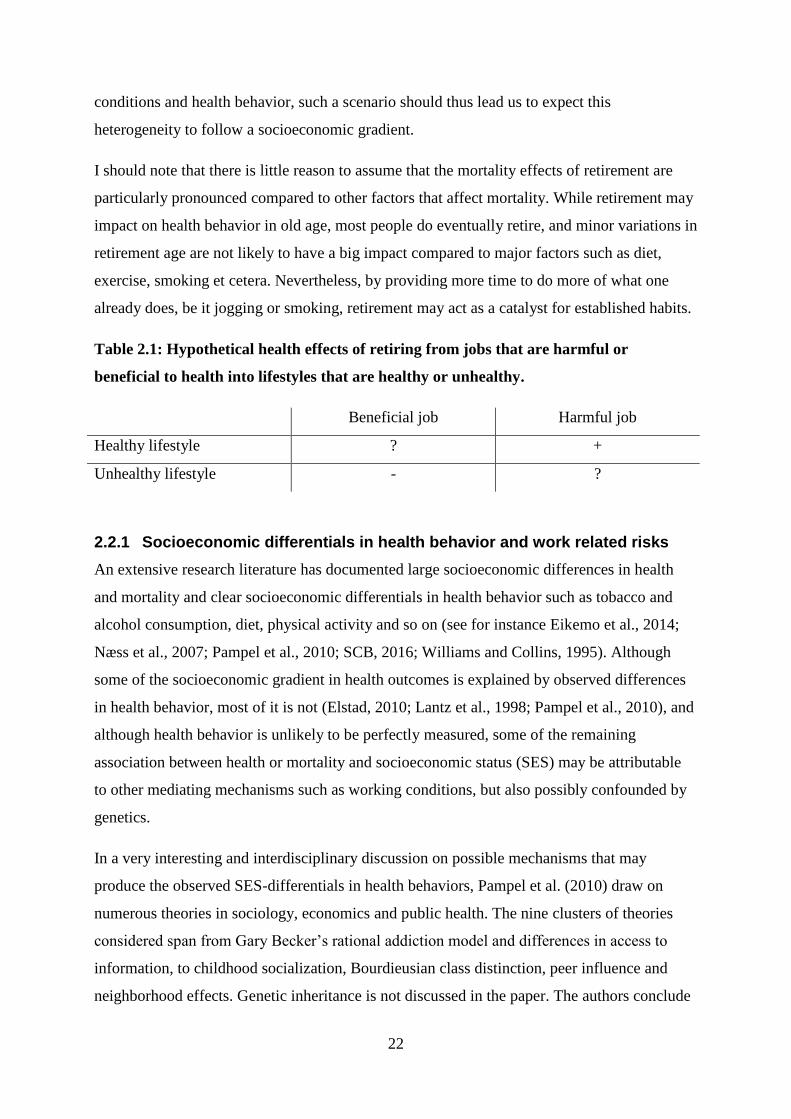
To simplify, one can imagine that there are two types of jobs; jobs that are harmful and jobs

that are beneficial to health, and that there are two types of retirement lifestyles; healthy and

unhealthy. In such a perspective, moving from a harmful job to a healthy lifestyle as a retiree

would be beneficial for health, and the reverse would be true with regard to retirement from a

healthy job into an unhealthy lifestyle. In a sense then, retirement would function as a catalyst

for the difference in “healthiness” between one’s job and spare time. This understanding

resembles the time constraints in the Grossman model discussed below. As illustrated in

Table 2.1, however, the effect of the two remaining possibilities is not given, as it would

depend on the relative health effect of the job and the lifestyle. If one also allows for the fact

that one’s lifestyle in retirement may to a large extent be a continuation of the lifestyle led

during one’s working life (in accordance with the continuity theory or the activity theory

discussed below), the increased spare time following retirement may lead to diverging health

behavior between those with healthy and unhealthy lifestyles, respectively. In other words,

there could be substantial effect heterogeneity. Given socioeconomic differences in working

22

conditions and health behavior, such a scenario should thus lead us to expect this

heterogeneity to follow a socioeconomic gradient.

I should note that there is little reason to assume that the mortality effects of retirement are

particularly pronounced compared to other factors that affect mortality. While retirement may

impact on health behavior in old age, most people do eventually retire, and minor variations in

retirement age are not likely to have a big impact compared to major factors such as diet,

exercise, smoking et cetera. Nevertheless, by providing more time to do more of what one

already does, be it jogging or smoking, retirement may act as a catalyst for established habits.

Table 2.1: Hypothetical health effects of retiring from jobs that are harmful or

beneficial to health into lifestyles that are healthy or unhealthy.

Beneficial job Harmful job

Healthy lifestyle ? +

Unhealthy lifestyle - ?

2.2.1 Socioeconomic differentials in health behavior and work related risks

An extensive research literature has documented large socioeconomic differences in health

and mortality and clear socioeconomic differentials in health behavior such as tobacco and

alcohol consumption, diet, physical activity and so on (see for instance Eikemo et al., 2014;

Næss et al., 2007; Pampel et al., 2010; SCB, 2016; Williams and Collins, 1995). Although

some of the socioeconomic gradient in health outcomes is explained by observed differences

in health behavior, most of it is not (Elstad, 2010; Lantz et al., 1998; Pampel et al., 2010), and

although health behavior is unlikely to be perfectly measured, some of the remaining

association between health or mortality and socioeconomic status (SES) may be attributable

to other mediating mechanisms such as working conditions, but also possibly confounded by

genetics.

In a very interesting and interdisciplinary discussion on possible mechanisms that may

produce the observed SES-differentials in health behaviors, Pampel et al. (2010) draw on

numerous theories in sociology, economics and public health. The nine clusters of theories

considered span from Gary Becker’s rational addiction model and differences in access to

information, to childhood socialization, Bourdieusian class distinction, peer influence and

neighborhood effects. Genetic inheritance is not discussed in the paper. The authors conclude

23

that researchers in the field should improve their research designs to better be able to

distinguish and contrast the different mechanisms possibly at work in producing SES-

gradients in heath behavior.

Retirement may affect health through several mechanisms, and the effects may depend on

socioeconomic factors. Such socioeconomic conditioning of the effects of retirement may

work through for instance socioeconomic differences in health behavior, family situations,

economic resources or working conditions. Thus, among other things, the health and mortality

effects of retirement should be expected to depend on the job one retires from and the lifestyle

one retires to. And the health relevant aspects of jobs and lifestyles should be expected to

follow socioeconomic gradients or divides.

2.3 Grossman’s microeconomic health capital framework

An important strand of theory regarding health behavior and mortality revolves around

Michael Grossman’s (1972) concept of health capital and his health investment model. As a

health economist working in the microeconomic tradition established by Gary Becker,

Grossman developed the concept as part of his work with building an economic model of

health behavior and investments in personal health.

2.3.1 Health capital and the health investment model

The main tenets of the health capital theory are, first, that health can be viewed as a stock that

depreciates over time, until it reaches zero and death occurs. The rate of depreciation

increases with age, at least after some threshold age. Second, people produce health, and may

invest in their own health through inputs such as exercise, diet and other aspects of their

lifestyle, use of their own time, and medical care, housing, and other market goods. Further,

health is more efficiently produced by people with more education. Through this production

of health, which increases the stock, people to some extent choose their own life span through

rational investment behavior. This second tenet was seen by some as a great advancement in

the field of health economics. It shifted the understanding of health economic theory from

seeing health as something that was exogenously determined (given) to seeing health as an

endogenous variable (resulting from individual actions and behaviors) (Fuchs, 1972). Third,

consumers’ demand for health is driven by two factors. On the one hand, health is considered

a consumption commodity, meaning that people, all else equal, prefer to be healthy – good

health increases utility. On the other hand, health is an investment commodity which returns

24

healthy days available for market or nonmarket activity, which again yields monetary or other

gains. Lastly, Grossman’s theory implies that the demand for medical care or health care

services is a derived demand, as people primarily demand good health rather than medical

care. Consequently, medical care is seen as an input in the production of health, not a

consumption good in itself.

The health capital concept forms part of a fairly comprehensive mathematical model which

attempts to describe rational decision-making in relation to one’s health behavior. However,

given the proliferation of different capital-concepts within sociology (Lyngstad, 2009), I will

mainly refer to investments in “health” rather than in health capital from here on. This

distinction is merely semantic. Further, I should specify that in the Grossman model,

investments in health are assumed to encompass intentional changes in health behavior, the

use of medical services, and other aspects of one’s life affecting health and where health

considerations impact on decisions. Health aspects relating to work and the work environment

are not explicitly part of the investments in Grossman’s theory.

2.3.2 Strengths and weaknesses of the Grossman model

In its original conception, Grossman’s model clearly has several weaknesses, some of which

he points out himself. Many relate to the simplifying assumptions of the model. One example

is the assumption that actors have full information, and that they thus know with certainty at

which age they will die. Such assumptions are obviously erroneous, and Brown and

Vickerstaff (2011) point out that people tend to be overly pessimistic with regard to their own

health and remaining life span – perhaps a case of biased beliefs (Rydgren, 2009: 73).

The action-theoretical basis of the model may also be subject to considerable (and

predictable) theoretical criticism from different perspectives, as it stands firmly in the

theoretical framework of the much-debated homo economicus. In the model, actors are

assumed to behave in the ways predicted by intricate calculations of costs and benefits, even

with regard to their lifestyle and health behavior. This view of rationality is akin to what

Elster (2015: 255) defines as hyperrationality – “[…] the propensity to search for the

abstractly optimal decision, that is, the decision that would be optimal if we were to ignore

the costs of the decision-making process itself”. In this case, these costs could be said to

approximately amount to the direct costs and opportunity costs of attaining a degree in

economics so that one could learn to do the necessary calculations, or at least hire someone to

do them at every decision point. The point made above should also be repeated here; if the

25

health consequences of much health affecting behavior are unintended, they can hardly be

said to be rational, simply because rationality implies intentionality.

Further, the amount of evidence showing that people tend to not behave purely rationally,

even when faced with relatively simple choices, is substantial (see Elster 2015: 256-261 for

examples – some of which are of an anecdotal kind). Such observations cast serious doubts on

the truthfulness, if not the utility, of a strict or narrow rationality paradigm. Importantly, many

aspects of health behavior are hard to conceive of as motivated purely by instrumentally

rational considerations; for instance, the sudden rush to the gyms in January appears to be

driven more by norms or feelings of guilt than by utility calculations. This is not to say that

rational explanation should be abandoned in general – the baby should not be thrown out with

the bathwater – rather, It might be beneficial to loosen some of the more restrictive

assumptions to allow for the many and obvious deviations from a strict understanding of

rationality (Boudon, 2003). In risk of making a programmatic statement; the more pragmatic

desires, beliefs and opportunities (DBO) model (Hedström, 2005: 37-66) could serve as an

alternative and more intuitively plausible model of action. That is, if one is willing to trade

formalism and predictive precision for realism.

However, keeping the shortcomings of Grossman’s model in mind, the fact still remains that

although “all models are wrong, some are useful” (Box and Draper, 1987: 424), and in my

view, Grossman’s general approach to health behavior does indeed give us some very useful

conceptual and analytical tools, as it can be used to specify some of the mechanisms through

which retirement may affect health and mortality. It also serves as a prominent and influential

example of a strand of theorizing whereby retirement is seen as an event or transition.

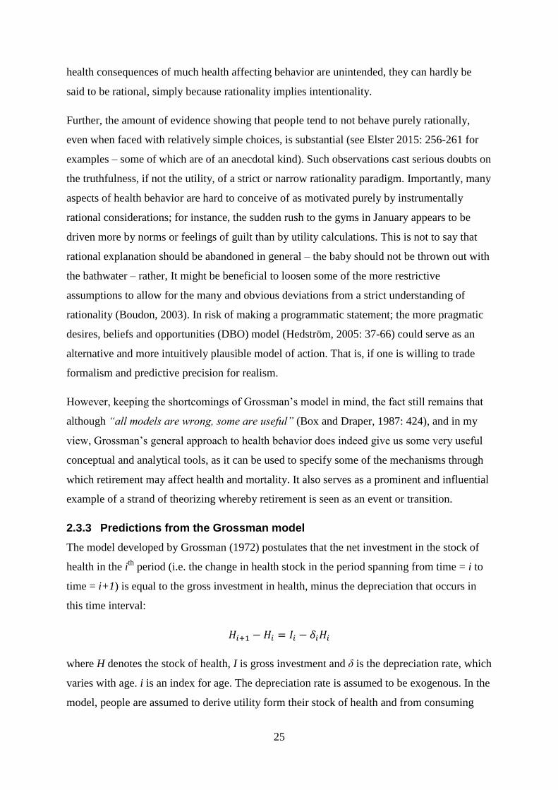
2.3.3 Predictions from the Grossman model

The model developed by Grossman (1972) postulates that the net investment in the stock of

health in the ith

period (i.e. the change in health stock in the period spanning from time = i to

time = i+1) is equal to the gross investment in health, minus the depreciation that occurs in

this time interval:

𝐻𝑖+1 − 𝐻𝑖 = 𝐼𝑖 − 𝛿𝑖𝐻𝑖

where H denotes the stock of health, I is gross investment and δ is the depreciation rate, which

varies with age. i is an index for age. The depreciation rate is assumed to be exogenous. In the

model, people are assumed to derive utility form their stock of health and from consuming

26

other commodities (Zi). As shown below, both health and the aggregate commodity Zi are

produced by the individual using time, human capital and goods and services purchased in the

market. Informally put, people may use their time and money on either health investments or

everything else. Both health and other things yield some utility. But health is also an

investment commodity, as fewer sick days mean that the actor can spend more time working

and earning money.

Applying Grossman’s framework to the study of the impact of retirement on health and

mortality, several important mechanisms through which retirement may affect health become

apparent. Full retirement (in the sense of quitting work completely and start receiving a

moderate monthly pension) would affect several of the components of the model that impact

on incentives or constraints that influence health decisions. Specifically, the model reveals

several contradictory mechanisms through which retirement may affect health. I will not

present or make use of the entire model here, since such an elaboration is unnecessary for the

purposes of this thesis. Instead, I will attempt to present each of these mechanisms in a brief

and semi-formal way.

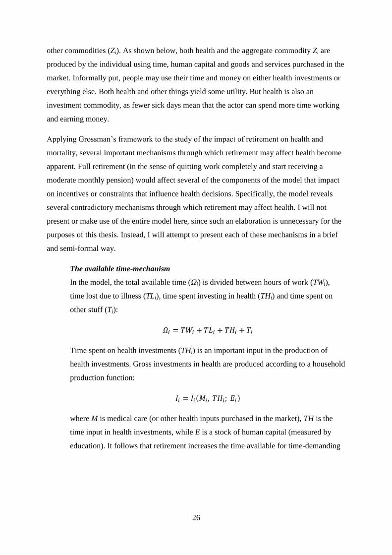
The available time-mechanism

In the model, the total available time (Ωi) is divided between hours of work (TWi),

time lost due to illness (TLi), time spent investing in health (THi) and time spent on

other stuff (Ti):

𝛺𝑖 = 𝑇𝑊𝑖 + 𝑇𝐿𝑖 + 𝑇𝐻𝑖 + 𝑇𝑖

Time spent on health investments (THi) is an important input in the production of

health investments. Gross investments in health are produced according to a household

production function:

𝐼𝑖 = 𝐼𝑖(𝑀𝑖, 𝑇𝐻𝑖; 𝐸𝑖)

where M is medical care (or other health inputs purchased in the market), TH is the

time input in health investments, while E is a stock of human capital (measured by

education). It follows that retirement increases the time available for time-demanding

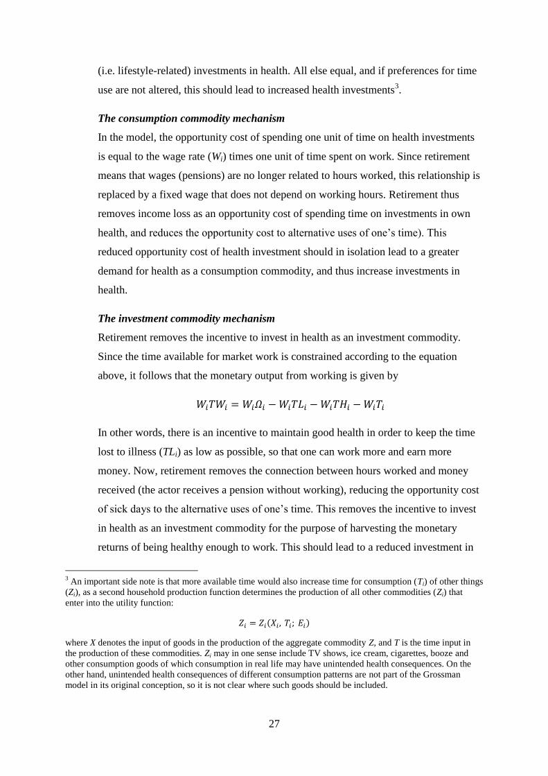
27

(i.e. lifestyle-related) investments in health. All else equal, and if preferences for time

use are not altered, this should lead to increased health investments3.

The consumption commodity mechanism

In the model, the opportunity cost of spending one unit of time on health investments

is equal to the wage rate (Wi) times one unit of time spent on work. Since retirement

means that wages (pensions) are no longer related to hours worked, this relationship is

replaced by a fixed wage that does not depend on working hours. Retirement thus

removes income loss as an opportunity cost of spending time on investments in own

health, and reduces the opportunity cost to alternative uses of one’s time). This

reduced opportunity cost of health investment should in isolation lead to a greater

demand for health as a consumption commodity, and thus increase investments in

health.

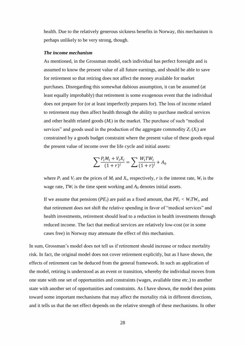
The investment commodity mechanism

Retirement removes the incentive to invest in health as an investment commodity.

Since the time available for market work is constrained according to the equation

above, it follows that the monetary output from working is given by

𝑊𝑖𝑇𝑊𝑖 = 𝑊𝑖𝛺𝑖 − 𝑊𝑖𝑇𝐿𝑖 − 𝑊𝑖𝑇𝐻𝑖 − 𝑊𝑖𝑇𝑖

In other words, there is an incentive to maintain good health in order to keep the time

lost to illness (TLi) as low as possible, so that one can work more and earn more

money. Now, retirement removes the connection between hours worked and money

received (the actor receives a pension without working), reducing the opportunity cost

of sick days to the alternative uses of one’s time. This removes the incentive to invest

in health as an investment commodity for the purpose of harvesting the monetary

returns of being healthy enough to work. This should lead to a reduced investment in

3 An important side note is that more available time would also increase time for consumption (Ti) of other things

(Zi), as a second household production function determines the production of all other commodities (Zi) that

enter into the utility function:

𝑍𝑖 = 𝑍𝑖(𝑋𝑖 , 𝑇𝑖 ; 𝐸𝑖)

where X denotes the input of goods in the production of the aggregate commodity Z, and T is the time input in

the production of these commodities. Zi may in one sense include TV shows, ice cream, cigarettes, booze and

other consumption goods of which consumption in real life may have unintended health consequences. On the

other hand, unintended health consequences of different consumption patterns are not part of the Grossman

model in its original conception, so it is not clear where such goods should be included.

28

health. Due to the relatively generous sickness benefits in Norway, this mechanism is

perhaps unlikely to be very strong, though.

The income mechanism

As mentioned, in the Grossman model, each individual has perfect foresight and is

assumed to know the present value of all future earnings, and should be able to save

for retirement so that retiring does not affect the money available for market

purchases. Disregarding this somewhat dubious assumption, it can be assumed (at

least equally improbably) that retirement is some exogenous event that the individual

does not prepare for (or at least imperfectly prepares for). The loss of income related

to retirement may then affect health through the ability to purchase medical services

and other health related goods (Mi) in the market. The purchase of such “medical

services” and goods used in the production of the aggregate commodity Zi (Xi) are

constrained by a goods budget constraint where the present value of these goods equal

the present value of income over the life cycle and initial assets:

∑𝑃𝑖𝑀𝑖 + 𝑉𝑖𝑋𝑖

(1 + 𝑟)𝑖= ∑

𝑊𝑖𝑇𝑊𝑖

(1 + 𝑟)𝑖+ 𝐴0

where Pi and Vi are the prices of Mi and Xi, respectively, r is the interest rate, Wi is the

wage rate, TWi is the time spent working and A0 denotes initial assets.

If we assume that pensions (PEi) are paid as a fixed amount, that PEi < WiTWi, and

that retirement does not shift the relative spending in favor of “medical services” and

health investments, retirement should lead to a reduction in health investments through

reduced income. The fact that medical services are relatively low-cost (or in some

cases free) in Norway may attenuate the effect of this mechanism.

In sum, Grossman’s model does not tell us if retirement should increase or reduce mortality

risk. In fact, the original model does not cover retirement explicitly, but as I have shown, the

effects of retirement can be deduced from the general framework. In such an application of

the model, retiring is understood as an event or transition, whereby the individual moves from

one state with one set of opportunities and constraints (wages, available time etc.) to another

state with another set of opportunities and constraints. As I have shown, the model then points

toward some important mechanisms that may affect the mortality risk in different directions,

and it tells us that the net effect depends on the relative strength of these mechanisms. In other

29

words, according to the Grossman model, the net effect of retirement on mortality can be

either positive, negative or zero (although, in the Norwegian context, it may lean more

towards the positive side than in some other contexts, because of the generous sickness

benefits and affordable healthcare). Also, the model can be said to allow for effect

heterogeneity in the sense that different subgroups may respond differently to changing

opportunities and incentives following retirement. A zero net effect may in such a case mask

substantial but diverging effects between subgroups. Finally, it should be noted that according

to the Grossman model, a lower stock of health at the point of retirement would be associated

with a shorter life span regardless of the net health effects of retirement. This would not,

however, be an effect of retirement per se, but would, to the extent that a low health stock

induces retirement, serve as a mechanism for negative health selection into retirement.

2.4 Gerontological theories about aging

Several theoretical perspectives from the gerontological research literature may also inform

the discussion about the effects of retirement on health and mortality. Most of these give

similar predictions about the direction of the effect. Some of them give predictions in line

with the Grossman model, but differ from it with regard to which mechanisms are in play.

Several of these theories also have similar theoretical underpinnings, namely the emphasis on

identity, roles, role expectations and role loss. In this regard they bear some resemblance to

Atchley’s process theory discussed below. Readers interested in the corpus of relevant social

gerontological theories are referred to Daatland and Solem (2000).

2.4.1 Activity theory and continuity theory

The activity theory of aging is not a theory about how people age, but about the prerequisites

for successful aging. It states that staying social and maintaining one’s activities and attitudes

from middle age enhances quality of life and delays the aging process (Havighurst, 2009

[1963]). Inherent in this theory is the view that people should avoid major life course

transitions in their later life, and that retirement is a potentially harmful transition unless the

stimulating activities people engage in as employees are somehow substituted by other

activities in retirement (Ekerdt, 1987). In one sense, then, the theory predicts that retirement

should have a harmful effect on health, if any. This prediction is in line with what would be

expected if the mechanisms that harm health in the Grossman model dominate. However, this

30

theory places emphasis on direct health benefits of working rather than seeing work and

health behavior as separate.

Whereas the activity theory may be seen as having some normative implications (or at least

strong recommendations) about how people should age, the closely related continuity theory

attempts to describe how people do age. It states that people tend to aim for, produce and

enjoy continuity in their life with regard to both psychological characteristics, perceptions of

self and social behavior. Continuity is seen as an adaptive strategy. But continuity is not

understood as static sameness, but dynamic consistency and coherence with the past (Atchley,

1989). As in activity theory, discontinuity is seen as a potential threat to mental health, but it

is not clear that retirement should be expected to induce such discontinuities; “Just because

logic suggests that there ought to be an identity crisis connected with retirement, it does not

follow that there will usually be one. Indeed, researchers have indicated that identity crises

connected with retirement are relatively rare” (Atchley, 1989: 187). In other words,

continuity theory predicts that retirement may be harmful to mental (and perhaps also

physical) health if it marks a sharp discontinuity in self-perception or identity, but it leans

heavily towards this not being the case. This prediction of a potential negative health effect of

retirement may be thought of as lasting or relatively short-term. If it is lasting, the prediction

could bear resemblance to one of the possible predictions of the Grossman model and to

disengagement theory. If it is short lived, the theory may be more closely related to the

stressful life event perspective discussed below.

2.4.2 Disengagement theory

For the present purposes, the most important postulate of the disengagement theory is that

disengagement from one’s central role in society tends to lead to crisis and demoralization4.

Within the framework of this theory, which was first formulated by Elaine Cumming and

William Earl Henry in the early 1960s, men’s central role is seen as that of a worker

providing for the family (“instrumental”) and women’s role is understood as that of a wife and

homemaker reducing tension within the family (“socioemotional”). Disregarding this

somewhat outdated gender distinction, the disengagement theory predicts that retirement from

work is an unavoidable step in the disengagement process. As I interpret the theory, this

disengagement will have adverse mental health consequences (and possibly also adverse

physical health outcomes) unless the lost role is substituted (Cumming and Henry, 1961: 210-

4 Disengagement theory postulates many things. The summary of the theory consists of nine (or ten) postulates

with ten corollaries.

31

218). In other words, the loss of the worker role and the social network, status etc. associated

with this role can be understood as a necessary stage in the disengagement process, but

nonetheless a stage that should serve to accelerate the mental and physical decline associated

with old age. The health trajectories of retirees should show a steeper decline than those of

workers as a consequence of the retirement disengagement. Although the retirement

disengagement is seen as a part of the general process of disengagement related to aging, the

retirement disengagement itself should be seen as an event or transition with potentially

adverse health consequences, similar to the Grossman model, activity theory and continuity

theory.

It should also be noted that the disengagement theory has been subject to substantial criticism.

This criticism has in turn been very neatly summed up and systematized by Arlie Hochschild

(1975). Essentially the theory is criticized for being unfalsifiable, for the use of all-inclusive

variables or catchall categories to describe variations in forms of disengagement, and for

assuming (or imputing meaning and interpretations into) actors’ perception without empirical

support; “[if] conscious reflections were fully taken into account and given weight, I think the

authors would find themselves with evidence which refutes the theory, were it posed as a

refutable theory” (Hochschild, 1975: 560).

2.4.3 Retirement as a stressful life event

The stressful life event perspective holds that the detachment from gainful employment and

the transition into retirement entails a loss of social networks, identity, income and other

benefits associated with employment. Essentially, the theory emphasizes the loss of

employment, rather than the acquisition of the retirement role. The general idea is that the

transition into retirement is a large-scale life change that induces stress and therefore increases

susceptibility to illness (Daatland and Solem, 2000:150; Minkler, 1981). In this regard it has

much in common with the activity theory (Ekerdt, 1987), but also with some of the other

theories discussed in this chapter. The degree to which retirement could be found to work as a

stress inducer may depend on the degree of control over- and on the timing of the retirement

event and on the point in the retirement process the stress level is measured (Minkler, 1981),

but there could be considerable heterogeneity in the extent to which retirement induces stress.

Although compatible with a process perspective in the sense that the stress period may be

relatively short (Minkler, 1981), I would argue that the view of retirement as a stressful life

32

event should on its own be regarded as an event or transition perspective which, similarly to

the Grossman model, predicts a one-directional (negative) effect on health.

2.4.4 The no effect assumption

Both the “stressful life event” perspective and the activity theory have been criticized by

sociologist David J. Ekerdt (1987) as examples of a priori reasoning based on the erroneous

assumption that retirement must have some effect on health:

Although the research literature contains virtually nothing to encourage the notion

that retirement is likely to harm the physical health of older workers, the idea persists

that retirement increases the risk of illness and death. (Ekerdt, 1987: 455)

In somewhat strong words, he has argued that the notion that retirement harms health is based

on anecdotes, fallacies, wishful thinking, a priori reasoning and misinterpretations of research

findings. This criticism can easily be extended to the other theories discussed in this chapter,

although they are not explicitly mentioned. In a sense, Ekerdt is arguing in favor of the null

hypothesis, namely that retirement does not impact on health or mortality.

Although not a theory in a strict sense, I include this assumption among the other theories

because it has formed an underlying assumption through most of the work I have done on this

thesis, To elaborate on this point, it is worth noting (as will become clear in the literature

review below) that neither of the theories discussed in this chapter, as applied to retirement

and mortality, have a well-established explanandum (what needs to be explained). There is no

well-established fact or causal relationship in need of an explanation; there is no consensus on

the health and mortality effects of retirement – at least there was no consensus at the point in

time when the different theories were developed. These theories have mostly been employed

by researchers to predict a hypothesized phenomenon (“retirement is harmful”), not as

explanations for an observed one (“how do we explain the observation that retirement

increases mortality risk?”). This should perhaps not be considered in line with ideals about

explanatory theorizing (Elster, 2015: 3-10), but as will be seen from the literature review

below, the lack of an explanandum is hardly surprising given the divergence in research

findings.

33

2.5 Atchley’s process approach

In his book entitled The Sociology of Retirement, Robert C. Atchley (1976) outlines a process

perspective on retirement. This theory is given special attention here as it can be taken to

predict an effect of retirement on mortality that varies with time in a way that sets it apart

from other theories in the field. According to this view, retirement should not be seen just as a

single event or change of state. Rather, retirement should be viewed as a process in which the

(prospective) retiree passes through a series of phases both before and after the transition to

retirement, as illustrated in Figure 2.2, and takes on the social role of retiree through this

process. In other words, this theory does not assume that people mechanically (or rationally)

respond to changes in opportunities and constraints relating to retirement. Rather, retirement

is a process of social role change and adaption that has a psychological effect on the

individual.

Figure 2.2: Phases of retirement (Atchley, X1976: 64).

Remote

phase

Near

phase

Honeymoon

phase

Disenchantment

phase

Reorientation

phase

Stability

phase

Termination

phase

Preretirement Retirement

Retirement event End of

retirement role

2.5.1 The phases of retirement

Although interesting in its own right, I will not draw on the entirety of Atchley’s process

theory in this thesis. Rather, I will pay special attention to the two phases that may affect

health in the period following retirement, i.e. the honeymoon phase and the disenchantment

phase.

The first two of Atchley’s retirement phases are labeled the remote phase and the near phase

of preretirement. The remote phase may begin a very long time before the actual retirement

transition, for instance at or before the start of an occupational career, and it would tend to

continue until one realizes that retirement age is nearing. During the remote phase, the

thought of retirement is a distant one. The near phase sets in when the aging employee

realizes that retirement is drawing near. It is often characterized by more negative sentiments

towards retirement, as people may be struck by the realities of facing a sharp reduction in

income, or realize that they lack the “leisure skills” necessary for a pleasant and meaningful

retirement. The person nearing retirement will also build up expectations or fantasies about

34

the upcoming life as a retiree, which may serve to smooth the transition if they are realistic,

but may make the transition more difficult if the expectations are unrealistically idyllic.

After the actual retirement event (assuming that there is such an event and not just a gradual

detachment from work), Atchley’s theory states that the retiree enters a honeymoon phase – a

euphoric period where the retiree enjoys his or her newfound freedom and spare time,

attempting to do all the things he or she did not have time to do while still working, including

leisure activities, physical activities, travelling and spending time with grandchildren.

According to Atchley (1976: 68), “[t]he person in the honeymoon period of retirement is often

like a child in a room full of new toys”. In a Norwegian context one may imagine (in line with

common stereotypes) that recent retirees spend more time outdoors, hiking, skiing, fishing,

gardening et cetera, compared to what they would have done if they had still been working.

In relation to health behavior, the honeymoon phase may induce a more healthy and active

lifestyle, but for some, the honeymoon phase may also have some adverse health

consequences if it for instance involves an increase in alcohol and/or tobacco consumption).

The net effect, however, is likely to be positive. The honeymoon is not for everyone, though,

and the lifestyle options may be limited or the joy of freedom thwarted by a lack of money,

poor health, weak or missing social or family bonds et cetera. In other words, some may skip

this phase altogether, and those who are subject to involuntary retirement could be especially

prone to never experience the bliss of retirement. The fast-paced and hectic period of activity

following retirement soon enough turns into a routine as the honeymoon comes to an end.

Depending on the nature of this routine people may either adjust fairly quickly to the new role

of being a retiree, or they may enter the fourth phase of the retirement process.

This fourth phase of retirement is aptly labeled the disenchantment phase, and may result

from problems adjusting to the life as a retiree. The idea is that the aforementioned

expectations about retirement may be unrealistic, leading to disappointment, disenchantment

and/or depression for retirees when they are faced with the realities of retirement. In essence,

people may get bored, experience a lack of meaning or anomie, or simply have trouble

structuring their lives when they no longer have a job or a social network related to work.

According to Atchley, factors such as having less money, poor health, problems with

managing one’s own life, loss of previous social roles, a formerly strong attachment to work

or moving away from one’s community may worsen the backlash from the honeymoon phase

35

and lead to deep depressions. With regard to health behavior, a disenchantment phase can

therefore be assumed to result in both physical and mental health deterioration.

The fifth and sixth phases of retirement are referred to as the reorientation phase and the

stability phase, respectively. The reorientation phase is the process of reemerging from the

lows of the disenchantment phase and finding new meaning in the role of retiree. Expectations

are adjusted and new arenas of involvement are discovered, for instance at senior centers. For

most people, the reorientation phase leads to stability in the sense that the retiree reconciles

with the new role and get into a routine and a lifestyle that, at least to some extent, is

experienced as meaningful and satisfying. The last phase of retirement is termed the

termination phase. Despite the somewhat morbid label, this phase does not necessarily

involve dying. Rather, this phase marks the transition from the role of retiree. Usually this

happens because increased frailty, illness and disability forces one to abandon the role of

retiree to take on the role of sick or disabled. But low income resulting from a loss of pension

benefits may also cause a transition into a role as economically dependent.

2.5.2 Strenghts, weaknesses and interpretations of Atchley’s theory

The process approach outlined by Atchley is not strictly a theory about retirement and health,

but a theory about retirement that has implications for health. Most importantly, it implies that

retirement may have consequences for health that vary over time. If one assumes that the

honeymoon phase is beneficial for health and that the disenchantment phase is detrimental for

health, it could follow that the mortality effects of retirement are not monotonic but time-

variant, in the sense that, all else equal, the mortality risk of retirees relative to those who

continue working may be reduced in one phase and increase in another. Such an interpretation

has been stated or implied repeatedly in the literature (Ekerdt, 1987; Minkler, 1981; Solem,

1987)5, and as I will show below, there is some evidence to support it. I will return to the

mortality implications of the process perspective below, but first, it is necessary to address an

important theoretical issue in the process perspective.

The process theory has a theoretical black box; why do people transition into the

disenchantment phase? It appears highly plausible that people who voluntarily retire for

reasons not related to health will enter into a honeymoon phase. For voluntary retirees,

retirement is a fulfillment of their desires, which will obviously make them happy. It will also

give them more time to pursue their interests in areas other than work, which should also

5 The reference to Atchley’s process theory is made only implicitly by Ekerdt.

36

make them happy, and make them healthier, given that these interests are beneficial to their

health. However, it is difficult to see the logical reason for why a large share of retirees would

then simply become disenchanted, unhappy or depressed some time after a very happy

retirement. What is the psychological mechanism that could cause such a pattern?

The expectations for retirement that are built up during the preretirement period would appear

to be the key to a plausible explanation of such a pattern. Atchley (1976: 69) in fact highlights

unrealistically high expectations (or fantasies) and subsequent disappointment as important

triggers for the honeymoon and disenchantment phase, respectively:

In a sense, the honeymoon period represents a living out of the preretirement fantasy.

The more unrealistic the preretirement fantasy turns out to have been, the more likely

it is the retirer [sic] will experience a feeling of emptiness and disenchantment

Put differently, people become happy in the honeymoon phase because they have high

expectations and are able to live them out, but they become sad and enter the disenchantment

phase when they realize that their expectations were too high. Expectations in this context can

be understood as a combination of beliefs and desires, perhaps constituting a case of wishful

thinking (Elster, 2015: 125-8), i.e. beliefs formed by desires, with the accompanying

dissonance between beliefs and reality. So, what are the problems with this interpretation of

the theory?

First, one could ask why people would develop unrealistically high expectations about

retirement in the near phase of preretirement when, according to Atchley (1976: 66),

“[a]ttitudes toward retirement generally become more negative during the near retirement

phase […]”. An answer to this could be that most people may remain positive to retirement, or

that ”more negative” may still mean that people have positive sentiments toward retirement,

only less so than they did before.

Second, one could ask how people can become happy by living out their expectations in the

honeymoon phase if these expectations are unrealistically high. Would this not make them

impossible to live out in the first place, leading to immediate disappointment? An answer to

this might be that the expectations are not unrealistic to fulfill, but unrealistic to maintain.

People cannot maintain a high activity level and euphoric state of mind for long periods of

time, and some regression to the mean should be expected. This reality leads to

disenchantment. Well, then one may ask why people do not just adapt their expectations (see

37

for instance Elster, 2015: 112) and move directly into the reorientation phase, rather than go

through the disenchantment phase first. Such a direct adjustment would be in line with the

psychological set point theory (or the “hedonic treadmill”) which tells us that the effects of

positive or negative experiences tend to be short-lived and that people quickly return to a set

point of happiness (see for instance Diener et al., 2006). An answer in accordance with

Atchley’s theory could be that people need time to adjust their expectations to the realities

facing them. The disappointment that comes with not being able to maintain their expected

lifestyle and level of happiness over time may in itself be enough to induce depression or

disenchantment, perhaps reinforced by the lack of a job and daily routine to serve as a

distraction. This could prevent a smooth transition from the honeymoon phase. Essentially,

this would be equivalent to saying that when people realize that they cannot be really happy

but have to settle for moderately happy, they become really sad. Although perhaps not

convincing, this explanation is at least plausible.

Lastly, Atchley’s theory assumes that people have systematically faulty expectations about

retirement. For the expectation/disappointment mechanism to be effective, people need to

have expectations that are systematically biased towards retirement as an unrealistically

positive role or state (see Rydgren, 2009: 73 for a discussion on biased beliefs), and this must

be the case for each new cohort of retirees. In other words, the experiences of older retirees

could not serve to correct these expectations, either because they are not communicated, or

because they are ignored. If one is to accept the expectation/disappointment mechanism of the

process theory, one also has to accept the premise of biased expectations. Although I am not

convinced that this premise is true, I personally see it as plausible. In any case, the hypothesis

that retirement is followed by a honeymoon phase and a disenchantment phase that both affect

mortality is one worth testing.

2.6 Comparing the predictions of the theories

The theories discussed above differ in several ways. One is the action theoretical assumptions

that underpin them. But more relevant for this thesis are the different predictions they make

about the direction and temporality of the effect of retirement on mortality. These are

summarized in Table 2.3.

Theories about health behavior and work related health risks are ambiguous about the

direction of the effect. While retiring from harmful jobs into healthy retirement lifestyles

38

would reduce mortality, retiring from beneficial jobs into unhealthy lifestyles would have the

opposite effect. The predicted effect of retiring is also ambiguous in the Grossman model, and

may depend on the relative strength of different mechanisms. If the available time mechanism

and/or consumption commodity mechanism dominates, retirement can be assumed to reduce

mortality, but the reverse would hold if thee investment commodity mechanism and/or

income mechanism dominates. Both the activity theory, the disengagement theory and the

stressful life perspective predict that retirement increases mortality. The continuity theory can

also be interpreted as predicting such an effect.

With regard to temporality, the effects predicted by the Grossman model and the

disengagement theory can be assumed to be monotonic, meaning that retirement should

increase the age-specific mortality of retirees for all subsequent time intervals, relative to

workers. The stressful life event perspective could, on the other hand, be interpreted to predict

a relatively short-term effect on age-specific mortality. It is not clear whether the continuity

theory, the activity theory or the theories about health behavior and work related health risks

predict a short-term or a long term, monotonic effect.

Both with regard to direction and temporality, Atchley’s process theory and the no effect

assumption stand out. While the no effect assumption predicts that retirement has no effect on

mortality, the process theory (or at least a common interpretation of it) predicts a time-varying

effect. Specifically, it predicts that age-specific mortality should first be lower in the period

following retirement, and then be higher, relative to those not retired. In the following

chapter, I will briefly review the research literature on retirement, health and mortality, before

returning to these theoretical predictions in chapter 4.

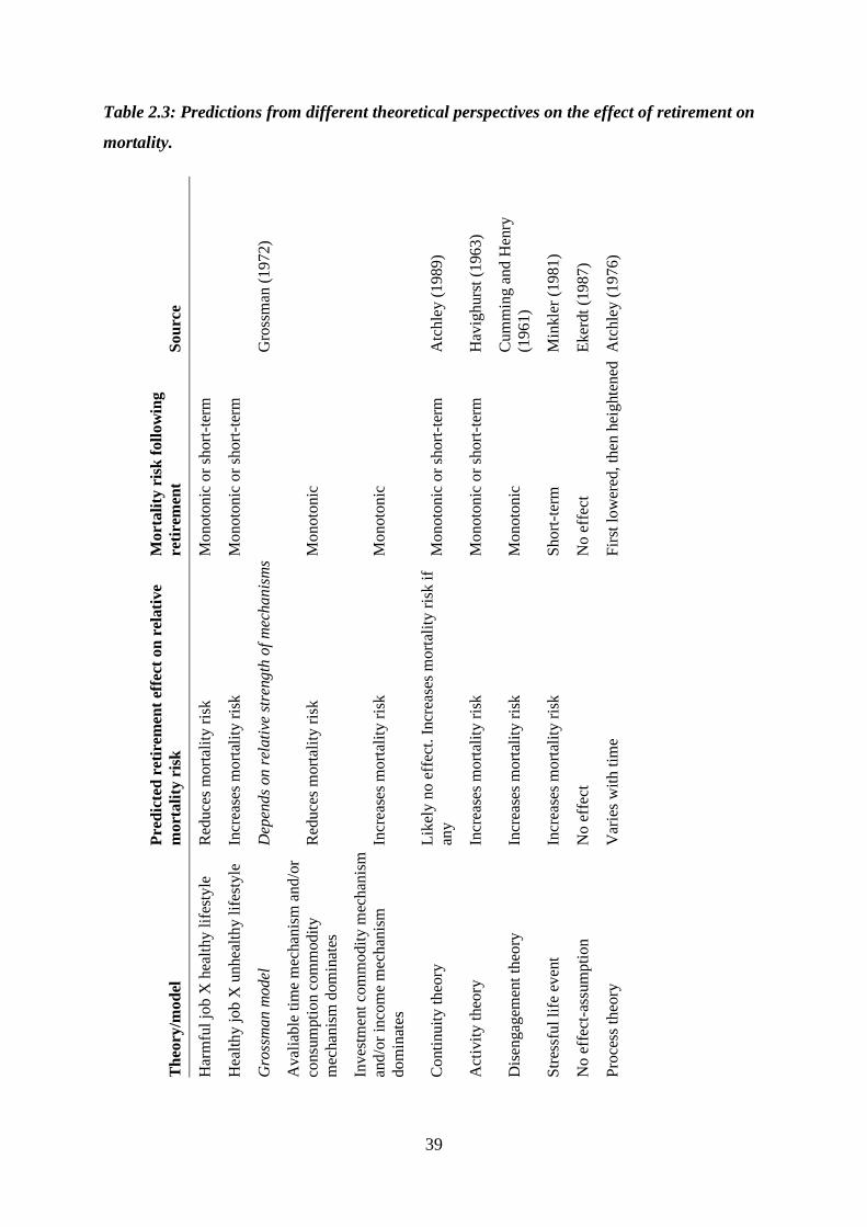
39

Table 2.3: Predictions from different theoretical perspectives on the effect of retirement on

mortality.

So

urc

e

Gro

ssm

an (

19

72)

Atc

hle

y (

19

89

)

Hav

igh

urs

t (1

96

3)

Cu

mm

ing

an

d H

enry

(19

61)

Min

kle

r (1

98

1)

Ek

erdt

(19

87

)

Atc

hle

y (

19

76

)

Pre

dic

ted

tim

e p

att

ern

of

Mort

ali

ty r

isk

foll

ow

ing

reti

rem

ent

Monoto

nic

or

short

-ter

m

Monoto

nic

or

short

-ter

m

Monoto

nic

Monoto

nic

Monoto

nic

or

short

-ter

m

Monoto

nic

or

short

-ter

m

Monoto

nic

Short

-ter

m

No e

ffec

t

Fir

st l

ow

ered

, th

en h

eig

hte

ned

Pre

dic

ted

ret

irem

ent

effe

ct o

n r

elati

ve

mort

ali

ty r

isk

Red

uce

s m

ort

alit

y r

isk

Incr

ease

s m

ort

alit

y r

isk

Dep

ends

on r

elati

ve s

tren

gth

of

mec

hanis

ms

Red

uce

s m

ort

alit

y r

isk

Incr

ease

s m

ort

alit

y r

isk

Lik

ely n

o e

ffec

t. I

ncr

ease

s m

ort

alit

y r

isk i

f

any

Incr

ease

s m

ort

alit

y r

isk

Incr

ease

s m

ort

alit

y r

isk

Incr

ease

s m

ort

alit

y r

isk

No e

ffec

t

Var

ies

wit

h t

ime

Th

eory

/mo

del

Har

mfu

l jo

b X

hea

lthy

lif

esty

le

Hea

lth

y j

ob

X u

nhea

lth

y l

ifes

tyle

Gro

ssm

an

mo

del

Aval

iab

le t

ime

mec

han

ism

an

d/o

r

consu

mpti

on

com

mod

ity

mec

han

ism

dom

inat

es

Inves

tmen

t co

mm

od

ity

mec

han

ism

and/o

r in

com

e m

ech

anis

m

dom

inat

es

Conti

nu

ity

th

eory

Act

ivit

y t

heo

ry

Dis

engag

emen

t th

eory

Str

essf

ul

life

ev

ent

No e

ffec

t-as

sum

pti

on

Pro

cess

th

eory

40

3 Empirical background

The contention that retirement may have an adverse effect on health has become

increasingly popular with the recent categorization of this phenomenon as a stressful

"life event." The small number of empirical studies examining the health outcomes of

retirement, however, appear neither to support nor to refute this hypothesis.

Moreover, the serious methodological problems inherent in most of these studies

caution against the generalization of findings. (Minkler, 1981: 117)

This observation was made by Meredith Minkler some 35 years ago. And, regrettably, it

appears to still be valid – at least up until very recently – despite the growing number of

studies on the relationship between retirement and health. In this chapter, I review the

literature on the relationship between retirement, health and mortality. I pay special attention

to recent studies that have attempted to circumvent the selection issues and biases that tend to

haunt studies in this area and that can thereby make strong claims for causal inference. The

studies reviewed here will later inform the formulation of the hypotheses in this thesis.

3.1 Descriptive studies

3.1.1 Association between retirement and health

The research literature abounds with studies investigating the relationship between retirement

and health. I will not attempt a thorough review of the entire literature, as this would be very

demanding, and because it is not directly relevant for the present paper, since I study mortality

rather than health. Rather, I will first briefly discuss a recent literature review published on the

topic and subsequently discuss a few research articles published after this review was

conducted.

van der Heide et al. (2013) have conducted a systematic review of longitudinal studies

investigating the relationship between retirement and health. The researchers found retirement

to have a beneficial “effect” on mental health, but found that the results with regard to

perceived or self-rated general health, and different measures of physical health were

contradictory. The observed association between retirement and relative mental health

improvements runs contrary to the disengagement theory and the stressful life event

perspective discussed above, and may also be at odds with activity theory and continuity

theory (depending on one’s interpretation of these theories). It may, however, be consistent

41

with a post-retirement “honeymoon” as envisioned by Atchley (1976) or with increased health

investments (Grossman, 1972). The review suggests that the contradictory findings may be

due to differences in quality, research design, follow-up-periods, context or other factors.

The review by van der Heide et al. (2013) can be said to suffer from a serious weakness; it

places considerable emphasis on general quality criteria of the papers reviewed, but it does

not consider the internal validity of the studies with regard to claims about causal inference

concerning the relationship between retirement and health. This is despite the fact that it

strongly implies that the examined associations reflect causal relationships – a claim that

could be considered dubious in light of the selection issues discussed below.

A few studies not included in the abovementioned literature review may shed additional light

on the retirement and health relationship. First, Stenholm et al. (2014) found physical

functioning to decline faster among retirees than among older employees in the US. Second,

Coppola and Spizzichino (2014) found retiring to be associated with higher risk of reporting

worsened health among men, but not among women in Italy. They suggested that this gender

difference reflected men’s stronger involvement in the labor market compared to women, and

that retirement was associated with a bigger risk as it involved a greater loss of role and status

for men. This would be in accordance with the stressful life event perspective discussed

above. Third, Syse et al. (2015) found Norwegian retirees (compared to workers) to be more

likely to report mental health improvements, increased physical activity, weight loss, and

changes in alcohol intake, and that they were less likely to report mental health deteriorations.

In other words, these more recent studies also point in different directions with regard to the

association between health and retirement.

Obviously, the association between retirement and poor health that some studies report may

be due to the “healthy worker effect” (Li and Sung, 1999; Shim et al., 2013), a special case of

selection bias whereby employed people are positively selected with regard to health, while

people who retire are negatively selected, or some other selection process. The healthy worker

effect is well documented – poor health predicts early work exits (Mein et al., 2000; Rice et

al., 2011). But the reverse case that some studies report – that retirement is associated with

relative health improvements – is more difficult to explain as reflecting some selection

process. However, some slightly less intuitively obvious non-causal mechanisms may produce

such results. The first is pointed out by Ekerdt et al. (1983). They show how retrospectively

reported health improvements may be attributable to reduced or changing role demands

42

related to retirement. The same point may extend to comparisons of pre- and post-retirement

health reporting. If your health hampers your functioning at work, and you retire from your

job, your health problems may be less acutely felt, without your health really improving.

Similarly, reported health improvements may reflect a purely psychological effect; “claims

for retirement's beneficial effect on health may […] be another way of expressing enthusiasm

for retirement life” (Ekerdt et al., 1983: 236). The second mechanism is of a more technical

kind, and has to do with the operationalization of health changes. When using change scores

(i.e. the difference between reported health status before and after some treatment – in this

case retirement) as an outcome, a mathematical bias produces effect heterogeneity in the

sense that a lower baseline score will be artificially correlated with a more positive change

score (Hankins, 2012). Since one can assume that low baseline health scores are correlated

with early retirement, this may lead to biased results. A similar biasing mechanism is the one

whereby health scales are capped at the top and bottom, so that health improvements among

those with good baseline health are hard to detect and vice versa.

3.1.2 Association between retirement and mortality

A brief review of the literature on retirement and mortality shows that some studies have

found earlier retirement to be associated with reduced mortality (Brockmann et al., 2009;

Munch and Svarer, 2005), while a number of other studies have found early retirement to be

associated with increased mortality (Bamia et al., 2008; Carlsson et al., 2012; Kühntopf and

Tivig, 2012; Morris et al., 1994; Quaade et al., 2002; Skirbekk et al., 2010; Waldron, 2001;

Wolfe, 1983; Wolfson et al., 1993; Wu et al., 2016). Other studies have shown mixed results

(Haynes et al., 1978; Litwin, 2007; Tsai et al., 2005).

Shim et al. (2013) have carried out a systematic review of the research literature on retirement

as a risk factor for mortality. They conclude that the results are mixed with regard to the

association between early retirement and mortality risk, but several of the studies considered

compare disability pensioners with workers or do not distinguish between disability

pensioners or other health-related retirees and other groups of retirees, or did not account for

selection or reverse causality in their research designs. The authors attribute the conflicting

results to factors such as the studies only having access to a limited set of control variables,

small samples or non-representative (subgroup) samples.

The authors further conclude that there is “strong and sufficient evidence” for retirement as a

risk factor for mortality. This conclusion is based on the fact that three high-quality studies

43

and five medium-high quality studies out of a total of thirteen found evidence in support of

this. This conclusion does not, however, extend to all types of retirement considered in the

review. If the studies investigating health-related retirement are excluded, the number of high-

and medium-high quality studies supporting retirement as a risk factor for mortality falls to

one and three, respectively. These findings highlight the importance of distinguishing between

different types of pensions, as there is good reason to suspect strong negative health selection

into health-related pension schemes such as disability pensions. Such a distinction is made

possible by the data used in this thesis.

The review conducted by Shim et al. (2013) can also be said to suffer from the same

weakness as the review by van der Heide et al. (2013); it emphasizes formal quality criteria,

but does not consider the internal validity of the implied claims about causal effects of

retirement on mortality. In the next sections, I will consider studies better suited for making

causal claims more carefully.

In sum, the majority of the studies that investigate the association between retirement and

mortality point towards early retirement being associated with increased mortality. There are

several possible explanations for such a relationship. First, the relationship may be a causal

one. Early retirement could increase the risk of dying, for instance through retirement-related

lifestyle changes, stress, role loss, or because of some protective effect of employment.

Alternatively, the relationship may reflect an instance of reverse causality if becoming fatally

ill induces early retirement (Skirbekk et al., 2010). Further, the relationship may be due to a

healthy worker effect or some other selection process. Similarly, some attributes, such as a

preference for a sedentary lifestyle, may cause both early retirement and a shortened life span.

Such an effect would constitute a case of omitted variable bias.

3.2 Studies designed for making causal claims

3.2.1 Effect of retirement on health

Several studies have investigated the causal effects of retirement on health. Commonly, they

have done this by exploiting the exogenous variation in retirement opportunities created by

different types of changes in pensions systems or pension eligibility rules, or variations in

pension rights that stem from arbitrary cutoff values for retirement eligibility.

44

Bingley and Pedersen (2011) used the introduction of an early retirement program in

Denmark as an instrument6 for retirement age in order to estimate health effects of early

retirement, and found that early retirement resulted in better health. Both Coe and Zamarro

(2011) and Hessel (2016) employed European data and used country-specific retirement ages

to instrument for retirement behavior. Both studies found retirement to be beneficial for self-

reported health. Coe and Lindeboom (2008) studied the impact of retirement on several health

measures, using early retirement windows in the US to instrument for retirement behavior.

They found no negative effect of retirement on health, but some indications of a temporary,

small and positive effect on self-reported health. Atalay and Barrett (2014) similarly exploited

an Australian pension reform to instrument for retirement age, and found retirement to have a

positive impact on both subjective and objective health measures for women. Eibich (2015)

used financial incentives in the German pension system in a regression discontinuity (RD)

design to study the effects of retirement on health. He found retirement to improve subjective

health and mental health and to reduce the use of outpatient care. The results further showed

that retirement improved health mainly through reduced work related stress, more sleep and

more exercise. Both Bound and Waidmann (2007) and Johnston and Lee (2009) used the

discontinuity in the probability of being retired at certain ages in England in RD designs to

study the impact of retirement on subjective and objective health measures. They found

retirement to improve subjective health, but retirement did not affect objective health

measures in Johnston and Lee’s study. Hallberg et al. (2015) studied the effects of an early

retirement offer given to military personnel in Sweden. They found this offer to reduce

inpatient care – an effect that was stronger among those with lower income and low

education. Bonsang et al. (2012) used eligibility age as an instrument for retirement age in a

study of cognitive functioning among older Americans. They found retirement to reduce

cognitive functioning around one year after retirement.

As hinted at above, the use of self-reported health measures in many of these studies may be

questioned as it is not obvious that self-reported health is a valid measure of objective health.

It has, however, been shown that self-rated health is a reasonably good predictor of mortality

and physical health (Holseter et al., 2015; Jylhä, 2009; Lee, 2000; Miilunpalo et al., 1997).

Measurement aside, most of the studies briefly reviewed here point towards retirement

actually having a positive effect on self-reported physical health. The evidence is less clear or

6 Instrumental variables and difference-in-differences methods are described in chapters 7.4 and 7.3,

respectively.

45

points in the opposite direction with regard to objective health measures and cognitive

functioning. The fact that these studies tend to find evidence of a positive subjective health

effect of retirement, while the studies reviewed by van der Heide et al. (2013) show more

contradictory results illustrates the importance of adequately dealing with selection bias in

studies of retirement and health-related outcomes. Further, these results could be said to lend

support to the criticism put forward by Ekerdt (1987).

3.2.2 Effect of retirement on mortality

Some studies investigating the effects of retirement on mortality have also attempted to

circumvent the selection bias into early retirement by using for instance early retirement

windows or changes in retirement regulations as instruments for retirement behavior. As

opposed to the studies using health as an outcome, however, the results from these studies

may appear somewhat confusing.

In the aforementioned working paper by Bingley and Pedersen (2011), the authors also

estimated the effect of early retirement on mortality before the age of 80. They found that

early retirement led to reduced mortality. Similarly, Bloemen et al. (2013) found earlier

retirement to reduce mortality among Dutch men. In their study of Swedish military

personnel, Hallberg et al. (2015) also found an early retirement offer to reduce mortality, and

the results indicated that this may have been due to a reduced risk of dying from acute

myocardial infarction. Kuhn et al. (2010) similarly studied a sample of Austrian blue-collar

workers. They used a change in unemployment insurance rules to instrument for retirement

age. Their instrumental variables (IV) estimates, however, showed an increased risk of dying

before the age of 67 among males (but not among females) as a result of early retirement.

Their results also indicated that the increased mortality risk may be associated with

cardiovascular disorders due to changes in health related behavior. In their paper, Coe and

Lindeboom (2008) measured mortality after four and six years in addition to their health

outcomes. The results of their IV estimations of the mortality effect of retirement were close

to zero and a long way from statistical significance. Similarly, a recent study on Norwegian

data using the lowering of the minimum retirement age in the contractual early retirement

system (AFP) both as an instrument for age of retirement and in a triple differences estimator

did not find any statistically significant effect of retirement age on mortality. This result was

robust despite the fact that the researchers also ran the analysis on several subgroups,

including men and blue-collar workers (Hernæs et al., 2013).

46

So, does age of retirement affect the age at which you die? Or does retirement status affect

mortality risk? In sum, the evidence for a causal relationship between retirement and mortality

is rather weak and mixed. One of the studies reviewed here found an increased mortality risk

due to early retirement, while other studies found early retirement to reduce mortality and yet

other studies have not found any statistically significant effects of retirement on mortality. In

other words, it is far from clear whether retirement age or retirement status affects mortality.

This thesis attempts to provide some clarity about this issue. But the question could also be

asked a bit differently. If the mortality implications of Atchley’s process perspective hold

true, the relevant factor is not at what age you retire or whether you are retired, but for how

long you have been retired. In such a case one would be better off asking “does the duration

of retirement affect mortality?” If retirement first lowers, then increases the mortality risk, the

effect would be notoriously difficult to capture. Measuring it would require both exogenously

induced retirement and highly detailed information about mortality at different durations

following retirement. Many studies reviewed in this section have not had access to, or have

not exploited, such detailed information. This thesis tests whether retirement age or retirement

status affects mortality. In addition, it adds to the research literature by using highly detailed

person-month data on retirement eligibility and mortality in an attempt to put the mortality

implications of the process theory to the test.

3.3 Is there evidence for the process theory?

There is some evidence to support the hypothesis that there are retirement phases that are

associated with health and mortality. Such empirical support has been found with regard to

psychological well-being (Kim and Moen, 2002; Richardson and Kilty, 1991), distress

(Nuttman-Shwartz, 2004), life satisfaction and involvement in physical activities (Ekerdt et

al., 1985), and mortality (Solem, 1987). Westerlund et al. (2009) and Martin and Doran

(1966) also found evidence of a sharp reduction in poor health and illness around the time of

retirement, followed by a gradual increase, perhaps consistent with a honeymoon effect. On

the other hand, Van Solinge and Henkens (2008) found no support for such phases with

regard to well-being, and both Price (2003) and Nuttman-Shwartz (2004) have emphasized

the variability of the retirement experience. The results mentioned here may also be driven by

selection processes rather than causal ones, though. Also, a cautionary note should be cited

regarding the interpretation of research findings as being in line with the process theory:

Ambiguous interpretations of research findings have also appeared in original work.

In two studies of retirement and mortality […] in which it was reported that retirement

47

was not detrimental to survival, the door was, nevertheless, left ajar to the opposite

conclusion by reading year-by-year fluctuations in postretirement mortality rates as

possibly indicating periods of stress or disenchantment with retirement. Speculations

such as these are available throughout literature reviews. (Ekerdt, 1987: 456)

Further, some of the studies supporting the process approach can be said to also be consistent

with one or more of the other theories discussed above, and none have explicitly tested the

implications of this theory for health and mortality using methods suited for causal inference.

48

4 Deduction of hypotheses

[…] the crucial question is whether people retire because they are sick or whether they

are sick because they retire Atchley (1976: 87)

One of the main issues in the research on the relationship between retirement and mortality is

the question of health selection and causality. In this chapter, I attempt to develop two sets of

hypotheses based on the theoretical and empirical contributions discussed above. The first set

of hypotheses relate to the descriptive associations between retirement and mortality. The

second set of hypotheses concern the causal effects of retirement on mortality.

It is useful to keep a few points in mind for the remainder of this chapter. Age-specific

mortality rates and the probability of dying at various ages are two related measures used to

describe age-specific mortality. The age patterns of these two measures are essentially the

same (Rowland, 2003: 275-89)). Both increase approximately exponentially with age among

adults, as illustrated in Figure 4.1. I therefore use the different terms interchangeably. The

probability of being dead at any given age, however, is a function of the products of the

conditional probabilities of dying at each previous age. This means that, depending on what

measure is used, a hypothetical effect of retirement on mortality can be illustrated by two

different patterns. One is based on age-specific rates or probabilities, measuring the risk or

probability of dying at each age (the flow or the event). The other is the probability of having

died before (or being dead at) each age or the proportion who are dead at that age (the stock or

state). Personally, I prefer to think about theory in age-specific terms (event). The

corresponding cumulative measures (state) are in some situations easier to calculate, and their

calculation does not entail endogenous selection (more on this below). In the analyses, I use

the two types of measures interchangeably. To distinguish between them can be a difficult

exercise. Therefore, I describe both in some detail here. It is also well known that mortality

rates differ for men and women, but in the discussions that follow I assume that gender

differences are accounted for.

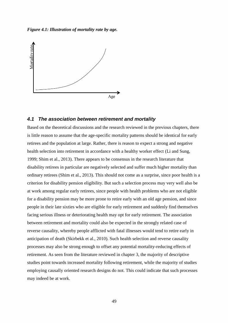
49

Figure 4.1: Illustration of mortality rate by age.

4.1 The association between retirement and mortality

Based on the theoretical discussions and the research reviewed in the previous chapters, there

is little reason to assume that the age-specific mortality patterns should be identical for early

retirees and the population at large. Rather, there is reason to expect a strong and negative

health selection into retirement in accordance with a healthy worker effect (Li and Sung,

1999; Shim et al., 2013). There appears to be consensus in the research literature that

disability retirees in particular are negatively selected and suffer much higher mortality than

ordinary retirees (Shim et al., 2013). This should not come as a surprise, since poor health is a

criterion for disability pension eligibility. But such a selection process may very well also be

at work among regular early retirees, since people with health problems who are not eligible

for a disability pension may be more prone to retire early with an old age pension, and since

people in their late sixties who are eligible for early retirement and suddenly find themselves

facing serious illness or deteriorating health may opt for early retirement. The association

between retirement and mortality could also be expected in the strongly related case of

reverse causality, whereby people afflicted with fatal illnesses would tend to retire early in

anticipation of death (Skirbekk et al., 2010). Such health selection and reverse causality

processes may also be strong enough to offset any potential mortality-reducing effects of

retirement. As seen from the literature reviewed in chapter 3, the majority of descriptive

studies point towards increased mortality following retirement, while the majority of studies

employing causally oriented research designs do not. This could indicate that such processes

may indeed be at work.

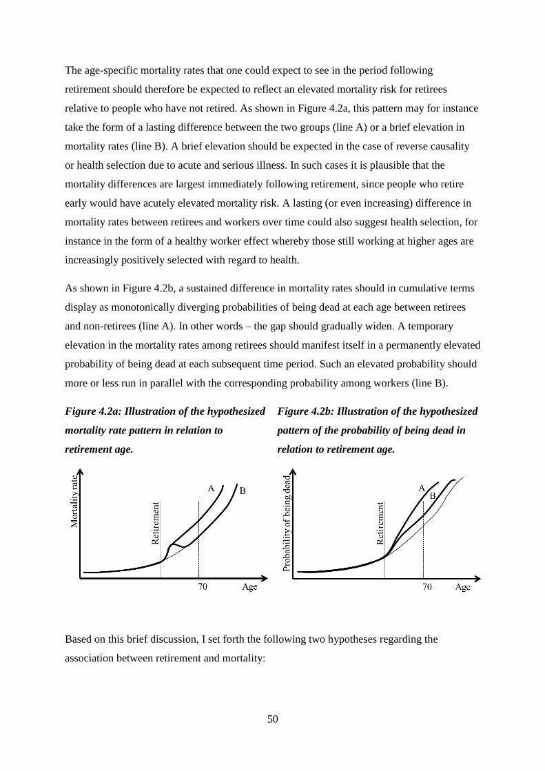
50

The age-specific mortality rates that one could expect to see in the period following

retirement should therefore be expected to reflect an elevated mortality risk for retirees

relative to people who have not retired. As shown in Figure 4.2a, this pattern may for instance

take the form of a lasting difference between the two groups (line A) or a brief elevation in

mortality rates (line B). A brief elevation should be expected in the case of reverse causality

or health selection due to acute and serious illness. In such cases it is plausible that the

mortality differences are largest immediately following retirement, since people who retire

early would have acutely elevated mortality risk. A lasting (or even increasing) difference in

mortality rates between retirees and workers over time could also suggest health selection, for

instance in the form of a healthy worker effect whereby those still working at higher ages are

increasingly positively selected with regard to health.

As shown in Figure 4.2b, a sustained difference in mortality rates should in cumulative terms

display as monotonically diverging probabilities of being dead at each age between retirees

and non-retirees (line A). In other words – the gap should gradually widen. A temporary

elevation in the mortality rates among retirees should manifest itself in a permanently elevated

probability of being dead at each subsequent time period. Such an elevated probability should

more or less run in parallel with the corresponding probability among workers (line B).

Figure 4.2a: Illustration of the hypothesized

mortality rate pattern in relation to

retirement age.

Figure 4.2b: Illustration of the hypothesized

pattern of the probability of being dead in

relation to retirement age.

Based on this brief discussion, I set forth the following two hypotheses regarding the

association between retirement and mortality:

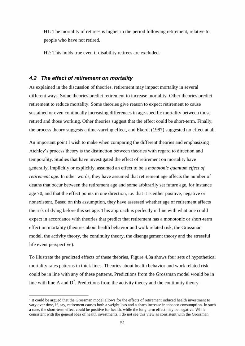
51

H1: The mortality of retirees is higher in the period following retirement, relative to

people who have not retired.

H2: This holds true even if disability retirees are excluded.

4.2 The effect of retirement on mortality

As explained in the discussion of theories, retirement may impact mortality in several

different ways. Some theories predict retirement to increase mortality. Other theories predict

retirement to reduce mortality. Some theories give reason to expect retirement to cause

sustained or even continually increasing differences in age-specific mortality between those

retired and those working. Other theories suggest that the effect could be short-term. Finally,

the process theory suggests a time-varying effect, and Ekerdt (1987) suggested no effect at all.

An important point I wish to make when comparing the different theories and emphasizing

Atchley’s process theory is the distinction between theories with regard to direction and

temporality. Studies that have investigated the effect of retirement on mortality have

generally, implicitly or explicitly, assumed an effect to be a monotonic quantum effect of

retirement age. In other words, they have assumed that retirement age affects the number of

deaths that occur between the retirement age and some arbitrarily set future age, for instance

age 70, and that the effect points in one direction, i.e. that it is either positive, negative or

nonexistent. Based on this assumption, they have assessed whether age of retirement affects

the risk of dying before this set age. This approach is perfectly in line with what one could

expect in accordance with theories that predict that retirement has a monotonic or short-term

effect on mortality (theories about health behavior and work related risk, the Grossman

model, the activity theory, the continuity theory, the disengagement theory and the stressful

life event perspective).

To illustrate the predicted effects of these theories, Figure 4.3a shows four sets of hypothetical

mortality rates patterns in thick lines. Theories about health behavior and work related risk

could be in line with any of these patterns. Predictions from the Grossman model would be in

line with line A and D7. Predictions from the activity theory and the continuity theory

7 It could be argued that the Grossman model allows for the effects of retirement induced health investment to

vary over time, if, say, retirement causes both a weight loss and a sharp increase in tobacco consumption. In such

a case, the short-term effect could be positive for health, while the long term effect may be negative. While

consistent with the general idea of health investments, I do not see this view as consistent with the Grossman

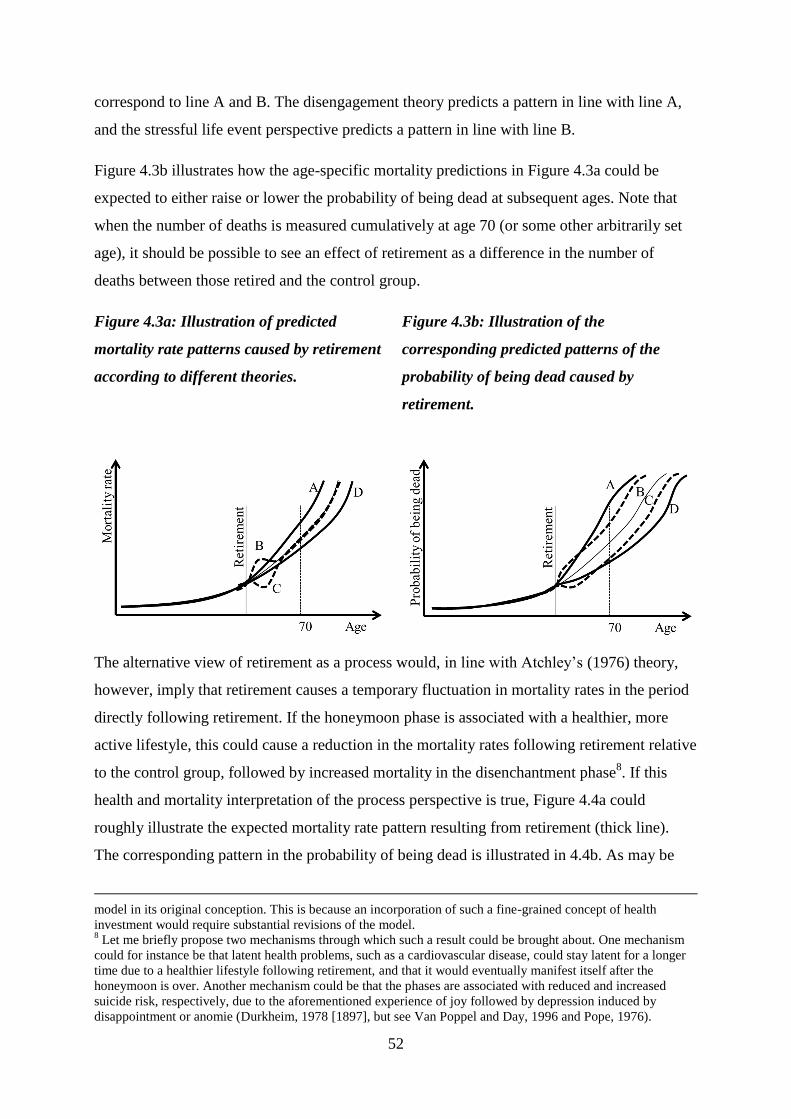
52

correspond to line A and B. The disengagement theory predicts a pattern in line with line A,

and the stressful life event perspective predicts a pattern in line with line B.

Figure 4.3b illustrates how the age-specific mortality predictions in Figure 4.3a could be

expected to either raise or lower the probability of being dead at subsequent ages. Note that

when the number of deaths is measured cumulatively at age 70 (or some other arbitrarily set

age), it should be possible to see an effect of retirement as a difference in the number of

deaths between those retired and the control group.

Figure 4.3a: Illustration of predicted

mortality rate patterns caused by retirement

according to different theories.

Figure 4.3b: Illustration of the

corresponding predicted patterns of the

probability of being dead caused by

retirement.

The alternative view of retirement as a process would, in line with Atchley’s (1976) theory,

however, imply that retirement causes a temporary fluctuation in mortality rates in the period

directly following retirement. If the honeymoon phase is associated with a healthier, more

active lifestyle, this could cause a reduction in the mortality rates following retirement relative

to the control group, followed by increased mortality in the disenchantment phase8. If this

health and mortality interpretation of the process perspective is true, Figure 4.4a could

roughly illustrate the expected mortality rate pattern resulting from retirement (thick line).

The corresponding pattern in the probability of being dead is illustrated in 4.4b. As may be

model in its original conception. This is because an incorporation of such a fine-grained concept of health

investment would require substantial revisions of the model. 8 Let me briefly propose two mechanisms through which such a result could be brought about. One mechanism

could for instance be that latent health problems, such as a cardiovascular disease, could stay latent for a longer

time due to a healthier lifestyle following retirement, and that it would eventually manifest itself after the

honeymoon is over. Another mechanism could be that the phases are associated with reduced and increased

suicide risk, respectively, due to the aforementioned experience of joy followed by depression induced by

disappointment or anomie (Durkheim, 1978 [1897], but see Van Poppel and Day, 1996 and Pope, 1976).

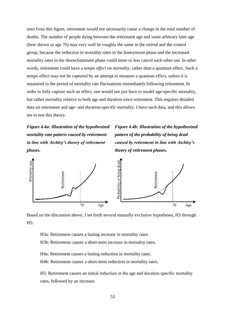
53

seen from this figure, retirement would not necessarily cause a change in the total number of

deaths. The number of people dying between the retirement age and some arbitrary later age

(here shown as age 70) may very well be roughly the same in the retired and the control

group, because the reduction in mortality rates in the honeymoon phase and the increased

mortality rates in the disenchantment phase could more or less cancel each other out. In other

words, retirement could have a tempo effect on mortality, rather than a quantum effect. Such a

tempo effect may not be captured by an attempt to measure a quantum effect, unless it is

measured in the period of mortality rate fluctuations immediately following retirement. In

order to fully capture such an effect, one would not just have to model age-specific mortality,

but rather mortality relative to both age and duration since retirement. This requires detailed

data on retirement and age- and duration-specific mortality. I have such data, and this allows

me to test this theory.

Figure 4.4a: Illustration of the hypothesized

mortality rate pattern caused by retirement

in line with Atchley’s theory of retirement

phases.

Figure 4.4b: Illustration of the hypothesized

pattern of the probability of being dead

caused by retirement in line with Atchley’s

theory of retirement phases.

Based on the discussion above, I set forth several mutually exclusive hypotheses, H3 through

H5:

H3a: Retirement causes a lasting increase in mortality rates.

H3b: Retirement causes a short-term increase in mortality rates.

H4a: Retirement causes a lasting reduction in mortality rates.

H4b: Retirement causes a short-term reduction in mortality rates.

H5: Retirement causes an initial reduction in the age and duration specific mortality

rates, followed by an increase.

54

H3a would be in accordance with theories about health behavior and work related risk, the

Grossman model, the activity theory, the continuity theory and the disengagement theory.

H3b corresponds with theories about health behavior and work related risk, the continuity

theory and the stressful life event perspective. H4a is deduced from the theories about health

behavior and work related risk and the Grossman model. H4b would be in accordance with

theories about health behavior and work related risk, while H5 corresponds with the process

theory. Obviously, there is a null hypothesis here as well, namely that retirement does not

affect mortality. This would be in accordance with the no effect assumption.

If there is an effect of retirement on mortality, and particularly if retirement increases

mortality risk, the fact that I (for reasons given below) sample cohorts where there is a large

difference in labor force participation between men and women leads me to expect that the

effect will be larger for men than for women. This is because the role loss associated with

retirement in the time period studied in this thesis (the 1970s and onward) is likely greater for

men than for women due to men’s breadwinner role in this generation (Birkelund and

Petersen, 2016). This would be in line with the view of retirement as a stressful life event, the

disengagement theory, the activity theory, the continuity theory, and the discussion in

Coppola and Spizzichino (2014). A similar argument may be based on the Grossman model,

although without a specified direction. Since women earn less and work more part-time, the

changes in income, incentives structure and available time following retirement may be

smaller for women than for men. This points towards a larger effect for men. Higher mortality

among men and thereby higher baseline risk also points in the same direction. In any case, I

can formulate H6:

H6: If retirement increases mortality risk, the effect is stronger for men than for

women.

As mentioned in section 2.2.1, it is likely that an effect of retirement on mortality follows a

socioeconomic gradient. But the direction is not obvious. Retirement from low-status manual

jobs associated with health risks such as exposure to cold weather, harmful chemicals etc.

may be beneficial to health, as clearly indicated by Westerlund et al. (2009). But people

voluntarily retiring early from such jobs might also be particularly negatively selected. Also,

the socioeconomic differentials in lifestyles may imply that people retiring from high-status

and well-paid jobs are more inclined to spend the increased spare time on activities that are

beneficial for their health. In that case, the increase in available time following retirement

could amplify the socioeconomic gradient in health behavior. On the other hand, people in

55

such occupations are also less likely to retire early. Ideally, it would be interesting to explore

effect heterogeneity with regard to different socioeconomic measures, such as income,

education and occupation groups. However, due to there being a lot of missing values on both

the occupation variable and the income variable, this is difficult. Therefore, I am left with

education levels as the best candidate for a socioeconomic indicator. Because people with

lower education are more likely to be in jobs that are associated with health risks, and may

therefore benefit more from retirement I suggest the following hypothesis:

H7: If retirement affects mortality risk, earlier retirement reduces mortality more, or

increases it less, for people with low education, relative to people with higher

educational levels.

Finally, as noted before, if retirement indeed has an effect on mortality, I do not expect this

effect to be large.

56

5 Choice of empirical strategy

To test the different hypotheses deduced in chapter 3, I have chosen two different empirical

strategies. First, I test hypotheses H1 and H2 concerning the association between retirement

and mortality through event history analyses. A discussion of the pros and cons of different

approaches to such analyses follows below. Second, I treat a pension reform that affected the

1903 through 1906 cohorts as a natural experiment, and exploit it as a source of exogenous

variation in retirement eligibility. I do this in an attempt to provide estimates of the

relationship between retirement and mortality that can be given a causal interpretation.

As stated earlier, I take retirement to mean work exits in relation to old age (usually in

combination with the uptake of pension benefits). For practical reasons, however, I

operationalize retirement as the uptake of benefits and do not condition on work exits. In

practice, then, I use the uptake of benefits as a proxy for retirement.

5.1 The association between retirement and mortality

Hypotheses H1 and H2 concern the association between retirement and mortality. Due to

strong health related selection into retirement, H1 should be expected to hold true regardless

of whether there exists a causal relationship between retirement and mortality. H2 specifically

addresses the issue of health-related selection into retirement though disability pensions. It

suggests that even when disability pensioners are excluded, the health selection may be strong

enough to produce a positive correlation between retirement and mortality. This selection

process could work in combination with a causal mechanism, or it could run counter to it (but

be strong enough to suppress it).

Ideally, and in isolation, these hypotheses could be tested on recent data on retirement and

mortality. But in the context of this thesis, it is more interesting to test these hypotheses on

cohorts that retired around the same time as those included in the second part of the analyses.

For reasons given below, I test hypotheses H3 though H7 about the causal relationship

between retirement and mortality on cohorts that retired in the early 1970s. To make the

results from the two parts comparable, I have chosen to test hypothesis H1 and H2 on the

1906 and 1907 cohorts. These became eligible for old age pensions at age 67, and were born

close enough in time to be comparable with regard to age-specific mortality. In addition, they

became eligible for retirement at or around the same time as those affected by the 1973

57

pension reform, which I use in the second part of the analysis. In fact, the 1906 and 1907

cohorts were the first cohorts to be fully affected by the reform.

The data I use in this thesis contains detailed person-year information on retirement and

mortality for these cohorts. It is also possible to distinguish between several types of pensions.

For the present purposes, the possibility to distinguish disability pensioners from other

pension benefit recipients is particularly important. To test hypothesis H1 and H2, I apply

discrete-time hazard regression methods to the retirement and mortality data, fitting separate

models that both include and exclude disability pensioners.

5.2 The effect of retirement on mortality

In order to test hypotheses H3 through H7 and provide estimates of the correlation between

retirement and mortality that can plausibly be given a causal interpretation, I need to identify

and exploit a source of exogenous variation in retirement age. People may decide for

themselves when to retire, to a large extent. And this decision is likely influenced by factors

that also affect mortality, such as health. As such, those who retire early and those who retire

late are likely different in many regards. This means that to estimate the effect of retirement, it

is necessary to identify a situation where it is plausible (under some conditions) to assume that

those who retire early and those who retire late are similar on salient properties. In other

words, an experiment or a natural experiment is required. True experiments in this area are

hard to come by. But to the best of my knowledge, there have been three different large-scale

Norwegian pension reforms that may serve as natural experiments. Here, I briefly discuss

these reforms in reverse chronological order, and point to the pros and cons of using each of

them in an attempt to estimate the causal effect of retirement on mortality. I then try to justify

the choice I have made.

5.2.1 The national insurance pension reform of 2011

The pension reform of 2011 comprised of several important elements. Among these was the

option of early retirement from age 62 for individuals with sufficient cumulative pensionable

income, increased flexibility in the form of the option of combining (full or partial) pension

outtake with continued (full or partial) work force participation, and strong economic

incentives to postpone retirement in relation to increases in life expectancy (The Ministry of

Labor and Social Inclusion/Arbeids- og inkluderingsdepartementet, 2006; Fredriksen and

Stølen, 2011).

58

At first glance, the pension reform of 2011 may be considered a good candidate for the role of

a natural experiment. It represents a major and exogenous change in individuals’ opportunities

for early retirement, as the entitled retirement age vas reduced from 67 to 62. Although many

people already had the option of retiring early through contractual early retirement schemes

(AFP), a considerable proportion of the affected cohorts did not, and they were effectively

given the opportunity to retire up to five years earlier than previous cohorts (Hernæs et al.,

2015). This feature of the reform alludes toward a difference-in-differences (DiD) strategy or

an instrumental variables (IV) approach whereby being in a cohort affected by the reform at a

given age functions as a treatment or instrument for retirement age. The cumulative earnings

threshold for eligibility into early retirement of 1,85 G for married and 2 G for unmarried

people (Fredriksen and Stølen, 2011) may also be considered a somewhat arbitrary cutoff – a

feature that makes this reform attractive for use in a regression discontinuity framework, if

one can overcome the issues related to self-selection into eligibility. In combination, the

reduction in retirement age and the eligibility threshold may be used in a triple differences

(DiDiD) estimator by using the between-cohorts variation in retirement eligibility age

resulting from the reform implementation and the within-cohort variation resulting from the

lifetime earnings threshold. In fact, Hernæs et al. (2015) have done something similar to this

approach in an attempt to estimate the impact of different aspects of the reform on labor

supply.

On the other hand, there are some major issues that discourage the use of this reform as I have

suggested here. First, the strong incentives to postpone retirement mean that many people may

in fact retire later than they otherwise would have, despite being given the opportunity to

retire earlier. In fact, the reform has on average been shown to increase the actual retirement

age (Fredriksen and Stølen, 2015). In an instrumental variables framework, this means that

there is likely to be a substantial number of defiers9 (people who do not take the treatment

because they are offered it or vice versa) (Angrist and Pischke, 2008: 156-7; 2014:112-5;

Borgen, 2013). In other words, a lot of people likely postponed their retirement because they

were affected by the reform, and despite the reform allowing them to retire earlier. Having a

lot of defiers in a sample strongly biases IV estimates (Borgen, 2013). This problem may,

however, be possible to overcome by controlling for the effects of such incentives or by

excluding individuals who are subject to them. Second, given that one cannot condition upon

actual retirement in a DiD framework, the changes in incentives and benefits associated with

9 An explanation of the concepts of defiers, compliers, always-takers and never-takers is given in section 7.4.

59

the pension reform make it difficult to ensure that an estimation of the effect of the reform

reflects the effect of lowered retirement age and not the effects of changes in benefits and

incentives structures. This problem may also be possible to overcome through control or

exclusion. Third, the fact that many people were already eligible for early retirement before

the reform through the contractual early retirement scheme makes it difficult (but not

impossible) to isolate the population that was affected by the reform. Fourth, the fact that the

reform was anticipated several years in advance means that people may have been able to

self-select into eligibility, for instance through increased labor market participation in the final

years before retirement eligibility age in order to reach the earnings threshold sooner. This is

more difficult to account for. Fifth, the fact that this reform is fairly recent means that the

effect is only observable for a short time period, meaning that only short-term effects may be

identified. Finally, few people die in their early sixties. The remaining life expectancy at age

62 was 20.5 years for men and 23.8 years for women in 2011 (SSB, n.a.). This means that

even if retirement age actually impacts mortality, it may be difficult to identify a statistically

significant short-term effect in these age groups. These issues have in sum led me to opt not to

use this reform in this thesis.

5.2.2 Lowering of the contractual early retirement age in the 1990s

Between 1989 and 1998, the minimum retirement age in the contractual early retirement

scheme (AFP) was lowered in a stepwise fashion from 67 to 62 years (NOU 1998: 19). As

mentioned before, this gradual reduction in the eligible retirement age for one group of

workers was used by Hernæs et al. (2013) in their IV and hazard rate triple differences

estimation of the effect of retirement on mortality.

The advantages of using this reform in an identification strategy are laid out in detail by

Hernæs et al. (2013), and are not discussed here. But I will mention a few drawbacks of using

this reform. First, the treatment groups are essentially identified by cohort membership and

AFP eligibility (i.e. being employed in an AFP firm). This means that the instrument could be

invalid if the trends in cohort mortality differ between those employed in AFP firms and those

who are not. The paper showed that this does not appear to be the case. However, it could in

theory still be so in the implausible scenario that such differential mortality trends and the

effect of retirement age pointed in opposite directions and more or less precisely cancelled

each other out. I personally find this unlikely. A more important point concerns the question

of whether this reform is the best candidate for identifying a hypothetical causal effect of

retirement on mortality. The remaining life expectancy at age 62 was 18 years for men and

60

22.2 years for women in 1998 (SSB, n.a.). Since few people died in their early 60s in the

1990s, a hypothetical causal effect may be too small to identify in this age group, but may still

be possible to identify at higher ages. Such a scenario would not be at odds with the findings

of Hernæs et al. (2013), but would point towards there being a mortality effect of retirement

in other age groups or periods than those that they studied. Also, the identification of the

treatment and control groups in this scenario is very complicated. Lastly, the fact that Hernæs

and colleagues have used this reform in their study also means that there would be little to

gain from using it again in this thesis, except for the purposes of replication. Using a different

sample and a different reform may, however, contribute more to the accumulating research

literature on this topic.

5.2.3 Lowering of the retirement age in the national insurance scheme in 1973

In the law on old age insurance was passed in 1937, the statutory minimum retirement age

was 70 years (Ministry of Social Affairs/Sosialdepartementet, 1971). In 1973, however, this

age limit was lowered to 67 (Amendment to the law on social insurance, 1972)10

. As a policy

experiment, this reform has some appealing features. First, it was a rather simple reform. The

main reform element was the lowering of the entitled retirement age by three years, and this

change happened at a single point in time – on the 1st of January 1973. This sets it apart from

the more complex reform of 2011 and the gradual reduction in entitled retirement age in the

contractual early retirement scheme in the 1990s. Second, the fact that the reform happened

more than forty years ago provides a long observation window and facilitates estimation of

the long-term effects of retirement on mortality. Third, the complexity of the 2011 reform

makes the identifiable treatment effect a very local one (meaning that the effect can only be

estimated for specific subgroups) (Hernæs et al., 2015), and the contractual early retirement

reform only affected those covered by the system. But the 1973 reform affected the majority

of the working population, meaning that it is theoretically less problematic to generalize the

results to different groups (though not necessarily across time). Fourth, the fact that the

important eligibility criterion is related to birth cohort membership means that people could

not self-select into treatment. People can’t change birth cohort like they can change jobs in

response to a policy reform. Finally, the reform happened in a period in time, and affected

people at ages, where the mortality was markedly higher than the later reforms discussed

above. More people die in their late than in their early sixties, and mortality was higher in

1973 than in the 1990s and after 2011. In fact, the remaining life expectancy at age 67 was

10

I originally got the idea to use this reform when I read Brunborg et al. (2008) and saw the figures on page 28.

61

just 12.6 years for men and 15.4 for women in 1973 (SSB, n.a.). The fact that Hernæs et al.

(2013) did not find an effect of the reform in the 1990s may be attributable to the fact that

they studied the effect of a recent reform affecting an age group with low mortality. In this

sense, the 1973 reform serves as a critical case (Flyvbjerg, 2006); if an effect of retirement on

mortality cannot be found when using the 1973 reform, it is unlikely that one can be found at

all.

A complicating matter is the fact that the 1973 reform was introduced together with a

“waiting supplement” (“ventetillegg”) that provided some incentive to delay retirement

(NAV, 2011). However, given that this benefit only worked as an incentive to postpone

retirement up to age 70 (the pre-reform limit), it is far less prone than the 2011-reform to

produce many defiers, although not everyone opted to retire at the earliest opportunity. In

theory, people who were affected by the reform, but who did not retire until after age 70,

should then be never-takers rather than defiers, since there was no incentive to defy beyond

age 70. This is because defiance would mean postponing retirement until age 70 or later,

when there was no more waiting supplement11

. Thus, people were not allowed to self-select

into retirement eligibility (i.e. the treatment groups), but once eligible for retirement, they

could decide on their retirement age within the constraints of the system.

Another complicating matter is the fact that not all employees were affected equally by the

reform. Some occupations in some firms and government institutions and offices already had

lower statutory retirement ages at the time of the reform. With regard to the government

employees, the jobs with lower retirement ages are listed in the recommendation from the

committee on retirement age (Pensjonsalderkomitéen, 1971). The inclusion of people with

lower statutory retirement ages will bias the estimates of the mortality effect of this reform

slightly towards zero12

.

11

Of course, it is always possible to come up with a just-so story about how the reform may generate defying

behavior. Here is an attempt: “In 1973, Peter had planned to retire early with his savings at age 68. The reform

gave him incentives to work until age 70, so he did. After all, he was a rational actor with transitive preferences,

who valued his leisure more than his wage, but less than his wage plus the waiting supplement. By age 70, Peter

had realized that he preferred working to retiring. His preference ordering had shifted, perhaps because old age

had deprived him of his rationality. Or maybe it had bereaved him of his spouse and life partner so that he felt

little reason to retire. In any case, Peter worked for two more years, until his health failed him, and he retired as a

defier at age 72.” The plausibility if this identification strategy partly rests on the implausibility of such

untestable just-so stories, i.e. on the likely number of defiers and the extent of their defiance being small

(Borgen, 2013). 12

By using data on occupations from the 1970 census, it could have been possible to remove some of this bias.

These census data contain information on occupation titles and industry/field (Vassenden, 1987).This could have

made it possible to (in broad strokes) exclude individuals who were in occupations less affected or unaffected by

62

Finally, the fact that this is an old reform makes it less appealing. Estimating the effect of

something that happened in 1973 is not exactly newsworthy. The relevance and external

validity of the findings to present day elderly may be questioned, since both working lives,

lifestyles health, mortality and the availability of health and welfare services have changed

considerably since then. However, I would argue that the mechanisms that potentially could

produce an effect in the early 1970s may very well still be at work today, though perhaps

tempered by other developments. Furthermore, the critical case argument made above makes

this reform theoretically interesting, as it could serve as a critical test of the theories

postulating an effect of retirement on mortality.

All in all, two estimation strategies based on the 1973 reform appear promising. The first is a

DiD-estimation whereby cohorts affected by the reform at different ages are compared to

cohorts that are not affected, with variation in treatment status arising from the between-

cohort variation in in age at the time of the reform implementation. This could provide an

estimate of the net effect of the reform (the intention to treat-effect) on the cohorts affected.

By also introducing within-cohort variation in eligibility at each age by distinguishing

between groups affected and not affected by the reform (for instance because they are

unemployed or homemakers) in a triple differences (DiDiD) estimator, it could be possible to

get a more precise estimate of an effect of being offered to retire earlier (Angrist and Pischke,

2014:119-20). Such an estimator would measure something more akin the effect of actually

being offered to retire (not just being in a cohort where most people were given this offer)

while also providing some some safeguard against the potential confounding of calendar year

effects (such as a rough flu season13

etc.). Introducing within-cohort variation in retirement

eligibility would in other words reduce bias since people eligible and not eligible for

retirement could be assumed to be subject to the same calendar year variations in mortality

risk. However, finding and identifying such groups appears to be be easier said than done14

.

The second promising strategy is to use the reform as an instrument for retirement age.

Assuming that which cohorts were affected by the reform is unrelated to the differences

the reform. But unfortunately, as shown in chapter 8, the number of missing values on the occupation variable is

too large to make such an analysis meaningful. 13

In fact, Norway was hit by a flu pandemic in 1977, commonly referred to as the “Russian flu”. This could

potentially bias the results by introducing calendar year effects. However, Mamelund and Iversen (2000) did not

find evidence of excess mortality associated with this flu pandemic. 14

One option could be to use housewives as a within-cohort control group. These would not be affected by the

reform since they were not employed. But if there are spillover effects of the husbands’ retirement, this could

also bias the results.

63

between cohorts in characteristics that affect mortality (such as education, health etc.), I can

assume that the between-cohort variation in retirement eligibility age is exogenous. Further,

assuming that the reform also had an effect on the retirement ages of the affected cohorts, it is

possible to use this reform-induced variation in retirement age to estimate the effect of retiring

earlier (or later). This first assumption is not directly testable, but the second one is, as I will

show below.

Policy reform instruments are frequently used in social research, as can be seen in the

literature review in chapter 3. This is partly because they are often plausibly exogenous.

Policy reforms that affect different segments of the target population differentially through

arbitrarily defined eligibility rules or timing can often be assumed to be unrelated to other

characteristics that affect the outcome of interest. This makes it easier to argue that a given

reform constitutes a valid instrument. An IV approach could also be theoretically more

interesting than a DiD approach, as it would (hopefully) yield estimates of the local average

treatment effect for the compliers (Angrist and Pischke, 2014: 111-5). It would thus give

estimates of the effect of retiring, not just being offered the opportunity to retire. To be

precise, I would measure the average effect of retiring a given number of years earlier than

one otherwise would have, within the age span of 67 to 70 years in the early- to mid-1970s,

because one is allowed to do so because of the reform. This may appear to be a very local and

narrow (though well-defined) effect, but it is theoretically interesting because it could be

interpreted as a retirement effect, not a reform effect, making it more plausible that the

findings may be generalized to other, similar contexts. The point that the treatment effect

would be local is important. If the effect can be assumed to vary across contexts, groups or

time, one should be careful about generalizing the results. A drawback is that IV estimation is

accompanied by large standard errors (Murray, 2006), leading to less precise estimates and an

increased risk of committing a type II error (i.e. failing to reject a false null hypothesis).

In sum then, I opt to use the 1973 reform to identify an effect of retirement on mortality. I find

this reform to be most appealing, as it gives a long follow-up period, relatively simple

identification, population-wide treatment effects and high chances of identifying an effect if

there is one. Nonetheless, the abovementioned drawbacks to using this reform should be kept

in mind.

64

6 Data

For the empirical analyses in this thesis, I rely on high quality register data from Norwegian

administrative registers, as well as on data from the 1970 census. The original datasets from

which my samples are drawn comprise the entire Norwegian resident population that has been

alive at some point since 1967.

Approval to use these data was obtained from the privacy ombudsman at Statistics Norway

and the sections responsible for the data at Statistics Norway. This process was coordinated

by the project manager. The approval is attached in the appendix, together with a note

confirming an approval to expand the sample to cover people alive in 1967-1969. All datasets

were provided by Statistics Norway.

6.1 Data sources

I use data from population registers (births, deaths, immigrations, emigrations, age, sex and

immigrant background), income records (pensionable income), welfare benefit registers

(pensions), and census data (occupation, industry and education levels).

The original data on demographic variables from the population registers were organized in

two files, each with one record per individual. Only observations with valid project-specific

ID numbers were included. One of the population register files contained information on

immigrant backgrounds while the other contained information on other characteristics Time-

invariant characteristics were corded as categorical variables, while events were coded as

dates, months or years. I only used information about events per month and year. For

immigration and emigration, only the first immigration date and the last emigration date were

used. Immigrant background was coded into three categories; immigrants, Nowegian-born

with two Norwegian-born parents, and all others. In some analyses, these last two groups

were merged. Income records were also organized with one record per individual, but with

one variable per year since 1967.

The data on welfare benefit recipiency was organized as one record per person-event. These

data also only had information on events per year. I coded one variable for each pension type

(old age pensions, disability pensions and all other pensions types combined) that contained

information on the first year of recipiency, as well as one variable indicating the first year

each individual received any type of pension. Before merging these data with the other

65

datasets, I deleted all records of the same individual except one, which then contained detailed

data on the year of entry into different pension types.

The census data was also coded with one record per individual. With regard to educational

levels, the nine groups in the original data were coded according to the 80-standard

(Vassenden, 1987). These have been collapsed into four groups – no education (including

preschool), primary education, secondary education/high school, and university/college

education. Occupations were also coded according to the 80-standard In chapter 8, I show the

proportions of the samples that belong to each of several broad occupational groups. But the

large number of missing values on this variable has led me to opt not to include it in the

analyses.

6.2 Merging, recoding and sample restrictions

Merging of datasets and preliminary recoding of variables was done in the SAS Enterprise

Guide 7.1 software package. An overview of the different steps in the sample restriction

process is provided in Table 6.1. Starting with one of the population register files, I deleted

1610 individuals who were not resident, dead or emigrated (people with missing status codes,

people who have disappeared, etc.). The two population register files were then merged using

the PROC SQL inner join procedure. This procedure discards all observations not present in

both datasets, ensuring that there are no duplicates or people with information from only one

of the files. I then deleted 40 individuals whose death times did not match in the two

population register files. I also deleted 11 people with missing times of both death and

emigration.

The income file was merged with the population register dataset using the PROC SQL left

join procedure. This procedure ensures that the population register files are given primacy, so

that observations from other files are only merged to observations in the population register

files if they can be linked to an individual in these files. In other words, observations in other

datasets that could not be matched with an individual in the population register files were

discarded, while all individuals in the population register files were retained. All cohorts

except those born between 1902 and 1907 were then discarded. All other datasets were then

sequentially merged with the combined population register and income files using the PROC

SQL left join procedure. Old age pension eligibility age was derived from each individual’s

birth year and birth month.

66

The complete dataset contained information on 255 138 individuals. This equals 99.35

percent of the original sample. Only counting people alive at age 65 reduces this number

considerably (by 26 426 individuals). This restriction is imposed in most analyses in this

thesis since imposing it means that I avoid issues related to the fact that the registers were

established in 1967. Based on this complete dataset, three separate files were produced,

exported to Stata format, and then used in the analyses. Analyses were performed with the

Stata 13.1 software package. The first file, which I will denote the “wide file” contains one

record per individual. It has information on event times in years and months. This file is used

to produce much of the descriptive statistics on time-invariant characteristics and to perform

the IV analyses. It contains information on 228 712 individuals who lived beyond age 65

when the 1907 cohort is included, and 189 634 individuals who lived beyond age 65 when it

is not. In one robustness check, I keep the 1907 cohort when estimating an IV model with a

linear cohort trend. The second file, hereby denoted the “long file with years” is organized as

a conventional panel dataset with one observation per person-year. Individuals are censored

before immigration and after emigration and death. This file is used for the event history

analyses. It contains information on 77 422 individuals from the 1906 and 1907 cohorts who

lived past age 65. The total number of person-year observations for this group is 1 348 473.

The third file can be denoted the “long file in months”. It contains one observation per person-

month and information on time-variant variables at each month. This dataset is not censored

at death, and each individual is followed until age 75 regardless of whether they die (although

I never use observations for ages higher than 70). This dataset contains information on

189 634 individuals from the 1902-1906 cohorts. It is used for the DiD and individual FE

models.

In both long files, time-variant statuses (such as not retired/retired) were coded so that they

refer to the first full month or year in which the person holds that status. Event variables were

coded so that they refer to the time intervals within which the event took place. Let me give

an example based on the long file with years. A person who is followed from 1970 to 1975

retired sometime in 1973. The retired-variable would then have the values 0,0,0,0,1,1. The

event variable would have the values 0,0,0,1,0,0.

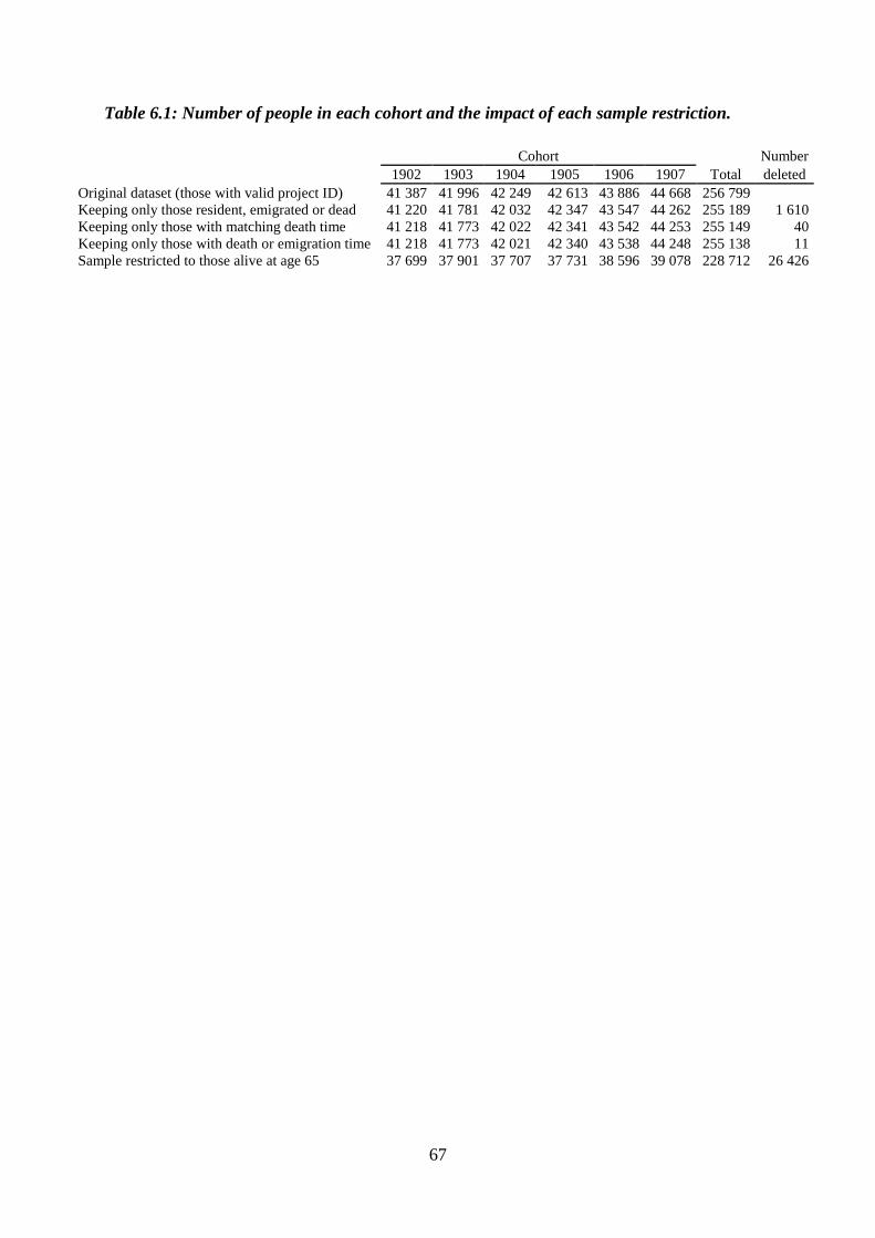
67

Table 6.1: Number of people in each cohort and the impact of each sample restriction.

Cohort

Number

1902 1903 1904 1905 1906 1907 Total deleted

Original dataset (those with valid project ID) 41 387 41 996 42 249 42 613 43 886 44 668 256 799

Keeping only those resident, emigrated or dead 41 220 41 781 42 032 42 347 43 547 44 262 255 189 1 610

Keeping only those with matching death time 41 218 41 773 42 022 42 341 43 542 44 253 255 149 40

Keeping only those with death or emigration time 41 218 41 773 42 021 42 340 43 538 44 248 255 138 11

Sample restricted to those alive at age 65 37 699 37 901 37 707 37 731 38 596 39 078 228 712 26 426

68

7 Methods The analyses in this thesis can be divided into two parts. First, I examine the association

between retirement age and mortality using event history analyses. These analyses shows how

mortality varies with retirement status and retirement duration (H1) and to what extent the

association is driven by health selection into disability pensions (H2). In the second part, I

employ two different methods suited for analyzing quasi-experimental data. I use these

methods to exploit the (presumably) exogenous variation in retirement eligibility age that

stems from the lowering of the retirement age in 1973. These analyses show whether and how

retirement affects mortality (H3 through H7).

7.1 Event history analysis

For the event history analyses in this thesis, I rely on discrete-time hazard regression models.

These models are useful for analyzing mortality data because they can estimate the

conditional odds, log-odds or hazards of failure in different time intervals. In many cases, the

researcher is interested in knowing the risk of failure (death) in some time interval t for the

population at risk in the time interval. This entails excluding those units that are not at risk (in

the case of mortality this could for instance be because they are not resident or because they

are dead) and condition on being at risk in the time interval. In an event history analysis, this

is achieved by censoring cases not at risk (Allison, 1995: 9-14; Rabe-Hesketh and Skrondal,

2008: 331-333). Note that censoring due to emigration is likely informative in the analyses

presented in this thesis (Allison, 1995: 13-14), since it is reasonable to assume that healthier

people are more likely to emigrate. But excluding people who eventually emigrate is not a

good option either, since that would be to condition on a collider variable (Elwert and

Winship, 2014). I simply do not see a good solution to this issue, except noting that the

proportions who emigrate at old ages are very low (see Table 8.1) and unlikely to affect the

results much.

In a discrete-time hazard regression model, time is measured at discrete intervals, and,

commonly, only integer values are used. In the version of the model that I apply here,

dummies for each time period are used to account for time. This way I do not have to make

any assumptions about the functional form of the relationship between the baseline hazard and

time (Rabe-Hesketh and Skrondal, 2008: 334-350). The discrete-time hazard regression

model can be estimated as a logistic regression model on censored panel data. Formally, the

model can be expressed as

69

𝑙𝑜𝑔𝑖𝑡[𝑃(𝑦𝑠𝑖 = 1|𝑫𝒔𝒊, 𝑨𝒔𝒊, 𝑿𝒔𝒊)] = 𝛽1 + 𝑫𝒔𝒊 + 𝑨𝒔𝒊 + 𝛽2𝑿𝒔𝒊

where y is the outcome of interest (death), i indexes individuals, s indexes age in years

starting at age 60 and running until each individual is censored, A is a set of dummies for each

age interval spanning from age 60 to censoring for each individual, D is a set of dummies for

each age interval following retirement, and X is a vector of both time-varying and time-

invariant covariates, including retirement status.

For the analyses of the association between retirement and mortality, I restrict my sample to

the 1906 and 1907 cohorts. Both of these cohorts became eligible for old age pensions at age

67, so variation in retirement age is likely endogenous. While not advantageous in its own

right, this endogeneity makes it interesting to compare the results to the estimates provided by

the DiD, individual FE and IV estimators. Also, it is interesting to know about the relationship

between different retirement types and mortality regardless of the causality of the relationship.

One reason is because strong health selection into early retirement could be seen as an

argument for improving the health of older workers to prolong their working lives.

Since data on the uptake of pension benefits is only available at yearly time intervals, these

analyses are based on the dataset containing information on person-years. Due to the limited

availability of relevant time-varying control variables for the cohorts under study, the analyses

are somewhat limited in scope. However, since these analyses are motivated by hypotheses

H1 and H2 concerning the mortality patterns following retirement by different pension types,

this is not a major concern. The main objective here is to examine whether or not the

mortality of retirees is higher in the period following retirement relative to people not retired,

and whether this holds true even if disability retirees are excluded. The question is not

whether or how such correlations are related to other time-varying covariates.

In the analyses reported below, I first estimate models where I regress death on retirement

duration dummies, age dummies and time-invariant controls. If there is no duration effect, just

an effect of being retired regardless of duration, this would yield similar point estimates for

each duration dummy. Second, I exclude disability pensioners to see if the association

between retirement or retirement duration and mortality is driven primarily by people

receiving disability pensions. Acknowledging the issues related to unobserved heterogeneity

in logistic regression (Mood, 2010), I report average marginal effects for the variables of

interest.

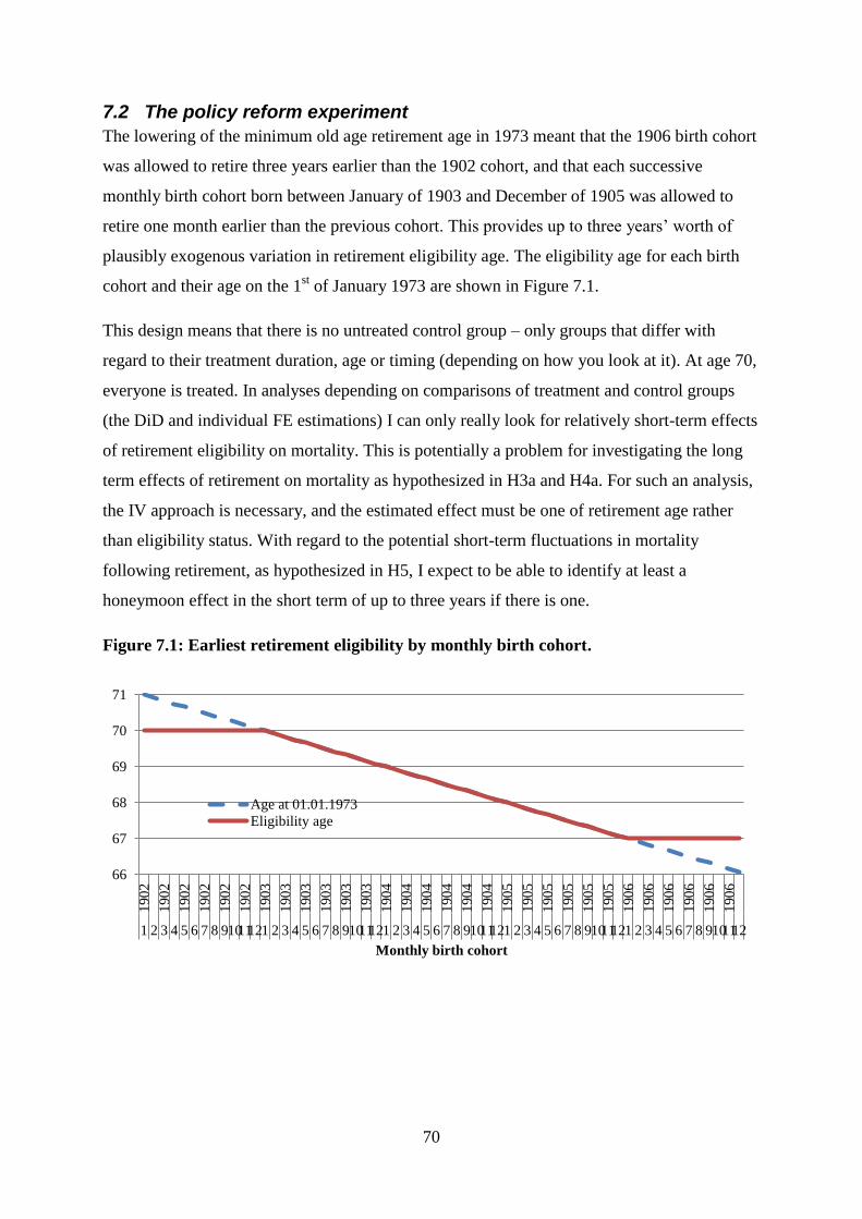
70

7.2 The policy reform experiment

The lowering of the minimum old age retirement age in 1973 meant that the 1906 birth cohort

was allowed to retire three years earlier than the 1902 cohort, and that each successive

monthly birth cohort born between January of 1903 and December of 1905 was allowed to

retire one month earlier than the previous cohort. This provides up to three years’ worth of

plausibly exogenous variation in retirement eligibility age. The eligibility age for each birth

cohort and their age on the 1st of January 1973 are shown in Figure 7.1.

This design means that there is no untreated control group – only groups that differ with

regard to their treatment duration, age or timing (depending on how you look at it). At age 70,

everyone is treated. In analyses depending on comparisons of treatment and control groups

(the DiD and individual FE estimations) I can only really look for relatively short-term effects

of retirement eligibility on mortality. This is potentially a problem for investigating the long

term effects of retirement on mortality as hypothesized in H3a and H4a. For such an analysis,

the IV approach is necessary, and the estimated effect must be one of retirement age rather

than eligibility status. With regard to the potential short-term fluctuations in mortality

following retirement, as hypothesized in H5, I expect to be able to identify at least a

honeymoon effect in the short term of up to three years if there is one.

Figure 7.1: Earliest retirement eligibility by monthly birth cohort.

66

67

68

69

70

71

190

2

190

2

190

2

190

2

190

2

190

2

190

3

190

3

190

3

190

3

190

3

190

3

190

4

190

4

190

4

190

4

190

4

190

4

190

5

190

5

190

5

190

5

190

5

190

5

190

6

190

6

190

6

190

6

190

6

190

6

1 2 3 4 5 6 7 8 91011121 2 3 4 5 6 7 8 91011121 2 3 4 5 6 7 8 91011121 2 3 4 5 6 7 8 91011121 2 3 4 5 6 7 8 9101112

Monthly birth cohort

Age at 01.01.1973

Eligibility age

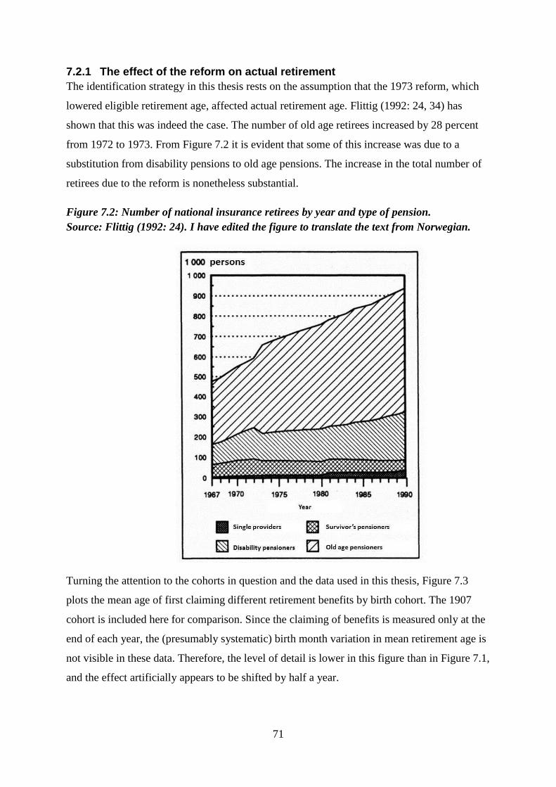
71

7.2.1 The effect of the reform on actual retirement

The identification strategy in this thesis rests on the assumption that the 1973 reform, which

lowered eligible retirement age, affected actual retirement age. Flittig (1992: 24, 34) has

shown that this was indeed the case. The number of old age retirees increased by 28 percent

from 1972 to 1973. From Figure 7.2 it is evident that some of this increase was due to a

substitution from disability pensions to old age pensions. The increase in the total number of

retirees due to the reform is nonetheless substantial.

Figure 7.2: Number of national insurance retirees by year and type of pension.

Source: Flittig (1992: 24). I have edited the figure to translate the text from Norwegian.

Turning the attention to the cohorts in question and the data used in this thesis, Figure 7.3

plots the mean age of first claiming different retirement benefits by birth cohort. The 1907

cohort is included here for comparison. Since the claiming of benefits is measured only at the

end of each year, the (presumably systematic) birth month variation in mean retirement age is

not visible in these data. Therefore, the level of detail is lower in this figure than in Figure 7.1,

and the effect artificially appears to be shifted by half a year.

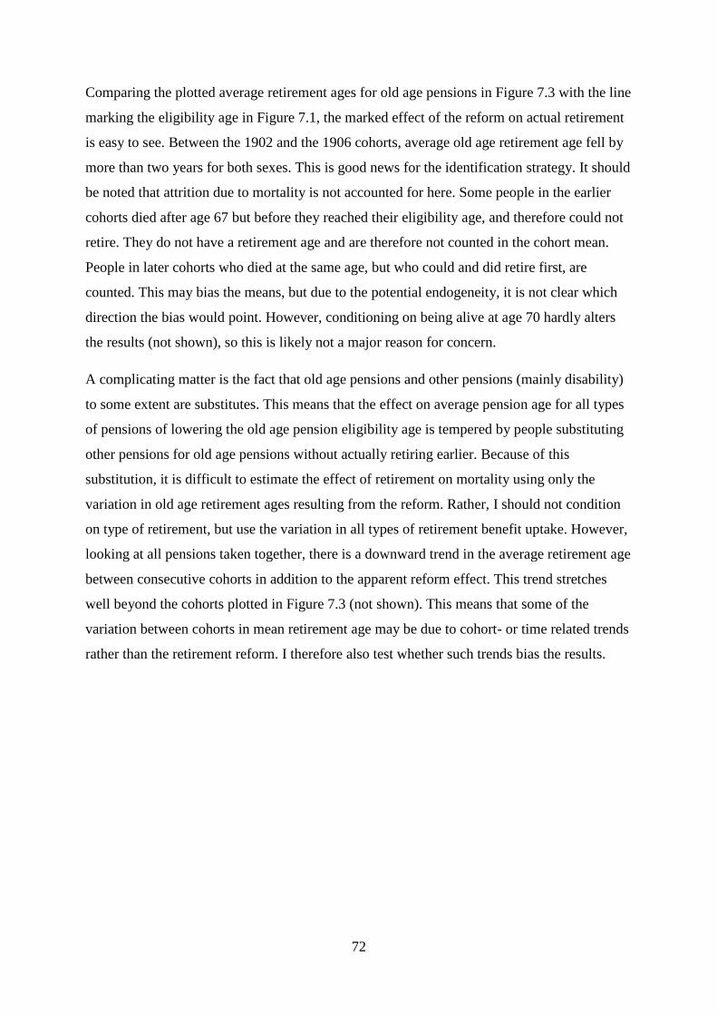
72

Comparing the plotted average retirement ages for old age pensions in Figure 7.3 with the line

marking the eligibility age in Figure 7.1, the marked effect of the reform on actual retirement

is easy to see. Between the 1902 and the 1906 cohorts, average old age retirement age fell by

more than two years for both sexes. This is good news for the identification strategy. It should

be noted that attrition due to mortality is not accounted for here. Some people in the earlier

cohorts died after age 67 but before they reached their eligibility age, and therefore could not

retire. They do not have a retirement age and are therefore not counted in the cohort mean.

People in later cohorts who died at the same age, but who could and did retire first, are

counted. This may bias the means, but due to the potential endogeneity, it is not clear which

direction the bias would point. However, conditioning on being alive at age 70 hardly alters

the results (not shown), so this is likely not a major reason for concern.

A complicating matter is the fact that old age pensions and other pensions (mainly disability)

to some extent are substitutes. This means that the effect on average pension age for all types

of pensions of lowering the old age pension eligibility age is tempered by people substituting

other pensions for old age pensions without actually retiring earlier. Because of this

substitution, it is difficult to estimate the effect of retirement on mortality using only the

variation in old age retirement ages resulting from the reform. Rather, I should not condition

on type of retirement, but use the variation in all types of retirement benefit uptake. However,

looking at all pensions taken together, there is a downward trend in the average retirement age

between consecutive cohorts in addition to the apparent reform effect. This trend stretches

well beyond the cohorts plotted in Figure 7.3 (not shown). This means that some of the

variation between cohorts in mean retirement age may be due to cohort- or time related trends

rather than the retirement reform. I therefore also test whether such trends bias the results.

73

Figure 7.3: Mean earliest retirement age for old age pensions and all pensions combined

(including disability pensions, survivor’s pensions etc), by sex and birth cohort.

7.3 Difference-in-differences

Most of the theoretical contributions discussed in chapter 2, suggest that retiring should have

some effect on mortality. Unless the effect has the form suggested by H5, I should be able to

measure an effect of retirement – positive or negative – on the mean probability of being dead

in the period after retirement.

In the difference-in-differences (DiD) framework presented here, I cannot condition on actual

retirement, as uptake is likely endogenous. Therefore, I am forced to treat retirement

eligibility as a proxy for retirement in order to provide estimates that can be given a causal

interpretation. Put differently, I measure an average effect of retirement eligibility, rather than

an effect of retirement. As I have shown above, the reform that lowered the eligibility age

appears to have had a strong effect on actual retirement behavior, so eligibility age appears to

be an acceptable proxy for retirement age.

Theoretically, I assume that the effect of being eligible for retirement on mortality is mediated

by the effect of eligibility on retirement uptake. Given due precautions, then, the results can

be considered a somewhat diluted retirement effect or a reduced form effect, whereby the

estimates measure the average effect of being treated (eligible) for those offered the treatment

(including both those who accept the offer and those who do not), compared to those not

offered the treatment (including both those who do not retire and those who retire despite not

65

66

67

68

69

70

71

1902 1903 1904 1905 1906 1907

Birth cohort

Old age pensions, men

Old age pensions, women

All pensions, men

All pensions, women

74

being eligible). Alternatively, the results can be interpreted as the net reform effect – the

effect of being offered to retire earlier. While the diluted retirement effect is the most

theoretically interesting interpretation, the net reform effect interpretation is the most policy

relevant. Since these analyses do not condition on actual uptake of old age pensions, there is

little reason to worry about the potential source of confounding that arises from the fact that

old age pension and disability pension are likely to be substitutes.

The DiD estimator relies on the assumption that in the absence of treatment, the time trends in

the treatment and control groups would be parallel. Using a DiD approach, I do not need to

worry too much about differences between the treatment and control groups as long as this

assumption holds. The DiD estimator exploits this parallel trends assumption to estimate the

effect of a policy change by estimating the difference between the observed outcome in the

treated group and the outcome that one would expect in the treated group if the trend in this

group had moved in parallel with that of the control group (Angrist and Pischke, 2008: 227-

241; 2014: 178-208).

Let me exemplify. A standard DiD approach uses aggregate data on different groups at two or

more points in time to measure the impact of a policy change or some similar change that

affects the treatment group but not the control group. The effect is measured as the difference

between the treatment and control group in differences between the pre- and post-treatment

outcomes. Hence the name. A typical application of this design could be measuring the

impact of some reform that affects a specific geographical area, for instance a labour market

regulation in US state A, on an outcome of interest, such as unemployment. This could be

done by comparing the difference between pre and post reform unemployment rate in state A

to the difference in the unemployment rates at the same points in time in the neighboring state

B (Angrist and Pischke, 2014: 178-208).

In this thesis, I apply this DiD logic in an OLS model, but with some modifications. The first

is that I use individual level data, rather than aggregate measures. This data is a panel, rather

than a cross- section15

. Treatment and control groups are defined by monthly birth cohort

membership, since eligibility age varies between cohorts. The time dimension in this setup is

not calendar time but age. The reason for this is that since the probability of being dead

increases nonlinearly with age, I cannot assume that the cohort trends in time-specific

15

Actually, since practically the entire population (defined as the 1902-1906/1907-cohorts) is sampled, the data

is both a panel and a repeated cross-section.

75

mortality would be parallel. The difference in the probability of being dead at age 70 and 67

are larger than the difference in the probability of being dead at ages 67 and 64. But by

regarding age as the time dimension, I can assume that in the absence of treatment, the

mortality patterns by age would be similar in the different cohorts (more on this below).

Including cohort dummies will also capture the time trends in mean cohort mortality. The

parallel trends assumption is violated if there are calendar year effects that impact mortality in

all cohorts in a given time period, or if cohort membership and age interact so that mortality at

certain ages is higher in some cohorts relative to the cohort mean than in other cohorts.

I use the 1902 cohort as a control group for the age span 67-70, because this cohort was not

eligible for old age pensions before they turned 70. The treatment group is the 1906 cohort

because they are treated (eligible) throughout this age span. All the cohorts in between start

off in the control group, but month by month, as the individuals age, one monthly birth cohort

moves from the control group into the treatment group. It is the resulting between- and

within-cohort variation in treatment status that I exploit. At age 70, everyone is treated, so

there is no longer a control group. The grouping by birth cohorts allows for multiple groups

with detailed variation in retirement timing. The fact that I have data on monthly eligibility

status and whether each person is alive or dead means that I have multiple data points for each

individual.

The DiD setup used here has four main components. The first is a dichotomous outcome

variable, namely whether person i is dead or alive at age a. This variable takes the value one if

the individual is dead, missing if the person is non-resident, and zero otherwise. In other

words, individuals are not censored at death. Rather, being dead is a state that I wish to

estimate the probability of being in. I want to estimate the proportion who are dead at each

age and in each cohort, and whether this proportion varies with retirement eligibility. This

distinction is important. Censoring at death introduces an endogenous condition (conditioning

on the outcome). If I censored at death, those who die at age 71 are excluded from the

calculation of mortality at age 72. But if mortality at age 71 is affected by the reform, I do not

wish to make such an exclusion, because it means that the mortality at age 72 would be

calculated on an endogenously selected subsample. Therefore, for the purposes of causal

inference, it is preferable to estimate the effect on the probability of being dead rather than the

conditional probability of dying.

76

The next component is a set of group dummies that identify each group in the data set. I

mainly rely on dummies for each monthly birth cohort, except for the 1902 control cohort. To

reduce random variation in the reference/control group, I include only one dummy for the

entire 1902 cohort. These dummies provide cohort fixed effects, meaning that the mean

differences in mortality between the cohorts are removed. In one part of the analysis, I

exchange the cohort fixed effects with individual fixed effects to account for all between-

individual variation in mortality not captured by the cohort dummies. There is no reason to

expect the results to change when individual fixed effects are introduced, but if the results do

not differ, this will provide some confidence that the DiD estimator is performing as it should.

Another component is a set of age dummies that capture the mean probability of being dead at

each age (absent of the treatment). I include one dummy for each age in months. If the parallel

trends assumption is true, these dummies should serve to remove the age variation in

mortality not related to treatment status or cohort membership, since they effectively subtract

the mean probability of being dead at each age. Finally, the treatment variable takes the value

one if person i is eligible for retirement at age a, and zero otherwise. In addition, I include

dummies on immigrant background and educational levels. Formally, what I estimate

separately for each sex is the following linear probability model:

𝑝(𝑑𝑒𝑎𝑑)𝑖𝑎𝑐 = 𝛽1 + 𝛽2𝑿𝒊 + 𝑽𝒊 + 𝑪𝒊 + 𝑨𝒊𝒂 + 𝛽3𝑇𝑖𝑎𝑐 + 휀𝑖

where i indexes individuals, a indexes age in months and c indexes monthly birth cohorts. X

is a set of observed characteristics (namely, dummies for immigrant status and educational

level), while V represents unobserved characteristics that may vary across individuals. C is a

set of dummies for each monthly birth cohort, A is similarly a set of dummies for monthly

age, and T is the treatment indicator. The βs represent regression coefficients.

As can be deduced from the previous paragraph, I include fairly detailed control for time

related variables. Including dummies for both birth month and age in months may appear

excessive, but it increases the likelihood that the remaining variation in mortality is due to

retirement eligibility. The reason why it is even possible to include dummies for both cohort

and age is that I do not include their interaction. Ideally, the analyses should also include

control for period-varying mortality effects (calendar year effects). Unfortunately, this is not

feasible, since cohort membership, age and time are perfectly collinear. I therefore had to

choose between controlling for age and controlling for time. Because of the reasons given

above and because mortality varies more with age than with time, I chose the former. This

77

dilemma could be solved by introducing within-cohort variation in retirement eligibility in a

difference-in-differences-in-differences (DiDiD) estimator. This would require identifying a

group not affected by the reform. I have not been able to identify such a group. This is a

potential weakness of this thesis, as the risk of bias by calendar year effects would be reduced

if such a group was included.

In the DiD model described here, a potential source of bias is the unconventional censoring

(or lack thereof) of individuals who die. People who die in the DiD model are not censored.

Therefore, people who die before their retirement eligibility age are included in the

calculation of the probability of being dead in the period after they would have reached this

age (had they been alive). They cannot be excluded, because they contribute to estimating the

mortality in the control group. Hence, those not at risk of dying because they are dead are

included in the calculations. To check if this is a major issue, I also estimate DiD models with

individual fixed effects (similar to the models presented here), but with censoring after death.

In addition to being informative about the effect of eligibility on mortality, these models are a

robustness check for the DiD models. This is because they essentially estimate the conditional

probability of dying at each age for the population at risk (i.e. those who are resident and

alive) and is not subject to the same censoring issues as the DiD model. On the other hand, it

is sensitive to the fact that conditioning on being alive is endogenous. This is why I include

these estimations as a robustness check and not as part of the main results.

Note finally that the DiD model and the hazard model are strongly related. The probability of

being dead at each age a is defined as the inverse of the survivor function S, and the survivor

function is the product of the inverse age-specific mortality hazards in each previous age

interval:

𝑃(𝑑𝑒𝑎𝑑)𝑎 = 1 − 𝑆𝑎 = 1 − ∏(1 − ℎ𝑠)

𝑎

𝑠=1

where h is the hazard and the subscript s is an indicator of time intervals until censoring at age

a (adapted from Rabe-Hesketh and Skrondal, 2008: 334-342).

7.4 Instrumental variables

In this thesis, I also want to estimate the effect of retirement age on mortality. In an ideal

experimental setting, I would be able to manipulate and randomize the retirement age. In such

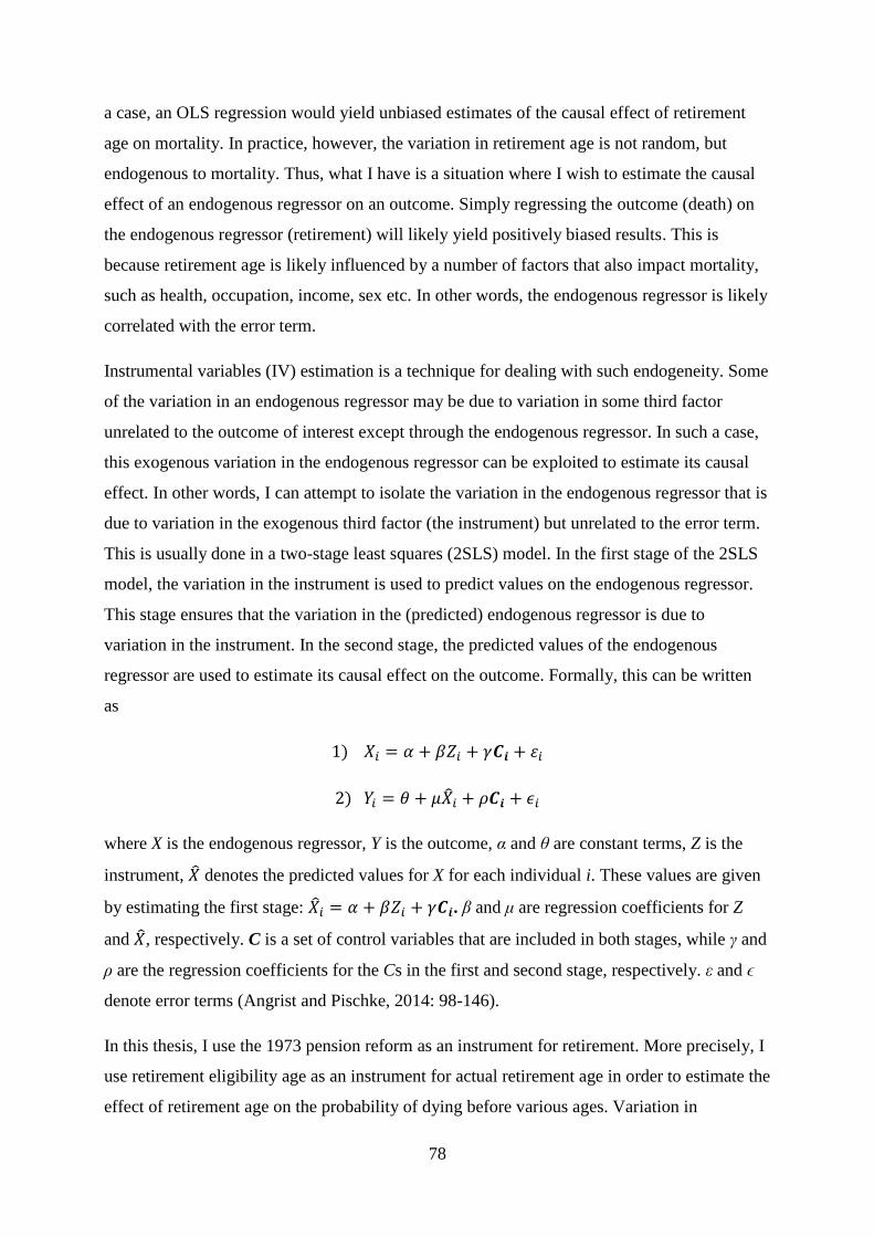
78

a case, an OLS regression would yield unbiased estimates of the causal effect of retirement

age on mortality. In practice, however, the variation in retirement age is not random, but

endogenous to mortality. Thus, what I have is a situation where I wish to estimate the causal

effect of an endogenous regressor on an outcome. Simply regressing the outcome (death) on

the endogenous regressor (retirement) will likely yield positively biased results. This is

because retirement age is likely influenced by a number of factors that also impact mortality,

such as health, occupation, income, sex etc. In other words, the endogenous regressor is likely

correlated with the error term.

Instrumental variables (IV) estimation is a technique for dealing with such endogeneity. Some

of the variation in an endogenous regressor may be due to variation in some third factor

unrelated to the outcome of interest except through the endogenous regressor. In such a case,

this exogenous variation in the endogenous regressor can be exploited to estimate its causal

effect. In other words, I can attempt to isolate the variation in the endogenous regressor that is

due to variation in the exogenous third factor (the instrument) but unrelated to the error term.

This is usually done in a two-stage least squares (2SLS) model. In the first stage of the 2SLS

model, the variation in the instrument is used to predict values on the endogenous regressor.

This stage ensures that the variation in the (predicted) endogenous regressor is due to

variation in the instrument. In the second stage, the predicted values of the endogenous

regressor are used to estimate its causal effect on the outcome. Formally, this can be written

as

1) 𝑋𝑖 = 𝛼 + 𝛽𝑍𝑖 + 𝛾𝑪𝒊 + 휀𝑖

2) 𝑌𝑖 = 𝜃 + 𝜇�̂�𝑖 + 𝜌𝑪𝒊 + 𝜖𝑖

where X is the endogenous regressor, Y is the outcome, α and θ are constant terms, Z is the

instrument, �̂� denotes the predicted values for X for each individual i. These values are given

by estimating the first stage: �̂�𝑖 = 𝛼 + 𝛽𝑍𝑖 + 𝛾𝑪𝒊. β and μ are regression coefficients for Z

and �̂�, respectively. C is a set of control variables that are included in both stages, while γ and

ρ are the regression coefficients for the Cs in the first and second stage, respectively. ε and ϵ

denote error terms (Angrist and Pischke, 2014: 98-146).

In this thesis, I use the 1973 pension reform as an instrument for retirement. More precisely, I

use retirement eligibility age as an instrument for actual retirement age in order to estimate the

effect of retirement age on the probability of dying before various ages. Variation in

79

retirement eligibility age stems from the reform, since the reform gave everyone born between

January 1903 and December 1905 the right to retire in 1973, and everyone born in 1906 the

right to retire at age 67.

There are two important assumptions made in an IV estimation. The first is that the

instrument is relevant, meaning that it affects the endogenous regressor. This assumption is

testable, and as I have shown above, the 1973 pension reform appears to have had a strong

effect on actual retirement age in the population. The second assumption is that the instrument

is valid. This requires that it is unrelated to other factors that may affect the outcome, meaning

that the variation in the instrument is exogenous (the independence assumption), and that the

only causal path between the instrument and the outcome is through the endogenous regressor

(the exclusion restriction). This last assumption means that there should be no other causal

channel connecting the instrument and the outcome (Angrist and Pischke, 2014: 98-146).

Unfortunately, this assumption is not directly testable, but the researcher can provide

theoretical and empirical arguments in support of it and discuss potential issues.

In this thesis, an important potential violation of the exclusion restriction stems from the fact

that the retirement eligibility instrument is derived from birth cohort membership. This means

that any link between birth cohort membership and mortality that does not go through the

eligibility instrument may bias the results. For instance, if later cohorts were more or

differently educated than earlier ones, and education affects mortality, I would have to

adequately control for such educational differences in the models. In the next section, I

discuss some possible sources of bias in the IV estimation.

IV estimators are known for producing fairly local average treatment effects. Imagine that a

group of test subjects are part of an experiment. This experiment is not a double blind one.

The test subjects know perfectly well whether or not they are given the treatment. Among

those offered the treatment, most accept it, but some do not. In the control group, no one is

offered the treatment. Therefore, most are untreated, but some manage to get hold of the

treatment on their own, and take it anyway. Each test subject can then be seen to belong to

one of four groups. The first is commonly referred to as the compliers. These comply with the

treatment, meaning that they take the treatment if they are offered it, but do not take it

otherwise. Second, the always-takers will always take the treatment, regardless of whether

they are in the treatment group or the control group. Never-takers, on the other hand, never

80

accept the treatment, regardless of group membership. Finally the defiers are people who do

not accept the treatment if they are offered it, but who take the treatment if they are not.

As mentioned before, having a large proportion of defiers in a sample strongly biases IV

estimates (Borgen, 2013). In an IV estimation, the estimated effect is the average treatment

effect for the compliers – the people who take the treatment because they are offered it, but

who otherwise would not have taken the treatment. In other words, the effect is the effect on

the people who were affected by the instrument (Angrist and Pischke, 2014: 98-146). While

not intuitive, this makes sense when considering the fact that it is impossible to measure the

effect of taking some treatment on someone who would never take it. Also, the effect on the

compliers is the most policy relevant effect, since this group would be the one (along with the

defiers) that would be affected by a reform.

81

8 Descriptive statistics and checks for balance For the main event history analyses presented in chapter 9, the sample is restricted to

individuals born in 1906 and 1907. For these analyses, I employ the long file in years

described in chapter 6. For the IV and DiD analyses, I sample individuals born between

January 1st 1902 and December 31

st 1906 who were alive at age 65. With regard to analyses

and statistics that include information on education and occupations, the samples are also

restricted to individuals registered with this information in the 1970 census. While the DiD

estimations utilize the long file in months, the IV analyses are based on the wide file. Both of

these files are also described in chapter 6.

8.1 Descriptive statistics

Table 8.1 shows descriptive statistics for the two samples. All statistics are shown

disaggregated by sex, since all analyses are done separately for men and women. All statistics

are also shown conditional on being alive at age 65. This condition is included to avoid issues

related to the fact that the registers contain information starting from 1967. Both samples have

a slight majority of women. The number of people who immigrated or emigrated in their late

60s or later is very low. This means that censoring due to immigration and emigration is

unlikely to be a major concern.

The number of immigrants in the samples is very low, as is the number of “others”. Therefore,

I am forced to merge the “others”-group with the Norwegian-born with two Norwegian-born

parents group in the discrete-time hazard models to ensure that the models converge. With

regard to educational levels, there are few missing cases. The occupation variable has a lot of

missing values – especially for women. This is the reason why I have chosen not to include it

in my models and why I have decided to investigate effect heterogeneity with regard to

education rather than occupation (the same argument applies to income).

Further, the vast majority received some kind of pension benefit, and the vast majority of

those who did, received old age pensions. Many of those who did receive old age pensions

also received some other type of pension first, such as a disability pension or a survivor’s

pension. Relatively few people died or emigrated without having received any kind of pension

benefit. It is also possible to discern from Table 8.1 that different pension types are related to

different retirement ages. In the table here, mean retirement age is calculated for all groups,

and then successively for more restricted subsamples by excluding people who also received

other types of pensions. Note that measuring the mean retirement age for old-age pensions (as

82

plotted in Figure 7.3) and measuring the mean retirement age for old-age pensioners by

excluding people who ever received other types of pensions gives two different estimates.

This is because a lot of people first received some other type of pension, and later received an

old age pension.

The mean death age conveys that, conditional on being alive at 65, the women and men in the

sample on average lived for 18 and 14 more years, respectively. This is close to the actual

remaining life expectancy in this period (SSB, n.a.). The standard deviations for these

estimates show that there is a lot of variation in longevity.

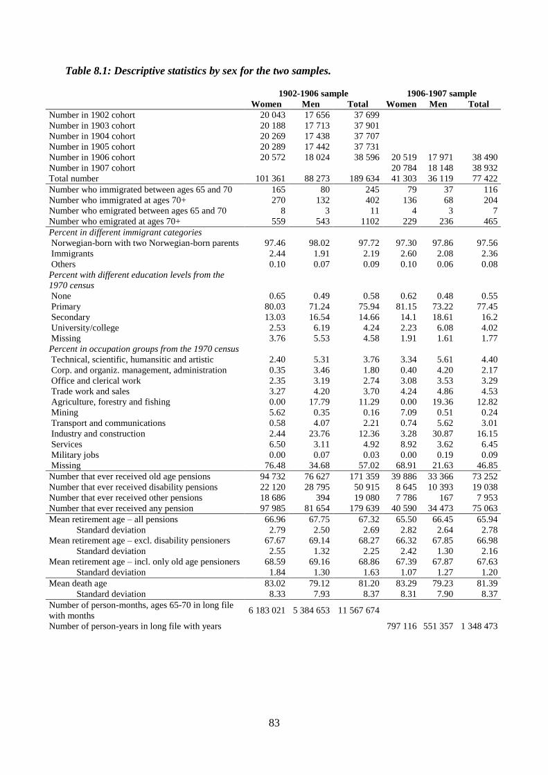
83

Table 8.1: Descriptive statistics by sex for the two samples.

1902-1906 sample 1906-1907 sample

Women Men Total Women Men Total

Number in 1902 cohort 20 043 17 656 37 699

Number in 1903 cohort 20 188 17 713 37 901

Number in 1904 cohort 20 269 17 438 37 707

Number in 1905 cohort 20 289 17 442 37 731

Number in 1906 cohort 20 572 18 024 38 596 20 519 17 971 38 490

Number in 1907 cohort

20 784 18 148 38 932

Total number 101 361 88 273 189 634 41 303 36 119 77 422

Number who immigrated between ages 65 and 70 165 80 245 79 37 116

Number who immigrated at ages 70+ 270 132 402 136 68 204

Number who emigrated between ages 65 and 70 8 3 11 4 3 7

Number who emigrated at ages 70+ 559 543 1102 229 236 465

Percent in different immigrant categories

Norwegian-born with two Norwegian-born parents 97.46 98.02 97.72 97.30 97.86 97.56

Immigrants 2.44 1.91 2.19 2.60 2.08 2.36

Others 0.10 0.07 0.09 0.10 0.06 0.08

Percent with different education levels from the

1970 census

None 0.65 0.49 0.58 0.62 0.48 0.55

Primary 80.03 71.24 75.94 81.15 73.22 77.45

Secondary 13.03 16.54 14.66 14.1 18.61 16.2

University/college 2.53 6.19 4.24 2.23 6.08 4.02

Missing 3.76 5.53 4.58 1.91 1.61 1.77

Percent in occupation groups from the 1970 census

Technical, scientific, humansitic and artistic 2.40 5.31 3.76 3.34 5.61 4.40

Corp. and organiz. management, administration 0.35 3.46 1.80 0.40 4.20 2.17

Office and clerical work 2.35 3.19 2.74 3.08 3.53 3.29

Trade work and sales 3.27 4.20 3.70 4.24 4.86 4.53

Agriculture, forestry and fishing 0.00 17.79 11.29 0.00 19.36 12.82

Mining 5.62 0.35 0.16 7.09 0.51 0.24

Transport and communications 0.58 4.07 2.21 0.74 5.62 3.01

Industry and construction 2.44 23.76 12.36 3.28 30.87 16.15

Services 6.50 3.11 4.92 8.92 3.62 6.45

Military jobs 0.00 0.07 0.03 0.00 0.19 0.09

Missing 76.48 34.68 57.02 68.91 21.63 46.85

Number that ever received old age pensions 94 732 76 627 171 359 39 886 33 366 73 252

Number that ever received disability pensions 22 120 28 795 50 915 8 645 10 393 19 038

Number that ever received other pensions 18 686 394 19 080 7 786 167 7 953

Number that ever received any pension 97 985 81 654 179 639 40 590 34 473 75 063

Mean retirement age – all pensions 66.96 67.75 67.32 65.50 66.45 65.94

Standard deviation 2.79 2.50 2.69 2.82 2.64 2.78

Mean retirement age – excl. disability pensioners 67.67 69.14 68.27 66.32 67.85 66.98

Standard deviation 2.55 1.32 2.25 2.42 1.30 2.16

Mean retirement age – incl. only old age pensioners 68.59 69.16 68.86 67.39 67.87 67.63

Standard deviation 1.84 1.30 1.63 1.07 1.27 1.20

Mean death age 83.02 79.12 81.20 83.29 79.23 81.39

Standard deviation 8.33 7.93 8.37 8.31 7.90 8.37

Number of person-months, ages 65-70 in long file

with months 6 183 021 5 384 653 11 567 674

Number of person-years in long file with years

797 116 551 357 1 348 473

84

8.2 Between-cohort variation in some potential confounders

The DiD identification strategy in this thesis does not hinge on a perfect balance between the

different cohorts/treatment groups in the sample. It is sufficient to provide a convincing

argument that the age-specific mortality trends in the different cohorts would run in parallel in

absence of the treatment (the lowering of the retirement eligibility age).

For the IV estimation, however, it is important that the different cohorts are well-balanced

with regard to potential confounders. Since the instrument is derived from monthly birth

cohort membership, it is important that these cohorts do not differ systematically on

properties that may affect mortality. Such differences would violate the independence

assumption. For instance, if education affects mortality and varies systematically between the

cohorts that are subject to different retirement eligibility rules, this would lead to biased

estimates of the effect of retirement on mortality. In other words; the instrument would be

invalid. Unfortunately, not all relevant variables are observable. Some variables, such as

health behavior or childhood nutrition may vary between cohorts, but are not observed. Other

variables may be observed (registered) but not included in the available datasets. In other

words, I can never achieve full certainty about the validity of the instrument. What I can do is

to check for balance on observed characteristics and perhaps find some reassurance if these do

not vary systematically between cohorts. This means that systematic differences between

cohorts on observables should be seen as grounds for concern. No differences, however, is not

in itself a confirmation that everything is fine. It just means that no obvious concerns have

been identified. Below, some proportions in the different yearly birth cohorts are shown.

The possibility of confounding by cohort-varying characteristics is an important reason why it

is important to use both the IV and DiD approach. In a sense, the DiD-estimation can be seen

as a robustness check for the IV estimation, since it takes advantage of the panel structure in

the dataset and therefore controls for time-invariant but cohort-varying confounders such as

sex, immigrant status, education, family background etc. But although I can never be sure, the

fact that these cohorts are born close in time means that I see little reason to expect large

differences between them on potentially important confounders. Also, such direct effects is a

bigger issue if the instrument is weak than if it is strong. Perhaps somewhat prematurely, I can

assure the reader that the instrument is very strong.

When looking at the figures below, it is worth noting that they are shown with spikes marking

95 % confidence intervals. The reason why the confidence intervals are not visible is that their

85

width is narrower than the default line width in Microsoft Excel, leaving them both invisible

and largely redundant. The reason for the different number of missing values associated with

the different variables is that sex and immigrant background are taken from the population

registers, income is taken from the tax registers, whereas educational level is taken from the

1970 census. The variables from the census data and the income variable have the most

missing observations. Also note that the statistics shown are conditional on being alive at age

65.

From Figure 8.1a it is evident that the different cohorts do not vary with regard to sex

composition. The proportions of men and women in each cohort are, for all practical

purposes, the same. This also goes for the proportion of immigrants, as shown in Figure 8.1b.

Only two groups – immigrants and people born in Norway with two Norwegian-born parents

– are shown, because the proportions in the other three categories in the dataset (Norwegian-

born children of immigrant parents etc.) are close to zero. As can be seen from Figure 8.1c, a

slight trend towards increasing proportions with primary and secondary education can be

observed through successively later cohorts. However, this trend is largely a result of the

lower proportions with missing values in later cohorts. If these are excluded (Figure 8.1d), the

trend in the proportion with only primary education is reversed and much weaker. Excluding

missing values also reduces the trend in the proportion with secondary education.

Both with regard to immigrant composition and educational levels, the minor differences

between the first and the last cohort are statistically significant. However, the differences are

so small that the statistical significance may be attributed to the large sample sizes rather than

to actual, substantial differences between the cohorts. Although substantially negligible, these

differences between cohorts nevertheless mean that that it may be important to control for

potential confounders that can be thought to both vary with cohort membership and affect

mortality in the IV estimation. It also means that one should be careful when interpreting the

results, as there may be other biasing differences between the cohorts. All in all, however, the

small differences with regard to sex, immigrant status and education suggest that there is no

immediate cause for concern. Rather, this comparison of proportions suggests that the cohort-

derived eligibility instrument is not systematically related to other characteristics.

A more pronounced issue arises from the differences between cohorts with regard to income.

Having no pensionable income can be seen as a proxy for retirement. Figure 8.1e shows that a

substantially lower proportion received no pensionable income at age 66 in the three latest

86

cohorts. However, income at age 66 is likely endogenous to the retirement reform. It may be a

result of adaption to changing retirement opportunities. Let me explain briefly. For people

who are eligible for both types of pension, disability pension and old age pension are

substitutes. If you are soon to be 66 years old and become ill, you may apply for a disability

pension or simply continue working until you become eligible for old age pension. If you are

not going to become eligible for old age pension before you turn 70 years old, you may be

more inclined to choose the former than if you will become eligible for old age pension at age

67. If having a pensionable income is indeed endogenous, or a collider variable (Elwert and

Winship, 2014), I should not control for it even if it is unevenly distributed between cohorts.

As can be seen from Figure 8.1e, the observed pattern is consistent with income at age 66

being endogenous to retirement eligibility, as lower proportions had zero income in the

affected cohorts.

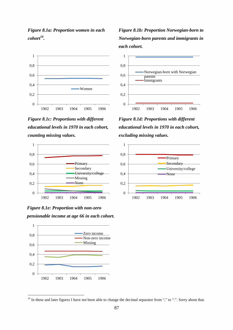
87

Figure 8.1a: Proportion women in each

cohort16

.

Figure 8.1b: Proportion Norwegian-born to

Norwegian-born parents and immigrants in

each cohort.

Figure 8.1c: Proportions with different

educational levels in 1970 in each cohort,

counting missing values.

Figure 8.1d: Proportions with different

educational levels in 1970 in each cohort,

excluding missing values.

Figure 8.1e: Proportion with non-zero

pensionable income at age 66 in each cohort.

16

In these and later figures I have not been able to change the decimal separator from “,” to “.”. Sorry about that.

0

0,2

0,4

0,6

0,8

1

1902 1903 1904 1905 1906

Women

0

0,2

0,4

0,6

0,8

1

1902 1903 1904 1905 1906

Norwegian-born with Norwegian

parentsImmigrants

0

0,2

0,4

0,6

0,8

1

1902 1903 1904 1905 1906

Primary

Secondary

University/college

Missing

None

0

0,2

0,4

0,6

0,8

1

1902 1903 1904 1905 1906

Primary

Secondary

University/college

None

0

0,2

0,4

0,6

0,8

1

1902 1903 1904 1905 1906

Zero income

Non-zero income

Missing

88

8.3 Parallel trends in the probability of being dead?

The DiD approach rests on the assumption that in the absence of differences in retirement

eligibility, the cohort trends in mortality by age would be parallel. The counterfactual

mortality trends of the cohorts in question cannot be observed, and therefore this assumption

cannot be tested directly. What I can do is to check if the trends are parallel in the period

before some of the cohorts were affected by the reform, and if the trends in the 1906 and 1907

cohorts, which were allowed to retire at the same age, are parallel throughout the age span in

question.

Figure 8.2 plots the proportions who are dead at the beginning of each age (measured in

months) by birth cohort. The numbers are estimated conditional on being alive at age 65. The

cohort mortality trends in ages that are comparable are drawn in thick lines, while the trends

are drawn in thin lines in periods where they are (presumably) not directly comparable due to

differences in retirement eligibility. The 1906 and 1907 cohort become eligible at the same

age (67 years/804 months), so these are comparable throughout the age span (up to 70

years/840 months). The other cohorts are only comparable in the period leading up to the

earliest retirement eligibility (67 years/804 months). As can be seen from the figure, the

trends are not perfectly parallel. However, the deviations are relatively small in the period up

to age 67, and although the lines showing the 1906 and 1907 cohort mortality trends diverge

slightly at the end of the period, they move closely together throughout the period. In other

words, there appears to be close to parallel trends in the age span 65-67 for all cohorts and in

the age span 67-70 for the 1906 and 1907 cohorts. But the fact that these trends are not

perfectly parallel could bias the results. Therefore, one should interpret the results with due

caution.

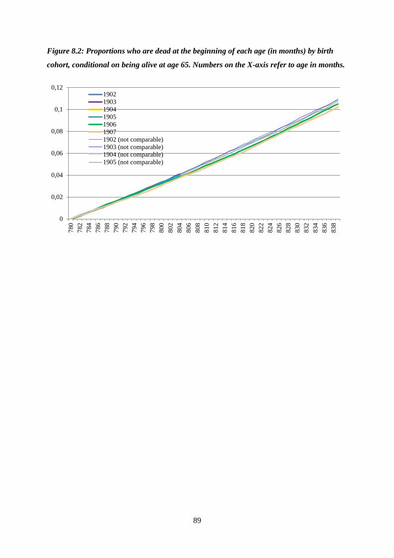
89

Figure 8.2: Proportions who are dead at the beginning of each age (in months) by birth

cohort, conditional on being alive at age 65. Numbers on the X-axis refer to age in months.

0

0,02

0,04

0,06

0,08

0,1

0,12

780

782

784

786

788

790

792

794

796

798

800

802

804

806

808

810

812

814

816

818

820

822

824

826

828

830

832

834

836

838

1902

1903

1904

1905

1906

1907

1902 (not comparable)

1903 (not comparable)

1904 (not comparable)

1905 (not comparable)

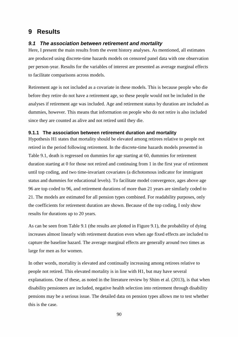
90

9 Results

9.1 The association between retirement and mortality

Here, I present the main results from the event history analyses. As mentioned, all estimates

are produced using discrete-time hazards models on censored panel data with one observation

per person-year. Results for the variables of interest are presented as average marginal effects

to facilitate comparisons across models.

Retirement age is not included as a covariate in these models. This is because people who die

before they retire do not have a retirement age, so these people would not be included in the

analyses if retirement age was included. Age and retirement status by duration are included as

dummies, however. This means that information on people who do not retire is also included

since they are counted as alive and not retired until they die.

9.1.1 The association between retirement duration and mortality

Hypothesis H1 states that mortality should be elevated among retirees relative to people not

retired in the period following retirement. In the discrete-time hazards models presented in

Table 9.1, death is regressed on dummies for age starting at 60, dummies for retirement

duration starting at 0 for those not retired and continuing from 1 in the first year of retirement

until top coding, and two time-invariant covariates (a dichotomous indicator for immigrant

status and dummies for educational levels). To facilitate model convergence, ages above age

96 are top coded to 96, and retirement durations of more than 21 years are similarly coded to

21. The models are estimated for all pension types combined. For readability purposes, only

the coefficients for retirement duration are shown. Because of the top coding, I only show

results for durations up to 20 years.

As can be seen from Table 9.1 (the results are plotted in Figure 9.1), the probability of dying

increases almost linearly with retirement duration even when age fixed effects are included to

capture the baseline hazard. The average marginal effects are generally around two times as

large for men as for women.

In other words, mortality is elevated and continually increasing among retirees relative to

people not retired. This elevated mortality is in line with H1, but may have several

explanations. One of these, as noted in the literature review by Shim et al. (2013), is that when

disability pensioners are included, negative health selection into retirement through disability

pensions may be a serious issue. The detailed data on pension types allows me to test whether

this is the case.

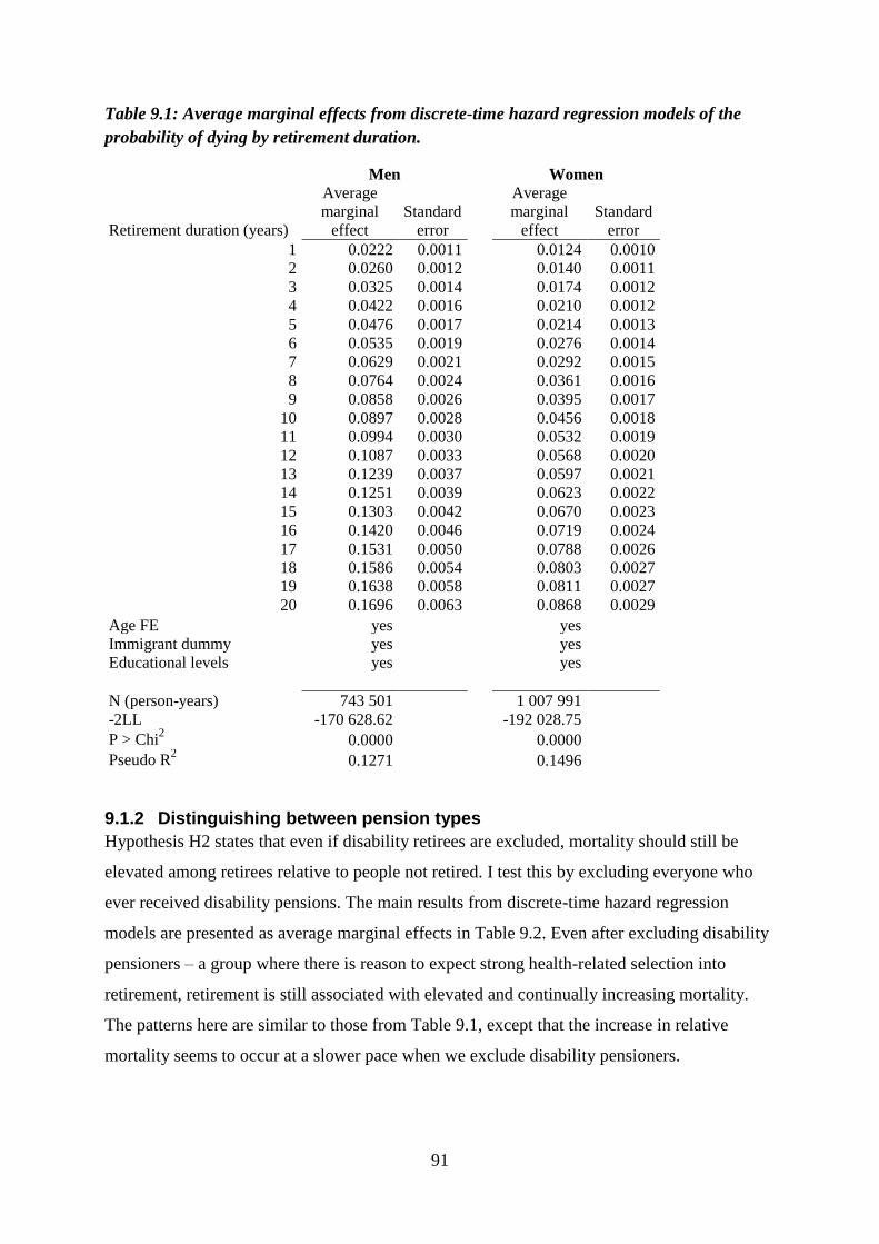
91

Table 9.1: Average marginal effects from discrete-time hazard regression models of the

probability of dying by retirement duration.

Men

Women

Retirement duration (years)

Average

marginal

effect

Standard

error

Average

marginal

effect

Standard

error

1 0.0222 0.0011

0.0124 0.0010

2 0.0260 0.0012

0.0140 0.0011

3 0.0325 0.0014

0.0174 0.0012

4 0.0422 0.0016

0.0210 0.0012

5 0.0476 0.0017

0.0214 0.0013

6 0.0535 0.0019

0.0276 0.0014

7 0.0629 0.0021

0.0292 0.0015

8 0.0764 0.0024

0.0361 0.0016

9 0.0858 0.0026

0.0395 0.0017

10 0.0897 0.0028

0.0456 0.0018

11 0.0994 0.0030

0.0532 0.0019

12 0.1087 0.0033

0.0568 0.0020

13 0.1239 0.0037

0.0597 0.0021

14 0.1251 0.0039

0.0623 0.0022

15 0.1303 0.0042

0.0670 0.0023

16 0.1420 0.0046

0.0719 0.0024

17 0.1531 0.0050

0.0788 0.0026

18 0.1586 0.0054

0.0803 0.0027

19 0.1638 0.0058

0.0811 0.0027

20 0.1696 0.0063

0.0868 0.0029

Age FE yes

yes

Immigrant dummy yes

yes

Educational levels yes

yes

N (person-years) 743 501

1 007 991

-2LL -170 628.62

-192 028.75

P > Chi2 0.0000

0.0000

Pseudo R2 0.1271

0.1496

9.1.2 Distinguishing between pension types

Hypothesis H2 states that even if disability retirees are excluded, mortality should still be

elevated among retirees relative to people not retired. I test this by excluding everyone who

ever received disability pensions. The main results from discrete-time hazard regression

models are presented as average marginal effects in Table 9.2. Even after excluding disability

pensioners – a group where there is reason to expect strong health-related selection into

retirement, retirement is still associated with elevated and continually increasing mortality.

The patterns here are similar to those from Table 9.1, except that the increase in relative

mortality seems to occur at a slower pace when we exclude disability pensioners.

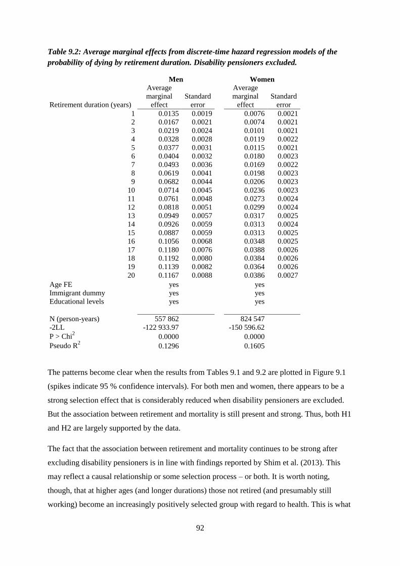
92

Table 9.2: Average marginal effects from discrete-time hazard regression models of the

probability of dying by retirement duration. Disability pensioners excluded.

Men

Women

Retirement duration (years)

Average

marginal

effect

Standard

error

Average

marginal

effect

Standard

error

1 0.0135 0.0019

0.0076 0.0021

2 0.0167 0.0021

0.0074 0.0021

3 0.0219 0.0024

0.0101 0.0021

4 0.0328 0.0028

0.0119 0.0022

5 0.0377 0.0031

0.0115 0.0021

6 0.0404 0.0032

0.0180 0.0023

7 0.0493 0.0036

0.0169 0.0022

8 0.0619 0.0041

0.0198 0.0023

9 0.0682 0.0044

0.0206 0.0023

10 0.0714 0.0045

0.0236 0.0023

11 0.0761 0.0048

0.0273 0.0024

12 0.0818 0.0051

0.0299 0.0024

13 0.0949 0.0057

0.0317 0.0025

14 0.0926 0.0059

0.0313 0.0024

15 0.0887 0.0059

0.0313 0.0025

16 0.1056 0.0068

0.0348 0.0025

17 0.1180 0.0076

0.0388 0.0026

18 0.1192 0.0080

0.0384 0.0026

19 0.1139 0.0082

0.0364 0.0026

20 0.1167 0.0088

0.0386 0.0027

Age FE yes

yes

Immigrant dummy yes

yes

Educational levels yes

yes

N (person-years) 557 862

824 547

-2LL -122 933.97

-150 596.62

P > Chi2 0.0000

0.0000

Pseudo R2 0.1296

0.1605

The patterns become clear when the results from Tables 9.1 and 9.2 are plotted in Figure 9.1

(spikes indicate 95 % confidence intervals). For both men and women, there appears to be a

strong selection effect that is considerably reduced when disability pensioners are excluded.

But the association between retirement and mortality is still present and strong. Thus, both H1

and H2 are largely supported by the data.

The fact that the association between retirement and mortality continues to be strong after

excluding disability pensioners is in line with findings reported by Shim et al. (2013). This

may reflect a causal relationship or some selection process – or both. It is worth noting,

though, that at higher ages (and longer durations) those not retired (and presumably still

working) become an increasingly positively selected group with regard to health. This is what

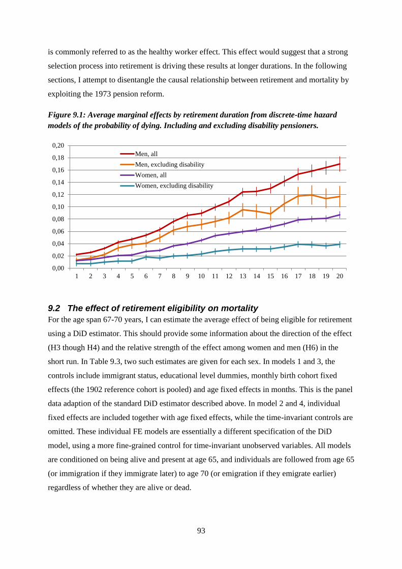
93

is commonly referred to as the healthy worker effect. This effect would suggest that a strong

selection process into retirement is driving these results at longer durations. In the following

sections, I attempt to disentangle the causal relationship between retirement and mortality by

exploiting the 1973 pension reform.

Figure 9.1: Average marginal effects by retirement duration from discrete-time hazard

models of the probability of dying. Including and excluding disability pensioners.

9.2 The effect of retirement eligibility on mortality

For the age span 67-70 years, I can estimate the average effect of being eligible for retirement

using a DiD estimator. This should provide some information about the direction of the effect

(H3 though H4) and the relative strength of the effect among women and men (H6) in the

short run. In Table 9.3, two such estimates are given for each sex. In models 1 and 3, the

controls include immigrant status, educational level dummies, monthly birth cohort fixed

effects (the 1902 reference cohort is pooled) and age fixed effects in months. This is the panel

data adaption of the standard DiD estimator described above. In model 2 and 4, individual

fixed effects are included together with age fixed effects, while the time-invariant controls are

omitted. These individual FE models are essentially a different specification of the DiD

model, using a more fine-grained control for time-invariant unobserved variables. All models

are conditioned on being alive and present at age 65, and individuals are followed from age 65

(or immigration if they immigrate later) to age 70 (or emigration if they emigrate earlier)

regardless of whether they are alive or dead.

0,00

0,02

0,04

0,06

0,08

0,10

0,12

0,14

0,16

0,18

0,20

1 2 3 4 5 6 7 8 9 10 11 12 13 14 15 16 17 18 19 20

Men, all

Men, excluding disability

Women, all

Women, excluding disability

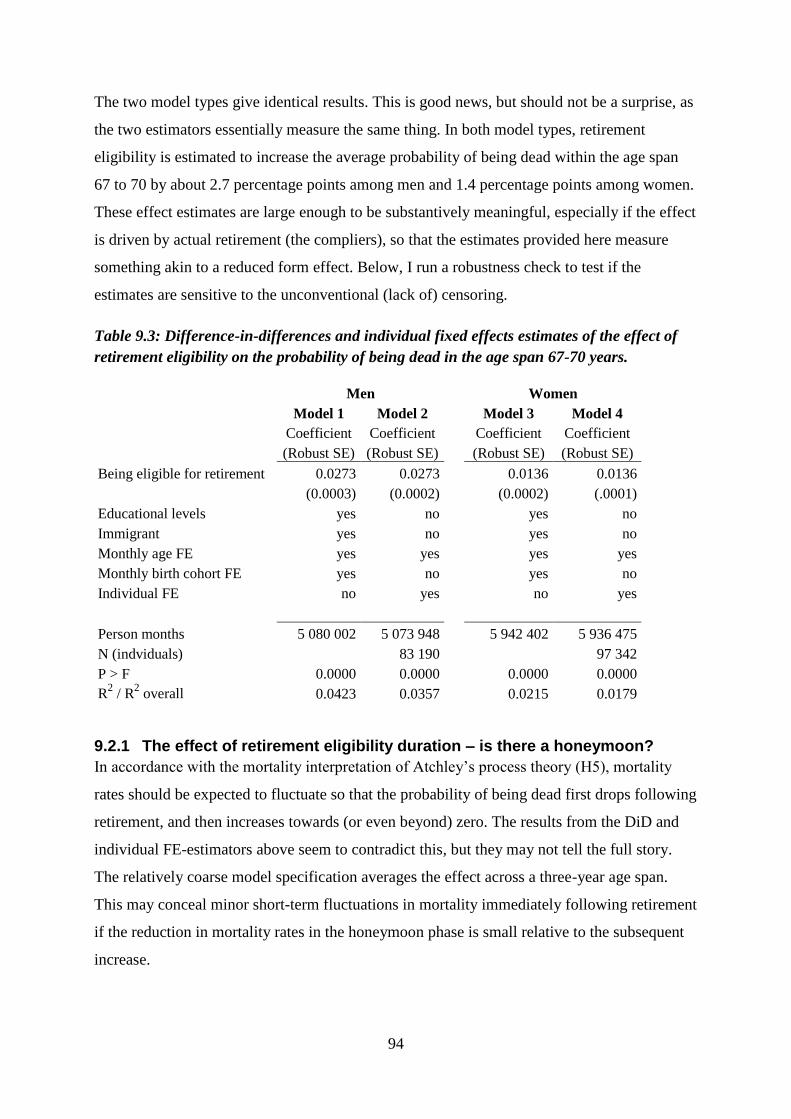
94

The two model types give identical results. This is good news, but should not be a surprise, as

the two estimators essentially measure the same thing. In both model types, retirement

eligibility is estimated to increase the average probability of being dead within the age span

67 to 70 by about 2.7 percentage points among men and 1.4 percentage points among women.

These effect estimates are large enough to be substantively meaningful, especially if the effect

is driven by actual retirement (the compliers), so that the estimates provided here measure

something akin to a reduced form effect. Below, I run a robustness check to test if the

estimates are sensitive to the unconventional (lack of) censoring.

Table 9.3: Difference-in-differences and individual fixed effects estimates of the effect of

retirement eligibility on the probability of being dead in the age span 67-70 years.

Men

Women

Model 1 Model 2

Model 3 Model 4

Coefficient Coefficient

Coefficient Coefficient

(Robust SE) (Robust SE)

(Robust SE) (Robust SE)

Being eligible for retirement 0.0273 0.0273

0.0136 0.0136

(0.0003) (0.0002)

(0.0002) (.0001)

Educational levels yes no

yes no

Immigrant yes no

yes no

Monthly age FE yes yes

yes yes

Monthly birth cohort FE yes no

yes no

Individual FE no yes

no yes

Person months 5 080 002 5 073 948

5 942 402 5 936 475

N (indviduals)

83 190

97 342

P > F 0.0000 0.0000

0.0000 0.0000

R2 / R

2 overall 0.0423 0.0357

0.0215 0.0179

9.2.1 The effect of retirement eligibility duration – is there a honeymoon?

In accordance with the mortality interpretation of Atchley’s process theory (H5), mortality

rates should be expected to fluctuate so that the probability of being dead first drops following

retirement, and then increases towards (or even beyond) zero. The results from the DiD and

individual FE-estimators above seem to contradict this, but they may not tell the full story.

The relatively coarse model specification averages the effect across a three-year age span.

This may conceal minor short-term fluctuations in mortality immediately following retirement

if the reduction in mortality rates in the honeymoon phase is small relative to the subsequent

increase.

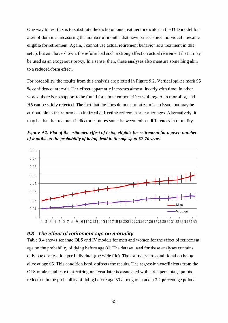
95

One way to test this is to substitute the dichotomous treatment indicator in the DiD model for

a set of dummies measuring the number of months that have passed since individual i became

eligible for retirement. Again, I cannot use actual retirement behavior as a treatment in this

setup, but as I have shown, the reform had such a strong effect on actual retirement that it may

be used as an exogenous proxy. In a sense, then, these analyses also measure something akin

to a reduced-form effect.

For readability, the results from this analysis are plotted in Figure 9.2. Vertical spikes mark 95

% confidence intervals. The effect apparently increases almost linearly with time. In other

words, there is no support to be found for a honeymoon effect with regard to mortality, and

H5 can be safely rejected. The fact that the lines do not start at zero is an issue, but may be

attributable to the reform also indirectly affecting retirement at earlier ages. Alternatively, it

may be that the treatment indicator captures some between-cohort differences in mortality.

Figure 9.2: Plot of the estimated effect of being eligible for retirement for a given number

of months on the probability of being dead in the age span 67-70 years.

9.3 The effect of retirement age on mortality

Table 9.4 shows separate OLS and IV models for men and women for the effect of retirement

age on the probability of dying before age 80. The dataset used for these analyses contains

only one observation per individual (the wide file). The estimates are conditional on being

alive at age 65. This condition hardly affects the results. The regression coefficients from the

OLS models indicate that retiring one year later is associated with a 4.2 percentage points

reduction in the probability of dying before age 80 among men and a 2.2 percentage points

0

0,01

0,02

0,03

0,04

0,05

0,06

0,07

0,08

1 2 3 4 5 6 7 8 9 10 11 12 13 14 15 16 17 18 19 20 21 22 23 24 25 26 27 28 29 30 31 32 33 34 35 36

Men

Women

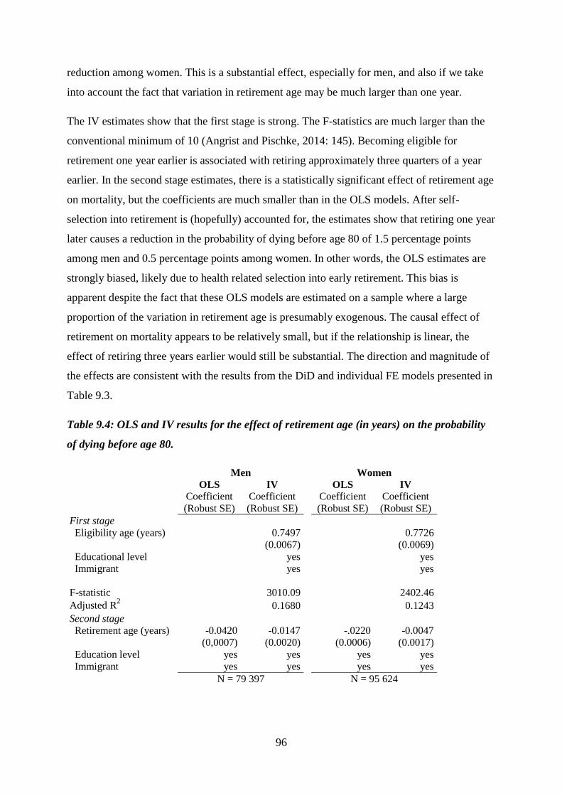
96

reduction among women. This is a substantial effect, especially for men, and also if we take

into account the fact that variation in retirement age may be much larger than one year.

The IV estimates show that the first stage is strong. The F-statistics are much larger than the

conventional minimum of 10 (Angrist and Pischke, 2014: 145). Becoming eligible for

retirement one year earlier is associated with retiring approximately three quarters of a year

earlier. In the second stage estimates, there is a statistically significant effect of retirement age

on mortality, but the coefficients are much smaller than in the OLS models. After self-

selection into retirement is (hopefully) accounted for, the estimates show that retiring one year

later causes a reduction in the probability of dying before age 80 of 1.5 percentage points

among men and 0.5 percentage points among women. In other words, the OLS estimates are

strongly biased, likely due to health related selection into early retirement. This bias is

apparent despite the fact that these OLS models are estimated on a sample where a large

proportion of the variation in retirement age is presumably exogenous. The causal effect of

retirement on mortality appears to be relatively small, but if the relationship is linear, the

effect of retiring three years earlier would still be substantial. The direction and magnitude of

the effects are consistent with the results from the DiD and individual FE models presented in

Table 9.3.

Table 9.4: OLS and IV results for the effect of retirement age (in years) on the probability

of dying before age 80.

Men

Women

OLS IV

OLS IV

Coefficient Coefficient

Coefficient Coefficient

(Robust SE) (Robust SE)

(Robust SE) (Robust SE)

First stage

Eligibility age (years) 0.7497 0.7726

(0.0067) (0.0069)

Educational level yes yes

Immigrant yes yes

F-statistic 3010.09 2402.46

Adjusted R2 0.1680 0.1243

Second stage

Retirement age (years) -0.0420 -0.0147 -.0220 -0.0047

(0,0007) (0.0020) (0.0006) (0.0017)

Education level yes yes yes yes

Immigrant yes yes yes yes

N = 79 397

N = 95 624

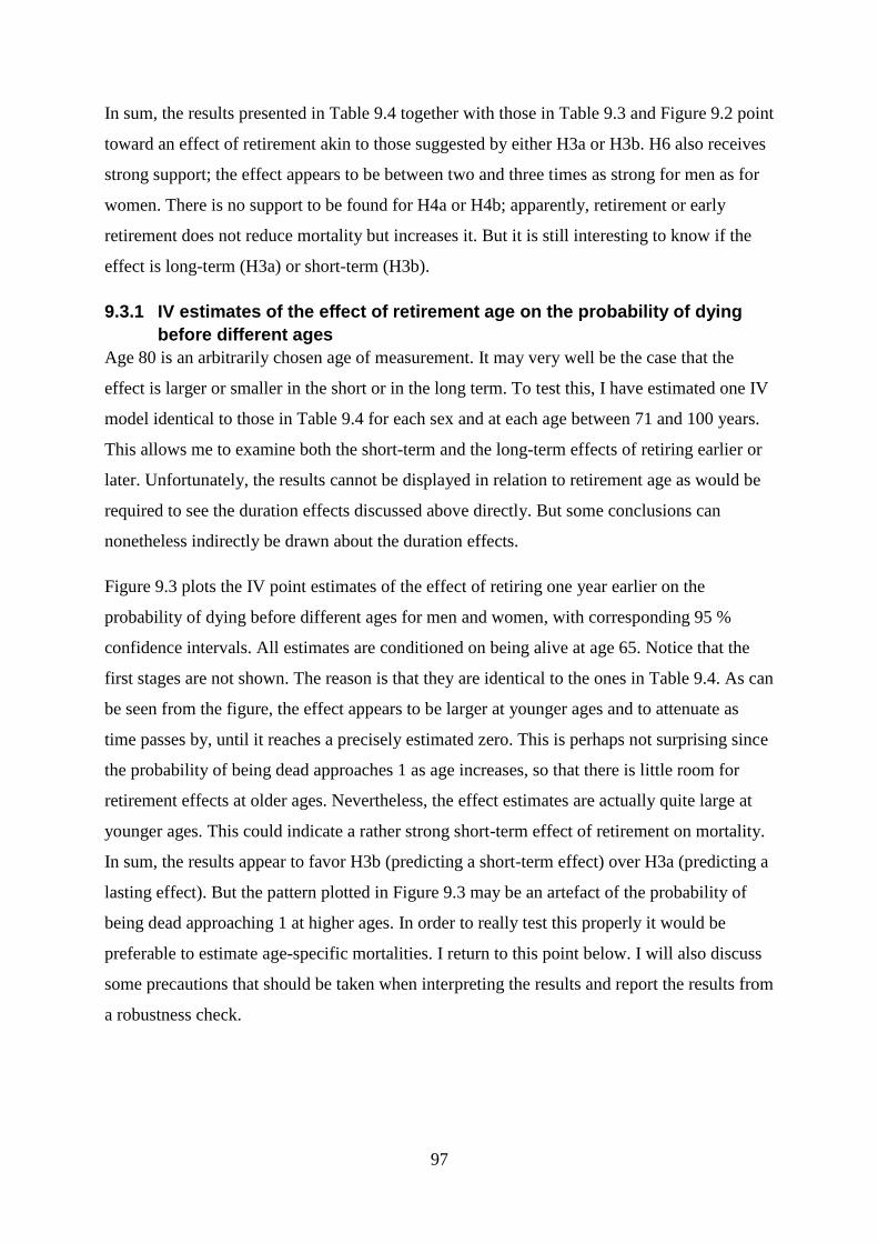
97

In sum, the results presented in Table 9.4 together with those in Table 9.3 and Figure 9.2 point

toward an effect of retirement akin to those suggested by either H3a or H3b. H6 also receives

strong support; the effect appears to be between two and three times as strong for men as for

women. There is no support to be found for H4a or H4b; apparently, retirement or early

retirement does not reduce mortality but increases it. But it is still interesting to know if the

effect is long-term (H3a) or short-term (H3b).

9.3.1 IV estimates of the effect of retirement age on the probability of dying

before different ages

Age 80 is an arbitrarily chosen age of measurement. It may very well be the case that the

effect is larger or smaller in the short or in the long term. To test this, I have estimated one IV

model identical to those in Table 9.4 for each sex and at each age between 71 and 100 years.

This allows me to examine both the short-term and the long-term effects of retiring earlier or

later. Unfortunately, the results cannot be displayed in relation to retirement age as would be

required to see the duration effects discussed above directly. But some conclusions can

nonetheless indirectly be drawn about the duration effects.

Figure 9.3 plots the IV point estimates of the effect of retiring one year earlier on the

probability of dying before different ages for men and women, with corresponding 95 %

confidence intervals. All estimates are conditioned on being alive at age 65. Notice that the

first stages are not shown. The reason is that they are identical to the ones in Table 9.4. As can

be seen from the figure, the effect appears to be larger at younger ages and to attenuate as

time passes by, until it reaches a precisely estimated zero. This is perhaps not surprising since

the probability of being dead approaches 1 as age increases, so that there is little room for

retirement effects at older ages. Nevertheless, the effect estimates are actually quite large at

younger ages. This could indicate a rather strong short-term effect of retirement on mortality.

In sum, the results appear to favor H3b (predicting a short-term effect) over H3a (predicting a

lasting effect). But the pattern plotted in Figure 9.3 may be an artefact of the probability of

being dead approaching 1 at higher ages. In order to really test this properly it would be

preferable to estimate age-specific mortalities. I return to this point below. I will also discuss

some precautions that should be taken when interpreting the results and report the results from

a robustness check.

98

Figure 9.3: IV point estimates and 95 % confidence intervals for the effect of retiring one

year earlier on the probability of dying before different ages.

9.3.2 IV estimates of age-specific mortality

To properly test H3b it would be preferable to estimate the effect of retirement age on age-

specific mortality. Using the IV setup in the previous section with some modifications, it is

possible to do this. For this analysis, I condition on being alive at the beginning of each age in

years and estimate the effect of retiring one year later on the probability of being dead at the

end of that age. Now, this condition is obviously endogenous. If the probability of dying at

age 72 is affected by retirement, then the probability of dying before age 72 is likely also

affected by retirement and so on. Therefore, the results should be interpreted with caution.

Nevertheless, the approach presented here provides conditional age-specific probabilities of

dying, and if they tell the same story as the numbers presented in Figure 9.3, they may still

inform on the age specific mortality effects that drive the results. For this analysis, I also look

at lower ages (and thus do not condition on being alive at age 65), but have only included ages

up to 89. Note that this approach does not properly account for emigration and immigration.

That is likely a minor issue here, though.

Figure 9.4 plots the effect of retiring one year later on age-specific probabilities of dying,

together with 95 % confidence intervals. There is see a clear and precisely estimated effect of

retirement age on age-specific mortality for ages up to 71 years. In other words, postponed

retirement appears to lower the probability of dying in the short run. Inversely, earlier

retirement increases mortality in the short run. At higher ages there is a lot of apparently

-0,04

-0,035

-0,03

-0,025

-0,02

-0,015

-0,01

-0,005

0

0,005

0,01

71

72

73

74

75

76

77

78

79

80

81

82

83

84

85

86

87

88

89

90

91

92

93

94

95

96

97

98

99

100

Men

Women

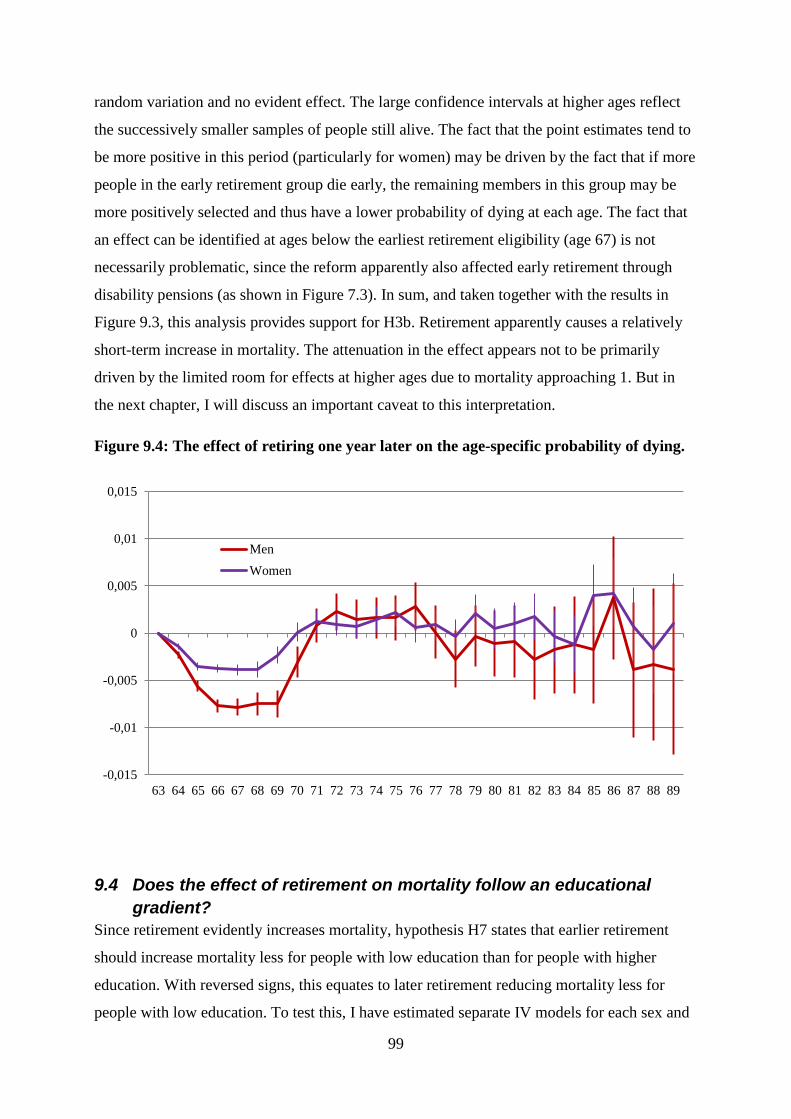
99

random variation and no evident effect. The large confidence intervals at higher ages reflect

the successively smaller samples of people still alive. The fact that the point estimates tend to

be more positive in this period (particularly for women) may be driven by the fact that if more

people in the early retirement group die early, the remaining members in this group may be

more positively selected and thus have a lower probability of dying at each age. The fact that

an effect can be identified at ages below the earliest retirement eligibility (age 67) is not

necessarily problematic, since the reform apparently also affected early retirement through

disability pensions (as shown in Figure 7.3). In sum, and taken together with the results in

Figure 9.3, this analysis provides support for H3b. Retirement apparently causes a relatively

short-term increase in mortality. The attenuation in the effect appears not to be primarily

driven by the limited room for effects at higher ages due to mortality approaching 1. But in

the next chapter, I will discuss an important caveat to this interpretation.

Figure 9.4: The effect of retiring one year later on the age-specific probability of dying.

9.4 Does the effect of retirement on mortality follow an educational

gradient?

Since retirement evidently increases mortality, hypothesis H7 states that earlier retirement

should increase mortality less for people with low education than for people with higher

education. With reversed signs, this equates to later retirement reducing mortality less for

people with low education. To test this, I have estimated separate IV models for each sex and

-0,015

-0,01

-0,005

0

0,005

0,01

0,015

63 64 65 66 67 68 69 70 71 72 73 74 75 76 77 78 79 80 81 82 83 84 85 86 87 88 89

Men

Women

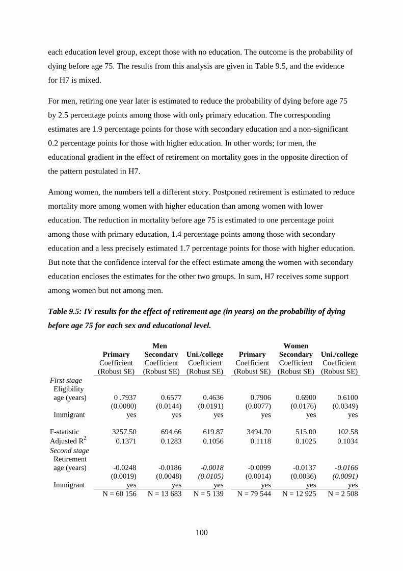
100

each education level group, except those with no education. The outcome is the probability of

dying before age 75. The results from this analysis are given in Table 9.5, and the evidence

for H7 is mixed.

For men, retiring one year later is estimated to reduce the probability of dying before age 75

by 2.5 percentage points among those with only primary education. The corresponding

estimates are 1.9 percentage points for those with secondary education and a non-significant

0.2 percentage points for those with higher education. In other words; for men, the

educational gradient in the effect of retirement on mortality goes in the opposite direction of

the pattern postulated in H7.

Among women, the numbers tell a different story. Postponed retirement is estimated to reduce

mortality more among women with higher education than among women with lower

education. The reduction in mortality before age 75 is estimated to one percentage point

among those with primary education, 1.4 percentage points among those with secondary

education and a less precisely estimated 1.7 percentage points for those with higher education.

But note that the confidence interval for the effect estimate among the women with secondary

education encloses the estimates for the other two groups. In sum, H7 receives some support

among women but not among men.

Table 9.5: IV results for the effect of retirement age (in years) on the probability of dying

before age 75 for each sex and educational level.

Men

Women Primary Secondary Uni./college

Primary Secondary Uni./college

Coefficient Coefficient Coefficient

Coefficient Coefficient Coefficient

(Robust SE) (Robust SE) (Robust SE)

(Robust SE) (Robust SE) (Robust SE)

First stage

Eligibility

age (years) 0 .7937 0.6577 0.4636

0.7906 0.6900 0.6100

(0.0080) (0.0144) (0.0191)

(0.0077) (0.0176) (0.0349)

Immigrant yes yes yes

yes yes yes

F-statistic 3257.50 694.66 619.87

3494.70 515.00 102.58

Adjusted R2 0.1371 0.1283 0.1056

0.1118 0.1025 0.1034

Second stage

Retirement

age (years) -0.0248 -0.0186 -0.0018

-0.0099 -0.0137 -0.0166

(0.0019) (0.0048) (0.0105)

(0.0014) (0.0036) (0.0091)

Immigrant yes yes yes

yes yes yes

N = 60 156 N = 13 683 N = 5 139

N = 79 544 N = 12 925 N = 2 508

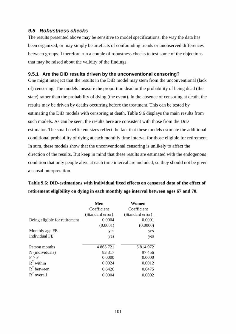
101

9.5 Robustness checks

The results presented above may be sensitive to model specifications, the way the data has

been organized, or may simply be artefacts of confounding trends or unobserved differences

between groups. I therefore run a couple of robustness checks to test some of the objections

that may be raised about the validity of the findings.

9.5.1 Are the DiD results driven by the unconventional censoring?

One might interject that the results in the DiD model may stem from the unconventional (lack

of) censoring. The models measure the proportion dead or the probability of being dead (the

state) rather than the probability of dying (the event). In the absence of censoring at death, the

results may be driven by deaths occurring before the treatment. This can be tested by

estimating the DiD models with censoring at death. Table 9.6 displays the main results from

such models. As can be seen, the results here are consistent with those from the DiD

estimator. The small coefficient sizes reflect the fact that these models estimate the additional

conditional probability of dying at each monthly time interval for those eligible for retirement.

In sum, these models show that the unconventional censoring is unlikely to affect the

direction of the results. But keep in mind that these results are estimated with the endogenous

condition that only people alive at each time interval are included, so they should not be given

a causal interpretation.

Table 9.6: DiD-estimations with individual fixed effects on censored data of the effect of

retirement eligibility on dying in each monthly age interval between ages 67 and 70.

Men Women

Coefficient Coefficient

(Standard error) (Standard error)

Being eligible for retirement 0.0004 0.0001

(0.0001) (0.0000)

Monthly age FE yes yes

Individual FE yes yes

Person months 4 865 721 5 814 972

N (individuals) 83 317

97 456

P > F 0.0000 0.0000

R2 within 0.0024 0.0012

R2 between 0.6426

0.6475

R2 overall 0.0004

0.0002

102

9.5.2 Are the IV results driven by cohort trends?

The instrument in the IV analyses is derived from cohort membership. This means that cohort

trends in unobserved characteristics that affect mortality would constitute a violation of the

exclusion restriction. This would lead to biased IV estimates. One example of such a violation

is if birth year affected childhood nutrition, which may again affect mortality. As mentioned

in section 7.2.1, there is also a cohort trend in retirement age which may affect the results. The

DiD models are not very sensitive to such trends, since they do not condition on uptake and

include cohort fixed effects. To test whether cohort trends drive the results, I have estimated

IV models similar to those presented in Table 9.4, but including a linear term for birth year.

To capture the nonlinearity in the relationship between mean pension age and cohort, I also

included the 1907 cohort in these models. The results show that the effect estimate for men

increases (to -0.0223), but that it is no longer statistically significant (P = 0.065). The effect

estimate for women also increases (to -0.0254), but so does the p-value (P = 0.057).

Apparently, the effect is not driven by a linear cohort trend, but suppressed by it. But

controlling for such a trend greatly reduces statistical power. The reduction in power is not

surprising given the strong correlation between eligibility age, retirement age and cohort. In

other words, this analysis does not give good reason to distrust the main results.

103

10 Discussion The results presented in the previous chapter are complex and their interpretation requires

some clarification and context. Therefore, I here provide a discussion of the results, their

potential interpretations and implications, and how they relate to the established research

literature. I then suggest some angles and topics for future research.

10.1 How is retirement associated with higher mortality?

Looking at the results presented in the previous chapter, it is possible to draw several

conclusions about the association between retirement and mortality. First, retirement is

associated with elevated and continually increasing mortality risk. Comparing retirees with

workers shows large and diverging differences in mortality between the two groups over time.

This result is in accordance with the theoretical expectation that regardless of the causal effect

of retirement on mortality, strong and negative health selection into retirement should result in

higher risk among retirees. In other words, hypothesis H1 received strong support.

Because disability pension is a common entry into retirement for people with poor health, it is

reasonable to assume that at least some of the association between retirement and mortality is

driven by negative health selection through disability pensions. However, there is also good

reason to assume that even if disability pensioners are excluded, the health selection effect

would still be strong. This assumption is particularly plausible if one considers the fact that

those not retired at higher ages and past earliest retirement age are increasingly positively

selected. The exclusion of disability retirees from the sample supports this assumption, and

thus supports H2. Excluding disability pensioners markedly weakens the association between

retirement and mortality, but does not remove it.

The fact that the results from the event history analyses showed a strong and increasing

association between retirement and mortality, while the IV estimation showed a small and

short-term effect, suggests that the event history results are highly biased and primarily driven

by some strong selection process. The fact that there was no apparent spike in mortality

following retirement (keeping in mind that age was measured in years at integer values)

further suggests that this process is likely not primarily an effect of terminally ill persons

retiring in anticipation of death. Rather, a healthy worker effect and/or an omitted variable

104

bias17

seem to be the most plausible explanations for the observed strong and increasing

association. But as the DiD, individual FE and IV results show, some of the observed

association appears to be due to a causal effect.

10.2 The effect of retirement on mortality – drawing a detailed picture

In the analyses in chapter 9, I attempt to draw a very detailed picture of how retirement affects

mortality over time. The fact that analyses with such a fine-grained time scale are even

possible is in itself a testimony to the quality and detail of the Norwegian register data. The

possibility of estimating the effect in the long term up to the age of 100 was made possible

because using the 1973 reform allowed for a long observation window. The need for such

detailed analyses of the temporal pattern of the retirement effect arose from the theoretical

discussions. As I have shown, a number of theories predict different effects of retirement on

mortality with regard to both direction and temporal profile. But the differences in the

predictions are both intricate and subtle. Exploiting the detailed information on time

variations in retirement eligibility, retirement and mortality allows for a deductive approach,

whereby the hypotheses that do not fit the results are abandoned.

The results are relatively clear, and are summarized in Table 10.1. The DiD and individual FE

results show that being eligible for retirement in itself increases mortality risk, most likely

through retirement. This gives reason to reject H4a and H4b. A similar analysis with

treatment duration dummies shows that there is apparently no honeymoon effect with regard

to mortality following retirement. Thus, it is safe to reject H5 as well. The IV estimations

support the main findings from the DiD and individual FE models. They also show that the

effect is apparently a short-term one. This last finding favors H3b over H3a. But this last

conclusion requires a few reservations (discussed below).

These findings are consistent with theories that predict short-term changes in health behavior

following retirement, theories postulating some protective effect of employment, and theories

that conceptualize retirement as a stressful life event or a continuity break. All analyses show

that the effects of retirement eligibility or retirement are much larger for men than for women

– between two and three times as large. This supports H6. But it should also be noted that the

observed differences between men and women may be strongly related to the gender roles

17

The omitted variable may be preferences, personality traits, genetic inheritance, occupation or other factors

affecting both health and proneness to retire early.

105

that characterized the cohorts studied here. As men and women have become more equal over

time, it is likely that such gender differences have attenuated.

Finally, there appears to be some effect heterogeneity along an educational gradient. For men,

the reduction in mortality resulting from postponed retirement appears to be larges among

those with lower education, while the reverse appears to be true for women. This means that

H7 can be soundly rejected for men, but that this hypothesis receives some support among

women. These heterogeneous effects are consistent with retirement affecting mortality by

inducing a discontinuity or role loss, if the role as a worker or employee is most important

among low-educated men and highly educated women. This mechanism is not implausible

given the gender roles in the generation under study. Aging men in the 1970s with low

education may be expected to be more invested in their traditional breadwinner role.

Similarly, highly educated women born around the turn of the century may be a very select

group, and they may have not adhered to traditional gender norms but had a strong personal

attachment to their work. But this is merely post-hoc speculation and should not be given too

much weight.

The conclusion that the effect of retirement on mortality is short-term should be drawn with

some caution. Its validity really boils down to whether the effect is one of retirement age,

retirement duration or retirement status. It is possible to imagine three different types of

effects of retirement. One is that being retired affects mortality, regardless of the age at which

you retired or the duration for which you have been retired. This effect would simply entail a

shift in the mortality rate curve. On the other hand, it is possible that retirement duration is

most important, either because retirement causes a short-term bump in the mortality rates, or

because retirement changes the slope of the increase in mortality risk with age. Third,

retirement age may be important (perhaps in interaction with the two other effects). This

would mean that the age at which you retire matters, over and above the effect of retirement

status and duration.

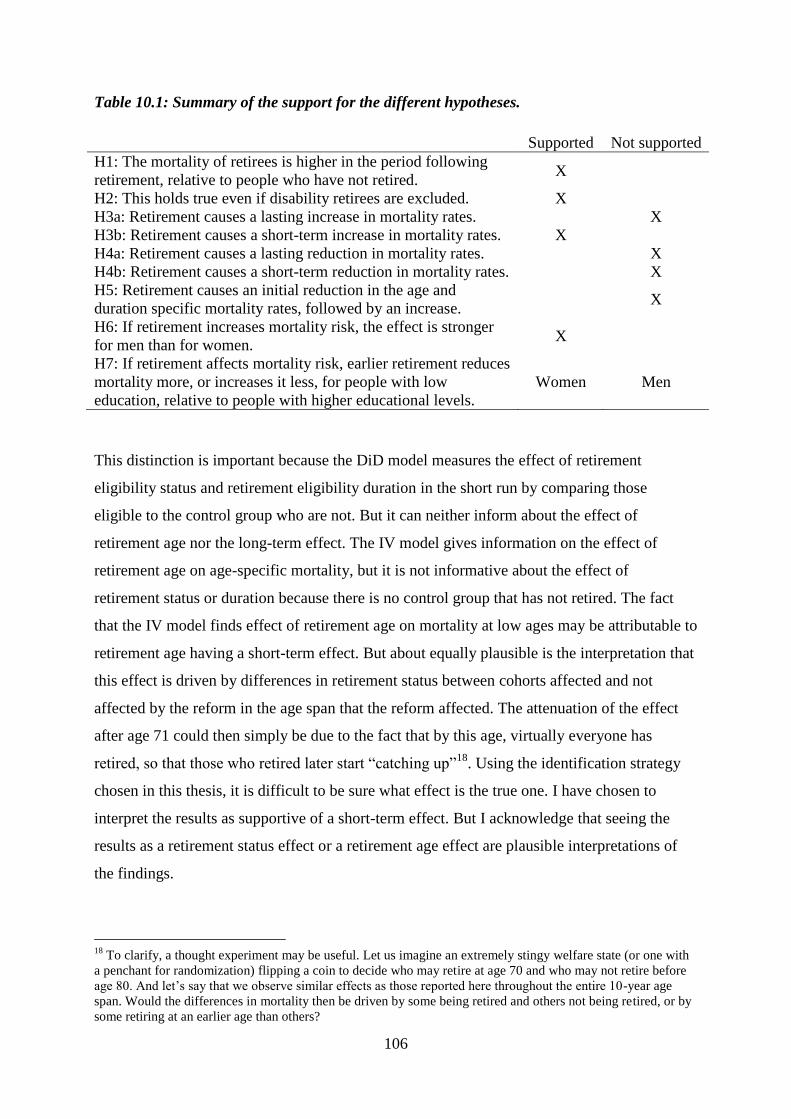
106

Table 10.1: Summary of the support for the different hypotheses.

Supported Not supported

H1: The mortality of retirees is higher in the period following

retirement, relative to people who have not retired. X

H2: This holds true even if disability retirees are excluded. X

H3a: Retirement causes a lasting increase in mortality rates. X

H3b: Retirement causes a short-term increase in mortality rates. X

H4a: Retirement causes a lasting reduction in mortality rates. X

H4b: Retirement causes a short-term reduction in mortality rates. X

H5: Retirement causes an initial reduction in the age and

duration specific mortality rates, followed by an increase. X

H6: If retirement increases mortality risk, the effect is stronger

for men than for women. X

H7: If retirement affects mortality risk, earlier retirement reduces

mortality more, or increases it less, for people with low

education, relative to people with higher educational levels.

Women Men

This distinction is important because the DiD model measures the effect of retirement

eligibility status and retirement eligibility duration in the short run by comparing those

eligible to the control group who are not. But it can neither inform about the effect of

retirement age nor the long-term effect. The IV model gives information on the effect of

retirement age on age-specific mortality, but it is not informative about the effect of

retirement status or duration because there is no control group that has not retired. The fact

that the IV model finds effect of retirement age on mortality at low ages may be attributable to

retirement age having a short-term effect. But about equally plausible is the interpretation that

this effect is driven by differences in retirement status between cohorts affected and not

affected by the reform in the age span that the reform affected. The attenuation of the effect

after age 71 could then simply be due to the fact that by this age, virtually everyone has

retired, so that those who retired later start “catching up”18

. Using the identification strategy

chosen in this thesis, it is difficult to be sure what effect is the true one. I have chosen to

interpret the results as supportive of a short-term effect. But I acknowledge that seeing the

results as a retirement status effect or a retirement age effect are plausible interpretations of

the findings.

18

To clarify, a thought experiment may be useful. Let us imagine an extremely stingy welfare state (or one with

a penchant for randomization) flipping a coin to decide who may retire at age 70 and who may not retire before

age 80. And let’s say that we observe similar effects as those reported here throughout the entire 10-year age

span. Would the differences in mortality then be driven by some being retired and others not being retired, or by

some retiring at an earlier age than others?

107

The implications of the different effects also vary. If the effect is one of retirement status or

retirement age, reductions in retirement age would expose those who retire earlier to elevated

mortality risk for a longer duration. This would lead to more people dying at all subsequent

ages. A short-term duration effect would not increase mortality at all ages, but simply shift the

bump in mortality risk to lower ages. In other words, the short-term duration effect is the less

dramatic one.

Keeping these reservations in mind, there are a couple of things that may be stated quite

firmly. Retirement increased mortality somewhat in the context and period studied here. And

there is apparently no honeymoon effect with regard to mortality.

In addition to the main results, this thesis also draws attention to the importance of

institutions, policies and welfare state programs and their profound impact on people’s lives.

As discussed previously, being retired may be a social role, but it is a role that is strongly

influenced by the institutional context. By allowing people to retire earlier, the welfare state

enabled a large-scale shift in the timing of people’s work exits. The reason why the IV

analyses presented here were even possible is that people respond to such changes in welfare

state regulations. In broader terms; people adapt their behavior to changing opportunity

structures, and those opportunity structures are strongly shaped by welfare state institutions

such as the national insurance scheme.

10.3 The research literature and the importance of context

How do the results fit into the research literature? As I have shown in chapter 3, there is more

or less consensus that retirement is associated with elevated mortality risk. The results from

the event history analyses are very much in line with these findings and the conclusions drawn

by Shim et al. (2013). The finding that excluding disability pensioners reduces the estimated

association for both women and men highlights the importance of distinguishing between

pension types. The fact that the results generally differ between the sexes also show the

importance of being sensitive to differences between men and women in the analyses. The

finding that most of the association between retirement and mortality is not causal but likely

driven by some selection process shows how important it is not to interpret associations as

reflecting causal processes. Without adequately dealing with selection bias, one runs the risk

of overstating or otherwise misstating an effect.

108

With regard to the estimates of the causal effects of retirement on mortality, these results

partly contradict previous findings. Bingley and Pedersen (2011) found that early retirement

led to reduced mortality before age 80. Bloemen et al. (2013) and Hallberg et al. (2015) also

found earlier retirement to reduce mortality. Coe and Lindeboom (2008) and Hernæs et al.

(2013) found no effect. Only one study, by Kuhn et al. (2010), has presented findings that are

similar to those presented here. One plausible explanation for the inconsistent findings in the

research literature might be that the contexts, samples and methods differ. Societies may

differ in many aspects that might condition the effect of retirement on mortality. Such

differences may be found with regard to for instance culture, pension schemes, labor markets,

welfare services, or health systems. Also, societies change, so that even within the same

national contexts, the effects of retirement may change over time. This could be driving the

difference in conclusions drawn by and Hernæs et al. (2013) and those presented here19

. Also,

different studies have studied different occupational groups and age groups. If the effects vary

with occupation and age, one should perhaps not be surprised that the findings diverge.

A closer look at samples, research designs, age groups and country and period contexts in

these studies does not give any clear clue as to why the results are contradictory, though. Nor

does it aid in the understanding of why the results in this thesis contradict most of them. Table

10.2 compares the studies mentioned above and the present thesis with regard to country

contexts, samples, time periods, ages, main methods employed and the direction of the main

results. There does not appear to be any clearly identifiable pattern. Apparently, context may

matter, but not in any predictable way.

Also, this thesis does not tip the balance in favor of one conclusion. If anything, it adds to the

confusion by drawing the conclusion that was least frequently found in the established

literature. Among the studies presented here, three found retirement to reduce mortality, two

found no effect, while one found retirement to increase mortality (3/2/1). Adding the present

thesis to the summary changes the score to 3/2/2.

19

Let me be absolutely clear; although I point out that the research design used in this thesis has some

advantages, I readily acknowledge that the design employed by Hernæs et al. (2013) is better in some regards.

Particularly, their use of a triple differences estimator is strength.

109

Table 10.2: Comparison of studies with causally oriented research designs. E

ffec

t of

reti

rem

ent

Red

uce

d

mo

rtal

ity

Red

uce

d

mo

rtal

ity

Red

uce

d

mo

rtal

ity

No

eff

ect

No

eff

ect

Incr

ease

d

mo

rtal

ity

Incr

ease

d

mo

rtal

ity

Met

ho

ds

IV

IV-D

iDiD

wit

h

ind

ivid

ual

FE

DiD

iD

IV

IV a

nd

DiD

iD

IV

IV,

DiD

an

d

ind

ivid

ual

FE

Ag

es a

ffec

ted

60-6

6

55

an

d a

bo

ve

55-6

0

50-7

0

62-6

7

Wo

men

50-5

3.5

,

men

55

-58.5

67-7

0

Tim

e

1979 r

eform

2005 w

indow

1992

-1997

win

dow

1992

-2004

win

dow

s

1990s

refo

rms

1988

-1993

win

dow

1973

ref

orm

Sam

ple

Blu

e co

llar

mal

e em

plo

yee

s fr

om

cohort

s 1906

-1921

Civ

il s

ervan

ts a

ged

53

‐60 d

uri

ng

1999

‐2005

Mil

itar

y p

erso

nnel

born

1938

-1939

Hea

lth a

nd r

etir

emen

surv

ey,

work

ing m

ales

in c

ohort

s 1931

-1941

Full

cohort

s 1928-1

938 i

n A

FP

firm

s

Blu

e co

llar

work

ers

in a

ffec

ted

regio

ns

in c

ohort

s 1929

-1941 (

men

)

and 1

934-1

941 (

wom

en)

Full

cohort

s 1902-1

906

Co

un

try

Den

mar

k

Net

her

lands

Sw

eden

US

A

No

rway

Au

stri

a

No

rway

Au

thors

Bin

gle

y a

nd P

eder

sen

(2

011

)

Blo

emen

et

al. (2

01

3)

Hal

lber

g e

t al

. (2

01

5)

Coe

and

Lin

deb

oo

m (

200

8)

Her

næ

s et

al.

(2

01

3)

Kuhn e

t al

. (2

01

0)

This

th

esis

110

10.4 Recommendations for future research

The results in this thesis cautiously support one hypothesis about the effect of retirement on

mortality, namely that retirement increases mortality in the short term. But this should not be

seen as a confirmation of the theories that predict a short-term increase in mortality following

retirement. The theories presented in chapter 2 do not only produce predictions. They also

postulate some mechanisms that produce the outcomes. The fact that this thesis’ results fit the

predictions of some theories better than others is not in itself evidence that the causal

mechanisms these theories postulate are true. This thesis does not test any mechanisms

(except that of selection) and it thus uninformative about the causal processes at work.

One might be tempted, then, to suggest that a natural next step would be to test what

mechanisms produce the results presented here. This could be done by for instance looking at

changes in stress levels or health behavior following some exogenously induced retirement

opportunity. But such a recommendation would be premature. Before embarking on the

attempt to find an explanation of the effect, there is a need to establish what that effect is. As

the previous section showed, there is currently no fact of the matter or established causal

relationship in the research literature to explain.

It goes without saying, then, that more research is needed to establish the effect of retirement

on mortality. One opportunity is to wait a few years and then exploit the Norwegian 2011

pension reform or some other recent pension reform that has taken place in another country.

Repeated studies of different natural experiment may bring us closer to some truth about the

effect and how it may vary with groups and contexts. An actual experiment whereby

randomly selected people are given the opportunity to retire early would be even better. Such

an experiment would be quite expensive, but less prone to the potential biases that always

haunt quasi-experimental research designs.

Another interesting topic could be to investigate the potential spillover effects of partners’

retirement for couples. Such an analysis could actually be done on the data used in this thesis

by matching individuals with their partners. But such an analysis has not been performed

here, as it falls outside of the scope of this thesis.

In any case, this thesis underlines the importance of adequately dealing with selection bias in

future research on this topic. Issues relating to selection, omitted variables and reverse

causation have recently received increasing attention within sociology, and further

111

developments in the use of experimental and quasi-experimental data for the purposes of

causal inference should be welcomed.

112

11 Conclusions A number of theories give diverging predictions about the relationship between retirement

and mortality. This thesis examined whether and how retirement is associated with mortality,

and whether and how retirement affects mortality. The analyses were performed on cohorts

born between 1902 and 1907, who for the most part retired in the 1970s.

The association between retirement and mortality was explored through event history analyses

using discrete-time hazard models. These results show that being retired is associated with a

continuously increasing probability of dying. Twenty years after retirement, the probability of

dying was 17.0 percent higher among retired men relative to men at the same age who were

not retired. The corresponding figure for women was 8.7 percent. Excluding disability

pensioners substantially reduced the probability of dying at all durations up to 20 years after

retirement. This indicates that health-related selection into retirement through disability

pensions is an important driver of the association between retirement and mortality.

A causal link between retirement and mortality was identified by treating a pension reform

that came into effect in 1973 as a natural experiment. Overnight, the minimum age for old age

retirement eligibility was lowered by three years, giving some birth cohorts the opportunity to

retire up to three years earlier than others. This variation in retirement eligibility was

exploited in difference-in-differences and individual fixed effects estimations of the effect of

retirement eligibility on mortality, and in instrumental variable estimations of the effect of

retirement age on mortality. The results from these analyses show that retirement eligibility or

earlier retirement increases mortality. Among men, the instrumental variable results indicate

that one year earlier retirement increases the probability of dying before age 80 by 1.5

percentage points. This is a substantive effect. For women the effect is smaller –

approximately 0.5 percentage points. Subgroup analyses uncovered some effect

heterogeneity. The effect was apparently largest among men with lower education and among

women with higher education. There was no evidence to support a “honeymoon effect” with

regard to mortality following retirement.

The difference-in-differences, individual fixed effects and instrumental variables results are

consistent, and the estimates appear to be robust. The effects appear to be driven primarily by

a relatively short-term increase in mortality following retirement, although other

interpretations of these findings are also plausible. Such a short-term effect is consistent with

theories conceptualizing retirement as a stressful life event or continuity break, with short-

113

term changes in health behavior following retirement, or with the loss of some protective

effect of employment. The results further indicate that the strong and continually increasing

association between retirement and mortality is primarily driven by an omitted variable bias

or some health-related selection process, such as a healthy worker effect.

The effects that are identified in this thesis are local and perhaps contingent on the national

context and the time period. This does not mean that a generalization of these findings across

contexts and time is impossible. But such a generalization should be done with care and

requires some theoretical justification. Nevertheless, retirement appears to have increased

mortality in 1970s’ Norway.

114

12 References

Allison, P. D. (1995). Survival analysis using SAS: A practical guide. Cary, NC: SAS

Institute: Inc.

Amendment to the law on social insurance (1972). Law of June 16th 1972 number 60 on

amendments of the law of June 17th 1966 number 12 on social insurance (folketrygd)

(1972).

Angrist, J. D., & Pischke, J.-S. (2008). Mostly harmless econometrics: An empiricist's

companion. Princeton and Oxford: Princeton university press.

Angrist, J. D., & Pischke, J.-S. (2014). Mastering 'metrics: The path from cause to effect.

Princeton and Oxford: Princeton University Press.

Arbeids- og inkluderingsdepartementet. (2006). St. melding nr. 5 (2006-2007). Opptjening og

uttak av alderspensjon i folketrygden. Oslo: Arbeids- og Inkluderingsdepartementet.

Atalay, K., & Barrett, G. F. (2014). The causal effect of retirement on health: New evidence

from Australian pension reform. Economics Letters, 125(3), 392-395

Atchley, R. C. (1976). The Sociology of Retirement. Cambridge, Massachusetts: Schenkman

Publishing Company, Inc.

Atchley, R. C. (1989). A continuity theory of normal aging. The Gerontologist, 29(2), 183-

190

Bamia, C., Trichopoulou, A., & Trichopoulos, D. (2008). Age at Retirement and Mortality in

a General Population Sample: The Greek EPIC Study. American Journal of

Epidemiology, 167(5), 561-569

Bingley, P., & Pedersen, P. J. (2011). Does early retirement keep you healthy and extend your

life? Preliminary version 2.1. The Danish National Center for Social Research,

Copenhagen School of Economics and Management, Aarhus University.

Birkelund, G. E., & Petersen, T. (2016). Likestilling. Utdanning, politikk og arbeid. In I.

Frønes & L. Kjølsrød (Eds.), Det norske samfunn. Bind 2. (Vol. 7, pp. 190-210). Oslo:

Gyldendal.

Bloemen, H., Hochguertel, S., & Zweerink, J. (2013). The causal effect of retirement on

mortality: Evidence from targeted incentives to retire early. IZA Discussion paper, No.

7570

Bonsang, E., Adam, S., & Perelman, S. (2012). Does retirement affect cognitive functioning?

Journal of Health Economics, 31(3), 490-501

Borgen, N. T. (2013). Instrumentvariabler - en introduksjon for samfunnsforskere. Sosiologi i

dag, 43(3)

Boudon, R. (2003). Beyond rational choice theory. Annual review of sociology, 29(1), 1-21

Bound, J., & Waidmann, T. (2007). Estimating the health effects of retirement. University of

Michigan Retirement Research Center Working Paper, 2007-168

Box, G. E. P., & Draper, N. R. (1987). Empirical model-building and response surfaces. New

York: Wiley.

Brathaug, A. L., & Skoglund, T. (2012). Historisk nasjonalregnskap. Langvarig vekst i norsk

økonomi. Retrieved from https://www.ssb.no/nasjonalregnskap-og-

konjunkturer/artikler-og-publikasjoner/langvarig-vekst-i-norsk-okonomi

Braut, G. S. (2015). Helse. Store medisinske leksikon.

Brockmann, H., Müller, R., & Helmert, U. (2009). Time to retire–Time to die? A prospective

cohort study of the effects of early retirement on long-term survival. Social science &

medicine, 69(2), 160-164

115

Brown, P., & Vickerstaff, S. (2011). Health Subjectivities and Labor Market Participation:

Pessimism and Older Workers’ Attitudes and Narratives Around Retirement in the

United Kingdom. Research on Aging, 33(5), 529-550

Brunborg, H., Fredriksen, D., Stølen, N. M., & Texmon, I. (2008). Levealdersutvikling og

delingstall Økonomiske analyser 4/2008. Oslo/Kongsvinger: Statistisk sentralbyrå.

Carlsson, S., Andersson, T., Michaëlsson, K., Vågerö, D., & Ahlbom, A. (2012). Late

retirement is not associated with increased mortality, results based on all Swedish

retirements 1991–2007. European Journal of Epidemiology, 27(6), 483-486

Coe, N. B., & Lindeboom, M. (2008). Does retirement kill you? Evidence from early

retirement windows. IZA Discussion paper, No. 3817

Coe, N. B., & Zamarro, G. (2011). Retirement effects on health in Europe. Journal of Health

Economics, 30(1), 77-86

Coppola, L., & Spizzichino, D. (2014). The effect of retirement on self-reported health: a

gender comparison in Italy. Vienna Yearbook of Population Research, 2014, 53-82

Cumming, E., & Henry, W. E. (1961). Growing old, the process of disengagement. New

York: Basic Books.

Daatland, S. O., & Solem, P. E. (2000). Aldring og samfunn. En innføring i sosialgerontologi.

Bergen: Fagbokforlaget.

Diener, E., Lucas, R. E., & Scollon, C. N. (2006). Beyond the hedonic treadmill: revising the

adaptation theory of well-being. American psychologist, 61(4), 305-314

Durkheim, E. (1978) [1897]. Selvmordet. Oslo: Gyldendal Norsk Forlag

Eibich, P. (2015). Understanding the effect of retirement on health: Mechanisms and

heterogeneity. Journal of Health Economics, 43, 1-12

Eika, T. (2008). Det svinger i norsk økonomi. Samfunnsspeilet, 5-6/2008, 98-111

Eikemo, T. A., Hoffmann, R., Kulik, M. C., Kulhánová, I., Toch-Marquardt, M., Menvielle,

G., Looman, C., Jasilionis, D., Martikainen, P., Lundberg, O., & Mackenbach, J. P.

(2014). How Can Inequalities in Mortality Be Reduced? A Quantitative Analysis of 6

Risk Factors in 21 European Populations. PLoS ONE, 9(11)

Ekerdt, D. J. (1987). Why the notion persists that retirement harms health. The Gerontologist,

27(4), 454-457

Ekerdt, D. J., Bossé, R., & Levkoff, S. (1985). An empirical test for phases of retirement:

Findings from the Normative Aging Study. Journal of Gerontology, 40(1), 95-101

Ekerdt, D. J., Bosse, R., & LoCastro, J. S. (1983). Claims that retirement improves health.

Journal of Gerontology, 38(2), 231-236

Elstad, J. I. (2010). Klasseforskjeller i helse: Et spørsmål om arbeid? In K. Dahlgren & J.

Ljunggren (Eds.), Klassebilder. Ulikhet og sosial mobilitet i Norge. Oslo:

Universitetsforlaget.

Elster, J. (2015). Explaining Social Behavior. More Nuts and Bolts for the Social Sciences

(2nd ed.). Cambridge: Cambridge University Press.

Elwert, F., & Winship, C. (2014). Endogenous Selection Bias: The Problem of Conditioning

on a Collider Variable. Annual review of sociology, 40(1), 31-53

Flittig, E. H. (1992). Folketrygden. Utviklingen fra 1967 til 1990 Rapporter 92/14.

Oslo/Kongsvinger: Statistisk sentralbyrå.

Flyvbjerg, B. (2006). Five misunderstandings about case-study research. Qualitative inquiry,

12(2), 219-245

Fredriksen, D., & Stølen, N. M. (2011). Utforming av ny alderspensjon i folketrygden.

Rapporter 22/2011. Oslo/Kongsvinger: Statistisk sentralbyrå.

Fredriksen, D., & Stølen, N. M. (2015). Evaluering av pensjonsreformen – Direkte

konsekvenser for arbeidsstyrken og offentlige budsjetter. Rapporter 2015/37.

Oslo/Kongsvinger: Statistisk sentralbyrå.

116

Fredriksen, S. (2005). Bad luck and the tragedy of modern medicine. Doctoral dissertation,

Faculty of medicine, University of Oslo, Oslo.

Fuchs, V. R. (1972). Foreword. In M. Grossman (Ed.), The Demand for Health: A Theoretical

and Empirical Investigation. National Bureau of Economic Research: Occasional

paper 119. New York: Columbia University Press.

Grossman, M. (1972). On the concept of health capital and the demand for health. The journal

of political economy, 80(2), 223-255

Hallberg, D., Johansson, P., & Josephson, M. (2015). Is an early retirement offer good for

your health? Quasi-experimental evidence from the army. Journal of Health

Economics, 44, 274-285

Hankins, M. (2012). Why change scores are generally a bad idea for PROMs data: the maths

part. Retrieved from https://mchankins.wordpress.com/2012/01/23/why-change-

scores-are-generally-a-bad-idea-for-proms-data-the-maths-part/ [accessed October

22nd 2016]

Havighurst, R. J. (2009 [1963]). Successful aging. In R. H. Williams, C. Tibbitts & W.

Donohue (Eds.), Processes of aging: Social and psychological perspectives (pp. 299-

320). New Brunswick, NJ: Transaction Publishers.

Haynes, S. G., McMichael, A. J., & Tyroler, H. A. (1978). Survival After Early and Normal

Retirement. Journal of Gerontology, 33(2), 269-278

Hedström, P. (2005). Dissecting the social: On the principles of analytical sociology:

Cambridge University Press.

Hernæs, E., Markussen, S., Piggott, J., & Roed, K. (2015). Pension Reform and Labor

Supply: Flexibility vs. Prescription. IZA discussion paper No. 8812

Hernæs, E., Markussen, S., Piggott, J., & Vestad, O. L. (2013). Does retirement age impact

mortality? Journal of Health Economics, 32(3), 586-598

Hessel, P. (2016). Does retirement (really) lead to worse health among European men and

women across all educational levels? Social science & medicine, 151, 19-26

Hochschild, A. R. (1975). Disengagement Theory: A Critique and Proposal. American

Sociological Review, 40(5), 553-569

Holseter, C., Dalen, J. D., Krokstad, S., & Eikemo, T. A. (2015). Selvrapportert helse og

dødelighet i ulike yrkesklasser og inntektsgrupper i Nord-Trøndelag. Tidsskrift for

Den norske legeforening, 135(5), 434-438

Johnston, D. W., & Lee, W.-S. (2009). Retiring to the good life? The short-term effects of

retirement on health. Economics Letters, 103(1), 8-11

Jylhä, M. (2009). What is self-rated health and why does it predict mortality? Towards a

unified conceptual model. Social science & medicine, 69(3), 307-316

Kim, J. E., & Moen, P. (2002). Retirement Transitions, Gender, and Psychological Well-

Being: A Life-Course, Ecological Model. The Journals of Gerontology Series B:

Psychological Sciences and Social Sciences, 57(3), 212-222

Kjølsrød, L. (2011). Small Country, Large Welfare State. In O. Molven & J. Ferkis (Eds.),

Healthcare, Welfare and Law. Health legislation as a mirror of the Norwegian

welfare state (pp. 13-27). Oslo: Gyldendal Akademisk.

Kuhn, A., Wuellrich, J.-P., & Zweimüller, J. (2010). Fatal attraction? Access to early

retirement and mortality. IZA discussion paper No. 5160

Kühntopf, S., & Tivig, T. (2012). Early retirement and mortality in Germany. European

Journal of Epidemiology, 27(2), 85-89

Lantz, P. M., House, J. S., Lepkowski, J. M., Williams, D. R., Mero, R. P., & Chen, J. (1998).

Socioeconomic factors, health behaviors, and mortality: Results from a nationally

representative prospective study of us adults. JAMA, 279(21), 1703-1708

117

Lee, Y. (2000). The predictive value of self assessed general, physical, and mental health on

functional decline and mortality in older adults. Journal of Epidemiology and

Community Health, 54(2), 123-129

Li, C.-Y., & Sung, F.-C. (1999). A review of the healthy worker effect in occupational

epidemiology. Occupational Medicine, 49(4), 225-229

Litwin, H. (2007). Does early retirement lead to longer life? Ageing and Society, 27(05), 739-

754

Lyngstad, T. H. (2009). Fri flyt av kapital? En kommentar til begrepsbruk i sosiologi og

annen samfunnsvitenskap. Sosiologisk tidsskrift, 17(3), 261-271

Mamelund, S.-E., & Iversen, B. G. (2000). Sykelighet og dødelighet ved pandemisk influensa

i Norge. Tidsskrift for Den norske lægeforening, 120(3), 360-363

Martin, J., & Doran, A. (1966). Evidence concerning the relationship between health and

retirement. The Sociological Review, 14(3), 329–343

Mein, G., Martikainen, P., Stansfeld, S. A., Brunner, E. J., Fuhrer, R., & Marmot, M. G.

(2000). Predictors of early retirement in British civil servants. Age and Ageing, 29(6),

529-536

Miilunpalo, S., Vuori, I., Oja, P., Pasanen, M., & Urponen, H. (1997). Self-rated health status

as a health measure: The predictive value of self-reported health status on the use of

physician services and on mortality in the working-age population. Journal of Clinical

Epidemiology, 50(5), 517-528

Minkler, M. (1981). Research on the health effects of retirement: an uncertain legacy. Journal

of Health and Social Behavior, 22(2), 117-130

Mood, C. (2010). Logistic regression: Why we cannot do what we think we can do, and what

we can do about it. European sociological review, 26(1), 67-82

Morris, J. K., Cook, D. G., & Shaper, A. G. (1994). Loss of employment and mortality.

British Medical Journal, 308(6937), 1135-1139

Munch, J. R., & Svarer, M. (2005). Mortality and socio-economic differences in Denmark: a

competing risks proportional hazard model. Economics & Human Biology, 3(1), 17-32

Murray, M. P. (2006). Avoiding invalid instruments and coping with weak instruments. The

Journal of Economic Perspectives, 20(4), 111-132

Mæland, J. G., & Hatland, A. (2016). Folketrygden. Store norske leksikon.

NAV (2011). Rundskriv § 19-19 Ventetillegg, Folketrygdloven (2011).

NOU 1998: 19. (1998). Fleksibel pensjonering. Oslo: Finansdepartementet.

Nuttman-Shwartz, O. (2004). Like a high wave: Adjustment to retirement. The Gerontologist,

44(2), 229-236

Nylenna, M. (2009). Helseatferd. Store medisinske leksikon.

Næss, Ø., Rognerud, M., & Strand, B. H. (2007). Sosial ulikhet i helse: en faktarapport

Rapport 2007:1. Oslo: Nasjonalt folkehelseinstitutt.

OECD. (2013). Pensions at a Glance 2013: OECD and G20 Indicators: OECD Publishing.

OECD/EU. (2014). Health at a Glance: Europe 2014: OECD Publishing.

Pampel, F. C., Krueger, P. M., & Denney, J. T. (2010). Socioeconomic disparities in health

behaviors. Annual review of sociology, 36, 349–370

Pensjonsalderkomitéen. (1971). Innstilling fra Pensjonsalderkomitéen. Innstillinger og

betenkninger. Oslo: Sosialdepartementet.

Pope, W. (1976). Durkheim's suicide: A classic analyzed. Chicago: University of Chicago

Press.

Price, C. A. (2003). Professional women's retirement adjustment: The experience of

reestablishing order. Journal of Aging Studies, 17(3), 341-355

118

Quaade, T., Engholm, G., Johansen, A. M. T., & Møller, H. (2002). Mortality in relation to

early retirement in Denmark: a population-based study. Scandinavian journal of public

health, 30(3), 216-222

Rabe-Hesketh, S., & Skrondal, A. (2008). Multilevel and longitudinal modeling using Stata.

College Station, Texas: STATA press.

Rice, N. E., Lang, I. A., Henley, W., & Melzer, D. (2011). Common health predictors of early

retirement: findings from the English Longitudinal Study of Ageing. Age and Ageing,

40(1), 54-61

Richardson, V., & Kilty, K. M. (1991). Adjustment to retirement: continuity vs. discontinuity.

The International Journal of Aging & Human Development, 33(2), 151-169

Rowland, D. T. (2003). Demographic methods and concepts. New York: Oxford University

Press.

Rydgren, J. (2009). Beliefs. In P. Hedström & P. Bearman (Eds.), The Oxford Handbook of

Analytical Sociology. Oxford: Oxford University Press.

SCB. (2016). Livslängd och dödlighet i olika sociala grupper Demografiska rapporter

2016:2. Stockholm: Statistiska centralbyrån, Prognosinstitutet.

Shim, M. J., Gimeno, D., Pruitt, S. L., McLeod, C. B., Foster, M. J., & Amick, B. C. (2013).

A Systematic Review of Retirement as a Risk Factor for Mortality. In N. Hoque, A.

M. McGehee & S. B. Bradshaw (Eds.), Applied Demography and Public Health (pp.

277-309). Dordrecht: Springer Netherlands.

Skirbekk, V., Telle, K., Nymoen, E., & Brunborg, H. (2010). Retirement and mortality in

Norway–Is there a real connection? In T. Salzmann, V. Skirbekk & M. Weiberg

(Eds.), Wirtschaftspolitische herausforderungen des demografischen wandels (pp.

201-222): Springer.

Solem, P. E. (1987). Mortality during the first five years after reaching retirement age. In L.

Levi (Ed.), Society, stress and disease: Vol 5 Aging and old age (pp. 236-248).

Oxford: Oxford University Press.

Sosialdepartementet. (1971). St. meld. nr. 13 (1971-72). Om nedsettelse av pensjonsalderen i

folketrygden m. v. Oslo: Sosialdepartementet.

SSB. (n.a.). Tabell: 07902: Dødelighetstabeller, etter kjønn og alder. Retrieved June 6th,

2016, from

https://www.ssb.no/statistikkbanken/selecttable/hovedtabellHjem.asp?KortNavnWeb=

dode&CMSSubjectArea=befolkning&checked=true

Stenholm, S., Westerlund, H., Salo, P., Hyde, M., Pentti, J., Head, J., Kivimäki, M., &

Vahtera, J. (2014). Age-related trajectories of physical functioning in work and

retirement: the role of sociodemographic factors, lifestyle and disease. Journal of

Epidemiology and Community Health, 68(6), 503-509

Stoltenberg, C. (2014). Daly. Store medisinske leksikon: Store norske Leksikon.

Syse, A., Veenstra, M., Furunes, T., Mykletun, R. J., & Solem, P. E. (2015). Changes in

Health and Health Behavior Associated With Retirement. Journal of aging and health,

0898264315624906

The World Bank. (n.a.). GDP per capita (current US$) Retrieved 22nd of August, 2016, from

http://data.worldbank.org/indicator/NY.GDP.PCAP.CD?year_high_desc=true

Tsai, S. P., Wendt, J. K., Donnelly, R. P., de Jong, G., & Ahmed, F. S. (2005). Age at

retirement and long term survival of an industrial population: prospective cohort

study. British Medical Journal, 331(995)

van der Heide, I., van Rijn, R. M., Robroek, S. J., Burdorf, A., & Proper, K. I. (2013). Is

retirement good for your health? A systematic review of longitudinal studies. BMC

Public Health, 13(1180)

119

Van Poppel, F., & Day, L. H. (1996). A test of Durkheim's theory of suicide--without

committing the "ecological fallacy". American Sociological Review, 61(3), 500-507

Van Solinge, H., & Henkens, K. (2008). Adjustment to and satisfaction with retirement: two

of a kind? Psychology and aging, 23(2), 422-434

Vassenden, K. (1987). Folke- og boligtellingene 1960, 1970 og 1980. Dokumentasjon av de

sammenlignbare filene. Rapporter fra Statistisk sentralbyrå 87/2. Oslo/Kongsvinger:

SSB.

Waldron, H. (2001). Links between early retirement and mortality ORES Working Paper

Number 93. Washington, DC: Social Security Administration, Office of Policy, Office

of Research, Evaluation, and Statistics.

Wardle, J., & Steptoe, A. (2003). Socioeconomic differences in attitudes and beliefs about

healthy lifestyles. Journal of Epidemiology and Community Health, 57(6), 440-443

Westerlund, H., Kivimäki, M., Singh-Manoux, A., Melchior, M., Ferrie, J. E., Pentti, J.,

Jokela, M., Leineweber, C., Goldberg, M., Zins, M., & Vahtera, J. (2009). Self-rated

health before and after retirement in France (GAZEL): a cohort study. The Lancet,

374(9705), 1889-1896

WHO (1946). Preamble to the Constitution of the World Health Organization as adopted by

the International Health Conference, New York, 19-22 June, 1946; signed on 22 July

1946 by the representatives of 61 States (Official Records of the World Health

Organization, no. 2, p. 100) and entered into force on 7 April 1948. (1946).

Williams, D. R., & Collins, C. (1995). US Socioeconomic and Racial Differences in Health:

Patterns and Explanations. Annual review of sociology, 21(1), 349-386

Wolfe, J. R. (1983). Perceived longevity and early retirement. The Review of Economics and

Statistics, 65(4), 544-551

Wolfson, M., Rowe, G., Gentleman, J. F., & Tomiak, M. (1993). Career earnings and death: a

longitudinal analysis of older Canadian men. Journal of Gerontology, 48(4), 167-179

World Health Organization. (2009). Global health risks: mortality and burden of disease

attributable to selected major risks: World Health Organization.

World Health Organization. (2015, January 2015). Noncommunicable diseases. Fact sheet.

Retrieved May 31st, 2016, from http://www.who.int/mediacentre/factsheets/fs355/en/

Wu, C., Odden, M. C., Fisher, G. G., & Stawski, R. S. (2016). Association of retirement age

with mortality: a population-based longitudinal study among older adults in the USA.

Journal of Epidemiology and Community Health, 70(9), 917-923

All references in this thesis are reported.

The number of words in this thesis is 36 642.

120

Appendix: approval from the privacy ombudsman

121

122

123