Temporal dynamics of hydrological threshold events

Temporal dynamics of hydrological threshold events

G. S. Mcgrath, C. Hinz, M. Sivapalan

To cite this version:

G. S. Mcgrath, C. Hinz, M. Sivapalan. Temporal dynamics of hydrological threshold events. Hy-drology and Earth System Sciences Discussions, Copernicus Publications, 2007, 11 (2), pp.923-938. <hal-00305060>

HAL Id: hal-00305060

https://hal.archives-ouvertes.fr/hal-00305060

Submitted on 26 Feb 2007

HAL is a multi-disciplinary open accessarchive for the deposit and dissemination of sci-entific research documents, whether they are pub-lished or not. The documents may come fromteaching and research institutions in France orabroad, or from public or private research centers.

L’archive ouverte pluridisciplinaire HAL, estdestinee au depot et a la diffusion de documentsscientifiques de niveau recherche, publies ou non,emanant des etablissements d’enseignement et derecherche francais ou etrangers, des laboratoirespublics ou prives.

https://hal.archives-ouvertes.fr

https://hal.archives-ouvertes.fr/hal-00305060

Hydrol. Earth Syst. Sci., 11, 923–938, 2007www.hydrol-earth-syst-sci.net/11/923/2007/© Author(s) 2007. This work is licensedunder a Creative Commons License.

Hydrology andEarth System

Sciences

Temporal dynamics of hydrological threshold events

G. S. McGrath1, C. Hinz1, and M. Sivapalan2

1School of Earth and Geographical Sciences, University of Western Australia, Crawley, Australia2Departments of Geography & Civil & Environmental Engineering, University of Illinois at Urbana-Champaign, USA

Received: 14 July 2006 – Published in Hydrol. Earth Syst. Sci. Discuss.: 1 September 2006Revised: 6 February 2007 – Accepted: 6 February 2007 – Published: 26 February 2007

Abstract. The episodic nature of hydrological flows suchas surface runoff and preferential flow is a result of the non-linearity of their triggering and the intermittency of rainfall.In this paper we examine the temporal dynamics of thresh-old processes that are triggered by either an infiltration ex-cess (IE) mechanism when rainfall intensity exceeds a spec-ified threshold value, or a saturation excess (SE) mechanismgoverned by a storage threshold. We use existing and newlyderived analytical results to describe probabilistic measuresof the time between successive events in each case, and inthe case of the SE triggering, we relate the statistics of thetime between events (the inter-event time, denoted IET) tothe statistics of storage and the underlying water balance.In the case of the IE mechanism, the temporal dynamics offlow events is found to be simply scaled statistics of rainfalltiming. In the case of the SE mechanism the time betweenevents becomes structured. With increasing climate ariditythe mean and the variance of the time between SE eventsincreases but temporal clustering, as measured by the coef-ficient of variation (CV) of the IET, reaches a maximum indeep stores when the climatic aridity index equals 1. In veryhumid and also very arid climates, the temporal clusteringdisappears, and the pattern of triggering is similar to that seenfor the IE mechanism. In addition we show that the mean andvariance of the magnitude of SE events decreases but the CVincreases with increasing aridity. The CV of IETs is foundto be approximately equal to the CV of the magnitude of SEevents per storm only in very humid climates with the CVof event magnitude tending to be much larger than the CV ofIETs in arid climates. In comparison to storage the maximumtemporal clustering was found to be associated with a max-imum in the variance of soil moisture. The CV of the timetill the first saturation excess event was found to be greatestwhen the initial storage was at the threshold.

Correspondence to: Christoph [email protected]

1 Introduction

Many rapid hydrological processes such as runoff (Horton,1933; Dunne, 1978), preferential flow (Beven and Germann,1982), and erosion (Fitzjohn et al., 1998), are not continu-ous, but are triggered by thresholds. For example surfacerunoff occurs when the rainfall intensity is greater than thesoils ability to adsorb it via infiltration. As a result some ofthese processes may even cease or are not even triggered ifthe rainfall event is too small. Because we consider rapidflow processes the duration of flow events is often small incomparison to the time between rainfall events. Therefore,what results from the threshold triggering, when we look ata time series, is a sequence of discrete, episodic events.

As the occurrence of these episodic processes is linkedto the timing and magnitude of rainfall events it is naturaltherefore, to consider improving our understanding of howthe temporal occurrence of these flow events relates to thestructure of rainfall. This is the focus of this paper.

The temporal dynamics of preferential flow triggering dueto between-storm and within-storm rainfall variability hasbeen previously explored via the numerical simulation ap-proach, using synthetic rainfall time series (Struthers et al.,2007a,b). Struthers et al. (2007b) were able to relate aspectsof the probability distribution function (pdf) and specific sta-tistical characteristics of the storm inputs to statistical prop-erties and aspects of the pdfs of preferential flow and runoffmagnitude and timing. The analysis was not able to separatethe contributions of the various runoff mechanisms to the sta-tistical properties of the resulting temporal flow dynamics. Asimpler, more general approach was required to further de-velop the ideas presented in this work.

There are two triggers which are shared by a number ofprocesses. Some processes are triggered, as already men-tioned, by a rainfall intensity threshold. Examples includemacropore flow through soil (Beven and Germann, 1982;Heppell et al., 2002), and surface runoff (Horton, 1933). Thistriggering is termed infiltration excess. Some processes aretriggered by a storage threshold or storm amount. These in-clude various types of preferential flow (Beven and Germann,

Published by Copernicus GmbH on behalf of the European Geosciences Union.

924 McGrath et al.: Temporal dynamics of threshold events

1982; Kung, 1990; Haria et al., 1994; Wang et al., 1998;Bauters, 2000; Dekker et al., 2001; Heppell et al., 2002),interception (Crockford and Richardson, 2000; Zeng et al.,2000), and hillslope outflow through subsurface flow path-ways (Whipkey, 1965; Mosley, 1976; Uchida et al., 2005;Tromp-van Meerveld and McDonnell, 2006). The storagethreshold will be referred to here as saturation excess, al-though the use of this term is not often associated with someof the above processes.

In this article we examine the simplest possible conceptu-alizations for these two triggers. For infiltration excess wewill use a threshold rainfall intensity (Horton, 1933; Heppellet al., 2002; Kohler et al., 2003) neglecting any soil mois-ture storage controls on the infiltration capacity. For satura-tion excess we use the opposite extreme, a threshold storage,depending only on the storm amount and not its intensity.While these two conceptualisations are very simplistic weexpect a mixture of the results from these two processes toreflect more complex triggers, where triggering is a functionof both rainfall intensity and storage.

The saturation excess mechanism captures the carry overof storage from one rainfall event to the next. As a resultthere is an enhanced probability that a second flow event willoccur shortly after a flow event has just occurred becausestorage is more likely to be nearer the threshold in this inter-val. We hypothesize that this leads to temporal clustering ofsaturation excess, which means that multiple events occur inshort periods of time separated by longer event-free intervals.

A second aspect of the paper is to address the issue of ob-servability. For some processes we cannot measure directlythe flux. Preferential flow is one such example. What we canobserve of preferential flow is the timing of episodic pesti-cide leaching events (Hyer et al., 2001; Fortin et al., 2002;Laabs et al., 2002; Kjær et al., 2005) which are driven bythis process. We also know that preferential flow is related tothresholds in soil moisture (Beven and Germann, 1982) andthis can be measured reasonably well. For other processes,like subsurface hillslope outflow via soil pipes, the flux andtiming might be observable but the internal, storage processmuch less so. There is clearly a need to better understandthe inter-relationships between timing, flux, and storage inorder to be able to make better predictions of these thresh-old processes where the internal dynamics are largely hidden(Rundle et al., 2006, this issue). In this paper it will be pos-sible to make this inter-comparison for the saturation excesstrigger.

The paper begins with a brief overview of the simple mod-els of rainfall adopted for this analysis. Based upon this wederive analytically the statistics of the time between thresh-old events for infiltration excess and saturation excess mech-anisms, and for saturation excess we also present existingand newly derived statistics of the runoff flux based upon theoriginal work of Milly (1993; 2001). Finally, we explore theresults in the context of storm properties and the climate set-ting.

2 Rainfall models

For modelling purposes we adopt simple stationary descrip-tions of rainfall without any seasonal dependence. Stormsare characterised only by three parameters, their total depthh [L], a maximum within-storm intensityImax [L/T], anda time between stormstb [T]. Storms are considered to beinstantaneous events, independent of one another, thereforesatisfying the Poisson assumption as used commonly in hy-drology (Milly, 1993; Rodriguez-Iturbe et al., 1999). Suchan assumption is considered valid at near daily time scales(Rodriguez-Iturbe and Isham, 1987).

As we are primarily concerned with an event based de-scription of processes, this rainfall model is appropriate tomake direct comparisons between the process and its driver.Our objective is to capture the inter-(rainfall)-event dynam-ics, i.e. this event did or did not trigger the threshold and notthe detail of within-event processes which is left for futureresearch.

The Poisson assumption implies that the random timebetween storms, the inter-storm time, that results is de-scribed by an exponential probability density function (pdf)(Rodriguez-Iturbe et al., 1999):

gT b [tb] =1

tbe−tb/tb (1)

which is fully characterised by its meantb [T]. Storm depthsare also assumed to follow an exponential pdffH [h] with ameanh [L]. The maximum within-storm rainfall intensity isalso considered to be exponentially distributed with a meanof Imax [L/T].

Clearly this rainfall model is a gross simplification ofreal rainfall, particularly as it neglects seasonality. How-ever its advantage is it makes the later derivations analyti-cally tractable. Considering it’s use to describe within a sea-son rainfall may be more appropriate, but the statistics wewill derive later may not necessarily reflect the transient dy-namics of storage in certain climates (Rodriguez-Iturbe et al.,2001). We also derive here statistics based upon an arbi-trary initial condition which may account for this transientbehaviour.

3 Statistics of temporal dynamics

Based on the rainfall signal and soil properties we would liketo quantify the probability that a given flow event, involvingthe exceedance of some kind of threshold, occurs. We use thetime between events as the random variable that characterisesthis event probability. This concept is illustrated for a rain-fall intensity threshold (Fig.1a) and a soil moisture storagethreshold (Fig. 1b). The random time to reach these thresh-olds for the first time is referred to as a first passage time(FPT) denoted asτ1, and the time between flow events is re-ferred to as the inter-event time (IET) denoted asτ2 andτ3 in

Hydrol. Earth Syst. Sci., 11, 923–938, 2007 www.hydrol-earth-syst-sci.net/11/923/2007/

McGrath et al.: Temporal dynamics of threshold events 925

(a)

5 10 15 20 25 30 35Time H daysL

20

40

60

80

100

120

140I m

axH

mm�d

ayL

Τ1 Τ2 Τ3

(b)

2 4 6 8 10 12 14 16 18Time HdaysL

00.20.40.60.81.

12.8.4.0.

Sto

rage

sR

ainf

all

mm

Τ1 Τ2 Τ3

s0

Fig. 1. Definition of the more general first passage timeτ1 and theinter-event timeτ2 andτ3 for (a) a threshold rainfall intensity infil-tration excess (IE) trigger, where in this example intensities aboveIξ=80 mm/day trigger an IE event; and(b) a storage, or satura-tion excess mechanism (SE), occurring whens=1. The variables0denotes the initial storage.

Fig. 1a and Fig. 1b. In the case of infiltration excess runoff, aflow event is triggered when the maximum rainfall intensitywithin a storm exceeds the infiltration capacityIξ . Simi-lalry, when the soil water storage reaches a critical capacitya saturation excess event is deemed to have been triggered.

To quantify the pdfs of the first passage times and the IETs,we use the first four central moments. For completeness wedefine the moments in this section and will derive analyticalexpressions for them in Sect. 5.2 and A. The meanTµ [T]and thekth central momentµk of the random variableτ arerelated to the pdfgT [τ ] by the following (Papoulis, 2001):

Tµ=E [τ ] =∫ ∞

−∞τ gT [τ ] dτ (2)

µk=E[

(τ − E [τ ])k]

=∫ ∞

−∞

(

τ − Tµ

) kgT [τ ] dτ (3)

for integersk ≥ 2, whereE [ ] denotes the expectationoperator. In addition to the mean and the varianceTσ2=µ2[T2], we will also use the dimensionless statistic, the coef-ficient of variation (CV),Tcv=

√

Tσ2

/

Tµ [−], the ratio of

Table 1. Storm and infiltration excess inter-event statistics

Statistic Storm Infiltration excess

Tµ tb tb eIξ /Imax

Tσ2 t2b

(

tb eIξ /Imax)2

Tcv 1 1Tε 2 2Tκ 6 6

the standard deviation to the mean, which gives a measureof the variability relative to the mean; the coefficient of

skewnessTε=µ3/

µ23/2 [−], which describes the asymme-

try of the probability distribution, where positive values in-dicate that the distribution has a longer tail towards largervalues than smaller values; and the coefficient of kurtosisTκ=µ4

/

µ22 − 3 [−], where positive values indicate a more

peaked distribution, in comparison to a normally distributedvariable, and ”fatter tails” i.e. an enhanced probability of ex-treme values (Papoulis, 2001).

In order to compare the statistical properties of flow eventtriggers with the rainfall signal, we summarise here the rain-fall in terms of IET statistics. The idea here is to compareand contrast storm IET and flow IET statistics for the vari-ous threshold driven processes. Events which are temporallyindependent of one another have an exponential IET pdf. Ta-ble1 lists the statistics for the storm IET.

A property of the exponential distribution is that the meanis equal to the standard deviation, and therefore the CV isequal to 1. The CV of the IETTcv is often used to distinguishtemporally clustered and unclustered processes (Teich et al.,1997). Temporal clustering is said to occur whenTcv>1,a Tcv=0 indicates no variability and exactly regular events,while aTcv<1 may indicate a quasi-periodic process (Woodet al., 1995; Godano et al., 1997).

4 Infiltration excess inter-event time statistics

Here we assume for simplicity that the infiltration capacityIξ is constant (Heppell et al., 2002; Kohler et al., 2003), andtherefore soil moisture controls on the infiltration capacityare considered insignificant. This approach provides an ex-treme contrast to the saturation excess mechanism consid-ered. It may actually better represent well more extreme rain-fall, where the antecedent soil moisture has little impact onevent triggering. For example Heppell et al. (2002) classi-fied preferential flow events in a clay loam soil as antecedentsoil moisture limited and non-antecedent limited events. Thenon-antecedent limited events were related to storms wherethe maximum within-storm rainfall intensity was much largerthan the mean storm intensity.

www.hydrol-earth-syst-sci.net/11/923/2007/ Hydrol. Earth Syst. Sci., 11, 923–938, 2007


This constant threshold filtering is the same as the rain-fall filtering described in Rodriguez-Iturbe et al. (1999) inthe context of the soil water balance. They showed that athreshold filtering of the depth of rainfall with Poisson ar-rivals resulted in a new Poisson process. The rate of eventsover this threshold equalled the storm arrival rate multipliedby the probability of exceeding the threshold storm depth bya single event (Rodriguez-Iturbe et al., 1999). The differ-ence for the IE trigger considered here lies only in seman-tics. When the maximum within-storm rainfall intensityImaxis exponentially distributed with meanImax the probabilitythat Imax>Iξ is equal toe−Iξ /Imax and therefore the result-

ing mean time between IE events is equal toT Iµ=tbe

Iξ /Imax.Table 1 lists the IET statistics that result.

A soil with Iξ=2Imax results in a mean IET which ise2

times longer than the mean storm IETtb, and a variancee4

times greater than the storm IET variancet2b . The higher cen-

tral moments remain unchanged. The IE filtering thereforeresults in temporal dynamics that are statistically the same asthe rainfall’s, but scaled by a factor related to the single eventprobability of exceeding the threshold. This is illustrated inFig. 2a, which is a semi-log plot of an example infiltrationexcess IET pdf, corresponding to the above example, shownin comparison to the rainfall IET pdf.

5 Saturation excess filtering

In this section saturation excess is described on the basis ofMilly’s (1993) nonlinear storage-runoff model. Milly (1994)used this model to describe the impact of rainfall intermit-tency and soil water storage on runoff generation at catch-ment scales, and which he successfully used to capture muchof the spatial variability in the annual water balance in catch-ments across much of continental USA. We use this mini-malist framework to model the triggering of runoff by theexceedance of a threshold value of storage. We first reviewhis analytical results for the statistics of soil moisture stor-age and the mean water balance components. We then goon to derive from these results the variance of the saturationexcess runoff flux on a per storm basis. We will later relatethese statistics to those of the temporal dynamics of satura-tion excess triggering.

5.1 Storage and the water balance

Milly’s (1993) water balance model is represented in termsof a simple bucket with a fixed storage capacityw0 [L] whichwets in response to random storm events and dries in theinter-storm period, of random duration, due to a constantevaporative demandEm [L/T]. The threshold soil moisture(sξ=1 [-]) for flow initiation is assumed to have been reachedwhen the store is filled to capacity. Any excess rainfall be-comes saturation excess. The resulting stochastic balanceequation for water storages [-] (a dimensionless storage nor-

malised byw0) is:

ds

dt= − L [s] +F [s, t ] (4)

wheret [T] denotes time,L [s] [T−1] the (normalised byw0)evaporative losses from storage.F [s, t ] [−] denotes instan-taneous random infiltration events (normalised byw0), oc-curring at discrete timesti . Infiltration is limited by the avail-able storage capacity i.e.F [s, ti ] = min

[

1 − s−i , hi

/

w0]

,wheres−

i [−] denotes the antecedent soil moisture andhi

[L] the random storm depth. Evaporation losses are givenby:

L [s] =

0 for s=0

Em

w0for 0<s ≤ 1

(5)

In this article we largely consider the transformation ofEq. (4) directly into the statistical properties of IETs, how-ever, we discuss briefly here how to numerically simulate astorage time series. This is done in part to help explain theconceptualisation of the process as well as to describe howwe generated example time series presented in Sect. 6.3.1.Simulation involves generating a random storm IETtb anda subsequent storm depthh from their respective probabilitydistributions. Storage at any timet in the inter-storm periodcan be calculated froms [t ] = max[0, s0 − Em(t − t0)/w0],wheret0 is the time of the last storm when soil moisture wass0. At the end of the inter-storm periodti=t0+tb storage im-mediately prior to the storm is given bys−

i . Storage increasesfrom s−

i to s+i = min

[

1, s−i +h/w0

]

due to the storm also ata time ti . This occurs as an instantaneous event with stor-age taking on two separate values immediately either side oftime ti . The simulation is then continued withs+

i as the news0 and so on.

From the above model and the characteristics of rainfallpresented before, two similarity parameters can be defined:the supply ratioα=w0

/

h, the ratio of storage capacity tomean storm depth, and the demand ratioβ=w0

/ (

Emtb)

,the ratio of storage capacity to mean potential inter-stormevaporation (Milly, 1993). Whenα=0 the rainfall supplyis infinitely larger than storage capacity and whenα=∞ thesupply is negligible compared to the amount in storage atcapacity. Similarlyβ=0 indicates infinite evaporative de-mand andβ=∞ negligible demand relative to the storagecapacity. Typically one could expect the parameters to rangefrom about 1 to 100 depending upon the process considered.For example a thin, near surface, water repellent layer with10 mm of storage could have realisticα values of 1 to 10depending upon the mean storm depth. Runoff controlled bystorage throughout the rooting depth may have much largervalues (Milly, 2001).

The ratioAI=(

Emtb) /

h=α/

β defines the relative bal-ance between mean potential inter-storm evaporation and themean storm depth and is otherwise known as the climatic



aridity index (Budyko, 1974; Arora, 2002). AnAI<1 de-scribes a humid climate,Ai>1 an arid climate andAI=1defines equal mean rainfall and mean potential evaporation.

Milly (1993) derived the pdf of water storage in the formof two derived distributions of storage: one for a time im-mediately before a stormfS− , the antecedent storage pdf,and one immediately after a stormfS+ . The pdf for storagefor all timesfS , that resulted from that analysis was foundto be equal tofS− (Milly, 2001). This was essentially be-cause storms were modelled as instantaneous events, with noduration, and the expected time of the next storm is an ex-ponential distribution emanating from a memoryless Poissonprocess for the rainfall arrivals. The pdf offS is given by(Milly, 2001):

fS=pβ e(α−β)s+qδ [s] (6)

whereδ denotes the Dirac delta function,p describes theprobability storage is at capacity (s=1), andq the probabilitythat the soil is dry (s=0) and are given by:

p=α − β

α eα−β(7a)

q=β − α

β eβ−α − α(7b)

The resulting meanSµ [-] and varianceSσ2 [-] of storageare given by Eq. (8) and Eq. (9) respectively (Milly, 2001):

Sµ=1

α − β+

1+β eβ−α

β eβ−α − α(8)

Sσ2=1

(α − β)2−

1+ (α+2) β eβ−α

(

β eβ−α − α)2

(9)

Based on the definition of the expected value of a func-tion g [x] of a random variablex , with a known pdffX [x](Papoulis, 2001):

E [g [x]] =∫ ∞

−∞g [x] fX [x] dx (10)

Milly (1993) derived the mean actual evaporationEa [L] perinter-storm period via:

Ea

h=

w0

h

∫ 1

0−L [s] fS [s] ds=1 −

α − β

α eα−β − β(11)

where the 0− is used to denote inclusion of the probabilitythats=0.

From mass balance considerations Milly (1993) then de-termined the mean runoff per stormQµ [L] as follows:

Qµ

h=1 −

Ea

h=

α − β

αeα−β − β(12)

Extending such analysis, we derive here for the first timethe variance of flux per storm eventQσ2

[

L2]

which we cal-culate from the definition of the variance of a function of two

random variablesG [x, y] which have a joint pdffXY [x, y](Papoulis, 2001) which is given by:

E[

(G [x, y] − E [G [x, y]])2]

=∫ ∞

−∞

∫ ∞

−∞(G [x, y] − E [G [x, y]])2 fXY [x, y] dx dy

(13)

The magnitude of saturation excess generated on a singleeventQi is given by:

Qi

[

hi, s−i

]

= max[

0, hi − w0(

1 − s−i

)]

(14)

which depends upon the two random variables, storm depthhi and the antecedent soil moistures−

i . As the pdf of soilmoisture immediately prior to a rainfall eventfS− is equiv-alent to the pdf of soil moisturefS Eq. (6) in this instance(Milly, 2001) and ash ands− are independent random vari-ables we can apply Eq. (13) and the condition Eq. (14) to thecalculation of the saturation excess runoff varianceQσ2 bythe following:

Qσ2

h2

=∫ 1

0−

∫ ∞

w0(1−s)

(

w0

h

(

h

w0− 1+s

)

−Qµ

h

)2

×

w0fH [h] fS [s] dh ds +∫ 1

0−

∫ w0(1−s)

0

(

−Qµ

h

)2

fH [h] w0fS [s] dh ds

=(α − β)

(

2α eα−β − α − β)

(

α eα−β − β)2

(15)

The statistics of storage (Eq. 8, Eq. 9) and the flux (Eq. 12,Eq. 15) will be explored in more detail later on.

5.2 Statistics of saturation excess timing

For the type of stochastic process modelled by Milly (1993),Masoliver (1987) and Laio et al. (2001) provided derivationsfor the mean time to reach a threshold for the first time.This methodology was subsequently applied to describe themean duration of soil moisture persistence between upperand lower bounds in order to investigate vegetation waterstress (Ridolfi et al., 2000).

The mean FPT describes the expected waiting time tillan event dependent upon the initial condition, of which themean IET is a special case. The temporal dynamics also con-sists of the variability about this mean behaviour, therefore inAppendix A we present, for the first time, an extension of thederivation for the mean first passage time (Laio et al., 2001)giving a general solution to the higher moments of the FPT,such as the variance.

Using equations (A5), (A13) and (A10), withn=1 , T0=1andL [s] as given by Eq. (5) we can derive the mean time



T sµ

[

s0, sξ]

till an arbitrary threshold storagesξ is reached forthe first time, when the initial storage wass0 ≤ sξ as:

T sµ

[

s0, sξ]

tb=

α(

αesξ (α−β) − βes0(α−β))

(α − β)2−

β(

α(

sξ − s0)

+1)

α − β(16)

This is the same result, after appropriate adjustment of pa-rameters, as given by Eq. (31) in Laio et al. (2001). Themean saturation excess IETT s

µ [1, 1] comes from substitu-tion of s0=sξ=1 in Eq. (16):

T sµ [1, 1]

tb=

αeα−β − β

α − β(17)

As a result of our more general derivation we can useequations (A5), (A13) and (A10) together withn=2, andT1=T s

µ

[

s0, sξ]

, to derive the raw momentT2. From therelationship between the central moments and the raw mo-ments (see Table A1), the FPT variance is calculated byT s

σ2

[

s0, sξ]

=T2−T 21 . After substitution ofs0=sξ=1 we can

show the variance of IET arising from the storage threshold,T s

σ2 [1, 1] is given by:

T sσ2 [1, 1]

t2b

=2αβeα−β (α+β+2)

(β − α)2+

(α+β)(

β2 − α2e2(α−β))

(β − α)3(18)

In this paper we do not present the full solutionfor T s

σ2

[

s0, sξ]

or the other higher moments as theyare rather cumbersome; however complete solutions forthe first four moments are provided as supplementarymaterial (http://www.hydrol-earth-syst-sci.net/11/923/2007/hess-11-923-2007-supplement.pdf). Table 2 summarises thefirst four central moments of the IET for three limiting cases,as discussed in more detail in the next section.

6 Results and Discussion

6.1 Climate controls on threshold storage events

This section discusses the analytical results for the statisticalproperties of the time between SE events and the statistics ofthe SE event magnitudes based on an investigation of threelimiting climates: a super humid climate with an aridity in-dexAI=0 by taking the limitα → 0 of the derived statistics;a super arid climate with an aridity indexAI=∞ by takingthe limit β→0; and an intermediate climate withAI=1 bytaking the limitβ→α. The analytical results correspondingto these limiting cases are summarised in Table 2.

6.1.1 Super humid climates:AI=0

In very humid climates the temporal statistics of saturationexcess IET are identical to that of the rainfall (see Table 2).This is because with an excess supply of rainfall and negli-gible evaporative demand the soil is always saturated. Thestatistics are consistent with an inter-event time which is ex-ponentially distributed. No filtering takes place as every rain-fall event triggers flow and all rainfall becomes saturationexcess (see Table 2). The rainfall signal is therefore an ex-cellent indicator of the timing, frequency and magnitude ofSE events.

6.1.2 Super arid climates:AI=∞

The IET statistics of SE events for an arid climate (Table 2)resemble those of the IE filtering described above (refer toTable 1). The average rate of SE events is scaled by theprobability of filling the store completely in a single eventi.e. by P [h>w0] =e−w0

/

h=e−α. For example, consider awater repellent soil with a distribution layer which triggersfinger flow after a critical water content (Dekker et al., 2001)equivalent to 10 mm of storage. In an extremely arid climate(β ≈ 0) with h=2 mm (α=5), andtb=5 days, the resultingmean and variance of the preferential flow IET is 5e5 daysand 25e10 days2 respectively. Again the statistics are con-sistent with an IET which is exponentially distributed. Theindependence of events is maintained because soil moistureis completely depleted before every rainfall event. In this in-stance a simple filtering of the rainfall, forh>w0, provides agood predictor of the timing, relative frequency and magni-tude of storage threshold flow events.

The mean saturation excess magnitudeQµ is also propor-tional to the mean storm depth scaled by the probability offilling the store on a single event (see Table 2). Unlike thesimple threshold filtering, as described by the temporal dy-namics, the variance of the magnitude of saturation excessevents per stormQσ2 is larger than would be expected foran exponentially distributed random variable with the givenmean. We believe this is due to the fact that the statistic in-cludes a large number of zero values where storms do nottrigger a threshold storage event. A CV of event magnitudeQcv=

√2eα − 1 indicates that in the limit of a very arid cli-

mate the relative variability of the magnitude of these eventsincreases with increasing storage capacity and decreasingstorm depth (increasingα ). For the example described above(α=5) the mean, variance and CV of event magnitudes areequal toQµ=0.013 mmQσ2=0.054 mm2 and Qcv=17.2respectively.

6.1.3 A balanced climate:AI=1

For the case when demand balances supply (AI=1),the mean saturation excess IET is 1+α times greaterthan the mean storm IETtb and the variance is


http://www.hydrol-earth-syst-sci.net/11/923/2007/hess-11-923-2007-supplement.pdf

http://www.hydrol-earth-syst-sci.net/11/923/2007/hess-11-923-2007-supplement.pdf


Table 2. Summary statistics of the saturation excess inter-event times and event magnitudes in three limiting climates

Statistic Rainfall Humid Intermediate AridAI=0 AI=1 AI=∞

T sµ [1, 1] tb tb tb (1+α) tb eα

T sσ2 [1, 1] t

2b t

2b

23

(

α3+2α2+2α+1)

t2b

(

tbeα)2

T scv [1, 1] 1 1

√3√2

√α3+2α2+2α+1

1+α≥ 1 1

T sε [1, 1] 2 2

√3(

4α5+20α4+40α3+45α2+30α+10)

5√

2α(α(α+3)+3)+3≥ 2 2

T sκ [1, 1] 6 6 B1α

7+B2α6+B3α

5+B4α4+B5α

3+B6α2+B7α+B8

35(2α(α(α+3)+3)+3)2 − 3 ≥ 6a 6

Qµ h h h1+α

heα

Qσ2 h2

h2 (1+2α)

(1+α)2 h2 2eα−1

e2α h2

Qcv 1 1√

1+2α√

2eα − 1

aConstantsBi are given byB1=408, B2=3276, B3=11214, B4=22050, B5=27720, B6=22680,B7=11340,B8=2835

2(

α3+2α2+2α+1) /

3 times greater than the variance of

storm IETs t2b (see Table 2). To put this into con-

text using the example described above for a water repel-lent soil i.e. w0=10 mm, h=2 mm per storm (α=5),and sayEm=2 mm/day andtb=1 day (β=5), results inT s

µ [1, 1] =6 days,T sσ2 [1, 1] =124 days2, T s

cv [1, 1] =1.86,T s

ε [1, 1] =644, andT sκ [1, 1] =17.7. In comparison the rain-

fall hasT rµ [1, 1] =1 day,T r

σ2 [1, 1] =1 day,T rcv [1, 1] =1 ,

T rε [1, 1] =2 , andT r

κ [1, 1] =6 (refer to Table 2). The co-efficient of variation of saturation excess inter-event times,being greater than 1, is indicative that the process is tempo-rally clustered.

Unlike the filtering that is associated with the IE mech-anism, the storage threshold filtering changes the form ofthe IET pdf. Figure 2b shows conceptually how the sat-uration excess IET pdf changes from an exponential formin very humid climates (the same pdf as the rainfall IET)to a more peaked, fatter tailed distribution atAI=1, revert-ing to an exponentially distributed variable again atAI=∞.Interestingly it can be seen for the parameters chosen thatextreme IETs are actually more probable whenAI=1 thanwhenAI=∞.

Referring again to the IET statistics forAI=1 (Table2),as the storage capacity increases, relative to the supply anddemand, (i.e. increasingα) the mean storage threshold IETincreases, as does the variance and this increases faster thanthe square of the mean, which results in an increase in the CV.Therefore the clustering of events in time tends to increasewith increasing storage capacity. Additionally increasingstorage capacity, relative to mean rainfall and evaporation,leads to an increased coefficient of skewness and coefficientof kurtosis indicating a more strongly peaked, fatter tailedpdf. This suggests both an increased likelihood of relatively

(a)-4

-3

-2

-1

0

log 1

0pd

f

(b)

5 10 15 20 25 30Inter-event time HdaysL

-4

-3

-2

-1

0

log 1

0pd

f

AI = 0

AI = 1

AI = ¥

Fig. 2. Conceptual description of the relationship between the rain-fall inter-event time (IET) probability density (pdf) and the IETpdf for (a) infiltration excess and(b) saturation excess. For (a)the dashing corresponds to rainfall (solid) and infiltration-excess(dashed) withIξ

/

Imax=5 andtb=1 day. For (b) dashing corre-sponds to rainfall (continuous), an aridity indexAI=0 (also con-tinuous),AI=1 (large dashes) and anAI=∞ (small dashes) withtb=1 day, andα=5 . Inter-event time pdf estimated atAI=1 from acontinuous simulation of 105 saturation excess events using Eq. (5)



(a)

1

2

3

4

5lo

g 10

TΜs@1

,1D�

t� b

Β=1

Β=10

Β=100

(b)

1

2

3

4

5

log 1

0TΣ

2s@1

,1D�

t� b2

Β=1Β=10

Β=100

(c)

0.5 1 1.5 2 2.5 3AI=Α�Β

2

4

6

8

Tcvs@1

,1D

Β=1

Β=10

Β=100

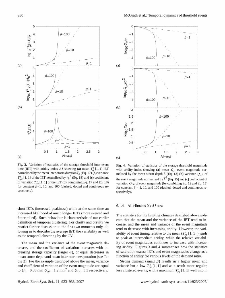
Fig. 3. Variation of statistics of the storage threshold inter-eventtime (IET) with aridity indexAI showing(a) meanT s

µ [1, 1] IETnormalised bythe mean inter-storm durationtb (Eq. 17)(b) varianceT sσ2 [1, 1] of the IET normalised bytb

2 (Eq. 18) and(c) coefficientof variationT s

cv [1, 1] of the IET (by combining Eq. 17 and Eq. 18)for constantβ=1, 10, and 100 (dashed, dotted and continuous re-spectively).

short IETs (increased peakiness) while at the same time anincreased likelihood of much longer IETs (more skewed andfatter tailed). Such behaviour is characteristic of our earlierdefinition of temporal clustering. For clarity and brevity werestrict further discussion to the first two moments only, al-lowing us to describe the average IET, the variability as wellas the temporal clustering by the CV.

The mean and the variance of the event magnitude de-crease, and the coefficient of variation increases with in-creasing storage capacity (largerα), or equal decreases inmean storm depth and mean inter-storm evaporation (see Ta-ble 2). For the example described above the mean, varianceand coefficient of variation of the event magnitude are equalto Qµ=0.33 mmQσ2=1.2 mm2 andQcv=3.3 respectively.

(a)

-4

-3

-2

-1

0

log 1

0QΜ�Γ

Β=1

Β=10Β=100

(b)

-4

-3

-2

-1

0

log 1

0QΣ

2�Γ

2

Β=1

Β=10Β=100

(c)

0.5 1 1.5 2 2.5 3AI=Α�Β

0.5

1

1.5

2

2.5

3

log 1

0Q

cv

Β=1

Β=10

Β=100

Fig. 4. Variation of statistics of the storage threshold magnitudewith aridity index showing(a) meanQµ event magnitude nor-malised by the mean storm depthh (Eq. 12)(b) varianceQσ2 of

the event magnitude normalised byh2

(Eq. 15) and(c) coefficient ofvariationQcv of event magnitude (by combining Eq. 12 and Eq. 15)for constantβ = 1, 10, and 100 (dashed, dotted and continuous re-spectively).

6.1.4 All climates 0<AI<∞

The statistics for the limiting climates described above indi-cate that the mean and the variance of the IET tend to in-crease, and the mean and variance of the event magnitudetend to decrease with increasing aridity. However, the vari-ability of event timing relative to the mean (T s

cv [1, 1] ) tendsto peak at intermediate aridity, while the relative variabil-ity of event magnitudes continues to increase with increas-ing aridity. Figures 3 and 4 summarises how the statisticsof saturation excess IETs and event magnitudes change as afunction of aridity for various levels of the demand ratio.

Strong demand (smallβ) results in a higher mean andvariance but a lowT s

cv [1, 1] and as a result more regular,less clustered events, with a maximumT s

cv [1, 1] well into in



the arid region (see Fig. 3). Strong demand also results in ahigher mean and variance of the event magnitude at the samearidity, but they tend to decrease as the aridity increases (seeFig. 4). While the mean and variance decrease with increas-ing aridity, the CV of the event magnitude increases.

The lower the demand, relative to the storage capacity(largerβ), the larger the mean and variance of the IET and thegreater the tendency for temporal clustering of events (largerT s

cv [1, 1]). The tendency for saturation excess events to clus-ter in time is most pronounced in deep stores when supplyequals demand i.e.AI=1. This is consistent with the obser-vation by Milly (2001) that as the storage capacity increasesthe maximum variance in soil moisture tends to peak nearerAI=1.

These results are at least qualitatively consistent with ob-servations of decreasing mean annual runoff with aridity(Budyko, 1974) and an increasing coefficient of variation ofannual runoff with a reduction in mean annual rainfall (Pot-ter et al., 2005). Temporal clustering has been observed inthe flood record (Franks and Kuczera, 2002; Kiem et al.,2003) however, this has been attributed to interactions be-tween the Inter-decadal Pacific Oscillation and the El NınoSouthern Oscillation changing rainfall patterns. Our quan-tification of temporal clustering here is based upon on a sta-tionary model of climate. We have as yet found no literaturequantifying saturation excess in terms of its temporal dynam-ics with which we can compare to the statistics derived here.

In summary our results suggest the following about thresh-old storage triggering: In very arid climates the relative vari-ability of the timing of events is low, as is the contributionof saturation excess to the water balance, as evidenced by alow mean event magnitude. However, the relative variabil-ity of the event magnitudeQcv is high; Saturation excessevents in semi-arid environments appear to be prone to highcoefficients of variation in both the magnitude of events andthe time between events, while contributing a non-negligibleproportion of the overall water balance; Sub-humid climateshave a large proportion of rainfall converted to runoff. Themagnitude of these events occur with a lowerQcv than semi-arid climates and temporal clustering may be a significantfeature of the dynamics; In humid climates storage thresholdevents contribute a significant proportion of the water bal-ance and the variability (relative to the mean) of the timingand magnitude of these events is low.

6.2 Frequency magnitude relationships

It is often the case that we can only observe directly the trig-gering of events but not the flux. For example the occur-rence of soil moisture above a critical value may indicatethat macropores are required to have been filled and as a re-sult preferential flow triggered. However, it is typically notpossible to measure the flux through either the soil matrixor the macropores, but only relative changes in storage. Thetiming of triggering and the magnitude of the events are re-

0.5 1 1.5 2 2.5 3AI

0.2

0.4

0.6

0.8

1

1.2

Tcvs@1

,1D�

Qcv

Β=1

Β=10Β=100

Fig. 5. Ratio of the coefficient of variation of event timingTcv [1, 1]and the coefficient of variation of the event magnitudeQcv as afunction of aridity. Dashing corresponds to constantβ=1 (largedashed),β=10 (dotted) andβ=100 (continuous).

lated to one another through soil moisture storage. Thereforein this section, we investigate the relationships between thestatistics of event timing and event magnitude.

6.2.1 Comparison of means

One would expect that the more frequently threshold stor-age events occur the greater the contribution of saturationexcess to the overall water balance. In fact for the thresh-old storage model the dimensionless mean saturation ex-cess event magnitude equals the dimensionless mean satu-ration excess frequency i.e.Qµ

/

h=tb/

T sµ [1, 1] as shown

by comparing Eq. (12) and Eq. (17). This makes physicalsense, for example whenT s

µ [1, 1] =∞, Qµ must be zero,

and whentb=T sµ [s0, 1], Qµ must equalh. Noting that

N=T sµ [1, 1]

/

tb describes the mean number of storms in the

IET, it can be shown using Eq. (11) thatQµ

/

h=tb/

T sµ [1, 1]

is equivalent toEa=h(

N − 1) /

N . More specifically thisindicates that the inputs (rainfall) must be greater than thelosses (actual evaporation) in the time between successiveevents. Intuitively this must be true irrespective of the na-ture of the loss functionL [s]. Whether such a relationshipbetween mean event magnitude and mean event frequencyshould hold for more general loss functionsL [s] is yet to beshown.

6.2.2 Comparison of relative variability

In addition to the issue of observability mentioned at the be-ginning of Sect. 6.2 the relationship between the variabilityof event magnitudes and the variability of the timing of eventtriggering may have important ecological implications. Forexample Sher et al. (2004) noted that the temporal variabilityof resource supply events in arid ecosystems may be as oreven more important ecologically than the variability in the



(a)

0.2 0.4 0.6 0.8 1SΜ

1

2

3

4

5lo

g 10

TΜs@1

,1D�

t� b

Β=1

Β=10

Β=100

(b)

0.02 0.04 0.06 0.08 0.1 0.12SΣ2

2

4

6

8

Tcvs@1

,1D

Β=1

Β=10

Β=100

(c)

0

0.5

1

Sto

rage@-D

✷

0

0.5

1

Sto

rage@-D

△

50 100 150 200 250 300Day

0

0.5

1

Sto

rage@-D

✸

Fig. 6. Relationship between soil moisture storage and the temporaldynamics showing(a) Mean inter-event timeT s

µ [1, 1] as a functionof mean soil moistureSµ; (b) Coefficient of variation of the inter-event timeT s

cv [1, 1] as a function of the variance of soil moistureSσ2; and(c) Soil moisture time series corresponding to symbols in(a) and (b). Dashing corresponds to constantβ=1 (large dashed),β=10 (dotted) andβ=100 (continuous). Time series generated asdescribed in Sect. 5.1 withtb=1 day,Em=0.5 mm/day,w0=5 mmandh=0.307 mm (✷), h=0.536 mm (△), andh=1.66 mm (✸).

magnitude of such events. Here we compare how the CV ofIETs relates to the CV of event magnitude in terms of theirratioT s

cv [1, 1] /Qcv as a function of aridity (see Fig. 5).For all climatesT s

cv [1, 1] ≤ Qcv. In humid climatesT s

cv [1, 1] ∼Qcv meaning event timing and the magnitude ofevent per storm are both similarly variable with respect totheir means. In very arid climatesT s

cv [1, 1] <Qcv indicatingless variability in event timing relative to its mean in compar-ison to event magnitude.

The ratio approaches a step function in the limit of a largestorage capacity, relative to the climatic forcing i.e. largeβ

(or α not shown), and the step occurs around an aridity in-dex of 1. Mean soil moisture essentially behaves the sameway when the storage capacity is large i.e. it is very close tosaturation for allAI<1 and very close to zero for allAI>1(Milly, 2001). The smaller the storage capacity relative tothe climate forcing (smallβ) the lower the aridity at whichT s

cv [1, 1] andQcv can be differentiated and the more grad-ual and smaller the difference with increasing aridity in com-parison to larger capacities. Therefore large stores are ex-pected to display much larger flux variability than temporalvariability. Despite increased variability in the timing of sat-uration excess events for deeper stores for sub-humid andsemi-arid environments (see Fig. 3), event magnitude vari-ability increases much more rapidly with increasing aridityand continues to do so forAI>1.

In terms of the issue of observability our results suggestthat the temporal variability of event triggering may givesome understanding of the relative variability of event mag-nitude in humid climates as they are of a similar magnitude inthis region. Based upon the relationship between mean eventfrequency and mean event magnitude the variance of eventmagnitude per storm event might even be estimated reason-ably. In arid climatesT s

cv [1, 1] is much less thanQcv andtells little about the event magnitude variability but none theless provides a reasonably certain measure (i.e. a standarddeviation about the same as the mean) of the variability ofevent timing.

Returning to the hypothesis of Sher et al. (2004), our re-sults suggest that the variability of the timing of potentialresource supply events, despite being of long duration on av-erage, is small in comparison to the mean. The temporalvariability is also much less than the variability in the mag-nitude of supply, at least on a per storm basis. This suggeststhat adaptations by plants and animals to cope with temporalvariability may be particularly beneficial in arid climates asit may be a reasonably certain (low variability) component ofthe hydrological variability.

6.3 Relationship between temporal statistics and storage

For some hydrological processes neither the flux nor the trig-gering are directly observable at the space and time scales atwhich they occur in the field. This is true in particular forpreferential flow. What is measurable, at least at the pointscale, is soil moisture storage. Therefore we explore herefirst how the temporal statistics relate to the statistics of stor-age and then the sensitivity of the temporal statistics to theinitial storage.

6.3.1 Triggering and soil moisture variability

Figure 6a shows the relationship between the dimensionlessmean saturation excess IETT s

µ [1, 1] and the mean storage



Sµ for constant evaporative demand (constantβ). This canalso be seen in the time series of storage Fig. 6c correspond-ing to the symbols in Fig. 6a. The mean IET increases non-linearly as the mean storage decreases, and also increaseswith increasing storage capacity (increasing values ofβ).The mean IET is most sensitive to changes in low mean soilmoisture. This sensitivity is also high at very high mean soilmoisture when the storage capacity is large relative to theclimatic forcing (largeβ).

It is evident by comparing the time series Fig. 6c andFig. 6a that high mean soil moisture is related to low soilmoisture variability and frequent event triggering. Low soilmoisture variability is also associated with a low mean soilmoisture and infrequent triggering. High variability in soilmoisture tends to be associated with intermediateSµ as thereis a greater potential for soil moisture fluctuations to explorethe entire capacity. This large variability in soil moisture isalso associated with high temporal clustering. It can be seenfrom the relationship betweenT s

cv [1, 1] and the variance ofstorageSσ2 (Fig. 6b) that for a constant evaporative demand(constantβ), the maximumT s

cv [1, 1] occurs whenSσ2 is alsoa maximum. This appears to be true for all but the smalleststores (seeβ=1 in Fig. 6b) but in this instance the degree oftemporal clustering is low in any case.

6.3.2 The role of initial storages0

So far we have largely discussed the controls on the IET, thatis the time between successive occurrences of storage at ca-pacity. The analytical derivation of FPT statisticsTx [s0, 1]allows us to determine the rainfall controls on the statisticalproperties of the time to trigger saturation excess flow forthe first time since an arbitrary initial storages0. Figure 1bshows this FPT asτ1.

The relevance is best explained by the following analogy.Let us assume that storage in the near surface determines theoccurrence of preferential flow in a highly nonlinear, thresh-old like way. We also know from an experiment that there isa rapid movement of rainfall to groundwater via this mecha-nism. If we take a measurement of the near surface soil mois-ture, that measurement is an initial condition relative to thetime of measurement. As it turns out our analysis (the FPTstatistics) reveals that this state of the system determines ourlevel of certainty about the time till the next preferential flowevent. Therefore we now have a measure of risk, the meanand variance of the time till the next pesticide leaching eventby preferential flow, on the basis of a single measurementof storage. This risk measure includes our knowledge of thestructure of rainfall as well as our uncertainty of the timingand magnitude of rainfall events yet to to come.

Figure 7 shows the effect of initial storage on the mean andthe CV of the time till the next saturation excess triggering.It can be seen that the mean FPTTµ [s0, 1] decreases ass0increases towards saturation and is more sensitive tos0 athigher soil moisture values. Also, as expected, the mean FPT

(a)0.2 0.4 0.6 0.8 1

0.5

1

1.5

2

2.5

3

3.5

Log 1

0TΜ@s

0,1D

Α=10 Β=10

Α=10 Β=3

Α=3 Β=10

(b)

0.2 0.4 0.6 0.8 1s0

0.5

1

1.5

2

2.5

3

TC

V@s

0,1D

Fig. 7. First passage time statistics vs. the initial soil moistures0.Shown are:(a) the meanTµ

[

s0, 1]

; and(b) the coefficient of vari-ationTcv

[

s0, 1]

; of the time to reachs=1 since an initial soil mois-tures0.

is longer the higher the aridity (compare ratios ofα andβ inFig. 7). On the other hand the CV of the FPTTcv [s0, 1]increases with increasing initial storage. At lows0 the morehumid the climate the lowerTcv [s0, 1] but this transitions athighers0 such that the more balanced climates and systemswith deeper storage capacity, relative to the climatic forcing(largerα andβ), tend to have a largerTcv [s0, 1].

Values ofTcv [s0, 1] whens0 is low are≤ 1. This can beexplained for the case of arid climates where the closers0 isto zero, as well as being close toSµ, only extreme rainfallwill trigger an event and for reasons discussed in Sect. 6.1.2event triggering displays similar but scaled statistical proper-ties to the rainfall. The more humid the climate the furtheraways0=0 is toSµ and one would expect a more steady, lessvariable, increase in storage towards capacity and therefore alowerTcv [s0, 1].

On the other hand when a storage threshold flow event hasjust occurred (s0 = 1) the mean time till the next flow eventis a minimum andTcv [s0, 1] is a maximum.Tcv [s0, 1] is ameasure of our uncertainty, relative to our expected value,of the timing of the next storage threshold event due to ouruncertainty in the timing and magnitude of rainfall. This im-plies that if a SE event has just occurred, while we can expecta second event to occur sooner than at any other time, ourability to predict when that will be, relative to the mean time,is actually at its poorest. The high variability of IETs when



the initial soil moisture is at saturation we believe is due tothe greater potential for both much longer periods betweenevents, as a result of the greater potential for drying, as wellas a high potential for shorter IETs due to the high potentialfor event triggering when storage is near capacity.

The variability of threshold hydrological processes seemssensitive to an initial storage near a threshold. Zehe andBloschl (2004) also found the variability of modelled plotand hillslope scale runoff to be highest when initial soil mois-ture was at a threshold. In their case they considered a sin-gle prescribed rainfall event but multiple realisations of sub-scale spatial variability of initial soil moisture in relation tothe spatially averaged initial soil moisture. When the spa-tially averaged soil moisture was at the threshold betweenmatrix flow and preferential flow, the variability of modelledrunoff was at its greatest.Tcv [s0, 1] is a measure of our un-certainty in the timing of the next event due to our uncer-tainty of the timing and magnitude of future rainfall eventson the basis of a measurement of storage. Additionally thevariability in runoff described by Zehe and Bloschl (2004) isa measure of uncertainty in the magnitude of the event due toan uncertain structure of sub-scale soil moisture. Combiningthese two results it suggests that the time between two con-secutive threshold flow events for which the flux is poorlypredictable is itself highly uncertain.

7 Summary and conclusions

Typically in hydrology we consider the transformation offlux(es) (rainfall, evaporation) to a flux (runoff). Here insteadwe focus on the transformation of (rainfall) event timing to(flow) event timing. We analytically derived statistics of thetemporal dynamics of the flow triggering due to a rainfall in-tensity threshold and a soil moisture threshold as models forinfiltration excess and saturation excess flow mechanisms re-spectively. The intensity threshold lead to dynamics that didnot change the form of the IET pdf. The storage thresholddid change the form of the IET pdf leading to temporal clus-tering of events which tended to peak around an aridity indexof one for deep stores.

The mean and the variance of the SE inter-event time werefound to increase with increasing climate aridity. The meanand the variance of the SE event magnitude per storm, de-creases with increasing aridity, while the CV increases withincreasing aridity. It is already established that hillslope sat-uration excess may dominate in humid climates and to beless significant in arid climates however, the results presentedhere is the first time that there has been a quantification of therelationships between the temporal structure of event timing,the magnitude of events and the storage across climate gra-dients.

While the two mechanisms explored are overly simplis-tic descriptions of real world processes, the results fromthese two extreme triggers suggest that the actual temporal

pattern of triggering will display a mixture of the unclus-tered and clustered dynamics observed here. There is alsoa need to better identify and predict thresholds which gov-ern some processes. For example Lehmann et al. (2006, thisissue) suggest that the threshold storm amount, governingpipe flow in steep forested hillslopes, may be an emergentproperty of the connectivity of zones of transient saturationat the soil/bedrock interface. However, there is currently lit-tle understanding of what determines the magnitude of thesethresholds at different sites (Uchida et al., 2005).

For analytical tractability we have neglected naturally tem-porally clustered rainfall that may occur at event to inter-annual time scales (Menabde and Sivapalan, 2000; Franksand Kuczera, 2002). The impact of temporally clustered rain-fall we expect will depend upon the degree of memory in thesystem which would be parameterised by the magnitude of amodifiedβ term. Systems with a smallβ would have littlememory of long rainfall IETs, while a largeβ would havethe potential to “remember” the clustered nature of rainfall.The results presented here will likely be significantly mod-ified when considering climates with strong seasonality andthis requires further investigation.

From the frequency-magnitude relationships we found thatthe dimensionless mean SE event magnitude was equal tothe dimensionless mean event frequency and the coefficientof variation of SE event magnitude was found to be alwaysgreater than, or at least equal to, the CV of the IET. Whileno aridity relationships were established for IE, it may bepossible to evaluate the contribution of IE as a deviation fromthe frequency-magnitude relationships derived here. Finallywe also established inter-relationships between storage andtiming, with a peak in the variance of soil moisture reflectingthe peak in temporal clustering of events.

Validation of the results presented here was beyond thescope of this paper. The generality of this work provides themeans to develop hypotheses and test the many assumptionswith numerical and empirical studies. The question of whatto measure and how will depend upon the process under con-sideration but ideally simulataneous measurments of eventbased flux, timing and storage in the context of the climateare required to further develop these ideas. Re-analysis ofexisting threshold phenomena in the context of the temporaldynamics of the process and rainfall may provide an alter-native. Such data may include long or ensemble records ofoverland flow, stream sediment dynamics, pesticide leaching,and pipe flow for example.



Appendix A

Derivation of saturation excess temporal statistics

The integral equation for the pdf of FPTs,gT , for processeslike the saturation excess one described in this paper wasgiven by (Laio et al., 2001) as:

∂g (t |s0)

∂t= − L [s0]

∂g (t |s0)

∂s0−

g (t |s0)

tb

+1

tb

∫ sξ

s0

fH [z − s0] g (t |z) dz (A1)

whereL [s0] [T−1] is the rate of losses from storage at an ini-tial storages0, at timet=0, fH [-] is the pdf of storm depthsnormalised by the storage capacity,z is a dummy variableof integration, andsξ is an arbitrary threshold soil moisture.The raw moments of the FPT are by definition:

T sn

[

s0, sξ]

=∫ ∞

0tngT (t |s0) dt (A2)

Eq. (A2) motivates us to generalise the derivation to higherorder moments by multiplying Eq. (A1) bytn, instead oft tojust get the mean as done by Laio et al. (2001). So multiply-ing Eq. (A1) by tn, assuming normalised storm depths areexponentially distributed and integrating by parts the timederivative and substitutingT s

n

[

s0, sξ]

, results in the follow-ing integro-differential equation for the FPT moments:

− nT sn−1

[

s0, sξ]

= − L [s0]dT s

n

[

s0, sξ]

ds0−

T sn

[

s0, sξ]

tb+

α

tb

∫ sξ

s0

e−α(z−s0)T sn

[

z, sξ]

dz (A3)

Integrating by parts the integral term in Eq. (A3), differen-tiating the entire equation with respect tos0, and substitutingfor the integral term by rearranging Eq. (A3), leads to a sec-ond order ordinary differential equation for the FPT momentsT s

n :

L [s0]d2T s

n

ds20

+dT s

n

ds0

(

dL [s0]

ds0− αL [s0] +

1

tb

)

=dT s

n−1

ds0− nαT s

n−1 (A4)

The general solution to Eq. (A4) is given by:

T sn [s0, sξ ]=C2+C1

∫ s0

1B1 [w, 1] dw+

∫ s0

1B2 [w, 1] dw

(A5)where:

ln(B1[a, b])=α (a − 1) +∫ b

a

1

L[x]

(

1

tb+

dL[x]dx

)

dx

(A6)

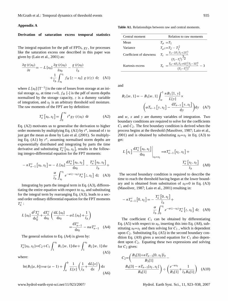
Table A1. Relationships between raw and central moments.

Central moment Relation to raw moments

Mean Tµ =T1

Variance Tσ2=T2 − T 21

Coefficient of skewness Tε =T3−3T1T2+2T 31

(

T2−T 21

)

3/2

Kurtosis excess Tκ =T4−4T1T3+6T 21 T2−3T 4

1(

T2−T 21

)2 − 3

and

B2 [w, 1] = − B1[w, 1]∫ 1

w

nB1 [1, y]

L[y]×

(

αTn−1[

y, sξ]

−dTn−1

[

y, sξ]

dy

)

dy (A7)

and w, x and y are dummy variables of integration. Twoboundary conditions are required to solve for the coefficientsC1 andC2. The first boundary condition is derived when theprocess begins at the threshold (Masoliver, 1987; Laio et al.,2001) and is obtained by substitutings0=sξ in Eq. (A3) toget:

L[

sξ] dT s

n

[

s0, sξ]

ds0

∣

∣

∣

∣

∣

s0=sξ

=nT sn−1

[

sξ , sξ]

+

T sn

[

sξ , sξ]

tb(A8)

The second boundary condition is required to describe thetime to reach the threshold having begun at the lower bound-ary and is obtained from substitution ofs0=0 in Eq. (A3)(Masoliver, 1987; Laio et al., 2001) resulting in:

− nT sn−1

[

0, sξ]

= −T s

n

[

0, sξ]

tb+

α

tb

∫ sξ

0e−α(z−s0)T s

n

[

z, sξ]

dz (A9)

The coefficientC1 can be obtained by differentiatingEq. (A5) with respect tos0, inserting this into Eq. (A8), sub-stitutings0=sξ and then solving forC1 , which is dependentuponC2. Substituting Eq. (A5) in the second boundary con-dition Eq. (A9) gives a second equation forC1 also depen-dent uponC2. Equating these two expressions and solvingfor C2 gives:

C2=(

B3[3]+nTn−1[0, sξ ]tbB3[1]

−

B4[3] − nTn−1[sξ , sξ ]B4[1]

)

÷(

e−αsξ

B3[1]+

1

tbB4[1]

)

(A10)



where

B4[A]=L[sξ ]BA[sξ , 1] −1

tb

∫ 1

s0

BA[w, 1]dw (A11)

and

B3[A]=∫ sξ

0αe−zα

∫ z

1BA[w, 1]dw dz+

∫ 1

0BA[w, 1]dw (A12)

The subscriptA is a reference toBA as given by Eq. (A6)or Eq. (A7). Substituting Eq. (A10) into one of the originalexpressions forC1 gives:

C1= −(

nTn−1[

sξ , sξ]

− eαsξ(

nTn−1[

0, sξ]

+

B3 [3]

tb

)

− B4 [3])

÷( 1

tbeαsξ B3 [1] +B4 [1]

)

(A13)

The central moments can be derived from these raw mo-ments using the relationships described in Table A1 and asdiscussed in Sect. 5.2.

Appendix B

List of Symbols

Symbol Description Units

Soil parametersIξ Infiltration capacity L/Tw0 Storage capacity Ls Normalised soil moisture storage –s0 Initial soil moisture –sξ Threshold soil moisture –

Climate parameters

h Storm depth Lh Mean storm depth Ltb Inter storm duration Ttb Mean inter-storm duration TEm Potential evaporation L/TImax Max within storm rainfall intensity L/TImax MeanImax L/T

Probability terms

fX Probability density X−1 a

gT First passage time probability density T−1

P [ ] Probability –Continued. . .

aUnits X correspond to the random variable

Symbol Description Units

µ Mean Xσ Standard deviation Xσ 2 Variance X2

cv Coefficient of variation –ε Coefficient of skewness –κ Coefficient of kurtosis –

Dimensionless hydrological parameters and statistics

α Supply ratio –β Demand ratio –AI Aridity index –Ea Mean actual evaporation LN Mean number of storms in the IET –Qx Saturation excess event magnitude

statistic

a

Sx Soil moisture storage statistic –T I

x

[

Iξ

]

Infiltration excess IET statistic b

T rx Storm IET statistic b

T sx

[

s0, sξ]

Statistic of the time to reachsξ since aninitial soil moistures0

b

aUnits correspond toQµ [L], Qσ2 [L2], andQcv [−]bUnits correspond toTµ [T], Tσ2 [T2], Tcv [−], Tε [−],

andTκ [−]

Acknowledgements. The research was made possible by an Aus-tralia Postgraduate Award (Industry) from the Australian ResearchCouncil in conjunction with the Centre for Groundwater Studies. Inaddition GSM would like to thank A. Porporato for his assistanceand comments on an early manuscript.

Edited by: G. Hancock

References

Arora, V.: The use of the aridity index to assess climate changeeffect on annual runoff., J. Hydrol., 265, 164–177, 2002.

Bauters, T.: Soil water content dependent wetting front characteris-tics in sands., J. Hydrol., 231-232, 244–254, 2000.

Beven, K. and Germann, P.: Macropores and water flow in soils.,Water Resour. Res., 18, 1311–1325, 1982.

Budyko, M.: Climate and Life., Academic Press, New York, 1974.Crockford, R. and Richardson, D.: Partitioning of rainfall into

throughfall, stemflow and interception : effect of forest type,groundcover and climate, Hydrol. Process., 14, 2903–2920,2000.

Dekker, L. W., Doerr, S. H., Oostindie, K., Ziogas, A. K., and Rit-sema, C. J.: Water repellency and critical soil water content in adune sand, Soil Sci. Soc. Am. J., 65, 1667–1674, 2001.

Dunne, T.: Field studies of hillslope flow processes, in: HillslopeHydrology, (edited by: M. J. Kirkby), John Wiley and Sons,Chichester, West Sussex, UK, 1978.



Fitzjohn, C., Ternan, J., and Williams, A.: Soil moisture variabil-ity in a semi-arid gully catchment: implications for runoff anderosion control., Catena, 32, 55–70, 1998.

Fortin, J., Gagnon-Bertrand, E., Vezina, L., and Rompre, M.: Pref-erential bromide and pesticide movement to tile drains underdifferent cropping practices, J. Environ. Qual., 31, 1940–1952,2002.

Franks, S. W. and Kuczera, G.: Flood frequency analysis: Evidenceand implications of secular climate variability, New South Wales,Water Resour. Res., 38, 1062, doi:10.1029/2001WR000 232,2002.

Godano, C., Alonzo, M., and Vildaro, G.: Multifractal approachto time clustering of earthquakes: Application to Mt. Vesuvioseismicity, Pure and Appl. Geophys., 149, 375–390, 1997.

Haria, A. H., Johnson, A. C., Bell, J. P., and Batchelor, C. H.: Water-movement and isoproturon behavior in a drained heavy clay soil, 1. Preferential flow processes, J. Hydrol., 163, 203–216, 1994.

Heppell, C. M., Worrall, F., Burt, T. P., and Williams, R. J.: Aclassification of drainage and macropore flow in an agriculturalcatchment, Hydrol. Process., 16, 27–46, 2002.

Horton, R.: The role of infiltration in the hydrologic cycle., Trans.Am. Geophys. Union, 14, 446–460, 1933.

Hyer, K. E., Hornberger, G. M., and Herman, J. S.: Processes con-trolling the episodic streamwater transport of atrazine and otheragrichemicals in an agricultural watershed, J. Hydrol., 254, 47–66, 2001.

Kiem, A. S., Franks, S. W., and Kuczera, G.: Multi-decadalvariability of flood risk, Geophys. Res. Let., 30, 1035,doi:10.1029/2002GL015 992, 2003.

Kjær, J., Olsen, P., Ullum, M., and Grant, R.: Leaching ofGlyphosate and Amino-Methylphosphonic Acid from Danishagricultural field sites., J. Environ. Qual., 34, 608–620, 2005.

Kohler, A., Abbaspour, K. C., Fritsch, M., and Schulin, R.: Us-ing simple bucket models to analyze solute export to subsurfacedrains by preferential flow, Vadose Zone J., 2, 68–75, 2003.

Kung, K.-J.: Preferential flow in a sandy vadose zone, 2 : Mecha-nisms and implications., Geoderma, 22, 59–71., 1990.

Laabs, V., Amelung, W., Pinto, A., and Zech, W.: Fate of pesti-cides in tropical soils of Brazil under field conditions, J. Environ.Qual., 31, 256–268, 2002.

Laio, F., Porporato, A., Ridolfi, L., and Rodriguez-Iturbe, I.: Meanfirst passage times of processes driven by white shot noise, Phys-ical Rev. E, 6303, 2001.

Lehmann, P., Hinz, C., McGrath, G., Tromp-van Meerveld, H. J.,and McDonnell, J. J.: Rainfall threshold for hillslope outflow: anemergent property of flow pathway connectivity., Hydrol. EarthSys. Sci. Discussions, 3, 2923–2961, 2006.

Masoliver, J.: 1st-Passage times for non-Markovian processes -Shot noise, Physical Rev. A, 35, 3918–3928, 1987.

Menabde, M. and Sivapalan, M.: Modeling of rainfall time seriesand extremes using bounded random cascades and Levy-stabledistributions, Water Resour. Res., 36, 3293–3300, 2000.

Milly, P. C. D.: An analytic solution of the stochastic storage prob-lem applicable to soil-water, Water Resour. Res., 29, 3755–3758,1993.

Milly, P. C. D.: Climate, interseasonal storage of soil-water, and theannual water-balance, Adv. Water Resour., 17, 19–24, 1994.

Milly, P. C. D.: A minimalist probabilistic description of root zonesoil water, Water Resour. Res., 37, 457–463, 2001.

Mosley, M.: Streamflow generation in a forested watershed., WaterResour. Res., 15, 795–806, 1976.

Papoulis, A.: Probability, Random Variables and Stochastic Pro-cesses, 3rd ed., McGraw-Hill, New York, 2001.

Potter, N. J., Zhang, L., Milly, P. C. D., McMahon, T. A., and Jake-man, A. J.: Effects of rainfall seasonality and soil moisture ca-pacity on mean annual water balance for Australian catchments,Water Resour. Res., 41, W06 007, doi:10.1029/2004WR003 697,2005.

Ridolfi, L., D’Odorico, P., Porporato, A., and Rodriguez-Iturbe, I.:Duration and frequency of water stress in vegetation: An analyt-ical model, Water Resour. Res., 36, 2297–2307, 2000.

Rodriguez-Iturbe, I. and Isham, V.: Some models for rainfall basedon stochastic point processes, Proc. Royal Soc. Lond. Ser. A-Math. Phys. Eng. Sci., 410, 269–288, 1987.

Rodriguez-Iturbe, I., Porporato, A., Ridolfi, L., Isham, V., and Cox,D. R.: Probabilistic modelling of water balance at a point: therole of climate, soil and vegetation, Proc. Royal Soc. Lond. Ser.A-Math. Phys. Eng. Sci., 455, 3789–3805, 1999.

Rodriguez-Iturbe, I., Porporato, A., Laio, F., and Ridolfi, L.: Plantsin water controlled ecosystems: active role in hydrologic processand response to water stress. I Scope and general outline., Adv.Water. Resour., 24, 695–705, 2001.

Rundle, J. B., Turcotte, D. L., Rundle, P. B., Yakovlev, G.,Shcherbakov, R., Donnellan, A., and Klein, W.: Pattern dynam-ics, pattern hierarchies, and forecasting in complex multi-scaleearth systems., Hydrol. Earth Syst. Sci. Discuss., 3, 1045–1069,2006,http://www.hydrol-earth-syst-sci-discuss.net/3/1045/2006/.

Sher, A., Goldberg, D., and Novoplansky, A.: The effect of meanand variance in resource supply on survival of annuals fromMediterranean and desert environments., Oecologica, 141, 353–362, 2004.

Struthers, I., Sivapalan, M., and Hinz, C.: Conceptual examina-tion of climatesoil controls upon rainfall partitioning in an open-fractured soil: I. Single storm response, Adv. Water Resour., 30(3), 505–517, 2007a.

Struthers, I., Sivapalan, M., and Hinz, C.: Conceptual examina-tion of climate soil controls upon rainfall partitioning in an open-fractured soil II: Response to a population of storms, Adv. WaterResour., 30 (3), 518–527, 2007b.

Teich, M., Heneghan, C., Lowen, S., Ozaki, T., and Kaplan, E.:Fractal character of the neural spike train in the visual system ofthe cat, J. Opt. Soc. Am. A, 14, 529–545, 1997.

Tromp-van Meerveld, H. and McDonnell, J.: Threshold relationsin subsurface stormflow 1. A 147 storm analysis of the Panolahillslope., Water Resour. Res., 42, 2006.

Uchida, T., van Meerveld, I. T., and McDonnell, J.: The role of lat-eral pipe flow in hillslope outflow response: an intercomparisonof non-linear hillslope response., J. Hydrol., 311, 117–133, 2005.

Wang, Z., Feyen, J., and Ritsema, C.: Susceptibility and predictabil-ity of conditions for preferential flow., Water Resour. Res., 34,2183–2190, 1998.

Whipkey, R.: Subsurface stormflow from forested slopes., Bull. Int.Assoc. Sci. Hydrol., 10, 74–85, 1965.

Wood, M. A., Simpson, P. M., Stambler, B. S., Herre, J. M., Bern-stein, R. C., and Ellenbogen, K. A.: Long-term temporal pat-terns of ventricular tachyarrhythmias., Circulation, 91, 2371–2377, 1995.


http://www.hydrol-earth-syst-sci-discuss.net/3/1045/2006/


Zehe, E. and Bloschl, G. N.: Predictability of hydrologic responseat the plot and catchment scales: Role of initial conditions, WaterResour. Res., 40, W10 202, doi:10.1029/2003WR002 869, 2004.

Zeng, N., Shuttleworth, J., and Gash, J.: Influence of temporal vari-ability of rainfall on interception loss. Part I. Point analysis., J.Hydrol., 228, 228–241, 2000.


Temporal dynamics of hydrological threshold events

Documents

Transcript of Temporal dynamics of hydrological threshold events