Hydrological modelling using convective scale rainfall modelling
240
Hydrological modelling using convective scale rainfall modelling – phase 3 Project: SC060087/R3
-
Upload
khangminh22 -
Category
Documents
-
view
0 -
download
0
Transcript of Hydrological modelling using convective scale rainfall modelling

Hydrological modelling using convective scale rainfall modelling – phase 3 Project: SC060087/R3

ii Hydrological modelling using convective-scale rainfall modelling – phase 3
The Environment Agency is the leading public body protecting and improving the environment in England and Wales.
It’s our job to make sure that air, land and water are looked after by everyone in today’s society, so that tomorrow’s generations inherit a cleaner, healthier world.
Our work includes tackling flooding and pollution incidents, reducing industry’s impacts on the environment, cleaning up rivers, coastal waters and contaminated land, and improving wildlife habitats.
This report is the result of research commissioned by the Environment Agency’s Evidence Directorate and funded by the joint Environment Agency/Defra Flood and Coastal Erosion Risk Management Research and Development Programme.
Published by: Environment Agency, Rio House, Waterside Drive, Aztec West, Almondsbury, Bristol, BS32 4UD Tel: 01454 624400 Fax: 01454 624409 www.environment-agency.gov.uk ISBN: 978-1-84911-180-5 © Environment Agency – February, 2010 All rights reserved. This document may be reproduced with prior permission of the Environment Agency. The views and statements expressed in this report are those of the author alone. The views or statements expressed in this publication do not necessarily represent the views of the Environment Agency and the Environment Agency cannot accept any responsibility for such views or statements. This report is printed on Cyclus Print, a 100% recycled stock, which is 100% post consumer waste and is totally chlorine free. Water used is treated and in most cases returned to source in better condition than removed. Email: [email protected]. Further copies of this report are available from our publications catalogue: http://publications.environment-agency.gov.uk or our National Customer Contact Centre: T: 08708 506506 E: [email protected].
Author(s): J. Schellekens, A.R.J. Minett, P. Reggiani, A.H. Weerts (Deltares); R.J. Moore, S.J. Cole, A.J. Robson,V.A. Bell (CEH Wallingford) Dissemination Status: Released to all regions Publicly available Keywords: Hydrological modelling, Probabilistic forecasts, Distributed Models, MOGREPS, STEPS Research Contractor: Rotterdamseweg 185, Delft, The Netherlands P.O. Box 177. 2600 MH Delft, The Netherlands tel: + 31 (0)88 335 8273 fax : +31 (0)88 335 8582 Environment Agency’s Project Manager: Simon Hildon, Evidence Directorate Theme manager: (acting) Stefan Laeger, Incident Management and Community Engagement Theme Collaborator(s): CEH Wallingford; Deltares Project Number: SC060087 Product Code: SCHO0210BRYT-E-P

Hydrological modelling using convective-scale rainfall modelling – phase 3 iii
Evidence at the Environment Agency Evidence underpins the work of the Environment Agency. It provides an up-to-date understanding of the world about us, helps us to develop tools and techniques to monitor and manage our environment as efficiently and effectively as possible. It also helps us to understand how the environment is changing and to identify what the future pressures may be.
The work of the Environment Agency’s Evidence Directorate is a key ingredient in the partnership between research, policy and operations that enables the Environment Agency to protect and restore our environment.
The Research & Innovation programme focuses on four main areas of activity:
• Setting the agenda, by informing our evidence-based policies, advisory and regulatory roles;
• Maintaining scientific credibility, by ensuring that our programmes and projects are fit for purpose and executed according to international standards;
• Carrying out research, either by contracting it out to research organisations and consultancies or by doing it ourselves;
• Delivering information, advice, tools and techniques, by making appropriate products available to our policy and operations staff.
Miranda Kavanagh
Director of Evidence

iv Hydrological modelling using convective-scale rainfall modelling – phase 3
Executive summary This project explores hydrological model concepts and associated computational methods that make best use of the latest Met Office technology in high resolution and probabilistic rainfall forecasting. Regional case studies in the South West and the Midlands were used to evaluate the hydrological models, and these were subsequently extended to include a nationwide test of the G2G (Grid-to-Grid) distributed hydrological model. The potential for operational use of ensemble rainfall forecast products such as MOGREPS (Met Office Global and Regional Ensemble Prediction System), STEPS (Short-Term Ensemble Prediction System) and NWP (Numerical Weather Prediction) were also investigated.
Two test cases were used in the project: the Boscastle flood of August 2004 in South West Region and the June/July 2007 floods in the Midlands. For these studies, existing or newly calibrated lumped hydrological models were used as benchmarks against which to assess the potential value of a distributed hydrological modelling approach to flood forecasting. For the Boscastle study, a split sample method was used where distinct calibration and verification periods were identified. For the Midlands test case (which was modelled as part of the nationwide study), paired benchmark catchments were identified, one of each pair being treated as gauged and the other as ungauged. The hydrological modelling included two lumped rainfall-runoff models of the type used operationally - the PDM (Probability Distributed Model) and MCRM (Midlands Catchment Runoff Model) – together with two distributed hydrological models: the physics-based REW (Representative Elementary Watershed) model (Boscastle test case only) and the physical-conceptual G2G model.
For the Boscastle test case, model performance ranged from good to excellent for catchments across the Tamar and Camel river basins. The lumped PDM model performed best, followed by the G2G model and then the REW model. For both the distributed models, the performance for ungauged sites was similar to the performance for gauged sites indicating the potential of these models to forecast floods at ungauged river locations. When used in combination with different resolution (12, four and one km) NWP model rainfall forecasts, hydrological models performed best using the higher resolution forecasts, with the greatest performance moving from 12 to four km. When driven with a pseudo-ensemble of high resolution NWP rainfall forecasts (produced by random position displacements within a defined radius) the distributed model was better able to capture differences between the ensemble members. The generated hydrographs showed a spread in size and shape that sensibly reflected the changing position of the storm pattern over the catchments assessed.
The test case over the Midlands considered rural and urban catchments of low relief in the Avon and Tame river basins respectively, providing a more challenging modelling problem than the higher relief Tamar and Camel catchments of the Boscastle test case. The G2G model was assessed with reference to the summer 2007 floods, using the lumped MCRM as a benchmark model reflecting operational practice in the Midlands. Whilst the site-specific lumped models, as expected, proved hard to improve, the G2G model performed well across a range of catchment types. However, problems arose where the natural flow regime was affected by water imports/exports in urban catchments. Floods in summer 2007 were examined in detail using ensemble rainfall forecasts from NWP and STEPS. Their use for flood warning is illustrated in flood risk maps showing the probability of exceedance of flows of a given return period, either as a spatial time series as the flood propagates through the river system or at a given time over a forecast horizon of given length. The sensitivity of the G2G model to the spatio-temporal structure of storms makes it particularly suitable for ensemble rainfall forecasts for probabilistic flood forecasting of convective-scale events.

Hydrological modelling using convective-scale rainfall modelling – phase 3 v
The success of the G2G model in the Boscastle test case resulted in a project extension to consider a nationwide study of the G2G model across England and Wales. Performance proved to be mixed, with R2 efficiency averaging 0.56 over a two-year period encompassing the summer 2007 floods. Model calibration and assessment was affected by problems with rainfall data obtained from the operational National Flood Forecasting System (NFFS) archive and by unaccounted for catchment abstractions and returns. Assessment using benchmark pairs of gauged/ungauged catchments indicates that the G2G model gives comparable performance for both, confirming its utility for forecasting at ungauged catchments. The G2G model offers a practical approach to nationwide flood forecasting that complements more detailed regional flood forecasting systems. It is able to represent a wide range of hydrological behaviours through its link with terrain and soil properties. The distributed model forecasts, however, are best used alongside, and not instead of, those from lumped catchment models in typical rainfall conditions.
The possibilities for using MOGREPS and STEPS ensemble rainfall forecast products were investigated within the current NFFS configurations for North East and Thames regions. Evaluation included configuration issues, data volumes, run times and options for displaying probabilistic forecasts within NFFS. A nationwide calibration of the G2G model was also tested in an operational NFFS environment and a trial system has been running since summer 2009. Although available, ensemble rainfall forecasts from MOGREPS were not extensive enough to fully verify its performance. Nevertheless, the use of MOGREPS in current Environment Agency regional forecasting can provide better information to the forecaster than deterministic forecasts alone. In addition, with careful configuration in NFFS, MOGREPS can be used in existing systems without a significant increase in system load. Configuration of STEPS ensemble rainfall forecasts for use as hydrological model input was demonstrated within the NFFS environment, and required relatively little effort to implement. No verification of the actual performance was possible.

vi Hydrological modelling using convective-scale rainfall modelling – phase 3
Contents
Executive summary iv
Contents vi
1 Introduction 1
2 Project approach 3 2.1 Objectives 3 2.2 Using convective-scale rainfall forecasts in NFFS 3
2.2.1 High resolution numerical weather prediction 3 2.2.2 Hydrological modelling 4 2.2.3 Analysis 4 2.2.4 Verification 5
2.3 Operational implementation of ensemble forecasting 5 2.4 National calibration of the G2G model 6 2.5 Operational implementation of nationwide G2G model 6
3 Hydrological models used in the project 7 3.1 Background 7 3.2 Distributed hydrological models 9
3.2.1 G2G 9 3.2.2 REW 16 3.2.3 Comparison of G2G and REW distributed hydrological models 23
3.3 Lumped benchmark models 26 3.3.1 PDM 26 3.3.2 TCM 28 3.3.3 MCRM 30
4 Test case: Boscastle, 16 August 2004 34 4.1 Introduction 34 4.2 Meteorological synopsis 34 4.3 Flood damage 35 4.4 Catchment information 35 4.5 Configuration of models and data 38 4.6 Model assessment strategy 42 4.7 REW model application 43
4.7.1 Terrain analysis 43 4.7.2 REW model setup 44 4.7.3 Camel 44 4.7.4 Tamar 50 4.7.5 Model performance (simulation mode) 54 4.7.6 Model performance (forecasting mode) 61

Hydrological modelling using convective-scale rainfall modelling – phase 3 vii
4.8 PDM model application 68 4.8.1 Model setup 68 4.8.2 Tamar at Gunnislake 68 4.8.3 Ottery at Werrington 69 4.8.4 Camel at Denby 70 4.8.5 Model performance (simulation mode) 71 4.8.6 Model performance (forecast mode) 75
4.9 G2G model application 77 4.9.1 Model setup 77 4.9.2 Tamar catchment 77 4.9.3 Camel catchment 79 4.9.4 Model performance (simulation mode) 81 4.9.5 Model performance (forecast mode) 82 4.9.6 Extended G2G model results 82
4.10 Use of high-resolution NWP rainfall and ensemble forecasting 86 4.10.1 High-resolution NWP forecasts 86 4.10.2 Generation of pseudo-ensembles 87 4.10.3 Selecting the scaling factor 88 4.10.4 Ensemble generation 89 4.10.5 Hydrological model forecasts using HyradK rainfall 90 4.10.6 Hydrological model forecasts using deterministic high resolution NWP
rainfall 93 4.10.7 Hydrological model forecasts using pseudo-ensembles of high
resolution NWP rainfall 98
5 Test case: Midlands, June/July 2007 102 5.1 Introduction 102 5.2 Assessment of G2G model performance 105 5.3 Ensemble flood forecasting 107
5.3.1 Introduction 107 5.3.2 July 2007 STEPS rainfall ensembles 107 5.3.3 July 2007 NWP rainfall pseudo-ensembles 111 5.3.4 June 2007 NWP rainfall pseudo-ensembles 113 5.3.5 Conclusions 114
6 Nationwide calibration of the G2G model 118 6.1 Introduction 118 6.2 Datasets used for the national G2G model 122
6.2.1 Sources of hydrometric data 122 6.2.2 Choice of spatial rainfall data input 124 6.2.3 Choice of potential evaporation data input 125
6.3 Calibration of the national G2G model 126 6.3.1 Calibration strategy 126 6.3.2 Assessment of G2G model performance 127

viii Hydrological modelling using convective-scale rainfall modelling – phase 3
6.4 Assessing the G2G model for ungauged catchments and against benchmark models 136
6.5 Assessing the G2G model in state-updating mode 140 6.6 Recommendations for use of the G2G model within a flood forecasting setup143 6.7 Next steps for development of the G2G model 144
7 Using MOGREPS and STEPS ensemble forecasts in NFFS 145 7.1 Introduction 145 7.2 STEPS and MOGREPS ensembles 146
7.2.1 STEPS 146 7.2.2 MOGREPS 146
7.3 Configuring ensemble forecasting in NFFS 147 7.3.1 Configuration changes to North East Region 148 7.3.2 Configuration changes to Thames Region 155 7.3.3 Configuration of STEPS in NFFS (Thames Region) 160
7.4 Forecast results using one-year of MOGREPS forecasts 161 7.5 STEPS forecast results 182 7.6 Presentation of ensemble results 184 7.7 System performance 187
7.7.1 Introduction 187 7.7.2 System specifications and setup 187 7.7.3 Forecast run times (run times of internal and external modules) 188 7.7.4 Improving total run times 189 7.7.5 Database size and data volumes 191
7.8 Discussion 194
8 Running G2G and HyradK in NFFS 197 8.1 Introduction 197 8.2 General configuration of the national system 197 8.3 Implementation of G2G 199 8.4 Implementation of HyradK 205
8.4.1 Other possibilities for visualisation 208 8.5 Sending results to regional systems 209 8.6 Performance 211
8.6.1 Discussion 214
9 Conclusions and recommendations 215 9.1 Conclusions 215 9.2 Recommendations 218
References 220
Phase 2 Completion Workshop report 224
List of abbreviations 230
Hydrological modelling using convective-scale rainfall modelling – phase 3 1
1 Introduction All operational flood forecasting systems share one fundamental problem: uncertainties associated with forecasts that are the result of uncertainties in inputs to the models, model concepts and parameterisation of the models. Improvements to existing hydrological forecasting systems are geared towards improving forecast skill and quantifying and reducing the uncertainty associated with the forecasts. One major source of uncertainty is the forecasted rainfall. From the early 1990s, meteorologists have been providing ensemble predictions of rainfall and an increasing number of hydrologists have begun to use these in (semi-) operational systems (such as Pappenberger et al., 2005; Gouweleeuw, et al., 2005).
The Met Office is the main source of meteorological forecast products for the Environment Agency. Its numerical weather prediction (NWP) capability is continuously being enhanced and new (ensemble) products made available. Currently, the nowcasting system STEPS (Short-Term Ensemble Prediction System) produces deterministic rainfall forecasts at a two-km resolution. In the near future these will be available to the Environment Agency in ensemble form. Also, for longer term numerical weather prediction a new ensemble forecasting system has been developed called MOGREPS (Met Office Global and Regional Ensemble Prediction System) which uses a coarser model resolution of 24 km. These developments offer new opportunities for the Environment Agency in probabilistic flood forecasting. However, more research is required to realise the benefits of these developments for flood warning.
In addition, the Met Office is working to improve the prediction of convective events by using much finer NWP model grid sizes. The Storm Scale Numerical Modelling project examined the ability of the new convective-scale configuration of the Met Office NWP model to predict thunderstorm rainfall. It found that a substantial gain in capability would be achieved in changing from the standard 12-km model to finer resolutions of four or one km, if suitable post-processing of the output was done. Changing from a 12-km to a four-km grid in 2008 has already brought benefits.
Hydrological models can provide useful river-flow predictions supporting flood warnings if the rainfall information they are supplied with is sufficiently accurate. These models have generally been used with raingauge data, radar analyses or extrapolated radar forecasts. More recently, longer term NWP model rainfalls have also been used. When adopted, rainfall prediction methods developed in the Storm Scale Numerical Modelling project should provide more accurate forecasts of intense rain resulting from convective storms. With such rainfall forecasts input into hydrological models, it should be possible to predict the risk of flooding more accurately and with longer lead times. However, the benefits for flood warning will only be fully realised if appropriate hydrological modelling concepts are used. The current lumped model concepts may not be able to use the higher spatial resolution provided by newer NWP forecasts because the rainfall input to these models needs to be averaged over the catchment. Spatial variation in precipitation between ensemble members may not be captured by these models for similar reasons.
This project aimed to investigate hydrological model concepts and associated computational methods that make best use of the latest Met Office developments in (probabilistic) rainfall forecasting. The project focused on making operational the use of ensemble forecast rainfalls generated by the Met Office’s regular weather models, as well as considering the potential of convective-scale rainfall predictions. In addition, the project looked at the possible use of a nationwide gridded hydrological model, G2G, that can use spatial rainfall estimates for past, present and future times and in ensemble form.

2 Hydrological modelling using convective-scale rainfall modelling – phase 3
The project was carried out in three phases:
• Phase 1 - Inventory and data collection
• Phase 2 - Pilot
• Phase 3 – Verification and synthesis
This report outlines the results of Phase 3 and incorporates results from Phase 2.
Hydrological modelling using convective-scale rainfall modelling – phase 3 3
2 Project approach
2.1 Objectives The following research questions were central to the project:
• How should high resolution – convective-scale – rainfall forecasts be used for flood forecasting? The project objectives with respect to this question were: (i) to identify the best ways of providing input to hydrological models from the output of convective-scale NWP models, and (ii) to develop methods for improving the short-range prediction of flooding associated with thunderstorms by using post-processed output from high-resolution NWP models as input into hydrological models, to generate an ensemble of forecast scenarios in order to improve forecast warning.
• How should ensembles of numerical weather predictions – both MOGREPS and STEPS – be used in flood forecasting and warning within the National Flood Forecasting System (NFFS)? The project objectives with respect to this question were: (i) to find an approach to probabilistic flood forecasting using ensembles of numerical weather predictions, and (ii) to make operational the use of ensembles of numerical weather predictions in a test environment running NFFS.
• Is it possible to run a nationwide study of one of the tested distributed hydrological models (G2G) operationally within Delft-FEWS, the software underlying the National Flood Forecasting System (NFFS)?
In general, the project aimed to propose a practical approach for the Environment Agency to adopt. The work focussed on ways in which high resolution NWP model precipitation forecasts could be used as input into hydrological models for flood warning. The potential usefulness of such a system was examined and recommendations made on improvements. These can be used by the Environment Agency to provide more accurate and reliable warnings of flood events.
2.2 Using convective-scale rainfall forecasts in NFFS
A method for using convective-scale rainfall predictions for flood forecasting was initially developed and tested in Phase 2 of this project for one case study. This case study was a convective storm event over an area for which hydrological modelling was feasible. The focus was on how to model the response for such events and how to use the forecast information in flood warning.
2.2.1 High resolution numerical weather prediction
Detailed numerical weather predictions were provided by the Met Office Joint Centre for Mesoscale Meteorology (JCMM) in Reading which is active in research on numerical modelling of convective-scale events. The high resolution configuration of the Met Office Unified Model (UM) was run for the test cases. Where model output data were already available, such data were used. With advice from the JCMM, a decision was made on which model resolution to use for this purpose. A series of model resolutions was tested, as it has been shown in previous studies that forecast ability of

4 Hydrological modelling using convective-scale rainfall modelling – phase 3
convective storms improves considerably with increasing NWP resolution. To represent the positional uncertainty that comes with high resolution rainfall predictions, pseudo-ensembles were created.
2.2.2 Hydrological modelling
A basic inventory was carried out of hydrological modelling concepts suitable for predicting runoff generated by intensive rain storms. The inventory was done on the basis of available literature and focused on model algorithms (rainfall-runoff models) available for operational use. Routing and hydrodynamic models were considered less relevant for this research as they rely on accurate predictions of lateral inflows with rainfall-runoff models. The modelling concepts currently applied in NFFS for the case studies were compared with distributed hydrological models.
Currently applied modelling concepts in the pilot areas are: (i) transfer functions (PRTF) and (ii) lumped conceptual hydrological models (‘standard’ PDM, TCM, MCRM or NAM). Distributed modelling concepts are by their nature more suitable for computing the spatially distributed response to convective-scale storm events. The following concepts were therefore tested in this study: (i) the distributed physical-conceptual hydrological model called the Grid-to-Grid model (G2G), and (ii) the physically-based distributed hydrological model called the Representative Elementary Watershed model (REW). The analysis was largely carried out in the near operational environment of NFFS. All modelling concepts being tested should be able to run in Delft-FEWS. For all models currently used in NFFS, Delft-FEWS module adapters are available. For the REW model such an adapter exists. A new module adapter for the G2G model was developed in Phase 2 of this project.
Geographical datasets were collected for the configuration of new hydrological models for the pilot catchment. Where existing forecasting hydrological models were used – transfer functions or lumped hydrological models like PDM or TCM – the geographical datasets were not relevant. The model calibration was based on a continuous dataset with rainfall events. The associated observed radar data (space-time grids) and raingauge measurements were collected. Spatio-temporal observed radar data were used but were improved with raingauge data adjustments. Available HyradK functionality w useds for this purpose. To be able to run such raingauge-adjustments operationally in the future, a Flood Early Warning System (FEWS) adapter was developed in Phase 2 of this project.
The model calibration aimed to properly represent flow generated under convective storm conditions. The calibration was partly carried out automatically and partly manually, using predefined criteria where possible. Models of a conceptual or physics-based form have, by nature, strong parameter interdependence. A combination of manual estimates (supported by interactive visualisation tools) and automatic estimates of sub-sets of parameters was found to work best. The calibration encompassed a set of agreed performance measures (including formal objective functions and visual hydrograph plots). A number of performance measures for assessing deterministic and probabilistic forecasts were considered within the project. How best to characterise uncertainty in model structure, initial states and parameter estimates were considered when developing and trialling probabilistic flood forecasting methods.
2.2.3 Analysis
The processing of high resolution NWP data and running of hydrological models in this case study were configured into a test setup of NFFS. The production of flood forecasts was done with NFFS in order to stay as close as possible to the regular forecasting procedures of the Environment Agency.

Hydrological modelling using convective-scale rainfall modelling – phase 3 5
For the test cases, rainfall products were generated containing multiple forecast scenarios from the high resolution NWP output. The rainfall products were fed into hydrological models to produce probabilistic forecasts within NFFS following the current forecasting procedures as much as possible. The forecasts were only produced and analysed for the period covered by the pilot case.
‘Raw’ hydrological forecast data were processed to form probabilistic forecasts and associated information. Methods were developed to present spatially distributed forecasts and probabilistic forecasting information. Use was made of existing presentation methods to depict the results of the various methods applied to forecast convective storms on the basis of high resolution NWP data.
The performance of hydrological predictions from the high resolution NWP output was analysed in terms of the impact of the applied hydrological model structure and resolution of the NWP forecast data used. In addition, we investigated whether post-processing of NWP data had an impact on flood forecasts. Performance measures were used to evaluate forecast quality for combinations of factors.
2.2.4 Verification
In Phase 3, the methods developed in Phase 2 were applied. Data processing and analysis was done on a single ‘verification’ basin to test the general applicability of the approach. Based on the outcome of Phase 2, the method was fine-tuned.
The refined approach was then applied to selected verification basins. The project ran through the same sequence of steps as in Phase 2. At the end of the verification phase, overall conclusions were drawn on the benefit of using high resolution NWP rainfall as input into a hydrological model for flood forecasting. In addition, an approach was formulated on the hydrological models, and calibration and computation methods, that could be applied.
Finally, the project synthesised the results of Phases 2 and 3. The synthesis focuses on how to improve flood forecasting on the basis of convective-scale weather forecasts in the future. Recommendations are made on future steps and research. The synthesis includes a projection of how the project results could be used by the Environment Agency.
2.3 Operational implementation of ensemble forecasting
Testing of ensembles generated by MOGREPS was carried out for two regions. These regions (North East and Thames) were selected in the first phase of the project as they have a major interest in probabilistic forecasting. In the final stage of the project, STEPS was evaluated using a stand-alone system as no operational data feed was available.
The configuration was based on the current configuration of NFFS. No distributed models were run in this test case. The configuration included importing and processing of NWP ensembles (from MOGREPS and STEPS), ensemble runs of forecasting models, and data displays including statistical analyses. Performance measures focused on testing probabilistic forecasting skill were evaluated.
A test environment was set up in Deltares on which prototypes of the systems developed in this project were run. A limited number of Environment Agency staff were given access to this system to become acquainted with the project’s outcomes via

6 Hydrological modelling using convective-scale rainfall modelling – phase 3
VPN/HTTPS. The systems were set up as live systems with a data feed from the Met Office to Deltares supplying the operational data.
The benefits of using NWP ensembles for flood forecasting were assessed in a workshop attended by scientists and forecasters involved in the pilot. Based on the outcome of this workshop, adjustments were made to the configuration prior to presenting the results to a larger audience in a feedback workshop.
2.4 National calibration of the G2G model Following successful use of the G2G model in the Phase 2 pilot, the scope of the Phase 3 work was extended to include a nationwide test of G2G across England and Wales. The Pitt Review of the summer 2007 (Pitt 2008) floods identified the need for a national flood forecasting system capable of providing indicative forecasts ‘everywhere’ and with several days lead time. It also recognised the need for flood forecasts for small ungauged and rapid response catchments. The G2G model could potentially meet both requirements.
The national G2G model was assessed using paired catchments in each region, one of each pair treated as ungauged. Flood records in summer 2007 were used for model verification.
2.5 Operational implementation of nationwide G2G model
The aim of this work was to explore how a nationwide G2G model could be made operational. To do so, a complete online system replicating NFFS was set up that ran the G2G model and used HyradK to pre-process the gauged rainfall data.
This work focused on efficient handling of large data grids and tuning the system for optimal performance. The link between Delft-FEWS and HyradK and G2G model adapters was tested. It also explored how the spatial discharge data from the model could best be presented to forecasters and how thresholds (based on return-period river flow grids) might be defined and displayed.
Within the test system, the use of results from a national model in eight Environment Agency regional systems was investigated and an example data transfer set up.

Hydrological modelling using convective-scale rainfall modelling – phase 3 7
3 Hydrological models used in the project
3.1 Background Hydrological models are essential in hydrological forecasting. They are used to achieve longer lead-time forecasts than is possible using measurements of river level or flow (at upstream sites) alone. Descriptions of different types of forecasting systems are given in Moore (1999), Werner et al. (2005) and Plate (2007).
Hydrological models also play a key role in translating the uncertainties associated with precipitation forecasts to resulting discharges. In the simplest form, an ensemble of precipitation forecasts is used to run a hydrological model resulting in an ensemble of hydrographs. However, the amount of lumping inherent in hydrological models compared to the resolution of the rainfall forecast may result in the loss of information during translation of the rainfall forecast into a discharge forecast.
Figure 3.1 Flow hydrographs (right) resulting from different storm types over a real catchment (left) from lumped and distributed hydrological models. The left side of Figure 3.1 shows that the position (and movement) of a storm in a catchment determines the resulting hydrograph at the outlet. An identical storm that
355000 360000 365000 370000 375000
4150
0042
0000
4250
0043
0000
4350
00
355000 360000 365000 370000 375000
4150
0042
0000
4250
0043
0000
4350
00
355000 360000 365000 370000 375000
4150
0042
0000
4250
0043
0000
4350
00
Storm total Catchment-wide storm Lower catchment storm Upper catchment storm
Distributed Model
Lumped Model
Hyetographs
Catchment-wide storm
Lower catchment storm
Upper catchment storm
Time (days)

8 Hydrological modelling using convective-scale rainfall modelling – phase 3
falls in the upper part of the catchment probably results in a smoother hydrograph than the same storm would give if it fell near the outlet. A lumped hydrological model driven by the same storm falling at different positions in the catchment would give identical results for both cases, as the rainfall input would be smeared over the entire catchment area (Figure 3.1, middle right). Contrastingly, a distributed hydrological may be able to capture this variation in precipitation input (Figure 3.1, top right). While lumped models can only forecast the flow at the catchment outlet a distributed model can typically produce flow at each grid cell. In theory this would allow the model to produce forecasts for interior ungauged sites.
The above would argue for the routine use of distributed hydrological models in operational forecasting. Although the use of distributed hydrological models seems to be increasing, current flood forecasting systems mostly rely on fairly simple conceptual lumped models. One exception is the Lisflood model that underlies the European Flood Alert System (Thielen-del Poze, 2009). Other distributed models used in operational forecasting systems are LARSIM (Ludwig and Bremicker, 2006) and TOPKAPI (Ciarapica and Todini, 2002).
A number of reasons cause forecasters to stick with their tried and trusted models. One reason is that a good forecasting system uses all available data to minimize the errors in the forecast. Measured flow at upstream locations is used to improve downstream forecasts and model variables can also be updated using measured flow. Both methods can be used in distributed models but may be far more complex to develop and apply. A second reason is that calibration of lumped conceptual models manually or automatically is relatively straightforward and for the most frequently used models, calibration procedures are available.
The spatial component introduced in distributed model makes calibration inherently more complex. One way to overcome this is to link model (physical) properties to land cover, soil/geology and terrain datasets leaving a small number of model parameters to be calibrated. When successful, this procedure may allow for a global calibration of the distributed model using a few key parameters. In the end, this may prove quicker than calibrating many site-specific lumped models. It has the further advantage of providing forecasts area-wide, not just at the gauged river locations used for model calibration.
Two distributed models were used in this project: the G2G model and the REW model. Use of the G2G model followed recommendations from two Environment Agency/Department for Environment, Food and Rural Affairs (Defra) projects/reports: Rainfall-runoff and other modelling for ungauged/low benefit locations and Spatio-temporal rainfall datasets and their use in evaluating the extreme event performance of hydrological models. The project reports highlighted the value of the G2G model for area-wide forecasting, for ungauged catchments and for modelling extreme and/or unusual storms. The REW model already existed in NFFS adapter form, had been developed under the International Association of Hydrological Sciences PUB (Prediction in Ungauged Basins) initiative, and experts in its development and use were part of the Deltares project team. The G2G and REW models provided contrasting formulations, the G2G being a physical-conceptual model configured on a grid and REW being a physically-based model configured on a mosaic of representative elementary catchment units. Three lumped catchment models (PDM, TCM and MCRM), in operational use within the NFFS, were used here as benchmarks in comparative model assessments or to support operational trials. These are outlined in Section 3.3.

Hydrological modelling using convective-scale rainfall modelling – phase 3 9
3.2 Distributed hydrological models
3.2.1 G2G
The Grid-to-Grid or G2G model is a grid-based runoff production and routing model (Moore et al., 2006, 2007; Bell et al., 2007, 2009). It is a physical-conceptual distributed model configured on a grid for area-wide flood forecasting, so it can be used to forecast river flows at both gauged and ungauged sites. The model is designed to be used with gridded rainfall estimates. Its simple physical-conceptual formulation allows the model to be configured directly using spatial datasets on terrain and, where necessary, soil, geology and land cover properties. The simplest form of the G2G model requires only digital terrain data. Terrain slope is used to infer the capacity of the land to absorb water and to infer flow paths whose lengths control water translation through a catchment. More complex forms employ soil/geology property and land cover data. The spatial dataset support leaves only a small number of regional model parameters to manually calibrate.
A schematic of the G2G model is given in Figure 3.2. The model can be split into two distinct parts: the runoff production scheme which acts in each grid-square to generate fast (‘surface’) and slow (‘subsurface’) runoffs; and the grid-to-grid flow routing scheme which routes these runoffs across the domain.
Figure 3.2 The G2G distributed hydrological model.
Saturation-excess surface runoff
Drainage
River
Subsurface flow-routing
Surface flow-routing
Precipitation Evaporation
Return flow
River flow
Runoff- producing soil column
10 Hydrological modelling using convective-scale rainfall modelling – phase 3
Runoff production scheme
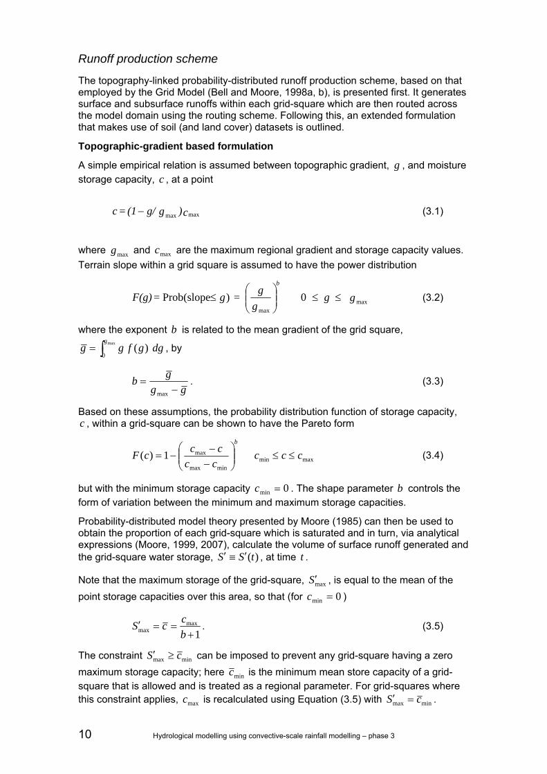
The topography-linked probability-distributed runoff production scheme, based on that employed by the Grid Model (Bell and Moore, 1998a, b), is presented first. It generates surface and subsurface runoffs within each grid-square which are then routed across the model domain using the routing scheme. Following this, an extended formulation that makes use of soil (and land cover) datasets is outlined.
Topographic-gradient based formulation
A simple empirical relation is assumed between topographic gradient, g , and moisture storage capacity, c , at a point
c)gg/ (1 = c maxmax− (3.1) where gmax and maxc are the maximum regional gradient and storage capacity values. Terrain slope within a grid square is assumed to have the power distribution
g g g
g = g = F(g)b
maxmax
0 )slope(Prob ≤≤⎟⎟⎠
⎞⎜⎜⎝
⎛≤ (3.2)
where the exponent b is related to the mean gradient of the grid square,
dggfggg
∫=max
0)( , by
gg
gb−
=max
. (3.3)
Based on these assumptions, the probability distribution function of storage capacity, c , within a grid-square can be shown to have the Pareto form
1)( maxminminmax
max ccc cc
cccFb
≤≤⎟⎟⎠
⎞⎜⎜⎝
⎛−−
−= (3.4)
but with the minimum storage capacity 0min =c . The shape parameter b controls the form of variation between the minimum and maximum storage capacities.
Probability-distributed model theory presented by Moore (1985) can then be used to obtain the proportion of each grid-square which is saturated and in turn, via analytical expressions (Moore, 1999, 2007), calculate the volume of surface runoff generated and the grid-square water storage, )(tSS ′≡′ , at time t .
Note that the maximum storage of the grid-square, maxS′ , is equal to the mean of the point storage capacities over this area, so that (for 0min =c )
1
maxmax +
==′bccS . (3.5)
The constraint minmax cS ≥′ can be imposed to prevent any grid-square having a zero maximum storage capacity; here minc is the minimum mean store capacity of a grid-square that is allowed and is treated as a regional parameter. For grid-squares where this constraint applies, maxc is recalculated using Equation (3.5) with minmax cS =′ .

Hydrological modelling using convective-scale rainfall modelling – phase 3 11
Losses from the grid-square probability-distributed store via evaporation and drainage to groundwater vary as functions of its water storage, ).(tSS ′≡′ Over the time interval
),( ttt Δ+ water is lost as evaporation at a rate aE from the water in store as a function of the potential evaporation rate, E , and the soil moisture deficit, SS ′−′max , such that
eb
a
SSS
EE
⎭⎬⎫
⎩⎨⎧
′′−′
−=max
max )(1 (3.6)
where the exponent eb is treated as a regional parameter (the same for all grid-squares) and commonly set to 2.0 or 2.5.
A power-law function is used for the drainage, id , from the grid-square probability-distributed store to groundwater storage
gbtgi SSkd )(1 ′−′= − (3.7)
where gk is a drainage time constant (here treated as a regional parameter), gb is an
exponent (commonly set to 3.0) and tS′ is the threshold storage below which there is no drainage, water being held under soil tension. The tension threshold allows water to remain in soil storage and be made available to evaporation: this can be of particular importance for permeable catchments. It is treated as a regional parameter and if, for a particular grid-square, tSS ′<′max then drainage from that grid-square can never occur.
The net rainfall rate, π , over the time interval to the grid-square is given by
dEP a −−=π (3.8)
where P is the grid-square rainfall. Simple water accounting coupled to the probability-distributed analytical expressions for volume of runoff and water storage. calculated for each grid-square, allow gridded surface and subsurface (drainage, d ) runoffs to be generated for input to the G2G model routing scheme.
Soil-based formulation
Instead of linking soil depth to topographic gradient in a surrogate way, the extended “soil-based” runoff production scheme makes explicit use of information on soil properties including depth. If L is the physical depth of the soil, at saturation this can hold a maximum water depth available for evaporation and drainage
LS rs )(max θθ −= (3.9)
where sθ and rθ are the saturation and residual water contents (water volume per unit volume of soil). In addition to this, a residual depth of water LS rr θ=′ held under soil tension forces can only be depleted by evaporation. The total depth of water in the soil column at saturation is therefore rSSS ′+=′ maxmax . At a given time the actual available and total water depths are LS r )( θθ −= and rSSS ′+=′ respectively, where θ is the actual water content. The quantities L , sθ and rθ are properties of the soil specified (or inferred) via datasets derived from soil surveys.
The PDM theory is invoked so that the maximum water holding capacity maxS′ is made up of a population of storage elements in the size range ),0( maxc that have a Pareto distribution with shape parameter b . Here it is assumed that b is related to maxS′

12 Hydrological modelling using convective-scale rainfall modelling – phase 3
through the relation max/2.5 Sb ′= , based on PDM catchment model results obtained across the UK (Bell et al., 2009). For permeable catchments (where L exceeds one metre) the b parameter is set to zero (all stores have depth maxc ) which has the effect of suppressing rapid runoff fluctuations. The volume of saturation-excess runoff generated from the assemblage of storage elements subject to net rainfall iπ is calculated in the normal way (Moore, 1985, 2006).
The volume of available water in the grid-cell of side xΔ is SxV 2Δ= . Water is added to by precipitation over the cell area 2xpΔ and via inflows from upstream contributing cells iq . Losses of water (expressed as flow rates) occur via lateral drainage Lq induced by the average slope of the soil column 0s , via downward percolation
(drainage) pq and as saturation-excess runoff sq . Evaporation 2xEaΔ is also lost over
the surface area of the cell with aE calculated using Equation (3.6); a value of 2.5 for the exponent eb has been assumed.
Lateral drainage (interflow) is given by
αxSCqL Δ= (3.10)
where the conveyance αmax0 / SsLkC L
s= with Lsk the lateral saturated hydraulic
conductivity obtained from soil data. The parameter α is the pore-size distribution factor, here taken to be unity. This expression derives from integrating the Brooks-Corey (1964) relation for hydraulic conductivity over the depth of soil column (Todini, 1995; Benning, 1995).
Percolation (vertical drainage) is given by
p
SSxkq v
sp
α
⎟⎟⎠
⎞⎜⎜⎝
⎛Δ=
max
2 , (3.11)
where vsk is the soil’s vertical saturated hydraulic conductivity. The exponent of the
percolation function pα can vary from around 11 (sand) to 25 (clay) according to Clapp and Hornberger (1978); a value of 15 is assumed here in the absence of supporting data.
Percolation is assumed to freely drain to groundwater as recharge. The volume of groundwater in the cell gV is added to by this recharge and lost via lateral groundwater
flow out of the cell gq , so by continuity
gpg qq
dtdV
−= . (3.12)
The lateral groundwater flow, governed by Darcy’s law and the slope of the bedrock bs , may be approximated (assuming a confined aquifer) by
gbg
g Vxsk
qΔ
= (3.13)

Hydrological modelling using convective-scale rainfall modelling – phase 3 13
where gk is the hydraulic conductivity of the aquifer. In the absence of suitable geological property data this has been replaced here by the nonlinear storage parameterisation
,0,0, >>= mVq gm
ggg κκ (3.14)
where gκ is a rate constant and m a nonlinear exponent (here taken to be 3.0).
Grid-to-grid flow routing scheme
The basis of the grid-to-grid flow routing scheme is a simple kinematic wave equation (Moore and Jones, 1978) which relates channel flow, q , and lateral inflow per unit length of river, u . The equation is extended in the G2G model to include a return flow term, R, representing surface-subsurface water transfers per unit length of river. In one dimension, the basic equation is of the form
)( Rucxqc
tq
+=∂∂
+∂∂
(3.15)
where c is the kinematic wave speed and x and t are distance along the reach and time respectively. This equation is used to represent the movement of water from one grid-cell to the next according to flow paths inferred from a digital terrain model. Equation (3.15) is applied separately to the surface and subsurface runoffs output from the runoff production scheme, thereby representing the simultaneous parallel water movement along fast (surface) and slow (subsurface) pathways. Different wave speeds over land and river (for surface and subsurface) pathways are accommodated. The return flow term allows transfer of water between subsurface and surface pathways, representing interactions on hillslopes and within river channels.
The finite-difference representation of Equation (3.15)
( ) ( )nk
nk
nk
nk
nk Ruqqq +++−= −
−−1111 θθ (3.16)
is used, where the dimensionless wave speed xtc ΔΔ= /θ ( 10 <<θ ) with xΔ and tΔ the time and space steps of the discretisation. In this two-dimensional application, Equation (3.16) provides a recursive formulation expressing flow out of the n ’th grid-cell at time k , n
kq , as a linear weighted combination of the flow out of the grid-cell (at the previous time), inflow to the grid-cell from adjacent grid-cells (at the previous time) and the total lateral inflow (runoff production) plus return flow in the grid-cell (at the same time).
The grid-to-grid routing scheme can be conceptualised as a network cascade of linear reservoirs (Moore et al., 2006, 2007; Bell et al., 2007, 2009). The return flow to the surface routing pathway is given by a return flow fraction r (between zero and one) of the water depth stored in the subsurface: this parameter can differ for land (denoted lr ) and river (denoted rr ) pathways. Note that, to ensure numerical stability, the routing time-step can be smaller than the model time-step used in the runoff production scheme.
An alternative routing scheme is available within the G2G model for representing river channel pathways that allows for the introduction of variable channel width, slope and roughness. This takes the Horton-Izzard nonlinear storage form (Dooge, 1973; Moore and Bell, 2001; Ciarapica and Todini, 2002)

14 Hydrological modelling using convective-scale rainfall modelling – phase 3
mkVqdtdV
−= (3.17)
where V is the volume of water stored in a channel reach, q is the reach inflow and m
c kVq = is the reach outflow. For a rectangular channel of width w , length xΔ and water depth S then xSwV Δ= . Manning’s equation can be invoked to relate cq to
water depth S giving mc CwSq = with exponent 3/5=m . Here the conveyance
nsC /0= with 0s the channel bed slope and n the Manning’s roughness coefficient.
It follows that mxwCwk )/( Δ= . Other values for m can be assumed if required, with two having the advantage of a simple analytical solution.
Channel width is estimated from the area drained (km2), A , and its standard average annual rainfall (mm), SAARR , using the expression for bankfull width derived by Bell and Moore (2004) for the UK:
139.15121.0
10009134.0 ⎟
⎠⎞
⎜⎝⎛= SAAR
bRAw . (3.18)
Model configuration support using spatial datasets
The G2G flow routing scheme is configured on a one-km grid, using for each cell the flow direction (one of eight directions) and the area drained. These quantities are inferred from a 50-m hydrologically-corrected Digital Terrain Model (DTM) - called the Integrated Hydrological DTM or IHDTM (Morris and Flavin, 1990) – which is derived from the Ordnance Survey 1:50,000 digitised contours and spot heights together with the digitised river networks. The COTAT+ method, developed by Paz et al. (2006) and assessed over mainland Britain by Davies and Bell (2009), was used to derive the one-km flow directions and areas drained from the 50-m DTM. The mean terrain slope within each one-km cell was also calculated from the 50-m DTM using the average maximum technique (Burrough, 1986) that employs the elevations of the three-by-three cell neighbourhood surrounding each cell. At present, the channel bed slope 0s is approximated by the mean terrain slope g .
Soil property information is based on an association table developed at the Centre for Ecology and Hydrology (CEH) (Ragab, personal communication) linking HOST soil class (Boorman et al., 1995) to soil properties derived from SEISMIC (Hallett et al., 1995). HOST is a one-km dataset of integer identifiers for 29 soil classes across the UK that takes account of soil type, hydrological response and substrate hydrogeology. The soil properties of relevance are:
• hydraulic conductivity at saturation, sk (cm d-1)
• soil depth to “C” and “R” horizons (cm)
• water content at field capacity, fcθ (fractional volume at 5 KPa)
• residual water content, rθ (half the fractional volume at 1,500 KPa)
The C-layer is defined as “mineral substrate, relatively unweathered ‘soft’ unconsolidated material, gravel or rock rubble” and the R-layer as “relatively unweathered, coherent rock”. Here, the depth to R-layer is treated as the soil depth; when absent the C-layer depth is used. As a rule of thumb the water content at saturation, sθ , is about twice the value at field capacity. Here, it is taken as one-and-a-

Hydrological modelling using convective-scale rainfall modelling – phase 3 15
quarter times the value since the HOST values of fcθ appear to have a larger range than those given in the literature (Dunne and Leopold, 1978) for fine sand to clay soils.
The value of sk for a given HOST class is related to vertical saturated hydraulic conductivity of the soil in the G2G model, v
sk , through a simple drainage conductivity
multiplier λ, such that vsk = λ sk . A working assumption is also made that L
sk =50 sk .
Model initialisation and forecast updating
Methods have been developed for model initialisation and forecast updating of the G2G model for use in real-time flood forecasting. Initialising the states of a distributed model using river flow observations at gauged locations in the model domain is required to avoid a long spin-up period for the model. Such initialisation is needed when first installing the model within a forecast system, and also in the event of a system or telemetry failure that precludes recovery from a previous set of stored model states. A simple initialisation scheme has been developed based on steady-state assumptions. Only an initial form of scheme is used at present. Test results have shown the effective spatial transfer of information from a gauged site used for model initialisation to other locations within the model domain. Whilst the model spin-up time required is considerably reduced by the initialisation scheme, some time is still needed especially where groundwater dominates the flow regime.
For forecast updating, a method of data assimilation is needed that incorporates flow measurements at gauged locations in the modelled region. The aim is to increase forecast accuracy by updating the states of the G2G distributed model in real-time using river flow observations sequentially at every time-step up to the time the forecast is constructed, and at every subsequent forecast time-origin. The sequential data assimilation scheme developed for the G2G model employs empirical state-correction as a simple, pragmatic alternative to more complex procedures based on the Kalman filter. Only an initial form of scheme is used at present. The principle employed is that the model water stores can be linearly scaled across model grid-cells to match the observed flows. State-updating is currently applied to all cells upstream of a gauged point (application downstream and to adjacent catchments has so far proved unstable because of the lack of a corrective feedback mechanism). If there are nested catchments the most upstream catchments are state-updated first. This is a simplistic approach in that all points within a sub-catchment receive the same scaling factor. At present the scheme only scales the water content of some of the model stores within a model cell; also, no account is taken of translation times between the gauged cell and the cells being adjusted.
Test results have shown that sequential data assimilation is more effective than a simple model re-initialisation at each time-origin. Forecast hydrographs generally improve as the forecast time-origin approaches the flood peak. Overall forecast accuracy, when compared to model simulations, is increased for lead times of interest at selected locations in the model domain assumed to be ungauged. This assessment applies to areas where the G2G flow simulations and the observed flows used for state-correction are both good. Developing better state-correction schemes for the G2G is part of ongoing research.

16 Hydrological modelling using convective-scale rainfall modelling – phase 3
3.2.2 REW
Introduction
A novel catchment modelling approach based on global balance laws for mass, momentum and energy is presented by Reggiani et al. (1998, 1999, 2000) and Reggiani and Rientjes (2005). The purpose of the work carried out by these authors was to integrate the micro-scale conservation equations for mass, momentum and energy over specially chosen integration regions, which make up a representative elementary watershed (REW). Reggiani and Schellekens (2003) explain why the concept should be investigated further and why it deserves more practical use.
REWs are defined in such a way as to allow the definition to be globally applicable and scale-independent, and thus recognizable at spatial scales from small sub-catchments or patches of a few hectares to entire systems of many square kilometres. In principle, it is as if they were extracted with a pastry cutter from the landscape.
The integration procedure yields, in contrast to micro- or macro-scale formulations, so-called mega-scale balance laws (for definitions see Gray et al. (1993)) that are obtained without making any a priori assumptions on the importance of various terms. These laws constitute scale-independent ordinary differential equations (ODE), which conserve physical properties for hydrologically representative zones within an REW in terms of spatially and temporally integrated variables.
Model capabilities
The REW model is a complex hydrological simulation tool designed to simulate a complete hydrological cycle system, underlain by a regional aquifer, which may extend beyond the topographic boundaries.
The tool can be used for different types of studies by looking at different components of the hydrological cycle and at processes that play a role at different timescales. It can, for instance, be used for event-based studies, such as the response of a catchment to an extreme precipitation, or the behaviour of the hydrological system under forcing conditions that are changing over longer time periods. Typical examples of possible applications and hydrological studies are: 1) hydrological water balance, 2) rainfall-runoff studies, 3) groundwater recharge and development studies, and 4) impact of climate change on the hydrological cycle.
The REW model has been adjusted by Deltares to run as part of a Delft-FEWS configuration. As such, no development was needed to fully use the REW model.
Similar to the G2G model and other distributed models, the REW model is sensitive to spatial patterns in the precipitation and storm movement over the catchment. Clearly, this also depends on the chosen size of the REW. The REW concept has already been used successfully for several sub-basins in the Rhine catchment in conjunction with European Centre for Medium-Range Weather Forecasts (ECMWF) ensemble forecasts.
In recent research by Deltares (Reggiani, personal communication) the REW model has been linked with an ensemble Kalman filtering technique to update its internal variables in real time, based on measured flow and remotely sensed soil moisture. Although ensemble Kalman filtering requires many more calculations than analytical updating, it is able to improve the forecasts of the model considerably. In addition, it gives information on uncertainties associated with the produced flows.

Hydrological modelling using convective-scale rainfall modelling – phase 3 17
Spatial discretisation of the landscape into modelling units
In the REW model, a catchment is partitioned into a series of discrete spatial units called representative elementary watersheds (REWs). REWs are defined from an analysis of the catchment topography and constitute a set of interconnected elements organised around the tree-like structure of the stream channel network, as shown in Figure 3.3.
Figure 3.3 Binary structure of the channel network.
REWs constitute three-dimensional regions, with a vertical prismatic mantle surface defined by the REW boundaries. REW boundaries coincide with topographic divides. They delineate portions of the land surface which capture precipitation. The contour of a REW mantle surface coincides with the perimeter of sub-basins. A schematic representation of a REW is depicted in Figure 3.4 .
Figure 3.4 A REW as a 3-D spatial region.

18 Hydrological modelling using convective-scale rainfall modelling – phase 3
The REW is delimited by the atmosphere at the top and by an impermeable layer at the bottom. The impermeable layer can be defined by a horizontal surface or can be given by interpolation of bedrock depth for a series of irregular points.
Sub-REW variability
To account for hydrological variability within a REW with features at scales smaller than the REWs determined from a Digitial Elevation Model (DEM) only, the unsaturated zone can be broken down further into smaller units, labelled representative elementary columns (RECs). These RECs are defined on the basis of an overlapping series of GIS maps such as land use and soil type. The procedure for breaking down the unsaturated zone allows the user to assign different soil properties to each unit. Figure 3.5 shows an example of a catchment broken down into RECs through combination of land use maps with REWs.
Modelled processes
The volume occupied by a REW contains typical flow zones encountered in a catchment. The following zones can be modelled explicitly and for every REW: 1) the unsaturated zone, 2) the saturated zone, 3) the subsurface storm-flow zone, 4) the saturated overland flow area, 5) the infiltration excess overland flow, 6) the channel reach and 7) a snow zone. Flow within the various domains evolves over different temporal scales and encompasses phenomena such as unsaturated and saturated porous media flow (subsurface zones) as well as overland and channel flow (land surface zones). Modelling of the various flow processes is described in the following paragraphs.
Figure 3.5 Overlap of a REW map with a soil map yields a smaller subdivision of the unsaturated zone within a REW into RECs.

Hydrological modelling using convective-scale rainfall modelling – phase 3 19
Unsaturated zone (U-zone)
The unsaturated zone is modelled by means of a Richards’ equation solver (Ross, 2003). The chosen solver for the partial differential equation (PDE) governing flow in unsaturated soil has the ability to linearise the mass flux between cells and allows a very fast solution of the equation, avoiding the need to search for iterative solutions. Compared to full non-linear solvers, the accuracy of the numerical solution is somewhat lower. But given the high uncertainty in the choice of soil parameters, the errors of approximation made in the choice of numerical method is considered of second order and thus negligible.
Saturated zone (S-zone)
The saturated zone is modelled as a two-dimensional aquifer. The groundwater zone is recharged through recharge flux from the unsaturated zone. The groundwater is then distributed laterally via horizontal REW mantle fluxes based on piezometric head differences between REWs. The piezometric head is the average water table level calculated for a REW via the mass balance equation. The mass balance equation is an ordinary differential equation (ODE) solved analytically, given the recharge flux from 1) the unsaturated zone eus, 2) the lateral groundwater distribution fluxes between the REW and neighbouring REWs em, 3) the seepage flux eso and 4) the exchange flux of groundwater with the river channel across the bed area esr. The seepage flux eso feeds the overland flow zone.
The length scales Λ over which piezometric head differences are dissipated between a REW and its neighbouring REWs is unknown; this is re-calculated at chosen time-steps based on first principles. For this, the Hardy-Cross (1936) network balancing method is used (see Figure 3.6). Given a piezometric head distribution calculated from the mass balance for the saturated zone of each REW at a given point in time, and given known groundwater losses across the catchment boundaries, dissipation length scales are calculated by successive approximation.
Figure 3.6 Groundwater calculations.
The procedure is parsimonious and based on a non-linear system of equations which preserve i) mass at each network node and ii) the head losses along a closed

20 Hydrological modelling using convective-scale rainfall modelling – phase 3
triangular loop, as shown in Figure 3.6. The horizontal aquifer flow field is subsequently calculated by resolving the momentum balance equation for the REW elements. An example of a vector of flow velocities for the Geer Aquifer (Belgium) is shown in Figure 3.7.
REW-average groundwater levels are interpolated at selected time-steps through bi-cubic spline functions (Inoue, 1986), providing a smooth groundwater surface between REW-average groundwater points. The fitting of the smooth surface is based on the finite element method (FEM), which calculates the surface by minimizing the elastic tension energy in the surface. The same procedure can be used to define the impermeable lower boundary of the catchment, if sparse measurement points of the bedrock depth are available. Figure 3.8 shows an example of a fitted surface.
Figure 3.7 Calculation of the groundwater flow field for the Geer basin (Belgium).
Figure 3.8 Water table surface interpolated with the bi-cubic spline method.
Hydrological modelling using convective-scale rainfall modelling – phase 3 21
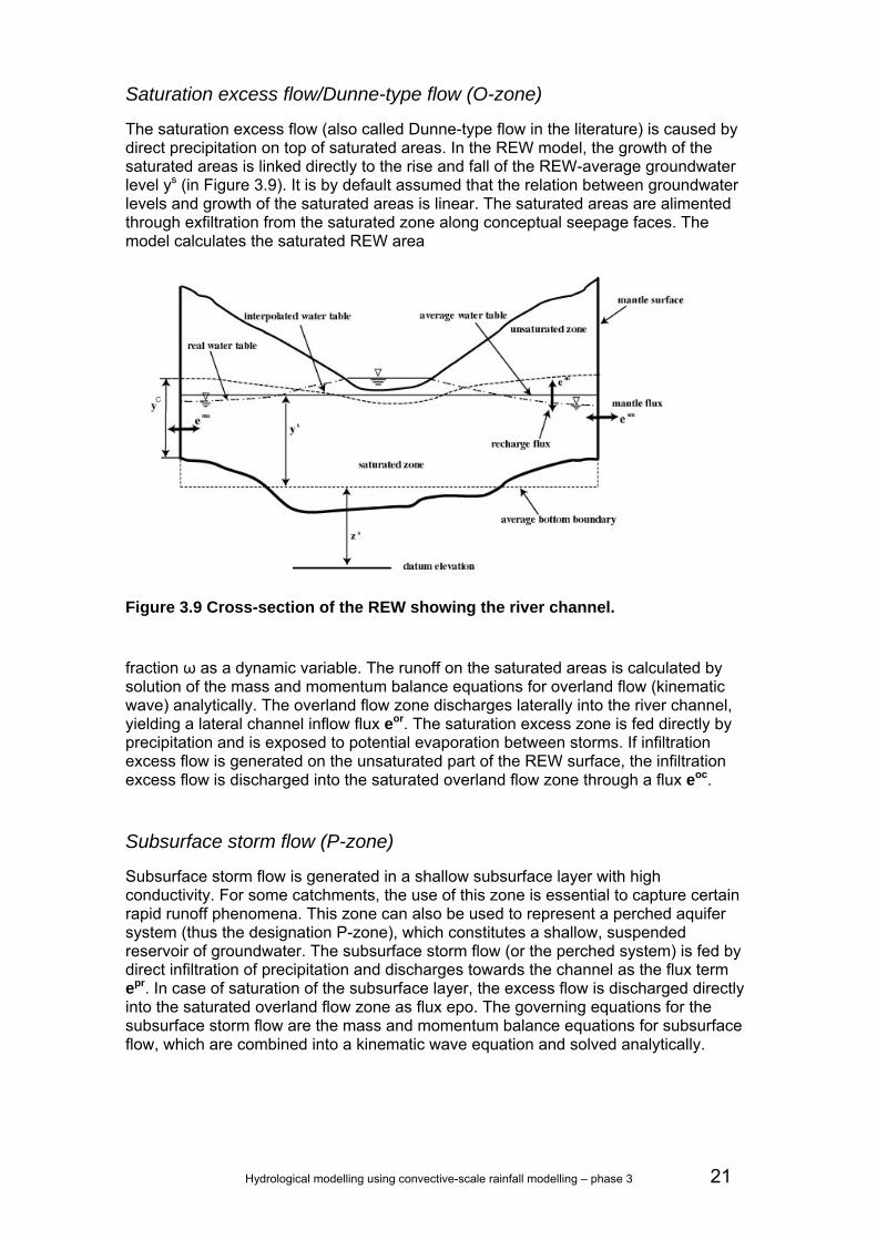
Saturation excess flow/Dunne-type flow (O-zone)
The saturation excess flow (also called Dunne-type flow in the literature) is caused by direct precipitation on top of saturated areas. In the REW model, the growth of the saturated areas is linked directly to the rise and fall of the REW-average groundwater level ys (in Figure 3.9). It is by default assumed that the relation between groundwater levels and growth of the saturated areas is linear. The saturated areas are alimented through exfiltration from the saturated zone along conceptual seepage faces. The model calculates the saturated REW area
Figure 3.9 Cross-section of the REW showing the river channel.
fraction ω as a dynamic variable. The runoff on the saturated areas is calculated by solution of the mass and momentum balance equations for overland flow (kinematic wave) analytically. The overland flow zone discharges laterally into the river channel, yielding a lateral channel inflow flux eor. The saturation excess zone is fed directly by precipitation and is exposed to potential evaporation between storms. If infiltration excess flow is generated on the unsaturated part of the REW surface, the infiltration excess flow is discharged into the saturated overland flow zone through a flux eoc.
Subsurface storm flow (P-zone)
Subsurface storm flow is generated in a shallow subsurface layer with high conductivity. For some catchments, the use of this zone is essential to capture certain rapid runoff phenomena. This zone can also be used to represent a perched aquifer system (thus the designation P-zone), which constitutes a shallow, suspended reservoir of groundwater. The subsurface storm flow (or the perched system) is fed by direct infiltration of precipitation and discharges towards the channel as the flux term epr. In case of saturation of the subsurface layer, the excess flow is discharged directly into the saturated overland flow zone as flux epo. The governing equations for the subsurface storm flow are the mass and momentum balance equations for subsurface flow, which are combined into a kinematic wave equation and solved analytically.

22 Hydrological modelling using convective-scale rainfall modelling – phase 3
Infiltration excess flow/Horton-type flow (C-zone)
The infiltration excess flow (also called Horton-type flow in the literature) is caused by precipitation that exceeds the infiltration capacity of the soil. As a result water builds up on the surface and runs off. In the REW model, the infiltration excess flow is modelled through analytical solution of the mass and momentum balance ordinary differential equations (ODE). The runoff flux eco is discharged directly into the saturated overland flow zone. The infiltration excess flow is fed by the precipitation rate during storms and by potential evaporation between storms.
Channel flow (R-zone)
The channel flow zone is recharged by fluxes from upstream links, er in , the outflow to the downstream reach er out and lateral inflow fluxes eor, esr, epr from the overland flow zone (O-zone), the aquifer (S-zone) and the subsurface storm-flow zone (or the perched zone, P-zone). The lateral inflows due to overland flow and the shallow subsurface storm-flow zone are controlled by the governing equations for these respective zones. The exchange with groundwater is dictated by the average head differences between the REW-average groundwater level and the river. The water between the two zones is exchanged through a river bed transition zone, for which a hydraulic conductivity and a thickness can be specified. For situations in which the average water level in the channel reach is higher than the water level in the surrounding aquifer, the flux esr causes the groundwater to be fed from the channel. If, on the other hand, the average water level in the aquifer increases with respect to the channel, the groundwater feeds the channel. This principle is shown in Figure 3.9, which features the REW-average water level, actual water level, water table interpolated via the Inoue (1986) algorithm and average water level in the channel.
Summary of exchange fluxes in the REW model
The most relevant model-internal and internal fluxes are shown in Table 3.1. The table specifies which fluxes are within zones in a REW and which ones are between a REW and neighbouring REWs or the outside environment (across catchment boundaries).
REW model calibration
The use of a physically-based approach where parameters are measurable can reduce the dimension of the parameter space significantly. Moreover, the search range for parameter values can be restricted by the physical range for each parameter. Based on these considerations, the number of parameters calibrated for the REW model can be reduced to five: the Manning roughness parameters for overland and channel flow, saturated conductivity of the soil (choosing a uniform conductivity), and parameter governing the partitioning of infiltration between components going into subsurface storm flow and deep groundwater flow. The last parameter calibrated is the exponent governing the expansion of the saturated areas as a function of groundwater level. This parameter can vary from values significantly less than one, via a value of one (linear relationship) to values larger than one. By fixing all other parameters, a full calibration of the REW model can be performed.

Hydrological modelling using convective-scale rainfall modelling – phase 3 23
Table 3.1 Hydrological fluxes within the REW model.
3.2.3 Comparison of G2G and REW distributed hydrological models
Having outlined the G2G and REW distributed hydrological models, it is useful to highlight the main differences between the two approaches as background to the performance assessments that follow. A clear difference between the REW and G2G approaches is in the way the landscape is discretised into modelling units. Whilst G2G employs a subdivision of the landscape into square grid elements, the REW employs irregularly-shaped modelling units. These are derived by subdividing the landscape on the basis of topographic divides and numbering according to the Strahler network numbering scheme. Both approaches have their respective strengths and weaknesses. The grid approach of G2G facilitates the setup of the model with the aid of distributed information, which is commonly available in gridded form. The distributed meteorological inputs to the model, such as precipitation and potential evaporation, are also facilitated by the gridded structure of the model, which can easily be matched with the model’s input data structure.
Flux description Symbol REW-internal
flux
Inter-REW flux
External boundary
flux
river-saturated zone esr yes no no
water table flux (unsaturated zone-saturated zone)
eus yes no no
infiltration ecu yes no no
inflow from infiltration excess flow zone to saturated overland flow zone
eco yes no no
lateral channel inflow eor yes no no
inter-REW groundwater flow
em no yes yes
lateral channel inflow from subsurface storm-flow zone
epr yes no no
exfiltration from subsurface storm-flow zone to saturated overland flow zone
epo yes no no
exfiltration (seepage flow) eso yes no no
channel in and outflow er out
er out
no yes yes

24 Hydrological modelling using convective-scale rainfall modelling – phase 3
While the G2G model preserves the spatial information at the level of resolution of the grid-cell, the REW approach performs additional aggregation of the sub-REW information. By means of a topographic analysis, which is controlled through user interaction (for example, the choice of spatial resolution of the REWs), the landscape is subdivided into irregular elements, defined by the topographic divides. At this stage, the initially gridded input is lumped into information which is spatially aggregated and averaged over the respective irregular spatial element.
The loss of spatial information at the level of the grid-cell of REW compared to G2G is compensated by the gain in computational speed from using fewer lumped modelling elements in REW. How this difference in approach is reflected in the quality of the simulations is the subject of analysis in this report.
Once modelling units are identified, balance equation for mass and energy governing water flow in between the grid-cells (G2G) or irregular elements (REW) are solved for interconnected reservoirs. The differential equations are solved by numerical methods or on the basis of analytical solutions, which can be applied under simplified and restrictive conditions.
For unsaturated zone water movement, the REW model employs a numerical solution of a linearised Richards equation, whilst G2G uses a depth-integrated steady-state formulation for flow in an unsaturated soil that takes into account vertical and lateral water movements. The G2G allows the water-holding capacity of the soil to be probability-distributed when calculating saturation-excess runoff.
The principal features distinguishing the two modelling approaches are summarised in Table 3.2.

Hydrological modelling using convective-scale rainfall modelling – phase 3 25
Table 3.2 Comparison of G2G and REW distributed hydrological models.
Feature G2G model REW model
Model type Physical-conceptual Physically-based
Landscape discretisation
Regular square grid Irregular elements following topography
Use of extra information
Digital Terrain Model Soil maps Land cover maps
Digital Terrain Model Soil maps Land cover maps Infrastructure maps
Meteorological forcing input
Precipitation gridded maps Potential evaporation gridded maps
Precipitation, temperature, relativeAir humidity and potential evaporation series at REW centroids
Overland flow Cell-to-cell routing Kinematic Wave equation (numerical solution)
Kinematic Wave (Runge Kutta or analytical solution)
Channel flow Cell-to-cell routing Kinematic Wave equation (numerical solution) or Horton-Izzard nonlinear storage equation (analytical or numerical solutions)
Kinematic Wave (Runge Kutta or analytical solution) Muskingum-Cunge non-linear reservoir routing
Unsaturated zone
Depth-integrated steady-state formulation, lateral and vertical drainage based on unsaturated zone Darcy’s law, free drainage boundary condition. Probability-distributed water-holding capacity controls saturation-excess runoff production
Richards equation with free drainage boundary condition
Saturated zone Non-linear storage relations and Darcy’s law Cell-to-cell (Kinematic Wave) routingwith return flow to channel
Krichhoff mass and energy balancefor groundwater network flow. Darcy’s law for lateral inter-REW groundwater flow
Snow Pack Model (research version) Energy balance model Utah State Snow Model
Programming language
Fortran, C++ C++, Fortran
Operating system interoperability
Windows, Unix Windows, Linux

26 Hydrological modelling using convective-scale rainfall modelling – phase 3
3.3 Lumped benchmark models
3.3.1 PDM
The Probability Distributed Moisture model, or PDM, is a fairly general conceptual rainfall-runoff model which transforms rainfall and evaporation data to flow at the catchment outlet (Moore, 1985, 1999, 2007; CEH Wallingford, 2005a).
Figure 3.10 illustrates the general form of the model. The PDM has been designed more as a toolkit of model components than a fixed model construct. A number of options are available in the overall model formulation which allows a broad range of hydrological behaviours to be represented.
Figure 3.10 The PDM rainfall-runoff model.
Runoff production at a point in the catchment is controlled by the absorption capacity of the soil to take up water: this can be conceptualised as a simple store with a given storage capacity. By considering that different points in a catchment have differing storage capacities and that the spatial variation of capacity can be described by a probability distribution, it is possible to formulate a simple runoff production model which integrates the point runoffs to yield the catchment surface runoff into surface storage. The standard form of PDM employs a Pareto distribution of store capacities, with the shape parameter b controlling the form of variation between minimum and maximum values minc and maxc respectively. Drainage from the probability-distributed moisture store passes into subsurface storage as recharge. The rate of drainage is in proportion to the water in store in excess of a tension water storage threshold.
Groundwater storage
Surface storage
Direct runoff
Probability-distributed soil moisture storage
Surface runoff
Baseflow
Recharge
P
E
S1
qs
qb
S3
S2
q

Hydrological modelling using convective-scale rainfall modelling – phase 3 27
The subsurface storage, representing translation along slow pathways to the basin outlet, is commonly chosen to be of cubic form, with outflow proportional to the cube of the water in store. An extended subsurface storage component (Moore and Bell, 2002) can be used to represent pumped abstractions from groundwater; losses to underflow and external springs can also be accommodated.
Runoff generated from the saturated probability-distributed moisture stores contribute to the surface storage, representing the fast pathways to the basin outlet. This is modelled here by a cascade of two linear reservoirs cast as an equivalent transfer function model (O’Connor, 1982). The outflow from surface and subsurface storages, together with any fixed flow representing, say, compensation releases from reservoirs or constant abstractions, forms the model output. Table 3.3 summarises the parameters involved in the standard form of PDM.
Table 3.3 Parameters of the PDM model.
Parameter name Unit Description
fc dτ
None hour
rainfall factor time delay
Probability-distributed store cmin cmax b
mm mm none
minimum store capacity maximum store capacity exponent of Pareto distribution controlling spatial variability of store capacity
Evaporation function be
none
exponent in actual evaporation function
Recharge function kg bg
St
h 1mm −gb none mm
groundwater recharge time constantexponent of recharge function soil tension storage capacity
Surface routing k1, k2
hour
time constants of cascade of two linear reservoirs
Groundwater storage routing kb m qc
h mmm-1 none m3 s-1
baseflow time constant exponent of baseflow nonlinear storage constant flow representing returns/abstractions

28 Hydrological modelling using convective-scale rainfall modelling – phase 3
For real-time application for flood forecasting, the PDM is provided with forecast updating schemes. There are two basic types: error-prediction (where the dependence in past model errors are used to predict future ones) and state-correction (where model errors are attributed to the model states going adrift, and adjustments made to them to bring the model back on track). The simple empirical state-correction scheme is applied here in its ‘super-proportional’ adjustment form. Further details are provided in Moore (1999) and CEH Wallingford (2005a).
3.3.2 TCM
The structure of the Thames Catchment Model, or TCM (Greenfield, 1984; Wilby et al., 1994; Moore and Bell, 2001), is based on subdivision of a basin into different response zones representing, for example, runoff from aquifer, clay, riparian and paved areas and sewage effluent sources. Within each zone the same vertical conceptualisation of water movement is used, the different characteristic responses from the zonal areas being achieved through choice of parameter set, some negating the effect of a particular component used in the vertical conceptualisation. The zonal flows are combined, passed through a simple routing model (optional), and go on to make up the basin runoff.
The conceptual representation of a hydrological response zone in the TCM is illustrated in Figure 3.11 using nomenclature appropriate to an aquifer zone. This zone structure is used for all types of response zone but with differing nomenclature; for example, percolation is better described as rainfall excess for zones other than aquifer. Within a given zone, water movement in the soil is controlled by the classical Penman storage configuration (Penman, 1949). In this, a near-surface storage of depth related to the rooting depth of the vegetation and to the moisture retention characteristics of the soil (the root constant depth), drains only when full into a lower storage of notional infinite depth. Evaporation occurs at the Penman potential rate whilst the upper store contains water and at a lower rate when only water from the lower store is available. The Penman stores are replenished by rainfall, but a fraction φ (typically 0.15, and usually only relevant to aquifer zones) is bypassed to contribute directly as percolation to a lower “unsaturated storage”. Percolation occurs from the Penman stores only when the total soil moisture deficit has been made up.
The total percolation forms the input to the unsaturated storage. This behaves as a linear reservoir, releasing water in proportion to the water stored at a rate controlled by the reservoir time constant, k . This outflow represents “recharge” to a further storage representing storage of water below the phreatic surface in an aquifer. Withdrawals are allowed from this storage to allow pumped groundwater abstractions to be represented. A quadratic storage representation is used, with outflow proportional to the square of the water in store and controlled by the nonlinear storage constant, K .
Total basin runoff derives from the sum of the flows from the quadratic store of each zonal component of the model delayed by a time dτ . Provision is also made to include a constant contribution from an effluent zone if required. A more recent extension of the model passes the combined flows through an additional channel flow routing component if required. This component of the model derives from the channel flow routing model developed by the Institute of Hydrology (Moore and Jones, 1978; Jones and Moore, 1980) which, in its basic form, takes the kinematic wave speed as fixed. The model employs a finite difference approximation to the kinematic wave model with lateral inflow. The delay and attenuation of the flood wave is controlled by the spatial discretisation used and a dimensionless wave speed parameter, θ . The parameters of the TCM are summarised in Table 3.4.
The TCM features (along with the Isolated Event Model, IEM) within the PSM (Penman Store Model) software, where further details can be found (Centre for Ecology and

Hydrological modelling using convective-scale rainfall modelling – phase 3 29
Hydrology, 2005). This includes details of the error-prediction and state-corrections methods available with the TCM for real-time forecast updating using river flow measurements.
Figure 3.11 Representation of a hydrological response zone within the Thames Catchment Model.
Unsatur storage
Soil Moistu
D
s Unsaturated storage
Saturated storage
Groundwater discharge to t fl
a
abstraction
D2
Soil moisture stores
Ea
Rc
Saturated storage
Groundwater discharge to streamflow
a
Abstraction
Q = S2/K
Recharge
Total percolation
P Precipitation
Soil surface
Actual evaporation
Direct percolation φ P´
Percolation
i
P´=max(0,P-E)
(1-φ )P´
S
q = s/k

30 Hydrological modelling using convective-scale rainfall modelling – phase 3
Table 3.4 Parameters of the Thames Catchment Model. Parameter name Unit Description
Zone parameters
A km2 Area of hydrological response zone
γ none Drying rate in lower soil zone (usually γ =0.3)
cR mm Depth of upper soil zone (drying or root constant)
PR mm Depth of lower soil zone (notionally infinite)
φ none Direct percolation factor (proportion of rainfall bypassing soil storage)
k hour Linear reservoir time constant
K mm hour Quadratic reservoir time constant
a m3 s-1 Abstraction rate from quadratic reservoir
Other parameters
zn none Number of zones
cq m3 s-1 Constant flow (effluent or river abstraction)
dτ hour Time delay
N none Number of channel sub-reaches
θ none Dimensionless wave speed, xtc ΔΔ /
3.3.3 MCRM
The rainfall-runoff model MCRM (Midlands Catchment Runoff Model) is based on classical conceptual water storage accounting principles applied to the land (soil and groundwater) and river channels. An outline of the model, previously known as the Severn-Trent Catchment Runoff Model, is provided by Bailey and Dobson (1981), Wallingford Water (1994) and Moore and Bell (2001). Reviews of the snowmelt component are given in Harding and Moore (1988) and Moore et al. (1996). A schematic of the rainfall-runoff model structure is shown in Figure 3.12 The Midlands Catchment Runoff Model. This figure omits the snowmelt, reservoir and error prediction components of the overall model: the interested reader is referred to Robson and Moore (2009) for a description of these and further details of the overall model.

Hydrological modelling using convective-scale rainfall modelling – phase 3 31
Figure 3.12 The Midlands Catchment Runoff Model.
q
Smax S
PfEc
Interception store
ftEr
Soil evaporation
Ps
Snowmelt
Rapid runoff
Rapid drainage
(1-c)us
us qr=cus
qd
Percolation qp
Baseflowqb
Sg Groundwater store
Soil moisture store
Dsurp
D
0
In-bank Out-of-bank
Sic Soc
qoc qic
Lag, τ and smooth, T
Throughflow qT
Non-linear channels
Soil store runoff qs

32 Hydrological modelling using convective-scale rainfall modelling – phase 3
The model comprises three main stores: an interception store, a soil moisture store and a groundwater store. Rapid runoff is generated from the soil moisture store, the proportion of input to the store becoming runoff increasing exponentially with decreasing soil moisture deficit. “Percolation” to the groundwater store occurs when the soil is supersaturated, increasing as a linear function of the negative deficit. When supersaturation exceeds a critical value, “rapid drainage” occurs as a power function of the negative deficit in excess of the critical value (the so-called excess water). This rapid drainage along with rapid runoff forms the soil store runoff.
Evaporation occurs preferentially from the interception store at a rate which is a fixed proportion of the catchment potential evaporation. A proportion of any residual evaporation demand is then met by water in the soil store, the proportion varying as a function of the soil moisture deficit. Drainage of the groundwater store to baseflow varies as a power function of water in storage, the exponent being fixed at 1.5.
The total output, made up of baseflow and soil store runoff, is then lagged and spread evenly over a specified duration to represent the effect of translation of water from the ground to the catchment outlet. Finally, the flow is smoothed using two nonlinear storage functions, one for routing in-bank flow and the other out-of-bank flow, the two components being summed to give the catchment model outflow.
A summary of the model parameters used in the Midlands Catchment Runoff Model is presented in Table 3.5 together with the units used in the model.

Hydrological modelling using convective-scale rainfall modelling – phase 3 33
Table 3.5 Parameters in the Midlands Catchment Runoff Model.
Parameter Unit Description
cf none Rainfall factor
maxS mm Capacity of interception store
f none Fraction of catchment evaporation potentially met by interception storage
0c none Minimum value of rapid runoff proportion
1c mm-1 Parameter in rapid runoff proportion function
maxc none Maximum value of rapid runoff proportion
maxpq mm h-1 Maximum percolation rate
surpD mm Maximum soil store moisture surplus
dγ none Soil function exponent controlling rapid drainage
dk 1mmh −dγ Soil function coefficient controlling rapid drainage
pT none Potential transpiration factor
mT none Minimum transpiration factor
DmaxE mm Deficit below which potential transpiration
factor applies DminE mm Deficit above which minimum transpiration
factor applies
gK hour mm0.5 Time constant in baseflow storage function
τ hour Time lag applied to total runoff
T hour Duration of time spread applied to total runoff
bfS mm Channel storage at bankfull
crk crγ−− 11mmh In-channel routing storage coefficient
crγ none In-channel routing storage exponent
ork orγ−− 11mmh Out-of-bank channel routing storage coefficient
orγ none Out-of-bank channel routing storage exponent
tΔ hour Time-step in hours (e.g. 0.25 for 15 min data)

34 Hydrological modelling using convective-scale rainfall modelling – phase 3
4 Test case: Boscastle, 16 August 2004
4.1 Introduction The extreme convective event that affected Boscastle and the surrounding area was chosen as the first test case for Phase 2 of the project. Following the devastating floods associated with the storm, the Environment Agency commissioned a review of the meteorology, hydrology, hydraulics and impacts of the event (HR Wallingford, 2005). The Met Office also provide a more detailed account of the meteorology (Golding, 2005).
A brief meteorological synopsis and summary of flood damage caused by the storm is given below. This is followed by a description of the catchments used in the case study and the associated hydrometric network. A detailed hydrological model analysis forms the core of this section. This assesses performance of the REW, G2G and PDM models over a large area of South West England. It also investigates the value of high resolution rainfall ensembles for probabilistic flood forecasting using the Boscastle storm as a case study.
4.2 Meteorological synopsis The heavy rainfall which affected North Cornwall on 16 August 2004 predominantly fell between 12:00 and 16:00 GMT and was produced by a sequence of convective storms that developed along a coastal convergence line caused by the change in friction between the land and sea. This effect was heightened by solar heating over land. The exact storm path of each heavy rain cell varied slightly but the variation between the Camel Estuary and Bude was sufficiently small that the heaviest rain fell on the same catchments throughout the period.
This is evident in Figure 4.1 which shows the rainfall accumulation using Nimrod composite radar data over the event. The extreme rainfall event was captured by a network of tipping-bucket raingauges (triangles in Figure 4.1 and daily storage gauges. Three gauges were situated near the core of the storm and confirmed the presence of extreme rainfall totals. In the 24-hour period to 09:00 GMT 17 August 2004, the daily storage gauge at Otterham (SX 169 916) recorded 200 mm, the daily storage gauge at Trevalec (SX 134 900) recorded 185 mm and the tipping-bucket raingauge at Trevalec recorded 155 mm, of which 154 mm fell in a six-hour period. The discrepancy between this and the Trevalec daily raingauge totals is most likely to be due to known problems with tipping-bucket raingauges during intense rainfall events.

Hydrological modelling using convective-scale rainfall modelling – phase 3 35
Figure 4.1 Accumulations of five-minute Nimrod radar rainfall data for the seven-hour period starting at 10:00 16 August 2004. Solid triangles denote raingauge locations. Northings and eastings are for British National Grid coordinates in metres.
4.3 Flood damage Several catchments across North Cornwall were affected by the resulting floods. The most severe flooding occurred on the Valency and Crackington Stream but the rivers Ottery and Neet also flooded. The Environment Agency-commissioned report (HR Wallingford, 2005) contains a detailed account of the considerable damage caused to Boscastle and Crackington Haven. Flash flooding affected at least 100 homes and businesses with a total of six properties destroyed. Roads, bridges and other infrastructure were badly damaged and 115 vehicles were swept away. Fortunately, due to the quick response of the emergency services, no lives were lost but around 100 people were rescued by helicopter. Other notable effects of the flash flood were the numerous trees swept away, causing trash dams and several new flow paths cut by the flows.
4.4 Catchment information The areas worst affected by the case study storm were Boscastle and Crackington Haven. These are ungauged catchments and flow measurements during the flood are not available for these locations. Other stations in the region registered a notable response and the most noteworthy occured for the Ottery at Werrington Park. The network of gauging stations near Boscastle that have flow measurements is presented in Figure 4.2 and listed in Table 4.1. Figure 4.2 also provides the 50-m resolution elevation data from the IHDTM (Integrated Hydrological Digital Terrain Model (Morris and Flavin, 1990)) and clearly shows the location of Bodmin Moor to the south of

36 Hydrological modelling using convective-scale rainfall modelling – phase 3
Boscastle and the western edge of Dartmoor to the east of the map. Maps of solid geology and the dominant HOST (Hydrology Of Soil Types (Boorman et al., 1995)) class number at a one-km resolution are also shown.
Table 4.1 Gauging station details (main case study catchments are in bold).
Station National Grid Reference
NRFA Station Number Area (km2)
Withey Brook at Bastreet 224400 076400 47013 15.74
Inny at Beals Mill 235900 077100 47020 104.99
Strat at Bush 223447 107996 N/A 10.75
St Neot at Craigs Hill 218400 066200 48009 22.89
Tamar at Crowford Bridge 229000 099100 47010 77.68
De Lank at De Lank 213300 076500 49003 21.74
Camel at Denby 201700 068200 49001 209.93 Tamar at Gunnislake 242600 072500 47001 920.11 Neet at Helebridge 221380 103830 N/A 76.40
Lyd at Lifton Park 238900 084200 47006 220.39
Lynher at Pillaton Mill 236900 062600 47004 135.27
Tamar at Polson Bridge 235300 084900 47019 471.74
Fowey at Restormel 209800 062400 48011 167.2
Camel at Slaughterbridge 210940 085720 N/A 9.04
Thrushel at Tinhay 239800 085600 47008 112.7
Fowey at Trekeivesteps 222700 069800 48001 36.80
Warleggan at Trengoffe 215900 067400 48004 25.26
Ottery at Werrington Park
233700 086600 47005 121.66
Neet at Woolstone Mill 222730 101810 N/A 37.15
Following analysis of the available data and consultation with the Environment Agency, three of these gauged catchments were chosen for the main focus of the hydrological case study: Ottery at Werrington Park, Tamar at Gunnislake and Camel at Denby. The remaining gauging stations were used to assess the ungauged performance of the distributed models. Using the information described above, along with the National River Flow Archive (http://www.ceh.ac.uk/data/nrfa/) station summaries and spatial catchment information, the selected catchments are discussed in more detail below.

Hydrological modelling using convective-scale rainfall modelling – phase 3 37
Figure 4.2 Maps over the Boscastle region of (a) relief (b) soild geology and (c) Hydrology Of Soil Types. Gauging stations and their catchment boundaries are also shown. Northings and eastings are for British National Grid coordinates in metres.
Ottery at Werrington Park
Ottery is a responsive natural catchment with a small drainage area (121 km2) and moderate relief. It is an ideal candidate for PDM rainfall-runoff modelling. The geology of the catchment is mainly carboniferous culm measures which are classified as having low permeability. There is little in the way of superficial deposits, except for a swath of river terrace deposits and alluvium centred along the main river channel. The HOST classification is split between two main classes: class 24 to the north and 21 to the south of the catchment. These correspond to mineral soils overlying a slowly
(b) Geology (c) Soil (HOST class)
(a) Relief

38 Hydrological modelling using convective-scale rainfall modelling – phase 3
permeable substrate with the presence of a gleyed or impermeable layer within the first 100 cm and no significant groundwater.
This gauging station is of particular interest as it recorded a significant flood response during the Boscastle storm and has a reasonable rating curve, although there is some out-of-bank flow and bypassing in large events. Used in combination with the downstream station at Gunnislake on the River Tamar, this pair of nested catchments is useful for calibrating the distributed hydrological models.
Tamar at Gunnislake
Tamar is a fairly responsive rural catchment of moderate relief and the largest gauged catchment (920 km2) in the case study which, in combination with the interior gauge at Werrington, makes it important for calibrating the distributed models. Due to the localised nature of the Boscastle storm, the station only registered a small flow response. It is not a natural choice for the PDM as a network of models would normally be used but the PDM should still perform reasonably well.
The geology (Figure 4.2 Maps over the Boscastle region of (a) relief (b) soild geology and (c) Hydrology Of Soil Types. Gauging stations and their catchment boundaries are also shown. Northings and eastings are for British National Grid coordinates in metres.) consists mainly of Carboniferous formations with some Devonian formations to the south-eastern edge. There are major alluvial flats in the middle reaches. Apart from the small areas of Bodmin Moor and Dartmoor that cover the western and eastern tips of the catchment, the hydrogeology is classified as having very low permeability. The HOST classification of the catchment is dominated by classes 21 and 24 to the north and 17 to the south. Class 17 corresponds to mineral soils overlying an impermeable (hard) substrate with no impermeable or gleyed layer within the first 100 cm and no significant groundwater.
Camel at Denby
Camel is a small- to medium-sized catchment (209 km2) suitable for both lumped and distributed models. The nothern part of the catchment was affected by the Boscastle storm and the station registered a moderate response during the Boscastle event. It is believed to have a good rating curve. There is a small reservoir (Crowdy) in the northeast part of the catchment that affects runoff.
The geology of the catchment consists of igneous rocks of mixed permeability underlying Bodmin Moor with Devonian formations of very low permeability elsewhere. There are superficial deposits of peat over Bodmin Moor and small areas of alluvial deposits elsewhere. The HOST classification shows undrained peat soils with an unconsolidated substrate and the presence of groundwater within two metres (class 12) over a majority of Bodmin Moor. The remainder of the catchment is dominated by HOST class 17.
4.5 Configuration of models and data The three modelling concepts explored in this project were:
• Probability Distributed Model (PDM) • Grid-to-Grid Model (G2G) • Representative Elementary Watershed Model (REW)
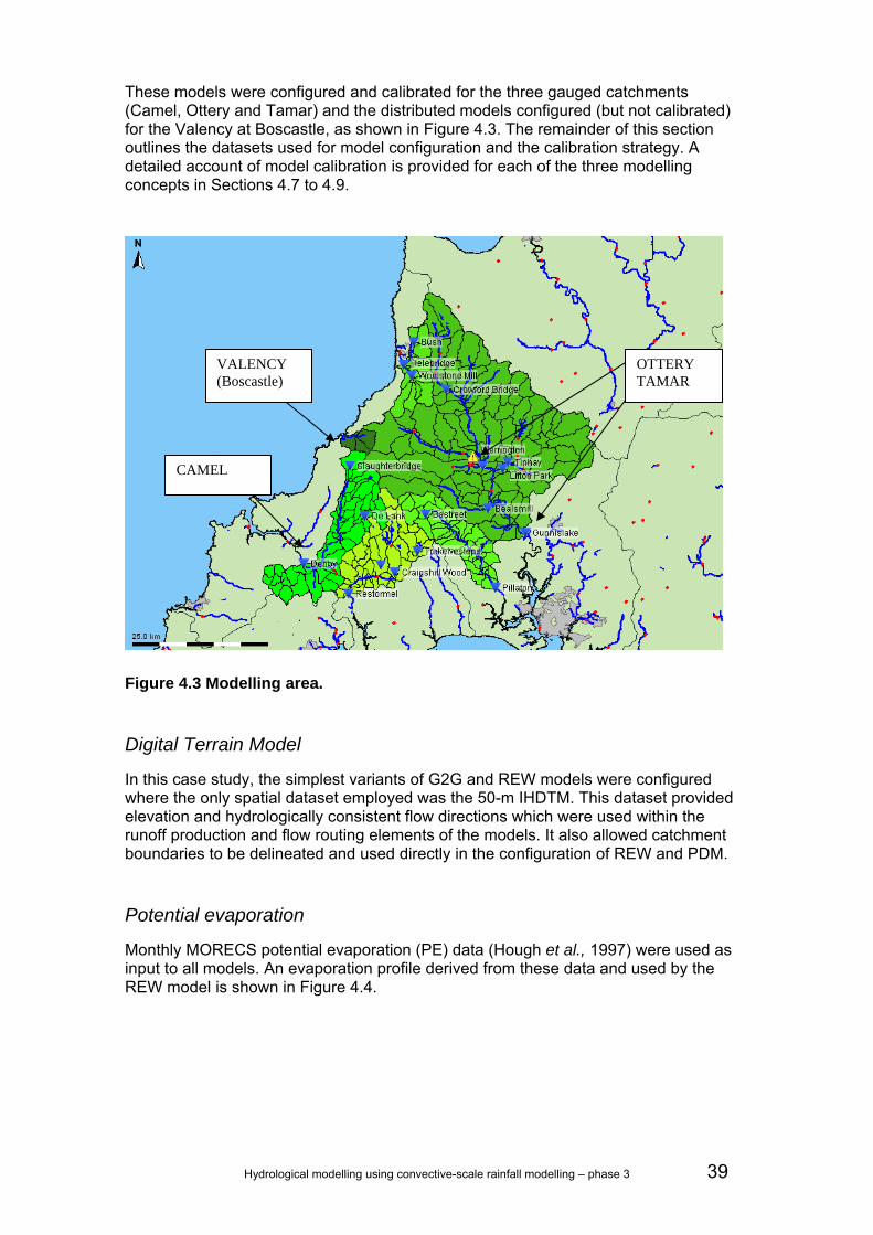
Hydrological modelling using convective-scale rainfall modelling – phase 3 39
These models were configured and calibrated for the three gauged catchments (Camel, Ottery and Tamar) and the distributed models configured (but not calibrated) for the Valency at Boscastle, as shown in Figure 4.3. The remainder of this section outlines the datasets used for model configuration and the calibration strategy. A detailed account of model calibration is provided for each of the three modelling concepts in Sections 4.7 to 4.9.
Figure 4.3 Modelling area.
Digital Terrain Model
In this case study, the simplest variants of G2G and REW models were configured where the only spatial dataset employed was the 50-m IHDTM. This dataset provided elevation and hydrologically consistent flow directions which were used within the runoff production and flow routing elements of the models. It also allowed catchment boundaries to be delineated and used directly in the configuration of REW and PDM.
Potential evaporation
Monthly MORECS potential evaporation (PE) data (Hough et al., 1997) were used as input to all models. An evaporation profile derived from these data and used by the REW model is shown in Figure 4.4.
OTTERY TAMAR
VALENCY (Boscastle)
CAMEL

40 Hydrological modelling using convective-scale rainfall modelling – phase 3
0
0.5
1
1.5
2
2.5
1 23 45 67 89 111 133 155 177 199 221 243 265 287 309 331 353
Figure 4.4 Daily evaporation profile used for REW modelling.
HyradK raingauge-adjusted radar data
The HyradK module adapter was used to generate raingauge-adjusted radar rainfall time series. Nimrod composite radar data and Environment Agency raingauge data were combined and the resulting HyradK rainfall grids used as input to all models. These gridded rainfall data were used directly by the G2G model and in the form of REW or catchment averages for the REW and PDM models respectively.
Raingauge data were provided for the area surrounding the case study catchments as well as within the catchments. Raingauges located outside the catchments can still have a positive impact on the HyradK rainfall estimates inside the catchment. Only a subset of the raingauges provided were included. The main criteria for selection was to maintain a consistent raingauge network over the 2002-2007 study period. Several new raingauges have been installed since 2005 but these were only included if they replaced an older raingauge that had ceased operation. Raingauges selected are listed in Table 4.2 and their locations shown in Figure 4.5.

Hydrological modelling using convective-scale rainfall modelling – phase 3 41
Table 4.2 Raingauges used by HyradK.
FEWS number Raingauge name FEWS
number Raingauge name FEWS number Raingauge name
49101 Bodmin 47106 Bastreet 48103 Penryn
49102 Lanreath 47107 Bealsmill 48104 Bissoe
49103 Trebrownbridge 47108 Mary Tavy 48105 Allet
49104 Colliford 47109 Huckworthy 48106 Luxulyan
49105 De Lank 47112 Lee Moor 50100 Bradworty
49106 Slaughterbridge 47113 Cornwood 50101 Parkham
47102 Crowford Bridge 48100 Trengwainton 50103 Allisland
47103 Canworthy Water 48101 Boscadjack 50105 East Okement Farm
47104 Yeolmbridge 48102 Rosewarne 50106 Sticklepath
FEWS number Raingauge name Comment
N/A Tinhay Replaced by Roadford
47105 Roadford Replaces Tinhay
N/A Gwills Replaced by Newquay
49147 Newquay Replaces Gwills
N/A Pillaton Replaced by Hatt
47157 Hatt Replaces Pillaton
N/A Trevalec Not telemetered but new Boscastle raingauge is nearby
N/A Roserrow Not telemetered but new St Teath raingauge is nearby
N/A Wadebridge Not telemetered but new St Teath raingauge is nearby
N/A Bridgerule Not in FEWS but new Holsworthy raingauge is nearby
N/A Woolstone Not in FEWS but new Trefrida raingauge is nearby
N/A Tamarstone Not in FEWS but new Tamar Lakes raingauge is nearby

42 Hydrological modelling using convective-scale rainfall modelling – phase 3
Figure 4.5 Location of raingauges selected for use with HyradK.
The raingauge data provided came in either time-of-tip form or as 15-minute accumulations and with resolutions of 0.2, 0.5 or 1.0 mm. Also, some records changed format or resolution during the study period. All data were processed to form 15-minute accumulations. Care was taken in processing the time-of-tip format data to differentiate between periods of no rainfall and periods when the record was missing.
The time series of 15-minute rainfall accumulations were then quality controlled using the follow methods:
70mm filter: 15-minute accumulations in excess of 70 mm were removed from the data and set to be missing. These were cross-referenced to radar data and Met Office weather summaries to confirm that they were indeed erroneous. A record of the values changed was made. 20-70mm filter: 15-minute accumulations above 20 mm were investigated further including use of radar data and Met Office weather summaries. A record was made of the values above 20 mm, also indicating whether these were assumed valid or treated as missing. Cumulative hyetographs: Cumulative hyetographs for groups of raingauges located close together were plotted and any anomalies (such as blocked raingauges, zero recorded rainfall) were investigated. Periods treated as suspect were replaced by missing values (-999.0) and a record of these kept.
4.6 Model assessment strategy Case study hydrometric data were provided for the period 2002-2007. After studying the available data and considering that the Boscastle event (16 August 2004) needed to be used for model verification, a split sample method was adopted where distinct calibration and verification periods were identified. These periods are listed in Table 4.3. All models were calibrated using the calibration period data only. The model calibrations were then tested independently over the verification period. The selection
HATT
ALLET
BODMIN
DELANK
GWILLS
BISSOE
TINHAY
PARKHAM
NEWQUAY
ROADFORD
LEE MOOR
LANREATH
CORNWOOD
TREVALEC
LUXULYAN
BASTREET
ALLISLAND
COLLIFORD
BEALSMILLMARY TAVY
BRADWORTHY
WADEBRIDGE
BOSCADJACK
HUCKWORTHY
BRIDGERULE
TAMARSTONE
STICKLEPATH
YEOLMBRIDGE
TRENGWAINTON
ROSEWARNE TBR
PILLATON MILL
WOOLSTONE MILL
TREBROWNBRIDGE
SLAUGHTERBRIDGE
CANWORTHY WATER
CROWFORD BRIDGE
PENRYN RESERVOIR
EAST OKEMENT FARM
ROSERROW GOLF COURSE
HyradK raingauges

Hydrological modelling using convective-scale rainfall modelling – phase 3 43
used encompassed a range of summer and winter events in both the calibration and verification periods.
Table 4.3 Calibration and verification periods.
Period Start date End date Calibration 00:00 09/01/2006 23:45 31/07/2007 Verification 00:00 01/01/2004 23:45 23/12/2005
Models were assessed in simulation mode and updating mode (forecast mode). All hydrological models employed the HyradK raingauge-adjusted radar data, with model simulations obtained assuming perfect foreknowledge of future rainfall. Different approaches for generating updated hydrological forecasts were used by the different models. For the PDM and G2G models, empirical state-correction schemes were chosen which use gauged observation at the point of interest up to the start of the forecast. The REW model uses an ARMA error-prediction model. More details about the approaches are given in the model results sections.
4.7 REW model application
4.7.1 Terrain analysis
Separate REW models were set up for the five catchments in the model domain covering parts of Cornwall and Devon. The selected catchments included the Tamar, the Camel, the Fowey, the Lynher and the Valency. Only the Tamar/Ottery and the Camel were calibrated and are presented in this section.
The first step in the model setup was analysis of the 50 x 50 m digital terrain maps (DTMs) for extraction of the stream channel network and determination of REWs. For terrain analysis the open-source software TARDEM from the University of Utah (Tarboton 1997) was used, which has been extended with the capability to extract REWs. The DTM analysis led to two separate catchment configurations: Tamar (with the Ottery as an internal catchment) and Camel.
The stream channel network was extracted with the stream-threshold area criterion. The threshold area is a minimal accumulated upstream area, expressed in number of pixels. Pixels with an accumulated area higher than the threshold area are defined as stream channel pixels. The network was extracted by assuming a cut-off Horton-Strahler threshold of order one, meaning that first and larger order channels were all part of the network. If larger REWs are desired, the Horton-Strahler threshold order can be set equal to two or higher.
Once TARDEM extracted the network and determined the sub-basin areas, the module REWANALYSIS was used to determine the three-dimensional REW geometries and REW interconnections. Examples presented later in Figure 4.6 and Figure 4.9 show the spatial discretisation of the Camel and the Tamar catchments into 51 and 81 REWs respectively.

44 Hydrological modelling using convective-scale rainfall modelling – phase 3
4.7.2 REW model setup
Preliminary considerations
Before describing the parameterisation and results of the model for the two study catchments, we outline the assumptions on which the catchments were modelled.
1. The REW model did not consider the presence of a vegetation cover and the catchments were thus modelled as if they were bare soil. The net precipitation was given by the sum of precipitation minus potential evaporation. As a result vegetation-related effects, such as interception or a more sophisticated SVAT (Surface-Vegetation-Atmosphere Transfer) scheme with root extraction, were neglected. Non-linear effects of soil-water depletion during summer months were thus not fully accounted for.
2. Parameters describing soil texture and structure were applied homogeneously across the catchment, the saturated zone (S-zone), the unsaturated zone (U-zone) and the subsurface storm-flow zone (P-zone). In principle it would be possible to assign different properties to the various zones and REWs, but in the absence of detailed soil information we used uniform values.
3. The raingauge-adjusted radar rainfall time series was used to obtain areal-averages over the REWs.
4. Potential evaporation was estimated from the monthly average MORECS data. These data were supplied on a coarse national grid covering the entire UK. The MORECS potential evaporation estimates relative to the grid-cell covering the study area were adopted for the simulations. The same evaporation time series were assigned to all REWs in the study catchments.
5. It was assumed that there was no lateral groundwater exchange across the external catchment boundaries. Only REW 1 (the REW in correspondence with the catchment outlet) was assumed to have a permeable outer boundary, thus admitting a minimal groundwater flux across the external catchment boundary. For the groundwater distribution algorithm to converge (the algorithm is based on the Hardy-Cross discharge rebalancing over closed network loops) at least one network node must be allowed to exchange water to preserve continuity of mass within the network.
6. Calibration of model parameters was done over a 15-minute time series of precipitation and evaporation over a calibration period from 9 January 2006 to 31 July 2007. Precipitation data were at 15-minute intervals while potential evaporation data were disaggregated from average monthly data to 15-minute data. The calibration was performed manually, where hydrodynamic parameters (soil texture and structure, Manning coefficients) were kept constant while five parameters determining geometric characteristics were kept variable.
4.7.3 Camel
The Camel catchment has a surface area of 209 km2. By means of a terrain analysis the catchment was separated into a total number of 51 REWs by assuming a surface threshold area of 100 pixels for channel heads. The DTM analysis result in a breakdown of the catchment into 51 modelling units or REWs (Figure 4.6).

Hydrological modelling using convective-scale rainfall modelling – phase 3 45
28
53
17
3
46
12
30
6
27
42
48
8
11
49
52
5
2
26
35
7 51
32
24
47
43
50
45
9
10
40
41
13
20
23
33
31
44
4
34 363722
39
16
29
21
19
14
18
25
1
38
Figure 4.6 The Camel watershed broken down into 51 REWs.
To determine the REWs we set a subsurface zone delimited by an “infinite” depth (300 m, parameter 4) bedrock layer and assigned uniform soil texture and structure parameters for all REWs, as indicated in Table 4.4.
Calibration
The exchange between the river channel and aquifer (parameter 1) was chosen very low (10-6), effectively setting the river-groundwater exchange to zero. In this context the depth of the river bed transition zone (parameter 2) was set to 1.5 m, but remained irrelevant as a model parameter.

46 Hydrological modelling using convective-scale rainfall modelling – phase 3
Table 4.4 REW model parameters for Camel catchment. No parameter value calibrated
1 hydraulic conductivity for channel bed (m s-1):
0.000001 n
2 river bed transition zone thickness (m):
1.5 n
3 exponent in power relationship (p=1 linear):
0.30 y
4 bedrock depth (m): 300 n
5 soil porosity (-): 0.5 n
6 saturated hydraulic conductivity S-zone (m s-1):
0.00005 n
7 saturated hydraulic conductivity U-zone (m s-1):
0.00005 n
8 Brooks-Corey soil parameter lambda (-): 1.00 n
9 Brooks-Corey pressure scaling parameter (m):
0.25 n
10 water content at saturation (-): 0.5 n
11 saturated hydraulic conductivity P-zone (m s-1):
0.005 y
12 exponent on transmissivity law (2<=g<=4):
3.8
y
13 depth of saturated subsurface flow layer (m):
0.5
y
14 exponent for surface precipitation partitioning:
0.3 y
An important calibration parameter is the exponent of the power-law relationship, which governs the expansion (contraction) of saturated areas as a function of water table position (parameter 3). We chose a relationship with an exponent that was less than linear (0.3), causing larger increases of the saturated area fraction for water table levels close to average channel bed elevation of the REW, and with decreasing saturated area expansion for groundwater-table levels above average channel bed elevation. This parameter was also made constant for all REWs and should in principle be set as variable between REWs. The most common range for this parameter is between zero and three.
The soil porosity (parameter 5) was set uniformly to 0.5 for the entire catchment and was not considered a calibration parameter. The hydraulic conductivity of the saturated zone (S-zone, parameter 6) and of the unsaturated zone (U-zone, parameter 7) were both set to 5x10⁻⁵ m s-1. This parameter was set at a constant value during the model setup. The Brooks-Corey parameters λ (parameter 8) and m (parameter 9) were set equal to one and 0.25 respectively, uniformly for all unsaturated zones of all REWs.

Hydrological modelling using convective-scale rainfall modelling – phase 3 47
The residual water content in the saturated zone was assumed equal to zero and the water content at saturation (parameter 10) equal to the soil porosity. The P-zone constituted an important store for the system. The P-zone is a subsurface storm-flow layer, which is described as a subsurface kinematic wave equation and a transmissivity law controlled by an exponent (parameter 12). The transmissivity law exponent is a calibration parameter.
The net precipitation falling onto the soil surface was split into two parts: i) one part going directly into the unsaturated soil and therefore into the Richards equation column, and ii) one part going into the P-zone. The splitting was governed by a power-law relationship, in which the mean saturation of the top 10 cells of the Richards equation layers were raised to a power β (parameter 14). In this fashion, the wetter the top soil became, the more water entered the P-zone.
The lateral flow in the P-zone occured in a layer with a constant depth of 0.5 m (parameter 13) and joined the river channel (R-zone). Excess water which could not be transferred in this layer flowed off as surface runoff, causing peaks in overland flow. Both parameters 13 and 14 were relevant calibration parameters controlling this process. This mechanism of runoff partitioning determined to a large part the reactions of the system and required special attention in the calibration process.
Results
Figure 4.7 shows the results of the calibration for the gauging station on the Camel at Denby. Note that the falling limb of the hydrograph is sometimes too steep for low discharges. This shortcoming is essentially attributable to limitations in the representation of surface runoff as a sheet flow in terms of an analytically solved kinematic wave equation for low discharges.
The issue is less prominent in the case of the Tamar catchment (see below) with higher surface runoff volumes. Better results can be achieved by using Manning coefficients that are higher and thus lie outside the range of typical values reported in the literature, or by representing overland flow with equations other than kinematic surface wave equations (such as simple storage-discharge power law relationships). Section 4.7.5 takes a closer look at the calibration results.
The departure of simulations from observations in the hydrograph recession phase could also be attributable to the fact that evaporation in the model is represented too simplistically in terms of monthly mean values form the MORECS dataset. To improve simulations, we recommend using daily or hourly time series of potential evaporation calculated with the Penman-Monteith method in place of the mean monthly values. In general, the model represents the discharge at Denby with reasonable accuracy.

48 Hydrological modelling using convective-scale rainfall modelling – phase 3
Figure 4.7 Modelled and observed discharges at Denby, 1 January 2005 to 1 October 2007. Precipitation at REW 1.
The strength of using a physically-based modelling system like the REW model is highlighted in the figure of various internal model fluxes and hydrological variables that can be computed by the model (Figure 4.8). These hydrological fluxes and variables such as REW-average water table positions and saturated area fractions are measurable quantities, which can be used for a variety of studies such as investigations of the impact of land-use change, erosion and the impact of climate change on water resources.
0 1 2 3 4 5 6 7 8 9
x 107
0
20
40
60
80
100Camel (Cornwall) at Denby, 01/01/2005−01/10/2007
Simulated at REW1Observed at Denby
0 0.5 1 1.5 2 2.5
x 104
0
5
10
15
20
25
30

Hydrological modelling using convective-scale rainfall modelling – phase 3 49
Figure 4.8 Model-internal hydrological fluxes for REWS 01 (blue), 10 (black), 20 (red), 25 (cyan), 29 (magenta), 39 (yellow) and 45 (green). Fluxes represent from top left: discharge at REW outlet (Qout), inflow of surface runoff into channel (eor), subsurface storm flow (epr), P-zone saturation (sp) , water table recharge (eus), saturation excess flow from P-zone into O-zone (epo), saturated area fractions ωo, seepage from S-zone into O-zone and groundwater table position (ys).
Figure 4.8 (and also Figure 4.12) show time-series plots of different internal state variables of the REW model. These include discharge at the outlet of a REW, discharge form the overland flow zone to the channel, inflow of subsurface storm flow into the river channel, saturation of the subsurface zone, water table recharge (percolation), infiltration excess flow, the percentage of saturated area fractions, the seepage exfiltration on saturated areas and finally the relative water table position (expressed as a percentage of the maximum level). These are just a few of the variables that can be calculated with a physically-based distributed hydrological model. They can in principle be observed in the field (such as percentage of saturated areas) and interpreted on physical grounds. For example, a clear connection can be seen between the saturation excess flow (second figure on top row) and level of saturation in the subsurface storm-flow zone (P-zone) (first figure in second row). If the P-zone becomes fully saturated (a value of one), the saturation excess flow starts to increase. Similarly there is a direct relation between the dynamics of the saturated area fraction

50 Hydrological modelling using convective-scale rainfall modelling – phase 3
and the average water table position. With increasing water table position, a larger part of the REW becomes saturated (see first and third figure in last row).
4.7.4 Tamar
The Tamar has a surface area of 920 km2. The catchment was separated into a total of 81 REWs by assuming a threshold drainage area of 100 pixels for the channel heads. The resulting channel network is represented in Figure 4.9.
76
7748
28
68
36
78
39
41
23
4
12
66
17
54
16
65
40
69
60
6
22
31
2
24
51
25
3
21
7370
27
3237
62
80
34
67
61
81
59
8
47
18
29
57
3856
7
42
63
79
46
30
33
4445
74
1
11
75
4326
71
55
52
5
19
58
4950
64
53
13
109
1415
72
20
35
Figure 4.9 The Tamar watershed broken down into 81 REWs.
Calibration
To calibrate the Tamar catchment we used comparable parameter values as for the Camel, assuming regional uniformity between catchments. The respective parameter values are summarised in Table 4.5.
Results
Figure 4.10 and Figure 4.11 show the calibration results at the two gauging stations on the Tamar at Gunnislake (catchment outlet) and Werrington Park further upstream on the Ottery. For both gauging stations peak behaviour is well captured, while there is a presence of spurious peaks during low flow periods. These peaklets are caused by the consistent presence of water in the subsurface storm-flow layer, which leads to surface saturation and runoff during small rainfall events.
However, the spurious peaks and departure of simulations from observations in the hydrograph recession phase could also be attributable to the fact that evaporation is represented too simplistically in terms of monthly mean values from the MORECS
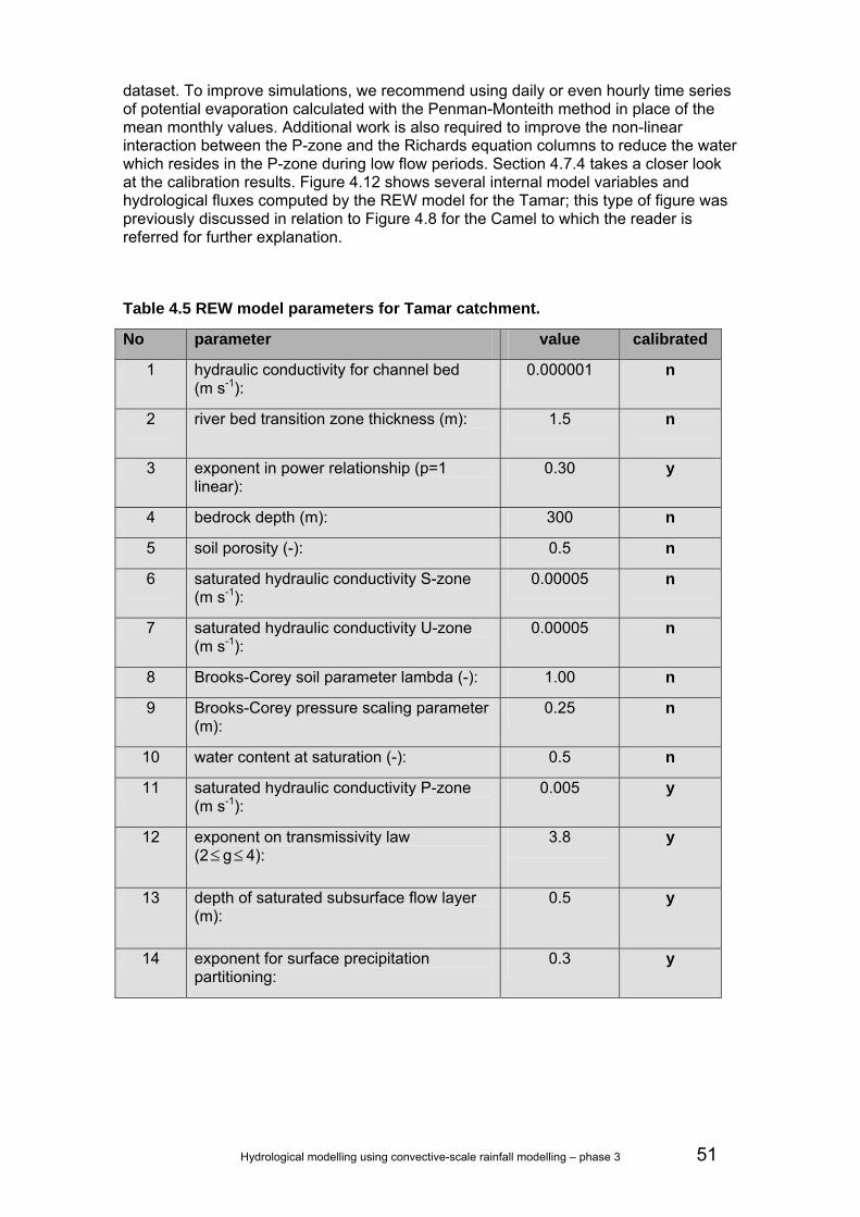
Hydrological modelling using convective-scale rainfall modelling – phase 3 51
dataset. To improve simulations, we recommend using daily or even hourly time series of potential evaporation calculated with the Penman-Monteith method in place of the mean monthly values. Additional work is also required to improve the non-linear interaction between the P-zone and the Richards equation columns to reduce the water which resides in the P-zone during low flow periods. Section 4.7.4 takes a closer look at the calibration results. Figure 4.12 shows several internal model variables and hydrological fluxes computed by the REW model for the Tamar; this type of figure was previously discussed in relation to Figure 4.8 for the Camel to which the reader is referred for further explanation.
Table 4.5 REW model parameters for Tamar catchment.
No parameter value calibrated
1 hydraulic conductivity for channel bed (m s-1):
0.000001 n
2 river bed transition zone thickness (m):
1.5 n
3 exponent in power relationship (p=1 linear):
0.30 y
4 bedrock depth (m): 300 n
5 soil porosity (-): 0.5 n
6 saturated hydraulic conductivity S-zone (m s-1):
0.00005 n
7 saturated hydraulic conductivity U-zone (m s-1):
0.00005 n
8 Brooks-Corey soil parameter lambda (-): 1.00 n
9 Brooks-Corey pressure scaling parameter (m):
0.25 n
10 water content at saturation (-): 0.5 n
11 saturated hydraulic conductivity P-zone (m s-1):
0.005 y
12 exponent on transmissivity law (2≤g≤ 4):
3.8
y
13 depth of saturated subsurface flow layer (m):
0.5
y
14 exponent for surface precipitation partitioning:
0.3 y

52 Hydrological modelling using convective-scale rainfall modelling – phase 3
Figure 4.10 Modelled and observed discharges at Gunnislake, 1 January 2005 to 1 October 2007. Precipitation at REW 1.
0 1 2 3 4 5 6 7 8 9
x 107
0
100
200
300
400
500
600
700
Measured at GunnislakeSimulated at REW1
0 0.5 1 1.5 2 2.5
x 104
0
5
10
15
20

Hydrological modelling using convective-scale rainfall modelling – phase 3 53
Figure 4.11 Modelled and observed discharges at Werrington , 1 January 2005 to 1 October 2007. Precipitation at REW 1.
0 1 2 3 4 5 6 7 8 9
x 107
0
50
100
150
200
Measured at WerringtonSimulated at REW32
0 0.5 1 1.5 2 2.5
x 104
0
5
10
15
20

54 Hydrological modelling using convective-scale rainfall modelling – phase 3
Figure 4.12 Model-internal hydrological fluxes for REWS 01 (blue), 10 (black), 05 (red) 23 (magenta), 25 (green), 33 (cyan). Fluxes represent from top left: discharge at REW outlet (Qout), inflow of surface runoff into channel (eor), subsurface storm flow (epr), P-zone saturation (sp), water table recharge (eus), saturation excess flow from P-zone into O-zone (epo), saturated area fractions ωo, seepage from S-zone into O-zone and groundwater table position (ys).
4.7.5 Model performance (simulation mode)
As shown in the previous sections, simulation results are acceptable for the Tamar gauging station at Gunnislake and the Camel at Denby, and less so for the Ottery gauging station at Werrington Park.
Table 4.6 lists performance measures for simulated versus observed discharge at gauge locations. R2 (Nash-Sutcliffe) efficiencies, such as those presented in Table 4.6, can range from minus infinity to one. An efficiency of one corresponds to a perfect match of modelled discharge to the observed data while an efficiency of zero indicates that model predictions are as accurate as the mean of the observed data. An efficiency below zero occurs when the observed mean is a better predictor than the model. Clarke (2008) provides a recent review of this performance statistic.

Hydrological modelling using convective-scale rainfall modelling – phase 3 55
Table 4.6 Model performance for calibration and verification periods, January 2006 to August 2007 and 2004-2005 respectively.
Location R2 efficiency Mean absolute error Bias
Tamar at Gunnislake 0.7144 7.4329 1.0264
Ottery at Werrington Park -0.1449 18.1382 18.1325
Cal
ibra
tion
Per
iod
Camel at Denby 0.6881 1.7286 0.1971
Tamar at Gunnislake 0.6938 6.3767 0.4156
Ottery at Werrington Park -0.0739 14.7813 14.7772
Ver
ifica
tion
Per
iod
Camel at Denby 0.6558 1.6859 -0.3004
While Gunnislake (Tamar) and Camel (Denby) exhibit satisfactory R2 efficiency values in the order of 0.7, these are negative for the Ottery at Werrington Park, indicating that the observed mean is a better predictor. The poor performance of the REW model at Werrington, however, is attributable to low discharge values of the Ottery at that location, which result in model bias and thus lower R2 efficiency.
Figure 4.13 and Figure 4.14 show measured and modelled discharge for a winter period for the three calibration sites plus a site within the Tamar catchment (Crowford Bridge) treated as ungauged during calibration. More internal sites are displayed in Figure 4.15 and Figure 4.16. Although all model parameters were taken as uniform throughout each catchment, results for the interior sites look rather promising and compare well to the sites used for calibration. One of the reasons for this may be attributed to the rather uniform geology within each of the two catchments. A closer look at the results for the Camel at Denby shows that the peaks are overestimated and the model reacts much too rapidly to rainfall. On the other hand, the baseflow component is underestimated.
The results for summer events are less promising for both catchments. The results for the Boscastle event itself are not very good, which has implications for the forecasts reported in the next section. In general, the peaks in summer are overestimated. However, for the Boscastle case the peaks are underestimated in the Tamar at all stations and overestimated at Denby in the Camel (Figure 4.17).
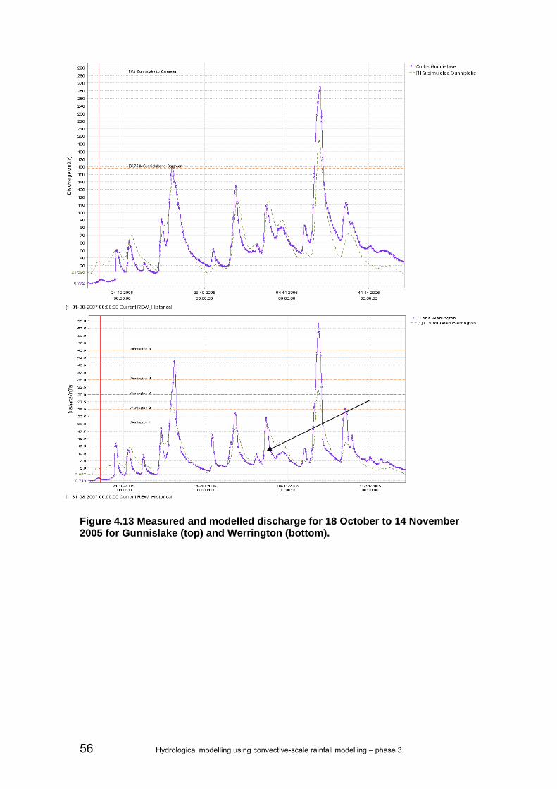
56 Hydrological modelling using convective-scale rainfall modelling – phase 3
Figure 4.13 Measured and modelled discharge for 18 October to 14 November 2005 for Gunnislake (top) and Werrington (bottom).

Hydrological modelling using convective-scale rainfall modelling – phase 3 57
Figure 4.14 Measured and modelled discharge for 18 October to 14 November 2005 for Denby and Crowford Bridge. Crowford Bridge is an internal site treated as ungauged during calibration. This gives an indication of how distributed models can be used to estimate discharge (and flooding) for ungauged sites.

58 Hydrological modelling using convective-scale rainfall modelling – phase 3
Figure 4.15 Results for a winter event for the internal sites Crowford Bridge, Lifton Park and Slaugtherbridge (bottom left). Both Tamar sites perform rather well. For Slaugterbridge a systematic error (offset) is visible. The latter will route down to Denby and influence those results.

Hydrological modelling using convective-scale rainfall modelling – phase 3 59
Figure 4.16 Measured and modelled discharge for 18 October to 14 November 2005 for internal sites. Top left to bottom right: De Lank, Beals Mill, Lifton Park and Tinhay.
Although the performance described in the previous paragraphs is fairly typical for many simulations, some features of the REW model are lacking and require further examination. The three main limitations, linked to the simple SVAT scheme used in the model, are:
1. Transpiration losses are not taken from the soil component itself but are part of a bulk ET component that is subtracted from the precipitation component. As a result the soil may not dry out enough in summertime (with high ET losses and low precipitation). Therefore, the model may start to generate quick runoff far to early.
2. No interception component is modelled. This may lead to an overestimation of the net precipitation component, especially in forested areas.
3. A monthly average evaporation is used. Evaporation is as important as precipitation, as it constitutes a meteorological forcing. A physically-based model is especially sensitive to input. We therefore recommend using daily, weekly or monthly evaporation records estimated on the basis of the Penman-Monteith equation in place of the monthly average MORECS data.
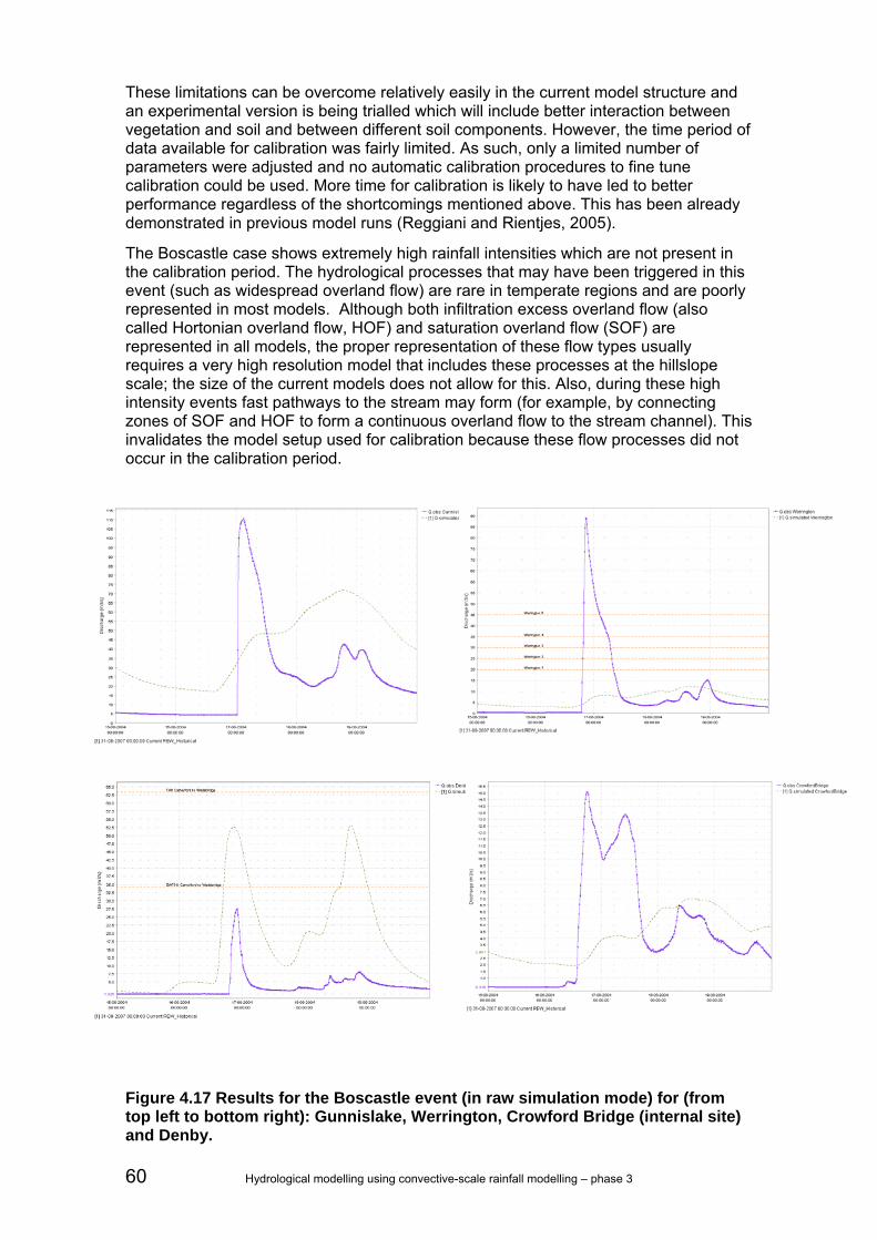
60 Hydrological modelling using convective-scale rainfall modelling – phase 3
These limitations can be overcome relatively easily in the current model structure and an experimental version is being trialled which will include better interaction between vegetation and soil and between different soil components. However, the time period of data available for calibration was fairly limited. As such, only a limited number of parameters were adjusted and no automatic calibration procedures to fine tune calibration could be used. More time for calibration is likely to have led to better performance regardless of the shortcomings mentioned above. This has been already demonstrated in previous model runs (Reggiani and Rientjes, 2005).
The Boscastle case shows extremely high rainfall intensities which are not present in the calibration period. The hydrological processes that may have been triggered in this event (such as widespread overland flow) are rare in temperate regions and are poorly represented in most models. Although both infiltration excess overland flow (also called Hortonian overland flow, HOF) and saturation overland flow (SOF) are represented in all models, the proper representation of these flow types usually requires a very high resolution model that includes these processes at the hillslope scale; the size of the current models does not allow for this. Also, during these high intensity events fast pathways to the stream may form (for example, by connecting zones of SOF and HOF to form a continuous overland flow to the stream channel). This invalidates the model setup used for calibration because these flow processes did not occur in the calibration period.
Figure 4.17 Results for the Boscastle event (in raw simulation mode) for (from top left to bottom right): Gunnislake, Werrington, Crowford Bridge (internal site) and Denby.
Hydrological modelling using convective-scale rainfall modelling – phase 3 61
4.7.6 Model performance (forecasting mode)
Introduction
To evaluate the performance of the model in forecast mode, workflows were set up in the stand-alone Delft-FEWS system to run the REW model in forecast mode. This was done as follows:
• For each forecast location with gauge data, an ARMA model was set up using automatic parameter determination to represent the operational setting (see Section 4.7.6).
• For the entire period, historical runs were made saving initial conditions for each day (at 00:00). This was done in raw simulation mode without updating.
• Input to the model in forecast mode was made up of: − Perfect rainfall forecast (the HyradK-adjusted radar) over the entire period. − Measured discharge up to the time of forecast, T0 (to the ARMA model).
• Forecasts were made for every 15-minute time-step during the selected periods.
• Fixed lead-time series were extracted from these forecasts for one, two, four, six, eight, 10 and 12 hour lead times.
The results give an indication of the performance of the REW model setup in forecast mode, assuming the HyradK-adjusted rainfall provides a good estimate of the actual rainfall over an REW. These results also serve to check the results of the high-resolution NWP forecasts for the Boscastle case.
Because of run-time limitations it was not possible to run forecasts for each 15-minute interval for the entire period. Therefore, the following periods were chosen to evaluate forecast performance using HyradK-adjusted rainfall (Table 4.7).
With respect to operational use, we found that the run time of the REW model for the Tamar catchment was about four minutes for a 24-hour period. This is much slower than a typical lumped model such as PDM and marginally slower than the G2G model. However, depending on catchment size and hardware used the run time might be acceptable in many applications.

62 Hydrological modelling using convective-scale rainfall modelling – phase 3
Table 4.7 Event periods (start and end times are at 00:00).
Period nr
Start date End date Over Gunnislake threshold
Summer / Winter
Comments
1 25/07/2003 26/07/2003 N S Possible convective event. Large response at Denby. Relevant for Boscastle event. NOT USED for REW
2 10/12/2003 10/02/2004 Y (3 times) W
3 15/08/2004 20/08/2004 N S Boscastle event.
4 02/10/2004 02/11/2004 Y (twice) W
5 14/12/2004 26/01/2005 Y (3 times) W
6 10/02/2005 15/02/2005 N W Interesting double peak. Isolated event. Just under threshold.
7 18/10/2005 14/11/2005 Y (2 times) W
8 26/11/2005 10/12/2005 Y (once) W
9 19/05/2006 27/05/2006 N S Just under threshold (peak ~125 m3s-1).
10 14/11/2006 14/12/2006 Y (4 times) W Includes largest peak on record.
11 07/02/2007 12/03/2007 Y (4 times) W
12 09/05/2007 19/05/2007 N S Under threshold (peak ~110 m3s-1).
ARMA model and configuration
The ARMA model is applied to improve model time-series predictions through combining modelled series and observed series. It uses as input an output series from a forecasting module (typically discharge from a routing or rainfall-runoff module) and the observed series at the same location. An updated series for the module output is again returned by the module. Updating is done through use of an error model to the residuals between module output and observed series. This error model is applied also to the forecast data to correct errors in the forecast.
Configuration of the error modelling module is used to determine its behaviour in establishing the statistical model of the error and how this is applied to derive the updated series.
Configuration items:
• Order_AR: (maximum) order of the AR component.
• Order_MA: 0.
• Order_Sel: Option to determine if the orders are to be derived automatically (with the maxima as defined above) or as given.
• Transform: Option to apply a transformation to residuals. This may be "none", "mean" or "boxcox".
• Lambda: A required parameter for the "boxcox" transformation option.

Hydrological modelling using convective-scale rainfall modelling – phase 3 63
Time-series definitions
Three types of time-series models can be distinguished, autoregressive or AR, moving average or MA and the combined ARMA type. An ARMA(p,q) process for a variable xn can be written as (Priestley, 1981):
1 1 1 1... ...n n p n p n n q n qx a x a x b bε ε ε− − − −+ + + = + + +
where the variable εn constitutes error terms from a purely random process. The process provides a sequence of independent identically distributed stochastic variables with zero mean and variance σε
2. The coefficients ai and bi are model parameters to be estimated. This process is purely AR for q=0 and MA for p=0.
AR estimation
Burg’s method, also denoted as maximum entropy (Burg, 1967; Kay and Marple, 1981), is used for parameter estimation to ensure that the model will be stationary. Asymptotic AR order selection criteria can give wrong orders if candidate orders are higher than 0.1N (N is the signal length). The finite sample criterion CIC(p) is used for model selection (see Broersen, 2000). The model with the smallest value of CIC(p) is selected. CIC uses a compromise between the finite sample estimator for the Kullbach-Leibler information (Broersen and Wensink, 1998) and the optimal asymptotic penalty factor of three (Broersen, 2000; Broersen and Wensink, 1996).
Box-Cox transformations
The Box-Cox transformation (Box and Cox, 1964) can be applied in the order selection and estimation of the coefficients. The object in doing so is usually to make the residuals more homoscedastic and closer to a normal distribution. The transform for a variable y is defined as:
( ) ( 1) /T y yλ λ= −
when the Box-Cox transform parameter λ is not equal to zero. When λ=0 then T(y)=log(y).
Application of the module
The implemented algorithm computes AR(p) models with p=0,1,…,N/2 and selects a single best AR model with CIC. This automatic mode has been used in this study. The settings used are shown below:
orderSelection true
order_ar 3
order_ma 3
subtractMean false
boxcoxTransformation false
lambda 0
Results
Graphs showing lead time versus model efficiency for the periods defined in Table 4.7 are presented in Figure 4.18 to Figure 4.20. A summary table is shown in Table 4.8. For most periods, the forecast model efficiency is better than the raw simulation

64 Hydrological modelling using convective-scale rainfall modelling – phase 3
(without the ARMA correction) for lead times up to about six hours, sometimes even up to 12 hours. For some cases, especially for Werrington, the forecast efficiency drops below the raw simulation after four hours. Better performance for longer lead time for those cases might be obtained by changing the ARMA model configuration to always go back to the raw simulation after a number of hours.
Although the use of updating within REW was not part of this study, initial tries using the Ensemble Kalman Filter in combination with REW show that this can improve forecast results considerably. As such, this could be used in further research instead of the simple output correction.
Figure 4.18 Model efficiency (R2) versus lead time for period 2 to 5 for Gunnislake, Denby and Werrington.

Hydrological modelling using convective-scale rainfall modelling – phase 3 65
Figure 4.19 Model efficiency (R2) versus lead time for period 6 to 9 for Gunnislake, Denby and Werrington.

66 Hydrological modelling using convective-scale rainfall modelling – phase 3
Figure 4.20 Model efficiency (R2) versus lead time for period 10 to 12 for Gunnislake, Denby and Werrington.

Hydrological modelling using convective-scale rainfall modelling – phase 3 67
Table 4.8 R2 model efficiency for all events. Grey cells denote that the forecast mode R2 for that lead time is lower than that of the raw simulation indicating under/overshoot of the ARMA model. The latter might be remedied by changing the configuration of the ARMA model.
.

68 Hydrological modelling using convective-scale rainfall modelling – phase 3
4.8 PDM model application
4.8.1 Model setup
The standard form of the PDM was initially used for all case studies with a cubic baseflow storage, a cascade of two unequal reservoirs for the surface storage and a truncated Pareto distribution of soil/vegetation absorption capacity. Where appropriate the soil tension capacity, St, influencing drainage to groundwater and evaporation, was allowed to be non-zero and modelling of catchment returns/abstractions was invoked by adding a constant flow, qc. Section 3.3.1 provides a more comprehensive model description.
The calibration process was split into two parts. Firstly, the process model parameters were calibrated in simulation mode where the model deterministically calculates simulated flow using only the input data (rainfall and potential evaporation), ignoring the observed flow (except for model initialisation). Secondly, the model was run in forecast mode which aims to emulate real-time application in an offline environment and is used to calibrate the state-updating parameters. In this case, HyradK raingauge-adjusted rainfall data were used as “perfect” foreknowledge of forecast rainfall. The calibrated PDM model parameters are presented in Table 4.9.
The 50-m IHDTM was used to delineate the catchment boundaries for the case study catchments and to provide the catchment areas needed by the PDM. The boundaries were used to calculate catchment average rainfall from the HyradK raingauge-adjusted radar rainfall estimates.
4.8.2 Tamar at Gunnislake
As stated before, flood forecasting of the Tamar catchment would normally be undertaken by a network of models so as to use the upstream gauging stations. However, this was beyond the scope of the project and the PDM should still perform reasonably well. As this was the largest catchment and included the Ottery sub-catchment, it was calibrated first.
The observations at Gunnislake reveal a fairly responsive catchment with a moderate baseflow contribution. Model parameters were calibrated manually (apart from the state-updating parameter). The size of the catchment is reflected in the long time delay parameter. A good model fit was achieved over the calibration period except for an overestimate of the model during wetting up of the catchment after the very dry summer of 2006 (this is evident across all catchments and models). This was alleviated somewhat by employing a minimum soil capacity storage which dampened the initial response of the catchment to rainfall.
Performance over the entire calibration period is presented in Figure 4.21 and shows that the PDM model captures the long-term slow response of the catchment well, with excellent agreement on the recessions. The peaks are also modelled well and overall the model calibration is acceptable. Further analysis is given in Section 4.8.5.

Hydrological modelling using convective-scale rainfall modelling – phase 3 69
Table 4.9 PDM model parameters for the Camel, Ottery and Tamar catchments.
Catchment Parameter name Camel at
Denby Ottery at
Werrington Park Tamar at
Gunnislake Rainfall factor fc
1.0
1.05
1.0
Time delay τd
0.75
2.5
3.25
Soil moisture cmin cmax b
22.0 68.0 0.3
24.0 59.0 0.6
45.0 140.0 0.450
Evaporation function be
2.75
2.75
2.75
Recharge function kg bg St
40000 2.67 16.5
25000
3.1 24.0
40000 2.47 65.0
Surface routing Cascade of 2 linear reservoirs k1 k21
6.0 3.5
3.5 3.75
5.0 8.0
Baseflow storage (cubic) kb
170.0
100.0
45.0
Returns/abstractions qc
0.6
0.05
2.0
State-updating gains gainb
1.6607 0.47636
1.7613 1.3217
1.5870 0.87134
4.8.3 Ottery at Werrington
Comparison of the observed flow hydrographs (Figure 4.21) at Werrington and the downstream station at Gunnislake immediately reveals differences in catchment behaviour. In particular, the Werrington catchment has a flashier response to rainfall. This is due to the smaller catchment area and different soil dominance within the catchment (see Section 4.4). Also, analysis of the major peaks at Werrington reveals a strange behaviour of the hydrograph with the recession limb falling quicker than the rising limb – this makes calibration even trickier.
As Werrington is a sub-catchment of the Gunnislake catchment, the Gunnislake PDM parameters were used as a starting point for the Werrington calibration. These were then manually refined and required shallower soil stores, quicker surface routing parameters and a shorter time delay. Interestingly, the Ottery catchment
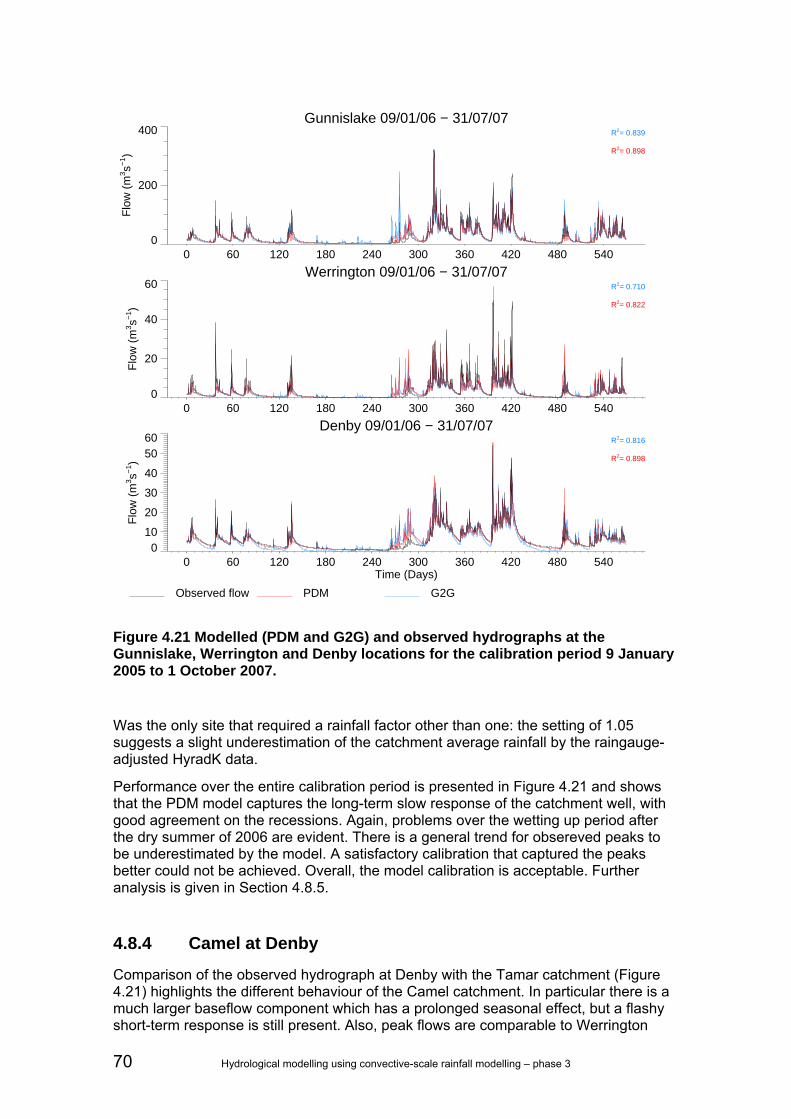
70 Hydrological modelling using convective-scale rainfall modelling – phase 3
Figure 4.21 Modelled (PDM and G2G) and observed hydrographs at the Gunnislake, Werrington and Denby locations for the calibration period 9 January 2005 to 1 October 2007.
Was the only site that required a rainfall factor other than one: the setting of 1.05 suggests a slight underestimation of the catchment average rainfall by the raingauge-adjusted HyradK data.
Performance over the entire calibration period is presented in Figure 4.21 and shows that the PDM model captures the long-term slow response of the catchment well, with good agreement on the recessions. Again, problems over the wetting up period after the dry summer of 2006 are evident. There is a general trend for obsereved peaks to be underestimated by the model. A satisfactory calibration that captured the peaks better could not be achieved. Overall, the model calibration is acceptable. Further analysis is given in Section 4.8.5.
4.8.4 Camel at Denby
Comparison of the observed hydrograph at Denby with the Tamar catchment (Figure 4.21) highlights the different behaviour of the Camel catchment. In particular there is a much larger baseflow component which has a prolonged seasonal effect, but a flashy short-term response is still present. Also, peak flows are comparable to Werrington
Gunnislake 09/01/06 − 31/07/07
0 60 120 180 240 300 360 420 480 540
0
200
400F
low
(m
3 s−1 )
Werrington 09/01/06 − 31/07/07
0 60 120 180 240 300 360 420 480 540
0
20
40
60
Flo
w (
m3 s−
1 )
Denby 09/01/06 − 31/07/07
0 60 120 180 240 300 360 420 480 540Time (Days)
010
20
30
40
5060
Flo
w (
m3 s−
1 )R2= 0.839
R2= 0.898
R2= 0.710
R2= 0.822
R2= 0.816
R2= 0.898
PDM G2GObserved flow

Hydrological modelling using convective-scale rainfall modelling – phase 3 71
despite being a larger catchment (210 km2 compared to 121 km2 for Werrington). Again, this can be attributed to the different soil and geology present in the Camel catchment relative to the Tamar catchment (see Section 4.4). In particular, the peat of Bodmin Moor and the deeper soils associated with the HOST classes gives rise to the different baseflow characteristic.
The Denby PDM parameters were manually calibrated from scratch and show some differences from those calibrated for the Werrington and Gunnislake models. A slower release from the subsurface store (kb) was needed to model the prolonged baseflow component of the observations. To keep the balance right between water moving to the subsurface store to maintain the baseflow component and the generation of sufficient surface runoff to model the short-term response requires careful selection of soil store related components. In particular, the soil stores were not too deep (cmax) to maintain the possibility of saturation excess on the short-term, whilst the recharge function allowed for sustained recharge to the subsurface store.
Performance over the entire calibration period is presented in Figure 4.21 and shows that the PDM model captures the long-term slow response of the catchment well, with good agreement on the recessions. Problems with the wetting up period after the dry summer of 2006 are evident once again. The observed peaks are also well modelled and overall the calibration is acceptable. Further analysis is given in Section 4.8.5.
4.8.5 Model performance (simulation mode)
The simulation mode of the PDM generally performed well at all three locations (Gunnislake, Werrington and Denby). The performance statistics of the PDM are presented in Table 4.10 whilst the simulated flows are compared with observed flows over the calibration period in Figure 4.21 and the evaluation period in Figure 4.22. The hydrograph simulations clearly show that the PDM successfully models the recession and seasonal behaviour of the catchments, with the only exception being the ‘wetting up’ period following the dry summer in 2006. Peak responses are also well modelled at Denby and Gunnislake. Modelling peak flows at Werrington was more challenging and marginally less successful, which is reflected in the slightly poorer performance statistics. To give an impression of the short-term behaviour of the model, example winter and summer events are presented in the left and right columns of Figure 4.23 respectively (note the relatively low peak flows for the summer).
The PDM simulation mode results over the Boscastle event are presented in Figure 4.24 and show mixed results. The Boscastle storm was an extreme convective event with high localised rainfall very different to the ‘typical’ storms used in model calibration. This poses real difficulties for a conceptual lumped model. In particular, the catchment average rainfall time series used as model input will smooth out these peak intensities, making it difficult to generate the large surface runoffs observed. However, the PDM simulations were rather good at Werrington in both magnitude and timing. This probably reflects the fact that Werrington had the largest percentage area coverage by the storm and so the lumped conceptualisation remained a good one. At Gunnislake and Denby, the percentage coverage was much less and the observed flows were underestimated by the PDM.

72 Hydrological modelling using convective-scale rainfall modelling – phase 3
Table 4.10 Simulation-mode performance of G2G and PDM models over calibration and verification periods.
Location R2 efficiency Mean absolute error Bias
PDM G2G PDM G2G PDM G2G
Tamar at Gunnislake 0.898 0.839 5.076 6.818 -0.635 0.334
Ottery at Werrington Park 0.822 0.710 0.864 1.094 -0.229 -0.377
Cal
ibra
tion
Per
iod
Camel at Denby 0.898 0.816 0.923 1.590 0.000 -0.228
Tamar at Gunnislake 0.913 0.871 4.170 5.282 -0.454 0.752
Ottery at Werrington Park 0.857 0.747 0.670 0.920 -0.046 -0.119
Ver
ifica
tion
Per
iod
Camel at Denby 0.922 0.839 0.722 1.285 0.103 0.023
Encouragingly, the performance statistics and simulation hydrographs give consistent performance over both calibration and evaluation periods, giving confidence that the model calibrations are robust. The impressive R2 statistics are all in excess of 0.822 and show that the flexibility afforded by the lumped conceptual formulation of the PDM can give good results and, in usual storm conditions, provides a tough benchmark to better.

Hydrological modelling using convective-scale rainfall modelling – phase 3 73
Figure 4.22 Modelled (PDM and G2G) and observed hydrographs at the Gunnislake, Werrington and Denby locations for the evaluation period 1 January 2004 to 23 December 2005.
Gunnislake 01/01/04 − 23/12/05
0 60 120 180 240 300 360 420 480 540 600 660 720
0
200
400F
low
(m
3 s−1 )
Werrington 01/01/04 − 23/12/05
0 60 120 180 240 300 360 420 480 540 600 660 720
0
20
40
60
80
100
Flo
w (
m3 s−
1 )
Denby 01/01/04 − 23/12/05
0 60 120 180 240 300 360 420 480 540 600 660 720Time (Days)
0
20
40
60
80
Flo
w (
m3 s−
1 )R2= 0.871
R2= 0.913
R2= 0.747
R2= 0.857
R2= 0.839
R2= 0.922
PDM G2GObserved flow

74 Hydrological modelling using convective-scale rainfall modelling – phase 3
Figure 4.23 Modelled (PDM and G2G) and observed hydrographs at the Gunnislake, Werrington and Denby locations for the evaluation winter period 18 October to 14 November 2005 and the summer period 19 to 27 May 2006.
Gunnislake 18/10/05 − 14/11/05
0 5 10 15 20 25
0
200
400F
low
(m
3 s−1 )
Gunnislake 19/05/06 − 27/05/06
0 1 2 3 4 5 6 7 8
020
40
60
80
100120
Werrington 18/10/05 − 14/11/05
0 5 10 15 20 25
010
20
30
40
5060
Flo
w (
m3 s−
1 )
Werrington 19/05/06 − 27/05/06
0 1 2 3 4 5 6 7 8
0
5
10
15
20
25
Denby 18/10/05 − 14/11/05
0 5 10 15 20 25Time (Days)
0
20
40
60
80
Flo
w (
m3 s−
1 )
Denby 19/05/06 − 27/05/06
0 1 2 3 4 5 6 7 8Time (Days)
05
10
15
20
2530
R2= 0.882
R2= 0.887
R2= 0.770
R2= 0.339
R2= 0.662
R2= 0.890
R2= 0.363
R2= 0.642
R2= 0.690
R2= 0.889
R2= 0.779
R2= 0.722
PDM G2GObserved flow

Hydrological modelling using convective-scale rainfall modelling – phase 3 75
Figure 4.24 Modelled and observed hydrographs using the PDM and G2G for the period 15 to 20 August 2004 covering the Boscastle event.
4.8.6 Model performance (forecast mode)
The forecast mode parameters of the PDM models (gains and gainb) were calibrated by employing the HyradK raingauge-adjusted radar data as a ‘perfect rainfall forecast’. Forecasts were made for lead times out to 24 hours at every 15-minute time-step within events. Empirical state-correction, which uses observed flow data to correct internal states of the PDM, was applied up to each forecast origin. Figure 4.25 presents model efficiency (R2) versus lead time over the entire calibration and evaluation periods for Gunnislake, Denby and Werrington. Results are also shown for the 12 shorter periods listed in Table 4.7 and used within the REW analysis of Section 4.7.6.
The forecast performance of all three PDM models is consistent over the calibration and evaluation periods. Figure 4.25 shows the considerable performance improvement state-correction offers for lead times out to around 12 hours, beyond which the forecast mode performance tails off to match the simulation mode performance as expected. The analysis over the shorter periods (1-12) show similar results to the calibration and evaluation periods for the longer winter events (2,4-8,10,11). Forecast performance over summer events (1, 3, 9, 12) is more variable.
Gunnislake 15/08/04 − 20/08/04
0 1 2 3 4 5
020
40
60
80
100120
Flo
w (
m3 s−
1 )Werrington 15/08/04 − 20/08/04
0 1 2 3 4 5
0
20
40
60
80
100
Denby 15/08/04 − 20/08/04
0 1 2 3 4 5Time (Days)
05
10
15
20
2530
Flo
w (
m3 s−
1 )
Polson 15/08/04 − 20/08/04
0 1 2 3 4 5Time (Days)
020
40
60
80
100120
R2<0
R2= 0.590
R2= 0.660
R2= 0.664
R2<0
R2= 0.035
R2= 0.598
PDM G2GObserved flow

76 Hydrological modelling using convective-scale rainfall modelling – phase 3
xp
p
0 5 10 15 20 250.0
0.2
0.4
0.6
0.8
1.0
Period 1
xpxp
x
p
0 5 10 15 20 250.0
0.2
0.4
0.6
0.8
1.0
Period 2p
pxp
0 5 10 15 20 250.0
0.2
0.4
0.6
0.8
1.0
Period 3
xpxp
x
p
0 5 10 15 20 250.0
0.2
0.4
0.6
0.8
1.0
Period 4
xpxp
x
p
0 5 10 15 20 250.0
0.2
0.4
0.6
0.8
1.0
Period 5
xpxpx
p
0 5 10 15 20 250.0
0.2
0.4
0.6
0.8
1.0
Period 6
x
pxp
x
p
0 5 10 15 20 250.0
0.2
0.4
0.6
0.8
1.0
Period 7
xpxp
x
p
0 5 10 15 20 250.0
0.2
0.4
0.6
0.8
1.0
Period 8
xpx
px
p
0 5 10 15 20 250.0
0.2
0.4
0.6
0.8
1.0
Period 9
xpxp
x
p
0 5 10 15 20 250.0
0.2
0.4
0.6
0.8
1.0
Period 10
xpxp
x
p
0 5 10 15 20 250.0
0.2
0.4
0.6
0.8
1.0
Period 11
p
x
0 5 10 15 20 250.0
0.2
0.4
0.6
0.8
1.0
Period 12
xpxp
xp
0 5 10 15 20 250.0
0.2
0.4
0.6
0.8
1.0
Evaluation
xpxp
xp
0 5 10 15 20 250.0
0.2
0.4
0.6
0.8
1.0
Calibration
Denby (g2g)Denby (PDM)Gunnislake (g2g)Gunnislake (PDM)Werrington (g2g)Werrington (PDM)
Lead time (hours)
Figure 4.25 Model efficiency (R2) versus lead time for periods 1 to 12 and the calibration and evaluation period for Gunnislake, Denby and Werrington. Results for the PDM and G2G are shown. The symbols p and x refer to the simulation-mode performance of the PDM and G2G models respectively.
R2

Hydrological modelling using convective-scale rainfall modelling – phase 3 77
4.9 G2G model application
4.9.1 Model setup
The only spatial dataset employed in configuring the G2G model was the 50-m IHDTM. This dataset was used in two ways:
(i) the average slope within each one-km grid-square was used within the runoff production scheme (Section 3.2.1);
(ii) flow paths were derived at a one-km resolution using the COTAT+ method of Paz et al. (2006) and employed within the flow routing scheme (Section 3.2.1).
Once the flow paths were derived, cummulative upstream drainage areas could be calculated for each one-km pixel and the grid-square identified for each gauged location. Gridded inputs of HyradK raingauge-adjusted rainfall and MORECS potential evaporation (40-km resolution) were directly used by the G2G model.
At the outset, the aim was to have a single set of G2G model parameters that would be used across all case studies. However, initial analysis of observed hydrographs in the region show a marked difference in behaviour between the faster responding catchments in the northeast and the more pronounced baseflow component of catchments in the southwest. These differences in observed behaviour could not be solely attributable to topographic controls and analysis of supporting datasets revealed a northeast to southwest split in soil and geology characteristics. Therefore, rather than use a single G2G model parameter set for the region, better model simulations were obtained by splitting the region into two, respecting this soil/geology division. This division is discussed in more detail in Section 4.4.
The small number of regional model process parameters were manually calibrated in simulation mode for both the Tamar and Denby regions. Principally, the main case study locations (Gunnislake, Werrington and Denby) were used in the model calibration, allowing the remaining gauged locations to be used to assess the ‘ungauged’ performance of the G2G model. The calibrated model parameters are given in Table 4.11. A standard form of empirical state-correction was used for the forecast mode assessment.
4.9.2 Tamar catchment
The Tamar G2G model covered the northeast of the case study region and encompassed the following gauged locations:
Gunnislake Werrington Crowford Bridge Bealsmill Tinhay
Polson Bridge Lifton Woolstone Helebridge Bush

78 Hydrological modelling using convective-scale rainfall modelling – phase 3
Table 4.11 G2G model parameters for the Camel and Tamar catchments.
Catchment Parameter name Tamar (Werrington Park and
Gunnislake) Camel (Denby)
Wave speeds Surface land, cl Surface river, cr Subsurface land, clb Subsurface river, crb
0.05 0.8
0.0015 0.004
0.04 0.7
0.001 0.003
Return flows Land, rl River, rr
0.03 0.05
0.0012 0.002
Runoff generation cmax Regional maximum minc Regional minimum St kd
125 10 0
6.77x10⁻⁸
140 10 0
8.3x10⁻⁸
Land/river designation Accumulated area threshold, a0
7
7
Routing time-step (mins) 5 5
During calibration, the main emphasis was on the Gunnislake and Werrington locations. Achieving a satisfactory manual calibration at both locations proved to be difficult, especially considering the strange behaviour of the observed flows noted at Werrington (Section 4.8.3). However, using both gauging stations helped to calibrate the wave routing speeds of the model.
Performance over the entire calibration period is presented in Figure 4.21 and shows that the G2G model captures the long-term slow response of the catchment well, with good agreement on the recessions at Werrington and Gunnislake. Like the PDM, the simulations reveal problems during the wetting up period after the dry summer of 2006. In general, the Tamar G2G model performs well at Gunnislake but performs slightly worse at Werrington. The G2G is comparable to the PDM at Gunnislake but tends to be slightly too responsive to rainfall in the summer. At Werrington the G2G tends to underestimates the peaks, even more so than the PDM. This is more apparent in Figure 4.26 which covers a shorter winter period. Figure 4.26 also highlights the rather good G2G performance at other ‘ungauged’ sites in the region including sites outside but adjacent to the Tamar catchment (Woolstone and Helebridge). Unsurprisingly, the worst performance occurs at Bealsmill which is on the ‘Denby’ side of the soil/geology division discussed above and explains the higher baseflow component in the observations. Further model analysis is given in Section 4.9.4.

Hydrological modelling using convective-scale rainfall modelling – phase 3 79
Figure 4.26 Modelled and observed hydrographs using the PDM and Tamar G2G for the period 19 November to 27 December 2006.
4.9.3 Camel catchment
The Camel G2G model covered the southwest of the case study region and encompassed the following gauged locations:
Denby Slaughterbridge De Lank Bastreet Pillaton
Trengoffe Craigshill Trekeivesteps Restormel
During calibration the main emphasis was on the Denby location. Compared to the Tamar, the Camel G2G model required deeper soil storage, slower wave routing speeds, greater drainage to the subsurface stores and slower return flows.
Gunnislake 09/11/06 − 27/12/06
0 10 20 30 40
0
200
400F
low
(m
3 s−1 )
Werrington 09/11/06 − 27/12/06
0 10 20 30 40
0
20
40
Lifton 09/11/06 − 27/12/06
0 10 20 30 40
0
50
100
150
200
250
Flo
w (
m3 s−
1 )
Polson 09/11/06 − 27/12/06
0 10 20 30 40
020
40
60
80
100
120140
Crowford 09/11/06 − 27/12/06
0 10 20 30 40
0
5
10
15
Flo
w (
m3 s−
1 )
Bealsmill 09/11/06 − 27/12/06
0 10 20 30 40
0
20
40
Woolstone 09/11/06 − 27/12/06
0 10 20 30 40Time (Days)
0
5
10
15
20
Flo
w (
m3 s−
1 )
Helebridge 09/11/06 − 27/12/06
0 10 20 30 40Time (Days)
0
5
10
15
20
R2= 0.945
R2= 0.952
R2= 0.726
R2= 0.895
R2= 0.829 R2= 0.866
R2= 0.711 R2= 0.519
R2= 0.558 R2= 0.742
PDM G2GObserved flow

80 Hydrological modelling using convective-scale rainfall modelling – phase 3
Performance over the entire calibration period is presented in Figure 4.21 and shows that the G2G model captures the long-term slow response of the catchment reasonably well, with just minor disagreement on the recession. Like the previous model results, the simulations reveal problems during the wetting up period after the dry summer of 2006. In general, the G2G model performs well at Denby and, apart from the recession problems, is comparable with the PDM results.
Figure 4.27 covers a shorter winter period and highlights the G2G performance at other ‘ungauged’ sites in the region including sites outside but adjacent to the Camel to Denby catchment. The performance at De Lank, an internal site, is good whereas the G2G tends to overestimate the peaks at Trengoffe and Restormel, but this is probably due to the reservoir influences which are not explicitly modelled here. Further model analysis is given in Section 4.9.4.
Figure 4.27 Modelled and observed hydrographs using the PDM and Camel G2G for the period 19 November to 27 December 2006.
Denby 09/11/06 − 27/12/06
0 10 20 30 40
0
20
40
Flo
w (
m3 s−
1 )
De Lank 09/11/06 − 27/12/06
0 10 20 30 40
01
2
3
4
56
Bastreet 09/11/06 − 27/12/06
0 10 20 30 40
0
2
4
6
8
10
Flo
w (
m3 s−
1 )
Pillaton 09/11/06 − 27/12/06
0 10 20 30 40
010
20
30
40
5060
Trengoffe 09/11/06 − 27/12/06
0 10 20 30 40Time (Days)
0
2
4
6
8
Flo
w (
m3 s−
1 )
Restormel 09/11/06 − 27/12/06
0 10 20 30 40Time (Days)
0
10
20
30
40
50
R2= 0.881
R2= 0.915
R2= 0.758
R2= 0.595 R2= 0.869
R2= 0.512 R2<0
PDM G2GObserved flow

Hydrological modelling using convective-scale rainfall modelling – phase 3 81
4.9.4 Model performance (simulation mode)
The simulation mode of the G2G generally performs well at all three case study locations (Gunnislake, Werrington and Denby). The performance statistics of the G2G are presented in Table 4.10 whilst the simulated flows are compared with observed flows over the calibration period in Figure 4.21 and the evaluation period in Figure 4.22. The hydrograph simulations clearly show that the G2G generally models the recession and seasonal behaviour of the catchments well, although there are minor disagreements on the recession for Denby. Otherwise, the only exception is the ‘wetting up’ period following the dry summer in 2006 – a problem for all models and catchments. Peak responses are also well modelled at Denby and Gunnislake. Modelling peak flows at Werrington was more difficult and marginally less successful, reflected in the slightly poorer performance statistics. The G2G model also tends to be too sensitive to rain during summer periods.
The results provided by the PDM prove difficult to better with the G2G model. However, this has to be balanced against the potential information at ‘ungauged’ locations provided by the G2G. Figure 4.28 graphically shows the model efficiency of the G2G at all locations for which observed flow data are available. The PDM results are also given for locations where they are available (Gunnislake, Werrington and Denby). The G2G results show that the model offers some benefit at the ‘ungauged’ locations. In particular, results using the Tamar G2G show some real utility (such as Polson, Lifton, Tinhay and Bealsmill). Some of the poorer model performance can be attributed to uncertain flow measurements (such as Woolstone and Bush) or artifical influences such as reservoirs (such as Craigshill and Restormel). Encouragingly, the G2G model performance is consistent across calibration and evaluation events.
Figure 4.28 Model efficiency (R2) for PDM and G2G models over calibration and evaluation periods. Results for G2G at ‘ungauged’ locations also given.
The G2G simulation performance over the Boscastle event is presented in Figure 4.24. The plots show that the G2G has difficulties simulating the peaks but, through the grid-
Calibration Period
0.00.2
0.4
0.6
0.81.0
R2
Werr
ington
Gunnis
lake
Denby
Crowfo
rd
N/A
Bealsm
ill
N/A
Tinhay
N/A
Polson
N/A
Lifton
N/A
Woo
lston
e
R2 <
0
N/A
Helebr
idge
N/A
Bush
R2 <
0
N/A
Slaugh
terbr
idge
R2 <
0
N/A
De Lan
k
N/A
Bastre
et
N/A
Pillato
n
N/A
Trengo
ffe
N/A
Craigs
hill
R2 <
0
N/A
Trekeiv
estep
s
N/A
Restor
mel
N/A
Evaluation Period
0.00.2
0.4
0.6
0.81.0
R2
Werr
ington
Gunnis
lake
Denby
Crowfo
rd
N/A
Bealsm
ill
N/A
Tinhay
N/A
Polson
N/A
Lifton
N/A
Woo
lston
e
R2 <
0
N/A
Helebr
idge
N/A
Bush
R2 <
0
N/A
Slaugh
terbr
idge
R2 <
0
N/A
De Lan
k
N/A
Bastre
et
N/A
Pillato
n
N/A
Trengo
ffe
N/A
Craigs
hill
R2 <
0
N/A
Trekeiv
estep
s
R2 <
0
N/A
Restor
mel
N/A
Key: Terrain G2G PDM
82 Hydrological modelling using convective-scale rainfall modelling – phase 3
based runoff-production scheme, it appears to generate reasonably realistic amounts of localised surface runoff. The main problem with the G2G results for the Boscastle event is that the simulated recession is too slow and prolonged. This may be due to the routing elements of the G2G model and, in particular, the slower wave speeds over land which areprobably not suitable for this intense summer event.
4.9.5 Model performance (forecast mode)
The forecast mode parameters of the G2G model were set to standard values. HyradK raingauge-adjusted radar data were used as a ‘perfect rainfall forecast’. Forecasts were made for lead times out to 24 hours at every 15-minute time-step within events. Empirical state-correction, which uses observed flow data to correct the routing water of the G2G, was applied up to each forecast origin. Figure 4.25 presents model efficiency (R2) versus lead time over the entire calibration and evaluation periods for the three main locations of Gunnislake, Denby and Werrington. Results are also shown for the 12 shorter periods listed in Table 4.7 and used within the REW analysis of Section 4.7.6.
The forecast performance of the G2G model is consistent at all three locations over both the calibration and evaluation periods, with the worst performance at Werrington. This is not surprising since the simulation mode results are also poorest at this location. Figure 4.25 shows the considerable performance improvement state-correction offers the G2G for lead times out to around 10-12 hours for Denby and Gunnislake and six to eight hours for Werrington. Beyond these lead times, the forecast mode performance tails off to match the simulation mode performance as expected. The analysis over the shorter periods (1-12) show similar results to the calibration and evaluation periods for the longer winter time events (2, 4-8, 10, 11). Forecast performance over the summer events (1, 3, 9, 12) is more variable. Generally, PDM forecasts perform best which reflects (i) the better simulation provided by PDM at gauged locations, and (ii) the fact that, due to time constraints, G2G forecast parameters were not optimised whereas PDM parameters were. Further research on state-correction for the G2G is ongoing.
4.9.6 Extended G2G model results
The geological map over the G2G modelled region shown in Figure 4.2 highlights the contrast between Carboniferous rocks in the northeast half and Devonian Old Red Sandstone with granitic igneous intrusions in the southwest half. This contrast is reflected in the HOST soil classes shown in Figure 4.2 with classes 24 (blue: shallow soils) and 21 (red: medium depth slowly permeable substrate) dominant in the northeast and 17 (green: deep soils over an impermeable layer) and 15 (blue: peat) in the southwest. These contrasting soil/geology patterns have been known to exert a control on flood response to storm rainfall, as seen through the G2G modelling across the region. Catchments to the southwest generally have a slower response because of deeper or peat soils. Rather than use a single G2G model parameter set for the region, better model simulations were obtained by splitting the region into two, respecting this soil/geology division. This provided a pragmatic approach to follow for this case study.
A major reason for the need to subdivide the region relates to inference of the soil’s water-holding capacity which controls runoff production in the G2G model. In the simplest formulation used here, terrain slope is used as a surrogate for the capacity of a soil to absorb water through a linear relation. In simple terms, thin soils are associated with steep slopes and deeper soils with flatter areas. Such a relationship can break down across regions of contrasting soil types, as evident in the study region. Splitting the region into the two contrasting areas and calibrating the G2G for each offers a simple way of improving modelled flows. However, use of a G2G model

Hydrological modelling using convective-scale rainfall modelling – phase 3 83
extended to incorporate soil/geology property information and requiring only one model parameter set is a more strategic way forward. Such a model was first prototyped by the Centre for Ecology and Hydrology for the Environment Agency under the project Rainfall-runoff and other modelling for ungauged/low-benefit locations (Moore et al., 2006) and developed further since. This variant of the G2G model was not available in module adapter form for real-time use in the NFFS, at the time of the Boscastle pilot study, but was available for use in the project as a research tool to explore the potential advantages of the extended G2G model. The use of this soil-based G2G model variant to the study region is discussed here.
HOST classes on a one-km grid linked to soil properties through an association table currently provide the source of soil information. The soil properties are soil depth, porosity, field capacity and residual values of water content, and saturated hydraulic conductivity. Soil depth and water content at field capacity are used to estimate the maximum storage capacity in each model grid-square. This capacity is distributed within the grid-square according to a Pareto distribution (like in the catchment PDM) but with the shape parameter b varying inversely with the square root of the maximum storage capacity. Downward percolation of water is controlled by available water in storage and the hydraulic conductivity of the soil. Lateral drainage is controlled in a similar way but including the influence of terrain slope and using a conductivity appropriate to lateral movement. Groundwater accumulates by percolation from the soil and drains via a nonlinear storage function with a rate constant parameter.
Within each grid-square, surface runoff is generated via saturation excess flow and subsurface runoff derives from groundwater drainage. These runoffs are routed from grid-to-grid as with the simple G2G using the flow paths identified from the DTM. However, a modified kinematic routing scheme is an available option and is used here for the surface runoff. It takes the form of a Horton-Izzard equation (nonlinear storage routing) and can accommodate varying channel width (inferred via geomorphological relations) and roughness. A return flow is allowed between subsurface and surface pathways, as in the simple G2G model, to accommodate surface-groundwater interactions. Further details of the extended G2G model, now available in module adapter form for use in NFFS, are given in Section 3.2.1.
Figure 4.29 compares flow simulations from the G2G model with the extended model incorporating soil property information across eight catchments over 38 days of the two-year evaluation period. In terms of R2 efficiency, neither model performs better overall. A similar conclusion follows from inspection of the hydrograph flood peaks and the models’ abilities to reproduce them. This is encouraging given that the extended G2G model employs only a single parameter set for all catchments: the simple G2G model employs two to cope with the soil/geology heterogeneity across the modelled region. The recession behaviour for the Lynher at Pillaton Mill is improved using the extended G2G but does not perform as well on the main peak. This contrasts with the De Lank in the Camel catchment where the recession behaviour is poorer whilst flood peak performance is similar. Flow simulations for other catchments can be compared leading to similarly contrasting, rather than consistent, conclusions.

84 Hydrological modelling using convective-scale rainfall modelling – phase 3
Figure 4.29 Modelled and observed hydrographs using the G2G and extended G2G for the period 19 November to 27 December 2006.
Figure 4.30 compares the G2G and extended G2G model performance in terms of R2 efficiency, plotted as bar charts, across all gauged catchments in the modelled region. Theperformance measure is plotted separately for calibration (around 18 months) and evaluation (around 24 months) periods. For a good majority of cases, and for both periods, the extended G2G model performs best over these longer assessment periods.
Gunnislake 09/11/06 − 27/12/06
0 10 20 30 40
0
200
400F
low
(m
3 s−1 )
Werrington 09/11/06 − 27/12/06
0 10 20 30 40
0
20
40
Denby 09/11/06 − 27/12/06
0 10 20 30 40
0
20
40
Flo
w (
m3 s−
1 )
Polson 09/11/06 − 27/12/06
0 10 20 30 40
020
40
60
80
100
120140
Bealsmill 09/11/06 − 27/12/06
0 10 20 30 40
0
20
40
Flo
w (
m3 s−
1 )
Helebridge 09/11/06 − 27/12/06
0 10 20 30 40
0
5
10
15
20
De Lank 09/11/06 − 27/12/06
0 10 20 30 40Time (Days)
01
2
3
4
56
Flo
w (
m3 s−
1 )
Pillaton 09/11/06 − 27/12/06
0 10 20 30 40Time (Days)
010
20
30
40
5060
R2= 0.945R2= 0.775
R2= 0.726R2= 0.570
R2= 0.881R2= 0.900
R2= 0.866R2= 0.773
R2= 0.519R2= 0.867
R2= 0.742R2= 0.810
R2= 0.758R2= 0.725
R2= 0.869R2= 0.808
G2G G2G ExtendedObserved flow
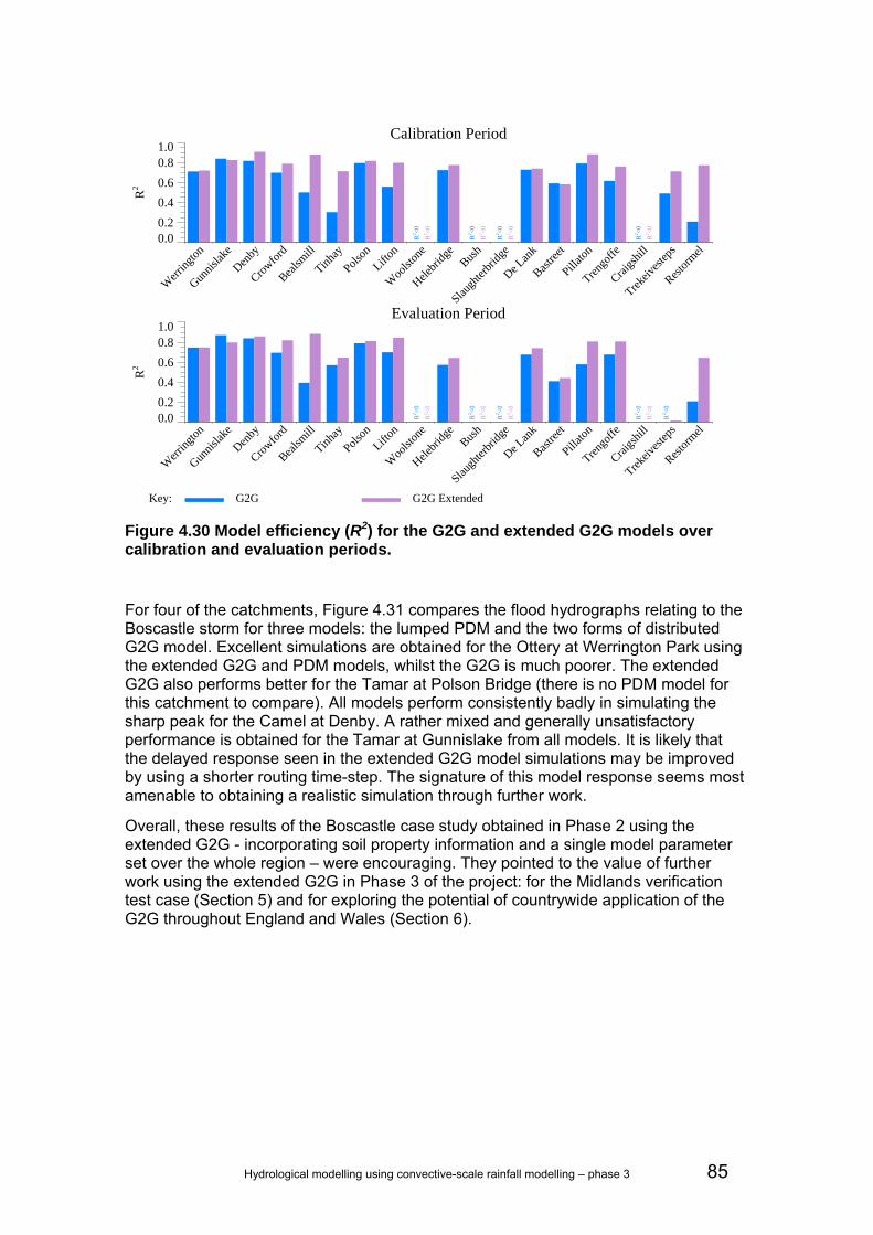
Hydrological modelling using convective-scale rainfall modelling – phase 3 85
Figure 4.30 Model efficiency (R2) for the G2G and extended G2G models over calibration and evaluation periods.
For four of the catchments, Figure 4.31 compares the flood hydrographs relating to the Boscastle storm for three models: the lumped PDM and the two forms of distributed G2G model. Excellent simulations are obtained for the Ottery at Werrington Park using the extended G2G and PDM models, whilst the G2G is much poorer. The extended G2G also performs better for the Tamar at Polson Bridge (there is no PDM model for this catchment to compare). All models perform consistently badly in simulating the sharp peak for the Camel at Denby. A rather mixed and generally unsatisfactory performance is obtained for the Tamar at Gunnislake from all models. It is likely that the delayed response seen in the extended G2G model simulations may be improved by using a shorter routing time-step. The signature of this model response seems most amenable to obtaining a realistic simulation through further work.
Overall, these results of the Boscastle case study obtained in Phase 2 using the extended G2G - incorporating soil property information and a single model parameter set over the whole region – were encouraging. They pointed to the value of further work using the extended G2G in Phase 3 of the project: for the Midlands verification test case (Section 5) and for exploring the potential of countrywide application of the G2G throughout England and Wales (Section 6).
Calibration Period
0.00.2
0.4
0.6
0.81.0
R2
Werr
ington
Gunnis
lake
Denby
Crowfo
rd
Bealsm
ill
Tinhay
Polson
Lifton
Woo
lston
e
R2 <
0
R2 <
0
Helebr
idge
Bush
R2 <
0
R2 <
0
Slaugh
terbr
idge
R2 <
0
R2 <
0
De Lan
k
Bastre
et
Pillato
n
Trengo
ffe
Craigs
hill
R2 <
0
R2 <
0
Trekeiv
estep
s
Restor
mel
Evaluation Period
0.00.2
0.4
0.6
0.81.0
R2
Werr
ington
Gunnis
lake
Denby
Crowfo
rd
Bealsm
ill
Tinhay
Polson
Lifton
Woo
lston
eR
2 <0
R2 <
0
Helebr
idge
Bush
R2 <
0
R2 <
0Slau
ghter
bridg
e
R2 <
0
R2 <
0
De Lan
k
Bastre
et
Pillato
n
Trengo
ffe
Craigs
hill
R2 <
0
R2 <
0
Trekeiv
estep
s
R2 <
0
Restor
mel
Key: G2G G2G Extended

86 Hydrological modelling using convective-scale rainfall modelling – phase 3
Figure 4.31 Modelled and observed hydrographs using the PDM, G2G and extended G2G for the period 15 to 20 August 2004.
4.10 Use of high-resolution NWP rainfall and ensemble forecasting
4.10.1 High-resolution NWP forecasts
At the time of the Boscastle event (2004) the operational deterministic NWP had a resolution of 12 km. Since then, the operational NWP resolution has increased to four km, with one km planned in the near future. To assess the potential benefits of high-resolution NWP rainfall for flood forecasting, one, four and 12 km resolution NWP forecasts were provided for the Boscastle event by Nigel Roberts at the JCMM (Joint Centre for Mesoscale Meteorology, Met Office). Forecasts from two origins were provided: 00UTC and 03UTC on 16 August 2004. Figure 4.32 gives example snapshots of the forecast rainfall data. Due to the method used to generate the high resolution forecasts, forecast rainfalls start at 01UTC and 04UTC respectively. More detail about the NWP forecasts is provided by Roberts (2006).
Gunnislake 15/08/04 − 20/08/04
0 1 2 3 4 5
0
50
100
150
Flo
w (
m3 s−
1 )
Werrington 15/08/04 − 20/08/04
0 1 2 3 4 5
020
40
60
80
100120
Denby 15/08/04 − 20/08/04
0 1 2 3 4 5Time (Days)
05
10
15
20
2530
Flo
w (
m3 s−
1 )
Polson 15/08/04 − 20/08/04
0 1 2 3 4 5Time (Days)
0
50
100
150
200
R2<0R2<0
R2= 0.590
R2= 0.660R2= 0.868R2= 0.664
R2<0R2<0
R2= 0.035
R2= 0.635R2= 0.807
PDM G2G G2G ExtendedObserved flow

Hydrological modelling using convective-scale rainfall modelling – phase 3 87
Figure 4.32 Forecast rainfall data from the high resolution NWP model as displayed in Delft-FEWS. The panels (from top left to bottom right) show the raingauge-adjusted radar image, the radar image, the four-km forecast and the 12-km forecast. The time for all panels is 12:00 16 August 2004 and the forecast origin for the forecast images is 01:00.
4.10.2 Generation of pseudo-ensembles
Ensembles of high resolution rainfall forecasts are due to become available in the near future. The nowcasting product STEPS (Short-Term Ensemble Prediction System), available out to six hours, went operational in October 2008 and ensembles of high resolution NWP are planned by 2011. In preparation for the imminent availability of these high resolution ensemble rainfall forecasts, and as they were not available for the Boscastle case study, we decided to generate ‘pseudo-ensembles’ from the deterministic one-km NWP forecast. The method developed for generating the ‘pseudo-ensembles’ closely involved Nigel Roberts (JCMM). To remain within the scope of the project, the intention was to derive a simple method to capture some of the spatial uncertainty associated with the deterministic NWP forecast. In its current form the method is not intended to be used immediately as a ‘post-processor’ of NWP rainfalls in an operational context.
The ‘pseudo-ensemble’ method developed consists of two stages:
1. Selecting a scaling factor to apply to each NWP forecast. 2. Generating ensemble members by randomly displacing the spatial origin
within a given displacement radius. The following sub-sections give more details of the method.

88 Hydrological modelling using convective-scale rainfall modelling – phase 3
4.10.3 Selecting the scaling factor
Table 4.12 gives a summary of the one-km NWP rainfall accumulations for the five-hour period ending 17:00 16 August 2004 from both the 00UTC and 03UTC forecasts. These are compared to two-km single site Nimrod data from Cobbacombe, the Nimrod composite product (essentially this is two-km data from the Predannack radar over the Boscastle catchment) and the raingauge-adjusted Nimrod composite data produced by HyradK (see Section 4.5). The one-km NWP appears to underestimate the spatial peak rainfall accumulations and catchment average rainfall relative to the radar data. Furthermore, radar pixels coincident with raingauge locations underestimated raingauge totals and hence use of HyradK raingauge-adjusted radar data increased Nimrod rain-rates, giving larger totals.
Table 4.12 Summary of different rainfall estimators accumulated over the five-hour period ending 17:00 16 August 2004. The domain used is (140000,000000) to (280000,140000).
Rainfall estimator Peak pixel
accumulation (mm)
Peak pixel location
Boscastle catchment
average (mm)
Domain average
(mm) One-km NWP 00UTC
54.22 53.24
SX 005 835 SX 145 875 34.30 3.07
One-km NWP 03UTC 44.03 SX 125 985 16.77 2.54
Cobbacombe two-km Nimrod 133.1 SX 150 890 92.66 N/A
Nimrod composite 115.68 SX 170 930 93.06 2.618 Raingauge-adjusted Nimrod composite
213.11 SX 125 905 170.0 3.996
At first glance, Table 4.12 suggests a significant scaling factor (above two) needs to be applied to each NWP forecast to give rainfall accumulations (over Boscastle) commensurate with the radar and raingauge data. However, analysis of the spatial accumulation maps presented in Figure 4.33 reveals differences in the spatial distribution over the Boscastle region. The lower row shows the existence of three areas of high rainfall from the 00UTC NWP forecast compared to a single concentrated area from the radar-based accumulations. By stepping through the individual NWP images, this can be traced to individual convective cells having slightly different trajectories that meant the core of those cells just missed the Boscastle catchment. In comparison, the radar images reveal an almost constant trajectory of cells over the Boscastle catchment and give rise to the higher pixel rainfall accumulations.
It is more appropriate to assess the one-km NWP at a larger spatial scale. Figure 4.33 shows the different rainfall sources averaged over 12-km pixels using the 00UTC forecast. This shows that the general location of heavy rain across the northwest Cornish coast is well predicted by NWP and in good agreement with raingauge-adjusted Nimrod estimates, except for amounts in the immediate vicinity of Boscastle which are between two and four times smaller. However, applying a blanket factor of two or more to the NWP data would distort the results away from Boscastle and give too high a domain average rainfall (see Table 4.12). As a compromise, a factor of 1.4 is used for the 00UTC forecast and 1.7 for the 03UTC forecast. The resulting rainfall accumulations for the scaled 00UTC forecast are presented in the final column of Figure 4.33. Although this would not be possible in a real-time context, it offers a

Hydrological modelling using convective-scale rainfall modelling – phase 3 89
pragmatic way to create a useful set of ensembles that reflects the high resolution NWP products which will be available soon.
Figure 4.33 Rainfall accumulations (mm) for the five-hour period ending 17:00 16 August 2004 using different rainfall sources. The 00UTC one-km NWP forecast is used. The bottom row is a close-up over Boscastle.
Figure 4.34 Rainfall accumulations (mm) for the five-hour period ending 17:00 16 August 2004 using different rainfall sources and accumulated over 12-km grid-squares. The 00UTC NWP forecast is used.
4.10.4 Ensemble generation
Following discussions with Nigel Roberts (JCMM), we established that the best way to generate the ensembles (within the constraints of the project) would be to displace the spatial origin of the (scaled) one-km forecast but maintain the temporal evolution. This would result in forecast rainfall accumulation maps with the same spatial distribution and totals, but shifted in space. For this particular storm, the maximum displacement is 20-km and is a representation of the perceived spatial accuracy of the forecast in this meteorological situation.
The argument is that any forecast displaced within the 20-km radius is equally likely to have occurred in reality. Any number of ensembles can be generated by randomly

90 Hydrological modelling using convective-scale rainfall modelling – phase 3
selecting the spatial displacement of the forecast within the 20-km radius. For simplicity, we restricted ourselves to displacement units of one km in both northing and easting and a maximum of 50 ensemble members. Figure 4.35 shows examples of three ensemble members along with the deterministic one-km NWP forecast.
4.10.5 Hydrological model forecasts using HyradK rainfall
Before assessing the hydrological model forecasts using both the deterministic and pseudo-ensemble forms of high resolution NWP, it would be informative to analyse the forecast mode performance of the hydrological models using the HyradK raingauge-adjusted radar estimates as ‘perfect rainfall’ forecasts. This was done at a broader level earlier in this section but more detailed analysis of the Boscastle event revealed certain model behaviour that needed to be taken into account before considering the NWP-based forecasts.
The lead time versus model efficiency plots using the HyradK rainfall are presented in Figure 4.28 for the PDM and G2G and show more sensitivity in the summer periods (1, 3, 9 and 12). The Boscastle event is period 3. The performance of the state-correction for both PDM and G2G is heavily influenced by the simulation mode performance of the models which are presented in Figure 4.24 for PDM and G2G models. To understand this further, Figure 4.36 presents the simulation mode results using the PDM and also a sequence of fixed-origin forecasts using state-correction. The simulation results (left column) show a consistent trend with the PDM providing a good simulation at the start of the period but then responding before the sharp rising limbs of the observed hydrographs. This means that the fixed-origin forecasts made before the PDM responds (red line, right column) are basically close to the simulation results. Forecasts made from origins after the PDM has responded but before the observations have started to rise are damped down through the state-correction (for example, blue line, right column). The performance of the fixed-origin forecasts made once the observations start to rise and after the peak vary from catchment to catchment.

Hydrological modelling using convective-scale rainfall modelling – phase 3 91
Figure 4.35 Forecast data from the high resolution NWP model as displayed in Delft-FEWS. The panels (from top left to bottom right) show the one-km deterministic forecast and the ensemble members 01, 02 and 03. The time for all panels is 12:00 16 August 2008, and the forecast origin is 01:00.
Fixed-origin forecasts are presented for the G2G in Figure 4.37 for Denby and Gunnislake along with the simulation mode results (blue line). These show some similarities to the PDM results, with the damping of the forecast made from origins after the G2G has responded but before the observations have started to rise (pink and green lines). The fixed-origin forecasts once the observations have started to rise vary from location to location. The results at Werrington are quite good, whilst the poorer performance at Denby is attributable to the timing error in the simulation mode results.

92 Hydrological modelling using convective-scale rainfall modelling – phase 3
Figure 4.36 PDM simulation mode results using HyradK raingauge-adjusted rainfall data (left column) and fixed-origin forecast results using state-correction and HyradK ‘perfect’ rainfall forecasts (right column).
Figure 4.37 G2G fixed-origin forecast results using state-correction and HyradK raingauge-adjusted radar data as ‘perfect’ rainfall forecasts. The blue line is the simulation mode result.
Denby 16/08/04 − 19/08/04
0 1 2 3
0
20
40
60
Flow
(m
3 s−1 )
Werrington 16/08/04 − 19/08/04
0 1 2 3Time (Days)
0
20
40
60
80
100
Flow
(m
3 s−1 )
R2<0R2<0R2<0R2<0R2<0R2<0
R2= 0.626R2<0R2<0
R2= 0.729R2= 0.903R2= 0.922
G2G

Hydrological modelling using convective-scale rainfall modelling – phase 3 93
In summary, the state-correction forecast updating approach is sensitive to poor modelling of the rising limb of the Boscastle event, particularly if the model responds before the observations. This explains the sensitivity reported in the lead time versus model efficiency plots over the summer periods reported earlier in this section. These issues must be considered when assessing the high resolution NWP-based hydrological forecasts in the following sections.
4.10.6 Hydrological model forecasts using deterministic high resolution NWP rainfall
NWP rainfall forecasts were provided at resolutions of one, four and 12 km and for two forecast origins: 00UTC and 03UTC on 16 August 2008. Due to the methods used to generate the high resolution (one and four km) NWP model results, the rainfall forecasts start at 01 and 04UTC respectively. The high resolution NWP models were run specifically for the Boscastle storm so the end time of all the forecasts is 18UTC. Since the NWP forecasts finish before the observed flows begin to rise, the NWP-based hydrological forecasts in the period after the model responds but before the observed flows rise will suffer the problems identified using the HyradK data in Section 4.10.5. This, combined with the fact that there are only two NWP forecast origins means that plots of lead-time performance against model efficiency are not very informative.
Bearing in mind the above comments, the best way to assess hydrological model performance using the different NWP resolutions is to run fixed-origin forecasts using the different NWP resolutions and HyradK raingauge-adjusted radar as ‘perfect’ rainfall forecasts for comparison. The first three hours of each NWP forecast were ignored as this represented the estimated time needed to generate and disseminate the forecasts in an operational context – this made no difference for the Boscastle case study as the rainfall didn’t start until around 12UTC.
Fixed-origin forecasts using the PDM and both the 00 and 03UTC NWP runs are presented in Figure 4.38 with hydrological forecast origins of 04 and 07UTC respectively (before the observations start to rise to avoid the ‘damping’ effect discussed above). This shows that the high resolution (one or four km) NWP-based hydrological forecasts generally perform better than the 12-km NWP-based ones and that 00UTC NWP runs provide better hydrological forecasts than 03UTC runs (this is in keeping with the analysis from a rainfall perspective by Roberts (2006)). The most conclusive evidence comes from the Werrington PDM model which had the best simulation results and allows a more direct analysis of the NWP-based hydrological forecasts without being confounded by shortcomings in hydrological model performance.
A more complete understanding of hydrological forecasts comes from looking at the spatial maps of rainfall accumulations (Figure 4.39) and analysis of the catchment average rainfalls (Table 4.13) over the Boscastle storm. For example, Figure 4.38 shows that for 03UTC the 12-km NWP forecasts give the best NWP-based hydrological forecasts at Denby, but Figure 4.39 shows that 12-km hydrological results are best for the wrong reasons since the spatial distribution of the forecast rainfall is completely wrong.
Fixed-origin forecasts using the G2G are presented for Werrington and Denby in Figure 4.38 and Figure 4.41 respectively. Theses show broad similarities with the PDM results such as the high resolution NWP results generally performing best. However, there are some interesting differences. For example, the Werrington G2G results (Figure 4.40) show more sensitivity in terms of timing of the forecast peak with the 00UTC NWP-based forecast having an earlier peak compared to the 03UTC one. This wasn’t the case for the PDM where the peak timings were similar. The sensitivity of the distributed

94 Hydrological modelling using convective-scale rainfall modelling – phase 3
G2G model relates to the spatial distribution of the forecast rainfall; Figure 4.39 shows that, for Werrington, the one- and four-km 00UTC accumulations have too much rain in the lower parts of the catchment which, through the distributed runoff and routing formulation of the G2G, gives the earlier model response. This highlights the importance of accurate spatial distributions of NWP rainfall for producing accurate flood forecasts.
In summary, the high resolution (one or four km) NWP rainfall forecasts offer real benefits for hydrological forecasting compared to the coarse 12-km NWP forecasts.
Figure 4.38 Fixed-origin PDM model forecasts at Werrington (top row), Gunnislake (middle row) and Denby (bottom row) using one-, four- and 12-km deterministic NWP and HyradK ‘perfect’ rainfall data. The 00UTC forecast is used in the left column and the 03UTC forecast is used in the right column.
1 km 4 km
12 km
HyradK
1 km4 km
12 km
HyradK
1 km
4 km
12 km
HyradK
1 km
4 km12 km
HyradK
1 km
4 km
12 km
HyradK
1 km
HyradK
4 km
12 km
00UTC NWP forecasts 03UTC NWP forecasts

Hydrological modelling using convective-scale rainfall modelling – phase 3 95
Table 4.13 Catchment average rainfall totals in mm for the three case study catchments using different sources of rainfall. Totals are for the five-hour period ending 17:00 16 August 2004.
Rainfall estimator Ottery at Werrington
Tamar at Gunnislake
Camel at Denby
1-km NWP 00UTC 21.68 10.63 8.40 4-km NWP 00UTC 23.41 15.89 8.68 12-km NWP 00UTC 3.93 3.7 4.65 1-km NWP 03UTC 8.85 5.74 3.40 4-km NWP 03UTC 17.58 11.63 3.87 12-km NWP 03UTC 3.41 4.06 4.82 Nimrod composite 28.87 11.29 3.98 Raingauge-adjusted Nimrod composite
43.1 15.34 8.0

96 Hydrological modelling using convective-scale rainfall modelling – phase 3
Figure 4.39 Rainfall accumulations (mm) for the five-hour period ending 17:00 16 August 2004 using one-km (top left), four-km (top right) and 12-km (bottom left) NWP and HyradK raingauge-adjusted radar (bottom right).
00UTC NWP forecasts
03UTC NWP forecasts

Hydrological modelling using convective-scale rainfall modelling – phase 3 97
Figure 4.40 Fixed-origin G2G model forecasts at Werrington using one-, four- and 12-km deterministic NWP and HyradK ‘perfect’ rainfall data: (a) using the 00UTC forecast and (b) using the 03UTC forecast. The blue line gives the simulation mode result using HyradK rainfall data as a reference.
Figure 4.41 Fixed-origin G2G model forecasts at Denby using one-, four- and 12-km deterministic NWP and HyradK ‘perfect’ rainfall data: (a) using the 00UTC forecast and (b) using the 03UTC forecast. The blue line gives the simulation mode result using HyradK rainfall data as a reference.
Denby 16/08/04 − 19/08/04
0 1 2 3
05
10
15
20
2530
Flow
(m
3 s−1 )
Denby 16/08/04 − 19/08/04
0 1 2 3Time (Days)
05
10
15
20
2530
Flow
(m
3 s−1 )
R2<0R2= 0.046R2= 0.032R2= 0.399R2= 0.312
R2<0R2= 0.048R2= 0.047
R2<0R2<0
(a)
(b)
HyradK simulation HyradK ‘perfect’ forecast
12 km NWP 4 km NWP 1 km NWP
HyradK simulation HyradK ‘perfect’ forecast
12 km NWP 4 km NWP 1 km NWP
Werrington 16/08/04 − 19/08/04
0 1 2 3
0
20
40
60
80
100Fl
ow (
m3 s−
1 )
Werrington 16/08/04 − 19/08/04
0 1 2 3Time (Days)
0
20
40
60
80
100
Flow
(m
3 s−1 )
R2= 0.626R2= 0.318
R2<0R2<0
R2= 0.054
R2= 0.626R2= 0.316
R2<0R2<0R2<0
G2G
HyradK simulation HyradK ‘perfect’ forecast
12 km NWP 4 km NWP 1 km NWP
HyradK simulation HyradK ‘perfect’ forecast
12 km NWP 4 km NWP 1 km NWP
(a)
(b)

98 Hydrological modelling using convective-scale rainfall modelling – phase 3
4.10.7 Hydrological model forecasts using pseudo-ensembles of high resolution NWP rainfall
As in the previous analysis (Section 4.10.6), the best way to assess hydrological model performance using the pseudo-ensembles of high resolution one-km NWP rainfalls is to run fixed-origin forecasts. Hydrological model forecasts using the 00UTC pseudo-ensembles are presented for the PDM, G2G and REW in Figure 4.42 to Figure 4.44 using a forecast origin of 04UTC on 16 August 2004.
Analysis of the results show that all models, whether lumped or distributed, are sensitive to the individual ensemble members. The spread of hydrological ensembles looks encouraging and suggests that the simple method used to generate the pseudo-ensembles is meaningful. At first, it may seem surprising that generating ensemble members through a small displacement (less than 20 km) could generate such sensitivity in the hydrological model outputs. However, as the Boscastle storm is small in spatial extent (see Figure 4.33) but large in rainfall magnitude, this relatively small displacement may cause large changes in total catchment rainfall. This means that both lumped and distributed models would be sensitive to the different ensemble members. In addition, the distributed G2G and REW models are also sensitive to the placement of a storm within the catchment. For example, the Tamar catchment will show a much more pronounced reaction at Gunnislake if a storm falls at the bottom of the catchment than if the storm falls in the headwaters of the catchment. This is evident in the shape of the forecast hydrographs, with the PDM responding in a similar qualitative way to most members (see Figure 4.42) whilst the G2G and REW model (see Figure 4.43 and Figure 4.44) shows considerable variation in the hydrograph shape across the different members and catchments.
The above has implications for the use of high resolution NWP in an operational setting. The spatial displacement used to generate the pseudo-ensembles is adopted in line with the perceived spatial accuracy of NWP forecasts (in this particular meteorological scenario). As can be seen from the graphs, this can have a major effect on flow from the investigated catchments. If only a deterministic forecast were available in this case, the forecaster might issue a warning for a single catchment only. However, the ensemble runs with a distributed model show that a serious event might be possible in most of the catchments in the area. Although the simulation performance of the hydrological models for the Boscastle event leaves room for improvement, the combination of a distributed model with high resolution ensemble rainfall forecasts gives a better indication of possible flood locations for such an extreme event.

Hydrological modelling using convective-scale rainfall modelling – phase 3 99
Figure 4.42 PDM model forecasts at Werrington, Gunnislake and Denby using the 00UTC one-km NWP pseudo-ensemble.

100 Hydrological modelling using convective-scale rainfall modelling – phase 3
Figure 4.43 G2G Model forecasts at Werrington and Gunnislake using the 00UTC one-km NWP pseudo-ensemble.

Hydrological modelling using convective-scale rainfall modelling – phase 3 101
Figure 4.44 REW forecasts for Gunnislake and Denby made using the pseudo-ensembles as input. Forecasts were made at hourly intervals from 04:00 to 20:00 16 August 2004.

102 Hydrological modelling using convective-scale rainfall modelling – phase 3
5 Test case: Midlands, June/July 2007
5.1 Introduction The first test case over part of South West Region was chosen to encompass the convective storm over Boscastle and embraced the Tamar (to Gunnislake) and Camel (to Denby) catchments. These catchments have moderate relief and flow regimes are reasonably simple and quite responsive. For second test case, we chose a more complex responding area of lower relief that was affected by the summer 2007 storms. These storms can broadly be described as of frontal origin with significant localised embedded convection, and thus significant convective-scale variability. Based on the model results for the Boscastle test case, it was agreed to use the G2G as the distributed model and to use the MCRM (Midlands Catchment Runoff Model) as the benchmark “native” lumped rainfall-runoff model.
Selecting the area of the Midlands Region to use in the test case involved informal discussion with a hydrologist in Midlands Region, study of summer 2007 flood reports and inspection of an inventory of NFFS Midlands raingauges, river gauging stations and catchments for which there are MCRM models. The choice of case study area was not straightforward. The Midlands Region experienced three periods of heavy rain in June (14-16, 19-20, 24-25) and one in July (20) 2007. The rather complex arrangement of rivers in the Severn-Trent Basin was affected differently by each of these storm events in terms of flood response. This meant the selection of a single coherent region for G2G modelling involved some compromises. Flooding on the River Teme - draining eastwards from the Welsh Borders to the River Severn - was one candidate case study considered. The final choice was to model the Avon (to Evesham, 2,210 km2) plus the Isbourne (90 km2) in the Severn Basin and the adjoining Upper Tame (to Lea Marston Lakes, 800 km2) in the Trent Basin: a total modelled area of around 3,100 km2. These catchments are embraced by a roughly 80 by 80 km square box with bottom left hand corner at 390000,220000. Figure 5.1 shows the modelled area and associated hydrometric network; the existing gauged locations where MCRM rainfall-runoff models are used in the NFFS are also indicated.
The Avon and Tame catchments provide contrasting rural and urban (Birmingham environs) land cover and, in relation to the Phase 2 South West case study, are of low relief with soil/geology control on runoff response likely to be influential. Tributaries of the Avon (Arrow, Badsey Brook and Isbourne) experienced significant flooding on 20 July 2007 whilst the Upper Tame was flooded on 16 June (notably in the vicinity of Tamworth and at Witton).
Discussion with the JCMM (Nigel Roberts) and study of the report Modelling Extreme Rainfall Events indicated that only the 20 July 2007 storm featured in the study report: however, it would be possible for the JCMM to provide high resolution NWP rainfalls for both storms for our project.
Table 5.1 provides details of the river gauging stations in the area to be modelled and mapped in Figure 5.1. River flow data at 15-minute intervals for all these

Hydrological modelling using convective-scale rainfall modelling – phase 3 103
Figure 5.1 Avon and Tame modelled area, associated hydrometric network and location of NFFS rainfall-runoff models at river gauging stations
Soar
Col
e
Tove
Re
a
Arro
w
Sto
ur
Avon
Dene
Chelt
Sen
ce
Leam
Bow
Bro
ok
Tame
Anker
Isb
ou
rne
Bly
the
Sow
e
Ch
erw
ell
Seve
rn
Ise
Eve
nlo
de
Hadle
y B
rk
Sor Brook
Ray
Great Ouse
Rothley
Sm
esto
w
Sal
war
pe
Dik
ler
Co
ln
Avon
Sence
Avon
2093
2613
2090
4087
2609
4094
54114
54108
54107
54106
54103
54102
54050
54049
54048
54036
54023
54019
54010
54007
54004
54002
28081
28080
28066
28039
28003
390000 400000 410000 420000 430000 440000 450000 460000 470000
23
00
00
24
00
00
25
00
00
26
00
00
27
00
00
28
00
00
29
00
00
30
00
00
River
MCRM models (gauged)
Other gauging stations
Midlands raingauges (NFFS)
54036 Isbourne at Hinton
28080 Tame at Lea Marston Lakes
54002 Avon at Evesham
Trent
Severn
Trent
Severn
Trent
Severn
Trent
Lu
gg
Wye
Ise
Dane
Blith
e
So
ar
Coln
Usk
Arrow
Alyn
Ray
Rea
Teme
Clun Co
le
Tove
Devon
Dove
Cor
ve
Dee
Wreake
Frome
Le
en
Tern
Sto
ur
Avon
Trothy
Onny
Churn
et
Eve
nlode
Pe
rry
Ou
ze
l
Leach
Nene
Maun
Ch
urn
Chelt
De
ne
With
am
Roden
Windrush
Sence
Leam
Worf
e
Ere
wa
sh
Chater
Bow
Bro
ok
Ch
erw
ell
Greet
Honddu
Mease
Sow
Le
ado
n
Gow
y
Monnow
Tame
Anker
Rea Brook
Meden
Thame
Pe
nk
Isb
ou
rne
Clywedog
Grw
yne
Ceiriog
Bly
the
Harper B
rk
Man
ifold
Sow
e
Rothley
Cound Brk
Dow
les
Caebitra
Kingston Brk
Yazor Brk
Sm
esto
wH
adle
y B
rk
Hamps
Ebbw
De
rwe
nt
Eye Brook
Sor Brook
Dik
ler
Great Ouse
Hen
mor
e Brk
Mee
ce B
rk
Slea
Tanat
Sal
war
pe
Ecclesbourne
Do
e L
ea
Black Brk
Chess
Weaver
Dover Beck
Amber
Willow
Brk
Wye
Wye
Dee
Rea
Dove
Wye
Avon
Arro
w
Tern
Teme
Sence
Soar
Sto
ur
Avon
From
e
350000 400000 450000
25
00
00
30
00
00
35
00
00

104 Hydrological modelling using convective-scale rainfall modelling – phase 3
Table 5.1 River gauging stations in the Tame (to Lea Marston Lakes) and Avon (to Evesham plus Isbourne to Hinton on the Green) catchments.
River Station name Station ID NFFS ID NGR Area km2
TAME Tame Lea Marston Lakes 28080 4080 4207 2937 799 Blythe Castle Farm 4094 4094 42125 28875 Cole Coleshill 28066 4066 4183 2874 130 Tame Water Orton 28003 4003 4169 2915 408 Rea Calthorpe Park 28039 4039 4071 2847 74 Tame Perry Park 4087 4087 4061 2919 Tame Bescot 28081 4081 4012 2958 169
AVON Isbourne Hinton on the Green 54036 2036 4023 2408 90.7 Avon Evesham 54002 2002 4040 2438 2,210 Badsey Brook Offenham 54023 2023 4063 2449 95.8 Arrow Broom 54007 2104 4086 2536 319 Arrow Studley 54107 2094 4076 2640 92.9 Stour Alscot Park 54010 2010 420833 250643 319 Avon Stratford 2093 2093 42052 25486 Stour Shipston 54106 2092 4260 2405 185.2 Dene Wellesbourne 54048 2048 4273 2556 102 Avon Warwick 54114 2091 4299 2653 1,012 Itchen Southam 2613 2613 4405 2627 Leam Kites Hardwick 2609 2609 4468 2686 Leam Eathorpe 54050 2050 4388 2688 300 Sowe Stoneleigh 54004 2004 4332 2731 262 Avon Stareton 54019 2019 4333 2715 347 Swift Rugby 2090 2090 45029 27664 243 Avon Lilbourne 54102 2088 4564 2778 108.9
stations for the two years 2007 and 2008 were transferred by Deltares from NFFS to CEH Wallingford to support model calibration and assessment. Since only hourly rainfalls were available in NFFS, raingauge data in time-of-tip form were provided to CEH by Environment Agency Midlands and these were processed to obtain 15-minute rainfall totals.
High resolution NWP model forecasts of rain-rate every five minutes were obtained from the JCMM for two storm events in summer 2007. The first involved forecasts from an origin at 10:05 out to 22:00 UTC on 15 June 2007 produced by NWP 1.5- and four-km model runs. The second involved NWP model runs for three forecast origins (03, 06, 09 UTC) on 20 July out to lead times of 18 hours, again using 1.5- and four-km model resolutions. Projection and format conversion of the forecasts was undertaken, producing one-km cartesian data on the UK National Grid in PP format, prior to transfer of the dataset to CEH. These were converted to Hyrad SIDB form for use in modelling. Pseudo-ensemble forms of the deterministic forecasts were made in a similar way to that described for the Boscastle storm.
The possibility of using STEPS ensemble rainfall forecasts out to six hours for these two events was discussed and progressed as an extension of the Phase 3 work. STEPS employs an extrapolation of the radar rainfall field that is tapered towards the NWP forecast with increasing lead time. The use of STEPS and NWP ensemble rainfall forecasts as input to the G2G model to produce ensemble flood hydrographs and real-time flood risk maps is presented in Section 5.3.

Hydrological modelling using convective-scale rainfall modelling – phase 3 105
The next section covers an assessment of the performance of the G2G model over the Avon and Tame case study catchments. For selected catchments, simulated flows from the MCRM are used as a benchmark in assessing performance, reflecting operational use of this rainfall-runoff model in the Midlands region. The G2G model used here is the national calibration described later in Section 6, rather than a case study-specific calibration over the Avon and Tame.
5.2 Assessment of G2G model performance The G2G model used for the Avon/Tame case study over the Midlands region was the model calibrated nationally and detailed later in Section 6. Here, the assessment of model performance was restricted to a comparison of G2G model simulations of river flow with those obtained from MCRM models used operationally at selected sites within the case study area. In this way, the MCRM served as a benchmark operational model against which the G2G model could be compared in performance as a simulator of river flow.
Comparison of G2G modelled flows with those from MCRM focusec on two pairs of catchments, one pair in urban Tame (Cole to Coleshill and Rea to Calthorpe Park) and the other pair on rural Avon (Badsey Brook to Offenham and Isbourne to Hinton). The Cole and Isbourne catchments were not used in the national calibration of the G2G and, therefore, can be regarded as ‘ungauged’ catchments when assessing the G2G model performance. Section 6 presents the G2G model performance for these and other Midlands case study catchments as part of the national assessment of this model. Further outputs from the two pairs of catchments are also presented in Section 6.4 as part of the benchmark assessment of G2G against lumped conceptual rainfall-runoff models of the type used currently.
Model parameters for MCRM were those used in the operational models and the rainfall input employed the raingauge weighting scheme applied in practice. MORECS-based profiles used operationally by the MCRM were used for the potential evaporation input. To be able to make comparisons with the G2G model simulations, the MCRM was run at the same 15-minute time-step rather than the hourly time-step used operationally. This was made possible through use of the MCRM module adapter recently developed to support running of the model at different time-steps (Robson and Moore, 2009). However, the G2G model uses different rainfall and PE inputs to that used for the MCRM.
Modelled hydrographs for the four catchments obtained using G2G and MCRM are shown along with observed flow in Figure 5.2 for the 20-21 July 2007 event. The MCRM shows similar behaviour to the G2G for Badsey Brook and Cole. For Isbourne MCRM overestimates observed flow whilst G2G underestimates it; note that MCRM simulates the flood peak on the Rea well.
For the event on 15 June 2007 only the urban Tame catchments were significantly affected, so hydrographs are only shown for the Rea and Cole in Figure 5.3. This shows the MCRM generally to underestimate peak flows; however, the small flow peaks on the Rea towards the end of the day are modelled well in magnitude. The G2G appears to respond too slowly on the Rea, whilst on the Cole the total volume of water modelled is too large.

106 Hydrological modelling using convective-scale rainfall modelling – phase 3
Figure 5.2 Hydrographs from the G2G and MCRM models for 20-21 July 2007. Red: G2G, Green: MCRM, Blue: observed.
Figure 5.3 Hydrographs from the G2G and MCRM models for 15-17 June 2007. Red: G2G, Green: MCRM, Blue: observed.
Hydrographs for January/February 2008 are shown later in Figure 6.11. In general, G2G is similar in performance to MCRM for Isbourne and performs less well for the other three catchments. For Cole and Rea, G2G tends to overestimate flows and for the Isbourne it underestimates flows.
Overall, MCRM performs better than G2G as would be expected from the use of a site-specific calibrated model. However, given the low-relief nature of these catchments, urban influences and expectation that G2G will perform best in higher relief, rural catchments, the G2G performance appears to be mixed and in line with expectations.

Hydrological modelling using convective-scale rainfall modelling – phase 3 107
5.3 Ensemble flood forecasting
5.3.1 Introduction
This section assesses the use of ensemble rainfall forecasts as input to the G2G model for the two summer 2007 extreme events over the Avon/Tame area.
STEPS ensemble rainfall forecasts were provided by the Met Office for two storm events over the Midlands region in summer 2007. These are summarised below.
(i) 20 July 2007
a. 00:00 forecast out to 18 hours
b. 03:00, 06:00 and 09:00 forecasts out to six hours
(ii) 15 June 2007
The first forecast out to 18 hours made at 00:00 20 July was too early to pick up the main rainfall. Of the subsequent three six-hour forecasts, the one made at 09:00 was associated with the most rain. Each ensemble contained 20 members. The STEPS ensemble forecast made on 15 June 2007 was not used, in part because the Met Office had reservations concerning the forecast and also because its impact on the flood response was secondary to earlier frontal rain.
Pseudo-ensemble rainfall forecasts were also generated from high resolution (1.5-km2) NWP model runs made by the JCMM (Reading) that produced deterministic rainfall forecasts on a one-km grid. Two sets of forecasts were used:
(i) 09:00 20 July 2007, taking data after 12:00 for a period of 16 hours
(ii) 09:00 15 June 2007, taking data after 12:00 for a period of 10 hours
Each NWP rainfall ensemble contained 50 members and was generated using the pseudo-ensemble generation procedure based on random displacements in space. Displacements were made within a 40-km radius to reflect the positional uncertainty of these two storms (in contrast to the 20-km displacement radius used for the Boscastle storm that had a more predictable location).
The G2G model was used here with ensemble forecasts to assess the likelihood, location and timing of possible flooding. Example results are presented for the Midlands (Tame and Avon) case study area for the storm on 20 July 2007 using STEPS and NWP rainfall ensembles, and for the earlier June event using the NWP rainfall ensembles.
5.3.2 July 2007 STEPS rainfall ensembles
STEPS ensemble rainfall forecasts made at 09:00 out to 15:00 were used as alternative estimates of future rainfall in the G2G model. The G2G model was run using sequential state-updating and using the raingauge-only rainfall estimate from HyradK as input to the model up to the forecast origin at 09:00. The 20 ensembles were used as alternative inputs to the model to obtain flow forecasts out to 48 hours, padding out the ensemble forecasts up to six hours with zero rainfall for the remaining 42 hours. Thus any rainfall occurring after 15:00 20 July is not taken into account in these runs. However, running the model out to 48 hours allows the rainfall input to the model to be

108 Hydrological modelling using convective-scale rainfall modelling – phase 3
propagated through the G2G model, enabling the movement of water to be traced downstream.
Figure 5.4 STEPS ensemble rainfall forecast made at 09:00 20 July 2007 out to six hours. Each image maps six-hour rainfall total in mm for the quantity indicated: three individual ensembles, average of 20 ensembles, UK radar rainfall composite, and HyradK raingauge-only rainfall estimate. The raingauge estimate is much greater than the radar estimate, and more graded (SW-NE) than the STEPS ensemble average.
Figure 5.4 compares the STEPS six-hour rainfall totals over the Avon/Tame case study area with radar and raingauge-only estimates; three sample members of the ensemble are shown along with the 20 member ensemble average. Although the STEPS ensemble average rainfall is comparable to that estimated from raingauges and it is much better than the radar estimate. This arises from the STEPS algorithm merging its radar extrapolation forecast towards the NWP rainfall forecast with increasing lead time, with the latter predicting more rain.
Forecast flow hydrographs for a selection of gauged sites across the Avon/Tame area using the STEPS ensemble rainfall forecasts as input are shown in Figure 5.5. The figure shows the wide range of possible responses from ensembles. Despite the variety, in several cases the ensemble hydrographs do not rise as high as the observed
Ensemble 1 Ensemble 2
Ensemble 3 Ensemble Average
Radar Composite HyradK raingauge

Hydrological modelling using convective-scale rainfall modelling – phase 3 109
flow. There are two key factors to take into account when assessing these results. One is the lack of accuracy of flow gauges at such high flows. The other is that STEPS will tend to underestimate the true rainfall, at least for shorter lead times when radar extrapolation dominates the forecast. This is evident where the deterministic simulation mode forecast hydrographs, shown for comparison, are generally higher than many of the ensemble forecast hydrographs. Note also that there is some offset between the deterministic and ensemble forecast hydrographs. This is because the start point for ensemble forecasts has been state-updated to match the flows, but the simulation mode modelled hydrograph has not been. It is unclear why there is such a wide discrepancy between even the highest ensemble forecast hydrograph and observed flows for Badsey Brook and Itchen.
Figure 5.5 Forecast flow hydrographs from the G2G model for a selection of gauging stations in the Avon/Tame case study area using the STEPS ensemble rainfall forecast made at 09:00 20 July 2007 out to six hours. Blue line: observed flow; Red line: simulation-mode G2G modelled flow (using a HyradK raingauge-only estimate of rainfall); Black line: forecast hydrographs from the 20 ensemble rainfalls (solid line: using STEPS forecasts; dotted line: extended using zero rainfall).
The concertina plots of Figure 5.6 show the same information as in Figure 5.5 but in a form that allows the spatial distribution of individual members to be assessed. The eighth ensemble evidently had a major impact on the flood responses of around half of the catchments, whilst the 15th had a more localised influence on the Stour.

110 Hydrological modelling using convective-scale rainfall modelling – phase 3
Figure 5.6 Concertina plot showing forecast flow hydrographs from the G2G model for a selection of gauging stations in the Avon/Tame case study. There are 20 hydrograph panels in each row, one for each member of the STEPS ensemble. Each hydrograph covers a 48-hour period starting at 09:00 20 July 2007. Blue: observed flow (the same across a row); Red: ensemble forecast hydrograph.
The ensemble forecast hydrographs were used to derive probability of exceedance real-time flood risk maps over the Avon/Tame case study area. For a given time and G2G model grid-cell, each ensemble flow estimate was compared with the 10-year return period flow for the cell (obtained using FEH methods); each threshold exceedence was counted and used to calculate the probability of exceedance for this time. This was repeated for all G2G grid-cells and the map of probabilities produced. Figure 5.7 shows examples for different times as the flood propagates through the river system. At the start, the highest risk of flooding is in the small headwater river channels. This can then be seen to feed down into the larger rivers over the next 24 hours.

Hydrological modelling using convective-scale rainfall modelling – phase 3 111
Figure 5.7 Probability of exceedance flood risk maps obtained using the G2G model and STEPS ensemble rainfall forecasts made at 09:00 20 July 2007. The G2G model is run beyond the six hours of STEPS rainfall forecast using zero rainfall to track the movement of water down the river network. Bright (red and pink) colours indicate high probabilities (>50%) of exceeding 10-year flood. Grey: one-km river network; Blue: river network with drainage area above 20 km2; Green: boundary of modelled area. During heavy rainfall, highest exceedance probabilities are on small rivers. As time progresses, main exceedance hotspots are on larger rivers and can be tracked moving downstream and meeting at confluences.
5.3.3 July 2007 NWP rainfall pseudo-ensembles
NWP pseudo-ensemble rainfall forecasts were used as input to the G2G model for the event on 20 July 2007. The 18-hour forecast starting at 09:00 was used, discarding the first three hours to account for model spin-up errors and to emulate typical delays in product availability. Thus, ensemble rainfall forecasts from 12:00 onwards were used
12:00 20 July 2007 18:00 20 July 2007
21:00 20 July 2007 03:00 21 July 2007
75-100%
50-75%
25-50%
10-25%
2-10%

112 Hydrological modelling using convective-scale rainfall modelling – phase 3
as alternative inputs to the G2G model, producing 50 ensemble forecast hydrographs as output.
The NWP pseudo-ensemble rainfall forecasts used as input to the G2G model produce greater flow responses than when using the nearest equivalent STEPS forecast. This is in part because the longer forecast includes more of the event rainfall; also the model is state-updated to a slightly later time. These can be compared in Figure 5.8 and Figure 5.5 respectively.
Figure 5.8 Forecast ensemble flow hydrographs from the G2G model using NWP pseudo-ensemble rainfalls as input. There are 50 NWP rainfall ensembles starting at 12:15 20 July 2007 and extending out to 16 hours. The G2G model is state-corrected up to 12:15. Ensembles are extended in time using zero rainfall (dotted line). Longer NWP forecasts provide a better indication of likely flooding than STEPS forecasts shown in Figure 5.5; for this case the ensemble flow forecasts appear more evenly spread relative to observed flows than those obtained using STEPS. Blue: observed flow; Red: G2G model simulation using perfect foreknowledge of the HyradK raingauge-only rainfall estimate.

Hydrological modelling using convective-scale rainfall modelling – phase 3 113
On the Badsey Brook, none of the ensemble runs remotely match the river flow observations. This large difference between modelled and observed flow is unlikely to be accounted for by hydrological model deficiency: it simply reflects the fact that the volume of water input as rainfall is not consistent with the recorded volume of flow. For the Isbourne, the observed flood peak is also not well matched by the model forecast: this looks likely to be a combination of a model timing issue and a deficit in the rainfall inputs. There are also timing issues for the Rea, Arrow at Broom and Stour. Had the G2G model responded more quickly, the modelled flood peak would have been earlier and higher on each of these catchments. For the Arrow at Studley, Itchen and Cole the G2G model’s timing is more plausible.
The distribution and extent of expected flooding risk obtained from the G2G model using NWP and STEPS rainfall ensembles as input is compared in Figure 5.9. The risk maps show the probability of exceedance of the 10-year flood over a 24-hour forecast horizon, that is, the percentage of flood hydrograph ensembles where the 10-year flood is exceeded at some time over the 24-hour period. Use of NWP rainfall ensemble suggests more extensive flooding with a greater likelihood.
Figure 5.9 Comparison of probability of exceedance flood risk maps obtained using NWP and STEPS ensembles as input to the G2G model. Forecast horizon is 24-hour period starting at 12:00 20 July 2007. Bright (red and pink) colours indicate high probabilities (>50%) of exceeding the 10-year flood. Grey: one-km river network; Blue: river network with drainage area above 20 km2. STEPS employs a six-hour forecast (09:00 origin) and NWP a longer forecast (same origin, but using data from 12:00). The longer NWP forecast produces a higher probability of exceedance. Only squares within green catchment boundaries were modelled.
5.3.4 June 2007 NWP rainfall pseudo-ensembles
The June 2007 event was chosen as an example of localised extreme flooding caused by a convective storm. This event followed on from previous heavy frontal rainfall. Areas reported to have experienced extreme flooding (Bourne Brook and its confluence with the Tame near Tamworth) on 15 and16 June 2007 were just outside of the Avon/Tame Midlands case study area for which gauged flow records were obtained.
(b) STEPS(a) NWP

114 Hydrological modelling using convective-scale rainfall modelling – phase 3
Additional modelled flows for the ungauged Bourne Brook catchment were produced for this storm event.
Figure 5.10 shows forecast flood hydrographs obtained from the G2G model using NWP rainfall ensembles for 12:00 to 22:00 15 June (09:00 origin). The flood event is complex and difficult to assess because the forecast begins on the recession of an earlier high flow event. In addition, there is a noticeable difference between the forecast (state-updated) and simulated G2G model flows that increases the overall uncertainty. The ensemble hydrographs appear to suggest that this second, more localised storm is more significant in some catchments than others: this can also be seen in Figure 5.11 where the real-time flood risk maps shows how flood risk was limited to the upper Tame and Sowe for this event. This is a very different spatial pattern to that seen in the July 2007 event (Figure 5.9).
Figure 5.12 shows the June and July events together for the upper Tame catchments. It is notable that the Tame at Bescot and the Bourne Brook show the biggest differences between the ensemble members and observed/modelled flows. This suggests that these areas were at the highest risk, and (retrospectively) at higher risk in the June event than in the July one.
5.3.5 Conclusions
NWP and STEPS ensembles were used to demonstrate how ensemble rainfall forecasts may be input to the G2G model to produce time series and maps that allow assessment of the timing, magnitude and risk of flooding. The longer lead-time NWP forecasts produce greater modelled flows than the six-hour STEPS forecasts for the 20 July event, reflecting the later rain not encompassed by the STEPS forecast. The 15 June event was a complicated event, with a very different spatial risk pattern of flooding.
In deriving probabilities, it was assumed that rainfall ensembles are equally likely forecast outcomes with their spread representing the underlying uncertainty. Also, that the flow ensembles derived using them as input to a hydrological model are also equally likely. By not taking account of sources of hydrological model uncertainty, the spread of uncertainty represented by the flow ensembles will be underestimated (subject to the assumptions of the rainfall ensembles) and this will affect the probability of flow exceedance estimates. In this form, NWP and STEPS ensembles can have real value as “indicative probabilities” in flood warning decision-making. The flood risk maps presented here offer good examples of this utility to flood warning operations.

Hydrological modelling using convective-scale rainfall modelling – phase 3 115
Figure 5.10 NWP ensemble runs starting from the state-updated G2G model at 12:00 15 June 2007 (using NWP 09:00 origin forecast). Observed flow is in blue, G2G modelled flow using HyradK raingauge-only rainfall is in red. The 50 ensemble forecasts cover 10 hours (solid black) and were extended using zero rainfall to expose routing of the water through the catchment (dotted black). For several catchments the forecasts start on the back of a high flow event, which makes assessment of the event rather tricky.

116 Hydrological modelling using convective-scale rainfall modelling – phase 3
Figure 5.11 Probability of exceedance flood risk maps obtained using an NWP rainfall ensemble as input to the G2G model. The forecast horizon is the 24-hour period starting at 12:00 15 June 2007. The NWP ensemble is a 10-hour forecast obtained from the 09:00 run. Bright (red and pink) colours indicate high probabilities (>50%) of exceeding the 10-year flood. Grey: one-km river network; Blue: river network with drainage area above 20 km2. The Bourne Brook (tributary in top left) was included in addition to Avon/Tame catchments (bounded by the green line). For this forecast period the confluence between Bourne Brook and Tame would be expected to be at very high risk of flooding. The risk area is on the upper Tame plus the Sowe: a very different spatial distribution to the 20 July 2007 (see Figure 5.9).

Hydrological modelling using convective-scale rainfall modelling – phase 3 117
Figure 5.12 Observed (blue) and G2G simulated flows (red) for June and July 2007 together with the G2G ensemble flow forecasts obtained using the 15 June NWP rainfall ensemble as input. For the June event, ensemble flow forecasts for the Tame at Bescot and Bourne Brook show a response that is much greater than observed and model simulated flows. The flow ensembles suggest that the highest relative risks are for the smaller catchments to the north-east.

118 Hydrological modelling using convective-scale rainfall modelling – phase 3
6 Nationwide calibration of the G2G model
6.1 Introduction The success of the G2G model on the Boscastle test case (Section 4) led to a decision to carry out a further regional case study (the Midlands in Section 5) and a national one. The aim was to configure and calibrate a single G2G model capable of producing river flow estimates on a one-km grid throughout England and Wales. Although a single model would not achieve the performance of a locally calibrated one, with support from digital datasets (particularly terrain and soils) the G2G model offered the prospect of useful forecasts for areas with a natural flow response.
Such a model would go some way towards meeting the need for an area-wide national flood forecasting system recognised in the Pitt Review of the summer 2007 floods (Pitt 2008). Indicative forecasts could be made everywhere and forecasts for ungauged catchments could support forecasting systems in the regions.
This section covers the calibration and assessment of a national G2G model capable of providing forecast coverage across England and Wales.
The strategy and considerations for G2G model nationwide calibration and assessment are summarised briefly below.
1. Use paired catchments in each of eight Environment Agency regions, one treated as gauged (available for calibration) and the other ungauged (only for assessment). These to be configured as time series G2G outputs in NFFS and “gauged” ones configured for state-updating. Gauged sites to have a rainfall-runoff model for comparison (PDM or other).
2. Use a wider set of gauged sites to support national calibration at 15-minute time-steps. (Some to be characteristic of selected paired catchments).
3. Choice of paired catchments needs to bear in mind:
(i) catchments used in test case for Boscastle storm in South West region (Tamar to Gunnislake and Camel to Denby);
(ii) catchments previously used for national G2G calibration at daily time-step;
(iii) previous modelling in catchments using PDM and G2G;
(iv) nature of catchments to prioritise on: large/small, upland-steep/lowland-flat, soil type, geology, land cover (rural/urban), good quality river gauging stations, natural flow regimes.
4. Use of national radar composite for rainfall estimation suggests catchments should ideally have good radar coverage.
5. Raingauge-radar merging will require choice of raingauge network to use, for example subset of Environment Agency raingauge network.
Following this strategy for nationwide calibration and assessment of the G2G model, the set of river gauging stations listed in Table 6.1 were identified for possible use. In part, Table 6.1 derives from the provisional menu of paired catchments for national calibration and assessment presented and discussed in Table 6.2. The catchments

Hydrological modelling using convective-scale rainfall modelling – phase 3 119
with numbers preceding their names are those used previously to support national G2G calibration at a daily time-step.
The set of 67 catchments finally used for model calibration are mapped in Figure 6.1. A further nine sites, not shown in this figure but indicated in Table 6.2, were used for model assessment for catchments assumed to be ungauged: one from each of the eight Environment Agency regions and a further one from the Midlands as part of the Avon/Tame case study.
Figure 6.1 Catchments used for national G2G model calibration.

120 Hydrological modelling using convective-scale rainfall modelling – phase 3
Table 6.1 River gauging stations considered for national calibration and assessment. Catchment NRFA
ID NFFS ID Comments
WALES 32. Wye at Cefn Brwyn 55008 Not NFFS Not use 11. Yscir at Pontaryscir 56013 056013_TG_408 Around 17% missing 12. Cynon at Abercynon 57004 057004_TG_9500 25. Taff at Pontypridd 57005 057005_TG_513 13.Tawe at Ynystanglws 59001 059001_TG_210 Not use (rating not on Test NFFS) 14. Teifi at Glan Teifi 62001 062001_TG_9115 20. Dee at Manley Hall 67015 067015_TG_132 Not use (rating not on Test NFFS) Rhondda@Trehafod: 57006 057006_TG_515 Taff@Fiddlers Elbow 057007_TG_504 SOUTH WEST 18. Exe at Thorverton 45001 45118 30. East Dart at Bellever 46005 46123 19. Taw at Umberleigh 50001 50140 Tamar@Gunnislake 47001 47117 Camel@Denby 49001 49109 Ottery@Werrington Park 47005 47129 Rating added to Test NFFS Crowford Bridge 47133 Rating added to Test NFFS Polson Bridge 47115 Tinhay 47142 Not use Lifton Park 47006 47116 Rating added to Test NFFS Beales Mill 47139 Rating added to Test NFFS De Lank 49129 Rating added to Test NFFS Slaughterbridge 49131 MIDLANDS 31. Dulas at Rhos-y-pentref 54025 2025 17. Trent at Colwick 28009 4009 27. Dove at Izaak Walton 28046 4046 8. Severn at Bewdley 54001 2001 24. Frome at Ebley Mill 54027 2027 THAMES 6. Mimram at Panshanger Pk 38003 4790TH Data not supplied 2. Thames at Kingston 39001 3400TH 3399TH for missing data 22. Blackwater at Swallowfield 39007 2469TH 7. Lambourn at Shaw 39019 2269TH 28. Dun at Hungerford 39028 2239TH 1. Mole at Kinnersley Manor 39069 3240TH Cherwell@Banbury 39026 1420TH Sor@Bodicote 39144 1437TH Thames@Sutton Courtenay 39046 1800TH Almost all missing NORTH EAST 16. Leven at Leven Bridge 25005 LEVENB1 Missing from May 2008 26. Greta at Rutherford Bridge 25006 RUTHBR1 4. Wharfe at Flint Mill Weir 27002 FLINTM1 3. Derwent at Buttercrambe 27041 BUTTCR1 21. Crimple at Burn Bridge 27051 Not NFFS Not use Hebden Water@Nutclough NTCLGH1 Around 25% missing Calder@Mytholmroyd 27088 CLDENE1 Missing from June 2008 Walsden Water@Walsden WALSDN1 Calder@Todmorden TODMDN1 Hebden Bridge HEBDBR1 Sowerby Bridge SOWRBY1 Around 31% missing Calder@Elland 27029 ELLAND1 Ripponden RIPPND1 NORTH WEST 34. Ribble at Samlesbury 71001 713019 15. Lune at Caton 72004 724629 Kent@Sedgwick 73005 730511 Mint@Mint Bridge 73011 730404 Kent@Bowston 73120 730120 Sprint@Sprint Mill 73203 730203 Kent@Victoria Bridge 73507 730507 ANGLIAN 10. Lt. Ouse at Abbey Heath 33034 Not NFFS Not use 5. Colne at Lexden 37005 E22761 Not use (rating not in Test NFFS) 28. Dun at Hungerford 39028 Not NFFS Not use Witham@Claypole Mill 30001 E2901 Data obtained from EA Anglian Saltersford Total 30005 E2862 Data obtained from EA Anglian Witham@Colsterworth 30017 E1652 Data obtained from EA Anglian SOUTHERN All data obtained from EA
Southern 29. Great Stour at Horton 40011 Sto.Horton.Wei NFFS starts 27/03/2007 23. Beult at Stile Bridge 40005 Med.StileB NFFS starts 27/03/2007 Brown Mill Sto.BroMil NFFS starts 23/01/2008 Chart Leacon Sto.ChaLea NFFS starts 29/01/2008 Ashford Crossing Sto.AshCro NFFS starts 23/01/2008 Not use
(no good flow) Aylesford Stream Sto.AylStr NFFS starts 23/01/2008 Smarden Med.Smard NFFS starts 27/03/2007 Not use
(no good flow)

Hydrological modelling using convective-scale rainfall modelling – phase 3 121
Table 6.2 Paired catchments for national calibration and assessment.
Region Gauging stations Comments Wales Rhondda@Trehafod: 57/6, 100 km2 –gauged
Cynon@Abercynon: 57/4, 106 km2 -neighbour supported by: Taff@Fiddlers Elbow Taff@Pontypridd: 57/5, 455 km2
Daily G2G calibration PDM for Rhondda (& Cynon) NFFS-PDM for all 4 Rhondda & Cynon are internal to Taff. Reservoir influence.
South West Phase 2 Regional Case Study Tamar+Camel
Tamar@Gunnislake: 47/1, 917 km2 -gauged Camel@Denby: 49/1, 209 km2 - neighbour supported by: Tamar@Gunnislake: 47/1, 917 km2
Ottery@Werrington Park: 47/5, 121 km2 Others needed: Tamar: Crowford Bridge, Polson Bridge, Polson Bridge, Tinhay, Lifton Park, Beales Mill Camel: De Lank, Slaughterbridge
Phase 2 calibration:G2G+PDM
Midlands Phase 3 Regional Case Study Avon+Tame
Avon: Badsey Brk@Offenham: 54/23, 96 km2 - gauged Isbourne@Hinton the Green: 54/36, 91 km2 -neighbour supported by: Arrow@Studley:54/107 Arrow@Broom: 54/7, 319 km2 Stour@Shipston Avon@Evesham: 54/2, 2210 km2 Tame: Rea@Calthorpe Park: 28/39, 74 km2 - gauged Cole@Coleshill: 28/66, 130 km2 - neighbour supported by: Tame@Lea Marston Lakes: 28/80, 799 km2
Daily G2G calibration for Evesham MCRM models for all except Evesham, Broom, Lea Marston Will require all flow stations for Regional Case Study Urban Tame catchments expected to have significant artificial influences and water balance problems.
Thames Cherwell@Banbury: 39/26, 199 km2 – gauged Sor@Bodicote: 39/144, 88 km2 - neighbour supported by: Thames@Sutton Courtenay: 39/46, 3414 km2 - external
TCM+ARMAs (except Sor) G2G + PDM models Neighbours & to Avon (Stour)
North West Kent@Sedgwick: 73/5, 209 km2 - gauged Mint@Mint Bridge: 73/11, 66 km2 - internal supported by: Kent@Bowston: 73/120, 70.61 km2 Sprint@Sprint Mill: 73/203, 34.60 km2 Kent@Victoria Bridge: 73/507, 183.0 km2
Terrain G2G + PDMs
North East Calder@Todmorden – 20 km2 – gauged Calder@Elland: 27/29, 342 km2 - external supported by: Calder@Mytholmroyd: 27/88, 172 km2 (147.03 in Nimrod Report) Walsden Water@Walsden – 13.61 km2 Hebden Bridge Hebden Water@Nutclough: 56.24 km2 Sowerby Bridge
PDMs (Nimrod for flood forecasting) Todmorden not affected by reservoirs.
Anglian Witham@Claypole Mill: 30/1, 298 km2 - gauged Witham@Saltersford Total: 30/5, 126 km2 - internal supported by: Witham@Colsterworth: 30/17, 51 km2
PDM calibration (not NFFS)
Southern Stour@Horton: 40/11, 345 km2 – gauged Beult@Stile Bridge: 40/5, 277 km2 - neighbour supported by: Stour: Brown Mill, Chart Leacon, Aylesford Stream
Daily G2G, NFFS PDMs

122 Hydrological modelling using convective-scale rainfall modelling – phase 3
Data, where available, for 2007 and 2008 were transferred to CEH from the regional NFFS archives of real-time data feeds held by Deltares. These data were inspected, as indicated in Table 6.1. CEH and Deltares worked together to address problem areas, such as identified stations not on NFFS and thus not convenient for use. Some stations on NFFS were only configured for level and not flow: these were prioritised and those requiring rating configuration indicated in the comments column of Table 6.1 and progressed as appropriate. Problem regions for data were Anglian and Southern. For Southern Region, data did not become available to NFFS until March 2007 or January 2008 for most stations. For Anglian Region, no data were available on NFFS for the stations identified on the upper Witham. Data were obtained directly from Southern and Anglian regions and information on PDM models for the Witham obtained from the consultants Faber Maunsell.
CEH developed software to manage the take-on of hydrometric data and to create databases in a form suitable for G2G and PDM modelling. Information on the hydrological properties of the different catchments was collated and summarised to guide the national calibration of the G2G model.
The use of HyradK (to form gridded rainfall estimates from radar and raingauge data) with the G2G model involved development of HyradK to operate on larger domains, sufficient to cover England and Wales. Deltares transferred raingauge data from the regional NFFS archives for 2007 and 2008 to CEH to support the creation of national gridded rainfall estimates. HyradK was successfully tested on the network of 735 telemetry raingauges involved in the national G2G trial. A new version of HyradK, configured to use the national network of raingauges together with the UK composite one-km radar, was delivered to Deltares for integration in the NFFS used to trial the national G2G model.
6.2 Datasets used for the national G2G model
6.2.1 Sources of hydrometric data
Raingauge and flow data used as input to the G2G model for calibration and assessment were predominantly obtained from regional NFFS archives of real-time data feeds. Use of hydrometric data from the system in real-time gives a good idea of how well the models will perform in real-time with live data. However, a downside of this approach was that the data contained a number of errors and gaps. This generated problems because the model calibration might be adjusting for data errors rather than representing ‘real’ catchment flow response behaviour. Equally, in assessing model performance it was difficult to establish to what extent lack of fit was due to issues with the data rather than shortcomings in the model.
Data from 735 raingauges distributed across England and Wales were used (Figure 6.2). The spread of gauges is somewhat uneven with a notable sparseness to the east. For the Midlands, 15-minute raingauge data were not available via the NFFS (only hourly), and 15-minute datasets had to be constructed from time-of-tip records supplied from the region (rainfall totals derived from WISKI are currently unreliable). This means that, in a real-time situation, rainfall in the Midlands will be poorly represented until 15-minute rainfall totals become available to the NFFS.

Hydrological modelling using convective-scale rainfall modelling – phase 3 123
Figure 6.2 Distribution of raingauges used in the G2G modelling.
Raingauge data obtained via the regional NFFS real-time archives were of variable quality. Problems included cases where groups of raingauges were not working in one area for a period of time. Individual raingauges also appeared to miss rainfall or record spurious values probably attributable to data recording errors. There was not scope within this project to correct for these errors.
Figure 6.3 shows the vagaries of tipping-bucket raingauge network records. The rainfall map shows totals over a three-month period obtained using the HyradK raingauge-only interpolation procedure. Two of the gauges used in the interpolation (Aru.HolStM and Med.Redgat: purple surrounded by blue) recorded virtually no rainfall. In contrast, the Aru.Itchin gauge exceeded 5,000 mm of rainfall (white patch) and the 276037TP gauge also had an anomalously high total (above 700 mm). The figure serves to highlight how such anomalous raingauge records can affect gridded and catchment rainfall estimates.
In compiling the national dataset of raingauges from the regional NFFS archives, issues arose because 16 raingauges were used by more than one region. In these instances, the raingauge location grid references and data values from the different archives were not always consistent. Therefore, only data from the most complete and reliable archives were used. Additional issues arose in the HyradK processing when pairs of raingauges were very close together (less than 250 m) and had very different data values. There were two such pairs: Woodhouse Mill and Wingerworth in North East Region and Quiton and Barford Bridge in Anglian Region. Further investigation revealed that data for Woodhouse were only available for a few days in February 2008 whilst data for Barford Bridge were suspect. Therefore, records for Woodhouse and Barford Bridge were removed from the raingauge dataset.

124 Hydrological modelling using convective-scale rainfall modelling – phase 3
Figure 6.3 Map of three-month rainfall totals estimated from the tipping-bucket raingauge network records using the HyradK raingauge-only gridded rainfall estimator. This shows the adverse effect of anomalous gauge records on the gridded rainfall estimator. Sites showing blue and purple recorded negligible rainfall, whilst sites in red and orange recorded more than three times the average.
The river flow data comprised records from 67 stations. Several obvious errors were found with the NFFS real-time archive data that hindered calibration: for example, there were spurious high values and some data gaps. For stations with the most serious problems, flow data were obtained from the Environment Agency WISKI database. Some hand correction was made to the remaining flow records but it was not possible to correct for all issues.
6.2.2 Choice of spatial rainfall data input
The G2G model employs spatial rainfall as input in the form of 15-minute totals (expressed as a rain-rate in mm per hour) on a one-km grid. The original intention of the project was to make use of the UK composite 1/2/5-km quality-controlled radar rainfall data and to adjust these using the raingauge data. The raingauge-adjusted radar dataset was created using CEH’s HyradK module adapter. Unfortunately, initial results showed several unexpected events attributable to the radar source that made model calibration untenable. HyradK was therefore used to generate gridded raingauge-only rainfall estimates as 15-minute totals on a one-km grid. Despite the known issues with the raingauge data, this produced a rainfall dataset which was more useable and reliable for model calibration. As discussed later when G2G model performance is assessed, the raingauge-only rainfall dataset gives a better national G2G model fit than rainfall estimates involving radar data, though there are considerable differences depending on the site and time period. Results are shown using raingauge-only rainfall estimates unless explicitly stated.
Figure 6.4 shows example hydrographs of how the unadjusted radar, raingauge-adjusted radar and raingauge-only rainfall estimates compare when used as input to the national G2G model. The top three graphs are for the Teifi catchment and appear to show that the raingauge-only estimate underestimates the storm rainfall, the radar

Hydrological modelling using convective-scale rainfall modelling – phase 3 125
overestimates it whilst the raingauge-adjusted radar gives the best results. In the bottom three hydrographs for the Blackwater catchment, the raingauge-only estimator does well but the radar estimator is affected by a large spurious peak. Raingauge adjustment to the radar gives some improvement but an anomalous peak remains. It was largely this type of problem that meant raingauge-adjusted radar rainfall estimate proved difficult to use for G2G model calibration.
Figure 6.4 Flow hydrographs obtained using raingauge-only, radar and raingauge-adjusted radar estimates of rainfall as input to the G2G model. The catchments are the Teifi (top 3) and the Blackwater (bottom 3).
6.2.3 Choice of potential evaporation data input
The source of potential evaporation (PE) data used as G2G model input was MOSES grid-square mean PE (now at two-km resolution but previously under Nimrod at five-km); hourly totals were used and spread uniformly to obtain 15-minute values. When missing, MORECS mean monthly average values on a 40-km grid were used, again uniformly distributed over time.

126 Hydrological modelling using convective-scale rainfall modelling – phase 3
6.3 Calibration of the national G2G model
6.3.1 Calibration strategy
Calibration of the G2G model was carried out using flow records for 67 river gauging stations spread across England and Wales. A further nine stations were treated as ungauged sites and their flow records used only for performance assessment. Gauged catchments were selected to give a range of hydrological regimes, considering soil (HOST type), upland/lowland, urban/rural and regional coverage and so on. Where possible, catchments used in previous studies were included. A few were removed from the original selection list (Table 6.1 and Table 6.2) where there were clear flow gauging issues such as poor data quality, no flows above a cutoff threshold.
The formulation of the G2G model aims to use spatial datasets as model support, leaving only a small set of countrywide parameters to estimate. Effectively there are about 10 parameters, of which four are critical. The DTM (Digital Terrain Model) is used to impose the water flow paths, including their pattern and length, whilst slopes inferred from changes in elevation can influence lateral flows. The HOST soil classes on a one-km grid linked to soil properties through the soil association table serve to support the local variation in hydrological response due to soil/geology effects. The HOST soil association table has a physical basis and its underlying soil properties were not changed, except for good reason, and such changes were kept to a minimum.
Calibration was performed manually. Initial parameter values were based on a previous G2G model national calibration that used daily data.
Two main sets of parameters were considered for optimisation:
• the runoff, routing and return flow parameters which are the same across the whole model domain;
• the soil association table, linking HOST class to soil properties, to support specification of the different hydrological properties of different soil types.
The first stages of the calibration were largely carried out by visual inspection and adjustment of national parameters, for example to improve timing and peakiness of events. Some soil properties in the association table were then adjusted to improve responses for particular HOST classes. Since there is a physical basis to the soil association table, as few changes as possible were made. Although several experiments were conducted, only a few changes that appeared to make a major difference were retained. Where only a small improvement occurred, the original values were reinstated.
Once a reasonable set of parameters was obtained, a simple optimisation process was carried out in which individual parameters were varied by a small percentage to see if improvements could be made. This was largely carried out using model runs over the first three months of 2008, with occasional confirmation runs over the full period.
Calibration proved to be a much more involved and laborious process than originally envisaged. This was due to the time taken to perform runs, amount of information to be assessed after any run, large number of parameters to be considered and their complex interdependencies. This was compounded with the difficulties encountered with the rainfall inputs and observed flows. The national calibration developed under this project is best seen as an initial one.
In retrospect, the project’s wide range of objectives compromised the level to which calibration could be carried out. For example, data to support model calibration and evaluation were largely drawn from NFFS archives to allow assessment of how well the

Hydrological modelling using convective-scale rainfall modelling – phase 3 127
system could perform in real-time conditions. Whilst this appeared to be a sound approach for model assessment, during calibration it became clear that basic errors in data were distorting the national calibration and affecting the assessment.
One aim of the project was to see how well the 2007 floods could be forecast using the G2G model. However, for many river gauging sites these floods were much larger than any other flood in the 2007-2008 period., As a consequence, these events were given a strong weighting in the calibration. This was a critical issue for model calibration as there might be large uncertainty in these flood flows, especially beyond the upper limit of rating curves used to estimate them from measured levels: true peak flood values were likely to be poorly estimated for extreme floods in real-time.
6.3.2 Assessment of G2G model performance
The main measure of model performance used here was the R2 efficiency statistic, expressing the proportion of variation in observed river flows accounted for by the model simulation. Although this simple statistic is easy to compare and appreciate, using only this statistic at each site does not account fully for the success that the G2G model may achieve across numerous sites in matching the range of flows and peakiness, response times and balance between base and peak flows. Whilst the G2G model may make many errors, when viewed as a whole it is largely capable of picking up the basic characteristics of flow variations across much of the country. For any ungauged site, this is a promising approach. In effect, using R2 efficiency can underestimate the model’s performance: it is not giving credit for the different flow volumes, characteristics and ranges which the model successfully simulates for a number of catchments with different hydrological regimes.
The G2G model is able to reproduce flow characteristics across a wide variety of catchment sizes and types. The examples displayed in Figure 6.5 show two small catchments with very different response regimes. At the top, the Lambourn gives a low R2 value despite the fact that a visual assessment shows that the model has picked up some key characteristics of this groundwater-dominated catchment.
The national G2G model assessment presented here is the first to be done for such a large number of sites, using a 15-minute time-step. The 15-minute timescale is much more demanding of the model, because the R2 statistic is rather unforgiving of timing errors. One of the development needs of the model is to improve its representation of response times (the difference between small upland catchments and large slower catchments is not fully captured at present).
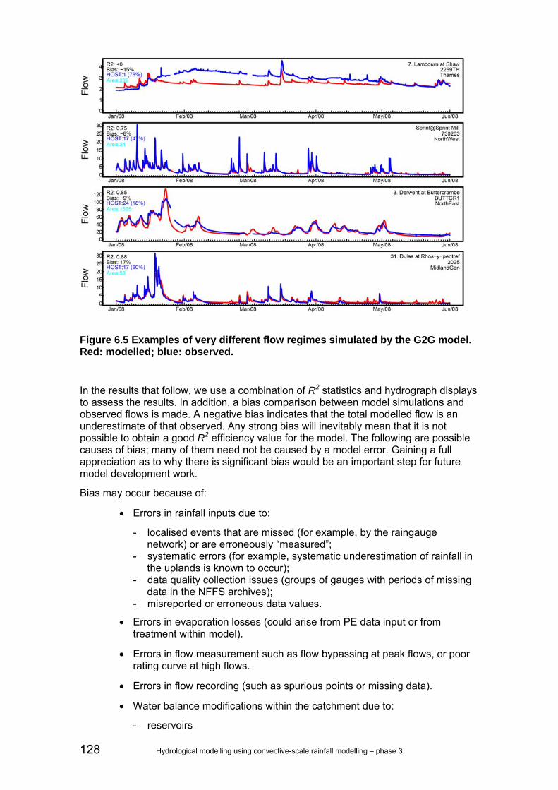
128 Hydrological modelling using convective-scale rainfall modelling – phase 3
Figure 6.5 Examples of very different flow regimes simulated by the G2G model. Red: modelled; blue: observed.
In the results that follow, we use a combination of R2 statistics and hydrograph displays to assess the results. In addition, a bias comparison between model simulations and observed flows is made. A negative bias indicates that the total modelled flow is an underestimate of that observed. Any strong bias will inevitably mean that it is not possible to obtain a good R2 efficiency value for the model. The following are possible causes of bias; many of them need not be caused by a model error. Gaining a full appreciation as to why there is significant bias would be an important step for future model development work.
Bias may occur because of:
• Errors in rainfall inputs due to:
- localised events that are missed (for example, by the raingauge network) or are erroneously “measured”;
- systematic errors (for example, systematic underestimation of rainfall in the uplands is known to occur);
- data quality collection issues (groups of gauges with periods of missing data in the NFFS archives);
- misreported or erroneous data values.
• Errors in evaporation losses (could arise from PE data input or from treatment within model).
• Errors in flow measurement such as flow bypassing at peak flows, or poor rating curve at high flows.
• Errors in flow recording (such as spurious points or missing data).
• Water balance modifications within the catchment due to:
- reservoirs

Hydrological modelling using convective-scale rainfall modelling – phase 3 129
- public water supply - sewage effluent - interactions with canals, lakes - groundwater movement not matched by model.
• Errors in the catchment boundary, especially when the subsurface catchment does not coincide with the surface catchment or when there are large differences between the “actual” catchment area (derived from the 50-m DTM, for example) and the one-km flow path derived area used by the G2G model.
Rainfall data input into the model appear to be a key cause of bias and thus poor model fit. Significant differences in model performance arise depending on which rainfall source is used. A further cause of bias arises from abstractions and returns which are not yet represented in the G2G model.
Further, the G2G model does not provide for any adjustment of the water balance to compensate for local effects. This contrasts with catchment models such as the PDM which include a rainfall adjustment factor. The factor can be calibrated to accommodate water losses and gains not explicitly included, as well as consistent biases in catchment-average rainfall estimates used as model input. In any catchment where the bias is more than a few percent, the performance of the model as judged by the R2 criterion is likely to be penalised compared with other models.
Another issue with calibration is that problems with rainfall data may be regional in nature. In many instances, the distribution of HOST soils classes is also regionally clustered. Hence, in calibration it is difficult to know whether the calibration is truly matching the soil response or is correcting for errors in the rainfall input data.
General results
Table 6.3 presents a summary of the R2 and bias performance measures obtained for 67 catchments across England and Wales. The measures are presented separately for 2007 and 2008 (note that the 2008 period was from January to October inclusive). For 2008, the performance measures are given for the different rainfall inputs (raingauge-only, raingauge-adjusted radar and radar).

130 Hydrological modelling using convective-scale rainfall modelling – phase 3
Table 6.3 R2 and bias performance measures for G2G model for 67 catchments. Catchments are ordered by predominant HOST soil class and are coloured by region. rg: raingauge-only, ra: raingauge-adjusted radar, ro: radar-only. A value of zero or less for R2 is recorded as zero. Figures at the bottom of columns are the average. Bias is presented as a percentage and is the percent difference in volume between observed and modelled flow. A positive bias means there was more modelled than observed flow.

Hydrological modelling using convective-scale rainfall modelling – phase 3 131
Three general observations can be drawn from Table 6.3:
• On average, use of the raingauge-only rainfall estimator gives the best performance (average R2=0.56) compared to raingauge-adjusted radar (0.49) and unadjusted radar (0.37).
• Using radar and raingauge-adjusted radar, the results show a positive bias (14 per cent), whereas the bias is one per cent using the raingauge-only rainfall estimator.
• Where there are significant differences in R2 between 2007 and 2008, this is often an indication of a data problem in one or the other period.
Where does the G2G model work well (average R2>0.75)?
The performance measures in Table 6.3 do not show any clear patterns in terms of what sort of catchments do well, and which do not. In part this is because when calibrating over a large area, some compromise is made between the different types of catchment. However, better performance might have been obtained for some of the more upland regions had separate calibrations been carried out.
Figure 6.6 shows a selection of catchments for a two-month period (January to February 2008) where the G2G model performs well. Catchments include upland and lowland sites, different regions, and a range of catchment sizes and response rates showing how the G2G model can perform well under a range of conditions. Figure 6.7 shows for two of the catchments a zoomed-in view over three days encompassing the first major flood peak.
Where does the G2G model work less well?
Problem of water balances
One of the issues arising during calibration was that of significant water balance differences (as measured by the bias). Figure 6.8 shows examples of catchments where bias occurs. For example, at Ripponden (on the River Ryburn in the Calder Valley) the model produces 50 per cent more water than is observed, whereas on the Ottery at Wellington Park (in the Tamar Valley), modelled flows are consistently lower than observed. Problems in the Midlands on the Tame and the Sowe are due to significant effluent discharge to the river.
Bias can be positive (too much modelled water) and negative (too little modelled water). In some cases (Tame, Sowe) the imbalance can be attributed to discharges into the river. For the Dove, the discrepancy may be due to karstic phenomenon such as sinkholes in the carboniferous limestone that can result in the surface and the subsurface catchment boundaries differing. For other catchments, it is unclear whether the bias is a modelling or measurement problem associated with the rainfall input or recorded flows.
Problem of different hydrological behaviour when HOST soil class is same
A basic premise of the G2G model is that hydrological behaviour can be driven by soil type in conjunction with topography (introducing geological factors not encompassed by soil type and land cover are under development). In the majority of cases, this seems to be a sound starting point. However, in this study some cases were encountered where catchments with the same HOST class had rather different hydrological responses.
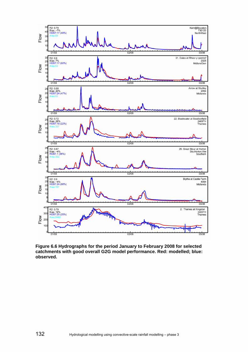
132 Hydrological modelling using convective-scale rainfall modelling – phase 3
Figure 6.6 Hydrographs for the period January to February 2008 for selected catchments with good overall G2G model performance. Red: modelled; blue: observed.

Hydrological modelling using convective-scale rainfall modelling – phase 3 133
Figure 6.7 Zoom-in over three days of hydrographs for the period January to February 2008 for two catchments with good overall G2G model performance. Red: modelled; blue: observed.
Figure 6.9 shows the modelled hydrological regime of catchments with dominant HOST class 24 (the percentage coverage is indicated in brackets). Hydrological regimes of the Midlands catchments (Blythe and Sowe) are well modelled. However, for the Pennine catchments in North East Region there is an obvious mismatch between the hydrological characteristics of observed and modelled river flows. These differences arise from the contrasting behaviours between lowland and upland catchments, for example with faster routing speeds needed for the latter. Introducing dependence of wave speed on terrain slope, and maybe channel roughness, is one of the possible ways forward.
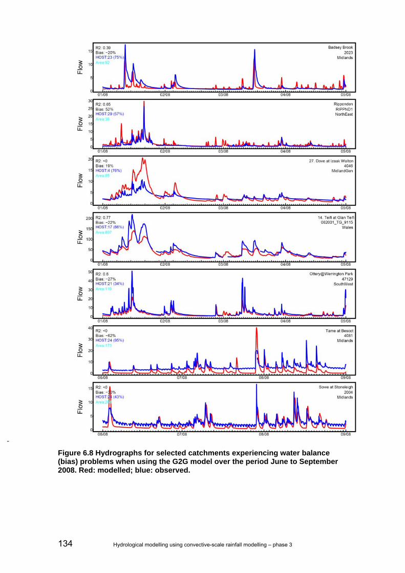
134 Hydrological modelling using convective-scale rainfall modelling – phase 3
-
Figure 6.8 Hydrographs for selected catchments experiencing water balance (bias) problems when using the G2G model over the period June to September 2008. Red: modelled; blue: observed.

Hydrological modelling using convective-scale rainfall modelling – phase 3 135
Figure 6.9 Hydrographs for selected catchments where the dominant HOST soil class is the same, but the responses are notably different. The Avon and Blythe are well modelled, but the Lune and Ribble show a consistent mismatch between modelled response and observed. These differences may be attributable to the underlying geology.
Problem of timing
The G2G model uses HOST soil classes as the primary means of controlling runoff production across different regions. Within the model, soil properties linked to these HOST classes largely affect the movement of water up and down the soil column and have less effect on movement sideways. Parameters of the routing component that affect the lateral movement of water across the grid-cells of the G2G model did not have any regional variation in the national configuration used here. It was thus difficult to match the timing of hydrological responses in some catchments. Some examples are shown in Figure 6.10. The G2G model is more flexible in its routing component but time constraints did not allow this to be explored to address the variability in response times observed here. Such trials should be done in future.

136 Hydrological modelling using convective-scale rainfall modelling – phase 3
Figure 6.10 Hydrographs for selected catchments showing timings that are too slow (top 2) and too fast (bottom 2). At the moment, it is difficult for the G2G model to match these timings.
6.4 Assessing the G2G model for ungauged catchments and against benchmark models
The strategy used to assess the national G2G model employed nine pairs of catchments, one from each of the eight regions of the Environment Agency, with an additional pair from Midlands Region to take account of the Tame and Avon urban/rural split. One catchment out of each pair was treated as a gauged site, and was included in the model calibration process described above. The other catchment was treated as ungauged, and not made available for model calibration.
The original plan was to only compare G2G model simulations with lumped benchmark models (PDM or MCRM) at the “gauged” sites used to calibrate G2G (see Table 6.2). However, as lumped models existed at most “ungauged” sites as well, these were included in the analysis. Details of lumped models used as benchmarks are given in Table 6.5: this includes information on the rainfall and PE data used and the origins of the calibrated model (NFFS model configurations were used where available and CEH calibrations from previous projects otherwise).

Hydrological modelling using convective-scale rainfall modelling – phase 3 137
Table 6.4 Details of the benchmark lumped models (PDM/MCRM) used for the paired gauged (yellow) and ungauged (grey) catchments.
Region Gauging station Model type
Model source
Rainfall data PE data
Wales Cynon at Abercynon PDM CEH HyradK - raingauge-only Sine curve profile Rhondda at Trehafod PDM CEH Single raingauge Sine curve profile Thames Sor at Bodicote PDM CEH HyradK - raingauge-only MORECS 137 Cherwell at Banbury PDM CEH HyradK - raingauge-only MORECS 137
Midlands Avon: Isbourne at Hinton the Green MCRM NFFS NFFS raingauge weights NFFS profile Badsey Brook at Offenham MCRM NFFS NFFS raingauge weights NFFS profile Tame: Cole at Coleshill MCRM NFFS NFFS raingauge weights NFFS profile Rea at Calthorpe Park MCRM NFFS NFFS raingauge weights NFFS profile South West Camel at Denby PDM CEH HyradK - gauge-adjusted radar MORECS 177 Tamar at Gunnislake PDM CEH HyradK - gauge-adjusted radar MORECS 177 North West Mint at Mint Bridge PDM CEH HyradK - raingauge-only Sine curve profile Kent at Sedgwick PDM CEH HyradK - raingauge-only Sine curve profile Anglian Witham at Saltersford Total N/A N/A N/A N/A Witham at Claypole Mill PDM NFFS NFFS raingauge weights MORECS 117 North East Calder at Elland N/A N/A N/A N/A Calder at Todmorden PDM NFFS NFFS raingauge weights Sine curve profile
Southern Beult at Stile Bridge PDM NFFS NFFS raingauge weights NFFS profile Stour at Horton PDM NFFS NFFS raingauge weights NFFS profile
The performance of the G2G model was assessed for both gauged and “ungauged” catchments using observed flows and benchmark models where available. For this, the G2G model was configured to run in simulation-mode only over the area covered by the 18 gauged and ungauged catchments. Table 6.5 and Figure 6.11 summarise the model performance using statistical measures (R2 efficiency and bias) and hydrograph displays respectively.
Overall, G2G model performance for ungauged catchments is encouragingly good compared with gauged sites. The statistics in Table 6.5 show little difference in performance between ungauged and gauged catchments, with river flows from the ungauged catchments modelled almost as well as the gauged. As with the model calibration assessment, there is a range of performance obtained and several cases of significant model bias which may indicate water transfers not represented by the G2G model. As expected, the extra flexibility afforded by site-specific calibration of the benchmark lumped models is reflected in the higher R2 efficiency and lower bias statistics for lumped models relative to the national G2G model. However, there are certain areas and periods of time where the G2G model performance measures are better than those for the lumped benchmark models, for example the Beult and Stour catchments in Southern Region, or are on a par.

138 Hydrological modelling using convective-scale rainfall modelling – phase 3
Table 6.5 R2 efficiency and bias performance measures for the G2G and benchmark lumped models (PDM/MCRM) using river flow simulations for the paired gauged (yellow) and ungauged (grey) catchments.
R2 efficiency Percentage bias 2007 2008 2007 2008
Name Host Region G2G PDM/ MCRM G2G PDM/
MCRM G2G PDM/ MCRM G2G PDM/
MCRM Cynon at Abercynon 24 Wales 0.66 0.85 0.54 0.86 18 20 19 19 Rhondda at Trehafod 15 Wales 0.58 0.86 0.73 0.93 -1 14 -11 8 Sor at Bodicote 2 Thames 0.64 0.77 0.42 0.60 8 7 10 -6 Cherwell at Banbury 25 Thames 0.59 0.71 0.51 0.69 17 -16 20 -30 Isbourne at Hinton 25 Midlands 0.69 0.47 0.7 0.83 20 11 2 3 Badsey Brook 23 Midlands 0.26 0.51 0.35 0.68 0 -43 -3 -20 Cole at Coleshill 24 Midlands 0.34 0.76 0 0.71 67 19 87 27 Rea at Calthorpe Park 24 Midlands 0.54 0.76 0.46 0.69 71 36 80 34 Camel at Denby 17 South West 0.82 0.91 0.68 0.85 -13 -1 -12 5 Tamar at Gunnislake 17 South West 0.68 0.93 0.54 0.90 -12 -2 -8 -1 Mint at Mint Bridge 17 North West 0.81 0.95 0.77 0.94 -6 7 -3 6 Kent at Sedgwick 17 North West 0.71 0.96 0.64 0.94 -8 1 -1 4 Saltersford Total 2 Anglian 0.38 N/A 0.44 N/A -10 N/A -2 N/A Witham at Claypole Mill 2 Anglian 0.72 0.74 0.78 0.71 -17 17 -15 -10 Calder at Elland 29 North East 0.65 N/A 0.56 N/A 2 N/A 5 N/A Calder at Todmorden 29 North East 0.62 0.83 0.77 0.79 34 -8 -18 5 Beult at Stilebridge 25 Southern 0.55 -0.05* 0.74 0.68 17 -39 14 53 Stour at Horton 1 Southern 0.63 0.11* 0.82 0.66 -15 -21 -2 26 Average 0.60 0.69 0.58 0.78 9.6 0.1 9.0 7.6
Average ungauged 0.62 0.67 0.54 0.78 11.4 3.4 13.3 15.1 Average gauged 0.59 0.71 0.62 0.78 7.67 -2.4 4.67 1.9
Note that raingauge data supplied from the NFFS real-time archive only began on 27 March 2007, so zero rainfall was used for the PDM in this period,
Performance measures are only one way of comparing models and can be heavily skewed by large events. Another way of assessing the G2G model is to inspect the simulated hydrographs. Hydrographs showing model performance for gauged and ungauged catchments over a two-month period at the start of 2008 are shown in Figure 6.11. As with the tabulated statistics, there is no obvious difference in overall performance of G2G modelled flows between ungauged and gauged catchments. Figure 6.11 also shows that the site-specific lumped hydrological models used as benchmarks are difficult to beat when using a nationally calibrated distributed model and for ‘typical’ catchment rainfall conditions. Nevertheless, the range of catchment behaviours broadly captured by the G2G model is still evident and, on occasions, the G2G model performs as well as or better than the lumped model (such as Sor at Bodicote and the Stour at Horton).

Hydrological modelling using convective-scale rainfall modelling – phase 3 139
Figure 6.11 Hydrographs for paired ungauged (left column) and gauged (right column) catchments using G2G (red) and benchmark (green) models (PDM or MCRM) over the period January and February 2008. The benchmark models were calibrated to each site including ‘ungauged’ catchments. There is no marked difference in fit between gauged and ungauged.

140 Hydrological modelling using convective-scale rainfall modelling – phase 3
6.5 Assessing the G2G model in state-updating mode
State-updating is a means of internal model correction to adjust for differences between modelled and observed flows. A simple state-updating scheme was used within the G2G model. The principle is that the model water stores can be linearly scaled across model grid-cells to match observed flows. State-updating is currently applied to all cells upstream of a gauged point. If there are nested catchments, the most upstream catchments are state-updated first. This is a simplistic approach in that all points within a sub-catchment receive the same scaling factor.
At present the scheme only scales the water content of some of the model stores within a model cell; also, no account is taken of translation times between the gauged cell and the cells being adjusted. There are obvious developments that can be made to this preliminary scheme and future improvements are planned.
A scheme was first developed in which state-updating could be applied to model cells upstream and downstream of a gauged cell, maximising the coverage of grid-cells that receive state-updating. Tests showed that this approach was unstable because cells downstream lack a corrective feedback mechanism. Transfer of corrections to adjacent catchments was also made, but trials of this scheme gave poor results. As a consequence, this functionality was disabled in recognition that a more sophisticated transfer scheme would be required for future state-updating.
The performance of state-updating in the G2G model was assessed using five of the nine “ungauged” study sites in the regional pairings detailed above. These were the five sites having a downstream gauged site from which to state-update: the other four sites had no downstream site available. Note that in each of the cases, the site used for state-updating was not the same as the paired gauged site discussed in the preceding section. Ungauged sites and associated sites are listed in Table 6.6 and illustrated in Figure 6.12.
Table 6.6 Comparison of G2G model performance in simulation mode and state-updating mode for five sites treated as “ungauged”.
Ungauged Site
Area (km2)
HOST class
State update from
Area (km2)
HOST class
R2 2007 Sim
R2
2008 Sim
R2 2007 Updated
R2 2008 Updated
Cynon at Abercynon
101 24 Taff at Pontypridd
455 26 0.66 0.54 0.33 <0
Sor at Bodicote 455 26 Thames at Kingston
9962 25 0.64 0.42 <0 <0
Cole at Coleshill 122 24 Tame at Lea Marston
807 24 0.34 <0 <0 <0
Mint at Mint Bridge 66 17 Kent at Victoria Bridge
181 17 0.81 0.77 0.88 0.88
Saltersford 129 2 Witham at Claypole Mill
305 2 0.38 0.44 0.62 0.08
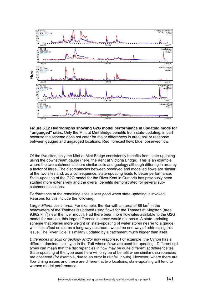
Hydrological modelling using convective-scale rainfall modelling – phase 3 141
Figure 6.12 Hydrographs showing G2G model performance in updating mode for “ungauged” sites. Only the Mint at Mint Bridge benefits from state-updating, in part because the scheme does not cater for major differences in area, soil or response between gauged and ungauged locations. Red: forecast flow; blue: observed flow.
Of the five sites, only the Mint at Mint Bridge consistently benefits from state-updating using the downstream gauge (here, the Kent at Victoria Bridge). This is an example where the two catchments share similar soils and geology although differing in area by a factor of three. The discrepancies between observed and modelled flows are similar at the two sites and, as a consequence, state-updating leads to better performance. State-updating of the G2G model for the River Kent in Cumbria has previously been studied more extensively and the overall benefits demonstrated for several sub-catchment locations.
Performance at the remaining sites is less good when state-updating is invoked. Reasons for this include the following.
Large differences in area. For example, the Sor with an area of 88 km2 in the headwaters of the Thames is updated using flows for the Thames at Kingston (area 9,962 km2) near the river mouth. Had there been more flow sites available to the G2G model for our use, this large difference in areas would not occur. A state-updating scheme that places more weight on state-updating of water stores nearer to a gauge, with little effect on stores a long way upstream, would be one way of addressing this issue. The River Cole is similarly updated by a catchment much bigger than itself.
Differences in soils or geology and/or flow response. For example, the Cynon has a different dominant soil type to the Taff whose flows are used for updating. Different soil types can mean that the discrepancies in flow may be quite different at different sites. State-updating of the type used here will only be of benefit when similar discrepancies are observed (for example, due to an error in rainfall inputs). However, where there are flow timing issues and these are different at two locations, state-updating will tend to worsen model performance

142 Hydrological modelling using convective-scale rainfall modelling – phase 3
Poor or moderate modelling performance at the site used to update from. In cases when G2G does not model flow particularly well, use of such a site for state-correction can be dangerous and likely to mean that large corrections applied nearby may be correcting for local effects (such as unmodelled river abstractions or effluent returns, flow bypassing, backwater effects). The Cole, Sor and Saltersford are examples where this occurs.
Recommendations for current usage of state-updating
Use of state-updated G2G model outputs is recommended only for locations that are local to a good river gauging station and which have similar types of flood response. In some regions, such as parts of North West and South West where there are strong regional similarities in response, state-updating may be useful over a wider area.
If catchments have a large difference in area, soil/geology or land use, state-updating is unlikely to improve performance and could be poor. We recommend that forecasts based on the simulation mode G2G model runs are used for these locations.
State-updating will benefit from having as many good river gauging stations as possible included in the G2G model configuration. Only river gauging stations that are performing well should be used for state-updating.
These recommendations are likely to change as state-updating methods improve.
Recommendations for development of state-updating
It would be worth considering the feasibility of developing schemes that apply greater weight to updating at closer distances to a gauged site, and possibly try to account for timing errors. It may also be helpful to consider how best to deal with state-updating across different soil types, as our assessment suggests that this can cause problems.
The better the G2G model is at simulating river flows, the easier it will be to implement a good state-updating scheme. Thus, improvements in the model will also improve state-updating performance.

Hydrological modelling using convective-scale rainfall modelling – phase 3 143
6.6 Recommendations for use of the G2G model within a flood forecasting setup The G2G model is not a replacement for the PDM and other catchment and river routing models. It aims to give a reasonable flow simulation for the majority of catchments over a large area, not an excellent simulation at selected locations. The purpose of the G2G model is to complement models individually calibrated to gauged catchments, providing some additional spatial information on flow variation that cannot be extracted from lumped models.
The G2G model does not perform as well as PDM/MCRM site-specific calibrated models for most catchments. This is to be expected since, compared with the PDM, there are:
• fewer calibration parameters – all G2G parameters are national rather than local in nature;
• no local adjustments for water balance in the G2G model – thus catchments with abstractions/effluent will not be well modelled, and may be much better modelled by other models which have water balance factors that can be calibrated for specific catchments using gauged flow records.
For some parts of the UK, the G2G model performance when fitted regionally (such as done here for South West) compares favourably with locally fitted models: they are not as good but are still quite good. State-updating procedures also perform well in these areas. The G2G model is likely to be a useful addition for flood forecasting in such regions.
For other parts of the UK, such as those more influenced by anthropogenic effects (abstractions, effluent returns, reservoirs, pumped-drainage areas), the G2G is unlikely to perform as well as locally fitted models. Performance may be improved in the future by taking account of anthropogenic effects through extra functionality supported by new datasets. It is not yet clear how useful the G2G model will be in such regions.
Use of the G2G model for ungauged catchments
The model performs moderately well over many catchments. Compared to other methods for forecasting at ungauged locations, the model is likely to give as good or better performance in many situations. For example, the model is expected to do better than parameter transfer methods. As a modelling approach to the ungauged catchment forecasting problem, it has the added advantage of spatial consistency.
Use of the G2G model in a spatial context
The model provides a spatial overview of a flood event. As demonstrated, G2G model gridded forecasts can be used alongside gridded datasets on flows of given return period to locate potential hotspots of flood risk within a catchment, highlighting particular reaches and confluences at risk as the flood develops.
The model incorporates the spatial effects of the rainfall pattern along with properties of the landscape that shape the flood response: these flood shaping forces are apparent in the ensemble flood hydrographs produced using ensemble rainfalls as input.

144 Hydrological modelling using convective-scale rainfall modelling – phase 3
6.7 Next steps for development of the G2G model The following are recommended steps for the next stage of development of the G2G model, with an indication of their priority:
• Implement handling of anthropogenic factors affecting river flows, such as abstractions, effluent discharges, water transfers and reservoirs. High/medium priority.
• Improve the routing scheme to better reflect different routing behaviours in upland and lowland rivers and the effects of slope, roughness and river width. This should improve time-of-travel in the G2G model across heterogeneous landscapes. High priority.
• Improve state-updating by developing and trialling methods that place more weight on adjustments to model grid-cells near the river gauging station location used for updating, and possibly take account of timing errors. High/medium priority.
• Consider how to improve the representation of groundwater, including use of more geological property information. Medium priority.
• Improve cold state initialisation. High/medium priority.
• Improve G2G model calibration using improved quality-controlled rainfall and river flow datasets. High priority.
• Incorporate a module for snowmelt. Medium priority.

Hydrological modelling using convective-scale rainfall modelling – phase 3 145
7 Using MOGREPS and STEPS ensemble forecasts in NFFS
7.1 Introduction Ensemble forecasting using MOGREPS precipitation forecasts was configured in the test NFFS system for two regions: Thames and North East. A test system was set up in Delft to receive MOGREPS forecasts from the Met Office and process these in an NFFS setup. During the project, a number of Environment Agency staff were given remote access to the system to evaluate it while it was being developed.
Criteria for selection of pilot regions were:
• widespread application of conceptual rainfall-runoff models;
• fast-running models;
• forecasting team interested in participating in the study.
These criteria led to the selection of Thames and North East region for the pilot.
• North East Region has short lead times to many of its upstream forecasting locations and is largely covered with PDM models. The forecasting time-step is 15 minutes and models run fast.
• Thames Region has longer lead times to its most important forecasting locations but has large, fast-responding urban areas within its forecasting responsibility. The region is largely covered with nested TCM models. The forecasting time-step is 15 minutes and models run fast. Due to the setup of the TCM models (nested), the larger of the currently available TCM models cover a long lead time which makes them less useful when using nowcasting ensembles and in some cases MOGREPS ensembles.
Initially, MOGREPS NWP rainfall ensembles were provided by the UK Met Office in experimental mode from the middle of January to the beginning of March 2008. Later, it was decide to continue the MOGREPS trial for the rest of the project.
This section reports on the configuration of the NFFS system to enable the use of MOGREPS forecasts, a basic assessment of forecast performance using MOGREPS and on the overall performance of the test system.
The combination of the above information can be used to determine if and how MOGREPS forecasts should be used within the NFFS.
During the Phase 2 completion workshop it became clear that, apart from MOGREPS, forecasters in many regions also wanted to see results of the STEPS product as this could provide them with a probabilistic way to deal with short lead-time forecasts. Many UK catchments are fast-responding and could benefit greatly from a good short-term forecast product.
Although STEPS was being trialed operationally, only four forecasts were available to the project with time-origins at 00:00, 03:00, 06:00 and 09:00 on 20 July 2007. For

146 Hydrological modelling using convective-scale rainfall modelling – phase 3
these forecasts 20 ensemble members were available (operational STEPS aims to use 50 ensemble members and one new forecast every hour) with 15-minute time-steps six hours ahead.
7.2 STEPS and MOGREPS ensembles Since spring 2007, the Met Office uses two systems to generate ensemble forecasts:
• STEPS – for short-term nowcasting of smaller scale short-lived weather features.
• MOGREPS – for short- and medium-range weather forecasting.
The ensemble rainfall forecasts provided the input for the pilot on ensemble flood forecasting with NFFS. Some background information about the ensemble prediction capability of both systems is presented here; the information was taken from the Met Office.
7.2.1 STEPS
Nowcasting bridges the gap between telemetry and radar observations on the one hand, and numerical weather prediction on the other. For the first hours into the future, NWP is relatively unreliable. Nowcasting therefore aims to predict weather conditions for several hours ahead (up to six hours). It is run at much higher spatial and temporal resolutions to capture the smaller scale weather features. Up to 2007, NIMROD and GANDOLF provided the nowcasting capability. In spring 2007, a new system called Short-Term Ensemble Prediction System (STEPS, Bowler et al., 2006) was introduced to replace both systems.
STEPS provides ensemble prediction capability for nowcasting. This anticipates the fact that the smaller scale weather features – like convective storms generating intensive flooding – are shorter lived and less predictable. With an ensemble prediction approach the uncertainty of the nowcasts of weather condition can to a certain extent be quantified.
STEPS blends extrapolation of radar observations, noise and NWP on a hierarchy of scales. Output from STEPS includes ensemble rain rate and accumulations. Nowcasts are generated up to six hours ahead for a two-km grid with a five-minute time-step.
The system produces a 50-member ensemble. Except for the deterministic run, the individual members are currently not blended into the MOGREPS forecasts but a research project is underway to develop a method for this purpose.
7.2.2 MOGREPS
In 2005, the Met Office introduced a new ensemble system called MOGREPS (Met Office Global and Regional Ensemble Prediction System, Bowler et.al, 2008) which included a 24-km resolution regional ensemble for the Atlantic and Europe. Ensemble forecasting is based on the principle of adding small perturbations to the best guess of the initial state of the atmosphere. The model is then run forward from the perturbed starting conditions to generate an ensemble of different forecasts.
The regional model (MOGREPS-R) is designed to provide ensemble forecasts for the short range (days 0-3) for the UK and Ireland. It provides 24-member ensemble with a grid resolution of 24 km for a forecast length of 54 hours (36 hours are used in this research). Boundary conditions for the regional model are provided by a global model

Hydrological modelling using convective-scale rainfall modelling – phase 3 147
(MOGREPS-G) with a 90-km grid and a forecast time of 72 hours producing a 24-member ensemble: see Figure 7.1. Both models are run twice daily at 0 and 12 UTC. Due to spin-up issues, and the fact that only two forecast are available per day, the first hours of MOGREPS runs are generally not used.
UK 4km
NAE 12km+EPS 24member,24km
Global 40km+EPS 24member,90km
50 levels
(UK 12km)UK 4km
NAE 12km+EPS 24member,24km
Global 40km+EPS 24member,90km
50 levels
50 levels
(UK 12km)
Figure 7.1 Model Coverage in MOGREPS (ref. Met Office).
The ensembles consist of one control run and 23 additional members. The control forecast is run at the same resolution as the other ensemble members but does not contain any perturbations to account for initial condition or model uncertainties - as such it runs from the best analysis of the initial state of the atmosphere. The control run can be compared with the standard deterministic weather forecast that is run at a 12-km resolution.
The 24 different predictions produced by the ensemble show a range of possible forecasts, allowing forecasters to quantify the uncertainty in an objective manner. If all 24 forecasts give similar solutions, this suggests a high confidence; when confidence is lower, the ensembles can help the forecaster to identify the most likely outcome, and also assess the risks of alternative solutions including more severe weather. Meteorologists now believe that the ensemble prediction systems provide a method of quantitatively assessing the uncertainty associated with numerical weather prediction forecasts. To provide a basis for probabilistic forecasting, meteorologists assume that the generated ensemble members have an equal probability. The latter is an important notion when ensemble forecasting and should provide the quantitative basis for probabilistic flood forecasting.
7.3 Configuring ensemble forecasting in NFFS Our configuration was based on the current configuration (March 2008) extracted from the NFFS for North East and Thames region. No distributed models were run in this test case: only the existing regional models were used.
The configuration changes included:
• Importing and processing of NWP ensembles (MOGREPS).
• Pre-processing of ensemble data to generate precipitation input.
• Ensemble runs of forecasting models.
• Data displays, including statistical analyses.
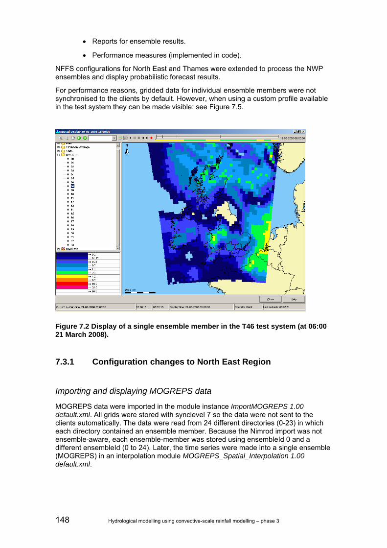
148 Hydrological modelling using convective-scale rainfall modelling – phase 3
• Reports for ensemble results.
• Performance measures (implemented in code).
NFFS configurations for North East and Thames were extended to process the NWP ensembles and display probabilistic forecast results.
For performance reasons, gridded data for individual ensemble members were not synchronised to the clients by default. However, when using a custom profile available in the test system they can be made visible: see Figure 7.5.
Figure 7.2 Display of a single ensemble member in the T46 test system (at 06:00 21 March 2008).
7.3.1 Configuration changes to North East Region
Importing and displaying MOGREPS data
MOGREPS data were imported in the module instance ImportMOGREPS 1.00 default.xml. All grids were stored with synclevel 7 so the data were not sent to the clients automatically. The data were read from 24 different directories (0-23) in which each directory contained an ensemble member. Because the Nimrod import was not ensemble-aware, each ensemble-member was stored using ensembleId 0 and a different ensembleId (0 to 24). Later, the time series were made into a single ensemble (MOGREPS) in an interpolation module MOGREPS_Spatial_Interpolation 1.00 default.xml.

Hydrological modelling using convective-scale rainfall modelling – phase 3 149
For importing and display of MOGREPS data the following files were updated:
WorkFlow Description
Import_workflow 2.33 default.xml Import workflow
ImportMOGREPS 1.00 default.xml MOGREPS import module instance
IdImportMOGREPS 1.00 default.xml MOGREPS ID mapping
IdMapDescriptors 2.24 default.xml New ID mapping descriptor added (RegionConfig folder)
ModuleInstanceDescriptors 2.39 default.xml
New MI descriptors added (RegionConfig folder)
Locations 2.39 default.xml MOGREPS location added to regional locations file
Grids 1.01 default.xml MOGREPS grid properties added to regional grids file
SpatialDisplay 2.28 default.xml Spatial display of MOGREPS grids
sa_global.properties MOGREPS import folder added to import folder tags
Processing MOGREPS data and SNOWP models
MOGREPS data were processed similarly to the non-ensemble Nimrod data that were part of the standard system. All processing was done in the Fluvial_FastResponse_Forecast_MOGREPS 1.00 default.xml workflow. In all existing processing modules, the end time was set to 36 hours to match the length of the MOGREPS forecasts.
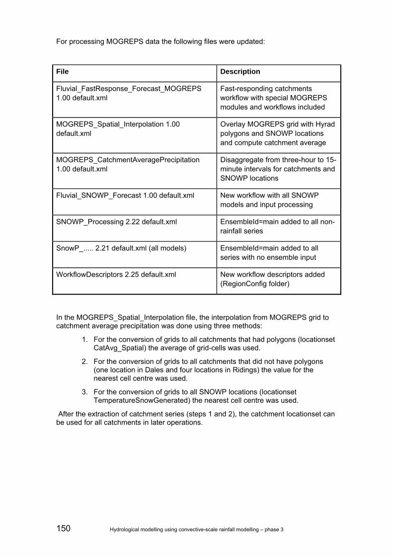
150 Hydrological modelling using convective-scale rainfall modelling – phase 3
For processing MOGREPS data the following files were updated:
File Description
Fluvial_FastResponse_Forecast_MOGREPS 1.00 default.xml
Fast-responding catchments workflow with special MOGREPS modules and workflows included
MOGREPS_Spatial_Interpolation 1.00 default.xml
Overlay MOGREPS grid with Hyrad polygons and SNOWP locations and compute catchment average
MOGREPS_CatchmentAveragePrecipitation 1.00 default.xml
Disaggregate from three-hour to 15-minute intervals for catchments and SNOWP locations
Fluvial_SNOWP_Forecast 1.00 default.xml New workflow with all SNOWP models and input processing
SNOWP_Processing 2.22 default.xml EnsembleId=main added to all non-rainfall series
SnowP_..... 2.21 default.xml (all models) EnsembleId=main added to all series with no ensemble input
WorkflowDescriptors 2.25 default.xml New workflow descriptors added (RegionConfig folder)
In the MOGREPS_Spatial_Interpolation file, the interpolation from MOGREPS grid to catchment average precipitation was done using three methods:
1. For the conversion of grids to all catchments that had polygons (locationset CatAvg_Spatial) the average of grid-cells was used.
2. For the conversion of grids to all catchments that did not have polygons (one location in Dales and four locations in Ridings) the value for the nearest cell centre was used.
3. For the conversion of grids to all SNOWP locations (locationset TemperatureSnowGenerated) the nearest cell centre was used.
After the extraction of catchment series (steps 1 and 2), the catchment locationset can be used for all catchments in later operations.

Hydrological modelling using convective-scale rainfall modelling – phase 3 151
Other files adjusted while implementing the MOGREPS changes were:
PREC_BACKUP_PROF 2.21 default.xml
Synchlevel changed from 5 to 1, end time set to 36 hours
Precip_CopyCatAvg 2.22 default.xml End time set to 36 hours
EVAP_..... 2.21 default.xml End time set to 36 hours
In the filters, new entries were made to show the results of MOGREPS data at SNOWP locations. Only the main regional filter group was updated; the area filter groups were not updated.
Filters 2.27 default.xml
Entries were added for MOGREPS precipitation, merged precipitation and Snow, SNOWP
Running the MOGREPS ensembles in SNOW, PDM, KW and ARMA modules
The Fluvial_FastResponse_Forecast_MOGREPS 1.00 default.xml included three sub-workflows for the three areas in North East. These sub-workflows contained all fast-responding catchment modules as well as some input processing modules for precipitation and temperature. Also, the flow to level modules to convert forecast flow to levels were included in these sub-workflows. The main changes included in the modules were:
1. Change GA config (forecast only) to include a main ensembleId in the non-ensemble series.
2. Increase forecast-length for all SNOW/PDM/KW/ARMA modules to 36 hours (as this is what MOGREPS provides).

152 Hydrological modelling using convective-scale rainfall modelling – phase 3
Besides the GA module instances, the following config files were also updated:
File Description
Fluvial_FastResponse_Forecast_MOGREPS 1.00 default.xml
Included fast-responding area workflows in ensemble mode
Northumbria_Meteo_Processing 2.02 default.xml EnsembleId=main added and end time set to 36 hours
Ridings_Meteo_Processing 2.01 default.xml EnsembleId=main added and end time set to 36 hours
Dales_Meteo_Processing 2.03 default.xml EnsembleId=main added and end time set to 36 hours
Snowconvertmm_Northumbria 2.01 default.xml End time set to 36 hours
Snowconvertmm_Aire 2.31 default.xml End time set to 36 hours
Snowconvertmm_Dales 2.01 default.xml End time set to 36 hours
Snowconvertmm_Ridings 2.01 default.xml End time set to 36 hours
TyneGenerate 2.21 default.xml Ensembleid=main added and end time set to 36 hours
NiddGenerate 2.21 default.xml Ensembleid=main added and end time set to 36 hours
TeesGenerate 2.21 default.xml Ensembleid=main added and end time set to 36 hours
Gaunless_PDM_ErrorModel_MergeInputs 1.01 default.xml
End time set to 36 hours
Gaunless_PDM_ErrorModel 1.01 default.xml Ensembleid=main added and end time set to 36 hours
Swale_PDM_ErrorModel 1.01 default.xml End time set to 36 hours
Swale_PDM_ErrorModel_MergeInputs 1.01 default.xml
Ensembleid=main added and end time set to 36 hours
....FastFlowToLevel 2.21 default.xml End time set to 36 hours
In the filters, new entries were made to show the results of the SNOW/PDM/KW and ARMA modules.
Filters 2.27 default.xml
Time series of all models that use MOGREPS data were added as well as merged precipitation

Hydrological modelling using convective-scale rainfall modelling – phase 3 153
Statistics
After running the catchment modules with the MOGREPS ensemble input, statistics were computed for the catchment rainfall and output series of PDM and ARMA modules. The following statistics for the ensemble series were computed: minimum, maximum, median, 25, 33, 66 and 75 percentiles. The following files were updated to compute the statistics.
File Description
Fluvial_FastResponse_Forecast_MOGREPS 1.00 default.xml
Statistics module added
MOGREPS_PDM_Statistics 1.00 default.xml Statistics for PDM, ARMA and rainfall catchment series added
Parameters 1.90 default.xml Statistics parameters for discharge and precipitation added
LocationSets 2.36 default.xml locationsets HydroDischargeARMA_Fast, .._Northumbria_Fast, .._Dales_Fast, ..ARMA_Ridings_Fast have been added
LocationSets 2.36 default.xml locationsets HydroDischargeERRORModel_Fast, .._Northumbria_Fast and _Dales_Fast have been added
Other changes:
• Location Dalton removed from HydroPDMDischargeUpdated_Dales locationset • Location KIRBYW1 added to HydroPDMDischargeUpdated_Dales locationset
In the filters, new entries were made to show the results of the PDM and ARMA updated series statistics and the precipitation catchment statistics.
Filters 2.27 default.xml Statistics for PDM, ARMA and P.merged added
Pre-defined displays
For display of the statistics as area graphs, the displaygroups were updated with MOGREPS groups for all catchments. First, five plot groups were made (RainfallMOGREPS, PDMSIMULATEDMOGREPS, PDMUPDATEDMOGREPS, ERRORMOGREPS and ARMAMOGREPS); in the displaygroups, these plotgroups were used:
DisplayGroups 2.34 default.xml Plotgroups added

154 Hydrological modelling using convective-scale rainfall modelling – phase 3
Figure 7.3 shows an example of a pre-defined display.
Figure 7.3 Example of a pre-defined display.
Reports
Reports of MOGREPS forecast output were generated in the new report module instance Report_MOGREPS 1.00 default.xml. This report module instance was included in the general Export_Current 2.35 default.xml workflow. To generate MOGREPS reports the following files were updated:
Export_Current 2.35 default.xml Report workflow with new MOGREPS report module added
Report_MOGREPS 1.00 default.xml Module instance that generates MOGREPS reports
fluvial_forecastlocation_template9 1.00 default.html
Template in reportTemplates folder, copied from Thames
Report_Export_ZIPFile 2.22 default.xml Export of MOGREPS report included
Report_Export 2.23 default.xml Export of MOGREPS report included
Report_Export 2.49 default.zip File northeast_navigation.js updated with MOGREPS links
Report_Export_ZIPFile 2.49 default.zip File northeast_navigation.js updated with Mogreps links

Hydrological modelling using convective-scale rainfall modelling – phase 3 155
An example report is shown in Figure 7.4.
Figure 7.4 Example report of North East MOGREPS results.
7.3.2 Configuration changes to Thames Region
Importing and displaying MOGREPS data
MOGREPS data were imported in the module instance ImportMOGREPS 1.00 default.xml. All grids were stored using synclevel 7. The data were read from 24 different directories (0-23) in which each directory contained an ensemble member. Because the Nimrod import was not ensemble-aware, each ensemble-member was stored using ensembleId 0 and a different ensembleId (0 to 24). Later, the time series were made into a single ensemble (MOGREPRS) in an interpolation module MOGREPS_Spatial_Interpolation 1.00 default.xml. To import and display MOGREPS data the following files were updated:

156 Hydrological modelling using convective-scale rainfall modelling – phase 3
WorkFlow Description
ImportTelemetry 2.12 default.xml Import workflow
ImportMOGREPS 1.00 default.xml MOGREPS import module instance
IdImportMOGREPS 1.00 default.xml MOGREPS ID mapping
IdMapDescriptors 2.08 default.xml New ID mapping descriptor added (RegionConfig folder)
ModuleInstanceDescriptors 2.83 default.xml
New MI descriptors added (RegionConfig folder)
Locations 2.14 default.xml MOGREPS location added to regional locations file
Grids 1.03 default.xml MOGREPS grid properties added to regional grids file
GridDisplay 2.11 default.xml Spatial display of MOGREPS grids
sa_global.properties MOGREPS import folder added to import folder tags
Processing MOGREPS data
MOGREPS data were processed similarly to the processing of non-ensemble Nimrod data. All processing was done in the Fast_All_MOGREPS 1.00 default.xml workflow. In all existing processing modules, the end time is set to 36 hours to match the length of MOGREPS forecasts. In the filters, new entries were made to show the results of MOGREPS data at SNOWP locations. Only the main regional filter group was updated; the area filter groups were not updated.
Running the MOGREPS TCM and ARMA modules
The Fast_All__MOGREPS 1.00 default.xml included all the modules and sub-workflows (running the catchment models) for Thames. These sub-workflows contained all catchment modules as well as some input processing modules for precipitation. Also, the flow to level modules to convert forecasted flow to levels were included in these sub-workflows. The main changes in the modules were:
1 Change GA config (forecast only) to include a main ensembleId in the non-ensemble series.
2 Increase forecast length for all TCM/ARMA modules to 36 hours (as this is what MOGREPS provides).
In the filters, new entries were made to show the results of MOGREPS forecasts.

Hydrological modelling using convective-scale rainfall modelling – phase 3 157
Statistics
After running the catchment modules with MOGREPS ensemble input, statistics were computed for the catchment rainfall and output series of TCM and ARMA modules. The following statistics for the ensemble series were computed: minimum, maximum, median, 25, 33, 66 and 75 percentiles. In the filters, new entries were made to show the results of the TCM and ARMA updated series statistics and the precipitation catchment statistics.
Pre-defined displays
For display of the statistics as area graphs, the displaygroups were updated with MOGREPS groups for all catchments, both for ‘plain’ TCM output and for the ARMA corrected discharge.
Reports
Reports of MOGREPS forecast output were generated in a new report module instance Report_MOGREPS 1.01 default.xml. This report module instance was included in the general Export_Current 2.01 default.xml workflow.
Thresholds
Currently, Thames Region has not set thresholds to TCM/ARMA results. For this project, the existing level thresholds were converted to flow for all TCM model locations that had a threshold. This was set for the deterministic forecast and for two-thirds of the ensemble forecast.

158 Hydrological modelling using convective-scale rainfall modelling – phase 3
Table 7.1 Overview of thresholds used, South East area.
LocationId Threshold? Rating Name/Rating ID
2989TH 2989TH 2989TH Addlestone
2620TH 2620TH 2620TH Binfield
4370TH 4370TH 4370TH Catford Hill
4180TH - - -
3270TH 3270TH - -
3290TH 3290TH - -
2427TH 2427TH - -
3061TH 3061TH 3061TH Flash Bridge
3229TH 3229TH 3229TH Gatwick Link
3210TH 3210TH - -
3080TH 3080TH - -
2936TH 2936TH 2936TH Guildford Street
4310TH 4310TH 4310TH Hayes Lane
3230TH 3230TH 3230TH Horley
3369TH 3369TH 3369TH 3369TH
3390TH 3390TH 3390TH Kingston Hogsmill
3240TH 3240TH 3240TH Kinnersley Manor
2442TH 2442TH - -
4389TH 4389TH 4389TH Manor House Gardens
2420TH - - -
2469TH - - -
3040TH 3040TH 3040TH Tilford
2927TH 2927TH 2927TH Trumps Green
2490TH 2490TH - -
3090TH 3090TH - -
2700TH 2700TH - -
3350TH 3350TH - -

Hydrological modelling using convective-scale rainfall modelling – phase 3 159
Table 7.2 Overview of thresholds used, North East area.
LocationId Threshold Rating Name/Rating ID
5427TH 5427TH - -
3829TH 3829TH 3829TH Colindeep Lane
3870TH 3870TH - -
2870TH 2870TH 2870TH Denham Colne
2879TH - - -
3826TH 3826TH 3826TH Edgware Hospital
5357TH 5357TH 5357TH Edmonton Green
5189TH 5189TH 5189TH Elizabeth Way
5420TH 5420TH 5420TH High Ongar
5470TH 5470TH 5470TH Loughton
5080TH 5080TH - -
3680TH 3680TH 3680TH Marsh Farm
3850TH 3850TH 3850TH Monks Park
5480TH 5480TH 5480TH Redbridge
5169TH 5169TH - -
2829TH 2829TH 2829TH Uxbridge PSTN Level/Flow
2810TH 2810TH 2810TH Warrengate Road
4690TH 4690TH - -
3839TH 3839TH 3839TH Wembley
4827TH 4827TH - -
3824TH 3824TH 3824TH Wolverton Road
5349TH 5349TH - -
5369TH 5369TH - -
5129TH 5129TH - -

160 Hydrological modelling using convective-scale rainfall modelling – phase 3
Table 7.3 Overview of thresholds used, West area.
LocationId Threshold Rating name/Rating ID
0260TH 0260TH - -
0660TH 0660TH - -
0790TH 0790TH - -
1020TH 1020TH - -
1080TH 1080TH - -
1090TH - - -
1290TH - - -
1290_w1TH 1290_w1TH - -
1290_w2TH - 1290_w2TH Cassington
1420TH 1420TH - -
1460TH - - -
1790TH 1790TH - -
1925TH 1925TH - -
1980TH 1980TH - -
2210TH 2210TH 2210TH Marlborough
2250TH 2250TH - -
2290TH 2290TH 2290TH Theale HMFF set to PSTN
2590TH 2590TH - -
7.3.3 Configuration of STEPS in NFFS (Thames Region)
The configuration for importing and running STEPS ensembles was based on the MOGREPS configuration for the project. Because of this, the effort in implementing STEPS in a stand-alone system proved to be simple, allowing a first test to be run after one day. A small adjustment to the Delft-FEWS code was needed to import the STEPS files in Nimrod format. This change is included in the 2009-02 Delft-FEWS release.
Similar to the MOGREPS configuration pre-defined displays were made to show the percentiles of the ensemble. Figure 7.5 shows an example of such a plot.

Hydrological modelling using convective-scale rainfall modelling – phase 3 161
Figure 7.5 Example of a plot showing STEPS results for a catchment in Thames Region.
7.4 Forecast results using one-year of MOGREPS forecasts
Hindcast procedure
A hindcast with MOGREPS was performed for Thames Region for the period July 2008 to February 2009. MOGREPS data were available from July 2008 onwards. For the purpose of the hindcast, a stand-alone version of the Thames_T46 configuration was used. All RTS data for the period January 2008 to February 2009 was imported into the database. The data between January 2008 and the start of the hindcast was used to hotstart the TCM models used for forecasting. After warming up the model, the historical workflow was run for each day at 09:00 to provide warm states at the start of each forecast. Subsequently, the forecast workflow was run twice a day (09:00 and 21:00). For the hindcast, two XML files of the Thames configuration were adjusted:
1. ARMAMergeFlow.xml. In this file, the relative view period was changed (from end=”72” to end=”0”). This prevented the observed flows being used in the ARMA procedure during the forecast window.
2. MergedPrecipitation_Forecast.xml. In this file, the relative view period of the measured rainfall was changed (from end=”36” to end=”0”). This prevented the historical rainfall being used in the forecast window.
Besides adjusting the XML files for the hindcast exercise, some export configuration files were created and added to the configuration to export the result for all forecast locations (71 TCM locations) to files for postprocessing using R (http://www.r-project.org/) outside the Delft-FEWS environment (linked via PI-XML files, exported from FEWS).

162 Hydrological modelling using convective-scale rainfall modelling – phase 3
To recap, the hindcast procedure used employed the following steps:
1) Import all data (RTS & MOGREPS) into the database using a stand-alone Thames_T46 configuration.
2) Adjust the Thames_T46 configuration to make sure only historical data are used during forecasting.
3) Run the Fluvial_Historical workflow for the period January to June 2008 (warm-up).
4) Run the Fluvial_Historical workflow at 09:00 (once every day) for the whole period July 2008 to February 2009.
5) Run Fast_All_MOGREPS at 09:00 and 21:00 (twice a day) for that period and export data.
6) Analyse results.
Hindcast results
The hindcast was done over an eight-month period. This proved to be too short to determine reliable statistics for flood events. Within the analysis of hindcast results, the problem of restricted sample size needs to be addressed. Ideally, verification would measure the performance of the forecasting system at important warning thresholds. However, to establish meaningful verification statistics, a sufficiently large number of observed events (an event being the flow or level exceeding a certain threshold) is needed. Typically, thresholds that are meaningful within the context of operational flow forecasting are relatively high. As the verification period considered here was relatively short, these may not have occurred or only so rarely that the number of events was not large enough to give a meaningful statistic.
For the analysis of results, eight locations were chosen (with thresholds set) to provide a representative cross-section of TCM models used in Thames Region. These locations are given in Table 7.4 together with the thresholds.

Hydrological modelling using convective-scale rainfall modelling – phase 3 163
Table 7.4 Thresholds (m3 s-1) and locations used in the evaluation.
Colindeep Lane
2989TH
Marsh Farm
3680TH
Redbridge
5480TH
Wolverton Road
3824Th
Addlestone
2989TH
Binfield
2250TH
Kinnersley Manor
3240TH
Newbury
2250TH
Standby 7.6 2 12.5 2 3.9 16 18 12.4
Bankfull 12.4 30.2 18 2.2 6 23 29 16
Floodplain 14.9 33 24.5 2.55 6.9 31.5 33 18.5
Property 17.68 39 35.1 4.75 10 45 61.5 22.4
Figure 7.6 to Figure 7.13 show scatter plots of MOGREPS forecasts versus calculated discharge observations. These scatter plots show how well forecasted values correspond to observed ones. As one would expect, the spread of forecasts narrows and the bias falls as the lead time of the forecast decreases. For some locations, this is more the case than for others. This has mainly to do with the response time of the catchment and if a precipitation event was predicted by MOGREPS. For instance, Newbury hardly shows any spread because no large precipitation event was predicted (and observed) during the period July 2008 to February 2009. Smaller catchments (see Binfield and Colindeep Lane) already show larger spreads at six-hour lead time due to catchment size/response time.
To verify the whole range of possible outcomes, the ranked probability score (RPS) can be used (Wilks, 1995). To verify flow rates, M categories are defined, which cover all possible outcomes. For all categories, the squared differences between the cumulative forecast probability and corresponding cumulative observation of each category are averaged to gain the RPS. The RPS is sensitive to distance; for example, if a forecast falls into a more distant category than the observation, it will be penalized more. Zero is the perfect score for RPS. Table 7.5 shows mean RPS values for the period July 2008 to February 2009 using the thresholds of Table 7.4. As mentioned before, these statistics do not indicate much because of the limited period of time. For instance, when calculating the skill score against naïve forecast (see
Table 7.6) the skill is almost zero (performance of MOGREPS equals that of the naïve forecast). What we can deduce from
Table 7.6 is that MOGREPS did not produce many false alarms (members ending up in other bins than in the one where the observation falls into) in the period July 2008 to February 2009.
The ranked probability skill score (RPSS) using the naïve (persistence) forecast as a reference was calculated and is shown in
Table 7.6. The RPSS measures the improvement of the multi-category probabilistic forecast relative to a reference forecast (usually the long-term or sample climatology). It is similar to the two-category Brier Skill Score, in that it takes climatological frequency into account. Because the denominator approaches zero for a perfect forecast, this score can be unstable when applied to small datasets. The rarer the event, the larger the number of samples needed

164 Hydrological modelling using convective-scale rainfall modelling – phase 3
to stabilise the score. The unstable behaviour (resulting in –Inf and -) is clearly visible in
Table 7.6. Perhaps the only result which has some credibility is the result for Kinnersley Manor (where we have multiple events over the whole range of observed values: see also Figure 7.12). For Kinnersley Manor, RPPS show there is skill in MOGREPS ensembles compared to the naïve forecast.

Hydrological modelling using convective-scale rainfall modelling – phase 3 165
Figure 7.6 Scatterplots of MOGREPS flow forecast versus flow observations (m3 s-1) for Colindeep Lane as a function of lead time.

166 Hydrological modelling using convective-scale rainfall modelling – phase 3
Figure 7.7 Scatterplots of MOGREPS flow forecast versus flow observations (m3 s-1) for Mars Farm as a function of lead time.

Hydrological modelling using convective-scale rainfall modelling – phase 3 167
Figure 7.8 Scatterplots of MOGREPS flow forecast versus flow observations (m3 s-1) for Redbridge as a function of lead time.

168 Hydrological modelling using convective-scale rainfall modelling – phase 3
Figure 7.9 Scatterplots of MOGREPS flow forecast versus flow observations (m3 s-1) for Wolverton Road as a function of lead time.

Hydrological modelling using convective-scale rainfall modelling – phase 3 169
Figure 7.10 Scatterplots of MOGREPS flow forecast versus flow observations (m3 s-1) for Addlestone as a function of lead time.
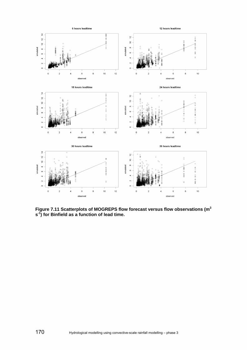
170 Hydrological modelling using convective-scale rainfall modelling – phase 3
Figure 7.11 Scatterplots of MOGREPS flow forecast versus flow observations (m3 s-1) for Binfield as a function of lead time.

Hydrological modelling using convective-scale rainfall modelling – phase 3 171
Figure 7.12 Scatterplots of MOGREPS flow forecast versus flow observations (m3 s-1) for Kinnersley Manor as a function of lead time.

172 Hydrological modelling using convective-scale rainfall modelling – phase 3
Figure 7.13 Scatterplots of MOGREPS flow forecast versus flow observations (m3 s-1) for Newbury as a function of lead time.

Hydrological modelling using convective-scale rainfall modelling – phase 3 173
Table 7.5 Mean RPS for the period July 2008 to February 2009 using the thresholds of Table 7.4.
Colindeep Lane
2989TH
Marsh Farm
3680TH
Redbridge
5480TH
Wolverton Road
3824Th
Addlestone
2989TH
Binfield
2250TH
Kinnersley Manor
3240TH
Newbury
2250TH
6 hours leadtime 0.000 0.007 0.004 0.001 0.002 0.000 0.004 0.001
12 hours leadtime 0.000 0.005 0.006 0.001 0.003 0.000 0.004 0.001
18 hours leadtime 0.000 0.009 0.006 0.001 0.005 0.000 0.005 0.001
24 hours leadtime 0.000 0.008 0.006 0.001 0.006 0.000 0.008 0.002
30 hours leadtime 0.000 0.010 0.005 0.000 0.007 0.000 0.008 0.002
36 hours leadtime 0.000 0.009 0.007 0.000 0.007 0.000 0.008 0.003
Table 7.6 Mean RPSS for the period July 2008 to February 2009 using the thresholds of Table 7.4 and naïve forecast (persistence) as reference forecast.
Colindeep Lane
2989TH
Marsh Farm
3680TH
Redbridge
5480TH
Wolverton Road
3824Th
Addlestone
2989TH
Binfield
2250TH
Kinnersley Manor
3240TH
Newbury
2250TH
6 hours leadtime 0.8524 0.210473 -0.16667 -Inf 0.333333 -Inf 0.588235 0
12 hours leadtime -Inf 0.605379 0.25 -Inf 0.31304 - 0.770448 0.5
18 hours leadtime 0.519032 0.450023 0.451571 -Inf 0.337467 - 0.782187 0.333333
24 hours leadtime -Inf 0.639668 0.539234 -Inf 0.408015 -Inf 0.715205 0.24826
30 hours leadtime 0.325112 0.545441 0.666822 -Inf 0.373642 -Inf 0.725603 0.196872
36 hours leadtime -Inf 0.642509 0.583501 -Inf 0.488848 -Inf 0.723337 -0.074

174 Hydrological modelling using convective-scale rainfall modelling – phase 3
For Colindeep Lane, Marsh Farm, Wolverton Road, Binfield and Newbury no threshold other than the Standby threshold was crossed (both by observations and MOGREPS forecasts) during the eight-month hindcast period. The results for these locations were not investigated further. The predicted and/or observed threshold crossings at Redbridge, Addlestone and Kinnersley Manor were investigated in more detail for events in November 2008, December 2008 and February 2009.
Figure 7.14, Figure 7.15 and Figure 7.16 show results for Redbridge, Addlestone and Kinnersley Manor for November 2008. Figure 7.14 and Figure 7.15 show that the forecasts for Redbridge and Addlestone contain threshold crossings that are not observed (10-11 November). Figure 7.16 shows the opposite for Kinnersley Manor: here the threshold crossings are predicted and observed.
Figure 7.17 and Figure 7.18 show results for Addlestone and Kinnersley Manor respectively for December 2008. Figure 7.17 shows that the MOGREPS forecast predicts the event (13-15 December) for Addlestone very well. The behaviour of the forecast in the lower left corner of Figure 7.17 is probably not due to MOGREPS but probably due to issues with errors in historical catchment average rainfall or with the TCM model being used. Figure 7.18 shows that the MOGREPS forecast for Kinnersley Manor gives an early indication of an event, although the event itself is somewhat underestimated.
Figure 7.20, Figure 7.21 and Figure 7.24 show the results for Redbridge, Addlestone and Kinnersley Manor for February 2009. For all three locations the event (9-11 February) is well predicted, although the MOGREPS ensembles tend to underestimate the events somewhat. This behaviour can also be observed in some of the scatter plots. Figure 7.21 shows (top line of the figure) that a few members of the MOGREPS ensemble produce threshold crossings that did not occur.

Hydrological modelling using convective-scale rainfall modelling – phase 3 175
Figure 7.14 Forecast results for 12 consecutive forecasts in November 2008 at Redbridge.

176 Hydrological modelling using convective-scale rainfall modelling – phase 3
Figure 7.15 Forecast results for 12 consecutive forecasts in November 2008 at Addlestone.

Hydrological modelling using convective-scale rainfall modelling – phase 3 177
Figure 7.16 Forecast results for 12 consecutive forecasts in November 2008 at Kinnersley Manor.
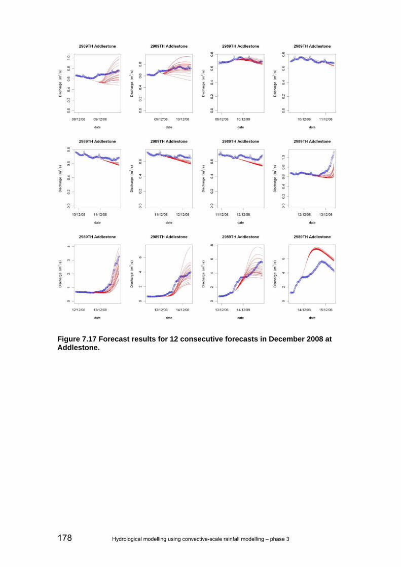
178 Hydrological modelling using convective-scale rainfall modelling – phase 3
Figure 7.17 Forecast results for 12 consecutive forecasts in December 2008 at Addlestone.

Hydrological modelling using convective-scale rainfall modelling – phase 3 179
Figure 7.18 Forecast results for 12 consecutive forecasts in December 2008 at Kinnersley Manor.

180 Hydrological modelling using convective-scale rainfall modelling – phase 3
Figure 7.19 Forecast results for 12 consecutive forecasts in December 2008 at Redbridge.

Hydrological modelling using convective-scale rainfall modelling – phase 3 181
Figure 7.20 Forecast results for 12 consecutive forecasts in February 2009 at Addlestone.
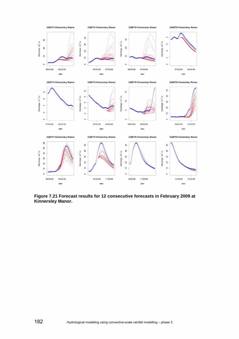
182 Hydrological modelling using convective-scale rainfall modelling – phase 3
Figure 7.21 Forecast results for 12 consecutive forecasts in February 2009 at Kinnersley Manor.

Hydrological modelling using convective-scale rainfall modelling – phase 3 183
7.5 STEPS forecast results This section briefly describes (qualitatively) the forecast results for a few sites in Thames Region. The amount of STEPS forecasts (four) was not sufficient to do any quantitative analysis. Also, no rain was present in North East Region for the event so only Thames Region could be used for the analysis.
Figure 7.22 shows forecasts using the TCM/ARMA model for Colindeep Lane using forecasts made one hour after the STEPS forecasts. In addition, the results of using up to six hours of actual rainfall in the forecast period (the red line) are shown. In the first forecast at 01:00, it is clear that the lead time of six hours is not enough to show any response in the catchment. The next forecast at 04:00 shows that some rain is forecast. This is more than what actually fell during that time and it does not represent the main event. Surprisingly, the next forecast at 07:00 shows hardly any rain. At this time however (4.5 hours into the forecast), the observed rain also starts to come into the six-hour forecast window. The last forecast at 10:00 is just before the event.
Figure 7.22 Forecasts for Colindeep Lane in the north-east part of Thames Region for 01:00, 04:00, 07:00 and 10:00 20 July 2007 going from top left to bottom right. The top half of each plot shows actual precipitation and STEPS-derived percentiles. The red line represents actual precipitation (top half) or discharge modelled by actual precipitation (perfect rainfall forecast) (bottom half). The blue line in the bottom half of the plots represents the measured discharge.
At this time some rain is forecast and the model reacts accordingly but the intensities are far lower than observed intensities. As can be seen from the red line in the bottom

184 Hydrological modelling using convective-scale rainfall modelling – phase 3
half of each plot, the model forecasts the measured peak rather well when fed with actual precipitation.
The same set of subsequent forecasts using STEPS for a catchment in the west part of Thames Region gives a slightly different picture, as shown in Figure 7.23. In this case the STEPS forecasts match the measured precipitation much better. In the last forecast at 10:00, the discharge spread - as modelled using the STEPS input - surrounds the result using measured precipitation, although earlier forecasts clearly underestimate the amount of precipitation that actually fell. For this larger catchment (about 5x20 km versus 8x8 km for Colindeep Lane) the catchment average precipitation at the peak of the event was significantly less than in the previous case, which might explain the better results.
Figure 7.23 Forecasts for Burton Dickler in the west part of Thames Region for 01:00, 04:00, 07:00 and 10:00 20 July 2007 going from top left to bottom right. The top half of each plot shows actual precipitation and STEPS-derived percentiles. The red line represents actual precipitation (top half) or discharge modelled by actual precipitation (perfect rainfall forecast) (bottom half). The blue line in the bottom half of the plots represents the measured discharge.

Hydrological modelling using convective-scale rainfall modelling – phase 3 185
The last example shown in Figure 7.24 is from a catchment in the south-east part of Thames Region, about 7x8 km in size. As can be seen from the plots, the forecast precipitation is underestimated (compare the red line in the top half of each plot to the blue ensemble spread). However, underestimation of the discharge is less. This seems to be due to the fact that the model at this location overestimates the flow when measured precipitation is used. Also visible in the plots is the fact that the forecast becomes better as the event progresses. This is because more measured precipitation is used for later forecasts and the ARMA model is applied to a period already including the hydrograph rise.
1 April 2008 17
Figure 7.24 Forecasts for Binfield in the south-east part of Thames Region for 01:00, 04:00, 07:00 and 10:00 20 July 2007 going from top left to bottom right. The top half of each plot shows actual precipitation and STEPS-derived percentiles. The red line represents actual precipitation (top half) or discharge modelled by actual precipitation (perfect rainfall forecast) (bottom half). The blue line in the bottom half of the plots represents the measured discharge.
7.6 Presentation of ensemble results During the project, several methods of displaying the ensemble results were tested and added to the Delft-FEWS system. Some were present already (spaghetti plots) but others were newly developed for the project. The most obvious way of displaying ensembles of time series is to show all ensemble members in a single plot as lines (Figure 7.25).

186 Hydrological modelling using convective-scale rainfall modelling – phase 3
Figure 7.25 Spaghetti plot showing all ensemble members as individual lines.
Although this type of plot is useful to the trained eye, it does not provide an easy way of estimating, for example, the probability of a threshold crossing unless you start counting lines. In many applications the lines are replaced by areas representing the percentiles. In Figure 7.26 an example of such a plot is shown.

Hydrological modelling using convective-scale rainfall modelling – phase 3 187
Figure 7.26 Plot showing the areas between the 33/66 percentiles and the 25/75 percentiles as shaded areas.
Figure 7.27 shows two other ways of representing ensemble output for the same event as that shown in Figure 7.26. The example was taken from the Delft-FEWS report module for Thames Region. The bottom part shows for each forecast (the last 10) the number of ensemble members that cross the Standby threshold. In this case it is clear that the last (most current) forecast is the first forecast to actually show any thresholds being exceeded. The top part shows (for the last forecast) the percentage of ensemble members that have crossed one of the listed thresholds.
Figure 7.27 Ensemble crossing tabular display.

188 Hydrological modelling using convective-scale rainfall modelling – phase 3
7.7 System performance
7.7.1 Introduction
Running the models in ensemble mode for MOGREPS ensemble members will affect forecast run times because the forecast workflow has to be repeated 24 times. This section describes how ensemble forecasts can be used practically at this stage and how use of MOGREPS would affect forecast run times.
The performance of the system is governed by the following factors:
1 System hardware components. 3 Forecast run times (run times of internal and external modules). 4 Database performance (and size). 5 Amount of data synchronized and network performance.
The following sections describe these factors individually.
7.7.2 System specifications and setup
The specifications of the test system are given in Table 7.7 whilst an overview of all components in the test system (also known as FHSnet) is shown in Figure 7.28.
Table 7.7 System specifications used in the test system.
Component Hardware
FSS AMD Dual core 2.19 Ghz, 3Gb RAM
DATABASE server AMD Dual core 2.19 Ghz, 3Gb RAM
MC server AMD Dual core 2.19 Ghz, 3Gb RAM
STEPS Test PC Intel Core Duo 2.10 Ghz, 2Gb Ram

Hydrological modelling using convective-scale rainfall modelling – phase 3 189
Figure 7.28 Components of the FHSnet Delft-FEWS test system; all internal network connections are 100Mb copper.
7.7.3 Forecast run times (run times of internal and external modules)
In a distributed system such as Delft-FEWS, the total forecast run time is made up of separate components. This section only deals with the time it takes the forecast to run on the FSS after initial synchronization has finished up to where the outgoing synchronization starts.
The times given in this section are based on the hardware used on the test system and actual numbers will be different with the use of other hardware. Average run times for the Thames and Northeast systems are shown in Table 7.8.
Table 7.8 Run times of the ensemble forecast in the Thames and North East test systems. *Run on different spec PC.
Thames
Fast_All_MOGREPS (24 members) 7 minutes
Fast_All 30 seconds
Fast_All_STEPS (15 members)* 9 minutes 10 sec (single run 49 sec)
North East
Fluvial_FastResponse_Forecast_MOGREPS 16 minutes
Fluvial_FastResponse_Forecast 1 minute
Given the fact that MOGREPS forecasts are produced twice a day at the moment, the run times shown in Table 7.8 are acceptable. Although longer than the normal runs, forecasts can be delivered in a timely manner. However, the picture will change if

190 Hydrological modelling using convective-scale rainfall modelling – phase 3
ensemble runs are not limited to fast-responding catchments only and, for example, also include the ISIS models. Estimated run times for this situation are shown in Table 7.9.
Table 7.9 Estimated run times for complete region forecast in ensemble mode. Normal run times are taken from Environment Agency online system.
Thames North East
Fluvial Forecast 00:06:04 Fluvial_FastResponse_Forecast 00:03:41
ISIS_TThames_Forecast 00:00:41 RiverFlow_Forecast 00:08:09
Estimated ensemble run time (Worst case= * 24)
Fluvial Forecast 02:24:00 Fluvial_FastResponse_Forecast 01:28:00
ISIS_TThames_Forecast 00:27:00 RiverFlow_Forecast 03:26:00
The STEPS results were obtained stand-alone on different (lower spec) hardware and must be treated as a worst-case scenario for the 15-member ensemble. Operationally STEPS should be delivered with 50 ensemble members. In that case the estimated run time of one STEPS forecast would be about 30 minutes 30 seconds. Given the fact that STEPS forecast would be delivered every hour, this would just be fast enough assuming STEPS forecasts would only be used for the fast response workflows and not the full fluvial forecast. However, the actual data volumes involved are considerable, as discussed later in this section.
7.7.4 Improving total run times
Clearly, if full forecasts were to run in ensemble mode on the current online Environment Agency system, some speed-up of the forecasts would be required. In addition, if the ensemble runs of just the fast-responding workflows were to be run more frequently, these would also need a speed increase.
The following options should be considered to speed up the ensemble runs:
1. Optimise external models. 2. Optimise data exchange. 3. Faster CPUs (cores) on each FSS. 4. Run ensemble members in parallel:
4.a Split-up workflows (e.g. members 1-12 on FSS01 and 13-24 on FSS02). 4.b Run the actual models at the GeneralAdapter level on a grid engine
(Condor). 4.c Make improvements to Delft-FEWS core to split (parts of) a workflow in
several threads on multi-CPU/core FSS.
Optimize external models
Hydrological models do not usually have much room for speed improvements as the equations used can usually be solved analytically at great speed. A hydrodynamic model originally developed for a study that required high accuracy – and later used for forecasting – might be adjusted to sacrifice some accuracy for speed. Alternatively, a hydrodynamic model might be replaced by a simple hydraulic routing model in ensemble runs for which less accuracy might be acceptable.

Hydrological modelling using convective-scale rainfall modelling – phase 3 191
Optimize data exchange
For fast-running external models that require a large amount of data, the exchange via PI XML can be sped up in two ways:
1. The XML only format may be replaced by the binary version of the PI XML (XML header with binary pay-load) to speed up the file reading and writing. This may improve performance significantly. It may require an update to the adapters involved. At present, only some adapters support this feature.
2. As of February 2009 the Delft-FEWS java PI library supports storing XML as Fast Infosets. Applications that use this library (Delft-FEWS, a number of National Weather Service adapters) can read/write these files (basically a binary implementation of XML, also supported by e.g XMLSpy) without changing the code.
Faster CPUs (cores) on FSS
An easy gain (in terms of work needed for configuration) may be had by upgrading CPUs on the FSS. In general, a new generation of CPUs provides twice the performance (at the same price) every two years. By replacing a two-year old FSS with a new one, a theoretical speed increase of 100 per cent may be obtained. This is for CPU speed only; the speed of hard drives increases at a slower rate.
Run ensemble members in parallel
• Split-up workflows (such as members 1-12 on FSS01 and 13-24 on FSS02). Assuming each FSS has its own dedicated CPU, this can speed up run times considerably. It can be used in combination with the other options. At the moment, this can only be done by changing the configuration and splitting the workflows manually, making it a significant change in the configuration and diffcult to maintain. Developments are planned to adjust the Delft-FEWS master controller code to do this automatically. If this is done, this option can be used without extra configuration or maintenance.
• Run the actual models at the GeneralAdapter level on a grid engine (Condor). Condor is a specialized workload management system for computationally intensive jobs. Condor provides the necessary tools such as job queuing, scheduling, priority management, resource monitoring, and resource management to enable multiple model runs to be made on multiple machines. Serial or parallel jobs can be submitted to Condor which are then placed into a queue, and run based on how Condor is configured. With this type of grid computing there is a normally an overhead (running 50 ensembles in parallel does not mean it will be 50 times quicker). The computational overhead is dependant on the amount of static and dynamic data which must be transferred between the forecasting shell and the node. When Delft-FEWS operates with a Condor grid, only the external models (run via the General Adapter) can be run in parallel. In addition, best performance can be expected from models with relatively long execution times that need limited amounts of data, such as hydrodynamic models. This option requires the set up (and maintenance) of a grid engine but this set up may be shared between regions.
• Improvements to Delft-FEWS core to split (parts of) a workflow in several threads on multi-CPU/core FSS. Today, most new machines

192 Hydrological modelling using convective-scale rainfall modelling – phase 3
come with dual core CPUs. While these can be used, for example, to run two FSS on a single box (one on each core) it does not speed up individual runs. By improving the Delft-FEWS code, separate ensembles may be started in separate threads and run in parallel within a single FSS instance. This option has several advantages: (i) it does not require any configuration (or very little) and (ii) it can be used in combination with all the other options. Clearly, this would require an investment in the Delft-FEWS code but once this investment is made, very little (or no) extra cost in terms of maintenance of the system and configuration are expected.
Figure 7.29 gives a schematic presentation of the options described above. Option B is part of the present functionality but only works well for long-running models and necessitates the installation and maintenance of a (Condor) grid engine.
Figure 7.29 Schematic representation of workload distribution via multiple forecasting shell servers and multi-core machines planned for future version of Delft-FEWS (A) and (B) layout of workload distribution when running external models on a Condor grid engine.
7.7.5 Database size and data volumes
Introduction and methods
Within Delft-FEWS all forecast time-series data are stored in a compressed form in the database. Per parameter a resolution can be set. Setting a resolution (default is full resolution, single precision) can substantially reduce the size of data in the database. The settings used in the test systems were fairly conservative: no value resolution was set for parameter groups discharge and precipitation, representing current practice in the NFFS. As such, all ensemble forecast data were stored with full resolution
Ensemble workflow (16 members on MC)
Ensemble workflow (member 9-16 on FSS01)
Ensemble workflow (member 1-8 on FSS00)
Eight cores, each running one member
Eight cores, each running one member
Ensemble workflow (16 members on MC)
Ensemble workflow (all members on FSS00)
Condor engine running GA part
A B

Hydrological modelling using convective-scale rainfall modelling – phase 3 193
representing a worst-case scenario. Savings in data size of up to 50 per cent can be expected by setting a resolution for discharge and precipitation.
All statistics were determined using the Delft-FEWS built-in database viewer. The statistics looked at time-series data only: other data associated with forecasts were not considered as these were small compared to the size of the time-series tables.
A subdivision was made between the Import data, Thames Region forecast and North East Region forecast. Gridded import data (the MOGREPS and STEPS forecasts) were imported in the system and remained in the forecasting shell and master controller database only. The forecast data, however, were also synchronised to the operator clients.
Import data
An import of one complete MOGREPS forecast (24 members) occupied a total of 0.622Mb in the Delft-FEWS database (on disk in Nimrod format the files occupied 2.4Mb). Based on a rolling barrel length of 10 days and two forecasts per day the addition of MOGREPS would increase the size of the FSS and master controller databases by 13.24Mb per region.
An import of one STEPS forecast (15 members only) occupied a total of 19Mb in the Delft-FEWS database (on disk in Nimrod format the files occupied 253Mb). Based on a rolling barrel length of one day and 24 forecasts per day the addition of STEPS would increase the size of the FSS and master controller databases by 456Mb per region if 15 members were used. For 50 members this could grow to 1.5Gb per region.
Thames Region MOGREPS forecasts
The total number of time series created during a Fast_All_MOGREPS workflow was 9,228 which occupied 4.8Mb of database space. The table below details this:
Overview Workflow: Fast_All_MOGREPS Total size: 4.2MB Number of timeseries: 9228 Number of Blobs (database records): 458 Details Moduleinstance Size per instance Instances Total ARMAMergeFlow 80.3kB 1 80.3kB ARMA_* 15.0kB 69 1.1MB CatchmentAveragePrecipitation 13.0kB 1 13.0kB FlowToLevel 29.6kB 1 29.6kB ImportTelemetry 8.4kB 1 8.4kB MOGREPS_Spatial_Interpolation 331.7kB 1 331.7kB MOGREPS_TCM_Statistics 703.3kB 1 703.3kB MergedPrecipitation_Forecast 896.4kB 1 896.4kB PersistPrecip 11.1kB 1 11.1kB TCM_* 10.7kB 69 1MB By far the largest amount of data was generated by the ARMA_* and TCM_* moduleinstances: these held the forecast results (per ensemble member) for the raw and error corrected forecast respectively. The MOGREPS_TCM_Statistics and MergedPrecipitation_Forecast module instances also contributed significantly to the

194 Hydrological modelling using convective-scale rainfall modelling – phase 3
amount of data. They held the percentile time series and the precipitation input to the TCM models respectively.
No major changes can be expected by leaving out data as all data that are currently produced (and synchronised) are displayed in graphs (and thus needed). However, a significant reduction can be made by setting a value resolution to the precipitation and discharge parameter groups.
Based on the current NFFS settings with a 10-day rolling barrel and two forecasts per day. the increase in data in the system for Thames Region (when using MOGREPS as configured here) would be approximately 84Mb.
North East Region MOGREPS forecasts
The total number of time series created during a _FastResponse_Forecast_MOGREPS workflow was 28,555 which occupied 9.7Mb of database space. The table below details this:
Overview Workflow: Fluvial_FastResponse_Forecast_MOGREPS Total size: 9.7MB Number of timeseries: 28555 Number of Blobs (database records): 1229 Details (only most important) Moduleinstance Size per
instance Instances Total
ARMA_* 14.0kB 103 1.7MB *FastFlowToLevel 13 1.8MB *Processing 4 0.811MB KW* and PDM* 89 1.4MB MOGREPS_CatchmentAveragePrecipitation 487.7kB 1 0.4877MB Show processing modules 18 0.3124MB No major changes can be expected by leaving out data as all data that are currently produced (and synchronised) are displayed in graphs (and thus needed). However, a significant reduction can be made by setting a value resolution to the precipitation and discharge parameter groups.
Based on the current NFFS settings with a 10-day rolling barrel and two forecasts per day, the increase in data in the system for North East Region (when using MOGREPS as configured here) would be approximately 194Mb.
Thames Region STEPS forecasts
The total number of time series created during a Fast_All_STEPS workflow was 8,083 which occupied 3.6Mb of database space. The following table details this:

Hydrological modelling using convective-scale rainfall modelling – phase 3 195
Overview Workflow: Fast_All_STEPS Total size: 4.2MB Number of timeseries: 8083 Number of Blobs (database records): 488 Details Moduleinstance Size per
instance Instances Total
ARMAMergeFlow 70.7kB 1 70.7kB ARMA_* 16.2kB 69 1.3MB STEPS_CatchmentAveragePrecipitation 277kB 1 277kB FlowToLevel 38.3kB 1 38.3kB ImportTelemetry 8.4kB 1 8.4kB STEPS_Spatial_Interpolation 277kB 1 277kB STEPS_TCM_Statistics 774.9kB 1 774.9kB MergedPrecipitation_Forecast 467.6kB 1 467.6kB PersistPrecip 12.1kB 1 12.1kB TCM_* 10.7kB 69 1MB By far the largest amount of data was generated by the ARMA_* and TCM_* module instances: these held the forecast results (per ensemble member) for the raw and error corrected forecasts respectively. The STEPS_TCM_Statistics and MergedPrecipitation_Forecast module instances also contributed significantly to the amount of data. They held the percentile time series and the precipitation input to the TCM models respectively.
No major changes can be expected by leaving out data as all data that are currently produced (and synchronised) are displayed in graphs (and thus needed). However, a significant reduction can be made by setting a value resolution to the precipitation and discharge parameter groups.
Based on a two-day rolling barrel and 24 forecasts per day, the increase in data in the system for Thames Region (when using STEPS as configured here) would be around 200Mb. These data were also synchronised to the OC. If a 50 member STEPS ensemble were used, the amount of data would increase to about 666Mb.
7.8 Discussion The effort to configure a system to run MOGREPS or STEPS alongside current forecasts proved to be relatively minor. About one week (including testing) per region was needed to implement MOGREPS. This excluded changes to the code to be able to import the MOGREPS and STEPS ensembles in Nimrod format.
Within the current set up, the system was configured to run MOGREPS only: no blending with short-range forecast products (such as STEPS) was done. In an operational setting some sort of blending might be considered, either within NFFS (which requires a considerable change in configuration) or outside of the system. As blending of Met Office products is dealt with in a separate project, this was not considered in this project but it may have an impact on an operational application of MOGREPS and STEPS within the NFFS.
Over the period of the hindcast - July 2008 to February 2009 - the MOGREPS ensembles gave good results. The amount of false alarms was low in this period. Small events (below threshold crossing) were often well predicted (not shown). For the

196 Hydrological modelling using convective-scale rainfall modelling – phase 3
two/three events that occurred in this hindcast period, MOGREPS was able to indicate that something was going to happen well in advance (24-36 hours). The timing of an Environment Agency warning based on the MOGREPS ensemble should be explored further and cannot be established on the basis of this limited analysis. Figure 7.21 (top of the figure) is a nice example showing this dilemma: A few members of the MOGREPS ensemble produce threshold crossings: how many should cross the threshold before issuing a warning? The scatter plots and other figures indicate that the MOGREPS ensemble may somewhat underpredict larger events although this should be confirmed by a hindcast over a longer period (with more events). Factors that make it sometimes difficult to judge the MOGREPS ensembles are the underlying TCM models and ARMA correction, or errors in the estimated catchment areal rainfall (see, amongst others, Figure 7.17 lower right).
An analysis of four STEPS forecasts (using only 15 ensemble members) showed that STEPS can provide good forecasts several hours ahead for some locations. However, results for other sites (the majority) were not good and the forecast precipitation was seriously underestimated. In addition, at the short lead times investigated here, the influence of the hydrological model and output correction were large, making it difficult to interpret the results.
In the worst-case scenario, running a forecast using the MOGREPS ensemble input would take 24 times as long as a normal forecast. Assuming an acceptable run time of one hour on the current NFFS infrastructure, it is only feasible if the current operational forecast takes less than 2.5 minutes. Currently, this is not the case for most regions. However, the NFFS FSS hardware is due for replacement and a speed-up of the forecast workflows by a factor of two is expected. In that case, most MOGREPS workflows could be run within one hour. Even so, a run time of one hour would mean that one FSS would be occupied for that entire period. Therefore, we suggest dedicating a separate FSS (usually a third) per region to run MOGREPS ensemble forecasts so that the current forecasting process is not influenced in any way.
To reduce run times further, the most cost-effective option (in the long run) may be to improve the Delft-FEWS core to use all available core on multi-core machines (assuming multi-core FSS will be installed). Presently, eight core servers are normal and can theoretically decrease the run time by a factor of eight if all cores are used simultaneously. The big advantage of this approach is that it needs no extra maintenance and set up compared to a normal FSS. In addition, it may be combined with other methods without much effort.
With respect to database size and greater synchronisation times, the addition of MOGREPS forecasts should have a minor effect on system performance of the NFFS. Data sizes are small compared to the current amount of data and because MOGREPS is only available two times per day (thus no more than two ensemble forecasts per day are required), the total amount of data is relatively small to the current sizes of the operational databases. However, synchronizing an ensemble forecast (9.7Mb for North East Region) over a dial-up connection is not practical. In addition, the extra forecasts will increase the total amount of traffic over the network although the total increase is expected to be no more than a tenth of the current data traffic within NFFS (estimate based on the database sizes).
If MOGREPS forecasts are to be implemented, we sugges setting a value resolution to the data (for discharge, level and precipitation) as this may decrease the size of data considerably. If needed, a separate parameter group may be made for ensemble forecasts so that non-ensemble parameters can still be stored at full resolution.
The amount of data generated if 50 member STEPS ensembles were used would be considerable and would probably exceed the capacity of current NFFS hardware (most probably also after the planned upgrade). Some options are available to decrease the amount of data: using a subset of the 50 ensemble members, limiting the model to be

Hydrological modelling using convective-scale rainfall modelling – phase 3 197
run in ensemble mode and reducing the number of time series to be stored. For example, the user may choose to only store calculated percentiles and discard the raw ensemble member time series after each run.
To summarise, the addition of MOGREPS forecasts to the current Environment Agency NFFS is feasible using current NFFS hardware. We cannot say much about the actual performance of MOGREPS, as (much) more hindcast data are needed for a quantitative analysis. However, a qualitative analysis of its performance shows that MOGREPS might be a useful addition to the current NFFS.

198 Hydrological modelling using convective-scale rainfall modelling – phase 3
8 Running G2G and HyradK in NFFS
8.1 Introduction This section documents how the G2G hydrological model and HyradK from CEH is implemented in Delft-FEWS, the system behind NFFS. It focuses on running the model and the configuration within Delft-FEWS. It does not describe how the model output resembles measured discharge: that part is dealt with in Sections 4 to 6.
This section can (together with the actual configuration) be used as a guide to set up an operational system using Delft-FEWS and G2G. All work described here was tested on a live system running at Deltares during the project.
Further detailed information on the CEH adapter files and how to set up the models themselves can be found in the accompanying CEH documentation (CEH Grid2Grid/HyradK User Guide).
8.2 General configuration of the national system
Locations, location sets and ID mapping
To create the configuration required to run a model on a national basis, it is necessary to combine components of the regional NFFS.
The national system uses a DBF file that combines data on locations, mapping to external sources and other attributes that can be used to uniquely identify the location as part of a location set. This new functionality available within Delft-FEWS allows simple location-specific information to be combined into one file, making configuration of a large number of locations simple.
This file can be found in the MapLayerFiles directory. The attributes of file EA_National_Locations2009-01.dbf which contains these data are shown in Table 8.1.

Hydrological modelling using convective-scale rainfall modelling – phase 3 199
Table 8.1 Attributes of DBF file.
Attributes Description Data source Notes
ID Unique ID From NFFS 2009.01 Modified to remove spaces and commas
NAME Name From NFFS 2009.01
DESC Description From NFFS 2009.01
SHORTNAME Short name From NFFS 2009.01
PARENTID Parent ID From NFFS 2009.01
X X coordinate CEH Gauge locations adjusted to match required updating locations in G2G
Y Y coordinate CEH
Z Elevation From NFFS 2009.01
NFFS_X From NFFS 2009.01 Original coordinates taken from NFFS
NFFS_Y From NFFS 2009.01 Original coordinates taken from NFFS
PARAM Parameter associated with location
From NFFS 2009.01 Taken from ID mapping, separated by comma where multiple parameters are available
SOURCE NFFS region From NFFS 2009.01 Where overlaps existed (e.g. raingauges between Anglian and Thames). Source of origin was used.
COMMENT Comment
G2G Data used in G2G CEH Supplied list of gauges required
HYRADK Data used in HyradK CEH Supplied list of gauges required
HOBS Observed stage ID map
From NFFS 2009.01 Telemetry ID mapping
HOBSUSDS Observed stage ID map
From NFFS 2009.01 Telemetry ID mapping
QOBS Observed flow ID map From NFFS 2009.01 Telemetry ID mapping
POBS Observed precipitation ID map
From NFFS 2009.01 Telemetry ID mapping
RATED Rating curve available From NFFS 2009.01 Telemetry ID mapping *Any modification to this file needs to be done in the program Open Office and not in Excel.
The locations were taken for all observed precipitation gauges (derived from the ImportTelemetry ID mapping) and the gauging stations requested by CEH for updating.

200 Hydrological modelling using convective-scale rainfall modelling – phase 3
The information was derived from 2009.01 test versions for all eight regions of NFFS made available for testing of the 2009.01 release of Delft-FEWS.
Rating curves
Converting observed stage to level is done via rating curves or rating tables. The rating curves or tables are derived from each of the regional systems (based on the 2009.01 configuration). In some cases the rating curves do not cover the higher and lower parts of the rating.
Import and telemetry data
The test system in Delft directed all regional telemetry data to the national system. As such, the national system was set up to combine the imports of telemetry data from all eight Environment Agency regions.
Midlands data were only available at an hourly time-step. These data were disaggregated on import to a 15-minute time-step for the purposes of this project.
Figure 8.1 shows a screen shot of the available rain gauges in the national system.
Figure 8.1 Overview of rain gauges available.
8.3 Implementation of G2G The G2G model is a distributed hydrological model that uses gridded estimates of rainfall and evaporation to calculate streamflows. It can use point measurements of flow to update state conditions in the model.

Hydrological modelling using convective-scale rainfall modelling – phase 3 201
The G2G model is a continuous simulation model. This means that at the end of a historical run, a model state is generated which can be used as a warm state for the forecast.
There are two options when running the G2G model: with or without state-updating. These are configured as two parallel workflows to highlight the difference between the two forecasts. More information about state updating in G2G can be found in the CEH documentation and Section 3.2.1. In order to run the model with state-updating, the following workflows are required:
• Fluvial_Updated_Historical – State-updated historical run.
• Fluvial_Updated_Forecast – State-updated forecast run.
To run the model without state-updating, the following workflows are required:
• Fluvial_Historical – Non-state updated historical run.
• Fluvial_Forecast – Non-state updated forecast run.
The states generated by the updated historical run and the non-updated historical run are handled separately.
Workflows
A workflow executes a set of tasks (known as modules). Each of the modules performs a specific task. These tasks can be data preparation, model execution, post processing and so on. The workflow used to run a historical G2G simulation and a description of each of the modules can be found in Table 8.2.

202 Hydrological modelling using convective-scale rainfall modelling – phase 3
Table 8.2 G2G historical simulation workflow.
Module Instance Description
G2G_National_Pre_Historical_Interpolate Spatial interpolation of gridded data and extrapolation of last observed evaporation data.
G2G_National_Pre_Historical_Prep Merging of gridded rainfall data. Based on the recommendations of CEH, the raingauge-only grid is used in preference to the corrected radar. To use the corrected radar, a ‘what if’ scenario can be used.
G2G_National_Pre_Historical_Dataprep Copies external historical Q.rated to a temporary series to t+36 as the run length in G2G is determined by the run length of the delivered series.
G2G_Module Tidies G2G directories and exports clean SIDB database and correct adapter configuration file.
G2G_National_Historical Exports the relevant state, grid data and scalar data. Executes G2G batch file and imports the model outputs.
Remove_G2G_Module Executes batch file which removes the SIDB database.
G2G_National_ToGauges_Historical Derives the flow at gauges from G2G outputs.
G2G_National_Post_Historical Compares the generated flow field with grids of return period flows (note: this is just a mock up). Also removes discharges below one m3 s-1 to save database space.
Data processing
Before the G2G model can be run, a continuous and complete time series of gridded data at a 1x1 km resolution has to be made for the entire domain of the G2G model (see steps 1 and 2 in Table 8.2). Several gridded sources of precipitation are available in NFFS:
• Observed radar (H7) at a 1x1 km resolution, five-minute time-steps.
• Forecast accumulation (UKPP H13) at a 2x2 km resolution, 15-minute time-steps, a forecast every 15 minutes (96 per day) six hours ahead.
• NWP forecast accumulation (UKPP N2) at a 4x4 km resolution, 15-minute time-steps 36 hours ahead, a forecast every six hours (four per day) 36 hours ahead.
• MOGREPS ensemble forecast at a 24x24 km resolution with 24 ensemble members. Two forecasts per day, 54 hours available, 36 hours used in this research, three-hourly time-steps.
In addition to this, HyradK can be used to generate corrected observed radar and raingauge-only grid estimates.

Hydrological modelling using convective-scale rainfall modelling – phase 3 203
The following data hierarchy is used to construct the input data for the G2G model:
• For the period up to T0 (time of forecast) the raingauge-only grid estimate from HyradK is the first data source.
• The backup is the corrected H7 product, then the H7 product. A ‘what if’ scenario can be used to modify this hierarchy, by for example setting the raingauge-only grid estimate to missing.
• The backup in this period is zero precipitation although for the last two hours up to T0 H13 forecasts or even NWP forecasts may be used as a backup source. As such, the zero precipitation option is only applied as a last resort.
• For the first six hours of the forecast the two-km H13 product will be used.
• From six to 36 hours in the forecast, the N2 four-km NWP product is used; this also serves as a backup for H13 in the first six hours of the forecast. If all fails, the zero precipitation backup option is used.
The procedure described above is depicted in Figure 8.2. The procedure is theoretical as in operational practice other sources of information, most notably the polling regime of the telemetry systems, may influence this. As H7 is delivered every 15 minutes, a fallback to H13 in the historical period is almost never needed. The availability of the HyradK-corrected H7 depends on the timely availability of observed rainfall data. This is complicated by the fact that different regions in the Environment Agency have different polling regimes and different polling times. As such, the corrected product may be available for parts of the UK only. If we assume that the HyradK-corrected H7 product does not decrease in quality for parts where no observed rainfall is available and is equivalent to the uncorrected H7 product, it is safe to use the HyradK-corrected H7 product as the primary input source to G2G.
Figure 8.2 Diagram showing the available precipitation sources relative to the time of forecast (T0) and their position in the precipitation data hierarchy when constructing input for the G2G model.
T0
P Backup
4k NWP
1k HyradK H7
1k H7
+6hr +36hr +54hr -2hr
2k H13
1k HyradK rain gauge only

204 Hydrological modelling using convective-scale rainfall modelling – phase 3
General adapter module
In general terms, all models which are considered external modules to FEWS are run using the general adapter which follows the form shown in Figure 8.3. This is how G2G is run in FEWS (see step 4 in Table 8.2).
Delft-FEWS
General Adapter
Module Adapter
Modulemoduleinput data
moduleoutput data
published interface
input data(pi xml)
Pre Post
output data(pi xml)
Figure 8.3 General adapter schematisation.
The external model files are the same for both the updated and non-updated model runs. The difference can be found in the <forceroooflag>0</forceroooflag> parameter in the CEH xml adapter file: this should be set to one to enable updating. The files are stored as a module dataset and the relevant adapter file is sent to the external modules directory before commencing the relevant run.
In the G2G_National module instance, gridded precipitation estimates and scalar PI time series of channel flow are provided as input data to the “fromfews” directory.
In the current implementation, the pre-, module adapter and post-phases of the adapter are replaced with the execution of a batch file which controls each of these processes. Further details can be found in the accompanying CEH documentation. Gridded estimates of streamflow are then returned to the “tofews” directory.
State information is also passed in zipped form between FEWS and G2G to allow G2G to run as a continuous simulation model.
Post-processing and display
This section describes how G2G gridded output is displayed in the NFFS user interface and how the raw G2G output is converted for display purposes (step 7 in Table 8.2). To evaluate the flood status over the whole of England and Wales, a step-wise approach is needed. First, an overview of the current status of the system (now, or over the last few hours) is needed. Next, an overview of what is about to happen in the forecast horizon is needed. For such an overview, a single image showing the maximum states

Hydrological modelling using convective-scale rainfall modelling – phase 3 205
over a period (the last days and whole forecast period) may be enough. This image will show the maximum status (flow or warning level) over these periods (Figure 8.4).
Figure 8.4 Screenshot of example warning level output.
This results in the following maps:
• Maximum discharge over the whole forecast period for each G2G grid-cell (excluding discharges below one m3).
• Maximum discharge over the last day for each G2G grid-cell (excluding discharges below one m3).
• Map showing the above two maps linked to a return period map (say one in 10 years) of discharge. This would show for each grid -ell if it was above a certain return period. In the absence of ‘real’ level/discharge thresholds for each grid-cell this would be a good measure of how severe a situation in a grid-cell is. Several maps may be used and combined in a single colour-coded map, for example: − Green < one year Q − Yellow > five year Q < 10 year Q − Orange >10 year Q < 20 year Q − Red > 20 year Q.
The raw results of G2G are post-processed at the end of each forecast and historical run. The PcrTransformation model in FEWS was used to carry out this post-processing as it provides most flexibility.
Outputs of the model are also extracted at certain gauged locations (step 6 in Table 8.2). These can then be compared to the observed data and potentially to the outputs of regional forecasts. The extracted results can also be compared to threshold warning levels. Figure 8.5 shows an example output of a hydrograph at a gauged location.

206 Hydrological modelling using convective-scale rainfall modelling – phase 3
Figure 8.5 Example output at gauged location.
8.4 Implementation of HyradK HyradK is a tool which allows integration of gridded estimates of rainfall with point measurements to create ‘corrected’ estimates of precipitation. It also is able to generate raingauge-only grids. In this set up of HyradK, both outputs are generated.
Similarly to the G2G implementation, gridded estimates of precipitation (derived from radar in this case) are provided to the “tofews” directory together with scalar series of observed rainfall. Input grids to HyradK should be delivered from FEWS in units of mm per hour. The mm per hour grids should also be converted on import to FEWS as mm.
The CEH batch script runs the necessary processes and returns the corrected precipitation grids to the “tofews” directory for import into Delft=FEWS.
The current implementation of HyradK is stateless.
Workflows
HyradK is currently run with every G2G run to ensure that the data are available. The workflow for HyradK (HyradK_National_Historical) is shown in Table 8.3.

Hydrological modelling using convective-scale rainfall modelling – phase 3 207
Table 8.3 HyradK workflow.
Module pnstance Description
HyradK_Module Tidies the HyradK directories and extracts a clean SIDB database.
HyradK_National_Historical Exports raingauge and radar actual grids, executes HyradK batch script and then imports raingauge-derived grids and corrected radar.
HyradK_Convert_Units_Historical Converts mm/hour grids to mm/time-step.
Remove_HyradK_Module Executes a script which removes the SIDB database.
The operation of the workflow is more simple than G2G since there is less need for pre- and post-processing. The current implementation of HyradK requires the gridded data to be supplied in units of mm per hour: therefore the grids are multiplied by four on export in the general adapter. The module HyradK_Convert_Units_Historical is then used to convert these units back to mm per 15 minutes.
Visualisation
The spatial display allows the forecaster to visualise the gridded precipitation estimates and to compare the outputs (Figure 8.6 to Figure 8.8)
Figure 8.6 H7 radar actuals in the spatial display.

208 Hydrological modelling using convective-scale rainfall modelling – phase 3
Figure 8.7 Corrected H7 radar actuals from HyradK.
Figure 8.8 Raingauge-only estimate from HyradK.

Hydrological modelling using convective-scale rainfall modelling – phase 3 209
8.4.1 Other possibilities for visualisation
Section 5.3.2 shows how G2G ensemble forecasts can be displayed through Hyrad and how probability of exceedance flood risk maps can be constructed. Delft-FEWS (NFFS) can produce similar maps operationally using the grid display. Other systems, notably the European Flood Alert System (EFAS), produce similar maps as shown in Figure 8.9.
Using the built-in ensemble statistics module in combination with the Pcraster module (Van Deursen and Wesseling, 1996) that is also part of Delft-FEWS, similar maps may be created as part of the forecasting. Standard NFFS configuration changes can be used to create these maps: no code development is needed.
The above maps link directly to the gridded model structure. However, for a forecaster it may be more important to know the maximum status inside a (warning) area or region. Such maps may be constructed by overlaying polygons (shape files) with the grids and extracting the maximum value within each polygon. The grid display within NFFS is capable of showing these.
Another consideration is the temporal aggregation needed for an instant overview of the forecasted situation. Temporal aggregation may be performed on the fly within the spatial display using a slider. Use of separate aggregated maps may also be considered, for example to show the maximum status within the next 24, 48 and 96 hours.

210 Hydrological modelling using convective-scale rainfall modelling – phase 3
Figure 8.9 Probability of exceedance flood risk maps used in the EFAS system (Thielen et al., 2009).
8.5 Sending results to regional systems Within the test system, a copy of the Thames and North East regions run operationally. To test how data could be exchanged between the systems, the configuration of both the national and the test system were adjusted:
• An export of modelled discharge (updated) for all G2G key locations was set up in the national system. This export used the standard Delft-FEWS export facility. The export went to each region separately and contained all G2G locations.
• The configurations of North East and Thames were adjusted to import the XML data and a filter set up to visualize the data alongside the regional forecast data.
Figure 8.10 shows how the process of sharing data between the national system and the regions was set up. In the set up each export was about 1.5Mb in XML format. Figure 8.11, Figure 8.12 and Figure 8.13 are screen dumps of the test system showing results from the national system within a regional system.

Hydrological modelling using convective-scale rainfall modelling – phase 3 211
Figure 8.10 Schematic layout of the connection between the national test system and North East and Thames regions.
Figure 8.11 Screen dump of the Thames test system showing the filter with G2G results and a plot of forecasted and measured flow.
NorthEast Test MC
National Test MC running G2G
Thames Test MC
Export G2G results in XML format
G2G Running on dedicated FSS
Retrieve G2G results via import

212 Hydrological modelling using convective-scale rainfall modelling – phase 3
Figure 8.12 Screendump of plot in Thames region showing measured flow, forecasted flow with G2G (bottom green line) and forecasted flow using the TCM model fed with MOGREPS ensemble data.
Figure 8.13 Screen dump of the North East test system showing the filter with G2G results.
8.6 Performance The workflow Fluvial_Updated_Forecast (which combines the HyradK and G2G workflows) was run as a benchmark test on a stand-alone PC (no initial synchronization of data required). The PC used was a dual core AMD Athlon 64 2.19GHz with 896Mb RAM. The results of the test are displayed in Table 8.4.
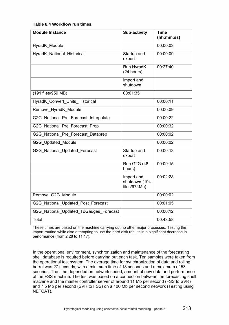
Hydrological modelling using convective-scale rainfall modelling – phase 3 213
Table 8.4 Workflow run times.
Module Instance Sub-activity Time (hh:mm:ss)
HyradK_Module 00:00:03
HyradK_National_Historical Startup and export
00:00:09
Run HyradK (24 hours)
00:27:40
Import and shutdown
(191 files/959 MB) 00:01:35
HyradK_Convert_Units_Historical 00:00:11
Remove_HyradK_Module 00:00:09
G2G_National_Pre_Forecast_Interpolate 00:00:22
G2G_National_Pre_Forecast_Prep 00:00:32
G2G_National_Pre_Forecast_Dataprep 00:00:02
G2G_Updated_Module 00:00:02
G2G_National_Updated_Forecast Startup and export
00:00:13
Run G2G (48 hours)
00:09:15
Import and shutdown (194 files/974Mb)
00:02:28
Remove_G2G_Module 00:00:02
G2G_National_Updated_Post_Forecast 00:01:05
G2G_National_Updated_ToGauges_Forecast 00:00:12
Total 00:43:58
These times are based on the machine carrying out no other major processes. Testing the import routine while also attempting to use the hard disk results in a significant decrease in performance (from 2:28 to 11:17).
In the operational environment, synchronization and maintenance of the forecasting shell database is required before carrying out each task. Ten samples were taken from the operational test system. The average time for synchronization of data and rolling barrel was 27 seconds, with a minimum time of 18 seconds and a maximum of 53 seconds. The time depended on network speed, amount of new data and performance of the FSS machine. The test was based on a connection between the forecasting shell machine and the master controller server of around 11 Mb per second (FSS to SVR) and 7.5 Mb per second (SVR to FSS) on a 100 Mb per second network (Testing using NETCAT).

214 Hydrological modelling using convective-scale rainfall modelling – phase 3
To reduce the run time, HyradK can be scheduled to run on a dedicated FSS every 15 minutes. This will decrease the run time of the total G2G workflow (as the HyradK processing is no longer needed in this workflow) to about 19 minutes. If this is done, the HyradK runs will keep one FSS occupied nearly all the time.
For the longer lead times (up to five days ahead) desired for the new National Flood Forecasting Centre, probabilistic forecasts are more appropriate than a single deterministic forecast. Due to hardware limitations, we did not test the G2G model using MOGREPS as a precipitation source. However, using simple extrapolations we estimated the run times and data volumes involved. MOGREPS has 24 ensemble members resulting in run times of more than eight hours for a single forecast. A number of options are available to decrease run times for the ensemble runs (see Section 7.7.4). As a first guess, the total run time could be about one hour if the ensemble could be split over 12 nodes. This assumption is based on a 50 per cent overhead due to IO contingency on multi-core FSS, synchronisation delays and the fact that parts of a workflow cannot be run in parallel.
Data volumes
Table 8.5 shows the amount of data generated in the test system.
Table 8.5 Data volumes for import and forecast data in the test system.
Data Description Number of files/day
Data/ day (Mb)
Size in local
datastore
No of forecast per day
Total per day
Rolling barrel length (days)
Grand total
Telemetry All national telemetry
Circa 1,100 24 0.15 1 0.15 365 54.75
Radar Actuals Nimrod 5-minute actuals (1 km)
288 270 28.6 1 28.6 10 286
Radar Forecast UKPP Radar Forecast (2 km)
2,304 1,180 93.7 1 93.7 10 937
NWP Forecast UKPP NWP Forecast (4 km)
576 74 5.3 1 5.3 10 53
Fluvial_Updated_Historical 24-hour run period 19.3 4 77.2 10 772 Fluvial_Historical 24-hour run period 19.9 4 79.6 10 796 Fluvial_Updated_Forecast 48-hour run period
(with warm state) 40.5 1 40.5 10 405
Fluvial_Forecast 48-hour run period (with warm state)
39.8 1 39.8 10 398
Total 364.85 3,701.75
The above shows that running G2G in deterministic mode generates a lot of data but not so much that NFFS should not be able to handle this.
For the above performance assessment, all work was done within a set up at Deltares that used the same software infrastructure as the NFFS. However, hardware is clearly different. We tried to scale the results based on the CPU performance and run times of the models in both the Deltares and Environment Agency systems. The conclusions here with respect to run times are based on these estimates. They are for run time and data volumes with the Delft-FEWS client server system only and do not include data handling by the HUB or DDS and traffic over the Environment Agency WAN.

Hydrological modelling using convective-scale rainfall modelling – phase 3 215
8.6.1 Discussion
Implementation of HyradK and G2G was broadly based on existing functionality in the respective software. A number of minor improvements could be made to improve the interaction and hence increase the performance of the coupled system.
Both HyradK and G2G use the SIDB database as the platform for reading and writing data. When data are imported, there is an automatic archiving process. To maintain only one set of databases and archives, all databases, archives and intermediate files are deleted before every new run and a new ‘clean’ database is exported. This ensures that there is no confusion between data already contained in the database with data supplied via the general adapter. Generating and then deleting the data is obviously a computational burden which is not required. Therefore, we recommend exploring the possibility of a trimmed-down version of the software/batch file for use in FEWS.
HyradK takes a relatively long time to run compared to G2G. It was originally designed to be run frequently for short periods of time. We recommend that the links between FEWS and HyradK are improved to increase performance or that HyradK continues to be used outside the FEWS environment. Improvements which could boost performance include:
• HyradK requires a dummy timings file, which has a 15-minute offset from the delivered grid data. Setting this as a fixed period means that the start overridable functionality in FEWS cannot be used (functionality that allows a user to change the relative start time of a run using the cold-state selection dialog in the Manual Forecast dialog of FEWS). This is a major disadvantage and could be solved in FEWS or HyradK.
• HyradK currently outputs ASCII grids – the performance between FEWS and HyradK could be improved by using more compressed binary grid exchange formats (such as BIL).
• HyradK can be scheduled to run on a dedicated FSS every 15 minutes. This will decrease the run time of the total G2G workflow (as the HyradK processing is no longer needed in this workflow).
Alternatives to HyradK to generate precipitation fields could also be considered. Within Delft-FEWS other methods -- such as dynamic Theissen polygons in PCRaster – are available. The advantage of these methods is that they can be run in-memory and do not require file system exchange of data with an external module.
Midlands telemetry data are currently provided at an hourly resolution: this should be changed to 15 minutes to match the other regions. This should provide better outputs from HyradK.
Both the current NFFS hardware and test hardware in Delft are not able to complete G2G with ensemble input from MOGREPS within acceptable run times. An investment in hardware is needed to be able to run a forecast in under one hour. In addition, an investment in the Delft-FEWS software is needed to be able to distribute ensemble members over multiple FSS and CPU cores, or the set up and maintenance of a Condor grid should be considered.

216 Hydrological modelling using convective-scale rainfall modelling – phase 3
9 Conclusions and recommendations
9.1 Conclusions Extensive modelling was carried out in the course of this project. Regional case studies included the Tamar and Camel catchments extending over a large area of South West England (Phase 2) together with the Avon and Tame catchments in Midlands Region (Phase 3). In addition, a prototype nationwide implementation of the distributed G2G model was configured and tested in Phase 3. These case study assessments included use of two lumped rainfall-runoff models (PDM and MCRM) and two distributed models: the physics-based REW model (Phase 2 only) and the physical-conceptual G2G model. Ensemble rainfall forecasts from NWP and STEPS were used as input to the G2G model to produce ensemble flood forecasts and real-time flood risk maps.
The possibilities for operational use of MOGREPS and STEPS forecast products were investigated within the current NFFS configuration for North East and Thames, involving use of PDM and TCM lumped rainfall-runoff models respectively. Evaluation included configuration issues, data volumes, run times and options for displaying probabilistic forecasts within NFFS. A nationwide calibration of the G2G model was also tested in an operational NFFS environment and a trial system has been running for over six months. This, in combination with the regional test cases (that also included a test using the NFFS platform, Delft-FEWS) were used to demonstrate the operational use of distributed models in combination with high resolution NWP and ensemble rainfall forecasts.
A brief set of conclusions from this investigation are set down here, serving to highlight the main outcomes.
Models: PDM, REW and G2G
The performance of PDM, REW and G2G models can be summarised as follows:
PDM performance
• Excellent performance across catchments in South West (R2 efficiency in range 0.82 to 0.92 for both calibration and evaluation periods).
• Good performance for set of benchmark catchments across UK (R2 efficiency in range 0.65 to 0.95),
• Simple lumped model and effective state-correction, but insensitive to storm pattern.
REW performance
• Good performance for South West area for winter periods but overall performance less, with R2 between 0.61 and 0.71 for both calibration and evaluation periods. The Camel performance is poor due to a bias at low flows.
• Ungauged performance is on a par with the gauged performance.
• Use of spatial soil information may improve the performance of the REW model considerably, as has been shown in other research.

Hydrological modelling using convective-scale rainfall modelling – phase 3 217
More general conclusions about the REW model are listed below:
• Sensitive to spatio-temporal structure of storms, depending on REW size.
• The REW model is sensitive to good evaporation estimates, most probably because of its use of the Richards equation for the unsaturated zone.
• Use of ARMA post-processing of REW forecast improves forecast performance for short lead times considerably, but in some cases worsens them for longer lead times (over eight hours).
• The inclusion of state-correction within REW through filtering techniques (such as a Kalman filter, already possible) or some analytical approach may improve forecast performance for longer lead times and also may improve forecasts for ungauged areas.
• The run time of the REW model for the Tamar catchment was about four minutes for a 24-hour period. Although (much) slower than a lumped model, it means that practical application in an operational system is possible without major investments in hardware.
G2G performance
• Good performance across catchments in South West (R2 efficiency in range 0.71 to 0.87 for both calibration and evaluation periods).
• National calibration incorporating soil properties allows a wide range of catchments (67 used in model calibration) and hydrological regimes to be modelled. Performance across UK was mixed – the R2 efficiency averaged 0.56 over a two-year period – but was affected by problems with rainfall inputs and unaccounted for catchment abstractions and returns.
• Assessment using benchmark pairs of gauged/ungauged catchments shows performance is similar for ungauged and gauged catchments, indicating that G2G is likely to provide reliable flow estimates at ungauged locations comparable in quality to those at gauged catchments of similar type.
• Midlands case study compared MCRM and G2G results for four benchmark catchments and two summer 2007 flood events. NWP and STEPS ensemble inputs were used to demonstrate probabilistic spatial risk assessment methods for major events. Outputs include maps of probability of exceedance of the 10-year flood over a 24-hour forecast horizon.
• Raingauge-only HyradK rainfall estimates proved more reliable than rainfall estimates using radar, even when adjusted using raingauges (provided the raingauge network coverage was reasonable).
• Model spin-up time was reduced by implementation of model initialisation.
• State-updating implemented, worked well in some regions but poorly in others. Only useful at locations where model simulation performance is good.
More general conclusions and practical implications for the planned use of the G2G model for operational flood forecasting and warning are summarised below.
• One spatially consistent calibration for a whole area (national or regional).
• Represents wide range of hydrological regimes via soil/geology formulation.
• Sensitive to spatio-temporal structure of storms.

218 Hydrological modelling using convective-scale rainfall modelling – phase 3
• Well suited to ungauged forecasting problem.
• Ensemble application can be used for spatial and temporal analysis of flood risk assessment, especially alongside lumped model results.
Modelling implications
Lumped modelling for a given location:
• provides good flood forecasts in typical conditions;
• is hard to better when calibrated to gauged catchments.
Distributed modelling can:
• make optimal use of available spatial data (such as DTM, HOST);
• identify locations vulnerable to flooding;
• help forecast floods shaped by “unusual” storm and catchment conditions absent from the historical record;
• provide a complete spatial picture of flood hazard across a region;
• respond sensibly to ensemble rainfall forecasts that vary in position;
• improve flood risk assessment when used alongside lumped models.
Implementation of MOGREPS and STEPS ensembles in current NFFS set ups
• The effort to configure a region in NFFS to run MOGREPS or STEPS alongside the current forecasts proved to be relatively minor.
• Over the period of the hindcast July 2008 to February 2009, the MOGREPS ensembles gave good results. The frequency of false alarms was low in this period. Also, small events (below threshold crossing) were often well predicted notwithstanding the rather coarse resolution.
• An analysis of four STEPS forecasts (using only 15 ensemble members) showed that STEPS can provide good forecasts several hours ahead for some locations. However, at the same time the results for other sites (the majority) were not good and the forecast precipitation was seriously underestimated.
• The amount of extra data within the Delft-FEWS part of the NFFS resulting from adding MOGREPS forecasts to the regions is about a tenth of the current volume. For STEPS this is larger and would probably double the amount of data if the current test set up was used. Further optimisation is possible.
• When using MOGREPS, the forecast run times remain acceptable for most regions using the current infrastructure. For STEPS, investment in calculation hardware (FSS) may be needed to get acceptable run times.
Operational implementation of the nationwide G2G model and HyradK
• Both HyradK and G2G can successfully run within the NFFS (Delft-FEWS) platform.
Hydrological modelling using convective-scale rainfall modelling – phase 3 219
• Run times of G2G and HyradK within Delft-FEWS were found to be acceptable although work on optimisation of the adapter could further decrease run times, especially for HyradK.
• Data volumes when running a national test of G2G and HyradK operationally were found to be well within the capabilities of the Delft-FEWS system.
9.2 Recommendations Our recommendations can be categorised as follows.
Recommendation for the use of high resolution NWP forecasts
• The Boscastle test case demonstrated the value of high resolution NWP rainfall forecasts for flood forecasting during localised convective storms: their use in such situations with flood forecasting models is recommended.
• Evidence from the case studies using pseudo-ensemble NWP forecasts suggests that ensemble NWP forecasts will be of benefit to flood warning: we recommend that they are trialled when operationally available.
Recommendations for operational use of G2G model and HyradK
The recommendations for operational use set out below relate to the G2G model and HyradK module adapters as used within this project. These are followed by recommendations for developments to the G2G and HyradK formulations.
Hydrometric data support within NFFS
• Use of raingauge data (15-minute totals) generally improves G2G model results compared to only radar rainfall data. Therefore, timely and routine polling and supply to the NFFS of 15-minute rainfall totals from the entire telemetry raingauge network should be investigated. (Note, the Midlands currently supplies hourly totals which will need to change and many raingauges are not currently configured within NFFS, especially in Anglia).
• All gauging stations for which there is telemetered 15-minute flow data should be configured in the NFFS to aid model assessment and forecasting.
Technical software improvements to module adapters and NFFS/Delft-FEWS
• Data transfers between G2G, HyradK and NFFS should be investigated and optimised further. Binary exchange format can speed this up.
• For an operation implementation of G2G with MOGREPS (or STEPS) ensembles, parallel running of the ensemble members should be used. Some development to Delft-FEWS will allow this on existing hardware without the need to administer a dedicated grid engine.
Considerations for operational use of current G2G model and HyradK
• G2G is not a replacement for lumped catchment models or detailed regional model networks. Flood forecasts from G2G should be interpreted alongside forecasts from the detailed regional model networks.

220 Hydrological modelling using convective-scale rainfall modelling – phase 3
• Ungauged catchments are likely to be comparatively well modelled. At present the modelled flows should be extracted from simulation mode runs of the G2G model.
• State-updated flow forecasts should be used with caution and alongside simulation mode modelled flows. State-updating transferred to upstream locations from gauged locations with poor or moderate performance is likely to produce worse performance at the upstream locations.
• The set of flow stations to use with the current state-correction scheme needs careful consideration in liaison with CEH.
Recommendations for improvements of G2G model and HyradK
• Improvement of the G2G model calibration by using the Environment Agency’s quality controlled WISKI archive (rather than the NFFS archive of real-time data feeds). This includes:
1. Generating a high quality rainfall input dataset by obtaining raingauge data (time-of-tip/15-minute totals) for the entire telemetry network.
2. Using more flow stations within the model calibration and assessment.
• Improved formulations of runoff production and flow routing and their relation to soil, geology and topography properties.
• Local adjustments for water balance in the G2G model to cope with abstractions/returns/reservoirs.
• Implementation of G2G Snow model component.
• Improved groundwater formulation.
• Better updating methods.
• Automated quality control of real-time raingauge data feeds should be developed as erroneous raingauge values can have a negative impact on G2G model performance.
• Although use of the HyradK raingauge-only product generally provides the best G2G model performance, this depends on the coverage and density of the raingauge network. Therefore a spatial rainfall product that uses raingauge-only estimates in some areas and radar-based estimates in others should be developed and trialled.
Recommendations for MOGREPS and STEPS
• The addition of MOGREPS forecasts to NFFS is feasible and should be considered, as it provides additional information to the forecasters.
• Further research using a long period of MOGREPS/STEPS forecasts is recommended to fully verify its performance within NFFS.
• For ensemble results in general, the Environment Agency should investigate how to translate the ‘normal’ (deterministic) thresholds to probabilistic thresholds to gain full benefit from the ensemble results.
• Maps showing the number of ensemble members above a certain threshold should be considered in future implementations. These can be made from G2G output but also from output from the current lumped models.
Hydrological modelling using convective-scale rainfall modelling – phase 3 221
References Bell, V.A., Kay, A.L., Jones, R.G. and Moore, R.J. 2007. Development of a high resolution grid-based river flow model for use with regional climate model output. Hydrol. Earth System Sci., 11(1), 532-549.
Bell, V.A., Kay, A.L., Jones, R.G., Moore, R.J. and Reynard, N.S. 2009. Use of soil data in a grid-based hydrological model to estimate spatial variation in changing flood risk across the UK. J. Hydrol., 377, 335-350.
Beven, K. and Binley, A. 1992. The future of distributed models: model calibration and uncertainty estimation. Hydrol. Processes, 6, 279-298.
Boorman, D.B., Hollis, J.M. and Lilly, A. 1995. Hydrology of soil types: a hydrologically based classification of the soils of the United Kingdom. IH Report No. 126, Institute of Hydrology, Wallingford, 137pp.
Bowler, N.E., Pierce, C.E. and Seed, A.W. 2006. STEPS: a probabilistic precipitation forecasting scheme which merges an extrapolation nowcast with downscaled NWP. Quarterly Journal of the Royal Meteorological Society, 132(620), 2127-2155.
Bowler, N.E., Arribas, A., Mylne, K.R., Robertson, K.B. and Beare, S.E. 2008. The MOGREPS short-range ensemble prediction system. Quarterly Journal of the Royal Meteorological Society, 134, 703-722.
Box, G.E.P and Cox, D.R. 1964. An analysis of transformations. J. Royal Statistical Soc. (Series B), 26, 211-252.
Broersen, P.M.T. 2000. Finite sample criteria for autoregressive order selection. IEEE Trans. Signal Processing, 48, 3550-3558.
Broersen, P.M.T. and Wensink, H.E. 1996. On the penalty factor for autoregressive order selection in finite samples. IEEE Trans. on Signal Processing, 44, 748-752.
Broersen, P.M.T. and Wensink, H.E. 1998. Autoregressive model order selection by a finite sample estimator for the Kullbach-Leibler discrepancy. IEEE Trans. Signal Processing, 46, 2058-2061.
Burg, J.P. 1967. Maximum entropy spectral analysis. Proc. 37th Meeting Soc. Exploration Geophys., Oklahoma City, OK, 1-6.
CEH Wallingford. 2005a. PDM Rainfall-Runoff Model. Version 2.2, Centre for Ecology & Hydrology, Wallingford. (Includes Guide, Practical User Guides, User Manual and Training Exercises).
CEH Wallingford. 2005b. PSM Rainfall-Runoff Model. Version 2.2, Centre for Ecology & Hydrology, Wallingford. (Includes Guide, Practical User Guides, User Manual and Training Exercises)
Ciarapica, L. and Todini, E. 2002. TOPKAPI: a model for the representation of the rainfall-runoff process at different scales. Hydrological Processes, 16, 207-229.
Clarke, RT. 2008. A critique of present procedures used to compare performance of rainfall-runoff models. J. Hydrol., 352, 379-387
Cross, H. 1936. Analysis of flow in networks of conduits or conductors, Bull. 286, Univ. of Illinois, Urbana, USA
Dooge, J.C.I. 1973. Linear theory of hydrologic systems. Tech. Bull. 1468, Agric. Res. Service, US Dept. Agric., Washington, USA, 327pp.

222 Hydrological modelling using convective-scale rainfall modelling – phase 3
Golding, B. (ed.) 2005. Boscastle and North Cornwall post-flood event study - Meteorological analysis of the conditions leading to flooding on 16th August 2004, Met Office Forecasting Research Technical Report No. 459, Met Office, UK, 85pp.
Gouweleeuw, B.T., Thielen, J., Franchello, G., De Roo, A.P.J. and Buizza, R. 2005. Flood forecasting using medium-range probabilistic weather prediction. Hydrology and Earth Systems Sciences, 9(4), 365-380.
Greenfield, B.J. 1984. The Thames Water Catchment Model. Internal Report, Technology and Development Division, Thames Water, UK.
Gray, W.G., Leijnse, A., Kolar, R.L. and Blain, C.A.. 1993. Mathematical tools for changing spatial scales in the analysis of physical systems. CRC Press: Boca Raton, FL.
Hough, M., Palmer, S., Weir, A., Lee, M. and Barrie, I. 1997. The Meteorological Office Rainfall and Evaporation Calculation System: MORECS version 2.0 (1995). An update to Hydrological Memorandum 45, The Met. Office, Bracknell.
HR Wallingford. 2005. Flooding in Boscastle and North Cornwall, August 2004. Phase 2, February 2005, HR Wallingford, UK.
Inoue, H. 1986. A least-squares smooth fitting for irregularly spaced data: Finite-element approach using the cubic B-spline basis. Geophysics, 51 (11), 2051-2066.
Jones, D.A. and Moore, R.J. 1980. A simple channel flow routing model for real-time use. Hydrological Forecasting, Proc. Oxford Symp., April 1980, IAHS Publ. No. 129, 397-408.
Kay, S.M. and Marple, S.L. 1981. Spectrum analysis-A modern perspective. Proc IEEE, 69, 1380-1419.
Ludwig, K. and Bremicker, M. (eds.) 2006. The water balance model LARSIM – design, content and applications. Freiburger Schriften zur Hydrologie, Band 22, Institut für Hydrologie der Universität Freiburg, Germany, 130pp.
Moore, R.J. 1985. The probability-distributed principle and runoff production at point and basin scales. Hydrol. Sci. J., 30(2), 273-297.
Moore, R.J. 1999. Real-time flood forecasting systems: perspectives and prospects. In: R. Casale and C. Margottini (Eds.), Floods and Landslides: Integrated Risk Assessment. Springer, Berlin, Germany, Chap. 11, 147-189.
Moore, R.J. 2007. The PDM rainfall-runoff model. Hydrol. Earth System Sci., 11(1), 483-499.
Moore, R.J. and Bell, V.A. 2001. Comparison of rainfall-runoff models for flood forecasting. Part 1: Literature review of models. Environment Agency R&D Technical Report W241, Research Contractor: Institute of Hydrology, September 2001, Environment Agency, 94pp.
Moore, R.J. and Bell, V.A. 2002. Incorporation of groundwater losses and well level data in rainfall-runoff models illustrated using the PDM. Hydrology and Earth System Sciences, 6(1), 25-38.
Moore, R.J., Bell, V.A., Cole, S.J. and Jones, D.A. 2007a. Rainfall-runoff and other modelling for ungauged/low-benefit locations. Science Report – SC030227/SR1, Research Contractor: CEH Wallingford, Environment Agency, Bristol, UK, 249pp.
Moore, R.J., Bell, V.A., Cole, S.J. and Jones, D.A. 2007b. Spatio-temporal rainfall datasets and their use in evaluating the extreme event performance of hydrological models. R&D Project FD2208, Report to the Environment Agency and Defra, CEH Wallingford, 257pp.

Hydrological modelling using convective-scale rainfall modelling – phase 3 223
Moore, R.J., Cole, S.J., Bell, V.A. and Jones, D.A. 2006. Issues in flood forecasting: ungauged basins, extreme floods and uncertainty. In: I. Tchiguirinskaia, K. N. N. Thein & P. Hubert (eds.), Frontiers in Flood Research. Eighth Kovacs Colloquium, UNESCO, Paris, June/July 2006, IAHS Publ. 305, 103-122.
Moore, R.J. and Jones, D.A. 1978. An adaptive finite-difference approach to real-time channel flow routing. In: Vansteenkiste, G.C. (ed.), Modelling, Identification and Control in Environmental Systems, North-Holland, Amsterdam, The Netherlands, 153-170.
Moore, R.J., Watson, B.C., Jones, D.A. and Black, K.B. 1991. Local recalibration of weather radar. In: I.D. Cluckie and C.G. Collier (Eds.), Hydrological Applications of Weather Radar, Ellis Horwood, Chichester, UK, 65-73.
Morris, D.G. and Flavin, R.W. 1990. A digital terrain model for hydrology. Proc. 4th Internat. Symp. on Spatial Data Handling, 23-27 July, Zürich, Vol. 1, 250-262.
O'Connor, K.M. 1982. Derivation of discretely coincident forms of continuous linear time-invariant models using the transfer function approach. J. Hydrol., 59, 1-48.
Pappenberger, F., Beven, K.J., Hunter, N.M., Bates, P.D., Gouweleeuw, B.T., Thielen, J., and de Roo, A.P.J. 2005. Cascading model uncertainty from medium range weather forecasts (10 days) through a rainfall-runoff model to flood inundation predictions within the European Flood Forecasting System (EFFS). Hydrology and Earth System Sciences, 9, 381-393.
Paz, A.R., Collischonn, W. and Lopes da Silveira, A.L. 2006. Improvements in large-scale drainage networks derived from digital elevation models. Water Resour. Res., 42(8), W08502, doi:10.1029/2005WR004544.
Pitt, M. 2008. The Pitt Review: Learning lessons from the 2007 floods.
Plate, E. J. 2007. Early warning and flood forecasting for large rivers with the lower Mekong as example. Journal of Hydro-environment Research, 1(2), 80-94.
Priestley, M.B. 1981. Spectral analysis and time series. New York:Academic.
Reggiani, P. and Schellekens, J. 2003. Modelling of hydrological responses: the representative elementary watershed approach as an alternative blueprint for watershed modelling. Hydrological Processes 17, 3785-3789.
Reggiani, P., Sivapalan, M. and Hassanizadeh, S.M. 1998. A unifying framework of watershed thermodynamics: 1. Balance equations for mass, momentum, energy and entropy and the second law of thermodynamics. Advances in Water Resources 22(4), 367-398.
Reggiani, P., Sivapalan, M., Hassanizadeh S.M and Gray, W.G. 1999. A unifying framework of watershed thermodynamics: 2. Constitutive relationships. Advances in Water Resources 23(1), 15-39.
Reggiani, P., Sivapalan, M. and Hassanizadeh, S.M. 2000. Conservation equations governing hillslope responses. Water Resources Research 38(7), 1845-1863.
Reggiani, P. and Rientjes, T.H.M. 2005. Internal flux parameterisation in the Representative Elementary Watershed (REW) approach: application to a natural basin. Water Resour. Res., 41, W04013, doi:10.1029/2004WR003693.
Roberts, N. 2006. Simulations of extreme rainfall events using the Unified Model with a grid spacing of 12, four and one km. Met Office Forecasting Research Technical Report No. 486, Met Office, UK, 49pp.
Robson, A.J. and Moore, R.J. 2009. Midlands Catchment Runoff Model: Model Description and User Guide. Version 1.0, February 2009, Report to the Environment Agency, Centre for Ecology & Hydrology, Wallingford, UK, 31pp.

224 Hydrological modelling using convective-scale rainfall modelling – phase 3
Ross, P.J. 2003. Modelling soil water and solute transport - fast, simplified numerical solutions. Agronomy J., 95, 1352-1361.
Tarboton, D. G. 1997. A new method for the determination of flow directions and contributing areas in grid digital elevation models, Water Resour. Res., 33(2), 309-319.
Thielen, J., Bartholmes, J., Ramos, M.-H. and de Roo, A. 2009. The European Flood Alert System. Part 1: Concept and development. Hydrology and Earth System Sciences, 13, 125-140.
Van Deursen, W. and Wesseling, C. 1996. Integrating dynamic environmental models in GIS: the development of a prototype dynamic simulation language. In Proceedings, HydroGIS 96: Application of Geographic Information Systems in Hydrology and Water Resources.
Wilby, R., Greenfield, B. and Glenny, C. 1994. A coupled synoptic hydrological model for climate change impact assessment. J. Hydrol., 153, 265-290.
Werner, M.G.F., Schellekens, J. and Kwadijk, J.C.J. 2005. Flood Early Warning Systems for hydrological (sub-) catchments. Encyclopedia of Hydrological Sciences, Wiley, UK.

Hydrological modelling using convective-scale rainfall modelling – phase 3 225
Phase 2 Completion Workshop report Day 1 - Phase 2 completion workshop Doug Whitfield - Introduction The meeting started with an overview of where this activity sits within the national science R&D programme and what we hoped to achieve during the workshop. Some progress towards understanding and managing the impact of low probability, high impact events (such as Boscastle) was seen as one possible useful outcome of the workshop. Karel Heynert – Objectives of the workshop Karel introduced the topics for presentation and discussion. How to make use of NWP ensembles and how to make use of the high resolution forecasts were the key research questions which this study (and workshop) aimed to answer. Bob Moore – Convective scale rainfall Bob presented the current products available from the Met Office four-km NWP to T+36 hours. In 2009 1.5-km resolution (to T+48 hours) is expected. Higher resolution weather prediction was shown to have significant benefits for predicting convective storms over the current 12-km resolution with better representation of synoptic (large scale) and local effects (orographic effects for example) as well as better predictions of the evolution of storms (e.g. storm tracks). The fundamental unpredictability was highlighted with variable nature in terms of exact location and timing for convective storms. The aim is to produce a forecast which can approximate the sizes, intensities and direction of the storm. The predictability depends on the area of interest. For forecasting, the timing and accumulations over a geographical area are the most important. The uncertainty can be dealt with through the use of ensembles; however for high resolutions NWP (1.5-km) this is currently too computationally expensive. The use of ‘pseudo-ensembles’ which perturb high resolution forecasts in space may offer a way to quantify the uncertainty. The method used for perturbation is currently based on expert knowledge and should vary per event and meteorological phenomena. Bob Moore, Steve Cole and Jaap Schellekens - Model concepts, calibration and evaluation An overview of the catchments studied was given, highlighting the location and size of catchments as well as differences in geology and soils. Steve gave an overview of the method used to adjust the radar observations using ‘observed’ precipitation from raingauges. Monthly MORECS potential evaporation data from the Met Office were used in the calibration of the hydrological models. Bob gave a technical overview of the lumped conceptual model PDM and the physical-conceptual distributed Grid-to-Grid (G2G) model. G2G in its simplest form employs a relationship between terrain slope and the capacity to absorb rainfall, that is probability-distributed, to represent runoff production within each grid-cell. (An extended form can employ soil properties in situations where this
226 Hydrological modelling using convective-scale rainfall modelling – phase 3
slope-based representation doesn’t suffice.) The model uses gridded rainfall estimates as input to each grid-cell. Water is routed from grid-cell to grid-cell over the modelled domain, thus providing an area-wide approach to flood forecasting. This means that it can predict various quantities - such as river flow, soil moisture and potentially flood risk - in all grid-squares, whether gauged or ungauged. This contrasts with source-to-sink distributed models that route flows directly from each grid-square to the catchment outlet of interest. Hillslope or river grid-cells are differentiated using a threshold drainage area approach and are assigned different velocities of travel. Flow propagation along surface and subsurface pathways from grid-cell to grid-cell employs a kinematic wave routing approach. The results of the calibration show good model simulation of flows for both calibration and verification periods (R2 efficiency 0.64-0.87). The results are promising for flood forecasting in ungauged catchments. The model is quick and easy to calibrate and includes effective state-correction routines for forecast updating. The PDM model is well established in the UK and produces excellent results for both calibration and verification periods. An overview was given of the method and some minor ‘wetting up’ deviations explained. R2 efficiency measures were in the range 0.82-0.92. The PDM also has robust and effective state-correction. However, the model is not sensitive to storm pattern due to its lumped nature. Lastly, Jaap Schellekens presented the calibration of the semi-distributed, physically-based REW (Representative Elementary Watershed) model. This model is based on sound physically-based formulations such as Richard’s equation and includes a groundwater model. The calibration, however, revealed some problems with recession in the Camel catchment. Further effort could improve the calibration. Bob Moore, Steve Cole and Jaap Schellekens - Forecasting the Boscastle event All models underestimated peak flows when hindcasting the Boscastle event of August 2004 using high resolution NWP. Using pseudo-ensembles, PDM was the only model to encompass the peak flow generated during this event. The discussion raised a number of interesting points about how the pseudo-ensembles were generated and whether this could be formalised to create a useful product. Also discussed was whether more point data could be assimilated into NWP predictions. The rate of rise experienced during the Boscastle event was extraordinary and none of the hydrological models were able to sufficiently reproduce this behaviour. This could be due to sheeting effects of flow with extraordinarily large precipitation events or due to soil compaction in the area. The distributed models were not proven to perform better than lumped in predicting this event in simulation mode. However, the distributed models (both REW and G2G) showed a much wider response in discharge when the pseudo-ensembles were used compared to the PDM model. This indicated that the spatial variation in precipitation was better captured by these models. Jaap Schellekens – Introduction to Phase 3 and further case studies Further verification events for Phase 3 are needed to determine whether additional benefit can be gained through the use of distributed models using high resolution NWP. The REW model will not be used further in Phase 3. Additional development needed to improve the calibration is thought to be beyond the scope of this project. Several events were mentioned including June and July 2007 events in the Midlands, Albrighton (Shropshire) in 2006, and July 2006 in Todmorden. The events of last summer were seen to be an interesting (and high profile) case study during which a

Hydrological modelling using convective-scale rainfall modelling – phase 3 227
series of convective and frontal storms were generated. Further investigation will be carried out in the early part of Phase 3 to assess their suitability as a test location. Some concerns were raised that radar data might not be available for this period due to an outage. It was concluded that the most important condition is the availability of high resolution NWP forecasts for the event. This should be verified with the Met Office. Jaap Schellekens – Results of ensemble test system Jaap presented interesting outputs from the ensemble test system (located in Delft). He highlighted the fact that the plume plots only represent some of the uncertainty in rainfall and do not allow for other sources of uncertainty. No hydrodynamic models were run due to the computational restrictions (runs would take two to three hours); however. he said this could be relatively easily implemented given further computational capacity. The control run should be plotted separately on the time series display since the deterministic output is based on higher resolution data, that is, it is not a like-for-like comparison. The computational burden of the nowcasting product from the Met Office - STEPS - was not tested in the scope of this project. Day 2 – Probabilistic Forecasting Workshop Day 2 brought together a wider audience of professionals from the Environment Agency. Representatives from operational managers, policy makers and forecasters were present to discuss broader issues of probabilistic forecasting. Doug Whitfield gave an introduction to the day, again highlighting where this piece of science sits within the national R&D programme. Marc Huband – Common sources of uncertainty Marc introduced the common sources of uncertainty in flood forecasting, stating that the uncertainty in rainfall prediction is only one source of uncertainty (albeit an important one) in a process which includes many uncertainties (such as in model parameters, high flow rating curves). He presented examples of how uncertainty varies within a catchment or along a coastal reach, and made the point that the overall model development process should include steps to reduce, correct (via updating) and understand the main sources of uncertainty. Kevin Sene – recent international developments Kevin briefly covered the historical background to probabilistic flood forecasting and its development since the 1980s in the USA. Examples included the European Flood Alert System (EFAS), and international collaborations within the HEPEX and COST-731 programmes. In the UK and Europe there are currently three large academic research programmes - FRMRC (Flood Risk Management Research Consortium), FREE (Flood Risk for Extreme Events) and FloodSite - which all include some research components related to probabilistic flood forecasting. Marc Huband –International examples Marc gave an overview of examples of probabilistic flood forecasting techniques used worldwide or under development. drawing on examples for river forecasting from the National Weather Service in the USA and SYKE in Finland and for coastal surge forecasting from the National Hurricane Centre in the USA.

228 Hydrological modelling using convective-scale rainfall modelling – phase 3
Karel Heynert – Probabilistic flood forecasting with NFFS Karel presented some examples from the current ensemble test system in Delft highlighting the potential for probabilistic forecasting within the Environment Agency, and also outlined reasons for adopting a probabilistic approach, and the issues to consider. Nigel Outhwaite – Pilot study in Thames Region – First impressions Nigel presented outputs from the pilot in Thames Region. His initial impressions were that the percentile plots were useful and that it was good to see the deterministic forecast as a comparison. The spaghetti plots were also useful since they gave an idea of how many forecasts might cross a particular threshold. There was some confusion over the interpretation of the percentile plots and the difference in NWP prediction grid-scale between MOGREPS and the deterministic NWP forecast, which produced forecasts that did not necessarily match. Nigel questioned the usefulness over short lead times (until STEPS is available) but thought that the longer term forecasts currently available may be a useful planning tool for staff resources and mobilisation. Extensions of the system to include hydrodynamic models and of the MOGREPS lead time (to say T+48 hours) were key areas for improvement. The blending project to merge STEPS and MOGREPS will allow more accurate forecasting at short lead times although this is not due to finish until 2010. Kevin Sene – Pilot study in North East Region – First impressions On behalf of Andy Lane from the North East regional forecasting team, Kevin presented the current methods used in the region to quantify uncertainty. These include ‘what if’ scenarios for rainfall conducted in consultation with Met Office forecasters, worst-case scenario modelling, comparison with historical events, comparisons with level-to-level correlations, and scenarios for washland operations. The use of summer/winter calibration comparisons has also been considered (although is not used at present). Kevin discussed possible uses of a probabilistic approach suggested by area and regional staff in consultations under the Probabilistic Flood Forecasting Scoping Study. Some examples for North East Region were discussed, including examples from an event in January 2008. The general examples included early warning for operational staff, operation of demountable defences and washlands, and potential improvements for forecasts in urban, fast-response and ungauged catchments. Another potential benefit was better understanding of how models were performing for input to future model development and data improvement programmes. Several examples were provided of potential uses for professional partners and in complex real-time control examples. Discussion (focus on forecasting) Some comments made in a wide-ranging discussion included:
• Several ways of interpreting and post-processing probabilistic outputs were discussed, including the visualisation tools being developed under the coastal flood forecasting R&D project.
• In some regions, there are high expectations of the potential of probabilistic forecasts and a probability-based warning system. There is a need to keep key decisionmakers informed about the development of probabilistic

Hydrological modelling using convective-scale rainfall modelling – phase 3 229
forecasting so that decisions about the future of the Environment Agency’s warning service are based on sound and realistic information.
• Some concerns were raised about the level of time and skill required by duty officers to interpret forecasts and over the potential additional workload that a probabilistic-based warning process would bring – however, others thought this was not likely to pose a serious burden. The need for training and guidance was discussed.
• Some forecasters were surprised that the Met Office consider each ensemble to have equal statistical value and perhaps had not appreciated the spread of inherent uncertainty in meteorological forecasting at longer lead times.
• The discussion also related to new products which will become available from the Met Office (such as STEPS, outputs from the blending ensembles project) and that the Environment Agency should be ready to receive these new products as they become available through research and adaptation.
• Sources of uncertainty other than rainfall were also discussed. It was acknowledged that other uncertainties exist, but that rainfall generates by far the greatest uncertainty for forecasting. The common view was to focus on the biggest uncertainty first.
Marc Huband – Practical exercise The practical session involved the determination of a simple cost-loss function based on a scenario provided by the facilitators, and was intended to generate discussion on how warnings could potentially be tailored to the needs of individual recipients, according to their risk tolerance. The exercise was based on a simple evacuation scenario but could equally have applied to the situation of installing a demountable barrier. Participants were divided into five teams, with each team provided with a different probability threshold to consider. The results of the exercise were presented, followed by a discussion on the assumptions in the analysis. This generated a good discussion on the cost associated with false alarms and hence the Environment Agency’s reputation, the changing costs over time, and associated responsibilities for estimating risk. Kevin Sene – Requirements for optimal use of probabilistic forecasts Kevin introduced a range of approaches to interpretation of probabilistic forecasts, including qualitative interpretation, threshold-based measures, decision theory and decision support frameworks. The simpler approaches include visual interpretations of clustering and persistence, and have been shown to work well in some studies. Various map-based, graphical and tabulated formats were presented. Drawing on techniques developed in meteorology and other fields (e.g. reservoir design), he then discussed how cost-loss theory and utility functions can be used to provide a more objective approach to decision-making, based on a user’s risk profile and the economic value of forecasts, and other factors, such as tolerance to false alarms. These techniques, already well established in other fields, show potential for flood warning situations, although this requires further research, particularly for extreme (rare) events. Marc Huband - Emergency response/early mobilisation Marc presented some ideas on the topic of whether being warned earlier but more frequently would assist in preparing for a possible flood? The presentation considered four key groups: Environment Agency flood forecasting and flood warning staff, professional partners, and the public. Examples included planning of staff rotas, installation of demountable defences, operational response and emergency works, widespread/major events, and installation of flood resilience measures. Common themes requiring additional research and study were highlighted for each example,

230 Hydrological modelling using convective-scale rainfall modelling – phase 3
including communication of information, threshold setting, and managing the perception of false alarms. Kevin Sene - Real-time control Kevin presented potential uses of probabilistic forecasts to improve the real-time operation of structures within the Environment Agency for flood control. Examples included washlands, tidal barriers, reservoirs, and river regulators. The optimisation problems were outlined in each case, including the need to consider multiple objectives. Three international examples of applying these techniques were then discussed from Italy, Taiwan and the USA. Doug Whitfield - Discussion (the wider vision)
The day concluded with a wider discussion of developments in probabilistic flood forecasting within the Environment Agency, and future plans, covering topics including policy, NFFS developments, STEPS, training, the Pitt Review (Pitt 2008) and communication of uncertainty.

Hydrological modelling using convective-scale rainfall modelling – phase 3 231
List of abbreviations ARMA Autoregressive Moving Average model
DEM Digital Elevation Model
DTM Digital Terrain Model
ECMWF European Centre for Medium-Range Weather Forecasts
EFAS European Flood Alert System
EPS Ensemble Prediction System
FEWS Flood Early Warning System
G2G Grid-to-Grid model
HOST Hydrology of Soil Types
IHDTM Integrated Hydrological Digital Terrain Model
MCRM Midlands Catchment Runoff Model
MOGREPS Met Office Global and Regional Ensemble Prediction System
MORECS Met Office Rainfall and Evaporation Calculation System
MOSES Met Office Surface Exchange Scheme
NFFS National Flood Forecasting System
NWP Numerical Weather Prediction model
PDM Probability Distributed Model
REW Representative Elementary Watershed
STEPS Short-Term Ensemble Prediction System
SVAT Surface-Vegetation-Atmosphere Transfer scheme
TCM Thames Catchment Model