An evaluation of the impact of model structure on hydrological modelling uncertainty for streamflow...

An evaluation of the impact of model structure on hydrological

modelling uncertainty for streamflow simulation

Michael B. Buttsa,*, Jeffrey T. Paynea,1, Michael Kristensenb, Henrik Madsena

aRiver and Flood Management Department, Water Resources Division, DHI Water and Environment,

Agern Alle 11, DK 2970 Hørsholm, DenmarkbHydrology, Soil and Waste Department, Water Resources Division, DHI Water and Environment,

Agern Alle 11, DK 2970 Hørsholm, Denmark

Received 11 August 2003; revised 21 January 2004; accepted 29 March 2004

Abstract

Operational flood management and warning requires the delivery of timely and accurate forecasts. The use of distributed and

physically based forecasting models can provide improved streamflow forecasts. However, for operational modelling there is a

trade-off between the complexity of the model descriptions necessary to represent the catchment processes, the accuracy and

representativeness of the input data available for forecasting and the accuracy required to achieve reliable, operational flood

management and warning. Four sources of uncertainty occur in deterministic flow modelling; random or systematic errors in the

model inputs or boundary condition data, random or systematic errors in the recorded output data, uncertainty due to

sub-optimal parameter values and errors due to incomplete or biased model structure. While many studies have addressed the

issues of sub-optimal parameter estimation, parameter uncertainty and model calibration very few have examined the impact of

model structure error and complexity on model performance and modelling uncertainty. In this study a general hydrological

framework is described that allows the selection of different model structures within the same modelling tool. Using this tool a

systematic investigation is carried out to determine the performance of different model structures for the DMIP study Blue

River catchment using a split sample evaluation procedure. This investigation addresses two questions. First, different model

structures are expected to perform differently, but is there a trade-off between model complexity and predictive ability?

Secondly, how does the magnitude of model structure uncertainty compare to the other sources of uncertainty? The relative

performance of different acceptable model structures is evaluated as a representation of structural uncertainty and compared to

estimates of the uncertainty arising from measurement uncertainty, parametric uncertainty and the rainfall input. The results

show first that model performance is strongly dependent on model structure. Distributed routing and to a lesser extent

distributed rainfall were found to be the dominant processes controlling simulation accuracy in the Blue River basin.

Secondly that the sensitivity to variations in acceptable model structure are of the same magnitude as uncertainties arising from

the other evaluated sources. This suggests that for practical hydrological predictions there are important benefits in exploring

different model structures as part of the overall modelling approach. Furthermore the model structural uncertainty should be

considered in assessing model uncertainties. Finally our results show that combinations of several model structures can be a

means of improving hydrological simulations.

q 2004 Elsevier B.V. All rights reserved.

Journal of Hydrology 298 (2004) 242–266

www.elsevier.com/locate/jhydrol

0022-1694/$ - see front matter q 2004 Elsevier B.V. All rights reserved.

doi:10.1016/j.jhydrol.2004.03.042

1 Present address: Natural Heritage Institute, 926 J Street, Suite 612, Sacramento, CA 95814, USA.

* Corresponding author. Tel.: þ45-451-69272; fax: þ45-451-69200.

E-mail address: [email protected] (M.B. Butts).

http://www.elsevier.com/locate/jhydrol

Keywords: Model structure uncertainty; Distributed hydrological modelling; Automatic calibration; Hydrological simulation uncertainty; Flow

forecasting

1. Introduction

Beven (2000) breaks down the development of a

hydrological model into the following steps:

1. The Perceptual model: deciding on the processes

2. The Conceptual model: deciding on the equations

3. The Procedural model: developing the model code

4. Model calibration: getting values of parameters

5. Model validation: confirming applicability and

accuracy

In many practical applications, the considerations

in steps 1 and 2 lead to the selection of an appropriate

existing model code Refsgaard (1996). While there

exist many hydrological modelling tools (for a

comprehensive overview see Singh, 1995; Beven,

2000) in most cases both the perceptual model

(determining the dominant flow mechanisms and the

most significant processes to be described) and the

conceptual model (the mathematical description of

these processes) is fixed. The selection of specific

perceptual and conceptual models determines the

model structure. A change to either the perceptual or

conceptual model then usually requires the selection

of another model code. Indeed the model structure is

often used as a way of classifying and distinguishing

different hydrological models (Singh, 1995). This is

also reflected in the DMIP study itself, where different

modelling tools having different structures are used in

the intercomparison (Reed et al., 2004).

There are several factors that argue for the value of

a modelling tool that allows changes in the model

structure. First, in many cases it is sufficient to only

treat the dominant flow processes while other

processes can be ignored. Secondly, as the

understanding of the hydrologist grows and evolves

either as a result of new information or as direct

feedback from the modelling exercise, his perception

of the important processes may change or evolve. In

some cases this may be a deliberate strategy where the

initial model structure used is quite simple and the

structure is adapted to improve the simulations made

by the model until acceptable results are achieved

(Atkinson et al., 2003; Farmer et al., 2003).

Thirdly, the ability to represent a particular process

in the model is often determined by the data available

either to parameterise the process description or

calibrate and validate the model simulations for that

process. As new data become available or are applied,

the model structure may require revision.

More importantly, different applications require

different levels of complexity to represent the same

hydrological system. For example a river model

developed for a flood design problem may need to

be much more detailed than a flood forecasting model

developed for flood warning in the same river.

Finally the ability to develop and apply new process

descriptions within the same modelling framework

provides a powerful research tool.

In a number of modelling systems it is possible to

exclude specific processes. In other tools changes in

either the model structure or the model code have lead

to variants of a particular tool (e.g. TOPMODEL,

Beven, 1997; TOPKAPI, Ciarapica and Todini, 2002;

TOPNET, Reed et al., 2004). However, as far as the

authors are aware there appears to be very few

hydrological modelling tools that provide

comprehensive facilities for modifying the model

structure and very few studies that have investigated

the effects of model structure in the context of

modelling performance and modelling uncertainty.

Koren et al. (2003) describe a research modelling

framework where it is possible to change the process

descriptions within a grid-based framework to

evaluate their accuracy in hydrological simulation

and forecasting. Other authors emphasise that it is

straightforward to include and use other process

descriptions within their models (e.g. Calver and

Wood, 1995), however, there appears to be relatively

little documentation of the systematic application of

such an approach. One of the few studies that have

carried out a systematic intercomparison of different

model structures is documented in the paper of

Refsgaard and Knudsen (1996). Three different

models embodying three quite different model

M.B. Butts et al. / Journal of Hydrology 298 (2004) 242–266 243

structures and degrees of spatial distribution are

compared using a systematic calibration and

validation procedure. Nevertheless, only relatively

few model structures are explored. Farmer et al.

(2003) and Atkinson et al. (2002, 2003) apply models

of increasing complexity to investigate the trade-off

between model complexity and prediction accuracy

and to determine the physical controls on flow

prediction. The different model structures investigated

were conceptual rainfall-runoff models based on one

or more simple storages where increasing complexity

is obtained by adding thresholds, more storages, etc.

These can be viewed as simplifications of a more

general conceptual model. The idea of using several

different models (model structures) for ensemble

simulations is well-established in weather and climate

prediction (e.g. World Meteorological Organisation

(WMO), 2001) but is relatively unexplored in the

hydrological literature, (Georgakakos et al., 2004).

In this study a hydrological modelling framework

is developed that permits changes in the model

structure, including both conceptual and physic-based

process descriptions, to be made within the same

modelling tool. This tool is used to evaluate

the performance of different model structures and

the impact of variations in model structure on the

uncertainty of hydrological simulations for one of the

DMIP basins, the Blue River basin in Oklahoma.

An evaluation of the different model structures is

carried out against a number of performance criteria

using split sample testing. The different simulations

provided by the different model structures provide an

ensemble of model simulations rather than a single

valued simulation. For these calibrated models,

the resulting variations in model simulations can be

interpreted as resulting from the uncertainty in model

structure. These variations are compared to estimates

of the impact of uncertainty in the rainfall input data

and uncertainty in the model parameters for the same

catchment. As pointed out by Georgakakos et al.

(2004), there are several studies that have examined

the influence of parametric and input uncertainty in

ensemble flow forecasting, however, few studies of

model structure uncertainties have been reported in

the hydrological literature. In the context of the DMIP

study, there is some evidence that an ensemble of

model simulations using different model structures

should be considered for operational forecasting

(Georgakakos et al., 2004). This new framework

allows the generation of such ensembles within the

same tool and this idea is further explored here.

2. The modelling framework

A general hydrological modelling tool has been

developed that allows the different model structures to

be applied within the same modelling framework.

This modelling framework tool integrates the current

capabilities of two existing tools, MIKE 11 and MIKE

SHE, and extends these models by providing varying

levels of model complexity, spatial variability and

model structure for the different catchment and

channel processes.

The MIKE 11 modelling system provides

distributed routing and distributed rainfall-runoff

modelling by dividing the basin of interest into

sub-catchments linked to the river network to capture

the spatial variations in either the meteorological

forcing, sub-basin characteristics and channel routing.

The continuous simulation of the rainfall-runoff

process in each sub-catchment is carried out here

using the NAM conceptual model (Butts et al., 2001;

Madsen, 2000; Refsgaard, 1997; Havnø et al., 1995).

The runoff from these basins becomes distributed

inflow to the river or channel network.

MIKE SHE represents a further development of the

SHE modelling concept described in Abbott et al.

(1986a,b). Each of the main processes within the

hydrological cycle and their mutual interaction are

represented as process-orientated modules and their

interaction. The SHE model is in fact an implemen-

tation of the modelling paradigm proposed by Freeze

and Harlan (1969). In this original blueprint different

flow processes are described by the governing partial

differential equations and these are then solved by

discrete numerical approximations in space and time

(Refsgaard and Storm, 1995; Abbott and Refsgaard,

1996; Storm and Refsgaard, 1996). The spatial

variations in meteorological forcing and hydrological

characteristics are then represented on this finite

difference grid. Until recently this blueprint formed

the basis of the modelling approach used in MIKE SHE.

However, there are a number of important

limitations to the applicability of such models.

Firstly it is widely recognised that such models require

M.B. Butts et al. / Journal of Hydrology 298 (2004) 242–266244

a significant amount of data and the cost of data

acquisition may be high (Calver and Wood, 1995).

Secondly the relative complexity of this model requires

substantial execution time. This may be of importance

for example in the case of flood forecasting where short

execution times are required to provide timely forecasts

or for evaluating the impact of climate changes where

several scenarios over extremely long time scales are

required. Their relative complexity may lead to over-

parameterised descriptions for simple applications such

as the simulation of discharges. Finally this type of

model attempts to represent flow processes at the grid

scale with mathematical descriptions that at best are

valid for small scale experimental conditions,

however, this is no guarantee for their validity at the

scale of the element grids used in hydrological models.

For example, there is considerable debate as to

whether the Darcian description of unsaturated flow is

valid at the plot scale (Flury et al., 1994; Hornberger

et al., 1991) and in some cases the laboratory scale

(Hollenbeck and Jensen, 1998; Mortensen et al., 2001)

let alone at the grid scale. The inherent heterogeneity of

natural soils means that any process description must

either ignore sub-grid variations and processes or

devise strategies to account for these. As there is very

little measurement information available at the grid

scale different strategies have been devised to derive

large scale or effective parameters from small scale

measurements (Refsgaard and Butts, 1999) so that the

flow description is effectively conceptual rather than

physics-based.

These limitations provide the motivation for the

inclusion of simpler conceptual models within the

same framework, to reduce execution time or to

address sub-grid processes for large scale modelling.

Similarly as pointed out in the Introduction there are

several advantages in providing modelling tools

where the process descriptions and modelling

structures can be adapted to the specific application.

Such a framework has been developed as part of the

new MIKE SHE/MIKE 11 modelling system.

3. Model structures

Variations in model structure are used here in the

context of simulation uncertainty. Four sources of

uncertainty occur in deterministic flow modelling;

† random or systematic errors in the model inputs

(boundary or initial conditions)

† random or systematic errors in the recorded output

data used to measure simulation accuracy

† uncertainties due to sub-optimal parameter values

† uncertainties due to incomplete or biased model

structure

Once the model structure is specified, the model

parameters need to be estimated or calibrated to

obtain the best simulation. While many studies have

addressed the issues of parameter estimation,

equifinality and model calibration (Beven and Freer,

2001; Madsen, 2003), very few have examined the

impact of model structure error and model complexity

on model performance.

Model structure includes a whole range of choices

and assumptions made by the modeller either

explicitly or implicitly in applying a hydrological

model. Examples of different model structures include

† different process descriptions

† different coupling of the processes

† different numerical discretisation

† different representations of the spatial variability-

zones, grids, sub-catchments, etc.

† different element scale and sub-grid process

representations including distribution functions,

different degrees of lumping, effective parameter-

isation, etc.

† different interpretations and classifications of soil

type, geology land use cover, vegetation, etc.

Different process descriptions can arise from a

number of ways. In the simplest case certain processes

are not important, for example groundwater flows in a

flood forecasting application, and can be omitted.

Alternatively a process may be modelled at different

degrees of approximation, for example channel flows

might be represented by a kinematic wave description

rather than a fully dynamic wave approximation of the

St Venant equations. Another possibility is to select

completely different mathematical representations of

the underlying process. For example using linear

reservoirs to represent sub-surface flow instead

of Darcy flow equations. Another important part of

the model structure is the definition of how


the different processes are coupled. Is there recharge

from the river into the surrounding aquifer or not?

The numerical discretisation of the mathematical

equations in space can be performed using finite

difference grids, finite element and finite volume, or

by using hydrological response units, zones and sub-

catchments, in the form of grids or polygons. The

grids used may be either one-, two- or three-

dimensional also giving rise to different model

structures. For a particular application the size of the

model elements may be varied to provide different

degrees of spatial resolution or to reduce computation

time. And in the case of large grids different degrees of

sub-grid parameterisation may be adopted. For

example a Richards equation solution to the unsatu-

rated flow (e.g. Storm and Refsgaard, 1996) may be

replaced by a VIC (Variable Infiltration Capacity)

approach (e.g. Lohman et al., 1998).

Especially for sub-surface processes the under-

lying geology is highly uncertain and subject to

interpretation. Therefore, different geological

interpretations can lead to different model structures.

The above list is by no means exhaustive and the

reader is referred to recent reviews of hydrological

modelling (Singh, 1995; Beven, 2000; Butts et al., 2002)

for more comprehensive overview of possible

modelling approaches and structures.

4. Methodology

4.1. Selecting model structures

For the purpose of this study the following

methodology was adopted. First an appropriate

model structure is selected. It was outside the limits

of this study to investigate all the possible model

structures. However, the structures used here cover a

wide range of the possible variations described in the

previous section that would be appropriate for

modelling the Blue River basin. The structures

selected here are all plausible alternatives for the

hydrological simulation of flood flows incorporating

the main processes occurring in the basin.

The complete list of the different model structures

investigated here and their main characteristics is

given in Table 1. A short explanation of the main

distinguishing features of each structure is given in

Table 2. In all cases the Blue River is modelled as a

single river channel (Fig. 1). The only exception being

Table 1

Matrix summary of model structures used in this study

ID Short name Processes Spatial distributions

Routing

equation

Unsaturated

zone

Bypass Drainage

flow

Groundwater Rainfall Parameters Elements

s1 Lumped Lumped Conceptual No No Conceptual Lumped Lumped Basin

s2 Distributed

Routing

Fully dynamic Conceptual No No Conceptual Sub-basin Lumped Sub-basin

s3 Muskingum Muskingum–Cunge Conceptual No No Conceptual Sub-basin Lumped Sub-basin

s4 Distributed

rainfall

Fully dynamic Conceptual No No Conceptual Sub-basin Lumped Sub-basin

s5 3 regions Fully dynamic Conceptual No No Conceptual Sub-basin 3 regions Sub-basin

g1 Aggregated

rainfall

Fully dynamic 1D gravity

drainage

No Yes 2D Darcy Flow Sub-basin 4 km grid Grid

g2 Gridded

rainfall


drainage

No Yes 2D Darcy flow 4 km grid 4 km grid Grid

g3 No drains Fully dynamic 1D gravity

drainage

No No 2D Darcy flow Sub-basin 4 km grid Grid

g4 Linear ,

reservoir


drainage

No Yes Conceptual Sub-basin 4 km

grid/sub-basin

Grid/sub-basin

g5 Bypass

infiltration


drainage

Yes Yes Conceptual Sub-basin 4 km

grid/sub-basin

Grid/sub-basin


(s1) where the routing is lumped rather than

distributed. The spatial data for rainfall-runoff

modelling is either treated as lumped for the entire

basin, or lumped across the sub-basins or distributed

across a uniform grid, Table 1. The sub-catchment

delineation used is shown in Fig. 1 and differs only

slightly from that used in other studies of the Blue

River (e.g. Boyle et al., 2001). The modelling grid is

identical to the NEXRAD 4 km grid (Fig. 1).

4.2. Calibration and validation

Once a particular model structure is selected the

resulting model is calibrated to the observed discharge

data for the Blue River basin. In the original DMIP

study the calibration period was defined from May

1993 to May 1999 followed by a short 13 month

validation period (Fig. 2). For the Blue River basin

very few significant flow peaks were found in the

validation period. Therefore, in this study an

alternative calibration and validation period were

chosen to more rigorously test the predictive ability of

the different model structures. A shorter calibration

period was chosen representing a wide range of flow

and several significant peaks. Two periods with a

similar number of significant peaks as the calibration

period were chosen for validation, Fig. 2. The period

of 3 years prior to the calibration period was used first

as a warm-up during the calibration. This period was

introduced to ensure the choice of initial conditions

did not affect the resulting calibrations. Then part of

this period was also used for validation (Fig. 2).

To calibrate the different model structures an

automatic multiple objective calibration method was

used. This method is based on the shuffled complex

evolution (SCE) method (Duan et al., 1992; Madsen,

2000, 2003) using bounds on the calibration

parameters. Automatic calibration together with split

sample testing permits an objective comparison of the

different model structures. In each case the same

calibration period and calibration objectives were

used. This approach still involved the subjective

choice of which parameters to include in the

calibration and what bounds to set on the parameter

range. Experience has shown that increasing

the number of degrees of freedom does not necessarily

increase the predictive ability of the model.

Model calibration becomes a curve fitting problem

when too many parameters are used and, therefore, the

simulations do not capture anymore the underlying

physical processes. This will often reduce predictive

power of the model. For the Blue River catchment,

the only calibration data available is the discharge at

the outlet. Therefore, the number of parameters used

for calibration was kept low, usually between four and

ten. In most cases an initial sensitivity study was

carried out on a larger set to reduce the number of

parameters used on calibration. In all cases bounds

were defined for each of the calibration parameters.

A description of the parameters used in the calibration

is given in Table 3. The number of parameters and

degrees of freedom used in the calibration of each

Table 2

Short description of model structures

ID Short name Description

s1 Lumped Completely lumped using the MIKE 11

NAM model concept

s2 Distributed routing Completely lumped with fully dynamic

distributed routing, using the MIKE 11

NAM model concept

s3 Muskingum Sub-basin distributed rainfall with

Muskingum–Cunge routing, using the

MIKE 11 NAM model concept

s4 Distributed rainfall Sub-basin distributed rainfall with fully

dynamic routing, using the MIKE 11

NAM model concept

s5 3 regions Sub-basin distributed rainfall with fully

dynamic routing, with 3 independent

parameter regions, using the MIKE 11

NAM model concept

g1 Aggregated rainfall Sub-basin distributed rainfall using the

MIKE SHE model concept

g2 Gridded rainfall 4 km NEXRAD gridded rainfall using

the MIKE SHE model concept

g3 No drains Sub-basin distributed rainfall using the

MIKE SHE model concept excluding

drain flow

g4 Linear reservoir Sub-basin distributed rainfall using the

MIKE SHE model concept for surface

and unsaturated soil processes and a

semi-distributed model for the

sub-surface processes

g5 Bypass infiltration Sub-basin distributed rainfall using the

MIKE SHE model concept for surface

and unsaturated soil processes with a

bypass conceptual model for rapid

infiltration in the unsaturated zone, and

a semi-distributed model for the

sub-surface processes


model structure are listed in Table 4. For grid-based

modelling the distribution of the soils for the Blue

River provided as part of the DMIP study were used

directly to distribute the soil properties. Standard

values for each soil type for the soil capillary and

hydraulic properties were used. During calibration

the overall conductivities were scaled by a single

factor keeping the relative values the same, Table 3.

Madsen (2000) compares the effect of using

different objective functions and combinations of

objectives on the calibration results and showed

significant trade-offs in using different calibration

Fig. 1. Spatial discretisation used in this study for the Blue River, OK. The figure on the left shows the 8 sub-catchments used in conceptual

modelling and the parameter regions used for calibration. The figure on the right shows the 4-km NEXRAD grid used for the grid-based modelling.

Fig. 2. The calibration and validation periods used for DMIP and this study for the Blue River basin. The location of the peak events used in the

DMIP study and the corresponding peak discharges are given.


criteria, Fi: The models in this study were calibrated

to give the best match to two criteria, the absolute

value of the average error lAEl and RMSE.

These represent the water balance error and the

match to the shape of the hydrographs, respectively,

and are often used in evaluating model performance

F1 ¼ lAEl ¼1

N

XNi¼1

ðSi 2 OiÞ

�� ð1Þ

F2 ¼ RMSE ¼

ffiffiffiffiffiffiffiffiffiffiffiffiffiffiffiffiffiffiffiffiffi1

N

XNi¼1

ðSi 2 OiÞ2

vuut ð2Þ

Si is the simulated discharge at each time step and

Oi is the observed value. N is the total number of

values within the time period of analysis. For the

optimisation, the two criteria are aggregated into one

measure (Madsen, 2003)

Fagg ¼X2

i¼1

wigiðFiÞ ð3Þ

where wi are the weights and gi are transformation

functions assigned to each measure. The transform-

ation functions are applied to compensate for differ-

ences in magnitudes of the different measures so that

all gi have about the same influence on the aggregated

objective function near the optimum. The weighting

uses a transformation to a common distance scale

gi ¼Fi

si

þ 1i ð4Þ

where si is determined as the standard deviation of the

ith objective function from the initially randomly

generated sample in the SCE optimisation. Similarly,

the transformation constant 1i is determined from the

initial sample as

1i ¼ maxj¼1;2

minFj

sj

( )( )2 min

Fi

si

; i ¼ 1; 2 ð5Þ

where the minimum operator is taken over the initial

samples and the maximum operator is evaluated for

each objective. When using two objectives, the

optimisation procedures will not, in general, provide

a unique solution where both objectives are optimised.

A balanced optimum where both measures contribute

equally is obtained by using the same weight to the two

measures in Eq. (3). The general solution to the

optimisation problem will consist of the Pareto set

(or non-dominated solutions) due to trade-off between

the two measures. Since the SCE algorithm evolves a

population of parameter sets, the algorithm will

provide an approximation of the Pareto front near

Table 3

List of parameters used in the calibrations

Parameter Units Description

Umax mm Maximum water content in

surface storage

Lmax mm Maximum water content in root

zone storage

CQOF % Overland runoff coefficient

CKIF h Time constant for interflow

CK1.2 h Time constant for routing

overland flow

CKBF h Time constant for routing base

flow

TOF % Root zone threshold value for

overland flow

TIF % Root zone threshold value for

interflow

TG % Root zone threshold value for

groundwater recharge

Soil conductivity

factor

– Changes the global values for soil

conductivity by a factor

River leakage

time constant

1/s Coefficient governing leakage

into riverbed

Drain time constant 1/s Coefficient governing leakage

into drains

Drain depth m Elevation based threshold for

determining drain flow

Overland

Manning’s M

m1/3/s Global overland flow roughness

Overland storage m Global overland flow threshold

storage

Interflow threshold m Threshold for reservoir interflow

Interflow conductivity

(vert)

days Time constant governing

interflow to river

Interflow conductivity

(horiz)

days Time constant governing

interflow to aquifer

Groundwater

conductivity

days Time constant governing aquifer

flow to river

Groundwater

availability

% Ratio of aquifer storage available

to root-zone for

evapotranspiration

Bypass fraction % Ratio of net precipitation allowed

to bypass infiltration

Bypass threshold 1 % Threshold water content below

which the bypass fraction is

reduced

Bypass threshold 2 % Minimum water content at which

bypass occurs


Table 4

Parameters used for automatic calibration for each of the model structures

M.B

.B

utts

eta

l./

Jou

rna

lo

fH

ydro

log

y2

98

(20

04

)2

42

–2

66

25

0

the point in objective function space that corresponds

to the balanced optimum. The set of parameters

designated as ‘optimal’ according to the balanced

aggregated measure was selected and used to derive

simulations for the validation period.

The most important parameter in the SCE algorithm

is the number of complexes. Sensitivity tests by Duan

et al. (1994) show that the dimensionality of the

calibration problem is the primary factor determining

the proper choice of this parameter. In general, the

larger value is chosen the higher the probability of

converging into the global optimum but at the expense

of a larger number of model simulations. In practical

applications, one should choose the number of

complexes to balance the trade-off between the

robustness of the algorithm and the computing time.

The number of complexes used for calibration of the

different models is shown in Table 4. For the other

algorithmic parameters the recommended values by

Duan et al. (1994) were used.

5. Results

The results for the calibration and validation period

for each of the simulations are shown in Table 5.

This table lists the average error (AE), the percent

Bias (%B), the root mean square error (RMSE),

correlation coefficient ðRÞ and a flow-duration curve

error index (EI) (Refsgaard and Knudsen, 1996):

R¼NXN

i¼1SiOi 2

XN

i¼1Si

XN

i¼1Oiffiffiffiffiffiffiffiffiffiffiffiffiffiffiffiffiffiffiffiffiffiffiffiffiffiffiffiffiffiffiffiffiffiffiffiffiffiffiffiffiffiffiffiffiffiffiffiffiffiffiffiffiffiffiffiffi

NP

S2i 2

XN

i¼1Si

� 2� �

NP

O2i 2

XN

i¼1Oi

� 2� �s

ð6Þ

EI ¼ 12

ÐlfoðqÞ2 fsðqÞldqÐ

foðqÞdqð7Þ

where foðqÞ is the flow duration curve based on the

observed hourly data and fsðqÞ is the flow duration

curve based on the simulated hourly data. EI

provides a measure of the difference between the

flow duration curves of the simulated and observed

hourly flows (perfect agreement for EI ¼ 1).

The RMSE and EI for the calibration and validation

periods are shown as a function of correlation in

Figs. 3 and 4, respectively.

Not surprisingly, the lumped conceptual rainfall-

runoff model with lumped routing (s1) performs

poorly, in both the calibration and validation period,

Table 5

Performance statistics for the model structures used in this study over calibration and validation periods

ID Short name Calibration period Validation Period

Avg. error

[AE] (m3/s)

Bias

[%B]

RMSE

(m3/s)

EI Correlation

[R ]

Avg. error

[AE] (m3/s)

Bias [%B] RMSE

(m3/s)

EI Correlation

[R ]

s1 Lumped 25.40 243.22 16.12 0.76 0.90 215.64 274.03 15.41 0.59 0.81

s2 Distributed

routing

0.01 0.07 11.86 0.96 0.92 25.21 224.68 14.47 0.85 0.73

s3 Muskingum 0.24 1.93 11.18 0.91 0.93 25.86 227.74 12.71 0.87 0.81

s4 Distributed

rainfall

20.07 20.58 11.65 0.94 0.92 26.18 229.27 13.32 0.87 0.79

s5 3 regions 20.08 20.61 10.79 0.95 0.93 26.23 229.49 13.46 0.88 0.78

g1 Aggregated

rainfall

0.00 0.02 12.86 0.97 0.91 22.54 212.05 12.45 0.91 0.81

g2 Gridded

rainfall

0.01 0.04 13.10 0.97 0.91 22.62 212.39 12.41 0.91 0.81

g3 No drains 0.00 0.01 13.95 0.90 0.91 23.88 218.34 13.78 0.93 0.78

g4 Linear

reservoir

0.14 1.09 16.47 0.88 0.84 0.56 2.65 16.67 0.88 0.66

g5 Bypass

infiltration

0.89 7.10 14.46 0.87 0.78 0.07 0.35 14.65 0.88 0.74

The statistics are defined in the text.


when compared to the distributed routing used in (s2).

The long narrow shape of the Blue River basin makes

distributed routing important. Indeed, distributed

routing gives the most significant improvement and

is one of the dominant processes in this catchment.

Similarly the use of distributed rainfall over the

8 sub-catchments (s3, s4, s5) further improves model

performance in both the calibration and validation

periods. These observations confirm similar results for

the Blue River presented previously by Boyle et al.

(2001) using another semi-distributed modelling

approach. They conclude that improvements in

model performance are demonstrably related to the

spatial distribution of model input and streamflow

routing although they do not use the split sample test

methodology used here. It is interesting that the

simple Muskingum–Cunge routing (s3) outperforms

the fully dynamic routing (s4) where both use the same

Fig. 3. Root means square error (RMSE) and correlation ðRÞ for the

calibration and validation period used in this study.Fig. 4. Flow duration error index (EI) and correlation ðRÞ for the

calibration and validation period used in this study.


conceptual rainfall-runoff model structure. However,

no calibration of the routing parameters was carried

out here. In both cases, a Manning M ¼ 30 [m1/3/s]

(Manning n ¼ 1=M ¼ 0:0333) was selected and used

to derive the routing parameters, so these differences

may simply arise from the selection of this value and

this should be explored further.

In the validation period the completely lumped

model has in fact the highest correlation but also the

largest bias and RMSE errors. Best performance in

the validation period is achieved by the (s3) using the

Muskingum–Cunge routing and (g1 and g2) using

fully dynamic routing and the grid-based model

structure. The structures (g1) and (g2) use the same

gridded model structure with spatially distributed soil

properties but different spatial distributions of rainfall.

In (g1) the NEXRAD rainfall is lumped or aggregated

over the sub-catchments defined in Fig. 1, while (g2)

uses the individual values of the NEXRAD grid

rainfall. It appears that using fully distributed rainfall

data does not improve the simulation accuracy in

either the calibration or validation period. The fact

that the additional information about the spatial

variability of the rainfall did not provide any

additional benefit is interesting. These results are, of

course, specific to this model structure and the Blue

River basin and this may well be a limitation of the

model structure itself. For example while the soil

properties are spatially distributed, the calibration was

lumped by using a single calibration factor for all soil

conductivities. Variations between individual cells or

each map units were not permitted in the calibration

process. This was done to avoid over-parameterisation

but this may limit the model’s ability to utilise the grid

rainfall. Alternatively the spatial resolution of

the model grid may be too coarse to capture the

underlying variability in runoff processes, smoothing

out the response to distributed rainfall. It may also be

due to the fact that rainfall input is biased so that

model performance is limited, for example, by

under-estimation of the rainfall. On the other hand,

it may well be that for simulating the catchment

flows the spatial resolution achieved using the

sub-catchment distribution is sufficient to capture

the runoff behaviour given the shape of the catchment.

Boyle et al. (2001) found that the simulation of the

peaks for the Blue River is controlled more strongly

by the spatial representation of the routing than by

the spatial representation of the precipitation. They

also found, using a semi-distributed model that while

improvement in model performance was obtained

using 3 sub-catchments, no additional benefit

was gained by increasing the number of sub-catch-

ments to 8.

This discussion highlights the fact that there is no

straightforward relationship to determine the level of

spatial resolution with which to represent spatial

variability in order to obtain accurate simulations and

to take full advantage of distributed modelling using

distributed rainfall. This is particularly the case where

the only information available for calibration or

model testing is the discharge at the basin outlet.

One of the main advantages of a distributed modelling

approach is the ability to make predictions internally

within a catchment. However, where no information

is available concerning the internal states of the

catchment then satisfactory predictions can be made

using less detailed spatial representations of the

catchment processes including rainfall. Indeed it can

be argued that one should strive to use only the

simplest possible model representation if the purpose

of the model is only to represent flows at the outlet.

The best overall model structure in both the

calibration and validation period is the (s3) structure.

This is also one of the simplest structures and typical

of those used in many flood forecasting applications.

This discussion also highlights the fact that the

various components of model uncertainty are strongly

interlinked. Uncertainty in the model simulations is

dependent on uncertainty in the forcing terms,

the model parameters and the model structure.

The model calibration process attempts to minimise

simulation errors using parameter estimation con-

ditional on the observations and on the model

structure. Where the input, output, and model

structure are subject to both systematic and random

errors then this calibration process could result in

parameter choices that attempt to compensate for

these uncertainties or constrain the calibration

process. Assigning simulation error to a single source

is therefore difficult. Rajaram and Georgakakos

(1989) propose a general framework that breaks

down the errors into the different components

including model structure errors. They argue that if

all other errors are accounted for then where large

residual errors are detected these are related to


potential structural error. But as pointed out in the

same paper this cannot be confirmed unless some

other structure is proposed that performs better and

indeed could just as well arise from inadequate

representation of the forcing term errors, e.g. rainfall

or measurement error or limitations in the parameter

estimation process. The resulting simulation errors are

therefore a combination of these. Nevertheless, it is

interesting to estimate how large the model structure

errors can plausibly be in relation to the other sources.

Later in this paper the different calibrated model

structures examined here are used to estimate the

sensitivity of the Blue River simulations to variations

in model structure in an attempt to determine the

order of magnitude of model structure uncertainty.

These estimates are conditioned on the observations

via the calibration process.

The best performing model structure, in the

calibration period, is the (s5) model. This model is

the most complex conceptual representation using

spatially distributed catchment properties as well as

distributed routing and distributed rainfall.

Three parameter regions were used to define the

distributed model parameters (Fig. 1). However, in

the validation period the performance is not nearly as

good. One explanation is that there is no benefit to

model performance associated with the distribution of

surface characteristics. Boyle et al. (2001) proposed

this and suggested that the impact of soil and

vegetation parameters is averaged out by the time

the flow reaches the outlet. However, this structure

has the largest number of calibration parameters and

the poor validation suggests that this model is

over-parameterised. This highlights the fact that

such split sample testing is essential in examining

the performance of different model structures and the

benefits of different levels of resolution of the spatial

variability in the forcing, the parameters and the

model structure.

In the calibration period the simpler, semi-distrib-

uted conceptual rainfall-runoff models perform

consistently better than the more complex grid-

based formulations. However, in the validation,

where low flow periods are more predominant, there

is no clear pattern and quite different model structures

perform equally well (Fig. 3).

The EI statistics provide some indication of how

well the model captures the distribution of flows found

in the streamflow record (Fig. 4). The flow duration

curves for the different model structures, Fig. 5,

show that while the models appear to match the

observed flow distribution reasonably well in

the calibration period, there is a general tendency to

underestimate the larger, less frequent flows in the

calibration and especially the validation period.

There is also a general tendency to underestimate

the flows in the validation period where low flows

appear to be more likely. What is not clear is whether

this is a limitation of the structures used here or this

Fig. 5. Measured and simulated flow duration curves for the

calibration and validation periods.


Fig. 6. Examples of the model structure ensemble and the estimated measurement uncertainty for two major peaks, one in the calibration period

and one in the validation period.


reflects for example some underestimation or bias in

the rainfall input. In general the grid-based

model structures provide a better match to the flow

duration curves which suggests that these may be

better at representing the full range of flows rather

than just the peaks.

Perhaps the most interesting observation is that

quite different model structures perform almost

equally well in the validation period but as can be

seen from the simulated flood hydrographs,

particularly event 5 in Fig. 6, they predict quite

different catchment response to rainfall. In the same

manner that more than one set of model parameters

can be found to satisfactorily represent catchment

flows, it appears that more than model structure can

also be found to represent catchment flows. The fact

that the predicted hydrographs are quite different

would suggest that it should be feasible to identify the

structures that best capture the important hydrological

mechanisms occurring in the catchment but this is not

reflected in the performance assessment. We believe

this is primarily a result of the limited amount of

information in the outflow hydrograph alone but is

also dependent on the calibration objectives used.

Further information, such as internal gauging stations,

is required if our goal is to determine the important

hydrological mechanisms acting within a catchment

as examining only the discharge at the outlet may

mask these.

We would also argue that future investigations of

equifinality be extended to include both parameter

sets and model structures that provide equally

plausible simulations. Actually in his description of

equifinality, Beven (2000) refers to both different

parameter sets and different model structures.

However, few studies have considered different

model structures presumably because of the compu-

tational requirements but also because of the difficulty

of using different model structures from different

model tools.

6. Uncertainty in the discharge measurement

Even where model performance is comparable,

there appears to be quite a substantial variation in the

hydrographs produced by the different model

structures. This variation of the different structures

can be used as an estimate of the uncertainty in

determining the most appropriate model structure.

Assuming that each model structure is equally likely

the results can be treated in a probabilistic framework.

This approach is adopted in Georgakakos et al. (2004)

for the DMIP models. Fig. 6 shows the ensemble of

simulations obtained by using all the model structures

in this study for two significant events with similar

peak discharges, one in the calibration period and one

in the validation period. For comparison, the

ensembles are shown together with the uncertainty

in the discharge measurement. A reasonable estimate

of the uncertainty in measured discharge for normal

flows is about 10%. For standard stream gauging

methods World Meteorological Organisation (WMO)

(1994) estimate the measurement uncertainty of

gauged streamflows as 5% standard error at 95%

confidence interval. If a rating curve is used to

estimate flows then additional uncertainty may arise

from looped rating effects or poor resolution over

some intervals due to the lack of gauging. This is often

the case for very large flow events or flooding where

extrapolation of the rating curve is required or flow

outside the main channel occurs and, therefore,

larger uncertainties can be expected for peak events.

Therefore, 10% uncertainty at the 95% confidence

interval is used here.

The variation produced by the different model

structures is wider than the estimated measurement

uncertainty for the peaks but there are still variations

in the observed hydrographs that are not reproduced

by any of the ensemble members. This could still be

due to an inadequate or biased model structure but

may also result from the other sources of uncertainty.

It is interesting to compare this with DMIP ensemble

results shown by Georgakakos et al. (2004).

Comparing our Fig. 6 with their Fig. 2, the variations

appears to be similar in magnitude but the ensemble

variations amongst the DMIP models are slightly

larger. As shown by Georgakakos et al. combinations

of different ensemble members may outperform

hydrological simulations from the best single model.

One possible interpretation of this is that the different

models provide model structures to the combined

model that are not found in the individual models.

Stated another way, different model structures may

better represent different parts of catchment response


and therefore improve the overall performance when

combined. This appears plausible from Fig. 6.

It is of interest to compare the order of magnitude

of the model structure uncertainty with other sources

of uncertainty in deterministic hydrological model-

ling, parametric uncertainty and uncertainty in the

model input or boundary conditions.

7. Parametric uncertainty

The calibrated models derived here are ‘optimal’ in

the sense that they represent an acceptable trade-off

between absolute average error and RMSE. Beven

and co-workers (Beven, 2000) argue that the concept

of an optimum parameter set is ill-founded. In the case

of the Blue River where the only calibration data is

discharge at the outlet, then many parameter sets that

are acceptable may occur in quite different parts of the

parameter space. This will be the case, for example,

if the model is not sensitive with respect to one or

more parameters or two sub-sets of parameters can

provide the same response using different

mechanisms. Instead, the concept of equifinality is

introduced where many possible parameter sets

and model structures may provide similar simulations

of the catchment response.

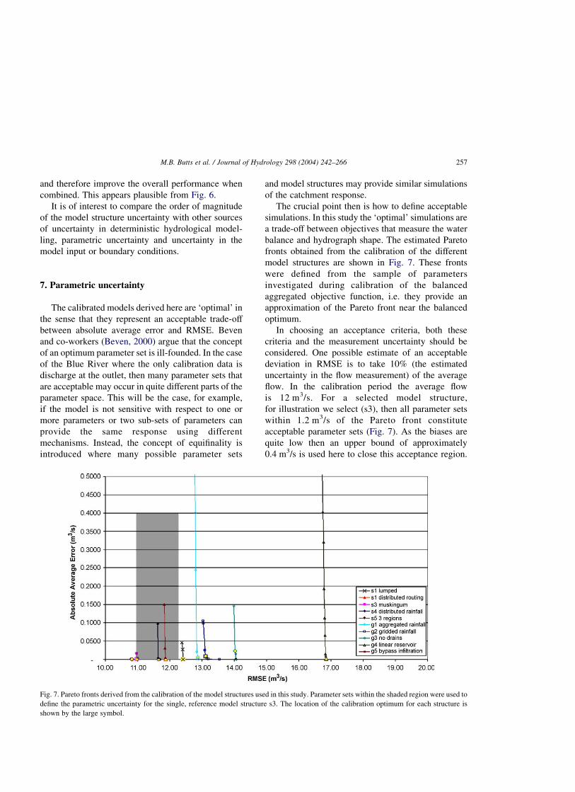
The crucial point then is how to define acceptable

simulations. In this study the ‘optimal’ simulations are

a trade-off between objectives that measure the water

balance and hydrograph shape. The estimated Pareto

fronts obtained from the calibration of the different

model structures are shown in Fig. 7. These fronts

were defined from the sample of parameters

investigated during calibration of the balanced

aggregated objective function, i.e. they provide an

approximation of the Pareto front near the balanced

optimum.

In choosing an acceptance criteria, both these

criteria and the measurement uncertainty should be

considered. One possible estimate of an acceptable

deviation in RMSE is to take 10% (the estimated

uncertainty in the flow measurement) of the average

flow. In the calibration period the average flow

is 12 m3/s. For a selected model structure,

for illustration we select (s3), then all parameter sets

within 1.2 m3/s of the Pareto front constitute

acceptable parameter sets (Fig. 7). As the biases are

quite low then an upper bound of approximately

0.4 m3/s is used here to close this acceptance region.

Fig. 7. Pareto fronts derived from the calibration of the model structures used in this study. Parameter sets within the shaded region were used to

define the parametric uncertainty for the single, reference model structure s3. The location of the calibration optimum for each structure is

shown by the large symbol.


Parameter sets within this region are considered to be

equally acceptable for predicting streamflow.

Using this criterion two other related model structures

also fall in this acceptance region.

The location of the Pareto fronts along the RMSE

axis shows the sensitivity of simulation accuracy to

model structure for the calibration period. The size of

the acceptance region for a single model in this case is

small compared to the sensitivity with respect to the

model structure in an RMSE sense. From a practical

point of view, this figure suggests that there is as much

scope for improving simulation accuracy by exploring

different model structures as there is from

different parameter sets. However, in many practical

hydrological studies the effects of different model

structures are seldom evaluated.

A simple estimate of the parametric uncertainty for

the model structure (s3) can be obtained from the

generated parameter sets of the SCE optimisation.

A representative ensemble of the acceptable

parameter sets was selected by using a simple latin

hypercube sampling approach, dividing the

acceptance region into 25 areas and randomly

selecting a set generated during the SCE optimisation

within each region. Strictly speaking the resulting

variation produced by this ensemble is a measure of

model sensitivity, Fig. 8. This figure is generated by

taking the upper and lower bounds of the ensemble

as a measure of the parametric uncertainty.

The ensemble range is similar in magnitude to the

observation uncertainty. The variations caused by

parametric uncertainty for this structure appear to

principally affect the magnitude of the peaks.

The variations in model structure provide more varied

hydrological response including the shape and timing

of the peaks.

This argues strongly for extending the model

calibration process usually carried out in hydrological

simulations to not only address parameter choices

within a particular model structure but also to address

the choice of both model structure and corresponding

parameters. While automatic calibration methods

seldom extend to exploring different model structures

the new modelling framework described here

represents a first step in this direction. The split

sample testing used here could provide a general

methodology for evaluating the different model

structures in such a process. As pointed out above

the usefulness of this process in identifying the

important hydrological flow mechanisms will depend

on the availability of other calibration data than the

discharge at the basin outlet or a more detailed

analysis of parts of the catchment response.

8. Rainfall uncertainty

It is expected that for a well-calibrated

hydrological model that adequately represents the

important runoff processes within the catchment that

the major factor contributing to the uncertainty in the

predicted flows is the uncertainty in rainfall. This is

confirmed to a large extent by our own experience in

many practical hydrological modelling studies.

Several authors suggest that this is the most important

contribution to model uncertainty. For example,

Refsgaard et al. (1983) show, using a Kalman filter

version of the NAM model, that the variations due to

uncertainty in rainfall estimation are significantly

larger than the uncertainty due to parameter

variations. However, this conclusion depends strongly

on catchment size and response time, the model and

the assumptions made in representing the different

sources of uncertainty.

The uncertainty in the rainfall may arise from

instrument bias or error, inadequate spatial or

temporal resolution and in the case of forecasts,

the inherent chaotic nature of weather systems.

A detailed analysis of the uncertainties and biases

for the NEXRAD precipitation has been addressed

elsewhere (Smith et al., 2004) and beyond the scope

of this study. Nevertheless, for the purposes of this

paper it is of interest to estimate the order of

magnitude of the uncertainty in streamflow

simulations due to uncertainties in the precipitation

input and to compare this to the other sources of

uncertainty.

As a first approximation only sub-catchment

rainfall aggregated from the radar rainfall is

considered and the uncertainty is assumed spatially

independent from sub-catchment to sub-catchment

and independent in time for the hourly values used.

Within each sub-catchment the rainfall uncertainty is

assumed to have the following simple structure:

P0i ¼ Pi þ a; a [ Nð0;sÞ ð8Þ


Fig. 8. Examples of the model structure ensemble and parametric measurement uncertainty for two major peaks, one in the calibration period

and one in the validation period. The dark solid lines show the upper and lower bounds of the model parameter ensemble and the reference

model structure s3.


where Pi is the ith sub-catchment rainfall based on

radar observations, P0i is the perturbed rainfall for the

ith sub-catchment and a is a random error. The value

of a is selected from a normal distribution Nð0;sÞ;

with zero mean and standard deviation, s: The

standard deviation was assumed as a first approxi-

mation to be linearly related to the sub-catchment

rainfall, i.e. s ¼ RPi: For the purpose of estimating

the order of magnitude of the impact of rainfall

uncertainties, a value of R ¼ 0:5 was selected. For this

approximate uncertainty model, the uncertainty

becomes zero when no rainfall is recorded by the

radar. Where values of P0i below zero are generated

the rainfall is set to zero. For the parameters selected

here, this will affect only a few percent of the sample

distribution. The above uncertainty model structure

assumes the rainfall uncertainties are independent in

space and time.

To determine the propagation of uncertainty due to

uncertainties in the measured rainfall, the transform-

ation of the rainfall uncertainty into uncertainty in the

runoff is calculated using a Monte Carlo approach

using a total of 200 samples. Fig. 9 compares the

model structure ensemble with the 95% confidence

intervals for uncertainty in the simulated discharge

obtained from this Monte Carlo procedure for the two

flood events considered earlier. These confidence

intervals were estimated using the ‘optimal’ model

structure (s3). The s3 structure is shown as a dark line

between the two bounds. The Monte Carlo procedure

was carried out over the entire simulation period used

on the DMIP study (Fig. 2). It is assumed that the

uncertainty in the precipitation input is the only

source of uncertainty.

In this case it appears that a 50% relative standard

deviation in the precipitation estimate ðR ¼ 0:5Þ has

only a limited impact on the accuracy of the

hydrological simulation when compared to the flow

measurement uncertainty and the other sources of

uncertainty. These results are again specific to the

model structure (s3) for the Blue River basin.

Certainly it is insufficient to explain the deviations

we see between the observed and simulated flows.

It should be recognised that this figure shows the

sensitivity of the selected model structure to

uncertainty in the rainfall input, conditioned on the

observations by the calibration process. The uncer-

tainty model used here does not account for

the significant biases that appear particularly in

radar-based precipitation measurement and this is

probably the largest contributing factor. Seo et al.

(2003) suggests there are significant systematic and

event-to-event biases in the precipitation data, which

should result in volume biases in the modelled

discharges. Perhaps more importantly the temporal

and spatial correlations are neglected. A more

thorough characterisation of the radar rainfall

uncertainties, including their spatial and temporal

correlation for the Blue River is required to verify

whether the low sensitivity to rainfall error found here

realistically represents the catchment response.

9. Model structure ensembles

An original outcome of the DMIP study, described

in Georgakakos et al. (2004) is the application of

multimodel ensembles for hydrological simulation.

In particular their analysis of the DMIP models

showed that combinations of different models provide

more reliable hydrological simulations than simu-

lations obtained from the single best performing

models. This, however, was not tested using an

independent validation period. Here we derive in a

similar manner new models from different

combinations of the different model structures used

in this study. An investigation of this is shown, for the

different combinations of model structures, using 2,

3,…,10 different structures, in Fig. 10. The model

simulations are weighted equally in all combinations.

One could also weight the different models according

to goodness-of-fit as in the GLUE methodology. In the

calibration period, many of the combinations of model

structures perform as well or better than the best

single model. More interesting is that in the

validation period many of the combinations of 2, 3

and 4 models still provide improvements in simu-

lation accuracy when compared to the best single

model. We also found that the ensemble average of all

10 model structures performs better than any single

model. These results for the split sample validation

provide a strong confirmation of the conclusion of

Georgakakos et al. (2004) that multimodel

(multiple model structure) ensembles may provide

important benefits for hydrological simulation.

The improvement appears to arise from


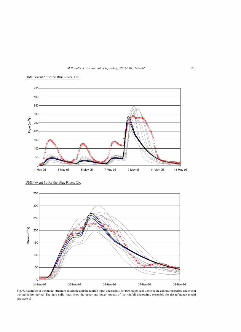
Fig. 9. Examples of the model structure ensemble and the rainfall input uncertainty for two major peaks, one in the calibration period and one in

the validation period. The dark solid lines show the upper and lower bounds of the rainfall uncertainty ensemble for the reference model

structure s3.


Fig. 10. Root means square error (RMSE) and correlation ðRÞ for the calibration and validation period used in this study for model structure

ensembles. The performance of combinations of 2,3,4,5,6,7,8,9 and 10 model structures is compared to the performance of the individual

structures (1 s).


the differences in hydrological response of the

different model structures which when added together

provide a better match to the observed flows.

10. Discussion and conclusions

A modelling framework has been developed to

explore different hydrological model structures in

both the rainfall-runoff and channel routing

components of their hydrological models. This frame-

work was then used in a systematic analysis of the

performance of a number of different model structures

for a particular basin, the Blue River, a test basin in

the Distributed Model Intercomparison Project

(DMIP), organised by the Office of Hydrologic

Development of the US National Weather Service.

Split sample testing was carried out and a variety of

performance measures were applied to evaluate the

ability of the different structures to simulate

streamflow. An automatic multiple objective

calibration procedure was used to determine an

‘optimal’ parameter set and to define the Pareto fronts

for each structure. The absolute value of the average

error and RMSE were used as the calibration criteria.

These ‘optimal’ models for each model structure were

used to create model structure ensembles to evaluate

model structure uncertainty and to evaluate the

performance of combinations of different model

structures.

The main findings are:

1. There are large variations in the model

performance amongst the selected model structures

used in this study. For the case of the Blue River

Basin, the model performance appears to be quite

sensitive to model structure. Substantial

improvements in model performance were

obtained in the Blue River by evaluating different

model structures. For practical hydrological

predictions this suggests that there can be import-

ant benefits in exploring different model structures

as part of the modelling approach. The modelling

framework developed here allows the hydrologist

to adopt such an approach and evaluate the

performance of different structures before a final

selection is made. The split sample testing

methodology can be used for this evaluation.

2. Using the RMSE and correlation criteria, an

optimal model structure (s3) was found that

performed best in both the calibration and

validation periods. This is one of the simplest

distributed model structures used. However, some

of the more complex grid-based rainfall-runoff

model structures were better at matching the

distribution of flows and performed as well or

better in the validation period. Ten quite different

model structures were evaluated in this study but

there is considerable scope for evaluating

other model structures and obtaining further

improvements in accuracy. Ideally a general

model calibration procedure should include both

model structure and parameter adjustment.

3. The performance of the sub-catchment based

conceptual models (s1–s5) confirm the results

from earlier work by Boyle et al. (2001) for the

Blue River. It was found that distributed routing

and distributed rainfall information increase the

simulation accuracy and predictive capability of

the model. This is more strictly tested here using

the split sample validation. The distributed

routing gave the largest improvement of the two

in this long narrow catchment. The (s5) model,

which also includes spatially distributed catchment

parameters provided an excellent calibration but

was outperformed by other models in the

validation. This might suggest as found by Boyle

et al. (2001), that the spatial distribution of

parameters does not improve performance.

However, it is likely that this model is simply

over-parameterised. The relationship between

model performance and the level of spatial

distribution used requires further study.

Split sample validation should be used to ensure

strict evaluation of the results. This also suggests

that there is an optimal number of calibration

parameters. Below this optimum not all the

processes are captured properly, while above this

optimum there is a good fit to the calibration data

but poor predictive power.

4. In a number of cases it appears that there is a

trade-off, where increasing the model complexity

does not increase model performance. The fully

dynamic routing (s2) does not outperform the

simpler Muskingum–Cunge routing (s3) when

the same conceptual rainfall-runoff description is


used. The (s5) structure with the largest number of

parameters and the greatest level of spatial

distribution of the sub-catchment-based structures

performs best in the calibration period but not

nearly as well in the validation period. Finally the

additional information in each of the NEXRAD

rainfall cells used in (g2) appears to provide

minimal if any benefit in simulation accuracy when

compared to the same model structure using

NEXRAD rainfall aggregated over sub-basins

(g1). However, as pointed out in the discussion

the reasons why increased complexity does not

necessary lead to better simulations may be caused

by several limitations. These include limitations in

the model structure itself, limitations in the

information available in the calibration data,

limitations in the accuracy and representative of

rainfall, or limitations in the parameter estimation

procedures. Further exploration of these

limitations is needed to derive, for example,

maximum benefit from the radar rainfall.

5. With the exception perhaps of the completely

lumped structure, the model structures selected

here are all plausible choices for hydrological

modelling of the Blue River basin. This study used

this range of plausible model structures as an

estimate of uncertainty due to model structure.

The resulting ensemble of model structure

simulations shows significant variations in the

shape and timing of the flood peaks. Uncertainty in

the measurement data was estimated together with

parametric and rainfall input uncertainty.

The parametric uncertainty was estimated from

the sensitivity of the simulations for a particular

model structure to choices of parameter sets that

provide the same level of performance. The impact

of rainfall uncertainty was estimated using a Monte

Carlo approach based on somewhat crude

assumptions about the properties of the rainfall

uncertainty. It was found that the sensitivity of

streamflow simulations to variations in

acceptable model structure was at least as large

as uncertainties arising from parametric and

measurement uncertainty. The model simulations

appeared to be less sensitive to rainfall uncertainty,

however, this was examined for one model

structure only. Furthermore, since the results are

based on rather simple assumptions regarding

the rainfall uncertainty, neglecting biases, and

other influences, such as neglecting the uncertainty

in the evapotranspiration, it is recommended that

further investigation of the impacts of uncertainty

in the model boundary conditions be carried out.

6. Finally the performance of new models derived by

combining the results of two or more of the

different model structures was evaluated.

The results show that many combinations could

be found that performed as well as or better than

the best individual model structures. We found that

the ensemble average of all 10 model structures

performs better than any single model.

These results using split sample validation provide

a strong confirmation of the conclusion of

Georgakakos et al. (2004) that multimodel

(multiple model structure) ensembles may provide

important benefits for hydrological simulation.

One interpretation of this result is that the different

model structures capture different aspects of the

catchment response and, therefore, more aspects of

the catchment response are captured in the

combined model.

Overall this study suggests that exploring an

ensemble of model structures provides a useful

approach both in defining significant errors in the

hydrological simulations and to improve the overall

accuracy of the simulations. The study has developed

a framework that allows hydrologists to investigate

different model structures. An important goal for

future work is the extension of this framework to other

structures. A more challenging problem is devising a

strategy for selecting appropriate model structures for

particular applications, with particular data.

The approach adopted here is one way forward.

Further work is required to evaluate how the different

sources of uncertainty can be treated together both for

hydrological simulation and hydrological forecasting.

It is also recommended that further research is needed

to evaluate the performance of model structure

ensembles in an operational context.

Acknowledgements

The authors would like to thank Michael Smith and

his colleagues on the staff of Hydrology Lab, OHD,


NWS for their assistance throughout this study.

David Tarboton, University of Utah, USA and Ross

Woods, National Institute of Water Research,

New Zealand, provided the gridded NEXRAD data

to the authors. The authors would like to acknowledge

Jacob Larsen DHI Water and Environment for

his assistance with the original submission and

Jean-Philippe Drecourt DHI Water and Environment

for fruitful discussions concerning parametric

uncertainty. The additional support to the second

author provided through the University of Washing-

ton’s Valle Exchange and Scholarship Program is also

acknowledged and appreciated. The development of

the methodology for propagation of rainfall

uncertainty was carried out by Anne Katrine Falk

DHI Water and Environment with the support of the

EU 5th Framework Research Programme, FLOOD

RELIEF, contract EVK1-CT2002-00171, http://

projects.dhi.dk/floodrelief/.

References

Abbott, M.B., Refsgaard, J.C., 1996. Distributed Hydrological

Modelling, Kluwer, Dordrecht.

Abbot, M.B., Bathurst, J.C., Cunge, J.A., O’Connell, P.E.,

Rasmussen, J., 1986a. An introduction to the European

Hydrological System—Systeme Hydrologique Europeen,

SHE. 1 History and philosophy of a physically-based distributed

modelling system. Journal of Hydrology 87, 45–59.

Abbot, M.B., Bathurst, J.C., Cunge, J.A., O’Connell, P.E.,

Rasmussen, J., 1986b. An introduction to the European

Hydrological System—Systeme Hydrologique Europeen,

SHE. 2 Structure of a physically-based distributed modelling

system. Journal of Hydrology 87, 61–77.

Atkinson, S., Woods, R.A., Sivapalan, M., 2002. Climate and

landscape controls on water balance model complexity over

changing time scales. Water Resources Research 38(12),

1314doi: 10.1029/2002WR001487, pp. 50.1–50.17.

Atkinson, S., Sivapalan, M., Woods, R.A., Viney, N.R., 2003.

Dominant physical controls of hourly streamflow predictions

and an examination of the role of spatial variability: Mahurangi

catchment, New Zealand. Advances in Water Resources 26(3),

219–235.

Beven, K.J., 1997. Distributed Hydrological Modelling:

Applications of the TOPMODEL Concept, Wiley, Chichester.

Beven, K.J., 2000. Rainfall-Runoff Modelling: The Primer, Wiley,

England.

Beven, K.J., Freer, J., 2001. Equifinality, data assimilation and

uncertainty estimation in mechanistic modelling of complex

environmental systems using the GLUE methodology. Journal of

Hydrology 249, 11–29.

Boyle, D.P., Gupta, H.V., Sorooshian, S., Koren, V., Zhang, Z.,

Smith, M., 2001. Toward improved streamflow forecasts: value

of semidistributed modeling. Water Resources Research 37(11),

2749–2759.

Butts, M.B., Klinting, A., van Kalken, T., Cadman, D., Fenn, C.,

Høst-Madsen, J., 2001. Design and development of an Internet-

based flood forecasting system using real-time rainfall, radar,

and river flow data. In: Falconer, R.A., Blain, W.R. (Eds.),

Proceedings of River Basin Management 2001, Cardiff, WIT

Press, pp. 139–148.

Butts, M.B., Hoest-Madsen, J., Refsgaard, J.C., 2002. Hydrologic

Forecasting, Encyclopaedia of Physical Science and Technol-

ogy, Third ed.

Calver, A., Wood, W.L., 1995. The Institute of Hydrology

distributed model. In: Singh, V.P., (Ed.), Computer Models of

Watershed Hydrology, Water Resources Publications, Color-

ado, USA, pp. 595–626.

Ciarapica, L., Todini, E., 2002. TOPKAPI: a model for the

representation of the rainfall-runoff process at different scales.

Hydrological Processes 16, 207–229.

Duan, Q., Sorooshian, S., Gupta, V., 1992. Effective and efficient

global optimization for conceptual rainfall-runoff models.

Water Resources Research 28(4), 1015–1031.

Duan, Q., Sorooshian, S., Gupta, V.K., 1994. Optimal use of the

SCE-UA global optimization method for calibrating watershed

models. Journal of Hydrology 158, 265–284.

Farmer, D., Sivapalan, M., Jothityangkoon, C., 2003. Climate, soil

and vegetation controls upon the variability of water balance in

temperate and semi-arid landscapes: downward approach to

hydrological prediction. Water Resources Research 39(2),

1035doi: 10.1029/2001WR000328.

Flury, M., Fluhler, H., Jury, W.A., Leuenberger, J., 1994.

Susceptibility of soils to preferential flow of water: a field

study. Water Resources Research 30, 1945–1954.

Freeze, R.A., Harlan, R.L., 1969. Blueprint for a physically-based

digitally-simulated hydrological response model. Journal of


Georgakakos, K.P., Seo, D.-J., Gupta, H., Schaake, J., Butts,

M.B., 2004. Characterising streamflow simulation uncertainty

through multimodel ensembles. Journal of Hydrology,

298(1–4), 222–241.

Havnø, K., Madsen, M.N., Dørge, J., 1995. MIKE 11—a

generalized river modelling package. In: Singh, V.P., (Ed.),

Computer Models of Watershed Hydrology, Water Resources

Publications, Colorado, USA, pp. 733–782.

Hollenbeck, K.J., Jensen, K.H., 1998. Experimental evidence of

randomness and non-uniqueness in unsaturated outflow

experiments designed for hydraulic parameter estimation.


Hornberger, G.M., Germann, P.F., Beven, K.J., 1991. Throughflow

and solute transport in an isloated sloping soil block in a forested

catchment. Journal of Hydrology 124, 81–99.

Koren, V.I., Reed, S., Smith, M., Zhang, Z., Seo, D.-J., 2003.

Hydrology Laboratory Research Modeling System (HL-RMS)

of the National Weather Service. Journal of Hydrology in

review.


http://projects.dhi.dk/floodrelief/

http://projects.dhi.dk/floodrelief/

Lohmann, D., Raschke, E., Nijssen, B., Lettenmaier, D.P., 1998.

Regional scale hydrology: I. Formulation of the VIC-2L model

coupled to a routing model. Hydrological Sciences Journal 43,

131–141.

Madsen, H., 2000. Automatic calibration of a conceptual rainfall-

runoff model using multiple objectives. Journal of Hydrology

235, 276–288.

Madsen, H., 2003. Parameter estimation in distributed

hydrological catchment modelling using automatic calibration

with multiple objectives. Advances in Water Resources 26,

205–216.

Mortensen, A.P., Glass, R.J., Hollenbeck, K.J., Jensen, K.H., 2001.

Visualization of microscale phase displacement processes in

retention and outflow experiments: Non-uniqueness of unsatu-

rated flow properties. Water Resources Research 37(6),

1627–1640.

Rajaram, H., Georgakakos, K.P., 1989. Recursive parameter

estimation of hydrologic models. Water Resources Research

25(2), 281–294.

Reed, S., Koren, V., Smith, M.B., et al., 2004. Overall Distributed

Model Intercomparison Project results. Journal of Hydrology

298(1–4), 60–34.

Refsgaard, J.C., 1996. Terminology, modelling protocol and

classification of hydrological model codes. In: Abbott, M.B.,

Refsgaard, J.C. (Eds.), Distributed Hydrological Modelling,

Kluwer, Dordrecht, pp. 17–39.

Refsgaard, J.C., 1997. Validation and intercomparison of

different updating procedures for real-time forecasting. Nordic


Refsgaard, J.C., Butts, M.B., 1999. Determination of grid scale

parameters in catchment modelling by upscaling local scale

parameters (Invited Paper). In: Fejen, J., Wiyo, K. (Eds.),

Modelling of Transport Processes in Soils, International Work-

shop of EurAgEng’s Field of Interest in Soil and Water, 24–26

November, 1999, Leuven, Belgium, pp. 650–665.

Refsgaard, J.C., Knudsen, J., 1996. Operational validation and

intercomparison of different types of hydrological models.


Refsgaard, J.C., Storm, B., 1995. MIKE SHE. In: Singh, V.P., (Ed.),

Computer Models of Watershed Hydrology, Water Resources

Publications, Colorado, USA, pp. 809–846.

Refsgaard, J.C., Rosbjerg, D., Markussen, L.M., 1983. Application

of the Kalman Filter to Real Time Operation and to Uncertainty

Analyses in Hydrological Modelling, Scientific Procedures

Applied to the Planning, Management and Design of Water

Resources Systems (Proceedings of the Hamburg Symposium,

August, 1983), IAHS publ-no. 147., pp. 273–282.

Seo, D.-J., Koren, V., Cajina, N., 2003. : Real-time variational

assimilation of hydrologic and hydrometeorological data into

operational hydrologic forecasting. Journal of Hydrometeorol-

ogy 4, 627–641.

Singh, V.P. (Ed.), 1995. Computer Models of Watershed Hydrol-

ogy, Water Resources Publications, Colorado, USA, p. 1130.

Smith, M.B., Seo, D.-J., Koren, V.I., Reed, S., Zhang, Z., Duan,

Q.-Y., Moreda, F., Cong, S., 2004. The Distributed Model

Intercomparison Project (DMIP): motivation and experiment

design. Journal of Hydrology 298(1–4), 4–26.

Storm, B., Refsgaard, A., 1996. Distributed physically-based

modelling of the entire land phase of the hydrological cycle.

In: Abbott, M.B., Refsgaard, J.C. (Eds.), Distributed Hydro-

logical Modelling, Kluwer, Dordrecht.

World Meteorological Organisation (WMO), 1994, Fifth ed., Guide

to Hydrological Practices: Data Acquisition, and Processing,

Analysis, Forecasting and Other Applications, WMO Publ. No.

168.

World Meteorological Organisation (WMO), 2001. Report on the

Operational Use of EPS to Forecast Severe Weather and

Extreme Events, WMO Commission on Basic Systems, Meeting

of Expert Team on Ensemble Prediction Systems, Tokyo, Japan

15–19 October 2001, CBS ET/EPS/Doc. 3(7) (9.X.2001),

Geneva Switzerland, pp. 7.


An evaluation of the impact of model structure on hydrological modelling uncertainty for streamflow...

Documents

Transcript of An evaluation of the impact of model structure on hydrological modelling uncertainty for streamflow...