Hydrol. Earth Syst. Sci., 15, 3195–3206, 2011www.hydrol-earth-syst-sci.net/15/3195/2011/doi:10.5194/hess-15-3195-2011© Author(s) 2011. CC Attribution 3.0 License.

Hydrology andEarth System

Sciences

Diffuse hydrological mass transport through catchments: scenarioanalysis of coupled physical and biogeochemical uncertainty effects

K. Persson, J. Jarsjo, and G. Destouni

Department of Physical Geography and Quaternary Geology, Stockholm University, 106 91, Stockholm, Sweden

Received: 8 April 2011 – Published in Hydrol. Earth Syst. Sci. Discuss.: 12 May 2011Revised: 26 September 2011 – Accepted: 10 October 2011 – Published: 20 October 2011

Abstract. This paper quantifies and maps the effects of cou-pled physical and biogeochemical variability on diffuse hy-drological mass transport through and from catchments. Itfurther develops a scenario analysis approach and investi-gates its applicability for handling uncertainties about bothphysical and biogeochemical variability and their differentpossible cross-correlation. The approach enables identifi-cation of conservative assumptions, uncertainty ranges, aswell as pollutant/nutrient release locations and situations forwhich further investigations are most needed in order to re-duce the most important uncertainty effects. The presentscenario results provide different statistical and geographicdistributions of advective travel times for diffuse hydrolog-ical mass transport. The geographic mapping can be usedto identify potential hotspot areas with large mass loading todownstream surface and coastal waters, as well as their op-posite, potential lowest-impact areas within the catchment.Results for alternative travel time distributions show that ne-glect or underestimation of the physical advection variabil-ity, and in particular of those transport pathways with muchshorter than average advective solute travel times, can leadto substantial underestimation of pollutant and nutrient loadsto downstream surface and coastal waters. This is particu-larly true for relatively high catchment-characteristic prod-uct of average attenuation rate and average advective traveltime, for which mass delivery would be near zero under as-sumed transport homogeneity but can be orders of magni-tude higher for variable transport conditions. A scenario ofhigh advection variability, with a significant fraction of rel-atively short travel times, combined with a relevant average

Correspondence to:K. Persson(klas.persson@natgeo.su.se)

biogeochemical mass attenuation rate, emerges consistentlyfrom the present results as a generally reasonable, conserva-tive assumption for estimating maximum diffuse mass load-ing, when the prevailing physical and biogeochemical vari-ability and cross-correlation are uncertain.

1 Introduction

Model estimations of diffuse hydrological mass transport arecritical for biogeochemical cycle understanding, and suc-cessful and efficient environmental management. In manyhydrological catchments with human activities, there are,apart from direct nutrient and pollutant discharges into sur-face waters, typically also diffuse sources at the land sur-face and below it, in soil, in mobile and immobile ground-water, and in sediments. Pollutants and excess nutrientsthat are transported from diffuse sources through the subsur-face water system may yield considerable long-term load-ing to downstream surface and coastal waters (Carpenter etal., 1998; Baresel and Destouni, 2007; Darracq et al., 2008;Basu et al., 2010; Howden et al., 2011). Catchment-scalewater quality modelling and prediction must account for thissubsurface transport, even if the main focus is on surfacewater quality.

However, all models of solute transport through subsur-face and surface water subsystems, and whole catchmentsare inevitably associated with uncertainties. Over the lastdecades, many successive publications have quantified dif-ferent types of uncertainty and investigated their implica-tions for the modelling and management of water pollution(e.g. Cvetkovic et al., 1992; Andricevic and Cvetkovic, 1996;Batchelor et al., 1998; Eggleston and Rojstaczer, 2000; Grenet al., 2000; Jarsjo et al., 2005). Key sources of uncertainty

Published by Copernicus Publications on behalf of the European Geosciences Union.

3196 K. Persson et al.: Diffuse hydrological mass transport through catchments

in the quantification of waterborne mass transport along thehydrological source-pathway-recipient continuum include:

– the spatiotemporal configuration, variability andhistoric-to-future development and change of drivingforces and conditions that determine source inputs,such as human activities, weather, climate and landcover/use conditions (Darracq et al., 2005; Hagemannand Jacob, 2007; Jacob et al., 2007; Edwards andWithers, 2008; Kysely and Beranova, 2009; Bergknutet al., 2010)

– the transport pathways from the sources to the down-stream observation points and receiving water environ-ments, and the variability of water flow and mass trans-port velocities and travel times among and along thesepathways (e.g. McGuire et al., 2005; Destouni et al.,2010; Beven, 2010; McDonnell et al., 2010)

– the variability of biogeochemical processes and theircombination and cross-correlation with the physicalmass transport along the different flow and transportpathways (e.g. Malmstrom et al., 2004, 2008; Dar-racq and Destouni, 2007; Cunningham and Fadel, 2007;Jardine, 2008)

– the errors of mass transport measurements implied bythe chosen measurement methods and the coverage gapsbetween the chosen measurement points in time andspace (e.g. Hannerz and Destouni, 2006; Beven, 2006;Jarsjo and Bayer-Raich, 2008; Destouni et al., 2008)

– the chosen model resolutions and possible neglect ofpotentially important contributing mass transport pro-cesses at different scales (e.g. Lindgren and Destouni,2004; Refsgaard et al., 2006; Destouni et al., 2006;Ganoulis, 2009).

Among all these sources of hydrological mass transport un-certainty, only some can be accounted for by realistic prob-ability assignment and statistical quantification. However,also the remaining, statistically unquantifiable uncertaintiesneed to be accounted for in some way. One way to achievethis is to consider scenarios that capture and bound differentpossible system characteristics and developments.

Recent studies of hydrological pollutant transport havecombined probabilistic and scenario uncertainty accounts,and discussed the needs and result implications of such com-bined approaches for rational guidance of management andabatement of water pollution (Baresel and Destouni, 2007;Persson and Destouni, 2009). These studies specifically ad-dressed water pollution from local sources, with to large de-gree known locations and relatively limited spatial extents(commonly referred to as point sources), for which boundingscenarios of different possible mass transport statistics could

be relatively well defined and quantified. However, for pollu-tant/nutrient/tracer transport from diffuse sources, with con-tinuous or patch-wise spatial distributions over more or lessthe whole landscape within a catchment area, such statisticsare considerably more difficult to obtain (e.g. McDonnell etal., 2010; Darracq et al., 2010a, b).

In this paper we use and develop a scenario analy-sis approach to quantify some relevant statistical uncer-tainty bounds for hydrological mass transport from spatiallywidespread sources at and below the land surface, throughsoil and groundwater, to surface and coastal waters withinand downstream of a catchment. We formulate and com-bine different scenarios of variability in physical and bio-geochemical mass transport processes at the catchment scale,and quantify and map the scenario-associated transport anddelivery of, for instance, tracer, pollutant or excess nutrientmass, from a diffuse source over the entire land area of acatchment to downstream surface or coastal water recipients.We further assess the possible convergence, as well as thedivergence and uncertainty among the different scenario re-sults. The hydrologically well-characterised Forsmark catch-ment in Sweden (e.g. Johansson et al., 2005; SKB, 2008;Werner et al., 2007; Jarsjo et al., 2008) is used as a specificcase study example.

Previous calculations of travel time distributions in theForsmark catchment example have only considered a sce-nario of essentially constantK, prevailing along relativelyhigh-conductive, preferential transport pathways through thecatchment (Darracq et al., 2010a, b; Destouni et al., 2010).These calculations are here extended for a second, quite op-posite flow and transport scenario, considering large spatialvariability in the transport-encounteredK. This scenario rep-resents a transport situation, where the flow and transportpathways go through and encounter the fullK variability thatprevails within a catchment, representing a realistic upperbound for the transport-encounteredK variability. The dif-ference between the hydrological mass transport results forthe constant and variableK scenarios indicates then the im-portance of uncertainty about the prevailingK heterogeneityin the catchment.

In addition to and combined with the different scenariosof physicalK heterogeneity and resulting advective traveltime distributions, we consider here also different scenariosconcerning the variability and cross-correlation withK ofthe biogeochemical rate of pollutant/nutrient mass attenua-tion (decay or immobilisation by physical, chemical or bio-logical processes) occurring along the mass transport path-ways. Natural attenuation depends on subsurface character-istics, such as water flow velocity and mineralogy, which arealso directly or indirectly related to hydraulic conductivity(Cunningham and Fadel, 2007; Jardine, 2008). Regardingbacterial degradation of organic contaminants, for instance,the subsurface permeability affects the availability of rate-limiting electron acceptors and donors, as well as the bacte-rial transport and community structure. Microbial processes

Hydrol. Earth Syst. Sci., 15, 3195–3206, 2011 www.hydrol-earth-syst-sci.net/15/3195/2011/

K. Persson et al.: Diffuse hydrological mass transport through catchments 3197

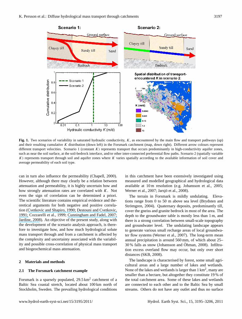
Fig. 1. Two scenarios of variability in saturated hydraulic conductivity,K, as encountered by the main flow and transport pathways (up)and their resulting cumulativeK distribution (down left) in the Forsmark catchment (map, down right). Different arrow colours representdifferent transport velocities. Scenario 1 (constantK) represents transport that occurs predominantly in high-conductivity aquifer zones,such as near the soil surface, at the soil-bedrock interface, and/or other inter-connected preferential flow paths. Scenario 2 (spatially variableK) represents transport through soil and aquifer zones whereK varies spatially according to the available information of soil cover andaverage permeability of each soil type.

can in turn also influence the permeability (Chapell, 2000).However, although there may clearly be a relation betweenattenuation and permeability, it is highly uncertain how andhow strongly attenuation rates are correlated withK. Noteven the sign of correlation can be determined a priori.The scientific literature contains empirical evidence and the-oretical arguments for both negative and positive correla-tion (Cvetkovic and Shapiro, 1990; Destouni and Cvetkovic,1991; Cozzarelli et al., 1999; Cunningham and Fadel, 2007;Jardine, 2008). An objective of the present study, along withthe development of the scenario analysis approach, is there-fore to investigate how, and how much hydrological solutemass transport through and from a catchment is affected bythe complexity and uncertainty associated with the variabil-ity and possible cross-correlation of physical mass transportand biogeochemical mass attenuation.

2 Materials and methods

2.1 The Forsmark catchment example

Forsmark is a sparsely populated, 29.5 km2 catchment of aBaltic Sea coastal stretch, located about 100 km north ofStockholm, Sweden. The prevailing hydrological conditions

in this catchment have been extensively investigated usingmeasured and modelled geographical and hydrological dataavailable at 10 m resolution (e.g. Johansson et al., 2005;Werner et al., 2007; Jarsjo et al., 2008).

The terrain in Forsmark is mildly undulating. Eleva-tions range from 0 to 50 m above sea level (Brydsten andStromgren, 2004). Quaternary deposits, predominantly till,cover the gneiss and granite bedrock in most of the area. Thedepth to the groundwater table is mostly less than 1 m, andthere is a strong correlation between small-scale topographyand groundwater level. The undulating landscape appearsto generate various small recharge areas of local groundwa-ter flow systems (Werner et al., 2007). The long-term meanannual precipitation is around 560 mm, of which about 25–30 % falls as snow (Johansson andOhman, 2008). Infiltra-tion excess overland flow may occur, but only over shortdistances (SKB, 2008).

The landscape is characterised by forest, some small agri-cultural areas and a large number of lakes and wetlands.None of the lakes and wetlands is larger than 1 km2, many aresmaller than a hectare, but altogether they constitute 19 % ofthe total catchment area. Some of these lakes and wetlandsare connected to each other and to the Baltic Sea by smallstreams. Others do not have any outlet and thus no surface

www.hydrol-earth-syst-sci.net/15/3195/2011/ Hydrol. Earth Syst. Sci., 15, 3195–3206, 2011

3198 K. Persson et al.: Diffuse hydrological mass transport through catchments

water connection to the sea. About 10 % of the area drains tostretches of the coast with no surface water outlet. Measure-ments of stream discharge are available from four gaugingstations, but the time series are too short to provide reliableinformation about the spatial variation of runoff in the area(Johansson andOhman, 2008).

2.2 Quantification of advective solute travel times forphysical heterogeneity scenarios

We quantified groundwater travel times in the Forsmarkcatchment for two different, quite opposite scenarios of howthe saturated hydraulic conductivityK may vary among andalong the different pathways of diffuse solute transport inthis example catchment area. In Fig. 1 the scenarios areschematically illustrated, and their respectiveK distributionsare shown. In scenario 1 the transport-encounteredK is es-sentially constant, representing transport that largely evadeslow-K zones and follows primarily preferential pathwaysthrough relatively high-K zones. The constantK value isthen set to 1.3 m d−1, which was the uniform mean value sug-gested by Johansson et al. (2005) for the upper soil layer andfor the soil – bedrock interface of Forsmark, based on fieldpermeability testing and generic data. The soil – bedrockinterface in this catchment is typically located at a depth ofless than 5 m (Johansson, 2008). In scenario 2, the transport-encounteredK varies both among and along the transportpathways through the catchment, in accordance with avail-able data on the geographical distribution of different soiltypes over the catchment (Jarsjo et al., 2008) and site-specificand generic data of typicalK values for the different soiltypes (Johansson, 2008). In this scenario, the geometricmean value ofK is 0.71 m d−1, and the standard deviationof ln K is 1.8.

The two scenarios 1 and 2 have thus very differentK dis-tributions (Fig. 1), which can be expected to bound manyalternative representations ofK variability in a catchment.StochasticK fluctuations around the mean localK values(constant in scenario 1 and variable in scenario 2) are notincluded in the present scenario analysis, for illustrative sim-plicity and because such fluctuations were found to have arelatively minor impact on the catchment-scale travel timedistribution. Persson and Destouni (2009) have also previ-ously investigated the effects of such stochastic fluctuationsfor transport from point sources in a scenario 1-situation,for which the relative importance of these fluctuations isthe greatest.

For the present two scenarios we used the same method-ology as described by Darracq et al. (2010a, b) and Destouniet al. (2010) to quantify the distributions of advective solutetravel times from a uniform source input over the whole landsurface of the Forsmark catchment to the nearest inland orcoastal surface water. Specifically, we used high-resolution(10× 10 m) elevation data to generate raster maps of groundslope and local flow direction (for simplicity, only a single

flow direction was considered for each model cell). Fromthese maps, we calculated advective solute travel times fromeach model cell through the groundwater to the nearest sur-face water. The total advective solute travel timeτ from eachmodel cell locationa, along the topographically derived flowand transport pathway, to the nearest downstream surface wa-ter at distancexCP, was then calculated from the horizontalcell-to-cell flow path lengths1xi of N cells froma to xCP

(i.e. xCP=

N∑i=1

1xi) and the estimated local mean advective

transport velocitiesvi along the transport pathway as

τ =

N∑i=1

1τi,with 1τi = 1xi

/vi andvi = [(Ki ·Ii)/ni ] (1)

whereIi is the local hydraulic gradient andni is the localeffective porosity. The statistical distribution, and from thatalso the mean and standard deviation ofτ , was obtained byrepeating this calculation of the flow paths toxCP and thepath-specificτ for all input pointsa over the entire catchmentsurface.

For both scenarios, the effective porosity was set to ben = 0.05, as reported by Johansson (2008). The hydraulicgradientI was set equal to the arithmetic average of theground slope in all model cells within each one of the sub-catchments of a total of 8783 outlets to the surface water net-work or the sea. Darracq et al. (2010a) have previously in-vestigated the effect of alternative hydraulic gradient scenar-ios for the Forsmark catchment, and the two resulting traveldistributions from the present twoK scenarios (shown anddiscussed further in the Results section below) bound the dif-ferent travel time distributions resulting from their differentI scenarios.

2.3 Quantification of mass delivery for physical-biogeochemical heterogeneity scenarios

Based on the estimated advective travel time distributions forthe two differentK variability scenarios, we further quanti-fied the total cumulative mass delivery to surface water fromall possible pollutant input locations over the whole land sur-face area in the Forsmark catchment. For an attenuation sce-nario of constant first-order mass attenuation rateλ, we quan-tified the delivered mass fractionα from each model cell atlocationa to the nearest surface water atxCP as

α = exp(−λτ) (2)

whereτ is the advective travel time along the pathway froma to xCP, calculated as described above in Eq. (1).

For theK variability scenario 2, we also quantified theadvective travel time-related mass deliveryα for three differ-ent scenarios of variability in local attenuation rateλ and itscross-correlation with localK:

Hydrol. Earth Syst. Sci., 15, 3195–3206, 2011 www.hydrol-earth-syst-sci.net/15/3195/2011/

K. Persson et al.: Diffuse hydrological mass transport through catchments 3199

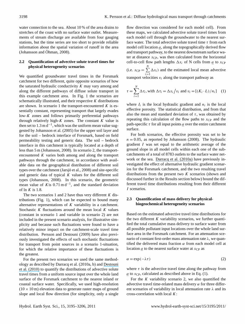
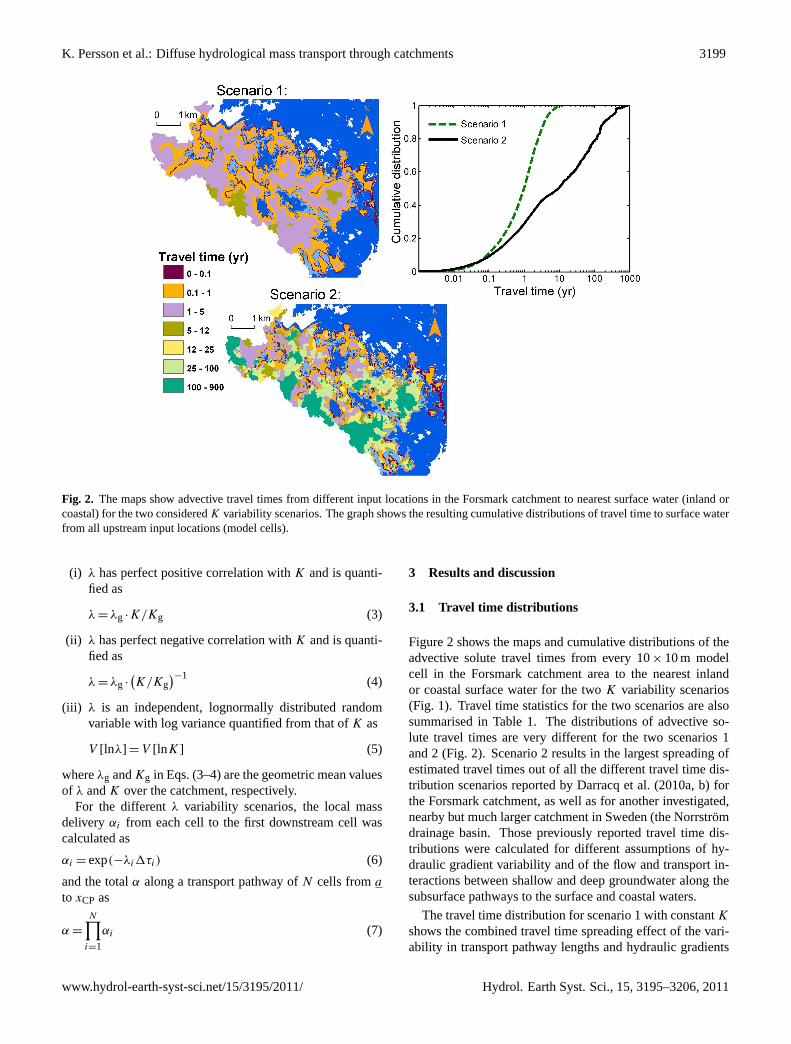
Fig. 2. The maps show advective travel times from different input locations in the Forsmark catchment to nearest surface water (inland orcoastal) for the two consideredK variability scenarios. The graph shows the resulting cumulative distributions of travel time to surface waterfrom all upstream input locations (model cells).

(i) λ has perfect positive correlation withK and is quanti-fied as

λ = λg ·K/Kg (3)

(ii) λ has perfect negative correlation withK and is quanti-fied as

λ = λg ·(K/Kg

)−1 (4)

(iii) λ is an independent, lognormally distributed randomvariable with log variance quantified from that ofK as

V [lnλ] = V [lnK] (5)

whereλg andKg in Eqs. (3–4) are the geometric mean valuesof λ andK over the catchment, respectively.

For the differentλ variability scenarios, the local massdelivery αi from each cell to the first downstream cell wascalculated as

αi = exp(−λi1τi) (6)

and the totalα along a transport pathway ofN cells froma

to xCP as

α =

N∏i=1

αi (7)

3 Results and discussion

3.1 Travel time distributions

Figure 2 shows the maps and cumulative distributions of theadvective solute travel times from every 10× 10 m modelcell in the Forsmark catchment area to the nearest inlandor coastal surface water for the twoK variability scenarios(Fig. 1). Travel time statistics for the two scenarios are alsosummarised in Table 1. The distributions of advective so-lute travel times are very different for the two scenarios 1and 2 (Fig. 2). Scenario 2 results in the largest spreading ofestimated travel times out of all the different travel time dis-tribution scenarios reported by Darracq et al. (2010a, b) forthe Forsmark catchment, as well as for another investigated,nearby but much larger catchment in Sweden (the Norrstromdrainage basin. Those previously reported travel time dis-tributions were calculated for different assumptions of hy-draulic gradient variability and of the flow and transport in-teractions between shallow and deep groundwater along thesubsurface pathways to the surface and coastal waters.

The travel time distribution for scenario 1 with constantK

shows the combined travel time spreading effect of the vari-ability in transport pathway lengths and hydraulic gradients

www.hydrol-earth-syst-sci.net/15/3195/2011/ Hydrol. Earth Syst. Sci., 15, 3195–3206, 2011

3200 K. Persson et al.: Diffuse hydrological mass transport through catchments

Table 1. Statistics of advective solute travel timeτ to nearest surface water for the twoK variability scenarios in Fig. 1.

Geometricmeanτ (yr)

Standard de-viation of lnτ

Arithmeticmeanτ (yr)

Coefficient ofvariation ofτ

Scenario 1 0.73 1.5 1.5 1.1Scenario 2 6.1 2.9 66 1.9

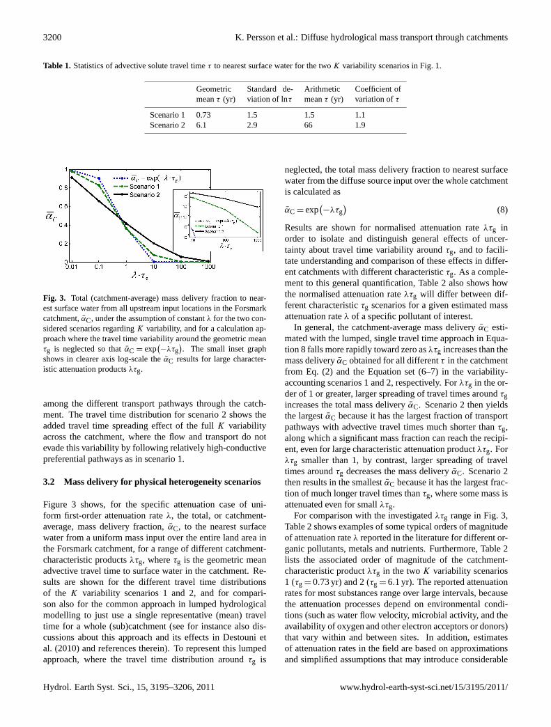
Fig. 3. Total (catchment-average) mass delivery fraction to near-est surface water from all upstream input locations in the Forsmarkcatchment,αC, under the assumption of constantλ for the two con-sidered scenarios regardingK variability, and for a calculation ap-proach where the travel time variability around the geometric meanτg is neglected so thatαC = exp

(−λτg

). The small inset graph

shows in clearer axis log-scale theαC results for large character-istic attenuation productsλτg.

among the different transport pathways through the catch-ment. The travel time distribution for scenario 2 shows theadded travel time spreading effect of the fullK variabilityacross the catchment, where the flow and transport do notevade this variability by following relatively high-conductivepreferential pathways as in scenario 1.

3.2 Mass delivery for physical heterogeneity scenarios

Figure 3 shows, for the specific attenuation case of uni-form first-order attenuation rateλ, the total, or catchment-average, mass delivery fraction,αC, to the nearest surfacewater from a uniform mass input over the entire land area inthe Forsmark catchment, for a range of different catchment-characteristic productsλτg, whereτg is the geometric meanadvective travel time to surface water in the catchment. Re-sults are shown for the different travel time distributionsof the K variability scenarios 1 and 2, and for compari-son also for the common approach in lumped hydrologicalmodelling to just use a single representative (mean) traveltime for a whole (sub)catchment (see for instance also dis-cussions about this approach and its effects in Destouni etal. (2010) and references therein). To represent this lumpedapproach, where the travel time distribution aroundτg is

neglected, the total mass delivery fraction to nearest surfacewater from the diffuse source input over the whole catchmentis calculated as

αC = exp(−λτg

)(8)

Results are shown for normalised attenuation rateλτg inorder to isolate and distinguish general effects of uncer-tainty about travel time variability aroundτg, and to facili-tate understanding and comparison of these effects in differ-ent catchments with different characteristicτg. As a comple-ment to this general quantification, Table 2 also shows howthe normalised attenuation rateλτg will differ between dif-ferent characteristicτg scenarios for a given estimated massattenuation rateλ of a specific pollutant of interest.

In general, the catchment-average mass deliveryαC esti-mated with the lumped, single travel time approach in Equa-tion 8 falls more rapidly toward zero asλτg increases than themass deliveryαC obtained for all differentτ in the catchmentfrom Eq. (2) and the Equation set (6–7) in the variability-accounting scenarios 1 and 2, respectively. Forλτg in the or-der of 1 or greater, larger spreading of travel times aroundτgincreases the total mass deliveryαC. Scenario 2 then yieldsthe largestαC because it has the largest fraction of transportpathways with advective travel times much shorter thanτg,along which a significant mass fraction can reach the recipi-ent, even for large characteristic attenuation productλτg. Forλτg smaller than 1, by contrast, larger spreading of traveltimes aroundτg decreases the mass deliveryαC. Scenario 2then results in the smallestαC because it has the largest frac-tion of much longer travel times thanτg, where some mass isattenuated even for smallλτg.

For comparison with the investigatedλτg range in Fig. 3,Table 2 shows examples of some typical orders of magnitudeof attenuation rateλ reported in the literature for different or-ganic pollutants, metals and nutrients. Furthermore, Table 2lists the associated order of magnitude of the catchment-characteristic productλτg in the twoK variability scenarios1 (τg = 0.73 yr) and 2 (τg = 6.1 yr). The reported attenuationrates for most substances range over large intervals, becausethe attenuation processes depend on environmental condi-tions (such as water flow velocity, microbial activity, and theavailability of oxygen and other electron acceptors or donors)that vary within and between sites. In addition, estimatesof attenuation rates in the field are based on approximationsand simplified assumptions that may introduce considerable

Hydrol. Earth Syst. Sci., 15, 3195–3206, 2011 www.hydrol-earth-syst-sci.net/15/3195/2011/

K. Persson et al.: Diffuse hydrological mass transport through catchments 3201

Table 2. Examples of pollutants and nutrients with corresponding estimates of first-order attenuation rateλ from reported field studies, andassociated order of magnitude of the attenuation productλτg for scenarios 1–2 in the Forsmark catchment area.

Example pollutants (for which givenλis consistent with field observations ofλ)

Attenuation rate(yr−1)

Attenuation product

Scenario 1τg = 0.73 yr

Scenario 2τg = 6.1 yr

Polychlorinated biphenyls (PCBs)(1),benzene(anaer;2,3), ethylbenzene(anaer;2,3),toluene(anaer;2,3,4), m,p,o-xylene(anaer;2,3),vinyl chloride(anaer;2,3), trichloroethene(anaer;2,3),naphthalene(anaer;2,4)

≤ 0.014 ≤ 0.01 ≤ 0.1

Polychlorinated biphenyls (PCBs)(1),zinc(5,6), phosphorus(7), benzene(anaer;2,3,8,9),ethylbenzene(anaer;2,3,9), toluene(anaer;2,3,4),m,p,o-xylene(anaer;2,3), vinyl chloride(anaer;2,3),trichloroethene(anaer;2,3), naphthalene(anaer;2,4),acenaphthylene(anaer;4)

0.14 0.1 1

Cadmium(5), copper(5), zinc(5,6),phosphorus(7,10), nitrogen(10), benzene(2,3,4,8,9,11),ethylbenzene(2,3,9,11), toluene(2,3,4,11,12),o-xylene(2,3,11), m,p-xylene(2,9,11), vinyl chloride(2,8),trichloroethene(2,8,11), naphthalene(2,4,11),a cenaphthylene(4,12), fluoranthene(11)

1.4 1 10

Benzene(aer;3,9,11), toluene(2,3,11,12),ethylbenzene(2,3,12), m,p,o-xylene(2,3,4,9,11,12),vinyl chloride(2,3), trichloroethene(2,3,11),naphthalene(2,12), acenaphthylene(12), acenaphthene(12),anthracene(12), fluoranthene(4,12)

14 10 100

Benzene(aer;3,12), toluene(aer;3,11,12),ethylbenzene(aer;3), trichloroethene(aer;3,11),vinyl chloride(aer;3) 140 100 1000

Benzene(aer;3), toluene(aer;3,11), ethylbenzene(aer;3)≥ 1400 ≥ 1000 ≥ 10000

(1) Sinkkonen and Paasivirta (2000),(2) Aronson and Howard (1997),(3) Suarez and Rifai (1999),4) Rogers et al. (2002),(5) Baresel et al. (2006),(6) Baresel and Destouni (2007),(7) Destouni et al. (2010),(8) Mulligan and Yong (2004),(9)Essaid et al. (2003),(10) Darracq et al. (2008)(11) Aronson et al. (1999),12) Bayer-Raich et al. (2006);(aer) Mainlyrelevant for aerobic conditions,(anaer) Mainly relevant for anaerobic conditions.

errors (Bekins et al., 1998; Suarez and Rifai, 1999; Washing-ton and Cameron, 2001; Mulligan and Yong, 2004). Never-theless, Table 2 demonstrates that the investigatedλτg rangein this paper is relevant for a wide range of different environ-mental pollutants and characteristic catchment conditions;the latter because the investigated travel time pdfs bound awide range of different possible catchment situations regard-ing advective transport and its associated uncertainties (seecomparisons between different scenarios and catchment ex-amples in Darracq et al., 2010a, b). For the quantification ofthe waterborne transport of some compounds of interest in aspecific (sub)catchment, the range of relevant reported atten-uation rates can be narrowed through a more detailed assess-ment of the prevailing environmental conditions in relation tothe ones reported at the sites where attenuation rates of these

compounds have been estimated in previous studies. Table 2further shows that for scenario 2 the catchment-relevantλτgrange for some substances under aerobic attenuation condi-tions may extend to even greater values than the maximumλτg = 1000 shown in Fig. 3. If the prevailing catchment-scaleτ variability is neglected or underestimated (Fig. 3),high-λτg conditions and resulting underestimation of pollu-tant deliveryαC may be more likely to occur in the field forthese and other substances than low-λτg conditions withαCoverestimation.

www.hydrol-earth-syst-sci.net/15/3195/2011/ Hydrol. Earth Syst. Sci., 15, 3195–3206, 2011

3202 K. Persson et al.: Diffuse hydrological mass transport through catchments

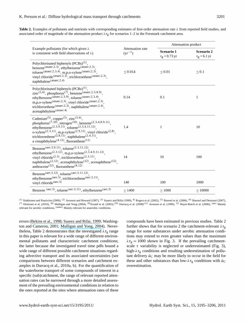
Fig. 4. Total (catchment-average) mass delivery fraction to near-est surface water from all upstream input locations in the Forsmarkcatchment,αC. Mass deliveryαC results are shown for differentassumptions regarding the correlation betweenK andλ in the K

variability scenario 2, relative toαC for theK variability scenario 1(in which bothK andλ are constant). Corresponding maps of localmass deliveryα to nearest surface water are shown in Fig. 5 for thefour specific result points indicated in this figure.

3.3 Mass delivery for physical-biogeochemicalheterogeneity scenarios

For the possibility that alsoλ varies, along withK and τ ,Fig. 4 shows for different cases of correlation betweenλ andK, the resulting catchment-averageαC in scenario 2, rela-tive to that in scenario 1, which has constantKandλ, andsmaller resultingτ variability (Fig. 2). Forλgτg < 10, thevariableλ cases of negative or noλ–Kcorrelation yield pol-lutant mass deliveryαC that is smaller than that of positivecorrelation or noλ variability. The negativeλ–K correla-tion implies that the zones with smaller than averageK havelarger than average attenuation rateλ, with both factors in-creasing pollutant attenuation relative to average conditions.In the case of noλ–K correlation, whereλ in each model cellis an independent random variable,λ is much greater than av-erage along considerable parts of most transport pathways;this variability manifestation then results in more attenuatedmass in total, and thereby smaller mass deliveryαC, com-pared to the constantλ variability case for a wide range ofaverageλgτg conditions. For positiveλ–K correlation, thezones with larger than averageλ also have larger than aver-ageK, so that theλ effect is to increase and theKeffect isto decrease pollutant attenuation; together these opposite ef-fects may balance the resulting attenuation close to averageλ andK conditions.

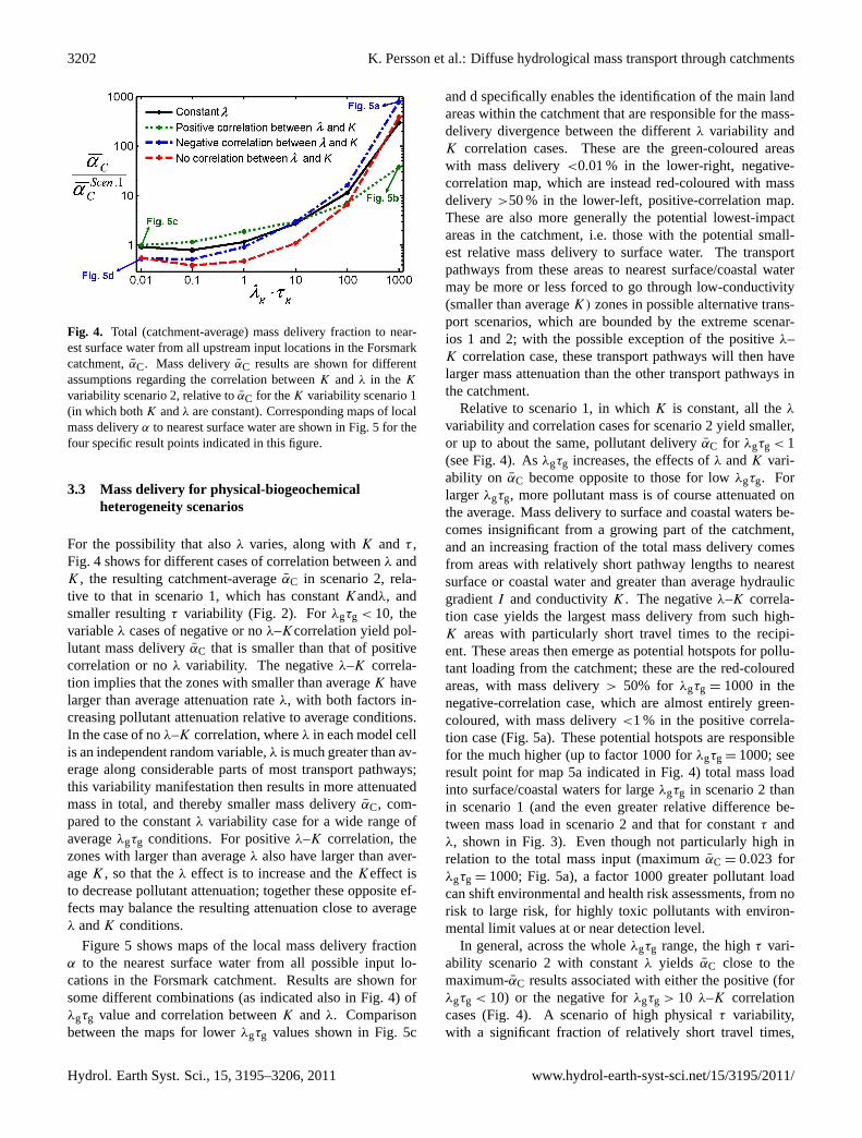
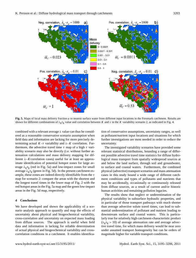
Figure 5 shows maps of the local mass delivery fractionα to the nearest surface water from all possible input lo-cations in the Forsmark catchment. Results are shown forsome different combinations (as indicated also in Fig. 4) ofλgτg value and correlation betweenK andλ. Comparisonbetween the maps for lowerλgτg values shown in Fig. 5c

and d specifically enables the identification of the main landareas within the catchment that are responsible for the mass-delivery divergence between the differentλ variability andK correlation cases. These are the green-coloured areaswith mass delivery<0.01 % in the lower-right, negative-correlation map, which are instead red-coloured with massdelivery >50 % in the lower-left, positive-correlation map.These are also more generally the potential lowest-impactareas in the catchment, i.e. those with the potential small-est relative mass delivery to surface water. The transportpathways from these areas to nearest surface/coastal watermay be more or less forced to go through low-conductivity(smaller than averageK) zones in possible alternative trans-port scenarios, which are bounded by the extreme scenar-ios 1 and 2; with the possible exception of the positiveλ–K correlation case, these transport pathways will then havelarger mass attenuation than the other transport pathways inthe catchment.

Relative to scenario 1, in whichK is constant, all theλvariability and correlation cases for scenario 2 yield smaller,or up to about the same, pollutant deliveryαC for λgτg < 1(see Fig. 4). Asλgτg increases, the effects ofλ andK vari-ability on αC become opposite to those for lowλgτg. Forlargerλgτg, more pollutant mass is of course attenuated onthe average. Mass delivery to surface and coastal waters be-comes insignificant from a growing part of the catchment,and an increasing fraction of the total mass delivery comesfrom areas with relatively short pathway lengths to nearestsurface or coastal water and greater than average hydraulicgradientI and conductivityK. The negativeλ–K correla-tion case yields the largest mass delivery from such high-K areas with particularly short travel times to the recipi-ent. These areas then emerge as potential hotspots for pollu-tant loading from the catchment; these are the red-colouredareas, with mass delivery> 50% for λgτg = 1000 in thenegative-correlation case, which are almost entirely green-coloured, with mass delivery<1 % in the positive correla-tion case (Fig. 5a). These potential hotspots are responsiblefor the much higher (up to factor 1000 forλgτg = 1000; seeresult point for map 5a indicated in Fig. 4) total mass loadinto surface/coastal waters for largeλgτg in scenario 2 thanin scenario 1 (and the even greater relative difference be-tween mass load in scenario 2 and that for constantτ andλ, shown in Fig. 3). Even though not particularly high inrelation to the total mass input (maximumαC = 0.023 forλgτg = 1000; Fig. 5a), a factor 1000 greater pollutant loadcan shift environmental and health risk assessments, from norisk to large risk, for highly toxic pollutants with environ-mental limit values at or near detection level.

In general, across the wholeλgτg range, the highτ vari-ability scenario 2 with constantλ yields αC close to themaximum-αC results associated with either the positive (forλgτg < 10) or the negative forλgτg > 10 λ–K correlationcases (Fig. 4). A scenario of high physicalτ variability,with a significant fraction of relatively short travel times,

Hydrol. Earth Syst. Sci., 15, 3195–3206, 2011 www.hydrol-earth-syst-sci.net/15/3195/2011/

K. Persson et al.: Diffuse hydrological mass transport through catchments 3203

Fig. 5. Maps of local mass delivery fractionα to nearest surface water from different input locations in the Forsmark catchment. Results areshown for different combinations ofλgτg value and correlation betweenK andλ in theK variability scenario 2, as indicated in Fig. 4.

combined with a relevant averageλ value can thus be consid-ered as a reasonable conservative scenario assumption whenfield data and information are lacking for more precisely de-termining actualK–τ variability andλ–K correlation. Fur-thermore, the advective travel timeτ map of a highτ vari-ability scenario may also be directly (i.e. without further at-tenuation calculations and mass delivery mapping for dif-ferentλ–Kcorrelation cases) useful for at least an approx-imate identification of potential hotspot zones for large av-erageλgτg (red in Fig. 5a) and low-impact zones for smallaverageλgτg (green in Fig. 5d). In the present catchment ex-ample, these zones are indeed directly identifiable from theτ

map for scenario 2: compare the areas with the shortest andthe longest travel times in the lower map of Fig. 2 with thered hotspot areas in the Fig. 5a map and the green low-impactareas in the Fig. 5d map, respectively.

4 Conclusions

We have developed and shown the applicability of a sce-nario analysis approach to quantify and map the effects ofuncertainty about physical and biogeochemical variability,cross-correlation and uncertainty on expected mass loadingfrom diffuse sources. The approach is useful when fielddata and information is lacking for reliable determinationof actual physical and biogeochemical variability and cross-correlation conditions in a catchment. It enables identifica-

tion of conservative assumptions, uncertainty ranges, as wellas pollutant/nutrient input locations and situations for whichfurther investigations are most needed in order to reduce theuncertainty.

The investigated variability scenarios have provided somerelevant statistical distributions, bounding a range of differ-ent possible advective travel time statistics for diffuse hydro-logical mass transport from spatially widespread sources atand below the land surface, through soil and groundwater,to surface and coastal waters. Furthermore, the combinedphysical (advective) transport scenarios and mass attenuationcases in this study bound a wide range of different catch-ment conditions and types of pollutants and nutrients thatmay be accidentally, occasionally or continuously releasedfrom diffuse sources, as a result of current and/or historichuman activities and remaining pollution legacies.

The results show that neglect or underestimation of thephysical variability in subsurface hydraulic properties, andin particular of those transport pathways with much shorterthan average advective solute travel times, can lead to sub-stantial underestimation of pollutant and nutrient loading todownstream surface and coastal waters. This is particu-larly true for relatively high catchment-characteristic product(λgτg > 10) of average attenuation rate and average advec-tive travel time, for which mass delivery would be near zerounder assumed transport homogeneity but can be orders ofmagnitude higher for variable transport conditions.

www.hydrol-earth-syst-sci.net/15/3195/2011/ Hydrol. Earth Syst. Sci., 15, 3195–3206, 2011

3204 K. Persson et al.: Diffuse hydrological mass transport through catchments

The study results further show that a scenario of high phys-ical advection variability, with a significant fraction of rela-tively short travel times (here scenario 2), combined with arelevant average biogeochemical attenuation rate, may be agenerally reasonable, conservative assumption for estimatingmaximum diffuse mass loading when the prevailing physi-cal and biogeochemical variability and cross-correlation areuncertain. A conservative travel time distribution can for in-stance be constructed by combining the shape of the statisti-cal distribution of travel times obtained for a scenario of highphysical advection variability around catchment-average ad-vection conditions, with some estimated, relatively shortmean advective travel time obtained for a transport scenariowith dominant, relatively fast preferential pathways, as in thepresent scenario 1.

As done here for scenario 2, scenarios of large relativetravel time spreading can consider the finest resolved avail-able catchment data on topography and soil variability, whichcan be further translated into hydraulic conductivity and hy-draulic gradient patterns, respectively. These patterns to-gether with transport pathway distances to nearest surfacewater (estimated from topography, land cover and soil data)yield travel time distribution scenarios. Not all of these un-derlying control factors of advection variability are equallyor similarly important in determining relevant travel time dis-tribution scenarios in different catchments. The individualeffects of different control factors may further have similar,overlapping effects on the resulting travel time distributions.For instance, fine-resolved variability in local topographicslopes can be translated into a scenario of high hydraulic gra-dient variability as done by Darracq et al. (2010a), yieldingsimilarly large spreading of travel times as does the presentscenario 2 with fine-resolvedK variability but coarser (sub-catchment-wise) hydraulic gradient resolution.

Our results also demonstrate how geographic mapping ofadvective travel times to a sensitive recipient from all po-tential pollutant and nutrient input locations within a catch-ment can be used to identify hotspot areas with large po-tential mass loading to the recipient, and their opposite, ar-eas with the potentially lowest loading within a catchment.Such substance-independent calculations and mapping of ad-vective travel times can thus be useful for at least approx-imate predictive identification of the parts of a catchmentarea where pollutant and nutrient releases are most and leastlikely to contribute much to pollution or eutrophication ofdownstream water systems, and where environmental pro-tection/remediation measures may be most and least neededand effective. Maps of advective travel times and mass de-livery to a recipient from different parts of a catchment arealso relevant for the assessment of the risk of pollution oreutrophication from multiple local sources and from diffusesources that are spatially variable.

Acknowledgements.We thank the Swedish Research Council(VR; project number 2006-4366, contract number 60436601) forfinancial support of this work, which has also been carried outin and links the frameworks of Stockholm University’s strategicenvironmental research programme EkoKlim and marine environ-mental research programme BEAM.

Edited by: B. Schaefli

References

Andricevic, R. and Cvetkovic, V.: Evaluation of risk from contam-inants migrating by ground water, Water Resour. Res., 32, 611–621, 1996

Aronson, D. and Howard, P. H.: Anaerobic biodegradation of or-ganic chemicals in groundwater: A summary of field and labo-ratory studies, Syracuse Research Corporation, North Syracuse,NY, USA, 1997.

Aronson, D., Citra, M., Shuler, K., Printup, H., and Howard, P. H.:Aerobic biodegradation of organic chemicals in environmentalmedia: A summary of field and laboratory studies, Syracuse Re-search Corporation, North Syracuse, NY, USA, 1999.

Baresel, C. and Destouni, G.: Uncertainty-accounting environmen-tal policy and management of water systems, Environ. Sci. Tech-nol., 41, 3653–3659,doi:10.1021/es061515e, 2007.

Baresel, C., Destouni, G., and Gren, I.-M.: The influence of metalsource uncertainty on cost-effective allocation of mine water pol-lution abatement in catchments, J. Environ. Manage., 78, 138–148,doi:10.1016/j.jenvman.2005.03.013, 2006.

Basu, N. B., Destouni, G., Jawitz, J. W., Thompson, S. E.,Loukinova, N. V., Darracq, A., Zanardo, S., Yaeger, M.A., Sivapalan, M., Rinaldo, A., and Rao, P. S. C.: Nutri-ent loads exported from managed catchments reveal emergentbiogeochemical stationarity. Geophys. Res. Lett., 37, L23404,doi:10.1029/2010GL045168, 2010.

Batchelor, B., Valdes, J., and Araganth, V.: Stochastic risk assess-ment of sites contaminated by hazardous waste, J. Environ. Eng.,124, 380–388, 1998.

Bayer-Raich, M., Jarsjo, J., Liedl, R., Ptak, T., and Teutsch, G.:Integral pumping test analyses of linearly sorbed groundwa-ter contaminants using multiple wells: Inferring mass flowsand natural attenuation rates, Water Resour. Res., 42, W08411,doi:10.1029/2005WR004244, 2006.

Bekins, B. A., Warren, E., and Godsy, E. M.: A comparison of zero-order, first-order, and Monod biotransformation models, GroundWater, 36, 261–268, 1998.

Bergknut, M., Meijer, S., Halsall, C.,Agren, A., Laudon, H.,Kohler, S., Jones, K. C., Tysklind, M., and Wiberg, K.: Mod-elling the fate of hydrophobic organic contaminants in a borealforest catchment: A cross disciplinary approach to assessing dif-fuse pollution to surface waters, Environ. Pollut., 158, 2964–2969, 2010.

Beven, K. J.: A manifesto for the equifinality thesis, J. Hydrol., 320,18–36, 2006.

Beven, K. J.: Preferential flow and travel time distributions: defin-ing adequate hypothesis tests for hydrological models, Hydrol.Process., 24, 1537–1547, 2010.

Brydsten, L. and Stromgren, M.: Digital elevation models for siteinvestigation programme in Forsmark. Swedish Nuclear Fuel and

Hydrol. Earth Syst. Sci., 15, 3195–3206, 2011 www.hydrol-earth-syst-sci.net/15/3195/2011/

K. Persson et al.: Diffuse hydrological mass transport through catchments 3205

Waste Management Company Report P-04-70, Stockholm, 2004.Carpenter, S. R., Caraco, N. F., Correll, D. L., Howarth, R. W.,

Sharpley, A. N., and Smith, V. H.: Nonpoint pollution of surfacewaters with phosphorus and nitrogen. Ecol. Appl., 8, 559–568,1998.

Chapell, F. H.: The significance of microbial processes in hydrologyand geochemistry, Hydrogeol. J., 8, 41–46, 2000.

Cozzarelli, I. M., Herman, J. S., Baedecker, M. J., and Fischer,J. M.: Geochemical heterogeneity of a gasoline-contaminatedaquifer, J. Contam. Hydrol., 40, 261–284, 1999.

Cunningham, J. A. and Fadel, Z. J.: Contaminant degradation inphysically and chemically heterogeneous aquifers, J. Contam.Hydrol., 94, 293–304, 2007.

Cvetkovic, V. and Dagan, G.: Transport of kinetically sorbing soluteby steady random velocity in heterogeneous porous formations,J, Fluid Mech., 265, 189–215, 1994.

Cvetkovic, V. and Shapiro, A.: Mass arrival of sorptive solute in het-erogeneous porous media, Water Resour. Res., 26, 2057–2067,1990.

Cvetkovic, V., Dagan, G., and Shapiro, A. M.: A soluteflux approach to transport in heterogeneous formations 2:Uncertainty analysis, Water Resour. Res., 28, 1377–1388,doi:10.1029/91WR03085, 1992.

Darracq, A. and Destouni, G.: Physical versus biogeochemi-cal interpretations of Nitrogen and Phosphorus attenuation instreams and its dependence on stream characteristics, GlobalBiogeochem. Cy., 21, GB3003,doi:10.1029/2006GB002901,2007.

Darracq, A., Greffe, F., Hannerz, F., Destouni, G., and Cvetkovic,V.: Nutrient transport scenarios in a changing Stockholm andMalaren valley region, Water Sci. Technol., 51, 31–38, 2005.

Darracq, A., Lindgren, G. A., and Destouni, G.: Long-term de-velopment of phosphorus and nitrogen loads through the subsur-face and surface water systems of drainage basins, Global Bio-geochem. Cy., 22, GB3022,doi:10.1029/2007GB003022, 2008.

Darracq, A., Destouni, G., Persson, K., Prieto, C., and Jarsjo, J.:Quantification of advective solute travel times and mass trans-port through hydrological catchments, Environ. Fluid Mech., 10,103–120,doi:10.1007/s10652-009-9147-2, 2010a.

Darracq, A., Destouni, G., Persson, K., Prieto, C., and Jarsjo, J.:Scale and model resolution effects on the distributions of ad-vective solute travel times in catchments, Hydrol. Process., 24,1697–1710,doi:10.1002/hyp.7588, 2010b.

Destouni, G. and Cvetkovic, V.: Field scale mass arrival of sorptivesolute into the groundwater, Water Resour. Res. 27, 1315–1325,1991.

Destouni, G., Lindgren, G., and Gren, I. M.: Effects of inlandnitrogen transport and attenuation modeling on coastal nitro-gen load abatement, Environ. Sci. Technol., 40, 6208–6214,doi:10.1021/es060025j, 2006.

Destouni, G., Hannerz, F., Prieto, C., Jarsjo, J., and Shibuo, Y.:Small unmonitored near-coastal catchment areas yielding largemass loading to the sea, Global Biogeochem. Cy., 22, GB4003,doi:10.1029/2008GB003287, 2008.

Destouni, G., Persson, K., Prieto, C., and Jarsjo J.: Generalquantification of catchment-scale nutrient and pollutant transportthrough the subsurface to surface and coastal waters, Environ.Sci. Technol., 44, 2048–2055, 2010.

Edwards, A. C. and Withers, P. J. A.; Transport and delivery of

suspended solids, nitrogen and phosphorus from various sourcesto freshwaters in the UK, J. Hydrol., 350, 144–153, 2008.

Eggleston, J. R. and Rojstaczer, S. A.: Can we predict subsurfacemass transport?, Environ. Sci. Technol., 34, 4010–4017, 2000.

Essaid, H. I., Cozzarell, I. M., Eganhouse, R. P., Herkelrath, W.N., Bekins, B. A., and Delin, G. N.: Inverse modeling of BTEXdissolution and biodegradation at the Bemidji, MN crude-oil spillsite, J. Contam. Hydrol., 67, 269–299, 2003.

Ganoulis, J.: Risk Analysis of Water Pollution: Second, revised andexpanded edition, WILEY-VCH Verlag, Weinheim, 2009.

Gren, I. M., Destouni, G., and Sharin, H.: Cost effective manage-ment of stochastic coastal water pollution, Environ. Model. As-sess., 5, 193–203, 2000.

Hagemann, S. and Jacob, D.: Gradient in the climate change sig-nal of European discharge predicted by a multi-model ensemble,Climatic Change, 81, 309–327, 2007.

Hannerz, F. and Destouni, G.: Spatial characterization of the BalticSea Drainage Basin and its unmonitored catchments, Ambio, 35,214–219, 2006.

Howden, N. J. K, Burt, T. P, Mathias, S. A., Worrall, F., and Whe-lan, M. J.: Modelling long-term diffuse nitrate pollution at thecatchment-scale: Data, parameter and epistemic uncertainty, J.Hydrol., 403, 337–351, 2011.

Jacob, D., Barring, L., Christensen, O. B., Christensen, J. H., Hage-mann, S., Hirschi, M., Kjellstrom, E., Lenderink, G., Rockel, B.,Schar, C., Seneviratne, S. I., Somot, S., van Ulden, A., and vanden Hurk, B.: An inter-comparison of regional climate modelsfor Europe: design of the experiments and model performance.Climatic Change 81(Supplement 1), 31–52, 2007.

Jardine, P. M.: Influence of coupled processes on contaminant fateand transport in subsurface environments, Adv. Agronomy, 99,doi:10.1016/S0065-2113(08)00401-X, 2008.

Jarsjo, J. and Bayer-Raich, M.: Estimating plume degrada-tion rates in aquifers: effect of propagating measurementand methodological errors, Water Resour. Res., 44, W02501,doi:10.1029/2006WR005568, 2008.

Jarsjo, J., Bayer-Raich, M., and Ptak, T.: Monitoring groundwatercontamination and delineating source zones at industrial sites:Uncertainty analyses using integral pumping tests, J. Contam.Hydrol., 79, 107–134, 2005.

Jarsjo, J., Shibuo, Y., and Destouni, G.: Spatial distribution of un-monitored inland water flows to the sea, J. Hydrol., 348, 59–72,2008.

Johansson, P.-O.: Description of surface hydrology and near-surface hydrogeology at Forsmark, Site descriptive modelling,SDM-Site Forsmark. Swedish Nuclear Fuel and Waste Manage-ment Co Report R-08-08, 2008.

Johansson, P.-O. andOhman, J.: Presentation of meteorological,hydrological and hydrogeological monitoring data from Fors-mark: Site descriptive modelling – SDM-Site Forsmark, SwedishNuclear Fuel and Waste Management Co Report R-08-10, 2008.

Johansson, P.-O., Werner, K., Bosson, E., and Juston, J.: De-scription of climate, surface hydrology, and near-surface hydrol-ogy. Preliminary site description. Forsmark area – version 1.2.Swedish Nuclear Fuel and Waste Management Co Report R-05-06, 2005.

Kysely, J. and Beranova, R.: Climate change effects on extremeprecipitation in central Europe: uncertainties of scenarios basedon regional climate models, Theor. Appl. Climatol., 95, 361–374,

www.hydrol-earth-syst-sci.net/15/3195/2011/ Hydrol. Earth Syst. Sci., 15, 3195–3206, 2011

3206 K. Persson et al.: Diffuse hydrological mass transport through catchments

2009.Lindgren, G. A. and Destouni, G.: Nitrogen loss rates in streams:

Scale-dependence and up-scaling methodology, Geophys. Res.Lett., 31, L13501, doi:10.1029/2004GL019996, 2004.

Malmstrom, M. E., Destouni, G., and Martinet, P.: Modeling ex-pected solute concentration in randomly heterogeneous flow sys-tems with multicomponent reactions, Environ. Sci. Technol., 38,2673–2679, 2004.

Malmstrom, M. E., Berglund, S., and Jarsjo, J.: Combined effects ofspatially variable flow and mineralogy on the attenuation of acidmine drainage in groundwater, Appl. Geochem. 23, 1419–1436,doi:10.1016/j.apgeochem.2007.12.029, 2008.

McDonnell, J. J., McGuire, K., Aggarwal, P., Beven, K., Biondi,D., Destouni, G., Dunn, S., James, A., Kirchner, J., Kraft, S.,Lyon, S., Malowszewski, P., Newman, L., Pfister, L., Rinaldo,A., Rodhe, A., Sayama, T., Seibert, J., Soloman, K., Soulsby,C., Stewart, M., Tetzlaff, D., Tobin, C., Troch, P., Weiler, M.,Western, A., Wormann, A., and Wrede, S.: How old is streamwater? Open questions in catchment transit time conceptualisa-tion, modelling and analysis, Hydrol. Process., 24, 1745–1754,2010.

McGuire, K. J., McDonnell, J. J., Weiler, M., Kendall, C., McG-lynn, B. L., Welker, J. M., and Seibert, J.: The role of topographyon catchment-scale water residence time, Water Resour. Res. 41,W05002.1–W05002.14, doi:10.1029/2004WR003657, 2005.

Mulligan, C. N. and Yong, R. N.: Natural attenuation of contami-nated soils, Environ. Int., 30, 587–601, 2004.

Persson, K. and Destouni, G.: Propagation of water pollu-tion uncertainty and risk from the subsurface to the sur-face water system of a catchment, J. Hydrol., 377, 434–444,doi:10.1016/j.hydrol.2009.09.001, 2009.

Rogers, S. W., Ong, S. K., Kjartanson, B. H., Golchin, J., andStenback, G. A.: Natural attenuation of polycyclic aromatichydrocarbon-contaminated sites: review. Pract. Periodical Haz.,Toxic, and Radioactive Waste Mgmt., 6, 141–155, 2002.

Refsgaard, J. C., van der Sluijs, J. P., Brown, J., and van der Keur, P.:A framework for dealing with uncertainty due to model structureerror, Adv. Water Resour., 29, 1586–1597, 2006.

Sinkkonen, S. and Paasivirta, J.: Degradation half-life times ofPCDDs, PCDFs and PCBs for environmental fate modeling,Chemosphere, 40, 943–949, 2000.

SKB: Site description of Forsmark at completion of the site inves-tigation phase: SDM-Site Forsmark. Swedish Nuclear Fuel andWaste Management Co Report TR-08-05, 2008.

Suarez, M. P. and Rifai, H. S.: Biodegradation rates for fuel hydro-carbons and chlorinated solvents in groundwater, BioremediationJournal, 3, 337–362, 1999.

Washington, J. W. and Cameron, B. A.: Evaluating degradationrates of chlorinated organics in groundwater using analyticalmodels, Environ. Toxicol. Chem., 20, 1909–1915, 2001.

Werner, K., Johansson, P., Brydsten, L., Bosson, E., Berglund, S.,Trojbom, M., and Nyman, H.: Recharge and discharge of near-surface hydrology, Swedish Nuclear Fuel and Waste Manage-ment Co Report R-07-08, 2007.

Hydrol. Earth Syst. Sci., 15, 3195–3206, 2011 www.hydrol-earth-syst-sci.net/15/3195/2011/