Assessment of a distributed biosphere hydrological model against streamflow and MODIS land surface...

Journal of Hydrology xxx (2009) xxx–xxx

ARTICLE IN PRESS

Contents lists available at ScienceDirect

Journal of Hydrology

journal homepage: www.elsevier .com/ locate / jhydrol

Assessment of a distributed biosphere hydrological model against streamflowand MODIS land surface temperature in the upper Tone River Basin

Lei Wang a,*, Toshio Koike a, Kun Yang b, Pat Jen-Feng Yeh c

a Department of Civil Engineering, The University of Tokyo, Bunkyo-ku, Tokyo 113-8656, Japanb Institute of Tibetan Plateau Research, Chinese Academy of Sciences, Beijing 100085, Chinac Institute of Industrial Science, The University of Tokyo, Tokyo 153-8505, Japan

a r t i c l e i n f o s u m m a r y

Article history:Received 19 August 2008Received in revised form 24 June 2009Accepted 2 August 2009Available online xxxx

This manuscript was handled by K.Georgakakos, Editor-in-Chief, with theassistance of Christa D. Peters-Lidard,Associate Editor

Keywords:Distributed biosphere hydrological modelWater cycleEnergy budgetLand surface temperatureStreamflowFlood

0022-1694/$ - see front matter � 2009 Elsevier B.V. Adoi:10.1016/j.jhydrol.2009.08.005

* Corresponding author. Address: River Lab, DepartmUniversity of Tokyo, Hongo 7-3-1, Bunkyo-ku, Tokyo5841 6107; fax: +81 3 5841 6130.

E-mail address: [email protected] (L. Wa

Please cite this article in press as: Wang, L., et atemperature in the upper Tone River Basin. J. H

Land surface temperature (LST) is a key parameter in land–atmosphere interactions. The recentlyreleased Moderate Resolution Imaging Spectroradiometers (MODIS) LST Version 5 products have pro-vided good tools to evaluate water and energy budget modelling for river basins. In this study, a distrib-uted biosphere hydrological model (WEB-DHM; so-called water and energy budget-based distributedhydrological model) that couples a biosphere scheme (SiB2) with a geomorphology-based hydrologicalmodel (GBHM), is applied to the upper Tone River Basin where flux observations are not available. Themodel facilitates a better understanding of the water and energy cycles in this region. After being cali-brated with discharge data, WEB-DHM is assessed against observed streamflows at four major gaugesand MODIS LST. Results show that long-term streamflows including annual largest floods are well repro-duced. As well, both daytime and nighttime LSTs simulated by WEB-DHM agree well with MODIS obser-vations for both basin-averaged values and spatial patterns. The validated model is then used to analyzewater and energy cycles of the upper Tone River Basin. It was found that from May to October, with rel-atively large leaf area index (LAI) values, the simulated daily maximum LST is close to soil surface tem-perature (Tg) since Tg is much greater than canopy temperature (Tc) in their peak values; while the dailyminimum LST appears similar to Tc. For other months with relatively small LAI values, the diurnal cyclesof LST closely follow Tg.

� 2009 Elsevier B.V. All rights reserved.

Introduction

The Tone River Basin is Japan’s largest with a catchment area of15,628.7 km2. It is the main water supply for about 27 million peo-ple living in the Kanto region, which includes the Tokyo Metropol-itan Area, the political and economic center of Japan.

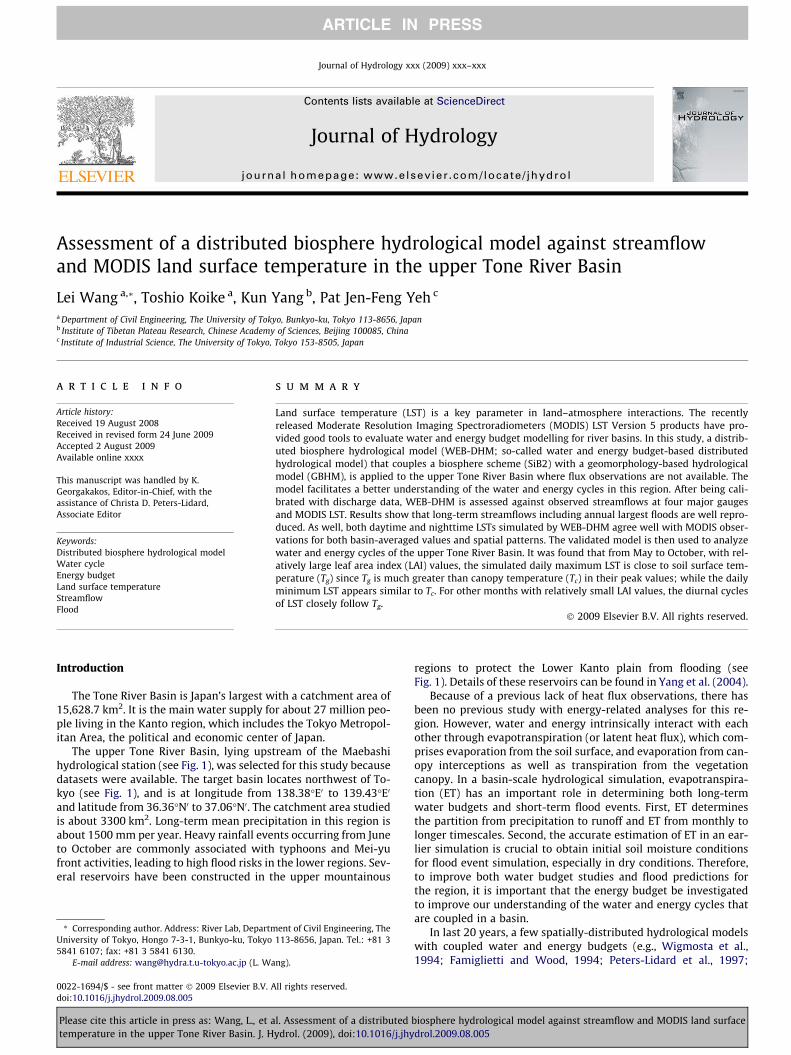
The upper Tone River Basin, lying upstream of the Maebashihydrological station (see Fig. 1), was selected for this study becausedatasets were available. The target basin locates northwest of To-kyo (see Fig. 1), and is at longitude from 138.38�E0 to 139.43�E0

and latitude from 36.36�N0 to 37.06�N0. The catchment area studiedis about 3300 km2. Long-term mean precipitation in this region isabout 1500 mm per year. Heavy rainfall events occurring from Juneto October are commonly associated with typhoons and Mei-yufront activities, leading to high flood risks in the lower regions. Sev-eral reservoirs have been constructed in the upper mountainous

ll rights reserved.

ent of Civil Engineering, The113-8656, Japan. Tel.: +81 3

ng).

l. Assessment of a distributedydrol. (2009), doi:10.1016/j.jhy

regions to protect the Lower Kanto plain from flooding (seeFig. 1). Details of these reservoirs can be found in Yang et al. (2004).

Because of a previous lack of heat flux observations, there hasbeen no previous study with energy-related analyses for this re-gion. However, water and energy intrinsically interact with eachother through evapotranspiration (or latent heat flux), which com-prises evaporation from the soil surface, and evaporation from can-opy interceptions as well as transpiration from the vegetationcanopy. In a basin-scale hydrological simulation, evapotranspira-tion (ET) has an important role in determining both long-termwater budgets and short-term flood events. First, ET determinesthe partition from precipitation to runoff and ET from monthly tolonger timescales. Second, the accurate estimation of ET in an ear-lier simulation is crucial to obtain initial soil moisture conditionsfor flood event simulation, especially in dry conditions. Therefore,to improve both water budget studies and flood predictions forthe region, it is important that the energy budget be investigatedto improve our understanding of the water and energy cycles thatare coupled in a basin.

In last 20 years, a few spatially-distributed hydrological modelswith coupled water and energy budgets (e.g., Wigmosta et al.,1994; Famiglietti and Wood, 1994; Peters-Lidard et al., 1997;

biosphere hydrological model against streamflow and MODIS land surfacedrol.2009.08.005

http://dx.doi.org/10.1016/j.jhydrol.2009.08.005

mailto:[email protected]

http://www.sciencedirect.com/science/journal/00221694

http://www.elsevier.com/locate/jhydrol


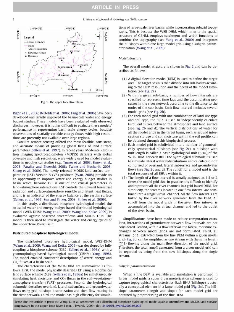
Fig. 1. The upper Tone River Basin.

2 L. Wang et al. / Journal of Hydrology xxx (2009) xxx–xxx

ARTICLE IN PRESS

Rigon et al., 2006; Bertoldi et al., 2006; Tang et al., 2006) have beendeveloped and largely improved the basin-scale water and energybudget studies. These models have been evaluated with observeddischarges; however, it is rather difficult to evaluate these models’performance in representing basin-scale energy cycles, becauseobservations of spatially variable energy fluxes with high resolu-tions are presently not available over large regions.

Satellite remote sensing offered the most feasible, consistent,and accurate means of providing global fields of land surfaceparameters (Sellers et al., 1997). In recent years, Moderate Resolu-tion Imaging Spectroradiometers (MODIS) datasets with globalcoverage and high resolution, were widely used for model evalua-tions in geophysical studies (e.g., Turner et al., 2003; Brown et al.,2008; Parajka and Bloeschl, 2008; Twine and Kucharik, 2008;Sheng et al., 2009). The newly-released MODIS land surface tem-perature (LST) Version 5 (V5) products (Wan, 2008) provide usan opportunity to improve water and energy budget studies inbasin scales, because LST is one of the crucial parameters inland–atmosphere interactions. LST controls the upward terrestrialradiation and surface-atmosphere sensible and latent heat fluxes,and it is an indicator of the energy balance at the earth’s surface(Sellers et al., 1997; Sun and Pinker, 2003; Pinker et al., 2009).

In this study, a distributed biosphere hydrological model, theso-called water and energy budget-based distributed hydrologicalmodel (WEB-DHM; Wang et al., 2009; Wang and Koike, 2009), isevaluated against observed streamflows and MODIS LSTs. Themodel is then used to investigate the water and energy cycles ofthe upper Tone River Basin.

Distributed biosphere hydrological model

The distributed biosphere hydrological model, WEB-DHM(Wang et al., 2009; Wang and Koike, 2009) was developed by fullycoupling a biosphere scheme (SiB2; Sellers et al., 1996a) with ageomorphology-based hydrological model (GBHM; Yang, 1998).The model enabled consistent descriptions of water, energy andCO2 fluxes at a basin scale.

The characteristics of the WEB-DHM are summarized as fol-lows. First, the model physically describes ET using a biophysicalland surface scheme (SiB2; Sellers et al., 1996a) for simultaneouslysimulating heat, moisture, and CO2 fluxes in the soil–vegetation–atmosphere transfer (SVAT) processes. Second, the hydrologicalsubmodel describes overland, lateral subsurface, and groundwaterflows using grid-hillslope discretization and then flow routing inthe river network. Third, the model has high efficiency for simula-

Please cite this article in press as: Wang, L., et al. Assessment of a distributedtemperature in the upper Tone River Basin. J. Hydrol. (2009), doi:10.1016/j.jhy

tions of large-scale river basins while incorporating subgrid topog-raphy. This is because the WEB-DHM, which inherits the spatialstructure of GBHM, employs catchment and width functions tocombine the topography (see Yang et al., 2000) and integratesthe hillslopes within one large model grid using a subgrid param-eterization (Wang et al., 2009).

Model structure

The overall model structure is shown in Fig. 2 and can be de-scribed as follows:

(1) A digital elevation model (DEM) is used to define the targetarea. The target basin is then divided into sub-basins accord-ing to the DEM resolution and the needs of the model simu-lation (see Fig. 2a).

(2) Within a given sub-basin, a number of flow intervals arespecified to represent time lags and the accumulating pro-cesses in the river network according to the distance to theoutlet of the sub-basin. Each flow interval includes severalmodel grids (see Fig. 2b).

(3) For each model grid with one combination of land use typeand soil type, the SiB2 is used to independently calculateturbulent fluxes between the atmosphere and land surface(see Fig. 2b and d). The vertical distributions of water forall the model grids in the target basin, such as ground inter-ception storage and soil moisture within the soil profile, canbe obtained through this biophysical process.

(4) Each model grid is subdivided into a number of geometri-cally symmetrical hillslopes (see Fig. 2c). A hillslope withunit length is called a basic hydrological unit (BHU) of theWEB-DHM. For each BHU, the hydrological submodel is usedto simulate lateral water redistributions and calculate runoffcomprised of overland, lateral subsurface and groundwaterflows (see Fig. 2c and d). The runoff for a model grid is thetotal response of all BHUs within it.

(5) The length of a flow interval is usually assigned as 1.5 or 2times the model grid size. In practice it is difficult to identifyand represent all the river channels in a grid-based DHM. Forsimplicity, the streams located in one flow interval are com-bined into a single virtual channel. All the flow intervals arelinked by the river network generated from the DEM. Allrunoff from the model grids in the given flow interval isaccumulated into the virtual channel and led to the outletof the river basin.

Simplifications have been made to reduce computation costs.First, interactions of groundwater between flow intervals are notconsidered. Second, within a flow interval, the lateral moisture ex-changes between model grids are not formulated. Third, allstreams (

PL) extracted from the fine DEM within a given model

grid (Fig. 2c) can be simplified as one stream with the same length(P

L) flowing along the main flow direction of the model grid.Therefore, the total runoff generated from a given model grid canbe regarded as being from the new hillslopes along the singlestream.

Subgrid parameterization

When a fine DEM is available and simulation is performed inlarger model grids, a subgrid parameterization scheme is used tocapture topographical characteristics. Each BHU (hillslope) is actu-ally a conceptual element in a large model grid (Fig. 2c). The hill-slope parameters (length and slope) for each model grid areobtained by preprocessing of the fine DEM.



Datum

Inter flowGroundwater table

Impervious Surface

Hillslope Unit

l

River

Precipitation

Soil surface

CO2H

Rlw

ET

Surface flow

Rsw

Grid size in the model

DEM grid size

(d)(c)

(b)(a)

2

1

3 5

4

7

6

9

8

Outlet

Flow Intervals Subbasin

Groundwater flow

λ

Fig. 2. Overall structure of WEB-DHM: (a) division from basin to sub-basins, (b) subdivision from sub-basin to flow intervals comprising several WEB-DHM grids, (c)discretization from a WEB-DHM grid to a number of geometrically symmetrical hillslopes, and (d) description of the water moisture transfer from atmosphere to river. Here,SiB2 is used to describe the transfer of the turbulent fluxes (energy, water, and CO2) between atmosphere and ground surface for each WEB-DHM grid, where Rsw and Rlw aredownward solar radiation and longwave radiation, respectively, H is the sensible heat flux, and k is the latent heat of vaporization; GBHM simulates both surface andsubsurface runoff using grid-hillslope discretization, and then simulates flow routing in the river network.

L. Wang et al. / Journal of Hydrology xxx (2009) xxx–xxx 3

ARTICLE IN PRESS

As illustrated in Fig. 2c, it is assumed that a large model gridcomprises a set of symmetrical hillslopes located along thestreams. Within a model grid, all hillslopes are viewed as beinggeometrically similar. A hillslope with unit width is a BHU and isrepresented by a rectangular inclined plane. The hillslope lengthwithin a model grid is calculated as

l ¼ A 2X

L.

; ð1Þ

where A is the model grid area andP

L is the total length of streamswithin the model grid extracted from the fine DEM. The total riverlength

PL decreases with increasing threshold area (O’Callaghan

and Mark, 1984; Tarboton et al., 1991). The model grid slope is ta-ken to be the mean of all subgrid slopes in the fine DEM.

Land surface temperature

The land surface submodel (SiB2) simulates energy and masstransfers among the soil, vegetation, and the atmosphere. De-


tails about the formulations of SiB2 are in Sellers et al.(1996a). The hydrological submodel describing lateral flowsand river routing can be found in Wang et al. (2009). Here,the governing equations for land surface temperature are de-scribed in details.

The land surface submodel has 11 prognostic physical statevariables: temperatures for canopy (Tc), soil surface (Tg), and deepsoil (Td); interception water stores for canopy (Mcw), and soil sur-face (Mgw); interception snow/ice stores for canopy (Mcs) and soilsurface (Mgs); soil wetness in the first layer (W1), root zone (W2)and deep soil zone (W3); and canopy conductance (gc). The govern-ing equations for temperatures are given as follows (Sellers et al.,1996a).

Canopy Cc@Tc

@t¼ Rnc � Hc � kEc � ncs; ð2Þ

Soil surface Cg@Tg

@t¼ Rng � Hg � kEg �

2pCd

sdðTg � TdÞ � ngs; ð3Þ




ARTICLE IN PRESS

Deep soil Cd@Td

@t¼ 1

2ð365pÞ1=2 ðRng � Hg � kEgÞ; ð4Þ

where Rnc, Rng are absorbed net radiations (W m�2); Hc, Hg are sen-sible heat fluxes (W m�2); Ec, Eg are evapotranspiration rates(kg m�2 s�1); Cc, Cg, Cd are effective heat capacities (J m�2 K�1); kis latent heat of vaporization (J kg�1); sd is daylength (s); and ncs,ngs are energy transfers due to phase changes in Mc (=Mcw þMcs)and Mg (=Mgw þMgs), respectively (W m�2). The subscript ‘‘c” refersto the canopy, ‘‘g” to the soil surface, and ‘‘d” to the deep soil. Theequations for calculating Cc, Cg, Cd are in Appendix E of Sellerset al. (1996a).

In the MODIS LST product, LST is the radiometric (kinetic) tem-perature related to the thermal infrared (TIR) radiation emittedfrom the land surface observed by an instantaneous MODIS obser-vation (Wan, 2008), where land surface means the top of the can-opy in vegetated areas or the soil surface in bare areas. For a modelgrid of mixed vegetation and bare soil, the LST can be estimatedfrom Tc and Tg if the emissivity of the model grid is assumed ashomogeneous (Becker and Li, 1995; Norman and Becker, 1995)

Tsim ¼ VT4c þ ð1� VÞT4

g

h i1=4ð5Þ

where V is green vegetation coverage assumed it varies temporallyin the study, which can be describe as (Kerr et al., 1992)

V ¼ ðNDVI � NDVIminÞ=ðNDVImax � NDVIminÞ: ð6Þ

On the other hand, the LAI has the relationship with NDVI as(Yin and Williams, 1997)

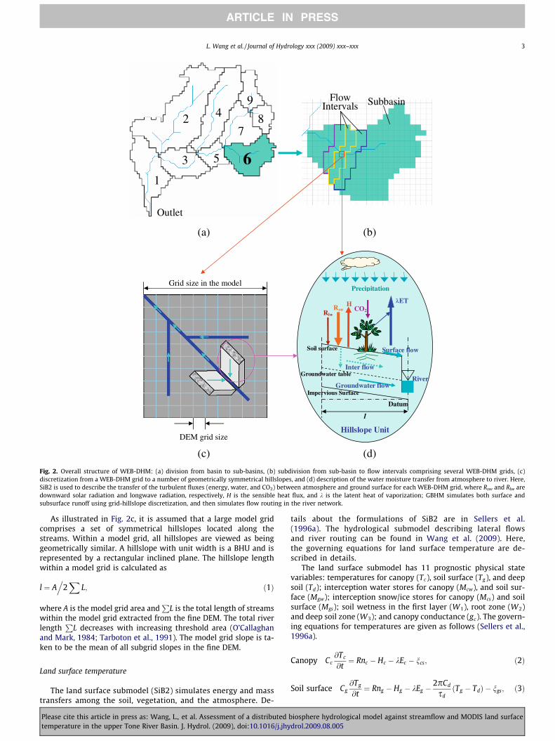
Fig. 3. Spatial distribution of DEM, grid slope, land u


LAI ¼ LAImax � ðNDVI � NDVIminÞ=ðNDVImax � NDVIminÞ: ð7Þ

Therefore, the green vegetation coverage V can be derived as

V ¼ LAI=LAImax; ð8Þ

where the maximum LAI values (LAImax) can be derived followingSellers et al. (1996b).

Datasets

The datasets of the upper Tone River Basin, as used in WEB-DHM, are as described below.

Digital data of elevation, and land use were obtained from theJapan Geographical Survey Institute. Subgrid topography was de-scribed by a 50 m resolution DEM. The elevation of this basin variesfrom about 100 m to 2500 m (upper left, Fig. 3). Grid slopes varyfrom 0� to 39� with a mean value of 16� for model grids (seeFig. 3, upper right). Land use data was reclassified to 3 SiB2 catego-ries, with broadleaf-deciduous trees as the dominant type (morethan 85%) (Fig. 3, lower left). The vegetation static parametersincluding morphological, optical and physiological properties weredefined following Sellers et al. (1996b). The dynamic vegetationparameters are Leaf Area Index (LAI), and the Fraction of Photosyn-thetically Active Radiation (FPAR) absorbed by the green vegeta-tion canopy, and can be obtained from satellite data. Global LAIand FPAR MOD15_BU 1 km data sets (Myneni et al., 1997) wereused in this study. These are 8-daily composites of MOD15A2 prod-ucts and are from the EOS Data Gateway of NASA. The MODIS LSTV5 products (Wan, 2008) used in this paper were also from the EOSData Gateway of NASA. These are also 1-km 8-daily composites

se, and soil type in the upper Tone River Basin.



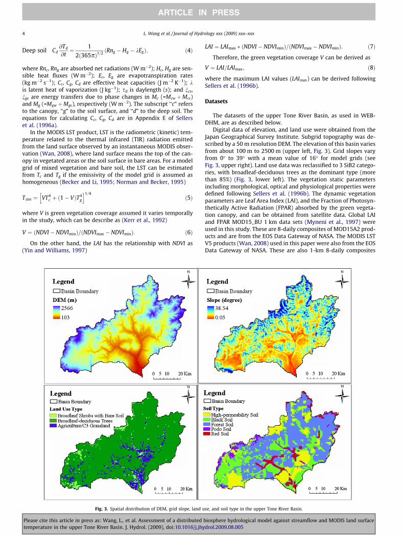
2001-2004 (Nash = 0.821; BIAS=5.0% )Calibrated at 2001 (Nash = 0.901; BIAS=-1.5% )

0

400

800

1200

1600

Jan/01 Jan/02 Jan/03 Jan/04

Dis

char

ge (

m3 s

-1)

Obs Sim

(a) Murakami

2001-2004 (Nash = 0.827; BIAS = 19.2% )

0

100

200

300

400

500

600


Dis

char

ge (

m3 s

-1)

Obs Sim

(b) Yakatabara

2001-2004 (Nash = 0.742; BIAS = -30.8% )

0

200

400

600

800

1000

1200

1400


Dis

char

ge (

m3 s

-1)

Obs Sim

(c) Iwamoto

2001-2004 (Nash = 0.728; BIAS = -29.9% )

0

500

1000

1500

2000

2500

3000


Dis

char

ge (

m3 s

-1)

Obs Sim

(d) Maebashi

Fig. 4. Observed and simulated daily streamflows at four control stations (Murakami (a), Yakatabara (b), Iwamoto (c), and Maebashi (d)) in the upper Tone River Basin from2001 to 2004. The model was only optimized at Murakami, using 2001 data.


ARTICLE IN PRESS

having cloud-contaminated LST values removed. The soil map(Fig. 3, lower right) is processed from a 1:200,000 scale GunmaPrefecture geological map.


Hourly precipitation data were obtained from Radar-AMeDAS(Automated Meteorological Data Acquisition System) rainfall anal-ysis data, which combines both radar and ground observations, and




ARTICLE IN PRESS

was provided by the Japanese Meteorological Agency (JMA). Thedata were available at 5 km spatial resolution until March of2001 and at 2.5 km spatial resolution after that. Surface meteoro-logical data other than precipitation, comprise air temperature, rel-

Table 1Basin-averaged values of the parameters used in the upper Tone River Basin.

Symbol Parameters

hs Saturated water contenthr Residual water contenta van Genuchten parametern van Genuchten parameteranik Hydraulic conductivity anisotropy ratiof Hydraulic conductivity decay factorMgwmax Maximum surface water detentionKs Saturated hydraulic conductivity for soil surfaceKg Hydraulic conductivity of groundwaterDr Root depth (D1 + D2)

Nash = 0.902

0

500

1000

1500

2000

0 12 24 36 48 60Hour (21-23 Aug 2001)

obs_hourly

sim_hourly

Nash = 0.727

0

400

800

1200

0 12 24 36 48 60Hour (21-23 Aug 2001)

1

1

2

Nash = 0.750

0500

1000150020002500

0 12 24 36 48 60Hour (10-12 Sep 2001)

Nash = 0.789

0

200

400

600

0 12 24 36 48 60Hour (10-12 Sep 2001)

1

1

2

0

500

1000

1500

0 12 24 36 48 60Hour (9-11 Jul 2002)

Nash = 0.819

0

500

1000

1500

0 12 24 36 48 60Hour (9-11 Jul 2002)

Nash = 0.957

10

20

30

Nash = 0.655

0

100

200

300

0 24 48 72 96Hour (13-17 Aug 2003)

Nash = 0.504

0

100

200

300

0 24 48Hour (9-11 Aug 2003)

1

Nash = 0.547

0

500

1000

1500

2000

0 24 48 72Hour (20-23 Oct 2004)

Nash = 0.809

0

200

400

600

0 24 48 72Hour (20-23 Oct 2004)

2

5

7

10

(a) Murakami (b) Yakatabara

Fig. 5. Observed and simulated hourly annual largest flood peaks at the stream gauges owith Nash–Sutcliffe coefficient (Nash). The y axis represents discharge (m3 s�1).


ative humidity, air pressure, and wind speed, as well as downwardsolar and longwave radiation. In this basin, the observed air tem-perature, wind speed, and sunshine duration were available from15 meteorological sites (see Fig. 1) in hourly resolution from the

Unit Basin-averaged value Source

0.51 FAO (2003)0.17 FAO (2003)0.01746 FAO (2003)1.524 FAO (2003)15.6 Optimization0.5 Optimization

m 0.01 Optimizationmm h�1 104.0 Optimizationmm h�1 1.0 Yang et al. (2004)m 1.43 Sellers et al. (1996b)

Nash = 0.935

0

500

000

500

000

0 12 24 36 48 60Hour (21-23 Aug 2001)

Nash = 0.867

0

1000

2000

3000

4000

0 12 24 36 48 60Hour (21-23 Aug 2001)

Nash = 0.830

0

500

000

500

000

0 12 24 36 48 60Hour (10-12 Sep 2001)

Nash = 0.741

0

1000

2000

3000

4000

0 12 24 36 48 60Hour (10-12 Sep 2001)

0

00

00

00

0 12 24 36 48 60Hour (9-11 Jul 2002)

Nash = 0.933

0

1000

2000

3000

4000

0 12 24 36 48 60Hour (9-11 Jul 2002)

Nash = 0.916

Nash = 0.685

0

250

500

750

000

0 24 48Hour (9-11 Aug 2003)

Nash = -0.167

0

250

500

750

1000

1250

0 24 48Hour (9-11 Aug 2003)

Nash = 0.742

0

50

00

50

00

0 24 48 72Hour (20-23 Oct 2004)

Nash = 0.646

0500

1000150020002500

0 24 48 72Hour (20-23 Oct 2004)

(c) Iwamoto (d) Maebashi

f Murakami (a), Yakatabara (b), Iwamoto (c), and Maebashi (d) from 2001 to 2004,



Table 2Comparison of observed and simulated annual largest flood peaks occurring at the main discharge gauges in the upper Tone River Basin (flood peak: m3 s�1, time: date (h)).

Year Gauge Observed (Obs) Simulated (Sim) Difference (Dif) Dif/Obs

Flood Time Flood Time Flood Time (h) Flood (%)

2001(1) Murakami 1467 Aug22(13) 1058 Aug22(12) �409 �1 �28Yakatabara 627 Aug22(13) 876 Aug22(12) 249 �1 40Iwamoto 1856 Aug22(13) 1620 Aug22(13) �236 0 �13Maebashi 3407 Aug22(14) 2515 Aug22(16) �892 2 �26

2001(2) Murakami 1802 Sep10(16) 1933 Sep10(18) 131 2 7Yakatabara 431 Sep11(06) 441 Sep11(05) 10 �1 2Iwamoto 1496 Sep11(08) 1289 Sep11(04) �207 4 �14Maebashi 3208 Sep11(10) 2762 Sep10(24) �446 10 �14

2002 Murakami 1103 Jul10(22) 1334 Jul10(22) 231 0 21Yakatabara 1008 Jul10(22) 955 Jul11(02) �53 4 �5Iwamoto 2473 Jul10(23) 2020 Jul11(02) �453 3 �18Maebashi 3319 Jul10(24) 3380 Jul11(03) 61 3 2

2003 Murakami 202 Aug15(11) 264 Aug15(11) 62 0 31Yakatabara 195 Aug10(07) 155 Aug10(15) �40 8 �21Iwamoto 822 Aug09(10) 624 Aug09(13) �198 3 �24Maebashi 1178 Aug09(23) 549 Aug09(21) �629 �2 �53

2004 Murakami 1368 Oct21(01) 1827 Oct21(02) 459 1 34Yakatabara 506 Oct21(02) 450 Oct21(02) �56 0 �11Iwamoto 957 Oct21(03) 686 Oct21(03) �271 0 �28Maebashi 2224 Oct21(03) 2309 Oct21(06) 85 3 4

260

270

280

290

300

310

320

1/1/01 7/1/01 1/1/02 7/1/02 1/1/03 7/1/03 1/1/04 7/1/04

LST

(K

)

Obs Sim TairDaytime BIAS = 1.06 K RMSE = 2.22 K

T sim = 1.0038*T obs

R = 0.9760260

280

300

320

260 280 300 320

MODIS LST (K)

Sim

ulat

ed L

ST (

K)

Daytime

250

260

270

280

290

300

310

1/1/01 7/1/01 1/1/02 7/1/02 1/1/03 7/1/03 1/1/04 7/1/04

LST

(K

)

Obs Sim TairNighttime BIAS = 1.67 K RMSE = 2.53 K

T sim = 1.006*T obs

R = 0.9736250

270

290

310

250 270 290 310

MODIS LST (K)

Sim

ulat

ed L

ST (

K)

Nighttime

Fig. 6. Comparison of 8-daily LSTs between model simulations (Tsim) and MODIS observations (Tobs) during daytime (upper) and nighttime (lower) averaged for the upperTone River Basin from 2001 to 2004. Time-series (left) and scatter plots (right). Here, the missing data in MODIS LSTs and their corresponding simulated LSTs, and input airtemperature have been exempted for comparison.


ARTICLE IN PRESS

AMeDAS annual report of the JMA. Relative humidity and air pres-sure were obtained from three radiation stations maintained byJMA and interpolated into the 15 meteorological sites using theAngular distance-weighted (ADW) interpolation method (Newet al., 2000). Downward solar radiation was then estimated fromsunshine duration, temperature, and humidity, using a hybridmodel developed by Yang et al. (2001, 2006). This model can effec-tively account for the effect of elevation and humidity on radiative


transfer processes, and has been well validated in lowland/high-land and humid/dry regions. Longwave radiation was then esti-mated from temperature, relative humidity, pressure, and solarradiation using the relationship between solar radiation and long-wave radiation (Crawford and Duchon, 1999).

Precipitation data were linearly interpolated from coarser (5 kmor 2.5 km) grids to model (500 m) grids, while all the other mete-orological variables (including wind speed) were interpolated to



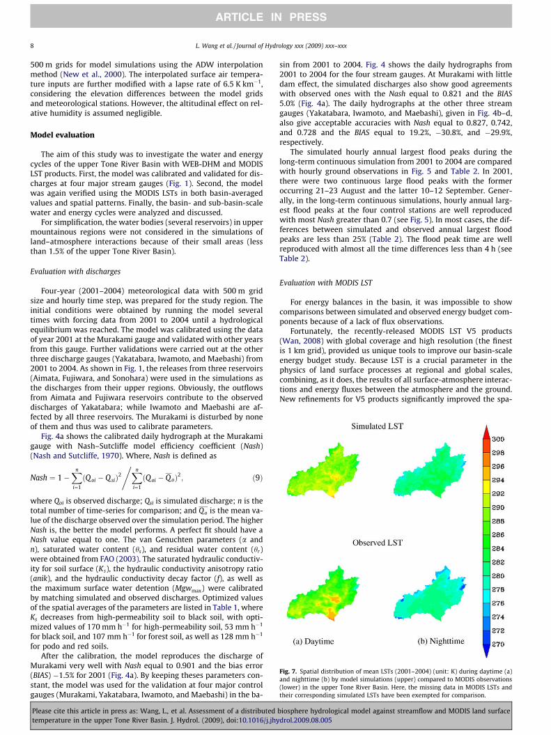
Fig. 7. Spatial distribution of mean LSTs (2001–2004) (unit: K) during daytime (a)and nighttime (b) by model simulations (upper) compared to MODIS observations(lower) in the upper Tone River Basin. Here, the missing data in MODIS LSTs andtheir corresponding simulated LSTs have been exempted for comparison.


ARTICLE IN PRESS

500 m grids for model simulations using the ADW interpolationmethod (New et al., 2000). The interpolated surface air tempera-ture inputs are further modified with a lapse rate of 6.5 K km�1,considering the elevation differences between the model gridsand meteorological stations. However, the altitudinal effect on rel-ative humidity is assumed negligible.

Model evaluation

The aim of this study was to investigate the water and energycycles of the upper Tone River Basin with WEB-DHM and MODISLST products. First, the model was calibrated and validated for dis-charges at four major stream gauges (Fig. 1). Second, the modelwas again verified using the MODIS LSTs in both basin-averagedvalues and spatial patterns. Finally, the basin- and sub-basin-scalewater and energy cycles were analyzed and discussed.

For simplification, the water bodies (several reservoirs) in uppermountainous regions were not considered in the simulations ofland–atmosphere interactions because of their small areas (lessthan 1.5% of the upper Tone River Basin).

Evaluation with discharges

Four-year (2001–2004) meteorological data with 500 m gridsize and hourly time step, was prepared for the study region. Theinitial conditions were obtained by running the model severaltimes with forcing data from 2001 to 2004 until a hydrologicalequilibrium was reached. The model was calibrated using the dataof year 2001 at the Murakami gauge and validated with other yearsfrom this gauge. Further validations were carried out at the otherthree discharge gauges (Yakatabara, Iwamoto, and Maebashi) from2001 to 2004. As shown in Fig. 1, the releases from three reservoirs(Aimata, Fujiwara, and Sonohara) were used in the simulations asthe discharges from their upper regions. Obviously, the outflowsfrom Aimata and Fujiwara reservoirs contribute to the observeddischarges of Yakatabara; while Iwamoto and Maebashi are af-fected by all three reservoirs. The Murakami is disturbed by noneof them and thus was used to calibrate parameters.

Fig. 4a shows the calibrated daily hydrograph at the Murakamigauge with Nash–Sutcliffe model efficiency coefficient (Nash)(Nash and Sutcliffe, 1970). Where, Nash is defined as

Nash ¼ 1�Xn

i¼1

ðQ oi � Q siÞ2Xn

i¼1

ðQ oi � QoÞ2,

; ð9Þ

where Qoi is observed discharge; Qsi is simulated discharge; n is thetotal number of time-series for comparison; and Qo is the mean va-lue of the discharge observed over the simulation period. The higherNash is, the better the model performs. A perfect fit should have aNash value equal to one. The van Genuchten parameters (a andn), saturated water content (hs), and residual water content (hr)were obtained from FAO (2003). The saturated hydraulic conductiv-ity for soil surface (Ks), the hydraulic conductivity anisotropy ratio(anik), and the hydraulic conductivity decay factor (f), as well asthe maximum surface water detention (Mgwmax) were calibratedby matching simulated and observed discharges. Optimized valuesof the spatial averages of the parameters are listed in Table 1, whereKs decreases from high-permeability soil to black soil, with opti-mized values of 170 mm h�1 for high-permeability soil, 53 mm h�1

for black soil, and 107 mm h�1 for forest soil, as well as 128 mm h�1

for podo and red soils.After the calibration, the model reproduces the discharge of

Murakami very well with Nash equal to 0.901 and the bias error(BIAS) �1.5% for 2001 (Fig. 4a). By keeping theses parameters con-stant, the model was used for the validation at four major controlgauges (Murakami, Yakatabara, Iwamoto, and Maebashi) in the ba-


sin from 2001 to 2004. Fig. 4 shows the daily hydrographs from2001 to 2004 for the four stream gauges. At Murakami with littledam effect, the simulated discharges also show good agreementswith observed ones with the Nash equal to 0.821 and the BIAS5.0% (Fig. 4a). The daily hydrographs at the other three streamgauges (Yakatabara, Iwamoto, and Maebashi), given in Fig. 4b–d,also give acceptable accuracies with Nash equal to 0.827, 0.742,and 0.728 and the BIAS equal to 19.2%, �30.8%, and �29.9%,respectively.

The simulated hourly annual largest flood peaks during thelong-term continuous simulation from 2001 to 2004 are comparedwith hourly ground observations in Fig. 5 and Table 2. In 2001,there were two continuous large flood peaks with the formeroccurring 21–23 August and the latter 10–12 September. Gener-ally, in the long-term continuous simulations, hourly annual larg-est flood peaks at the four control stations are well reproducedwith most Nash greater than 0.7 (see Fig. 5). In most cases, the dif-ferences between simulated and observed annual largest floodpeaks are less than 25% (Table 2). The flood peak time are wellreproduced with almost all the time differences less than 4 h (seeTable 2).

Evaluation with MODIS LST

For energy balances in the basin, it was impossible to showcomparisons between simulated and observed energy budget com-ponents because of a lack of flux observations.

Fortunately, the recently-released MODIS LST V5 products(Wan, 2008) with global coverage and high resolution (the finestis 1 km grid), provided us unique tools to improve our basin-scaleenergy budget study. Because LST is a crucial parameter in thephysics of land surface processes at regional and global scales,combining, as it does, the results of all surface-atmosphere interac-tions and energy fluxes between the atmosphere and the ground.New refinements for V5 products significantly improved the spa-




ARTICLE IN PRESS

tial coverage of LSTs, especially in highland regions, and increasedthe accuracy and stability of MODIS LST products. Comparisons be-tween V5 LSTs and in situ values in 47 clear-sky cases (LST rangefrom �10 �C to 58 �C, and atmospheric column water vapor rangefrom 0.4 to 3.5 cm) indicate that the accuracy of the MODIS LSTproducts is better than 1 K in most cases (39 out of 47) and the rootmean squared error (RMSE) is less than 0.7 K for all 47 cases (Wan,2008).

Since the WEB-DHM has been validated by simulating multiple-site streamflows in the upper Tone River Basin, once the model hasbeen again verified with basin-scale evolution of MODIS LSTs,greater confidence can be obtained for further analyses on waterand energy cycles in the basin. Here, the missing data in 8-dailyMODIS LSTs and their corresponding simulated LSTs have been ex-empted for comparison.

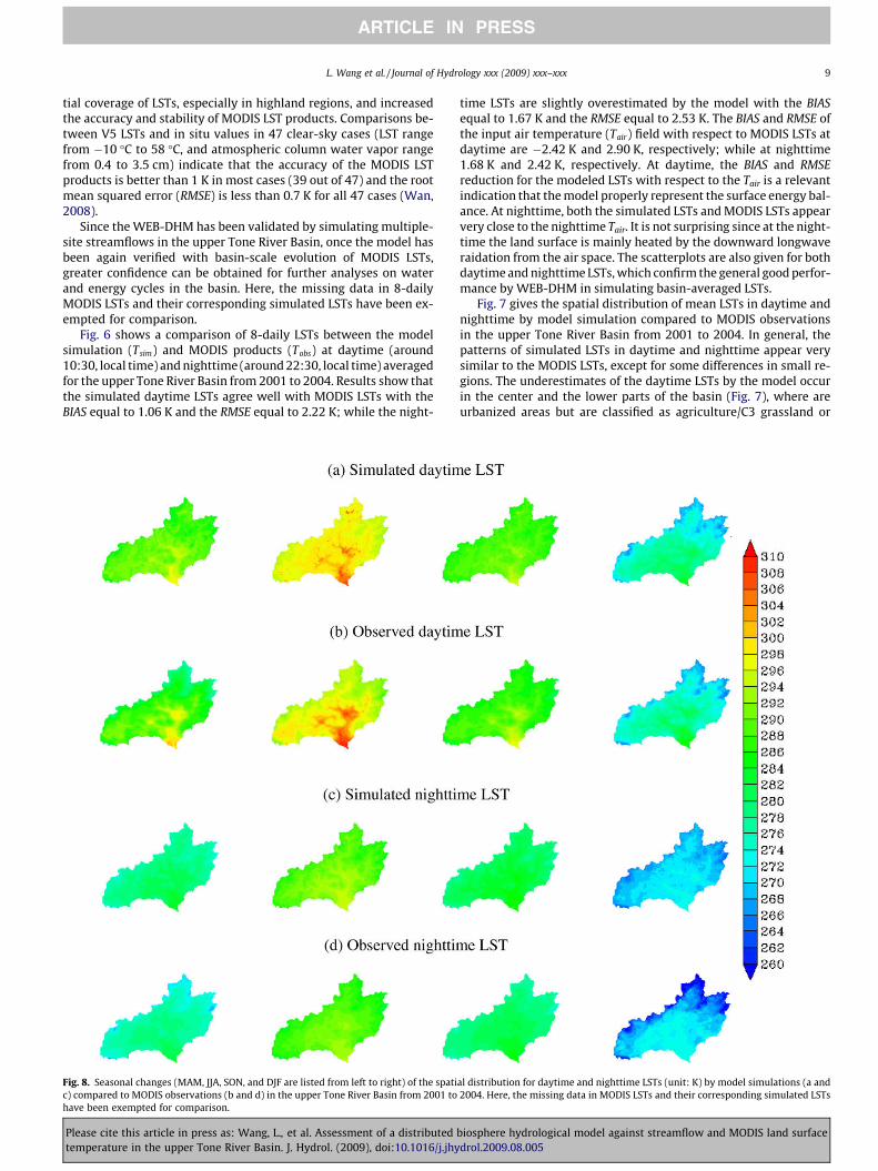
Fig. 6 shows a comparison of 8-daily LSTs between the modelsimulation (Tsim) and MODIS products (Tobs) at daytime (around10:30, local time) and nighttime (around 22:30, local time) averagedfor the upper Tone River Basin from 2001 to 2004. Results show thatthe simulated daytime LSTs agree well with MODIS LSTs with theBIAS equal to 1.06 K and the RMSE equal to 2.22 K; while the night-

Fig. 8. Seasonal changes (MAM, JJA, SON, and DJF are listed from left to right) of the spatic) compared to MODIS observations (b and d) in the upper Tone River Basin from 2001 tohave been exempted for comparison.


time LSTs are slightly overestimated by the model with the BIASequal to 1.67 K and the RMSE equal to 2.53 K. The BIAS and RMSE ofthe input air temperature (Tair) field with respect to MODIS LSTs atdaytime are �2.42 K and 2.90 K, respectively; while at nighttime1.68 K and 2.42 K, respectively. At daytime, the BIAS and RMSEreduction for the modeled LSTs with respect to the Tair is a relevantindication that the model properly represent the surface energy bal-ance. At nighttime, both the simulated LSTs and MODIS LSTs appearvery close to the nighttime Tair. It is not surprising since at the night-time the land surface is mainly heated by the downward longwaveraidation from the air space. The scatterplots are also given for bothdaytime and nighttime LSTs, which confirm the general good perfor-mance by WEB-DHM in simulating basin-averaged LSTs.

Fig. 7 gives the spatial distribution of mean LSTs in daytime andnighttime by model simulation compared to MODIS observationsin the upper Tone River Basin from 2001 to 2004. In general, thepatterns of simulated LSTs in daytime and nighttime appear verysimilar to the MODIS LSTs, except for some differences in small re-gions. The underestimates of the daytime LSTs by the model occurin the center and the lower parts of the basin (Fig. 7), where areurbanized areas but are classified as agriculture/C3 grassland or

al distribution for daytime and nighttime LSTs (unit: K) by model simulations (a and2004. Here, the missing data in MODIS LSTs and their corresponding simulated LSTs




ARTICLE IN PRESS

broadleaf shrubs with bare soil in SiB2 land use map (see Fig. 3).The overestimates of the modeled daytime and nighttime LSTs inthe area with highest altitudes are possibly attributed to the errorsin input air temperature. Due to no meteorological sites available, ahomogeneous lapse rate (6.5 K km�1) has been adopted to accountfor the air temperature dependence on elevation, and therefore, er-rors in the interpolated air temperature may occur in the upper-most mountain regions.

Fig. 8 displays the seasonal changes of the spatial distribution ofdaytime and nighttime LSTs by model simulation compared toMODIS observations. The patterns of simulated LSTs in differentseasons are again visually similar to the MODIS LSTs, but the modelsimulation underestimates the daytime LSTs for the central andlower regions (especially for the daytime LSTs in MAM and JJA),and overestimates both the daytime and nighttime LSTs for theuppermost mountain regions (especially for the daytime LSTs inJJA, and for the nighttime LSTs in DFJ).

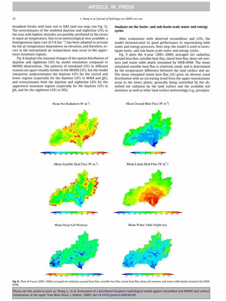
Fig. 9. Plots of 4-year (2001–2004) averaged net radiation, ground heat flux, sensible heaDHM.


Analyses on the basin- and sub-basin-scale water and energycycles

After evaluations with observed streamflows and LSTs, themodel demonstrated its good performance in representing bothwater and energy processes. Next step, the model is used to inves-tigate basin- and sub-basin-scale water and energy cycles.

Fig. 9 plots the 4-year (2001–2004) averaged net radiation,ground heat flux, sensible heat flux, latent heat flux, deep soil wet-ness and water table depth simulated by WEB-DHM. The meansimulated sensible heat flux is relatively small, and is determinedby the temperature difference between the land surface and air.The mean simulated latent heat flux (LE) gives an obvious zonaldistribution with an increasing trend from the upper mountainousareas to the lower plains; generally being controlled by the ab-sorbed net radiation by the land surface and the available soilmoisture, as well as other land surface meteorology (e.g., precipita-

t flux, latent heat flux, deep soil wetness, and water table depth simulated by WEB-



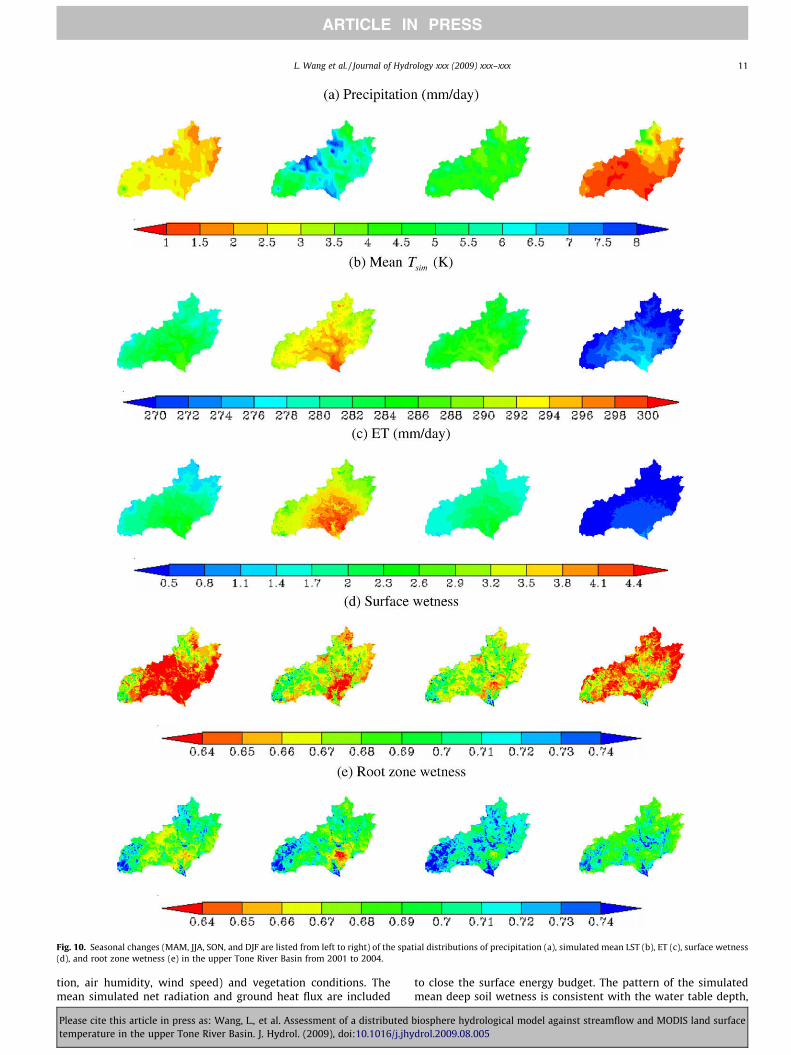
Fig. 10. Seasonal changes (MAM, JJA, SON, and DJF are listed from left to right) of the spatial distributions of precipitation (a), simulated mean LST (b), ET (c), surface wetness(d), and root zone wetness (e) in the upper Tone River Basin from 2001 to 2004.


ARTICLE IN PRESS

tion, air humidity, wind speed) and vegetation conditions. Themean simulated net radiation and ground heat flux are included


to close the surface energy budget. The pattern of the simulatedmean deep soil wetness is consistent with the water table depth,




ARTICLE IN PRESS

having wetter soil in areas with lower water tables, while thewater table depth closely follows the grid slope in the model (Figs.3 and 9). The water table exhibits a spatial structure that is influ-enced by the grid slope and is characterized by relatively shallowwater levels in the flat regions and relatively deep water levelsalong the steep hilltops.

Fig. 10 illustrates the seasonal changes of the spatial distribu-tions of precipitation, and simulated mean LST, ET, and surfacewetness, as well as root zone wetness. The observed precipitationshows obvious seasonal variations with the largest in summer (JJA)and the least in winter (DJF) (Fig. 10a). Mean LST also experiencesits highest value in summer (JJA; Fig. 10b), and consequently re-sults in the largest ET for this season Fig. 10c). Contrarily, winter(DJF) has both the lowest LST (Fig. 10b) and the least precipitation(Fig. 10a), and thus the least ET for the season (Fig. 10c). The sur-

0

50

100

150

200

250

Jan Feb Mar Apr May Jun

Wat

er (

mm

/mon

th)

PrecipitationETDischarge_simDischarge_obs

(a) Discharge:

265

275

285

295

305

Jan Feb Mar Apr May Jun Ju

Tem

pera

ture

(K

)

LAI LST(b)

-100

0

100

200

300

400

500

Jan Feb Mar Apr May Jun Jul

Hea

t Flu

x (W

m-2

)

LST_mean(c)

Fig. 11. Variables averaged for the upper area of the Murakami gauge from 2001 to 2004ET; (b) monthly-mean LAI, as well as the diurnal variations of LST, Tg, Tc and Tair; and (c) m


face soil wetness patterns are mainly determined by precipitation,bare soil evaporation, grid slope and soil pattern. Root zone wet-ness patterns for all seasons show good consistencies with meandeep soil wetness and the water table maps (Figs. 10e and 9). Bothsurface and root zone wetness show similar seasonal changes(Fig. 10d and e). The wettest surface soil and root zone occur in au-tumn (SON), other than summer (JJA), since autumn has muchsmaller ET than summer while precipitation does not decrease alot from the summer to autumn because of typhoons and Mei-yufront activities. The driest season is in the spring (MAM) whenthere is relatively little precipitation but obviously increased ET(Fig. 10c) resulting from increased land surface temperature.(Fig. 10b).

Fig. 11 shows monthly water and energy cycles averaged at theupper area of the Murakami gauge from 2001 to 2004. In the sub-

Jul Aug Sep Oct Nov Dec

BIAS = 5.0% Nash = 0.838

l Aug Sep Oct Nov Dec

0

1

2

3

4

5

6L

eaf

Are

a In

dex

Tg Tc Tair

Aug Sep Oct Nov Dec

260

270

280

290

300

310

Tem

pera

ture

(K

)

H LE

: (a) mean monthly observed discharge and precipitation, simulated discharge andean monthly LST, and diurnal variations of sensible and latent heat fluxes (H and LE).




ARTICLE IN PRESS

basin the hydrological cycles are less interfered with by reservoirs.The simulated mean monthly water balance components showsthat in the sub-basin, heavy precipitation mainly occurs fromMay to October, months commonly associated with typhoonsand Mei-yu front activities. Considering the relatively high LSTsin these months (see ‘‘LST_mean” in Fig. 11c), relatively large ETsare obtained from May to October (Fig. 11a). Monthly dischargelargely concentrates during the period from July to October, andis well reproduced by WEB-DHM with the BIAS and Nash equal to5.0% and 0.838, respectively.

Monthly mean diurnal cycles of LSTs, Tg, Tc, and Tair are given inFig. 11b, and compared to the mean monthly LAI. From May toOctober, with relatively large LAI values, the simulated daily max-imum LST is close to Tg since Tg is much greater than Tc in theirpeak values; while the daily minimum LST appears similar to Tc.For other months with relatively small LAI values, the diurnal cy-cles of LST closely follow Tg. For all months, the simulated dailyminimum LST appears very close to Tair; while the simulated dailymaximum LST is much higher than Tair.

Fig. 11c illustrates the mean monthly LST, as well as the diurnalvariations of sensible and latent heat fluxes. The monthly changesof the daily maximum latent heat flux generally follow themonthly-mean LST with peaks in July and August. The diurnal var-iation of sensible heat flux is partly shaped by the diurnal change ofthe LST, with the largest diurnal variations in the spring (MAM).

Conclusions

In this study, a distributed biosphere hydrological model (WEB-DHM) was used to investigate the water and energy cycles in theupper Tone River Basin where flux observations are not available.

First, the model was calibrated and validated for discharges atfour major stream gauges and demonstrated good performancesin flood predictions, with initial soil water content before a floodevent being estimated in a long-term simulation.

Second, the MODIS V5 LST products, with high resolution andreliable accuracies, were used to evaluate the model’s performancein representing energy processes in the basin. The results showthat the WEB-DHM reasonably accurately represents both daytimeand nighttime LSTs for both time-series processes and spatial pat-terns, with the only calibration being for a year-long discharge atone stream gauge.

Third, basin- and sub-basin-scale water and energy cycles wereanalyzed and discussed. It was found that from May to October,with relatively large LAI values, the simulated daily maximumLST is close to Tg since Tg is much greater than Tc in their peak val-ues; while the daily minimum LST appears similar to Tc. For othermonths with relatively small LAI values, the diurnal cycles of LSTclosely follow Tg .

By using a distributed hydrological model that has physicallyformulated water and energy budgets in the SVAT system, the re-cently-released MODIS V5 LST products have a big potential to im-prove water and energy studies for basins without fluxobservations (e.g., ungauged basins). This is because these toolshave global coverage and high resolution.

Acknowledgements

This study was funded by Core Research for Evolutional Scienceand Technology, the Japan Science and Technology Corporation.Parts of this work were also support by grants from the Ministryof Education, Culture, Sports, Science and Technology of Japan,and Japan Aerospace Exploration Agency. Global 8-daily MODISTerra Land Surface Temperature and LAI/FPAR 1 km data sets arefrom the EOS Data Gateway of NASA. The third author (Kun Yang)


is supported by ‘‘100-Talent” Project of the Chinese Academy ofSciences.

References

Becker, F., Li, Z., 1995. Surface temperature and emissivity at various scales:Definition, measurement and related problems. Remote Sensing Reviews 12,225–253.

Bertoldi, G., Rigon, R., Over, T.M., 2006. Impact of watershed geomorphiccharacteristics on the energy and water budgets. Journal ofHydrometeorology 7, 389–403.

Brown, L., Thorne, R., Woo, M.K., 2008. Using satellite imagery to validate snowdistribution simulated by a hydrological model in large northern basins.Hydrological Processes 22, 2777–2787.

Crawford, T.M., Duchon, C.E., 1999. An improved parameterization for estimatingeffective atmospheric emissivity for use in calculating daytime downwellinglongwave radiation. Journal of Applied Meteorology 38, 474–480.

Famiglietti, J.S., Wood, E.F., 1994. Multiscale modeling of spatially-variable waterand energy balance processes. Water Resources Research 30, 3061–3078.

FAO, 2003. Digital Soil Map of the World and Derived Soil Properties, Land andWater Digital Media Series Rev. 1, United Nations Food and AgricultureOrganization, CD-ROM.

Kerr, Y.H., Lagouarde, J.P., Imbernon, J., 1992. Accurate land surface temperatureretrieval from AVHRR data with use of an improved split window algorithm.Remote Sensing of Environment 41, 197–209.

Myneni, R.B., Nemani, R.R., Running, S.W., 1997. Algorithm for the estimation ofglobal land cover, LAI and FPAR based on radiative transfer models. IEEETransactions on Geoscience and Remote Sensing 35, 1380–1393.

Nash, J.E., Sutcliffe, J.V., 1970. River flow forecasting through conceptual modelspart I – A discussion of principles. Journal of Hydrology 10 (3), 282–290.

New, M., Hulme, M., Jones, P., 2000. Representing twentieth-century space-timeclimate variability. Part II: Development of 1901-96 monthly grids of terrestrialsurface climate. Journal of Climate 13, 2217–2238.

Norman, J.M., Becker, F., 1995. Terminology in thermal infrared remote sensing ofnatural surfaces. Agricultural and Forest Meteorology 77, 153–166.

O’Callaghan, J.F., Mark, D.M., 1984. The extraction of drainage networks from digitalelevation data. Computer Vision, Graphics and Image Processing 28, 328–344.

Parajka, J., Bloeschl, G., 2008. The value of MODIS snow cover data in validating andcalibrating conceptual hydrologic models. Journal of Hydrology 358, 240–258.

Peters-Lidard, C.D., Zion, M.S., Wood, E.F., 1997. A soil-vegetation-atmospheretransfer scheme for modeling spatially variable water and energy balanceprocesses. Journal of Geophysical Research 102, 4303–4324.

Pinker, R.T., Sun, D., Hung, M.-P., Li, C., Basara, J.B., 2009. Evaluation of satelliteestimates of land surface temperature from GOES over the United States.Journal of Applied Meteorology and Climatology 48 (1), 167–180.

Rigon, R., Bertoldi, G., Over, T.M., 2006. GEOtop: a distributed hydrological modelwith coupled water and energy budgets. Journal of Hydrometeorology 7, 371–388.

Sellers, P.J., Randall, D.A., Collatz, G.J., Berry, J.A., Field, C.B., Dazlich, D.A., Zhang, C.,Collelo, G.D., Bounoua, L., 1996a. A revised land surface parameterization (SiB2)for atmospheric GCMs, part I: model formulation. Journal of Climate 9, 676–705.

Sellers, P.J., Los, S.O., Tucker, C.J., Justice, C.O., Dazlich, D.A., Collatz, G.J., Randall,D.A., 1996b. A revised land surface parameterization (SiB2) for atmosphericGCMs, part II: the generation of global fields of terrestrial biosphysicalparameters from satellite data. Journal of Climate 9, 706–737.

Sellers, P.J., Dickinson, R.E., Randall, D.A., Betts, A.K., Hall, F.G., Berry, J.A., Collatz,G.J., Denning, A.S., Mooney, H.A., Nobre, C.A., Sato, N., Field, C.B.,HendersonSellers, A., 1997. Modeling the exchanges of energy, water, andcarbon between continents and the atmosphere. Science 275, 502–509.

Sheng, J.F., Wilson, J.P., Lee, S., 2009. Comparison of land surface temperature (LST)modeled with a spatially-distributed solar radiation model (SRAD) and remotesensing data. Environmental Modelling and Software 24, 436–443.

Sun, D., Pinker, R.T., 2003. Estimation of land surface temperature from ageostationary operational environmental satellite (GOES-8). Journal ofGeophysical Research 108 (D11), 4326. doi:10.1029/2002JD002422.

Tang, Q., Oki, T., Kanae, S., 2006. A distributed biosphere hydrological model(DBHM) for large river basin. Annual Journal of Hydraulic Engineering – JSCE 50,37–42.

Tarboton, D.G., Bras, R.L., Rodriguez-Iturbe, I., 1991. On the extraction of channelnetworks from digital elevation data. Hydrological Processes 5, 81–100.

Turner, D.P., Ritts, W.D., Cohen, W.B., Gower, S.T., Zhao, M.S., Running, S.W., Wofsy,S.C., Urbanski, S., Dunn, A.L., Munger, J.W., 2003. Scaling gross primaryproduction (GPP) over boreal and deciduous forest landscapes in support ofMODIS GPP product validation. Remote Sensing of Environment 88, 256–270.

Twine, T.E., Kucharik, C.J., 2008. Evaluating a terrestrial ecosystem model withsatellite information of greenness. Journal of Geophysical Research –Biogeosciences 113, G03027. doi:10.1029/2007JG000599.

Wan, Z.M., 2008. New refinements and validation of the MODIS land-surfacetemperature/emissivity products. Remote Sensing of Environment 112, 59–74.

Wang, L., Koike, T., 2009. Comparison of a distributed biosphere hydrological modelwith GBHM. , Annual Journal of Hydraulic Engineering – JSCE 53, 103–108.

Wang, L., Koike, T., Yang, K., Jackson, T., Bindlish, R., Yang, D., 2009. Development ofa distributed biosphere hydrological model and its evaluation with the


http://dx.doi.org/10.1029/2002JD002422

http://dx.doi.org/10.1029/2007JG000599



ARTICLE IN PRESS

Southern Great Plains Experiments (SGP97 and SGP99). Journal of GeophysicalResearch – Atmospheres 114, D08107. doi:10.1029/2008JD010800.

Wigmosta, M.S., Vail, L.W., Lettenmaier, D.P., 1994. A distributed hydrology-vegetation model for complex terrain. Water Resources Research 30, 1665–1679.

Yang, D., 1998. Distributed Hydrological Model Using Hillslope Discretization BasedOn Catchment Area Function: Development and Applications, Ph.D. Thesis,Univ. of Tokyo, Tokyo.

Yang, D., Herath, S., Musiake, K., 2000. Comparison of different distributedhydrological models for characterization of catchment spatial variability.Hydrological Processes 14, 403–416.


Yang, K., Huang, G., Tamai, N., 2001. A hybrid model for estimating global solarradiation. Solar Energy 70, 13–22.

Yang, D., Koike, T., Tanizawa, H., 2004. Application of a distributed hydrologicalmodel and weather radar observations for flood management in the upper ToneRiver of Japan. Hydrological Processes 18, 3119–3132.

Yang, K., Koike, T., Ye, B., 2006. Improving estimation of hourly, daily, and monthlysolar radiation by importing global data set. Agricultural and ForestMeteorology 137, 43–55.

Yin, Z.S., Williams, T.H.L., 1997. Obtaining spatial and temporal vegetation datafrom landsat MSS and AVHRR/NOAA satellite images for a hydrologic model.Photogrammetric Engineering and Remote Sensing 63 (1), 69–77.


http://dx.doi.org/10.1029/2008JD010800


Assessment of a distributed biosphere hydrological model against streamflow and MODIS land surface...

Documents

Transcript of Assessment of a distributed biosphere hydrological model against streamflow and MODIS land surface...