StreamFlow 1.0 - GMD
29
Geosci. Model Dev., 9, 4491–4519, 2016 www.geosci-model-dev.net/9/4491/2016/ doi:10.5194/gmd-9-4491-2016 © Author(s) 2016. CC Attribution 3.0 License. StreamFlow 1.0: an extension to the spatially distributed snow model Alpine3D for hydrological modelling and deterministic stream temperature prediction Aurélien Gallice 1 , Mathias Bavay 2 , Tristan Brauchli 1 , Francesco Comola 1 , Michael Lehning 1,2 , and Hendrik Huwald 1 1 School of Architecture, Civil and Environmental Engineering (ENAC), École Polytechnique Fédérale de Lausanne (EPFL), Lausanne, Switzerland 2 SLF, WSL Institute for Snow and Avalanche Research, 7260 Davos, Switzerland Correspondence to: Mathias Bavay ([email protected]) Received: 29 June 2016 – Published in Geosci. Model Dev. Discuss.: 10 August 2016 Revised: 7 November 2016 – Accepted: 23 November 2016 – Published: 21 December 2016 Abstract. Climate change is expected to strongly impact the hydrological and thermal regimes of Alpine rivers within the coming decades. In this context, the development of hydrological models accounting for the specific dynamics of Alpine catchments appears as one of the promising ap- proaches to reduce our uncertainty of future mountain hy- drology. This paper describes the improvements brought to StreamFlow, an existing model for hydrological and stream temperature prediction built as an external extension to the physically based snow model Alpine3D. StreamFlow’s source code has been entirely written anew, taking advan- tage of object-oriented programming to significantly improve its structure and ease the implementation of future devel- opments. The source code is now publicly available online, along with a complete documentation. A special emphasis has been put on modularity during the re-implementation of StreamFlow, so that many model aspects can be represented using different alternatives. For example, several options are now available to model the advection of water within the stream. This allows for an easy and fast comparison be- tween different approaches and helps in defining more re- liable uncertainty estimates of the model forecasts. In partic- ular, a case study in a Swiss Alpine catchment reveals that the stream temperature predictions are particularly sensitive to the approach used to model the temperature of subsurface flow, a fact which has been poorly reported in the literature to date. Based on the case study, StreamFlow is shown to repro- duce hourly mean discharge with a Nash–Sutcliffe efficiency (NSE) of 0.82 and hourly mean temperature with a NSE of 0.78. 1 Introduction Mountainous areas play a major role in hydrology by ac- cumulating precipitation as snow and ice during the winter and redistributing it as melt water during spring and summer. Downstream areas hereby receive larger amounts of water during the hot season, when demand – especially in terms of agriculture – is highest. In fact, Viviroli et al. (2011) es- timate that more than 40 % of the world’s mountainous re- gions provide an important supply for low-land water use. Accordingly, more than one-sixth of the world’s population is currently living in areas depending on snow melt for their water supply (Barnett et al., 2005). Apart from its relevance for downstream areas, mountain hydrology also strongly im- pacts hydropower production (e.g. Schaefli et al., 2007; Fin- ger et al., 2012; Majone et al., 2016), determines the habi- tat suitability of numerous aquatic organisms (e.g. Short and Ward, 1980; Hari et al., 2006; Wilhelm et al., 2015; Padilla et al., 2015) and even plays a noticeable role in the global emission of carbon dioxide into the atmosphere (Butman and Raymond, 2011; Raymond et al., 2013). Mountainous environments have recently been identified as being especially sensitive to climate change (e.g. Barnett et al., 2005; Stewart et al., 2005; Viviroli et al., 2011). In par- ticular, winter air temperature over the last 70 years has been Published by Copernicus Publications on behalf of the European Geosciences Union.
-
Upload
khangminh22 -
Category
Documents
-
view
3 -
download
0
Transcript of StreamFlow 1.0 - GMD

Geosci. Model Dev., 9, 4491–4519, 2016www.geosci-model-dev.net/9/4491/2016/doi:10.5194/gmd-9-4491-2016© Author(s) 2016. CC Attribution 3.0 License.
StreamFlow 1.0: an extension to the spatially distributed snowmodel Alpine3D for hydrological modelling and deterministicstream temperature predictionAurélien Gallice1, Mathias Bavay2, Tristan Brauchli1, Francesco Comola1, Michael Lehning1,2, and Hendrik Huwald1
1School of Architecture, Civil and Environmental Engineering (ENAC), École Polytechnique Fédérale de Lausanne (EPFL),Lausanne, Switzerland2SLF, WSL Institute for Snow and Avalanche Research, 7260 Davos, Switzerland
Correspondence to: Mathias Bavay ([email protected])
Received: 29 June 2016 – Published in Geosci. Model Dev. Discuss.: 10 August 2016Revised: 7 November 2016 – Accepted: 23 November 2016 – Published: 21 December 2016
Abstract. Climate change is expected to strongly impact thehydrological and thermal regimes of Alpine rivers withinthe coming decades. In this context, the development ofhydrological models accounting for the specific dynamicsof Alpine catchments appears as one of the promising ap-proaches to reduce our uncertainty of future mountain hy-drology. This paper describes the improvements brought toStreamFlow, an existing model for hydrological and streamtemperature prediction built as an external extension tothe physically based snow model Alpine3D. StreamFlow’ssource code has been entirely written anew, taking advan-tage of object-oriented programming to significantly improveits structure and ease the implementation of future devel-opments. The source code is now publicly available online,along with a complete documentation. A special emphasishas been put on modularity during the re-implementation ofStreamFlow, so that many model aspects can be representedusing different alternatives. For example, several options arenow available to model the advection of water within thestream. This allows for an easy and fast comparison be-tween different approaches and helps in defining more re-liable uncertainty estimates of the model forecasts. In partic-ular, a case study in a Swiss Alpine catchment reveals thatthe stream temperature predictions are particularly sensitiveto the approach used to model the temperature of subsurfaceflow, a fact which has been poorly reported in the literature todate. Based on the case study, StreamFlow is shown to repro-duce hourly mean discharge with a Nash–Sutcliffe efficiency
(NSE) of 0.82 and hourly mean temperature with a NSE of0.78.
1 Introduction
Mountainous areas play a major role in hydrology by ac-cumulating precipitation as snow and ice during the winterand redistributing it as melt water during spring and summer.Downstream areas hereby receive larger amounts of waterduring the hot season, when demand – especially in termsof agriculture – is highest. In fact, Viviroli et al. (2011) es-timate that more than 40 % of the world’s mountainous re-gions provide an important supply for low-land water use.Accordingly, more than one-sixth of the world’s populationis currently living in areas depending on snow melt for theirwater supply (Barnett et al., 2005). Apart from its relevancefor downstream areas, mountain hydrology also strongly im-pacts hydropower production (e.g. Schaefli et al., 2007; Fin-ger et al., 2012; Majone et al., 2016), determines the habi-tat suitability of numerous aquatic organisms (e.g. Short andWard, 1980; Hari et al., 2006; Wilhelm et al., 2015; Padillaet al., 2015) and even plays a noticeable role in the globalemission of carbon dioxide into the atmosphere (Butman andRaymond, 2011; Raymond et al., 2013).
Mountainous environments have recently been identifiedas being especially sensitive to climate change (e.g. Barnettet al., 2005; Stewart et al., 2005; Viviroli et al., 2011). In par-ticular, winter air temperature over the last 70 years has been
Published by Copernicus Publications on behalf of the European Geosciences Union.

4492 A. Gallice et al.: Hydrological modelling and stream temperature prediction in Alpine3D
observed to increase by more than twice the global mean inthe European Alps (Beniston, 2012), and this trend is fore-casted to remain unchanged in the next decades (Kormannet al., 2015b). Rising air temperature will be responsible forless precipitation falling as snow in winter and an earlier on-set of snow melt in spring (e.g. Barnett et al., 2005; Bavayet al., 2009, 2013). As a consequence, the spring freshet willoccur earlier in the season and, assuming mean annual pre-cipitation to remain constant, will also have a reduced mag-nitude (e.g. Stewart et al., 2005; Kormann et al., 2015a, b, toname just a few). Some studies predict an increase in winterprecipitation, which could at least partially compensate forthe decreased fraction of solid precipitation and sustain thespring freshet close to its actual level (Schaefli et al., 2007;Beniston, 2012; Finger et al., 2012; Fatichi et al., 2015). Au-tumn and winter stream discharge is expected to increasein magnitude and variability as a result of the higher frac-tion of precipitation falling as rain, which might result ingreater flood risks in winter (Barnett et al., 2005; Bavayet al., 2009; Finger et al., 2012; Beniston, 2012). Summerdischarge will likely be much reduced and the drought riskstherefore more pronounced, at least in the watersheds withlittle or no glacier cover (Schaefli et al., 2007; Stewart et al.,2015). In glaciated catchments, increased summer ice meltmight (over)compensate for the reduced snow melt on anannual average basis (Bavay et al., 2013; Kormann et al.,2015a). This compensation is, however, expected to last onlyuntil the glaciers have shrunk to the point where ice melt dis-charge starts to decrease as well, a phenomenon which hasalready been observed in some parts of the world (see, e.g.studies mentioned in Kormann et al., 2015a). In summary, thehydrological regimes of many mountainous catchments areforecasted to shift from glacio-nival and nival signatures tonivo-pluvial or even pluvial regimes (Aschwanden and Wein-gartner, 1985; Beniston, 2012).
As a result of the changes in climate and hydrologicalregime, the thermal regime of the mountain streams willchange as well in the coming decades (e.g. Morrison et al.,2002; Null et al., 2013; Ficklin et al., 2014; Stewart et al.,2015). Due to the strong correlation between stream and airtemperatures (e.g. Mohseni et al., 1998; Caissie, 2006), theincrease in air temperature is expected to be associated withglobally higher stream temperatures over the year (e.g. Fer-rari et al., 2007; Ficklin et al., 2012). The increase in meanannual precipitation predicted by some studies will onlyslightly mitigate this temperature rise through an increaseof the mean annual discharge – and hence the heat capac-ity – of the streams (Ficklin et al., 2012, 2014). The reduc-tion of the spring freshet will diminish the buffering effectof snowmelt on stream temperature, hereby leading to largerstream temperature increases in spring (Ficklin et al., 2014).Similarly, lower summer flows in little-glaciated catchmentsare likely to result in increased mean summer stream temper-ature and more frequent extreme temperature events (Stewartet al., 2005; Null et al., 2013). All these predictions support
the hypothesis that stream temperature will respond in a non-linear way to the air temperature rise.
The climate-change-induced modifications of the hydro-logical and thermal regimes of alpine streams are expectedto strongly impact their ecology. The forthcoming air tem-perature rise will lead to a modification of the riparian vege-tation, which in turn will affect the stream ecosystem (Haueret al., 1997). The higher stream temperatures will also haveconsequences on the cold-water fish species encountered inmountain streams, whose fry emergence date (Elliott and El-liott, 2010), growth rate (Hari et al., 2006) and death rate(Wehrly et al., 2007) are all mostly dependent on stream tem-perature. Future increases in stream temperature are expectedto result in a shift of the suitable habitat for such speciesto higher elevations, where dams and other physical barriersmight limit their migration and result in a reduction of theirhabitat (Hauer et al., 1997; Hari et al., 2006). However, recentstudies indicate that this habitat loss may be less importantthan was thought until now, since the high elevation gradi-ents in mountainous areas imply only a small reduction offish territory per degree increase in stream temperature (e.g.Isaak et al., 2016).
The modification of the stream ecology is only one ex-ample of the consequences of climate change on mountainstreams. In order to better evaluate and predict these conse-quences, numerous numerical models have been developedover the last decades. Most of them concentrate either onthe prediction of discharge (e.g. Grillakis et al., 2010; Bürgeret al., 2011; Schaefli et al., 2014; Ragettli et al., 2014) or wa-ter temperature (e.g. Caldwell et al., 2013; Tung et al., 2014;Hébert et al., 2015; Toffolon and Piccolroaz, 2015), but feware able to simulate the two at the same time (e.g. Loinazet al., 2013; MacDonald et al., 2014; Comola et al., 2015).Regarding the models predicting only discharge, they can beclassified – among other possibilities and in order of increas-ing spatial resolution – either as lumped, semi-distributed orfully distributed (e.g. Khakbaz et al., 2012). Lumped mod-els are often based on empirical equations and only allow forthe computation of stream discharge at the catchment out-let. Fully distributed models, on the other hand, typicallysolve the full mass and momentum conservation equations,but require extensive computational resources (e.g. Beven,2012). As a trade-off between the two approaches, semi-distributed models have become quite popular over the lastdecades, since they can be applied over large areas while atthe same time be able to account for subcatchment charac-teristics (Khakbaz et al., 2012; Beven, 2012). An equivalentsort of classification is commonly applied to stream temper-ature models, which are usually separated into statistical andmechanistic models (Caissie, 2006). Statistical models re-quire less input data and are usually easier to use, but theirlack of physical basis is often seen as a limit to the validity oftheir predictions in the context of climate change studies (e.g.Piccolroaz et al., 2016). On the contrary, more credit is gen-erally given to the long-term forecasts of the deterministic
Geosci. Model Dev., 9, 4491–4519, 2016 www.geosci-model-dev.net/9/4491/2016/

A. Gallice et al.: Hydrological modelling and stream temperature prediction in Alpine3D 4493
Table 1. List of semi-distributed hydrological models which simulate both stream discharge and stream temperature and have been reviewedin the context of the present study.
Model name Publication Time resolution Target geographic location
LARSIM-WT Haag and Luce (2008) hourly, daily small to large river basinsMODEL-Y Sullivan et al. (1990) hourly forested catchmentsSHADE-HSPF Chen et al. (1998) hourly forested catchmentsVIC-RMB van Vliet et al. (2012) daily large river basinsCEQUEAU St-Hilaire et al. (2000) hourly, daily forested catchments in CanadaUBC Morrison et al. (2002) hourly large river basinsGISS GCM Ferrari et al. (2007) monthly large river basinsSWAT Ficklin et al. (2012) daily, monthly medium- to large-scale catchmentsMIKE-SHE MIKE11 Loinaz et al. (2013) hourly medium-scale catchmentsWEAP21-RTEMP Null et al. (2013) weekly large river basinsDHSVM Sun et al. (2015) hourly small forested or urban catchmentsGENESYS MacDonald et al. (2014) hourly mountainous catchmentsPCR-GLOBWB van Beek et al. (2012) daily large river basins
stream temperature models, although their accuracy is aboutthe same – if not worse (Ficklin et al., 2014) – than that of thestatistical models. It should be mentioned that an intermedi-ate sort of model, referred to as hybrid, has recently been de-veloped (Gallice et al., 2015; Toffolon and Piccolroaz, 2015)and shown by Piccolroaz et al. (2016) to be suitable for cli-mate change studies.
As opposed to the separate simulation of discharge andstream temperature, the coupled modelling of the two offersnew perspectives to investigate the effects of climate changeon mountain hydrology (e.g. Ficklin et al., 2014). For exam-ple, the variations of temperature resulting from the fluctua-tions in discharge can be better resolved (e.g. van Vliet et al.,2012; Null et al., 2013). The use of both discharge and tem-perature measurement data to calibrate the model has alsobeen shown by Comola et al. (2015) to improve the qual-ity of the simulation. Surprisingly, only a few coupled hy-drothermal models have been developed to date (see Table 1),probably as a result of the rather small size of the scientificcommunity involved in stream temperature research. Out ofthe 13 semi-distributed coupled models listed in Table 1, only1 was specifically developed for mountainous environments(MacDonald et al., 2014). The other ones were either tai-lored to large-scale applications (Morrison et al., 2002; Fer-rari et al., 2007; van Vliet et al., 2012; van Beek et al., 2012;Null et al., 2013) or aimed at being used over low-altitudecatchments (e.g. Sullivan et al., 1990; Chen et al., 1998; Haagand Luce, 2008), except for the model of Sun et al. (2015)which has been tested over Alpine watersheds. In addition,all of these models simulate the snowpack energy balanceusing a more or less simplified approach, most of them re-lying on the degree-day method (e.g. van Beek et al., 2012;Null et al., 2013; MacDonald et al., 2014).
The present study aims at presenting the improvementsbrought to the semi-distributed model recently developed byComola et al. (2015) for coupled streamflow discharge and
temperature simulations. This model, referred to as Stream-Flow in the following, was specifically developed for highAlpine environments, as it builds upon the detailed snowmodel Alpine3D (Lehning et al., 2006). It was decided toentirely rewrite the code of Comola et al. so as to fully ex-ploit the advantages offered by object-oriented programmingin terms of flexibility and code structure. In particular, thenew model is much more modular, allowing for various com-ponents of the hydrological cycle to be modelled using dif-ferent approaches. Some of these approaches which were notpresent in the original model of Comola et al. have been im-plemented, hereby offering a wider range of modelling pos-sibilities to the end user. In its present form, the model appli-cation is restricted to catchments located above the tree lineor with little to no vegetation cover along the stream, due tothe absence of a proper riparian vegetation module. This con-straint should be relaxed in the very near future with the nextversion of StreamFlow. The mass- and energy-balance equa-tions implemented in the model are detailed in Sect. 2, andthe new code structure in Sect. 3. The model is applied to acase study in Sect. 4 in order to demonstrate some of its fea-tures and provide an assessment of its accuracy. Conclusionsare found in Sect. 5.
2 Model description
StreamFlow is built as an independent extension to the spa-tially distributed snow model Alpine3D (Lehning et al.,2006, 2008). The latter was developed to study multiple sub-jects such as the impact of climate change on snow cover(Bavay et al., 2009, 2013), the effect of wind and topographyon snow deposition (Mott and Lehning, 2010; Mott et al.,2014) or the sublimation of drifting snow (Groot Zwaaftinket al., 2013). Alpine3D operates on a regular mesh grid andessentially runs the one-dimensional Snowpack model overeach grid cell independently. Snowpack computes the time
www.geosci-model-dev.net/9/4491/2016/ Geosci. Model Dev., 9, 4491–4519, 2016

4494 A. Gallice et al.: Hydrological modelling and stream temperature prediction in Alpine3D
2. Delineation of the
stream network and
subdivision of the
catchment into
subwatersheds
3. Collection of the water
percolating at the
bottom of the soil
columns belonging to
each subwatershed
4. Transfer of water to
the stream via linear
reservoir models, and
computation of the
outflow temperatures
of the reservoirs
5. Computation of
discharge and
temperature within the
stream network
Alpine3D
TauDEM
StreamFlow
Alpine3D simulation
(computation of the
water and heat fluxes
within the snowpack
and within the soil)
1.
Figure 1. Schematic representation of the work flow in StreamFlow. Note that the first two steps are not performed in StreamFlow itself butin Alpine3D and with the help of TauDEM, respectively.
evolution of the vertical snow profile, as well as the verti-cal profiles of soil moisture and soil temperature (Bartelt andLehning, 2002; Lehning et al., 2002b, a). It accounts for thecanopy layer (Gouttevin et al., 2015) and can simulate thevertical water transport using either the Richards equation ora simple bucket scheme (Wever et al., 2014, 2015).
StreamFlow is implemented as a semi-distributed model,i.e. based on the subdivision of the catchment into subwater-sheds. This subdivision is typically performed using the well-known tool suite TauDEM (Tarboton, 1997), which extractsboth the stream network and its corresponding set of subwa-tersheds from the digital elevation model (DEM). The streamnetwork is automatically partitioned into so-called “streamreaches”, where each reach is uniquely associated with a sub-watershed and corresponds to the portion of the stream net-work which specifically drains the subwatershed in question.It should be stressed that subwatersheds are independent anddistinct from each other, i.e. they do not spatially overlap andare considered not to interact from a hydrological point ofview. Stream reaches, on the other hand, are connected toeach other: the computation of discharge and temperature ina given reach requires the same variables to be computed inits upstream tributaries first.
As schematically represented in Fig. 1, StreamFlow pur-sues the simulation of the water flow from the point where
Alpine3D stops modelling it. Each subwatershed is approxi-mated in StreamFlow as a linear reservoir. The total percola-tion rate computed by Alpine3D at the bottom of all the soilcolumns belonging to a given subwatershed is considered byStreamFlow as the inflow rate into the associated linear reser-voir. The latter then computes the discharge and temperatureof the subsurface water flux generated by the subwatershed.Note that the term “subsurface water flux” (or, shorter, “sub-surface flux”) will be used in the remainder of this paper asa generic word representing both the fast and slow compo-nents of subsurface flow, which are sometimes referred to asinterflow and baseflow in the literature. The subsurface wa-ter flux produced by each subwatershed is delivered as lateralinflow to its associated stream reach (see Fig. 1). In otherwords, the subwatersheds are used in StreamFlow to com-pute the amount of subsurface water and heat penetrating thestream network. As such, the model is only able to reproduceso-called “gaining streams”, as opposed to “losing streams”which would require a mechanism to transfer water from thestream network to the subwatersheds. As a final step, Stream-Flow advects water and energy within the stream networkdown to the catchment outlet point. To this end, dischargeand temperature are computed within each stream reach, no-tably taking the water and heat inflows originating from theupstream reaches and from the subsurface flux into account.
Geosci. Model Dev., 9, 4491–4519, 2016 www.geosci-model-dev.net/9/4491/2016/

A. Gallice et al.: Hydrological modelling and stream temperature prediction in Alpine3D 4495
The different processing steps of StreamFlow are describedin more detail below.
2.1 Subwatershed modelling
In StreamFlow, the discharge Qsubw (m3 s−1) of the sub-surface water flux generated by each subwatershed is com-puted independently from its temperature Tsubw (K). This al-lows for the different temperature modelling approaches tobe combined with every discharge computation alternative.
2.1.1 Water transfer
Only the linear reservoir approach developed by Comolaet al. (2015) has been implemented so far for the estima-tion of the subsurface flux discharge, but the modular struc-ture of StreamFlow supports the integration of more com-plex, physically based algorithms. The approach of Comolaet al. represents each subwatershed as two superposed lin-ear reservoirs, the lower one being filled at a maximum in-flow rate Rmax (m s−1) and the upper one receiving the ex-cess inflow water. The model behaviour is controlled by threeuser-specified parameters: the mean characteristic residencetimes τ res,u (s) and τ res,l (s) in the upper and lower reservoirs,and Rmax. The complete mathematical background underly-ing this approach is detailed in Comola et al. (2015); a sum-mary of the main equations and an explanatory figure can befound in Appendix A. Depending on the approach used tospatially discretize the stream reaches, water flowing out ofeach subwatershed is either transferred to its associated reachas a whole or partitioned between the different cells compos-ing the stream reach (see below).
2.1.2 Computation of the subwatershed outflowtemperature
Three alternatives are available in StreamFlow for the esti-mation of the subsurface flux temperature. The first approachcorresponds to the one developed by Comola et al. (2015),which performs a simplified energy balance of subsurfacewater at the subwatershed scale. Since this method specifi-cally requires the subwatershed outlet discharge to be mod-elled exactly as in Sect. 2.1.1, it is not compatible with po-tential future alternatives for modelling the subsurface waterflux. It computes the temperature of water stored in each oneof the two superposed reservoirs based on the temperature ofinfiltrating water, taking thermal exchange with the surround-ing soil into account. It requires the specification of a param-eter, ksoil (s), which corresponds to the characteristic time ofthermal diffusion between the water stored in the reservoirsand the soil. The complete description of this technique canbe found in Comola et al. (2015) and is also summarized inAppendix A for convenience.
The second method implemented in StreamFlow for thecomputation of Tsubw is adapted from the approach used inthe Hydrological Simulation Program–Fortran (HSPF; Bick-
(a) (b)
Flow Flow
Reach Cell
Figure 2. Available methods for spatially discretizing the streamreaches in StreamFlow: (a) the lumped approach, treating eachstream reach as a lumped entity, and (b) the discretized approach,subdividing each reach into smaller entities called cells. Eachstream reach is represented using a different shade of blue in thefigure. The grid shown in brown corresponds to the DEM used byTauDEM to identify the subwatersheds and the stream network.
nell et al., 1997). This technique essentially approximates thetime evolution of Tsubw by smoothing and adding an offset tothe time series of air temperature Ta (K):
dTsubw
dt=
1τHSPF
(Ta− Tsubw+DHSPF
). (1)
In the above equation, Ta is taken as the mean air tempera-ture over the subwatershed as computed by Alpine3D, andthe smoothing coefficient τHSPF (s) and the temperature off-set DHSPF (K) can be freely specified by the user. This equa-tion is solved in StreamFlow using a second-order Crank–Nicolson scheme.
Finally, the third technique for estimating the temperatureof the subsurface flux relies on the assumption that infiltratedwater is in thermal equilibrium with the surrounding soil ma-trix. As such, Tsubw can be considered to have the same valueas the local soil temperature Tsoil averaged between the soilsurface and a given depth zd (m). In practice, Tsubw is deter-mined at any point along the stream network by identifyingthe cell of the Alpine3D mesh in which it is located, and thenaveraging the soil temperature values computed by Alpine3Din this cell down to depth zd. We consider this approach forcomputing the subsurface flux temperature to be more phys-ically based than the first two presented above. As such, weexpect this method to provide better results, except in streamsdominated by deep groundwater contributions, since it is lessable than the other two methods to simulate an almost con-stant subsurface flux temperature over the year.
2.2 Stream network modelling
As mentioned above, the computation of discharge and tem-perature within the stream network is based on the subdivi-sion of the latter into reaches. Each reach is uniquely asso-ciated with its corresponding subwatershed and is automat-ically identified by TauDEM based on a geomorphologicalanalysis of the DEM. The stream reaches can be modelled inStreamFlow using two different approaches (see Fig. 2):
www.geosci-model-dev.net/9/4491/2016/ Geosci. Model Dev., 9, 4491–4519, 2016

4496 A. Gallice et al.: Hydrological modelling and stream temperature prediction in Alpine3D
a. The first is a lumped approach, in which each reachis treated as a single entity whose mean water depth,outlet discharge and temperature are to be computed.This method was already implemented by Comola et al.(2015) in the first version of StreamFlow. In this ap-proach, each reach collects the subsurface water fluxoriginating from its associated subwatershed as a whole;no spatial discretization is performed.
b. The second is a discretized approach, which subdi-vides each reach into smaller spatial units referred toas “cells” in the following. The cells are delineated us-ing the grid pattern of the DEM used by TauDEM toidentify the subwatersheds and the stream network (seeFig. 2); as a consequence, all cells do not have the samelength within a single reach. This discretization methodprovides higher spatial resolution than the lumped ap-proach and supports more advanced techniques for wa-ter and temperature routing (e.g. the resolution of theshallow water equations). In this approach, the waterflowing out of each subwatershed is transferred to thecells of its corresponding stream reach, proportionallyto the specific drainage area of each cell.
The different methods available in StreamFlow for in-stream routing of water and energy are described below.
2.2.1 Water routing
Stream discharge can be computed using two different ap-proaches, which can both be used with lumped or discretizedreaches. A third approach, namely the shallow water equa-tion solver for the discretized reaches, is currently being de-veloped and should be available in the near future.
The first water routing technique is the same as the one al-ready available in the original version of StreamFlow, namelythe instantaneous advection of water down to the catchmentoutlet. This approach is based on the fact that, in small catch-ments, the amount of time required for a rain drop to reachthe catchment outlet is mostly dominated by the time spentwithin the hillslopes (see, e.g. Comola et al., 2015). Waterdepth h (m) is computed using a power function of dischargeQ (m3 s−1), i.e. h= αhQβh , where the coefficients αh and βhcan be calibrated or specified a priori.
The second approach corresponds to the well-knownMuskingum–Cunge technique, shown by Cunge (1969) to bea diffusive-wave approximation of the shallow water equa-tions. StreamFlow implements the modified three-point vari-able parameter method developed by Ponce and Changanti(1994), which is first-order accurate in time and second-orderaccurate in space. This method can be used with both lumpedand discretized stream reaches. In discretized reaches, it esti-mates discharge Qn+1
i (m3 s−1) at the outlet of cell i at timetn+1 = tn+1t (see, e.g. Tang et al., 1999) as
Qn+1i = c1Q
ni−1+ c2Q
n+1i−1 + c3Q
ni , (2)
where 1t (s) denotes the time step, Qni−1 the sum of the
outlet discharge of cell i− 1 and the lateral subsurfaceflow discharge into cell i at time tn, and the coefficients{ck}k=1,2,3 (–) are computed as
c1 =kixi + 0.51t
ki(1− xi)+ 0.51t,
c2 =−kixi + 0.51t
ki(1− xi)+ 0.51t,
c3 =ki(1− xi)− 0.51tki(1− xi)+ 0.51t
.
Parameters ki (s) and xi (–) can be related to hydraulic prop-erties of the stream cell,
ki =li
cr, (3)
xi =12
min(
1, 1−Qr
crwS0li
), (4)
with li (m) denoting the cell length, w (m) the stream width,S0 (–) the local bed slope in cell i, cr (ms−1) a representa-tive wave celerity andQr (m3 s−1) a representative discharge.Manning’s formula is used to derive cr fromQr under the as-sumption of a rectangular channel cross-section,
cr =53
(S0
nm2
)3/10(Qr
w
)2/5
, (5)
where nm (sm−1/3) is the Manning coefficient, whose valueis generally accepted to be within the approximate range0.03–0.10 for small natural streams (e.g. Phillips and Ta-dayon, 2006). Qr is computed as
Qr =Qni−1+Q
n+1i−1 +Q
ni
3. (6)
Manning’s formula is also used to determine the water depthhn+1i (m) in cell i at time tn+1 based on Qn+1
i :
hn+1i =
(nmQ
n+1i
wS0
)3/5
. (7)
In order to avoid numerical instabilities, the time step 1tis chosen according to the recommendations of Tang et al.(1999):
maxi
(2kixi
)61t6min
i
(2ki(1− xi)
). (8)
Equation (8) must be verified for all cells belonging to theentire stream network.
When using lumped stream reaches, Eqs. (2)–(8) have tobe adapted as follows: li is to be replaced with the reachlength, S0 with the average bed slope over the reach andQni−1 with the sum of the outlet discharge(s) of the upstream
reach(es) and the lateral subsurface flow discharge into the
Geosci. Model Dev., 9, 4491–4519, 2016 www.geosci-model-dev.net/9/4491/2016/
A. Gallice et al.: Hydrological modelling and stream temperature prediction in Alpine3D 4497
stream reach at time tn. In addition, Qni and hni have to be
interpreted as the outlet discharge and mean water depth inthe reach at time tn.
Both water routing techniques assume the stream widthw to be spatially constant within each reach. Several meth-ods are available for the computation of w, such as a linearfunction of the total area drained by the stream reach. Thepossibility is also offered to set w as a power-law functionof the reach outlet discharge, hereby making w time depen-dent. Each of these methods requires the specification of twoparameters, which should be set prior to the StreamFlow sim-ulation.
2.2.2 Stream energy-balance computation
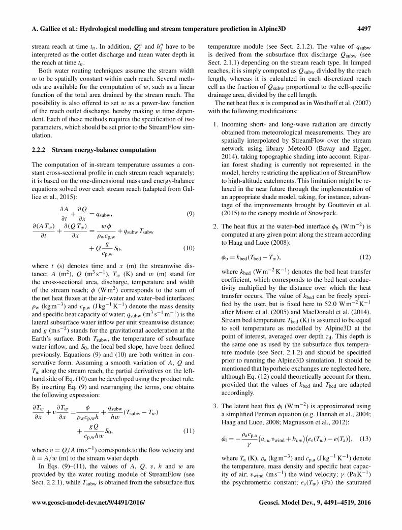
The computation of in-stream temperature assumes a con-stant cross-sectional profile in each stream reach separately;it is based on the one-dimensional mass and energy-balanceequations solved over each stream reach (adapted from Gal-lice et al., 2015):
∂A
∂t+∂Q
∂x= qsubw, (9)
∂(ATw)
∂t+∂(QTw)
∂x=
wφ
ρwcp,w+ qsubw Tsubw
+Qg
cp,wS0, (10)
where t (s) denotes time and x (m) the streamwise dis-tance; A (m2), Q (m3 s−1), Tw (K) and w (m) stand forthe cross-sectional area, discharge, temperature and widthof the stream reach; φ (Wm2) corresponds to the sum ofthe net heat fluxes at the air–water and water–bed interfaces;ρw (kgm−3) and cp,w (Jkg−1 K−1) denote the mass densityand specific heat capacity of water; qsubw (m3 s−1 m−1) is thelateral subsurface water inflow per unit streamwise distance;and g (ms−2) stands for the gravitational acceleration at theEarth’s surface. Both Tsubw, the temperature of subsurfacewater inflow, and S0, the local bed slope, have been definedpreviously. Equations (9) and (10) are both written in con-servative form. Assuming a smooth variation of A, Q andTw along the stream reach, the partial derivatives on the left-hand side of Eq. (10) can be developed using the product rule.By inserting Eq. (9) and rearranging the terms, one obtainsthe following expression:
∂Tw
∂x+ v
∂Tw
∂x=
φ
ρwcp,wh+qsubw
hw(Tsubw− Tw)
+gQ
cp,whwS0, (11)
where v =Q/A (m s−1) corresponds to the flow velocity andh= A/w (m) to the stream water depth.
In Eqs. (9)–(11), the values of A, Q, v, h and w areprovided by the water routing module of StreamFlow (seeSect. 2.2.1), while Tsubw is obtained from the subsurface flux
temperature module (see Sect. 2.1.2). The value of qsubwis derived from the subsurface flux discharge Qsubw (seeSect. 2.1.1) depending on the stream reach type. In lumpedreaches, it is simply computed asQsubw divided by the reachlength, whereas it is calculated in each discretized reachcell as the fraction of Qsubw proportional to the cell-specificdrainage area, divided by the cell length.
The net heat flux φ is computed as in Westhoff et al. (2007)with the following modifications:
1. Incoming short- and long-wave radiation are directlyobtained from meteorological measurements. They arespatially interpolated by StreamFlow over the streamnetwork using library MeteoIO (Bavay and Egger,2014), taking topographic shading into account. Ripar-ian forest shading is currently not represented in themodel, hereby restricting the application of StreamFlowto high-altitude catchments. This limitation might be re-laxed in the near future through the implementation ofan appropriate shade model, taking, for instance, advan-tage of the improvements brought by Gouttevin et al.(2015) to the canopy module of Snowpack.
2. The heat flux at the water–bed interface φb (Wm−2) iscomputed at any given point along the stream accordingto Haag and Luce (2008):
φb = kbed(Tbed− Tw), (12)
where kbed (Wm−2 K−1) denotes the bed heat transfercoefficient, which corresponds to the bed heat conduc-tivity multiplied by the distance over which the heattransfer occurs. The value of kbed can be freely speci-fied by the user, but is fixed here to 52.0 Wm−2 K−1
after Moore et al. (2005) and MacDonald et al. (2014).Stream bed temperature Tbed (K) is assumed to be equalto soil temperature as modelled by Alpine3D at thepoint of interest, averaged over depth zd. This depth isthe same one as used by the subsurface flux tempera-ture module (see Sect. 2.1.2) and should be specifiedprior to running the Alpine3D simulation. It should bementioned that hyporheic exchanges are neglected here,although Eq. (12) could theoretically account for them,provided that the values of kbed and Tbed are adaptedaccordingly.
3. The latent heat flux φl (Wm−2) is approximated usinga simplified Penman equation (e.g. Hannah et al., 2004;Haag and Luce, 2008; Magnusson et al., 2012):
φl =−ρacp,a
γ
(avwvwind+ bvw
)(es(Tw)− e(Ta)
), (13)
where Ta (K), ρa (kgm−3) and cp,a (Jkg−1 K−1) denotethe temperature, mass density and specific heat capac-ity of air; vwind (ms−1) the wind velocity; γ (PaK−1)the psychrometric constant; es(Tw) (Pa) the saturated
www.geosci-model-dev.net/9/4491/2016/ Geosci. Model Dev., 9, 4491–4519, 2016
4498 A. Gallice et al.: Hydrological modelling and stream temperature prediction in Alpine3D
vapour pressure measured at stream temperature; ande(Ta) (Pa) the actual vapour pressure measured atair temperature. The values of parameters avw (–)and bvw (ms−1) are chosen after Webb and Zhang(1997), namely avw = 2.20× 10⁻³ and bvw = 2.08×10⁻³ ms−1, although they can be changed by the user.
4. The sensible heat flux φh (Wm−2) is computed basedon an approach similar to the one used in Comola et al.(2015), namely
φh =−ρacp,a(avwvwind+ bvw
)(Tw − Ta
). (14)
This expression for φh is preferred over the one used inWesthoff et al. (2007), since the latter contains a termes(Tw)− e(Ta) in the denominator which we observedto be responsible for numerical instabilities when Twapproaches Ta (not shown).
In the case of lumped stream reaches, StreamFlow usesthe first-order upwind finite difference approximation ofEqs. (9)–(10) to estimate stream temperature Tw,j in eachreach j (see, e.g. Westhoff et al., 2007):
AjdTw,j
dt=Qin,j
Lj(Tin,j − Tw,j )+ qsubw,j (Tsubw,j − Tw)
+wjφj
ρwcp,w+LjQj
g
cp,wS0, (15)
where Aj (m2), Qj (m3 s−1), S0 (–), Lj (m) and wj (m)denote the cross-sectional area, outlet discharge, mean bedslope, length and width of reach j , and φj (Wm−2) corre-sponds to the net heat flux into reach j . Qin,j and Tin,j standfor the discharge and temperature of water draining into thereach inlet.Qin,j is simply computed as the sum of the outletdischarges of the upstream reaches, whereas Tin,j is approx-imated as the discharge-weighted mean of the outlet temper-atures of the upstream reaches. Tsubw,j and qsubw,j denotethe temperature and discharge per unit streamwise distanceof the subsurface water inflow into reach j . Equation (15) isdiscretized in time using an implicit Euler scheme, whose so-lution is obtained thanks to the simplified Brent root-findingmethod proposed by Stage (2013).
In discretized stream reaches, Eq. (11) is solved using asplitting scheme (e.g. LeVeque, 2002). The idea is to de-compose the equation into two simpler ones, where the so-lution of the first equation serves as the initial condition forthe second one. Similarly to Loinaz et al. (2013), we chosehere to separate heat advection from the accounting of theheat sources, since standard approaches are available for thenumerical resolution of advection in the absence of sources.The resulting splitting scheme is the following (adapted from
Loinaz et al., 2013):
∂Tw
∂t+ v
∂Tw
∂x= 0, (16)
dTwdt=
φ
ρwcp,wh+qsubw
hw(Tsubw− Tw)
+gQ
cp,whwS0. (17)
Equation (16) is discretized over each stream reach using anexplicit upwind finite volume scheme with second-order pre-cision in space and first-order precision in time (Berger et al.,2005):
T n+1w,i = T
nw,i −
vni 1t
li
(T Lw,i+1/2− T
Lw,i−1/2
). (18)
In the above equation, T nw,i (K) and vni (ms−1) denote thestream temperature and flow velocity in reach cell i at timetn,1t corresponds to the time step and li is the length of celli. T Lw,i+1/2 (K) refers to the so-called “left state” at the rightboundary of cell i, which is computed as
T Lw,i+1/2 = Tn
w,i +12ψi(T
nw,i − T
nw,i−1), (19)
where the factor ψi (–), known as a “slope limiter”, is in-troduced so as to limit numerical dispersion. Many slopelimiters have been derived for regular space discretizations(LeVeque, 2002), but very few are available for irregularmeshes (Berger et al., 2005; Zeng, 2013). StreamFlow im-plements the slope limiter developed by Zeng (2013),
ψi =B(r + rk)
1+Ark, (20)
with
r =Tw,i+1− Tw,i
Tw,i − Tw,i−1,
A=li−1+ li
li + li+1,
B =2li
li + li+1,
k =
⌈B
2min(1,A)−B
⌉.
The solution to Eq. (18) is used as initial condition forEq. (17), which is discretized in time according to an implicitEuler scheme and solved using the root-finding method de-veloped by Stage (2013). A validation of the splitting schemecan be found in Appendix B, where it is compared with an-alytical solutions to the heat-balance equation in two simpletest cases.
Geosci. Model Dev., 9, 4491–4519, 2016 www.geosci-model-dev.net/9/4491/2016/

A. Gallice et al.: Hydrological modelling and stream temperature prediction in Alpine3D 4499
3 Model implementation
In order to allow for the calibration of its parameters, Stream-Flow was developed as a stand-alone program rather thanbeing seamlessly integrated into Alpine3D. This permits ahigher flexibility, since Alpine3D – whose typical computa-tion time is of the order of 24 h when simulating a 1-yearperiod on a standard personal computer – does hereby notneed to be newly run each time a new parameter set is testedin StreamFlow. Regarding the computation time of Stream-Flow itself, we observed the simulation duration to be highlydependent on the methods used to compute the transport ofwater and heat along the stream network. In general, thelumped approaches are associated with much-reduced com-putation times as compared to the discretized methods, andthe Muskingum–Cunge water routing technique is slowerthan its instantaneous advection counterpart. As an indica-tion, the stream temperature simulations reported in Sect. 4,which were run on a personal computer with 2 GB of RAMand an Intel® Core™ i7 processor, took between a few sec-onds (with the lumped instantaneous routing approach) andmore than 24 h (with the discretized Muskingum–Cunge ap-proach) to complete.
For the sake of consistency, StreamFlow is, similarly toAlpine3D, implemented in C++ and compiled using CMake.The choice was made to use version C++11 of the C++ lan-guage, since it offers new practical features such as anony-mous functions or the “range-based” FOR loops as comparedto the C++99 standard (Lippman et al., 2012) – regardless ofthe fact that C++11 is meant to supersede C++99 in the longterm. The same coding strategy as detailed in Bavay and Eg-ger (2014) is used here, namely the following:
– Advantage is taken of the object-oriented nature of C++to clearly structure the code and make it as modular aspossible, so as to facilitate understandability and easefuture developments.
– The dependence towards third-party software is avoidedas much as possible in order to limit installation is-sues. The only external utility required by StreamFlowis the library MeteoIO (Bavay and Egger, 2014), whichis used to read input files and interpolate meteorologicaldata in space and time.
– Significant effort is put into documenting the code, bothfor end users and future developers. Online documenta-tion provides indications regarding the installation pro-cedure and the steps to follow in order to launch asimulation (see http://models.slf.ch/p/streamflow/doc/).In addition, technical documentation is directly inte-grated into the source code using the doxygen tool (vanHeesch, 2008).
– Particular attention is paid to keeping the coding styleconsistent. This task is facilitated by the small size
of the development team – mostly one person – andthe young age of the project – the creation of Stream-Flow dates from 2015. The coding style is essentiallythe same as in MeteoIO, with additional conventionsregarding the naming of class attributes (see http://models.slf.ch/p/streamflow/page/CodingStyle/).
– When compiling the code, all possible gcc warnings areactivated and requested to be passed successfully. Thecode currently compiles on Windows, Linux and OS X.
– The program is designed so as to be as flexible as pos-sible. In particular, its behaviour can be adapted with-out recompiling the code by modifying the configura-tion file, which regroups all adjustable parameters. Ad-ditionally, the use of library MeteoIO for preprocessingallows input data to be provided in a large variety offormats.
– Daily automated tests were set into place using CTest.This ensures that potential errors introduced by codemodifications are rapidly identified and corrected, there-fore increasing code stability.
The following sections provide some details about the codeimplementation and the program work flow.
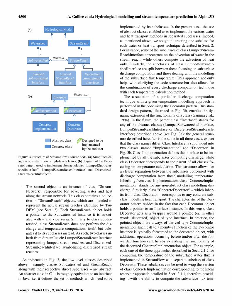
3.1 Program main architecture
The architecture of the program core is depicted as a Uni-fied Modelling Language diagram (UML diagram; see, e.g.Booch et al., 2005) in Fig. 3. The code is essentially struc-tured around a main class, “HydrologicalModel”, which re-groups two different objects:
– The first object is an instance of class “Watershed”, incharge of computing the transport of water and heatwithin the hillslopes. This class is itself a container stor-ing a collection of “Subwatershed” objects, each oneof them representing one of the subwatersheds delin-eated by TauDEM (see Sect. 2). The computation ofdischarge and temperature at the outlet of each sub-watershed is not performed in class Subwatershed di-rectly, but in its subclasses instead. The idea behind thisapproach is to implement each alternative method forthe computation of the subwatershed outflow dischargeand/or temperature in a different subclass of class Sub-watershed. Thus, since no spatially discretized tech-niques have been implemented in the code to date, classSubwatershed only has one subclass, LumpedSubwater-shedInterface, which defines the interface to be imple-mented by lumped subwatersheds – i.e. subwatershedsbeing treated as single points (see Sect. 2.1.1). Futurecode developments could include the definition of a sec-ond interface inherited from Subwatershed, represent-ing the subwatersheds as spatially distributed entities.
www.geosci-model-dev.net/9/4491/2016/ Geosci. Model Dev., 9, 4491–4519, 2016
4500 A. Gallice et al.: Hydrological modelling and stream temperature prediction in Alpine3D
n
1
HydrologicalModel
Watershed StreamReach
Subwatershed StreamReach
Lumped
Subwatershed
Interface
Lumped
StreamReach
Interface
Discretized
StreamReach
Interface
n
1
Interface
Decorator Implementation
Concrete
Decorator
Concrete
Implementation
Abstract class
Concrete class
(a)
(b)
Designed to be implemented by the end user
Points to…
Points to…
Figure 3. Structure of StreamFlow’s source code. (a) Simplified di-agram of StreamFlow’s high-level classes; (b) diagram of the Deco-rator pattern used to implement abstract classes “LumpedSubwater-shedInterface”, “LumpedStreamReachInterface” and “Discretized-StreamReachInterface”.
– The second object is an instance of class “Stream-Network”, responsible for advecting water and heatalong the stream network. This class contains a collec-tion of “StreamReach” objects, which are intended torepresent the actual stream reaches identified by Tau-DEM (see Sect. 2). Each StreamReach object holdsa pointer to the Subwatershed instance it is associ-ated with – and vice versa. Similarly to class Subwa-tershed, class StreamReach does not perform the dis-charge and temperature computations itself, but dele-gates it to its subclasses instead. As such, two classes in-herit from StreamReach: LumpedStreamReachInterfacerepresenting lumped stream reaches, and Discretized-StreamReachInterface symbolizing discretized streamreaches.
As indicated in Fig. 3, the low-level classes describedabove – namely classes Subwatershed and StreamReach,along with their respective direct subclasses – are abstract.An abstract class in C++ is roughly equivalent to an interfacein Java, i.e. it defines the set of methods which need to be
implemented by its subclasses. In the present case, the useof abstract classes enabled us to implement the various waterand heat transport methods in separated subclasses. Indeed,as mentioned above, we sought at creating one subclass foreach water or heat transport technique described in Sect. 2.For instance, some of the subclasses of class LumpedStream-ReachInterface concentrate on the advection of water in thestream reach, while others compute the advection of heatonly. Similarly, the subclasses of class LumpedSubwater-shedInterface are split between those focusing on subsurfacedischarge computation and those dealing with the modellingof the subsurface flux temperature. This approach not onlyhelps with clarifying the code structure but also allows forthe combination of every discharge computation techniquewith each temperature calculation method.
The association of a particular discharge computationtechnique with a given temperature modelling approach isperformed in the code using the Decorator pattern. This stan-dard design pattern, illustrated in Fig. 3b, enables the dy-namic extension of the functionality of a class (Gamma et al.,1994). In the figure, the parent class “Interface” stands forany of the abstract classes (LumpedSubwatershedInterface,LumpedStreamReachInterface or DiscretizedStreamReach-Interface) described above (see Fig. 3a): the general struc-ture described hereafter is the same in all three cases, expectthat the class names differ. Class Interface is subdivided intotwo classes, named “Implementation” and “Decorator” inFig. 3b. Class Implementation defines the interface to be im-plemented by all the subclasses computing discharge, whileclass Decorator corresponds to the parent of all classes fo-cusing on temperature calculation. This structure allows fora clearer separation between the subclasses concerned withdischarge computation from those modelling temperature.Inheriting from class Implementation, class “ConcreteImple-mentation” stands for any non-abstract class modelling dis-charge. Similarly, class “ConcreteDecorator” – which inher-its from class Decorator – corresponds to any concrete sub-class modelling heat transport. The characteristic of the Dec-orator pattern resides in the fact that each Decorator objectholds a pointer to an Interface instance. In this sense, classDecorator acts as a wrapper around a pointed (or, in otherwords, decorated) object of type Interface. In practice, thepointed objects are always of derived type ConcreteImple-mentation. Each call to a member function of the Decoratorinstance is typically forwarded to the decorated object, withadditional operations occurring before and/or after the for-warded function call, hereby extending the functionality ofthe decorated ConcreteImplementation object. For example,each one of the three approaches described in Sect. 2.1.2 forcomputing the temperature of the subsurface water flux isimplemented in StreamFlow as a separate subclass of classDecorator. These subclasses can be used to wrap the versionof class ConcreteImplementation corresponding to the linearreservoir approach detailed in Sect. 2.1.1, therefore provid-ing it with the ability to compute the subsurface flux tem-
Geosci. Model Dev., 9, 4491–4519, 2016 www.geosci-model-dev.net/9/4491/2016/

A. Gallice et al.: Hydrological modelling and stream temperature prediction in Alpine3D 4501
perature. It should be mentioned that classes Implementationand Decorator have been designed in StreamFlow so as tobe easily subclassed by a casual developer, therefore facili-tating the implementation of future discharge or temperaturecomputation methods.
3.2 Input reading
For StreamFlow to run properly, Alpine3D has to be config-ured so as to output the grids of the water percolation rateat the bottom of the soil columns. In case stream temper-ature is to be computed, StreamFlow additionally expectsgrids of soil temperature from Alpine3D (see Sect. 2.1.2),on top of the same meteorological measurements as those re-quired by Alpine3D as input. These measurements will beinterpolated by MeteoIO over the stream reaches, taking to-pographic shading into account in the case of incoming short-wave radiation.
Similarly to MeteoIO, StreamFlow processes its input filesin a centralized manner, hereby facilitating the understandingand reuse of the code by casual developers. All required filesare parsed by a single class, “InputReader”, which supportsvarious input formats thanks to the integrated use of MeteoIOutilities (see Bavay and Egger, 2014). It delegates the actualparsing of the input files to low-end classes, devised to beeasily modified or enriched by end users.
3.3 Output writing
As a result of its semi-distributed nature, StreamFlow isable to output the discharge and temperature of the subsur-face water flux produced by each subwatershed, as well asthe water depth, discharge and temperature in each streamreach. Output files are currently produced in the SMETformat (see https://models.slf.ch/docserver/meteoio/SMET_specifications.pdf), for which various utilities – such as pars-ing and visualizing functions in Matlab and Python – areavailable in MeteoIO. The possibility is offered to the userto generate output files only for certain subwatersheds and/orstream reaches.
As for the parsing of the input files, the writing of the out-put data is handled by a high-level class, “OutputWriter”,which delegates the actual generation of the output files tolow-level classes. As mentioned in the previous section, thisarchitecture both facilitates future developments and easesthe understanding of the global code structure.
3.4 Calibration module
StreamFlow comes with an optimization module used to cal-ibrate the model parameters. It aims to identify the parameterset minimizing the so-called “objective function”. The lattercan be freely specified by the user based on the followingstandard error measures:
– the root mean square error (RMSE);
– the Nash–Sutcliffe efficiency (NSE; Nash and Sutcliffe,1970), also known as the coefficient of determinationR2;
– the mean absolute error (MAE), corresponding to theaverage over all time steps of the model error absolutevalues; and
– the bias, defined as the mean value of the model errorsover all time steps.
Each one of the above four measures can be evaluated eitherfor water depth, discharge or temperature, bringing a totalof 12 different error measures at disposal. StreamFlow alsosupports the case where measurement data are available atmore than one point along the stream network. The objec-tive function can be defined as any weighted sum of some(or all) of the available error measures, hereby making themodel calibration entirely flexible. Monte Carlo simulationsare currently used for calibrating the model, but other well-known optimization algorithms, such as DREAM (Vrugt andTer Braak, 2011) or GLUE (Beven and Binley, 1992), couldbe easily integrated into the code.
For the sake of modularity and flexibility, the list of modelparameters is not managed centrally in the source code. In-stead, each parametrizable class is responsible for defin-ing its own associated parameters. This operation is per-formed through inheritance of a dedicated abstract class,“ParametrizableObject”, which essentially possesses twomember functions: “getParameters” and “setParameters” forobtaining and modifying the class parameters, respectively.The calibration module can then reconstruct the complete listof model parameters by simply calling method getParameterson each object inheriting from ParametrizableObject. Basedon this list, it can compute new parameter values to be tested,which are transferred back to the individual objects througha call to their method setParameters.
In addition to its name, value and units, each model param-eter in StreamFlow is associated with a range of physicallyacceptable values and a flag specifying whether it should becalibrated or not. The physically acceptable range is used bythe calibration module to restrict the search domain for thebest parameter value. The properties of each parameter canbe freely set by the user in the program configuration file.In particular, the calibration flag can be individually set totrue or false for every parameter, hereby making it possibleto calibrate only a given subset of parameters.
4 Case study
In view of assessing its accuracy and demonstrating someof its capabilities, StreamFlow is tested over a high-altitudecatchment in Switzerland. Section 4.1 presents the test catch-ment and the measurement data used to validate the model.The model setup is described in Sect. 4.2 and the simulationresults are detailed in Sect. 4.3.
www.geosci-model-dev.net/9/4491/2016/ Geosci. Model Dev., 9, 4491–4519, 2016

4502 A. Gallice et al.: Hydrological modelling and stream temperature prediction in Alpine3D
#
#
#
1750
2750
2250
20002500
2750
0 1 2 km
YÉ
±
Outlet
Am Rin
Dürrboden
Figure 4. Map of the Dischma catchment displaying the subwater-sheds (coloured areas) and stream network (light blue line) derivedfrom the DEM using TauDEM. The locations of the stream gaugesare indicated as red triangles.
4.1 Study site and measurement data
StreamFlow is tested over the Dischma catchment, locatedin the eastern Swiss Alps (see insert in Fig. 4). The gaug-ing station operated by the Swiss Federal Office for the En-vironment (FOEN) at the location named Davos Krieges-matte – referred to as “Outlet” in Fig. 4 – is chosen as thecatchment outlet. At this point, the watershed has an areaof 43.3 km2 and is mostly covered with pasture (36 %), rockoutcrops (24 %) and bare soil (16 %), with only 2 % of glaciercover (Schaefli et al., 2014). Very little riparian vegetation ispresent along the stream, which ensures that the current ab-sence of riparian shade model in StreamFlow does not have alarge influence on the quality of the stream temperature sim-ulation. The watershed elevation ranges from about 1700 mto more than 3100 m above sea level. Its hydrological regimewas classified as glacio-nival by Aschwanden and Weingart-ner (1985), i.e. the stream discharge is low in winter andpeaks in June–July due to snow and ice melt, therefore cor-responding to a typical watershed over which StreamFlow ismeant to be used. More information on the Dischma catch-ment can be found in, e.g. Zappa et al. (2003) and Schaefliet al. (2014).
Water depth, discharge and temperature are continuouslymonitored by the FOEN at the catchment outlet. In comple-ment to the quality control performed by the FOEN, hourlymean data are also corrected here using the procedure de-
scribed in Gallice et al. (2015), namely a combination ofvisual inspection and automatized outlier identification. Inaddition to the FOEN station, two temporary gauging sta-tions were installed starting on 16 January 2015 at the loca-tions named Am Rin and Dürrboden, indicated as red trian-gles in Fig. 4. The gauging station at Am Rin was positionedin a small stream coming from a side valley, just above itsconfluence with the main stream, and remained in place un-til 17 July 2015. The station at Dürrboden was deployed inthe upper part of the main stream, just below the confluencewith the rivulet coming from the glacier. It was dismantledon 25 September 2015. Both stations continuously measuredwater depth and stream temperature with a sampling rate of1 h. Discharge was manually estimated using the salt dilutiontechnique on a few days during winter and spring, which en-abled the derivation of a rating curve to convert the contin-uous water depth measurements into discharge values (e.g.Weijs et al., 2013). The data from the gauging stations at AmRin and Dürrboden are corrected using the same protocol asthe data provided by the FOEN.
The meteorological data used to run the Alpine3D simula-tion and compute the stream temperature in StreamFlow areobtained from two different sources:
a. One of the sources is the Swiss Federal Office of Mete-orology and Climatology, MeteoSwiss, which operatesa country-wide network of automatic weather stations.Two of these are in the vicinity of the Dischma catch-ment: the Davos and Weissfluhjoch stations, whose re-spective locations are about 5 and 8.5 km on the north-west of the catchment outlet. They are both equippedwith heated rain gauges, the one at Davos being un-shielded and the one at Weissfluhjoch shielded. Thesestations provide measurements of air temperature, rel-ative humidity, incoming long- and short-wave radia-tion, precipitation, wind direction and snow height ev-ery hour.
b. The other source is the Intercantonal Measurement andInformation System (IMIS), a network of automatedweather stations mostly used for avalanche forecastingin Switzerland (Lehning et al., 1999). Four of thesestations are used in the present study, whose distancesto the catchment outlet are 0.9, 4.7, 5.9 and 9.5 km.They provide hourly measurements of air temperature,relative humidity, outgoing short-wave radiation, windspeed and snow depth.
All meteorological time series are visually inspected to detectsensor failure. Data flagged as erroneous are removed fromthe time series.
4.2 Model setup
As mentioned previously, StreamFlow requires Alpine3D tobe executed first. In the present case, Alpine3D is run over a
Geosci. Model Dev., 9, 4491–4519, 2016 www.geosci-model-dev.net/9/4491/2016/
A. Gallice et al.: Hydrological modelling and stream temperature prediction in Alpine3D 4503
grid with 100 m resolution and with an internal time step of15 min. The simulated time period extends over 3 hydrolog-ical years, namely from 1 October 2012 to 1 October 2015.All meteorological input data are spatially interpolated us-ing the inverse-distance weighting approach with lapse rate,except for solar radiation and precipitation. Solar radiationis computed based on the measurements at the Weissfluhjochstation alone, taking atmospheric attenuation into account foreach grid cell separately. Precipitation is interpolated usingthe data measured at the Davos station only. It is correctedfor undercatch using the approach advocated by the WorldMeteorological Organization (WMO) for Hellmann gauges(Goodison et al., 1998), before being distributed over eachgrid cell based on a lapse rate proportional to the measuredprecipitation intensity at Davos. Another procedure using thedata from the Weissfluhjoch station in addition to the onefrom Davos was also tested for interpolating precipitation.However, it was rejected since it largely overestimated the to-tal amount of precipitation falling over the catchment, due tothe existence of a strong north–south precipitation gradientin the area, making the measurements at the Weissfluhjochstation – located further north – less representative of the sit-uation in the Dischma catchment than those at the Davos sta-tion – located closer to the catchment (Voegeli et al., 2016).
As an additional preliminary step to the StreamFlow sim-ulation, the stream network and its corresponding set of sub-watersheds are, as described in Sect. 2, extracted from a 25 mresolution DEM provided by the Swiss Federal Office ofTopography, SwissTopo (see https://shop.swisstopo.admin.ch/en/products/height_models/dhm25). Application of theautomatic Peuker–Douglas extraction method providedby TauDEM (see http://hydrology.usu.edu/taudem/taudem5/help53/PeukerDouglas.html) results in a subdivision of thecatchment into 39 subwatersheds, ranging in size from 0.2 hato 6.4 km2 (see Fig. 4). It should be mentioned that the dif-ference in resolution between the DEM provided as inputto Alpine3D (100× 100 m) and the one used to extract thestream network (25×25 m) is seamlessly handled by Stream-Flow. This allows, as in the present case, for Alpine3D to berun over a coarser grid than StreamFlow, hereby saving com-putational power and resources.
StreamFlow is configured so as to compute the widthw of each stream reach as w = awAreach,tot+ bw, whereAreach,tot (m2) denotes the total area drained by the reach– including its upstream reaches. Parameters aw (m−1) andbw (m) are determined approximately based on the width ofthe main stream estimated at sample locations using aerialphotographs of the Dischma catchment. In addition, the val-ues of parameters αh and βh, which are required by the modelto estimate water depth when simulating discharge based onthe instantaneous advection technique (see Sect. 2.2.1), arederived from the discharge gauging curve provided by theFOEN at the catchment outlet. All model parameters usedfor the StreamFlow simulations presented in the next sec-tion are summarized in Table 2, along with their respective
calibration ranges when appropriate. For the purpose of re-ducing the impact of the initial conditions on the modelledstream variables, a warm-up period of 1 year is considered.In other words, the model is run over a random year beforeeach simulation, and its state at the end of the warm-up pe-riod is used as an initial condition for the actual simulation.This approach is observed to improve the quality of the sim-ulation – notably of modelled discharge – by letting enoughtime for the amount of water stored in the linear reservoirsrepresenting the subwatersheds to adapt to the inflow condi-tions (not shown). The model is calibrated over hydrologicalyear 2013 using Monte Carlo simulations, and validated overhydrological years 2014 and 2015. Calibration is performedin two steps:
1. All parameters associated with water routing, whetherwithin the hillslopes or along the stream network, arecalibrated by maximizing the Nash–Sutcliffe efficiencyof simulated discharge at the catchment outlet. Only theparameters associated with the modelling of the subsur-face flux discharge are actually calibrated in this step(namely Rmax, τ res,u and τ res,l), since the only parame-ter related to water routing within the stream channels(i.e. Manning’s coefficient) is fixed to some predefinedvalue (see Sect. 4.3 and Table 2).
2. The parameters calibrated in step 1 are kept fixed totheir respective best values, while the parameters re-lated to stream temperature modelling are calibrated bymaximizing the NSE of simulated temperature at thecatchment outlet. This step is repeated for each methodused to compute the temperature of the subsurface wa-ter flux (see Sect. 2.1.2). The parameters associated withthe water heat balance in the stream network are fixedto specific values based on physical considerations (seeTable 2).
In order to better assess the accuracy of StreamFlow, theapproach advocated by Schaefli and Gupta (2007) is fol-lowed here. The error measures associated with StreamFloware compared to those of a simplistic benchmark model, soas to verify whether StreamFlow allows for more robust pre-dictions than those that could be made based on a basicprocedure. Two benchmark models are actually consideredhere, one for discharge and one for temperature. Both areconstructed by averaging, for each hour of each day of theyear, the values of discharge and temperature measured atthe catchment outlet on those particular hours and days be-tween 2005 and 2014. For example, the output of the dis-charge benchmark model on 1 January at 13:00 UTC is thesame for all years and corresponds to the average of the 10discharge values measured at the catchment outlet on 1 Jan-uary at 13:00 UTC from 2005 to 2014.
www.geosci-model-dev.net/9/4491/2016/ Geosci. Model Dev., 9, 4491–4519, 2016

4504 A. Gallice et al.: Hydrological modelling and stream temperature prediction in Alpine3D
Table 2. Parameters used by StreamFlow to simulate water depth, discharge and temperature using various approaches. The parameters aredescribed in more detail in the main text (Sect. 2 and Appendix A). First column of the table mentions the part of the model in which theparameter is used. The absence of a calibration range (marked as n/a) indicates a fixed parameter.
Model part Parameter Units Defined inCalibrated or Calibration Rationale for the chosenchosen value range value or calibration range
Subwatershed Rmax (mm day−1) main text 6.93 [0,50] Comola et al. (2015)outflow discharge τ res,u (day) Eq. (A5) 22.5 [0,60] Comola et al. (2015)(Sect. 2.1.1) τ res,l (day) Eq. (A6) 567.1 [0,600] Comola et al. (2015)
Subwatershed ksoil (day) Eqs. (A7)–(A8) 49.6 [0,50] Comola et al. (2015)outflow temperature τHSPF (day) Eq. (1) 58.2 [0.1,100](Sect. 2.1.2) DHSPF (◦C) Eq. (1) 0.99 [−3,1]
zd (m) main text 2.40 n/a
Channel aw (m−1) main text 1.52× 10⁻⁷ n/a aerial photographswater discharge bw (m) main text 0.39 n/a aerial photographs(Sect. 2.2.1) αh (m1−3βh sβh ) main text 0.57 n/a discharge gauging curve
at watershed outletβh (−) main text 0.32 n/a same as for αhnm (−) Eqs. (5) and (7) 0.04, 0.07, 0.10 n/a Phillips and Tadayon (2006)
Channel avw (−) Eq. (13) 2.20× 10⁻³ n/a Webb and Zhang (1997)water temperature bvw (ms−1) Eq. (13) 2.08× 10⁻³ n/a Webb and Zhang (1997)(Sect. 2.2.2) kbed (Wm−2 K−1) Eq. (12) 52.0 n/a Moore et al. (2005) and
MacDonald et al. (2014)
Oct 2012 Oct 2013 Oct 2014 Oct 20150.0
0.5
1.0
1.5
2.0
Hou
rly sn
ow d
epth
[m] Measured
Simulated
Figure 5. Comparison between the measured (blue line) and sim-ulated (red line) time evolution of snow depth at the Stillberg me-teorological station. The simulated curve corresponds to the meansnow depth as computed by Alpine3D over the 100× 100 m gridcell containing the Stillberg station.
4.3 Model evaluation
4.3.1 Results of the Alpine3D simulation
The Alpine3D simulation is observed to rather accuratelycapture the time evolution of the snow pack. As an exam-ple, Fig. 5 depicts the simulated snow depth in comparisonwith the measured one at the Stillberg meteorological station,which is located at an altitude of 2085 m above sea level onthe western slope of the catchment. It can be noticed that theonset of snow accumulation and the timing of the melting pe-riod are satisfyingly reproduced, in addition to the fact thatthe snow depth appears to be overall well simulated. A more
Table 3. Comparison of the total volume of water (Vin,simu) simu-lated by Alpine3D to percolate at the bottom of the watershed soilcolumns over each year, and the measured total volume of water(Vout,meas) flowing out of the catchment each year via the river.
Hydrological Vin,simu Vout,meas Relativeyear (m3) (m3) difference (%)
2013 5.28× 10⁷ 5.64× 10⁷−6.3
2014 5.88× 10⁷ 5.57× 10⁷ 5.72015 5.57× 10⁷ 5.18× 10⁷ 7.6
quantitative assessment of the accuracy of the Alpine3D sim-ulation is obtained by considering the global volume of watertransiting through the watershed each year. Thus, the mea-sured cumulated volume of water (Vout,meas) flowing throughthe catchment outlet each year is compared to the simulatedcumulated volume of water (Vin,simu) percolating at the bot-tom of all the soil columns belonging to the watershed overthe same year. As can be observed in Table 3, the relativedifference between Vout,meas and Vout,simu remains within therange ±8 % for all 3 hydrological years.
4.3.2 StreamFlow simulations of discharge and waterdepth
As mentioned in the previous section, StreamFlow parame-ters related to discharge computation are calibrated againstmeasured discharge at the catchment outlet. To this end,
Geosci. Model Dev., 9, 4491–4519, 2016 www.geosci-model-dev.net/9/4491/2016/

A. Gallice et al.: Hydrological modelling and stream temperature prediction in Alpine3D 4505
Oct 2012 Oct 2013 Oct 2014 Oct 20150
2
4
6
8
10
12
Hou
rly d
isch
arge
[m3
s−1
]
Calibration Validationperiod period(a)
(c)
(b)
30 May2015
03 Jun 07 Jun23456789
Hou
rly d
isch
arge
[m3
s−1
]
(b)
13 Sep2015
17 Sep 21 Sep 25 Sep 29 Sep1
2
3
4
5(c) Measured
Best simulationBest 300 simulations
Figure 6. Comparison between the measured (blue line) and simulated (red line) time evolution of hourly mean discharge at the watershedoutlet. Panel (a) pictures the entire simulated period, and panels (b) and (c) correspond to zooms on two selected time periods (their extentsare indicated as black rectangles in panel a). The simulated curve was obtained with StreamFlow configured so as to advect water in thestream channels using the instantaneous routing approach. The uncertainty range corresponds to the 300 best runs of the model out of the10 000 Monte Carlo simulations.
10 000 Monte Carlo simulations are run, with StreamFlowconfigured so as to use a time step of 1 h and advect wa-ter in the stream channels based on the instantaneous rout-ing scheme (see Sect. 2.2.1). Figure 6 presents a comparisonof the simulated and measured hourly mean discharges overthe 3 considered hydrological years. The uncertainty rangeof the simulated curve is defined by all parameter sets as-sociated with a NSE larger than 0.85 during the calibrationperiod, which amounts to a total of 300 curves. As observedin panel a, the simulation corresponding to the highest NSEvalue matches globally well with the observations, except fora few discharge peaks which are not well captured in 2013and 2015. The simulation uncertainty range appears to berelatively narrow on an annual scale. When looking at a finerscale, it can be observed that the daily fluctuations of dis-charge are relatively well captured by the model as, for exam-ple, shown in panel b for the period 29 May to 8 June 2015.On the other hand, the absence of a fast runoff componentin StreamFlow prevents the model to correctly capture short-lived discharge peaks. As displayed in panel c, the modelledrecession in these cases is much too slow compared to theobserved one. This model limitation could be fixed by im-plementing a new method for transferring water across thesubwatersheds, based on a more physically based approachthan the linear reservoir method used here. For example, theRichards equation could be solved within the soil of eachsubwatershed, provided that the computational resources athand are sufficient. The modularity of StreamFlow would al-low for such a modification to be easily integrated into theexisting code.
Table 4 presents quantitative error measures of dischargemodelled over the validation period at the three gaugingpoints located in the Dischma catchment (see Fig. 4), for thesame StreamFlow configuration as in Fig. 6. The accuracyof the benchmark model at the catchment outlet is also indi-cated in the table for comparison. It should be mentioned thatthe benchmark model could not be evaluated at the two inter-mediate stations since the measurement time series at thesepoints extend over less than a year (see Sect. 4.1). As ob-served in the table, the discharge NSE value associated withthe best StreamFlow simulation is larger than 0.80 at all threepoints, as opposed to the NSE value of the benchmark modelnot exceeding 0.74. On the other hand, the values of the NSElog – defined as NSE computed with the logarithm of thedischarge values – are quite comparable between both mod-els. This is not particularly surprising in view of the strongseasonality of the baseflow component of discharge, partic-ularly during the winter season. The NSE log value at pointAm Rin is rather low, but should be considered with cautionsince the discharge gauging curve at this point is rather un-certain (not shown). The bias of StreamFlow is observed tobe positive at all three gauging points, which certainly resultsfrom the slight overestimation of the rate of water percolatingat the bottom of the soil columns in the Alpine3D simulation(see above). Overall, the performance of StreamFlow regard-ing discharge computation based on the instantaneous waterrouting scheme can be considered satisfying. Its accuracy iscomparable to the one of other existing hydrological modelsapplied over high Alpine catchments (e.g. MacDonald et al.,2014; Schaefli et al., 2014).
www.geosci-model-dev.net/9/4491/2016/ Geosci. Model Dev., 9, 4491–4519, 2016

4506 A. Gallice et al.: Hydrological modelling and stream temperature prediction in Alpine3D
Table 4. Accuracy of the hourly discharge simulations performed by StreamFlow using the instantaneous water routing technique. Theperformance of the discharge benchmark model is indicated in the last row for comparison. The third column contains the period over whichthe error measures are computed. NSE log corresponds to the Nash–Sutcliffe efficiency computed with the logarithm of the discharge values.
Model Location Time periodRMSE NSE NSE log Bias
(m3 s−1) (−) (−) (m3 s−1)
StreamFlowOutlet entire validation period 0.60 0.82 0.90 0.14Dürrboden 17 Jan to 25 Sep 2015 0.30 0.81 0.91 0.11Am Rin 17 Jan to 17 Jul 2015 0.10 0.82 0.76 0.02
Benchmark Outlet entire validation period 0.73 0.74 0.88 −0.04
0 10 20 30 40 50 60τres,u [day]
0
5
10
15
20
Rm
ax [m
m d
ay−
1] (a) r=−0.68
0
0.05
0.1
0.15
Freq
uenc
y [-
]
0 100 200 300 400 500 600τres,l [day]
0
5
10
15
20
Rm
ax [m
m d
ay−
1] (b) r=−0.32
0 0.05 0.1 0.15Frequency [-]
0
0.05
0.1
0.15
Freq
uenc
y [-
]
0 10 20 30 40 50 60τres,u [day]
0
100
200
300
400
500
600
τ res,l [d
ay]
(c) r=0.27
Figure 7. The 300 best sets of StreamFlow parameters associated with water transport (see Table 2 for more information on the parameters).Each panel contains the values of two parameters displayed as a function of each other: (a) Rmax versus τ res,l, (b) τ res,u versus τ res,l and(c)Rmax versus τ res,u. Each x or y axis spans the entire calibration range of its associated parameter. The parameter distributions are indicatedin blue on the sides of the corresponding panels; for example, the distribution of the 300 best Rmax values is shown on the right-hand sideof panel (a). Pearson’s correlation coefficient r between each pair of parameters is indicated in the upper right-hand corner of the associatedgraph.
Regarding the calibration parameters, it appears that thevalues of Rmax and τ res,u are rather well identified (seeFig. 7). Indeed, their respective distributions based on thebest 300 parameter sets are contained within a rather narrowinterval, clearly separated from the bounds of the respectivecalibration ranges. Within this interval, however, the two pa-rameters are strongly correlated with one another, as picturedin panel c of Fig. 7. This points at the equifinality of the pa-rameter sets (Bárdossy, 2007), since an increase in τ res,u con-jugated with a decrease in Rmax keeps the model accuracy al-most constant. As opposed to τ res,u andRmax, parameter τ res,l
is associated with a broad distribution, sticking to the upperboundary of the calibration interval (see panel a of Fig. 7).As such, StreamFlow appears to be relatively insensitive tothe value of τ res,l, as further emphasized by the low correla-tion between τ res,l and the other two parameters (Bárdossy,2007).
In order to evaluate the influence of the channel wa-ter routing scheme on the modelled discharge, StreamFlowwas run with the following configurations in complement tothe instantaneous routing technique evaluated above: (a) theMuskingum–Cunge approach with lumped stream reaches
Geosci. Model Dev., 9, 4491–4519, 2016 www.geosci-model-dev.net/9/4491/2016/

A. Gallice et al.: Hydrological modelling and stream temperature prediction in Alpine3D 4507
Oct 2013 Oct 20140.0
0.2
0.4
0.6
0.8
1.0
1.2H
ourly
mea
n w
ater
dep
th [m
]
MeasuredLumped instant. routing
Lumped M.-C. (nm =0.04)Lumped M.-C. (nm =0.10)
Figure 8. Water depth as simulated by StreamFlow in hydrologi-cal year 2014 using various channel water routing techniques. Themeasured water depth is indicated in blue and shown here onlyas an indication (see text). Regarding the curves associated withthe Muskingum–Cunge routing technique, only those obtained us-ing lumped stream reaches are shown (orange and violet curves).Those corresponding to discretized stream reaches almost overlapwith their lumped counterparts, with the difference between eachpair of curves amounting to a RMSE of 0.5 mm for nm = 0.04 and3.9 mm for nm = 0.10 over the entire period 2013–2015.
and Manning’s coefficient nm set to 0.04; (b) same as (a) butwith nm = 0.10; and (c)–(d) same as (a)–(b) but with dis-cretized stream reaches. The chosen values for Manning’scoefficient correspond to the lower and upper boundariesof the uncertainty interval estimated in the Dischma catch-ment based on the work of Phillips and Tadayon (2006).The results indicate that the modelled hourly mean dischargecurves in all cases (a) to (d) almost identically correspondto the one depicted in Fig. 6, up to a maximum RMSE of0.03 m3 s−1 between all curves over the entire simulated pe-riod (not shown). Similarly, the error measures reported inTable 4 are also valid in cases (a) to (d). The routing tech-nique therefore appears to have only a very limited impacton the simulated discharge in the Dischma catchment, whichis easily explained by the small size of the watershed (Schae-fli et al., 2014). Indeed, the average streamwise distance be-tween the stream cells and the catchment outlet is about6.6 km, which – assuming a flow velocity of 1 ms−1 – cor-responds to a mean travel time of about 2 h down to thecatchment outlet. This also explains the observed low sen-sitivity of StreamFlow to the value of Manning’s coefficientin the present case. As expected, the above results suggestthat, in small- to medium-sized catchments, the use of spa-tially discretized stream reaches to simulate discharge is notassociated with any marked improvement with respect to thelumped approach.
Albeit discharge is simulated unequivocally by all waterrouting techniques, water depth and flow velocity are not.As pictured in Fig. 8 for hydrological year 2014, differ-ences between the simulated water depth curves are quitelarge, with, for example, a RMSE of 44.5 cm between the
curve associated with the instantaneous routing techniqueand the one corresponding to the Muskingum–Cunge ap-proach with nm = 0.04. The instantaneous water routingtechnique predicts a higher water depth here as compared tothe Muskingum–Cunge approach, reflecting the values of thegauging curve coefficients αh and βh (see Sect. 2.2.1 and Ta-ble 2). In addition, the predictions based on the Muskingum–Cunge technique depend on the value of Manning’s coeffi-cient, as expected from Eq. (7): the higher nm, the higher thesimulated water depth. However, as for the case of discharge,the water depth estimations do not appear to benefit from theuse of discretized stream reaches as opposed to lumped ones,since both corresponding curves almost overlap for a fixednm (see legend of Fig. 8). It should be mentioned that com-parison with the measured water depth is hazardous sincethe modelled river width at the outlet gauging station wasnot verified to correspond to the observed one. The measuredcurve is therefore only shown here as an indication. The factthat it diverges from the curve associated with the instanta-neous advection approach during winter is due to the factthat the discharge gauging curve of FOEN is linear for smallwater depth values, and adopts the form of a power func-tion as in StreamFlow only for larger values of h. Given thatsimulated discharge is almost the same for all water routingtechniques, the differences in simulated water depth result inlarge differences in the simulated flow velocity as well (notshown).
4.3.3 StreamFlow simulations of stream temperature
Turning now to the stream temperature simulations, we firstdetermine an appropriate value for the soil temperature av-eraging depth zd (see Sect. 2.1.2 and Eq. 12). Five differentpossibilities are considered here: 0.15, 0.30, 0.60, 1.20 and2.40 m. Using StreamFlow configured so as to approximatethe temperature of the subsurface flux as the depth-averagedsoil temperature (Sect. 2.1.2), we find that the choice zd =
2.40 m leads to the best results in terms of temperature-basedNSE (not shown). This rather large value may be due to therelatively low resolution of the vertical soil temperature pro-file computed by Alpine3D, which was configured here touse a coarse vertical discretization of the soil columns in or-der to spare computational power. The value zd = 2.40 m isnevertheless used in the remainder of this study, since empha-sis is on demonstrating the model capabilities rather than per-forming particularly accurate simulations. Similarly, it can beobserved based on Table 2 that the calibrated values of somestream temperature parameters (notably ksoil and DHSPF) areclose to the respective upper limits of their associated cali-bration ranges. For the sake of conciseness, however, we pro-ceed with the parameter values presented in Table 2 and post-pone the in-depth evaluation of the model sensitivity with re-spect to its parameters to a future publication.
Figure 9 displays stream temperature as simulated byStreamFlow over the hydrological years 2013–2015, with
www.geosci-model-dev.net/9/4491/2016/ Geosci. Model Dev., 9, 4491–4519, 2016

4508 A. Gallice et al.: Hydrological modelling and stream temperature prediction in Alpine3D
Table 5. Accuracy of the hourly stream temperature predictions of StreamFlow (with zd = 2.40 m), based on various approaches for advectingwater in the stream channels and computing the temperature of the subsurface water flux. The accuracy of the temperature benchmarkmodel at the catchment outlet is indicated in the last row for comparison. All error measures are computed over the entire validation period(1 October 2013 to 1 October 2015), except at points Am Rin and Dürrboden for which the considered time period is the same as in Table 4.
Model Channel water routing schemea Subwatershed outflow Location RMSE NSE Biastemperature schemeb (◦C) (–) (◦C)
StreamFlow
Instantaneous advection (lumped) Soil temperature Outlet 1.45 0.78 −0.88Dürrboden 1.45 0.78 0.75Am Rin 1.11 0.89 −0.05
Instantaneous advection (discr.) Soil temperature Outlet 1.40 0.80 −0.85Muskingum–Cunge (nm = 0.07, lumped) 1.49 0.77 −0.85Muskingum–Cunge (nm = 0.07, discr.) 1.46 0.78 −0.80
Instantaneous advection (lumped) Energy balance Outlet 2.06 0.56 −1.63HSPF 1.69 0.70 0.54
Benchmark – – Outlet 1.14 0.87 −0.03
a The indications “lumped” and “discr.” between brackets refer to the spatial discretization of the stream reaches (see Sect. 2.2).b The schemes described in Sect. 2.1.2 for the computation of the subsurface flux temperature are denoted as follows here: “soil temperature” for the schemeassuming the subsurface flux to be in thermal equilibrium with surrounding soil, “energy balance” for the original scheme implemented in StreamFlow and “HSPF”for the scheme inspired from the Hydrological Simulation Program–Fortran.
Oct 2012 Oct 2013 Oct 2014 Oct 20150
2
4
6
8
10
12
Dai
ly m
ean
tem
pera
ture
[◦
C]
(c)
(b)
(a)
02 Mar2014
06 Mar 10 Mar 14 Mar012345678
Hou
rly m
ean
tem
p. [◦
C]
(b) Best simulationUncertainty rangeMeasured
13 Jul2015
17 Jul 21 Jul 25 Jul6
8
10
12
14
16(c)
Figure 9. Comparison between the simulated (red line) and measured (blue line) time evolution of stream temperature at the catchmentoutlet. Panel (a) pictures the entire simulated period (hydrological years 2013 to 2015), with temperature aggregated into daily mean valuesfor visibility. Panels (b) and (c) display the hourly mean temperature over two selected periods of 14 days (their respective extents areindicated as black rectangles in panel a). The simulated curve was obtained with StreamFlow based on the instantaneous water routingscheme, with the temperature of the subsurface water flux being approximated as the soil temperature averaged over a depth of 2.40 m. Theuncertainty range (displayed in light red) is obtained by evaluating StreamFlow for each one of the 300 best sets of parameters Rmax, τ res,uand τ res,u identified during calibration step 1 (see Sect. 4.2).
channel water being advected based on the instantaneousrouting scheme and subwatershed outflow temperature beingapproximated as the depth-averaged soil temperature (sameconfiguration as above). As evident from panel a, stream tem-perature is generally underestimated by the model on a dailytimescale, particularly during the snow melt season in spring.We attribute this discrepancy to soil temperature as simu-
lated by Alpine3D being too low, since its value averageddown to 2.40 m typically remains around 0 ◦C until mid-June (not shown). This underestimation of soil temperatureis in turn expected to result from the coarse soil vertical dis-cretization used in the Alpine3D simulation (see above). Asa workaround, the soil temperature averaging depth zd couldbe increased, since it would result in larger soil temperature
Geosci. Model Dev., 9, 4491–4519, 2016 www.geosci-model-dev.net/9/4491/2016/

A. Gallice et al.: Hydrological modelling and stream temperature prediction in Alpine3D 4509
Table 6. Values chosen for the parameters of test cases 1 and 2,and used to validate the numerical splitting scheme presented inSect. 2.2.2.
Name Units Value
τ (s) 2× 10⁶
ω (s−1) 2π/3600aσ (Ks−1) 5× 10⁻³
bσ (Ks−1) 2× 10⁻⁴
av (s−1) 1/12 800bv (ms−1) 0.5ain (K) 1.5bin (K) 283.15
values while at the same time not lengthening the computa-tion time of the Alpine3D simulation. This approach is notpresented here in more detail in order to keep the article con-cise, but simply mentioned as a hint to interested readers.Past the snow melt season, soil temperature is modelled byAlpine3D to rapidly increase (not shown), which might ex-plain the better agreement between the simulated and mea-sured stream temperature curves during summer.
Panels b and c of Fig. 9 present a zoom on two selectedperiods during winter and summer, respectively. StreamFlowis observed to be capable of simulating the diurnal cycle ofstream temperature, albeit its magnitude is in general too low.It should be specified that temperature is cut off at 0 ◦C bythe model in winter in order to avoid unphysical values. Theunderestimation of the magnitude of the diurnal cycle mayoriginate from an overestimation of water depth or, equiva-lently, from an underestimation of the stream width. This hy-pothesis can unfortunately hardly be tested, since water depthand stream width are difficult to quantify in small mountain-ous streams with irregular, boulder-covered beds. We verifiedwhether the latent and sensible heat fluxes are not underesti-mated by StreamFlow. To this end, we increased the valuesof coefficients avw and bvw by 50 % (see Eq. 13 and Table 2);however, this did not result in a marked improvement of thesimulated diurnal cycle (not shown). The effect of the heatexchange with the stream bed was also tested by reducingthe value of kbed by 50 % (see Eq. 12 and Table 2), but thishad almost no impact on the simulated temperature curve ei-ther (not shown). The underestimation of the diurnal cycletherefore appears to mostly originate from the approach se-lected for the modelling of the subsurface flux temperature,as discussed in more detail below. From the inspection of allthree panels in Fig. 9, it can be stated that modelled tem-perature is not particularly affected by the uncertainty in thevalues of hydrological parametersRmax, τ res,u and τ res,l. As amatter of fact, the uncertainty range of the simulated temper-ature curve remains globally narrow, except around middaywhere it reaches a value up to 1 ◦C on some days (see panelb). This limited sensitivity of modelled temperature with re-
Oct 2013 Oct 20140
2
4
6
8
10
Dai
ly m
ean
stre
am te
mp.
[◦
C]
MeasuredSimulated (soil temp.)
Simulated (energy balance)Simulated (HSPF)
Figure 10. Comparison between various predictions of stream tem-perature at the catchment outlet, where the temperature of the sub-surface water flux is computed based on the following methods:the original scheme implemented in StreamFlow (energy balance),the technique of the Hydrological Simulation Program–Fortran(HSPF), or as soil temperature averaged over a depth of 2.40 m (soiltemp.). All curves are aggregated into daily mean values for visibil-ity.
spect to simulated discharge (and water depth) further hintsat the probable role of the subsurface flux temperature on theunderestimation of the temperature diurnal cycle.
The values of the error measures associated with Fig. 9are summarized in Table 5. The NSE value of the hourlymean temperature curve (0.78) is much lower than the oneof the benchmark model (0.87), which denotes a strong im-provement potential. This has to be put into perspective withthe fact that the Dischmabach river is rather small and heav-ily turbulent, and therefore more challenging to model ascompared to larger, low-altitude rivers. In addition, the NSEvalue is comparable to the one reported by MacDonald et al.(2014) over a mountainous watershed of similar size and al-titudinal range as the Dischma catchment. The RMSE equals1.45 ◦C, which is not very far from the RMSE of the bench-mark model (1.14 ◦C). On the other hand, the bias is ratherlarge (−0.88 ◦C), as already noted from the observation ofFig. 9 above. Regarding the model performance at the twointermediate gauging points, the values of the error mea-sures at Dürrboden are found to be essentially the same asat the outlet point, except for the positive bias (see Table 5).The latter indicates that the modelled stream temperatures atthese two points are – contrary to the temperature at the out-let point – not underestimated, which results from the factthat the stream temperature values measured at the interme-diate points are much closer to the simulated soil temperaturecurve in spring as compared to the stream temperature mea-sured at outlet point (not shown). Concerning Am Rin, theapparent better values for RMSE, NSE and bias have to beweighted against the short time period over which they areevaluated (17 January to 17 July 2015).
As already discussed above, the simulated stream temper-ature is not particularly sensitive to the modelled discharge
www.geosci-model-dev.net/9/4491/2016/ Geosci. Model Dev., 9, 4491–4519, 2016

4510 A. Gallice et al.: Hydrological modelling and stream temperature prediction in Alpine3D
(and water depth). This fact is confirmed by the values ofthe error measures reported in Table 5 for four tempera-ture simulations, each one based on a different water rout-ing scheme, namely the instantaneous advection techniqueor the Muskingum–Cunge approach, combined with eithera lumped or discretized modelling of the stream reaches. Inthe simulations based on the Muskingum–Cunge approach,Manning’s coefficient is fixed to 0.07, which corresponds tothe middle of the above-defined range of plausible values inthe case of the Dischmabach river. It appears that all foursimulations are associated with a similar accuracy in termsof stream temperature modelling, as indicated by the narrowrange of NSE (0.77–0.80) and RMSE (1.40–1.49 ◦C) values.Contrary to the discharge simulations, the discretized repre-sentation of the stream reaches here enables a slight improve-ment of the results as compared to the lumped approach,mainly due to a better resolution of the diurnal cycle (notshown).
In a recent study, Leach and Moore (2015) reviewed theapproaches implemented in some of the most popular streamtemperature models for approximating the temperature of thesubsurface water flux. Based on a comparison with data col-lected in a small Canadian watershed, they concluded thatnone of them performed well, except for the method im-plemented in the HSPF model approaching the observationsrelatively closely. More interestingly, the authors pointed atlarge discrepancies between the predictions of the variousmodels. As a further step, we propose here to investigatethe effect of the modelled subsurface flux temperature onthe simulated stream temperature at the catchment outlet. Tothis end, three StreamFlow simulations are run with the sameconfiguration as above – namely lumped reaches and the in-stantaneous routing scheme – except that the temperature ofthe subsurface flux is computed each time based on a differ-ent method out of the three available ones (see Sect. 2.1.2). Itshould be mentioned that, in virtue of the modular structureof StreamFlow, changing from one method to the next sim-ply requires one line to be modified in the configuration file.The simulation results are displayed in Fig. 10, and the cor-responding error measures can be found in Table 5. It can beobserved that the approach used to compute the temperatureof the subsurface flux has a strong influence on the accuracyof the modelled stream temperature. The method originallyimplemented in StreamFlow appears to perform worse (NSEof 0.56, RMSE of 2.06 ◦C), followed by the HSPF approach(NSE of 0.70, RMSE of 1.69 ◦C). The method based on thedepth-averaged soil temperature is associated with the bestperformance measures (see above). Overall, the three meth-ods seem to determine the temperature of in-stream water toa large extent, leading to variations of more than 4 ◦C be-tween the different curves (see Fig. 10). These observationspoint at the strong need for additional field investigations ofthe dynamics of the subsurface flux temperature, as alreadymentioned by Leach and Moore (2015).
5 Conclusions
Combined modelling of hydrological and thermodynamicprocesses offers promising perspectives for the predictionof stream temperature at the catchment scale. The presentstudy describes a new coupled hydrothermal model, namedStreamFlow, which is currently intended to be used in highAlpine environments. Designed as an independent extensionto the spatially distributed snow model Alpine3D, it has beenwritten entirely anew compared to its initial version. The re-sulting code has a clear and modular structure which takesadvantage of some of the latest available object-oriented fea-tures. Several of the hydrological processes represented inthe model can be simulated using various alternatives. Forexample, the advection of water in the stream channels canbe computed using either the Muskingum–Cunge techniqueor an instantaneous routing approach. This modularity en-ables the model to be adapted to the specific needs of eachuser, but also provides a rapid means to estimate the uncer-tainty of the simulation results by comparing the predictionsof the various modelling alternatives.
Based on an evaluation over a high Alpine catchment,the model accuracy is shown to be satisfying, with Nash–Sutcliffe efficiencies for the hourly mean discharge andhourly mean temperature being equal to 0.82 and 0.78, re-spectively. The various water routing techniques available inStreamFlow do not appear to have a marked effect on thequality of the simulations. On the other hand, it was observedthat the approach used to compute the temperature of the sub-surface water inflow strongly impacts the simulated streamtemperature at the catchment outlet. This effect has not beenreported in any previous study and points at the need for moreintensive field investigations of the subsurface flux tempera-ture.
Several improvements can be brought to the actual stateof the model. The representation of riparian shading wouldallow StreamFlow to be applied in lower-altitude, vegetatedwatersheds. However, similarly to the case of the subsurfaceinflow temperature, the shading by riparian vegetation is acomplex phenomenon which is difficult to simulate and re-quires further research (Moore et al., 2005). The modellingof the ice and snow sheet forming over the stream in win-ter could also be included in StreamFlow, although little re-search has been conducted on this subject in high-altitudeAlpine streams to date. Finally, additional modelling alter-natives could be implemented for various components ofStreamFlow, such as the approach developed by Leach andMoore (2015) for the estimation of the subsurface inflowtemperature, or the full Saint-Venant equations for the rout-ing of water in the stream channels.
In the near future, we plan to use StreamFlow in order toevaluate the effects of climate change on the hydrologicalfunctioning of high Alpine watersheds. In particular, advan-tage will be taken of the coupled hydrothermal nature of the
Geosci. Model Dev., 9, 4491–4519, 2016 www.geosci-model-dev.net/9/4491/2016/

A. Gallice et al.: Hydrological modelling and stream temperature prediction in Alpine3D 4511
model in order to investigate the impact of the future dis-charge modifications on stream temperature.
6 Code availability
The source code of StreamFlow is available under the GNULesser General Public License v3.0 (LGPL v3) at http://models.slf.ch/p/streamflow/ upon creation of a free ac-count. Installation instructions can be found at http://models.slf.ch/p/streamflow/page/Installing-StreamFlow/, and the de-tailed procedure to launch a StreamFlow simulation at http://models.slf.ch/p/streamflow/page/Running-StreamFlow/.
www.geosci-model-dev.net/9/4491/2016/ Geosci. Model Dev., 9, 4491–4519, 2016

4512 A. Gallice et al.: Hydrological modelling and stream temperature prediction in Alpine3D
Appendix A: Formulation of the subwatershed linearreservoir model
This section briefly describes the approaches which were al-ready present in the original version of the code for com-puting the discharge and temperature of the subsurface flowgenerated by each subwatershed.
A1 Subwatershed outflow discharge computation
As illustrated in Fig. A1a, the original model developed byComola et al. (2015) approximates each subwatershed as thevertical superposition of two linear reservoirs, where the up-per one simulates the fast response to rainfall events and thelower one the slow response. Water percolating at the bottomof the subwatershed soil columns fills the lower reservoir upto a maximum flow rateRmax (ms−1), the excess water drain-ing into the upper reservoir. This translates into the followingequations for the water levels Sres,u (m) and Sres,l (m) in theupper and lower reservoirs, respectively:
dSres,u
dt= Ires,u−
Qres,u
Asubw, (A1)
dSres,l
dt= Ires,l−
Qres,l
Asubw, (A2)
where the water inflow rates Ires,u (ms−1) and Ires,l (ms−1)into the upper and lower reservoirs are expressed as Ires,u =
I − Ires,l and Ires,l =min(I,Rmax
), with I (ms−1) denoting
the total flow rate of water percolating at the bottom of thesubwatershed soil columns and Asubw (m2) the subwatershedsurface area. Qres,u (m3 s−1) and Qres,d (m3 s−1) correspondto the discharge at the outlet of the upper and lower reser-voirs, which are linearly related to the reservoir water levels,
Qres,u = AsubwSres,u
τres,u, (A3)
Qres,l = AsubwSres,l
τres,l. (A4)
The characteristic residence times τres,u (s) and τres,l (s) areexpressed as power functions of the subwatershed area:
τres,u = τ res,u
(Asubw
Atot
) 13, (A5)
τres,l = τ res,l
(Asubw
Atot
) 13, (A6)
where τ res,u (s) and τ res,l (s) are two user-specified parame-ters and Atot (m2) denotes the area of the entire parent wa-tershed. The total dischargeQsubw (m3 s−1) flowing from thesubwatershed into the stream is then computed as Qsubw =
Qres,u+Qres,l. The subwatershed behaviour can be adjustedby modifying the values of parameters Rmax, τ res,u and τ res,l.
Tres,u
Tres,l
Tsubw
Tsoil
Tsoil
T soil
Sres,u
Sres,l
Qres,u
Qres,l
Qsubw Ires,u
Ires,l
I
(a)
(b)
Figure A1. Illustrations of the models devised by Comola et al.(2015) for the computation of (a) subsurface flux discharge and(b) subsurface flux temperature. The symbols are defined in the text.
A2 Subwatershed outflow temperature computation
The method developed by Comola et al. (2015) for the com-putation of the subwatershed outflow temperature Tsubw (K)is depicted in Fig. A1b. Temperatures Tres,u (K) and Tres,l (K)of water stored in the upper and lower reservoirs are com-puted as
dTres,u
dt=Ires,u
Sres,u(Tsoil− Tres,u)+
Tsoil− Tres,u
ksoil, (A7)
dTres,l
dt=Ires,l
Sres,l(Tsoil− Tres,l)+
T soil− Tres,u
ksoil, (A8)
where ksoil (s) is a calibration parameter corresponding to thecharacteristic time of thermal diffusion and Tsoil (K) refersto soil temperature at the bottom of the subwatershed soilcolumns as modelled by Alpine3D. T soil denotes the annual
Geosci. Model Dev., 9, 4491–4519, 2016 www.geosci-model-dev.net/9/4491/2016/
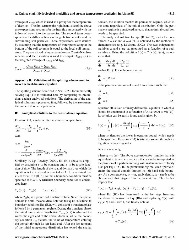
A. Gallice et al.: Hydrological modelling and stream temperature prediction in Alpine3D 4513
average of Tsoil, which is used as a proxy for the temperatureof deep soil. The first term on the right hand-side of the abovetwo expressions accounts for the heat flux associated with theinflow of water into the reservoirs. The second term corre-sponds to the diffusive heat exchange between water and thesurrounding soil particles. These expressions were derivedby assuming that the temperature of water percolating at thebottom of the soil columns is equal to the local soil temper-ature. They are solved using a second-order Crank–Nicolsonscheme, and their solution is used to compute Tsubw (K) asthe weighted average of Tres,u and Tres,l:
Tsubw =Qres,uTres,u+Qres,lTres,l
Qres,u+Qres,l. (A9)
Appendix B: Validation of the splitting scheme used tosolve the heat-balance equation
The splitting scheme described in Sect. 2.2.2 for numericallysolving Eq. (11) is validated here by comparing its predic-tions against analytical solutions. The derivation of the ana-lytical solutions is presented first, followed by the assessmentthe numerical scheme precision.
B1 Analytical solutions to the heat-balance equation
Equation (11) can be written in a more compact form:
∂Tw
∂x+ v
∂Tw
∂x=
1τTw + σ , (B1)
with
τ =−hw
qsubw,
σ =φ
ρwcp,wh+qsubw
hwTsubw+
gQ
cp,whwS0.
Similarly to, e.g. Lowney (2000), Eq. (B1) above is simpli-fied by assuming τ to be constant and σ to be a sole func-tion of time. The length of the spatial domain over which theequation is to be solved is denoted as L. It is assumed thatv > 0 for all x ∈ [0,L], so that a boundary condition must bespecified at x = 0. A Dirichlet boundary condition is consid-ered here:
Tw(0, t)= Tin(t) for all t>0, (B2)
where Tin(t) is a prescribed function of time. Since the spatialdomain is finite, the analytical solution to Eq. (B1), subject toboundary condition Eq. (B2), will consist of a transient phasefollowed by a permanent regime. During the transient phase,the initial temperature distribution Tw,ini(x, t) is advected to-wards the right end of the spatial domain, while the bound-ary condition Tin dictates the value of temperature enteringthe domain through its left-hand end. After the last remnantof the initial temperature distribution has exited the spatial
domain, the solution reaches its permanent regime, which isthe same regardless of the initial distribution. Only the per-manent regime is considered here, so that no initial conditionneeds to be specified.
The analytical solution to Eqs. (B1)–(B2), under the con-ditions τ = cst and σ = σ(t), is obtained by the method ofcharacteristics (e.g. LeVeque, 2002). The two independentvariables x and t are parametrized as a function of a pathvariable s. Using the definition θ(s)= T
(x(s), t (s)
), we ob-
serve that
dθds=∂Tw
∂t
dtds+∂Tw
∂x
dxds
,
so that Eq. (11) can be rewritten as
dθds=
1τθ + σ , (B3)
if the parameterizations of x and t are chosen such that
dtds= 1, (B4)
dxds= v. (B5)
Equation (B3) is an ordinary differential equation in which σshould be understood as a function of s, i.e. σ(s)= σ
(t (s)
).
Its solution can be easily found and is given by
θ(s)=
s∫s0
(σ(s′)+
θ(s0)
τ
)exp
(s− s′
τ
)ds′+ θ(s0), (B6)
where s0 denotes the lower integration bound, which needsto be specified. Equation (B4) is trivially solved through in-tegration between s0 and s:
t (s)= s+ s0− t0,
where t0 = t (s0). The above expression for t implies that s isequivalent to time (i.e. s ≡ t), so that x can be interpreted asthe position of a particle moving with instantaneous velocityv as per Eq. (B5). In the permanent regime, each “particle”enters the spatial domain through its left-hand side bound-ary. As a consequence, s0 – or, equivalently, t0 – needs to bechosen such that x(s0)= 0 in the present case. This furtherimplies that
θ(s0)= Tw(x(s0), t (s0)
)= Tw(0, t0)= Tin(t0), (B7)
where Eq. (B2) has been used in the last step. Insertingthe above expression in Eq. (B6) and replacing θ(s) withTw(x, t) and s with t , one finally obtains
Tw(x, t)=
t∫t0
(σ(t ′)+
Tin(t0)
τ
)exp
(t − t ′
τ
)ds′
+ Tin(t0). (B8)
www.geosci-model-dev.net/9/4491/2016/ Geosci. Model Dev., 9, 4491–4519, 2016

4514 A. Gallice et al.: Hydrological modelling and stream temperature prediction in Alpine3D
100 101 102
Time step [s]
10-1
100R
MSE
[◦
C]
(a)
101 102 103
Space step [m]
10-2
10-1
100
101
RM
SE [◦
C]
(b)
Test case 1Test case 2
Figure B1. Root mean square error (RMSE) of the splitting schemeused to solve the heat-balance equation in test cases 1 (blue) and 2(green). The RMSE is computed by comparing the simulated andanalytical temperature profiles at the end of the simulation (8 h).Panel (a) indicates the splitting scheme RMSE for various timesteps with a fixed spatial discretization length of 128 m, and (b) thesplitting scheme RMSE for various spatial discretization lengthswith a fixed time step of 1 s.
Closed-form expressions of the above equation can befound by choosing simple formulations for σ and v. Twocases are considered here:
Test case 1: Constant velocity and sinusoidal expression forσ :
v(x, t)= cst, for all x ∈ [0,L], t>0, (B9)σ(t)= aσ sin(ωt)+ bσ , for all t>0, (B10)
with ω (s−1), aσ (Ks−1) and bσ (Ks−1) constant. Thistest aims at assessing the ability of the splitting schemeto correctly account for time-varying heat sources.
Test case 2: Velocity varying linearly in space and no σ
term:
v(x, t)= avx+ bv , for all x ∈ [0,L], t>0, (B11)σ(t)= 0, for all t>0, (B12)
where av (s−1) and bv (ms−1) are constant and cho-sen such that v > 0 for all x ∈ [0,L]. This test intends
0 2 4 6 8 10 12Distance [km]
4
6
8
10
12
14
Tem
pera
ture
[◦
C] (a)
0 2 4 6 8 10 12Distance [km]
8
9
10
11
12
13
14
Tem
pera
ture
[◦
C] (b)
AnalyticalSimulated
Figure B2. Stream temperature profile at the end of the simulation(8 h) in (a) test case 1 and (b) test case 2. The analytical temperatureprofiles are displayed in blue, and those simulated by the splittingscheme in red.
to validate the robustness of the splitting scheme in thecase of non-uniform flow velocity profiles.
In both cases, the expression of Tin is chosen similarly tothe one of, e.g. Lowney (2000), who aimed at reproducingnatural diurnal variations of stream temperature,
Tin(t)= ain sin(ωt)+ bin, (B13)
where ain (K) and bin (K) are constant, and ω is the same asin Eq. (B10).
B1.1 Analytical solution of test case 1
In test case 1, the solution to Eq. (B5) under the constraintx(s0)= 0 is straightforward due to v being constant:
x(s)= v(s− s0).
Replacing s with t and solving for t0, one obtains
t0 = t −x
v.
After inserting this expression in Eq. (B8), replacing σ
with its sinusoidal formulation and performing the integra-tion, one gets the closed-form expression of the solution to
Geosci. Model Dev., 9, 4491–4519, 2016 www.geosci-model-dev.net/9/4491/2016/

A. Gallice et al.: Hydrological modelling and stream temperature prediction in Alpine3D 4515
Eq. (11) in the permanent regime (i.e. for t > L/v):
Tw(x, t)= Tin
(t −
x
v
)exp
( xτv
)+ bσ τ
[exp
( xτv
)− 1
]−
aσ τ
1+ (τω)2(
sin(ωt)+ τωcos(ωt))
+aσ τ
1+ (τω)2
(sin[ω(t −
x
v
)]+ τωcos
[ω(t −
x
v
)])exp
( xτv
),
(B14)
with Tin as defined in Eq. (B13). It should be mentioned thatthe above expression is actually valid for any formulation ofTin, not just Eq. (B13).
B1.2 Analytical solution of test case 2
In case v is expressed as in Eq. (B11), the solution to Eq. (B5)satisfying x(s0)= 0 becomes
x(s)=bv
av
(exp[av(s− s0)] − 1
).
The expression for t0 is obtained by replacing s with t in theabove equation:
t0 = t −1av
ln(av
bvx+ 1
).
The analytical solution of test case 2 is obtained by insertingthe above expression for t0 in Eq. (B8), imposing σ = 0 andperforming the integration
Tw(x, t)= Tin
(t −
1av
ln(av
bvx+ 1
))(av
bvx+ 1
)1/(avτ). (B15)
The above solution describes the permanent regime, i.e. it isvalid for all t> ln(avL/bv+1)/av . As opposed to the solutionof test case 1, which has already been reported by Lowney(2000), the present one has – to the best of our knowledge –not been presented in any publication to date.
B2 Validation of the numerical splitting scheme
The splitting scheme is validated over a spatial domain ofL= 12.8 km, for a simulated time period of 8 h. Table 6 con-tains the values of the parameters considered in test cases 1and 2.
Figure B1 shows the RMSE of the splitting scheme com-pared to the analytical solutions of both test cases, for vari-ous time steps and spatial discretization lengths. Based on theRMSE values associated with test case 1, it can be suggestedthat the scheme is of first order in time and second orderin space, as expected from its formulation (see Sect. 2.2.2).This is, however, less visible in test case 2, probably as a re-sult of the RMSE varying over a smaller range of time stepsand spatial discretizations lengths as in the first case. In allcases, however, the scheme RMSE remains within acceptablebounds. As can be observed in Fig. B2, the numerical schemeis also able to satisfactorily reproduce the strong fluctuationsof the temperature profile in both test cases, except for theminima and maxima which are truncated.
www.geosci-model-dev.net/9/4491/2016/ Geosci. Model Dev., 9, 4491–4519, 2016

4516 A. Gallice et al.: Hydrological modelling and stream temperature prediction in Alpine3D
Author contributions. A. Gallice rewrote and enhanced Stream-Flow based on the original code developed by F. Comola, per-formed the analysis, produced the figures and wrote the manuscript.M. Bavay helped designing the structure of StreamFlow, wrote theCMake scripts to compile the code and set up the CTest environ-ment. He also provided much appreciated guidance on MeteoIO us-age and various aspects of C++ coding. T. Brauchli installed the twointermediate gauging stations in the Dischma catchment, performedthe salt dilution gaugings and helped a lot in setting up the Alpine3Dsimulation. F. Comola gave much help regarding the structure andusage of the original version of StreamFlow and suggested someof the analyses presented in this work. All co-authors helped writethe manuscript, and H. Huwald and M. Lehning co-supervised thework.
Acknowledgements. This work was financially supported by theSwiss Federal Office for the Environment (FOEN), which is alsogreatly acknowledged for the free access to its hydrological data.All plots have been produced with the Matplotlib Python library(Hunter, 2007).
Edited by: J. NealReviewed by: two anonymous referees
References
Aschwanden, H. and Weingartner, R.: Die Abflussregimes derSchweiz, Publikation gewässerkunde nr. 65, Geographisches In-stitut der Universität Bern, 1985.
Bárdossy, A.: Calibration of hydrological model parameters forungauged catchments, Hydrol. Earth Syst. Sci., 11, 703–710,doi:10.5194/hess-11-703-2007, 2007.
Barnett, T., Adam, J., and Lettenmaier, D.: Potential impacts ofa warming climate on water availability in snow-dominated re-gions, Nature, 438, 303–309, doi:10.1038/nature04141, 2005.
Bartelt, P. and Lehning, M.: A physical SNOWPACK model forthe Swiss avalanche warning. Part I: numerical model, Cold Reg.Sci. Technol., 35, 123–145, doi:10.1016/S0165-232X(02)00074-5, 2002.
Bavay, M. and Egger, T.: MeteoIO 2.4.2: a preprocessing libraryfor meteorological data, Geosci. Model Dev., 7, 3135–3151,doi:10.5194/gmd-7-3135-2014, 2014.
Bavay, M., Lehning, M., Jonas, T., and Löwe, H.: Simulations of fu-ture snow cover and discharge in Alpine headwater catchments,Hydrol. Process., 23, 95–108, doi:10.1002/hyp.7195, 2009.
Bavay, M., Grünewald, T., and Lehning, M.: Response of snowcover and runoff to climate change in high Alpine catch-ments of Eastern Switzerland, Adv. Water Resour/, 55, 4–16,doi:10.1016/j.advwatres.2012.12.009, 2013.
Beniston, M.: Impacts of climatic change on water and associatedeconomic activities in the Swiss Alps, J. Hydrol., 412–413, 291–296, doi:10.1016/j.jhydrol.2010.06.046, 2012.
Berger, M., Aftosmis, M. J., and Murman, S. M.: Analysis of SlopeLimiters on Irregular Grids, in: 43rd AIAA Aerospace SciencesMeeting, Reno, NV, USA, nAS Technical Report NAS-05-007,2005.
Beven, K. and Binley, A.: The future of distributed models: Modelcalibration and uncertainty prediction, Hydrol. Process., 6, 279–298, doi:10.1002/hyp.3360060305, 1992.
Beven, K. J.: Rainfall-Runoff Modelling: The Primer, 2nd Edn.,Wiley-Blackwell, 2012.
Bicknell, B. R., Imhoff, J. C., Kittle, J. L., Donigian, A. S., andJohanson, R. C.: Hydrological Simulation Program–FORTRANUser’s Manual for Version 11, U.S. Environmental ProtectionAgency, National Exposure Research Laboratory, Athens, GA,USA, 1997.
Booch, G., Rumbaugh, J., and Jacobson, I.: The Unified ModelingLanguage User Guide, 2nd Edn., Addison-Wesley Professional,2005.
Bürger, G., Schulla, J., and Werner, A. T.: Estimates of future flow,including extremes, of the Columbia River headwaters, WaterResour. Res., 47, W10520, doi:10.1029/2010WR009716, 2011.
Butman, D. and Raymond, P.: Significant efflux of carbon dioxidefrom streams and rivers in the United States, Nat. Geosci., 4,839–842, doi:10.1038/ngeo1294, 2011.
Caissie, D.: The thermal regime of rivers: a review, FreshwaterBiol., 51, 1389–1406, doi:10.1111/j.1365-2427.2006.01597.x,2006.
Caldwell, R. J., Gangopadhyay, S., Bountry, J., Lai, Y., and Elsner,M. M.: Statistical modeling of daily and subdaily stream temper-atures: Application to the Methow River Basin, Washington, Wa-ter Resour. Res., 49, 4346–4361, doi:10.1002/wrcr.20353, 2013.
Chen, Y., Carsel, R., McCutcheon, S., and Nutter, W.: Stream Tem-perature Simulation of Forested Riparian Areas: I. Watershed-Scale Model Development, J. Environ. Eng., 124, 304–315,doi:10.1061/(ASCE)0733-9372(1998)124:4(304), 1998.
Comola, F., Schaefli, B., Rinaldo, A., and Lehning, M.: Thermody-namics in the hydrologic response: Travel time formulation andapplication to Alpine catchments, Water Resour. Res., 51, 1671–1687, doi:10.1002/2014WR016228, 2015.
Cunge, J. A.: On the subject of a flood propagation computationmethod (Muskingum method), J. Hydraul. Res., 7, 205–230,doi:10.1080/00221686909500264, 1969.
Elliott, J. M. and Elliott, J. A.: Temperature requirements ofAtlantic salmon Salmo salar, brown trout Salmo trutta andArctic charr Salvelinus alpinus: predicting the effects of cli-mate change, J. Fish Biol., 77, 1793–1817, doi:10.1111/j.1095-8649.2010.02762.x, 2010.
Fatichi, S., Rimkus, S., Burlando, P., Bordoy, R., and Molnar,P.: High-resolution distributed analysis of climate and anthro-pogenic changes on the hydrology of an Alpine catchment, J. Hy-drol., 525, 362–382, doi:10.1016/j.jhydrol.2015.03.036, 2015.
Ferrari, M. R., Miller, J. R., and Russell, G. L.: Modeling changes insummer temperature of the Fraser River during the next century,J. Hydrol., 342, 336–346, doi:10.1016/j.jhydrol.2007.06.002,2007.
Ficklin, D. L., Luo, Y., Stewart, I. T., and Maurer, E. P.: Develop-ment and application of a hydroclimatological stream tempera-ture model within the Soil and Water Assessment Tool, WaterResour. Res., 48, W01511, doi:10.1029/2011WR011256, 2012.
Ficklin, D. L., Barnhart, B. L., Knouft, J. H., Stewart, I. T., Mau-rer, E. P., Letsinger, S. L., and Whittaker, G. W.: Climate changeand stream temperature projections in the Columbia River basin:habitat implications of spatial variation in hydrologic drivers,
Geosci. Model Dev., 9, 4491–4519, 2016 www.geosci-model-dev.net/9/4491/2016/

A. Gallice et al.: Hydrological modelling and stream temperature prediction in Alpine3D 4517
Hydrol. Earth Syst. Sci., 18, 4897–4912, doi:10.5194/hess-18-4897-2014, 2014.
Finger, D., Heinrich, G., Gobiet, A., and Bauder, A.: Projectionsof future water resources and their uncertainty in a glacierizedcatchment in the Swiss Alps and the subsequent effects on hy-dropower production during the 21st century, Water Resour. Res.,48, W02521, doi:10.1029/2011WR010733, 2012.
Gallice, A., Schaefli, B., Lehning, M., Parlange, M. B., andHuwald, H.: Stream temperature prediction in ungauged basins:review of recent approaches and description of a new physics-derived statistical model, Hydrol. Earth Syst. Sci., 19, 3727–3753, doi:10.5194/hess-19-3727-2015, 2015.
Gamma, E., Helm, R., Johnson, R., and Vlissides, J.: Design pat-terns: elements of reusable object-oriented software, Addison-Wesley, 1994.
Goodison, B., Louie, P., and Yang, D.: WMO Solid PrecipitationMeasurement Intercomparison, Tech. Rep. WMO/TD-No. 872,IOM No. 67, World Meteorological Organization, 1998.
Gouttevin, I., Lehning, M., Jonas, T., Gustafsson, D., and Mölder,M.: A two-layer canopy model with thermal inertia for an im-proved snowpack energy balance below needleleaf forest (modelSNOWPACK, version 3.2.1, revision 741), Geosci. Model Dev.,8, 2379–2398, doi:10.5194/gmd-8-2379-2015, 2015.
Grillakis, M. G., Tsanis, I. K., and Koutroulis, A. G.: Appli-cation of the HBV hydrological model in a flash flood casein Slovenia, Nat. Hazards Earth Syst. Sci., 10, 2713–2725,doi:10.5194/nhess-10-2713-2010, 2010.
Groot Zwaaftink, C. D., Mott, R., and Lehning, M.: Seasonal sim-ulation of drifting snow sublimation in Alpine terrain, Water Re-sour. Res., 49, 1581–1590, doi:10.1002/wrcr.20137, 2013.
Haag, I. and Luce, A.: The integrated water balance and water tem-perature model LARSIM-WT, Hydrol. Process., 22, 1046–1056,doi:10.1002/hyp.6983, 2008.
Hannah, D. M., Malcolm, I. A., Soulsby, C., and Youngson, A. F.:Heat exchanges and temperatures within a salmon spawningstream in the Cairngorms, Scotland: seasonal and sub-seasonaldynamics, River Res. Appl., 20, 635–652, doi:10.1002/rra.771,2004.
Hari, R. E., Livingstone, D. M., Siber, R., Burkhardt-Holm, P.,and Güttinger, H.: Consequences of climatic change for wa-ter temperature and brown trout populations in Alpine riversand streams, Glob. Change Biol., 12, 10–26, doi:10.1111/j.1365-2486.2005.001051.x, 2006.
Hauer, F. R., Baron, J. S., Campbell, D. H., Fausch, K. D.,Hostetler, S. W., Leavesley, G. H., Leavitt, P. R., McKnight,D. M., and Stanford, J. A.: Assessment of climate changeand freshwater ecosystems of the rocky mountains, usa andcanada, Hydrol. Process., 11, 903–924, doi:10.1002/(SICI)1099-1085(19970630)11:8<903::AID-HYP511>3.0.CO;2-7, 1997.
Hébert, C., Caissie, D., Satish, M., and El-Jabi, N.: Predictinghourly stream temperatures using the equilibrium temperaturemodel, Journal of Water Resource and Protection, 7, 322–338,doi:10.4236/jwarp.2015.74026, 2015.
Hunter, J. D.: Matplotlib: A 2D graphics environment, Comput. Sci.Eng., 9, 90–95, 2007.
Isaak, D. J., Young, M. K., Luce, C. H., Hostetler, S. W.,Wenger, S. J., Peterson, E. E., Ver Hoef, J. M., Groce, M. C.,Horan, D. L., and Nagel, D. E.: Slow climate velocitiesof mountain streams portend their role as refugia for cold-
water biodiversity, P. Natl. Acad. Sci. USA, 113, 4374–4379,doi:10.1073/pnas.1522429113, 2016.
Khakbaz, B., Imam, B., Hsu, K., and Sorooshian, S.: From lumpedto distributed via semi-distributed: Calibration strategies forsemi-distributed hydrologic models, J. Hydrol., 418–419, 61–77,doi:10.1016/j.jhydrol.2009.02.021, 2012.
Kormann, C., Francke, T., and Bronstert, A.: Detection of regionalclimate change effects on alpine hydrology by daily resolutiontrend analysis in Tyrol, Austria, J. Water Clim. Change, 6, 124–143, doi:10.2166/wcc.2014.099, 2015a.
Kormann, C., Francke, T., Renner, M., and Bronstert, A.: Attribu-tion of high resolution streamflow trends in Western Austria –an approach based on climate and discharge station data, Hy-drol. Earth Syst. Sci., 19, 1225–1245, doi:10.5194/hess-19-1225-2015, 2015b.
Leach, J. A. and Moore, R. D.: Observations and mod-eling of hillslope throughflow temperatures in a coastalforested catchment, Water Resour. Res., 51, 3770–3795,doi:10.1002/2014WR016763, 2015.
Lehning, M., Bartelt, P., Brown, B., Russi, T., Stöckli, U., andZimmerli, M.: SNOWPACK model calculations for avalanchewarning based upon a new network of weather and snow sta-tions, Cold Reg. Sci. Technol., 30, 145–157, doi:10.1016/S0165-232X(99)00022-1, 1999.
Lehning, M., Bartelt, P., Brown, B., and Fierz, C.: A physi-cal SNOWPACK model for the Swiss avalanche warning. PartIII: meteorological forcing, thin layer formation and evalua-tion, Cold Reg. Sci. Technol., 35, 169–184, doi:10.1016/S0165-232X(02)00072-1, 2002a.
Lehning, M., Bartelt, P., Brown, B., Fierz, C., and Satyawali, P.: Aphysical SNOWPACK model for the Swiss avalanche warning.Part II: Snow microstructure, Cold Reg. Sci. Technol., 35, 147–167, doi:10.1016/S0165-232X(02)00073-3, 2002b.
Lehning, M., Völksch, I., Gustafsson, D., Nguyen, T. A., Stähli,M., and Zappa, M.: ALPINE3D: a detailed model of mountainsurface processes and its application to snow hydrology, Hydrol.Process., 20, 2111–2128, doi:10.1002/hyp.6204, 2006.
Lehning, M., Löwe, H., Ryser, M., and Raderschall, N.:Inhomogeneous precipitation distribution and snow trans-port in steep terrain, Water Resour. Res., 44, W07404,doi:10.1029/2007WR006545, 2008.
LeVeque, R. J.: Finite volume methods for hyperbolic problems,Cambridge University Press, 2002.
Lippman, S. B., Lajoie, J., and Moo, B. E.: C++ Primer, 5th Edn.,Addison-Wesley, 2012.
Loinaz, M. C., Davidsen, H. K., Butts, M., and Bauer-Gottwein, P.:Integrated flow and temperature modeling at the catchment scale,J. Hydrol., 495, 238–251, doi:10.1016/j.jhydrol.2013.04.039,2013.
Lowney, C. L.: Stream temperature variation in regulatedrivers: Evidence for a spatial pattern in daily minimum andmaximum magnitudes, Water Resour. Res., 36, 2947–2955,doi:10.1029/2000WR900142, 2000.
MacDonald, R. J., Boon, S., and Byrne, J. M.: A process-basedstream temperature modelling approach for mountain regions,J. Hydrol., 511, 920–931, doi:10.1016/j.jhydrol.2014.02.009,2014.
Magnusson, J., Jonas, T., and Kirchner, J. W.: Tempera-ture dynamics of a proglacial stream: Identifying domi-
www.geosci-model-dev.net/9/4491/2016/ Geosci. Model Dev., 9, 4491–4519, 2016

4518 A. Gallice et al.: Hydrological modelling and stream temperature prediction in Alpine3D
nant energy balance components and inferring spatially inte-grated hydraulic geometry, Water Resour. Res., 48, W06510,doi:10.1029/2011WR011378, 2012.
Majone, B., Villa, F., Deidda, R., and Bellin, A.: Impact of cli-mate change and water use policies on hydropower potential inthe south-eastern Alpine region, Sci. Total Environ., 543, Part B,965–980, doi:10.1016/j.scitotenv.2015.05.009, 2016.
Mohseni, O., Stefan, H. G., and Erickson, T. R.: A nonlinear regres-sion model for weekly stream temperatures, Water Resour. Res.,34, 2685–2692, doi:10.1029/98WR01877, 1998.
Moore, R. D., Sutherland, P., Gomi, T., and Dhakal, A.: Ther-mal regime of a headwater stream within a clear-cut, coastalBritish Columbia, Canada, Hydrol. Process., 19, 2591–2608,doi:10.1002/hyp.5733, 2005.
Morrison, J., Quick, M. C., and Foreman, M. G.: Climate changein the Fraser River watershed: flow and temperature projections,J. Hydrol., 263, 230–244, doi:10.1016/S0022-1694(02)00065-3,2002.
Mott, R. and Lehning, M.: Meteorological modeling of very high-resolution wind fields and snow deposition for mountains, J. Hy-drometeorol., 11, 934–949, doi:10.1175/2010JHM1216.1, 2010.
Mott, R., Scipión, D., Schneebeli, M., Dawes, N., Berne, A., andLehning, M.: Orographic effects on snow deposition patterns inmountainous terrain, J. Geophys. Res.-Atmos., 119, 1419–1439,doi:10.1002/2013JD019880, 2014.
Nash, J. and Sutcliffe, J.: River flow forecasting through conceptualmodels part I – A discussion of principles, J. Hydrol., 10, 282–290, doi:10.1016/0022-1694(70)90255-6, 1970.
Null, S. E., Viers, J. H., Deas, M. L., Tanaka, S. K., and Mount,J. F.: Stream temperature sensitivity to climate warming in Cal-ifornia’s Sierra Nevada: impacts to coldwater habitat, ClimaticChange, 116, 149–170, doi:10.1007/s10584-012-0459-8, 2013.
Padilla, A., Rasouli, K., and Déry, S. J.: Impacts of variability andtrends in runoff and water temperature on salmon migration inthe Fraser River Basin, Canada, Hydrol. Sci. J., 60, 523–533,doi:10.1080/02626667.2014.892602, 2015.
Phillips, J. and Tadayon, S.: Selection of Manning’s roughness co-efficient for natural and constructed vegetated and non-vegetatedchannels, and vegetation maintenance plan guidelines for vege-tated channels in central Arizona, Tech. Rep. Scientic Investiga-tions Report 2006–5108, U.S. Geological Survey, Reston, Vir-ginia, USA, 2006.
Piccolroaz, S., Calamita, E., Majone, B., Gallice, A., Siviglia,A., and Toffolon, M.: Prediction of river water tempera-ture: a comparison between a new family of hybrid modelsand statistical approaches, Hydrol. Process., 30, 3901–3917,doi:10.1002/hyp.10913, 2016.
Ponce, V. and Changanti, P.: Variable-parameter Muskingum-Cunge method revisited, J. Hydrol., 162, 433–439,doi:10.1016/0022-1694(94)90241-0, 1994.
Ragettli, S., Cortés, G., McPhee, J., and Pellicciotti, F.: An evalua-tion of approaches for modelling hydrological processes in high-elevation, glacierized Andean watersheds, Hydrol. Process., 28,5674–5695, doi:10.1002/hyp.10055, 2014.
Raymond, P., Hartmann, J., Lauerwald, R., Sobek, S., McDonald,C., Hoover, M., Butman, D., Striegl, R., Mayorga, E., Humborg,C., Kortelainen, P., Dürr, H., Meybeck, M., Ciais, P., and Guth,P.: Global carbon dioxide emissions from inland waters, Nature,503, 355–359, doi:10.1038/nature12760, 2013.
Schaefli, B. and Gupta, H. V.: Do Nash values have value?, Hydrol.Process., 21, 2075–2080, doi:10.1002/hyp.6825, 2007.
Schaefli, B., Hingray, B., and Musy, A.: Climate change and hy-dropower production in the Swiss Alps: quantification of po-tential impacts and related modelling uncertainties, Hydrol.Earth Syst. Sci., 11, 1191–1205, doi:10.5194/hess-11-1191-2007, 2007.
Schaefli, B., Nicótina, L., Imfeld, C., Da Ronco, P., Bertuzzo,E., and Rinaldo, A.: SEHR-ECHO v1.0: a Spatially ExplicitHydrologic Response model for ecohydrologic applications,Geosci. Model Dev., 7, 2733–2746, doi:10.5194/gmd-7-2733-2014, 2014.
Short, R. A. and Ward, J. V.: Macroinvertebrates of a Colorado HighMountain Stream, The Southwestern Naturalist, 25, 23–32, 1980.
Stage, S. A.: Comments on an improvement to the Brent’s method,International Journal of Experimental Algorithms, 4, 1–16, 2013.
Stewart, I. T., Cayan, D. R., and Dettinger, M. D.: Changes towardEarlier Streamflow Timing across Western North America, J. Cli-mate, 18, 1136–1155, doi:10.1175/JCLI3321.1, 2005.
Stewart, I. T., Ficklin, D. L., Carrillo, C. A., and McIntosh,R.: 21st century increases in the likelihood of extreme hy-drologic conditions for the mountainous basins of the South-western United States, J. Hydrol., 529, Part 1, 340–353,doi:10.1016/j.jhydrol.2015.07.043, 2015.
St-Hilaire, A., Morin, G., El-Jabi, N., and Caissie, D.: Water tem-perature modelling in a small forested stream: implication of for-est canopy and soil temperature, Can. J. Civil Eng., 27, 1095–1108, doi:10.1139/l00-021, 2000.
Sullivan, K., Tooley, J., Doughty, K., Caldwell, J., and Knud-sen, P.: Evaluation of prediction models and characteriza-tion of stream temperature regimes in Washington, Tech. Rep.Timber/Fish/Wildlife Rep. No. TFW-WQ3-90-006, WashingtonDept. Nat. Resources, Olympia, Washington, 1990.
Sun, N., Yearsley, J., Voisin, N., and Lettenmaier, D. P.: A spa-tially distributed model for the assessment of land use impactson stream temperature in small urban watersheds, Hydrol. Pro-cess., 29, 2331–2345, doi:10.1002/hyp.10363, 2015.
Tang, X., Knight, D. W., and Samuels, P. G.: Variable pa-rameter Muskingum-Cunge method for flood routingin a compound channel, J. Hydraul. Res., 37, 591–614,doi:10.1080/00221689909498519, 1999.
Tarboton, D. G.: A new method for the determination of flow direc-tions and upslope areas in grid digital elevation models, WaterResour. Res., 33, 309–319, doi:10.1029/96WR03137, 1997.
Toffolon, M. and Piccolroaz, S.: A hybrid model for river water tem-perature as a function of air temperature and discharge, Environ.Res. Lett., 10, 114011, doi:10.1088/1748-9326/10/11/114011,2015.
Tung, C.-P., Lee, T.-Y., Huang, J.-C., Perng, P.-W., Kao, S.-J., andLiao, L.-Y.: The development of stream temperature model ina mountainous river of Taiwan, Environ. Monit. Assess., 186,7489–7503, doi:10.1007/s10661-014-3942-z, 2014.
van Beek, L. P. H., Eikelboom, T., van Vliet, M. T. H., andBierkens, M. F. P.: A physically based model of global fresh-water surface temperature, Water Resour. Res., 48, W09530,doi:10.1029/2012WR011819, 2012.
van Heesch, D.: Doxygen: Source code documentation genera-tor tool, available at: http://www.doxygen.org/ (last access: 24February 2014), 2008.
Geosci. Model Dev., 9, 4491–4519, 2016 www.geosci-model-dev.net/9/4491/2016/

A. Gallice et al.: Hydrological modelling and stream temperature prediction in Alpine3D 4519
van Vliet, M. T. H., Yearsley, J. R., Franssen, W. H. P., Lud-wig, F., Haddeland, I., Lettenmaier, D. P., and Kabat, P.: Cou-pled daily streamflow and water temperature modelling inlarge river basins, Hydrol. Earth Syst. Sci., 16, 4303–4321,doi:10.5194/hess-16-4303-2012, 2012.
Viviroli, D., Archer, D. R., Buytaert, W., Fowler, H. J., Greenwood,G. B., Hamlet, A. F., Huang, Y., Koboltschnig, G., Litaor, M.I., López-Moreno, J. I., Lorentz, S., Schädler, B., Schreier, H.,Schwaiger, K., Vuille, M., and Woods, R.: Climate change andmountain water resources: overview and recommendations forresearch, management and policy, Hydrol. Earth Syst. Sci., 15,471–504, doi:10.5194/hess-15-471-2011, 2011.
Voegeli, C., Lehning, M., Wever, N., and Bavay, M.: Scaling pre-cipitation input to distributed hydrological models by measuredsnow distribution, Front. Earth Sci., in preparation, 2016.
Vrugt, J. A. and Ter Braak, C. J. F.: DREAM(D): an adaptiveMarkov Chain Monte Carlo simulation algorithm to solve dis-crete, noncontinuous, and combinatorial posterior parameter es-timation problems, Hydrol. Earth Syst. Sci., 15, 3701–3713,doi:10.5194/hess-15-3701-2011, 2011.
Webb, B. W. and Zhang, Y.: Spatial and seasonal variability inthe components of the river heat budget, Hydrol. Process., 11,79–101, doi:10.1002/(SICI)1099-1085(199701)11:1<79::AID-HYP404>3.0.CO;2-N, 1997.
Wehrly, K. E., Wang, L., and Mitro, M.: Field-Based Estimatesof Thermal Tolerance Limits for Trout: Incorporating ExposureTime and Temperature Fluctuation, T. Am. Fish. Soc., 136, 365–374, doi:10.1577/T06-163.1, 2007.
Weijs, S. V., Mutzner, R., and Parlange, M. B.: Could electrical con-ductivity replace water level in rating curves for alpine streams?,Water Resour. Res., 49, 343–351, doi:10.1029/2012WR012181,2013.
Westhoff, M. C., Savenije, H. H. G., Luxemburg, W. M. J., Stelling,G. S., van de Giesen, N. C., Selker, J. S., Pfister, L., and Uh-lenbrook, S.: A distributed stream temperature model using highresolution temperature observations, Hydrol. Earth Syst. Sci., 11,1469–1480, doi:10.5194/hess-11-1469-2007, 2007.
Wever, N., Fierz, C., Mitterer, C., Hirashima, H., and Lehning, M.:Solving Richards Equation for snow improves snowpack melt-water runoff estimations in detailed multi-layer snowpack model,The Cryosphere, 8, 257–274, doi:10.5194/tc-8-257-2014, 2014.
Wever, N., Schmid, L., Heilig, A., Eisen, O., Fierz, C., and Lehning,M.: Verification of the multi-layer SNOWPACK model with dif-ferent water transport schemes, The Cryosphere, 9, 2271–2293,doi:10.5194/tc-9-2271-2015, 2015.
Wilhelm, L., Besemer, K., Fragner, L., Peter, H., Weckwerth, W.,and Battin, T.: Altitudinal patterns of diversity and functionaltraits of metabolically active microorganisms in stream biofilms,ISME Journal, 9, 2454–2464, doi:10.1038/ismej.2015.56, 2015.
Zappa, M., Pos, F., Strasser, U., Warmerdam, P., and Gurtz, J.:Seasonal Water Balance of an Alpine Catchment as Evaluatedby Different Methods for Spatially Distributed Snowmelt Mod-elling, Hydrol. Res., 34, 179–202, 2003.
Zeng, X.: A general approach to enhance slope limiters on non-uniform rectilinear grids, arXiv:1301.0967, available at: http://arxiv.org/abs/1301.0967, 2013.
www.geosci-model-dev.net/9/4491/2016/ Geosci. Model Dev., 9, 4491–4519, 2016