Response to Referee #1 - GMD

Response to Referee #1

Thank you for your compliments and constructive suggestions to improve the manuscript. Referee #1’s comments are individually listed below with a corresponding author response. Line numbers in author responses correspond to the revised manuscript.

Comment: General: Throughout the manuscript the word “climatological” or “climatology” is used instead of the word “average” or “mean” with regard to pollen. For example, lines 161- 162 state that: “For deciduous broadleaf forest (DBF) taxa, the Southeast has the highest climatological pollen maximum reaching up to about 700-1200 grains m-3 around day 100.” This is confusing because it is applied to a non climatic/meteorological variable, and because it is used in a manuscript which also focusses on climate. It would be much better to simply state: “For deciduous broadleaf forest (DBF) taxa, the Southeast has the highest average pollen maximum reaching up to about 700-1200 grains m-3 around day 100.” Similarly, lines 159-160 could be modified from: “Figure 2 shows the observed climatological PFT daily pollen counts averaged over all stations within the defined subregions.” to: “Figure 2 shows the observed average daily PFT pollen counts averaged over all stations within the defined subregions.”. And so on.

Response: All instances of “climatological” or “climatology” with regards to pollen emission fluxes and counts have been changed to “average”, sometimes with added specificity (e.g, “8-year average pollen time series”, Line 164). Comment: Line 17, Abstract: “PFT” is used without being given in full earlier in the Abstract, so please provide both the full and abbreviated form here.

Response: PFT defined as “plant functional type” at first use in the in abstract (Line 17). Comment: Line 40, Introduction: The authors may wish to refer to two recently published works that relate to the introductory material here and/or elsewhere in the Introduction: Sofiev M, Prank M. Impacts of climate change on aeroallergen dispersion, transport, and deposition. In: Beggs PJ (Editor). Impacts of Climate Change on Allergens and Allergic Diseases. Cambridge University Press, Cambridge, 2016. pp 50-73. Beggs PJ, Šikoparija B, Smith M. Aerobiology in the International Journal of Biometeorology, 1957–2017. International Journal of Biometeorology 2017. DOI: 10.1007/s00484-017-1374-5 [see section on “Aerobiological modelling and forecasting”] Response: Beggs et al. 2017 is now cited on a new line that reads, “The interest and growing wealth of knowledge of allergenic pollen is reviewed by Beggs et al. (2017).” (Lines 40-41). Sofiev & Prank 2016 was found useful for the discussion of climate-scale pollen dispersion models, thus it cited in a new line of the introduction, “Only recently have regional-scale modeling studies of pollen dispersion been conducted for Europe, and they have been used to assess the impacts of climate change on airborne pollen distributions.” (Lines 45-47). Comment: Line 98: This sentence makes reference to “the Finnish emergency modeling system (SILAM)”. It would be better to change this to “the Finnish System for Integrated modeLling of Atmospheric coMposition (SILAM)” as given in the Introduction section of Sofiev et al. (2013). Response: This correction to the acronym “SILAM” has been made on Lines 110-111.

Comment: Line 130, paragraph 1 of section 2.1: Table 1 does not relate to “NAB pollen count data ranging from 2003-2010 at all stations in the continental United States”, so delete reference to it and just refer to Figure 1. Response: The reference to Table 1 was intended to be a reference to Table S1; Table S1 is now referenced at the end of paragraph 1 of section 2.1, and any reference to Table 1 has been deleted. Comment: Line 139: This line includes a reference to Table 2. There is no Table 2 in the manuscript. Should it be Table S2? Response: The reference to Table 2 was intended to be toward Table S2. It has been corrected on Line 152. Comment: Line 140: Change “Cupresseceae” to “Cupressaceae”. Response: This spelling correction was made on Line 150. Comment: Lines 155-159, paragraph 1 of section 2.2: Currently just two of the four boundaries of each of the five subregions are provided. Please provide upper and lower limits of both latitude and longitude for each subregion. Response: We have revised the subregion boundaries to include full boundaries as displayed in Figure 1. (Lines 167-173). Comment: Lines 161-170: The paragraph in these lines seems to contain several values that do not match what is shown in Figure 2. Specifically, deciduous broadleaf forest (DBF) taxa in the Southeast does not have an average pollen maximum reaching up to about 700-1200 grains m-3. Figure 2b shows that it only reaches up to about 500 grains m-3. In the Northeast, DBF does not reach up to an average of 400 grains m-3. It peaks just above 240 grains m-3. And finally, a sharp maximum of 775 grains m-3 does not appear in the Mountain subregion. The sharp maximum is only about 360 grains m-3. The paragraph should be carefully checked. Line 173: As above, please check the numbers 400 and 200 in this line. Response: We thank the reviewer for drawing this to our attention. Figure 2 data was found to have errors, and as a result does not match the text as noted by the reviewer. We have revised Figure 2 with the correct data and now the figure is consistent with the manuscript text. Comment: Lines 184-186: The discussion regarding C3 and C4 grasses here and/or elsewhere in the manuscript may be enhanced through reference to the following article: Medek DE, Beggs PJ, Erbas B, Jaggard AK, Campbell BC, Vicendese D, Johnston FH, Godwin I, Huete AR, Green BJ, Burton PK, Bowman DMJS, Newnham RM, Kate- laris CH, Haberle SG, Newbigin E, Davies JM. Regional and seasonal variation in airborne grass pollen levels between cities of Australia and New Zealand. Aerobiologia 2016;32(2):289-302. DOI: 10.1007/s10453-015-9399-x Response: Thank you for the suggestion. Medek et al. 2016 has been cited in the main discussion of C3 and C4 grass phenology in Section 2.2. New lines of text are as follows: “Similarly, Medek et al. (2016) observed two grass pollen peaks in Australia, with a stronger, late-summer peak at lower Southern latitudes where there is higher incidence of C4 grass. However, the authors note that sometimes this may be due to a second flowering of some C3 grass species.” (Lines 211-213). This paper was also used in the discussion of phenological trends in Section 4.2 with new text as follow: “Trends for grass in Australasia show that the correlation of the end date of the pollen season with average spring temperature is positive, while the same relationship for the start date is negative, suggesting also that season start dates are earlier and season duration increases with warmer climates (Medek et al. 2016).” (Lines 408-410). Comment: Line 278: Change “met” to “meteorological”. Response: Correction made from “met” to “meteorological”. (Line 339).

Comment: Line 343: With respect to the Parry et al. 2007 citation, it should be Confalonieri et al. 2007 because the former are the book editors and the latter are the chapter authors. Change also in the References list (i.e., chapter authors first, book editors later in the reference). Further, here and/or elsewhere in this paragraph (lines 342-352) could benefit from reference to the following: Ziska LH. Impacts of climate change on allergen seasonality. In: Beggs PJ (Editor). Impacts of Climate Change on Allergens and Allergic Diseases. Cambridge University Press, Cambridge, 2016. pp 92-112. Ziska L, Knowlton K, Rogers C, Dalan D, Tierney N, Elder MA, Filley W, Shropshire J, Ford LB, Hedberg C, Fleetwood P, Hovanky KT, Kavanaugh T, Fulford G, Vrtis RF, Patz JA, Portnoy J, Coates F, Bielory L, Frenz D. Recent warming by latitude associated with increased length of ragweed pollen season in central North America. Proceedings of the National Academy of Sciences of the United States of America 2011;108(10):4248– 4251. DOI: 10.1073/pnas.1014107108 Response: The reference to Parry et al. 2007 has been changed to Confalonieri et al. 2007 as suggested. The additional references are excellent examples of general and advanced discussions on pollen phenology. Ziska 2016 is cited several times throughout the manuscript : “The spatiotemporal heterogeneity of climate change may affect which regions and seasons will be most influenced by climate change (Ziska 2016).” (Line 415-416), with a second citation on Line 419-420 and a third citation in the introduction: “Climatic changes in large-scale pollen distributions are mostly absent from scientific literature, though multiple studies on phenological changes in the pollen season have been published” (Lines 43-44). Ziska et al. 2011 has been cited in the discussion of ragweed phenology in Section 4.2: “The apparent trend in the season end date for Ambrosia with PYAAT could be due to the increased number of frost-free days, consistent with global warming, and a strong relationship between frost-free days and changes of ragweed season length” (Lines 410-413). Comment: Line 359: This line includes a reference to Table 2. There is no Table 2 in the manuscript. Should the reference be to Table 1? Reponse: We apologize for this mistake. The table reference in section 4.3 should be to Table 1. This has been corrected. Comment: Lines 505-507, section 5.2.4: This sentence, and this section, seems to neglect any mention that the first of the two observed ragweed peaks in the Mountain subregion (from about day 100 to day 140) is entirely missed by the model. Response: We have added a note about the spring ragweed peak in the Mountain subregion in the discussion (“There is a yet unidentified observed spring peak of ragweed pollen at about day 125 in the Mountain subregion, possibly due to an identification error.” lines 641-642), though no known source can yet be identified for these somewhat unusual ragweed pollen counts. Comment: Note also that the lower row of plots in Figure 12 is mislabelled (except for the first in the row). What are currently r-u should really be q-t. q was missed somehow. Response: Thank you for pointing out this error. Figure 12 has been updated with corrected panel labels, now including q and excluding u. Comment: Line 532: See earlier comment regarding Parry et al. 2007. Also, a couple of additional references that would be strong support for this sentence are: Lake IR, Jones NR, Agnew M, Goodess CM, Giorgi F, Hamaoui-Laguel L, Semenov MA, Solomon F, Storkey J, Vautard R, Epstein MM. Climate change and future pollen allergy in Europe. Environmental Health Perspectives 2017;125(3):385–391. DOI: 10.1289/EHP173 Ziello C, Sparks TH, Estrella N, Belmonte J, Bergmann KC, Bucher E, et al. Changes to airborne pollen counts across Europe. PLoS One 2012;7(4):e34076. DOI: 10.1371/journal.pone.0034076 Response: Additional references Ziello et al. 2012 and Lake et al. 2017 have been added to the citation in Line 664 as they support this discussion point. In addition, Lake et al. 2017 was cited in Lines 45-47 in the discussion of recent pollen dispersion modeling efforts.

Comments: Line 570: Change “estimating” to “estimation”. Response: Change made on Line 703. Comment: Line 584: Change “Association for” to “Academy of”. Response: Change made on Line 718. Comment: References: These should be carefully checked to ensure the details and format are correct. Details should be carefully checked against the PDF of each article. Response: All references have been checked against their articles, and the details have been corrected for any references that were missing components or incorrectly formatted. Comment: Line 731, Figure 1 caption: Instead of using the word “black” to describe the shading of the Pacific Northwest subregion, perhaps the term “dark grey” would be better. Response: “black” updated to “dark grey” in Figure 1 caption as suggested. Comment: Figure 2: The RAG and GRA lines are too similar. They are fine when enlarged on screen but when printed they are difficult to tell apart. Perhaps one could be red and the other black (meaning the four lines would be black, red, green, and blue). Response: The line colors in Figure 2 have been updated such that the previously red ragweed line is now magenta. This appears to provide good contrast for all lines in this plot. Comment: Line 733, Figure 2 caption: As stated earlier in the comments with respect to the manuscript as a whole, remove the word “climatological” and replace it with “average”, such as: Average daily observed time series of pollen count data . . . Response: This language has been updated from “climatological” to “average”. Comment: Line 740, Figure 3 caption: BELD is defined as “Biogenic Emissions Landuse Database” in Section 3.1 paragraph 2, not “Biogenic Emissions Land cover Database” as it is here in the figure caption. Which is correct? Response: We apologize for this confusion. The correct name is “Biogenic Emissions Landuse Database”. The Figure 3 caption has been updated to reflect this. Comment: Line 748, Figure 4 caption: Indicate that ragweed is “(g)”. Response: Figure 4 caption has been updated accordingly. Comment: Line 757, Figure 6 caption: Change the start of the caption to: Monthly average pollen emissions potential . . . Response: This correction has been made to the Figure 6 caption. Comment: Lines 777-782, Figure 12 caption: Change the three occurrences of climatological/climatology. The caption can start: Average daily (2003-2010) time series of pollen counts . . . Response: The Figure 12 caption has been updated accordingly. Comment: Line 778: Change RAG from “p-u” to “p-t”.

Response: The Figure 12 caption has been updated to reflect the changes to the panel labels in the figure. Comment: Line 782: Add to the end of the very last sentence “by region and PFT”, i.e.: Note: scale of y-axes varies by region and PFT. Response: This addition has been made to the Figure 12 caption. Comment: Table 1: The numbers in the production factor (P) column should include the same number of numbers after the decimal point (I suggest 1, e.g., 89.1, 210.0, etc.), and the numbers should be aligned right in the column, not aligned left. Response: All values right aligned. Decimal places are left unchanged for production factors as those are formatted to reflect the correct number of significant digits in that data. Linear regression values are also updated so that all numbers are rounded to two decimal places. Best, Matthew Wozniak

1

A prognostic pollen emissions model for climate models 1

(PECM1.0) 2

Matthew C. Wozniak1, Allison L. Steiner1 3 1Climate and Space Sciences and Engineering, University of Michigan, Ann Arbor, MI 48109, USA 4

Correspondence to: Matthew C. Wozniak ([email protected]) 5

Abstract. We develop a prognostic model of Pollen Emissions for Climate Models (PECM) for use within regional 6

and global climate models to simulate pollen counts over the seasonal cycle based on geography, vegetation type 7

and meteorological parameters. Using modern surface pollen count data, empirical relationships between prior-year 8

annual average temperature and pollen season start dates and end dates are developed for deciduous broadleaf trees 9

(Acer, Alnus, Betula, Fraxinus, Morus, Platanus, Populus, Quercus, Ulmus), evergreen needleleaf trees 10

(Cupressaceae, Pinaceae), grasses (Poaceae; C3, C4), and ragweed (Ambrosia). This regression model explains as 11

much as 57% of the variance in pollen phenological dates, and it is used to create a “climate-flexible” phenology 12

that can be used to study the response of wind-driven pollen emissions to climate change. The emissions model is 13

evaluated in a regional climate model (RegCM4) over the continental United States by prescribing an emission 14

potential from PECM and transporting pollen as aerosol tracers. We evaluate two different pollen emissions 15

scenarios in the model, using: (1) a taxa-specific land cover database, phenology and emission potential, and (2) a 16

plant functional type (PFT) land cover, phenology and emission potential. The simulated surface pollen 17

concentrations for both simulations are evaluated against observed surface pollen counts in five climatic subregions. 18

Given prescribed pollen emissions, the RegCM4 simulates observed concentrations within an order of magnitude, 19

although the performance of the simulations in any subregion is strongly related to the land cover representation and 20

the number of observation sites used to create the empirical phenological relationship. The taxa-based model 21

provides a better representation of the phenology of tree-based pollen counts than the PFT-based model, however we 22

note that the PFT-based version provides a useful and "climate-flexible" emissions model for the general 23

representation of the pollen phenology over the United States. 24

25

Matthew Wozniak� 8/2/2017 5:14 PMDeleted: PFT26 Matthew Wozniak� 8/2/2017 5:14 PMDeleted: -27

2

1 Introduction 28

Pollen grains are released from plants to transmit the male genetic material for reproduction. When lofted into the 29

atmosphere, they represent a natural source of coarse atmospheric aerosols, ranging typically from 15 to 60 µm in 30

diameter, while sometimes exceeding 100 µm (Cecchi 2014; Sofiev et al. 2014). In the mid-latitudes, much of the 31

vegetation relies dominantly on anemophilous, or wind-driven, pollination (Lewis et al. 1983), representing a 32

closely coupled relationship of pollen emissions to weather and climate. Anemophilous pollinators include woody 33

plants such as trees and shrubs, as well as other non-woody vascular plants such as grasses and herbs. Pollen 34

emissions are directly affected by meteorological (e.g., temperature, wind, relative humidity) and climatological 35

(e.g., temperature, soil moisture) factors (Weber 2003). Aerobiology studies indicate that after release, pollen can be 36

transported on the order of ten to a thousand kilometers (Sofiev et al. 2006; Schueler and Schlünzen 2006; 37

Kuparinen et al. 2007) but there are still large uncertainties regarding emissions and transport of pollen. 38

Prognostic pollen emissions are useful for the scientific community and public, specifically for forecasting 39

allergenic conditions or predicting the flow of genetic material. The interest and growing wealth of knowledge of 40

allergenic pollen has been recently reviewed by Beggs et al. (2017). To date, most pollen emissions models focus on 41

relatively short, seasonal time scales and smaller locales for a limited selection of taxa (Sofiev et al. 2013; Liu et al. 42

2016; R. Zhang et al. 2014). Climatic changes in large-scale pollen distributions are mostly absent from scientific 43

literature, though multiple studies on phenological changes in the pollen season have been published (Ziska 2016; 44

Yue et al. 2015; Y. Zhang et al. 2015a). Only recently have regional-scale modeling studies of pollen dispersion 45

been conducted for Europe, and they have been used to assess the impacts of climate change on airborne pollen 46

distributions (Sofiev and Prank 2016; Lake et al. 2017). In contrast to most meteorological pollen models, climate 47

models require long-term (e.g., decadal to century scale) emissions at a range of resolutions covering continental 48

regions up to the global scale. This distinction in both time and space requires a flexible model that can account for 49

emissions without taxon-specific emission data (i.e. differentiation between genera or species) and can be used 50

within aggregated vegetation descriptions, such as plant functional types (PFTs). Given recent interest in airborne 51

biological particles and their role in climate (Despres et al. 2012; Myriokefalitakis et al. 2017), an emissions model 52

that captures longer temporal scales and broader spatial scales is key to developing global inventories and 53

understanding pollen’s role in the climate system. Here we develop a model for use in the climate modeling 54

community that can be used specifically to simulate pollen emissions on the decadal or centurial time scale for large 55

regions using conventional climate or Earth system models. 56

Existing pollen forecasting models are often classified as either process-bsased phenological models or observation-57

based models (Scheifinger et al. 2013). Process-based phenological models employ a parameterization of plant 58

physiology and climatic conditions (e.g., relating the timing of flowering to a chilling period, photoperiod, or water 59

availability). Pollen season phenology in an anemophilous species is inherently connected to its environment via 60

relationships in the growing season dynamics (e.g. bud burst and temperature, (Fu et al. 2012)), and many models 61

apply the same techniques to flowering as for bud burst (Chuine et al. 1999). This approach to phenology could be 62

suited to climate models, given its flexibility for adaptive phenological events and regional-scale studies. Typically, 63

these types of phenological models are taxa specific as well as regionally dependent, e.g., Betula in Europe or 64

Matthew Wozniak� 8/25/2017 12:15 PMDeleted: from65 Matthew Wozniak� 8/25/2017 12:16 PMDeleted: 10 66 Matthew Wozniak� 8/9/2017 9:33 PMDeleted: 70 67 Matthew Wozniak� 8/25/2017 12:33 PMDeleted: Mikhail 68

Matthew Wozniak� 8/23/2017 11:24 AMDeleted: M. 69

Matthew Wozniak� 8/8/2017 12:27 PMDeleted: Mikhail 70

3

ragweed in California (Sofiev et al. 2013; Siljamo et al. 2013; R. Zhang et al. 2014). These models are usually 71

calibrated to local data only even though distinct geographic differences exist for pollen phenology. Thus, such 72

models may not perform equally well in other locations. Though process-based models draw a connection between 73

an atmospheric state variable, i.e. temperature, and pollen emissions, at least three parameters are required for 74

optimization and they are susceptible to overfitting (Linkosalo et al. 2008). While some process-based models may 75

be scaled up to larger regions while maintaining appreciable accuracy (García-Mozo et al. 2009), such models are 76

generally not practical for implementation in larger-scale climate modeling with regional climate models (RCMs) 77

and global climate models (GCMs) because sufficient land cover data is not available at the appropriate taxonomic 78

level. 79

In contrast to process-based models, observation-based methods determine the phenology of vegetation with 80

statistical-empirical approaches (e.g., relating the start of the pollen season with mean temperatures preceding the 81

pollen event) and often rely on regression models or time series modeling (Scheifinger et al. 2013). Time series 82

modeling utilizes observations to define the deterministic and stochastic variability of pollen count observations and 83

is frequently used in aerobiological studies (Moseholm et al. 1987; Box et al. 1994). Regression models, either using 84

a single or multiple explanatory variable(s), exploit past relationships to define the magnitude of emissions as well 85

as timing variables such as the start date and duration of the pollen season (Emberlin et al. 1999; M. Smith and 86

Emberlin 2005; Galán et al. 2008). Using local pollen count data, Zhang et al. (2015b) completed a regional 87

phenological analysis using multiple linear regressions for pollen in Southern California for six taxa. Olsson and 88

Jönsson (2014) show that empirical models based solely on spring temperature perform just as well as process-based 89

models using the temperature forcing concept, and better than those including a chilling or dormancy-breaking 90

requirement. 91

Observation-based methods assume stationarity, or the likelihood that the statistics of pollen counts or climate 92

variables are not changing over time. For these models to apply outside of calibration period, they require that the 93

driving pattern or relationship is maintained in the future (or past). For example, as the Earth’s climate changes, 94

these models do not represent the complex connections between pollen emissions and a warming world aside from 95

the relationships determined empirically. However, these models provide clear and often simple formulations that 96

have predictable behaviors and forgo the nuance of fitting ambiguous and uncertain parameters. We therefore 97

choose to employ elements of the observational methods for this pollen emissions model formulation, as described 98

in Section 4. 99

In addition to understanding the release of pollen grains, a second consideration is the large-scale transport of pollen. 100

Once emitted to the atmosphere, pollen is mixed within the atmospheric boundary layer by turbulence, and 101

depending on large-scale conditions, can be transported far from the emission source. Prior studies have used both 102

Lagrangian (Hunt et al. 2002; Hidalgo et al. 2002) and Eulerian techniques to simulate the transport of pollen, with 103

the former typically used for studies of crop germination and the latter primarily for allergen forecasting. For 104

example, Helbig et al. (2004) used the meteorological model KAMM (Karlsruher Meteorologisches Modell) with 105

the DRAIS (Dreidimensionales Ausbreitungs- und Immissions-Simulationsmodell) turbulence component to 106

simulate daily pollen counts for region over Europe. Schueler and Schlünzen (2006) use a mesoscale atmospheric 107

4

model (METRAS) to quantify the release, transport and deposition of oak pollen for a two-day period over Europe. 108

Sofiev et al. (2013) includes the long-range transport of birch pollen over Western Europe by developing a birch 109

pollen map and a flowering model to trigger release in the Finnish System for Integrated modeling of Atmospheric 110

coMposition (SILAM). Efstathiou et al. (2011) developed a pollen emissions model for use within the regional air 111

quality model (the Community Multi-scale Air Quality model (CMAQ)), and tested their model with birch and 112

ragweed taxa. Zhang et al. (2014) implements a similar pollen emissions scheme with a regional numerical weather 113

prediction model (the Weather Research and Forecasting (WRF) modeling system). Zink et al. (2013) developed a 114

generic pollen modeling parameterization for use with a numerical weather prediction model (COSMO-ART) that is 115

flexible to include differing pollen taxa. Collectively, these relatively new developments suggest a growing interest 116

in the prognostic estimation of pollen on the short-term for seasonal allergen forecasting on the weather (e.g., one to 117

two weeks) time scale. 118

In this manuscript, we build on these coupled emissions-transport models and develop a comprehensive emissions 119

model (Pollen Emissions for Climate Models; PECM) for use at climate model time scales that covers the majority 120

of pollen sources in sub-tropical to temperate climes, including woody plants, grasses and ragweed. First, we 121

summarize the spatial distribution and seasonality of pollen counts for various taxa in the United States based on 122

current observations (Section 2). Then we develop new pollen emissions parameterization for climate studies 123

(Section 4), transport these emissions over the continental United States (CONUS) using the Regional Climate 124

Model version 4 (RegCM4) (Giorgi et al. 2012), and evaluate the results using eight years of observed pollen count 125

data (Section 5). We implement two different land cover classification schemes to illustrate the uncertainties 126

associated with vegetation representation for trees including: (1) detailed family- or genus- level tree distributions 127

over CONUS, and (2) the use of plant functional type (PFT) level distributions, which groups vegetation types by 128

physiological characteristics (Section 3). As the latter provides a greater opportunity for expansion into regional and 129

global scale climate models over multiple domains, we discuss the effects that the PFT-based categorization has on 130

the total estimated source strength of pollen. Finally, the limitations of this emissions framework and suggestions for 131

future developments are included (Section 6). 132

2 Observed pollen Phenology 133

2.1 Data description 134

The National Allergy Bureau (NAB) of the American Academy of Allergy, Asthma and Immunology (AAAAI) 135

conducts daily pollen counts at 96 sites in cities across the United States (US), its territories and several locations in 136

southern Canada. All NAB sites implement a volumetric air sampler and certified pollen count experts to conduct 137

daily pollen counts (grains m-3) for up to 42 plant taxa at either the family level (e.g., Cupressaceae, Poaceae), genus 138

level (e.g., Acer, Quercus), or for four generic categories termed “Other Grass Pollen,” “Other Tree Pollen,” “Other 139

Weed Pollen” or “Unidentified.” We use NAB pollen count data ranging from 2003-2010 at all stations in the 140

continental United States (Figure 1) for selected taxa to develop and evaluate PECM, and to determine the 141

phenology of wind-driven pollen. Individual station locations and descriptions are included in Table S1. 142

Matthew Wozniak� 8/2/2017 5:43 PMDeleted: Finnish emergency modeling 143 system144

Matthew Wozniak� 8/2/2017 6:04 PMDeleted: ; Table 1145

5

We evaluate the observed pollen counts to determine the vegetation types that emit the largest magnitude of pollen 146

over the continental United States. Since many of the taxa reported at the 96 NAB sites frequently have very low 147

pollen counts (e.g., less than 10 grains m-3), a threshold for the grain count is set to select the taxa with the highest 148

pollen counts. We calculate the average of the annual maximum pollen count across all years (2003-2010), Pavgmax, 149

at each site for each counted taxon. We then select taxa to include in PECM using two criteria: (1) the maximum of 150

Pavgmax among all stations exceeds 100 grains m-3, and (2) the average Pavgmax among all stations exceeds 70 grains m-151 3 (Table S2). Using these two criteria, 13 taxa are selected for inclusion in the model, including Acer, Alnus, 152

Ambrosia, Betula, Cupressaceae, Fraxinus, Poaceae, Morus, Pinaceae, Platanus, Populus, Quercus and Ulnus. 153

These thirteen taxa account for about 77% of the total pollen counted across the United States during 2003-2010. 154

The 13 dominant pollen types are grouped into four main categories by plant functional type: deciduous broadleaf 155

forest (DBF), evergreen needle-leaf forest (ENF), grasses (GRA) and ragweed (RAG). Plant functional type is a 156

land cover classification commonly used in the land surface component of climate models, and this categorization 157

will allow flexibility to apply the emissions model to other climate models. The DBF category includes 9 genus-158

level taxa (Acer, Alnus, Betula, Fraxinus, Morus, Platanus, Populus, Quercus, and Ulmus) and the ENF category 159

includes two family-level taxa (Cupressaceae and Pinaceae). The grass PFT utilizes pollen count data from the 160

Poaceae family, although we note that the grass PFT classification may include herbs and other non-woody species 161

that may emit pollen as well. Ambrosia (ragweed) is segregated as its own category (RAG), due to its high pollen 162

counts in the early autumn and unique land cover features. Daily pollen counts were summed for each PFT prior to 163

calculating an 8-year average pollen time series. 164

165

2.2 Observed seasonality of pollen emissions 166

Pollen counts are analyzed over five subregions based on their climatic differences (Figure 1; Table S1) to identify 167

emissions patterns over the continental United States. These five subregions are the Northeast (temperate; 38°-48ºN 168

and 70º-100°W; 34 stations), the Southeast (temperate, subtropical; 25-38°N and 70º-100°W; 29 stations), Mountain 169

(varied climate; 25º-48ºN and 100º-116°W; 9 stations), California (Mediterranean, varied climate; 25º-40ºN and 170

116°-125ºW; 13 stations) and the Pacific Northwest (temperate rainforest; west of 116°W and north of 40°N; 4 171

stations). Figure 2 shows the observed average PFT daily pollen counts averaged over all stations within the defined 172

subregions. 173

For deciduous broadleaf forest (DBF) taxa, the Southeast has the highest average pollen maximum reaching up to 174

about 700-1200 grains m-3 around day 100. In the Northeast, DBF is the dominant PFT, reaching up to an average 175

of 400 grains m-3 and peaking slightly later (around day 120) than the Southeast. California sites show an average 176

peak around 150 grains m-3 occurring slightly earlier around day 80. A sharp maximum of 775 grains m-3 appears in 177

the Mountain subregion at about day 80, with a secondary emission reaching around 150 grains m-3 on day 125. In 178

the Northwest, DBF pollen has the earliest maximum (day 70) at about the same magnitude as California (~200 179

grains m-3). In some locations, there is a secondary DBF peak in the late summer and early fall due to the late 180

flowering of Ulmus crassifolia and Ulmus parvifolia, located predominantly in the Southeast and California (Lewis, 181

Matthew Wozniak� 8/2/2017 6:07 PMDeleted: e182

Matthew Wozniak� 8/2/2017 5:14 PMDeleted: a climatological 183 Matthew Wozniak� 8/9/2017 11:06 AMDeleted: ; Figure 1184 Matthew Wozniak� 8/9/2017 10:55 AMDeleted: include 185 Matthew Wozniak� 8/9/2017 10:54 AMDeleted: north of 186 Matthew Wozniak� 8/9/2017 10:54 AMDeleted: east of 187 Matthew Wozniak� 8/9/2017 10:55 AMDeleted: south of 188 Matthew Wozniak� 8/9/2017 10:56 AMDeleted: east of 189 Matthew Wozniak� 8/9/2017 10:56 AMDeleted: and 190 Matthew Wozniak� 8/9/2017 10:57 AMDeleted: west of 191 Matthew Wozniak� 8/9/2017 10:57 AMDeleted: and south of 40°N192 Matthew Wozniak� 8/2/2017 5:17 PMDeleted: climatological 193 Matthew Wozniak� 8/2/2017 5:17 PMDeleted: climatological 194 Matthew Wozniak� 8/2/2017 5:18 PMDeleted: climatological maximum195

6

et al.1983). In the Southeast this occurs between days 225 and 300, while in California this occurs twice around day 196

245 and day 265. 197

The two ENF families exhibit pollen release at two distinct but overlapping times, with Cupressaceae peaking before 198

Pinaceae. Cupressaceae in the Southeast emits pollen earlier than in other subregions, with a maxima at just over 199

400 grains m-3 around day 10 and counts above 200 grains m-3 in December of the prior year. Cupressaceae 200

dominates the total emissions for the Southeast, with a smaller maximum from Pinaceae of about 180 grains m-3 201

near day 110. In the Northeast, the bimodality of ENF is evident with the Cupressacaeae family reaching a 202

maximum of 100 grains m-3 near day 85 with a secondary Pinaceae maximum approximately 65 days later at about 203

half the magnitude (~50 grains m-3). In the Mountain and Pacific Northwest subregions, the maximum occurs around 204

day 50-80 and can reach up to 350 grains m-3 in the Mountain subregion, but in both subregions is generally much 205

lower than the eastern United States (approximately 50 grains m-3). In the California subregion, ENF emissions are 206

comparatively low (< 50 grains m-3) which is likely due to the bias in sampling locations. 207

The grasses (Poaceae) have comparatively low average pollen counts (<25 grains m-3) throughout the season in all 208

subregions except the Northwest, where the maximum reaches 75 grains m-3. However, the average maximum 209

Poaceae pollen count at individual stations is close to 100 grains m-3, with the individual annual maxima reaching 210

several hundreds of pollen grains m-3. In the AAAAI data, there are two distinct maxima in the Northeast Poaceae 211

count, and we attribute the first seasonal maximum to C3 grasses (peak around day 155) and the second grass 212

maximum mainly to C4 grasses (peak around day 250). Observations by Craine et al. (2011) of Poaceae in an 213

American prairie have indicated that C3 and C4 grass flowering occurs at distinctly different times, with C3 in the 214

late spring and C4 in mid- to late summer. Similarly, Medek et al. (2016) observed two grass pollen peaks in 215

Australia, with a stronger, late-summer peak at lower Southern latitudes where there is higher incidence of C4 grass. 216

However, the authors note that sometimes this may be due to a second flowering of some C3 grass species. Although 217

the C3-C4 separation cannot be confirmed in the AAAAI pollen count data because they are not distinguished during 218

pollen identification, this distinction is included in the model as discussed in Sections 3.1 and 4.2 below. In the 219

Southeast, this separation of the Poaeceae pollen counts is less apparent because both of the emission maxima are 220

broader and intersect one another. In the Southeast, the first observed pollen maximum (assessed as C3 grass pollen) 221

peaks earlier around day 140, while the second maximum (assessed as C4 grasses) have a similar, yet smaller value 222

around day 250. In the Mountain subregion, the first grass maximum occurs later in the year (day 175) and the 223

second grass maximum occurs around day 250 in the late summer. Pollen counts in California are only substantial 224

during the earlier flowering time (C3 grasses) and have a similar duration to the Northeast, peaking at around day 225

135. For the Pacific Northwest, there is one strong early peak of grass pollen in the middle of the summer (day 170) 226

and a secondary maximum is negligible, although counts below 10 grains m-3 register around days 250-270. 227

Ragweed (Ambrosia) pollen is segregated from other grasses and herbs because of the strong allergic response in 228

humans to this specific species and the unique timing of emissions. Because it is a short-day plant (i.e. its 229

phenology driven by a shortening photoperiod and cold temperatures (Deen et al. 1998)), ragweed pollen seasons 230

are generally constrained to the late summer with the exception of the Mountain region where some counts occur in 231

the spring. Emissions in the Northeast reach a maximum around day 240 at 60 grains m-3 while they occur slightly 232

Matthew Wozniak� 8/2/2017 5:18 PMDeleted: climatological 233

Matthew Wozniak� 8/7/2017 10:17 AMMoved (insertion) [1]Matthew Wozniak� 8/7/2017 10:17 AMDeleted: at234 Matthew Wozniak� 8/7/2017 10:17 AMDeleted: at235

Matthew Wozniak� 8/7/2017 10:17 AMMoved up [1]: In the AAAAI data, there 236 are two distinct maxima in the Northeast 237 Poaceae count, and we attribute the first 238 seasonal maximum to C3 grasses (peak at day 239 155) and the second grass maximum to C4 240 grasses (peak at day 250). 241 Matthew Wozniak� 8/7/2017 10:45 AMDeleted: 242 Matthew Wozniak� 8/7/2017 10:45 AMDeleted: itself243

7

later in the Southeast, peaking around day 270 with twice the magnitude (120 grains m-3). Ragweed pollen in the 244

Mountain subregion with an expected peak at around day 245, but also an earlier peak at around day 130 with no 245

confirmed cause. Ambrosia is not detected in the station averages for California and the Pacific Northwest, although 246

some individual sites in these regions record relatively low counts on the order of 10 grains m-3. 247

248

3 Model input data 249

3.1 Land cover data 250

With a goal of developing regional to global pollen emissions, one of the greatest limitations is the description of 251

vegetation at the appropriate taxonomic level and spatial resolution. While land cover databases specific to species 252

level are available for some regions, they are not available globally. Alternatively, vegetation land cover in regional 253

to global models can be represented by classifications based on biophysical characteristics. For climate models, a 254

common approach to represent land cover is with plant functional types (PFT), and global PFT data is readily 255

available and used by many regional and global climate models to describe a variety of terrestrial emissions 256

(Guenther et al. 2006) and biophysical processes in land-atmosphere exchange models. The creation of a pollen 257

emissions model with PFT categorization would be of use at a broad range of spatial scales and domains while 258

integrating more readily with climate models. In the pollen emissions model development and evaluation (Sections 259

4 and 5), we compare two different vegetation descriptions of broadleaf deciduous and evergreen needleleaf trees 260

including (1) family- or genus-specific land cover and (2) land cover categorized by PFT. 261

The Biogenic Emissions Landuse Database version 3 (BELD) provides vegetation species distributions at 1 km 262

resolution over the continental United States based on satellite imagery, aerial photography and ground surveys, as 263

well as other land cover classification data such as geographical boundaries (Kinnee et al. 1997; 264

https://www.epa.gov/air-emissions-modeling/biogenic-emissions-landuse-database-version-3-beld3). The BELD 265

database includes 230 different tree, shrub and crop taxa across the United States as a fraction of the grid cell area at 266

either the genus or species level. For family and genus level pollen emissions, the BELD land cover fraction for the 267

11 dominant pollen-emitting tree taxa identified in Section 2.1 is utilized (Table 1; Figure 3). For species level land 268

cover data, land cover fraction is calculated as the aggregate of all species within a family or genus. 269

For the PFT land cover, we use the Community Land Model 4 (CLM4) (Oleson et al. 2010) surface dataset that 270

employs a 0.05º resolution satellite-derived land cover fraction from the International Geosphere Biosphere 271

Programme (IGBP) classification (Lawrence and Chase 2007). We sum all three biome PFT categories (temperate, 272

tropical and boreal) for deciduous broadleaf forests (DBF) and two biome PFT categories (boreal and temperate) for 273

evergreen needleaf forests (ENF) to produce the model PFT land cover. 274

Figures 4a-d compare the BELD land cover (summed by PFT) and CLM4 land cover for the two tree PFTs. Region 275

by region comparison of land cover for all BELD taxa and each tree PFT (from both BELD and CLM4) is given in 276

Table 2. An important distinction is that CLM4 land cover extends beyond U.S. borders because it is derived from a 277

global dataset, whereas BELD is constrained to the continental United States. BELD and CLM4 land cover show 278


Matthew Wozniak� 8/10/2017 3:03 PMDeleted: CLM4 280

Matthew Wozniak� 8/10/2017 3:06 PMDeleted: IGBP281

8

general agreement on the regional distribution of both tree PFTs. DBF is predominantly in the eastern portion of the 282

United States with a gap in the Midwestern corn belt. ENF is present in the Southeast, the Northeast along the U.S.-283

Canadian border, along the Cascade and Coastal mountain ranges and throughout the northern Rockies. A notable 284

difference is the CLM4 representation of ENF, which shows a strong, dense band extending from the Sierra Nevadas 285

through the Canadian Rockies. The BELD ENF broadly covers the Rocky Mountain Range, yet more diffusely (land 286

cover percentage up to 76%), whereas the CLM4 dataset shows sparser and dense ENF land cover (e.g., up to 100%) 287

in the same range. For the DBF category, another notable difference is that the strong band of oaks around the 288

Central Valley of California, which is evident in BELD but missing from the CLM4 data set. Additionally, the 289

CLM4 has far greater densities of DBF along the Appalachian range than BELD. Overall, the CLM4 land cover 290

fractions for forest PFTs are higher on average than the summed BELD taxa, about 2 to 10 times as much in each 291

region, with the exception of California subregion DBF where CLM4 landcover is about half of that in the BELD 292

dataset (Table 2). 293

Grass spatial distributions are given by C3 (non-arctic) and C4 grass PFT land cover classes from CLM4 (Figure 294

4e,f), which correspond to the observed family-level Poaceae pollen subdivided into C3 and C4 categories (described 295

in Section 2.2). C3 coverage is evident across the United States, with broad coverage throughout the Southeast, 296

Midwest, and northern Great Plains (Fig. 4e). C4 coverage is concentrated in the Southeast and Southern Great 297

Plains at lower densities (Fig. 4f). 298

Ragweed requires a different land cover treatment, as land cover distributions are not available for ragweed across 299

the entire continental United States. Ragweed is known to arise in areas of human disturbances (Forman and 300

Alexander 1998; Larson 2003), and is found mainly in disturbed or developed areas such as cities and farms (Katz et 301

al. 2014; Clay et al. 2006). Ambrosia land cover (Figure 4g) is derived from the urban and crop categories of the 302

CLM4 land cover, which are sourced from LandScan 2004 (Jackson et al. 2010) and the CLM4 datasets, 303

respectively. The urban data is subdivided by urban intensity, which is determined by population density. We 304

assume that ragweed is unlikely to grow in the densest of urban areas (such as city centers), and utilize the lowest 305

urban density category that is also the most widespread. Ragweed land cover (plants m-2) in urban areas is 306

determined by multiplying the average urban ragweed stemdensity given by Katz et al. (2014) by the urban land 307

cover fraction. For crops, the CLM4 subdivides land cover fraction into categories including corn and soybean 308

crops, and Clay et al. (2006) provide ragweed stem densities in soybean and corn cropland. Thus, we calculate the 309

ragweed land cover in stems m-2 (frag): 310

1 𝑓!"# = 𝛼 𝑑!"#𝑓!"# + 𝑑!"#$𝑓!"#$ + 𝛽(𝑑!"#𝑓!"#)

where dsoy, dcorn and durb represent the stem density (stems m-2) of ragweed in soybean, corn and urban areas, 311

respectively, and the fsoy, fcorn and furb represent the fractional land cover for soybean, corn and urban, respectively. α 312

and β are tuning parameters to that are determined by a preliminary evaluation between modeled and observed 313

ragweed pollen counts, where α= 0.01 for crop and β= 0.1 . Zink et al. (2017) show that a ragweed land cover 314

representation developed by combining land use and local pollen count information evaluates better against 315

observed pollen counts than even ragweed ecological models, giving confidence to this choice of land cover 316

representation. 317


Matthew Wozniak� 8/10/2017 3:06 PMDeleted: IGBP319 Matthew Wozniak� 8/8/2017 12:47 PMDeleted: more 320 Matthew Wozniak� 8/10/2017 3:06 PMDeleted: IGBP321 Matthew Wozniak� 8/10/2017 3:06 PMDeleted: IGBP322 Matthew Wozniak� 8/10/2017 3:06 PMDeleted: IGBP323 Matthew Wozniak� 8/10/2017 3:06 PMDeleted: IGBP324



Matthew Wozniak� 8/9/2017 9:39 PMDeleted: fraction 327 Matthew Wozniak� 8/9/2017 9:39 PMDeleted: LCrag328

9

All land cover data are regridded to a 25 km resolution across the United States to provide emissions at the same 329

spatial resolution as the regional climate model (see Section 5). 330

331

3.2 Meteorological data for phenology 332

To develop the emissions model, we use two sources of meteorological data. The first is a high-resolution 333

meteorological dataset to develop the phenological relationships for the timing of pollen release. Because reliable 334

measurements are not available at all pollen count stations and there is uncertainty in the siting of these stations 335

(e.g., they may be in urban areas with highly heterogeneous temperature), we use a gridded observational 336

meteorological product for consistency across all sites (Maurer et al. 2002). The gridded Maurer dataset interpolates 337

station data to a 1/8º grid across the continental United States on a daily basis, representing a high spatial resolution 338

gridded data product where data from each meteorological station has been subject to consistent quality control. 339

Higher resolution DayMet temperatures (daily 1 km) (Thornton et al. 2014) were used in lieu of Maurer data at 340

NAB sites where the Maurer dataset did not provide information at the collocated grid cell (Table S1). For offline 341

emission calculations input into the regional climate model, we use annual-average temperatures computed from 342

monthly Climate Research Unit (CRU) temperature data (Harris et al. 2014). This data was interpolated from a 343

0.5ºx0.5º grid to the 25 km regional climate model grid used for pollen transport. 344

345

4 PECM model description 346

4.1 Emission potential 347

The pollen emissions model is a prognostic description of the potential emissions flux of pollen (Epot; grains m-2 d-1) 348

for an individual taxon i: 349

2 𝐸!"#,! 𝑥, 𝑦, 𝑡 = 𝑓!(𝑥, 𝑦)𝑝!""#!$,!

𝛾!!!",! 𝑥, 𝑦, 𝑡 𝑑𝑡!"#!

𝛾!!!",! 𝑥, 𝑦, 𝑡

for a model grid cell of location x and y at time t. In this expression, f(x,y) is the vegetation land cover fraction 350

(Section 2.1; m2 vegetated m-2 total area), pannual is the daily production factor (grains m-2 yr-1), and 𝛾phen is the 351

phenological evolution of pollen emissions that controls the release of pollen (description below). Equation 2 can 352

apply to either a single taxa or PFT, depending on the prescription of land cover through f(x,y). In the simulations 353

described here, emissions are calculated offline based on this equation and provided as input to a regional climate 354

model (RCM). This emission potential is later adjusted based on meteorological factors in the RCM where the 355

pollen grains are transported as aerosol tracers (Section 5.1.1). In the future, Equation 2 can be coupled directly 356

within the climate model for online calculation of emissions. The phenological and production factors are described 357

in greater detail below. 358

Matthew Wozniak� 8/2/2017 7:12 PMDeleted: met 359

10

4.2 Phenological factor (γphen) 360

Based on the observed pollen counts, a Gaussian distribution is used to model the phenological timing of pollen 361

release (γphen): 362

3 𝛾!!!",! 𝑥, 𝑦, 𝑡 = 𝑒!(!!! !,! )!

!!(!,!)!

where µ(x,y) and 𝜎(x,y) are the mean and half-width of the Gaussian, respectively, and can be determined based on 363

the start day-of-year (sDOY) and end day-of-year (eDOY) calculated by an empirical phenological model: 364

4 𝜇 𝑥, 𝑦 =𝑠𝐷𝑂𝑌 𝑥, 𝑦 + 𝑒𝐷𝑂𝑌(𝑥, 𝑦)

2

5 𝜎 𝑥, 𝑦 =𝑒𝐷𝑂𝑌 𝑥, 𝑦 − 𝑠𝐷𝑂𝑌(𝑥, 𝑦)

𝑎

The fit parameter, a, accounts for the conversion between the empirical phenological dates based on a pollen count 365

threshold and the equivalent width of the emissions curve. Based on evaluation versus observations, a = 3 was 366

selected for initial offline simulations. 367

Linear regressions of observed sDOY and eDOY from individual pollen count stations versus temperature are used 368

to empirically determine sDOY and eDOY that drive γphen. An important criteria is the grain count used to determine 369

the sDOY and eDOY, and we utilize a count threshold adaptable to bimodal emission patterns such as those noted 370

for Ulmus and Poaceae. Sofiev et al. (2013) selected dates on which the 5th and 95th percentile of the annual index 371

(annual sum of pollen counts) were reached, while Liu et al. (2016) combined a 5 grains m-3 threshold with the 372

additional condition that 2.5% (97.5%) of the annual sum of pollen was reached before the start (end) date. Here, 373

we implement a pollen count threshold of 5 grains m-3 and found this was sufficient to reproduce the observed 374

seasonal cycle. To account for smaller signals that may be due to count errors (e.g., an exceedance of the 5 grains m-375 3 threshold but not followed by an increase in emissions), we used a moving window with a threshold of 25 grains 376

m-3 for the sum of pollen counts in the nearest 10 neighboring days; when the sum of the neighbors failed to meet 377

this threshold, the data point was omitted. In this manner, we calculated the sDOY and eDOY for the full 8-year 378

time series for each taxon at each station. If more than one start or end date was found in a single year at a single 379

station for a taxon that was not clearly bimodal, only the first set of dates was retained for the linear regression. For 380

taxa with an observed bi-modal peak, the second peak was treated as a separate taxon (e.g. early and late Ulmus, C3 381

and C4 Poaceae) with a separate phenology. Once the sDOY and eDOY were determined, outliers in these dates 382

were determined by bounding the data for each taxon at four times the mean absolute deviation of sDOY and eDOY. 383

Near surface atmospheric temperature (e.g., 2m height) is an important factor of vegetation phenology. In the 384

interest of having a regional model of emissions that prognostically calculates the start dates, the previous year 385

annual average temperature (PYAAT) based on near-surface atmospheric temperature from Maurer et al. (2002) and 386

Thornton et al. (2014) (Section 2.2) is the explanatory variable in the linear regressions. For example, for a start 387

date of February 2, 2007, the PYAAT would be the mean temperature for the year 2006. For Pinus and 388

Cupressaceae, PYAAT is calculated differently from July 1, 2005 - June 30, 2006 because emissions of these 389

families begin in the early winter (December). Prior studies have shown that the meteorology of the year previous 390

to the pollen season influences pollen production, especially temperature, suggesting that PYAAT may be a good 391

Matthew Wozniak� 8/25/2017 1:31 PMDeleted: -392 Matthew Wozniak� 8/25/2017 1:31 PMDeleted: -393

11

predictor variable (Menzel and Jochner 2016). While emissions in this study are calculated using offline 394

meteorological data, this also could be coupled to a dynamic land surface model to predict reasonably accurate 395

pollen phenological dates. 396

To exemplify this method, Figure 5 shows the phenological dates and regression lines for the Betula (birch) genus, 397

with all 13 modeled taxon shown in Figures S1 and S2. The sDOY and eDOY of the pollen season show a moderate 398

and considerable trend with temperature for most taxa and PFTs (Table 1; Figures S1 & S2). The linear regression 399

models for sDOY explain 41% of the variance on average for DBF taxa, 47% on average for ENF taxa, 48% for C3 400

Poaceae, and 8% for Ambrosia while having a negligible R2 for C4 Poaceae. For eDOY, the linear regression models 401

explain 21% of the variance on average for DBF taxa, 29% for ENF, 4% for C3 Poaceae, 32% for C4 Poaceae, and 402

37% for Ambrosia. All trends except C4 Poaceae, late elm, and Ambrosia are negative, indicating that warmer 403

previous-year temperatures result in earlier start and end dates. For most tree taxa, the trend of both sDOY and 404

eDOY are negatively correlated with PYAAT, with a steeper negative slope for sDOY. The correlation for the 405

duration of the pollen season (eDOY – sDOY) is then positive for all taxa except Cupressaceae. This suggests that 406

warmer climates have earlier pollen season start and end dates but longer season lengths. 407

Trends for grass in Australasia show that the correlation of the end date of the pollen season with average spring 408

temperature is positive, while the same relationship for the start date is negative, suggesting also that season start 409

dates are earlier and season duration increases with warmer climates (Medek et al. 2016). The apparent trend in the 410

season end date for Ambrosia with PYAAT could be due to the increased number of frost-free days, consistent with 411

global warming, and a strong relationship between frost-free days and changes of ragweed season length (Easterling 412

2002; Ziska et al. 2011). 413

This agrees with earlier findings that suggest the pollen season will, on average, start earlier with a warmer global 414

climate and have a longer duration (Confalonieri et al. 2007). The spatiotemporal heterogeneity of climate change 415

may affect which regions and seasons will be most influenced by climate change (Ziska 2016). In fact, there is 416

imperfect agreement that earlier start dates and longer seasons will occur unanimously throughout the United States 417

region, at least for trees (Yue et al. 2015). It is understood that photoperiod and the dormancy-breaking process 418

controlled by chilling temperatures play a significant role in the phenology of trees (Myking and Heide 1995; Ziska 419

2016), and it is generally accepted that a plethora of other factors, such as plant age, mortality, and nutrient 420

availability also affect observed phenological dates (Jochner et al. 2013). However, even without these factors, the 421

current phenological model is applicable to large regions and provides a clear response of plants to inter-annual 422

climate variability as well as long-term climate changes. For this first assessment of PECM, we assume that the 423

pollen production factor (pannual) does not change with time and that the phenological model described above 424

captures the main features of pollen emissions. 425

4.3 Annual pollen production (pannual) 426

Annual production factors (grains m-2 year-1, where m-2 refers to vegetated area, or grains stem-1 year-1 for ragweed) 427

for each modeled taxon are provided in Table 1. The annual pollen production factor (pannual) defines the amount of 428

pollen produced per vegetation biomass per year based on literature values. Tormo Molina et al. (1996) report the 429

Matthew Wozniak� 8/25/2017 1:30 PMDeleted: 430

Matthew Wozniak� 8/16/2017 2:33 PMDeleted: A shows 431

Matthew Wozniak� 8/16/2017 2:36 PMDeleted: ,432

Matthew Wozniak� 8/16/2017 3:13 PMDeleted: the 433 Matthew Wozniak� 8/16/2017 2:38 PMDeleted: of other empirical modeling studies 434 Matthew Wozniak� 8/7/2017 1:52 PMDeleted: Though such an outcome is more 435 intuitive, 436

12

annual pollen productivity in grains tree-1 year-1 measured from three representative trees from several taxa. Morus 437

has no known reference for production factor and was assumed to be 10x107 grains m-2 year-1, conservatively at the 438

low end of the range for other deciduous broadleaf taxa. Other tree taxa and grasses are reported in grains m-2 year-1, 439

while ragweed is reported in grains stem-1 year-1 (Helbig et al. 2004; Jato, Rodríguez-Rajo, and Aira 2007; Hidalgo, 440

Galán, and Domínguez 1999; Prieto-Baena et al. 2003; Fumanal, Chauvel, and Bretagnolle 2007). To convert the 441

production factors from Tormo Molina et al. (1996) (grains tree-1 year-1), the production factors for each 442

representative tree are multiplied by the tree crown area, calculated as the circular area of the tree crown diameter 443

given in Table II of Tormo Molina et al. (1996). The resulting individual production factors (grains m-2 year-1) are 444

then averaged for each taxa. 445

After sensitivity experiments of running pollen emissions in RegCM4, we find that the literature value of 446

pannual for Poaceae provides better agreement with observations for C4 grass when reduced by a factor of 10, thus we 447

use this value. To obtain the coefficient of daily pollen production over the duration of the phenological curve, 𝛾phen, 448

the integral of the daily pollen production is normalized to pannual as demonstrated by Equation 2. 449

4.4 Offline emissions simulations 450

We calculate emissions offline for two versions of PECM that differ in the land cover input data for woody plants. 451

The first uses the detailed BELD tree database (Figure 3) for tree pollen emissions (hereinafter the “BELD” 452

simulation), and the second uses globally based PFT data for tree pollen emissions (Figures 4b and 4d) (hereinafter 453

the “PFT” simulation). For the grass and ragweed taxa, the emissions calculations are identical between the two 454

simulations as the input land cover is the same for these two categories. While the family and genus level is useful 455

for the allergen community, the respective taxon land cover databases needed to develop a global, adaptable model 456

are not always available. While many plant traits are found to vary quite strongly within individual PFTs (Reichstein 457

et al. 2014), the PFT convention is accepted and remains in use in climate models, particularly because of the lack of 458

species-level land cover data at large scales. For the PFT version, pollen counts from individual taxa were summed 459

within each PFT prior to calculation of the phenological regression (Table 1). We exclude the bimodality in Ulmus 460

for the PFT version because it is the only tree taxon that exhibits this behavior, and late Ulmus pollen emissions are 461

relatively small compared to the major DBF season. The production factors for each PFT are calculated as the 462

unweighted average of the production factors for all the taxa within the PFT (Table 1). 463

Figures 6-11 show the monthly averages of the 2003-2010 emissions potential calculated by the offline models 464

described in Section 4.1 (Epot; Equation 2). The seasonal cycle can be clearly identified in the emissions potential, 465

with the onset of pollen emissions beginning in the warmer south and moving northward along the gradient of 466

annual average temperature. Colder locales such as those at high elevations can interrupt this general trend. Though 467

pollen seasons generally end later in the colder parts of the domain just as they start later, modeled pollen emission 468

seasons tend to be shorter at colder locations for most taxa (about 1 day per 1ºC, on average). The highest maximum 469

emissions for DBF occur over the Appalachian range between April and May for both the BELD and PFT versions 470

(Figures 6 and 7). For ENF, the maximum occurs in April in the American West for the BELD version where 471

Cupressaceae land cover is dominant, while it is consistent in magnitude between the Southeast and West Coast for 472

Matthew Wozniak� 8/25/2017 12:59 PMDeleted: a number of473 Matthew Wozniak� 8/25/2017 1:00 PMDeleted: .474 Matthew Wozniak� 8/10/2017 1:53 PMDeleted: The 475 Matthew Wozniak� 8/23/2017 11:39 AMDeleted: similar to476 Matthew Wozniak� 8/17/2017 8:57 PMDeleted: other tree taxa, grasses and ragweed 477 are reported in either grains 478 Matthew Wozniak� 8/9/2017 9:42 PMDeleted: per tree or stem, or grains per unit 479 vegetated area 480 Matthew Wozniak� 8/17/2017 8:55 PMDeleted: All values are converted to an 481 annual production factor (grains m-2 year-1) for 482 each modeled taxon (Table 2). 483 Matthew Wozniak� 8/25/2017 1:03 PMDeleted: Tormo Molina et al. 484 Matthew Wozniak� 8/17/2017 9:00 PMDeleted: for C4 grass485 Matthew Wozniak� 8/17/2017 9:00 PMDeleted: in 486

Matthew Wozniak� 8/25/2017 1:04 PMDeleted: climatology 487

13

the PFT-based version (Figures 8 and 9). The grass PFT maximum emissions occur in June in the northern Rockies 488

for C3 and in September in the South-Central Great Plains for C4 (Figure 10). Ragweed pollen emissions reach their 489

maximum during September throughout the Corn Belt where soybean and corn crops dominate the land surface, 490

with local maxima apparent in urban centers (Figure 11). 491

492

5 Emissions implementation and evaluation 493

5.1 Emissions implementation in a regional climate model 494

To evaluate PECM, emissions calculated offline are included within a regional climate model to compare simulated 495

atmospheric pollen concentrations with ground-based observations from the NAB pollen network. The two 496

phenological pollen emissions estimates (BELD and PFT) described above are prescribed as daily emissions, after 497

which they are scaled by meteorological factors and undergo atmospheric transport. We use the Regional Climate 498

Model version 4 (Giorgi et al. 2012), which is a limited-area climate model that includes a coupled aerosol tracer 499

module (Solmon et al. 2006) that readily accommodates pollen tracers (Liu et al. 2016). The pollen tracer transport 500

scheme is extended from one to four bins in this study to simulate the four PFTs (DBF, ENF, GRA, and RAG), with 501

tracer bin particle effective diameters of 28 µm, 40 µm, 35 µm and 20µm, respectively. Additionally, the temporal 502

emissions input is updated to accommodate daily pollen emissions (grains m-2 day-1). 503

RegCM4 is based on the hydrostatic version of the Penn State/NCAR mesoscale model MM5 (Grell et al. 1994) and 504

configured for long-term climate simulations. In our RegCM4 configuration, we use the Community Land Model 505

version 4.5 (CLM4.5; (Oleson et al. 2010)), the Emanuel cumulus precipitation scheme over land and ocean 506

(Emanuel 1991), and the SUBEX resolvable scale precipitation (Pal et al. 2000). The horizontal resolution is 25-km 507

with 144x243 grid cells on a Lambert Conformal Projection centered on 39ºN, 100ºW with parallels at 30ºN and 508

60ºN (Figure 1). The vertical resolution includes 18 vertical sigma levels. Boundary conditions are driven by ERA-509

Interim Reanalysis while sea surface temperatures are prescribed from NOAA Optimum Interpolation SSTs (Dee et 510

al. 2011; Smith et al. 2008). Two 8-year simulations of pollen emissions and transport in RegCM4 were conducted 511

from 2003-2010 with the BELD and PFT version of the offline emissions model. Six months of spin-up (July-512

December 2002) are run for both simulations that we exclude from the following analysis. 513

In the model, we calculate the fate of four pollen tracers corresponding to the four PFTs (DBF, ENF, GRA and 514

RAG) from the PECM offline emissions. Because individual tracers add to the computational cost of the 515

simulations, BELD-based tree emissions are summed into DBF and ENF PFTs before they are emitted into the 516

model atmosphere. To calculate the emissions, the emission potential calculated offline for each PFT (Epot) is scaled 517

according to surface meteorology following the methods of Sofiev et al. (2013): 518

5 𝐸!"##$%,! 𝑥, 𝑦, 𝑡 = 𝐸!"#,! 𝑥, 𝑦, 𝑡 𝑓!𝑓!𝑓!

6 𝑓! = 1.5 − 𝑒!(!!"!!!"#$)/!

519

520

Matthew Wozniak� 8/9/2017 9:46 PMDeleted: and 521

14

7 𝑓! =

1, 𝑝𝑟 < 𝑝𝑟!"#𝑝𝑟!!"! − 𝑝𝑟𝑝𝑟!!"! − 𝑝𝑟!"#

, 𝑝𝑟!"# < 𝑝𝑟 < 𝑝𝑟!!"!

0, 𝑝𝑟 > 𝑝𝑟!!"!

8 𝑓! =

1, 𝑟ℎ < 𝑟ℎ!"#𝑟ℎ!!"! − 𝑟ℎ𝑟ℎ!!"! − 𝑟ℎ!"#

, 𝑟ℎ!"# < 𝑟ℎ < 𝑟ℎ!!"!

0, 𝑟ℎ > 𝑟ℎ!!"!

where fw, fr, and fh are the wind, precipitation and humidity factors, respectively. The meteorological parameters in 522

these equations are from online RegCM variables, including u10 and uconv as the 10-meter horizontal wind speed and 523

vertical wind speed, and pr and rh are precipitation and relative humidity with low and high thresholds. These 524

scaling factors account for the effects of wind, precipitation and humidity on the emission of pollen from flowers 525

and cones. The humidity and precipitation factors are piecewise linear functions of the near-surface (10 m) RH and 526

total precipitation and range from 0 (high precipitation or humidity) to 1 (no precipitation or low humidity). The 527

wind factor ranges from 0.5 to 1.5, as even in calm conditions turbulent motions can trigger pollen release with high 528

winds releasing more pollen. These scaled emissions are then transported according to the tracer transport equation 529

(Equation 9) of Solmon et al. (2006) that includes advection, horizontal and vertical diffusion (FH and FV), 530

convective transport (Tc), as well as wet (RWls and RWc, representing large scale and convective precipitation 531

removal) and dry deposition (Dd) of an individual tracer (χ), represented by i = 1 to 4 for each PFT pollen emission: 532

9 𝜕𝜒!

𝜕𝑡= 𝑉 ⋅ ∇𝜒! + 𝐹!! + 𝐹!! + 𝑇!! + 𝑆! − 𝑅!!"# − 𝑅!!" − 𝐷!!

5.1 Model evaluation against observations 533

We evaluate the efficacy of PECM in simulating the timing and magnitude of pollen emissions across the 534

continental United States by evaluating RegCM4 tracer concentrations versus observations. We compare the average 535

daily simulated near-surface pollen counts and observed, ground-based pollen counts for each of the four modeled 536

PFTs (Figure 12). The observed pollen time series in Figure 12 are the spatial average of the average daily pollen 537

counts at all pollen counting stations comprising each of the five major U.S. subregions (Section 2.2) and are 538

compared with the modeled average daily pollen counts, which averages the individual grid cells that contain the 539

pollen counting stations. Interannual variability is assessed using the relative mean absolute deviation for each day 540

of the average time series. The inter-annual variability in observed daily pollen counts throughout the year is, on 541

average, 81, 78, 78 and 77% of the mean (DBF, ENF, grass and ragweed, respectively), while this variability from 542

the simulations is 53% for the BELD version of the DBF model and 61% for the PFT version, 55% and 92% for the 543

BELD and PFT versions of the ENF model, 43% for grasses, and 49% for ragweed (Figure 12). This indicates that 544

the model is capturing the relative inter-annual variability of the pollen counts between PFTs, but not all of the 545

variability in pollen counts from season to season. The unexplained variability in pollen concentrations could be due 546

to the lack of sensitivity of annual pollen production factor to the environment, as this may be closely tied with 547

precipitation (Duhl et al. 2013) or temperature (Jochner et al. 2013). Additionally the average observed and 548

simulated pollen counts are analyzed using box-and-whisker plots to assess the models’ representivity of pollen 549

Matthew Wozniak� 8/2/2017 5:20 PMDeleted: daily climatology of 550 Matthew Wozniak� 8/2/2017 5:24 PMDeleted: 551 Matthew Wozniak� 8/2/2017 5:21 PMDeleted: climatological 552 Matthew Wozniak� 8/2/2017 5:21 PMDeleted: daily climatology 553 Matthew Wozniak� 8/25/2017 1:07 PMDeleted: climatology554 Matthew Wozniak� 8/2/2017 5:25 PMDeleted: climatology555

Matthew Wozniak� 8/2/2017 5:26 PMDeleted: climatological 556 Matthew Wozniak� 8/2/2017 5:26 PMDeleted: is 557

15

count magnitude in spite of phenology (Figure 13). These metrics are discussed in detail by PFT and U.S. subregion 558

below. 559

5.2.1 DBF 560

In the Northeast, the BELD model captures both the observed seasonal timing and the magnitude of DBF pollen 561

counts (Figure 12a). Observed DBF phenology is also simulated by the PFT-based emissions with even greater 562

statistical accuracy in reproducing the observed pollen counts, though the BELD model more accurately reproduces 563

the annual maximum (Figure 13a). The accuracy in this subregion is not surprising, as Northeastern pollen counting 564

stations contributed the greatest number of data points to the phenological regression analyses. Observed DBF 565

pollen counts in the Southeast have a large maximum that is greater than the average seasonal maximum of all four 566

other subregions and all three other PFTs (Figure 12b), which is predominantly from Quercus. Neither the BELD 567

nor PFT version of the simulation recreates this sharp peak, but they do simulate a large majority of the pollen count 568

distribution (Figure 13b), especially the PFT-based model for which the lower 75% of simulated average pollen 569

counts agrees well with the lower 75% of observed average pollen counts. The PFT model does not specifically 570

resolve Quercus, and while the BELD model does resolve Quercus, it fails to model this maximum. This may be 571

because the linear regression producing the phenological dates is an average, where a longer season may result from 572

earlier start dates and/or later end dates that will reduce the maximum of the Gaussian distribution of pollen counts 573

in the time series. In the Mountain region, there is an observed maximum early in the spring that is not simulated by 574

either model because the DBF phenology at several cold Mountain sites is exceptionally early, and falls well below 575

the regression lines (Figures S1, S2). However, both the BELD and PFT model simulate the second Mountain 576

subregion peak with the correct magnitude. The BELD simulated maximum DBF in California is about 40 days later 577

than the observed peak, also due to the regionally anomalous phenology in California as compared with the rest of 578

the U.S., and though the PFT model peaks much closer to the observations, it underestimates DBF pollen counts. In 579

the Pacific Northwest, the observed pattern is quite similar to the DBF pollen phenology in the Mountain subregion 580

with only a slightly weaker early spring peak due to low-elevation pollen. The observed phenological pattern (Fig. 581

12e) and pollen count magnitudes (Fig. 12e) are both more accurately simulated by the BELD model, likely due to 582

the earlier spring maximum that does not appear in the PFT simulation. 583

5.2.2 ENF 584

Like DBF, the BELD ENF in the Northeast is well represented by simulating two distinct Cupressaceae and 585

Pinaceae maxima, although the model slightly underestimates observed Pinaceae pollen counts (Figure 12f). The 586

PFT model ENF phenology emits from the start of the earlier Cupressaceae season to the end of the later Pinaceae 587

season, while overestimating the maximum pollen count by about a factor of 2. In the Southeast, the winter peak is 588

not captured by the model phenology (Figure 12g). However, the spring Pinaceae maximum is accurately captured 589

by the BELD simulation. The PFT model follows the observed Pinaceae phenology more closely, though 590

overestimating pollen counts by a factor of 2 to 3 and estimating a later ending date by about 40 days. In the 591

Mountain subregion, ENF start and end dates are simulated by the BELD model with improved accuracy than the 592


Matthew Wozniak� 8/2/2017 5:27 PMDeleted: climatological 594 Matthew Wozniak� 8/2/2017 5:27 PMDeleted: climatological 595

Matthew Wozniak� 8/8/2017 1:01 PMDeleted: which 596 Matthew Wozniak� 8/10/2017 2:28 PMDeleted: maxima in597

Matthew Wozniak� 8/10/2017 2:48 PMDeleted: due to negligible BELD land cover 598 fractions for Cupressaceae (Figure 4c)599

16

DBF phenology in this subregion, though the predicted spring maximum is later than observed (Figure 12h). As with 600

DBF, there is good agreement between the BELD model with the later part of the season in this subregion. The PFT 601

model, again, simulates the peak ENF emissions in the later part of the season and overpredicts the pollen counts by 602

a factor of 2 to 3. In the California subregion, the tails of the pollen distributions by both models closely resemble 603

the pollen count magnitudes, yet the majority of these pollen counts (the top 75%, Figure 13i) lie above the observed 604

maximum (Figure 12i). Finally, in the Pacific Northwest, the BELD model phenology shows some agreement with 605

the model mean (Figure 13j), with the simulated pollen count showing a stronger Gaussian distribution than 606

observed (Figure 12j). In contrast, the PFT model grossly overpredicts the observed pollen counts by up to a factor 607

of 10 at its maximum, likely due to the greater representation of the ENF PFT than the BELD model in this region. 608

The simulated average start date of the PFT model is within a few days of the observed average start date, while the 609

end date is about 20 days later than observed. 610

5.2.3 Grasses 611

Grass phenology across all subregions for both C3 and C4 types is captured by the emissions estimates (Figure 12 k-612

o). However, the pollen count magnitude in Northeastern C3 grass peak is overestimated by about a factor of seven, 613

even when using the minimum value of the annual production factor in the range estimated by Prieto-Baena (2003) 614

(Figure 12k). The secondary peak, which we attribute to C4 grasses and is only about half as large, is well-615

represented. In the Southeast, the simulated pollen count magnitudes are much closer to observations, while the C3 616

peak is overestimated here by only a factor of 2 and the C4 peak is within 5 grains m-3 (Figure 12l). In this region, 617

the observed duration of the pollen emissions is not fully captured by the simulated grass phenology in the 618

Southeast, and this is probably due to the non-Gaussian shape of the observed time series. In the Mountain 619

subregion, the C3 pollen count is overestimated by the model, but the phenology is represented by a gradual rise in 620

low emissions beginning in March to match the maximum burst of emissions in June (Figure 12m). C4 grass pollen 621

counts are not simulated in the Mountain region due to the relatively low C4 land cover in the CLM4 dataset (Figure 622

4f). In California there is a single observed grass peak, which the model attributes to C3 pollen, and the peak count 623

in the simulation is about 5 days late and about 2 to 10 times too large (Figure 12n). In the Pacific Northwest, the 624

average C3 season is accurately simulated with the exception that the phenology is shifted 20 days earlier than 625

observed (Figure 12o). A small C4 peak in the observations at around day 260 is not simulated in this region due to 626

negligible land cover for C4 grasses in the CLM4 land cover data (Figure 4f). 627

5.2.4 Ragweed 628

Simulated ragweed phenology in the Northeast, Southeast, and Mountain subregions follows the observed 629

phenology of late-summer ragweed very closely, where the peaks of both the simulated and the observed time series 630

averages occur within a day of each other (Figures 12p-t). Close evaluation of each regional phenological time series 631

reveals that many of the observed features, like those determined by the rate of increase or decrease of the pollen 632

count, are reproduced by the model. The magnitude of the modeled ragweed maxima in the Northeast and Mountain 633

subregions is slightly greater than observed (Figures 12p and 12r), while there is a clear underestimation by a factor 634

Matthew Wozniak� 8/2/2017 5:27 PMDeleted: climatological 635 Matthew Wozniak� 8/2/2017 5:27 PMDeleted: climatological 636




Matthew Wozniak� 8/2/2017 5:28 PMDeleted: climatology 640

17

of 4 or 5 in the Southeast (Figure 12q). There is a yet unidentified observed spring peak of ragweed pollen at about 641

day 125 in the Mountain subregion, possibly due to an identification error. The observed average ragweed pollen 642

counts in California and the Pacific Northwest are negligible, though the simulation predicts them to be similar in 643

magnitude and timing to the other three subregions (Figure 12s and 12t). These discrepencies may be due to the 644

land use description developed for ragweed (Section 3.1), which may overestimate the ragweed potential in the 645

western United States, or potentially the relatively spare observational stations in these regions may be poorly placed 646

relative to emissions sources. 647

648

6 Conclusions 649

We have developed a climate-flexible pollen emissions model (PECM) for the 13 most prevalent wind-pollinating 650

taxa in the United States based on observed pollen counts. PECM was adapted to the PFT categorization common to 651

climate and Earth system models with four major temperate-zone PFTs (DBF, ENF, grasses and ragweed), thus it is 652

possible to apply this model to larger geographic regions where specific taxon-level data is unavailable. We 653

evaluated PECM using a regional climate model (RegCM4) to transport emissions and evaluated resulting pollen 654

counts versus observations. PECM generally captures the observed phenology, and observed surface pollen 655

concentrations can be simulated within an order of magnitude. While many emissions models to date have focused 656

on smaller geographical regions with more detailed land cover information and pollen information, this model 657

represents the first of its kind to simulate multiple taxa over broad spatial areas. This transition to a larger scale does 658

have its disadvantages, and we define several major sources of uncertainty to consider when scaling up pollen 659

emissions to the regional or global scale: (1) pollen production factors, (2) climatic sensitivities in phenological 660

timing, (3) land cover data, and (4) taxa specificity. We discuss each of these uncertainties in greater detail. 661

A large source of uncertainty is the use of a constant annual production factor for pollen (Section 4.3). It has been 662

reported that wind-driven pollen production has increased historically and is expected, potentially, to increase in the 663

near future (R. Zhang et al. 2014; Lake et al. 2017; Confalonieri et al. 2007; Ziello et al. 2012). Some of more 664

effective improvements to the emission model would be to create a pollen production model that is sensitive to 665

multiple environmental factors such as soil moisture, temperature and nutrient status (Jochner et al. 2013). The 666

interannual variability in observed daily pollen counts is, on average, substantially greater than that of the modeled 667

pollen counts, which is likely due to this lack of production sensitivity. The current production factors for woody 668

plants could be enhanced by studies that extend the number of representative units (i.e. individual trees) of 669

vegetation used to determine the average pollen production. In a PFT representation, there is an inevitable limitation 670

to the accuracy of any single PFT’s ability to account for taxa differences within the PFT. Furthermore, the current 671

model also assumes that there are no interspecies differences that affect the performance of the BELD model as well 672

as the PFT model, whereas in reality it may vary by an order of magnitude within a genus (Duhl et al. 2013). 673

However, despite the assumption of a constant production factor, observed surface pollen counts for all PFTs are 674

typically reproduced within a single order of magnitude, as apparent in emission model evaluation. 675


18

Second, the use of observed relationships between pollen count and temperature to determine the phenological 677

pollen start and end date also adds uncertainty to our modeling framework. Firstly, we assume stationarity in the 678

phenological relationships, and this assumption may be violated. Secondly, based on the subregions defined for the 679

analysis, there appears to be a bias in the linear regressions toward subregions with more available pollen counting 680

stations, therefore affecting performance differences in these regions. Lastly, even though generally the Gaussian 681

time series model of the pollen phenology performs well in our analysis, in the PFT representation the Gaussian 682

absorbs or misses some of the phenological details in the observed pollen seasonality, and in some cases taxa (e.g. 683

grasses in the Southeast subregion) may not be captured by the existing phenology. 684

Third, the specificity of land cover data provides an important constraint in the overall simulation of emissions. The 685

representation of land cover is a key factor to accurately capturing regional features, especially in areas with a high 686

degree of topographical variation and therefore greater variance in the land cover. For example, we notice large 687

differences in the two model simulations when considering tree-specific taxa, such as in the western United States 688

for ENF (Section 5.2.2). Also, our definition of the land cover available for ragweed used assumptions based on 689

crop cover and urban area, which overestimated emissions in the western United States (Section 5.2.4). 690

Interestingly, even though ragweed lacks an exact spatial distribution, distinct observed features of the ragweed 691

phenology in three of the five subregions emerged using the current ragweed land cover parameterization. 692

Fourth, the aggregation of emissions to the PFT level affects the representativeness of the production factors, 693

phenology and land cover. When comparing the two models of the tree pollen (BELD versus PFT), the individual 694

phenology of each of the 11 tree taxa are resolved by the BELD simulation, whereas they are either folded into or 695

excluded from the single phenology modeled by the PFT simulation. This results from either treating the taxa in the 696

phenological regressions individually, as in the BELD model, or as a sum, as in the PFT model. With a few 697

exceptions (e.g., the ENF family distinctions), the PFT model does generally reproduce the regional phenology 698

throughout the United States domain, which is a priority of this study. 699

Despite these limitations, the empirical formulation presented here is the first of its kind to predict a broad range of 700

different pollen emissions across a large geographic region. Even with univariate phenology and invariable pollen 701

production factors, the model includes seasonal dynamics sensitive to climate change consistent with observations 702

and is also able to simulate observed pollen magnitudes. As a result, the model can be useful for estimation of how 703

allergenic risk or plant reproductive potential will be redistributed by climate change, as well as studying pollen as 704

an aerosol in the climate system. While the empirical phenological models can be reproduced for any set of regional 705

pollen counting stations, PECM as a whole can be easily adapted to various community climate and earth system 706

models, global and regional, to extend research on the relationships and interactions between pollen and climate. 707

708

7 Code and Data Availability 709

Source code for Pollen Emissions for Climate Models (PECM) is written as FORTRAN90 (*.f90) and available in 710

the supplementary material as plain text. Input data is explained in Section 3 of this manuscript. 711

712

Matthew Wozniak� 8/2/2017 7:28 PMDeleted: estimating 713

19

8 Acknowledgements 714

This work was supported by NSF Grant to AGS 0952659 to ALS. We thank Melissa Zagorski and Yang Li of 715

University of Michigan for contributions to the emissions model development, and Fabien Solmon and Li Liu of the 716

International Centre for Theoretical Physics for RegCM support and their prior work. We gratefully acknowledge 717

the use of the American Academy of Allergy Asthma and Immunology (AAAAI) pollen count data, with individual 718

station acknowledgments fully provided in Table S1. 719

720

Matthew Wozniak� 8/2/2017 7:28 PMDeleted: Association 721 Matthew Wozniak� 8/2/2017 7:28 PMDeleted: for 722

20

References 723

724

Beggs, Paul J, Branko Šikoparija, and Matt Smith. 2017. “Aerobiology in the International Journal of 725

Biometeorology, 1957–2017.” International Journal of Biometeorology, 1957–2017. Accessed August 8. 726

doi:10.1007/s00484-017-1374-5. 727

Box, George E.P., Gwilym M. Jenkins, and Gregory C. Reinsel. 1994. Time Series Analysis: Forecasting and 728

Control. Upper Saddle River, NJ: Prentice Hall. doi:10.1016/j.ijforecast.2004.02.001. 729

Cecchi, Lorenzo. 2014. “Introduction.” In Allergenic Pollen: A Review of the Production, Release, Distribution and 730

Health Impacts, edited by Mikhail Sofiev and Karl-Christian Bergmann, 1–7. New York, London: Springer 731

Science+Business Media Dordrecht. doi:10.1007/978-94-007-4881-1. 732

Chuine, Isabelle, P. Cour, and D. D. Rousseau. 1999. “Selecting Models to Predict the Timing of Flowering of 733

Temperate Trees: Implications for Tree Phenology Modelling.” Plant, Cell and Environment 22 (1): 1–13. 734

doi:10.1046/j.1365-3040.1999.00395.x. 735

Clay, S A, B Kreutner, D E Clay, C Reese, J Kleinjan, and F Forcella. 2006. “Spatial Distribution, Temporal 736

Stability, and Yield Loss Estimates for Annual Grasses and Common Ragweed (Ambrosia Artimisiifolia) in a 737

Corn/soybean Production Field over Nine Years.” Weed Science 54 (2): 380–90. 738

http://www.scopus.com/inward/record.url?eid=2-s2.0-739

33750295452&partnerID=40&md5=6931902680ebbd9303c2bd99f3ddc4a7. 740

Confalonieri, U., B. Menne, R. Akhtar, K.L. Ebi, M. Hauengue, R.S. Kovats, B. Revich, and A. Woodward. 2007. 741

“Human Health.” In Climate Change 2007: Impacts, Adaptation and Vulnerability. Contribution of Working 742

Group II to the Fourth Assessment Report of the Intergovernmental Panel on Climate Change, edited by M.L. 743

Parry, O.F. Canziani, J.P. Palutikof, P.J. van der Linden, and C.E. Hanson, 391–431. Cambridge, UK: 744

Cambrige University Press. 745

Craine, Joseph M, Elizabeth M Wolkovich, E Gene Towne, and Steven W Kembel. 2011. “Flowering Phenology as 746

a Functional Trait in a Tallgrass Prairie.” 747

Dee, D P, S M Uppala, A J Simmons, P Berrisford, P Poli, S Kobayashi, U Andrae, et al. 2011. “The ERA-Interim 748

Reanalysis: Configuration and Performance of the Data Assimilation System.” Quarterly Journal of the Royal 749

Meteorological Society Q. J. R. Meteorol. Soc 137: 553–97. doi:10.1002/qj.828. 750

Deen, William, Tony Hunt, Clarence J Swanton, and William Deen. 1998. “Influence of Temperature , Photoperiod 751

, and Irradiance on the Phenological Development of Common Ragweed (Ambrosia Artemisiifolia).” Weed 752

Science 46 (5): 555–60. 753

Despres, Viviane R., J. Alex Huffman, Susannah M. Burrows, Corinna Hoose, Aleksandr S. Safatov, Galina Buryak, 754

Janine Frohlich-Nowoisky, et al. 2012. “Primary Biological Aerosol Particles in the Atmosphere: A Review.” 755

Tellus, Series B: Chemical and Physical Meteorology. doi:10.3402/tellusb.v64i0.15598. 756

Duhl, T. R., R. Zhang, a. Guenther, S. H. Chung, M. T. Salam, J. M. House, R. C. Flagan, et al. 2013. “The 757

Simulator of the Timing and Magnitude of Pollen Season (STaMPS) Model: A Pollen Production Model for 758

Regional Emission and Transport Modeling.” Geoscientific Model Development Discussions 6 (2): 2325–68. 759

21

doi:10.5194/gmdd-6-2325-2013. 760

Easterling, David R. 2002. “Recent Changes in Frost Days and the Frost-Free Season in the United States.” Bulletin 761

of the American Meteorological Society 83: 1327–1332. http://journals.ametsoc.org/doi/pdf/10.1175/1520-762

0477%282002%29083%3C1327%3ARCIFDA%3E2.3.CO%3B2. 763

Efstathiou, Christos, Sastry Isukapalli, and Panos Georgopoulos. 2011. “A Mechanistic Modeling System for 764

Estimating Large-Scale Emissions and Transport of Pollen and Co-Allergens.” Atmospheric Environment 45: 765

2260–76. doi:10.1016/j.atmosenv.2010.12.008. 766

Emanuel, Kerry. A. 1991. “A Scheme for Representing Cumulus Convention in Large-Scale Models.” Journal of 767

the Atmospheric Sciences 48 (21): 2313–35. ftp://texmex.mit.edu/pub/emanuel/PAPERS/convect91.pdf. 768

Emberlin, J., J. Mullins, J. Corden, S. Jones, W. Millington, M. Brooke, and M. Savage. 1999. “Regional Variations 769

in Grass Pollen Seasons in the UK, Long-Term Trends and Forecast Models.” Clinical and Experimental 770

Allergy 29 (3): 347–56. doi:10.1046/j.1365-2222.1999.00369.x. 771

Forman, Richard T T, and Lauren E Alexander. 1998. “ROADS AND THEIR MAJOR ECOLOGICAL EFFECTS.” 772

Annu. Rev. Ecol. Syst 29: 207–31. 773

Fu, Yongshuo H., Matteo Campioli, Gaby Deckmyn, and Ivan A. Janssens. 2012. “The Impact of Winter and Spring 774

Temperatures on Temperate Tree Budburst Dates: Results from an Experimental Climate Manipulation.” 775

PLoS ONE 7 (10). doi:10.1371/journal.pone.0047324. 776

Fumanal, Boris, Bruno Chauvel, and Francois Bretagnolle. 2007. “ESTIMATION OF POLLEN AND SEED 777

PRODUCTION OF COMMON RAGWEED IN FRANCE.” Ann Agric Environ Med 14: 233–36. 778

doi:10.1093/annonc/mdw163. 779

Galán, C, García-, H Mozo, L Vázquez, L Ruiz, C Guardia, and Díaz. 2008. “Modeling Olive Crop Yield in 780

Andalusia, Spain.” E Agronomy Journal 100 (1). 781

http://search.proquest.com/docview/194514400/fulltextPDF/5D1BBD9891A04649PQ/1?accountid=14667. 782

García-Mozo, H., C. Galán, J. Belmonte, D. Bermejo, P. Candau, C. Díaz de la Guardia, B. Elvira, et al. 2009. 783

“Predicting the Start and Peak Dates of the Poaceae Pollen Season in Spain Using Process-Based Models.” 784

Agricultural and Forest Meteorology 149 (2): 256–62. doi:10.1016/j.agrformet.2008.08.013. 785

Georg a, Grell, Jimy Dudhia, and David R Stauffer. 1994. “A Description of the Fifth-Generation Penn State/NCAR 786

Mesoscale Model (MM5).” NCAR Technical Note NCAR/TN-398+STR, no. December: 121. 787

doi:10.5065/D60Z716B. 788

Giorgi, F., E. Coppola, F. Solmon, L. Mariotti, M. B. Sylla, X. Bi, N. Elguindi, et al. 2012. “RegCM4: Model 789

Description and Preliminary Tests over Multiple CORDEX Domains.” Climate Research 52 (1): 7–29. 790

doi:10.3354/cr01018. 791

Guenther, A., T. Karl, P. Harley, C. Wiedinmyer, P. I. Palmer, and C. Geron. 2006. “Estimates of Global Terrestrial 792

Isoprene Emissions Using MEGAN (Model of Emissions of Gases and Aerosols from Nature).” Atmospheric 793

Chemistry and Physics 6: 3181–3210. doi:10.1016/j.cognition.2008.05.007. 794

Harris, I, P D Jones, T J Osborn, and D H Lister. 2014. “Updated High-Resolution Grids of Monthly Climatic 795

Observations – the CRU TS3 . 10 Dataset” 642 (May 2013): 623–42. doi:10.1002/joc.3711. 796

22

Helbig, Nora, Bernhard Vogel, Heike Vogel, and Franz Fiedler. 2004. “Numerical Modelling of Pollen Dispersion 797

on the Regional Scale.” Aerobiologia 3: 3–19. 798

Hidalgo, Pablo J, Carmen Galán, and Eugenio Domínguez. 1999. “Pollen Production of the Genus Cupressus.” 799

Grana 38 (5): 296–300. doi:10.1080/001731300750044519. 800

Hidalgo, Pablo J, Antoine Mangin, Carmen Galán, Odile Hembise, Luis M Vázquez, and Oscar Sanchez. 2002. “An 801

Automated System for Surveying and Forecasting Olea Pollen Dispersion.” Aerobiologia 18: 23–31. 802

Hunt, J. C. R., H. L. Higson, P. J. Walklate, and J. B. Sweet. 2002. “Modelling the Dispersion and Cross-803

Fertilisation of Pollen from GM Crops.” 804

Jackson, Trisha L, Johannes J Feddema, Keith W Oleson, Gordon B Bonan, and John T Bauer. 2010. 805

“Parameterization of Urban Characteristics for Global Climate Modeling.” 806

doi:10.1080/00045608.2010.497328. 807

Jato, Victoria, F. Javier Rodríguez-Rajo, and M. Jesús Aira. 2007. “Use of Phenological and Pollen-Production Data 808

for Interpreting Atmospheric Birch Pollen Curves.” Annals of Agricultural and Environmental Medicine 14 809

(2): 271–80. 810

Jochner, Susanne, Josef Hofler, Isabelle Beck, Axel Gottlein, Donna Pauler Ankerst, Claudia Traidl-Hoffmann, and 811

Annette Menzel. 2013. “Nutrient Status: A Missing Factor in Phenological and Pollen Research?” Journal of 812

Experimental Botany 64 (7): 2081–92. doi:10.1093/jxb/ert061. 813

Katz, Daniel S W, Benjamin T. Connor Barrie, and Tiffany S. Carey. 2014. “Urban Ragweed Populations in Vacant 814

Lots: An Ecological Perspective on Management.” Urban Forestry and Urban Greening 13 (4). Elsevier 815

GmbH.: 756–60. doi:10.1016/j.ufug.2014.06.001. 816

Kinnee, Ellen, Chris Geron, and Thomas Pierce. 1997. “United States Land Use Inventory For Estimating Biogenic 817

Ozone Precursor Emissions.” Ecological Applications 7 (1): 46. 818

Kuparinen, Anna, Tiina Markkanen, Hermanni Riikonen, and Timo Vesala. 2007. “Modeling Air-Mediated 819

Dispersal of Spores, Pollen and Seeds in Forested Areas.” doi:10.1016/j.ecolmodel.2007.05.023. 820

Lake, Iain R., Natalia R. Jones, Maureen Agnew, Clare M. Goodess, Filippo Giorgi, Lynda Hamaoui-Laguel, 821

Mikhail A. Semenov, et al. 2017. “Climate Change and Future Pollen Allergy in Europe.” Environmental 822

Health Perspectives 125 (3): 385–91. 823

https://www.ncbi.nlm.nih.gov/pmc/articles/PMC5332176/pdf/EHP173.pdf. 824

Larson, Diane L. 2003. “Native Weeds and Exotic Plants: Relationships to Disturbance in Mixed-Grass Prairie.” 825

Plant Ecology 169 (2): 317–33. doi:10.1023/A:1026046810307. 826

Lawrence, Peter J., and Thomas N. Chase. 2007. “Representing a New MODIS Consistent Land Surface in the 827

Community Land Model (CLM 3.0).” Journal of Geophysical Research: Biogeosciences 112 (1). 828

doi:10.1029/2006JG000168. 829

Lewis, Walter H., Prathibha. Vinay, and Vincent E. Zenger. 1983. Airborne and Allergenic Pollen of North 830

America. Baltimore: Johns Hopkins University Press. https://mirlyn.lib.umich.edu/Record/000779939. 831

Linkosalo, Tapio, Hanna K Lappalainen, and Pertti Hari. 2008. “A Comparison of Phenological Models of Leaf Bud 832

Burst and Flowering of Boreal Trees Using Independent Observations.” Tree Physiology 28 (12): 1873–82. 833

23

doi:10.1093/treephys/28.12.1873. 834

Liu, Li, Fabien Solmon, Robert Vautard, Lynda Hamaoui-laguel, Csaba Zsolt Torma, and Filippo Giorgi. 2016. 835

“Ragweed Pollen Production and Dispersion Modelling within a Regional Climate System , Calibration and 836

Application over Europe,” 2769–86. doi:10.5194/bg-13-2769-2016. 837

Maurer, E. P., A. W. Wood, J. C. Adam, D. P. Lettenmaier, and B. Nijssen. 2002. “A Long-Term Hydrologically 838

Based Dataset of Land Surface Fluxes and States for the Conterminous United States: Update and 839

Extensions.” Journal of Climate, 3237–51. doi:http://dx.doi.org/10.1175/1520-840

0442(2002)015<3237:ALTHBD>2.0.CO;2. 841

Medek, Danielle E, Paul J. Beggs, Bircan Erbas, Alison K. Jaggard, Bradley C. Campbell, Don Vicendese, Fay H 842

Johnston, et al. 2016. “Regional and Seasonal Variation in Airborne Grass Pollen Levels between Cities of 843

Australia and New Zealand.” Aerobiologia 32 (2): 289–302. doi:10.1007/s10453-015-9399-x. 844

Menzel, Annette, and Susanne Jochner. 2016. “Impacts of Climate Change on Aeroallergen Production and 845

Atmospheric Concentration.” In Impacts of Climate Change on Allergens and Allergic Diseases, edited by 846

Paul J. Beggs, 10–28. Cambridge, UK: Cambridge University Press. 847

Moseholm, L., E. R. Weeke, and B. N. Petersen. 1987. “Forecast of Pollen Concentrations of Poaceae (Grasses) in 848

the Air by Time Series Analysis.” Pollen et Spores 29 (2–3): 305–21. 849

Myking, T., and O. M. Heide. 1995. “Dormancy Release and Chilling Requirement of Buds of Latitudinal Ecotypes 850

of Betula Pendula and B. Pubescens.” Tree Physiology 15 (11). Oxford University Press: 697–704. 851

doi:10.1093/treephys/15.11.697. 852

Myriokefalitakis, S, G Fanourgakis, and M Kanakidou. 2017. “The Contribution of Bioaerosols to the Organic 853

Carbon Budget of the Atmosphere.” In Perspectives on Atmospheric Sciences, 845–51. doi:10.1007/978-3-854

319-35095-0_121. 855

Oleson, K, D Lawrence, G Bonan, M Flanner, and Kluzek E. 2010. “Technical Description of Version 4.0 of the 856

Community Land Model (CLM).” NCAR Technical Note NCAR/TN-478+STR, 257. 857

Olsson, Cecilia, and Anna Maria Jönsson. 2014. “Process-Based Models Not Always Better than Empirical Models 858

for Simulating Budburst of Norway Spruce and Birch in Europe.” Global Change Biology, 3492–3507. 859

doi:10.1111/gcb.12593. 860

Pal, Jeremy S, Eric E Small, and Elfatih A B Eltahir. 2000. “Simulation of Regional-Scale Water and Energy 861

Budgets: Representation of Subgrid Cloud and Precipitation Processes within RegCM.” JOURNAL OF 862

GEOPHYSICAL RESEARCH 105594 (27): 579–29. http://geode.colorado.edu/~small/docs/2000JGR.pdf. 863

Prieto-Baena, José C, Pablo J Hidalgo, Carmen Galán, and Eugenio Domínguez. 2003. “Pollen Production in the 864

Poaceae Family.” Grana 42 (3): 153–59. 865

http://www.tandfonline.com/doi/pdf/10.1080/00173130310011810?needAccess=true. 866

Reichstein, Markus, Michael Bahn, Miguel D. Mahecha, Jens Kattge, and Dennis D. Baldocchi. 2014. “Linking 867

Plant and Ecosystem Functional Biogeography.” Proceedings of the National Academy of Sciences 111 (38): 868

201216065. doi:10.1073/pnas.1216065111. 869

Scheifinger, Helfried, Jordina Belmonte, Jeroen Buters, Sevcan Celenk, Athanasios Damialis, Chantal Dechamp, 870

24

Herminia García-Mozo, et al. 2013. “Monitoring, Modelling and Forecasting of the Pollen Season.” In 871

Allergenic Pollen, edited by Mikhail Sofiev and Karl-Christian Bergmann. New York, London: Springer 872

Science+Business Media Dordrecht. doi:10.1007/978-94-007-4881-1_4. 873

Schueler, Silvio, and Katharina Heinke Schlünzen. 2006. “Modeling of Oak Pollen Dispersal on the Landscape 874

Level with a Mesoscale Atmospheric Model.” Environmental Modeling and Assessment 11 (3): 179–94. 875

doi:10.1007/s10666-006-9044-8. 876

Siljamo, Pilvi, Mikhail Sofiev, Elena Filatova, Łukasz Grewling, Siegfried Jäger, Ekaterina Khoreva, Tapio 877

Linkosalo, et al. 2013. “A Numerical Model of Birch Pollen Emission and Dispersion in the Atmosphere. 878

Model Evaluation and Sensitivity Analysis.” International Journal of Biometeorology 57 (1): 125–36. 879

doi:10.1007/s00484-012-0539-5. 880

Smith, M., and J. Emberlin. 2005. “Constructing a 7-Day Ahead Forecast Model for Grass Pollen at North London, 881

United Kingdom.” Clinical and Experimental Allergy 35 (10): 1400–1406. doi:10.1111/j.1365-882

2222.2005.02349.x. 883

Smith, Thomas M, Richard W Reynolds, Thomas C Peterson, and Jay Lawrimore. 2008. “Improvements to NOAA’s 884

Historical Merged Land-Ocean Surface Temperature Analysis (1880-2006).” Journal of Climate 21 (10): 885

2283–96. doi:10.1175/2007JCLI2100.1. 886

Sofiev, M., P. Siljamo, H. Ranta, T. Linkosalo, S. Jaeger, A. Rasmussen, A. Rantio-Lehtimaki, E. Severova, and J. 887

Kukkonen. 2013. “A Numerical Model of Birch Pollen Emission and Dispersion in the Atmosphere. 888

Description of the Emission Module.” International Journal of Biometeorology 57 (1): 45–58. 889

doi:10.1007/s00484-012-0532-z. 890

Sofiev, M., P. Siljamo, H. Ranta, and A. Rantio-Lehtimäki. 2006. “Towards Numerical Forecasting of Long-Range 891

Air Transport of Birch Pollen: Theoretical Considerations and a Feasibility Study.” International Journal of 892

Biometeorology 50 (6): 392–402. doi:10.1007/s00484-006-0027-x. 893

Sofiev, Mikhail, Jordina Belmonte, Regula Gehrig, Rebeca Izquierdo, Matt Smith, Aslog Dahl, and Pilvi Siljamo. 894

2014. “Airborne Pollen Transport.” In Allergenic Pollen: A Review of the Production, Release, Distribution 895

and Health Impacts, edited by Mikhail Sofiev and Karl-Christian Bergman, 127–59. New York, London: 896

Springer Science+Business Media Dordrecht. doi:10.1007/978-94-007-4881-1. 897

Sofiev, Mikhail, and Marje Prank. 2016. “Impacts of Climate Change on Aeroallergen Dispersion, Transport, and 898

Deposition.” In Impacts of Climate Change on Allergens and Allergic Diseases, edited by Paul J. Beggs, 50–899

73. Cambridge, UK: Cambrige University Press. 900

Solmon, F., F. Giorgi, and C. Liousse. 2006. “Aerosol Modelling for Regional Climate Studies: Application to 901

Anthropogenic Particles and Evaluation over a European/African Domain.” Tellus, Series B: Chemical and 902

Physical Meteorology 58 (1): 51–72. doi:10.1111/j.1600-0889.2005.00155.x. 903

Thornton, P.E., M.M. Thornton, B.W. Mayer, Nate Wilhelmi, Yaxing Wei, Ranjeet Devarakonda, and R.B. Cook. 904

2014. “Daymet: Daily Surface Weather Data on a 1-Km Grid for North America, Version 2. Data Set.” Oak 905

Ridge National Laboratory Distributed Active Archive Center, Oak Ridge, Tennessee, USA. 906

doi:http://dx.doi.org/10.3334/ORNLDAAC/1219. 907

25

Tormo Molina, Rafael, Adolfo Muñoz Rodríguez, Silva Palacios, and Francisco Gallardo Lopes. 1996. “Pollen 908

Production in Anemophilous Trees.” Grana 35: 38–46. doi:10.1080/00173139609430499. 909

Weber, Richard W. 2003. “Meteorologic Variables in Aerobiology.” Immunology and Allergy Clinics of North 910

America 23 (3): 411–22. doi:10.1016/S0889-8561(03)00062-6. 911

Yue, X., N. Unger, T. F. Keenan, X. Zhang, and C. S. Vogel. 2015. “Probing the Past 30-Year Phenology Trend of 912

US Deciduous Forests.” Biogeosciences 12 (15): 4693–4709. doi:10.5194/bg-12-4693-2015. 913

Zhang, R., T. Duhl, M. T. Salam, J. M. House, R. C. Flagan, E. L. Avol, F. D. Gilliland, et al. 2014. “Development 914

of a Regional-Scale Pollen Emission and Transport Modeling Framework for Investigating the Impact of 915

Climate Change on Allergic Airway Disease.” Biogeosciences 11 (6): 1461–78. doi:10.5194/bg-11-1461-916

2014. 917

Zhang, Yong, Leonard Bielory, Ting Cai, Zhongyuan Mi, and Panos Georgopoulos. 2015. “Predicting Onset and 918

Duration of Airborne Allergenic Pollen Season in the United States.” Atmospheric Environment 103. Elsevier 919

Ltd: 297–306. doi:10.1016/j.atmosenv.2014.12.019. 920

Zhang, Yong, Leonard Bielory, Zhongyuan Mi, Ting Cai, Alan Robock, and Panos Georgopoulos. 2015. 921

“Allergenic Pollen Season Variations in the Past Two Decades under Changing Climate in the United States.” 922

Global Change Biology 21 (4): 1581–89. doi:10.1111/gcb.12755. 923

Ziello, Chiara, Tim H Sparks, Nicole Estrella, Jordina Belmonte, Karl C Bergmann, Edith Bucher, Maria Antonia 924

Brighetti, et al. 2012. “Changes to Airborne Pollen Counts across Europe.” PLoS ONE 7 (4). 925

doi:10.1371/journal.pone.0034076. 926

Zink, K., a. Pauling, M. W. Rotach, H. Vogel, P. Kaufmann, and B. Clot. 2013. “EMPOL 1.0: A New 927

Parameterization of Pollen Emission in Numerical Weather Prediction Models.” Geoscientific Model 928

Development 6 (6): 1961–75. doi:10.5194/gmd-6-1961-2013. 929

Zink, Katrin, Pirmin Kaufmann, Blaise Petitpierre, Olivier Broennimann, Antoine Guisan, Eros Gentilini, Mathias 930

W Rotach, Mathias W Rotach MathiasRotach, and uibkacat Katrin Zink. 2017. “Numerical Ragweed Pollen 931

Forecasts Using Different Source Maps: A Comparison for France.” Int J Biometeorol 61: 23–33. 932

doi:10.1007/s00484-016-1188-x. 933

Ziska, Lewis H. 2016. “Impacts of Climate Change on Allergen Seasonality.” In Impacts of Climate Change on 934

Allergens and Allergic Diseases, edited by Paul J. Beggs, 93–112. Cambridge, UK: Cambrige University 935

Press. 936

Ziska, Lewis, Kim Knowlton, Christine Rogers, Dan Dalan, Nicole Tierney, Mary Ann Elder, Warren Filley, et al. 937

2011. “Recent Warming by Latitude Associated with Increased Length of Ragweed Pollen Season in Central 938

North America.” Proceedings of the National Academy of Sciences of the United States of America 108 (10): 939

4248–51. doi:10.1073/pnas.1014107108. 940

941

942

26

943 Figure 1. Locations of AAAAI station locations and geographic regions used in this study: Northeast (NE; 38°-944

48ºN, 70º-100°W) in blue, Southeast (SE; 25º-38°N, 70º-100°W) in green, Mountain (MT; 25º-48ºN, 100°-116°W) 945

in red, California (CA; 25º-40°N, 116°-125ºW) in orange, and Pacific Northwest (PNW; 40°-48ºN, 116°-125ºW) in 946

dark grey. 947

948

Matthew Wozniak� 8/9/2017 10:06 PMDeleted: >949 Matthew Wozniak� 8/9/2017 10:06 PMDeleted: <950 Matthew Wozniak� 8/9/2017 10:06 PMDeleted: <951 Matthew Wozniak� 8/9/2017 10:07 PMDeleted: <952 Matthew Wozniak� 8/9/2017 10:08 PMDeleted: W to 953 Matthew Wozniak� 8/9/2017 10:08 PMDeleted: <954 Matthew Wozniak� 8/9/2017 10:08 PMDeleted: >955 Matthew Wozniak� 8/9/2017 10:08 PMDeleted: 956 Matthew Wozniak� 8/9/2017 10:09 PMDeleted: >957 Matthew Wozniak� 8/9/2017 10:09 PMDeleted: >958 Matthew Wozniak� 8/9/2017 10:09 PMDeleted: 959 Matthew Wozniak� 8/2/2017 7:29 PMDeleted: black960

27

961

Figure 2. Daily observed average time series of daily pollen count data (2003-2010) for the four representative 962

plant functional types (DBF, ENF, grasses, ragweed) averaged over the five regions in Figure 1: (a) Northeast, (b) 963

Southeast, (c) Mountain, (d) California, and (e) Pacific Northwest. 964

965

966

967

UnknownFormatted: Font:Bold

Matthew Wozniak� 8/8/2017 11:01 PMDeleted: <sp>968


Matthew Wozniak� 4/28/2017 3:04 PMComment [1]: Up the font in axes.


28

970

Figure 3. Land cover fraction (% coverage) for 11 tree taxa from the Biogenic Emissions Landuse Database 971

(BELD3) regridded to a 25km resolution grid, including: a) Acer (maple), b) Alnus (alder), c) Betula (birch), d) 972

Cupressaceae (cedar/juniper), e) Fraxinus (ash), f) Morus (mulberry), g) Pinaceae (pine), h) Platanus (sycamore), i) 973

Populus (poplar/aspen), j) Quercus (oak), k) Ulmus (elm). 974

975

Matthew Wozniak� 8/10/2017 2:57 PM

Deleted: 976 Matthew Wozniak� 8/2/2017 7:30 PMDeleted: Land cover977

29

978 Figure 4. BELD3 (a, c) and CLM4 (b, d, e, f) land cover for the four PFT categories that produce pollen emissions, 979

including (1) deciduous broadleaf forest for (a) BELD3 and (b) CLM4, (2) evergreen needleaf forest for (c) BELD3 980

and (d) CLM4, (3) grasses, including (e) C3 grasses and (f) C4 grasses, and (g) ragweed, represented by crop and 981

urban CLM4 categories. 982

983

Matthew Wozniak� 8/10/2017 3:06 PMDeleted: IGBP984 Matthew Wozniak� 8/10/2017 3:06 PMDeleted: IGBP985 Matthew Wozniak� 8/10/2017 3:06 PMDeleted: IGBP986 Matthew Wozniak� 8/2/2017 7:31 PMDeleted: 4987 Matthew Wozniak� 8/10/2017 3:06 PMDeleted: IGBP988

30

989 Figure 5. Phenological regressions for Betula (birch) pollen for (a) Start Day of Year (sDOY) and (b) End Day of 990

Year (eDOY) versus previous year annual average temperature (PYAAT; ºC). Each point signifies one station per 991

year for pollen count data from 2003-2010 (total denoted as N). 992

993

31

994 Figure 6. Monthly average emissions potential (E; Equation 1) for BELD model DBF (2003-2010), in grains m-2 995

day-1. a) January, b) February, c) March, d) April, e) May, f) June, g) July, h) August, i) September, j) October, k) 996

November, l) December. 997

998


32

1000 Figure 7. Same as Figure 6, but for PFT model DBF. 1001

1002

33

1003 Figure 8. Same as Figure 6, but for BELD model ENF. 1004

1005

34

1006 Figure 9. Same as Figure 6, but for PFT model ENF. 1007

1008

35

1009 Figure 10. Same as Figure 6, but for C3 + C4 grass. 1010

1011

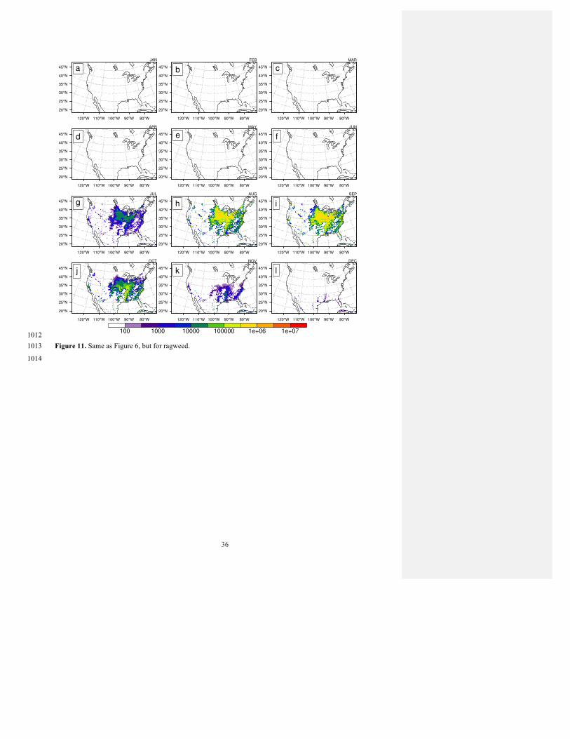
36

1012 Figure 11. Same as Figure 6, but for ragweed. 1013

1014

37

1015

Figure 12. Average (2003-2010) time series of daily pollen counts comparing model and observations for four 1016

PFTs (a-e, deciduous broadleaf, DBF; f-j, evergreen needleleaf, ENF; k-o, grasses, GRA; p-t, ragweed, RAG) across 1017

5 U.S. subregions (columns from left to right: Northeast, NE; Southeast, SE; Mountain, MT; California; Pacific 1018

Northwest, PNW). Shading for the observations and model represents the mean absolute deviation from the 1019

average for each day of the time series. Note: scale of y-axes varies by region and PFT. 1020

1021


Matthew Wozniak� 8/8/2017 10:26 PM

Deleted: 1022

Matthew Wozniak� 8/2/2017 7:32 PMDeleted: Daily climatological1023 Matthew Wozniak� 8/2/2017 7:33 PMDeleted: u1024 Matthew Wozniak� 8/2/2017 7:32 PMDeleted: climatological 1025 Matthew Wozniak� 8/2/2017 7:33 PMDeleted: climatology1026

38

1027

Figure 13. Box-and-whisker plots showing the statistical spread of the pollen count magnitudes from the regional averages presented in Figure 12. Columns 1028

from left to right: Northeast, NE (a,f); Southeast, SE (b, g) ; Mountain, MT (c,h); California (d,i); Pacific Northwest, PNW (e,j). DBF and ENF PFTs are shown 1029

in the top row (a-e) and grass and ragweed PFTs are shown in the bottom row (f-j). Box and whiskers from bottom to top represent the minimum, lower quartile, 1030

median, upper quartile, and maximum. Maxima that are not visible in panels b, c and e are 1,177 grains m-3, 1,233 grains m-3, and 766 gains m-3 respectively. All 1031

y-axes are the same scale for each row. 1032 Matthew Wozniak� 8/17/2017 8:51 PMDeleted: 1033 Matthew Wozniak� 8/17/2017 8:51 PMDeleted: noted on plot as a number1034

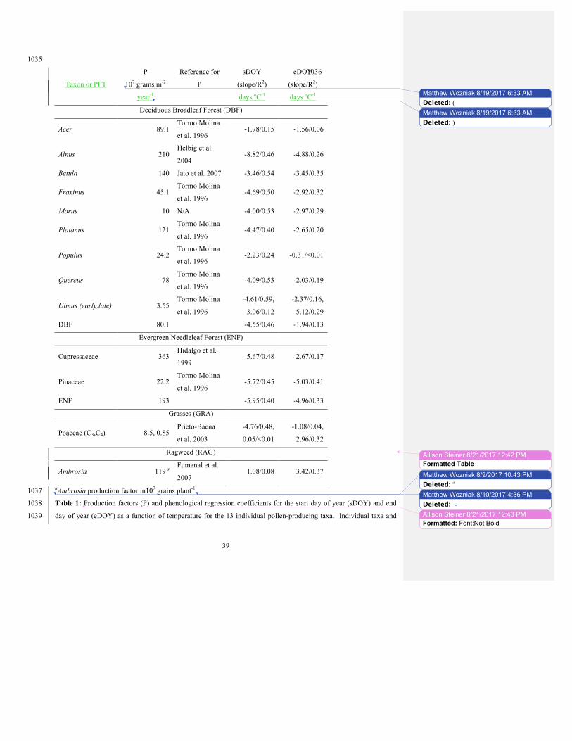
39

1035 1036

aAmbrosia production factor in107 grains plant-1. 1037

Table 1: Production factors (P) and phenological regression coefficients for the start day of year (sDOY) and end 1038

day of year (eDOY) as a function of temperature for the 13 individual pollen-producing taxa. Individual taxa and 1039

Taxon or PFT

P

107 grains m-2

year-1

Reference for

P

sDOY

(slope/R2)

days ºC-1

eDOY

(slope/R2)

days ºC-1

Deciduous Broadleaf Forest (DBF)

Acer 89.1 Tormo Molina

et al. 1996 -1.78/0.15 -1.56/0.06

Alnus 210 Helbig et al.

2004 -8.82/0.46 -4.88/0.26

Betula 140 Jato et al. 2007 -3.46/0.54 -3.45/0.35

Fraxinus 45.1 Tormo Molina

et al. 1996 -4.69/0.50 -2.92/0.32

Morus 10 N/A -4.00/0.53 -2.97/0.29

Platanus 121 Tormo Molina

et al. 1996 -4.47/0.40 -2.65/0.20

Populus 24.2 Tormo Molina

et al. 1996 -2.23/0.24 -0.31/<0.01

Quercus 78 Tormo Molina

et al. 1996 -4.09/0.53 -2.03/0.19

Ulmus (early,late) 3.55 Tormo Molina

et al. 1996

-4.61/0.59,

3.06/0.12

-2.37/0.16,

5.12/0.29

DBF 80.1 -4.55/0.46 -1.94/0.13

Evergreen Needleleaf Forest (ENF)

Cupressaceae 363 Hidalgo et al.

1999 -5.67/0.48 -2.67/0.17

Pinaceae 22.2 Tormo Molina

et al. 1996 -5.72/0.45 -5.03/0.41

ENF 193 -5.95/0.40 -4.96/0.33

Grasses (GRA)

Poaceae (C3,C4) 8.5, 0.85 Prieto-Baena

et al. 2003

-4.76/0.48,

0.05/<0.01

-1.08/0.04,

2.96/0.32

Ragweed (RAG)

Ambrosia 119 a Fumanal et al.

2007 1.08/0.08 3.42/0.37

Matthew Wozniak� 8/19/2017 6:33 AMDeleted: (1040 Matthew Wozniak� 8/19/2017 6:33 AMDeleted: )1041

Allison Steiner� 8/21/2017 12:42 PMFormatted TableMatthew Wozniak� 8/9/2017 10:43 PMDeleted: a1042 Matthew Wozniak� 8/10/2017 4:36 PMDeleted: 1043 Allison Steiner� 8/21/2017 12:43 PMFormatted: Font:Not Bold

40

families are organized into the four PFTs, with the two aggregated tree PFTs denoted as DBF and ENF. Regression 1044

slope (days/ºC) and coefficient of determination are provided for both sDOY and eDOY (slope/R2).1045

Matthew Wozniak� 8/23/2017 11:40 AMDeleted: in gray shading1046

Allison Steiner� 8/21/2017 12:43 PMComment [2]: No longer shaded… did you mean to exclude? Either add back in or modify the caption.

Allison Steiner� 8/21/2017 12:43 PMFormatted: Font:Not Bold

41

Land cover class NE SE MT CA PNW

Acer 6.79E+04 2.88E+04 1.89E+03 1.97E+02 3.09E+03

Alnus 3.37E+00 1.23E-01 6.49E+01 1.71E+02 9.56E+03

Betula 2.99E+04 2.68E+03 2.78E+02 2.64E+00 4.82E+02

Fraxinus 3.96E+04 1.10E+04 3.14E+03 3.94E+01 2.76E+02

Morus 3.99E+03 2.25E+03 3.89E+01 0.00E+00 0.00E+00

Platanus 3.18E+03 3.38E+03 1.33E+01 1.44E+02 0.00E+00

Populus 5.48E+04 1.23E+03 4.37E+04 1.96E+02 1.55E+03

Quercus 1.30E+05 2.25E+05 2.51E+04 2.82E+04 1.40E+04

Ulmus 4.96E+04 2.81E+04 1.37E+03 0.00E+00 0.00E+00

BELD DBF 3.79E+05 3.03E+05 7.56E+04 2.90E+04 2.90E+04

CLM DBF 6.67E+05 4.03E+05 1.72E+05 7.93E+03 4.18E+04

Cupressaceae 1.85E+04 2.11E+04 7.84E+04 9.64E+03 2.35E+04

Pinaceae 8.34E+04 1.58E+05 1.79E+05 2.95E+04 1.10E+05

BELD ENF 1.02E+05 1.79E+05 2.58E+05 3.91E+04 1.34E+05

CLM ENF 1.44E+06 4.26E+05 4.66E+05 4.57E+04 5.34E+05

Table 2: Total spatial coverage (km2) of tree taxa and PFTs from BELD and CLM land cover datasets in the 5 U.S. 1047

subregions (Northeast, NE; Southeast, SE; Mountain, MT; California; Pacific Northwest, PNW). All individual tree 1048

taxa are from the BELD database. BELD DBF and ENF land cover are the sums of the land cover of the taxa 1049

belonging to each PFT. 1050

1051

42

1052 Figure S1. Linear regressions of the phenological relationship between start day-of-year (sDOY) and previous year annual average temperature (PYAAT) for all 1053

taxa. Each point signifies one station per year for pollen count data from 2003-2010 (total denoted as N). (j) ulmus_2 denotes a second (later) pollen peak in 1054

Ulmus and (o) poac_2 denotes a second (later) pollen peak in Poaceae. 1055

43

1056

1057 Figure S2. Same as Figure S1, but for end day-of-year (eDOY) versus PYAAT. 1058

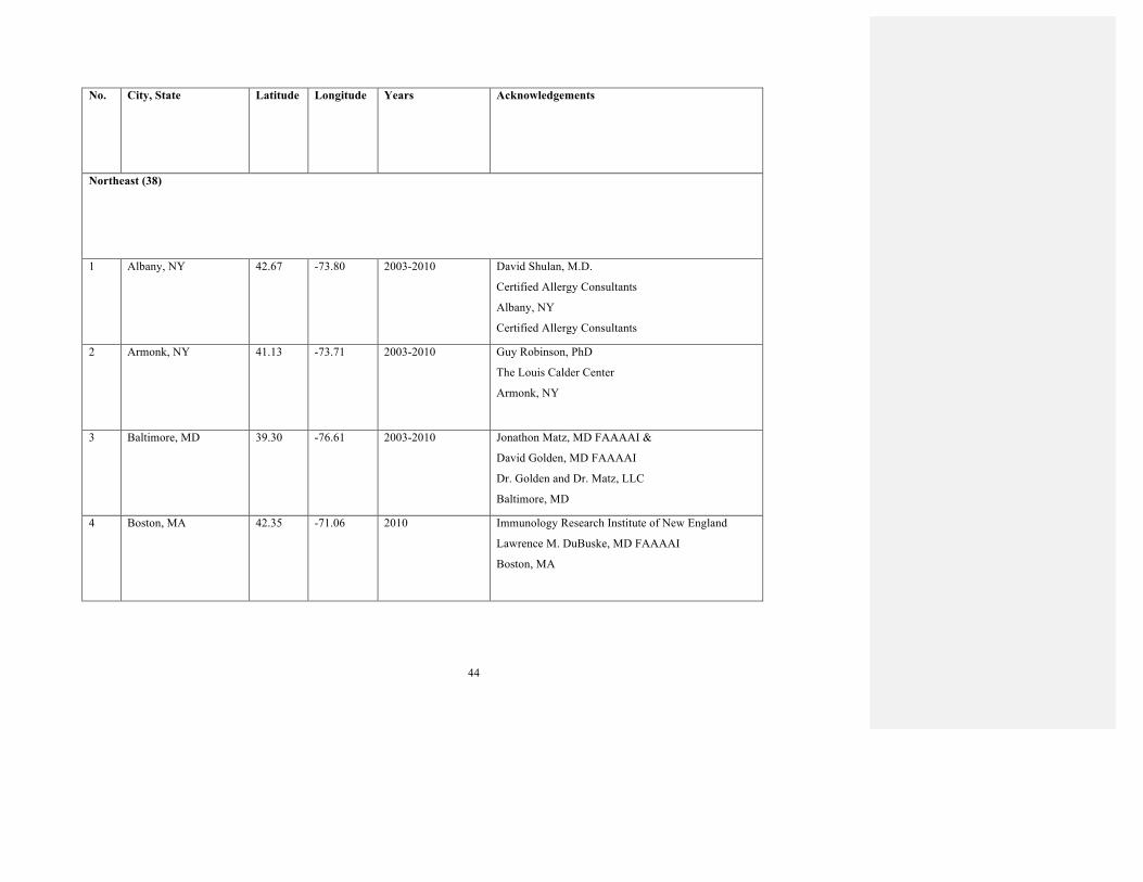
44

No. City, State Latitude Longitude Years Acknowledgements

Northeast (38)

1 Albany, NY 42.67

-73.80

2003-2010 David Shulan, M.D.

Certified Allergy Consultants

Albany, NY

Certified Allergy Consultants

Albany, NY

2 Armonk, NY 41.13

-73.71

2003-2010 Guy Robinson, PhD

The Louis Calder Center

Armonk, NY

3 Baltimore, MD 39.30 -76.61 2003-2010 Jonathon Matz, MD FAAAAI &

David Golden, MD FAAAAI

Dr. Golden and Dr. Matz, LLC

Baltimore, MD

4 Boston, MA 42.35 -71.06 2010 Immunology Research Institute of New England

Lawrence M. DuBuske, MD FAAAAI

Boston, MA

45

5 Brooklyn, NY 40.65 -73.95 2004-2010 Clifford W. Bassett, MD & Mehdi Vesaghi, MD

Long Island College Hospital

Brooklyn, NY

6 Chelmsford, MA 42.60 -71.37 2003-2005 Julian Melamed, M.D.

Chelmsford, MA

7 Cherry Hill, NJ 39.90 -75.00 2003-2010 Larchment Medical Center II

Donald J. Dvorin, MD FAAAAI

Cherry Hill, NJ

8 Chicago, IL 41.84 -87.68 2003-2010 John Shane, PhD

McCrone Research Institute

Chicago, IL

9 Dayton, OH 39.78 -84.20 2003-2010 Mr. Andy Roth

RAPCA

Dayton, OH

10* Erie, Pennsylvania 42.13 -80.09 2003-2007, 2009-

2010

Philip E. Gallagher, MD FAAAAI

Allergy & Asthma Associates of Northeastern PA

Erie, PA

46

11 Hamilton, Ontario 43.25 -79.1 2003-2005 Jason A. Ohayan, MD

Hamilton, ON

12 Indianapolis, IN 39.78 -86.15 2003-2009 L.Y. Frank Wu, M.D.

St. Vincent Professor Building

Indianapolis, IN

13 Kansas City, MO 39.12 -94.55 2003-2007, 2009-

2010

Jay Portnoy, MD FAAAAI

Children's Mercy Hospital

Kansas City, MO

14 La Crosse, WI 43.83 -91.23 2003-2010 N/A

15 Lexington, KY 38.043 -84.46 2003-2006,2008-

2010

Beth Miller, M.D.

University of Kentucky Asthma Allergy &

Immunology

Lexington, KY

16 Lincoln, NE 40.82 -96.69 2004-2009 Fred Keichel, MD

Allergy, Asthma & Immunology Associates

Lincoln, NE

47

17 London, ON 42.98 -81.25 2003-2005 James Anderson, MLT

OSHTECH

London, ON

18 Louisville, KY 38.22 -85.74 2003-2010 James L. Sublett, MD FAAAAI

Family Allergy & Asthma

Louisville, KY

19 Madison, WI 43.08 -89.39 2003-2010 Robert Bush, MD FAAAAI

UW Medical School

Madison, WI

20 Melrose Park, IL 41.90 -87.86 2003-2010 Joseph G. Leija, MD FAAAAI

Dr. Joseph Leija

Melrose Park, IL

21 Minneapolis, MN 44.96 -93.27 2010 Harold B. Kaiser, MD FAAAAI

Clinical Research Institute

Minneapolis, MN

22 Newark, NJ 40.72 -74.17 2003-2009 Alan Wolff, M.D.

UMDNJ

Newark, NJ

48

23* New Castle, DE 39.62 -75.56 2005-2010 Michael McDowell

Division of Air Quality, DNREC, State of Delaware

New Castle, DE

24 New York, NY 40.08 -78.43 2003-2010 Guy Robinson, PhD

Fordham College at Lincoln Center

New York, NY

25 Niagrara Falls, ON 43.09 -79.09 2003-2005 Dr. Michael Alexander, MD

Niagara Falls, ON

26 Olean, NY 42.08 -78.43 2003-2010 Fred Lewis, MD FAAAAI

Olean, NY

27 Philadelphia, PA 40.01 -75.13 2003-2007, 2010 Donald J. Dvorin, MD FAAAAI

Allergic Disease Associates, P.C.

Philadelphia, PA

28 Pittsburgh, PA (2) 40.44 -79.98 2003-2010 David Skoner, MD FAAAAI

Allegheny General Hospital

Pittsburgh, PA

David Nash, M.D.

Children's Hosp. of Pittsburgh

Pittsburgh, PA

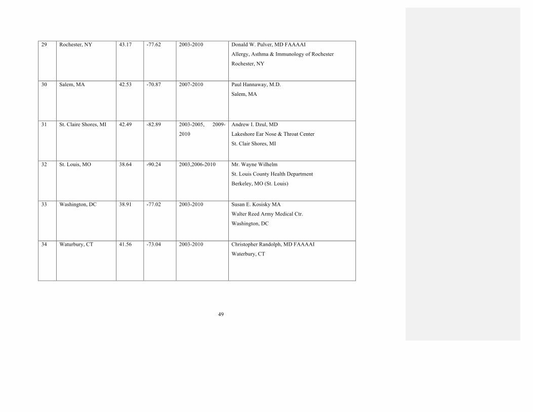
49

29 Rochester, NY 43.17 -77.62 2003-2010 Donald W. Pulver, MD FAAAAI

Allergy, Asthma & Immunology of Rochester

Rochester, NY

30 Salem, MA 42.53 -70.87 2007-2010 Paul Hannaway, M.D.

Salem, MA

31 St. Claire Shores, MI 42.49 -82.89 2003-2005, 2009-

2010

Andrew I. Dzul, MD

Lakeshore Ear Nose & Throat Center

St. Clair Shores, MI

32 St. Louis, MO 38.64 -90.24 2003,2006-2010 Mr. Wayne Wilhelm

St. Louis County Health Department

Berkeley, MO (St. Louis)

33 Washington, DC 38.91 -77.02 2003-2010 Susan E. Kosisky MA

Walter Reed Army Medical Ctr.

Washington, DC

34 Waturbury, CT 41.56 -73.04 2003-2010 Christopher Randolph, MD FAAAAI

Waterbury, CT

50

35 Waukesha, WI 43.01 -88.24 2007-2009 Walter Brummund, MD, PhD, FAAAAI

Allergy & Asthma Centers, S.C.

Waukesha, WI

36 Wauwatosa, WI 43.06 -88.03 2003-2006 Walter Brummund, MD, PhD, FAAAAI

Allergy & Asthma Centers, S.C.

Waukesha, WI

37 York, PA 39.96 -76.73 2003-2010 Michael S. Nickels, MD PhD

Allergy and Asthma Consultants, Inc.

York, PA

Southeast (33)

1 Atlanta, GA 33.76 -84.42 2003-2010 Santley M. Fineman, MD MBA FAAAAI

Atanta Allergy and Asthma

Marietta, GA (Atlanta)

2 Austin, TX 30.31 -97.95 2003-2005 Kim T. Hovanky, MD FAAAAI &

Sheila M. Amar, MD FAAAAI, FACAAI

Allergy & Asthma Center of Georgetown

Austin, TX (Georgetown)

51

3 Baton Rouge, Louisiana 30.45 -91.13 2003-2005 James M. Kidd III

Kidd Allergy Clinic

Baton Rouge, LA

4 Birmingham, AL 33.53 -86.80 2010 Weilly Soong, MD FAAAAI

Birmingham-Southern College/Alabama Allergy &

Asthma Center

Birmingham, AL

5 Charlotte, NC 35.20 -80.83 2003-2007 John T. Klimas, MD FAAAAI

Carolina Asthma and Allergy Center

Charlotte, NC

6 College Station, TX 30.60 -96.31 2003-2010 David R. Weldon, MD FAAAAI, FACAAI

Scott & White Clinic

College Station, TX

7 Corpus Christi, TX 27.69 -97.29 2003-2005 Gary L. Smith, M.D.

Corpus Christi, TX

8 Dallas, TX 32.79 -96.77 2003-2010 Jeffrey Adelglass, M.D.

Dr. Jeffrey Adelglass

Dallas, TX

52

9 Fargo, ND 46.88 -96.82 2003-2010 Dan Dalan, MD FAAAAI

Allergy & Asthma Care Center

Fargo, ND

10 Flower Mound, TX 33.03 -97.09 2006-2010 Marie H Fitzgerald, MD

North Texas Pollen Station

Flower Mound, TX

11 Fort Smith, AK 35.37 -94.38 2003-2006 N/A

12 Georgetown, TX 30.65 -97.69 2006-2010 Kim T. Hovanky, MD FAAAAI &

Sheila M. Amar, MD FAAAAI, FACAAI

Allergy & Asthma Center of Georgetown

Austin, TX (Georgetown)

13 Greenville, SC 34.84 -82.37 2003-2010 Neil L Kao MD FAAAAI

Allergic Disease and Asthma Center

Greenville, SC

14 Houston, TX 29.77 -95.39 2005-2010 Mr. Tony Huynh

City of Houston

Houston, TX

53

15 Huntsville, AL 34.71 -86.63 2003-2010 Ms. Debra Hopson

Natural Resources & Environmental Management

Huntsville, AL

16 Knoxville, TN 35.97 -83.95 2003-2010 Michael Miller, MD FAAAAI

Allergy, Asthma and Immunology

Knoxville, TN

17 Little Rock, AK 34.72 -92.35 2004-2010 Karl V Sitz, MD

Little Rock Allergy & Asthma Clinic

Little Rock, AR

18 Miami, FL 25.78 -80.21 2003-2005 Elene Ubals, MD &

Richard Schiff, MD, PhD

Miami, FL

19 New Orleans, LA 30.07 -89.93 2008-1010 W Edward Davis MD MS MBA MMM

Ochsner Clinic Foundation

New Orleans, LA

20 Ocala, FL 29.19 -82.13 2003-2005 Dr. Karl M Altenburger

Allergy and Asthma Care of Florida

Ocala, FL

54

21 Oklahoma City, OK (2) 35.47 -97.51 2003-2010 Warren V. Filley, MD FAAAAI

OK Allergy Asthma Clinic, Inc.

Oklahoma City, OK

Martha Tarpay, MD

Allergy & Asthma Center

Oklahoma City, OK

22 Omaha, NE 41.26 -96.01 2003-2010 N/A

23 Orlando, FL 28.51 -81.37 2006-2007 Bruce A. Hornberger, MD FAAAAI

Allergy & Asthma Center of East Orlando

Orlando, FL

24 Oxford, AL 33.61 -85.84 2010 Robert Grubbe, MD

Allergy & Asthma Center, LLC

Oxford, AL

25 Rogers, AK 36.33 -94.13 2006-2010 Curtis L. Hedberg, MD FAAAAI

Hedberg Allergy & Asthma Center

Rogers, AR (Fort Smith)

26* Sarasota, FL 27.34 -82.53 2003-2010 Mary Jelks, MD FAAAAI

Sarasota, FL

55

27 Savannah, GA 32.02 -81.13 2008-2010 Brad H. Goodman, M.D. &

Bruce D. Finkel, M.D.

Coastal Allergy & Asthma, P.C.

Savannah, GA

28 Tallahasseee, FL 30.46 -84.28 2003-2005 Ronald Saff, M.D.

Tallahassee, FL

29 Tampa, FL 27.96 -82.48 2003-2010 Richard Lockey, MD FAAAAI

University of South Florida

Tampa, FL

30 Tulsa, OK 36.13 -95.92 2003-2010 Estelle Levetin, PhD FAAAAI

University of Tulsa

Tulsa, OK

31 Waco, TX (2) 31.57 -97.18 2003-2010 N.J. Amar, MD FAAAAI

Allergy and Asthma Center

Waco, TX

Pramila K. Daftary, MD FAAAAI

Allergy & Asthma Care of Waco

Waco, TX

Mountain (8)

56

1 Bismarck, ND 46.81 -100.77 2003-2005, 2010 Dan Dalan, M.D.

North Dakota DOH East Lab

Bismarck, ND

2 Colorado Springs (2) 38.86 -104.76 2003-2010 William Storms, MD FAAAAI

The William Storms Allergy Clinic

Colorado Springs, CO

Robert A. Nathan, MD FAAAAI & Daniel F. Soteres,

MD MPH FAAAAI

Asthma & Allergy Associates, PC

Colorado Springs, CO

3 Draper, UT 40.52 -111.86 2009-2010 Duane J. Harris, MD FAAAAI

Intermountain Allergy & Asthma Clinic

Draper, UT

4* Missoula, MT 46.87 -114.01 2006-2007, 2009-

2010

Emily Weiler

U of Montana, Ctr for Environmental Health Sciences

Missoula, MT

5 Salt Lake City, UT 40.78 -111.93 2003-2004, 2008 N/A

6 Scottsdale, AZ 33.69 -111.87 2006-2007 Michael E. Manning, M.D.

Scottsdale, AZ

57

7* Twin Falls, ID 42.56 -114.46 2003-2010 N/A

California (13)

1 La Jolla, CA 32.84 -117.26 2003-2010 Robert Reid, Jr, MD

Scripps Memorial Hospital

LaJolla, CA

2 Orange, CA 33.81 -117.82 2003-2010 Sherwin A. Gillman, M.D.

Children's Hospital of Orange County-Pediatric

Subspecialty Faculty

Orange, CA

3 Pasadena, CA 34.16 -118.14 2004-2005, 2010 Philip Taylor, PhD

The Pollen Group

Pasadena, CA

4 Pleasanton, CA 37.67 -121.89 2003-2010 N/A

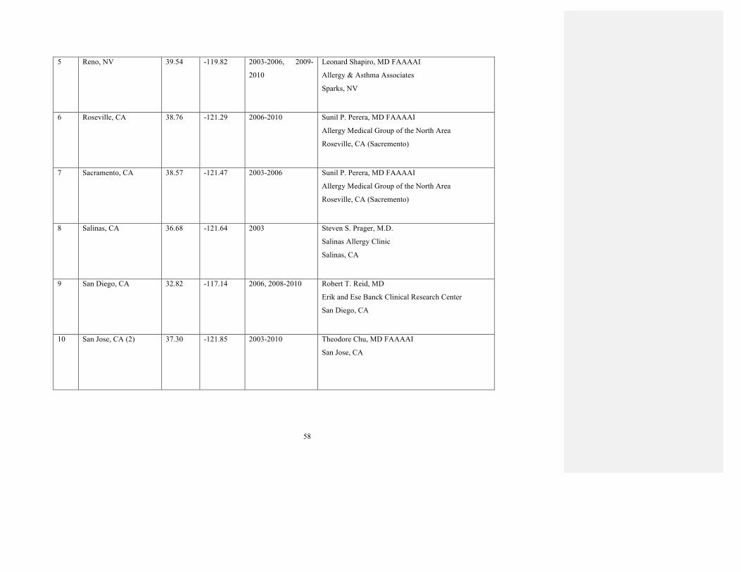
58

5 Reno, NV 39.54 -119.82 2003-2006, 2009-

2010

Leonard Shapiro, MD FAAAAI

Allergy & Asthma Associates

Sparks, NV

6 Roseville, CA 38.76 -121.29 2006-2010 Sunil P. Perera, MD FAAAAI

Allergy Medical Group of the North Area

Roseville, CA (Sacremento)

7 Sacramento, CA 38.57 -121.47 2003-2006 Sunil P. Perera, MD FAAAAI

Allergy Medical Group of the North Area

Roseville, CA (Sacremento)

8 Salinas, CA 36.68 -121.64 2003 Steven S. Prager, M.D.

Salinas Allergy Clinic

Salinas, CA

9 San Diego, CA 32.82 -117.14 2006, 2008-2010 Robert T. Reid, MD

Erik and Ese Banck Clinical Research Center

San Diego, CA

10 San Jose, CA (2) 37.30 -121.85 2003-2010 Theodore Chu, MD FAAAAI

San Jose, CA

59

11 Santa Barbara, CA 34.43 -119.72 2003-2010 Myron Liebhaber, M.D.

Sansum - Santa Barbara Medical Foundation Clinic

Santa Barbara, CA

12 Stockton, CA 37.97 -121.31 2009-2010 Gregory W. Bensch, MD FAAAAI & George W

Bensch, MD FAAAAI

Allergy, Immunology and Asthma Medical Group

Stockton, CA

Pacific NW (4)

1 Crescent City, CA 41.76 -124.20 2009-2010 N/A

2* Eugene, OR 44.05 -123.11 2003-2010 Kraig W. Jacobson, MD, FAAAAI

Allergy & Asthma Research Group

Eugene, OR

3 Seattle, WA 47.62 -122.35 2003-2010 N/A

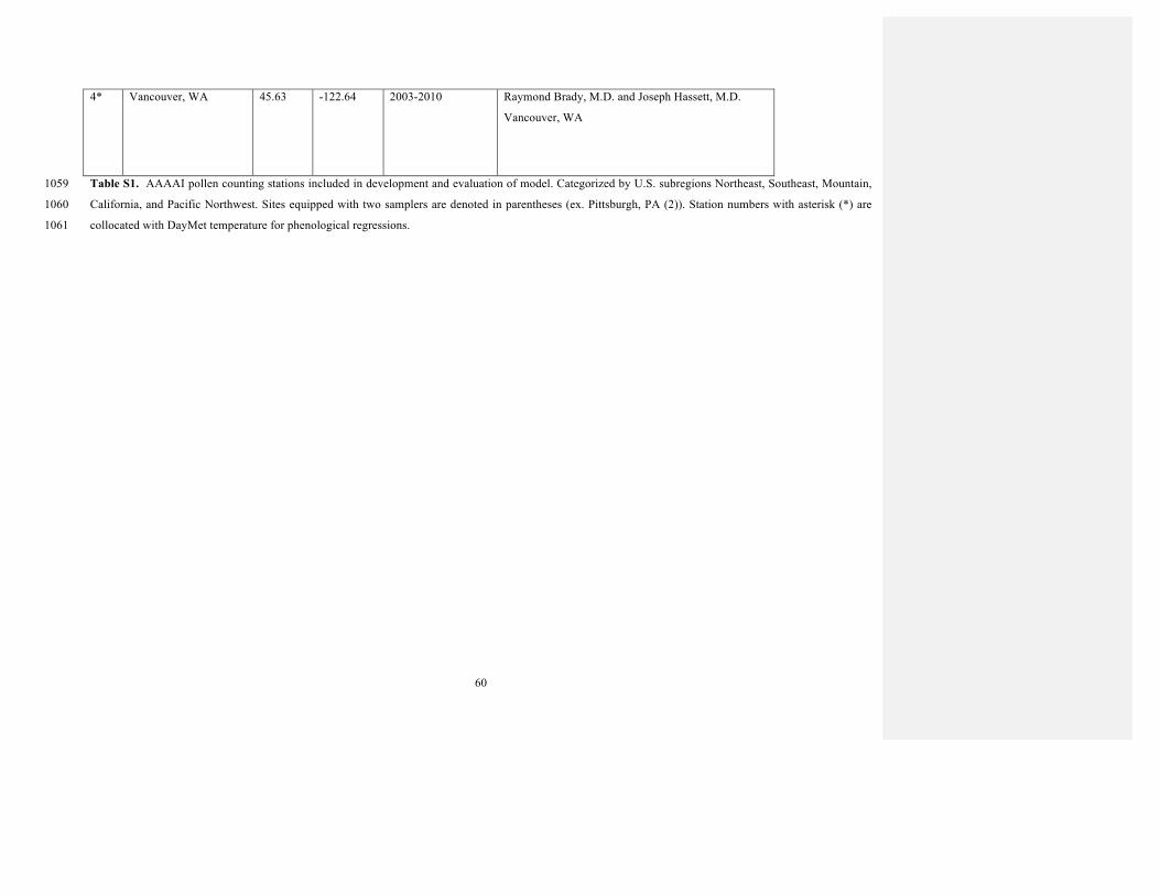
60

4* Vancouver, WA 45.63 -122.64 2003-2010 Raymond Brady, M.D. and Joseph Hassett, M.D.

Vancouver, WA

Table S1. AAAAI pollen counting stations included in development and evaluation of model. Categorized by U.S. subregions Northeast, Southeast, Mountain, 1059

California, and Pacific Northwest. Sites equipped with two samplers are denoted in parentheses (ex. Pittsburgh, PA (2)). Station numbers with asterisk (*) are 1060

collocated with DayMet temperature for phenological regressions. 1061

61

1062

Taxon

Maximum Pavgmax

(grains m-3)

Average Pavgmax

(grains m-3)

Acer 535 212

Alnus 176 73

Ambrosia 379 193

Arecaceae 27 13

Artemisia 76 36

Asteraceae 64 28

Betula 564 232

Carpinus/Ostrya 71 29

Carya 126 54

Celtis 155 65

Chenopodiaceae/Amaranthaceae 80 29

Corylus 13 5

Cupressaceae 1949 960

Cyperaceae 37 12

Eupatorium 27 13

Fagus 66 17

Fraxinus 462 227

Graminae / Poaceae 197 98

Juglans 71 34

Ligustrum 13 6

Liquidambar 109 44

Morus 940 398

Myrica 50 25

Olea 197 43

Other Grass Pollen 85 42

Other Tree Pollen 863 332

Other Weed Pollen 160 51

Pinaceae 645 328

Plantago 33 13

Platanus 191 103

Populus 367 158

Prosopis 34 16

Pseudotsuga 7 3

62

Quercus 2106 1081

Rumex 59 23

Salix 123 58

Tilia 19 6

Tsuga 12 5

Typha 19 10

Ulmus 556 249

Unidentified Pollen 198 57

Urticaceae 86 36

Table S2. Maximum and average Pavgmax used for selecting pollen taxa for this study. Shaded taxa are selected taxa 1063

based on minimum of 1) 100 grains m-3 for the maximum Pavgmax and 2) 70 grains m-3 for the average Pavgmax. 1064

1065

1066

Matthew Wozniak� 8/9/2017 11:27 AMDeleted: SI 1067

Response to Referee #1 - GMD

Documents

Transcript of Response to Referee #1 - GMD